Embed Size (px)
Citation preview

FINITE ELEMENT ANALYSIS OF A TWO-DIMENSIONAL LINEAR ELASTIC SYSTEMS WITH A PLANE “RIGID MOTION”
S. VLASE, C. DĂNĂŞEL, M.L. SCUTARU, M. MIHĂLCICĂ
TRANSILVANIA University of Braşov, RO-500036, B-dul Eroilor, 29, Romania, E-mail: [email protected]
Received January 24, 2014
Discretizing a mechanical structure as part of finite element analysis makes it necessary to use a variety of finite elements, according to the shape and geometry of the analyzed system. Two-dimensional finite elements are widely used in finite element analysis and using them is generally easy and fast. For mechanical systems that also exhibit a general “rigid” plane motion, dynamic analysis enforces the use of numerous additional terms that can no longer be neglected. In this paper we determine motion equations for a two-dimensional finite element and we distinguish the additional terms that can eventually change the qualitative behavior of the system. The motion equations are obtained using Lagrange’s equations.
Key words: finite element, nonlinear system, elastic element, shell finite element.
1. INTRODUCTION
Any multibody mechanical system consists, more or less, of elastic elements. A first approximation in the study of technical systems is given by the rigid elements hypothesis. The hypothesis works very well in the dynamic analysis of systems which are sufficiently slow or mildly loaded. If, however, the velocities and the loads are high, the elastic behavior of the components will generally negatively influence the operation of the system. We also need to study the phenomena of resonance and loss of stability as manifestations of elasticity. The analytic approach of such problems, using the classical theorems of the mechanics of continuous systems, leads to practically unsolvable systems of differential equations. This leaves us with the numerical methods, represented mainly by the finite element method. The advantages of this approach result from Gerstmayr and Schöberl, 2006, Khulief, 1992, Vlase, 1989. The motion equations yielded by the finite element method have a complex form, are strongly nonlinear and contain a number of additional terms resulting from the „rigid” motion inside the system. Previous papers on this topic analyzed systems with a single deformable element and a plane motion (see for example Bagci, 1983, Bahgat and
Rom. Journ. Phys., Vol. 59, Nos. 5–6, P. 476–487, Bucharest, 2014

2 Finite element analysis of a two-dimensional system 477
Willmert, 1976, Cleghorn et al., 1981, Fanghella et al., 2003, Nath and Ghosh, 1980, Sung, 1986) or more complex systems. The results obtained were synthetized by Ibrahimbegović et al., 2000, Thompson and Sung, 1986. For a general three-dimensional motion of systems modeled with one or three-dimensional finite elements we mention Vlase, 2012, 2013a. The researches in the domain also targeted some more complex aspects of the problem, about the calculus, experimental verification and control for the mechanical systems, usually having some form of simplicity (imposed by the difficulty of the numerical approach - Deü et al., 2008, Mayo and Domínguez, 1996, Piras and Mills, 2005). The influence of damping, the stability and the use of composite materials in such systems were also aspects which were studied (see Neto et al., 2006, Shi et al., 2001, Zhang and Erdman, 2001, Zhang et al., 2007) along with the thermal effects (see Hou and Zhang, 2009). The main difficulty is constituted by the symbolic representation of the equations of motion and by the adequate selection of integration methods. Models for the bi and tri-dimensional motion were developed by Thompson and Sung, 1986. This paper aims to perform the dynamic analysis and to determine the equations of motion for a two-dimensional finite element, having a “rigid” plan-parallel motion. It is previously considered that the field of velocities and accelerations was already determined for all the elements of the system (considered rigid). A finite element in a "rigid" motion along with the body which it discretizes will be analyzed. In order to determine the equations of motion, the Lagrange equations will be used. For this, it is necessary to determine the kinetic energy and the internal energy for the elements of the mechanical system (considered linear elastic). If the obtained equations will be compared with the steady state response equations, new terms will be found. These appear due to the relative motion of independent coordinates relative to the mobile reference systems which are attached to the elements of the mechanical system (Coriolis effects) and they will determine changes in stiffness and in the inertial terms along with the appearance of some conservative damping.
2. MOTION’S EQUATIONS
Let's consider a two-dimensional finite element with a plan parallel motion. The type of finite element which will be used will determine the shape functions and the final form for the matrix coefficients. In what follows it is considered that the deformations are small enough not to influence the general rigid motion of the system.
Both the problem of the rigid motion of the system and the field of velocities and accelerations for each two-dimensional element of the multicorp systems are considered to be solved (see Pennestri, 2009). The finite element is related to the

S. Vlase et al. 3 478
local coordinates system Oxy, which is mobile and which participates to the whole motion (fig. 1), so it has a known rigid motion. Let's consider v ( , , 0)o o oX Y being the velocity and a ( , , 0)o o oX Y being the acceleration of the origin of the mobile reference system related to the fixed reference system OXY, to which the whole motion of the mechanical system relates. We will consider ω (0, 0, )zω as being the angular velocity of the solid containing the finite element and ε (0, 0, )ε as being the angular acceleration of the same solid.
The change in the values of the position vector r GM , of a random point M of the finite element when going from the local Oxy reference system into the global fixed OXY reference system is obtained using a rotation transformation matrix R. If we consider r GM , as being the position vector of the M point, we have:
r GM , = r GO , + r G = r GO , + ⋅R r L , (1)
where we consider G defining the vectorial entities which have their components relating to the global reference system and L defining the vectorial entities which have their components relating to the local reference system.
Fig.1 – A bidimensional finite element with plan motion.
The rotation transformation matrix R has, in this situation, a very simple form:
R cos sinsin cos
θ − θ = θ θ
. (2)
If the M point is subjected to a displacement f L , transforming into the M' point, we will have:

4 Finite element analysis of a two-dimensional system 479
r GM ,' = r GO , + ⋅R ( r L + f L ) (3)
where r GM ,' is the position vector of the point M' with its components relating to
the global reference system. The continuous displacement field f (x,y) L is approximated in the finite element method, depending on the nodal displacements, using the relationship:
( ) ( ),L e Lx y t=f N δ (4)
where the elements of the N matrix (which contains the interpolation functions) depend on the type of the chosen finite element. The velocity of the M' point, related to the fixed coordinate system, will be:
,0 L L L 0 L e,L e L′ = + + + = + + δ +M ,Gv r Rr Rf Rf r Rr RN RNδ (5)
The velocity components are defined related to the global coordinates system. The equations of motion will be obtained in the local coordinates system.
The kinetic energy of the considered element will be determined using the relationship:
21 1d
2 2c V VE v V= ρ = ρ∫ ∫ v T
LM ,' v LM ,' dV . (6)
When we determined the kinetic energy, we could have been representing the velocity in the global coordinates system, the result for the kinetic energy remaining the same. This happens because the scalar product of two vectors remains the same, no matter which reference system we use.
The deformation energy is:
Ep = 1 d2
TV
V∫ σ ε . (7)
For the ease of understanding, we remember that the generalized Hooke law is:
σ = D ε, (8)
where, for a two-dimensional finite element (plane state of deformation) we have:
D
1 0 00 1 0
(1 )(1 2 )1 20 0
2
E
− µ
= − µ − µ − µ − µ
(9)
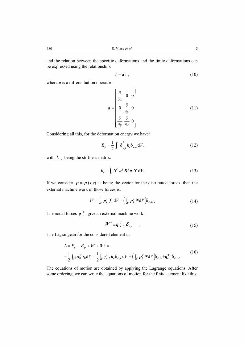
S. Vlase et al. 5 480
and the relation between the specific deformations and the finite deformations can be expressed using the relationship:
ε = a f , (10)
where a is a differentiation operator:
a
0 0
0 0
0
x
y
y x
∂ ∂ ∂
= ∂ ∂ ∂ ∂ ∂
(11)
Considering all this, for the deformation energy we have:
,,
1 2
T
p e e LV e LE = ∫ kδ δ dV, (12)
with k e being the stiffness matrix:
ek =T
T TV∫ N a D a N dV. (13)
If we consider pp = (x,y) as being the vector for the distributed forces, then the external machine work of those forces is:
( ) ,d dT TL e LL LV VW V V= =∫ ∫p f p N δ . (14)
The nodal forces q Te give an external machine work:
cW = q T
Le, Le,δ . (15)
The Lagrangean for the considered element is:
( ) T0 , e,L e,L, e,L0
1 1= d – d d + .2 2
cc p
T T Te e Le L LV V V
L E E W W
V V V
= − + + =
ρ γ +∫ ∫ ∫r r k p N qδ δ δ (16)
The equations of motion are obtained by applying the Lagrange equations. After some ordering, we can write the equations of motion for the finite element like this:

6 Finite element analysis of a two-dimensional system 481
( NNT
V∫ ρdV) δ Le, + 2 ( NRRN TT
V∫ ρdV)
δ Le, +( k e + NRRN TT
V∫ ρdV) Le,δ = (17)
= q e + pN T
V∫ L dV – ( ∫VN TρdV) TR r O – rRRN TT
V∫ ρdV
We can write the equations of motion in concentrated form:
( ) ( )
( ) ( )
2
200
2
– – – .
e e e e e
* i i Te e,L e,L e,L
+ + + + =
= + ie
m c k k k
q q q q m R r
δ δ ε ω δ
ε ω
e,L e,L e,L (18)
where we considered:
q *,Le = pN
T
V∫ L dV ; m iOe = ∫VN T ρdV ;
m e = NNT
V∫ ρdV = m 11 + m 22 ;
c e (ω)= NRRN TT
V∫ ρdV ; (19)
k e (ε) + k e (ω2) = NRRN TT
V∫ ρdV ;
q iLe , (ε) + q i
Le , (ω) = rRRN TT
V∫ ρdV .
The matrix products where the rotation transformation matrix appears can easily be calculated, as this matrix is determined by only one element, the angle θ. The anti-symmetric matrix:
ω = R R T 0 0 1
0 1 0−ω −
= = ω ω (20)
represents the angular velocity operator corresponding to the angular velocity ω. We also have:
R R T 20 1 1 01 0 0 1−
= ε − ω
. (21)
In both the global and local reference systems, the angular velocity and angular acceleration vectors have the same components. If we consider )1(N and )2(N being the rows of the matrix N, with the notations:
m 1x = ∫V N (1)T x ρdV ; m y1 = ∫V N T
)1( y ρdV ; m 11 = ∫V N )1( N (1)T ρdV ;
m x2 = ∫V N T)2( x ρdV ; m y2 = ∫V N T
)2( y ρdV ; m 22 = ∫V N )2( N (2)T ρdV ; (22)

S. Vlase et al. 7 482
we can obtain the equations of motion for the finite element, with explicit dependencies to the angular velocity ω and angular acceleration ε. Previously, we solve the integrals with the given notations and we can obtain a detailed form for the equations of motion. Therefore, we have:
m e = ( m 11 + m 22 )e; c e (ω) =ω ( ) emm 1221 −
k e (ε) + k e (ω2) ε= ( )1221 mm − e2ω− ( )2211 mm − e (23)
q iLe , (ε) + q i
Le , (ω) = ( )yx mm 12 −ε e - ( )yx mm 212 +ω e
The equations of motion will be, in this case:
( m 11 + m 22 ) e δ Le, + ω2 ( m 21 – m 12 ) e δ Le, +
+ [k e + ( )1221 mm −ε e - ( )22112 mm +ω ]e Le,δ = (24)
= exteq + liaison
eq – ( )yx mm 12 −ε e + ( )yx mm 212 +ω e – m i
Oe R T r O .
The unknowns in the finite element analysis of such a system are of two kinds: nodal displacements and contact forces. Using a correct assembly of the equations of motion, written by each finite element, the algebraic unknowns (the contact forces) can be removed (see Blajer and Kołodziejczyk, 2011, Khang, 2011, Vlase, 1987a,1987b). The equations of motion for the whole multibody system will be possible to be written as a system of 2nd order non-linear differential equations. The matrix coefficients of this system of equations have the following properties:
• The inertial matrix m is symmetric; • The damping matrix c is a skew symmetric matrix. The terms defined by
this matrix represent the Coriolis accelerations, due to relative motions of nodal displacements with respect to the mobile reference coordinate system, linked to the moving parts of the system studied;
• The stiffness matrix k contains both symmetric and skew symmetric terms. Moreover, this matrix can have singularities due to the rigid motion of the system that have to be removed before conducting the study of the system.
3. MODAL ANALYSIS OF A ROTATING DISK
Let’s consider a rotating disk. If we consider a stationary motion, the disk will rotate with an angular velocity ω. In a very small interval ∆t we may consider that the angular velocity is constante and we intend to achieve the modal analysis of rotating disk. We will use the method previously presented for carrying out the calculation and compare the result with that obtained by applying the classic version of the method of finite elements. We consider two cases:
8 Finite element analysis of a two-dimensional system 483
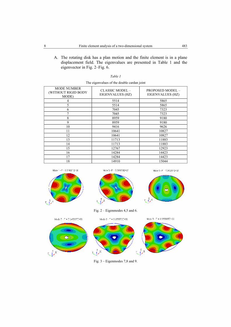
A. The rotating disk has a plan motion and the finite element is in a plane displacement field. The eigenvalues are presented in Table 1 and the eigenvector in Fig. 2–Fig. 6.
Table 1
The eigenvalues of the double cardan joint
MODE NUMBER (WITHOUT RIGID BODY
MODE)
CLASSIC MODEL – EIGENVALUES (HZ)
PROPOSED MODEL – EIGENVALUES (HZ)
4 5514 5865 5 5514 5865 6 7045 7323 7 7045 7323 8 8959 9180 9 8959 9180 10 9416 9626 11 10641 10827 12 10641 10827 13 11713 11883 14 11713 11883 15 12767 12923 16 14284 14423 17 14284 14423 18 14910 15044
Fig. 2 – Eigenmodes 4,5 and 6.
Fig. 3 – Eigenmodes 7,8 and 9.

S. Vlase et al. 9 484
Fig. 4 – Eigenmodes 10,11 and 12.
Fig. 5 – Eigenmodes 13, 14 and 15.
Fig. 6 – Eigenmodes 16,17 and 18.
B. The rotating disk has a plan motion and the finite element is in a general displacement field. The eigenmodes are presented in Fig.7-Fig.11.

10 Finite element analysis of a two-dimensional system 485
Fig. 7 – Eigenmodes 7,8 and 9.
Fig. 8 – Eigenmodes 10,11 and 12.
Fig. 9 – Eigenmodes 13,14 and 15.
Fig.10 – Eigenmodes 16,17 and 18.

S. Vlase et al. 11 486
Fig. 11 – Eigenmodes 19,20 and 21.
4. CONCLUSIONS
The additional terms in the equations of motion will influence the dynamic response of the system. It may happen that a resonant state or a loss of stability state to be reached. The modifications of eigenvalues considering a rotating disc (along its own axis) is presented in the paper. An upwards displacement for all the eigenvalues can be observed - this happens because an increase in stiffness takes place in this situation (rotation), due to the inertial forces. The vibration modes remain practically the same, while a small change in the amplitudes can be observed. The presence of inertial and Coriolis effects can significantly modify, in some situations, the dynamic response of the system.
REFERENCES
1. C. Bagci, Elastodynamic Response of Mechanical Systems using Matrix Exponential Mode Uncoupling and Incremental Forcing Techniques with Finite Element Method. Proceeding of the Sixth Word Congress on Theory of Machines and Mechanisms, India, p. 472 (1983).
2. Bahgat, B.M., Willmert, K.D., Finite Element Vibrational Analysis of Planar Mechanisms. Mechanism and Machine Theory, vol.11, p. 47 (1976).
3. Blajer W., Kołodziejczyk K., 2011, Improved DAE formulation for inverse dynamics simulation of cranes, Multibody Syst Dyn 25: 131–143.
4. Cleghorn, W.L., Fenton, E.G., Tabarrok, K.B., Finite Element Analysis of High-Speed Flexible Mechanism. Mech.Mach.Theory, 16, p. 407 (1981).
5. Deü J.-F., Galucio A.C., Ohayon R., 2008, Dynamic responses of flexible-link mechanisms with passive/active damping treatment. Computers & Structures, Volume 86, Issues 3–5, pp. 258–265.
6. Fanghella P., Galletti C., Torre G., 2003, An explicit independent-coordinate formulation for the equations of motion of flexible multibody systems. Mech. Mach. Theory, 38, p. 417–437.
7. Gerstmayr, J., Schöberl, J., A 3D Finite Element Method for Flexible Multibody Systems, Multibody System Dynamics, Volume 15, Number 4, 305–320 (2006).
8. Hou W., Zhang X., 2009, Dynamic analysis of flexible linkage mechanisms under uniform temperature change. Journal of Sound and Vibration, Volume 319, Issues 1–2, Pages 570–592.

12 Finite element analysis of a two-dimensional system 487
9. Ibrahimbegović, A., Mamouri, S., Taylor, R.L., Chen, A.J., Finite Element Method in Dynamics of Flexible Multibody Systems: Modeling of Holonomic Constraints and Energy Conserving Integration Schemes, Multibody System Dynamics, Volume 4, Numbers 2–3, 195–223 (2000).
10. Khang N.V., Kronecker product and a new matrix form of Lagrangian equations with multipliers for constrained multibody systems, Mechanics Research Communications, Volume 38, Issue 4, pp. 294–299, 2011.
11. Khulief, Y.A., On the finite element dynamic analysis of flexible mechanisms. Computer Methods in Applied Mechanics and Engineering, Volume 97, Issue 1, Pages 23–32 (1992).
12. Mayo J, Domínguez J., 1996, Geometrically non-linear formulation of flexible multibody systems in terms of beam elements: Geometric stiffness. Computers & Structures, Volume 59, Issue 6, Pages 1039–105.
13. P.K. Nath, A. Ghosh, Kineto-Elastodynamic Analysis of Mechanisms by Finite Element Method, Mech.Mach.Theory, 15, pp. 179 (1980).
14. Neto M.A., Ambrósio J.A.C, Leal R.P., 2006, Composite materials in flexible multibody systems. Computer Methods in Applied Mechanics and Engineering, Volume 195, Issues 50–51, p. 6860–6873.
15. Pennestri', E., de Falco, D., Vita, L., An Investigation of the Influence of Pseudoinverse Matrix Calculations on Multibody Dynamics by Means of the Udwadia-Kalaba Formulation, Journal of Aerospace Engineering, Volume 22, Issue 4, pp. 365–372 (2009).
16. Piras G., Cleghorn W.L., Mills J.K., 2005, Dynamic finite-element analysis of a planar high speed, high-precision parallel manipulator with flexible links. Mech. Mach. Theory, Volume 40, Issue 7, p. 849–862.
17. Shi Y.M., Li Z.F., Hua H.X., Fu Z.F., Liu T.X., 2001, The Modelling and Vibration Control of Beams with Active Constrained Layer Damping. Journal of Sound and Vibration, Volume 245, Issue 5, p. 785–800.
18. Sung, C.K., 1986, An Experimental Study on the Nonlinear Elastic Dynamic Response of Linkage Mechanism. Mech. Mach. Theory, 21, p.121–133.
19. Thompson, B.S., Sung, C.K., A Survey of Finite Element Techniques for Mechanism Design. Mech.Mach.Theory, 21, nr. 4, p. 351–359 (1986).
20. Vlase, S., Contributions to the elastodynamic analysis of the mechanisms with the finite element method. Ph.D., TRANSILVANIA University (1989).
21. Vlase, S., A Method of Eliminating Lagrangean Multipliers from the Equations of Motion of Interconnected Mechanical Systems. Journal of applied Mechanics, ASME Transactions, vol. 54, nr. 1 (1987a).
22. Vlase, S., Elimination of Lagrangean Multipliers. Mechanics Research Communications, vol. 14, pp. 17–22 (1987b).
23. Vlase S., Dynamical Response of a Multibody System with Flexible Elements with a General Three Dimensional Motion, Rom. J. Phys., 57 (3–4), 676–693, 2012.
24. Vlase, S., Teodorescu, Elasto-dynamics of a solid with a general “rigid” motion using FEM model. Part I, Rom. J. Phys., 58 (7–8), 872–881, 2013.
25. Zhang X., Erdman A.G., 2001, Dynamic responses of flexible linkage mechanisms with viscoelastic constrained layer damping treatment. Computers & Structures, Volume 79, Issue 13, p. 1265–1274.
26. Zhang X., Lu J., Shen Y., 2007, Simultaneous optimal structure and control design of flexible linkage mechanism for noise attenuation. Journal of Sound and Vibration, Volume 299, Issues 4–5, p. 1124–1133.