1

Chapter 2: Finite Difference Approximations

2.1) Introduction

The first chapter introduced us to several of the different kinds of partial

differential equations (PDEs) that govern the evolution of physical systems. We also

derived the Navier Stokes equations and learned that when the parabolic, i.e. non-ideal

terms, are dropped we obtain the Euler equations as a hyperbolic limit. When modeling

high speed flows with very low viscosities, we saw that the Euler equations provide a

good starting approximation. However, we also saw that non-ideal effects such as

radiative processes, viscosity and thermal conduction can play an important role in those

flows. Self-gravity and chemical or nuclear reactions may also become important in

modeling certain systems. Such flows usually have a large range of temperatures and

densities. As a result, the detailed transport coefficients can be very non-linear. However,

the emergence of fast computers over the last few decades has spurred engineers and

mathematicians, along with astrophysicists and space physicists, to build very successful

methods for treating these systems of equations. Our purpose in this book is to study

numerical techniques for the solution of these equations. The computer only solves a

discrete approximation for the actual PDE. We call this approximation a finite difference

approximation (FDA). The FDA is only a computer-friendly proxy for the PDE. The

solution of the PDE can be specified at all points of interest in space. The solution of the

FDA, on the other hand, may be specified only at discrete locations in space. It is not

always guaranteed that the FDA saliently converges to the solution of the PDE. Obtaining

such guarantees is the task that we undertake in this chapter. The methods developed in

this book would be of direct interest to computational astrophysicists, space physicists,

plasma physicists, applied mathematicians and engineers who seek a gentle and practical

introduction to the systems that interest them.

A look at the Euler equations, or several of the other hyperbolic systems

catalogued in Chapter 1, shows us that they have strong non-linearities. Their

linearization has shown us, however, that they have a property that is common to all

2

hyperbolic systems : small perturbations to a constant state cause certain well-known

families of waves to propagate away from the point of disturbance. Consequently, an

acceptable first start in trying to understand such systems might consist of understanding

much simpler scalar hyperbolic systems. We can further simplify our task by studying

linear systems since there is much insight to be gained from that study. As a result, we

focus on linear hyperbolic equations in this chapter, treating them as simple prototypes

for the more complex systems to be studied later.

An examination of the non-ideal terms in the Navier Stokes equations from

Chapter 1 shows that we have to contend with physical effects such as viscosity and

thermal conduction. In the previous chapter we saw that they contribute as parabolic

terms. If radiation is treated in the flux limited diffusion approximation, a popular choice

for large three-dimensional applications, then the radiation equation also has a parabolic

dependence. Since the temperatures and densities in several scientific and engineering

simulations can have a range of scales, the coefficients for the above-mentioned non-

ideal terms can have a strong dependence on temperature and density. As before, it is

advantageous to begin our study with something simple. Hence, we will also study linear

parabolic equations in this chapter and we use them as models for the more complex

parabolic terms to be studied later.

The presence of radiative heating and cooling or chemical reactions or nuclear

reactions in a hydrodynamical problem can result in PDEs with stiff source terms. At a

naïve level, a stiff source term is one whose contributions can exceed the contributions

coming from other terms in the PDE. It is easier to devise time-explicit treatments than it

is to design time-implicit methods for treating source terms. However, the presence of

stiff source terms can cause several numerical difficulties in a problem and those

difficulties can only be ameliorated with a time-implicit formulation for the source terms.

While a detailed study of stiff source terms will be undertaken in a later chapter, we get

our first glimpse of the role of source terms via studying model systems in this chapter.

3

Any numerical method should carry some guarantees that it will converge to the

physical solution. Even for the very simple case of a scalar, linear PDE, it is not

guaranteed that any numerical method that one might devise will converge to the physical

solution. In this chapter, we take our first stab at obtaining such guarantees. For parabolic

equations such guarantees will indeed be obtained in this chapter. For hyperbolic

problems such a study will spill over to the next chapter. The solution methods for all the

PDEs mentioned in this chapter are described in the mathematical literature as initial

boundary value problems. They consist of specifying a set of initial conditions in the

domain of interest along with self-consistent boundary conditions at the boundary of the

domain and then evolving the solution of the given PDE in time. In this chapter we also

begin a study of boundary conditions for PDEs. Section 2.2 introduces us to meshes and

the process of discretizing a problem on a mesh. Section 2.3 introduces us to the accuracy

of a solution method while Section 2.4 explains why solution methods need to be

consistent with the governing PDE. Section 2.5 gives us our first exposure to stability

analysis. Section 2.6 presents a von Neumann stability analysis of linear parabolic

equations, including a study of time-explicit and time-implicit solution methods. Section

2.7 presents a von Neumann stability analysis of linear hyperbolic equations. The

parabolic and hyperbolic equations that we treat in this chapter are not just linear but they

are also scalar equations. The study undertaken in this chapter will, nevertheless, put us

in a good position to study much more complicated systems in the next few chapters.

2.2) Meshes and Discretization on a Mesh

To solve a problem on a computer we need to represent the physical data in a

certain physical region of interest. We call that physical region our computational

domain. It is intuitively evident that the more data we can provide at more points in

space, the better our representation will be. For the sake of simplicity, consider a

rectangular patch of physical space, i.e. a rectangular computational domain, over which

we want to study a two-dimensional physical problem. We might contemplate

subdividing the space by using a computational mesh. The zones of a sample 5×5 mesh in

two dimensions are shown in Fig. 2.1a. We could now ascribe data to each of those

4

zones. For instance, we could talk about the data in zone (3,2) of our two dimensional

mesh. For example, if we are solving the Euler equations in conserved variables, we

would assign density, two components of momentum density and an energy density to

each zone of this two-dimensional mesh.

We would also expect that a larger mesh would yield a better solution than the

coarser mesh shown in Fig. 2.1a. The small 5×5 zone mesh that we have displayed in Fig.

2.1a would be very inadequate for an actual hydrodynamical problem where experience

has shown that we need to represent each interesting structure that forms in the physical

problem with at least ten to thirty zones in each direction when a reasonably good

numerical method is being used. Meshes should, therefore, be chosen judiciously so that

all the intended physical features can be accurately represented on the mesh. Attention

should also be paid to the computer’s available memory because it determines how large

a mesh can be put on the computer. The CPU speed then determines whether a problem

of a particular size can be solved numerically in an acceptable amount of wall clock time.

We may also want to put multiple CPUs to work on a problem in order to decrease its

time to solution.

A look at the mesh in Fig. 2.1a shows that there are various geometrically

meaningful locations within each zone. Where we place each piece of data within a zone

often depends on what attribute we endow to that data. The placement of data within a

mesh is often referred to more formally as collocation of data. Notice that when solving

the Euler equations in conserved variables, we evolve the densities of mass momentum

and energy. As a result, it is advantageous to place, i.e. collocate, each of these densities

at the volumetric center of each zone, also known as the zone’s barycenter. Such a zone-

centered collocation is shown in Fig. 2.1b where the dots show the locations at which the

data is placed. To take an example from Section 1.3 and Fig. 1.4, we know that the

densities in the Euler equation evolve in response to the hydrodynamical fluxes. Thus if

we put a two-dimensional control volume around each zone in Fig. 2.1b, the evolution of

the densities in each zone will take place in response to mass fluxes defined at its faces.

This tells us that the fluxes in the x-direction should be collocated at the x-faces of the

5

mesh as shown in Fig. 2.1c. Another instance of a face-centered collocation occurs in

electromagnetics or MHD where it is most natural to think in terms of fluxes of magnetic

field. As a result, many popular numerical methods for Maxwell’s equations or MHD

rely on face-centered collocations for the magnetic field components, i.e. the x-

component of the magnetic field is collocated at the x-faces of the mesh and the y-

component of the field is collocated at the y-faces of the mesh. Another interesting

example derives from the solution of the Poisson equation with Dirichlet boundary

conditions. For such a problem the data is specified at the boundaries of the

computational domain. As a result, a vertex-centered collocation would be most favored

as shown in Fig. 2.1d. Fig. 1.2 shows the different kinds of collocations that are best

suited to the different examples we have considered in this paragraph.

The placement of data on a mesh can also play an important role in determining

how we formulate our solution strategy. There are two competing philosophies on this

front. On the one hand, we can think of the data being literally placed at the points shown

in Figs. 2.1b to 2.1d. This yields a finite difference formulation. On the other hand, we

6

could imagine that the data is spread out over the zone, yielding a finite volume

formulation. For example, a zone-centered fluid density in a finite volume formulation is

spread out over the entire volume of that zone. Likewise, a fluid flux that is defined at a

zone face in a finite volume sense has to be averaged over the whole face. In practice,

finite difference formulations tend to be a bit faster but are not so adept at treating

problems with complex geometries. They are also slightly easier for the beginner, which

is why the ideas developed later in this chapter are all based on finite difference methods.

Finite volume methods are the mainstay in several computational fluid dynamics (CFD

hereafter) applications. They can be formulated for problems with complex geometry.

They also take well to mesh adaptation.

Before we delve into the differences between finite difference and finite volume

formulations, it is important to set up some notation on how data is labeled on a mesh.

Fig. 2.2 shows us a single zone in a two-dimensional mesh. If the zone is the ith zone in

the x-direction and the jth zone in the y-direction, we refer to it as being the zone (i,j). The

zone may have a size ∆x in the x-direction and a size ∆y in the y-direction. It is traditional

to locate the origin at the zone’s center so that the zone covers the domain

[ ] [ ]/ 2, / 2 / 2, / 2x x y y−∆ ∆ × −∆ ∆ . The various locations in the zone and the indices they

are given are shown in Fig. 2.2. We see that ( ),i j is used to label the zone center. The x-

face centers are labeled by ( )1/ 2,i j+ and ( )1/ 2,i j− . The y-face centers are labeled by

( ), 1/ 2i j + and ( ), 1/ 2i j − . The vertices of the zone are labeled by ( )1/ 2, 1/ 2i j+ + ,

( )1/ 2, 1/ 2i j+ − , ( )1/ 2, 1/ 2i j− + and ( )1/ 2, 1/ 2i j− − . On a three-dimensional mesh

it is possible to identify zone-centers, face-centers, edge-centers and vertices of a zone.

7

Let us provide the reader with an example of how these collocations of data are

used. Our example consists of illustrating the difference between finite difference and

finite volume formulations of the same PDE. Consider a PDE that can be formally

written as U F G 0t x y+ + = where the conserved variables in U are being updated in

response to the x-fluxes F and the y-fluxes G. Since this is a time-dependent PDE, we

assume that the solution is specified at a certain time nt on a uniform mesh like the one

in Fig. 2.1b. Thus a solution ,Uni j is specified at each mesh point (i,j) with zones of size

x∆ and y∆ in the x- and y-directions. The subscripts in ,Uni j identify the zone “(i,j)”, the

superscript “n” identifies the time. Our task is to obtain the solution at a subsequent time 1n nt t t+ = + ∆ , where t∆ is referred to as a timestep. By applying the timestep several

times on a computer, we can obtain the solution at any later time. Since this is just a

formal example, we avoid the process of specifying F and G as functions of the variable

U. For the sake of simplicity we also assume that physical values of these fluxes are

available at all points in space and time.

A finite difference formulation of that PDE that evolves the zone in question from

a time nt to a time 1n nt t t+ = + ∆ is written as

( ) ( )1 1/2 1/2 1/2 1/2, , 1/2, 1/2, , 1/2 , 1/2U U F F G Gn n n n n n

i j i j i j i j i j i jt tx y

+ + + + ++ − + −

∆ ∆= − − − −

∆ ∆ (2.1)

Notice that the subscripts in the above equation pertain to spatial locations on the mesh.

The superscripts refer to temporal locations in the time interval 1,n nt t + . The superscript

of “ 1/ 2n + ” in the above equation denotes a half time point that is between nt and 1nt + .

In our finite difference formulation the conserved variables are literally defined only at

the zone center and the fluxes are only defined at the time 1/2 / 2n nt t t+ = + ∆ at the face

centers.

8

Interestingly, a finite volume formulation for the same PDE would look quite

similar but mean quite a different thing. It would be written as

( ) ( )1 1/2 1/2 1/2 1/21/2, 1/2,, , , 1/2 , 1/2U U F F G G

n n n n n ni j i ji j i j i j i j

t tx y

+ + + + ++ − + −

∆ ∆= − − − −

∆ ∆ (2.2)

The difference between finite difference and finite volume formulations becomes clear

when one realizes that relative to the zone shown in Fig. 2.2 the volumetric and facial

averages in eqn. (2.2) are defined by

( ) ( )

( )1

/2 /2/2 /21 1

, ,

/2 /2 /2 /2

/21/2 1/21/2, 1/2,

/2

1 1U U , , ; U U , , ;

1 1F F / 2, , ; F

n

n

y y y yx x x xn nn ni j i j

y y x x y y x x

y yt tn ni j i j

y yt t

x y t dx dy x y t dx dyx y x y

x y t dy dtt y

+

=∆ =∆=∆ =∆+ +

=−∆ =−∆ =−∆ =−∆

=∆=+ ++ −

=−∆=

≡ ≡∆ ∆ ∆ ∆

≡ ∆ ≡∆ ∆

∫ ∫ ∫ ∫

∫ ∫ ( )

( ) ( )

1

1 1

/2

/2

/2 /21/2 1/2

, 1/2 , 1/2

/2 /2

F / 2, , ;

1 1G G , / 2, ; G G , / 2,

n

n

n n

n n

y yt t

y yt t

t t x x t t x xn ni j i j

x x x xt t t t

x y t dy dtt y

x y t dx dt x y t dx dtt x t x

+

+ +

=∆=

=−∆=

= =∆ = =∆+ +

+ −

=−∆ =−∆= =

−∆∆ ∆

≡ ∆ ≡ −∆∆ ∆ ∆ ∆

∫ ∫

∫ ∫ ∫ ∫

(2.3)

We therefore see that eqn. (2.2) is a more natural interpretation of fluid flow when the

zone is viewed as a control volume and the solution process is viewed as a space-time

integration of U F G 0t x y+ + = over the domain

[ ] [ ]/ 2, / 2 / 2, / 2 , n nx x y y t t t −∆ ∆ × −∆ ∆ × + ∆ . Such an integration immediately yields

eqns. (2.2) and (2.3). Fig. 1.4 and eqn. (1.41) from Chapter 1 have already shown us how

a similar integration by parts can be used to simplify the above-mentioned space-time

integration. Eqn. (2.2) then simply states that the time rate of change of the conserved

variables U inside the zone [ ] [ ]/ 2, / 2 / 2, / 2x x y y−∆ ∆ × −∆ ∆ depends only on the space-

time averaged flux through the boundaries of the zone. In order for eqn. (2.3) to be

meaningfully interpreted, the conserved variables should have meaning at all spatial

points in the zone. Likewise, the x- and y-fluxes should have meaning at all points on the

x- and y-faces and also at all intermediate times between nt and 1nt + .

9

In this book we mostly focus on mesh-based methods for treating PDEs. There is

an extensive literature that shows that such methods do converge to the true solution of

the governing equations if everything is done right (Richtmeyer & Morton 1967, Harten

1983, LeVeque 1990). Early demonstrations of the convergence of mesh based methods

for linear hyperbolic equations to their governing PDEs were provided by Courant,

Friedrichs & Lewy (1928, 1967), Charney, Fjørtoft and von Neumann (1950) and

Richtmeyer & Morton (1967). The analysis of non-linear hyperbolic equations was

started in Lax (1972) and Harten (1983) and several novel contributions continue to be

made. Similar demonstrations for parabolic systems were initially devised by Crank and

Nicholson (1947) and are catalogued in Richtmeyer & Morton (1967). Those who are

more mathematically inclined might enjoy Strikwerda (1989). Such proofs of the

convergence of mesh-based methods to their governing PDEs are now routine fare in the

applied math literature.

Particle based methods have also been attempted for solving some of the

hyperbolic equations of interest, and particle methods have seen their greatest use in

astrophysics (Gingold & Monaghan 1977, Monaghan 2005). These methods do have the

advantage of being in a fully Lagrangian form, which is desirable for certain applications.

However, the literature that proves their ability to converge to the physical equations

being modeled continues to be scanty (Balsara 1995, Monaghan 1997, Ferrari et al 2009).

Recently, there has been an effort to combine the best aspects of particle methods with

the best aspects of mesh-based methods (Iske 2003, Springel 2010).

Finite Volume Methods on Unstructured Meshes

Many of the methods developed in this book are best illustrated on structured

meshes of the sort illustrated in Fig. 2.1. Such meshes are simpler to work with because

they are logically rectangular and all zones can be accessed with a simple indexing.

However, a lot of practical work in engineering and science often involves the use of

unstructured meshes. Such meshes have the advantage that they permit one to represent

complicated, configuration-specific geometries. The figure below shows how a set of

10

triangles was used for meshing the boundary of an airfoil. Using triangles in two-

dimensions and tetrahedra in three-dimensions is the most common form of mesh

generation for problems that require fitting meshes to complex boundaries. There are,

however, several more sophisticated alternatives, including isoparametric elements that

can conform to the surface curvature of a given structure (Ergatoudis et al. 1968,

Barsoum 1976, Bfer 1985, Korczak & Patera 1986). The process of producing meshes for

complex geometries is known as mesh generation and it has a vast literature supporting

it. We will not delve into that literature but refer the reader to the texts by Thompson,

Warsi and Mastin (1982), Hansen, Douglass and Zardecki (2005) Frey and George

(2008).

Unstructured meshes are not the only available method for mapping complex

geometries. For simpler problems, structured, boundary-conforming meshes may also be

used and they can be combined with composite or overset mesh technologies to represent

very complex shapes, Henshaw (2002). Cut cell approaches applied to structured meshes

also represent another approach for modeling geometric complexity (DeZeeuw and

Powell 1993, Aftosmis, Berger & Melton 1997, Yang et al. 1997).

11

The advantages of the finite volume approach become readily apparent when

working with unstructured meshes. Consider the triangle T1 shown above and denote its

spatial extent by A1. Let the area of the triangle be denoted by 1A . Let its vertices be

labeled V1, V2 and V3 and let that same labeling extend to the outward-pointing normals

1̂n , 2n̂ and 3n̂ in the faces that lie opposite to the vertices. Written explicitly, we have in

component form 1 1; 1;ˆ ˆ ˆx yn n x n y= + and so on. Please take note of the convention for

labeling the vertices: when traversing the vertices from V1 to V2 , V2 to V3 and V3 to V1 ;

the interior of the triangle lies to the left of the boundary. Let 1s be a coordinate along the

line segment 2 3V V and let 23l denote the length of that line segment. The fluxes specified

in the face 2 3V V will be parametrized with the coordinate 1s . Similarly, let 2s and 3s

denote the coordinates along the line segments 3 1V V and 1 2VV respectively and let the

lengths of those line segments be given by 31l and 12l . As before, the fluxes in the faces

3 1V V and 1 2VV will be parametrized by 2s and 3s . A finite volume discretization of

U F G 0t x y+ + = over triangle T1 would require us to collocate the conserved variables at

the center of the triangle and integrate the PDE over the space-time domain

1 , n nA t t t × + ∆ . Let 1UnT denote the area average of the conserved variable over triangle

T1 at time nt . As in the case of structured meshes, the time rate of update of the

12

conserved variables is given by the fluxes at the boundaries of the triangle. The resulting

update equation, analogous to eqn. (2.2), is given by

( )1 1

1/2 1/2 1/2123 31 1223 31 12

1

U U + + n n nn n

T Tt l l l

A+ + ++ ∆

= − H H H

with the following definitions that are closely analogous to eqn. (2.3):

( ) ( ) ( )( )

( ) ( )( )

( ) ( )( )

13

1

1 2

11

3

2

1

1/223 1; 1 1; 1 1

1 23

1/231 2; 2 2; 2 2

31

1/212 3; 3 3; 3 3

12

1 1U U , , ; F , G , ;

1 F , G , ;

1 F , G ,

n

n

n

n

Vt tnn n

T x yA Vt t

Vt tn

x yVt t

Vn

x yVt

x y t dx dy n s t n s t ds dtA t l

n s t n s t ds dtt l

n s t n s t ds dtt l

+

+

=+

=

=+

=

+

=

≡ ≡ +∆

≡ +∆

≡ +∆

∫ ∫ ∫

∫ ∫

∫

H

H

H1n

n

t t

t

+=

∫

Observe that our update equation is dimensionally consistent. In subsequent chapters we

will learn how to obtain physically consistent representations of the fluxes at the faces.

When a tetrahedral mesh is used to cover a three-dimensional domain, the area

average above becomes a volume average while the facial averages of the fluxes become

area averages on the faces of the tetrahedra. While the math becomes more detailed, the

ideas transcribe seamlessly from triangles in two-dimensions to tetrahedra in three

dimensions. The present study is only meant to illustrate the generality of the finite

volume approach and demonstrate its utility in solving problems on geometrically

complex domains.

2.3) Taylor Series and Accuracy of Discretizations

We expect that as a mesh is made finer the solution that is represented on it

becomes better, i.e. more accurate. But we would like to quantify this notion of accuracy.

For a problem having a fixed size, we expect the accuracy to depend on the size “∆x” of

the zones that make up the mesh. The Taylor series expansion of a smooth function gives

us a way to make this quantification more accurate.

13

Thus say that we have a sufficiently differentiable function “u(x)” in one variable

“x” for which we know the derivatives ( ) ( ) ( ) ( )u , u , u , u ,...x xx xxx xxxxx x x x at the origin

0x = . As we increase the number of derivatives, we can increase the accuracy with

which we can predict “u(h)” a small distance “h” away from the origin. We thus have

2 3 41 1 1u( ) = u(0) + u (0) + u (0) + u (0) + u (0) +...2 6 24x xx xxx xxxxh h h h h (2.4)

We know from calculus that as the terms of the Taylor series are extended, our predicted

solution also becomes more accurate. We want to carry that concept of accuracy over to

our discrete numerical representation. Let us, therefore, take the origin at the ith mesh

point of a uniform one-dimensional mesh, see Fig. 2.3. Fig. 2.3 shows the continuous

curve that we wish to specify at a set of mesh points { }2 1 1 2..., , , , , ,...i i i i ix x x x x− − + + . We do

that by specifying the mesh function { }2 1 1 2..., u , u , u , u , u ,...i i i i i− − + + which, for the simple

finite difference approximations that we are exploring here, is just the set of values taken

by the function at the specified mesh points. The (i+1)th mesh point is located at “∆x”

and the (i−1)th mesh point is located at “−∆x” . Using our formulae for the Taylor series

we get

2 3 41

2 3 41

1 1 1u u( ) = u(0) + u (0) + u (0) + u (0) + u (0) +...2 6 24

u u(0)1 1 1u u( ) = u(0) u (0) + u (0) u (0) + u (0) +...2 6 24

i x xx xxx xxxx

i

i x xx xxx xxxx

x x x x x

x x x x x

+

−

≡ ∆ ∆ ∆ ∆ ∆

≡

≡ − ∆ − ∆ ∆ − ∆ ∆

(2.5)

Note that eqn. (2.5) implicitly assumes that the data is specified on a uniform mesh with a

distance “ x∆ ” between mesh points. Subtracting the third equation above from the first

and dividing by “2∆x” gives

14

21 1u u 1u (0) = u (0) + ...2 6

i ix xxx x

x+ −−

− ∆∆

(2.6)

Notice from eqn. (2.6) that u (0)x is the actual first derivative that we seek. The term

( ) ( )1 1u u 2i i x+ −− ∆ in eqn. (2.6) is referred to as the finite difference approximation (or

FDA for short) of the first derivative. It does not furnish an exact representation of

u (0)x as shown by the higher order terms in eqn. (2.6). The second term on the right hand

side of eqn. (2.6) is given by 2u (0) 6xxx x∆ and gives us the truncation error in our FDA.

It is the term that dominates the error in the first derivative as 0x∆ → . Notice from eqn.

(2.6) that our FDA is second order accurate owing to the 2x∆ dependence in the

truncation error. Realize too that the mesh function is only capable of giving us a FDA.

The FDA will necessarily have an associated truncation error whose magnitude we can

estimate with the use of calculus. We can make a further illustration for the second

derivative by using the three equations in eqn. (2.5) to get

21 12

u 2u + u 1u (0) = u (0) ...12

i i ixx xxxx x

x+ −−

− ∆ +∆

(2.7)

We see from eqn. (2.7) that u (0)xx has been approximated to second order of accuracy. It

is left as a student exercise to show that

2 1 1 2u + 8 u 8 u uu (0) 12

i i i ix x

+ + − −− − +≅

∆ (2.8)

is a fourth order accurate approximation for the first derivative. In other words, the

student should show that the truncation error is proportional to 4x∆ .

15

Stencil Width and Order of Accuracy

Comparing eqns. (2.6) and (2.8) allows us to make an interesting point. We see

that as the order of accuracy increases, so too do the number of terms in the FDA. The

mesh points used in forming a specified FDA is called the stencil. We see, therefore, that

the three point stencil for eqns. (2.6) and (2.7) is given by { }1 1u , u , ui i i+ − whereas the five

point stencil for eqn. (2.8) is { }2 1 1 2u , u , u , u , ui i i i i+ + − − . Thus a more accurate

representation of the numerical method usually requires a larger stencil. One of the

consequences of having a larger stencil is an increased computational cost. The

computational cost is more formally referred to as computational complexity. Thus a

higher order method has to be demonstrably more accurate to the point where the benefits

resulting from increased accuracy offset the increased computational complexity. This

can usually be done. However, in some problems, increasing the accuracy could also

yield diminishing returns.

A further consequence of having a larger stencil emerges when solving implicit

problems. Iterative methods for the solution of such problems converge a lot slower as

the stencil size increases. This problem is usually harder to overcome.

When solving a problem on a parallel supercomputer, the physical domain

associated with the problem has to be chunked out. Each chunk of data then resides on a

given processor. The processors can communicate with each other much like the way we

16

humans communicate on a telephone network. Moving data across processors involves

overheads associated with inter-processor communication. There is a minimum amount

of time associated with establishing communication between processors and that time is

called latency. Data can only be communicated at a finite speed on the supercomputer’s

network and that speed is called the bandwidth. Problems that use larger stencils require

more data to be communicated between processors; i.e. they use up more bandwidth.

2.4) Finite Difference Approximations and Their Consistency

The development of the previous section has shown that there is indeed a

difference between the differential form of an equation and its finite difference

approximation. For example, the differential form of the scalar heat conduction equation

with a constant conduction coefficient in one dimension is given by u ut xxσ= . Here the

conduction coefficient “σ ” is a positive constant. We wish to evolve this equation on a

uniform one-dimensional mesh with zones of size “ x∆ ” using a sequence of timesteps of

size “ t∆ ”. One possible FDA for the heat equation is given by

1

1 12

u u u 2u + u = n n n n ni i i i i

t xσ

++ − − −

∆ ∆ (2.9)

Such a time-update strategy is referred to as a time-explicit update strategy. We will see

later that eqn. (2.9) is a perfectly acceptable way of evolving the heat conduction

equation if the time step t∆ is small enough. An examination of eqn. (2.9) shows that it

is first order accurate in time even though it is indeed second order accurate in space. We

see, therefore, that the truncation error of the FDA of a PDE can have different orders in

space and time. Eqn. (2.9) can be solved on a finite difference mesh which can be thought

of as a lattice work in space and time as shown in Fig. 2.4a. We can then use eqn. (2.9)

to identify the stencil for the scheme. The stencil for this scheme is shown by the dashed

band in Fig. 2.4a. Notice too that eqn. (2.9) produces a numerical domain of dependence

where the solution 1uni

+ at time 1n nt t t+ = + ∆ is only dependent on three pieces of data

17

{ }1 1u , u , un n ni i i+ − at time nt . Please focus on the zones contained in the dashed band in Fig.

2.4a. The process can then be repeated from time nt to 1nt − and so on to trace out a

complete numerical domain of dependence. Observe too that for this particular temporal

discretization, a slight perturbation to a constant initial state will only propagate a finite

distance in each time step. Thus a perturbation to the solution uni at time nt will only

influence { }1 1 11 1u , u , un n n

i i i+ + ++ − at time 1nt + . This establishes the numerical range of influence

for the FDA. We see, therefore, that just as there is a domain of dependence and a range

of influence for a PDE, as we saw in the previous Chapter, there is a corresponding

domain of dependence and a range of influence for its FDA. We also see that the domain

of dependence for the PDE and its time-explicit FDA do not coincide. The same is true

for the range of influence. In fact, the PDE for the heat conduction equation tells us that a

small fluctuation at a point will affect all points in space within a finite time interval,

regardless of how small that time interval may be. The FDA in eqn. (2.9) tells us that a

small fluctuation in one zone only influences the two zones around it in the next time

step. We see, therefore, that depending on the discretization used, the PDE and its FDA

can do two quite different things. In a later section we will see that this difference

translates into a much smaller stable time step for our time-explicit FDA. We therefore

begin to appreciate that the structure of the FDA plays an important role in determining

what our solution strategy will do.

18

In light of the above paragraph we may well ask whether there exist other FDAs

for the one-dimensional heat conduction equation? It is instructive to offer up two

alternatives, both of which will do an adequately good job of producing reasonable

solutions under the right circumstances. The first one is given by

1 1 1 1

1 12

u u u 2u + u = n n n n ni i i i i

t xσ

+ + + ++ − − −

∆ ∆ (2.10)

We see now that the right hand side of eqn. (2.10) couples the entire solution at all mesh

points at time 1nt + . Such a time-update strategy is referred to as a time-implicit update

strategy and the update in eqn. (2.10) requires the inversion of a banded sparse matrix.

The stencil for eqn. (2.10) is shown by the dotted band in Fig. 2.4a. Because of the

implicit time-update, the solution at any given mesh point at time nt will couple to all

mesh points at time 1nt + , thus having a range of influence that spans the whole mesh at a

later time. The domain of dependence of eqn. (2.10) is again quite different from that of

(2.9). Notice too that the domain of dependence and range of influence of the FDA in

eqn. (2.10) more closely mimics that of the PDE. This greater fidelity between the PDE

and its FDA confers the benefit that the FDA in eqn. (2.10) is stable for all possible time

19

steps, as we shall soon see. By contrast, the FDA in eqn. (2.9) is only stable for a limited

range of time steps. However, the enhanced stability comes at the expense of carrying out

a matrix inversion at every time step for eqn. (2.10).

Notice that the time-explicit and time-implicit FDAs in eqns. (2.9) and (2.10) are

only first order accurate in time. An interesting alternative emerges by considering

( )1 1 1 1

1 1 1 12 2

u u u 2u + u u 2u + u = + 1 with 0 1n n n n n n n ni i i i i i i i

t x xα σ α σ α

+ + + ++ − + − − − −

− ≤ ≤ ∆ ∆ ∆

(2.11)

The above FDA can mimic a scheme that is fully explicit or fully implicit depending on

the choice of α . The most interesting choice is the semi-implicit one with 1/ 2α =

which makes eqn. (2.11) second order accurate in space and time. In other words, setting

1/ 2α = makes the FDA in eqn. (2.11) centered in space and time, thus making it second

order accurate in time. It is instructive for the reader to identify the stencil of eqn. (2.11)

as well as its domain of dependence and range of influence and we leave that as an

exercise for the reader.

The previous discussion has shown us that we can arrive at different FDAs of a

given PDE, each having slightly different properties. The corresponding accuracies may

also differ. It is natural to think that the accuracy of our FDA should be “good enough”,

but it is even more important to be able to quantify such a concept. The concept of

consistency offers us just that. We, therefore, say that a FDA is consistent if it tends to

the PDE in the limit where 0t∆ → and 0x∆ → . It is easy to see that eqns. (2.9) to

(2.11) are all consistent approximations of the one dimensional, scalar heat equation with

a constant conduction coefficient. We realize, therefore, that an accurate enough finite

difference approximation will produce a consistent approximation of the PDE. Even first

order accuracy in space and time is adequate for establishing consistency. But will a

consistent approximation guarantee that our FDA will always represent the physics

correctly? In other words, we all agree that a consistent FDA is necessary for the

physically correct solution, but is a consistent FDA a sufficient condition for correctly

20

representing the physics of the problem? The answer to that is an emphatic no! It is

indeed possible to have consistent FDAs to a PDE which will not represent the physics

correctly as we will see in the next section.

Quantifying Order of Accuracy

Quantifying the order of accuracy of a numerical scheme plays a very important

role in the design of new schemes. After one has implemented a numerical method it is

very important to demonstrate that it meets its design accuracy. An inability to meet that

accuracy is often symptomatic of a few remaining bugs in the implementation. An

examination of eqns. (2.6) to (2.8) shows that the leading term in the truncation error,

written here as E∆ , for an mth order accurate scheme varies with the mesh size x∆ as mE x∆ ∝ ∆ . To realize the same accuracy in space and time, the temporal accuracy of the

FDA should match the spatial accuracy of the FDA. It should, therefore, be possible to

run the scheme with a known solution (preferably an analytic one) that is differentiable at

least up to order “m”. After doing this with a range of mesh sizes x∆ , the logarithm of

the error E∆ should vary linearly with the logarithm of the mesh size x∆ . If the

numerical method meets its design accuracy the plot of ( )log E∆ versus ( )log x∆ should

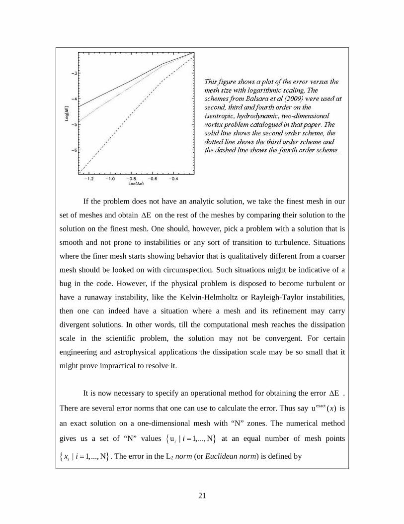
show linear variation with slope “m” as 0x∆ → . The plot below provides an example

where we have inter-compared the accuracies of various methods for numerical

hydrodynamics with order of accuracy ranging from 2 to 4. The same isentropic,

hydrodynamic, two-dimensional vortex problem was run on progressively finer meshes

using higher order schemes catalogued in Balsara et al. (2009). We see that the higher

order schemes converge to the correct solution a lot faster than the lower order schemes.

We also see that convergence is obtained only in the asymptotic limit 0x∆ → . All

schemes reach their design accuracy from below, i.e. on very coarse meshes they fall

short of their design accuracy. However, the higher order schemes seem to reach their

asymptotic convergence on much coarser meshes than the lower order schemes.

21

If the problem does not have an analytic solution, we take the finest mesh in our

set of meshes and obtain E∆ on the rest of the meshes by comparing their solution to the

solution on the finest mesh. One should, however, pick a problem with a solution that is

smooth and not prone to instabilities or any sort of transition to turbulence. Situations

where the finer mesh starts showing behavior that is qualitatively different from a coarser

mesh should be looked on with circumspection. Such situations might be indicative of a

bug in the code. However, if the physical problem is disposed to become turbulent or

have a runaway instability, like the Kelvin-Helmholtz or Rayleigh-Taylor instabilities,

then one can indeed have a situation where a mesh and its refinement may carry

divergent solutions. In other words, till the computational mesh reaches the dissipation

scale in the scientific problem, the solution may not be convergent. For certain

engineering and astrophysical applications the dissipation scale may be so small that it

might prove impractical to resolve it.

It is now necessary to specify an operational method for obtaining the error E∆ .

There are several error norms that one can use to calculate the error. Thus say exactu ( )x is

an exact solution on a one-dimensional mesh with “N” zones. The numerical method

gives us a set of “N” values { }u | 1,..., Ni i = at an equal number of mesh points

{ } | 1,..., Nix i = . The error in the L2 norm (or Euclidean norm) is defined by

22

( )2N

exact2

= 1

1E = u u ( )N i i

ix∆ −∑

The L2 norm is also sometimes referred to as the energy norm, because of its quadratic

dependence. It turns out that it is easiest to prove theorems associated with the

convergence of elliptic and parabolic equations in that norm. As a result, demonstrations

of the accuracy of schemes for elliptic or parabolic equations are always carried out in the

L2 norm. Another much-favored norm is the L1 norm and it given by

N

exact1

= 1

1E = u u ( )N i i

ix∆ −∑

The L1 norm is the norm that is preferred when demonstrating the convergence of a

solution strategy for hyperbolic systems. This is because many of the important theorems

associated with the convergence of methods for treating hyperbolic equations are proven

in the L1 norm. The L∞ norm (or maximum norm) is also quite popular and is given by

exact

= 1,...,NE = max u u ( )i ii

x∞∆ −

As one can observe, the L∞ norm predominantly depends on the small number of zones

that have maximal deviation from the exact solution. Also please note that the above

three formulae only hold in a finite difference sense. Thus if one is using a finite volume

formulation one must upgrade the formulae by taking volume integrals of the relevant

quantities within a zone. This is especially true when going beyond second order

accuracy.

2.5) The Stability of Finite Difference Approximations

23

For an arbitrarily specified PDE there is indeed no single theory that ensures that

the FDA will converge to the physical solution of the PDE. However, for linear equations

there is indeed one more attribute that we require of our FDA. That attribute is stability.

The Lax-Richtmeyer theorem guarantees the following: Given a properly posed linear

initial boundary value problem and a finite difference approximation to it that satisfies

the consistency condition, stability is then a necessary and sufficient condition for

convergence. Thus for linear systems with well-posed initial and boundary conditions a

useful mnemonic may well be :

consistency + stability = convergent scheme.

For a proof of the Lax-Richtmeyer theorem please see pages 45 to 48 of Richtmeyer and

Morton (1967). Notice though that the Lax-Richtmeyer theorem only holds for linear

systems while the Euler system, to take but one example, is decidedly non-linear. We will

see later that there are further requirements for such systems. However, the dual

requirements of consistency and stability are always required of any FDA arising from

any PDE.

Notice that in the previous paragraph we intentionally mentioned the word

“stability” without defining it. The reason is that we were trying to elicit the reader’s

natural understanding of stability. Bridges, skyscrapers, boats, cars and planes can fail if

the natural oscillations that they are liable to experience from the wind, the ground or

water cause them to jostle too much. Avoiding such situations plays an important role in

the design of such systems. Even the slightest spurious effect can excite such oscillations

in these systems and the safest design principle is to ensure that the structure of

successful bridges, skyscrapers, boats, cars and planes can damp out all possible

oscillations that they are liable to experience. A similar design philosophy applies to the

design of successful FDAs for PDEs. The fact that computers have finite precision means

that discretization errors can, in and of themselves, excite such spurious oscillations on an

ever so small scale in any numerical method. Unwanted oscillations can also arise from

imperfectly specified initial conditions, large fluctuations in the solution itself, the

24

presence of source terms and an imperfect specification of the boundary conditions. In

other words, Murphy’s law applies and whatever can go wrong will go wrong. The

purpose of stability analysis is to protect our solution process from such errors. It turns

out that the same “linear stability analysis” that one uses for ensuring the stability of

physical systems can also be applied to a numerical scheme, as was first shown by Crank

and Nicholson (1947) and Charney, Fjørtoft and von Neumann (1950). In honor of von

Neumann, the stability analysis of FDAs of differential equations is also known as von

Neumann stability analysis. It is also known as Fourier stability analysis.

The following example gives us our first exposure to stability analysis within the

context of ordinary differential equations. Consider the very simple ordinary differential

equation u ut σ= − with constant σ . With an initial condition u(0), it has the solution

u( ) = u(0) e tt σ− . Thus if we discretize it in time as nt n t= ∆ we realize that the exact

equation satisfies 1 u( ) = e u( )n t nt tσ+ − ∆ . Thus let us posit 1u un nλ+ = for the numerical

solution where un is the solution at time nt . Here λ is called the amplification factor

and whether a numerical scheme is stable or not depends on the value of λ produced by

our FDA. Notice that the ordinary differential equation would have given us 1 u e un t nσ+ − ∆= . Comparing λ to e tσ− ∆ also enables us to gauge the quality of our FDA.

First consider the time-explicit scheme

1u u u

n nn

tσ

+ −= −

∆ (2.12)

Inserting our ansatz, 1u un nλ+ = , in eqn. (2.12) gives us 1 tλ σ= − ∆ . Thus if the initial

condition is 0u we have the solution after “n” time steps at time nt given by 0u un nλ= .

Notice that 0λ ≥ only when 1t σ∆ ≤ . Since the physical solution remains positive, we

might demand that the numerical solution does the same. Say we demand a more relaxed

condition for stability by saying that the amplitude of the solution should at least decay

exponentially in time. Our relaxed stability condition requires 1λ ≤ so that we get the

25

timestep restriction: 2t σ∆ ≤ . Fig. 2.5a shows the variation of λ with t∆ for the time-

explicit scheme. We see, therefore, that the stability analysis restricts the time step of the

time-explicit FDA in eqn. (2.12) if the scheme is to remain stable.

Next consider the time-implicit scheme

1

1u u un n

n

tσ

++−

= −∆

(2.13)

It yields ( )1 1 tλ σ= + ∆ . Fig. 2.5b shows the variation of λ with t∆ for the time-

implicit scheme. Notice that the time-implicit scheme gives us 0 1λ< < for all non-zero,

finite values of the time step t∆ . The time-implicit FDA in eqn. (2.13) is, therefore,

unconditionally stable (also known as A-stable) for all values of the time step t∆ . We

also see from Fig. 2.5b that λ approximates e tσ− ∆ quite closely. We say, therefore, that

the time-explicit scheme has a rather small domain of stability whereas the time-implicit

scheme is unconditionally stable.

2.6) von Neumann Stability Analysis for Linear Parabolic Equations

The Lax-Richtmeyer theorem from the previous section gives us a large measure

of confidence when inventing numerical methods for linear problems. In the real world

there are only a few systems of interest that are governed by linear PDEs. The constant

26

coefficient heat conduction equation, Maxwell’s equations in a vacuum, the linearized

shallow water equations and the linearized acoustics equations form a small set of

physically useful linear PDEs. However, most of the problems we care about are non-

linear, small perturbations to constant mean states in such problems also result in linearly

evolving fluctuations, recall Section 1.5. For problems with non-linearities, the Lax-

Richtmeyer theorem is still a necessary condition for obtaining a physical solution,

though it may not be sufficient. As a result, all the systems of interest to us still do need

to meet the three considerations that are stipulated by the Lax-Richtmeyer theorem : (a)

The initial and boundary conditions should be correctly specified. (b) The numerical

method should be consistent, a requirement that is easily met if the scheme is accurate

enough (or at least first order accurate). (c) The numerical method should be stable; and a

demonstration of stability is usually a little harder. The further study in this chapter will

focus on linear equations and their stability. In the next two sub-sections we study linear,

scalar parabolic equations. Sub-section 2.6.1 presents the stability analysis for time-

explicit linear parabolic equations. Sub-section 2.6.2 presents the stability analysis for

time-implicit and semi-implicit linear parabolic equations. Sub-section 2.6.3 presents an

improvement on the methods of the previous sub-section. Sub-section 2.6.4 serves to

remind us that the boundary conditions for parabolic equations have to be set carefully.

Sub-section 2.6.5 gives us an introduction to the matrices that arise in the course of

solving parabolic problems implicitly.

2.6.1) Stability Analysis for Time-explicit Linear Parabolic Equations

Let us consider the linear heat conduction equation in one dimension. It is given

by u ut xxσ= where σ is a positive, constant coefficient. We discretize the problem on a

uniform mesh with zone size x∆ and take time steps of fixed size t∆ . The spatial mesh

points are located at jx j x= ∆ with j being an integer, as shown in Fig. 2.4a. A

numerical scheme that is first order accurate in time and second order accurate in space is

given by eqn. (2.9) and the update equation that evolves the solution from nt to 1n nt t t+ = + ∆ can be written as

27

( )11 1u u u 2u + un n n n n

j j j j jµ++ −= + − (2.14)

where we define 2 t xµ σ≡ ∆ ∆ for the rest of this section. Thus if the initial and

boundary conditions are properly specified, applying eqn. (2.14) to each and every mesh

point will advance the mesh by one time step and multiple time steps should advance the

solution to any time point that we desire. For the purposes of a von Neumann stability

analysis, it is easiest to assume that the domain is infinite, i.e. we are wishing away the

complexities associated with realistic boundary conditions. While von Neumann stability

analysis can also be carried out on a finite mesh with physical boundaries, we keep our

present study as simple as possible. An infinite system should be translation-invariant

and, as we know from having analyzed other physical systems, carrying out a stability

analysis consists of finding the eigenmodes at which the system naturally oscillates. In

view of the linearity of eqn. (2.14) and the translation invariance of the model problem, it

is natural to use Fourier modes for our eigenmodal analysis. The linearity of eqn. (2.14)

ensures that there is no mode mixing. As a result we write our conjectured eigenmodal

solutions at times nt and 1nt + as

k k 1 1

k ku =U e ; u =U ej ji x i xn n n nj j

+ + (2.15)

Note that for each wavenumber “k” and time step “n”, the modal weight kUn is a single

number. Also note that for the rest of this chapter 1i ≡ − . Writing k k 1 ku =U e ji x i xn n

j+ ∆

+

and k k 1 ku =U e ji x i xn n

j− ∆

− , substituting them in eqn. (2.14) and eliminating a common

factor of k e ji x gives

( ) ( )1 k k k k k

2k

U = U 1 e 2 + e = U 1 2 cos (k ) 1

= U 1 4 sin ( k / 2)

n n i x i x n

n

x

x

µ µ

µ

+ ∆ − ∆ + − + ∆ − − ∆

(2.16)

28

The last equation in eqn. (2.16) shows that our conjecture that Fourier modes might

indeed be the appropriate eigenmodes was borne out. We can, therefore, define an

amplification factor for our FDA in eqn. (2.14) as

1

2kFDA

k

U(k) = 1 4 sin ( k / 2)U

n

n xλ µ+

≡ − ∆ (2.17)

We can also define an amplification factor for the same eigenmode when it is evolved

using the original PDE. We see that it is given by

2

2 22 (k )

k (k )PDE (k) = e = e = e

txt xx

σσ µλ

∆ − ∆ − ∆ − ∆∆ (2.18)

Notice that the discreteness of the computational mesh limits the number of wave

numbers that we need to consider. Since features with a wavelength that is smaller than

2 x∆ cannot be represented on a mesh, we realize that we only need to restrict attention

to the range of wave numbers “k” given by k xπ π− ≤ ∆ ≤ . Eqn. (2.18) shows us that

PDE (k) 1λ ≤ so that the solution obtained from the PDE is unconditionally stable for all

choices of the wavenumber “k” and time step t∆ . However, Eqn. (2.17) shows us that

FDA (k) 1λ ≤ is not valid for all values of “µ” and all permissible values of “k”. We,

therefore, say that the time-explicit scheme in eqn. (2.14) is only conditionally stable and

that stability only obtains when 1 2µ ≤ , which is equivalent to ( )2 2 t x σ∆ ≤ ∆ . Notice

that for a given choice of mesh, restricting µ is tantamount to restricting the timestep.

Figs. 2.6a, 2.6b and 2.6c show the amplification factors for the PDE (shown as a solid

curve) and its time-explicit FDA (shown as a dashed curve) for 0.25, 0.5 and 1.5µ =

respectively. Since the amplification factors are symmetric, we only plot them over the

range 0 k x π≤ ∆ ≤ . We see that FDA (k)λ always differs from PDE (k)λ showing that

the FDA always differs at least a little from the original PDE, a fact that will also be true

for time-implicit formulations. The extent to which FDA (k)λ approximates PDE (k)λ

determines the goodness of our FDA. In the long wavelength limit, i.e. when k 0→ , we

29

see that FDA (k) 1λ → . This is what we expect from any consistent and stable scheme

because Fourier modes with wavelengths that are much larger than the mesh size should

indeed be accurately represented on the mesh. By observing Fig. 2.6b at k x π∆ = we

see that 0.5µ = is marginally stable. Fig. 2.6c clearly shows that 1.5µ = is unstable for a

large range of wave numbers. Observe from Fig. 2.6c that the wavelengths that go

unstable are indeed the shortest wavelengths and we will see this trend borne out even in

simulations where the constraints on the time step are violated.

The von Neumann stability analysis also plays an important role in determining

the behavior of numerical schemes. To make that connection between the stability

analysis and numerical scheme design we present numerical examples here. These

examples illustrate the difference in the numerical results when the dictates of the

stability analysis are respected and when they are violated. We solve the heat equation on

a 64 zone mesh spanning the unit interval [ ]0,1 . The variables are collocated at the

vertices of the zones, as shown in Fig. 2.4a. The heat conduction coefficient σ was set to

unity. A pulse of unit height was set up in the domain [ ]0.4,0.6 . The boundaries were

held to zero so that we have 0 64u u 0n n= = for all time steps “n” . The Dirichlet boundary

conditions that we have chosen are most easily implemented on a face-centered mesh like

the one shown in Fig. 2.4a, making it the natural choice for this problem. The problem

was solved to a final time of 0.05. Figs. 2.7a and 2.7b each show the solution at

0, 0.01 and 0.05t = . Fig. 2.7a corresponds to 0.4µ = , which is stable and Fig. 2.7b

30

corresponds to 0.5008µ = , which is unstable. Fig. 2.7a shows that the solution remains

smooth and well-behaved during the course of its evolution, a behavior that is consistent

with a numerically stable treatment of the heat conduction problem. By contrast, Fig.

2.7b shows that the solution becomes oscillatory and that the oscillations increase with

time when the stability limits are violated. For larger values of µ the solution can even

become negative in certain parts of the computational domain, showing that violating the

stability limit for the FDA indeed does produce a spurious solution. Notice the explosive

growth on small scales in Fig. 2.7b, and please do make the connection that Fig. 2.6c

predicts that the amplification factor would have its largest growth for modes with the

smallest wavelengths.

Notice that the PDE u ut xxσ= with u( , 0) = Q ( )x t xδ= as the initial condition

and u( , ) = 0x t= ±∞ as the boundary condition has a similarity solution given by

2

1/2

Qu( , ) = Exp (4 ) 4

xx tt tπ σ σ

−

(2.19)

Here ( )xδ is the Dirac-δ function. While this is not exactly the problem whose solution

is shown in Fig. 2.7, we point out that it is quite similar. The connection becomes tighter

31

when one points out that “Q” measures the amount of thermal energy contained in

physical space and that the total energy is conserved, i.e. for all times 0t ≥ we have

u( , ) dx = Qx

x t∞

=−∞∫ (2.20)

Eqn. (2.20) also holds on finite domains as long as the fluxes at the physical boundaries

are negligible. Our simulation will, therefore, be most consistent with the physics of the

problem if it respects the conservation principle in a discrete fashion. This can be made

self-evident for the solution strategy explored in this sub-section by writing eqn. (2.14) in

the conservation form given by

( ) ( ) ( )1 111/2 1/2 1/2 1/2

u u u uu u f f where f and f

n n n nj j j jn n n n n n

j j j j j jtx x x

σ σ+ −++ − + −

− −∆= + − = =

∆ ∆ ∆

(2.21)

We see, therefore, that our solution strategy also respects a conservation principle so that

the discrete analogue of eqn. (2.20) is also satisfied. For the simple case of an infinite

computational domain, the reader should now find it easy to show that the thermal energy

is conserved from one timestep to the next, i.e.

1u u n nj j

j jx x

∞ ∞+

=−∞ =−∞

∆ = ∆∑ ∑ (2.22)

For a finite computational domain with fluxes at the boundaries, eqn. (2.22) would of

course have to be modified to include the effect of the fluxes from the boundaries.

2.6.2) Stability Analysis for Time-implicit and Semi-implicit Linear Parabolic

Equations

In this sub-section we focus on the same heat conduction problem u ut xxσ= that

we studied in the previous sub-section. As in the previous sub-section, we will carry out

32

our von Neumann stability analysis on an infinite, uniform, one-dimensional mesh

without regard to boundary conditions. The only change consists of using the time-

implicit FDA given in eqn. (2.10). The update equation that evolves the solution from nt

to 1n nt t t+ = + ∆ can be written as

( )1 1 1 11 1u u 2u + u un n n n n

j j j j jµ+ + + ++ −− − = (2.23)

where, as before, we have 2 t xµ σ≡ ∆ ∆ . Notice that the terms that represent the second

derivative u xx have been moved over to the left hand side of eqn. (2.23) to emphasize

that the solution procedure is time-implicit. As before, notice that eqn. (2.23) is still in

flux conservative form because it can be written as

( ) ( ) ( )1 1 1 11 11 1 1 1 1

1/2 1/2 1/2 1/2

u u u uu u f f where f and f

n n n nj j j jn n n n n n

j j j j j jtx x x

σ σ+ + + ++ −+ + + + +

+ − + −

− −∆= + − = =

∆ ∆ ∆

(2.24)

The eigenmodal solutions are still specified by eqn. (2.15). Writing k k 1 11 ku =U e ji x i xn n

j+ ∆+ +

+

and k k 1 11 ku =U e ji x i xn n

j− ∆+ +

− , substituting them in eqn. (2.23) and eliminating a common

factor of k e ji x gives us

+1 2

k kU 1+4 sin ( k / 2) = Un nxµ ∆ (2.25)

which enables us to obtain the amplification factor for the time-implicit FDA in eqn.

(2.10) as

+1

kFDA 2

k

U 1(k) = = U 1+4 sin ( k / 2)

n

n xλ

µ ∆ (2.26)

33

Notice that the denominator in the previous equation is positive and always greater than

unity. Thus we have FDA0 (k) 1< λ ≤ for the time-implicit FDA, thus showing that the

scheme is unconditionally stable.

Figs. 2.8a, 2.8b and 2.8c show the amplification factors for the PDE and its time-

explicit FDA for 0.25, 0.5 and 10.0µ = respectively. Since the amplification factors are

symmetric, we only plot them over the range 0 k x π≤ ∆ ≤ . We see that the fully-

implicit scheme is unconditionally stable for all values of µ , i.e. for all values of the time

step t∆ . Note though that FDA (k)λ can be much larger than PDE (k)λ for several of the

larger values of the wave number “k”. Consequently, while stability is ensured by the

numerical scheme in eqn. (2.10) we are not ensured that the method will be highly

accurate. Fortunately, when dealing with parabolic PDEs, we realize that all modes are

damped, with the high frequency modes being damped the most. Consequently, it is

possible to defend the position that the loss of accuracy does not influence the quality of

the solution too much as long as the method is unconditionally stable.

Let us now consider the same numerical example that we used in the previous

sub-section. Figs. 2.9a and 2.9b show the solution obtained at various times with the

time-implicit scheme using = 6.55 and 32.75µ respectively. We see that regardless of

the value of µ, the solution is stable and free of any of the unphysical wiggles that we

observed in Fig. 2.7b. Figs. 2.9a and 2.9b show us that the unconditional stability

34

predicted by the von Neumann stability analysis is indeed borne out by our numerical

example.

We now turn our attention to the semi-implicit scheme obtained by setting

1/ 2α = in eqn. (2.11). The update equation that evolves the solution from nt to 1n nt t t+ = + ∆ can be written as

( )( ) ( )1 1 1 11 1 1 1u 1 u 2u + u u + u 2u + un n n n n n n n

j j j j j j j jµ α µα+ + + ++ − + −− − − = − (2.27)

Notice that with 1/ 2α = the time derivative in eqn. (2.11) becomes symmetric about

time 1/2 / 2n nt t t+ = + ∆ , making the scheme second order in time. Eqn. (2.27) with

1/ 2α = is known as the Crank-Nicholson scheme (Crank and Nicholson 1947). It is

more accurate than the fully explicit and fully implicit schemes that we have studied

before, making it very interesting to us. The eigenmodal analysis using solutions

specified by eqn. (2.15) gives us

( )

2+1k

FDA 2k

1 4 sin ( k / 2)U(k) = = U 1+ 4 1 sin ( k / 2)

n

n

x

x

µ αλ

µ α

− ∆ − ∆

(2.28)

35

When 1/ 2α ≥ the scheme is conditionally stable for ( )1 2 4µ α< − . When 1/ 2α < the

scheme is unconditionally stable. Figs. 2.10a, 2.10b and 2.10c show the amplification

factors for 0.25, 0.5 and 10.0µ = respectively. Fig. 2.10b shows us the very interesting

result that when 0.5µ = the amplification factors for the FDA and PDE almost coincide,

showing the value of the second order of accuracy. Fig. 2.10c, however, shows us that for

large values of µ we have a substantial range of wave numbers that have an

amplification factor that is very close to −1 . This is not a desirable feature of the semi-

implicit scheme because it shows that the scheme is not effective in damping out a large

range of small-scale wavelengths.

Let us consider the same numerical example that we used in the previous sub-

section one more time. Figs. 2.11a and 2.11b show the solution obtained at various times

with the Crank-Nicholson scheme using = 3.5 and 10.0µ respectively. Fig. 2.11a shows

that with values of µ that are not too large the scheme indeed produces physical results.

However, Fig. 2.11b shows that for large values of µ the Crank-Nicholson scheme

indeed does produce unphysical wiggles. Since the scheme is unconditionally stable we

do observe that those wiggles die out as time progresses. In other words, notice that the

late time solution, shown by the dotted curve in Fig. 2.11b, has smaller wiggles than the

early time dashed curve in Fig. 2.11b. However, as was shown in Fig. 2.10c , the half-

implicit scheme is not very effective at damping out these small scale wiggles. The

36

numerical example therefore shows us that our anticipation from the von Neumann

stability analysis in Fig. 2.10 is indeed borne out in our numerical example. Fig. 2.11b

further shows us that the utility of the half-implicit scheme is limited.

A final observation about parabolic terms in PDEs is worth making here. Notice

that a time-explicit treatment of PDEs with parabolic terms require 2t x∆ ∝ ∆ . Thus as

the mesh is refined, i.e. as x∆ becomes smaller and smaller, the time step can become

unacceptably small, making a strong case in favor of time-implicit treatments. Typical

PDEs of interest in science and engineering have both a hyperbolic part and a parabolic

part. Our study of numerical methods for hyperbolic PDEs in the next section will show

us that the timestep is proportional to the mesh size, i.e. t x∆ ∝ ∆ . Thus the timestep has a

favorable scaling as the mesh is refined and we wish to retain that favorable scaling for

PDEs that combine hyperbolic and parabolic parts. The parabolic terms in such situations

are almost always treated with time-implicit methods. An interesting exception arises

when the parabolic time step is smaller than the hyperbolic time step by a modest factor,

a situation that is often encountered in several applications. In such situations there are

very interesting Super TimeStepping techniques for retaining the time-explicit nature of

the parabolic update while taking a time step that is as large as the hyperbolic time step

(Meyer, Balsara & Aslam 2012, 2013).

37

2.6.3) Stability Analysis for the Time-implicit TR-BDF2 Method

The previous section showed us that the Crank-Nicholson scheme, despite its

second order accuracy, might suffer from some deficiencies. Specifically, Fig. 2.11b

showed us that unphysical spikes can appear in problems with discontinuous initial

conditions. It turns out that it is futile to search for a second order scheme that corrects

this problem while requiring only one matrix inversion per time step. However, the TR-

BDF2 scheme is a two stage method that is indeed second order accurate and overcomes

the deficiencies of the Crank-Nicholson method. This is achieved at the cost of two

matrix inversions per time step. The method was first presented by Bank et al. (1985) but

the variant we present here is from Tyson et al. (2000). The first stage uses a trapezoidal

update that evolves the solution a half step as follows:

( ) ( )1/2 1/2 1/2 1/21 1 1 1u u 2u + u u + u 2u + u

4 4n n n n n n n nj j j j j j j j

µ µ+ + + ++ − + −− − = − (2.29)

This accounts for the TR part of the acronym. The second stage is a second order

accurate backward difference formula (acronym BDF2) that uses the original solution

and the solution from the previous equation to get

( )1 1 1 1 1/21 1

1 4u u 2u + u u u3 3 3

n n n n n nj j j j j j

µ+ + + + ++ −− − = − + (2.30)

Eqns. (2.29) and (2.30) together specify the TR-BDF2 scheme. The scheme is also very

useful when dealing with stiff source terms in addition to the parabolic terms.

The von Neumann stability analysis for a two stage scheme is most easily

accomplished by asserting the same Fourier dependence for the intermediate stage in eqn.

(2.29) to get

38

2+1/21/2 k

2k

1 sin ( k / 2)U(k) = = U 1+ sin ( k / 2)

nn

n

x

x

µλ

µ+

− ∆ ∆

(2.31)

Compare the previous equation with eqn. (2.28) to see how it was derived. The final

amplification factor for the TR-BDF2 scheme is then given by

( )( )

1/2+1k

FDA 2k

4 (k) 1 3U(k) = = U 1+ 4/3 sin ( k / 2)

nn

n x

λλ

µ

+ −

∆ (2.32)

Again, comparing the previous equation with eqn. (2.26) proves useful.

Fig. 2.12a, 2.12b and 2.12c show the amplification factors with

0.25, 0.5 and 10.0µ = respectively. Comparing these results with Figs. 2.8a and 2.8b,

we see that the amplification factors show a substantial improvement over the fully

implicit scheme from the previous sub-section. Comparing Fig. 2.12c with Fig. 2.10c we

see that the magnitude of the amplification factor is much smaller for the short

wavelength modes when the TR-BDF2 scheme is used. As a result, the scheme swiftly

damps out the modes that need to be damped out when large time steps are taken. A

comparison with Fig. 2.8c shows that the damping will, however, not be as rapid as in a

fully implicit scheme. Fig. 2.13a and 2.13b show the solution of the same numerical

example as before, this time with = 6.55 and 32.75µ respectively. We see that Fig.

39

2.13b shows a very substantial improvement over Fig. 2.11b. The solution at an early

time of 0.01 in Fig. 2.13b still shows some small deficiencies stemming from the fact that

the scheme has not damped all the short wavelength modes as rapidly as is required by

the PDE; but the emergence of spurious spikes is eliminated.

2.6.4) Boundary Conditions for Parabolic Equations

By examining u ut xxσ= along with eqn. (2.23) notice that the FDA looks very

much like that of the one-dimensional Poisson equation. It should, therefore, not be

surprising that the boundary conditions that we utilize for parabolic equations closely

parallel the boundary conditions for elliptic equations. As with elliptic equations, at any

given time we can specify the value of the solution “u” at a boundary. This leads to

Dirichlet boundary conditions. Alternatively, we could specify the gradient of the

solution in the direction that is perpendicular to the boundary, yielding the Neumann

boundary conditions. For our simple, one-dimensional problem this is tantamount to

specifying “ u x ” at the boundary. The most general boundary condition is referred to as a

mixed boundary condition, also known as the Robin boundary condition. It consists of

specifying a linear combination of the solution and its gradient along the normal to the

bounding surface at any given time in the solution process. Thus at the left and right

40

boundaries of our one-dimensional example we can specify mixed boundary conditions

by demanding

a u + b u = c ; a u + b u = cl x l l r x r r (2.33)

where the “l” and “r” subscripts denote the left and right boundaries respectively. Notice

that mixed boundary conditions are general enough to subsume Dirichlet and Neumann

boundary conditions.

The only other boundary condition that one should be mindful of occurs at

periodic boundaries. Note that when a periodic boundary condition is asserted, it applies

to the all points on the face of a computational domain. Since one face is periodically

mapped to another face, it reduces the degrees of freedom on the mesh.

2.6.5) Introduction to Matrix Methods for Parabolic Equations

Observe from eqns. (2.23) or (2.27) that the structure of the left hand sides of

those equations calls for an implicit solution. In this sub-section we focus on eqn. (2.23).

Say that we divide a one-dimensional domain into J zones of equal size and let us also

assume that the data is collocated at zone faces, as shown in Fig. 2.4a. The initial

conditions can be specified by providing any reasonable set of values at all the zones of

the mesh at 0t = . The finite difference form of the boundary conditions in eqn. (2.33)

yields

1 1 1 1

0 1 1(b a ) u + a u = c ; a u + (b a ) u = cn n n nl l l l r J r r J rx x x x+ + + +

−∆ − ∆ − ∆ + ∆ (2.34)

The boundary conditions provided by eqn. (2.34) have to be satisfied simultaneously with

eqn. (2.23) with j ranging from 1 to J−1 . The coefficients in eqn. (2.34) can vary as time

progresses. Thus one has to solve a matrix equation of rank J+1 given by

41

10

111

122

111

1

b a a cu(1 2 ) uu

(1 2 ) uu =

... ... ... ..(1 2 ) uu

a b a cu

nl l l l

nn

nn

nnJJ

nr r r rJ

x x

x x

µ µ µµ µ µ

µ µ µ

+

+

+

+−−

+

∆ − ∆ − + − − + − − + −

− ∆ + ∆

(2.35)

Only the non-zero parts of the above matrix have been filled in. We see that the matrix

that has to be inverted is a sparse, banded matrix. As long as the matrix is non-singular it

can be solved. Notice too that if the boundaries had been specified to be periodic, the top

right and bottom left elements of the above matrix would have non-zero terms and the

rank of the matrix would be reduced by one.

Eqn. (2.35) gives us our first glimpse of the banded matrices that have to be

inverted when solving parabolic equations. For two-dimensional and three-dimensional

problems the matrices will have block-diagonal form. Fig. 2.14 shows a schematic

example of the sort of sparse, block-diagonal matrix that results when solving two-

dimensional problems. The lines denote non-zero bands. Such matrices are known as

sparse matrices and there are several excellent sparse matrix solution methods that are

available. Fig. 2.14 shows us that most of the matrix elements of sparse matrices are zero.

Thus their representation on a computer should avoid allocating storage for the zero

elements. There are several sparse matrix storage formats for storing just the non-zero

elements of sparse matrices on a computer.

42

The solution of the sparse matrices that result from discretization of PDEs is a

major research enterprise in itself. Fortunately, there are several popular and efficient

solution methods available to us. Matrix solution methods fall into two classes. There are

direct matrix solution methods which attempt to arrive at an exact solution of the matrix

in a finite number of steps. Well-designed direct solvers are available in packages like

ScaLAPACK and SuperLU. Iterative matrix solution methods also exist and they attempt

to solve the matrix problem to a specified accuracy by a sequence of iterative steps. The

MUDPACK, MGNet, PETSc, Trilinos and HYPRE packages provide a very nice

collection of well-designed iterative methods. Each iterative step in such methods is

designed to have a low operation count, however, if one wishes to reduce the error by

several orders of magnitude, the number of iterations can be rather large. The

convergence of iterative solvers is strongly influenced by one’s choice of a

preconditioner. The preconditioner is usually a method that replaces the original matrix

with an approximate matrix whose solution is more easily found. Preconditioning the

solution is often tantamount to removing small wavelength errors in the solution.

Selecting a good physics-based preconditioner is one of the most critical steps when

iterative methods are used.

Picking the right accuracy for a problem is an art in itself when iterative methods

are used, and the computationalist’s intuitive understanding of the physical problem can

43

play a large role in that process. It must also be mentioned that there are several perfectly

good, computationally inexpensive iterative methods that don’t necessarily converge for

each and every problem that they might be applied to. The few iterative methods that do

guarantee convergence can also be prohibitively expensive at times. As a result, matching

the right iterative method to the physical problem is quite an art. With all this said, the

cautious computationalist might be inclined to confine himself to the use just the direct

solution methods. It is, therefore, worth mentioning that iterative methods offer much

better performance as the problem size is scaled up. Their memory footprint is usually

much smaller. They also parallelize very well, making them an essential part of our study

in the ensuing chapters.

The Connection Between Parabolic Equations and Elliptic Equations

There is an intimate connection between solution techniques for elliptic equations

and parabolic equations. We develop that connection here. Thus consider Poisson’s

problem for a self-gravitating object in one dimension, u 4 G xx π ρ= . To make our study

interesting, let us also say that we wish to solve it on a mesh with “J” zones of size x∆ .

To illustrate facets of the solution process that we have not brought out so far, let us use

periodic geometry. As with parabolic equations, we wish to use a face-centered mesh so

that our mesh function is given by { }0 1 1u , u ,..., u , uJ J− . Periodic geometry requires that

0u u J= which reduces our degrees of freedom. The integral compatibility condition

(also known as the Jeans swindle in astrophysics) that applies to periodic geometries also

requires 0ρ = , where the averaging is done over the mesh. This ensures that the

gravitational acceleration is towards the over-dense regions in the computational domain

and away from the under-dense regions. With the periodic boundary conditions, 0u u J= ,

we have the following FDA: 2

1 2 12

1 1

21 1

u 2 u u 4 G for 1u 2 u u 4 G for 2 1

u 2 u u 4 G for

J

j j j j

J J J

x jx j J

x j J

π ρ

π ρ

π ρ− +

−

− + − = − ∆ =

− + − = − ∆ ≤ ≤ −

− + − = − ∆ =

The discretization of the Poisson equation with periodic boundary conditions then yields

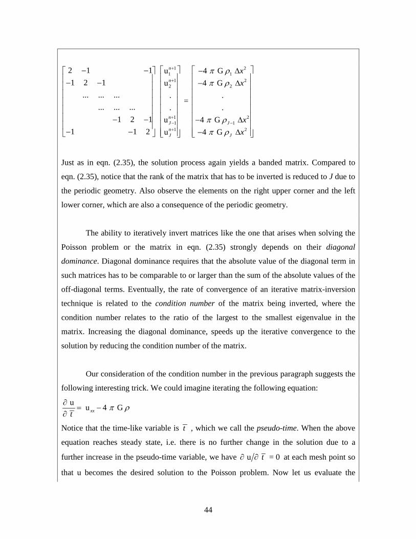
44

1 2

1 11 2

2 2

1 21 11 2

2 1 1 u 4 G 1 2 1 u 4 G

... ... ... . . =

... ... ... . .1 2 1 u 4 G

1 1 2 u 4 G

n

n

nJ JnJ J

xx

xx

π ρπ ρ

π ρπ ρ

+

+

+− −+

− − − ∆ − − − ∆ − − − ∆

− − − ∆

Just as in eqn. (2.35), the solution process again yields a banded matrix. Compared to

eqn. (2.35), notice that the rank of the matrix that has to be inverted is reduced to J due to

the periodic geometry. Also observe the elements on the right upper corner and the left

lower corner, which are also a consequence of the periodic geometry.

The ability to iteratively invert matrices like the one that arises when solving the

Poisson problem or the matrix in eqn. (2.35) strongly depends on their diagonal

dominance. Diagonal dominance requires that the absolute value of the diagonal term in

such matrices has to be comparable to or larger than the sum of the absolute values of the

off-diagonal terms. Eventually, the rate of convergence of an iterative matrix-inversion

technique is related to the condition number of the matrix being inverted, where the

condition number relates to the ratio of the largest to the smallest eigenvalue in the

matrix. Increasing the diagonal dominance, speeds up the iterative convergence to the

solution by reducing the condition number of the matrix.

Our consideration of the condition number in the previous paragraph suggests the

following interesting trick. We could imagine iterating the following equation:

u u 4 G xxt

π ρ∂= −

∂

Notice that the time-like variable is t , which we call the pseudo-time. When the above

equation reaches steady state, i.e. there is no further change in the solution due to a

further increase in the pseudo-time variable, we have u = 0t∂ ∂ at each mesh point so

that u becomes the desired solution to the Poisson problem. Now let us evaluate the

45

salutary effect that the inclusion of a pseudo-time variable has on the matrix. We see that

eqn. (2.35) is more diagonally dominant than the matrix equation that results from the

Poisson problem. Thus inclusion of a pseudo-time variable accelerates the convergence

of the iterative method that is used for matrix inversion. Each iteration can then be

thought of as a fully-implicit time step in the pseudo-time variable. The boundary

conditions are kept fixed throughout this iteration process. Convergence is reached when

the change in the mesh function after each successive iteration becomes smaller than a

pre-specified tolerance. Thus we can solve Poisson’s problem with an iterative method

more easily by treating it as a parabolic problem that has to be iterated to a time-

stationary state by using a pseudo-time variable.

2.7) von Neumann Stability Analysis of Linear Hyperbolic Equations

The previous section has shown that the von Neumann stability analysis of FDAs

of parabolic PDEs yields several insights that are directly applicable to their numerical

solution. We now turn to the von Neumann stability analysis of FDAs for hyperbolic

PDEs. We start with the linear, scalar advection equation u a u 0t x+ = . For the sake of

simplicity, we set “a > 0”. The previous chapter has shown that the solution of such a

PDE evolves along characteristics given by 0 a x x t= + in the x,t-plane, as shown in Fig.

2.15. Thus given an initial condition ( )0u x for all locations on the x-axis at time 0t = ,

the solution at a later time is simply given by ( ) ( )0u , u a x t x t= − . I.e., with a>0 we just

slide the original profile to the right along the x-axis with a speed given by “a”. Notice

that the one-dimensional solution propagates as a shape-preserving wave because the

characteristics are parallel straight lines in space-time. When solving the problem on a

finite computational domain, one has to consider the role of boundary conditions. The

fact that the solution only propagates along characteristics also implies that the solution

should be specified at the boundaries where characteristics come into the computational

domain, known as inflow boundaries. However, the solution is completely determined at

boundaries where the characteristics flow out of the computational domain, known as

46

outflow boundaries. Thus we should be mindful never to over-specify the boundary

conditions for a hyperbolic problem.

Notice that the advection equation is very similar in form to the equation that was

discretized in eqn. (2.1). As a result, we will use a zone-centered mesh like the one shown

in Fig. 2.4b. Thus we have a uniform mesh with zone size x∆ with zone-centers located

at ( )1/ 2jx j x= − ∆ . We wish to evolve the solution with time steps of size t∆ at time

points given by nt n t= ∆ . Here j and n are taken to be integers. As in the previous

section, we simplify the dependence on boundary conditions by analyzing the problem on

an infinite domain. Consequently j ranges from −∞ to ∞ . To help us guess at the form

of the amplification factor for the FDAs explored here, let us first evaluate the

amplification factor for the PDE. The advection problem is linear so we don’t expect any

mode mixing. Recall from eqn. (2.15) that it might again be acceptable to use Fourier

modes for our eigenmodal solutions. The amplification factor of the PDE is then given by

a (k )

a k (k )PDE (k) = e = e = e

ti xi t i xx µλ

∆ − ∆ − ∆ − ∆∆ (2.36)

where we define a t xµ ≡ ∆ ∆ for the rest of this section. Notice from eqn. (2.36) that the

amplification factor is complex, which is as it should be for any wave-like solution. From

eqn. (2.36) we infer that

[ ][ ]

PDE

PDE1PDE

PDE

(k) = 1 k

Im (k)(k) tan k a

Re (k)t

λ

λθ

λ−

∀

≡ = − ∆

(2.37)

The first part of eqn. (2.37) shows that the PDE for the advection equation is not

dissipative, i.e. the amplitude of the eigenmode propagates undiminished. The second

part of eqn. (2.37) shows that the PDE is not dispersive, i.e. waves with all possible

wavelengths propagate with the same speed. As a result, we expect our FDAs of the

advection equation to have a complex amplification factor. A good numerical scheme for

47

hyperbolic equations should minimize dissipation and dispersion. In the next few sub-

sections we go through the von Neumann stability analysis for several schemes that will

give us insight into the treatment of hyperbolic PDEs.

The ensuing five short sub-sections explore the schemes that interest us here. Sub-

sections 2.7.1, 2.7.2, 2.7.3, 2.7.4 and 2.7.5 explore the forward Euler scheme, the Lax-

Friedrichs scheme, the Lax-Wendroff scheme, the two-step Runge-Kutta scheme and the

donor cell scheme respectively. Sub-section 2.7.6 summarizes the insights gained in the

previous sub-sections.

2.7.1) Forward Euler Scheme (Never Used)

Let us now attempt our first, and most naïve, discretization of the advection

equation.

( )1

1 1 11 1

u u u u = a u = u u u

2 2

n n n nj j j j n n n n

j j j jt xµ+

+ − ++ −

− −− ⇔ − − ∆ ∆

(2.38)

48

This scheme is known as the forward Euler scheme. The above scheme can be written in

a flux conservative form with fluxes that are spatially second order accurate and given by

( )1/2 1f a u + u 2n n nj j j+ += . We see, therefore, that the overall forward Euler scheme is first

order accurate in time and second order accurate in space.

We expect our FDA to have a complex amplification factor. Consequently, we

will have to analyze the amplitude and phase of the amplification factor for our FDA to

gain further insight. As before, we set k ku =U e ji xn n

j , k k 1 ku =U e ji x i xn n

j+ ∆

+ ,

k k 1 ku =U e ji x i xn n

j− ∆

− and k 1 1ku =U e ji xn n

j+ + . The amplification factor for eqn. (2.38) turns out

to be

1

FDAU(k) = = 1 sin ( k )U

nknk

i xλ µ+

− ∆ (2.39)

Notice that FDA (k) 1λ > for all wavenumbers “k” and all values of the time step t∆ so

that our forward Euler scheme in eqn. (2.38) is unconditionally unstable. We see,

therefore, that numerical methods that might initially seem very reasonable to us may

indeed turn out to be unstable.

2.7.2) Lax-Friedrichs Scheme

Now let us try the Lax-Friedrichs scheme which is given by a slight modification

of the forward Euler scheme:

( )( ) ( )

11 1

1 1 11 1 1 1

1u u u u u 12 = a u u u u u2 2 2

n n nn nj j jj j n n n n n

j j j j jt xµ

++ −

+ − ++ − + −

− + −− ⇔ = + − − ∆ ∆

(2.40)

The scheme can be written in flux conservative form, as was done in eqn. (2.1), by

writing it as

49

( ) ( ) ( )11/2 1/2 1/2 1 1

au u f f with f u + u u u2 2

n n n n n n n n nj j j j j j j j j

t xx t

++ − + + +

∆ ∆= − − = − −

∆ ∆ (2.41)

The first round bracket in the flux term 1/2f nj+ in eqn. (2.41) can be thought of as being an

averaging of the physical flux from the two zones that abut the zone boundary at 1/2jx + .

Comparing the second round bracket in the definition of 1/2f nj+ to the similar terms in eqn.

(2.21) we see that they act like a dissipative flux. This dissipative flux has a stabilizing

effect on the Lax-Friedrichs scheme. However, notice another flaw in the dissipative flux;

the amount of dissipation does not go to zero as 0t∆ → . In other words, using a Lax-

Friedrichs scheme on a mesh with a finite zone size will cause the solution to keep

diffusing regardless of how small we make the time step t∆ . We see, therefore, that an

examination of the flux form has given us an early insight into the nature and weakness

of the Lax-Friedrichs scheme.

Further insight can be obtained by writing out the amplification factor for the

scheme. We get

1

FDAU(k) = = cos ( k ) sin ( k )U

nknk

x i xλ µ+

∆ − ∆ (2.42)

We can then write

[ ]

2 2FDA

1FDA

PDE

(k) = 1 + ( 1) sin ( k )

tan tan( k )(k)(k) ( k )

x

xx

λ µ

µθθ µ

−

− ∆

∆=

∆

(2.43)

Notice that the scheme is stable for 1µ ≤ which is same as / a / at x xµ∆ ≡ ∆ ≤ ∆ .

When working with hyperbolic systems, µ is referred to as the Courant-Friedrichs-

Lewy number (also popularly referred to as the Courant number or the CFL number) in

50

honor of the people who first deciphered this stability limit, see Courant, Friedrichs &

Lewy (1928, 1967).

Let us focus on the stencil for the Lax-Friedrichs scheme and see the insights it

provides. Observe the dashed band in Fig. 2.4b for a depiction of the stencil for this

scheme. The domain of dependence coincides with the stencil. The characteristic curve

for rightward advection ( a>0 ) is also shown in Fig. 2.4b. Restricting the CFL number

ensures that our numerical domain of dependence contains the physical domain of

dependence. For a one-dimensional scalar advection problem, the physical domain of

dependence for 1unj+ is indeed the foot point of the characteristic on the x-axis at the

previous time level. Consequently, restricting the CFL number guarantees that the foot

point of the characteristic curve in Fig. 2.4b lies within the numerical domain of

dependence. This ensures that information is correctly propagated by our numerical

scheme.

Fig. 2.16 shows FDA (k)λ as a solid curve and FDA PDE(k) (k)θ θ as a dashed curve

plotted as a function of k x∆ for the Lax-Friedrichs scheme with 0.4µ = . Notice that for

long wavelength modes, i.e. when k x 0∆ → , we have FDA (k) 1λ → and

FDA PDE(k) (k) 1θ θ → . This shows that when a wave spans a large number of zones, the

Lax-Friedrichs scheme does advect the wave with fidelity. A well-behaved advection

scheme should have FDA (k) ~ 1λ and FDA PDE(k) (k) ~ 1θ θ for as large a range of

wavenumbers as possible. We see that the scheme produces large phase errors in the

propagation of waves, especially in the limit of large wave numbers (short wavelengths),

i.e. when k x π∆ → . Improper propagation of short wavelength modes can be a serious

deficiency for a scheme, especially when those waves are not rapidly damped, as is the

case for the Lax-Friedrichs scheme.

51

As with parabolic equations, we wish to show that the von Neumann stability

analysis also plays an important role in determining the behavior of numerical schemes.

We make that connection between stability analysis and numerical scheme design by

presenting numerical examples here. We therefore propagate certain profiles around the

unit interval, [ ]0.5,0.5x ∈ − . We set the propagation speed “a” to unity. The interval was

discretized with 100 zones and periodic boundary conditions were used. Periodic

boundary conditions enable us to examine the behavior of the advection scheme for long

durations of time because they allow the solution to leave the right boundary and reenter

the domain from the left boundary. Our first profile consists of a Gaussian profile

( ) ( )20.1u , 0 xx t e−= = which is plotted in Fig. 2.17a at times t=0 (solid curve), t=1(dashed

curve) and t=2(dotted curve). Thus the dashed and dotted curves in Fig. 2.17a show the

profile after it has propagated around the domain once and twice respectively. Our second

profile consists of setting ( ) [ ]u , 0 1 0.05,0.05x t x= = ∀ ∈ − and ( )u , 0 0x t = =

elsewhere. This top-hat profile is intended to mimic the shock fronts that we will have to

contend with later in this book. Consequently, we wish to advect the square wave without

generating spurious wiggles and without producing any overshoots and undershoots. The

sharp corners in the square wave imply that this profile has a significant amount of power

in Fourier modes on the smallest scale of the mesh. It is shown in Fig. 2.17b at times of

t=0 (solid curve), t=0.25 (dashed curve) and t=0.75 (dotted curve). Thus the dashed and

dotted curves in Fig. 2.15b show the profile after it has propagated through one-fourth

52

and three-fourths of the domain respectively. A CFL number of 0.4 was used in all

calculations. Fig. 2.17a shows us that the Gaussian profile undergoes a substantial

amount of diffusion, owing to the poorly controlled diffusion terms in the Lax-Friedrichs

scheme. Fig. 2.17b shows us that the square pulse also undergoes a substantial amount of

diffusion as it propagates. The large amount of diffusion is a consequence of the

scheme’s first order of accuracy in time, though it is indeed second order accurate in

space. We also see several small scale wiggles developing in the solution which is a

manifestation of the fact that the Lax-Friedrichs scheme makes large phase errors in the

propagation of small wavelengths. The small scale wiggles in Fig. 2.17b go under the

formal name of staircasing and highlight another deficiency in the Lax-Friedrichs

scheme. Notice from eqn. (2.40) that the updated mesh function in zone “j”, i.e. 1unj+ ,

only depends on 1unj+ and 1un

j− and does not depend on unj . This causes a curious

decoupling between the update of the even-indexed zones and the odd-indexed zones and

the staircasing that one observes in Fig. 2.17b is a result of this even-odd decoupling. The

Lax-Friedrichs scheme, in the form presented here, is no longer used in any practical

computations and the insights gained from Fig. 2.17b instruct us to avoid schemes that

are liable to produce even-odd decoupling.

2.7.3) The Lax-Wendroff Scheme

53

The Lax-Friedrichs scheme had the deficiency that it was not second order

accurate in time. The Lax-Wendroff scheme is derived by using the Taylor series

expansion to achieve second order accuracy in space and time, see Lax & Wendroff

(1960). The Lax-Wendroff procedure described below is worth studying because it is still

used as a building block in many useful schemes, even if the Lax-Wendroff scheme in the

form described here is seldom used. Thus one can write

21u ( , + ) = u ( , ) + u ( , ) + u ( , ) + ...2

n n n nj j t j tt jx t t x t t x t t x t∆ ∆ ∆ (2.44)

The third and higher order terms in eqn. (2.44) are truncated. The structure of the PDE

u a u 0t x+ = allows us to replace terms having temporal derivatives by terms having

spatial derivatives. Thus we set u a ut x= − and 2u a u a u a utt xt tx xx= − = − = in eqn.

(2.44) which gives us

2 21u ( , + ) = u ( , ) a u ( , ) + a u ( , )2

n n n nj j x j xx jx t t x t t x t t x t∆ − ∆ ∆ (2.45)

The corresponding FDA is then given by

( ) ( )

11 1 1 12

2

21

1 1 1 1

u u u u u 2 u + u1 = a + a 2 2

u u u u u 2 u + u2 2

n n n n n n nj j j j j j j

n n n n n n nj j j j j j j

tt x x

µ µ

++ − + −

++ − + −

− − −− ∆ ⇔ ∆ ∆ ∆

= − − + −

(2.46)

By comparing eqn. (2.46) to eqn. (2.38) we observe that the first term on the right hand

side of the first line of eqn. (2.46) would yield the forward Euler scheme, which is

unstable. The second term on the right hand side of eqn. (2.46) adds an extra t∆ -

dependent dissipation which stabilizes the forward Euler scheme. The Taylor series in

54

eqn. (2.45) shows that this extra dissipative term, which has the form 2 2a u ( , ) 2n

xx jt x t∆ , was indeed necessary.

The amplification factor for the Lax-Wendroff scheme is given by

1

2 2FDA

U(k) = = 1 sin ( k ) 2 sin ( k / 2)U

nknk

i x xλ µ µ+

− ∆ − ∆ (2.47)

We can then write

[ ]

2 2 4FDA

1FDA2

PDE

(k) 1 4 (1 ) sin ( k / 2)

(k) 1 sin ( k ) tan (k) (k ) 1 2 sin ( k / 2)

x

xx x

λ µ µ

θ µθ µ µ

−

= − − ∆

∆ = ∆ − ∆

(2.48)

The Lax-Wendroff scheme is stable for 1µ ≤ . Fig. 2.18 shows FDA (k)λ as a solid curve

and FDA PDE(k) (k)θ θ as a dashed curve plotted as a function of k x∆ for the Lax-Wendroff

scheme with 0.4µ = . We see that FDA PDE(k) (k) 0θ θ → especially in the limit of large

wave numbers (short wavelengths), i.e. when k x π∆ → . As a result, we expect short

wavelength modes in the simulations that use this scheme to propagate much slower than

the long wavelength modes. By comparing Figs. 2.16 and 2.18 we see that the smallest

value of FDA (k)λ for the Lax-Wendroff scheme is larger than that of the Lax-Friedrichs

scheme, giving the Lax-Wendroff scheme a smaller dissipation over a larger range of

wave numbers. We also see that FDA PDE(k) (k)θ θ for the Lax-Wendroff scheme is closer

to unity for a larger range of wavenumbers than that of the Lax-Friedrichs scheme,

making the Lax-Wendroff scheme less dispersive. The improved properties of the Lax-

Wendroff scheme are indeed a consequence of its second order accuracy in space and

time.

55

Figs. 2.19a and 2.19b repeat the tests with the Gaussian and square pulse that

were first shown in Figs. 2.17a and 2.17b respectively. Fig. 2.19a shows that the

Gaussian profile propagates almost flawlessly. This is because of the higher accuracy of

the Lax-Wendroff scheme and also because the Gaussian pulse does not contain much

amplitude in the small wavelength modes. Since all of the dispersion in the Lax-

Wendroff scheme occurs for small wavelength modes which are practically absent in the

Gaussian pulse, the Gaussian is advected very well. Note though that at a time of 2.0 the

Gaussian solution in Fig. 2.19a does show a very small undershoot. Fig. 2.19b shows

deficiencies mainly because the square wave contains small wavelength modes with a

significant amount of amplitude in them. Based on our Fourier analysis we expect the

propagation of the short wavelength modes to lag that of the long wavelength modes

when the Lax-Wendroff scheme is used and indeed Fig. 2.19b shows ringing modes on

small scales that trail the original pulse. In other words, the Lax-Wendroff scheme is

dispersive. Alternatively, and equivalently, we can observe that the source of the

dispersion stems from the fact that we ignored the 3u ( , ) u ( , )n nttt j xxx jx t a x t= − term in

eqn. (2.44). Thus the error term for the Lax-Wendroff scheme has the form 3u ( , )n

xxx ja x t− and such an error term contributes as a dispersion term. Fig. 2.19b shows

that the square pulse retains more amplitude than it did in Fig. 2.17b. However, it also has

the deficiency that the solution shows large overshoots and undershoots.

56

If the square pulse represented a pulse of fluid density, the Lax-Wendroff scheme

would produce negative densities, a very undesirable situation. The ability of an

advection scheme to evolve a solution in such a way that positive initial conditions

remain so for all time is called the positivity property. The Lax-Wendroff scheme clearly

lacks such a property, which can be seen by writing eqn. (2.46) as

( ) ( ) ( )1 21 1u 1 u 1 u 1 u

2 2n n n nj j j j

µ µµ µ µ++ −= − − − + + . (2.49)

For 1µ ≤ we cannot guarantee that all the coefficients of unj , 1un

j+ and 1unj− in the

equation above are positive. As a result, we cannot ensure that 1unj+ is positive for all

possible positive initial conditions. A rather pessimistic theorem by Godunov, which we

will study in the next chapter, then informs us that within the context of linear schemes,

enforcing positivity restricts the order of accuracy to first order. Godunov’s theorem

points out what the sensitive reader might have suspected all along. It tells us that the

difficulties that our second order accurate schemes experience in advecting

discontinuities might indeed be self-inflicted. Higher spatial derivatives become

progressively ill-defined at discontinuities. Yet our Taylor series in eqn. (2.45), from

57

which we indeed derived our Lax-Wendroff scheme, tries to retain all those terms. As

with the Lax-Friedrichs scheme, the Lax-Wendroff scheme shows its worst deficiencies

in propagating solutions with discontinuities.

2.7.4) The Two-stage Runge-Kutta Scheme

The two-stage Runge-Kutta scheme has many parallels to the Lax-Wendroff

scheme. Just like the Lax-Wendroff scheme, it is second order in space and time. In the

form presented here, it also suffers from deficiencies that parallel those of the Lax-

Wendroff scheme. However, we will see in the next chapter that with some small

improvements it can become one of the powerful building blocks with which we will

design successful schemes for hyperbolic PDEs. We present it in a form that reminds us

of the conservative structure of eqn. (2.1). This is intentional, because that form presages

its future use.

( ) ( )

( ) ( )

1/21/2 1/2 1/2 1

1 1/2 1/2 1/2 1/2 1/21/2 1/2 1/2 1

1u u f f with f a u u2 2

1u u f f with f a u u2

n n n n n n nj j j j j j j

n n n n n n nj j j j j j j

tx

tx

++ − + +

+ + + + + ++ − + +

∆= − − = +

∆∆

= − − = +∆

(2.50)

Thus the first stage in eqn. (2.50), which is the first line in that equation, may be

interpreted as a predictor stage. It takes the solution from nt to / 2nt t+ ∆ . The second

stage in eqn. (2.50), which is also the second line in that equation, may be interpreted as a

corrector stage. It takes the solution from nt to nt t+ ∆ by using the time-centered fluxes

provided by the first stage. The second order accuracy in time is made evident by the

time-centered fluxes in the second stage. The second order accuracy in space is also made

clear by the form of the fluxes at the zone-faces. Because each of the two stages is

conservative, the entire scheme is conservative.

The two stages in eqn. (2.50) can be combined to yield a single stage scheme

given by

58

( ) ( )2

11 1 2 2u u u u u 2 u + u

2 8n n n n n n nj j j j j j j

µ µ++ − + −= − − + − (2.51)

Comparing eqn. (2.51) to eqns. (2.45) and (2.46) makes the connection between the two-

stage Runge-Kutta scheme and the Lax-Wendroff scheme very clear. Eqn. (2.51) is the

form of the scheme that is most suitable for von Neumann stability analysis. We will not

detail a von Neumann stability analysis for the present scheme. Instead we leave that as

an exercise for the reader. Fig. 2.20 shows results from the two-stage Runge-Kutta

scheme for the two test problems that were first catalogued in Fig. 2.17. For the Gaussian

pulse in Fig. 2.20a we see that the two-stage Runge-Kutta scheme performs just as well

as the Lax-Wendroff scheme. The square wave in Fig. 2.20b shows even larger

oscillations than it did in Fig. 2.19b. The larger oscillations are a consequence of the

wider stencil that is used by the two-step Runge-Kutta scheme. Just like the Lax-

Wendroff scheme, the two-stage Runge-Kutta scheme is stable in one dimension for

1µ ≤ . In two and three dimensions its stability reduces to 1/ 2µ ≤ and 1/ 3µ ≤

respectively.

59

2.7.5) First Order Accurate Upwind Scheme (i.e. Donor Cell Scheme)

This scheme derives its name from the fact that information always flows from

the upwind direction to the downwind direction in the advection equation. We now try to

build that bit of intuition into our numerical scheme. Thus for a>0 we can write the first

order accurate upwind scheme as

1

1u u u u = a

n n n nj j j j

t x

+− − −

− ∆ ∆ (2.52)

This scheme is also known as the donor cell scheme because the upwind cell donates its

flux to the downwind cell. With a>0, realize that the zone “j-1” is upwind of the zone “j”

that is being updated in eqn. (2.52). Note that this scheme is only first order accurate in

space and time. As a result, we expect it to be strongly dissipative and dispersive. Like

the schemes in the previous four sub-sections, the upwind scheme is stable for 0 1µ≤ ≤ .

Unlike the previous schemes, all of which used a symmetrical stencil, the present scheme

uses a one-sided stencil and, therefore, contains a directional bias. Fig. 2.4b shows the

stencil. Following the style of demonstration adopted in eqn. (2.49), it can be shown that

the present scheme is positivity preserving.

The dissipation and dispersion of the present scheme are visible in Figs. 2.21a and

2.21b which show the advection of the Gaussian and square profiles that were first

presented in Fig. 2.17 . The Gaussian profile shows a substantial amount of diffusion, as

expected for a first order accurate scheme. Note though that the solution to the square

pulse is free of wiggles, showing that something useful has been achieved.

60

Notice that eqn. (2.52) only applies to cases where a>0 . We can easily upgrade it

to include both signs of the propagation speed as follows:

( ) ( ) ( ) ( )

11 1

11 1

u u u u u u = a a

a au u u u u u where a max a,0 and a min a,0

n n n n n nj j j j j j

n n n n n nj j j j j j

t x x

t tx x

+− ++ −

+ −+ + −

− +

− − −− − ⇔ ∆ ∆ ∆ ∆ ∆

= − − − − ≡ ≡∆ ∆

(2.53)

Many of the higher order upwind schemes that we will study in the next several chapters

rely on following the direction of wave propagation. Moreover, they can be thought of as

higher order extensions of the scheme presented in eqn. (2.53). Thus the structure of eqn.

(2.53) presages a fair bit of our future study.

It is also interesting to relate the donor cell scheme from this section to the

forward Euler scheme from Sub-section 2.7.1. Both schemes are temporally first order

accurate. The donor cell scheme can be written in flux conservative form with the flux

( ) ( )1/2 1 1f a u + u 2 u u 2n n n n nj j j j ja+ + += − − . The first part of this flux, i.e. the term

61

( )1a u + u 2n nj j+ , is just the flux from the forward Euler scheme; and that scheme is

unstable. The second part of this flux, i.e. the term ( )1u u 2n nj ja +− − , can be interpreted

as a diffusive term. We invite the reader to explicitly write out the contribution from this

second part of the flux and see that it acts like a diffusion term. It is this diffusive part

that renders the donor cell scheme stable. The diffusive part of the flux also makes the

donor cell scheme first order accurate in space. In the next chapter we will study methods

for mitigating the very high level of diffusion inherent in schemes that are first order

accurate in space while retaining their desirable property that they can propagate

discontinuous solutions like the top-hat profile studied here.

2.7.6) Section Summary for Hyperbolic Equations

To summarize the results from this section, we see that second order accurate

linear schemes do advect smooth profiles like the Gaussian pulse very well indeed.

However, note that they all show a deficiency when advecting discontinuous solutions.

The first order upwind scheme is the only advection scheme that we have studied so far

that does not produce spurious oscillations when advecting discontinuous solutions. Thus

a desirable scheme would be one which combines the higher order accuracy of the Lax-

Wendroff or Runge-Kutta schemes with the stabilizing properties of the first order

upwind scheme. If we keep looking for linear schemes that combine the best attributes of

the Lax-Wendroff or Runge-Kutta schemes as well as the first order upwind scheme, we

realize that such a scheme cannot exist. I.e. if we search for schemes within the strict

confines of the Lax-Richtmeyer theorem, which casts its net over all linear schemes for

linear equations, there is no way out of the dilemma that we face. Godunov’s theorem,

also suggests that within the confines of linear schemes, there is no second order accurate

positivity preserving scheme. The way out consists of non-linear hybridization , as we

will see in the next chapter. I.e. based on the local nature of the solution we pick the most

accurate scheme if the solution is smooth. If the solution begins to develop an

increasingly strong local discontinuity, we pick increasing fractions of the upwind

scheme. In the immediate vicinity of a strong jump in the solution, the solution strategy

62

should revert entirely to the upwind scheme. Doing this automatically is an art that we

will study in the next chapter. (A strong jump in the solution refers to a situation where

the jump in the solution from one zone to the next, i.e. 1u = u uj j+∆ − , is comparable to

the magnitude of the solution “u” itself. In the parlance of discontinuous functions, such a

discontinuity is referred to as an O(1) discontinuity and we speak of it as an “order-one

discontinuity”.) The advection of discontinuous solutions in a positivity preserving

fashion will be one of the topics of our study in the next chapter. We will see in that

chapter that the better non-linearly hybridized schemes also minimize directional bias.

Positivity for Parabolic Problems

The gentle reader who has put up with all these travails for the advection equation

might also want to ask whether there is a positivity property for parabolic equations.

Indeed there is. Fortunately, it only says that linear positivity-preserving schemes for the

constant coefficient heat equation are restricted to being either first or second order

accurate. Since second order accurate solutions are usually good enough, the constraints

from the positivity property are not as restrictive for linear parabolic problems. Non-

linear, solution-dependent, conduction coefficients occur quite frequently in nature and

can, however, introduce difficulties of their own.

The Modified Wave Number and its Relation to Dispersion

The discussion in the last two sections has emphasized consistency and stability

as the most important attributes of a finite difference approximation. An actual numerical

scheme will try to optimize other attributes depending on the scientific goals of the

computational scientist. A very instructive example emerges in the field of numerical

turbulence research where small scale fluid structures are generated on all scales in the

simulation of a turbulent fluid. In fact, given the high resolution flow simulations that

have become possible on modern computers, if there is a propensity for turbulent flows to

develop, they will indeed develop. The emphasis in such simulations is on capturing all

63

the wave structures that develop on all the length scales that can be reasonably

represented on a computational mesh (Lele 1992).

One would naively think that a more accurate representation of the difference

operator would yield better results; i.e. eqn (2.8) is better than eqn. (2.6) when

representing the gradient operator. To a large extent, that is true. Yet, quite interestingly,

it turns out that eqn. (2.8) does not provide the best fourth order accurate representation

of the gradient operator. To that end, let us consider the Padé approximation of the

gradient operator that is attributed to Collatz (1966)

2 2 1 1; 1 ; ; 1

u u u u u u + u

4 2j j j j

x j x j x j b ax x

α α + − + −− +

− −+ = +

∆ ∆.

With 1 3α = , 14 9a = and 1 9b = the scheme can be shown to be fourth order accurate.

Notice right away that to obtain the gradient ;u x j at any zone “j”, one has to invert a

tridiagonal system. This adds to the cost.

Since the above equation and eqn. (2.8) are both fourth order accurate, we

therefore ask whether the additional cost yields any advantage. To that end, let us analyze

the problem in Fourier space by setting u U e ji k xj k= and

; ;u U e ji k xx j x k= , just as we

did in eqn. (2.15). We can now study the Fourier representation of the gradient operator

for the fourth order Padé approximation and the explicit fourth order difference operator

from eqn. (2.8). Realize, therefore, that for exact differentiation we can write

;

exact

U U

x k

k

ki

=

.

For the fourth order central finite difference approximation in eqn. (2.8) we can write

( ) ( )( )th

;

FDA, 4

U8 sin sin 2 6

Ux k

k

k ki

= −

,

where the above expression has been simplified by setting 1x∆ = so that the range of “k”

is given by [ ]0,k π∈ . The above equation is referred to as the modified wave number of

the finite difference approximation being considered. In the most ideal of circumstances

64

we would like to have ( ) ( )th; ;FDA, 4 exactU U U Ux k k x k ki i→ . Any consistent FDA will

have this property over some portion of the range of permitted wave numbers, and

indeed, ( ) th; FDA, 4U Ux k ki k→ for 1k . The better ones will retain this property over a

larger range of wave numbers. A scheme that retains this property over a larger range of

wave numbers is said to have better resolving efficiency because it will provide a more

faithful representation of the difference operator. For the fourth order Padé finite

difference operator we have

( ) ( )( ) ( )( )th

;

Pade, 4

U sin + sin 2 2 1 2 cos

Ux k

k

a k b k ki

α

= +

.

Notice that the advection equation, u + a u = 0t x , causes all wave numbers k to

propagate with the same speed, i.e. it does not introduce any dispersion in a wave’s

propagation. Because the modified wave numbers of finite difference approximations

differ from the ideal, all numerical schemes for the advection equation introduce some

dispersion. We would like to minimize the numerical dispersion.

The figure below shows us the modified wave numbers for the second order finite

difference operator, the fourth order finite difference operator and the fourth order Padé

scheme. The straight, solid line shows ( ); exactU Ux k ki , thereby permitting us to evaluate

how well the schemes approximate the ideal of dispersion-free wave propagation. We see

that the fourth order finite difference operator has considerably superior resolving

efficiency compared to its second order counterpart. However, the fourth order Padé

scheme does indeed justify its additional cost because its resolving efficiency is even

better than the fourth order finite difference operator. The Padé schemes are forerunners

of a class of compact finite difference schemes by Lele (1992).

65

References

Aftosmis, M.J., Berger, M.J. and Melton, J.E., Robust and Efficient Cartesian Mesh Generation for Component-Based Geometry, AIAA Paper 97-0196, Reno, NV., Jan. (1997)

Balsara, D.S., vonNeumann stability analysis of smoothed particle hydrodynamics –

suggestions for optimal algorithms, Journal of Computational Physics, 121 (1995) 357-

372

Balsara, D.S., Rumpf, T., Dumbser, M. & Munz, C.-D. , Efficient, high accuracy ADER-

WENO schemes for hydrodynamics and divergence-free magnetohydrodynamics, Journal

of Computational Physics, 228 (2009) 2480-2516

Bank, R., Coughran, W.J., Fichtner, W., Grosse, E. Rose, D. and Smith, R., Transient

simulation of silicon devices and circuits, IEEE Transactions on Computer-Aided Design,

(1985), 436-451

Barsoum, R.S., On the use of isoparametric finite elements in linear fracture mechanics,

Int. J. Numer. Methods in Eng. 10(1) (1976) 25-37

Bfer, G., An isoparametric joint/interface elements for finite element analysis, Int. J.

Numer. Methods in Eng, 21(4) (1985) 585-600

66

Charney, J. G., Fjørtoft, R., von Neumann, J., Numerical Integration of the barotropic

vorticity equation, Tellus, 2 (1950) 237–254

Collatz, L., The Numerical Treatment of Differential Equations, Springer-Verlag, New

York, (1966) p. 538

Courant, R. Friedrichs, K.O. and Lewy, H., Uber die partiellen Differenzedgleichungen

der mathematiches Physik, Math. Ann., 100 (1928) 32-74

Courant, R. Friedrichs, K.O. and Lewy, H., On the partial difference equations of

mathematical physics, IBM Journal, 11 (1967) 215-234

Crank, J. and Nicholson, P., A Practical Method for Numerical Evaluation of Solutions of

Partial Differential Equations of Heat Conduction Type, Proceedings of the Cambridge

Philosophical Society, 43 (1947) 50-67

De Zeeuw, D. and Powell, K.G., An adaptively refined Cartesian mesh solver for the

Euler equations, Journal of Computational Physics, 104 (1993) 56-68

Ergatoudis, I., Irons, B.M., and Zienkiewicz, O.C., Curved, isoparametric,

"quadrilateral" elements for finite element analysis, Int. J. Solids Structure. 4:3 (1968) 1-

42

Hansen, G.A. Douglass, R.W. and Zardecki, A., Mesh Enhancement, Selected Elliptic

Methods, Foundations and Applications, Imperial College Press (2005)

Ferrari, A., Dumbser, M., Toro, E.F. and Armanini, A., A New 3D Parallel SPH scheme

for Free Surface Flows. accepted for publication in Computers & Fluids

Frey, P. and George, P.-L., Mesh Generation, Wiley (2008)

67

Gingold, R. A. and Monaghan, J.J., Smoothed particle hydrodynamics – Theory and

application to non-spherical stars, Monthly Notices of the Royal Astronomical Society

181 (1977)

375

Harten, A., High resolution schemes for conservation laws, Journal of Computational

Physics, 49 (1983) 357-393

Henshaw, W.D., An index to Overture documentation, (2002),

http://www.llnl.gov/casc/Overture

Iske, A., Multiresolution methods in Scattered Data Modeling, Springer, (2003)

Korczak, K.Z., and Patera, A.T., An isoparametric spectral element method for solution

of the Navier-Stokes equations in complex geometry, Journal of Computational Physics,

62(2) (1986) 361-382

Lax, P.D. and Wendroff, B., Systems of conservation laws, Communications in Pure and

Applied Mathematics, 13 (1960) 217-237

Lax, P.D., Hyperbolic Systems of Conservation Laws and the Mathematical Theory of

Shock Waves, SIAM Regional Conference in Applied Mathematics # 11 (1972)

Lele, S.K., Compact Finite Difference Schemes with Spectral-like Resolution, Journal of

Computational Physics, 103 (1992) 16-42

LeVeque, R.J, Numerical Methods for Conservation Laws, Birkhäuser (1990)

Meyer, C., Balsara, D.S. & Aslam, T., A Second Order Accurate Super TimeStepping

Formulation for Anisotropic Thermal Conduction, Monthly Notices of the Royal

Astronomical Society, 422 (2012) 2102-21

68

C. Meyer, D.S. Balsara & T. Aslam, Exploring a New Class of Stabilized Runge-Kutta-

Legendre Methods, submitted, J. Comp. Phys. (2012)

Monaghan, J.J., Smoothed particle hydrodynamics, Rep. Progress Phys. 68 (2005) 1703–

1759

Monaghan, J.J, SPH and Riemann solvers, Journal of Computational Physics, 136 (1997)

298-307

Richtmeyer, R.D. and Morton, K.W., Difference Methods for Initial-value Problems,

Wiley-Interscience (1967)

Springel, V., E pur si muove: Galilean Invariant Cosmological Simulations on a Moving

Mesh, Monthly Notices of the Royal Astronomical Society, 401 (2010) 791

Strikwerda, C.J., Finite Difference Schemes and Partial Differential Equations, Chapman

& Hall (1989)

Thompson, K.W., Warsi, J.F. and Mastin, C.W., Grid Generation: Foundations and

Applications, North-Holland (1982)

Tyson, R., Stern, L.G. and LeVeque, R., Fractional step methods applied to a chemotaxis

model, J. Math. Biol., 41 (2000) 455-475

Yang, G. et al., A Cartesian cut cell method for compressible flows, Aeronautical Journal,

101 (1997) 57-65

Problem Set

69

2.1) Integrate U F G 0t x y+ + = over the domain

[ ] [ ]/ 2, / 2 / 2, / 2 , n nx x y y t t t −∆ ∆ × −∆ ∆ × + ∆ . Use Gauss law (or equivalently integrate

by parts) to show that it yields eqn. (2.2).

2.2) For a smooth function u(x) that is discretized on a one-dimensional mesh in the x-

direction (a) Show that ( )1u (0) = u ux i i x+ − ∆ is a first order accurate approximation of

the first derivative. (b) Show that ( ) ( )2 1 1 2u (0) = u + 8 u 8 u u 12 x i i i i x+ + − −− − + ∆ is a

fourth order accurate approximation of the first derivative. Write out the truncation error

explicitly. (c) Find a fourth order accurate approximation of the second derivative u (0)xx .

Write out the truncation error explicitly.

2.3) It is usually harder to obtain finite difference approximations when the mesh is not

uniform. Thus say that the jth mesh point of a one-dimensional mesh is located at the

origin. Say too that the (j+1)th mesh point is located at ∆x1 and the (j−1)th mesh point is

located at −∆x2 . Build a second order accurate representation of the first derivative at the

origin for that stencil. Can one also build a second order accurate representation of the

second derivative at the origin from the same stencil?

2.4) If a PDE had a third spatial derivative term in it, would a three point stencil be

adequate for providing a second order accurate finite difference approximation?

2.5) Consider the differential equation u ut σ= − and say we choose to use the FDA

1 1u u u u 2

n n n n

tσ

+ +− += −

∆

What is its domain of stability? I.e. for what values of t∆ does it yield 1λ ≤ ? Plot out

λ as a function of t∆ and use it to predict the kind of solution that it yields when

2t σ∆ > .

70

2.6) Consider the differential equation u ut σ= − and say we choose to use the three-

stage, time-centered scheme given by

1 1u u u2

n nn

tσ

+ −−= −

∆

Is this scheme stable? Be sure to plot out both of the values of λ that the stability

analysis yields as a function of t∆ .

2.7) Say we want to solve u ut σ= − numerically for a time “T” . We do so by taking “n”

time steps with the result that each time step is T/nt∆ = . The time-implicit scheme from

eqn. (2.13) then gives us ( )nu(T) = u(0) 1 T nσ+ . Show that in the limit where n → ∞

the numerical solution goes over to the analytic one.

2.8) Consider introducing a pseudo-time variable to the solution of the Poisson problem

on a face-centered, periodic one-dimensional mesh with “J” zones. I.e. the governing

equation becomes

u u 4 G xxt

π ρ∂= −

∂

Show that the matrix equation is then given by

( )( )

( )( )

( )( )

( )

2 21 11

12 21

2 22

12 21 1 11

2

2 1 1 u 4 G u

1 2 1 u 4 G u... ... ... ..

= ... ... ... ..

u1 2 1 u 4 G u1 1 2 u 4

nn

nn

n nJ J Jn

nJJ

x t t x

x t t x

x t t x

x t t

π ρ

π ρ

π ρ

+

+

+− − −+

+ ∆ ∆ − − ∆ − ∆ − + ∆ ∆ − ∆ − ∆ − + ∆ ∆ − ∆ − ∆ − − + ∆ ∆ ∆ − ( ) 2 G J xπ ρ

∆

71

Notice that the inclusion of a pseudo-time variable has increased the diagonal dominance

of the matrix.

2.9) Derive the amplification factors in eqns. (2.26) and (2.28) for the fully implicit and

half-implicit schemes for solving the parabolic equation u ut xxσ= .

2.10) Analogous to the matrix equation in eqn. (2.35) which applies to a fully implicit

scheme, write out a matrix equation for the half-implicit scheme given in eqn. (2.27).

2.11) Can you provide the characteristics for : (a) the wave equation, (b) Maxwell’s

equations, (c) the Euler equations, (d) the MHD equations and (e) the radiative transfer

equation? In multiple dimensions we have characteristic surfaces. What is the

characteristic surface for the bow wave around a speedboat? Similarly, what is the

characteristic surface around a supersonic bullet?

2.12) Show that the backward Euler scheme

1 1 1

1 1u u u u= a

2

n n n nj j j j

t x

+ + ++ − − −

− ∆ ∆

for the linear, scalar advection problem is unconditionally stable. Why would you not

want to use it in practice?

2.13) Work out the amplification factor for the first order upwind scheme in eqn. (2.52)

and show that it is stable for 0 1µ≤ ≤ . Do this by first showing that

( )1

FDAU(k) = = 1 cos ( k ) sin ( k )U

nknk

x i xλ µ µ µ+

− + ∆ − ∆

and

72

2FDA

1FDA

PDE

(k) 1 4 (1 ) sin ( k / 2)

(k) 1 sin ( k ) tan (k) (k ) 1 + cos ( k )

x

xx x

λ µ µ

θ µθ µ µ µ

−

= − − ∆

∆= ∆ − ∆

Plot out its amplitude and phase as a function of k x∆ .

2.14) Derive the modified wave number for the Padé approximation of the gradient

operator. See the box at the end of Section 2.7.

Computer Exercises

2.1) Using eqn. (2.14) reproduce the results given in Fig. 2.7.

2.2) Using eqn. (2.23) reproduce the results given in Fig. 2.9.

2.3) Using eqn. (2.27) reproduce the results given in Fig. 2.11.

2.4) Using eqn. (2.40), code up the Lax-Friedrichs scheme and reproduce the results in

Fig. 2.17. Operate your Lax-Friedrichs scheme with 1µ = and show that the profiles

propagate unchanged, i.e. we obtain the theoretically best form of propagation. Examine

eqn. (2.40) to convince yourself that this is just a fortuitous aspect of the Lax-Friedrichs

scheme.

2.5) Using eqn. (2.50) program the two-step Runge-Kutta scheme on a computer. Apply

it to the Gaussian and square pulse problems that were first shown in Fig. 2.17.