FINITE DIFFERENCE

AND PDE Haryo Tomo

Finite differences

Finite volumes

- time-dependent PDEs

-> robust, simple concept, easy to

parallelize, regular grids, explicit method

Finite elements - static and time-dependent PDEs

-> implicit approach, matrix inversion, well founded,

irregular grids, more complex algorithms,

engineering problems

- time-dependent PDEs

-> robust, simple concept, irregular grids, explicit

method

Numerical methods: properties

Particle-based

methods

Pseudospectral

methods

- lattice gas methods

- molecular dynamics

- granular problems

- fluid flow

- earthquake simulations

-> very heterogeneous problems, nonlinear problems

Boundary element

methods

- problems with boundaries (rupture)

- based on analytical solutions

- only discretization of planes

-> good for problems with special boundary conditions

(rupture, cracks, etc)

- orthogonal basis functions, special case of FD

- spectral accuracy of space derivatives

- wave propagation, ground penetrating radar

-> regular grids, explicit method, problems with

strongly heterogeneous media

Other numerical methods

What is a finite difference? Common definitions of the derivative of f(x):

dx

xfdxxff

dxx

)()(lim

0

dx

dxxfxff

dxx

)()(lim

0

dx

dxxfdxxff

dxx

2

)()(lim

0

These are all correct definitions in the limit dx->0.

But we want dx to remain FINITE

What is a finite difference? The equivalent approximations of the derivatives are:

dx

xfdxxffx

)()(

dx

dxxfxffx

)()(

dx

dxxfdxxffx

2

)()(

forward difference

backward difference

centered difference

The big question:

How good are the FD approximations?

This leads us to Taylor series....

Taylor Series Taylor series are expansions of a function f(x) for some

finite distance dx to f(x+dx)

What happens, if we use this expression for

dx

xfdxxffx

)()(

?

...)(!4

)(!3

)(!2

)(dx)()( ''''4

'''3

''2

' xfdx

xfdx

xfdx

xfxfdxxf

Taylor Series ... that leads to :

The error of the first derivative using the forward

formulation is of order dx.

Is this the case for other formulations of the derivative?

Let’s check!

)()(

...)(!3

)(!2

)(dx1)()(

'

'''3

''2

'

dxOxf

xfdx

xfdx

xfdxdx

xfdxxf

... with the centered formulation we get:

The error of the first derivative using the centered

approximation is of order dx2.

This is an important results: it DOES matter which formulation

we use. The centered scheme is more accurate!

Taylor Series

)()(

...)(!3

)(dx1)2/()2/(

2'

'''3

'

dxOxf

xfdx

xfdxdx

dxxfdxxf

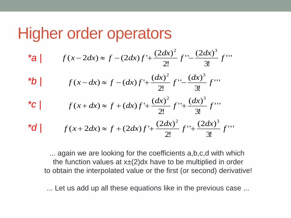
'''!3

)2(''

!2

)2(')2()2(

32

fdx

fdx

fdxfdxxf *a |

*b |

*c |

*d |

... again we are looking for the coefficients a,b,c,d with which

the function values at x±(2)dx have to be multiplied in order

to obtain the interpolated value or the first (or second) derivative!

... Let us add up all these equations like in the previous case ...

'''!3

)(''

!2

)(')()(

32

fdx

fdx

fdxfdxxf

'''!3

)(''

!2

)(')()(

32

fdx

fdx

fdxfdxxf

'''!3

)2(''

!2

)2(')2()2(

32

fdx

fdx

fdxfdxxf

Higher order operators

Problems: Stability

2

2

22

)()(2

)()(2)()(

sdtdttptp

dxxpxpdxxpdx

dtcdttp

1 dx

dtc

Stability: Careful analysis using harmonic functions shows that a stable numerical calculation is subject to special conditions (conditional stability). This holds for many numerical problems. (Derivation on the board).

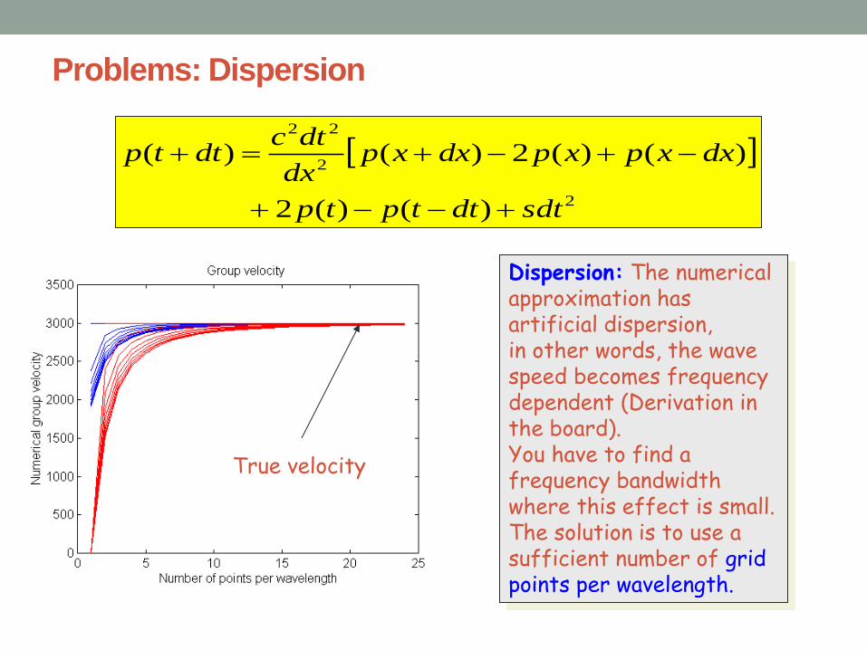
Problems: Dispersion

2

2

22

)()(2

)()(2)()(

sdtdttptp

dxxpxpdxxpdx

dtcdttp

Dispersion: The numerical approximation has artificial dispersion, in other words, the wave speed becomes frequency dependent (Derivation in the board). You have to find a frequency bandwidth where this effect is small. The solution is to use a sufficient number of grid points per wavelength.

True velocity

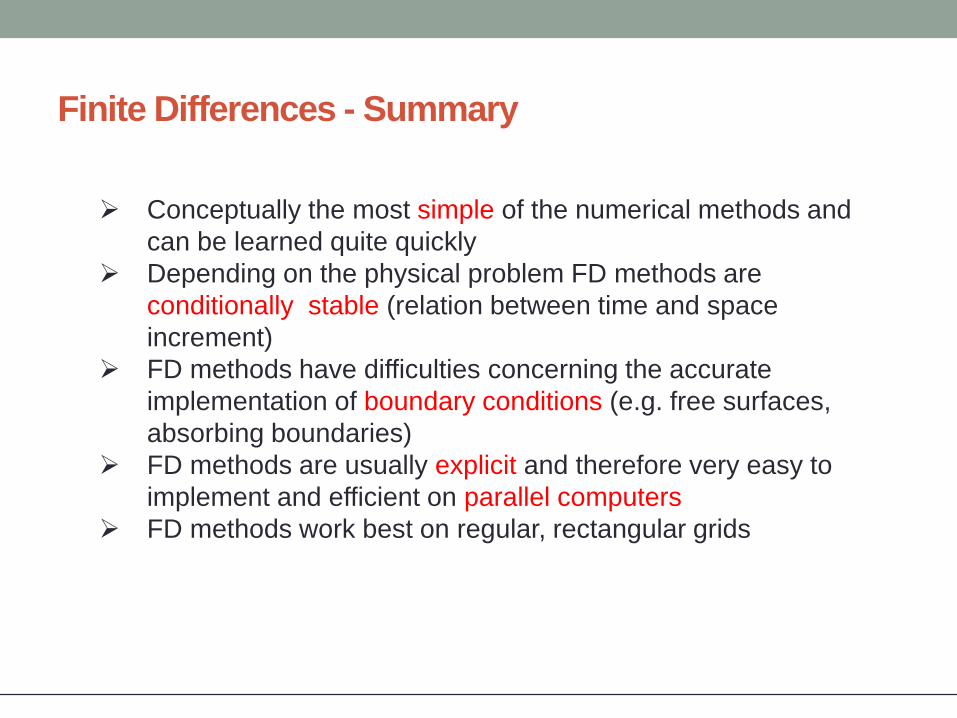
Finite Differences - Summary

Conceptually the most simple of the numerical methods and

can be learned quite quickly

Depending on the physical problem FD methods are

conditionally stable (relation between time and space

increment)

FD methods have difficulties concerning the accurate

implementation of boundary conditions (e.g. free surfaces,

absorbing boundaries)

FD methods are usually explicit and therefore very easy to

implement and efficient on parallel computers

FD methods work best on regular, rectangular grids

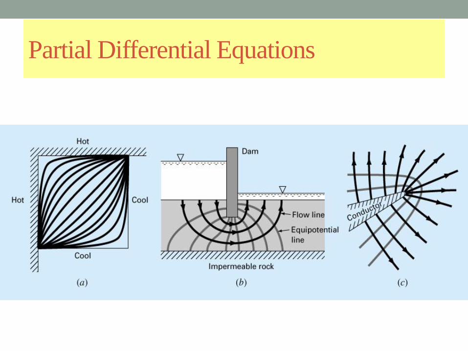
Partial Differential Equations

by Lale Yurttas, Texas A&M

University Part 8 14

PERSAMAAN DIFERENSIAL PARSIAL

• Persamaan Umum

• Menyatakan bagaimana variabel tak bebas Ø berubah

terhadap variabel bebas x,y. Disini a,b,c,d,e,f, dan g

mungkin merupakan fungsi dari Ø

02

22

2

2

gf

ye

xd

yc

yxb

xa

Jenis2 PDP

• Ditentukan oleh harga b2-4ac

< 0, eliptic

= 0, parabolic

> 0, hyperbolic

• Adveksi…

• Difusi….

• Gelombang…

JENIS-

JENIS

PDP

by Lale Yurttas, Texas A&M

University 18

The Laplacian Difference Equations/

04

022

2

2

0

,1,1,,1,1

2

1,,1,

2

,1,,1

2

1,,1,

2

2

2

,1,,1

2

2

2

2

2

2

jijijijiji

jijijijijiji

jijiji

jijiji

TTTTT

yx

y

TTT

x

TTT

y

TTT

y

T

x

TTT

x

T

y

T

x

T

by Lale Yurttas, Texas A&M

University Chapter 29

Laplacian difference

equation.

Holds for all interior points

Laplace Equation

O[(x)2]

O[(y)2]

by Lale Yurttas, Texas A&M

University Chapter 29 20

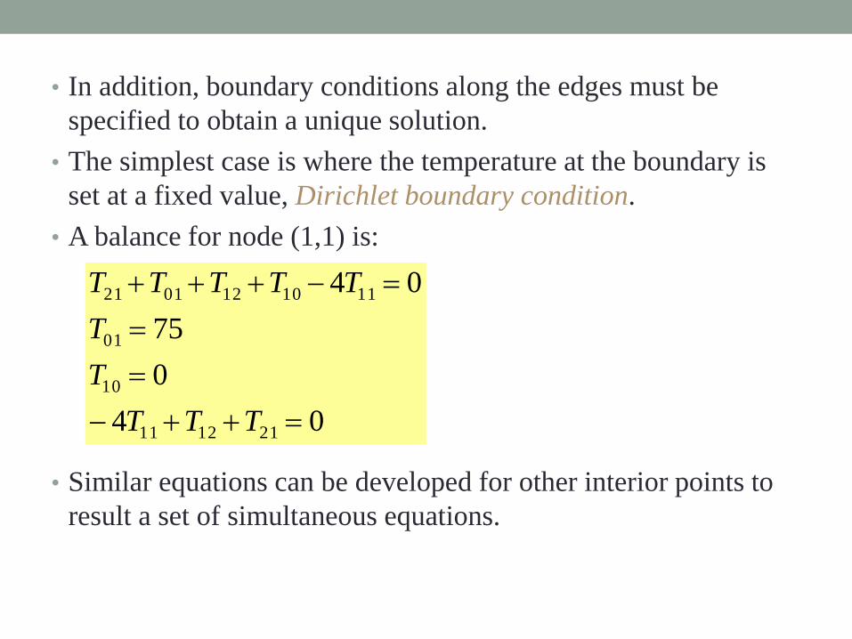
• In addition, boundary conditions along the edges must be

specified to obtain a unique solution.

• The simplest case is where the temperature at the boundary is

set at a fixed value, Dirichlet boundary condition.

• A balance for node (1,1) is:

• Similar equations can be developed for other interior points to

result a set of simultaneous equations.

04

0

75

04

211211

10

01

1110120121

TTT

T

T

TTTTT

by Lale Yurttas, Texas A&M

University Chapter 29 21

1504

1004

1754

504

04

754

504

04

754

332332

33231322

231312

33322231

2332221221

13221211

323121

22132111

122111

TTT

TTTT

TTT

TTTT

TTTTT

TTTT

TTT

TTTT

TTT

• The result is a set of nine simultaneous equations with nine

unknowns:

x

Diffusion

Equation Diffusion 2

2

x

hD

t

h

h

x

d

hu D

x

x

x

du dd

uu x

x

h

duh x x t

x

duh x x t

x

d

hu D

x

duh

t x

0t

2

2

h hD

t x

Diffusion Equation

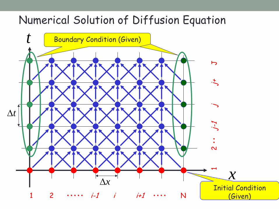
Numerical Solution of Diffusion Eq.

( )h i

( 1)h i

( 1)h i

1

( ) ( 1)h h i h i

x x

x

h

2

( 1) ( )h h i h i

x x

2

2

2 1

1h h h

x x x x

x

t

x

t

1 2 ・・・・・ i-1 i i+1 ・・・・ N

1

2

・・

j-1

j

j

+

J

),( jih

)1,1( jih

Numerical Calculation of Diffusion Equation

t

jihjih

t

h

),()1,(

2

2

2

( 1, ) ( , ) ( , ) ( 1, )

( 1, ) 2 ( , ) ( 1, )

h D h i j h i j h i j h i jD

x x x x

h i j h i j h i jD

x

2

( , 1) ( , )

{ ( 1, ) 2 ( , ) ( 1, )}

h i j h i j

D th i j h i j h i j

x

Unknown

Known

Numerical Solution of Diffusion Equation

x

t

x

t

1 2 ・・・・・ i-1 i i+1 ・・・・ N

1

2

・・

j-1

j

j

+

J

Initial Condition (Given)

Boundary Condition (Given)

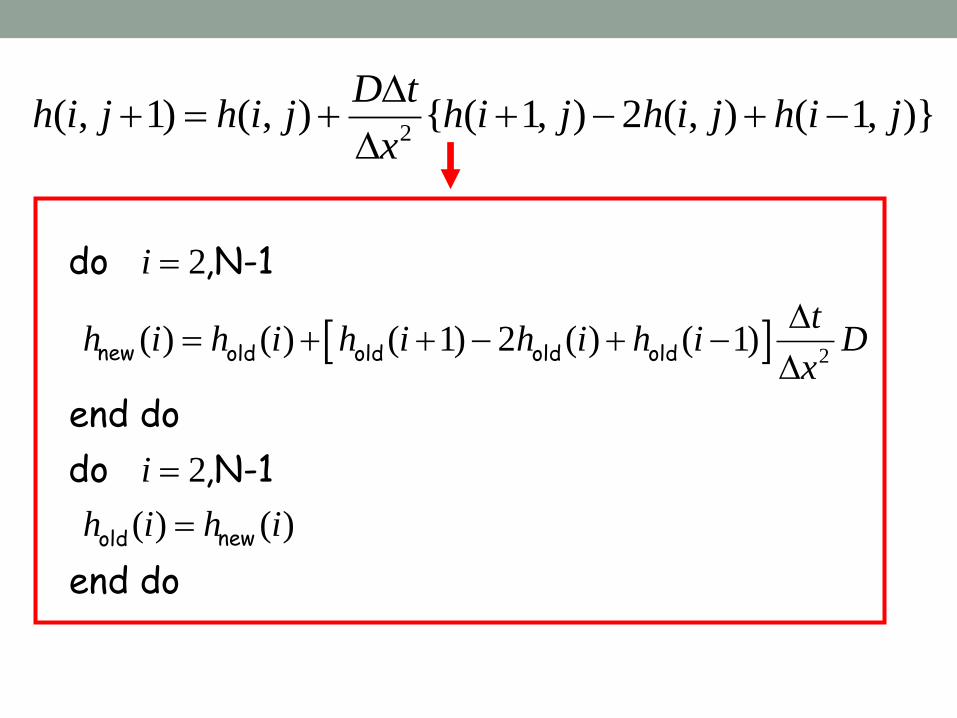
2

2

( ) ( ) ( 1) 2 ( ) ( 1)

2

( ) ( )

new old old old old

newold

do ,N-1

end do

do ,N-1

end do

i

th i h i h i h i h i D

x

i

h i h i

2( , 1) ( , ) { ( 1, ) 2 ( , ) ( 1, )}

D th i j h i j h i j h i j h i j

x

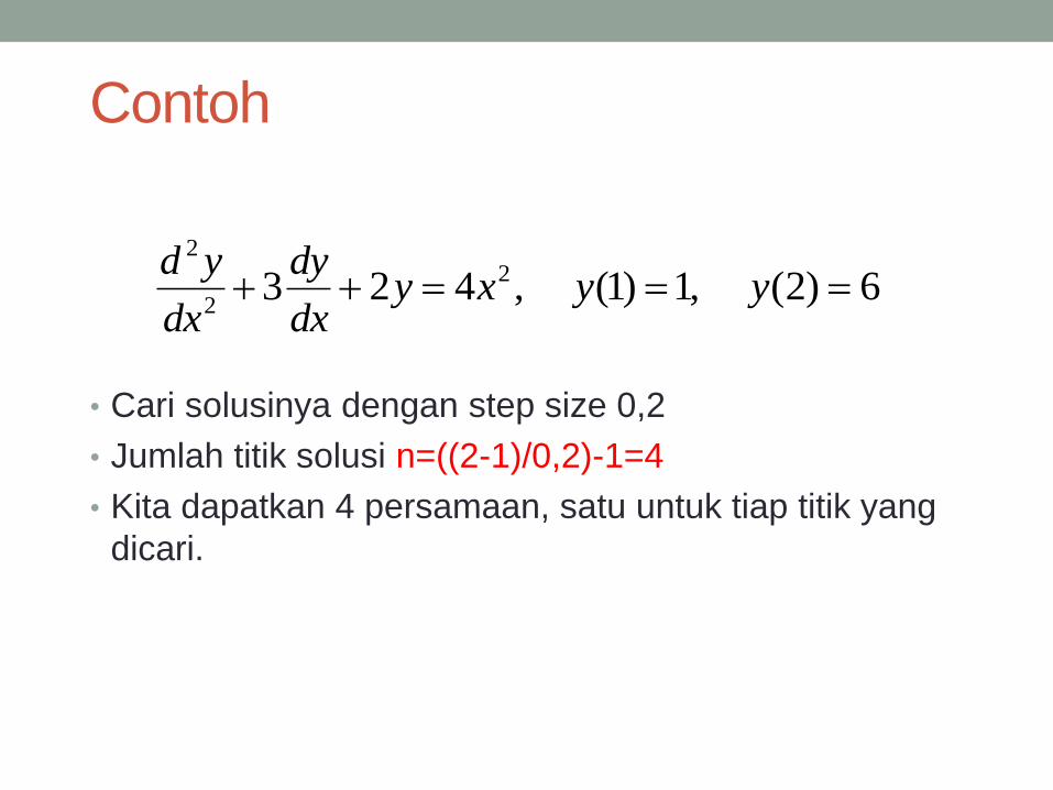
Contoh

• Cari solusinya dengan step size 0,2

• Jumlah titik solusi n=((2-1)/0,2)-1=4

• Kita dapatkan 4 persamaan, satu untuk tiap titik yang

dicari.

6)2(,1)1(,423 2

2

2

yyxydx

dy

dx

yd

Penyelesaian dengan Beda Hingga

Persamaannya:

Buat persamaan untuk semua titik, mulai dari i=1,

hingga i=4

x0=a x1 x2 x3 x4 x5=b

211

2

11 422

32

iiiiiii xy

h

yy

h

yyy

Domain Solusi

y5=6

y0=1

x0=1 x5=2

Penyelesaian dg Finite Diff.

• Dengan h = 0,2

• Buat persamaan untuk semua titik, mulai dari i=1,

hingga i=4

• Masukkan nilai-nilai x1=1,2 hingga x4 =1,8 dan kondisi

batas y0 = 1 dan y5 = 6

2

11 45,17485,32 iiii xyyy

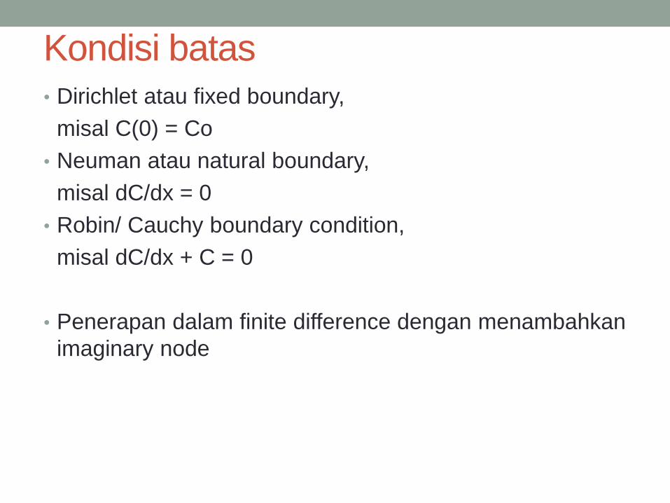
Kondisi batas • Dirichlet atau fixed boundary,

misal C(0) = Co

• Neuman atau natural boundary,

misal dC/dx = 0

• Robin/ Cauchy boundary condition,

misal dC/dx + C = 0

• Penerapan dalam finite difference dengan menambahkan

imaginary node

penyelesaian

persamaan

parabolik

dengan

skema

eksplisit

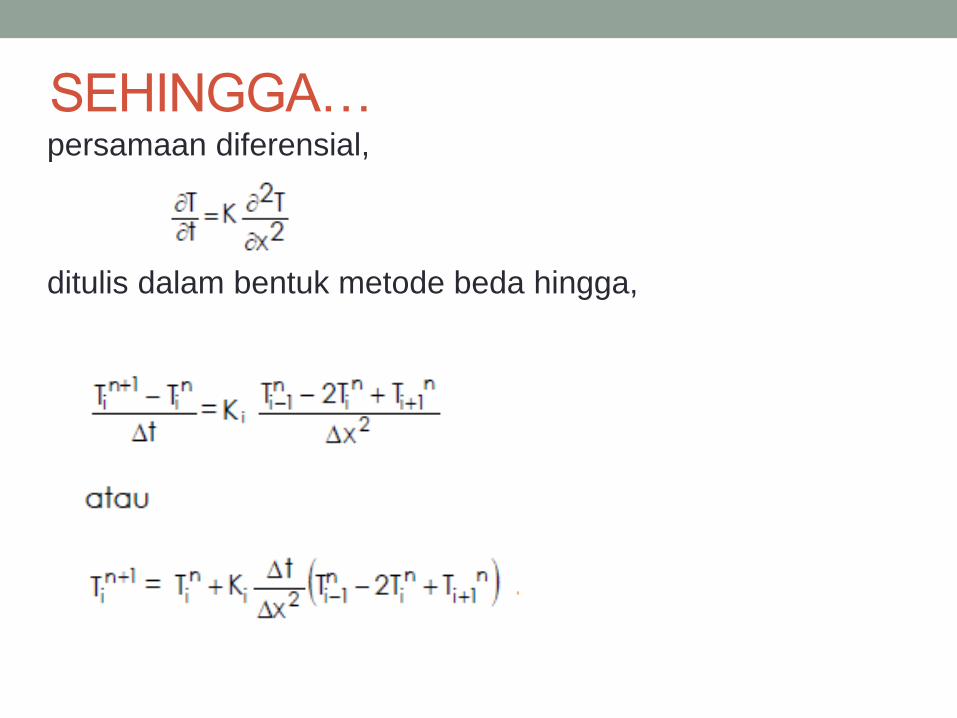
persamaan diferensial,

ditulis dalam bentuk metode beda hingga,

SEHINGGA…

penyelesaian

persamaan

eliptik laplace

….equation

Stabilitas skema eksplisit

k

k

penyelesaian

persamaan

parabolik

dengan

skema

implisit