Finding sparse systems of parameters*

ELSEVIER

JOURNAL OF PURE AND APPLIED ALGEBRA

Journal of Pure and Applied Algebra 94 (1994) 143-157

Finding sparse systems of parameters*

David Eisenbud”, Bernd Sturmfels***b

“Department of Mathematics. Brand& University, Waltham, MA 02254, USA

bDepartment of Mathematics, Cornell University, Ithaca, NY 14853, USA

Communicated by M.-F. Roy; received 1 February 1993; revised 17 May 1993

Abstract

For several computational procedures such as finding radicals and Noether normalizations, it is important to choose as sparse as possible a system of parameters in a polynomial ideal or modulo a polynomial ideal. We describe new strategies for these tasks, thus providing solutions to problems (1) and (2) posed by D. Eisenbud et al. [Invent. Math. 110 (1992) 207-2361.

To accomplish the first task we introduce a notion of “setwise complete intersection”. We prove that a set of monomials generating an ideal of codimension c in a polynomial ring can be partitioned into c disjoint sets forming a setwise complete intersection, although the corresponding result is false for arbitrary sets of polynomials. We reduce the general case to the monomial case by a deformation argument. For homogeneous ideals the output is homogeneous. Our analysis of the second task is based on a concept of Noether complexity for homogeneous ideals and its characterization in terms of Chow forms.

Introduction

LetkbeafieldandletS= k[x,, . , x,] be the polynomial ring. Let J be an ideal

of S, possibly 0, and let R = S/J. Given a finite set 9 c R, generating a proper ideal I,

it is a prerequisite for many algebraic computations to find a maximal system of

parameters in the ideal 1. By this we mean a system of codim(Z) elements of I which

generate an ideal of the same codimension; see for example [5, 6, 10, 14, 151. The

feasibility of the subsequent computation often hinges on the fact that the system of

parameters is “nice”; typically, that it consists of polynomials which are reasonably

sparse, and of low degree.

In this paper we address the question of how to compute a system of parameters

which is as sparse as possible. Given a set of polynomials F that generate an ideal of

*Both authors were partially supported by the NSF during the preparation of this paper. The second

author was also supported by an A.P. Sloan Fellowship. **Corresponding author. Email: [email protected].

0022-4049/94/$07.25 0 Elsevier Science B.V. All rights reserved. SSDI 0022-4049(93)E0135-Q

144 D. Eisenbud, B. SturmfelslJournal of Pure and Applied Algebra 94 (1994) 143-157

codimension c, we study the ways of dividing % into subsets %I, %Z, . . . , %c E %

such that iffy is a sufficiently general linear combination of elements from %i then

fi, . . ,fc form a system of parameters modulo J.

In the first section we treat the case J = 0. This arises when computing the radical of

an ideal. Our main result in this case is Theorem 1.3, which says that if the elements of

% are monomials, and somewhat more generally, then the %i may be chosen to be

disjoint subsets of % We give examples to show that this result fails for arbitrary

polynomials, but we can reduce the general case to this one by a deformation

argument, using partial Grbbner bases. Although it is unpleasant to have to compute

a Griibner basis for this purpose, and the worst-case complexity of the computation is

certainly very bad, the payoff is high: if the input polynomials are homogeneous of

varying degrees, the output can be made homogeneous without any loss of sparseness

from the inhomogeneous case.

In the second section we consider the case of arbitrary J, and we present a simple

“greedy” algorithm (Algorithm 2.1). We then concentrate on the important case when

J is homogeneous and unmixed, and I is the ideal (x1, . . . , x,). This is the problem of

Noether normalization. In this case we compare some possible meanings of the term

“sparse”, with the conclusion that the “correct” measure of sparseness will vary with

the application at hand. Choosing one of these, we define the Noether complexity,

which is the sparseness of the sparsest possible Noether normalization. It is character-

ized in terms of the Chow form of J (Theorem 2.7) and can thus be computed in

single-exponential time in m (cf. [3]). Another simple approach to computing

a Noether normalization of J is to lift one from any initial ideal of J; this lifting

method is explained following Proposition 2.8. We demonstrate by explicit examples

that, in general, neither this lifting method nor the greedy algorithm attains the

Noether complexity.

To simplify the discussion, we assume throughout that k is an infinite field, though

in practice any sufficiently large field will do. In order to use our algorithms it is

necessary to compute the codimensions of various ideals. Good methods for doing

this are discussed in [l] and [2].

1. Systems of parameters in a polynomial ring

We retain the notation of the Introduction. In this section we treat the case J = 0,

and assume that % is a subset of a proper ideal I of the polynomial ring

S = k[xI, . . . ,x,1.

1.1. Some obvious approaches and their drawbacks

Let c be the codimension of I. A set of c linear combinations of the polynomials

in % with sufficiently general coefficients in k is a system of parameters, but unfortu-

nately does not have the desired sparseness. Further, if the polynomials in % are

D. Eisenbud, B. Sturmfels J Journal of Pure and Applied Algebra 94 (1994) 143-157 145

homogeneous but of different degrees and a homogeneous system of parameters is

required, then in this approach one must first replace % by a set of polynomials all of

the same degree, for example by multiplying each one by a power of a generic linear

form, or by replacing each by the ideal it generates in degree equal to the maximal

degree in % This process dramatically destroys sparseness, and raises the degrees of

the elements of %in a way that seems unnecessary.

It is thus natural to ask for the smallest subsets %r, %Z, . . . , Fc c F such that the

linear combinations

generate an ideal of codimension c (that is, form a system of parameters) for some

choice of coefficients ri,f. Supposing that no proper subset of %-generates an ideal of

codimension c, an optimal result of this type would be to take %i, %Z, . . . , Tc to be

a partition of %, that is, disjoint subsets whose union is %

A first hope might be that one could define the sets %j inductively by the condition

that

is the smallest initial subset generating an ideal of codimension j. But this is wrong

even for monomial ideals as the following example from [S] shows:

Cautionary Example 1.1. Let m = 4 and %= (x1x2, x2x3, xi, x1x3}. We have c = 3

and the partition suggested above is

GVZ}> {XZ& x:1> (x1.G).

However, no sequence of the form

x1x2, &x3 + Pxz, x1x3

is a system of parameters, since it is contained in the height-2 ideal (x1, ,?x2x3 + ,&).

On the other hand, the partition

{Xi-G)> (xzx3, x1x3), {4>

does have the desired property.

Unfortunately, partitions with the desired property need not exist. The following

example was worked out in conversation with Joe Harris.

Cautionary Example 1.2. Let { Cij} 1 s i s j s 5 be any ten distinct irreducible space

curves in lP3, and take d an integer large enough so that for each i the ideal of the

union of the six C,, whose indices p,q do not include i is generated by forms of degree

d. For i = 1, . . . ,5 let gi be a general form of degree d vanishing on these six curves

C,,. Let %= {gl, . . . , g5}. It is easy to see that % has no zeros in P3 and hence

generates an ideal of codimension 4.

146 D. Eisenbud, B. Sturmfels/Journal of Pure and Applied Algebra 94 (1994) 143-157

We claim that there is no partition of %into four disjoint subsets %i and choice of

coefficients ri,f such that (*) generates an ideal of codimension 4. If such a partition

existed, then three of the sets %i would have to be singletons. Hence some three forms

gi,gj,gk would have to be a system of parameters, and vanish only at finitely many

points in p3. Since gi, gj, gk vanish on the curve C,,, where {i, j, k, u, v} = { 1, . . ,5},

this is impossible.

There is no example of this type with d = 2, but here is one with d = 3: Let

Pl> *.. > p5 be general points in [Fp3, let Cij be the line passing through pi and pj, and let

Z+ be the equation of the plane containing the three points Pi, pj, pk. The six lines not

involving a particular index i form a tetrahedron. The ideal of their union is generated

by the set %i of four cubic forms made by taking products, three at a time, of the

l,,, with i 4 {s, t, u}, so we may take d = 3 in the argument above.

Theorem 1.3 will show that good partitions do exist for monomial ideals, and this is

the basis of our method. The reason that they exist is essentially that a monomial ideal

of codimension c is always contained in an ideal generated by c elements-in fact, by

c of the variables.

1.2. A method for finding a sparse system of parameters

The following theorem is our first main result. We fix any term order “i” on the

polynomial ring S and we write in,(%) for the set of initial terms of the polynomials

in %

Theorem 1.3. Suppose that in,(%) generates an ideal of codimension c. There exist partitions %= %I v ..’ v %C such that for each i the monomials in,(%i) have a vari-

able in common. If %is any such partition, then for almost all ri,f E k, the polynomials (*)

generate an ideal of codimension c. Further, each f E %-may be multiplied by any factor of

in,(f) without spoiling this property.

It is known that the hypothesis of Theorem 1.3 is satisfied if %is a Grobner basis of

an ideal of codimension c (see e.g. [S]). This suggests the following algorithm for

finding a sparse system of parameters.

Algorithm 1.3’.

Input: A set of generators %for an ideal I of codimension c.

Enlarge %-step by step toward a Grobner basis, using the Buchberger algorithm, until

in<(%) generates an ideal of codimension c. Next replace this partial Griibner basis

by a minimal subset which has the same property. Partition this new %-into subsets %i

as in Theorem 1.3, for example as follows: Choose a prime (xi,, . . . , xi,) containing

in,(%). Such primes exist because every associated prime of a monomial ideal is

D. Eisenbud, B. SturmfelslJournal of Pure and Applied Algebra 94 (1994)143-157 147

generated by a subset of the variables. For p = 1,2, . . . ,c define 9rp inductively to be

the set of all elements of 9 - uj sp ~j whose initial terms are divisible by xi,.

If the polynomials in 9 are homogeneous, and a homogeneous system of para-

meters is desired, let di be the maximal degree in Fi, and multiply each polynomial in

9$ by a power of one of the variables in its own initial term to bring it up to degree di.

Choose random elements ri,f in k, and verify that the polynomialsfi in (*) generate

an ideal of codimension c. If they do not, try a new random choice.

Output: The sequence fi, . . ,fc.

Before starting Algorithm 1.3’, it may be worthwhile to change to the order for

which the initial forms of Fgenerate an ideal of largest possible codimension. This can

be done using the polyhedral methods in [7].

One subtask to be solved in Algorithm 1.3’ is to find the minimal prime

(Xi,, . . . , Xi,). This is often an easy task, but we remark that in general it amounts to

solving a combinatorial problem which is NP-complete. To see this, consider the case

where in,(F) consists of square-free quadratic monomials XiXj, representing the

edges of a graph G with vertex set {xi, . . . , x,). A subset S of the vertices of G is called

stable if no two elements in S are connected by an edge in G. Our subtask amounts to

finding a maximal stable set of G, a problem which is known to be NP-complete [ 161.

Our proof of Theorem 1.3 is based on the following criterion for a sequence of sets

of polynomials to be what one might describe as a “setwise system of parameters”:

Proposition 1.4. Let PI, . . . , 9c c S be sets of polynomials. Iffor every U G { 1, . . . , c}

the set of polynomials Ujsv ~j generates an ideal of codimension 2 card U, then for

almost every choice of ri,,- in k the polynomials fi, . . , fc in (*) generate an ideal of codimension c in S.

Remarks. (i) The term “for almost every choice” in Proposition 1.4 (and the term

“random” in Algorithm 1.3’) means that ri,s can be chosen in some Zariski-open

subset of the coefficient space.

(ii) Example 1.1 shows that we cannot weaken the hypothesis by restricting U to be

an initial subset of { 1, , . . , c}. (iii) The converse of Proposition 1.4 holds after localizing at any prime containing

all the his. (Reason: In a local domain with saturated chain condition, codim

( fi, . . ,fc) = c implies codim ( fi, . . , fd) = d f or all d < c.) It follows that it holds,

even without localizing, if each 9i consists of homogeneous polynomials of positive

degree. (Reason: The local codimension of the ideal generated by ujeu9j is mini-

mized in the localization at the origin.)

The following example shows that the converse is false in general. We are grateful to

Alicia Dickenstein for pointing it out.

148 D. Eisenbud, B. SturrnfelsJJournal of Pure and Applied Algebra 94 (1994) 143-157

Cautionary Example 1.5. Let m = 3, %I = {fI = (x1 + 1)x2}, %2 = {f2 = (x1 +

1)x3), and %s = {_& = x1]. Thenf,,f,,_& generate an ideal of codimension 3 butfi,f2

generate an ideal of codimension 1.

1.3. Proofs

Proof of Proposition 1.4. We first show that the conclusion holds in the “generic

situation”. Let k’ be the polynomial ring with variables ri,f forfe %i and i = 1, . . . , c.

We will show that the polynomials f, , , fc in (*) generate an ideal of codimension

c in SOkk’. Equivalently, let A be the affine space with the ri,f as coordinates, and let

J3 be the affine space with coordinates x1, . . . ,x,. Let X be the subvariety of A x B

defined by fi, , fc. We will show that the codimension of X is c.

Let x2 : X -+ B be the projection to the second factor of the product. The fiber of z2

over a point p E B is a linear space. Since thefi involve disjoint sets of variables ri,f, its

codimension equals c minus the number of indices i such that the polynomials in %i all

vanish at p. For each subset U z (1, , c} let Y, denote the set of p E B such that the

polynomials in u j E u %j all vanish at p but some polynomial in each %j for j # U does

not vanish at p. The constructible sets Y, define a stratification of B such that over

each stratum the fibers of z2 have constant codimension c - cardU. Therefore the

codimension of X in A x I3 equals min {c - card U + codim Y, 1 U G { 1, . . . , c}}. The

hypothesis states that if Y, is nonempty, then the codimension of Y, is 2 card U. We

conclude that the codimension of X is 2 c.

To conclude the proof, consider the projection x1 : X + A onto the first factor of the

product. We must show that the codimension in B of almost every fiber of n1 is 2 c.

For any dominant map of irreducible varieties, almost every fiber has dimension equal

to the dimension of the source minus the dimension of the target. Thus in our situation

almost every fiber has codimension in B equal to the codimension in A x B of the

union of those components of X that dominate A. This second codimension is 2 the

codimension of X in A x B, which we have shown to be 2 c. 0

Proof of Theorem 1.3. The codimension of the ideal generated by the initial terms of

a set of polynomials is I that of the ideal of the polynomials themselves. Thus if the

sets in,(%i) satisfy the hypothesis of Proposition 1.4, then so do the sets %i.

Consequently it suffices to treat the case where %-consists of monomials. We must find

a partition satisfying the first condition of Theorem 1.3, and show that any such

partition satisfies the hypothesis of Proposition 1.4.

Since every associated prime of a monomial ideal is generated by a subset of the

variables, we may assume (after renumbering variables if necessary) that % is con-

tained in the ideal (x1, . . , x,). Since a monomial is contained in this ideal if and only if

it is divisible by one of the variables (x1, . . . , xc), we may partition %into subsets %i

consisting only of monomials divisible by xi. The following lemma concludes the

proof:

D. Eisenbud. B. Sturmfels/Journal of Pure and Applied Algebra 94 (1994)143-157 149

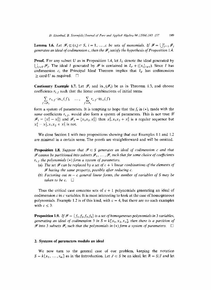
Lemma 1.6. Let %i E (xi) c S, i = 1, . . . , c be sets of monomials. lf %= uf= I cFj generates an ideal of codimension c, then the %j satisfy the hypothesis of Proposition 1.4.

Proof. For any subset U as in Proposition 1.4, let Iv denote the ideal generated by

Ujcn pj. The ideal I generated by 9 is contained in 1” + ((Xi}i8”). Since 1 has

codimension c, the Principal Ideal Theorem implies that I, has codimension

2 card U as required. 0

Cautionary Example 1.7. Let pi and in_,(Fi) be as in Theorem 1.3, and choose

coefficients ri, s such that the linear combinations of initial terms

c ‘1.f .in-JfL . . . . C r,,f.indf) fEF1 SEFc

form a system of parameters. It is tempting to hope that thefi in (*), made with the

same coefficients ri,f, would also form a system of parameters. This is not true: If

9i = {x: - x2) and Fz = {x1x2,x~} then x:,xlxz + xi is a regular sequence but

x: - x$,x1x2 + x; is not.

We close Section 1 with two propositions showing that our Examples 1.1 and 1.2

are minimal in a certain sense. The proofs are straightforward and will be omitted.

Proposition 1.8. Suppose that %C S generates an ideal of codimension c and that

%-cannot be partitioned into subsets %I, . . , Fc such that for some choice of coejjicients

ri,/. the polynomials (*) form a system of parameters.

(a) The set %can be replaced by a set oft + 1 linear combinations of the elements of

% having the same property, possibly after reducing c.

(b) Factoring out m - c general linear forms, the number of variables of S may be

taken to be c. 0

Thus the critical case concerns sets of c + 1 polynomials generating an ideal of

codimension c in c variables. It is most interesting to look at the case of homogeneous

polynomials. Example 1.2 is of this kind, with c = 4, but there are no such examples

with c I 3:

Proposition 1.9. If % = { fi,f2, f3, f4} 1s a set of homogeneous polynomials in 3 variables,

generating an ideal of codimension 3 in S = k[xI,xl,xj], then there is a partition of

%into 3 subsets %i such that the polynomials in (*) form a system of parameters. 0

2. Systems of parameters modulo an ideal

We now turn to the general case of our problem, keeping the notation

S = k[xI, . . . ,x,1 as in the Introduction. Let J c S be an ideal, let R = S/J and let

150 D. Eisenbud, B. SturmfelslJournal of Pure and Applied Algebra 94 (1994) 143-157

%c S be a finite subset. Let I be the ideal generated by %, and suppose that the

codimension of Z modulo J is c in the sense that c = codim(Z + J) - codim(J).

We say that fi, . . . , fc E I is a maximal system of parameters for I modulo J if

codim(P + (fi, . . ,fc)) 2 codim(Z + J) for every minimal prime P of J. (This notion

is most natural if the ideal J is unmixed.) We wish to choose as sparse as possible

a maximal system of parameters for I modulo J.

The simplest and most common problem calling for systems of parameters is that of

finding a Noether normalization for a homogeneous ideal. If c is the Krull dimension

of R, this is the problem of finding elements fi , . . , fc in R such that R is a finitely

generated module over the subring k [fi, . . . ,fc] c R. (The elementsf, , . . . ,fc are then

necessarily algebraically independent, so that the subring is isomorphic to a poly-

nomial ring. See [4] and [ 1 l] for a discussion from a computer algebra point of view.)

We will focus primarily on this case, but first we present a method for handling the

general problem. The approach differs from that of Section 1 in that it chooses onefi at

a time, essentially employing overlapping sets %i.

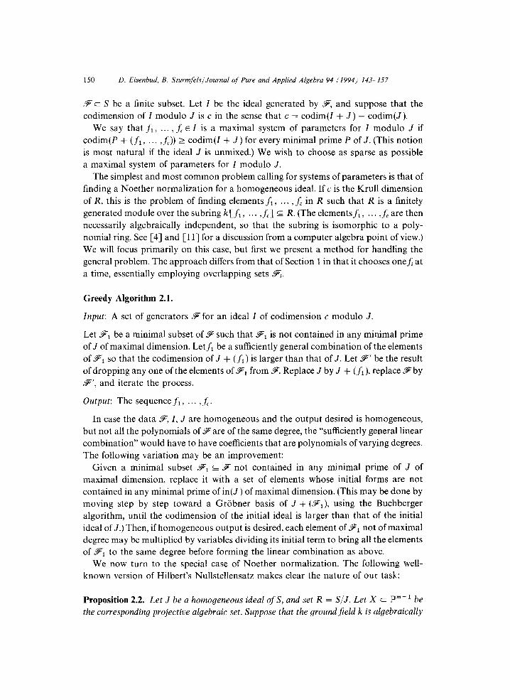
Greedy Algorithm 2.1.

Input: A set of generators %for an ideal Z of codimension c modulo J.

Let %i be a minimal subset of %such that %i is not contained in any minimal prime

of J of maximal dimension. Letfi be a sufficiently general combination of the elements

of %i so that the codimension of J + (fi) is larger than that of J. Let %’ be the result

of dropping any one of the elements of %i from % Replace J by J + (fi), replace %-by

%-‘, and iterate the process.

Output: The sequencef,, . . . ,fc.

In case the data %, I, J are homogeneous and the output desired is homogeneous,

but not all the polynomials of %-are of the same degree, the “sufficiently general linear

combination” would have to have coefficients that are polynomials of varying degrees.

The following variation may be an improvement:

Given a minimal subset %i & % not contained in any minimal prime of J of

maximal dimension, replace it with a set of elements whose initial forms are not

contained in any minimal prime of in(J) of maximal dimension. (This may be done by

moving step by step toward a Grobner basis of J + (%I), using the Buchberger

algorithm, until the codimension of the initial ideal is larger than that of the initial

ideal of J.) Then, if homogeneous output is desired, each element of %i not of maximal

degree may be multiplied by variables dividing its initial term to bring all the elements

of %r to the same degree before forming the linear combination as above.

We now turn to the special case of Noether normalization. The following well-

known version of Hilbert’s Nullstellensatz makes clear the nature of our task:

Proposition 2.2. Let J be a homogeneous ideal of S, and set R = S/J. Let X c Pm-l be the corresponding projective algebraic set. Suppose that the groundjield k is algebraically


closed. If fi, , fC E R are homogeneous polynomials, then R is a finitely generated

module over the subring k[ fi, . , fc] G R if and only if the system of equations

fi(x) = ... =fc(x) = 0 has no solution in X.

Proof (Sketch). By the Nullstellensatz the condition that there are no solutions is

equivalent to the condition that R/( fi, . . . , f,) 1s a finite-dimensional vector space.

Because R is graded and zero in negative degree, a basis for this space lifts to a finite

set of generators for R over the subring k[ fi, . , fC]. 0

In the Noether normalization problem one usually wants thef; to be linear forms.

We will henceforth consider only this case, and suppose that % = {x1, . . . , x,,,}, so that

I = (%) is the irrelevant ideal. In this situation Algorithm 2.1 has the effect of reducing

at each step the number of variables to be considered, and this increases its efficiency.

Here is a monomial example, which also suggests a possibility for improving the

algorithm:

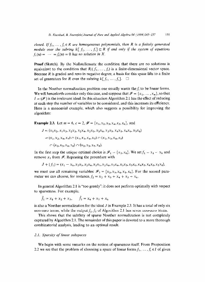
Example 2.3. Let m = 6, c = 2, % = {x1, x2, x3, x4, x5, xc>, and

J = (XI.%, x1x3> x2x3, x2x4~ x2% x3x4, x3x5> x4x5, xqx6, x5x6)

= h, x2, x4> x5) n (x1, x3, x4, x5) (7 (x2, x3> x4, x5)

f’ (x2, x3, x4, x6) f7 (x2, x3, x5, x6).

In the first step the unique Optimd choice is %i = {x1,x6}. We set fi = x1 - x6 and

remove x1 from % Repeating the procedure with

J + (fi) = (XI - x6, %.x3, x2x4, x2x5> x2x6, x3x4, x3x5, x3x6, x4x59 x4x6, x5x6)t

we must use all remaining variables: %2 = {x2,x3,x4,x5,~s}. For the second para-

meter we can choose, for instance, fi = x2 + x3 + x4 + x5 + x6.

In general Algorithm 2.1 is “too greedy”: it does not perform optimally with respect

to sparseness. For example,

J = xi + x2 + x3, f2 = x4 + x5 + x6

is also a Noether normalization for the ideal J in Example 2.3. It has a total of only six

non-zero terms, while the output fi,f2 of Algorithm 2.1 has seven non-zero terms.

This shows that the subtlety of sparse Noether normalization is not completely

captured by Algorithm 2.1. The remainder of this paper is devoted to a more thorough

combinatorial analysis, leading to an optimal result.

2.1. Sparsity of linear subspaces

We begin with some remarks on the notion of sparseness itself. From Proposition

2.2 we see that the problem of choosing a space of linear forms fi, . . . ,fc ~1 of given

152 D. Eisenbud, B. Sturmfels/Journal of Pure and Applied Algebra 94 (1994) 143-157

degree d that are a homogeneous system of parameters modulo a homogeneous ideal

J, is equivalent to the following geometric problem: given an algebraic set X of

dimension c - 1 in a projective space pm- ‘, find a linear subspace L of codimension

c not meeting X. Equivalently, we may think of L as coming from a linear subspace

M of an affine space A”, which is supposed to meet the cone over X only in the origin.

We wish to choose M to be as sparse as possible, relative to some given system of

coordinates for Pm-i. There are several possible definitions of sparseness, and they

conflict with one another. In general, if we agree on a way to represent the space M,

then we can speak of a space allowing the sparsest possible representation in this form.

Perhaps the three most obvious representations are these: M might be represented by

the coordinates of a basis of M (basis representation), by the coordinates of a basis for

the space M’ of linear functionals vanishing on M (cobasis representation), or by

Plucker coordinates, the maximal minors of some matrix representing the basis or

dual basis (Pliicker representation). In each case the number of nonzero coordinates is

a measure of sparseness ~ we call them basis sparseness, cobasis sparseness, and

Pliicker sparseness respectively.

It is not hard to show that for l-dimensional subspaces (and thus also for hyper-

planes) the three measures of sparseness agree in the sense that all three choose the

same space as the sparsest in a particular set of subspaces. But in general no two of

these measures agree on naming the sparsest subspace, as may be seen from the

following examples. In each case the subspace considered is the row space of the given

matrix. As we will not make use of these facts, we leave their verification to the

interested reader.

First, to show that Plucker sparseness does not agree with basis sparseness: The

space Ml represented by the matrix

Ml++ (

1000000

0111111 1

has basis sparseness 7 and Plucker sparseness 6, while the space M2 represented by

(

1110000

M2”o 0 0 1110 1

has basis sparseness 6 and Plucker sparseness 9.

The sparseness of a space M is the same as the cobasis sparseness of Ml, so the

spaces Mi and Mi illustrate the same point for cobasis sparseness.

It is harder to give examples in which basis sparseness and cobasis sparseness

disagree, but the reader may check that if L1 and Lz are the 3-dimensional subspaces

of a 9-dimensional vectorspace I/ represented by the matrices

:

111111 11 1

L,tt 0 0 0 1 1 1 2 2 2

0 1 2 0 1 2 10 11 12


and

111111 11 1

L2” : 0 0 0 1 1 1 2 3 4

0 1 2 0 1 2 10 11 12

then the basis sparseness of L1 is 6 + 6 + 7 = 19, whereas that of L2 is

6 + 6 + 6 = 18. The cobasis sparseness of each is 3 + 3 + 3 + 4 + 4 + 4 = 21. Now

consider the subspaces

M3 = Lt @L; and M4 = L2@Li in V@V*.

The basis sparsenesses spaces of these are 40 = 19 + 21 and 39 = 18 + 21 respec-

tively. But as M$ = (L, @Li)’ = L: @L2, and similarly for M,, the cobasis sparse-

nesses for M3 and M4 are 39 = 18 + 21 and 40 = 19 + 21, reversing the order of the

basis sparsenesses.

2.2. Sparse Noether normalization using Chow forms

We now return to the problem of Noether normalization. We will work in terms of

basis sparseness of the space generated by the linear forms in the solution to the

Normalization problem; our discussion can be adapted, by considering different

expressions of the Chow form, to cobasis or Plucker sparseness as well. Let J be

a homogeneous unmixed ideal in S, and let X denote its projective variety in Pm- ‘.

Changing notation somewhat, we suppose that X has degree p and dimension d - 1.

We will show how to compute a Noether normalization consisting of linear forms

J = CilXl + Ci2X2 + “’ + CtmXm, i = 1,2, . . . ,d, (1)

which is optimal in the sense that the number of non-zero coefficients Cij is minimal - that is, the basis sparseness of the space spanned by thefi is minimal. We call the

number of nonzero cij the Noether complexity of X.

Let Rx = Rx(cij) = Rx( fi, . . . , fd) denote the Chow form of X. This classical

polynomial is characterized by the property that it vanishes if and only if the linear

subspace defined byfr (x) = ... =&(x) = 0 meets X; see e.g. [12, Section 1.1.6.11 and

the references given in [3]. The notation concerning Chow forms tends to vary from

author to author. The specific notation to be employed here is taken from [9] and

r-131, namely, we express R, as a polynomial in brackets [il i2 . . . id],

llil< ... < id I m. These are the d x d-minors of the d x m-matrix (cij), or, equiva-

lently, the Plucker coordinates of the codimension k flat defined by the vanishing of

the linear forms in (1). By Proposition 2.2, the Noether normalization problem for R is

equivalent to the problem of finding a non-root of the Chow form Rx.

Example 2.4. (Hypersurfaces, d = m - 1). Suppose J is the principal ideal generated

by a homogeneous polynomial F(xi, x2, . . . , x,), defining a hypersurface X c Pm- ‘.

154 D. Eisenbud, B. SturmfelslJournai of Purr and Applied Algebra 94 (1994) 143-157

In terms of brackets its Chow form equals

Rx = F([234 . m], - [134 . . . m],[124 . . . m], . . . ,( - 1)“-‘[23 . . . m - 11).

(2)

The Noether normalizations of X are precisely the (m - 1) x m-matrices (cij) for which

the bracket polynomial (2) does not vanish.

It is our objective to compute a d x m-matrix (cij), which is a non-root of the Chow

form Rx, and which is as sparse as possible with this property. Since (cij) must have

maximal rank d, the Noether complexity of X is at least d = dim(X) + 1. It is exactly

d if and only if X is in Noether normal position with respect to some coordinate flat.

Observation 2.5. The coordinate forms xi,, xi2, . . . , Xid are a Noether normalization for

X ifand only if the bracket power [il i2 . . iJ’ appears with non-zero coeficient in Rx.

Let V = {Cij 1 1 I i I d, 1 I j 5 m} denote the set of variables. For any polynomial

fe k [ V] we define a simplicial complex A(f) as follows: A subset W c V’ is a face of

A(f) if and only if there exists a non-root off whose zero coordinates are precisely W.

Equivalently, Wis not a face of A(f) w h enever f lies in the ideal generated by W. If we

write supp(m) for the set of variables dividing a monomial m, we see that the maximal

faces of d(f) are the complements of the minimal sets of the form supp(m) where m is

a monomial off: In particular, for each monomial m, the complex A(m) is a simplex,

consisting of all subsets of V\supp(m). Thus we get the first statement of the following:

Lemma 2.6. Let f be a homogeneous polynomial in k[ V]. Then A(f) is the union of the

simplices A(m), where m ranges over all monomials off with minimal support. Also, A(f)

is the union of the simplices A(in,( f)), w h ere < ranges over all term orders on k[ V].

Proof. We have already proved the first statement. To prove the second it suffices to

observe that because f is homogeneous, every monomial off with minimal support is

the initial monomial off with respect to some term order. 0

This lemma together with the above observations implies the following theorem.

Theorem 2.7. The Noether complexity of a projective variety X equals the least number

of variables cij appearing in any initial monomial in, (Rx) = nc,j of its Chow form. 0

Example 2.3. (continued) The reducible curve X c P5 defined by J has Chow form

Rx = [14].[15].[16]~[26]c361

= (c11c24 - c14cz1)~(cllc*5 - c15c21)

.(CllCX - C16C21)~(C12C26 - C164.(C13C26 - Cl&d

D. Eisenbud, B. Sturmfels/Journal of Pure and Applied Algebra 94 /1994)143-157 155

The coefficient matrices offi& andfl,& considered above are seen to be non-roots of

RX. The Noether complexity of the curve X is equal to 6 (cf. Theorem 2.7). q

The most systematic approach to solving our problem would be to explicitly

compute the Chow form Rx. By the results of [3], this can be done in single

exponential time (in m). Theorem 2.7 implies that the Noether complexity and an

optimal Noether normalization for X can be computed in single exponential time.

Unfortunately, this approach is not useful in practice, since the complete expansion

of the Chow form into monomials ncr,j is usually too big. Hence the Caniglia

algorithm is only of theoretical interest with regard to our problem. In fact, the

problem of computing the Noether complexity of a monomial ideal is NP-hard. The

following proof of this fact has been pointed out to us by Jesus DeLoera. Let G be any

graph on I/= (x,, . . . ,x,} and IG the ideal generated by all square-free cubic mono-

mials xixjxk, and all XiXj not corresponding to an edge of G (this is the Stanley-Reisner

ideal of G viewed as a simplicial complex). The Noether complexity of I, equals the

minimal number 2n - 1 S1 1 - 1 S2 1, where Sr, S, c I/ ranges over all disjoint pairs of

stable sets of G. Here Si indexes the zero entries in row i of a sparsest Noether

normalization (cij). If we had a polynomial time algorithm for finding S1 and S1, then

we could solve the NP-hard problem of computing a maximal stable set in any graph

G1 as follows. Let G2 be a disjoint copy of Gr, and let G be the graph obtained from

their union G1 u G2 by connecting each vertex of G1 with each vertex of Gz. Applying

our algorithm to G we obtain a maximal stable set Si for G = Gi, i = 1,2.

For practical computations we propose an approach using (truncated) Grobner

basis computations for the ideal J. The following proposition, which is easily derived

from the proof of Lemma 2.6, shows that the Noether complexity of a homogeneous

ideal is bounded above by the Noether complexity of any of its initial ideals.

Proposition 2.8. Let (Cij) be any Noether normalization of the initial monomial ideal

in,(J), wherew = (ol, . . . , co,) E Z” represents any term order for J. Then, for almost all

t E k, the matrix (cij. t”j) is a Noether normalization of J. 0

From this we get the following lifting algorithm: Choose any term order on S, and

compute a truncated Griibner basis {gi, . . . ,gl} for J, subject to the truncation

condition that the monomial ideal L = (in(fi), . . . , in(fi)) has the same radical as

in,(J). Compute the Chow form RL of L, e.g., using method in Proposition 3.4 of [13].

The bracket monomial RL has precisely the same bracket factors as RincJj. We have

d (RL) = d (Ri”(J,) c d (Rx). (3)

Choose any maximal face of the simplicial complex A(R,). This gives rise to

a Noether normalization for in(J) and, using Proposition 2.8, we get a Noether

normalization for J.

In order to find a sparser Noether normalization we may repeat this procedure for

as many different term orders as we can. In fact, whenever this is feasible, one might

156 D. Eisenbud. B. Sturmfels/Journal of Pure and Applied Algebra 94 (1994) 143-157

like to compute a universal Griibner basis % for J, that is, a finite subset of J which is

a Griibner basis simultaneously for all term orders on S. From a universal Grijbner

basis and the knowledge of the maximal faces of d (R,) we can read off the minimum

of the Noether complexities of all initial ideals of J. However, this minimum will

generally not agree with the Noether complexity of J, as the following example shows.

Cautionary Example 2.9. A homogeneous ideal J whose Noether complexity is

smaller than the Noether complexity of any of its initial ideals in(J). Let m = 6 and

consider

J = (x2.$ - x1x6, x3, x4) f-J (XIX4 - x3xS9 x2, x6) n (x3x6 - x2x4, xl> x5).

The variety X of J is a union of three toric surfaces in P5. Here the Chow form equals

Rx = ([126][156] - [125][256])*([135][345] - [145][134])

.( [234] [246] - [236] [346]).

The matrix

(Cij) = 1: % i i % 81

is a non-root of Rx and hence defines a Noether normalization. It is optimal because

each term appearing in the complete expansion of Rx contains at least six of the

variables cij. This proves that the Noether complexity of X equals six.

The ideal J has six distinct initial ideals, each of which is isomorphic to

in(J) = (x2x5, x3, x4) n (x1x4, x2, x6) n (x2x4, x1, 4.

The complete expansion of the initial Chow form

Kin(J) = [126][156][135][345][236][346]

has 13,452 terms. Each of these terms contains at least eight variables. Hence the

Noether complexity of each initial ideal of J equals eight.

References

[l] D. Bayer and M. Stillman, Computation of Hilbert functions, J. Symbolic Comput. 14 (1992) 31-50.

[2] A. Bigatti, M. Caboara and L. Robbiano, On the computation of HilbertGPoincart series, Applicable

Algebra in Engrg. Comm. and Comput. 2 (1993) 21-33. [3] L. Caniglia, How to compute the Chow form of an unmixed polynomial ideal in subexponential time,

Applicable Algebra Engrg. in Comm. and Comput. 1 (1990) 25-41. [4] A. Dickenstein, N. Fitchas, M. Giusti and C. Sessa, The membership problem for polynomial ideals is

solvable in subexponential time, Discrete Appl. Math. 33 (1991) 73-94.


[S] D. Eisenbud, Open problems in computational algebraic geometry, in: D. Eisenbud and L. Robbiano,

eds., Proceedings of the Cortona Conference on Computational Algebraic Geometry (Cambridge

University Press, Cambridge, 1993) 49970.

[6] D. Eisenbud, C. Huneke and W. Vasconcelos, Direct methods for primary decomposition, Invent.

Math. 110 (1992) 2077236. [7] P. Gritzmann and B. Sturmfels, Minkowski addition of polytopes: Computational complexity and

applications to Grobner bases, SIAM J. Discrete Math. 6 (1993) 2466269.

[S] M. Kalkbrener and B. Sturmfels, Initial complexes of prime ideals, Adv. in Math. (1994), to appear.

[9] M. Kapranov, B. Sturmfels and A. Zelevinsky, Chow polytopes and general resultants, Duke Math.

J. 67 (1992) 1899218.

[lo] T. Krick and A. Logar, An algorithm for the computation of the radical of an ideal in the ring of

polynomials, in: Proceedings 9th AAECC, Lecture Notes in Computer Science, Vol. 539 (Springer,

New York, 1991) 1955205.

[l l] A. Logar, A computational proof of the Noether Normalization lemma, in: Proceedings 6th AAECC,

Rome, 1988, Lecture Notes in Computer Science, Vol. 357 (Springer, Berlin, 1988) 259-273

[12] I. Shafarevich, Basic Algebraic Geometry (Springer, New York, 1977).

[13] B. Sturmfels, Sparse elimination theory, in: D. Eisenbud and L. Robbiano, eds., Proceedings of the

Cortona Conference on Computational Algebraic Geometry, (Cambridge University Press, Cam-

bridge, 1993) 264-298.

[14] W. Vasconcelos, Constructions in commutative algebra, in: D. Eisenbud and L. Robbiano, eds.,

Proceedings of the Cortona Conference on Computational Algebraic Geometry, (Cambridge Univer-

sity Press, Cambridge. 1993) 151-197.

[15] W. Vasconcelos, The top of a system of equations, Bol. Sot. Mat. Mex. (2), issue dedicated to Jose Adem (1994).

[16] M.R. Carey and D.S. Johnson, Computers and Intractability: A Guide to the Theory of NP-

Completeness (Freeman, San Francisco, 1979).

Documents

Finding sparse systems of parameters*