Finding Needles in Haystacks:

Tools for Finding Structure in Large Datasets

Brian D. Ripley

Visualization

Challenge is to explore data in more than two or perhaps three dimensions.

via projections

Principal components is the most obvious technique: kD projection of datawith largest variance matrix (in several senses). Usually ‘shear’ the view togive uncorrelated axes.

Lots of other projections looking for ‘interesting’ views, for example group-ings, outliers, clumping. Known as (exploratory) projection pursuit.

Implementation via numerical brute-force: freely available in GGobi.‘Random’ searching (so-called grand tours) are not viable even in 5D.

Glyph representations

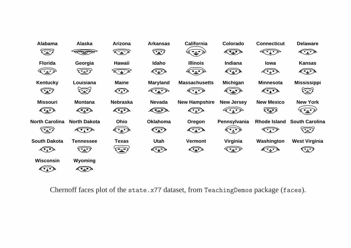
There are many ways to represent each case by a small diagram, of whichChernoff’s faces are the most (in)famous.

Wilkinson, L. (2005) The Grammar of Graphics. Second ed. Springer.

These glyph plots do depend on the ordering of variables and perhaps alsotheir scaling, and they do rely on properties of human visual perception. Sothey have rightly been criticised as subject to manipulation, and one shouldbe aware of the possibility that the effect may differ by viewer. (Especiallyif colour is involved; it is amazingly common to overlook the prevalence ofred–green colour blindness.)

Alabama

Alaska

Arizona

Arkansas

California

Colorado

Connecticut

Delaware

Florida

Georgia

Hawaii

Idaho

Illinois

Indiana

Iowa

Kansas

Kentucky

Louisiana

Maine

Maryland

Massachusetts

Michigan

Minnesota

Mississippi

Missouri

Montana

Nebraska

Nevada

New Hampshire

New Jersey

New Mexico

New York

North Carolina

North Dakota

Ohio

Oklahoma

Oregon

Pennsylvania

Rhode Island

South Carolina

South Dakota

Tennessee

Texas

Utah

Vermont

Virginia

Washington

West Virginia

Wisconsin

Wyoming

Chernoff faces plot of the state.x77 dataset, from S-PLUS.

Alabama Alaska Arizona Arkansas California Colorado Connecticut Delaware

Florida Georgia Hawaii Idaho Illinois Indiana Iowa Kansas

Kentucky Louisiana Maine Maryland Massachusetts Michigan Minnesota Mississippi

Missouri Montana Nebraska Nevada New Hampshire New Jersey New Mexico New York

North Carolina North Dakota Ohio Oklahoma Oregon Pennsylvania Rhode Island South Carolina

South Dakota Tennessee Texas Utah Vermont Virginia Washington West Virginia

Wisconsin Wyoming

Chernoff faces plot of the state.x77 dataset, from TeachingDemos package (faces).

Alabama Alaska Arizona Arkansas California Colorado Connecticut Delaware

Florida Georgia Hawaii Idaho Illinois Indiana Iowa Kansas

Kentucky Louisiana Maine Maryland Massachusetts Michigan Minnesota Mississippi

Missouri Montana Nebraska Nevada New Hampshire New Jersey New Mexico New York

North Carolina North Dakota Ohio Oklahoma Oregon Pennsylvania Rhode Island South Carolina

South Dakota Tennessee Texas Utah Vermont Virginia Washington West Virginia

Wisconsin Wyoming

Chernoff faces plot of the state.x77 dataset, from TeachingDemos package (faces2).

AlabamaAlaska

ArizonaArkansas

CaliforniaColorado

Connecticut

DelawareFlorida

GeorgiaHawaii

IdahoIllinois

Indiana

IowaKansas

KentuckyLouisiana

MaineMaryland

Massachusetts

MichiganMinnesota

MississippiMissouri

MontanaNebraska

Nevada

New HampshireNew Jersey

New MexicoNew York

North CarolinaNorth Dakota

Ohio

OklahomaOregon

PennsylvaniaRhode Island

South CarolinaSouth Dakota

Tennessee

TexasUtah

VermontVirginia

WashingtonWest Virginia

Wisconsin

Wyoming Frost

Life ExpHS GradIncome

Murder

Illiteracy

R version of stars plot of the state.x77 dataset.

Leptograpsus variegatus Crabs

200 crabs from Western Australia. Two colour forms, blue and orange;collected 50 of each form of each sex. Are the colour forms species?

Measurements of carapace (shell) length CL and width CW, the size of thefrontal lobe FL, rear width RW and body depth BD.

.

10 15

15 20

15

20

10

15FL

8 10 12 14

14 16 18 20

14

16

18

20

8

10

12

14

RW

15 20 25 30

30 35 40 45

30

35

40

45

15

20

25

30CL

20 30

40 50

40

50

20

30

CW

8 10 12 14

14 16 18 20

14

16

18

20

8

10

12

14BD

Blue male Blue female Orange Male Orange female

-1.5 -1.0 -0.5

-0.5 0.0 0.5

-0.5

0.0

0.5

-1.5

-1.0

-0.5Comp. 1

-0.15 -0.10 -0.05

0.00 0.05 0.10

0.00

0.05

0.10

-0.15

-0.10

-0.05

Comp. 2

-0.10 -0.05 0.00

0.00 0.05 0.10

0.00

0.05

0.10

-0.10

-0.05

0.00Comp. 3

Blue male Blue female Orange Male Orange female

First three principal components on log scale.

(a) (b)

(c) (d)

Projections of the Leptograpsus crabs data found by projection pursuit. View (a) is arandom projection. View (b) was found using the natural Hermite index, view (c) bythe Friedman–Tukey index and view (d) by Friedman’s (1987) index.

Multidimensional Scaling

Aim is to represent distances between points well.

Suppose we have distances (dij) between all pairs of n points, or a dissim-ilarity matrix. Classical MDS plots the first k principal components, andminimizes ∑

i �=j

d2ij − d̃2

ij

where (d̃ij) are the Euclidean distances in the kD space.

More interested in getting small distances right. Sammon (1969) proposed

min E(d, d̃) =1∑

i �=j dij

∑i �=j

(dij − d̃ij)2

dij

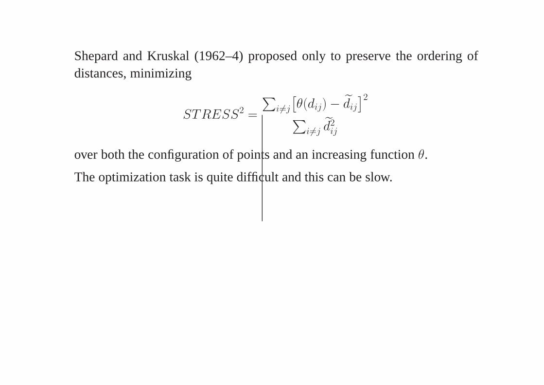
Shepard and Kruskal (1962–4) proposed only to preserve the ordering ofdistances, minimizing

STRESS2 =

∑i �=j

[θ(dij) − d̃ij

]2

∑i �=j d̃2

ij

over both the configuration of points and an increasing function θ.

The optimization task is quite difficult and this can be slow.

Multidimensional scaling

-0.10

0.0

0.10

-1.5 -1.0 -0.5 0.0 0.5 1.0

Blue maleBlue female

Orange MaleOrange female

An order-preserving MDS plot of the (raw) crabs data.

-0.15

-0.10

-0.05

0.0

0.05

0.10

-0.1 0.0 0.1 0.2

Blue maleBlue female

Orange MaleOrange female

After re-scaling to (approximately) constant carapace area.

A Forensic Example

Data on 214 fragments of glass collected at scenes of crimes. Each has ameasured refractive index and composition (weight percent of oxides of Na,Mg, Al, Si, K, Ca, Ba and Fe).

Grouped as window float glass (70), window non-float glass (76), vehiclewindow glass (17) and other (containers, tableware, headlamps) (22).

RI

Na

Mg

Al

Si

K

Ca

Ba

Fe

WinF

-4 -2 0 2 4 6 8

WinNF Veh

-4 -2 0 2 4 6 8

RI

Na

Mg

Al

Si

K

Ca

Ba

Fe

Con Tabl

-4 -2 0 2 4 6 8

Head

Strip plot by type of glass.

WinFWinNF

VehConTabl

Head

RI

-5 0 5 10 15

Na

12 14 16

Mg

0 1 2 3 4

WinFWinNF

VehConTabl

Head

Al

0.5 1.5 2.5 3.5

Si

70 71 72 73 74 75

K

0 1 2 3 4 5 6

WinFWinNF

VehConTabl

Head

Ca

6 8 10 12 14 16

Ba

0.0 1.0 2.0 3.0

Fe

0.0 0.2 0.4

Strip plot by type of analyte.

WinFWinNFVehConTablHead

Isotonic multidimensional scaling representation.