ELSEVIER European Journal of Operational Research 82 (1995) 111-124

EUROPEAN JOURNAL

OF OPERATIONAL RESEARCH

Theory and Methodology

Financial planning with fractional goals

Marc H . Goedhart, Jaap Spronk *

Tinbergen Institute and Department of Finance, Erasmus University Rotterdam, P.O. Box 1738, 3000 DR Rotterdam, Netherlands

Received July 1993; revised November 1993

Abstract

When solving financial planning problems with multiple goals by means of multiple objective programming, the presence of fractional goals leads to technical difficulties. In this paper we present a straightforward interactive approach for solving such linear fractional programs with multiple goal variables. The approach is illustrated by means of an example in financial planning.

Keywords: Financial planning; Fractional programming; Goal programming; Multiple-criteria decision making

1. Introduct ion

In this paper, we define financial planning in a firm as a structured process of identification and selection of present and future capital investment projects while taking account of the financing of these projects over time. The alternative financial plans to be considered by the firm's management are hard if not impossible to evaluate on the exclusive basis of the objective adopted by financial theory: the maximization of the share-holders' wealth or equivalently, the market value of the firm (see for example Brealey and Myers, 1988, Chapter 1). Management should for example not neglect the interests of participants other than the shareholders, even though they may de facto be the most powerful group of participants. For each financial p lan, management should try to assess all effects considered to be important by the most influential participants, which might also include the firm's bankers and employees. This gives rise to the notion that financial planning is essentially a decision problem with a complex of multiple and possibly conflicting goals, i.e. a multi-criteria decision problem. In the past, several decision methods were applied to the financial planning process, for example linear programming (Weingartner, 1966, e.g.), and multi-criteria decision methods such as goal programming and interactive methods (Zeleny, 1982, e.g., see White, 1990, for a bibliography). The decision method chosen in this paper is called Interactive Multiple Goal Programming (IMGP), an interactive multi-criteria decision method that is relatively simple to use and that has been applied to a variety of decision problems, among which are financial planning and macro-economic planning (Spronk, 1981, Goedhar t and Spronk, 1990, and Veeneklaas, 1990, for example).

* Corresponding author.

0377-2217/95/$09.50 © 1995 Elsevier Science B.V. All rights reserved SSD1 0377-2217(94)00034-A

112 M.H. Goedhart, J. Spronk / European Journal of Operational Research 82 (1995) 111-124

Another interesting feature of financial planning problems, apart from the multiplicity of goals, is the fact that many possible goals have the form of ratios. Examples are the maximization of the return on investment, of the number of times-interest-earned, or the minimization of the deviation of a target debt-to-equity ratio, etc. In fact, many decision problems in not only financial planning, but also macro-economic planning and operations management, to name a few, give rise to ratio-types of goals. Inclusion of these goals in otherwise linear programs is not straightforward - especially in case of multiple goal variables - and several algorithms exist for solving these so-called fractional programs (see for example Schaible and Ibaraki, 1983, and Craven, 1988, for an overview).

In this report we shall concentrate on the incorporation of fractional goal variables in linear programs with multiple goal variables. We consider only goal variables that are a single ratio of which both nominator and denominator are linear in the instrument variables. Variables with a more complicated ratio structure, e.g. the sum of two ratios, are treated elsewhere (see Schaible, 1981, for a bibliography). In Section 2 we briefly discuss Charnes and Cooper's well-known variable transformation method for dealing with a fractional goal variable in single goal linear programs (see Charnes and Cooper, 1962). However, for fractional linear programs with multiple goals several complications arise which preclude a straightforward treatment (see for example Kornbluth and Steuer, 1981b). In Section 3 we propose a method for dealing with multiple fractional goal variables in a fairly straightforward manner within Interactive Multiple Goal Programming (for details on IMGP we refer to Spronk, 1981). Thanks to the fact that IMGP separately solves a series of ordinary linear programs that are related via goal constraints, it is possible to integrate the variable transformation method in IMGP when dealing with multiple goal problems with fractional goals.

2. Linear fractional programming with multiple goals

A single goal linear fractional program is considered to have the following structure:

Max g=(cTx+a) / (dTx+19) (1)

s.t. x ~ S = { x ~ n l A x = b , x > O , b ~ m}

where: g : Fractional goal variable. c,d: Vectors of coefficients. x : Vector of instrument variables. a,19: Scalar constants.

It is assumed that the feasible set S is bounded and non-empty and that the denominator dTx + 19 is non-zero everywhere in S. In the literature, several parametric and gradient-based methods have been proposed to solve this type of linear program (see Schaible and Ibaraki, 1983, for an overview). Here, we discuss only the well-known variable transformation method of Charnes and Cooper (1961), which can be easily incorporated in IMGP. Charnes and Cooper's method transforms a fractional linear program into at most two ordinary linear programs. Solving the transformed program(s) is equivalent to solving the original fractional problem. Under the additional assumption that the denominator dWx + 19 is strictly positive throughout the feasible set, the original fractional problem can be replaced by a single transformed version in an ordinary linear programming format. In problem (1) the following substitution is made:

t= 1/(dTx +19) and y =xt. (2)

The resulting program is fractional in its constraints instead of the goal function and as t was assumed to be a strictly positive scalar variable, we may multiply the constraints by t and subsequently rewrite

M.H. Goedhart, J. Spronk / European Journal of Operational Research 82 (1995) 111-124 113

problem (1) as:

Max g = cXy + at (3)

s.t. Ay - bt < 0,

dTy + fit = 1, y > O , t > O , y E ~ n, t ~ .

Thus, the original non-linear fractional program is transformed into a straightforward linear program by the introduction of one additional scalar instrument variable t. If the denominator t of the goal function is not strictly positive over the feasible set of the original problem, a second transformation is necessary. In that case, a solution to the fractional problem is found by solving both transformed versions (see Charnes and Cooper, 1962, for details).

However, for fractional linear programs with multiple goals, such a straightforward solution is not possible. Consider the following fractional program with k goal variables and linear constraints:

Max gl = ( cTX + a l ) / ( dTx + 81) (4)

Max gk=(c x s.t. x ~ S = { x ~ " [ A x = b , x > _ O , b ~ m } .

Unfortunately, this type of programs cannot be handled by straightforward transformation. A transfor- mation of any of the fractional goal variables gi (i = 1 . . . . . k), as described in the previous section, would introduce non-linearities in the other goal variables. Therefore multiple goal problems retain their non-linear format, which leads to a number of complications with respect to the structure of the set of efficient solutions. The set of efficient points in a fractional multiple goal program is not necessarily closed; some interior points of the feasible set may be efficient while others are not, and efficient extreme points need not all be connected by a path of efficient edges (Kornbluth and Steuer, 1981b). This makes it difficult to determine the complete set of efficient points. The special structure of fractional multiple goal programs as far as the set of efficient points is concerned, has consequences for the applicability of various methods for solving linear programs with multiple goal variables.

The effectiveness of solution methods that rely on the determination of (part of) the set of efficient points is reduced by the special character of fractional programs. As the efficient set may be too difficult to determine, Kornbluth and Steuer (1981b) propose an algorithm for multiple objective linear fractional programming (MOLFP) that generates the set of so-called weakly-efficient points by means of a simplex-based algorithm. However, the computational requirements of their algorithm are very high compared to those of vector-maximum algorithms for the non-fractional linear case. Sometimes, problem (4) may be appropriately translated to a goal programming format. In that case a solution can be obtained by means of special methods for fractional goal programming problems (see for example Charnes and Cooper, 1977, and Kornbluth and Steuer, 1981a). Charnes and Cooper's method for fractional goal programming problems, which seems especially useful in case of a large number of fractional goal variables, generates a sequence of approximations converging to the optimum of the fractional problem. For an effective way of solving fractional programs with this method see Armstrong, Charnes and Haksever (1987).

3. IMGP and fractional goals

It is clear that fractional goal variables in multiple goal programs give rise to technical difficulties. These may be quite substantial if solution methods based on some efficiency concept are used, and can

114 M.H. Goedhart, J. Spronk /European Journal of Operational Research 82 (1995) 111-124

sometimes be handled with less trouble in the goal programming case. In this section we propose a straightforward method for solving multiple goal programs such as (4) by means of Interactive Multiple Goal Programming (IMGP, see Spronk, 1981, Chapter 6). In IMGP, the multiple goal program

Max gl (5)

Max gk

s.t. x ~ S is converted into a series of the following k linear programs. For i = 1 . . . . . k we obtain:

Max gi (6)

s.t. g i > ~ J f o r j - 1 , . . . , k and j ~ i , x ~ S .

Each of these so-called '~,-constraint programs' has k - 1 goal constraints representing minimally required levels on the corresponding goal variables. During the interactive procedure, constraints on the values of the goal variables gJ are formulated and the right-hand side values of these constraints, ~i are changed one by one from iteration to iteration. To be more precise, the procedure starts by representing a vector of minimum goal values to the decision maker, together with a set of indicators of potential improvements depicted by the optimal goal values ~i in the corresponding i-th objective '~,-constraint program'. Both vectors appear in a so-called potency-matrix:

Potency Matrix Goal 1 Goal i Goal n

Ideal value ~ l ~ i ~ n Minimal value ~, 1 ~i ~ n

In the first iteration, very low minimum 1 goal values are chosen (viewed by the decision maker as absolute minimum conditions or even worse) in order to ensure that no potentially acceptable solutions are excluded. The decision maker then has to indicate whether or not the solutions meeting these minimum requirements are satisfactory. If so, he can choose one of these solutions. If not, he has to indicate which of the minimum goal values ~,J should be increased. O n the basis of the new vector of minimum goal values, a new vector of indicators of potential improvements of these values is calculated from the ~-constraint programs and both vectors are presented to the decision maker. Then he has to indicate w h e t h e r the shift in the indicated minimum goal value is outweighed by the shifts in the potential values ~i of the other goal variables. If so, the decision maker gets the opportunity to revise his earlier wishes with respect to the changed minimum goal value. If not, the change of the minimum goal value is accepted and the decision maker can continue to raise any of the other or even the same minimum goal value. Of course, by raising the minimum goal values, the set of feasible solutions is reduced. The decision maker thus has several options. He can continue until the remaining set of feasible solutions becomes very small. Another possibility he has is to select a suitable solution from the set of solution satisfying the minimum conditions. (For instance, IMGP produces at each iteration among other things a s e t of efficient solutions.) It can be shown that if the set of efficient solutions to (5) is non-empty, the interactive process convergences towards an efficient and most preferred solution in a finite number of iterations. Finally, a set of feasible solutions satisfying the minimum conditions on the goal values can be subjected to a second analysis by the decision maker. In his decision environment, the decision maker may wish some elbow-room, thus requiring more than just one solution. Or, given this set of solutions resulting, goal variables that were not included in this first analysis can be taken account of

1 We assume for the ease of presentation that all goal variables are to be maximized.

M.H. Goedhart, J. Spronk / European Journal of Operational Research 82 (1995) 111-124 115

in the second analysis. Compared to several other multi-criteria optimization methods, IMGP offers a number of advantages. In contrast to goal programming for example, the decision maker is not required to explicitly specify a-priori preferences over all possible solutions. In comparison to vector maximum techniques, IMGP is easy to implement by means of standard linear programming software. Further- more, when dealing with fractional goal variables it is possible to use a separate optimization technique for each distinct goal variable in the corresponding 'g-constraint' program. Fractional goal variables can therefore be handled very effectively in IMGP by means of a variable transformation as in the Ordinary linear fractional program of Section 1.

Now reconsider the general formulation in (4) of a multiple goal fractional program. It is assumed that all k denominators are strictly positive for all x ~ S. On implementation of the procedure, the original multiple goal program is converted into a series of k 'g-constraint' fractional linear programs, just as in a non-fractional IMGP problem. For every i = 1 . . . . . k the following fractional linear program results:

M a x g i = (cTx + O l i ) / ( d T x -~ fli) (7)

s.t. ( c T x + a j ) / ( d T x + ~ y ) > _ g j f o r j = l . . . . , k and j ~ i ,

x ~ S . In each of these programs, all j goal variables have been turned into fractional constraints that can therefore be cross-multiplied to obtain ordinary linear constraints. Each i-th 'g-constraint' program as in (7) is equivalent to the fractional linear program

Max g i = ( c T x q-OLi) / (dTx q-[3i) (8)

forj= . . . . . and i - i , s. t .

x ~ S .

Thus, k linear programs with a fractional goal function are obtained that now can easily be solved by means of a substitution according to Charnes and Cooper 's well-known variable transformation method:

Let:

1

dTi x -I- ~i

This results

Max

t i (a scalar variable), and y i = x t i . (9)

in:

gi = c~Yi + aiti (10)

s.t. ( c f - g j d ~ ) Y i - ( g i ~ j - a i ) t i > _ O f o r j = l . . . . , k and j v~ i ,

A y i - bt i < O, T di Yi q- [~i ti = 1,

Yi >~ O, t i >_ O.

Again, the terms gj stand for the minimally required values for the goal variables other than the one maximized in the current 'g-constraint program'. Just as in a non-fractional IMGP problem, the decision maker interactively sets the required values gj for all goal variables until a set of solutions is obtained that are satisfactory. The transformed program (10) is equivalent to the original fractional program (7), in the sense that there is a one-to-one correspondence between a solution to (10) and a solution to the original program (see Craven, 1988, p.22). Thus, if IMGP converges to an efficient and most preferred solution in a finite number of steps, the same will hold for the fractional IMGP procedure. The only computational difference between this problem and a 'normal ' linear IMGP problem is that here k

116 M.H. Goedhart, J. Spronk / European Journal of Operational Research 82 (1995) 111-124

distinct 2 linear programs are solved, whereas normally the k linear programs will differ with respect to the goal level constraints only. The combined solution to the series of k linear programs as formulated in (10) equals the solution to the original fractional program of (7).

4. A financial planning model

In this section we present a financial planning model including multiple goals that contains a fractional goal variable. We show how a financial plan can be selected using IMGP as described above. The company's management has to evaluate a set of investment projects, simultaneously considering a series of financing decisions. The first goal variable in the model is assumed to be the company's total market value.

Following Myers and Pogue (1974), the company's total market value is defined as the sum of the unlevered present values of its investment projects plus the present value of its financing decisions, in this case the value of tax savings produced by debt financing. The unlevered present value of investment projects is assumed to be estimated directly by management as an input to the model and is defined as the project's market value when fully financed with equity. Although in financial literature other possible goal variables are often t ranslated into 'cost factors' that are subtracted from total market value or into constraints in the model (see for example Myers and P0gue, 1974), some separate goals are treated here explicitly. We have chosen for the following three additional goal variables in our model: the stability of accounting earnings over time, the average interest cover ratio (or 'times interest-is-earned ratio') over the first five years of the planning period and the employment level in the company.

Description of the model

The planning model covers 11 periods, in which the tax rate is assumed to be 40% and the interest rate for company debt is fixed at 10%. The instrument variables are a number of investment projects, the amount of debt and lendings in each period, and the cash held in each period. Management can choose from twenty investment projects, that represent the first type of instrument variables. The relevant characteristics of the projects consist of the unlevered present values A i, the after-tax cash flows in each period C[, the contribution to the periodic earnings before interest and taxes El, and the contribution to the total employment level in the company W i (see the Appendix for a full model description). The possibility of adopting an investment project is modelled by means of the continuous variables x i (0 < x i < 1, for i = 0 , . . . ,20) , and x ° represents the company's existing assets. The second instrument variable is the amount of debt issued each year. All debt issues have a maturity of one year and can therefore be seen as one-period loans D t, representing the principal borrowed at the beginning and repaid at the end of the same period t. Denoting the tax rate by T and the interest rate for debt by ra, the present value of debt is given by

10

E (rd " T ' D , ) / ( 1 + rd) ' . (11) t = 0

The nominator represents the tax savings caused by a shift from all-equity financing to partial debt financing (see also Myers and Pogue, 1974). Finally, the set of instrument variables includes the amount of cash held in each period, L t. Investing company funds in cash has a negative present value because on

2 I.e., the 'g-constraint programs' have different instrument vectors Yi and different constraints. Furthermore, at most k of these different linear programs will be necessary, in the case that k fractional goal variables exist with different denominators.

M.H. Goedhart, J. Spronk /European Journal of Operational Research 82 (1995) 111-124 117

cash no interest is received. If the riskfree interest rate is rf (with rf _< r d ) , the - negative - present value of having an annual cash level of L t during the planning horizon amounts to 3

10 ~_, ( - r f "Lt)/(1 + Ff). (12) t=O

The goal variables include the the total present - or market - value of the firm, the stability of accounting earnings over time, the average interest cover ( ' times-interest-earned'), and the employment level. The firm's total market value is to be maximized and is defined as follows:

20 10 rd . T" n t lO r f • L t

= D ° - • ( l + r f ) ' + L° (13) Max g l i=oEAi ' x i+ t=0E ( 1 q_ r d ) / t = 0

as all bankruptcy or issuing costs are assumed to be zero. The second management goal is to stabilize the pattern of accounting earnings over the planning period around the following target growth path:

E * = E t _ I . ( I + g E ) for t = l . . . . ,10, (14)

where E* is the target for earnings in period t, and ge = 5% is the target growth rate defined by management. In the present model, management is assumed to be interested in minimizing g2, the largest negative deviation from the yearly earnings target:

Min g2 > e 7 for t = l . . . . . 10 : (15)

with 20

E E [ ' x i , e + +e t = E S for t = l . . . . . 10. i = 0

This is the second goal variable. As an example of an organizational factor that may influence financial policy, the number of people employed in the firm was chosen. It is assumed that to avoid labour disputes, management wants to maximize the employment level in the company. With W / being the incremental number of jobs per investment project, the third goal variable is defined as

20 Max g3 = ~ W i "Xi" (16)

i = 0

The model is deterministic and t he uncertainty that is inherent to financial planning is largely accounted for exogenously. The unlevered present values of the projects for example, already include the value of the risk associated with these investments. On the other hand, the risk of bankruptcy in case of more debt financing is represented endogenously. Some financial planning models handle this risk by formulating chance constraints on the debt level, to prevent that " the probability that the firm will get into trouble reaches an unacceptable level" (Myers and Pogue, 1974, p.591). In our model a different approach is chosen, which is more familiar in practice, namely to limit the risk of being unable to pay the interest on debt out of company earnings, which means that the interest cover (or the number of ' t imes-interest-earned') should be maximized. The average interest cover over the first 5 years of the planning period is defined as the ratio of accounting earnings to interest charges and is the final goal variable (see Eq. (17)). The constraints for the balance of payments fully specify the planning model.

M a x g4 = ~ E E [ " x i / r d "D t • ( 1 7 ) t = 0 i ~ 0 t

3 The levels of debt and cash in the first year after the planning period, D l l and L i l , are limited to 1.5 times D10 and L10 respectively.

118 M.H. Goedhart, J. Spronk /European Journal o f Operational Research 82 (1995) 111-124

Table 1 Potency Matrices during iterations

Iteration Required goal values Ideal goal values

Goal 1 Goal 2 Goal 3 Goal 4 Goal 1 + Goal 2 + Goal 3 + Goal 4 +

5 6 7 8

9 10

442.58 77.76 3.69 2.51 778.66 0.15 344.00 6.09 442.58 54.04 80.00 2.51 764.33 0.15 344.00 6.09 650.00 54.04 80.00 2.93 764.33 0.64 300.85 4.93 650.00 50.00 80.00 2.93 763.74 0.64 300.85 4.93 650.00 50.00 80.00 3.00 763.74 0.64 292.25 4.93 650.00 50.00 150.00 3.00 748.28 0.64 292.25 4.27 700.00 50.00 150.00 3.00 748.28 3.02 228.35 3.72 700.00 25.00 150.00 3.00 744.93 3.02 225.97 3.39 725.00 25.00 150.00 3.00 744.93 12.63 186.02 3.25

725.00 15.00 150.00 3.00 731.11 12.63 162.53 3.16 731.11 15.00 150.00 3.13 731.11 15.00 150.00 3.13

Transformation of the ratio goal variable

The multi-criteria problem of selecting a financial plan for the model stated above can not be directly solved by means of a linear multi-criteria approach because the fourth goal variable, which corresponds to the interest-cover, is fractional. However, by making a suitable transformation to the '~,-constraint program' of this goal variable, in the way outlined in the previous section, the planning problem can still be handled straightforwardly with IMGP. The necessary transformations are the following:

(4 t, ~'= E r a ' D r , (18) t=O

in which z is a scalar variable;

O t = D t . ,r, 2 i = x i . ,l ", L t = L t . z ,

etc., for all instrument variables. This leads to the following transformed version of the interest cover's 'g-constraint program' (cf. with

(10) when a , /3 = 0 and d T has many zero-valued elements): 4 20

M a x g 4 : E E E ~ . x i ( 1 9 ) t = o i=0

20 10 rd. T- / ) t 10 ?-f. L t

s.t. i=oF-'Ai'2i+ ,=0E ( l+ra)t = (1 +r f ) t

20

E E [ . 2 i ' ~ t + > ( E * - g 2 ) ' ' r for t = l . . . . . 10, i~0 2o

W i " 2i > g3 "r , i=o

2, t~S*. As stated, the transformed program always has the same value for the goal function as the original

one if all instrument variables are appropriately transformed. S* is the modified feasible set following from the transformation. In this particular example, many of the right-hand side values in the original

M.H. Goedhart, J. Spronk /European Journal of Operational Research 82 (1995) 111-124

Table 2 Optimal values for instrument variables

119

Variable Value Variable Value Variable Value Variable Value Variable Value

X o 1.00 D o 400 E 0 100 X 1 0.39 D 1 450 E 1 109.42 X z 1.00 D 2 446.62 E 2 104.76 X 4 1.00 D 3 389.79 E 3 158.14 X 5 1.00 D 4 393.66 E 4 178.69 X 6 1.00 D 5 202.71 E 5 186.22 S 7 0.59 E 6 195.26 X s 0.20 E 7 190.02 )(10 1.00 E s 201.06 S l l 0.95 E 9 196.11 S14 0,81 El0 190.92

X15 1.00 X2o 1.00

EMI 1 0 L 0 15 EMI 2 10.13 L 6 33.81 EMI 5 1.40 L~ 82.11 EMI 6 0.28 L 8 303.85 EMI 7 15.00 L 9 525.58 EMI 9 15.00 L10 637.80 EMIxo 15.00 Lll 850.12

m o d e l a re zero, which impl ies tha t the feas ib le set does no t change a g rea t dea l as can also be seen f rom (10) when mos t e l e m e n t s o f vec to r b a re zero. In fact , the m a i n change is the add i t i on of an ext ra co lumn in the t a b l e a u for the c -var iab le and the fol lowing ext ra res t r ic t ion:

4

r d " / ) t = 1. (20) t=0

T h e '~ -cons t r a in t p r o g r a m s ' for the o the r t h r e e goal var iab les g l , g2 and g3 do no t have to be t r a n s f o r m e d b e c a u s e in each p r o g r a m the ' h a r d ' f rac t iona l cons t ra in t s on the r e q u i r e d va lue for g4 can b e c ross -mul t ip l i ed as follows:

4 20 4 E E E ~ "xi> E ra'g,4"Ot. (21)

t=o i=0 t~0

Selection o f a financial plan

Below, we have s imu la t ed the in te rac t ive so lu t ion p rocess for an imag ina ry dec is ion m a k e r who ob ta ins a un ique so lu t ion to the p l ann ing p r o b l e m in 10 i t e ra t ions wi th I M G P (see T a b l e 1). The idea l va lue G o a l i +, p r e s e n t e d for the goal va r iab les at i t e r a t i on 0 a re o b t a i n e d by op t imiz ing each of the goal va r i ab les s epa ra t e ly wi thou t any res t r i c t ions on the va lues of the o t h e r goals. T h e n in each subsequen t i t e ra t ion , one o f the goal cons t ra in t s is u p d a t e d . A t t he first i t e r a t i on the min ima l ly r e q u i r e d va lue for the e m p l o y m e n t level ( G o a l 3_) , is set to 80 jobs b e c a u s e a loss of m o r e t han 20 jobs 4 is no t accep tab le to the dec is ion maker . A s a consequence , the idea l va lue for the m a r k e t va lue Goa l 1 + somewha t d e t e r i o r a t e s bu t this loss in va lue is found accep tab le . T h e r e f o r e the dec is ion m a k e r ma in ta ins t h e 80 jobs level and con t inues by increas ing the min ima l ly r e q u i r e d m a r k e t va lue in the second i t e ra t ion to 650. This l eads to lower idea l va lues for all o t h e r goal va r iab les bu t be c a use a high m a r k e t va lue is i m p o r t a n t to the dec i s ion maker , this t r ade -o f f is c o n s i d e r e d r ea sonab le . The vec tors of r e q u i r e d and idea l goal va lues ( the so-ca l led po t ency ma t r i ces ) resu l t ing f rom these and all subsequen t changes in goal cons t ra in t s du r ing the in te rac t ive p r o c e d u r e a re p r e s e n t e d in Tab le 1, wi th the u p d a t e d goal cons t r a in t in each i t e r a t i on in italics. By in te rac t ive ly u p d a t i n g the goal cons t ra in t s the dec i s ion m a k e r has r e a c h e d a

4 The current level of employment, W o is assumed to be 100.

120 M.H. Goedhart, J. Spronk / European Journal of Operational Research 82 (1995) 111-124

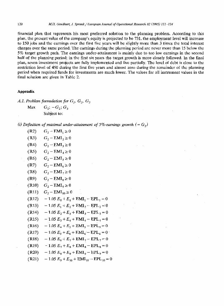
f inancial p lan tha t r epresen t s his most p r e f e r r e d solut ion to the p lanning problem. Accord ing to this

plan, the p resen t va lue of the company ' s e q u i t y is p ro j ec t ed to be 731, the e m p l o y m e n t level will increase

to 150 jobs and the earn ings over the first five years will be slightly m o r e than 3 t imes the total in teres t

charges o v e r the same per iod. T h e earn ings dur ing the p lanning pe r iod are neve r m o r e than 15 be low the

5% ta rge t growth path. T h e earn ings u n d e r - a t t a i n m e n t is mainly due to too low earn ings in the second

ha l f of t h e p lann ing per iod; in the first six years the t a rge t growth is m o r e closely fol lowed. In the final

plan, seven inves tment projects are fully i m p l e m e n t e d and five partially. T h e level o f debt is close to the

res t r ic t ion level o f 450 dur ing the first five years and a lmost ze ro dur ing the r e m a i n d e r of the p lanning

pe r iod w h e n r equ i r ed funds for inves tments are m u c h lower. T h e values for all i n s t rument values in the

final solut ion are given in Tab le 2.

Appendix

A.1. Problem formulation for G 1, G 2, G 3

Max G1; , G 2 ; G 3

Subject to:

(i) Definition o f maximal under-attainment o f 5%-earnings growth (= G e)

( R 2 ) G 2 - E M I 1 _> 0

( R 3 ) G e - E M I z ___ 0

( R 4 ) G z - E M I 3 > 0

( R 5 ) G 2 - E M I 4 >__ 0

( R 6 ) G 2 - E M I 5 > 0

( R 7 ) G a - E M I 6 ___ 0

( R 8 ) G 2 - E M I 7 _> 0

(R9) G 2 - E M I 8 >_ 0

(R10) G 2 - E M I 9 _> 0

( R l l ) G a - E M I l o > 0

(R12) - 1.05 E o + E 1 + E M I 1 - E P L 1 = 0

(R13) - 1.05 E 1 + E z + E M I a - E P L a = 0

(R14) - 1.05 E 2 + E 3 + E M I 3 - E P L 3 = 0

(R15) - 1.05 E 3 + E 4 + E M I 4 - E P L 4 = 0

(R16) - 1.05 E 4 + E 5 + E M I 5 - E P L 5 - 0

(R17) - 1.05 E 5 + E 6 + E M I 6 - E P L 6 = 0

(R18) - 1.05 E 6 + E 7 + E M I 7 - E P L 7 = 0

(R19) - 1.05 E7 + E 8 + E M I s - E P L 8 = 0

(R20) - 1.05 E 8 + E 9 + E M I 9 - E P L 9 = 0

(R21) - 1.05 E 9 q- ElO -b E M I lO - E P L lO = 0

M.H. Goedhart, J. Spronk ~European Journal of Operational Research 82 (1995) 111-124 121

(R24)

(R25)

(R26)

(R28)

(ii) Equations for the balance o f funds

(R22) 130 X o - 10 X 1 - 50 X 6 - 200 X 7 - 100 XlZ - 1.06 D O + D 1 + L o - L 1 = 0

(R23) 130 X o + 2 X 1 - 10 X z + 10 X 6 + 18 X 7 - 300 X 8 - 100 X 9 + 50 X12 - 50 X2o - 1.06 D 1

+ D2 + L 1 - L2 = O

130 X o + 2 X 1 + 2 X 2 - 10 X 3 + 10 X 6 + 18 X 7 + 100 X 8 + 40 X 9 - 100 Xlo + 50 X12

- - 100 X16 -{'- 10 X20 - - 1 . 0 6 D 2 q- D 3 + L 2 - L 3 = 0

120 X o + 2 X 1 + 2 X2q--2 X 3 - 10 X 4 q- 10 X6 -'l- 18 X 7 + 100 X 8 + 4 0 X 9 -- 50 XlO

- 100 X l l q'- 50 X12 - 100 X13 "[- 40 X16 -'t- 11 X2o - 1.06 D 3 + D 4 + Z 3 - Z 4 = 0

120 X o + 2 X 1 + 2 X2q-2 X 3 + 2 X 4 - 10 X 5 q- 10 X6 -]-- 18 X T - 100 X 8 + 4 0 X 9

(R29)

(R30)

(R32)

(R33)

(R34)

+ 40 Xlo

120 X o +

+ 30 Xlo

- L 6 = 0

120 X o +

q- 50 X13

- L 7 = 0

110 X o +

q'- 50 X14

H o Xo +

"}- 50 X14

11o Xo +

"]'- 50 S14

11o X o +

"[- 40 X16

+ 50 Xl l + 50 2(13 + 40 X16 - 20 X17 -']'- 12 X2o - 1.06 D 4 + D s + L 4 - L 5 = 0

2 X 1 + 2 X 2 + 2 X 3 + 2 X4q-2 Xsq- 10 X6q- 18 XT+ 10o X 8 - 6 0 X 9

+ 40 Xl l + 50 )(13 + 40 X16 + 8 X17 - 20 X18 + 13 X2o - 1.06 D s + D 6 -? L 5

2 X 1 + 2 X 2 + 2 X 3 + 2 X 4 + 2 X s + 10 X 6 + 18 X 7 + 4 0 X 9 + 2 0 Xlo + 30 Xl l

- 200 X14 + 40 X16 + 6 X17 + 8 X18 - 20 X19 + 14 X2o - 1.06 D 6 q- D 7 q- L 6

2 X 1 + 2 X 2 + 2 X 3 + 2 X 4 + 2 X s + 10 X 6 + 18 X 7 + 4 0 X 9 + 10 Xlo + 20 X u

+ 40 X16 + 4 X17 -'[- 6 XlS + 8 )(19 + 15 X2o - 1.06 0 7 q- D s + L 7 - L 8 = 0

2 X 1 + 2 X 2 + 2 X 3 + 2 X 4 + 2 X s + 10 X 6 + 18 X 7 + 4 0 X 9 + 10 Xlo + 20 )(11

+ 40 X16 + 2 X17 + 4 Xls + 6 X19 + 15 X2o - 1.06 D s + D 9 + L s - L 9 = 0

2 X 1 + 2 X 2 + 2 X 3 + 2 X 4 + 2 X 5 + 10 X 6 + 18 XT+ 40 X 9 + 10 X l o + 1 0 Xl l

-- 100 X15 "-}- 40 X16 q- 2 X18 + 4 X19 + 15 X2o - 1.06 0 9 + O10 q- L 9 - L l O = 0

2 X 1 + 2 X 2 + 2 X 3 + 2 X 4 + 2 X 5 + 10 ) ( 6 + 18 X 7 - 60 X g + 10 X l o + 5 0 X15

+ 2 X19 + 15 X2o - 1.06 Olo + D11 + Llo - L l l = 0

(iii) Definition

(R35)

(R36)

(R37)

(R38)

(R39)

(R40)

(R41)

(R42)

of accounting earnings

100 X o - Eo = 0

103 X o + 1.5 X 1 + 7 X 6 - 2 X 7 + 10 X12 -- E 1 = 0

105 X o + 1.5 X 1 + 1.5 X 2 + 7 X 6 - 2 X 7 - 50 X 8 + 20 X 9 + 15 X12 + 2 X2o - E 2 = 0

112 X o + 1.5 X 1+ 1.5 X 2 + 1.5 X 3 + 7 X 6 - 2 X 7 + 70 X 8 + 20 X 9 + 20 Xlo + 25 X12

- 10 X16 + 4 2(20 - E 3 = 0

108 X o + 1.5 X 1 + 1.5 X 2 + 1.5 X 3 + 1.5 X4 + 7 X 6 - 2 X 7 + 80 X s + 2 0 X 9 + 2 0 Xlo

+ 20 Xl1 + 10 X13 + 6 X2o - E 4 = 0

110 2(o+ 1.5 X 1 + 1.5 X 2 + 1,5 X 3 + 1.5 X 4 + 1.5 X 5 + 7 X 6 - 2 X 7 + 9 0 ) ( 8 + 20 X 9

+ 20 Xlo + 20 X l l + 15 X13 + 8 X 2 o - E 5 = 0

115 X o + 1.5 X 1 + 1.5 X 2 + 1.5 X 3 + 1.5 X 4 + 1.5 X 5 + 7 X 6 - 2 X 7 + 100 X 8 + 2 0 X 9

q- 20 Xlo q- 20 X l l q- 25 X13 4- 10 X2o - E 6 = 0

120 X o + 1.5 X 1 + 1.5 X 2 + 1.5 X 3 + 1.5 X 4 + 1.5 X 5 + 7 X 6 - 2 X 7 + 2 0 X 9 + 20 Xlo

-[- 20 X l l -[- 10 X14 q- 20 X16 --~ 12 X2o - E 7 = 0

122 M.H. Goedhart, J. Spronk /European Journal of Operational Research 82 (1995) 111-124

(R43) 125 X o + 1.5 X 1 + 1.5 X e + 1.5 X 3 + 1.5 X 4 + 1.5 X~ + 7 X 6 - 2 X 7 + 20 X 9 + 20 Xao

+ 20 X l l + 15 X14 + 30 X16 + 14 Xzo - E 8 = 0

(R44) 130 X o + 1.5 X~ + 1.5 X e + 1.5 X 3 + 1.5 X 4 + 1.5 X 5 + 7 X 6 - 2 X 7 + 20 X 9 + 20 Xlo

+ 25 S14 --[- 30 X16 --I- 15 S2o - E 9 --- 0

(R45) 135 X o + 1.5 X1 + 1.5 X e + 1.5 X 3 + 1.5 X 4 + 1.5 X 5 + 7 X 6 - 2 X 7 + 20 X 9 + 20 Xlo

-l- 10 X15 -{- 20 S16 -t- 15 S2o - Elo = 0

(iv) Initial values for debt and cash holdings

(R46) D o = 4 0 0

(R47) L o = 15

(v) Dividend constraints

(R48) D~ < 4 5 0

(R49) D e < 4 5 0

(R50) D 3 < 450

(R51) D 4 < 450

(R52) D 5 <450

(R53) D 6 _< 500

( R 5 4 ) D 7 _< 500

(R55) D 8 < 5 0 0

(R56) D 9 _< 500

(R57) D~o_<500

(R100) - 1 . 5 D l o + D l l _ < 0

(R101) - 1 . 5 L l o + L l a < 0

(vi) Definition of company's adjusted present value ( = market value G 1)

(R58) - G 1 + 1 0 0 0 X o + 1 0 X a + 9 X z + X 3 + 7 X 4 + 6 X s + 6 0 X 6 - 4 0 X 7 + 4 0 X s + l O X 9

+ 20 Xlo + 10 Y l l + 20 X12 + 10 X13 -l- 5 XI4 + 15 X16 - 10 X17 - 15 )(18 - 20 X19

+ 30 X2o - 0.96 D o + 0.036 Dx + 0.033 D 2 + 0.03 D 3 + 0.027 D 4 + 0.025 D 5 + 0.023 D 6

+ 0.021 D 7 + 0.019 D 8 + 0.017 D 9 + 0.015 Dlo + 0.014 Dim + L 0 - 0.074 L~ - 0.069 L 2

- 0.064 L 3 - 0.059 L 4 - 0.054 L 5 - 0.05 L 6 - 0,047 L 7 - 0.043 L 8 - 0.04 L 9 - 0.037 LIO

- 0.0343 L11 = 0

(vii) Definition of employment level in the company (= G 3)

(R59) - G 3 + 100 X o - 10 X 1 - 8 X 2 - 7 X 3 - 6 X 4 - 5 X 5 - 45 X 6 + 200 X 7 - 90 X 8 - 27 X9

+ 15 X12 + 15 X13 + 15 X14 + 5 Xls + 12 X17+ 12 X18 + 12 X19+ 2 X2o= 0

(viii) Definition of earnings (= G 4) and interest charges ( = GG 4) over the first 5 years

(R64) - G 4 + 528 X o + 6 X 1 + 4.5 X 2 + 3 X 3 + 1.5 X 4 --]- 28 X 6 - - 8 X 7 + 100 X 8 + 60 X 9

+ 40 Xlo + 20 X l l + 50 X12 + 10 X13 - 10 X16 + 12 X2o = 0

(R65) 0 . 1 D o + 0 . 1 D I + 0 . 1 D 2 + 0 . 1 D 3 + 0 . 1 D 4 - G G 4 = 0

M.H. Goedhart, J. Spronk ~European Journal of Operational Research 82 (1995) 111-124

(ix) Goal restrictions

(R60) G 1 - G ~ > O

(R61) G 2 - G~ < 0

(R62) G 3 - G~ > 0

(R63) G 4 - G ~ G G 4 > 0

G* is the required value (a constant) on the other goal variables j 4~ i

(x) Bounds

F R E E G 1

F R E E G 2

F R E E G 3

FIX X o

SUB X 1

1.00000

1.00000, etc. for all other xj ( j = 2 , . . . , 20)

123

A.2. Problem formulation for G 4

Largely equal to that for the other goal variables. Only the constraint blocks (iv), (v) and (ix) are changed to the following:

(iv') Initial values for debt and cash holdings

(R46) D 0 - 4 0 0 t = 0

(R47) L 0 - 1 5 t = 0

(v') Dividend constraints

(R48) D 1 - 450 t < 0

(R49) D 2 - 4 5 0 t < 0

(R50) D 3 - 450 t < 0

(R51) D 4 - 450 t_< 0

(R52) D 5 - 4 5 0 t _ < 0

(R53) 06 - 500 t ~ 0

(R54) D 7 - 500 t < 0

(R55) D 8 - 5 0 0 t < 0

(R56) D 9 - 500 t ~ 0

(R57) Dlo - 500 t < 0

(R100) - 1 . 5 D l o + D l l < 0

(R101) - 1 . 5 L l o + L l l < 0

124 M.H. Goedhart, J. Spronk /European Journal of Operational Research 82 (1995) 111-124

(ix') Goal restrictions

(R60) G 1 - G ~ t ~> 0

(R61) G 2 - G ~ t_<0

(R62) G 3 - G~ t ___ 0

(R63) 1 = 0.1 D O + 0.1 D 1 + 0.1 D 2 + 0.1 D 3 + 0.1 0 4

G 7 is the requi red value (a cons tant ) on the other goal var iables j ~ i

(x') Bounds

F R E E G 1 G 2 G 3

All o ther bounds a re replaced by the following constraints :

(R66) X 0 - t = 0

(R67) X 1 - t _~ 0

(R68) X2 - t < O etc. for all o ther x j bounds ( j = 3 , . . . , 2 0 )

(R86) X z 0 - t < 0 .

References

Armstrong, R., Charnes, A., and Haksever, C. (1987), "Successive linear programming for ratio goal problems", European Journal of Operational Research 32, 426-434.

Brealey, R.A., and Myers, S.C. (1988), Principles of Corporate Finance, McGraw-Hill, New York. Charnes, A., and Cooper, W.W. (1962), "Programming with fractional functionals", Naval Research Logistics Quarterly 9, 181-186. Charnes, A., and Cooper, W.W. (1977), "Goal programming and multiple objective optimizations", European Journal of

Operational Research 1, 39-54. Craven, B.D. (1988), Fractional Programming, Heidermann, Berlin. Goedhart, M.H., and Spronk, J. (1990), "Multi-factor financial planning: An outline and illustration", in: J. Spronk and B.

Matarazzo (eds.), Modelling for Financial Decisions, Springer-Verlag, Berlin, 25-42. Kornbluth, J.S.H. (1980), "Computational experience with multiple objective linear fractional programming algorithms", in: J.

Morse (ed.), Organizations: Multiple Agents with Multiple Criteria, Springer-Verlag, Berlin. Kornbluth, J.S.H., and Steuer, R.E. (1981a), "Goal programming with linear fractional criteria", European Journal of Operational

Research 8, 58-65. Kornbluth, J.S.H., and Steuer, R.E. (1981b), "Multiple objective linear fractional programming", Management Science 27/9,

1024-1039. Myers, S.C., and Pogue, G.A. (1974), "A programming approach to corporate financial management", Journal of Finance 29,

579-599. Schaible, S. (1981), "Fractional programming: Applications and algorithms", European Journal of Operational Research 7, 111-120. Schaible, S., and Ibaraki, T. (1983), "Fractional programming", European Journal of Operational Research 12, 325-338. Spronk, J. (1981), Interactive Multiple Goal Programming, Martinus Nijhoff, Boston, MA. Steuer, R.E. (1986), Multiple Criteria Optimization: Theory, Computation and Application, Wiley, New York. Veeneklaas, F.R. (1990), "Dovetailing technical and economic analysis", Ph.D. Dissertation, Erasmus University Rotterdam. Weingartner, H.M. (1966). "Capital budgeting of interrelated projects: Survey and synthesis", Management Science 12/7, 213-244. White, D.J. (1990), "A bibliography on the applications of mathematical programming multi-objective methods", Journal of the

Operational Research Society 41, 669-691. Zeleny, M. (1982), Multiple Criteria Decision Making, McGraw-Hill, New York.