Financial Optimization Problems

�Siu Lung Law

St. Anne’s College

University of Oxford

A thesis submitted for the degree of

Doctor of Philosophy

Trinity 2005

This thesis is dedicated to

my parents

for their continual support throughout the years

Acknowledgements

Firstly, I would like to thank C.V.C.P., St. Anne’s College and the

Croucher Foundation for providing monetary support. Equally impor-

tant, I am grateful to my supervisor Dr. Jeff Dewynne, who has given

me a lot of useful advice. I am also grateful to Dr. Chiu Fan Lee, who

has helped me enormously in the multi-dimensional problem. Dr. Paul

Wilmott’s initial supervision and Dr. Sam Howison’s support at the end

are also very much appreciated.

Abstract

The major objective of this thesis is to study optimization problems in

finance. Most of the effort is directed towards studying the impact of

transaction costs in those problems. In addition, we study dynamic mean-

variance asset allocation problems. Stochastic HJB equations, Pontryagin

Maximum Principle and perturbation analysis are the major mathemati-

cal techniques used.

In Chapter 1, we introduce the background literature. Following that, we

use the Pontryagin Maximum Principle to tackle the problem of dynamic

mean-variance asset allocation and rediscover the doubling strategy.

In Chapter 2, we present one of the major results of this thesis. In this

chapter, we study a financial optimization problem based on a market

model without transaction costs first. Then we study the equivalent prob-

lem based on a market model with transaction costs. We find that there

is a relationship between these two solutions. Using this relationship, we

can obtain the solution of one when we have the solution of another.

In Chapter 3, we generalize the results of chapter 2.

In Chapter 4, we use Pontryagin Maximum Principle to study the problem

limit of the no-transaction region when transaction costs tend to 0. We

find that the limit is the no-transaction cost solution.

Contents

1 Introduction 1

1.1 Overview of Research . . . . . . . . . . . . . . . . . . . . . . . . . . . 1

1.2 Introduction . . . . . . . . . . . . . . . . . . . . . . . . . . . . . . . . 2

1.3 Statement of Originality . . . . . . . . . . . . . . . . . . . . . . . . . 3

1.4 Weiner Process . . . . . . . . . . . . . . . . . . . . . . . . . . . . . . 3

1.5 Deterministic Control Problem . . . . . . . . . . . . . . . . . . . . . . 5

1.5.1 Dynamic Programming . . . . . . . . . . . . . . . . . . . . . . 6

1.5.2 Pontryagin Maximum Principle . . . . . . . . . . . . . . . . . 7

1.6 Stochastic Control . . . . . . . . . . . . . . . . . . . . . . . . . . . . 8

1.6.1 Dynamic Programming . . . . . . . . . . . . . . . . . . . . . . 9

1.6.2 Pontryagin Maximum Principle . . . . . . . . . . . . . . . . . 9

1.7 Markowitz Mean-Variance Efficient Frontier . . . . . . . . . . . . . . 10

1.8 Utility Function . . . . . . . . . . . . . . . . . . . . . . . . . . . . . . 14

1.9 Constant Relative Risk Aversion . . . . . . . . . . . . . . . . . . . . . 14

1.10 Merton’s Investment-Consumption Model . . . . . . . . . . . . . . . . 16

1.11 Long Term Growth Model . . . . . . . . . . . . . . . . . . . . . . . . 19

1.12 Example of Pontryagin Maximum Principle . . . . . . . . . . . . . . 20

1.12.1 Market Model Equations . . . . . . . . . . . . . . . . . . . . . 21

1.12.2 Applying the Maximum Principle . . . . . . . . . . . . . . . . 22

1.12.3 Kolmogorov Equation and Transition Probability . . . . . . . 24

1.12.4 Discussion . . . . . . . . . . . . . . . . . . . . . . . . . . . . . 27

1.12.5 Dynamic Asset Allocation with Margin Constraints . . . . . . 28

1.13 Investment with Transaction Costs . . . . . . . . . . . . . . . . . . . 29

1.13.1 Atkinson, Pliska & Wilmott . . . . . . . . . . . . . . . . . . . 29

1.13.2 Atkinson and Al-Ali . . . . . . . . . . . . . . . . . . . . . . . 31

1.13.3 Atkinson and Mokkhavesa (2001) . . . . . . . . . . . . . . . . 32

1.13.4 Mokkhavesa and Atkinson (2002) . . . . . . . . . . . . . . . . 32

1.13.5 Atkinson and Mokkhavesa (2004) . . . . . . . . . . . . . . . . 33

i

2 Dynamic Asset Allocation with Transaction Costs 34

2.1 Introduction . . . . . . . . . . . . . . . . . . . . . . . . . . . . . . . . 34

2.2 Market Model without Transaction costs . . . . . . . . . . . . . . . . 35

2.3 Formulation of Bellman’s Equation in the No Transaction Costs Problem 36

2.4 Solving Bellman’s Equation in the No Transaction Costs Problem . . 38

2.4.1 Long Term Growth Model . . . . . . . . . . . . . . . . . . . . 39

2.4.2 Constant Relative Risk Aversion (CRRA) Model . . . . . . . 40

2.5 Market Model with Transaction costs . . . . . . . . . . . . . . . . . . 41

2.6 Formulation of Bellman’s Equation under Transaction costs . . . . . . 42

2.6.1 Change of Variables . . . . . . . . . . . . . . . . . . . . . . . . 48

2.6.2 Sales and Purchase Regions . . . . . . . . . . . . . . . . . . . 49

2.6.3 No-Transaction Region . . . . . . . . . . . . . . . . . . . . . . 51

2.6.4 The O(k−2/3) Equation . . . . . . . . . . . . . . . . . . . . . . 52

2.6.5 The O(k−1/3) Equation . . . . . . . . . . . . . . . . . . . . . . 52

2.6.6 The O(1) Equation . . . . . . . . . . . . . . . . . . . . . . . . 52

2.6.7 The O(k1/3) Equation . . . . . . . . . . . . . . . . . . . . . . 53

2.6.8 The O(k2/3) Equation . . . . . . . . . . . . . . . . . . . . . . 54

2.7 Example . . . . . . . . . . . . . . . . . . . . . . . . . . . . . . . . . . 57

2.7.1 Long Term Growth Model . . . . . . . . . . . . . . . . . . . . 57

2.7.2 Constant Relative Risk Aversion (CRRA) Model . . . . . . . 58

2.8 Financial Interpretations . . . . . . . . . . . . . . . . . . . . . . . . . 60

2.8.1 Long Term Growth Model . . . . . . . . . . . . . . . . . . . . 63

2.8.2 CRRA Model . . . . . . . . . . . . . . . . . . . . . . . . . . . 71

2.9 The Choice of Asymptotic Scales . . . . . . . . . . . . . . . . . . . . 82

2.9.1 H0, H1, H2, · · ·, H2m−1 . . . . . . . . . . . . . . . . . . . . . . 84

2.9.2 H2m, H2m+1, H2m+2, · · ·, H3m−1 . . . . . . . . . . . . . . . . . 84

2.9.3 H3m, H3m+1, H3m+2, · · ·, H4m−1 . . . . . . . . . . . . . . . . . 85

2.9.4 H4m . . . . . . . . . . . . . . . . . . . . . . . . . . . . . . . . 86

3 Two Generalizations of the Dynamic Asset Allocation with Trans-

action Cost Model 88

3.1 Introduction . . . . . . . . . . . . . . . . . . . . . . . . . . . . . . . . 88

3.2 Stock Price Dependence . . . . . . . . . . . . . . . . . . . . . . . . . 88

3.2.1 Without Transaction Costs . . . . . . . . . . . . . . . . . . . . 89

3.2.2 Solving Bellman’s Equation with No Transaction Costs . . . . 90

3.2.3 Modified Long Term Growth Model . . . . . . . . . . . . . . . 91

ii

3.2.4 Modified Constant Relative Risk Aversion (CRRA) Model . . 92

3.2.5 With Transaction Costs . . . . . . . . . . . . . . . . . . . . . 93

3.2.6 Modified Long Term Growth Model . . . . . . . . . . . . . . . 100

3.2.7 Modified Constant Relative Risk Aversion (CRRA) Model . . 101

3.2.8 Financial Interpretations . . . . . . . . . . . . . . . . . . . . . 102

3.2.9 Modified Long Term Growth model . . . . . . . . . . . . . . . 103

3.2.10 Modified CRRA model . . . . . . . . . . . . . . . . . . . . . . 104

3.3 Multi-Asset . . . . . . . . . . . . . . . . . . . . . . . . . . . . . . . . 115

3.3.1 Without Transaction Costs . . . . . . . . . . . . . . . . . . . . 115

3.3.2 Solving Bellman’s Equation with No Transaction Costs . . . . 117

3.3.3 Long Term Growth Model . . . . . . . . . . . . . . . . . . . . 118

3.3.4 Constant Relative Risk Aversion (CRRA) Model . . . . . . . 118

3.3.5 With Transaction Costs . . . . . . . . . . . . . . . . . . . . . 119

3.3.6 Financial Interpretations . . . . . . . . . . . . . . . . . . . . . 126

3.3.7 Two Dimensional Case . . . . . . . . . . . . . . . . . . . . . . 127

3.3.8 Financial Interpretations . . . . . . . . . . . . . . . . . . . . . 130

4 The Convergence of the No Transaction Region in the Transaction

Costs Problem 131

4.1 Introduction . . . . . . . . . . . . . . . . . . . . . . . . . . . . . . . . 131

4.2 Market Model without Transaction Costs . . . . . . . . . . . . . . . . 133

4.3 Applying the Maximum Principle on the No Transaction Costs Problem134

4.4 Market Model with Transaction Costs . . . . . . . . . . . . . . . . . . 136

4.5 The Order of Et(ΨB) . . . . . . . . . . . . . . . . . . . . . . . . . . . 140

4.6 Transaction Costs Level Tends to 0 . . . . . . . . . . . . . . . . . . . 142

4.7 Examples . . . . . . . . . . . . . . . . . . . . . . . . . . . . . . . . . 142

5 Conclusion 143

5.1 Results Achieved . . . . . . . . . . . . . . . . . . . . . . . . . . . . . 143

5.2 Future Work . . . . . . . . . . . . . . . . . . . . . . . . . . . . . . . . 143

A Nomenclature 145

A.1 All Chapters . . . . . . . . . . . . . . . . . . . . . . . . . . . . . . . . 145

A.2 Chapter 1 . . . . . . . . . . . . . . . . . . . . . . . . . . . . . . . . . 147

A.3 Chapter 2 . . . . . . . . . . . . . . . . . . . . . . . . . . . . . . . . . 147

A.4 Chapter 3 . . . . . . . . . . . . . . . . . . . . . . . . . . . . . . . . . 147

A.5 Chapter 4 . . . . . . . . . . . . . . . . . . . . . . . . . . . . . . . . . 148

iii

Chapter 1

Introduction

1.1 Overview of Research

This thesis is concerned with mathematics in finance.

In the study of finance, and in fact in science, mathematics can always play an

important role. The process of study involves building models, working out the

implications or predictions of the models and testing whether they fit with the facts.

Mathematics can contribute in the process of working out the implications of the

assumptions. Only after obtaining implications, we can compare them with reality,

and thus verify the models. Whether a model or a theory is accepted or rejected is

solely based on whether its predictions fit the facts better or explain the phenomenon

better than other existing models. Mathematics plays a pivotal role in this process.

An example of application of mathematics is this: we want to compare a new

option pricing model with the Black-Scholes Model. In order to test whether the

new model actually is better than the Black-Scholes model, the first step is to use

mathematics to work out the implications predicted by the new model and the Black-

Scholes Model under different circumstances. Only after that we can test how good

the new model is compared to the Black-Scholes Model.

By comparing the implications worked out by mathematics, we can accept or

reject a model. For example, the Black-Scholes Model [10] is preferred to Sprenkle

[45] in options pricing solely because the Black-Scholes Model gives predictions more

consistent with observation in the same way the theory of relativity is preferred to

Newton’s theory in predicting the trajectories of different planets. These comparison

can never be made if there is no mathematics.

The theme of this thesis is to use mathematics to work out the implication of the

introduction of transaction costs in finance. In Chapter 2, we present one of the major

results of this thesis, which is about the impact of small proportional transaction costs

1

in a general, dynamic, finite-horizon financial optimization problem. In other words,

suppose we have a solution of an optimization problem based on a market model

without transaction costs, and now we want to introduce transaction costs into the

market model, what is the relationship between the new solution and the original

solution? We successfully find an analytic relationship between these two solutions.

Using this relationship, we can obtain the solution of one when we have the solution

of another. The mathematical techniques we use include stochastic HJB equations

and perturbation analysis.

In Chapter 3, we generalize the result in Chapter 2. Firstly, we consider the

case that the reward function depends on the stock price. Secondly, we consider the

multi-asset case. The form of the analytic solutions obtained are similar to those in

Chapter 2, but of course they are more complicated. Also, we find that many of the

financial interpretations may no longer hold in a more general setting.

In Chapter 4, we use Pontryagin Maximum Principle [30] to study the problem

of whether the solution of transaction cost problem tends to the solution of the no

transaction cost problem as transaction cost tends to zero. We find that under certain

conditions, the transaction cost solution does converge.

1.2 Introduction

Firstly, we review the Markowitz Mean-Variance Portfolio problem. Then we in-

troduce stochastic calculus, which is the most important technique in mathematical

finance. We next introduce Merton’s Investment and Consumption model as well as

the long term growth model and the Constant Relative Risk Aversion model. Also,

we discuss the Black-Scholes model.

After that, we introduce the major mathematical techniques we use in this thesis,

the HJB (Hamilton-Jacobi-Bellman) equation and Pontryagain’s Maximum Princi-

ple. These are the two major approaches to stochastic control. For the purpose of

demonstration, however, we detail the non-stochastic versions of these two techniques

and only state the stochastic versions.

Afterwards, we review other important works in portfolio management.

The final part of this chapter is an example of applying the stochastic Pontryagin’s

Maximum Principle to the problem of dynamic mean-variance portfolio selection. We

2

find that the resultant ‘optimal’ strategy is the doubling strategy.

1.3 Statement of Originality

Chapter 2, Chapter 3 and Chapter 4 are mainly new material.

In the last part of Chapter 1, we use the stochastic Maximum Principle to solve

the problem of dynamic mean-variance portfolio selection. The discovery that the

resultant optimal strategy is the doubling strategy is new. Of course, the doubling

strategy itself is not; see [23].

Most of the material in this chapter is a review of other people’s work and they

only serve as background study.

1.4 Weiner Process

Many models of stock prices involve a Wiener Process to model the random behavior

of stock prices. In our later chapters, we need these to model the continuous time

price process for dynamic optimization. The following results are largely taken from

Bjork [9], Hull [29], Neftci [40] and Wilmott [51].

The first thing we introduce is the Wiener Process, or Brownian motion. A process

X(t) is called a Wiener Process if it satisfies:

1. For any t and ∆t > 0,

X(t + ∆t)−X(t) ∼ N(0, ∆t); (1.1)

where N(µ, σ2) represents a normal distribution with mean µ and variance σ2.

2. X is continuous in time with probability one; and

3. the increments are independent. That is for any r < s < t < u, X(u) − X(t)

and X(s)−X(r) are independent.

The Wiener Process allows us to define a stochastic integral, and thus an Ito

Process. A process S(t) is called an Ito Process if it can be written as

S(t) = S(0) +

∫ t

0

µ(t, S(t))dt +

∫ t

0

σ(t, S(t))dX(t) (1.2)

3

for some functions µ and σ of t and S.

In (1.2), the integral with respect to dt can be interpreted as a normal Riemann

Integral. The integral with respect to dX(t), however, has to be interpreted carefully.

In fact, that integral is a random variable. Let 0 = t(n)0 < t

(n)1 < t

(n)2 < · · · < t

(n)n = t

be a partition of the interval [0, t]. Note that there are superscripts (n). This is

because the choice of partition for [0, t] depends on n, how many times we want to

divide [0, t]. The stochastic integral with respect to dX(t) is the random variable

such that

limn→∞

E0

{[ ∫ t

0

σ(t, S(t))dX(t)

]−

[ n−1∑

k=0

σ(t(n)k , S(t

(n)k ))[X(t

(n)k+1)−X(t

(n)k )]

]}= 0.

where Et is the expectation operator given information at time t.

Note that the above definition is non-anticipatory. The term

σ(t(n)k , S(t

(n)k ))[X(t

(n)k+1)−X(t

(n)k )]

means the function σ does not anticipate what X(t(n)k+1) will be.

The Ito Process is used frequently to model various items in the financial markets.

For example, interest rates, commodity prices and stock prices are often modelled by

it.

Usually we use the following shorthand for equation (1.2):

dS = µ(t, S)dt + σ(t, S)dX. (1.3)

The price of many financial contracts can be expressed as a function of the prices of

its underlyings and time. Therefore, it is very important to know how to manipulate

functions of the Ito Process. One important mathematical result is Ito’s Lemma,

which follows.

Suppose there is an Ito Process S which follows equation (1.3). Let G(S, t) be a

function of S and t. Then Ito’s Lemma states that

dG = {∂G

∂t+

1

2σ2∂2G

∂S2}dt +

∂G

∂SdS. (1.4)

4

In terms of equation (1.2), this is shorthand for

G(t) = G(0) +

∫ t

0

{∂G

∂t+

1

2σ2∂2G

∂S2

}dt +

∫ t

0

∂G

∂SdS(t)

= G(0) +

∫ t

0

{∂G

∂t+

1

2σ2∂2G

∂S2

}dt

+

∫ t

0

∂G

∂S(µ(t, S)dt + σ(t, S)dX) (1.5)

1.5 Deterministic Control Problem

In the next few sections, we describe mathematical techniques in solving control

problems. As we can see later, some approaches for dealing with transaction costs and

asset allocation involve control problems. Also, our work in later chapters involves

stochastic control. Before explaining those techniques, in this section, we explain

what a control problem is.

We first consider a deterministic control problem, or a non-stochastic control

problem. The usual variables used in controls problems are time t, state variables xi,

control variables uj, equations of motion, and the value function J .

Time, t, is continuous. We use 0 to denote the initial time, and T is the terminal

time. At any time t between 0 and T , we use the state variables, x1, x2, · · · , xn

to denote the state of the system. The state variables are functions of time. At

t = 0, the state variables are in the initial state x1(0), x2(0), · · · , xn(0) and at t = T ,

the state variables are in the terminal state x1(T ), x2(T ), · · · , xn(T ). At any time

0 < t < T choices have to be made. Those choices made are denoted by the controls

u1, u2, · · · , um. The state variables evolve according to the equations of motion, which

we take to be

dx1

dt= µ1(x(t),u(t), t)

dx2

dt= µ2(x(t),u(t), t)

...dxn

dt= µn(x(t),u(t), t). (1.6)

where

5

x(t) = (x1(t), x2(t), · · · , xn(t)),

u(t) = (u1(t), u2(t), · · · , um(t)).

The aim of the control problem is to choose the control variables u as function of

time in order to maximize a value function J of the form

maxu(t)

J =

∫ T

0

I(x(t),u(t), t)dt + F (x(T ), T ).

We let J∗ be the solution of the above equation, that is

J∗ = maxu(t)

J.

There are two approaches in solving the deterministic control problem. One is dy-

namic programming, and the other is Pontryagin Maximum Principle.

1.5.1 Dynamic Programming

One approach to solve the control problem is dynamic programming. The central

idea of dynamic programming is Bellman’s Principle of Optimality [7] which asserts

that

An optimal policy has the property that, whatever the initial state and

decision are, the remaining decisions must constitute an optimal policy

with regard to the state resulting from the first decision.

We let J∗ be the optimal value function for the problem at time t at a state of x(t).

Consider a “small” increment of time ∆t. By applying the Principle of Optimality,

we have the following fundamental recurrence relation:

J∗(x(t), t) = maxu(t)

{I(x(t),u(t), t)∆t + J∗(x(t) + ∆x(t), t + ∆t)

}+ o(∆t).

(1.7)

We use a Taylor series expansion

J∗(x(t) + ∆x(t), t + ∆t) = J∗(x(t), t) +n∑

i=1

∂J∗

∂xi

∆xi +∂J∗

∂t∆t + o(∆t)

(1.8)

6

and we substitute equation (1.8) into equation (1.7), take the limit as ∆t → 0, and

use equation (1.6) to obtain

−∂J∗

∂t= max

u(t)

{I(x(t),u(t), t) +

n∑i=1

∂J∗

∂xi

µi(x(t),u(t), t)

}, (1.9)

which is the Hamilton-Jacobi-Bellman (HJB) equation.

The boundary condition for the HJB equation is the terminal condition

J∗(x(T ), T ) = F (x(T ), T ). (1.10)

Usually, the HJB equation is very difficult to solve. Only in very few cases can

analytical solutions be found. This is because the equation itself is more compli-

cated than a partial differential equation, as we need to find u(t) which achieves the

maximum. Most of the time, the HJB equation can only be solved numerically.

1.5.2 Pontryagin Maximum Principle

Another common approach to solve the control problems is the Pontryagin Maximum

Principle [43]. First we explain what the Maximum Principle is, then we show how

it may be deduced.

We define H, the Hamiltonian, as

H = I(x(t),u(t), t) +n∑

i=1

Ψiµi(x(t),u(t), t) (1.11)

where Ψi are the adjoint processes, which are defined by

∂Ψi

∂t= −∂H

∂xi

Ψi(T ) =∂F

∂xi

, i = 1, . . . , n. (1.12)

The maximum principle states that if u∗i are controls that maximize J , they also

maximize H.

One way to understand the maximum principle is to notice that actually the

Hamiltonian H and the adjoint processes Ψi are

H = I(x(t),u(t), t) +n∑

i=1

∂J∗

∂xi

µi(x(t),u(t), t)

Ψi =∂J∗

∂xi

, i = 1, . . . , n. (1.13)

7

In other words, H is the function inside the big bracket in equation (1.9). This is

very clear if we substitute it into equation (1.12).

For the terminal condition, from equation (1.10), we have

∂J∗

∂xi

(T ) =∂F

∂xi

.

The above equation can be derived from differentiating (1.9) with respect to xi.

When we want to apply Pontryagin Principle to solve an optimization problem,

usually firstly we solve the adjoint processes, and then we find out the control variables

that maximize the Hamiltonian, and thus J .

1.6 Stochastic Control

Studying the deterministic control problem gives us the background to study the more

difficult stochastic control problem, which we frequently see in this thesis. In the case

of stochastic control problem, we have

dx1 = µ1(x(t),u(t), t)dt + σ1(x(t),u(t), t)dX1

dx2 = µ2(x(t),u(t), t)dt + σ2(x(t),u(t), t)dX2

...

dxn = µn(x(t),u(t), t)dt + σn(x(t),u(t), t)dXn (1.14)

instead of equation (1.6). The Xi are Brownian motions, with correlations ρij, that

is,

dXidXj = ρijdt,

ρii = 1.

The value function we want to maximize remains

maxu(t)

J = E0

{ ∫ T

0

I(x(t),u(t))dt + F (x(T), T )}

.

8

1.6.1 Dynamic Programming

The way to derive the HJB equation in stochastic control problems is similar to the

deterministic case. The major difference is instead of using Taylor’s series expansion,

we use Ito’s Lemma to expand equation (1.8). Expanding equation (1.8), therefore,

gives

J∗(x(t) + ∆x(t), t + ∆t) = J∗(x(t), t) +n∑

i=1

∂J∗

∂xi

∆xi +∂J∗

∂t∆t

+1

2

n∑i=1

n∑j=1

σiσjρij∂2J∗

∂xi∂xj

∆t. (1.15)

Putting this into equation (1.7), the HJB equation becomes

−∂J∗

∂t= max

u(t)

{I(x(t),u(t), t)

+n∑

i=1

∂J∗

∂xi

µi(x(t),u(t), t) +1

2

n∑i=1

n∑j=1

σiσjρij∂2J∗

∂xi∂xj

}.

J∗(x(T), T ) = F (x(T), T ). (1.16)

For all the technical details regarding the stochastic HJB equation, see Bjork [9].

1.6.2 Pontryagin Maximum Principle

Adapting the Pontryagin Maximum Principle to stochastic control problems is usu-

ally very difficult. This is especially true for those control problems in which the

volatilities (σi) are functions of the control, see Haussmann [25] for details. For nec-

essary condition to achieve the optimum, see Peng [42]. For sufficient conditions, see

Zhou [53].

The stochastic control problems we study in this thesis, however, are simpler. This

is because the σ terms do not depend on the control. So, for the stochastic Maximum

Principle we use, there is only a minor difference with respect to the non-stochastic

version. Expectations with respect to the current information should be taken for the

9

values of the Hamiltonian. In other words, instead of maximizing H, we maximize

Et(H), which is

Et(H) = Et

{I(x(t),u(t), t)

+n∑

i=1

Ψi(µi(x(t),u(t), t) + σi(x(t),u(t), t)dXi

dt)

}(1.17)

where the Ψi are defined, as before, as

∂Ψi

∂t= −∂H

∂xi

, i = 1, · · · , n,

Ψi(T ) =∂F

∂xi

, i = 1, · · · , n. (1.18)

dXdt

is not defined in the conventional sense.1 However, we keep it as it is to use it as a

rule of thumb. We find that later on we can use this rule of thumb to solve the adjoint

processes Ψi as well as the Hamiltonian H. We demonstrate how this can be done in

our example later in this chapter. Also, there is an excellent heuristic demonstration

of this in Putyatin [44].

The maximum principle can also be used in control problems with constraints

by using Lagrange Multipliers. We also demonstrate how this can be done in our

example later. For details in applying the Lagrange multiplier in stochastic Maximum

Principle, consult Haussmann [25].

1.7 Markowitz Mean-Variance Efficient Frontier

Markowitz’s [33] portfolio theory is one of the most important works in mathematical

finance. This approach is still very commonly used in asset allocation models.

The major contribution of his work is to define the meaning of efficient. An

efficient portfolio is a portfolio such that given a certain, attainable, level of risk,

it can achieve the highest expected return or, equivalently, given a certain level of

expected return, it has the lowest risk. A rational investor, therefore, prefers to

allocate his assets such that his portfolio becomes efficient.

In the Markowitz model, risk is measured in terms of variances (and covariances)

of returns, and the investor wants to decide how to invest his total resources, Π, into

1In fact, dXdt is formally defined as white noise.

10

n different type of stocks. Let Ai denote the amount of resources invested in stock i,

so

A1 + · · ·+ An = Π. (1.19)

There may be some constraints on Ai. For example, if short sales are not allowed,

then we have the constraints Ai ≥ 0. In this illustration, however, we do not impose

any constraints other than equation (1.19).

In the Markowitz model a stock is characterized by its expected return µi and

standard deviation of returns σi. The standard deviation σi or variance σ2i is used to

quantify the assets risks,

µi = E(

S ′i − Si

Si

)(1.20)

σ2i = var

(S ′i − Si

Si

)(1.21)

where Si and S ′i refer to the price of the security i at the beginning and the end of

the investment period respectively. We also assume there are correlations between

the returns of the stocks, and let −1 ≤ ρij ≤ 1 be the correlation of the returns of

stocks i and j.

In reality, it is very difficult to estimate the value of µi and ρij. A big assumption

for the Markowitz theory is the investor is able to estimate these parameters and they

are constant over time.

For the sake of convenience, we use the following matrix notation

~µ =

µ1...

µn

,

~A =

A1...

An

,

Σ =

σ21 σ1σ2ρ12 . . . σ1σnρ1n...

.... . .

...σ1σnρ1n σ2σnρ2n . . . σ2

n

,

11

and the superscript T to denote transpose.

The return of the portfolio, µΠ, is simply the weighted average of the return of

the n securities, and the risk of the portfolio is measured by the standard deviation,

σΠ, of the return of the portfolio, so

µΠ =~AT ~µ

Π, (1.22)

σΠ =√

~ATΣ ~A. (1.23)

Therefore, the problem of choosing an efficient portfolio is to maximize µΠ for

a given, feasible, σΠ, or equivalently, to minimize σΠ for a given µΠ, by choosing

different combinations of Ai. Usually, it is simpler to solve the second version of this

problem, that is, to find

minA1,...,An

~ATΣ ~A

given the restriction~AT ~µ

Π= µΠ

for some constant µΠ. This problem can be solved by using Lagrange Multipliers [30],

which transforms the optimization problem into the following linear equations

∇A

(( ~ATΣ ~A)− λ1(

~AT ~µ

Π− µΠ)− λ2

~AT~1

)= 0,

~AT ~µ

Π= µΠ,

~AT~1 = Π. (1.24)

with λ1, λ2 as Lagrange Multipliers and ∇A as the gradient operator with respect to

all the Ai.

For a given µΠ there is a unique minimum risk σΠ(µΠ). The curve in σ− µ space

traced out by σΠ(µΠ) as µΠ varies is the efficient frontier.

Usually, a risk-free bond is also included in the model. A risk-free bond has a

guaranteed return of r, zero variance and thus zero correlation with other stocks. The

resulting efficient frontier is a straight line tangent to the original efficient frontier.

That portfolio on the original efficient frontier is called the market portfolio M and

the line is called the capital market line. The interpretation of this is the new efficient

12

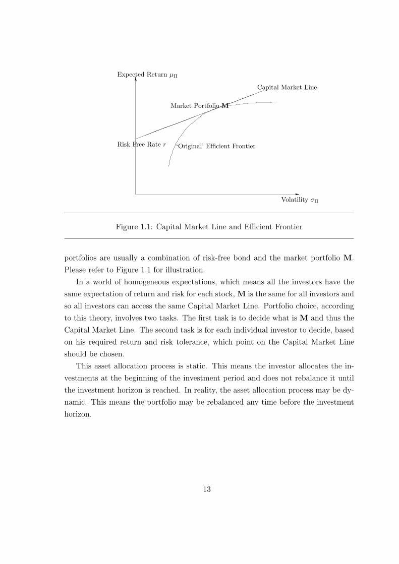
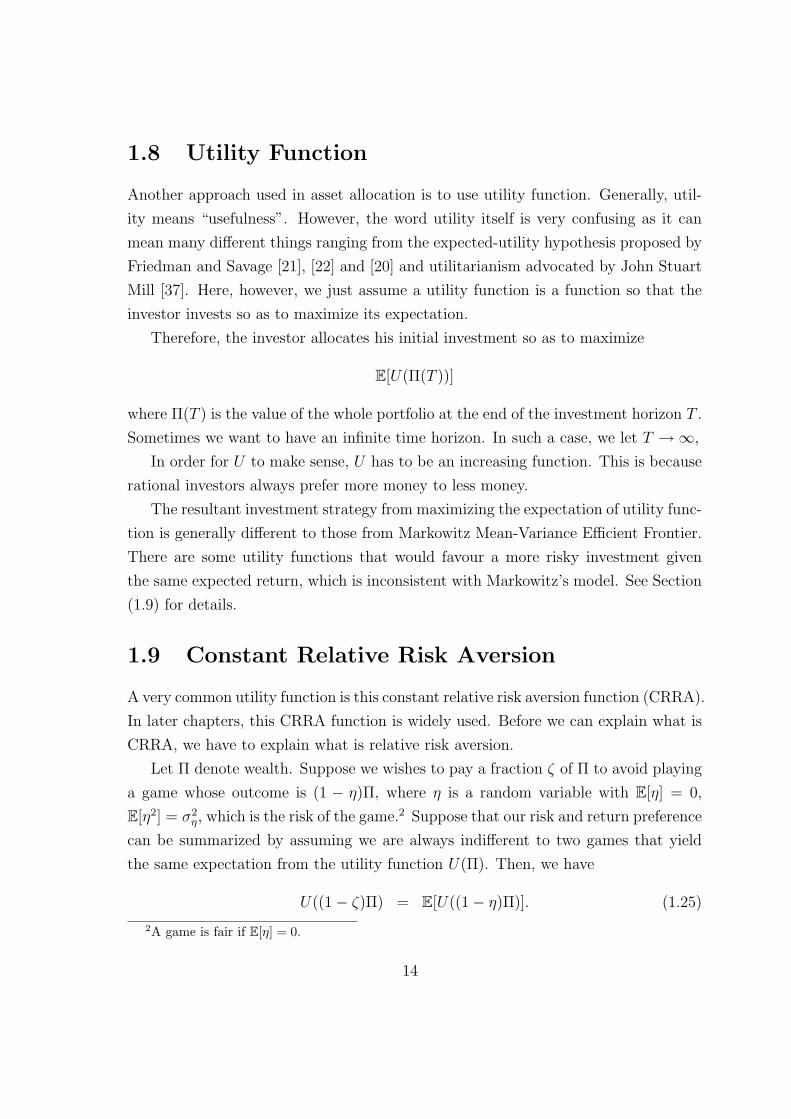
Capital Market Line

Market Portfolio M

Expected Return µΠ

Risk Free Rate r

Volatility σΠ

‘Original’ Efficient Frontier

Figure 1.1: Capital Market Line and Efficient Frontier

portfolios are usually a combination of risk-free bond and the market portfolio M.

Please refer to Figure 1.1 for illustration.

In a world of homogeneous expectations, which means all the investors have the

same expectation of return and risk for each stock, M is the same for all investors and

so all investors can access the same Capital Market Line. Portfolio choice, according

to this theory, involves two tasks. The first task is to decide what is M and thus the

Capital Market Line. The second task is for each individual investor to decide, based

on his required return and risk tolerance, which point on the Capital Market Line

should be chosen.

This asset allocation process is static. This means the investor allocates the in-

vestments at the beginning of the investment period and does not rebalance it until

the investment horizon is reached. In reality, the asset allocation process may be dy-

namic. This means the portfolio may be rebalanced any time before the investment

horizon.

13

1.8 Utility Function

Another approach used in asset allocation is to use utility function. Generally, util-

ity means “usefulness”. However, the word utility itself is very confusing as it can

mean many different things ranging from the expected-utility hypothesis proposed by

Friedman and Savage [21], [22] and [20] and utilitarianism advocated by John Stuart

Mill [37]. Here, however, we just assume a utility function is a function so that the

investor invests so as to maximize its expectation.

Therefore, the investor allocates his initial investment so as to maximize

E[U(Π(T ))]

where Π(T ) is the value of the whole portfolio at the end of the investment horizon T .

Sometimes we want to have an infinite time horizon. In such a case, we let T →∞,

In order for U to make sense, U has to be an increasing function. This is because

rational investors always prefer more money to less money.

The resultant investment strategy from maximizing the expectation of utility func-

tion is generally different to those from Markowitz Mean-Variance Efficient Frontier.

There are some utility functions that would favour a more risky investment given

the same expected return, which is inconsistent with Markowitz’s model. See Section

(1.9) for details.

1.9 Constant Relative Risk Aversion

A very common utility function is this constant relative risk aversion function (CRRA).

In later chapters, this CRRA function is widely used. Before we can explain what is

CRRA, we have to explain what is relative risk aversion.

Let Π denote wealth. Suppose we wishes to pay a fraction ζ of Π to avoid playing

a game whose outcome is (1 − η)Π, where η is a random variable with E[η] = 0,

E[η2] = σ2η, which is the risk of the game.2 Suppose that our risk and return preference

can be summarized by assuming we are always indifferent to two games that yield

the same expectation from the utility function U(Π). Then, we have

U((1− ζ)Π) = E[U((1− η)Π)]. (1.25)

2A game is fair if E[η] = 0.

14

Since

U((1− ζ)Π) = U(Π)− ζΠU ′(Π) + . . .

U((1− η)Π) = U(Π)− ηΠU ′(Π) +η2Π2U ′′(Π)

2+ . . . ,

and taking expectations on both sides, for η ¿ 1, we arrive at

ζ = −1

2σ2

η

ΠU ′′(Π)

U ′(Π).

The relative risk aversion, RRA, is defined as the function R(Π),

R(Π) = −ΠU ′′(Π)

U ′(Π). (1.26)

Suppose the relative risk aversion, R(Π), is a constant γ. Then, we have

ζ =1

2σ2

ηγ

where σ2η can be interpreted as risk and ζ as the amount paid to avoid this risk. From

this, we can actually find out what is the possible U(Π) by solving equation (1.26)w

ith R(Π) = γ. In this case we find that

U(Π) =

{Π(1−γ)−1

1−γif γ 6= 1

log Π if γ = 1

A function that is in this form is called Constant Relative Risk Aversion(CRRA).

When γ = 0, it means the investor is risk neutral. This means the investor is

indifferent to risk, and he does not pay anything to avoid risk. Hence the investor

takes an infinite amount of risk if the risky asset pays out more than the risk-free.

When γ > 0, the investor is risk averse. This means the investor is willing to sacrifice

some positive fraction of their wealth to avoid risk. When γ < 0, the investor is risk

seeking. This means the investor is willing to sacrifice some positive fraction of their

wealth to seek risk.

Since the RRA of the utility function U(Π) is invariant under the transformation

U(Π) −→ aU(Π) + b

15

where a > 0 and b are arbitrary constants. Therefore, a utility function in the form

U(Π) =Πγ

γ

with γ 6= 0 is also considered as CRRA. In the case of γ = 0,

U(Π) = logΠ.

Here

γ = 1− γ

so γ = 1 corresponds to risk neutral, γ < 1 to risk averse and γ > 1 risk seeking.

1.10 Merton’s Investment-Consumption Model

Merton’s investment-consumption model [36] is a good example of dynamic asset

allocation and stochastic control based on a HJB equation approach.

Merton’s model is about a risk averse investor who has an initial amount of re-

sources Π0 and wants to allocate resources in risky investments, risk-free bonds in-

vestment and consumption so as to maximize the expected life-time utility 3. Here,

the utility is an increasing concave function of rate of resources used in consumption,

C, in the form

U(C) =Cγ

γ

where γ < 1 is a constant. A sufficient condition for the problem to be solvable is

∂2U(C)

∂C2< 0,

which gives us the restriction γ < 1. As we can recall from the Section 1.9, this utility

function is equivalent to the CRRA function and γ = 1− γ. So, this γ determines how

risk-averse the investor is. The expected life-time utility, which the investor wants to

maximize, is

E0

{ ∫ ∞

0

eνtU(C(t))dt}

3For simplicity, we don’t consider the bequest function as in Merton [36] and we only consideran infinite, rather than a finite, time horizon.

16

where Et is the expectation operator given information up to time t and ν < 0 is a

discounting factor for future utility. 4

The setting of the market model is as follows. There is only one risky asset and

risk-free bond in the market. In the equation describing the risky asset, S is the

price, µ and σ are all constants, and they represent its drift and volatility, and X is

a standard Brownian motion as described in the Section (1.4). So, the equation is

dS = µSdt + σSdX. (1.27)

In the equation for describing the riks-free bond, r, a constant, represents the

risk-free rate, and B is the amount invested. Also, we assume the resources for

consumption can only be taken out from the bank rather than from the risky asset.

At all times, C ≥ 0, which means the rate of consumptions cannot be negative.5 So,

we have

dB = (rB − C)dt. (1.28)

Let Π represents the value of the whole portfolio, that is the sum of resources invested

in stocks and risk-free bond, and λ represents the proportion of resources invested in

risky assets. The controls, which refers to the choices that the investor can make, are

C and λ. Therefore, the model for the value of the portfolio is

dΠ = [(λ(µ− r) + r)Π− C]dt + λΠσdX. (1.29)

In order to apply the stochastic dynamic programming technique, we define

J(Π, t) = maxλ,C

Et

{ ∫ ∞

t

eντU(C(τ))dτ}

, (1.30)

and

J(Π) = maxλ,C

E0

{ ∫ ∞

0

eντU(C(τ))dτ}

. (1.31)

4Strictly speaking, U(C) here is the rate of utility, rather than utility.5As the rate of consumption has to be positive, we find that it is necessary to have

−ν − γr − γ(µ− r)2

2σ2(1− γ)> 0.

17

We note that the values of

maxλ,C

Et

{ ∫ ∞

t

eν(τ−t)U(C(τ))dτ}

are the same for all values of t. So, we have

J(Π, t) = J(Π)eνt

and thus∂J

∂t= νJ.

The corresponding HJB equation6 becomes

0 = maxλ,C

[− νJ + rΠ

dJ

dΠ+ U(C) + [(µ− r)λΠ− C]

dJ

dΠ+

σ2λ2Π2

2

d2J

dΠ2

].(1.32)

We differentiate equation (1.32) with respect to C and λ, and we find that the

maximum is obtained when

C∗ = J1/(γ−1)Π

and

λ∗ = −(µ− r)JΠ

σ2ΠJΠΠ

,

where JΠ is short hand for ∂J/∂Π and JΠΠ for ∂2J/∂Π2. There are indeed maxima

because, if we differentiate equation (1.32) with respect to C and λ twice we have

(γ − 1)Cγ−2

and

σ2Π2 ∂2J

∂Π2,

and both of them are negative.

We put C∗ and λ∗ into equation (1.32) and find that

rΠJΠ − (µ− r)JΠ

2σ2ΠJΠΠ

+1− γ

γJ

γγ−1

Π − νJ = 0.

6See section 1.6.1 for more details

18

It can be shown that the solutions are

J(Π) =1

γC∗γ−1Π (1.33)

C∗ =Π

1− γ[−ν − γr − γ(µ− r)2

2σ2(1− γ)] (1.34)

λ∗ =µ− r

σ2(1− γ). (1.35)

It is worth noticing that λ∗ is proportional to the Sharpe Ratio

µ− r

σ2.

The Sharpe Ratio is a common measure of performance, which can be interpreted as

“reward per variability”. Also, it is proportional to 1/(1−γ), where 1−γ is the term

relative risk aversion of Section(1.9). When γ is closer to 1, the investor is closer to

risk neutral, and we can see that the investor invests more in the risky stock market.

1.11 Long Term Growth Model

A small variation of the consumption model is this long term growth model. In this

model, instead of considering consumption (putting C = 0), the aim is to maximize

the long term growth of the portfolio. According to the Kelly Criterion [31], this

means maximizing the logarithm of the value of the portfolio. In other words, given

an investment period between 0 and T , our goal is to maximize the function

E0

{log

{Π(T )

}}.

As in the previous section, we let

J(Π, t) = maxEt

{log(Π(T ))

}. (1.36)

The corresponding HJB equation is

0 = maxλ(t)

{∂J

∂t+ [rΠ + (µ− r)λ(t)Π(t)]

∂J

∂Π+

σ2λ2Π2

2

∂2J

∂Π2

}. (1.37)

and the final condition is

J(Π, T ) = log(Π),

19

where λ is the portion of resources invested in stock.

We differentiate equation (1.37) with respect to λ, and we find that the maximum

is obtained when

λ = −(µ− r)JΠ

σ2ΠJΠΠ

. (1.38)

This point is indeed a maximum because, by differentiating it with respect to λ

again, we have

σ2 ∂2J

∂Π2< 0, (1.39)

if we assume that the backward parabolic HJB equation (1.37) preserves concavity.

If we substitute equation (1.38) into equation (1.37), we have

0 =∂J

∂t+ rΠ

∂J

∂Π− (µ− r)2( ∂J

∂Π)2

2σ2 ∂2J∂Π2

. (1.40)

We find that

J(Π, t) = log Π + (r +(µ− r)2

2σ2)(T − t) (1.41)

and

λ =(µ− r)

σ2(1.42)

satisfy equation (1.40) as well as the terminal condition.

So,

E0

{log

{Π(T )

}}= log Π0 + (r +

(µ− r)2

2σ2)T

Therefore, the optimal investment is independent of time and the current level of

wealth. Interestingly though, the ratio of total resources to the resources invested in

stock is exactly the Sharpe Ratio.

1.12 Example of Pontryagin Maximum Principle

In this section, we study an example of the application of the stochastic Pontryagin

Maximum Principle. Our example is on the problem of dynamic mean-variance asset

allocation without transaction costs. This means we manage a portfolio dynamically,

20

so as to minimize the variance of the value of the portfolio at some time horizon T ,

while keeping the expected value of the portfolio equal to a target value ξ. We assume

there are no short selling or margin restrictions and trading takes place in continuous

time.

The outline of solving the problem is as follows. We firstly apply the stochastic

version of the Pontryagin Maximum principle. This helps us to reduce the problem to

the problem of maximizing the Hamiltonian. Afterwards, we guess a strategy, and we

use Kolmogorov backward equation to establish the transition probabilities of that

strategy, which helps us to verify that the strategy indeed maximize the Hamiltonian.

Thus, we establish the optimal solution.

The solution we eventually discover is similar to the doubling strategy discovered

by Harrison and Kreps [23], which means the optimal solution has no practical value.

This is because we do not impose any restrictions on the class of admissible strategies.

Still, we consider this study is worthwhile. There are several reasons. Firstly, what

we do is completely different to the way Harrison and Kreps discovered their doubling

strategy. Secondly, this problem helps us to understand how the Pontryagin maximum

principle works and also the possible difficulties it has when it is applied to other

problems. Also, it helps us to understand the importance of those finer technical

details of the principle. Thirdly, variance minimization is a natural objective to

manage a portfolio. Therefore, the problem itself is interesting although the result

is not practical. In fact, there is a recent work [44] which attempts to solve this

mean-variance problem.

1.12.1 Market Model Equations

The setup of the market model is as follows. 7 Let S(t) be the spot price of a stock

at time 0 ≤ t ≤ T , where T is the time horizon of the investment period. Let A(t),

B(t) and Π(t) be the value of assets invested in stocks, risk free bonds and the total

value of assets respectively,

Π(t) = A(t) + B(t). (1.43)

7Actually the doubling strategy does not need to depend on this particular market model. Wejust use this market model just as an example to illustrate the problem.

21

We assume S(t) follows a geometric Brownian motion with growth rate µ > 0 and

volatility σ > 0. The risk free bond, B(t), is compounded continuously with risk free

rate r. For simplicity, we assume µ, r, and σ are constants. Cash flows generated

from the purchase or sale of stocks, denoted by u, are immediately invested in or

withdrawn from the risk free bond account.

Our model can be represented by the following equations

dS = µSdt + σSdX

dA = (µA + u)dt + σAdX

dB = rBdt− udt

dΠ = rΠdt + (µ− r)Bdt + σ(Π−B)dX (1.44)

where X is a standard Brownian motion process.

At time t = 0, an investor has an initial amount Π(0) of resources. The problem

is to allocate investments over the given time horizon so as to minimize

E0

{var(Π(T ))

}

where Et is the conditional expectation given information up to time t. At the same

time, the strategy has to satisfy

E0(Π(T )) = ξ (1.45)

where ξ can be considered as a target we wish to achieve.

For simplicity, we choose to minimize E0(Π(T )2) instead of minimizing the vari-

ance directly.

1.12.2 Applying the Maximum Principle

According to the stochastic version of the Pontryagin maximum principle, the optimal

policy also maximizes the negative expected value of a Hamiltonian H, which we

proceed to find. The Hamiltonian, H, is defined as

H(B,A, u) = ΨB(rB − u)

+ΨA(µA + u + σAdX

dt). (1.46)

22

Although dX/dt is undefined in the usual sense, we can use it in a formal sense. By

doing this we can solve the adjoint process ΨA correctly. The adjoint process, ΨA,

becomes

∂ΨA

∂t= −∂H

∂A= −ΨA(µ + σ

dX

dt), (1.47)

and final value, ΨA(T ) can be obtained from

ΨA(T ) =∂

∂B(−1

2(A + B)2) + λ

∂(A + B)

∂B

∣∣∣∣B=B(T )

= −Π(T ) + λ

∣∣∣∣B=B(T )

(1.48)

where λ is the Lagrange multiplier which makes the constraint possible.8

Similarly, ΨB is defined as

∂ΨB

∂t= −∂H

∂B= − rΨB (1.49)

and

ΨB(T ) = −Π(T ) + λ. (1.50)

Solving equations (1.47) to (1.50) yields

ΨA = (−Π(T ) + λ)S(T )

S(t);

ΨB = (−Π(T ) + λ)er(T−t). (1.51)

Substituting equation (1.51) into equation (1.46) and dropping the terms that

are not dependent on the control u, the problem of maximizing Et(J) reduces to the

maximization of either side of the expression

(Et(ΨA)− Et(ΨB))u =[Et(−Π(T ) + λ)

S(T )

S(t)

−Et(−Π(T ) + λ)er(T−t)]u (1.52)

8The Lagrange multiplier is analogous to the Lagrange multiplier we introduced in the sectionon Mean Variance Portfolio Theory.

23

By applying the maximum principle, we simplify our original problem. Now, the

problem of maximization of equation (1.46) becomes the problem of maximization

of either side of equation (1.52).

1.12.3 Kolmogorov Equation and Transition Probability

Maximizing either side of equation (1.52) means

u =

+∞ if Et(ΨA) > Et(ΨB)0 if Et(ΨA) = Et(ΨB)−∞ if Et(ΨA) < Et(ΨB)

The above equations mean the solution is to keep on buying or selling until

Et(ΨA) = Et(ΨB). From now on, we represent our optimal strategy in terms of

A and B rather than u. Our problem becomes finding A(t) and B(t) such that

Et(ΨA) = Et(ΨB). The values of Et(ΨA) and Et(ΨB), which dictates the current

choice of action, are in some way determined by the choice of A(t1) and B(t1)

(t1 ∈ [t, T ]), which is the policy we plan to have in the future.

We have an example here to illustrate the problem. Consider the case of S0 = 1

and Π0eµT < λ < Π0e

(µ+σ2)T .9 Suppose there are two future strategies, strategy I

and strategy II say. In strategy I, we invest an amount of Π(t) in shares and 0 in risk

free bonds at time t. In strategy II, we invest Π(t) in risk free bonds and 0 in shares

at time t. So, in strategy I,

E0(ΨA) = E0((−Π(T ) + λ)S(T )/S0)

= E0((−Π0S(T ) + λ)S(T ))

= −Π0e(2µ+σ2)T + λeµT

< 0 (1.53)

and

E0(ΨB) = E0((−Π(T ) + λ)erT )

= E0((−Π0S(T ) + λ)erT )

= (−Π0eµT + λ)erT )

9The Lagrange multiplier usually cannot be anything we want. However, as we show later, inthis particular problem it is possible to have λ take any value.

24

> 0

> E0(ΨA). (1.54)

So for strategy I it is optimal to sell shares. As for strategy II,

E0(ΨA) = E0((−Π(T ) + λ)S(T )/S0)

= (−Π0erT + λ)eµT

> 0 (1.55)

and

E0(ΨB) = E0((−Π(T ) + λ)erT )

= (−Π0erT + λ)erT )

< (−Π0erT + λ)eµT )

= E0(ΨA), (1.56)

therefore, it is optimal to buy shares.

The above example illustrates very clearly that we cannot choose a future strategy

randomly in calculating Et(ΨA) and Et(ΨB). So, how do we decide what values should

we use for A(t1) and B(t1) (t1 ∈ [t, T ]) in calculating Et(ΨA) and Et(ΨB)?

According to the maximum principle, in fact the future optimal strategy should

be used in calculating Et(ΨA) and Et(ΨB). Therefore, the problem of this section

becomes finding A(Π, S, t) and B(Π, S, t), t ∈ [0, T ] such that Et(ΨA) = Et(ΨB) for

all t ∈ [0, T ].

Now, in order to compute Et(ΨA) and Et(ΨB), we use Kolmogorov backward

equation [51]for the transition density of Π(T )S(T )S(t)

and Π(T ). This can help us to de-

termine the values of Et(ΨA) and Et(ΨB) so that we can determine their values so as to

choose our strategy. In the following, the transition probability pS(Π0, t0; Π1, t1) (t1 >

t0) is the conditional probability that p(Π(t1) = Π1|Π(t0) = Π0) and pΠ(Π0, S0, t0; Π1, S1, t1)

is the conditional probability that p(Π(t1) = Π1, S(t1) = S1|Π(t0) = Π0, S(t0) = S0).

We now change the variables of equation (1.44) so that we can apply the Kol-

mogorov equation to investigate the transition probability.

dS = µSdt + σSdX

dΠ = (rΠ + (µ− r)A)dt + σAdX (1.57)

25

According to Wilmott et al. [52], Kolmogorov backward equation for the probability

densities are

∂pS

∂τ= (rΠ0 + (µ− r)A0)

∂pS

∂Π0

+σ2

2Π2

0

∂2pS

∂Π20

, (1.58)

∂pΠ

∂τ= (rΠ0 + (µ− r)A0))

∂pΠ

∂Π0

+ µS0∂pΠ

∂S0

+σ2

2

(Π2

0

∂2pΠ

∂Π20

+ 2Π0S0∂2pΠ

∂Π0∂S0

+ S20

∂2p1

∂S20

), (1.59)

respectively, where τ = t1 − t0 and t1 is considered constant.

Taking expectation on both sides equation (1.58) and equation (1.59) , we find

that these two equations admit the solutions

pS = Et(−Π(T ))

and

pΠ = Et(−Π(T ))S(T )

S(t)

respectively. The boundary conditions become

ET (−Π(T )) = −Π(T )

and

ET (−Π(T ))S(T )

S(T )= −Π(T ).

The solution of A(Π, S, t) is

A(Π, S, t) =λ− Πer(τ+t2)

eµ(τ+t2) − er(τ+t2)(1.60)

where t2 is T − t1, the time between t1 and expiry.

Putting the above A(Π, S, t) to the Kolmogorov equations, equation (1.58) and

equation (1.59) become

∂pS

∂τ= (rΠ0 + (µ− r)

λ− Πer(τ+t2)

eµ(τ+t2) − er(τ+t2))∂p0

∂Π0

+σ2

2Π2

0

∂2p0

∂Π20

(1.61)

∂pΠ

∂τ= (rΠ0 + (µ− r)

λ− Πer(τ+t2)

eµ(τ+t2) − er(τ+t2)))

∂p1

∂Π0

+ µS0∂p1

∂S0

+σ2

2

(Π2

0

∂2p1

∂Π20

+ 2Π0S0∂2p1

∂Π0∂S0

+ S20

∂2p1

∂S20

)(1.62)

26

respectively.

We find that

Et(Π(τ)) = A(t)eµτ + (Π(t)− A(t))erτ (1.63)

is a solution of equation (1.61) .

As we want Et(Π(τ)) = ξ, all we need is to put λ = ξ.

If we put t2 = 0, which means t1 = T , and consider the boundary condition

ET (Π(T )) = limt→T Et(Π(T )) = ξ, equation (1.63) becomes

Et(Π(τ)) = ξ (1.64)

for any t.

Therefore, our strategy ‘guarantees’ that the expectation is always equal to ξ. As

for the solution of equation (1.62), we have

Et(Π(τ)S(τ)) = ξeµτ . (1.65)

Since λ = ξ, Et(ΨA) is always equal to Et(ΨB). So we verify that our choice of

A(t) is correct and the resulting strategy is optimal.

1.12.4 Discussion

The strategy we discuss above seems to guarantee that the eventual portfolio value

is always equal to ξ. If we calculate the variance of the portfolio value at T using

equation (1.58) , we find that it is equal to 0. This means that the strategy seems

to make the portfolio another risk free bond, with possibly higher return than r, the

risk free interest rate. How is this achieved?

In fact, we have rediscovered a strategy similar to Harrison and Kreps [23] famous

doubling strategy. The idea of that doubling strategy can be described as the contin-

uous version of the strategy that wins one dollar for sure from betting on an infinite

sequence of coin flips. The coin flipping strategy is as follows. Suppose we win after

first flip, we stop. If we lose, then we continue to bet, but doubling the stake, until we

win, and then we stop. This strategy “guarantees” we must win one dollar eventually

because the probability of losing forever is 0.

The strategy we discover is similar. The strategy is to invest more in stocks if

the value of the portfolio is further away from the target, ξ, and invest less in stocks

27

if the value of the portfolio is closer to the target. This is similar to “doubling” the

stakes when we lose and stop when we win.

Mathematically, this optimal strategy is undesirable as well. This is because

E∫ T

0

|A|dS

is not finite. In most of the commonly used definition of admissible strategy, this

integral has to be finite in order to be admissible.

Note that there are many strategies which can minimize the variance and at the

same time maintain the expectation of the portfolio as ξ. This strategy is only one

of them. It is not difficult to think of another one. For example, we can invest all

our resources from the portfolio in risk free bonds until T/2 and then start to use the

strategy. This also achieves the same result.

The strategy threatens the no arbitrage principle we would expect from equation

(1.44). This is because this strategy can create arbitrage opportunities by achieving

a risk free return higher than r. Heath and Jarrow [26], therefore, propose the use

of short sale restrictions or margin restrictions as they found that such restrictions

exclude arbitrage strategy like this.

1.12.5 Dynamic Asset Allocation with Margin Constraints

Heath and Jarrow [26] examined the problem of the doubling strategy within a con-

tinuous frictionless market. By frictionless, they mean that there are no transaction

costs, no short-sale restrictions, and no taxes and that asset shares are infinitely divis-

ible. They also assume the existence of two securities, described by equation (1.44) .

They showed that the introduction of margin restrictions can eliminate the possibility

of a doubling strategy. As we see later, the strategy obtained previously no longer

works given those restrictions as well.

Heath and Jarrow then went on to examine the impact of margin constraints

on options pricing. They showed that while margin constraints impose restrictions

on trading, they should have no effect on the price of options in the market and the

Black-Scholes value still holds. We do not go into that detail because it is not relevant

to our work.

The way Heath and Jarrow modeled the margin constraints is by imposing the

following restrictions on trading

28

Π = A + B ≥{

L+|A| if A > 0L−|A| if A < 0

where 0 ≤ L+, L− ≤ 1 are constants.

To understand what the above equations mean, we can consider several cases.

Suppose both A and B are positive, then the inequalities impose no restriction. Sim-

ilarly, the above constraints restrict all the trading strategies with both A and B

negative. When A is negative and B is positive, it means short sale. The equations

mean on top of the proceedings from the short sales, an extra L− portion of the

stock prices needs to come from the investor’s own fund. When B is negative and A

is positive, it means the investor is buying the stock on margin and so the investor

needs to provide L+ portion of the stock price.

Imposing such restrictions, as shown by Heath and Jarrow, eliminates the use of

the doubling strategies. Heath and Jarrow’s proof is very subtle. We refer readers to

[26] for the details.

Our strategy obtained in the previous section also no longer works given those

restrictions. Here we consider a very simple example. Suppose L+ = 1. This is

equivalent to B ≥ 0 and so no borrowing is allowed. Now let’s assume we start with

resources Π(0) = Π0. If the target we have ξ is bigger than Π0eµT , even we use the

most aggressive strategy available, that is to invest all our resources in stock all the

time, the expected value of our portfolio is only equal to Π0eµT , which is smaller than

ξ. So the previous strategy no longer works.

1.13 Investment with Transaction Costs

Most of our work is related the portfolio management with transaction costs. There-

fore, we are going to review some of the more important works here.

1.13.1 Atkinson, Pliska & Wilmott

Atkinson et al. [5] make a very successful attempt at solving a problem in portfolio

management. Their work is a further study on a model developed by Morton and

Pliska [39].

29

The setup of Morton and Pliska is as follows. An investor has an infinite in-

vestment interval in which to invest. The value of stock, S(t), follows a geometric

Brownian motion with growth rate µi > 0 and volatility σi > 0. The risk free bonds,

B, are compounded continuously with risk free rate r. Cash generated by or needed

for the purchase or sale of stocks is immediately invested or withdrawn from the risk

free bond account. The model is represented by

dSi = µiSidt + σiSidXi, i = 1, · · · , n,

dB = rBdt

= r(Π−n∑

i=1

Ai)dt

dΠ = rBdt +n∑

i=1

µiAidt +n∑

i=1

σiAidXi

= r(Π−n∑

i=1

Ai)dt +n∑

i=1

µiAidt +n∑

i=1

σiAidXi

where the Xis are standard Brownian motions with dX2i = dt and correlated by

dXidXj = ρijdt, i, j = 1, · · · , n. There are no redundant assets and so the covariance

matrix.

Σ =

σ21 σ1σ2ρ12 . . . σ1σnρ1n...

.... . .

...σ1σnρ1n σ2σnρ2n . . . σ2

n

is non-singular. Let Π(t) denote the value of the portfolio at time t. The transaction

costs are proportional to the value of the portfolio Π(t) at the time of the transaction.

Therefore, the transaction cost of a single transaction is

kΠ(t).

The problem of the investor is to maximize the asymptotic growth rate

limT→∞

E[log Π(T )]

T.

Many works in the study of transaction costs suffer from the following problem.

That is the computation of the optimal trading strategies is very difficult. Even

30

solving a problem with one or two assets is enormously difficult, not to mention 20

to 30. This means the model has no practical value.

Morton and Pliska have the same problem in the work. Thanks to Atkinson and

Wilmott [6] and Atkinson et al. [5], this problem is overcome by using perturbation

analysis to find a solution which is a good approximation to the real solution when k

is small. The solution is very easy to compute. Their solutions are even good enough

for the case of many risky assets. Therefore, they have effectively solved the problem.

1.13.2 Atkinson and Al-Ali

Atkinson and Al-Ali [1] study the problem of introducing transaction costs into Mer-

ton’s Investment and Consumption Model. They assume

dS = µSdt + σSdX

dB = (rB − C)dt− (1 + k+)dL(t) + (1− k−)dM(t)

dΠ = µ(Π−B)dt + rBdt + σ(Π−B)dX − k+dL(t)− k−dM(t)

where L(t) and M(t) represent the cumulative purchase and sale of assets A in [0, t],

and k+ and k− represent the ratio of the transaction costs when risky assets are

bought or sold. So, k+L(t) and k−M(t) represent the total transaction costs paid to

purchase stocks and selling risky assets till time t respectively.

Similar to Merton’s model, the objective is to maximize 10

E0

{ ∫ ∞

0

eνt Cγ

γdt

}.

Perturbation analysis is used in this study. They find that the solution tends

to Merton’s solution when the transaction costs tend to 0. An explicit solution is

obtained for the optimal trading policy.

They then extend the model and consider the case with two and then subsequently

many risky assets. They allowed different transaction costs in purchasing and selling

risky for each risky assets. In this case, they also successfully solved the optimal

trading policy.

This result is consistent with the numerical result of Akian et al. [2].

10Here, we use the same notation as in the section on Merton’s Model.

31

1.13.3 Atkinson and Mokkhavesa (2001)

Atkinson and Mokkavesa [3] make a study on the utility function. Their study is

based on Merton’s Investment and Consumption Model. The problem they attempt

to solve is to determine the utility function given the investment and consumption

behavior of an investor. They were successful in many different cases.

Firstly, they consider the infinite time horizon case. The setup of their model is

similar to Merton’s Investment Consumption Model we examine. So, they assume

dB = (rB − C)dt, (1.66)

dS = µSdt + σSdX, (1.67)

dΠ = [(λ(µ− r) + r)Π− C]dt + λΠσdX. (1.68)

Instead of giving a utility function U(C(t)) and trying to find out what is the optimal

investment and consumption policy(λ∗, C∗), Atkinson et al. instead solve U(C(t))

when (λ∗, C∗) are given. They find that if

C∗ = Π/β1, (1.69)

λ∗ = β2, (1.70)

then the governing equation for U(C) is given by

0 = U ′′(C)C

{β1

[β2

2(µ− r) + r

]− 1

}+ U ′(C)

{β1

[β2

2(µ− r) + r

]+ νβ1

}.

In addition to the infinite time horizon problem, in the same paper, Atkinson and

Mokkhavesa [3] also solve other cases like two-assets time-dependent, multi-assets

time-dependent, and two assets time-dependent with a single stochastic state variable.

1.13.4 Mokkhavesa and Atkinson (2002)

Mokkhavesa and Atkinson [38] extend the results of Atkinson and Al-Ali [1]. They

have obtained a result which can applied to any consumption utility function C on

a one risky asset framework. The resultant strategy is expressed as a function of the

value function.

32

1.13.5 Atkinson and Mokkhavesa (2004)

Atkinson and Mokkhavesa [4] extends the results of Mokkhavesa and Atkinson [38].

They formulate the problem with more than one uncorrelated risky assets.

33

Chapter 2

Dynamic Asset Allocation withTransaction Costs

2.1 Introduction

In this chapter, we consider a general problem in dynamic asset allocation with trans-

action costs. We assume that we are able to solve the equivalent problem without

transaction costs first. With the presence of small transaction costs in the new prob-

lem, we find that the optimal strategy is to hold a number of assets that is approxi-

mately the same as the optimal strategy without transaction costs and the portfolio

should only be rebalanced when it is too far away from the optimal number. From

this level we find a formula for the position of the free boundaries where transactions

should be made in terms of the optimal amount of cash held in the no transaction costs

problem. We also find that when the level of transaction costs, k, tend to zero, the

band-width of the no-transaction region tends to zero and the no-transaction region

converges to the no transaction costs solution. Furthermore, we find that the effect

of a transaction cost, say k, in the limit k → 0 to the reward function is O(k2/3).

Bellman’s principle is used to establish the problem as a free boundary boundary,

then we use a perturbation analysis to establish the position of the free boundary.

For details regarding perturbation analysis, consult Hinch [27].

34

2.2 Market Model without Transaction costs

The setup of the market model is as follows. Let S(t) be the spot price of a stock at

time 0 ≤ t ≤ T , where T is the time horizon of the investment period. We assume S(t)

follows a geometric Brownian motion with constant growth rate µ > 0 and constant

volatility σ > 0. So, the equation for S(t) is

dS = µSdt + σSdX

where X is a standard Brownian motion. Let A(t) denotes the value of resources

invested in stock. So,

dA = µAdt + σAdX

when there is no money put in or withdrawn.

Let B(t) be the value of resources invested in risk-free bond. The risk-free bonds

are compounded continuously at the risk free rate r. So, the equation for B(t) is

dB = rBdt,

when again, there is no transfer of money from the stock account.

Let Π(t) be the value of assets invested in stocks, risk-free bonds and the total

value of assets respectively,

Π(t) = A(t) + B(t). (2.1)

Cash flows generated from the purchase or sale of stocks are immediately invested

or withdrawn from the risk free bond account. Also, we use B as the controller

representing the amount of cash invested in the risk-free bonds. The equation for the

value of the portfolio, therefore, becomes

dΠ = (µA + rB)dt + σAdX

= µ(Π−B)dt + rBdt + σ(Π−B)dX (2.2)

At time t = 0, an investor has an amount Π0 of resources. The problem is to

allocate investments over the given time horizon so as to maximize

E0

{ ∫ T

0

I(Π(t))dt + F (Π(T ))

},

35

where Et is the conditional expectation given information up to time t, I and F are

strictly increasing concave differentiable functions. This means the following must

hold

∂I

∂Π> 0,

∂F

∂Π> 0,

∂2I

∂Π2≤ 0

∂2F

∂Π2≤ 0. (2.3)

and one of their second partial derivatives has to be strictly less than 0. The functions

I and F can represent anything from utility to the year end bonus of a trader. Of

course, the dimensions of ∫ T

0

I(Π(t))dt

and

F (Π(T ))

have to be the same in order for the problem to make sense. So, for example if F (Π)

is utility then I(Π) is a rate of utility.

We restate the above equation in dynamic programming form so as to apply the

Bellman principle of optimality. Therefore, we define the optimal expected value

function J(Π, t) as

J(Π, t) = maxB(t)

Et

{∫ T

t

I(Π(t))dt + F (Π(T ))

}. (2.4)

2.3 Formulation of Bellman’s Equation in the No

Transaction Costs Problem

Bellman’s principle and Ito’s Lemma can be used to derive the Bellman equation for

J(Π, t) in (2.4), which is

0 = maxB∈Θ

{∂J

∂t+ I + [rB + µ(Π−B)]

∂J

∂Π+

σ2(Π−B)2

2

∂2J

∂Π2

}. (2.5)

36

At t = T , we have

J(Π, T ) = F (Π). (2.6)

If we differentiate the expression inside the expression to be maximized in (2.5)

with respect to B, we have

−(µ− r)∂J

∂Π− σ2(Π−B)

2

∂2J

∂Π2.

Differentiating it twice, we have

σ2 ∂2J

∂Π2.

The maximum is achieved when the (optimal) amount invested in the risky assets,

B∗, is given by

−(Π−B∗)∂2J

∂Π2=

(µ− r)

σ2

∂J

∂Π. (2.7)

This equation is very useful later on in determining the transaction boundaries in the

proportional transaction cost case.

We assume the backward parabolic partial differential equation (2.5) preserves

concavity. This is a property of many parabolic partial differential equations and

although we cannot prove it in general for equation (2.5) we have found that concavity

is preserved in all the cases for which we have found analytic solutions. So, we assume

that J is concave and so

σ2 ∂2J

∂Π2≤ 0.

Since F (T ) and I(t) are strictly increasing functions, so we can suppose J is also

a strictly increasing function. 1 This means that the right hand side of equation (2.7)

must be positive, and as we assume

∂2J

∂Π2< 0,

we have Π − B > 0, which means the optimal value invested in stocks is always

positive. The above equation also guarantees that the optimal value of B is unique.

1Suppose Π1 > Π2, then we can divide Π1 into two pools of money: Π2 and x where x is positive.We can consider the strategy where we invest the pool of Π2 according to the optimal strategy whenthe portfolio value is only Π2 and invest x only in the risk free bond. The value J(Π1) is as least aslarge as the value function produced by our strategy, which in turn is larger than J(Π2). Therefore,J is a strictly increasing function.

37

2.4 Solving Bellman’s Equation in the No Trans-

action Costs Problem

In general, the above Bellman equation can only be solved numerically. In this section,

however, we try to construct I and F such that analytic solutions exist.

From equation (2.7) we see that

B∗ =(µ− r)

σ2

∂J

∂Π/∂2J

∂Π2+ Π (2.8)

where B∗ is the optimal amount invested in risk-free bonds. Putting this back into

equation (2.5), we have

0 =∂J

∂t+ I + rΠ

∂J

∂Π− (µ− r)2

2σ2(∂J

∂Π)2/

∂2J

∂Π2. (2.9)

From equation (2.9) , we know that for any function J , as long as we set

I = −{∂J

∂t+ rΠ

∂J

∂Π− (µ− r)2

2σ2(∂J

∂Π)2/

∂2J

∂Π2}, (2.10)

we can have exact solutions. Of course, we still have to make sure that the functions

J and I thus defined make economic sense and satisfy (2.3).

We can study this in more details if we consider the following change of variables:

τ = T − t

x = log Π. (2.11)

Then we have

B∗ = Π

{(µ− r)Jx

σ2(Jxx − Jx)+ 1

}(2.12)

and the Bellman equation (2.9) becomes

I = Jτ − rJx +(µ− r)2J2

x

2σ2(Jxx − Jx). (2.13)

We now look for travelling wave solutions of the form

J(Π, t) = f(x− ντ). (2.14)

38

We find that

∂J

∂t= −νf ′(x− ντ)

∂J

∂Π=

1

Πf ′(x− ντ)

∂2J

∂Π2=

1

Π2(f ′′(x− ντ)− f ′(x− ντ))

and putting all these back into equations (2.8) and (2.10), we have

B∗ = Π

{(µ− r)f ′

σ2(f ′′ − f ′)+ 1

}(2.15)

and

I = −(ν + r)f ′ +(µ− r)2f ′2

2σ2(f ′′ − f ′). (2.16)

Now, we look at some special cases of f .

2.4.1 Long Term Growth Model

We recall the long term growth model from Section 1.11, the long term growth model

is an example of the above class of solution. In the long term growth model,

f(x− ντ) = x− ντ, ν = −(r +

(µ− r)2

2σ2

). (2.17)

Therefore,

J(Π, t) = log Π + (r +(µ− r)2

2σ2)(T − t).

(2.18)

and so the terminal function F (Π(T )) = log Π, and we find

B∗ = Π

{1− (µ− r)

σ2

}(2.19)

and

I = 0, (2.20)

which is exactly the same as those in Section 1.11.

39

2.4.2 Constant Relative Risk Aversion (CRRA) Model

Here, we consider the case that

f(x− ντ) = exp(γ(x− ντ)),

(2.21)

which means

J(Π, t) = eν(T−t)Πγ,

and the terminal function F (Π(T )) = Πγ, which is equivalent to the constant relative

risk aversion (CRRA) utility function; refer to Section 1.9 for details.

Therefore, from equation (2.15) and equation (2.16), we have

B∗ = Π

{1 +

(µ− r)

σ2(γ − 1)

}(2.22)

and

I =( γ(µ− r)2

2(γ − 1)σ2− γr + ν

)J

=( γ(µ− r)2

2(γ − 1)σ2− γr + ν

)eν(T−t)Πγ. (2.23)

Although these are formally solutions of equation (2.10) for any value of γ and

ν, we must choose their value so that (2.3) are satisfied which gives

γ < 1

and

ν ≥ γr − γ(µ− r)2

2(1− γ)σ2.

This means we can interpret I as the CRRA utility function of a risk averse investor.

As discussed in Section 1.9, γ represents how risk averse the investor is. The

bigger the γ, the more the investor is risk-seeking. The closer γ to 1, the more the

investor is close to risk-neutral. This means the investor borrows money from the

bank (B∗ → −∞) and invests the proceedings in the risky asset as the return of the

risky asset is higher. When

1− γ =(µ− r)

σ2, (2.24)

40

B∗ = 0. This means the investor invests all his resources into the risky asset. When

1− γ <(µ− r)

σ2, (2.25)

the optimal amount of resources invested in bond, B∗, can be negative. So, the

investor is borrowing money to invest in stocks. As γ becomes smaller and smaller,

the investor invests less and less in stocks. Nonetheless, no matter how small γ is,

B∗ < Π

{1− (µ− r)

σ2

}. (2.26)

This means the investor always invest in stock, no matter how risk averse he is.

2.5 Market Model with Transaction costs

Now we consider the problem with transaction costs. Let k > 0 represents the portion

of transaction of stocks used as transaction costs. So if the investor buys a number of

stocks whose “true” value is S, the investor pays (1 + k)S in cash and if the investor

sells the stocks, the investor obtains (1− k)S in cash.

We begin the study of the transaction costs problem by first stating the market

model equations when there are transaction costs. They are

dS = µSdt + σSdX

dB = rBdt− (1 + k)dL(t) + (1− k)dM(t)

dΠ = µ(Π−B)dt + rBdt + σ(Π−B)dX − kdL(t)− kdM(t) (2.27)

where L(t) and M(t) represent the cumulative purchase and sale of assets A during

[0, t], and which we use as the controls. In the transaction costs problem, B is only

used to denote the value of assets invested in risk-free bonds and it is no longer used as

a control. Using L(t) and M(t) rather than B as controls makes it easier to formulate

the optimization problem as a free boundary problem.

41

2.6 Formulation of Bellman’s Equation under Trans-

action costs

Now we define the optimal expected value function J(Π, B, t) as

J(Π, B, t) = maxL,M

Et

{∫ T

t

I(Π(t))dt + F (Π(T ))

}. (2.28)

The functions I and F here are assumed not to depend on k, and so they are exactly

the same as the I and F in equation (2.4). The function J here is different to the J

in Section 2.3 as now we have introduced transaction costs, and as a result J depends

on B.

The corresponding Bellman equation is

maxl,m

{I +

∂J

∂t+ (rB − (1 + k)l + (1− k)m)

∂J

∂B

+(rB + µ(Π−B)− kl− km)∂J

∂Π+

σ2(Π−B)2

2

∂2J

∂Π2

}= 0

(2.29)

where

L(t) =

∫ t

0

l(t)dt

and

M(t) =

∫ t

0

m(t)dt.

The optimal trading policy, therefore, can be deduced from the following three

cases:

1.

−(1 + k)∂J

∂B− k

∂J

∂Π< 0 (2.30)

and

(1− k)∂J

∂B− k

∂J

∂Π≥ 0, (2.31)

42

where the maximum is achieved by choosing l = 0 and m = ∞2, which means

selling at the maximum rate;

2.

−(1 + k)∂J

∂B− k

∂J

∂Π≥ 0 (2.32)

and

(1− k)∂J

∂B− k

∂J

∂Π< 0, (2.33)

where the maximum is achieved by choosing l = ∞ and m = 0, which means

buying at the maximum rate;

3.

−(1 + k)∂J

∂B− k

∂J

∂Π< 0 (2.34)

and

(1− k)∂J

∂B− k

∂J

∂Π< 0, (2.35)

where the maximum is achieved by choosing l = 0 and m = 0, which means

neither buying nor selling.

Note that it is impossible to have

−(1 + k)∂J

∂B− k

∂J

∂Π> 0 (2.36)

and

(1− k)∂J

∂B− k

∂J

∂Π> 0, (2.37)

as we assume J is an increasing function of Π.

The optimal trading strategy, therefore, given t, Π and B, involves three possi-

ble regions: a sales region, a purchase region and a no-transaction region. The no

transaction region is the region in the middle, see Figure (2.1) for an illustration.

2To be more rigorous, we should firstly make the restriction m ≤ K for some constant K. Thenwe let K →∞.

43

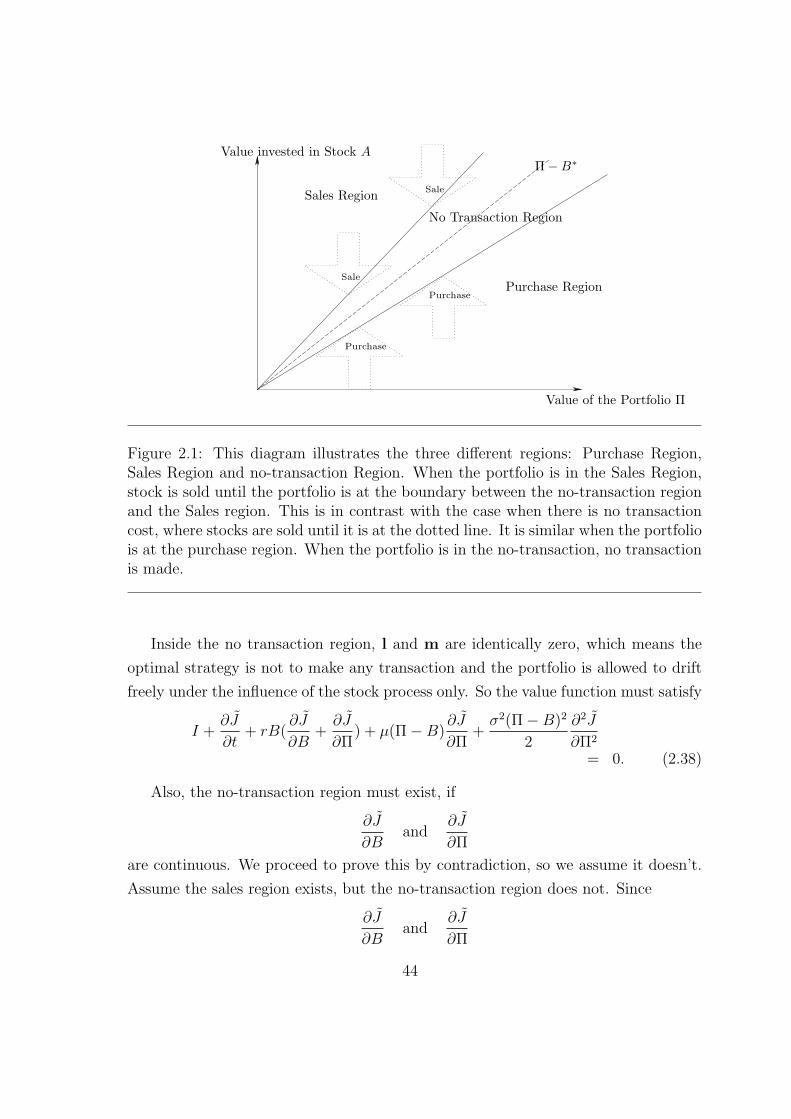
Sale

Sale

Purchase

Purchase

Value invested in Stock A

Value of the Portfolio Π

Π−B∗

Sales Region

Purchase Region

No Transaction Region

Figure 2.1: This diagram illustrates the three different regions: Purchase Region,Sales Region and no-transaction Region. When the portfolio is in the Sales Region,stock is sold until the portfolio is at the boundary between the no-transaction regionand the Sales region. This is in contrast with the case when there is no transactioncost, where stocks are sold until it is at the dotted line. It is similar when the portfoliois at the purchase region. When the portfolio is in the no-transaction, no transactionis made.

Inside the no transaction region, l and m are identically zero, which means the

optimal strategy is not to make any transaction and the portfolio is allowed to drift

freely under the influence of the stock process only. So the value function must satisfy

I +∂J

∂t+ rB(

∂J

∂B+

∂J

∂Π) + µ(Π−B)

∂J

∂Π+

σ2(Π−B)2

2

∂2J

∂Π2

= 0. (2.38)

Also, the no-transaction region must exist, if

∂J

∂Band

∂J

∂Π

are continuous. We proceed to prove this by contradiction, so we assume it doesn’t.

Assume the sales region exists, but the no-transaction region does not. Since

∂J

∂Band

∂J

∂Π

44

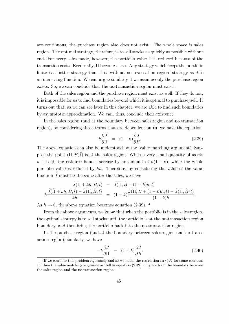
are continuous, the purchase region also does not exist. The whole space is sales

region. The optimal strategy, therefore, is to sell stocks as quickly as possible without

end. For every sales made, however, the portfolio value Π is reduced because of the

transaction costs. Eventually, Π becomes−∞. Any strategy which keeps the portfolio

finite is a better strategy than this ‘without no transaction region’ strategy as J is

an increasing function. We can argue similarly if we assume only the purchase region

exists. So, we can conclude that the no-transaction region must exist.

Both of the sales region and the purchase region must exist as well. If they do not,

it is impossible for us to find boundaries beyond which it is optimal to purchase/sell. It

turns out that, as we can see later in this chapter, we are able to find such boundaries

by asymptotic approximation. We can, thus, conclude their existence.

In the sales region (and at the boundary between sales region and no transaction

region), by considering those terms that are dependent on m, we have the equation

k∂J

∂Π= (1− k)

∂J

∂B. (2.39)

The above equation can also be understood by the ‘value matching argument’. Sup-

pose the point (Π, B, t) is at the sales region. When a very small quantity of assets

h is sold, the risk-free bonds increase by an amount of h(1 − k), while the whole

portfolio value is reduced by kh. Therefore, by considering the value of the value

function J must be the same after the sales, we have

J(Π + kh, B, t) = J(Π, B + (1− k)h, t)

kJ(Π + kh, B, t)− J(Π, B, t)

kh= (1− k)

J(Π, B + (1− k)h, t)− J(Π, B, t)

(1− k)h.

As h → 0, the above equation becomes equation (2.39). 3

From the above arguments, we know that when the portfolio is in the sales region,

the optimal strategy is to sell stocks until the portfolio is at the no-transaction region

boundary, and thus bring the portfolio back into the no-transaction region.

In the purchase region (and at the boundary between sales region and no trans-

action region), similarly, we have

−k∂J

∂Π= (1 + k)

∂J

∂B. (2.40)

3If we consider this problem rigorously and so we make the restriction m ≤ K for some constantK, then the value matching argument as well as equation (2.39) only holds on the boundary betweenthe sales region and the no-transaction region.

45

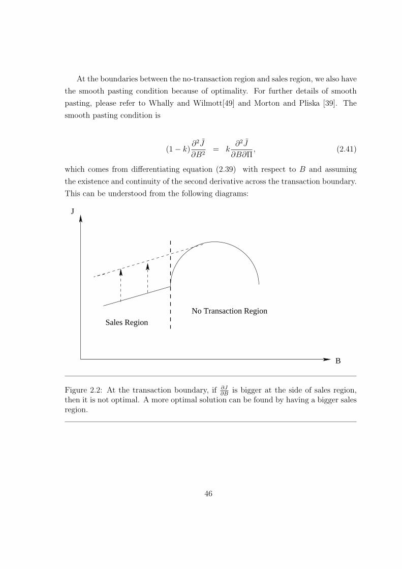
At the boundaries between the no-transaction region and sales region, we also have

the smooth pasting condition because of optimality. For further details of smooth

pasting, please refer to Whally and Wilmott[49] and Morton and Pliska [39]. The

smooth pasting condition is

(1− k)∂2J

∂B2= k

∂2J

∂B∂Π, (2.41)

which comes from differentiating equation (2.39) with respect to B and assuming

the existence and continuity of the second derivative across the transaction boundary.

This can be understood from the following diagrams:

J

B

Sales Region

No Transaction Region

Figure 2.2: At the transaction boundary, if ∂J∂B

is bigger at the side of sales region,then it is not optimal. A more optimal solution can be found by having a bigger salesregion.

46

J

B

Sales Region No Transaction Region

Figure 2.3: At the transaction boundary, if ∂J∂B

is smaller at the side of sales region,then it is not optimal. A more optimal solution can be found by having a smallersales region.

From these two diagrams, we can see at the point of transaction boundary, ∂J∂B

exists and should be continuous across the boundary, or otherwise it is not optimal.

Therefore, using the same notation as in the value matching argument, we have

∂J(Π + kh, B, t)

∂B=

∂J(Π, B + (1− k)h, t)

∂B

So, we have

k(∂J(Π + kh, B, t)

∂B− ∂J(Π, B, t)

∂B

)/(kh)

= (1− k)(∂J(Π, B + (1− k)h, t)

∂B− ∂J(Π, B, t)

∂B

)/((1− k)h).

As h → 0, it becomes equation (2.41).

Similarly, at the boundaries between the no-transaction region and purchase re-

gion, have the following smooth pasting condition:

47

(1 + k)∂2J

∂B2= −k

∂2J

∂B∂Π. (2.42)

Also, when t = T ,

J(Π, B, T ) = F (Π(T )). (2.43)

2.6.1 Change of Variables

We translate the B coordinate according to

B = B(Π, t) + k1/3β, (2.44)

where B is the value of risk-free bonds we have when the level of transaction costs

tends to zero, k → 0. As we can see later, this is actually the same as the optimal

value of risk free bond held in the no transaction costs problem. We also assume that

β is O(1). The choice of the order k1/3 in the expansion is inevitable and we explain

this choice in Section 2.9.

We set H(Π, β, t) = J(Π, B, t).

We have

∂J

∂B= k−1/3∂H

∂β,

∂J

∂Π=

∂H

∂Π− k−1/3∂H

∂β

∂B

∂Π,

∂J

∂t=

∂H

∂t− k−1/3∂H

∂β

∂B

∂t,

∂2J

∂Π2=

∂2H

∂Π2− k−1/3(2

∂2H

∂β∂Π

∂B

∂Π+

∂H

∂β

∂2B

∂Π2)

+k−2/3∂2H

∂β2(∂B

∂Π)2. (2.45)

Also, we let

48

H(Π, β, t) = H0(Π, β, t) + k1/3H1(Π, β, t)

+k2/3H2(Π, β, t) + kH3(Π, β, t)

+k4/3H4(Π, β, t) + · · · . (2.46)

and assume that H0, H1, H2, H3, H4, · · · as well as all of their derivatives are all of

O(1). H0 is the value function when transaction costs level k → 0. Later, we find

that its value is the same as the value function J in equation (2.4).

2.6.2 Sales and Purchase Regions

3.2.5 After the change of coordinates, the sales region equation (2.39), becomes

k(∂H

∂Π− k−1/3∂H

∂β

∂B

∂Π) = (1− k)k−1/3∂H

∂β, (2.47)

and equation (2.40) , the equation at purchase region, becomes

k(∂H

∂Π− k−1/3∂H

∂β

∂B

∂Π) = −(1 + k)k−1/3∂H

∂β. (2.48)

The smoothing pasting condition for the sales boundary becomes

k2/3(∂2H

∂Π∂β− k−1/3∂2H

∂β2

∂B

∂Π) = (1− k)k−2/3∂2H

∂β2, (2.49)

and the smoothing pasting condition for the purchase boundary becomes

k2/3(∂2H

∂Π∂β− k−1/3∂2H

∂β2

∂B

∂Π) = −(1 + k)k−2/3∂2H

∂β2. (2.50)

When we substitute equation (2.46) into equation (2.47), the equation at the

sales region, and collect terms of the same order in k, we have 4

∂H0

∂β= 0, (2.51)

4We assume that all these derivatives are of O(1). In other words, there is no boundary layersexist. This can be justified by the fact that the system is self consistent. Also, k doesn’t appear tokill off any high derivatives as k → 0 so singular perturbations are unlikely.

49

∂H1

∂β= 0, (2.52)

∂H2

∂β= 0, (2.53)

∂H3

∂β− (1− ∂B

∂Π)∂H0

∂β= 0, (2.54)

∂H4

∂β− (1− ∂B

∂Π)∂H1

∂β− ∂H0

∂Π= 0. (2.55)

Similarly, if we substitute equation (2.46) into equation (2.48), the equation at

the purchase region, and collect terms of the same order in k, we have

∂H0

∂β= 0, (2.56)

∂H1

∂β= 0, (2.57)

∂H2

∂β= 0, (2.58)

∂H3

∂β+ (1− ∂B

∂Π)∂H0

∂β= 0, (2.59)

∂H4

∂β+ (1− ∂B

∂Π)∂H1

∂β+

∂H0

∂Π= 0. (2.60)

If we substitute equation (2.46) into equation (2.49), the smooth pasting equation

for the sales boundary, and collect terms of the same order in k, we have

∂2H0

∂β2= 0, (2.61)

∂2H1

∂β2= 0, (2.62)

∂2H2

∂β2= 0, (2.63)

∂2H3

∂β2− (1− ∂B

∂Π)∂2H0

∂β2= 0, (2.64)

∂2H4

∂β2− (1− ∂B

∂Π)∂2H1

∂β2− ∂2H0

∂Π∂β= 0. (2.65)

Similarly, the smooth pasting equation for the purchase boundary becomes

∂2H0

∂β2= 0, (2.66)

50

∂2H1

∂β2= 0, (2.67)

∂2H2

∂β2= 0, (2.68)

∂2H3

∂β2+ (1− ∂B

∂Π)∂2H0

∂β2= 0, (2.69)

∂2H4

∂β2+ (1− ∂B

∂Π)∂2H1

∂β2+

∂2H0

∂Π∂β= 0. (2.70)

Finally, equation (3.28), the final condition, becomes

H0(Π, β, T ) = F (Π), (2.71)

H1(Π, β, T ) = 0, (2.72)

H2(Π, β, T ) = 0, (2.73)

H3(Π, β, T ) = 0, (2.74)

H4(Π, β, T ) = 0. (2.75)

2.6.3 No-Transaction Region

After the change of coordinates, the equation in the no transaction region, (2.38),

becomes

I +∂H

∂t− k−1/3∂H

∂β

∂B

∂t

+r(B + k1/3β)(k−1/3∂H

∂β+

∂H

∂Π− k−1/3∂H

∂β

∂B

∂Π)

+µ(Π− (B + k1/3β))(∂H

∂Π− k−1/3∂H

∂β

∂B

∂Π)

+σ2(Π− (B + k1/3β))2

2

[∂2H

∂Π2− 2k−1/3 ∂H

∂β∂Π

∂B

∂Π

+k−2/3∂2H

∂β2(∂B

∂Π)2 − k−1/3∂H

∂β

∂2B

∂Π2

]= 0. (2.76)

When we substitute equation (2.46) into equation (2.76), the equation in the no

transaction region, and collect terms of the same order in k, we have the following

results.

51

2.6.4 The O(k−2/3) Equation

We find that

1

2σ2(

∂B

∂Π)2(Π−B)2∂2H0

∂β2= 0. (2.77)

If we combine this with equation (2.51), equation (2.56), equation (2.61) and

equation (2.66), we can conclude that H0 is independent of β. In other words, we

have H0 = H0(Π, t).

2.6.5 The O(k−1/3) Equation

If we collect terms of the order O(k−1/3) and use the result that H0 is independent of

β, we have

1

2σ2(

∂B

∂Π)2(Π−B)2∂2H1

∂β2= 0. (2.78)

If we consider equation (2.78) along with equation (2.52), equation (2.57), equa-

tion (2.62) and equation (2.67), we can also conclude that H1 is independent of β.

Therefore, we have H1 = H1(Π, t).

2.6.6 The O(1) Equation

If we collect those terms of order O(1) and using the result that H0 and H1 are

independent of β, we have

1

2σ2(

∂B

∂Π)2(Π−B)2∂2H2

∂β2= −

{I +

∂H0

∂t+ rB

∂H0

∂Π

+µ(Π−B)∂H0

∂Π+

σ2(Π−B)2

2

∂2H0

∂Π2

}.

(2.79)

If we combine equation (2.79) with equations (2.53), (2.58), (2.63), and (2.68),

we can conclude that H2 is independent of β and so the left hand side of equation

(2.79) is equal to 0. In other words, we have

0 = I +∂H0

∂t+ rB

∂H0

∂Π+ µ(Π−B)

∂H0

∂Π+

σ2(Π−B)2

2

∂2H0

∂Π2.

52

Now, we recall that we define B as the optimal value invested in the risk-free

bonds when the transaction costs k tends to 0. We now show that actually this is

equal to the optimal value invested in risk-free bonds in the no transaction costs

problem.

We begin our proof by first showing that J ≥ H0. Recall from equation (2.5) that

0 = maxB∈Θ

{I +

∂J

∂t+ rB

∂J

∂Π

+µ(Π−B)∂J

∂Π+

σ2(Π−B)2

2

∂2J

∂Π2

}

with

J(Π, T ) = F (Π(T )).

If we compare the partial differential equation in equation (2.5) with the right hand

side of equation (2.79) and the final condition equation (2.71), we find that they

are essentially the same and in equation (2.5), B is chosen so as to maximize J .

Therefore, we have J ≥ H0.5

Now, we want to show that H0 ≥ J . We recall from equation (2.29) that L and

M are chosen so as to maximize J , and thus H. Also, since H0 is of the lowest order

in the expansion of H, maximizing H means maximizing H0. So L and M are chosen,

and so is B, to maximize H0. Hence, H0 = J . Since the optimal solution of equation

(2.5) is unique, so B must be equal to the solution of B in equation (2.5). In other

words, B is the optimal value invested in risk-free securities in the no transaction

costs problem.

2.6.7 The O(k1/3) Equation

If we collect those terms of O(k1/3) and use the result that H0, H1 and H2 are

independent of β, we have

5Recall that we assume a solution exists for equation (2.5).

53

1

2σ2(

∂B

∂Π)2(Π−B)2∂2H3

∂β2=

{σ2(Π−B)

∂2H0

∂Π2+ (µ− r)

∂H0

∂Π

}β −

{∂H1

∂t+ rB

∂H1

∂Π+ µ(Π−B)

∂H1

∂Π

+σ2(Π−B)2

2

∂2H1

∂Π2

}. (2.80)

If we combine equation (2.80) with equation (2.54), equations (2.59), (2.64) and

(2.69), we can conclude that H3 is also independent of β.

Therefore, we have

∂H1

∂t+ rB

∂H1

∂Π+ µ(Π−B)

∂H1

∂Π+

σ2(Π−B)2

2

∂2H1

∂Π2= 0. (2.81)

From the final condition equation (2.72), we know that H1(T ) = 0. We can, thus,

conclude that actually H1(Π, β, t) = 0.

Also, we have

∂H0

∂Π/∂2H0

∂Π2= −σ2(Π−B)

(µ− r). (2.82)

This equation is actually the same as equation (2.7), the optimal B∗ equation. As

we can see later, it is very useful in deducing the transaction boundary.

2.6.8 The O(k2/3) Equation

Collecting terms of the order O(k2/3) and using the result that H0, H2 are independent

of β and H1 = 0, we have

1

2σ2(

∂B

∂Π)2(Π−B)2∂2H4

∂β2= −1

2σ2∂2H0

∂Π2β2 −

{∂H2

∂t+ rB

∂H2

∂Π

+µ(Π−B)∂H2

∂Π+

σ2(Π−B)2

2(∂2H2

∂Π2)

}.

(2.83)

Therefore,

54

H4 = H44β

4 + H24β

2 + H14β + H0

4 (2.84)

where

H44 = − 1

12

∂2H0

∂Π2/[(Π−B)

∂B

∂Π

]2

, (2.85)

H24 = −

{∂H2

∂t+ rB

∂H2

∂Π+

µ(Π−B)∂H2

∂Π+

σ2(Π−B)2

2

∂2H2

∂Π2

}/

{σ2(

∂B

∂Π)2(Π−B)2

},

(2.86)

H14 and H0

4 are both functions of Π and t.

Let β+ and β− denote the purchase boundary and the sales boundary respectively.

From the smooth pasting equation (2.65) and equation (2.70), we know that at

β+ and β−,

∂2H4

∂β2= 0, (2.87)

as H0 and H1 are independent of β. Therefore, β+ and β− are the roots of the equation

12H44β

2 + 2H24 = 0, (2.88)

and thus we have

β± = ±√− H2

4

6H44

. (2.89)

Now, using equation (2.60), we have

4H44β

3+ + 2H2

4β+ + H14 = −∂H0

∂Π. (2.90)

We use the value of H24 established in equation (2.88), we have

−8H44β

3+ + H1

4 = −∂H0

∂Π. (2.91)

55

Similarly, we can use equation (2.55) to find an equation for β−. So, we have

−8H44β

3− + H1

4 =∂H0

∂Π. (2.92)

If we apply the relationship β+ = −β− to the above equation, we have

8H44β

3+ + H1

4 =∂H0

∂Π. (2.93)

By considering equation (2.91) and equation (2.93), we have

H14 = 0. (2.94)

So we have

β+ =1

2

{∂H0

∂Π/H4

4

}1/3

. (2.95)

If we substitute equation (2.85) and equation (2.82) into the above equation, we

have

β± = ±(Π−B)

{3σ2

2(µ− r)

[∂B

∂Π

]2}1/3

. (2.96)

We can use equation (2.96) to find the value of H24 . In fact, H2

4 is

H24 = 1/2

∂2H0

∂Π2

{3σ2

2(µ− r)/∂B

∂Π

}2/3

. (2.97)

So we have

1

2σ2[

∂B

∂Π(Π−B)]2

∂2H0

∂Π2

{3σ2

2(µ− r)/∂B

∂Π

}2/3

= −{

∂H2

∂t+ rB

∂H2

∂Π+ µ(Π−B)

∂H2

∂Π+

σ2(Π−B)2

2

∂2H2

∂Π2

}(2.98)

which can be used to find the value of H2. Of course,H2, is the leading order adjust-

ment term for the value function.

56

2.7 Example

The above formulae can be easily applied to many no transaction costs problem

solutions and thus we can obtain the solution for the corresponding small transaction

costs problem. Here, we use those exact solutions we obtained for the no-transaction

cost problem for illustration.

We recall that in obtaining exact solutions in the no transaction cost problem, we

make the following change of variables:

τ = T − t

x = log Π. (2.99)

We have

B∗ = Π

{(µ− r)Jx

σ2(Jxx − Jx)+ 1

}. (2.100)

Therefore,

β± = ∓ (µ− r)Jx

σ2(Jxx − Jx)

{3σ2

2(µ− r)

[ (µ− r)Jx

σ2(Jxx − Jx)+ 1

]2}1/3

. (2.101)

For travelling wave solutions

β± = ∓ (µ− r)f ′

σ2(f ′′ − f ′)

{3σ2

2(µ− r)

[ (µ− r)f ′

σ2(f ′′ − f ′)+ 1

]2}1/3

. (2.102)

Now, we study the long term growth model and the CRRA model in more detail.

2.7.1 Long Term Growth Model

We recall from the long term growth model from Section 1.11. We can apply the

result from this chapter to that model.

From equation (1.41) and equation (1.42) , we have

H0(Π, t) = log Π + (r +(µ− r)2

2σ2)(T − t) (2.103)

and

B = Π(1− (µ− r)

σ2). (2.104)

57

So, we have

β± = ±Π

{3(σ2 − µ + r)2(µ− r)2

2σ8

}1/3

,

and the leading order adjustment term for the value function, H2 is given by the

equation

1

2

{3(σ2 − µ + r)2(µ− r)2

2σ5

}2/3

=

{∂H2

∂t+ rB

∂H2

∂Π+ µ(Π−B)

∂H2

∂Π+

σ2(Π−B)2

2

∂2H2

∂Π2

}

and the boundary condition

H2(Π, T ) = 0.

Solving gives us the solution

H2(Π, t) = −T − t

2

{3(σ2 − µ + r)2(µ− r)2

2σ5

}2/3

. (2.105)

This result is consistent with the result obtained by Davis and Norman [18].

Interpretation of the above results are given in Section 2.8.

2.7.2 Constant Relative Risk Aversion (CRRA) Model

We recall from the CRRA model that

B = Π

{1 +

(µ− r)

σ2(γ − 1)

}. (2.106)

and

H0 = eν(T−t)Πγ.

So, we have

β± = ∓Π

{3(µ− r + σ2(γ − 1))2(µ− r)2

2σ8(γ − 1)5

}1/3

(2.107)

58

and the leading order adjustment term for the value function, H2, is given by the

equation

γ

2Πγ exp (ν(T − t))

{9(σ2(γ − 1) + µ− r)4(µ− r)4

4(γ − 1)7σ10

}1/3

= −{

∂H2

∂t+ rB

∂H2

∂Π+ µ(Π−B)

∂H2

∂Π+

σ2(Π−B)2

2

∂2H2

∂Π2

}

(2.108)

and the boundary conditions

H2(Π, T ) = 0,

H2(0, t) = 0. (2.109)

The above equations for H2 can be solved by expressing H2 as a series in (T − t),

i.e.,

H2(Π, t) = Πγ

∞∑n=1

Hn2 (T − t)n (2.110)

where H12 , H

22 , H

32 , . . . are all constants independent of Π and t, and their values can

be obtained by expressing the left hand side of equation (2.108) as

γ

2Πγ

{9(σ2(γ − 1) + µ− r)4(µ− r)4

4(γ − 1)7σ10

}1/3 ∞∑n=0

(ν(T − t))n

n!

and considering the terms H12 , H

22 , H

32 · · · one by one.

So, we have

H12 =

γ

2

{9(σ2(γ − 1) + µ− r)4(µ− r)4

4(γ − 1)7σ10

}1/3

Hn+12 =

1

n + 1

{νnγ

2n

(9(σ2(γ − 1) + µ− r)4(µ− r)4

4(γ − 1)7σ10

)1/3

−( γ(µ− r)2

2(γ − 1)σ2− γr

)Hn

2

}. (2.111)

In order to show the above series converges for some regions, we firstly need to show

that the sequences Hn2 , n = 1, 2, 3, . . . is bounded above.

59

We notice that there exist M0 such that

M0 >∣∣∣ν

nγ

2n

(9(σ2(γ − 1)2 + µ− r)4(µ− r)4

4(γ − 1)17σ10

)1/3∣∣∣

for all n if we assume |ν| ≤ 1. Also, for sufficiently large n∗, we have that

1

1 + n

( γ(µ− r)2

2(γ − 1)σ2− γr

)< 1/2

for all n > n∗. So, for all such n, we have

Hn+12 =

1

1 + n

{νnγ

2n

(9(σ2(γ − 1)2 + µ− r)4(µ− r)4

4(γ − 1)7σ10

)1/3

−( γ(µ− r)2

2(γ − 1)σ2− γr

)Hn

2

}

≤ 1

1 + n

{∣∣∣νnγ

2n

(9(σ2(γ − 1)2 + µ− r)4(µ− r)4

4(γ − 1)17σ10

)1/3∣∣∣

+∣∣∣ γ(µ− r)2

2(γ − 1)σ2− γr

∣∣∣Hn2

}

<1

2

(M0 + Hn

2

)

≤ max(M0, Hn2 ).

By a simple induction argument, we know that the whole sequence is bounded by

some constant M1. So, whenever |T − t| < 1, the series must converge. 6

2.8 Financial Interpretations

Our asymptotic analysis gives us some insights on the effect of transaction costs on

the portfolio optimization problem. We firstly summarize our findings about portfolio

optimization in general, then we illustrate those interpretations that only apply to

the Long Term Growth Model and the CRRA model.

1. Transaction costs do not shift the optimal strategy to risk-free bonds or the

stocks. In fact, the no transaction-cost optimal strategy is the midpoint of the

no-transaction region.

6Actually the series converge for all t.

60

2. The width of the no-transaction region is directly proportional to k1/3, and so

the larger the transaction costs, the larger the no-transaction region.

3. The width of the no-transaction region depends on the function I and F ,

through the functions

Π−B and∂B

∂Π.

4. We can break down β+ (or β−) in equation (2.96) into three terms (Ξ, Υ, and

Γ).

β+ = (Π−B)︸ ︷︷ ︸Ξ

(∂B

∂Π

)2/3

︸ ︷︷ ︸Υ

(3σ2

2(µ− r)

)1/3

︸ ︷︷ ︸Γ

,

β− = − (Π−B)︸ ︷︷ ︸Ξ

(∂B

∂Π

)2/3

︸ ︷︷ ︸Υ

(3σ2

2(µ− r)

)1/3

︸ ︷︷ ︸Γ

. (2.112)

If we assume the optimal strategy in the no transaction cost problem is to invest

a fixed ratio of the portfolio into bond, i.e.,

B = B∗ = Πb

for some constant b, then the term Ξ = Π(1 − b) is the optimal value invested

in stocks in the no transaction costs problem. The term Υ is b2/3, and the term

Γ is a constant which is inversely proportional to the cube root of the Sharpe

Ratio. Therefore, equation (2.112) becomes

β+ = Π(1− b)b2/3

(3σ2

2(µ− r)

)1/3

β− = −Π(1− b)b2/3

(3σ2

2(µ− r)

)1/3

(2.113)

and so the no transaction region width starts from 0 when b = 0 and increases

with b and reaches maximum when

b =2

5,

and afterwards it decreases with b and reaches 0 again when b = 1. This can

be understood that b = 0 means investing all the resources into stock, and so

61

even with transaction cost, there is no need to rebalance. Similarly, if b = 1, the

no transaction region width is 0 as this means investing all the resources into

bonds and so there is no need to change. When b is close to 0 or 1, it means

most of the portfolio is either invested in bond or stock. We conjecture that

even with the movement of the stock prices, the ratio between stocks and the

value of the portfolio does not change a lot, and so not a lot of rebalancing is

needed.7 So, it is possible to afford a smaller no transaction region. When b

is not close to either end, the portfolio’s composition changes rapidly and so a

bigger no transaction region is needed.

5. The impact of the risk premium, µ− r, or actually the Sharpe Ratio,

µ− r

σ2

to the no-transaction region, is unclear. If b is independent of the Sharpe Ratio,

increasing the risk premium or Sharpe Ratio narrows the no-transaction region.

This can be understood intuitively. The higher the Sharpe Ratio, the less risk

one needs to take on. So it is better, even with the presence of transaction

cost, to trade closer to the no transaction cost optimal strategy. However,

as illustrated from the long term growth model and the CRRA model, the

risk premium and Sharpe Ratio widen the no-transaction cost region. This is

because the Sharpe Ratio appears in b and so it overwhelms the term Γ.

6. Similarly, the volatility, σ, usually appears in b. If we hold b constant and

assumes it is independent of σ, we find that the higher σ, the wider the no

transaction region. It can be understood that that the higher the volatility, the

more expensive it is to keep a narrow no transaction region. This can also be

illustrated in equation (2.98), the equation for the leading order adjustment

term H2, in where the term of the left hand side increases with σ, if we keep b

a constant and let∂2H0

∂Π2

7For example, if the portfolio is worth 100, and 90 is invested in stocks. If the price of the stockgoes up 10 percent. Then 1− b = 99/109 ≈ 0.908. If instead of investing 90 in stocks, 50 is investedinstead. If the price of the stock goes up 10 percent, then 1− b = 55/105 ≈ 0.524.

62

independent of σ. This in turn increases the magnitude of H2. In the long term

growth model and CRRA model, however, σ, does appear in the terms

Π−B and∂B

∂Π,

and so σ instead narrows the no transaction region.

7. Transaction costs have an effect of order 2/3 on the value function.

Constantinides [15] studied the effect of introducing transaction costs into Mer-

ton’s consumption model by considering the various values of the model parameters.

Our study, of course, does not incorporate the possibility of consumption. We com-

pare our findings with his and we summarize them below.

1. He found that “transaction costs broaden the region of no transactions”, which

is consistent with ours.

2. He found that both volatility of the stocks and the transaction costs “shift

the region of no transactions toward the risk-free bonds”. This is inconsistent

with ours. The reason of this inconsistencies, we conjecture, is because in his

model, resources used for consumptions are taken from risk-free bonds and so

the optimal strategy may have a bias for risk-free bonds.

3. He found that the width of the no-transaction region is insensitive to the vari-

ance of the stocks. As shown in our study, whether the no-transaction region is

insensitive to the variance of the stocks may depend on what kind of objective

functions the investor is maximizing.

Now, we move from the general portfolio optimization and focus on the Long Term

Growth Model and the CRRA Model.

2.8.1 Long Term Growth Model

We plot the graph of the no-transaction region with σ, µ, r and t. The results are in

Figures 2.4 to 2.7.

We can see from Figures 2.4, 2.5 and 2.6 that the width of the no-transaction region

increases with the Sharpe Ratio. We can verify this relationship by differentiating β+

63

(or β−) with the Sharpe Ratio. The width increases with the Sharpe Ratio when it

is between 0 and 1/√

2.

As we explain earlier, this is because Sharpe Ratio appears in both

Π−B and∂B

∂Π.

We then examine how these variables affect the value function k2/3H2. Firstly, by

inspection of the equation for H2, it is independent of Π, but is directly proportion

to time to expiry, see Figure 2.9. Also, an increase of Sharpe Ratio increases its

magnitude. This can be confirmed by Figure 2.8.

Again, this is because Sharpe Ratio appears in both

Π−B and∂B

∂Π.

64

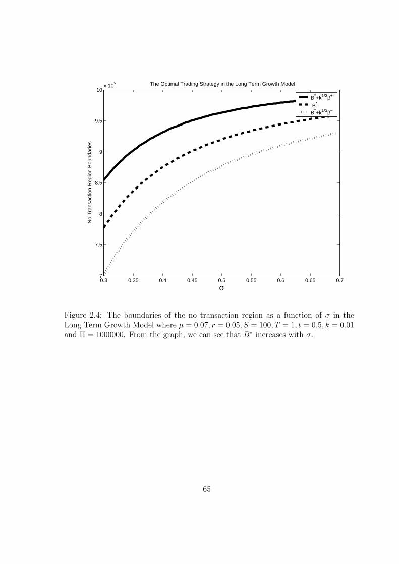
0.3 0.35 0.4 0.45 0.5 0.55 0.6 0.65 0.77

7.5

8

8.5

9

9.5

10x 10

5 The Optimal Trading Strategy in the Long Term Growth Model

σ

No

Tra

nsac

tion

Reg

ion

Bou

ndar

ies

B*+k1/3β+

B* B*+k1/3β−

Figure 2.4: The boundaries of the no transaction region as a function of σ in theLong Term Growth Model where µ = 0.07, r = 0.05, S = 100, T = 1, t = 0.5, k = 0.01and Π = 1000000. From the graph, we can see that B∗ increases with σ.

65

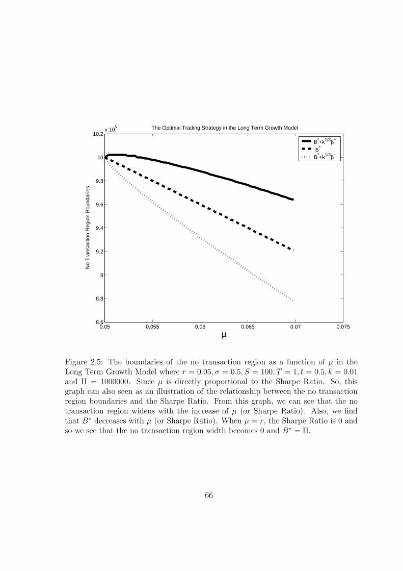
0.05 0.055 0.06 0.065 0.07 0.0758.6

8.8

9

9.2

9.4

9.6

9.8

10

10.2x 10

5 The Optimal Trading Strategy in the Long Term Growth Model

µ

No

Tra

nsac

tion

Reg

ion

Bou

ndar

ies

B*+k1/3β+

B* B*+k1/3β−

Figure 2.5: The boundaries of the no transaction region as a function of µ in theLong Term Growth Model where r = 0.05, σ = 0.5, S = 100, T = 1, t = 0.5, k = 0.01and Π = 1000000. Since µ is directly proportional to the Sharpe Ratio. So, thisgraph can also seen as an illustration of the relationship between the no transactionregion boundaries and the Sharpe Ratio. From this graph, we can see that the notransaction region widens with the increase of µ (or Sharpe Ratio). Also, we findthat B∗ decreases with µ (or Sharpe Ratio). When µ = r, the Sharpe Ratio is 0 andso we see that the no transaction region width becomes 0 and B∗ = Π.

66

0 0.01 0.02 0.03 0.04 0.05 0.06 0.076

6.5

7

7.5

8

8.5

9

9.5

10

10.5x 10

5 The Optimal Trading Strategy in the Long Term Growth Model

r

No

Tra

nsac

tion

Reg

ion

Bou

ndar

ies

B*+k1/3β+

B* B*+k1/3β−

Figure 2.6: The boundaries of the no transaction region in the Long Term GrowthModel as a function of r where µ = 0.07, σ = 0.5, S = 100, T = 1, t = 0.5, k = 0.01and Π = 1000000. This graph is equal to a reflection of Figure 2.5. This is becausethe equations for β+ and β− are in terms of µ− r. An increase in r is equivalent toa corresponding decrease in µ.

67

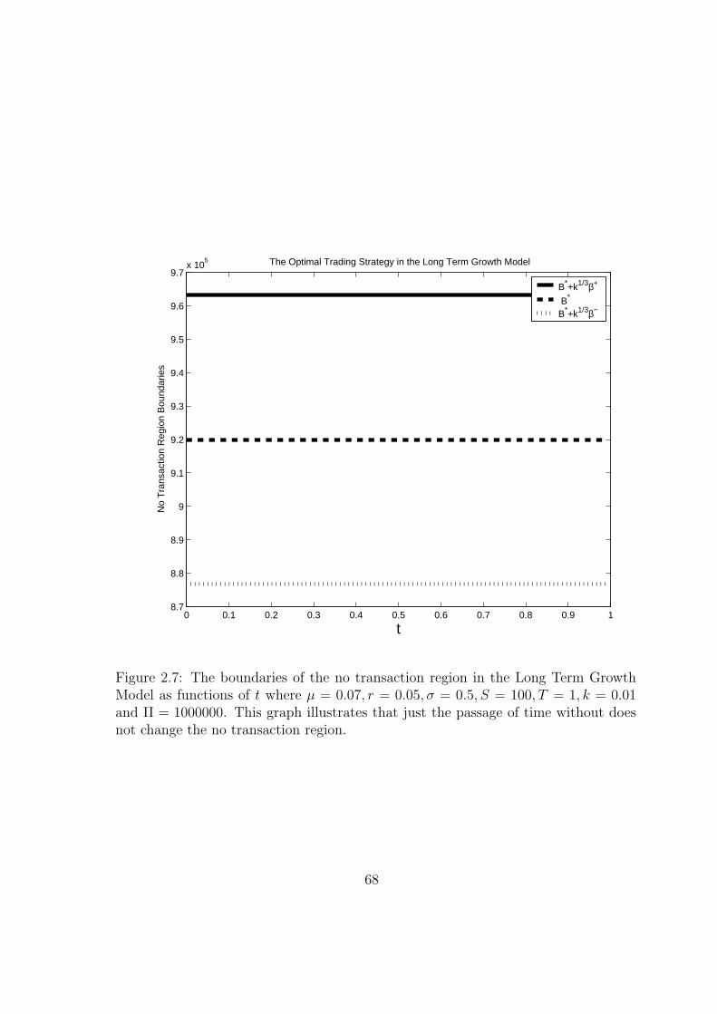
0 0.1 0.2 0.3 0.4 0.5 0.6 0.7 0.8 0.9 18.7

8.8

8.9

9

9.1

9.2

9.3

9.4

9.5

9.6

9.7x 10

5 The Optimal Trading Strategy in the Long Term Growth Model

t

No

Tra

nsac

tion

Reg

ion

Bou

ndar

ies

B*+k1/3β+

B* B*+k1/3β−

Figure 2.7: The boundaries of the no transaction region in the Long Term GrowthModel as functions of t where µ = 0.07, r = 0.05, σ = 0.5, S = 100, T = 1, k = 0.01and Π = 1000000. This graph illustrates that just the passage of time without doesnot change the no transaction region.

68

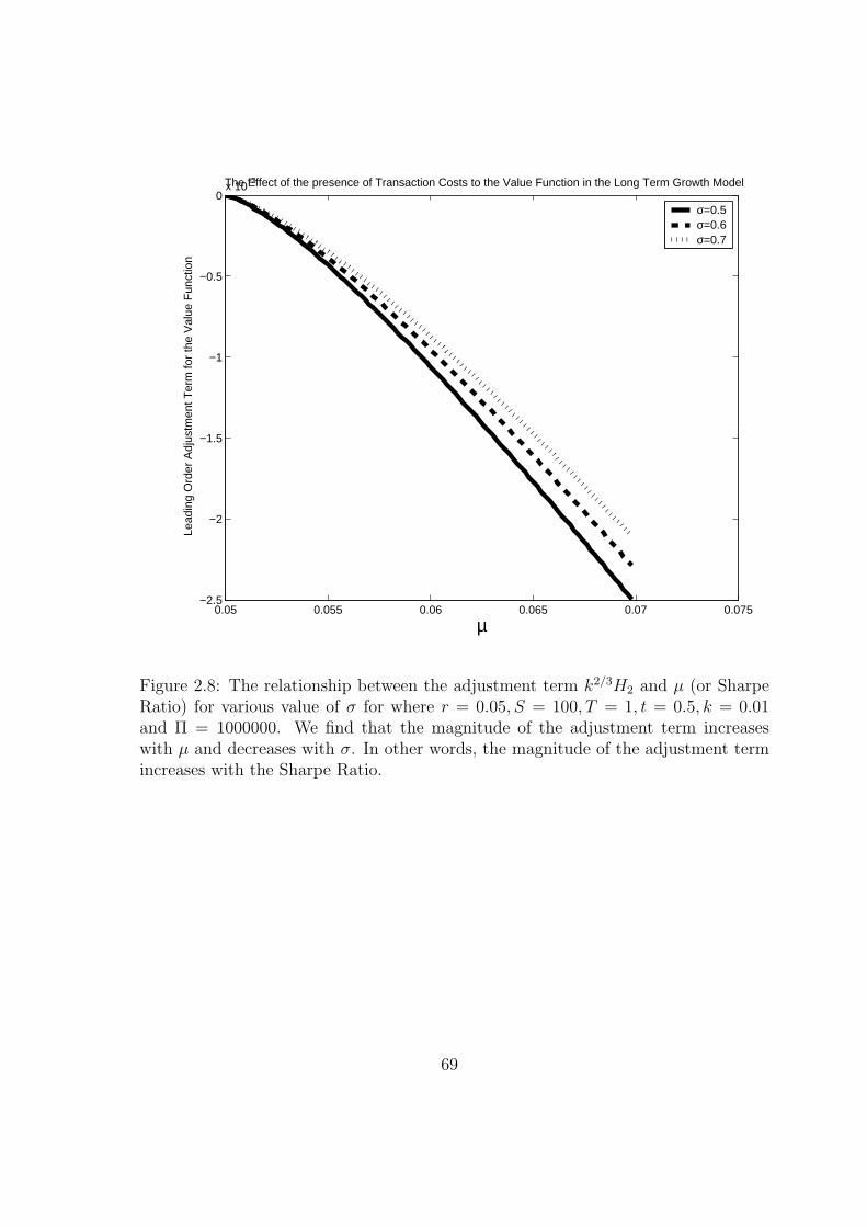
0.05 0.055 0.06 0.065 0.07 0.075−2.5

−2

−1.5

−1

−0.5

0x 10

−3The Effect of the presence of Transaction Costs to the Value Function in the Long Term Growth Model

µ

Lead

ing

Ord

er A

djus

tmen

t Ter

m fo

r th

e V

alue

Fun

ctio

n

σ=0.5σ=0.6σ=0.7

Figure 2.8: The relationship between the adjustment term k2/3H2 and µ (or SharpeRatio) for various value of σ for where r = 0.05, S = 100, T = 1, t = 0.5, k = 0.01and Π = 1000000. We find that the magnitude of the adjustment term increaseswith µ and decreases with σ. In other words, the magnitude of the adjustment termincreases with the Sharpe Ratio.

69

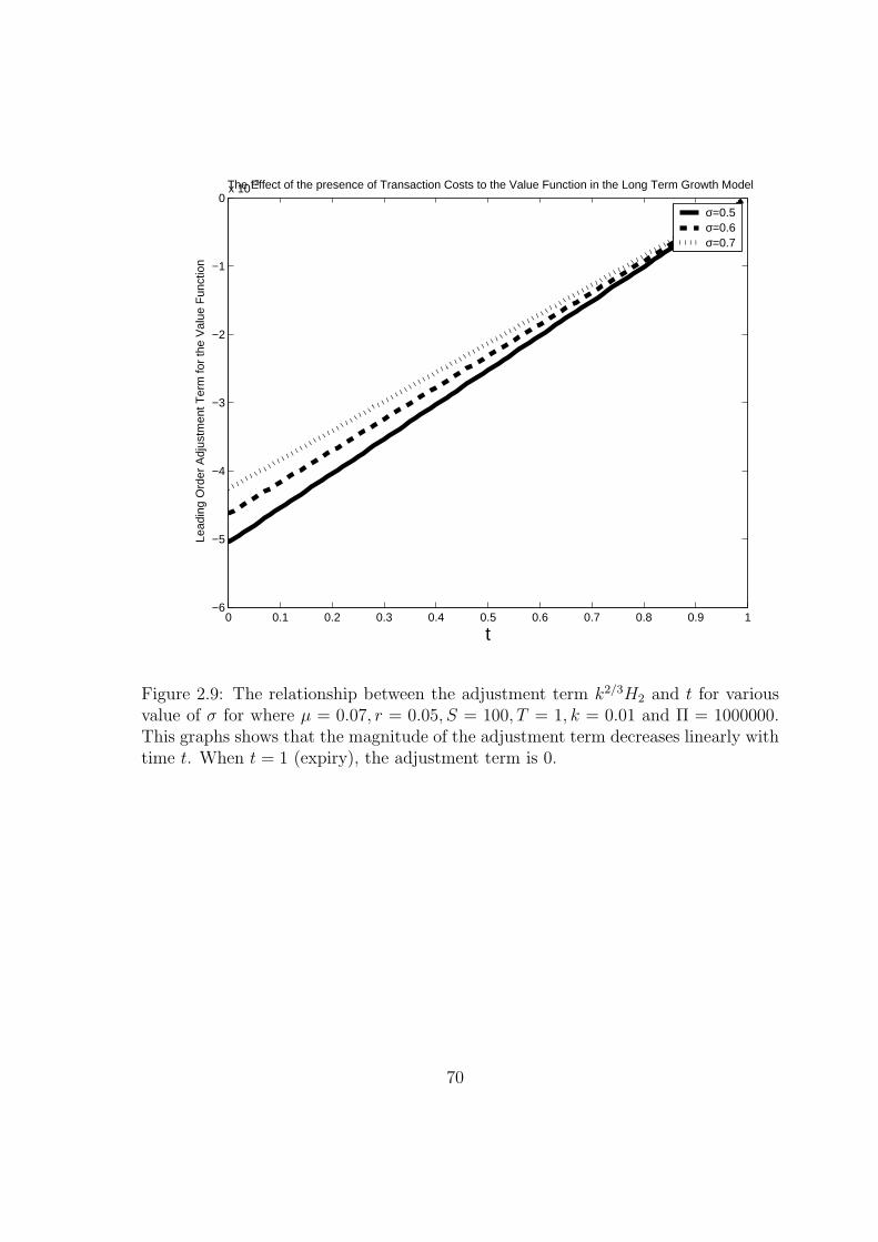
0 0.1 0.2 0.3 0.4 0.5 0.6 0.7 0.8 0.9 1−6

−5

−4

−3

−2

−1

0x 10

−3The Effect of the presence of Transaction Costs to the Value Function in the Long Term Growth Model

t

Lead

ing

Ord

er A

djus

tmen

t Ter

m fo

r th

e V

alue

Fun

ctio

nσ=0.5σ=0.6σ=0.7

Figure 2.9: The relationship between the adjustment term k2/3H2 and t for variousvalue of σ for where µ = 0.07, r = 0.05, S = 100, T = 1, k = 0.01 and Π = 1000000.This graphs shows that the magnitude of the adjustment term decreases linearly withtime t. When t = 1 (expiry), the adjustment term is 0.

70

2.8.2 CRRA Model

We plot the graph of the no-transaction region as functions of σ, µ, r, t and γ. The

results are Figures 2.10 to 2.14.

The relationship between the no-transaction region with σ,µ, r, t are similar to

the relationship in the Long Term Growth Model. The difference between the CRRA

model and the Long Term Growth Model is the addition of the variables γ and ν.

As we can see from the formulae, ν does not appear in the equations for β+ and

β−. So, ν does not affect the no transaction region at least not at any order included

in our asymptotic.

Regarding γ, from Figure 2.14, we can see that it has a huge effect on B as well

as β+ and β−, and thus the no transaction region. When γ becomes bigger, we find

that the optimal amount invested in bonds in the no transaction cost problem, B∗

decreases rapidly. When

γ = 1− µ− r

σ2, (2.114)

which means γ = 0.92 in Figure 2.14, we find that B∗ = 0. Beyond that, when

γ > 0.92, B∗ becomes negative and this means the investor borrows money to invest

in stocks. This can be explained intuitively. When γ is closer to 1, the investor is

closer to risk neutral, and thus the investor invest more in stocks, as they provide a

better expected return, and thus invests less in bonds. Regarding the width of the

no transaction region, it increases with γ initially, then it decreases. Finally, when

γ > 0.92, it increases rapidly. This can be explained by our conjectured “b effect” in

point 4 of this section.

Next, we investigate the relationship of the leading order adjustment term k2/3H2

with µ, r, t and ν. The results are in Figures 2.15 to 2.18.

The relationship between the leading order adjustment term k2/3H2 and t is very

interesting, see Figure 2.17. We look at the function H2 as in equation (2.110) and

find that its relationship with t is very complicated and so it is very difficult to find

a clear relationship. Yet, the graph seems to suggest that the relationship may well

be a linear one.

The analysis of the graphs for H2 relative to µ and rare equally interesting. Firstly,

we can see that γ in general increases the magnitude of H2. We conjecture that it

is because it increases the value of H0, as it is proportional to Πγ. Secondly, we find

71

that the relationship between H2 and µ, r are no longer linear as in the Long Term

Growth Model. H2 increases with Sharpe Ratio initially, and then decreases, and

then increases again. We attempt to explain why the shape is like this. When r = µ

(or Sharpe Ratio is equal to 0), all of the resources are invested in bonds. When

1 − γ is equal to the Sharpe Ratio, all the investments are in stocks. At these two

points, the transaction cost trading strategy and the no transaction cost strategy are

the same, and so H2 = 0. When the Sharpe Ratio is away from these two points, the

transaction cost trading strategy and the no transaction cost strategy differ more,

and so the magnitude of H2 increases correspondingly.

Interestingly, an increase of magnitude in H2 corresponds to to an increase with the

width of the no transaction region. This can be verified from the figures we have here.

We conjecture this is because the wider the no transaction region, the transaction cost

trading strategy is further away from the no transaction cost optimal trading strategy.

From Figure 2.18, we can see that the effect of ν on H2 is very small compared to

γ.

72

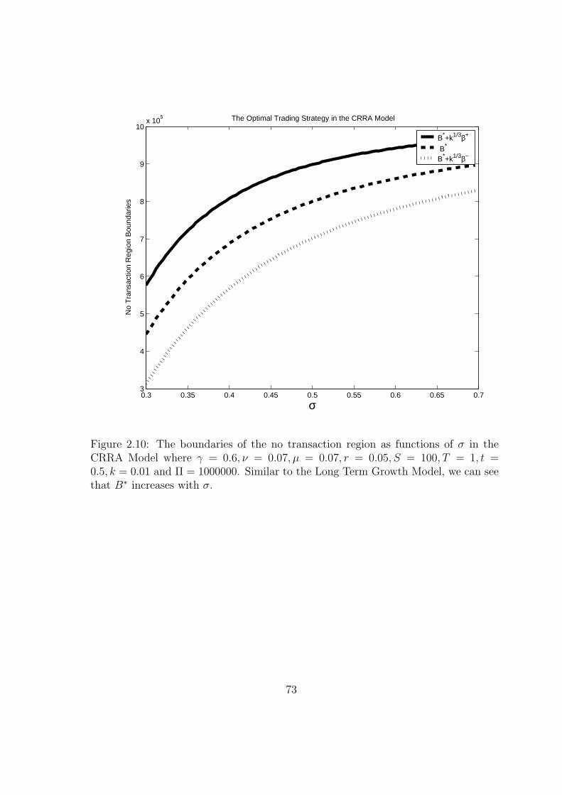
0.3 0.35 0.4 0.45 0.5 0.55 0.6 0.65 0.73

4

5

6

7

8

9

10x 10

5 The Optimal Trading Strategy in the CRRA Model

σ

No

Tra

nsac

tion

Reg

ion

Bou

ndar

ies

B*+k1/3β+

B* B*+k1/3β−

Figure 2.10: The boundaries of the no transaction region as functions of σ in theCRRA Model where γ = 0.6, ν = 0.07, µ = 0.07, r = 0.05, S = 100, T = 1, t =0.5, k = 0.01 and Π = 1000000. Similar to the Long Term Growth Model, we can seethat B∗ increases with σ.

73

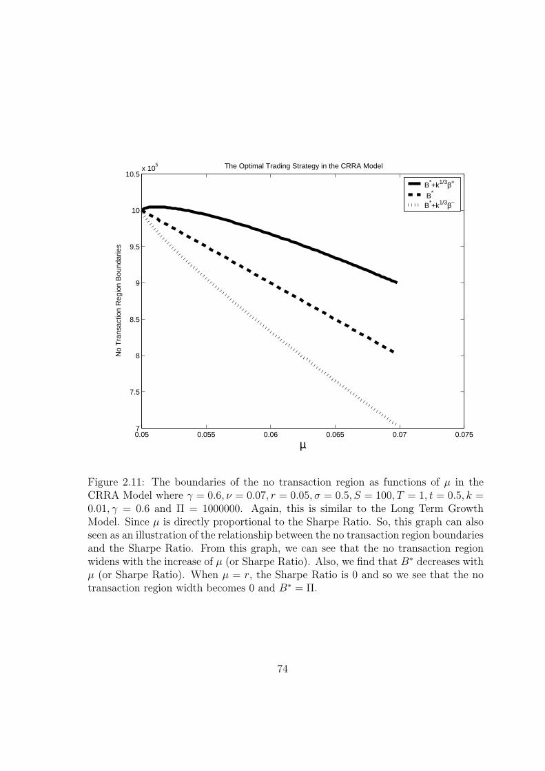
0.05 0.055 0.06 0.065 0.07 0.0757

7.5

8

8.5

9

9.5

10

10.5x 10

5 The Optimal Trading Strategy in the CRRA Model

µ

No

Tra

nsac

tion

Reg

ion

Bou

ndar

ies

B*+k1/3β+

B* B*+k1/3β−

Figure 2.11: The boundaries of the no transaction region as functions of µ in theCRRA Model where γ = 0.6, ν = 0.07, r = 0.05, σ = 0.5, S = 100, T = 1, t = 0.5, k =0.01, γ = 0.6 and Π = 1000000. Again, this is similar to the Long Term GrowthModel. Since µ is directly proportional to the Sharpe Ratio. So, this graph can alsoseen as an illustration of the relationship between the no transaction region boundariesand the Sharpe Ratio. From this graph, we can see that the no transaction regionwidens with the increase of µ (or Sharpe Ratio). Also, we find that B∗ decreases withµ (or Sharpe Ratio). When µ = r, the Sharpe Ratio is 0 and so we see that the notransaction region width becomes 0 and B∗ = Π.

74

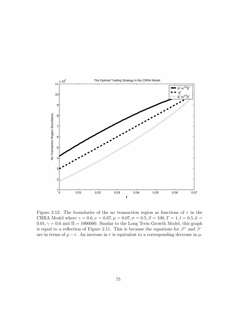
0 0.01 0.02 0.03 0.04 0.05 0.06 0.071

2

3

4

5

6

7

8

9

10

11x 10

5 The Optimal Trading Strategy in the CRRA Model

r

No

Tra

nsac

tion

Reg

ion

Bou

ndar

ies

B*+k1/3β+

B* B*+k1/3β−

Figure 2.12: The boundaries of the no transaction region as functions of r in theCRRA Model where γ = 0.6, ν = 0.07, µ = 0.07, σ = 0.5, S = 100, T = 1, t = 0.5, k =0.01, γ = 0.6 and Π = 1000000. Similar to the Long Term Growth Model, this graphis equal to a reflection of Figure 2.11. This is because the equations for β+ and β−

are in terms of µ− r. An increase in r is equivalent to a corresponding decrease in µ.

75

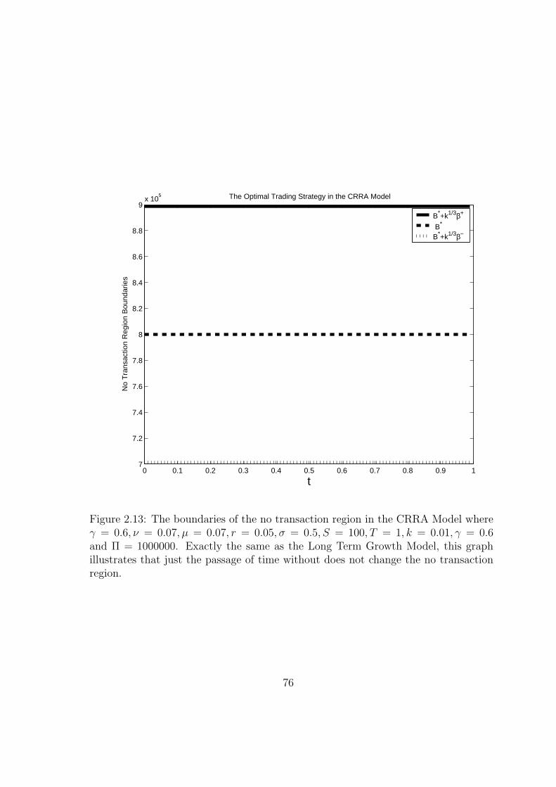
0 0.1 0.2 0.3 0.4 0.5 0.6 0.7 0.8 0.9 17

7.2

7.4

7.6

7.8

8

8.2

8.4

8.6

8.8

9x 10

5 The Optimal Trading Strategy in the CRRA Model

t

No

Tra

nsac

tion

Reg

ion

Bou

ndar

ies

B*+k1/3β+

B* B*+k1/3β−

Figure 2.13: The boundaries of the no transaction region in the CRRA Model whereγ = 0.6, ν = 0.07, µ = 0.07, r = 0.05, σ = 0.5, S = 100, T = 1, k = 0.01, γ = 0.6and Π = 1000000. Exactly the same as the Long Term Growth Model, this graphillustrates that just the passage of time without does not change the no transactionregion.

76

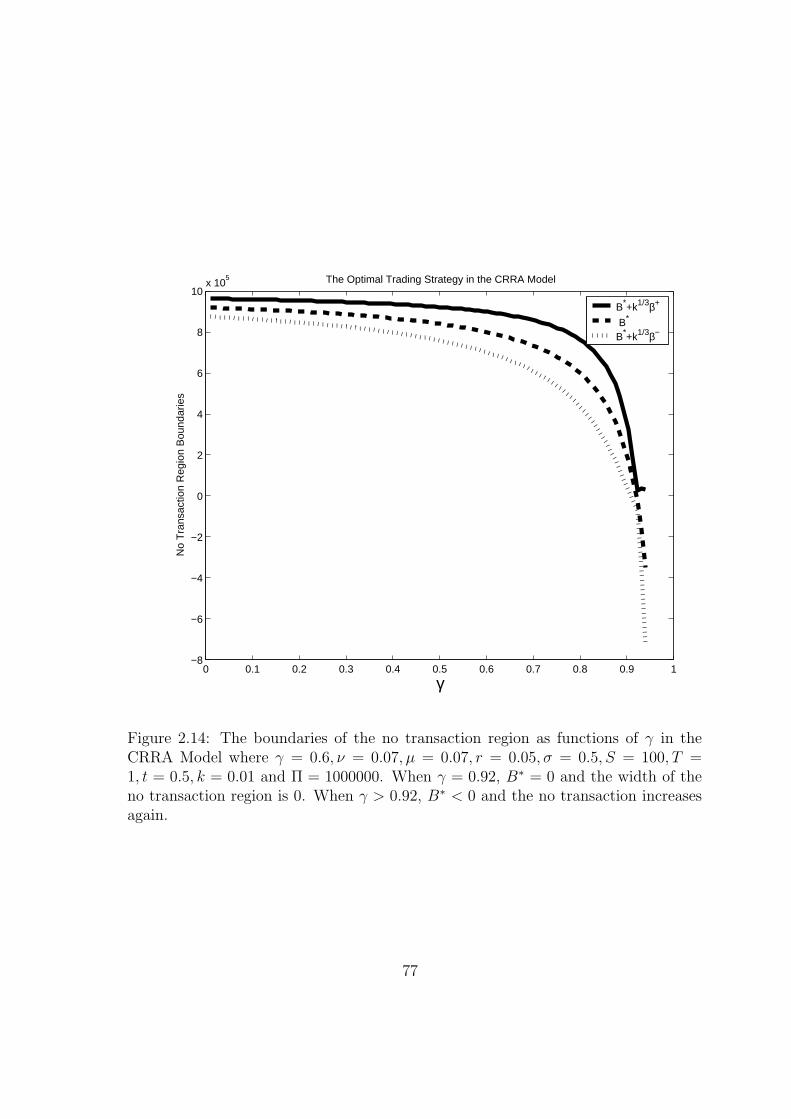
0 0.1 0.2 0.3 0.4 0.5 0.6 0.7 0.8 0.9 1−8

−6

−4

−2

0

2

4

6

8

10x 10

5 The Optimal Trading Strategy in the CRRA Model

γ

No

Tra

nsac

tion

Reg

ion

Bou

ndar

ies

B*+k1/3β+

B* B*+k1/3β−

Figure 2.14: The boundaries of the no transaction region as functions of γ in theCRRA Model where γ = 0.6, ν = 0.07, µ = 0.07, r = 0.05, σ = 0.5, S = 100, T =1, t = 0.5, k = 0.01 and Π = 1000000. When γ = 0.92, B∗ = 0 and the width of theno transaction region is 0. When γ > 0.92, B∗ < 0 and the no transaction increasesagain.

77

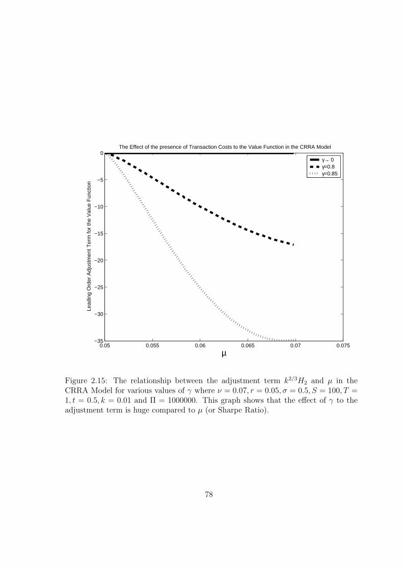
0.05 0.055 0.06 0.065 0.07 0.075−35

−30

−25

−20

−15

−10

−5

0The Effect of the presence of Transaction Costs to the Value Function in the CRRA Model

µ

Lead

ing

Ord

er A

djus

tmen

t Ter

m fo

r th

e V

alue

Fun

ctio

n

γ→ 0γ=0.8γ=0.85

Figure 2.15: The relationship between the adjustment term k2/3H2 and µ in theCRRA Model for various values of γ where ν = 0.07, r = 0.05, σ = 0.5, S = 100, T =1, t = 0.5, k = 0.01 and Π = 1000000. This graph shows that the effect of γ to theadjustment term is huge compared to µ (or Sharpe Ratio).

78

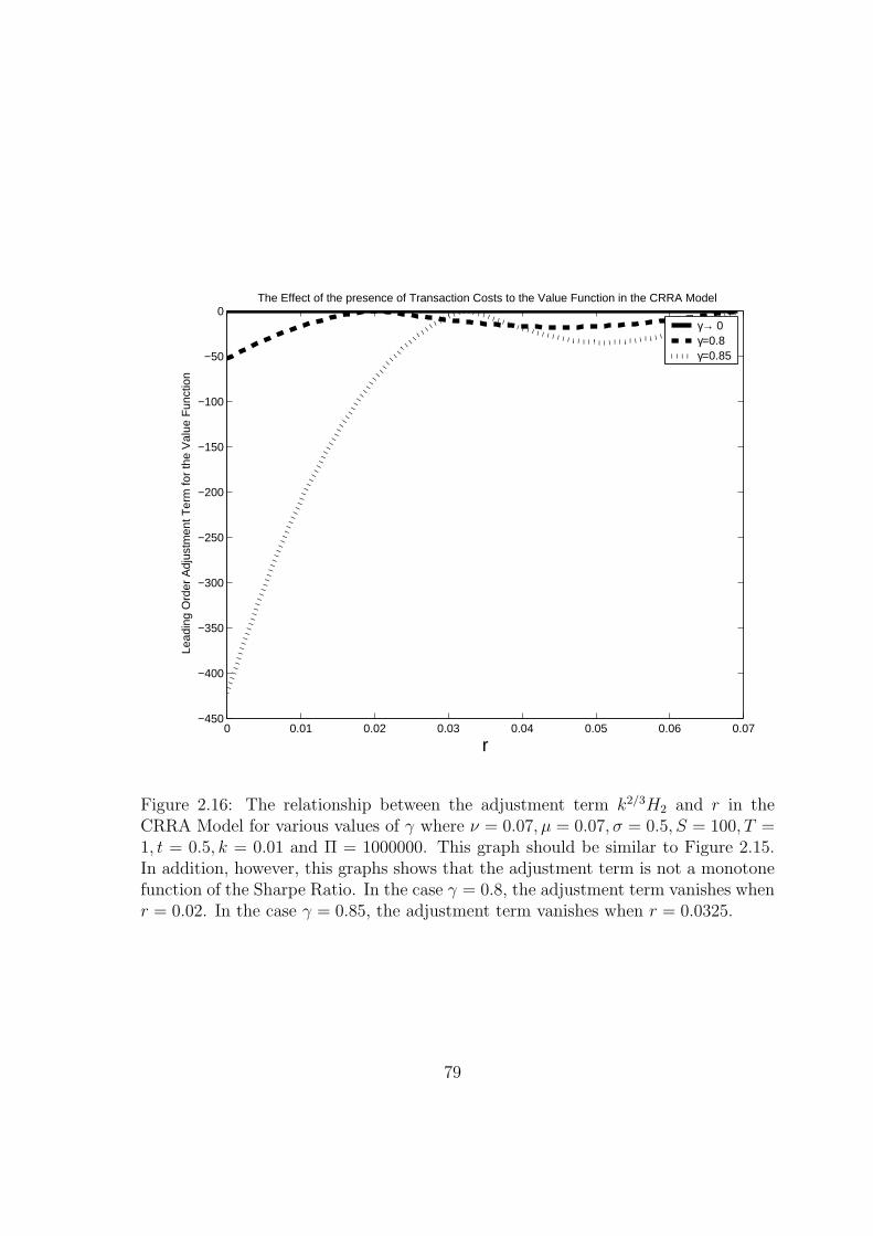
0 0.01 0.02 0.03 0.04 0.05 0.06 0.07−450

−400

−350

−300

−250

−200

−150

−100

−50

0The Effect of the presence of Transaction Costs to the Value Function in the CRRA Model

r

Lead

ing

Ord

er A

djus

tmen

t Ter

m fo

r th

e V

alue

Fun

ctio

n

γ→ 0γ=0.8γ=0.85

Figure 2.16: The relationship between the adjustment term k2/3H2 and r in theCRRA Model for various values of γ where ν = 0.07, µ = 0.07, σ = 0.5, S = 100, T =1, t = 0.5, k = 0.01 and Π = 1000000. This graph should be similar to Figure 2.15.In addition, however, this graphs shows that the adjustment term is not a monotonefunction of the Sharpe Ratio. In the case γ = 0.8, the adjustment term vanishes whenr = 0.02. In the case γ = 0.85, the adjustment term vanishes when r = 0.0325.

79

0 0.1 0.2 0.3 0.4 0.5 0.6 0.7 0.8 0.9 1−80

−70

−60

−50

−40

−30

−20

−10

0The Effect of the presence of Transaction Costs to the Value Function in the CRRA Model

t

Lead

ing

Ord

er A

djus

tmen

t Ter

m fo

r th

e V

alue

Fun

ctio

n

γ→ 0γ=0.8γ=0.85

Figure 2.17: The relationship between the adjustment term k2/3H2 and t in theCRRA Model for various values of γ where ν = 0.07, µ = 0.07, r = 0.05, σ = 0.5, S =100, T = 1, k = 0.01 and Π = 1000000. Despite the complicated relationship betweent and the adjustment term as shown in equation (2.110), the relationship seems tobe linear.

80

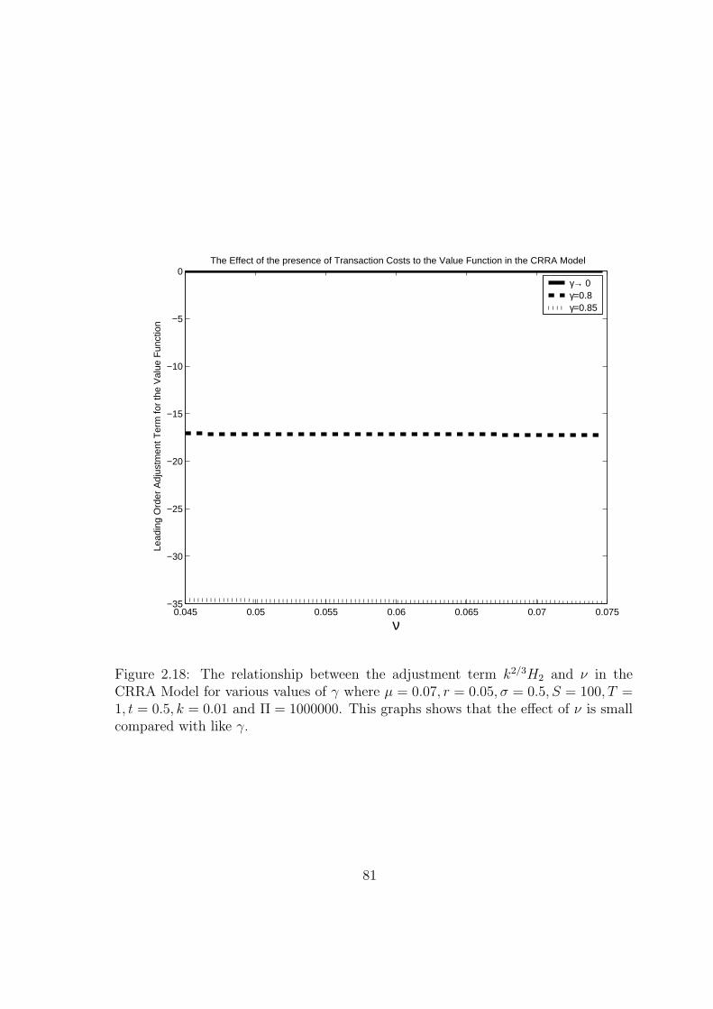
0.045 0.05 0.055 0.06 0.065 0.07 0.075−35

−30

−25

−20

−15

−10

−5

0The Effect of the presence of Transaction Costs to the Value Function in the CRRA Model

ν

Lead

ing

Ord

er A

djus

tmen

t Ter

m fo

r th

e V

alue

Fun

ctio

n

γ→ 0γ=0.8γ=0.85

Figure 2.18: The relationship between the adjustment term k2/3H2 and ν in theCRRA Model for various values of γ where µ = 0.07, r = 0.05, σ = 0.5, S = 100, T =1, t = 0.5, k = 0.01 and Π = 1000000. This graphs shows that the effect of ν is smallcompared with like γ.

81

2.9 The Choice of Asymptotic Scales

Here, we justify why we choose k1/3 in the coordinate translation

B = B(Π, t) + k1/3β,

and in the expansion

H(Π, β, t) = H0(Π, β, t) + k1/3H1(Π, β, t)

+k2/3H2(Π, β, t) + kH3(Π, β, t)

+k4/3H4(Π, β, t) + · · · .

So, we let

B = B(Π, t) + kαβ, (2.115)

and

H(Π, β, t) = H0(Π, β, t) + kεH1(Π, β, t)

+k2εH2(Π, β, t) + k3εH3(Π, β, t)

+k4εH4(Π, β, t) + · · · . (2.116)

We can safely assume that ε is a rational number.

So, we can rewrite equation (2.116) as

H(Π, β, t) = H0(Π, β, t) + k1/nH1(Π, β, t)

+k2/nH2(Π, β, t) + k3/nH3(Π, β, t)

+k4/nH4(Π, β, t) + · · · (2.117)

for some integer n. If we consider those terms of O(1), O(1 + 1/n), O(1 + 2/n),

O(1 + 3/n), · · ·, we must have

α =m

n

for some integer m. If α 6= m/n, we have

∂H0

∂Π=

∂H1

∂Π=

∂H2

∂Π=

∂H3

∂Π= · · · = 0,

which means H is independent of Π.

82

Therefore, we also rewrite equation (2.115) as

B = B(Π, t) + km/nβ. (2.118)

In fact, Π has a first order effect on H. So,

∂H0

∂Π6= 0.

If we look at those terms of O(k−mn ), O(k−

m−1n ), O(k−

m−2n ),O(k−

m−3n ), · · ·, O(1), we

have∂H0

∂β=

∂H1

∂β=

∂H2

∂β=

∂H3

∂β= · · · = ∂Hm+n−1

∂β= 0,

∂Hm+n

∂β6= 0. (2.119)

We can obtain a similar result for the purchase region boundary.

As for the smooth pasting conditions for the sales region, we have

∂2H0

∂β2=

∂2H1

∂β2=

∂2H2

∂β2=

∂2H3

∂β2= · · · = ∂2H4m−1

∂β2= 0,

∂2H4m

∂β2= − ∂2H0

∂β∂Π.

For the smooth pasting condition of the purchase region, we have

∂2H0

∂β2=

∂2H1

∂β2=

∂2H2

∂β2=

∂2H3

∂β2= · · · = ∂2H4m−1

∂β2= 0,

∂2H4m

∂β2=

∂2H0

∂β∂Π.

Regarding the final condition, we have

H0 = F (T ),

H1 = H2 = H3 = H4 = · · · = 0.

Now, we look at the equation in the no-transaction region. We have the equations

below.

83

2.9.1 H0, H1, H2, · · ·, H2m−1

The equations for H0, H1, H2, · · ·, H2m−1 are similar to equation (2.77) and equation

(2.78) . They are

1

2σ2(

∂B

∂Π)2(Π−B)2∂2H0

∂β2= 0, (2.120)

1

2σ2(

∂B

∂Π)2(Π−B)2∂2H1

∂β2= 0, (2.121)

1

2σ2(

∂B

∂Π)2(Π−B)2∂2H2

∂β2= 0, (2.122)

...1

2σ2(

∂B

∂Π)2(Π−B)2∂2H2m−1

∂β2= 0. (2.123)

If we use the same argument as in Sections 2.6.4 and 2.6.5, we can conclude that H0,

H1, H2, · · ·, H2m−1 are all independent of β.

2.9.2 H2m, H2m+1, H2m+2, · · ·, H3m−1

As for equation (2.77), the equations for H2m, H2m+1, H2m+2, · · ·, H3m−1 are as

follows

1

2σ2(

∂B

∂Π)2(Π−B)2∂2H2m

∂β2

= −{

I +∂H0

∂t+ rB

∂H0

∂Π+ µ(Π−B)

∂H0

∂Π+

σ2(Π−B)2

2

∂2H0

∂Π2

}, (2.124)

1

2σ2(

∂B

∂Π)2(Π−B)2∂2H2m+1

∂β2

= −{

I +∂H1

∂t+ rB

∂H1

∂Π+ µ(Π−B)

∂H1

∂Π+

σ2(Π−B)2

2

∂2H1

∂Π2

}, (2.125)

1

2σ2(

∂B

∂Π)2(Π−B)2∂2H2m+2

∂β2

= −{

I +∂H2

∂t+ rB

∂H2

∂Π+ µ(Π−B)

∂H2

∂Π+

σ2(Π−B)2

2

∂2H2

∂Π2

}, (2.126)

...

84

1

2σ2(

∂B

∂Π)2(Π−B)2∂2H3m−1

∂β2

= −{

I +∂Hm−1

∂t+ rB

∂Hm−1

∂Π+ µ(Π−B)

∂Hm−1

∂Π+

σ2(Π−B)2

2

∂2Hm−1

∂Π2

}.

As in Section 2.6.6, we can also deduce that H2m, H2m+1, H2m+2, · · ·, H3m−1 are all

independent of β. Also, using the argument in Section 2.6.7, we find that H1, H2,

· · ·, Hm−1 are all identically zero.

2.9.3 H3m, H3m+1, H3m+2, · · ·, H4m−1

The equations we have for H3m, H3m+1, H3m+2, · · ·, H4m−1 are similar to equation

(2.80). They are

1

2σ2(

∂B

∂Π)2(Π−B)2∂2H3m

∂β2

=

{σ2(Π−B)

∂2H0

∂Π2+ (µ− r)

∂H0

∂Π

}β

−{

∂Hm

∂t+ rB

∂Hm

∂Π+ µ(Π−B)

∂Hm

∂Π+

σ2(Π−B)2

2

∂2Hm

∂Π2

},

1

2σ2(

∂B

∂Π)2(Π−B)2∂2H3m+1

∂β2

=

{σ2(Π−B)

∂2H1

∂Π2+ (µ− r)

∂H1

∂Π

}β

−{

∂Hm+1

∂t+ rB

∂Hm+1

∂Π+ µ(Π−B)

∂Hm+1

∂Π+

σ2(Π−B)2

2

∂2Hm+1

∂Π2

},

1

2σ2(

∂B

∂Π)2(Π−B)2∂2H3m+2

∂β2

=

{σ2(Π−B)

∂2H2

∂Π2+ (µ− r)

∂H2

∂Π

}β

−{

∂Hm+2

∂t+ rB

∂Hm+2

∂Π+ µ(Π−B)

∂Hm+2

∂Π+

σ2(Π−B)2

2

∂2Hm+2

∂Π2

},

...

85

1

2σ2(

∂B

∂Π)2(Π−B)2∂2H4m−1

∂β2

=

{σ2(Π−B)

∂2Hm−1

∂Π2+ (µ− r)

∂Hm−1

∂Π

}β

−{

∂H2m−1

∂t+ rB

∂H2m−1

∂Π+ µ(Π−B)

∂H2m−1

∂Π+

σ2(Π−B)2

2

∂2H2m−1

∂Π2

}.

We apply the same argument as in Section 2.6.7, and we can conclude that H3m,

H3m+1, H3m+2, · · ·, H4m−1 are all independent of β. Also, Hm, Hm+1, · · ·, H2m−1 are

all identically zero.

2.9.4 H4m

The equation for H4m is similar to equation (2.83), which is

1

2σ2(

∂B

∂Π)2(Π−B)2∂2H4m

∂β2

= −1

2σ2∂2H0

∂Π2β2 −

{∂H2m

∂t+ rB

∂H2m

∂Π+ µ(Π−B)

∂H2m

∂Π+

σ2(Π−B)2

2

∂2H2m

∂Π2

}.

(2.127)

Therefore, H4m must be dependent on β as

∂2H0

∂Π26= 0

in equation (2.127).

We recall from equation (2.119) that Hm+n is the first term that is dependent of

β. So, we can conclude that m + n = 4m and so n = 3m.

Thus, we justify the coordinate translation

B = B(Π, t) + k1/3β.

Also, we find that H1, H2, · · ·, H2m−1 all are equal to zero. So, our finding that

the effect of transaction costs on the value function is of second order is still valid.

It is true that H2m+1, H2m+2, · · ·, H3m−1 and H3m+1, H3m+2, · · ·, H4m−1 may not

vanish. They, however, have no effect on the transaction boundaries and the leading

86

order value function adjustment term. Therefore, our choice of expansion for H

H(Π, β, t)

= H0(Π, β, t) + k1/3H1(Π, β, t) + k2/3H2(Π, β, t) + kH3(Π, β, t)

+k4/3H4(Π, β, t) + · · ·

is justified.

87

Chapter 3

Two Generalizations of theDynamic Asset Allocation withTransaction Cost Model

3.1 Introduction

In the previous chapter, we worked on a problem in dynamic asset allocation with

transaction costs. In this chapter, we extend the study in several different directions.

The first generalization we consider is to allow the value function to be dependent on

the stock price S. This in principle enable us to study those optimization problems

with options in the portfolio. Secondly, we allow more than one stock, but the

objective function is as in Chapter 2.

In both of these generalizations, the mathematics is similar to that in Chapter 2,

but the results we obtain here, however, are not entirely the same. The formulae for

the transaction boundaries in these generalized cases are usually very complicated.

The properties of the no-transaction costs region may also be very different.

3.2 Stock Price Dependence

We study the problem when the value function J is dependent of S.

88

3.2.1 Without Transaction Costs

As in Chapter 2, we study the problem with no transaction costs first. Using the

same notation and setup as there, the market model equations are equation (2.2).

dB = rBdt

dS = µSdt + σSdX

dA = µAdt + σAdX

dΠ = µ(Π−B)dt + rBdt + σ(Π−B)dX

At time t = 0, an investor has an amount of Π0 of resources. The problem is to

allocate investments over the given time horizon so as to maximize

E0

{ ∫ T

0

I(Π(t), S(t))dt + F (Π(T ), S(T ))

}

where Et is the conditional expectation given information up to time t. I and F are

supposed to be strictly increasing concave differentiable functions of Π and S.

We rewrite the above equation in dynamic programming form so as to apply the

Bellman principle of optimality. Therefore, we define the optimal expected value

function J(Π, S, t) as

J(Π, S, t) = maxBEt

{∫ T

t

I(Π(t), S(t))dt + F (Π(T ), S(T ))

}. (3.1)

Applying Bellman’s Principle and Ito’s Lemma gives us

0 = maxB

{∂J

∂t+ I + rB

∂J

∂Π+ µ(Π−B)

∂J

∂Π+ µS

∂J

∂S

+σ2

2

{S2 ∂2J

∂S2+ 2S(Π−B)

∂2J

∂Π∂S+ (Π−B)2 ∂2J

∂Π2

}. (3.2)

At t = T , we have

J(Π, S, T ) = F (Π, S). (3.3)

89

3.2.2 Solving Bellman’s Equation with No Transaction Costs

Here, in the same spirit as the previous chapter, we attempt to provide some exact

solutions of the no transaction problem.

By differentiating equation (3.2) , we can find B∗, the optimal amount of assets

invested in risk-free bonds, which is

B∗ = Π + ((µ− r)

σ2

∂J

∂Π+ S

∂2J

∂Π∂S)/

∂2J

∂Π2(3.4)

where B∗ is the optimal amount invested in risk-free bonds. Putting this back into

equation (3.2), we have

0 =∂J

∂t+ I + rΠ

∂J

∂Π− (µ− r)2

2σ2(∂J

∂Π)2/

∂2J

∂Π2

+µS∂J

∂S− (µ− r)S

∂J

∂Π

∂2J

∂Π∂S/∂2J

∂Π2+

σ2S2 ∂2J∂S2 − ∂2J

∂Π∂S

2

2 ∂2J∂Π2

. (3.5)

As for equation (2.9), we know that for any function J , as long as we set the

function I accordingly,

I = −{

∂J

∂t+ rΠ

∂J

∂Π− (µ− r)2

2σ2(∂J

∂Π)2/

∂2J

∂Π2

+µS∂J

∂S− (µ− r)S

∂J

∂Π

∂2J

∂Π∂S/∂2J

∂Π2+

σ2S2 ∂2J∂S2 − ∂2J

∂Π∂S

2

2 ∂2J∂Π2

}, (3.6)

we can have exact solutions. As in Chapter 2, we have to make sure that the functions

J and I thus defined make economic sense, which means

∂I

∂Π≥ 0,

∂J

∂Π≥ 0,

∂2J

∂Π2< 0. (3.7)

We again consider the following change of variables:

τ = T − t

x = log Π

y = log S.

J(x, y, τ) = J(Π, S, t) (3.8)

90

We have

B∗ = Π

{(µ− r)Jx + σ2Jxy

σ2(Jxx − Jx)+ 1

}(3.9)

and

I = Jτ − rJx − µJy +σ2Jy

2− σ2Jyy

2+

((µ− r)Jx + σ2Jxy)2

2σ2(Jxx− Jx). (3.10)

Now, we look at some special cases of J(τ, x, y).

3.2.3 Modified Long Term Growth Model

We recall the long term growth model from Section 1.11. Now, we want to modify

the long term growth model so that it depends on S. We let 1

J(x, y, τ) = x + βy − ντ. (3.11)

Therefore,

J(Π, S, t) = log Π + β log S − ν(T − t).

(3.12)

and so the terminal function

F (Π(T ), S(T )) = log Π + β log S,

and we find

B∗ = Π

{1− (µ− r)

σ2

}(3.13)

and

I = −ν − (µ− r)2

2σ2− r − µβ +

βσ2

2. (3.14)

We notice that I in fact is a constant. Therefore, it does not affect our problem at all.

It is included here so that we can have a very tidy J . Therefore, this optimization

problem is just to maximize the expectation of the terminal function F (Π(T ), S(T )).

1Note β here is not the β from Chapter 2.

91

The amount of resources invested in stock is the same as in our previous Long

Term Growth Model in Section 1.11. There is a reason. Those terms involving S(T )

in the terminal function F (Π(T ), S(T )) can be separated from those terms involving

Π(T ). Therefore,

J(Π, S, t) = maxBEt

{log Π(T ) + β log S(T )

}

= maxB

{Et log Π(T ) + Etβ log S(T )

}

= maxB

{Et log Π(T )

}+ Et

{β log S(T )

}

= maxB

{Et log Π(T )

}+ β(µ(T − t)− 1

2σ2(T − t)). (3.15)

The control B does not affect Et(β log S(T )). Therefore, the addition of S dependence

in this case has no effect at all on the investment policy.

3.2.4 Modified Constant Relative Risk Aversion (CRRA) Model

Here, we consider the case where

J(x, y, τ) = exp (γx + αy − ντ)

(3.16)

which means

J(Π, S, t) = eν(T−t)ΠγSα,

with the terminal function F (Π(T )) = ΠγSα.

Therefore, we have

B∗ = Π

{1− α

1− γ− µ− r

σ2(1− γ)

}(3.17)

and

I =(γ(µ− r)2 − 2rγασ2 + 2µασ2 + σ4α2

2(γ − 1)σ2− γr + ν +

σ2α

2

)J

=(γ(µ− r)2 − 2rγασ2 + 2µασ2 + σ4α2

2(γ − 1)σ2− γr + ν +

σ2α

2

)eν(T−t)ΠγSα.

(3.18)

92

Although these are formally solutions of equation (3.2) for any values of γ and

ν, we must choose the value of γ, ν and α properly so that the criteria in (3.7) are

satisfied. This means choosing γ and ν such that

γ < 1

and

ν > γr − γ(µ− r)2 − 2rγασ2 + 2µασ2 + σ4α2

2(γ − 1)σ2− σ2α

2.

The amount invested in stocks in this modified CRRA model is different to our

previous CRRA model, and it is no longer proportional the Sharpe ratio, but it is still

inversely proportional to 1 − γ, the relative risk aversion factor. The value function

J is also different.

We notice that when

α = (1− γ)− µ− r

σ2, (3.19)

B∗ = 0. This means the investor does not invest in bonds at all. He puts all his

investments in stocks.

3.2.5 With Transaction Costs

Now we consider the problem with transaction costs. As in the previous chapter, let

k > 0 represents the portion of of stock price used as transaction costs.

The market model equations become

dS = µSdt + σSdX1

dB = rBdt− (1 + k)dL(t) + (1− k)dM(t)

dΠ = µ(Π−B)dt + rBdt + σ(Π−B)dβt − kdL(t)− kdM(t) (3.20)

where L(t) and M(t) represent the cumulative purchase and sale of assets A in [0, t],

which we use as the controls. As in Chapter 2, B is only used to denote the value of

assets invested in stocks here and it is no longer used as a control.

The optimal expected value function J(Π, B, t) is

J(Π, B, S, t) = maxL,M

Et

{∫ T

t

I(Π(t), S(t))dt + F (Π(T ), S(T ))

}. (3.21)

93

Applying Bellman’s Principle and Ito’s Lemma , we have

maxl,m∈Θ

{I +

∂J

∂t+ (rB − (1 + k)dl + (1− k)m)

∂J

∂B

+(rB + µ(Π−B)− kl− km)∂J

∂Π+ µS

∂J

∂S

+σ2

2

{S2 ∂2J

∂S2+ 2S(Π−B)

∂2J

∂Π∂S+ (Π−B)2σ2 ∂2J

∂Π2

}= 0. (3.22)

In the no-transaction region, therefore, the value function J satisfies

I +∂J

∂t+ rB(

∂J

∂B+

∂J

∂Π) + µ(Π−B)

∂J

∂Π+ µS

∂J

∂S

+σ2

2

{S2 ∂2J

∂S2+ 2S(Π−B)

∂2J

∂Π∂S+ (Π−B)2 ∂2J

∂Π2

}= 0. (3.23)

In the sales region (and at the boundary between sales region and no transaction

region), J satisfies

−k∂J

∂Π= (1 + k)

∂J

∂B. (3.24)

In the purchase region (and at the boundary between sales region and no trans-

action region), J satisfies

k∂J

∂Π= (1− k)

∂J

∂B. (3.25)

The smooth pasting equation at the boundaries between the no-transaction region

and sales region is

(1− k)∂2J

∂B2= k

∂2J

∂B∂Π, (3.26)

and at the boundaries between the no-transaction region and purchase region is

(1 + k)∂2J

∂B2= −k

∂2J

∂B∂Π. (3.27)

Also, when t = T , we have the final condition

J(Π, T ) = F (Π). (3.28)

94

We translate the B coordinate according to

B = B(Π, S, t) + k1/3β, (3.29)

where B is the value of risk-free bonds we have when the level of transaction costs

tends to zero, k → 0.

We let H(Π, β, S, t) = J(Π, B, S, t). We have

∂J

∂B= k−1/3∂H

∂β,

∂J

∂Π=

∂H

∂Π− k−1/3∂H

∂β

∂B

∂Π,

∂J

∂t=

∂H

∂t− k−1/3∂H

∂β

∂B

∂t,

∂J

∂S=

∂H

∂S− k−1/3∂H

∂β

∂B

∂S,

∂2J

∂Π2=

∂2H

∂Π2− k−1/3(2

∂2H

∂β∂Π

∂B

∂Π+

∂H

∂β

∂2B

∂Π2) + k−2/3∂2H

∂β2(∂B

∂Π)2,

∂2J

∂S2=

∂2H

∂S2− k−1/3(2

∂2H

∂β∂S

∂B

∂S+

∂H

∂β

∂2B

∂S2) + k−2/3∂2H

∂S2(∂B

∂S)2,

∂2J

∂S∂Π=

∂2H

∂S∂Π− k−1/3(

∂2H

∂β∂S

∂B

∂Π+

∂2H

∂β∂Π

∂B

∂S+

∂H

∂β

∂2B

∂S∂Π)

+k−2/3∂2H

∂β2

∂B

∂S

∂B

∂Π. (3.30)

Also, we let

H(Π, β, S, t) = H0(Π, β, S, t) + k1/3H1(Π, β, S, t)

+k2/3H2(Π, β, S, t) + kH3(Π, β, S, t)

+k4/3H4(Π, β, S, t) + · · · (3.31)

and assume that H0, H1, H2, H3, H4, . . . and their derivatives are all of O(1). H0 is

the value function when transaction costs level k → 0.

95

After the change of coordinates and collecting terms of the same order the sales

region equation, as in Section , we have

∂H0

∂β= 0, (3.32)

∂H1

∂β= 0, (3.33)

∂H2

∂β= 0, (3.34)

∂H3

∂β− (1− ∂B

∂Π)∂H0

∂β= 0, (3.35)

∂H4

∂β− (1− ∂B

∂Π)∂H1

∂β− ∂H0

∂Π= 0. (3.36)

Similarly, we have the following equations for the purchase region,

∂H0

∂β= 0, (3.37)

∂H1

∂β= 0, (3.38)

∂H2

∂β= 0, (3.39)

∂H3

∂β+ (1− ∂B

∂Π)∂H0

∂β= 0, (3.40)

∂H4

∂β+ (1− ∂B

∂Π)∂H1

∂β+

∂H0

∂Π= 0. (3.41)

As for the smooth pasting equation for the sales boundary, we have

∂2H0

∂β2= 0, (3.42)

∂2H1

∂β2= 0, (3.43)

∂2H2

∂β2= 0, (3.44)

∂2H3

∂β2− (1− ∂B

∂Π)∂2H0

∂β2= 0, (3.45)

∂2H4

∂β− (1− ∂B

∂Π)∂2H1

∂β2− ∂2H0

∂Π∂β= 0. (3.46)

Similarly, the smooth pasting equation for the purchase boundary becomes

∂2H0

∂β2= 0, (3.47)

96

∂2H1

∂β2= 0, (3.48)

∂2H2

∂β2= 0, (3.49)

∂2H3

∂β2+ (1− ∂B

∂Π)∂2H0

∂β2= 0, (3.50)

∂2H4

∂β+ (1− ∂B

∂Π)∂2H1

∂β2+

∂2H0

∂Π∂β= 0. (3.51)

The final condition becomes

H0(Π, β, S, T ) = F (Π, S) (3.52)

H1(Π, β, S, T ) = 0 (3.53)

H2(Π, β, S, T ) = 0 (3.54)

H3(Π, β, S, T ) = 0 (3.55)

H4(Π, β, S, T ) = 0. (3.56)

As in Chapter 2, we now consider the equation at the no-transaction region. After

translating the coordinates, expanding H according to equation (3.31) , and collecting

terms of the same order in k, we have the equations below.

1. O(k−2/3) Equation

1

2σ2

{∂B

∂Π(Π−B) + S

∂B

∂S

}2∂2H0

∂β2= 0. (3.57)

Using the same argument as in Section 2.6.4, we can conclude that H0 is inde-

pendent of β.

2. O(k−1/3) Equation

1

2σ2

{S

∂B

∂Π(Π−B) + S

∂B

∂S

}2∂2H1

∂β2= 0. (3.58)

Similarly, we can conclude that H1 is independent of β.

3. O(1) Equation

−1

2σ2

{S

∂B

∂Π(Π−B) + S

∂B

∂S

}2∂2H2

∂β2

= I +∂H0

∂t+ rB

∂H0

∂Π+ µS

∂H0

∂S+ µ(Π−B)

∂H0

∂Π

+σ2[S2

2

∂2H0

∂S2+

(Π−B)2

2

∂2H0

∂Π2+ S(Π−B)

∂2H0

∂S∂Π

]. (3.59)

97

As in Section 2.6.6, H2 here is independent of β. Also, we have H0 = J .

4. O(k1/3) Equation

1

2σ2

{∂B

∂Π(Π−B) + S

∂B

∂S

}2∂2H3

∂β2

=

{σ2(Π−B)

∂2H0

∂Π2+ σ2S

∂2H0

∂Π∂S+ (µ− r)

∂H0

∂Π

}β

−{

∂H1

∂t+ rB

∂H1

∂Π+ µ(Π−B)

∂H1

∂Π+ µS

∂H1

∂S

+σ2[S2

2

∂2H1

∂S2+

(Π−B)2

2

∂2H1

∂Π2+ S(Π−B)

∂2H1

∂S∂Π

]}.

(3.60)

Like Section 2.6.7, we know that H3 is independent on β. Also, we have H1 = 0.

Unlike Section 2.6.7, we have

σ2(Π−B)∂2H0

∂Π2+ σ2S

∂2H0

∂Π∂S+ (µ− r)

∂H0

∂Π= 0 (3.61)

instead of equation (2.82). This equation, though, reduces to equation (2.82)

when H0 is independent of S.

5. O(k2/3) Equation

1

2σ2

{∂B

∂Π(Π−B) + S

∂B

∂S

}2∂2H4

∂β2

= −1

2σ2∂2H0

∂Π2β2 −

{∂H2

∂t+ rB

∂H2

∂Π+ µ(Π−B)

∂H2

∂Π+ µS

∂H2

∂S

+σ2[S2

2

∂2H2

∂S2+

(Π−B)2

2

∂2H2

∂Π2+ S(Π−B)

∂2H2

∂S∂Π

]}. (3.62)

As in Section 2.6.8, we can let

H4 = H44β

4 + H24β

2 + H14β + H0

4 . (3.63)

Instead of equation (2.85), however, we have

H44 = − 1

12

∂2H0

∂Π2/[(Π−B)

∂B

∂Π+ S

∂B

∂S

]2

, (3.64)

98

which reduces to equation (2.85) when B is independent of S, and

H24 = −

{∂H2

∂t+ rB

∂H2

∂Π+ µ(Π−B)

∂H2

∂Π+ µ

∂H2

∂S

+σ2[S2

2

∂2H2

∂S2+

(Π−B)2

2

∂2H2

∂Π2

+S(Π−B)∂2H2

∂S∂Π

]}/σ2

{∂B

∂Π(Π−B) + S

∂B

∂S

}2

(3.65)

in general.

Therefore, H14 and H0

4 are both functions of Π, S and t, but not β.

Using the same argument as in Section 2.6.8, we have

H14 = 0 (3.66)

and

β+ = −{3∂H0

∂Π

[(Π−B)∂B

∂Π+ S ∂B

∂S

]2

2∂2H0

∂Π2

}1/3

β− =

{3∂H0

∂Π

[(Π−B)∂B

∂Π+ S ∂B

∂S

]2

2∂2H0

∂Π2

}1/3

. (3.67)

However, unlike Section 2.6.8, where we could use equation (2.82) to simplify

the expression∂H0

∂Π/∂2H0

∂Π2,

where we can no longer use the analogous equation (3.61) to simplify equation

(3.67). So, equation (3.67) is the simplest form we can get for the boundaries.

The value H24 can be obtained by the relationship

H24 = −6H4

4β2, (3.68)

which we can put it into equation (3.65) to find H2, which is the leading order

adjustment term for H.

99

3.2.6 Modified Long Term Growth Model

We now apply the transaction cost formulae to the modified long term growth model.

We recall that

H0(Π, S, t) = log Π + α log S − ν(T − t) (3.69)

and

B = Π(1− (µ− r)

σ2). (3.70)

So, we have

β± = ∓Π

{3(σ2 − µ + r)2(µ− r)2

2σ8

}1/3

, (3.71)

and the leading order adjustment term for the value function, H2 is given by the

equation

1

2

{3(σ2 − µ + r)2(µ− r)2

2σ5

}2/3

=

{∂H2

∂t+ rB

∂H2

∂Π+ µ(Π−B)

∂H2

∂Π+ µS

∂H2

∂S

+σ2[S2

2

∂2H2

∂S2+

(Π−B)2

2

∂2H2

∂Π2+ S(Π−B)

∂2H2

∂S∂Π

]}. (3.72)

and the boundary condition

H2(Π, T ) = 0.

Solving gives us the solution

H2(Π, T ) = −T − t

2

{3(σ2 − µ + r)2(µ− r)2

2σ5

}2/3

. (3.73)

Comparing this with the corresponding terms with the long term growth model in

the previous chapter which does not depend on S, they are exactly the same.

100

3.2.7 Modified Constant Relative Risk Aversion (CRRA) Model

We recall from the modified CRRA model that

H0(Π, S, t) = eν(T−t)ΠγSα,

and

B = Π

{1 +

(σ2α + µ− r)

σ2(γ − 1)

}. (3.74)

So, we have

β+ = −Π

{3(µ− r + σ2γ − σ2 + σ2α)2(µ− r + σ2α)2

2σ8(γ − 1)5

}1/3

β− = Π

{3(µ− r + σ2γ − σ2 + σ2α)2(µ− r + σ2α)2

2σ8(γ − 1)5

}1/3

. (3.75)

and the leading order adjustment term for the value function, H2 is given by the

equation

1

2γ(γ − 1)−7/3ΠγSα exp ν(T − t)

{3(µ− r + σ2γ − σ2 + σ2α)2(µ− r + σ2α)2

2σ5

}2/3

= −{

∂H2

∂t+ rB

∂H2

∂Π+ µ(Π−B)

∂H2

∂Π+ µS

∂H2

∂S

+σ2[S2

2

∂2H2

∂S2+

(Π−B)2

2

∂2H2

∂Π2+ S(Π−B)

∂2H2

∂S∂Π

]}(3.76)

and the boundary conditions

H2(Π, T ) = 0

H2(0, t) = 0. (3.77)

As in the previous CRRA model, the above equations for H2 can be solved by

expressing H2 as a series of (T − t), i.e.

H2(Π, t) = ΠγSα

∞∑n=0

Hn2 (T − t)n (3.78)

where H12 , H

22 , H

32 · · · are all constants independent of Π and t, and their values can

be obtained by expressing the left hand side of equation (3.76) as

1

2γ(γ − 1)−7/3ΠγSα

{3(µ− r + σ2γ − σ2 + σ2α)2(µ− r + σ2α)2

2σ5

}2/3 ∞∑n=1

(ν(T − t))n

n!

101

and considering the terms H12 , H

22 , H

32 · · · one by one.

So, we have

H12 =

1

2γ(γ − 1)−7/3

{3(µ− r + σ2γ − σ2 + σ2α)2(µ− r + σ2α)2

2σ5

}2/3

Hn+12 =

1

n + 1

{νnγ(γ − 1)−7/3

2n

(3(µ− r + σ2γ − σ2 + σ2α)2(µ− r + σ2α)2

2σ5

)2/3

−(γ(µ− r)(µ− r + ασ2)

2(γ − 1)σ2− γr − µα− σ2α(α− 1)

2

)Hn

2

}. (3.79)

3.2.8 Financial Interpretations

Many of the financial interpretations on the model in Chapter 2 still applies to our

new model. For clarity, we list all the interpretations that apply to the current model,

even though they may look repetitive to those in previous chapter.

1. The width of the no-transaction region is dependent on whether the terms

∂B

∂Π

and∂B

∂S

are of the same sign. If they are of the same sign, the no-transaction region is

wider.

2. Transaction costs do not shift the optimal strategy to risk-free bonds or the

stocks. In fact, the no transaction costs optimal strategy is the midpoint of the

no transaction region.

3. The width of the no-transaction region is proportional to the optimal value

invested in stocks in the no transaction costs problem.

4. The width of the no-transaction region is directly proportional to k1/3, and so

the larger the transaction costs, the larger the no-transaction region.

5. The width of the no-transaction region depends on the functions I and F .

102

6. As illustrated in the long term growth model and CRRA model, the volatility,

σ, usually appears in the terms

∂B

∂S,

∂B

∂Π,∂H0

∂Πand

∂2H0

∂Π2

and so it is impossible for us to just inspect equation (3.67) and decide the

effect of volatility on the bandwidth of the no-transaction region. In fact, the

exact effect of volatility, σ, on the bandwidth of the no-transaction region is

unclear. The impact of volatility in the no-transaction regions in the long term

growth model and CRRA model varies.

7. The impact of the risk premium, µ− r, or actually the Sharpe Ratio,

µ− r

σ2,

to the no-transaction region is unclear. From equation (3.67) , it seems that the

Sharpe Ratio narrows the no-transaction cost region. In the long term growth

model, the Sharpe Ratio widens the no-transaction cost region. In the CRRA

model, the no-transaction cost boundary equations do not relate directly to risk

premium and Sharpe Ratio.

8. Transaction costs have an effect of order k2/3 on the value function.

9. In the Long Term Growth Model, H2, the leading adjustment term of the value

function, is in fact independent of Π and S, but is directly proportion to time

before expiry. Also, an increase in Sharpe Ratio increases H2.

10. In the Modified CRRA Model, the effect of the transaction costs on the value

function is proportional to Πγ and Sβ. Also, the effect Sharpe Ratio to H2, the

leading adjustment term of the value function is also unclear, as H2 does not

seem to relate directly with it. The effect of γ and β on H2 is unknown, and it

depends on its values compared with other values µ, r, σ.

3.2.9 Modified Long Term Growth model

This Modified Long Term Growth Model is essentially the same as the one in the

previous chapter. This is because the difference between the objective function our

these two Long Term Growth Model is α log S, which cannot be controlled. Therefore,

we do not discuss it in details here.

103

3.2.10 Modified CRRA model

We plot the graph of the no-transaction region with σ,µ, r, t ,γ and α. The results

are shown in Figures 3.5 to Figure 3.4.

The relationship between the no-transaction region in this modified CRRA model

with σ, µ, r, t are similar to the relationship in the CRRA model. The difference

between these two models is the addition of the variable α.

Indeed, there are a few interesting points in Figure 3.4, the graph for α. Firstly,

we notice that the width of the no transaction region becomes 0 at some point. If we

look at the formula for β+ and β− (the position of the no transaction region), we find

that actually when

α = (1− γ)− µ− r

σ2,

which in that particular graph is when α = 0.32, both β+ and β− are equal to 0.

Also, B = B∗ = 0, this means all the resources are invested in stocks. Hence, the no

transaction region does not really matter. When α > 0.32, B > 0, which means it

is optimal to borrow money and invest in stock. This is similar to the relationship

between the no transaction region width and γ in the CRRA model in the previous

chapter.

Now, we investigate the relationship of the leading order adjustment term k2/3H2

with µ, r, t and ν. The results are in Figures 3.6 to 3.9.

Analogous to the findings in the CRRA model in the previous chapter, from

figure 3.9, we can see that the effect of ν to H2 is very small compared to γ. Also,

the relationship between the leading order adjustment term k2/3H2 and t looks linear,

despite of the complex relationship between in the formula. See Figure 3.8.

The analysis of the graphs for H2 relative to µ and r are also similar to the

CRRA model. Firstly, we can see that α in general (not always though) increases the

magnitude of H2. We conjecture that it is because it increases the value of H0, as it

is proportional to Sα. Secondly, we find that the relationship between H2 and µ, r

are not linear, which is similar to the CRRA model. H2 increases with r initially, and

then decreases, and then increases again. Our explanation is similar to the one in the

CRRA model, which we repeat here. When r = µ, all of the resources are invested in

bonds. When 1−γ−α is equal to the Sharpe Ratio, all the investments are in stocks.

In these two points, the transaction cost trading strategy and the no transaction cost

104

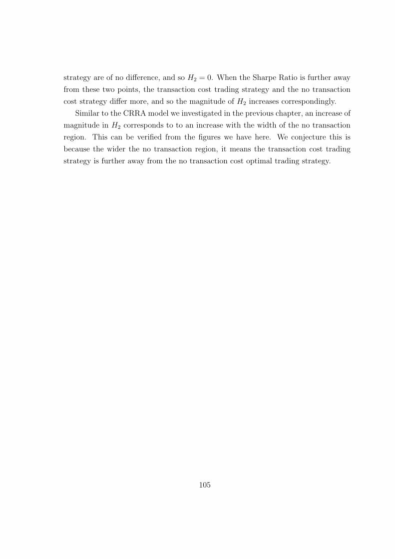
strategy are of no difference, and so H2 = 0. When the Sharpe Ratio is further away

from these two points, the transaction cost trading strategy and the no transaction

cost strategy differ more, and so the magnitude of H2 increases correspondingly.

Similar to the CRRA model we investigated in the previous chapter, an increase of

magnitude in H2 corresponds to to an increase with the width of the no transaction

region. This can be verified from the figures we have here. We conjecture this is

because the wider the no transaction region, it means the transaction cost trading

strategy is further away from the no transaction cost optimal trading strategy.

105

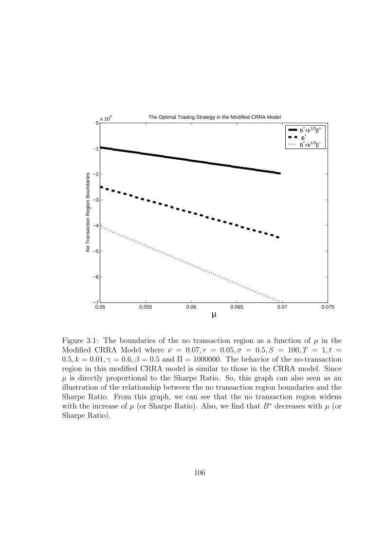
0.05 0.055 0.06 0.065 0.07 0.075−7

−6

−5

−4

−3

−2

−1

0x 10

5 The Optimal Trading Strategy in the Modified CRRA Model

µ

No

Tra

nsac

tion

Reg

ion

Bou

ndar

ies

B*+k1/3β+

B* B*+k1/3β−

Figure 3.1: The boundaries of the no transaction region as a function of µ in theModified CRRA Model where ν = 0.07, r = 0.05, σ = 0.5, S = 100, T = 1, t =0.5, k = 0.01, γ = 0.6, β = 0.5 and Π = 1000000. The behavior of the no-transactionregion in this modified CRRA model is similar to those in the CRRA model. Sinceµ is directly proportional to the Sharpe Ratio. So, this graph can also seen as anillustration of the relationship between the no transaction region boundaries and theSharpe Ratio. From this graph, we can see that the no transaction region widenswith the increase of µ (or Sharpe Ratio). Also, we find that B∗ decreases with µ (orSharpe Ratio).

106

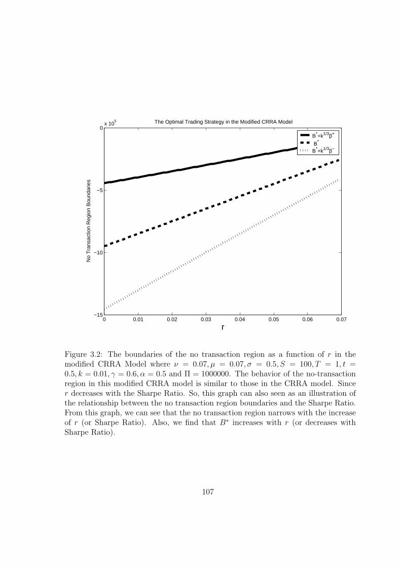
0 0.01 0.02 0.03 0.04 0.05 0.06 0.07−15

−10

−5

0x 10

5 The Optimal Trading Strategy in the Modified CRRA Model

r

No

Tra

nsac

tion

Reg

ion

Bou

ndar

ies

B*+k1/3β+

B* B*+k1/3β−

Figure 3.2: The boundaries of the no transaction region as a function of r in themodified CRRA Model where ν = 0.07, µ = 0.07, σ = 0.5, S = 100, T = 1, t =0.5, k = 0.01, γ = 0.6, α = 0.5 and Π = 1000000. The behavior of the no-transactionregion in this modified CRRA model is similar to those in the CRRA model. Sincer decreases with the Sharpe Ratio. So, this graph can also seen as an illustration ofthe relationship between the no transaction region boundaries and the Sharpe Ratio.From this graph, we can see that the no transaction region narrows with the increaseof r (or Sharpe Ratio). Also, we find that B∗ increases with r (or decreases withSharpe Ratio).

107

0 0.1 0.2 0.3 0.4 0.5 0.6 0.7 0.8 0.9 1−8

−7

−6

−5

−4

−3

−2

−1x 10

5 The Optimal Trading Strategy in the Modified CRRA Model

t

No

Tra

nsac

tion

Reg

ion

Bou

ndar

ies

B*+k1/3β+

B* B*+k1/3β−

Figure 3.3: The boundaries of the no transaction region as a function of t in theModified CRRA Model where ν = 0.07, µ = 0.07, r = 0.05, σ = 0.5, S = 100, T =1, k = 0.01, γ = 0.6, α = 0.5 and Π = 1000000. Similar to the CRRA model,this graph illustrates that just the passage of time without does not change the notransaction region.

108

0 0.1 0.2 0.3 0.4 0.5 0.6 0.7 0.8 0.9 1−2.5

−2

−1.5

−1

−0.5

0

0.5

1x 10

6 The Optimal Trading Strategy in the modified CRRA Model

β

No

Tra

nsac

tion

Reg

ion

Bou

ndar

ies

B*+k1/3β+

B* B*+k1/3β−

Figure 3.4: The boundaries of the no transaction region as a function of α in theModified CRRA Model where ν = 0.07, µ = 0.07, r = 0.05, σ = 0.5, S = 100, T =1, t = 0.5, γ = 0.6, k = 0.01 and Π = 1000000. When α = 0.32, both β+ and β− areequal to 0. Also, B = B∗ = 0, this means all the resources are invested in stocks.Hence, the no transaction region does not really matter. When α > 0.32, B > 0,which means it is optimal to borrow money and invest in stock. This is similar to therelationship between the no transaction region width and γ in the CRRA model.

109

0.3 0.35 0.4 0.45 0.5 0.55 0.6 0.65 0.7−14

−12

−10

−8

−6

−4

−2

0x 10

5 The Optimal Trading Strategy in the Modified CRRA Model

σ

No

Tra

nsac

tion

Reg

ion

Bou

ndar

ies

B*+k1/3β+

B* B*+k1/3β−

Figure 3.5: The boundaries of the no transaction region as a function of σ in theCRRA Model where ν = 0.07, µ = 0.07, r = 0.05, S = 100, T = 1, t = 0.5, k =0.01, γ = 0.6 and Π = 1000000. Similar to CRRA, we can see that B∗ increases withσ.

110

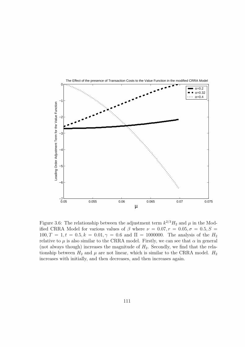
0.05 0.055 0.06 0.065 0.07 0.075−7

−6

−5

−4

−3

−2

−1

0The Effect of the presence of Transaction Costs to the Value Function in the modified CRRA Model

µ

Lead

ing

Ord

er A

djus

tmen

t Ter

m fo

r th

e V

alue

Fun

ctio

n

α=0.2α=0.32α=0.4

Figure 3.6: The relationship between the adjustment term k2/3H2 and µ in the Mod-ified CRRA Model for various values of β where ν = 0.07, r = 0.05, σ = 0.5, S =100, T = 1, t = 0.5, k = 0.01, γ = 0.6 and Π = 1000000. The analysis of the H2

relative to µ is also similar to the CRRA model. Firstly, we can see that α in general(not always though) increases the magnitude of H2. Secondly, we find that the rela-tionship between H2 and µ are not linear, which is similar to the CRRA model. H2

increases with initially, and then decreases, and then increases again.

111

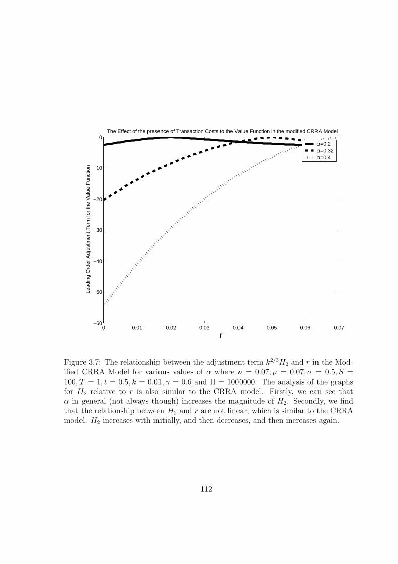
0 0.01 0.02 0.03 0.04 0.05 0.06 0.07−60

−50

−40

−30

−20

−10

0The Effect of the presence of Transaction Costs to the Value Function in the modified CRRA Model

r

Lead

ing

Ord

er A

djus

tmen

t Ter

m fo

r th

e V

alue

Fun

ctio

n

α=0.2α=0.32α=0.4

Figure 3.7: The relationship between the adjustment term k2/3H2 and r in the Mod-ified CRRA Model for various values of α where ν = 0.07, µ = 0.07, σ = 0.5, S =100, T = 1, t = 0.5, k = 0.01, γ = 0.6 and Π = 1000000. The analysis of the graphsfor H2 relative to r is also similar to the CRRA model. Firstly, we can see thatα in general (not always though) increases the magnitude of H2. Secondly, we findthat the relationship between H2 and r are not linear, which is similar to the CRRAmodel. H2 increases with initially, and then decreases, and then increases again.

112

0 0.1 0.2 0.3 0.4 0.5 0.6 0.7 0.8 0.9 1−14

−12

−10

−8

−6

−4

−2

0The Effect of the presence of Transaction Costs to the Value Function in the modified CRRA Model

t

Lead

ing

Ord

er A

djus

tmen

t Ter

m fo

r th

e V

alue

Fun

ctio

n

α=0.2α=0.32α=0.4

Figure 3.8: The relationship between the adjustment term k2/3H2 and t in the Mod-ified CRRA Model for various values of α where ν = 0.07, µ = 0.07, r = 0.05, σ =0.5, S = 100, T = 1, k = 0.01, γ = 0.6 and Π = 1000000. Despite of the very compli-cated formula of the adjustment term, the relationship between the adjustment termand t looks linear.

113

0.045 0.05 0.055 0.06 0.065 0.07 0.075−7

−6

−5

−4

−3

−2

−1

0The Effect of the presence of Transaction Costs to the Value Function in the modified CRRA Model

ν

Lead

ing

Ord

er A

djus

tmen

t Ter

m fo

r th

e V

alue

Fun

ctio

n

α=0.2α=0.32α=0.4

Figure 3.9: The relationship between the adjustment term k2/3H2 and ν in the Mod-ified CRRA Model for various values of α where µ = 0.07, r = 0.05, σ = 0.5, S =100, T = 1, t = 0.5, k = 0.01, γ = 0.6 and Π = 1000000. we can see that the effect ofν to H2 is very small compared to α

114

3.3 Multi-Asset

In this section, we study how to extend the result of Chapter 2 into a multi-asset

version. The notation we use here is the same as in Chapter 2, and not related to

that of Section 3.2.

The extension here is not as straightforward as in the previous section. The major

problem is here we can no longer use B as the control in the no-transaction costs

problem and thus use it as the variable to perturb in the transaction costs problem.

Instead, here we will use Ai, the value invested in stock i. This makes the analysis

more complicated.

3.3.1 Without Transaction Costs

As always, we study the no-transaction costs problem first.

We use the notation and a setup similar to the previous sections. Now, however,

we consider a market with investment opportunities of n stocks and a risk free bond.

Let Si(t) be the spot price of stock i at time t. Similar to previous chapters, we

assume Si(t) follows a geometric Brownian motion with growth rate µi > 0 and

volatility σi > 0. The risk free bonds, B, compounds continuously with risk free rate

r. The volatilities σi, growth rates µi and interest rate r are constants.

The models for Si and B are

dSi = µiSidt + σiSidXi, i = 1, · · · , n,

dB = rBdt

where Xi , i = 1, . . . , n, are standard Brownian motions whose correlations −1 ≤ρij ≤ 1 are constants, ρij, representing the correlation coefficient between Brownian

motions Xi and Xj. There are no redundant assets and so the covariance matrix, Σ,

Σ =

σ21 σ1σ2ρ12 . . . σ1σnρ1n...

.... . .

...σ1σnρ1n σ2σnρ2n . . . σ2

n

is non-singular.

115

As usual, let Ai(t) be the value of assets invested in stock i. Let Π(t) be the value

of the whole portfolio,

Π = B +n∑

i=1

Ai.

We assume cash generated or needed from the purchase or sale of stocks is immediately

invested or withdrawn from the risk free bonds. So, Π can be described as

dΠ = rBdt +n∑

i=1

µiAidt +n∑

i=1

σiAidXi

= r(Π−n∑

i=1

Ai)dt +n∑

i=1

µiAidt +n∑

i=1

σiAidXi

The Ai, i = 1, . . . , n, are the non-anticipating controller representing the value being

invested in stock i.

As in Chapter 2, at time t = 0, an investor has an amount Π0 of resources. The

problem is to allocate investments over the given time horizon so as to maximize

E0

{ ∫ T

0

I(Π(t))dt + F (Π(T ))

}.

We restate the above equation in dynamic programming form so as to apply

Bellman principle of optimality. Therefore, we define the optimal expected value

function J(Π, t) as

J(Π, t) = maxBEt

{ ∫ T

t

I(Π(t))dt + F (Π)

}. (3.80)

Applying the Bellman Principle and Ito’s Lemma gives us the Bellman Equations,

which is

0 = maxA1,A2,...,An

{∂J

∂t+ I + r(Π−

n∑i=1

Ai)∂J

∂Π

+n∑

i=1

µiAi∂J

∂Π+

[ n∑i=1

n∑j=1

1

2σiσjρijAiAj

]∂2J

∂Π2

}, (3.81)

with ρij = 1 for i = 1, . . . , n.

At t = T , we have

J(Π, T ) = F (Π(T )). (3.82)

116

3.3.2 Solving Bellman’s Equation with No Transaction Costs

As in the previous section, we can solve the Bellman Equation by differentiating

equation (3.81) with the controls.

∂

∂Ak

{∂J

∂t+ I + r(Π−

n∑i=1

Ai)∂J

∂Π+

n∑i=1

µiAi∂J

∂Π+

[ n∑i=1

n∑j=1

1

2σiσjρijAiAj

]∂2J

∂Π2

}

= (µ− r)JΠ +n∑

i=1

σkiAiJΠΠ.

If we define

~µ =

µ1 − r...

µn − r

,

~A =

A1...

An

,

Σ =

σ21 σ1σ2ρ12 . . . σ1σnρ1n...

.... . .

...σ1σnρ1n σ2σnρ2n . . . σ2

n

,

and the superscripts T and −1 to denote transpose and inverse, respectively. There-

fore, we have

JΠ~µ + Σ ~AJΠΠ = 0. (3.83)

or equivalently

~A = − JΠ

JΠΠ

Σ−1~µ. (3.84)

We rewrite equation (3.81) in matrix notation as

0 = max~A

{∂J

∂t+ I + rΠ

∂J

∂Π+ ~µ

T ~A +1

2~ATΣ ~A

∂2J

∂Π2

}. (3.85)

If we put equation (3.84) back into equation (3.81), we have

0 =∂J

∂t+ I + rΠ

∂J

∂Π− 1

2~µ

TΣ−1~µ

J2Π

JΠΠ

. (3.86)

When n = 1, equation (3.86) becomes

0 =∂J

∂t+ I + rΠ

∂J

∂Π− 1

2

(µ− r

σ

)2 J2Π

JΠΠ

. (3.87)

This is consistent with the result in the previous chapter.

117

3.3.3 Long Term Growth Model

We can apply this multi-asset optimization to the Long Term Growth Model as in

Section 1.11, which is to maximize E[log Π].

We have

J(Π, t) = log Π + (r +1

2~µ

TΣ−1~µ)(T − t).

(3.88)

and

~A∗ = ΠΣ−1~µ (3.89)

So, when n = 1, we have

A∗ =(µ− r)

σ

2

Π. (3.90)

The result here is consistent to those in Section 1.11.

3.3.4 Constant Relative Risk Aversion (CRRA) Model

As for the CRRA model in Chapter 2, the objective functions of the this multi-asset

version are

I(Π, t) =( γ(µ− r)2

2(γ − 1)σ2− γr + ν

)eν(T−t)Πγ

F (Π(T )) = Π(T )γ. (3.91)

This gives us

J(Π, t) = eν(T−t)Πγ,

and

~A =ΠΣ−1~µ

1− γ. (3.92)

118

3.3.5 With Transaction Costs

Now we consider the problem with transaction costs. As in the previous chapter, let

k > 0 represents the portion of transaction of any stock used as transaction costs.

For simplicity, we also assume ρij = 0 whenever i 6= j.

The market model equations become

dSi = µiSidt + σiSidXi,

dB = rBdt− (1 + k)dLi(t) + (1− k)dMi(t)

= r(Π−n∑

i=1

Ai)dt− (1 + k)dLi(t) + (1− k)dMi(t),

dAi = µiAidt + dLi(t)− dMi(t)dt + σiAidXi, i = 1, · · · , n,

dΠ = r(Π−n∑

i=1

Ai)dt +n∑

i=1

µiAidt +n∑

i=1

σiAidXi

−n∑

i=1

kdLi(t)−n∑

i=1

kdMi(t), (3.93)

where Li(t) and Mi(t) represent the cumulative purchase and sale of assets Ai in [0, t],

which we use as the controls. Here, Ai are only used to denote the value of assets

invested in risk-free bonds here and it is no longer used as a control.

The optimal expected value function J(Π, A1, A2, · · · , An, t) is

J(Π, A1, A2, · · · , An, t) = maxLi,Mi

E{ ∫ T

t

I(Π(t))dt + F (Π(T ))

}. (3.94)

Applying Bellman’s Principle, we have

maxli,mi

{I +

∂J

∂t+

n∑i=1

(µiAi + li −mi)∂J

∂Ai

+

(r(Π−

n∑i=1

Ai) +n∑

i=1

(µiAi − kdli − kmi))∂J

∂Π

+n∑

i=1

(1

2σ2

i A2i

∂2J

∂A2i

+1

2σ2

i A2i

∂2J

∂Π2+ σ2

i A2i

∂2J

∂Π∂Ai

)= 0. (3.95)

In the no-transaction region, therefore, the value function J satisfies

119

0 = I +∂J

∂t+

(r(Π−

n∑i=1

Ai) +n∑

i=1

µiAi

)∂J

∂Π

+n∑

i=1

(1

2σ2

i A2i

∂2J

∂A2i

+1

2σ2

i A2i

∂2J

∂Π2+ σ2

i A2i

∂2J

∂Π∂Ai

). (3.96)

In the sales region for stock i, i = 1, . . . , n, (and at the boundary between sales

region and no transaction region), J satisfies

k∂J

∂Π= − ∂J

∂Ai

. (3.97)

In the purchase region for stock i, i = 1, . . . , n, (and at the boundary between

sales region and no transaction region), J satisfies

k∂J

∂Π=

∂J

∂Ai

. (3.98)

The smooth pasting equation at the boundaries between the no-transaction region

and sales region for stock i, i = 1, . . . , n, is

∂2J

∂A2i

= −k∂2J

∂Ai∂Π, (3.99)

and at the boundaries between the no-transaction region and purchase region is

∂2J

∂A2i

= k∂2J

∂Ai∂Π. (3.100)

Also, when t = T , we have the final equation

J(Π, A1, A2, · · · , An, T ) = F (Π). (3.101)

For i = 1, . . . , n, we translate the Ai coordinate according to

Ai = Ai(Π, t) + k1/3αi, (3.102)

where A is the value of stock i we have when the level of transaction costs, ki, tends

to zero.

We let H(Π, α1, α2, · · · , αn, t) = J(Π, A1, A2, · · · , An, t).

120

We have

∂J

∂Ai

= k−1/3 ∂H

∂αi

,

∂J

∂Π=

∂H

∂Π−

n∑i=1

k−1/3 ∂H

∂αi

∂Ai

∂Π,

∂J

∂t=

∂H

∂t−

n∑i=1

k−1/3 ∂H

∂αi

∂Ai

∂t,

∂2J

∂A2i

= k−2/3∂2H

∂α2i

,

∂2J

∂Ai∂Aj

= k−2/3 ∂2H

∂αi∂αj

, i 6= j,

∂2J

∂Π2=

∂2H

∂Π2−

n∑i=1

k−1/3(2∂2H

∂αi∂Π

∂Ai

∂Π+

∂H

∂αi

∂2Ai

∂Π2) +

n∑i=1

n∑j=1

k−2/3 ∂2H

∂αi∂αj

∂Ai

∂Π

∂Aj

∂Π,

∂2J

∂Π∂Ai

= k−1/3 ∂2H

∂Π∂αi

− k−2/3

n∑j=1

∂2H

∂αi∂αj

∂Aj

∂Π.

Also, we let

H(Π, , α1, α2, · · · , αn, t) = H0(Π, α1, α2, · · · , αn, t) + k1/3H1(Π, , α1, α2, · · · , αn, t)

+k2/3H2(Π, α1, α2, · · · , αn, t) + kH3(Π, α1, α2, · · · , αn, t)

+k4/3H4(Π, α1, α2, · · · , αn, t) + · · · . (3.103)

H0, H1, H2, H3, H4, · · · are all of O(1). H0 is the value function when transaction costs

level k → 0.

After the change of coordinates and collecting terms of the same order the sales

region equation, for i = 1, . . . , n, we have

∂H0

∂αi

= 0 (3.104)

∂H1

∂αi

= 0 (3.105)

∂H2

∂αi

= 0 (3.106)

121

∂H3

∂αi

−n∑

j=1

∂Aj

∂Π

∂H0

∂αj

= 0 (3.107)

∂H4

∂αi

+∂H0

∂Π−

n∑j=1

∂Aj

∂Π

∂H1

∂αj

= 0. (3.108)

Similarly, we have the following equations for the purchase region,

∂H0

∂αi

= 0 (3.109)

∂H1

∂αi

= 0 (3.110)

∂H2

∂αi

= 0 (3.111)

∂H3

∂αi

+n∑

j=1

∂Aj

∂Π

∂H0

∂αj

= 0 (3.112)

∂H4

∂αi

− ∂H0

∂Π+

n∑j=1

∂Aj

∂Π

∂H1

∂αj

= 0. (3.113)

As for the smooth pasting equation for the sales boundary, we have

∂2H0

∂α2i

= 0 (3.114)

∂2H1

∂α2i

= 0 (3.115)

∂2H2

∂α2i

= 0 (3.116)

∂H3

∂α2i

−n∑

j=1

∂Aj

∂Π

∂2H0

∂α2j

= 0 (3.117)

∂H4

∂α2i

+∂2H0

∂Π∂αi

−n∑

j=1

∂Aj

∂Π

∂2H1

∂αi∂αj

= 0. (3.118)

Similarly, the smooth pasting equation for the purchase boundary becomes

∂2H0

∂α2i

= 0 (3.119)

∂2H1

∂α2i

= 0 (3.120)

∂2H2

∂α2i

= 0 (3.121)

122

∂H3

∂α2i

+n∑

j=1

∂Aj

∂Π

∂2H0

∂α2j

= 0 (3.122)

∂H4

∂α2i

− ∂2H0

∂Π∂αi

+n∑

j=1

∂Aj

∂Π

∂2H1

∂αi∂αj

= 0. (3.123)

The final condition equation becomes

H0(Π, α1, α2, · · · , αn, T ) = F (Π) (3.124)

H1(Π, α1, α2, · · · , αn, T ) = 0 (3.125)

H2(Π, α1, α2, · · · , αn, T ) = 0 (3.126)

H3(Π, α1, α2, · · · , αn, T ) = 0 (3.127)

H4(Π, α1, α2, · · · , αn, T ) = 0. (3.128)

Like what we have done before, we now consider the equation at the no-transaction

region. After translating the coordinates, expanding H according to equation (3.103),

and collecting terms of the same order in k, we have the equations below.

1. O(k−2/3) Equation

D(H0) = 0 (3.129)

where D is an operator defined as

D =1

2(

n∑i=1

σ2i A

2i )(

n∑i=1

n∑j=1

∂2

∂αi∂αj

∂Ai

∂Π

∂Aj

∂Π)

+1

2(

n∑i=1

σ2i A

2i

∂2

∂α2i

)

−n∑

i=1

(σ2i A

2i )(

n∑j=1

∂2

∂αi∂αj

∂Aj

∂Π)

=n∑

i=1

n∑j=1

∂2

∂αi∂αj

{1

2

∂Ai

∂Π

∂Aj

∂Π(

n∑

l=1

σ2l A

2l )

+1

2σ2

i A2i −

∂Ai

∂Πσ2

i A2i

}

=n∑

i=1

n∑j=1

∂2

∂αi∂αj

Dij, (3.130)

123

where

Dij =1

2

∂Ai

∂Π

∂Aj

∂Π(

n∑

l=1

σ2l A

2l ) +

1

2σiσjρijAiAj − ∂Ai

∂Πσ2

i A2i (3.131)

Note that in the definition for Dij, the term ρij vanishes whenever i 6= j. Using

the same argument as in Section 2.6.4, we can conclude that H0 is independent

of αi for i = 1, . . . , n.

2. O(k−1/3) Equation

D(H1) = 0. (3.132)

Similarly, we can conclude that H1 is independent of αi for i = 1, . . . , n.

3. O(1) Equation

D(H2) = −M(H0), (3.133)

with M is an operator defined as

M =∂

∂t+ I + r(Π−

n∑i=1

Ai)∂

∂Π

+n∑

i=1

µiAi∂

∂Π+

( n∑i=1

1

2σ2

i A2i

)∂2

∂Π2. (3.134)

Similar to Section 2.6.6, H2 here is independent of αi, i = 1, . . . , n. Also, we

have H0 = J .

4. O(k1/3) Equation

D(H3) = −n∑

i=1

∂M(H0)

∂Ai

αi −M(H1). (3.135)

As in Section 2.6.7, we know that H3 is independent of αi for i = 1, . . . , n. Also,

we have H1 = 0.

Unlike Section 2.6.7, we have

n∑i=1

∂M(H0)

∂αi

Ai = 0 (3.136)

instead of equation (2.82).

124

5. O(k2/3) Equation

DH4 = −1

2

n∑i=1

σ2i

∂2H0

∂Π2α2

i −MH2. (3.137)

In other words, it is

n∑i=1

n∑j=1

∂2H4

∂αi∂αj

Dij = −1

2

n∑i=1

σ2i

∂2H0

∂Π2α2

i −MH2.

(3.138)

Again, the ρij above vanishes whenever i 6= j.

We notice that the no transaction boundary for stock i is dependent on the

holdings of other stocks (αj). Here, we study the case for the transaction

boundary for stock 1 with α2 = α3 = · · · = αn = 0.

We let α+ be the boundary between the purchase region and the no transaction

region for α1 when α2 = α3 = · · · = αn = 0. Similarly, we let α− be the

boundary between the sales region and the no transaction region. Therefore,

from equation (3.138), equation (3.108) and equation (3.118) we know that

α− satisfy

∂H4

∂α1

+∂H0

∂Π= 0

∂H4

∂α21

= 0. (3.139)

Similarly, from equation (3.138), equation (3.113) and equation (3.123) we

know that α+ satisfy

∂H4

∂α1

− ∂H0

∂Π= 0

∂H4

∂α21

= 0. (3.140)

We let

H4 = H44α

41 + H2

4α21 + H1

4α1 + H04 + α∗, (3.141)

where α∗ vanishes when α2 = α3 = · · · = αn = 0.

125

From equation (3.118) and equation (3.123), we know that α+ and α− satisfy

∂H4

∂α21

= 0. (3.142)

So, α+ and α− are the roots of

0 = 6H44α

21 + H2

4 . (3.143)

So, we know that α+ = −α− because the sum of roots vanishes.

Now, we use equation (3.108) and equation (3.113). This gives us α− satisfies

−∂H0

∂Π= 4H4

4α3− + 2H2

4α− + H14 . (3.144)

Similarly, α+ satisfies

∂H0

∂Π= 4H4

4α3+ + 2H2

4α+ + H14 . (3.145)

Adding equation (3.144) with equation (3.145), we have

H14 = 0. (3.146)

Putting equation (3.143) into equation (3.145), we have

∂H0

∂Π= 16H4

4α3+ (3.147)

and

H24 = −

(27H44

8

(∂H0

∂Π

)2)1/3

. (3.148)

3.3.6 Financial Interpretations

Although we have not solved the above equations precisely, still it gives us some

insights on the effect of transaction costs on the portfolio optimization problem. We

summarize our findings below.

126

1. The midpoint of the no-transaction region for stock i may no longer be the

optimal solution of the no transaction costs problem. In fact, the midpoint

depends on the value of other stocks held. This is because if we solve equation

(3.138),

H4 = H44α

4i + H3

4α3i + H2

4α2i + H1

4αi + H04 , (3.149)

with H44 , H3

4 , H24 and H1

4 are all functions of αj with j 6= i. This is because H34

may not vanish. From equation (3.118) and equation (3.123), we know that

6H34 is the sum of α+

i and α−i , which are the position of the sales boundary and

the purchase boundary of stock i. So, it is possible

α+i + α−i 6= 0. (3.150)

2. The width of the no-transaction region for every stock i is still directly pro-

portional to k1/3, and so the larger the transaction costs, the larger the no-

transaction region.

3. The effect of transaction costs on the value function is of the order k2/3.

3.3.7 Two Dimensional Case

Now we look in detail at the case where there are two risky assets and the bond. In

other words, n = 2.

We let

H4 = aα41 + bα3

1α2 + cα21α

22 + dα1α

32 + eα4

2 + fα21 + gα1α2 + hα2

2

+pα1 + qα2 + r. (3.151)

From the previous section, we know that p = q = 0.

So, we have

DH4 = α21(12aD11 + 3b(D12 + D21) + 2cD22)

+α1α2(6bD11 + 4c(D12 + D21) + 6dD22)

+α22(2cD11 + 3d(D12 + D21) + 12eD22)

+2fD11 + g(D12 + D21) + 2hD22. (3.152)

127

Using equation (3.138), so the solution for (a, b, c, d, e) is

(a, b, c, d, e) = (− σ21(D12 + D21)

24D11(D12 + D21)

∂2H0

∂Π2, 0, 0, 0,− σ2

2(D12 + D21)

24D22(D12 + D21)

∂2H0

∂Π2)

+x(− 1

4D211

,1

D11(D12 + D21), 0,− 1

D22(D12 + D21),

1

4D222

)

+y(− D22

2D11(D12 + D21)+

D12 + D21

4D211

,− 1

D11

,3

D12 + D21

,− 1

D22

,

− D11

2D22(D12 + D21)+

D12 + D21

4D222

) (3.153)

where x and y are constants.

Obviously, x = 0 or otherwise H4 is not symmetric over α1 and α2.

Now, we consider the transaction boundary for stock 1 (α+, α−) when α2 = α∗.

From equation (3.118) and equation (3.123), we know that α+ and α− are the

roots of α1 in the equation of

12aα21 + 6bα1α∗ + 2cα2

∗ + 2f = 0. (3.154)

Therefore, we have

α+ + α− = −bα∗2a

α+α− =cα2

∗ + f

6a(3.155)

Now, we use equation (3.108) and equation (3.113). This gives us an equation

for α+ and α−,

4a(α3+ + α3

−) + 3b(α2+ + α2

−)α∗ + 2c(α+ + α−)α2∗

+2dα3∗ + 2f(α+ + α−) + 2gα∗ = 0, (3.156)

which means

4a(α+ + α−)((α+ + α−)2 − 3α+α−)

+3b((α+ + α−)2 − 2α+α−)α∗

+2c(α+ + α−)α2∗ + 2dα3

∗ + 2f(α+ + α−) + 2gα∗ = 0. (3.157)

128

Therefore, we have

4a(−bα∗2a

)((−bα∗2a

)2 − 3cα2

2 + f

6a)

+3b((−bα∗2a

)2 − 2cα2

2 + f

6a)α∗

+2c(−bα∗2a

)α2∗ + 2dα3

∗ + 2f(−bα∗2a

) + 2gα∗ = 0. (3.158)

Since the above relationship holds for all α∗, so the coefficient for α3∗ and α∗ have to

be both identically zero. In other words, we have

b3

4a2− bc

a+ 2d = 0 (3.159)

and

−bf

a+ 2g = 0. (3.160)

By considering the transaction boundary for α2, similarly we have

d3

4e2− cd

e+ 2b = 0 (3.161)

and

−dh

e+ 2g = 0. (3.162)

We can use equation (3.159) and equation (3.161) to solve for y. Indeed, we find

that there is a unique solution of y = 0.

So, we have b = 0, c = 0 and d = 0, which implies g = 0.

Using equation (3.148) , we have

f = −(27a

8

(∂H0

∂Π

)2)1/3

(3.163)

and

h = −(27e

8

(∂H0

∂Π

)2)1/3

. (3.164)

So, α+ and α− are

α± = ±√− f

6a. (3.165)

Also, H2 can be solved by using the equation

MH2 = −2fD11 − 2hD22. (3.166)

129

3.3.8 Financial Interpretations

The above equations are very long and complex. Still, we have find some pattern

about the behavior or the solution.

1. The midpoint of the no-transaction region for stock i is the same as the optimal

solution of the no transaction costs problem. This is because b = d = 0.

2. The distance of the holding of a stock to the no transaction cost optimum

solution (α∗) has no effect on the no transaction region of another stock. This

is very clear from equation (3.165).

3. The width of the no-transaction region for every stock i is still directly pro-

portional to k1/3, and so the larger the transaction costs, the larger the no-

transaction region.

4. The effect of transaction costs on the value function is of the order k2/3.

5. The relations between µ, r or σ to the transaction boundary or the effect of

transaction costs on the value function is very complex and not clear cut.

130

Chapter 4

The Convergence of the NoTransaction Region in theTransaction Costs Problem

4.1 Introduction

In this chapter, we use the Pontryagin Maximum Principle to demonstrate a mathe-

matical relationship between the solution for an optimization problem without trans-

action costs and the solution for the otherwise same optimization problem with trans-

action costs. The optimization problem we are considering here is more general than

those in previous chapters.

We consider the problem without transaction costs first. In that problem, an

investor has a fixed time investment interval [0, T ]. The investor can invest his re-

sources in risk free bonds or in stock i, where i = 1, 2, · · ·n. At time t, the investor

has an amount of Ai(t) in stock i and B(t) in the risk free bond. His problem is to

allocate investments over the given time horizon so as to maximize a certain objective

function of Π where

Π = B +n∑

i=1

Ai.

We assume in the above optimization problem there is a unique interior solution

A∗i for stocks i = 1, . . . , n.

Now we consider the transaction costs problem. In this transaction costs problem,

however, there are two difference. Firstly, of course, there are transaction costs. By

131

transaction costs we mean that a cost has to be paid when the investor buys or

sells stocks. Let ki > 0 represents the portion of transaction of stocks i used as

transaction costs. So if the investor buys a number of stocks i whose “true” value is

Ai, the investor pays (1 + ki)Ai in cash. If the investor sells the stocks, the investor

obtains (1 − ki)Ai in cash. Secondly, instead of maximizing J(Π), the problem is to

maximize J(Π), where

Π = B +n∑

i=1

κiAi

with κiAi represents the liquidation value of Ai; κiAi depends on ki and the sign of

Ai such that for i = 1, · · · , n, if Ai > 0

1− ki < κi ≤ 1

and if Ai < 0

1 ≤ κi < 1 + ki.

In this chapter, we demonstrate the following. In the optimization problem with

transaction costs, for every stock i = 1, . . . , n, the optimal strategy is not to transact

when the value of investments in stock i is close to the no transaction costs optimal

strategy A∗i . Let us call the region where it is optimal not to transact at all the

no-transaction region. When the portfolio is too far away from A∗i , it is optimal to

buy or sell so as to bring it back to the no-transaction region. Also as the level of

transaction costs ki tends to 0, the no-transaction region tends to A∗i .

We recall that one of the important results in our analysis at Chapter 3 is that

the no-transaction region in the transaction cost problem converges to the optimal no

transaction cost solution when the transaction costs level k → 0. That result is similar

to the result in this chapter. This chapter’s result, however, is more general. This is

because the value function J we want to maximize can depend on the transaction costs

ki through the variables κi. Also, we allow different transaction costs for different

stocks.

Many transaction costs problems usually involve HJB equations which lead to a

free boundary problem. Perturbation analysis usually is very useful in determining

the free boundary. A common difficulty, however, in applying perturbation analysis in

such problems is the determination of the limit of the no transaction region when the

132

transaction costs tend to zero. Failure to resolve this difficulty makes the perturbation

analysis less robust than desired. The result in this chapter, of course, solves precisely

this problem.

4.2 Market Model without Transaction Costs

We now proceed by first considering the case of no transaction costs.

The setup of the market model is similar to Chapter 3 multi asset Section. We

consider a market with investment opportunities of n stocks and risk free bonds. Let

Si(t) be the spot prices of stock i at time t. We assume that S(t) follows a geometric

Brownian motion with growth rate µi > 0 and variance σ2i > 0. The risk free bonds,

B, are compounded continuously with risk free rate r. The variance σ2i , drift µi of

asset i, and the risk free rate r are assumed to be constants. Assuming there is no

transfer of money between stocks and the risk free bond, the model is represented by

dSi = µiSidt + σiSidXi, i = 1, · · · , n,

dB = rBdt.

Here, Xi are standard Brownian motions with dX2i = dt and dXidXj = ρijdt, i, j =

1, · · · , n, where −1 ≤ ρij ≤ 1 is the correlation coefficient between Brownian motions

Xi and Xj. There are no redundant assets and so the covariance matrix, Σ,

Σ =

σ21 σ1σ2ρ12 . . . σ1σnρ1n...

.... . .

...σ1σnρ1n σ2σnρ2n . . . σ2

n

is non-singular. The correlation coefficients ρij are constants.

Let Ai(t) be the value of assets invested in stocks i. Let Π(t) be the value of the

whole portfolio, so

Π = B +n∑

i=1

Ai.

Let ui be the non-anticipating controller representing the amount of cash being trans-

ferred between the risk free bonds B and the stock account i. Cash generated or

needed from the purchase or sale of stocks are immediately invested or withdrawn

from the risk free bonds.

133

The model is represented by

dB = (rBdt−n∑

i=1

ui)dt

dAi = µiAidt + uidt + σiAidXi, i = 1, · · · , n.

The investor has an amount of A0i in stocks i and B0 in risk free bonds at time

t = 0. The problem is to allocate investments over the given time horizon [0, T ] so as

to maximize the expected value function J(Π0; t = 0), which is

J(Π0; t = 0) = maxu1,u2,···,un

E0

{ ∫ T

0

I(Π(t), t)dt + F (Π(T ))

}. (4.1)

The functions I and F represents the objectives whose expectation the investor wants

to maximize. They are continuously differentiable functions. Of course, the dimen-

sions of ∫ T

0

I(Π(t))dt

and

F (Π(T ))

are the same. Thus, J is a positive increasing functions of Π. F is also a concave

function of Π. Also, we assume the portfolio Π has to be positive at all times. If it is

equal to 0, the investment process ends.

4.3 Applying the Maximum Principle on the No

Transaction Costs Problem

According to the stochastic version of the the Pontryagin maximum principle, the

optimal policy also maximizes the expected value of a Hamiltonian H, which we

proceed to find.

The Hamiltonian, H, is defined as

H(B,A1, · · · , An, V1, · · · , Vn, u1, · · · , un)

= I + ΨB(rB −n∑

i=1

ui) +n∑

i=1

ΨAi (µAi + ui + σAi

dXi

dt)

(4.2)

134

where dXi/dt, i = 1, · · · , n, are the formal derivative of the Brownian motions, i.e.,

white noises, ΨAi and ΨB are the adjoint processes and ΨB is defined by

∂ΨB

∂t= −∂H

∂B= − rΨB (4.3)

with the boundary value, ΨB(T ), obtained from the transversality condition

ΨB(T ) =∂F (Π(T ))

∂B(T )

=dF (Π(T ))

dΠ(T ). (4.4)

Similarly, ΨAi , i = 1, · · · , n, are defined by

∂ΨAi

∂t= − ∂H

∂Ai

= −ΨAi (µi + σi

dXi

dt), (4.5)

and

ΨAi (T ) =

∂F (Π(T ))

∂Ai(T )

=dF (Π(T ))

dΠ(T ). (4.6)

Solving equations (4.3) to (4.6) yields

ΨB =∂F (Π(T ))

∂Π(T )er(T−t);

ΨAi =

dF (Π(T ))

dΠ(T )

Si(T )

Si(t). (4.7)

Substituting equation (4.7) into 4.2 and dropping the terms that are not depen-

dent on the controls u, the problem of maximizing Et(J) reduces to the maximization

of the following expression:

n∑i=1

(Et(Ψ

Ai −ΨB)ui

)=

n∑i=1

Et

{∂F (Π(T ))

∂Π(T )

S(T )

S(t)− ∂F (Π(T ))

∂Π(T )er(T−t)

}ui,

135

where the expectations are taken on every possible stocks movement path with opti-

mal decisions taken.

Maximizing the expression in 4.8 means choosing1 ui = +∞ when Et(ΨAi ) −

Et(ΨB) > 0, i.e., buying stocks i as quickly as possible when Et(ΨAi ) > Et(ΨB),

choosing ui = −∞ when Et(ΨAi ) − Et(ΨB) < 0, i.e., selling as many stocks i as

possible when Et(ΨAi ) < Et(ΨB), and choosing ui = 0 when Et(Ψ

Ai ) − Et(ΨB) = 0,

i.e., do not buy or sell stocks i when Et(ΨAi ) = Et(ΨB). Achieving Et(Ψ

Ai ) = Et(ΨB)

means that the right number of stocks i and risk free bonds is held.

If there is a unique interior optimal solution as we have assumed, the expressions

in equation (4.8) is always equals zero if the optimal strategy is used. This can be

seen as follows. Suppose there are more stocks i in the portfolio than optimal, the

maximum principle instructs to sell, and so Et(ΨAi )−Et(ΨB) < 0. And suppose there

are less stocks i in the portfolio than optimal, the maximum principle will instruct to

buy, and so Et(ΨAi )−Et(ΨB) > 0. Since the function Et(Ψ

Ai )−Et(ΨB) is continuous,

at the optimal point Et(ΨAi )− Et(ΨB) = 0.

Therefore finding the optimal strategy is equivalent to the problem of finding a

strategy such that Et(ΨA)− Et(ΨB) = 0.

From now on, we call the optimal holding value of stock i in the no transaction

costs problem A∗i .

4.4 Market Model with Transaction Costs

Now we consider the problem with transaction costs. Let ki > 0 represent the portion

of transaction of stocks i used as transaction costs. So if the investor buys a number

of stocks i whose “true” value is Ai, the investor pays (1 + ki)Ai in cash. If the

investor sells the stocks, the investor obtains (1− ki)Ai in cash.

So our market model equations become

dSi = µiSidt + σiSidXi, i = 1, · · · , n,

dB =(rBdt−

n∑i=1

(ui + ki|ui|))dt

dAi = µiAidt + uidt + σiAidXi, i = 1, · · · , n. (4.8)

1To be more rigorous, we should firstly make the restriction |ui| < M for some constant M . Thenwe let M →∞.

136

Instead of maximizing J(Π), this problem is to maximize J(Π), where Π is the

‘liquidation’ value of Π with

Π = B +n∑

i=1

κiAi

and κi depends on ki and the sign of Ai such that for i = 1, · · · , n, if Ai > 0,

1− ki < κi ≤ 1

and if Ai < 0,

1 ≤ κi < 1 + ki.

Rigorously speaking, we cannot define Π as above. This is because J(Π) is not

continuously differentiable at Ai = 0, which is a necessary condition for the applica-

tion of the Maximum Principle. A solution for this is to change the definition of Π

for those values close to Ai = 0 so as to smooth out the corner. The effect of this on

the values of Π and J(Π) and thus to the optimization problem is minimal.

In a manner similar to the problem without transaction costs, the problem reduces

to the maximization of the following expression

n∑i=1

((Et(Ψ

Ai )− Et(ΨB))︸ ︷︷ ︸

Φ1i

ui − ki Et(ΨB)︸ ︷︷ ︸Φ2

i

|ui|)

(4.9)

where ΨAi and ΨB are the adjoint processes of the Hamiltonian of the transaction

costs problem. Since the value function J now depends on Π rather than Π, ΨAi are

not the same as ΨAi . They are given now by

ΨAi = κi

∂F (Π(T ))

∂Π(T )

Si(T )

Si(t). (4.10)

As before, ΨB is equal to

ΨB =∂F (Π(T ))

∂Π(T )er(T−t). (4.11)

Also, note that in this problem the expectations of ΨAi and ΨB are different to the no

transaction cost problem. This is because with transaction costs the optimal strategy

is different and also the portfolio value changes with each transaction.

137

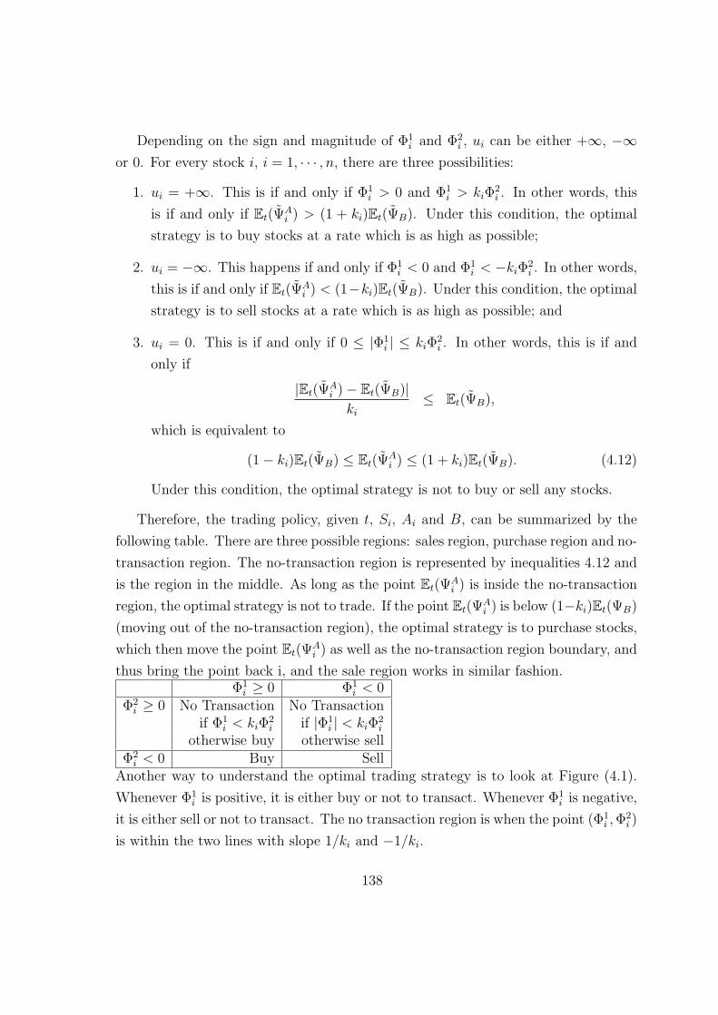
Depending on the sign and magnitude of Φ1i and Φ2

i , ui can be either +∞, −∞or 0. For every stock i, i = 1, · · · , n, there are three possibilities:

1. ui = +∞. This is if and only if Φ1i > 0 and Φ1

i > kiΦ2i . In other words, this

is if and only if Et(ΨAi ) > (1 + ki)Et(ΨB). Under this condition, the optimal

strategy is to buy stocks at a rate which is as high as possible;

2. ui = −∞. This happens if and only if Φ1i < 0 and Φ1

i < −kiΦ2i . In other words,

this is if and only if Et(ΨAi ) < (1−ki)Et(ΨB). Under this condition, the optimal

strategy is to sell stocks at a rate which is as high as possible; and

3. ui = 0. This is if and only if 0 ≤ |Φ1i | ≤ kiΦ

2i . In other words, this is if and

only if

|Et(ΨAi )− Et(ΨB)|

ki

≤ Et(ΨB),

which is equivalent to

(1− ki)Et(ΨB) ≤ Et(ΨAi ) ≤ (1 + ki)Et(ΨB). (4.12)

Under this condition, the optimal strategy is not to buy or sell any stocks.

Therefore, the trading policy, given t, Si, Ai and B, can be summarized by the

following table. There are three possible regions: sales region, purchase region and no-

transaction region. The no-transaction region is represented by inequalities 4.12 and

is the region in the middle. As long as the point Et(ΨAi ) is inside the no-transaction

region, the optimal strategy is not to trade. If the point Et(ΨAi ) is below (1−ki)Et(ΨB)

(moving out of the no-transaction region), the optimal strategy is to purchase stocks,

which then move the point Et(ΨAi ) as well as the no-transaction region boundary, and

thus bring the point back i, and the sale region works in similar fashion.Φ1

i ≥ 0 Φ1i < 0

Φ2i ≥ 0 No Transaction No Transaction

if Φ1i < kiΦ

2i if |Φ1

i | < kiΦ2i

otherwise buy otherwise sellΦ2

i < 0 Buy SellAnother way to understand the optimal trading strategy is to look at Figure (4.1).

Whenever Φ1i is positive, it is either buy or not to transact. Whenever Φ1

i is negative,

it is either sell or not to transact. The no transaction region is when the point (Φ1i , Φ

2i )

is within the two lines with slope 1/ki and −1/ki.

138

slope = −1/kislope = 1/ki

No Transaction Region

Purchase Region

Purchase RegionSales Region

Sales Region

Φ1i

Φ2i

as ki → 0

Figure 4.1: The table in the previous page can be visualised by this figure. Theno transaction region is within the two lines with slope 1/ki and −1/ki. As ki → 0,these two lines become closer and closer to the Y-axis and so the no-transaction regionbecomes smaller and smaller.

139

If the portfolio is at the purchase region, the optimal strategy is to purchase stocks

as quickly as possible. It is inevitable that the portfolio enters the no-transaction

region eventually. We proceed to prove this by contradiction so we assume it doesn’t.

As both ΨAi and ΨB are continuous, the portfolio does not enter the sales region as

well. So, the optimal strategy is to purchase stocks as quickly as possible without end.

For every purchase made, however, the portfolio value Π is reduced because of the

transaction costs. Eventually, Π is equal to 0, the lower limit allowed for the portfolio

value and the investment process ends. Any strategy which keeps the portfolio Π > 0

is a better strategy than this strategy as both I and F are increasing functions. So,

we can conclude that this strategy is not optimal and thus it cannot be the optimal

solution.

A similar conclusion holds for the sales region.

We can, therefore, conclude that the no-transaction region exists.

4.5 The Order of Et(ΨB)

We now proceed to prove that if given that the portfolio is at the no transaction-

region,

Et(ΨB) = o(1). (4.13)

This result, as we can see later, is pivotal in obtaining the conclusion of this chapter.

We recall from equation (4.11) that

ΨB =∂F

∂Πer(T−t).

For i = 1, · · · , n, therefore,

Et(ΨB|Π(t) = Π) = Et

{∂F

∂Πer(T−t)|Π(t) = Π

}

We find that the above function is bounded above by another function M(k1, k2, · · · , kn),

which we define as

M(k1, k2, · · · , kn) = Et

{∂F

∂Π(Π(T ) + T)er(T−t)|k1, k2, · · · , kn, Π(t) = Π

},

(4.14)

140

where E is the expectation operator taken for every possible stock movement path

and the strategy used is the same as those strategy used in equation (4.9). We define

T as the total value accumulated at time T if the money spent in transaction costs

in [0, T ] has been invested in risk-free bonds instead.

For every possible stock movement path, therefore, the portfolio value Π(T ) + T

in equation (4.14) is larger than the portfolio value Π(T ) in equation (4.9). As

F (Π(T )) is a concave function,∂F (Π(T ))

∂Π(T )

is an increasing function. It follows that

Et(ΨB|k1, k2, · · · , kn, Π(t) = Π) ≤ M(k1, k2, · · · , kn)

for any level of transaction costs k1, k2, · · · , kn.

Now, let M, a constant, defined as

M = supu1,u2,···,un

Et

{∂F (Π)

∂Πer(T−t)

}, (4.15)

where the expectation is taken for every possible stock movement path and the strat-

egy used is the optimal strategy to maximize

∂F (Π(T ))

∂Π(T ).

Therefore,

M(k1, k2, · · · , kn) ≤ M

for all level of transaction costs k1, k2, · · · , kn.

Since M is a constant independent of k1, k2, · · · , kn, and

Et(ΨB) ≤ M

and thus

Et(ΨB) = O(1). (4.16)

141

4.6 Transaction Costs Level Tends to 0

Now, we show that when the transaction costs level tends to 0, the no transaction

region converges to the optimal strategy without transaction costs.

When ki → 0, i = 1, . . . , n, kiΦ2i of equation (4.9) must converge to 0. This is

because Φ2i = O(1). So, Φ1

i converges to 0. This means the limit of the corresponding

strategy must be an optimal strategy for the no transaction cost problem. Since such

a strategy is unique, we can conclude that the limit must be the same as the no

transaction cost strategy. The result follows.

4.7 Examples

We can apply the results in this chapter on the long term growth model and the

CRRA model. In the long term growth model, we know from Section 3.3.3 that the

no transaction costs problem has a unique solution. Similarly, in the CRRA model, it

has been shown in Section 3.3.4 the no transaction cost solution exist and is unique.

Therefore, the result of this chapter can be applied to these two problems. In other

words, the solution of the transaction costs problem converge to the no transaction

costs problem when k → 0.

142

Chapter 5

Conclusion

5.1 Results Achieved

We have studied the impact of transaction costs on the problems of portfolio opti-

mizations for a general function. Firstly, we studied the case of of only one risky

asset. In such a problem, we find that the transaction-region converges to the no

transaction costs optimal solution when the level of transaction costs tend to 0. We

have found that the width of the boundaries are of the order k1/3 while the adjustment

term for the value function is of order k2/3. Also, we have successfully obtained the

approximate formulae for the boundaries of the no-transaction region and the leading

order adjustment term for the value functions.

We have also applied the formulae we have obtained on some functions. In par-

ticularly, we look at the long term growth model and the CRRA model. The result

on the long term growth model is consistent with Davis and Norman [18].

In the later chapters, we extend the results to the cases where (1) the payoff

function is dependent on S, the price of the stock; and (2) there are more than one

uncorrelated risky assets. In these cases, we have also established similar results to

the case with one risky asset, although the formulae for for the no transaction region

boundary are different.

5.2 Future Work

There are several directions in which our work can be extended. For instance,

143

1. The study of dynamic mean-variance asset allocation with presence of short

sales restrictions or margin restrictions;

2. Extend the work in Chapter 2 and Chapter 3 to study the case of stochastic

volatility, discrete rebalancing, and Multi-Asset with different transaction costs

for different stocks.

3. Extend the first part of Chapter 3 to develop a theory to price options with the

consideration of transaction costs.

144

Appendix A

Nomenclature

The followings are some of the notations we often use in our thesis:

A.1 All Chapters

∗ Optimal solution

A(t) Value invested at stocks at time t (used as controls in chapter 3 in the multi-asset

no transaction costs problem)

Ai The optimal value of stock i held in the when k → 0

αi Ai = Ai + k1/3αi

B(t) Risk free bonds held at time t (used as controls in Chapter 2 in the no transac-

tion costs problem)

B The optimal value of risk free bond held when k → 0

β B = B + k1/3β

E Expectation Operator

F (Π(T ) Reward function at time T

γ A parameter in the Constant Relative Risk Aversion Model (CRRA), and 1−γ

represents the relative risk aversion

145

H The value function, after the change of coordinates, in the transaction costs

problem we sought to maximize

H Hamiltonian

I(Π(T )) The rate of reward during the whole investment period

J the value function in the no-transaction cost problem we sought to maximize

J the value function in the transaction cost problem we sought to maximize

Hn the value function in the transaction cost problem after change of coordinates

we sought to maximize

k kS transaction cost for a single transaction of 1 stock at price S, and k is

assumed to be constant

µ growth rate of the stock

n the number of stocks in the market

Π(t) is the value of the portfolio, which equals to B(t) + A(t)

Ψ adjoint processes of the Hamiltonian

r interest rate and assumed to be constant (given)

ρij Correlation between stock i and stock j

S(t) Value of stock at time t (decided by geometric Brownian motion)

σ volatility of the stock

Σ Covariance Matrix

t Time

T Time for the Investment Horizon

X Brownian Motion

146

A.2 Chapter 1

C Consumption

δt a small increment of time

λ the portion of resources invested in stock in the long term growth model, Mer-

ton’s Investment Consumption Model, or the Langrange multiplier in the Pon-

tryagin Maximum Principle illustration

ν discount factor in Merton’s Investment Consumption Model

p0 condition probability of p(Π(t1) = Π1|Π(t0) = Π0)

p1 condition probability of p(Π(t1) = Π1, S(t1) = S1|Π(t0) = Π0, S(t0) = S0)

u controller representing the cash flows used to buy stocks

U utility function

ξ target return of the portfolio

A.3 Chapter 2

L cumulative purchase of assets A during [0, t]

M cumulative sale of assets A during [0, t]

A.4 Chapter 3

α a factor in the modified CRRA model

D an operator defined as

D =1

2(

n∑i=1

n∑j=1

σiσjρijAiAj)(n∑

i=1

n∑j=1

∂2

∂αi∂αj

∂Ai

∂Π

∂Aj

∂Π)

+1

2(

n∑i=1

n∑j=1

σiσjρijAiAj∂2

∂αi∂αj

)

−n∑

i=1

(n∑

j=1

σiσjρijAiAj)(n∑

j=1

∂2

∂αi∂αj

∂Aj

∂Π)

147

Dij an operator defined as

Dij =1

2

∂Ai

∂Π

∂Aj

∂Π(

n∑

k=1

n∑

l=1

σkσlρklAkAl)

+1

2σiσjρijAiAj − ∂Ai

∂Π(

n∑

k=1

σiσkρikAiAk) (A.1)

M an operator defined as

M =∂

∂t+ I + r(Π−

n∑i=1

Ai)∂

∂Π

+n∑

i=1

µiAi∂

∂Π+

( n∑i=1

n∑j=1

1

2σiσjρijAiAj

)∂2

∂Π2(A.2)

A.5 Chapter 4

κi Ratio that stock i is worth when liquidated, and so κiAi epresents the liquidation

value of Ai

Φ1i Et(Ψ

Ai )− Et(ΨB)

Φ2i Et(ΨB)

ΨAi Ajoint processes of asset i in the transaction cost problem

ΨB Ajoint processes of B in the transaction cost problem

(Π) Liquidation value of Π in the transaction cost problem

ui Control for asset i

148

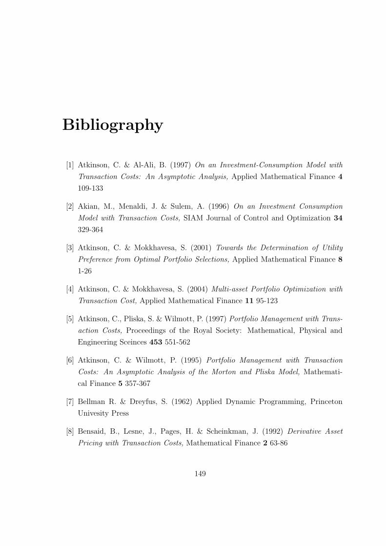
Bibliography

[1] Atkinson, C. & Al-Ali, B. (1997) On an Investment-Consumption Model with

Transaction Costs: An Asymptotic Analysis, Applied Mathematical Finance 4

109-133

[2] Akian, M., Menaldi, J. & Sulem, A. (1996) On an Investment Consumption

Model with Transaction Costs, SIAM Journal of Control and Optimization 34

329-364

[3] Atkinson, C. & Mokkhavesa, S. (2001) Towards the Determination of Utility

Preference from Optimal Portfolio Selections, Applied Mathematical Finance 8

1-26

[4] Atkinson, C. & Mokkhavesa, S. (2004) Multi-asset Portfolio Optimization with

Transaction Cost, Applied Mathematical Finance 11 95-123

[5] Atkinson, C., Pliska, S. & Wilmott, P. (1997) Portfolio Management with Trans-

action Costs, Proceedings of the Royal Society: Mathematical, Physical and

Engineering Sceinces 453 551-562

[6] Atkinson, C. & Wilmott, P. (1995) Portfolio Management with Transaction

Costs: An Asymptotic Analysis of the Morton and Pliska Model, Mathemati-

cal Finance 5 357-367

[7] Bellman R. & Dreyfus, S. (1962) Applied Dynamic Programming, Princeton

Univesity Press

[8] Bensaid, B., Lesne, J., Pages, H. & Scheinkman, J. (1992) Derivative Asset

Pricing with Transaction Costs, Mathematical Finance 2 63-86

149

[9] Bjork, T. (1999) Arbitrage Theory in Continuous Time, Oxford University Press

[10] Blacks, F & Scholes, M. (1973) The Pricing of Options and Corporate Liabilities,

Journal of Finance 81 637-654

[11] Boyle, P. & Emanuel, D. (1980) Discretely Adjusted Option Hedges, Journal of

Financial Economics 8 259-282

[12] Boyle, P. & Vorst, T. (1992) Option Replication in Discrete Time with Transac-

tion Costs, Journal of Finance 47 271-293

[13] Brealey, R. & Myers, S. (2000) Principles of Corporate Finance, McGraw-Hill

[14] Clewlow, L. & Hodges, S. (1997) Optimal Delta-Hedging under Transactions

Costs, Journal of Economic Dynamics and Control 21 1353-1376

[15] Constantinides, G. (1986) Capital Market Equlibrium with Transaction Costs,

The Journal of Political Economy 94 842-862

[16] Cox, J., Ross, S. & Rubinstein, M. (1979) Option Pricing: A Simplified Ap-

proach, Journal of Financial Economics 7 229-263

[17] Davis, H., Panas, V. & Zariphopoulou, T. (1993) European Option Pricing with

Transaction Costs, SIAM Journal of Control and Optimization 31 470-493

[18] Davis, H. & Norman, A. R. (1990) Portfolio Selection with Transaction Costs,

Mathematics of Operations Research 15 676-713

[19] Edirsinghe, C., Vasanttilak, N & Uppal R. (1993) Optimal Replication of Op-

tions with Transations Costs and Trading Restrictions, Journal of Financial and

Quantitative Analysis 28 117-138

[20] Friedman, M. (1955) What All is Utility? The Economic Journal 65 405-409

[21] Friedman, M. & Savage, L. J. (1948) The Utility Analysis of Choices Involving

Risk, The Journal of Political Economy 56 279-304

[22] Friedman, M. & Savage, L. J. (1952) The Expected-Utility Hypothesis and the

Measurability of Utility, The Journal of Political Economy 60 463-474

150

[23] Harrison, J. & Kreps, D. (1979) Martingales and Arbitrage in Multiperiod Secu-

rities Markets, Journal of Economic Theory 20 381-408

[24] Harrison, J. & Pliska S. (1981) Martingales and Stochastic Integrals in the Theory

of Continuous Trading, Stochastic Processes and their Applications 11 215-260

[25] Haussmann, U. G. (1986) A stochastic maximum principle for the optimal control

of diffusion processs, Pitman Research Notes in Mathematics, no. 151. Harlow,

UK: Longman Scientific and Technical, 1986.

[26] Heath, D. & Jarrow, R. (1987) Arbitrage, Continuous Trading, and Margin Re-

quirements, Journal of Finance 42 1129-1142

[27] Hinch, E. (1991) Perturbation Methods, Cambridge University Press

[28] Hodges, S. & Neuberger A. (1989) Optimal Replication of Contingent Claims

under Transaction Costs, The Review of Futures Markets 8 222-239

[29] Hull, J. (1996) Options, Futures, and Other Derivatives, Prentice Hall Interna-

tional

[30] Intriligator, M. D. (2002) Mathematical Optimization and Economic Theory

(Classics in Applied Mathematics, 39), Society for Industrial and Applied Math-

ematics

[31] Kelly, J. L. (1956) A new interpretation of information rate, Bell System Tech-

nical Journals 35 917-926

[32] Leland, H. (1985) Option Pricing and Replication with Transaction Costs, Jour-

nal of Finance 40 1283-1301

[33] Markowitz, H. (1952)Portfolio Selection, Journal of Finance 7 77 - 91

[34] Merton, R. (1973) Theory of Rational Option Pricing, Bell Journal of Economic

and Management Science 4 141-183

[35] Merton, R. (1989) On the Application of the Continuous Time Theory of Finance

to Financial Intermediation and Insurance, The Geneva Papers on Risk and

Insurance225-261

151

[36] Merton, R. (1992) Continuous Time Finance, Blackwell

[37] Mill, J. S. (1993) On Liberty, J. M. Dent

[38] Mokkhavesa, S. & Atkinson, C.(2002) Perturbation Solution of Optimal Port-

folio Theory with Transaction Costs for Any Utility Function, IMA Journal of

Management Mathematics 13 131-151

[39] Morton, A. & Pliska, S. (1995) Optimal Portfolio Management with Fixed Trans-

action Costs, Mathematical Finance 5 337-356

[40] Neftci, S. N. (2000) An Introduction to the Mathematics of Financial Derivatives,

Academic Press

[41] Oksendal, Brent (1998) Stochastic Differential Equations : An Introduction With

Applications, Springer

[42] Peng, S.(1990)A General Stochastic Maximum Principle for Optimal Control

Problems, SIAM Journal of Control and Optimization 23 966-979

[43] Pontryagin, L. S., Bolytanskii, V. G., Gamkrelidze, R. V., & Mischenko, E. F.

The mathematical Theory of Optimal Processes, Pergamon

[44] Putyatin, V.(1998)Mathematical models of securities markets, University of

Southampton Ph. D. Thesis

[45] Sprenkle, C. (1961) Warrant Prices as Indications of Expectations, Yale Eco-

nomics Essays 179-232

[46] Taleb, N. (1996) Dynamic Hedging : Managing Vanilla and Exotic Options,

Wiley

[47] Toft, K. (1996) On the Mean-Variance Tradeoff in Option Replication with Trans-

action Costs, Journal of Financial and Quantitative Analysis 31 233-263

[48] Whalley, A. E. & Wilmott P. (1994) Optimal Hedging for Options with Small

but Arbitrary Transaction Cost Structure, Ociam Working Paper, Mathematical

Institue, Oxford

152

[49] Whalley, A. E. & Wilmott P. (1997) An Asymptotic Analysis of an the Davis,

Panas & Zariphopoulou Model for Option Pricing with Transaction Costs, Math-

ematical Finance 7 307-324

[50] Whalley, A. E. & Wilmott P. (Oct-94) Hedge with an Edge, Risk Magazine 7

82-85

[51] Wilmott, P. (1998) Derivatives : The Theory and Practice of Financial Engi-

neering, John Wiley

[52] Wilmott, P., Dewynne, J. & Howison, S (1993) Option Pricing: Mathematical

Models and Computation, Oxford Financial Press

[53] Zhou, X. Y. (1996) Sufficient Conditions of Optimality for Stochastic Systems

with Controllable Diffusions, IEEE Transactions on Automatic Control 41 1176-

1179

153