FINANCIAL MODELLING AND EMPIRICAL ANALYSIS On S&P500

AMERICAN UNIVERSITY IN DUBAI

FINANCIAL MODELLING AND EMPIRICAL ANALYSIS

CCoommppaarriissoonn ooff GGoollddmmaann SSaacckkss ssttoocckkss ddaattaa aannaallyyssiiss wwiitthh SS&&PP 550000 iinnddeexx ddaattaa aannaallyyssiiss

Irfan A. Khan - 0505009092

4/17/2010

Abstract: The paper contains the valid results on the returns of Goldman Sacks for two years and, to test whether it moves along with the S&P500 Index, a series of histograms, box-whisker plots, best-fit plots, confident intervals and summary statistics of both population and random sample has been used to analysis the validity and accuracy of the data.

Page 2 of 15

Collections of data (Prices and Return) for Goldman Sacks (Ticker GS) and S&P 500

The data of daily prices for GS which is traded in New York Stock Exchange and S&P 500 was

retrieved from Yahoo Finance for the range dated from 26th March 2008 to 26th March 2009, and

the daily return was calculated through Holding Period Returns [HPR] formula [(Price old – Price

new)/Price new].

Calculation of the mean, standard deviation, max, min, 1st quartile, median, 3rd

quartile for both the returns of the whole data (Population) for 2 years:

GS analysis:

Through Stat-Tools:

Through Excel Functions:

Pop. Mean Pop SD % Pop Mean % Pop SD

0.000955488 0.043325542 0.0955% 4.3326%

Quartile 3 Median Quartile 1 Max Min

0.0182 0.0000 -0.0181 0.2648 -0.1896

Interpretation of the analyzed data on daily return for GS stocks:

The average or mean return on GS stock is 0.096% daily for the past 2 years. This

entails that on average, if an investor buys a GS stock and sells it the next day, the investor will

receive 0.096% of the stock price. The standard deviation is a measure of variation and it verifies

the distribution of the stock prices around the mean. GS’s standard deviation is equals to 4.33%,

which means on average, the distance of the returns on GS stock from its mean is 4.33%. The

maximum daily return on the GS stock during the past 2 years was 26.48%. However, the minimum

daily return gained on the GS stock in the past 2 years was -18.96%. GS 1st quartile is -1.81% this

shows that 25% of the returns are under -1.81% and 75% of the returns are higher from -1.81%. GS

median is 0% which denotes that 50% of the daily returns are less than 0% and 50% of the daily

Return

One Variable Summary Goldman Sachs Population #1

Mean 0.00096 Std. Dev. 0.04333 Median 0.00000 Mean Abs. Dev. 0.02777 Minimum -0.18958 Maximum 0.26475 1st Quartile -0.01815 3rd Quartile 0.01814

Page 3 of 15

returns are higher than 0%. GS 3rd quartile is 1.82% which denotes that 25% of the daily return are

higher than 1.82% and 75% of the daily returns are less than 1.82%.

S&P 500 analysis:

Through Stat-Tools:


Pop. Mean Pop SD % Pop Mean % Pop SD

-0.000045999 0.021554822 -0.0046% 2.1555%

Quartile 3

Median Quartile 1

Max Min

0.0087 0.0013 -0.0094 0.1158 -0.0903

Interpretation of the analyzed data on daily return for S&P 500 Index:

The average or mean return on S&P 500 Index is -0.0046% daily for the past 2

years. This entails that on average, if an investor buys a S&P 500 Index and sells it the next day, the

investor will receive -0.0046% of the index price. The standard deviation is a measure of variation

and it verifies the distribution of the stock prices around the mean. S&P 500’s standard deviation is

equals to 2.155%, which means on average, the distance of the returns on S&P 500 Index from its

mean is 2.155%. The maximum daily return on the S&P 500 Index during the past 2 years was

11.58%. However, the minimum daily return gained on the S&P 500 Index in the past 2 years was –

0.0903%. GS 1st quartile is -0.0094% this shows that 25% of the returns are under -0.0094% and

75% of the returns are higher than -0.0094%. GS median is 0.13% which denotes that 50% of the

daily returns are less than 0.13% and 50% of the daily returns are higher than 0.13%. GS 3rd

quartile is 0.87% which denotes that 25% of the daily return are higher than 0.87% and 75% of the

daily returns are less than 0.87%.

Return

One Variable Summary S&P Population

Mean -0.00005

Std. Dev. 0.02155

Median 0.00127

Mean Abs. Dev. 0.01425

Minimum -0.09035

Maximum 0.11580

1st Quartile -0.00951

3rd Quartile 0.00864

Page 4 of 15

Histogram of Return / Goldman Sachs Population #1

0

50

100

150

200

250

300-0

.16687

-0.1

2143

-0.0

7600

-0.0

3057

0.0

1487

0.0

6030

0.1

0573

0.1

5117

0.1

9660

0.2

4203

Fre

quency

StatTools Student VersionFor Academic Use Only










Plotting Histogram for GS and S&P 500 daily returns of the whole data (Population)

for 2 years:

GS Histogram

Return / Goldman Sachs Population #1

Histogram Bin Min Bin Max Bin Midpoint Freq. Rel. Freq. Prb. Density

Bin #1 -0.18958 -0.14415 -0.16687 2 0.0040 0.1 Bin #2 -0.14415 -0.09872 -0.12143 9 0.0179 0.4 Bin #3 -0.09872 -0.05328 -0.07600 22 0.0437 1.0 Bin #4 -0.05328 -0.00785 -0.03057 154 0.3056 6.7 Bin #5 -0.00785 0.03758 0.01487 256 0.5079 11.2 Bin #6 0.03758 0.08302 0.06030 47 0.0933 2.1 Bin #7 0.08302 0.12845 0.10573 6 0.0119 0.3 Bin #8 0.12845 0.17388 0.15117 4 0.0079 0.2 Bin #9 0.17388 0.21932 0.19660 2 0.0040 0.1 Bin #10 0.21932 0.26475 0.24203 2 0.0040 0.1

Interpretation of the GS Histogram;

GS return histogram is almost symmetric (bell-shaped).

The returns with the highest frequency of 256 lies between -0.00785 and 0.03758

with 50.79% probability of making between that range if an investors invests.

Page 5 of 15

Histogram of Return / Data Set #2

0

50

100

150

200

250

300

-0.0

8004

-0.0

5943

-0.0

3881

-0.0

1820

0.0

0242

0.0

2303

0.0

4365

0.0

6426

0.0

8488

0.1

0549

Fre

quency











The returns with the lowest frequency of 2 lies between the ranges of -0.18958 to -

0.14415, 0.17388 to 0.21932 and 0.21932 to 0.26475 with 0.4% probability for each

range of making between that ranges if an investor invests.

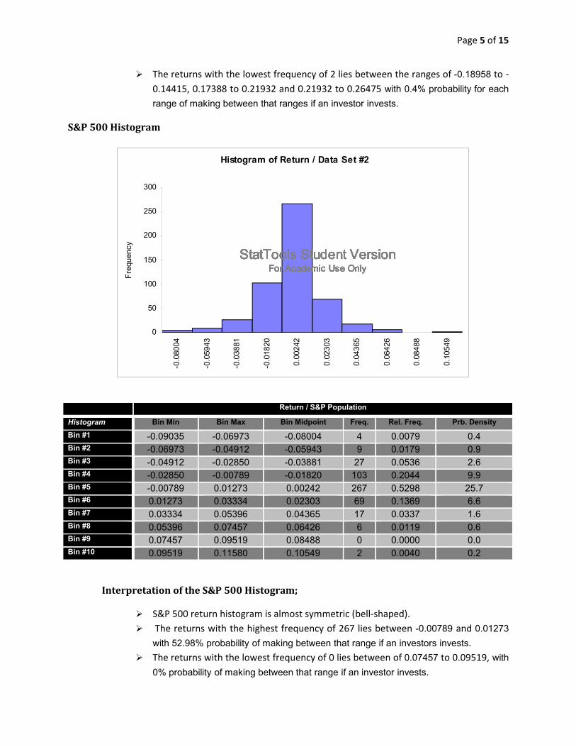
S&P 500 Histogram

Return / S&P Population

Histogram Bin Min Bin Max Bin Midpoint Freq. Rel. Freq. Prb. Density

Bin #1 -0.09035 -0.06973 -0.08004 4 0.0079 0.4 Bin #2 -0.06973 -0.04912 -0.05943 9 0.0179 0.9 Bin #3 -0.04912 -0.02850 -0.03881 27 0.0536 2.6 Bin #4 -0.02850 -0.00789 -0.01820 103 0.2044 9.9 Bin #5 -0.00789 0.01273 0.00242 267 0.5298 25.7 Bin #6 0.01273 0.03334 0.02303 69 0.1369 6.6 Bin #7 0.03334 0.05396 0.04365 17 0.0337 1.6 Bin #8 0.05396 0.07457 0.06426 6 0.0119 0.6 Bin #9 0.07457 0.09519 0.08488 0 0.0000 0.0 Bin #10 0.09519 0.11580 0.10549 2 0.0040 0.2

Interpretation of the S&P 500 Histogram;

S&P 500 return histogram is almost symmetric (bell-shaped).

The returns with the highest frequency of 267 lies between -0.00789 and 0.01273

with 52.98% probability of making between that range if an investors invests.

The returns with the lowest frequency of 0 lies between of 0.07457 to 0.09519, with

0% probability of making between that range if an investor invests.

Page 6 of 15

Testing the Empirical Rule:

GS returns:

S&P 500 returns:

Category Upper limit Frequency

More than 3 stdev below mean -0.064710 5

Between 2 and 3 stdevs below mean

-0.043156 12


-0.021601 39

Between mean and 1 stdev below mean

-0.000046 174

Between mean and 1 stdev above mean

0.021509 224

Between 1 and 2 stdevs above mean

0.043064 38


0.064618 7

More than 3 stdevs above mean

5

Percentages within k stdevs of mean

Empirical rule 68% 95% 99.70% Actual data 78.97% 94.25% 98.02%

Category Upper limit Frequency

More than 3 stdev below mean -0.1290 3


-0.0857 8


-0.0424 37

Between mean and 1 stdev below mean

0.0010 210

Between mean and 1 stdev above mean

0.0443 196


0.0876 38


0.1309 4

More than 3 stdevs above mean

8

Percentages within k stdevs of mean

Empirical rule 68% 95% 99.70% Actual data 80.56% 95.44% 97.82%

Plotting Box-Plots for GS and S&P 500 daily

for 2 years:

GS returns:

1) Mild outliers in the right tail of dist.

mild outlier= q3+1.5IQR

0.0726 starting of the mild outlier

0.1270 ending of the mild outlier

We will consider a return as a mild outlier if it falls between

2) Return will be considered as exceptionally good return.

the interval is 0.12700 plus infinity

3) Mild outliers in the left tail of dist.

mild outlier= q1-1.5iqr

-0.0726 starting of the mild outlier

-0.1270 ending of the mild outlier

The return is extremely bad return if it falls below

Plots for GS and S&P 500 daily returns of the whole data


starting of the mild outlier

ending of the mild outlier

We will consider a return as a mild outlier if it falls

0.0726 and


plus infinity




The return is extremely bad return -0.12702

Page 7 of 15

returns of the whole data (Population)

0.1270

S&P 500 returns:


mild outlier= q3+1.5IQR

0.03587 starting of the mild outlier

0.06310 ending of the mild outlier

We will consider a return as a mild outlier if it between


the interval is 0.06310 plus infinity


mild outlier= q1-1.5iqr

-0.03674 starting of the

-0.06397 ending of the mild outlier

The return is extremely bad return if it falls below




We will consider a return as a mild outlier if it falls

0.03587 and

eturn will be considered as exceptionally good return.

plus infinity

ild outliers in the left tail of dist.



The return is extremely bad return if it falls -0.06397

Page 8 of 15

0.06310

Page 9 of 15

Calculation of the mean and standard deviation for both GS and S&P 500 returns of

the sampled data (from the Population of 2 years):

Samplings involve choosing a sample from a population. The sample should be randomly chosen

and should be a representative of the data. The method for obtaining the sampl is by using the

“=Rand ()” excel function to acquire random numbers. We afterward arrange that information into

ascending order and choose the first 100 observations as our sample data.

GS analysis:

Through Stat-Tools:

Return

One Variable Summary Goldman Sachs Sample 100

Mean 0.00057

Std. Dev. 0.04815

Median -0.00056


Minimum -0.12130

Maximum 0.24997

Range 0.37128

Count 100



Interquartile Range 0.03376


Sample Mean Sample SD % Sample Mean

% Sample SD

0.000568478 0.048153791 0.0568% 4.82%


0.0162 0.0002 -0.0152 0.2500 -0.1213

Interpretation of the analyzed data on sample daily return for GS stocks:

The sample average or sample mean return on GS stock is 0.0568% daily. This

entails that on average, if an investor buys a GS stock and sells it the next day, the investor will

receive 0.0568% of the stock price. The standard deviation is a measure of variation and it verifies

the distribution of the stock prices around the mean. GS’s standard deviation is equals to 4.82%,

Page 10 of 15

which means on average, the distance of the returns on GS stock from its mean is 4.33%. The

maximum daily return on the GS stock was 25%. However, the minimum daily return gained on the

GS stock was -12.13%. GS 1st quartile is -1.52% this shows that 25% of the returns are under -

1.52% and 75% of the returns are higher from -1.52%. GS median is 0.02% which denotes that 50%

of the daily returns are less than 0.02% and 50% of the daily returns are higher than 0.02%. GS 3rd

quartile is 1.62% which denotes that 25% of the daily return are higher than 1.62% and 75% of the

daily returns are less than 1.62%.

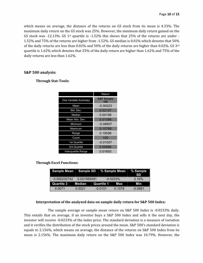
S&P 500 analysis:

Through Stat-Tools:


Sample Mean Sample SD % Sample Mean % Sample SD

-0.000232742 0.021565491 -0.0233% 2.16%


0.0071 0.0021 -0.0101 0.1079 -0.0881

Interpretation of the analyzed data on sample daily return for S&P 500 Index:

The sample average or sample mean return on S&P 500 Index is -0.0233% daily.

This entails that on average, if an investor buys a S&P 500 Index and sells it the next day, the

investor will receive -0.0233% of the index price. The standard deviation is a measure of variation

and it verifies the distribution of the stock prices around the mean. S&P 500’s standard deviation is

equals to 2.156%, which means on average, the distance of the returns on S&P 500 Index from its

mean is 2.156%. The maximum daily return on the S&P 500 Index was 10.79%. However, the

Return

One Variable Summary S&P Sample

100

Mean -0.00023

Std. Dev. 0.02157

Median 0.00198


Minimum -0.08807

Maximum 0.10789

Range 0.19596

Count 100



Interquartile Range 0.01693

Page 11 of 15

minimum daily return gained on the S&P 500 Index was –8.81%. GS 1st quartile is -1.01% this

shows that 25% of the returns are under -1.01% and 75% of the returns are higher than -1.01%. GS

median is 0.21% which denotes that 50% of the daily returns are less than 0.21% and 50% of the

daily returns are higher than 0.21%. GS 3rd quartile is 0.71% which denotes that 25% of the daily

return are higher than 0.71% and 75% of the daily returns are less than 0.71%.

Comparison and conclusion for the sample mean, sample standard deviation to the

population mean and population standard deviation.

The sample mean for GS is lower than the population mean, while the sample mean of S&P500

higher than the population mean. Also, the sample standard deviation for GS is higher than the

population standard deviation, while the sample standard deviation of S&P500 is same to the

population standard deviation.

Since the sample means and standard deviations differ from the population means and standard

deviations, they could be not good representatives for the population.

Page 12 of 15

Best distribution that fits the sample data

GS Sampled returns:

Logistic Normal

The best distribution that fits the GS sample data is the Logistics and the Normal comes number 7 in

the list of best distributions.

S&P Sampled returns:

LogLogistic Normal

The best distribution that fits the S&P 500 sample data is the LogLogistics and the Normal comes

number 4 in the list of best distributions.

Logistic(-0.00033128, 0.022046)

0

2

4

6

8

10

12

-0.1

5

-0.1

0

-0.0

5

0.0

0

0.0

5

0.1

0

0.1

5

0.2

0

0.2

5

0.3

0

< >5.0% 5.0%90.0%

-0.0652 0.0646

BestFit Student VersionFor Academic Use Only

Normal(0.00056600, 0.048151)

0

2

4

6

8

10

12

-0.1

5

-0.1

0

-0.0

5

0.0

0

0.0

5

0.1

0

0.1

5

0.2

0

0.2

5

0.3

0

< >5.0% 5.0%90.0%

-0.0786 0.0798


LogLogistic(-0.87524, 0.87499, 86.710)

0

5

10

15

20

25

30

-0.1

0

-0.0

8

-0.0

6

-0.0

4

-0.0

2

0.0

0

0.0

2

0.0

4

0.0

6

0.0

8

0.1

0

0.1

2

< >5.0% 5.0%90.0%

-0.0295 0.0300


Normal(-0.00023274, 0.021565)

0

5

10

15

20

25

30

-0.1

0

-0.0

8

-0.0

6

-0.0

4

-0.0

2

0.0

0

0.0

2

0.0

4

0.0

6

0.0

8

0.1

0

0.1

2

< >5.0% 5.0%90.0%

-0.0357 0.0352


Page 13 of 15

95% and 90% confidence intervals for the population mean

GS Returns:

Return

Conf. Intervals (One-Sample) Goldman Sachs Sample 100

Sample Size 100 Sample Mean 0.00057 Sample Std Dev 0.04815 Confidence Level (Mean) 95.0% Degrees of Freedom 99 Lower Limit -0.00899 Upper Limit 0.01012

Interpretation: We are 95% confident that the returns will lie between the limits of

-0.00899 and 0.01012.

Return

Conf. Intervals (One-Sample) Goldman Sachs Sample 100

Sample Size 100 Sample Mean 0.00057 Sample Std Dev 0.04815 Confidence Level (Mean) 90.0% Degrees of Freedom 99 Lower Limit -0.00743 Upper Limit 0.00856


-0.00743 and 0.00856.

Page 14 of 15

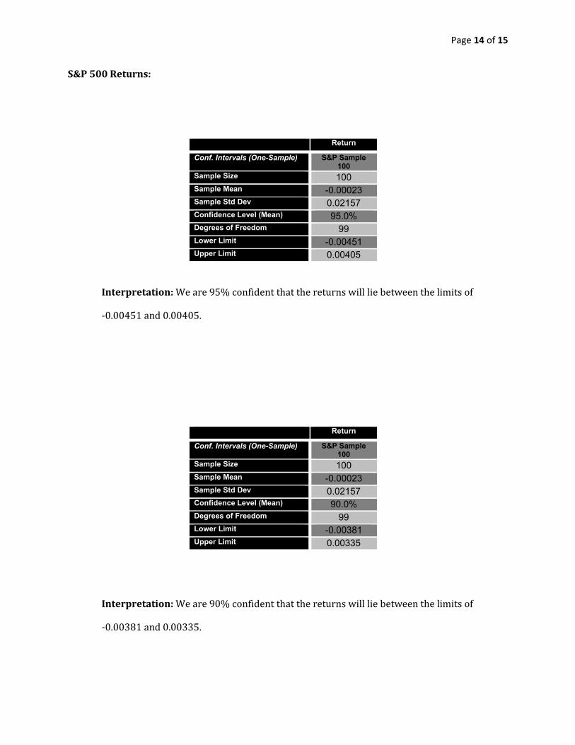
S&P 500 Returns:

Return

Conf. Intervals (One-Sample) S&P Sample 100

Sample Size 100 Sample Mean -0.00023 Sample Std Dev 0.02157 Confidence Level (Mean) 95.0% Degrees of Freedom 99 Lower Limit -0.00451 Upper Limit 0.00405


-0.00451 and 0.00405.

Return

Conf. Intervals (One-Sample) S&P Sample 100

Sample Size 100 Sample Mean -0.00023 Sample Std Dev 0.02157 Confidence Level (Mean) 90.0% Degrees of Freedom 99 Lower Limit -0.00381 Upper Limit 0.00335


-0.00381 and 0.00335.

Page 15 of 15

Simple regression conducted on the S&P 500 Index

Multiple R-Square

Adjusted StErr of Durbin

Summary R R-Square Estimate Watson

0.6795 0.4617 0.4562 0.030970615 2.0115

Degrees of Sum of Mean of F-Ratio p-Value ANOVA

Table Freedom Squares Squares

Explained 1 0.080633249 0.080633249 84.0649 < 0.0001

Unexplained 98 0.093999544 0.000959179

Coefficient Standard

t-Value p-Value Lower Upper

Regression Table Error Limit Limit

Constant 0.00320442 0.003102904 1.0327 0.3043 -

0.002953193 0.009362033 S&P-Return-risk free rate 1.196832687 0.130534767 9.1687 < 0.0001 0.93779069 1.455874684

R-Square

The r-square is 46.71%, therefore it’s not a very good regression and not good for prediction.

P-value

The p-value for Beta 1 or S&P500 index is less than 5%, therefore it’s significant.

Documents

FINANCIAL MODELLING AND EMPIRICAL ANALYSIS On S&P500