Financial Intermediation Chainsin an OTC Market∗

Ji ShenPeking University

shenjitoq@gmail.com

Bin WeiFederal Reserve Bank of Atlanta

bin.wei@atl.frb.org

Hongjun YanRutgers University

hongjun.yan.2011@gmail.com

December 29, 2015

∗We thank Bruno Biais, Briana Chang, Marco Di Maggio, Darrell Duffie, Nicolae Garleanu,Pete Kyle, Ricardo Lagos, Lin Peng, Matt Spiegel, Dimitri Vayanos, S. Viswanathan, Pierre-Olivier Weill, Randall Wright, and seminar participants at BI Norwegian Business School, Frank-furt School of Finance and Management, UCLA, University of Mannheim, Yale, The 8th AnnualConference of The Paul Woolley Centre for the Study of Capital Market Dysfunctionality, The11th World Congress of the Econometric Society, 2015 Summer Workshop on Money, Banking,Payments and Finance, and Summer Institute of Finance Meeting, for helpful comments. Theviews expressed here are those of the authors and do not necessarily reflect the views of the FederalReserve Bank of Atlanta or the Federal Reserve System. The latest version of the paper is availableat https://sites.google.com/site/hongjunyanhomepage/.

Financial Intermediation Chainsin an OTC Market

Abstract

This paper analyzes financial intermediation chains in a search model with an endogenous

intermediary sector. We show that the chain length and price dispersion among inter-dealer

trades are decreasing in search cost, search speed, and market size, but increasing in in-

vestors’ trading needs. Using data from the U.S. corporate bond market, we find evidence

broadly consistent with these predictions. Moreover, as search speed approaches infinity, the

search equilibrium does not always converge to the centralized-market equilibrium: prices

and allocation converge, but the trading volume may not. Finally, the efficiency of the

intermediary sector size is analyzed.

JEL Classification Numbers: G10.

Keywords : Search, Chain, Financial Intermediation.

1 Introduction

Financial intermediation chains appear to be getting longer over time, that is, more and more

layers of intermediaries are involved in financial transactions. For instance, with the rise of

securitization in in the U.S., the process of channeling funds from savers to investors is getting

increasingly complex (Adrian and Shin (2010)). This multi-layer nature of intermediation

also appears in many other markets. For example, the average daily trading volume in the

Federal Funds market is more than ten times the aggregate Federal Reserve balances (Taylor

(2001)). The trading volume in the foreign exchange market appears disproportionately large

relative to international trade.1

These examples suggest the prevalence of intermediation chains. What determines the

chain length? How does it respond to the changes in economic environment? What are

the implications on asset prices, trading volume, and investor welfare? To analyze these

questions, we need theories that endogenize the chain of intermediation. The literature so

far has not directly addressed these issues. Our paper attempts to fill this gap.

The full answer to the above questions is likely to be complex and hinges on a variety

of issues (e.g., transaction cost, trading technology, regulatory and legal environment, firm

boundary). As an initial step, however, we abstract away from many of these aspects to

analyze a simple model of an over-the-counter (OTC) market, and assess its predictions

empirically.2

In the model, investors have heterogeneous valuations of an asset. Their valuations

change over time, leading to trading needs. When an investor enters the market to trade,

he faces a delay in locating his trading partner. In the mean time, he needs to pay a search

cost each period until he finishes his transaction. Due to the delay and search cost, not all

investors choose to stay in the market continuously, giving rise to a role of intermediation.

Some investors choose to be intermediaries. They stay in the market continuously and act as

1According to the Main Economic Indicators database, the annual international trade in goods andservices is around $4 trillion in 2013. In that same year, however, the Bank of International Settlementestimates that the daily trading volume in the foreign exchange market is around $5 trillion.

2OTC markets are enormous. According to the estimate by the Bank for International Settlements, thetotal outstanding OTC derivatives is around 711 trillion dollars in December 2013.

1

dealers. Once they acquire the asset, they immediately start searching to sell it to someone

who values it more. Similarly, once they sell the asset, they immediately start searching to

buy it from someone who values it less. In contrast, other investors act as customers : once

their trades are executed, they leave the market to avoid the search cost. We solve the model

in closed-form, and the main implications are the following.

First, when the search cost is lower than a certain threshold, there is an equilibrium

with an endogenous intermediary sector. Investors with intermediate valuations of the asset

choose to become dealers and stay in the market continuously, while others (who have with

high or low valuations) choose to be customers, and leave the market once their transactions

are executed. Intuitively, if an investor has a high valuation of an asset, once he obtains

the asset, there is little benefit for him to stay in the market since the chance of finding

someone with an even higher valuation is low. Similarly, if an investor has a low valuation

of the asset, once he sells the asset, there is little benefit for him to stay in the market. In

contrast to the above equilibrium, when the search cost is higher than the threshold, there is

an equilibrium with no intermediary. Only investors with very high or low valuations enter

the market, and they leave the market once their trading needs are satisfied. In this case,

the investors with intermediate valuations have weak trading needs, and choose to stay out

of the market to avoid search cost.

Second, at each point in time, there is a continuum of prices for the asset. When a

buyer meets a seller, their negotiated price depends on their specific valuations. The delay

in execution in the market makes it possible to have multiple prices for the asset. Naturally,

as the search speed improves, the price dispersion reduces, and converges to zero when the

search speed goes to infinity.

Third, we characterize two equilibrium quantities on the intermediary sector, which can

be easily measured empirically. The first is the dispersion ratio, the price dispersion among

inter-dealer trades divided by the price dispersion among all trades in the economy.3 The sec-

ond is the length of the intermediation chain, the average number of layers of intermediaries

3For convenience, we use “intermediary” and “dealer” interchangeably, and refer to the transactionsamong dealers as “inter-dealer trades.”

2

for all customers’ transactions. Intuitively, both variables reflect the size of the intermediary

sector. When more investors choose to become dealers, the price dispersion among inter-

dealer trades is larger (i.e., the dispersion ratio is higher), and customers’ transactions tend

to go through more layers of dealers (i.e., the chain is longer).

Our model implies that both the dispersion ratio and the chain length are decreasing in

the search cost, the speed of search, and the market size, but are increasing in investors’ trad-

ing frequency. Intuitively, a higher search cost means that fewer investors find it profitable to

be dealers, leading to a smaller intermediary sector and hence a smaller dispersion ratio and

chain length. Similarly, with a higher search speed or a larger market size, intermediation

is less profitable because customers can find alternative trading partners more quickly. This

leads to a smaller intermediary sector (relative to the market size). Finally, when investors

need to trade more frequently, the higher profitability attracts more dealers and so increases

the size of the intermediary sector.

We test these predictions using data from the U.S. corporate-bond market. The Trade Re-

porting and Compliance Engine (TRACE) records transaction prices, and identifies traders

with the Financial Industry Regulatory Authority (FINRA) membership as “dealers,” and

others as “customers.” This allows us to construct the dispersion ratio and chain length.

We run Fama-MacBeth regressions of the dispersion ratio and chain length of a corporate

bond on proxies for search cost, market size, the frequency of investors’ trading needs. Our

evidence is broadly consistent with the model predictions. It is worth noting the difference

between the dependent variables in the two regressions: The dispersion ratio is constructed

based on price data while the chain length is based on quantity data. Yet, for almost all

our proxies, their coefficient estimates have the same sign across the two regressions, as

implied by our model. For example, relative to other bonds, investment-grade bonds’ price

dispersion ratio is on average larger by 0.007 (t = 2.62), and their chain length is longer

by 0.245 (t = 32.17). If one takes the interpretation that it is less costly to make market

for investment-grade bonds (i.e., the search cost is lower), then this evidence is consistent

with our model prediction that the dispersion ratio and chain length are decreasing in search

cost. We also include in our regressions five other variables as proxies for search cost, the

3

frequency of investors’ trading needs, and market size. Among all 12 coefficients, 11 are

highly significant and consistent with our model predictions.4

Fourth, when the search speed goes to infinity, the search-market equilibrium does not

always converge to a centralized-market equilibrium. Specifically, in the case without inter-

mediary (i.e., the search cost is higher than a certain threshold), as the search speed goes

to infinity, all equilibrium quantities (prices, volumes, and allocations) converge to their

counterparts in the centralized-market equilibrium. However, in the case with intermedi-

aries (i.e., the search cost is lower than the threshold), as the search speed goes to infinity,

all the prices and asset allocations converge but the trading volume in the search-market

equilibrium remains higher than that in the centralized-market equilibrium. Moreover, this

volume difference is larger if the search cost is smaller, and converges to infinity when the

search cost goes to 0.

Intuitively, in the search market, intermediaries act as “middlemen” and generate “ex-

cess” trading. As noted earlier, when the search speed increases, the intermediary sector

shrinks. However, thanks to the faster search speed, each dealer executes more trades, and

the total excess trading volume is higher. As the search speed goes to infinity, the trading

volume in the search market remains significantly higher than that in a centralized market.

Moreover, the volume difference increases when the search cost becomes smaller because

a smaller search cost implies a larger intermediary sector, which leads to a higher excess

trading volume in the search market.

This insight sheds light on why a centralized-market model has trouble explaining trading

volume, especially in an environment with a small transaction cost. We argue that even for

the U.S. stock market, it seems plausible that some aspects of the market are better captured

by a search model. For example, the cheaper and faster trading technology in the last a few

decades made it possible for investors to exploit many high frequency opportunities that used

to be prohibitive. Numerous trading platforms were set up to compete with main exchanges;

hedge funds and especially high-frequency traders directly compete with traditional market

4The only exception is the coefficient for issuance size in the price dispersion ratio regression. As explainedlater, we conjecture that this is due to dealers’ inventory capacity constraint, which is not considered in ourmodel.

4

makers. The increase in turnover in the stock market in the last a few decades was likely to

be driven partly by these “intermediation” trades.

Fifth, the relation between dispersion ratio, chain length and investors’ welfare is am-

biguous. As noted earlier, a higher dispersion ratio and longer chain may be due to a lower

search cost. In this case, they imply higher investors welfare. On the other hand, they may

be due to a slower search speed. In that case, they imply lower investors welfare. Hence, the

dispersion ratio and chain length are not clear-cut welfare indicators.

Finally, we examine the efficiency of the intermediary sector in our model by comparing

its size with the size of the intermediary sector that would be chosen by a social planner. Our

results are reminiscent of the well-known Hosios (1990) condition that efficiency is achieved

only for a specific distribution of bargaining powers. In particular, we find that the size of

the intermediary sector is efficient if buyers and sellers have the same bargaining power, but

is generally inefficient otherwise.

1.1 Related literature

Our paper belongs to the recent literature that analyzes OTC markets in the search frame-

work developed by Duffie, Garleanu, and Pedersen (2005). This framework has been ex-

tended to include risk-averse agents (Duffie, Garleanu, and Pedersen (2007)), unrestricted

asset holdings (Lagos and Rocheteau (2009)). It has also been adopted to analyze a number

of issues, such as security lending (Duffie, Garleanu, and Pedersen (2002)), liquidity pro-

vision (Weill (2007)), on-the-run premium (Vayanos and Wang (2007), Vayanos and Weill

(2008)), cross-sectional returns (Weill (2008)), portfolio choices (Garleanu (2009)), liquidity

during a financial crisis (Lagos, Rocheteau, and Weill (2011)), price pressure (Feldhutter

(2012)), order flows in an OTC market (Lester, Rocheteau, and Weill (2014)), commercial

aircraft leasing (Gavazza 2011), high frequency trading (Pagnotta and Philippon (2013)), the

roles of benchmarks in OTC markets (Duffie, Dworczak, and Zhu (2014)), adverse selection

and repeated contacts in opaque OTC markets (Chang (2014), Zhu (2012)) the effect of the

supply of liquid assets (Shen and Yan (2014)) as well as the interaction between corporate

default decision and liquidity (He and Milbradt (2013)). Another literature follows Kiyotaki

5

and Wright (1993) to analyze the liquidity value of money. In particular, Lagos and Wright

(2005) develop a tractable framework that has been adopted to analyze liquidity and asset

pricing (e.g., Lagos (2010), Lester, Postlewaite, and Wright (2012), and Li, Rocheteau, and

Weill (2012), Lagos and Zhang (2014)). Trejos and Wright (2014) synthesize this literature

with the studies under the framework of Duffie, Garleanu, and Pedersen (2005).

Our paper is related to the literature on the trading network of financial markets, see,

e.g., Viswanathan and Wang (2004) analyze inter-dealer trades. Gofman (2010), Babus and

Kondor (2012), Malamud and Rostek (2012), Chang and Zhang (2015). Atkeson, Eisfeldt,

and Weill (2014) analyze the risk-sharing and liquidity provision in an endogenous core-

periphery network structure. Neklyudov (2014) analyzes a search model with investors with

heterogeneous search speeds to study the implications on the network structure.

Intermediation has been analyzed in the search framework (e.g., Rubinstein and Wolin-

sky (1987), and more recently Wright and Wong (2014), Nosal Wong and Wright (2015)).

However, the literature on financial intermediation chains has been recent. Adrian and Shin

(2010) document that the financial intermediation chains are becoming longer in the U.S.

during the past a few decades. Li and Schurhoff (2012) document the network structure of

the inter-dealer market for municipal bonds. Di Maggio, Kermani, and Song (2015) analyze

the trading relation during a financial crisis. Glode and Opp (2014) focuses on the role

of intermediation chain in reducing adverse selection. Afonso and Lagos (2015) analyze an

OTC market for Federal Funds. The equilibrium in their model features an intermediation

chain, although they do not focus on its property.

Our paper is closest to Hugonnier, Lester, and Weill (2014). They analyze a model with

investors with heterogenous valuations, highlighting that heterogeneity magnifies the impact

of search frictions. In order to analyze intermediation, we generalize their model to include

search cost and derive the intermediary sector, price dispersion ratio, and the intermediation

chain, and also conduct empirical analysis of the intermediary sector.

The rest of the paper is as follows. Section 2 describes the model and its equilibrium.

Section 3 analyzes the price dispersion and intermediation chain. Section 4 contrasts the

search market equilibrium with a centralized market equilibrium. Section 5 examines the

6

efficiency of the size of the intermediary sector. Section 6 tests the empirical predictions.

Section 7 concludes. All proofs are in the appendix.

2 Model

Time is continuous and goes from 0 to∞. There is a continuum of investors, and the measure

of the total population is N . They have access to a riskless bank account with an interest

rate r. There is an asset, which has a total supply of X units with X < N . Each unit of

the asset pays $1 per unit of time until infinity. The asset is traded at an over-the-counter

market.

Following Duffie, Garleanu, and Pedersen (2005), we assume the matching technology as

the following. Let Nb and Ns be the measures of buyers and sellers in the market, both of

which will be determined in equilibrium. A buyer meets a seller at the rate λNs, where λ > 0

is a constant. That is, during [t, t + dt) a buyer meets a seller with a probability λNsdt.

Similarly, a seller meets a buyer at the rate λNb. Hence, the probability for an investor to

meet his partner is proportional to the population size of the investors on the other side

of the market. The total number of matched pairs per unit of time is λNsNb. The search

friction reduces when λ increases, and disappears when λ goes to infinity.

Investors have different types, and their types may change over time. If an investor’s

current type is ∆, he derives a utility 1 + ∆ when receiving the $1 coupon from the asset.

One interpretation for a positive ∆ is that some investors, such as insurance companies,

have a preference for long-term bonds, as modeled in Vayanos and Vila (2009). Another

interpretation is that some investors can benefit from using those assets as collateral and

so value them more, as discussed in Bansal and Coleman (1996) and Gorton (2010). An

interpretation of a negative ∆ can be that the investor suffers a liquidity shock and so finds

it costly to carry the asset on his balance sheet. We assume that ∆ can take any value in a

closed interval. Without loss of generality, we normalize the interval to[0,∆

].

Each investor’s type changes independently with intensity κ. That is, during [t, t+ dt),

with a probability κdt, an investor’s type changes and is independently drawn from a random

7

variable, which has a probability density function f (·) on the support[0,∆

], with f (∆) < ∞

for any ∆ ∈[0,∆

]. We use F (·) to denote the corresponding cumulative distribution

function.

Following Duffie, Garleanu, and Pedersen (2005), we assume each investor can hold either

0 or 1 unit of the asset. That is, an investor can buy 1 unit of the asset only if he currently

does not have the asset, and can sell the asset only if he currently has it.

2.1 Investors’ choices

All investors are risk-neutral and share the same time discount rate r. They face a search

cost of c per unit of time, with c ≥ 0. That is, when an investor searches to buy or sell in the

market, he incurs a cost of cdt during [t, t+ dt). An investor’s objective function is given by

supθτ

Et

[∫ ∞

t

e−r(τ−t) [θτ (1 + ∆τ )− 1τc] dτ −∫ ∞

t

e−r(τ−t)Pτdθτ

],

where θτ ∈ {0, 1} is the investor’s holding in the asset at time τ ; ∆τ is the investor’s type

at time τ ; 1τ is an indicator variable, which is 1 if the investor is searching in the market to

buy or sell the asset at time τ , and 0 otherwise; and Pτ is the asset’s price that the investor

faces at time τ and will be determined in equilibrium.

We will focus on the steady-state equilibrium. Hence, the value function of a type-

∆ investor with an asset holding θt at time t can be denoted as V (θt,∆). That is, the

distribution of all other investors’ types is not a state variable, since it stays constant over

time in the steady state equilibrium.

A non-owner (whose θt is 0) has two choices: search to buy the asset or stay inactive.

We use Vn(∆) to denote the investor’s expected utility if he chooses to stay inactive, and

follows the optimal strategy after his type changes. Similarly, we use Vb(∆) to denote the

investor’s expected utility if he searches to buy the asset, and follows the optimal strategy

after he obtains the asset or his type changes. Hence, by definition, we have

V (0,∆) = max(Vn(∆), Vb(∆)). (1)

An asset owner (whose θt is 1) has two choices: search to sell the asset or stay inactive.

8

We use Vh(∆) to denote the investor’s expected utility if he chooses to be an inactive holder,

and follows the optimal strategy after his type changes. Similarly, we use Vs(∆) to denote

the investor’s expected utility if he searches to sell, and follows the optimal strategy after he

sells his asset or his type changes. Hence, we have

V (1,∆) = max(Vh(∆), Vs(∆)). (2)

We conjecture, and will verify later, that in equilibrium, equation (1) implies that a

non-owner’s optimal choice is given by{stay out of the market if ∆ ∈ [0,∆b),search to buy the asset if ∆ ∈ (∆b,∆],

(3)

where the cutoff point ∆b will be determined in equilibrium. A type-∆b non-owner is indif-

ferent between staying out of the market and searching to buy the asset. Note that due to

the search friction, a buyer faces delay in his transaction. In the meantime, his type may

change, and he will adjust his action accordingly. Similarly, we conjecture that equation (2)

implies that an owner’s optimal choice is{search to sell his asset if ∆ ∈ [0,∆s),stay out of the market if ∆ ∈ (∆s,∆],

(4)

where the ∆s will be determined in equilibrium. A type-∆s owner of the asset is indifferent

between the two actions. A seller faces potential delay in his transaction. In the meantime,

if his type changes, he will adjust his action accordingly. If an investor succeeds in selling

his asset, he becomes a non-owner and his choices are then described by equation (3).

Suppose a buyer of type x ∈[0,∆

]meets a seller of type y ∈

[0,∆

]. The surplus from

the transaction is

S (x, y) = [V (1, x) + V (0, y)]︸ ︷︷ ︸total utility after trade

− [V (0, x) + V (1, y)]︸ ︷︷ ︸total utility before trade

. (5)

The pair can agree on a transaction if and only if the surplus is positive. We assume that

the buyer has a bargaining power η ∈ (0, 1), i.e., the buyer gets η of the surplus from the

transaction, and hence the price is given by

P (x, y) = V (1, x)− V (0, x)− ηS(x, y), if and only if S(x, y) > 0. (6)

9

The first two terms on the right hand side reflect the value of the asset to the buyer: the

increase in the buyer’s expected utility from obtaining the asset. Hence, the above equation

implies that the transaction improves the buyer’s utility by ηS(x, y).

We conjecture, and verify later, that when a buyer and a seller meet in the market, the

surplus is positive if and only if the buyer’s type is higher than the seller’s:

S (x, y) > 0 if and only if x > y. (7)

That is, when a pair meets, a transaction occurs if and only if the buyer’s type is higher

than the seller’s type. With this conjecture, we obtain investors’ optimality condition in the

steady state as the following.

Vh (∆) =1 + ∆+ κE [max {Vh (∆

′) , Vs (∆′)}]

κ+ r, (8)

Vs (∆) =1 + y − c

κ+ r+λ (1− η)

κ+ r

∫ ∆

∆

S (x,∆)µb (x) dx+κE [max {Vh(∆

′),Vs(∆′)}]

κ+ r, (9)

Vn (∆) =κE [max {Vn (∆

′) , Vb (∆′)}]

κ+ r, (10)

Vb (∆) = − c

κ+ r+

λη

κ+ r

∫ ∆

0

S (∆, x)µs (x) dx+κE [max {Vb (∆) , Vn}]

κ+ r, (11)

where ∆′ is a random variable with a PDF of f(·).

2.2 Intermediation

Decision rules (3) and (4) determine whether intermediation arises in equilibrium. There

are two cases. In the first case, ∆b ≥ ∆s, there is no intermediation. When an investor

has a trading need, he enters the market. Once his transaction is executed, he leaves the

market and stays inactive. In the other case ∆b < ∆s, however, some investors choose to

be intermediaries and stay in the market continuously. If they are non-owners, they search

to buy the asset. Once they receive the asset, however, they immediately search to sell the

asset. For convenience, we call them “dealers.”

Details are illustrated in Figure 1. Panel A is for the case without intermediation, i.e.,

∆b ≥ ∆s. If an asset owner’s type is below ∆s, as in the upper-left box, he enters the market

10

to sell his asset. If successful, he becomes a non-owner and chooses to be inactive since his

type is below ∆b, as in the upper-right box. Similarly, if a non-owner’s type is higher than

∆b, as in the lower-right box, he enters the market to buy the asset. If successful, he becomes

an owner and chooses to be inactive because his type is above ∆s, as in the lower-left box.

The dashed arrows in the diagram illustrate investors’ chooses to enter or exit the market

when their types change. Suppose, for example, an owner with a type below ∆s is searching

in the market to sell his asset, as in the upper-left box. Before he meets a buyer, however,

if his type changes and becomes higher than ∆s, he will exit the market and become an

inactive owner in the lower-left box. Finally, note that all investors in the interval (∆s,∆b)

are inactive regardless of their asset holdings.

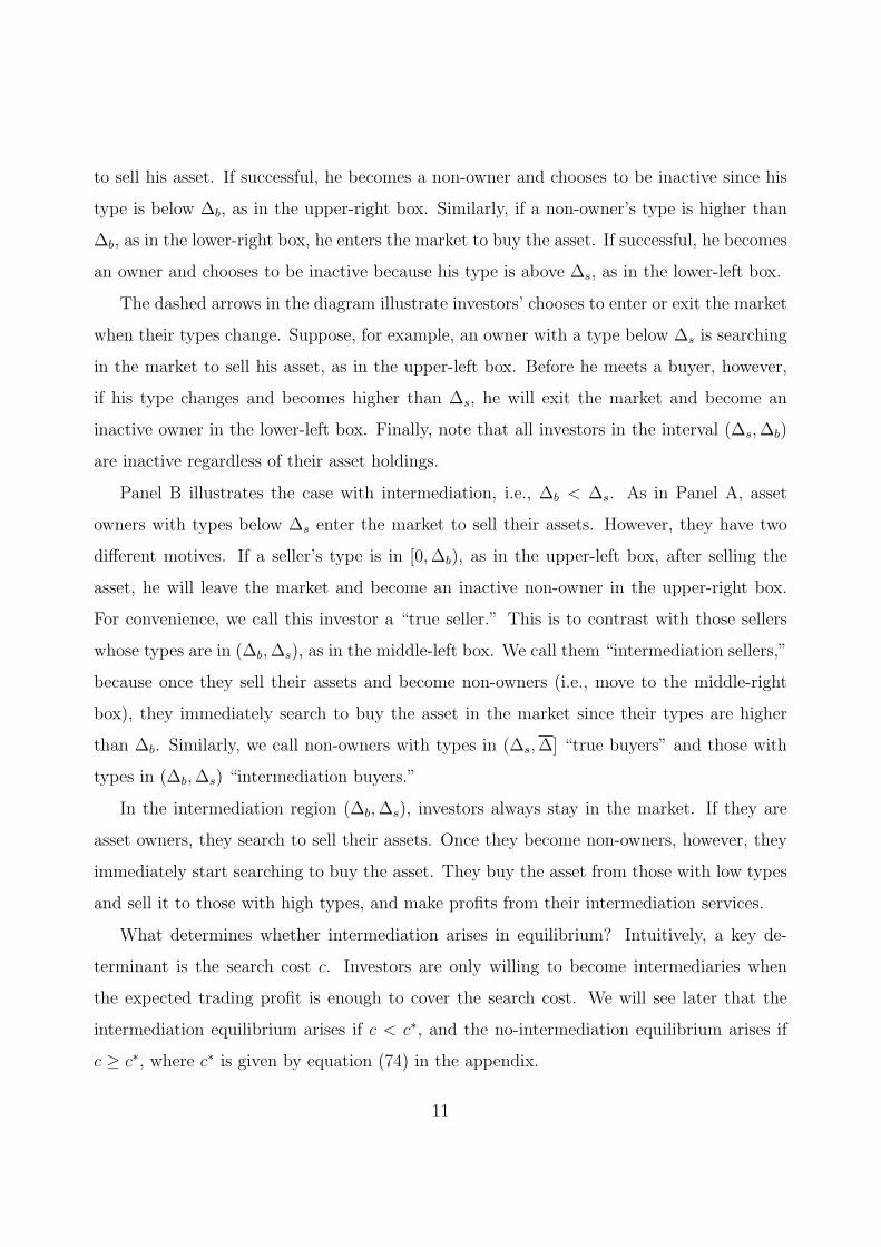
Panel B illustrates the case with intermediation, i.e., ∆b < ∆s. As in Panel A, asset

owners with types below ∆s enter the market to sell their assets. However, they have two

different motives. If a seller’s type is in [0,∆b), as in the upper-left box, after selling the

asset, he will leave the market and become an inactive non-owner in the upper-right box.

For convenience, we call this investor a “true seller.” This is to contrast with those sellers

whose types are in (∆b,∆s), as in the middle-left box. We call them “intermediation sellers,”

because once they sell their assets and become non-owners (i.e., move to the middle-right

box), they immediately search to buy the asset in the market since their types are higher

than ∆b. Similarly, we call non-owners with types in (∆s,∆] “true buyers” and those with

types in (∆b,∆s) “intermediation buyers.”

In the intermediation region (∆b,∆s), investors always stay in the market. If they are

asset owners, they search to sell their assets. Once they become non-owners, however, they

immediately start searching to buy the asset. They buy the asset from those with low types

and sell it to those with high types, and make profits from their intermediation services.

What determines whether intermediation arises in equilibrium? Intuitively, a key de-

terminant is the search cost c. Investors are only willing to become intermediaries when

the expected trading profit is enough to cover the search cost. We will see later that the

intermediation equilibrium arises if c < c∗, and the no-intermediation equilibrium arises if

c ≥ c∗, where c∗ is given by equation (74) in the appendix.

11

Our formulation captures two important features of the intermediation sector. First,

while customers leave the market once they finish their trades, intermediaries stay in the

market continuously. Second, relative to intermediaries, customers tend to have more ex-

treme valuations of the asset. For tractability, however, we also adopt some simplifications.

For instance, all investors are assumed to be ex ante identical. One consequence is that the

intermediaries in our model have a chance to become customers after shocks to their types.

This is not as unrealistic as it appears: Of course, in reality, the identities of “dealers” and

“customers” are persistent. However, identities do switch when, for example, new dealers

enter, or existing dealers exit the market. For instance, Lehman Brothers was a major dealer

for corporate bonds before it filed for bankruptcy in 2008. After this shock, Lehman Brothers

is more like a customer in this market, trying to sell its holdings. More generally, however,

traders’ identities are perhaps more persistent than implied by our formulation. In practice,

some institutions specialize and act as dealers for an extended period of time. This feature

can be captured in our framework by introducing a switching cost. It is natural to expect

that, with this cost, investors will not switch their identities between dealers and customers,

unless they experience very large shocks to their types. However, this extension makes the

model much less tractable and we leave it to future research.

2.3 Demographics

We will first focus on the intermediation equilibrium case, and leave the analysis of the

no-intermediation case to Section 4.3. Due to the changes in ∆ and his transactions in

the market, an investor’s status (type ∆ and asset holding θ) changes over time. We now

describe the evolution of the population sizes of each group of investors. Since we will focus

on the steady-state equilibrium, we will omit the time subscript for simplicity.

We use µb(∆) to denote the density of buyers, that is, buyers’ population size in the

region (∆,∆ + d∆) is µb(∆)d∆. Similarly, we use µn(∆), µs(∆), and µh(∆) to denote the

density of inactive non-owners, sellers, and inactive asset holders, respectively.

In the steady state, the cross-sectional distribution of investors’ types is given by the

probability density function f (∆). Hence, the following accounting identity holds for any

12

∆ ∈[0,∆

]:

µs (∆) + µb (∆) + µn (∆) + µh (∆) = Nf (∆) . (12)

Decision rules (3) and (4) imply that for any ∆ ∈ (∆s,∆],

µn (∆) = µs (∆) = 0. (13)

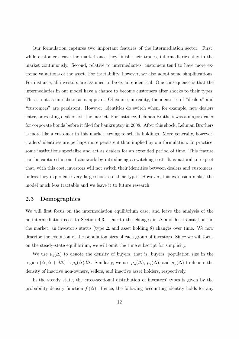
In the steady state, the group size of inactive holders remains a constant over time,

implying that for any ∆ ∈ (∆s,∆],

κµh (∆) = κXf (∆) + λNsµb (∆) . (14)

The left hand aside of the above equation is the “outflow” from the group of inactive holders:

The measure of inactive asset holders in interval (∆,∆+d∆) is µh (∆) d∆. During [t, t+ dt),

a fraction κdt of them experience changes in their types and leave the group. Hence, the

total outflow is κµh (∆) d∆dt. The right hand side of the above equation is the “inflow”

to the group: A fraction κdt of asset owners, who have a measure of X, experience type

shocks and κXf (∆) d∆dt investors’ new types fall in the interval (∆,∆ + d∆). This is

captured by the first term in the right hand side of (14). The second term reflects the inflow

of investors due to transactions. When buyers with types in (∆,∆+ d∆) acquire the asset,

they become inactive asset holders, and the size of this group is λNsµb (∆) d∆dt. Similarly,

for any ∆ ∈ [0,∆b), we have

µb (∆) = µh (∆) = 0, (15)

κµn (∆) = κ (N −X) f (∆) + λNbµs (∆) . (16)

For any ∆ ∈ (∆b,∆s), we have

µn (∆) = µh (∆) = 0, (17)

κµs (∆) = κXf (∆)− λµs (∆)

∫ ∆

∆

µb (x) dx+ λµb (∆)

∫ ∆

0

µs (x) dx. (18)

2.4 Equilibrium

Definition 1 The steady-state equilibrium with intermediation consists of two cutoff points

∆b and ∆s, with 0 < ∆b < ∆s < ∆, the distributions of investor groups (µb (∆), µs (∆),

13

µn (∆), µh (∆)), and asset prices P (x, y), such that

• the asset prices P (x, y) are determined by (6),

• choices (3) and (4) are optimal for all investors,

• (µb (∆), µs (∆), µn (∆), µh (∆)) are time invariant, i.e., satisfy (12)–(18),

• market clears: ∫ ∆

0

[µs(∆) + µh(∆)] d∆ = X. (19)

Theorem 1 If c < c∗, where c∗ is given by equation (74), there exists a unique steady-state

equilibrium with ∆b < ∆s. The value of ∆b is given by the unique solution to

c =λκηX

[κ+ r + λNb (1− η)] (κ+ λNb)

∫ ∆b

0

F (x) dx, (20)

the value of ∆s is given by the unique solution to

c =λκ (1− η) (N −X)

(κ+ r + ληNs) (κ+ λNs)

∫ ∆

∆s

[1− F (x)] dx, (21)

where Ns and Nb are given by (54) and (56).

The distributions of investor groups (µb (∆), µs (∆), µn (∆), µh (∆)) are given by equa-

tions (46)–(53).

When a type-x buyer (x ∈ (∆b,∆]) and a type-y seller (y ∈ [0,∆s)) meet in the market,

they will agree to trade if and only if x > y, and their negotiated price is given by (6), with

the value function V (·, ·) given by (69)–(72).

This theorem shows that when the cost of search is smaller than c∗, there is a unique

intermediation equilibrium. Investors whose types are in the interval (∆b,∆s) choose to be

dealers. They search to buy the asset if they do not own it. Once they obtain the asset,

however, they immediately start searching to sell it. They make profits from the differences

in purchase and sale prices to compensate the search cost they incur. In contrast to these

intermediaries, sellers with a type ∆ ∈ [0,∆s) and buyers with a type ∆ ∈ (∆b,∆] are true

buyers and true sellers, and they leave the market once they finish their transactions.

14

Note that investors’ type distributions (µb (∆) , µs (∆) , µn (∆) , µh (∆)) determine the

speed with which investors meet their trading partners, which in turn determines investors’

type distributions. The equilibrium is the solution to this fixed-point problem. The above

theorem shows that the distributions can be computed in closed-form, making the analysis

of the equilibrium tractable.

To illustrate the equilibrium, we define R(∆), for ∆ ∈ [0,∆], as

R(∆) ≡ µs (∆) + µh (∆)

µb (∆) + µn (∆).

That is, R(∆) is the density ratio of asset owners (i.e., sellers and inactive holders) to

nonowners (i.e., buyers and inactive nonowners). It has the following property.

Proposition 1 In the equilibrium in Theorem 1, R(∆) is weakly increasing in ∆: R′(∆) > 0

for ∆ ∈ (∆b,∆s), and R′(∆) = 0 for ∆ ∈ [0,∆b) ∪ (∆s,∆].

The above proposition shows that high-∆ investors are more likely to be owners of the asset

in equilibrium. The intuition is the following. As noted in (7), when a buyer meets a seller,

transaction happens if and only if the buyer’s type is higher than the seller’s. Hence, if a

nonowner has a higher ∆ he is more likely to find a willing seller. On the other hand, if an

owner has a higher ∆ he is less likely to find a willing buyer. Consequently, in equilibrium,

the higher the investor’s type, the more likely he is an owner.

Proposition 2 In the equilibrium in Theorem 1, we have ∂P (x,y)∂x

> 0 and ∂P (x,y)∂y

> 0.

The price of each transaction is negotiated between the buyer and the seller, and depends on

the types of both. Since there is a continuum of buyers and a continuum of sellers, there is

a continuum of equilibrium prices at each point in time. The above proposition shows that

the negotiated price is increasing in both the buyer’s type and the seller’s type. Intuitively,

the higher the buyer’s type x, the more he values the asset. Hence, he is willing to pay a

higher price. On the other hand, the higher the seller’s type y, the less eager he is in selling

the asset. Hence, only a higher price can induce him to sell.

15

3 Intermediation Chain and Price Dispersion

If a true buyer and a true seller meet in the market, the asset is transferred without going

through an intermediary. On other occasions, however, transactions may go through multiple

dealers. For example, a type-∆ dealer may buy from a true seller, whose type is in [0,∆b),

or from another dealer whose type is lower than ∆. Then, he may sell the asset to a true

buyer, whose type is in (∆s,∆], or to another dealer whose type is higher than ∆. That is,

for an asset to be transferred from a true seller to a true buyer, it may go through multiple

dealers.

What is the average length of the intermediation chain in the economy? To analyze this,

we first compute the aggregate trading volumes for each group of investors. We use TVcc to

denote the total number of shares of the asset that are sold from a true seller to a true buyer

(i.e., “customer to customer”) per unit of time. Similarly, we use TVcd, TVdd, and TVdc to

denote the numbers of shares of the asset that are sold, per unit of time, from a true seller

to a dealer (i.e., “customer to dealer”), from a dealer to another (i.e., “dealer to dealer”),

and from a dealer to a true buyer (i.e., “dealer to customer”), respectively. To characterize

these trading volumes, we denote Fb(∆) and Fs(∆), for ∆ ∈ [0,∆], as

Fb(∆) ≡∫ ∆

0

µb(x)dx,

Fs(∆) ≡∫ ∆

0

µs(x)dx.

That is, Fb(∆) is the population size of buyers whose types are below ∆, and Fs(∆) is

population size of sellers whose types are below ∆.

Proposition 3 In the equilibrium in Theorem 1, we have

TVcc = λFs(∆b) [Nb − Fb(∆s)] , (22)

TVcd = λFs(∆b)Fb(∆s), (23)

TVdc = λ [Ns − Fs(∆b)] [Nb − Fb(∆s)] , (24)

TVdd = λ

∫ ∆s

∆b

[Fs(∆)− Fs(∆b)] dFb(∆). (25)

16

The above proposition characterizes the four types of trading volumes. For example, true

sellers are those whose types are below ∆b. The total measure of those investors is Fs(∆b).

True buyers are those whose types are above ∆s, and so the total measure of those investors

is Nb −Fb(∆s). This leads to the trading volume in (22). The results on TVcd and TVdc are

similar. Note that in these 3 types of trades, every meeting results in a transaction, since

the buyer’s type is always higher than the seller’s. For the meetings among dealers, however,

this is not the case. When a dealer buyer meets a dealer seller with a higher ∆, they will not

be able to reach an agreement to trade. The expression of TVdd in (25) takes into account

the fact that transaction occurs only when the buyer’s type is higher than the seller’s.

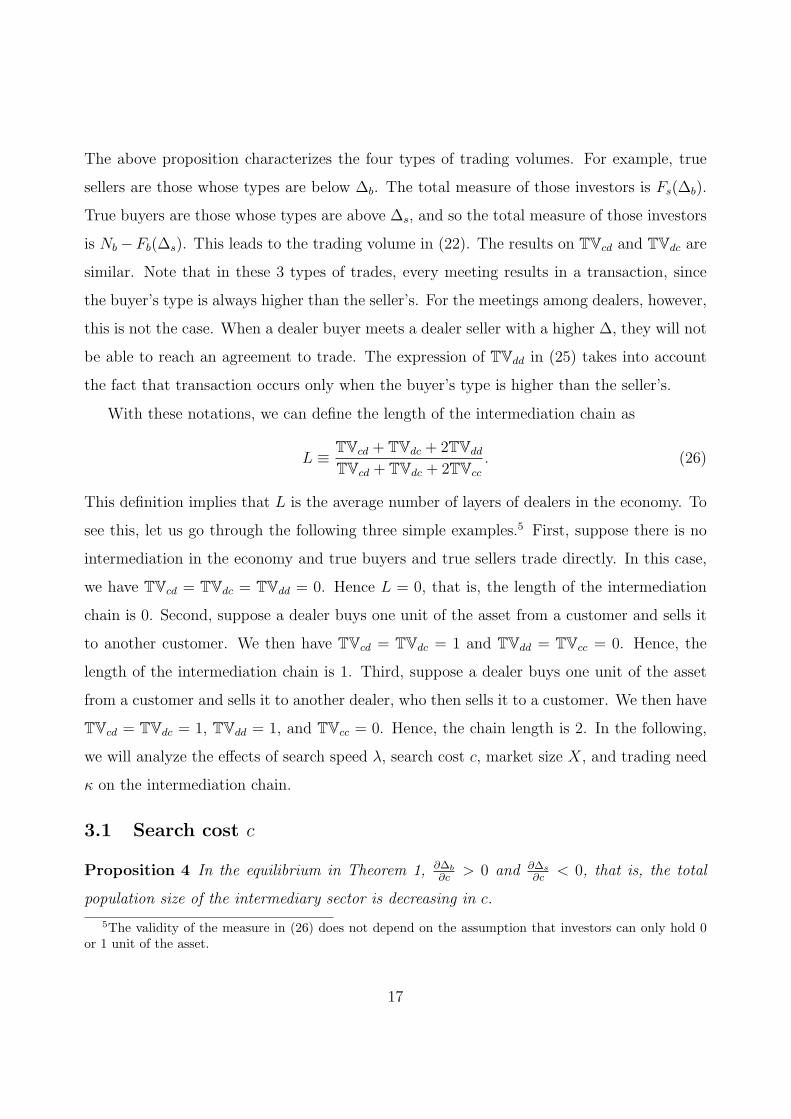
With these notations, we can define the length of the intermediation chain as

L ≡ TVcd + TVdc + 2TVdd

TVcd + TVdc + 2TVcc

. (26)

This definition implies that L is the average number of layers of dealers in the economy. To

see this, let us go through the following three simple examples.5 First, suppose there is no

intermediation in the economy and true buyers and true sellers trade directly. In this case,

we have TVcd = TVdc = TVdd = 0. Hence L = 0, that is, the length of the intermediation

chain is 0. Second, suppose a dealer buys one unit of the asset from a customer and sells it

to another customer. We then have TVcd = TVdc = 1 and TVdd = TVcc = 0. Hence, the

length of the intermediation chain is 1. Third, suppose a dealer buys one unit of the asset

from a customer and sells it to another dealer, who then sells it to a customer. We then have

TVcd = TVdc = 1, TVdd = 1, and TVcc = 0. Hence, the chain length is 2. In the following,

we will analyze the effects of search speed λ, search cost c, market size X, and trading need

κ on the intermediation chain.

3.1 Search cost c

Proposition 4 In the equilibrium in Theorem 1, ∂∆b

∂c> 0 and ∂∆s

∂c< 0, that is, the total

population size of the intermediary sector is decreasing in c.

5The validity of the measure in (26) does not depend on the assumption that investors can only hold 0or 1 unit of the asset.

17

Intuitively, investors balance the gain from trade against the search cost. The search cost has

a disproportionately large effect on dealers since they stay active in the market constantly.

Hence, when the search cost c increases, fewer investors choose to be dealers and so the size

of the intermediary sector becomes smaller, i.e., the interval (∆b,∆s) shrinks. Consequently,

the smaller intermediary sector leads to a shorter intermediation chain, as summarized in

the following proposition.

Proposition 5 In the equilibrium in Theorem 1, ∂L∂c

< 0, that is, the length of the financial

intermediation chain is decreasing in c.

When c increases to c∗, the interval (∆b,∆s) shrinks to a single point and the intermediary

sector disappears. Hence, we have limc→c∗ L = 0. On the other hand, as c decreases, more

investors choose to be dealers, leading to more layers of intermediation and a longer chain

in the economy. What happens when c goes to zero?

Proposition 6 In the equilibrium in Theorem 1, when c goes to 0, we obtain:

∆b = 0, ∆s = ∆,

Ns = X, Nb = N −X,

L = ∞.

As the search cost c diminishes, the intermediary sector (∆b,∆s) expands. When c goes

to 0, (∆b,∆s) becomes the whole interval (0,∆). That is, almost all investors (except zero

measure of them at 0 and ∆) are intermediaries, constantly searching in the market. Hence,

Ns = X and Nb = N −X, that is, virtually every asset holder is trying to sell his asset and

every non-owner is trying to buy. Since virtually all transactions are intermediation trading,

the length of the intermediation chain is infinity.

This proposition demonstrates that our model is a generalization of Hugonnier, Lester,

and Weill (2014), where the search cost c is 0. Their analysis highlights that heterogeneity

magnifies the impact of search frictions, while our focus is the endogenous intermediation

sector size and the resulting intermediation chains.

18

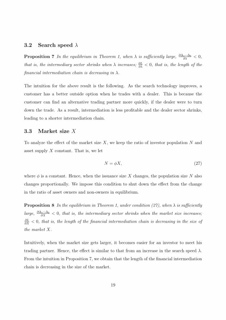
3.2 Search speed λ

Proposition 7 In the equilibrium in Theorem 1, when λ is sufficiently large, ∂∆s−∆b

∂λ< 0,

that is, the intermediary sector shrinks when λ increases; ∂L∂λ

< 0, that is, the length of the

financial intermediation chain is decreasing in λ.

The intuition for the above result is the following. As the search technology improves, a

customer has a better outside option when he trades with a dealer. This is because the

customer can find an alternative trading partner more quickly, if the dealer were to turn

down the trade. As a result, intermediation is less profitable and the dealer sector shrinks,

leading to a shorter intermediation chain.

3.3 Market size X

To analyze the effect of the market size X, we keep the ratio of investor population N and

asset supply X constant. That is, we let

N = ϕX, (27)

where ϕ is a constant. Hence, when the issuance size X changes, the population size N also

changes proportionally. We impose this condition to shut down the effect from the change

in the ratio of asset owners and non-owners in equilibrium.

Proposition 8 In the equilibrium in Theorem 1, under condition (27), when λ is sufficiently

large, ∂∆s−∆b

∂X< 0, that is, the intermediary sector shrinks when the market size increases;

∂L∂X

< 0, that is, the length of the financial intermediation chain is decreasing in the size of

the market X.

Intuitively, when the market size gets larger, it becomes easier for an investor to meet his

trading partner. Hence, the effect is similar to that from an increase in the search speed λ.

From the intuition in Proposition 7, we obtain that the length of the financial intermediation

chain is decreasing in the size of the market.

19

3.4 Trading need κ

Proposition 9 In the equilibrium in Theorem 1, when λ is sufficiently large, ∂(∆s−∆b)∂κ

> 0,

and ∂L∂κ

> 0, that is, the intermediary sector expands and the length of the intermediation

chain increases when the frequency of investors’ trading need increases.

The intuition for the above result is as follows. Suppose κ increases, i.e., investors need to

trade more frequently. This makes it more profitable for dealers. Hence, the intermediary

sector expands as more investors choose to become dealers, leading to a longer intermediation

chain.

3.5 Price dispersion

Theorem 1 shows that there is a continuum of prices for the asset in equilibrium. How is the

price dispersion related to search frictions? It seems reasonable to expect the price dispersion

to decrease as the market frictions diminishes. However, this intuition is not complete, and

the relationship between price dispersion and search frictions is more subtle.

To see this, we use D to denote the price dispersion

D ≡ Pmax − Pmin, (28)

where Pmax and Pmin are the maximum and minimum prices, respectively, among all prices.

Proposition 2 implies that

Pmax = P (∆,∆s), (29)

Pmin = P (∆b, 0). (30)

That is, Pmax is the price for the transaction between a buyer of type ∆ and a seller of

type ∆s. Similarly, Pmin is the price of the transaction between a buyer of type ∆b and a

seller of type 0. The following proposition shows that effect of the search speed on the price

dispersion.

Proposition 10 In the equilibrium in Theorem 1, when λ is sufficiently large, ∂D∂λ

< 0.

20

The intuition is the following. When the search speed is faster, investors do not have to

compromise as much on prices to speed up their transactions, because they can easily find

alternative trading partners if their current trading partners decided to walk away from their

transactions. Hence, the dispersion across prices becomes smaller when λ increases.

However, the relation between the price dispersion and the search cost c is more subtle.

As the search cost increases, fewer investors participate in the market. On the one hand,

this makes it harder to find a trading partner and so increases the price dispersion as the

previous proposition suggests. There is, however, an opposite driving force: Less diversity

across investors leads to a smaller price dispersion. In particular, as noted in Proposition

4, ∆s is decreasing in c, that is, when the search cost increases, only investors with lower

types are willing to pay the cost to try to sell their assets. As noted in (29), this reduces

the maximum price Pmax. On the other hand, when the search cost increases, only investors

with higher types are willing to buy. This increases the minimum price Pmin. Therefore,

as the search cost increases, the second force decreases the price dispersion. The following

proposition shows that the second force can dominate.

Proposition 11 In the equilibrium in Theorem 1, the sign of ∂D∂c

can be either positive or

negative. Moreover, when c is sufficiently small, we have ∂D∂c

< 0.

Price dispersion in OTC markets has been documented in the literature, e.g., Green, Hol-

lifield, and Schurhoff (2007). Jankowitsch, Nashikkar, and Subrahmanyam (2011) proposes

that price dispersion can be used as a measure of liquidity. Our analysis in Proposition 10

confirms this intuition that the price dispersion is larger when the search speed is lower,

which can be interpreted as the market being less liquid. However, Proposition 11 also illus-

trates the potential limitation, especially in an environment with a low search cost. It shows

that the price dispersion may decrease when the search cost is higher.

3.6 Price dispersion ratio

To further analyze the price dispersion in the economy, we define dispersion ratio as

DR ≡ P dmax − P d

min

Pmax − Pmin

, (31)

21

where P dmax and P d

min are the maximum and minimum prices, respectively, among inter-dealer

transactions. That is, DR is the ratio of the price dispersion among inter-dealer transactions

to the price dispersion among all transactions.

This dispersion ratio measure has two appealing features. First, somewhat surprisingly,

it turns out to be easier to measure DR than D. Conceptually, price dispersion D is the

price dispersion at a point in time. When measuring it empirically, however, we have to

compromise and measure the price dispersion during a period of time (e.g., a month or a

quarter), rather than at an instant. As a result, the asset price volatility directly affects

the measure D. In contrast, the dispersion ratio DR alleviates part of this problem since

asset price volatility affects both the numerator and the denominator. Second, as noted in

Proposition 11, the effect of search cost on the price dispersion is ambiguous. In contrast,

our model predictions on the price dispersion ratio are sharper, as illustrated in the following

proposition.

Proposition 12 In the equilibrium in Theorem 1, we have ∂DR∂c

< 0; when λ is sufficiently

large, we have ∂DR∂λ

< 0, ∂DR∂κ

> 0, and under condition (27) we have ∂DR∂X

< 0.

Intuitively, DR is closely related to the size of the intermediary sector. All these parameters

(c, λ,X, and κ) affect DR through their effects on the interval (∆b,∆s). For example, as

noted in Proposition 4, when the search cost c increases, the intermediary sector (∆b,∆s)

shrinks, and so the price dispersion ratio DR decreases. The intuition for the effects of all

other parameters (λ,X, and κ) is similar.

In summary, both DR and L are closely related to the size of the intermediary sector.

All the parameters of (c, λ,X, and κ) affect both DR and L through their effects on the

size of the intermediary sector, i.e., the size of the interval (∆b,∆s). Indeed, by comparing

the above results with Propositions 5, 7, 8, and 9, we can see that, for all four parameters

(c, λ,X, and κ), the effects on DR and L have the same sign.

22

3.7 Welfare

What are the welfare implications from the intermediation chain? For example, is a longer

intermediation chain an indication of higher or lower investors’ welfare? Propositions 5–12

have shed some light on this question. In particular, a longer intermediation chain is a sign

of a lower c, a lower λ, a higher κ, or a lower X, which have different welfare implications.

Hence, the chain length and dispersion ratio are not clear-cut indicators of investors’ welfare.

For example, a lower c means that more investors search in equilibrium. Hence, high-∆

investors can obtain the asset more quickly, leading to higher welfare for all investors. On the

other hand, a lower λ means that investors obtain their desired asset positions more slowly,

leading to lower welfare for investors. Therefore, if the intermediation chain L becomes

longer because of a lower c, it is a sign of higher investor welfare. However, if it is due to a

slower search speed λ, it is a sign of lower investor welfare. A higher κ means that investors

have more frequent trading needs. If L becomes longer because of a higher κ, holding

the market condition constant, this implies that investors have lower welfare. Finally, if L

becomes longer because of a smaller X, it means that investors execute their trades more

slowly, leading to lower welfare for investors. To formalize the above intuition, we use W to

denote the average expected utility across all investors in the economy. The relation between

investors’ welfare and those parameters is summarized in the following proposition.

Proposition 13 In the equilibrium in Theorem 1, we have ∂W∂c

< 0; when λ is sufficiently

large, we have ∂W∂λ

> 0, ∂W∂κ

< 0, and under condition (27) ∂W∂X

> 0.

4 On Convergence

When the search friction disappears, does the search market equilibrium converge to the

equilibrium in a centralized market? Since Rubinstein and Wolinsky (1985) and Gale (1987),

it is generally believed that the answer is yes. This convergence result is also demonstrated

in Duffie, Garleanu, and Pedersen (2005), the framework we adopted.

However, we show in this section that as the search technology approaches perfection

(i.e., λ goes to infinity) the search equilibrium does not always converge to a centralized

23

market equilibrium. In particular, consistent with the existing literature, the prices and

allocation in the search equilibrium converge to their counterparts in a centralized-market

equilibrium, but the trading volume may not.

4.1 Centralized market benchmark

Suppose we replace the search market in Section 2 by a centralized market and keep the rest

of the economy the same. That is, investors can execute their transactions without any delay.

The centralized market equilibrium consists of an asset price Pw and a cutoff point ∆w. All

asset owners above ∆w and nonowners below ∆w stay inactive. Moreover, each nonowner

with a type higher than ∆w buys one unit of the asset instantly and each owner with a type

lower than ∆w sells his asset instantly, such that all investors find their strategies optimal,

the distribution of all groups of investors remain constant over time, and the market clears.

This equilibrium is given by the following proposition.

Proposition 14 In this centralized market economy, the equilibrium is given by

∆w = F−1

(1− X

N

), (32)

Pw =1 +∆w

r. (33)

The total trading volume per unit of time is

TVw = κX

(1− X

N

). (34)

As shown in (33), the asset price is determined by the marginal investor’s valuation ∆w.

Asset allocation is efficient since (almost) all investors whose types are higher than ∆w are

asset owners, and (almost) all investors whose types are lower than ∆w are nonowners.

Trading needs arise when investors’ types change. In particular, an asset owner becomes a

seller if his new type is below ∆w and a nonowner becomes a buyer if his new type is above

∆w. In this idealized market, they can execute their transactions instantly. Hence, at each

point in time, the total measure of buyers and sellers are infinitesimal, and the total trading

volume during [t, t+ dt) is TVwdt.

24

4.2 The limit case of the search market

Denote the total trading volume in the search market economy in Section 2 as

TV ≡ TVcc + TVcd + TVdc + TVdd. (35)

The following proposition reports asymptotic properties of the search equilibrium.

Proposition 15 When λ goes to infinity, the equilibrium in Theorem 1 is given by

limλ→∞

∆b = limλ→∞

∆s = ∆w, (36)

limλ→∞

P (x, y) = Pw for any x < y, (37)

limλ→∞

µh(∆) =

{Nf(∆) if ∆ > ∆w,

0 if ∆ < ∆w,(38)

limλ→∞

µn(∆) =

{0 if ∆ > ∆w,

Nf(∆) if ∆ < ∆w,(39)

limλ→∞

µb(∆) = limλ→∞

µs(∆) = 0, (40)

limλ→∞

TV− TVw

TVw

= logc

c, (41)

where c is a constant, with c > c, and is given by

c =

√∫ ∆w

0

F (x)

F (∆w)dx

√∫ ∆

∆w

1− F (x)

1− F (∆w)dx. (42)

As λ goes to infinity, many aspects of the search equilibrium converge to their counterparts in

a centralized market equilibrium. First, the interval (∆b,∆s) shrinks to a single point at ∆w

(equation (36)), and the size of the intermediary sector goes to zero. Second, all transaction

prices converge to the price in the centralized market, as shown in equation (37). Third,

the asset allocation in the search equilibrium converges to that in the centralized market.

As shown in equations (38)–(40), almost all investors whose types are higher than ∆w are

inactive asset holders, and almost all investors whose types are lower than ∆w are inactive

nonowners. The population sizes for buyers and sellers are infinitesimal.

However, there is one important difference. The equation (41) shows that as λ goes to

infinity, the total trading volume in the search market equilibrium is higher than the volume

25

in the centralized market equilibrium. This is surprising, especially given the result in (36)

that the size of the intermediary sector shrinks to 0.

It is worth emphasizing that this result is not a mathematical quirk from taking limit.

Rather, it highlights an important difference between a search market and an idealized cen-

tralized market. Intuitively, the excess trading in the search market is due to intermediaries,

who act as middlemen, buying the asset from one investor and selling to another. As λ

increases, the intermediary sector shrinks. However, thanks to the faster search technology,

each intermediary can execute more trades such that the total excess trading induced by

intermediaries increases with λ despite the reduction of the intermediary sector size. As λ

goes to infinity, the trading volume in the search market remains significantly higher than

that in a centralized market.

As illustrated in (41), the difference between TV and TVw is larger when the search cost

c is smaller, and approaches infinity when c goes to 0. As noted in Proposition 4, the smaller

the search cost c, the larger the intermediary sector. Hence, the smaller the search cost c,

the larger the excess trading generated by middlemen.

These results shed some light on why centralized market models have trouble explaining

trading volume, especially in markets with small search frictions. Even in the well-developed

stock market in the U.S., some trading features are perhaps better captured by a search

model. Over the past a few decades, the cheaper and faster technology makes it possible

for investors to exploit opportunities that were prohibitive with a less developed technology.

Numerous trading platforms were set up to compete with main exchanges; hedge funds and

especially high-frequency traders directly compete with traditional market makers. It seems

likely that the increase in turnover in the stock market in the past a few decades was driven

partly by the decrease in the search frictions in the market. Intermediaries, such as high

frequency traders, execute a large volume of trades to exploit opportunities that used to be

prohibitive.

In summary, our analysis suggests that a centralized market model captures the behavior

of asset prices and allocations when market frictions are small. However, it is not well-suited

for analyzing trading volume, even in a market with a fast search speed, especially in the

26

case when the search cost is small.

4.3 Equilibrium without intermediation

Our discussion so far has focused on the case c < c∗. We now briefly summarize the analysis

for the other case. As noted in Section 3.1, when c increases to c∗, the interval (∆b,∆s)

shrinks to a point and the intermediary sector disappears. As one might have expected,

intermediaries disappear in the equilibrium for the case of c ≥ c∗.

Similar to the analysis in Section 2, we can construct an equilibrium for the case c ≥ c∗.

The only difference is that as described in Panel A of Figure 1, two cutoff points ∆b and ∆s are

such that ∆b ≥ ∆s. In the equilibrium in Theorem 1, investors with intermediate valuations

become intermediaries and stay in the market continuously. In contrast, in this case with

a higher search cost, investors with intermediate valuations choose not to participate in the

market. Only those with strong trading motives (buyers with types higher than ∆b and

sellers with types lower than ∆s) are willing to pay the high search cost to participate in the

market. In the limit case where λ goes to infinity, as in Proposition 15, equations (36)–(40)

still hold. However, we now have

limλ→∞

TV = TVw.

That is, as λ goes to infinity, both ∆b and ∆s converge to ∆w. The inactive sector shrinks

to a point. Moreover, the prices, allocation, and the trading volume all converge to their

counterparts in a centralized market equilibrium. This result further confirms our earlier

intuition that, in the intermediation equilibrium in Section 2, the difference between TV and

TVw is due to the extra trading generated by intermediaries acting as middlemen.

4.4 Alternative matching functions

Section 4.2 shows that the non-convergence result on volume is due to the fact that while λ

increases, the intermediary sector shrinks but each one can trade more quickly. The higher

trading speed dominates the reduction in the size of the intermediary sector. One natural

question is whether this result depends on the special matching function in our model. As

explained in Section 2, for tractability, we adopt the matching function λNbNs. Does our

27

non-convergence conclusion depend on this assumption?

To examine this, we modify our model to have a more general matching function: We now

assume that the matching function is λQ(Nb, Ns), where Q(·, ·) is homogeneous of degree k

(k > 0) in Nb and Ns. The matching function in our previous analysis, λNbNs, is a special

case with homogeneity of degree 2. The rest of the model is kept the same as in Section 2.

We construct an intermediation equilibrium that is similar to the one in Theorem 1, and let

λ go to infinity to compare the limit equilibrium with the centralized market equilibrium.

The conclusions based on this general matching function remain the same as those in

Section 4.2. When λ goes to infinity, both the prices and allocation converge to their coun-

terparts in a centralized market equilibrium, but the trading volume does not. Interestingly,

the trading volume in this generalized model converges to exactly the same value as in our

previous model, and is given by (41).

5 Efficiency

This section analyzes the efficiency of the intermediary sector size. Specifically, let’s imagine

a social planner, who can determine the choices of all investors. That is, the social planner

chooses the two cutoff points in (3) and (4) to maximize the average of all investors’ expected

utility over their life time. Investors follow this decision rule set by the social planner,

and face the same market frictions as described in Section 2. Compared to this social

planer equilibrium, does the decentralized equilibrium in Section 3 have efficient amount

of intermediaries? In other words, if we use ∆eb and ∆e

s to denote the two cut-off points

in the social planner case, the question becomes: does the interval (∆eb,∆

es) coincide with

(∆b,∆s) in Theorem 1? The asymptotic analysis in the following proposition shows that

this is generally not the case.

Proposition 16 Suppose λ is sufficiently large. If η = 1/2, the intermediary sector in the

decentralized equilibrium is close to that in the social planner case:

∆b = ∆eb + o(λ−1/2), (43)

∆s = ∆es + o(λ−1/2). (44)

28

If η = 1/2, however, the decentralized equilibrium may have too much or too little interme-

diation.

The above results are reminiscent of the Hosios (1990) condition that efficiency is achieved

only for a specific distribution of bargaining powers between buyers and sellers. The matching

function we adopted is symmetric for buyers and sellers, and our proposition shows that the

efficiency is achieved when the buyers and sellers have the same bargaining power. In the

case of η = 1/2, however, the decentralized equilibrium is generally inefficient. We illustrate

in the proof of this proposition that the decentralized equilibrium may have too much or too

little intermediation, depending on the distribution of investors’ types F (·).

6 Empirical Analysis

In this section, we conduct empirical tests of the model predictions on the intermediation

chain length L and the price dispersion ratio DR. We choose to analyze the U.S. corporate

bond market, which is organized as an OTC market. Moreover, a large panel dataset is

available that makes it possible to conduct the tests reliably. Finally, some of the propositions

in Section 3 were proved under the condition that λ is sufficiently large. It might be natural

to expect that the search speed in the corporate bond market in the U.S. is sufficiently fast.

6.1 Hypotheses

Our analysis in Section 3 provides predictions on the effects of search cost c, market size

X, trading need κ, and search technology λ. There is perhaps little variation in the search

technology λ across corporate bonds in our sample during 2002–2012. Hence, our empirical

analysis will focus on the cross-sectional analysis on the effects of c, X, and κ.

Specifically, we obtain a number of observable variables that can be used as proxies for

these three parameters. Table 1 summarizes the interpretations of our proxies and model

predictions. We use issuance size as a proxy for the market size X. Another variable that

captures the effect of market size is bond age, i.e., the number of years since issuance. The

idea is that after a corporate bond is issued, as time goes by, a larger and larger fraction of

29

the issuance reaches long-term buy-and-hold investors such as pension funds and insurance

companies. Hence, the active size of the market becomes smaller as the bond age increases.

With these interpretations, Propositions 8 and 12 imply that the intermediation chain length

L and price dispersion ratio DR should be decreasing in the issuance size, but increasing in

bond age.

We use turnover as a proxy for the frequency of investors’ trading need κ. The higher

the turnover, the more frequent the trading needs are. Propositions 9 and 12 imply that the

chain length L and dispersion ratio DR should be increasing in turnover.

As proxies for the search cost c, we use credit rating, time to maturity, and effective

bid-ask spread. The idea is that these variables are related to the cost that dealers face. For

example, all else being equal, it is cheaper for dealers to make market for investment-grade

bonds than for high-yield or non-rated bonds, perhaps because dealers face less inventory

risk and less capital charge for holding investment-grade bonds. Hence, our interpretation

is that the search cost c is smaller for investment-grade bonds. Moreover, bonds with longer

maturities are more risky, and so more costly for dealers to make market (i.e., c is higher).

Finally, everything else being equal, a larger effective bid-ask spread implies a higher profit

for dealers (i.e., c is lower). With these interpretations, Propositions 4 and 12 imply that the

chain length L and price dispersion ratio DR should be larger for investment-grade bonds,

and for bonds with shorter time to maturity or larger bid-ask spreads.

Our goal here is to assess if our model can describe the behavior of intermediation chains

and price dispersion in the corporate bond market. We are certainly not drawing causal-

ity inferences. Rather, we attempt to examine if the correlations appear consistent with

the model implications in equilibrium. We keep in mind the possible endogeneity of the

independent variables, especially the effective bid-ask spread, and re-run our analysis after

dropping this variable.

6.2 Data

Our sample consists of corporate bonds that were traded in the U.S. between July 2002 and

December 2012. We combine two databases: the Trade Reporting and Compliance Engine

30

(TRACE) and the Fixed Income Securities Database (FISD). TRACE contains information

about corporate bond transactions, such as date, time, price, and volume of a transaction.

The dataset also classifies all transactions into “dealer-to-customer” or “dealer-to-dealer”

transactions.6 We rely on this classification to construct our measure of chain length L and

price dispersion ratio DR.

The FISD database contains information about a bond’s characteristics, such as bond

type, date and amount of issuance, maturity, and credit rating. We merge the two databases

using 9-digit CUSIPs. The initial sample from TRACE contains a set of 64,961 unique

CUSIPs; among them, 54,587 can be identified in FISD. We include in our final sample

corporate debentures ($8.5 trillion total issuance amount, or 62% of the sample), medium-

term notes ($2.2 trillion total issuance amount, or 16% of the sample), and convertibles ($0.6

trillion issuance amount, or 4% of the sample). In total, we end up with a sample of 25,836

bonds with a total issuance amount of $11.3 trillion.

We follow the definition in (26) to construct the chain length L for each corporate bond

during each period, where TVcd + TVdc is the total dealer-to-customer trading volume and

TVdd is the total dealer-to-dealer trading volume during that period. In our data, TVcc = 0,

that is, there is no direct transaction between two customers. Hence, the chain length is

always larger than or equal to 1.

We obtain the history of credit ratings on the bond level from FISD. For each bond, we

construct its credit rating history at the daily frequency: for each day, we use credit rating

by S&P if it is available, otherwise, we use Moody’s rating if it is available, and use Fitch’s

rating if both S&P and Moody’s ratings are unavailable. In the case that a bond is not rated

by any of the three credit rating agencies, we classify it as “not rated.” We use the rating

on the last day of the period to create a dummy variable IG , which equals one if a bond

has an investment-grade rating, and zero otherwise.

We use Maturity denote the time to maturity of a bond, measured in years, use Age to

denote the time since issuance of a bond, denominated in years, use Size to denote issuance

6According to TRACE User Guide, FINRA members are classified as “dealers” and non-FINRA memberinstitutions and retail accounts are classified as “customers.”

31

size of a bond, denominated in million dollars, and use Turnover to denote the total trading

volume of a bond during the period, normalized by its Size.

To measure the effective bid-ask spread of a bond, denoted as Spread, we follow Bao, Pan,

and Wang (2011) to compute the square root of the negative of the first-order autocovariance

of changes in consecutive transaction prices during the period, which is based on Roll (1984)’s

measure of effective bid-ask spread.

We follow the definition in equation (31) to construct the price dispersion ratio, DR, for

each bond and time period, where P dmax and P d

min are the maximum and minimum transaction

prices among dealer-to-dealer transactions according to the classification by TRACE, and

Pmax and Pmin are the maximum and minimum transaction prices among all transactions.

6.3 Summary statistics

Table 2 reports the summary statistics for variables measured at the monthly frequency. To

rule out extreme outliers, which are likely due to data error, we winsorize our sample by

dropping observations below the 1st percentile and above 99th percentile. For the overall

sample, the average chain length is 1.73. There is significant variation. The chain length

is 7.00 and 1.00 at the 99th and 1st percentiles, respectively. For investment-grade bonds,

the average chain length is 1.81 and the 99th percentile is 7.53, both higher than their

counterparts for the overall sample.

The average price dispersion ratio is 0.50 for the overall sample, and 0.51 for investment-

grade bonds. For the overall sample, the average turnover is 0.08 per month and the average

issuance size is $462 million. Investment-grade bonds have a larger average issuance size of

$537 million, and a turnover of 0.07. The effective bid-ask spread is 1.43% for the overall

sample, and 1.32% for the investment-grade subsample. The average bond age is around 5

years and the time to maturity is around 8 years.

6.4 Cross-sectional analysis

We run Fama-MacBeth regressions of chain length on the variables in Table 1, and the results

are reported in Table 3. As shown in column 1, the signs of all coefficients are consistent

32

with the model predictions, and all coefficients are highly significantly different from 0. The

coefficient for IG is 0.245 (t = 32.17) implying that, holding everything else constant, the

chain length for investment-grade bonds is longer than that for other bonds by 0.245 on

average, which is significant given that the mean chain length is 1.73.

The coefficient for Turnover is 0.199 (t = 11.48), suggesting that the chain length in-

creases with the frequency of investors’ trading needs. The coefficients for Size and Age are

−0.012 (t = 3.73) and 0.025 (t = 23.92), implying that the chain length is decreasing in the

size of the market. Also consistent with the model prediction, the coefficient for Maturity is

significantly negative. The coefficient for Spread is 0.073 (t = 17.17). Under the interpreta-

tion that a higher spread implies a lower search cost for dealers, this is consistent our model

that the chain length is decreasing in the search cost.

We then run another Fama-MacBeth regression, using the price dispersion DR as the

dependent variable. Our model predicts that the signs of coefficients for all the variables

should be the same as those in the regression for L. As shown in the third column of Table

3, five out of the six coefficients have the same sign as those in the regression for L in

column 1. For example, as shown in the third column of Table 3, the coefficient for IG is

0.007 (t = 2.62) implying that, holding everything else constant, the price dispersion for

investment grade bonds is larger than that for other bonds by 0.007 on average. Similarly,

as implied by our model, the coefficients for other variables such as Turnover, Age, Maturity,

and Spread are all significant and have the same sign as in the regression for L.

The only exception is the coefficient for Size. Contrary to our model prediction, the

coefficient is significantly positive. Intuitively, our model implies that, for a larger bond, it

is easier to find trading partners. Hence, it is less profitable for dealers, leading to a smaller

intermediary sector, and consequently a shorter intermediation chain and a smaller price

dispersion ratio. However, our evidence is only consistent with the implication on the chain

length. One conjecture is that our model abstracts away from the variation in transaction

size and dealers’ inventory capacity constraints. For example, in our sample, the monthly

maximum transaction size for the largest 10% of the bonds is more than 50 times larger

than that for the smallest 10% of the bonds. When facing extremely large transactions from

33

customers, with inventory capacity constraints, a dealer may have to offer price concessions

when trading with other dealers, leading to a larger price dispersion ratio. However, this

channel has a much weaker effect on the chain length, which reflects the average number

of layers of intermediation and so is less sensitive to the transactions of extreme sizes. As

a result, our model prediction on the chain length holds but the prediction on the price

dispersion does not.

As a robustness check, we reconstruct all variables at the quarterly frequency and re-

peat our analysis. As shown in the second and fourth columns, the results at the quarterly

frequency are similar to those at the monthly frequency. The only difference is that the coef-

ficient for Maturity becomes insignificant. Finally, we acknowledge the potential endogeneity

concern for the independent variables, especially Spread. Hence, we rerun our regressions

after dropping Spread, and our results remain very similar for all other variables.

In summary, despite its simple structure, our model appears to describe reasonably well

the intermediary sector in the U.S. corporate bond market. Especially, the dispersion ratio

DR is constructed based on price data while the chain length L is based on quantity data.

Yet, for almost all our proxies, their coefficients have the same sign across the two regressions

for DR and L, as implied by our model.

7 Conclusion

We analyze a search model with an endogenous intermediary sector and an intermediation

chain. The equilibrium is characterized in closed-form. Our model shows that the length

of the intermediation chain and price dispersion ratio are decreasing in search cost, search

speed, market size, but are increasing in investors’ trading need. Based on the data from the

U.S. corporate bond market, our evidence is broadly consistent with the model predictions.

As search frictions diminish, the search market equilibrium does not always converge

to a centralized market equilibrium. In particular, the prices and allocations in the search

market equilibrium converge to their counterparts in a centralized market equilibrium, but

the trading volume does not converge in the case with intermediaries. The difference between

34

the two trading volumes across the two equilibria increases when the search cost becomes

smaller, and approaches infinity when the search cost goes to zero. These results suggest

that a centralized market model captures the behavior of asset prices and allocations when

market frictions are small. However, it is not well-suited for analyzing trading volume, even

in a market with a fast search speed, especially in the case when the search cost is small.

35

8 Appendix

Proof of Theorem 1

The proof is organized as follows. Step I, we take ∆b, ∆s and decision rules (3) and (4) as

given to derive densities µs (∆), µb (∆), µn (∆), µh (∆). Step II, from the two indifference

conditions at ∆b and ∆s, we obtains equations (20) and (21) that pin down ∆b and ∆s. Step

III, we verify that decision rules (3) and (4) are indeed optimal for all investors.

Step I. We now show that µi(∆) for i = b, s, h, n are given by following. For ∆ ∈ [0,∆b),

µb (∆) = µh (∆) = 0, (45)

µn (∆) =κ (N −X) + λNbN

κ+ λNb

f (∆) , (46)

µs (∆) =κX

κ+ λNb

f (∆) . (47)

For ∆ ∈ (∆b,∆s),

µn (∆) = µh (∆) = 0, (48)

µs (∆) =Nf (∆)

2

1− N −NF (∆)−X − κλ√[

N −NF (∆)−X − κλ

]2+ 4κ

λ(N −X) [1− F (∆)]

, (49)

µb (∆) =Nf (∆)

2

1 + N −NF (∆)−X − κλ√[

N −NF (∆)−X − κλ

]2+ 4κ

λ(N −X) [1− F (∆)]

. (50)

For ∆ ∈(∆s,∆

],

µn (∆) = µs (∆) = 0, (51)

µb (∆) =κ (N −X)

κ+ λNs

f (∆) , (52)

µh (∆) =κX + λNsN

κ+ λNs

f (∆) . (53)

From (3) and (4), we have (45), (48), and (51). Substituting (51) into (12), we obtain

µb (∆) + µh (∆) = Nf (∆) .

From the above equation and (14), we obtain (52) and (53). The market clearing condition

36

(19), together with (45) and (48), implies that∫ ∆

∆s

µh (∆) d∆+Ns = X.

Substituting (53) into the above equation, we get an equation of Ns,

N2s +

(κλ+N −X −NF (∆s)

)Ns −

κX

λF (∆s) = 0

from which we get

Ns =1

2

√[κλ+N −X −NF (∆s)

]2+ 4

κX

λF (∆s)−

1

2

[κλ+N −X −NF (∆s)

]. (54)

The derivation for the region ∆ ∈ [0,∆b) is similar. We obtain (46) and (47), with

N2b +

(κλ−N +X +NF (∆b)

)Nb −

κ

λ(N −X) [1− F (∆b)] = 0. (55)

Solving the above equation for Nb, we obtain

Nb =N−NF (∆b)−X− κ

λ

2+

1

2

√[N −NF (∆b)−X− κ

λ

]2+ 4

κ

λ(N −X) [1−F (∆b)]. (56)

The derivation for the region ∆ ∈ (∆b,∆s) is the following. We rewrite (18) as

κdFs (∆)

d∆= κXf (∆)− λ [Nb − Fb (∆)]

dFs (∆)

d∆+ λFs (∆)

dFb (∆)

d∆. (57)

After some algebra, we get

κdFs (∆)

d∆= κXf (∆)− d

d∆[λ (Nb − Fb (∆))Fs (∆)] .

Integrating both sides from ∆b to ∆ ∈ (∆b,∆s), we have

κ [Fs (∆)−Fs (∆b)] = κX [F (∆)−F (∆b)]−λ [(Nb − Fb (∆))Fs (∆)−NbFs (∆b)] , (58)

where we have used the fact that Fb (∆b) = 0.

Substituting (47) into the definition of Fs (·), we have

Fs (∆b) =κX

κ+ λNb

F (∆b) . (59)

37

Substituting (48) into (12), we get

µs (∆) + µb (∆) = Nf (∆) . (60)

We can rewite the above equation as

dFb (∆)

d∆+

dFs (∆)

d∆= Nf (∆) .

Integrating both sides from ∆b to ∆ ∈ (∆b,∆s], after some algebra, we obtain

Fs (∆) = Fs (∆b)− Fb (∆) +N [F (∆)− F (∆b)] . (61)

Substituting (59) and (61) into (58), we get a quadratic euqation of Fb (∆), from which we

obtain the solution for Fb (∆). Differentiating it with respect to ∆, we obtain µb (∆) in (50).

From (60) we obtain µs (∆) in (49).

Step II. Let’s first determine Vn (∆) and Vh (∆) for ∆ ∈[0,∆

]. Equation (10) implies

that Vn (∆) is a constant for all ∆. We denote it by Vn ≡ Vn (∆). Equation (8) implies that

Vh (∆) is linear in ∆ with a positive slope

dVh (∆)

d∆=

1

κ+ r. (62)

We now compute the slope for Vs (∆) for the region ∆ ∈ [0,∆b). From (9), we have

Vs (∆) =1 + ∆− c

κ+ r+

κE [max {Vh (∆′) , Vs (∆

′)}]κ+ r

+λ (1− η)

κ+ r

∫ ∆s

∆b

[Vs (x) + Vn − Vb (x)− Vs (∆)]µb (x) dx

+λ (1− η)

κ+ r

∫ ∆

∆s

[Vh (x) + Vn − Vb (x)− Vs (∆)]µb (x) dx.

Differentiating both sides of the equation with respect to ∆, we obtain

dVs (∆)

d∆=

1

κ+ r + λ (1− η)Nb

. (63)

Similarly, for ∆ ∈ (∆b,∆s), we get

dVs (∆)

d∆=

1

κ+ r− λ (1− η)

κ+ r

[dVs (∆)

d∆− dVb (∆)

d∆

] ∫ ∆

∆

µb (x) dx. (64)

38

Let’s now determine the slope for Vb (∆) for ∆ ∈(∆s,∆

]. From (11), we have

Vb (∆) = − c

κ+ r+

κE [max {Vb (∆′) , Vn}]

κ+ r

+λη

κ+ r

∫ ∆b

0

[Vh (∆) + Vn (x)− Vb (∆)− Vs (x)]µs (x) dx

+λη

κ+ r

∫ ∆s

∆b

[Vh (∆) + Vb (x)− Vb (∆)− Vs (x)]µs (x) dx.

Differentiating both sides with respect to ∆, after some algebra, we obtain

dVb (∆)

d∆=

1

κ+ r

ληNs

κ+ r + ληNs

for ∆ ∈(∆s,∆

]. (65)

Similarly, for ∆ ∈ (∆b,∆s), we have

dVb (∆)

d∆=

λη

κ+ r

[dVs (∆)

d∆− dVb (∆)

d∆

] ∫ ∆

0

µs (x) dx. (66)

From (64) and (66), we can solve for the dVs(∆)d∆

and dVs(∆)d∆

for ∆ ∈ (∆b,∆s). Then, we have

the following

dVs (∆)

d∆=

{1

κ+r+λ(1−η)Nbfor ∆ ∈ [0,∆b)

1κ+r

κ+r+ληFs(∆)κ+r+λ(1−η)[Nb−Fb(∆)]+ληFs(∆)

for ∆ ∈ (∆b,∆s). (67)

dVb (∆)

d∆=

{1

κ+rληFs(∆)

κ+r+λ(1−η)[Nb−Fb(∆)]+ληFs(∆)for ∆ ∈ (∆b,∆s)

1κ+r

ληNs

κ+r+ληNsfor ∆ ∈

(∆s,∆

] . (68)

From the above expressions for the slopes, we obtain the following

Vn =κ

r

∫ ∆s

∆b

dVb (z)

dz[1− F (z)] dz +

κ

r

1

κ+ r

ληNs

κ+ r + ληNs

∫ ∆

∆s

[1− F (z)] dz. (69)

Vb (∆) = Vn +

{ ∫ ∆

∆b

dVb(z)dz

dz for z ∈ [∆b,∆s]∫ ∆s

∆b

dVb(z)dz

dz + 1κ+r

ληNs

κ+r+ληNs(∆−∆s) for z ∈

(∆s,∆

] , (70)

Vh (∆) = Vh (∆s) +∆−∆s

κ+ r, (71)

where

Vh (∆s) =1+∆s

r− κ

r

∫ ∆b

0F (z) dz

κ+ r + λNb (1− η)− κ

r

∫ ∆s

∆b

dVs (z)

dzF (z) dz +

κ

r

∫ ∆

∆s[1− F (z)] dz

κ+ r,

39

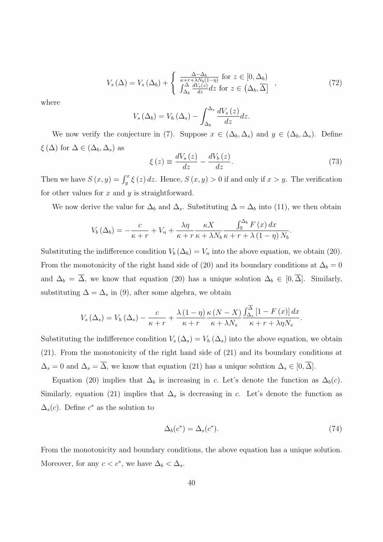
Vs (∆) = Vs (∆b) +

{∆−∆b

κ+r+λNb(1−η)for z ∈ [0,∆b)∫ ∆

∆b

dVs(z)dz

dz for z ∈(∆b,∆

] , (72)

where

Vs (∆b) = Vh (∆s)−∫ ∆s

∆b

dVs (z)

dzdz.

We now verify the conjecture in (7). Suppose x ∈ (∆b,∆s) and y ∈ (∆b,∆s). Define

ξ (∆) for ∆ ∈ (∆b,∆s) as

ξ (z) ≡ dVs (z)

dz− dVb (z)

dz. (73)

Then we have S (x, y) =∫ x

yξ (z) dz. Hence, S (x, y) > 0 if and only if x > y. The verification

for other values for x and y is straightforward.

We now derive the value for ∆b and ∆s. Substituting ∆ = ∆b into (11), we then obtain

Vb (∆b) = − c

κ+ r+ Vn +

λη

κ+ r

κX

κ+ λNb

∫ ∆b

0F (x) dx

κ+ r + λ (1− η)Nb

.

Substituting the indifference condition Vb (∆b) = Vn into the above equation, we obtain (20).

From the monotonicity of the right hand side of (20) and its boundary conditions at ∆b = 0

and ∆b = ∆, we know that equation (20) has a unique solution ∆b ∈ [0,∆]. Similarly,

substituting ∆ = ∆s in (9), after some algebra, we obtain

Vs (∆s) = Vh (∆s)−c

κ+ r+

λ (1− η)

κ+ r

κ (N −X)

κ+ λNs

∫ ∆

∆s[1− F (x)] dx

κ+ r + ληNs

.

Substituting the indifference condition Vs (∆s) = Vh (∆s) into the above equation, we obtain

(21). From the monotonicity of the right hand side of (21) and its boundary conditions at

∆s = 0 and ∆s = ∆, we know that equation (21) has a unique solution ∆s ∈ [0,∆].

Equation (20) implies that ∆b is increasing in c. Let’s denote the function as ∆b(c).

Similarly, equation (21) implies that ∆s is decreasing in c. Let’s denote the function as

∆s(c). Define c∗ as the solution to

∆b(c∗) = ∆s(c

∗). (74)

From the monotonicity and boundary conditions, the above equation has a unique solution.

Moreover, for any c < c∗, we have ∆b < ∆s.

40

Step III. We now verify that a non-owner’s optimal choice is given by (3) and that an

owner’s optimal choice is given by (4). We can prove both by contradiction.

Let’s first consider the case for an owner with ∆ ∈(∆s,∆

]. Suppose this owner deviates

from the equilibrium choice (4), i.e, rather than staying inactive, he searches in the market

during a period [t, t+ dt) and then returns to the equilibrium strategy (3) and (4). Let’s use

Vo (∆) to denote the investor’s expected utility if he follows this alternative strategy:

Vo (∆) = (1 + ∆− c) dt+ κE [max {Vh (∆′) , Vs (∆

′)}] dt

+λdt (1− η)

∫ ∆

∆

S (x,∆)µb (x) dx+ e−rdt (1− κdt)Vh (∆) ,

where S (x,∆) denotes the trading surplus if this owner meets a buyer of type x > ∆:

S (x,∆) = Vh (x) + Vb (∆)− Vb (x)− Vo (∆) ,

where we have used the result that the trading surplus is negative if the buyer’s type is lower

than the owner. For the owner to deviate, it has to be the case that Vo (∆) > Vh (∆). Hence,

the trade surplus is bounded by

S (x,∆) < Vh (x) + Vb (∆)− Vb (x)− Vh (∆) .

Substituting (70) into the right hand side of the above inequality, we obtain

S (x,∆) <x−∆

κ+ r + ληNs

. (75)

By comparing Vo (∆) and Vh (∆), we obtain

Vo (∆)− Vh (∆) = −cdt+ λdt (1− η)

∫ ∆

∆

S (x,∆)µb (x) dx. (76)

Substituting (75) and (52) into the above equation, we obtain

Vo (∆)− Vh (∆) < −λ (1− η)κ (N −X)

∫ ∆

∆s[1− F (x)] dx

(κ+ λNs) (κ+ r + ληNs)dt < 0. (77)

This contradicts Vo (∆) > Vh (∆). The proofs for other values for ∆ and the decision rule

(3) are similar.

41

Proof of Propositions 1–3

Propositions 1 and 2 can be obtained by differentiation. To prove Proposition 3, note that

TVcc is the total volume of trades between sellers with types [0,∆b), whose population size

is Fs (∆b), and buyers with types(∆s,∆

], whose population size is Nb − Fb (∆s). Note that

any meeting between the two groups will lead to a trade. Hence, the total volume is given

by (22). By the same logic, we obtain TVcc and TVdc in (23) and (24).

TVdd is the total volume of trades between sellers with types y ∈ (∆b,∆s) and buyers

with types x ∈ (∆b,∆s). However, trade occurs if and only if x > y. For any ∆ ∈ (∆b,∆s),

the density of buyers is dFb (∆). They only trade with sellers whose types are below ∆,

and whose population size is Fs (∆) − Fs (∆b). Hence, type-∆ investors’ trading volume is

λ [Fs (∆)− Fs (∆b)] dFb (∆). Integrating this volume for ∆ ∈ (∆b,∆s), we obtain (25).

Proof of Proposition 4–6

Based on equations (20) and (56), after some tedious algebra, we obtain d∆b

dc> 0 and dNb

dc< 0.

Similarly, Equations (21) and (54) imply d∆s

dc> 0 and dNs

dc< 0. Differentiating L with respect

to c, we can obtain dLdc

< 0. From (20) and (21), we can see that c = 0 implies that ∆b = 0,

and ∆s = ∆. This implies that Nb = N −X, Ns = X, and L = ∞.

Proof of Proposition 7

Let’s first conduct asymptotic analysis when λ is sufficiently large. Denote the limit of ∆b

and ∆s under λ → ∞ by

∆∞b ≡ lim

λ→∞∆b,

∆∞s ≡ lim

λ→∞∆s.

We can rewrite (20) as

λN2b +

(κ+

κ+ r

1− η

)Nb +

κ (κ+ r)

(1− η)λ=

κηX

(1− η) c

∫ ∆b

0

F (x) dx. (78)

When λ goes to infinity, the right hand side of (78) converges to a positive constant (it is

42

easy to see that ∆∞b = 0):

limλ→∞

κηX

(1− η) c

∫ ∆b

0

F (x) dx =κηX

(1− η) c

∫ ∆∞b

0

F (x) dx.

Hence, the left hand side of (78) also converges to this postive constant, which implies

Nb =Mb√λ+ o

(λ−1/2

), where Mb =

√κηX

(1− η) c

∫ ∆∞b

0

F (x) dx. (79)

Substituting the above equation into (55),

[NF(∆b)−N+X]

(Mb√λ+ o(λ−1/2)

)+

1

λ

(M2

b − κ (N −X) [1− F (∆∞b )]

)+ o(

1

λ) = 0. (80)

The above equation implies that

NF (∆b)−N +X = O(1√λ).

From the above equation, we have

∆∞b = ∆w,

∆b −∆∞b = O(

1√λ). (81)

where ∆w ≡ F−1(N−XN

). Hence, we can write (81) as

∆b = ∆w +mb√λ+ o

(λ−1/2

), (82)

where mb is a constant. Substituting this expression of ∆b into (80), and setting the coeffi-

cient of 1/λ to zero, we obtain

mb =1

Nf (∆w)

[κX

(1− X

N

)Mb

−Mb

].

Following a similar logic, we obtain

∆∞s = ∆w

Ns =Ms√λ+ o

(λ−1/2

)with Ms =

√κ (1− η) (N −X)

ηc

∫ ∆

∆w

[1− F (x)] dx, (83)

∆s = ∆w +ms√λ+ o

(λ−1/2

)with ms =

1

Nf (∆w)

[Ms −

κX(1− X

N

)Ms

]. (84)

43

Finally, we can verify that ∆s > ∆b in the asymptotic case if ms > mb, which can be

shown as equivalent to c < c. With the expressions of ∆b, ∆s, Nb, Ns we can obtain all other

equilibrium quantities in the asymptotic case.

With the above results, we can now prove Proposition 7 by expanding L as the following

L = lnc

c+

Z√λg(cc

)+ o

(λ−1/2

), (85)

where Z is a positive constant and is given by

Z ≡ κ

2Nc

√ηX

(N −X) (1− η)

∫ ∆w

∆

F (y)

F (∆w)dy +

√(N −X) (1− η)

ηX

∫ ∆

∆w

1− F (x)

1− F (∆w)dx

,

and g (·) is the following function

g (x) ≡ 3x−(1 +

1

x

)lnx− 1, for x ∈ [0, 1].

It is easy to show that g (x) > 0. Hence, (85) implies dLdλ

< 0 when λ is sufficiently large.

Proof of Propositions 8–9

Equation (85) implies that when λ is sufficiently large, we have ∂L∂κ

> 0, and that under

condition (27), we have ∂L∂X

< 0. To prove the rest of the two propositions, we expand

∆s −∆b as the following

∆s −∆b =Y√λ+ o

(λ−1/2

),

where Y is given by

Y =1− c

c

ϕ√Xf (∆w)

√ κη

(1− η) c

∫ ∆w

∆

F (y) dy +

√κ (1− η)

ηc(ϕ− 1)

∫ ∆

∆w

[1− F (x)] dx

.

The above equation implies that ∂(∆s−∆b)∂κ

> 0, and under condition (27), ∂(∆s−∆b)∂X

< 0.

Proof of Proposition 10 and 11

When λ is sufficiently large, we can expand D as

D =

√c√λ

∆w√κ(1−η)X

η

∫ ∆w

0F (x) dx

+

(∆−∆w

)√κη(N−X)(1−η)

∫ ∆

∆w[1− F (x)] dx

+ o

(1√λ

).

44

It is direct to see that ∂D∂λ

< 0 and ∂D∂c

> 0 in this case.

If c is close to zero, D can be expanded as

D =

∫ ∆s

∆b

ξ (z) dz +O(√

c),

where ∆s = ∆ − O (√c) and ∆b = O (

√c). It can be shown that ∂

∂c

(∫ ∆s

∆bξ (z) dz

)< 0, so

we obtain ∂D∂c

< 0 when c is sufficiently small.

Proof of Proposition 12

From the definition, we have

P dmax = P (∆s,∆s) ,

P dmin = P (∆b,∆b) .

Substituting them and (29) and (30) into (31), and differentiating it, we obtain ∂DR∂c

< 0.

It is easy to show that

P dmax − P d

min = O(λ−1

),

Pmax − Pmin = O(λ−1/2

).

It follows that DR = O(λ−1/2). Therefore, ∂DR∂λ

< 0 when λ is sufficiently large. Similarly,

we can show that, when λ is sufficiently large, we have

∂

∂κ

(P dmax − P d

min

)> 0,

∂

∂κ(Pmax − Pmin) < 0,

which implies ∂DR∂κ

> 0. Furthermore, under the condition in (27), we can show

P dmax − P d

min = O

(1

λX

),

Pmax − Pmin = O

(1√λX

),

which implies that DR = O( 1√λX

). Therefore, when λ is sufficiently large, we have ∂DR∂X

< 0.

45

Proof of Proposition 13

The average expected utility across all investors in the economy is defined by

W ≡ 1

N

∑i∈{b,s,h,n}

[∫ ∆

0

Vi (∆)µi (∆) d∆

].

When λ is sufficiently large, we have the following

W = Ww − mw√λ+ o

(λ−1/2

),

where Ww is average expected utility in a centralized market and is given by

Ww =1

r

∫ ∆

∆w

(1 + ∆) d∆,

and mW is given by

mw =1

r

√κc

η (1− η)X

√1

ϕ

(1− 1

ϕ

)∫ ∆

∆w

[1− F (x)] dx+1

ϕ

√∫ ∆w

∆

F (x) dx

.

By examining mw, we can obtain all the conclusions in this proposition.

Proof Proposition 14

In a centralized market, transactions can be executed instantly, hence, all investors whose

types are higher than ∆w are holding the total X units of the asset. This implies

F (∆w) = 1− X

N, (86)

which leads to (32). Similar to the proof for Theorem 1, we can obtain the expected utility

of an asset owner V co (∆) and of an non-owner V c

n (∆)

V co (∆) =

1 + ∆+ κE [max {V cn (∆) , V c

n (∆) + Pw}]κ+ r

,

V cn (∆) =

κE [max {V co (∆)− Pw, V

cn (∆)}]

κ+ r.

The indifference condition of a type-∆w investor is

V co (∆) = V c

n (∆w) + Pw.

The above three equations lead to (33). During [t, t + dt), κXdt investors’ types change.

F (∆w) of them have new types below ∆w, and sell their assets. Hence, the trading volume

is given by (34).

46

Proof Proposition 15

From the asymptotic analysis in the proof of Proposition 7, we obtain (36)–(40). Substituting

them into (22)–(25), we obtain (41).

Proof Proposition 16

The social welfare, denoted by W e, is the discounted sum of all realized cash flows from

holding the asset net of total search cost, i.e.,

W e =1

r

∫ ∆

0

(1 + ∆) [µh (∆) + µs (∆)] d∆− 1

rc (Nb +Ns) .

where µh (·) and µs (·) are given in Theorem 1. After some algebra, the social planner’s the

first-order condition with respect to ∆s can be simplified to

c =

∫ ∆

∆s

1− F (∆)

1− F (∆s)d∆

X−Ns

1−F (∆s)

(2Ns −X + κ

λ

)+(NX − 2NNs − κX

λ

)NNs +

κXλ

.

When λ is sufficiently large, we have the following asymptotics

∆es = ∆w +

mes√λ+ o(λ−1/2),

N es =

M es√λ+ o(λ−1/2),

where

mes =

1

Nf (∆w)

[M e

s −κX

(1− X

N

)M e

s

],

M es =

√η

1− ηMs.

Similarly, the first order condition with respect to ∆b is given by

c =κX

∫ ∆b

0F (∆) d∆

(κ+ λNb)2 .

When λ is sufficiently large, we have the following asymptotics

∆eb = ∆w +

meb√λ+ o(λ−1/2),

N eb =

M eb√λ+ o(λ−1/2),

47

where

meb =

1

Nf (∆w)

[κX

(1− X

N

)M e

b

−M eb

],

M eb =

√1− η

ηMb.

When η = 12, we have M e

b = Mb and M es = Ms. From (82) and (84), we obtain (43)

and (44). Otherwise, the decentralized equilibrium is generally inefficient. For example, in

the case of η > 12, the intermediary sector in the decentralized equilibrium is too big (i.e.,

∆s −∆b > ∆es −∆e

b) ifηcb

(1−η)cs> 1, and is too small if ηcb

(1−η)cs< 1, where

cb ≡∫ ∆w

0

F (∆)

F (∆w)d∆,

cs ≡∫ ∆

∆w

1− F (∆)

1− F (∆w)d∆.

48

References

Adrian, Tobias and Hyun Song Shin, 2010, The Changing Nature of Financial Intermedia-tion and the Financial Crisis of 2007-09, Annual Review of Economics 2, 603–618.

Afonso, Gara and Ricardo Lagos, 2014, An Empirical Study of Trade Dynamics in the FedFunds Market, working paper.

Afonso, Gara and Ricardo Lagos, 2015, Trade Dynamics in the Market for Federal Funds,Econometrica, forthcoming.

Atkeson, Andrew, Andrea Eisfeldt, and Pierre-Olivier Weill, 2014, Entry and Exit in OTCDerivatives Markets, working paper.

Babus, Ana and Peter Kondor, 2012, Trading and information diffusion in OTC markets,working paper.

Bao, Jack, Jun Pan, and Jiang Wang, 2011, The Illiquidity of Corporate Bonds, Journal ofFinance 66, 911–946.

Chang, Briana, 2014, Adverse Selection and Liquidity Distortion, working paper.

Chang, Briana and Shengxing Zhang, 2015, Endogenous Market Making and Network For-mation, working paper.

Di Maggio, Marco, Amir Kermani, and Zhaogang Song, 2015, The Value of Trading Rela-tionship in Turbulent Times.

Duffie, Darrell, Nicolae Garleanu, and Lasse Pedersen, 2002, Securities Lending, Shortingand Pricing, Journal of Financial Economics, 66, 307–339.

Duffie, Darrell, Nicolae Garleanu, and Lasse Pedersen, 2005, Over-the-Counter Markets,Econometrica, 73, 1815–1847.

Duffie, Darrell, Nicolae Garleanu, and Lasse Pedersen, 2007, Valuation in Over-the-CounterMarkets, Review of Financial Studies, 66, 307–339.

Duffie, Darrell, Piotr Dworczak, and Haoxiang Zhu, 2014, Benchmarks in Search Markets,working paper.

Feldhutter, Peter, 2012, The same bond at different prices: Identifying search frictions andselling pressures, Review of Financial Studies 25, 1155–1206.

Gale, Douglas, 1987, Limit Theorems for Markets with Sequential Bargaining, Journal ofEconomic Theory 43, 20–54.

Garleanu, Nicolae, 2009, Portfolio choice and pricing in illiquid markets, Journal of Eco-nomic Theory, 144, 532–564.

Gavazza, Alessandro, 2011, Leasing and secondary markets: Theory and evidence fromcommercial aircraft, Journal of Political Economy, 119, 325–377.

49

Glode, Vincent and Christian Opp, 2014, Adverse Selection and Intermediation Chains,working paper.

Gofman, Michael, 2010, A network-based analysis of over-the-counter markets, workingpaper.

Green, Richard, Burton Hollifield, and Norman Schurhoff, 2007, Financial Intermediationand the Costs of Trading in an Opaque Market, Review of Financial Studies 20, 275–314.

He, Zhiguo, and Konstantin Milbradt, 2013, Endogenous Liquidity and Defaultable Debt,Econometrica, forthcoming.

Hosios, Arthur, 1990, On the Efficiency of Matching and Related Models of Search andUnemployment, Review of Economic Studies 57, 279–298.

Hugonnier, Julien, Benjamin Lester, and Pierre-Olivier Weill, 2014, Heterogeneity in De-centralized Asset Markets, working paper.

Jankowitsch, Rainer, Amrut Nashikkar, and Marti Subrahmanyam, 2011, Price dispersionin OTC markets: A new measure of liquidity, Journal of Banking and Finance 35,343–357.

Kiyotaki, Nobuhiro and Randall Wright, 1993, A search-theoretic approach to monetaryeconomics, American Economic Review, 83, 63–77.

Lagos, Ricardo, 2010, Asset Prices and Liquidity in an Exchange Economy, Journal ofMonetary Economy, 57, 913–930.

Lagos Ricardo, and Guillaume Rocheteau, 2009, Liquidity in Asset Markets with SearchFrictions, Econometrica, 77, 403–426.

Lagos, Ricardo, Guillaume Rocheteau, and Pierre-Olivier Weill, 2011, Crises and Liquidityin OTC markets, Journal of Economic Theory, 146, 2169–2205.

Lagos, Ricardo and Randall Wright, 2005, A unified framework for monetary theory andpolicy analysis, Journal of political Economy, 113, 463–484.

Lagos, Ricardo, and Shengxing Zhang, 2014, Monetary Exchange in Over-the-Counter Mar-kets: A Theory of Speculative Bubbles, the Fed Model, and Self-fulfilling LiquidityCrises, working paper.

Lester, Benjamin, Andrew Postlewaite, and Randall Wright, 2012, Information, liquidity,asset prices, and monetary policy, Review of Economic Studies, 79, 1209–1238.

Lester, Benjamin, Guillaume Rocheteau, and Pierre-Olivier Weill, 2014, Competing fororder flow in OTC markets, working paper.

Li, Dan and Norman Schurhoff, 2012, Dealer networks, working paper.

Li, Yiting, Guillaume Rocheteau, and Pierre-Olivier Weill, 2012, Liquidity and the threatof fraudulent assets, Journal of Political Economy, 120, 815–846.

50

Malamud, Semyon and Marzena Rostek, 2012, Decentralized exchange, working paper.

Neklyudov, Artem, 2014, Bid-Ask Spreads and the Over-the-Counter Interdealer Markets:Core and Peripheral Dealers, working paper.

Nosal, Ed, Yuet-Yee Wong, and Randall Wright, 2015, More on Middlemen: EquilibriumEntry and Efficiency in Intermediated Markets, Journal of Money, Credit and Banking,forthcoming.

Pagnotta, Emiliano and Thomas Philippon, 2013, Competing on speed, working paper.

Roll, Richard, 1984, A simple implicit measure of the effective bid-ask spread in an efficientmarket, Journal of Finance 39, 1127–1139.

Rubinstein, Ariel and Asher Wolinsky, 1985, Equilibrium in a Market with SequentialBargaining, Econometrica 53, 1133–1150.

Shen, Ji, and Hongjun Yan, 2014, A Search Model of Aggregate Demand for Liquidity andSafety, working paper.

Taylor, John, 2001, Expectations, Open Market Operations, and Changes in the FederalFunds Rate, Federal Reserve Bank of St. Louis Review, 83, 33–47.

Trejos, Alberto and Randall Wright, 2014, Search-based models of money and finance: Anintegrated approach, Journal of Economic Theory, forthcoming.

Vayanos, Dimitri, and Tan Wang, 2007, Search and Endogenous Concentration of Liquidityin Asset Markets, Journal of Economic Theory, 66, 307–339.

Vayanos, Dimitri, and Pierre-Olivier Weill, 2008, A Search-Based Theory of the On-the-runPhenomenon, Journal of Finance, 63, 1361–1398.

Vayanos, Dimitri, and Jean-Luc Vila, 2009, A Preferred-Habitat Model of the Term-Structure of Interest Rates, working paper.

Viswanathan, S. and James Wang, 2004, Inter-Dealer Trading in Financial Markets, Journalof Business, 77, 987–1040.

Weill, Pierre-Olivier, 2007, Leaning Against the Wind, Review of Economic Studies, 74,1329–1354.

Weill, Pierre-Olivier, 2008, Liquidity Premia in Dynamic Bargaining Markets, Journal ofEconomic Theory, 140, 66–96.

Wright, Randall and Yuet-Yee Wong, 2014, Buyers, Sellers and Middlemen: Variations onSearch-Theoretic Themes, International Economic Review 55, 375–397.

Zhu, Haoxiang, 2012, Finding a Good Price in Opaque Over-the-Counter Markets, Reviewof Financial Studies, 25 1255–1285.

51

Table 1: Model Predictions

This table summarizes the model predictions. The first column are the variables that wewill measure empirically. The second column reports the variables in our model, for whichthe variable in the first column is a proxy. The third column reports the predicted relationwith the length of the intermediation chain L and the price dispersion ratio DR. L is theratio of the volume of transactions generated by dealers to that generated by customers,and is defined in (26). DR is the price dispersion among inter-dealer trades divided by theprice dispersion among all trades, and is defined in (31). Size is the initial face value ofthe issuance size of the corporate bond, denominated in million dollars. Age is the timesince the issuance, denominated in years. Turnover is the total trading volume of a bond inface value during the period, normalized by Size. IG is a dummy variable, which is 1 if thebond is rated as investment grade, and 0 otherwise. Maturity is the the time until maturityof a bond, measured in years. Spread of a bond is the square root of the negative of thefirst-order autocovariance of changes in consecutive transaction prices of the bond.

Variable Proxy for Relation with L and DRSize X −Age X +Turnover κ +IG c +Maturity c −Spread c +

52

Table 2: Summary Statistics

This table reports the summary statistics of the variables defined in Table 1, all of whichare measured at the monthly frequency. For each variable, the table reports its mean,standard deviation, the 99th, 75th, 50th, 25th, and 1st percentiles, as well as the number ofobservations.

Mean S.D. 99% 75% 50% 25% 1% Obs.L All 1.73 0.96 7.00 2.10 1.36 1.02 1.00 862109

IG 1.81 0.97 7.53 2.25 1.48 1.05 1.00 526272DR All 0.50 0.31 1.00 0.76 0.54 0.25 0.00 683379

IG 0.51 0.31 1.00 0.75 0.54 0.27 0.00 436993Turnover All 0.08 0.12 1.02 0.10 0.04 0.01 0.00 866831(per month) IG 0.07 0.11 0.76 0.08 0.03 0.01 0.00 528698Spread All 1.43 1.46 14.88 1.81 1.02 0.56 0.05 590883(%) IG 1.32 1.24 6.77 1.69 0.97 0.54 0.04 372473Size All 462 1645 3000 500 275 150 2.00 866832($million) IG 537 2029 3000 600 300 175 3.11 528698Age All 4.86 4.50 18.91 6.91 3.73 1.64 0.02 866832(year) IG 5.06 4.56 18.89 7.32 3.91 1.71 0.04 528698Maturity All 8.19 9.35 33.37 9.57 5.08 2.37 0.08 866523(year) IG 8.67 9.91 35.17 10.08 5.00 2.25 0.08 528434

53

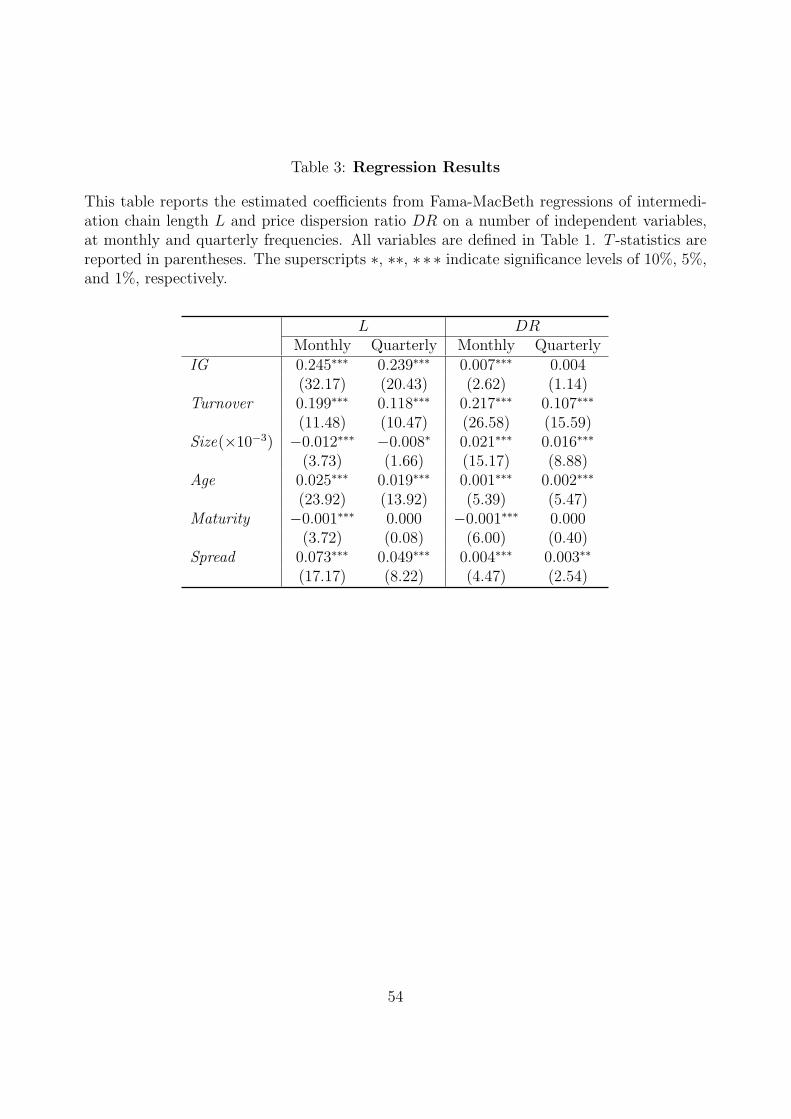
Table 3: Regression Results

This table reports the estimated coefficients from Fama-MacBeth regressions of intermedi-ation chain length L and price dispersion ratio DR on a number of independent variables,at monthly and quarterly frequencies. All variables are defined in Table 1. T -statistics arereported in parentheses. The superscripts ∗, ∗∗, ∗∗∗ indicate significance levels of 10%, 5%,and 1%, respectively.

L DRMonthly Quarterly Monthly Quarterly

IG 0.245∗∗∗ 0.239∗∗∗ 0.007∗∗∗ 0.004(32.17) (20.43) (2.62) (1.14)

Turnover 0.199∗∗∗ 0.118∗∗∗ 0.217∗∗∗ 0.107∗∗∗

(11.48) (10.47) (26.58) (15.59)Size(×10−3) −0.012∗∗∗ −0.008∗ 0.021∗∗∗ 0.016∗∗∗

(3.73) (1.66) (15.17) (8.88)Age 0.025∗∗∗ 0.019∗∗∗ 0.001∗∗∗ 0.002∗∗∗

(23.92) (13.92) (5.39) (5.47)Maturity −0.001∗∗∗ 0.000 −0.001∗∗∗ 0.000

(3.72) (0.08) (6.00) (0.40)Spread 0.073∗∗∗ 0.049∗∗∗ 0.004∗∗∗ 0.003∗∗

(17.17) (8.22) (4.47) (2.54)

54

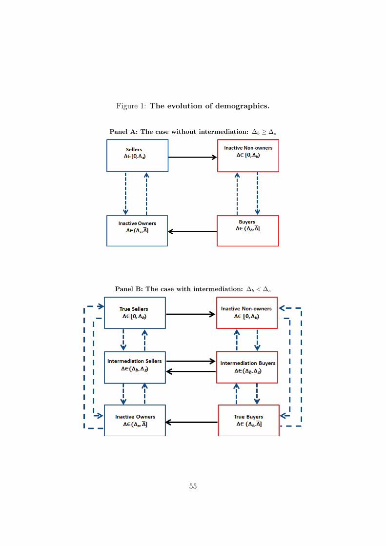
Figure 1: The evolution of demographics.

Panel A: The case without intermediation: ∆b ≥ ∆s

Panel B: The case with intermediation: ∆b < ∆s

55