Financial Integration and Consumption Smoothing: Bridging

Theory and Empirics∗

Ergys Islamaj †

February 2012

Abstract

Does financial liberalization increase consumption smoothing? Yes. This paper develops an

empirical framework based on a firmly grounded theoretical model and provides empirical evidence

that more financial liberalization improves consumption smoothing. Everything else equal, financial

liberalization improves consumption smoothing, although in a nonlinear fashion. On the other hand,

increased cross-country productivity correlations provide fewer incentives for risk sharing. The extent

of consumption risk sharing also depends on the level of impediments to trade in foreign capital.

Empirical results show a stronger effect of financial liberalization on consumption smoothing for

more open economies.

∗I am thankful to Susan Collins, Jonathan Heathcote, Robert Cumby, and Behzad Diba for valuable help and guidance.Any mistakes are my own. I also want to thank Ayhan Kose, Mathew Canzoneri, Jinhui Bai, Carlos Urrutia and participantsat Georgetown University Macroeconomic Seminar.†Department of Economics, Vassar College, 125 Raymond Av, #165, Poughkeepsie, NY 12603. email:

erislamaj@vassar.edu

1

1 Introduction

The past two decades have witnessed a surge in cross-border capital flows and a sharp decline in capital

account restrictions in industrial countries as well as emerging markets and less developed economies.

Standard open macroeconomic models predict that this would unambiguously lead to better international

consumption risk sharing1 . The intuition would be that as countries open their international financial

markets, they would be able to off-load some of their income risks to the rest of the world, de-linking do-

mestic consumption from country-specific disturbances. In return, domestic consumption will vary with

the common component of international income growth. However, the empirical literature studying the

effects of financial liberalization on consumption smoothing is at best inconclusive, failing to unambigu-

ously show improvements in international consumption risk sharing, especially for the emerging markets

and other developing economies. This study investigates this disconnect and offers plausible answers

about the relationship between financial liberalization and consumption smoothing.

The empirical literature on the effects of financial liberalization on international consumption smoothing

has been elusive of theory, without having an explicit equilibrium framework in mind.2 Its predictions

come from a complete markets model, which conjectures that the ability to insure against different states

of nature should be reflected in: a) a low correlation between own consumption and own output (own

refers to households for micro studies and country for international studies), b) a high correlation between

own consumption and aggregate/rest of the world income or consumption (aggregate refers to total do-

mestic for micro studies within a country, and is either foreign or global for international studies), and c)

a low volatility of consumption. Some studies have been looking at these correlations trying to interpret

it as a test of highly integrated markets. Failing to find the predicted patterns in the data, further studies

1Mace(1991), Lewis(1996), Obstfeld and Rogoff (1996)2a notable exception would be Lewis(1996)

2

have been more pragmatic and chosen to interpret the magnitudes of these measures as deviations from

the complete markets outcome, investigating the same measures for different market openness realizations

across countries and across time. But, even when market incompleteness has been considered, like for

example, controlling for financial impediments, in most cases the analyses have been ad-hoc, probably

not testing the implications of an incomplete markets framework.

Using a simple general equilibrium model, this study develops a well-defined framework and can test

more directly the effects of financial impediments on measures of international consumption risk sharing.

The results can be summarized as follows. First, the actual level of financial impediments matters for

consumption smoothing, and the relationship between the two is nonlinear. While liberalization has

little effect on consumption smoothing when financial markets are relatively closed, its impact grows as

financial markets become more open. Empirical analysis finds that more liberalization leads to better

consumption risk sharing. Second, this study shows both theoretically and empirically that increased

productivity correlations with the rest of the world are associated with less international risk sharing

(using consumption-based measures). While the net effect of cross-country productivity correlations on

consumption risk sharing is small in magnitude, the analysis presented in this paper shows that it inter-

acts with financial impediments and should be considered by the literature.

Why do researchers care about consumption risk sharing? Eliminating consumption risks can have sub-

stantial economic effects. There is a large literature about the extent of the benefits of international

risk sharing, which shows that these benefits can be large for developing economies. (See Kose, Prasad,

Rogoff and Wei (2007) for a review.) For example, Athanosoulis and van Wincoop (2000) estimate that

eliminating idiosyncratic consumption uncertainty (relative to world average riskiness) would have the

same benefit as a 6.6% permanent increase in the level of per capita consumption of a typical developing

3

country. The empirical analysis in this paper finds that developing countries can further reduce their

consumption risks by decreasing financial impediments. Furthermore, this study suggests that the extent

of these benefits will depend on cross-country productivity similarities. Investigating these channels can

help researchers better understand the benefits of financial globalization.

One of the main benefits of financial globalization is that it provides increased opportunities to protect

consumers from the risks associated with idiosyncratic income shocks. Cochrane (1991) and Mace (1991)

were among the first studies to argue that consumption should not vary across individuals in response

to idiosyncratic shocks; just as borrowing and lending opportunities imply that consumption should

not vary over time in response to forecastable shocks.3 These two studies have been the genesis of an

extensive literature aimed at understanding the effects of financial integration on international consump-

tion smoothing. Obstfeld (1994) and Lewis (1996) were among the first influential studies to investigate

consumption risk sharing in an international context. In this case, own would refer to country’s consump-

tion and output. By the same analogy, in the presence of open financial markets, country’s consumption

should be more correlated with the common component of the consumption of the foreign countries they

trade assets with, and less correlated with domestic output.

Most standard models in open macroeconomics give similar predictions. In the simplest complete mar-

kets model, marginal utility growth should be equated across countries so that consumption growth rates

should be highly correlated. Dynamic stochastic general equilibrium (DSGE) models, in particular, have

been able to generate some quantitative predictions along these lines. These types of models predict that

in the absence of trade in goods and financial assets (the case of autarky), the correlations of domestic

3They use reported income, which includes after-tax wages and salaries, pension income, interest income, and variouslump-sum receipts. Hence, some of the risk sharing has already taken place and is included in the reported income measure.However, at least some risk sharing takes place between receipts of reported income and actual consumption.

4

consumption with world output (or world consumption) would be less than unity provided that output is

not perfectly correlated across countries (Backus, Kehoe and Kydland (1995)). In contrast, in a scenario

with complete markets that enables perfect risk sharing, it should be possible to decouple fluctuations

in consumption from those of output. Cross-country correlations of consumption growth rates would be

predicted to be perfect or very high. Moreover, consumption across countries would be more correlated

than output. Pakko (1998) also shows that in a two-country endowment economy the correlation between

domestic consumption and domestic output should be lower than the correlation between domestic con-

sumption and world output in the presence of integrated financial markets4 .

Empirical literature investigating the effects of globalization on consumption risk sharing has failed to

document a robust relationship between financial integration and consumption smoothing. Kose, Prasad

and Terrones (2009) show that emerging markets and other developing economies have not been able to

benefit from increased opportunities to smooth consumption, despite the surge in financial flows into and

out of these countries . Some other studies have been able to document better consumption risk sharing

for more open economies (Lewis (1996), Beckaert, Harvey and Lundblad (2005)), but their estimates are

nowhere near the predictions of the theoretical models.

Researchers have also attempted to build models that sometimes reverse these predictions and can be

more in line with some of the results presented below. For example, Baxter and Crucini (1995), Heathcote

and Perri (2001, 2004), Lewis (1996), show theoretically scenarios that might lead to different outcomes

than those presented above. As will be discussed further in the paper, some of these studies require very

strong conditions. But, with very few exceptions, these models have not been incorporated into empirical

studies to date.

4This is a direct consequence of the fact that under integrated markets marginal utilities of consumption between thetwo countries would be perfectly correlated.

5

This study will argue that among the key problems with the existing empirical literature is the lack of

a well-defined framework. In a simple framework, this paper will show a nonlinear relationship between

financial liberalization, consumption smoothing and cross-country productivity similarities. Everything

else equal, more liberalization means better consumption smoothing, but consumption based measures of

risk sharing might deteriorate because of increased productivity correlations with the rest of the world.

The paper is organized as follows. The next section develops a theoretically based empirical framework to

estimate the effects of financial impediments and cross-country productivity correlation on consumption

smoothing. First, it offers a summary of the literature and points out the main messages of the previous

studies. These main messages are then incorporated in a simple general equilibrium model, and some

testable implications of this model are discussed. In the end, it develops an empirical framework that will

serve as the basis for the empirical analysis. Section 3 offers a review of the different available indicators

as well as a discussion of their strengths and weaknesses, before moving into a more formal empirical

analysis. Section 4 describes the data used and Section 5 shows the results of the empirical tests. Some

robustness analysis is discussed in Section 6 and Section 7 summarizes the conclusions and offers some

discussion for suggested future work.

2 Bridging Theory and Empirics

In theory, one of the main benefits of financial globalization is that it provides increased opportunities

to protect consumers from the risks associated with idiosyncratic income shocks. In a representative

agent framework, integrated world asset markets would imply that the ex-post difference between any two

countries’intertemporal marginal rates of substitution is uncorrelated with any random variable on which

contractual payoffs can be conditioned. Any idiosyncratic consumption risk systematically related to some

6

verifiable random event will be traded, leaving ex-post differentials in marginal utility to be functions

of nonverifiable events only. Thus, a country’s consumption will not co-vary with its production as any

fluctuations in output caused by known ex-ante randomness in the production process can be de-linked

from consumption via capital markets. Under financial integration, growth in individual consumption

should be closely correlated to the aggregate consumption pool and less correlated to individual income5 .

2.1 Literature Review

There is an extensive literature aimed at understanding the effects of financial integration on consumption

smoothing. Usually, consumption-based measures of risk sharing come from a benchmark model with

complete markets. For example, Obstfeld and Rogoff (1996) compare the case of financial autarky and

complete markets, where financial markets are modeled as contingency assets. They show that in the

later case consumption does not co-move with own output, but with an aggregate measure of income (or

consumption). Baxter and Crucini (1995) and Backus, Kehoe and Kydland (1995) also predict that in

the case of absence of trade in financial assets domestic consumption should not be correlated with world

income (or consumption) provided output is not correlated across countries, whereas under complete

markets cross-country consumptions should be highly correlated.

Tables 1-3 give a summary of studies investigating the effects of financial integration on consumption

smoothing6 . These studies differ in terms of methods they employ, the data sets they use and how they

define financial integration. Usually, the literature on consumption risk sharing has asked two main ques-

tions. The first is whether there is perfect consumption risk sharing. According to one-good, two-country

5Previous studies have looked at the regression: log(Cjt+1

Cjt

) = β1log(Cat+1Cat

)+β2log(Xjt+1

Xjt

)+εjt+1, where cjt , c

at , X

jt denote

country’s j consumption, aggregate consumption and country’s j income respectively. In a financially open world we wouldexpect a statistically significant ( and high) β1 and an insignificant (and close to zero) β2.

6Note that some studies have looked at more than one hypothesis of consumption smoothing and can appear in morethan one table.

7

macro economy models, a high degree of financial liberalization should be reflected in low correlations

of domestic consumption and domestic output and high correlations of domestic consumption and world

income/consumption. This would mean that cross-country consumption correlations would be higher

than cross-country output correlations. If these patterns were observed in the data that would have led

researchers to interpret it as evidence of highly integrated financial markets. Out of ten studies that look

at international consumption risk sharing in Table 1, one finds mixed evidence of perfect consumption

smoothing, whereas nine others reject the hypothesis of perfect risk sharing at very high levels of statisti-

cal significance. In addition, one finds that even among US states there are still unexplored opportunities

of consumption risk sharing.

One might suspect that the predictions of this line of literature might be unrealistic. Even for a highly

integrated economy, output volatility might signal changes in future income resulting in responses to con-

sumption, and therefore, the expectation of completely independent consumption (growth) and income

(growth) might be a little farfetched. Also, agreeing that some consumption risk sharing may take place

from borrowing and lending on credit markets and other formal and informal insurance arrangements

would suggest that domestic consumption (growth) would be correlated with domestic income (growth)

and need not be completely correlated with world income.

This has led researchers to be more pragmatic and interpret the magnitudes of the correlations mentioned

above as deviations from complete markets outcome. Another group of studies has explored the hypoth-

esis of whether countries have benefitted more from consumption risk sharing opportunities during more

open financial liberalization realizations. To answer these questions, they have used two approaches.

First, they ask if there are differences in consumption risk sharing across different groups of countries,

i.e., financially integrated versus financially non-integrated countries. For example, if correlation between

8

domestic consumption and domestic output is our measure of consumption risk sharing, we should ex-

pect to see a lower correlation for countries with more open financial markets. Table 2 summarizes these

studies. All the ten studies in Table 2 show evidence of consumption smoothing for more financially open

economies. Among them, two studies differentiate countries based on available indicators of financial

openness7 , whereas the rest assume that developed countries are more open than developing economies.

In addition, two of these studies suggest that business cycle properties matter.

Second, the literature has asked what happens to consumption smoothing across time. Table 3 sum-

marizes these results. Out of eleve studies looking at the extent of consumption risk sharing across

time, seven find that there have been improvements in consumption smoothing as countries have become

more liberalized. Among them, two, Bekaert, Harvey and Lundblad (2005) and Islamaj (2008), look

at a group of developed and developing economies and distinguish between relatively open and rela-

tively closed periods of financial integration. The rest implicitly assume that countries have tended to

become more liberalized across time8 and are able to find evidence of consumption smoothing only for

the group of developed countries. From the remaining studies, two show mixed evidence of consumption

smoothing and two show that consumption smoothing has deteriorated even for the developed economies.

What can explain the findings of the empirical literature on consumption risk sharing? First, studies that

have carefully distinguished between relatively open and relatively closed economies, or relatively open

and relatively closed periods have been more successful in finding evidence of consumption smoothing.

This would suggest that the actual level of financial impediments matters for consumption smoothing,

and it might be necessary to depart from the complete markets framework in order to capture the ef-

7Lewis (1996) uses capital account restrictions reported from IMF’s Annual Reports on Exchange Arrangements andExchange Restrictions (AREAER) and Bekaert, Harvey and Lundblad (2005) use equity market openness measures.

8Evidence does show that in the last two decades there has been an increase in cross-border capital flows and a declinein financial restrictions between countries.

9

fects of financial openness on consumption risk sharing. Researchers have attempted to build models

with incomplete markets that sometimes reverse these predictions and can be more in line with some of

the results presented above. For example, Lewis (1996) Heathcote and Perri (2001, 2004), Baxter and

Crucini (1995) show theoretical scenarios of market incompleteness that might lead to different outcomes

than those presented above. Lewis (1996) and Heathcote and Perri (2004) incorporate impediments to

financial markets explicitly in the model and this can allow them to study what happens to consumption

smoothing as markets change from autarky, to partial integration, to full integration under a unified

framework.

Tables 2 and 3 also show that in some cases studies have been successful in finding improvements in

consumption smoothing, once they account for properties of business cycles9 . Heathcote and Perri (2004)

investigate theoretically the effects of productivity shock correlations with the rest of the world on mea-

sures of consumption risk sharing. The intuition would be that as productivity processes between countries

become more similar, there are fewer incentives to diversify risks by investing in a foreign country. Islamaj

(2008) shows that these correlations may, indeed, be empirically relevant. This study will incorporate

cross-country productivity similarities in an incomplete markets model and show empirically that they

have affected measures of consumption smoothing.

Also, some studies suggest nonlinearities in the relations between financial liberalization and consumption

risk sharing10 . For example, Kose, Prasad and Terrones (2003) find empirical evidence that financial

liberalization improves consumption smoothing only after a threshold level on financial flows is reached.

The nature of these nonlinearities can be better captured in a well-defined framework that allows for a

closed form solution. This study uses a general equilibrium framework and avoids potential problems

9Artis and Hoffmann (2007, 2008a), Islamaj (2008)10Kose, Prasad and Terrones (2003), Heathcote and Perri (2004).

10

that are associated with other ad-hoc studies.

2.2 A Simple Model

A simple general equilibrium model that contains some of the features mentioned above, market incom-

pleteness and cross-country productivity shock correlations, can give some good insights about what

happens to consumption based measures of international consumption risk sharing as countries get more

financially integrated.

Consider a two-country exchange (Lucas tree) economy. Capital (the tree) in each country is used to

produce a perishable output, the quantity of which depends on the realization of the state of nature

s. Domestic output is denoted X(s) and foreign output is Y(s). Prior to any trade, the representative

domestic agent owns all of domestic capital stock, while the foreign agent owns foreign capital. At the

start of each period, the domestic household buys claims to a fraction θf of the foreign capital stock,

given the budget constraint. Then, the state of nature is revealed, contracts are honored, and agents

consume output to which they have claims.

To formalize:

At the start of the period, the domestic household buys a fraction θf of the foreign tree subject to the

budget constraint:

θfP∗ = (1− τ)[P − θP ]

where τ is and iceberg cost.

One can find the foreign share as,

11

θP + θfP ∗

1− τ = P =⇒ θf = (1− τ)P

P ∗(1− θ)

where P and P ∗ are the prices of the domestic and foreign stocks respectively, and (1−θ) is the proportion

of the domestic stock sold.

An important assumption is that foreign capital is subject to a proportional tax, τ . This will represent

transaction costs in purchasing foreign capital and later will allow us to define financial liberalization.

The advantage of defining financial liberalization in this manner is that it allows us to map the effect of

the degree of liberalization on consumption smoothing for each level of financial impediments. Given a

choice for θ, consumption in state s is given by:

c(s) = θX(s) + θfY (s) = θX(s) +P

P ∗(1− θ)(1− τ)Y (s) (1)

where θ represents fraction of domestic output held, X(s) and Y(s) represent domestic and foreign out-

puts, respectively, and τ represents impediments to trade in foreign capital11 .

The domestic household solves:

maxθ{E[u(ct(s))]}

such that (1) and θ ≤ 1.

11Market clearing for stocks implies: θ + λf = 1 and θf + λ = 1, where λ and λf represent the holdings of domesticand foreign capital share of the foreign consumer. Market clearing for consumption good requires: c(s) + c∗ + (θfY (s) +λfX(s))τ = X(s) + Y (s).

12

First Order Conditions can be writen as:

FOCθ : E[u′(ct(s))Xt(s)] =

P

P ∗(1− τ)E[u′(ct(s))Yt(s)]

(provided θ < 1)

Consider the case in which the utility is exponential

u(c) = − 1Aexp{−Ac}

where A is the coeffi cient of risk aversion.

Assume that X and Y are jointly normally distributed with means µx and µy, respectively, equal variance

σ2 and correlation coeffi cient ρ12 .

It can be shown that, θ, the amount of domestic endowment that a consumer chooses to keep, can be

determined endogenously, and is a function of τ , ρ, µx and µy. This is an interesting observation since

it relates the actual amount of financial flows to the financial restrictions imposed on the international

markets. In that case, we can derive θ, the holdings of the domestic tree as13 :

12 Initially assume µx = µy = µ. In that case, the joint distribution over foreign and domestic endowments is perfectlysymmetric and as a result P = P ∗.13Note that if τ → 0 =⇒ θ → 1

2, and if τ → 1 =⇒ θ → 1

13

θ = min{1,(1− ρ− τ) + τ µ

Aσ2

(2− τ)(1− ρ) }

This would suggest that studies that use financial flows as a measure of financial integration may suffer

from an endogeneity problem. Given an expression for θ, we can derive expressions for all the measures

of consumption smoothing used in the literature that depend only on τ , ρ and µ. ρ is the cross-country

correlation of productivity shocks and µ can be interpreted as the mean of output in each country. τ

represents financial impediments in capital markets and can be thought as exogenously determined by a

government authority. Thus, we have expressions for measures of consumption smoothing that depend

on exogenous variables only. In contrast to earlier studies, this framework suggests that: first, consump-

tion smoothing depends on financial liberalization in a non-linear fashion, and second, that consumption

smoothing depends not only on the degree of financial openness, but also on the nature of the underlying

shocks. These points will be discussed in detail in the next subsection.

The assumption of normal distribution of productivity shocks might be a little problematic, since nor-

mally distributed shocks would produce negative values for output with positive probability. In practice,

when studying the predictions of this model, it is assumed that the mean of output is a large positive

number and the standard deviation is small, so as to minimize the probability of consumers facing nega-

tive output realizations. These assumptions are in line with the data.

2.3 Testable Implications

The fraction of domestic and foreign assets held (portfolio choice) will depend on τ , the actual level of

impediments to foreign capital. So will the consumption based measures of consumption risk sharing.

14

The exact relationship between these variables can be seen best in graphs. Figures 1 and 2 show these

measures of consumption smoothing (vertical axis) and the level of financial impediments (horizontal

axis), for different levels of cross-country productivity shock correlations. Low impediments means more

liberalized markets. In Figures 1 and 2 µ = 2, σ = 0.1 and A = 1. At a consumption level µ, these values

translate to a coeffi cient of relative risk aversion (corresponding to Aµ) of 214 . Figure 1 shows what

happens to the correlation between domestic consumption and domestic output as transactions costs

decrease15 and Figure 2 shows the relationship between impediments to foreign capital and cross-country

correlation of consumptions. The next sub-section points out some testable implications that this model

might have.

2.3.1 Correlation between domestic consumption and output:

Figure 1 shows what happens to the correlation between domestic consumption and domestic output as

impediments to trading foreign capital, τ , decrease. A low correlation between consumption and output

means that countries are better able to share consumption risks. For a given ρ, as the country becomes

more liberalized the correlation between consumption and output in the domestic country decreases,

albeit in a nonlinear fashion (note that for high values of τ there is little or no change in consumption

smoothing when τ decreases). Figure 1 also highlights that for fixed values of τ , as ρ increases (this is

shown by an upward shift in the curve in Figure 1 consumption smoothing deteriorates (the correlation

between consumption and output increases). The intuition would be that as ρ increases, productivity

processes between the domestic country and the rest of the world become more similar, making the gains

from diversifying consumption risk smaller. Even if the country liberalizes, the net result may be deteri-

oration in consumption smoothing if ρ has increased. This might be shown by moving from point A to

point B in Figure 1.

14and a percentage deviation of output (corresponding to 100× σµ) of 5 percent.

15Figures 1-2 assume µ = 2, A = 1 and σ = 0.1

15

Thus, lower financial restrictions will improve, whereas more similar productivity processes will deteriorate

consumption smoothing. For these parameter values, even small impediments to trading foreign capital

will shut down international financial markets, as the gains of sharing risks for this parameterization

are small. This is in line with the findings of the literature for developed countries (Cole and Obstfeld

(1991)). Theoretically, τ would correspond to an array of policy and institutional arrangements, which

would be hard to measure. In practice, financial openness measures, which are also imperfect (see section

3), will be used to estimate these implications. They may represent only a subset of τ in the model,

but can be thought of as being effective only after other institutional arrangements, like the existence of

financial institutions, are set in place.

2.3.2 Cross-Country Consumption Correlations:

Figure 2 shows the relationship between financial restrictions and cross-country consumption correlations

for different ρ. In this case, a higher correlation means better risk sharing. Again, everything else equal,

fewer impediments to trade in foreign capital, correspond to better consumption smoothing. For very

high frictions, as τ decreases, there is no change in cross-country correlations of consumption. Only for

low enough impediments to foreign capital would fewer restrictions correspond to better consumption

smoothing.

Again, for a fixed τ , consumption smoothing may change if productivity correlations with the rest of the

world change. For high (restrictive) costs to trading foreign capital, cross-country consumption correla-

tions are determined by productivity correlations, ρ, by definition. For low levels of financial restrictions,

a higher ρ corresponds to deterioration in consumption smoothing. This might seem a little counter-

intutitive as an increase in ρ will increase output correlations by definition, and in return will increase

16

consumption correlations. But, on the other hand, an increase in ρ has a huge negative effect on the

portfolio share of foreign assets, which in turn decreases cross-country correlations for plausible parame-

ter values. The second effect dominates and a higher ρ corresponds to a deterioration in consumption

smoothing. See Heathcote and Perri (2004) for more details.

To summarize, first, everything else equal, there exists a nonlinear relationship between financial liberal-

ization and consumption smoothing. The nonlinearity feature makes clear distinctions between different

measures of consumption smoothing as to how they respond to financial liberalization. Loosely speaking,

for a fixed ρ (assuming that the tax is non-restrictive) more liberalization would mean more consumption

smoothing, but an incremental change in financial integration would have a different quantitative effect on

consumption smoothing across the different measures. For example, for low impediments, an incremental

decrease in τ would show more improvement in risk sharing if one calculates risk sharing using corr(c,X)

than if one uses cross-country correlations of consumption (note that for low impediments the graph for

corr(c,X) is steeper than the graphs for corr(c, c∗)). The opposite is true for high (but non-restrictive)

impediments to foreign capital. When using corr(c,X) to measure consumption risk sharing, financial

liberalization improves consumption smoothing with increasing returns, whereas, when using corr(c, c∗)

as a measure of consumption risk sharing, liberalization improves consumption smoothing with decreas-

ing returns. Also, the effect of productivity shock correlation on measures of consumption risk sharing

appears to be different, depending on the actual level of financial restrictions. These nonlinearities are

not mereley a mathematical fact, but have important implications for the effect of financial liberalization

and cross-country productivity correlations on consumption smoothing. An empirical framework shown

in the next section will test these implications.

The literature so far has treated different measures of consumption smoothing similarly and has not

17

differentiated between the two. These measures can respond differently to financial liberalization. The

difference is not only qualitative, as discussed in the previous paragraph, but also quantitative. Using

cross-country consumption correlations, consumption smoothing will change from 0 to 1 as the country

moves from financial autarky to complete liberalization. On the other hand, the same liberalization

implies a change from 1 to 0.6 when using correlation between domestic consumption and income as a

measure of consumption smoothing16 . Islamaj 2009b will also show that in a two-country, two-sector

framework, an increase in cross-country productivity shock correlation may have different effects on dif-

ferent measures of consumption smoothing. More research on the different measures of consumption risk

sharing may be needed.

Also, productivity shock correlation with the rest of the world matters for consumption smoothing.

Recently, some research accounting for business cycle properties has shown success in relating consumption

smoothing and financial integration and this simple model gives a clear idea of how productivity shocks

correlations affect consumption based measures of risk sharing.

2.4 Empirical Framework

In this section, I present the empirical framework that is used in the empirical analysis. The framework

is derived from the theoretical model shown above, and in that sense, I am making a direct link between

theory and empirics.

Remember equation (1) that says: c(s) = θX(s) + θfY (s)

i.e., at the end of each period, once the state of nature is realized, the domestic consumer gets his

portion of the domestic output and what he owns of the foreign output.

16This is the reported value for corr(c,X) when τ = 0 and ρ = 0. The y-intercept will change for different values of ρ.

18

One can estimate:

ct = β1tXt + β2tYt (2)

where Xt is the domestic output, Yt is the foreign output. Note that the coeffi cients in front of domestic

output and world output are changing over time, and not fixed as assumed by some of the previous

literature.

It can be shown that one can estimate17 :

β1t = γ1τ′t + γ2ρ

′t + γ3ρ

′tτ′t (3)

β2t = δ0 + δ1τ′t + δ2ρ

′t + δ3ρ

′tτ′t (4)

where18

τ ′t =1

(2− τ t)

17See the Appendix (2.8) for more detail. Note that β1t is positively related to τ .18γ1 = 1, γ2 = 1−

µAσ2

, γ3 = 2(µAσ2− 1), δ0 = 1, δ1 = 1, δ2 = µ

Aσ2− 1, δ3 = 2(1− µ

Aσ2) Note that τ is positively related

to τ ′t

19

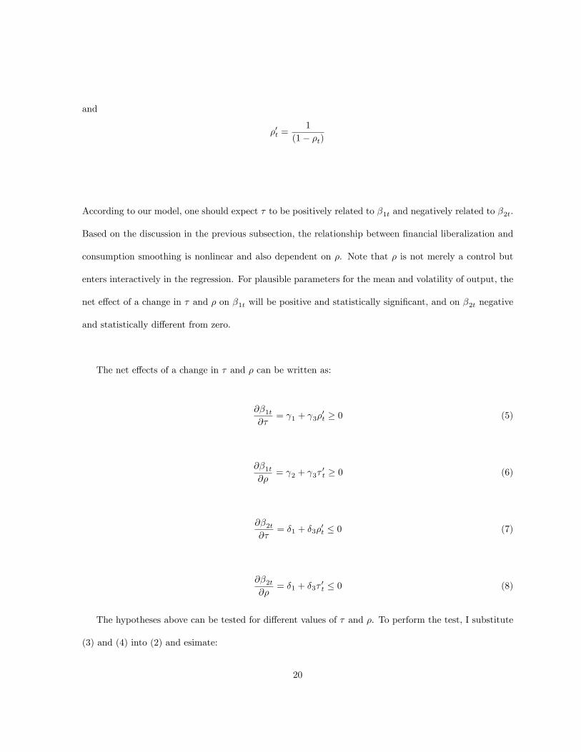
and

ρ′t =1

(1− ρt)

According to our model, one should expect τ to be positively related to β1t and negatively related to β2t.

Based on the discussion in the previous subsection, the relationship between financial liberalization and

consumption smoothing is nonlinear and also dependent on ρ. Note that ρ is not merely a control but

enters interactively in the regression. For plausible parameters for the mean and volatility of output, the

net effect of a change in τ and ρ on β1t will be positive and statistically significant, and on β2t negative

and statistically different from zero.

The net effects of a change in τ and ρ can be written as:

∂β1t∂τ

= γ1 + γ3ρ′t ≥ 0 (5)

∂β1t∂ρ

= γ2 + γ3τ′t ≥ 0 (6)

∂β2t∂τ

= δ1 + δ3ρ′t ≤ 0 (7)

∂β2t∂ρ

= δ1 + δ3τ′t ≤ 0 (8)

The hypotheses above can be tested for different values of τ and ρ. To perform the test, I substitute

(3) and (4) into (2) and esimate:

20

4ct = 4(β1tXt) +4(β2tYt) + εt (9)

ctYt= β1t

Xt

Yt+ β2t + ξt (10)

ct = β1tXt + β2tYt + νt (11)

where εt, ξt and νt represent measurement error. The null hypotheses test whether the net effects of

a change in τ or ρ are statistically significant and if they have the predicted sign. Equation (9) comes

from first-differencing equation (2). Differencing the variables has the advantage that it makes the series

stationary. However, the model presented earlier suggested that knowing only the change in liberalization

may not be enough to capture the effects of liberalization on consumption smoothing19 . Although this

equation can capture some of the effects of openness on consumption risk sharing, one should look at the

regression in levels for a more complete picture.

Equation (10) looks at the same relationship for level output and consumption per capita, hoping to

capture some of the long term effects of financial liberalization on consumption smoothing. Stationarity

19 In the short run, consumption might also be affected by expected future changes in income, as suggested by the PIH,and the effects of financial liberalization can be blurred. Some of the long effects of financial liberalization can be capturedonly with level regressions (See Artis and Hoffmann (2007) for a more detailed analysis).

21

is imposed by dividing by foreign output. The drawback is that world output volatility can be influenced

by countries that do not necessarily trade with the country under consideration, or fluctuations in world

output may not necessarily affect domestic output and domestic consumption. The appearance of world

output on both the RHS and LHS of equation (10) may bias the results. Another way is to test like in

equation (11) where levels of consumption and output are considered. This relationship can, in principle,

be estimated consistently by OLS. However, consumption and output series can be co-integrated and OLS

may suffer potential simultaneity and serial correlation of the errors. The panel dynamic OLS (PDOLS)

estimator suggested by Mark and Sul (2003) accounts for serial correlation and potential simultaneity by

including leads and lags of the differences of the right hand side variables. Different numbers of leads

and lags give similar results, which suggest that the estimations are consistent across specifications. The

next section describes the data and other details about the tests.

3 Rule Based Measures of Financial Liberalization

A natural starting point for any data-based discussion of the effects of financial integration on consump-

tion smoothing is a review of different available indicators of financial liberalization. In particular, any

such study would be interested to know how each indicator matches with the tax τ on foreign capital,

especially since different degrees of financial openness have different implications for the effects of more

liberalization on consumption based measures of risk sharing. Unfortunately, measuring financial inte-

gration is a challenging enterprise (Edison et. al. (2002)).

It is important to understand how to interpret financial liberalization. In our model financial liberal-

ization is represented by a tax, τ , in trading foreign capital. For τ = 0 the markets are fully open and

consumers can insure against idiosyncratic country risk ex-ante. For τ = 1 the country is said to be in

financial autarky. The model also tells us that τ should be interpreted as a rule-based measure of finan-

22

cial openness. It is a decision which can be thought of as exogenous (of course in the real world it can

be correlated with the government’s perception of the economic situation and other factors20), and the

actual flows of foreign capital in and out of a country can be represented by θ, which is also a function of τ .

More specifically, if any of the existing measures tells us that the country is fully open, is this situation

correctly represented by a τ = 0 in the model? Also, as a country goes from being fully closed to fully

open, does this correspond to a decrease in τ from 1 (one) to 0 (zero)? As researchers have attempted

to develop finer measures of financial integration, do these measures give us extra information in terms

of the actual degree of financial openness? For example, one such widely available measure is the IMF

AREAER measure of capital restrictions. It is constructed as an on/off indicator of the existence of

rules/restrictions that inhibit cross-border flows for each country in each year. If no restrictions are

present the indicator will be 1 (one), and if any restriction is present it will be 0 (zero). To make it

compatible with our model, we can calculate (1 - IMF Measure) and so zero would correspond to no

restrictions and one would represent the case of any restrictions on the capital account. As discussed, τ

in the model would correspond to an array of policy and institutional arrangements that would allow for

the ex-ante diversification of any income risks. The question becomes, does a change from zero to one in

the IMF measure of financial restrictions correspond to a movement from point C to zero in our model,

or a move form point B to point A as shown in the Figure 3, for example? It is hard to tell from just one

measure and in a previous study Islamaj (2008) makes use of an array of available indicators to rectify

the problem.

Table 4 shows different indicators of financial liberalization. The IMF indicator, reported in Annual Re-

ports on Exchange Arrangements and Exchange Restrictions (AREAER), has been available for a large

20See Eichengreen (2001) for a review.

23

set of countries since 1966. But the indicator has certain disadvantages. First, it is a yes/no measure,

providing no information about the intensity of the capital controls. Second, it does not distinguish be-

tween restrictions on capital inflows and outflows. Starting in 1996, the IMF replaced the single indicator

of capital account restrictions with a set of indicators for the existence of particular restrictions on capital

inflows and outflows. This is a better measure of the array of restrictions on financial markets, but a

drawback is that the new data are not directly compatible with the old data.

Quinn (1997, 2003) constructs an index that attempts to capture the intensity of enforcement of controls

through a careful reading of the descriptions in the AREAER. Unfortunately, its coverage for developing

countries is limited and only for selected years. Brune et. al. (2001) have developed an index with more

extensive coverage that also picks up information from 5 different categories of AREAER (which are an

aggregation of the 13 categories in the new AREAER). The main drawback is that these data are not

publicly available.

Bekaert, Harvey and Lundblad construct an index based in the dates of equity market liberalization.

Still, this is a 0/1 indicator and equity market liberalization may be only a part of the liberalization

process countries have been going through in the past two decades.

Miniane constructs an index for 34 countries for the period 1983-2004 using information from the

AREAER accounts and based on the 13 categories of the new classification of the AREAER. The main

drawback is that there is limited country coverage. Chinn and Ito calculate the first standardized prin-

cipal components of the four major categories of AREAER; presence of multiple exchange rates, current

account restrictions, capital account restrictions and requirement of the surrender of export proceeds.

For controls on capital transactions, they use the share of five-year window that the capital controls were

24

not in effect. This indicator is available for 163 countries from 1970-2006. Edwards (2005) also constructs

an index for 1970-2000 that combines three data sources: a) Quinn (2003), b) Mody and Murshid (2002),

which is the simple average of four AREAER categories, and c) country specific sources. Some missing

data are also imputed.

Kaminsky and Schmukler (2003) develop an index for 28 countries by looking at domestic financial sector

liberalization as well as openness of the equity markets to foreign investment, besides capital account

restrictions. Further along these lines, Abiad and Mody (2005) construct a similar index for 35 countries

for the period 1973-1996. They put more weight on reforms in the domestic sector and look at restric-

tions on capital accounts, privatization in the financial sector, operational restrictions, barriers of foreign

participation in the banking system, interest rates controls and credit controls. These studies add new

dimensions to the liberalization indicators, which can represent an array of institutional arrangements

that would enhance financial integration, and are still based on rule-based measures. A disadvantage is

that they are of limited availability, and also they involve new sources of measurement error and potential

simultaneity with the income growth.

As seen from the discussion above, the measurement of the extent of financial openness is a diffi cult

enterprise. These studies have tried to capture the complexity of real world capital controls with varying

degrees of success. Although, it is hard to say anything decisive about the actual degree of financial

openness for most countries, these indicators do share some common features. First, all of them show a

decreasing trend in financial restrictions over the years, consistent with the belief of increased globaliza-

tion seen in the surge in cross-border financial flows. They also suggest that more developed countries

have been more financially open, consistent with the belief that industrial countries have interacted more

with the rest of the world.

25

For countries like Belgium, Canada, Germany, Netherlands, Panama, UK and US, all the indicators

show a very open economy for the period 1970-2003 (Netherlands and UK have liberalized around mid

70’s). Another group of countries, among them Austria, Denmark, Finland, New Zealand, Singapore

and Sweden, seem to have gone through a major liberalization in their financial markets in the 80’s and

have been very open since then. A few other countries, like France, Greece, Ireland, Italy, Japan, Peru,

Portugal and Spain, have opened their markets a little later, in the 90’s. These countries may have still

not reaped the benefits of globalization. Of the remaining countries, mostly developing economies, a few

have liberalized late in the 90’s, whereas a significant number of these economies have had substantial

restrictions in their financial markets during the period 1970-2003, according to the available indicators

of financial openness.

Instead of regarding one indicator as better than the others, this paper will use multiple indicators as

each of them gives us some extra information about the actual degree of financial liberalization. The

results are similar for different indicators of financial liberalization.

4 Data

All the tests are carried out with widely available data and the STATA files are available from the author

upon request. The dataset ranges from 1970-200321 . Output and consumption per capita data come

from Penn World Tables, version PWT 6.2.

Financial liberalization data come from the sources in Table 4 which are publicly available. All data are

turned into yearly format and are normalized between zero and one, where zero means no restrictions,

21Check Bosworth and Collins (2003) for a list of countries.

26

and one means closed markets. Then τ ′t and ρ′t are constructed using τ and ρ as described in the previous

section.

Cross-country productivity is constructed using productivity data from Bosworth and Collins (2003).

First, bilateral correlations are calculated for each country. Then, for each country, productivity correla-

tions with rest of the world are constructed by taking the weighted average of the bilateral correlations,

where the weights are import shares as reported by the Direction of Trade Statistics Yearbook database

provided by the IMF. Rolling windows of different length are constructed for the bilateral correlations

and the results do not depend on the window length.

5 Results

Test results for equation number (9) are shown in Table 5. The first difference of consumption per capita

is regressed on the first difference of GDP per capita and various measures of financial liberalization

as described by the equation. All the financial indicators used are described in Table 4. The results

presented are for 10-year rolling windows of productivity correlations for the variable ρ, but the results

are robust to different window lengths.

Table 5 shows the net effects of financial liberalization and changes in cross-country productivity cor-

relations on β1t and β2t. p-values are shown in parenthesis. The effects of liberalization are estimated

for the average values of ρ, whereas the effects of a change in ρ are estimated for low values of τ (25th

percentile), as for high τ the effects can be ambiguous as discussed previously in the paper. The net

effect is as predicted and statistically significant in most cases. The results are stronger for the effects

of τ , whereas the effects of a change in productivity shock correlations with the rest of the world are

smaller, although in some cases statistically different from zero. Our main hypothesis would be that

27

financial impediments affect the measures of consumption smoothing. As it can be seen, overall we fail

to reject H0 for all the available indicators of financial liberalization. For example, for the Miniane indi-

cator (column 1), a one unit decrease in our constructed financial liberalization measure (lower τ ′t) has

decreased β1t, the regression coeffi cient of domestic consumption on domestic output (in differences), by

0.16 units. This would suggest an increase in consumption risk sharing. On the other hand, an increase

in productivity correlations with the rest of the world that increases ρ′t by one unit would decrease β2t by

0.11 units, showing a deterioration on consumption smoothing. In general, the effects of a change in cross-

country productivity correlations are low in magnitude and sometimes not statistically different from zero.

These results are even stronger for the regressions in levels, which potentially capture some of the longer

term effects. Table 6 shows results for equation (10). Again, the results suggest strong effects of financial

liberalization and cross-country productivity correlations on consumption smoothing. A one unit decrease

in financial restrictions affects β1t by 0.26 units and β2t by -0.45 units. A higher estimate compared to

the results in Table 5 can be interpreted as this regression capturing some long term effects of financial

integration on consumption smoothing. As expected, the effects of financial liberalization on consumption

risk sharing may be blurred in the short run. According to the Permanent Income Hypothesis (PIH),

consumers may adjust their consumption in anticipation of future expected changes of their permanent

income and this may be one reason why in certain periods their consumption may de-link from their

income, even though there is no change in financial openness.

On the other hand, the results of equation (10) may be influenced by the foreign output, Y, which ap-

pears in the denominator of both right and left hand sides of the equation. Fluctuations in aggregate

world income that may not have necessarily been reflected in country’s consumption and output may be

erroneously captured by equation (10). One can also estimate equation (11) which uses data on the levels

28

of domestic consumption and income per capita and can potentially capture some long term effects. The

problem in this case would be that consumption and income are non-stationary and they can commove

together. To account for co-integration, Panel Dynamic OLS is used22 . By adding first differenced leads

and lags of the non-stationary variables on the RHS, PDOLS accounts for bias that may come from

simultaneity and serial correlation. Different numbers of leads and lags show similar results and Table 7

presents the results for one lead and one lag. As shown in Table 7, the effects of financial liberalization on

β1t are stronger in this case, compared to Table 5. In the case of the Miniane measure of financial open-

ness, a decrease in impediments to trading foreign capital that decreases τ ′ by one unit would decrease

β1t by 0.26 units, suggesting a strong effect of financial liberalization on consumption smoothing. For

example, if a country goes from being completely closed to completely open, like the Miniane indicator

suggests for Denmark, Finland, etc, the decrease in financial impediments would have decreased β1t by

approximately 0.26 units (Table 7).

Another point that this study makes is that the effects of liberalization on consumption smoothing is

different for different levels of impediments to foreign capital. It would be interesting to perform the same

tests for different levels of financial liberalization and compare the results. But, a simple high-low differ-

entiation might not be a good idea. We are ignoring the Capital Account and Current Account measures

since they are 0/1 indicators. Figure 4 shows the distribution for four of the constructed measures of

financial liberalization used in the regressions above. As can be seen from the figures, the distribution

is pretty scarce and a further segregation of these distributions might spoil the results since in some

cases quite a few observations are clustered around the same values. Thus, one should be careful when

trying to differentiate among levels of liberalization. We want to differentiate among different degrees of

impediments to trade in foreign capital and at the same time, we want our variables to have a nontrivial

22Mark and Sul (2003).

29

distribution.

Table 8 shows the results for equation (11) when we perform the same tests on the most open 75 percent

of the sample (High) and the least open 75 percent (Low). The idea would be that for high degrees of

openness, the effects of financial liberalization on consumption smoothing should be stronger. Looking

back at Figure 1, this can be interpreted as being at the left side of Figure 1. The results suggest that the

effects are indeed stronger for the most open part of the sample23 . For example, for the Miniane indicator,

the effect of a unit change in liberalization is 0.22 units for the least open part of the sample, whereas it

increases to 0.35 for the most open realizations24 . The same tests for the equation in differences suggest

similar results (not reported here).

To summarize, this section shows statistically significant evidence that more financial liberalization im-

proves consumption smoothing, whereas increased productivity correlations with the rest of the world

deteriorate consumption based measures of international consumption risk sharing. It also provides sup-

portive evidence that the effects of liberalization on consumption smoothing are stronger for lower levels

of financial impediments.

6 Robustness Analysis

Pair-wise correlations between the different measures (not reported here) show that the measures are

somewhat correlated with each other (coeffi cients between .387-.86), but at the same time the coeffi cients

imply that there are differences between the measures (correlations are not close to 1) and that we are

gaining new information from each indicator. The Kaminsky & Schmukler and Abiad & Mody indicators

23 t-tests comparing that one coeffi cient is statistically greater that the other confirm these results.24 coeffi cient estimates can be found in Table 8.

30

are in general less correlated with the other indicators and this reflects the inclusion of measures for

sectors other than capital and current account in these indicators. The other indicators, which are more

closely related to the IMF AREAER’s are more similar to each other, although there are still differences

which suggest each indicator is different from the other. As argued, we don’t regard any of them as better

than the others, but make use of all the information they provide.

The results presented in Tables 5-8 used cross-country productivity correlations for 10-year rolling win-

dows. The same tests were carried out for different time lengths. 9-year, 8-year and 7-year rolling windows

were also considered and the results were very similar, suggesting that the length of the rolling window

does not make a difference.

As mentioned in the data section, cross-country productivity correlations were weighted using data from

the Direction of Trade Statistics Yearbook. The results presented here were done using the weights for

each year as reported in DOTS and for the years in which data is not available the most recent available

share is used. Other weighting schemes were used, like fixing the shares from a given year as weights,

or using an average over all the years, but the results were very similar. Thus, the results are robust to

different ways of generating the productivity correlations with the rest of the world, ρ.

Estimates of ρ suggest that the correlations of productivity processes in the developed countries are

higher than those of the developing countries and that they have been changing over time25 . For exam-

ple, the average ρ for the industrialized economies is around 0.2, whereas for the developing economies

is around 0.07. The same coeffi cient is very high for Canada, around 0.53, and also high for the US and

25The quantitative considerations in Heathcote and Perri (2004) suggest that the nature of international shocks haschanged since the beginning of the 1980’s. Imbs (2006) also finds that financial integration increases business cyclecorrelations.

31

other European countries26 . This might explain why some of the studies could not document evidence

of consumption smoothing. For example, Heathcote and Perri find that international consumption risk

sharing between US, Europe, Canada and Japan has deteriorated. The exceptionally high productivity

correlations with the rest of the world for the developed economies may explain these results. When it

comes to developing economies, probably the reason why studies do not find improvements in consump-

tion risk sharing is the relatively high level of financial impediments.

Results are similar when the sample is standardized to include only countries that have available data for

both the Miniane and Kaminsky and Schmukler indicators. Thus, the sample size is the intersection of

the Kaminsky & Schmukler and Miniane samples for the years 1983-2002. Again, the results presented

in Tables 2.5-2.6 hold, suggesting that these results are robust to the sample size27 . For the regressions

in levels, the results were robust to using different leads and lags in the PDOLS methodology.

The regressions in this study were not constrained, but the estimates suggest that for all actual values of

τ and ρ the shares of domestic output will be lower than 1, which was the upper bound on θ imposed by

the model. The model also suggests some other constraints on the estimates, which might be subject to

further research.

Overall, the results presented in this paper are robust to different specifications and different ways of

constructing some of the underlying variables. More importantly, the results are not driven by the set of

developed countries, but hold for developed as well as developing countries.

26ρ is 0.2 for the US, 0.17 for the UK, 0.3 for Denmark, and relatively high for Europe. Contact the author for moredetailed statistics.27The results still hold when the sample is dictated by the Miniane indicator only and by the Kaminsky and Schmukler

indicator only.

32

7 Conclusions and Suggestions for Future Work

Standard open macroeconomic models predict that under financially open markets consumers would be

able to benefit from increased risk sharing opportunities. The empirical evidence shows only mixed ev-

idence. This paper investigates the effects of financial liberalization on international consumption risk

sharing and tries to answer the question of why empirical studies fail to observe improvements in consump-

tion smoothing as countries have become more liberalized. First it constructs an empirical framework

based on a firmly grounded theoretical model, emphasizing a direct link between theory and empirics

that the author thinks has been missing in the previous literature. Then, empirical evidence shows that

financial liberalization improves consumption risk sharing. The direct effect of cross-country productivity

similarities on consumption risk sharing appears to be low, but the analysis presented in this paper sug-

gests that they should be considered by the literature as they can deteriorate measures of consumption

smoothing via their interaction with measure of financial impediments.

This study adds to the literature of the effects of globalization on consumption smoothing in three dif-

ferent ways. First, it provides an extensive survey of the current literature and discusses in detail the

strengths and weaknesses of each study. This paper divides studies according to the question they ask.

Some studies have been looking at the hypothesis of perfect consumption risk sharing and concluded that

there is no perfect risk sharing. Others have been more pragmatic and looked at risk sharing across groups

of countries and through time. Whereas most studies reject the hypothesis of perfect risk sharing, there

is some evidence that more open countries have shared more consumption risks or that some countries

have benefited more from risk sharing benefits during more financially open periods. This suggests that

the actual level of financial impediments to trading foreign capital matters for consumption smoothing

and should be explicitly modeled. Another factor that can affect measures of consumption smoothing

is the productivity correlation with the rest of the world. The more similar the productivity processes

33

between countries, the fewer incentives there are for consumers to share risks by purchasing foreign assets.

Second, this study develops an empirical framework based on a theoretical model that may shed light

on why we fail to see more consumption risk sharing as financial integration has increased. Consumers

trade output claims in a two country endowment economy, where output stems from a stochastic process.

First trade occurs, then shocks are realized and consumers consume their claims. The purchase of foreign

assets is subject to a tax. The model shows how consumption based measures of consumption risk sharing

depend on the degree of impediments to foreign capital and on the similarity of productivity processes.

This model has some nice testable implications. An empirical framework is constructed showing a way to

directly measure the effects of financial liberalization and productivity correlations with the rest of the

world on measures of consumption smoothing.

Third, this paper provides empirical evidence that more financial liberalization improves consumption

smoothing. The effect of financial openness on consumption smoothing is not only statistically significant,

but also economically important. The results hold for developed and developing countries.

This study assumed that cross-country productivity correlations are exogeneous and not related to fi-

nancial liberalization. Future work could focus on investigating whether productivity similarities with

the rest of the world have been influenced by financial liberalization. That would determine a potential

endogeneity problem that might exist in this paper and help capture better the relation between financial

liberalization and consumption smoothing.

Also, more work could be done in defining open and closed periods of financial openness and comparing

the extent of consumption smoothing. So far, it has been hard to distinguish between open and closed

34

periods of financial openness because of imperfections in measures of financial liberalization. Different

indicators can say different things about the extent of openness of a given country on a given year. For

those countries for which different indicators suggest a similar degree of openness, preliminary results

show that the effects of financial liberalization on consumption smoothing are stronger (not reported in

this study) than the results presented in this paper. Future research should focus on identifying more

objective criteria of openness and studying the effects of financial liberalization on different economic

indicators. Focusing on countries for which there is no disagreement among indicators about the degree

of openness can help researchers better understand the benefits of financial globalization.

8 Appendix

At the start of the period, the domestic household buys a fraction θf of the foreign tree subject to the

budget constraint(8):

θP + θfP ∗

1− τ = P =⇒ θf = (1− τ)P

P ∗(1− θ)

where P and P ∗ are the prices of the domestic and foreign stocks respectively, and (1−θ) is the proportion

of the domestic stock sold.

Given a choice for θ, consumption in state s is given by:

c(s) = θX(s) + θfY (s) = θX(s) +P

P ∗(1− θ)(1− τ)Y (s) (12)

where θ represents fraction of domestic output held, X(s) and Y(s) represent domestic and foreign out-

35

puts, respectively, and τ represents impediments to trade in foreign capital.

The domestic household solves:

maxθ{E[u(ct(s))]}

such that (12) and θ ≤ 1.

First Order Conditions can be writen as:

FOCθ : E[u′(ct(s))Xt(s)] =

P

P ∗(1− τ)E[u′(ct(s))Yt(s)]

(provided θ < 1)

Consider the case in which the utility is exponential

u(c) = − 1Aexp{−Ac}

where A is the coeffi cient of risk aversion.

Assume that X and Y are jointly normally distributed with means µx and µy, respectively, equal variance

σ2 and correlation coeffi cient ρ28 .

Then:

FOCθ : E[u′(ct(s))Xt(s)] = (1− τ)E[u′(ct(s))Yt(s)]

28 Initially assume µx = µy . This assumption will be dropped later. Because, the joint distribution over foreign anddomestic endowments is perfectly symmetric P = P∗ as a result.

36

cov(u′(ct(s)), Xt(s)) + E[u′(ct(s))]E[Xt(s)] = (1− τ){cov(u′(ct(s)), Yt(s)) + E[u′(ct(s))]E[Yt(s)]}

Applying Stein’s Lemma, it can be calculated that:

θ =(1− ρ− τ) + τ µ

Aσ2

(2− τ)(1− ρ)

provided θ < 1

for the symmetric case: c(s) = θX(s) + (1− θ)Y (s)

θ =1

(2− τ) −τ

(1− ρ)(2− τ) +τ µAσ2

(1− ρ)(2− τ) =1

(2− τ) + (µ

Aσ2− 1) τ

(1− ρ)(1− τ)

=1

(2− τ) + (µ

Aσ2− 1) 1

(1− ρ) (−1 +2

2− τ ) =1

(2− τ) − (µ

Aσ2− 1) 1

(1− ρ) + 2(µ

Aσ2− 1) 1

(1− ρ)1

2− τ

and

(1− θ) = 1− 1

(2− τ) −τ

(1− ρ)(2− τ) +τ µAσ2

(1− ρ)(2− τ)

=2− τ − 2ρ+ τρ− 1 + ρ+ τ − τ µ

Aσ2

(1− ρ)(2− τ) =1− ρ+ τρ− τ µ

Aσ2

(1− ρ)(2− τ)

=1

2− τ + 1−2

2− τ −1

1− ρ + 21

2− τ1

1− ρ +µ

Aσ21

1− ρ −2µ

Aσ21

2− τ1

1− ρ

= 1− 1

2− τ + (µ

Aσ2− 1) 1

1− ρ + 2(1−µ

Aσ2)1

1− ρ1

2− τ

37

References

[1] Artis, Michael J and Mathias Hoffmann, 2007. "The Home Bias and Capital Income Flows between

Countries and Regions," IEW - Working Papers iewwp316, Institute for Empirical Research in

Economics - IEW.

[2] Artis, Michael J and Mathias Hoffmann, 2008a. "Financial Globalization, International Business

Cycles and Consumption Risk Sharing," Scandinavian Journal of Economics, Blackwell Publishing,

vol. 110(3), pages 447-471, 09.

[3] Artis, Michael J and Mathias Hoffmann, 2008b. "Declining Home Bias and the Increase in Interna-

tional Risk Sharing: Lessons from European Integration," CEPR Discussion Papers 6617, C.E.P.R.

Discussion Papers.

[4] Ambler, Steven, Emanuela Cardia and Christian Zimmermann, 2004, “International Business Cycles:

What are the Facts?”Journal of Monetary Economics, Vol. 51 (2), pages 257-276.

[5] Athanosoulis, S and E. van Wincoop, 2000. “Growth Uncertainty and Risk-Sharing,” Journal of

Monetary Economics 45, pp. 477-505.

[6] Asdrubali, Pierfederico, Bent E. Sorensen, and Oved Yosha, 1996, “Channels of Interstate Risk

Sharing: United States 1963—90,”Quarterly Journal of Economics, Vol. 111, No. 4, pp.1081—1110.

[7] Backus, David, Patrick Kehoe, and Finn Kydland„1995, “International Business Cycles: Theory

and Evidence,”in Frontiers of Business Cycle Research, ed. by Thomas Cooley (Princeton: Princeton

University Press), pp. 331—356.

38

[8] Bai, Yan, and Jing Zhang, 2005, “Financial Integration and International Risk Sharing”Working

Paper, University of Michigan.

[9] Baxter, Marianne, 1995, “International Trade and Business Cycles,” in

Handbook of International Economics Vol. III, ed. by Gene Grossman and Kenneth Rogoff

(Amsterdam: North-Holland).

[10] Bekaert, Geert, Campbell R. Harvey, and Christian Lundblad, 2005, “Does Financial Liberalization

Spur Economic Growth?”Journal of Financial Economics, Vol. 77 (July), pp. 3—55.

[11] Bosworth, Barry, and Susan M. Collins.2003. “The Empirics of Growth: An Update.”Brookings

Papers on Economic Activity 2003, no. 2: 113-206.

[12] Canova, Fabio, and Morten Ravn, 1996, “International Consumption Risk Sharing,” International

Economic Review, Vol. 37, No. 3, pp. 573—601.

[13] Chinn, Menzie, and Hiro Ito, 2006, “What Matters for Financial Development? Capital Controls,

Institutions, and Interactions,”Journal of Development Economics, Vol. 61(1), pp. 163-192.

[14] Cochrane, John H, 1991, “A Simple Test of Consumption Insurance,”Journal of Political Economy,

Vol. 99 (5), pages 957-76,

[15] Cole, H.L., and M. Obstfeld, 1991, “Commodity trade and international risk sharing,” Journal of

Monetary Economics 28, 3-24.

[16] Edison, Hali J., Michael Klein, Luca Ricci, and Torsten Sløk, 2004, “Capital Account Liberalization

and Economic Performance: Survey and Synthesis,”IMF Staff Papers, Vol. 51, No. 2 (Washington:

IMF).

39

[17] Edison, Hali, Ross Levine, Luca Ricci, and Torsten Sløk, 2002, “International Financial Integration

and Economic Growth,”Journal of International Monetary and Finance, Vol. 21, No. 6 (November),

pp. 749—76.

[18] Edison, Hali J., and Warnock, Francis E., 2003, “A Simple Measure of the Intensity of Capital

Controls,”Journal of Empirical Finance, Vol. 10, No. 1/2, pp. 81—103.

[19] Edwards, Sebastian, 2005, “Capital Controls, Sudden Stops and Current Account Reversals,”NBER

Working Paper No. 11170.

[20] Eichengreen, Barry J., 2001, “Capital Account Liberalization: What Do Cross-Country Studies Tell

Us?”World Bank Economic Review, Vol. 15 (October), pp. 341—65

[21] Heathcote, Jonathan and Fabrizio Perri, 2003, “Why Has the U.S. Economy Become Less Correlated

With the Rest of the World?”American Economic Review, Vol. 93 (2), pp. 63—69.

[22] Heathcote, Jonathan and Fabrizio Perri, 2004, “Financial Globalization and Real Regionalization,”

Journal of Economic Theory, Vol. 119:1, pp. 207-43

[23] Heathcote, Jonathan and Fabrizio Perri, 2008, “The International Diversification Puzzle Is Not as

Bad as You Think,”Working Paper, Georgetown University.

[24] Imbs, Jean, 2006, “The Real Effects of Financial Integration,”Journal of International Economics,

Vol. 68:2, pp. 296—324.

[25] Islamaj, Ergys, 2008, “Why Don’t We Observe Improvements in Consumption Smoothing as Coun-

tries get more Financially Integrated”Economics Letters 100 (2008) 169-172

[26] Islamaj, Ergys, 2009b, “Commodity Trade, Financial Integration and International Consumption

Smoothing”Working Paper, Georgetown University

40

[27] Kalemli-Ozcan, Sebnem, Bent E. Sørensen, and Oved Yosha, 2001b, “Economic Integration, Indus-

trial Specialization and the Asymmetry of Macroeconomic Fluctuations,”Journal of International

Economics, Vol. 55, pp. 107—37.

[28] Kaminsky, Graciela and Sergio L. Schmukler, 2008, Short-Run Pain, Long-Run Gain: Financial

Liberalization and Stock Market Cycles(2008). Review of Finance, Vol. 12, Issue 2, pp. 253-292,

2008.

[29] Kose, Ayhan M., Eswar S. Prasad, and Marco E. Terrones, 2003a, “How Does Globalization Affect

the Synchronization of Business Cycles?”American Economic Review, Vol. 93 (2), pp. 57—63.

[30] Kose, Ayhan M., Eswar S. Prasad, and Marco E. Terrones, 2003b, "Financial Integration and Macro-

economic Volatility" (2003b). IMF Working Paper No. 03/50

[31] Kose, Ayhan M., Eswar S. Prasad, and Marco E. Terrones, 2009. "Does financial globalization

promote risk sharing?," Journal of Development Economics, Elsevier, vol. 89(2), pages 258-270,

July.

[32] Kose, Ayhan M., Eswar S. Prasad, Kenneth Rogoff and Shang-Jin Wei, 2007. "Financial Global-

ization, Growth and Volatility in Developing Countries," NBER Chapters, in: Globalization and

Poverty, pages 457-516 National Bureau of Economic Research, Inc

[33] Kose, Ayhan M., Eswar S. Prasad, Kenneth Rogoff and Shang-Jin Wei, 2009. "Financial Global-

ization: A Reappraisal," IMF Staff Papers, Palgrave Macmillan Journals, vol. 56(1), pages 8-62,

April.

[34] Kose, Ayhan M., Christopher Otrok and Charles Whiteman, 2003, “International Business Cycles:

World, Region, and Country Specific Factors,”American Economic Review, Vol. 93, pp. 1216—39.

41

[35] Kose, Ayhan M., Christopher Otrok and Charles Whiteman, 2008, “Understanding the Evolution of

World Business Cycles,” forthcoming, Journal of International Economics.

[36] Lane, Philip R. & Gian Maria Milesi-Ferretti, 2007. "The external wealth of nations mark II: Re-

vised and extended estimates of foreign assets and liabilities, 1970-2004," Journal of International

Economics, Elsevier, vol. 73(2), pages 223-250, November.

[37] Lewis, Karen K., 1996, “What Can Explain the Apparent Lack of International Consumption Risk

Sharing?”Journal of Political Economy, Vol. 104, No. 2, pp. 267—297.

[38] Mace, Barbara, 1991, “Full Insurance in the Presence of Aggregate Uncertainty,”Journal of Political

Economy, Vol. 99, pp. 928—56.

[39] Mark, Nelson C. and Donggyu Sul, 2003, “Cointegration vector estimation by panel DOLS and

long-run money demand,”Oxford Bulletin of Economics and Statistics, Vol 65, 655-680.

[40] Miniane, Jacques, 2004, “A New Set of Measures on Capital Account Restrictions,” Staff Papers,

International Monetary Fund, Vol. 51, No. 2, pp. 276—308.

[41] Mody, Ashoka, and Antu Panini Murshid, 2005, “Growing Up With Capital Flows,” Journal of

International Economics, Vol. 65, No. 1 (January), pp. 249—66.

[42] Obstfeld, Maurice, 1994, “Are Industrial-Country Consumption Risks Globally Diversified?” in

Capital Mobility: The Impact of Consumption, Investment and Growth, ed. by L. Leiderman and

A. Razin (New York; Cambridge University Press), pp. 13—47.

[43] Obstfeld, Maurice and Kenneth Rogoff, 2001, “The Six Major Puzzles in International Macroeco-

nomics Solved,”NBER Macroeconomics Annual 2000, Vol. 15, No. 1, pp. 339—90.

[44] Obstfeld, Maurice and Kenneth Rogoff, 1996, Foundations of International Macroeconomics (Cam-

bridge: MIT Press).

42

[45] Pakko, Michael, 1998, “Characterizing Cross-Country Consumption Correlations,”Review of Eco-

nomics and Statistics, Vol. 80, No. 1, pp. 169—174.

[46] Pakko, Michael “A spectral analysis of the cross-country consumption correlation puzzle”Economics

Letters 84 (2004), 341-347

[47] Quinn, Dennis, 2003. “Capital Account Liberalization and Financial Globalization, 1890—1999: A

Synoptic View,”International Journal of Finance and Economics, Vol. 8, No. 3, pp. 189—204.

[48] Sorensen, Bent E., and Oved Yosha, 1998, “International Risk Sharing and European Monetary

Unification,”Journal of International Economics, Vol. 45, pp. 211—38.

[49] Sorensen, Bent E., Yi-Tsung Wu, and Yu Zhu , 2007, “Home Bias and International Risk Sharing:

Twin Puzzles Separated at Birth,” Journal of International Money and Finance, Vol. 26:4, pp.

587-605.

[50] Stock, James H. and Mark W. Watson, 2005, “Understanding Changes in International Business

Cycles.”Journal of the European Economic Association, Vol. 3:5, pp. 968-1006

[51] Stockman, Alan, and Linda Tesar, 1995, “Tastes and Technology in a Two-Country Model of the

Business Cycle: Explaining International Comovements,”American Economic Review, Vol. 85, No.

1, pp. 168—85.

[52] Stulz, René, 2005, “The Limits of Financial Globalization,” Journal of Finance, Vol. 60, No. 4

(August), pp. 1595—1637.

43

44  

Table 1: Studies Investigating Perfect Consumption Risk Sharing 

Study  Data  Methodology  Risk Sharing  Comments Cochrane (1991)  PSDI  

1980‐1983  Cross‐Sectional  Regress consumption growth on 

independent variables. 

Yes  For short unemployment and involuntary move.  Income not a good variable 

Mace (1991)  CES 1980‐1983  Panel  Consumption Growth on aggregate 

consumption growth and income growth 

Mixed  True for exponential utility, not true for power utility 

Obstfeld (1993)  PWT 5, G‐7  1950‐1988 

Check correlations btw consumption growth rates, and world consumption (output) growth. 

Regress consumption growth on world consumption growth. 

No  Using world consumption produces less bias  Low degree of freedom  Cross‐country consumption correlations lower than 

cross‐country output correlations 

Backus, Kehoe and Kydland (1995) 

OECD 1970:1‐1990:2 

Hodrick‐Prescott filtered cross‐correlation of consumption and output btw US and other OECD 

No  Cross‐country correlations of consumption lower than output counterparts 

Asdrubali, Sorensen and Yosha (1996) 

US states, 1963‐1990 

Decompose the cross‐sectional variance of gross state product data into various components representing different channels of risk sharing 

No  39% of shocks to gross state product are insured by capital markets, 13 by government and 23 by credit markets 

Sorensen and Yosha (1998) 

OECD,  1966‐1990 

Decompose GDP for each country into various components 

No  Only 40% of the income risk is smoothed mainly through domestic savings and budget deficits 

Pakko (1998)  OECD and PWT 5 all years 

Cross‐country consumption and output correlations 

Correlation of consumption with own and world output 

Both Hodrick‐Prescot and First‐Differenced 

No  Cross‐country correlation low  Not robustly lower than output correlations  Correlation of consumption with own output 

robustly higher than with world output 

Lewis (1996)  PWT 5, 73 countries 1950‐1992 Disaggregated consumption 48 countries 5‐year periods 1950‐1985 

Regress tradeables’ consumption growth on output, non‐tradeables and leisure 

Use capital market restrictions  panel  

No  Hypothesis of perfect risk sharing rejected. 

45  

Canova and Ravn (1996) 

9 OECD countries, 1970‐1990 

Regress proxies for real, fiscal, monetary and demographic factors on errors from regression of domestic to foreign consumption 

GMM 

Yes for short‐term, no in long‐run 

Full insurance against high frequency fluctuations in real, fiscal, monetary and demographic variables 

Aggregate consumption co‐varies with lagged demographic and labor market variable in medium‐long run 

Cross‐country consumption correlations are different from 1 

Bai and Zhang (2005) 

21 developed 19 developing 1973‐1998 IFS, WDI, PWT 6.1 

Regress cross sectionally consumption growth on GDP growth 

Regress in a panel and use World consumption as control 

No  Respective coefficients very different from 1 and zero 

Amler, Cardia and Zimmermann (2004) 

OECD  1960:1‐2000:4 

Use GMM to estimate and test hypothesis concerning pair wise cross‐country correlations of macroeconomic variables 

No  Cross‐country correlations of consumption are low and not higher than output correlations 

Pakko (2004)  OECD  1973:1–2002:4 

Correlations with rest of the world (consumption and output) 

Spectral decomposition 

No  Non‐uniform ranking of consumption and output co‐movements across different frequency bands 

Cross‐country output and consumption correlations may not be a robust measure of international risk sharing   

Kose, Otrok and Whiteman (2003) 

1960‐1990 PWT, 60 countries 

Bayesian dynamic latent factor model to study co‐movement of macroeconomic aggregates across the world, across regions and within countries 

No  Evidence of world cycle, which drives output growth fluctuations and is persistent across time 

Consumption dynamics driven by country and idiosyncratic factors 

Country factors less persistent than world factors  

 

 

 

46  

Table 2: Studies Investigating Consumption Risk Sharing Across (Different Groups of) Countries 

Study  Data  Methodology  Risk Sharing 

Comments 

Lewis (1996)  PWT 5, 73 countries 1950‐1992 Disaggregated consumption 48 countries 5‐year intervals 1950‐1985 

Regress tradeables’ consumption growth on output, non‐tradeables, leisure and capital market restrictions 

panel  

Yes  Restricted countries’ consumptions are more correlated to domestic output 

AREAER measure used for restrictions  

Canova and Ravn (1996) 

9 OECD  1970‐1990 

See Table 1  Yes  Consumption correlations are higher for Europe 

Crucini (1999)  Canadian Provinces, US states and G‐7 Various years 

Adapt a permanent income model to allow for various degrees of income pooling 

Consumption equation consistent with range from complete markets to autarky 

2‐stage estimation 

Yes  Canadian Provinces and US states risk share more than G‐7 countries 

Kose, Prasad and Terrones (2003) 

76 countries ‐21 industrial and 55 developing MFIE (22) and LFIE (33) WDI, IFS 1960‐1999 

Volatility of consumption and output ‐10 years and whole sample 

Volatility of consumption over income Q (adjusted by TOT) 

Regress volatility of consumption/income on financial flows (+square term) current and capital account restrictions, trade openness, income, ToT, M2, inflation 

Panel  

yes  C, Y, Q less volatile in industrialized countries  

Bai and Zhang (2005) 

See Table 1  See Table 1  Yes  Coefficient of domestic C on output is lower for industrialized countries and the one on world C is higher 

Artis and Hoffmann (2004) 

See table 3  See table 3  Yes  US states risk share more than OECD countries 

US states do not perfectly risk share Artis and Hoffmann (2006) 

OECD vs US states 1960‐1990 

Regress level C on level world C and level output 

Argues that level regressions are better suited at capturing country‐fixed effects 

Panel OLS  Panel dynamic OLS 

Yes  US states risk share more  They still share only 50% of risks  Countries with higher degrees of 

integration (measured by the amount of international assets they trade) risk share more 

47  

Artis and Hoffmann (2007) 

OECD, E(M)U 1990‐2004 

Panel OLS  Levels 

Yes  E(M)U countries risk share more than OECD 

Bekaert, Harvey and Lundblad (2005) 

See table 3  See table 3  Yes  Countries with open capital accounts experience greater reduction in consumption growth volatility after opening equity markets 

Kose, Prasad and Terrones (2007) 

PWT+WDI 1960‐2004 72 countries 

Co‐movement with national output  w/ world output/consumption  regressions 

Yes  industrial countries have been better able to smooth consumption 

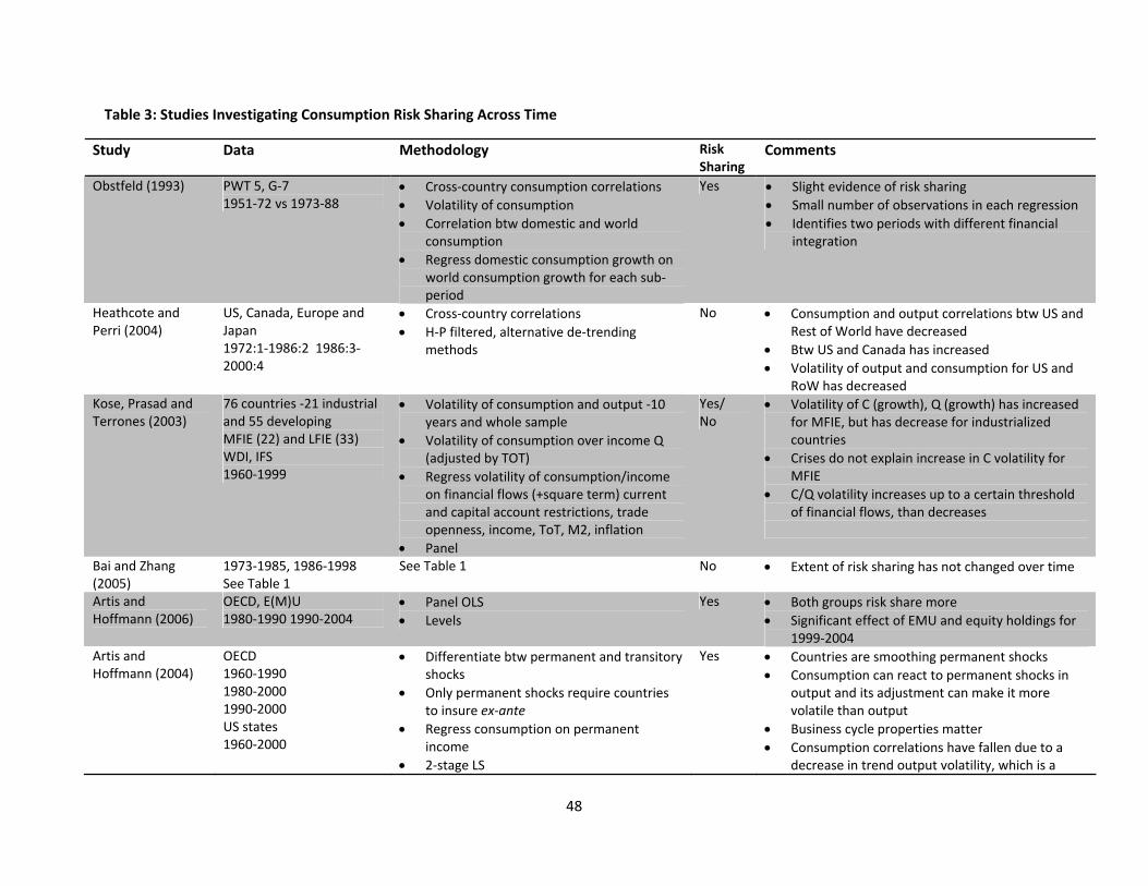
48  

Table 3: Studies Investigating Consumption Risk Sharing Across Time 

Study  Data  Methodology  Risk Sharing 

Comments 

Obstfeld (1993)  PWT 5, G‐7 1951‐72 vs 1973‐88 

Cross‐country consumption correlations  Volatility of consumption  Correlation btw domestic and world 

consumption  Regress domestic consumption growth on 

world consumption growth for each sub‐period 

Yes  Slight evidence of risk sharing  Small number of observations in each regression  Identifies two periods with different financial 

integration 

Heathcote and Perri (2004) 

US, Canada, Europe and Japan 1972:1‐1986:2  1986:3‐2000:4 

Cross‐country correlations  H‐P filtered, alternative de‐trending 

methods 

No  Consumption and output correlations btw US and Rest of World have decreased 

Btw US and Canada has increased  Volatility of output and consumption for US and 

RoW has decreased Kose, Prasad and Terrones (2003) 

76 countries ‐21 industrial and 55 developing MFIE (22) and LFIE (33) WDI, IFS 1960‐1999 

Volatility of consumption and output ‐10 years and whole sample 

Volatility of consumption over income Q (adjusted by TOT) 

Regress volatility of consumption/income on financial flows (+square term) current and capital account restrictions, trade openness, income, ToT, M2, inflation 

Panel  

Yes/ No  

Volatility of C (growth), Q (growth) has increased for MFIE, but has decrease for industrialized countries 

Crises do not explain increase in C volatility for MFIE 

C/Q volatility increases up to a certain threshold of financial flows, than decreases  

Bai and Zhang (2005) 

1973‐1985, 1986‐1998 See Table 1 

See Table 1  No  Extent of risk sharing has not changed over time 

Artis and Hoffmann (2006) 

OECD, E(M)U 1980‐1990 1990‐2004 

Panel OLS  Levels 

Yes  Both groups risk share more  Significant effect of EMU and equity holdings for 

1999‐2004 Artis and Hoffmann (2004) 

OECD  1960‐1990 1980‐2000 1990‐2000 US states 1960‐2000 

Differentiate btw permanent and transitory shocks 

Only permanent shocks require countries to insure ex‐ante 

Regress consumption on permanent income 

2‐stage LS 

Yes  Countries are smoothing permanent shocks  Consumption can react to permanent shocks in 

output and its adjustment can make it more volatile than output 

Business cycle properties matter  Consumption correlations have fallen due to a 

decrease in trend output volatility, which is a 

49  

common component is domestic and rest of the world C 

Artis and Hoffmann (2006) 

OECD 1960‐1990 1990‐2004 

See table 2  Yes  level regressions capture long term‐effects  limited risk sharing in the short‐term  evidence of risk sharing in the medium and long 

run Islamaj (2008)  WDI 

Periods based on relatively open vs closed periods 

using available rule‐based financial integration indicators identify open and closed periods for each country 

check correlations of domestic consumption growth and domestic output growth for each sub‐period 

control for productivity shock correlations with rest of the world 

Yes  preliminary evidence suggest that after controlling for productivity shock correlations with rest of the world, we can explain the lack of consumption smoothing as countries have become more integrated  

Sorensen, Wu, Yosha and Zhu (2008) 

24 OECD 1993‐2003 

Panel OLS  growth 

Yes  Risk sharing increased  Home bias decreased  FDI is better than debt for consumption risk 

sharing Bekaert, Harvey and Lundblad (2005) 

95 countries 40 emerging markets 1980‐2000 5‐year 

Volatility 5 years before and after equity market liberalization 

Panel   Various indicators of financial liberalization 

Yes  Less volatility of consumption growth to GDP growth 

Results are weaker for emerging markets 

Kose, Prasad and Terrones (2007) 

PWT+WDI 1960‐1984 1985‐2004 72 countries 

Co‐movement with national output  w/ world output/consumption  9‐year rolling window  Regressions for each sub‐period  Effects of financial flows on risk sharing 

Mixed  industrial countries have been better able to smooth consumption over time 

no evidence for emerging markets and other developing countries 

financial flows have improved risk sharing in industrial countries 

composition can’t explain  

 

 

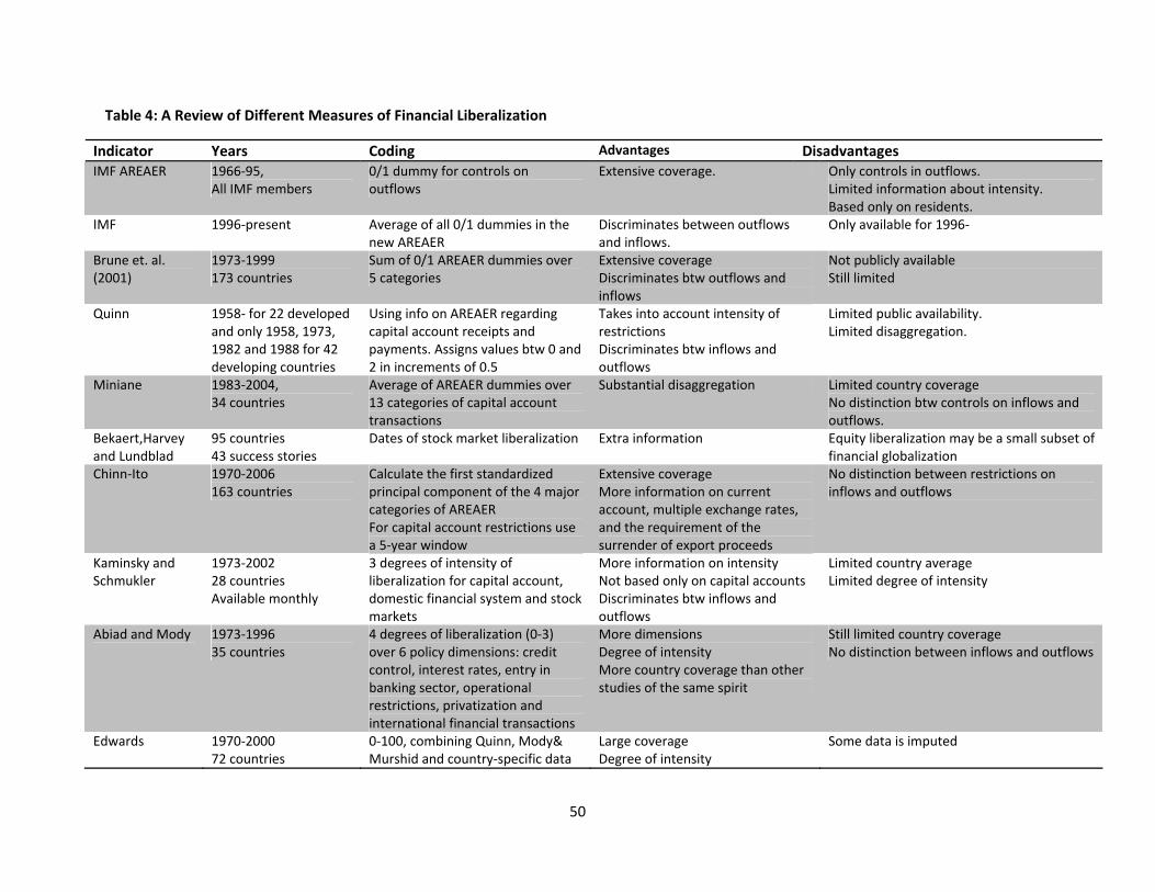
50  

Table 4: A Review of Different Measures of Financial Liberalization 

Indicator  Years  Coding  Advantages  Disadvantages IMF AREAER  1966‐95, 

All IMF members 0/1 dummy for controls on outflows 

Extensive coverage.  Only controls in outflows. Limited information about intensity. Based only on residents. 

IMF  1996‐present  Average of all 0/1 dummies in the new AREAER 

Discriminates between outflows and inflows. 

Only available for 1996‐  

Brune et. al. (2001) 

1973‐1999 173 countries 

Sum of 0/1 AREAER dummies over 5 categories 

Extensive coverage Discriminates btw outflows and inflows 

Not publicly available Still limited 

Quinn   1958‐ for 22 developed and only 1958, 1973, 1982 and 1988 for 42 developing countries 

Using info on AREAER regarding capital account receipts and payments. Assigns values btw 0 and 2 in increments of 0.5 

Takes into account intensity of restrictions Discriminates btw inflows and outflows 

Limited public availability. Limited disaggregation.  

Miniane   1983‐2004, 34 countries  

Average of AREAER dummies over 13 categories of capital account transactions 

Substantial disaggregation  Limited country coverage No distinction btw controls on inflows and outflows. 

Bekaert,Harvey and Lundblad 

95 countries 43 success stories 

Dates of stock market liberalization  Extra information  Equity liberalization may be a small subset of financial globalization 

Chinn‐Ito  1970‐2006 163 countries 

Calculate the first standardized principal component of the 4 major categories of AREAER For capital account restrictions use a 5‐year window 

Extensive coverage More information on current account, multiple exchange rates, and the requirement of the surrender of export proceeds  

No distinction between restrictions on inflows and outflows 

Kaminsky and Schmukler 

1973‐2002 28 countries Available monthly 

3 degrees of intensity of liberalization for capital account, domestic financial system and stock markets 

More information on intensity Not based only on capital accounts Discriminates btw inflows and outflows 

Limited country average Limited degree of intensity 

Abiad and Mody  1973‐1996 35 countries 

4 degrees of liberalization (0‐3) over 6 policy dimensions: credit control, interest rates, entry in banking sector, operational restrictions, privatization and international financial transactions 

More dimensions Degree of intensity More country coverage than other studies of the same spirit 

Still limited country coverage No distinction between inflows and outflows 

Edwards  1970‐2000 72 countries 

0‐100, combining Quinn, Mody& Murshid and country‐specific data 

Large coverage Degree of intensity 

Some data is imputed 

51  

Table 5: Net Effect of Liberalization and Cross‐country Productivity Correlations, eqn (5). 

Miniane  Chinn‐Ito  Capital Account 

Current Account 

Kaminsky &Shmukler 

Abiad & Mody 

Edwards 

∂β1/∂τ  0.16  0.13  0.06  0.06  0.16  0.13  0.20  [0.000]***  [0.000]***  [0.000]***  [0.000]***  [0.000]***  [0.000]***  [0.000]***  ∂β2/∂τ ‐0.25  ‐0.10  ‐0.06  ‐0.05  ‐0.19  ‐0.11  ‐0.16  [0.008]***  [0.000]***  [0.000]***  [0.000]***  [0.000]***  [0.017]**  [0.000]***  ∂β1/∂ρ  0.04  0.01  0.05  0.03  0.03  0.05  ‐0.02  [0.364]  [0.000]***  [0.000]***  [0.000]***  [0.429]  [0.353]  [0.000]***  ∂β2/∂ρ  ‐0.11  ‐0.03  ‐0.10  ‐0.05  ‐0.06  ‐0.14  0.012  [0.038]**  [0.000]***  [0.000]***  [0.000]***  [0.636]  [0.051]*  [0.000]***  Note: This Table shows the net effect of financial liberalization and cross‐country productivity correlations on β1 and β2 for the equation in differences. The coefficients estimated are shown in Table X in the Appendix. p‐values are shown in parenthesis. The effect of a change in tax τ is calculated for the median productivity correlation with rest of the world ρ=0.09, whereas the effect of a change in ρ corresponds to low τ for reasons explained in the text. 

 

Table 6: Effects of Liberalization and Cross‐country Productivity Correlations, eqn (6). 

Miniane  Chinn‐Ito  Capital Account 

Current Account 

Kaminsky &Shmukler 

Abiad & Mody 

Edwards 

∂β1/∂τ  0.26  0.18  0.15  0.10  0.20  0.05  0.27  [0.000]***  [0.000]***  [0.000]***  [0.000]***  [0.000]***  0.0183**  [0.000]***  ∂β2/∂τ ‐0.45  ‐0.16  ‐0.19  ‐0.12  ‐0.18  0.03  ‐0.18  [0.000]***  [0.000]***  [0.000]***  [0.000]***  [0.000]***  0.2526  [0.000]***  ∂β1/∂ρ  ‐0.01  0.01  0.09  0.03  0.01  0.0314  ‐0.03  [0.212]  [0.070]*  [0.000]***  [0.000]***  [0.185]  [0.044]**  [0.000]***  ∂β2/∂ρ  0.04  ‐0.04  ‐0.18  ‐0.08  ‐0.05  ‐0.16  0.00  [0.259]  [0.000]***  [0.000]***  [0.000]***  [0.044]*  [0.000]***  [0.773]  Note: This Table shows the net effect of financial liberalization and cross‐country productivity correlations on β1 and β2 for the equation that divides by World GDP. The coefficients estimated are shown in Table X in the Appendix. p‐values are shown in parenthesis. The effect of a change in tax τ is calculated for the median productivity correlation with rest of the world ρ=0.09, whereas the effect of a change in ρ corresponds to low τ for reasons explained in the text. 

 

52  

Table 7: Effects of Liberalization and Cross‐country Productivity Correlations, eqn (6). 

Miniane  Chinn‐Ito  Capital Account 

Current Account 

Kaminsky &Shmukler 

Abiad & Mody 

Edwards 

∂β1/∂τ  0.26  0.19  0.18  0.09  0.25  0.03  0.31  [0.000]***  [0.000]***  [0.000]***  [0.000]***  [0.000]***  [0.154]  [0.000]***  ∂β2/∂τ ‐0.48  ‐0.19  ‐0.22  ‐0.13  ‐0.16  0.03  ‐0.23  [0.000]***  [0.000]***  [0.000]***  [0.000]***  [0.000]***  [0.407]  [0.000]***  ∂β1/∂ρ  ‐0.06  0.02  0.08  0.01  ‐0.01  0.01  ‐0.04  [0.000]***  [0.001]***  [0.000]***  [0.059]*  [0.381]  [0.655]  [0.000]***  ∂β2/∂ρ  0.15  ‐0.07  ‐0.17  ‐0.05  0.00  ‐0.14  0.00  [0.001]***  [0.016]**  [0.000]***  [0.000]***  [0.938]  [0.000]***  [0.5089]  Note: This Table shows the net effect of financial liberalization and cross‐country productivity correlations on β1 and β2 for the equation in levels. The coefficients estimated are shown in Table X in the Appendix. p‐values are shown in parenthesis. The effect of a change in tax τ is calculated for the median productivity correlation with rest of the world ρ=0.09, whereas the effect of a change in ρ corresponds to low τ for reasons explained in the text. 

 

Table 8. Effects of Financial Liberalization for Low and High Levels of Liberalization 

  Miniane  Chinn‐Ito  Kaminsky &Shmukler 

Abiad & Mody 

Edwards 

0.22  0.14  0.11  0.03  0.21 Low 

[0.000]***  [0.000]***  [0.000]***  [0.422]  [0.000]*** 

0.35  0.18  0.44  0.01  0.45 

 ∂β1/∂τ 

High [0.000]***  [0.000]***  [0.000]***  [0.797]  [0.000]*** 

‐0.35  ‐0.13  ‐0.10  0.05  ‐0.05 Low [0.000]***  [0.000]***  [0.005]***  [0.198]  [0.182] 

High  ‐0.67  ‐0.14  ‐0.26  0.064  ‐0.54 

 

∂β2/∂τ 

  [0.000]***  [0.000]***  0.0137**  [0.265]  [0.000]***  Note: This Table shows the net effect of financial liberalization and cross‐country productivity correlations on β1 and β2 for the equation in levels. The coefficients estimated are shown in Table X in the Appendix. p‐values are shown in parenthesis. In each case, the upper row (Low) uses the 75% least open tail of the sample and the lower row uses the 75% most open part of the sample. 

 

 

53  

Figure1: Financial Liberalization and Correlation between Own Consumption and Income:  Less Sm

oothing

More S

moo

thing

More Liberalization

µ = 2, A = 1, σ = 0.1 (HP 04)

Less Liberalization

A

B

 

Figure 2: Financial Liberalization Correlation between Own Consumption and ROW Income 

AA

B

More S

moo

thing

Less Sm

oothing

More Liberalization

µ = 2, A = 1, σ = 0.1 (HP 04)

Less Liberalization 

Notes: Figure 1‐2 shows a mapping of impediments to trade in purchasing foreign capital and different measures of consumption smoothing as described in the model above for the symmetric case. The parameters used are µ=2, A=1 and σ=0.1 

54  

 Figure 3: Mapping Financial Liberalization Indicators into the Model  

0    A    B    1  τ   

              1 to A? 

           B to0 ? 

  B to A? 

Note: This Figure is used to explain the mapping of a financial liberalization indicator in our model.  

 

 

Figure 4: Distribution of Constructed Liberalization Measures

05

1015

20Den

sity

.5 .6 .7 .8 .9 1Chinn-Ito

02

46

810

Den

sity

.5 .6 .7 .8 .9 1Miniane

05

1015

20Den

sity

.5 .6 .7 .8 .9 1Kaminsky & Schmukler

05

1015

Den

sity

.5 .6 .7 .8 .9 1Edwards