Embed Size (px)
Citation preview

Financial Entanglement: A Theory of
Incomplete Integration, Leverage, Crashes,
and Contagion
Online Appendix
Nicolae Garleanu, Stavros Panageas, and Jianfeng Yu
A. Extensions
A. 1. An infinite horizon version of the baseline model
In this section we develop an intertemporal version of the model. The intertemporalversion allows us to extend the intuitions of our comparative statics exercises to aframework where the shocks to the participation technology are recurrent.
Specifically, we keep the key assumptions of the baseline model (Section II.B.),and in particular the assumption that investors only participate in an arc surround-ing their home location. However, we assume that investors maximize expecteddiscounted utility from consumption
−∞∑t=0
βtE0
[e−γct,i
],
where t denotes (discrete) calendar time. We assume that dividends at locationi ∈ [0, 1) are given by
(1) Dt,i = (1− ρ)
t∑k=−∞
ρt−kεk,i,
where ρ < 1,
(2) εt,i ≡ 1 + σ
(B
(t)i −
∫ 1
0B
(t)j dj
),
and B(t)i denotes a family of Brownian Bridges on [0, 1] drawn independently across
times t ∈ {−∞, . . . , 1, 2, . . . ,∞}.We make a few observations about this dividend structure. First, we note that
equation (2) coincides with equation (3). Accordingly,∫ 1
0 εt,idi = 1, and therefore,
equation (1) implies that∫ 1
0 Dt,i = 1 for all t, so that the aggregate dividend is alwaysequal to one. Second, dividends at individual locations follow AR(1) processes, sinceequation (1) implies
(3) Dt,i = (1− ρ) εt,i + ρDt−1,i.
1
Moreover, since (2) coincides with (3), the increments of two dividend processes attwo locations i and j have the covariance structure of equation (4).
In terms of participation decisions, we keep the same cost assumption as in thebaseline model and further assume that investors participate in a single interval of
length ∆(i)t centered at their “home” location. Participation costs are paid period
by period in advance of trading. Specifically, an investor’s intertemporal budgetconstraint is given by
(4) ct,i +Ft
(∆
(i)t
)+
∫ 1
0Pt,jdX
(i)t,j +PB,tX
(i)B,t =
∫ 1
0(Pt,j +Dt,j) dX
(i)t−1,j +X
(i)B,t−1.
We note that in equation (4) we allow the entire cost function Ft(∆) = κtgt (∆) tobe different across different periods in order to capture the effect of repeated shocksto the participation technology.
This intertemporal version of the model presents a challenge that is absent ina static framework: If the interest rate varies over time, then the value functionof an agent is not exponential in wealth. In fact, a closed-form expression for thevalue function most likely does not exist. Furthermore, once the value function isno longer exponential, portfolios are no longer independent of wealth, and hence theentire wealth distribution matters — an infinite-dimensional state variable.
In order to maintain the simple structure of the solution, therefore, we makenecessary assumptions to achieve a constant interest rate in the presence of randomparticipation costs, while safeguarding market clearing for bond markets, risky-asset markets, and consumption markets.1 The following proposition states thatit is possible to achieve this outcome by judiciously specifying the distribution ofthe participation costs. The main thrust of the proposition, however, concerns theexpression for the risky-asset prices.
Proposition 1 There exist an interval [∆l,∆u], a (non-trivial) distribution func-tion Ψ (·) on [∆l,∆u], and a cost function F (·; ∆t) : [∆l,∆u]→ R+ such that, if ∆t
is drawn in an i.i.d. fashion from Ψ, then(i) investors optimally choose ∆ = ∆t, thus incurring cost F (∆t; ∆t);(ii) the risk-free rate is constant over time and given as the unique positive solutionto
1 = β (1 + r)E
[eγ2
2
(r
1+r−ρ
)2(1−ρ)2ω(∆)
],(5)
where the expectation is taken over the distribution of ∆;(iii) the risky-asset prices equal
(6) Pt,j (∆t, Dt,j) = φ (Dt,j − 1) +1
r− Φ1ω (∆t)− Φ0
1Alternatively, in the interest of simplicity, we could fix the interest exogenously to themodel and let aggregate lending adjust accordingly.
2
with φ ≡ ρ1+r−ρ and
Φ1 = γr(1− ρ)2
(1 + r − ρ)2(7)
Φ0 =Φ1
r
E
[eγ2
2
(r
1+r−ρ
)2(1−ρ)2ω(∆)
ω (∆)
]E
[eγ2
2
(r
1+r−ρ
)2(1−ρ)2ω(∆)
] > 0.(8)
Furthermore, investors’ optimal portfolios of risky assets are given by (12).
Equation (6) decomposes the price of a security into three components. As inall CARA models, one of these components equals the expected discounted valueof future dividends, φ(Dt,j − 1) + r−1. The other two capture the risk premium.The term Φ1ω(∆t) is the risk premium associated with the realization of time-t+ 1dividend uncertainty, to which each investor is exposed according to the breadth ∆t
of her time-t portfolio. Finally, Φ0 equals the sum of the expected discounted valueof risk premia due to future realizations of dividend innovations and ∆t.
We emphasize that the risk premium decreases with ∆t and is common for allsecurities. Alternatively phrased, increases in capital movements across locationsare correlated with higher prices for all risky securities (and hence lower expectedexcess returns). Importantly, these movements in the prices of risky securities areuncorrelated with movements in aggregate output or the interest rate, which areboth constant by construction.
A further immediate implication of equation (6) is that the presence of repeatedshocks to participation costs introduces correlation in security prices that exceedsthat of their dividends. Indeed, taking two securities j and k, and noting thatV ar (Dt,j) = V ar (Dt,k) , we can use equation (6) to compute
corr (Pt,j , Pt,i) =V ar(Φ1ω (∆t)) + φ2cov (Dt,j , Dt,k)
V ar(Φ1ω (∆t)) + φ2V ar (Dt,j)>cov (Dt,j , Dt,k)
V ar (Dt,j)= corr (Dt,j , Dt,i) .
The intuition is that movements in market integration cause common movementsin the pricing of risk which make prices more correlated (and volatile) than theunderlying dividends.
We collect some basic properties of the price due to the randomness in ∆t in thefollowing proposition.
Proposition 2 (i) Pt,i increases with ∆t, and therefore corr(Pt,i,∆t) > 0;(ii) Et[Pi,t+1 − (1 + r)Pi,t] decreases with ∆t;(iii) corr(Pt,i, Pt,j) > corr(Dt,i, Dt,j);(iv) Φ0 is higher (and hence the unconditional expected price is lower) than the oneobtaining for ∆t constant and equal to E[∆].
3
0 0.01 0.02 0.03 0.04 0.05 0.06 0.07 0.08 0.09 0.10.04
0.045
0.05
0.055
0.06
0.065
0.07
0.075
0.08
0.085
I
Min
imiz
ed v
ariance
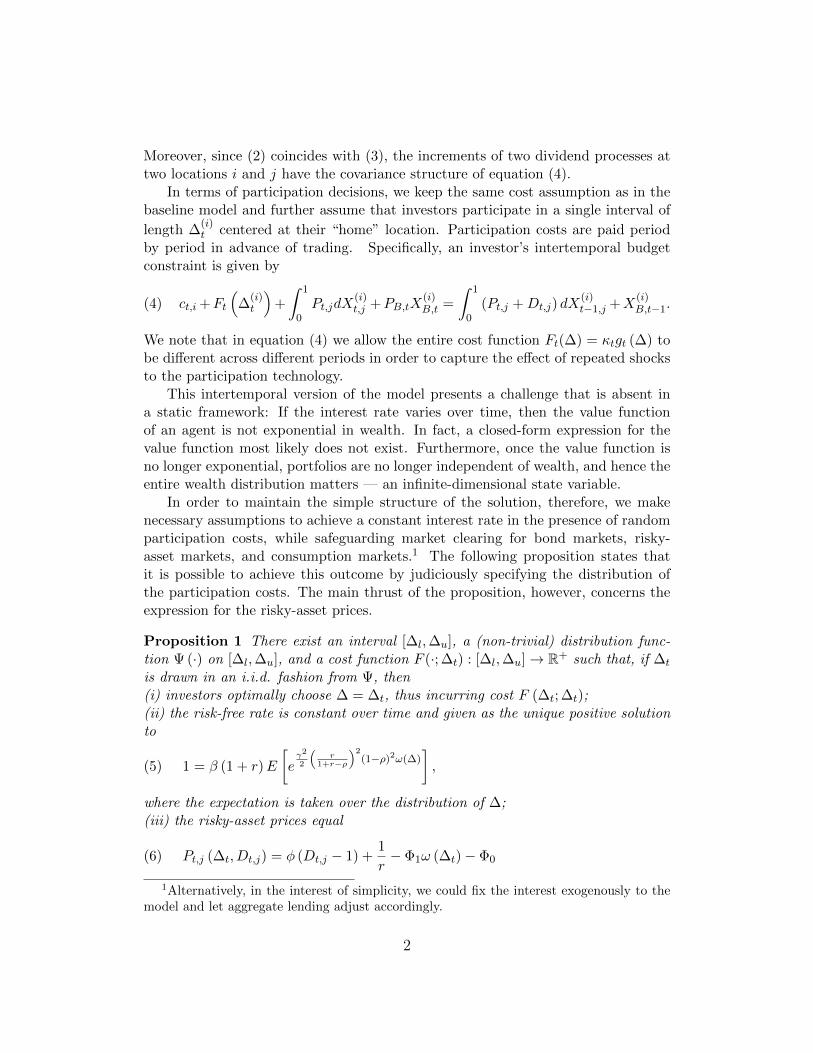
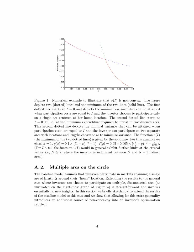
Figure 1: Numerical example to illustrate that v(I) is non-convex. The figuredepicts two (dotted) lines and the minimum of the two lines (solid line). The firstdotted line starts at I = 0 and depicts the minimal variance that can be attainedwhen participation costs are equal to I and the investor chooses to participate onlyon a single arc centered at her home location. The second dotted line starts atI = 0.05, i.e. at the minimum expenditure required to invest in two distinct arcs.This second dotted line depicts the minimal variance that can be attained whenparticipation costs are equal to I and the investor can participate on two separatearcs with locations and lengths chosen so as to minimize variance. The function v(I)(the minimum of the two dotted lines) is given by the solid line. For this example wechose σ = 1, g(x) = 0.1×
((1− x)−6 − 1
), f(y) = 0.05 + 0.005×
((1
2 − y)−2 − 10.25
).
(For I > 0.1 the function v(I) would in general exhibit further kinks at the criticalvalues IN , N ≥ 2, where the investor is indifferent between N and N + 1 distinctarcs.)
A. 2. Multiple arcs on the circle
The baseline model assumes that investors participate in markets spanning a singlearc of length ∆ around their “home” location. Extending the results to the generalcase where investors can choose to participate on multiple, disconnected arcs (asillustrated on the right-most graph of Figure 4) is straightforward and involvesessentially no new insights. In this section we briefly sketch how to extend the resultsof the baseline model to this case and we show that allowing for this extra generalityintroduces an additional source of non-concavity into an investor’s optimizationproblem.
4

To start, we introduce the function
v(I) = minNi,−→a i,−→∆i,G
(i)j
V ar
(∫ 1
0DjdG
(i)j
)
s.t. I ≥ F
(−→a i,
Ni∑n=1
∆i,n
).
In words, the function v(I) is the minimal variance, per share purchased, of theportfolio payoff that can be obtained by an investor who is willing to spend anamount I on participation costs. Proceeding similarly to Section B. under theassumption that Pj = P for all j, the facts that U is exponential and all Dj are nor-mally distributed imply that maximizing utility over the choice of Ni, {ai,1; ..; ai,Ni},{∆i,1; ..; ∆i,Ni}, G
(i)j , and wfi is equivalent to solving2
maxwfi ,I
Pwfi +(
1− wfi)∫ 1
0E[Dj ]dG
(i)j −
γ
2
(1− wfi
)2v (I)− I.(9)
Given that E[Dj ] = 1, equation (9) can be rewritten as
(10) V = maxI,wfi
Pwfi +(
1− wfi)− γ
2
(1− wfi
)2v(I)− I.
In the baseline version of the model (Section B.), where the investor chooses toinvest in a single arc around her home location, v is a convex function of the totalcost I.3 In the general case where investors’ portfolios are invested on disconnectedarcs, the function v (I) is in general non-convex with kinks at the expenditure levelsIn where it becomes optimal to invest in n + 1 rather than n distinct arcs. Figure1 provides an illustration. This non-convexity of v (I) , which may arise when (andonly when) investors participate in markets located on multiple distinct arcs, con-stitutes an additional reason for the maximization problem (10) to be non-concave.This reason is distinct from the non-concavity arising from the interaction betweenleverage and participation decisions that we identify in Section C., and strengthensthe conclusion that a symmetric equilibrium may not exist.
2To ensure that the optimization problem (9) has a solution it is convenient either toimpose a collateral constraint such as (23) or to introduce some (potentially small but pos-itive) aggregate risk in dividends. Either of these assumptions coupled with the additionalassumption lim∆→1 g (∆) = ∞ suffices to ensure the existence of a solution to (9). Alter-natively, one can ensure that (9) has an interior solution by requiring that, upon plugging
in the optimal value of wfi , the maximand in (10) tends to negative infinity as I goes toinfinity. Given the lower bound on P provided by the autarky equilibrium, it suffices that
limI→∞(σ2
12
)2 γv(I) − I = −∞. This condition may be harder to verify than Assumption 1,
since it is not readily expressed in terms of primitive parameters.3To see this, note that v′ (I) = ω′(∆)
κg′(∆) , where ∆ (I) = g−1(Iκ
). Differentiating again
gives v′′ (I) = 1κω′′(∆)g′(∆)−ω′(∆)g′′(∆)
(g′(∆))2∆′ (I) > 0.
5
B. Proofs
Proof of Lemma 1. Property 2 follows immediately from integrating (3). Toshow property 3, note that, for any i ∈ (0, 1), limd(i,j)→0Dj = limj→iDj = Di a.s.by the continuity of the Brownian motion. Continuity at 0 follows from the factthat B0 = B1.
We turn now to property 1. Since E(Bi) = 0 for all i ∈ [0, 1], E(Dj) = 1. Tocompute cov(Di, Dj) we start by noting that cov (Bs, Bt) = E(BsBt) = s (1− t) fors ≤ t.Therefore, for any t ∈ [0, 1],∫ 1
0E (BtBu) du =
∫ t
0u(1− t)du+
∫ 1
tt(1− u)du(11)
=1
2(1− t)t2 +
1
2(1− t)2t =
t (1− t)2
.
Accordingly,
V ar
(∫ 1
0Budu
)= E
[(∫ 1
0Budu
)2]
= E
[(∫ 1
0Budu
)(∫ 1
0Btdt
)](12)
=
∫ 1
0
(∫ 1
0E(BuBt)du
)dt =
∫ 1
0
t (1− t)2
dt =1
12,
where the second line of (12) follows from Fubini’s Theorem and (11). Combining(12) and (11) gives
1
σ2V ar (Dt) = V ar (Bt) + V ar
(∫ 1
0Budu
)− 2cov
(Bt,
∫ 1
0Budu
)(13)
= t (1− t) +1
12− 2
∫ 1
0E(BtBu)du =
1
12.
This calculation finishes the proof of property 1. For property 4, take any s ≤ tand use (11) and (12) to obtain
cov (Ds, Dt)
σ2= cov
(Bs −
∫ 1
0Budu,Bt −
∫ 1
0Budu
)(14)
= E(BsBt)− E(Bs
∫ 1
0Bu
)du− E
(Bt
∫ 1
0Bu
)du+
1
12
= s (1− t)− s (1− s)2
− t (1− t)2
+1
12
=(s− t)(1 + s− t)
2+
1
12.
This establishes property 4.Proof of Proposition 1. We start by establishing the following lemma.
6

Lemma 1 The (bounded-variation) function L with L−∆2
− = 0 and L∆2
= 1 that
minimizes V ar
(∫ ∆2
−∆2
− Dj dLj
)is given by (12). Moreover, the minimal variance
is equal to ω (∆) .
Proof of Lemma 1. To simplify notation, we prove a “shifted” versionof the lemma, namely finding the minimal-variance portfolio on [0,∆] rather than[−∆
2 ,∆2 ]. The two versions are clearly equivalent, since covariances depend only on
the distances between locations, rather than the locations themselves.We start by defining q (d) = 1
12 −d(1−d)
2 and therefore q′ (d) = −12 + d. In light
of (4), q(d) = 1σ2 cov (Di, Dj) whenever d (i, j) = d. If Lu =
∫ u0− dLu is a variance-
minimizing portfolio of risky assets, it must be the case that the covariance betweenany gross return Rs = Ds
P for s ∈ [0,∆] and the portfolio∫ ∆
0− RudLu =∫ ∆
0−DuP dLu
is independent of s. Thus, the quantity
1
σ2cov
(Ds,
∫ ∆
0−DudLu
)=
1
σ2
[∫ s
0−cov (Ds, Du) dLu +
∫ ∆
scov (Ds, Du) dLu
]=(15)
=
∫ s
0−q (s− u) dLu +
∫ ∆
sq (u− s) dLu
is independent of s. Letting L (s) = 1− L (s) and integrating by parts we obtain∫ s
0−q (s− u) dLu = L (s) q (0)− L
(0−)q (s) +
∫ s
0−Luq
′ (s− u) du(16) ∫ ∆
sq (u− s) dLu = L (s) q (0)− L (∆) q (∆− s) +
∫ ∆
sLuq
′ (u− s) du.(17)
Using (16) and (17) inside (15) and recognizing that q (0) = 112 , L (0−) = 0, and
L (∆) = 0, we obtain that (15) equals
(18) Q(s) ≡ 1
12+
∫ s
0−Luq
′ (s− u) du+
∫ ∆
sLuq
′ (u− s) du.
This expression is independent of s ∈ [0,∆] if and only if Q′(s) = 0. Differentiating(18) and setting the resulting expression to zero yields
Q′(s) =
∫ s
0−Luq
′′ (s− u) du−∫ ∆
sLuq
′′ (u− s) du+ Lsq′ (0)− Lsq′ (0)
=
∫ ∆
0−Ludu−∆ + s− Ls +
1
2= 0,(19)
where we used q′ (0) = −12 , q′′ = 1, and L (s) = 1− L (s). Since (19) needs to hold
for all s ∈ [0,∆], it must be the case that Ls = A + s for an appropriate constantA. To determine A, we subsitute Ls = A+ s into (19) and solve for A to obtain
A =1−∆
2.
7

It is immediate that the standardized portfolio corresponding to the solution Lwe computed is L∗ of (12).
Using the variance-minimizing portfolio inside (18), implies after several simpli-
fications, that Q = 112 (1−∆)3 and hence cov
(Ds,
∫ ∆0− DudLu
)= Qσ2 = ω (∆) .
Accordingly,
V ar
(∫ ∆
0−DudLu
)= cov
(∫ ∆
0−DsdLs,
∫ ∆
0−DudLu
)=
∫ ∆
0−cov
(Ds,
∫ ∆
0−DudLu
)dLs
= ω(∆)
∫ ∆
0−dLs = ω (∆) .
With Lemma 1 in hand it is possible to confirm that the allocations and pricesof Proposition 1 constitute a symmetric equilibrium — assuming that one exists.We already argued that all agents choose the same standardized portfolio (as agent∆2 ). Furthermore, since in a symmetric equilibrium all agents must hold the same
allocation of bonds, clearing of the bond market requires wfi = 0 for all i. By
equation (18), wfi = 0 is supported as an optimal choice for an investor only ifPi = P is given by (15). Similarly, in light of (19), equation (14) is a necessaryoptimality condition for the interval ∆∗. Since the values of P and ∆∗ implied by(15) and (14) are unique, they are necessarily the equilibrium values of P and ∆∗
that characterize a symmetric equilibrium. Hence, when a symmetric equilibriumexists, it is unique in the class of symmetric equilibria.
Existence of a symmetric equilibrium implies that wfi = 0 is optimal, and so are
the choices ∆∗ and G(i)i+j = L∗j given prices Pi = P. It remains to show that markets
clear. We already addressed bond-market clearing. To see that the stock marketsclear, we start by noting that, since Pi = W0,i = P for all i, the market clearing
condition amounts to∫i∈[0,1) dG
(i)j = 1. We have
∫i∈[0,1) dG
(i)j =
∫i∈[0,1) dL
∗j−i =∫
j∈[0,1) dL∗j = 1.
Proof of Proposition 2. Let w∗ (P ) denote the set of optimal wfi solvingthe maximization problem (17) when the price in all markets is P. We first notethat the assumption that no symmetric equilibrium exists implies that there existsno P such that 0 ∈ w∗(P ). (If such a P existed, then we could simply repeat thearguments of Proposition 1 to establish the existence of a symmetric equilibriumwith price Pi = P, and interval choice ∆i = ∆∗(P )).
We next show that since there exists no P such that 0 ∈ w∗(P ), it follows thatw∗(P ) cannot be single-valued for all P. We argue by contradiction. Suppose to thecontrary that w∗(P ) is single-valued. Since the theorem of the maximum implies thatw∗(P ) is a upper-hemicontinuous correspondence, it follows that w∗(P ) is actuallya continuous function. Inspection of (17) shows that w∗(1) = 1. Moreover, asP → −∞, the optimal solution to (17) becomes negative: w∗ (−∞) < 0. Then an
8

application of the intermediate value theorem gives the existence of P such thatw∗ (P ) = 0, a contradiction.
Combining the facts that a) there exists no P such that 0 ∈ w∗(P ), b) w∗(P )is multi-valued for at least one value of P , and c) w∗(P ) is upper-hemicontinuous,implies that there exists at least one P such that {w1, w2} ∈ w∗(P ) with w1 > 0and w2 < 0. An implication of the necessary first-order condition for the optimal-ity of the interval choice ∆∗ (P ) is that ∆∗ (P ) is also multi-valued with ∆1 < ∆2.Furthermore, since prices in all locations are equal, the (standardized) optimal port-folio of an agent choosing ∆k is the variance-minimizing portfolio of Proposition 1,denoted L∗,k.
From this point onwards, an equilibrium can be constructed as follows. Bydefinition, the tuples
{∆1, w1, dL
∗,1} and{
∆2, w2, dL∗,2} are optimal. Hence it
only remains to confirm that asset markets clear. Define π ≡ − w2w1−w2
∈ (0, 1).By construction, πw1 + (1− π)w2 = 0 and, therefore, if in every location π agentschoose
{∆1, w1, dL
∗,1} and the remaining fraction (1− π) choose{
∆2, w2, dL∗,2} ,
then the bond market clears by construction. To see that the stock markets clear,we start by noting that, since Pi = W0,i = P , the market clearing condition forstock i amounts to
π
∫[0,1]
dL∗,1j−i + (1− π)
∫[0,1]
dL∗,2j−i = 1,
which holds because L∗,kj for k ∈ {1, 2} is a measure on the circle.We prove next that symmetric and asymmetric equilibria (with different prices)
cannot co-exist. Inspection of (17) shows that the optimal wfi is increasing inP in the sense that if P1 < P2 then w1 < w2 for any w1 ∈ w∗(P1) and w2 ∈w∗(P2).4 Accordingly, if a symmetric equilibrium exists, i.e., if there is a P suchthat 0 ∈ w∗(P ) then there cannot exist P 6= P with the property that {w1, w2} ∈w(P ) and yet w1 > 0 and w2 < 0, which is a requirement for the existence ofan asymmetric equilibrium. Hence symmetric and asymmetric equilibria cannotco-exist. The fact that w∗(P ) is an increasing correspondence also implies thatasymmetric equilibria are essentially unique, in the sense that asymmetric equilibriaassociated with different equilibrium prices cannot co-exist.
Remark 1 The existence proof of an asymmetric equilibrium (when a symmetricequilibrium fails to exist) obtains also in the presence of the leverage constraint (23)that we introduce in Section IV..
Proof of Proposition 3. Conjecture first that in equilibrium Pj = P forall j and let π ∈ [0, 1] denote the fraction of funds invested in the local market.
4To see that this statement is correct, consider the maximum V (P,wfi ) of the maximand
in (17) over ∆ and note that it cross-partial derivative with respect to P and wfi is positive:
∂P∂wfiV (P,wfi ) > 0.
9

Assuming that a given investor chooses N = 2 (that is, chooses to invest in her ownlocation and another location at distance d), equation (4) allows the computationof the minimal portfolio variance:
ω (d) = σ2 minπ
{(π2 + (1− π)2
) 1
12+ 2π (1− π)
(1
12− d (1− d)
2
)}(20)
= σ2
(1
12− 1
4d (1− d)
).
The optimal distance d for an investor choosing N = 2 satisfies a first-ordercondition similar to equation (19), namely
(21) −γ2
(1− wf
)2 ω′ (d)
ω2 (d)= κf ′ (d) .
Since ω′ (d) = 0 when and only when d = 12 , and f ′ (d) = 0, it follows that d = 1
2is optimal for an investor choosing N = 2. Hence the minimal portfolio variance of aninvestor choosing N = 1 is equal to ω (0) = σ2
12 , while the minimal portfolio variance
for an investor choosing N = 2 is ω(
12
)= σ2
48 . Assuming that the equilibrium isof the asymmetric, location-invariant type, we can use equation (17) to express theindifference between the choices N = 1, respectively N = 2 and d = 1
2 , as
(22)
Pwf1 +(
1− wf1)−γ
2
(1− wf1
)2ω (0) = Pwf2 +
(1− wf2
)−γ
2
(1− wf2
)2ω
(1
2
)−κf0.
Using the first-order conditions for leverage
(23) 1− P = γ(
1− wf2)ω
(1
2
)= γ
(1− wf1
)ω (0)
inside (22) yields — after some simplifications — the equilibrium price (24).To verify that the postulated equilibrium is indeed an equilibrium, we proceed as
in the proof of Proposition 2. For P (κ) to be an equilibrium price in all locations, it
must also be case that 1−wf1 ≤ 1 ≤ 1−wf2 , so that setting π =wf2
wf2−wf1
> 0 ensures
market clearing (of bond markets and all risky asset markets). In light of (23), the
requirement 1 − wf1 ≤ 1 ≤ 1 − wf2 is equivalent to P ∈[1− γω (0) , 1− γω
(12
)].
This requirement is satisfied as long as κ ∈ (κ1, κ2).
Lemma 2 Consider an investor located at i /∈[−k
2 ; k2], and therefore investing in
markets [i− ∆2 , i+ ∆
2 ]. Suppose that P (x) is continuously differentiable everywhere
10
on [i− ∆2 , i+ ∆
2 ]. With dX(i)l the number of shares purchased on the account of an
investor at i in market l and j ≡ i− ∆2 ,
X(i)
j+∆=
1
γω(∆) [1− 1− ∆
2
(Pj + Pj+∆
)−∫ j+∆
jPu du
].(24)
Furthermore, the function X is given by
X(i)j+l =
P ′j+lγσ2
+X(i)
j+∆
1−∆ + 2l
2+
1
1− ∆
Pj+∆ − Pjγσ2
.(25)
If an investor is located at i ∈ [−k2 ,
k2 ] and only invests in market i then the respective
demand for risky asset i is given by
(26) X(i)i =
1
γω (0)(1− Pi) .
Proof of Lemma 2. Notice that optimization problem of agent i is equivalentto
maxX
Pi +
∫ j+∆
j−(1− Pu) dXu −
γ
2V ar
(∫ j+∆
j−DudXu
)(27)
Thus, the first-order condition requires that
(28) γ cov
(Ds,
∫ j+∆
j−DudXu
)= 1− Ps
for all s ∈[j, j + ∆
]. Letting q (d) be defined as in Lemma 1 we can rewrite (28) as
(29)
∫ s
j−q (s− u) dXu +
∫ j+∆
sq (u− s) dXu =
1− Psγσ2
.
Let X (s) = X(j + ∆
)−X (s) and integrating by parts we obtain∫ s
j−q (s− u) dXu = X (s) q (0)−X
(j−)q (s) +
∫ s
jXuq
′ (s− u) du(30) ∫ j+∆
sq (u− s) dXu = X (s) q (0)− X
(∆)q (∆− s) +
∫ j+∆
sXuq
′ (u− s) du(31)
Substituting (30) and (31) into (29), recognizing that q (0) = 112 , X (j−) = 0, and
X(j + ∆
)= 0, we obtain
(32)1
12X(j + ∆
)+
∫ s
jXuq
′ (s− u) du+
∫ j+∆
sXuq
′ (u− s) du =1− Psγσ2
.
11

Since this relation must hold for all s, we may differentiate both sides of (32) toobtain
(33)
∫ s
jXuq
′′ (s− u) du−∫ j+∆
sXuq
′′ (u− s) du+Xsq′ (0)− Xsq
′ (0) = − P′s
γσ2.
This equation holds for all s ∈ (j, j + ∆). Noting that q′′ = 1, q′ (0) = −12 , X (s) =
X(j + ∆
)−X (s), and using (33) to solve for Xs yields
(34) Xs =
∫ j+∆
jXudu+
(s− j +
1
2− ∆
)X(j + ∆
)+P ′sγσ2
.
Integrating (34) from j to j + ∆ and solving for∫ j+∆j Xudu leads to
(35)
∫ j+∆
jXudu =
1
1− ∆
[X(j + ∆
)∆
(1− ∆
2
)+P(j + ∆
)− P (j)
γσ2
],
so that
Xs =1
1− ∆
[X(j + ∆
)∆
(1− ∆
2
)+P(j + ∆
)− P (j)
γσ2
]+(
s− j +1
2− ∆
)X(j + ∆
)+P ′sγσ2
.(36)
Evaluating (32) at s = j + ∆, and noting that q′ (s) = −12 + s leads to
(37)1
12X(j + ∆
)+
∫ j+∆
jXu
[−1
2+(∆− u
)]du =
1− Pj+∆
γσ2.
An implication of (34) is that Xu = Xj +P ′u−P ′jγσ2 + X
(j + ∆
)u. Using this
expression for Xu inside (37), carrying out the requisite integrations and using in-
tegration by parts to express∫ j+∆j
(P ′uγσ2
)u du =
Pj+∆
γσ2 (j + ∆)− Pjγσ2 j−
∫ j+∆j
Puγσ2du,
leads (after some simplifications) to
X(j + ∆
)( 1
12+
∆3
6− ∆2
4
)−
∆(1− ∆
)2
(Xj −
P ′jγσ2
)−Pj+∆ − Pj
2γσ2+
∫ j+∆
j−
Pu − Pjγσ2
du
=1− P∆
γσ2.(38)
Finally, evaluating (34) at j gives
(39)
(Xj −
P ′jγσ2
)=
∫ j+∆
jXudu+
(1
2− ∆
)X(j + ∆
).
12
Equations (35), (38), and (39) are three linear equations in three unknowns.Solving for X(j+ ∆) and using the definition of ω
(∆)
leads to (24). Equation (36)simplifies to (25). Finally, (26) is a direct consequence of (28) when ∆ = 0.
Proof of Proposition 4. For any j ∈(k2 ,
12
]and l ∈
(− ∆
2 ,∆2
), we have from
Lemma 2:
X(j)
j− ∆2
=P ′j− ∆
2
γσ2+Pj− ∆
2
− Pj+ ∆
2
γσ2(1−∆)+
1−∆
2X
(j)
j+ ∆2
dX(j)j+l =
(P ′′j+lγσ2
+X(j)
j+ ∆2
)dl
X(j)
j+ ∆2
−X(j)(j+ ∆
2
)− = −P ′j+ ∆
2
γσ2−Pj− ∆
2
− Pj+ ∆
2
γσ2(1−∆)+
1−∆
2X
(j)
j+ ∆2
.
Specialize the first equation to j = 12 + ∆
2 , the second to j = 12−l for all l ∈
(− ∆
2 ,∆2
),
and the third to j = 12 −
∆2 and aggregate to obtain the total demand for asset 1
2 :
1 =1−∆
2X
( 12
+ ∆2
)12
+∆+
1−∆
2X
( 12− ∆
2)
12
+
∫ ∆2
− ∆2
X( 1
2−l)
12−l+ ∆
2
dl +P ′′1
2
γσ2∆ +
P 12−∆ + P 1
2+∆ − 2P 1
2
2γσ2(1−∆).
Suppose now that Pj ≥ 1− γω(∆) on[
12 −∆, 1
2 + ∆], with strict inequality on
a positive measure set. It then follows from equation (24) that X(j)
j+ ∆2
≤ 1, so that
0 <P ′′1
2
γσ2∆ +
P 12−∆ + P 1
2+∆ − 2P 1
2
2γσ2(1−∆).
This inequality contradicts the assumption that P is maximized at 12 .
Proof of Proposition 1. We adopt a guess-and-verify approach. We startby noting that the beginning-of-period wealth of investor i at time t+ 1 is Wt+1,i ≡∫ 1
0 (Pt+1,j +Dt+1,j) dX(i)t,j +X
(i)B,t. We then conjecture that, as long as
F (∆) =M
γ+γ
2
(r
1 + r − ρ
)2
(1− ρ)2 ω (∆t)(40)
for some M > −γ2
2
(r
1+r−ρ
)2(1− ρ)2 ω (∆u), (ii) and (iii) obtain. We show at the
end that the function F can be chosen to ensure (i).
We also conjecture and verify that investors’ holdings of risky assetsX(i)t,j coincide
with G(i)t,j of Proposition 1, and that their bond holdings equal
(41) X(i)B,t = Wt,i − (1 + r)P t,i − rΦt,
13

where P t,i ≡∫ 1
0 Pt,jdX(i)t,j is the average price that investor i pays for her portfolio.
Here, to simplify notation, we defined Φt ≡ Φ1ω(∆t) + Φ0.We first ensure that with these postulates markets clear. Clearly, all risky mar-
kets clear, since the holdings of risky assets are the same as in Proposition 1. Toshow that bond markets clear, we proceed inductively. First we note that investors
are endowed with no bonds at time zero. Hence∫ 1
0 X(i)B,−1di = 0 and therefore∫ 1
0 W0,idi =∫ 1
0 (P0,i +D0,i) di. Next we postulate that∫ 1
0 X(i)B,t−1di = 0, so that∫ 1
0 Wt,idi =∫ 1
0 Pt,idi +∫ 1
0 Dt,jdj. Integrating our postulate (41) for X(i)B,t across all
investors, we obtain
(42)
∫ 1
0X
(i)B,tdi =
∫ 1
0Wt,idi− (1 + r)
∫ 1
0P t,idi− rΦt.
We next note that that (a)∫ 1
0 Dt,jdj = 1, by construction of the dividend process;
(b)∫ 1
0 Wt,idi =∫ 1
0 Pt,idi+∫ 1
0 Dt,jdj = r−1−Φt + 1, using the induction hypothesis,
(6), and (a); and (c)∫ 1
0 P t,idi =∫ 1
0 Pt,idi = r−1 − Φt. Using these three facts, itfollows immediately that the right-hand side of (42) is zero, so that the bond marketclears.
If investors set their bond holdings according to (41), then their budget con-straint implies a consumption of
(43) ct,i = Wt,i −1
1 + rX
(i)B,t − P t,i − Ft.
Using the definition of Wt,i and market clearing condition for bond holdings inside(43), and integrating across i implies that the market for consumption goods clears:∫ 1
0 ct,idi = 1− Ft.Having established market clearing given the postulated policies and prices, we
next turn to optimality. Equation (43) implies
ct+1,i − ct,i = Wt+1,i −Wt,i −1
1 + r
(X
(i)B,t+1 −X
(i)B,t
)−(P t+1,i − P t,i
)− (Ft+1 − Ft)
=
(r
1 + r
)(Wt+1,i −Wt,i) +
r
1 + r(Φt+1 − Φt)− (Ft+1 − Ft) ,(44)
where the second line follows from (41). We next use the definition of Wt,i and (41)to obtain
Wt+1,i −Wt,i =
∫ 1
0(Pt+1,j +Dt+1,j) dX
(i)t,j +X
(i)B,t −Wt,i
=
∫ 1
0(Pt+1,j +Dt+1,j) dX
(i)t,j − (1 + r)P t,i − rΦt.(45)
14

Substituting (45) into (44) and using (6) and (41) leads to
ct+1,i − ct,i =
(r
1 + r
)[(1 + φ)
∫ 1
0Dt+1,jdX
(i)t,j
− (1 + r)φ
∫ 1
0Dt,jdX
(i)t,j − (1− rφ)
∫ 1
0dX
(i)t,j
]− (Ft+1 − Ft) .(46)
Next use the fact Dt+1,j = ρDt,j + (1− ρ) εt+1,j along with φ = ρ1+r−ρ , (1 + φ) ρ =
(1 + r)φ, and (1 + φ) (1− ρ) = (1− rφ) inside (46) to arrive at
(47) ct+1,i − ct,i =
(r
1 + r − ρ
)(1− ρ)
∫ 1
0(εt+1,j − 1) dX
(i)t,j − (Ft+1 − Ft) .
Having established (47), the dynamics of agent i’s consumption under our pos-tulate, we next turn attention to the Euler equations, starting with the bond Eulerequation
(48) 1 = β (1 + r)Ete−γ(ct+1,i−ct,i).
Substituting (47) into (48) and noting that∫ 1
0 (εt+1,j − 1) dX(i)t,j is normally dis-
tributed with mean zero and variance ω (∆t) gives
(49) 1 = β (1 + r) eγ2
2
(r
1+r−ρ
)2(1−ρ)2ω(∆t)−γFtEt
(eγFt+1
).
Now suppose that for any r and a given desired distribution Ψ (∆) we set
(50) Ft (∆t; r) =M
γ+γ
2
(r
1 + r − ρ
)2
(1− ρ)2 ω (∆t) .
Then equation (49) can be written as (5). Since (1 + r)Eeγ2
2
(r
1+r−ρ
)2(1−ρ)2ω(∆)
isequal to 1 when r = 0 and increases monotonically to infinity as r increases, itfollows that there exists a unique positive r such that equation (5) holds. For thatvalue of r, all investors’ bond Euler equations are satisfied.
Finally, we need to determine Φt so as to ensure that the Euler equations forrisky assets hold, i.e., that
(51) Pt,j = βEt
[e−γ(ct+1,i−ct,i) (Pt+1,j +Dt+1,j)
].
To that end, we use (6) and (3) to express (51) as
(52)
1
r−Φt+φ(Dt,j−1) = βEt
[e−γ(ct+1,i−ct,i)
(1
r− Φt+1 + (1 + φ) (ρDt,j + (1− ρ) εt+1,j)− φ
)].
15
We next note that
(53) βEt
[e−γ(ct+1,i−ct,i)
](1 + φ) ρDt,j =
(1 + φ) ρ
1 + rDt,j = φDt,j
using (48). Equation (53) simplifies (52) to
1
r− Φt − φ = βEt
[e−γ(ct+1,i−ct,i)
(1
r− Φt+1 + (1 + φ) (1− ρ) εt+1,j − φ
)]=
1
r(1 + r)− βEt
[e−γ(ct+1,i−ct,i)Φt+1
]+
1
1 + r(−φ+ (1 + φ) (1− ρ))(54)
+ (1 + φ) (1− ρ)βEt
[e−γ(ct+1,i−ct,i)(εt+1,j − 1)
].
Using (47), Stein’s Lemma, the fact that cov(∫ 1
0 (εt+1,j − 1) dX(i)t,j , εt+1,j
)= ω (∆)
(see Proposition 1), and (48) implies
(55) βEt
[e−γ(ct+1,i−ct,i)εt+1,j
]=
1− γ r1+r−ρ (1− ρ)ω (∆t)
1 + r.
Substituting (55) into (54) gives linear equations in Φ0 and Φ1, solved by (7), re-spectively (8).
To complete the proof of the claim that ∆t is chosen optimally, we provide anexplicit example of a family of functions for Ft (∆) that has the desired properties.To start, we compute the value function of an investor adopting the policies ofProposition 1. Equation (48) along with (47) imply that
V (Wt,i,∆t) = −1
γ
∑t≥0
βtEt[e−γct,i
]= −1
γe−γc0,i
1 +∑t≥1
βtEt
[e−γ
∑t−1m=0(cm+1,i−cm,i)
]= −1
γe−γc0,i
∑t≥0
(1 + r)−t = −1 + r
γre−γc0,i .
In turn, equations (41), (43), and (50) imply
V (Wt,i,∆t) = −1 + r
γre−
γr1+r
Wt,i+z(∆t),(56)
where zt (∆t) ≡ − r1+rγΦt +M + γ2
2
(r
1+r−ρ
)2(1− ρ)2 ω (∆t) .
Next we suppose that we no longer impose that the investor choose ∆ = ∆t,(where ∆t is the time-t random draw of ∆ that we imposed in Proposition 1).Instead ∆ is chosen optimally. However, prices are still given by Pt,j (∆t, Dt,j) from
16
equation (6). We will construct a function κtgt (∆) that renders the choice ∆ = ∆t
optimal at the total cost specified in (50).
Throughout we let X(i)t (∆; ∆t) denote the optimal number of total risky assets
chosen by investor i, and assuming that that investor chooses ∆ and prices aregiven by Pt,j (∆t, Dt,j) . For future reference, we note that by construction of the
price function Pt,j (∆t, Dt,j) it follows that X(i)t (∆t; ∆t) = 1. Using (56) the first
order condition characterizing an optimal ∆ is
F ′t (∆) = h (∆; ∆t) ,
where
(57) h (∆; ∆t) = − 1
1 + r
γ
2
(r
1 + r − ρ
)2
(1− ρ)2(X
(i)t (∆; ∆t)
)2ω′ (∆) .
Next we fix a value of ∆t and we simplify notation by writing h (∆) rather thanh (∆; ∆t) . We also let q (x) denote some continuous function with q (0) = 1 andq (x) > 1 for x > 0. Let η ∈ [0, 1], take some positive (small) ε < ∆t
2 , and considerthe function
(58) F ′t (∆) =
∆ε ηh (ε) for ∆ ≤ εηh (∆) for ∆ ∈ (ε,∆t − ε]ηh (∆t − ε) ∆t−∆
ε + h (∆t)∆−∆t+ε
ε for ∆ ∈ (∆t − ε,∆t]h (∆) q(∆) for ∆ > ∆t + ε.
.
By construction, F ′t (0) = 0 and F ′t (∆) is continuous and increasing in ∆. Moreimportantly, F ′t (∆t) = h (∆t) , and hence ∆ = ∆t satisfies the necessary first ordercondition (57). Moreover, since F ′t (∆) < (>)h (∆) for ∆ < (>)∆t, it follows that∆ = ∆t is optimal for any ε > 0 and η ∈ [0, 1]. Finally,
(59) limε→0
∫ ∆t
0F ′t (∆) = η
∫ ∆t
0h (x) dx > 0.
Now suppose that nature draws ∆t = ∆u > 0. By choosing M that is sufficiently
close to −γ2
(r
1+r−ρ
)2(1− ρ)2 ω
(∆)
it follows that
(60) 0 <M
γ+γ
2
(r
1 + r − ρ
)2
(1− ρ)2 ω (∆u) <
∫ ∆u
0h (x) dx.
Combining equations (59) and (60) it follows that for sufficiently small ε > 0there exists some η ∈ [0, 1] so that
(61)
∫ ∆u
0F ′t (x) dx =
M
γ+γ
2
(r
1 + r − ρ
)2
(1− ρ)2 ω (∆u) > 0.
17

Hence, when ∆t = ∆u the cost function κtgt (∆) renders ∆ = ∆u, while alsosatisfying (50). The same argument implies that for any value of ∆t that satisfies
(62) 0 <M
γ+γ
2
(r
1 + r − ρ
)2
(1− ρ)2 ω (∆t) <
∫ ∆t
0h (x) dx,
there exists η ∈ [0, 1] and sufficiently small ε > 0 such that the optimal ∆ coincides
with ∆t, and (50) holds. Continuity of ω (∆t) and of∫ ∆t
0 h (x) dx in ∆t implies thatas long as ∆ is sufficiently close to ∆u, there always exists η ∈ [0, 1] and ε > 0 (bothdepending on the random draw ∆t) such that ∆ = ∆t is optimal and (50) holds.
Proof of Proposition 2. Parts (i)–(iii) are proved in the main body of thetext. Part (iv) comes down to noticing that
cov (ez, z) > 0(63)
for any random variable z — in particular, for z = ω(∆). The second statement of(iv) follows from the first and Jensen’s inequality applied to the convex function ω.
C. An interpretation of participation costs
Throughout the paper we maintain the assumption that participation in “distant”markets incurs participation costs. In this appendix5 we discuss how these costscould arise as information-acquisition costs that permit an investor to avoid thelower net returns earned by an investor unfamiliar with the asset class. Indeed, wewish to re-emphasize that we construe the notion of distance broadly, as a stand-in for the level of familiarity of investors in one location with all aspects of thefinancial environment in another. We also wish to emphasize that our notion oflocations is meant to be very broad, in particular encompassing asset classes thatmay be especially opaque to uninformed investors (e.g., mortgage pools and smallstocks in distant countries).
C. 1. Regular firms and common investors
Timing and the set of locations are the same as in Section II.. In each location thereare measure-one continua of investors and firms, but both are of two types: Investorsare either “common investors” or “swindlers”, while firms are either “regular” or“fraudulent”.
5This appendix borrows from Garleanu et al. (2013). We present a self-contained versionof the model to keep the effort required of the interested reader to a minimum. Anotherrelated paper that derives portfolio concentration as a result of endogenous informationacquisition is Van Nieuwerburgh and Veldkamp (2010).
18
Common investors in each location constitute a fraction ν ∈ (0, 1) of the popula-tion in that location. They are identically endowed with an equal-weighted portfolioof all regular firms in that location i. The total measure of regular firms in eachlocation is also ν. All regular firms in location i produce the same random output:Dik = Di, where k identifies the firm. The dividend is given by equation (3), as inthe paper:
(64) Di ≡ 1 +
(Bi −
∫ 1
0Bjdj
).
Swindlers are a fraction 1− ν of the population in each location. Each swindleris endowed with the entirety of shares (normalized to one) of one fraudulent firm.Fraudulent firms produce zero output (Dik = 0).
For every firm in every location, there is a market for shares where any investorcan submit a demand. As before, there exists a market for the riskless bond, avail-able in zero net supply. Since investors don’t consume at time zero, we use the bondas the numeraire, and normalize its price to one (r = 0).
C. 2. Budget constraints
Letting Bci denote the amount that a common investor in location i invests inriskless bonds, and Xci
jk denote a bivariate signed measure giving the number sharesof firm k in location j she invests in, the time-one wealth of a common investorlocated in i is given by
(65) W ci1 ≡ Bci +
∫j∈L
∫k∈[0,1]
Djk dXcijk.
The first term on the right hand side of (65) is the amount that the investor receivesfrom her bond position in period 1, while the second term captures the portfolio-weighted dividends of all the firms that the investor holds. The time-zero budgetconstraint of a common investor in location i is given by
Bci +
∫j∈L
∫k∈[0,1]
Pjk dXcijk =
1
ν
∫k∈[0,1]
Pikρikdk,(66)
where ρik is an indicator function taking the value one if the firm k in locationi is a regular firm and zero otherwise, and Pjk refers to the price of security kin location j. The left-hand side of (66) corresponds to the sum of the investor’sbond and risky-security spending, while the right-hand side reflects the value of the(equal-weighted) portfolio of regular firms the investor is endowed with.
C. 3. Signals
Each investor may obtain a signal of the type — regular or fraudulent — of everyfirm in every location. The precision of these signals depends on the locations ofthe investor and the firm.
19

Specifically, we assume that each fraudulent firm in every location is assignedin an i.i.d. fashion a uniformly distributed index u ∈ [0, 1 − ν], which reflects thedifficulty with which it can be identified as fraudulent. This index is not observedby anyone.
After the index is drawn, investors in every location i may obtain a signal abouteach firm in location j. (All investors in i who choose to become informed obtainthe same signal about any given firm.) This signal characterizes the firm as eitherregular or fraudulent. The signal is imperfect. It correctly identifies every regularfirm as such. However, it fails to identify all fraudulent firms: it correctly identifiesa fraudulent firm that has drawn an index u with probability πu and misclassifies itas regular with probability 1− πu. Note that we take πu independent of i and j.
We introduce the index u to obtain a heterogeneous distribution of the demandfor the shares of fraudulent firms in the same location by investors in other locations.We assume that for some (positive-measure) set of values u πu = 1, i.e., there existin every location a positive measure of fraudulent firms that are correctly classifiedas fraudulent by all informed agents. No one knows, however, the identity of thesefirms before trading takes place. (Even conditional on prices and each agent’s owntrades, only the swindler can infer the u of her own firm in equilibrium).
Given this setup, Bayes’ rule implies that the probability that a firm in locationj is regular given that investor i’s signal identifies it as regular is given by
(67) p ≡ ν
ν +∫ 1−ν
0 (1− πu) du.
The law of large numbers implies then that p can also be interpreted as thefraction of firms in a given location j that are regular, given that the signal ofinvestor i has identified them as regular.
The signals are costly. Specifically, the investor in location i can acquire signalsabout all the firms in a given location j, by paying exactly the same “participationcosts” that we assume in Section B.. We denote the cost function by F .
C. 4. Earnings manipulation and swindler’s problem
We next introduce an assumption whose sole purpose is to ensure endogenouslythat agents do not short fraudulent shares. Before proceeding, we note that one candispense with all the assumptions of this section, by simply imposing a no-shortingconstraint.
Specifically, we assume that swindlers have the ability to manipulate the earningsof fraudulent firms. A swindler l in location i has the ability to borrow any amountLil ≥ 0 of her choosing at time 0, divert these funds into the firm, and reportearnings equal to Lil in period 1. (Equivalently, we could assume that the swindlercan take an action to produce earnings Lil by incurring a personal non-pecuniarycost of effort, which would have a value Lil in monetary terms.)
20
The budget constraint of a swindler is similar to (66) except that ν−1∫k∈[0,1] Pikρ(i,k)dk
is replaced by Pil:
Bsil +
∫j∈L
∫k∈[0,1]
PjkdXsiljk = Pil.(68)
Note that, as before, the notation allows investors’ portfolios to have atoms,which is further useful here because, in equilibrium, swindlers optimally hold a non-infinitesimal quantity of shares of their own firms. We denote the post-trade numberof shares held by the swindler who owns firm l in location i by Sil = dXsil
il .The time-1 wealth of a swindler is
(69) W sil1 ≡ Bsil +
∫j∈L
∫k∈[0,1]
DjkdXsiljk + Lil
(Sil − 1
).
The difference with (65) is the term Lil(Sil − 1
), which represents the swindler’s
consumption gains when performing a diversion Lil, while owning a post-trade num-ber of shares in her company equal to Sil. This increase is intuitive. If Sil − 1 < 0,i.e., if the swindler reduces her ownership of shares by being a net seller, then shehas no incentive to perform earnings diversion since she will recover only a fractionof her personal funds that she diverts into the company; thus Lil = 0. If, however,
the swindler is a net buyer of her own security(Sil − 1 > 0
), then the ability to
manipulate earnings becomes infinitely valuable, since Lil can be chosen arbitrarilylarge. Intuitively, the swindler can report arbitrarily large profits at the expenseof outside investors who hold negative positions (short sellers) in the fraudulentfirm. As a consequence, in equilibrium all other investors optimally refrain fromshorting, even when they know for sure that the firm is fraudulent. The reasoningis as follows: With positive probability πu = 1; accordingly all investors’ signalsidentify the fraudulent firm as such, and investors do not find it optimal to submita positive demand for that firm in equilibrium. Therefore, any prospective shorterunderstands that any short position that she establishes implies Sil > 1, and is(unboundedly) loss-making. Since the quality of the signal (u) is not observed byanyone6, a prospective shorter must assign positive probability to such an occur-rence, and hence avoids short-selling.
Before proceeding, we reiterate that our earnings-manipulation assumption servesonly as a deterrent to shorting, and is intentionally stylized so as to expedite thepresentation of the results that follow. In reality there are many other reasons whyinvestors are deterred from short selling firms with tightly controlled float, such as“short squeezes”, which we do not model here.7 The exact nature of the shorting
6In equilibrium only the swindler can infer the u of her own firm.7A short squeeze refers to the possibility of cornering the shorting market by restricting
the amount of securities that are available for lending and forcing short sellers to close
21
deterrent is inconsequential for our results. (See, e.g., Lamont (2012) for an em-pirical study documenting various short-selling deterrence mechanisms employed byfirms.)
C. 5. Optimization problem
All investor are maximizing a CARA utility with parameter γ over time-1 wealth.Common investors are price takers. Taking the interest rate, the prices for
risky assets, and the actions of the swindlers as given for all firms in all locations,a common investor maximizes her expected utility subject to (66). The investorconditions on her own information set Fi (i.e., on her signals about every security),as well as on the prices of all securities in all markets.
The problem of the swindler is similar to the one of the common investor withtwo exceptions: a) she takes into account the impact of her trading on the priceof her stock, and b) she needs to decide whether to manipulate the earnings of hercompany. Similarly to a common investor, the swindler who owns firm l in locationi maximizes her utility over Bsil and dXsil
jk subject to the budget constraint (68).
C. 6. Equilibrium
An equilibrium is a collection of prices Pi for all risky assets, asset demands, andbond holdings expressed by all investors in all locations, such that: 1) Markets forall securities clear: ν
∫i∈L dX
cijk +
∫i∈L∫ 1l=ν dX
siljk = 1 for all j, k; 2) Risky-asset and
bond holdings,{Xcijk, B
ci}
, are optimal for regular investors in all locations given
prices and the investors’ expectations; 3) Optimal bond holdings Bsil, diversionamounts Lsil, and asset holdings for all securities Xsil
jk (including a swindler’s own
holdings of her own firm Sil) are optimal for swindlers given their expectations; 4)All investors update their beliefs about the type of stock k in location j by usingall available information to them — prices, interest rate, and private signals — andBayes’ rule, whenever possible.
Our equilibrium concept contains elements of both a rational expectations equi-librium and a Bayes-Nash equilibrium. All investors make rational inferences aboutthe type of each security based on their signals, the equilibrium prices, and the in-terest rate, by using Bayes’ rule and taking the optimal actions of all other investors(regular and swindlers) in all locations as given. The assumption of a continuum ofregular investors implies that they are price takers in all markets. In forming divi-dend anticipations about a given security, they take prices and the optimal diversionstrategies of swindlers as given.
out their positions. Short squeezes can be detrimental to short sellers. We do not modelthese deterrence mechanisms here since they would require the introduction of more tradingperiods in the model.
22

Swindlers, on the other hand, are endowed with the shares of a fraudulent com-pany and can manipulate its earnings. Thus they take into account the impact oftheir trades on the security they are trading. In formulating a demand for theirsecurity, swindlers have to consider how different prices might affect the percep-tions of other investors about the type of their security. As is standard, Bayes’ ruledisciplines investors’ beliefs only for demand realizations that are observed in equi-librium. As is usual in a Bayes-Nash equilibrium, there is freedom in specifying howout-of-equilibrium prices affect investor posterior distributions of security types.
We note that the distinction between regular investors, who are rational price-takers and swindlers who are strategic about the impact of their actions on the priceof their firm is helpful for expediting the presentation of results, but not crucial.We can show8 that our equilibrium concept is the limit (as the number of tradersapproaches infinity) of a sequence of economies with finite numbers of traders —both regular and swindlers — who are all strategic about their price impact andrational about their inferences, as in Kyle (1989).
C. 7. Non-participation
We are finally ready to state the result of this appendix, which states that non-participation can arise as the result of a choice not to obtain signals about givenmarkets. As in Section II., we focus for simplicity on location invariance.
Proposition 3 Consider an equilibrium to the economy in Section II., defined by
the price P and the share holdings X(i)j . Consider also the class of asymmetric-
information economies, defined in this appendix, that are indexed by ν and obey therestrictions γ(ν) = γ/ν, F = νF , and p(ν)/ν decreases in ν with limν→0 p(ν)/ν =∞.
Then there exists a value ν > 0 such that, as long as ν ≤ ν, an equilibrium existsin the asymmetric-information economy that exhibits the following properties.
(i) All prices in location i are equal, Pik = Pi = P = pP .
(ii) There is neither shorting nor dividend manipulation in equilibrium— in par-ticular, of fraudulent firms.
(iii) If an investor i in the participation-cost economy participates in a set Si of lo-cations, then the same investor acquires signals for locations Si and no others,and only trades in these locations; in fact, the share holdings are proportional(excluding swindler’s holdings of own firm share):∫
k∈LdXci
jk =
∫k∈L
dXsiljk =
ν
pdX
(i)j .(70)
8See Garleanu et al. (2013) for details.
23
Proposition 3 provides an information-theoretic interpretation of participationcosts. The investors in the main body of the paper can be thought of as actingin an environment in which they have the following choice. They can either pay a“participation” cost — exactly the same as specified in Section B. — to learn in-formative signals of the types of securities in a given location, or simply limit theirinvestments in that location to uninformed (index) portfolios. According to Propo-sition 3, in case their information advantage in markets where they are informed issufficiently large compared to markets where they are uninformed, then it is optimalto allocate their limited capital exclusively in locations where they are not subjectto an informational disadvantage, thus foregoing some diversification benefits. Putdifferently, they only invest in a location when they have paid the cost to becomeinformed about it.
C. 8. Proof of Proposition 3
Proof. We structure the proof in two steps. We start by assuming that no short-ing or dividend manipulation is possible, and verify that the prescribed prices andportfolios constitute an equilibrium. We then check that property (ii) obtains as aresult of optimal behavior.
Step 1. Suppose first that investors in the asymmetric-information economy(AIE) obtain signals and invest in the same locations Si that the investors in thebase-case, participation-cost economy (PCE) choose to participate in. We note thata bad signal identifies a firm as fraudulent for sure, and therefore the investor doesnot purchase any share in such a firm. Since the signals on any market j containnoise (so that every firm has the same probability of being misclassified), it is optimalto allocate the funds in location j in an equal way across the firms that are identifiedas regular. In particular, letting Ki
j be the set of firms in location j for which agenti’s signal is positive, the quantity
dZij ≡∫k∈Ki
j
ρjkdXcijk(71)
is deterministic and equal to
dZij = p
∫k∈Ki
j
dXcijk ≡ p dXci
j .(72)
24

Given the prices, all competitive investors maximize
E
[∫j∈Si
∫k∈Ki
j
(Djk − P
)dXci
jk
]− γ
2V ar
(∫j∈Si
∫k∈Ki
j
Djk dXcijk
)(73)
= E
[∫j∈Si
∫k∈Ki
j
(Dj − P
1
p
)ρjk dX
cijk
]− γ
2V ar
(∫j∈Si
∫k∈Ki
j
Djρjk dXcijk
)
=
∫j∈Si
(E[pDj ]− P
)dXci
j −γ
2V ar
(∫j∈Si
pDjdXcij
)=
∫j∈Si
(E[Dj ]− P ) dZij −γ
2νV ar
(∫j∈Si
DjdZij
).(74)
It consequently follows that, if dX(i)j satisfies the first-order conditions of the
investor in the PCE, dZijk = ν dX(i)j satisfies the first-order conditions of a common
investor in the AIE. We therefore conclude that (70) holds on Si.To verify that the markets for all regular firms clear, it suffices to note that
common investors in i purchase dZcij shares of regular firms in location j, thus
ν dX(i)j . The swindlers in i solve exactly the same problem, in addition to that
of trading in their own firm. Consequently the total demand for regular firms in
location j is ν∫i dX
(i)j = ν, the same as the supply. We verify later that markets
clear for the fraudulent firms, as well.We next check that for ν sufficiently low no agent wishes to invest outside Si.
The agent’s concave objective implies that, if a better portfolio existed than the oneoptimal on Si, then trading towards that portfolio would be beneficial. Thus, if W ci
1
is the optimal wealth achievable on Si, then, for t ∈ (0, 1),
E[W ci1 ]− γ
2V ar(W ci
1 )
≤ E[W ci
1 + t
∫j,k
(Djk − P
)dXjk
]− γ
2V ar
(W ci
1 + t
∫j,kDjk dXjk
),
which gives, by letting t go to zero,
E
[∫j,k
(Djk − P
)dXjk
]− γ Cov
(W ci
1 ,
∫j,kDjk dXjk
)≥ 0.(75)
Since both sides are linear in dXjk, and the inequality holds with equality forj ∈ Si, it must hold for at least one location j /∈ Si. (Remember that the agent
25

cannot distinguish between firms in location j.) Thus,
0 ≤ E[∫
k
(Djk − P
)dXjk
]− γ Cov
(W ci
1 ,
∫kDjk dXjk
)= (ν − P )
∫kdXjk − γ Cov
(W ci
1 , νDj
)∫kdXjk
=(ν − pP − γ Cov
(W i
1, νDj
)) ∫kdXjk,
= ν(
1− γ Cov(W i
1, Dj
)− p
νP)∫
kdXjk,(76)
where we used the fact that agent i in the AIE takes the same risky positions (whenrestricted to Si) as agent i in the PCE, multiplied by ν.
Expression (76), however, is clearly negative as long as P > 0 and p/ν largeenough. This conclusion represents a contradiction, thus implying that the investorcannot achieve a higher utility by purchasing (a non-zero measure of) shares locatedoutside Si.
We can write down the investor’s certainty-equivalent as a function of the choiceSi by combining (74) with (70) and adding the information costs:
ν
(∫j∈Si
(E[Dj ]− P ) dX(i)j −
γ
2V ar
(∫j∈Si
DjdX(i)j
))− F
= ν
(∫j∈Si
(E[Dj ]− P ) dX(i)j −
γ
2V ar
(∫j∈Si
DjdX(i)j
)− F
).(77)
The tradeoff between diversification and costs is therefore the same in the AIEas in the PCE, implying that any choice of Si optimal in the AIE is optimal in thePCE.
Step 2. Consider now the problem of a swindler. Her investment in her own(fraudulent) firm is independent of the choices she makes with respect to informationacquisition and investment in the other firms — in particular, in these respects shebehaves just like a common investor.
In her own firm, the swindler submits a demand that may affect prices. Weassume the following off-the-equilibrium-path beliefs: a firm whose price is not equalto P is inferred to be fraudulent with probability one. Since no one buys a firmbelieved fraudulent for sure, the swindler’s only chance of making a profit off theirfraudulent firm is to submit a demand that is perfectly elastic at price P . Indeed,it is immediate to see that, if the demand by investors other than the swindler at Pis positive, then the swindler makes a profit, equal to P times this demand.
Furthermore, if no investor shorts this firm, then the aggregate demand (ex-cluding the swindler) is positive, and therefore the swindler does not manipulatedividends. We discussed this decision in detail above, following equation (69).
Conversely, if the aggregate demand by investors other than the swindler werenegative, then the swindler would manipulate in unlimited amounts — Lil =∞ —
26

and the agents who shorted would make an infinite loss. The assumptions madeon π (i.e., on the correlation structure of the firm-specific shocks u) imply that,with strictly positive probability, all investors’ signals identify firm l as fraudulent.(However, investors do not know that other investors have also identified such afirm as fraudulent). This means that, with positive probability, no investor besidethe swindler submits a positive demand for this firm. A shorting agent, therefore,would make an infinite loss for any short position, since in that case market clearingwould imply Sil > 1.9
D. An alternative formulation of the leverage
constraint
In this section we elaborate further on the interaction between borrowing con-straints and high price sensitivity to participation costs. Specifically, we introducea “limited-liability” constraint that places an endogenous bound on borrowing, andshow that it plays a similar role to constraint (23) in the text. In particular, we showa qualitatively similar amplification result to Section IV., as depicted in Figure 8:An increase in the participation cost parameter implies an amplified – and possiblydiscontinuous – reaction of the equilibrium price as compared to the case where thelimited-liability constraint is not imposed.
Before formalizing and analyzing the constraint, we provide a new dividendstructure. An important novel feature of this structure is that all dividends arenon-negative, so that the notion of limited liability is economically meaningful.Specifically, let Γj be a Gamma process on [0, 1), so that for u > s we have
Γu − Γs ∼ Γ (k (u− s) ; ν) .
Extending dΓ to the entire real line as before — that is, via dΓs = dΓsmod 1 — wedefine
(78) Dj = µ+
∫ j+ 12
j− 12
ws−jdΓs
9To make this argument precise for an economy with a continuum of agents, in Garleanuet al. (2013) we consider a sequence of finite economies with increasing numbers of strategictraders and show that investors do not find it optimal to short stocks in any equilibriumalong the sequence. However, their price impact declines monotonically as the number oftraders increases. (Intuitively, the reason is that the danger of trading against a swindlerreceiving zero outside demand for her share is present no matter how small is the size ofa short position.) Since we want to construe our economy with a continuum of agentsas a limit of finite economies, we must assume that any short position against a swindlerreceiving zero outside demand would give rise to earnings manipulation.
27
for some µ ≥ 0 and weights wi ≥ 0 periodic with period 1 and symmetric around 0.In the interest of concreteness, in our numerical illustration below we define wi = 1if i ∈ [−1
4 ,14 ] and wi = 0 otherwise. Conveniently, for this choice of w, Dj and Dj+ 1
2
are independent.More important, specification (78) generally implies that dividends are positive
and the joint distribution of the dividends in any n locations depends exclusivelyon the distances on the circle between the locations.
An agent located in location i maximizes utility over end-of-period wealth W1,i
net of participation costs, that is, she maximizes
−1
γE0e
−γ(W1,i−Fi),
where Fi refers to the participation costs incurred by the agent, depending on herparticipation choices. For the participation costs we adopt the same structure asin Section IV.. Specifically we assume that by paying a cost κ, an investor canparticipate not only in her location but also in the location diametrically “opposite”hers on the circle. Otherwise the investor can only invest in the risky asset in herown location. Proceeding as in Section IV., the indifference of agent i betweeninvesting exclusively in location i and incurring the cost κ to participate also inlocation i+ 1
2 means
(79) max1−wf2
−Ee−γ(P+ 1
2
(1−wf2
)∑j=i,i+ 1
2(Dj−P )−κ
)= max
1−wf1−Ee−γ
(P+(
1−wf1)
(Di−P )),
where we have used the definition of an agent’s objective and her budget constraint.Note that 1−wf2 , respectively 1−wf1 , is the leverage choice of an agent who decidesto invest across the two locations, respectively only in her own location.
For future reference, we provide an analytic expression for the dependence of Pon κ in the absence of any constraint on leverage. The implicit function theoremapplied to equation (79) yields10
(80)dP
dκ= − 1
wf1 − wf2
< 0,
Now suppose that, due to the no-recourse nature of lending contracts, borrowingis restricted so as to ensure that there is no default in equilibrium.11 Thus, borrowingis subject to the constraint
(81) XS2 D
min +(XB
2 − κ)≥ 0,
10It is possible to show that there exist values of κ for which only asymmetric equilibriaexist.
11Richer contracts, through which the borrower and lender share some risk, can be en-visaged. Note, however, that such a contract would allow an agent (partial) diversificationacross locations at zero cost, and thus run counter to the central friction of the paper.
28
0.05 0.1 0.15 0.20.6
0.65
0.7
0.75
0.8
Cost (κ)
Price
No constraint
Constraint
0.05 0.1 0.15 0.20.6
0.65
0.7
0.75
0.8
Cost (κ)
Price
No constraint
Constraint
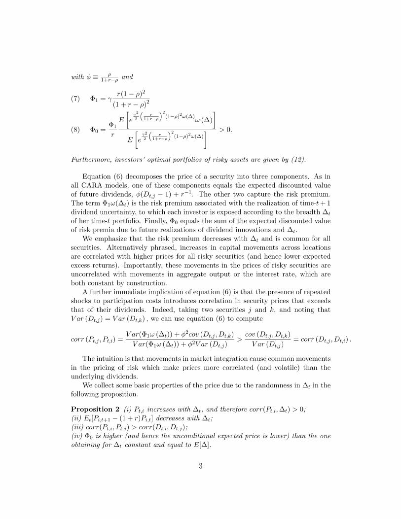
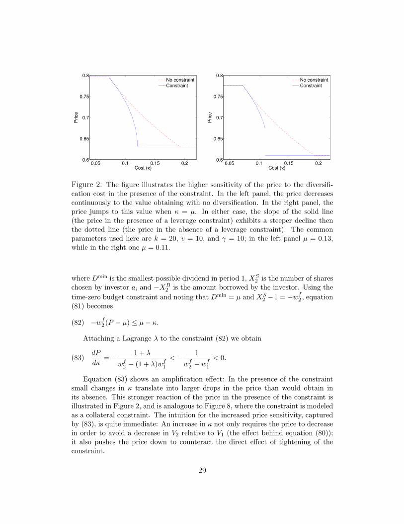
Figure 2: The figure illustrates the higher sensitivity of the price to the diversifi-cation cost in the presence of the constraint. In the left panel, the price decreasescontinuously to the value obtaining with no diversification. In the right panel, theprice jumps to this value when κ = µ. In either case, the slope of the solid line(the price in the presence of a leverage constraint) exhibits a steeper decline thenthe dotted line (the price in the absence of a leverage constraint). The commonparameters used here are k = 20, v = 10, and γ = 10; in the left panel µ = 0.13,while in the right one µ = 0.11.
where Dmin is the smallest possible dividend in period 1, XS2 is the number of shares
chosen by investor a, and −XB2 is the amount borrowed by the investor. Using the
time-zero budget constraint and noting that Dmin = µ and XS2 −1 = −wf2 , equation
(81) becomes
(82) −wf2 (P − µ) ≤ µ− κ.
Attaching a Lagrange λ to the constraint (82) we obtain
(83)dP
dκ= − 1 + λ
wf2 − (1 + λ)wf1< − 1
wf2 − wf1
< 0.
Equation (83) shows an amplification effect: In the presence of the constraintsmall changes in κ translate into larger drops in the price than would obtain inits absence. This stronger reaction of the price in the presence of the constraint isillustrated in Figure 2, and is analogous to Figure 8, where the constraint is modeledas a collateral constraint. The intuition for the increased price sensitivity, capturedby (83), is quite immediate: An increase in κ not only requires the price to decreasein order to avoid a decrease in V2 relative to V1 (the effect behind equation (80));it also pushes the price down to counteract the direct effect of tightening of theconstraint.
29

Depending on the parameters, the price may even drop discontinuously to thevalue obtaining in the no-diversification equilibrium. The point is made most starklyin the case κ = 0 and µ = 0. At these values there is diversification, and no leverage.Any increase in κ, on the other hand, drives the price discontinuously down to theno-diversification value. More generally, it can happen that, as κ approaches µ,enough agents continue to diversify — even if their leverage is virtually zero —for the price to be above the no-diversification value that obtains when κ > µ.However, once κ exceeds µ the price drops discontinuously, as the right panel ofFigure 2 illustrates. Thus, as in Section IV., a small change in κ can cause thenature of the equilibrium to change, which induces a discontinuous change in theprice.
To conclude, even if one modeled borrowing limitations as resulting from a no-default requirement, the price function is steeper in κ than when the constraint isabsent, and can even be discontinuous, similar to section IV., where the constraintis modeled as a simple leverage constraint.
30

References
Garleanu, N., S. Panageas, and J. Yu (2013). Impediments to financial trade: Theoryand measurement. Working Paper.
Lamont, O. A. (2012). Go down fighting: Short sellers vs. firms. Review of AssetPricing Studies 2 (1), 1 – 30.
Van Nieuwerburgh, S. and L. Veldkamp (2010). Information acquisition and under-diversification. Review of Economic Studies 77 (2), 779 – 805.
31