Embed Size (px)
Citation preview


Financial Econometrics
Set against a backdrop of rapid expansions of interest in the modelling and analysis offinancial data and the problems to which they are applied, this textbook, now in its secondedition, offers an overview and discussion of the contemporary topics surrounding financialeconometrics, covering all major developments in the area in recent years in an informativeand succinct way.
Extended from the first edition of mainly time series modelling, the new edition alsotakes in discrete choice models, estimation of censored and truncated samples, as well aspanel data analysis that has witnessed phenomenal expansion in application in finance andfinancial economics since the publication of the first edition of the book. Virtually all majortopics on time series, cross-sectional and panel data analysis have been dealt with. Subjectscovered include:
• unit roots, cointegration and other comovements in time series• time varying volatility models of the GARCH type and the stochastic volatility
approach• analysis of shock persistence and impulse responses• Markov switching• present value relations and data characteristics• state space models and the Kalman filter• frequency domain analysis of time series• limited dependent variables and discrete choice models• truncated and censored samples• panel data analysis
Refreshingly, every chapter has a section of two or more examples and a section of empiricalliterature, offering the reader the opportunity to practise right away the kind of research goingon in the area. This approach helps the reader develop interest, confidence and momentumin learning contemporary econometric topics.
Graduate and advanced undergraduate students requiring a broad knowledge of tech-niques applied in the finance literature, as well as students of financial economics engagedin empirical enquiry, should find this textbook to be invaluable.
Peijie Wang is Professor of Finance at IÉSEG School of Management, Catholic Universityof Lille. He is author of An Econometric Analysis of the Real Estate Market (Routledge2001) and The Economics of Foreign Exchange and Global Finance.

Routledge Advanced Texts in Economics and Finance
Financial EconometricsPeijie Wang
Macroeconomics for Developing Countries, second editionRaghbendra Jha
Advanced Mathematical EconomicsRakesh Vohra
Advanced Econometric TheoryJohn S. Chipman
Understanding Macroeconomic TheoryJohn M. Barron, Bradley T. Ewing and Gerald J. Lynch
Regional EconomicsRoberta Capello
Mathematical FinanceCore theory, problems and statistical algorithmsNikolai Dokuchaev
Applied Health EconomicsAndrew M. Jones, Nigel Rice, Teresa Bago d’Uva and Silvia Balia
Information EconomicsUrs Birchler and Monika Bütler
Financial Econometrics, second editionPeijie Wang

Financial EconometricsSecond edition
Peijie Wang

First published 2003Second edition 2009by Routledge2 Park Square, Milton Park, Abingdon, Oxon OX14 4RN
Simultaneously published in the USA and Canadaby Routledge270 Madison Avenue, New York, NY 10016
Routledge is an imprint of the Taylor & Francis Group,an informa business
© 2003, 2009 Peijie Wang
All rights reserved. No part of this book may be reprinted or reproduced orutilised in any form or by any electronic, mechanical, or other means, nowknown or hereafter invented, including photocopying and recording, or inany information storage or retrieval system, without permission in writingfrom the publishers.
British Library Cataloguing in Publication DataA catalogue record for this book is availablefrom the British Library
Library of Congress Cataloging in Publication DataWang, Peijie, 1965–
Financial econometrics / Peijie Wang.p. cm.
Includes bibliographical references and index.ISBN 978-0-415-42670-1 (hb) – ISBN 978-0-415-42669-5 (pb)
– ISBN 978-0-203-89287-9 (eb) 1. Finance–Econometric models.2. Time-series analysis. 3. Stochastic processes. I. Title.
HG106.W36 2008332.01′5195–dc22 2008004917
ISBN 10: 0-415-42670-7 (hbk)ISBN 10: 0-415-42669-3 (pbk)ISBN 10: 0-203-89287-9 (ebk)
ISBN13: 978-0-415-42670-1 (hbk)ISBN13: 978-0-415-42669-5 (pbk)ISBN13: 978-0-203-89287-9 (ebk)
This edition published in the Taylor & Francis e-Library, 2008.
“To purchase your own copy of this or any of Taylor & Francis or Routledge’scollection of t housands of eBooks please go to www.eBookstore.tandf.co.uk.”
ISBN 0-203-89287-9 Master e-book ISBN
Contents
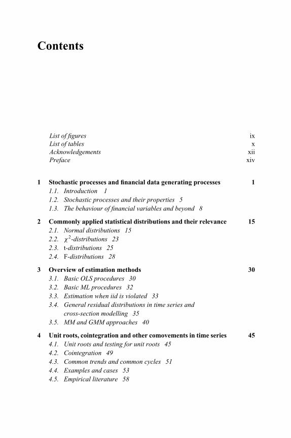
List of figures ixList of tables xAcknowledgements xiiPreface xiv
1 Stochastic processes and financial data generating processes 11.1. Introduction 11.2. Stochastic processes and their properties 51.3. The behaviour of financial variables and beyond 8
2 Commonly applied statistical distributions and their relevance 152.1. Normal distributions 152.2. χ2-distributions 232.3. t-distributions 252.4. F-distributions 28
3 Overview of estimation methods 303.1. Basic OLS procedures 303.2. Basic ML procedures 323.3. Estimation when iid is violated 333.4. General residual distributions in time series and
cross-section modelling 353.5. MM and GMM approaches 40
4 Unit roots, cointegration and other comovements in time series 454.1. Unit roots and testing for unit roots 454.2. Cointegration 494.3. Common trends and common cycles 514.4. Examples and cases 534.5. Empirical literature 58
vi Contents
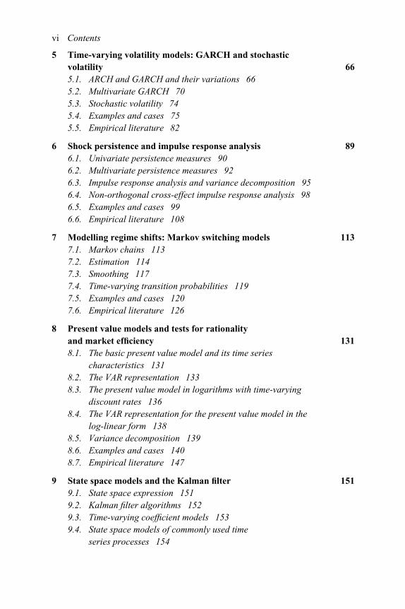
5 Time-varying volatility models: GARCH and stochasticvolatility 665.1. ARCH and GARCH and their variations 665.2. Multivariate GARCH 705.3. Stochastic volatility 745.4. Examples and cases 755.5. Empirical literature 82
6 Shock persistence and impulse response analysis 896.1. Univariate persistence measures 906.2. Multivariate persistence measures 926.3. Impulse response analysis and variance decomposition 956.4. Non-orthogonal cross-effect impulse response analysis 986.5. Examples and cases 996.6. Empirical literature 108
7 Modelling regime shifts: Markov switching models 1137.1. Markov chains 1137.2. Estimation 1147.3. Smoothing 1177.4. Time-varying transition probabilities 1197.5. Examples and cases 1207.6. Empirical literature 126
8 Present value models and tests for rationalityand market efficiency 1318.1. The basic present value model and its time series
characteristics 1318.2. The VAR representation 1338.3. The present value model in logarithms with time-varying
discount rates 1368.4. The VAR representation for the present value model in the
log-linear form 1388.5. Variance decomposition 1398.6. Examples and cases 1408.7. Empirical literature 147
9 State space models and the Kalman filter 1519.1. State space expression 1519.2. Kalman filter algorithms 1529.3. Time-varying coefficient models 1539.4. State space models of commonly used time
series processes 154
Contents vii
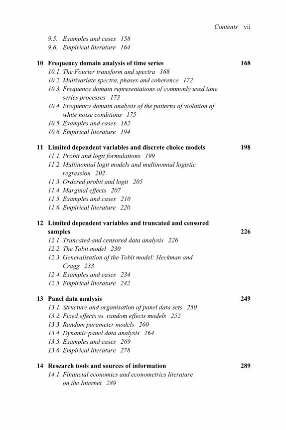
9.5. Examples and cases 1589.6. Empirical literature 164
10 Frequency domain analysis of time series 16810.1. The Fourier transform and spectra 16810.2. Multivariate spectra, phases and coherence 17210.3. Frequency domain representations of commonly used time
series processes 17310.4. Frequency domain analysis of the patterns of violation of
white noise conditions 17510.5. Examples and cases 18210.6. Empirical literature 194
11 Limited dependent variables and discrete choice models 19811.1. Probit and logit formulations 19911.2. Multinomial logit models and multinomial logistic
regression 20211.3. Ordered probit and logit 20511.4. Marginal effects 20711.5. Examples and cases 21011.6. Empirical literature 220
12 Limited dependent variables and truncated and censoredsamples 22612.1. Truncated and censored data analysis 22612.2. The Tobit model 23012.3. Generalisation of the Tobit model: Heckman and
Cragg 23312.4. Examples and cases 23412.5. Empirical literature 242
13 Panel data analysis 24913.1. Structure and organisation of panel data sets 25013.2. Fixed effects vs. random effects models 25213.3. Random parameter models 26013.4. Dynamic panel data analysis 26413.5. Examples and cases 26913.6. Empirical literature 278
14 Research tools and sources of information 28914.1. Financial economics and econometrics literature
on the Internet 289

viii Contents
14.2. Econometric software packages for financial and economicdata analysis 291
14.3. Learned societies and professional associations 29414.4. Organisations and institutions 299
Index 313

Figures
2.1 Normal distributions 162.2 States of events: discrete but increase in numbers 162.3 From discrete probabilities to continuous probability density
function 172.4 Illustrations of confidence intervals 182.5 Two-tailed and one-tailed confidence intervals 192.6 Lognormal distribution 222.7 χ2-distributions with different degrees of freedom 242.8 t-distributions with different degrees of freedom 262.9 t-tests and the rationale 285.1 Eigenvalues on the complex plane 817.1 Growth in UK GDP 1229.1 Trend, cycle and growth in US GDP 161
10.1 Lower frequencies dominate (compounding effect) 17910.2 Higher frequencies dominate (mean-reverting tendency) 18010.3 Mixed complicity 18110.4 Business cycle patterns: sectors A and B 18310.5 Business cycle patterns: sector D 18410.6 Business cycle patterns: sector E 18510.7 Business cycle patterns: sector F 18610.8 Business cycle patterns: sectors G and H 18710.9 Business cycle patterns: sector I 188
10.10 Business cycle patterns: sectors J and K 18910.11 Business cycle patterns: sectors L–Q 19010.12 Business cycle patterns: GDP 19111.1 Predicted probability by probit and logit 20011.2 Probability density of probit and logit 201
Tables
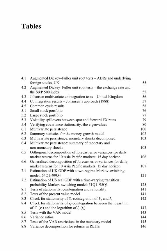
4.1 Augmented Dickey–Fuller unit root tests – ADRs and underlyingforeign stocks, UK 55
4.2 Augmented Dickey–Fuller unit root tests – the exchange rate andthe S&P 500 index 55
4.3 Johansen multivariate cointegration tests – United Kingdom 564.4 Cointegration results – Johansen’s approach (1988) 574.5 Common cycle results 585.1 Small stock portfolio 765.2 Large stock portfolio 775.3 Volatility spillovers between spot and forward FX rates 795.4 Verifying covariance stationarity: the eigenvalues 806.1 Multivariate persistence 1006.2 Summary statistics for the money growth model 1026.3 Multivariate persistence: monetary shocks decomposed 1036.4 Multivariate persistence: summary of monetary and
non-monetary shocks 1036.5 Orthogonal decomposition of forecast error variances for daily
market returns for 10 Asia Pacific markets: 15 day horizon 1066.6 Generalised decomposition of forecast error variances for daily
market returns for 10 Asia Pacific markets: 15 day horizon 1077.1 Estimation of UK GDP with a two-regime Markov switching
model: 64Q1–99Q4 1217.2 Estimation of US real GDP with a time-varying transition
probability Markov switching model: 51Q1–95Q3 1258.1 Tests of stationarity, cointegration and rationality 1418.2 Tests of the present value model 1418.3 Check for stationarity of St-cointegration of Vt and It 1428.4 Check for stationarity of st-cointegration between the logarithm
of Vt (vt) and the logarithm of It (it) 1438.5 Tests with the VAR model 1438.6 Variance ratios 1448.7 Tests of the VAR restrictions in the monetary model 1458.8 Variance decomposition for returns in REITs 146
Tables xi
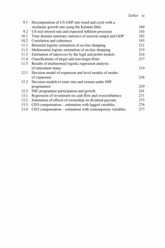
9.1 Decomposition of US GDP into trend and cycle with astochastic growth rate using the Kalman filter 160
9.2 US real interest rate and expected inflation processes 16310.1 Time domain summary statistics of sectoral output and GDP 18210.2 Correlation and coherence 19311.1 Binomial logistic estimation of on-line shopping 21111.2 Multinomial logistic estimation of on-line shopping 21311.3 Estimation of takeovers by the logit and probit models 21611.4 Classifications of target and non-target firms 21711.5 Results of multinomial logistic regression analysis
of retirement status 21912.1 Decision model of expansion and level models of modes
of expansion 23612.2 Decision models to enter into and remain under IMF
programmes 23912.3 IMF programme participation and growth 24113.1 Regression of investment on cash flow and overconfidence 27113.2 Estimation of effects of ownership on dividend payouts 27313.3 CEO compensation – estimation with lagged variables 27613.4 CEO compensation – estimation with contemporary variables 277

Acknowledgements
The idea of updating this book in contemporary financial econometrics, as ofwriting the first edition of the book, developed from my experience of advisingdoctoral and masters students in their research, to provide them with up-to-date andaccessible materials either as research tools or as the advancement of the subjectitself. Providing up-to-date materials requires updating the book at an intervalwithin which substantial advancements, either in theory or application or both,have taken place.
Since the publication of the first edition of the book, great interest has beenshown in discrete choice models, estimation of censored and truncated samplesand panel data analysis, and in particular, these models’ application in finance andfinancial economics. Therefore, the new edition of the book has included thesemodels and methods, extending the first edition in which the covered topics weremainly on time series modelling. However, this task has been proven neither easynor straightforward, and has involved much work and rework on the manuscript.It is not an exaggeration to say that this new edition of the book may never havebeen completed without the support and encouragement from Rob Langham, theRoutledge economics editor, with whom many consultations have taken place atvarious stages of the development of the book. I am particularly grateful to TomSutton, whose excellent, efficient and effective editorial work ensures that thenew edition maintains the same high standard as the first edition, while facinga more challenging operation in pooling many diverse and interwoven topicstogether.
During the writing of this edition of the book, I received fantastic support frommany individuals whom I have worked with in this period. A few of my colleaguesalso made helpful comments on a range of my written material related to the book.I would like to express my gratitude to them, including Yun Zhou, Pingshun Zhang,Habibah Tolos, Duanduan Song, Frank McDonald, Benedicto Lukanima, Andreade Laine, Trefor Jones, Jinying Hu and Alan Benson. They have contributed tothe new edition of the book from various perspectives.
In the meantime, I would like to thank once again those who contributed to thefirst edition of the book, especially my former colleagues Bob Ward and JamesFreeman, and Stuart Hey, Terry Clague and Heidi Bagtazo of Routledge. It was

Acknowledgements xiii
the quality and appeal of the first edition that made the book evolve into a newedition.
Finally, I thank the production and marketing teams of Routledge who bring thebook to the reader.
PJWJanuary 2008

Preface
This book focuses on econometric models widely and frequently used in theexamination of issues in financial economics and financial markets, which arescattered in the literature yet to be integrated into a single-volume, multi-theme, and empirical research-oriented text. The book, providing an overview ofcontemporary topics related to the modelling and analysis of financial data, is setagainst a backdrop of rapid expansions of interest in both the models themselvesand the financial problems to which they are applied. Extended from the firstedition of mainly time series modelling, the new edition also takes in discretechoice models, estimation of censored and truncated samples, as well as paneldata analysis that has witnessed phenomenal expansion in application in financeand financial economics since the publication of the first edition of the book.Virtually all major topics on time series, cross-sectional and panel data analysishave been dealt with.
We assume that the reader has already had knowledge in econometrics andfinance at the intermediate level. So basic regression analysis and time seriesmodels such as the OLS, maximum likelihood and ARIMA, while being referredto from time to time in the book, are only briefly reviewed but are not brought up asa book topic; nor the concept of market efficiency and models for asset pricing. Forthe former, there are good books such as Basic Econometrics by Gujarati (2002),Econometric Analysis by Greene (2008), and Introduction to Econometrics byMaddala (2001); and for the latter, the reader is recommended to refer to Principlesof Corporate Finance by Brealey, Myers and Allen (2006), Corporate Finance byRoss, Westerfield and Jaffe (2008), Investments by Sharpe, Alexander and Bailey(1999), Investments by Bodie, Kane and Marcus, (2008), and Financial Marketsand Corporate Strategy by Grinblatt and Titman (2002).
The book has two unique features – every chapter (except the first threeintroductory chapters and the final chapter) has a section of two or more examplesand cases, and a section of empirical literature, offering the reader the opportunityto practice right away the kind of research in the area. The examples and cases,either from the literature or of the book itself, are well executed, and the resultsare explained in detail in plain language. This would, as we hope, help the readergain interest, confidence, and momentum in learning contemporary econometrictopics. At the same time, the reader would find that the way of implementation

Preface xv
and estimation of a model is unavoidably influenced by the view of the researcheron the issue in a social science subject; nevertheless, for a serious researcher, itis not easy to make two plus two equal to any desired number she or he wantsto get. The empirical literature reviewed in each chapter is comprehensive and upto date, exemplifying rich application areas at both macro and micro levels limitedonly by the imagination of human beings. The section demonstrates how a modelcan and should match practical problems coherently and guide the researcher’sconsideration on the rationale, methodology and factors in the research. Overall,the book is methods, models, theories, procedures, surveys, thoughts and tools.
To further help the reader carry out an empirical modern financial econometricsproject, the book introduces research tools and sources of information in thefinal chapter. These include on-line information on, and the websites for, theliterature on research in financial economics and financial markets; commonlyused econometric software packages for time series, cross-sectional and paneldata analysis; professional associations and learned societies; and internationaland national institutions and organisations. A website link is provided wheneverit is possible. The provision is based on our belief that, to perfect an empiricalstudy, one has to understand the wider background of the business environment,market operations and institutional roles, and to frequently upgrade and update theknowledge base which is nowadays largely through internet links.
The book can be used in graduate programmes in financial economics, financialeconometrics, international finance, banking and investment. It can also be used asdoctorate research methodology materials and by individual researchers interestedin econometric modelling, financial studies, or policy evaluation.
References
Bodie, Zvi, Kane, Alex and Marcus, Alan, J. (2008), Investments 7th edn, McGraw-Hill.Brealey, Richard, A., Myers, Stewart, C. and Allen, Franklin (2006), Principles of
Corporate Finance 8th ed, McGraw-Hill.Greene, William, H. (2008), Econometric Analysis 8th edn, Prentice Hall.Grinblatt, Mark and Titman, Sheridan (2002), Financial Markets and Corporate Strategy
2nd ed, McGraw-Hill.Gujarati, Damodar (2002), Basic Econometrics 4th edn, McGraw-Hill.Maddala, G.S. (2001), Introduction to Econometrics 3rd edn, Wiley.Ross, Stephen, A., Westerfield, Randolph, W. and Jaffe, Jeffrey (2008), Corporate Finance
8th edn, McGraw-Hill.Sharpe, William, F., Alexander, Gordon, J. and Bailey, Jeffery, V. (1999), Investments
6th edn, Prentice-Hall International.

1 Stochastic processes and financialdata generating processes
1.1. Introduction
Statistics is the analysis of events and the association of events, with a probability.Econometrics pays attention to economic events, the association between theseevents, and between these events and human beings’ decision-making – gov-ernment policy, firms’ financial leverage, individuals’ investment/consumptionchoice, and so on. The topics of this book, financial econometrics, focus onthe variables and issues of financial economics, the financial market and theparticipants.
The financial world is an uncertain universe where events take place everyday, every hour, and every second. Information arrives randomly and so do theevents. Nonetheless, there are regularities and patterns in the variables to beidentified, effect of a change on the variables to be assessed, and links between thevariables to be established. Financial econometrics attempts to perform the analysisof these kinds through employing and developing various relevant statisticalprocedures.
There are generally three types of economic and financial variables – the ratevariable, the level variable and the ratio variable. The first category measures thespeed at which, for example, wealth is generated, or savings are made, at one pointof time (continuous time) or in a short interval of time (discrete time). The rate ofreturn on a company’s stock or share is a typical rate variable. The second categoryworks out the amount of wealth, such as income and assets, being accumulatedover a period (continuous time) or in a few of short time intervals (discrete time).A firm’s assets and a country’s GDP are typical level variables, though they aredifferent in a certain sense in that the former is a stock variable and the latter is aflow variable. The third category consists of two sub-categories, one is the type Iratio variable or the component ratio variable, and the other is the type II ratio,the contemporaneous relativity ratio variable. The unemployment rate is rathera ratio variable, a type I ratio variable, than a rate variable. The exchange rateis more precisely a typical type II ratio variable instead of a rate variable. Thisclassification of variables does not necessarily correspond to the classification ofvariables into flow variables and stock variables in economics. For example, wewill see in Chapter 8 that both income and value should behave similarly in terms

2 Stochastic processes and financial data generating processes
of statistical characteristics as non-stationary variables, though the former is a flowvariable and the latter a stock variable, if the fundamental relationship betweenthem is to hold.
Before we can establish links and chains of influence amongst the variablesin concern, which are in general random or stochastic, we have to assess theirindividual characteristics first. That is, with what probability may the variabletake a certain value, or how likely may an event (the variable taking a givenvalue) occur? Such assessment of the characteristics of individual variables ismade through the analysis of their statistical distributions. Bearing this in mind,a number of stochastic processes, which are commonly encountered in empiricalresearch in economics and finance, are presented, compared and summarised inthe next section. The behaviour and valuation of economic and financial variablesare discussed in association with these stochastic processes in Section 1.3, withfurther extension and generalisation.
Independent identical distribution (iid) and normality in statistical distributionsare commonly supposed to be met, though from time to time we would modify theassumptions to fit the real world problem more appropriately. If the rate variablesare, as widely assumed, iid and normally distributed around a constant mean, thenits corresponding level variable would be log normally distributed around a meanwhich is increasing exponentially over time, and the level variable in logarithmsis normally distributed around a mean which is increasing linearly over time. Thisis the reason why we usually work with the level variables in their logarithms.
Prior to proceeding to the main topics of this book, a few of most commonlyassumed statistical distributions applied in various subjects are reviewed inChapter 2, in conjunction with their rationale in statistics and relevance in finance.The examination of statistical distributions of stochastic variables helps assesstheir characteristics and understand their behaviour. Then, primary statisticalestimation methods, covering the ordinary least squares, the maximum likelihoodmethod and the method of moments and the generalised method of moment, arebriefly reviewed in Chapter 3. The iid and iid under normal distributions are firstlyassumed for the residuals from fitting the model. Then, the iid requirements aregradually relaxed, leading to general residual distributions typically observed intime series and cross-section modelling. This also serves the purpose of introducingelementary time series and cross-section models and specifications, based on whichand from which most models in the following chapters of this book are developedand evolved.
The classification of financial variables into rate variables and level variablesgives rise to stationarity and non-stationarity in financial time series, though theremight be no clear-cut match of the economic and financial characteristic and thestatistical characteristic in empirical research; whilst the behaviour and propertiesof ratio variables may be even more controversial. Related to this issue, Chapter 4analyses unit roots and presents the procedures for testing for unit roots. Then thechapter introduces the idea of cointegration where a combination of two or morenon-stationary variables becomes stationary. This is a special type of link amongststochastic variables, implying that there exists a so-called long-run relationship.

Stochastic processes and financial data generating processes 3
The chapter also extends the analysis to cover common trends and common cycles,the other major types of links amongst stochastic variables in economics andfinance.
One of the violations to the iid assumption is heteroscedasticity, i.e. the varianceis not the same from each of the residuals; and modifications are consequentlyrequired in the estimation procedure. The basics of this issue and the ways tohandle it have been learned from introductory econometrics or statistics or can belearned in Chapter 3 on overview of estimation methods. What we introduce herein Chapter 5 is specifically a kind of variance which changes with time, or time-varying variance. Time-varying variance or time-varying volatility is frequentlyfound in many financial time series so has to be dealt with seriously. Two types oftime-varying volatility models are discussed, one is GARCH (Generalised AutoRegressive Conditional Heteroscedasticity) and the other is stochastic volatility.
How persistent is the effect of a shock is important in financial markets. It is notonly related to the response of, say, financial markets to a piece of news, but is alsorelated to policy changes, of the government or the firm. This issue is addressedin Chapter 6, which also incorporates impulse response analysis, a related subjectwhich we reckon should be under the same umbrella. Regime shifts are importantin the economy and financial markets as well, in that regime shifts or breaks inthe economy and market conditions are often observed, but the difficulties are thatregime shifts are not easily captured by conventional regressional analysis andmodelling. Therefore, Markov switching is introduced in Chapter 7 to handle theissues more effectively. The approach helps improve our understanding about aneconomic process and its evolving mechanism constructively.
Some economic and financial variables have built-in fundamental relationshipsbetween them. One of such fundamental relationships is that between income andvalue. Economists regard that the value of an asset is derived from its future incomegenerating power. The higher the income generating power, the more valuableis the asset. Nevertheless, whether this law governing the relationship betweenincome and value holds is subject to empirical scrutiny. Chapter 8 addresses thisissue with the help of econometric procedures, which identify and examine thetime series characteristics of the variables involved.
Econometric analysis can be carried out in the conventional time domain asdiscussed in the above, and can also be performed through some transformations.Analysis in the state space is one of such endeavours, presented in Chapter 9. Whatthe state space does is to model the underlying mechanisms through the changesand transitions in the state of its unobserved components, and establish the linksbetween the variables of concern, which are observed, and those unobserved statevariables. It explains the behaviour of externally observed variables by examiningthe internal, dynamic and systematic changes and transitions of unobserved statevariables, to reveal the nature and cause of the dynamic movement of the variableseffectively. State space analysis is usually executed with the help of the Kalmanfilter, also introduced in the chapter.
State space analysis is nonetheless still in the time domain, though it is notthe conventional time domain analysis. With spectral analysis of time series in
4 Stochastic processes and financial data generating processes
Chapter 10, estimation is performed in the frequency domain. That is, time domainvariables are transformed into frequency domain variables prior to the analysis, andthe results in the frequency domain may be transformed back to the time domainwhen necessary. Such transformations are usually achieved through the Fouriertransform and the inverse Fourier transform and, in practice, through the FastFourier Transform (FFT) and the Inverse Fast Fourier Transform (IFFT). Thefrequency domain properties of variables are featured by their spectrum, phaseand coherence, to reflect individual time series’ characteristics and the associationbetween several time series, in the ways similar to those in the time domain.
Deviating from the preceding chapters of the book, Chapters 11 and 12 studymodels with limited dependent variables. The dependent variable in these twochapters is not observed on the whole range or whole sample, it is discrete,censored or truncated. Also deviating from the preceding chapters, data setsanalysed in Chapters 11 and 12 are primarily cross-sectional. That is, they are datafor multiple entities, such as individuals, firms, regions or countries, consideredto be observed at a single time point. Issues associated with choice are addressedin Chapter 11. Firms and individuals encounter choice problems from time totime. Choice is deeply associated with people’s daily life, firms’ financing andinvestment activities, managers’ business dealings and financial market operations.In financial terms, people make decisions on choice aimed at achieving higherutility of their work, consumption, savings, investment and their combinations.Firms make investment, financing and other decisions, supposedly aimed atmaximising shareholder value. A firm may choose to use financial derivativesto hedge interest rate risk, or choose not to use financial derivatives. A firm maydecide to expand its business into foreign markets, or not to expand into foreignmarkets. The above choice problems can be featured by binary choice modelswhere the number of alternatives or options is two, in a usual frame of ‘to do’ or ‘notto do’. General discrete choice models emerge when the number of alternativesor options is extended to be more than two. Since discrete choice models arenon-linear, marginal effects are specifically considered.
In addition to discrete choice models where a dependent variable possessesdiscrete values, the values of dependent variables can also be censored or truncated.Chapter 12 examines issues in estimation of models involving limited dependentvariables with regard to censored and truncated samples. Estimation of truncatedor censored samples with certain conventional regression procedures can causebias in parameter estimation. This chapter discusses the causes of the bias andintroduces pertinent procedures to correct the bias arising from truncation andcensoring, as well as the estimation procedures that produce unbiased parameterestimates. A wider issue of selection bias is specifically addressed.
The use of panel data and application of panel data modelling have increaseddrastically in the last five years in finance and related areas. The volume ofstudies and papers employing panel data has been multifold, in recognition of theadvantages offered by panel data approaches as well as panel data sets themselves,and in response to the growing availability of data sets in the form of panel.Chapter 13 introduces various panel data models and model specifications andaddresses various issues in panel data model estimation. Panel data covered in this

Stochastic processes and financial data generating processes 5
chapter refer to data sets consisting of cross-sectional observations over time, orpooled cross-section and time series data. They have two dimensions, one for timeand one for the cross-section entity. Two major features that do not exist with theone-dimension time series data or the one-dimension cross-sectional data are fixedeffects and random effects, which are analysed, along with the estimation of fixedeffects models, random effects models and random parameter models. Issues ofbias in parameter estimation for dynamic panel data models are then addressedand a few approaches to estimating dynamic panel models are presented.
Financial econometrics is only made possible by the availability of vasteconomic and financial data. Problems and issues in the real world have inspiredthe generation of new ideas and stimulated the development of more powerfulprocedures. The last chapter of the book, Chapter 14, is written to make such areal world and working environment immediately accessible by the researcher,providing information on the sources of literature and data, econometric softwarepackages and organisations and institutions ranging from learned societies andregulators to market players.
1.2. Stochastic processes and their properties
The rest of this chapter presents stochastic processes frequently found in thefinancial economics literature and relevant to such important studies as marketefficiency and rationality. In addition, a few terms fundamental to modellingfinancial time series are introduced. The chapter discusses stochastic processesin the tradition of mathematical finance, as we feel that there rarely exist links,at least explicitly, between mathematical finance and financial econometrics, todemonstrate the rich statistical properties of financial securities and their economicrationale ultimately underpinning the evolution of the stochastic process. After pro-viding definitions and brief discussions of elementary stochastic processes in thenext section, we begin with the generalisation of the Wiener process in Section 1.3,and gradually progress to show that the time path of many financial securities canbe described by the Wiener process and its generalisations which can accommodatesuch well known econometric models or issues as ARIMA (Auto RegressiveIntegrated Moving Average), GARCH (Generalised Auto Regressive ConditionalHeteroscedasticity), stochastic volatility, stationarity, mean-reversion, error cor-rection and so on. Throughout the chapter, we do not particularly distinguishdiscrete and continuous time series and what matters to the analysis is that the timeinterval is small enough. The results are almost identical though this treatment doesprovide more intuition to real world problems. There are many stochastic processesbooks available, e.g., Ross (1996) and Medhi (1982). For modelling of financialsecurities, interested readers can refer to Jarrow and Turnbull (1999).
1.2.1. Martingales
A stochastic process Xn (n = 1,2, . . .), with E[Xn
]< ∞ for all n, is a martingale, if:
E[Xn+1 | X1, . . .Xn
]= Xn (1.1)

6 Stochastic processes and financial data generating processes
Further, if a stochastic process Xn (n = 1,2, . . .), with E[Xn
]< ∞ for all n, is a
submartingale, if:
E[Xn+1 | X1, . . .Xn
]≥ Xn (1.2)
and is a supermartingale if:
E[Xn+1 | X1, . . .Xn
]≤ Xn (1.3)
1.2.2. Random walks
A random walk is the sum of a sequence of independent and identically distributed(iid) variables Xi (i = 1,2, . . . ), with E
[Xi
]< ∞. Define:
Sn =n∑
i=1
Xi (1.4)
Sn is referred as a random walk. When Xi takes only two values, +1 and −1, withP{Xi = 1} = p and P{Xi = −1} = 1 − p, the process is named as the Bernoullirandom walk. If p = 1 − p = 1
2 , the process is called a simple random walk.
1.2.3. Gaussian white noise processes
A Gaussian process, or Gaussian white noise process, or simply white noiseprocess, Xn, (n = 1,2, . . .) is a sequence of independent random variables, each ofwhich has a normal distribution:
Xn ∼ N (0,σ 2) (1.5)
with the probability density function being:
fn(x) = 1
σ√
2πe−(x2/2σ 2) (1.6)
The sequence of these independent random variables of the Gaussian whitenoise has a multivariate normal distribution and the covariance between any twovariables in the sequence, Cov(Xj,Xk ) = 0 for all j �= k .
A Gaussian process is a white noise process because, in the frequency domain, ithas equal magnitude in every frequency, or equal component in every colour. Weknow that the light with equal colour components, such as sunlight, is white.Readers interested in frequency domain analysis can refer to Chapter 10 fordetails.
1.2.4. Poisson processes
A Poisson process N (t) (t ≥ 0) is a counting process where N (t) is an integerrepresenting the number of ‘events’ that have occurred up to time t, and the process

Stochastic processes and financial data generating processes 7
has independent increments, i.e. the number of events have occurred in interval(s, t] is independent from the number of events in interval (s + τ , t + τ ].
Poisson processes can be stationary and non-stationary. A stationary Poissonprocess has stationary increments, i.e. the probability distribution of the numberof events occurred in any interval of time is only dependent on the length of thetime interval:
P{N (t + τ ) − N (s + τ )} = P{N (t) − N (s)} (1.7)
Then the probability distribution of the number of events in any time length τ is:
P{N (t + τ ) − N (t) = n} = e−lt (lt)n
n! (1.8)
where l is called the arrival rate, or simply the rate of the process. It can be shownthat:
E{N (t)} = lt, Var{N (t)} = lt (1.9)
In the case that a Poisson process is non-stationary, the arrival rate is a function oftime, thereby the process does not have a constant mean and variance.
1.2.5. Markov processes
A sequence Xn (n = 0,1, . . .) is a Markov process if it has the following property:
P{Xn+1 =xn+1 |Xn =xn,Xn−1 =xn−1,X1 =x1,X0 =x0
}=P{Xn+1 =xn |Xn =xn
}(1.10)
The Bernoulli random walk and simple random walk are the cases of Markovprocesses. It can be shown that the Poisson process is a Markov process as well.
A discrete time Markov process that takes finite or countable number of integervalues xn, is called a Markov chain.
1.2.6. Wiener processes
A Wiener process, also known as Brownian motion, is indeed the very basicelement in stochastic processes:
�z(t) = ε√
�t, �t → 0ε ∼ N (0,1)
}(1.11)
The Wiener process can be derived from the simple random walk, replacing timesequence by time series when time intervals become smaller and smaller and
8 Stochastic processes and financial data generating processes
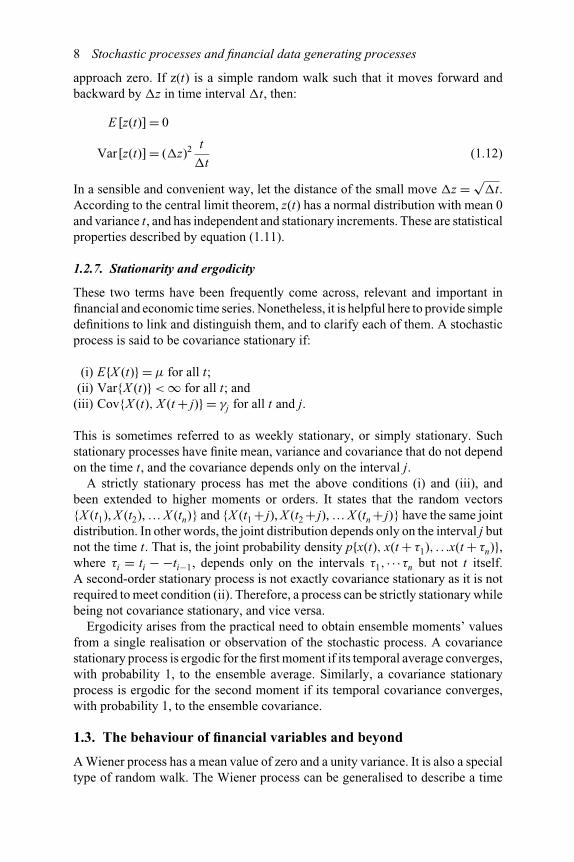
approach zero. If z(t) is a simple random walk such that it moves forward andbackward by �z in time interval �t, then:
E [z(t)] = 0
Var[z(t)] = (�z)2 t
�t(1.12)
In a sensible and convenient way, let the distance of the small move �z = √�t.
According to the central limit theorem, z(t) has a normal distribution with mean 0and variance t, and has independent and stationary increments. These are statisticalproperties described by equation (1.11).
1.2.7. Stationarity and ergodicity
These two terms have been frequently come across, relevant and important infinancial and economic time series. Nonetheless, it is helpful here to provide simpledefinitions to link and distinguish them, and to clarify each of them. A stochasticprocess is said to be covariance stationary if:
(i) E{X (t)} = μ for all t;(ii) Var{X (t)} < ∞ for all t; and(iii) Cov{X (t), X (t + j)} = γj for all t and j.
This is sometimes referred to as weekly stationary, or simply stationary. Suchstationary processes have finite mean, variance and covariance that do not dependon the time t, and the covariance depends only on the interval j.
A strictly stationary process has met the above conditions (i) and (iii), andbeen extended to higher moments or orders. It states that the random vectors{X (t1), X (t2), … X (tn)} and {X (t1 + j), X (t2 + j), … X (tn + j)} have the same jointdistribution. In other words, the joint distribution depends only on the interval j butnot the time t. That is, the joint probability density p{x(t), x(t + τ1), . . .x(t + τn)},where τi = ti − −ti−1, depends only on the intervals τ1, · · ·τn but not t itself.A second-order stationary process is not exactly covariance stationary as it is notrequired to meet condition (ii). Therefore, a process can be strictly stationary whilebeing not covariance stationary, and vice versa.
Ergodicity arises from the practical need to obtain ensemble moments’ valuesfrom a single realisation or observation of the stochastic process. A covariancestationary process is ergodic for the first moment if its temporal average converges,with probability 1, to the ensemble average. Similarly, a covariance stationaryprocess is ergodic for the second moment if its temporal covariance converges,with probability 1, to the ensemble covariance.
1.3. The behaviour of financial variables and beyond
A Wiener process has a mean value of zero and a unity variance. It is also a specialtype of random walk. The Wiener process can be generalised to describe a time
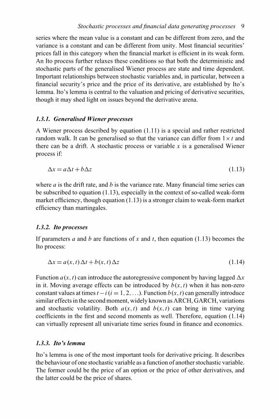
Stochastic processes and financial data generating processes 9
series where the mean value is a constant and can be different from zero, and thevariance is a constant and can be different from unity. Most financial securities’prices fall in this category when the financial market is efficient in its weak form.An Ito process further relaxes these conditions so that both the deterministic andstochastic parts of the generalised Wiener process are state and time dependent.Important relationships between stochastic variables and, in particular, between afinancial security’s price and the price of its derivative, are established by Ito’slemma. Ito’s lemma is central to the valuation and pricing of derivative securities,though it may shed light on issues beyond the derivative arena.
1.3.1. Generalised Wiener processes
A Wiener process described by equation (1.11) is a special and rather restrictedrandom walk. It can be generalised so that the variance can differ from 1× t andthere can be a drift. A stochastic process or variable x is a generalised Wienerprocess if:
�x = a�t + b�z (1.13)
where a is the drift rate, and b is the variance rate. Many financial time series canbe subscribed to equation (1.13), especially in the context of so-called weak-formmarket efficiency, though equation (1.13) is a stronger claim to weak-form marketefficiency than martingales.
1.3.2. Ito processes
If parameters a and b are functions of x and t, then equation (1.13) becomes theIto process:
�x = a (x, t)�t + b (x, t)�z (1.14)
Function a (x, t) can introduce the autoregressive component by having lagged �xin it. Moving average effects can be introduced by b (x, t) when it has non-zeroconstant values at times t− i (i = 1,2, . . .). Function b (x, t) can generally introducesimilar effects in the second moment, widely known as ARCH, GARCH, variationsand stochastic volatility. Both a (x, t) and b (x, t) can bring in time varyingcoefficients in the first and second moments as well. Therefore, equation (1.14)can virtually represent all univariate time series found in finance and economics.
1.3.3. Ito’s lemma
Ito’s lemma is one of the most important tools for derivative pricing. It describesthe behaviour of one stochastic variable as a function of another stochastic variable.The former could be the price of an option or the price of other derivatives, andthe latter could be the price of shares.

10 Stochastic processes and financial data generating processes
Let us write equation (1.14) in the continuous time:
dx = a(x, t)dt + b(x, t)dz (1.15)
Let y be a function of stochastic process x, Ito’s lemma tells us that y is also an Itoprocess:
dy =(
∂y
∂xa + ∂y
∂t+ 1
2
∂2y
∂x2 b2
)dt + ∂y
∂xbdz (1.16)
It has a drift rate of:
∂y
∂xa + ∂y
∂t+ 1
2
∂2y
∂x2 b2 (1.17)
and a variance rate of:
(∂y
∂x
)2
b2 (1.18)
Equation (1.16) is derived by using the Taylor series expansion and ignoring higherorders of 0, details can be found in most mathematics texts at the undergraduatelevel.
Ito’s lemma has a number of meaningful applications in finance and economet-rics. Beyond derivative pricing, it reveals why and how two financial or economictime series are related to each other. For example, if two non-stationary (precisely,integrated of order 1) time series share the same stochastic component, the secondterm on the right-hand side of equations (1.15) and (1.16), then a linear combinationof them is stationary. This phenomenon is called cointegration in the sense of Engleand Granger (1987) and Johansen (1988) in the time series econometrics literature.The interaction and link between them are most featured by the existence of anerror correction mechanism. If two non-stationary time series are both the functionsof an Ito’s process, then they have a common stochastic component but may inaddition have individual stochastic components as well. In this case, the two timeseries have a common trend in the sense of Stock and Watson (1988) but they arenot necessarily cointegrated. This analysis can be extended to deal with stationarycases, e.g. common cycles in Engle and Issler (1995) and Vahid and Engle (1993).
1.3.4. Geometric Wiener processes and financial variable behaviourin the short-term and long-run
We can subscribe a financial variable, e.g. the share price, to a random walk processwith normal distribution errors:
Pt+1 = Pt + νt, νt ∼ N (0, σ 2P ) (1.19)
Stochastic processes and financial data generating processes 11
More generally, the price follows a random walk with a drift:
Pt+1 = Pt +φ + νt, νt ∼ N (0, σ 2P ) (1.20)
where φ is a constant indicating an increase (and less likely, a decrease) of theshare price in every period. Nevertheless, a constant absolute increase or decreasein share prices is also not quite reasonable. A realistic representation is that therelative increase of the price is a constant:
Pt+1 − Pt
Pt
= μ+ ξt, ξt ∼ N (0, σ 2) (1.21)
So:
�Pt = Pt+1 − Pt = μPt + Ptξt = μPt +σPtε
ε ∼ N (0,1)(1.22)
Notice �t = t + 1 − t = 1 can be omitted in or added to the equations. Let �t bea small interval of time (e.g. a fraction of 1), then equation (1.22) becomes:
�Pt = μPt�t +σPtε√
�t (1.23)
= μPt�t +σPt�z
Equation (1.23) is an Ito process in that its drift rate and variance rate are functionsof the variable in concern and time. Applying Ito’s lemma, we obtain the logarithmof the price as follows:
�pt = pt+1 − pt =[μ− σ 2
2
]�t +�z (1.24)
where pt = ln(Pt) has a drift rate of μ′ = μ − (σ 2/2) and variance rate of σ 2.Equation (1.24) is just a generalised Wiener process instead of an Ito process inthat its drift rate and variance rate are not the functions of Pt and t. This simplifiesanalysis and valuation empirically.
If we set σ = 0, the process is deterministic and solution is:
Pt = P0(1 +μ)t ≈ P0eμt (1.25)
and
pt = p0 + t ln(1 +μ) ≈ p0 +μt (1.26)
The final result in equations (1.25) and (1.26) is obtained when μ is fairly smalland is also the continuous time solution. From above analysis we can concludethat share prices grow exponentially while log share prices grow linearly.

12 Stochastic processes and financial data generating processes
When σ �= 0, rates of return and prices deviate from above-derived values.Assuming there is only one shock (innovation) occurring in the kth period,ε(k) = σ , then:
Pt = P0(1 +μ)(1 +μ) · · · (1 +μ+σ ) · · · (1 +μ)(1 +μ)(1 +μ) (1.27)
for the price itself, and
pt = p0 + (t − 1) ln(1 +μ) + ln(1 +μ+σ ) ≈ p0 +σ +μ t (1.28)
for the log price. After k , the price level increases by σ permanently (in everyperiod after k). However, the rate of change or return is μ + σ in the kth periodonly; after k , the rate of return changes back to μ immediately after k .
The current rate of return or change does not affect future rates of return orchange, so it is called a short-term variable. This applies to all similar financialand economic variables in the form of first difference. The current rate of returnhas an effect on future prices, either in original forms or logarithms, which aredubbed as long-run variables. Long-run variables often take their original form orare in logarithms, both being called variables in levels in econometric analysis. Wehave observed from above analysis that adopting variables in logarithms gives riseto linear relationships which simplify empirical analysis, so many level variablesare usually in their logarithms.
In the above analysis of the share price, we reasonably assume that the changein the price is stationary and the price itself is integrated of order 1. Whereasunder some other circumstances the financial variables in their level, not in theirdifference, may exhibit the property of a stationary process. Prominently, two ofsuch variables are the interest rate and the unemployment rate. To accommodatethis, a mean-reversion element is introduced in the process. Taking the interestrate for example, one of the models can have the following specification:
�rt = a (b − rt)�t +σ rt�z, a > 0, b > 0 (1.29)
Equation (1.29) says that the interest rate decreases when its current value is greaterthan b and it increases when its current level is below b, where b is the mean valueof the interest rate to which the interest rate reverts. A non-stationary process,such as that represented by equation (1.23), and a mean-reverse process, suchas equation (1.29), differ in their statistical properties and behaviour. But moreimportant are the differences in their economic roles and functions.
1.3.5. Valuation of derivative securities
In finance, Ito’s lemma has been most significantly applied to the valuation ofderivative securities, leading to so-called risk-neutral valuation principle. It canalso be linked to various common factor analysis in economics and finance, notablycointegration, common trends and common cycles.
Stochastic processes and financial data generating processes 13
Let us write equation (1.23) in the continuous time for the convenience ofmathematical derivative operations:
dPt = μPt dt +σPt dz (1.30)
Let πt be the price of a derivative security written on the share. According to Ito’slemma, we have:
dπt =(
∂πt
∂Pt
μPt +∂πt
∂t+ 1
2
∂2πt
∂P2t
σ 2P2t
)dt + ∂πt
∂Pt
σPt dz (1.31)
Now set up a portfolio which eliminates the stochastic term in equations (1.30)and (1.31):
t = −πt +∂πt
∂Pt
Pt (1.32)
The change in t :
d t = −dπt +∂πt
∂Pt
dPt
=(
−∂πt
∂t− 1
2
∂2πt
∂P2t
σ 2P2t
)dt
(1.33)
is deterministic involving no uncertainty. Therefore, t must grow at the risk-freeinterest rate:
d t = rf t dt (1.34)
where rf is the risk-free interest rate. This shows the principle of risk neutralvaluation of derivative securities. It should be emphasised that risk neutralvaluation does not imply people are risk neutral in pricing derivative securities. Incontrast, the general setting and background are that risk-averse investors makeinvestment decisions in a risky financial world.
Substituting from equations (1.32) and (1.33), equation (1.34) becomes:
(∂πt
∂t+ 1
2
∂2πt
∂P2t
σ 2P2t
)dt = rf
(πt −
∂πt
∂Pt
Pt
)dt (1.35)
∂πt
∂t+ ∂πt
∂Pt
rf Pt +1
2
∂2πt
∂P2t
σ 2P2t = rf πt (1.36)
Equation (1.36) establishes the price of a derivative security as the function ofits underlying security and is a general form for all types of derivative securities.Combining with relevant conditions, such as the exercise price, time to maturity,

14 Stochastic processes and financial data generating processes
and the type of the derivative, a specific set of solutions can be obtained. It can beobserved that solutions are much simpler for a forward/futures derivative, or anyderivatives with their prices being a linear function of the underlying securities. Itis because the third term on the left-hand side of equation (1.36) is zero for suchderivatives.
Consider two derivative securities both written on the same underlying securitysuch as a corporate share. Then, according to Ito’s lemma, the two stochasticprocesses for these two derivatives subscribe to a common stochastic processgenerated by the process for the share price, and there must be some kind offundamental relationship between them. Further, if two stochastic processes orfinancial time series are thought to be generated from or partly from a commonsource, then the two time series can be considered as being derived from or partlyderived from a common underlying stochastic process, and can be fitted into theanalytical framework of Ito’s lemma as well. Many issues in multivariate timeseries analysis demonstrate this feature.
References
Engle, R.F. and Granger, C.W.J. (1987), Co-integration and error correction Representation,estimation, and testing, Econometrica, 55, 251–267.
Engle, R.F. and Issler, J.V. (1995), Estimating common sectoral cycles, Journal of MonetaryEconomics, 35, 83–113.
Jarrow, R.A. and Turnbull, S. (1999), Derivative Securities 2nd edn., South-WesternCollege Publishing, Cincinnati, Ohio.
Johansen, S. (1988), Statistical analysis of cointegration vectors, Journal of EconomicDynamics and Control, 12, 231–254.
Medhi, J. (1982), Stochastic Processes, Wiley Eastern, New Delhi.Ross, S.M. (1996), Stochastic Processes 2nd edn., John Wiley, Chichester, England.Stock, J.H. and Watson, M.W. (1988), Testing for common trends, Journal of the American
Statistical Association, 83, 1097–1107.Vahid, F. and Engle, R.F. (1993), Common trends and common cycles, Journal of Applied
Econometrics, 8, 341–360.
2 Commonly applied statisticaldistributions and their relevance
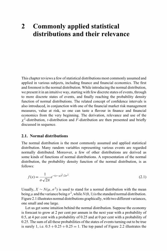
This chapter reviews a few of statistical distributions most commonly assumed andapplied in various subjects, including finance and financial economics. The firstand foremost is the normal distribution. While introducing the normal distribution,we present it in an intuitive way, starting with few discrete states of events, throughto more discrete states of events, and finally reaching the probability densityfunction of normal distributions. The related concept of confidence intervals isalso introduced, in conjunction with one of the financial market risk managementmeasures, value at risk, so one can taste a flavour in finance and financialeconomics from the very beginning. The derivation, relevance and use of theχ2-distribution, t-distribution and F-distribution are then presented and brieflydiscussed in sequence.
2.1. Normal distributions
The normal distribution is the most commonly assumed and applied statisticaldistribution. Many random variables representing various events are regardednormally distributed. Moreover, a few of other distributions are derived assome kinds of functions of normal distributions. A representation of the normaldistribution, the probability density function of the normal distribution, is asfollows:
f (x) = 1
σ√
2πe−(x−μ)2/2σ 2
(2.1)
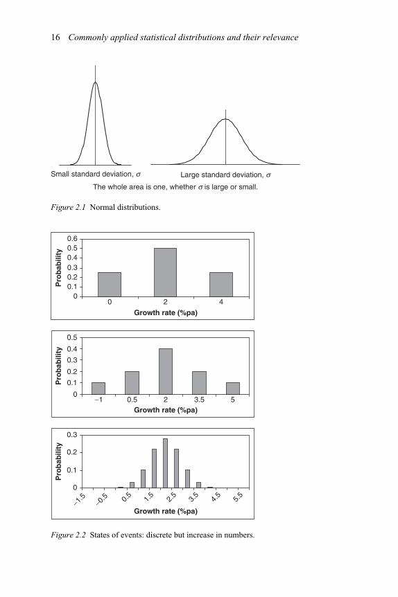
Usually, X ∼ N (μ,σ 2) is used to stand for a normal distribution with the meanbeingμ and the variance beingσ 2, while N (0, 1) is the standard normal distribution.Figure 2.1 illustrates normal distributions graphically, with two different variances,one small and one large.
Let us get some intuition behind the normal distribution. Suppose the economyis forecast to grow at 2 per cent per annum in the next year with a probability of0.5, at 4 per cent with a probability of 0.25 and at 0 per cent with a probability of0.25. The sum of all these probabilities of the states of events turning out to be trueis surely 1, i.e. 0.5 + 0.25 + 0.25 = 1. The top panel of Figure 2.2 illustrates the
16 Commonly applied statistical distributions and their relevance
The whole area is one, whether s is large or small.
Small standard deviation, s Large standard deviation, s
Figure 2.1 Normal distributions.
00
−1 0.5 2 3.5 5
2 4
0.10.20.30.40.50.6
Growth rate (%pa)
Growth rate (%pa)
Growth rate (%pa)
Pro
bab
ility
Pro
bab
ility
Pro
bab
ility
0
0.1
0.2
0.3
0.4
0.5
0
0.1
0.2
0.3
−1.5
−0.5 0.
51.
52.
53.
54.
55.
5
Figure 2.2 States of events: discrete but increase in numbers.

Commonly applied statistical distributions and their relevance 17
probable economic growth in the next year. With only three states of events, this israther rough and sketchy both mathematically and graphically. So let us increasethe states of events to five, the case illustrated by the middle panel of Figure 2.1.In that case, the economy is forecast to grow at 2 per cent with a probability of0.4, at 3.5 per cent and 0.5 per cent with a probability of 0.2, and at 5 per cent and−1 per cent with a probability of 0.1. Similar to the first case, the sum of all theprobabilities is 0.4 + 0.2 + 0.2 + 0.1 + 0.1 = 1. This is more precise than the firstcase. The bottom panel of Figure 2.1 is a case with even more states of events,15 states of events. The economy is forecast to grow at 2 per cent with a probabilityof 0.28, at 2.5 per cent and 1.5 per cent with a probability of 0.2181, at 3 per centand 1 per cent with a probability of 0.1030, and so on. It looks quite like the normaldistribution of Figure 2.1. Indeed, it is approaching normal distributions.
With a standard normal distribution, the probability that the random variable xtakes values between a small interval �x = [x,x +�x) is:
f (x) ·�x = 1√2π
e−x2/2�x (2.2)
This is the shaded area in Figure 2.3.When �x → 0, the probability is:
f (x)dx = 1√2π
e−x2/2 dx (2.3)
While the probability density function of the standard normal distribution is definedas follows:
f (x) = 1√2π
e−x2/2 (2.4)
Given any probability density function, the relationship between probabilitydensity function f (x) and probability P(x1 ≤ x < x2) is:
P(x1 < x ≤ x2) =x2∫
x1
f (x)dx (2.5)
Figure 2.3 From discrete probabilities to continuous probability density function.
18 Commonly applied statistical distributions and their relevance
(a) Confidence interval
i
95% confidence interval
90% confidence interval
x
(b) Intuitive illustration of confidence intervals
Figure 2.4 Illustrations of confidence intervals.
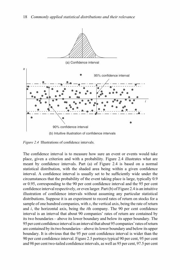
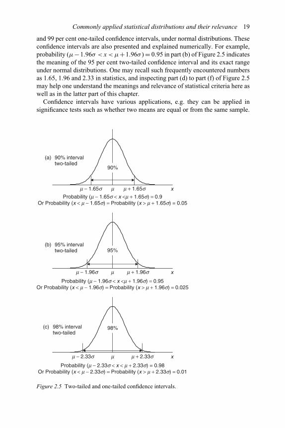
The confidence interval is to measure how sure an event or events would takeplace, given a criterion and with a probability. Figure 2.4 illustrates what aremeant by confidence intervals. Part (a) of Figure 2.4 is based on a normalstatistical distribution, with the shaded area being within a given confidenceinterval. A confidence interval is usually set to be sufficiently wide under thecircumstances that the probability of the event taking place is large, typically 0.9or 0.95, corresponding to the 90 per cent confidence interval and the 95 per centconfidence interval respectively, or even larger. Part (b) of Figure 2.4 is an intuitiveillustration of confidence intervals without assuming any particular statisticaldistributions. Suppose it is an experiment to record rates of return on stocks for asample of one hundred companies, with x, the vertical axis, being the rate of returnand i, the horizontal axis, being the ith company. The 90 per cent confidenceinterval is an interval that about 90 companies’ rates of return are contained byits two boundaries – above its lower boundary and below its upper boundary. The95 per cent confidence interval is an interval that about 95 companies’ rates of returnare contained by its two boundaries – above its lower boundary and below its upperboundary. It is obvious that the 95 per cent confidence interval is wider than the90 per cent confidence interval. Figure 2.5 portrays typical 90 per cent, 95 per centand 98 per cent two-tailed confidence intervals, as well as 95 per cent, 97.5 per cent
Commonly applied statistical distributions and their relevance 19
and 99 per cent one-tailed confidence intervals, under normal distributions. Theseconfidence intervals are also presented and explained numerically. For example,probability (μ−1.96σ < x < μ+1.96σ ) = 0.95 in part (b) of Figure 2.5 indicatesthe meaning of the 95 per cent two-tailed confidence interval and its exact rangeunder normal distributions. One may recall such frequently encountered numbersas 1.65, 1.96 and 2.33 in statistics, and inspecting part (d) to part (f) of Figure 2.5may help one understand the meanings and relevance of statistical criteria here aswell as in the latter part of this chapter.
Confidence intervals have various applications, e.g. they can be applied insignificance tests such as whether two means are equal or from the same sample.
90%
m − 1.65s m + 1.65smProbability (m − 1.65s < x <m + 1.65s) = 0.9
Or Probability (x < m − 1.65s) = Probability (x > m + 1.65s) = 0.05
95%
m − 1.96s m + 1.96sm
Probability (m − 1.96s < x <m + 1.96s) = 0.95Or Probability (x < m − 1.96s) = Probability (x > m + 1.96s) = 0.025
x
x
98%
m − 2.33s m + 2.33sm
Probability (m − 2.33s < x < m + 2.33s) = 0.98Or Probability (x < m − 2.33s) = Probability (x > m + 2.33s) = 0.01
x
(a) 90% interval two-tailed
(b) 95% interval two-tailed
(c) 98% interval two-tailed
Figure 2.5 Two-tailed and one-tailed confidence intervals.
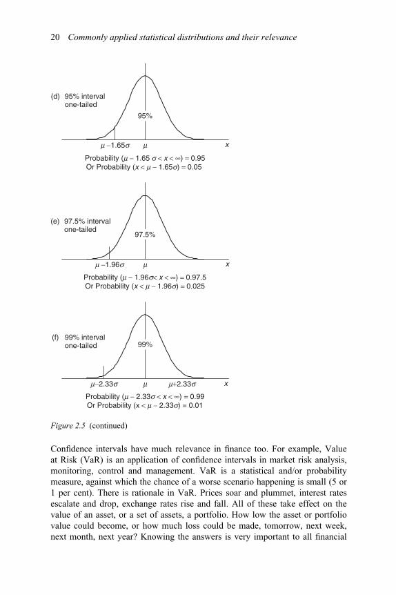
20 Commonly applied statistical distributions and their relevance
m −1.65s m
Probability (m − 1.65 s < x < ∞) = 0.95Or Probability (x < m − 1.65s) = 0.05
m −1.96s m
Probability (m − 1.96s< x < ∞) = 0.97.5Or Probability (x < m − 1.96s) = 0.025
x
x
m−2.33s m+2.33sm
Probability (m − 2.33s < x < ∞) = 0.99Or Probability (x < m − 2.33s) = 0.01
x
(e) 97.5% interval one-tailed
(f) 99% interval one-tailed
(d) 95% interval one-tailed
95%
97.5%
99%
Figure 2.5 (continued)
Confidence intervals have much relevance in finance too. For example, Valueat Risk (VaR) is an application of confidence intervals in market risk analysis,monitoring, control and management. VaR is a statistical and/or probabilitymeasure, against which the chance of a worse scenario happening is small (5 or1 per cent). There is rationale in VaR. Prices soar and plummet, interest ratesescalate and drop, exchange rates rise and fall. All of these take effect on thevalue of an asset, or a set of assets, a portfolio. How low the asset or portfoliovalue could become, or how much loss could be made, tomorrow, next week,next month, next year? Knowing the answers is very important to all financial

Commonly applied statistical distributions and their relevance 21
institutions and regulators. The following three examples show the application ofVaR in relation to confidence intervals.
Example 2.1
Suppose the rate of return and the standard deviation of the rate of returnon a traded stock are 10 per cent and 20 per cent per annum respectively;current market value of your investment in the stock is £10,000. What is theVaR over a one-year horizon, using 5 per cent as the criterion?
It is indeed an application of one-tailed 95 per cent confidence intervals,where μ = 10 per cent, σ = 20 per cent, per annum. It can be easily workedout that μ−1.65σ = 0.1−1.65×0.2 =−0.23 =−23 per cent. That is, thereis a 5 per cent chance that the annual rate of return would be −23 per cent orlower. Therefore there is a 5 per cent chance that the asset value would be£10,000×(1−23 per cent) = £7,700 or lower in one year. £7,700 is the VaRover a one-year horizon. The result can be interpreted as follows. There is a5 per cent chance that the value of your investment in the stock will be equalto or lower than £7,700 in one year; or there is a 95 per cent chance that thatvalue will not be lower than £7,700 in one year. Another interpretation isthat there is a 5 per cent chance that you will lose £10,000−£7,700 = £2,300or more in one year; or there is a 95 per cent chance you will not lose morethan £2,300 in one year.
Example 2.2
Using the same information as in the previous example, what is the VaRover a one-day horizon with the 5 per cent criterion?
We adopt 250 working days per year, then μ = 0.1/250 = 0.0004,σ = 0.2/(250)0.5 = 0.012649; μ − 1.65σ = 0.0004 − 1.65 × 0.012649 =−0.02047 = −2.047 per cent. This result indicates that there is a 5 per centchance that the daily rate of return would be −2.047 per cent or lower.Therefore there is a 5 per cent chance that the asset value would be£10,000× (1−2.047 per cent) = £9,795.29 or lower in one day. £9,795.29is the VaR over a one-day horizon. The result can be interpreted as follows.There is a 5 per cent chance that the value of your investment in thestock will be equal to or lower than £9,795.29 tomorrow; or there is a95 per cent chance that that value will not be lower than £9,795.29 tomorrow.Another interpretation is that there is a 5 per cent chance that you will lose£10,000−£9,795.29 = £204.71 or more tomorrow; or there is a 95 per centchance you will not lose more than £204.71 tomorrow.
22 Commonly applied statistical distributions and their relevance
Example 2.3
This example demonstrates that the more volatile the rate of return, the loweris the VaR. If the standard deviation of the rate of return on the traded stockis 30 per cent per annum and all other assumptions are unchanged, what isthe VaR over a one-day horizon, using 5 per cent as the criterion?
We still adopt 250 working days per year, then μ = 0.1/250 = 0.0004,σ = 0.3/(250)0.5 = 0.018974; μ − 1.65σ = 0.0004 − 1.65 × 0.018974 =−0.03091 = −3.091 per cent. That is, there is a 5 per cent chance thatthe daily rate of return would be −3.091 per cent or lower. Thereforethere is a 5 per cent chance that the asset value would be £10,000 ×(1−3.091 per cent) = £9,690.94 or lower in one day. £9,690.94 is the VaRover a one-day horizon, which is lower compared with £9,795.29 when theσ = 20 per cent per annum in the previous case.
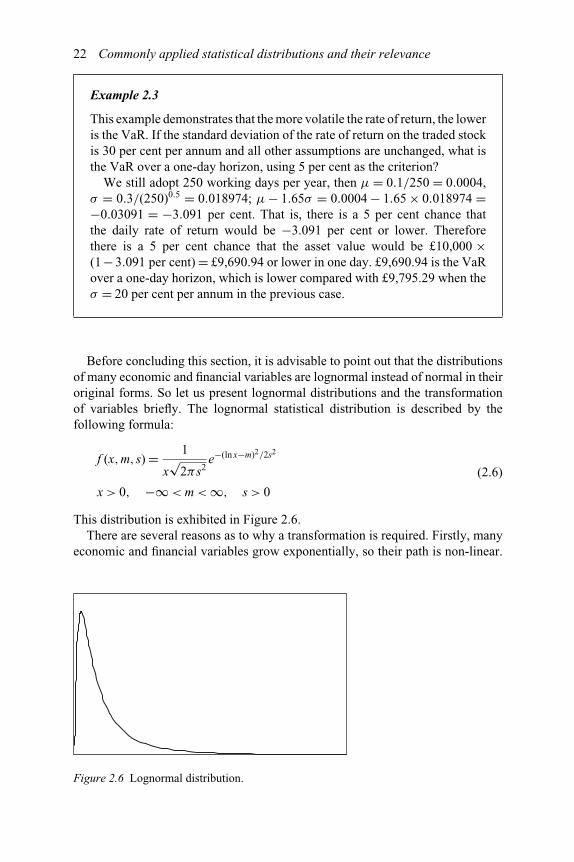
Before concluding this section, it is advisable to point out that the distributionsof many economic and financial variables are lognormal instead of normal in theiroriginal forms. So let us present lognormal distributions and the transformationof variables briefly. The lognormal statistical distribution is described by thefollowing formula:
f (x,m,s) = 1
x√
2πs2e−(ln x−m)2/2s2
x > 0, −∞ < m < ∞, s > 0
(2.6)
This distribution is exhibited in Figure 2.6.There are several reasons as to why a transformation is required. Firstly, many
economic and financial variables grow exponentially, so their path is non-linear.
Figure 2.6 Lognormal distribution.

Commonly applied statistical distributions and their relevance 23
Transforming these variables with a logarithm operation achieves linearity. That is,the variables after the logarithm transformation grow linearly on a linear path.Secondly, the transformation through logarithm operations changes the variablesin concern from absolute terms to relative terms, so comparison can be madecross-sections and over time. For example, the difference between the price inDecember and that in November is an absolute increase or change in price inone month; while the difference in the logarithm of the price in December andthat in November is a relative increase or change in price in one month, i.e.a percentage increase or change. A monthly increase of £10 in one stock and amonthly increase of £12 in another stock cannot be directly compared. However,a 2 per cent monthly increase in one stock and a 1.5 per cent monthly increasein another clearly show the difference and superiority. Finally, the logarithmtransformation may help achieve stationarity in time series data, though thisstatement may be controversial. Probably, one of the most convenient reasonsfor many economic and financial variables to follow lognormal distributions is thenon-negative constraint. That is, these variables can only take values that are greaterthan or equal to zero. Due partly to this, values closer to zero are compressed andthose far away from zero are stretched out. Lognormal distributions possess thesefeatures.
2.2. χ2-distributions
The χ2-distribution arises from the need in estimation of variance. It is associatedwith many test statistics, as they are about the variances under alternativespecifications. It also leads to some other distributions, e.g. those involving bothmean and variance.
The sum of the squares of m independent standard normal random variablesobeys a χ2-distribution with m degrees of freedom. Let Zi (i = 1,2, . . .m) denotem independent N (0, 1) random variables, then:
V = Z21 + Z2
2 +·· ·+ Z2m ∼ χ2
(m) (2.7)
The above random variable is said to obey a χ2-distribution with m degreesof freedom. χ2
(m) has a mean of m and a variance of 2m, and is always non-
negative. Figure 2.7 demonstrates several χ2-distributions with different degreesof freedom. When m, the degree of freedom, becomes very large, the shape oftheχ2-distribution looks rather like a normal distribution.
The following case shows the need of χ2-distributions in estimation of variance.Consider a sample:
Yi = β + ei, i = 1, . . .T (2.8)
where Yi ∼ N (β,σ 2), ei ∼ N (0,σ 2), and cov(ei,ej) = 0 for j �= i.

24 Commonly applied statistical distributions and their relevance
0.00
0.05
0.10
0.15
0.20
0 10 20 30 40 50 60
Chi-sq(4) Chi-sq(10) Chi-sq(20)
Figure 2.7 χ2-distributions with different degrees of freedom.
An estimator of β is:
b = Y1 + Y2 +·· ·+ YT
T= 1
T
T∑i=1
Yi (2.9)
and an estimator of σ 2 is:
σ 2 = e21 + e2
2 +·· ·+ e2T
T= 1
T
T∑i=1
e2i (2.10)
Note that when ei is unknown, an estimator of σ 2 is:
σ 2 = 1
T
T∑i=1
e2i (2.11)
where the estimator of ei is obtained through:
ei = Yi − b (2.12)
So, what kind of statistical distribution does σ 2 obey and what are the propertiesof the distribution? The answer is χ2-distributions.
We can transform the errors in equation (2.8), resulting in:
(e1
σ
)2 +(e2
σ
)2 +·· ·+(eT
σ
)2 =T∑
i=1
(ei
σ
)2 ∼ χ2(T ) (2.13)
and
T∑i=1
(ei
σ
)2
= T σ 2
σ 2 ∼ χ2(T−1) (2.14)
Commonly applied statistical distributions and their relevance 25
Due to loss of one degree of freedom inT∑
i=1ei = 0, the degrees of freedom of the
χ2-distribution in equation (2.14) become T − 1.The distribution of σ 2 is worked out as:
σ 2 ∼ σ 2
Tχ2
(T−1) (2.15)
It is biased, since
E(σ 2)= σ 2
TE(χ2
(T−1)
)= (T − 1)
Tσ 2 �= σ 2
Correction is therefore required to obtain an unbiased estimator of σ 2. Notice:
E
(T
T − 1σ 2
)= σ 2
T − 1E(χ2
(T−1)
)= σ 2
an unbiased estimator of σ 2 is:
σ 2 = T
T − 1σ 2 = 1
T − 1
T∑i=1
e2i ∼ σ 2
T − 1χ2
(T−1) (2.16)
as we can see that:
E
(T
T − 1σ 2
)= σ 2
T − 1E(χ2
(T−1)
)= σ 2 (2.17)
2.3. t-distributions
The t-distribution arises from the need in estimation of the accuracy of an estimate,or joint evaluation of the mean and variance of the estimate, or the acceptabilityof the estimate, when the variance is unknown. Many individual parameters,such as sample means and regression coefficients, obey t-distributions. It is acombination of two previously learned distributions, the normal distribution andthe χ2-distribution.
Let Z obey an N (0, 1) distribution andχ2T follow aχ2-distribution with T degrees
of freedom, then:
t = Z√χ2
(T )
/T
∼ t(T ) (2.18)
The random variable of the above kind is said to obey a t-distribution withT degrees of freedom. Figure 2.8 shows t-distributions with different degrees

26 Commonly applied statistical distributions and their relevance
0
0.1
0.2
0.3
0.4
0.5
−6 −4 −2 0 2 4 6
N(0, 1) t (3 t (100)
Figure 2.8 t-distributions with different degrees of freedom.
of freedom.When degrees of freedom become infinite, a t-distribution approachesa normal distribution.
Now let us consider the need in estimation of the accuracy of an estimate.Use the previous example of equation (2.8) and recall that an estimator ofthe sample mean is equation (2.9). The mean of the estimator represented byequation (2.9) is:
E (b) = E
(1
T
T∑i=1
Yi
)= β (2.19)
Its variance is:
Var (b) = Var
(1
T
T∑i=1
Yi
)= σ 2
T(2.20)
Therefore:
b ∼ N
(β,
σ 2
T
)(2.21)
The above can be rearranged to:
b −β
σ/√
T= Z ∼ N (0,1) (2.22)
Equation (2.22) measures the ‘meaningfulness’ of b, or the closeness of b to β.When σ 2 is unknown, we have to apply σ 2, then:
b ∼ N
(β,
σ 2
T
)(2.23)

Commonly applied statistical distributions and their relevance 27
The measure of ‘meaningfulness’ becomes:
b −β
σ/√
T(2.24)
Unlike the measure in equation (2.22), the above measure in equation (2.24) doesnot obey a normal distribution. Let us make some rearrangements:
b −β
σ/√
T= b −β
σ/√
T
/σ /
√T
σ/√
T= b −β
σ/√
T
/√σ 2
σ 2 (2.25)
Note in the above, the numerator is N (0, 1), and the denominator is the square rootof χ2
(T−1)/(T − 1), which leads to t-distributions with (T −1) degrees of freedom.From:
b −β
σ/√
T − 1= t(T−1) (2.26)
the probability for b to be a reasonable estimator of β is given as:
P(−tα/2,(T−1)σ /
√T − 1 ≤ b −β ≤ tα/2,(T−1)σ /
√T − 1
)= 1 −α (2.27)
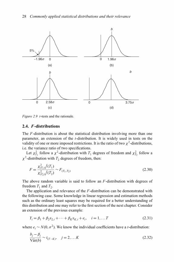
Equations (2.26) and (2.27) can be used to test the null hypothesis H0: b=β, againstthe alternative H1: b �= β. This is called the t-test. Usually t-tests are one-tailed,with the one-sided test statistic:
P(−tα,(T−1)σ /
√T − 1 ≤ b −β ≤ ∞
)= 1 −α (2.28)
The reasons for adopting one-tailed t-tests can be made clear from inspectingFigure 2.9. Part (a) of Figure 2.9 shows a small corner accounting for only 5 per centof the whole area; the distance is 1.96 times of the standard deviation to the left oforigin. If we shift the whole distribution to the right by this distance with the meanbeing the estimator of β, b, as shown with part (b) of Figure 2.9, then, a t-statisticof 1.96 means that there is only 5 per cent chance that b ≤ 0; or b is statisticallydifferent from zero at the 5 per cent significance level. The larger the t-statistic,the higher is the significance level. For example, with a t-statistic of 2.58, thechance for b ≤ 0 is even smaller, observed in part (c) of the Figure 2.9; and witha t-statistic of 3.75, the chance for b ≤ 0 is almost negligible, as demonstrated bypart (d) of Figure 2.9.
Alternatively, the variable can be squared:
t2(T−1) = (b −β)2
σ 2/T= Z2
χ2(T−1)
/(T − 1)
= χ2(1)
χ2(T−1)
/(T − 1)
(2.29)
It is the simplest of F-distributions to be discussed in the next section.
28 Commonly applied statistical distributions and their relevance
b
0 1.96s−1.96s
5%
0
(a) (b)
(c) (d)
b b
0 3.75s2.58s0
Figure 2.9 t-tests and the rationale.
2.4. F-distributions
The F-distribution is about the statistical distribution involving more than oneparameter, an extension of the t-distribution. It is widely used in tests on thevalidity of one or more imposed restrictions. It is the ratio of two χ2-distributions,i.e. the variance ratio of two specifications.
Let χ2T1
follow a χ2-distribution with T1 degrees of freedom and χ2T2
follow aχ2-distribution with T2 degrees of freedom, then:
F = χ2(T1)
/(T1)
χ2(T2)
/(T2)
∼ F(T1,T2) (2.30)
The above random variable is said to follow an F-distribution with degrees offreedom T1 and T2.
The application and relevance of the F-distribution can be demonstrated withthe following case. Some knowledge in linear regression and estimation methodssuch as the ordinary least squares may be required for a better understanding ofthis distribution and one may refer to the first section of the next chapter. Consideran extension of the previous example:
Yi = β1 +β2x2,i +·· ·+βKxK,i + ei, i = 1, . . .T (2.31)
where ei ∼ N (0,σ 2). We know the individual coefficients have a t-distribution:
bj −βj
Var(b)∼ t(T−K), j = 2, . . .K (2.32)
Commonly applied statistical distributions and their relevance 29
or:
t2(T−K) = (bj −βj)
2
Var(bj)= χ2
(1)
χ2(T−K)
/(T − K)
= (bj −βj)[Var(bj)
]−1(bj −βj) (2.33)
Replacing the above single parameters by vectors and matrices, we have essentiallyobtained the joint distribution of the regression coefficients:
(b − β)′ [
Cov(b)]−1
(b − β)
K − 1= χ2
(K−1)
/(K − 1)
χ2(T−K)
/(T − K)
(2.34)
where:
b = [b2 · · · bK
]′β = [β2 · · · βK
]′
Cov(b) =
⎡⎢⎢⎣
Var(b2) · · · Cov(b1,bK )· · ·
Cov(bK ,b1) Var(bK )
⎤⎥⎥⎦
The above is an F-distribution with (K −1) and (T −K) degrees of freedom. TheF-statistic is in fact the ratio of the explained variance and unexplained variance.
The t-statistic and the F-statistic are widely used to test restrictions, e.g. one,several or all regression coefficients are zero. Define SSEU as the unrestricted sumof squared errors:
SSEU = e′e = (y − bx)′ (y − bx) (2.35)
SSER as the restricted sum of squared errors:
SSER = e∗′e∗ = (y − b∗x) ′ (y − b∗x) (2.36)
With T observations, K regressors, and J restrictions, the F-test is:
(SSER − SSEU )/
J
SSEU
/(T − K)
= F[J , (T−K)] (2.37)
If the restrictions are valid, then SSER will not be much larger than SSEU , and theF-statistic will be small and insignificant. Otherwise, the F-statistic will be largeand significant.
3 Overview of estimation methods
This chapter briefly reviews primary statistical estimation methods, firstly underthe assumptions that the residuals from fitting the model obey independent identicaldistributions (iid) and the distributions may be further assumed to be normal,and then under more general conditions where iid of residuals is violated. Forprogression purposes, we firstly introduce the ordinary least squares method (OLS)and the maximum likelihood (ML) method under iid. Then, we relax the iidrequirements and extend the OLS and the ML methods with certain modifications.Further relaxations of residual distribution requirements lead to general residualdistributions typically observed in time series and cross-section modelling, whichare addressed next. Finally, we present the estimation methods based on momentconditions, including the method of moments (MM) and the generalised methodof moments (GMM), which are claimed to be more efficient, relaxed and easier inestimation processes and computation, and are getting momentum in applicationsin recent years.
3.1. Basic OLS procedures
Given a regression relation such as:
yi = β1 +β2xi + ei, ei ∼ iid(0,σ 2), i = 1, . . .N (3.1)
the idea of the OLS is to minimise the sum of squared errors:
N∑i=1
e2i =
N∑i=1
(yi − b1 − b2xi)2 (3.2)
The minimisation process is as follows. Taking derivatives of the above summationwith respect to β1 and β2 respectively and setting them to zero:
− 2N∑
i=1
(yi − b1 − b2xi) = 0
− 2N∑
i=1
xi (yi − b1 − b2xi) = 0
(3.3)

Overview of estimation methods 31
Making rearrangements of the above equations leads to:
Nb1 + b2
N∑i=1
xi =N∑
i=1
yi
b1
N∑i=1
xi + b2
N∑i=1
x2i =
N∑i=1
xiyi
(3.4)
Then the OLS estimators of β1 and β2, b1 and b2, are solved as:
b1 =N
N∑i=1
xiyi −N∑
i=1xi
N∑i=1
yi
NN∑
i=1x2
i −(
N∑i=1
xi
)2 (3.5)
b2 =
N∑i=1
x2i
N∑i=1
yi −N∑
i=1xi
N∑i=1
xiyi
NN∑
i=1x2
i −(
N∑i=1
xi
)2 (3.6)
The above analysis can be extended to multivariate cases, expressed in a compactform with vectors and matrices:
y = Xβ+ e, e ∼ iid(0,σ 2
)(3.7)
where y is an (N×1) vector containing N observations of the dependent variable, Xis an (N ×K) matrix with K being the number of regressors including the intercept,i.e. Xi =
[1 x2,i · · · xk,i
], β is a (K×1) vector of coefficients, and e is an (N × 1)
vector of residuals.The OLS procedure is to minimise:
(y − Xb)′ (y − Xb) (3.8)
The minimisation leads to:
X′ (y − Xb) = 0 (3.9)
Then the estimated coefficients are obtained as:
b = (X′X)−1
X′y (3.10)
The corresponding covariance matrix of the estimated coefficients is:
Cov(b) = σ 2(X′X
)−1(3.11)
32 Overview of estimation methods
where:
σ 2 = e′eT − K
(3.12)
and:
e = y − Xb (3.13)
3.2. Basic ML procedures
As long as a computable probability density function form can be figured out,the ML method and procedures can usually be applied. Nevertheless, the mostcommonly assumed function form is normal distributions or a function form thatcan be transformed into normal distributions. Given the same regression relation asin the previous section, but further assuming the error term is normally distributed,the model becomes:
yi = β1 +β2xi + εi
εi ∼ N (0,σ 2), Cov(εi,εj
)= 0, for j �= i, i = 1, . . . N(3.14)
The ML method is to maximise the joint probability density function of normaldistributions:
f (ε1, . . . εN ) = 1
σ√
2πe−[ε21
/2σ 2
]· · · 1
σ√
2πe−[ε2N
/2σ 2
]
= 1
σ√
2πe−[(y1−b1−b2x1)2
/2σ 2
]· · · 1
σ√
2πe−[(yN −b1−b2xN )2
/2σ 2
] (3.15)
Taking logarithms of the joint probability density function results in:
Ln( f ) = −N · Ln(σ ) − N
2Ln(2π ) − 1
2σ 2
N∑i=1
(yi − b1 − b2xi)2 (3.16)
To maximise the above function is indeed to minimise the third term on the right-hand side, leading to the same results as in the OLS case. Extending the aboveanalysis to the multivariate setting:
y = Xβ+ ε
ε ∼ N (0,σ 2)(3.17)
where all the descriptions, except that normality is imposed on ε, are the same asbefore. The joint probability density function is:
f (ε) =(
1
σ√
2π
)N
e−[ε′ε/
2σ 2]=(
1
σ√
2π
)N
e−[(y−Xb)′(y−Xb)
/2σ 2
](3.18)
Overview of estimation methods 33
The logarithm of the above probability density function is:
Ln( f ) = −N · Ln(σ ) − N
2Ln(2π ) − (y − Xb)′ (y − Xb)
2σ 2 (3.19)
Similar to the simple ML case represented by equations (3.14) to (3.16), tomaximise the above function is indeed to minimise the third term on the right-hand side of the above equation, leading to the same results as in the OLS case.The corresponding covariance matrix of the estimated coefficients is also the sameas in the OLS case. It can be concluded that, under the assumption of normaldistributions of errors, the OLS and the ML yield the same estimation results forregression parameters.
3.3. Estimation when iid is violated
Violation of iid distributions generally takes place in the forms of heteroscedastic-ity, cross-correlation and serial correlation or autocorrelation. Heteroscedasticitymeans that the variances of errors are not equal between them, as againsthomoscedastic, identical distribution. In this section, we just use one simpleexample each to illustrate what heteroscedasticity and serial correlation arerespectively and their consequences. We leave more general residual distributionsto be dealt with in the next section of this chapter, where elementary time series andcross-section modelling will be briefly introduced and discussed, based on whichand from which most models in the following chapters of this book are developedand evolved. For the simple case of heteroscedasticity, suppose in the followingregression equation the variance is proportional to the size of the regressor:
yi = β1 +β2xi + ei
Var(ei) = σ 2xi, Cov(ei,ej) = 0, for j �= i, i = 1, . . . N(3.20)
It is assumed, though, Cov(ei, ej) = 0, for j �= i still holds. That is, there is nocross-correlation if i and j represent different units with data being collected at thesame time or having no time implications; or there is no autocorrelation if i and jrepresent different time points. To deal with this heteroscedasticity, the OLS canbe generalised to achieve iid distributions. One way to achieve iid is to divide bothsides of the equation by
√xi, leading to a new regression relation:
y∗i = β1x∗
1,i +β2x∗2,i + e∗
i (3.21)
where y∗i = yi
/√xi, x∗
1,i = 1/√
xi, x∗2,i = √
xi, and e∗i = ei
/√xi.
Heteroscedasticity has been removed after the transformation, proven by thefollowing:
Var(e∗i ) = Var(ei)
xi
= σ 2 (3.22)

34 Overview of estimation methods
We can now apply the OLS to the transformed regression equation. The aboveprocedure is one type of the generalised least squares (GLS), or the weighted leastsquares (WLS). One of the constraints is that the value of the scaling regressormust be non-negative.
With heteroscedastic error terms and further assuming normality, the corre-sponding joint probability density function for equation (3.20) is:
f (ε1, . . . εN ) = 1
σ√
2πx1
e−[ε21
/2x1σ 2
]· · · 1
σ√
2πxN
e−[ε2N
/2xN σ 2
]
= 1
σ√
2πx1
e−[(y1−b1−b2x1)2
/2x1σ 2
](3.23)
· · · 1
σ√
2πxN
e−[(yN −b1−b2xN )2
/2xN σ 2
]
We can maximise the above joint probability density function without transforma-tion, though a transformation would correspond to that with the GLS more closely.Notice the original probability density function is:
f (εi) dεi = 1
σ√
2πxi
e−[ε2i
/2xiσ
2]dεi (3.24)
where the variances are heteroscedastic. Let ε∗i = εi/
√xi, then dε∗
i = dεi/√
xi, andthe above function becomes a homoscedastic normal distribution:
f (ε∗i ) dε∗
i = 1
σ√
2πe−[ε∗i 2/
2σ 2]dε∗
i (3.25)
One of the advantages of the ML method is that one can do estimation withouttransformation, as long as the probability density function can be written downexplicitly.
Let us turn to autocorrelation now. If in the following regression:
yt = β1 +β2xt + et, t = 1, . . . T (3.26)
Cov(et ,et−k ) = ρkσ2 �= 0, with t representing time, then it is said that there
is autocorrelation of order k in the residual. A simple case is the first-orderautocorrelation where Cov(et ,et−1) = ρ1σ
2 �= 0, and Cov(et ,et−k ) = 0 for k ≥ 2:
yt = β1 +β2xt + et
et = ρ1et−1 + νt, Cov(νt,ντ ) = 0 for τ �= t, t = 1, . . . T(3.27)
The following rearrangements can remove such autocorrelation. Lag equation(3.27) by one period and then multiply both sides by ρ1:
ρ1yt−1 = ρ1β1 +ρ1β2xt−1 +ρ1et−1 (3.28)

Overview of estimation methods 35
Then, subtracting both sides of equation (3.28) from the corresponding sides ofequation (3.27) leads to:
yt −ρ1yt−1 = β1 −ρ1β1 +β2xt −ρ1β2xt−1 + νt (3.29)
We can perform transformations such as y∗t = yt −ρ1yt−1 and x∗
t = xt −ρ1xt−1 toremove autocorrelation.
A simpler practice is to include the lagged variables on the right-hand side sothe residual becomes iid, as shown below:
yt = μ+ρ1yt−1 +α1xt +α2xt−1 + νt (3.30)
Then the OLS or ML can be easily applied to obtain parameter estimates.
3.4. General residual distributions in time series andcross-section modelling
This section briefly presents elementary time series and cross-section modellingwith two interrelated purposes. One is to introduce more general types of statisticaldistributions of residuals commonly found with statistical data sets, most, if notall of them, are either time series or cross-sectional data or a combination oftime series and cross-sectional data. The other, interrelated with the first andalready mentioned in the first, is to introduce elementary time series and cross-section modelling, because most models in the following chapters of this bookare developed and evolved based on and from these elementary time series andcross-section models and specifications.
In short, this section deals with correlation, both in time series and in cross-sections. Let us address correlation in time series first. A common finding in timeseries regression is that the residuals are correlated with their own lagged values.Since this correlation is sequential in time, it is then called serial correlation.This serial correlation violates the standard assumption of regression theory thatdisturbances are not correlated with other disturbances. There are a number ofproblems associated with serial correlation. The OLS is no longer efficient amonglinear estimators. Since prior residuals help to predict current residuals, we cantake advantage of this information to form a better prediction of the dependentvariable. Furthermore, standard errors computed using the classic OLS formulaare not correct, and are generally understated. Finally, if there are lagged dependentvariables on the right-hand side, OLS estimators are biased and inconsistent.
Serial correlation takes place for various reasons and can take different forms.Firstly, effects of shocks do not realise immediately. Technical diffusion as aprocess typically possesses this feature. Inefficient financial markets, especiallyin the weak form, are linked to serial correlation in statistical terms. Liquidityconstraints imply some corresponding action cannot be taken immediately and thedelay brings about serial correlation. Recent development in bounded rationalitysuggests that human beings’ expectations are not always rational; human beings
36 Overview of estimation methods
do not always behave rationally, not because they do not want to but becausethey have limitations. This is also a cause of serial correlation. Secondly, datacollection and processing processes may generate serial correlation. For example,data collected at different time points at different constituent units may causeserial correlation. Averaging monthly data to form quarterly data, or in general,averaging higher frequency data to form lower frequency data introduces serialcorrelation. Contrary to intuitive belief, using more data does not automaticallylead to the benefit of information utilisation. In many cases, it is more desirable tosimply sample, say, every first month in a quarter to represent that quarter, than touse all the months in a quarter for that quarter.
Serial correlation can take the form of autoregression (AR), moving average(MA) and their combinations. In an AR process, the residual in the current periodis correlated to the residual in the previous periods. For example, the following isan AR process of order 1, expressed as AR(1):
yt = μ+ et
et = ρ1et−1 + νt, Cov(νt,ντ ) = 0 for τ �= t, t = 1, . . . T(3.31)
where μ is the mean value of the process, et is a disturbance term, or calledunconditional residual, νt is innovation in the disturbance, also known as the one-period-ahead forecast error or the prediction error. νt is the difference betweenthe actual value of the dependent variable and a forecast made on the basis of theindependent variables and the past forecast errors. In general, an AR process oforder p, AR( p), takes the form of:
yt = μ+ et
et = ρ1et−1 +ρ2et−2 +·· ·+ρpet−p + νt
Cov(νt,ντ ) = 0 for τ �= t, t = 1, . . . T
(3.32)
The above equations can be expressed as:
yt = μ(1 −ρ1 −ρ2 −·· ·−ρp
)+ρ1yt−1 +ρ2yt−2 +·· ·+ρpyt−p + νt (3.33)
That is, we can express yt as a function of its past values. In general, there canbe exogenous explanatory variables or no exogenous explanatory variable on theright hand side of the above equations. The above representations are simple butalso typical for the illustration of AR processes, though exogenous explanatoryvariables are usually involved when we refer to AR models.
The other commonly used time series model involves MA processes. In an MAprocess, the current innovation, or forecast error, as well as its lagged values, entersthe estimation and forecast equation. A simple case of MA processes of order 1,expressed as MA(1), is:
et = νt + θνt−1
Cov(νt,νt−1) = 0, t = 1, . . . T(3.34)

Overview of estimation methods 37
In general, an MA process of order q, MA(q), takes the form of:
et = νt + θ1νt−1 +·· ·θqνt−q
Cov(νt,ντ ) = 0 for τ �= t, t = 1, . . . T(3.35)
The autoregressive and moving average specifications can be combined to forman ARMA specification:
yt = μ+ et +ρ1et−1 +·· ·+ρpet−p + νt + θ1νt−1 +·· ·θqνt−q
Cov(νt,ντ ) = 0 for τ �= t, t = 1, . . . T(3.36)
The above is an ARMA (p,q) process, autoregression of order p and movingaverage of order q.
The family of univariate time series models are not complete without a thirdelement, orders of integration. Recall one of the requirements for regressionanalysis is that the data to be analysed must be stationary. A time series mayor may not be stationary. Taking difference operations usually can make a non-stationary time series become stationary. When a time series requires d times ofdifferencing to become stationary, it is said to be integrated of order d, designatedI (d). A stationary time series is I (0). A time series involving all the three elementsis called autoregressive integrated moving average (ARIMA) process, consistingof these three parts. The first part is the AR term. Each AR term corresponds to theuse of a lagged value of the unconditional residual in estimation and forecasting.The second part is the integration order term. A first-order integrated componentmeans that the model is designed for the first difference of the original series.A second-order component corresponds to applying the second difference, and soon. The third part is the MA term. An MA forecasting model uses lagged valuesof the forecast error to improve the current forecast. A first-order moving averageterm uses the most recent forecast error, a second-order term uses the forecast errorfrom the two most recent periods, and so on. An ARIMA(p, d, q) model can beexpressed by the following representation:
�dyt = μ+ et +ρ1et−1 +·· ·+ρpet−p + νt + θ1νt−1 +·· ·θqνt−q
Cov(νt,ντ ) = 0 for τ �= t, t = 1, . . . T(3.37)
where �d is a difference operator for d times of differencing.ARIMA models can be estimated by applying the ML method when innovations
or forecast errors are assumed to follow normal distributions and other numericalmethods involving, sometimes, a large number of iterations. It was computertime-consuming in the past but is no longer a concern nowadays. As statedearlier, a common finding in time series regressions is that the residuals arecorrelated with their own lagged values. This serial correlation violates thestandard assumption of regression theory that disturbances are not correlated with
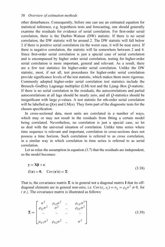
38 Overview of estimation methods
other disturbances. Consequently, before one can use an estimated equation forstatistical inference, e.g. hypothesis tests and forecasting, one should generallyexamine the residuals for evidence of serial correlation. For first-order serialcorrelation, there is the Durbin–Watson (DW) statistic. If there is no serialcorrelation, the DW statistic will be around 2. The DW statistic will fall below2 if there is positive serial correlation (in the worst case, it will be near zero). Ifthere is negative correlation, the statistic will lie somewhere between 2 and 4.Since first-order serial correlation is just a special case of serial correlationand is encompassed by higher order serial correlation, testing for higher-orderserial correlation is more important, general and relevant. As a result, thereare a few test statistics for higher-order serial correlation. Unlike the DWstatistic, most, if not all, test procedures for higher-order serial correlationprovide significance levels of the test statistic, which makes them more rigorous.Commonly adopted higher-order serial correlation test statistics include theBreusch–Godfrey Lagrange multiplier (LM) test and the Ljung–Box Q-statistic.If there is no serial correlation in the residuals, the autocorrelations and partialautocorrelations at all lags should be nearly zero, and all Q-statistics should beinsignificant with large p-values. A test statistic for nth-order serial correlationwill be labelled as Q(n) and LM(n). They form part of the diagnostic tests for thechosen specification.
In cross-sectional data, most units are correlated in a number of ways,which may or may not result in the residuals from fitting a certain modelbeing correlated. Nevertheless, no correlation is just a special case, so letus deal with the universal situation of correlation. Unlike time series wheretime sequence is relevant and important, correlation in cross-sections does notpossess a time horizon. Such correlation is referred to as cross correlation,in a similar way in which correlation in time series is referred to as serialcorrelation.
Let us relax the assumption in equation (3.7) that the residuals are independent,so the model becomes:
y = Xβ+ e
E(e) = 0, Cov(e′e) = �(3.38)
That is, the covariance matrix � is in general not a diagonal matrix I that its off-diagonal elements are in general non-zero, i.e. Cov(ei,ej) = σij = ρijσ
2 �= 0, fori �= j. The covariance matrix is illustrated as follows:
� =
⎡⎢⎢⎢⎢⎣
σ 2 ρ12σ2 .. ρ1N σ 2
ρ21σ2 σ 2 .. ρ2N σ 2
.. .. .. ..
ρN1σ2 ρN2σ
2 .. σ 2
⎤⎥⎥⎥⎥⎦ (3.39)

Overview of estimation methods 39
On many occasions, ρij = ρ, for all i �= j, for cross-sectional data, since there is notime sequence in cross-sections. Then the covariance matrix becomes:
� =
⎡⎢⎢⎢⎢⎣
σ 2 ρσ 2 .. ρσ 2
ρσ 2 σ 2 .. ρσ 2
.. .. .. ..
ρσ 2 ρσ 2 .. σ 2
⎤⎥⎥⎥⎥⎦ (3.40)
The GLS procedure is to minimise:
(y − Xb)′ �−1 (y − Xb) (3.41)
The minimisation leads to:
X′�−1 (y − Xb) = 0 (3.42)
Then the estimated coefficients are obtained as:
b = (X′�−1X)−1
X′�−1y (3.43)
It is noted that the covariance matrix of equation (3.40) is not readily available andhas to be estimated first. The usual practice is to apply the OLS first for the purposeof calculating the residuals, from which the covariance matrix can be derived. Theestimation of the covariance matrix in the later chapters when the GLS is involvedfollows the same procedure.
Further assuming normal distributions for the residuals, equation (3.38) becomes:
y = Xβ+ ε
ε ∼ N (0,�)(3.44)
Its joint probability density function is:
f (ε) = �−1
(1√2π
)N
e−[(
ε′�−1ε)/
2]= �−1
(1√2π
)N
e−[(y−Xb)′�−1(y−Xb)
/2]
(3.45)
Taking logarithms of the above probability density function leads to:
Ln( f ) = 1
2
[−N × Ln(2π ) + Ln(∣∣�−1
∣∣)− (y − Xβ)′ �−1 (y − Xβ)]
(3.46)
The maximisation of the above function is equivalent to minimising equation(3.41) with the GLS procedure, which produces the same parameter estimates.
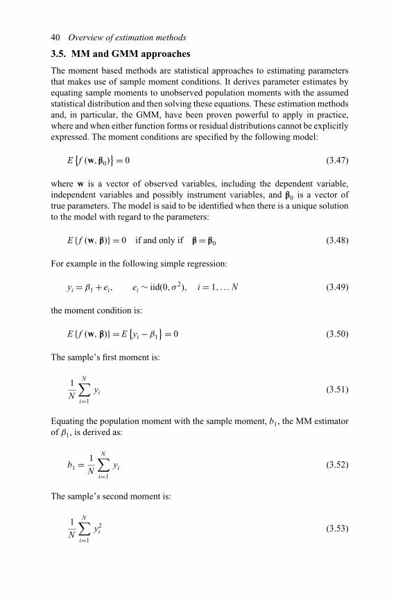
40 Overview of estimation methods
3.5. MM and GMM approaches
The moment based methods are statistical approaches to estimating parametersthat makes use of sample moment conditions. It derives parameter estimates byequating sample moments to unobserved population moments with the assumedstatistical distribution and then solving these equations. These estimation methodsand, in particular, the GMM, have been proven powerful to apply in practice,where and when either function forms or residual distributions cannot be explicitlyexpressed. The moment conditions are specified by the following model:
E{f (w,β0)
}= 0 (3.47)
where w is a vector of observed variables, including the dependent variable,independent variables and possibly instrument variables, and β0 is a vector oftrue parameters. The model is said to be identified when there is a unique solutionto the model with regard to the parameters:
E { f (w, β)} = 0 if and only if β = β0 (3.48)
For example in the following simple regression:
yi = β1 + ei, ei ∼ iid(0,σ 2), i = 1, . . . N (3.49)
the moment condition is:
E { f (w, β)} = E{yi −β1
}= 0 (3.50)
The sample’s first moment is:
1
N
N∑i=1
yi (3.51)
Equating the population moment with the sample moment, b1, the MM estimatorof β1, is derived as:
b1 = 1
N
N∑i=1
yi (3.52)
The sample’s second moment is:
1
N
N∑i=1
y2i (3.53)
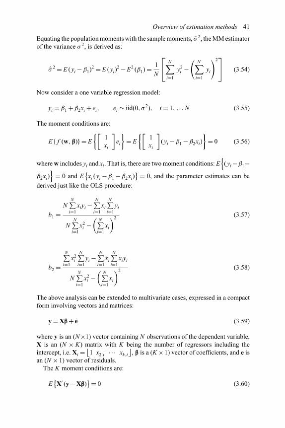
Overview of estimation methods 41
Equating the population moments with the sample moments, σ 2, the MM estimatorof the variance σ 2, is derived as:
σ 2 = E (yi −β1)2 = E (yi)2 − E2 (β1) = 1
N
⎡⎣ N∑
i=1
y2i −(
N∑i=1
yi
)2⎤⎦ (3.54)
Now consider a one variable regression model:
yi = β1 +β2xi + ei, ei ∼ iid(0,σ 2), i = 1, . . . N (3.55)
The moment conditions are:
E { f (w, β)} = E
{[1xi
]ei
}= E
{[1xi
](yi −β1 −β2xi)
}= 0 (3.56)
where w includes yi and xi. That is, there are two moment conditions: E{(yi −β1−
β2xi)}
= 0 and E{xi (yi −β1 −β2xi)
} = 0, and the parameter estimates can be
derived just like the OLS procedure:
b1 =N
N∑i=1
xiyi −N∑
i=1xi
N∑i=1
yi
NN∑
i=1x2
i −(
N∑i=1
xi
)2 (3.57)
b2 =
N∑i=1
x2i
N∑i=1
yi −N∑
i=1xi
N∑i=1
xiyi
NN∑
i=1x2
i −(
N∑i=1
xi
)2 (3.58)
The above analysis can be extended to multivariate cases, expressed in a compactform involving vectors and matrices:
y = Xβ+ e (3.59)
where y is an (N×1) vector containing N observations of the dependent variable,X is an (N × K) matrix with K being the number of regressors including theintercept, i.e. Xi =
⌊1 x2,i · · · xk,i
⌋, β is a (K ×1) vector of coefficients, and e is
an (N × 1) vector of residuals.The K moment conditions are:
E{X′ (y − Xβ)
}= 0 (3.60)

42 Overview of estimation methods
which is indeed the results from minimising:
E{
(y − Xβ)′ (y − Xβ)}
(3.61)
and the estimated parameters are derived just like the OLS procedure:
b = (X′X)−1
X′y (3.62)
In general, the moment conditions can be written as:
E{Z′ (y − Xβ)
}= 0 (3.63)
where Z is a vector of regressors that contains some of X and may containinstrument variables, and β is a vector of coefficients. When there are J momentconditions and J is equal to K , the above model is just-identified. If J is greaterthan K , the model is over-identified. The model is under-identified if J is smallerthan K . Under-identification happens when one or more variables in vector X areendogenous and consequently:
E{X′
end (y − Xβ)} �= 0 (3.64)
where Xend is a sub-set of X and are endogenous. Instruments are required whena sub-set of X are endogenous or correlated with the residual. Over-identificationemerges when one or more instrument variables are employed, so that the numberof moment conditions is greater than the number of variables in X. This gives riseto the GMM. Let us define:
g (β) = E{Z′ (y − Xβ)
}(3.65)
There are two features of the GMM. Instead of choosing K moment conditionsfrom the J moment conditions, the GMM uses all J moment conditions; then,instead of minimising the quadratic form of the moment conditions, the GMMminimises weighted quadratic moment conditions. The procedure for derivingGMM estimators are usually as follows. First formulate a quadratic form of thedistance, or the weighted quadratic moment conditions:
q (β) = g′ (β)Wgg (β) (3.66)
Then GMM estimators of β, b, are derived as:
b = arg minβ
q (β) = arg minβ
g′ (β)Wgg (β) (3.67)
where argmin is the global minimisation operation. The choice of weight matricesis important in implementing the GMM.
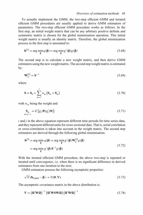
Overview of estimation methods 43
To actually implement the GMM, the two-step efficient GMM and iteratedefficient GMM procedures are usually applied to derive GMM estimators ofparameters. The two-step efficient GMM procedure works as follows. In thefirst step, an initial weight matrix that can be any arbitrary positive definite andsymmetric matrix is chosen for the global minimisation operation. This initialweight matrix is usually an identity matrix. Therefore, the global minimisationprocess in the first step is amounted to:
b[1] = arg minβ
q (β) = arg minβ
g′ (β)g (β) (3.68)
The second step is to calculate a new weight matrix, and then derive GMMestimators using the new weight matrix. The second step weight matrix is estimatedby:
W[2]g = S−1 (3.69)
where
S = S0 +l∑
m=1
wm
(Sm + S′
m
)(3.70)
with wm being the weight and
Smm=j−i
= E{gi (θ)g′
j (θ)}
(3.71)
i and j in the above equation represent different time periods for time series data,and they represent different units for cross-sectional data. That is, serial correlationor cross-correlation is taken into account in the weight matrix. The second stepestimators are derived through the following global minimisation:
b[2] = arg minβ
q (β) = arg minβ
g′ (β)W[2]g g (β)
= arg minβ
g′ (β)S−1g (β)(3.72)
With the iterated efficient GMM procedure, the above two-step is repeated oriterated until convergence, i.e. when there is no significant difference in derivedestimators from one iteration to the next.
GMM estimators possess the following asymptotic properties:
√N (bGMM − β) → N (0,V) (3.73)
The asymptotic covariance matrix in the above distribution is:
V = (�′W�)−1 (
�′WSW�)(
�′W�)−1
(3.74)

44 Overview of estimation methods
where:
� = E
[∂g (X,Z,β)
∂β
]= E
[Z′X]
(3.75)
As shown from equation (3.72), efficient GMM estimators are derived from settingthe weight matrix to S−1, then the asymptotic covariance matrix for efficient GMMestimators are reduced to:
V = (�′S−1�)−1
(3.76)
4 Unit roots, cointegration andother comovements in time series
The distinction between long-run and short-term characteristics in time serieshas attracted much attention in the last two decades. Long-run characteristicsin economic and financial data are usually associated with non-stationarity intime series and called trends. Whereas short-term fluctuations are stationary timeseries and called cycles. Economic and financial time series can be viewed ascombinations of these components of trends and cycles. Typically, a shock toa stationary time series would have an effect which would gradually disappear,leaving no permanent impact on the time series in the distant future. Whereas ashock to a non-stationary time series would permanently change the path of thetime series; or permanently move the activity to a different level, either higher ora lower level.
Moreover, the existence of common factors among two or more time series mayhave such effect that the combination of these times series demonstrates no featureswhich individual time series possess. For example, there could be a common trendshared by two time series. If there is no further trend which exists in only onetime series, then it is said that these two time series are cointegrated. This kind ofcommon factor analysis can be extended and applied to stationary time series aswell, leading to the idea of common cycles.
This chapter first examines the properties of individual time series with regard tostationarity and tests for unit roots. Then, cointegration and its testing proceduresare discussed. Finally, common cycles and common trends are analysed to furtherscrutinise comovements amongst variables.
4.1. Unit roots and testing for unit roots
Chapter 1 has provided a definition for stationarity. In the terminology of timeseries analysis, if a time series is stationary it is said to be integrated of order zero,or I (0) for short. If a time series needs the difference operation once to achievestationarity, it is an I (1) series; and a time series is I (n) if it is to be differencedfor n times to achieve stationarity. An I (0) time series has no roots on or insidethe unit circle but an I (1) or higher-order integrated time series contains roots onor inside the unit circle. So, examining stationarity is equivalent to testing for theexistence of unit roots in the time series.

46 Unit roots, cointegration and other comovements in time series
A pure random walk, with or without a drift, is the simplest non-stationary timeseries:
yt = μ+ yt−1 + εt, εt ∼ N (0,σ 2ε ) (4.1)
where μ is a constant or drift, which can be zero, in the random walk. It is non-stationary as Var(yt) = tσ 2
ε → ∞ as t → ∞. It does not have a definite meaneither. The difference of a pure random walk is the Gaussian white noise, or thewhite noise for short:
�yt = μ+ εt, εt ∼ N (0,σ 2ε ) (4.2)
The variance of �yt is σ 2ε and the mean is μ.
The presence of a unit root can be illustrated as follows, using a first-orderautoregressive process:
yt = μ+ρyt−1 + εt, εt ∼ N (0,σ 2ε ) (4.3)
Equation (4.3) can be recursively extended, yielding:
yt = μ+ρyt−1 + εt
= μ+ρμ+ρ2yt−2 +ρεt−1 + εt
. . .
= (1 +ρ +·· ·+ρn−1)μ+ρnyt−n + (1 +ρL +·· ·+ρn−1Ln−1
)εt (4.4)
where L is the lag operator. The variance of yt can be easily worked out:
Var(yt) = 1 −ρn
1 −ρσ 2
ε (4.5)
It is clear that there is no finite variance for yt if ρ ≥ 1. The variance is σ 2ε /(1 −ρ)
when ρ < 1.Alternatively, equation (4.3) can be expressed as:
yt = μ+ εt
(1 −ρL)= μ+ εt
ρ ((1/ρ) − L)(4.6)
which has a root r = 1/ρ.1 Compare equation (4.5) with equation (4.6), we can seethat when yt is non-stationary, it has a root on or inside the unit circle, i.e. r ≥ 1;while a stationary yt has a root outside the unit circle, i.e. r < 1. It is usually saidthat there exists a unit root under the circumstances where r ≥ 1. Therefore, testingfor stationarity is equivalent to examining whether there is a unit root in the timeseries. Having gained the above idea, commonly used unit root test procedures areintroduced and discussed in the following.
Unit roots, cointegration and other comovements in time series 47
4.1.1. Dickey and Fuller
The basic Dickey–Fuller (DF) test (Dickey and Fuller, 1979, 1981) is to examinewhether ρ < 1 in equation (4.3), which can, after subtracting yt−1 from both sides,be written as:
�yt = μ+ (ρ − 1)yt−1 + εt
= μ+ θyt−1 + εt
(4.7)
The null hypothesis is that there is a unit root in yt , or H0: θ = 0, against thealternative H1: θ < 0, or there is no unit root in yt . The DF test procedure emergedsince under the null hypothesis the conventional t-distribution does not apply.So whether θ < 0 or not cannot be confirmed by the conventional t-statistic forthe θ estimate. Indeed, what the Dickey–Fuller procedure gives us is a set ofcritical values developed to deal with the non-standard distribution issue, whichare derived through simulation. Then, the interpretation of the test result is no morethan that of a simple conventional regression.
Equations (4.3) and (4.7) are the simplest case where the residual is white noise.In general, there is serial correlation in the residual and �yt can be represented asan autoregressive process:
�yt = μ+ θyt−1 +p∑
i=1
φi�yt−i + εt (4.8)
Corresponding to equation (4.8), Dickey and Fuller’s procedure becomes theaugmented Dickey–Fuller test, or the ADF test for short. We can also includea deterministic trend in equation (4.8). Altogether there are four test specificationswith regard to the combinations of an intercept and a deterministic trend.
4.1.2. Phillips and Perron
Phillips and Perron’s (1988) approach is one in the frequency domain, termedas the PP test. It takes the Fourier transform of the time series �yt such as inequation (4.8), then analyses its component at the zero frequency. The t-statisticof the PP test is calculated as:
t =√
r0
h0
tθ − (h0 − r0)
2h0σσθ (4.9)
where
h0 = r0 + 2M∑
τ=1
(1 − j
T
)rj
is the spectrum of �yt at the zero frequency,2 rj is the autocorrelation function atlag j, tθ is the t-statistic of θ , σθ is the standard error of θ , and σ is the standard error

48 Unit roots, cointegration and other comovements in time series
of the test regression. In fact, h0 is the variance of the M -period differenced series,yt − yt−M ; while r0 is the variance of the one-period difference, �yt = yt − yt−1.
Although it is not the purpose of the book to describe technical details of testingprocedures, it is helpful to present intuitive ideas behind them. We inspect twoextreme cases, one the time series is a pure white noise and the other a pure randomwalk. In the former, rj = 0, j �= 0 and r0 = h0, so t = tθ and the conventionalt-distribution applies. In the latter, h0 = M × r0. If we look at the first term on theright-hand side of equation (4.9), t is adjusted by a factor of
√1/M ; and it is further
reduced by value of the second term ≈ σθ/2σ . So, the PP test gradually reducesthe significance of the θ estimate as ρ moves from zero towards unity (or as θ
moves from −1 to 0) to correct for the effect of non-conventional t-distributions,which becomes increasingly severe as ρ approaches unity.
4.1.3. Kwiatkowski, Phillips, Schmidt and Shin
Recently a procedure proposed by Kwiatkowski, Phillips, Schmidt and Shin(1992), known as the KPSS test named after these authors, has become a popularalternative to the ADF test. As the title of their paper, ‘Testing the null hypothesis ofstationarity against the alternative of a unit root’, suggests, the test tends to acceptstationarity, which is the null hypothesis, in a time series. Whereas in the ADF testthe null hypothesis is the existence of a unit root, stationarity is more likely to berejected. Many empirical studies have employed the KPSS procedure to confirmstationarity in such economic and financial time series as the unemployment rateand the interest rate, which, arguably, must be stationary for economic theories,policies and practice to make sense. Others, such as tests for purchasing powerparity (PPP), are less restrictive by the theory. Confirmation or rejection of PPPis both acceptable in empirical research using a particular set of time series data,though different test results give rise to rather different policy implications. Itis understandable that, relative to the ADF test, the KPSS test is less likely toreject PPP.
4.1.4. Panel unit root tests
Often in an empirical study, there is more than one time series to be examined.These time series are the same kind of data, such as the real exchange rate, currentaccount balance or dividend payout, but they are for a group of economies orcompanies. These time series probably have the same length with the same startdate and end date, or can be adapted without losing general properties. Undersuch circumstances, a test on pooled cross-section time series data, or panel data,can be carried out. Panel unit root tests provide an overall aggregate statistic toexamine whether there exists a unit root in the pooled cross-section time seriesdata and judge the time series property of the data accordingly. This, on the onehand, can avoid obtaining contradictory results in individual time series to whichno satisfactory explanations can be offered. On the other hand, good asymptoticproperties can be reached with relatively small samples in individual time series,

Unit roots, cointegration and other comovements in time series 49
which are sometimes too small to be effectively estimated. In the proceduredeveloped by Levin and Lin (1992, 1993), when the disturbances are i.i.d., the unitroot t-statistic converges to the normal distribution; when fixed effects or serialcorrelation is specified for the disturbances, a straightforward transformation ofthe t-statistic converges to the normal distribution too. Therefore, their unit roott-statistic converges to the normal distribution under various assumptions aboutdisturbances. Due to the presence of a unit root, the convergence is achieved morequickly as the number of time periods grows than as the number of individualsgrows. It is claimed that the panel framework provides remarkable improvementsin statistical power compared to performing a separate unit root for each individualtime series. Monte Carlo simulations indicate that good results can be achievedin relatively small samples with 10 individual time series and 25 observations ineach time series. Im et al. (1995) develop a t (t bar) statistic based on the averageof the ADF t-statistics for panel data. It is shown that under certain conditionsthe t-statistic has a standard normal distribution for a finite number of individualtime series observations, as long as the number of cross-sections is sufficientlylarge. Commenting on and summarising Levin and Lin (1992, 1993) and Im et al.(1995) procedures, Maddala and Wu (1999) argue that the Levin and Lin test is toorestrictive to be of interest in practice. While the test of Im et al. relaxes Levin andLin’s assumptions, it presents test results which merely summarise the evidencefrom a number of independent tests of the sample hypothesis. They subsequentlysuggest the Fisher test as a panel data unit root test and claim that the Fisher testwith bootstrap-based critical values is the preferred choice.
4.2. Cointegration
Cointegration is one of the most important developments in time series econo-metrics in the last quarter century. A group of non-stationary I (1) time seriesis said to have cointegration relationships if a certain linear combination ofthese time series is stationary. There are two major approaches to testing forcointegration, the Engle–Granger two-step method (Engle and Granger, 1987)and the Johansen procedure (Johansen, 1988, 1991; Johansen and Juselius, 1990).In addition, procedures for panel cointegration (Kao and Chiang, 1998; Moon andPhillips, 1999; Pedroni, 1999) have been recently developed, in the same spirit ofpanel unit roots and to address similar issues found in unit root tests. Since mostpanel cointegration tests employ the same estimation methods of or make minoradjustments in relation to the asymptotic theory of non-stationary panel data, theyare not to be discussed in this chapter. The Engle–Granger method involves firstlyrunning regression of one variable on another, and secondly checking whetherthe regression residual from the first step is stationary using, say, an ADF test. Inthis sense, the Engle–Granger method is largely the unit root test and will not bedeliberated either. This chapter only presents the Johansen procedure which is totest restrictions imposed by cointegration on a VAR model:
yt = μ+ A1yt−1 +·· ·Apyt−p + εt (4.10)

50 Unit roots, cointegration and other comovements in time series
where yt is a k-dimension vector of variables which are assumed to be I (1)series (but can also be I (0)), Ai, i = 1, . . .p is the coefficient matrix, andεt is a k-dimension vector of residuals. Subtracting yt−1 from both sides ofequation (4.10) yields:
�yt = μ+yt−1 +1�yt−1 +·· ·+p−1�yt−p+1 + εt (4.11)
where:
=p∑
i=1
Ai − I
and:
i = −p∑
j=i+1
Aj
We can observe from equation (4.11) that only one term in the equation, yt−1, isin levels, cointegration relations depend crucially on the property of matrix . Itis clear that yt−1 must be either I (0) or zero except that yt is already stationary.There are three situations:
(a) = αβ′ has a reduced rank 0 < r < k ,(b) = αβ′ has a rank of zero, and(c) = αβ′ has a full rank.
Under situation (a), α and β are both k × r matrices and have a rank of r. Thereare r cointegration vectors β′yt which are stationary I (0) series. It is equivalentto having r common trends among yt . The stationarity of β′yt implies a long-run relationship among yt or a sub-set of yt – the variables in the cointegrationvectors will not depart from each other over time. β′yt are also error correctionterms in that departure of individual variables in the cointegration vectors fromthe equilibrium will be subsequently reversed back to the equilibrium – a dynamicadjustment process called error correction mechanism (ECM). Equation (4.11) istherefore called VAR with ECM. Under situation (b), there is no cointegrationrelation among ytand the variables in levels do not enter equation (4.11) andequation (4.11) becomes a simple VAR without ECM. The variables in levels arealready stationary under situation (c).
Depending on whether yt and/or cointegration vectors have an interceptand/or deterministic trend, there are five models in practice: (a) there are nodeterministic trends in yt and no intercepts in cointegration vectors; (b) thereis no deterministic trend in yt but there are intercepts in cointegration vectors;(c) there are deterministic trends in yt and intercepts in cointegration vectors;(d) there are deterministic trends in yt and in cointegration vectors; (e) there arequadratic trends in yt and deterministic trends in cointegration vectors. For details

Unit roots, cointegration and other comovements in time series 51
of these specifications, see Johansen and Juselius (1990), and for the criticalvalues of test statistics see Osterwald-Lenum (1992). The Johansen test is akind of principal component analysis where eigenvalues of are calculatedthrough a maximisation procedure. Then, five specifications or hypotheses aretested using the maximum eigenvalue statistic and the trace statistic which oftenconvey contradictory messages. To test the hypothesis that there are r cointegrationvectors against the alternative of (r+1) cointegration vectors, there is the followingmaximum eigenvalue statistic:
lmax = −T ln(1 − lr+1) (4.12)
where lr is the eigenvalue corresponding to r cointegration vectors and T is thenumber of observations. The trace statistic is calculated as:
ltrace = −Tk∑
i=r+1
ln(1 − li) (4.13)
Indeed, the trace statistic for the existence of r cointegration vectors is the sum ofthe maximum eigenvalue statistics for from zero up to r cointegration vectors.
4.3. Common trends and common cycles
It should be noted that cointegration is not exactly the same as common trendanalysis. While cointegration implies common trends it also requires non-existenceof uncommon trends. A group of time series variables can share one or morecommon trends but the variables are not cointegrated because, for example, oneof the variables, y2t , also possesses, in addition to the common trends, a trendwhich is unique to itself and uncommon to others. Under such circumstances, thecointegration vector β′yt in equation (4.11) will exclude y2t and it appears that y2t
does not share common trends with other variables in yt . Consider the followingk-variable system:
y1t = a11T1t +·· ·+ a1rTrt + τ1t + c1t + ε1t
y2t = a21T1t +·· ·+ a2rTrt + τ2t + c2t + ε2t
. . .
ykt = ak1T1t +·· ·+ akrTrt + τkt + ckt + εkt
(4.14)
where Tit, i = 1, . . .r is the ith common trend, τjt, j = 1, . . .k is the unique trendin yjt , and cjt, j = 1, . . .k is the cycle or stationary component in yjt . If there areno unique trends, i.e. τjt = 0, j = 1, . . .k , then from linear algebra we know that acertain linear combination of yjt, j = 1, . . .k is zero when r < k . So there are onlycycles or stationary components, cjt, j = 1, . . .k , left in the linear combination ofyjt, j = 1, . . .k , which exhibits no trends. This is exactly the idea of cointegration
52 Unit roots, cointegration and other comovements in time series
discussed above. When there is unique trend in, for example, y2t (i.e. τ2t �= 0;τjt = 0, j �= 2), y2t will not be cointegrated with any other variables in the system asany linear combination involving y2t will be non-stationary, though y2t does sharecommon trends with the rest of the variables. It is clear that if y2t does join othervariables in β′yt , it must contain no unique trend. For convenience, common trendsare treated as the same as cointegration in this chapter. That is, unique trends areexcluded from analysis.
In the following, we extend cointegration and common trend analysis to thecase of cycles. It is said (Engle and Kozicki, 1993; Vahid and Engle, 1993; Engleand Issler, 1995) there are common cycles (in the same spirit, uncommon cyclesare excluded from analysis) among yt in equation (4.10) if there exists a vector β
such that:
β′yt = β′εt (4.15)
That is, a combination of the time series in yt exhibits no cyclical movement orfluctuation. Common trends and common cycles are two major common factorsdriving economic and financial variables to move and develop in a related way.3
It is therefore helpful to inspect them together in a unified dynamic system.According to the Wold representation theorem, time series or a vector of time
series can be expressed as an infinite moving average process:
�yt = C(L)εt, C(L) = I + C1L + C2L2 +·· · (4.16)
C(L) can be decomposed as C(1) + (1 − L)C∗(L), therefore:
�yt = C(1)εt + (1 − L)C∗(L)εt, C∗i =∑j>i
−Cj, C∗0 = I − C(1)
(4.17)
Taking the summation to get the variables in levels:
yt = C(1)∞∑i=0
εt−i + C∗(L)εt (4.18)
Equation (4.18) is the Stock and Watson (1988) multivariate generalisation of theBeveridge and Nelson (1981) trend-cycle decomposition and is referred to as theBNSW decomposition. Common trends in the sense of cointegration require:
β′C(1) = 0 (4.19)
and common cycles require:
β′C∗(L) = 0 (4.20)
Equation (4.18) can be written as the sum of two components of trends and cycles:
yt = Tt + Ct (4.21)

Unit roots, cointegration and other comovements in time series 53
When the sum of the rank of β, r, and the rank of β, s, is equal to k , the stack of β
and β is a k × k full rank matrix:
B =[β β
](4.22)
and trends and cycles can be exclusively expressed in the common factor coefficientvectors, β and β, and their combinations. According to equations (4.19) and (4.20):
[β β
]′yt =
[β′yt
β′yt
]=⎡⎣ β′C∗(L)εt
β′C(1)∞∑i=0
εt−i
⎤⎦
So:
yt =[β′
β′
]−1⎡⎣ β′C∗(L)εt
β′C(1)∞∑i=0
εt−i
⎤⎦ (4.23)
Define B−1 = [β−1 β−1]4
and refer to equation (4.18), we have:
yt = [β−1 β−1]⎡⎣ β′C∗(L)εt
β′C(1)∞∑i=0
εt−i
⎤⎦= β−1β′C∗(L)εt + β−1β′C(1)
∞∑i=0
εt−i
= β−1β′yt + β−1β′yt = Ct + Tt (4.24)
Therefore, we get Ct = β−1β′yt , and Tt = β−1β′yt , exclusively expressed in thecommon factor coefficient vectors, β and β, and their combinations.
4.4. Examples and cases
It is probably not worthwhile demonstrating any unit root test examples indi-vidually nowadays since these tests have been made straightforwardly simple.Nevertheless, unit root tests are still routine procedures prior to cointegrationanalysis, i.e. studies of cointegration will almost inevitably involve unit roottests. Accordingly, one case on cointegration and one case on common cyclesare presented in the following which largely cover the topics of this chapter.
Example 4.1
This is a case on dynamic links and interactions between AmericanDepository Receipts (ADRs) and their underlying foreign stocks by Kimet al. (2000). ADRs are certificates issued by a US bank which represent
Continued

54 Unit roots, cointegration and other comovements in time series
indirect ownership of a certain number of shares in a specific foreign firm.Shares are held on deposit in the firm’s home bank. ADRs are traded inUS dollars and investors receive dividends in US dollars too. Therefore,returns on ADRs reflect the domestic returns on the stock as well as theexchange rate effect. ADRs have become popular in the US due to theirdiversification benefits, especially when US investors have little knowledgein foreign countries’ business and political systems, and risks associatedwith investing in foreign securities may be overestimated.
In addition to the factors of underlying foreign stocks and the exchangerate, the paper has also considered the influence of the US stock market onADRs returns. To this end, they use the cointegration approach and othermodels to examine the effect on ADR of the three factors. Their resultsshow that the price of the underlying stock is most important, whereas theexchange rate and the US market also have an impact on ADR prices. Weonly present results related to cointegration analysis of 21 British firms. Thedata set used in the paper is daily closing prices from 4 January 1988 to31 December 1991.
The first thing to do prior to cointegration tests is almost a routine checkon whether there is a unit root in the time series data, as we require I (1)series to carry out cointegration analysis. The paper adopts the ADF testto examine the existence of a unit root, with the critical values being takenfrom Davidson and Mackinnon (1993), obtained from a much larger setof simulations than those tabulated by Dickey and Fuller. The lag lengthin the ADF test is chosen such that the Q-statistic at 36 lags indicates noserial correlation in the residuals. The lag length can also be chosen byusing the Akaike information criterion (AIC) or Schwarz criterion (SC), ormore ideally, a combination of the Q-statistic and one of the AIC or SCwhich, though, may produce non-conciliatory recommendations. It can beseen from Table 4.1 that all the series, except series 8 and 19 (interestinglyboth ADRs and underlying stocks), have a unit root in levels and no unit rootin the first difference. Although the null hypothesis of a unit root is rejectedfor series 8 and 19 in levels, the rejection is at a rather low 10 per centsignificance level. So, all the series are treated as I (0) and cointegrationanalysis can be carried out for all of them. In Table 4.2, the exchange rateand one of the US stock market indices, S&P500, are also confirmed to beI (1) series, and can be included in cointegration analysis as well.
The results of cointegration analysis between ADRs, correspondingforeign stocks, the exchange rate and the S&P500 index, are reported inTable 4.3. The lag length k is chosen by Sims’ likelihood ratio test. Bothtrace and eigenvalue test statistics indicate that for all 21 groups, there existsat least one cointegrating relationship among the variables. Nine groups haveat least two and three groups have at least three cointegrating relationships.

Unit roots, cointegration and other comovements in time series 55
Table 4.1 Augmented Dickey–Fuller unit root tests – ADRs and underlyingforeign stocks, UK
Firm ADR Underlying
Level First difference Level First difference
1 −2.559 −35.842∗∗∗ −2.461 −22.132∗∗∗2 −1.245 −13.821∗∗∗ −1.725 −19.753∗∗∗3 −1.652 −14.873∗∗∗ −1.823 −12.694∗∗∗4 −2.235 −15.985∗∗∗ −1.927 −13.346∗∗∗5 −1.985 −26.879∗∗∗ −1.969 −28.566∗∗∗6 −2.237 −27.522∗∗∗ −1.878 −25.997∗∗∗7 −2.334 −20.464∗∗∗ −1.200 −23.489∗∗∗8 −2.652∗ −30.435∗∗∗ −2.800∗ −29.833∗∗∗9 −1.287 −10.156∗∗∗ −2.382 −14.489∗∗∗
10 −1.823 −26.372∗∗∗ −1.014 −21.788∗∗∗11 −1.021 −27.825∗∗∗ −1.087 −19.482∗∗∗12 −1.934 −29.225∗∗∗ −2.425 −27.125∗∗∗13 −2.324 −13.223∗∗∗ −1.894 −12.854∗∗∗14 −1.997 −17.325∗∗∗ −1.823 −16.478∗∗∗15 −1.333 −11.528∗∗∗ −1.458 −37.311∗∗∗16 −1.223 −10.285∗∗∗ −1.253 −18.244∗∗∗17 −1.110 −16.742∗∗∗ −2.182 −33.245∗∗∗18 −1.559 −14.522∗∗∗ −1.285 −17.354∗∗∗19 −2.678∗ −22.485∗∗∗ −2.677∗ −15.660∗∗∗20 −1.546 −14.266∗∗∗ −1.024 −14.266∗∗∗21 −2.364 −22.333∗∗∗ −1.625 −24.757∗∗∗
Asymptotic critical values are from Davidson and Mackinnon (1993). Lag length K is chosensuch that the Q-statistic at 36 lags indicates absence of autocorrelation in the residuals.Estimation period is 4 January 1988–31 December 1991.∗significant at the 10 per cent level; ∗∗significant at the 5 per cent level; ∗∗∗significant at the1 per cent level.
Table 4.2 Augmented Dickey–Fuller unit root tests – the exchange rate and theS&P 500 index
Level First difference
£ vis-à-vis $ −1.625 −19.124∗∗∗S&P 500 index −2.115 −20.254∗∗∗
Asymptotic critical values are from Davidson and Mackinnon (1993). Lag length K is chosensuch that the Q-statistic at 36 lags indicates absence of autocorrelation in the residuals.Estimation period is 4 January 1988–31 December 1991.∗significant at the 10 per cent level; ∗∗significant at the 5 per cent level; ∗∗∗significant at the1 per cent level.
Continued

56 Unit roots, cointegration and other comovements in time series
Table 4.3 Johansen multivariate cointegration tests – United Kingdom
Firm Trace lmax
r = 0 r ≤ 1 r ≤ 2 r ≤ 3 r = 0 r ≤ 1 r ≤ 2 r ≤ 3
1 91.22∗∗∗ 21.28 2.95 1.04 70.11∗∗∗ 10.09 1.89 1.042 52.18∗∗∗ 12.45 6.06 1.25 36.37∗∗∗ 10.65 4.75 1.253 68.02∗∗∗ 20.24 5.79 0.50 84.67∗∗∗ 12.34 5.00 0.504 105.24∗∗∗ 28.45∗ 7.64 1.25 96.77∗∗∗ 19.65∗ 6.75 1.255 45.33∗ 11.02 1.24 0.37 39.32∗∗∗ 9.88 1.05 0.376 163.26∗∗∗ 32.84∗∗ 9.75 3.94 141.21∗∗∗ 27.87∗∗∗ 13.25∗∗ 3.947 85.24∗∗∗ 19.45 2.25 1.00 66.47∗∗∗ 10.65 1.75 1.008 150.33∗∗∗ 30.02∗ 8.24 3.54 120.32∗∗∗ 20.78∗ 6.45 3.549 49.23∗∗ 12.02 1.29 0.98 29.32∗∗ 9.78 9.24 0.98
10 50.24∗∗ 13.45 1.54 1.08 46.37∗∗∗ 10.65 3.25 1.0811 190.33∗∗∗ 38.02∗∗∗ 18.24∗∗∗ 3.99 145.31∗∗∗ 28.88∗∗ 11.48 3.9912 96.96∗∗∗ 21.84 3.00 1.52 72.50∗∗∗ 12.09 2.69 1.5213 150.24∗∗∗ 30.00∗ 7.34 3.24 120.22∗∗∗ 20.74∗ 5.45 3.2414 199.43∗∗∗ 42.02∗∗∗ 19.24∗∗∗ 4.57 150.32∗∗∗ 38.99∗∗∗ 18.45∗∗∗ 4.5715 153.33∗∗∗ 31.25∗∗ 8.66 3.25 125.43∗∗∗ 21.27∗∗ 5.75 3.2516 81.43∗∗∗ 21.34 5.24 2.08 52.45∗∗∗ 17.24 3.78 2.0817 210.24∗∗∗ 68.24∗∗∗ 21.78∗∗∗ 4.02 139.32∗∗∗ 34.28∗∗∗ 16.27∗∗ 4.0218 62.96∗∗∗ 13.11 1.75 0.99 42.11∗∗∗ 10.09 1.29 0.9919 49.24∗∗ 9.92 1.24 0.61 27.88∗∗ 8.45 1.05 0.6120 120.33∗∗∗ 24.91 6.24 2.01 84.56∗∗∗ 15.74 3.45 2.0121 173.86∗∗∗ 33.24∗∗ 8.03 4.06 121.54∗∗∗ 33.34∗∗∗ 10.49 4.06
The cointegration equation is based on four variables: (1) British ADRs, (2) British underlyingshares, (3) British pound spot exchange rates, and (4) the S&P 500 index cash prices. Estimationperiod is 4 January 1988–31 December 1991.∗significant at the 10 per cent level; ∗∗significant at the 5 per cent level; ∗∗∗significant at the1 per cent level.
Each group’s cointegrating vector is calculated and incorporated in the VARto form a VAR–ECM model. Based on the estimated VAR–ECM model, thepaper has further performed variance decomposition and impulse responseanalysis which are beyond the reach of this chapter.5 While cointegrationanalysis indicate a dynamic adjustment process and long-run equilibriumrelationship among ADRs and the three factors, results from variancedecomposition and impulse responses suggest that the largest effect onADRs is due to shocks in their underlying stocks. Nevertheless, the exchangerate also has a role and that role is growing in recent years. The effect ofthe US stock market has been found but the effect is small. More likely, thelast link might be superficial and due to a common factor driving both theUS and foreign markets or the US stock market and the foreign exchangemarket.
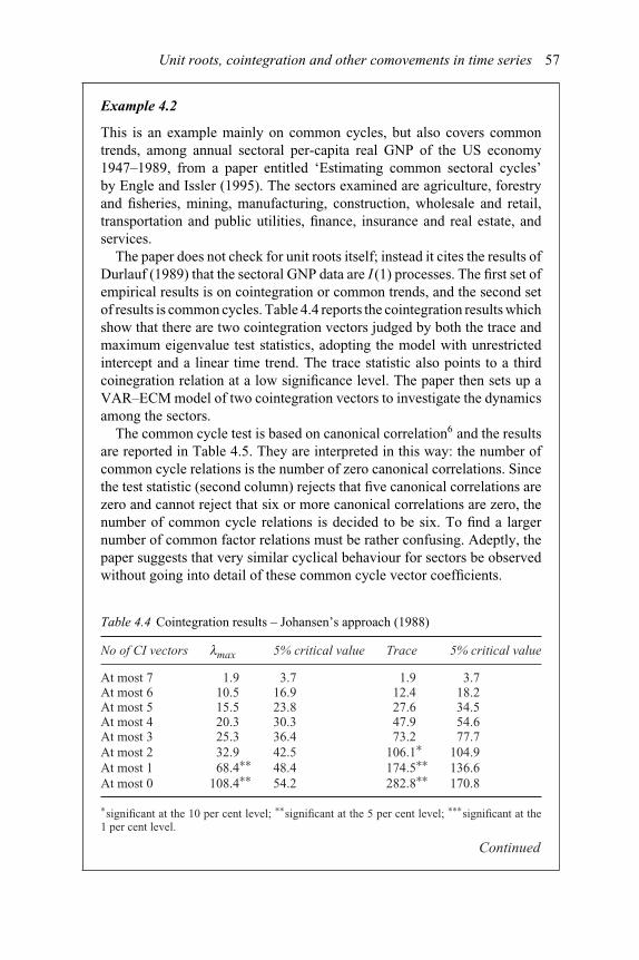
Unit roots, cointegration and other comovements in time series 57
Example 4.2
This is an example mainly on common cycles, but also covers commontrends, among annual sectoral per-capita real GNP of the US economy1947–1989, from a paper entitled ‘Estimating common sectoral cycles’by Engle and Issler (1995). The sectors examined are agriculture, forestryand fisheries, mining, manufacturing, construction, wholesale and retail,transportation and public utilities, finance, insurance and real estate, andservices.
The paper does not check for unit roots itself; instead it cites the results ofDurlauf (1989) that the sectoral GNP data are I (1) processes. The first set ofempirical results is on cointegration or common trends, and the second setof results is common cycles. Table 4.4 reports the cointegration results whichshow that there are two cointegration vectors judged by both the trace andmaximum eigenvalue test statistics, adopting the model with unrestrictedintercept and a linear time trend. The trace statistic also points to a thirdcoinegration relation at a low significance level. The paper then sets up aVAR–ECM model of two cointegration vectors to investigate the dynamicsamong the sectors.
The common cycle test is based on canonical correlation6 and the resultsare reported in Table 4.5. They are interpreted in this way: the number ofcommon cycle relations is the number of zero canonical correlations. Sincethe test statistic (second column) rejects that five canonical correlations arezero and cannot reject that six or more canonical correlations are zero, thenumber of common cycle relations is decided to be six. To find a largernumber of common factor relations must be rather confusing. Adeptly, thepaper suggests that very similar cyclical behaviour for sectors be observedwithout going into detail of these common cycle vector coefficients.
Table 4.4 Cointegration results – Johansen’s approach (1988)
No of CI vectors lmax 5% critical value Trace 5% critical value
At most 7 1.9 3.7 1.9 3.7At most 6 10.5 16.9 12.4 18.2At most 5 15.5 23.8 27.6 34.5At most 4 20.3 30.3 47.9 54.6At most 3 25.3 36.4 73.2 77.7At most 2 32.9 42.5 106.1∗ 104.9At most 1 68.4∗∗ 48.4 174.5∗∗ 136.6At most 0 108.4∗∗ 54.2 282.8∗∗ 170.8
∗significant at the 10 per cent level; ∗∗significant at the 5 per cent level; ∗∗∗significant at the1 per cent level.
Continued
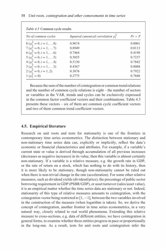
58 Unit roots, cointegration and other comovements in time series
Table 4.5 Common cycle results
No of common cycles Squared canonical correlation ρ2i Pr > F
8 (ρ2i = 0, i = 1, . . .8) 0.9674 0.0001
7 (ρ2i = 0, i = 1, . . .7) 0.8949 0.0113
6 (ρ2i = 0, i = 1, . . .6) 0.7464 0.4198
5 (ρ2i = 0, i = 1, . . .5) 0.5855 0.7237
4 (ρ2i = 0, i = 1, . . .4) 0.5130 0.7842
3 (ρ2i = 0, i = 1, . . .3) 0.4367 0.8088
2 (ρ2i = 0, i = 1,2) 0.3876 0.7922
1 (ρ21 = 0) 0.2775 0.7848
Because the sum of the number of cointegration or common trend relationsand the number of common cycle relations is eight – the number of sectorsor variables in the VAR, trends and cycles can be exclusively expressedin the common factor coefficient vectors and their combinations. Table 4.5presents these vectors – six of them are common cycle coefficient vectorsand two of them common trend coefficient vectors.
4.5. Empirical literature
Research on unit roots and tests for stationarity is one of the frontiers incontemporary time series econometrics. The distinction between stationary andnon-stationary time series data can, explicitly or implicitly, reflect the data’seconomic or financial characteristics and attributes. For example, if a variable’scurrent state or value is derived through accumulation of all previous increases(decreases as negative increases) in its value, then this variable is almost certainlynon-stationary. If a variable is a relative measure, e.g. the growth rate in GDP,or the rate of return on a stock, which has nothing to do with its history, thenit is more likely to be stationary, though non-stationarity cannot be ruled outwhen there is non-trivial change in the rate (acceleration). For some other relativemeasures, such as dividend yields (dividend/price), the percentage of public sectorborrowing requirement in GDP (PSBR/GDP), or asset turnover (sales/asset value),it is an empirical matter whether the time series data are stationary or not. Indeed,stationarity of this type of relative measures amounts to cointegration, with thecoinegration vector being restricted to [1, −1], between the two variables involvedin the construction of the measure (when logarithm is taken). So, we derive theconcept of cointegration, another frontier in time series econometrics, in a verynatural way, closely related to real world phenomena. Extending this relativemeasure to cross-sections, e.g. data of different entities, we have cointegration ingeneral forms, to examine whether these entities progress in pace or proportionallyin the long-run. As a result, tests for unit roots and cointegration infer the

Unit roots, cointegration and other comovements in time series 59
attributes of economic and financial variables and their relationships reflectedby the characteristics of time series data. To a lesser significant extent, there isresearch in common cycles that two or more variables, which are stationary, movein a rather similar way in the short-term.
Much research on the subjects focuses on both economic analysis and financialmarkets, in a variety of application areas. So let us start with the interest rateand the exchange rate which are to the common interest of most economicand financial variables. Examining well known international parity conditionsof Covered Interest Parity (CIP), Uncovered Interest Parity (UIP), the ForwardRate Hypothesis (FRH), Purchasing Power Parity (PPP), and the InternationalFisher Effect (IFE), Turtle and Abeysekera (1996) adopt cointegration proceduresto test the validity of these hypotheses implied by the cointegration relationshipbetween spot rates, forward rates, interest rates, and inflation rates using monthlydata from January 1975 to August 1990 for Canada, Germany, Japan, and the UKagainst the US. They claim that the cointegration test results generally supportthe relationships considered. In a more focused study, MacDonald and Nagayasu(2000) investigate the long-run relationship between real exchange rates and realinterest rate differentials with a panel data set consisting of 14 industrialisedcountries, over the recent floating period. Similar to a few of other empiricalstudies with panel data, the procedure of panel unit root and cointegration teststends to favour stationarity with which the paper finds evidence of statisticallysignificant long-run relationships between real exchange rates and real interestrate differentials. Likewise, Wu and Fountas (2000) suggest bilateral real interestrate convergence between the US and the rest of the G7 countries, and Felminghamet al. (2000) find interdependence between the Australian short-term real interestrates and those of the US, Japan, the UK, Canada, Germany, and New Zealandduring 1970 and 1997, after accommodating regime shifts in the time series.Fountas and Wu (1999) show similar findings of real interest rate convergenceamong European monetary mechanism countries for the period of 1979–1993.Chiang and Kim (2000) present a set of empirical results for Eurocurrency marketrates. They find the domestic short-term interest rate is cointegrated with longer-term interest rates of a particular country; and the domestic short-term interest rateis also cointegrated with the comparable foreign short-term interest rate adjustedfor the foreign exchange forward premium/discount. They consequently set upan error correction model including both cointegration vectors, and claim thatthe model has improvements in explaining short-term interest rate movements.Extending research in foreign exchange rates to a non-standard setting, Siddiki(2000) examines the determinants of black market exchange rates in India usingannual data from 1955 to 1994 in the framework of unit root and cointegrationanalysis. The paper confirms that the import capacity of official foreign exchangereserves and restrictions on international trade are two important determinants ofblack market rates in India, and finds that black market rates are negatively affectedby a low level of official foreign exchange reserves and positively affected by ahigh level of trade restrictions, as well as interest rate policies. Of more practicalorientation is a study by Darrat et al. (1998) on the possible link between the

60 Unit roots, cointegration and other comovements in time series
mortgage loan rate and the deposit rate, and the question of which rate leads theother. While the deposit-cost mark-up theory suggests that the cost of attractingfunds (deposit rates) determines prices (mortgage loan rates), mortgage loan ratesmay induce changes in deposit interest rates in a mechanism of the reverse chain ofevents. The authors employ cointegration and Granger causality tests to empiricallyexamine these alternative hypotheses, using monthly data over the period of 1970to 1994. The results appear to accommodate both hypotheses, that there existsa bi-directional causality between mortgage loan rates and deposit interest ratesin an error correction model where the two types of rates exhibit a cointegrationrelationship. Many recent studies of the kind can be found, for example, in Toma(1999), Wright (2000), Cheng (1999), Pesaran et al. (2000), and Koustas andSerletis (1999).
Research on long-run relationships in stock markets is controversial in thatit constitutes a contest to market efficiency. Adopting a pragmatic stance inempirical analysis, Harasty and Roulet (2000) employ the Engle–Granger two-step method for cointegration analysis and error correction modelling of stockmarket movements in 17 countries. They present in- and out-of-sample tests ofthe model’s ability to forecast future stock market returns, and their results, itis claimed, indicate that the error correction model does have predictive powerand can thus be a useful tool in the investment decision process. A long-runcointegration relationship has also been found to exist in Eastern European stockmarkets between 1995 and 1997 by Jochum et al. (1999). They report that thecointegration relationship has disappeared after the 1977 stock market crisis. Witha total sample period of three years and the post-crisis sub-period of only oneyear, these results can hardly be of helpful implications, though the problem ismainly due to the availability of data. Olienyk et al. (1999) attempt to avoidthe problems of non-synchronous trading, fluctuations in foreign exchange rates,non-liquidity, trading restrictions, and index replication by using World EquityBenchmark Shares (WEBS) to effectively represent the world’s stock markets.They observe that long-run relationship exists among the 18 market indices, aswell as between individual closed-end country funds and their own country’sWEBS. They further find that there exists short-term Granger causality betweenthese series, implying market inefficiencies and short-term arbitrage opportunities.In an effort to explain market efficiency in the context of cointegration, Hassapiset al. (1999) extend the work by Dwyer and Wallace (1992) through investigatingthe linkages among international commodity markets in the long-run and the short-term. Efficiency in these markets requires that the corresponding real exchangerates be martingales with respect to any information set available in the publicdomain. In a VAR consisting only of real exchange rates, it is shown that necessaryand sufficient conditions for joint efficiency of all the markets under considerationamount to the VAR being of order one (Markovness) and non-cointegrated. Onthe contrary, in a VAR extended by other potentially ‘relevant’ variables, such asthe corresponding real interest rates, non-cointegration and Markovness are onlysufficient conditions for the same commodity markets to be characterised as jointlyefficient.

Unit roots, cointegration and other comovements in time series 61
In labour market studies, the relationships between wage costs and employmenthave been subject to extensive scrutiny for many decades. The new techniques ofunit root tests and cointegration offer an additional dimension to the research interms of the long-run characteristics of wages and employment and the long-run relationship between wages and employment. In this framework, Benderand Theodossiou (1999) investigate the relationship between employment andreal wages for ten countries since 1950. Their results suggest that there is littleevidence of cointegration between real wages and employment and consequentlyreject the neoclassical hypothesis of a long-run relationship between these twoimportant variables. Including more variables in the analysis of the Mexican labourmarket, Lopez (1999) finds cointegration relationships between employmentand output, and among nominal wages, minimum wages, the price index, andlabour productivity. The results do not directly contradict those of Bender andTheodossiou (1999) but they offer explanations to the dynamic adjustment ofemployment and wages to a set of macroeconomic variables. Similarly, Carstensenand Hansen (2000) find two common trends, which push unemployment, in theWest German labour market with a structural VAR incorporating cointegration.
Various other recent application examples cover the examination of the Fishereffect by Koustas and Serletis (1999) in Belgium, Canada, Denmark, France,Germany, Greece, Ireland, Japan, the Netherlands, the UK and the US withresults generally rejecting the Fisher hypothesis, and by Malliaropulos (2000)for the US who supports the hypothesis; interactions between the stock marketand macroeconomic variables by Choi et al. (1999) who suggest that stockmarkets help predict industrial production in the US, UK, Japan and Canada outof G-7, and by Nasseh and Strauss (2000) where not only domestic, but alsointernational, macroeconomic variables, enter the cointegration vectors to sharelong-run relationships with stock prices; long-run relationships between real estateas represented by REITs, and the bond market and stock market by Glascock et al.(2000); and joint efficiency of the US stock market and foreign exchange marketsby Rapp et al. (1999). It is indeed a very long list but yet to exhaust all the studiesin these areas.
Notes
1 Readers familiar with difference equations, deterministic and/or stochastic, wouldunderstand this easily. Equation (4.6) also has a pole at p = ∞, which is not as importantin relation to the topic.
2 Precisely, it is the spectrum obtained from letting �yt pass a rectangular window ofsize M .
3 Other common factors include regime shifts, see, for example, co-break in Hendry andMizon (1998).
4 Notice β−1 is not the inverse matrix of β (such inverse matrix does not exist), it is simply
the first r columns of B−1 =[β′β′]−1
, similarly β−1 is the last s columns of B−1.
5 We can introduce briefly the ideas of variance decomposition and impulse response here.Variance decomposition is to inspect the contributions to one sector’s variance from all

62 Unit roots, cointegration and other comovements in time series
other sectors, including itself, so the relative importance of these sectors can be evaluated.Impulse response analysis is to examine the impact of a unit shock in one sector on theother; similar to variance decomposition, the influence of one sector on the other andthe relative importance of all the sectors to an individual sector can be evaluated. Bothimpulse response and variance decomposition, especially the former, are usually carriedout over a long time horizon; and impulse response is normally presented in the form ofvisual graphs.
6 A technique similar to, if all appropriate, Johansen’s multivariate cointegration analysisand is its stationary counterpart. The technique is not widely applied as more than onecommon cycle relation, similar to more than one cointegration relation, is difficult tobe conferred a meaningful economic interpretation. If feasible, pair wise analysis willusually be applied.
Questions and problems
1 Discuss the concept of stationarity and non-stationarity in relation to the char-acteristics of financial variables, e.g. prices and returns are the accumulationof income (dividends) over time, so are their statistical properties.
2 Describe a unit root process and show it does not have a constant limitedvariance.
3 Discuss the cointegration relationship in econometrics and the comovementof certain non-stationary financial and economic variables, e.g. dividends andprices, inflation and nominal interest rates, and industrial production and stockmarket returns.
4 What are the features of common cycles in contrast to common trends andcointegration?
5 Discuss the common cycle relationship in econometrics and the comovementof certain stationary variables in economics and finance.
6 Discuss in what circumstances cointegration implies market inefficiency andin what circumstances cointegration means market efficiency.
7 Collect data from Datastream to test for unit roots in the following time series:
(a) GDP of the UK, US, Japan, China, Russia, and Brazil in logarithms,(b) total return series of IBM, Microsoft, Sage, Motorola, Intel, Vodafone,
and Telefonica in logarithms,(c) nominal interests in selected countries.
What do you find of their characteristics?8 Test for unit roots in the above time series in log differences. What do you
find of their characteristics?9 Collect data from Datastream to test for cointegration between the following
pairs:
(a) the sterling vis-à-vis US$ exchange rates, spot and 30 days forward,(b) Tesco and Sainsbury’s share prices,(c) UK underlying RPI and the Bank of England base rate.
Discuss your findings.

Unit roots, cointegration and other comovements in time series 63
References
Bender, K.A. and Theodossiou, I. (1999), International comparisons of the real wage–employment relationship, Journal of Post Keynesian Economics, 21, 621–637.
Beveridge, S. and Nelson, C.R. (1981), A new approach to decomposition of economic timeseries into permanent and transitory components with particular attention to measurementof the ‘business cycles’, Journal of Monetary Economics, 7, 151–174.
Carstensen, K. and Hansen, G. (2000), Cointegration and common trends on the WestGerman labour market, Empirical Economics, 25, 475–493.
Cheng, B.S. (1999), Beyond the purchasing power parity: testing for cointegration andcausality between exchange rates, prices, and interest rates, Journal of InternationalMoney and Finance, 18, 911–924.
Chiang, T.C. and Kim, D. (2000), Short-term Eurocurrency rate behavior and specificationsof cointegrating processes, International Review of Economics and Finance, 9,157–179.
Choi, J.J., Hauser, S. and Kopecky, K.J. (1999), Does the stock market predict real activity?Time series evidence from the G-7 countries, Journal of Banking and Finance, 23,1771–1792.
Darrat, A.F., Dickens, R.N. and Glascock, J.L. (1998), Mortgage loan rates and depositcosts: are they reliably linked? Journal of Real Estate Finance and Economics, 16,27–42.
Davidson, R. and MacKinnon, J.G. (1993), Estimation and Inference in Econometrics,Oxford University Press, England.
Dickey, D.A. and Fuller, W.A. (1979), Distribution of the estimators for autoregressivetime series with a unit root, Journal of the American Statistical Association, 74,427–431.
Dickey, D.A. and Fuller, W.A. (1981), The likelihood ratio statistics for autoregressive timeseries with a unit root, Econometrica, 49, 1057–1072.
Durlauf, S.N. (1989), Output persistence, economic structure, and the choice of stabilisationpolicy, Brookings Papers on Economic Activity, 2, 69–136.
Dwyer, G.P. Jr. and Wallace, M.S. (1992), Cointegration and market efficiency, Journal ofInternational Money and Finance, 11, 318–327.
Engle, R.F. and Granger, C.W.J. (1987), Co-integration and error correction: Representa-tion, estimation, and testing, Econometrica, 55, 251–267.
Engle, R.F. and Issler, J.V. (1995), Estimating common sectoral cycles, Journal of MonetaryEconomics, 35, 83–113.
Engle, R.F. and Kozicki, S. (1993), Testing for common features, Journal of Business andEconomic Statistics, 11, 369–395.
Felmingham, B., Qing, Z. and Healy, T. (2000), The interdependence of Australian andforeign real interest rates, Economic Record, 76, 163–171.
Fountas, S. and Wu, J.L. (1999), Testing for real interest rate convergence in Europeancountries, Scottish Journal of Political Economy, 46, 158–174.
Glascock, J.L., Lu, C. and So, R.W. (2000), Further evidence on the integration of REIT,bond, and stock returns, Journal of Real Estate Finance and Economics, 20, 177–194.
Harasty, H. and Roulet, J. (2000), Modelling stock market returns, Journal of PortfolioManagement, 26(2), 33–46.
Hassapis, C., Kalyvitis, S.C. and Pittis, N. (1999), Cointegration and joint efficiency ofinternational commodity markets, Quarterly Review of Economics and Finance, 39,213–231.

64 Unit roots, cointegration and other comovements in time series
Hendry, D.F. and Mizon, G.E. (1998), Exogeneity, causality, and co-breaking in economicpolicy analysis of a small econometric model of money in the UK, Empirical Economics,23, 267–294.
Im, K.S., Pesaran, M.H. and Shin, Y. (1995), Testing for unit roots in heterogeneouspanels, University of Cambridge, Department of Applied Economics Working Paper,Amalgamated Series: 9526.
Jochum, C., Kirchgassner, G. and Platek, M. (1999), A long-run relationship betweenEastern European stock markets? Cointegration and the 1997/98 crisis in emergingmarkets, Weltwirtschaftliches Archiv – Review of World Economics, 135, 454–479.
Johansen, S. (1988), Statistical analysis of cointegration vectors, Journal of EconomicDynamics and Control, 12, 231–254.
Johansen, S. (1991), Estimation and hypothesis testing of cointegration vectors in Gaussianvector autoregressive models, Econometrica, 59, 1551–1580.
Johansen, S. and Juselius, K. (1990), Maximum likelihood estimation and inference oncointegration – with applications to the demand for money, Oxford Bulletin of Economicsand Statistics, 52, 169–210.
Kao, C. and Chiang, M.H. (1998), On the estimation and inference of a cointegratedregression in panel data, Centre for Policy Research Working Paper, Syracuse University.
Kim, M., Szakmary, A.C. and Mathur, I. (2000), Price transmission dynamics betweenADRs and their underlying foreign securities, Journal of Banking and Finance, 24,1359–1382.
Koustas, Z. and Serletis, A. (1999), On the Fisher effect, Journal of Monetary Economics,44, 105–130.
Kwiatkowski, D., Phillips, P.C.B, Schmidt, P. and Shin, Y. (1992), Testing the nullhypothesis of stationarity against the alternative of a unit root: how sure are we thateconomic time series have a unit root? Journal of Econometrics, 54, 159–178.
Levin, A. and Lin, C.F. (1992), Unit root tests in panel data: asymptotic and finite sampleproperties, University of California, San Diego Department of Economics WorkingPaper: 92–23.
Levin, A. and Lin, C.F. (1993), Unit root tests in panel data: new results, University ofCalifornia, San Diego Department of Economics Working Paper: 93–56.
Lopez, G.J. (1999), The macroeconomics of employment and wages in Mexico, Labour,13, 859–878.
MacDonald, R. and Nagayasu, J. (2000), The long-run relationship between real exchangerates and real interest rate differentials: a panel study, IMF Staff Papers, 47, 116–128.
Maddala, G.S. and Wu, S. (1999), A comparative study of unit root tests with panel dataand a new simple test, Oxford Bulletin of Economics and Statistics, 61(0) (special issue),631–652.
Malliaropulos, D. (2000), A note on nonstationarity, structural breaks, and the Fisher effect,Journal of Banking and Finance, 24, 695–707.
Moon, H.R and Phillips, P.C.B (1999), Maximum likelihood estimation in panels withincidental trends, Oxford Bulletin of Economics and Statistics, 60(0) (special issue),711–747.
Nasseh, A. and Strauss, J. (2000), Stock prices and domestic and internationalmacroeconomic activity: a cointegration approach, Quarterly Review of Economics andFinance, 40, 229–245.
Olienyk, J.P., Schwebach, R.G. and Zumwalt, J.K. (1999), WEBS, SPDRs, and countryfunds: an analysis of international cointegration, Journal of Multinational FinancialManagement, 9, 217–232.
Unit roots, cointegration and other comovements in time series 65
Osterwald-Lenum, M. (1992), A note with quantiles of the asymptotic distribution of themaximum likelihood cointegration rank test statistics, Oxford Bulletin of Economics andStatistics, 54, 461–472.
Pedroni, P. (1999), Critical values for cointegration tests in heterogeneous panels withmultiple regressors, Oxford Bulletin of Economics and Statistics, 61(0) (special issue),653–670.
Pesaran, M.H., Shin, Y. and Smith, R.J. (2000), Structural analysis of vector error correctionmodels with exogenous I (1) variables, Journal of Econometrics, 97, 293–343.
Phillips, P.C.B. and Perron. P. (1988), Testing for a unit root in time series regression,Biometrika, 75, 335–346.
Rapp, T.A., Parker, M.E. and Phillips, M.D. (1999), An empirical investigation of the jointefficiency of the U.S. stock and foreign exchange markets, Journal of Economics, 25,63–71.
Siddiki, J.U. (2000), Black market exchange rates in India: an empirical analysis, EmpiricalEconomics, 25, 297–313.
Stock, J.H. and Watson, M.W. (1988), Testing for common trends, Journal of the AmericanStatistical Association, 83, 1097–1107.
Toma, M. (1999), A positive model of reserve requirements and interest on reserves: aclearinghouse interpretation of the Federal Reserve System, Southern Economic Journal,66, 101–116.
Turtle, H.J. and Abeysekera, S.P. (1996), An empirical examination of long run relationshipsin international markets, Journal of Multinational Financial Management, 6,109–134.
Vahid, F. and Engle, R.F. (1993), Common trends and common cycles, Journal of AppliedEconometrics, 8, 341–360.
Wright, G. (2000), Spot and period rates in the wet bulk shipping market: testing for long-runparity, Journal of Transport Economics and Policy, 34, 291–300.
Wu, J.L. and Fountas, S. (2000), Real interest rate parity under regime shifts and implicationsfor monetary policy, The Manchester School of Economic and Social Studies, 68,685–700.

5 Time-varying volatility modelsGARCH and stochastic volatility
Time-varying volatility models have been popular since the early 1990s in empiri-cal research in finance, following an influential paper ‘Generalized AutoregressiveConditional Heteroskedasticity’ by Bollerslev (1986). Models of this type arewell known as GARCH in the time series econometrics literature. Time-varyingvolatility has been observed and documented in as early as 1982 (Engle, 1982)and was initially concerned with an economic phenomenon – time varying andautoregressive variance of inflation. Nevertheless, it was data availability andstrong empirical research interest in finance, motivated by exploring any kind ofmarket inefficiency, that encouraged the application and facilitated the develop-ment of these models and their variations. For instance, the GARCH in meanmodel is related to asset pricing with time-varying risk instead of constant risk inthe traditional models such as the CAPM. An EGARCH (Exponential GARCH)model addresses asymmetry in volatility patterns which are well observed incorporate finance and financial markets and can sometimes be attributed to leverageeffects. GARCH with t-distributions reflects fat tails found in many types offinancial time series data where the assumption of conditional normality is violated.Finally, multivariate GARCH models are helpful tools for investigating volatilitytransmissions and patterns between two or more financial markets.
Although GARCH family models have time varying variance, the variance isnot stochastic. Therefore, GARCH is not exactly the ARMA equivalent in thesecond moment. Stochastic volatility, as discussed in section 5.3, is not only time-varying, but also stochastic, and is probably the closest equivalent to an AR orARMA process in the second moment.
5.1. ARCH and GARCH and their variations
5.1.1. ARCH and GARCH models
A stochastic process is called ARCH (AutoRegressive Conditional Heteroscedas-ticity) if its time varying conditional variance is heteroscedastic with auto-regression:
yt = εt, εt ∼ N (0,σ 2t ) (5.1a)
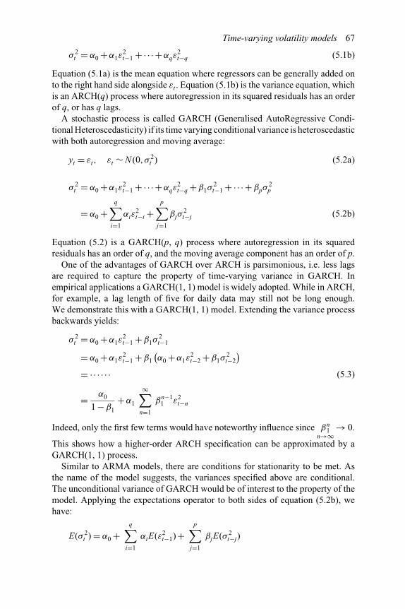
Time-varying volatility models 67
σ 2t = α0 +α1ε
2t−1 +·· ·+αqε
2t−q (5.1b)
Equation (5.1a) is the mean equation where regressors can be generally added onto the right hand side alongside εt . Equation (5.1b) is the variance equation, whichis an ARCH(q) process where autoregression in its squared residuals has an orderof q, or has q lags.
A stochastic process is called GARCH (Generalised AutoRegressive Condi-tional Heteroscedasticity) if its time varying conditional variance is heteroscedasticwith both autoregression and moving average:
yt = εt, εt ∼ N (0,σ 2t ) (5.2a)
σ 2t = α0 +α1ε
2t−1 +·· ·+αqε
2t−q +β1σ
2t−1 +·· ·+βpσ
2p
= α0 +q∑
i=1
αiε2t−i +
p∑j=1
βjσ2t−j (5.2b)
Equation (5.2) is a GARCH(p, q) process where autoregression in its squaredresiduals has an order of q, and the moving average component has an order of p.
One of the advantages of GARCH over ARCH is parsimonious, i.e. less lagsare required to capture the property of time-varying variance in GARCH. Inempirical applications a GARCH(1, 1) model is widely adopted. While in ARCH,for example, a lag length of five for daily data may still not be long enough.We demonstrate this with a GARCH(1, 1) model. Extending the variance processbackwards yields:
σ 2t = α0 +α1ε
2t−1 +β1σ
2t−1
= α0 +α1ε2t−1 +β1
(α0 +α1ε
2t−2 +β1σ
2t−2
)= ·· · · · ·
= α0
1 −β1
+α1
∞∑n=1
βn−11 ε2
t−n
(5.3)
Indeed, only the first few terms would have noteworthy influence since βn1
n→∞→ 0.
This shows how a higher-order ARCH specification can be approximated by aGARCH(1, 1) process.
Similar to ARMA models, there are conditions for stationarity to be met. Asthe name of the model suggests, the variances specified above are conditional.The unconditional variance of GARCH would be of interest to the property of themodel. Applying the expectations operator to both sides of equation (5.2b), wehave:
E(σ 2t ) = α0 +
q∑i=1
αiE(ε2t−1) +
p∑j=1
βjE(σ 2t−j)

68 Time-varying volatility models
Noting E(σ 2t ) = E(ε2
t−i) = E(σ 2t−j) is the unconditional variance of the residual,
which is solved as:
σ 2 = E(σ 2t ) = α0
1 −q∑
i=1αi +
p∑j=1
βj
It is clear that for the process to possess a finite variance, the following conditionmust be met:
q∑i=1
αi +p∑
j=1
βj < 1 (5.4)
In commonly used GARCH(1, 1) models, the condition is simply α1 +β1 < 1.Many financial time series have persistent volatility, i.e. the sum of αi and βj
is close to being unity. A unity sum of αi and βj leads to so-called IntegratedGARCH or IGARCH as the process is not covariance stationary. Neverthe-less, this does not pose as serious a problem as it appears. According toNelson (1990), Bougerol and Picard (1992) and Lumsdaine (1991), even if aGARCH (IGARCH) model is not covariance stationary, it is strictly stationary orergodic, and the standard asymptotically based inference procedures are generallyvalid. See Chapter 1 of this book for various definitions of stationarity andergodicity.
5.1.2. Variations of the ARCH/GARCH model
Variations are necessary to adapt the standard GARCH model to the need arisingfrom examining the time series properties of specific issues in finance andeconomics. Here we present the model relating the return on a security to its time-varying volatility or risk – ARCH-M, and the models of asymmetry – ExponentialGARCH (EGARCH) and Threshold GARCH (TGARCH).
The ARCH-M model
When the conditional variance enters the mean equation for an ARCH process,the ARCH-in-Mean or simply the ARCH-M model is derived:
yt = λ1x1 +·· ·λmxm +ϕσ 2t + εt, εt ∼ N (0,σ 2
t ) (5.5a)
σ 2t = α0 +α1ε
2t−1 +·· ·+αqε
2t−q (5.5b)
where xk , k = 1, . . . m are exogenous variables which could include lagged yt .In the sense of asset pricing, if yt is the return on an asset of a firm, then xk ,
k = 1, . . . m would generally include the return on the market and possibly other
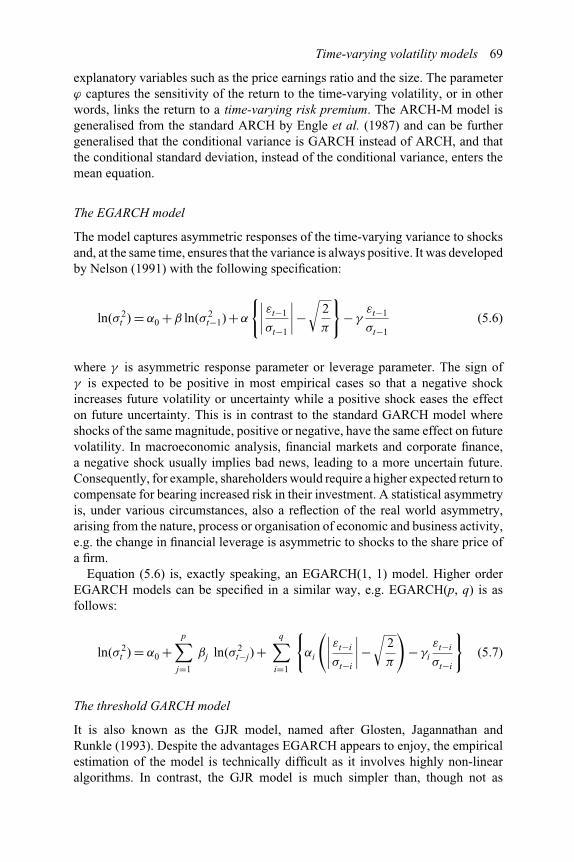
Time-varying volatility models 69
explanatory variables such as the price earnings ratio and the size. The parameterϕ captures the sensitivity of the return to the time-varying volatility, or in otherwords, links the return to a time-varying risk premium. The ARCH-M model isgeneralised from the standard ARCH by Engle et al. (1987) and can be furthergeneralised that the conditional variance is GARCH instead of ARCH, and thatthe conditional standard deviation, instead of the conditional variance, enters themean equation.
The EGARCH model
The model captures asymmetric responses of the time-varying variance to shocksand, at the same time, ensures that the variance is always positive. It was developedby Nelson (1991) with the following specification:
ln(σ 2t ) = α0 +β ln(σ 2
t−1) +α
{∣∣∣∣ εt−1
σt−1
∣∣∣∣−√
2
π
}− γ
εt−1
σt−1
(5.6)
where γ is asymmetric response parameter or leverage parameter. The sign ofγ is expected to be positive in most empirical cases so that a negative shockincreases future volatility or uncertainty while a positive shock eases the effecton future uncertainty. This is in contrast to the standard GARCH model whereshocks of the same magnitude, positive or negative, have the same effect on futurevolatility. In macroeconomic analysis, financial markets and corporate finance,a negative shock usually implies bad news, leading to a more uncertain future.Consequently, for example, shareholders would require a higher expected return tocompensate for bearing increased risk in their investment. A statistical asymmetryis, under various circumstances, also a reflection of the real world asymmetry,arising from the nature, process or organisation of economic and business activity,e.g. the change in financial leverage is asymmetric to shocks to the share price ofa firm.
Equation (5.6) is, exactly speaking, an EGARCH(1, 1) model. Higher orderEGARCH models can be specified in a similar way, e.g. EGARCH(p, q) is asfollows:
ln(σ 2t ) = α0 +
p∑j=1
βj ln(σ 2t−j) +
q∑i=1
{αi
(∣∣∣∣ εt−i
σt−i
∣∣∣∣−√
2
π
)− γi
εt−i
σt−i
}(5.7)
The threshold GARCH model
It is also known as the GJR model, named after Glosten, Jagannathan andRunkle (1993). Despite the advantages EGARCH appears to enjoy, the empiricalestimation of the model is technically difficult as it involves highly non-linearalgorithms. In contrast, the GJR model is much simpler than, though not as
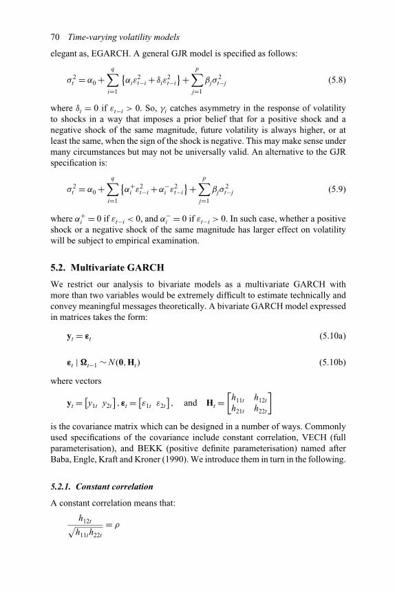
70 Time-varying volatility models
elegant as, EGARCH. A general GJR model is specified as follows:
σ 2t = α0 +
q∑i=1
{αiε
2t−i + δiε
2t−i
}+p∑
j=1
βjσ2t−j (5.8)
where δi = 0 if εt−i > 0. So, γi catches asymmetry in the response of volatilityto shocks in a way that imposes a prior belief that for a positive shock and anegative shock of the same magnitude, future volatility is always higher, or atleast the same, when the sign of the shock is negative. This may make sense undermany circumstances but may not be universally valid. An alternative to the GJRspecification is:
σ 2t = α0 +
q∑i=1
{α+
i ε2t−i +α−
i ε2t−i
}+p∑
j=1
βjσ2t−j (5.9)
where α+i = 0 if εt−i < 0, and α−
i = 0 if εt−i > 0. In such case, whether a positiveshock or a negative shock of the same magnitude has larger effect on volatilitywill be subject to empirical examination.
5.2. Multivariate GARCH
We restrict our analysis to bivariate models as a multivariate GARCH withmore than two variables would be extremely difficult to estimate technically andconvey meaningful messages theoretically. A bivariate GARCH model expressedin matrices takes the form:
yt = εt (5.10a)
εt | �t−1 ∼ N (0,Ht) (5.10b)
where vectors
yt =[y1t y2t
],εt =
[ε1t ε2t
], and Ht =
[h11t h12t
h21t h22t
]
is the covariance matrix which can be designed in a number of ways. Commonlyused specifications of the covariance include constant correlation, VECH (fullparameterisation), and BEKK (positive definite parameterisation) named afterBaba, Engle, Kraft and Kroner (1990). We introduce them in turn in the following.
5.2.1. Constant correlation
A constant correlation means that:
h12t√h11th22t
= ρ
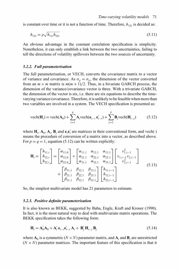
Time-varying volatility models 71
is constant over time or it is not a function of time. Therefore, h12t is decided as:
h12t = ρ√
h11th22t (5.11)
An obvious advantage in the constant correlation specification is simplicity.Nonetheless, it can only establish a link between the two uncertainties, failing totell the directions of volatility spillovers between the two sources of uncertainty.
5.2.2. Full parameterisation
The full parameterisation, or VECH, converts the covariance matrix to a vectorof variance and covariance. As σij = σji, the dimension of the vector convertedfrom an m × m matrix is m(m + 1)/2. Thus, in a bivariate GARCH process, thedimension of the variance/covariance vector is three. With a trivariate GARCH,the dimension of the vector is six, i.e. there are six equations to describe the time-varying variance/covariance. Therefore, it is unlikely to be feasible when more thantwo variables are involved in a system. The VECH specification is presented as:
vech(Ht) = vech(A0) +q∑
i=1
Aivech(εt−i ε′t−i) +
p∑j=1
Bjvech(Ht−j) (5.12)
where Ht, A0, Ai, Bj and εtε′t are matrices in their conventional form, and vech(·)
means the procedure of conversion of a matrix into a vector, as described above.For p = q = 1, equation (5.12) can be written explicitly:
Ht =⎡⎣h11,t
h12,t
h22,t
⎤⎦=
⎡⎣α11,0
α12,0α22,0
⎤⎦+
⎡⎣α11,1 α12,1 α13,1
α21,1 α22,1 α23,1α31,1 α32,1 α33,1
⎤⎦⎡⎣ ε2
1,t−1ε1,t−1 ε2,t−1
ε22,t−1
⎤⎦
+⎡⎣β11,1 β12,1 β13,1
β21,1 β22,1 β23,1β31,1 β32,1 β33,1
⎤⎦⎡⎣h11,t−1
h12,t−1h22,t−1
⎤⎦
(5.13)
So, the simplest multivariate model has 21 parameters to estimate.
5.2.3. Positive definite parameterisation
It is also known as BEKK, suggested by Baba, Engle, Kraft and Kroner (1990).In fact, it is the most natural way to deal with multivariate matrix operations. TheBEKK specification takes the following form:
Ht = A′0A0 + A′
i εt−iε′t−i Ai + B′
j Ht−j Bj (5.14)
where A0 is a symmetric (N ×N ) parameter matrix, and Ai and Bj are unrestricted(N × N ) parameter matrices. The important feature of this specification is that it

72 Time-varying volatility models
builds in sufficient generality, allowing the conditional variances and covariancesof the time series to influence each other, and at the same time, does not requireto estimate a large number of parameters. For p = q = 1 in a bivariate GARCHprocess, equation (5.14) has only 11 parameters compared with 21 parameters in theVECH representation. Even more importantly, the BEKK process guarantees thatthe covariance matrices are positive definite under very weak conditions; and it canbe shown that under certain non-linear restrictions on Ai and Bj, equation (5.14)and the VECH representation are equivalent (Engle and Kroner, 1995). In thebivariate system with p = q = 1, equation (5.14) becomes:[
h11,t h12,t
h21,t h22,t
]=[α11,0 α12,0α21,0 α22,0
]
+[α11,1 α12,1α21,1 α22,1
]′[ε2
1,t−1 ε1,t−1ε2,t−1
ε1,t−1ε2,t−1 ε22,t−1
][α11,1 α12,1α21,1 α22,1
]
+[β11,1 β12,1β21,1 β22,1
]′[h11,t−1 h12,t−1h21,t−1 h22,t−1
][β11,1 β12,1β21,1 β22,1
](5.15)
We can examine the sources of uncertainty and, moreover, assess the effectof signs of shocks with equation (5.15). Writing the variances and covarianceexplicitly:
h11,t = α11,0 + (α211,1ε
21,t−1 + 2α11,1α21,1ε1,t−1ε2,t−1 +α2
21,1ε22,t−1)
+ (β211,1h11,t−1 + 2β11,1β21,1h12,t−1 +β2
21,1h22,t−1) (5.16a)
h12,t = h21,t = α12,0 + [α11,1α12,1ε21,t−1 + (α12,1α21,1 +α11,1α22,1)ε1,t−1ε2,t−1
+α21,1α22,1ε22,t−1]+ [β11,1β21,1h11,t−1 + (β12,1β21,1
+β11,1β22,1)h12,t−1 +β21,1β22,1h22,t−1] (5.16b)
h22,t = α22,0 + (α212,1 ε2
1,t−1 + 2α12,1α22,1ε1,t−1ε2,t−1 +α222,1ε
22,t−1)
+ (β212,1h11,t−1 + 2β12,1β22,1h12,t−1 +β2
22,1h22,t−1) (5.16c)
Looking at the diagonal elements in the above matrix, i.e. h11,t and h22,t , we canassess the impact of the shock in one series on the uncertainty or volatility ofthe other, and the impact could be asymmetric or only be one way effective. Inparticular, one might also be interested in assessing the effect of the signs of shocksin the two series. To this end the diagonal elements representing theprevious shockscan be rearranged as follows:
α211,1ε
21t−1 + 2α11,1α21,1ε1,t−1ε2,t−1 +α2
21,1ε22t−1 = (α11,1ε1,t−1 +α21,1ε2,t−1)2
(5.17a)
α212,1ε
21t−1 + 2α12,1α22,1ε1,t−1ε2,t−1 +α2
22,1ε22t−1 = (α12,1ε1,t−1 +α22,1ε2,t−1)2
(5.17b)
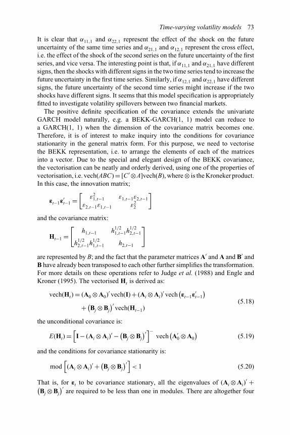
Time-varying volatility models 73
It is clear that α11,1 and α22,1 represent the effect of the shock on the futureuncertainty of the same time series and α21,1 and α12,1 represent the cross effect,i.e. the effect of the shock of the second series on the future uncertainty of the firstseries, and vice versa. The interesting point is that, if α11,1 and α21,1 have differentsigns, then the shocks with different signs in the two time series tend to increase thefuture uncertainty in the first time series. Similarly, if α12,1 and α22,1 have differentsigns, the future uncertainty of the second time series might increase if the twoshocks have different signs. It seems that this model specification is appropriatelyfitted to investigate volatility spillovers between two financial markets.
The positive definite specification of the covariance extends the univariateGARCH model naturally, e.g. a BEKK-GARCH(1, 1) model can reduce toa GARCH(1, 1) when the dimension of the covariance matrix becomes one.Therefore, it is of interest to make inquiry into the conditions for covariancestationarity in the general matrix form. For this purpose, we need to vectorisethe BEKK representation, i.e. to arrange the elements of each of the matricesinto a vector. Due to the special and elegant design of the BEKK covariance,the vectorisation can be neatly and orderly derived, using one of the properties ofvectorisation, i.e. vech(ABC) =[C ′⊗A]vech(B), where ⊗ is the Kroneker product.In this case, the innovation matrix;
εt−1ε′t−1 =
[ε2
1,t−1 ε1,t−1ε2,t−1
ε2,t−1ε1,t−1 ε22
]
and the covariance matrix:
Ht−1 =[
h1,t−1 h1/21,t−1h1/2
2,t−1
h1/22,t−1h1/2
1,t−1 h2,t−1
]
are represented by B; and the fact that the parameter matrices A′ and A and B′ andB have already been transposed to each other further simplifies the transformation.For more details on these operations refer to Judge et al. (1988) and Engle andKroner (1995). The vectorised Ht is derived as:
vech(Ht) = (A0 ⊗ A0)′ vech(I) + (Ai ⊗ Ai)′ vech
(εt−1ε
′t−1
)+ (Bj ⊗ Bj
)′vech(Ht−1)
(5.18)
the unconditional covariance is:
E(Ht) =[I − (Ai ⊗ Ai)
′ − (Bj ⊗ Bj
)′]−vech
(A′
0 ⊗ A0
)(5.19)
and the conditions for covariance stationarity is:
mod[(Ai ⊗ Ai)
′ + (Bj ⊗ Bj
)′]< 1 (5.20)
That is, for εt to be covariance stationary, all the eigenvalues of (Ai ⊗ Ai)′ +(
Bj ⊗ Bj
)′are required to be less than one in modules. There are altogether four

74 Time-varying volatility models
eigenvalues for a bivariate GARCH process as the Kroneker product of two (2×2)matrices produces a (4×4) matrix. These eigenvalues would be complex numbersin general. When the dimension of the covariance is one, equation (5.20) reducesto equation (5.4) for the univariate case.1
5.3. Stochastic volatility
ARCH/GARCH processes are not really stochastic, rather they are deterministicand the conditional variance possesses no unknown innovations at the time.ARCH and GARCH are not exactly the second moment equivalent to AR andARMA processes in the mean. Stochastic volatility, as favoured by Harvey et al.(1994), Ruiz (1994), Andersen and Lund (1997) and others, is probably theclosest equivalent to an AR or ARMA process in describing the dynamics ofvariance/covariance. Let us look at a simple case:
yt = σtεt
εt ∼ N (0,σ 2ε )
ht = ln σ 2t ∼ ARMA(q,p)
(5.21)
The logarithm of the variance in a stochastic volatility model, ht = ln σ 2t , behaves
exactly as a stochastic process in the mean, such as random walks or AR or ARMAprocesses. For example, if ht is modelled as an AR(1) process, then:
ht = α +ρht−1 + νt
νt ∼ N (0,σ 2ν )
(5.22)
Alternatively when ht is modelled as an ARMA(1, 1) process:
ht = α +ρht−1 + νt + θνt−1
νt ∼ N (0,σ 2ν )
(5.23)
When the stochastic part of volatility, νt , does not exist (i.e.σ 2ν = 0), equation (5.22)
does not reduce to ARCH(1) but to GARCH(1, 0). So the difference in modellingvariance is substantial between GARCH and stochastic volatility approaches. Toestimate stochastic volatility models, expressing equation (5.21) as:
gt = ht + κt (5.24)
where gt = ln(y2
t
), and κt = ln
(ε2
t
). We can see that ht becomes part, or a
component, of the (transformed) time series, in contrast to traditional statisticalmodels where the variance expresses the distribution of variables in a differentway. As the time series now has more than one component, neither is readilyobservable, so the components are often referred to as unobserved components.These components together form the whole system and individually describe the
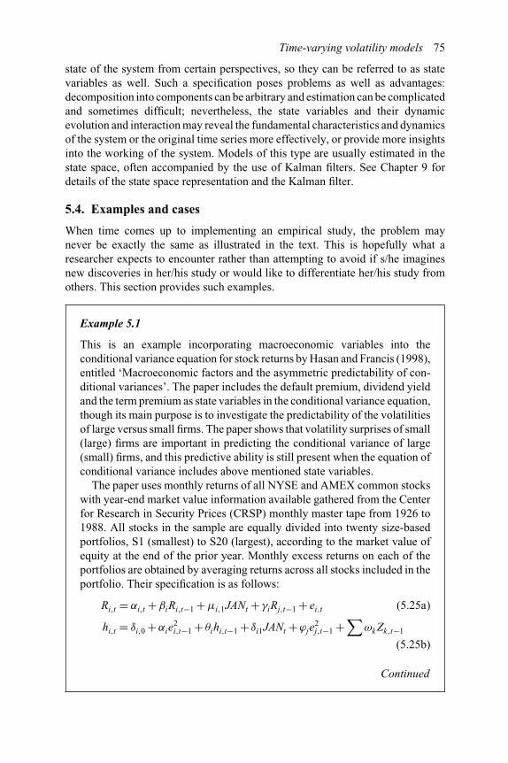
Time-varying volatility models 75
state of the system from certain perspectives, so they can be referred to as statevariables as well. Such a specification poses problems as well as advantages:decomposition into components can be arbitrary and estimation can be complicatedand sometimes difficult; nevertheless, the state variables and their dynamicevolution and interaction may reveal the fundamental characteristics and dynamicsof the system or the original time series more effectively, or provide more insightsinto the working of the system. Models of this type are usually estimated in thestate space, often accompanied by the use of Kalman filters. See Chapter 9 fordetails of the state space representation and the Kalman filter.
5.4. Examples and cases
When time comes up to implementing an empirical study, the problem maynever be exactly the same as illustrated in the text. This is hopefully what aresearcher expects to encounter rather than attempting to avoid if s/he imaginesnew discoveries in her/his study or would like to differentiate her/his study fromothers. This section provides such examples.
Example 5.1
This is an example incorporating macroeconomic variables into theconditional variance equation for stock returns by Hasan and Francis (1998),entitled ‘Macroeconomic factors and the asymmetric predictability of con-ditional variances’. The paper includes the default premium, dividend yieldand the term premium as state variables in the conditional variance equation,though its main purpose is to investigate the predictability of the volatilitiesof large versus small firms. The paper shows that volatility surprises of small(large) firms are important in predicting the conditional variance of large(small) firms, and this predictive ability is still present when the equation ofconditional variance includes above mentioned state variables.
The paper uses monthly returns of all NYSE and AMEX common stockswith year-end market value information available gathered from the Centerfor Research in Security Prices (CRSP) monthly master tape from 1926 to1988. All stocks in the sample are equally divided into twenty size-basedportfolios, S1 (smallest) to S20 (largest), according to the market value ofequity at the end of the prior year. Monthly excess returns on each of theportfolios are obtained by averaging returns across all stocks included in theportfolio. Their specification is as follows:
Ri,t = αi,t +βiRi,t−1 +μi,1JANt + γiRj,t−1 + ei,t (5.25a)
hi,t = δi,0 +αie2i,t−1 + θihi,t−1 + δi1JANt +ϕje
2j,t−1 +
∑ωkZk,t−1
(5.25b)
Continued
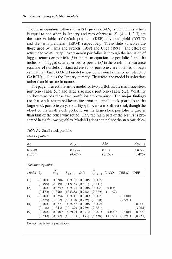
76 Time-varying volatility models
The mean equation follows an AR(1) process. JANt is the dummy whichis equal to one when in January and zero otherwise. Zk,t(k = 1,2,3) arethe state variables of default premium (DEF), dividend yield (DYLD)and the term premium (TERM) respectively. These state variables arethose used by Fama and French (1989) and Chen (1991). The effect ofreturn and volatility spillovers across portfolios is through the inclusion oflagged returns on portfolio j in the mean equation for portfolio i, and theinclusion of lagged squared errors for portfolio j in the conditional varianceequation of portfolio i. Squared errors for portfolio j are obtained throughestimating a basic GARCH model whose conditional variance is a standardGARCH(1, 1) plus the January dummy. Therefore, the model is univariaterather than bivariate in nature.
The paper then estimates the model for two portfolios, the small size stockportfolio (Table 5.1) and large size stock portfolio (Table 5.2). Volatilityspillovers across these two portfolios are examined. The major findingsare that while return spillovers are from the small stock portfolio to thelarge stock portfolio only, volatility spillovers are bi-directional, though theeffect of the small stock portfolio on the large stock portfolio is greaterthan that of the other way round. Only the main part of the results is pre-sented in the following tables. Model (1) does not include the state variables,
Table 5.1 Small stock portfolio
Mean equation
μ0 R1,t−1 JAN R20,t−1
0.0048 0.1896 0.1231 0.0287(1.705) (4.679) (8.163) (0.475)
Variance equation
Model δ0 e21,t−1 h1,t−1 JAN e2
20,t−1 DYLD TERM DEF
(1) −0.0001(0.998)
0.0284(2.039)
0.9305(41.915)
0.0005(0.464)
0.0022(2.741)
(2) −0.0001(0.470)
0.0259(1.890)
0.9341(43.648)
0.0008(0.738)
0.0021(2.629)
−0.003(1.167)
(3) −0.0001(0.228)
0.0254(1.812)
0.9316(43.310)
0.0009(0.789)
0.0023(2.650)
−0.0001(2.991)
(4) −0.0001(0.134)
0.0273(1.843)
0.9286(39.142)
0.0008(0.729)
0.0024(2.681)
−0.0001(3.014)
(5) −0.0001(0.740)
0.0009(0.092)
0.9694(82.117)
0.0012(1.193)
0.0018(3.556)
−0.0005(4.160)
−0.0001(0.693)
−0.0001(0.751)
Robust t-statistics in parentheses.

Time-varying volatility models 77
Table 5.2 Large stock portfolio
Mean equation
μ0 R20,t−1 JAN R1,t−1
0.0064 0.0497 −0.0082 0.1013(3.867) (1.295) (1.413) (6.051)
Variance equation
Model δ0 e220,t−1 h20,t−1 JAN e2
1,t−1 DYLD TERM DEF
(1) 0.0002(2.981)
0.1610(3.347)
0.6511(10.148)
−0.0001(0.194)
0.0237(2.986)
(2) 0.0003(2.563)
0.1595(3.324)
0.6504(9.926)
−0.0001(0.226)
0.0239(3.043)
−0.0001(0.795)
(3) 0.0001(1.811)
0.1544(3.252)
0.6293(9.986)
−0.0001(0.205)
0.0282(3.442)
0.0004(2.492)
(4) 0.0001(1.321)
0.1549(3.214)
0.6460(9.567)
−0.0003(0.089)
0.0244(4.489)
0.0003(1.989)
(5) 0.0001(0.820)
0.1502(3.270)
0.6322(10.214)
−0.0001(0.393)
0.2974(3.733)
0.0002(0.784)
0.0008(2.055)
−0.0001(1.111)
Robust t-statistics in parentheses.
Models (2)–(4) include one of the state variables each, and Model (5)incorporates all the state variables. As there is not much difference in themean equation results, only the results from Model (5) are provided.
Example 5.2
This is an example of the bivariate GARCH model applied to the foreignexchange market by Wang and Wang (2001). In this study, the daily spot andforward foreign exchange rates of the British pound, German mark, Frenchfranc and Canadian dollar against the US dollar are used. All of the data setsstart from 02/01/76 and end on 31/12/90; so there are 3,758 observationsin each series. These long period high frequency time series data enable usto observe a very evident GARCH phenomenon in a bivariate system. Thesystem of equations for the spot exchange rate, St , and the forward exchangerate, Ft , is specified as an extended VAR, which incorporates a forwardpremium into a simple VAR. In addition, the covariance of the extendedVAR is time-varying which allows for and mimics volatility spillovers
Continued
78 Time-varying volatility models
or transmission between the spot and forward foreign exchange markets.The model is given as follows:
�st = c1 + γ1( ft−1 − st−1) +m∑
i=1
α1i�st−i +m∑
i=1
β1i�ft−i + ε1t
�ft = c2 + γ2( ft−1 − st−1) +m∑
i=1
α2i�st−i +m∑
i=1
β2i�ft−i + ε2t
(5.26)
εt | t−1 ∼ N (0, Ht)
where st = Ln(St), ft = Ln(Ft), �st = st − st−1, �ft = ft − ft−1, and Ht is thetime-varying covariance matrix with the BEKK specification.
The inclusion of the forward premium is not merely for setting up an ECMmodel, it keeps information in levels while still meeting the requirementsfor stationarity. Although there are arguments about the property ofthe forward premium, its inclusion makes the system informationallyand economically complete by reserving information in levels (originalvariables) and reflecting expectations in the market.
The bivariate GARCH effects are, in general, strong in both the spotand forward markets, though there exists a clear asymmetry in the volatilityspillover patterns. That is, there are volatility spillovers from the spot marketto the forward, to a lesser extent, compared with the other way round.Table 5.3 presents the results based mainly on the second moment.
In addition, the parameter for the forward premium is also reported, asit would validate the cointegration between the spot and forward exchangerates and the need to incorporate the forward premium. Consider the Britishpound first. a12 and a21 are both significant at 1 per cent level, but themagnitude of the former is about half the size of the latter, implying thatthe effect of the shock in the forward market on the spot market volatilityis bigger than that on the forward market induced by the shock in the spotmarket. Turning to the effects of the previous uncertainty, while b21 issignificant, b12 is not significant at all, so the volatility spillovers are onedirectional from the forward to the spot. Notice, b22 is also insignificant,which means there is only ARCH in the forward exchange rate. Furtherscrutiny on the signs of a12 and a22 suggests that the future volatility in theforward market would be higher if the two shocks have different signs. In thecase of the German mark, the asymmetry is more apparent, where a12 is notsignificant at all but a21 is significant at 1 per cent level. As such, the shockin the forward market would affect the future volatility in the spot market,but the shock in the spot market has no influence on the future volatilityin the forward market. In addition, a11 and a21 have different signs, so the

Time-varying volatility models 79
Table 5.3 Volatility spillovers between spot and forward FX rates
�st = c1 + γ1( ft−1 − st−1) +m∑
i=1α1i�st−i +
m∑i=1
β1i�ft−i + ε1t
εt∣∣ t−1 ∼ N (0,Ht)
�ft = c2 + γ2( ft−1 − st−1) +m∑
i=1α2i�st−i +
m∑i=1
β2i�ft−i + ε2t
[h11,t h12,th21,t h22,t
]=[c11 c12c21 c22
]+[a11 a12a21 a22
]′ [ε21,t−1 ε1,t−1ε2,t−1
ε1,t−1ε2,t−1 ε22,t−1
]
[a11 a12a21 a22
]+[b11 b12b21 b22
]′ [h11,t−1 h12,t−1h12,t−1 h22,t−1
] [b11 b12b21 b22
]
BP DM FF CD
c1 0.00025∗∗ −0.00058∗∗∗ 0.00012 0.00013∗∗(2.3740) (4.3591) (1.2106) (2.2491)
γ1 −0.12034∗∗∗ −0.23731∗∗∗ −0.03214 −0.05255(3.9301) (5.5473) (1.3884) (1.8081)∗
c2 0.00027∗∗ −0.00057∗∗∗ 0.00014 0.00015∗∗(2.5077) (4.0781) (1.4735) (2.5582)
γ2 −0.12536∗∗∗ −0.23203∗∗∗ −0.05197∗∗ −0.05436∗(4.0293) (5.1272) (2.2460) (1.8156)
a11 0.51775∗∗∗ −0.20555∗∗∗ 1.00020∗∗∗ 0.53282∗∗∗(13.3029) (3.8590) (148.5928) (8.4157)
a12 −0.24576∗∗∗ 0.00539 0.03776∗∗∗ −0.05055(6.8053) (0.1062) (5.4583) (0.8144)
a21 0.45452∗∗∗ 1.17328∗∗∗ −0.06149∗∗∗ 0.40725∗∗∗(11.5872) (22.2677) (8.7868) (6.5068)
a22 1.21688∗∗∗ 0.96138∗∗∗ 0.89990∗∗∗ 0.98706∗∗∗(33.3811) (19.1147) (124.5143) (16.0892)
b11 0.43475∗∗∗ 1.00966∗∗∗ 0.24888∗∗∗ 0.52226∗∗∗(4.8987) (16.8606) (8.0209) (8.0757)
b12 −0.10742 −0.18033∗∗∗ −0.04565 0.01389(1.2389) (3.5195) (1.4180) (0.2278)
b21 −0.66683∗∗∗ −1.16582∗∗∗ 0.10881∗∗∗ −0.22376∗∗∗(7.5985) (19.1740) (3.5734) (3.5935)
b22 −0.13151 −0.05456 0.40644∗∗∗ 0.28611∗∗∗(1.5358) (1.0563) (12.7895) (4.7730)
t-statistics in parentheses.∗significant at 10 per cent level; ∗∗significant at 5 per cent level; ∗∗∗significant at 1 per centlevel.Constant terms in the second moment are not reported.
Continued

80 Time-varying volatility models
shock with opposite signs in these two markets would be inclined to increasethe future volatility in the spot market. As far as the previous variance isconcerned, b12 and b21 are both significant, but the size of the former ismuch smaller than that of the latter, so the asymmetry exists in this respecttoo. Again, b22 is not significant; the forward rate would only have theARCH effect if it were not considered in a bivariate system. The strongestasymmetry occurs in the exchange rates of the Canadian dollar. The volatilityspillovers are absolutely one directional from the forward rate to the spotrate. That is: a12 and b12 are not significant at any conventional levels,whereas a21 and b21 are both significant at 1 per cent level. Similar tothe British pound, in the case of the French franc, the influence of theprevious variance is clearly one directional from the forward to the spotmeasured by b12 and b21. Although the GARCH effect is strong in theforward rate as well as in the spot rate, b22 is close to being twice as bigas b11. Regarding the previous shocks, the influence is also more fromforward to spot; both a12 and a21 are significant but a21 is much biggerthan a12. Therefore, the four currencies have similar asymmetric volatilityspillover patterns. Another interesting point in the franc example is that thepremium is not significant in both the spot and forward equations when thecovariance matrix is assumed as constant. The premium is significant inthe forward equation when estimated in a multivariate GARCH framework.This suggests that the rejection/acceptance of a cointegration relationshipis, to a certain extent, subject to the assumption on the properties of thecovariance.
In Table 5.4, all four eigenvalues for each currency are reported. Theirpositioning on the complex plane is displayed in Figure 5.1. It can beenseen that the biggest of the eigenvalues for each currency is around 0.96in modules, so the time varying volatility is highly persistent. In the French
Table 5.4 Verifying covariance stationarity: the eigenvalues. Unconditional
covariance: E(σ 2t ) = [I − (A∗ ⊗ A∗)′ − (B∗ ⊗ B∗)′]−1 vec(C∗′
0 C∗0 )
(A∗ ⊗A∗)′ +(B∗ ⊗B∗)′ BP DM FF CD
λ1 (real, imaginary)λ1 (mod)
0.963, 0.0000.963
0.969, 0.0000.969
1.003, 0.0001.003
0.969, 0.0000.969
λ2 (real, imaginary)λ2 (mod)
0.852, 0.0000.852
0.570, 0.0000.570
0.995,−0.0220.996
0.699, 0.0000.699
λ3 (real, imaginary)λ3 (mod)
0.628, 0.0000.628
0.022, 0.0000.022
0.995, 0.0220.996
0.698, 0.0000.698
λ4 (real, imaginary)λ4 (mod)
0.608, 0.0000.608
0.017, 0.0000.017
0.988, 0.0000.988
0.600, 0.0000.600
In a situation that all eigenvalues are smaller than one in modules, the covariance is confirmedstationary.

Time-varying volatility models 81
BP DM
l4
l3
l2
l1l2 l1
l4
l3
l3l1
l2l4
l1
l2l4
l3
CDFF
Eigenvalues of covariance matrices on the complex plane(the horizontal axis is for the real part, and the vertical axis is for the imaginarypart of the eigenvalue. the reference circle is the unit circle)
Figure 5.1 Eigenvalues on the complex plane.
franc case, the biggest module of eigenvalue is just above unity, suggestingthat the unconditional covariance does not exist. There are two explanationsto provide for this. First, according to Nelson (1990), Bougerol and Picard(1992) and Lumsdaine (1991), even if a GARCH (IGARCH) model is notcovariance stationary, it is strictly stationary or ergodic, and the standardasymptotically based inference procedures are generally valid. Second, thederivation of eigenvalues is based on the assumption that the spot varianceand forward variance are equal in size. Nevertheless, the forward varianceis smaller than the spot variance in the French franc case. Taking this intoaccount, all of the modules of eigenvalue for the French franc become
Continued

82 Time-varying volatility models
less than one and the covariance stationary exists. The analysis on theeigenvalues of the Kroneker product of the covariance matrices reveals thatthe time varying volatility is also highly persistent in a bivariate setting forforeign exchange rate data. In addition, though the BEKK specification hasproved a helpful analytical technique for volatility transmissions, especiallythe impact of the signs of the shocks in different markets, in empiricalresearch, the covariance stationarity is not so easy to satisfy and is notalways guaranteed.
5.5. Empirical literature
While time-varying volatility has found applications in almost all time seriesmodelling in economics and finance, it attracts most attention in the areasof financial markets and investment where vast empirical literature has beengenerated, which has in turn brought about new forms and variations of this familyof models. Time-varying volatility has become the norm in financial time seriesmodelling, popularly accepted and applied by academics and professionals alikesince the 1990s. Moreover, analysis of interactions between two or more variablesin the first moment, such as in VAR and ECM, is extended through the use oftime-varying volatility models, to the second moment to examine such importantissues as volatility spillovers or transmissions between different markets.
One of the most extensively researched topics is time-varying volatilityuniversally found in stock market indices. Although findings vary from one marketto another, a pattern of time-varying volatility, which is also highly persistent, iscommon to most of them. Nevertheless, many of studies attempt to exploit newfeatures and add variations in model specifications to meet the specific need ofempirical investigations. To examine the characteristics of market opening news,Gallo and Pacini (1998) apply the GARCH model and evaluate the impact of thenews on the estimated coefficients of the model. They find that the differencesbetween the opening price of one day and the closing price of the day beforehave different characteristics and have the effect of modifying the direct impact ofdaily innovations on volatility which reduces the estimated overall persistence ofinnovations. It is also claimed that the inclusion of this news variable significantlyimproves out-of-sample forecasting, compared with the simple GARCH model’sperformance. Brooks et al. (2000) adopt the power ARCH (PARCH) modelproposed by Ding et al. (1993) to stock market returns in ten countries and a worldindex. As PARCH removes the restriction implicitly imposed by ARCH/GARCH,i.e. the power transformation is achieved by taking squaring operations of theresidual or to the power of 2, it can possess richer volatility patters such asasymmetry and leverage effects. They find that the PARCH model is applicableto these return indices and that the optimal power transformation is remarkablysimilar across countries. Longin (1997) employs the analytical framework of
Time-varying volatility models 83
Kyle (1985) where there are three types of traders: informed traders, liquiditytraders and market makers. In such a setting, the paper models information as anasymmetric GARCH process that large shocks are less persistent in volatility thansmall shocks. This, it is claimed, allows one to derive implications for tradingvolume and market liquidity. The study by Koutmos (1992) is one of the typicalempirical applications of GARCH in finance in early times – risk–return trade-offin a time-varying volatility context and asymmetry of the conditional variance inresponse to innovations. The Exponential GARCH in Mean (EGARCH-M) modelis chosen for above obvious reasons and the findings support the presence of thesewell observed phenomena in ten stock market return indices. Newly added tothis literature is evidence from so-called emerging markets and the developingworld. Investigating the behaviour of the Egyptian stock market in the contextof pricing efficiency and the return-volatility relationship, Mecagni and Sourial(1999) employ a GARCH-M model to estimate four daily indices. Their resultssuggest that there is tendency of volatility clustering in returns, and a positive butasymmetric link between risk and returns which is statistically significant duringmarket downturns. They claim that the asymmetry in the risk–return relationship isdue to the introduction of circuit breakers. Husain (1998) examines the Ramadhaneffect in the Pakistani stock market using GARCH models. Ramadhan, the seasonof the holy month of fasting, is expected to have effects on stock market behaviourone way or another. The study finds that the market is indeed tranquil as theconditional variance declines in that month, but the season does not appear to haveimpact on mean returns. Applying TGARCH models to two Eastern Europeanmarkets, Shields (1997) reports findings contrary to those in the west that thereis no asymmetry in the conditional variance in response to positive and negativeshocks in these Eastern European markets.
International stock market linkages have attracted increasing attention in theprocess of so-called globalisation in a time when there are no major wars.Seeking excess returns through international diversification is one of the strategiesemployed by large multinational financial institutions in an ever intensifyingcompetitive financial environment, while national markets, considered individ-ually, appear to have been exploited to their full so that any non-trivial profitableopportunities do not remain in the context of semi-strong market efficiency.In particular, US investors have gradually given up the stand of regardingforeign markets as alien lands and changed their risk perspectives – internationaldiversification benefits are more than off-setting perceived additional risks. In themeantime, international asset pricing theory has been developed largely with astratified approach which regards the international financial market as segmentedas well as linked markets, adding additional dimensions to the original capital assetpricing model which is, ironically, universal, or in other words, global. Under suchcircumstances, it is not strange that applications of multivariate GARCH modelshave mushroomed during this period.
Investigating one of the typical features in emerging financial markets, Fong andCheng (2000) test the information based hypothesis that the rate of informationabsorption in the conditional variance is faster for foreign shares (open to foreigners
84 Time-varying volatility models
and locals) than for local shares (open to locals only) using bivariate GARCH(1, 1)model for nine dual listed stocks over the period 1991–1996. Their evidenceindicates that the rate of information absorption is consistent with what proposedby Longin (1997), that the rate of information absorption varies inversely withthe number of informed traders. They claim that removing foreign ownershiprestrictions is likely to improve both market efficiency and liquidity. Internationalrisk transmission or volatility spillovers between two or more financial markets isby far the most intensively researched area. In this fashion, Kim and Rui (1999)examine the dynamic relationship among the US, Japan and UK daily stock marketreturn volatility and trading volume using bivariate GARCH models. They findextensive and reciprocal volatility spillovers in these markets. The results fromreturn spillovers, or Granger causality in the mean equations, seem to confirmall reciprocal relationship but exclude London’s influence on the New YorkStock Exchange. Tay and Zhu (2000) also find such dynamic relationship inreturns and volatilities in Pacific-Rim stock markets. Chou et al. (1999) testthe hypothesis that the short-term volatility and price changes spill over fromdeveloped markets to emerging markets using the US and Taiwan data. Theyfind substantial volatility spillover effect from the US stock market to the Taiwanstock market, especially for the model using close-to-open returns. There is also,it is claimed, evidence supporting the existence of spillovers in price changes.In contrast to the majority of the findings, Niarchos et al. (1999) show thatthere are no spillovers in means and conditional variances between the USand Greek stock markets and suggest that the U.S. market does not have astrong influence on the Greek stock market. Many similar studies have emergedin recent years, for example, Dunne (1999) and Darbar and Deb (1997), tomention a few.
Inflation uncertainty remains one of the main application areas of GARCHmodelling, following the first paper of this type on the topic by Engle (1982). In arecent study, Grier and Perry (1998), without much surprise, provide empiricalevidence that inflation raises inflation uncertainty, as measured by the conditionalvariance of the inflation rate, for all G7 countries in the period from 1948 to 1993.Their results on the causal relationship from inflation uncertainty to inflation aremixed. In three countries, increased inflation uncertainty lowers inflation; whilein two countries increased inflation uncertainty raises inflation. These findingshave been extended to cover the developing world as well. Applying a similartesting procedure, Nas and Perry (2000) find evidence supporting the claim thatinflation raises inflation uncertainty in Turkey over the full sample period of 1960to 1998 and in the three sub-samples. They again show mixed results for theeffect of inflation uncertainty on inflation, and claim that this is due to institutionaland political factors in the monetary policy making process in Turkey between1960 and 1998. Wang et al. (1999) examine the causal relationships betweeninflation, inflation uncertainty as measured with the conditional variance of theaggregate inflation rate, and relative price variability in sectoral price indices.They find that, although inflation does Granger cause inflation uncertainty, relativeprice variability is more a source of inflation uncertainty than the inflation level
Time-varying volatility models 85
itself. In contrast, Grier and Perry (1996) present different findings in respectof these relationships and appear to contradict the results of their other studies.Various studies on the topic include Brunner and Hess (1993), and Loy andWeaver (1998).
On foreign exchange markets, time-varying volatility models have been widelyadopted to study various issues ranging from time-varying risk premia, volatilityspillovers between the spot and forward exchange market, hedging strategies,to the effect of monetary policy. Searching for an explanation for the departurefrom Uncovered Interest Parity (UIP), Tai (1999) examines the validity of therisk premium hypothesis using a GARCH-M(1, 1) model. The empirical evidencesupports the notion of time-varying risk premia in explaining the deviations fromUIP. It also supports the idea that the foreign exchange risk is not diversifiableand hence should be priced in both foreign exchange market and equity market.Hu’s (1997) approach is to examine the influence of macroeconomic variableson foreign exchange risk premia. The paper assumes that money and productionfollow a joint stochastic process with bivariate GARCH innovations based onLucas’s asset pricing model and implies that the risk premium in the foreignexchange market is due to time-varying volatilities in macroeconomic variables.Testing the model for three currencies shows that the time-varying risk premiumis able to explain the deviation of the forward foreign exchange rate from thefuture spot rate. It is claimed that the model partially supports the efficientmarket hypothesis after accounting for time-varying risk premia. Investigatingthe effect of central bank intervention, Dominguez (1993) adopts GARCH modelsto test whether the conditional variance of exchange rates has been influencedby the intervention. The results indicate that intervention need not be publiclyknown for it to influence the conditional variance of exchange rate changes.Publicly known Fed intervention generally decreases exchange rate volatility,while secret intervention operations by both the Fed and the Bundesbank generallyincrease the volatility. Kim and Tsurumi (2000), Wang and Wang (1999),Hassapis (1995), Bollerslev and Melvin (1994), Copeland and Wang (1993),Mundaca (1991), Bollerslev (1990) and many other studies are also in thisimportant area.
As mentioned earlier time-varying volatility has become the norm in financialtime series modelling, popularly accepted and applied by academics and pro-fessionals alike since the 1990s. Therefore it does not appear to be feasible toexhaust listing the application areas and individual cases. Among other thingsnot covered by the brief survey in this section, there are applications in optionmodelling, dynamic hedging, the term structure, interest rates and interest raterelated financial instruments.
Note
1 Equation (5.14) becomes h11,t = α211,0 +
q∑i=i
α211,iε
2t−i+
p∑j=1
β211, j , so α2
11,0, α211,i and
β211,j are equivalent to α0, αi and βj in equation (5.4) respectively.

86 Time-varying volatility models
Questions and problems
1 Describe ARCH and GARCH in comparison with AR and ARMA in the meanprocess.
2 Discuss many variations of GARCH and their relevance to financial mod-elling.
3 What is the stochastic volatility model? Discuss the similarities and differ-ences between a GARCH type model and a stochastic volatility model.
4 Compare different specifications of multivariate GARCH models and com-ment on their advantages and disadvantages.
5 Collect data from Datastream to test for GARCH phenomena, using thefollowing time series:
(a) foreign exchange rates of selected industrialised nations and devel-oping economies vis-à-vis the US$, taking the log or log differencetransformation if necessary prior to the test,
(b) CPI of the UK, US, Japan, China, Russia, and Brazil, taking any necessarytransformation prior to the test,
(c) total return series of IBM, Microsoft, Sage, Motorola, Intel, Vodafone,and Telefonica, taking any necessary transformation prior to the test.
What do you find of their characteristics?6 Collect data from Datastream and apply various multivariate GARCH models
to the following time series:
(a) the spot and forward foreign exchange rates of selected industrialisednations and developing economies vis-à-vis the US$, taking the log orlog difference transformation if necessary prior to the test,
(b) the stock market return indices of the US (e.g. S&P500) and the UK (e.g.FTSE100),
(c) the stock market return indices of Japan and Hong Kong.
What do you find of their links in the second moment?7 Discuss and comment on the new developments in modelling time-varying
volatilities.
References
Andersen, T.G. and Lund, J. (1997), Estimating continuous-time stochastic volatility modelsof the short-term interest rate, Journal of Econometrics, 77, 343–377.
Baba, Y., Engle, R.F., Kraft, D.F. and Kroner, K.F. (1990), Multivariate simultaneousgeneralised ARCH, Mimeo, Department of Economics, University of California,San Diego.
Bollerslev, T. (1986), Generalized autoregressive conditional heteroskedasticity, Journalof Econometrics, 31, 307–327.
Bollerslev, T. (1990), Modelling the coherence in short-run nominal exchange rates: amultivariate generalized ARCH model, Review of Economics and Statistics, 72, 498–505.
Bollerslev, T. and Melvin, M. (1994), Bid-ask spreads and volatility in the foreign exchangemarket: an empirical analysis, Journal of International Economics, 36, 355–372.
Time-varying volatility models 87
Bougerol, P. and Picard, N. (1992), Stationarity of GARCH processes and some nonnegativetime series, Journal of Econometrics, 52, 115–127.
Brooks, R.D., Faff, R.W., McKenzie, M.D. and Mitchell, H. (2000), A multi-country studyof power arch models and national stock market returns, Journal of International Moneyand Finance, 19, 377–397.
Brunner, A.D. and Hess, G.D. (1993), Are higher levels of inflation less predictable? A state-dependent conditional heteroscedasticity approach, Journal of Business and EconomicStatistics, 11, 187–197.
Chen, N.F. (1991), Financial investment opportunities and the macroeconomy, Journal ofFinance, 46, 529–554.
Chou, R.Y., Lin, J.L. and Wu, C.S. (1999), Modeling the Taiwan stock market andinternational linkages, Pacific Economic Review, 4, 305–320.
Copeland, L. and Wang, P.J. (1993), Estimating daily seasonals in financial time series: theuse of high-pass spectral filters, Economics Letters, 43, 1–4.
Darbar, S.M. and Deb, P. (1997), Co-movements in international equity markets, Journalof Financial Research, 20, 305–322.
Ding, Z., Granger, C.W.J. and Engle, R.F. (1993), A long memory property of stock marketreturns and a new model, Journal of Empirical Finance, 1, 83–106.
Dominguez, K.M. (1993), Does central bank intervention increase the volatility of foreignexchange rates? National Bureau of Economic Research Working Paper: 4532.
Dunne, P.G. (1999), Size and book-to-market factors in a multivariate GARCH-in-Meanasset pricing application, International Review of Financial Analysis, 8, 35–52.
Engle, R.F. (1982), Autoregressive conditional heteroscedasticity with estimates of thevariance of United Kingdom inflation, Econometrica, 50, 987–1007.
Engle, R.F. and Kroner, K.F. (1995), Multivariate simultaneous generalized ARCH,Econometric Review, 11, 122–150.
Engle, R.F., Lilien, D.M. and Robins, R.P. (1987), Estimating time varying risk premia inthe term structure: the ARCH-M model, Econometrica 55, 391–407.
Fama, E. and French, K. (1989), Business conditions and expected returns on stocks andbonds, Journal of Financial Economics, 25, 23–49.
Fong, W.M. and Cheng, P.L. (2000), On the rate of information absorption in the conditionalvariance of SES dual listed stocks, International Journal of Theoretical and AppliedFinance, 3, 205–217.
Gallo, G.M. and Pacini, B. (1998), Early news is good news: the effects of market openingon market volatility, Studies in Nonlinear Dynamics and Econometrics, 2, 115–131.
Glosten, L.R., Jagannathan, R. and Runkle, D. (1993), On the relation between the expectedvalue and the volatility of the normal excess return on stocks, Journal of Finance, 48,1779–1801.
Grier, K.B. and Perry, M.J. (1996), Inflation, inflation uncertainty, and relative pricedispersion: evidence from bivariate GARCH-M models, Journal of Monetary Economics,38, 391–405.
Grier, K.B. and Perry, M.J. (1998), On inflation and inflation uncertainty in the G7 countries,Journal of International Money and Finance, 17, 671–689.
Harvey, A., Ruiz, E. and Shephard, N. (1994), Multivariate stochastic variance models,Review of Economic Studies, 61, 247–264.
Hasan, I. and Francis, B.B. (1998), Macroeconomic factors and the asymmetricpredictability of conditional variances, European Financial Management, 4, 207–230.
Hassapis, C. (1995), Exchange risk in the EMS: some evidence based on a GARCH model,Bulletin of Economic Research, 47, 295–303.

88 Time-varying volatility models
Hu, X.Q. (1997), Macroeconomic uncertainty and the risk premium in the foreign exchangemarket, Journal of International Money and Finance, 16, 699–718.
Husain, F. (1998), Seasonality in the Pakistani equity market: the Ramadhan effect, PakistanDevelopment Review, 37, 77–81.
Judge, G.G., Hill, R.C., Griffiths, W.E., Lütkepohl, H. and Lee, T.C. (1988), Introductionto the Theory and Practice of Econometrics, John Wiley & Sons, Inc, New York.
Kim, S. and Rui, M. (1999), Price, volume and volatility spillovers among New York,Tokyo and London stock markets, International Journal of Business, 4, 41–61.
Kim, S. and Tsurumi, H. (2000), Korean currency crisis and regime change: amultivariate GARCH model with Bayesian approach, Asia-Pacific Financial Markets,7, 31–44.
Koutmos, G. (1992), Asymmetric volatility and risk return tradeoff in foreign stock markets,Journal of Multinational Financial Management, 2, 27–43.
Kyle, A.S. (1985), Continuous auctions and insider trading, Econometrica, 53, 1315–1335.Longin, F.M. (1997), The threshold effect in expected volatility: a model based on
asymmetric information, Review of Financial Studies, 10, 837–869.Loy, J.P. and Weaver, R.D. (1998), Inflation and relative price volatility in Russian food
markets, European Review of Agricultural Economics, 25, 373–394.Lumsdaine, R.L. (1991), Asymptotic properties of the maximum likelihood estimator
in GARCH(1, 1) and IGARCH(1, 1) models, Princeton University Department ofEconomics manuscript.
Mecagni, M. and Sourial, M.S. (1999), The Egyptian stock market: efficiency tests andvolatility effects, International Monetary Fund Working Paper: 99/48.
Mundaca, B.G. (1991), The volatility of the Norwegian currency basket, ScandinavianJournal of Economics, 93, 53–73.
Nas, T.F. and Perry, M.J. (2000), Inflation, inflation uncertainty, and monetary policy inTurkey: 1960–1998, Contemporary Economic Policy, 18, 170–180.
Nelson, D.B. (1990), Stationarity and persistence in the GARCH(1, 1) model, EconometricTheory, 6, 318–334.
Nelson, D.B. (1991), Conditional heteroskedasticity in asset returns: a new approach,Econometrica, 59, 347–370.
Niarchos, N., Tse, Y., Wu, C. and Young, A. (1999), International transmission ofinformation: a study of the relationship between the U.S. and Greek stock markets,Multinational Finance Journal, 3, 19–40.
Ruiz, E. (1994), Quasi-maximum likelihood estimation of stochastic volatility models,Journal of Econometrics, 63, 289–306.
Shields, K.K. (1997), Threshold modelling of stock return volatility on Eastern Europeanmarkets, Economics of Planning, 30, 107–125.
Tai, C.S. (1999), Time-varying risk premia in foreign exchange and equity markets:evidence from Asia-Pacific countries, Journal of Multinational Financial Management,9, 291–316.
Tay, N.S.P. and Zhu, Z. (2000), Correlations in returns and volatilities in Pacific-Rim stockmarkets, Open Economies Review, 11, 27–47.
Wang, P.J. and Wang, P. (1999), Foreign exchange market volatility in Southeast Asia,Asia Pacific Financial Markets, 6, 235–252.
Wang, P.J. and Wang, P. (2001), Equilibrium adjustment, basis risk and risk transmission inspot and forward foreign exchange markets, Applied Financial Economics, 11, 127–136.
Wang, P.J., Wang, P. and Topham, N. (1999), Relative price variability and inflationuncertainty, Applied Economics, 31, 1531–1539.

6 Shock persistence and impulseresponse analysis
From the study of unit roots in Chapter 4 we have known the distinctivecharacteristics of stationary and non-stationary time series. Nevertheless, one ofthe main concerns in Chapter 4 was whether a time series has a unit root ornot, but there was no further examination regarding different properties of non-stationary time series – whether they are a pure random walk or possess serialcorrelation. Further, what is the serial correlation structure of a time series ifit is not a pure random walk? There are generally two categories of non-purerandom walk time series. If the time series can be viewed as a combinationof a pure random walk process and a stationary process with serial correlation,the long-run effect would be smaller than that of a pure random walk, and thetime series contains unit roots due to its non-stationary component. If there isno stationary component in the time series which is not a pure random walkeither, then the first difference of the time series is a stationary process with serialcorrelation, and the long-run effect would be larger that that of a pure randomwalk. There would be, to a certain degree, mean-reverting tendency in the formercategory due to its stationary component; and there would be compounding effectin the latter. The interest in this chapter is then centred on the characteristicsand behaviour of time series associated with their correlation structure, andrelative contribution and importance of the two components: the trend which isa pure random walk, and the cycle (after taking the first difference in the lattercategory) which is a stationary process involving serial correlation, in the long-run. How persistent is a time series depends on the relative contribution of the twocomponents.
This chapter first discusses measures of persistence in time series in bothunivariate and multivariate cases. Then the chapter introduces impulse responseanalysis, which, in a similar way but from a different perspective to persistenceanalysis, shows graphically the path of response in a time series to a shock to itselfor to another time series. Both orthogonal impulse response analysis and non-orthogonal cross-effect impulse response analysis are considered, together withtheir related and respective variance decomposition.
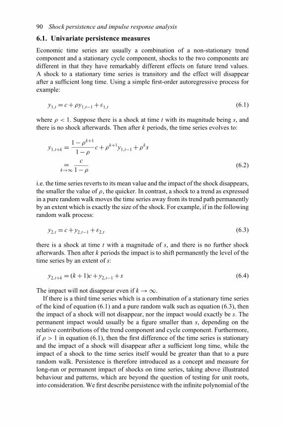
90 Shock persistence and impulse response analysis
6.1. Univariate persistence measures
Economic time series are usually a combination of a non-stationary trendcomponent and a stationary cycle component, shocks to the two components aredifferent in that they have remarkably different effects on future trend values.A shock to a stationary time series is transitory and the effect will disappearafter a sufficient long time. Using a simple first-order autoregressive process forexample:
y1,t = c +ρy1,t−1 + ε1,t (6.1)
where ρ < 1. Suppose there is a shock at time t with its magnitude being s, andthere is no shock afterwards. Then after k periods, the time series evolves to:
y1,t+k = 1 −ρk+1
1 −ρc +ρk+1y1,t−1 +ρk s
=k→∞
c
1 −ρ(6.2)
i.e. the time series reverts to its mean value and the impact of the shock disappears,the smaller the value of ρ, the quicker. In contrast, a shock to a trend as expressedin a pure random walk moves the time series away from its trend path permanentlyby an extent which is exactly the size of the shock. For example, if in the followingrandom walk process:
y2,t = c + y2,t−1 + ε2,t (6.3)
there is a shock at time t with a magnitude of s, and there is no further shockafterwards. Then after k periods the impact is to shift permanently the level of thetime series by an extent of s:
y2,t+k = (k + 1)c + y2,t−1 + s (6.4)
The impact will not disappear even if k → ∞.If there is a third time series which is a combination of a stationary time series
of the kind of equation (6.1) and a pure random walk such as equation (6.3), thenthe impact of a shock will not disappear, nor the impact would exactly be s. Thepermanent impact would usually be a figure smaller than s, depending on therelative contributions of the trend component and cycle component. Furthermore,if ρ > 1 in equation (6.1), then the first difference of the time series is stationaryand the impact of a shock will disappear after a sufficient long time, while theimpact of a shock to the time series itself would be greater than that to a purerandom walk. Persistence is therefore introduced as a concept and measure forlong-run or permanent impact of shocks on time series, taking above illustratedbehaviour and patterns, which are beyond the question of testing for unit roots,into consideration. We first describe persistence with the infinite polynomial of the
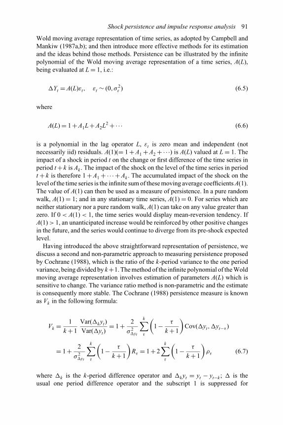
Shock persistence and impulse response analysis 91
Wold moving average representation of time series, as adopted by Campbell andMankiw (1987a,b); and then introduce more effective methods for its estimationand the ideas behind those methods. Persistence can be illustrated by the infinitepolynomial of the Wold moving average representation of a time series, A(L),being evaluated at L = 1, i.e.:
�Yt = A(L)εt, εt ∼ (0,σ 2ε ) (6.5)
where
A(L) = 1 + A1L + A2L2 +·· · (6.6)
is a polynomial in the lag operator L, εt is zero mean and independent (notnecessarily iid) residuals. A(1)(= 1 + A1 + A2 + ·· ·) is A(L) valued at L = 1. Theimpact of a shock in period t on the change or first difference of the time series inperiod t +k is Ak . The impact of the shock on the level of the time series in periodt + k is therefore 1 + A1 + ·· · + Ak . The accumulated impact of the shock on thelevel of the time series is the infinite sum of these moving average coefficients A(1).The value of A(1) can then be used as a measure of persistence. In a pure randomwalk, A(1) = 1; and in any stationary time series, A(1) = 0. For series which areneither stationary nor a pure random walk, A(1) can take on any value greater thanzero. If 0 < A(1) < 1, the time series would display mean-reversion tendency. IfA(1) > 1, an unanticipated increase would be reinforced by other positive changesin the future, and the series would continue to diverge from its pre-shock expectedlevel.
Having introduced the above straightforward representation of persistence, wediscuss a second and non-parametric approach to measuring persistence proposedby Cochrane (1988), which is the ratio of the k-period variance to the one periodvariance, being divided by k +1. The method of the infinite polynomial of the Woldmoving average representation involves estimation of parameters A(L) which issensitive to change. The variance ratio method is non-parametric and the estimateis consequently more stable. The Cochrane (1988) persistence measure is knownas Vk in the following formula:
Vk = 1
k + 1
Var(�kyt)
Var(�yt)= 1 + 2
σ 2�yt
k∑τ
(1 − τ
k + 1
)Cov(�yt,�yt−τ )
= 1 + 2
σ 2�yt
k∑τ
(1 − τ
k + 1
)Rτ = 1 + 2
k∑τ
(1 − τ
k + 1
)ρτ (6.7)
where �k is the k-period difference operator and �kyt = yt − yt−k ; � is theusual one period difference operator and the subscript 1 is suppressed for
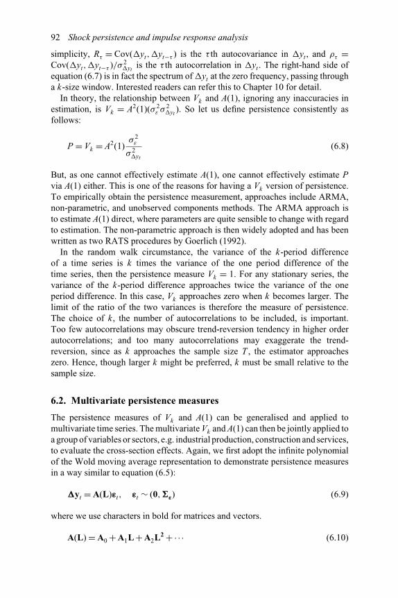
92 Shock persistence and impulse response analysis
simplicity, Rτ = Cov(�yt,�yt−τ ) is the τ th autocovariance in �yt , and ρτ =Cov(�yt,�yt−τ )/σ 2
�ytis the τ th autocorrelation in �yt . The right-hand side of
equation (6.7) is in fact the spectrum of �yt at the zero frequency, passing througha k-size window. Interested readers can refer this to Chapter 10 for detail.
In theory, the relationship between Vk and A(1), ignoring any inaccuracies inestimation, is Vk = A2(1)(σ 2
ε σ 2�yt
). So let us define persistence consistently asfollows:
P = Vk = A2(1)σ 2
ε
σ 2�yt
(6.8)
But, as one cannot effectively estimate A(1), one cannot effectively estimate Pvia A(1) either. This is one of the reasons for having a Vk version of persistence.To empirically obtain the persistence measurement, approaches include ARMA,non-parametric, and unobserved components methods. The ARMA approach isto estimate A(1) direct, where parameters are quite sensible to change with regardto estimation. The non-parametric approach is then widely adopted and has beenwritten as two RATS procedures by Goerlich (1992).
In the random walk circumstance, the variance of the k-period differenceof a time series is k times the variance of the one period difference of thetime series, then the persistence measure Vk = 1. For any stationary series, thevariance of the k-period difference approaches twice the variance of the oneperiod difference. In this case, Vk approaches zero when k becomes larger. Thelimit of the ratio of the two variances is therefore the measure of persistence.The choice of k , the number of autocorrelations to be included, is important.Too few autocorrelations may obscure trend-reversion tendency in higher orderautocorrelations; and too many autocorrelations may exaggerate the trend-reversion, since as k approaches the sample size T , the estimator approacheszero. Hence, though larger k might be preferred, k must be small relative to thesample size.
6.2. Multivariate persistence measures
The persistence measures of Vk and A(1) can be generalised and applied tomultivariate time series. The multivariate Vk and A(1) can then be jointly applied toa group of variables or sectors, e.g. industrial production, construction and services,to evaluate the cross-section effects. Again, we first adopt the infinite polynomialof the Wold moving average representation to demonstrate persistence measuresin a way similar to equation (6.5):
�yt = A(L)εt, εt ∼ (0,�ε) (6.9)
where we use characters in bold for matrices and vectors.
A(L) = A0 + A1L + A2L2 +·· · (6.10)
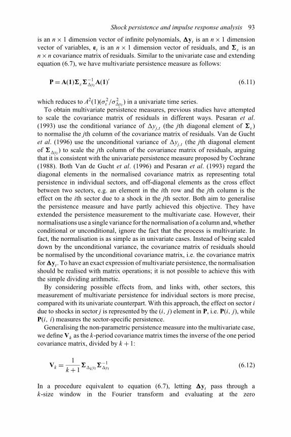
Shock persistence and impulse response analysis 93
is an n × 1 dimension vector of infinite polynomials, �yt is an n × 1 dimensionvector of variables, εt is an n × 1 dimension vector of residuals, and �ε is ann× n covariance matrix of residuals. Similar to the univariate case and extendingequation (6.7), we have multivariate persistence measure as follows:
P = A(1)�ε�−1�yt
A(1)′ (6.11)
which reduces to A2(1)(σ 2ε /σ 2
�yt) in a univariate time series.
To obtain multivariate persistence measures, previous studies have attemptedto scale the covariance matrix of residuals in different ways. Pesaran et al.(1993) use the conditional variance of �yj,t (the jth diagonal element of �ε)to normalise the jth column of the covariance matrix of residuals. Van de Guchtet al. (1996) use the unconditional variance of �yj,t (the jth diagonal elementof ��yt
) to scale the jth column of the covariance matrix of residuals, arguingthat it is consistent with the univariate persistence measure proposed by Cochrane(1988). Both Van de Gucht et al. (1996) and Pesaran et al. (1993) regard thediagonal elements in the normalised covariance matrix as representing totalpersistence in individual sectors, and off-diagonal elements as the cross effectbetween two sectors, e.g. an element in the ith row and the jth column is theeffect on the ith sector due to a shock in the jth sector. Both aim to generalisethe persistence measure and have partly achieved this objective. They haveextended the persistence measurement to the multivariate case. However, theirnormalisations use a single variance for the normalisation of a column and, whetherconditional or unconditional, ignore the fact that the process is multivariate. Infact, the normalisation is as simple as in univariate cases. Instead of being scaleddown by the unconditional variance, the covariance matrix of residuals shouldbe normalised by the unconditional covariance matrix, i.e. the covariance matrixfor �yt . To have an exact expression of multivariate persistence, the normalisationshould be realised with matrix operations; it is not possible to achieve this withthe simple dividing arithmetic.
By considering possible effects from, and links with, other sectors, thismeasurement of multivariate persistence for individual sectors is more precise,compared with its univariate counterpart. With this approach, the effect on sector idue to shocks in sector j is represented by the (i, j) element in P, i.e. P(i, j), whileP(i, i) measures the sector-specific persistence.
Generalising the non-parametric persistence measure into the multivariate case,we define Vk as the k-period covariance matrix times the inverse of the one periodcovariance matrix, divided by k + 1:
Vk = 1
k + 1��k yt
�−1�yt
(6.12)
In a procedure equivalent to equation (6.7), letting �yt pass through ak-size window in the Fourier transform and evaluating at the zero
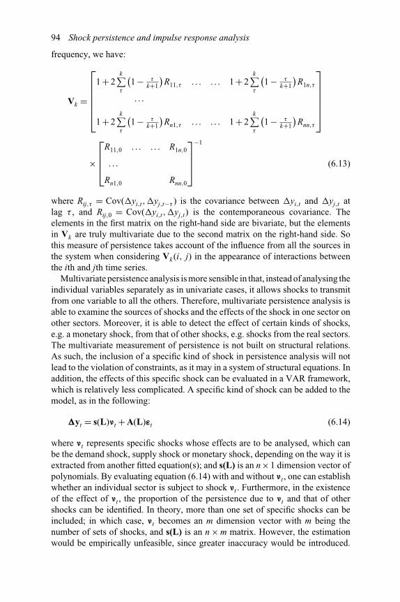
94 Shock persistence and impulse response analysis
frequency, we have:
Vk =
⎡⎢⎢⎢⎢⎢⎣
1 + 2k∑τ
(1 − τ
k+1
)R11,τ . . . . . . 1 + 2
k∑τ
(1 − τ
k+1
)R1n,τ
. . .
1 + 2k∑τ
(1 − τ
k+1
)Rn1,τ . . . . . . 1 + 2
k∑τ
(1 − τ
k+1
)Rnn,τ
⎤⎥⎥⎥⎥⎥⎦
×
⎡⎢⎢⎣
R11,0 . . . . . . R1n,0
. . .
Rn1,0 Rnn,0
⎤⎥⎥⎦
−1
(6.13)
where Rij,τ = Cov(�yi,t,�yj,t−τ ) is the covariance between �yi,t and �yj,t atlag τ , and Rij,0 = Cov(�yi,t,�yj,t) is the contemporaneous covariance. Theelements in the first matrix on the right-hand side are bivariate, but the elementsin Vk are truly multivariate due to the second matrix on the right-hand side. Sothis measure of persistence takes account of the influence from all the sources inthe system when considering Vk (i, j) in the appearance of interactions betweenthe ith and jth time series.
Multivariate persistence analysis is more sensible in that, instead of analysing theindividual variables separately as in univariate cases, it allows shocks to transmitfrom one variable to all the others. Therefore, multivariate persistence analysis isable to examine the sources of shocks and the effects of the shock in one sector onother sectors. Moreover, it is able to detect the effect of certain kinds of shocks,e.g. a monetary shock, from that of other shocks, e.g. shocks from the real sectors.The multivariate measurement of persistence is not built on structural relations.As such, the inclusion of a specific kind of shock in persistence analysis will notlead to the violation of constraints, as it may in a system of structural equations. Inaddition, the effects of this specific shock can be evaluated in a VAR framework,which is relatively less complicated. A specific kind of shock can be added to themodel, as in the following:
�yt = s(L)νt + A(L)εt (6.14)
where νt represents specific shocks whose effects are to be analysed, which canbe the demand shock, supply shock or monetary shock, depending on the way it isextracted from another fitted equation(s); and s(L) is an n×1 dimension vector ofpolynomials. By evaluating equation (6.14) with and without νt , one can establishwhether an individual sector is subject to shock νt . Furthermore, in the existenceof the effect of νt , the proportion of the persistence due to νt and that of othershocks can be identified. In theory, more than one set of specific shocks can beincluded; in which case, νt becomes an m dimension vector with m being thenumber of sets of shocks, and s(L) is an n × m matrix. However, the estimationwould be empirically unfeasible, since greater inaccuracy would be introduced.

Shock persistence and impulse response analysis 95
In addition, this approach would be less appealing if it is to lose its advantagesof no subjective assumptions and restrictions. Nevertheless, if there are only twotypes of shocks, e.g. demand versus supply, or monetary versus real, then νt canonly be one of the two types of shocks, otherwise equation (6.14) would be over-identified.
Persistence can be decomposed into separate components due to the specificshock and that due to other shocks:
Ps = A(1)s(1)�2νs(1)′�−1
�ytA(1)′ (6.15)
Po = A(1)�ε�−1�yt
A(1)′ (6.16)
and total persistence is:
PT = Ps + Po (6.17)
If the specific shock is chosen as demand or monetary disturbance, then theunderlying assumption is that the demand or monetary shock may also have along-run effect, as the persistence measure is about the effect on the levels ofvariables. This assumption can be empirically ruled out or ruled in which, in fact,becomes a hypothesis. Although Blanchard and Quah (1989) arguably excludedthe demand shock from having a long-run effect, their empirical work suggeststhat the effect of a demand shock would decline to vanish in about 25 quarters orfive to six years. In such a long period, the probability of a structural changeor break would be rather high. If a structural change does happen, it wouldoverride any supply shocks and the effects of demand and supply shocks wouldbe mixed.
6.3. Impulse response analysis and variance decomposition
Impulse response analysis is another way of inspecting and evaluating theimpact of shocks cross-section. While persistence measures focus on the long-run properties of shocks, impulse response traces the evolutionary path of theimpact over time. Impulse response, together with variance decomposition, formsinnovation accounting for sources of information and information transmission ina multivariate dynamic system.
Considering the following VAR process:
yt = A0 + A1yt−1 + A2yt−2 +·· ·+ Akyt−k +μt (6.18)
where yt is an n × 1 vector of variables, A0 is an n × 1 vector of intercept,Aτ (τ = 1, . . .,k) are n×n matrices of coefficients, μt is an n dimension vector ofwhite noise processes with E(μt) = 0, �μ = E(μtμ
′t) being non-singular for all t,
and E(μtμ′s) for t �= s. Without losing generality, exogenous variables other than
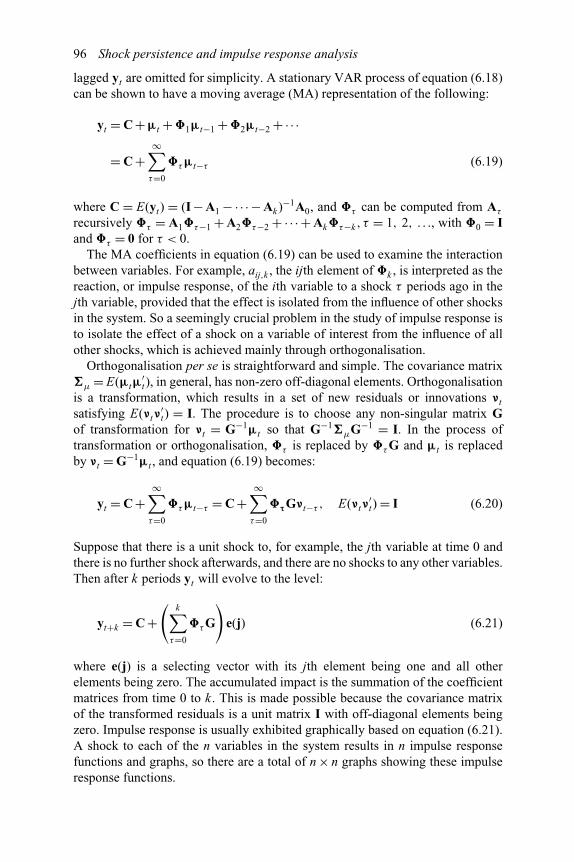
96 Shock persistence and impulse response analysis
lagged yt are omitted for simplicity. A stationary VAR process of equation (6.18)can be shown to have a moving average (MA) representation of the following:
yt = C +μt + 1μt−1 + 2μt−2 +·· ·
= C +∞∑
τ=0
τμt−τ (6.19)
where C = E(yt) = (I − A1 −·· ·− Ak )−1A0, and τ can be computed from Aτ
recursively τ = A1 τ−1 + A2 τ−2 + ·· · + Ak τ−k ,τ = 1, 2, . . ., with 0 = Iand τ = 0 for τ < 0.
The MA coefficients in equation (6.19) can be used to examine the interactionbetween variables. For example, aij,k , the ijth element of k , is interpreted as thereaction, or impulse response, of the ith variable to a shock τ periods ago in thejth variable, provided that the effect is isolated from the influence of other shocksin the system. So a seemingly crucial problem in the study of impulse response isto isolate the effect of a shock on a variable of interest from the influence of allother shocks, which is achieved mainly through orthogonalisation.
Orthogonalisation per se is straightforward and simple. The covariance matrix�μ = E(μtμ
′t), in general, has non-zero off-diagonal elements. Orthogonalisation
is a transformation, which results in a set of new residuals or innovations νt
satisfying E(νtν′t) = I. The procedure is to choose any non-singular matrix G
of transformation for νt = G−1μt so that G−1�μG−1 = I. In the process oftransformation or orthogonalisation, τ is replaced by τ G and μt is replacedby νt = G−1μt , and equation (6.19) becomes:
yt = C +∞∑
τ=0
τμt−τ = C +∞∑
τ=0
τGνt−τ , E(νtν′t) = I (6.20)
Suppose that there is a unit shock to, for example, the jth variable at time 0 andthere is no further shock afterwards, and there are no shocks to any other variables.Then after k periods yt will evolve to the level:
yt+k = C +(
k∑τ=0
τ G
)e(j) (6.21)
where e(j) is a selecting vector with its jth element being one and all otherelements being zero. The accumulated impact is the summation of the coefficientmatrices from time 0 to k . This is made possible because the covariance matrixof the transformed residuals is a unit matrix I with off-diagonal elements beingzero. Impulse response is usually exhibited graphically based on equation (6.21).A shock to each of the n variables in the system results in n impulse responsefunctions and graphs, so there are a total of n × n graphs showing these impulseresponse functions.

Shock persistence and impulse response analysis 97
To achieve orthogonalisation, the Choleski factorisation, which decomposesthe covariance matrix of residuals �μ into GG′ so that G is lower triangularwith positive diagonal elements, is commonly used. However, this approach is notinvariant to the ordering of the variables in the system. In choosing the orderingof the variables, one may consider their statistical characteristics. By constructionof G, the first variable in the ordering explains all of its one-step forecast variance,so consign a variable which is least influenced by other variables, such as anexogenous variable, to the first in the ordering. Then choose the variable withleast influence on other variables as the last variable in the ordering. The otherapproach to orthogonalisation is based on the economic attributes of data, such asthe Blanchard and Quah structural decomposition. It is assumed that there are twotypes of shocks, the supply shock and the demand shock. While the supply shockhas permanent effect, the demand shock has only temporary or transitory effect.Restrictions are imposed accordingly to realise orthogonalisation in residuals.
Since the residuals have been orthogonalised, variance decomposition isstraightforward. The k-period ahead forecast errors in equation (6.19) or(6.20) are:
k−1∑τ=0
τ Gνt−τ+k−1 (6.22)
The covariance matrix of the k-period ahead forecast errors are:
k−1∑τ=0
τ GG′
′τ =
k−1∑τ=0
τ�μ ′τ (6.23)
The right-hand side of equation (6.23) just reminds the reader that the outcomeof variance decomposition will be the same irrespective of G. The choice orderivation of matrix G only matters when the impulse response function isconcerned to isolate the effect from the influence from other sources.
The variance of forecast errors attributed to a shock to the jth variable can bepicked out by a selecting vector e(j), the idea of variance decomposition, with thejth element being one and all other elements being zero:
Var(j, k) =(
k−1∑τ=0
τ Ge(j)e(j)′G
′
′τ
)(6.24)
Further, the effect on the ith variable due to a shock to the jth variable, or thecontribution to the ith variable’s forecast error by a shock to the jth variable, canbe picked out by a second selecting vector e(i) with the ith element being one andall other elements being zero.
Var(ij,k) = e(i)′(
k−1∑τ=0
τ Ge(j)e(j)′G
′
′τ
)e(i) (6.25)

98 Shock persistence and impulse response analysis
In relative terms, the contribution is expressed as a percentage of the totalvariance:
Var(ij,k)∑nj=1 Var(ij,k)
(6.26)
which sums up to 100 per cent.
6.4. Non-orthogonal cross-effect impulse response analysis
There are other ways to evaluate the effect of a shock. One of the main advantages ofapplying orthogonalised residuals is that the impact at time k due to a unit shock tothe jth variable at time 0 is simply the summation of matrices τ G, over 0 ≤ τ ≤ k ,being timed by the selecting vector e(j). That is, there is no need to consider theeffect due to shocks to other than the jth variable because such effect does notexist. Then it would be a reasonable idea that we do not perform orthogonalisationbut consider the effect arising from the non-orthogonalisation of residuals, or thecross-effect, in impulse response analysis. With non-orthogonal residuals, whenthere is a shock to the jth variable of the size of its standard deviation, there areshocks to other variables in the meantime through their correlations. Let δj standfor such shocks:
δj =
⎡⎢⎢⎢⎣
ρ1j
. . .
1
ρnj
⎤⎥⎥⎥⎦√σjj =
⎡⎢⎢⎢⎣
σ1j
. . .
σjj
σnj
⎤⎥⎥⎥⎦ 1√
σjj
= �μe(j)1√σjj
(6.27)
With such a shock to the jth variable at time 0 and suppose there is no furthershock afterwards, yt will evolve to the level after k periods:
yt+k = C +(
k∑τ=0
τ
)e(j)
1√σjj
(6.28)
So, it appears that orthogonalisation can be avoided. But bearing in mind that, innon-orthogonal impulse response analysis, we cannot simply give a shock of onestandard deviation to the equation of interest, the jth equation, only; we should, inthe meantime, give a ‘shock’ to each of other equations of the size of the squareroot of its covariance with the jth shock. It indeed means that we have to considerboth the direct effect of the jth shock and the indirect effect of the jth shock throughother series in the system. Moreover, the outcome would be in general different tothat from orthogonal impulse response analysis.
Let us work out variance decomposition in a slightly different way. We considersingle elements first. The k-period ahead forecast errors in equation (6.28) are:
k−1∑τ=0
τ�μe(j)1√σjj
(6.29)
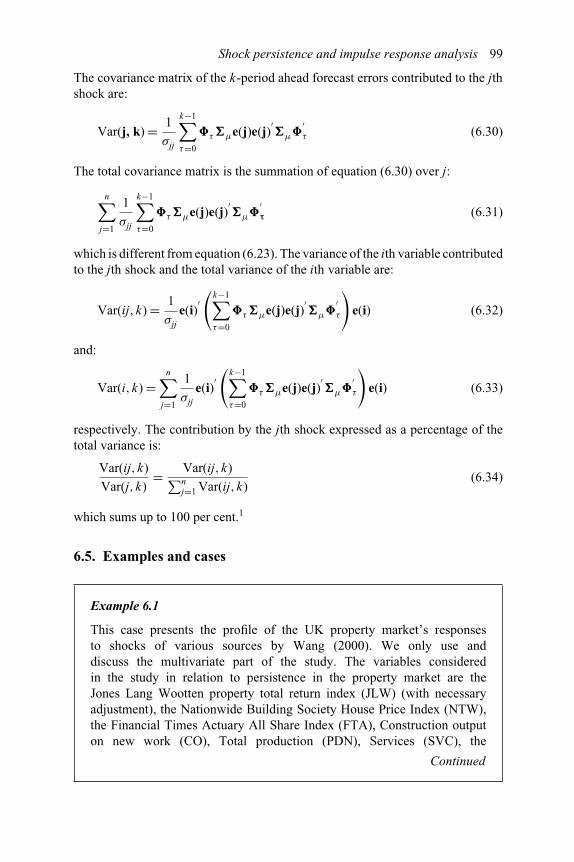
Shock persistence and impulse response analysis 99
The covariance matrix of the k-period ahead forecast errors contributed to the jthshock are:
Var(j, k) = 1
σjj
k−1∑τ=0
τ�μe(j)e(j)′�μ
′τ (6.30)
The total covariance matrix is the summation of equation (6.30) over j:
n∑j=1
1
σjj
k−1∑τ=0
τ�μe(j)e(j)′�μ
′τ (6.31)
which is different from equation (6.23). The variance of the ith variable contributedto the jth shock and the total variance of the ith variable are:
Var(ij,k) = 1
σjj
e(i)′(
k−1∑τ=0
τ�μe(j)e(j)′�μ
′τ
)e(i) (6.32)
and:
Var(i,k) =n∑
j=1
1
σjj
e(i)′(
k−1∑τ=0
τ�μe(j)e(j)′�μ
′τ
)e(i) (6.33)
respectively. The contribution by the jth shock expressed as a percentage of thetotal variance is:
Var(ij,k)
Var(j,k)= Var(ij,k)∑n
j=1 Var(ij,k)(6.34)
which sums up to 100 per cent.1
6.5. Examples and cases
Example 6.1
This case presents the profile of the UK property market’s responsesto shocks of various sources by Wang (2000). We only use anddiscuss the multivariate part of the study. The variables consideredin the study in relation to persistence in the property market are theJones Lang Wootten property total return index (JLW) (with necessaryadjustment), the Nationwide Building Society House Price Index (NTW),the Financial Times Actuary All Share Index (FTA), Construction outputon new work (CO), Total production (PDN), Services (SVC), the
Continued
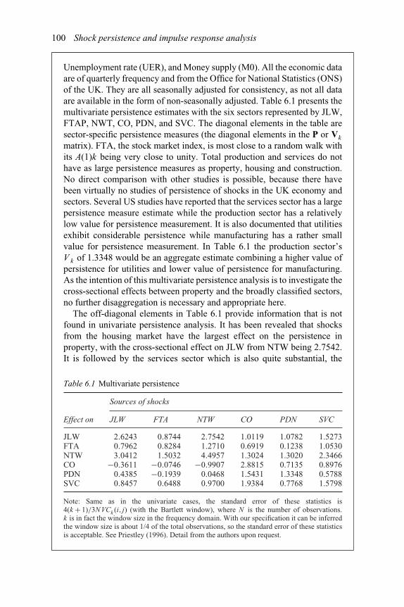
100 Shock persistence and impulse response analysis
Unemployment rate (UER), and Money supply (M0). All the economic dataare of quarterly frequency and from the Office for National Statistics (ONS)of the UK. They are all seasonally adjusted for consistency, as not all dataare available in the form of non-seasonally adjusted. Table 6.1 presents themultivariate persistence estimates with the six sectors represented by JLW,FTAP, NWT, CO, PDN, and SVC. The diagonal elements in the table aresector-specific persistence measures (the diagonal elements in the P or Vk
matrix). FTA, the stock market index, is most close to a random walk withits A(1)k being very close to unity. Total production and services do nothave as large persistence measures as property, housing and construction.No direct comparison with other studies is possible, because there havebeen virtually no studies of persistence of shocks in the UK economy andsectors. Several US studies have reported that the services sector has a largepersistence measure estimate while the production sector has a relativelylow value for persistence measurement. It is also documented that utilitiesexhibit considerable persistence while manufacturing has a rather smallvalue for persistence measurement. In Table 6.1 the production sector’sV k of 1.3348 would be an aggregate estimate combining a higher value ofpersistence for utilities and lower value of persistence for manufacturing.As the intention of this multivariate persistence analysis is to investigate thecross-sectional effects between property and the broadly classified sectors,no further disaggregation is necessary and appropriate here.
The off-diagonal elements in Table 6.1 provide information that is notfound in univariate persistence analysis. It has been revealed that shocksfrom the housing market have the largest effect on the persistence inproperty, with the cross-sectional effect on JLW from NTW being 2.7542.It is followed by the services sector which is also quite substantial, the
Table 6.1 Multivariate persistence
Sources of shocks
Effect on JLW FTA NTW CO PDN SVC
JLW 2.6243 0.8744 2.7542 1.0119 1.0782 1.5273FTA 0.7962 0.8284 1.2710 0.6919 0.1238 1.0530NTW 3.0412 1.5032 4.4957 1.3024 1.3020 2.3466CO −0.3611 −0.0746 −0.9907 2.8815 0.7135 0.8976PDN 0.4385 −0.1939 0.0468 1.5431 1.3348 0.5788SVC 0.8457 0.6488 0.9700 1.9384 0.7768 1.5798
Note: Same as in the univariate cases, the standard error of these statistics is4(k + 1)/3NVCk (i, j) (with the Bartlett window), where N is the number of observations.k is in fact the window size in the frequency domain. With our specification it can be inferredthe window size is about 1/4 of the total observations, so the standard error of these statisticsis acceptable. See Priestley (1996). Detail from the authors upon request.

Shock persistence and impulse response analysis 101
production sector, and construction. Shocks in the stock market have effectson the persistence in property, but they are the smallest among all selectedvariables, with the cross-sectional effect on JLW being 0.8744.
Regarding the effects of the property market on other sectors, again,the largest impacts seem to be felt in the housing market, with the cross-sectional effect on NTW from JLW being 3.0412. So the commercial andnon-commercial property markets have very close links in this perspective.The effects of shocks on the services sector (0.8457) are larger than thoseon the production sector (0.4385), as expected. A negative figure for theeffects on construction suggests, in statistical terms, that the one periodcovariance and the n (n → ∞) period covariance have different signs. Thisis only possible in covariance but not in variance. The empirical meaning ofa negative cross-sectional persistence measure would be: a positive shockin the property market which also results in an increase in construction (i.e.a positive one period covariance is assumed) would eventually lead to adecrease in construction output, or contraction in the construction industry,in the long-run. This revelation of the interaction between the propertymarket and the construction sector has profound economic implications.
The reported multivariate persistence measurement estimates are derivedwith an unrestricted VAR model of order 2 (the inverse of the matrixis effectively corresponding to an infinite moving average process). Therestricted model, which drops the regressors whose t-statistic of coefficientis less than one, is also tested. The two sets of results are similar, so theunrestricted model is adopted for reasons that it is easy to implement in thefuture and in slightly different situations.2 This is consistent with Cochrane’s(1988) recommendation of including all autocorrelation terms even if theyare insignificant. Both models are estimated with SUR (Seemingly UnrelatedRegression), though there are no efficiency gains from using an OLSprocedure to applying SUR in the unrestricted model.
The paper further decomposes shocks into monetary and non-monetarycomponents. The above tests have analysed the ‘sources’ of shocks, and thesources are sectors. In the following, the sources are divided into monetaryand non-monetary ones. The reasons for adopting this line of research are asfollows. Traditionally, the effect of a monetary shock is viewed as only beingtemporary or transitory, while a real shock has both permanent and transitoryeffects. In the long-run, the effect of the monetary shock disappears and theonly effect left is due to the real shock. Similarly, a demand shock is viewedas temporary and a supply shock as permanent. In separating or decomposinga monetary shock from non-monetary shocks, one is able to evaluate thelong-run and short-term effects more effectively. However, the traditionalview, which suggests that the monetary shock is not held responsible for
Continued

102 Shock persistence and impulse response analysis
any permanent or long-run effects, may be over-assertive and should beempirically tested. In this study, if the effect of the monetary shock is notlong lasting, then the monetary shock would have no contribution to thepersistence measure. Obviously, different test results would have differentimplications for policy-making and practice, especially with regard to along-run perspective.
Monetary shocks can be derived from estimating a money supply growthmodel and obtaining its residuals. The money supply growth model isspecified as follows:
�Mt = α +β�Mt−1 + γ�SVCt−1 + δUERt−1 + νt (6.35)
where Mt is money supply, SVCt is services output and UERt is theunemployment rate. M0, the narrowly defined money, is chosen as themoney supply variable in this model. The reasons for using M0 insteadof M4, the broad money supply, are empirical. There is a big break inthe M4 series in the fourth quarter of 1981 caused by the switch betweenthe old banking sector and the new monetary sector. In July 1989, AbbeyNational’s conversion to a public limited company caused minor breaks tothe M0 series and major breaks in the M4 series. Although the first breaksin the fourth quarter of 1981 were removed from the changes in M4, theremoval of the breaks in the changes in M4 resulted in as much distortion asthe retaining of the breaks in M4 levels. Besides these breaks, the M0 andM4 series had a similar pattern. Beyond the concern in breaks, M0 is moreliquid and more public sensitive in representing demand factors, separatedfrom supply factors or real factors. Table 6.2 reports the summary statisticsfor the money growth model.
The multivariate shock persistence model has been re-estimated withmonetary shocks, the residuals from the money supply growth model, beingincluded. All the estimates are reported in Table 6.3, and a summary withsector-specific estimates and the percentage of monetary and non-monetaryeffects is provided in Table 6.4. The first line for each variable in Table 6.3
Table 6.2 Summary statistics for the money growth model
α β γ δ Q
M0 0.0155∗∗∗ 0.4551∗∗∗ 0.3616∗∗∗ −0.0011∗∗ 19.9744(3.2723) (4.1013) (2.6350) (2.4180) (0.2753)
Q-Ljung–Box statistic for serial correlation, the order is selected as 1/4 of the observationsused.p-Value in parentheses.∗∗significant at 5 per cent level; ∗∗∗significant at 1 per cent level.
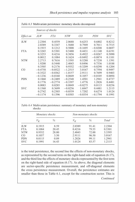
Shock persistence and impulse response analysis 103
Table 6.3 Multivariate persistence: monetary shocks decomposed
Sources of shocks
Effect on JLW FTA NTW CO PDN SVC
JLW 2.2304 0.4559 2.0688 0.6253 0.6802 0.82122.0389 0.3347 1.5680 0.7949 0.7011 0.75150.1915 0.1212 0.5008 −0.1695 −0.0208 0.0697
FTA 0.3265 0.5301 0.5480 0.4431 −0.1140 0.61910.3253 0.4216 0.3856 0.4922 −0.0267 0.50900.0012 0.1084 0.1624 −0.0492 −0.0874 0.1101
NTW 2.2713 0.7616 3.3395 0.5288 0.7238 1.13911.9208 0.5440 2.4043 0.8496 0.7536 1.01880.3505 0.2176 0.9352 −0.3209 −0.0298 0.1204
CO −0.4758 −0.0522 −1.2515 3.0167 0.7594 0.9497−0.3522 −0.0362 −1.0157 2.9111 0.7699 0.9403−0.1236 −0.0160 0.0849 0.1057 −0.0105 0.0094
PDN 0.1860 −0.2489 −0.2548 1.4501 1.2941 0.47370.1776 −0.2774 −0.3397 1.4776 1.2826 0.44810.0083 0.0285 0.0849 −0.0275 0.0115 0.0256
SVC 0.1568 0.3699 −0.0256 1.6847 0.4481 1.21150.2742 0.2303 −0.0559 1.7202 0.6274 1.0124
−0.1174 0.1396 0.0303 −0.0354 −0.1794 0.1991
Table 6.4 Multivariate persistence: summary of monetary and non-monetaryshocks
Monetary shocks Non-monetary shocks
VK % VK % Total
JLW 0.1915 8.59 2.0389 91.41 2.2304FTA 0.1084 20.45 0.4216 79.55 0.5301NTW 0.9352 28.00 2.4043 72.00 3.3395CO 0.1057 3.50 2.9111 96.50 3.0167PDN 0.0115 0.89 1.2826 99.11 1.2941SVC 0.1991 16.43 1.0124 83.57 1.2115
is the total persistence, the second line the effects of non-monetary shocks,as represented by the second term on the right-hand side of equation (6.17),and the third line the effects of monetary shocks represented by the first termon the right-hand side of equation (6.17). As above, the diagonal elementsare sector-specific persistence measurement, and off-diagonal elementsthe cross persistence measurement. Overall, the persistence estimates aresmaller than those in Table 6.1, except for the construction sector. This is
Continued

104 Shock persistence and impulse response analysis
because of the inclusion of the monetary shocks, which are expected to havesmaller effects in the long run, in the model. In previous estimation withoutan explicit monetary shock variable (or a monetary variable), the persistenceeffects due to monetary shocks are mixed with other shocks. Further scrutinyhas found that the decrease in the persistence measure happens in thosesectors which are subject to monetary shocks to a substantial degree, e.g.housing, where monetary shocks account for 28 per cent in total persistence,services 16 per cent, and stock market 20 per cent. Monetary shocks onlyaccount for 4 per cent of total persistence in construction, and an evensmaller figure of less than 1 per cent in the production sector, so theirtotal persistence estimates are largely unaffected. In summary, a broadlydefined production sector, including construction, or the real economy, orthe supply side of economy, is not subject to monetary shocks in the long-run; whereas the services sector, broadly defined to include housing andthe stock market, or the demand side of economy, or the consumption, isvery much influenced by monetary shocks. Commercial property, due toits fundamental links to the real economy and financial markets, reasonablystands in between, with the effects of monetary shocks being responsible for9 per cent of total persistence measurement, and a large part of persistenceis from non-monetary shocks caused in the real sector of the economy.
Example 6.2
In a recent paper, Dekker et al. (2001) apply both orthogonal and non-orthogonal cross-effect, or generalised, impulse response analysis to stockmarket linkages in Asia-Pacific. They use daily closing data of returns fora rather short period from the 1st January 1987 to the 29th May 1998, onten market indices in the region, namely, Australia’s SE All Ordinary, HongKong Hang Seng, Japan’s Nikkei 225 Average, Malaysia’s Kuala LumpurComposite, New Zealand SE Capital 40, the Philippines SE Composite,Singapore Strait Times Industrial, Taiwan SE Weighted, Thailand’sBangkok Book Club, and the US Standard & Poor 500 Composite. Theirmodels were tested using the indices as expressed in the US dollar as well asin local currencies. It is claimed that both data sets produce consistent resultsso only the results from using local currencies are reported in the paper.Amongst the ten economies, Malaysia, the Philippines, Taiwan and Thailandare classified as emerging markets and the rest as developed markets.
The models and the treatment of variables are exactly those in Pesaran andShin (1998). Consequently, variance decomposition with the generalisedimpulse response procedure inevitably runs into the problem that thetotal variance does not sum to 100 per cent. The paper deals with theproblem by standardising the total variance, or scaling the total variance

Shock persistence and impulse response analysis 105
to 100 per cent. Although cointegration relationships are found in the data,the authors choose to apply an unrestricted VAR in the first differencewithout incorporating the error correction term, having reviewed the relevantliterature in which an unrestricted VAR is preferred to a vector errorcorrection model (VECM) in short horizons. The paper performs impulseresponse analysis over 15 days and presents 5-, 10- and 15-day ahead forecastvariance decomposition. In orthogonal response analysis, the variables areordered according to the closing time, with the most exogenous market,which in this case is the US, being the first. Table 6.5 presents the resultsfrom orthogonal variance decomposition, while Table 6.6 is for those fromgeneralised variance decomposition. As there is no substantial variation,only the results for day 15 are provided.
The paper makes common sense comparison between the orthogonaland the generalised variance decomposition results. For example, withclosing time ordering in orthogonal variance decomposition, New Zealandis ordered before Australia. The ordering appears to have a distorting effecton the variance decomposition results: shocks in the New Zealand marketexplain a much larger proportion of variance of 10.70 per cent in theAustralian market, compared with a rather small figure of 1.99 per centcontributed by the Australian market to the New Zealand market, on day 15.This seems to be difficult to justify, considering the relative size of thetwo markets. In contrast, generalised variance decomposition providesapparently reasonable results that the contribution of the New Zealandmarket to the Australian market is 8.31 per cent, while shocks in theAustralian market account for a large amount of 11.43 per cent of the totalvariance in the New Zealand market, on day 15. Following this commonsense discussion, the paper employs Table 6.6 for further analysis. Thereare three main conclusions. First, the US market is the most influentialin Asia-Pacific. No other markets contribute more than 2 per cent of theUS total forecast variance, while the contribution of the US market to othermarkets is significant with many of them being over 10 per cent. Second, thelevel of exogeneity of a market is proportional to the amount of the forecastvariance explained by the market itself. The US, with over 90 per centtotal forecast variance being accounted for by itself, is the most exogenous.While Singapore is the most endogenous because over 50 per cent totalforecast variance is attributed to shocks in the other markets. Third, marketswith strong economic ties and close geographic links, such as the pairs ofAustralia and New Zealand and Malaysia and Singapore, have significantinteraction with each other. Impulse response graphs conform the aboveresults. Impulse analysis also indicates that the impact of shocks disappearsquickly, usually in no more than one day.
Continued

Tab
le6.
5O
rtho
gona
ldec
ompo
sition
offo
reca
ster
ror
vari
ance
sfo
rda
ily
mar
ketr
etur
nsfo
r10
Asi
aPac
ific
mar
kets
:15
day
hori
zon
Inno
vation
sin
Effec
ton
Aus
tral
iaH
ong
Kon
gJa
pan
Mal
aysi
aN
ewZea
land
Phi
lipp
ines
Sing
apor
eTai
wan
Tha
ilan
dU
SA
llfo
reig
n
Aus
tral
ia61
.86
1.24
340.
4190
0.77
3610
.70
0.99
370.
3472
0.50
100.
1912
22.9
538
.14
Hon
gK
ong
3.79
5476
.76
2.20
840.
5356
2.56
522.
4665
0.48
480.
6669
0.66
029.
8596
23.2
4Ja
pan
2.40
330.
3245
86.3
80.
1338
1.91
090.
3719
0.48
581.
0619
0.23
656.
6953
13.6
2M
alay
sia
1.49
568.
0847
1.67
2554
.56
1.62
341.
8302
19.2
00.
9947
0.78
829.
7527
45.4
4N
ewZ
eala
nd2.
4478
1.05
010.
5868
0.43
8177
.92
0.44
020.
6593
0.30
930.
2064
15.9
422
.08
Phi
lipp
ines
0.25
800.
7532
0.60
741.
2595
0.81
8489
.93
0.49
300.
9431
0.73
284.
2023
10.0
7Sin
gapo
re3.
9231
9.87
901.
5353
1.00
092.
1997
3.67
9960
.75
1.14
060.
6726
15.2
239
.25
Tai
wan
0.64
900.
3131
0.15
350.
1467
0.85
700.
2967
0.45
6594
.41
0.37
862.
3381
5.59
Tha
ilan
d0.
7661
2.79
760.
7318
1.65
070.
7751
2.17
373.
9772
1.12
1980
. 13
5.88
0219
.87
US
0.89
250.
6491
0.23
730.
2788
0.37
920.
5864
0.47
000.
3024
0.63
1395
.57
4.43
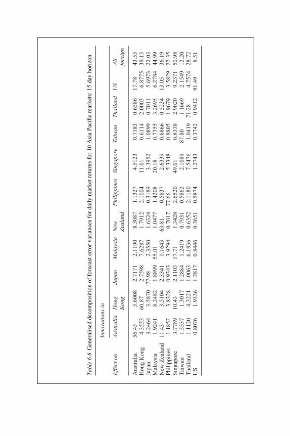
Tab
le6.
6G
ener
alis
edde
com
posi
tion
offo
reca
ster
ror
vari
ance
sfo
rda
ily
mar
ketr
etur
nsfo
r10
Asi
aPac
ific
mar
kets
:15
day
hori
zon
Inno
vation
sin
Effec
ton
Aus
tral
iaH
ong
Kon
gJa
pan
Mal
aysi
aN
ewZea
land
Phi
lipp
ines
Sing
apor
eTai
wan
Tha
ilan
dU
SA
llfo
reig
n
Aus
tral
ia56
.45
5.60
082.
7171
2.11
908.
3087
1.13
274.
5123
0.71
830.
6586
17.7
843
.55
Hon
gK
ong
4.35
5360
.87
2.75
987.
6287
1.79
122.
1004
11.0
10.
6114
2.00
036.
8775
39.1
3Ja
pan
3.24
643.
5870
77.9
82.
3550
1.63
240.
3189
3.39
521.
0899
0.70
115.
6973
22.0
3M
alay
sia
1.92
418.
2482
1.88
9955
.01
1.04
771.
4208
20.1
80.
7355
3.26
956.
2784
44.9
9N
ewZ
eala
nd11
.43
3.51
042.
3341
1.16
4363
.81
0.58
372.
6339
0.68
660.
5234
13.0
536
.19
Phi
lipp
ines
1.18
523.
8328
0.93
433.
9294
0.70
1777
.66
5.33
480.
8805
1.96
793.
5829
22.3
5Sin
gapo
re3.
7789
10.4
32.
1103
17.7
11.
3428
2.65
2049
.01
0.83
382.
9020
9.23
7150
.98
Tai
wan
1.55
371.
3017
1.28
841.
2419
0.79
310.
5862
2.10
8987
.80
1.16
692.
1549
12.2
0T
hailan
d1.
1120
4.32
211.
0063
6.18
360.
6352
2.11
807.
5476
1.04
1971
. 28
4.75
7428
.72
US
0.80
761.
9336
1.38
170.
8446
0.36
510.
5874
1.27
430.
3742
0.94
1291
.49
8.51
108 Shock persistence and impulse response analysis
6.6. Empirical literature
Persistence and impulse response are much an empirical matter. Persistence looksinto the long-run behaviour of time series in response to shocks and reflectsthe relative contribution and importance of the trend and the cycle. Inspectingthe persistence profile of a time series, the effect of shocks in the long-run canbe evaluated, which is of help to both macro economic policy formation andmicro investment decision making. The other aspects in the study of the effect ofshocks are the response profile over the whole time horizon of interest, includingthe magnitudes of the response, termed as impulse response analysis, and theexamination of the sources of the disturbance, termed as variance decomposition.Many multivariate models, such as the VAR, are complemented with impulseresponse analysis and variance decomposition, after the model has been set up andtested. All of these reflect the importance of this chapter in empirical studies.
Following the initiatives of Campbell and Mankiw (1987a, b) and Cochrane(1988), whose concerns are the behaviour of US aggregate GNP/GDP data,persistence in macroeconomic time series have been further investigated in thesectors, in other economies and in other economic and financial variables. Pesaranet al. (1993) extend measures of persistence into multivariate cases and examine thepersistence profile in ten US GNP sectors, though they do not consider the cross-effect of persistence between sectors. Most of the sectors are found to be verypersistent in response to shocks, with the persistence measure being greater thanone, suggesting there is compounding effect. In comparison, utilities exhibit largestcompounding persistence followed by services, while persistence in manufacturingis relatively lower. Mayadunne et al. (1995) have carried out similar research usingthe Australian data and made comparison with the US results. Concerned with therandom walk hypothesis in foreign exchange rates, Van de Gucht et al. (1996)examine persistence in seven daily foreign spot exchange rates of the Canadiandollar, the French franc, the Swiss franc, the German mark, the Italian lire, theJapanese yen and the British pound vis-à-vis the US dollar over the period of3 September 1974 to 27 May 1992. They find departure from the random walkbenchmark but the departure is not substantial when the standard errors in thepersistence measure are taken into consideration. Moreover, there is increasingmean-reverting component in more recent periods. The cross-effect of shocks isalso checked and that between European currencies is found to be similar; further,the cross-effect between European currencies is larger than that between Europeancurrencies and that of the Japanese yen and the Canadian dollar. Cashin et al. (2000)study the persistence of shocks to world commodity prices, using monthly IMFdata on primary commodities between 1957 and 1998. They find that shocks tocommodity prices typically have significantly persistent effect and the persistenceprofile varies, based on which the effect of national and international schemes ofearnings stabilisation may be formed and evaluated. Their analysis is not in favourof a stabilisation scheme, as they argue that the cost of the stabilisation scheme willlikely exceed any associated smoothing benefits. Other studies in the area includeGreasley and Oxley (1997), Linden (1995), and Demery and Duck (1992).

Shock persistence and impulse response analysis 109
Impulse response and variance decomposition have been widely employed toobserve cross-effects of shocks, evaluated on the basis of a pre-specified andtested multivariate model. In the last decade, one of the extensively studied areasis capital market links and interactions, owing to an increasingly integrating globalfinancial market offering opportunities that never existed before or exhausted inthe domestic market. Investigating capital market integration in the Pacific basin inthe context of impulse response, Phylaktis (1999) studies specifically the speed ofadjustment of real interest rates to long-run equilibrium following a shock in eachof these markets. It is found that countries in the region are closely linked withworld financial markets. Moreover, the association of these markets with Japan isstronger than that with the US. Tse et al. (1996) examine information transmissionin three Eurodollar futures markets of Imm, Simex and Liffe. Employing impulseresponse analysis and variance decomposition which explores further the commonfactor in the cointegration system, it is found that the common factor is drivenby the last trading market in the 24-hour trading sequence. Each of the marketsimpounds all the information and rides on the common stochastic trend duringtrading hours, and the three markets can be considered one continuously tradingmarket. In a study of equity market linkages in ASEAN countries, Roca et al.(1998) use impulse response analysis and variance decomposition based on aVAR with error correction to investigate the extent and structure of price linkagesamong these markets. They find evidence of short-term linkages among all but theIndonesian market. But in the long-run, the linkages, if any, are weak. Specifically,the Malaysian market is the most influential, i.e. its shocks considerably contributeto the forecast variance in other markets; while the Singapore and Thailand marketshave most strong interaction with other markets, i.e. shocks in the Singapore andThailand markets account for a large proportion of forecast variance in othermarkets and, in the meantime, shocks in other markets attribute to a large amount offorecast variance in Singapore and Thailand markets. Finally, their results indicatethat the Indonesian market is isolated and not linked with any other ASEANmarket.
Impulse response has been widely applied to regional studies and real estatewhere the response to shocks from various sources is one of the major concerns.Baffoe-Bonnie (1998) analyses the effect of key macroeconomic variables onhouse prices and the stock of houses sold in the framework of VAR and impulseresponse analysis. The results suggest that macroeconomic variables producecycles in housing prices and houses sold. Considerable amount of the forecastvariance in the housing market can be attributed to shocks in the employmentgrowth and mortgage rate at both national and regional levels. The study alsoreveals that the dynamic behaviour of housing prices and the number of housessold vary substantially among different regions and at different time periods. Hort(2000) employs impulse response analysis based on the estimation of a VARmodel of the after-tax mortgage rate, house prices and sales, to examine pricesand turnover in the owner-occupied housing market. The empirical results in thepaper support that the adjustment of house price expectations following a shockto demand is slow due to informational imperfections in the housing market.

110 Shock persistence and impulse response analysis
There also exist asymmetries in buyers and sellers’ responses such that sales areexpected to respond prior to prices where buyers are assumed to respond prior tosellers. Tse and Webb (1999), concerned with the effectiveness of land tax andcapital gain tax in curbing hoarding of land and speculation, evaluate the effects ofproperty tax on housing in Hong Kong. Using an impulse response function, theydemonstrate that the transaction tax has a dynamic negative impact on housingreturns, as the imposition of capital gain tax impairs the liquidity of propertytransaction, lowers the rate of return on property investment, and reduces revenuefrom land sales. They also show that the capital gain tax is capitalised into housingprices.
Various other studies can be found in the areas of business cycles and monetarypolicy evaluation, real and nominal exchange rate behaviour and linkages, PPP,debt markets, employment, regions and sectors, in virtually any dynamic modelsinvolving the analysis of effect and cross-effect of shocks.
Notes
1 Pesaran and Shin (1998) and Microfit use the total variance of the orthogonal case in thedenominator, so the components do not sum up to 100 per cent.
2 The restricted model involves deletion of the lagged variables, with the t-statistic oftheir coefficients being less than one, and re-estimation. Therefore, the implementationof the model is complicated and the model differs in every case, whereas the unrestrictedmodel decides the lag length, then includes all lagged variables. So, the implementationand estimation are ‘standard’.
Questions and problems
1 What is meant by persistence? How is persistence measured?2 Compare persistence analysis and the test for unit roots.3 Discuss the advantages of the procedure in this chapter to standardise the
multivariate persistence measure and its rationale.4 Describe impulse response analysis and its application in evaluating the impact
of shocks and policy changes.5 Why is orthogonalisation required in impulse response analysis?6 What is meant by generalised impulse response analysis? Can generalised
impulse response analysis avoid all the complications in orthogonalisationwhile achieving the same goal?
7 The contribution by the shock in each of the sources, expressed as a percent-age of the total variance, sums to 100 per cent in this chapter. Discuss itsrationale.
8 Collect data from various sources and test for persistence in the followingtime series:
(a) the spot foreign exchange rates of selected industrialised nations anddeveloping economies vis-à-vis the US$, testing one individual timeseries each time,

Shock persistence and impulse response analysis 111
(b) GDP of selected countries, testing one individual time series eachtime,
(c) nominal interests in selected countries, testing one individual time serieseach time.
What do you find of their characteristics?9 Collect data from various sources and test for multivariate persistence in the
following groups of time series:
(a) the spot foreign exchange rates of selected industrialised nations vis-à-visthe US$,
(b) the spot foreign exchange rates of selected developing economiesvis-à-vis the US$,
(c) GDP of selected countries,(d) nominal interests in selected countries.
What do you find of their characteristics?10 Collect data from various sources and carry out (orthogonal) impulse response
analysis in the following groups of time series:
(a) sectoral output indices in the UK,(b) GDP of the UK, the US and Japan(c) stock market return indices of the UK, the US and Japan.
What do you find of their characteristics?11 Collect data from various sources and carry out generalised impulse response
analysis in the following groups of time series:
(a) sectoral output indices in the UK,(b) GDPs of the UK, the US and Japan(c) stock market return indices of the UK, the US and Japan.
What do you find of their characteristics? Analyse the differences in yourfindings from (9) and (10).
References
Baffoe-Bonnie, J. (1998), The dynamic impact of macroeconomic aggregates on housingprices and stock of houses: a national and regional analysis, Journal of Real EstateFinance and Economics, 17, 179–197.
Blanchard, O.J. and Quah, D. (1989), The dynamic effects of aggregate demand and supplydisturbances, American Economic Review, 79, 655–673.
Campbell, J.Y. and Mankiw, N.W. (1987a), Are output fluctuations transitory?, QuarterlyJournal of Economics, 102, 857–880.
Campbell, J.Y. and Mankiw, N.W. (1987b), Permanent and transitory components inmacroeconomic fluctuations, American Economic Review, 77 (Papers and Proceedings),111–117.
Cashin, P., Liang, H. and McDermott, C.J. (2000), How persistent are shocks to worldcommodity prices? IMF Staff Papers, 47, 177–217.
112 Shock persistence and impulse response analysis
Cochrane, J.H. (1988), How big is the random walk in GDP?, Journal of Political Ecomony,96, 893–920.
Dekker, A., Sen, K. and Young, M.R. (2001), Equity market linkages in the Asia PacificRegion: a comparison of the orthogonalised and generalised VAR approaches, GlobalFinance Journal, 12, 1–33.
Demery, D. and Duck, N.W. (1992), Are economic fluctuations really persistent?,A reinterpretation of some international evidence, Economic Journal, 102, 1094–1101.
Goerlich, P. (1992), Cochrane.src, RATS, Estima.Greasley, D. and Oxley, L. (1997), Shock persistence and structural change, Economic
Record, 73, 348–362.Hort, K. (2000), Prices and turnover in the market for owner-occupied homes, Regional
Science and Urban Economics, 30, 99–119.Linden, M. (1995), Finnish GNP series 1954/I–1990/IV: small shock persistence or trend
stationarity? Some evidence with variance ratio estimates, Empirical Economics, 20,333–349.
Mayadunne, G., Evans, M. and Inder, B. (1995), An empirical investigation of shockpersistence in economic time series, Economic Record, 71, 145–156.
Pesaran, M.H. and Shin, Y. (1998), Generalized impulse response analysis in linearmultivariate models, Economics Letters, 58, 17–29.
Pesaran, M.H., Pierse, R.G. and Lee, K.C., (1993), Persistence, cointegration andaggregation: a disaggregated analysis of output fluctuations in the US economy, Journalof Econometrics, 56, 67–88.
Phylaktis, K. (1999), Capital market integration in the Pacific Basin region: an impulseresponse analysis, Journal of International Money and Finance, 18, 267–287.
Priestley, M.B. (1996), Spectral Analysis and Time Series 9th edn (1st edn 1981), AcademicPress, London.
Roca, E.D., Selvanathan, E.A. and Shepherd, W.F. (1998), Are the ASEAN equity marketsinterdependent?, Asean Economic Bulletin, 15, 109–120.
Tse, R.Y.C. and Webb, J.R. (1999), Property tax and housing returns, Review of Urban andRegional Development Studies, 11, 114–126.
Tse, Y., Lee, T.H. and Booth, G.G. (1996), The international transmission of informationin eurodollar futures markets: a continuously trading market hypothesis, Journal ofInternational Money and Finance, 15, 447–465.
Van de Gucht, L.M., Dekimpe, M.G. and Kwok, C.C.Y. (1996), Persistence in foreignexchange rates, Journal of International Money and Finance, 15, 191–220.
Wang, P.J. (2000), Shock persistence in property and related markets, Journal of PropertyResearch, 17, 1–21.
7 Modelling regime shiftsMarkov switching models
Recent renewed interests in Markov chain processes and Markov switching modelsare largely fascinated by Hamilton (1989, 1994). While the major contributorswith economic significance to the popularity of this family of models are theintensified studies in business cycles in the last two decades in the frontier ofmacro and monetary economics, and the proliferating use of mathematical tools inthe exploitation of excess returns in a seemingly efficient while volatile financialmarket. The regime shift or state transition features of Markov switching, whenapplied properly, are able to illustrate and explain economic fluctuations aroundboom–recession or more complicated multi-phase cycles. In financial studies, thestate transition process can be coupled with bull–bear market alternations, whereregimes are less clearly defined but appear to have more practical relevance.However, estimation of Markov switching models may be technically difficult andthe results achieved may be sensitive to the settings of the procedure. Probably,rather than producing a set of figures of immediate use, the approach helpsimprove our understanding about an economic process and its evolving mechanismconstructively, as with many other economic and financial models.
7.1. Markov chains
A Markov chain is defined as a stochastic process{St, t = 0,1, . . .
}that takes finite
or countable number of integer values denoted by i, j, and that the probability ofany future value of St+1 equals j, i.e., the conditional distribution of any future stateSt+1, given the past state S0,S1, . . .,St−1 and the present state St , is only dependenton the present state and independent of the past states. That is:
P{St+1 = j |St = it,St−1 = it−1,S1 = i1,S0 = i0
}= P{St+1 = j |St = it
}= pij
(7.1)
pij is the probability that the state will next be j when the immediate precedingstate is i, and can be called the transition probability from i into j. Suppose there
114 Modelling regime shifts
are N states, then all the transitions can be expressed in a transition matrix:
P =
⎡⎢⎢⎢⎢⎣
p11 p12 . . p1N
p21 p22 . . p2N
. . . . .
. . . . .
pN1 pN2 . . pNN
⎤⎥⎥⎥⎥⎦ (7.2)
The probability is non-negative and the process must transit into some state,including the current state itself, so that:
N∑j=1
pij = 1, i = 1,2, . . .,N (7.3)
Above are one-step transition probabilities. It is natural for us to extend the one-step case and consider n-step transitions that are clearly functions and results ofseveral one-step transitions. For example, a two-step transition P
{St+2 = j |St = i
}probability is the summation of the probabilities of transitions from state i into allthe states, then from all the states into state j:
N∑k=1
P{St+2 = j |St+1 = k
}P{St+1 = k |St = i
}
More generally, define the n-step transition probability as:
P{St+n = j |St = i
}= pnij (7.4)
A formula called the Chapman–Kolmogorov equation holds for calculating multi-step transition probabilities:
pm+nij =
N∑k=1
pnik pm
kj, i, j = 1,2, . . .N (7.5)
7.2. Estimation
The estimation of a Markov chain process or Markov switching model is achieved,naturally, by considering the joint conditional probability of each of future states, asa function of the joint conditional probabilities of current states and the transitionprobabilities. This procedure is called filtering: the conditional probabilities ofcurrent states are input, passing through or being filtered by the system of dynamictransformation that is the transition probability matrix, to produce the conditionalprobabilities of future states as output. The conditional likelihood function can beobtained in the meantime, and the parameter can be estimated accordingly.
Modelling regime shifts 115
Suppose there is a simply two-state Markov chain process:
yt = μ1S1 +μ2S2 + εt (7.6)
where S1 = 1 when in state 1 and 0 otherwise, S2 = 1 when in state 2 and 0otherwise, and εt is a white noise residual. We are interested to know how the jointprobability of yt and St transits over time. This can be achieved in two major steps.The first is to have an estimate of the conditional probability P(St = st |yt−1), i.e.,the probability of being in state st , based on information available at time t − 1.According to the transition probability and property, that is straightforward. Thesecond is to consider the joint probability density distribution of yt and St , sothe probability of being in state st is updated to P(St = st |yt), using informationavailable at time t. The procedure is as follows:
(i) estimating the probability of being in state st , conditional on informationat t − 1:
P(St = st |yt−1) = P(St = st |St−1 = st−1) × P(St−1 = st−1 |yt−1)
(ii) (a) calculating the joint density distribution of yt and St :
f (yt,St = st |yt−1)
= f (yt |St = st,yt−1) × P(St = st |yt−1)
= f (yt |St = st,yt−1) × P(St = st |St−1 = st−1) × P(St−1 = st−1 |yt−1)(7.7)
(b) calculating the density distribution of yt :
f (yt |yt−1) =2∑
st=1
f (yt,St = st |yt−1) (7.8)
(c) calculating the following:
P(St = st |yt) = f (yt,St = st |yt−1)
f (yt |yt−1)(7.9)
that is the updated joint probability of yt and St .
Consider now a general N -state Markov chain process yt that has autoregressionof order r in its residual εt and is also the function of the exogenous variablext and its lags. This is the typical dynamic process of autoregression, frequentlyencountered in contemporary empirical economics and finance, if there is only onestate. When variable yt in a Markov chain process has autoregression of order r,
116 Modelling regime shifts
the joint conditional probability of the current state and r previous states, basedon information set including all its lags up to r periods before period 0, i.e.:
P(St = st,St−1 = st−1,. . .St−1 = st−r | t−1) (7.10)
should be considered, where t−1 = (yt−1,yt−2, . . .y−r,xt−1,xt−2, . . .x−r) is theinformation set available at time t − 1. The filtering procedure, which is toupdate the joint conditional probability of equation (7.6) from the previous jointconditional probability, is as follows:
(1) calculating the joint density distribution of yt and St :
f (yt,St = st,St−1 = st−1,. . .St−r−1 = st−r−1 | t−1)
= f (yt |St = st,St−1 = st−1,. . .St−r−1 = st−r−1, t−1)
× P(St = st,St−1 = st−1,. . .St−r−1 = st−r−1 | t−1)
= f (yt |St = st,St−1 = st−1,. . .St−r−1 = st−r−1, t−1)
× P(St = st |St−1 = st−1) × P(St−1 = st−1,. . .St−r−1 = st−r−1 | t−1)(7.11)
(2) calculating the density distribution of yt :
f (yt | t−1)
=N∑
st=1
N∑st−1=1
· · ·N∑
st−r=1
f (yt,St = st,St−1 = st−1,. . .St−r−1 = st−r−1 | t−1)
(7.12)
(3) calculating the following that, unlike the non-serial correlation residual case,is not yet the output of the filter:
P(St = st,St−1 = st−1, . . .St−r−1 = st−r−1 | t)
= f (yt,St = st,St−1 = st−1,. . .St−r−1 = st−r−1 | t−1)
f (yt | t−1)
(7.13)
(4) the output of the filter is then the summation over the states at lag r:
P(St = st,St−1 = st−1,. . .St−r = st−r | t)
=N∑
st−r−1=1
P(St = st,St−1 = st−1,. . .St−r−1 = st−r−1 | t)(7.14)

Modelling regime shifts 117
During the above course the probability of the states at time t, based on currentlyavailable information, is obtained:
P(St = st | t) =N∑
st=1
N∑st−1=1
· · ·N∑
st−r=1
P(St = st,St−1 = st−1,. . .St−r = st−r | t)
(7.15)
The log likelihood function is also derived:
L(θ ) =T∑
t=1
f (yt | t−1;θ ) (7.16)
where θ represents the vector of parameters. There are few techniques that aresingled out for estimating the log likelihood function, such as the Gibbs samplingand the EM algorithm, but maximum likelihood remains a useful, convenientand largely appropriate method in practice. Maximising equation (7.16) leads toderivation of the estimates with regard to parameters and states.
Using the simple instance of the two-state Markov chain process of equa-tion (7.6) and assuming a normally distributed residual, we write down itsmaximum likelihood function explicitly, that can be routinely extended to morecomplicated cases, as follows:
L(θ ) =T∑
t=1
f (yt |yt−1;θ )
=T∑
t=1
2∑st=1
f (yt |St = st,yt−1;θ ) × P(St = st |yt−1)
=T∑
t=1
2∑st=1
2∑st−1=1
{f (yt |St = st,yt−1;θ ) × P(St = st |St−1 = st−1)
×P(St−1 = st−1 |yt−1)}
=T∑
t=1
{1√
2πσε
exp
(−(yt −μ1)2
2σ 2ε
)× [p11 × PtL(1) + p21 × PtL(2)
]
+ 1√2πσε
exp
(−(yt −μ2)2
2σ 2ε
)× [p21 × PtL(1) + p22 × PtL(2)
]}
(7.17)
where PtL(1) = P(St−1 = 1 |yt−1) and PtL(2) = P(St−1 = 2 |yt−1) for simplicity.
7.3. Smoothing
Similar to the case of the Kalman filter to be introduced in Chapter 9, thestates at time t have been estimated based on the information set at t in the

118 Modelling regime shifts
above procedure. It may be of interest to review the states at a later time whenmore information is available, or infer the states using the whole information setup to the last observation at time T . An inference made about the present statesusing future information is called smoothing, with the inference made with thewhole information set being full smoothing, or simply smoothing. Smoothingmay be of no use to problems such as real time control in cybernetics, but itprovides more desirable results when an insightful understanding of the process isthe major concern; for example, in the economic science for revealing the workingmechanism of dynamic economic systems and shaping future policies.
Smoothing is to revise P(St = st | t), the probability of the states at time t basedon currently available information, to P(St = st | T ), the probability of the statesat time t based on the whole information set. Put simply, it replaces t by T inthe probability. Smoothing involves two steps when there is no lag in yt , and threesteps and one approximation when there are lags in yt .
(1) Calculating (to save space, St = st has been simplified as St):
P(St−r, . . .St,St+1 | T )
= P(St−r+1, . . .St,St+1 | T ) × P(St−r |St−r+1, . . .St,St+1, T )
= P(St−r+1, . . .St,St+1 | T ) × P(St−r |St−r+1, . . .St,St+1, t)
= P(St−r+1, . . .St+1 | T ) × P(St−r, . . .St+1, t)
P(St−r+1, . . .St,St+1 | t)
= P(St−r+1, . . .St+1 | T ) × P(St−r, . . .St, t) × P(St+1 |St)
P(St−r+1, . . .St,St+1 | t)(7.18)
The second equality involving P(St−r |St−r+1, . . .St,St+1, T ) = P(St−r |St−r+1, . . .St,St+1, t) is exact only if:
f (yt+1, Tt |St−r,St−r+1. . .St,St+1, t)
= f (yt+1, Tt |St−r+1, . . .St,St+1, t) (7.19)
holds. It is because, define Tt = T − t , it follows:
P(St−r |St−r+1. . .St,St+1, T ) = P(St−r |St−r+1, . . .St,St+1, t, Tt)
= f (yt+1,St−r, Tt |St−r+1. . .St,St+1, t)
f (yt+1, Tt |St−r+1. . .St,St+1, t)
= f (yt+1, Tt |St−r . . .St,St+1, t) × P(St−r |St−r+1. . .St,St+1, t)
f (yt+1, Tt |St−r+1. . .St,St+1, t)(7.20)

Modelling regime shifts 119
(2) Summing up over St+1 = 1,2, . . .N :
P(St−r, . . .St | T ) =N∑
st+1=1
P(St−r, . . .St,St+1 | T ) (7.21)
Equation (7.21) is already the smoothed states when there is no serial corre-lation in the residual or there is no lagged yt involved. When there are lags,smoothing is similar to equation (7.15), finally achieved through the followingsummation:
P(St | T ) =N∑
st=1
N∑st−1=1
· · ·N∑
st−r=1
P(St,St−1, . . .St−r | T ) (7.22)
7.4. Time-varying transition probabilities
It is natural to extend the above analysis to allow the Markov chain model additionalflexibility, by introducing time-varying transition probabilities. Let us define thetime-varying transition probability as follows:
P{St+1 = j |St = it, | t+1
}= pij(t + 1) (7.1′)
Then the transition probability matrix is:
P(t) =
⎡⎢⎢⎢⎢⎣
p11(t) p12(t) . . . p1N (t)p21(t) p22(t) . . . p2N (t)
. . . . . .
. . . . . .
. . . . . .
pN1(t) pN2(t) . . . pNN (t)
⎤⎥⎥⎥⎥⎦ (7.2′)
The choice of types of time-varying transition probabilities is an empirical issue,though those used in binary choice models in the form of probit and logit arelogically adopted, with the similar rationale argued for the probit and logit model.In addition, there is the exponential function and the cumulative normal distributionfunction. The exponential function and the cumulative normal distribution functionare symmetric, with the mirror image on the vertical axis, so any departure from themean value will increase the probability. While a logic function is asymmetric witha positive departure and a negative departure from the mean value having oppositeeffects. These time-varying functions are also similar to what are widely usedin smoothing transition models. The use of time-varying transition probabilitieshas an additional advantage, that is, such specifications limit the value of theprobability in the range of [0, 1] at the same time, or indeed, in any desirableranges. This prevents unreasonable outcome from occurring in the execution ofa programme. Even if the transition probability is not time-varying, using somefunctional forms to set the range of the probability is always helpful.
120 Modelling regime shifts
The logit function of transition probabilities is:
pij(t) = 1
1 + exp{− tβ
′ij
} (7.23)
whereβ′ij is a vector of coefficients on the set of dependent and exogenous variables.
exp{− tβ
′ij
}can change from 0 to ∞, containing the probability in the range of
[0, 1]. In a simple example, when − tβ′ij =ωij0 −γijyt−1, equation (7.23) becomes:
pij(t) = 1
1 + exp{ωij0 − γijyt−1
}It has a mean value of 0.5 when yt = ωij/γij and will increase when yt > ωij/γij
with pij(t)yt−1→∞
→ 0 decrease when yt < ωij/γij with pij(t)yt−1→−∞
→ 1, provided γij is
positive. A cumulative normal distribution has the similar pattern.An exponential type transition probability is specified as follows:
pij(t) = 1 − exp{−( tβ′ij)
2} (7.24)
exp{−( tβ′ij)
2} can change from 1 to 0, limiting the probability in the range of[0, 1]. Using the same example of − tβ
′ij =ωij0 −γijyt−1, equation (7.24) becomes:
pij(t) = 1 − exp{−(ωij0 − γijyt−1)2}
It has the maximum value of unity when yt = ωij/γij , and will decrease when yt
departs from ωij/γij , no matter whether yt − (ωij/γij) is positive or negative.The above two specifications have direct economic meanings and implications,
e.g., symmetric responses related only to the distance of departure from a centralpoint or the equilibrium, no matter what is the direction or the sign of departure;and asymmetric effects where both the distance and the sign are relevant. If thepurpose is to restrict the value of the probability only, then many simpler and morestraightforward specifications, such as the one used in Example 7.1 in section 7.5,can perform satisfactorily.
7.5. Examples and cases
Example 7.1
We use the Markov chain model to illustrate regime shifts in business cycleconditions in UK GDP data at the factor price running from the first quarterof 1964 to the fourth quarter of 1999.

Modelling regime shifts 121
Table 7.1 Estimation of UK GDP with a two-regime Markov switching model:64Q1–99Q4
μ1 0.7491e−2∗∗∗(0.1281e−2)
μ2 −0.1517e−1∗∗∗(0.5446e−2)
σ1 0.8591e−4∗∗∗(0.7592e−5)
σ2 0.6626e−4 (0.4354e−4)ω11
a 3.2153∗∗∗ (1.1569)ω22
b 0.7245 (1.0248)
∗∗∗significant at the 1 per cent level. Standard errors in parentheses.aThe parameter from using a simple function, p = eω
/(1 + eω), to impose restrictions on therange of the probability. p11, the transition probability of staying in normal periods, is 0.9613,according to the function.bEquivalent to a p22, the transition probability of remaining in a recession, of 0.6736.
The model has two means for recessions and normal times respectively.The residual follows an autoregressive process of order 1 and has differentvolatility or variance in the two regimes. Let yt be the logarithm of GDP, S1be state for normal times, and S2 be state for recessions:
�yt = μ+μ2S2 +ρ�yt−1 +ωt
ωt ∼ (0,S1σ21 + S2σ
22 )
(7.25)
With this specification, the growth rate is μ in normal times, and μ+μ2 inrecessions. While the variance is σ 2
1 in normal periods and σ 22 in recessions.
We adopt equation (7.23) to restrict the transition probability in the rangeof [0, 1], though the transition probability is not time-varying. The resultsfrom estimating the model are reported in Table 7.1.
It has been found that UK GDP growth is about 0.7 per cent perquarter (μ1), translating into an annual growth rate of 3 per cent, duringnormal times in the estimation period. In recessions, the growth rate isa negative 0.7 per cent (μ1 + μ2), or a negative 3 per cent per annum.The transition probability of staying in normal periods, or from normal tonormal is 0.9613, being calculated from ω11,0 and using a simple function,p = eω/(1 + eω), to impose restrictions on the range of the probability. Withsimilar transformation, the transition probability of remaining in a recessionis 0.6736. This transition probability is, however, statistically insignificantand therefore unreliable. One of the reasons is that the duration of recessionsis relatively short, so the probability of staying in the recession varies,especially when the economyis nearing the end of a recession. The duration
Continued

122 Modelling regime shifts
of being in normal times is:
1
1 − p11
= 1
1 − 0.9613≈ 26 quarters or 6.5 years
The duration of an average recession is:
1
1 − p22
= 1
1 − 0.6736≈ 3 quarters
Growth in GDP
−0.04
−0.02
0
0.02
0.04
0.06
60 64 68 72 76 80 84 88 92 96
Probability
0.00
0.20
0.40
0.60
0.80
1.00
60 64 68 72 76 80 84 88 92 96
Probability, full sample smoothed
0.00
0.20
0.40
0.60
0.80
1.00
60 64 68 72 76 80 84 88 92 96
Figure 7.1 Growth in UK GDP.
Modelling regime shifts 123
As observed before, the errors associated with p22 are large so the durationof recessions could well deviate from three quarters by a large margin. Thetwo regimes also have different volatility. In normal times, the standarddeviation of the residual is 0.8591e−4 (σ1), or about 0.009 per cent perquarter, being statistically significant at the 1 per cent level. While thestandard deviation seems smaller in recessions with σ2 being 0.6626e−4, itdoes not suggest lower volatility as the statistic is statistically insignificant.Since recession periods are relatively short with much fewer observationsbeing available, this statistic is unreliable. We can see from Table 7.1 thatthe standard error of it is 0.4354e−4. So the standard deviation of the residualcan be very large as well as very small. This does cast more uncertainty inrecessions.
The business cycle regime characteristics of UK GDP are exhibited inFigure 7.1. Notice the probability of being in one of the states is time-varying,regardless whether the transition probabilities are constant or not. Panel (a) inFigure 7.1 is the growth rate of UK GDP between the first quarter in 1964and the fourth quarter in 1999. Panel (b) shows the probability of being inthe state of recession without smoothing, and Panel (c) is the full samplesmoothed probability for the same state. As in most empirical studies, thereis only very small difference between the two representations of probability.
Example 7.2
Oil price volatility has long been considered a factor influencing the stateof business cycles and, in particular, plunging the economy into recessionswhen there is a sharp increase in the oil price, or an oil price crisis. Therefore,the oil price is frequently used as a variable of impact in time-varyingtransition probabilities. One of the examples is a study by Raymond andRich (1997) entitled ‘Oil and the macroeconomy: a Markov state-switchingapproach’. Their modelling of time-varying transition probabilities followsFilardo (1994); and the treatment of the oil price series follows Hamilton(1996), having considered the asymmetric effects of oil price changes onbusiness cycles. The net oil price increase variable proposed by Hamilton(1996) is equal to the percentage change in the current real oil price abovethe maximum of the previous four quarters if positive and zero otherwise.Bearing this characteristic in mind, their mean equation is:
�yt = α0 +α1St +n∑
i=1
βio+t−i + εt, α1 < 0
εt ∼ N (0,σ 2ε )
(7.26)
Continued
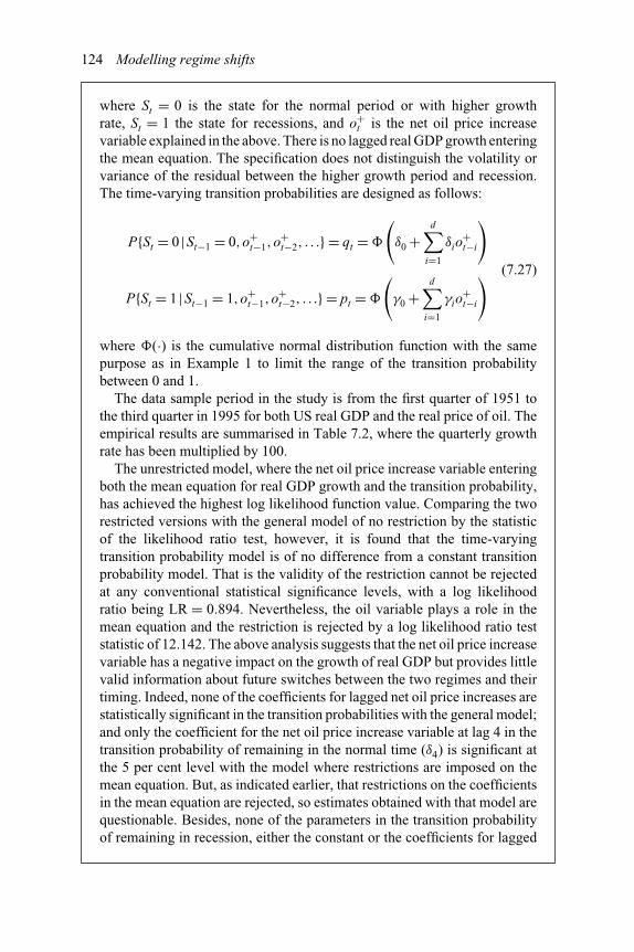
124 Modelling regime shifts
where St = 0 is the state for the normal period or with higher growthrate, St = 1 the state for recessions, and o+
t is the net oil price increasevariable explained in the above. There is no lagged real GDP growth enteringthe mean equation. The specification does not distinguish the volatility orvariance of the residual between the higher growth period and recession.The time-varying transition probabilities are designed as follows:
P{St = 0 |St−1 = 0,o+t−1,o+
t−2, . . .} = qt = �
(δ0 +
d∑i=1
δio+t−i
)
P{St = 1 |St−1 = 1,o+t−1,o+
t−2, . . .} = pt = �
(γ0 +
d∑i=1
γio+t−i
) (7.27)
where �(·) is the cumulative normal distribution function with the samepurpose as in Example 1 to limit the range of the transition probabilitybetween 0 and 1.
The data sample period in the study is from the first quarter of 1951 tothe third quarter in 1995 for both US real GDP and the real price of oil. Theempirical results are summarised in Table 7.2, where the quarterly growthrate has been multiplied by 100.
The unrestricted model, where the net oil price increase variable enteringboth the mean equation for real GDP growth and the transition probability,has achieved the highest log likelihood function value. Comparing the tworestricted versions with the general model of no restriction by the statisticof the likelihood ratio test, however, it is found that the time-varyingtransition probability model is of no difference from a constant transitionprobability model. That is the validity of the restriction cannot be rejectedat any conventional statistical significance levels, with a log likelihoodratio being LR = 0.894. Nevertheless, the oil variable plays a role in themean equation and the restriction is rejected by a log likelihood ratio teststatistic of 12.142. The above analysis suggests that the net oil price increasevariable has a negative impact on the growth of real GDP but provides littlevalid information about future switches between the two regimes and theirtiming. Indeed, none of the coefficients for lagged net oil price increases arestatistically significant in the transition probabilities with the general model;and only the coefficient for the net oil price increase variable at lag 4 in thetransition probability of remaining in the normal time (δ4) is significant atthe 5 per cent level with the model where restrictions are imposed on themean equation. But, as indicated earlier, that restrictions on the coefficientsin the mean equation are rejected, so estimates obtained with that model arequestionable. Besides, none of the parameters in the transition probabilityof remaining in recession, either the constant or the coefficients for lagged

Modelling regime shifts 125
Table 7.2 Estimation of US real GDP with a time-varying transition probabilityMarkov switching model: 51Q1–95Q3
Restricted: oil has noeffect on transitionprobabilities
Restricted: oil has noeffect in the meanequation
No restrictions:the general model
α0 1.066∗∗∗(0.097)
0.929∗∗∗(0.076)
1.018∗∗∗(0.081)
α0 +α1 −0.068(0.310)
−0.593∗∗(0.294)
−0.081(0.341)
β1 −0.031∗∗∗(0.012)
– −0.026∗∗(0.012)
β2 −0.013(0.012)
– −0.008(0.013)
β3 −0.027∗∗(0.012)
– −0.032∗∗∗(0.013)
β4 −0.046∗∗∗(0.011)
– −0.021(0.014)
δ0 1.484∗∗∗(0.375)
1.866∗∗∗(0.322)
1.750∗∗∗(0.361)
δ3 – −0.053(0.069)
−0.044(0.051)
δ4 – −0.154∗∗(0.073)
−0.139(0.090)
γ0 0.334(0.387)
1.012(1.008)
0.779(0.704)
γ3 – 0.918(0.846)
0.948(1.043)
γ4 – −0.485(0.344)
−0.502(0.410)
σε 0.714∗∗∗(0.050)
0.753∗∗∗(0.047)
0.732∗∗∗(0.048)
Loglikelihood
−209.320 −214.944 −208.873
∗∗significant at the 5 per cent level; ∗∗∗significant at the 1 per cent level. Standard errors inparentheses.
oil price increases, are statistically significant. This is consistent with thefindings in Example 7.1.
From applying equation (7.27) and the estimates in Table 7.2, q, theaverage transition probability of remaining in the normal period, is 0.931;and p, the average transition probability of remaining in recession, is0.631. The average duration of being in normal times is 1/(1 − q) =1/(1 − 0.931) ≈ 14.5 quarters or slightly more than 3.5 years. The duration
Continued

126 Modelling regime shifts
of an average recession is 1/(1 − p) = 1/(1 − 0.631) ≈ 2.7 quarters.These durations, especially the duration of normal periods, are relativelyshorter than those in Example 7.1 with the UK case. The difference maysuggest that the UK economy has a longer duration of normal periods butsuffers more severely in recessions, or arise from the sensitivity of theparameters to estimation procedures and data sets.
7.6. Empirical literature
Markov switching approaches have attracted much attention in financial andeconomic modelling in recent years, due to business cycle characteristics high-lighted in macroeconomics and monetary economics, and a changing businessand investment environment featured by bull–bear market alternations in financialstudies. Collectively, these cyclical movements can be termed as regime shifts,common to most modern market economies. As the Markov switching modelclearly defines two or more states or regimes, it can reveal the dynamic process ofthe variables of concern vividly and provide the researcher and policy maker witha clue of how these variables have evolved in the past and how they may change inthe future. Nevertheless, the implementation and execution of a Markov switchingmodel, though not complicated, may be technically difficult as it is rather sensitiveto the choice of initial values, other settings such as the lag length, and even thedata sample.
Stock market behaviour is one of the areas to which Markov switching has beenwidely applied. In a paper entitled ‘Identifying bull and bear markets in stockreturns’, Maheu and McCurdy (2000) use a Markov switching model to classifyreturns into a high-return stable state and a low-return volatile state. They callthe two states bull and bear markets respectively. Using 160 years’ US monthlydata, they find that bull markets have a declining hazard function although thebest market gains come at the start of a bull market. Volatility increases withduration in bear markets. Driffill and Sola (1998) investigate whether there isan intrinsic bubble in stock prices so that stock prices deviate from the valuespredicted by the present value model or deviate from the fundamental relationshipbetween income and value. They claim that a Markov switching model is a moreappropriate representation of dividends. Allowing for dividends to switch betweenregimes they show that stock prices can be better explained than by the bubblehypothesis. When both the bubble and the regime switching in the dividendprocess are considered, the incremental explanatory contribution of the bubbleis low. Assoe (1998) examines regime switching in nine emerging stock marketreturns. The author claims that changes in government policies and capital marketreforms may lead to changes in return generating processes of capital markets.The results show strong evidence of regime switching behaviour in emerging
Modelling regime shifts 127
stock market returns with regard to volatility which foreign investors concernmost. Other research includes Dewachter and Veestraeten (1998) on jumps inasset prices which are modelled as a Markov switching process in the traditionof event studies; Scheicher’s (1999) investigation into the stock index of theVienna Stock Exchange with daily data from 1986 to 1992, adopting Markovswitching and GARCH alternatives; and So et al. (1998) who examine the S&P500weekly return data with the Markov switching approach to modelling stochasticvolatility, and identified high, medium, and low volatility states associated with thereturn data.
The business and investment environment can be reasonably characterised byswitching between different regimes as well. In this regard, Asea and Blomberg(1998) investigate the lending behaviour of banks over lending cycles, using theMarkov switching model with a panel data set consisting of approximately twomillion commercial and industrial loans granted by 580 banks between 1977 and1993. They demonstrate that banks change their lending standards from tightnessto laxity systematically over the cycle. Town (1992), based on the well observedphenomenon that mergers take place in waves, fits the merger data into a Markovswitching model with shifts between two states of high and low levels of activityand claims improvements over ARIMA models.
The changing pattern of interest rates is indicative of business cycle conditionsand could be subject to regime shifts itself. To investigate how real interest ratesshift, Bekdache (1999) adopts a time varying parameter model with Markovswitching conditional heteroscedasticity to capture two sources of shifts in realinterest rates: shifts in the coefficients and shifts in the variance. The former relatesthe ex ante real rate to the nominal rate, the inflation rate and a supply shockvariable, and the latter is unconditional shifts in the variance of the stochasticprocess. The results prefer a time varying parameter model to Markov switchingwith limited states. Dewachter (1996) studies interest rate volatility by examiningboth regime shifts in the variance and links between volatility and levels of theinterest rate. While regime shifts are found in the variance, the contribution ofvolatility-level links cannot be ignored. The above findings suggest that univariateor single element regime shifts in interest rate modelling fail to fully characteriseinterest rate dynamics.
Probably the majority of applied research is in the area of business cycles whererecent studies are still burgeoning. In addition to classifying the economy intotwo states of booms and recessions, Kim and Nelson (1999) further investigatewhether there has been a structural break in post-war US real GDP growthtowards stabilisation. They employ a Bayesian approach to identifying a structuralbreak at an unknown change-point in a Markov-switching model. Their empiricalresults suggest a break in GDP growth toward stabilisation at the first quarterof 1984, and a narrowing gap between growth rates during recessions andbooms. Filardo and Gordon (1998) specify a time varying transition probabilitymodel where the information contained in leading indicator is used to forecasttransition probabilities and, in turn, to calculate expected business cycle durations.
128 Modelling regime shifts
Both studies employ Gibbs sampling techniques. Other research in the categorycovers Diebold et al. (1993), Filardo (1994), Ghysels (1994), Luginbuhl andde Vos (1999), Kim and Yoo (1996), and Raymond and Rich (1997) as illustratedin Example 7.2.
It should be noted that the empirical application of Markov switching modelsis not always superior to an alternative or simple model, and is not withoutdeficiencies. Aware of these problems, Boldin (1996) explores the robustness ofHamilton’s (1989) two-regime Markov switching model framework. ApplyingHamilton’s exact specification to a revised version of real GNP, the authorfinds that parameter estimates are similar to those reported by Hamilton onlywhen the author uses the same sample period (1952–1984) and a particularset of initial values for the maximum likelihood procedure. Two other localmaximums exist that have higher likelihood values, and neither correspond tothe conventional recession–expansion dichotomy. When the sample period isextended, there is no longer a local maximum near the parameter set reportedby Hamilton. Exploring the model and data further, the author rejects cross-regime restrictions of Hamilton specification, but also finds that relaxing theserestrictions increases the number of local maximums. In a study on the predictionof US business cycle regimes, Birchenhall et al. (1999) compare the use oflogistic classification methods and Markov switching specifications for theidentification and prediction of post-war US business cycle regimes as definedby the NBER reference turning point dates. They examine the performanceof logistic procedures in reproducing the NBER regime classifications and inpredicting one and three months ahead growth rates using leading indicatorvariables. They show that the logistic classification model provides substantiallymore accurate business cycle regime predictions than the Markov switchingmodel. Nevertheless, as said at the beginning of this chapter, one of the majorcontributions the Markov switching approach made is probably to help improveour understanding about an economic process. This may partly explain itscontemporary popularity. In addition to above discussed empirical literature, avariety of applications can be further found in foreign exchange rates, bond yields,inflation, and so on.
Questions and problems
1 Describe the state and the state transition probability in a Markov chain.2 What is the Chapman–Kolmogorov equation for calculating multi-step
transition probabilities?3 Cite examples of economic and financial variables which can be shown as a
Markov process.4 What is smoothing is the estimation of a Markov process? Why is smoothing
required?5 Discuss the advantages of adopting time-varying transition probabilities in
the Markov process.
Modelling regime shifts 129
6 Collect data from various sources, and estimate a two-state constant transitionprobability model in the following time series (using RATS, GAUSS or otherpackages):
(a) industrial production of selected countries,(b) CPI of the G7,(c) GDP of the US, Argentina, France, Algeria, and India.
7 Estimate a two-state time-varying transition probability model in the abovetime series.
References
Asea, P.K. and Blomberg, B. (1998), Lending cycles, Journal of Econometrics, 83(1–2),89–128.
Assoe, K.G. (1998), Regime-switching in emerging stock market returns, MultinationalFinance Journal, 2(2), 101–132.
Bekdache, B. (1999), The time-varying behaviour of real interest rates: a re-evaluation ofthe recent evidence, Journal of Applied Econometrics, 14(2), 171–190.
Birchenhall, C.R., Jessen, H., Osborn, D.R. and Simpson, P. (1999), PredictingU.S. business-cycle regimes, Journal of Business and Economic Statistics, 17(3),313–323.
Boldin, M.D. (1996), A check on the robustness of Hamilton’s Markov switching modelapproach to the economic analysis of the business cycle, Studies in Nonlinear Dynamicsand Econometrics, 1(1), 35–46.
Dewachter, H. (1996), Modelling interest rate volatility: regime shifts and level links,Weltwirtschaftliches Archiv, 132(2), 236–258.
Dewachter, H. and Veestraeten, D. (1998), Expectation revisions and jumps in asset prices,Economics Letters, 59(3), 367–372.
Diebold, F.X., Lee, J.H. and Weinbach, G.C. (1993), Regime switching with time varyingtransition probabilities, Federal Reserve Bank of Philadelphia Research Working Paper,93–12.
Driffill, J. and Sola, M. (1998), Intrinsic bubbles and regime-switching, Journal of MonetaryEconomics, 42(2), 357–373.
Filardo, A.J. (1994), Business cycle phases and their transitional dynamics, Journal ofBusiness and Economic Statistics, 12(3), 299–308.
Filardo, A.J. and Gordon, S.F. (1998), Business cycle durations, Journal of Econometrics,85(1), 99–123.
Ghysels, E. (1994), On the periodic structure of the business cycle, Journal of Business andEconomic Statistics, 12(3), 289–298.
Hamilton, J.D. (1989), A new approach to the economic analysis of nonstationary timeseries and the business cycle, Econometrica, 57(2), 357–384.
Hamilton, J.D. (1994), Time Series Analysis, Princeton University Press, Princeton,New Jersey.
Hamilton, J.D. (1996), This is what happened to the oil price-macroeconomy relationship,Journal of Monetary Economics, 38, 215–220.
Kim, C.J. and Nelson, C.R. (1999), Has the U.S. economy become more stable? a Bayesianapproach based on a Markov-switching model of the business cycle, Review of Economicsand Statistics, 81(4), 608–616.

130 Modelling regime shifts
Kim, M.J. and Yoo, J.S. (1996), A Markov switching factor model of coincident and leadingindicators, Journal of Economic Research, 1(2), 253–72.
Luginbuhl, R. and de Vos, A. (1999), Bayesian analysis of an unobserved-componenttime series model of GDP with Markov-switching and time-varying growths, Journal ofBusiness and Economic Statistics, 17(4), 456–465.
Maheu, J.M. and McCurdy, T.H. (2000), Identifying bull and bear markets in stock returns,Journal of Business and Economic Statistics, 18(1), 100–112.
Raymond, J.E. and Rich, R.W. (1997), Oil and the macroeconomy; a Markov state-switchingapproach, Journal of Money, Credit, and Banking, 29(2), 193–213.
Scheicher, M., (1999), Nonlinear dynamics: evidence for a small stock exchange, EmpiricalEconomics, 24, 45–59.
So, M.K.P., Lam, K. and Li, W.K. (1998), A stochastic volatility model with Markovswitching, Journal of Business and Economic Statistics, 16(2), 244–253.
Town, R.J. (1992), Merger waves and the structure of merger and acquisition time series,Journal of Applied Econometrics, 7(supplement), S83–100.

8 Present value models and tests forrationality and market efficiency
The present value model states that the present value of an asset is derived fromits earning power, or the ability to generate future income. This crucially dependson the expectations about future income and the discount rate at which people orinvestors would sacrifice a portion of their current income for future consumption,after adjusting for uncertainty or risk involved in the process. Although the presentvalue of an asset, or economic value, as against accounting value, is the best toreflect its true value, it involves expectations on future income, the discount rateand rationality of people. Therefore the present value model is difficult to applyproperly in practice. To link the present value of an asset to its future income in theframework of cointegration analysis, as proposed by Campbell and Shiller (1987),has provided a useful tool for testing expectations and rationality in financialmarkets.
8.1. The basic present value model and its time seriescharacteristics
The present value of an asset is its all future income discounted:
Vt =∞∑
τ=1
1
(1 + rt) · · · (1 + rt+τ )EtIt+τ (8.1)
where Vt is the present value of the asset, It+1 is income derived from possessingthis asset in period (t, t+1], Et is expectations operator, and rt is the discount ratein period (t, t+1].
When the discount rate is constant, i.e., rt = r, equation (8.1) becomes:
Vt =∞∑
τ=1
1
(1 + r)τEtIt+τ (8.1′)
Subtracting Vt/(1 + r) from both sides leads to:
Vt −Vt
1 + r=
∞∑τ=1
1
(1 + r)τEtIt+τ −
∞∑τ=1
1
(1 + r)τEtIt+τ−1+
It
1 + r
132 Present value models and tests for rationality and market efficiency
Re-arrangement of the above yields:
Vt −It
r= 1 + r
r
∞∑τ=1
1
(1 + r)τEt�It+τ (8.2)
Equation (8.2) states that if Vt and It+1 are I (1) series, then a linear combinationof them is stationary too and the two series are cointegrated. Campbell andShiller (1987) define (Vt − It)/r as spread, St . Obviously, the spread links a stockvariable, Vt , to a flow variable, It . It is not strange that a flow variable divided bythe rate of flow (in this case r) is a stock variable; or a stock variable times therate of flow is a flow variable. If income is constant over time, then total wealthor value of an asset is simply the current income flow divided by the rate at whichincome is generated, i.e., the spread is equal to zero. Otherwise, the spread is afunction of the expected changes in future incomes discounted. A positive spreadreflects an overall growth in future incomes, and a negative spread is associatedwith income declines.
Nevertheless, the seemingly stationarity of the right-hand side in equation (8.2)is problematic, or at least unrealistic. The growth or change in income as expressedin equation (8.2) is in an absolute term, It − It−1, instead of a relative term,(It − It−1)/It−1. Let us adopt a version of the Gordon dividend growth model:
Vt =∞∑
τ=1
EtIt+τ
(1 + r)τ=
∞∑τ=1
(1 + g)τ It(1 + Etut+τ )
(1 + r)τ(8.3)
subtracting (1 + g)Vt/(1 + r) from both sides, we have:
Vt −(1 + g)Vt
1 + r=
∞∑τ=1
(1 + g)τ It(1 + Etut+τ )
(1 + r)τ−
∞∑τ=1
(1 + g)τ It(1 + Etut+τ−1)
(1 + r)τ
+ (1 + g)It
1 + r
and re-arrangement yields:
Vt −(1 + g)It
r − g= 1 + r
r − g
∞∑τ=1
(1 + g)τ Et�ut+τ
(1 + r)τ(8.4)
where �ut+τ = � ln It+τ − g. Equation (8.4) reduces to the Campbell and Shiller(1987) formulation when g = 0. �It is in general non-stationary.
Define Vt −[(1 + g)It/(r − g)] as the full spread, Sf t . Equation (8.4) says totalwealth or value of an asset is simply the current income flow (notice It+1 = (1+g)It
is the income in the current period) divided by, instead of the discount rate, thedifference between the discount rate and the growth rate. Equation (8.4) is, infact, the Gordon valuation model for constant growing perpetuities. The important

Present value models and tests for rationality and market efficiency 133
message here is that there exists a cointegration or long-run relationship betweenthe value and the income, as revealed by equations (8.2) and (8.4). Moreover, ifincome obeys a constant growth process, the spread in the sense of Campbell andShiller (1987) is not stationary, but the full spread as defined above is stationary.Therefore, caution has to be taken in explaining and interpreting the cointegrationvector. If (1+g)/(r−g) is mistaken as 1/r, then (r−g)/(1+g) might be mistakenas the discount rate r and the practice would under estimate the true discount rateif there is growth in income.1 Later in this chapter, we will see how to imposerestrictions and carry out empirical tests.
Equation (8.2) can also be written as:
St = Vt −1
rIt = 1 + r
rEt�Vt+1 (8.5)
If there is a rational bubble bt , satisfying:
bt = 1
1 + rEtbt+1
i.e.:
bt+1 = (1 + r)bt + ζt+1, ζt ∼ iid(0,σ 2ζ ) (8.6)
in equation (8.1′), it will appear on the right-hand side of equation (8.2), but willnot appear on the right-hand side of equation (8.5). bt has a root outside the unitcircle and is explosive or non-stationary. Consequently, even if �It is stationary,the spread is non-stationary if there is a rational bubble in equation (8.1′), inducingnon-stationarity in �Vt through equation (8.5). Therefore, testing for rationality isequivalent to testing for cointegration between the present value variable, Vt , andthe income variable, It .
8.2. The VAR representation
Equations (8.2) and (8.5) also suggest a way to compute the variables in aVAR (I assume I had introduced such terminologies in earlier chapters). Letzt = [St . . . St−p+1 �It . . . �It−p+1
]′, the VAR can be written in the companion
form:[St
�It
]=[a11(L) a12(L)a21(L) a22(L)
][St−1�It−1
]+[μ1t
μ2t
](8.7)
where
St = [St . . . St−p+1
]′, �It = [�It . . . �It−p+1
]′μ1t = [ν1t 0 . . .
]′, μ2t = [ν2t 0 . . .
]′

134 Present value models and tests for rationality and market efficiency
a11(L) =
⎡⎢⎢⎣
a11,1 . . . . . . a11,p
1 . . .
. . .
1
⎤⎥⎥⎦ , a12(L) =
⎡⎢⎢⎣
a12,1 . . . . . . a12,p
0 . . .
. . .
0
⎤⎥⎥⎦
a21(L) =
⎡⎢⎢⎣
a21,1 . . . . . . a21,p
0 . . .
. . .
0
⎤⎥⎥⎦ , a22(L) =
⎡⎢⎢⎣
a22,1 . . . . . . a22,p
1 . . .
. . .
1
⎤⎥⎥⎦
Or, in a compact form:
zt = Azt−1 +μt (8.8)
The implication of this representation is that the spread, St , must linearly Grangercause �It , unless St is itself an exact linear combination of current and lagged �It .Therefore, St would have incremental predicting power for �It . Further, let e1′ ande2′ be (1 × 2p) row vectors with zero in all cells except unity in the first elementfor the former and in the (p + 1) element for the latter, respectively, i.e.:
St = e1′zt (8.9)
�It = e2′zt (8.10)
Notice:
E{zt+k |Ht
}= Akzt (8.11)
where Ht is the information set with all available information about St and �It attime t. Applying equations (8.9), (8.10) and (8.11) to (8.2) yields:
e1′zt = 1
r
∞∑i=1
1
(1 + r)i e2′Aizt = e2′ 1
r(1 + r)A
[I − 1
1 + rA
]−1
zt (8.12)
Equation (8.12) imposes restrictions on the VAR parameters if rationality is tohold, i.e.:
e1′[I − 1
1 + rA
]= e2′ 1
r(1 + r)A (8.13)
Accordingly, the ‘theoretical’ spread can be introduced as:
S∗t = e2′ 1
r(1 + r)A
[I − 1
1 + rA
]−1
zt (8.14)
Present value models and tests for rationality and market efficiency 135
It can be seen that the difference between the actual and ‘theoretical’ spreads is:
St − S∗t =
∞∑i=1
1
(1 + r)i E(ξt+i |Ht) (8.15)
where ξt = Vt −[(1 + r)Vt−1 − It
]= Vt − Et−1Vt is the innovation in forecastingVt . Testing the restrictions in equation (8.13) is equivalent to testing that the right-hand side of equation (8.15) is just white noise with a mean of zero. Also, usingvolatility test, the variance ratio var(St)/var(S∗
t ) should not be significantly largerthan unity if the present value model is to hold. In addition, volatility test can becarried out with the innovation ξt and the innovation in the expected present value:
ξ ∗t ≡ 1
r
∞∑i=0
1
(1 + r)i
[E(�It+i |Ht) − E(�It+i |Ht−1)
]
= S∗t − (1 + r)S∗
t−1 + 1
r�It
(8.16)
The variance ratio var(ξt )/var(ξ ∗t ) can be viewed as the ‘innovation variance ratio’,
and var(St)/var(S∗t ) as the ‘level variance ratio’. Notice ξt can also be written in
the similar expression of equation (8.16):
ξt ≡ Vt −[(1 + r)Vt−1 − It
]= Vt −
1
rIt+1 + 1
rIt+1 − (1 + r)Vt−1 + (1 + r)It −
1
rIt
= St − (1 + r)St−1 + 1
r�It+1 (8.17)
The implications of the above equations can be summarised in the following.If the market is rational for an asset, then its value/price and income variablesshould be cointegrated and its spread should be stationary. Without a cointegrationrelation between the price and income, the spread is non-stationary and a ‘rationalbubble’, which by definition is explosive, would exist in the market. If the marketis efficient and the present value model holds, then the ‘theoretical’ spread shouldnot systematically differ from the actual spread, and both variance ratios shouldnot be significantly larger then unity. The prediction power of the spread for �It isconditional on agents’ information set. If agents do not have information useful forpredicting �It beyond the history of �It , then St is a linear combination of currentand lagged �It without prediction ability. Prediction may or may not be improvedsimply because the price and income variables are cointegrated. Therefore, inthis chapter, we use cointegration between the price and income as a criterionfor rationality against the existence of bubble in the market. In addition, we usethe VAR representation and the variance ratios derived from the VAR system toexamine whether the present value model holds and how far the market is fromefficient.
136 Present value models and tests for rationality and market efficiency
8.3. The present value model in logarithms with time-varyingdiscount rates
The previous section has shown that a ratio relationship between the value andincome variables is more appropriate than a ‘spread’ relationship between thetwo variables, in the context of a constant discount rate and growth in income. Asmost economic and financial variables grow exponentially, linear relationships areonly appropriate for variables in their logarithm, not for variables in their originalform. This is equivalent to say that variables in their original form have ratiorelationships, instead of linear relationships. In a sense, a right modelling strategyreflects impeccably both the economic and financial characteristics and the datagenerating process and makes these two considerations fit into each other. In thissection, we further generalise the present value model along this line and allowfor a time-varying rate of return or discount rate in the model.
In this section, we deliberate value, income and their relationship in a contextof stock market investment explicitly, i.e., value and income variables arecharacterised by observable share prices and dividends. Let us express the rateof total return in the logarithm form:
rt = ln
(Pt+1 + Dt+1
Pt
)(8.18)
Notice rt is an approximation of the exact rate of total return. However, thisexpression is in common with general practice and leads, conventionally, to thelinear relationship among all variables involved.
As already known, total return can be split into price appreciation and thedividend yield. The idea is also valid in the log-linear form. To see this, expandingequation (8.18) as:
rt = ln
(Pt+1 +Dt+1
Pt
)= ln
[Pt+1
Pt
(1+ Dt+1
Pt+1
)]= ln
(Pt+1
Pt
)+ln
(1+ Dt+1
Pt+1
)
≈(lnPt+1 −lnPt
)+ Dt+1
Pt+1
=(pt+1 −pt
)+e(dt+1−pt+1) (8.19)
where, pt = lnPt , and dt = lnDt . The first term on the right-hand side is priceappreciation, and the last term on the right-hand side reflects the dividend yield(notice the exact dividend yield is Dt+1/Pt). As the last term on the right-hand sideis not linear, further transformation and approximation are required. Finally, aftera series of development, the rate of total return can be expressed as:
rt ≈ κ + (1 − l)pt+1 − pt + ldt+1 (8.20)
where l = e(d−p)′ = (D/P)′ is a constant between the minimum and maximumdividend yields, and κ = (d − p)′ e(d−p)′ = ln (D/P)′ × (D/P)′ is also a constant.

Present value models and tests for rationality and market efficiency 137
With the rate of total return, price and dividend being linked in a log-linearrelationship as in equation (8.20), it is now possible to express the present valuemodel in a log-linear form too. Furthermore, no restriction on the rate of return rt
to be constant is required to derive the log-linear form present value model. Thus,the model could accommodate the time-varying rate of return or discount rate andis more general and closer to reality.
Solving equation (8.20) forward, we obtain:
pt = κ
l+
T∑τ=0
{(1 − l)τ
(ldt+1+τ − rt+τ
)}+ (1 − l)T pT+1 (8.21)
when T → ∞, the last term on the right-hand side → 0, and equation (8.21)
pt = κ
l+
∞∑τ=0
(1 − l)τ(ldt+1+τ − rt+τ
)(8.22)
Equation (8.22) is the log-linear counterpart of equation (8.1), and is notadvantageous compared with the latter. Both are able to deal with the time-varying discount rate, but equation (8.1) is exact whereas equation (8.22) isan approximation. However, the benefit would be seen when the value–incomeor price–dividend relationship is examined. Extracting dt from both sides ofequation (8.22) and re-arrangement yield:
pt − dt = − (dt − pt) = κ
l+
∞∑τ=0
(1 − l)τ(�dt+1+τ − rt+τ
)(8.23)
It can be observed that if dt is I (1) and rt is I (0), the left-hand side of equation (8.23)is also I (0), or stationary. That is, the price and dividend in their logarithm arecointegrated. Notice no conditions are placed on rt to derive the cointegrationrelationship, in contrast with equation (8.2). This is obviously advantageous,compared with the ‘spread’ form specification.
Equations (8.22) and (8.23) are derived as ex post, but they also hold ex ante.Taking expectations operations on both sides of equations (8.22) and (8.23), wehave:
pt = κ
l+ Et
{ ∞∑τ=0
(1 − l)τ(ldt+1+τ − rt+τ
)}(8.22′)
and:
pt − dt = − (dt − pt) = κ
l+ Et
{ ∞∑τ=0
(1 − l)τ(�dt+1+τ − rt+τ
)}(8.23′)
Previously in section 8.1, we have shown that value (price) and income (dividend)would be cointegrated with a cointegration vector [1, −1/r], if the absolute changes
138 Present value models and tests for rationality and market efficiency
in income are stationary or constant. If the income stream has a constant growthrate, instead of constant absolute increase, then they would be cointegrated witha cointegration vector [1, −1/(r − g)]. Recall the derivation of a cointegrationrelationship is dependent on rt ≡ r, so the cointegration relationship is ratherrestrictive. With the log-linear form present value model, the cointegration vectoris always [1, −1]. The proportional relation for the price and dividend is reflectedby the constant and variables on the right-hand side of equation (8.23) orequation (8.23′), which are time-varying in general. The cointegration betweenprice and dividend is not affected by whether the discount rate is assumed to beconstant or not as in section 8.1. As we know prices, dividends and most financialvariables grow exponentially, there should be a log-linear relationship among them.Consequently, models in the log-linear form are generally sound, financially andstatistically.
8.4. The VAR representation for the present value model inthe log-linear form
The VAR representation of the log-linear form is similar to that of the originalform. Let zt = [st . . . st−p+1 rt −�dt+1 . . . rt−p −�dt−p+1
]′, where st = dt −pt .
st is, roughly, the log dividend yield (the exact log divided yield is dt+1 − pt).Compared with section 8.2, the spread St is replaced by the log-dividend yield,and the absolute changes in dividends are replaced by the difference between thepercentage changes in dividends and the discount rate (Recall, in sections 8.1and 8.2, rt is restricted to a constant and did not appear in the zt vector). With thesame A matrix as in section 8.2, the compact form is:
zt = Azt−1 +μt (8.8′)
The selecting vector e1 picks up st from zt and the following holds, conditionalon Ht , the information in the VAR:
st = e1′zt =∞∑
τ=0
(1 − l)τ e2′Aτ+1zt = e2′A[I − (1 − l)A
]−1zt (8.24)
Therefore:
e1′ = e2′A[I − (1 − l)A
]−1(8.25)
or:
e1′ [I − (1 − l)A]− e2′A = 0 (8.26)
The log dividend yield satisfying the conditions in equation (8.25) or equa-tion (8.26) is the theoretical log dividend yield, written as s∗
t . Notice again thereare no restrictions imposed on rt , so tests on the validity of the present value model
Present value models and tests for rationality and market efficiency 139
in the log-linear form are not subject to the assumption about the discount rate.That is, the present value model can be accepted or rejected no matter the discountrate is treated as time-varying or not. The variance ratio test on s∗
t and st can becarried out to examine whether the present value model holds.
Furthermore, dividend volatility and return volatility can also be tested,respectively. If the discount rate is constant over time, it could be excluded from thezt vector, and the theoretical log dividend yield with a constant discount rate, s∗
d,t , isobtained. The hypothesis for a constant discount rate is Hr0: s∗
d,t = s∗t . In a separate
study, Campbell and Shiller (1989) reject constant discount rate in the US stockmarket, employing the Cowles/S&P data set (1871–1986) and the NYSE data set(1926–1986). In a similar way, if �dt = g, i.e., the dividend growth is constant,then �dt can be excluded from the zt vector too, and the theoretical log dividendyield with the constant dividend growth, s∗
r,t , emerges. The hypothesis for dividendgrowth to be constant is Hd0: s∗
r,t = s∗t , though it has little financial meaning. The
variance ratio test can also be employed to test these two hypotheses.
8.5. Variance decomposition
As returns may be volatile, we are interested in the sources of volatility.Substituting equation (8.22′) into equation (8.20) yields an expression forinnovation in the total rate of return:
rt − Et
{rt
}= Et+1
{ ∞∑τ=0
(1 − l)τ �dt+1+τ
}− Et
{ ∞∑τ=0
(1 − l)τ �dt+1+τ
}
−[
Et+1
{ ∞∑τ=1
(1 − l)τ rt+τ
}− Et
{ ∞∑τ=1
(1 − l)τ rt+τ
}](8.27)
Equation (8.27) can be written in compact notations, with the left-hand side termbeing νt , the first term on the right-hand side ηd,t , and the second term on theright-hand side ηr,t :
νt = ηd,t −ηr,t (8.28)
where νt is the innovation or shock in total returns, ηd,t represents the innovationdue to changes in expectations about future income or dividends, andηr,t representsthe innovation due to changes in expectations about future discount rates or returns.
Again, we use VAR to express the above innovations. Vector zt contains, firstof all, the rate of total return or discount rate. Other variables included are relevantto forecast the rate of total return:
zt = Azt−1 + εt (8.29)
with the selecting vector e1 which picks out rt from zt , we obtain:
νt = rt − Et
{rt
}= e1′εt (8.30)

140 Present value models and tests for rationality and market efficiency
Bring equations (8.29) and (8.30) into the second term on the right-hand side ofequation (8.27) yields:
ηr,t = Et+1
{ ∞∑τ=1
(1 − l)τ rt+τ
}− Et
{ ∞∑τ=1
(1 − l)τ rt+τ
}
= e1′∞∑
τ=1
(1 − l)τ Aτ εt = e1′ (1 − l)A[I − (1 − l)A
]−1εt (8.31)
While ηd,t can be easily derived according to the relationship in equation (8.28)as follows:
ηd,t = νt +ηr,t = e1′{I + (1 − l)A
[I − (1 − l)A
]−1}εt (8.32)
The variance of innovation in the rate of total return is the sum of the varianceof ηr,t , innovation due to changes in expectations about future discount rates orreturns, ηd,t , innovation due to changes in expectations about future income ordividends, and their covariance, i.e.:
σ 2ν = σ 2
η,d +σ 2η,r − 2cov(ηd,t,ηr,t) (8.33)
8.6. Examples and cases
The present value model discussed in this chapter has provided a powerful approachto modelling value–income or price–dividend relationships via exploiting theirtime series characteristics, namely, cointegration and restrictions on the VAR.In this section, several examples in financial markets and international eco-nomics and finance are presented to illustrate how the research is empiricallycarried out.
Example 8.1
This is a case in US stock market behaviour in Campbell and Shiller (1987).The price and dividend data were of annual frequency from 1971 to 1986in a broad stock index mainly represented by Standard and Poor’s withadjustments. The model used was in the original form, i.e., without logarithmoperations. The main results are summarised in Tables 8.1 and 8.2.
The unit root test, which uses one of the Perron–Phillips test statistics,confirms that the stock price and dividend are I (1) variables. The spread isstationary, when it is calculated with a discount rate of 3.2 per cent estimatedwith cointegration, but the spread is non-stationary when a discount rateof 8.2 per cent from the sample mean is applied. Based on these results,Campbell and Shiller suggest that a ‘rational bubble’ is not present but the
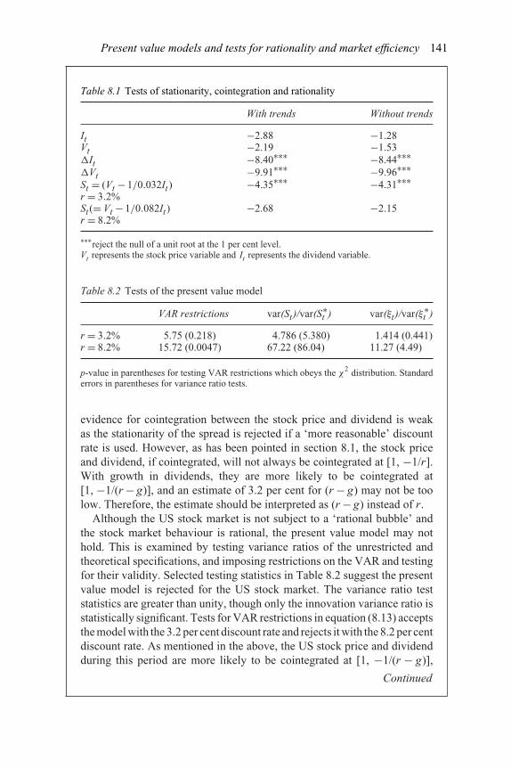
Present value models and tests for rationality and market efficiency 141
Table 8.1 Tests of stationarity, cointegration and rationality
With trends Without trends
It −2.88 −1.28Vt −2.19 −1.53�It −8.40∗∗∗ −8.44∗∗∗�Vt −9.91∗∗∗ −9.96∗∗∗St = (Vt − 1/0.032It) −4.35∗∗∗ −4.31∗∗∗r = 3.2%St(= Vt − 1/0.082It) −2.68 −2.15r = 8.2%
∗∗∗reject the null of a unit root at the 1 per cent level.Vt represents the stock price variable and It represents the dividend variable.
Table 8.2 Tests of the present value model
VAR restrictions var(St )/var(S∗t ) var(ξt )/var(ξ∗
t )
r = 3.2% 5.75 (0.218) 4.786 (5.380) 1.414 (0.441)r = 8.2% 15.72 (0.0047) 67.22 (86.04) 11.27 (4.49)
p-value in parentheses for testing VAR restrictions which obeys the χ2 distribution. Standard
errors in parentheses for variance ratio tests.
evidence for cointegration between the stock price and dividend is weakas the stationarity of the spread is rejected if a ‘more reasonable’ discountrate is used. However, as has been pointed in section 8.1, the stock priceand dividend, if cointegrated, will not always be cointegrated at [1, −1/r].With growth in dividends, they are more likely to be cointegrated at[1, −1/(r − g)], and an estimate of 3.2 per cent for (r − g) may not be toolow. Therefore, the estimate should be interpreted as (r − g) instead of r.
Although the US stock market is not subject to a ‘rational bubble’ andthe stock market behaviour is rational, the present value model may nothold. This is examined by testing variance ratios of the unrestricted andtheoretical specifications, and imposing restrictions on the VAR and testingfor their validity. Selected testing statistics in Table 8.2 suggest the presentvalue model is rejected for the US stock market. The variance ratio teststatistics are greater than unity, though only the innovation variance ratio isstatistically significant. Tests for VAR restrictions in equation (8.13) acceptsthe model with the 3.2 per cent discount rate and rejects it with the 8.2 per centdiscount rate. As mentioned in the above, the US stock price and dividendduring this period are more likely to be cointegrated at [1, −1/(r − g)],
Continued
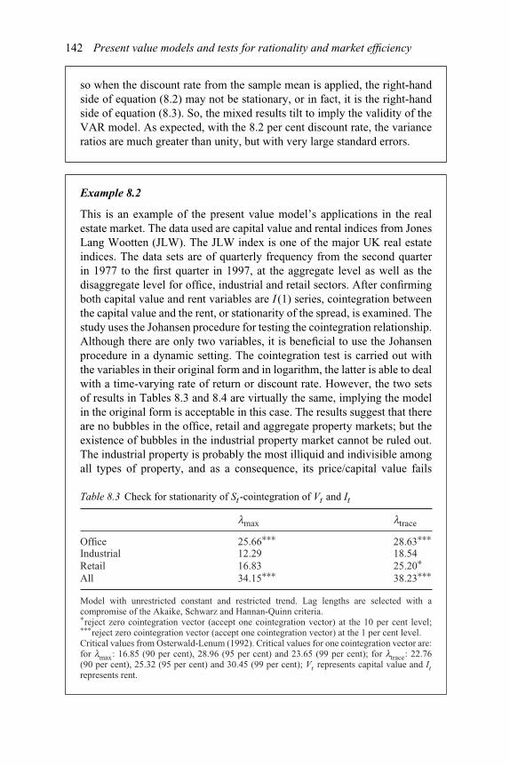
142 Present value models and tests for rationality and market efficiency
so when the discount rate from the sample mean is applied, the right-handside of equation (8.2) may not be stationary, or in fact, it is the right-handside of equation (8.3). So, the mixed results tilt to imply the validity of theVAR model. As expected, with the 8.2 per cent discount rate, the varianceratios are much greater than unity, but with very large standard errors.
Example 8.2
This is an example of the present value model’s applications in the realestate market. The data used are capital value and rental indices from JonesLang Wootten (JLW). The JLW index is one of the major UK real estateindices. The data sets are of quarterly frequency from the second quarterin 1977 to the first quarter in 1997, at the aggregate level as well as thedisaggregate level for office, industrial and retail sectors. After confirmingboth capital value and rent variables are I (1) series, cointegration betweenthe capital value and the rent, or stationarity of the spread, is examined. Thestudy uses the Johansen procedure for testing the cointegration relationship.Although there are only two variables, it is beneficial to use the Johansenprocedure in a dynamic setting. The cointegration test is carried out withthe variables in their original form and in logarithm, the latter is able to dealwith a time-varying rate of return or discount rate. However, the two setsof results in Tables 8.3 and 8.4 are virtually the same, implying the modelin the original form is acceptable in this case. The results suggest that thereare no bubbles in the office, retail and aggregate property markets; but theexistence of bubbles in the industrial property market cannot be ruled out.The industrial property is probably the most illiquid and indivisible amongall types of property, and as a consequence, its price/capital value fails
Table 8.3 Check for stationarity of St-cointegration of Vt and It
lmax ltrace
Office 25.66∗∗∗ 28.63∗∗∗Industrial 12.29 18.54Retail 16.83 25.20∗All 34.15∗∗∗ 38.23∗∗∗
Model with unrestricted constant and restricted trend. Lag lengths are selected with acompromise of the Akaike, Schwarz and Hannan-Quinn criteria.∗reject zero cointegration vector (accept one cointegration vector) at the 10 per cent level;∗∗∗reject zero cointegration vector (accept one cointegration vector) at the 1 per cent level.Critical values from Osterwald-Lenum (1992). Critical values for one cointegration vector are:for lmax: 16.85 (90 per cent), 28.96 (95 per cent) and 23.65 (99 per cent); for ltrace: 22.76(90 per cent), 25.32 (95 per cent) and 30.45 (99 per cent); Vt represents capital value and Itrepresents rent.

Present value models and tests for rationality and market efficiency 143
Table 8.4 Check for stationarity of st-cointegration between the logarithm of Vt(vt) and the logarithm of It (it)
lmax ltrace
Office 24.16∗∗∗ 26.98∗∗Industrial 14.67 17.66Retail 14.81 23.88∗All 28.67∗∗∗ 33.11∗∗∗
See notes in Table 8.3.∗reject zero cointegration vector (accept one cointegration vector) at the 10 per cent level;∗∗reject zero cointegration vector (accept one cointegration vector) at the 5 per cent level;∗∗∗reject zero cointegration vector (accept one cointegration vector) at the 1 per cent level.
to reflect its future income in transactions. Though this phenomenon isgenerally ruled as the existence of bubbles, it should not simply be madeequal to speculation. A ‘thin’ market for industrial property transactionsmay reasonably explain a large part of this particular statistical result for theindustrial property.
The validity of the present value model is examined and the testingstatistics are reported in Tables 8.5 and 8.6. The validity of the VAR modelis rejected in all types of properties except the office property. In general, thespread causes the change in the rent, implying that the spread can help predictfuture rent; but changes in rent do not cause the spread in the aggregateand industrial properties, and they cause the spread in the office and retailproperties at a lower significant level. The rejection of the VAR model isalso reflected in Table 8.6 for variance ratio tests. The ratio of the varianceof the spread to that of the ‘theoretical’ spread, i.e., the ‘levels variance
Table 8.5 Tests with the VAR model
St causes �It �It causes St Restrictions on VAR Q(18)
�It St
Office 17.6613∗∗∗ 3.3616∗∗ 1.1121 15.2080 14.2482Industrial 9.4856∗∗∗ 1.5721 2.5610∗∗∗ 17.9259 17.7638Retail 11.3278∗∗∗ 3.2626∗∗ 3.5616∗∗∗ 13.8085 10.6911All 23.3608∗∗∗ 2.0033 1.9635∗∗ 16.3478 11.8133
∗∗significant at the 5 per cent level; ∗∗∗significant at the 1 per cent level.Test statistics are F-test for causality test and restrictions on the VAR model, with respectivedegrees of freedom.Q(18) is the Ljung–Box statistic for serial correlation up to 18 lags, in the rent equation (�It )and the spread equation (St ) respectively.
Continued
144 Present value models and tests for rationality and market efficiency
Table 8.6 Variance ratios
var(St )/var(S∗t ) var(ξt )/var(ξ∗
t )
Office 144.82/66.29 = 2.1846∗∗∗ 73.96/39.95 = 1.8513∗∗∗Industrial 273.90/24.64 = 11.1161∗∗∗ 59.36/27.74 = 2.1399∗∗∗Retail 512.83/113.00 = 4.538∗∗∗ 207.76/53.07 = 3.9148∗∗∗All 184.15/85.19 = 2.1616∗∗∗ 67.34/33.23 = 2.0265∗∗∗
∗significantly different at the 10 per cent level; ∗∗∗significantly different at the 1 per cent level.
ratio’, is statistically significant in all types of properties. The ‘innovationvariance ratio’ is also significant in all the cases, but the value is usuallysmaller. Observing these statistical numbers in detail, it is found that theoffice property is the least inefficient with the smallest ‘innovation varianceratio’; and the industrial and retail properties are the most inefficient. Thisphenomenon is also reflected in the cointegration test, where capital valueand rent are not cointegrated for the industrial property, and capital valueand rent are cointegrated at a less significant level of 10 per cent for theretail property judged by the value of ltrace.
Example 8.3
The present value model with cointegration can also be applied tointernational economics and finance. An example is in MacDonald andTaylor (1993) on the monetary model for exchange rate determination. Weneed some transformation before getting the present value representationfor the monetary model. The flexible price monetary model is based on thefollowing three equations:
m′t − p′
t = γ y′t − li′t (8.34)
st = p′t (8.35)
i′t = Et
(�st+1
)= Et
(st+1
)− st (8.36)
where m′t is money supply, p′
t is price level, y′t is income, i′t is interest rate,
st is the exchange rate, γ is the income elasticity, and l is the interest rate(semi) elasticity. All variables are in the logarithm; and except the exchangerate, all variables are the difference between the domestic variable and theforeign variable, e.g., p′
t = pt − p∗t . Equation (8.34) states a relative money
market equilibrium requirement, equation (8.35) is the PPP (PurchasingPower Parity) condition, and equation (8.36) is the UIP (Uncovered

Present value models and tests for rationality and market efficiency 145
Interest rate Parity). Let xt = m′t − γ y′
t , then the exchange rate can beexpressed as:
st = p′t = xt + li′t = xt + l
(Et(st+1) − st
)(8.37)
or:
st = xt
1 + l+ l
1 + lEt(st+1) (8.38)
Equation (8.38) can be solved forward and lead to:
st =∞∑
τ=0
lτ
(1 + l)τ+1 Et(xt+τ+1) (8.39)
as: (l
1 + l
)T
Et(st+1) → 0 when T → ∞
Equation has the same structure as the present value model, and it is easy towork out the following ‘spread’:
st − xt =∞∑
τ=0
lτ
(1 + l)τEt(�xt+τ+1) (8.40)
Applying the same logic in section 8.1, the implication of equation (8.40) isthat the exchange rate and xt should be cointegrated and the ‘spread’ shouldbe stationary, if the monetary model is to hold and a rational bubble doesnot exist in the foreign exchange market.
MacDonald and Taylor use the Johansen procedure (Johansen 1988 andJohansen and Juselius 1990) for the cointegration test, as st −xt involve fivevariables. Using the exchange rate data for the deutsche mark vis-à-vis theUS dollar, they rule out rational bubbles in mark–dollar exchange market.However, with four estimates of l, they firmly reject the VAR model withthe imposed restrictions. These are summarised in Table 8.7.
Table 8.7 Tests of the VAR restrictions in the monetary model
VAR restrictions var(St )/var(S∗t )
l = 0.050 0.29 e + 07 (0.000) 0.11 e + 03 (0.000)l = 0.030 0.81 e + 07 (0.000) 0.30 e + 03 (0.000)l = 0.015 0.33 e + 08 (0.000) 0.12 e + 04 (0.000)l = 0.001 0.73 e + 10 (0.000) 0.29 e + 06 (0.000)
p-value in parentheses. Testing statistic for the VAR restrictions obeys χ2 distribution. The
variance ratio test employs the F-statistic.
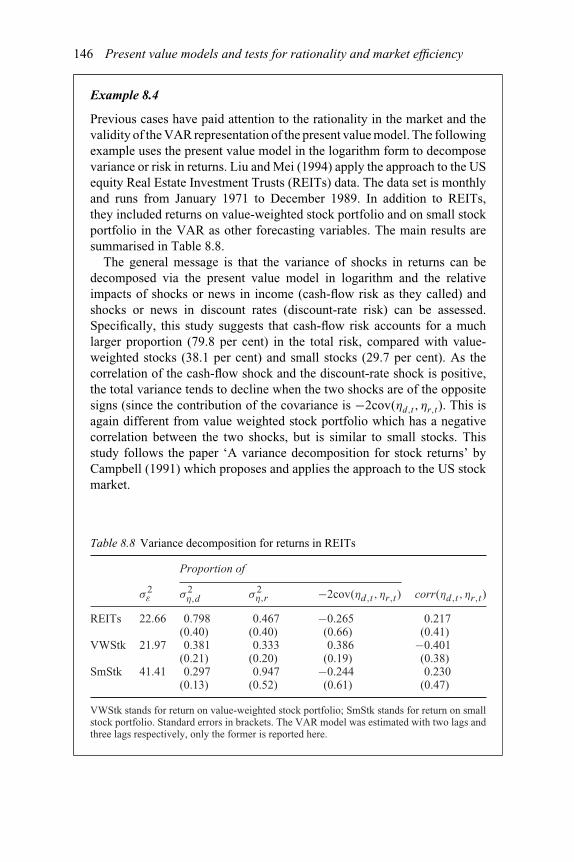
146 Present value models and tests for rationality and market efficiency
Example 8.4
Previous cases have paid attention to the rationality in the market and thevalidity of the VAR representation of the present value model. The followingexample uses the present value model in the logarithm form to decomposevariance or risk in returns. Liu and Mei (1994) apply the approach to the USequity Real Estate Investment Trusts (REITs) data. The data set is monthlyand runs from January 1971 to December 1989. In addition to REITs,they included returns on value-weighted stock portfolio and on small stockportfolio in the VAR as other forecasting variables. The main results aresummarised in Table 8.8.
The general message is that the variance of shocks in returns can bedecomposed via the present value model in logarithm and the relativeimpacts of shocks or news in income (cash-flow risk as they called) andshocks or news in discount rates (discount-rate risk) can be assessed.Specifically, this study suggests that cash-flow risk accounts for a muchlarger proportion (79.8 per cent) in the total risk, compared with value-weighted stocks (38.1 per cent) and small stocks (29.7 per cent). As thecorrelation of the cash-flow shock and the discount-rate shock is positive,the total variance tends to decline when the two shocks are of the oppositesigns (since the contribution of the covariance is −2cov(ηd,t,ηr,t). This isagain different from value weighted stock portfolio which has a negativecorrelation between the two shocks, but is similar to small stocks. Thisstudy follows the paper ‘A variance decomposition for stock returns’ byCampbell (1991) which proposes and applies the approach to the US stockmarket.
Table 8.8 Variance decomposition for returns in REITs
Proportion of
σ 2ε σ 2
η,d σ 2η,r −2cov(ηd,t ,ηr,t) corr(ηd,t ,ηr,t)
REITs 22.66 0.798(0.40)
0.467(0.40)
−0.265(0.66)
0.217(0.41)
VWStk 21.97 0.381(0.21)
0.333(0.20)
0.386(0.19)
−0.401(0.38)
SmStk 41.41 0.297(0.13)
0.947(0.52)
−0.244(0.61)
0.230(0.47)
VWStk stands for return on value-weighted stock portfolio; SmStk stands for return on smallstock portfolio. Standard errors in brackets. The VAR model was estimated with two lags andthree lags respectively, only the former is reported here.

Present value models and tests for rationality and market efficiency 147
8.7. Empirical literature
The present value model links the (present) value of an asset to the futureincome or cash flows generated from possessing that asset in a fundamental way.Study of the validity of the present value model with cointegration analysis is apowerful method in empirical finance research. The analysis can be extended toinvestigate issues in bond markets, foreign exchange markets and other securitiesmarkets as well, where the relationships between the variables do not appear to bestraightforward.
One of the important financial variables is the interest rate, which is centralto the valuation of many other financial securities. As such, the term structureof interest rates, i.e., the relationships between long term and short term interestrates, or generally speaking, between interest rates of various maturities, havebeen a focus of study in a volatile financial investment environment. Applyingthe present value model, Veenstra (1999) investigates the relationship betweenspot and period freight rates for the ocean dry bulk shipping market, where theperiod rate is formulated as expectations of future spot rates. Formal tests onthe VAR model reject the restriction imposed by the present value model. Butthe author argues that there is considerable evidence that the present value modelis valid in ocean dry bulk shipping market after having considered alternativeand informal test results. Nautz and Wolters (1999) test the expectations theoryof the term structure, focusing on the question of how monetary policy actionsindicated by changes in the very short rate affect long term interest rates. Theyclaim that the expectations hypothesis implies that very long rates should onlyreact to unanticipated changes of the very short rate, which only requires rationalexpectations but not stationary risk premia. That is, they challenge that there shouldbe a cointegration relationship between very short rates and very long rates, andprovide their explanation for the determinants of the term structure of interestrates.
There are a number of studies on foreign exchange rate determination similarto Example 8.3 in Section 8.6. Smith (1995) applies the present value model toformulate nominal exchange rates as discounted expected future fundamentals. Theauthor rejects the validity of the present value relationship based on the findings thatthe discount rate obtained is statistically significantly negative. Nagayasu (1998)analyses Japanese long-run exchange rates using several exchange rate models,including the present value model. The author finds that the long run specificationis sensitive to the specification of the model. A relevant area of study is howthe current account is determined and influenced by the forcing variables. In thisregard, Otto (1992) examines the post war data for the US and Canada, applyingthe present value relationship based upon the permanent income hypothesis ofprivate consumption behaviour under rational expectations. The study stronglyrejects the stringent restrictions imposed on the present value model with the USand Canadian data.
Research on the stock market remains one of the most active areas in which thepresent value model is empirically investigated, as the relationships between the

148 Present value models and tests for rationality and market efficiency
price and dividends are explicitly defined and stock market investment accountsfor the largest amount of all types of investment in the world. Investigating stockprices on the Shanghai Stock Exchange, Chow et al. (1999) adopt the log-linearversion of the present value model. Surprisingly, they find the model explains wellthe prices of 47 traded stocks as observed at the beginning of 1996, 1997 and 1998.There is some doubt cast on the use of such a data sample. Chow and Liu (1999)claim that stock prices can move in more volatile fashion than could be warrantedby future dividend movements, when there is memory in the duration of dividendswings, if a constant discount rate is used in the present value model. The memoryin the duration of a dividend swing will generate a spurious bias in the stock priceand induce excess volatility in the stock price as if rational bubbles exist. Morestudies can be found in the papers by, for example, Crowder and Wohar (1998)and Lee (1995).
Due to the unique characteristics of low liquidity and high transaction costs, thebehaviour of farmland and housing prices has been subject to extensive studieswith regard to rationality and the existence of bubbles in the market. Bearingthis in mind, Lence and Miller (1999) investigate whether the farmland ‘constant-discount-rate present-value-model (CDR-PVM) puzzle’ is due to transaction costs.They first discuss the theoretical implications of transaction costs for the CDR-PVM of farmland, then test the model with Iowa farmland prices and rents. Theirempirical results regarding the validity of the CDR-PVM in the presence of typicaltransaction costs are not conclusive. Meese and Wallace (1994) examine theefficiency of residential housing markets by inspecting price, rent, and cost ofcapital indices generated from a transactions level data base for Alameda and SanFrancisco Counties in Northern California. They reject both constant and non-constant discount rate versions of the price present value model in the short term.Nevertheless, long-run results are consistent with the present value relation whenthey adjust the discount factor for changes in both tax rates and borrowing costs.Their explanation for the short term rejection and long run consistency is the hightransaction costs in the housing market. Clayton (1996), Lloyd (1994) and Pindyck(1993) are also in this category of empirical research.
Note
1 Estimated with the cointegration regression, Campbell and Shiller (1987) reported a3.2 per cent discount rate for the US broad stock market index from 1871 to 1986, whichwas substantially lower than the estimated mean rate of return of 8.2 per cent duringthis period. The difference in the two estimates, in fact, implies a 4.8 per cent growth individends.
Questions and problems
1 Why and how could the underlying economic processes and characteristicsbe better represented and reflected in an appropriate modelling strategy andframework? How could the consideration on statistics and the considerationon economics and finance be fitted into each other?
Present value models and tests for rationality and market efficiency 149
2 What are the advantages of linking value and income with the present valuemodel in the original form? What are the shortcomings associated with thiskind of modelling?
3 What are the advantages of linking value and income with the present valuemodel in the logarithm form? Is modelling with the logarithm form an overallimprovement over that with the original form, and why? Is it perfect?
4 It is often claimed that cointegration of two or more financial time series meansmarket inefficiency. But in this chapter, cointegration between the price anddividend is a prerequisite for market efficiency, though it does not guaranteemarket efficiency. Explain.
5 Collect data from Datastream to test for cointegration between the price anddividend, using UK market indices:
(a) with the original data,(b) data in logarithm.
6 Collect two companies’ data from Datastream to test for cointegration betweenthe price and dividend. One of the companies is a fast growing firm, and theother is rather stable. Again data are in the following forms:
(a) the original data,(b) data in logarithm.
Discuss the two sets of results you have obtained. Do they differ? Explain.
References
Campbell, J.Y. (1991), A variance decomposition for stock returns, The Economic Journal,101, 157–179.
Campbell, J.Y. and Shiller, R.J. (1987), Cointegration and tests of present value models,Journal of Political Economy, 95, 1062–1088.
Campbell, J.Y. and Shiller, R.J. (1989), The dividend-price ratio and expectations of futuredividends and discount factors, Review of Financial Studies, 1, 195–228.
Chow, G.C., Fan, Z.Z. and Hu, J.Y. (1999), Shanghai stock prices as determined by thepresent-value model, Journal of Comparative Economics, 27(3), 553–561.
Chow, Y.F. and Liu, M. (1999), Long swings with memory and stock market fluctuations,Journal of Financial and Quantitative Analysis, 34(3), 341–367.
Clayton, J. (1996), Rational expectations, market fundamentals and housing price volatility,Real Estate Economics, 24(4), 441–470.
Crowder, W.J. and Wohar, M.E. (1998), Stock price effects of permanent and transitoryshocks, Economic Inquiry, 36(4), 540–552.
Johansen, S. (1988), Statistical analysis of cointegration vectors, Journal of EconomicDynamics and Control, 12(2/3), 231–254.
Johansen, S. and Juselius, K. (1990), Maximum likelihood estimation and inference oncointegration – with applications to the demand for money, Oxford Bulletin of Economicsand Statistics, 52(2), 169–210.
Lee, B.S. (1995), Fundamentals and bubbles in asset prices: evidence from U.S. andJapanese asset prices, Financial Engineering and the Japanese Markets, 2(2), 89–122.

150 Present value models and tests for rationality and market efficiency
Lence, S.H. and Miller, D.J. (1999), Transaction costs and the present value modelof farmland: Iowa, 1900–1994, American Journal of Agricultural Economics, 81(2),257–272.
Liu, C.H. and Mei, J. (1994), An analysis of real-estate risk using the present value model,Journal of Real Estate Finance and Economics, 8, 5–20.
Lloyd, T. (1994), Testing a present value model of agricultural land values, Oxford Bulletinof Economics and Statistics, 56(2), 209–223.
MacDonald, R. and Taylor, M. (1993), The monetary approach to the exchange rate –rational expectations, long-run equilibrium, and forecasting, IMF Staff Papers, 40,89–107.
Meese, R. and Wallace, N.E. (1994), Testing the present value relation for housing prices:should I leave my house in San Francisco?, Journal of Urban Economics, 35(3), 245–266.
Nagayasu, J. (1998), Japanese effective exchange rates and determinants: prices, real interestrates, and actual and optimal current accounts, International Monetary Fund WorkingPaper: WP/98/86.
Nautz, D. and Wolters, J. (1999), The response of long-term interest rates to newsabout monetary policy actions: empirical evidence for the U.S. and Germany,Weltwirtschaftliches Archiv, 135(3), 397–412.
Osterwald-Lenum, M. (1992), A note with quantiles of the asymptotic distribution of themaximum likelihood cointegration rank test statistics, Oxford Bulletin of Economics andStatistics, 54, 461–472.
Otto, G. (1992), Testing a present-value model of the current account: evidence from theU.S. and Canadian time series, Journal of International Money and Finance, 11(5),414–430.
Pindyck, R. (1993), The present value model of rational commodity pricing, EconomicJournal, 103, 511–530.
Smith, G.W. (1995), Exchange rate discounting, Journal of International Money andFinance, 14, 659–666.
Veenstra, A.W. (1999), The term structure of ocean freight rates, Maritime Policy andManagement, 26(3), 279–293.

9 State space models and theKalman filter
A dynamic system can be described by changes in the state of its components. Thevariables of concern, which are observable, are represented as dynamic functionsof these components, which are unobservable. The unobserved components, alsocalled state variables, transit from one state to another or evolve according tocertain rules which are not easy or straightforward to be applied to the observedvariables themselves. This kind of dynamic modelling of systems is called thestate space method. It explains the behaviour of externally observed variablesby examining the internal, dynamic and systematic properties of the unobservedcomponents. Therefore, this modelling strategy, if applied properly, may revealthe nature and cause of dynamic movement of variables in an effective andfundamental way.
State space models can be estimated using the Kalman filter, named after Kalman(1960, 1963), which was originally for and is still widely used in automatic controland communications. Initial application results are in Kalman and Bucy (1961) andsubsequent developments are summarised by Kalman (1978). Clark (1987) wasamong the first to apply the state space model, using the Kalman filter, to economicanalysis. Harvey (1989) and Hamilton (1994) contain a substantial element of thismodelling method.
9.1. State space expression
The state space representation of a dynamic system can be formulated as:
yt = Hξt + Axt +μt (9.1)
ξt+1 = Fξt + Bxt+1 + νt+1 (9.2)
where yt is an n × 1 vector of observed variables, ξt is a r × 1 vector of statevariables, xt is a k ×1 vector of exogenous variables, and H , A and F are coefficientmatrices of dimension n× r, n× k and r × r respectively. μt and νt are vectors ofresiduals of dimension n × 1 and r × 1, with the following covariance matrices:
Cov(μtμt) = R, Cov(νtνt) = Q, Cov(μtνt) = 0 (9.3)

152 State space models and the Kalman filter
Equation (9.1) is the observation equation or measurement equation; andequation (9.2) is the state equation or transition equation. They can be estimatedby the Kalman filter algorithm to be illustrated in the next section.
9.2. Kalman filter algorithms
The Kalman filter can be better demonstrated in three steps, though at least thefirst two steps can be easily combined. The three steps are prediction, updating,and smoothing.
9.2.1. Predicting
This step is to predict, based on information available at t − 1, the state vectorξt|t−1, its covariance matrix Pt|t−1 and derive an estimate of yt accordingly:
ξt,t−1 = Fξt−1|t−1 (9.4)
Pt,t−1 = FPt−1|t−1F′ + Q (9.5)
yt|t−1 = Hξt|t−1 + Axt|t−1 (9.6)
9.2.2. Updating
At this stage, the inference about ξt is updated using the observed value of yt :
ψt = HPt|t−1H′ + R (9.7)
Kt = Pt|t−1H′(ψt)
−1 (9.8)
εt = yt − yt|t−1 (9.9)
ξt,t = ξt|t−1 + Ktεt (9.10)
Pt,t = (I − KtH )Pt|t−1 (9.11)
where Kt is the Kalman filter gain, ψt can be regarded as the system widevariance/covariance matrix, and εt the system wide vector of residuals. Thenestimation of the Kalman filter is straightforward. The conditional densityfunction is:
f (yt |It−1) = (2π )n/2∣∣ψt
∣∣1/2exp
(−ε
′tψtεt
2
)(9.12)
where It−1 is the information set at time t − 1. The Kalman filter can beestimated by maximising the log likelihood of the density function

State space models and the Kalman filter 153
(ignoring the constant part):
Max :T∑
t=1
log f (yt |It−1)=−nT
2log(2π )+Max :−1
2
T∑t=1
{log(ψt)+
(ε
′tψtεt
)}(9.13)
Estimated parameters and state variables can be obtained accordingly.At the prediction stage, inference is made based on the information contained in
state variables only. This inference, however, has to be revised, based on therealisation of, and interaction with, observable variables. This is done at theupdating stage. State variables evolve in their own way and the filter is like ablack box at the prediction stage. But the purposes of introducing state variablesare estimation, presentation, and revelation of the governing stochastic process ofyt in an alternative, if not a better way. These can only be achieved by comparingthe actual value of yt and that predicted by state variables. Corresponding errorcorrection is made to update state variables so they closely track the dynamicsystem. The linkage between state variables and observed variables is maintainedthis way.
9.2.3. Smoothing
The state variables estimated during the above two stages use all past informationand the current realisation of yt , not the whole sample information which includesfuture information that has not arrived at the time. For real time control andsimilar applications, these are all required and can be expected. For some otherapplications, however, it may be of interest to know the estimate of a state variableat any given time t, based on the whole information set up to the last observationat time T . This procedure is smoothing which updates state variables backwardsinstead of forwards from T − 1:
ξt,T = ξt|t + Vt
(ξt+1|T − ξt+1|t
)(9.14)
Pt,T = Pt|t + Vt
(Pt+1|T − Pt+1|t
)V
′t (9.15)
where
Vt = Pt|t F′P−1
t+1|t (9.16)
ξt|T is a inference of ξt based on the whole sample and Pt|T is its covariance matrix.As the inference of the state variable vector and its covariance matrix at T, ξT |Tand PT |T , is known from equations (9.10) and (9.11), all of ξt|T and Pt|T can berecursively obtained through equations (9.14)–(9.16).
9.3. Time-varying coefficient models
Previously, we use state variables as unobserved components of yt , the observableeconomic or financial variables, in the analysis of dynamic systems. We can also

154 State space models and the Kalman filter
use state variables for other purposes to better describe a system or relax someuntested restrictions in the formulation of the system. One of the most commonrestrictions is that coefficients of a model are constant. State space models caneasily set up a dynamic model that let the coefficients time-vary. If we modifyequations (9.1) and (9.2) as follows:
yt = H (zt)ξt + Azt +μt (9.17)
ξt+1 = F(zt)ξt + νt+1 (9.18)
That is, the matrices H and F , which are constant in equations (9.1) and (9.2),become functions of zt , which includes lagged yt and exogenous variables xt .This treatment allows state variables ξt to be time-varying coefficients. Equation(9.17) is a usual regressional model except that its coefficients are time-varying.Equation (9.18) is the unobserved process governing the evolution of thecoefficients.
A simplest time-varying coefficient model is to let ξt follow a random walk:
ξt+1 = ξt + νt+1 (9.19)
Other specifications include autoregressive processes so that the coefficients aremean-reverting. In all these case, F(zt) is just a constant.
9.4. State space models of commonly used timeseries processes
9.4.1. AR(p) process
yt = c +υt
υt = ρ1υt−1 +·· ·+ρpυt−p + εt
εt ∼ N (0,σ 2ε )
(9.20)
There are a few expressions, one of them is as follows. The observationequation is:
yt = c + [1 0 . . . 0]⎡⎢⎢⎢⎣
υt
υt−1...
υt−p
⎤⎥⎥⎥⎦ (9.21)

State space models and the Kalman filter 155
The state equation is:
⎡⎢⎢⎢⎣
υt+1υt...
υt−p+1
⎤⎥⎥⎥⎦=
⎡⎢⎢⎢⎢⎣
ρ1 ρ2 · · ρp
1 0 · · 00 1 0 · 0· ·0 · · 1 0
⎤⎥⎥⎥⎥⎦
⎡⎢⎢⎢⎣
υt
υt−1...
υt−p
⎤⎥⎥⎥⎦ (9.22)
Therefore, the construction elements of the model are:
yt = yt, ξ′t = [υt υt−1 . . . υt−p
], xt = c
H = [1 0 . . . 0], F =
⎡⎢⎢⎢⎢⎣
ρ1 ρ2 · · ρp
1 0 · · 00 1 0 · 0· ·0 · · 1 0
⎤⎥⎥⎥⎥⎦ , A = 1, B = 0
μt = 0, ν′t = [εt 0 . . . 0
]
Q =
⎡⎢⎢⎢⎢⎣
σ 2ε 0 · · 00 0 · · 0· · · · ·
0 · · · 0
⎤⎥⎥⎥⎥⎦ , R = 0
9.4.2. ARMA(p, q) process
yt = c +ρ1yt−1 +·· ·+ρp yt−p + εt + θ1εt−1 +·· ·+ θt−qεt−q
εt ∼ N (0,σ 2ε )
(9.23)
The observation equation is:
yt = [1 θ1 · · · θq
]⎡⎢⎢⎢⎣
εt
εt−1...
εt−q
⎤⎥⎥⎥⎦+ [1 ρ1 · · · ρp
]⎡⎢⎢⎢⎣
cyt−1
...
yt−p
⎤⎥⎥⎥⎦ (9.24)
The state equation is:
⎡⎢⎢⎢⎣
εt+1εt...
εt−q+1
⎤⎥⎥⎥⎦=
⎡⎢⎢⎢⎢⎣
0 0 · · 01 0 · · 00 1 0 · 0· ·0 · · 1 0
⎤⎥⎥⎥⎥⎦
⎡⎢⎢⎢⎣
εt
εt−1...
εt−q
⎤⎥⎥⎥⎦+
⎡⎢⎢⎢⎣
εt+10...
0
⎤⎥⎥⎥⎦ (9.25)
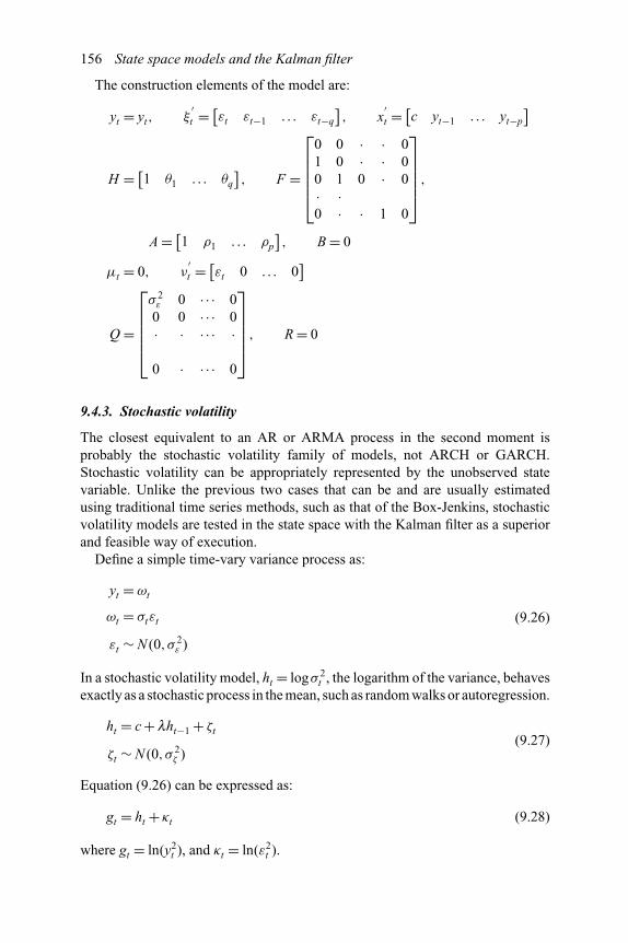
156 State space models and the Kalman filter
The construction elements of the model are:
yt = yt, ξ′t = [εt εt−1 . . . εt−q
], x
′t = [c yt−1 . . . yt−p
]
H = [1 θ1 . . . θq
], F =
⎡⎢⎢⎢⎢⎣
0 0 · · 01 0 · · 00 1 0 · 0· ·0 · · 1 0
⎤⎥⎥⎥⎥⎦ ,
A = [1 ρ1 . . . ρp
], B = 0
μt = 0, ν′t = [εt 0 . . . 0
]
Q =
⎡⎢⎢⎢⎢⎣
σ 2ε 0 · · · 00 0 · · · 0· · · · · ·
0 · · · · 0
⎤⎥⎥⎥⎥⎦ , R = 0
9.4.3. Stochastic volatility
The closest equivalent to an AR or ARMA process in the second moment isprobably the stochastic volatility family of models, not ARCH or GARCH.Stochastic volatility can be appropriately represented by the unobserved statevariable. Unlike the previous two cases that can be and are usually estimatedusing traditional time series methods, such as that of the Box-Jenkins, stochasticvolatility models are tested in the state space with the Kalman filter as a superiorand feasible way of execution.
Define a simple time-vary variance process as:
yt = ωt
ωt = σtεt
εt ∼ N (0,σ 2ε )
(9.26)
In a stochastic volatility model, ht = logσ 2t , the logarithm of the variance, behaves
exactly as a stochastic process in the mean, such as random walks or autoregression.
ht = c + lht−1 + ζt
ζt ∼ N (0,σ 2ζ )
(9.27)
Equation (9.26) can be expressed as:
gt = ht + κt (9.28)
where gt = ln(y2t ), and κt = ln(ε2
t ).

State space models and the Kalman filter 157
The observation equation is:
gt = [1 0][ ht
ht−1
]+ κt (9.29)
The state equation is:[ht+1ht
]=[l 01 0
][ht
ht−1
]+[10
]c +[ζt+10
](9.30)
The construction elements are:
yt = gt, ξ′t = [ht ht−1
], xt = c
H = [1 0], F =
[l 01 0
], A = 0, B =
[10
]
μt = κt, ν′t = [ζt 0
]Q =
[σ 2
ζ 00 0
], R = σ 2
κ
As the model is not log normal (i.e., y2t is not log normal or Ln(y2
t ) is not normal),it cannot be estimated by the usual maximum likelihood method. Nevertheless,when the random variables in concern are orthogonal, maximising the likelihoodfunction will yield exactly the same estimates of the parameters, except forthe standard errors of the parameters, which can be calculated by a differentformula. This procedure is referred to as the Quasi Maximum Likelihood (QML)method, suggested by White (1982). Specifically, the QML estimation of stochasticvolatility models is discussed in Harvey et al. (1994) and Ruiz (1994). Otherestimation procedures include the Monte Carlo Maximum Likelihood suggestedby Sandmann and Koopman (1998), where the basic stochastic volatility model isexpressed as a linear state space model with log χ2 disturbances. The likelihoodfunction is approximated by decomposing it into a Gaussian part, estimated by theKalman filter, and the rest is evaluated by simulation.
9.4.4. Time-varying coefficients
Specify a simple market model modified by using time-varying coefficients:
Rt = αt +βtRmt + εt
αt = αt−1 + ν1t
βt = βt−1 + ν2t
(9.31)
where Rt return on an individual security, Rmt is return on the market, and thecoefficients follow a random walk.
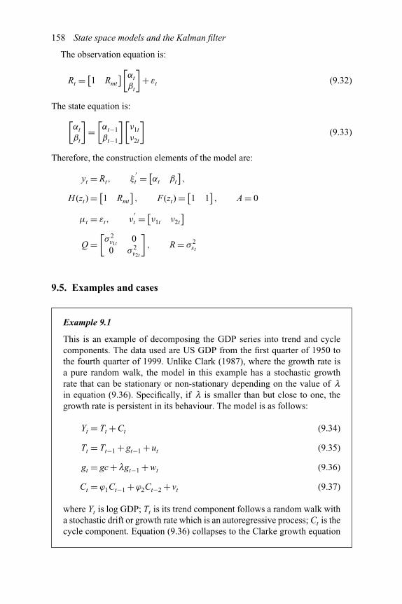
158 State space models and the Kalman filter
The observation equation is:
Rt = [1 Rmt
][αt
βt
]+ εt (9.32)
The state equation is:[αt
βt
]=[αt−1βt−1
][ν1t
ν2t
](9.33)
Therefore, the construction elements of the model are:
yt = Rt, ξ′t = [αt βt
],
H (zt) = [1 Rmt
], F(zt) = [1 1
], A = 0
μt = εt, ν′t = [ν1t ν2t
]Q =
[σ 2
ν1t0
0 σ 2ν2t
], R = σ 2
εt
9.5. Examples and cases
Example 9.1
This is an example of decomposing the GDP series into trend and cyclecomponents. The data used are US GDP from the first quarter of 1950 tothe fourth quarter of 1999. Unlike Clark (1987), where the growth rate isa pure random walk, the model in this example has a stochastic growthrate that can be stationary or non-stationary depending on the value of lin equation (9.36). Specifically, if l is smaller than but close to one, thegrowth rate is persistent in its behaviour. The model is as follows:
Yt = Tt + Ct (9.34)
Tt = Tt−1 + gt−1 + ut (9.35)
gt = gc + lgt−1 + wt (9.36)
Ct = ϕ1Ct−1 +ϕ2Ct−2 + vt (9.37)
where Yt is log GDP; Tt is its trend component follows a random walk witha stochastic drift or growth rate which is an autoregressive process; Ct is thecycle component. Equation (9.36) collapses to the Clarke growth equation

State space models and the Kalman filter 159
when restrictions gc = 0 and l = 1 are imposed. There are other reasonableassumptions. If l is set to be zero, then the growth rate is a stationarystochastic series around a constant mean value. The growth rate is constantover time when wt is zero as well. So, in the empirical inquiries, there arethree sets of restrictions imposed against the general form of equation (9.36).
Write equations (9.34)–(9.37) in the state space form, the observationequation is:
Yt = [1 1 0 0]⎡⎢⎢⎣
Tt
Ct
Ct−1gt
⎤⎥⎥⎦ (9.38)
The state equation is:
⎡⎢⎢⎣
Tt+1Ct+1Ct
gt+1
⎤⎥⎥⎦=
⎡⎢⎢⎣
1 0 0 10 ϕ1 ϕ2 00 1 0 00 0 0 l
⎤⎥⎥⎦⎡⎢⎢⎣
Tt
Ct
Ct−1gt
⎤⎥⎥⎦+
⎡⎢⎢⎣
000gc
⎤⎥⎥⎦+
⎡⎢⎢⎣
vt+1ut+1
0wt+1
⎤⎥⎥⎦ (9.39)
The construction elements of the model are:
yt = Yt, ξ′t = [Tt Ct Ct−1 gt
], x
′t = [0 0 0 gc
]
H = [1 1 0 0], F =
⎡⎢⎢⎣
1 0 0 10 ϕ1 ϕ2 00 1 0 00 0 0 l
⎤⎥⎥⎦ , A = 0, B = 1
μt = 0, ν′t = [ut vt 0 wt
]
Q =
⎡⎢⎢⎣
σ 2u 0 0 00 σ 2
v 0 00 0 0 00 0 0 σ 2
w
⎤⎥⎥⎦ , R = 0
The estimation results are reported in Table 9.1. Graphs of the trend, cycle,and growth rate are plotted in Figure 9.1. Inspecting the three standarddeviations can give us some ideas about the behaviour of the GDP series.σ v, the standard deviation of the cycle component, measures the contributionof cycles. There are no cyclical fluctuations when σv is zero (ϕ1 +ϕ2 mustbe zero at the same time for the cycles to be stochastic). If σw, the standarddeviation of the growth rate, and l are zero, the time series collapses to a
Continued
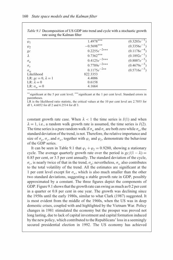
160 State space models and the Kalman filter
Table 9.1 Decomposition of US GDP into trend and cycle with a stochastic growthrate using the Kalman filter
ϕ1 1.4978∗∗∗ (0.3203e−1)ϕ2 −0.5698∗∗∗ (0.3356e−1)gc 0.2255e−2∗∗∗ (0.1178e−4)l 0.7362∗∗∗ (0.1892e−1)σu 0.4125e−2∗∗∗ (0.8007e−3)σv 0.7789e−2∗∗∗ (0.4679e−3)σw 0.1175e−2∗∗ (0.5716e−3)Likelihood 822.3353LR: gc = 0, l = 1 4.4006LR: l = 0 0.6158LR: σw = 0 4.1664
∗∗significant at the 5 per cent level; ∗∗∗significant at the 1 per cent level. Standard errors inparentheses.LR is the likelihood ratio statistic, the critical values at the 10 per cent level are 2.7055 fordf 1, 4.6052 for df 2 and 6.2514 for df 3.
constant growth rate case. When l < 1 the time series is I (1) and whenl = 1, i.e., a random walk growth rate is assumed, the time series is I (2).The time series is a pure random walk if σw and σv are both zero while σu, thestandard deviation of the trend, is not. Therefore, the relative importance andsize of σu, σv, and σw, together with ϕ1 and ϕ2, demonstrate the behaviourof the GDP series.
It can be seen in Table 9.1 that ϕ1 + ϕ2 = 0.9280, showing a stationarycycle. The average quarterly growth rate over the period is gc/(1 − l) =0.85 per cent, or 3.5 per cent annually. The standard deviation of the cycle,σv, is nearly twice of that in the trend, σu; nevertheless, σw also contributesto the total volatility of the trend. All the estimates are significant at the1 per cent level except for σw, which is also much smaller than the othertwo standard deviations, suggesting a stable growth rate in GDP, possiblyapproximated by a constant. The three figures depict the components ofGDP. Figure 9.1 shows that the growth rate can swing as much as 0.2 per centin a quarter or 0.8 per cent in one year. The growth was declining sincethe 1950s until the early 1980s, similar to what Clark (1987) suggested. Itis most evident from the middle of the 1960s, when the US was in deepdomestic crises, coupled with and highlighted by the Vietnam War. Policychanges in 1981 stimulated the economy but the prosper was proved notlong lasting, due to lack of capital investment and capital formation inducedby the new policy, which contributed to the Republicans’ loss in a seeminglysecured presidential election in 1992. The US economy has achieved

Log US GDP
7
8
9
10
Q1 51 Q1 59 Q1 67 Q1 75 Q1 83 Q1 91 Q1 99
GDP Trend
Log US GDP
−0.1
−0.05
0
0.05
0.1
Q1 51 Q1 59 Q1 67 Q1 75 Q1 83 Q1 91 Q1 99
cycle
Log US GDP
0.007
0.008
0.009
0.01
Q1 51 Q1 59 Q1 67 Q1 75 Q1 83 Q1 91 Q1 99
growth
Figure 9.1 Trend, cycle and growth in US GDP.Continued

162 State space models and the Kalman filter
in most of the 1990s with consistently increasing and stable growth in GDP,started from the Gulf war period and the collapse of the Soviet Union.
The likelihood ratio test does not reject any restrictions, though therandom walk growth hypothesis is very close to being marginally rejected.Ranking in accordance with the likelihood function value, growth is bestdescribed as a mean-reverting stochastic process, followed by a constantplus white noise growth rate, a constant growth rate, and a random walkgrowth rate is the least favourable. The results show that different views on,and explanations to, some economic behaviour can be largely right at thesame time.
Example 9.2
This is an example from Foresi et al. (1997) on interest rate models that arecrucial to bond pricing. Only those parts relevant to the state space modelare extracted here. The bond price is usually modelled as a function of theshort-term interest rate in the bond pricing literature; and the short-terminterest rate, usually called the short rate, follows some kind of generalisedWiener processes. The idea of the paper is simply that the nominal bond priceis determined by the riskless real short-term interest rate and the expectedinstantaneous inflation rate. As the two variables are unobservable, a statespace specification is proved helpful.
Basically, the paper specifies two unobserved state variables, the risklessreal short-term interest rate, rt , and the expected instantaneous inflationrate, πt , as a vector of bivariate generalised Wiener processes (t subscriptsuppressed):
dr = (a1 + b11r + b12π ) +σrdzr
dπ = (a2 + b21r + b22π ) +σπdzπ
(9.40)
Then the continuously-compounded nominal yield on zero-coupon bonds, attime t and having τ periods to maturity, yn,t,τ , and inflation forecast at time tfor t + τ , yi,t,τ , are treated as functions of above state variables (t subscriptsuppressed):
yn,τ = jn,τ +αn,τ,11r +αn,τ,12π + εn
yi,τ = ji,τ +αi,τ,21r +αi,τ,22π + εi
(9.41)
where jn,τ and ji,τ are functions of τ and independent of the state variables,which are therefore not analysed here.
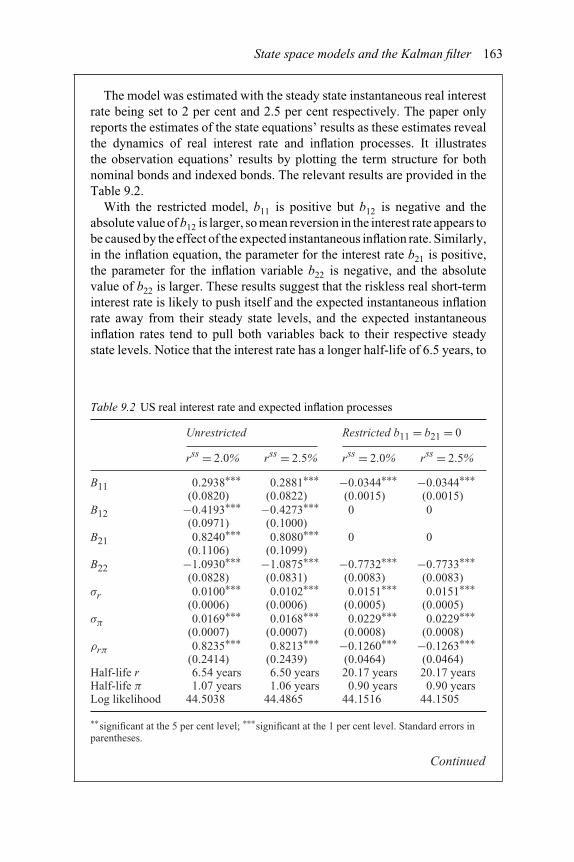
State space models and the Kalman filter 163
The model was estimated with the steady state instantaneous real interestrate being set to 2 per cent and 2.5 per cent respectively. The paper onlyreports the estimates of the state equations’ results as these estimates revealthe dynamics of real interest rate and inflation processes. It illustratesthe observation equations’ results by plotting the term structure for bothnominal bonds and indexed bonds. The relevant results are provided in theTable 9.2.
With the restricted model, b11 is positive but b12 is negative and theabsolute value of b12 is larger, so mean reversion in the interest rate appears tobe caused by the effect of the expected instantaneous inflation rate. Similarly,in the inflation equation, the parameter for the interest rate b21 is positive,the parameter for the inflation variable b22 is negative, and the absolutevalue of b22 is larger. These results suggest that the riskless real short-terminterest rate is likely to push itself and the expected instantaneous inflationrate away from their steady state levels, and the expected instantaneousinflation rates tend to pull both variables back to their respective steadystate levels. Notice that the interest rate has a longer half-life of 6.5 years, to
Table 9.2 US real interest rate and expected inflation processes
Unrestricted Restricted b11 = b21 = 0
rss = 2.0% rss = 2.5% rss = 2.0% rss = 2.5%
B11 0.2938∗∗∗ 0.2881∗∗∗ −0.0344∗∗∗ −0.0344∗∗∗(0.0820) (0.0822) (0.0015) (0.0015)
B12 −0.4193∗∗∗ −0.4273∗∗∗ 0 0(0.0971) (0.1000)
B21 0.8240∗∗∗ 0.8080∗∗∗ 0 0(0.1106) (0.1099)
B22 −1.0930∗∗∗ −1.0875∗∗∗ −0.7732∗∗∗ −0.7733∗∗∗(0.0828) (0.0831) (0.0083) (0.0083)
σr 0.0100∗∗∗ 0.0102∗∗∗ 0.0151∗∗∗ 0.0151∗∗∗(0.0006) (0.0006) (0.0005) (0.0005)
σπ 0.0169∗∗∗ 0.0168∗∗∗ 0.0229∗∗∗ 0.0229∗∗∗(0.0007) (0.0007) (0.0008) (0.0008)
ρrπ 0.8235∗∗∗ 0.8213∗∗∗ −0.1260∗∗∗ −0.1263∗∗∗(0.2414) (0.2439) (0.0464) (0.0464)
Half-life r 6.54 years 6.50 years 20.17 years 20.17 yearsHalf-life π 1.07 years 1.06 years 0.90 years 0.90 yearsLog likelihood 44.5038 44.4865 44.1516 44.1505
∗∗significant at the 5 per cent level; ∗∗∗significant at the 1 per cent level. Standard errors inparentheses.
Continued
164 State space models and the Kalman filter
compare with a half-life of 1.1 years for expected inflation. This reinforcesthe claim that there is stronger mean-reverting tendency in expected inflationthan in the interest rate. When b12 and b21 are set to zero as in the restrictedmodel, any mean reversion in a variable must come from itself. That is,b11 and b22 must be negative. The estimates in the table are negative asexpected; and the size of b22 is much larger, reflecting that there is farstronger mean-reverting tendency in expected inflation. Any joint movementin the two variables is now through the correlation between dzπ and dzr ,as the inter-temporal links have been cut off. In the restricted model, theinstantaneous correlation between the interest rate variable and the expectedinflation variable is around −0.13, a number appears to be more reasonablethan its counterpart in the unrestricted model, which is 0.82.
The authors claim that the Kalman filter method enables them to identifythe separate influences of real rates of return and inflation expectations.Based on the Kalman filter parameter estimates, they could achieveimprovements in construct yield curves and calculating investors’ requiredpremia for risk from changes in real interest rates and inflation. Thereis one point subject to further scrutiny: the paper says that the restrictedmodel, where b12 and b21 are set to 0, or the interest rate process andthe inflation process have no inter-temporal causal relationship and anylink between them is their instantaneous correlation, performs better andthe yield curves constructed from the restricted model appear to be morerealistic. Then the query is: can this be justified by the economics of interestrate-inflation dynamics or is this an estimation problem technically? Thehalf-life of 20 years for the interest rate in the restricted model also seems tobe rather long. The reason could be simple: changes in the real interest rateare responses to changes in the economic environment, realised, anticipatedand/or unanticipated. Without other economic variables playing a role, theevolution path of the interest rate is unlikely to change or to be altered,resulting in a longer half-life.
9.6. Empirical literature
There are growing applications of the Kalman filter in state space models, butthe number is small relative to other popular models such as cointegration andGARCH. One of the reasons is that state space models are not easy to implement.On the one hand, most econometric software packages either do not have Kalmanfilter procedures or have the procedures which are too basic to be of practical use.On the other hand, estimates of parameters are rather sensitive to the choice ofinitial values and other settings of the filter.
Recent use of the Kalman filter can be found in financial markets and theeconomy, at micro and macro levels. In bond pricing and interest rate models,Babbs and Nowman (1998) estimate a two-factor term structure model which
State space models and the Kalman filter 165
allows for measurement errors by using the Kalman filter. Duan and Simonato(1999) and the above example by Foresi et al. (1997) are similar cases. All thesestudies claim that the state space model provides good fit to the yield curves ofconcern. Jegadeesh and Pennacchi (1996) model the target level of the interestrate, to which the short-term interest is to revert, in the state space, in a two-factorequilibrium model of the term structure. They compare the term structure of spotLIBOR and Eurodollar futures volatility to that predicted by their two-factor modeland find significant improvements over the one-factor model that does not includethe target level of the interest rate.
On stock market behaviour, Gallagher et al. (1997) decompose the stockindices of 16 countries into transitory (cycles), permanent (trends) and seasonalcomponents. They find evidence of mean-reversion in stock prices and concludethat stock prices are not pure random walks, though the transitory component issmall and does not explain more than 5 per cent of stock price variations for 12 ofthe 16 countries. Jochum (1999) hypothesises that the risk premium on the Swissstock market consists of two components: the amount of volatility and the unit priceof risk. The unit price of risk is time-varying and estimated by the Kalman filter,so investors’ behaviour can be examined in different phases of market movement.McKenzie et al. (2000) estimate a time-varying beta model for the Australianmarket using the Kalman filter. The study is one of typical examples of time-varying coefficient models. Using the cumulative sum of squares (CUSUMSQ)test, they find beta parameter instability for all 24 industries inspected when theworld market index is the relevant benchmark of the model, as the recursivelyestimated residuals exceeded the 5 per cent critical boundary. They find betainstability for 20 out of the 24 industry betas when the domestic market indexserves as the benchmark. They conclude that time-varying betas estimated relativeto the domestic index, though not universally superior, are preferred in certaincircumstances. Whether the slightly inferior performance of the world index modelis caused by more instability in betas has yet to be examined, though the graphsin the paper appear to suggest so.
The dividend payment pattern is one of the areas where state space models are ofempirical relevance. The information content of dividends is debatably importantin practice and in research, whereas it can only be inferred. In a traditional way ofinterpreting dividends as a long-run performance signal arising from informationasymmetry, Daniels et al. (1997) investigate whether and how dividends are relatedto earnings by decomposing earnings into permanent and transitory componentsusing the Kalman filter. They examine 30 firms’ dividends and earnings and claimthat there is a more robust relationship between dividends and permanent earnings,compared with that between dividends and current earnings. Marseguerra (1997)models insider information regarding the firm as an unobserved state variable thatcan be inferred through dividends and earnings announcements, and finds thatinformation contained in dividend announcements varies and is a supplement tothe information set already available to the market.
Other various applications include Moosa (1999) that extracts the cyclicalcomponents of unemployment and output; Serletis and King (1997) on trendsand convergence of EU stock markets using a time-varying parameter model; and
166 State space models and the Kalman filter
Daniels and Tirtiroglu (1998) on decomposition of total factor productivity of UScommercial banking into stochastic trend and cycle components.
Broadly speaking, decompose trend and cycle in economic time series, e.g.,GDP, industrial production, the unemployment rate, stock prices and stock indices;unobserved variables, e.g., expectations, real interest rates, real costs; permanentand transitory components; time-vary parameters, e.g., time-varying betas.
Questions and problems
1 What is the state variable and what is an unobserved component in a statespace model?
2 Discuss the advantages of the state space model and the difficulties in theempirical implementation of the model.
3 Describe the three steps of the Kalman filter algorithm in estimating a statespace model.
4 Collect data from various sources, and estimate the following time series usingthe conventional ARIMA and in the state space using the Kalman filter (usingRATS, GAUSS or other packages):
(a) GDP of selected countries,(b) total return series of Tesco, Sainsbury’s and ICI.
Compare your results from the two approaches.5 The implementation of the Kalman filter is always complicated and the results
may be sensitive to even slightly different settings. To practice, collect datafrom various sources and repeat the same procedure of Example 1 for GDPof a few selected countries.
References
Babbs, S.H. and Nowman, K.B. (1998), Econometric analysis of a continuous time multi-factor generalized Vasicek term structure model: International evidence, Asia-PacificFinancial Markets, 5(2), 59–183.
Clark, P.K. (1987), The cyclical component of the U.S. economic activity, Quarterly Journalof Economics, 102(4), 797–814.
Daniels, K., Shin, T.S. and Lee, C.F. (1997), The information content of dividendhypothesis: a permanent income approach, International Review of Economics andFinance, 6(1), 77–86.
Daniels, K.N. and Tirtiroglu, D. (1998), Total factor productivity growth in U.S. commercialbanking for 1935–1991: A latent variable approach using the Kalman filter, Journal ofFinancial Services Research, 13(2), 119–135.
Duan, J.C. and Simonato, J.G. (1999), Estimating and testing exponential-affine termstructure models by Kalman Filter, Review of Quantitative Finance and Accounting,13(2), 111–135.
Foresi, S., Penati, A. and Pennacchi, G. (1997), Estimating the cost of U.S. indexed bonds,Federal Reserve Bank of Cleveland Working Paper 9701.

State space models and the Kalman filter 167
Gallagher, L.A. Sarno, L. and Taylor, M.P. (1997), Estimating the mean-revertingcomponent in stock prices: A cross-country comparison, Scottish Journal of PoliticalEconomy, 44(5), 566–582.
Hamilton, J.D. (1994), Time Series Analysis, Princeton University Press, Princeton,New Jersey.
Harvey, A.C. (1989), Forecasting, Structural Time Series Models and the Kalman Filter,Cambridge University Press, Cambridge, England.
Harvey, A.C., Ruiz, E. and Sheppard, N. (1994), Multivariate stochastic variance models,Review of Economic Studies, 61(2), 247–264.
Jegadeesh, N. and Pennacchi, G.G. (1996), The behavior of interest rates implied by theterm structure of eurodollar futures, Journal of Money, Credit and Banking, 28(3),426–446.
Jochum, C. (1999), Volatility spillovers and the price of risk: Evidence from the Swissstock market, Empirical Economics, 24(2), 303–322.
Kalman, R.E. (1960), A new approach to linear filtering and prediction problems,Transactions of ASME Series D, Journal of Basic Engineering, 82, 35–45.
Kalman, R.E. (1963), New methods of Wiener filtering theory, in Bogdanoff, J.L. andKozin, F. (eds), Proceedings of the First Symposium on Engineering Applications ofRandom Function Theory and Probability, 270–388, Wiley, New York.
Kalman, R.E. (1978), A retrospective after twenty years: from the pure to the applied,Chapman Conference on Applications of the Kalman filter to Hydrology, Hydraulicsand Water Resources, American Geophysical Union, Pittsburgh.
Kalman, R.E. and Bucy, R.S. (1961), New results in linear filtering and predictionproblems, Transactions of ASME Series D, Journal of Basic Engineering, 83,95–108.
Marseguerra, G. (1997), The information content of dividends: an application of theKalman filter, Rivista Internazionale di Scienze Economiche e Commerciali, 44(4),725–751.
McKenzie, M.D., Brooks, R.D. and Faff, R.W. (2000), The use of domestic and worldmarket indexes in the estimation of time-varying betas, Journal of MultinationalFinancial Management, 10(1), 91–106.
Moosa, I.A. (1999), Cyclical output, cyclical unemployment, and Okun’s coefficient: astructural time series approach, International Review of Economics and Finance, 8,293–304.
Ruiz, E. (1994), Quasi-maximum likelihood estimation of stochastic volatility models,Journal of Econometrics, 63(1), 289–306.
Sandmann, G. and Koopman, S.J. (1998), Estimation of stochastic volatility models viaMonte Carlo maximum likelihood, Journal of Econometrics, 87(2), 271–301.
Serletis, A. and King, M. (1997), Common stochastic trends and convergence of EuropeanUnion stock markets, The Manchester School of Economic and Social Studies, 65(1),44–57.
White, H. (1982), Maximum likelihood estimation of misspecified models, Econometrica,50, 1–25.

10 Frequency domain analysis oftime series
Spectral analysis, or studies in the frequency domain, is one of the unconventionalsubjects in time series econometrics. The frequency domain method has existed fora long time and has been extensively used in electronic engineering such as signalprocessing, communications, and automatic control. Although the application ofthe frequency domain method in econometrics may have as long a history as thatin engineering, it has been sporadic and regarded unorthodox and often plays asupplementary role.
Analysis in the frequency domain does not bring in new or additionalinformation, it is simply an alternative method with which information isobserved, abstracted and processed. This is sometimes helpful. Depending onthe characteristics of the issues, analysis in one domain may be more powerfulthan in the other. For example, cycles are better and more explicitly observedand represented in the frequency domain; while correlations in the time domainand cross spectra in the frequency domain deal with the relationship betweentwo time series from different perspectives and, in the meantime, have definedlinks.
This chapter first introduces the Fourier transform, which is one of the mostcommonly used transformations of time series and the spectrum, the frequencydomain expression of time series. In the similar spirit of covariance analysis,cross spectra, coherence and phases in multivariate time series are discussed next.In the following two sections of the chapter, frequency domain representationsof commonly used time series processes are presented and frequency domainpersistence measures are developed.
10.1. The Fourier transform and spectra
A continuous non-periodic time series has a continuous Fourier spectrum. Fora periodic time series, its Fourier transform is discrete Fourier series. We onlyintroduce the Fourier transform for non-periodic time series, as periodicity is rarein economic and financial time series. We do so to avoid confusion also. Thenwe quickly proceed to the discrete Fourier transform, which is most common infinance and economics. Let f (t) (−∞ < t < ∞) be a continuous non-periodic time
Frequency domain analysis of time series 169
series, then its Fourier transform (FT) is defined as:
F(ω) =∞∫
t=−∞f (t) e−jωtdt (10.1)
F(ω) is also called the spectral density function of f (t). There exists an inverseFourier transform (IFT), which is continuous, so that:
f (t) = 1
2π
π∫−π
F(ω) e jωtdω (10.2)
One of the most important and relevant properties of the Fourier transformis time delay or lags. Let F(ω) be the Fourier transform of f (t), then theFourier transform of f (t − t0) is e−jωt0 F(ω). This can be proved briefly asfollows:
∞∫t=−∞
f (t − t0) e−jωtdt =∞∫
t=−∞f (t) e−jω(t+t0)dt
= e−jωt0
∞∫t=−∞
f (t) e−jωtdt = e−jωt0F(ω)
In practice, for a discrete time series with N observations, such as ineconomics and finance, the Fourier transform would usually be the discreteFourier transform (DFT). The pair of DFT and inverse discrete Fourier transform(IDFT) is:
F(k) =N−1∑
n=−(N−1)
f (n) e−jn(2πk/N ) (10.1)
and
f (n) = 1
N
N−1∑k=−(N−1)
F(k) e jk(2πn/N ) (10.2)
with �ω = 2π/N ,F(k) = F(k�ω) = F(2πk/N ). That is, time domain series canbe expressed with different frequency components. Equation (10.1) or (10.1) isthe energy spectrum. In the case of stochastic processes, the Fourier transformis concerned with the power spectrum or the power spectral density function(which can be simply called spectral density function when there is no confusion).1

170 Frequency domain analysis of time series
The spectral density function of a discrete random process �1Xt = Xt − Xt−1(t = 1, . . . N ) is:
h(k) =N−1∑
τ=−(N−1)
R(τ ) e−jτ (2πk/N ) (10.3)
where R(τ ) is the autocovariance function of �1Xt , i.e. R(τ ) = E{(�1Xt −μ)(�1Xt−τ − μ)} and μ = E{�1Xt}. The inverse Fourier transform of equation(10.3) is:
R(τ ) = 1
N
N−1∑k=−(N−1)
h(k) e jk(2πτ/N ) (10.4)
Setting τ = 0 in equation (10.4), we have:
R(0) = E{(�1Xt)2} = 1
N
N−1∑k=−(N−1)
h(k) e jk(2πτ/N ) (10.5)
It is the mean squared value of the process and has the meaning of power ofthe process, so equation (10.3) is called the power spectrum. Equation (10.1) or(10.1), in contrast, is the energy spectrum as it has the features of electrical currentor voltage.
R(τ ) usually takes real values and is an even function, i.e. R(−τ ) = R(τ ).Accordingly, the spectral density function can be written as:
h(k) = σ 2X + 2
N−1∑τ=1
R(τ )cos
(2πτk
N
)(10.6)
Empirically, h(k) has to be truncated and estimated. The simplest way oftruncation is to let R(τ ) pass through a rectangular window or ‘truncatedperiodogram’ window, i.e.:
h(k) =M∑
τ=−M
R(τ )cos
(2πτk
N
)(10.7)
So:
E{h(k)
}=
M∑τ=−M
(1 − |τ |
N
)R(τ ) cos
(2πτk
N
)→ h(k), as M → ∞
(10.8)

Frequency domain analysis of time series 171
In general, the truncated spectral density function takes the form:
h(k) =M∑
τ=−M
l(τ )R(τ ) cos
(2πτk
N
)(10.9)
where l(τ ) is the window function. The variance of h(k) is:
Var[h(k)
]∼ (1 + δk,0)h2(k)
1
N
⎧⎨⎩
N−1∑τ=−(N−1)
l2N (τ )
⎫⎬⎭
= (1 + δk,0)h2(k)1
N
N−1∑θ=(N−1)
W 2N (θ )
(10.10)
where
WN (θ ) =N−1∑
θ=−(N−1)
l2N (τ ) e−jθ (2πk/N ) (10.11)
is the spectral expression of the window, and δk,0 is impulse function taking valueof unity at k = 0.
A rectangular window, though simple, does not perform well due to itssudden change at the cut-off points which may produce some peculiar frequencycomponents. The Bartlett window is usually used. It is defined as:
l(τ ) =⎧⎨⎩1 − |τ |
M, |τ | ≤ M
0 |τ | > M(10.12)
With Bartlett’s window, the variance of h(k) is:
Var[h(k)
]∼ 2M
3Nh2(k), for k �= 0 (10.13)
and
Var[h(k)
]∼ 4M
3Nh2(k), for k = 0 (10.14)
If k takes value of zero in equation (10.8) it becomes:
E{h(0)
}=
M∑τ=−M
(1 − |τ |
N
)R(τ )
= R(0) + 2M∑
τ=1
(1 − |τ |
N
)R(τ )
(10.15)

172 Frequency domain analysis of time series
Equation (10.15) is, in fact, the M period variance of �M Xt = Xt − Xt−M .Dividing equation (10.15) by the variance of �1Xt , σ
2�1X , yields Cochrane’s (1988)
version of persistence. Therefore, the Cochrane measure is a specific case ofequation (10.8), and assesses the long-run behaviour of time series at the zerofrequency only. It appears that such measures, as represented by Campbell andMankiw (1987a, b), Cochrane (1988) and Pesaran et al. (1993) are the necessarycondition(s) for a random walk, not sufficient conditions, as other points on thespectrum are not evaluated against the random walk hypothesis and it is possiblethat they deviate from unity jointly significantly. There are no significance teststatistics associated with them either, though Var
[h(0)
]is available to provide
a guideline for the accuracy of the measures, which is decided by the ratio ofthe window size to the number of observations, M/N , only. In other words, thewindow size should be small relative to the number of observations to achievereliability in the measure. To investigate persistence and associated time seriesproperties properly, the whole spectrum of the time series should be examined,instead of at the zero frequency point. These will be proposed and conducted inthe following section.
10.2. Multivariate spectra, phases and coherence
If we replace R(τ ), the autocovariance function of �1Xt , by the covariance betweentwo time series, i.e. CovX ,Y (τ ) = E{(�1Xt −μX )(�1Yt−τ −μY )}, μX = E{�1Xt}and μY = E{�1Yt}, then we get the cross spectrum of the two time series in theform of:
hX ,Y (k) =N−1∑
τ=−(N−1)
CovX ,Y (τ ) e−jτ (2πk/N ) (10.16)
Cov(τ ) is in general not an even function, so equation (10.16) cannot take the formof equation (10.6), and hX ,Y (k) is in general a complex number:
hX ,Y (k) = c(k) cos
(2πk
Nτ
)+ jq(k) sin
(2πk
Nτ
)(10.17)
Unlike the univariate Fourier transform where the imaginary part is zero, the crossspectrum has both magnitude and phase as follows:
m(k) =√
c2(k) + q2(k) (10.18)
and:
p(k) = tan−1 q(k)
c(k)(10.19)
Equations (10.18) and (10.19) are called magnitude spectrum and phase spectrum,respectively. It can be seen, from the above analysis, that if CovX ,Y (τ ) is an even
Frequency domain analysis of time series 173
function, then the phase spectrum is zero, i.e. there is no overall lead of seriesXt over series Yt , and vice versa. With equations (10.18) and (10.19), the crossspectrum can also be expressed as:
hX ,Y (k) = m(k) e jp(k) (10.20)
so that both magnitude and phase are shown explicitly.Another measure of the closeness of two time series is coherence, defined, in a
very similar way to the correlation coefficient, as:
CohX ,Y (k) = hX ,Y (k)
h1/2X ,X (k)h1/2
Y ,Y (k)(10.21)
If we make comparison of the measures in the frequency domain with those inthe time domain, then the cross spectrum of equation (10.17) is correspondingto covariance in the time domain, which is not standardised; the coherence aswith equation (10.21) is corresponding to correlation in the time domain, whichare standardised by the square roots of the two time series’ spectra and thetwo time series’ standard deviations respectively; and the phase of equation(10.19) addresses leads and lags. As with the non-standardised cross spectrum,the closeness of two time series is not straightforwardly observed, the measure ofcoherence, together with the phase measure, is widely adopted in economic andfinancial research.
To generalise the above bi-variate analysis to the multivariate case, let:
� =
⎡⎢⎢⎣
Cov11(τ ) · · · Cov1m(τ )
· · ·Covm1(τ ) · · · Covmm(τ )
⎤⎥⎥⎦ (10.22)
be the covariance matrix of an m-variable system of time series. Then the crossspectra of the time series can also be expressed in a matrix:
H =
⎡⎢⎢⎣
h11(k) . . . h1m(k)
. . .
hm1(k) . . . hmm(k)
⎤⎥⎥⎦ (10.23)
where hil(k) (i, l = 1, . . . m) takes the form of equation (10.16).
10.3. Frequency domain representations of commonly usedtime series processes
10.3.1. AR(p) process
Yt = ρ1Yt−1 +·· ·+ρpYt−p + εt, εt ∼ N (0,σ 2ε ) (10.24)

174 Frequency domain analysis of time series
Re-arranging equation (10.24) as:
Yt −ρ1Yt−1 −·· ·−ρpYt−p = εt (10.24′)
Taking the Fourier transform and applying the property of time delaying yield:
FY (k)[1 −ρ1 e−j(2πk/N ) −·· ·−ρp e−jp(2π/N )
]= Fε(k) (10.25)
So that the power spectrum or simply the spectrum of an AR process is:
hY (k)
= σ 2ε[
1−ρ1 e−j(2πk/N ) −···−ρp e−jp(2πk/N )][
1−ρ1 e j(2πk/N ) −···−ρp e jp(2πk/N )]
(10.26)
10.3.2. MA(q) process
Yt = εt + θ1εt−1 +·· ·+ θqεt−q, εt ∼ N (0,σ 2ε ) (10.27)
The Fourier transform of this process is:
FY (k) = Fε(k)[1 + θ1 e−j(2πk/N ) +·· ·+ θq e−jq(2πk/N )
](10.28)
So the spectrum is:
hY (k) = σ 2ε
[1 + θ1 e−j(2πk/N ) +·· ·+ θq e−jq(2πk/N )
]× [1 + θ1 e j(2πk/N ) +·· ·+ θq e jq(2πk/N )
] (10.29)
10.3.3. VAR (p) process
Yt = A1Yt−1 +·· ·+ ApYt−p + εt, εt ∼ N (0,�) (10.30)
where Yt is an m × 1 vector of variables, and Ai, i = 1, . . . p are m × m matricesof coefficients. Taking the Fourier transform yields:
FY (k)[1 − A1 e−j(2πk/N ) −·· ·− Ap e−jp(2πk/N )
]= F�(k) (10.31)
Therefore, the spectra of the VAR process is:
hY (k) = [1 − A1 e−j(2πk/N ) −·· ·− Ap e−jp(2πk/N )]−1
×�[1 − A1 e j(2πk/N ) −·· ·− Ap e jp(2πk/N )
]−1(10.32)

Frequency domain analysis of time series 175
10.4. Frequency domain analysis of the patterns of violationof white noise conditions
10.4.1. Statistical distributions in the frequency domain of near whitenoise processes
Assuming a time series X (t) possesses the usual properties that it is stationary,is continuous in mean square, and has higher moments up to the fourth moment,then the spectrum of the process, or the spectral distribution function, exists withthe following relationships:
f (ω) = 1
2πN
N∑τ=−N
R(τ ) e−iτω = 1
2πN
N∑τ=−N
R (τ )cos(τω)
= σ 2X
2π+ 1
π
N∑τ=1
R(τ )cos(τω) = C0
2πN+ 1
πN
N−1∑τ=1
Cτ cos(τω)
(10.33)
R(τ ) = σ 2x
π∫−π
eiτωdF(ω) (10.34)
where:
Cτ =N−τ∑t=1
XtXt+τ , C0 =N∑
t=1
XtXt = Nσ 2X , and F(ω) =
ω∫0
f (ω)dω
is the integral spectrum of the process.For a pure white noise process, C0 obeys a χ2-distribution with E{C0} = N ,
Var{C0} = 2N ; and Cτ obey normal distributions with E{Cτ } = 0, Var{Cτ } = N ,for τ = 1, . . . N − 1. In the following, we show how a white noise process isdistributed in the frequency domain, and the conditions on which a particularprocess can be accepted as a white noise process. We call such a process nearwhite noise processes in contrast to a pure theoretical white noise. It can beshown that:
LimN→∞P
{max
0≤ω≤πN 1/2
∣∣∣F(ω) − ω
2π
∣∣∣≤ α
}= P
{max
0≤ω≤π|ξ (ω)| ≤ α
}(10.35)
where ξ (ω) is a Gaussian process with:
P {ξ (0) = 0} = 1 (10.36a)
P {ξ (π ) = 0} = 1 (10.36b)
E {ξ (ω)} = 0, 0 ≤ ω ≤ π (10.36c)

176 Frequency domain analysis of time series
E {ξ (ν)ξ (ω)} = 3ν(π −ω)
4π2 , 0 ≤ ν < ω ≤ π (10.36d)
E{[ξ (ω)]2}= 3ω(π −ω)
4π2 , 0 ≤ ω ≤ π (10.36e)
Equation (10.35) can be verified as follows. The integral spectrum of the timeseries process, or the integral of the spectrum of equation (10.33), is:
F(ω) =ω∫
0
f (ω)dω = v∗n(ω)
2πN+
N−1∑τ=1
Cτ
πN
sin τω
τ(10.37)
where v∗n(ω) =
π∫0
C0(ω)dω. Then:
N 1/2[Fp(ω) − ω
2π
]= N 1/2
2π
[v∗
n(ω)
N−ω
]+
N−1∑τ=1
Cτ
πN 1/2
sin τω
τ(10.38)
Previous studies2 treat C0 as a stochastic variable in the time domain, but aconstant in the frequency domain irrespective of the value of ω. There is a problemmainly concerning the boundary condition: C0 can be greater or smaller than Nat point ω = π , which does not guarantee F(π ) = 1
2 [F(π ) is half of the totalpower], the requirement that the power of the standardised time series is unity (thesecond term on the right-hand side of equation (10.38) is zero at point ω = π ).We resort to the Kolmogorov-Smirnov theorem for a realistic representation ofthe distribution of C0.
The distribution of the first term on the right-hand side can be obtained byapplying the Kolmogorov-Smirnov theorem. Define:
zn(t) = N1/2
[vn(t)
N− t
], 0 ≤ t ≤ 1 (10.39)
where vn(t) − vn(s) is the number of successes in N independent trials, withprobability t − s of successes in each trial; P
{vn(0) = 0
}= 1, P{vn(1) = N
}= 1;
E{vn(t) − vn(s)
}= N (t −s), E{[
vn(t) − vn(s)]2}= 2N (t −s) [1 − (t − s)], 0 ≤ s <
t ≤ 1; E{[
vn(t1) − vn(s1)][
vn(t2) − vn(s2)]}= 0, 0 ≤ s1 < t1 ≤ s2 < t2 ≤ 1. Then,
the m-variable distribution of the random variables zn(t1), . . . ,zn(tm), 0 ≤ t1 · · ·< tm ≤ 1 is Gaussian, and:
P{zn(0) = 0
}= 1, P{zn(1) = 0
}= 1 (10.40a)
E{zn(t)
}= 0, 0 ≤ t ≤ 1 (10.40b)
E{[
zn(t) − zn(s)]2}= (t − s) [1 − (t − s)] , 0 ≤ s < t ≤ 1 (10.40c)

Frequency domain analysis of time series 177
Now, let ω = π t and define:
z∗n(ω) = N 1/2
2π
[v∗
n(ω)
N−ω
](10.41)
we have:
P{v∗
n(0) = 0}= 1, P
{v∗
n(π ) = N}= 1 (10.42a)
E{v∗
n(ω) − v∗n(ν)}= N (ω − ν), 0 ≤ ν < ω ≤ π (10.42b)
E{[
v∗n(ω) − v∗
n(ν)]2}= N (ω − ν) [π − (ω − ν)] , 0 ≤ ν < ω ≤ π (10.42c)
and, the m-variable distribution of the random variables z∗n(ω1), . . . ,z∗
n(ωm), 0 ≤ω1 < · · · < ωm ≤ π is Gaussian, with:
P{z∗n(0) = 0
}= 1, P{z∗n(π ) = 0
}= 1 (10.43a)
E{z∗n(ω)
}= 0, 0 ≤ ω ≤ π (10.43b)
E{[
z∗n(ω) − z∗
n(ν)]2}= (ω − ν) [π − (ω − ν)]
4π2 , 0 ≤ ν < ω ≤ π (10.43c)
Equations (10.43a)–(10.43c) imply:
E{[
z∗n(ω)
]2}= ω(π −ω)
4π2 (10.44a)
E{z∗n(ν)z∗
n(ω)}= ν(π −ω)
4π2 , 0 ≤ ν < ω ≤ π (10.44b)
Equation (10.44) indicates that the first term on the right-hand side of equation(10.38) is in fact z∗
n(ω).Let us now consider the distribution of the second term on the right-hand side.
It can be observed, when N approaches infinite, that:
E {s(ω)s(ν)} = LimN→∞E
{(N−1∑τ=1
Cτ
πN 1/2
sin τω
τ
)(N−1∑τ=1
Cτ
πN 1/2
sin τν
τ
)}
= LimN→∞
1
π2
N−1∑τ=1
sin τω
τ
sin τν
τ= ν(π −ω)
2π2 , 0 ≤ ν < ω ≤ π
(10.45)
E{[s(ω)]2}= Lim
N→∞E
⎧⎨⎩(
N−1∑τ=1
Cτ
πN1/2
sin τω
τ
)2⎫⎬⎭ Lim
N→∞1
π2
N−1∑τ=1
(sin τω
τ
)2
= ω(π −ω)
2π2 (10.46)

178 Frequency domain analysis of time series
Therefore:
s (ω) = LimN→∞
N−1∑τ=1
Cτ
πN ½
sin τω
τ= 2z∗
n(ω) (10.47)
Finally, bringing the results into equation (10.38) yields:
ξ (ω) = 3z∗n(ω) (10.48)
The above has verified equation (10.35).
10.4.2. Patterns of violation of white noise conditions
This section discusses and abstracts typical patterns in time series where whitenoise conditions are violated. Behaviour of a particular process will be examined,in accordance with its frequency domain characteristics, which is of more empiricalrelevance. From Equations (10.35) and (10.36), three patterns can be characterisedwith regard to their violation of white noise conditions, setting against thebenchmark of a pure white noise process.
Pattern 1
Lower frequency components stochastically dominate higher frequency compo-nents in the frequency range (�1, �2) if ξ (ω) > 0, � 1 <ω <�2. Lower frequencycomponents stochastically consistently dominate higher frequency components ifξ (ω) > 0, 0 < ω < π , and the time series is said to possess the features of thecompounding effect.
By definition and according to theorem 1, ξ (ω) is the difference between theintegral of the process under examination and the integral of a pure white noiseprocess, being scaled by N , when N → ∞, i.e.:
ξ (ω) = LimN→∞N 1/2
ω∫0
(Ip(ω) − 1
2π
)dω
Figure 10.1 shows the features of such stochastic processes. The top panel ofthe figure is the time domain response to a unit size shock of a time series withcompounding features, against a random walk response. The dashed line indicatesthe evolution path of the time series if no shocks have ever occurred. The middlepanel is a typical spectrum for such time series, and the bottom panel is the ξ (ω)statistic for such time series. The spectrum in Figure 10.1 is a monotonous decreasefunction of ω, with ξ (ω) > 0, 0 < ω < π , and ξ ′′
ω(ω) < 0, 0 < ω < π , whereξ ′′ω(ω) is the second-order derivative of ξ (ω) with respect to ω.3 Stochastically
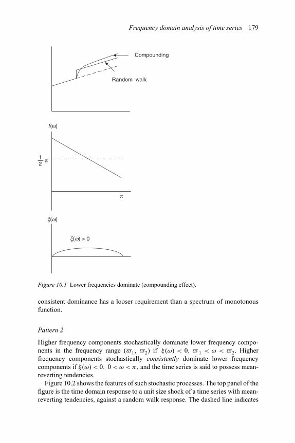
Frequency domain analysis of time series 179
Compounding
Random walk
f(ω)
π
12— π
x(w) > 0
x(w)
Figure 10.1 Lower frequencies dominate (compounding effect).
consistent dominance has a looser requirement than a spectrum of monotonousfunction.
Pattern 2
Higher frequency components stochastically dominate lower frequency compo-nents in the frequency range (�1, �2) if ξ (ω) < 0, � 1 < ω < �2. Higherfrequency components stochastically consistently dominate lower frequencycomponents if ξ (ω) < 0, 0 < ω < π , and the time series is said to possess mean-reverting tendencies.
Figure 10.2 shows the features of such stochastic processes. The top panel of thefigure is the time domain response to a unit size shock of a time series with mean-reverting tendencies, against a random walk response. The dashed line indicates

180 Frequency domain analysis of time series
f(ω)
x(w) < 0
x(w)
Stationary
Random walk
Mean-reverting
Random walk
π
12— π
Figure 10.2 Higher frequencies dominate (mean-reverting tendency).
the evolution path when there are no shocks to the time series. The middle panel isa typical spectrum for such time series, and the bottom panel is the ξ (ω) statistic forsuch time series. The spectrum in Figure 10.2 is a monotonous increase functionof ω, with ξ (ω) < 0, 0 < ω < π , and ξ ′′
ω(ω) > 0, 0 < ω < π . Stochasticallyconsistent dominance has a looser requirement than a spectrum of monotonousfunction. Relevant discussions for pattern 1 apply here.
Pattern 3
Higher (lower) frequency components do not stochastically consistently dominatelower (higher) frequency components if there exist sub-sets of frequencies ω+, ω−and ω0 that ξ (ω) > 0, ω ∈ ω+, ξ (ω) < 0, ω ∈ ω− and ξ (ω) = 0,ω ∈ ω0; and thetime series is said to possess the features of mixed complexity.

Frequency domain analysis of time series 181
π π
Mixed complicity
Random walkRandom walk
Mixed complicity
f(ω) f(ω)
x(w) > 0
x(w) < 0
(a) (b)
x(w) > 0
x(w) < 0
x(w) x(w)
12— π 1
2— π
Figure 10.3 Two cases of mixed complicity.
Figure 10.3 demonstrates the features of such stochastic processes. Relevantdiscussions for pattern 1 apply here. Figure 10.3(a) shows a case where there aremore powers in the medium range frequencies, while Figure 10.3(b) shows a casewhere there are more powers in the low and high frequencies. The top panel ofthe figures is the time domain response to a unit size shock of a time series withthe features of mixed complexity, against a random walk response. The dashedline indicates the evolution path when there are no shocks to the time series. Themiddle panel is typical spectra for such time series, and the bottom panel is theξ (ω) statistics for such time series.

182 Frequency domain analysis of time series
10.5. Examples and cases
Example 10.1
To demonstrate the frequency domain analysis of the patterns of violationof white noise conditions developed in this chapter, we scrutinise businesscycle patterns in UK sectoral output empirically. The data sets used inthis study are UK aggregate GDP and output in seven main GDP sectors,starting in the first quarter, 1955, ending in the first quarter, 2002, and theyare seasonally adjusted at the 1995 constant price. The data sets for thetwo sub-sectors within the Services sector start from the first quarter in1983. The seven main sectors used in the study are: Agriculture, Forestryand Fishing (A&B); Manufacturing (D); Electricity, Gas and Water Supply(E); Construction (F); Distribution, Hotels, Catering and Repairs (G&H);Transport, Storage and Communication (I); and Services (J–Q, includingbusiness services and finance, and government and other services). TheMining and Quarrying sector (C) is excluded, as its weight in UK GDPis minimal and has been declining over decades; and more importantly,its change has been mainly influenced by unconventional economic forcesand other factors. The Services sector is examined in two parts of BusinessServices and Finance (J&K) and Government and Other Services (L–Q),since the attributes and features of these two types of services are ratherdifferent and, consequently, may possess different response patterns inbusiness cycle fluctuations. However, the two disaggregate services seriesonly came into existence in the first quarter of 1983, instead of the firstquarter of 1955 for the seven main sectors.
The time domain summary statistics of these sectors’ output and GDPare provided in Table 10.1. Sector J&K, Business Services and Finance,sector I, Transport, Storage and Communication, and sector E, Electricity,Gas and Water Supply, enjoy a greater than average growth rate, thoughthe Business Services and Finance sector has experienced a decrease in itsgrowth rate. The lowest growing sectors are A&B, Agriculture, Forestryand Fishing, and D, Manufacturing. The Manufacturing sector has alsogone through a decline in its growth during this period, along with sector F,Construction. As being analysed above, sector L–Q, Government and OtherServices, has the most smoothed growth, with its standard deviation ingrowth being the smallest and much smaller than that for all the other sectors.
Table 10.1 Time domain summary statistics of sectoral output and GDP
A&B D E F G&H I J&K L–Q J–Q GDP
Mean 0.3810 0.3298 0.7864 0.4682 0.5732 0.7903 0.8945 0.4673 0.6188 0.6001Std 2.3046 1.7676 4.2544 2.7480 1.4162 1.5019 0.9018 0.3678 0.7042 1.0121

Frequency domain analysis of time series 183
Log of sector A&B output index
3.5
4.0
4.5
5.0
A&B
xi(omega) of sector A&B
−1.0−0.6−0.20.20.61.01.41.8
0 0.5 1 1.5 2 2.5 3
omega
xi(omega) 95% confidence interval
Spectrum of sector A&B
0.00.51.01.52.02.53.0
0 0.5 1 1.5 2 2.5 3
omega
Spectrum
1955
:01
1957
:01
1959
:01
1961
:01
1963
:01
1965
:01
1967
:01
1969
:01
1971
:01
1973
:01
1975
:01
1977
:01
1979
:01
1981
:01
1983
:01
1985
:01
1987
:01
1989
:01
1991
:01
1993
:01
1995
:01
1997
:01
1999
:01
2001
:01
Figure 10.4 Business cycle patterns: sector A&B.
The most volatile sector is E, Electricity, Gas and Water Supply, followedby F, Construction, and A&B, Agriculture, Forestry and Fishing.
The estimated statistics for sectoral output sectors and GDP are plottedin the middle panel of Figures 10.4 – 10.12. We use confidence intervals toexamine and assess the features of the process, which is easily perceptible.
Continued

184 Frequency domain analysis of time series
1955
:01
1957
:01
1959
:01
1961
:01
1963
:01
1965
:01
1967
:01
1969
:01
1971
:01
1973
:01
1975
:01
1977
:01
1979
:01
1981
:01
1983
:01
1985
:01
1987
:01
1989
:01
1991
:01
1993
:01
1995
:01
1997
:01
1999
:01
2001
:01
Log of sector D output index
3.5
4.0
4.5
5.0
D
xi(omega) of sector D
−1.0
0 0.5 1 1.5 2 2.5 3−0.5
0.0
0.5
1.0
omega
xi(omega) 95% confidence interval
Spectrum of sector D
0.00.51.01.52.02.5
0 0.5 1 1.5 2 2.5 3
omega
Spectrum
Figure 10.5 Business cycle patterns: sector D.
In addition, output series themselves are exhibited in the top panel andspectra are presented in the bottom panel of these figures. We examinethe ξ (ω) statistic and inspect the associated patterns for GDP sectors inrelation to their institutional features. Four sectors show the features ofcompounding effects to varied degrees. They are sector A&B, Agriculture,Forestry and Fishing; sector D, Manufacturing; sector I, Transport, Storageand Communication; and sector J&K, Business Services and Finance.

Frequency domain analysis of time series 185
1955
:01
1957
:01
1959
:01
1961
:01
1963
:01
1965
:01
1967
:01
1969
:01
1971
:01
1973
:01
1975
:01
1977
:01
1979
:01
1981
:01
1983
:01
1985
:01
1987
:01
1989
:01
1991
:01
1993
:01
1995
:01
1997
:01
1999
:01
2001
:01
Log of sector E output index
3.0
3.5
4.0
4.5
5.0
E
xi(omega) of sector E
−1.0
−0.5
0.0
0.5
1.0
0 0.5 1 1.5 2 2.5 3
omega
xi(omega) 95% confidence interval
Spectrum of sector E
0.0
0.5
1.0
1.5
2.0
0 0.5 1 1.5 2 2.5 3
omega
Spectrum
Figure 10.6 Business cycle patterns: sector E.
This conforms to their institutional characteristics and the ways in whichthey are subject to the influence of a range of factors in relation tobusiness cycle patterns. However, an empirical examination of thesesectors’ output data further renders us specific insights into the sectors.Among the four sectors, compounding effects in response to shocks areconfirmed overwhelmingly in sector A&B and sector J&K in that the near
Continued
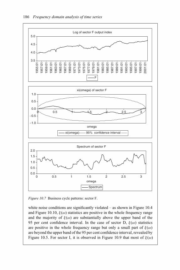
186 Frequency domain analysis of time series
Log of sector F output index
3.5
4.0
4.5
5.0
F
xi(omega) of sector F
−1.0
−0.5
0.00 0.5 1 1.5 2 2.5 3
0.5
1.0
omega
xi(omega) 95% confidence interval
Spectrum of sector F
0.0
0.5
1.0
1.5
2.0
0 0.5 1 1.5 2 2.5 3
omega
Spectrum
1955
:01
1957
:01
1959
:01
1961
:01
1963
:01
1965
:01
1967
:01
1969
:01
1971
:01
1973
:01
1975
:01
1977
:01
1979
:01
1981
:01
1983
:01
1985
:01
1987
:01
1989
:01
1991
:01
1993
:01
1995
:01
1997
:01
1999
:01
2001
:01
Figure 10.7 Business cycle patterns: sector F.
white noise conditions are significantly violated – as shown in Figure 10.4and Figure 10.10, ξ (ω) statistics are positive in the whole frequency rangeand the majority of ξ (ω) are substantially above the upper band of the95 per cent confidence interval. In the case of sector D, ξ (ω) statisticsare positive in the whole frequency range but only a small part of ξ (ω)are beyond the upper band of the 95 per cent confidence interval, revealed byFigure 10.5. For sector I, it is observed in Figure 10.9 that most of ξ (ω)

Frequency domain analysis of time series 187
xi(omega) of sector G&H
–1.0
–0.5
0.0
0.5
1.0
omega
xi(omega) 95% confidence interval
0 0.5 1 1.5 2 2.5 3
Spectrum of sector G&H
0.00.51.01.52.02.53.0
omega
Spectrum
0 0.5 1 1.5 2 2.5 3
Log of sector G&H output index
3.5
4.0
4.5
5.0
G&H
1997
:01
1999
:01
2001
:01
1995
:01
1993
:01
1991
:01
1989
:01
1987
:01
1985
:01
1981
:01
1983
:01
1979
:01
1977
:01
1975
:01
1973
:01
1971
:01
1969
:01
1967
:01
1965
:01
1963
:01
1961
:01
1959
:01
1957
:01
1955
:01
Figure 10.8 Business cycle patterns: sector G&H.
are positive and only a small part of ξ (ω) are beyond the upper band ofthe 95 per cent confidence interval. So, compounding effects are not asstrong in sector D and sector I as in sector A&B and sector J&K. Sincethese sectors possess the features of compounding effects in their response
Continued
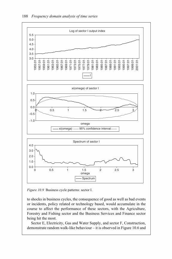
188 Frequency domain analysis of time series
Log of sector I output index
3.0
3.5
4.0
4.5
5.0
5.5
I
xi(omega) of sector I
−1.0
−0.5
0.0
0.5
1.0
omega
xi(omega) 95% confidence interval
Spectrum of sector I
0.0
1.0
2.0
3.0
4.0
omega
Spectrum
0 0.5 1 1.5 2 2.5 3
0 0.5 1 1.5 2 2.5 3
1997
:01
1999
:01
2001
:01
1995
:01
1993
:01
1991
:01
1989
:01
1987
:01
1985
:01
1983
:01
1981
:01
1979
:01
1977
:01
1975
:01
1973
:01
1971
:01
1969
:01
1967
:01
1965
:01
1963
:01
1961
:01
1959
:01
1957
:01
1955
:01
Figure 10.9 Business cycle patterns: sector I.
to shocks in business cycles, the consequence of good as well as bad eventsor incidents, policy related or technology based, would accumulate in thecourse to affect the performance of these sectors, with the Agriculture,Forestry and Fishing sector and the Business Services and Finance sectorbeing hit the most.
Sector E, Electricity, Gas and Water Supply, and sector F, Construction,demonstrate random walk-like behaviour – it is observed in Figure 10.6 and

Frequency domain analysis of time series 189
Log of sector J&K output index
3.5
4.0
4.5
5.0
J&K
xi(omega) of sector J&K
−1.0−0.6−0.20.20.61.01.41.8
omega
xi(omega) 95% confidence interval
Spectrum of sector J&K
0.0
2.0
4.0
6.0
8.0
omega
Spectrum
2000
:01
2001
:01
2002
:01
1999
:01
1998
:01
1997
:01
1996
:01
1995
:01
1994
:01
1993
:01
1992
:01
1991
:01
1990
:01
1989
:01
1988
:01
1987
:01
1986
:01
1985
:01
1984
:01
1983
:01
0 1 2 31.5 2.50.5
0 1 2 31.5 2.50.5
Figure 10.10 Business cycle patterns: sector J&K.
Figure 10.7, respectively, that all the values of the ξ (ω) statistic are confinedto the 95 per cent confidence interval and the near white noise conditionsare not violated. Between the two, the Construction sector exhibits a weakmean-reverting tendency, while the Electricity, Gas and Water Supplysector displays some weak features of mixed complexity, to a statistically
Continued

190 Frequency domain analysis of time series
Log of sector L–Q output index
4.0
4.2
4.4
4.6
4.8
5.0
L–Q
xi(omega) of sector L–Q in difference
−1.5
−1.0
−0.5
0.0
0.5
1.0
omega
xi(omega) 95% confidence interval
Spectrum of sector L–Q in difference
0.0
1.0
2.0
3.0
4.0
omega
Spectrum
2000
:01
2001
:01
2002
:01
1999
:01
1998
:01
1997
:01
1996
:01
1995
:01
1994
:01
1993
:01
1992
:01
1991
:01
1990
:01
1989
:01
1988
:01
1987
:01
1986
:01
1985
:01
1984
:01
1983
:01
0 1 2 31.5 2.50.5
0 1 2 31.5 2.50.5
Figure 10.11 Business cycle patterns: sector L–Q.
insignificant degree. These findings also conform to the two sectors’institutional features and indicate that, between the two sectors, theConstruction sector would display relatively less persistent response patternsin business cycles due to its lower regulatory requirements. SectorG&H, Distribution, Hotels, Catering and Repairs, is associated with amixed complicity response pattern in business cycles and exhibits some
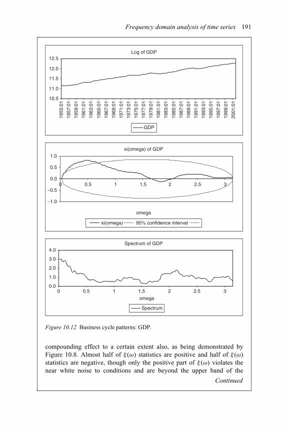
Frequency domain analysis of time series 191
Log of GDP
10.5
11.0
11.5
12.0
12.5
GDP
xi(omega) of GDP
−1.0
−0.5
0.0
0.5
1.0
omega
xi(omega) 95% confidence interval
Spectrum of GDP
0.0
1.0
2.0
3.0
4.0
omega
Spectrum
1997
:01
1999
:01
2001
:01
1995
:01
1993
:01
1991
:01
1989
:01
1987
:01
1985
:01
1983
:01
1981
:01
1979
:01
1977
:01
1975
:01
1973
:01
1971
:01
1969
:01
1967
:01
1965
:01
1963
:01
1961
:01
1959
:01
1957
:01
1955
:01
0 1 2 31.5 2.50.5
32.5210 1.50.5
Figure 10.12 Business cycle patterns: GDP.
compounding effect to a certain extent also, as being demonstrated byFigure 10.8. Almost half of ξ (ω) statistics are positive and half of ξ (ω)statistics are negative, though only the positive part of ξ (ω) violates thenear white noise to conditions and are beyond the upper band of the
Continued
192 Frequency domain analysis of time series
95 per cent confidence interval. Some of the negative ξ (ω) statistics are closeto, but yet to reach, the lower band of the 95 per cent confidence interval.These findings fit into the institutional characteristics of the Distribution,Hotels, Catering and Repairs sector fairly appropriately.
Sector L–Q, Government and Other Services, as expected, exhibits abusiness cycle pattern rather different from that in all other sectors, revealedby Figure 10.11. It possesses mean-reverting tendencies to such an extentthat is almost for a stationary time series. All the values of the ξ (ω) statisticare negative, most of them having violated the near white noise conditionsand being below the lower band of the 95 per cent confidence interval.It can be observed in Table 10.1 that the sector has the most smoothedgrowth, with its standard deviation in growth being much smaller than thatfor all all the other sectors, mainly arising from the sector’s characteristicsof experiencing infrequent shocks in business cycles. Smoothed growth,or a small standard deviation in growth, does not necessarily mean a lowerpersistence or close to being stationary. It is infrequent shocks that, to alarge extent, contribute to the features demonstrated by the Governmentand Other Services sector.
The behaviour of the aggregate GDP must reflect the business cyclefeatures demonstrated by GDP sectors that are dominated by persistent,sizeable compounding effects in their response to shocks in business cycles.It is observed in Figure 10.12 that the majority of ξ (ω) statistics are positive,with a few of them being beyond the upper band of the 95 per centconfidence interval or having violated the near white noise conditions.Although the result from the analysis of the aggregate GDP makes knownits business cycle response patterns and features, which match the outcomeand conclusion of sectoral analysis, it is sectoral analysis, in reference to theinstitutional background and characteristics of the sectors, that reveals howdifferent sectors behave differently in business cycles and exhibit a specificand different business cycle pattern, and lays theoretical cornerstones forGDP’s overall business cycle features.
Example 10.2
This is a case studying comovements among financial markets by meansof cross spectra and phases in the frequency domain, in a paper entitled‘Pre- and post-1987 crash frequency domain analysis among Pacific rimequity markets’ by Smith (2001). The paper examines five stock marketsof Australia, Hong Kong, Japan, the US, and Canada pair-wise, using theindividual stock market index data of Morgan Stanley International CapitalPerspectives, measured in local currencies. The period surrounding the
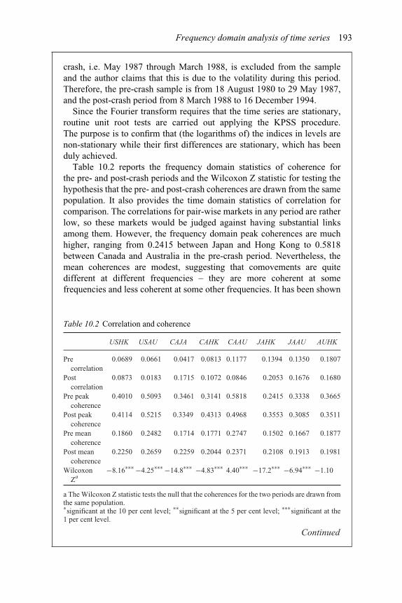
Frequency domain analysis of time series 193
crash, i.e. May 1987 through March 1988, is excluded from the sampleand the author claims that this is due to the volatility during this period.Therefore, the pre-crash sample is from 18 August 1980 to 29 May 1987,and the post-crash period from 8 March 1988 to 16 December 1994.
Since the Fourier transform requires that the time series are stationary,routine unit root tests are carried out applying the KPSS procedure.The purpose is to confirm that (the logarithms of) the indices in levels arenon-stationary while their first differences are stationary, which has beenduly achieved.
Table 10.2 reports the frequency domain statistics of coherence forthe pre- and post-crash periods and the Wilcoxon Z statistic for testing thehypothesis that the pre- and post-crash coherences are drawn from the samepopulation. It also provides the time domain statistics of correlation forcomparison. The correlations for pair-wise markets in any period are ratherlow, so these markets would be judged against having substantial linksamong them. However, the frequency domain peak coherences are muchhigher, ranging from 0.2415 between Japan and Hong Kong to 0.5818between Canada and Australia in the pre-crash period. Nevertheless, themean coherences are modest, suggesting that comovements are quitedifferent at different frequencies – they are more coherent at somefrequencies and less coherent at some other frequencies. It has been shown
Table 10.2 Correlation and coherence
USHK USAU CAJA CAHK CAAU JAHK JAAU AUHK
Precorrelation
0.0689 0.0661 0.0417 0.0813 0.1177 0.1394 0.1350 0.1807
Postcorrelation
0.0873 0.0183 0.1715 0.1072 0.0846 0.2053 0.1676 0.1680
Pre peakcoherence
0.4010 0.5093 0.3461 0.3141 0.5818 0.2415 0.3338 0.3665
Post peakcoherence
0.4114 0.5215 0.3349 0.4313 0.4968 0.3553 0.3085 0.3511
Pre meancoherence
0.1860 0.2482 0.1714 0.1771 0.2747 0.1502 0.1667 0.1877
Post meancoherence
0.2250 0.2659 0.2259 0.2044 0.2371 0.2108 0.1913 0.1981
WilcoxonZa
−8.16∗∗∗ −4.25∗∗∗ −14.8∗∗∗ −4.83∗∗∗ 4.40∗∗∗ −17.2∗∗∗ −6.94∗∗∗ −1.10
a The Wilcoxon Z statistic tests the null that the coherences for the two periods are drawn fromthe same population.∗significant at the 10 per cent level; ∗∗significant at the 5 per cent level; ∗∗∗significant at the1 per cent level.
Continued
194 Frequency domain analysis of time series
that coherences are low at high frequencies. In all the cases, except thepairs of the US and Hong Kong, Canada and Hong Kong and Japan andHong Kong, the coherence falls while the frequency increases. For thepairs of the US and Hong Kong, Canada and Hong Kong and Japan andHong Kong, the peak occurs at the frequency between 0.1 and 0.2 (5–10days). The paper also presents phase diagrams for the pairs of the markets.Without a consistent pattern, the phase diagrams are mainly of practicalinterest.
The Wilcoxon Z statistic suggests that, in every case except the pair ofAustralia and Hong Kong, the pre- and post-crash coherences are statisticallydifferent, or the coherences for the two periods are drawn from differentpopulations. Moreover, both peak and mean coherences have increased inthe post-crash period as against the pre-crash period in all the cases except thepair of Canada and Australia, implying increased post-crash comovementsamong these markets.
10.6. Empirical literature
Frequency domain analysis is most popular in business cycle research becausethe research object and the method match precisely. Garcia-Ferrer and Queralt’s(1998) study is typical in the frequency domain–decomposing business cycles intolong, medium and short term cycles following Schumpeter’s work. They claimthat the frequency domain properties of the time series can be exploited to forecastbusiness cycle turning points for countries exhibiting business cycle asymmetries.Cubadda (1999) examines common features in the frequency domain and thetime domain. Understandably, the author has concluded that the serial correlationcommon feature is not informative for the degree and the lead–lag structure oftheir comovements at business cycle frequencies. Since the lead–lag relationshipin the frequency domain is not an exact mapping of the serial correlation commonfeature in the time domain, the former (latter) does not contain all the informationpossessed by the latter (former), but does contain additional information notpossessed by the latter (former). As being pointed out earlier, transformation doesnot generate extra new information, it simply provides another way of viewing andprocessing information, which may be more effective in certain aspects. Bjornland(2000) is, technically, on business cycle phases. The author finds that consumptionand investment are consistently pro-cyclical with GDP in the time domain and thefrequency domain. However, the business cycle properties of real wage and pricesare not so clear-cut, depending on the de-trending methods used. Although thenumber is considerably less than that in the traditional time domain, there arestill a few empirical studies in the area from time to time, for example, Entorf(1993) on constructing leading indicators from non-balanced sectoral business

Frequency domain analysis of time series 195
survey data, Englund et al. (1992) on Swedish business cycles, Canova (1994) onbusiness cycle turning points, and King and Rebelo (1993) on the Hodrick–Prescottfilter.
As analysis in the frequency domain offers a different way of examining timeseries properties and patterns, it is naturally applied to issues such as unit roots,VAR and cointegrated variables. Choi and Phillips (1993) develop frequencydomain tests for unit roots. Their simulation results indicate that the frequencydomain tests have stable size and good power in finite samples for a variety oferror-generating mechanisms. The authors conclude that the frequency domaintests have some good performance characteristics in relation to time domainprocedures, although they are also susceptible to size distortion when there isnegative serial correlation in the errors. Olekalns (1994) also considers frequencydomain analysis as an alternative to the Dickey–Fuller test. With regard to dynamicmodels, error correction in continuous time is considered by Phillips (1991) in thefrequency domain. Stiassny (1996) proposes a frequency domain decompositiontechnique for structural VAR models and argues, with an example, the benefit ofadopting this technique in providing another dimension of the relationships amongvariables. Examining univariate impulse responses in the frequency domain,Wright (1999) estimates univariate impulse response coefficients by smoothing theperiodogram and then calculating the corresponding impulse response coefficientsand forms the confidence intervals of the coefficients through a frequency domainbootstrap procedure.
Other empirical studies on varied topics can be found in Cohen (1999) onanalysis of government spending, Wolters (1995) on the term structure of interestrates in Germany, Koren and Stiassny (1995) on the causal relation between taxand spending in Austria, Copeland and Wang (1993) on combined use of timedomain and frequency domain analyses, and Bizer and Durlauf (1990) on thepositive theory of government finance, to list a few.
Notes
1 This can also be the product of the Fourier transform and its conjugate.2 For example Bartlett (1950), Grenander and Rosenblatt (1953, 1957), and Priestley
(1996).
3 ξ ′ω(ω) = N1/2
[Ip(ω) − 1
2π], ξ ′′
ω(ω) = N1/2I ′p(ω).
Questions and problems
1 What is spectral analysis of time series? Does spectral analysis render new ormore information?
2 Discuss the advantages and disadvantages of the analysis in the frequencydomain.
3 Describe the Fourier transform and the inverse Fourier transform.4 What are phases and coherence in spectral analysis? Contrast them with
leads/lags and correlation in the time domain.
196 Frequency domain analysis of time series
5 Collect data from various sources and perform the Fourier transform for thefollowing time series (using RATS, GAUSS or other packages):
(a) GDP of selected countries,(b) total return series of selected companies,(c) foreign exchange rates of selected countries vis-à-vis the US$.
6 Collect data from DataStream and estimate phases and coherence for thefollowing pairs of time series:
(a) the spot and forward foreign exchange rates of the UK£ vis-à-vis the US$,(b) the spot foreign exchange rates of the UK£ and Japanese yen vis-à-vis
the US$.
7 Collect data from various sources and estimate phases and coherence for thefollowing pairs of time series:
(a) GDP of the US and the Canada,(b) GDP and retail sales of the UK.
8 Collect data from DataStream and estimate phases and coherence for thefollowing pairs of time series:
(a) total returns of Tesco and Sainsbury’s,(b) total returns of Intel and Motorola.
References
Bartlett, M.S. (1950), Periodogram analysis and continuous spectra, Biometrika, 37, 1–16.Bizer, D.S. and Durlauf, S.N. (1990), Testing the positive theory of government finance,
Journal of Monetary Economics, 26, 123–141.Bjornland, H.C. (2000), Detrending methods and stylised facts of business cycles in
Norway: an international comparison, Empirical Economics, 25, 369–392.Campbell, J.Y. and Mankiw, N.W. (1987a), Are output fluctuations transitory?, Quarterly
Journal of Economics, 102, 857–880.Campbell, J.Y. and Mankiw, N.W. (1987b), Permanent and transitory components in
macroeconomic fluctuations, American Economic Review, 77 (Papers and Proceedings),111–117.
Canova, F. (1994), Detrending and turning points, European Economic Review,38, 614–623.
Choi, I. and Phillips, P.C.B. (1993), Testing for a unit root by frequency domain regression,Journal of Econometrics, 59, 263–286.
Cochrane, J.H. (1988), How big is the random walk in GDP?, Journal of Political Ecomony,96, 893–920.
Cohen, D. (1999), An analysis of government spending in the frequency domain, Boardof Governors of the Federal Reserve System Finance and Economics DiscussionSeries: 99/26.
Copeland, L.S. and Wang, P.J. (1993), Estimating daily seasonals in financial time series:the use of high-pass spectral filters, Economics Letters, 43, 1–4.

Frequency domain analysis of time series 197
Cubadda, G. (1999), Common serial correlation and common business cycles: a cautiousnote, Empirical Economics, 24, 529–535.
Englund, P., Persson, T. and Svensson, L.E.O. (1992), Swedish business cycles: 1861–1988,Journal of Monetary Economics, 30, 343–371.
Entorf, H. (1993), Constructing leading indicators from non-balanced sectoral businesssurvey series, International Journal of Forecasting, 9, 211–225.
Garcia-Ferrer, A. and Queralt, R.A., (1998), Using long-, medium-, and short-term trendsto forecast turning points in the business cycle: some international evidence, Studies inNonlinear Dynamics and Econometrics, 3, 79–105.
Grenander, U. and Rosenblatt, M. (1953), Statistical spectral analysis arising from stationarystochastic processes, Annals of Mathematical Statistics, 24, 537–558.
Grenander, U. and Rosenblatt, M. (1957), Statistical Analysis of Stationary Time Series,Wiley, New York.
King, R.G. and Rebelo, S.T. (1993), Low frequency filtering and real business cycles,Journal of Economic Dynamics and Control, 17, 207–331.
Koren, S. and Stiassny, A. (1995), Tax and spend or spend and tax? an empiricalinvestigation for Austria, Empirica, 22, 127–149.
Olekalns, N. (1994), Testing for unit roots in seasonally adjusted data, Economics Letters,45, 273–279.
Pesaran, M.H., Pierse, R.G. and Lee, K.C., (1993), Persistence, cointegration andaggregation: a disaggregated analysis of output fluctuations in the US economy, Journalof Econometrics, 56, 67–88.
Phillips, P.C.B. (1991), Error correction and long-run equilibrium in continuous time,Econometrica, 59, 967–980.
Priestley, M.B. (1996), Sprectral Analysis and Time Seties 9th edition (1st edition 1981),Academic Press, London.
Smith, K.L. (2001), Pre- and post-1987 crash frequency domain analysis among PacificRim equity markets, Journal of Multinational Financial Management, 11, 69–87.
Stiassny, A. (1996), A spectral decomposition for structural VAR models, EmpiricalEconomics, 21, 535–555.
Wolters, J. (1995), On the term structure of interest rates – empirical results for Germany,Statistical Papers, 36, 193–214.
Wright, J.H. (1999), Frequency domain inference for univariate impulse responses,Economics Letters, 63, 269–277.
11 Limited dependent variables anddiscrete choice models
Firms and individuals encounter choice problems from time to time. An investmentdecision is indeed to make a choice; so is a savings decision – whether to saveand how much to save. One particular kind of choice is binary choice. Forexample, a firm may choose to use financial derivatives to hedge interest raterisk, or choose not to use financial derivatives. A firm may decide to expand itsbusiness into foreign markets, or not to expand into foreign markets. Further,if the firm decides to expand its business overseas, it may acquire an existingfirm in the foreign country as part of its strategic plan, or establish a newplant in the foreign country. In pension provisions, if employees are entitledto choose between a defined benefit plan and a defined contribution plan, theyhave to make a decision of binary choice. On the other hand, employers maydecide to close the defined benefit plan to new members or continue to offerthe defined benefit plan to new members. There are numerous such examples ofbinary choice in people’s daily life, firms’ financing and investment activities,managers’ business dealings, and financial market operations. Binary choicecan be extended to discrete choice in general, i.e. there are more than twoalternatives to choose from but the values of the variable are still discrete, suchas 0, 1, 2, or 1, 2, 3, 4. A simple example can be firms’ choice of overseas stockexchanges for dual listings, e.g. they may choose one of New York, Tokyo, orLondon. Binary or discrete choice models can be generalised to refer to anycases where the dependent variable is discrete, such as discrete responses andcategories.
In addition to discrete choice models where a dependent variable possessesdiscrete values, the values of dependent variables can also be censored or truncated.That is, the variable is not observed over its whole range. A dependent variablethat is discrete, truncated or censored is a limited dependent variable. This chapteraddresses discrete choice models while the next chapter deals with truncation andcensoring. The chapter first presents the commonly used formulations of probitand logit for binary choice models. General discrete choice models are introducednext in the multinomial logit framework, followed by ordered probit and orderedlogit. Since discrete choice models are non-linear, marginal effects are consideredspecifically in one section. Deviating from the preceding chapters of the book, datasets analysed in this chapter and the next are primarily cross-sectional. That is,

Limited dependent variables and discrete choice models 199
they are data for multiple entities, such as individuals, firms, regions or countries,observed at a single time point.
11.1. Probit and logit formulations
In a binary choice model, the dependent variable takes the value of either 1 or 0,with a probability that is a function of one or more independent variables. A binaryvariable is sometimes said to obey a binomial distribution; while a discrete variabletaking more than two discrete values is said to possess a multinomial distribution,a topic to be studied in the next section. When the dependent variable is binaryor discrete, some assumptions on linear regression estimation procedures, suchas the OLS where the dependent variable is continuous, do not hold. Alternativemethods have to be employed for the formulation and estimation of binary anddiscrete choice modelling appropriately. Probit and logit models are two commonlyused models to formulate binary choice, response or categorisation. The probitmodel derives its name from the probit function, so does the logit model from thelogistic function. Regression for estimating the probit model is referred to probitregression, and regression for estimating the logit model is commonly known aslogistic regression.
The underlying process of the observed binary variable is supposed to be anunobserved latent variable. Their relationship and presentation are:
Y ∗ = Xβ+ ε (11.1a)
Y ={
1, if Y ∗ ≥ 00, if Y ∗ < 0
(11.1b)
The unobserved variable is a continuous function of a linear combination of a setof explanatory variables, which measures the utility of an activity. If the functionvalue or utility is high enough, the activity will be undertaken and 1 is chosen.Otherwise, if the function value or utility is not high enough, the activity will notbe undertaken and 0 is chosen.
The probit function is the inverse cumulative distribution function of the normaldistribution. The probit model employs an inverse probit function, so it is a kind ofthe cumulative standard normal distribution. Let Y be a binary variable that takesthe value of either 1 or 0. The probit model is defined as:
P (Y = 1 |Xβ) = � (Xβ) (11.2)
where X is a vector of explanatory variables, β is a vector of the correspondingcoefficients, and � (z) is the cumulative normal distribution. The probit modelstates that the probability of Y taking the value of 1 follows the cumulativestandard normal distribution of a linear function of the given set of explanatoryvariables X.
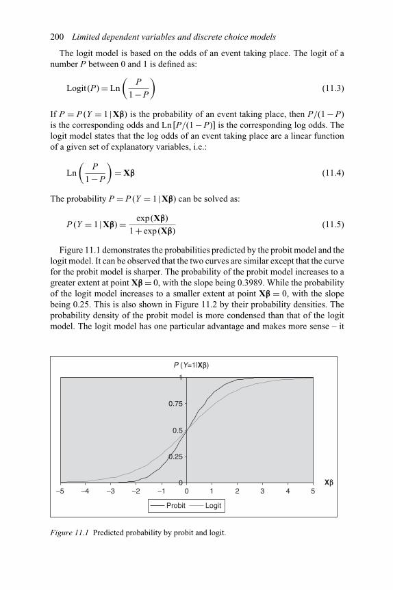
200 Limited dependent variables and discrete choice models
The logit model is based on the odds of an event taking place. The logit of anumber P between 0 and 1 is defined as:
Logit (P) = Ln
(P
1 − P
)(11.3)
If P = P (Y = 1 |Xβ) is the probability of an event taking place, then P/(1 − P)is the corresponding odds and Ln [P/(1 − P)] is the corresponding log odds. Thelogit model states that the log odds of an event taking place are a linear functionof a given set of explanatory variables, i.e.:
Ln
(P
1 − P
)= Xβ (11.4)
The probability P = P (Y = 1 |Xβ) can be solved as:
P (Y = 1 |Xβ) = exp(Xβ)
1 + exp(Xβ)(11.5)
Figure 11.1 demonstrates the probabilities predicted by the probit model and thelogit model. It can be observed that the two curves are similar except that the curvefor the probit model is sharper. The probability of the probit model increases to agreater extent at point Xβ = 0, with the slope being 0.3989. While the probabilityof the logit model increases to a smaller extent at point Xβ = 0, with the slopebeing 0.25. This is also shown in Figure 11.2 by their probability densities. Theprobability density of the probit model is more condensed than that of the logitmodel. The logit model has one particular advantage and makes more sense – it
00 1−1 2−2 3−3 4−4 5−5
0.25
0.5
0.75
1
Probit Logit
P (Y=1|Xb)
Xb
Figure 11.1 Predicted probability by probit and logit.
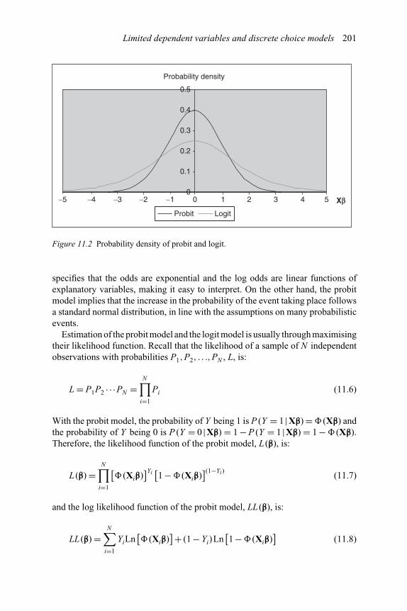
Limited dependent variables and discrete choice models 201
Probability density
00
0.1
0.2
0.3
0.4
0.5
Probit Logit
Xb543−3−4−5 2−2 1−1
Figure 11.2 Probability density of probit and logit.
specifies that the odds are exponential and the log odds are linear functions ofexplanatory variables, making it easy to interpret. On the other hand, the probitmodel implies that the increase in the probability of the event taking place followsa standard normal distribution, in line with the assumptions on many probabilisticevents.
Estimation of the probit model and the logit model is usually through maximisingtheir likelihood function. Recall that the likelihood of a sample of N independentobservations with probabilities P1,P2, . . .,PN , L, is:
L = P1P2 · · ·PN =N∏
i=1
Pi (11.6)
With the probit model, the probability of Y being 1 is P (Y = 1 |Xβ) = � (Xβ) andthe probability of Y being 0 is P (Y = 0 |Xβ) = 1 − P (Y = 1 |Xβ) = 1 − � (Xβ).Therefore, the likelihood function of the probit model, L (β), is:
L (β) =N∏
i=1
[� (Xiβ)
]Yi[1 −� (Xiβ)
](1−Yi) (11.7)
and the log likelihood function of the probit model, LL (β), is:
LL (β) =N∑
i=1
YiLn[� (Xiβ)
]+ (1 − Yi)Ln[1 −� (Xiβ)
](11.8)

202 Limited dependent variables and discrete choice models
Similarly, for the logit model, the probability of Y being 1 is:
P (Y = 1 |Xβ) = exp(Xβ)
1 + exp(Xβ)
and the probability of Y being 0 is:
P (Y = 0 |Xβ) = 1 − P (Y = 1 |Xβ) = 1 − exp(Xβ)
1 + exp(Xβ)
Therefore, the likelihood function of the logit model, L (β), is:
L (β) =N∏
i=1
[exp(Xiβ)
1 + exp(Xiβ)
]Yi[1 − exp(Xiβ)
1 + exp(Xiβ)
](1−Yi)
(11.9)
and the log likelihood function of the logit model, LL (β), is:
LL (β) =N∑
i=1
YiLn
[exp(Xiβ)
1 + exp(Xiβ)
]+ (1 − Yi)Ln
[1 − exp(Xiβ)
1 + exp(Xiβ)
](11.10)
Coefficient estimates can be derived, adopting procedures that maximise the abovelog likelihood functions.
11.2. Multinomial logit models and multinomial logisticregression
The multinomial distribution is an extension of the binomial distribution when andwhere there are more than two discrete outcomes – choices, responses or categories.Estimation of multinomial logit models is usually dealt with by multinomiallogistic regression. A simplest multinomial logit model is one where the dependentvariable can have three discrete values of 0, 1 and 2. Let P1 denote P (Y = 1 |Xβα)and P2 denote P (Y = 2 |Xγα). Let P0 = P (Y = 0 |Xα) be the base category orreference category. Let β = βα −α and γ = γα −α. In a similar but not an exactlycomparable way in which odds are applied in the previous section, we constructtwo binomial logit models with reference to the base category of P0:
Ln
(P1
P0
)= Xβ (11.11a)
Ln
(P2
P0
)= Xγ (11.11b)

Limited dependent variables and discrete choice models 203
Note P0 = 1 − P1 − P2, so:
Ln
(P1
P0
)= Ln
(P1
1 − P1 − P2
)= Xβ (11.12a)
Ln
(P2
P0
)= Ln
(P2
1 − P1 − P2
)= Xγ (11.12b)
The probability P (Y = 1 |Xβ) can therefore be solved as:
P (Y = 1 |Xβ) = exp(Xβ)
1 + exp(Xβ) + exp(Xγ)(11.13a)
the probability P (Y = 2 |Xγ) is:
P (Y = 2 |Xγ) = exp(Xγ)
1 + exp(Xβ) + exp(Xγ)(11.13b)
and the probability P (Y = 0 |Xα) is:
P (Y = 0) = 1
1 + exp(Xβ) + exp(Xγ)(11.13c)
The pair-wise likelihood functions of the above multinomial logit model againstthe reference category are:
L (β) =N∏
i=1
[exp(Xiβ)
1 + exp(Xiβ)
]Yi[1 − exp(Xiβ)
1 + exp(Xiβ)
](1−Yi)
, Yi = 0,1
(11.14a)
L (β) =N∏
i=1
[exp(Xiγ)
1 + exp(Xiγ)
]Yi/2[1 − exp(Xiγ)
1 + exp(Xiγ)
][1−(Yi/2)]
, Yi = 0,2
(11.14b)
and the log likelihood functions of the above multinomial logit model are:
LL(β)=N∑
i=1
YiLn
[exp(Xiβ)
1+exp(Xiβ)
]+(1−Yi)Ln
[1− exp(Xiβ)
1+exp(Xiβ)
]Yi =0,1
(11.15a)
LL(β)=N∑
i=1
Yi
2Ln
[exp(Xiγ)
1+exp(Xiγ)
]+(1− Yi
2
)Ln
[1− exp(Xiγ)
1+exp(Xiγ)
]Yi =0,2
(11.15b)
In general, a multinomial model with m + 1 discrete outcomes has m pairs oflog ‘odds’ against the reference category. Let P0 = P (Y = 0 |Xβ0) be the base

204 Limited dependent variables and discrete choice models
category or reference category, Pj = P(Y = j |Xβ0
j
)(j = 1, . . .m) and βj = β0
j −β0( j = 1, . . .m). Then these m pairs of log odds are:
Ln
(P1
P0
)= Xβ1 (11.16a)
Ln
(P2
P0
)= Xβ2 (11.16b)
. . .
Ln
(Pm
P0
)= Xβm (11.16c)
The probability P (Y = 1 |Xβ1), P (Y = 2 |Xβ2), . . . P (Y = m |Xβm) can be jointlysolved as:
P (Y = 1 |Xβ1) = exp(Xβ1)
1 +∑mj=1 exp
(Xβj
) (11.17a)
P (Y = 2 |Xβ2) = exp(Xβ2)
1 +∑mj=1 exp
(Xβj
) (11.17b)
. . .
P (Y = m |Xβm) = exp(Xβm)
1 +∑mj=1 exp
(Xβj
) (11.17c)
P (Y = 0) = 1
1 +∑mj=1 exp
(Xβj
) (11.17d)
The pair-wise likelihood functions of the above general multinomial logit modelagainst the reference category are:
L (β) =N∏
i=1
[exp(Xiβ1)
1 + exp(Xiβ1)
]Yi[1 − exp(Xiβ1)
1 + exp(Xiβ1)
](1−Yi)
, Yi = 0,1
(11.18a)
L (β) =N∏
i=1
[exp(Xiβ2)
1 + exp(Xiβ2)
]Yi/2[1 − exp(Xiβ2)
1 + exp(Xiβ2)
][1−(Yi/2)]
, Yi = 0,2
(11.18b)
. . .
L (β) =N∏
i=1
[exp(Xiβm)
1 + exp(Xiβm)
]Yi/m[1 − exp(Xiβm)
1 + exp(Xiβm)
][1−(Yi/m)]
, Yi = 0,m
(11.18c)

Limited dependent variables and discrete choice models 205
and the log likelihood functions of the above general multinomial logit model are:
LL (β) =N∑
i=1
YiLn
[exp(Xiβ1)
1 + exp(Xiβ1)
]+ (1 − Yi)Ln
[1 − exp(Xiβ1)
1 + exp(Xiβ1)
]
Yi = 0,1 (11.19a)
LL (β) =N∑
i=1
Yi
2Ln
[exp(Xiβ2)
1 + exp(Xiβ2)
]+(
1 − Yi
2
)Ln
[1 − exp(Xiβ2)
1 + exp(Xiβ2)
]
Yi = 0,2 (11.19b)
. . .
LL (β) =N∑
i=1
Yi
mLn
[exp(Xiβm)
1 + exp(Xiβm)
]+(
1 − Yi
m
)Ln
[1 − exp(Xiβm)
1 + exp(Xiβm)
]
Yi = 0,m (11.19c)
11.3. Ordered probit and logit
Discrete variables that can be ordered are ordinal variables. Ordered probitand ordered logit are two models used to analyse ordinal dependent variables.Typical ordinal cases are formatted responses to questionnaire surveys, such asthe following:
StronglyDisagree
Disagree Neither agreenor disagree
Agree Stronglyagree
1 2 3 4 5
The scaling need not be 1 to 5 and the increment need not be one. It can be, forexample, −2, −1, 0, 1, 2; or 0, 5, 10.
Let Y ∗ be an unobserved latent variable that underlies the observed ordinalvariable Y in the following way:
Y ∗ = Xβ+ ε (11.20a)
Y = i, if ωi−1 ≤ Y ∗ < ωi, i = 1, . . .k (11.20b)
where ωi is the cut-point. With an ordered probit, the probability of the ith choiceor category is chosen is:
P (Y = i |Xβ) = P (Xβ+ ε < ωi) − P(Xβ+ ε < ωi−1
)= P (ε < −Xβ+ωi) − P
(ε < −Xβ+ωi−1
)= � (−Xβ+ωi) −�
(−Xβ+ωi−1
)(11.21)

206 Limited dependent variables and discrete choice models
where � (z) denotes the cumulative normal distribution. The cumulative probabil-ity for Y ≤ i, conditional on Xβ, is:
P (Y ≤ i |Xβ) =i∑
j=1
P (Y = j |Xβ)
= � (−Xβ+ω1) +� (−Xβ+ω2) −� (−Xβ+ω1)
+·· ·+� (−Xβ+ωi) −�(−Xβ+ωi−1
)= � (−Xβ+ωi) (11.22)
While the cumulative probability for Y > i, conditional on Xβ, is:
P (Y > i |Xβ) = 1 − P (Y ≤ i |Xβ) =k∑
j=i+1
P (Y = j |Xβ) = � (Xβ−ωi)
(11.23)
Using ordered logit for odinal variables, we refer to odds as expected. The oddsare the logit of the cumulative probability for Y ≤ i or the ratio of the cumulativeprobability for Y ≤ i to the cumulative probability for the rest:
Logit [P (Y ≤ i |Xβ)] = P (Y ≤ i |Xβ)
P (Y > i |Xβ)=∑i
j=1 P (Y = j |Xβ)∑kj=i+1 P (Y = j |Xβ)
(11.24)
and the log odds are:
Ln {Logit [P (Y ≤ i |Xβ)]} = Ln
[P (Y ≤ i |Xβ)
P (Y > i |Xβ)
]
= Ln
⎡⎣ i∑
j=1
P (Y = j |Xβ)
⎤⎦− Ln
⎡⎣ k∑
j=i+1
P (Y = j |Xβ)
⎤⎦= ωi − Xβ
(11.25)
We also write the odds and log odds in the following way for the purpose to contrastthe multinomial logit model and ordered logit model:
Ln {Logit [P (Y > i |Xβ)]} = Ln
[P (Y > i |Xβ)
P (Y ≤ i |Xβ)
]
= Ln
⎡⎣ k∑
j=i+1
P (Y = j |Xβ)
⎤⎦− Ln
⎡⎣ i∑
j=1
P (Y = j |Xβ)
⎤⎦= Xβ−ωi
(11.26)
Note that the allocation of 0,1,2, . . . is arbitrary in multinomial logit models, i.e.we can code 0 for red, 1 for blue, and 2 for yellow; but we can also code 0 for

Limited dependent variables and discrete choice models 207
blue, 1 for yellow, and 2 for red. However, we cannot alter 0,1,2, . . . arbitrarily.e.g. for four colours of sky blue, light blue, blue and dark blue, we may code themthis way: 0 for sky blue, 1 for light blue, 2 for blue and 3 for dark blue. We mayalso code them that way: 0 for dark blue, 1 for blue, 2 for light blue and 3 for skyblue. But we cannot code them like this: 0 for blue, 1 for sky blue, 2 for light blueand 3 dark blue. Another example of contrast is coffee, tea and chocolate on theone hand, and a short latte, a tall latte and a grande latte on the other hand. For theformer it can be a case of a multinomial logit model and, for the latter, a case ofan ordered logit model.
11.4. Marginal effects
There is no need to examine marginal effects for linear probability models that wehave experienced, such as linear regression. This is because the marginal effectin such models is constant. The marginal effect measures the effect of a one unitchange in one of the explanatory variables on the dependent variable, holding allother explanatory variables constant. In linear probability models such as linearregression, this is simply the coefficient of the explanatory variable. For binarychoice models, the probability of the dependent variable being one is a non-linearfunction of its explanatory variables, though the underlying process of the observedbinary variable, supposed to be an unobserved latent variable, is a linear function ofexplanatory variables. This applies to discrete choice models in general, includingmultinomial and ordered choice models. Consequently, the marginal effect in thesemodels is non-constant. The marginal effect changes and is specific to the givenvalue of the explanatory variable.
Recalling the probit model of equation (11.2), the marginal effect of the probitmodel can be derived as follows:
∂P (Y = 1 |Xβ)
∂X= ∂ [� (Xβ)]
∂X= φ (Xβ)β′ (11.27)
For example, if X = [X1 X2
]is a 1 × 2 row vector of explanatory variables,
β =[β1β2
]is a 2 × 1 column vector of coefficients, then:
∂P (Y = 1 |Xβ)
∂X
=[∂P (Y = 1 |β1X1 +β2X2)
∂X1
∂P (Y = 1 |β1X1 +β2X2)
∂X2
]
=[∂[� (β1X1 +β2X2)
]∂X1
∂[� (β1X1 +β2X2)
]∂X2
]
= φ (β1X1 +β2X2)[β1 β2
](11.28)
It is the derivative of the probability of Y = 1, conditioning on the explanatoryvariables, with respect to each of the explanatory variables. Since φ (Xβ) generally
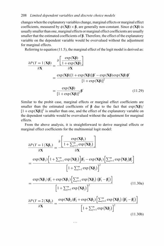
208 Limited dependent variables and discrete choice models
changes when the explanatory variables change, marginal effects or marginal effectcoefficients, measured by φ (Xβ) × β, are generally non-constant. Since φ (Xβ) isusually smaller than one, marginal effects or marginal effect coefficients are usuallysmaller that the estimated coefficients of β. Therefore, the effect of the explanatoryvariable on the dependent variable would be overvalued without the adjustmentfor marginal effects.
Referring to equation (11.5), the marginal effect of the logit model is derived as:
∂P (Y = 1 |Xβ)
∂X=
∂
[exp(Xβ)
1 + exp(Xβ)
]∂X
= exp(Xβ) [1 + exp(Xβ)]β′ − exp(Xβ)exp(Xβ)β′
[1 + exp(Xβ)]2
= exp(Xβ)
[1 + exp(Xβ)]2 β′ (11.29)
Similar to the probit case, marginal effects or marginal effect coefficients aresmaller than the estimated coefficients of β due to the fact that exp(Xβ)/[1 + exp(Xβ)]2 is smaller than one, and the effect of the explanatory variable onthe dependent variable would be overvalued without the adjustment for marginaleffects.
From the above analysis, it is straightforward to derive marginal effects ormarginal effect coefficients for the multinomial logit model:
∂P (Y = 1 |Xβ1)
∂X=
∂
[exp(Xβ1)
1 +∑mj=1 exp
(Xβj
)]
∂X
=exp(Xβ1)
[1 +∑m
j=1 exp(Xβj
)]β′
1 − exp(Xβ1)[∑m
j=1 exp(Xβj
)β′
j
][1 +∑m
j=1 exp(Xβj
)]2
=exp(Xβ1) β′
1 + exp(Xβ1)[∑m
j=1 exp(Xβj
) (β′
1 − β′j
)][1 +∑m
j=1 exp(Xβj
)]2 (11.30a)
∂P (Y = 2 |Xβ2)
∂X=
exp(Xβ2)β′2 + exp(Xβ2)
[∑mj=1 exp
(Xβj
) (β′
2 − β′j
)][1 +∑m
j=1 exp(Xβj
)]2
(11.30b)
. . .
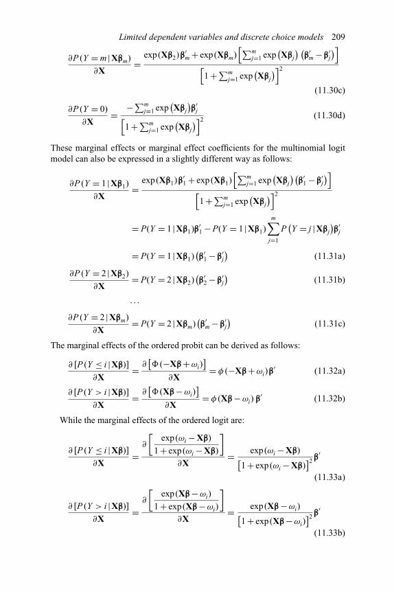
Limited dependent variables and discrete choice models 209
∂P (Y = m |Xβm)
∂X=
exp(Xβ2)β′m + exp(Xβm)
[∑mj=1 exp
(Xβj
) (β′
m − β′j
)][1 +∑m
j=1 exp(Xβj
)]2
(11.30c)
∂P (Y = 0)
∂X= −∑m
j=1 exp(Xβj
)β′
j[1 +∑m
j=1 exp(Xβj
)]2 (11.30d)
These marginal effects or marginal effect coefficients for the multinomial logitmodel can also be expressed in a slightly different way as follows:
∂P (Y = 1 |Xβ1)
∂X=
exp(Xβ1)β′1 + exp(Xβ1)
[∑mj=1 exp
(Xβj
)(β′
1 − β′j
)][1 +∑m
j=1 exp(Xβj
)]2
= P(Y = 1 |Xβ1)β′1 − P(Y = 1 |Xβ1)
m∑j=1
P(Y = j |Xβj
)β′
j
= P(Y = 1 |Xβ1)(β′
1 − β′j
)(11.31a)
∂P (Y = 2 |Xβ2)
∂X= P(Y = 2 |Xβ2)
(β′
2 − β′j
)(11.31b)
. . .
∂P (Y = 2 |Xβm)
∂X= P(Y = 2 |Xβm)
(β′
m − β′j
)(11.31c)
The marginal effects of the ordered probit can be derived as follows:
∂ [P (Y ≤ i |Xβ)]
∂X= ∂
[� (−Xβ+ωi)
]∂X
= φ (−Xβ+ωi)β′ (11.32a)
∂ [P (Y > i |Xβ)]
∂X= ∂
[� (Xβ−ωi)
]∂X
= φ (Xβ−ωi) β′ (11.32b)
While the marginal effects of the ordered logit are:
∂ [P (Y ≤ i |Xβ)]
∂X=
∂
[exp(ωi − Xβ)
1 + exp(ωi − Xβ)
]∂X
= exp(ωi − Xβ)[1 + exp(ωi − Xβ)
]2 β′
(11.33a)
∂ [P (Y > i |Xβ)]
∂X=
∂
[exp(Xβ−ωi)
1 + exp(Xβ−ωi)
]∂X
= exp(Xβ−ωi)[1 + exp(Xβ−ωi)
]2 β′
(11.33b)
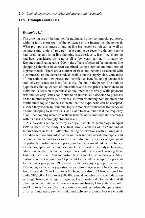
210 Limited dependent variables and discrete choice models
11.5. Examples and cases
Example 11.1
The growing use of the Internet for trading and other commercial purposes,within a fairly short spell of the existence of the Internet, is phenomenal.What prompts customers to buy on-line has become a relevant as well asan interesting topic of research on e-commerce recently, though peoplehad rarely taken this on-line shopping issue seriously, if on-line shoppinghad been considered an issue at all a few years earlier. In a study byKoyuncu and Bhattacharya (2004), the effects of selected factors on on-lineshopping behaviour have been examined, using binomial and multinomiallogistic models. There are a number of risks and benefits associated withe-commerce, on the demand side as well as on the supply side. Quicknessof transactions and low prices are identified as benefits, and payment riskand delivery issues are identified as risk factors in the paper. The authorshypothesise that quickness of transactions and lower prices contribute to anindividual’s decision to purchase on the Internet positively while paymentrisk and delivery issues contribute to an individual’s decision to purchaseon the Internet negatively. Their results from estimating both binomial andmultinomial logistic models indicate that the hypothesis can be accepted.Further, they use the multinomial logistic model to estimate the frequency ofon-line shopping by individuals, and claim to have found that the frequencyof on-line shopping increases with the benefits of e-commerce and decreaseswith its risks, a seemingly obvious result.
A survey data set collected by Georgia Institute of Technology in April1998 is used in the study. The final sample consists of 1842 individualInternet users in the US after eliminating observations with missing data.The data set contains information on each individual’s demographic andeconomic characteristics as well as the individual’s degrees of agreementon particular on-line issues of price, quickness, payment risk, and delivery.The demographic and economic characteristics used in the study include age,education, gender, income and experience with the Internet. Among these1842 Internet users, 1504 are on-line buyers and 338 are non-buyers. Maleon-line shoppers account for 54 per cent for the whole sample, 58 per centfor the buyer group, and 39 per cent for the non-buyer group respectively.The coding for the survey questions is as follows. Age is in 11 bands rangingfrom 1 for under 21 to 11 for over 65; Income is also in 11 bands, from 1 forunder $10,000 to 11 for over $100,000 annual household income; Educationis in eight bands; With regard to gender, 1 is for male and 0 for female and allother responses; Internet experience is in nine bands, 1 for under 6 monthsand 9 for over 7 years; The four questions regarding on-line shopping issuesof price, quickness, payment risk, and delivery are on a 1–5 scale, with

Limited dependent variables and discrete choice models 211
1 being strongly disagree, 2 being disagree, 3 being neither disagree noagree, 4 being agree and 5 being strongly agree.
First, they use a binomial logistic model to evaluate the impact ofan individual’s reaction to price, quickness, payment risk, and deliveryissues on that individual’s on-line shopping decision. Table 11.1 reportsthe results from estimating the binomial model. The second and thirdcolumns are for their benchmark model, which includes only the variablesrepresenting demographic and economic factors and on-line shoppingexperience. The last two columns are for their full model, further includingindividuals’ degrees of agreement on the four survey questions regardingprice, quickness, payment risk, and delivery. Both the coefficients andmarginal effects coefficients are reported. All the coefficients, except that forthe age variable, are statistically significant at the 10 per cent level or higherfor both models. Nevertheless, the level of significance of the coefficientsfor the demographic and economic character variables falls when the on-line shopping character variables are included. According to these results,
Table 11.1 Binomial logistic estimation of on-line shopping
Coefficient Marginal effect Coefficient Marginal effect
Constant −1.233∗∗∗(0.268)
−0.161∗∗∗(0.035)
0.110(0.577)
0.011(0.058)
Age 0.042(0.026)
0.005(0.003)
0.024(0.028)
0.002(0.003)
Income 0.075∗∗∗(0.023)
0.097∗∗∗(0.003)
0.052∗∗(0.025)
0.005∗∗(0.002)
Education 0.140∗∗∗(0.050)
0.018∗∗∗(0.007)
0.114∗∗(0.054)
0.012∗∗(0.006)
Gender 0.527∗∗∗(0.129)
0.069∗∗∗(0.017)
0.423∗∗∗(0.144)
0.043∗∗∗(0.015)
Experience 0.266∗∗∗(0.033)
0.035∗∗∗(0.004)
0.204∗∗∗(0.035)
0.021∗∗∗(0.003)
Quickness 0.394∗∗∗(0.069)
0.040∗∗∗(0.007)
Price 0.297∗∗∗(0.076)
0.030∗∗∗(0.008)
Risk −0.687∗∗∗(0.074)
−0.069∗∗∗(0.007)
Delivery −0.186∗∗(0.087)
−0.019∗∗(0.009)
Standard errors in parentheses.∗significant at the 10 per cent level; ∗∗significant at the 5 per cent level; ∗∗∗significant at the1 per cent level.Marginal effects evaluated at the sample means.
Continued

212 Limited dependent variables and discrete choice models
income, education and internet experience all have a positive effect on theon-line shopping decision. That is, the higher the household income, themore likely the individual would shop on-line; the higher the individual’seducation, the more likely that individual would shop on-line; the moreinternet experience the individual has, the more likely that individual wouldshop on-line. However, it is unclear why being a male is more likely toshop on-line. The effect of the four on-line shopping issues is as expected.The advantages of better prices and time-saving offered by on-line shoppinginduce individuals to buy on-line, with the two coefficients for the variablesrepresenting these two aspects of on-line shopping being positive and highlysignificant at the 1 per cent level. The risk of making on-line payment isconfirmed a concern for not using the Internet for shopping, with a highlysignificant negative coefficient for the variable. To a lesser extent, a longperiod for delivering the item purchased via the Internet has a negative effecton the on-line shopping decision, with the coefficient for the variable beingnegatively significant at the 5 per cent level.
They then examine the effect of the four on-line issues on individuals’on-line purchasing frequencies. They set five different categories accordingto the frequency with which on-line shopping takes place. 0 denotes thecategory for individuals who do not make on-line shopping at all; 1 denotesthe category for individuals who do on-line shopping less than once eachmonth; 2 denotes the category for individuals who do on-line shoppingabout once each month; 3 denotes the category for individuals who doon-line shopping several times each month; and 4 denotes the categoryfor individuals who do on-line shopping about once per week or morefrequently. In their multinomial logistic analysis, the base category is thoseindividuals who do not shop on-line at all. Table 11.2 reports the resultsfrom estimating the multinomial model.
Unlike binomial models where the sign of the marginal effects coefficientis always the same as that of the coefficient, the sign of the marginal effectscoefficient can be different from that of its corresponding coefficient. Thereare several examples in Table 11.2. Equations (11.30) and (11.31) revealthe fact and reason why the sign of the marginal effects coefficient maybe different from that of the coefficient for multinomial models. Let uspay attention to panel B, the results of the full model. The marginal effectscoefficient has changed the sign vis-à-vis its corresponding coefficient for allthe four on-line shopping variables, as well as income, education and gender,for Prob(y = 1), the category for individuals who do on-line shoppingless than once each month. The sign of the marginal effects coefficientis not desirable, while the sign of the coefficient is as expected, for allthe four on-line shopping variables of price, quickness, payment risk anddelivery for this category. In their study, the advantages of better prices
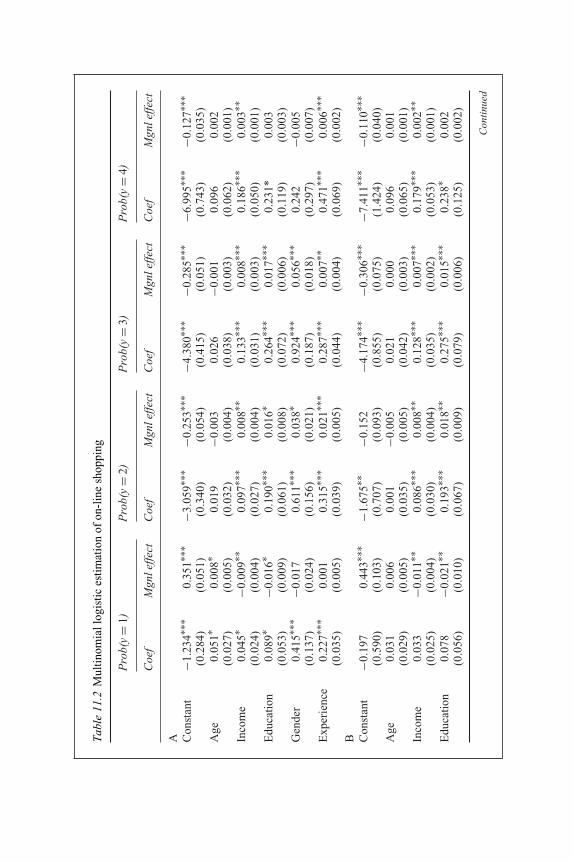
Tab
le11
.2M
ultino
mia
llog
istic
estim
atio
nof
on-l
ine
shop
ping
Pro
b(y
=1)
Pro
b(y
=2)
Pro
b(y
=3)
Pro
b(y
=4)
Coe
fM
gnle
ffec
tC
oef
Mgn
leffec
tC
oef
Mgn
leffec
tC
oef
Mgn
leffec
t
A Con
stan
t−1
.234
∗∗∗
(0.2
84)
0.35
1∗∗∗
(0.0
51)
−3.0
59∗∗
∗(0
.340
)−0
.253
∗∗∗
(0.0
54)
−4.3
80∗∗
∗(0
.415
)−0
.285
∗∗∗
(0.0
51)
−6.9
95∗∗
∗(0
.743
)−0
.127
∗∗∗
(0.0
35)
Age
0.05
1∗(0
.027
)0.
008∗
(0.0
05)
0.01
9(0
.032
)−0
.003
(0.0
04)
0.02
6(0
.038
)−0
.001
(0.0
03)
0.09
6(0
.062
)0.
002
(0.0
01)
Inco
me
0.04
5∗(0
.024
)−0
.009
∗∗(0
.004
)0.
097∗∗
∗(0
.027
)0.
008∗∗
(0.0
04)
0.13
3∗∗∗
(0.0
31)
0.00
8∗∗∗
(0.0
03)
0.18
6∗∗∗
(0.0
50)
0.00
3∗∗(0
.001
)E
duca
tion
0.08
9∗(0
.053
)−0
.016
∗(0
.009
)0.
190∗∗
∗(0
.061
)0.
016∗
(0.0
08)
0.26
4∗∗∗
(0.0
72)
0.01
7∗∗∗
(0.0
06)
0.23
1*(0
.119
)0.
003
(0.0
03)
Gen
der
0.41
5∗∗∗
(0.1
37)
−0.0
17(0
.024
)0.
611∗∗
∗(0
.156
)0.
038∗
(0.0
21)
0.92
4∗∗∗
(0.1
87)
0.05
6∗∗∗
(0.0
18)
0.24
2(0
.297
)−0
.005
(0.0
07)
Exp
erie
nce
0.22
7∗∗∗
(0.0
35)
0.00
1(0
.005
)0.
315∗∗
∗(0
.039
)0.
021∗∗
∗(0
.005
)0.
287∗∗
∗(0
.044
)0.
007∗∗
(0.0
04)
0.47
1∗∗∗
(0.0
69)
0.00
6∗∗∗
(0.0
02)
B Con
stan
t−0
.197
(0.5
90)
0.44
3∗∗∗
(0.1
03)
−1.6
75∗∗
(0.7
07)
−0.1
52(0
.093
)−4
.174
∗∗∗
(0.8
55)
−0.3
06∗∗
∗(0
.075
)−7
.411
∗∗∗
(1.4
24)
−0.1
10∗∗
∗(0
.040
)A
ge0.
031
(0.0
29)
0.00
6(0
.005
)0.
001
(0.0
35)
−0.0
05(0
.005
)0.
021
(0.0
42)
0.00
0(0
.003
)0.
096
(0.0
65)
0.00
1(0
.001
)In
com
e0.
033
(0.0
25)
−0.0
11∗∗
(0.0
04)
0.08
6∗∗∗
(0.0
30)
0.00
8∗∗(0
.004
)0.
128∗∗
∗(0
.035
)0.
007∗∗
∗(0
.002
)0.
179∗∗
∗(0
.053
)0.
002∗∗
(0.0
01)
Edu
cation
0.07
8(0
.056
)−0
.021
∗∗(0
.010
)0.
193∗∗
∗(0
.067
)0.
018∗∗
(0.0
09)
0.27
5∗∗∗
(0.0
79)
0.01
5∗∗∗
(0.0
06)
0.23
8∗(0
.125
)0.
002
(0.0
02)
Con
tinu
ed

Tab
le11
.2co
ntin
ued
Pro
b(y
=1)
Pro
b(y
=2)
Pro
b(y
=3)
Pro
b(y
=4)
Coe
fM
gnle
ffec
tC
oef
Mgn
leffec
tC
oef
Mgn
leffec
tC
oef
Mgn
leffec
t
Gen
der
0.36
1∗∗(0
.147
)−0
.018
(0.0
26)
0.50
5∗∗∗
(0.1
76)
0.02
6(0
.023
)0.
828∗∗
∗(0
.209
)0.
042∗∗
∗(0
.016
)0.
210
(0.3
17)
−0.0
03(0
.005
)E
xper
ienc
e0.
188∗∗
∗(0
.036
)0.
003
(0.0
06)
0.23
8∗∗∗
(0.0
42)
0.01
4∗∗∗
(0.0
05)
0.19
5∗∗∗
(0.0
49)
0.00
1(0
.003
)0.
379∗∗
∗(0
.074
)0.
003∗∗
∗(0
.001
)Q
uick
ness
0.31
4∗∗∗
(0.0
70)
−0.0
37∗∗
∗(0
.014
)0.
514∗∗
∗(0
.089
)0.
031∗∗
(0.0
12)
0.80
9∗∗∗
(0.1
12)
0.04
2∗∗∗
(0.0
10)
0.98
4∗∗∗
(0.1
97)
0.01
0∗∗∗
(0.0
04)
Pri
ce0.
218∗∗
∗(0
.078
)−0
.043
∗∗∗
(0.0
14)
0.49
3∗∗∗
(0.0
97)
0.04
6∗∗∗
(0.0
13)
0.57
4∗∗∗
(0.1
16)
0.02
7∗∗∗
(0.0
09)
0.63
3∗∗∗
(0.1
89)
0.00
6∗∗(0
.003
)R
isk
−0.5
22∗∗
∗(0
.077
)0.
065∗∗
∗(0
.013
)−1
.008
∗∗∗
(0.0
90)
−0.0
87∗∗
∗(0
.013
)−1
.129
∗∗∗
(0.1
04)
−0.0
47∗∗
∗(0
.009
)−1
.158
∗∗∗
(0.1
59)
−0.0
09∗∗
(0.0
04)
Del
iver
y−0
.138
(0.0
89)
0.02
3(0
.015
)−0
.303
∗∗∗
(0.1
04)
−0.0
29∗∗
(0.0
13)
−0.3
03∗∗
(0.1
19)
−0.0
12(0
.008
)−0
.417
∗∗(0
.182
)−0
.004
(0.0
03)
Sta
ndar
der
rors
inpa
rent
hese
s.∗ si
gnifi
cant
atth
e10
per
cent
leve
l;∗∗
sign
ifica
ntat
the
5pe
rce
ntle
vel;
∗∗∗ si
gnifi
cant
atth
e1
per
cent
leve
l.M
argi
nale
ffec
tsev
alua
ted
atth
esa
mpl
em
eans
.

Limited dependent variables and discrete choice models 215
and quickness offered by on-line shopping still attract the individuals inthis category to shop on-line as suggested by the positive coefficients forthese two variables, significant at the 1 per cent level. But these advantagesattract individuals to shop on-line more frequently, resulting in negativemarginal effects of these two variables. This is in relation to the morefrequent on-line buyers in categories 2, 3 and 4, not in relation to the non-buyers in the base category 0, and should not be misinterpreted. Koyuncu andBhattacharya (2004), by basing their explanations on the marginal effectscoefficients exclusively, have encountered apparent trouble. They state withpuzzlement: ‘Unexpectedly, we found that the quickness and price variablesmake negative while the risk variable makes positive and statisticallysignificant contributions to the probability of purchasing from the Internetfor those individuals who do on-line shopping less than once each month’,which has misinterpreted their own empirical results. For the remainingthree categories, the sign of the marginal effects coefficient of all the fourvariables of price, quickness, payment risk and delivery is as expected. Anordered logit would be more appropriate to model this on-line shoppingcase where the dependent variable is the frequency with which individualsshop on-line. If they had chosen an ordered logit model, the marginaleffects coefficients for the price and quickness variables for category 1would have been positive. There would have been no misinterpretation andconfusion then.
Example 11.2
Mergers and acquisitions (M&As), or corporate takeovers, are amongthe most important investment decisions made by acquiring firms and,consequently, have attracted immense attention from academia andprofessionals alike. Over years, many studies have been carried out toexamine the motivations for M&As and the factors that have an influenceon a takeover decision made by acquiring firms. In an empirical study topredict which firms become takeover targets, Espahbodi and Espahbodi(2003) employ four models of binary choice of logit, probit, discriminant,and recursive partitioning to examine a dataset gathered from Mergers andAcquisitions, a bi-monthly periodical. This section focuses on their logit andprobit results while briefly remarking on recursive partitioning. They haveexamined the November–December, September–October, and July–Augustissues in 1997 only, claiming that it is to minimise the time series distortion
Continued

216 Limited dependent variables and discrete choice models
in their models. Regardless, there are a few approaches available to dealwith the effect on model estimation of the changing economic environmentand the resulting operating characteristics of firms; or indeed, the issuesassociated with these changes should be addressed not avoided. Utilities andfinancial institutions are dropped from the study. The final sample consists of133 target firms, deemed by them to be large enough for analysis, probablylarge enough for statistical considerations.
After lengthy discussions of 18 financial variables and additionally severalnon-financial variables that may identify a takeover target firm, Espahbodiand Espahbodi (2003) adopt four of them, namely, free cash flow over totalassets, existence of golden parachutes, the State of Delaware incorporationdummy variable and market value of equity over total firm value, in theirlogit and probit analysis. The State of Delaware incorporation dummyvariable is included since Delaware has tougher takeover laws than otherstates. As a result, firms incorporated in Delaware may be subject to lowerprobabilities of a hostile takeover. Whereas, friendly takeovers may increaseas such firms can use the anti-takeover laws as a leverage to extract ahigher price for their firms. The dummy takes a value of 1 if a firm isincorporated in Delaware and 0 otherwise. The sign of the coefficientfor the dummy and its significance are thus uncertain, claimed by theauthors.
The results from estimating the logit model and probit model are presentedin Table 11.3. Columns 2 and 3 are for the logit model and columns 4 and 5for the probit model results. Free cash flow over total assets is found to bepositively related to the likelihood of a takeover of the firm significantlyby both models, which is consistent with the hypotheses with regard to
Table 11.3 Estimation of takeovers by the logit and probit models
Logit Probit
Coefficient t-stat Coefficient t-stat
Free cash flow over total assets 1.428∗∗∗ 2.76 0.813∗∗∗ 2.86Existence of golden parachutes 0.612∗ 1.95 0.366∗ 1.91State of Delaware incorporation
dummy variable0.340 1.61 0.204∗ 1.65
Market value of equity over totalfirm value
−0.606 −1.36 −0.353 −1.33
Constant −0.811 0.508Likelihood ratio −285.4 −285.2R2 19.39 19.49
∗significant at the 10 per cent level; ∗∗∗significant at the 1 per cent level.

Limited dependent variables and discrete choice models 217
Table 11.4 Classifications of target and non-target firms
Logit Probit
Classified as Classified as
Target Non-target
Total Target Non-target
Total
Act
ual A
ctual
Target 83 50 133 82 51 133 TargetNon-target 153 232 385 147 238 385 Non-targetTotal 236 282 518 229 289 518 Total
Correctclassification
62.4% 60.3% 61.7% 61.8% Correctclassification
investment opportunities and agency costs. Existence of golden parachutesis also expected to increase the likelihood of takeover under both theincentive alignment and management entrenchment hypotheses, which isconfirmed by the results of both models. A higher ratio of market valueof equity over total firm value tends to reduce the likelihood of a takeoverof the firm, with a negative but insignificant coefficient in both models,albeit consistent with the growth option hypothesis. The Delaware dummyvariable has a positive coefficient that is marginally significant. The resultindicates that the target firms are using the tough anti-takeover laws inDelaware to negotiate a higher price for stockholders, claimed by theauthors.
The classification of target and non-target firms, or prediction oftakeovers, is presented in Table 11.4, with the left panel by the logit modeland the right panel by the probit model. The correct classification rate is62.4 per cent for target firms and 60.3 per cent for non-target firms bythe logit model. That is, only 62.4 per cent of the firms predicted by themodel to be a takeover target were actually a target; and only 60.3 per centof the firms predicted by the model to be non-targets were actually non-targets. The probit model produces similar disappointing results. The correctclassification rate is 61.7 per cent for target firms and 61.8 per cent for non-target firms. The authors also use a recursive partitioning model to predicttakeover targets, which looks like a decision trees model without feedbackmechanism. It is alleged that the accuracy of the classification or predictionis increased to 89.5 per cent for target firms and 88.1 per cent for non-targetfirms. However, it is unclear how the recursive partitioning model results arecompared with the logit and probit results, since they employ considerablydifferent variables in the modelling. Nonetheless, it is not the interest of thissection to discuss this method at length.

218 Limited dependent variables and discrete choice models
Example 11.3
One of the most serious debated issues in many countries in the world is anaging population. The implications of aging populations are serious, creatinga need to study other related important issues, notably, the retirement system.The choice and provision of retirement systems have attracted the interestof numerous parties, including governments, the general public, employees,employers and academics. In this area of research, Kim and DeVaney(2005) investigate whether older workers choose partial or full retirement,or continue to work full-time. They employ multinomial logistic regressionto examine data from the first and fifth waves of the Health and RetirementStudy (HRS) collected in 1992 and 2000, an ongoing longitudinal datasetthat focuses on the retirement and demographic characteristics of olderAmericans in the 1990s. The dependent variable of the model is retirementstatus measured by self-reported retirement or working status and change inthe number of hours worked during the 8-year period between Wave 1and Wave 5. The dependent variable takes the value of 0 for full-timework, 1 for partial retirement and 2 for full retirement, with full-time workbeing the reference category. The independent variables are divided into fivesets of household assets and income, pension and health insurance factors,health status, occupational characteristics, and demographic characteristics.The values and coding of the independent variables in Table 11.5 aredescribed as follows. Variables under household assets and income arecontinuous and measured in US dollars. Variables under pension andhealth insurance are discrete with 1 for a ‘yes’ answer and 0 for ‘no’.The first two variables under health status are discrete, taking the valueof 1 for a ‘yes’ answer and 0 for ‘no’; it is obviously the numberof occurrences for the next two variables. Variables under occupationalcharacteristics and demographic characteristics are all discrete, being 1 fora ‘yes’ answer and 0 for ‘no’, with the exception of age that is measured inyears.
Table 11.5 reports the results of multinomial logistic regression analysis.Let us look at the results for full retirement first. Household investment assetscontribute to a decision to take full retirement positively, while older workerswith more household debt are more likely to work full-time instead of takingfull retirement. Older workers with a defined benefit plan or both definedbenefit and defined contribution plans are more likely to retire fully. Healthstatus is found to be negatively related to full retirement – older workers withexcellent or very good health are more likely to continue full-time work.Self-employment is negatively related to the likelihood of full retirementversus full-time work, i.e. self-employed workers are more likely to continuework at old ages. The meaning of work is also a contributing factor tothe retirement decision. Older workers who consider the meaning of work
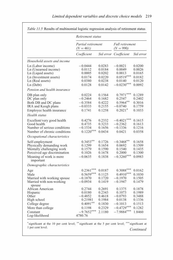
Limited dependent variables and discrete choice models 219
Table 11.5 Results of multinomial logistic regression analysis of retirement status
Retirement status
Partial retirement(N = 461)
Full retirement(N = 990)
Coefficient Std error Coefficient Std error
Household assets and incomeLn (Labor income) −0.0444 0.0283 −0.0021 0.0200Ln (Unearned income) 0.0112 0.0184 0.0049 0.0026Ln (Liquid assets) 0.0005 0.0202 0.0013 0.0165Ln (Investment assets) 0.0174 0.0220 0.0519∗∗∗ 0.0182Ln (Real assets) 0.0380 0.0238 0.0140 0.0120Ln (Debt) 0.0128 0.0142 −0.0230∗∗∗ 0.0092Pension and health insurance
DB plan only 0.0224 0.1564 0.7971∗∗∗ 0.1289DC plan only −0.2464 0.1682 0.2547 0.2402Both DB and DC plans −0.3584 0.4222 0.5964∗∗ 0.3016IRA and Keogh plans −0.0333 0.2155 −0.0740 0.1759Employee health insurance 0.1741 0.1258 0.2021∗ 0.1033Health status
Excellent/very good health 0.4276 0.2332 −0.4021∗∗∗ 0.1615Good health 0.4735 0.3233 −0.2362 0.1613Number of serious conditions −0.1534 0.1656 −0.1336 0.1216Number of chronic conditions 0.1220∗∗∗ 0.0434 0.0421 0.0358Occupational characteristics
Self-employment 0.3453∗∗ 0.1726 −0.3468∗∗ 0.1658Physically demanding work 0.1299 0.1654 0.0692 0.1509Mentally challenging work 0.1579 0.1590 0.1540 0.1435Perceived age discrimination 0.1026 0.1678 0.2000 0.1300Meaning of work is more
important−0.0635 0.1838 −0.3260∗∗∗ 0.0983
Demographic characteristics
Age 0.2361∗∗∗ 0.0187 0.3088∗∗∗ 0.0162Male 0.5659∗∗∗ 0.1125 0.4910∗∗∗ 0.1030Married with working spouse −0.1870 0.1720 −0.1970 0.1505Married with non-working
spouse−0.0934 0.1419 −0.1947 0.1479
African American 0.2744 0.2691 0.1375 0.1878Hispanic 0.0180 0.2343 0.1073 0.1989Other −0.4852 0.4618 −0.0793 0.3488High school 0.21981 0.1984 0.0138 0.1336College degree 0.4091∗∗ 0.1830 −0.1013 0.1513More than college 0.1198 0.2329 −0.4729∗∗∗ 0.1282Constant −9.7652∗∗∗ 2.1180 −7.9884∗∗∗ 1.8460Log-likelihood 4780.76
∗significant at the 10 per cent level; ∗∗significant at the 5 per cent level; ∗∗∗significant at1 per cent level.
Continued

220 Limited dependent variables and discrete choice models
is more important than money are more likely to continue full-time workvis-à-vis full retirement. Obviously, age is confirmed to be positively relatedto the likelihood of full retirement. According to their results, older maleworkers are more likely to take full retirement than their female counterparts.Kim and DeVaney (2005) argue that the finding probably reflects the factthat women experience more career interruption for family matters and, asa result, they tend to remain in their full-time jobs. Education is found to berelated to retirement decisions. Older workers with more education than acollege degree are more likely to choose to continue full-time work.
The boundary between partial retirement and full-time work is apparentlyless clear-cut than that between full retirement and full-time work.Consequently, fewer coefficients in the partial retirement case arestatistically significant. Household assets and income do not contribute topartial retirement decisions at all. The number of chronic health conditionsis found to be positively related to partial retirement, suggesting that olderworkers with chronic conditions have difficulties to work full-time but theyare willing to work part-time, or more likely to choose partial retirement. Incontrast to a decision to choose between full-time work and full retirement,self-employment is found to be positively related to the likelihood of partialretirement versus full-time work. Kim and DeVaney (2005) claim that,because the self-employed have the flexibility to establish their hours, thechoice of partial retirement versus full-time work is rational. The resultsfor age and gender are the same as in the case of full retirement versus fullretirement. Older workers with a college degree are found to be more likelyto partially retire, which is also in contrast to the case of full retirementversus full-time work to a certain extent.
11.6. Empirical literature
Choice is deeply associated with everyday life, be it social or personal, collectiveor individual. In financial terms, people make choice aimed at achieving higherutility of their work, consumption, savings, investment, and their combinations.Corporations make choices supposedly aimed at maximising shareholder values.Binary choice and discrete choice models such as probit, binomial and multinomiallogistic regression have been traditionally applied to social science research,employment studies and the labour market, health services and insurance.Recently, however, there has been growing interest in corporate decision makinginvolving choice explicitly, as well as in financial market investment choice at themicro level and monetary policy at the macro level.
Examining the factors that have an effect on bank switching in small firmsin the UK Howorth et al. (2003) employ binomial and multinomial logisticregression to identify the characteristics that discriminate between three groups

Limited dependent variables and discrete choice models 221
of small firms. The three groups of firms are classified as a group of firmsconsidering switching banks, a group of firms that had switched banks in theprevious three years and a group of firms that had not switched banks and werenot considering doing so. They test the hypothesis that some small firms may be‘informationally captured’ in that they are tied into their current bank relationshipdue to difficulties in conveying accurate information about their performance.Their empirical results are not conclusive with regard to this hypothesis. There issome evidence in support of the hypothesis where rapidly changing informationand particularly changing technology are characteristics associated with firmsthat were considering switching but had not switched. However, there is nosignificant evidence to indicate that superior performing firms are more likelyto be ‘informationally captured’, as growth and perceived business success areboth the factors that influence firms to switched banks. Other factors considered tobe relevant to bank-switching decisions in the paper include difficulties obtainingfinance, dissatisfaction with the service provided, and the use of alternative sourcesof finance. Reiljan (2002) studies the determinants of foreign direct investment(FDI) inEstonia. The author firstly adopts principal component analysis to establishfive major components of determinants of foreign direct investment, and then runsmultinomial logistic regression to investigate the impact of these determinantson different groups of foreign investors. The impact of financial information andvoluntary disclosures on contributions to not-for-profit organisations is scrutinisedby Parsons (2007). Her study consists of two experiments, with one experimentbeing a survey with potential donors and the other laboratory based experiment.Potential donors were sent, via a direct mail campaign, fund-raising appealscontaining varying amounts of financial and non-financial information in orderto determine whether individual donors are more likely to contribute whenaccounting information or voluntary disclosures are provided. Participants in alaboratory experiment were asked to assess the usefulness of the different versionsof the fund-raising appeals. It is claimed that the results of logistic regressionprovides evidence that some donors who have previously donated use financialaccounting information when making a donation decision. The results suggestthat non-financial service efforts and voluntary accomplishments disclosures arenot clear-cut factors for determining whether and how much to give by donors,though these non-financial factors are considered to be useful by participants inthe laboratory experiment for making donation decisions. Factors that restrictthe use of credit cards in the Gulf Cooperation Council (GCC) countries areexamined by Metwally and Prasad (2004). They adopt the logit model and theprobit model to analyse the factors considered to determine the probability of usingcredit cards more frequently in domestic transactions. The study has supposedlycovered the GCC countries of Bahrain, Kuwait, Oman, Qatar, Saudi Arabia andthe United Arab Emirates, but it appears to be conducted in Qatar only, wherea sample of 385 consumers was surveyed. Respondents who hold credit cardswere asked to indicate their degree of agreement on 23 statements relating totheir reluctance to use credit cards frequently in domestic transactions on a five-point scale. They use principal component analysis to reduce the 23 explanatory

222 Limited dependent variables and discrete choice models
variables as represented by the 23 statements to five factors, and then use the factorscores of the five extracted factors as explanatory variables in logit and probitregression. Their logit and probit regression results suggest that the probabilityof using credit cards more frequently in domestic transactions in Qatar wouldbe higher, the closer the credit-card price to cash price and the smaller the debt-service ratio. They also examine the effect of demographic variables on the use ofcredit cards. Their results indicate that there is a high degree of similarity betweenQatar and developed countries regarding the effect of these variables on the useof credit cards.
The world has been in an accelerating process of globalisation over the lastthree decades. Under such an economic environment, companies’ overseas marketlistings have become a rather familiar phenomenon. This provides companieswith more opportunities in terms of choice, but creates a new decision-makingarea for companies to tackle seriously as well. In a paper entitled ‘The choice oftrading venue and relative price impact of institutional trading: ADRs versus theunderlying securities in their local markets’, Chakravarty et al. (2004) addresstwo issues of the choice of trading venues and the comparison of trading costsacross the venues. They identify institutional trading in the US in non-US stocks,i.e. ADRs, from 35 foreign countries and in their respective home markets, usingproprietary institutional trading data. Then they use multinomial logistic regressionto examine the factors that influence institutions’ decisions to trade a cross-listedstock solely in the ADR market versus solely on its home exchange. They allegethat stocks with tentatively higher local volume, with non-overlapping tradinghours, and with smaller market capitalisation are more likely to be traded ontheir home exchanges only while less complex decisions are more likely to beexecuted as ADRs only, relative to stocks that are traded by institutions in bothvenues. They also claim that the trading cost of ADRs is often higher than thatof the equivalent security at home in terms of overall trading costs. Further,their multivariate analysis on institutional trading costs indicates that the costdifference between trading in the security’s home country and its respective ADRis smaller for stocks associated with less complex trades, relatively lower localtrading volume and overlapping trading hours, and for stocks originating from theemerging markets.
In a traditional corporate finance area of dividend policy, Li et al. (2006) examinefive determinants of dividend policy in Taiwanese companies. Their study employsa multinomial logistic model and divides the sample companies into two groups ofhigh-tech and non-high-tech companies. They claim that the stability of dividends,debt ratio as well as profitability, are significant determinants of dividend policyregardless of high-tech and non-high-tech companies, and the size of the firm andits future growth opportunity have significant effects on dividend policy in non-high-tech companies but insignificant effects on high-tech companies. Readerswith experience in financial analysis may recall the use of Z-scores in predictingbankruptcy by Altman (1968). Based on the analysis in this chapter, the probitmodel or the logit model should be superior in performing such a prediction. Thesenon-linear models are attempted by Ginoglou et al. (2002) to predict corporate

Limited dependent variables and discrete choice models 223
failure of problematic firms in Greece, using a data set of 40 industrial firms,with 20 of them being healthy and 20 of them problematic, for the purpose ofachieving improved prediction of corporate failure. However, the use of probit orlogit models are not popular for classification issues involving accounting ratios,bankruptcy prediction in particular. Barniv and McDonald (1999) review severalcategorisation techniques and compare the performance of logit or probit withalternative procedures. The alternative techniques are applied to two researchquestions of bankruptcy prediction and auditors’ consistency in judgements. Fourempirical criteria provide some evidence that the exponential generalised beta ofthe second kind (EGB2), lomit, and burrit improve the log likelihood functionsand the explanatory power, compared with logit and other models. EGB2, lomitand burrit also provide significantly better classifications and predictions thanlogit and other techniques.
With aging becoming an increasingly important issue and current pensionplans appear to be in crisis in many countries, research on pension or retirementplans is gaining momentum. In addition to Example 11.3 in the previous section,Cahill et al. (2005) have raised a question ‘Are traditional retirements a thing ofthe past?’ and attempted the question with new evidence on retirement patternsand bridge jobs. They investigate whether permanent, one-time retirements arecoming to an end just as the trend towards earlier retirements did nearly 20 yearsago. In particular, their study explores how common bridge jobs are amongtoday’s retirees, and how uncommon traditional retirements have become. Thedeterminants of bridge jobs are examined with a multinomial logistic regressionmodel, using data from the Health and Retirement Study for the work histories andretirement patterns of a cohort of retirees aged 51 to 61 in 1992 over a ten-year timeperiod in both a cross-sectional and longitudinal context. They find that one-half totwo-thirds of the respondents with full-time career jobs take on bridge jobs beforeexiting the labour force completely. Moreover, their study has documented thatbridge job behaviour is most common among younger respondents, respondentswithout defined-benefit pension plans, and respondents at the lower- and upper-end of the wage distribution. They allege that traditional retirements will be theexception rather than the rule, based on the implications of their findings suggestingthat changes in the retirement income landscape since the 1980s appear to betaking root.
There have been many other applications of binary and discrete choice modelsin virtually every area of social sciences broadly defined. For example, Skaburskis(1999) adopts a multinomial logistic model and a naïve nested logistic model tostudy the choice of tenure and building type. These models are estimated to relatedifferences in household size, age, income and housing prices to differences in thechoice of tenure and building type. The estimated models show that the demand forlower-density options decreases with a decrease in household size and an increasein age and real income. Higher rents tend to induce the demand for owner-occupiedsingle-family detached houses. Higher price levels for the ownership option shiftdemand towards all of the higher-density options, particularly towards high-riserental apartments. The effects of public premiums on children’s health insurance

224 Limited dependent variables and discrete choice models
coverage are investigated by Kenney et al. (2006). They employ multinomiallogistic models, focusing on premium costs and controlling for other factors. Thestudy uses 2000 to 2004 Current Population Survey data to examine the effects ofpublic premiums on the insurance coverage of children whose family income isbetween 100 per cent and 300 per cent of the federal poverty level. The magnitudeof the estimated effects varies across the models. Nevertheless, it is claimed thatthe results consistently indicate that raising public premiums reduces enrolmentin public programmes, with some children who forgo public coverage havingprivate coverage instead and others being uninsured. The results further indicatethat public premiums have larger effects when applied to lower-income families.
Questions and problems
1 Describe binary choice and, in general, discrete choice, with a few examplesin daily life, corporate and individual.
2 What is defined as a limited dependent variable? What are features of limiteddependent variables?
3 Describe and discuss the probit model with regard to its functional form.4 Describe and discuss the logit model with regard to its functional form and in
relation to logistic regression.5 Contrast the probit model with the logit model, paying attention to their
probability density functions.6 Present and describe the multinomial logit model and multinomial logistic
regression, and further discuss their role in modelling discrete choice.7 What are defined as ordered probit and ordered logit? What differentiates an
ordered logit model from a multinomial logit model?8 What are marginal effects in discrete choice models? Why are the issues of
marginal effects raised and addressed specifically for discrete choice modelsbut not mentioned for linear regression and other linear models?
9 Collect data from various sources, e.g. Acquisition Monthly, Thomson ONEBanker and company annual reports, and then estimate a probit model anda logistic regression model for the choice of payment methods in mergersand acquisitions (using LIMDEP, GAUSS, RATS or other packages). Thedependent variable is choice of payment methods, with choice of cash as 0and choice of share exchange as 1. The independent variables may includethe relative size of the bidder to the target, a measure of free cash flow of thebidder, a measure of the performance of the bidder and that of the target.
10 Collect data on dual listings from various sources, e.g. Thomson ONEBanker, the websites of relevant stock exchanges and companies, and thenrun multinomial logistic regression for the choice of foreign stock exchangesfor dual listings (using LIMDEP, GAUSS, RATS or other packages). Thedependent variable is choice of foreign stock exchanges for dual listings, withchoice of New York being 0, London being 1 and Tokyo being 2 (or thereader’s own choice of foreign stock exchanges). The independent variablesmay include firm size, a measure of performance, financial leverage, an

Limited dependent variables and discrete choice models 225
industry dummy, and a region dummy, or any variables that the reader reckonsreasonable.
References
Altman, E.I. (1968), Financial ratios, discriminant analysis and prediction of corporatebankruptcy, Journal of Finance, 23, 589–609.
Barniv, R. and McDonald, J.B. (1999), Review of categorical models for classificationissues in accounting and finance, Review of Quantitative Finance and Accounting, 13,39–62.
Cahill, K.E., Giandrea, M.D. and Quinn, J.F. (2005), Are traditional retirements a thingof the past? new evidence on retirement patterns and bridge jobs, U.S. Bureau of LaborStatistics Working Papers: 384.
Chakravarty, S., Chiyachantana, C.N. and Jiang, C. (2004), The choice of trading venueand relative price impact of institutional trading: ADRs versus the underlying securitiesin their local markets, Purdue University Economics Working Paper.
Espahbodi, H. and Espahbodi, P. (2003), Binary choice models and corporate takeover,Journal of Banking and Finance, 27, 549–574.
Ginoglou, D., Agorastos, K. and Hatzigagios, T. (2002), Predicting corporate failure ofproblematic firms in Greece with LPM logit probit and discriminant analysis models,Journal of Financial Management and Analysis, 15, 1–15.
Howorth, C., Peel, M.J. and Wilson, N. (2003), An examination of the factors associated withbank switching in the U.K. small firm sector, Small Business Economics, 20, 305–317.
Kenney, G., Hadley, J. and Blavin, F. (2006–2007), Effects of public premiums on children’shealth insurance coverage: Evidence from 1999 to 2003, Inquiry, Winter 2006–2007, 43,345–361.
Kim, H. and DeVaney, S.A. (2005), The selection of partial or full retirement by olderworkers, Journal of Family and Economic Issues, 26, 371–394.
Koyuncu, C. and Bhattacharya, G. (2004), The impacts of quickness, price, payment risk,and delivery issues on on-line shopping, Journal of Socio-Economics, 33, 241–251.
Li, M.Y.L., Wang, M.L., Wang, A.T. and Wang, C.A. (2006), Determinants of dividendpolicy of high-tech versus traditional companies: An empirical study using Taiwanesedata, Empirical Economics Letters, 5, 105–115.
Metwally, M.M. and Prasad, J. N. (2004), Factors restricting use of credit cards inGCC countries, International Journal of Applied Business and Economic Research, 2,171–188.
Parsons, L.M. (2007), The impact of financial information and voluntary disclosures oncontributions to not-for-profit organizations, Behavioral Research in Accounting, 19,179–196.
Reiljan, E. (2002), Analysis of foreign direct investment determinants in Estonia, Journalof East-West Business, 8, 103–121.
Skaburskis, A. (1999), Modelling the choice of tenure and building type, Urban Studies,36, 2199–2215.
12 Limited dependent variables andtruncated and censored samples
In addition to discrete choice models where a dependent variable possesses discretevalues, the values of dependent variables can also be censored or truncated. Thatis, the variable is not observed over its whole range. For example, in a survey ofMBA graduates two years after their graduation, relevant information is collected,including their salaries. If one is interested in what determines the salary level, amodel may be set up accordingly where salary is the dependent variable. The surveysets a lower limit and an upper limit for the salary range in case the respondentsare not willing to reveal the exact salary beyond a certain range. Therefore, thevalue of the salary variable takes the figure given in the response when it falls inthe given range, but is censored at both the lower and upper end. If a graduate doesnot respond, the observation corresponding to him is excluded or truncated fromthe sample, and neither the dependent variable nor the independent variables areavailable.
A dependent variable that is truncated or censored is a limited dependentvariable, as is a dependent variable that is discrete discussed in the previous chapter.This chapter pays attention to issues in estimation of models involving limiteddependent variables with regard to censored and truncated samples. Estimationof truncated or censored samples with conventional regression procedures suchas the OLS can cause bias in parameter estimates. To correct for the bias, specialtechniques and treatments pertinent to truncated and censored data have to beapplied. However, the problem can be largely solved by using the maximumlikelihood estimation procedure. So, we present the likelihood and log likelihoodfunctions for truncated and censored data samples first while demonstrating theirdistributions. Then we proceed to discuss the issue of bias in parameter estimationproduced by the OLS procedure of the Tobit model, only for the purpose tointroduce a wider issue of selection bias. Selection bias is addressed by referringto the work of Heckman (1976, 1979) and Cragg (1971).
12.1. Truncated and censored data analysis
We have learned limited dependent variables whose values are limited to discretevalues in the previous chapter. There are other types of limited dependent variablesthat we introduce and study in this chapter. From time to time, samples can
Limited dependent variables and truncated and censored samples 227
be limited due to the values of the dependent variable. When this happens, thedependent variable is referred to as limited dependent variables. The two frequentlyexperienced situations where samples are limited by limited dependent variablesare truncated and censored samples. With a truncated sample, an observation isexcluded from the sample if the value of the dependent variable does not meetcertain criteria. In a censored sample, the dependent variable is not observed overits entire range for some of the observations.
A sample can be left truncated, right truncated, or truncated at both ends. In aleft truncated sample, being truncated at TRa, any observations are excluded fromthe sample if the dependent variable is smaller than or equal to TRa:
Yi = Xiβ+ εi, εi ∼ N(0,σ 2
), Yi > TRa, i = 1, . . . ,N (12.1)
The probability of Yi > TRa is the probability of εi > TRa −Xiβ, the cause of errorscontributing to the bias, which should be subtracted from the likelihood function.Therefore, the likelihood function is adjusted and becomes:
L =N∏
i=1
φ (Yi − Xiβ)[1 −� (TRa − Xiβ)
]
=N∏
i=1
1
σφ
(Yi − Xiβ
σ
)�
(Xiβ− TRa
σ
)(12.2)
where φ (ε) is the density function of normal distributions and � (ε) is thecumulative normal distribution, with ε ∼ N
(0,σ 2
). Note φ (ε/σ ) = σφ (ε),
� (ε/σ )=� (ε) and� (−ε)= 1−� (ε). The corresponding log likelihood functionfollowing the adjustment is:
LL =N∑
i=1
Ln[φ (Yi − Xiβ)
]− N∑i=1
Ln[1 −� (TRa − Xiβ)
]
= 1
σ
N∑i=1
Ln
[φ
(Yi − Xiβ
σ
)]−
N∑i=1
Ln
[�
(Xiβ− TRa
σ
)]
= −N
2Ln(2πσ 2
)− 1
2σ 2
N∑i=1
(Yi − Xiβ)2 −N∑
i=1
Ln
[�
(Xiβ− TRa
σ
)](12.3)
For a right truncated sample, being truncated at TRb, any observations are excludedfrom the sample if the dependent variable is greater than or equal to TRb:
Yi = Xiβ+ εi, εi ∼ N(0,σ 2
), Yi < TRb, i = 1, . . . ,N (12.4)
228 Limited dependent variables and truncated and censored samples
Following similar considerations as for the left truncated sample, the log likelihoodfunction of a right truncated sample is:
LL =N∑
i=1
Ln[φ (Yi − Xiβ)
]− N∑i=1
Ln[1 −� (Xiβ− TRb)
]
= 1
σ
N∑i=1
Ln
[φ
(Yi − Xiβ
σ
)]−
N∑i=1
Ln
[�
(TRb − Xiβ
σ
)]
= −N
2Ln(2πσ 2
)− 1
2σ 2
N∑i=1
(Yi − Xiβ)2 −N∑
i=1
Ln
[�
(TRb − Xiβ
σ
)](12.5)
and the log likelihood function of a sample that is truncated at both ends is:
LL =N∑
i=1
Ln[φ (Yi − Xiβ)
]
−N∑
i=1
Ln[1 −� (TRa − Xiβ)
]− N∑i=1
Ln[1 −� (Xiβ− TRb)
]
= 1
σ
N∑i=1
Ln
[φ
(Yi − Xiβ
σ
)]
−N∑
i=1
Ln
[�
(Xiβ− TRa
σ
)]−
N∑i=1
Ln
[�
(TRb − Xiβ
σ
)]
= −N
2Ln(2πσ 2
)− 1
2σ 2
N∑i=1
(Yi − Xiβ)2
−N∑
i=1
Ln
[�
(TRb − Xiβ
σ
)+�
(Xiβ− TRa
σ
)], TRa < TRb (12.6)
The presentation of the likelihood function for censored data is similar. Considera sample that is left censored at ca:
Yi =⎧⎨⎩
Y ∗i = Xiβ+ εi, εi ∼ N
(0,σ 2
), ifYi > ca
ca, ifYi ≤ ca
i = 1, . . . ,N (12.7)
For non-censored observations, their likelihood function is:
Li = φ (Yi − Xiβ) = 1
σφ
(Yi − Xiβ
σ
)(12.8)

Limited dependent variables and truncated and censored samples 229
and their log likelihood function is the standard log likelihood in conventionalregression:
LLi = Ln[φ (Yi − Xiβ)
]= −1
2Ln(2πσ 2
)− (Yi − Xiβ)2
2σ 2 (12.9)
For censored observations, their likelihood function is:
Li = � (ca − Xiβ) = �
(ca − Xiβ
σ
)(12.10)
and their log likelihood function becomes:
LLi = Ln
[�
(ca − Xiβ
σ
)]= Ln
[� (ca − Xiβ)
](12.11)
So, the likelihood function of the sample is:
L =N∏
i=1
φ (Yi − Xiβ)(1−δi) � (ca − Xiβ)δi
=N∏
i=1
[1
σφ
(Yi − Xiβ
σ
)](1−δi)
�
(ca − Xiβ
σ
)δi
(12.12)
where δi = 1 if the observations are censored and δi = 0 if the observations are notcensored. The log likelihood function of the sample, therefore, is:
LL=−N∑
i=1
(1−δi)
[1
2Ln(2πσ 2
)+ (Yi −Xiβ)2
2σ 2
]+
N∑i=1
δi Ln
[�
(ca −Xiβ
σ
)](12.13)
For a sample that is right censored at cb:
Yi =⎧⎨⎩
Y ∗i = Xiβ+ εi, εi ∼ N
(0,σ 2
), ifYi < cb
cb, ifYi ≥ cb
i = 1, . . . ,N
(12.14)
the log likelihood function of non-censored observations is the standard loglikelihood in conventional regression as presented in equation (12.9). The loglikelihood function of censored observations is:
LLi = Ln
[1 −�
(cb − Xiβ
σ
)]= Ln
[�
(Xiβ− cb
σ
)](12.15)
230 Limited dependent variables and truncated and censored samples
So, the log likelihood function of the sample is:
LL=−N∑
i=1
(1−ϑi)
[1
2Ln(2πσ 2
)+ (Yi −Xiβ)2
2σ 2
]+
N∑i=1
ϑi Ln
[�
(Xiβ−cb
σ
)](12.16)
where ϑi = 1 if the observations are censored and ϑi = 0 if the observations arenot censored.
In general, a sample that is left censored at ca and right censored at cb has thefollowing log likelihood function:
LL = −N∑
i=1
(1 − δi −ϑi)
[1
2Ln(2πσ 2
)+ (Yi − Xiβ)2
2σ 2
]
+N∑
i=1
δi Ln
[�
(ca − Xiβ
σ
)]+
N∑i=1
ϑi Ln
[�
(Xiβ− cb
σ
)], ca < cb
(12.17)
where δi = 1 if the observations are left censored and δi = 0 if the observationsare not left censored, ϑi = 1 if the observations are right censored and ϑi = 0 ifthe observations are not right censored. Note any one observation cannot be leftcensored and right censored at the same time, i.e., Yi ≤ ca and Yi ≥ cb cannothold together. So the circumstance of δi = 1 and ϑi = 1 will not occur for anyobservation.
12.2. The Tobit model
The Tobit model is a kind of the modelling method for censored data samples,named after Tobin (1958). To simplify the matter, which is also fairly realpractically, the model is usually left censored at 0, taking the form:
Yi =⎧⎨⎩
Y ∗i = Xiβ+ εi, εi ∼ N
(0,σ 2
), if Y ∗
i > 0
0, if Y ∗i ≤ 0
i = 1, . . . ,N
(12.18)
Now consider a probit type model for the full sample, including both censored andnon-censored data:
Y ∗i = Xiβ+ εi, εi ∼ N
(0,σ 2
)(12.19a)
Yi =⎧⎨⎩
1, if Y ∗i > 0
0, if Y ∗i ≤ 0
(12.19b)

Limited dependent variables and truncated and censored samples 231
We have learned from the previous chapter that the likelihood function of theabove probit model, L (β), is:
L (β) =N∏
i=1
[� (Xiβ)
]Yi[1 −� (Xiβ)
](1−Yi) (12.20)
The first moment or the expected value of Y ∗i conditional on Y ∗
i > 0 is:
E (Y ∗i |Y ∗
i > 0) = Xiβ+ E (εi |εi > −Xiβ)
= Xiβ+σE
(εi
σ| εi
σ> −Xiβ
σ
)
= Xiβ+σφ(Xiβ/σ)
�(Xiβ/σ) = Xiβ+σli
(Xiβ
σ
)(12.21)
where li is called the inverse Mill’s ratio. Since this would be the estimates by theOLS including non-censored observations only, and is not equal to Xiβ, the OLSis inconsistent and produces biased results. Note that the exclusion of the censoredobservations in the analysis amounts to estimation of a truncated example. That is,we run the OLS regression of the dependent variable on the explanatory variableswith non-censored observations, the estimates are biased due to the restrictionimposed on the sample or the exclusion of the censored observations. However,this bias may be corrected, since the bias arises from the given positive correlationbetween εi and Xiβ; it is linked to the inverse Mill’s ratio and, as a result, maybe corrected. This analysis of bias suggests a two-step or two-stage procedure. Inthe first stage, a probit type model is estimated for the full sample, including bothcensored and non-censored data. The values of the dependent variable are madediscrete; the values of the dependent variable for uncensored observations are setto 1 and the values of the dependent variable for censored observations are set to0. The inverse Mill’s ratio can be obtained accordingly. In the second stage of theestimation procedure, only non-censored data, or the truncated sample, are appliedto the regression. The dependent variable is regressed on the explanatory variablesand the inverse Mill’s ratio obtained in the first stage estimation. This correctsthe bias caused by the restriction imposed on sample selection or the exclusionof censored observations. This is the idea of the Heckman (1979) model, whichgeneralises the Tobit model.
Let us review what is defined as the inverse Mill’s ratio prior to proceeding tomore general selection models in the next section, where this ratio is frequentlyused. Consider the probability density function of a standard normal distribution:
φ (z) = 1√2π
e−z2(12.22)
232 Limited dependent variables and truncated and censored samples
Its first moment conditional on z > c:
E (z |z > c) =∞∫
c
zφ (z |z > c)dz
=∞∫
c
zφ (z)
P (z > c)dz = 1
1 −� (c)
∞∫c
zφ (z)dz
= −1
1 −� (c)
∞∫c
d[φ (z)] = φ (c)
1 −� (c)(12.23)
is known as the inverse Mill’s ratio:
l (c) = φ (c)
1 −� (c)= φ (−c)
� (−c)(12.24)
In general, the inverse Mill’s ratio for a normal distribution with a mean of μ anda standard deviation of σ , N
(μ,σ 2
), is:
l (c) = φ((c −μ)
/σ)
1 −�((c −μ)
/σ) = φ
((μ− c)
/σ)
�((μ− c)
/σ) (12.25)
When c = 0, the above inverse Mill’s ratio becomes:
l (c) = φ(μ/σ)
� (μ/σ )(12.26)
It is simply the ratio of the value of the probability density function to the valueof the cumulative normal distribution at point μ.
The Tobit model is widely used for its simplicity, straightforwardness andrelevance, despite the criticisms. More advanced models have been developed andextended, ranging from estimation procedures, such as the maximum likelihood,to model specifications, such as the Cragg (1971) model and the Heckman (1979)model to be introduced in the next section. Although the maximum likelihoodprocedure can produce consistent unbiased coefficient estimates, the two-stageOLS procedure is still used for the following reasons. Firstly, the bias can be easilycorrected. The execution of OLS procedures is much simpler than the maximisationof the log likelihood function. The latter involves non-linear iterations, whichis sensitive to the choice of initial values of the parameters and may fail toconverge sometimes, despite that computing time and speed are no longer a concernnowadays. Secondly, we would like to know the different effects of the dependentvariable on parameter estimates by using the truncated sample and the ‘full’ samplethat does not exist, or the extent to which the estimated parameter is biased. Someinference for the ‘full’ sample’s characteristics may result from such analysis.
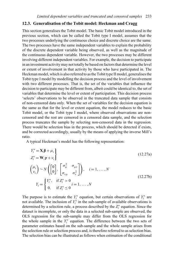
Limited dependent variables and truncated and censored samples 233
12.3. Generalisation of the Tobit model: Heckman and Cragg
This section generalises the Tobit model. The basic Tobit model introduced in theprevious section, which can be called the Tobit type I model, assumes that thetwo processes underlying the continuous choice and discrete choice are the same.The two processes have the same independent variables to explain the probabilityof the discrete dependent variable being observed, as well as the magnitude ofthe continuous dependent variable. However, the two processes may be differentinvolving different independent variables. For example, the decision to participatein an investment activity may not totally be based on factors that determine the levelor extent of involvement in that activity by those who have participated in. TheHeckman model, which is also referred to as the Tobit type II model, generalises theTobit type I model by modelling the decision process and the level of involvementwith two different processes. That is, the set of the variables that influence thedecision to participate may be different from, albeit could be identical to, the set ofvariables that determine the level or extent of participation. This decision process‘selects’ observations to be observed in the truncated data sample that consistsof non-censored data only. When the set of variables for the decision equation isthe same as that for the level or extent equation, the model reduces to the basicTobit model, or the Tobit type I model, where observed observations are non-censored and the rest are censored in a censored data sample, and the selectionprocess truncates the sample by selecting non-censored data in the regression.There would be selection bias in the process, which should be detected if exists,and be corrected accordingly, usually by the means of applying the inverse Mill’sratio.
A typical Heckman’s model has the following representation:
Y ∗i = Xiβ+μi
Z∗i = Wiγ + νi
}(12.27a)
(μi
νi
)∼ N
([00
],
[σ 2
μ σμν
σνμ σ 2ν
]), i = 1, . . . ,N
Yi ={
Y ∗i , if Z∗
i > 0
0, if Z∗i ≤ 0
i = 1, . . . ,N
(12.27b)
The purpose is to estimate the Y ∗i equation, but certain observations of Y ∗
i arenot available. The inclusion of Y ∗
i in the sub-sample of available observations isdetermined by a selection rule, a process described by the Z∗
i equation. Since thedataset is incomplete, or only the data in a selected sub-sample are observed, theOLS regression for the sub-sample may differ from the OLS regression forthe whole sample in the Y ∗
i equation. The difference between the two sets ofparameter estimates based on the sub-sample and the whole sample arises fromthe selection rule or selection process and, is therefore referred to as selection bias.The selection bias can be illustrated as follows when estimation of the conditional
234 Limited dependent variables and truncated and censored samples
mean of Y ∗i , the mean of Y ∗
i conditional on Z∗i > 0, is attempted:
E (Y ∗i |Z∗
i > 0) = E (Y ∗i |νi > −Wiγ)
= Xiβ+ E (μi |νi > −Wiγ)
= Xiβ+ σμν
σν
φ(Ziγ/σν
)�(Ziγ/σν
)= Xiβ+ σμν
σν
li (12.28)
where li is the inverse Mill’s ratio. In recognition of this selection bias, Heckmanproposes a two-stage procedure to obtain consistent parameter estimates. In the firststep, the parameters of the probability of Z∗
i > 0 are estimated using a probit modelfor the whole sample. The inverse Mill’s ratio is estimated during the course. Allthese parameter estimates are consistent. In the second step, the following equationis estimated by the OLS:
Y ∗i = Xiβ+ ξli + εi (12.29)
for the sub-sample selected by Z∗i > 0. The resulting parameter estimates
are consistent. If ξ is significantly different from zero, i.e., if the hypothesisξ = 0 is rejected, then there exists selection bias. Otherwise, there is noselection bias, or the Z∗
i equation is irrelevant and can be dropped out from theanalysis.
12.4. Examples and cases
Example 12.1
In a study of bank expansions in California, Ruffer and Holcomb Jr (2001)use a typical two stage estimation procedure, examining the expansiondecision by banks first, and then the level of expansions or the expansionactivity rate next. A probit model is employed for the first stage analysisof expansion decisions, which also produces the inverse Mill’s ratio forthe second stage analysis to correct selection biases in the examination ofexpansion activity rates in a Heckman type regression. The authors choosethe same variables for both the decision model and the level model exceptthe inclusion of a new market dummy in the second stage analysis, andjustify their stance by stating that they feel there are no theoretical reasonsto exclude any of the variables in either stage of the estimation. The variablesthat are considered to be relevant to expansion decisions and activity levels

Limited dependent variables and truncated and censored samples 235
have been chosen as future population growth, market deposit, bank deposit,market share, the Herfindahl Hirschman index as a measure for marketconcentration, and bank specialisation. The new market dummy variable isexcluded from the probit model because, by definition, a bank that expandsin a new market is engaged in an expansion.
There are two types of expansions in this study: expansion by acquiringa bank branch (to buy) and expansion by building a new branch (to build).The authors examine these two types of expansions separately in the secondstage analysis, though the two types of expansions are aggregated in theprobit model for expansion decisions. The data set used in this studyconsists of 70,246 observations. There are 65,763 observations where thebank is not present in a particular market, so an expansion decision is toexpand into a new market for these observations. In most cases reflectingthese observations, banks choose not to expand. Only 71 out of the 65,763observations correspond to an expansion where the bank does not existat the beginning of the period. In their probit model, the bank makes theexpansion decision for each market and time period. Since there are 31relevant geographic markets in the data set, each bank in existence in agiven year has 31 observations, one for each market. There are 517 differentbanks and 5,450 different branches covered by the study. The number ofbranches per bank ranges from a minimum of one to a maximum of 1,007.Over the five year period covered by the data set, 590 branches are built,629 branches are acquired, and 38 banks are involved in an acquisition. Ofthe 590 branches that are built, 69 cases are expansions into a new market;and of the 629 acquisitions, only two of them expand into a new market.Since some banks have acquired more than one bank branch in one year,the number of acquisitions is not the same as the number of banks involvedin acquisitions.
The results from estimating the decision model and the level modelare reported in Table 12.1. Four year dummies are incorporated to catchthe difference in expansion activities taking place in different years, as thedata are not arranged as a panel data set, which is to be introduced in thenext chapter. The results indicate that market deposits, bank deposits, andmarket share have a positive effect on bank expansion decisions, whilemarket concentration, measured by the Herfindahl Hirschman index, isnegatively associated with bank expansion decisions. That is, when a marketbecomes larger in terms of total market deposits in that market, probabilityof expanding in that market by a bank becomes higher. Larger banks, withlarger bank deposits, are more likely to engage in expansion activities. Asa bank’s market share becomes greater, the bank is more likely to expand.The authors claim that market concentration is a barrier to entry, based on
Continued

236 Limited dependent variables and truncated and censored samples
Table 12.1 Decision model of expansion and level models of modes of expansion
Probit Acquisionactivity rate
Buildingactivity rate
Constant −2.1769 −46.4050 −37.1714(.1135) (30.9878) (24.8817)
Future population growth −2.01132 −0.3659 −.2453(.006829) (.4574) (0.3897)
Market deposit .8781e−8∗∗∗ 0.1315e−6 0.2176e−6∗∗(.9056e−9) (0.1068e−6) (.8695e−7)
Herfindahl Hirschman index −2.2904∗∗∗ −75.0874∗∗ 19.7346(0.3882) (34.0893) (28.2156)
Bank deposit .2516e−7∗∗∗ 0.7744e−6∗∗∗ .1110e−6(.4044e−8) (0.2768e−6) (.2211e−6)
Market share 3.7910∗∗∗ 63.2080 18.4181(.6109) (46.9135) (37.9271)
Bank specialisation .9925∗∗∗ 17.4543 7.3618(.05279) (9.3844) (7.4099)
Year 1 (1985 dummy) −.04203 −9.0733∗∗ 4.6661(.05816) (3.5729) (3.0358)
Year 2 (1986 dummy) −.02342 1.0285 −.5466(0.05725) (3.4595) (2.9419)
Year 3 (1987 dummy) 0.06288 −.5245 −1.1592(.05313) (3.314) (2.8162)
Year 4 (1988 dummy) −.03432 −7.0231∗∗ .8277(0.05466) (3.3087) (2.8083)
New market 17.2656∗∗∗ 58.1125∗∗∗(3.00027) (2.6511)
Lambda 25.1645∗∗ 16.9925(12.1623) (9.7621)
R2 0.1208 0.5834
Standard errors in parentheses.∗significant at the 10 per cent level; ∗∗significant at the 5 per cent level; ∗∗∗significant at the1 per cent level.
the negative and statistically significant coefficient for the HerfindahlHirschman index. In addition, they allege that the role of bank specialisationis as conjectured: a positive and statistically significant coefficient impliesthat a bank is more likely to expand in a market in which it has a largerpercentage of its current total deposits invested. Nevertheless, while thecoefficient is able to indicate expansion, it seems to be unable to identifythe market in which a bank is to expand. Population growth is found to haveno effect on expansion decisions, and there are no year to year variations asindicated by the insignificant year dummies.

Limited dependent variables and truncated and censored samples 237
Although the authors point out that they use the same variables for boththe decision model and the level model, the ‘same’ variables in their modelsare in fact not the same. For example, the bank deposit data of the banks thatchoose to expand in the decision model cover the data for both modes ofexpansion by acquiring an existing bank branch and building a new branch;whereas the level model deals with the expansion activities separately foreach of the two modes of expansion. Yet, the inverse Mill’s ratio fromrunning the probit model is valid theoretically and helpful to the second stageOLS estimation of the two level models. The level model results appear tobe reasonable that the market wide measure of market deposits contributepositively to building activity rates while the bank specific measure ofbank deposits contribute positively to acquisition activity rates. When amarket becomes larger, fewer bank branches are for sale in that market,and the feasible way of expansion seems to be building new branches;whereas larger banks are more inclined to engage in acquisition activitiespositively. Obviously, the Herfindahl Hirschman index plays a different rolein the two modes of expansion. The coefficient for the index is negativelysignificant in the level model for acquisition activity rates, and it is positivebut insignificant in the level model for building activity rates. When a marketis more concentrated, fewer acquisitions take place, resulting in a negativelysignificant coefficient. Expansions in a more concentrated market tend to bebuilding new branches, albeit this mode of expansion is also unlikely to beattempted when market concentration goes up, suggested by the fact that thecoefficient, though positive, is insignificant. The authors concede that someof the variables that play an important role in the probit model do not havesignificant effect on the level of expansion activities, which may questionthe selection of variables, especially for the second stage regression. Forinstance, the coefficient for the market share variable and that for the bankspecialisation variable are insignificant in both cases of acquisition activityrates and building activity rates. Future population growth has no effect onthe level of expansion as well as the decision to expand, i.e., the variableplays no role at all in this study. Acquisition activities are significantly lowerin 1985 and 1988 than in the benchmark year of 1989, though the backgroundto the drop in acquisition activities is not explicated. The study also dividesthe sample into two sub-samples according to bank size, and repeats theabove estimation procedure for small banks and large banks respectively. Itis reported that the results for small banks are similar to those for the wholesample. For large banks, only market deposits and bank deposits have apositive effect on the decision to expand as expected. None of the variableshave any effect on the level of expansion activities, except the new marketdummy that is positive and significant, indicating that expansions into newmarkets by large banks are primarily through the building of new branchesin the case of this study.

238 Limited dependent variables and truncated and censored samples
Example 12.2
This study by Przeworski and Vreeland (2000) examines the effect of IMFprogrammes on participating countries’ economic growth, which adoptsHeckman’s procedure to correct the selection bias in their estimation ofeconomic growth. The first stage analysis involves probit decision modelsfor entering an IMF programme and remaining under an IMF programme.Participation in an IMF programme is a joint decision by the governmentand the IMF. Therefore, for a country to enter and to remain underIMF agreements, both the government and the IMF must want to do sofor varied reasons. The authors have identified seven variables for thedecision model for entering and remaining under the IMF programme bygovernments. They are reserves, deficit, debt service, investment, yearsunder, number under, and lagged election. The reserve variable is the averageannual foreign reserves in terms of monthly imports. Deficit, measuredas budget surplus following the World Bank convention, is the annualgovernment budget surplus as a proportion of GDP. Debt service is theannual debt service as a proportion of GDP. Investment is real gross domesticinvestment as a proportion of GDP. Years under, the number of years acountry has spent under IMF agreements, is considered to be relevant togovernments’ IMF participation decisions. Number under, the number ofother countries around the world currently participating in IMF programmes,is also deemed to have an influence on a government’s IMF participationdecisions. Lagged election is a dummy variable taking the value of 1 ifthere was a legislative election in the previous year and 0 otherwise. Thefinal data set used in this study covers 1,024 annual observations of 79countries for the period between 1970 and 1990, after removing observationsand countries with incomplete information from their basic data set thatincludes 4,126 annual observations of 135 countries for the period between1951 and 1990.
The results from estimating the decision model by governments arereported in the upper panel of Table 12.2. All of the seven variables have astatistically significant effect on a government’s decision to enter into an IMFprogramme; whereas only one of the variables, the number of other countriesaround the world currently participating in IMF programmes, influences agovernment’s decision to remain under IMF agreements significantly atthe 5 per cent level. The coefficient for the reserves variable is negative,being significant at the 5 per cent level. This is reasonable that governmentsare more likely to enter into IMF programmes when their countries’ foreignreserves are low. Similar is the role of the deficit variable measured in budgetsurplus and of the investment variable. The coefficient for both variables issignificantly negative at the 1 per cent level. That is, governments with highdeficit or lower budget surplus are more likely to seek entry into IMF

Limited dependent variables and truncated and censored samples 239
Table 12.2 Decision models to enter into and remain under IMF programmes
Decision model for entering Decision model for remaining
Government
Constant −2.27∗∗∗ (0.611) −0.01 (0.592)Reserves −0.83∗ (0.424) −0.26 (0.475)Deficit −0.95∗∗∗ (0.277) −0.29 (0.329)Debt service 1.38∗∗∗ (0.516) 0.65 (0.678)Investment −6.06∗∗∗ (1.789) −0.17 (1.922)Years under 0.36∗ (0.212) −0.36 (0.266)Number under 0.44∗∗∗ (0.178) 0.38 (0.190)Lagged election 0.87∗∗∗ (0.288) −0.01 (0.352)
IMF
Constant 2.14∗ (1.241) 2.84 (2.016)BOP −0.91∗∗∗ (0.370) −0.41∗ (0.230)Number under −0.73∗∗∗ (0.268) −0.39 (0.429)Regime 0.43∗ (0.260) 0.33 (0.273)
Standard errors in parentheses.∗significant at the 10 per cent level; ∗∗significant at the 5 per cent level; ∗∗∗significant at the1 per cent level.
programmes; and countries with lower real gross domestic investmentare more inclined to enter as well. As expected, governments are morelikely to enter into IFM agreements when debt service is higher, indicatedby a positive coefficient that is significant at the 1 per cent level. Thecoefficient for the variable years under, the number of previous years acountry has spent under IMF agreements, is positive but significant at amodest 10 per cent level. This indicates that a government is more inclinedto enter into a new IMF agreement if the country has spent a longerperiod under IMF programmes in the past, though not resolutely. It appearsthat there is a peer effect on a government’s decision to enter into IMFagreements, suggested by a positive coefficient, highly significant at the1 per cent level, for the variable standing for the number of other countriesaround the world currently participating in IMF programmes. The laggedelection dummy is also significant at the 1 per cent level, indicating that agovernment is more likely to sign an IMF agreement at a time when thenext election is distant. Only one out of the seven variables, the number ofother countries around the world currently participating in IMF programmes,has a positive peer effect on a government’s decision to remain underIMF agreements. The coefficient for the variable is positive and significant
Continued

240 Limited dependent variables and truncated and censored samples
at the 5 per cent level, suggesting that a government is more likely tocontinue its IMF participation when more countries choose to involve IMFengagements.
The authors include three variables in the decision models for the IMF.They are BOP, the balance of payments; number under, the number ofother countries around the world currently participating in IMF programmes,as a proxy for the IMF budget; and regime, a dummy variable taking thevalue of 1 for dictatorship governments and 0 for democracies. The resultsfrom estimating the decision model by the IMF are reported in the lowerpanel of Table 12.2. According to these results, the IMF is less likelyto provide a country with a programme arrangement if the country has alarger balance of payments surplus, and vice versa, shown by a significantlynegative coefficient for the variable at the 1 per cent level. The variablestanding for the number of other countries around the world currentlyparticipating in IMF programmes is a proxy for the IMF budget here.A highly significantly negative coefficient for the variable indicates thatthe IMF acts under budget constraints – the IMF signs less countries whenmore countries are already under IMF programmes. The regime dummy ispositive but only modestly significant at the 10 per cent level, suggesting theIMF is more likely to sign with dictatorship governments than democraticgovernments. The authors explain that this may be because dictatorshipgovernments are easier to negotiate with; while in democracies oppositionsmay have more power to scrutinise the agreement with the IMF, so theinitiated agreements may not be signed in the end. Regarding the decisionof the IMF to retain countries under its programmes, only the balance ofpayments has a significant effect with the coefficient for the variable beingnegative and significant at the 10 per cent level. The authors allege that oncenegotiations have been concluded, the IMF’s costs of negotiation have beenmet, and all that matters is whether balance of payments deficit continues tobe large.
It is found that IMF programme participation lowers growth ratesfor as long as countries remain under a programme (Table 12.3). Onceparticipating countries leave the programme, they grow faster than if theyhad remained under the programme, but not faster than they would havegrown without IMF participation.
The second stage analysis of the study applies Heckman’s selection biascorrection procedure to the growth model, including the inverse Mill’s ratiosderived from the decision model as additional independent variables inthe regression. The purpose is to evaluate the effect of IMF participationon growth. There were 465 observations for countries participating inIMF programmes; the observed average growth rate for these countries was2.04 per cent per annum. There were 559 observations for countries not
Limited dependent variables and truncated and censored samples 241
Table 12.3 IMF programme participation and growth
Under Not under
Estimatedcoefficient
Observedmean
Estimatedcoefficient
Observedmean
Constant −1.73∗∗∗ 1.00 −0.13 1.00(0.44) (0.38)
K/K 0.47∗∗∗ 2.01 0.44∗∗∗ 7.15(0.01) (0.02)
L/L 0.53∗∗∗ 2.80 0.56∗∗∗ 2.69(0.01) (0.02)
lG 4.31∗∗∗ 0.14 0.07 −0.73(1.48) (0.23)
lI 6.17∗∗∗ 0.12 0.09 −0.82(2.23) (0.29)
E(Y /Y
)2.00 2.04 3.53 4.39
(5.93) 6.68 (5.50) 7.15Observations 465 559Durbin–Watson 1.75 1.89Adjusted R2 0.71 0.59F-test 0.00, p = 0.99 1.68, p = 0.19
k/k, growth in capital; L/L, growth in labour; E(Y /Y ), expected growth in output; lG ,coefficient of the inverse Mill’s ratio for government; lI , coefficient of the inverse Mill’s ratiofor IFM.Standard errors in parentheses.∗significant at the 10 per cent level; ∗∗significant at the 5 per cent level; ∗∗∗significant at the1 per cent level.
under IMF programmes; the observed average growth rate for thesecountries was 4.39 per cent per annum. The weighted average growth rate forparticipating and non-participating countries combined was 3.32 per cent perannum. The authors raise the question of whether this difference is due to theconditions the countries faced or due to IMF programme participation. Theyclassify these conditions by the size of the domestic deficit and of foreignreserves. Scrutiny reveals that those countries under good conditions but notunder IMF programmes were 1.02 per cent faster in growth than countrieswhich experienced the same conditions while under IMF programmes;Those countries under bad conditions and under IMF programmes couldhave been 1.79 per cent faster in growth if they had not participated in IFMprogrammes. Accordingly they conclude that, while countries facing badconditions grew slower, participation in IMF programmes lowered growthunder all conditions.

242 Limited dependent variables and truncated and censored samples
12.5. Empirical literature
As has been introduced at the beginning of this chapter from time to time weencounter samples where data are truncated or censored. While we may not be ableto get hold of a sample free of truncation or censoring under certain circumstances,correction for the bias introduced by truncation and censoring is a way to obtaincorrect parameter estimates. We will learn in the following that many studiesadopt the strategy of bias correction modelling in empirical investigations intovarious issues in finance, economics and related areas. The techniques and specialtreatments pertinent to truncated and censored data discussed earlier in this chapterhave been widely applied. In particular, the Heckman procedure is followed tohighlight selection bias; whilst the maximum likelihood method is available thatdoes not produce bias in estimation.
Diversification is at the centre of finance. While diversification in financialmarket investment is almost universally advocated, whether firms should diversifyin their business lines has been subjected to intense debate. One of the mostcited reasons is that, since shareholders can achieve diversification through theirinvestment on the stock market, there is no need for the firm to do the job forthem. Moreover, some have argued that, instead of generating any benefit fromsuch firm-level diversification, the strategy actually destroys firm value. In arecent study, Villalonga (2004) re-examines the issue and raises the question‘does diversification cause the “diversification discount” ’? The sample used inthe study is gathered from Compustat and consists of 60,930 firm-years during1978–1997, of which 20,173 firms-years are diversified or multi-segment and40,757 are single-segment. The results from the preliminary analysis of cross-section discounts and longitudinal discounts indicate that diversification destroysvalue, in line with the results in the two studies the author refers to. Then, thestudy embarks on a two-stage estimation procedure. It uses a probit model topredict the propensity to diversify by firms. The independent variables employedat this stage include total assets, profitability, investment, percentage of ordinaryshares owned by institutions, percentage of ordinary shares owned by insiders,R&D expenditure and firm age for firm characteristics; previous year’s industryQ, fraction of firms in the industry that are diversified, and fraction of industrysales accounted for by diversified firms for industry characteristics; and a fewvariables for macroeconomic characteristics. In addition, dummies are used formembership of S&P, major exchange listings, foreign incorporation and dividendpayouts, where the dummy takes the value of 1 if a firm belongs to S&P, listedon NYSE, AMEX or NASDAQ, is incorporated abroad, and paid dividends. Thesecond stage analysis is to evaluate the effect of diversification on firm valuethrough estimating ‘the average treatment effect on the treated’ for diversifyingfirms. The ‘cause’ is the treatment and the ‘effect’ is the change in excess valuefrom year t−1 to year t+1. The treatment variable or indicator takes the value of 1for firm-years in which the number of segments increases from one to two or morethrough either acquisitions or internal growth, and 0 for single-segment years.Three measures of excess value are adopted in the second stage analysis; they are
Limited dependent variables and truncated and censored samples 243
asset multiplier, sales multiplier and industry-adjusted Q. The change in excessvalue is the dependent variable in the value equation or second stage regression.The treatment indicator or variable is the principal independent variable in thesecond stage regression, into which the inverse Mill’s ratio estimated from thefirst stage probit model enters as an additional variable in the Heckman model.Total assets, profitability, investment, previous year’s industry Q and S&P dummyare included as control variables. If diversification destroys value, the coefficientof the treatment variable should be significantly negative for diversification tocontribute to excess value negatively significantly. The author employs othermodels in addition to the Heckman’s, and the results indicate the coefficientsof the treatment variable are insignificant for all three measures of excess valueestimated by all these models, though their signs are negative. Based on theseresults, the author claims that, on average, diversification does not destroy value.
One of the major phenomena in globalisation is increased activities in foreigndirect investment (FDI) across borders, in addition to proliferating global portfolioinvestment. Firms from developed economies invest directly between them, in thedeveloping world, and vice versa. In this area, the spillover effect from FDI hasbeen scrutinised by Chuang and Lin (1999), Sinani and Meyer (2004) and Knellerand Pisu (2007). Sinani and Meyer (2004) conduct an empirical study to estimatethe impact of technology transfer from FDI on the growth of sales of domesticfirms in Estonia during the period from 1994 to 1999. The sample used in thestudy contains yearly information on Estonian firms from 1994 to 1999, obtainedfrom the Estonian Statistical Agency. It consists of 2,250 observations, of whichthere are 405 firms in 1994, 434 in 1995, 420 in 1996, 377 in 1997, 320 in 1998 and294 firms in 1999. After the first differencing operation being applied to sales andinput variables, 1,339 observations remain for domestic firms and 359 for foreignfirms. The authors adopt the Heckman two-stage procedure to control for sampleself selection bias. Firstly, they estimate the probability that a firm is included in thesample based on the firm’s profit, its labour productivity and its industry affiliation.Then, the resulting inverse Mill’s ratio is included as an additional independentvariable in the regression for spillovers effect to correct for selection bias orexclusions. The dependent variable is firm-level growth of sales for domesticfirms. The principal independent variable is a measure of spillovers in the previousyear. In the study, the share of foreign firms in industry employment, that in salesand that in equity are used as the measures of spillovers. Several control variablesenter the regression as well, including intangible assets, investment in the previousyear, human capital, the products of a previous year’s measure of spillovers andintangible assets, investment in the previous year and human capital, export, theforeign Herfindahl Hirschman index, the domestic Herfindahl Hirschman index,industry dummies and time dummies. It is found that the magnitude of the spillovereffect depends on the characteristics of incoming FDI and of the recipient localfirm. More specifically, spillovers vary with the measure of foreign presence usedand are influenced by the recipient firm’s size, its ownership structure and itstrade orientation. Chuang and Lin (1999) investigate the effect of FDI and R&Don productivity. Their data set includes 13,300 Taiwanese manufacturing firms
244 Limited dependent variables and truncated and censored samples
randomly sampled from, and accounted for about 9 per cent of all registered firmsin the region, drawn from a report on 1991 industrial and commercial consensus.The final sample consists of 8,846 firms after removing firms with incompletedata on certain variables. Part of their paper is on the relationship between FDIand R&D. They claim that firms may self-select into R&D or non-R&D groups, andapply Heckman’s two-stage procedure, which confirm the existence of selectionbias with a significant inverse Mill’s ratio in the second stage regression. In thefirst stage probit analysis, the firm’s tendency or likelihood of engaging in R&Dactivities is modelled in such a way that it may be influenced by the followingvariables: FDI in terms of the share of foreign assets at the industry level, a dummyvariable representing foreign ownership of the firm, a dummy variable representingtechnology purchase, outward foreign investment, the capital-labour ratio, and theage of the firm since its establishment. All these independent variables are foundto have a positive effect on firms’ likelihood of engaging in R&D activities atthe 5 per cent significance level statistically. In the second stage regression, theauthors employ the same variables to estimate their effect on R&D expenditure,measured by the ratio of the firm’s R&D expenditure to its total sales. When theinverse Mill’s ratio is not included in the regression, the FDI variable is foundto have a positive effect on R&D expenditure. However, the inverse Mill’s ratio,when included in the regression, is significant at the 5 per cent level, indicatingthat firms self-select into the R&D group. With the inverse Mill’s ratio beingincluded, the coefficient of the FDI variable becomes insignificant with a negativesign, which implies that there is no clear relationship between FDI and R&Dactivities. The authors interpret their results by referring to the cited studies in theirpaper that local firms need to enhance their technical capacity via their own R&Dfirst, in order to absorb and digest new technology from abroad. So, FDI andR&D tend to be complementary. The rest of the variables that have an effect onR&D expenditure are foreign ownership, technology purchase, age and outwardforeign investment. In contrast to the probit results, the effect on the level of R&Dactivity of these variables is all negative, to which the authors have offered someexplanations. In a recent paper, Kneller and Pisu (2007) study export spilloversfrom FDI. In particular, their empirical study is centred on two equations of exportdecision and export share regression, where the independent variables enteringboth equations are the same. The coefficient of the inverse Mill’s ratio is reportedin the paper to indicate the existence of selection bias. The authors obtain theirdata from OneSource: UK Companies Volume 1, October 2000; and the numberof observations included in the study are 19,066 in the time period of 1992–1999. The effect of foreign presence is estimated, using the complied horizontalmeasurement, the backward measurement and the forward measurement indicesas independent variables. According to and interpreting the results, the decision ofdomestic firms on export engagement does not seem to be influenced by contactswith multinational corporations. However, foreign presence in the same upstreamand downstream industries is found to have an effect on the amount of export byfirms. Significantly negative forward export spillovers and significantly positivebackward spillovers are found to exist. Export-oriented multinationals produce

Limited dependent variables and truncated and censored samples 245
positive horizontal export spillovers statistically significantly; whereas the sameeffect is also found from domestic market-oriented multinationals, albeit to a lessextent.
Testing Gibrat’s law for small, young and innovating firms, Calvo (2006)investigates whether small, young and innovating firms have experienced a greateremployment growth than other Spanish firms over the period 1990–2000. Thesample used in the study consists of 1,272 manufacturing firms, 967 of themsurvived for the entire ten year period, which results in selection bias. Therefore,Heckman’s two-stage procedure is adopted to correct the selection bias, where theinverse Mill’s ratio obtained from the first stage probit model is incorporated in thesecond stage regression. In addition, the maximum likelihood method is employed.The author alleges that all his results reject Gibrat’s law and support the propositionof the paper that small firms have grown larger; moreover, old firms grow lessthan young ones. Innovation in process and product is found to have a significantpositive effect on the firm’s survival and its employment growth. Power andReid (2005) examine the relationship between flexibility, firm-specific turbulenceand the performance of long-lived small firms. Their study is fieldwork basedand uses information gathered directly from small firm entrepreneurs. Measuresof flexibility and firm-specific turbulence with 28 distinct attributes are used inthe study. Then the effect of flexibility and firm-specific turbulence on long-run performance is estimated, using GLS and Heckman’s selectivity correctionprocedure. It is claimed that firm-specific turbulence has a negative effect onperformance, while greater flexibility of the small firm improves performance.
A great portion of studies that involve the problem of selectivity are in the areasof labour economics and human resource management, as they are where theissue originates. This section only selects two of them to illustrate the application,focusing on the financial aspect of the study. Gender and ethnic wage structuresand wage differentials in Israel are examined by Neuman and Oaxaca (2005).They decompose the difference in wages into endowments, discrimination andselectivity components. Selection and wage equations are estimated for each ofthe demographic groups of Eastern women, Western women, Eastern men andWestern men respectively. Heckman’s two-stage procedure is used in the wageequations to correct selection bias. Then wage differentials are decomposed intothat of endowments, discrimination and selectivity. Gender wage differentials areclaimed to be significantly larger than ethnic differentials. Their four alternativedecompositions yield different results. Information on the relative shares ofthe endowments, discrimination and selectivity components leads to a moreeffective way to close wage gaps. McCausland et al. (2005) investigate whethersignificant differences exist in job satisfaction (JS) between individuals receivingperformance-related pay (PRP) and those on alternative compensation plans. Thestudy uses data from four waves of the British Household Panel Survey (BHPS)1998–2001, a nationally representative survey that interviews a random sample ofaround 10,000 individuals in approximately 5,500 households in Britain each year.It contains information on employees’ personal and employment characteristics.Respondents in employment are asked about their satisfaction in seven aspects

246 Limited dependent variables and truncated and censored samples
of their jobs, i.e., promotion prospects, total pay, relations with supervisors, jobsecurity, ability to work on own initiative, the actual work itself and hours ofwork. They are also asked to rate their overall JS. The final sample used in thestudy consists of 26,585 observations on 9,831 individuals, 16.26 per cent of themare with PRP schemes. This sample is split into PRP and non-PRP sub-samples inempirical analysis. Heckman’s two-stage procedure is then applied to correct forboth self-selection of individuals into their preferred compensation scheme and theendogeneity of wages in a JS framework. A probit model is estimated in the firststage analysis. The resulting inverse Mill’s ratios are then included in the secondstage regression equations, one for the PRP group and the other for the non-PRPgroup. It is found that, on average, the predicted JS of workers with PRP schemesis lower than that of those on other pay schemes. However, for high-paid workers,PRP has a positive effect on JS. Interpreting the results, the authors argue that PRPis perceived to be controlling for lower-paid employees, but viewed as supportiverewards by higher-paid workers who derive utility benefit from PRP schemes. Thefindings suggest that PRP is not universally applicable. While PRP schemes maywork effectively for high-paid professions in generating incentives, they can becounterproductive for low-paid occupations.
Questions and Problems
1 What is featured by a censored sample? What is featured by a truncatedsample?
2 Why and how do censoring and truncation arise? At what points do censoringand truncation usually come across?
3 Contrast censoring with truncation, and then contrast limited dependentvariables associated with censoring and truncation with limited dependentvariables associated with discrete choice.
4 Describe and discuss the Tobit model with reference to its implementationand estimation, and the issues in its estimation.
5 What is selection bias? How does selection bias arise? By what means canselection bias be detected and how can selection bias be corrected?
6 What is defined as an inverse Mill’s ratio? What is its links to the issues ofbias in estimation of censored and truncated samples?
7 Present the Heckman model and illustrate the two-stage estimation procedure,paying attention to the decision process and the level of involvement process.
8 Compare and contrast the Tobit model with the Heckman model with regardto their assumptions and estimation.
9 Collect data on corporate use of derivatives in risk management from varioussources, e.g., Thomson ONE Banker and company annual reports. Implementa Tobit model by firstly estimating a probit model for the whole sample forcorporate decisions as whether to use derivatives in risk management; andthen secondly, if a decision is made for using derivatives, the amount ofderivatives used in risk management by the sub-sample of derivatives userfirms (using LIMDEP, GAUSS, RATS or other packages). The dependent
Limited dependent variables and truncated and censored samples 247
variable is corporate use of derivatives. The independent variables may includefirm size, financial leverage, the market-to-book ratio, interest coverage ratio,quick ratio, foreign exposure, and an industry dummy.
10 Repeat the above case using Heckman’s two-stage procedure. Specificallyelaborate on the decision process and the level of involvement process bychoosing and justifying the set of independent variables for the two processesrespectively.
11 Collect data on outward FDI at the firm level from various sources, e.g.,company annual reports and relevant websites and databases. Implement aTobit model by firstly estimating a probit model for corporate decisions toengage in outward FDI for the whole sample; and then secondly if a decisionis made for engaging in FDI overseas, the value of FDI by individual firmsin the sub-sample of FDI firms (using LIMDEP, GAUSS, RATS or otherpackages). The dependent variable is FDI of firms. The independent variablesmay include firm size, the market-to-book ratio, financial leverage, and anindustry dummy.
12 Repeat the above case using Heckman’s two-stage procedure. Specifically,elaborate on the process in which a firm decides whether to engage in outwardFDI or not and the process for the level of involvement of the firm, bychoosing and justifying the set of independent variables for the two processesrespectively.
References
Calvo, J.L. (2006), Testing Gibrat’s law for small, young and innovating firms, SmallBusiness Economics, 26, 117–123.
Chuang, Y.C. and Lin, C.M. (1999), Foreign direct investment, R&D and spilloverefficiency: evidence from Taiwan’s manufacturing firms, Journal of DevelopmentStudies, 35, 117–137.
Cragg, J.G. (1971), Some statistical models for limited dependent variables with applicationto the demand for durable goods, Econometrica, 39, 829–844.
Heckman, J.J. (1976), The common structure of statistical models of truncation, sampleselection and limited dependent variables and a simple estimator for such models, Annalsof Economic and Social Measurement, 5, 475–492.
Heckman, J.J. (1979), Sample selection bias as a specification error, Econometrica, 47,153–161.
Kneller, R. and Pisu, M. (2007), Industrial linkages and export spillovers from FDI, WorldEconomy, 30, 105–134.
McCausland, W.D., Pouliakas, K. and Theodossiou, I. (2005), Some are punished and someare rewarded: a study of the impact of performance pay on job satisfaction, InternationalJournal of Manpower, 26, 636–659.
Neuman, S. and Oaxaca, R.L. (2005), Wage differentials in the 1990s in Israel:endowments, discrimination, and selectivity, International Journal of Manpower, 26,217–236.
Power, B. and Reid, G.C. (2005), Flexibility, firm-specific turbulence and the performanceof the long-lived small firm, Review of Industrial Organization, 26, 415–443.

248 Limited dependent variables and truncated and censored samples
Przeworski, A. and Vreeland, J.R. (2000), The effect of IMF programs on economic growth,Journal of Development Economics, 62, 385–421.
Ruffer, R.L. and Holcomb Jr., J.P. (2001), To build or buy: an empirical study ofthe characteristics affecting a bank’s expansion decisions, Journal of Economics andBusiness, 53, 481–495.
Sinani, E. and Meyer, K.E. (2004), Spillovers of technology transfer from FDI: the case ofEstonia, Journal of Comparative Economics, 32, 445–466.
Tobin, J. (1958), Estimation of relationships for limited dependent variables, Econometrica,26, 24–36.
Villalonga, B. (2004), Does diversification cause the ‘diversification discount?’ FinancialManagement, 33, 5–27.

13 Panel data analysis
Panel data covered in this chapter refer to data sets consisting of cross-sectionalobservations over time, or pooled cross section and time series data. They have twodimensions, one for time and one for the cross-section entity. We have been familiarwith the time dimension already, using a subscript t to the variable to stand for thetime dimension, with t = 1,2, . . . T for T observations at the T time points. Forthe cross-sectional data, the entity can be individuals, firms, regions or countries,as introduced in the two preceding chapters. The subscript n to the variable isusually adopted to represent the cross-section dimension, with n = 1,2, . . . N forN observations for N different entities, e.g., N firms. There can be other forms ofpanels, as long as there are two dimensions for the observations; but only paneldata with a time dimension and a cross-section dimension are covered in thischapter.
Because two dimensions of data are involved, representation and estimationof panel data are different from what we have learned for one-dimension datasets, time series or cross-sectional. Both variations amongst entities and patternsin time are to be examined, which enriches the study. Effects with reference toentity, or time, or both, emerge and have to be dealt with, leading to models withfixed effects, random effects, random coefficients or random parameters, and soon. More information is available in terms of volume, and richer information isavailable that blends. Statistically, a panel data set can provide more observationsto enjoy the large sample status, so the central limit theorem may apply whereits respective single dimensional time series or cross-sectional data set fails,making estimation and inference more efficient. The problems associated withthe analysis of non-stationary data in time series may be eased from the cross-sectional dimension when the number of independent cross-sectional entities issufficiently large.
Panel data have been traditionally used in social-economic research. Forexample, the British Household Panel Survey (BHPS) started its first interviewsof households in 1991, with follow-up interviews of these original householdsbeing carried out annually. Two of the widely used US panel data sets are Panel
250 Panel data analysis
Study of Income Dynamics (PSID) and The National Longitudinal Surveys ofLabor Market Experience (NLS). Both were established in the 1960s. There aremany other panels, such as The European Community Household Panel (ECHP),The Survey of Income and Program Participation (SIPP) of the US, and TheGerman Socio-Economic Panel (SOEP). Nevertheless, panel data have long beenused in financial studies as well as economic research, with panel-like datasets being created intentionally or unintentionally. Regression of one of thefirm performance measures, such as market return, on several financial ratiosover time constitutes a kind of panel data analysis. A panel data approach toexamining purchasing power parity (PPP) has been attempted time and again.One of the British and Irish financial databases, Financial Analysis Made Easy(FAME), contains information on 3.4 million companies in the UK and Ireland,2.4 million of which are in a detailed format. For the top 2.4 million companiesthe reports typically include 29 profit and loss account and 63 balance sheetitems, cash flow and ratios, credit score and rating, etc. Similar companyaccounts and financial ratio data are covered by DIANE for France, DAFNEfor Germany and Austria, and REACH for the Netherlands, to mention a few;while AMADEUS provides pan-European financial information in the abovedomains. Thomson ONE Banker extends the coverage of such information toalmost all countries in the world. In a sense, the use of panel data in financeand financial economics predated that in social-economic research, and is veryextensive too.
This chapter first presents the structure and organisation of panel data sets. Twomajor features that do not exist with the one dimension time series data or theone dimension cross-sectional data are fixed effects and random effects. So, fixedeffects models and random effects models and their estimation are discussed next,followed by random parameter models and their estimation. Then the chapterproceeds to present dynamic panel data models, addresses the issue of bias inparameter estimation and discusses a few approaches to estimating dynamic panelmodels.
13.1. Structure and organisation of panel data sets
Panel data sets in this chapter are pooled time series and cross-sectional data.We may organise data by stacking individual entities’ time series to form apanel with the following structure for an N entity T period and K independentvariable panel. In the illustration below, each cross-sectional block is simply aconventional time series arrangement for one entity, with a dependent variable yt
and K independent variables xkt, k = 1, . . . K; t = 1, . . . T . When pooling the timeseries of the cross-sectional entities together, a panel is formed that requires anadditional subscript i to indicate and distinguish the entity. So, for the secondentity, for example, the dependent variable is designated y2t and K independentvariables are xk2t, k = 1, . . . K; t = 1, . . . T . The above panel is balanced, whereall entities possess an observation at all time points. When some entities do notpossess an observation at certain time points while some other entities do, the panel

Panel data analysis 251
is said to be unbalanced. We focus our study on balanced panel data in thischapter.
i t y x1 … xK
1 1 y11 x111 … xK111 … … … … …1 T y1T x11T … xK1T
2 1 y21 x121 … xK212 … … … … …2 T y2T x12T … xK2T
… … … … … …… … … … … …N 1 yN1 x1N1 … xKN1N … … … … …N T yNT x1NT … xKNT
A balanced panel data set can be in the form of unstacked data. Althoughthe structure of stacked data by cross-section is straightforward and easy tofollow, the structure of unstacked data is usually what we get when downloadingdata. Therefore, learning the structure of unstacked data is helpful for thetransformation and organisation of panel data sets used in empirical estimation andanalysis.
t y1 x11 … xK1 … yN x1N … xKN
1 y11 x111 … xK11 … yN1 x1N1 … xKN1… … … … … … … … … …T y1T x11T … xK1T … yNT x1NT … xKNT
The basic regression equation for panel data is yit = Xitβ + ωit, i = 1, . . . N ;t = 1, . . . T . One of the benefits for using panel data is that analysis of paneldata can reveal individual variation that is unobservable in time series, and revealtime variation that is unobservable in cross-sections. This implies that the errorterm ωit may be systematically higher or lower for some individual entities thanfor other individual entities, or that the error term ωit may be systematicallyhigher or lower for some time periods than for other time periods. The formeris accounted for by individual effects and the latter by time effects. Depending onthe assumptions followed, the variation in time and cross-sections can be capturedby a constant or a random variable, giving rise to fixed effects models and randomeffects models. Moreover, the coefficient may be different for each individualentity, which corresponds to a random coefficients or random parameters model;and in that case, β also has a subscript i to become βi. These models and theirestimation will be studied in Sections 13.2 and 13.3.
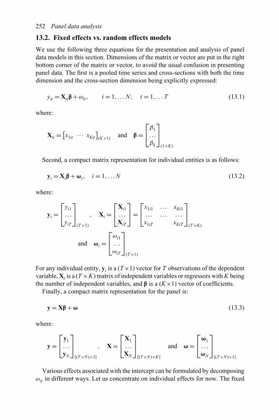
252 Panel data analysis
13.2. Fixed effects vs. random effects models
We use the following three equations for the presentation and analysis of paneldata models in this section. Dimensions of the matrix or vector are put in the rightbottom corner of the matrix or vector, to avoid the usual confusion in presentingpanel data. The first is a pooled time series and cross-sections with both the timedimension and the cross-section dimension being explicitly expressed:
yit = Xitβ+ωit, i = 1, . . . N ; t = 1, . . . T (13.1)
where:
Xit = [x1it · · · xKit
](K×1)
and β =⎡⎣β1
. . .
βk
⎤⎦
(1×K)
Second, a compact matrix representation for individual entities is as follows:
yi = Xiβ+ωi, i = 1, . . . N (13.2)
where:
yi =⎡⎣yi1
. . .
yiT
⎤⎦
(T×1)
, Xi =⎡⎣Xi1
. . .
XiT
⎤⎦=
⎡⎣x1i1 . . . xKi1
. . . . . . . . .
x1iT xKiT
⎤⎦
(T×K)
and ωi =⎡⎣ωi1
. . .
ωiT
⎤⎦
(T×1)
For any individual entity, yi is a (T×1) vector for T observations of the dependentvariable, Xi is a (T ×K) matrix of independent variables or regressors with K beingthe number of independent variables, and β is a (K×1) vector of coefficients.
Finally, a compact matrix representation for the panel is:
y = Xβ+ω (13.3)
where:
y =⎡⎣y1
. . .
yN
⎤⎦
[(T×N )×1], X =
⎡⎣X1
. . .
XN
⎤⎦
[(T×N )×K]and ω =
⎡⎣ω1
. . .
ωN
⎤⎦
[(T×N )×1]
Various effects associated with the intercept can be formulated by decomposingωit in different ways. Let us concentrate on individual effects for now. The fixed

Panel data analysis 253
effects model assumes that:
ωit = ci + εit (13.4)
where ci is individual-specific and time-invariant unobserved heterogeneity andis a constant for entity i, Cov(ci,Xit) �= 0, Cov(εit,Xit) = 0, Var(εit) = σ 2
ε ; and εit
is pure residuals uncorrelated with each other and uncorrelated with independentvariables. A compact matrix representation for the panel data model with fixedeffects is:
y = c + Xβ+ ε (13.5)
where:
c =⎡⎣c1
. . .
cN
⎤⎦
[(T×N )×1], ε =
⎡⎣ε1
. . .
εN
⎤⎦
[(T×N )×1], ci =
⎡⎣ ci
. . .
ci
⎤⎦
(T×1)
and εi =⎡⎣εi1
. . .
εiT
⎤⎦
(T×1)
Fixed effects models cannot be readily estimated by the OLS. There are fewapproaches that augment the OLS, such as resorting to dummies, applying firstdifferencing over time, and performing the within transformation.
To show how the dummy variable approach, the dummy variable least squares(DVLS), works, let Ii be a (T×1) vector of 1’s, I be a [(T × N ) × N ] matrix of Ii
and 0, and δ be a (N×1) vector of dummy coefficients, i.e.:
Ii =⎡⎣ 1
. . .
1
⎤⎦
(T×1)
, I =⎡⎣ I1 0 . . . 0
. . . . . . . . . . . .
0 . . . 0 IN
⎤⎦
[(T×N )×N ], δ =
⎡⎣δ1
. . .
δN
⎤⎦
(N×1)
Then a rearranged representation of equation (13.5) can be estimated by the OLS,which produces unbiased fixed effects estimators:
y = [X,I][β
δ
]+ ε (13.6)
It follows that, b and d, the DVLS estimators of β and δ, are:[bd
]= ([X,I]′[X,I])−1[X,I]′y + ([X,I]′[X,I])−1[X,I]′ ε
=[β
δ
]+ ([X,I]′[X,I])−1[X,I]′ ε (13.7)
The fixed effects in a panel data model can be either significant or insignificant. Ifδ1 = δ2 = ·· · δN = δ, then δ is simply a common intercept for all the entities within

254 Panel data analysis
the panel or for the whole panel. So, restrictions can be imposed on the estimateddummy coefficients. If the restrictions of δ1 = δ2 = ·· · δN = δ are rejected, thepanel data model is regarded to possess the features of fixed effects and thereare fixed effects variations across entities. Otherwise, if the restrictions of δ1 =δ2 = ·· · δN = δ are rejected, then there are no fixed effects variations in interceptsand the whole panel has just one common intercept.
When the residual, εit , is distributed normally, the maximum likelihoodprocedure can be applied to obtain fixed effects estimators of parameters. Thelikelihood function and the log likelihood function are as follows:
L =N∏
i=1
φ (yi − Xiβ− Iiδ) =N∏
i=1
1
σε
φ
(yi − Xiβ− Iiδ
σε
)
=N∏
i=1
(2πσ 2
ε
)−T/2exp
(−[
(yi − Xiβ− Iiδ)′(yi − Xiβ− Iiδ)
2σ 2ε
])(13.8)
LL =N∑
i=1
Ln
{1
σε
φ
(yi − Xiβ− Iiδ
σε
)}
=N∑
i=1
Ln
{(2πσ 2
ε
)−(N×T )/2exp
(−[
(yi − Xiβ− Iiδ)′(yi − Xiβ− Iiδ)
2σ 2ε
])}
= −N × T
2Ln(2πσ 2
ε
)− 1
2σ 2ε
N∑i=1
(yi − Xiβ− Iiδ
)′(yi − Xiβ− Iiδ
)(13.9)
where φ(z) is the density function of normal distributions.Further, let us consider both individual effects and time effects in the fixed
effects panel data model presented as follows:
y = c + h + Xβ+ ε (13.10)
where:
h =⎡⎣hJ
. . .
hT
⎤⎦
[(T×N )×1]and hT =
⎡⎣h1
. . .
hT
⎤⎦
(T×1)
and the rest is the same as in equation (13.5).The dummy variable approach, the DVLS, can be applied to estimate both
individual effects and time effects in the panel data model. However, if we use
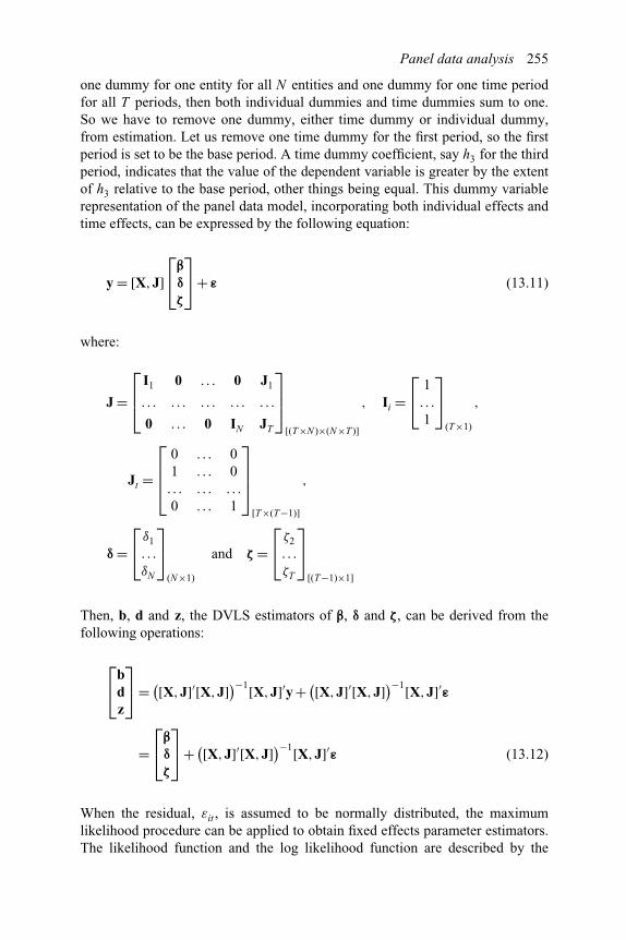
Panel data analysis 255
one dummy for one entity for all N entities and one dummy for one time periodfor all T periods, then both individual dummies and time dummies sum to one.So we have to remove one dummy, either time dummy or individual dummy,from estimation. Let us remove one time dummy for the first period, so the firstperiod is set to be the base period. A time dummy coefficient, say h3 for the thirdperiod, indicates that the value of the dependent variable is greater by the extentof h3 relative to the base period, other things being equal. This dummy variablerepresentation of the panel data model, incorporating both individual effects andtime effects, can be expressed by the following equation:
y = [X,J]⎡⎣β
δ
ζ
⎤⎦+ ε (13.11)
where:
J =⎡⎢⎣
I1 0 . . . 0 J1
. . . . . . . . . . . . . . .
0 . . . 0 IN JT
⎤⎥⎦
[(T×N )×(N×T )]
, Ii =⎡⎣ 1
. . .
1
⎤⎦
(T×1)
,
Jt =
⎡⎢⎢⎣
0 . . . 01 . . . 0. . . . . . . . .
0 . . . 1
⎤⎥⎥⎦
[T×(T−1)]
,
δ =⎡⎣δ1
. . .
δN
⎤⎦
(N×1)
and ζ =⎡⎣ζ2
. . .
ζT
⎤⎦
[(T−1)×1]
Then, b, d and z, the DVLS estimators of β, δ and ζ, can be derived from thefollowing operations:
⎡⎣b
dz
⎤⎦= ([X,J]′[X,J])−1[X,J]′y + ([X,J]′[X,J])−1[X,J]′ε
=⎡⎣β
δ
ζ
⎤⎦+ ([X,J]′[X,J])−1[X,J]′ε (13.12)
When the residual, εit , is assumed to be normally distributed, the maximumlikelihood procedure can be applied to obtain fixed effects parameter estimators.The likelihood function and the log likelihood function are described by the
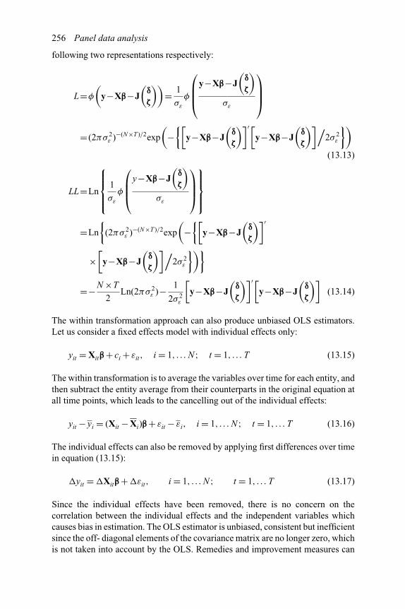
256 Panel data analysis
following two representations respectively:
L=φ
(y−Xβ−J
(δ
ζ
))= 1
σε
φ
⎛⎜⎜⎝
y−Xβ−J
(δ
ζ
)σε
⎞⎟⎟⎠
= (2πσ 2ε )−(N×T )/2exp
(−{[
y−Xβ−J
(δ
ζ
)]′[y−Xβ−J
(δ
ζ
)]/2σ 2
ε
})(13.13)
LL=Ln
⎧⎪⎪⎨⎪⎪⎩
1
σε
φ
⎛⎜⎜⎝
y−Xβ−J
(δ
ζ
)σε
⎞⎟⎟⎠⎫⎪⎪⎬⎪⎪⎭
=Ln
{(2πσ 2
ε )−(N×T )/2exp
(−{[
y−Xβ−J
(δ
ζ
)]′
×[y−Xβ−J
(δ
ζ
)]/2σ 2
ε
})}
=−N ×T
2Ln(2πσ 2
ε )− 1
2σ 2ε
[y−Xβ−J
(δ
ζ
)]′[y−Xβ−J
(δ
ζ
)](13.14)
The within transformation approach can also produce unbiased OLS estimators.Let us consider a fixed effects model with individual effects only:
yit = Xitβ+ ci + εit, i = 1, . . . N ; t = 1, . . . T (13.15)
The within transformation is to average the variables over time for each entity, andthen subtract the entity average from their counterparts in the original equation atall time points, which leads to the cancelling out of the individual effects:
yit − yi = (Xit −�Xi)β+ εit − εi, i = 1, . . . N ; t = 1, . . . T (13.16)
The individual effects can also be removed by applying first differences over timein equation (13.15):
�yit = �Xitβ+�εit, i = 1, . . . N ; t = 1, . . . T (13.17)
Since the individual effects have been removed, there is no concern on thecorrelation between the individual effects and the independent variables whichcauses bias in estimation. The OLS estimator is unbiased, consistent but inefficientsince the off- diagonal elements of the covariance matrix are no longer zero, whichis not taken into account by the OLS. Remedies and improvement measures can
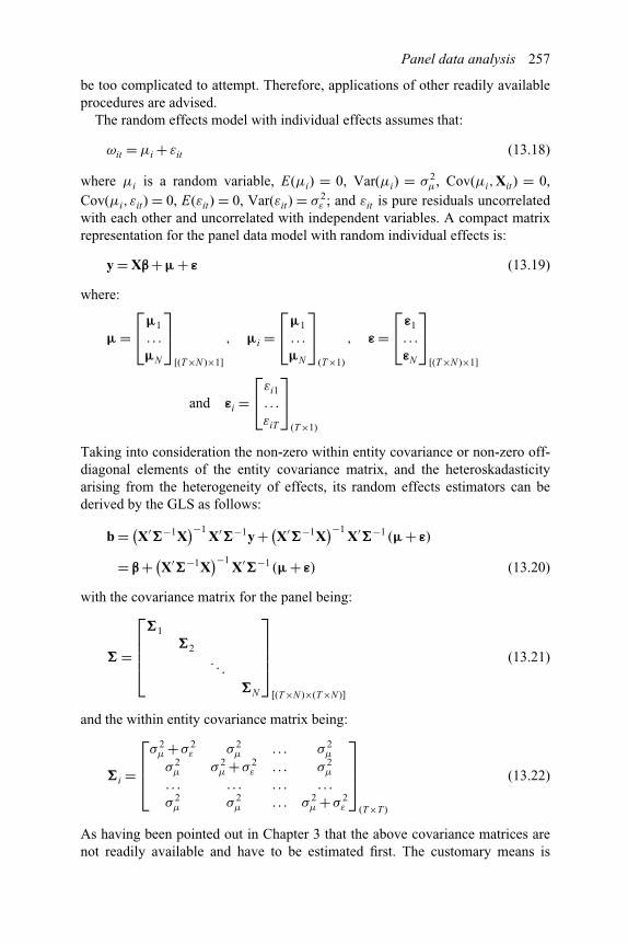
Panel data analysis 257
be too complicated to attempt. Therefore, applications of other readily availableprocedures are advised.
The random effects model with individual effects assumes that:
ωit = μi + εit (13.18)
where μi is a random variable, E(μi) = 0, Var(μi) = σ 2μ, Cov(μi,Xit) = 0,
Cov(μi,εit) = 0, E(εit) = 0, Var(εit) = σ 2ε ; and εit is pure residuals uncorrelated
with each other and uncorrelated with independent variables. A compact matrixrepresentation for the panel data model with random individual effects is:
y = Xβ+μ+ ε (13.19)
where:
μ =⎡⎣μ1
. . .
μN
⎤⎦
[(T×N )×1], μi =
⎡⎣μ1
. . .
μN
⎤⎦
(T×1)
, ε =⎡⎣ε1
. . .
εN
⎤⎦
[(T×N )×1]
and εi =⎡⎣εi1
. . .
εiT
⎤⎦
(T×1)
Taking into consideration the non-zero within entity covariance or non-zero off-diagonal elements of the entity covariance matrix, and the heteroskadasticityarising from the heterogeneity of effects, its random effects estimators can bederived by the GLS as follows:
b = (X′�−1X)−1
X′�−1y + (X′�−1X)−1
X′�−1 (μ+ ε)
= β+ (X′�−1X)−1
X′�−1 (μ+ ε) (13.20)
with the covariance matrix for the panel being:
� =
⎡⎢⎢⎢⎣
�1�2
. . .
�N
⎤⎥⎥⎥⎦
[(T×N )×(T×N )]
(13.21)
and the within entity covariance matrix being:
�i =
⎡⎢⎢⎣
σ 2μ +σ 2
ε σ 2μ . . . σ 2
μ
σ 2μ σ 2
μ +σ 2ε . . . σ 2
μ
. . . . . . . . . . . .
σ 2μ σ 2
μ . . . σ 2μ +σ 2
ε
⎤⎥⎥⎦
(T×T )
(13.22)
As having been pointed out in Chapter 3 that the above covariance matrices arenot readily available and have to be estimated first. The customary means is
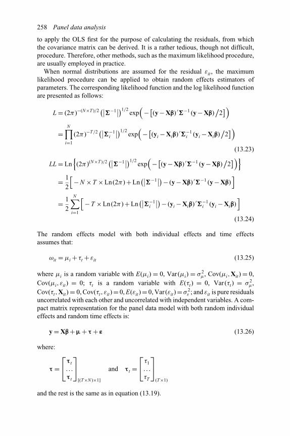
258 Panel data analysis
to apply the OLS first for the purpose of calculating the residuals, from whichthe covariance matrix can be derived. It is a rather tedious, though not difficult,procedure. Therefore, other methods, such as the maximum likelihood procedure,are usually employed in practice.
When normal distributions are assumed for the residual εit , the maximumlikelihood procedure can be applied to obtain random effects estimators ofparameters. The corresponding likelihood function and the log likelihood functionare presented as follows:
L = (2π )−(N×T )/2 (∣∣�−1∣∣)1/2
exp(
− [(y − Xβ) ′�−1 (y − Xβ)/
2])
=N∏
i=1
(2π )−T/2 (∣∣�−1i
∣∣)1/2exp(
− [(yi − Xiβ) ′�−1i (yi − Xiβ)
/2])
(13.23)
LL = Ln{(2π )(N×T )/2 (∣∣�−1
∣∣)1/2exp(
− [(y − Xβ) ′�−1 (y − Xβ)/
2])}
= 1
2
[− N × T × Ln(2π ) + Ln
(∣∣�−1∣∣)− (y − Xβ) ′�−1 (y − Xβ)
]
= 1
2
N∑i=1
[− T × Ln(2π ) + Ln
(∣∣�−1i
∣∣)− (yi − Xiβ) ′�−1i (yi − Xiβ)
](13.24)
The random effects model with both individual effects and time effectsassumes that:
ωit = μi + τt + εit (13.25)
where μi is a random variable with E(μi) = 0, Var(μi) = σ 2μ, Cov(μi,Xit) = 0,
Cov(μi,εit) = 0; τt is a random variable with E(τt) = 0, Var(τt) = σ 2μ,
Cov(τt,Xit) = 0, Cov(τt,εit) = 0, E(εit) = 0, Var(εit) = σ 2ε ; and εit is pure residuals
uncorrelated with each other and uncorrelated with independent variables. A com-pact matrix representation for the panel data model with both random individualeffects and random time effects is:
y = Xβ+μ+τ + ε (13.26)
where:
τ =⎡⎣τ t
. . .
τ t
⎤⎦
[(T×N )×1]and τ t =
⎡⎣τ1
. . .
τT
⎤⎦
(T×1)
and the rest is the same as in equation (13.19).

Panel data analysis 259
Taking into consideration the non-zero within entity covariance or non-zerooff-diagonal elements of the entity covariance matrix, and the heteroskadasticityarising from the heterogeneity of effects, its random effects estimators of β, b, canbe derived by the GLS as follows:
b = (X′�−1X)−1
X′�−1y + (X′�−1X)−1
X′�−1 (μ+τ + ε)
= β+ (X′�−1X)−1
X′�−1 (μ+τ + ε) (13.27)
with the covariance matrix for the panel being:
� =
⎡⎢⎢⎢⎣
�1 �12 . . . �1N
�21 �2
. . .. . .
�N1 �N
⎤⎥⎥⎥⎦
[(T×N )×(T×N )]
(13.28)
where the within entity covariance matrix is:
�i =
⎡⎢⎢⎣
σ 2μ +σ 2
ε σ 2μ . . . σ 2
μ
σ 2μ σ 2
μ +σ 2ε . . . σ 2
μ
. . . . . . . . . . . .
σ 2μ σ 2
μ . . . σ 2μ +σ 2
ε
⎤⎥⎥⎦
(T×T )
(13.29)
and the between entities covariance matrix is:
�ij =
⎡⎢⎢⎣
σ 2τ 0 . . . 00 σ 2
τ . . . 0. . . . . . . . . . . .
0 . . . σ 2τ
⎤⎥⎥⎦
(T×T )
(13.30)
With normally distributed residuals εit , the maximum likelihood procedure can beapplied. The corresponding likelihood function and the log likelihood function areas follows:
L = (2π )−(N×T )/2 (∣∣�−1∣∣)1/2
exp(
− [(y − Xβ) ′�−1 (y − Xβ)/
2])
(13.31)
LL = Ln
{(2π )(N×T )/2
(∣∣�−1∣∣)1/2
exp(
− [(y − Xβ) ′�−1 (y − Xβ)/
2])}
= −1
2
[− N × T × Ln(2π ) + Ln
(∣∣�−1∣∣)− (y − Xβ)′ �−1 (y − Xβ)
](13.32)
Both fixed effects and random effects models can be estimated by the maximumlikelihood method. When residuals obey normal distributions, the maximumlikelihood method produces the same estimated parameters as the OLS.

260 Panel data analysis
13.3. Random parameter models
The random parameter or random coefficient model with individual heterogeneityassumes:
βi = β+μi (13.33)
in the panel equation of:
yit = Xit (β+μi) + εit = Xitβ+ Xitμi + εit, i = 1, . . . N ; t = 1, . . . T(13.34)
where:
μi =⎡⎣μi1
. . .
μiK
⎤⎦
(K×1)
So, a compact matrix representation of the random parameter model forindividual entities takes the following form:
yi = Xi (β+μi) + εi = Xiβ+ Xiμi + εi, i = 1, . . . N (13.35)
Let us construct a new matrix of independent variables Z that stack in such afashion:
Z =⎡⎣X1 0 . . . 0
. . . . . . . . . . . .
0 . . . 0 XN
⎤⎦
[(T×N )×(K×N )]
(13.36)
Then, a compact matrix representation for the panel data model with individualheterogeneity in random parameters can be expressed as:
y = Xβ+ Zμ+ ε (13.37)
where:
μ =⎡⎣μ1
. . .
μN
⎤⎦
[(K×N )×1]
with E(μi) = 0, Var(μi) = σ 2μ, Cov(μi,Xit) = 0, Cov(μi,εit) = 0, E(εit) = 0,
Var(εit) = σ 2ε ; and εit is pure residuals uncorrelated with each other and
uncorrelated with independent variables.Taking into consideration the non-zero within entity covariance or non-zero
off-diagonal elements of the entity covariance matrix, and the heteroskadasticity
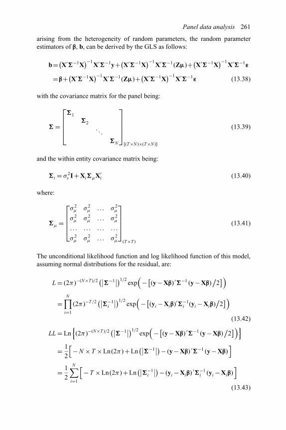
Panel data analysis 261
arising from the heterogeneity of random parameters, the random parameterestimators of β, b, can be derived by the GLS as follows:
b=(X′�−1X)−1
X′�−1y+(X′�−1X)−1
X′�−1 (Zμ)+(X′�−1X)−1
X′�−1ε
=β+(X′�−1X)−1
X′�−1 (Zμ)+(X′�−1X)−1
X′�−1ε (13.38)
with the covariance matrix for the panel being:
� =
⎡⎢⎢⎢⎣
�1�2
. . .
�N
⎤⎥⎥⎥⎦
[(T×N )×(T×N )]
(13.39)
and the within entity covariance matrix being:
�i = σ 2ε I + Xi�μX′
i (13.40)
where:
�μ =
⎡⎢⎢⎢⎣
σ 2μ σ 2
μ . . . σ 2μ
σ 2μ σ 2
μ . . . σ 2μ
. . . . . . . . . . . .
σ 2μ σ 2
μ . . . σ 2μ
⎤⎥⎥⎥⎦
(T×T )
(13.41)
The unconditional likelihood function and log likelihood function of this model,assuming normal distributions for the residual, are:
L = (2π )−(N×T )/2 (∣∣�−1∣∣)1/2
exp(
− [(y − Xβ) ′�−1 (y − Xβ)/
2])
=N∏
i=1
(2π )−T/2 (∣∣�−1i
∣∣)1/2exp(
− [(yi − Xiβ)′�−1i (yi − Xiβ)
/2])
(13.42)
LL = Ln{(2π )−(N×T )/2 (∣∣�−1
∣∣)1/2exp(
− [(y − Xβ) ′�−1 (y − Xβ)/
2])}
= 1
2
[− N × T × Ln(2π ) + Ln
(∣∣�−1∣∣)− (y − Xβ) ′�−1 (y − Xβ)
]
= 1
2
N∑i=1
[− T × Ln(2π ) + Ln
(∣∣�−1i
∣∣)− (yi − Xiβ) ′�−1i (yi − Xiβ)
](13.43)

262 Panel data analysis
respectively. Its conditional likelihood function and log likelihood function are:
L =N∏
i=1
φ (yi − Xiβ) =N∏
i=1
1
σε
φ
(yi − Xiβ
σε
)
=N∏
i=1
(2πσ 2
ε
)−T/2exp
(−[
(yi − Xiβ) ′ (yi − Xiβ)
2σ 2ε
])(13.44)
LL =N∑
i=1
Ln
{1
σε
φ
(yi − Xiβ
σε
)}
=N∑
i=1
Ln
{(2πσ 2
ε
)−T/2exp
(−[
(yi − Xiβ) ′ (yi − Xiβ)
2σ 2ε
])}
= −N × T
2Ln(2πσ 2
ε
)− 1
2σ 2ε
N∑i=1
(yi − Xiβ) ′ (yi − Xiβ) (13.45)
respectively.Random parameter models with regard to both individual and time entities take
the following form:
yit = Xitβ+ Xitμi + Xitτ t + εit, i = 1, . . . N ; t = 1, . . . T (13.46)
where:
τ t =⎡⎣τt1
. . .
τtK
⎤⎦
(K×1)
We may construct a new matrix of independent variables Wi for entity i and a newmatrix of independent variables for the panel as follows:
Wi =⎡⎣Xi1 0 . . . 0
. . . . . . . . . . . .
0 . . . 0 XiT
⎤⎦
[T×(T×K)]
(13.47)
W =⎡⎣W1
. . .
WN
⎤⎦
[(T×N )×(T×K)]
(13.48)
A compact matrix representation for the panel data model with both individualand time heterogeneity in random parameters becomes:
y = Xβ+ Zμ+ Wτ + ε (13.49)

Panel data analysis 263
where:
τ =⎡⎣τ1
. . .
τT
⎤⎦
[(K×T )×1]
The GLS estimators of β, b, can be obtained as follows:
b = (X′�−1X)−1
X′�−1y + (X′�−1X)−1
X′�−1 (Zμ)
+ (X′�−1X)−1
X′�−1 (Wτ) + (X′�−1X)−1
X′�−1ε
= β+ (X′�−1X)−1
X′�−1 (Zμ) + (X′�−1X)−1
X′�−1 (Wτ)
+ (X′�−1X)−1
X′�−1ε
(13.50)
with the covariance matrix for the panel being:
� =
⎡⎢⎢⎢⎣
�1 �12 . . . �1N
�21 �2
. . .. . .
�N1 �N
⎤⎥⎥⎥⎦
[(T×N )×(T×N )]
(13.51)
where the within entity covariance matrix is:
�i = σ 2ε I + Xi�μX′
i (13.52)
with:
�μ =
⎡⎢⎢⎣
σ 2μ σ 2
μ . . . σ 2μ
σ 2μ σ 2
μ . . . σ 2μ
. . . . . . . . . . . .
σ 2μ σ 2
μ . . . σ 2μ
⎤⎥⎥⎦
(T×T )
(13.53)
and the between entities covariance matrix is:
�ij =
⎡⎢⎢⎣
σ 2τ 0 . . . 00 σ 2
τ . . . 0. . . . . . . . . . . .
0 . . . σ 2τ
⎤⎥⎥⎦
(N×N )
(13.54)
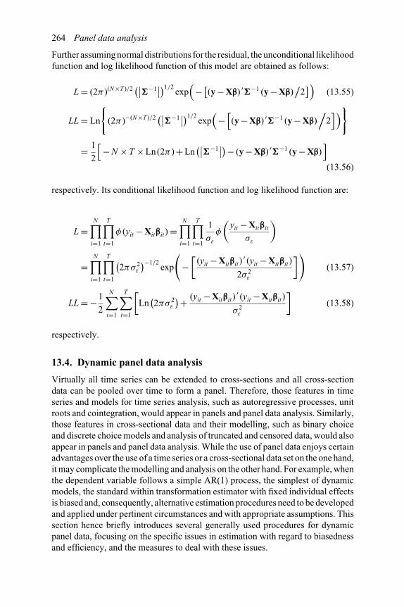
264 Panel data analysis
Further assuming normal distributions for the residual, the unconditional likelihoodfunction and log likelihood function of this model are obtained as follows:
L = (2π )(N×T )/2 (∣∣�−1∣∣)1/2
exp(
− [(y − Xβ) ′�−1 (y − Xβ)/
2])
(13.55)
LL = Ln
{(2π )−(N×T )/2 (∣∣�−1
∣∣)1/2exp(
−[(y − Xβ) ′�−1 (y − Xβ)
/2])}
= 1
2
[− N × T × Ln(2π ) + Ln
(∣∣�−1∣∣)− (y − Xβ) ′�−1 (y − Xβ)
](13.56)
respectively. Its conditional likelihood function and log likelihood function are:
L =N∏
i=1
T∏t=1
φ (yit − Xitβit) =N∏
i=1
T∏t=1
1
σε
φ
(yit − Xitβit
σε
)
=N∏
i=1
T∏t=1
(2πσ 2
ε
)−1/2exp
(−[
(yit − Xitβit)′ (yit − Xitβit)
2σ 2ε
])(13.57)
LL = −1
2
N∑i=1
T∑t=1
[Ln(2πσ 2
ε
)+ (yit − Xitβit)′ (yit − Xitβit)
σ 2ε
](13.58)
respectively.
13.4. Dynamic panel data analysis
Virtually all time series can be extended to cross-sections and all cross-sectiondata can be pooled over time to form a panel. Therefore, those features in timeseries and models for time series analysis, such as autoregressive processes, unitroots and cointegration, would appear in panels and panel data analysis. Similarly,those features in cross-sectional data and their modelling, such as binary choiceand discrete choice models and analysis of truncated and censored data, would alsoappear in panels and panel data analysis. While the use of panel data enjoys certainadvantages over the use of a time series or a cross-sectional data set on the one hand,it may complicate the modelling and analysis on the other hand. For example, whenthe dependent variable follows a simple AR(1) process, the simplest of dynamicmodels, the standard within transformation estimator with fixed individual effectsis biased and, consequently, alternative estimation procedures need to be developedand applied under pertinent circumstances and with appropriate assumptions. Thissection hence briefly introduces several generally used procedures for dynamicpanel data, focusing on the specific issues in estimation with regard to biasednessand efficiency, and the measures to deal with these issues.

Panel data analysis 265
A dynamic panel data model is a model in which the lagged dependent variableappears on the right-hand side of the equation. Nickell (1981) has addressed theissue of biases in dynamic panel models. Arellano and Bond (1991), Arellanoand Bover (1995), and Blundell and Bond (1998) put forward several GMMprocedures, which have promoted the application of dynamic panel data modelsin empirical research in recent years. The simplest dynamic panel model is wherethe dependent variable follows an AR(1) process. The following presentationaugments equation (13.1) by including the lagged dependent variable, yi,t−1, alongwith Xit , as a regressor:
yit = ρyi,t−1 + Xitβ+ωit i = 1, . . . N ; t = 1, . . . T (13.59)
where |ρ| < 1 to ensure stationarity.For simplicity and without affecting the outcome, we do not include exogenous
independent variables Xit for the moment and only consider individual effects inthe discussion. Hence equation (3.59) becomes:
yit = ρyi,t−1 +μi + εit, i = 1, . . . N ; t = 1, . . . T (13.60)
We do not specify whether μi is fixed effects or random effects; but we will seethat it is irrelevant and the effects can always be regarded as fixed. Nickell (1981)shows that the LSDV estimator of equation (13.60) is biased. It is because thecorrelation between the lagged dependent variable and the transformed residualdoes not disappear. After the within transformation, equation (13.60) becomes:
yit − yi = ρ(yi,t−1 − yi,−1
)+ εit − εi, i = 1, . . . N ; t = 1, . . . T (13.61)
It is clear that εi is correlated with yi,t−1, so ρ, the LSDV estimator of ρ, is biased,since:
ρ =∑T
t=1
∑Ni=1 (yit −yi)
(yi,t−1 −yi,−1
)∑T
t=1
∑Ni=1
(yi,t−1 −yi,−1
)2 +∑T
t=1
∑Ni=1 (εit −εi)
(yi,t−1 −yi,−1
)∑T
t=1
∑Ni=1
(yi,t−1 −yi,−1
)2(13.62)
The last term does not converge to zero when N → ∞ but T is not large. Nickell(1981) demonstrates that:
p limN→∞
(ρ −ρ) =⎧⎨⎩ 2ρ
1 −ρ2 −[
1 +ρ
T − 1
(1 − 1
T
(1 −ρT
)(1 −ρ)
)]−1⎫⎬⎭
−1
(13.63)
For a reasonably large T , the above is approximately:
p limN→∞
(ρ −ρ) ≈ 1 +ρ
1 − T(13.64)
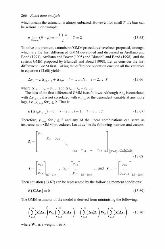
266 Panel data analysis
which means the estimator is almost unbiased. However, for small T the bias canbe serious. For example:
p limN→∞
(ρ −ρ) = −1 +ρ
2, T = 2 (13.65)
To solve this problem, a number of GMM procedures have been proposed, amongstwhich are the first differenced GMM developed and discussed in Arellano andBond (1991), Areliano and Bover (1995) and Blundell and Bond (1998), and thesystem GMM proposed by Blundell and Bond (1998). Let us consider the firstdifferenced GMM first. Taking the difference operation once on all the variablesin equation (13.60) yields:
�yit = ρ�yi,t−1 +�εit, i = 1, . . . N ; t = 2, . . . T (13.66)
where �yit = yit − yi,t−1 and �εit = εit − εi,t−1.
The idea of the first differenced GMM is as follows. Although �εit is correlatedwith �yi,t−1, it is not correlated with yi,t−2 or the dependent variable at any morelags, i.e., yi,t−j for j ≥ 2. That is:
E(�εityi,t−j
)= 0, j = 2, . . . t − 1, t = 3, . . . T (13.67)
Therefore, yi,t−j for j ≥ 2 and any of the linear combinations can serve asinstruments in GMM procedures. Let us define the following matrices and vectors:
Zi =
⎡⎢⎢⎢⎣
yi,1yi,1 yi,2
. . .
yi,1 yi,2 ... yi,T−2
⎤⎥⎥⎥⎦[
(T−2)× (T−2)(T−1)2
](13.68)
εi =⎡⎣εi,3
...
εi,T
⎤⎦
[(T−2)×1]
, yi =⎡⎣yi,3
...
yi,T
⎤⎦
[(T−2)×1]
, and yi,−1 =⎡⎣ yi,2
...
yi,T−1
⎤⎦
[(T−2)×1]
Then equation (13.67) can be represented by the following moment conditions:
E(Z′
i�εi
)= 0 (13.69)
The GMM estimator of the model is derived from minimising the following:
(N∑
i=1
Z′i�εi
)′WN
(N∑
i=1
Z′i�εi
)=(
N∑i=1
�ε′iZi
)WN
(N∑
i=1
Z′i�εi
)(13.70)
where WN is a weight matrix.
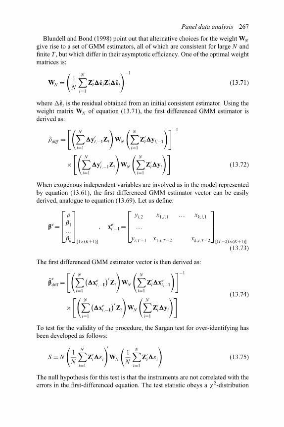
Panel data analysis 267
Blundell and Bond (1998) point out that alternative choices for the weight WN
give rise to a set of GMM estimators, all of which are consistent for large N andfinite T , but which differ in their asymptotic efficiency. One of the optimal weightmatrices is:
WN =(
1
N
N∑i=1
Z′i�εiZ
′i�εi
)−1
(13.71)
where �εi is the residual obtained from an initial consistent estimator. Using theweight matrix WN of equation (13.71), the first differenced GMM estimator isderived as:
ρdiff =[(
N∑i=1
�y′i,−1Zi
)WN
(N∑
i=1
Z′i�yi,−1
)]−1
×[(
N∑i=1
�y′i,−1Zi
)WN
(N∑
i=1
Z′i�yi
)](13.72)
When exogenous independent variables are involved as in the model representedby equation (13.61), the first differenced GMM estimator vector can be easilyderived, analogue to equation (13.69). Let us define:
βe =
⎡⎢⎢⎣
ρ
β1...
βk
⎤⎥⎥⎦
[1×(K+1)]
, xei,−1 =
⎡⎢⎢⎣
yi,2 x1,i,1 ... xk,i,1
...
yi,T−1 x1,i,T−2 xk,i,T−2
⎤⎥⎥⎦
[(T−2)×(K+1)]
(13.73)
The first differenced GMM estimator vector is then derived as:
βe
diff =[(
N∑i=1
(�xe
i,−1
)′Zi
)WN
(N∑
i=1
Z′i�xe
i,−1
)]−1
×[(
N∑i=1
(�xe
i,−1
)′Zi
)WN
(N∑
i=1
Z′i�yi
)] (13.74)
To test for the validity of the procedure, the Sargan test for over-identifying hasbeen developed as follows:
S = N
(1
N
N∑i=1
Z′i�εi
)′WN
(1
N
N∑i=1
Z′i�εi
)(13.75)
The null hypothesis for this test is that the instruments are not correlated with theerrors in the first-differenced equation. The test statistic obeys a χ2-distribution

268 Panel data analysis
with m degrees of freedom under the null, where m is equal to the number ofinstruments subtracting the number of parameters in the model.
In addition to lagged levels of the dependent variable as instruments forequations in first differences, Blundell and Bond (1998) propose the use of laggedfirst differences of the dependent variable as instruments for equations in levels.This is referred to as the system GMM. Imposed are the following additionalmoment restrictions:
E(ωit�yi,t−1
)= 0, t = 4, . . . T (13.76)
E(ωi3�yi,2
)= 0 (13.77)
where ωit = μi + εit . Accordingly, the instrument matrix using the conditionsexpressed in equation (13.76) and equation (13.77) is as follows:
Z+i =
⎡⎢⎢⎢⎢⎣
Zi 0 0 . . . 00 �yi2 . . .
. . . �yi3. . . . . . 0
0 0 0 . . . �yi,T−1
⎤⎥⎥⎥⎥⎦{
[2(T−2)]×[
(T−2)(T+1)2
]}(13.78)
with Zi being defined by equation (13.67). Analogue to the first differenced GMMprocedure, the system GMM estimator is derived from minimising the followingfunction:(
N∑i=1
(Z+
i
)′�εi
)′WN
(N∑
i=1
(Z+
i
)′�εi
)=(
N∑i=1
�ε′iZ
+i
)WN
(N∑
i=1
(Z+
i
)′�εi
)
(13.79)
The system GMM estimator is then given by:
ρsys =[(
N∑i=1
y′i,−1Z+
i
)WN
(N∑
i=1
(Z+
i
)′yi,−1
)]−1
×[(
N∑i=1
y′i,−1Z+
i
)WN
(N∑
i=1
(Z+
i
)′yi
)](13.80)
Similar to the first differenced GMM case, when exogenous independent variablesare involved, the system GMM estimator vector can be derived as follows:
βe
sys =[(
N∑i=1
(xe
i,−1
)′Z+
i
)WN
(N∑
i=1
(Z+
i
)′xe
i,−1
)]−1
×[(
N∑i=1
(xe
i,−1
)′Z+
i
)WN
(N∑
i=1
(Z+
i
)′yi
)](13.81)

Panel data analysis 269
13.5. Examples and cases
Example 13.1
Investment is one of the most important corporate activities taken byfirms and pursued by CEOs on behalf of the firms and shareholders.Personal characteristics of CEOs may therefore influence corporateinvestment behaviour. Malmendier and Tate (2005) argue that managerialoverconfidence can account for corporate investment distortions andhypothesise that overconfident managers overestimate the returns to theirinvestment projects and view external funds as unduly costly. Using paneldata on personal portfolio and corporate investment decisions of Forbes500 CEOs, they test the overconfidence hypothesis. The two well-publicisedtraditional explanations for investment distortions are the misalignment ofmanagerial and shareholders interests and asymmetric information betweencorporate insiders and the capital market. Both cause investment to besensitive to the level of cash flows in the firm. The alternative explanationproposed by Malmendier and Tate (2005) in this study relates corporateinvestment decisions to personal characteristics of the CEO of the firm.They argue that overconfident CEOs systematically overestimate the returnto their investment projects. Consequently, they overinvest if they havesufficient internal funds for investment and are not disciplined by the capitalmarket or corporate governance mechanisms. They curb their investment ifthey do not have sufficient internal funds, since they are reluctant to issuenew equity which undervalues the stock of their company by the market andnew investors.
Measures of CEO overconfidence in this study are constructed basedon the overexposure of CEOs to the idiosyncratic risk of their firms. Thefirst two measures, Holder 67 and Longholder, are linked to the timing ofoptions’ exercises. Risk-averse CEOs should exercise their options earlygiven a sufficiently high stock price. A CEO is regarded overconfident ifhe persistently exercises options later than suggested by the benchmark; heis overconfident in his ability to keep the company’s stock price rising andthat he wants to profit from expected price increases by holding the options.In this regard, Holder 67 adopts 67% in-the-money during the fifth year asthe threshold. If an option is more than 67% in-the-money at some point inyear 5, the CEO should have exercised at least some portion of the packageduring or before the fifth year. This threshold corresponds to a risk-aversionmeasure of three in a constant relative risk-aversion utility specification. Thefirst instance, if any, is then identified, at which the CEO failed to exercisesuch an option during or before the fifth year. From this point in time onward,the CEO is classified as overconfident if he subsequently exhibits the same
Continued

270 Panel data analysis
behaviour at least one more time during his tenure as CEO. To the extreme,if a CEO is optimistic enough about his firm’s future performance that heholds options all the way to expiration, he is regarded overconfident asLongholder. The last measure, Net Buyer, classifies CEOs who habituallyincrease their holdings of their company’s stock as overconfident. Moreprecisely, a CEO is identified as overconfident if he was net buyer of hiscompany’s stock during his first five years in the sample.
The data sample used in this empirical study consists of 477 large publiclytraded US firms from 1980 to 1994. The included firm must appear at leastfour times on one of the lists of the largest US companies compiled by theForbes magazine in the period from 1984 to 1994. The data set providesdetailed information on the stock ownership and set of option packages forthe CEO of each company, year by year. The data set is supplemented byCompustat and other databases for related information on company andCEO profiles. This is a straightforward panel of time series and cross-sectional data set. Due to some restrictions and deletions with reasons givenin the paper, the number of observations is 1058 for Holder 67, 3742 forLongholder and 842 for Net Buyer.
The empirical part of the study runs regression of investment on cash flow,market value of assets over book value of assets, a measure of overconfidenceand a set of controlling variables. These controlling variables includecorporate governance, stock ownership, and vested options. Cash flow isearnings before extraordinary items plus depreciation and is normalised bycapital at the beginning of the year. The market value of assets over the bookvalue of assets at the beginning of the year is represented by Q. Holder 67,Longholder and Net Buyer are dummies, taking the value of one if the CEOis classified as being overconfident and zero otherwise by the respectivemeasure. Stock ownership is the fraction of company stock owned by theCEO and his immediate family at the beginning of the year. Vested optionsare the CEO’s holdings of options that are exercisable within 6 months ofthe beginning of the year, as a fraction of common shares outstanding.Vested options are multiplied by 10 so that the mean is comparable tostock ownership. Size is the natural logarithm of assets at the beginningof the year. Corporate governance is the number of outside directors whocurrently serve as CEOs of other companies. Industries are defined as the 12Fama-French industry groups. The dependent variable in the regression isInvestment, defined as firm capital expenditures and normalised by capital atthe beginning of the year. The study adopts the panel data model with fixedeffects in its empirical analysis, with fixed time effects, fixed firm effectsand fixed industry effects. The main results with regard to the effect of CEOoverconfidence on investment that are related to panel data analysis aresummarised and reported in Table 13.1. The coefficients of the interaction

Panel data analysis 271
Table 13.1 Regression of investment on cash flow and overconfidence
Holder 67 Longholder Net buyer
Cash-flow 1.7044 0.656 1.555(10.20)∗∗∗ (7.50)∗∗∗ (6.99)∗∗∗
Q −0.0088 0.0851 0.0770(0.44) (7.89)∗∗∗ (3.57)∗∗∗
Stock-ownership (%) −0.1834 0.196 −0.0964(0.33) (2.41)∗∗ (0.24)
Vested-options 0.1398 0.003 0.0639(1.17) (0.03) (0.42)
Size 0.0543 −0.0494 −0.0790(2.88)∗∗∗ (5.12)∗∗∗ (3.12)∗∗∗
Corporate-governance −0.0071 0.0023 0.0071(0.92) (0.59) (0.74)
(Q)× (Cash-flow) 0.0648 −0.0099 −0.0721(3.28)∗∗∗ (1.02) (3.17)∗∗∗
(Stock-ownership) × (Cash-flow) −0.6897 0.002 0.3991(1.67)∗ (0.01) (0.56)
(Vested-options) × (Cash-flow) −0.2981 0.2847 −0.0012(2.62)∗∗∗ (3.97)∗∗∗ (0.01)
(Size) × (Cash-flow) −0.1754 −0.053 −0.1653(8.77)∗∗∗ (5.04)∗∗∗ (6.02)∗∗∗
(Corporate-governance) × (Cash-flow) 0.0441 −0.0096 0.0006(2.65)∗∗∗ (1.07) (0.03)
Holder 67 −0.0495(1.96)∗
(Holder 67) × (Cash-flow) 0.2339(4.70)∗∗∗
Longholder −0.0504(2.65)∗∗∗
(Longholder) × (Cash-flow) 0.1778(5.51)∗∗∗
Net-buyer 1.0615(2.83)∗∗∗
(Net-buyer) × (Cash-flow) 0.4226(4.33)∗∗∗
Year-fixed-effects Yes Yes YesFirm-fixed-effects Yes Yes Yes(Year-fixed-effects) × (Cash-flow) Yes Yes Yes(Industry-fixed-effects) × (Cash-flow) No No No(Firm-fixed-effects) × (Cash-flow) No No NoObservations 1058 3742 842Adjusted R2 0.62 0.54 0.54
Constant included.t-statistic in parentheses.∗significant at the 10 per cent level; ∗∗significant at the 5 per cent level; ∗∗∗significant at the1 per cent level.
Continued
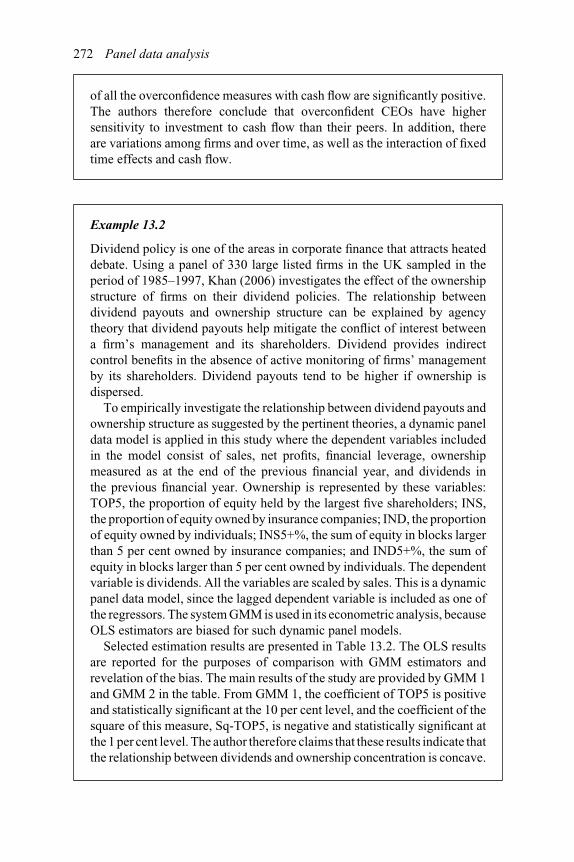
272 Panel data analysis
of all the overconfidence measures with cash flow are significantly positive.The authors therefore conclude that overconfident CEOs have highersensitivity to investment to cash flow than their peers. In addition, thereare variations among firms and over time, as well as the interaction of fixedtime effects and cash flow.
Example 13.2
Dividend policy is one of the areas in corporate finance that attracts heateddebate. Using a panel of 330 large listed firms in the UK sampled in theperiod of 1985–1997, Khan (2006) investigates the effect of the ownershipstructure of firms on their dividend policies. The relationship betweendividend payouts and ownership structure can be explained by agencytheory that dividend payouts help mitigate the conflict of interest betweena firm’s management and its shareholders. Dividend provides indirectcontrol benefits in the absence of active monitoring of firms’ managementby its shareholders. Dividend payouts tend to be higher if ownership isdispersed.
To empirically investigate the relationship between dividend payouts andownership structure as suggested by the pertinent theories, a dynamic paneldata model is applied in this study where the dependent variables includedin the model consist of sales, net profits, financial leverage, ownershipmeasured as at the end of the previous financial year, and dividends inthe previous financial year. Ownership is represented by these variables:TOP5, the proportion of equity held by the largest five shareholders; INS,the proportion of equity owned by insurance companies; IND, the proportionof equity owned by individuals; INS5+%, the sum of equity in blocks largerthan 5 per cent owned by insurance companies; and IND5+%, the sum ofequity in blocks larger than 5 per cent owned by individuals. The dependentvariable is dividends. All the variables are scaled by sales. This is a dynamicpanel data model, since the lagged dependent variable is included as one ofthe regressors. The system GMM is used in its econometric analysis, becauseOLS estimators are biased for such dynamic panel models.
Selected estimation results are presented in Table 13.2. The OLS resultsare reported for the purposes of comparison with GMM estimators andrevelation of the bias. The main results of the study are provided by GMM 1and GMM 2 in the table. From GMM 1, the coefficient of TOP5 is positiveand statistically significant at the 10 per cent level, and the coefficient of thesquare of this measure, Sq-TOP5, is negative and statistically significant atthe 1 per cent level. The author therefore claims that these results indicate thatthe relationship between dividends and ownership concentration is concave.
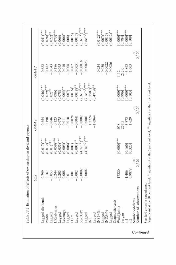
Tab
le13
.2E
stim
atio
nof
effe
cts
ofow
ners
hip
ondi
vide
ndpa
yout
s
OLS
GM
M1
GM
M2
Lag
ged-
divi
dend
s0.
799
(0.0
17)∗∗
∗0.
654
(0.0
46)∗∗
∗0.
682
(0.0
41)∗∗
∗Pro
fits
0.16
7(0
.012
)∗∗∗
0.19
8(0
.029
)∗∗∗
0.18
2(0
.028
)∗∗∗
Lag
ged
−0.0
53(0
.01)
∗∗∗
−0.0
46(0
.02)
∗∗−0
.043
(0.0
22)∗∗
1/R
eal-
sale
s0.
244
(0.0
59)∗∗
∗0.
123
(0.0
86)
0.18
6(0
.073
)∗∗∗
Lag
ged
−0.2
03(0
.053
)∗∗∗
−0.0
75(0
.078
)−0
.095
(0.0
66)
Lev
erag
e0.
008
(0.0
05)∗
0.01
1(0
.005
)∗∗0.
010
(0.0
06)∗
Lag
ged
−0.0
1(0
.006
)∗−0
.010
(0.0
07)
−0.0
08(0
.008
)T
OP5
0.00
1(0
.001
)0.
0028
(0.0
016)
∗0.
0021
(0.0
015)
Lag
ged
−0.0
02(0
.001
)∗∗−0
.004
1(0
.001
8)∗∗
−0.0
051
(0.0
017)
Sq-
TO
P5
−0.0
002
(4.7
e−5)∗∗
∗−0
.000
2(7
.3e−5
)∗∗∗
−0.0
0016
(6.3
e−5)∗∗
∗L
agge
d0.
0002
(4.3
e−5)∗∗
∗0.
0001
(7.1
e−5)∗∗
∗0.
0002
3(6
.8e−5
)∗∗∗
INS
1.27
24(0
.750
7)∗∗
∗L
agge
d−1
.096
4(0
.471
9)∗∗
INS5+
%0.
034
(0.0
12)∗∗
∗L
agge
d−0
.030
(0.0
07)∗∗
∗IN
D5+
%−0
.002
2(0
.001
5)L
agge
d0.
0026
(0.0
012)
∗∗D
iagn
ostic-
test
sW
ald(
join
t)17
320
[0.0
00]∗∗
∗10
58[0
.000
]∗∗∗
1112
.[0
.000
]∗∗∗
Sar
gan
257.
5[0
.996
]21
2.0
[0.7
84]
m1
−1.4
06[0
.160
]−3
.873
[0.0
00]∗∗
∗−3
.893
[0.0
00]∗∗
∗m
20.
9878
[0.3
23]
1.62
9[0
.103
]1.
603
[0.1
09]
Num
ber-
of-fi
rms
330
330
330
Num
ber-
of-
obse
rvat
ions
2,37
02,
370
2,37
0
Sta
ndar
der
rors
inpa
rent
hese
s.∗ si
gnifi
cant
atth
e10
per
cent
leve
l;∗∗
sign
ifica
ntat
the
5pe
rce
ntle
vel;
∗∗∗ si
gnifi
cant
atth
e1
per
cent
leve
l.
Continued
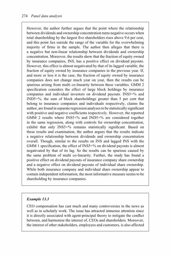
274 Panel data analysis
However, the author further argues that the point where the relationshipbetween dividends and ownership concentration turns negative occurs whentotal shareholding by the largest five shareholders rises above 9.6 per cent,and this point lies outside the range of the variable for the overwhelmingmajority of firms in the sample. The author then alleges that there isa negative but non-linear relationship between dividends and ownershipconcentration. Moreover, the results show that the fraction of equity ownedby insurance companies, INS, has a positive effect on dividend payouts.However, this effect is almost negativated by that of its lagged variable, thefraction of equity owned by insurance companies in the previous year. If,and more or less it is the case, the fraction of equity owned by insurancecompanies does not change much year on year, then the results can bespurious arising from multi co-linearity between these variables. GMM 2specification considers the effect of large block holdings by insurancecompanies and individual investors on dividend payouts. INS5+% andIND5+%, the sum of block shareholdings greater than 5 per cent thatbelong to insurance companies and individuals respectively, claims theauthor, are found in separate regression analyses to be statistically significantwith positive and negative coefficients respectively. However, the reportedGMM 2 results where INS5+% and IND5+% are considered togetherin the same regression, along with controls for ownership concentration,exhibit that only INS5+% remains statistically significant. Based onthese results and examination, the author argues that the results indicatea negative relationship between dividends and ownership concentrationoverall. Though, similar to the results on INS and lagged INS with theGMM 1 specification, the effect of INS5+% on dividend payouts is almostnegativated by that of its lag. So the results can be spurious caused bythe same problem of multi co-linearity. Further, the study has found apositive effect on dividend payouts of insurance company share ownershipand a negative effect on dividend payouts of individual share ownership.While both insurance company and individual share ownership appear tocontain independent information, the most informative measure seems to beshareholding by insurance companies.
Example 13.3
CEO compensation has cast much and many controversies in the news aswell as in scholarly work. The issue has attracted immense attention sinceit is directly associated with agent-principal theory to mitigate the conflictbetween, and harmonise the interest of, CEOs and shareholders. Moreover,the interest of other stakeholders, employees and customers, is also affected

Panel data analysis 275
by the compensation CEOs receive. In a recent attempt to establish a linkbetween CEO compensation and firm performance, Lilling (2006) employsthe GMM to examine a panel data set of North American companies. Thedata are drawn from over 24,000 public companies in various industries from1993 to 2005. For usual reasons of mission data and/or unavailability of data,the final sample consists of only 1,378 firms with 6,755 total observations.
The study puts forward four hypotheses, and then empirically teststhese hypotheses using the dynamic panel model. These hypotheses are:(1) there is a positive link between firm performance represented by marketvalue of the firm and CEO compensation; (2) as the size of a firm grows interms of sales, CEO compensation increases; (3) as a CEO has an additionalyear of experience, his compensation increases; and (4) a CEO hiredexternally will be compensated more than a CEO who is hired internally.Subsequently, in empirical dynamic panel data regression, the logarithm ofmarket value of the firm for firm performance, the logarithm of sales forfirm size, CEO tenure in years and a dummy for internally hired CEOs areincluded as independent variables in the model. Besides, ROA is adopted asan additional measure for firm performance, as well as a gender dummy. Thedependent variable is the logarithm of total CEO compensation, includingsalary, bonus, restricted stock grant value, stock options, and other benefits.The dependent variable at lag one is taken in as one of the regressors, so themodelling is a typical dynamic panel data approach.
The empirical results are reported in Table 13.3 and Table 13.4, with theformer using lagged firm performance and the latter using contemporaryfirm performance in estimation. The first differenced GMM and the systemGMM have produced similar results while fixed effects estimators are ratherdifferent. Analysis and discussion are based on GMM results, since fixedeffects may cause bias in parameter estimates. The coefficients of laggedCEO compensation are positive and highly significant at the 1 per centlevel, indicating the series of CEO compensation are fairly persistent. Thisimplies that the lagged level variables provide weak instruments for thedifferences in the first differenced GMM model; hence the author allegesthe system GMM approach is more suitable than the first differenced GMMin this case. According to the estimated coefficients, CEO compensation isstrongly linked to the market value of the firm, and it is more responsiveto the market value of the firm in the current year than that in theprevious year. The coefficient estimated by the system GMM is 0.358in Table 13.3 and greater at 0.405 in Table 13.4; and the coefficientestimated by the first differenced GMM is 0.214 in Table 13.3 and greaterat 0.444 in Table 13.4, all of them significant at the 1 per cent level. Theseresults support the statement of the first hypothesis in the paper that there
Continued
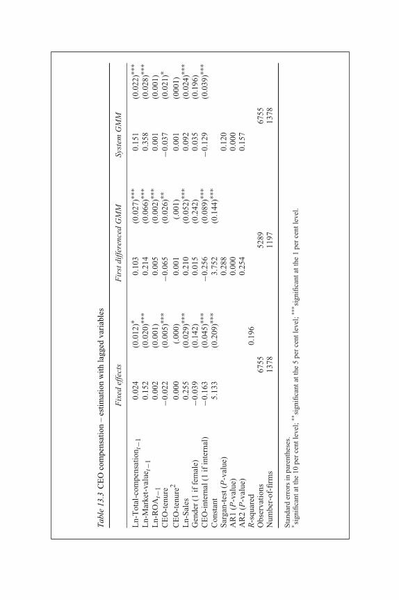
Tab
le13
.3C
EO
com
pens
atio
n–
estim
atio
nw
ith
lagg
edva
riab
les
Fix
edef
fect
sF
irst
differ
ence
dG
MM
Syst
emG
MM
Ln-
Tot
al-c
ompe
nsat
ion t
−10.
024
(0.0
12)∗
0.10
3(0
.027
)∗∗∗
0.15
1(0
.022
)∗∗∗
Ln-
Mar
ket-
valu
e t−1
0.15
2(0
.020
)∗∗∗
0.21
4(0
.066
)∗∗∗
0.35
8(0
.028
)∗∗∗
Ln-
RO
At−
10.
002
(0.0
01)
0.00
5(0
.002
)∗∗∗
0.00
1(0
.001
)C
EO
-ten
ure
−0.0
22(0
.005
)∗∗∗
−0.0
65(0
.026
)∗∗−0
.037
(0.0
21)∗
CE
O-t
enur
e20.
000
(.00
0)0.
001
(.00
1)0.
001
(000
1)L
n-Sal
es0.
255
(0.0
29)∗∗
∗0.
210
(0.0
52)∗∗
∗0.
092
(0.0
24)∗∗
∗G
ende
r(1
iffe
mal
e)−0
.039
(0.1
42)
0.01
5(0
.242
)0.
035
(0.1
96)
CE
O-i
nter
nal(
1if
inte
rnal
)−0
.163
(0.0
45)∗∗
∗−0
.256
(0.0
89)∗∗
∗−0
.129
(0.0
39)∗∗
∗C
onst
ant
5.13
3(0
.209
)∗∗∗
3.75
2(0
.144
)∗∗∗
Sar
gan-
test
(P-v
alue
)0.
288
0.12
0A
R1
(P-v
alue
)0.
000
0.00
0A
R2
(P-v
alue
)0.
254
0.15
7R
-squ
ared
0.19
6O
bser
vation
s67
5552
8967
55N
umbe
r-of
-firm
s13
7811
9713
78
Sta
ndar
der
rors
inpa
rent
hese
s.∗ si
gnifi
cant
atth
e10
per
cent
leve
l;∗∗
sign
ifica
ntat
the
5pe
rce
ntle
vel;
∗∗∗ si
gnifi
cant
atth
e1
per
cent
leve
l.

Tab
le13
.4C
EO
com
pens
atio
n–
estim
atio
nw
ith
cont
empo
rary
vari
able
s
Fix
edef
fect
sF
irst
differ
ence
dG
MM
Syst
emG
MM
Ln-
Tot
al-c
ompe
nsat
ion t
−10.
018
(0.0
13)
0.09
2(0
.027
)∗∗∗
0.14
2(0
.021
)∗∗∗
Ln-
Mar
ket-
valu
e0.
345
(0.0
18)∗∗
∗0.
444
(0.0
73)∗∗
∗0.
405
(0.0
30)∗∗
∗L
n-R
OA
0.00
3(0
.001
)∗∗−0
.004
(0.0
03)
−0.0
07(0
.002
)∗∗∗
CE
O-t
enur
e−0
.021
(0.0
05)∗∗
∗−0
.020
(0.0
26)
−0.0
21(0
.020
)C
EO
-ten
ure2
0.00
0(0
.000
)−0
.001
(0.0
01)
0.00
0(0
.001
)L
n-Sal
es0.
123
(0.0
28)∗∗
∗0.
150
(0.0
50)∗∗
∗0.
063
(0.0
23)∗∗
∗G
ende
r−0
.069
(0.1
38)
−0.2
04(0
.276
)0.
086
(0.1
86)
CE
O-i
nter
nal
−0.1
49(0
.043
)∗∗∗
−0.2
39(0
.089
)∗∗∗
−0.1
29(0
.038
)∗∗∗
Con
stan
t4.
648
(0.2
06)∗∗
∗3.
521
(0.1
47)∗∗
∗Sar
gan-
test
(P-v
alue
)0.
326
0.18
7A
R1
(P-v
alue
)0.
000
0.00
0A
R2
(P-v
alue
)0.
155
0.06
4R
-squ
ared
0.25
Obs
erva
tion
s67
5552
8967
55N
umbe
r-of
-firm
s13
7811
9713
78
Sta
ndar
der
rors
inpa
rent
hese
s.∗ si
gnifi
cant
atth
e10
per
cent
leve
l;∗∗
sign
ifica
ntat
the
5pe
rce
ntle
vel;
∗∗∗ si
gnifi
cant
atth
e1
per
cent
leve
l.
Continued
278 Panel data analysis
is a positive link between firm performance represented by the marketvalue of the firm and CEO compensation. The association betweenCEO compensation and the other firm performance measure, ROA, iscontroversial. The coefficient is negative and highly significant at the1 per cent level by the author’s preferred model of the system GMM inTable 13.4, where contemporary ROA is used, while it is significantlypositive at the 1 per cent level by the first differenced GMM in Table 13.3,where lagged ROA is used. No explanations are provided and these resultson ROA seem to be ignored. Tables 13.3 and 13.4 also report a stronglink between CEO compensation and sales, a proxy for firm size. Thecoefficient is all significantly positive at the 1 per cent level in both tables,indicating the validity of the statement of the second hypothesis that CEOcompensation increases with growth in sales. The third hypothesis, CEOcompensation increases with CEO tenure, is modestly supported by theresults. The coefficient is positive and significant at the 10 per cent level bythe system GMM and at the 5 per cent level by the first differenced GMMin Table 13.3 and negative and insignificant in Table 13.4. Moreover, noneof squared CEO tenure is significant in both tables. The internally promotedCEOs are less compensated than externally recruited CEOs, evidenced bya negative coefficient for the internal CEO dummy that is significant atthe 1 per cent level in both tables and by both models. This supports thestatement of the fourth hypothesis in the study that an externally hired CEOwill be compensated more than a CEO who is hired internally.
13.6. Empirical literature
The use of panel data and application of panel data modelling have increasedsignificantly since the first edition of this book. This is particularly evident infinance and related areas. The volume of studies and papers employing paneldata has been multifold, in recognition of the advantages offered by panel dataapproaches as well as panel data sets themselves, and in response to the growingavailability of data sets in the form of panel. Prior to the 1990s, panel datawere traditionally and predominantly used in social-economic research and socialscience research, despite various cases in economics and finance such as studieson PPP, estimation of stocks’ betas and inquiries into firm performance. Althoughthe use of panel data in finance and financial economics may have predatedthat in social-economic research, it is the recent five years that have witnessedproliferating applications of panel data sets and panel data approaches in theseareas.
Firm performance and firm value are of importance to shareholders, as wellas all other stakeholders, including employees, bondholders, customers and themanagement team. Employing a panel data set consisting of 12,508 firms over

Panel data analysis 279
a nine-year period from 1993 to 2001, Goddard et al. (2005) examine thedeterminants of profitability of firms in the manufacturing and services sectorin four European countries of Belgium, France, Italy and the UK. They findevidence of a negative effect of size on profitability and a positive effect of marketshare on profitability, and the effect is greater in manufacturing than in services.The relationship between a firm’s financial leverage and its profitability is foundto be negative, with liquidity contributing to firms’ profitability. In addition toExample 13.3 on CEO compensation and firm performance, there are a few similarstudies in recent years, such as Kato and Kubo (2006) and Kato et al. (2007), amongothers. Kato and Kubo (2006) pointedly spell out that prior studies on Japaneseexecutive compensation have been constrained by the lack of longitudinal dataon individual CEO pay. Using a panel data set on individual CEOs’ salary andbonus of Japanese firms spanning 10 years from 1986 to 1995, they study the pay-performance relationship for Japanese CEO compensation. It is documented thatJapanese CEO cash compensation is sensitive to firm performance, especially firmperformance in terms of accounting measures, and the findings are claimed to beconsistent. This implies that, to a certain extent, stock market performance tendsto play a less important role in the determination of Japanese CEO compensation.They also find that the bonus system makes CEO compensation more responsiveto firm performance in Japan, in contrast to the argument in the literature oncompensation that bonuses are disguised wages/salaries. Using a panel data setwith 246 publicly traded firms in Korea from 1998 to 2001, Kato et al. (2007)investigate the link between executive compensation and firm performance inKorea. They find that cash compensation of Korean executives is significantlyrelated to stock market performance. This is in contrast to the findings on JapaneseCEO compensation in Kato and Kubo (2006), where CEO compensation is linkedto accounting measures of firm performance consistently but it is linked to stockmarket performance to a lesser extent. The findings in these two studies suggest thatthere is a difference between Japan and Korea in CEO compensation. Nevertheless,Kato et al. (2007) find that the magnitude of the pay-performance sensitivity inKorea is comparable to that of the US and Japan. Further analysis is claimed toreveal that such significant executive pay-performance link is embedded with non-Chaebol firms and no such link exists for Chaebol firms. The authors thereforeargue for corporate governance reforms in Korea, aiming primarily at Chaebolfirms. Bhabra (2007) investigates the relationship between insider stock ownershipand firm value, using a panel of 54 publicly traded firms in New Zealand for theperiod 1994–1998. In order to limit the effect of outliers, firms with a Tobin’s Qgreater than 4.00 are excluded.
Also excluded are firms with insider ownership being lower than 0.1 per cent.It is alleged that insider ownership and firm value are positively related forownership levels below 14 per cent and above 40 per cent and inversely relatedat intermediate levels of ownership. These results are fairly robust to differentmeasures of firm performance, including Tobin’s Q, market to book ratio andROE and to several different estimation techniques. Employing a panel ofnon-financial companies that trade on the Spanish Continuous Market for the

280 Panel data analysis
period 1998–2000, Minguez-Vera et al. (2007) evaluate the effect of ownershipstructure on firm value. It is claimed to have found a positive effect of theownership by major shareholders on firm value and a positive effect of the degreeof control on Tobin’s Q. However, relationship between the ownership of largeblock shareholders and firm value is insignificant; a positive effect is identifiedwhen the major shareholders are individuals.
Foreign direct investment (FDI) has been an intensive activity over the last threedecades, with significant effects on firms at the micro level as well as on the nationaleconomy at the macro level, in an accelerating process of globalisation and amongstnational economies and ever-interwoven multi-national companies. Cross-countrycases themselves constitute cross-sectional data sets that conveniently becomepanel data over time, which provides rich sources for empirical studies as wellas develops motivations for model enhancement. Employing a panel data set for22 countries over the period 1984–2000, Asiedu (2006) examines the impact ofnatural resources, market size, government policies, political instability and thequality of the host country’s institutions on FDI. It is found that natural resourcesand large markets promote FDI, along with lower inflation, good infrastructure,an educated population, openness to FDI, less corruption, political stability and areliable legal system. The author alleges that a decline in corruption from the levelof Nigeria to that of South Africa has the same positive effect on FDI as increasingthe share of fuels and minerals in total exports by about 35 per cent, suggesting thatcountries that are small or lack natural resources can also attract FDI by improvingtheir institutions. Naude and Krugell (2007) use a panel of 43 African countriesfor the period 1970–1990 in an empirical study. They identify governmentconsumption, inflation, investment, political stability, accountability, regulatoryburden and rule of law, and initial literacy as the determinants of FDI in Africa. Itis claimed that geography does not seem to have a direct influence on FDI flows toAfrica. Hansen and Rand (2006) use a panel data set for 31 developing countriesover 31 years to conduct Granger causality tests for FDI and growth relationships.They find that FDI has a lasting impact on GDP, while GDP has no long-runimpact on the FDI-to-GDP ratio. Based on this finding, they conclude that FDIcauses growth. Similarly, Eller et al. (2006) examine the impact of financial sectorFDI on economic growth via the efficiency channel, employing a panel data set for11 Central and Eastern European countries for the period 1996–2003. They claimto have found a hump-shaped impact of financial sector FDI on economic growth.Using a panel data set for eight Asian countries and regions of China, Korea,Taiwan, Hong Kong, Singapore, Malaysia, Philippines and Thailand for the period1986–2004, Hsiao and Hsiao (2006) test Granger causalities between GDP, exportsand FDI. The Granger causality test results indicate that FDI has unidirectionaleffects on GDP directly and also indirectly through exports. In addition, there existbidirectional causalities between exports and GDP. Investigating whether FDI isa channel of technology transfer and knowledge spillovers, Bwalya (2006) usesfirm-level data from Zambia to analyse the nature and significance of productivityexternalities of FDI to local firms. The data set used in the study includes 125 firmsin sectors of food, textile, wood and metal and is obtained from the World Bank

Panel data analysis 281
through the Regional Program on Enterprise Development survey conducted in1993, 1994 and 1995. A firm is classified as ‘foreign’ if it has at least 5 per centforeign shareholding in it. It is claimed that significant inter-industry knowledgespillovers have been found through linkages, whereas there is little evidence insupport of intra-industry productivity spillovers from FDI. The net impact of FDIdepends on the interaction between intra-industry and inter-industry productivityeffects. Kostevc et al. (2007) pay attention to the relationship between FDI andthe quality of the institutional environment in transition economies. Using a paneldata set of 24 transition economies for the period 1995–2002, they assert that thereis significant impact of various institutional characteristics on the inflow of foreigncapital. It is found that the quality of the institutional environment has significantlyinfluenced the level of FDI in transition economies in the observed period.
The study by Kimino et al. (2007) is different in that it examines FDI flowsinto Japan, in contrast to most studies in the area where developing countries areon the receiving side of FDI. The data used in the study consist of a panel of17 source countries for the period 1989–2002. Six hypotheses have been tested:(1) there is a positive relationship between the market size of source countriesand FDI inflows to Japan; (2) there is a negative relationship between sourcecountry exports and FDI inflows to Japan; (3) there is a positive relationshipbetween appreciation of the source country currency and FDI inflows to Japan;(4) there is a negative relationship between the cost of borrowing differentialsand FDI inflows to Japan; (5) there is a positive relationship between labour costdifferentials and FDI inflows to Japan; and (6) there is a positive relationshipbetween the investment climate of source countries and FDI inflows to Japan.Accepting the null of the second hypothesis, their results suggest that FDI intoJapan is inversely related to trade flows, such that trade and FDI are substitutes.It is found that FDI increases with home country political and economic stability,confirming the statement of the sixth hypothesis. The authors argue that resultsregarding exchange rates, relative borrowing costs and labour costs in explainingFDI flows are sensitive to econometric specifications and estimation approaches,based on the testing results on the third, fourth and fifth hypotheses. The paper playsdown the barriers to inward investment penetration in Japan and the negative effectof cultural and geographic distance. Meanwhile, it emphasises that the attitude torisk in the source country is a major factor strongly related to the size of FDI flowsto Japan.
Branstetter (2006) scrutinises whether FDI is an important channel for themediation of knowledge spillovers by analysing international knowledge spilloversoriginated from Japan’s FDI in the US at the firm level. The study uses patentcitation data to infer knowledge spillovers and empirical analysis is based on apanel data set for 189 Japanese firms for the years 1980–1997. Data on FDI arecompiled from Firms Overseas Investment 1997 and 1999 editions, while patentdata are obtained from the US Patent and Trademark Office and the NBER PatentCitation database. Testing the hypothesis that FDI is a channel of knowledgespillovers for Japanese multinationals undertaking direct investments in the US,the paper has found evidence that FDI increases the flow of knowledge spillovers

282 Panel data analysis
both from and to the investing Japanese firms. Using longitudinal panel data onJapanese firms for the years 1994–2000, Kimura and Kiyota (2006) examine therelationship between exports, FDI and firm productivity. The longitudinal paneldata set is compiled through making use of the micro database of the Results ofthe Basic Survey of Japanese Business Structure and Activities by Research andStatistics Department, Ministry of Economy, Trade and Industry. The numberof firms included amounts to over 22,000 each year. The main findings arestraightforward: the most productive firms engage in exports and FDI, mediumproductive firms engage in either exports or FDI, and the least productive firmsfocus only on the domestic market. It has been found that exports and FDI appearto improve firm productivity once the productivity convergence effect is controlledfor. Firms that retain a presence in foreign markets either by exports orFDI show thehighest productivity growth. This overall contributes to improvements in nationalproductivity. In an attempt to contribute to the debate as to whether outward FDIcomplements or substitutes for a home country’s exports, Seo and Suh (2006)investigate the experience of Korean outward FDI in the four ASEAN countries ofIndonesia, Malaysia, the Philippines, and Thailand during the 1987–2002 period.It is found that contemporaneous FDI flows marginally contribute to Korea’sexports to the four ASEAN countries, but FDI stocks in these countries do nothave discernible trade substituting effects on either exports or imports by Korea.Todo (2006) investigates knowledge spillovers from FDI in R&D, using firm-levelpanel data from the Japanese manufacturing industries for the period 1995–2002.Data are collected from Basic Survey of Enterprise Activities by Ministry ofEconomy, Trade and Industry that covers all Japanese firms in manufacturingindustries that employ 50 employees or more. To distinguish between spilloversfrom production and R&D activities of foreign firms, the empirical study estimatesthe effect of each of physical capital and R&D stocks of foreign firms in the industryon the total factor productivity (TFP) level of domestic firms in the same industry.The analysis has found positive effects of R&D stocks of foreign firms on theproductivity of domestic firms when the effects of capital stocks of foreign firmsare absent. The author therefore alleges that knowledge of foreign firms spills overthrough their R&D channels, not through their production activities. Moreover,the extent of spillovers from R&D stocks of foreign firms is substantially greaterthan that of spillovers from R&D stocks of domestic firms. Barrios et al. (2005)examine the impact of FDI on the development of local firms by focusing ontwo likely effects of FDI: a competition effect which deters entry of domesticfirms and positive market externalities which foster the development of thelocal industry. They argue that the competition effect first dominates but it isgradually outweighed by positive externalities. Their plant level data span theperiod 1972–2000 and are from the source of the annual Employment Surveycollected by Forfás, the policy and advisory board for industrial developmentin Ireland. Since the response rate to this survey is estimated by Forfás to begenerally well over 99 per cent, they claim that their data set can be seen asincluding virtually the whole population of manufacturing firms in Ireland. It isclaimed that evidence for Ireland tends to support this result. For the manufacturing

Panel data analysis 283
sector, it is found that the competition effect may have deterred local firms’ entryinitially. However, this initial effect of competition is later outweighed by theeffect of positive externalities. Overall the impact of FDI is largely positive forthe domestic industry.
PPP has been one of the ever-lasting topics subjected to intensive scrutiny inthe history of economic thought. There is a slight difference in the constructionbetween the panel of PPP and, say, the panel for firm performance and itsdeterminants. Here we usually have the time series of individual pairs of countriesand the exchange rates between their currencies first; then we pool them acrosssections; and the estimation power may be enhanced not only for taking in moreinformation and observations but also for taking into account potential cross-section relations and interactions. Whereas, for the study of firm performance,cross-sections come first; and then the estimation is enhanced by pooling themover time, with time patterns being identified in the meantime. PPP is important asa theory in economics; it is as well relevant to corporate decisions and strategies ofinternational dimensions where a sound assessment of the economic environmentin which the firm is to operate is crucial to success. Tests for PPP empiricallyamount to testing cointegration between the price levels in a pair of countriesand the exchange rate between their currencies; or testing stationarity of the realexchange rate that is the nominal exchange rate adjusted by two countries’ pricelevels. Using an annual sample of 21 OECD country CPI-based real exchange ratesfrom 1973 to 1998, and controlling for multiple sources of bias, Choi et al. (2006)estimate the half-life to be 3 years with a 95 per cent confidence interval rangingfrom 2.3 to 4.2 years. That is, it takes three years for a deviation from PPP to fallto its half size. The shorter the half-life, the speedier is the convergence to PPPfollowing some divergence. A sample with 26 annual observations certainly fallsshort of the basic requirements for statistical estimation. Increasing the numberof data points by combining the cross-section with the time series should givemore precise estimates, as the authors pointedly stress in the paper, which yieldsover 500 observations for their empirical study. Murray and Papell (2005) testfor PPP with a panel of 20 countries’ quarterly real exchange rates vis-à-vis theUS dollar, from the first quarter in 1973 to the second quarter in 1998, when thenominal exchange rates between the countries in the euro zone became irreversiblyfixed. The 20 countries included in the study are: Australia, Austria, Belgium,Canada, Denmark, Finland, France, Germany, Greece, Ireland, Italy, Japan, theNetherlands, New Zealand, Norway, Portugal, Spain, Sweden, Switzerland andthe UK. They assert that half-life remains 3–5 years for the post-1973 periodfollowing the float of exchange rates. That a flexible exchange rate regime doesnot expedite PPP convergence seems puzzling, mystifying the PPP puzzle thathas already existed so long. Harris et al. (2005) investigate PPP for a group of17 countries using a panel based test of stationarity that allows for arbitrary cross-sectional dependence. They use monthly data of real exchange rates of 17 countriesof Austria, Belgium, Canada, Denmark, Finland, France, Germany, Greece, Italy,Japan, the Netherlands, Norway, Portugal, Spain, Sweden, Switzerland and theUK, vis-à-vis the US dollar between 1973: 01 and 1998: 12. They treat the short-run

284 Panel data analysis
time series dynamics non-parametrically to avoid the need to fit separate, andpotentially mis-specified, models for the individual series. It is documented thatsignificant evidence is found against the PPP null hypothesis even when allowanceis made for structural breaks. Testing for unit roots in real exchange rates of84 countries against the US dollar, presumably for varied periods, Alba and Papell(2007) examine long-run PPP. They claim to have found stronger evidence of PPPin countries more open to trade, closer to the US, with lower inflation and moderatenominal exchange rate volatility, and with similar economic growth rates as theUS. It is also observed that PPP holds for panels of European and Latin Americancountries, but not for African and Asian countries. Based on the above results, theauthors conclude that their findings demonstrate that country characteristics canhelp explain both adherence to and deviations from long-run PPP. Questioning theunit root test results of PPP in previous studies adopting panel methods, Banerjeeet al. (2005) offer the reasons why PPP usually holds when tested for in paneldata but usually does not hold in univariate analysis. They challenge the usualexplanation for this mismatch that panel tests for unit roots are more powerfulthan their univariate counterparts. They demonstrate that the assumption of non-presence of cross-section cointegration relationships in existing panel methods isdubious. Cross-section cointegration relationships would tie the units of the paneltogether, which tends to make the test results appear stationary. Using simulations,they show that if this important underlying assumption of panel unit root tests isviolated, the empirical size of the tests is substantially higher than the nominallevel, and the null hypothesis of a unit root is rejected too often even when it istrue. Subsequently, they warn against the ‘automatic’ use of panel methods fortesting for unit roots in macroeconomic time series, in addition to testing for PPP.
There appear to be numerous subjects and abundant studies and papers wherepanel data and panel data methods are employed in recent three–five years. Nierand Baumann (2006) study the factors that influence banks to limit their risk ofdefault. They have constructed and used a panel data set consisting of observationson 729 individual banks from 32 different countries over the period 1993–2000in their empirical estimation. Their results suggest that government safety netsresult in lower capital buffers and that stronger market discipline stemming fromuninsured liabilities and disclosure results in larger capital buffers, holding otherfactors constant. It is found that the effect of disclosure and uninsured fundingis reduced when banks enjoy a high degree of government support. Followingcertain deliberation, they claim that, while competition leads to greater risk takingincentives, market discipline is more effective in curbing these incentives incountries where competition among banks is strong. On firms’ risk managementpractice, Fehle and Tsyplakov (2005) propose an infinite-horizon, continuous-time model of a firm that can dynamically adjust the use of risk managementinstruments. The model aims at reducing uncertainties in product prices andthereby mitigating financial distress losses and reducing taxes. In the model,the firm can adjust its use, the hedge ratio and maturity of risk managementinstruments over time, and transaction costs are associated with initiation andadjustment of risk management contracts. They claim that the model produces a
Panel data analysis 285
number of new time-series and cross-sectional implications on how firms useshort-term instruments to hedge long-term cash flow uncertainties. They thenuse quarterly panel data on gold mining firms between 1993 and 1999 to fit theproposed model. A non-monotonic relation between measures of financial distressand risk management activity is found with the panel data set, claimed to beconsistent with the model. The importance of R&D in business has been graduallyacknowledged over time. To answer what drives business R&D, Falk (2006) usesa panel of OECD countries for the period 1975–2002 with data measured asfive-year averages. Korea, Mexico, Czech Republic and Hungary are excludedsince they joined OECD fairly recently. It is found that tax incentives for R&Dhave a significantly positive impact on business R&D expenditure, regardless ofthe specification and estimation techniques. R&D expenditure by universities isfound to be significantly positively related to business sector R&D expenditure,and the author claims that this result indicates that public sector R&D and privateR&D are complementary to each other. It is also found that direct R&D subsidiesand high-tech export shares are significantly positively related to business-sectorR&D intensity to a certain extent. Venture capital (VC) has attracted much mediaattention and attention of academics recently. Schertler (2007) investigate whethercountries with high knowledge capital show higher volumes of VC investmentsthan countries with low knowledge capital. To this end, a panel data set of15 European countries over the years 1991–2001 is used. Included variables in thispanel data set enable the model to test the impact of previous years’ knowledgecapital on the volume of today’s VC investments. There is evidence that themeasure of total knowledge capital, which is the sum of government-financedand business-financed knowledge capital, has strong explanatory power for VCinvestments. The result is robust with regard to various measures of knowledgecapital, such as the number of patent applications, the number of R&D researchersor gross expenditures on R&D. In addition, weak evidence is found that the measureof government-financed knowledge capital has a positive effect on VC investmentswith a delay of several years.
Questions and problems
1 What is defined as panel data? How do cross-sectional data and longitudinaldata/time series data form a panel data set?
2 Present and describe several commonly used panel data resulting from surveysin social-economic research, such as The National Longitudinal Surveys ofLabor Market Experience of the US.
3 How do data samples used for testing PPP constitute panel data? What are theadvantages of adopting panel data approaches to examining PPP?
4 Why is it claimed that the use of panel data in finance and financial economicspredated that in social-economic research, and the use is very extensive too?Provide a few of examples.
5 Describe and contrast stacked and unstacked panel data structures in theorganisation and presentation of panel data.

286 Panel data analysis
6 What are fixed effects in panel data modelling? What are random effectsin panel data modelling? Contrast them with each other with respect to theassumptions on the residual’s correlation structure.
7 What are featured by random parameter or random coefficient models inpanel data modelling? Contrast random parameter models with random effectsmodels.
8 What is meant by dynamic panel data analysis? What kinds of issues mayarise in performing dynamic panel data analysis?
9 Describe and discuss commonly applied approaches to estimating dynamicpanel data models.
10 Collect data on variables related to the determination of corporate capitalstructure from FAME or Thomson ONE Banker and company annual reports.Construct a panel data set for N firms over a T year period with K independentvariables. Build a panel data model where the dependent variable is thedebt-to-equity ratio or financial leverage (using EViews, LIMDEP, RATSor other packages). Firm size, profitability, profit variability, business risk,growth opportunities, non-debt tax shields, cash holdings, dividend payouts,collateral assets, asset tangibility, uniqueness, shareholder structure andconcentration, and an industry dummy may be considered for independentvariables.
11 Repeat the above with the lagged debt-to-equity ratio or financial leveragebeing included as an additional regressor. The model becomes dynamic sopertinent approaches and procedures should be followed.
12 Collect data on inward FDI at the country level for N host countries overa T year period and with K independent variables. Build and then estimate apanel data model (using EViews, LIMDEP, RATS or other packages). Thedependent variable is inward FDI flows to the host country (with necessarytransformation/scaling). The independent variables may include host countryinfrastructure, relative labour costs, changes in, and stability of, exchangerates, political stability and legal systems
13 Repeat the above with the lagged inward FDI flows being included as anadditional regressor. Apply pertinent approaches and procedures to estimatethis dynamic panel data model.
14 Collect foreign exchange spot rates and the corresponding forward rates forseveral currencies vis-à-vis the euro over a certain period. Build a panel datamodel to test the hypothesis that the forward premium is an unbiased predictorof future spot rate changes.
References
Alba, J.D. and Papell, D.H. (2007), Purchasing power parity and country characteristics:evidence from panel data tests, Journal of Development Economics, 83, 240–251.
Arellano, M. and Bond, S.R. (1991), Some tests of specification for panel data: Monte Carloevidence and an application to employment equations, Review of Economic Studies, 58,277–297.
Panel data analysis 287
Arellano, M. and Bover, O. (1995), Another look at the instrumental-variable estimation oferror components models, Journal of Econometrics, 68, 29–52.
Asiedu, E. (2006), Foreign direct investment in Africa: the role of natural resources,market size, government policy, institutions and political instability, World Economy, 29,63–77.
Banerjee, A., Marcellino, M. and Osbat, C. (2005), Testing for PPP: should we use panelmethods? Empirical Economics, 30, 77–91.
Barrios, S., Gorg, H. and Strobl, E. (2005), Foreign direct investment, competitionand industrial development in the host country, European Economic Review, 49,1761–1784.
Bhabra, G.S. (2007), Insider ownership and firm value in New Zealand, Journal ofMultinational Financial Management, 17, 142–154.
Blundell, R. and Bond, S. (1998), Initial conditions and moment restrictions in dynamicpanel data models, Journal of Econometrics, 87, 115–143
Branstetter, L. (2006), Is foreign direct investment a channel of knowledge spillovers?evidence from Japan’s FDI in the United States, Journal of International Economics, 68,325–344.
Bwalya, S.M. (2006), Foreign direct investment and technology spillovers: evidencefrom panel data analysis of manufacturing firms in Zambia, Journal of DevelopmentEconomics, 81, 514–526.
Choi, C.Y, Mark, N.C. and Sul, D. (2006), Unbiased estimation of the half-life to PPPconvergence in panel data, Journal of Money, Credit, and Banking, 38, 921–938.
Eller, M., Haiss, P. and Steiner, K. (2006), Foreign direct investment in the financial sectorand economic growth in Central and Eastern Europe: the crucial role of the efficiencychannel, Emerging Markets Review, 7, 300–319.
Falk, M. (2006), What drives business research and development (R&D) intensity acrossorganisation for Economic Co-operation and Development (OECD) countries? AppliedEconomics, 38, 533–547.
Fehle, F. and Tsyplakov, S. (2005), Dynamic risk management: theory and evidence,Journal of Financial Economics, 78, 3–47.
Goddard, J., Tavakoli, M. and Wilson, J.O.S. (2005), Determinants of profitability inEuropean manufacturing and services: evidence from a dynamic panel model, AppliedFinancial Economics, 15, 1269–1282.
Hansen, H. and Rand, J. (2006), On the causal links between FDI and growth in developingcountries, World Economy, 29, 21–41.
Harris, D., Leybourne, S. and McCabe, B. (2005), Panel stationarity tests for purchasingpower parity with cross-sectional dependence, Journal of Business and EconomicStatistics, 23, 395–409.
Hsiao, F.S.T. and Hsiao, M.C.W. (2006), FDI, exports, and GDP in East and SoutheastAsia – panel data versus time-series causality analyses, Journal of Asian Economics, 17,1082–1106.
Kato, T. and Kubo, K. (2006), CEO compensation and firm performance in Japan: evidencefrom new panel data on individual CEO pay, Journal of the Japanese and InternationalEconomies, 20, 1–19.
Kato, T., Kim, W. and Lee, J.H. (2007), Executive compensation, firm performance, andChaebols in Korea: evidence from new panel data, Pacific-Basin Finance Journal, 15,36–55.
Khan, T. (2006), Company dividends and ownership structure: evidence from UK paneldata, Economic Journal, 116, C172–C189.

288 Panel data analysis
Kimino, S., Saal, D.S. and Driffield, N. (2007), Macro determinants of FDI inflows to Japan:an analysis of source country characteristics, World Economy, 30, 446–469.
Kimura, F. and Kiyota, K. (2006), Exports, FDI, and productivity: dynamic evidence fromJapanese firms, Review of World Economics/Weltwirtschaftliches, 142, 695–719.
Kostevc, C., Redek, T. and Susjan, A. (2007), Foreign direct investment and institutionalenvironment in transition economies, Transition Studies Review, 14, 40–54.
Lilling, M.S. (2006), The link between CEO compensation and firm performance: doessimultaneity matter? Atlantic Economic Journal, 34, 101–114.
Malmendier, U. and Tate, G. (2005), CEO overconfidence and corporate investment,Journal of Finance, 60, 2661–2700.
Minguez-Vera, A. and Martin-Ugedo, J.F. (2007), Does ownership structure affect value?a panel data analysis for the Spanish market, International Review of Financial Analysis,16, 81–98.
Murray, C.J. and Papell, D.H. (2005), Do panels help solve the purchasing power paritypuzzle? Journal of Business and Economic Statistics, 23, 410–415.
Naude, W.A. and Krugell, W.F. (2007), Investigating geography and institutions asdeterminants of foreign direct investment in Africa using panel data, Applied Economics,39, 1223–1233.
Nickell, S.J. (1981), Biases in dynamic models with fixed effects, Econometrica, 49,1417–1426.
Nier, E. and Baumann, U. (2006), Market discipline, disclosure and moral hazard in banking,Journal of Financial Intermediation, 15, 332–361.
Schertler, A. (2007), Knowledge capital and venture capital investments: new evidencefrom European panel data, German Economic Review, 8, 64–88.
Seo, J.S. and Suh, C.S. (2006), An analysis of home country trade effects of outward foreigndirect investment: the Korean experience with ASEAN, 1987–2002, ASEAN EconomicBulletin, 23, 160–170.
Todo, Y. (2006), Knowledge spillovers from foreign direct investment in R&D: evidencefrom Japanese firm-level data, Journal of Asian Economics, 17, 996–1013.

14 Research tools and sourcesof information
This chapter is intended to help the reader carry out an empirical modernfinancial economics or econometrics project. The chapter recommends relevanton-line information and literature on research in financial markets and financialeconomics. Some commonly used econometrics software packages for time seriesanalysis, as well as cross-sectional and panel data analysis, are introduced. Wefeel that perfection of an empirical study can only be achieved against a widerbackground of the business environment, market operations and institutional roles,and by frequently upgrading the knowledge base. To this end, the coverage ofthis chapter is extended to include major monetary and financial institutions,international organisations, stock exchanges and option and futures exchanges,and professional associations and learned societies. Most materials are in theform of websites, which can be accessed almost instantly from anywhere inthe world. In doing so, this chapter does not only endow the reader withvarious tools and information for empirical research, but also prompts and/orreminds the researcher of the factors and players to be considered in theresearch.
14.1. Financial economics and econometrics literatureon the Internet
Mostly and increasingly, finance journals are covered by lists of economics journalson the web. The following two sites are comprehensive and frequently used byacademia and professionals alike:
http://www.oswego.edu/∼economic/journals.htm
at the State University of New York (SUNY), Oswego; and
http://www.helsinki.fi/WebEc
at University of Helsinki, Finland. These sites provide editorial information, tablesof contents and abstracts for most of the listed journals. To make access to full

290 Research tools and sources of information
papers, one has to contact the publisher. More and more, there are Internet journalarchive service agencies, one of the most influential is:
http://www.jstor.org
For major finance journals, it is worthwhile visiting:
http://www.cob.ohio-state.edu/fin/journal/jofsites.htm#otjnl
at the Ohio State University. Indeed, the Ohio State University maintains wide-ranging financial sites:
http://www.cob.ohio-state.edu/fin/journal/jofsites.htm
including Finance Journals, Institutional Working Paper Sites, Personal WorkingPaper Sites, The Finance Profession, Research Centers, Link Collections, AssetPricing and Investments, Derivatives, Corporate Finance and Governance, Finan-cial Institutions, Research Software and Data, Educational Resources, Of Interestto Students, and Miscellanies.
Not only economics journals, but also finance journals, classify paper topicsby the JEL (Journal of Economic Literature) Classification System. The JELclassification numbers are now also available on the web:
http://www.aeaweb.org/journal/elclasjn.html
Social Science Research Network (SSRN) is very active in disseminatingresearch output. Its website is:
http://www.ssrn.com
SSRN consists of five sub-networks: Accounting Research Network (ARN),Economics Research Network (ERN), Latin American Network (LAN), FinancialEconomics Network (FEN), and Legal Scholarship Network (LSN). The mostrelevant networks for the topics in this book are FEN and ERN. SSRN publishesworking papers and abstracts of journal papers, downloadable free of charge. Itencourages scholars to electronically submit their working papers and the abstractsand rank the papers by download, so it constitutes an efficient channel for gatheringinformation on the most recent developments in the areas.
Other useful sites include:
Resources for Economists on the Internet
http://www.rfe.org
This site is sponsored by the American Economic Association and maintainedby the Economics Department at the State University of New York, Oswego.It lists more than 2,000 resources in 97 areas available on the Internet, withreasonable descriptions. Covered are organisations and associations, data andsoftware, mailing lists and forums, meetings, conferences and announcements,

Research tools and sources of information 291
and more. Its Economics Search Engine is helpful for economists to searchthe Internet for economic information. There is even an area for blogs andcommentaries.
CRSP
http://www.crsp.com
CRSP stands for Center for Research in Securities Prices that was founded in 1960.It is a research centre of Chicago Graduate School of Business. CRSP files covercommon stocks listed on the NYSE, AMEX and NASDAQ stock markets, USGovernment Treasury issues, and US mutual funds. CRSP has a wide variety offinancial and economic indices (market, total return, cap-based and custom) andother statistics used to gauge the performance of the broader market and economy ingeneral. CRSP also provides proxy graphs for 10K SEC filing, monthly cap-basedreports and custom data sets and extractions.
Mimas
http://www.mimas.ac.uk
Mimas is a JISC and ESRC-supported national data centre run by ManchesterComputing, at the University of Manchester. It provides the UK higher education,further education and research community with networked access to key dataand information resources – socio-economic, spatial and scientific data, andbibliographic – to support teaching, learning and research across a wide rangeof disciplines. Mimas services are available free of charge to users at eligibleinstitutions.
Econometric Links
http://econometriclinks.com
Maintained by The Econometrics Journal, the site covers software, codes, data andother sections and the links are wide-ranged. For example, it links to numerouscodes for a variety of software packages, including RATS, GAUSS, Matlab,Mathematica, SHAZAM, Fortran and C++. The site also brings together variousdata sources such as Bureau of Economic Analysis data, Morgan Stanley CapitalInternational, Datasets from the National Bureau of Economic Research, andDow Jones indexes. A rich list of journals in statistics and econometrics andtheir web links are provided, as is information on econometrics conferencesand workshops.
14.2. Econometric software packages for financial andeconomic data analysis
None of modern financial econometrics projects can be executed without makinguse of an econometrics package. Following is a list of popular contemporary

292 Research tools and sources of information
packages being widely, but not exclusively, used by financial economists andeconometricians.
EViews
http://www.eviews.com
EViews, or Econometric Views, is a menu-driven and user-friendly package. Themost recent version is EViews 6. It can easily handle most modern econometricmodels such as binary dependent variable models, univariate GARCH, crosssection and panel data, and so on. Its help system in the electronic form isexcellent, e.g., the Estimation Methods part provides detailed information on modelspecification and estimation, as well as the background and origin of the model.However, the menu-driven feature also means that the package is not flexible toadapt to the need of specific requirements. Although there are many variationsof GARCH available, they are all univariate. The state space model and theKalman filter can only do basic things, which are far from enough to cope with therequirement encountered in modern empirical studies featured by sophisticatedmodel specifications and extensions. For more detail and purchase informationvisit the website given.
RATS
http://www.estima.com
RATS, Regressional Analysis of Time Series, is one of the most authoritativepackages in the area. With RATS version 7 there are many new features andimprovements over the previous versions, such as more instrument variable/GMMsupport, and improved graphics. Like EViews, RATS also has User’s Guide andReference Manual in the electronic form, though it is an industry norm now. Oneof the advantages for using RATS is that, while a specialist package for time seriesanalysis equipped with many readily executable procedures, the user can write oreasily adapt a procedure for her/his own specific needs, or s/he can even write aprocedure from scratch. Therefore, even if GARCH procedures were not provided,the user can write one with, e.g., RATS functions and the maximum likelihoodprocedure. As such, virtually all kinds of contemporary time series models can beestimated with RATS, though sometimes it involves great complexity and requiresmuch experience and skill. Mainly a time series package, one can also programmemodels of cross section and panel data with RATS. In addition to conventionalanalysis in the time domain, RATS can estimate time series in the frequencydomain, also knownas spectral analysis of time series. Spectral analysiswithRATSincludes the Fourier transform, spectra and cross spectra, and coherence and phase.All of these are at the application level capable of handling empirical issues in busi-ness cycles and other problems involving cyclical movements and phase leads. Thereader is recommended to visit Estima’s website where informative newslettersare published and useful procedures are logged and updated at some frequencies.

Research tools and sources of information 293
LIMDEP
http://www.limdep.com
LIMDEP, according to its name, was initially specialised in estimation ofmodels involving limited dependent variables, models introduced in Chapter 11,Chapter 12 and to some extent, Chapter 13 of this book. However, having beendeveloped and evolved over years, it is now a complete econometrics package,as claimed by its developer and provider, Econometric Software, Inc. As such,LIMDEP Version 9.0 is an integrated programme for estimation and analysis oflinear and nonlinear models, with cross section, time series and panel data. SinceLIMDEP has long been a leader in the fields of discrete choice, censoring andtruncation, panel data analysis, frontier and efficiency estimation, its collectionof procedures for analysing these models is very comprehensive compared withother packages. The main feature of the package is a suite of more than 100built-in estimators for all forms of the linear regression model, and stochasticfrontier, discrete choice and limited dependent variable models, including modelsfor binary, censored, truncated, survival, count, discrete and continuous variablesand a variety of sample selection models. LIMDEP is widely used for teachingand research by higher education institutions, government departments andagencies, research establishments, business communities and industries around theworld.
TSP
http://www.tspintl.com
To some extent, TSP, or Time Series Processor, is similar to RATS. So we do notintroduce it in detail and the reader can refer to the website of TSP Internationalfor detail.
GAUSS
http://www.aptech.com
GAUSS is powerful in matrix operations. The GAUSS Mathematical andStatistical System is a fast matrix programming language, one of the mostpopular software packages for economists and econometricians as well as forscientists, engineers, statisticians, biometricians, and financial analysts. Designedfor computationally intensive tasks, the GAUSS system is ideally suited forthe researcher who does not have the time required to develop programs inC or FORTRAN but finds that most statistical or mathematical ‘packages’are not flexible or powerful enough to perform complicated analysis or towork on large problems. Compared with RATS, GAUSS is more power-ful and efficient but requires higher levels of programming knowledge andskills.

294 Research tools and sources of information
Microfit
http://www.econ.cam.ac.uk/microfit
Microfit is a menu-driven easy to use econometric package written especially formicrocomputers, and is specifically designed for the econometric modelling oftime series data. The strength of the package lies in the fact that it can be used atdifferent levels of technical sophistication. For experienced users of econometricprogrammes it offers a variety of univariate and multivariate estimation methodsand provides a large number of diagnostic and non-nested tests not readily availablein other packages. As a result, Microfit is one of the most frequently usedeconometric packages by economists and applied econometricians.
SAS
http://www.sas.com
SAS is a large multi-purpose statistical package. It can process almost all modelestimation problems in this book. But as it is large it is not usually available on PCs.It also requires more knowledge in software.
Matlab
http://www.mathworks.com
Matlab was initially developed for solving engineering problems. Now there aremore and more economists and econometricians using this package. It is widelyused for optimisation, control system design, signal and image processing andcommunications. Of the most relevance to this book are statistics and data analysis,and financial modelling and analysis.
Mathematica
http://www.wolfram.com/products/mathematica
Economists and econometricians increasingly use this package as well. Itsmathematics and algorithms cover matrices, algebra, optimisation, statistics,calculus, discrete mathematics and number theory. With regard to statisticsand data analysis, Mathematica provides integrated support both for classicalstatistics and for modern large-scale data analysis. Its symbolic character allowsbroader coverage, with symbolic manipulation of statistical distributions, symbolicspecification of functions and models, and general symbolic representations oflarge-scale data properties. Incorporating the latest numerics and computationalgeometry algorithms, Mathematica provides high-accuracy and high-reliabilitystatistical results for datasets of almost unlimited size.
14.3. Learned societies and professional associations
This section lists major learned societies and professional associations in the fieldsof finance, economics, econometrics as well as real estate and accounting.
Research tools and sources of information 295
American Finance Association (AFA)
http://www.afajof.org
The American Finance Association is the premier academic organisation devotedto the study and promotion of knowledge about financial economics. The AFA wasplanned at a meeting in December 1939 in Philadelphia. The Journal of Financewas first published in August 1946. Association membership has grown steadilyover time and the AFA currently has over 8,000 members. The AFA sponsors anannual meeting in each January, usually at the same city and during the same daysas the American Economic Association.
American Economic Association (AEA)
http://www.vanderbilt.edu/AEA
The American Economic Association was organised in 1885 at Saratoga,New York. Approximately 22,000 economists are members and there are 5,500institution subscribers. Over 50 per cent of the membership is associatedwith academic institutions around the world, 35 per cent with business andindustry and the remainder largely with US federal, state, and local govern-ment agencies. The Mission Statement of the AEA is: the encouragement ofeconomic research, especially the historical and statistical study of the actualconditions of industrial life; the issue of publications on economic subjects; andthe encouragement of perfect freedom of economic discussion, including anAnnual Meeting (in each January). The Association as such will take nopartisan attitude, nor will it commit its members to any position on practicaleconomic questions. The three traditional publications by the AEA are amongstthe most influential, with American Economic Review being one of the old-est, starting in 1911, Journal of Economic Literature being renowned for itsclassification system, and Journal of Economic Perspectives being unique inattempting to fill the gap between the general interest press and most otheracademic economics journals. The AEA has scheduled to launch four newjournals in 2009: Applied Economics, Economic Policy, Macroeconomics andMicroeconomics in an age of journal proliferation. The impact has yet to beappreciated.
American Accounting Association (AAA)
http://aaahq.org
TheAmericanAccounting Association promotes worldwide excellence in account-ing education, research and practice. Founded in 1916 as the American Associationof University Instructors in Accounting, its present name was adopted in 1936.The Association is a voluntary organisation of persons interested in accountingeducation and research. The mission of the AAA is to foster worldwide excellencein the creation, dissemination and application of accounting knowledge and skills.

296 Research tools and sources of information
The AAA publishes The Accounting Review, Accounting Horizons and Issues inAccounting Education.
Econometric Society
http://www.econometricsociety.org
The Econometric Society is an international society for the advancement ofeconomic theory in its relation to statistics and mathematics. The EconometricSociety was founded in 1930, at the initiative of the Yale economist Irving Fisher(the Society’s first president) and the Norwegian economist Ragnar Frisch, whosome forty years later was the first economist (together with Jan Tinbergen) tobe awarded the Nobel Prize. The first organisational meeting of the Society washeld in Cleveland, Ohio, on 29 December 1930. The first scientific meetings of theSociety were held in September 1931, at the University of Lausanne, Switzerland,and in December 1931, in Washington D.C.
The journal Econometrica published its first issue in 1933, with Frisch as editor-in-chief, and with a budget that was initially subsidised by the financier AlfredCowles. Frisch had coined the word ‘econometrics’ only a few years earlierin 1926. The journal started out publishing four issues of 112 pages per yearand did not grow beyond 500 pages per year until the 1950s. Since the 1970sEconometrica has published six issues per year containing roughly 1,600 annualpages.
Financial Management Association International (FMA)
http://www.fma.org
Established in 1970, the Financial Management Association International isa global leader in developing and disseminating knowledge about financialdecision making. The mission of the FMA is to broaden the common interestsbetween academicians and practitioners, provide opportunities for professionalinteraction between and among academicians, practitioners and students, promotethe development and understanding of basic and applied research and of soundfinancial practices, and to enhance the quality of education in finance. FMA’smembers include finance practitioners and academicians and students who areinterested in the techniques and advances which define the field of finance. Over5,000 academicians and practitioners throughout the world are members of theFMA. The FMA publishes Financial Management, Journal of Applied Financeand FMA Survey and Synthesis Series.
European Economic Association (EEA)
http://www.eeassoc.org
The European Economic Association, launched in 1984, is an internationalscientific body, with membership open to all persons involved or interested in

Research tools and sources of information 297
economics. The aims of the EEA are: to contribute to the development andapplication of economics as a science in Europe; to improve communication andexchange between teachers, researchers and students in economics in the differentEuropean countries; and to develop and sponsor co-operation between teachinginstitutions of university level and research institutions in Europe. In pursuingthese aims, the EEA is particularly eager to foster closer links between theory-oriented and policy-oriented economists, as well as between students and moresenior economists, from all parts of Europe. The EEA holds annual congresses,usually in August, and summer schools. The primary publication of the EEA is TheJournal of the European Economic Association, known as European EconomicReview prior to 2003. It is, though, a little eerie with such a title change, ata time when the attachment of the readership and authorship of a journal toits sponsoring association becomes decreasingly relevant. Other major scholarlyassociations have just gone through a changeover process in harmony with thetrend. For example, we will see in the following that European Finance Review,of the European Finance Association, was renamed Review of Finance in 2004,and The American Real Estate and Urban Economics Association Journal wasrenamed as Real Estate Economics in 1995. The EEA also publishes EconomicPolicy.
European Finance Association (EFA)
http://www.efa-online.org
The European Finance Association was established in 1974 and is the oldest financeassociation in Europe. European Finance Review, renamed Review of Finance in2004, is the association’s main publication and is regarded as one of leading financejournals in the world. The association holds annual meetings all over Europe,usually in August. Participation of the annual meeting is not confined to Europeand geography does not play a role in any major aspects of the annual meeting,including topics and organisation.
European Financial Management Association (EFMA)
http://www.efmaefm.org
The European Financial Management Association was founded in 1994 toencourage research and disseminate knowledge about financial decision makingin all areas of finance as it relates to European corporations, financial insti-tutions and capital markets. 20 years after the establishment of the EFA, thelaunch of the EFMA has intensified finance research activity in Europe to agreat extent through introducing competition. The Association’s membershipconsists of academics, practitioners and students from Europe and the rest ofthe world who are interested in the practice of sound financial managementtechniques and are dedicated in understanding and solving financial problems.The EFMA holds annual meetings in each June and publishes European FinancialManagement.

298 Research tools and sources of information
Royal Economic Society (RES)
http://www.res.org.uk
Established in the nineteenth century, the Royal Economic Society is one of theoldest economic associations in the world. Currently it has over 3,000 individualmembers, of whom 60 per cent live outside the United Kingdom. It is a professionalassociation which promotes the encouragement of the study of economic sciencein academic life, government service, banking, industry and public affairs. TheEconomic Journal, first published the 1990s, is one of the oldest in the world. TheRES launched a new journal The Econometrics Journal in 1998.
American Real Estate and Urban Economics Association (AREUEA)
http://www.areuea.org
The American Real Estate and Urban Economics Association was originated at the1964 meeting of the Allied Social Science Association in Chicago. The AREUEAgrew from discussions of individuals that recognised a need for more informationand analysis in the fields of real estate development, planning and economics.The continuing efforts of this non-profit association has advanced the scope ofknowledge in these disciplines and has facilitated the exchange of informationand opinions among academic, professional and governmental people who areconcerned with urban economics and real estate issues. The AREUEA’s journal,Real Estate Economics (formerly The American Real Estate and Urban EconomicsAssociation Journal prior to 1995) is published quarterly and is distributed ona calendar year subscription basis. The journal contains research and scholarlystudies of current and emerging real estate issues.
American Real Estate Society (ARES)
http://www.aresnet.org
American Real Estate Society was founded in 1985 to serve the educational,informational, and research needs of thought leaders in the real estate industry andreal estate professors at colleges and universities. The REAS has several affiliatedsocieties, with the largest, The International Real Estate Society (IRES), beingfounded in 1993. The REAS publishes Journal of Real Estate Research, Journalof Real Estate Literature, and Journal of Real Estate Portfolio Management.
International Institute of Forecasters (IIF)
http://www.forecasters.org
The International Institute of Forecasters’ objectives are to stimulate the gener-ation, distribution, and use of knowledge on forecasting. The IIF was foundedin 1981 as a non-profit organisation. The IIF sponsors an annual InternationalSymposium of Forecasting in each June and publishes International Journal ofForecasting.

Research tools and sources of information 299
14.4. Organisations and institutions
14.4.1. International financial institutions and other organisations
International Monetary Fund (IMF)
http://www.imf.org
The IMF is an international organisation of 185 member countries, establishedto promote international monetary co-operation, exchange stability, and orderlyexchange arrangements; to foster economic growth and high levels of employment;and to provide temporary financial assistance to countries to help ease balanceof payments adjustment. Since the IMF was established in 1946, its purposeshave remained unchanged but its operations, which involve surveillance, financialassistance, and technical assistance, have developed to meet the changing needsof its member countries in an evolving world economy.
World Bank
http://www.worldbank.org
The World Bank is the world’s largest financial source of development assistance.It consists of two development institutions owned by 185 member countries,the International Bank for Reconstruction and Development (IBRD) and theInternational Development Association (IDA). Since its inception in 1944, theBank uses its financial resources, highly trained staff, and extensive knowledgebase to help each developing country onto a path of stable, sustainable, andequitable growth in the fight against poverty.
Organisation for Economic Co-operation and Development (OECD)
http://www.oecd.org
The Organisation for Economic Co-operation and Development has been called athink tank, and monitoring agency. Evolved from the Organisation for EuropeanEconomic Co-operation (OEEC), the OECD was formed in 1961. The OECDgroups 30 member countries in an organisation that, most importantly, providesgovernments a setting in which to discuss, develop and perfect economic andsocial policy. It is rich, in that OECD countries produce two thirds of the world’sgoods and services, but it is not an exclusive club. Essentially, membership islimited only by a country’s commitment to a market economy and a pluralisticdemocracy. The core of original members has expanded from Europe and NorthAmerica to include Japan, Australia, New Zealand, Finland, Mexico, the CzechRepublic, Hungary, Poland and Korea. There are many more contacts with the restof the world through programmes with countries in the former Soviet bloc, Asia,and Latin America, which, in some cases, may lead to membership.
Exchanges between OECD governments are facilitated by information andanalysis provided by a Secretariat in Paris. Parts of the OECD Secretariat collect

300 Research tools and sources of information
data, monitor trends, analyse and forecast economic developments, while othersresearch social changes or evolving patterns in trade, environment, agriculture,technology, taxation and more. This work, in areas that mirror the policy-makingstructures in ministries of governments, is done in close consultation with policy-makers who will use the analysis, and it underpins discussion by member countrieswhen they meet in specialised committees of the OECD. Much of the research andanalysis is published.
European Bank for Reconstruction and Development (EBRD)
http://www.ebrd.org
The European Bank for Reconstruction and Development was established in 1991.It exists to foster the transition towards open market-oriented economies and topromote private and entrepreneurial initiative in the countries of central and easternEurope and the Commonwealth of Independent States (CIS) committed to andapplying the principles of multiparty democracy, pluralism and market economics.
Asian Development Bank (ADB)
http://www.adb.org
The ADB is a multilateral development finance institution dedicated to reducingpoverty in Asia and the Pacific. Established in 1966, the ADB is now owned andfinanced by 67 member countries, of which 48 countries are from the region andthe rest from the other parts of the world. The ADB helps improve the qualityof people’s lives by providing loans and technical assistance for a broad range ofdevelopment activities.
Bank for International Settlements (BIS)
http://www.bis.org
This website has links to all central banks websites. The BIS is an internationalorganisation which fosters co-operation among central banks and other agenciesin pursuit of monetary and financial stability. The BIS functions as: a forumfor international monetary and financial co-operation where central bankers andothers meet and where facilities are provided to support various committees,both standing and ad hoc; a bank for central banks, providing a broad rangeof financial services; a centre for monetary and economic research, contributingto a better understanding of international financial markets and the interactionof national monetary and financial policies; an agent or trustee, facilitating theimplementation of various international financial agreements. The BIS operatesthe Financial Stability Institute (FSI) jointly with the Basel Committee onBanking Supervision. The BIS also hosts the secretariats of the FinancialStability Forum (FSF) and the International Association of Insurance Supervisors(IAIS).

Research tools and sources of information 301
14.4.2. Major stock exchanges, option and futures exchanges, andregulators
New York Stock Exchange (NYSE)
http://www.nyse.com
The New York Stock Exchange traces its origins to a founding agreement, theButtonwood Agreement by 24 New York City stockbrokers and merchants, in1792. The NYSE registered as a national securities exchange with the US Securitiesand Exchange Commission on 1 October 1934. The Governing Committee wasthe primary governing body until 1938, at which time the Exchange hired itsfirst paid president and created a thirty-three member Board of Governors. TheBoard included Exchange members, non-member partners from both New Yorkand out-of-town firms, as well as public representatives.
In 1971 the Exchange was incorporated as a not-for-profit corporation. In 1972the members voted to replace the Board of Governors with a twenty-five memberBoard of Directors, comprised of a Chairman and CEO, twelve representativesof the public, and twelve representatives from the securities industry. Subject tothe approval of the Board, the Chairman may appoint a President, who wouldserve as a director. Additionally, at the Board’s discretion, they may elect anExecutive Vice Chairman, who would also serve as a director. On 4 April 2007,NYSE Euronext was created by the combination of NYSE Group and Euronext(to be introduced later), which brings together six cash equities exchanges infive countries of the US, France, the Netherlands, Belgium and Portugal, andsix derivatives exchanges in these five countries plus the UK, where LondonInternational Financial Futures and Options Exchange operates, which becamepart of Euronext in 2002. Prior to the merger with Euronext, the NYSE mergedwith the Archipelago Exchange (ArcaEx) in 2006 and the latter acquired the PacificExchange a year earlier.
London Stock Exchange (LSE)
http://www.londonstockexchange.com
The London Stock Exchange was formed in 1760 by 150 brokers as a club for sharetrading. It changed to the current name in 1773. Since 1986, trading has moved frombeing conducted face-to-face on a market floor to being performed via computerand telephone from separate dealing rooms. This is due to the introduction of SEAQand SEAQ International, two computer systems displaying share price informationin brokers’ offices around the UK. The LSE became a private limited companyunder the Companies Act 1985. In 1991 the Exchange replaced the governingCouncil of the Exchange with a Board of directors drawn from the Exchange’sexecutive, customer and user base. In recent years there have been major changes inthe Exchange: the role of the Exchange as UK listing authority with the Treasurywas transferred to the Financial Services Authority in 2000; and the Exchangebecame a Plc and has been listed since July 2001.

302 Research tools and sources of information
Tokyo Stock Exchange (TSE)
http://www.tse.or.jp
In the 1870s, a securities system was introduced in Japan and public bondnegotiation began. This resulted in the request for a public trading institutionand the ‘Stock Exchange Ordinance’ was enacted in May 1878. Based on thisordinance, the ‘Tokyo Stock Exchange Co. Ltd.’ was established on 15 May 1878and trading began on 1 June. The TSE functions as a self-regulated, non-profitassociation. Established under a provision of the Securities and Exchange Law,the TSE is managed and maintained by its members.
National Association of Securities Dealers Automated Quotations (NASDAQ)
http://www.nasdaq.com
The National Association of Securities Dealers Automated Quotations is the firstand the largest electronic screen based stock trading market. The NASDAQ wasestablished on 8 February 1971. With approximately 3,200 companies, it listsmore companies and, on average, trades more shares per day than any othermarket. As a response to changes in technology and a challenge to the traditionaltrading system, the NASDAQ was referred to as an over-the-counter tradingarrangement as late as in 1987. However, its growth and development seemunstoppable in an era of global technology advances. In November 2007, theNASDAQ acquired the Philadelphia Stock Exchange, the oldest stock exchangein the US.
Chicago Mercantile Exchange (CME)
http://www.cme.com
The Chicago Mercantile Exchange was established in 1919, evolved from theChicago Butter and Egg Board founded in 1898. Initially, its members tradedfutures contracts on agricultural commodities via open outcry. This system oftrading, which is still in use today, essentially involves hundreds of auctions goingon at the same time. Open outcry is an efficient means of ‘price discovery’, aterm widely referred to one of the roles played by futures markets. Its speed andefficiency have been further enhanced by the introduction of a variety of tradingfloor technologies. Nowadays, the CME open outcry platform and trading floorsystems are linked to the CME® Globex® electronic trading platform, which allowsmarket participants to buy and sell the products almost wherever and whenever, attrading booths on its Chicago trading floors, at offices or homes, during and afterregular trading hours.
In 2007, the new CME group was formed by the CME’s merger with the ChicagoBoard of Trade (to be introduced next), the latter being the oldest derivativesexchange in the world. Nevertheless, the two derivatives exchanges had tradedeach other’s products long before the merger. The CME group is the largest and

Research tools and sources of information 303
most diverse derivatives exchange in the world. The combined volume of tradesin 2006 exceeded 2.2 billion contracts, worth more than $1,000 trillion. Threequarters of its trades are executed electronically.
Chicago Board of Trade (CBOT)
http://www.cbot.com
The Chicago Board of Trade was established in 1848 and is the world’s oldestderivatives exchange. More than 3,600 CBOT members trade 48 different futuresand options products at the CBOT, resulting in 2000 annual trading volumeof more than 233 million contracts. Early in its history the CBOT listed fortrading only agricultural instruments, such as wheat, corn and oats. In 1975,the CBOT expanded its offering to include financial contracts, initially, the USTreasury Bond futures contract which is now one of the world’s most activelytraded.
The CBOT presently is a self-governing, self-regulated not-for-profit, non-stock corporation that serves individuals and member firms. The governing bodyof the exchange consists of a Board of Directors that includes a Chairman,First Vice Chairman, Second Vice Chairman, 18 member directors, five publicdirectors, and the President. The Exchange is administered by an executive staffheaded by the President and Chief Executive Officer. In 2007, the CBOT andthe CME have merged to form the new CME group, reclaiming the CBOT’sposition as one of the leading and dominant derivatives exchanges in theworld.
Chicago Board Options Exchange (CBOE)
http://www.cboe.com
The Chicago Board Options Exchange was founded in 1973. Prior to that time,options were traded on an unregulated basis and did not have to adhere to theprinciple of ‘fair and orderly markets’. At the opening on 26 April 1973, the CBOEtraded call options on 16 underlying stocks. Put options were introduced in 1977.By 1975, options had become so popular that other securities exchanges beganentering the business. The quick acceptance of listed options propelled CBOEto become the second largest securities exchange in the country and the world’slargest options exchange. In 1983, options on stock indices were introduced bythe CBOE. Today, the CBOE accounts for more than 51 per cent of all US optionstrading and 91 per cent of all index options trading. The CBOE now lists optionson over 1,200 widely traded stocks.
The CBOE was originally created by the CBOT but has always been managedand regulated as an independent entity. Due to increased volume in the early1980s, the CBOE outgrew its trading facilities at the CBOT and moved into itsown building in 1984.

304 Research tools and sources of information
Euronext
http://www.euronext.com
Euronext is a pan-European financial market, consisting of the AmsterdamExchange, the Brussels Exchange, the Lisbon Exchange, the London InternationalFinancial Futures and Options Exchange (to be introduced next), and the ParisBourse. It was formed in 2000 through a merger between the Paris, Amsterdamand Brussels exchanges and was listed on 6 June the next year. In 2002, the LisbonExchange and the London’s derivatives exchange become part of Euronext. On 4April 2007, NYSE Euronext was created by the merger between the NYSE Groupand Euronext.
The history of Euronext can be traced back to 1602 when the Amsterdam StockExchange started to take shape. At the time, the Dutch East India Company, theworld’s first company to issue shares of stock on a large scale, was established,fostering the Amsterdam Stock Exchange. The Paris Bourse was created in 1724,several decades ahead of the establishment of the NYSE and the LSE. The LisbonExchange, then known as the Business Man’s Assembly, was established in 1769;and the Brussels Stock Exchange was created in 1801.
London International Financial Futures and Options Exchange (LIFFE)
http://www.liffe.com
Unlike the case of the CBOT and CBOE where the latter was created by the formerand they are now separated exchanges, the LIFFE was created when the originalLIFFE, the London International Financial Futures Exchange, merged with theLondon options exchange. Notice that the acronym does not include the first letterof Options though Options is with the full name. In February 1999, the LIFFE’sshareholders voted unanimously for a corporate restructuring which progressed theLIFFE further towards becoming a profit-oriented commercial organisation. Witheffect from April 1999, the restructuring split the right to trade and membershipfrom shareholding, simplified a complex share structure and enabled non-membersto purchase shares in LIFFE (Holdings) plc. In 2002, the LIFFE was acquired byEuronext and the latter merged with the NYSE in 2007. So, the LIFFE is now partof the NYSE Euronext group.
Philadelphia Stock Exchange (PHLX)
http://www.phlx.com
The Philadelphia Stock Exchange was founded in 1790 as the first organised stockexchange in the United States. The PHLX trades more than 2,200 stocks, 922equity options, 10 index options, and 100 currency pairs.
The PHLX is reputed for its invention of exchange traded currency options in1982. By 1988, currency options were trading in volumes as high as $4 billion perday in underlying value. Currency options put the Exchange on international maps,bringing trading interest from Europe, Pacific Rim and the Far East, and leading the

Research tools and sources of information 305
Exchange to be the first securities exchange to open international offices in moneycentres overseas. Currency options made the PHLX an around-the-clock operation.In September 1987, Philadelphia was the first securities exchange in the UnitedStates to introduce an evening trading session, chiefly to accommodate increasingdemand for currency options in the Far East, and the exchange responded togrowing European demand by adding an early morning session in January 1989.In September 1990, The PHLX became the first exchange in the world to offeraround-the-clock trading by bridging the gap between the night session and theearly morning hours. Although the exchange subsequently scaled back its tradinghours, its current currency option trading hours from 2:30 a.m. to 2:30 p.m. (thePhiladelphia time) are longer than any other open outcry auction marketplace. ThePHLX was acquired by the NASDAQ in November 2007.
Shanghai Stock Exchange (SSE)
http://www.sse.com.cn
The Shanghai Stock Exchange was founded on 26 November 1990 and startedtrading on 19 December the same year. It is a non-profit-making membershipinstitution regulated by the China Securities Regulatory Commission. Locatedin Shanghai, the SEE has enjoyed its geographical advantages, not only becauseof Shanghai’s status as the financial centre of the PRC, but also because of itsneighbouring provinces’ technology and manufacturing muscles. There were over37.87 million investors and 837 listed companies by the end of December 2004.The total market capitalisation of SSE listed companies reached RMB 2.6 trillionand capital raised from the SSE exceeded RMB 45.7 billion in 2004.
Shenzhen Stock Exchange (SZSE)
http://www.szse.cn
The Shenzhen Stock Exchange was established on 1 December 1990. Like the SSE,the SZSE is regulated by the China Securities Regulatory Commission. Shenzhenis located in southern Guangdong province, opposite Hong Kong. Chosen to beone of the special economic zones, the city of Shenzhen has developed rapidly inthe last three decades and it appeared logical for the city of Shenzhen, along withShanghai, to house one of the two stock exchanges. There were 579 companieslisted on the SZSE, the total market capitalisation of these companies amounted toRMB 1.8 trillion and RMB 62.1 billion of funds was raised on the SZSE in 2006.
Securities and Exchange Commission (SEC)
http://www.sec.gov
The SEC’s foundation was laid in an era that was ripe for reform. Before theGreat Crash of 1929, there was little support for federal regulation of the securitiesmarkets. This was particularly true during the post-World War I surge of securitiesactivity. Proposals that the federal government require financial disclosure and

306 Research tools and sources of information
prevent the fraudulent sale of stock were never seriously pursued. Tempted bypromises of ‘rags to riches’ transformations and easy credit, most investors gavelittle thought to the dangers inherent in uncontrolled market operation. During the1920s, approximately 20 million large and small shareholders took advantage ofpost-war prosperity and set out to make their fortunes in the stock market. It isestimated that of the $50 billion in new securities offered during this period, halfbecame worthless.
The primary mission of the US Securities and Exchange Commission (SEC) isto protect investors and maintain the integrity of the securities markets. As moreand more first-time investors turn to the markets to help secure their futures, payfor homes, and send children to college, these goals are more compelling than ever.
The laws and rules that govern the securities industry in the United Statesderive from a simple and straightforward concept: all investors, whether largeinstitutions or private individuals, should have access to certain basic factsabout an investment prior to buying it. To achieve this, the SEC requires publiccompanies to disclose meaningful financial and other information to the public,which provides a common pool of knowledge for all investors to use to judgefor themselves if a company’s securities are a good investment. Only throughthe steady flow of timely, comprehensive and accurate information can peoplemake sound investment decisions. The SEC also oversees other key participantsin the securities world, including stock exchanges, broker-dealers, investmentadvisors, mutual funds, and public utility holding companies. Here again, theSEC is concerned primarily with promoting disclosure of important information,enforcing the securities laws, and protecting investors who interact with thesevarious organisations and individuals.
Crucial to the SEC’s effectiveness is its enforcement authority. Each yearthe SEC brings between 400–500 civil enforcement actions against individualsand companies that break the securities laws. Typical infractions include insidertrading, accounting fraud, and providing false or misleading information aboutsecurities and the companies that issue them. Fighting securities fraud, however,requires teamwork. At the heart of effective investor protection is an educated andcareful investor. The SEC offers the public a wealth of educational informationon its Internet website at www.sec.gov. The website also includes the EDGARdatabase of disclosure documents that public companies are required to file withthe Commission.
Though it is the primary overseer and regulator of the US securities markets, theSEC works closely with many other institutions, including Congress, other federaldepartments and agencies, the self-regulatory organisations, e.g. stock exchanges,state securities regulators, and various private sector organisations.
China Securities Regulatory Commission (CSRC)
http://www.csrc.gov.cn
The China Securities Regulatory Commission is a ministry level agency of the StateCouncil (central administration) of the PRC, established in 1992. It is modelled

Research tools and sources of information 307
after the US SEC and functions similarly to that of the SEC. Its basic functionsare: to establish a centralised supervisory system for securities and futures marketsand to assume direct leadership over securities and futures market supervisorybodies; to strengthen the supervision over securities and futures and relatedbusiness, including stock and futures exchange markets, the listed companies,and companies engaged in securities trading, investment and consultancy, andraise the standard of information disclosure; to increase the abilities to prevent andhandle financial crisis; to organise the drafting of laws and regulations for securitiesmarkets, study and formulate the principles, policies and rules related to securitiesmarkets, formulate development plans and annual plans for securities markets, anddirect, co-ordinate, supervise and examine matters related to securities in variousregions and relevant departments.
Financial Services Authority (FSA)
www.fsa.gov.uk
The FSA is a relatively new organisation, which was founded in 1997 when theUK government announced its decision to merge the supervision of banking andinvestment under one regulatory organisation. This created a tripartite regulatorysystem and arrangements involving the Treasury, the Bank of England and the FSA.The FSA’s predecessor was known as the Securities and Investments Board (SIB),created in May 1997 and changed to its current name in October 1997. TheFSA is an independent, non-governmental body. The FSA board is appointed byan executive chairman, with three managing directors and eleven non-executivedirectors.
The first stage of the recent reform of UK financial services regulationwas completed in June 1998, when responsibility for banking supervision wastransferred to the FSA from the Bank of England. The Financial Services andMarkets Act of the UK, which received Royal Assent in June 2000 and wasimplemented on 1 December 2001, transferred to the FSA the responsibilitiesof several other organisations: Building Societies Commission, Friendly Soci-eties Commission, Investment Management Regulatory Organisation, PersonalInvestment Authority, Register of Friendly Societies, and Securities and FuturesAuthority.
The FSA regulates the financial services industry and has four objectives underthe Financial Services and Markets Act 2000: maintaining market confidence;promoting public understanding of the financial system; the protection of con-sumers; and fighting financial crime. The FSA is the UK’s financial watchdog,keeping an eye on the goings-on in the City. It regulates and oversees the financialsystem, and plays an important part in ensuring that training within the bankingindustry is up to scratch. Find out more about the FSA’s important role in thisbriefing. All companies in the financial services market, from banks to pensioncompanies, must be FSA accredited. After accreditation, these companies aresupervised and inspected on a regular basis. The FSA imposes levies on accreditedcompanies.

308 Research tools and sources of information
Following the Northern Rock fiasco, the FSA has experienced some shake-upsin its supervision arrangements and functions, one of which is to increase resourcesfor its overall banking sector capability. This has enhanced the FSA’s power inthe UK’s tripartite regulatory system and rationalised the coordination betweenthe three parties to a certain extent.
China Banking Regulatory Commission (CBRC)
http://www.cbrc.gov.cn
The China Banking Regulatory Commission and the China Insurance RegulatoryCommission (to be introduced next) are ministry level agencies of the State Councilof the PRC, with the former focusing on the supervision of banking institutions andthe latter on the supervision of insurance companies. The CBRC was establishedin 2003, with its functions being partly transferred from the People’s Bank ofChina, the central bank, and partly newly created due to the change and expansionin the banking sector. The CBRC, together with the China Insurance RegulatoryCommission, is modelled after the FSA of the UK to a certain extent, the wisdom ofwhich has yet to be tested. The main functions of the CBRC include: to formulatesupervisory rules and regulations governing banking institutions; to authorise theestablishment, changes, termination and business scope of banking institutions;to conduct on-site examination and off-site surveillance of banking institutions,and take enforcement actions against rule-breaking behaviour; and to conductfit-and-proper tests on the senior managerial personnel of banking institutions;to compile and publish statistics and reports of the overall banking industry inaccordance with relevant regulations.
China Insurance Regulatory Commission (CIRC)
http://www.circ.gov.cn
The China Insurance Regulatory Commission is a ministry level agency of theState Council of the PRC, a sister agency of the CBRC. Established in 1998 as asub-ministry level agency, the CIRC was upgraded to the ministry level in 2003.Its main functions cover: To formulate guidelines and policies for developinginsurance business, draw up development strategies and plans for the insuranceindustry; to formulate laws, rules and regulations for insurance supervision, andrules and regulations for the industry; to approve the establishment of insurancecompanies in various forms; to approve the categories of insurance schemes relatedto public interests, impose insurance articles and rates of premium for compulsoryinsurance schemes and newly developed life insurance schemes, and accept filingfor the record of articles and premium rates of other insurance schemes; tosupervise the payment ability and market conduct of insurance companies; tosupervise policy-oriented insurance and compulsory insurance operations; andto investigate and mete out punishment against unfair competition and illegalconduct of insurance institutions and individuals as well as the operations ofnon-insurance institutions and disguised insurance operations.

Research tools and sources of information 309
14.4.3. Central banks
Board of Governors of the Federal Reserve System
http://www.federalreserve.gov
The Federal Reserve, the central bank of the United States, was founded byCongress in 1913 to provide the nation with a safer, more flexible, and morestable monetary and financial system. Today the Federal Reserve’s duties fallinto four general areas: conducting the nation’s monetary policy; supervisingand regulating banking institutions and protecting the credit rights of consumers;maintaining the stability of the financial system; and providing certain financialservices to the US government, the public, financial institutions, and foreign officialinstitutions.
The Federal Reserve System was designed to ensure its political independenceand its sensitivity to divergent economic concerns. The chairman and the sixother members of the Board of Governors who oversee the Federal Reserveare nominated by the President of the United States and confirmed by theSenate. The President is directed by law to select governors who provide ‘a fairrepresentation of the financial, agricultural, industrial and geographical divisionsof the country’.
Each Reserve Bank is headed by a president appointed by the Bank’s nine-member board of directors. Three of the directors represent the commercial banksin the Bank’s region that are members of the Federal Reserve System. The otherdirectors are selected to represent the public with due consideration to the interestof agriculture, commerce, industry, services, labor and consumers. Three of thesesix directors are elected by member banks and the other three are chosen by theBoard of Governors.
The 12 Reserve Banks supervise and regulate bank holding companies as wellas state chartered banks in their District that are members of the Federal ReserveSystem. Each Reserve Bank provides services to depository institutions in itsrespective District and functions as a fiscal agent of the US government.
Federal Reserve Bank of New York
http://www.ny.frb.org
The Federal Reserve Bank of New York is one of 12 regional Reserve Bankswhich, together with the Board of Governors in Washington, D.C., comprise theFederal Reserve System. Stored inside the vaults of the New York Fed building ishundreds of billions of dollars of gold and securities. But what is unique and mostsignificant about the Bank is its broad policy responsibilities and the effects of itsoperations on the US economy.
The New York Fed has supervisory jurisdiction over the Second FederalReserve District, which encompasses New York State, the 12 northern counties ofNew Jersey, Fairfield County in Connecticut, Puerto Rico and the Virgin Islands.Though it serves a geographically small area compared with those of other Federal
310 Research tools and sources of information
Reserve Banks, the New York Fed is the largest Reserve Bank in terms of assetsand volume of activity.
European Central Bank (ECB)
http://www.ecb.int
The European System of Central Banks (ESCB) is composed of the EuropeanCentral Bank (ECB) and the national central banks (NCBs) of all 15 EU MemberStates. The ‘Eurosystem’ is the term used to refer to the ECB and the NCBsof the Member States which have adopted the euro. The NCBs of the MemberStates which do not participate in the euro area, however, are members of theESCB with a special status – while they are allowed to conduct their respectivenational monetary policies, they do not take part in the decision-making withregard to the single monetary policy for the euro area and the implementation ofsuch decisions.
In accordance with the Treaty establishing the European Community (the‘Treaty’) and the Statute of the European System of Central Banks and of theEuropean Central Bank (the ‘Statute’), the primary objective of the Eurosystemis to maintain price stability. Without prejudice to this objective, it shall supportthe general economic policies in the Community and act in accordance with theprinciples of an open market economy.
The basic tasks to be carried out by the Eurosystem are: to define and implementthe monetary policy of the euro area; to conduct foreign exchange operations; tohold and manage the official foreign reserves of the Member States; and to promotethe smooth operation of payment systems.
People’s Bank of China
http://www.pbc.gov.cn
The central bank of the People’s Republic of China is the People’s Bankof China. In the early times of the People’s Republic, the Bank, though aministerial department of the State Council, was co-ordinated by the Ministryof Finance. It was largely a commercial bank with high street branches allover the country. During the 1980s, its commercial and corporate bankingfunctions were reorganised and grouped into a new and separate bank, theIndustrial and Commercial Bank of China, probably the largest bank in the world.Since then the People’s Bank plays solely the role of a central bank and iscompletely independent of the Ministry of Finance but is not separated from theAdministration. The People’s Bank used to have branches at the province’s levelfor regional monetary policy matters or the monitoring of monetary policy ofthe Headquarters, which have now been reorganised to form regional branches(each covering several provinces/municipal cities), a structure similar to thatof the US Federal Reserve System. Following the establishment of the ChinaBanking Regulatory Commission in 2003, the role and responsibilities for banking

Research tools and sources of information 311
supervision of the People’s Bank have been transferred to the newly foundedcommission. The People’s Bank now plays an important role solely in the areasof monetary policy.
Bank of Japan
http://www.boj.or.jp
The role of the Bank of Japan is similar to that of the pre-1997 Bank of Englandin that the Treasury or the Ministry of Finance makes important decisions andmonetary policy and the Bank implements monetary policy.
The Bank of Japan’s missions are to maintain price stability and to ensurethe stability of the financial system, thereby laying the foundations for soundeconomic development. To fulfil these two missions, the Bank conducts thefollowing activities: issuance and management of banknotes; implementationof monetary policy; providing settlement services and ensuring the stabilityof the financial system; treasury and government securities-related operations;international activities; and compilation of data, economic analyses and researchactivities.
Bank of Russia
http://www.cbr.ru
The Central Bank of the Russian Federation (Bank of Russia) was founded on13 July 1990, on the basis of the Russian Republic Bank of the State Bank ofthe USSR. Accountable to the Supreme Soviet of the RSFSR, it was originallycalled the State Bank of the RSFSR. In November 1991 when the Commonwealthof Independent States was founded and Union structures dissolved, the SupremeSoviet of the RSFSR declared the Central Bank of the RSFSR to be the only bodyof state monetary and foreign exchange regulation in the RSFSR. The functions ofthe State Bank of the USSR in issuing money and setting the rouble exchange ratewere transferred to it. The Central Bank of the RSFSR was instructed to assume,before 1 January 1992, full control of the assets, technical facilities and otherresources of the State Bank of the USSR and all its institutions, enterprises andorganisations.
The Bank of Russia carries out its functions, which were established by theConstitution of the Russian Federation (Article 75) and the Law on the CentralBank of the Russian Federation (Bank of Russia) (Article 22), independentlyfrom the federal, regional and local government structures. In 1992–1995, tomaintain the stability of the banking system, the Bank of Russia set up a system ofsupervision and inspection of commercial banks and a system of foreign exchangeregulation and foreign exchange control. As an agent of the Ministry of Finance, itorganised a government securities market, known as the GKO market, and beganto participate in its operations.

312 Research tools and sources of information
Schweizerische Nationalbank
http://www.snb.ch
Schweizerische Nationalbank, or the Swiss National Bank in English, is the centralbank of Switzerland and, as such, conducts the country’s monetary policy. It isobliged by the Constitution and by statute to act in accordance with the interestsof the country as a whole. Its primary goal is to ensure price stability, while takingdue account of economic developments, creating and promoting an appropriateenvironment for economic growth.
The Swiss National Bank has two head offices, one in Berne and one in Zurich,with a branch with cash distribution services in Geneva and five representativeoffices in major Swiss cities. Furthermore, it has 16 agencies operated by cantonalbanks that help secure the supply of money to the country. The Bank Counciloversees and controls the conduct of business by the Swiss National Bank whilethe Governing Board runs the bank.
Bank of Canada
http://www.bankofcanada.ca
The Bank of Canada is the central bank of the country. It has responsibilities forCanada’s monetary policy, bank notes, financial system and funds management.Its principal role, as defined in the Bank of Canada Act, is to promote the economicand financial welfare of Canada. The Bank of Canada was founded in 1934 as aprivately owned corporation. In 1938, it became a Crown corporation belonging tothe federal government. Since that time, the Minister of Finance has held the entireshare capital issued by the Bank. Ultimately, the Bank is owned by the people ofCanada.
As the central bank, the Bank of Canada’s four main areas of responsibilityare as follows: to conduct monetary policy, with the goal being to contributeto solid economic performance and rising living standards for Canadians bykeeping inflation low, stable, and predictable; to issue Canada’s bank notes andbe responsible for their design and security, distribution, and replacement; toactively promote safe, sound and efficient financial systems, both within Canadaand internationally; and to provide high quality, effective, and efficient funds-management services for the Canadian federal government, the Bank of Canada,and other clients.

Index
Page references followed by e indicate a boxed example; f indicates anillustrative figure; t indicates a table
χ2-distributions 23–5; with different degreesof freedom 24f
Abbey National 102eAccounting Horizons 296Accounting Research Network (ARN) 290Accounting Review, The 296Africa 280, 284Akaike information criterion (AIC) 54eAlba and Papell 284Altman, E.I. 222AMADEUS 250American Accounting Association
(AAA) 295–6American Depository Receipts (ADRs)
53–6e, 222American Economic Association (AEA) 295American Economic Review 295American Finance Association (AFA) 295American Real Estate Society (ARES) 298American Real Estate and Urban Economics
Association (AREUEA) 298AMEX 242, 291Applied Economics 295Archipelago Exchange (ArcaEx) 301ARCH-M 68–9, 80eArellano and Bond 265, 266Arellano and Bover 265, 266Asea and Blomberg 127Asia 284, 299Asian Development Bank 300Asia-Pacific markets 104–7e, 109Asiedu, E. 280Australia 105e, 106–7t, 165,192–4e, 283, 299Austria 195, 250, 283autocorrelation 33, 34–5autoregression (AR) 36, 74, 76e, 156; AR (1)
264, 265; AR (p) process 154–5, 173–4
see also ARCH; ARCH-M; ARIMA;ARMA; bivariate GARCH; EGARCH;GARCH; GARCH-M; PARCH;TGARCH; univariate GARCH; VAR
autoregressive conditional heteroscedasticity(ARCH) 9, 66–7, 74
autoregressive integrated moving average(ARIMA) 5, 37
autoregressive and moving average (ARMA)37, 74, 92, 127, 155–6
Baba, Engle, Kraft and Kroner 71 see alsoBEKK
Banerjee et al. 284Bank for International Settlements (BIS) 300Bank of Canada 312Bank of England 307Bank of Japan 311Bank of Russia 311bankruptcy 222–3Barniv and McDonald 223Barrios et al. 282Bartlett window 100t, 171Basel Committee on Banking
Supervision 300Bayesian approach 127Bekdache, B. 127BEKK 70, 71–4, 78e, 82e;
BEKK-GARCH 73Belgium 61, 279, 283, 301, 304Bender and Theodossiou 61Bernoulli random walk 6, 7beta instability 165Beveridge and Nelson 52Bhabra, G.S. 279binary choice 198, 199, 207, 220, 223, 264,
292, 293
314 Index
binomial distribution 199, 202binomial logistic models 210e, 211t,
212e, 220Birchenhall et al. 128bivariate GARCH 70–4, 77–8e, 84, 85Bizer and Durlauf 195black market rates, India 59Blanchard and Quah 95, 97Blundell and Bond 265, 266, 267–8BNSW decomposition 52Board of Governors of the Federal Reserve
System 309Boldin, M.D. 128Bollerslev, T. 66, 85Bollerslev and Melvin 85bond pricing 162e, 164Bougerol and Picard 68, 81eBox-Jenkins stochastic volatility models 156Branstetter, L. 281–2Breusch-Godfey Lagrange multiplier
(LM) test 38British Household Panel Survey (BHPS)
245–6, 249Brooks et al. 82Brunner and Hess 85bull and bear markets 126Bureau of Economic Analysis 291Bureau of Economic Research 291business cycles 113, 120–8, 120–6e,
183–91f, 192e, 194–5Bwalya, S.M. 280–1
C++ 291Cahill et al. 223Calvo, J.L. 245Campbell, J.Y. 146eCampbell and Mankiw 91, 108, 172Campbell and Shiller 131, 132, 139,
140–2e, 148Canada 59, 61, 77–82e, 108, 147, 12–4e, 283Canova, F. 195CAPM 66Carstensen and Hansen 61cash flow study 146e, 147, 269–72eCashin et al. 108Center for Research in Securities Prices
(CRSP) 75e, 291Central and Eastern European countries
280, 300CEOs: compensation 274–8e, 276t, 277t,
279; overconfidence 269–72e, 271tChaebol 279Chakravarty et al. 222Chapman-Kolmogorov equation 114Cheng, B.S. 60Chiang and Kim 59
Chicago Board Options Exchange (CBOE)303, 304
Chicago Board of Trade (CBOT) 302,303, 304
Chicago Mercantile Exchange (CME) 302–3children’s health insurance 223–4China 280China Banking Regulatory Commission
(CBRC) 308, 310China Insurance Regulatory Commission
(CIRC) 308China Securities Regulatory Commission
(CSRC) 305, 306–7Choi and Phillips 195Choi et al. 61, 283Choleski factorisation 97Chow and Liu 148Chow et al. 148Chu et al. 84Chuang and Lin 243–4Clark, P.K. 151, 158e, 160eClayton, J. 148Cochrane, J.H. 91, 93, 101e, 108, 172Cohen, D. 195cointegration 2, 49–51, 54e, 57t, 59, 105e,
109, 133, 133, 135, 137–8, 140, 140–5e,141t, 142t, 147, 148, 164, 264, 284
common cycles 10, 51–3, 57–8e, 58t;decomposing GDP series into trend andcycle components 158–62e, 160t, 161f, 166
Commonwealth of Independent States(CIS) 300
compounding effect 179fconfidence intervals 18f; two-tailed and
one-tailed 19–20f; VaR and 21–3econstant correlation 70–1constant-discount-rate present-value-model
(CDR-PVM) 148continuous probability density function 17fCopeland and Wang 85, 195Covered Interest Parity (CIP) 59Cowles, Alfred 296Cowles/S&P 139Cragg, J.G. 226, 232cross-correlation 33cross-sectional 35, 38–9, 249, 250, 251, 252,
264, 280, 283, 284, 285, 292, 293Crowder and Wohar 148cumulative sum of squares (CUSUMSQ) 165Czech Republic 285, 299
DAFNE 250Daniels and Tirtiroglu 166Daniels et al. 165Darbar and Deb 84Darrat et al. 59
Index 315
Davidson and Mackinnon 54e, 55eDekker et al. 104–7eDelaware dummy variable 216e, 217eDemery and Duck 108Denmark 61, 283derivative securities, valuation of 12–14developing countries 280Dewachter and Veestraeten 127DIANE 250Dickey and Fuller (DF) 47, 195; augmented
(ADF) 47, 48, 54e, 55tDiebold et al. 128discrete choice models 198–225, 264, 293discrete Fourier transform (DFT) 169discrete probabilities 17fdiversification 242dividend policy 272–4e, 273tDominguez, K.M. 85Dow Jones 291Driffill and Sola 126Duan and Simonato 165dummy variable least squares (DVLS) 253,
254–5, 265Dunne, P.G. 84Durbin-Watson (DW) statistic 38Dwyer and Wallace 60dynamic panel data analysis 264–8
Eastern Europe 83Econometric Society 296Econometrica 296Econometrics Journal, The 298Economic Journal, The 298Economic Policy (AEA) 295Economic Policy (EEA) 297Economics Research Network (ERN) 290Egypt 83eigenvalues 80–2e, 80t, 81fEller et al. 280EM algorithm 117Engle, R.F. 84Engle and Granger 10, 49, 60Engle and Issler 10, 52Engle and Kozicki 52Engle et al. 69Englund et al. 195Entorf, H. 194ergodicity 8, 68error correction mechanism (ECM) 50, 56e,
78e, 82Espahbodi and Espahbodi 215–17eEstonia 221, 243ethnic wage differentials 245Euronext 301, 304Europe 108,165, 284, 299, 304, 305
European Bank for Reconstruction andDevelopment (EBRD) 300
European Central Bank (ECB) 310European Community Household Panel
(ECHP) 250European Economic Association (EEA)
296–7European Economic Review 297European Finance Association (EFA) 297European Financial Management 297European Financial Management Association
(EFMA) 297Eviews 292exchange rates 1, 20, 54, 59–60, 77–82e, 85,
108, 110, 144–5e, 147, 284exponential GARCH (EGARCH) 66, 69, 83exponential generalised beta of the second
kind (EGB2) 223exports and FDI 244–5, 280; productivity and
282–3
Falk, M. 285Fama and French 76eFar East 304, 305farmland 148fast Fourier transform (FFT) 4F-distributions 28–9Federal Reserve Bank of New York 309–10Fehle and Tsyplakov 284–5Felmingham et al. 59Filardo, A.J. 123e, 128Filardo and Gordon 127Financial Analysis Made Easy (FAME) 250Financial Economics Network (FEN) 290Financial Management 296Financial Management Association
International (FMA) 296Financial Services Authority (FSA) 301,
307–8Financial Stability Forum (FSF) 300Financial Stability Institute (FSI) 300Financial Times Actuary All Share Index
(FTA) 99e, 100t, 103tfinancial variables, behaviour of 8–14Finland 283, 289, 299Fisher, Irving 296Fisher test 49fixed effects 251, 270e, 271t, 275e,
276t, 277t; random effects models vs.251, 252–9
FMA Survey Synthesis Series 296Fong and Cheng 83Forbes magazine 269e, 271eforeign direct investment (FDI) 243–4,
280–3; exports 244–5, 280, 280–3;

316 Index
knowledge spillovers 280, 281–2;productivity, exports and 282–3
Foresi et al. 162–4e, 165Forfás 282Fortran 291Forward Rate Hypothesis (FRH) 59France 61, 77–82e, 108, 250, 279, 283, 299,
301, 304frequency domain analysis of time series
168–96; commonly used processes 173–4;cross spectra and phases 192–4e, 193t;patterns of violation of white noiseconditions 175–81, 182–92e
Frisch, Ragnar 296Fourier transform 4; spectra and 168–72
G7 59, 61, 84Gallagher et al. 165Gallo and Pacini 82GARCH-M 83, 85Garcia-Ferrer and Queralt 194GAUSS 291, 293Gaussian white noise processes 6, 46, 175,
176, 177GDP 1, 58, 194, 238e; UK 120–3e, 121t,
122f, 126e, 182–92e, 182t; USA 108,123–6e, 125t, 127, 158–62e, 160t,161f, 280
gender wage differentials 245general residual distributions 35–9generalised autoregressive conditional
heteroscedasticity (GARCH) 3, 5, 9, 66,67–8, 74, 76e, 80e, 81e, 83, 84, 85, 164,292; BEKK-GARCH 73
generalised least squares (GLS) 34, 39, 245,257, 259
generalised method of moments (GMM)40–44, 265, 266–8, 272–4e, 273t, 274–8e,276t, 277t
Germany 59, 61, 77–82e, 108, 195, 250, 283Ghysels, E. 128Gibbs sampling 117, 128Gibrat’s law 245Ginoglou et al. 222–3GJR model 69–70GKO market 311Glascock et al. 61Globex 302GNP 57–8e, 108, 128Goddard et al. 279Goerlich, P. 92Gordon dividend growth model 132Granger causality 60, 84, 134, 280Greasley and Oxley 108Greece 61, 84, 223, 283Grier and Perry 84, 85
Gulf Cooperation Council (GCC) countries221–2
Hamilton, J.D. 113, 123e, 128, 151Hansen and Francis 75–7eHansen and Rand 280Harasty and Roulet 60Harris et al. 283–4Harvey, A.C. 151Harvey et al. 157Hassapis, C. 85Heckman, J.J. 226, 231, 232, 233, 234, 234e,
238e, 240e, 242, 243, 244, 245, 246Herfindahl Hirschman 235e, 236e, 237e, 243heterogeneity 257, 259, 260, 261heteroscedasticity 3, 33–4, 127 see also
ARCH; ARCH-M; bivariate GARCH;EGARCH; GARCH, GARCH-M;PARCH; TGARCH; univariate GARCH
heteroskadasticity 257, 259, 260–1Hodrick-Prescott filter 195Holder 67 269, 270eHong Kong 104e, 106–7t, 110, 192–4e, 280Hort, K. 109Howarth et al. 220Hsiao and Hsiao 280Hungary 285
Im et al. 49Imm 109impulse response analysis 95–9, 105–7e,
106t, 107t , 108–10; univariate 195independent identical distribution (iid) 2, 3,
33–5India 59Indonesia 282inflation 59, 66, 84, 127, 163–4e, 163tinstitutions 299–312interest rates 12, 20, 59–60, 85, 127, 144e,
147; state space model 162–4e, 163t, 164–5International Association of Insurance
Supervisors (IAIS) 300International Bank for Reconstruction and
Development (IBRD) 299International Development Association
(IDA) 299International Fisher Effect (IFE) 59International Institute of Forecasters (IIF) 298International Journal of Forecasting 298International Monetary Fund (IMF) 299; role
in economic growth 238–41e, 239t, 241einternet, use of: for information 5, 289–91;
for shopping 210–15e, 211t, 213–14tinverse discrete Fourier transform (IDFT) 169inverse fast Fourier transform (IFFT) 4inverse Fourier transform (IFT) 4, 169

Index 317
inverse Mill’s ratio 231–2, 233, 234, 234e,237e, 240e, 241t, 243, 244, 245, 246
Ireland 61, 250, 282–3Israel 245Issues in Accounting Education 296Italy 108, 279, 283Ito processes 9Ito’s lemma 9–10, 11; valuation of derivative
securities 12–14
Japan 59, 61, 84, 104e, 106–7t, 108, 109, 147,192–4e, 279, 281–2, 283, 299
Jegadeesh and Pennacchi 165job satisfaction, pay and compensation 245–6Jochum, C. 165Jochum et al. 60Johansen, S. 10, 49, 51, 56t, 57t, 142e, 145eJohansen and Juselius 51Jones Lang Wootten index (JLW) 99e, 100t,
101e, 103t, 142eJournal of Applied Finance 296Journal of Economic Literature classification
system (JEL) 290, 295Journal of Economic Perspectives 295Journal of Finance, The 295Journal of Real Estate Literature 298Journal of Real Estate Portfolio
Management 298
Kalman, R.E. 151Kalman and Bucy 151Kalman filter 3, 75, 117, 151, 152–3, 156,
157, 160t, 164e, 164–5; predicting 152;smoothing; 153; updating 152–3
Kato and Kubo 279Kato et al. 279Kenney et al. 224Khan, T. 272–4eKim and DeVaney 218–20eKim and Nelson 127Kim and Rui 84Kim and Tsurumi 85Kim and Yoo 128Kim et al. 53eKimino et al. 281Kimura and Kiyota 282King and Rebelo 195Kneller and Pisu 243, 244–5knowledge spillovers 281–2Kolmogorov-Smirnov theorem 176Korea 279, 280, 282, 285Kostevc et al. 281Koustas and Serletis 60, 61Koutmos, G. 83Koyuncu and Bhattacharya 210–15eKroneker product 74
Kwiatkowski, Phillips, Schmidt and Shin(KPSS) 48, 193e
Kyle, A.S. 83
labour market 61, 249–50 see also retirement;salaries; small firms
Latin America 284, 299Latin American Network (LAN) 290learned societies 294–8Lee, B.S. 148Legal Scholarship Network (LSN) 290Lence and Miller 148Levin and Lin 49Li et al. 222Lilling, M.S. 274–8eLIMDEP 293limited dependent variables 4, 293; discrete
choice models 198–225; truncated andcensored models 226–47
Linden, M. 108Liu and Mei 146eLjung-Box Q-statistic 38, 102t, 143tLloyd, T. 148logarithms with time-varying discount rates,
present value model in 136–8, 142e, 143tlog-linear form, VAR representation for the
present value model in 138–9, 146elognormal distribution 22flomit and burrit 223London International Financial Futures and
Options Exchange (LIFFE) 109, 304London Stock Exchange 301, 304Longholder 269, 270eLongin, F.M. 82, 84Lopez, G.T. 61Loy and Weaver 85LSDV see dummy variable least squaresLuginbuhl and de Vos 128Lumsdaine, R.L. 68, 81e
McCausland et al. 245–6MacDonald and Nagayasu 59MacDonald and Taylor 144–5eMacroeconomics 295Maddala and Wu 49Maheu and McCurdy 126Malaysia 104e, 105e, 106–7t, 109, 280, 282Malliaropulos, D. 61Malmendier and Tate 269–72eMarkov processes 3, 7, 60, 113–29; chains
113–14, 119, 120–3e, 121t, 122t;estimation of 114–17 see also smoothing;time-varying transition probabilities
Marseguerra, G. 165martingales 5–6, 9Mathematica 291, 294

318 Index
Matlab 291, 294maximum likelihood (ML) procedures, basic
32–3Mayadunne et al. 108mean-reverting tendency 180fMecagni and Sourial 83Meese and Wallace 148mergers and acquisitions (M&As) 215–17e,
216t, 217tmethod of moments (MM) and generalised
MM (GMM) 40–4, 265, 266–7,272–4e, 273t
Mexico 61, 285, 299Microeconomics 295Microfit 294MIMAS 291Minguez-Vera et al. 280mixed complicity 181fMonte Carlo Maximum Likelihood 157Moose 165Morgan Stanley Capital International 291mortgage loan rates 60moving average (MA) 36–7, 96; MA (q) 174
see also ARIMA; ARMAmultinomial logit models and multinomial
logistic regression 202–5, 207, 208, 209,210e, 212e, 213–14t, 219t, 220, 222, 223–4
Mundaca, B.G. 85Murray and Papell 283
Nagayasu 147Nas and Perry 84Nasseh and Strauss 61National Association of Securities Dealers
Automated Quotations (NASDAQ) 242,291, 302, 304
National Bureau of Economic Research(NBER) 128, 281
National Longitudinal Surveys of LaborMarket Experience (NLS) 250
Nationwide Building Society House PriceIndex (NTW) 99e, 100t, 101e, 103t
Naude and Krugell 280Nautz and Wolters 147Nelson, D.B. 68, 81eNet Buyer 270Netherlands 61, 250, 283, 301, 304Neuman and Oaxaca 245New York Stock Exchange (NYSE) 84, 139,
291, 301, 304New Zealand 59, 104e, 105e, 106–7t,
279, 299Niarchos et al. 84Nickell 265Nier and Baumann 284Nigeria 280
normal distributions 15–23Northern Rock 308Norway 283not-for-profit organisations 221
Office for National Statistics (ONS) 100eOhio State University 290oil price volatility 123–6eOlekalns, N. 195Olienyk et al. 60ordered probit and logit 205–7ordinary least squares (OLS) procedures
30–2, 33, 34, 35, 39, 101e, 226, 231,232, 233, 234, 237e, 253, 256, 258, 259,272e, 273t
Organisation for Economic Co-operation andDevelopment (OECD) 283, 285, 299–300
organisations 299–312orthogonalisation 96, 97, 98, 105–6e, 106tOsterwald-Lenum, M. 51Otto, G. 147
Pacific Exchange 301Pacific Rim 84, 192–4e, 193t, 304Pakistan 83panel data analysis 4–5, 249–86, 292, 293;
structure and organisation of panel datasets 250–1
Panel Study of Income Dynamics (PSID)249–50
panel unit root tests 48–9, 284parameterisation 70–4PARCH (power ARCH) 82parity conditions: Covered Interest Parity
(CIP) 59; Purchasing Power Parity (PPP)48, 59, 110, 144e, 250, 278, 283–4;Uncovered Interest rate Parity (UIP) 85,144–5e
Parsons, L.M. 221People’s Bank of China 310–11performance and value, firm 278–80Perron-Phillips test statistics 140epersistence, effect of a shock 3, 108–10;
multivariate 92–5, 99–104e, 100t, 102–3t,108; univariate 90–2 see also impulseresponse analysis
Pesaran and Shin 104ePesaran et al. 60, 93, 172Philadelphia Stock Exchange (PHLX) 304–5Philippines 104e, 106–7t, 280, 282Phillips, P.C.B. 195Phillips and Perron (PP) 47–8Phylaktis, K. 109Pindyck, R. 148Poisson processes 6–7Portugal 283, 301, 304
Index 319
Power and Reid 245present value models 3, 131–49Priestley 100t, 195probit and logit formulations 119, 199–202,
200f, 201f, 220, 221, 242; bank expansion236t, 237e; bankruptcy 222–3; marginaleffects 207–9; ordered probit and logit205–7; takeovers 216t, 217t; Tobit model230–1 see also binomial logistic models;multinomial logit models
productivity, FDI and 282–3professional associations 294–8property market 61, 99–104e, 109–10,
142–4e, 146e, 148, 223Przeworski and Vreeland 238–41ePurchasing Power Parity (PPP) 48, 59, 110,
144e, 250, 278, 283–4
Q-statistic 54eQuasi Maximum Likelihood (QML) 157
R&D 243–4, 243, 282, 285Ramadhan effect 83random effects 251; fixed effects models
vs. 252–9random parameter models 260–4random walks 6, 46, 89, 90, 92, 108, 154,
156, 157, 160e, 172, 179f, 180f, 181fsee also Bernoulli; Wiener
Rapp et al. 61rational bubbles 133, 135, 140–1e, 142–3e,
145e, 148rationality, test for 141tRATS (Regressional Analysis of Time
Series) 92, 291, 292, 293Raymond and Rich 123–6e, 128REACH 250Real Estate Economics 298Real Estate Investment Trusts (REITs)
61, 146tReal Estate Research 298Reiljan, E. 221Resources for Economists on the Internet
290–1retirement 218–20e, 219t, 223Review of Finance 297risk: cash flow 146e; management 284–5;
premium 85ROA 275e, 278Roca et al. 109Royal Economic Society (RES) 298Ruffer and Holcomb Jr. 234–7eRuiz, E. 157
salaries: gender and ethnic wagestructures 245; job satisfaction and
pay 245–6; PRP 246; survey of MBAgraduates 226
Sandmann and Koopman 157Sargan test 267SAS 294Scheicher 127Schertler, A. 285Schumpeter 194Schwartz criterion 54eSecurities and Exchange Commission (SEC)
305–6, 307seemingly unrelated regression (SUR) 101eSeo and Suh 282serial correlation 33, 37–8; nth order 38Serletis and King 165Shanghai Stock Exchange (SSE) 148, 305SHAZAM 291Shenzhen Stock Exchange (SZSE) 305Shields, K.K. 83Siddiki, J.U. 59Simex 109Sinani and Meyer 243Singapore 104e, 105e, 106–7t, 109, 280Skaburskis, A. 223small firms 245Smith (1995) 147Smith, K.L. (2001) 192–4esmoothing 117–19, 153Social Science Research Network
(SSRN) 290Socio-Economic Panel (SOEP), Germany 250software packages 291–4South Africa 280Soviet bloc, former 299Spain 245, 279–80, 283spectral analysis 3–4, 168–96; multivariate
spectra, phases and coherence 172–3Standard and Poor (S&P) 54e, 104e, 127,
139, 242, 243state of events: discrete but increase in
numbers 16fstate space analysis 3, 151–66; models of
commonly used time series processes154–8; state space expression 151–2
State University of New York 289, 290stationarity 2, 8, 45, 68, 90, 141t, 142t, 143t;
frequency domain analysis of time series175, 180f, 192e, 193e
Stiassny, A. 195stochastic processes 2–3, 8, 66, 113, 293
volatility 74–5, 127, 156–7; white noiseconditions 176, 178–81
stock portfolios: large 77t; small 76t , 146t;value-weighted 146t
Stock and Watson 10, 52
320 Index
Survey of Income and Program Participation(SIPP) 250
Sweden 195, 283Swiss National Bank 312Switzerland 108, 165, 283
Tai, C.S. 85Taiwan 84, 104e, 106–7t, 222, 243–4, 280Tay and Zhu 84Taylor series 10t-distributions 25–8; rationale and 28f; with
different degrees of freedom 26fTGARCH (threshold GARCH)
69–70, 8Thailand 104e, 106–7t, 109, 280, 282Thomson ONE Banker 250time series, frequency domain analysis of
168–96; commonly used processes 173–4time series, state space models of commonly
used 154–8Time Series Processor (TSP) 293time-varying beta model 165, 166time-varying coefficient models 153–4,
157–8time-varying discount rates, present
value model in logarithms with136–8
time-varying transition probabilities 119–20,123–6e
time-varying volatility models 66–86, 76e,77–80e, 79t
Tobin’s Q 279–80Tobit model 226, 230–2; generalisation of
233–4Tokyo Stock Exchange 302Toma, M. 60Town, R.J. 127trends: common 10, 51–2, 57–8e;
decomposing GDP series into trend andcycle components 158–62e, 160t, 161f, 16
truncated and censored models 226–47, 293;analysis 226–30, 264
Tse and Webb 110Turkey 84Turtle and Abeysekera 59
UK 59, 61, 77–82e, 84, 108, 279, 283, 301;dividend policy 272–4e; GDP 120–3e,121t, 122f, 126e, 182–92e, 182t; 120–3e,121t, 122f, 126e, 182–92e, 182t; BHPS245–6, 249; export spillovers 244–5;FAME 250; Johansen multivariatecointegration rate 56e; property market99–104e, 142–4e; switching banks 220–1
Uncovered Interest rate Parity (UIP) 85,144–5e
unemployment rate (UK) 100t, 102eunit roots 45–9, 53–6e, 58–61, 89, 140–1e,
141t, 193e, 195, 264, 284univariate GARCH 292University of Helsinki 289University of Manchester 291US Patent and Trademark Office 281USA 59, 61, 77–82e, 83, 84, 105e, 106–7t,
109, 147, 148, 166, 281, 283–4, 299, 301;ADRs 53–6e, 222; bank expansion 234–7e;CEOs 269–72e, 274–8e; GDP 108,123–6e, 125t, 127, 158–62e, 160t, 161f,280; GNP 57–8e; 108; panel data sets249–50; property market 61, 146t;retirement 218–20e; shopping online210–15e; stock market behaviour studies140–2e, 192–4e; takeovers 216e, 217e
Vahid and Engle 10, 52Value at Risk (VaR) 20–3, 21–3eVan de Gucht et al. 93, 108variance decomposition: impulse response
analysis and 95–8; volatile returns and139–40, 146t
variance ratios 144tVECH 70, 71vector correction model (VECM) 105evector autoregression (VAR) 49, 50,
56e, 58e, 60, 61, 77e, 82, 94, 95–6, 101e,105e, 108, 109, 195; present value model133–5, 139, 140,140–5e, 141t, 143t, 145t,147; present value model in log-linear form138–9, 146e; VAR (p) 174
Veestra, A.W. 147venture capital 285Vienna Stock Exchange 127Villalonga, B. 242
Wang, P.J. 99–104eWang and Wang 77–82e, 85Wang et al. 84weighted least squares (WLS) 34white noise 6, 46, 175–81, 179f, 180f,
182–92eWiener processes 5, 7–8; generalised 8–9,
162e; geometric 10–12Wilcoxon Z statistic 193–4e, 193tWold representation theorem 52, 91, 92Wolters, J. 195World Bank 280–1, 299World Equity Benchmark Shares (WEBS) 60Wright, G. 60Wright, J.H. 195Wu and Fountas 59
Z scores 222Zambia 280