Financial Development and Growth When it Takes Time-to-Build

Financial Development and Growth

When it Takes Time-to-Build

Johannes A. Barga, Wolfgang Drobetzb, Erwin Hansenc, Rodrigo Wagnerd

This draft: January 2020

Abstract

We revisit the classic debate on financial development and growth (Rajan and Zingales, 1998) under the

lens of investment cycle’s heterogeneity between industries in the economy. This feature, known as

time-to-build, recognizes that projects take more time to be completed in some industries than in others.

Our first contribution is computing a new, updated measure of time-to-build for a broad set of industries

based on the behavior of U.S. corporations. Our second contribution is studying the mediating effect of

time-to-build on the relationship between financial development and growth. On theoretical grounds, it

is ambiguous whether this slow investment profile amplifies or moderates the relationship. Empirically,

we find that among industries that require more external funding, those with longer time-to-build tend

to be less sensitive to the financial development of the country. This finding is consistent with theories

in which slow or long-run projects tend to be disproportionally funded with retained earnings rather than

by external sources of funding.

Keywords: Financial development, External financial dependence, Industry growth, Time-to-Build,

Capital expenditure (CapEx)

JEL Classification: G32, G31, G38, O41.

a Hamburg Business School, University of Hamburg, Germany b Hamburg Business School, University of Hamburg, Germany c Facultad de Economía y Negocios, Universidad de Chile d UAI Business School, Chile. Corresponding email: [email protected]

mailto:[email protected]

2

1 Introduction

Dating back to at least Schumpeter (1911), researchers have tried to understand the relationship

between financial development and economic growth. Theoretically, well-developed financial

systems should support economic growth by reallocating capital to investment projects that

generate the highest value and by effectively reducing risk arising from moral hazard, adverse

selection and financing costs (Aghion et al., 2018). Although there has been research suggesting

a positive relationship between financial development and economic growth (King and Levine,

1993; Levine and Zervos, 1998), Rajan and Zingales (1998) were the first who analyzed the

underlying dynamics and characteristics of this relationship. Introducing a new approach that

compares within-country, between-industry differences, the authors show that financial devel-

opment facilitates economic growth by reducing the cost of external financing to financially

dependent industries. Particularly, an industry with a relatively higher dependence on external

financing develops faster in a country which financial system is higher developed than in a

country with undeveloped financial markets. This result is in line with Beck (2003), Love

(2003) and Beck et al. (2005) who find that financial development supports economic growth

by reducing (external) financing constraints.

In this study, we revisit the relationship between growth and financial dependence but explicitly

considering the length of the investment cycle in different industries and recognizing its heter-

ogeneities. We address this issue by studying time-to-build1, the time that is required to com-

plete an investment project in a given industry (Tsyplakov, 2008). This feature of common

investment projects has already been picked up in various research areas like business cycles

(Kydland and Prescott, 1982), investment behavior (Majd and Pindyck, 1987; Bar-Ilan and

Strange, 1996) or capital structure (Tsyplakov, 2008) and helped to explain their existence and

structure. A central characteristic of time-to-build is that it not only raises the problem that one

have to evaluate future market conditions, but also increases the probability that the project will

be abandoned before its completion (Majd and Pindyck, 1987; Alvarez and Keppo, 2002).

These factors significantly raise the uncertainty for investors and impede the chances to get

external financing for the project. Thus, the resulting lack of investment projects hampers eco-

nomic growth.

1 Alternative terms include, among others, construction lag, gestation lag or investment lag.

3

As growth is one of the elementary parts of the relationship posed by Schumpeter (1911), the

abovementioned theoretical considerations on time-to-build raise the research question of

whether time-to-build also affects the relationship between financial development and eco-

nomic growth. Dealing with this question, this paper incorporates time-to-build as an additional

interaction variable into the original regression setup of Rajan and Zingales (1998). The results

suggest that high levels of time-to-build mitigate the positive growth effect that well-developed

financial systems have on industries, which are relatively more in need of external financing.

This finding is in line with theories that suggest that slow and lumpy investment projects are

primarily funded by internal funds and are thus less dependent on the development of the na-

tional financial market.

To the best of our knowledge, we are the first who introduces time-to-build to the interplay

between financial development and economic growth. Therefore, our paper contributes mainly

to two lines of literature. First, it enlarges the body of literature that aims to provide further

understanding on the fundamental relationship between financial development and economic

growth by introducing alternative variables that channel this relationship. Second, it adds a new

strand of literature to the research area that deals with the analysis of time-to-build as a moder-

ating variable of economic phenomena.

The remainder of this paper is structured as follows: Section 2 provides a theoretical back-

ground on the relationship between financial development and economic growth as well as on

time-to-build. Building on this, Section 3 and Section 4 describe our methodology and data.

Empirical results are presented in Section 5. Finally, Section 6 summarizes the main points of

this paper.

2 Literature Review

This study fits in two strands of literature: the relationship between financial development and

economic growth and time-to-build.

2.1 Financial Development and Economic Growth

One of the first who raises the idea of a positive relationship between financial development

and economic growth was Schumpeter (1911). Within his theory of economic development,

banks have the task to provide credit to entrepreneurs who use this credit, in turn, to alter the

4

traditional flow of the economy through innovations. Those innovations ensure a more effective

allocation of resources and are thus the drivers of economic growth. Accordingly, in the frame-

work of Schumpeter (1911), financial development benefits economic growth through the abil-

ity of providing credit and thereby growth potential to entrepreneurs.

Criticism to this finding is posed by, among others, Robinson (1952) or Lucas (1988). They

cast doubt on the validity of the positive influence of financial development on economic

growth and state that financial development rather follows than leads economic growth. Nev-

ertheless, motivated by Schumpeter’s (1911) and Goldsmith’s (1969) observation of a parallel-

ism between financial development and economic growth, a growing body of literature has

developed that aims to empirically prove the positive relationship between financial develop-

ment and economic growth. King and Levine (1993), for example, show that there is a strongly

positive relationship not only between high levels of financial development and current fast

rates of growth, but also between high levels of financial development and future fast rates of

growth. Showing that current well-developed financial systems may lead to outstandingly fast

growth rates and improvements in the efficiency of capital allocation over the next 10 to 30

years, King and Levine’s (1993) results support the original notion of Schumpeter (1911). A

similar positive impact of financial intermediaries on growth is provided by Beck et al. (2000).

While the aforementioned studies characterize financial development mainly by the develop-

ment of the banking sector, the following studies broaden the view on the financial sector by

additionally including capital markets. First theoretical ideas thereon date back to Levine

(1991). He states that well-developed capital markets, especially liquid stock markets, have two

important features: First, investors may diversify their investments by investing in a large num-

ber of firms rather than in only one firm and, second, investors may sell stakes of a firm at any

time when liquidity is needed without disrupting the firm’s operations. Therefore, well-devel-

oped capital markets encourage firm investments and consequently growth by reducing produc-

tivity risk and liquidity risk. This growth benefiting effect of developed financial markets is

further supported by, among others, Bencivenga et al. (1995).

While financial development has been divided into the development of the banking sector and

the development of the financial markets so far, Demirgüç-Kunt and Maksimovic (1996), Lev-

ine and Zervos (1998) and Beck and Levine (2004) develop models that integrate both measures

of financial development. They also show that in the case of a simultaneous consideration,

5

higher levels of development have a significantly positive correlation with current and future

rates of growth.

Building on the mentioned suggestions of a positive relationship between financial develop-

ment and economic growth, Rajan and Zingales (1998) develop an influential model that anal-

yses the channel through which financial development enhances growth. Overcoming the crit-

icism of omitted variables in previous studies, the authors show by analyzing within-country,

between-industry differences that financial development disproportionally helps those indus-

tries to grow that are relatively higher dependent on external financing. This reasoning along

with the used method and variables is subsequently used in multiple other studies (Cetorelli and

Gambera, 2001; Beck and Levine, 2002; Laeven et al., 2002; Claessens and Laeven, 2003;

Fisman and Love, 2003; Beck et al., 2004 and Fisman and Love, 2007).

2.2 Time-to-Build

Before introducing time-to-build in the aforementioned research area of financial development

and economic growth, this subchapter provides an overview on how time-to-build is considered

so far within economic literature. Ever since Aftalion (1927) described “the long period re-

quired for the production of fixed capital” as crucial for the description of business cycles, time-

to-build became an important feature in the analysis of economic phenomena. Reviewing pre-

vious literature, we identify three areas of research that constitute the main literature on time-

to-build thus far: business cycles, investment behavior and capital structure. The large body of

literature presented in this subsection suggests that one cannot neglect time-to-build in the anal-

ysis of the relationship between financial development and economic growth.

With the intention to explain the existence and structure of business cycles, Kydland and Pres-

cott (1982) fit a general equilibrium model to U.S. quarterly data from the period following

World War II. After reviewing commonly used technologies to describe business cycles, the

authors conclude that the neoclassical model as well as the adjustment cost model are not ade-

quate. To solve this problem, they integrate time-to-build into their model. Assuming a time-

to-build of four quarters, Kydland and Prescott (1982) achieve a better fit to the data on hand

compared to the traditional models. Thus, they conclude, that their model is superior in explain-

ing key elements of the business cycles like “the cyclical variances of economic time series, the

covariances between real output and other series, and the autocovariance of output” (Kydland

and Prescott, 1982).

6

Although Rouwenhorst (1991) or Stadler (1994) cast doubt on the full validity of the influence

of time-to-build in Kydland and Prescott’s (1982) model, the model is picked up and adapted

in several other studies. Christiano and Todd (1996), for example, extend this model by imple-

menting a so-called time-to-plan before the actual time-to-build. This model maintains the orig-

inal results and additionally shows that productivity leads hours worked and that business in-

vestments lag output over the business cycle. Altug (1989) further refined the model of Kydland

and Prescott (1982) by assuming that investments in structures and investments in equipment

have different lengths of time-to-build. Taking up Altug’s (1989) model, Del Boca et al. (2008)

state that there are differences in the evidence of the time-to-build effect. While this evidence

is given for structure investments with time-to-build lengths in the range of two to three years,

it is only given up to a time-to-build of one year in the case of equipment investments. Wen

(1998) identified an additional demand-side effect of time-to-build and added it to the model of

Kydland and Prescott (1982).

The second main research area where time-to-build is often included is the area of investment

behavior. Majd and Pindyck (1987) contribute to this area by analyzing investment projects, for

which investment decisions and cash outlays occur irreversibly and sequentially over time, a

constant maximum rate exists at which investments and construction can proceed, and no cash

flow is generated before completion. In this environment, time-to-build is the amount of time

that results from dividing the project’s total cash outlay by the maximum rate of investment per

year. To give an illustration, if there is an investment project that requires a total cash outlay of

$6 million and the maximum rate of investment per year is $2 million, the minimum time for

completion, i.e. the time-to-build, is three years. Majd and Pindyck (1987) argue that traditional

investment decision rules, like the discounted cash flow rule, might undervalue investment pro-

jects when they ignore that in front of each sequential payment, the firm can decide whether to

exercise the payment or cut off the project and continue at a later stage. Thus, they introduce a

compound option approach, which characterizes each sequential payment as a new option.

Based on their model, the authors find that time-to-build hampers the continuation of invest-

ment projects and reduces the overall value. This effect is further strengthened if there is uncer-

tainty in the form of high standard deviation of stock market returns. Additionally, Alvarez and

Keppo (2002) find that the existence of time-to-build decreases the incentives to execute an

investment.

7

Contrary, Bar-Ilan and Strange (1996) show that time-to-build may offset uncertainty and re-

duce inertia. They argue that due to the existence of a lag between the start and the completion

of an investment project, the opportunity costs of delaying an investment project do not base

on the output prices today but rather on the future output prices when the project will be com-

pleted and cash flows be generated. According to them, a long time-to-build increases the like-

lihood of extremely high output prices while the downside potential is reduced by the oppor-

tunity to abandon the project. In this context, as investment projects cannot be completed im-

mediately, the postponement of an investment project with time-to-build increases the oppor-

tunity costs as the threat arises to miss out future high cash flows. Consequently, investors hurry

to start their investment projects, as they do not want to miss high cash flows simply because

the project is not yet completed. Therefore, in contrast to Majd and Pindyck (1987), Bar-Ilan

and Strange (1996) show that time-to-build rather hastens than hampers investments. This is

further supported by Bar-Ilan et al. (2002), Pacheco-de-Almeida and Zemsky (2003) and Sarkar

and Zhang (2013).

The third and youngest strand of literature incorporating time-to-build deals with capital struc-

ture and leverage dynamics. As in the case of investment behavior, there is still disagreement

in the literature on how time-to-build projects are financed. Sarkar and Zhang (2015), for ex-

ample, postulate that for lumpy investments a firm’s leverage ratio is an increasing function of

time-to-build. They ground this finding on the fact that higher debt levels increase the firm’s

tax shield, which may offset the lower project value due to the longer delay of cash inflows.

This finding is not only consistent with Agliardi and Koussis (2013), but also with Marchica

and Mura (2010) and DeAngelo et al. (2011), who describe debt financing of unexpected in-

vestment shocks as an opportunity to remain financially flexible, while saving the costs of is-

suing equity and maintaining the current cash balances.

Opposing to this, Tsyplakov (2008) shows, after including time-to-build and investment lump-

iness into a dynamic capital structure model, that leverage ratios are time-varying over the

course of an investment project. As investment projects with time-to-build do not immediately

generate cash flows, there are no immediate income streams that can service debt or need to be

protected by a tax shield. Therefore, according to Tsyplakov (2008), investment projects with

longer time-to-build are financed with a significantly larger fraction of equity. Once the invest-

ment project is completed and generates cash, firms can readjust their capital structure to a

higher fraction of debt to reduce their taxable income via the tax shield. Besides the tax shield’s

8

irrelevance during the project’s construction lag, Dudley (2012) argues that using cash and eq-

uity for financing time-to-build projects prevents the firm from debt induced bankruptcy costs.

Despite this argumentation towards financing of long time-to-build projects with equity, it is

unclear, whether firms use internal or external equity. To analyze this issue, one can interpret

time-to-build projects as projects that postpone demand shifts to the future. Assuming investors

to be shortsighted and managers to be better informed, the stock prices should be undervalued

at the time of the project start and managers should exploit this situation by repurchasing equity

(or at least not issuing additional equity). In fact, DellaVigna and Pollet (2013) can observe this

rational behavior of managers only in the case of short time-to-build projects. For long time-to-

build projects, the usage of internal funds for the reduction of external equity is not observable.

This suggest that in the absence of additional debt and equity issuing, the internal funds must

be used to finance the long time-to-build project. Also Frank and Goyal (2009)support for this

intuition by referring to Tsyplakov (2008) and assuming that firms stock pile retained earnings

until they spend their money on capital expenditures.

3 Empirical Model

To explore our research question whether and how time-to-build affects the relationship of fi-

nancial development and economic growth, we base our analysis on the widely used regression

model of Rajan and Zingales (1998). Thus, we first replicate their exact regression model in

order to check its applicability to our more recent dataset:

𝐺𝐺𝐺𝐺𝐺𝐺𝐺𝐺𝐺𝐺ℎ𝑗𝑗,𝑘𝑘 = 𝛽𝛽1 ∙ 𝐼𝐼𝐼𝐼𝐼𝐼𝐼𝐼𝐼𝐼𝐺𝐺𝐺𝐺𝐼𝐼 𝑆𝑆ℎ𝑎𝑎𝐺𝐺𝑎𝑎𝑗𝑗,𝑘𝑘

+ 𝛽𝛽2 ∙ �𝐸𝐸𝐸𝐸𝐺𝐺𝑎𝑎𝐺𝐺𝐼𝐼𝑎𝑎𝐸𝐸 𝐷𝐷𝑎𝑎𝐷𝐷𝑎𝑎𝐼𝐼𝐼𝐼𝑎𝑎𝐼𝐼𝐷𝐷𝑎𝑎𝑗𝑗 × 𝐹𝐹𝐹𝐹𝐼𝐼𝑎𝑎𝐼𝐼𝐷𝐷𝐹𝐹𝑎𝑎𝐸𝐸 𝐷𝐷𝑎𝑎𝐷𝐷𝑎𝑎𝐸𝐸𝐺𝐺𝐷𝐷𝐷𝐷𝑎𝑎𝐼𝐼𝐺𝐺𝑘𝑘�

+ 𝜄𝜄𝑗𝑗 + 𝜅𝜅𝑘𝑘 + 𝜀𝜀𝑗𝑗,𝑘𝑘 ,

(1)

where 𝐺𝐺𝐺𝐺𝐺𝐺𝐺𝐺𝐺𝐺ℎ𝑗𝑗,𝑘𝑘 describes the average annual growth rate of output of industry j in country k,

𝐼𝐼𝐼𝐼𝐼𝐼𝐼𝐼𝐼𝐼𝐺𝐺𝐺𝐺𝐼𝐼 𝑆𝑆ℎ𝑎𝑎𝐺𝐺𝑎𝑎𝑗𝑗,𝑘𝑘 refers to industry j’s average share in country k’s total output in manufac-

turing in 2001, 𝐸𝐸𝐸𝐸𝐺𝐺𝑎𝑎𝐺𝐺𝐼𝐼𝑎𝑎𝐸𝐸 𝐷𝐷𝑎𝑎𝐷𝐷𝑎𝑎𝐼𝐼𝐼𝐼𝑎𝑎𝐼𝐼𝐷𝐷𝑎𝑎𝑗𝑗 represents industry j’s dependence on external finance

and 𝐹𝐹𝐹𝐹𝐼𝐼𝑎𝑎𝐼𝐼𝐷𝐷𝐹𝐹𝑎𝑎𝐸𝐸 𝐷𝐷𝑎𝑎𝐷𝐷𝑎𝑎𝐸𝐸𝐺𝐺𝐷𝐷𝐷𝐷𝑎𝑎𝐼𝐼𝐺𝐺𝑘𝑘 quantifies country k’s financial market development. 𝜄𝜄𝑗𝑗 and 𝜅𝜅𝑘𝑘

represent industry and country fixed effects, respectively, and 𝜀𝜀𝑗𝑗,𝑘𝑘 is the error term.

9

Next, similar to Fisman and Love (2007), we add another interaction term to the basic regres-

sion model in Equation (1). In particular, we add the product of time-to-build and financial

development:

𝐺𝐺𝐺𝐺𝐺𝐺𝐺𝐺𝐺𝐺ℎ𝑗𝑗,𝑘𝑘 = 𝛽𝛽1 𝐼𝐼𝐼𝐼𝐼𝐼𝐼𝐼𝐼𝐼𝐺𝐺𝐺𝐺𝐼𝐼 𝑆𝑆ℎ𝑎𝑎𝐺𝐺𝑎𝑎𝑗𝑗,𝑘𝑘

+ 𝛽𝛽2�𝐸𝐸𝐸𝐸𝐺𝐺𝑎𝑎𝐺𝐺𝐼𝐼𝑎𝑎𝐸𝐸 𝐷𝐷𝑎𝑎𝐷𝐷𝑎𝑎𝐼𝐼𝐼𝐼𝑎𝑎𝐼𝐼𝐷𝐷𝑎𝑎𝑗𝑗 × 𝐹𝐹𝐹𝐹𝐼𝐼𝑎𝑎𝐼𝐼𝐷𝐷𝐹𝐹𝑎𝑎𝐸𝐸 𝐷𝐷𝑎𝑎𝐷𝐷𝑎𝑎𝐸𝐸𝐺𝐺𝐷𝐷𝐷𝐷𝑎𝑎𝐼𝐼𝐺𝐺𝑘𝑘�

+ 𝛽𝛽3 �𝑇𝑇𝐹𝐹𝐷𝐷𝑎𝑎-𝐺𝐺𝐺𝐺-𝐵𝐵𝐼𝐼𝐹𝐹𝐸𝐸𝐼𝐼𝑗𝑗 × 𝐹𝐹𝐹𝐹𝐼𝐼𝑎𝑎𝐼𝐼𝐷𝐷𝐹𝐹𝑎𝑎𝐸𝐸 𝐷𝐷𝑎𝑎𝐷𝐷𝑎𝑎𝐸𝐸𝐺𝐺𝐷𝐷𝐷𝐷𝑎𝑎𝐼𝐼𝐺𝐺𝑘𝑘� + 𝜄𝜄𝑗𝑗 + 𝜅𝜅𝑘𝑘 + 𝜀𝜀𝑗𝑗,𝑘𝑘 ,

(2)

where 𝑇𝑇𝐹𝐹𝐷𝐷𝑎𝑎-𝐺𝐺𝐺𝐺-𝐵𝐵𝐼𝐼𝐹𝐹𝐸𝐸𝐼𝐼𝑗𝑗 stands for the average time-to-build of industry j. Note that we do not

include the “missing” interaction between 𝑇𝑇𝐹𝐹𝐷𝐷𝑎𝑎-𝐺𝐺𝐺𝐺-𝐵𝐵𝐼𝐼𝐹𝐹𝐸𝐸𝐼𝐼𝑗𝑗 and 𝐸𝐸𝐸𝐸𝐺𝐺𝑎𝑎𝐺𝐺𝐼𝐼𝑎𝑎𝐸𝐸 𝐷𝐷𝑎𝑎𝐷𝐷𝑎𝑎𝐼𝐼𝐼𝐼𝑎𝑎𝐼𝐼𝐷𝐷𝑎𝑎𝑗𝑗 in

Equation (2) as such an interaction would only vary by industry j, and thus be wiped out by our

industry fixed effect 𝜄𝜄𝑗𝑗.

Finally, as we want to analyze the influence of time-to-build on Rajan and Zingales’ (1998)

original interaction term of external dependence and financial development, we further adjust

our model by implementing a triple interaction term covering time-to-build, external depend-

ence and financial development. We estimate the following model:

𝐺𝐺𝐺𝐺𝐺𝐺𝐺𝐺𝐺𝐺ℎ𝑗𝑗,𝑘𝑘 = 𝛽𝛽1 ∙ 𝐼𝐼𝐼𝐼𝐼𝐼𝐼𝐼𝐼𝐼𝐺𝐺𝐺𝐺𝐼𝐼 𝑆𝑆ℎ𝑎𝑎𝐺𝐺𝑎𝑎𝑗𝑗,𝑘𝑘

+ 𝛽𝛽2 ∙ �𝐸𝐸𝐸𝐸𝐺𝐺𝑎𝑎𝐺𝐺𝐼𝐼𝑎𝑎𝐸𝐸 𝐷𝐷𝑎𝑎𝐷𝐷𝑎𝑎𝐼𝐼𝐼𝐼𝑎𝑎𝐼𝐼𝐷𝐷𝑎𝑎𝑗𝑗 × 𝐹𝐹𝐹𝐹𝐼𝐼𝑎𝑎𝐼𝐼𝐷𝐷𝐹𝐹𝑎𝑎𝐸𝐸 𝐷𝐷𝑎𝑎𝐷𝐷𝑎𝑎𝐸𝐸𝐺𝐺𝐷𝐷𝐷𝐷𝑎𝑎𝐼𝐼𝐺𝐺𝑘𝑘� + 𝛽𝛽3

∙ �𝑇𝑇𝑇𝑇𝐵𝐵𝑗𝑗 × 𝐹𝐹𝐹𝐹𝐼𝐼𝑎𝑎𝐼𝐼𝐷𝐷𝐹𝐹𝑎𝑎𝐸𝐸 𝐷𝐷𝑎𝑎𝐷𝐷𝑎𝑎𝐸𝐸𝐺𝐺𝐷𝐷𝐷𝐷𝑎𝑎𝐼𝐼𝐺𝐺𝑘𝑘� + 𝛽𝛽4

∙ �𝑇𝑇𝑇𝑇𝐵𝐵𝑗𝑗 × 𝐸𝐸𝐸𝐸𝐺𝐺𝑎𝑎𝐺𝐺𝐼𝐼𝑎𝑎𝐸𝐸 𝐷𝐷𝑎𝑎𝐷𝐷𝑎𝑎𝐼𝐼𝐼𝐼𝑎𝑎𝐼𝐼𝐷𝐷𝑎𝑎𝑗𝑗 × 𝐹𝐹𝐹𝐹𝐼𝐼𝑎𝑎𝐼𝐼𝐷𝐷𝐹𝐹𝑎𝑎𝐸𝐸 𝐷𝐷𝑎𝑎𝐷𝐷𝑎𝑎𝐸𝐸𝐺𝐺𝐷𝐷𝐷𝐷𝑎𝑎𝐼𝐼𝐺𝐺𝑘𝑘� + 𝜄𝜄𝑗𝑗

+ 𝜅𝜅𝑘𝑘 + 𝜀𝜀𝑗𝑗,𝑘𝑘 .

(3)

Using the model in Equation (3), the coefficient 𝛽𝛽4 indicates whether time-to-build amplifies

(+) or moderates (-) Rajan and Zingales’ (1998) original interaction coefficient between exter-

nal dependence and financial development.

4 Data, Descriptive Statistics and Time-to-Build Measurement

We build a dataset by merging information from three main sources: COMPUSTAT Funda-

mentals North America (2018) of Standard & Poor’s, INDSTAT 4 (2018) of the United Nations

Industrial Development Organization (UNIDO) and World Bank Open Data (2018). Due to

10

differences in the structure of the data sources and therefrom-arising data constraints, our sam-

ple contains data for the manufacturing sector2 from 2001 to 2012.

4.1 Growth and Industry Share

As indicated by the description of our regression equations, the dependent variable in each re-

gression is the average annual growth rate of output3. This rate is calculated for each industry

in every country by taking the geometric mean over the years between the earliest and latest

available value of output4. Country averages of annual growth rates of output are reported in

column 4 of Table 1. For industry averages see column 9 of Table 2.

Data on this country-specific as well as industry-specific variable is obtained from the UNIDO

industrial statistics database INDSTAT 4 and classified by the International Standard Industrial

Classification of All Economic Activities (ISIC). During our observation window between

2001 and 2012, there has been a successive change in the ISIC classification standard from ISIC

Revision 3 to ISIC Revision 4. In the course of this change, several industries of the manufac-

turing sector have been reclassified. To remain consistent and have a longer time series of con-

tinuous data, we translate ISIC Revision 4 codes back to ISIC Revision 3 codes. While the

matching of ISIC Revision 3 and ISIC Revision 4 is not possible on the 3-digit (industry groups)

and 4-digit (industry class) level due to a great amount of substantial reclassifications, we exe-

cute the matching on the 2-digit (industry division) level based on the concordance tables pro-

vided by the UNIDO. Subsequently, we correct for inflation using the Consumer Price Index

for All Urban Consumers of the Federal Reserve Bank of St. Louis (CPIAUCSL, 2018). Con-

sistent with Rajan and Zingales (1998), we drop data that is separated by at least five years to

prevent biases arising from poorly maintained data.

To calculate our control variable, the share of industry i in country j in the first year of the

sample, i.e. 2001, we use the same UNIDO dataset and follow the description of Rajan and

2 Among others, the same industry restriction can be found in Koeva (2000) and Del Boca et al. (2008). Apart

from the common usage, this industry restriction is evident for our analysis approach as firms in the manufac-turing sector usually have distinct and clearly identifiable investment projects (i.e. construction of a factory), which is crucial for our measure of time-to-build.

3 While Rajan and Zingales (1998) use value added data for the determination of industry growth, they raise the concern that they actually want to measure growth in output but do not have the data for that. As we can access output data across industries and countries via the INDSTAT 4 database, we address Rajan and Zingales’ (1998) concern by using the more appropriate output data. Nonetheless, not tabulated calculations using value added instead of output yield similar results.

4 An alternative calculation (not reported) of the average annual growth rates can be done by using differences in logarithms of value added. This, however, yields similar results.

11

Zingales (1998). For every country, this variable is obtained by dividing the output of each

industry in 2001 by the total output in that country in 2001.

4.2 Financial Development

The aim of the financial development variable is to reflect how easy borrowers and savers can

interact (through financial intermediaries) and how confident they are in the national financial

system. A well-developed financial system should thus be associated with improved communi-

cation, monitoring, risk management and valuation as well as a stable legal and regulatory

framework (Rajan and Zingales, 1998; Levine 2005).

Within the previous literature, a variety of measures for financial development has been used.

Those measures include, among others, accounting standards, liquidity ratios or balance-based

indicators (Levine, 2005). For the sake of comparison of our results and due to data availability

reasons, we use the market capitalization ratio proposed by Rajan and Zingales (1998) as our

measure of financial development. This measure has also been used in a number of related

studies like those of Beck and Levine (2002) and Fisman and Love (2007). Following this line

of literature, the quantification of financial development in this paper is calculated as the ratio

of domestic credit to private sector plus stock market capitalization over gross domestic product

(GDP). Using data from World Bank Open Data, Table 1 shows the calculated capitalization

ratios for 104 countries in column 3. Its components are presented in the first two columns.

[Insert Table 1 here]

4.3 External Dependence

Having specified economic growth and financial development, we now define those variables,

for which we want to analyze to what extend the interaction with financial development benefits

or impedes economic growth.

Unfortunately, we do not have explicit data on the actual use of external financing. Even if there

were such data, it would probably reflect the equilibrium between supply and demand for ex-

ternal funds and would therefore not be usable for our analysis, as we are only interested in the

pure value of the latter. As an alternative, we follow the measuring approach of Rajan and

Zingales (1998) and use annual fundamentals data from Compustat for U.S. firms between 2001

and 2012.

12

By using data, which only consists of publicly traded firms from the U.S., the question may

arise whether this data set is appropriate to run a regression analysis across industries and across

countries. Rajan and Zingales (1998) promote the usage of this data by highlighting three main

arguments. First, they argue that technological shocks primarily occur worldwide and increase

investment opportunities above the internal available funds. Consequently, the demand for and

the dependence on external finance raises in the specific industry in all countries. For example,

it is very likely that the invention of smartphones increased the demand for external funds not

only in the U.S. (e.g. Apple), but also for firms in other parts of the world (e.g. Samsung in

South Korea, Huawei in China, HTC in Taiwan). Second, as the U.S. capital markets are among

the most developed markets in the world and as large, publicly listed firms face the least fric-

tions for raising capital, Compustat provides data form a nearly perfect capital market. This

allows us to assume that the amount of external finance used by the reported firms is a compar-

atively pure measure of their actual demand. Third, the high disclosure requirements for pub-

licly traded firms in the U.S. result in a highly comprehensive data set.

Having chosen the dataset, we now calculate the actual external dependence. Like Rajan and

Zingales (1998), we define the use of external finance as capital expenditures minus cash flow

from operations. While Compustat provides us with an already defined variable for capital ex-

penditures, we further define cash flow from operations, in accordance with Rajan and Zingales

(1998), as the sum of the following Compustat items: income before ordinary taxes, deprecia-

tions and amortizations; deferred taxes; equity in net loss earnings; sale of property, plant and

equipment and investments gain; funds from other operations; decreases in inventories; de-

creases in receivables; increases in payables. To make this measure comparable over countries

and industries, we calculate for each firm the ratio of capital expenditures that is not financed

with cash flow from operations by summing up the use of external finance, as described above,

over the whole sample period and dividing it by the sum of capital expenditures over the whole

sample period. Finally, the industry’s external dependence is obtained by taking the industry

median. This measuring approach allows us to correct for temporal fluctuations, to reduce out-

liers and to account for natural differences between larger and smaller firms. Sorted by industry

division, Table 2 summarizes the calculated figures of external dependence in column 8.

13

4.4 Time-to-Build

While the preceding variables were mainly defined in accordance with Rajan and Zingales

(1998) to ensure comparability, we now address the variable that has not been considered in the

analysis of financial development and economic growth so far: time-to-build. To define this

variable, we use quarterly fundamentals data from the Compustat universe and adopt the above-

mentioned notion that the U.S. markets are nearly frictionless. Thus, in accordance with the

argumentation on external dependence in Subsection 4.3, we use U.S. data to create a world-

wide proxy of time-to-build. To calculate our time-to-build variable, Compustat provides us

with detailed accounting information on 1,919 U.S. companies.

We compute time-to-build figures by replicating the measuring approach of Tysplakov (2008).5

As publicly listed U.S. firms must report their fundamentals quarterly, this accounting-based

approach frees us from the reliance on the willingness of firms to participate in surveys. Fur-

thermore, it provides us with an efficient way to deal with a large data set and allows us to

analyze multiple investment projects per firm.6 Thus, after correcting the data for inflation using

the CPIAUCSL and securing currency equality (in USD), we calculate for each firm and each

quarter the investment ratio and depreciation ratio by dividing the quarterly capital expenditures

and depreciations, respectively, by fixed assets (quarterly value of property, plant and equip-

ment, PPE). Then, we indicate “big ticket” investment ratios as investment ratios which are one

standard deviation above the mean investment ratio of a certain company. Having found such

a “big ticket”, we determine the biggest depreciation ratio in the following five years (20 quar-

ters) and calculate the time-to-build as the difference between the “big ticket” and the following

biggest depreciation.7 It is important to note, that Tsyplakov’s (2008) suggestion of using a five

years window is associated with two further restrictions on the data set: First, we can only

5 Within the economic literature, some alternative, source-dependent measuring approaches have been developed.

In some cases, data is provided in such an explicit way that both the start date and the (expected) completion date of an investment project are available. In those cases, one can simply determine the time-to-build by calcu-lating the difference between both dates (Mayer and Sonenblum, 1955; Kalouptsidi, 2014). In other cases, how-ever, other systematical measuring approaches need to be developed. Those approaches range from surveys (Mayer, 1960), over value weighted mean construction periods (Montgomery, 1995) to manual reviews of com-pany news (Koeva, 2000).

6 In comparison to Koeva (2000), for example, we examine more than 50 times as many investment projects as her.

7 Essential for the chosen measuring approach is on the one hand, that the Generally Accepted Accounting Princi-ples (GAAP) regulate that firms are only allowed to deduct depreciations after the building of the new assets is finalized and on the other hand that the U.S. tax law allows for accelerated depreciations (Tsyplakov, 2008).

14

consider those investments which are followed by at least 20 quarters with consecutive infor-

mation on depreciation ratios and, second, the fixed size of the observation window does not

allow analyzing industries that have significantly longer lead times.

As many of the investment projects have not only one lump investment at the beginning of the

project, but rather a stream of investments throughout the beginning of its construction phase,

we investigate different definitions of a project. First, we assume that consecutive quarters of

big investment ratios belong together to one big investment project until there is one quarter of

no “big ticket” between them (“TTB1” measure). Second, consecutive quarters of big invest-

ment ratios are assumed to be one big investment project until there are two quarters of no “big

ticket” in-between (“TTB2” measure). And, third, consecutive quarters of big investment ratios

are still one big investment project until there are three consecutive quarters of no “big ticket”

between them (“TTB3” measure, see Figure 1 for illustration).

[Insert Figure 1 here]

To avoid an interference of overlapping investment projects, we adjust Tsyplakov’s (2008) ap-

proach in such a way that we can investigate multiple projects per company. This is done by

assigning high depreciations ratios only to one investment project. This means, in case there is

a depreciation ratio which is the maximum within the 20-quarter-window of two different in-

vestment projects, this specific depreciation ratio is assigned to the first investment project and

the second investment project is matched with the second highest depreciation ratio in its 20-

quarter-window (see Figure 2 for illustration). The latter approach is applicable for overlapping

investment projects, as we solely work with mean figures of time-to-build.

[Insert Figure 2 here]

Following Tsyplakov’s (2008) adjusted measuring approach as described above, column 2, 4

and 6 of Table 2 show our time-to-build measures.


15

We find an average time-to-build of 11.7 quarters for all three specifications of time-to-build.8

In the light of the large variation in time-to-build estimates,9 we provide new empirical evidence

to the question of how long time-to-build lasts.

5 Empirical Results

Having clarified the regression setup and defined all relevant variables, this section presents the

results obtained from the regression equations that were defined in Section 3. Following the

structure of that section, we first present the results of the replication of Rajan and Zingales

(1998), then deal with the introduction of the double-interaction term between time-to-build

and financial development, and finally concentrate on the interaction of time-to-build with the

original interaction term of external dependence and financial development. For each regres-

sion, we apply all three measures of time-to-build. In the second part of this section, we demon-

strate the robustness of our results by running our regressions again with alternative measures

of financial development. All regressions include country and industry fixed effects. The stand-

ard errors are clustered at the country and industry level.

5.1 Main Test

Table 3 reports the results of our replication of Rajan and Zingales’ (1998) original regression

setup. The coefficient of industry share is significantly negative at the 1% level and the one of

the interaction between external dependence and financial development is significantly positive

at the 5% level. This indicates that growth is negatively influenced by the industry share and

positively by the interaction between external dependence and financial development. Espe-

cially the latter finding shows that Rajan and Zingales’ (1998) original conclusion also holds

true for our up-to-date dataset: industries that are relatively more in need of external financing

8 Opposing to our adjusted measuring approach, Tsyplakov’s (2008) original measuring approach does not require

that each “big ticket” investment has to be followed by at least 20 quarters with consecutive information on depreciation ratios in order to be considered. Ignoring this requirement, we find average time-to-build of 2.21 compared to 2.14 years proposed by Tsyplakov.

9 Just to name a few examples in order to illustrate the large variety of time-to-build figures: Mayer (1960) reveals a time-to-build of 21 months by running a survey with 110 U.S. companies and asking them about plant buildings or plant additions. Ghemawat (1984) mentions that in the U.S. titanium dioxide industry, the construction of a typical plant takes four years. Lieberman (1987) states about two years for the construction of a new plant in the chemical industry. Majd and Pindyck (1986) report that the production of a new line of aircraft takes eight to ten years and that the construction of a new underground mine or the development of a large petrochemical plant requires at least five years. Koeva’s (2000) review of company news reveals an average time-to-build of approx-imately two years, with a peak of 86 months in the utilities industry. Del Boca et al. (2008) work with a time-to-build of 12 quarters for structures and four quarters for equipment. Salomon and Martin (2008) obtain an average time-to-build of 28 months in the semiconductor industry, with a minimum of nine and a maximum of 55 months.

16

develop disproportionally faster in countries with higher-developed financial systems. This suc-

cessful replication of Rajan and Zingales’ (1998) results allows us to conclude that the proposed

methodology is still applicable to more up-to-date data, and that we can reliably build our fur-

ther analysis on their basic model.


We now concentrate on the results of the regression that includes an interaction between time-

to-build and financial development in addition to the interaction term between external depend-

ence and financial development. Table 4 shows in column 1-3 that for all three measures of

time-to-build, the interaction coefficient of external dependence and financial development re-

mains significantly positive at the 1% or 5% level. This result is consistent with the regression

results in Table 3 and those of Rajan and Zingales (1998). The newly introduced interaction

coefficient between time-to-build and financial development, however, shows no significance.

Accordingly, the simultaneous implementation of the interaction term of financial development

with external dependence and the interaction term of financial development with time-to-build

indicates that it is still the former that generates influence on economic growth.


Table 5 summarizes the results of the regression analysis that bases on the aforementioned re-

gression and additionally includes a triple-interaction term between time-to-build, external de-

pendence and financial development. Columns 1-3 show, as before, that the coefficient estimate

for industry share is significantly negative at the 1% level. The coefficient estimates of the

interaction variable of external dependence and financial development are still significantly

positive at the 1% or 5% level. Surprisingly, the interaction coefficient of financial development

with our first measure of time-to-build (column 1) is significantly negative at the 10% level

while the interaction coefficients of financial development with the other two measures of time-

to-build remain insignificant (columns 2-3) like in Table 4. Fitting this exceptional result in the

context of our results so far, one has to minimize the relevance of the reported significance at

the 10% level. It has to be taken into consideration that a significance level of 10% only gives

a likelihood of 90% that the coefficient is different from zero. Thus, there is a high probability

that the significance for the TTB1 × FD coefficient is stated by chance.

17

Independent of this, the interaction coefficients of time-to-build with external dependence and

financial development are significantly negative for all three measures of time-to-build. The

significance levels are 5% percent for the interaction with TTB1 and TTB3 and 1% for the

interaction with TTB2. The coefficient estimates indicate that given a high interaction coeffi-

cient between external dependence and financial development, a high time-to-build mitigates

the positive influence on growth.


5.2 Robustness Test

So far results of our main test show that the growth benefiting effect well-developed financial

systems have on industries that are relatively more in need of external financing is mitigated by

high levels of time-to-build. Although we already consider different measures of time-to-build

in order to ensure robustness, one may argue that our results so far depend on the way financial

development is defined. To alleviate this concern, we introduce alternative measures of finan-

cial development in the following subsection. On the one hand, this procedure raises the robust-

ness of our results and, on the other hand, it allows a broader insight in the relationship between

financial development and economic growth. To avoid redundant repetitions of similar regres-

sions, we focus on our preferred measure of time-to-build, namely TTB2.

In preparation of the robustness test, we generate alternative measures of financial development

by decomposing the financial development measure proposed by Rajan and Zingales (1998)

into its components. This leaves us with two new measures of financial development: domestic

credit to private sector over GDP (“Domestic Credit”), and market capitalization over GDP

(“Market Capitalization”). Descriptive statistics for both are summarized in Table 1, columns

1 and 2.

Table 6 shows that the replication of Rajan and Zingales’ (1998) original analysis still holds

true when using domestic credit or market capitalization as measures of financial development.

All coefficient estimates are significant, and the signs are in line with our previous replication

analysis. With the exception of the ED × Market Capitalization coefficient, which is significant

at the 5% level, all coefficients are highly significant at the 1% level. Thus, as in the previous

subsection, we can conclude that the methodology proposed in Rajan and Zingales’ (1998)

18

original paper is still applicable and that we can reliably build our further robustness tests on

this basic model.


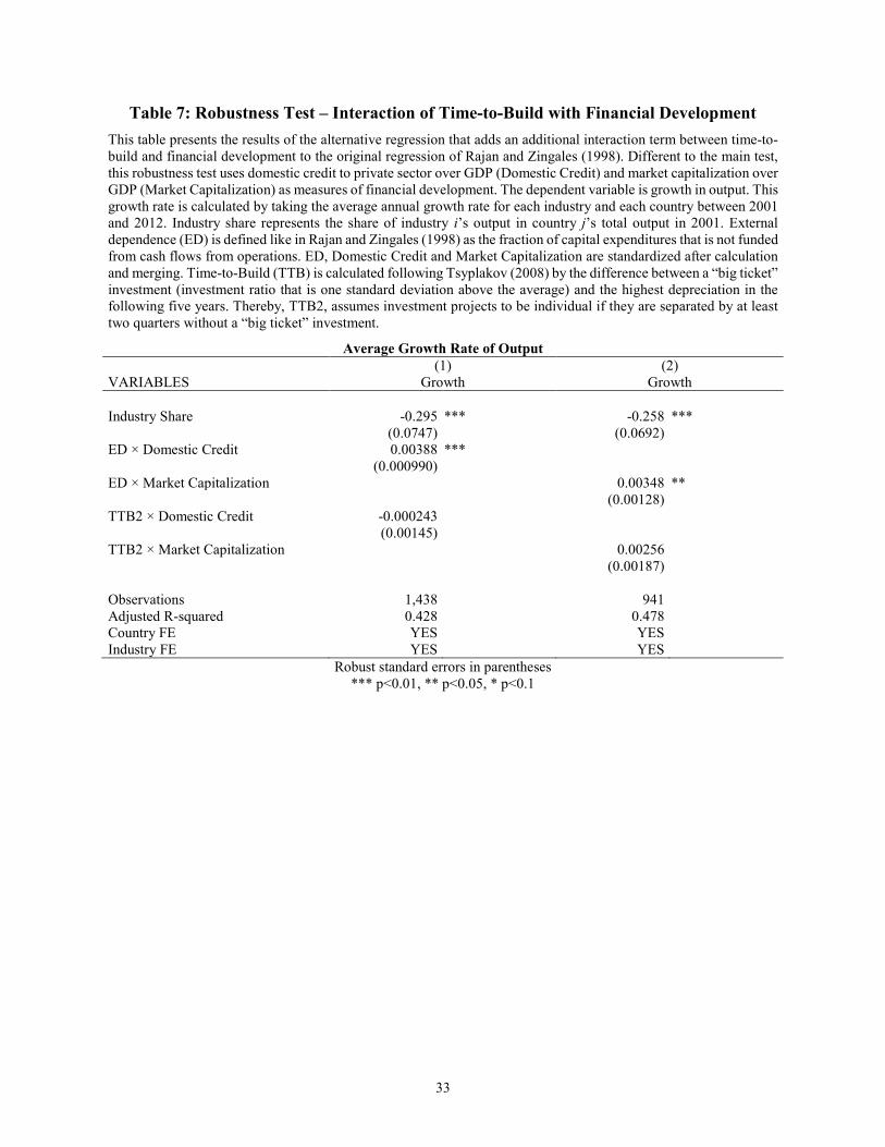
For the analysis of the double-interaction of time-to-build, Table 7 shows the results of the

robustness test. Again, the results show high significance levels and are in line with our main

test in the previous subsection. Accordingly, as for the robustness test before, the results from

our main test are still robust and not fundamentally altered when incorporating alternative

measures of financial development.


Our third robustness test, the application of the alternative measure of financial development in

the triple-interaction term between time-to-build, external dependence and financial develop-

ment, supports the findings of our main test. For both financial development proxies, Table 8

shows that all coefficients remain highly significant at the 1% level and do not deviate much

from the regression results of our main test.


For all cases, the test of alternative measures of financial development supports the results of

our main test. Therefore, our results are not only robust to different measures of time-to-build

as already indicated in Subsection 5.1, but also to different measures of financial development.

This further strengthens the confidence in the validity of the results and the relevance of this

paper’ contribution to the understanding of the relationship between financial development and

economic growth. We do not only provide robust evidence that, in the presence of time-to-

build, the growth of industries that are comparably more dependent on external financing is less

sensitive to the development of the national financial market, but we also show, as indicated in

Table 8, that this holds true for both the debt and the equity market. These results suggest that

firms tend to finance most of their investments that take time-to-build with internal funds.

19

6 Conclusion

In this paper, we introduce time-to-build as a new moderating variable into the well-known

relationship between financial development and economic growth. Building on Rajan and Zin-

gales’ (1998) influential study, we corroborate their central argument that industries with rela-

tively higher need of external financing grow disproportionally faster in countries with well-

developed financial systems with up-to-date data from 2001 to 2012. Most importantly, the

introduction of time-to-build in this context reveals that high levels of time-to-build mitigate

the growth benefiting effect highly developed financial systems have on industries that are rel-

atively higher dependent on external financing. Theoretically, this result shows that industries

with long investment cycles relies heavily in internal sources of financing rather than external

ones (Frank and Goyal, 2009).

An additional contribution of this study is that we provide new empirical data on the distribution

of time-to-build across industries. Although the further development of Tsyplakov’s (2008)

measuring approach allows us to make use of an extensive dataset, this procedure restricts our

analysis in two ways. First, we can only consider very big investment projects (“big tickets”)

and, second, the accuracy of our measurement is limited to quarters. Further research could

possibly help overcome this limitation. Particularly, the application of text mining in connection

with formerly manual measuring approaches seems to be promising in achieving this goal.

20

References

Aftalion, A., 1927, The theory of economic cycles based on the capitalistic technique of pro-

duction, Review of Economics and Statistics, 9(4), 165-170.

Aghion, P., P. Howitt and R. Levine, 2018, Financial development and innovation-led growth,

2018, in T. Beck and R. Levine, Eds.: Handbook of finance and development, Edward

Elgar Publishing, Cheltenham, UK.

Agliardi, E. and N. Koussis, 2013, Optimal capital structure and the impact of time-to-build,

Finance Research Letters, 10, 124-130.

Altug, S., 1989, Time-to-build and aggregate fluctuations: Some new evidence, International

Economic Review, 30(4), 889-920.

Alvarez, L.H.R. and J. Keppo, 2002, The impact of delivery lags on irreversible investment

under uncertainty, European Journal of Operational Research, 136, 173-180.

Bar-Ilan, A. and W.C. Strange, 1996, Investment lags, American Economic Review, 86(3), 610-

622.

Bar-Ilan, A., A. Sulem and A. Zanello, 2002, Time-to-build and capacity choice, Journal of

Economic Dynamics & Control, 26, 69-98.

Beck, T., 2003, Financial dependence and international trade, Review of International Econom-

ics, 11(2), 296-316.

Beck, T., A. Demirgüç-Kunt and V. Maksimovic, 2005, Financial and legal constraints to

growth: Does firm size matter?, Journal of Finance, 60(1), 137-177.

Beck, T. and R. Levine, 2002, Industry growth and capital allocation: does having a market- or

bank-based system matter?, Journal of Financial Economics, 64, 147-180.

Beck, T. and R. Levine, 2004, Stock markets, banks and growth: Panel evidence, Journal of

Banking & Finance, 28, 423-442.

Beck, T. and R. Levine and N. Loayza, 2000, Finance and the sources of growth, Journal of

Financial Economics, 58, 261-300.

Bencivenga, V.R., B.D. Smith and R.M. Starr, 1995, Transaction costs, technological choice,

and endogenous growth, Journal of Economic Theory, 67, 153-177.

Cetorelli, N. and M. Gambera, 2001, Banking Market Structure, Financial Dependence and

Growth: International Evidence from Industry Data, Journal of Finance, 56(2), 617-648.

21

Christiano, L.J. and R.M. Todd, 1996, Time to plan and aggregate fluctuations, Quarterly Re-

view, 20(1), 14-27.

Claessens, S. and L. Laeven, 2003, Financial development, property rights, and growth, Journal

of Finance, 58(6), 2401-2436.

DeAngelo, H., L. DeAngelo and T.M. Whited, 2011, Capital structure dynamics and transitory

debt, Journal of Financial Economics, 99, 235-261.

Del Boca, A., M. Galeotti, C.P. Himmelberg and P. Rota, 2008, Investment and time to plan

and build: A comparison of structures vs. equipment in a panel of Italian firms, Journal

of the European Economic Association, 6(4), 864-889.

DellaVigna, S. and J.M. Pollet, 2013, Capital budgeting versus market timing: An evaluation

using demographics, Journal of Finance, 68(1), 237-270.

Demirgüç-Kunt, A. and V. Maksimovic, 1998, Law, finance, and firm growth, Journal of Fi-

nance, 53(6), 2107-2137.

Dudley, E., 2012, Capital structure and large investment projects, Journal of Corporate Fi-

nance, 18, 1168-1192.

Fisman, R. and I. Love, 2003, Trade credit, financial intermediary development, and industry

growth, Journal of Finance, 58(1), 353-374.

Fisman, R. and I. Love, 2007, Financial dependence and growth revisited, Journal of the Euro-

pean Economic Association, 5(2-3), 470-479.

Frank, M.Z. and V.K. Goyal, 2009, Capital structure decisions: Which factors are reliably im-

portant?, Financial Management, 38(1),1-37.

Ghemawat, P., 1984, Capacity expansion in the titanium dioxide industry, Journal of Industrial

Economics, 33(2), 145-163.

Goldsmith, R.W., 1969, Financial structure and development, Yale University Press, New Ha-

ven, NY.

Kaplouptsidi, M., 2014, Time to build and fluctuations in bulk shipping, American Economic

Review, 104(2), 564-608.

King, R.G. and R. Levine, 1993, Finance and growth: Schumpeter might be right, Quarterly

Journal of Economics, 108(3), 717-737.

22

Koeva, P., 2000, The facts about time-to-build, IMF Working Paper, International Monetary

Fund.

Kydland, F.E. and E.C. Prescott, 1982, Time to build and aggregate fluctuations, Econometrica,

50(6), 1345-1370.

Laeven, L., D. Klingebiel and R. Kroszner, 2002, Financial crises, financial dependence, and

industry growth, Policy Research Working Paper No. 2855, The World Bank.

Levine, R., 1991, Stock markets, growth, and tax policy, Journal of Finance, 46(4), 1445-1465.

Levine, R., 2005, Finance and growth: Theory and evidence, 2005, in P. Aghion and S.N.

Durlauf, Eds.: Handbook of Economic Growth, Volume 1A, Elsevier, Amsterdam.

Levine, R. and S. Zervos, 1998, Stock markets, banks, and economic growth, American Eco-

nomic Review, 88(3), 537-558.

Lieberman, M.B., 1987, Excess capacity as a barrier to entry: An empirical appraisal, Journal

of Industrial Economics, 35(4), 607-627.

Love, I., 2003, Financial development and financing constraints: International evidence form

the structural investment model, Review of Financial Studies¸ 16(3), 765-791.

Lucas, R.E., Jr., 1988, On the mechanics of economic development, Journal of Monetary Eco-

nomics, 22, 3-42.

Majd, S. and R.S. Pindyck, 1987, Time to build, option value, and investment decisions, Jour-

nal of Financial Economics, 18, 7-27.

Marchica, M.-T. and R. Murat, 2010, Financial flexibility, investment ability, and firm value:

Evidence from firms with spare debt capacity, Financial Management, 39(4), 1339-1365.

Mayer, T., 1960, Plan and equipment lead times, Journal of Business, 33(2), 127-132.

Mayer, T. and S. Sonenblum, 1955, Lead times for fixed investment, Review of Economics and

Statistics, 37(3), 300-304.

Montogomery, M.R., 1995, ‘Time-to-build’ completion patterns for nonresidential structures,

1961-1991, Economics Letters, 48, 155-163.

Pacheco-de-Almeida, G. and P. Zemsky, 2003, The effect of time-to-build on strategic invest-

ment under uncertainty, RAND Journal of Economics, 34(1), 166-182.

Rajan, R.G. and L. Zingales, 1998, Financial dependence and growth, American Economic Re-

view, 88(3), 559-586.

23

Robinson, J., 1952, The generalization of the general theory, 1952, in J. Robinson, Ed.: The

rate of interest and other essays, Macmillan, London.

Rouwenhorst, K.G., 1991, Time to build and aggregate fluctuations: A reconsideration, Journal

of Monetary Economics, 27, 241-254.

Salomon, R. and X. Martin, 2008, Learning, knowledge transfer, and technology implementa-

tion performance: A study of time-to-build in the global semiconductor industry, Man-

agement Science, 57(7), 1266-1280.

Sarkar, S. and C. Zhang, 2013, Implementation lag and the investment decision, Economic Let-

ters, 119, 136-140.

Sarkar, S. and C. Zhang, 2015, Investment policy with time-to-build, Journal of Banking &

Finance, 55, 142-156.

Schumpeter, J.A., 1911, Theorie der wirtschaftlichen Entwicklung, Duncker & Humblot,

Leipzig.

Stadler, G.W., 1994, Real business cycles, Journal of Economic Literature, 32(4), 1750-1783.

Tsyplakov, S., 2008, Investment friction and leverage dynamics, Journal of Financial Econom-

ics, 89, 423-443.

Wen, Y., 1998, Investment cycles, Journal of Economic Dynamics and Control, 22, 1139-1165.

24

Figure 1: Illustration of Time-to-Build Measures Figure 1 illustrates by means of a stylized data cutout how “big tickets” are aggregated to distinct investment projects. “Big ticket” is equal to 1 if the corresponding investment ratio is one standard deviation above the mean investment ratio. For the latter three columns, 1 indicates the start of an investment project and the hatched area outlines which “big ticket” investments belong to the same investment project. A TTB1 project is separated from a following investment project if there is at least one quarter of no “big ticket”. TTB2 projects are separated by at least two quarters of no “big ticket” and TTB3 projects have at least three quarters of no “big ticket” in-between.

Company (gvkey) Quarter Investment

ratio Depreciation

ratio Big

ticket TTB1 project

TTB2 project

TTB3 project

1078 1988q2 0.071 0.041 1 1 1 1 1078 1988q3 0.065 0.040

1078 1988q4 0.089 0.028 1 1

1078 1989q1 0.069 0.038

1078 1989q2 0.062 0.037

1078 1989q3 0.090 0.041 1 1 1

1078 1989q4 0.062 0.036

1078 1990q1 0.072 0.041 1 1

1078 1990q2 0.071 0.039 1

1078 1990q3 0.063 0.038

1078 1990q4 0.078 0.040 1 1

1078 1991q1 0.064 0.040

1078 1991q2 0.067 0.039

1078 1991q3 0.050 0.037

1078 1991q4 0.102 0.035 1 1 1 1 1078 1992q1 0.079 0.041 1

1078 1992q2 0.084 0.038 1

1078 1992q3 0.084 0.037 1

1078 1992q4 0.099 0.031 1

1078 1993q1 0.067 0.038

1078 1993q2 0.073 0.040 1 1

1078 1993q3 0.072 0.037 1

1078 1993q4 0.073 0.031 1

25

Figure 2: Illustration of Single Depreciation Usage By means of a stylized data cutout, Figure 2 illustrates how one depreciation is only used for one investment project. For both investment projects, one starting in 1989q2 and one starting in 1989q4, the 1993q3 depreciation ratio (red) is the maximum depreciation ratio in their respective 20 quarter observation windows. According to our adjustment of Tsyplakov’s (2008) measuring approach, however, this depreciation is only used for the first investment project starting in 1989q2. For the second investment project starting in 1989q4, the second highest depreciation ratio (green) of its 20 quarter window is used for the determination of the project’s end date.

Company (gvkey) Quarter Investment

Ratio Depreciation

ratio Big

ticket TTB1 project

1010 1989q2 0.051 0.015 1 1 1010 1989q3 0.040 0.015

1010 1989q4 0.056 0.016 1 1 1010 1990q1 0.043 0.015 1

1010 1990q2 0.051 0.015

1010 1990q3 0.025 0.015

1010 1990q4 0.030 0.015

1010 1991q1 0.016 0.015

1010 1991q2 0.011 0.015

1010 1991q3 0.014 0.015

1010 1991q4 0.006 0.015

1010 1992q1 0.015 0.016

1010 1992q2 0.010 0.016

1010 1992q3 0.013 0.016

1010 1992q4 0.018 0.015

1010 1993q1 0.010 0.017

1010 1993q2 0.013 0.021

1010 1993q3 0.026 0.022

1010 1993q4 0.022 0.018

1010 1994q1 0.018 0.018

1010 1994q2 0.013 0.019

1010 1994q3 0.026 0.019

26

Table 1: Descriptive Statistics, by Country This table presents summary statistics for all 104 countries for which we have data from World Bank Open Source and UNIDO INDSTAT 4. Financial development (FD) in column 3 is defined like in Rajan and Zingales (1998) as the market capitalization ratio which is obtained by dividing the sum of domestic credit to private sector (column 1) and market capitalization (column 2) through GDP. The average annual growth rates of output in column 4 are obtained by taking the geometric mean over the years between the earliest and latest available value.

Country (1)

Domestic Credit

(2) Market Capital-

ization

(3) FD

(4) Growth in Out-

put Afghanistan 4.78 0.42 Albania 5.99 0.15 Algeria 8.01 0.03 Armenia 7.57 0.14 Australia 88.69 99.18 187.87 0.14 Austria 89.71 12.77 102.49 0.08 Azerbaijan 9.36 0.24 Bahrain 41.82 73.52 115.34 0.15 Bangladesh 24.18 1.81 25.99 0.21 Belgium 65.94 69.73 135.66 0.08 Bermuda 69.50 0.12 Bolivia (Plurinational State of) 53.56 0.14 Botswana 16.59 0.11 Brazil 29.00 33.29 62.30 0.15 Bulgaria 14.45 0.58 15.03 0.16 Burundi 16.30 -0.01 Canada 173.23 83.55 256.78 0.01 Chile 73.63 79.33 152.97 0.05 China 110.04 30.90 156.57 0.29 China, Hong Kong Special Ad-

ministrative Region 148.98 298.74 447.72 0.03

China, Macao Special Administra-tive Region

63.86 0.01

Colombia 24.25 34.46 63.72 0.14 Congo 4.90 0.27 Cyprus 142.10 79.19 239.49 0.01 Czechia 37.27 12.07 49.34 0.14 Denmark 138.83 51.67 190.50 0.01 Ecuador 23.97 0.11 Egypt 54.93 86.99 136.28 0.15 Eritrea 29.03 0.04 Estonia 40.60 0.14 Ethiopia 21.28 0.20 Fiji 35.66 0.08 Finland 52.72 147.35 200.07 0.06 France 76.98 85.34 162.32 0.03 Georgia 7.52 0.24 Germany 112.04 54.94 166.98 0.07 Greece 50.08 62.23 112.31 0.02 Hungary 32.60 19.18 53.48 0.09 Iceland 97.46 0.15 India 29.01 46.55 78.60 0.18 Indonesia 20.29 14.33 34.62 0.18 Iran (Islamic Republic of) 30.08 5.82 35.90 0.06 Iraq 1.27 0.34 Ireland 71.85 69.00 140.85 0.05 Israel 76.76 44.11 120.87 0.06 Italy 60.59 45.38 105.97 0.04 Japan 183.18 52.62 235.80 0.05 Jordan 75.71 0.19

27

Kazakhstan 15.98 5.52 21.50 0.26 Kenya 25.22 8.05 33.27 0.17 Kuwait 56.63 64.87 121.49 0.14 Kyrgyzstan 3.83 0.13 Latvia 0.10 Lithuania 0.13 Luxembourg 78.81 106.76 185.57 0.09 Madagascar 8.38 -0.05 Malawi 5.21 0.16 Malaysia 129.10 128.23 257.34 0.12 Malta 97.72 31.32 161.41 -0.09 Mauritius 57.82 21.56 79.38 0.05 Mexico 12.88 16.69 29.56 0.11 Mongolia 9.14 0.38 Morocco 42.60 0.13 Namibia 41.31 4.24 45.55 0.07 Nepal 29.42 0.05 Netherlands 111.67 117.92 229.59 0.06 New Zealand 106.70 33.08 139.78 0.08 Norway 96.29 39.92 136.21 0.05 Oman 40.13 20.89 61.02 0.20 Panama 102.53 20.81 123.35 0.10 Paraguay 26.80 0.31 Peru 23.80 18.82 42.62 0.14 Philippines 37.53 27.86 65.39 0.12 Poland 23.61 13.66 37.26 0.14 Portugal 114.96 38.12 153.08 0.06 Qatar 34.89 0.30 Republic of Korea 106.06 43.88 149.94 0.10 Republic of Moldova 14.76 0.23 Romania 8.58 2.71 11.29 0.14 Russian Federation 16.84 0.22 Saudi Arabia 27.09 -0.10 Senegal 14.98 0.19 Serbia 31.39 6.73 24.51 0.11 Singapore 115.68 129.57 245.25 0.10 Slovakia 33.81 1.77 42.07 0.21 Slovenia 0.19 16.58 28.26 0.06 South Africa 138.79 121.28 260.07 0.13 Spain 95.13 74.80 169.93 0.05 Sri Lanka 30.73 8.45 39.19 -0.02 State of Palestine 21.48 12.80 34.28 0.10 Sweden 90.51 98.58 189.09 0.07 Switzerland 140.56 189.27 329.83 0.08 Tajikistan 22.91 0.37 Thailand 93.08 29.88 122.96 0.11 The former Yugoslav Republic of

Macedonia 16.30 0.09

Trinidad and Tobago 41.91 44.07 85.98 0.12 Tunisia 61.51 10.11 71.62 0.10 Turkey 15.03 24.16 39.19 0.19 Ukraine 13.03 0.18 United Kingdom of Great Britain

and Northern Ireland 121.89 132.56 254.45 0.02

United Republic of Tanzania 5.38 3.83 9.22 0.18 Uruguay 53.85 0.13 Viet Nam 39.29 0.26 Yemen 5.73 0.20 Mean 52.34 52.82 122.13 0.12 Median 37.27 38.12 118.10 0.12 Standard deviation 43.88 52.55 88.82 0.09

Table 2: Descriptive Statistics, by Industry This table presents summary statistics for all 20 manufacturing industry divisions, I extracted from the UNIDO INDSTAT 4 data set based on ISIC Revision 3 codes. The number of investment projects in columns 1, 3 and 5 represent the number of investment projects that are used in each industry division for the calculation of the corresponding time-to-build measures in columns 2, 4 and 6. In accordance with Tsylakov (2008), time-to-build is calculated as the difference between a “big ticket” investment (investment ratio that is one standard deviation above the average) and the highest depreciation in the following 5 years. Thereby, a TTB1 project is separated from a following investment project if there is at least one quarter of no “big ticket”. TTB2 projects are separated by at least two quarters of no “big ticket” and TTB3 projects have at least three quarters of no “big ticket” in-between. Time-to-build is measured in quarters. Number of firms (column 7) indicates the number of firms within each industry division that is used for the calculation of external dependence (ED, column 8). ED is defined, as stated in Rajan and Zingales (1998), as the fraction of capital expenditures that is not funded from cash flows from operations. Thereby, cash flows from operations are defined as sum of the following Compustat items: income before ordinary taxes, depreciations and amortizations; deferred taxes; equity in net loss earnings; sale of property, plant and equipment and investments gain; funds from other operations; decreases in inventories; decreases in receivables; increases in payables. The average annual growth rates of output in column 9 are obtained by taking the geometric mean over the years between the earliest and latest available value.

Industry Division

(1) Number of Investment Projects 1

(2) TTB1


(4) TTB2


(6) TTB3

(7) Number of

Firms

(8) ED

(9) Growth in

Output

Food and beverages 302 12.39 263 12.28 246 12.28 219 0.24 0.13 Tobacco 16 10.19 13 11.85 13 11.85 7 0.63 0.07 Textiles 25 10.36 24 10.13 23 9.78 27 -0.37 0.06 Wearing apparel 105 11.49 88 11.43 82 11.57 84 0.00 0.08 Leather 54 12.43 45 12.47 41 12.85 30 -2.93 0.07 Wood and straw 43 10.49 39 10.56 34 10.74 39 0.13 0.12 Paper 68 12.87 59 12.97 55 13.05 65 -0.08 0.12 Printing and media 43 13.12 39 13.33 36 12.94 39 -0.25 0.06 Coke and refined petroleum 66 12.09 53 12.17 50 12.30 73 0.17 0.20 Chemicals and pharmaceuticals 1282 11.84 1114 11.60 1006 11.51 1262 8.49 0.15 Rubber and plastics 116 11.71 99 11.86 90 12.01 100 0.10 0.15 Other non-metallic mineral products 55 12.71 46 12.02 40 12.33 50 0.42 0.14 Basic metals 97 10.96 75 10.52 66 10.30 98 0.32 0.14 Fabricated metal products 176 10.74 139 10.63 129 10.62 121 -0.91 0.14 Computer, electronic and optical products 1627 11.67 1364 11.47 1234 11.50 1207 0.83 0.09 Electrical equipment 181 12.03 157 11.85 145 11.68 159 0.85 0.15 Machinery and equipment 371 11.98 316 11.71 277 11.47 266 0.19 0.17 Motor vehicles 166 11.92 143 11.41 128 11.78 139 0.58 0.15 Transport equipment 154 12.18 141 12.12 121 11.88 83 0.03 0.12 Furniture and other manufacturing 409 11.03 338 10.86 298 10.86 360 0.83 0.14 Mean 267.80 11.71 227.75 11.66 205.70 11.67 221.40 0.46 0.12 Median 110.50 11.88 93.50 11.78 86.00 11.73 91.00 0.18 0.14 Standard deviation 424.32 0.84 360.49 0.83 325.61 0.87 357.40 2.06 0.04

29

Table 3: Replication of Rajan and Zingales (1998) This table presents the results of the replication of Rajan and Zingales’ (1998) original regression. The dependent variable is growth in output. This growth rate is calculated by taking the average annual growth rate for each industry and each country between 2001 and 2012. Industry share represents the share of industry i’s output in country j’s total output in 2001. External dependence (ED) is defined like in Rajan and Zingales (1998) as the fraction of capital expenditures that is not funded from cash flows from operations. Our main measure of financial development (FD) is defined as the market capitalization ratio measure of Rajan and Zingales (1998). It is the sum of domestic credit to private sector and market capitalization divided by GDP. ED and FD are standardized after calculation and merg-ing.

Average Growth Rate of Output (1) VARIABLES Growth Industry Share -0.257 *** (0.0680) ED × FD 0.00334 ** (0.00118) Observations 941 Adjusted R-squared 0.478 Country FE YES Industry FE YES

Robust standard errors in parentheses *** p<0.01, ** p<0.05, * p<0.1

30

Table 4: Interaction of Time-to-Build with Financial Development This table presents the results of the regression that adds an additional interaction term between time-to-build and financial development to the original regression of Rajan and Zingales (1998). The dependent variable is growth in output. This growth rate is calculated by taking the average annual growth rate for each industry and each country between 2001 and 2012. Industry share represents the share of industry i’s output in country j’s total output in 2001. External dependence (ED) is defined like in Rajan and Zingales (1998) as the fraction of capital expenditures that is not funded from cash flows from operations. Our main measure of financial development (FD) is defined as the market capitalization ratio measure of Rajan and Zingales (1998). It is the sum of domestic credit to private sector and market capitalization divided by GDP. ED and FD are standardized after calculation and merging. Time-to-Build (TTB) is calculated following Tsyplakov (2008) by the difference between a “big ticket” investment (investment ratio that is one standard deviation above the average) and the highest depreciation in the following five years. Thereby, TTB1 (TTB2, TTB3) assumes investment projects to be individual if they are separated by at least one (two, three) quarters without a “big ticket” investment.

Average Growth Rate of Output (1) (2) (3) VARIABLES Growth Growth Growth Industry Share -0.256 *** -0.257 *** -0.256 *** (0.0674) (0.0678) (0.0677) ED × FD 0.00332 ** 0.00333 *** 0.00327 *** (0.00127) (0.00113) (0.00110) TTB1 × FD -0.00201 (0.00189) TTB2 × FD -0.000130 (0.00212) TTB3 × FD -0.000807 (0.00169) Observations 941 941 941 Adjusted R-squared 0.478 0.478 0.478 Country FE YES YES YES Industry FE YES YES YES


31

Table 5: Interaction of Time-to-Build with External Dependence and Financial Development

This table presents the results of the regression that adds an interaction term between time-to-build and financial development as well as a triple-interaction term between time-to-build, external dependence and financial develop-ment to the original regression of Rajan and Zingales (1998). The dependent variable is growth in output. This growth rate is calculated by taking the average annual growth rate for each industry and each country between 2001 and 2012. Industry share represents the share of industry i’s output in country j’s total output in 2001. External depend-ence (ED) is defined like in Rajan and Zingales (1998) as the fraction of capital expenditures that is not funded from cash flows from operations. Our main measure of financial development (FD) is defined as the market capitalization ratio measure of Rajan and Zingales (1998). It is the sum of domestic credit to private sector and market capitalization divided by GDP. ED and FD are standardized after calculation and merging. Time-to-Build (TTB) is calculated following Tsyplakov (2008) by the difference between a “big ticket” investment (investment ratio that is one standard deviation above the average) and the highest depreciation in the following five years. Thereby, TTB1 (TTB2, TTB3) assumes investment projects to be individual if they are separated by at least one (two, three) quarters without a “big ticket” investment.

Average Growth Rate of Output (1) (2) (3) VARIABLES Growth Growth Growth Industry Share -0.257 *** -0.257 *** -0.256 *** (0.0670) (0.0674) (0.0671) ED × FD 0.139 ** 0.0762 *** 0.0826 ** (0.0540) (0.0253) (0.0317) TTB1 × FD -0.00508 * (0.00246) TTB2 × FD -0.00227 (0.00274) TTB3 × FD -0.00353 (0.00247) TTB1 × ED × FD -0.0114 ** (0.00454) TTB2 × ED × FD -0.00625 *** (0.00212) TTB3 × ED × FD -0.00682 ** (0.00268) Observations 941 941 941 Adjusted R-squared 0.478 0.477 0.478 Country FE YES YES YES Industry FE YES YES YES


32

Table 6: Robustness Test – Replication of Rajan and Zingales (1998) This table presents the results of an alternative replication of Rajan and Zingales’ (1998) original regression. Differ-ent to the main test, this robustness test uses domestic credit to private sector over GDP (Domestic Credit) and market capitalization over GDP (Market Capitalization) as measures of financial development. The dependent variable is growth in output. This growth rate is calculated by taking the average annual growth rate for each industry and each country between 2001 and 2012. Industry share represents the share of industry i’s output in country j’s total output in 2001. External dependence (ED) is defined like in Rajan and Zingales (1998) as the fraction of capital expenditures that is not funded from cash flows from operations. ED, Domestic Credit and Market Capitalization are standardized after calculation and merging.

Average Growth Rate of Output (1) (2) VARIABLES Growth Growth Industry Share -0.295 *** -0.258 *** (0.0747) (0.0684) ED × Domestic Credit 0.00390 *** (0.00101) ED × Market Capitalization 0.00334 ** (0.00147) Observations 1,438 941 Adjusted R-squared 0.428 0.478 Country FE YES YES Industry FE YES YES


33

Table 7: Robustness Test – Interaction of Time-to-Build with Financial Development This table presents the results of the alternative regression that adds an additional interaction term between time-to-build and financial development to the original regression of Rajan and Zingales (1998). Different to the main test, this robustness test uses domestic credit to private sector over GDP (Domestic Credit) and market capitalization over GDP (Market Capitalization) as measures of financial development. The dependent variable is growth in output. This growth rate is calculated by taking the average annual growth rate for each industry and each country between 2001 and 2012. Industry share represents the share of industry i’s output in country j’s total output in 2001. External dependence (ED) is defined like in Rajan and Zingales (1998) as the fraction of capital expenditures that is not funded from cash flows from operations. ED, Domestic Credit and Market Capitalization are standardized after calculation and merging. Time-to-Build (TTB) is calculated following Tsyplakov (2008) by the difference between a “big ticket” investment (investment ratio that is one standard deviation above the average) and the highest depreciation in the following five years. Thereby, TTB2, assumes investment projects to be individual if they are separated by at least two quarters without a “big ticket” investment.

Average Growth Rate of Output (1) (2) VARIABLES Growth Growth Industry Share -0.295 *** -0.258 *** (0.0747) (0.0692) ED × Domestic Credit 0.00388 *** (0.000990) ED × Market Capitalization 0.00348 ** (0.00128) TTB2 × Domestic Credit -0.000243 (0.00145) TTB2 × Market Capitalization 0.00256 (0.00187) Observations 1,438 941 Adjusted R-squared 0.428 0.478 Country FE YES YES Industry FE YES YES


34

Table 8: Robustness Test – Interaction of Time-to-Build with External Dependence and Financial Development

This table presents the results of the regression that adds an interaction term between time-to-build and financial development as well as a triple-interaction term between time-to-build, external dependence and financial develop-ment to the original regression of Rajan and Zingales (1998). Different to the main test, this robustness test uses domestic credit to private sector over GDP (Domestic Credit) and market capitalization over GDP (Market Capital-ization) as measures of financial development. The dependent variable is growth in output. This growth rate is cal-culated by taking the average annual growth rate for each industry and each country between 2001 and 2012. Industry share represents the share of industry i’s output in country j’s total output in 2001. External dependence (ED) is defined like in Rajan and Zingales (1998) as the fraction of capital expenditures that is not funded from cash flows from operations. ED, Domestic Credit and Market Capitalization are standardized after calculation and merging. Time-to-Build (TTB) is calculated following Tsyplakov (2008) by the difference between a “big ticket” investment (investment ratio that is one standard deviation above the average) and the highest depreciation in the following five years. Thereby, TTB2, assumes investment projects to be individual if they are separated by at least two quarters without a “big ticket” investment.

Average Growth Rate of Output (1) (2) VARIABLES Growth Growth Industry Share -0.296 *** -0.259 *** (0.0740) (0.0685) ED × Domestic Credit 0.0684 *** (0.0179) ED × Market Capitalization 0.110 *** (0.0308) TTB2 × Domestic Credit -0.00215 (0.00174) TTB2 × Market Capitalization -0.000539 (0.00333) TTB2 × ED × Domestic Credit -0.00552 *** (0.00152) TTB2 × ED × Market Capitalization -0.00912 *** (0.00257) Observations 1,438 941 Adjusted R-squared 0.428 0.478 Country FE YES YES Industry FE YES YES


Documents

Financial Development and Growth When it Takes Time-to-Build