Financial development and economic growth - Europapublications.jrc.ec.europa.eu/repository/bitstream/JRC103421/jrc103421... · The relation between financial development and economic

KARAGIANNIS Stylianos

KVEDARAS Virmantas

A European perspective

Financial development and economicgrowth

2016

EUR 28324 EN

This publication is a Science for Policy report by the Joint Research Centre (JRC), the European Commission’s science and knowledge service. It aims to provide evidence-based scientific support to the European policy-making process. The scientific output expressed does not imply a policy position of the European Commission. Neither the European Commission nor any person acting on behalf of the Commission is responsible for the use which might be made of this publication.

Contact information Name: Stylianos Karagiannis Address: Joint Research Centre, Via R. fermi 2749, 21027, Ispra (VA) ITALY E-mail: [email protected] Tel.:+39 0332 783926

JRC Science Hub https://ec.europa.eu/jrc

JRC103421

EUR 28324 EN

PDF ISBN 978-92-79-64573-0 ISSN 1831-9424 doi:10.2791/53648

Luxembourg: Publications Office of the European Union, 2016

Reproduction is authorised provided the source is acknowledged.

How to cite: Author(s); title; EUR; doi

All images © European Union 2016

Title Financial development and economic growth. A European perspective.

Abstract This report provides empirical evidence on the relationship between financial development and economic growth inthe European Union and the Euro area. Results indicate that the type of financing fund receiver matters in the financial depth-growth link.

1

Table of contents

Executive summary ................................................................................................ 2

1. Introduction ....................................................................................................... 4

2. Literature review ................................................................................................ 8

3. Empirical Strategy and Data ............................................................................. 12

4. Empirical Results .............................................................................................. 16

4.1. The financial depth – growth nexus ................................................................... 16

4.1.1. Replicating and extending the literature ....................................................... 16

4.1.2. Financial structure and growth .................................................................... 20

4.2. Financial depth, growth and swings of asset prices in housing and stock markets.... 37

4.3. Shifts of financial structure and growth empirics ................................................. 44

5. Conclusions ...................................................................................................... 45

References .............................................................................................................. 47

List of abbreviations and definitions ............................................................................ 49

List of figures ........................................................................................................... 50

List of tables ............................................................................................................ 51

Appendix ................................................................................................................. 52

Appendix A: Definitions and County Groups ................................................................. 52

2

Executive summary

Although much debated in the recent literature, the link between financial development and

economic growth is still of upmost importance, as it attempts to answer how and why the

varying level of development of financial systems affects growth differentials among

countries. Evidence on the relation are still ambiguous, as early studies support the existence

of a positive association, while more recent contributions suggest a nonlinear (U-shaped)

correspondence.

This report empirically examines the association between financial development and economic

growth in several regions, emphasizing the European Union (EU) and the Euro area (EMU)

context. In detail, the following analysis is offered in order to increase the understanding of

the potential association. First, an investigation of the finance-growth nexus, with emphasis

on possible non-linear effects. Second, an extension of this analysis incorporating a

disaggregation of the financial structure by type of financing (bank credit, debt securities, and

stock market) as well as type of fund receivers (households, non-financial corporations, and

financial corporations), in order to further extend our understanding of the potential

associations. Third, an analysis is included of the effects of upswings or downswings of asset

prices of various intensity and specifically on the relative market-based and bank-based

financing impact on economic growth during periods of moderate and extreme price volatility

in housing and stock markets . Finally, a simulation of the impact on economic growth due to

the reallocation of credit available in the economy among different sources is provided (i.e.

banks and the stock market). To the best of our knowledge there is a lack of studies

investigating this relationship at the EU and EMU level, while there is no research studying

the importance of financial deepening and structure while considering jointly the type of

instruments of financing and the type of fund receiver.

Results obtained from the empirical analysis indicate that an economy’s financial structure

has a central role in the association between financial development and economic growth.

Specifically, it is shown that credit provided by banks (as a % of GDP) has a non-linear effect

on growth and, given the actual financing structure, the peak of the positive impact (turning

point) is close to 50% of the GDP. Therefore most of the European countries would have

benefited in terms of economic growth rates if bank credit penetration relative to the gross

domestic product were smaller during the analyzed period.

The type of financing matters in the financial depth-growth link, as bank credit appears to

have the most negative impact (conditionally on substantial financing of households) and

stock market a more positive one. The type of fund receiver is also important, as credit to

3

households and outstanding debt securities to financial corporations appear to exhibit a

negative and significant impact on economic growth, whereas credit to nonfinancial firms

tends to have a positive one. An interesting result obtained indicates that the unconditional

impact of outstanding debt securities is negative, whereas larger share of debt securities can

even foster economic growth when GDP growth rates are low relative to lending interest rates

and/or stock market volatility is high.

With respect to varying impact during swings of asset prices, an increase in bank credit during

housing market booms affects economic growth negatively and, in general, economic growth

rates are hindered by larger credit to deposit ratios. Finally, empirical simulations indicate

that the impact of changes in the financial composition on economic growth rates is

economically significant, but depends on the general penetration of finance and the initial

conditions of a particular economy in a specific period. Namely, the impact depends both on

the size and structure of finance (both in terms of type of financing instrument and fund user)

in a particular year and the actual distance from the level of credit yielding the largest

contribution to growth (the ‘turning point’).

4

1. Introduction

The relation between financial development and economic growth is much debated. As hypothesized by

Schumpeter (1934) and supported by King and Levine (1993) with numerous papers thereafter, the

varying level of development of financial systems affects economic growth differentials among countries.

The impact channels vary from just additional financial funds, available to finance investment projects due

to larger volumes of savings, to more efficient reallocation of funds, thus reaching proper entrepreneurs

and leading to higher productivity (see e.g. Beck et al., 2000). The initial literature (see an overview in

Panizza, 2014) suggested a positive association between financial depth (measured e.g. by the amount of

domestic credit as a percentage of gross domestic product1) and economic growth, while more recent

empirical work provides evidence of nonlinear (often an inverse U-shaped) relationship as documented

in Arcand et al. (2015), Cecchetti and Kharroubi (2012), Law and Singh (2014), and Sahay et al. (2015). It

is not excluded that the relationship is even more complex and the impact varies with a country’s level of

economic and institutional development or level of integration (Demirgüç-Kunt et al., 2013; Masten et al.,

2008), quality of the financial system or its structure (Beck et al., 2014; Gambacorta et al., 2014), and

other factors.

The recent overall finding of non-linearity of relationship between financial development (mainly

bank credit) and economic growth points to a seeming presence of ‘too much finance’, potentially

connected to large financing of households (see e.g. Beck et al., 2012). These findings have been derived

mainly using the aggregate credit data of financial institutions and relying on large sets of countries. Some

recent research concentrated also on smaller sets of more homogeneous countries like members of the

Organization for the Economic Co-operation and Development (OECD) or some groups of developing

countries (see e.g. Cournède et al., 2015, and Samargandi et al., 2015, correspondingly). It is of further

interest therefore to find out if the results are similar for the European Union (EU) countries and/or the

Euro area (EMU) member states that are relatively more homogeneous, especially the later ones.

Furthermore, we aim also at establishing the impact not only of the total financial deepening, but also of

its structure both in terms of the type of instrument of financing2 and the type of fund receiver3

(beneficiary of financing), as well as to further evaluate if and how the finance-growth dependence is

1 Abbreviated as GDP hereafter. 2 Namely, private domestic credit by banks, private outstanding debt securities issued domestically, as well as the

stock market capitalization of listed domestic companies. Loosely speaking, we could refer to them as bank credit,

debt securities, and stock financing. 3 Namely, by separating credit to households and credit to non-financial corporations as well as splitting the

outstanding debt securities into those issued by financial and non-financial corporations.

5

sensitive to the growth/slump of asset prices (namely, the stock market and housing prices) in the EU

member states.

Consequently, the report focuses on three issues. The first relates to the relationship between

financial depth, the structure of the financial systems and economic growth. Namely, it includes: (i) the

replication, update and extension of the seminal paper of Arcand et al. (2015) on the finance-growth

nexus, with emphasis on possible non-linear effects; (ii) the disaggregation of the financial structure by

types of instrument of financing in order to estimate their relative effects on growth, and (iii) the

differentiation between the type of fund receiver with the estimation of their effects on growth.

The second relates to the investigation of the effects of swings in financial asset prices and

specifically the empirical analysis of financing impact during periods of moderate and extreme volatility

(i.e. house and stock market growth and slumps, and booms and busts). To do so we reproduce and extend

the relevant part of the paper offered by Langfield and Pagano (2016).

The third relates to the estimation of the potential growth effects in the EU countries due to the

possible realignment of the financial sector composition, as regards the quantity of credit they provide in

the economy. In other words, we simulate the possible impact on economic growth due to the reallocation

of credit provided in the economy among different sources (i.e. banks, private debt securities or the stock

market).

Although the report concentrates on the EU and EMU cases, we also present the estimation

results of the same specifications for the OECD, as well as for all countries having the relevant data. This

aims at evaluating if previous results apply for various countries and at establishing patterns robust across

different groups of countries, which would allow being more confident in results obtained for the EU and

EMU (that also have smaller samples). Furthermore, we use for comparison both the World Bank (WB)

and the Bank for International Settlements (BIS) data since the former has larger country coverage,

whereas the later provides series adjusted for structural-breaks. Since the usual specifications of growth

equations imply implicitly that the equations are dynamic, we employ the dynamic panel models. The

Anderson and Hsiao (AH, 1982), the Generalized Method of Moments (GMM) by Arellano and Bond

(1991), or more specifically the system GMM of Arellano and Bover (1995) and Blundell and Bond (1998),

and fixed Effects (FE) estimators are used for parameter estimation. The AH estimator is preferred in our

case, but the GMM is useful to test for admissibility of properly lagged series as instruments. Furthermore,

6

under endogeneity, FE and instrumental variables-based estimates are expected to differ substantially.

Hence, we employ all of them in the sensitivity analysis.

Our econometric research strategy of measurement of financial deepening impact on growth rates

is to start from the simplest specification and then to introduce gradually richer ones with more detailed

structure and/or non-linearity. Namely, we first consider the impact only of bank credit a la Arcand et al.

(2015). Then, besides bank credit, we introduce other instruments to capture financing through debt

securities and stock market, since omitted variables might bias the findings otherwise. Afterwards, we

consider further decomposition including not only the different types of financing instruments, but also

separating between various fund receivers. Finally, we consider specifications merged both non-linearity

as well as different types of instruments and fund receivers. The gradual approach thus reveals the whole

picture and sensitivity to different specifications without also falling into potential problems connected

with relatively small number of degrees of freedom and possible overfitting, which would be connected

with the consideration only of the richest specification.

Benefitting from panel data estimation techniques mainly over the 1989-2013 period stemming

from different datasets, our empirical results present a robust picture on the link between financial

development, its structure, and economic growth in the EU and EMU. Specifically, the obtained

estimations demonstrate that:

• credit provided by banks (as a % of GDP) has a non-linear effect on growth and, given the actual

financing structure, the peak of positive impact (turning point) is closer to 50% of GDP

(substantially lower than that established in Arcand et al., 2015);

• the turning point depends on financing structure: if all bank credit were directed towards

financing of non-financial corporations, the peak of positive impact would shift to around 65% in

the core EMU countries, with estimates derived from the EU sample being somewhat smaller;

• the type of financing (private bank credit, outstanding private debt securities, stock market

capitalization) matters in the financial depth-growth link: conditionally on the historical pattern

of credit composition, bank credit appears to have the most negative impact and stock market a

more positive one;

• findings do not seem to be specifically related to or generated by the last financial crisis and hold

when examining various horizons of future economic growth;

• the type of fund receiver is very important: credit to households appears to exhibit a negative and

significant impact on economic growth, whereas credit to nonfinancial firms tends to have a

7

positive one; outstanding debt securities to financial corporations also have a significantly

negative impact on growth, whereas that of non-financial corporations tend to be insignificant,

consequently, bank credit to non-financial corporations contributed to the economic growth and,

on average, was more effective in terms of promoting it as compared with debt securities of non-

financial corporations;

• although the unconditional impact of outstanding debt securities is negative, when GDP growth

rates are low relative to lending interest rates and stock market volatility is high, larger share of

debt securities can even foster economic growth;

• increased bank credit during housing market booms affects economic growth negatively and, in

general, economic growth rates are hindered by larger credit to deposit ratios;

• the impact of changes in the financial composition on economic growth rates depends on the

initial size (penetration) and structure of finance of a particular economy.

The rest of this report is organized as follows. Section 2 provides a literature review on the financial

development-growth relation. Section 3 presents the data and the empirical strategy. Section 4 presents

the results while Section 5 concludes.

8

2. Literature review

This section discusses some empirical literature investigating the link between finance and economic

growth. To this end, findings presented below concentrate on the issue of financial depth and its relation

with non-linearities, the quantity of credit available in the economy and the different sources that provide

it (bank vs. non-bank credit or firm- and household-oriented credit).

The presence of nonlinearities in the finance – growth relationship

Recent research on the linkages between economic growth and financial development, measured

in terms of private credit, revealed the presence of possible nonlinearities of the relationship4; this

questions the previously established consensus of positive impact of financial development on economic

growth (see e.g. an overview in Panizza, 2014). For instance, Arcand et al. (2015), Cecchetti and Kharroubi

(2012) and Law and Singh (2014) using cross-sectional and longitudinal data of a mixture of developed

and developing countries demonstrated the potential presence of inverse-U-shaped relationship and/or

existence of thresholds after which growth is negatively affected by further financial development.

Studying the experience of middle income countries Samargandi et al. (2015) and Coricelli et al. (2012) as

well find the presence of such a relationship relying on longer time series panels and firm-level data.

However, Gambacorta et al. (2014) do not find a statistically significant impact for high-income countries.

Similarly, for the sample of OECD countries considered in Cournède et al. (2015), the estimated turning

point of financial penetration impact on economic growth is about twice smaller than that estimated in

Arcand et al. (2015), which was obtained from a global set of countries.

Considering the level of economic growth in non-homogeneous samples

The aforementioned non-linearity could be a feature more relevant for developing countries or

could also be an outcome of mixing different types of countries, according to Masten et al. (2008). This

suggests that the development level could be an important additional factor to be taken into

4 Although other kinds of non-linearity were also considered in the literature (see e.g. Ketteni et al., 2007, who point

out that non-linearity in initial conditions is present and, after taking it into account, the impact of finance on growth

is linear), in more recent years the attention was focused on nonlinear impact of financial development on economic

growth.

9

consideration and should be either properly modelled or, more generally, countries should be pre-

classified before the analysis.

Since this report concentrates on the EU and EMU, the level of development of its member states

(MS) is of great importance for two reasons. First, the impact of financial development on growth in the

EU countries can be different from that observed in other countries. Second, the EU itself consists of quite

inhomogeneous countries and, correspondingly, it is not certain that a single unambiguous conclusion

could be drawn for the whole EU or even the EMU. Hence, we use the more homogeneous group of EMU

countries named EMU1999 i.e. countries that became members of the Euro zone since 1999 (their list is

presented in Table 2A in Appendix A). Nevertheless, the empirical estimations should be read with caution

as they might not fully relate to all member-states.

Intensity of structural change and time varying parameters

There might be certain underlying causes behind such a different impact in e.g. low- and high-

income countries. For instance, in developing countries the (unconstrained) structural change is likely to

happen more swiftly. Therefore, the potential structural change coupled with adequate financial

development leads to greater benefits in terms of economic growth, whereas the structural change in

developed countries is smoother and such constraints are often less important.

In the same way, too much finance in developing countries - as compared to that required for the

potential needs of structural change - does not increase growth rates any further. For example Ductor and

Grechyna (2015) find that impact becomes negative when rapid growth in financial development is not

accompanied by sufficient growth in real output. This complements the idea considered in Demirgüç-Kunt

et al. (2013) regarding the optimal structure of finance given the different development level of a country.

The above results point to the potentially time-varying ‘optimal level’ of financial development

that depends on the intensity of (potential) structural change in a country. Accounting for potential time-

varying parameters is also relevant in general, given that the previously estimated positive impact of

financial development on economic growth vanishes after the 1990s period (see Rousseau and Wachtel,

2011). Furthermore, a question remains if the recent sever financial crisis had an influence on parameters

and the impact of finance on economic growth.

10

Sources and channels of financial development

Financial development can take various forms, therefore its impact might also depend on the

particular sources of financing used in an economy. Relevant empirical evidence argue that the stock-

market-based financial development contributes more to economic growth than the bank-based financial

development (see Valickova et al., 2015). In addition, the contribution of bank-based credit to growth

diminishes, while stock-based contribution to growth increases with the level of development (see

Demirgüç-Kunt et al., 2013).

However, these findings often represent average implications and might depend on specific

circumstances and certain constraints. For instance, if economic growth is constrained by the absence of

sufficient human capital, it is quite likely that the bank-based loan system can relax this constraint by

providing resources needed for education, whereas it is less clear how improvements of stock- or bond-

market-financing conditions would contribute to it, at least directly.

On the other hand, capital constraint can be relaxed using any of these sources of financing that

enhance investment. Thus not only the financing sources (e.g. stocks, bonds, loans), but also the channels

through which the financial penetration is taking place can be of great importance.

Fund receivers’ vs type of financing

Beck et al. (2012) and Cournède et al. (2015) stress that private credit towards firms and

households can have different impact on economic growth. Arcand et al. (2015) reconfirm in their

sensitivity analysis that firm credit does not have a significant non-linear indication, as measured by the

quadratic term of financial development indicator (also cautioning to potential problems of small sample).

These findings correlate well with those established for stocks-based financing. Although stocks,

bonds, and loans differ not only by the type of fund receiver but also in many other ways (among others,

in terms of control power and guaranties available to funds providers, duration, riskiness, etc.), the fact

that stocks and enterprise credit are served to firms and not households could point to important

behavioral differences of household and firm fund receivers, potentially, with less importance of which

particular kind of financing was used as a source of funds i.e. bank or market-based.

11

Direct and indirect effects are present

In many cases, financing facilitates economic growth indirectly by performing specific functions,

for example through additional investments, relaxation of working capital constraints that bind the

expansion of firms, the facilitation of international trade and the enhancement of investments in

education (Beck, 2012). As a result, the impact of financial development on economic growth is often

estimated to be lower when the investment variable is included (see Valickova et al., 2015). Overall, we

can infer that in order to understand the relevant mechanisms of the financial development-growth

impact and to separate their direct and indirect effects, not only the linear analysis of these factors is

needed but also the study of their interactions.

Crises and regime change

Financial development and particular the structure of financing can impact not only economic

growth, but also the resilience of the financial system per se to sever shocks. Breitenlechner et al. (2015)

report that larger financial sectors lead to significantly worse economic outcomes in the case of a banking

crisis, even if a positive effect on growth was observed during non-turbulence periods. Furthermore, the

impact of sever crises on gross domestic product is three times as sever for bank-oriented economies in

comparison with the market-oriented ones (see Gambacorta et al., 2014). On the other hand, it might be

also related not only to the structural, but individual healthiness of financial institutions. For instance,

Balta and Nikolov (2013) state that the more developed financial markets could have even helped to

cushion the impact of the crisis, but this is conditional on a sound balance sheet structure of banks.

Therefore, it is worth investigating further the resilience of economic system with different financial

structures in extreme regimes, allowing for regime-dependent impact parameter changes and taking into

account specific soundness of the system.

These aspects are especially important to understand given that: (i) the changes of financing

patterns after the last crisis seem to be long-lasting (or even permanent) and, (ii) firms that exchanged

bank loans towards bonds and equities have benefited from faster growth after the crisis (see e.g. Balta

and Nikolov, 2013).

12

3. Empirical Strategy and Data

Let i ∈ {1,2,…,N} and t ∈ {1,2,…,T} stand for country and period indices, correspondingly. For a

fixed value of future horizon h, the following econometric model with country and period fixed effects

(λi,h and µt,h, respectively) is under consideration:

��,��(�) =λ�,� +µ�,� + α��,� +θθθθ

��,� + ε�,��(�) , (1)

where ��,��(�)

stands for the average GDP per capita growth rate over the h ≥ 1 periods ahead5, ��,� denotes

the natural logarithm of income per capita, ��,� includes explanatory variables to be discussed shortly,

α�and θθθθ are the corresponding real-valued parameter and a vector of parameters, whereas ε�,��(�)

stands

for the usual zero mean error term. It should be pointed out that the model is dynamic because future

values ��,��, � > 0, enter ��,��(�)

. Furthermore, since ��,��(�)

contains only future values, both, ��,� and ��,�

are predetermined thus avoiding at least contemporaneous endogeneity in eq. (1).

In the sequel, we present the results of estimation of model (1) using several parameter

estimators. Namely, we employ the AH, GMM, and FE estimators. The box below contains some details

of the choice of the preferred estimator in our situation.

Estimation of parameters

When the number of periods T grows to infinity, θθθθ� in eq. (1) can be consistently estimated by

e.g. the FE estimator. However, when T is fixed, due to incidental parameters problem consistent

estimation of θθθθ� cannot be directly obtained from eq. (1) and the first difference based instrumental

variable estimators of Anderson and Hsiao (1982), or generalized method of moments based Arelano and

Bond (1991) or Arellano and Bover (1995) and Blundell and Bond (1998) are usually applied because of

their consistency.

In larger samples, the GMM estimator is known to be more efficient when T is fixed, but the AH

estimator is consistent under both N and T asymptotics (Phillips and Han, 2014). The last property is very

important in our case, because we attempt to estimate the impact of financial deepening on economic

growth in the EMU which has a very limited number of countries thus forcing us to rely more on T → ∞

5 Namely, ��,��(�) = 100⋅

�

�� ∆��,��

�

��, where for all i and t the first difference ∆yi,t = yi,t - yi,t-1. It should be pointed

out that very similar results appear when geometric mean of gross growth rates is used instead (the gross rates are

here needed as straightforward growth rates may also be negative).

13

rather than on N → ∞ asymptotics. Because of this and in order to increase the number of observations,

we also avoid aggregation of initial data into e.g. 5 or 10 years periods, which would not only substantially

reduce the number of effective periods (to about 2-4), but also might impose pre-aggregation bias, while

the removal of business cycle effects is also questionable, since the length of business cycles might vary

both in time and among different countries.

Consequently, the AH instrumental variable estimator will be used hereafter as the main one

(using ��,�� to instrument ��,�). For additional robustness checks, we also report the results obtained

employing the system GMM and FE estimators. In all the cases the inference is based on standard errors

adjusted for clustering.

The vector of explanatory variables ��,� contains various linear and nonlinear terms (logarithms,

their squares, interactions, etc.) of economic series. The two main groups will be that of control variables

and the financial series.

The included control variables are standard in the literature and, besides the (logarithm of) initial

level of income ��,� (which in tables below will be abbreviated by LGDP), comprise also logarithm of

enrolment in secondary education (LEDU), logarithm of government consumption (LGC), logarithm of

trade openness (LOPEN) and the inverse hyperbolic sign transform6 (IHST) of inflation (LINF). The precise

definition of variables is given in Appendix B and the sources of original data are explicated in Table 1A of

Appendix A. The data period varies depending on particular specifications due to availability of more

detailed data on the financing structure. Apart from the replication of Arcand et al. (2015), the typical

data sample is 1990 to 2013 and is constrained by the availability of data related to a finer structure of

finance.

Regarding the explanatory financial variables (all measured as a % of GDP) we use various

transformations of the private credit (PC) by deposit money banks, outstanding domestic private debt

securities (PDS) and stock market capitalization (SMC). In addition, in several cases we also use various

sub-components of these aggregate variables. See Appendix B for the exact definition and

transformations to be used in different tables that will follow hereafter.

6 We apply the IHST instead of the natural logarithm in the cases where the values take also zero and/or negative

values.

14

In order to perform the above empirical estimations several datasets provided by the World Bank

and the Bank for International Settlements are utilized (see Table 1A in Appendix A), while the results

presented also refer to different groups of countries (all available countries, OECD, EU and EMU1999) 7

and time periods that vary depending on specific variables under investigation (e.g. data on debt securities

and stock market initiates only since 1989-1990, while the data from the Global Financial Development

Database restricts sample of original series to 2013). We use both the WB and BIS data since the former

has larger country coverage, whereas the later provides structural-breaks-adjusted series.

Our econometric research strategy of measurement of financial deepening impact on growth rates

is to start from the simplest specification and then to introduce gradually richer ones with more detailed

structure and/or non-linearity. Namely, we first consider the impact only of bank credit a la Arcand et al.

(2015). Then, besides bank credit, we introduce other instruments to capture financing through debt

securities and stock market. Afterwards we consider further decomposition including not only the

different types of financing instruments, but also separating between various receivers of finance

(households, non-financial firms, and financial firms). Finally, we consider a merged specification covering

both non-linearity as well as different types of instruments and fund receivers.

Please note that data series discussed above come with a number of limitations regarding their

availability in terms of time, continuity and respective structural breaks. The limitations and the respective

implications for modelling are presented analytically in the box below.

Some reservations and sensitivity analysis

Although we attempted to take some complications listed below into account by various means, the

presented results should be considered with some caution due to several reasons.

First, the sample size is relatively limited (data on debt securities and stock market capitalization are

available only since 1989-1990). Consequently, we use yearly data without pre-averaging that would

further shrink the number of observations. This is necessary because we aim at measuring impacts in the

EMU and thus the number of countries is very limited and we cannot count on methods relying on

asymptotics where the number of countries increase to infinity. Nevertheless, for the sensitivity analysis,

we also present results relying on the system GMM and the FE estimators. In addition, to increase the

number of observations we consider also larger groups of countries and, given consistent results among

them, we are more confident in the findings established for the EMU. Note that larger groups cover also

potentially less homogenous countries where impact of financial deepening and/or its structure might

differ. Also, we have included in our estimations several additional indicators like credit to deposits ratio,

7 Please refer to Table 2A in the Appendix for the description of the different groups of countries.

15

interaction of bank credit with income per capita and the share of different industries (as % of GDP), but

they turned out to be less robust in the final specifications than other reported series.

Second, a preliminary analysis of the data on bank credit available from the Global Financial

Development Database of the World Bank (WB) revealed not only some gaps in the observations, but also

a number of structural breaks. Given this, we perform an additional sensitivity analysis by using also the

Bank for International Settlements (BIS) database, where the credit data is also adjusted for breaks. It

should be pointed out that we use both sources, because the country coverage in the WB databases is

larger. Thus, the choice is between a larger country coverage with WB data or likely less noisy series with

BIS data.

Third, estimations that rely on this particular period (1989-2013) are informative about processes that

took place during these years but might be less relevant for other ones (either past or future), particularly

if relative situations substantially changed e.g. there were important changes in financial structure or their

inter-dependence. In order to account for this, we aim at including all components of interest, which

however limits the degree of freedom, especially when additional control variables are further included.

Consequently, there is a tradeoff between weak inferences versus potential biases due to omitted

variables. Therefore we present several specifications by starting from the coarse one which is extended

to more detailed structure and/or richer non-linearity.

Fourth, and related to the third, even though the period we use is not very long, it is not free of crises,

and in particular the latest financial crisis which was relatively sever. Omitting the data of 2008-2013

would further shrink the number of observations. Instead of this we investigate the stability of parameter

estimates by including financing sources interaction terms with the crisis period dummies. Because in the

main estimations we use the five year ahead periods of growth rates as defined in eq. (1), we include

interaction terms starting from 2003, then 2004, 2005, etc. For instance, year 2003 five year average

growth rate includes only the 2008 crisis period. Thus, the crisis impact might be varying. It should also be

pointed out that there is no need to include additional dummies without interaction, since our

specifications already include fixed period effects.

Fifth, although for the identification of nonlinearities we use nonparametric estimators at the

exploratory stage of analysis, due to insufficiently large number of observations and the known

dimensionality problem, we prefer to parameterize the identified non-linearity instead of estimating it

non-parametrically. It might however induce certain estimation bias if parameterization does not

completely capture the non-linearity. To that end, we present several alternative parametric

specifications. Furthermore, we should note that for the EU and EMU, the statistical inference that relies

on clustering by countries often was based on singular estimated covariance matrix of moment conditions

because of insufficient degree of freedom. To mitigate this issue we considered estimation of models

without period effects, but the results were barely affected (as for example illustrated in Table 7).

16

4. Empirical Results

This section first presents the empirical results on the financial depth – growth nexus by gradual

introduction of more and more detailed structure of finance coupling it also with the non-linear impact of

finance on economic growth. Afterwards, the sensitivity is explored of bank-based and market-based

financing impact on growth to the conditions in housing and stock markets. Finally, the simulations of

growth differences are presented due to a hypothetical change of composition of financing.

4.1. The financial depth – growth nexus

4.1.1. Replicating and extending the literature As a first step in the investigation of the relationship between financial depth and growth we reproduce

the Arcand et al. (2015) study with a focus on different groups of countries (see countries covered by

various groups in Table 2A of Appendix A), including the OECD, EU, and EMU1999 (see Table 1, below).

Using the same specification, codes and data8 we reproduce the empirics for the full sample of countries,

where credit to the private sector as a % of GDP (PC) is found to have a positive and significant relation

with growth, while its quadratic (non-linear) term (PC2) exhibits a negative one (see column 1). This result

is in line with the findings of Arcand et al. (2015) and previous related research (Beck and Levine, 2004).

However, when we limit our sample to OECD, the ESM9, EU or EMU1999 MS the effect is no longer present

in all our estimations for both variables (see columns 2 to 6, respectively)10 and even the switches of signs

appear. From this set of empirical estimations we can infer that financial deepening-growth relation is

possibly region- and/or country-specific, which in our case refers to more developed economies. It should

be pointed out that such a change of the shape cannot be completely explained by the supposition that

all more developed economies have larger financial penetration and therefore are on the downwards-

sloping part of the inversed-U curve11. First, in the beginning of the period the credit to GDP ratios in a

number of them were barely around a quarter or even one fifth of the GDP. Second, not all of investigated

8 Following Arcand et al. (2015) the five year averages are used. The original data and codes are available from the

journal’s site. See http://link.springer.com/article/10.1007%2Fs10887-015-9115-2 9 The European Single Market, covering the EU countries, Iceland, Liechtenstein, Norway, and Switzerland. 10 Please note that GMM two step results are not available for EMU1999 MS due to the limited number of

observations (column 5) thus one step estimations are provided (column 6). 11 It is also of interest to point out that estimation with the OECD countries excluded from the sample yields positive

impact of private credit on GDP growth rates with highly significant linear and negative, but insignificant square

term.

17

countries had large ratios of private credit to GDP even in the end of the previous century. This finding

also provides grounds to further explore the financial depth – growth nexus.

In order to better understand the relation in question and the obtained estimation we do not

restrict ourselves only to the quadratic shape and proceed further by plotting the nonlinear effect12 of

credit to the private sector on economic growth for all countries, EU and EMU MS in two different time

periods (1960-2010 & 1990-2010) (see Figure 1, below). Results obtained provide a quite differentiated

picture. For the full sample estimations the concentration of the effects provide grounds for the

justification of nonlinearities found in Arcand et al. (2015) (see Fig. 1A & 1B, for 1960-2010 & 1990-2010,

respectively). Whereas the picture for both EU and EMU is mixed, with none or less obvious nonlinearities

present (see Fig. 1C & 1D and Fig. 1E & 1F). So, following Arcand et al. (2015) and the available empirics,

the pattern of financial depth impact on economic growth in Europe appears to be quite different from

that established previously for all the countries, while a less apparent non-monotonic relationship is

supported as well.

It should be also pointed out that the previous results might be unstable also because a single

financial development indicator of private credit is used ignoring the contribution and potential relevance

of other kinds of financing. Consequently, due to omitted variables, the results might hinge on the

correlation structure between private credit and, say, debt securities and/or stock market indicators as

well as their relative historical development. This is the issue that we investigate next.

12 It is obtained from the respective semiparametric models where the shape of private credit link to growth is

estimated non-parametrically and the other standard control variables enter log-linearly.

18

(1) (2) (3) (4) (5) (6)

GMM GMM GMM GMM GMM

GMM

(one step)

VARIABLES \ Countr.: All avlb. OECD ESM EU EMU1999 EMU1999

LGDP -0.728** -2.612 -2.129*** -8.598 0.189 -0.900***

(0.310) (2.918) (0.455) (12.74) (1.359) (0.348)

LEDU 2.270*** 1.470 -4.180 7.168* 0 -0.223

(0.615) (5.124) (5.851) (3.773) (0) (0.789)

LGC -1.461** -6.029** -2.702 -2.673 0 -2.571***

(0.742) (3.039) (3.424) (3.531) (0) (0.879)

LOPEN 1.087** -1.265 -0.655 -3.857 0 0.670**

(0.511) (3.954) (2.511) (5.283) (0) (0.293)

LINF -0.273 -0.0311 -1.177*** -1.414*** 5.756 -0.702**

(0.210) (0.367) (0.414) (0.420) (6.489) (0.285)

PC 3.628** -1.360 -3.651 -0.618 0 -1.350

(1.726) (5.474) (5.892) (13.91) (0) (2.208)

PC2 -2.021*** -1.541 1.340 -1.173 -8.180 0.243

(0.729) (2.705) (2.200) (8.355) (7.191) (1.208)

Observations 917 278 225 195 108 108

Number of id 133 33 30 27 11 11

Standard errors in parentheses

*** p<0.01, ** p<0.05, * p<0.1

Table 1: Arcand et al. (2015) results: regional sensitivity. Dependent variable: GDP per capita

growth rates (5 year average). Data and code source: Arcand et al. (2015). Estimator: Generalized

Method of Moments. Period coverage: 1960-2010 (5 year averages).Figure 1: Nonparametric

part of credit impact on growth in a semiparametric regressions with all countries, the EU, and

the EMU1999 countries (by columns) in 1960-2010 and 1990-2010 periods (by rows). Arcand et

al. (2015) panel data and specification.

19

Figure 1: Nonparametric part of credit impact on growth in a semiparametric regressions with all countries, the EU, and the

EMU1999 countries (by columns) in 1960-2010 and 1990-2010 periods (by rows). Arcand et al. (2015) panel data and specification.

Fig. 1A: All available (1960-2010) Fig. 1C: EU (1960-2010) Fig. 1E: EMU1999 (1960-2010)

Fig. 1B: All available (1990-2010) Fig. 1D: EU (1990-2010) Fig. 1F: EMU1999 (1990-2010)

-15

-10

-50

510

0 .5 1 1.5 2credit to the private sector

95% CI linear fit B-spline smooth

-4-2

02

4



-4-2

02

4



-10

-50

510



-20

24



-10

12

3

.5 1 1.5 2credit to the private sector


20

4.1.2. Financial structure and growth As a next step to our empirical strategy we proceed with the disaggregation of the financial structure into

credit offered by banks (LPC), outstanding private issued debt securities (LPDS), together with the stock

market capitalization (LSMC) (see Table 2). As pointed out in the Empirical Strategy and Data section, we

use yearly data hereafter. Note that all aforementioned variables are denominated as percentage of GDP

and in log terms (that were more significant) and that in this group of empirics three different estimators

are used for validity issues, namely the AH, FE and GMM.

The results using the WB data in Table 2 reveal that, while both credit by banks and debt securities

have mostly a negative and statistically significant effect on growth, stock market capitalization presents

a consistently positive and, as regards EMU MS, even significant influence (see columns 4 and 12 in Table

2). The tendency is rather stable across different estimators and similar whenever either the WB or BIS

data are used (see Figures 2 and 3 that plot the respective coefficient estimates of the three financial

series under investigation). In fact, with the BIS data (Figure 3), the relative ranking of the impact starting

from the most negative for bank credit to less negative for debt securities and more positive for stock

market capitalization is even more consistent among different groups of countries.

It should be also pointed out that, although not reported, the Hansen test of over-identifying

restrictions in the GMM case cannot reject the adequacy of instruments at the usual significance levels

(neither is rejected the absence of serial correlation of second order of errors). Hence, it does not look

that the derived estimates would be substantially susceptible to the endogeneity problem e.g. caused by

expectations of finance providers about higher growth rates in the future.

In order to further check the robustness of the results that Table 2 offers we perform two

additional sets of estimations, namely: (i) to evaluate if results are driven by the financial crisis, interaction

terms of respective dummy variable periods are included13 (Table C1 in Appendix C), and (ii) to assess

whether results are robust to potentially different business cycles, the re-estimation of the previous

specification is performed using different future horizons of averaging of the dependent variable (Table

C2 and Figure C1 in Appendix C). Both sets of estimations provide similar results revealing robustness of

the previous findings, as the relative ranking between private credit by banks, outstanding debt securities,

and stock market capitalization tends to remain the same.

13 Please notice that the interacted terms are defined in line two of Table C1.

21

(1) (2) (3) (4) (5) (6) (7) (8) (9) (10) (11) (12)

Estimator: AH AH AH AH FE FE FE FE GMM GMM GMM GMM

VARIABLES \ Countr.: All avlb. OECD EU EMU1999 All avlb. OECD EU EMU1999 All avlb. OECD EU EMU1999

LGDP -14.31*** -12.82*** -15.91*** -11.76*** -7.980*** -6.990*** -10.44*** -8.650*** 0.0958 0.272** -0.231** 0.931***

(3.267) (2.740) (3.203) (1.829) (2.257) (1.635) (2.854) (2.105) (0.141) (0.122) (0.0920) (0.330)

LEDU 1.537** 0.557 0.318 0.0200 2.234* -0.138 -0.294 -0.100 0.282 2.922*** -0.783 -0.535*

(0.645) (0.383) (0.454) (0.685) (1.235) (0.855) (0.830) (0.972) (1.038) (1.048) (0.982) (0.319)

LGC 1.107 2.613** -0.303 4.019*** 0.733 2.004 0.752 3.265 -0.845 -0.867 1.242 0.514

(1.119) (1.331) (1.705) (1.389) (1.968) (1.641) (2.956) (3.619) (1.371) (1.156) (1.461) (0.778)

LOPEN 0.625 1.146* 1.344* 2.797*** 1.224 2.710** 2.782* 4.044*** 1.661*** 1.213*** 1.619*** 0.642***

(0.687) (0.604) (0.773) (0.404) (1.359) (1.013) (1.459) (1.092) (0.489) (0.401) (0.422) (0.241)

LINF 1.130 0.202 -3.156** -1.534 -1.822 -7.649** -20.57*** 5.126 -7.620*** -7.863* -21.36*** -29.50***

(1.010) (0.931) (1.385) (3.367) (3.613) (3.604) (5.481) (8.822) (2.910) (4.515) (5.135) (9.617)

LPC -0.861*** -0.411* -0.601** -0.468 -1.705*** -0.508 -0.918** -0.618 -1.467*** -0.723* -0.754** 0.00283

(0.310) (0.237) (0.296) (0.525) (0.479) (0.315) (0.366) (0.654) (0.371) (0.387) (0.319) (0.347)

LPDS -0.177*** -0.233* -0.226* -0.546*** -0.304 -0.502** -0.404** -0.588*** -0.267 -0.481*** -0.467*** -1.294***

(0.0598) (0.139) (0.129) (0.124) (0.213) (0.194) (0.194) (0.157) (0.171) (0.155) (0.134) (0.192)

LSMC 0.0249 0.0788 0.0263 0.214** 0.246 0.417** 0.0258 0.160 0.539* 0.110 0.154 0.157**

(0.0748) (0.0692) (0.0618) (0.0849) (0.209) (0.152) (0.260) (0.245) (0.316) (0.187) (0.204) (0.0730)

Observations 468 360 232 135 533 404 263 152 533 404 263 152

R-squared 0.675 0.737 0.787 0.897 0.585 0.756 0.833 0.927

Number of cntr_id 43 30 23 11 43 30 23 11 43 30 23 11

Robust standard errors in parentheses

*** p<0.01, ** p<0.05, * p<0.1

Table 2: Type of finance impact on growth. Dependent variable: yearly GDP per capita average growth rates over 5 year periods ahead.

Credit data source: World Bank. Unbalanced panel with sample initiating mainly from 1990 (LGDP instrumented also with previous

data).

22

Figure 2: Coefficients of financing components in a log-linear model of

economic growth as in eq. (1) for different groups of countries (WB data,

AH estimator)

Figure 3: Coefficients of financing components in a log-linear model of

economic growth as in eq. (1) for different groups of countries (BIS data,

AH estimator).

Note: LPC - private credit by banks to GDP; LPDS - outstanding private

debt securities to GDP; LSMC - stock market capitalization to GDP.

Note: LPC - private credit by banks to GDP; LPDS - outstanding private debt

securities to GDP; LSMC - stock market capitalization to GDP.

-1

-0.8

-0.6

-0.4

-0.2

0

0.2

0.4

All avlb. OECD EU EMU1999

LPC LPDS LSMC

-3.5

-3

-2.5

-2

-1.5

-1

-0.5

0

0.5

All avlb. OECD EU EMU1999

LPC LPDS LSMC

23

To investigate if some non-linearity remains after taking different types of financing into account,

we perform the local polynomial smoothing of projection of residuals of previously discussed equation on

the three types of financing. Figure 4 (see below) offers the plots of the nonlinear individual effects of

bank credit, outstanding private issued debt securities and the stock market capitalization on residuals of

growth equations discussed previously for all the countries (Fig. 4A, 4B & 4C, respectively) and the EMU

MS (Fig. 4D, 4E & 4F, respectively). Plots explicitly reveal for the EMU group of countries that bank credit

has a smoothed inverted U shape close to the left-hand side of the figure (Fig. 4D), private issued debt

securities follow a more negative trend (Fig. 4E) while stock market capitalization presents less obvious

pattern (Fig. 4F). Similar inferences can be made for the figures that provide the same estimates for the

full sample of countries (Fig.4A, 4B & 4C, respectively).

Table 3 provides the findings when we extend our previous analysis by first parameterizing the

potential non-linearity and, initially, including the quadratic (non-linear) term of credit offered by bank

(LPC2) (columns 1-4). Results confirm the pattern of Figure 4 i.e. both the linear and the quadratic term

of bank credit is found to be statically significant, that is positive and negative, respectively. Also, both

private issued debt securities (LPDS) and the stock market capitalization (LSMC) variables retain their

signs. Furthermore, we did not detect significant non-linearity for them anymore. The negative impact of

outstanding private debt securities is slightly puzzling. Hence, we investigate whether their impact

depends on specific economic conditions. Given that debt securities are often of longer term, we expect

them to contribute to stability when markets are volatile (as suggested in Contesi and Russ, 2013) and/or

economic growth is insufficient to pay for current interest rates.

Positive impact of debt securities in connection with volatile or difficult periods when income

growth is insufficient to pay out debts can stem from several sources. First, if long term debt securities

are used to finance some real projects and not for trading, having a bond issued before a troublesome

period and of sufficient duration to overcome it, enables a firm to continue the implementation of

investment projects further. On the contrary, banks often have the right and willingness to inquire for

more collateral needed to cover their loans whenever e.g. the prices of collateral drop due to uncertainty

and/or volatility. This might create substantial liquidity problems both for the direct debtors (as well as

their debtors and so on) and divert time and efforts from the implementation of relevant projects to

search for additional means to survive. Second, the more debt securities market is developed, the easier

and better it serves as an alternative mode of finance on its own. This reduces potential pressures and

probability of bank actions that they might be willing to take during uncertain and/or difficult periods.

24

Figure 4: Nonparametric regressions of residuals of log-linear model on type of financing components to GDP (private credit by banks

to GDP, outstanding private debt securities to GDP, and stock market capitalization to GDP). Results for all countries and the EMU1999

countries represented in the rows. Variability bounds account only for nonparametric regression.

Fig. 4A: Private credit by banks, All countries Fig. 4B: Private debt securities, All countries Fig. 4C: Stock market, All countries

Fig. 4D: Private credit by banks, EMU1999 Fig. 4E: Private debt securities, EMU1999 Fig. 4F: Stock market, EMU1999

-10

-50

5re

s_all

0 100 200 300pr.cr.bank

95% CI res_all lpoly smooth

kernel = epanechnikov, degree = 0, bandwidth = 14.75, pwidth = 22.12

Local polynomial smooth

-10

-50

5re

s_all

0 50 100 150ds.prv.out




-10

-50

510

res_all

0 500 1000 1500mt.cap.gdp



Local polynomial smooth-5

05

res_

em

u

50 100 150 200pr.cr.bank

95% CI res_emu lpoly smooth



-50

5re

s_

em

u

0 20 40 60 80 100ds.prv.out




-50

510

res_

em

u0 50 100 150 200 250

mt.cap.gdp




25

(1) (2) (3) (4) (5) (6) (7) (8) (9) (10) (11) (12)

VARIABLES \ Countries: All avlb. OECD EU EMU1999 All avlb. OECD EU EMU1999 All avlb. OECD EU EMU1999

LGDP -14.87*** -13.03*** -17.67*** -11.66*** -14.94*** -12.39*** -16.39*** -11.67*** -16.50*** -12.61*** -15.61*** -13.26***

(2.948) (2.630) (2.614) (1.858) (2.772) (2.348) (2.435) (2.069) (2.744) (2.400) (2.638) (1.973)

LEDU 1.643*** 0.685* 0.411 0.0751 1.475*** 0.607 0.390 0.636 1.720*** 0.893* 0.566 0.331

(0.578) (0.390) (0.452) (0.685) (0.566) (0.398) (0.370) (0.705) (0.580) (0.463) (0.526) (0.679)

LGC 0.825 2.332* 0.0157 4.776*** 0.494 2.319 0.0544 4.968*** 0.0483 2.083 -0.282 2.143***

(1.011) (1.289) (1.764) (1.291) (1.032) (1.449) (1.719) (1.262) (0.920) (1.290) (0.911) (0.780)

LOPEN 0.636 1.053* 1.123 2.839*** 0.756 1.179* 1.119 2.980*** 0.859 1.296** 1.528** 3.345***

(0.660) (0.592) (0.734) (0.401) (0.689) (0.670) (0.725) (0.374) (0.668) (0.645) (0.670) (0.461)

LINF 0.708 0.291 -2.581** -1.186 0.529 -0.626 -3.710*** 0.170 0.233 -0.710 -4.122*** 3.547

(0.981) (0.967) (1.205) (3.209) (1.047) (1.406) (1.274) (3.477) (1.070) (1.610) (1.178) (4.129)

LPC 4.070** 3.125*** 6.506** 4.419 4.441* 4.151* 4.138 3.445 3.758 2.705 2.539 -8.663

(1.653) (1.030) (2.961) (4.314) (2.275) (2.196) (2.557) (4.493) (2.497) (2.355) (2.769) (6.028)

LPC2 -0.607*** -0.427*** -0.878** -0.580 -0.676** -0.554* -0.589* -0.476 -0.579* -0.368 -0.385 0.977

(0.213) (0.133) (0.382) (0.536) (0.307) (0.286) (0.327) (0.523) (0.337) (0.298) (0.349) (0.650)

LPDS -0.180*** -0.235* -0.232** -0.481*** -0.214*** -0.278** -0.293** -0.594*** -0.527*** -0.589** -0.842* -1.402***

(0.0544) (0.129) (0.109) (0.157) (0.0570) (0.134) (0.117) (0.119) (0.188) (0.259) (0.442) (0.305)

LPDS*SM_VOL80 - - - - 0.0540*** 0.0435** 0.0662*** 0.0430*** 0.0435** 0.0446** 0.0679*** 0.0351**

(0.0175) (0.0195) (0.0209) (0.0167) (0.0172) (0.0220) (0.0210) (0.0155)

LPDS*exp(RIR-RGDPGR) - - - - - - - - 0.340* 0.356 0.676 0.801**

(0.192) (0.231) (0.416) (0.339)

LSMC 0.0150 0.0854 0.0191 0.220*** -0.0198 0.0476 -0.00734 0.180*** -0.0209 0.0493 -0.0404 0.100*

(0.0760) (0.0691) (0.0583) (0.0778) (0.0782) (0.0678) (0.0510) (0.0580) (0.0768) (0.0719) (0.0519) (0.0607)

Observations 468 360 232 135 424 323 212 127 371 270 161 84

R-squared 0.690 0.745 0.798 0.899 0.684 0.728 0.808 0.908 0.707 0.756 0.860 0.937

Number of cntr_id 43 30 23 11 39 28 20 10 37 26 19 9


*** p<0.01, ** p<0.05, * p<0.1

Table 3: Sensitivity: non-linear impact (LPC, LPC2). Dependent variable: yearly GDP per capita average growth rates over 5 year periods

ahead. Credit data source: World Bank. Estimator: Anderson-Hsiao. Unbalanced panel with sample initiating mainly from 1990 (LGDP

instrumented also with previous data)

26

Hence, the sensitivity of previous estimations is further examined with the introduction of two

additional variables: (i) the interaction between outstanding debt securities and the indicator function,

taking value one when volatility of the stock market exceeds its 8th decile (LPDS*SM_VOL80), and (ii) the

interaction between outstanding debt securities and the difference between real lending interest rates

and the real GDP growth rates (LPDS*exp(RIR-RGDPGR)). The latter variable captures the spread between

available lending rates and growth and thus provides insights on the underlying financial conditions.

Empirics robustly reveal that the interaction between debt securities and stock market volatility

has a positive coefficient (see columns 5-12 of Table 3) thus reducing the unconditional negative effect of

debt securities. This correlates with the insight e.g. by Contessi and Russ (2013) that market-based funding

can act as a cushion in times of higher volatility. When the interaction between debt securities, interest

rates and growth enters the equation, findings exhibit a clearly positive association with growth, and thus

revealing that in periods with relatively high interest rates or low GDP growth rates, long-term based debt

security financing helps retain economic activity. It is of interest to note further that the (non-linear)

private credit impact becomes insignificant, corroborating that the newly introduced variables are

correlated with the developments in the bank credit market as we hypothesized discussing the economic

mechanism behind it. On the other hand, the number of explanatory variables becomes fairly large for

the given number of observations, hence the small number of degrees of freedom might be truly binding

the inference.

In the previous specification we used a simple way (with LPC and LPC2) to parametrize the non-

linearity observed in Figure 4. However, in the original Arcand et al. (2015) paper the PC and square of PC

(PC2) were used. If we augment the model with these terms and retain the significant ones, we get the

results presented in Table 4. They correspond perfectly with Figure 4, as the LPC and PC terms are able to

capture the hump-shaped nonlinearity observed around 50% of credit to GDP, whereas the PC and PC2

capture the U-shaped part observed around 200%. The previous results remain similar qualitatively and

quantitatively while all the other variables of interest preserve the same signs and significance. It is also

of interest to note that the estimations provided already in Table 1 column 7 (that are related to the EMU

MS case) had pointed out that PC and PC2 could have been rather driven/capturing the U-shaped part.

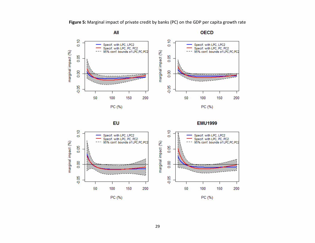
Relying on the results presented in Appendix E, Figure 5 plots the marginal effects of bank credit

by banks on GDP growth rates in connection with column (3) of Table 3 and Table 4 (i.e. specifications

with LPC and LPC2, and PC, PC2, and LPC, respectively). It shows that the positive effect of bank credit on

27

growth disappear much faster than that established in Arcand et al. (2015) who based on panel data found

that the optimal point of credit was ranging from 79% to 144% in different specifications.

28

(1) (2) (3) (4) (5) (6) (7) (8) (9) (10) (11) (12)

VARIABLES All avlb. OECD EU EMU1999 All avlb. OECD EU EMU1999 All avlb. OECD EU EMU1999

LGDP -14.85*** -13.45*** -17.50*** -11.89*** -14.78*** -12.43*** -16.12*** -11.80*** -16.62*** -12.70*** -14.97*** -13.02***

(2.823) (2.651) (2.609) (1.869) (2.688) (2.215) (2.261) (1.782) (2.696) (2.257) (2.504) (2.013)

LEDU 1.677*** 0.706* 0.424 0.127 1.424*** 0.616 0.380 0.633 1.614*** 0.882* 0.520 0.323

(0.553) (0.372) (0.452) (0.659) (0.553) (0.403) (0.393) (0.716) (0.569) (0.457) (0.521) (0.676)

LGC 0.832 2.187* -0.0434 4.606*** 0.353 2.134 -0.459 4.903*** 0.0331 2.093 -0.376 2.151**

(0.985) (1.297) (1.752) (1.302) (1.048) (1.523) (1.763) (1.276) (0.930) (1.333) (0.910) (0.840)

LOPEN 0.634 0.977 1.105 2.698*** 0.825 1.206* 0.929 2.931*** 0.958 1.364** 1.438** 3.482***

(0.651) (0.611) (0.758) (0.313) (0.691) (0.700) (0.753) (0.419) (0.678) (0.660) (0.692) (0.465)

LINF 0.749 0.486 -2.650** -0.542 0.433 -0.442 -3.360** 0.326 0.0590 -0.732 -3.966*** 3.041

(0.990) (0.957) (1.334) (3.664) (1.058) (1.351) (1.389) (4.045) (1.085) (1.518) (1.126) (4.175)

LPC 1.840** 1.653*** 1.983 2.949** 2.724*** 3.015*** 3.082* 1.114 2.672*** 2.484*** 2.321 -5.668*

(0.756) (0.635) (1.537) (1.503) (0.960) (0.947) (1.591) (4.264) (1.020) (0.838) (1.485) (3.259)

PC -0.0630*** -0.0459** -0.0555 -0.0721** -0.0998*** -0.0869*** -0.0916** -0.0299 -0.101*** -0.0772*** -0.0761** 0.101

(0.0208) (0.0181) (0.0435) (0.0333) (0.0306) (0.0280) (0.0427) (0.0763) (0.0328) (0.0248) (0.0378) (0.0618)

PC2 0.00012*** 8.25e-05** 9.22e-05 0.00014* 0.00024*** 0.00021*** 0.00022** 4.36e-05 0.00027*** 0.00021*** 0.0002** -0.00019

(4.09e-05) (3.53e-05) (0.000116) (7.52e-05) (8.26e-05) (7.13e-05) (0.00010) (0.000154) (9.34e-05) (6.60e-05) (0.000102) (0.000133)

LPDS -0.183*** -0.238** -0.230** -0.415*** -0.214*** -0.283** -0.298*** -0.581*** -0.502** -0.633*** -0.943** -1.457***

(0.0528) (0.120) (0.110) (0.136) (0.0536) (0.121) (0.108) (0.0863) (0.196) (0.243) (0.451) (0.297)

LDS*SM_VOL80 0.0473*** 0.0349* 0.0520*** 0.0423*** 0.0446*** 0.0451** 0.0665*** 0.0349**

(0.0159) (0.0180) (0.0161) (0.0163) (0.0167) (0.0216) (0.0213) (0.0158)

LPDS*exp(RIR-RGDPGR) 0.311 0.386* 0.754* 0.819**

(0.197) (0.227) (0.422) (0.333)

LSMC -0.0101 0.0640 0.0174 0.201*** -0.0142 0.0526 -0.00858 0.182*** -0.0191 0.0480 -0.0554 0.103*

(0.0735) (0.0631) (0.0573) (0.0685) (0.0748) (0.0649) (0.0523) (0.0578) (0.0720) (0.0686) (0.0493) (0.0586)

Observations 468 360 232 135 424 323 212 127 371 270 161 84

R-squared 0.695 0.749 0.798 0.901 0.691 0.735 0.814 0.908 0.715 0.763 0.863 0.938

Number of cntr_id 43 30 23 11 39 28 20 10 37 26 19 9

Robust standard errors in parentheses; *** p<0.01, ** p<0.05, * p<0.1

Table 4: Sensitivity: non-linear impact (LPC, PC, PC2). Dependent variable: yearly GDP per capita average growth rates over 5 year periods ahead. Credit data

source: World Bank. Estimator: Anderson-Hsiao. Unbalanced panel with sample initiating mainly from 1990 (LGDP instrumented also with previous data).

29

Figure 5: Marginal impact of private credit by banks (PC) on the GDP per capita growth rate

30

In the case of the EMU1999, the point estimate of marginal impact (the solid lines) becomes zero

and the peak of credit impact on GDP growth rates is reached at levels when the bank credit makes up

about half of GDP. For other groups of countries the turning point is even less than that. These findings

would show that the actual bank credit penetration in many economies could be way more harmful for

economic growth than estimated previously. However, the established turning point is likely to be

conditional on who receives the credit i.e. not only the amount, but also the structure of credit is

important. This is the issue that we consider next.

4.1.3. Disaggregation of credit, fund receiver, and further robustness checks

Up to this point of our empirical strategy we looked at the financing structure and potential non-linear

impact. Next we turn to the questions if different fund receivers also matter for economic growth and for

that purpose we further disaggregate credit to the private sector into more detailed components (see

Table 5). We differentiate private credit into the one received by households (LPCHSH) and non-financial

corporations (LPCNFC), as well as the outstanding private debt securities into the ones issued by financial

(LDSFCO) and non-financial corporations (LDSNFC) (all relative to GDP and in log terms).

Taking into account period effects, the results provide a rather robust association between the

variables in question (see columns 1-4). In detail, credit towards households is found to have a detrimental

association with growth, while the credit for non-financial corporations has a non-significant effect or

even the positive and significant impact in the case of the EMU1999. On the other hand, securities issued

by financial corporations have also a negative impact on growth mainly in the EU and EMU MS while no

significant effect is estimated for the securities issued by non-financial corporations. However, it should

be pointed out that the globalization of financial institutions that recently became especially intense (see

REF ???) may be partially responsible for such an effect, because the domestic savings attracted e.g.

through debt securities can be outsourced to other markets thus reducing local funding of investments.

The presented results are robust and stronger in terms of statistical significance when no period

effects are considered (columns 5-8). In general, the separation of bank private credit into that flowing to

households and non-financial firms has much clearer impact difference as compared with that of the split

of outstanding debt securities issued by the financial and non-financial corporations (see Figure 6).

31

(1) (2) (3) (4) (5) (6) (7) (8)

period effs. period effs. period effs. period effs.

no period

effs.

no period

effs.

no period

effs.

no period

effs.

VARIABLES \ Countr.: All avlb. OECD EU EU1999 All avlb. OECD EU EU1999

LGDP 3.749 -5.097 -11.32** -8.356* 4.504 0.151 -1.089 -5.979

(6.203) (5.517) (4.436) (4.502) (9.163) (9.290) (9.098) (6.670)

LEDU 0.558 0.115 0.118 0.0475 3.670*** 3.475*** 3.755*** 3.366***

(0.645) (0.419) (0.510) (0.572) (0.814) (0.889) (1.068) (1.265)

LGC 8.057** 2.189 0.747 3.881*** 10.85** 6.878*** 7.505*** 7.287***

(4.065) (1.632) (2.553) (1.495) (4.231) (2.347) (2.659) (1.632)

LOPEN 0.789 -0.472 0.660 2.609*** -0.837 -1.716 -1.574 -0.897

(1.291) (1.008) (1.295) (0.559) (1.391) (1.517) (1.841) (1.541)

LINF 1.236 -2.983 -0.363 -6.580*** -3.938 -5.567* -7.682** -17.25***

(4.265) (2.025) (2.448) (2.528) (4.210) (2.983) (3.633) (3.533)

LPCHSH -2.977*** -2.214*** -1.462*** -1.573** -4.237*** -4.084*** -4.108*** -3.785***

(0.938) (0.701) (0.520) (0.779) (1.010) (1.001) (0.970) (0.524)

LPCNFC -0.454 0.812 0.216 0.659* -0.444 0.395 0.523 0.381

(1.008) (0.511) (0.455) (0.395) (0.894) (0.671) (0.684) (0.382)

LPDSFCO -0.203 -0.314 -0.332* -0.309** -0.517** -0.479** -0.414** -0.394***

(0.207) (0.218) (0.170) (0.121) (0.255) (0.221) (0.206) (0.151)

LPDSNFC -0.0436 -0.200 -0.228 -0.0504 -0.0442 -0.128 -0.159 -0.332**

(0.234) (0.198) (0.198) (0.0915) (0.285) (0.263) (0.280) (0.153)

LSMC -0.0941 0.147 0.0375 0.0838 -0.0853 -0.0624 -0.0321 0.0616

(0.180) (0.149) (0.149) (0.0797) (0.117) (0.112) (0.111) (0.0948)

Observations 259 241 175 132 259 241 175 132

R-squared 0.553 0.733 0.786 0.886 0.268 0.371 0.443 0.540

Number of cntr_id 25 22 16 9 25 22 16 9


*** p<0.01, ** p<0.05, * p<0.1

Table 5: Detailed split by types of financing and subjects. Dependent variable: yearly GDP per

capita average growth rates over 5 year periods ahead. Credit data source: Bank for International

Settlements. Estimator: Anderson-Hsiao. Unbalanced panel with sample initiating mainly from

1989 (LGDP instrumented also with previous data).

We can further infer from the analysis of structural impact that in more developed countries (and

especially the EMU1999 MS) bank credit to non-financial corporations contributes and not hinders

economic growth. Furthermore, it is more effective in terms of promoting growth relative to the financing

using debt securities of non-financial corporations. Hence, the negative average impact of bank credit

established previously in Tables 2, C1, and C2 hinges on the large share of credit going to households and

financial institutions.

32

Figure 6: Coefficients in a log-linear model of economic growth as in eq. (1) of different financing components and subjects in

different groups of countries (AH estimator)

Note: LPCHSH - private credit to household to GDP; LPCNFC - private credit to non-financial corporations to GDP; LPDSFCO - debt

securities issued by financial corporations to GDP; LPDSNFC - debt securities issued by non-financial corporations to GDP.

-3.5

-3

-2.5

-2

-1.5

-1

-0.5

0

0.5

1

1.5

All avlb. OECD EU EU1999

LPCHSH LPCNFC

-0.35

-0.3

-0.25

-0.2

-0.15

-0.1

-0.05

0

All avlb. OECD EU EU1999

LDSFCO LDSNFC

33

In addition to our empirical estimations on the finance-growth nexus we provide further

robustness checks with emphasis on the overall findings of this section; that is we merge financial

structure, non-linearity and fund receiver specifications into a single equation. It should be noted that at

this point our effort is to keep number of parameters as low as possible while accounting for any related

influences. For that purpose we augment our previous specifications with the ratios of household to firm’s

private credit and of debt securities issued by financial and non-financial corporations

In particular, Table 6 (see below) offers the empirics of the non-linear impact of financial depth

to growth similar to Table 3, with the inclusion of two interaction terms14: (i) the interaction between

bank issued credit and the ratio of credit to household and non-financial corporations (LPC*PCRAT), and

(ii) the interaction between outstanding debt securities and the ratio of debt securities issued by financial

and non-financial corporations (LPC*DSRAT). The results are consistent with previous findings from Table

5 that credit to households’ affects growth negatively. Furthermore, in the EMU1999 MS both interaction

terms have a negative and statistically significant effect on growth (see columns 4 and 8 in Table 6), thus

underlying the importance of financial structure in the financial depth-growth relation. As previously, the

impact of the allocated debt securities is less clear-cut whenever we look at its impact on growth in

different country groups.

Switching to data from the BIS and re-estimating all main previous specifications (see Table 7)

confirm the importance of financial structure as results present nearly the same signs and significances

(see e.g. columns 9-12 related to the latest specification discussed in this section). The important

difference being that non-linearity of bank credit impact in Table 7 becomes (more) significant than that

which was observed using the WB data in Table 6 after the introduction of variables representing the

structure (ratios) of finance receivers. It should be also pointed out that this appearance of significance of

parameter estimates can be attributed to the usage of the BIS data corrected for breaks, since the country

coverage in the OECD, EU, and EMU MS cases is the same in both estimations.

14 It should be pointed out that the signs of estimations remain the same if additional unconditional shifts of

composition are also included i.e. PCRAT and/or DSRAT, but significance of non-linear impact of bank credit become

less strong due to their high multicollinearity with the introduced series (as well these series are significant only in

one case each). Nevertheless, the specification without these shifts seems to be more economically intuitive yielding

the total effect of logarithm of private credit by banks as a function of the ratio of credit to households and firms,

i.e. the impact is represented by (α0 + α1·PCRAT)·LPC, and would say that the total impact of logarithm of private

credit (LPC) would decrease with increasing ratio of household to firm credit (PCRAT) whenever α1<0 as is currently

in Table 7.

34

It should be noted further that the interaction term of credit with the household-to-firm in

specifications presented in the last two tables affects the shape and peak of the impact of credit on GDP

growth rates. Those presented in Figure 5 can be thought as connected with the averages of actual

household-to-firm financing ratios. Using the most significant results of Column (12) from Table 7 we

derive using results presented in Appendix E that, whenever all bank credit is devoted to firms, the peak

of the positive impact of bank credit on growth is reached whenever it makes up about 65% of GDP.

Summarizing all the empirics of financing and growth nexus provided in Section 4.1, we first can

confirm that there is a significant non-linearity of bank credit also in the EU and EMU member states,

although the peak of non-linear impact seems to be reached at significantly smaller levels of credit-to-

GDP in comparison with the previous findings established mostly relying on global country sets and using

only credit data without taking other types of financing into account.

Given the historical composition and use of financing, the split of finance by the type of instrument

(bank credit, debt securities, and stock market financing) reveals robustly that there was too much of bank

credit and its reduction would have benefited economic growth. The analysis by the fund receiver

discloses further that the main suspect of problems connected with bank credit is the credit flowing to

households.

These findings are quite robust to various perturbations in the performed sensitivity analyses as

well as using different datasets, although the results of final specifications, which account for various

structure as well as non-linearity, seem to be more significant with the BIS data that are adjusted for

structural breaks.

35

(1) (2) (3) (4) (5) (6) (7) (8)

Countries: All avlb. OECD EU EMU1999 All avlb. OECD EU EMU1999

LGDP -12.28*** -10.67*** -15.55*** -13.36*** -6.033 -14.00* -15.84** -11.93***

(4.170) (3.432) (5.722) (4.320) (4.664) (7.353) (7.097) (4.455)

LEDU 0.835 0.667* 0.390 0.613 0.637 0.321 0.332 0.581

(0.527) (0.404) (0.349) (0.685) (0.571) (0.393) (0.418) (0.780)

LGC 2.063 2.398 -0.288 3.800*** 4.313 0.172 -0.979 3.937***

(1.557) (1.500) (2.626) (1.370) (2.774) (2.317) (3.154) (1.227)

LOPEN 1.006 1.103 0.970 2.140*** 0.388 -0.783 0.0676 2.107***

(0.635) (0.747) (0.891) (0.620) (1.074) (0.879) (1.296) (0.650)

LINF -0.414 -0.330 -4.329*** -1.482 0.678 -2.550 0.261 -4.814*

(1.439) (1.483) (1.316) (2.697) (3.169) (1.820) (2.469) (2.902)

LPC 5.783** 4.195* 4.554* 4.517 0.263 4.943 6.286 5.820

(2.816) (2.303) (2.602) (5.131) (4.120) (3.769) (4.712) (5.548)

LPC2 -0.765** -0.531* -0.602* -0.557 -0.0456 -0.551 -0.720 -0.764

(0.373) (0.294) (0.327) (0.563) (0.460) (0.442) (0.576) (0.611)

LPDS -0.315*** -0.264** -0.289*** -0.595*** -0.209 -0.333* -0.586*** -0.0720

(0.0628) (0.128) (0.104) (0.113) (0.163) (0.191) (0.153) (0.180)

LPDS*SM_VOL80 0.0438** 0.0436** 0.0688*** 0.0346** 0.0173 0.0538** 0.0579** 0.0343

(0.0188) (0.0199) (0.0220) (0.0146) (0.0257) (0.0226) (0.0281) (0.0222)

LSMC -0.00385 0.0615 -0.0508 0.135** 0.198 0.262 0.116 0.106*

(0.0915) (0.0842) (0.0746) (0.0530) (0.129) (0.170) (0.175) (0.0598)

LPC*PCRAT -0.163 -0.255* -0.326** -0.393*** -0.348 -0.407** -0.364*** -0.316**

(0.154) (0.144) (0.139) (0.136) (0.222) (0.176) (0.119) (0.133)

LPDS*DSRAT -0.000115 -0.000389 0.000501* -0.00271*

(0.000731) (0.000694) (0.000262) (0.00143)

Observations 325 296 189 117 229 211 151 111

R-squared 0.666 0.709 0.800 0.915 0.676 0.777 0.806 0.907

Number of cntr_id 31 26 17 10 25 22 16 9


*** p<0.01, ** p<0.05, * p<0.1

Table 6: Sensitivity: Non-linear impact with structure ratios. Dependent variable: yearly GDP per

capita average growth rates over 5 year periods ahead. Credit data source: World Bank and Bank

for International Settlements. Estimator: Anderson-Hsiao. Unbalanced panel with sample

initiating mainly from 1990 (LGDP instrumented also with previous data).

36

Robust standard errors in parentheses. *** p<0.01, ** p<0.05, * p<0.1

Table 7: Sensitivity: results with BIS data of credit and debt securities. Dependent variable: yearly GDP per capita average growth rates

over 5 year periods ahead. Credit data source: Bank for International Settlements. Estimator: Anderson-Hsiao. Unbalanced panel with

sample initiating mainly from 1990 (LGDP instrumented also with previous data).

(1) (2) (3) (4) (5) (6) (7) (8) (9) (10) (11) (12)


LGDP 3.507 -6.063 -12.13** -8.641* 1.361 -15.71 -25.58** -13.98*** -1.743 -19.99** -27.12*** -15.99***

(5.801) (6.506) (4.771) (4.595) (6.346) (12.36) (11.22) (4.803) (6.518) (9.902) (10.32) (5.294)

LEDU 0.684 0.274 0.149 0.157 0.972 0.383 0.287 0.581 0.947 0.289 0.139 0.496

(0.608) (0.496) (0.545) (0.675) (0.661) (0.465) (0.505) (0.773) (0.613) (0.418) (0.468) (0.657)

LGC 7.318** 2.216 0.352 3.770** 6.609* 0.0982 -3.024 2.342* 5.828 -0.755 -3.469 1.589

(3.589) (1.949) (2.737) (1.701) (3.540) (3.287) (4.333) (1.320) (3.660) (2.744) (3.786) (1.535)

LOPEN 0.758 -0.391 0.280 2.662*** 0.579 -0.827 -0.873 1.943*** 0.256 -1.148 -1.025 1.451*

(1.290) (1.058) (1.256) (0.647) (1.197) (0.971) (1.323) (0.692) (1.200) (0.865) (1.172) (0.777)

LINF 0.305 -3.595* -1.451 -8.387*** 0.311 -3.623* -1.069 -5.242* 0.316 -3.511 -0.574 -3.520

(4.013) (1.970) (2.406) (3.250) (4.002) (2.034) (3.646) (2.891) (3.772) (2.372) (4.406) (2.562)

LPC -3.320*** -1.882*** -1.453*** -1.187* 1.892 10.95 18.95 11.08*** 3.404 14.84 22.20** 12.80***

(1.149) (0.728) (0.544) (0.689) (5.144) (9.640) (11.81) (3.970) (5.539) (9.267) (11.29) (4.652)

LPC2 -0.608 -1.481 -2.411* -1.416*** -0.715 -1.847* -2.740** -1.526***

(0.615) (1.124) (1.424) (0.449) (0.628) (1.087) (1.369) (0.532)

LPDS -0.280* -0.272** -0.509*** -0.343** -0.290** -0.244*** -0.346*** -0.303** -0.210 -0.201** -0.309** -0.299

(0.151) (0.135) (0.147) (0.143) (0.143) (0.0913) (0.103) (0.131) (0.146) (0.0998) (0.142) (0.184)

LPDS*SM_VOL80 0.0122 0.0364* 0.0497** 0.0343** 0.0200 0.0385** 0.0492* 0.0346**

(0.0218) (0.0196) (0.0238) (0.0164) (0.0204) (0.0190) (0.0257) (0.0160)

LSMC -0.00304 0.182 0.0712 0.0990 -0.00923 0.178 0.0769 0.0966*** 0.00769 0.207* 0.0726 0.0873**

(0.162) (0.157) (0.161) (0.0840) (0.165) (0.133) (0.140) (0.0352) (0.155) (0.125) (0.135) (0.0383)

LPC*PCRAT -0.295 -0.345** -0.275** -0.437***

(0.238) (0.156) (0.118) (0.111)

LPDS*DSRAT 0.000134 0.000260 0.000997 -0.000547

(0.000483) (0.000522) (0.000657) (0.00136)

Observations 267 248 182 139 257 238 174 131 248 230 167 124

R-squared 0.556 0.733 0.795 0.885 0.599 0.794 0.820 0.907 0.658 0.804 0.819 0.914

Number of cntr_id 25 22 16 9 25 22 16 9 25 22 16 9

37

4.2. Financial depth, growth and swings of asset prices in housing and

stock markets

Financial structure can have different impact on economic growth during different market conditions e.g.

the upswings or downswings of asset prices of various intensity. In order to consider such effects and

financing structure (namely, the bank-based vs market-based) impact on economic growth rates, we

proceed by following a part of the study offered by Langfield and Pagano (2016) with some extensions.

Specifically, the hypothesis is tested that bank-based financial structures feature lower economic growth,

particularly during times of smaller or larger swings in asset prices of stock and housing markets. According

to this hypothesis, banks’ credit creation features inefficiencies that could be detrimental to economic

growth, both in the upswing and the downswing of asset prices, where also these inefficiencies can be

magnified during times of crisis.

As in the previous section, one of our aims is to evaluate whether findings established previously

(namely, in Langfield and Pagano, 2016) that were obtained relying on a broader set of countries also hold

whenever we consider narrower regions. Although our general interest again is mainly in the EU and EMU

MS, we also provide empirics for the OECD as well as the full sample of countries.

To evaluate the impact of structure, we generate an additional bank-market ratio variable defined

as the ratio between private credit to outstanding debt securities and stock market capitalization (PC_MK)

and estimate the specification a la Langfield and Pagano by including dummies of growth and slump

periods of the stock market (Table 8 & 10) and the housing market (Table 10 & 11). In detail, Table 8

provides the findings of the estimations referring to stock market growth and slump periods (SM growth

and SM slump, respectively), taking the value 1 when a country’s stock market increase or decrease at an

average annual rate of at least 10%, 5%, 3%, and 2% over 5 years (see columns 1-4, 5-8, 9-12 and 13-16,

respectively). The interaction variable between the aforementioned dummies and the bank-market ratio

is also used. The considered range of various growth rates represents different intensity/pressure of asset

prices: from bums and boosts to more moderate growth and slump periods.

Results reveal that for the whole sample of countries bank-market ratio is negatively correlated

with GDP growth, in line with Langfield and Pagano (2016) (see columns 1, 5, 9, 13). So, an increase in the

size of a country’s banking sector relative to securities and stock market capitalization is associated with

lower GDP growth in the subsequent five-year period, when conditioning on the variation of asset prices

is taken into account. However, for the more developed group of economies non-significant estimates are

found. The interaction term between bank-market ratio and growth periods of the stock market does not

38

present any statistical significance results, in line with Langfield and Pagano (2016), while the respective

slump dummy exhibits a positive association with GDP in the subsequent 5 year period. Interestingly,

when we include the standard control variables in our specification results differ substantially, as the

statistically significant negative effect of the bank-market ratio is no longer present15 (see Table 9, columns

5-12). The latter also holds for the interactions between growth and slump periods and the bank-market

ratio, as no significant relations are found. On the other hand, it is of interest to note that the credit to

deposit ratio (CRED_DEP), which has been introduced as a measure of systemic risk, consistently has a

negative sign and often becomes significant. It should be also noted that for the last exercise we used the

threshold of 2% which gave stable signs of variables of interest in different groups of countries and can

be thought as representing if there is relative gain or loss in the considered markets in real terms.

15 It should be pointed out that insignificance of financial-market-structure-connected series remains also when

credit to deposit ratio (CRED_DEP) is absent from specifications presented in Columns (9) –(12) of Table 11.

39

(1) (2) (3) (4) (5) (6) (7) (8) (9) (10) (11) (12) (13) (14) (15) (16)

Threshold (annual): 10% 10% 10% 10% 5% 5% 5% 5% 3% 3% 3% 3% 2% 2% 2% 2%

VARIABLES \ Countries: All avlb. OECD EU EU1999 All avlb. OECD EU EU1999 All avlb. OECD EU EU1999 All avlb. OECD EU EU1999

PC_MK -1.304*** -0.569 -0.136 -0.0291 -1.202*** -0.403 0.0127 -0.128 -1.150*** -0.392 -0.277 -0.554 -1.109*** -0.525 -0.335 -0.677

(0.399) (0.369) (0.424) (1.028) (0.408) (0.339) (0.452) (0.871) (0.399) (0.332) (0.532) (0.680) (0.396) (0.333) (0.570) (0.619)

PC_MK (SM slump) 1.215*** 0.0863 0.0120 -55.45 1.163*** 0.126 0.0539 -0.408 1.059** 0.0725 0.309 -0.136 1.016** 0.263 0.459 0.0142

(0.397) (0.657) (0.707) (68.30) (0.391) (0.490) (0.382) (0.337) (0.393) (0.363) (0.281) (0.493) (0.385) (0.365) (0.360) (0.716)

PC_MK (SM growth) 0.621 0.525 0.293 0.0945 0.219 0.0351 -0.115 -0.203 0.221 -0.0197 0.180 0.00314 0.0753 0.107 0.246 0.136

(0.409) (0.339) (0.355) (0.581) (0.374) (0.320) (0.327) (0.483) (0.377) (0.295) (0.413) (0.638) (0.366) (0.265) (0.411) (0.793)

SM slump -0.765 0.321 0.446 58.52 -1.017** -0.212 0.156 1.010* -0.839** -0.0258 -0.112 0.761 -0.872** -0.223 -0.212 0.752

(0.537) (0.751) (0.956) (71.10) (0.467) (0.457) (0.632) (0.457) (0.384) (0.330) (0.469) (0.765) (0.352) (0.349) (0.571) (0.876)

SM growth -0.534 -0.182 0.0860 0.268 -0.0868 0.113 0.292 0.491 -0.0151 0.164 -0.154 0.0759 0.0203 0.00473 -0.116 0.0328

(0.372) (0.328) (0.419) (0.588) (0.344) (0.297) (0.474) (0.733) (0.335) (0.287) (0.499) (0.900) (0.343) (0.225) (0.620) (1.033)

Constant 2.399*** 0.498 -0.679 -0.614 2.211*** 0.340 -0.799 -0.460 2.016*** 0.323 -0.430 0.128 2.053*** 0.468 -0.494 0.0965

(0.633) (0.569) (0.716) (1.882) (0.644) (0.614) (0.906) (1.736) (0.582) (0.626) (0.940) (1.377) (0.588) (0.611) (1.023) (1.275)

Observations 450 320 195 122 450 320 195 122 450 320 195 122 450 320 195 122

R-squared 0.321 0.611 0.672 0.722 0.313 0.596 0.662 0.727 0.306 0.594 0.663 0.731 0.307 0.594 0.665 0.737

Number of cntr_id 40 27 19 10 40 27 19 10 40 27 19 10 40 27 19 10


Table 8: Impact of ratio of private credit to outstanding debt securities and stock market capitalization on economic growth (and its

interaction with growth and slump indicators of stock market), various thresholds. Dependent variable: yearly GDP per capita average

growth rates over 5 year periods ahead. Credit data source: World Bank. Estimator: Fixed Effects. Unbalanced panel with sample

initiating mainly from 1989.

40

(1) (2) (3) (4) (5) (6) (7) (8) (9) (10) (11) (12)

VARIABLES \ Countr. All avlb. OECD EU EU1999 All avlb. OECD EU EU1999 All avlb. OECD EU EU1999

CRED_DEP -2.327** -0.989 -0.700 -3.880** -1.494** -0.701* -0.217 -0.509

(1.009) (0.833) (1.048) (1.609) (0.583) (0.378) (0.230) (0.738)

PC_MK -1.109*** -0.525 -0.335 -0.677 -0.528 -0.327 -0.469 -0.134 -0.115 0.185 -0.182 -0.213

(0.396) (0.333) (0.570) (0.619) (0.404) (0.435) (0.694) (0.668) (0.313) (0.290) (0.201) (0.280)

PC_MK (SM slump) 1.016** 0.263 0.459 0.0142 0.643* 0.283 0.665 0.125 0.196 0.200 0.222 0.115

(0.385) (0.365) (0.360) (0.716) (0.347) (0.405) (0.489) (0.672) (0.247) (0.281) (0.298) (0.355)

PC_MK (SM growth) 0.0753 0.107 0.246 0.136 -0.0271 0.0939 0.460 -0.0793 -0.275 -0.0226 0.0509 -0.209

(0.366) (0.265) (0.411) (0.793) (0.363) (0.283) (0.457) (0.502) (0.300) (0.185) (0.191) (0.287)

SM slump -0.872** -0.223 -0.212 0.752 -0.437 -0.134 -0.329 0.636 -0.212 -0.0540 -0.00668 0.196

(0.352) (0.349) (0.571) (0.876) (0.371) (0.392) (0.711) (0.819) (0.311) (0.301) (0.386) (0.501)

SM growth 0.0203 0.00473 -0.116 0.0328 0.259 0.121 -0.250 0.408 0.540* 0.326 0.206 0.425

(0.343) (0.225) (0.620) (1.033) (0.344) (0.254) (0.776) (0.767) (0.314) (0.198) (0.332) (0.511)

LGDP -8.496*** -7.436*** -14.24*** -14.21***

(2.711) (2.303) (3.195) (2.123)

LEDU 5.720*** -1.511 -1.169 -0.100

(1.588) (1.462) (1.769) (1.178)

LGC 0.118 -0.405 -6.253 -2.314

(2.185) (2.394) (4.735) (3.340)

LOPEN 1.413 3.199** 4.011** 4.417**

(1.582) (1.195) (1.780) (1.576)

LINF -5.209 -10.08* -11.61 6.591

(4.454) (5.551) (6.966) (5.606)

Observations 450 320 195 122 426 296 171 122 386 282 168 121

R-squared 0.307 0.594 0.665 0.737 0.396 0.596 0.661 0.825 0.588 0.742 0.855 0.941

Number of cntr_id 40 27 19 10 39 26 18 10 37 26 18 10


Table 9: Impact of ratio of private credit to outstanding debt securities and stock market capitalization on economic growth (and its

interaction with growth and slump indicators of stock market), 2% annual threshold. Dependent variable: yearly GDP per capita

average growth rates over 5 year periods ahead. Credit data source: World Bank. Estimator: Fixed Effects. Unbalanced panel with

sample initiating mainly from 1989

41

In the next two groups of estimations we re-estimate the specification taking into account housing

prices instead of stock market ones (see Tables 10 & 11 below). We can once more infer that negative

effect of the bank-market ratio vanishes when the standard set of control variables is included in our

estimations. This also holds for the interaction referring to the slump period of the housing market and

the bank-market ratio. The interesting insight is that relative increase of credit financing during periods

of high growth in the housing market reduces economic growth rates: it has consistently negative sign of

impact and also significant for the cases of all countries and EU member states (columns (9) and (11)). This

is again fully consistent with the previously results established in Tables 5 and 7.

We next summarize the empirical findings about the bank-to-market based financing impact on

economic growth under different conditions in stock and housing markets as represented by their asset

prices. For larger sample of countries there is evidence that, evaluating unconditionally, expansion of

relative bank-based financing hurts economic growth, whereas the negative effect disappears during the

slumps of stock market (the positive coefficient of interaction term PC_MK (SM slump) is insignificantly

different in absolute terms from the negative coefficient of unconditional credit-to-market impact

revealed by PC_MK indicator). For the EU and EMU both the unconditional impact and the cushion effect

does not seem to be significant and all the effects become insignificant after including the ‘standard

controls’.

For larger sample of countries, the boom in housing prices coupled with relative expansion of

credit reduces the growth rates and survives the conditioning on the control variables. It also remains

significant in the EU case when the controls are included. In fact, the credit-to-market interaction with

housing booms (PC_MK (HS growth)) term is among the two variables that consistently retain the (negative)

sign across various groups of countries and specifications. The other one being the credit-to-deposit

variable. It seems therefore that there is a general tendency for future growth rates to decrease when

the credit is not financed out of savings and when there are booms of housing prices coupled with

expansion of bank credit relative to market-based financing.

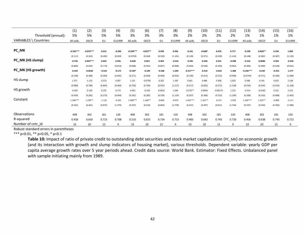
42

(1) (2) (3) (4) (5) (6) (7) (8) (9) (10) (11) (12) (13) (14) (15) (16)

Threshold (annual): 5% 5% 5% 5% 3% 3% 3% 3% 2% 2% 2% 2% 1% 1% 1% 1%

VARIABLES \ Countries: All avlb. OECD EU EU1999 All avlb. OECD EU EU1999 All avlb. OECD EU EU1999 All avlb. OECD EU EU1999

PC_MK -0.335*** -0.970*** 0.312 -0.300 -0.328*** -0.837** 0.439 0.436 -0.161 -0.668* 0.476 0.777 -0.100 -0.850** 0.194 1.060

(0.111) (0.310) (0.493) (0.693) (0.0759) (0.364) (0.520) (1.101) (0.128) (0.371) (0.539) (1.142) (0.148) (0.382) (0.387) (1.135)

PC_MK (HS slump) -0.742 2.044*** 0.629 0.456 -0.638 0.923 0.404 -0.435 -0.295 -0.204 0.241 -0.998 -0.216 0.0680 0.504 -0.450

(0.866) (0.692) (0.774) (0.414) (0.668) (0.561) (0.857) (0.968) (0.444) (0.506) (0.330) (0.962) (0.484) (0.490) (0.328) (0.831)

PC_MK (HS growth) -0.344 -0.0630 -0.524 -0.175 -0.530* -0.109 -0.568 -1.095 -0.317*** -0.419 -0.654 -1.468 -0.336*** -0.239 -0.353 -1.577

(0.338) (0.389) (0.394) (0.442) (0.271) (0.404) (0.494) (0.924) (0.109) (0.415) (0.535) (0.999) (0.0744) (0.371) (0.506) (1.008)

HS slump 1.371 -1.135 0.223 0.587 1.131 -0.0758 0.202 1.595 0.601 0.488 0.368 2.020 0.588 0.145 0.655 2.136

(0.980) (0.780) (0.892) (0.469) (0.756) (0.760) (0.925) (1.217) (0.517) (0.662) (0.272) (1.158) (0.550) (0.594) (0.433) (1.238)

HS growth -0.342 -0.183 0.255 0.174 -0.461 -0.160 -0.0632 1.049 -0.576** 0.0946 -0.00175 1.215 -0.314 -0.0185 0.322 2.141

(0.430) (0.281) (0.373) (0.404) (0.291) (0.285) (0.534) (1.124) (0.267) (0.306) (0.533) (1.199) (0.208) (0.316) (0.688) (1.463)

Constant 1.106*** 1.239** -1.122 -0.192 1.598*** 1.166** -0.836 -0.975 1.455*** 1.161** -0.727 -1.070 1.226*** 1.325** -0.899 -2.117

(0.262) (0.461) (0.972) (1.379) (0.337) (0.510) (0.863) (1.778) (0.322) (0.497) (0.811) (1.744) (0.297) (0.544) (0.783) (1.998)

Observations 408 302 181 120 408 302 181 120 408 302 181 120 408 302 181 120

R-squared 0.458 0.650 0.723 0.708 0.510 0.655 0.734 0.715 0.483 0.642 0.743 0.720 0.456 0.638 0.743 0.722

Number of cntr_id 33 20 15 9 33 20 15 9 33 20 15 9 33 20 15 9


*** p<0.01, ** p<0.05, * p<0.1

Table 10: Impact of ratio of private credit to outstanding debt securities and stock market capitalization (PC_MK) on economic growth

(and its interaction with growth and slump indicators of housing market), various thresholds. Dependent variable: yearly GDP per

capita average growth rates over 5 year periods ahead. Credit data source: World Bank. Estimator: Fixed Effects. Unbalanced panel

with sample initiating mainly from 1989.

43

(1) (2) (3) (4) (5) (6) (7) (8) (9) (10) (11) (12)

VARIABLES \ Countr.: All avlb. OECD EU EU1999 All avlb. OECD EU EU1999 All avlb. OECD EU EU1999

CRED_DEP -1.513* -0.709 -0.796 -4.089*** -1.180** -0.685* -0.399 -1.272

(0.836) (0.782) (0.912) (1.203) (0.522) (0.342) (0.247) (0.967)

PC_MK -0.161 -0.668* 0.476 0.777 0.0118 -0.565 0.581 0.613 0.127 -0.0139 0.0753 -0.0692

(0.128) (0.371) (0.539) (1.142) (0.102) (0.420) (0.638) (0.643) (0.114) (0.312) (0.242) (0.335)

PC_MK (HS slump) -0.295 -0.204 0.241 -0.998 -0.168 -0.0801 0.0230 1.106* 0.485 0.821* 0.159 -0.0121

(0.444) (0.506) (0.330) (0.962) (0.448) (0.563) (0.380) (0.538) (0.295) (0.410) (0.324) (0.554)

PC_MK (HS growth) -0.317*** -0.419 -0.654 -1.468 -0.312*** -0.537 -0.715 -0.679 -0.322*** -0.263 -0.359* -0.247

(0.109) (0.415) (0.535) (0.999) (0.107) (0.402) (0.536) (0.426) (0.0887) (0.337) (0.189) (0.377)

HS slump 0.601 0.488 0.368 2.020 0.338 0.254 0.753 -0.245 -0.643 -0.999* -0.466 -0.522

(0.517) (0.662) (0.272) (1.158) (0.587) (0.790) (0.463) (0.500) (0.384) (0.512) (0.580) (0.621)

HS growth -0.576** 0.0946 -0.00175 1.215 -0.431 0.215 0.112 0.619 0.175 0.435 0.0868 0.205

(0.267) (0.306) (0.533) (1.199) (0.266) (0.304) (0.724) (0.672) (0.241) (0.277) (0.271) (0.471)

LGDP -7.174*** -7.414*** -14.13*** -12.60**

(1.543) (2.193) (2.973) (3.815)

LEDU 2.902* -0.569 -0.427 -0.735

(1.501) (1.053) (0.718) (1.018)

LGC -0.121 0.568 -0.625 -0.265

(1.986) (2.113) (3.812) (4.111)

LOPEN 2.719* 3.786*** 4.967*** 4.146**

(1.341) (1.303) (1.487) (1.604)

LINF -18.32*** -7.995 10.03 10.37

(5.225) (6.681) (11.76) (11.86)

Observations 408 302 181 120 379 273 152 120 339 260 149 119

R-squared 0.483 0.642 0.743 0.720 0.519 0.647 0.751 0.845 0.726 0.792 0.918 0.919

Number of cntr_id 33 20 15 9 32 19 14 9 30 19 14 9


*** p<0.01, ** p<0.05, * p<0.1

Table 11: Impact of ratio of private credit to outstanding debt securities and stock market capitalization (PC_MK) on economic growth

(and its interaction with growth and slump indicators of housing market), 2% annual threshold. Dependent variable: yearly GDP per

capita average growth rates over 5 year periods ahead. Credit data source: World Bank. Estimator: Fixed Effects. Unbalanced panel

with sample initiating mainly from 1990.

44

4.3. Shifts of financial structure and growth empirics

To illustrate economic significance of the established results, we provide in the final part of this report

some estimates on the possible impact of a change of financial composition in terms of the amount of

credit provided in the economy among different sources (i.e. bank credit, debt securities or the stock

market). In order to avoid too many assumptions we restrict ourselves to a very simple scenario of an

increase of stock market capitalization in the EU MS by 10 percentage points, with the respective

reduction of private credit originating from banks deriving the impact for various countries depending on

their actual structure of financing (see Figure D1 in Appendix D). Note that the solid horizontal line signifies

the overall median of impact (derived from all years), whereas the thinner one represents that of the

particular year, and the relative coefficients are derived from Table 2, column 3 (see above).

Looking at the median impact of the described shift by 10 percentage points, we can infer that in

1995 it would have led to a median raise in 5-year GDP growth rates by more than 0.11 percentage point

thereafter (see top-left chart). If the same shift of financial structure would have been implemented later

on, the median impact becomes smaller. For instance, its implementation in 2013 would yield already

only about 0.06 percentage point faster median 5-year growth rates (see bottom-right chart). Overall

there is a path dependency of economic significance of structural policy on growth, implied by that the

higher is the financial penetration, the lower will be a particular effect of this policy.

The above conclusions are based on the log-linear model estimated using credit series from the

WB GFDD database. It should be pointed out that these data series on credit seem to have structural

breaks for e.g. France, Denmark, Sweden. Hence, in Figure D2 of Appendix D we also present the

calculated impact using the BIS credit data and the respective estimated model with log-linear financial

series (see column 3 of Table 7). The ranking of the impact in the countries remains similar as well as the

fading out impact for the later years of intervention, but the median impact on economic growth rates is

higher and now reaches 0.21 percentage points (from 0.27 in 1995, to 0.14 in 2013).

The fading out effect of the impact established previously using the log-linear specification is

connected with higher penetration of financing; to achieve the same impact on growth with higher levels

of financial penetration requires larger adjustments in terms of structure. It is not the case anymore with

the non-linear model. We therefore repeat the exercise using non-linear estimated model (see columns 7

and 11 of Table 7) and present the results in Figures D3 and D4 (see Appendix D), respectively. Since the

later specification with the ratio of households to firm credit is available only for the data from BIS and

the specifications in Table 7 for the EU and EMU are more significant than that with the WB presented in

45

Table 3, we rely in these simulations on the BIS data-linked estimates. Results connected with both

specifications produce similar qualitative pattern with slightly higher median impact (ranging from 0.21 in

1995 to 0.32 in 2008) when derived using column 7 of Table 7 and somewhat smaller (ranging from 0.14

in 1995 to 0.29 in 2008) when derived using column 11 of Table 7.

As it is revealed by Figures 8 and 9, a simple and uniform reduction of the share of credit is no

more beneficial for certain countries, because it could even worsen economic growth situation in some

of them, provided that credit would have deviated even further from the peak of impact (turning point)

due to this implemented policy.

5. Conclusions

This report offers insights on the financial development and economic growth debate, while emphasizing

on relevant empirics for the European Union and the Euro area. The empirical findings can be grouped in

several categories. First, results highlight that financial structure and growth are inextricably linked.

Specifically, credit provided by banks presents an inverted U-like effect on growth (although having more

general non-linearity than a simple inverted U-shape). For the EMU MS the threshold (peak of positive

impact) is found to be close to 50%. This is conditional on the actual financing structure with substantial

share of bank credit going to households. If all credit were directed towards financing of non-financial

corporations, the estimated turning point would shift to around 65%. Estimates using the whole EU

sample give similar but somewhat smaller thresholds. Consequently, large bank credit penetration

relative to GDP, especially with heavy financing of households, can be more harmful to economic growth

than estimated/thought previously.

Second, the structure of financing matters for economic growth: both the type of instrument of

financing (bank loans, debt securities, and stock market) and the type of fund receivers (households, firms

or financial corporations). Starting from the type of financing, bank credit appears to have the most

negative impact and stock market a more positive one on economic growth during the analyzed period.

Interestingly, the unconditional impact of outstanding debt securities tends to be negative, but when GDP

growth rates are low relative to lending interest rates and/or stock market volatility is high, larger share

of debt securities can facilitate economic growth.

Third, further disaggregation by beneficiaries of financial means reveals that the established

negative impact of bank credit is connected with substantial financing of households. On the contrary,

46

bank credit to non-financial corporations tends to contribute to economic growth instead of hindering it.

Furthermore, it seems to be more effective in terms of promoting economic growth relative to the

financing using debt securities of non-financial corporations on average. In a similar manner, debt

securities issued by the financial corporations seem to induce negative influence on future economic

growth rates. Partially, this can be connected with that the domestic savings are outsourced to other

markets thus reducing local funding of investments rather than due to poor performance of the financial

institutions per se.

Fourth, and consistent with the third, expansion of bank credit relative to market-based financing

during housing market booms affects economic growth negatively. Housing market booms facilitate

expansion of credit to households both due to the increased needs for those acquiring housing and

because of larger value of collateral acceptable to banks. This, together with larger return rates in this

market, can divert and even reduce the means devoted to financing of productive firm investments. There

also seem to be a general tendency for future growth rates to decrease whenever credit amounts are

larger relative to (financed not out of) savings.

Finally, from the policy perspective, several alternatives connected with the financial deepness

and its structure would seem to promote economic growth. Regarding the banking sector, it can be

achieved both by reducing the bank credit to GDP levels in a number of European countries (as Europe’s

financial structure has become strongly bank-based with substantial bank credit penetration), and also by

directing more credit towards non-financial corporations. The later has smaller economic impact on

average, but the former depends nontrivially on the initial conditions of a particular economy (namely,

the actual distance from the peak of credit impact, level of financial penetration of all modes of finance,

etc.). Further development of debt securities market seem to be beneficial mostly with facilitation of

growth during difficult periods, whereas further development of stock market seems to be favorable in

general.

47

References

Anderson, T. W., and Hsiao, C. 1981. Estimation of dynamic models with error components. Journal of

the American Statistical Association, 76, 598–606.

Arcand, J.L., Berkes, E., Panizza, U. (2015): Too much finance? Journal of Economic Growth 20, 105—148.

Arellano, M., and Bond, S. 1991. Some tests of specification for panel data: Monte Carlo evidence and an

application to employment equations. Review of Economic Studies, 58, 277–297.

Arellano, M., and Bover, O. 1995. Another look at the instrumental variable estimation of error-

components models. Journal of Econometrics, 68, 29–51

Balta, N., Nikolov, P. (2013): Financial dependence and growth since the crisis. Quarterly report on the

euro area 2013, 12(3), 7—18.

Beck, T. (2012): Finance and Growth: Lessons from the literature and the recent crisis, July 2012. Prepared

for the LSE Growth Commission.

Beck, T., Buyukkarabacak, B., Rioja, F., Valev, N. (2012): Who gets the credit? And does it matter?

Household vs. firm lending across countries. B.E. Journal of Macroeconomics” Contributions, 12, 1—44.

Beck, T., Levine, R. (2004): Stock markets, banks, and growth: Panel evidence. “Journal of Banking and

Finance”, 28, 423—442.

Beck, T., Levine, R., Loayza, N. (2000): Finance and the Sources of Growth. “Journal of Financial

Economics”, 58, 261—300.

Blundell, R., and Bond, S. (1998). Initial conditions and moment restrictions in dynamic panel data models.

Journal of Econometrics, 87, 115–143.

Breitenlechner, M., Gächter, M., Sindermann, F. (2015): The finance-growth nexus in crisis. Economics

Letters 132, 31—33.

Cecchetti, S.G., Kharroubi, E. (2012) Reassessing the impact of finance on growth. BIS Working Papers No

381.

Contessi, S., Li, L., and Russ, K. (2013) Bank vs. Bond Financing Over the Business Cycle. Federal Reserve

Bank of St. Louis, Economic Synopses 2013 No.31

Coricelli, F., Driffield, N., Pal, S., Roland, I. (2012): When does leverage hurt productivity growth? A firm-

level analysis. Journal of International Money and Finance 31(6), 1674—1694.

Cournède, B., Denk, O. (2015): Finance and economic growth in OECD and G20 countries. OECD Economics

Department Working Papers, No. 1223, OECD Publishing, Paris.

Cournède, B., Denk, O., Hoeller, P. (2015): Finance and inclusive growth. OECD Economic Policy Papers,

No. 14, OECD Publishing, Paris.

Demirgüç-Kunt, A., Feyen, E., Levine, R. (2013) The evolving importance of banks and securities markets.

World Bank Economic Review 27, 476—490.

48

Ductor, L., Grechyna, D. (2015): Financial development, real sector, and economic growth. International

Review of Economics and Finance 37, 393—405.

Gambacorta, L., Yang, J., Tsatsaronis, K. (2014): Financial structure and growth. BIS Quarterly Review,

March, 21—35.

Ketteni, E., Mamuneas, T., Savvides, A., Stengos, T. (2007): Is the Financial Development and Economic

Growth Relationship Nonlinear? Economics Bulletin 15(4), 1—12.

King, R.G., and Levine, R. (1993): Finance and Growth: Schumpeter Might Be Right. Quarterly Journal of

Economics 108, 717—738.

Langfield, S. and Pagano, M. (2016): Bank bias in Europe: effects on systemic risk and growth. Economic

Policy, 51—106.

Law, S.H., Singh, N. (2014): Does too much finance harm economic growth? Journal of Banking & Finance

41, 36—44.

Masten, A., Coricelli, F., Masten, I. (2008): Non-linear growth effects of financial development: Does

financial integration matter? Journal of International Money and Finance 27, 295—313.

Panizza, U. (2014): Financial Development and Economic Growth: Known Knowns, Known Unknowns, and

Unknown Unknowns. Revue d’èconomie du dèveloppement 22, 35—65.

Phillips, C.B., and Han, C. (2014). True limit distribution of the Anderson-Hsiao IV estimators in panel

autoregresson. Cowles Foundation Discussion Paper No. 1963.

Rousseau, P.L., Wachtel, P. (2011): What is Happening to the Impact of Financial Deepening on Economic

Growth? Economic Inquiry 49(1), 276—288.

Sahay, R., Cihak, M., N’Diaye ,P., Barajas, A., Bi, R., Ayala, D., Gao, Y., Kyobe, A., Nguyen, L., Saborowski,

C., Svirydzenka, K., Yousefi, S.R. (2015): Rethinking Financial Deepening: Stability and Growth in Emerging

Markets. Staff Discussion Notes SDN/15/08.

Samargandi, N., Fidrmuc, J., and Ghosh, S. (2015): Is the Relationship between Financial Development and

Economic Growth Monotonic for Middle Income Countries? World Development 68, 66—81.

Schumpeter, J.A. 1934 (2008): The Theory of Economic Development: An Inquiry into Profits, Capital,

Credit, Interest and the Business Cycle, translated from the German by Redvers Opie, New Brunswick

(U.S.A.) and London (U.K.): Transaction Publishers.

Valickova, P., Havranek, T., Horvath, R. (2015): Financial development and economic growth: A meta-

analysis. Journal of Economic Surveys 29(3), 506—526.

49

List of abbreviations and definitions

GDP: GDP per capita (constant LCU).

PC: The financial resources provided to the private sector by domestic money banks as a share of GDP.

PC: (BIS) Total credit received by non-financial sector (adjusted for breaks).

PDS: Total amount of domestic private debt securities (amount outstanding) issued in domestic markets

as a share of GDP.

SMC: Market capitalization of listed domestic companies as a percentage of GDP.

PCHSH: Private credit received by households.

PCNFC: Private credit received by non-financial corporations.

DSFCO: Debt securities issued by financial corporations.

DSNFC: Debt securities issued by non-financial corporations.

SM_VOL: Stock price volatility which is the average of the 360-day volatility of the national stock market

index.

RGDPGR: Annual percentage growth rate of GDP at market prices based on constant local currency.

RIR: Real interest rate: the lending interest rate adjusted for inflation as measured by the GDP deflator.

CRED_DEPOS: Bank credit to bank deposits (%).

EDU: Gross enrolment ratio, secondary, both sexes (%).

GC: General government final consumption expenditure as a percentage of GDP.

OPEN: Trade openness (calculated as exports plus imports divided by GDP).

INF: Inflation, measured by the consumer price index (annual %).

50

List of figures

Figure 1: Nonparametric part of credit impact on growth in a semiparametric regressions with all

countries, the EU, and the EMU1999 countries (by columns) in 1960-2010 and 1990-2010 periods (by

rows). Arcand et al. (2015) panel data and specification. ......................................................................... 18

Figure 2: Coefficients of financing components in a log-linear model of economic growth as in eq. (1) for

different groups of countries (WB data, AH estimator) ............................................................................. 22

Figure 3: Coefficients of financing components in a log-linear model of economic growth as in eq. (1) for

different groups of countries (BIS data, AH estimator). ............................................................................. 22

Figure 4: Nonparametric regressions of residuals of log-linear model on type of financing components to

GDP (private credit by banks to GDP, outstanding private debt securities to GDP, and stock market

capitalization to GDP). Results for all countries and the EMU1999 countries represented in the rows.

Variability bounds account only for nonparametric regression. ................................................................ 24

Figure 5: Marginal impact of private credit by banks (PC) on the GDP per capita growth rate ................. 29

Figure 6: Coefficients in a log-linear model of economic growth as in eq. (1) of different financing

components and subjects in different groups of countries (AH estimator) ............................................... 32

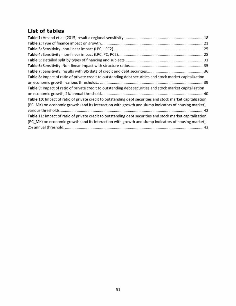
51

List of tables

Table 1: Arcand et al. (2015) results: regional sensitivity. ......................................................................... 18

Table 2: Type of finance impact on growth. ............................................................................................... 21

Table 3: Sensitivity: non-linear impact (LPC, LPC2). ................................................................................... 25

Table 4: Sensitivity: non-linear impact (LPC, PC, PC2). ............................................................................... 28

Table 5: Detailed split by types of financing and subjects .......................................................................... 31

Table 6: Sensitivity: Non-linear impact with structure ratios. .................................................................... 35

Table 7: Sensitivity: results with BIS data of credit and debt securities. .................................................... 36

Table 8: Impact of ratio of private credit to outstanding debt securities and stock market capitalization

on economic growth various thresholds.. ................................................................................................. 39


on economic growth, 2% annual threshold. ............................................................................................... 40


(PC_MK) on economic growth (and its interaction with growth and slump indicators of housing market),

various thresholds ....................................................................................................................................... 42


(PC_MK) on economic growth (and its interaction with growth and slump indicators of housing market),

2% annual threshold. .................................................................................................................................. 43

52

Appendix

Appendix A: Definitions and County Groups

Table 1A: Definitions and Sources of Original Data

Variable Definition Source

GDP GDP per capita (constant LCU). World Bank; World Development

Indicators (WDI); 2015

PC

The financial resources provided to the private

sector by domestic money banks as a share of

GDP. Domestic money banks comprise

commercial banks and other financial

institutions that accept transferable deposits,

such as demand deposits.

Global Financial Development

Database (WB); 2015

PC (BIS) Total credit received by non-financial sector

(adjusted for breaks).

Bank for International Settlements

(BIS), Credit to the Non-financial

Sector; 2016

PDS

Total amount of domestic private debt securities

(amount outstanding) issued in domestic

markets as a share of GDP. It covers long-term

bonds and notes, treasury bills, commercial

paper and other short-term notes.

Global Financial development

Database (WB); Original source: Bank

for International Settlements (BIS);

2016

SMC Market capitalization of listed domestic

companies as a percentage of GDP.

World Bank; World Development

Indicators (WDI).

PCHSH Private credit received by households.



Sector; 2016.

PCNFC Private credit received by non-financial

corporations.



Sector; 2016

DSFCO Debt securities issued by financial corporations. Bank for International Settlements (BIS)

Debt Securities Statistics; 2016.

DSNFC Debt securities issued by non-financial

corporations.

Bank for International Settlements (BIS)

Debt Securities Statistics; 2016.

SM_VOL

Stock price volatility which is the average of the

360-day volatility of the national stock market

index.


Database (WB); 2015

RGDPGR Annual percentage growth rate of GDP at

market prices based on constant local currency.



RIR

Real interest rate: the lending interest rate

adjusted for inflation as measured by the GDP

deflator.



CRED_DEPOS Bank credit to bank deposits (%).


Database (WB); 2015. Original source:

International Financial Statistics (IFS),

International Monetary Fund (IMF).

EDU Gross enrolment ratio, secondary, both sexes

(%).


Indicators (WDI).

53

GC General government final consumption

expenditure as a percentage of GDP.



OPEN Trade openness (calculated as exports plus

imports divided by GDP).



INF Inflation, measured by the consumer price index

(annual %).



Table 2A: Groups of Countries

Groups Countries No.

Full Sample

AUS,AUT,BEL,CAN,CHL,CHE,COL,CYP,CZE,DEU,DNK,ESP,FIN,FRA,GBR,

GRC,HKG,HRV,HUN,IDN,IND,ISL,IRL,ITA,JPN,KOR,LBN,LUX,MEX,MLT,

MYS,NLD,NOR,PER,PHL,POL,PRT,SVN,SVK,SWE,THA,TUR,USA,ZAF.

44

OECD AUS,AUT,BEL,CAN,CHL,CHE,CZE,DEU,DNK,EST,FIN,FRA,GBR,GRC,HUN,

ISL,IRL,ITA,JPN,KOR,LUX,MEX,NLD,NZL,NOR,POL,PRT,SVN,SVK,ESP, SWE,TUR,USA. 33

EU AUT,BEL,BGR,CZE,CYP,DEU,DNK,EST,FIN,FRA,GBR,GRC,HRV,HUN,IRL,

ITA,ESP,LTU,LVA,LUX,MLT,NLD, POL,PRT,ROU,SVN,SVK,SWE. 27

EMU1999 AUT,BEL,FIN,FRA,DEU,IRL,ITA,LUX,NLD,PRT,ESP. 11

* These countries constitute the corresponding groups of countries starting from Table 2. The

number of observations available in the specific estimations can be smaller due to data limitation.

54

Appendix B: Economic variables and specifications

From the economic perspective, the vector of explanatory variables ��,� in eq. (1) covers a couple

of different types of variables. First, some standard control variables are included almost in all cases

covering:

LGDP – logarithm of income per capita,

LEDU – logarithm of gross enrolment ratio16, secondary, both sexes (%),

LGC – logarithm of general government final consumption expenditure (% of GDP),

LOPEN – logarithm of trade (% of GDP),

LINF – the inverse hyperbolic sigh transform (IHST) of consumer price inflation rate in % (CPI), i.e.

log(CPI/100+sqrt(1+(CPI/100)^2)), where the IHST allows avoiding problems related to zero and

negative values appearing when the usual log transformation is applied.

Second, ��,� also covers several financial series under consideration used in different specifications:

a) in Table 1, following Arcand et al. (2015), we include:

i. PC - private credit by deposit money banks to GDP (%),

ii. PC2 – square of PC;

b) in Tables 2–4, in order to account for different financial structure we include:

i. LPC – logarithm of PC,

ii. LPDS – logarithm of outstanding domestic private debt securities to GDP (%),

iii. LSMC – logarithm of market capitalization of listed domestic companies (% of GDP);

c) in Tables 5–6, we look at nonlinear impact by augmenting the specification indicated in b) with

LPC2 (square of LPC) and additional interaction terms of LPDS with

i. SM_VOL80 – an indicator if stock market volatility is higher than the 8th decile,

ii. exp(RIR-RGDPGR) – exponent of the difference between real interest rates (RIR) and the

growth rate of real GDP (RGDPGR);

16 In this we follow Gambacorta et al. (2014), however main results remain unchanged if e.g. Barro and Lee logarithm

of total average years of total schooling, age 25+ were used. We prefer the former one, because it has positive

impact in most of considered equations, whereas the latter one becomes negative more often.

55

d) in Table 7, we look at the impact of structural composition of credit and outstanding private debt

securities by including (in addition to LSMC):

i. LPCHSH – logarithm of market value of credit to households & NPISHs (% to GDP),

ii. LPCNFC – logarithm of market value of credit to Non-financial corporation (% to GDP),

iii. LPDSFCO – IHST of outstanding debt securities by financial corporations (% to GDP)

iv. LPDSNFC – IHST of outstanding debt securities by non-financial corporations (% to GDP).

e) in Tables 8–9, we augment the Table 5 specification with interaction terms of LPC with ratio of

private credit to households (PCHSH) to credit to non-financial corporations (PCNFC) and LPDS

with ratio of outstanding private debt securities by financial corporations (PDSFCO) to that of non-

financial corporations (PDSNFC), i.e.:

i. LPC*PCRAT = LPC*(PCHSH/ PCNFC),

ii. LPDS*DSRAT = LPDS*(PDSFCO / PDSNFC),

f) in Tables 10–12, similar to Langfield and Pagano (2016) the impact of financial structure is

investigated by including:

i. PC_MK – ratio of PC to sum of outstanding private debt securities and stock market

capitalization,

ii. PC_MK (SM slump) – PC_MK interaction with stock market slump intensity indicator,

iii. PC_MK (SM growth) – PC_MK interaction with stock market growth intensity indicator,

iv. SM slump – stock market slump intensity indicator,

v. SM growth – stock market growth intensity indicator,

vi. CRED_DEP – credit to deposits ratio.

Appendix C: Sensitivity analysis of type of financing

instrument impact on economic growth

56

(1) (2) (3) (4) (5) (6) (7) (8) (9) (10) (11) (12)

Interaction term: LPC LPC LPC LPC LPDS LPDS LPDS LPDS LSMC LSMC LSMC LSMC


LGDP -17.25*** -13.78*** -20.82*** -11.30*** -15.45*** -12.86*** -16.76*** -11.21*** -14.39*** -12.84*** -16.96*** -11.75***

(3.330) (2.877) (4.357) (1.450) (3.170) (2.700) (3.156) (1.875) (3.190) (2.843) (3.640) (2.193)

LEDU 1.213** 0.526 0.379 -0.490 1.447** 0.684 0.470 -0.100 1.559** 0.580 0.336 -0.0478

(0.558) (0.402) (0.507) (0.499) (0.633) (0.423) (0.573) (0.582) (0.675) (0.395) (0.484) (0.622)

LGC 0.743 2.458* -0.846 4.795*** 1.258 2.756** -0.398 3.611** 1.106 2.530* -0.364 3.716***

(1.141) (1.371) (2.078) (1.210) (1.066) (1.292) (1.600) (1.631) (1.107) (1.343) (1.918) (1.232)

LOPEN 0.485 0.978* 0.677 2.818*** 0.549 1.132* 0.883 2.855*** 0.608 1.137* 1.125 2.695***

(0.552) (0.588) (0.741) (0.340) (0.615) (0.588) (0.803) (0.286) (0.680) (0.589) (0.732) (0.361)

LINF 0.533 0.178 -2.532 0.216 0.994 0.129 -3.477* -1.558 1.125 0.331 -2.468 -1.995

(0.980) (0.921) (1.922) (3.776) (0.974) (0.992) (1.852) (3.855) (1.002) (0.924) (1.793) (3.890)

LPC -0.536** -0.310 -0.527** -0.374 -0.842*** -0.418* -0.611** -0.430 -0.851*** -0.387* -0.623** -0.410

(0.231) (0.209) (0.263) (0.473) (0.309) (0.236) (0.290) (0.489) (0.305) (0.219) (0.299) (0.471)

LPDS -0.176*** -0.247* -0.205 -0.591*** -0.159** -0.251* -0.238 -0.568*** -0.175*** -0.228 -0.212* -0.531***

(0.0537) (0.138) (0.132) (0.133) (0.0650) (0.151) (0.154) (0.129) (0.0616) (0.143) (0.125) (0.128)

LSMC -0.0193 0.0725 0.0414 0.267*** 0.0106 0.0887 0.0294 0.219*** 0.0345 0.101 0.0896 0.265***

(0.0709) (0.0698) (0.0638) (0.0702) (0.0727) (0.0698) (0.0647) (0.0814) (0.0947) (0.0860) (0.0859) (0.0875)

Interact.term * I(year>=2003) -0.322** -0.166 -0.462*** 0.0729 -0.0673* -0.0878*** -0.111** 0.0485 -0.0543 -0.0685 -0.103 0.00887

(0.137) (0.114) (0.149) (0.137) (0.0375) (0.0277) (0.0476) (0.124) (0.0581) (0.0798) (0.0953) (0.116)

Interact.term * I(year>=2004) -0.335* -0.00622 -0.241 0.840* -0.171*** -0.0677 -0.165 0.217 -0.000170 0.0994 -0.0385 -0.167

(0.184) (0.183) (0.327) (0.468) (0.0618) (0.105) (0.115) (0.503) (0.109) (0.142) (0.246) (0.305)

Interact.term * I(year>=2005) -0.286*** -0.242*** -0.160 -0.223 -0.0755 0.0127 -0.00693 -0.384*** -0.0193 -0.174* -0.0843 -0.240*

(0.0707) (0.0866) (0.100) (0.160) (0.0565) (0.0799) (0.0652) (0.0895) (0.0966) (0.104) (0.0696) (0.125)

Interact.term * I(year>=2006) -0.231** -0.0585 -0.378* -0.389 -0.0379 0.0884 -0.0294 0.255 0.0393 0.00753 -0.139 -0.0383

(0.0956) (0.0817) (0.208) (0.294) (0.0529) (0.107) (0.0983) (0.193) (0.0487) (0.0606) (0.109) (0.214)

Interact.term * I(year>=2007) -0.361*** -0.220** -0.201 -0.574*** -0.0791 -0.0349 0.0220 -0.0185 0.000738 0.00526 -0.0229 -0.00393

(0.0742) (0.0896) (0.169) (0.213) (0.0566) (0.0728) (0.0914) (0.172) (0.0613) (0.0745) (0.0933) (0.215)

Interact.term * I(year>=2008) -0.343** -0.0741 -0.313 0.0834 -0.0704** -0.0358 0.00799 0.296 0.0340 0.0350 -0.0857 0.0190

(0.134) (0.109) (0.223) (0.247) (0.0346) (0.0472) (0.0659) (0.223) (0.0520) (0.0692) (0.138) (0.177)

Observations 468 360 232 135 468 360 232 135 468 360 232 135

R-squared 0.718 0.748 0.801 0.908 0.693 0.743 0.799 0.901 0.676 0.740 0.791 0.900

Number of cntr_id 43 30 23 11 43 30 23 11 43 30 23 11

Table C1: Sensitivity: crisis period dummy interaction terms (an interaction term used in each case is specified in the second line, which is bolded). Dependent variable: yearly GDP per capita average growth rates over 5 year periods ahead. Credit data source: World Bank. Estimator: Anderson-Hsiao. Unbalanced panel with sample initiating mainly from 1990 (LGDP instrumented also with previous data).

57

(1) (2) (3) (4) (5) (6) (7) (8) (9) (10) (11) (12) (13) (14) (15) (16)

Future

periods: h=3 h=3 h=3 h=3 h=4 h=4 h=4 h=4 h=6 h=6 h=6 h=6 h=7 h=7 h=7 h=7

VARIABLES All avlb. OECD EU EMU1999 All avlb. OECD EU EMU1999 All avlb. OECD EU EMU1999 All avlb. OECD EU EMU1999

LGDP -16.68*** -15.36*** -17.62*** -17.91*** -11.69*** -9.293** -12.52*** -9.661** -12.67*** -11.41*** -15.58*** -13.59*** -12.37*** -9.203** -13.40*** -14.66***

(4.326) (4.246) (4.778) (5.426) (3.887) (3.712) (4.202) (4.308) (2.889) (3.224) (3.586) (2.306) (2.897) (4.137) (3.668) (2.518)

LEDU -0.332 -0.908 -0.552 0.667 1.069 0.418 0.468 0.886** 0.519 -0.214 -0.488 0.241 0.585* -0.0157 -0.0839 0.390**

(0.859) (0.856) (0.761) (0.542) (0.832) (0.478) (0.473) (0.433) (0.506) (0.421) (0.487) (0.289) (0.322) (0.322) (0.360) (0.186)

LGC 2.733** 4.623** 0.780 1.357 2.160 4.797*** 3.098** 4.399** 0.756 1.077 -1.105 1.259 0.434 0.978 -1.014 -1.004

(1.342) (1.895) (1.932) (2.318) (1.369) (1.601) (1.515) (1.919) (0.792) (1.264) (2.031) (0.952) (0.769) (1.482) (1.537) (1.263)

LOPEN 0.428 0.938 1.676** 3.165*** 0.712 1.479* 1.860** 4.050*** 0.666 1.426*** 1.307** 1.421** 0.320 0.944 0.974*** 0.717

(0.674) (0.682) (0.750) (1.070) (0.664) (0.791) (0.918) (0.421) (0.510) (0.537) (0.646) (0.629) (0.481) (0.594) (0.361) (0.479)

LINF 3.326** 3.178 -6.262*** -3.770 2.554** 1.416 -1.463 -2.648 -0.0485 -1.607* -3.812** -0.121 0.265 -0.542 -2.203 3.342

(1.644) (2.677) (1.893) (3.820) (1.172) (1.757) (2.010) (1.886) (1.048) (0.899) (1.819) (3.190) (0.772) (0.721) (1.829) (2.994)

LPC -1.563*** -0.774** -0.943** -1.261* -1.174*** -0.690** -0.705* -0.871 -0.758*** -0.306* -0.628*** -0.835** -0.484*** -0.377*** -0.561*** -0.238

(0.446) (0.304) (0.422) (0.749) (0.335) (0.283) (0.389) (0.568) (0.293) (0.167) (0.208) (0.372) (0.188) (0.144) (0.138) (0.194)

LPDS -0.0343 -0.106 -0.311** -0.474* -0.0922 -0.184 -0.307** -0.488*** -0.0934* -0.105 -0.0916 -0.241*** 0.0225 -0.166 -0.154 -0.151

(0.0863) (0.203) (0.157) (0.255) (0.0863) (0.190) (0.126) (0.142) (0.0498) (0.129) (0.114) (0.0780) (0.0850) (0.208) (0.180) (0.142)

LSMC 0.255** 0.186* -0.164 -0.296** 0.121 0.0356 0.00288 -0.0954 -0.0122 0.0242 -0.0363 -0.0445 0.0198 0.101 -0.0219 0.106

(0.112) (0.113) (0.168) (0.149) (0.0887) (0.0645) (0.0567) (0.124) (0.0943) (0.0494) (0.0608) (0.139) (0.0700) (0.0659) (0.0590) (0.0856)

Observations 528 397 256 151 499 379 245 143 432 337 215 126 394 312 196 117

R-squared 0.673 0.717 0.820 0.863 0.639 0.690 0.772 0.882 0.662 0.693 0.785 0.867 0.656 0.677 0.771 0.874

Number of

cntr_id 44 30 23 11 43 30 23 11 43 30 23 11 42 29 23 11


*** p<0.01, ** p<0.05, * p<0.1

Table C2: Sensitivity: different future periods. Dependent variable: yearly GDP per capita average growth rates over 5 year periods

ahead. Credit data source: World Bank. Estimator: Anderson-Hsiao. Unbalanced panel with sample initiating mainly from 1990 (LGDP

instrumented also with previous data).

58

Figure C1: Coefficients of financing components in a log-linear model of economic growth as in eq. (1) for different

future growth periods h∈{3,4,6,7} and groups of countries (AH estimator).

Note: LPC - private credit by banks to GDP; LDC - outstanding private debt securities to GDP; LSMC - stock market

capitalization to GDP.

-1.8

-1.6

-1.4

-1.2

-1

-0.8

-0.6

-0.4

-0.2

0

0.2

0.4

LPC LDS LSMC

59

Appendix D: Simulated impact of changing financials

composition

Figure D1: Impact with 95% confidence bounds on growth (in p.p.) from reducing private credit

while increasing stock market capitalization to GDP by 10 p.p. (EU AH estimation), WB data, log-

linear model (column 3 of Table 2).

Note: solid horizontal line signifies the overall median of impact (derived from all years),

whereas the thinner one represents that of the particular year.

60


while increasing stock market capitalization to GDP by 10 p.p. (EU AH estimation), BIS data, log-




61


while increasing stock market capitalization to GDP by 10 p.p. (EU AH estimation) BIS data, non-




62


while increasing stock market capitalization to GDP by 10 p.p. (EU AH estimation) BIS data, non-




63

Appendix E: Calculation of marginal impact and turning

point

Denote by x the argument of interest (some financial series in our case) and let z be the part explaining

the dependent variable which does not depend on x. Then y = f(x,z) + z defines the value of the dependent

variable y (growth rate in our case) at given values of x and z, where f: A×B → ℜ, A,B ⊂ ℜ. Namely, we

consider the parameterization of (financial) impact of x by

f(x,z) = α x + β ln(x) + δ ln(x)^2+ φ z⋅ln(x)

with the marginal impact

∂y/∂x = ∂f(x,z)/∂x = α + (β + φ z)/x + 2δ ln(x)/x.

In simpler specifications α = 0 and/or φ = 0 are pre-imposed. Under proper values of parameters

that ensure the negative second order derivative at the extreme, the peak of impact x*(z) satisfies

α x*(z) + 2δ ln(x*(z)) = - (β + φ z),

which, forα = 0, simply yields

x*(z) = exp{ - (β +φ z)/2δ }.

For instance, when z stands for the ratio of bank credit to households and non-financial corporations

(correspondingly, with parameters satisfying β > 0, φ < 0, δ < 0), the turning point of f (in terms of x)

corresponding to total amount of credit going only to firms is given by x*:= x*(0).

Europe Direct is a service to help you find answers to your questions about the European Union

Free phone number (*): 00 800 6 7 8 9 10 11

(*) Certain mobile telephone operators do not allow access to 00 800 numbers or these calls may be billed.

A great deal of additional information on the European Union is available on the Internet.

It can be accessed through the Europa server http://europa.eu

How to obtain EU publications

Our publications are available from EU Bookshop (http://bookshop.europa.eu),

where you can place an order with the sales agent of your choice.

The Publications Office has a worldwide network of sales agents.

You can obtain their contact details by sending a fax to (352) 29 29-42758.

http://bookshop.europa.eu/

doi:10.2791/53648

ISBN 978-92-79-64573-0

LF-NA-28324-EN

-N

Documents

Financial development and economic growth - Europapublications.jrc.ec.europa.eu/repository/bitstream/JRC103421/jrc103421... · The relation between financial development and economic