Financial Crises, Risk Premia, and the TermStructure of Risky Assets∗

Tyler MuirEmail: t-muir@kellogg.northwestern.edu

Web: www.kellogg.northwestern.edu/faculty/muir/

Job Market Paper

January 21, 2013

Abstract

The literature on rare disasters shows that low probability events can explain high,time-varying risk premia. I find that large spikes in risk premia occur around financialcrises but not around other disasters such as wars. A model with financial intermedi-aries generates endogenous financial crises that quantitatively match those in the data,while also replicating high equity risk premia and volatility. Compared to a standarddisasters framework, the model makes additional empirical predictions which I confirmin the data. First, the equity of the intermediary sector strongly forecasts stock returns.Second, financial crises are temporary, which implies that the term structure of riskyassets is downward sloping during financial crises when risk premia are concentratedin the near term. The model explains the level and slope of the term structure of riskyassets including equities, corporate bonds, and VIX, both unconditionally and in acrisis. I then use the term structure of risky assets to infer the daily probability andpersistence of a financial crisis in real time, providing a useful tool to analyze policyresponses in a crisis.

∗Kellogg School of Management, Department of Finance. I would especially like to thank my com-mittee, Arvind Krishnamurthy, Andrea Eisfeldt, Dimitris Papanikolaou, and Ravi Jagannathan. I wouldalso like to thank Jason Chen, Anna Cieslak, Rob Dam, Jules van Binsbergen, Jonathan Parker, VictorTodorov, Torben Andersen, Nicola Fusari, Arik Bendor, Annette Vissing-Jorgensen, and seminar partici-pants at Kellogg. I thank Barclays and Moody’s Analytics for providing data on credit spreads, returns,and default probabilities. All errors are mine. The most recent version of this paper can be found atwww.kellogg.northwestern.edu/faculty/muir/Muir_JMP.pdf .

1 Introduction

A recent literature shows that rare disasters can theoretically explain a range of asset pricing

facts. For example, Barro (2006) and Gabaix (2012) show that a small probability of a

rare disaster for the representative consumer can lead to a high equity premium and time-

variation in this probability can lead to return predictability.1 In this paper I argue that we

should focus on financial crises as the rare disasters of interest for asset pricing. I document

the behavior of risk premia around financial crises and find that the equity premium and

credit spreads increase by around three times their unconditional levels. In contrast, non-

financial disasters show little movement in risk premia, despite the fact that they show

larger movements in GDP and consumption. I explain these facts with a macro model

that features intermediation frictions, along the lines of He and Krishnamurthy (2012b)

and Brunnermeier and Sannikov (2012), and which endogenously generates financial crises

as times when intermediary equity capital is low. The model generates risk premia which

fluctuate only with the probability of a financial crisis because the stochastic discount factor

(SDF) in the model depends largely on the equity capital of the financial sector rather than

aggregate consumption.

By putting more economic structure on the idea of disasters, the model generates addi-

tional empirical implications. For example, the model implies that risk premia should depend

on the equity of the financial sector, which I confirm in the data. Most importantly, crisis

probabilities evolve endogenously and the model generates temporary financial crises. This

is because low intermediary equity capital implies high risk premia, but high risk premia lead

to higher expected growth in asset values which results in higher future equity capital. The

model generates a dynamic term structure of crisis probabilities which is typically upward

sloping but becomes strongly downward sloping in a crisis. Since risk premia depend on

the probability of a crisis, this implies that the term structures for risky assets is downward

sloping in a crisis as well, which matches empirical patterns for corporate bonds, equities,

and VIX. Finally, I show how the empirical term structure of risky assets can be used to

infer the daily term structure of crisis probabilities as perceived by market participants in

the data in real time. These probabilities are informative for the expected duration of crises

and expected path of recovery, providing a useful tool for evaluating the impact of major

events such as policy responses in a crisis.

The first contribution of this paper is to show that financial crises are economically

the most interesting “disasters” for asset pricing. I split historical disasters into wars and

1See also Barro et al. (2011), Gourio (2012), and Wachter (2012).

1

financial crises and show that large increases in risk premia occur around financial crises but

not war related disasters. Specifically, Figure 1 shows an increase in the log dividend yield

of around 50% during financial crises which translates into an estimated 20% rise in the

equity premium, about triple its unconditional level. However, financial crises are not worse

in terms of the size of the disaster: in war related disasters GDP and consumption fall by a

cumulative amount of around 47% vs. only 11% for financial crises. These facts are diffi cult

to reconcile with the typical disasters literature where the stochastic discount factor (SDF)

is based on aggregate consumption growth. In rare disasters models, both the probability

and potential size of a disaster contribute to risk premia. Therefore, at the beginning of

war related disasters such as the start of both world wars, we should see large increases in

risk premia as the probability and severity of a war related disaster increases. The fact that

large increases in risk premia occur instead around financial crises is more consistent with

a model in which the SDF depends on the health of the financial sector and thus a high

marginal value of wealth is tied to financial crises.2 As further evidence of this, I also split

U.S. recessions into those containing a financial crisis and those which do not. I find similar

effects: recessions without financial crises result in significantly lower changes in volatility

and risk premia.

I explain these facts using a model that features intermediation frictions so that the

stochastic discount factor (SDF) depends on intermediary equity rather than household

consumption. This means the “disasters”that matter in terms of state-pricing are financial

crises which are defined to be times when the equity capital of the intermediary sector is low.

I model intermediaries as sophisticated investors subject to an equity capital constraint as in

He and Krishnamurthy (2012a) and Brunnermeier and Sannikov (2012). When intermediary

equity is high, prices are high and risk premia are low. However, when intermediary equity is

low and the equity capital constraint is more binding, risk premia are high as the risk-bearing

capacity of intermediaries declines. This generates a “financial crisis.”

The second contribution of this paper is to show that a calibrated version of this model

can quantitatively account for a range of asset pricing facts. I calibrate the model to match

the annual drop in output around financial crises and study the resulting asset pricing and

output dynamics. The model quantitatively matches the spikes in risk premia associated with

financial crises as well as the average decline of stock prices and the duration of financial

crises. Moreover, the model captures the large variation of recovery times from financial

crises that can take many years. The calibrated model also matches unconditional risk

2See also Adrian et al. (2012) for empirical evidence along these lines. The authors construct an SDFbased on intermediary balance sheets to explain the cross-section of asset returns.

2

premia and volatility and generates time-varying risk premia that are tied to the equity

of the financial sector. I also show that the model generates recessions with and without

financial crises, and that, as in the data, risk premia are significantly higher in the latter. I

contribute to the literature on intermediaries and asset pricing by connecting these models

to the literature on disasters, showing they can quantitatively explain many asset pricing

facts, and explicitly testing their key empirical predictions. For example, the model ties

movements in risk premia to the equity capital or net worth of the financial sector, and I

confirm this prediction in the data. As in the model, the equity of the financial sector divided

by GDP has strong forecasting power for both stock and corporate bond returns, predicting

around 17% of the variation in annual returns. This provides an explicit link between risk

premia and the financial sector that is related to similar findings by Adrian et al. (2011)

and Adrian et al. (2012). Relative to these papers, I use a measure of risk premia explicitly

implied by a model and show that the predictive values quantitatively match those in the

model.

The third contribution of this paper is to show how the term structure of risky assets

relates to the term structure of crisis probabilities. Crises in the model are temporary and

thus tend to feature risk premia which are higher in the short term. To understand this,

note that crises are times when intermediary equity is low and risk premia are high. High

risk premia increase the expected growth rate of intermediary equity, since they hold risky

assets, implying that future equity is likely to increase. This means crises are temporary and

that, conditional on being in a crisis, the probability of remaining in a crisis is high in the

short term but low in the longer term as intermediary equity recovers. The term structure of

crisis probabilities is downward sloping during a crisis, which implies that the term structure

of risky assets will also be downward sloping.

I confirm these predictions in the data by studying the term structure of investment grade

corporate bond yield spreads, equities, and VIX. Each of these term structures is typically

upward sloping, but slopes downward in crises. I particularly focus on corporate bond spreads

because of their longer data availability. For example, I construct the corporate yield curve

during each financial crisis and recession since 1929 and show that the inverted slope is typical

of financial crises, but not recessions in general. Using Moody’s expected default frequency

(EDF), which provides the term structure of expected default probabilities, I find that this

downward slope is due to downward sloping risk premia rather than probabilities of default.

I also find similar patterns in the VIX term structure. The model is able to quantitatively

match both the upward slope of these term structures in good times as well as the downward

slope in crisis times. My findings corroborate and extend work by van Binsbergen et al.

3

(2012b) who find similar patterns in the term structure of equity yields, but in a shorter

sample from 2002-2011. I thus contribute to the term structure of risk premia literature by

examining multiple asset classes jointly over longer samples, explicitly connecting these term

structure facts to financial crises, and showing that a model with intermediary frictions can

explain their conditional level and slope. In contrast, van Binsbergen et al. (2012a) argue

that these facts are a major challenge to leading asset pricing models (for example, Bansal

and Yaron (2004), Campbell and Cochrane (1999), and Barro (2006)).

Finally, I use the strong link between the term structure of crisis probabilities and term

structure of risky assets to back out the term structure of crisis probabilities empirically.

Since the term structure of risky assets by definition embeds crisis expectations at various

horizons, this is a natural place to measure crisis probabilities in the model. At each point

in time, I use the data to infer the term structure of crisis probabilities with striking results.

Over a long sample, the model identifies the Great Depression, early 1980s and recent Great

Recession as times of financial crises. The model estimates the probability of remaining in

each of these crises to be around 60% at the one year horizon and 20% at the two year

horizon, thus providing speeds of recovery. Next, using daily data during the recent 2008-09

financial crisis, I analyze how the daily term structure of crisis probabilities evolves and

responds to major events. Most notably, I find that the equity injection into the financial

sector and the Federal Reserve lowering interest rates to zero both substantially bring down

the probability of remaining in a crisis in one year by around 20%. This provides a potentially

useful way to evaluate policy responses designed to aid the economic recovery. I contribute to

the measurement of systemic risk by using a structural model to extract a full term structure

of crisis probabilities using the term structures of risky assets.

This paper proceeds as follows. Section 2 discusses why we should focus on financial

crises for asset pricing. Section 3 presents the model and calibration. Section 4 calibrates

the model and compares it to the data. Section 5 analyzes the term structure of risk premia

surrounding financial crises and uses these term structures to measure crisis probabilities at

various horizons. Section 6 concludes.

2 Why Financial Crises?

Rare DisastersThe rare disasters literature (Barro (2006), Rietz (1988), and Gabaix (2012)) argues that

asset prices and risk premia can be explained by rare disasters which are defined as any large

decline in consumption and/or GDP. Empirically, most of these disasters are major wars or

4

financial crises. In these models the equity premium is a linear function of the probability

of the rare disaster, and a 1-2% probability of disaster can match the equity premium with

low risk aversion. Gabaix (2012) shows that the expected no-disaster equity premium is

approximately given by

Et [Rt+1]− rf = ptEt[B−γt+1

(1−Rdis

t+1

)](1)

where pt is the probability of disaster, Bt+1 is the size or severity of the disaster (i.e. a

30% loss in output means Bt = 0.7), Rdist+1 is the gross return conditional on disaster, and

γ is risk aversion. Therefore the equity premium moves one-for-one with an increase in the

probability of disaster, and increases exponentially with the size and potential severity of

disaster where the sensitivity depends on the risk aversion parameter γ. Typically, the rare

disasters literature exogenously specifies a process for pt to generate both high unconditional

risk premia and time-varying risk premia.

At its core, the rare disasters literature posits that small probabilities of a state with

extremely high marginal value of wealth, in this case B−γt+1, can account for high uncondi-

tional risk premia. The rare disasters literature has focused on consumption disasters since

they have used a representative agent approach which ties the marginal value of wealth to

aggregate consumption growth.

Why Financial Crises?I argue that we should focus on financial crises as the rare disasters of interest for asset

pricing. I show that financial crises are associated with dramatic increases in risk premia,

whereas other disasters are not. My dataset is based on GDP data from Barro et al. (2011)

and dividend yields from Global Financial Data. In Barro (2006) each disaster is essentially

a financial crisis, largely associated with the Great Depression, or a war related disaster,

largely associated with one of the world wars. I therefore split these events and study the

behavior of risk premia around each event. For financial crises, I use the dates and sample of

countries given in Reinhart and Rogoff (2009), as well as the financial crises in Barro (2006),

and dates for U.S. financial crises (Bordo and Haubrich (2012) and Jorda et al. (2010)). For

war related disasters, my sample is from Barro (2006) who identifies these disasters based

on GDP growth falling below 15%; each of these disasters occurs during the first and second

world wars. The appendix contains further details on the data and dates used.

Figure 1 plots risk premia and GDP growth in a 10 year window around financial crises

and war related disasters with the disaster occuring in year zero. I use the log dividend

yield to measure risk premia, which is common in the literature. Below I also show for U.S.

data how dividend yields correspond to risk premia and dividend growth both in and out of

5

financial crises.

The top panel shows that log dividend yields increase by around 40-50% during financial

crises. Using standard predictive regressions I find a unit increase in the dividend yield

during a financial crisis increases the equity premium by 40% or more, hence the increase

in dividend yields in a financial crisis corresponds to an increase in the equity premium of

16-20%, around triple its unconditional level.3 In contrast, there is no substantial spike at

the start of war related disasters.4 Table 1 presents the changes in risk premia over different

horizons and uses more flexible dating by computing the peak dividend yield in a window

several years around the disaster. In this case changes in risk premia around financial crises

increase to 80% compared to 20% for war related disasters. The rare disasters literature

would specify that as long as the probability of a consumption disaster rises, there will be

a one-for-one rise in risk premia. It should be clear that at, or near, the beginning of a war

the probability of a severe disaster and large drop in output would increase, particularly

for large scale world wars. The above method would then pick up any increase in disaster

probability at any point around the event as reflected in the dividend yield. In typical

disaster calibrations, a 2% increase in this probability would result in a more than doubling

of the equity premium and thus a large increase in dividend yields. Yet we see essentially

no large increase in risk premia throughout these episodes.5

The bottom panel of Figure 1 shows GDP growth around financial crises and war related

disasters and Table 1 presents peak to trough declines in GDP and consumption around

these events.6 We see much larger drops in wars with a cumulative drop in GDP of 47%,

as compared to financial crises which have a cumulative drop of 11%. The numbers using

consumption are similar. I also find the distribution of disasters around wars to be more

extreme, meaning the potential for a very large loss is higher, which should further increase

the equity premium for wars. Thus, all else equal, this should drastically increase risk premia

before wars as the expected severity of a disaster is significantly larger.7 An increase in risk

3I run a predictive regression using the trend break methodology in Lettau and Van Nieuwerburgh (2008)to account for slow moving trends in ln(d/p). My results are consistent with their findings, see their Table1. In fact, if I add a dummy for a financial crisis this coeffi cient increases from 0.3 to 0.5. See Table 9.

4However, only 11 of the 24 countries have available dividend yields over the relevant period partly dueto some markets shutting down (see Barro et al. (2011)). The results are nearly identical if I only includecountries with both price and quantity data available.

5One concern is price controls which were imposed in some countries during the war. I emphasize thatthis disaster probability should be reflected in dividend yields in a window prior to the beginning of thedisaster.

6See also Cerra and Saxena (2008) for a discussion of GDP responses to wars vs. financial crises.7A closely related issue with the typical consumption disasters literature is that consumption disasters

must occur simultaneously with a stock market crash. However, correlation between consumption growth

6

premia and lower expected growth should both contribute to higher dividend yields. In

unreported results, I also find no large increase in risk premia around such events as the

Cuban Missile Crisis which increased the chance of nuclear disaster, Pearl Harbor, or the

start of the U.S. Civil War. Thus the probability of war related disasters seems an unlikely

candidate for explaning large variation or levels of risk premia. This finding is related

to Berkman et al. (2011) who look at political crises that could potentially escalate into

conflict or war-related disasters: “we conclude that there is no evidence to directly support

the hypothesis that the expected stock market excess return is an increasing function of

expected disaster risk.” However, Berkman et al. (2011) do find higher volatility, lower

realized stock returns, and higher earnings-price ratios around these events. They also find

that these events do forecast future GDP and consumption growth, suggesting they affect

stock prices through bad news about fundamentals and dividend growth, but not necessarily

risk premia.

Figure 3 plots the time-series of dividend yields and BaaAaa default spread in U.S. data

with shaded areas for wars vs. financial crises, where I plot any time the U.S. entered into

a war and any time the U.S. entered, or nearly entered, a financial crisis.8 For the period

1834-1919, I use the consumption to price ratio and, when availaible, the dividend yield. The

consumption to price ratio supplements the dividend yield for the period 1834-1872 where the

dividend series is not available, and both co-move strongly in the later sample suggeting the

consumption to price ratio provides a good proxy for the dividend yield. During the period

1919-2012, I use monthly data on the BaaAaa spread and dividend yield. The BaaAaa

spread is an additional measure of risk premia that forecasts both stock and corporate bond

returns.9 The plot shows many spikes in risk premia associated with financial crises, but

very few around wars.

The above results suggest that financial crises are important events for understanding

risk premia, while other disasters are less important. Intuitively, this suggests that the SDF

(stochastic discount factor) is particularly high during financial crises, thus generating the

large equity premium and time varying risk premia that fluctuate with the probability of a

financial disaster. This conclusion has been echoed in other work, most notably empirical

and stock returns is weak, and this weakness continues to be an issue over disaster periods (Julliard andGhosh (2012) discuss timing issues between stock declines and consumption around rare disasters).

8Here I use a broader definition of financial crisis that includes the dates of 1973-1975 and 1988-1991 asin Lopez-Salido and Nelson (2010). While most other work argues that this was not in fact a full financialcrisis, the goal here is to show that a likely increase in the probability of a financial crisis can increase riskpremia.

9Both measures forecast excess returns on stocks and corporate bonds. The dividend yield is a strongerforecaster of stocks while the BaaAaa spread more strongly forecasts corporate bonds.

7

work by Adrian et al. (2012) who find that an SDF based on intermediary balance sheets

can explain the cross-section of expected returns including bonds as well as stocks sorted on

size, book to market, and momentum. Also, Gandhi and Lustig (2012) find a size premium

in bank stocks which they argue is compensation for financial crisis risk, supporting the idea

that the SDF is particularly high during financial crises.

I show that these results are not solely due to the fact that financial crises tend to occur

in recessions. Aside from disasters, recessions have also been a popular explanation for

movements in risk premia (see Lustig and Verdelhan (2012) for evidence that risk premia

tend to be higher in recessions and the habits model of Campbell and Cochrane (1999)

which features high risk premia in recessions). I split U.S. recessions into those which

contained a financial crisis and those that did not and repeat my exercise as above where I

use dates from Gorton (1988) and Bordo and Haubrich (2012). The results are plotted in

Figure 2. The results are striking —recessions associated with financial crises tend to feature

increased dividend yields, high volatility, and high credit spreads, recessions not associated

with financial crises do not. In recessions associated with financial crises, dividend yields

increase by 30%, volatility increases from 15% to 50%, and the default spread increases

from 1% to 3%. Each of these increases much less in non-financial recessions if at all,

with dividend yields increasing to at most about 10% right after the onset of the recession,

volatility increasing from 15% up to 20%, and the default spread increasing up to 1.5%.

Note however in the bottom panel, that while GDP growth is lower in financial recessions,

it is not drastically lower. Therefore, it seems unlikely that the higher volatility and risk

premia are due to financial recessions being significantly “worse”in terms of GDP growth.

This once again suggests to focus on financial crises in understanding high risk premia.

Finally, one may be concerned that the observed spikes in dividend yields during financial

crises correspond to expected growth and not risk premia.10 This might especially be a worry

since financial crises often result in lower growth. However, I find that for U.S. data dividend

yields actually forecast returns more strongly during financial crises. To see this, Table 9

runs standard predicitive regressions of future returns and dividend growth on dividend

yields with a dummy for financial recessions and a dummy for non-financial recessions. I

use two methodologies: the first uses “raw”dividend yields while the second allows for two

breaks in the mean of dividend yields as advocated by Lettau and Van Nieuwerburgh (2008).

We can see in the top panel that, for either method, returns are more predictable in financial

recessions with the coeffi cient on the dividend yield ranging from around 0.4 to 0.5 in these

10See Cochrane (1994), van Binsbergen and Koijen (2010) for discussions —by definition dividend yieldsmust correspond to risk premia or expected dividend growth.

8

episodes, imlying that a unit increase in dividend yield during a financial crisis translates

to a 40-50% increase in the equity premium. In contrast, the evidence for dividend growth

is mixed: using raw dividend yields suggests a coeffi cient of 0.09, while using the two break

method suggests a coeffi cient of -0.19. Therefore, we can conclude that a 30% increase in

dividend yields during a financial recession corresponds to between a 12-15% rise in expected

returns and, potentially, a fall in expected dividend growth of at most 8%. These findings

are consistent with Lustig and Verdelhan (2012) who find that increases in dividend yields

during recessions primarily correspond to risk premia and not dividend growth.

3 Model

The model is based on the growing literature on intermediaries, asset pricing, and macroeco-

nomics and is most closely related to He and Krishnamurthy (2012b) and Brunnermeier and

Sannikov (2012). I first review this literature and point out the similarities and differences

of my model. A key point is that while this literature uses different micro-foundations that

give rise to intermediary frictions, they generally share two main features: (1) the economy

and asset prices depend on intermediary equity capital or “net worth”and (2) this effect is

typically larger in bad economic times. My main goal is to capture these features in a simple

framework. Readers familiar with this literature can skip directly to the model.

3.1 Literature on Intermediaries and Macroeconomics

Mymodel is related to the recent theoretical literature on financial intermediaries and macro-

economics and is most similar to He and Krishnamurthy (2012b).11 These models feature

exactly solved dynamic frameworks with intermediary frictions that build on the earlier

financial frictions literature of Holmstrom and Tirole (1997) and Bernanke et al. (1996).

First, intermediary equity capital, also called “net worth,” is the key state variable in the

economy. Low intermediary equity implies high risk premia and low investment where the

latter typically follows from standard q-theory: low valuations imply low investment, though

some of these models do not feature production. Second, the effects of intermediary equity

are non-linear and are “sharp” in bad times when intermediary equity is low. That is, in

normal times fundamental shocks have minor effects, but when the intermediary sector is

under-capitalized, a negative shock is amplified to have large effects.

11See also Brunnermeier and Sannikov (2012), He and Krishnamurthy (2012a), He and Krishnamurthy(2012c), Haddad (2011), Maggiori (2011), Rampini and Viswanathan (2012), and Danielsson et al. (2011).

9

The model here assumes a particular micro-friction —that intermediaries are limited in

their ability to raise equity based on a moral hazard argument. This should be thought

of as a convenience rather than being essential to the results. For example, other models

instead limit the amount of debt financing intermediaries are able to obtain (see especially

Danielsson et al. (2011), Geanakoplos (2012), and Adrian and Boyarchenko (2012)). The

difference between these assumptions is the channel through which intermediaries affect

asset prices. With the equity capital constraint, intermediaries are forced to bear a larger

share of the asset risk in bad times when their equity is low and hence risk premia must

rise (He and Krishnamurthy (2012a), Brunnermeier and Sannikov (2012)). With the debt

constraint, intermediaries are forced to liquidate assets they can no longer fund during crises

and “less informed,”more risk-averse, or more pessimistic agents must hold them, driving risk

premia up (Danielsson et al. (2011), Fiore and Uhlig (2012), Geanakoplos (2012), Adrian and

Boyarchenko (2012)). These models give different implications for the leverage of financial

institutions, with the first featuring counter-cyclical leverage and the latter having leverage

being pro-cyclical. Empirically, it appears that leverage for financial institutions depends

largely on the type of institution. Intermediaries such as broker-dealers and hedge funds

typically have pro-cyclical leverage due to short term debt constraints (see, e.g., Adrian

et al. (2012) and Ang et al. (2011)), whereas institutions such as commercial banks, who

essentially have unlimited access to short term debt financing due to deposit insurance,

appear to have counter-cyclical leverage. This heterogeneity in the intermediary sector is

both interesting and important, but is not a focus of this paper.

Regardless of the friciton typically modeled, the main features of interest outlined above

are essentially unchanged —in particular the equity of the financial sector is the key state

variable in both models, with low equity implying high risk premia. The goal of this paper

is distinct from the theoretical literature on intermediary frictions: rather than seeing if a

particular micro-friction can generate a model in which intermediaries affect asset pricing,

I instead ask whether such a model quantitatively matches asset pricing data and data on

financial crises.

To summarize, the model presented here has two main features generally shared by this

literature:

Feature 1 (Risk premia): Intermediary capital affects risk premia and outputThis feature can result from several possible channels: intermediaries may be “special,”

for example, in their abilitiy to collateralize loans (Rampini and Viswanathan (2012)), invest

in risky securities (He and Krishnamurthy (2012a)), monitor projects (Holmstrom and Tirole

(1997)), mitigate information asymmetry (Fiore and Uhlig (2012)), or reduce search frictions

10

(Duffi e and Strulovici (2012)). Intermediaries may also simply be less risk averse than

households in a heterogeneous agent model (Longstaff and Wang (2008)). Finally, they

may face balance sheet constraints that dynamically change their effective risk aversion

(Danielsson et al. (2011)). Therefore a large range of realistic assumptions can generate the

feature that low intermediary capital is associated with high risk premia and output. As we

will see, this observation also has strong empirical support.12

Feature 2 (Non-linear effects): The effects of intermediaries on the economyare larger when their captial is lowFeature 2 says that in good times when intermediaries are well capitalized, a negative

shock to their balance sheet will have minor, if any, effects. However, when in a crisis, the

economy is more sensitive to intermediary capital. This feature is consistent with models in

He and Krishnamurthy (2012b), Brunnermeier and Sannikov (2012), and Danielsson et al.

(2011) among others.

3.2 Model of Financial Crises

There are two agents in the economy: households who consume and intermediaries who

make investment decisions. The key assumptions are that intermediaries are better at mak-

ing investment decisions than households, but that households can only contribute a limited

amount of equity to intermediaries. The first assumption makes it more effi cient for house-

holds to give funds to intermediaries while the second assumption implies asset prices will

depend on the amount of capital households can contribute due to frictions. I refer to inter-

mediary equity capital as the amount of equity households provide to intermediaries at any

given time.

Time is continuous and there is a tree which bears fruit, or output, Y that evolves

according to:

dYtYt

= (µ− g(rpt)) dt+ σdZt (2)

where Zt is a Brownian motion, µ is the long run growth rate of the economy, and g(rpt)

is the transitory portion of growth which depends on the endogenously determined risk

premium (rp) in the economy. The term g(rpt) is very small on average, but can be large in

financial crises. Informally, we can imagine that investment is cut when intermediaries are

12Also see Adrian et al. (2012) and Adrian et al. (2011) for studies of the link between intermediaries andaggregate asset prices and Mitchell et al. (2007), Koijen and Yogo (2012), and Duffi e (2010) and the manyreferences therein for evidence of intermediary frictions and/or intermediary capital effects on particularmarkets.

11

undercapitalized and risk premia are high. This approach is also consistent with a typical

production economy where investment depends on risk premia by q-theory logic. In q-theory,

high risk premia mean low valuations and high cost of capital which translates into lower

investment, thus lowering economic growth. Output volatility, σ, is constant.

Let P denote the price of the tree which is a claim to the stream of dividends {Y }. Themarket return is defined as:

dRt =dPt + Yt

Pt(3)

Given the process for output and definition of returns, I next describe in detail the

decisions of households and intermediaries.

3.2.1 Households

Households are risk neutral and discount the future at rate ρ. Households make decisions to

maximize

E

∞∫0

e−ρtCtdt

(4)

Households make decisions over consumption and investment. They can invest in a risk

free asset which earns rt or they can invest in intermediaries and earn dRE,t. I assume

households are bad at managing the tree themselves and if they hold the tree directly it

depreciates at constant rate δ forever and they are not able to sell back the tree to interme-

diaries. Because of this, households would be willing to pay at most P = Yρ+δ

which follows

from the Gordon growth formula. Provided P ≥ P , households will not hold any of the risky

asset. This will be important in setting a lower bound on the price dividend ratio. Lastly,

if households invest in the intermediary, they can invest at most E units of capital where E

is taken as given by households and will be discussed in the next section. One can loosely

think of this as a moral hazard constraint that limits the amount of equity households can

contribute to the intermediary (see He and Krishnamurthy (2012c), He and Krishnamurthy

(2012b)).

The households decisions will result in the following in equilibrium: (1) the interest rate

must be equal to the time discount rate, thus rt = ρ must hold, (2) provided the expected

return from equity in intermediaries is greater than or equal to r, households will give the

maximal amount of funds E to intermediaries, (3) households will not buy the tree provided

the price doesn’t fall below P = Yr+δ.

12

Households’wealth evolves according to:

dWt

Wt

= − CtWt

dt+EtWt

dRE +Wt − EtWt

rtdt (5)

Where I am assuming households give the maximal amount to intermediaries (equiva-

lently the expected return on the intermediaries portfolio is at least as high as the risk free

rate: E [dRE] ≥ r). I will show that this condition always holds.

3.2.2 Intermediaries

As in He and Krishnamurthy (2012b), intermediaries can only raise a certain amount of

equity capital from households. Once intermediaries raise capital from households, they

make a portfolio choice decision over the risky asset and the risk free asset. Thus, their

liabilities will be made up of equity from households and any risk free borrowing while their

asset side will typically be made up of risky assets. After returns are earned, a fraction ψ of

intermediaries die in each period.

There is a continuum of intermediaries who can each raise equity εt from households.

Intermediaries have log preferences over their consumption which is a constant fraction of

the equity raised from households CIt = λεt. We should think of λ as an infinitesimal fee

intermediaries charge households as a fraction of equity they manage. That is, the fee is

small enough that it does not affect the return intermediaries offer households and so that

λεt does not affect aggregate consumption.

Given their preferences and the stochastic death rate ψ, intermediaries seek to maximize

E

∞∫0

e−ψt ln (λεt) dt

(6)

The amount of equity capital intermediaries can raise, ε, evolves as

dεtεt

= αt (dR− rdt) + rdt (7)

Where αt is the portfolio choice of the intermediary. Intuitively, this says that intermedi-

aries can raise more capital when past returns are high. It captures the idea that households

will be less willing or able to invest in the intermediary when past returns are poor. This can

be due to informational reasons, or to a moral hazard argument (see He and Krishnamurthy

(2012c) for a model which formalizes this).

13

Given the log objective function, the intermediaries’ problem is reduced to a simple

mean-variance portfolio choice problem

maxαt

αt(µR,t − rt

)− 1

2(αtσR)2 (8)

That is, intermediaries behave “as if”they have preferences over the equity given to them

by households directly and optimize the return of this equity in a mean-variance fashion.

The first order conditions are:

µR,t − rt = αtσ2R (9)

Define E as the aggregate equity raised by intermediaries. E evolves as

dEtEt

= αt (dR− rdt) + (r − ψ) dt+ dγt (10)

Where αt is given by the above equation and ψ reflects the death rate. The term dγt ≥ 0

reflects entry, which I describe when describing the boundary conditions. Entry happens

when the price falls to the households private value.

The return to households holding a unit of equity in the intermediary is thus:

dRE = αt (dR− rdt) + rdt (11)

Note that by the intermediaries’first order condition, µRE ≥ r hence the households will

give maximum possible equity to the intermediary at all times. This comes from the assump-

tion of risk neutrality of households. Without this assumption, there are regions where the

capital constraint doesn’t bind and households contribute less capital than the constraint

allows (He and Krishnamurthy (2012b)). Since the tightness of the constraint essentially

determines risk premia, the assumption here provides a direct link between intermediary

equity and risk premia. Moreover, this risk neutrality assumption here results in a constant

risk free rate, whereas the interest rate in He and Krishnamurthy (2012b) can be highly

negative and volatile in crises.

3.2.3 Equilibrium and Solution

An equilibrium consists of prices and allocations such that agents’ decisions are chosen

optimally given prices and the market clears. Given risk neutrality of households, we must

have r = ρ, which implies the risk free rate is constant. At this interest rate households are

indifferent between current and future consumption. As long as E > 0, so that intermediaries

are able to raise capital, the risky asset is held entirely by the intermediary sector, meaning

14

αtEt = Pt. For this to hold, it must be that P ≥ Yr+δ, where Y

r+δis the households valuation

of the risky asset if held directly and I discuss this more fully below.

We must also have that households consume all output Ct = Yt and own all wealth Pt =

Wt. Recall that this requires that the fraction λ of households’equity that intermediaries

consume is arbitrarily small. Intuitively intermediaries’ consumption makes up a trivial

amount of overall consumption, therefore I make this assumption for greater ease in solving

the model. One could instead define “total”consumption as Y ∗t = Yt + λEt. In this case,

Ct = Yt holds and household wealth is the present value of the tree (Yt) hence Pt = Wt.

SolutionI conjecture a price function Pt = p(et)Yt, where I define et = Et

Yt, the ratio of intermediary

equity to total output, as the main state variable. Given this conjecture, we can calculate

the market return using Ito’s Lemma as

dRt =dPt + Yt

Pt=dYtYt

+p′

pdet + σσe

p′

pdt+

1

2σ2e

p′′

pdt+

1

pdt (12)

Given our assumption on p(et) ≥ 1r+δ, the intermediary will hold the entire risky asset.

Hence by market clearing

αt =PtEt

=p(et)

et(13)

I define aggregate “risk aversion”as:

Γ (et) =p(et)

et(14)

Then using market clearing and intermediary optimality

µR,t − rt = Γ (et)σ2R,t (15)

which justifies Γ (et) as the risk aversion of a ficticious representative agent with mean-

variance preferences. We can see two main features of risk premia, µR,t − rt. First, risk

premia depend on intermediary capital so that low capital implies high risk premia and vice

versa. Second, these effects are non-linear due to the 1etterm in Γ (et) —when intermediary

capital is high, changes in capital will have small effects on risk premia, but when it is low

risk premia will spike and be particularly sensitive to further changes in intermediary capital.

This means volatility will be high as small changes in intermediary capital can lead to large

changes in prices.

15

It is further useful to define the Stochastic Discount Factor (or pricing kernel), which

prices all assets:

dΛt

Λt

= −rdt− λtdBt = −ρdt− Γ (et)σR,tdBt (16)

This points to the failure of the CCAPM in the model, which is the major conceptual

difference betwen my model and the typical disasters literature. For the CCAPM to hold

the SDF would be based off of aggregate consumption growth, thus the diffusion term on

the SDF (λt) would need to be λt = ασC,t = ασ, which would imply a constant price of

risk. Instead, assets are priced off the intermediary’s marginal rate of substitution, hence

λt = ασE,t and the SDF is a function of intermediary capital. This will make financial crises,

defined as times when et is low, the times when risk premia are highest.

Next we can combine the return equation (12) with optimality (15) to derive the ODE:

µ− g(rpt) +p′

pµe + σσe

p′

p+

1

2σ2e

p′′

p+

1

p− r =

p

etσ2R (17)

It remains to solve for the expressions µe, σe, σR in the above equation.

We know using equation (12) for dR

σR = σ +p′

pσe (18)

Finally, we can apply Ito’s Lemma to get the dynamics for et = EtYt

det ≡ µe,tdt+ σe,tdBt

= et(µE − µ+ g(rpt) + σ2 − σσE

)dt+ et (σE − σ) dBt

This gives us µe and σe in terms of µE and σE. Looking at the dynamics for E

σE =p

eσR (19)

µE =p

e(µR − r)− ψ + r = σ2

E − ψ + r (20)

Thus, we can combine these (using σR from above) to solve for all three volatilities

σR = σ(p− p′e)p (1− p′) (21)

σe = σ(p− e)(1− p′) (22)

σE = σ(p− p′e)e (1− p′) (23)

16

We can therefore substitute in µe, σe, σR to our ODE in equation (17).

Finally, I assume that expected economic growth takes the form g(rpt) = aΓ (et), where

a > 0. Intuitively this specifies that economic growth is low when risk aversion (Γ (et)) is

high so that growth depends on the risk premium in the economy. This can be justified by a

q-theory argument where higher risk premia raise the cost of capital which lowers investment

and output, though these effects are not explicitly modeled here for simplicity.

To solve the ODE, we need to specify the boundary conditions. As et becomes large, we

know prices are no longer dependent on intermediary capital hence p′ (∞) = 0. The lower

boundary condition is as follows. I assume that new intermediaries enter when the price

reaches 1r+δ, which is the households willingness to pay for the asset. I assume that at this

price there is an intervention in the economy to prevent the households from buying the risky

assets and thus economic growth falling permanently. This can be thought of as new capital

coming in because the low price and high Sharpe ratio is attractive (He and Krishnamurthy

(2012b)), or as the government injecting new capital into the economy to prevent growth

from falling permanently. This means that e is a reflecting barrier and p′ (e) = 0 since the

price will not change on entry. This condition, together with the condition, p (e) = 1r+δ,

determines the endogenous entry point e. It turns out that the economy rarely ever hits this

lower bound. I discuss these conditions in more detail in the appendix and give details on

the numerical solution.

4 Calibration and Comparison to Data

4.1 Calibration and Basic Moments

Table 2 contains the calibrated parameters. I assume standard parameters where available.

I set the volatility of aggregate output growth to 5%, which is consistent with historical US

GDP data. I use GDP data from 1900-2012, but results are robust to longer samples as well.

This value for GDP volatility is not significantly different using an international dataset as in

Barro et al. (2011). I specify the parameters of the conditional mean of output, µ− aΓ (et),

to match several moments. The parameter µ is chosen at 2.5% to match average economic

growth. The parameter a governs the amplification of output in a crisis and the role for

transitory fluctuations in growth. I therefore choose a based on the average one year drop

in output in a financial crisis. Time-variation in aΓ (et) will represent transitory declines in

the growth rate of GDP in a crisis, though most of this decline will be through the Brownian

shocks. It is important to note that while a is chosen to match output growth during a crisis

17

year, it does not imply that the model will match the dynamic response of output to a crisis

several years out.

The depreciation rate δ governs entry on behalf of households and determines how low

the price dividend ratio will fall. I choose a depreciation rate of 13% so that the implied

price dividend ratio is 6.25. I calibrate this parameter to roughly match the lower bound on

the price dividend ratio in the data. For the U.S. the lowest value in the past 100 years is

around 10, while when using international data this value can fall as low as 4. If I simulate

the model, the average minimum price dividend ratio observed in 100 years of annual data

is just over 9, which is close to the lowest value observed in U.S. data.

I plot the model solution in Figure 4. As we can see risk premia and volatility are

increasing as intermediary equity falls. These effects are non-linear and the sensitivity of

these variables to intermediary equity is significantly higher in bad times. For reference, I

plot a dashed vertical line which represents the 7th percentile of the state variable, which

will represent the cutoff for a crisis in the economy.

Basic MomentsTable 3 compares moments in the model to the data. I simulate the model monthly but

report annualized moments and aggregate the simulated data to compute annual observations

when necessary. The model calibration matches average moments quite well. By design the

model matches average economic growth and volatility of output. The model also matches

the equity premium (6.9% vs. 7.4% in the data), volatility (20% vs. 19%), and hence the

market Sharpe ratio.13 The model also matches the “volatility”of volatility (10.3% in the

model vs. 9.2% in the data). The model is low on the log price-dividend ratio (2.8 in the

model vs. 3.3 in the data) and is too high on the risk-free rate (the real risk free rate is less

than 1% per year in my sample). However, the risk free rate is more consistent with values

from a longer sample, 1.5% in Barro (2006) and 2.9% in Campbell and Cochrane (1999).

The biggest challenge for the model is the persistence of the dividend yield (0.5 vs. 0.8 in

the data), which also results in low volaitlity of dividend yields. However, this value is closer

to Lettau and Van Nieuwerburgh (2008) who use trend breaks in the dividend yield and find

a persistence of 0.6 and volatility of 0.2. In my setting, I could likely add slow persistence

in the mean dividend growth rate to generate higher dividend yield persistence. Taken as a

whole, Table 3 suggests that the model does a good job of matching standard moments on

13Note that the Sharpe ratio is computed as the unconditional average return over unconditional volatilityof returns, which in the model is somewhat different than the average conditional Sharpe ratio because ofthe co-movement between expected returns and volatility. The average conditional Sharpe ratio is 0.42 vsan unconditional Sharpe ratio of 0.35, which reflects this co-movement in the model.

18

output and asset prices for U.S. data.

4.2 Definition of a Crisis and Crisis Moments

Defining a crisis in both the model and data is a challenge. Empirically, there is not wide-

spread agreement on what exactly constitutes a financial crisis. In the model it is clear that

a crisis should be defined by low realizations of the state variable et, but et takes on a

continuum of values so deciding on the exact cutoff is potentially arbitrary.

I choose to base my cutoff to target the average probability of a financial crisis. Reinhart

and Rogoff (2009) estimate the share of years spent in a banking crisis since 1945 to be 7.2%

for advanced economies and 11% for emerging markets. The United States has historically

spent 18% of years in a crisis since the crisis of 1914 (when the Federal Reserve was created)

and 15% since 1800. However, of the more recent crises since 1914, only the years 1930-1933

and 2007-2009 were “severe” in terms of the large number of bank failures, large loss in

output, spike in unemployment, and panic in financial markets. The term severe or systemic

is used to categorize crises by Reinhart and Rogoff(2009) to distinguish from less devastating

crises. This would put the probability of a severe crisis at 7% for the U.S.

I choose the cutoff of et that defines a crisis so that the economy spends 7% of its time in

the crisis region to match the percentage of time the U.S. has spent in a “severe”or systemic

crisis, but one could also think of this as the average time spent in a crisis for the advanced

economies. In calibrations, I will use international data, but as Reinhart and Rogoff (2009)

note the impacts of crises are “an equal opportunity menace” that affect advanced and

emerging countries equally. My definition of a crisis should not be seen as crucial, but rather

a good way to illustrate the effects of a crisis and compare to the data. In the model, most

of the action in these events comes from the far left tail (events below 2%).

Given this definition of a crisis, I show that the model produces declines in GDP and

increases in dividend yields during a crisis that are in line with severe crises in the data. I

plot this in Figure 5. The data used is a panel of international crises from Reinhart and

Rogoff (2009) (see appendix). Relative to the data, the model matches GDP with one year

growth immediately after a crisis being 9% below trend, but shows a smaller increase in

dividend yields (about 30% vs. 50%).Table 4, Panel C, supports these conclusions. I run a

panel regression of dividend yields on crisis dummies (controlling for lagged dividend yields)

in the data and find that a financial crisis increases one year dividend yields by 41% in my

larger sample (24% using only historical US crises), vs. 32% in the model.

I provide average equity and GDP declines and duration of these declines from previous

19

peak to trough in both the model and the data in Table 4. Peak is taken as the largest value

over the previous 3 year window before the crisis, while trough is taken over the subsequent

25 years. I choose 3 years based on Figure 5 which shows this is typically when GDP starts to

decline going in to a crisis. The results are quite similar if I use an unrestricted window before

the crisis to compute the peak, but due to the continuous time model, this can occasionally

result in the model choosing peak that is extremely far away from the crisis.

The average duration of a crisis in the model is 3.3-4.5 years which is slightly longer than

the 3-3.4 years in the data. Stocks decline by 40% on average in the model, compared to

56% in the data, while GDP declines by 16% in the model and 11% in the data.14 Further,

I also give the distribution of GDP declines in Panel B, by comparing the 10th and 90th

percentile losses in GDP as well as the maximum loss. The depth and duration of crises

has been a source of recent interest and controversy given the current U.S. experience (see

Reinhart and Rogoff (2009) and Bordo and Haubrich (2012)). The 10th percentile in the

model has a decline of 10% and duration of 1.6 years, whereas the data has a decline of only

1% and duration of 1 year. This is because the model has only one shock. A crisis cannot

occur without a fairly large shock to output since a shock to output is needed for asset prices,

and intermediary equity, to fall. This is why the model also features an average decline in

GDP that is relatively too large. However, for the 90th percentile, the model has a decline of

25% in GDP and duration of 9 years, while in the data these numbers are 23% and 5 years,

respectively. This suggests that the model does fairly well in replicating the distribution of

crisis outcomes. Finally, I compute the maximum loss and duration at 41% and 16 years in

the model vs. 50% and 15 years in the data. It is also worth noting that there are only 28

crises in my GDP data, so this distribution is meant to be suggestive rather than definitive.

In the model I form simulated data from 28 crises, calculate each of these statistics, then

repeat this 10,000 times and take the average, so for example “maximum loss”is interpreted

as the worst outcome one is likely to see if one observes only 28 crises.

4.3 Comparing Financial and Non-financial Recessions

The model captures the difference between financial and non-financial recessions in terms of

risk premia. In the model I define a recession as two quarters of negative GDP growth. I

then split recessions into two categories —financial recessions (where et falls into the crisis

range) and non-financial recessions where it does not. I plot GDP growth, the log dividend

yield, and volatility in each episode and compare these to the data in Figure 6. In the data

14The declines in GDP in a financial crisis are also similar to those found in Cerra and Saxena (2008).

20

I take all NBER recessions and split them into these groups based on whether a financial

crisis occured within the recession. For non-financial recessions I use beginning of recession

starting dates and for financial recessions I try to use dates as close as possible to the

financial crisis. The top panel shows the data, while the bottom shows the model. As in the

data, dividend yields and volatility spike during financial recessions but not non-financial

ones. The model also shows that financial recessions are “worse”in terms of GDP growth.

In the model, when we condition on intermediary equity being low, it is more likely that

fundamental shocks to output (Y ) are currently negative, and have been negative in the

recent past. This is because with a one shock model the only way to get low intermediary

equity is through negative shocks to output (Y ). Because of this, the model features low

GDP growth coming into a financial recession and therefore high GDP growth coming into

a non-financial recession. However, aside from the limitation of the single shock, the model

appears to do a good job in replicating the data. Table 6 provides the changes in dividend

yields in the model across these episodes. As we can see, dividend yields increase by around

30% over the course of a financial recession, whereas non-financial recessions see little change.

4.4 The Link Between Risk Premia and Intermediary Equity

The model says that risk premia fluctuate with the health of the financial sector. While

the previous sections have established the link between financial crises and risk premia, this

section directly shows that intermediary equity measures risk premia by showing that it

strongly predicts asset returns and is “priced” in the cross-section of stock returns. This

supports the main channel through which risk premia operate in the model, and formalizes

the observed link between risk premia and financial crises in the previous sections.

I measure intermediary equity (et) as the total market value of the financial intermediary

sector divided by GDP. I calculate market value as price times total shares outstanding of the

financial sector in CRSP. I define the financial sector as having an SIC code beginning with 6,

though more refined definitions work equally well. For example, one can exclude real estate

firms or only focus on commercial and investment banks. A major caveat, however, is that

this measure does not include private financial intermediaries such as hedge funds or private

equity. I take quarterly GDP from NIPA and create a monthly series by assuming the current

monthly growth rate is equal to the previous quarters growth rate so that I do not use any

future data in constructing the estimated current months GDP. Monthly data is preferred in

order to forecast returns at monthly horizons because in the model there are high frequency

movements in risk premia. The analysis using only quarterly data is nearly identical when

21

predicting returns at quarterly or longer horizons. I define et = ln (FinMktCapt/GDPt).

I run predictive regressions for asset returns as:

Ret+k = β0 + β1et + β2t+ εt+k

where k is the number of months ahead and Ret+k is the excess return over the risk free

rate. I include a linear time trend t to account for an increasing trend in et over time as

the financial sector has grown. Alternatively, one can linearly detrend the series, but this

technically requires using future data not known at time t. Therefore I simply account for

the trend by including it in the regression.

Table 7, Panel A provides the results for forecasting the market excess return for various

horizons and shows that the R2 ranges from 2% (monthly) to 17% (annually) to 44% (5 year

horizon) over the 1948-2012 time period. This is in comparison with the price-dividend ratio

which ranges from 1% to 8% to 29% over the same time period, highlighting the substantial

forecasting power of intermediary equity.15 The sign is negative, which is consistent with low

intermediary capital corresponding to high risk premia. Intermediary equity also forecasts

annual excess corporate bond returns with an R2 of 17%, and the annual excess return of

the financial sector with an R2 of 20%. I repeat these exercises in the model. All signs

are consistent with the model, and many of the values are comparable. One key difference,

however, is that in the model predictability is relatively stronger at shorter horizons and

relatively weaker at longer horizons, and coeffi cients decline with horizon. This implies

that movements in risk premia are less persistent in the model than in the data. In sum,

intermediary equity has substantial forecasting power for asset returns over many frequencies,

lending support to the view that it co-moves with risk premia. Figure 7 plots et (linearly

detrended) in the data along with the subsequent 5-year market return and shows the high

correlation between the two series. The lowest realizations of et occur in 2008-2009, 1990,

and 1982, respectively —all times when the U.S. experienced trouble in the financial sector.

Turning to Panel B, I show that et is “priced” in the cross-section of stock returns. In

the model et enters the SDF along with the market return, motivating a two factor model

for expected returns:

E[Re] = a+ βR,mktλmkt + βR,eλe + εt+k

where βR,mkt = cov(Rmkt,R)var(Rmkt)

and likewise for βR,e. According to the model, we should see

positive prices of risk for exposure to intermediary equity since low et states are ones with

15In unreported results, I also find the forecasting power to outperform the BaaAaa spread, except on theforecasts relating to corporate bond yields and returns.

22

high marginal value of wealth. Assets that co-vary with et are thus risky and must offer

high returns. To test this, I use 35 excess returns from Ken French’s website: 25 size and

book-to-market portfolios and 10 momentum portfolios. I run standard two-pass regressions

where I first estimate βs in a time-series regression and then run a cross-sectional regression

of average returns on these βs. Intermediary capital indeed has a positive and statistically

significant price of risk at 0.43 with a t-stat of 2.76. I use Shanken (1992) standard errors

which correct for first stage estimation of βs. The two-factor intermediary model is able

to explain about half of the variation in average returns in these portoflios with an adjust

R-squared of 49%, though only intermediary equity carries a significant price of risk. As

a benchmark, I compare this to a four factor model which includes the Fama-French and

momentum factors. This four factor model explains 86% of the variation in average returns.

While there is no true cross-section in the model, these findings still support the implication

that intermediary equity enters the pricing kernel.

These results extend previous research linking intermediary balance sheets to risk premia

(Adrian et al. (2012), Adrian et al. (2011)). First, my results use market valuations of

intermediary net worth, whereas previous results use book value. My measure of risk premia

is explicitly implied by a large number of models, linking my results closely to theory. Second,

previous results focus on subsets of the intermediary sector (e.g., broker-dealers or shadow

banks) whereas this paper uses the entire sector as a whole. I also use higher frequency

data and a much longer sample. Finally, I use the same measure to show both time-series

predictive power and cross-sectional pricing power, while these papers study each separately.

These results are meant to compliment the previous literature on intermediaries and risk

premia and to show that the main implications of the model hold in the data. The results

are also consistent with my analysis in Figure 2 on the strong link between financial crises

and risk premia in the U.S. historical experience.

5 The Term Structure of Risky Assets

We have seen that the model generates high and time-varying risk premia through time-

variation in the probability of a financial crisis. However, because crises in the model are

endogenous and temporary, the model has specific implications for the term structure of

crisis probabilities; that is, the probability of a crisis occuring at different horizons. Since

risk premia are strongly related to crises, this in turn has implications for the term structure

of risky assets. In good times, crisis probabilities are concentrated in the long term and the

term structure of risky assets is upward sloping. In contrast, in bad times crisis probabilities

23

are concentrated in the short term and the term structure of risky assets is downward sloping.

Studying the term structure of risky asset is useful for two reasons. First, it directly

tests unique predictions of the model. In fact, most standard asset pricing models imply a

term structure of risk premia that is always upward sloping (Bansal and Yaron (2004) and

Campbell and Cochrane (1999)) or is constant over time (Barro (2006)).16 This distinction is

important since the equity premium is the sum of the premium on the individual dividends

at each horizon, so focusing only on the overall equity risk premium can be potentially

misleading about a model’s success. Second, the close link between crisis probabilities and

the term structure of risky assets will give us a way to measure the term structure of crisis

probabilities empirically, which is useful in measuring systemic risk.

I will focus on three risky asset term structures: dividend strips, corporate bonds, and

VIX. Dividend strips pay off aggregate dividend growth N periods from now, corporate

bonds pay off $1 N years from now except in case of default, and VIX can be thought of

as a contract that pays off the integrated variance N years from now so that it is the “risk

neutral”expectation of integrated variance. For corporate bonds and dividend strips, I will

focus on yield spreads —the assets’yield minus the yield of a risk free asset with identical

maturity, which van Binsbergen et al. (2012b) call forward yields. Yields are defined in the

usual way as the negative of log prices divided by maturity. See the appendix for more

details of these definitions.

5.1 The Term Structure of Risky Assets in the Model

The Term Structre of Crisis ProbabilitiesI define the “term structure of crisis probabilities”as the probability of being in a crisis N

years from now. Thinking about how this term structure evolves turns out to be incredibly

useful to the model dynamics.

I define three regions in the model. The first are “normal”times, when the probability

of a financial disaster is low, intermediaries are well capitalized, and risk premia are low. I

define this region based on the highest 80% of the realizations of intermediary capital, e.

The next region is the “danger”region, which I define as realizations of intermediary equity

in the interval [7%, 20%]. The danger region is a weakening of the financial system, but not

yet a financial crisis. In the danger region there is a non-trivial probably of ending up in a

financial crisis in the near future. Finally, the lowest 7% of the realizations of intermediary

16See van Binsbergen et al. (2012a) for the implications of these models for the term structure of riskpremia.

24

equity make up the crisis region, characterized by a sharp increase in risk premia.

I plot the average term structure of crisis probabilities, conditional on being in a given

region, in Figure 9. In the normal region, the term structure of crisis probabilities is upward

sloping. This is because the probability of receiving a shock large enough to put the economy

in a crisis tomorrow is essentially zero. However, as we increase maturities, the probability

of a crisis in later years converge to 7% —the unconditional probability of being in a crisis.

Moving next to the “danger”area, a crisis is still unlikely in the very near term, but is quite

possible in a year. As we increase the maturity the probability of a crisis will again fall to

the unconditional value of 7%, resulting in a hump-shaped term structure. Lastly, the term

structure is deeply inverted when in the crisis state. It is unlikely that the crisis will end in

the very near term, but it will almost certainly end in several years. The intuition is that

high risk premia mean that intermediary equity will likely grow at a high rate in the future.

As this happens and intermediary equity capital is restored, the economy will exit the crisis

region and risk premia will fall drastically.

Now that we understand the term structure of crisis probabilities, we can understand the

term structure of risk premia and risky assets. Financial crises are states where the marginal

value of wealth is incredibly high and hence are valuable states to hedge. Therefore, assets

whose payoffs fall in these states have high risk premia, and therefore high yields. Since

bonds will tend to default in a crisis and dividend growth is typically poor, we can see that

the term structure of risk premia on equity, corporate bonds, and VIX will essentially match

the term structure of crisis probabilities. We will get “inversion” in crisis times, while in

“normal”times these term structures will be upward sloping.

To formally define and study these assets in the model, note that we know the SDF

(pricing kernel) and thus can price any assets by simply modeling their cash flows. The

appendix goes through the details to compute VIX and dividend strips. Essentially, since

the dividend process is given, and since we can simulate the volatility process, both dividend

strips and VIX are straightforward to calculate. My strategy for calibrating corporate default

is outlined in the next subsection. For dividend strips and corporate bonds, I will study yields

(log prices divided by maturity in years) over the risk free rate which I will refer to as equity

yields and corporate bond yield spreads.

Figure 10 plots the time-series evolution of several term structures in a 50 year sample

of simulated data with a crisis occuring around year 24. I plot 1 and 5 year conditonal

crisis probabilities, growth expectations, corporate bond spreads, corporate default rates,

and equity risk premia. I also plot 1 and 12 month VIX, where I use months because VIX

data is typically given in months. We see in each case the slopes switch sign during the

25

crisis —near term crisis probabilities are high, near term growth expectaions are low, and

near term risk premia on corporate bonds and equities are high compared to the long term.

These term structures are thus useful in capturing the expected depth and duration of the

crisis.

5.1.1 Calibrating Default and Matching Corporate Yield Spreads

I calibrate the corporate bond default process and compare resulting model spreads to the

data. Corporate bonds are an asset that pays 1 if default does not occur and pays (1−LGD),

where LGD is the loss given default, in case default occurs. Once we have the cash flow

process, we can price corporate bonds using the simulated SDF. The appendix goes through

these details. I will calibrate the default process to target a basket of investment grade

corporate bonds.17

I specify default to occur if realized dividend / output growth over its long run average

falls below a threshold K (which is a constant) at any time before maturity in my simulated

monthly data.18 This has several desirable features that match the empirical data (see Duffi e

and Singleton (2003) for a review of the empirical literature). First it implies realized default

will be pro-cyclical and highly correlated with GDP. Duffi e and Singleton (2003) find the

correlation between realized defaults and GDP growth at around 0.8 and Chen (2010) finds

that macro factors such as consumption and GDP explain 50% of the variation in realized

default rates. Second, it implies expected default will be higher in bad times when et is low

since expected growth is typically low in these times, so it is more likely that growth will be

below its long run average. This will match the cyclical properties of expected default rates

and make corporate bonds risky since they will tend to default in bad times. However, since

low GDP does not on its own constitute a financial crisis in the model, default episodes can

still occur outside financial crises. This matches observations in Giesecke et al. (2012) who

find that default episodes distinct from financial crises, but default episodes which ocurr in

financial crises have particularly severe economic consequences.

In calibrating the cutoff K for the bond to default, I use Moody’s Expected Default

17Note that this is different from modeling default for a single firm since firms can be downgraded andno longer considered investment grade. I will calibrate a default process that resembles the overall defaultprobability for the basket of bonds.18Specifically, we can define the process dzt = dYt

Yt− E

[dYY

]dt as output growth minus its unconditional

mean and Zt,N =∫ t+Nt

dzt. Then we can define default to occur for a time t N year bond if Zt,N < K atany point before maturity N . The process dzt will have positive mean outside a crisis and negative meanduring a crisis. This makes default more likely in a crisis. However, since crises are temporary, the negativemean will also be temporary. In both cases default rates will be higher in the longer term (i.e. 10 years vs.1 year) because the process starts far away from the default boundary.

26

Frequency, or EDF, data from 1982-2012 to calibrate average expected default and expected

default conditional on a crisis for a basket of investment grade bonds. Moody’s provides 1 to

5 year annualized expected default rates. For default rates above 5 years, they set forward

default rates to the forward default rate from years 4 to 5, so I will focus on matching the

level and slope of the 1 to 5 year default probabilities. I take averages of expected defaults

across 1 to 5 years and target this average. With my choice of K, this average is 0.52%

in the model compared to 0.48% in the data. Next, I compare average default in “crisis”

times since I will want to correctly match the increase in default rates during bad times.

In the data, I take average probabilities of default conditional on the probability of default

being above the 93 percentile because in the model crises are defined as occuring 7% of the

time. This turns out to be similar to using the crisis dates from Bordo and Haubrich (2012),

because the dates chosen are all either in 1982, or 2008-2010. Using crisis dates from the

literature is challenging because we need to determine the exact starting and ending months

of the crises and may face the problem of having too few crisis dates to base our inference

on. I find the probability of default in the data to be 1.17% in a crisis and 1.48% in the

model. I report these results in Panel A of Table 5.

I also compute the slope of the default curve in normal times and crises. In the data

these are 0.28% and 0.20%, respectively, while in the model they are 0.67% and 0.53%. The

slopes in the model are higher than in the data because there are no jumps in the model,

so short term bonds are very unlikely to default. However, the key feature that I match is

that the slope is positive in both normal times and crises, but becomes slightly more flat in

crises.

The remaining issue is the loss given default (LGD) which can also be defined based on

the recovery rate. For this, I refer to Chen (2010) who finds a mean recovery rate of 48%. I

therefore use a constant LGD of 50%. However, as Chen (2010) points out, recovery rates

vary over time and have a correlation of -0.77 with default rates (see his Table 4). Chen

(2010) finds a volatility of recovery rates of 7%. While I will not model time-varying LGD

explicitly, slightly elevated default rates during crises can compensate for this. For example,

what matters essentially is the probability of default times the recovery rate in default. With

slightly higher probabilities of default in bad times, it is “as if”I have a time-varying LGD,

especially since default rates and LGD are highly correlated. If we assume recovery rates

are normally distributed, then the mean of 48% and standard deviation of 7% estimated by

Chen (2010) implies that the expected recovery rate conditional on recovery rates being in

the lowest 7% of their realizations is about 35% which translates to a 65% LGD. I will use this

estimate for the empirical LGD conditional on a crisis, so that E [LGD|crisis] = 0.65. When

27

comparing to the data I will compare expected default times LGD in both the model and

the data. I show that in the data this value is 0.24% unconditionally and 0.76% in a crisis,

while in the model this value is 0.26% unconditionally and 0.74% in a crisis. Therefore, my

procedure matches the interaction of cyclical recovery rates and cyclical default probabilities.

I now compare correponding bond yield spreads. My data on these come from Barclay’s

Investment Grade yield spreads. Barclay’s matches all promised payments to the appropriate

risk-less curve to create yield spreads. The spreads are also adjusted for optionality and

hence are labeled option adjusted spreads. The model implied yields spreads are 1.02%

unconditionally compared to 1.33% in the data. In a crisis, spreads increase to 3.6% in the

model compared to 4.1% in the data. The slightly higher yields in the data in both cases

could potentially be due to the differential tax treatment of corporate bonds and Treasuries

(Elton et al. (2001)) which is absent in my model. The volatility of yield spreads is 1.05%

in the model and 0.88% in the data, therefore the model does a good job matching both the

level and variation in yield spreads.

I also compare my calibrated investment grade bond to the BaaAaa spread in the data.

This will be useful in the later estimation section because the BaaAaa spread has a long

history which I can use to make inference about the state of the economy.19 My goal here

is simply to construct a bond that behaves similarly to the default spread and hence can be

used for estimation purposes. I will use the calibrated investment grade bond to proxy for a

BaaAaa spread. The results suggest the average yields, volatility of yields, and largest 7%

of yields are all in line with the investment grade calibration. Again, in the data I define

“crisis” as the highest 7% of realizations of the BaaAaa spread — but again all of these

realizations occur during the Great Depression, banking crisis of 1982, or recent financial

crisis, which are the three typically defined banking crises over this period, and again this

calculation avoids me having the specify the exact beginning and end of each crisis. The

average BaaAaa yield in the data is 1.14% with a volatility of 0.72% and level in a crisis of

3.12%. These values are fairly similar to the investment grade bond in the model. Taken

together, this suggests my constructed invesment grade bond will work well as a proxy for

the BaaAaa spread since they behave quite similarly.

19My data for the BaaAaa spread is from FRED, 1927-2012 in accordance with the time period used laterfor the estimation.

28

5.2 The Term Structure of Risky Assets in the Data

I next explore the term structure of risky assets in the data. van Binsbergen et al. (2012b)

study the equity yields market and find “inversion” in the term structure of equity yields

during the 2008-09 financial crisis but have only 10 years of data, making it diffi cult to

generalize the results (see Figure 15). I extend these results by also analyzing corporate

bond yields and VIX, and by studying a longer sample to connect these episodes specifically

to financial crises. The appendix contains details on data sources.

I plot corporate yields spreads for various maturities in the top panel of Figure 11. My

data are from Barclay’s and contain option-adjusted corporate yield spreads for investment

grade firms from 1988-2012. I decompose corporate yield spreads into expected default and

risk premia in the middle and lower panels of Figure 11 using Moody’s Expected Default

Frequency data.20 As in previous research, I find the risk premium component to be the

largest source of credit spread fluctuations (Collin-Dufresne et al. (2001), Gilchrist and Za-

krajsek (2012), Giesecke et al. (2011)). I find that the slope of the corporate yield curve is

directly related to the slope of the term structure of risk premia: the correlation between

these two slopes is about 1. In contrast, the slope of the default curve does not change

drastically over time. Moreover, as the model predicts, we only see the “inversion” in the

corporate yield curve in financial crises (1990 and 2008),21 but not during the 2001 recession

and dot com crash. I confirm that this is a more general feature of the data by constructing

corporate yield spreads during all U.S. financial crises since 1920 in Figure 8. I supplement

data before 1988 with hand collected corporate bond yields over government yields from

the New York Times (see appendix for details). I also plot the corporate yield curve for

non-financial recessions, where I collect data from the recession mid-point. The evidence

in Figure 8 suggests that the inversion in the corporate yield curve is typically a feature of

financial crises, but not recessions in general. This therefore directly ties the inverted term

structure of risky assets and risk premia to financial crises in U.S. data.

Finally, I plot the VIX term structure in Figure 13. I decompose the term structure into

an expected volatility (or square root of expected variance) component and a risk premium

component by running a VAR to forecast log variances. For VIX, the majority of the level

20Previous studies that document inversion in credit spread curves typically attribute this to defaultrisk (Arellano and Ramanarayanan (2012)). Standard structural models of default can generate downwardsloping default curves, but typically only for risky firms which are close to default. However, even this isquestionable as Helwege and Turner (1999) find upward sloping curves even for speculative grade firms. HereI focus only on investment grade firms which have upward sloping default rates.211990 represents the end of the S&L crisis and is considered in the window of financial crisis in, e.g,

Reinhart and Rogoff (2009) and Lopez-Salido and Nelson (2010).

29

and slope is due to the expected volatility component. We see inversion in VIX during 2008

which corresponds mostly to higher short term expected volatility but also to higher short

term risk premia. The slope of the risk premium curve again closely matches the slope of

the VIX term structure —the correlation between the two is 0.80 and statistically significant,

suggesting that the shape of the term structure of VIX and the shape of the term structure

of volatility risk premia move together. For VIX, the slope also largely reflects the shape of

the term structure of expected volatility.

The following section goes through the estimation and decomposition of each of these

term structures into risk premia and cash flows in more detail.

Empirical decomposition of cash flows and risk premiaEach asset class I consider can be decomposed into a cash flow component and a risk

premium component. Let rp denote the risk premium of a particular asset class, ef repre-

sent the forward equity yield, cf represent the corporate bond yield spread, vart,t+n denote

integrated variance from t to t+N , pd(n) denote the annualized default rate,22 LGD denote

loss given default, and super-script (n) denote years to maturity. Then

V IX(n)t =

(1

nEt [vart,t+n]

) 12

+ rpv(n)t (24)

ef(n)t = −Et

[1

nln

(Dt+n

Dt

)]+ rpe

(n)t (25)

cf(n)t =

1

npd

(n)t LGD

(n)t + rpc

(n)t (26)

In words, VIX is equal to an expected variance and a volatility risk premium component,

forward equity yields are equal to an expected dividend growth component and a risk pre-

mium component, and corporate bonds are equal to a default component and a risk premium

component. If variance is expected to be high, growth expected to be low, or default ex-

pected to be high, the corresponding yields will naturally increase. Similarly, if the volatility,

dividend, or corporate bond risk premiums increase, yields will increase. Notice in each case

we observe the left hand side. My strategy is to estimate one object on the right hand side

then use the equality above to obtain the remaining object of interest. For example, van

Binsbergen et al. (2012b) estimate expected dividend growth using a predictive regression

then define the risk premium as the residual using the observed forward equity yield.

I outline my strategy to do the same for both VIX and Corporate bonds.

22I use default rate and probability of default interchangeably. They are approximately the same because− ln(1 − PD) ≈ PD. This approximation is especially close here because I work with investment gradebonds whose default rates are always close to zero. 1

npd(n)t is then the annualized default rate.

30

Corporate Bond DecompositionCorporate yield spreads are due to a default component and a risk premium component

cf(n)t =

1

npd

(n)t LGDt + rpc

(n)t

I separate the default and risk premium components using Moody’s EDF term structure.

Moody’s Analytics estimates default probabilities by combining a structural model of default

with rigorous empirical analysis on predicting default, making their measure both theoreti-

cally grounded and highly accurate in terms of capturing default probabilities. Given these

probabilities of default at each horizon, I assume a constant loss given default (LGD) of

50%. The results are not senstive to higher choices of loss given default, including assuming

100% loss given default, or assuming a time-varying LGD that is correlated with default

rates. Given the default component, we can define the risk premium component as

rpc(n)t = cf

(n)t −

1

npd

(n)t LGDt

I show that these estimated risk premiums are sensible. Specifically, I regress corporate

bond returns on the estimated risk premium and find strong predictive power. Recall that

the risk premium component should equal expected excess bond returns:

rpc(n)t = Et

[rc

(n)t+1 − rf

(n)t+1

]where rc(n)

t+1 is the return on a corporate bond of maturity n and rf(n)t+1 is the return on a

Treasury bond of maturity n. This motivates the following predictive regression:

rc(n)t+1 − rf

(n)t+1 = αn + β′nrpc

(n)t + εn,t

I find the above regression has (1) coeffi cients which are statistically signficant and near

one in magnitude and (2) R2 values that are large (2-5% at monthly horizon and 15-40%

at annual horizons). This validates rpc(n)t as an accurate measure of corporate bond risk

premia. The large amount of predictability suggests that much of the variation in corporate

bond yields is due to changes in risk premia, an assessment consistent with earlier results.

Finally, the results for the slope of the term structure also holds using CDS data, which

does not rely on matching the appropriate Treasury curve and which is a more liquid mar-

ket.23 To decompose the CDS curve, I run regressions of average CDS on the average

Moody’s EDF measure, since the CDS data do not map directly to the firm / ratings in the

23Results available from author.

31

Moody’s EDF data. I define the predicted value as the default component and the residual

as the risk premium component. This decomposition implicitly assumes that fluctuations in

default probabilities for the CDS data are linearly related to the average default probability

on investment grade bonds. Using the CDS data also allows me to rule out a selection bias

critique. Despite the fact that I try to control for credit quality, one may still be concerned

that in crisis times there is an increase in short term bond issuance by lower rated firms

which could generate the downward slope.24 Using the CDS data allows me to only include

firms which have quoted CDS rates for all maturities, thus mitigating any selection bias in

bond issuance. I use the CDS data only as robustness since reliable data is not available

before 2004.

VIX DecompositionRecall the decomposition for VIX:25

V IX(n)t =

(1

nEt [vart,t+n]

) 12

+ rpv(n)t

I estimate the expected variance using a standard VAR and define the risk premium com-

ponent using the realized VIX. Define rv as realized volatility over the preceding month and

let “hats”denote demeaned values. I estimate expected log variance as follows

xt =[ln (rvt) , ln

(V IX t

)](27)

xt+1 = Γxt + ηt+1 (28)

Et [xt+n] = Et

[[ln (rvt+n) , ln

(V IX t+n

)]]= Γnxt (29)

I specify the system in logs as it is better behaved and also means we can use volatility

and variance interchangeably since log volatility is half log variance. Variances can be ap-

proximated as log-normal so a linear system becomes a better fit in logs, and without logs

the forecasting equation places a large amount of weight on a few observations (particularly,

September-October of 2008). I can then approximate monthly variance n periods from now

as:

Et [vart+n−1,t+n] ≈ exp (Et [ln (vart+n−1,t+n)])

24For example, Helwege and Turner (1999) show empirically how selection bias can affect the observedslope of the corporate yield cruve.25Many authors decompose the VIX in terms of variance as:

(V IX

(n)t

)2=(Et[1nvart,t+n

])+rpv

(n)t . This

is similar, but the advantage of my decomposition is that the units are more easily interpretable in terms ofVIX and volatility. In the above decomposition in terms of variances, the series are dominated by infrequentspikes.

32

which I can compute by interating the VAR forward and adding back the average log

variance. The downside of this specification is that the approximation ignores a Jensen’s

inequality term.

I can define the risk premium term using:

Et

[1

nvart,t+n

]≈ 1

n

n∑i=1

exp (Et [ln (vart+i−1,t+i)]) (30)

rpv(n)t = V IX

(n)t −

(Et

[1

nvart,t+n

]) 12

(31)

The results are not substantially different using a specification without logs. I use daily

data on VIX from CBOE and create a daily series of realized volatility over the past 22

trading days. Therefore, while the above system uses daily observations, I forecast at the

monthly horizon, meaning I forecast realized volatility over the next trading 22 days. I use

VIX data with maturity 1 month as the short end, and maturity 3 months at the long end.

Technically, I can extend the analysis out to 12 months, but this requires iterating the VAR

forward 12 months which is problematic if there is “long memory” in volatility which the

VAR does not capture. While the system above is simple in comparison to other methods

such as GARCH(1,1), Drechsler and Yaron (2011) find that simple predictive regressions

along these lines actually provide accurate forecasting power, mostly due to the forecasting

power of VIX.

5.3 Comparing the Model with the Data

I compare the term structure of risky assets in the data and the model. In the data, I define

the crisis, danger, and normal regions based on the percentile realizations of the level of

yields. That is, I take the largest 7% of realizations of corporate yields and VIX as the crisis

periods, yields in the 7%-20% as the danger region, and all other yields as being in the normal

region. For the crisis region these all correspond to the 2008-2009 period (except VIX which

has a large but short lived spike around 2002). Therefore this definition is mostly useful in

defining the danger region. Note that this definition is equally valid for the model since the

level of yields corresponds one-to-one with the level of intermediary capital. Finally, defining

the crisis region this way has the added advantage that it does not rely on exactly specifying

crisis start and end dates. For variables like VIX and credit spreads this is crucial because

these varibles spike enormously and also drop enormously when crises are over, and hence

capturing the correct window is crucial.

33

The top panel of Figure 12 plots the term structure of corporate yield spreads in the

data for the crisis, danger, and normal regions while the bottom panel plots the analagous

object in the model. In the model, I form baskets of spreads based on maturity and take

averages, analagous to the data I have where the baskets are 0-3, 3-5, 5-7, 7-10, and 10-15

years.26 The two look remarkably similar in terms of level and slope in each of the three

regimes. The only difference is that yields are slightly lower in the model and that slope is

more negative in a crisis. During crises, the short term yiels in the model is 5.5% and about

the same in the data, whereas the long term yield is only 3% in the model vs. just under

4% in the data. These numbers are reported in Table 8.

I repeat this exercise using the VIX term structure in Figure 14. I plot the VIX term

structure for maturities 1, 2, 3, 6, 9, and 12 months. The model replicates the shape of the

VIX term structure fairly well in each regime both in terms of level and slope. The main

difference is that, in the model, the VIX level is higher in a crisis (60% vs. 45%) and the

slope is more negative (-16% vs. -6%). Also, in the model the VIX level is too low in normal

times at around 15% vs. 20% in the data.

Therefore, the model is able to match the key features of the term structures of risk and

risk premia in the data through the temporary nature of financial crises. Because during

a financial crisis, crisis probabilities are concentrated in the near term, assets paying off in

the near term tend to become riskier and also tend to face higher risk premia since marginal

utility is high in these times. In contrast, during normal times disaster probabilities are

concentrated in longer term securities. In turn, the close link between probabilities of crises

at different horizons and these term structures in the model suggests that using these term

structures in the data are an ideal place to study crisis probabilities.

To further emphasize the intuition of temporary spikes in risk premia during crisis, I also

show in Table 8 that dividend yields are much less persistent during crises than normal times.

In the data, dividend yield persistence goes from 0.89 in normal times to 0.7 in crises. Using

two structural breaks in dividend yields as in Lettau and Van Nieuwerburgh (2008), these

numbers are 0.67 and 0.36, respectively. Thus the data is consistent with the implication

that risk premia are less persistent during crises, meaning the spikes in crises are temporary.

26By forming baskets, I mitigate the issue discussed earlier that short term (i.e. less than 1 year) defaultrates are extremely low, making short term yields extremely low. Averaging yields from 0 to 3 years willinclude bonds with non-zero probabilities of default. Thus, the model will not replicate yield spreads forvery short term bonds.

34

5.4 Measuring Probabilities of a Crisis

I provide measurements of the probabilities of a crisis at different horizons using asset price

data and data on risky asset term structures. In the model, everything is a function of the

single state variable e. Therefore, my procedure follows two steps. First, choose the value of

e most likely in the model given the data. Second, I map this value of e back into the implied

term structure of crisis probabilities. These probabilities, once in a crisis, also correspond

directly to speeds and probabilities of recovery.

Let G represent a vector of model implied variables minus counterparts in the data which

we are trying to set to zero: Gt (e) = (mt,mod(e)−mt,data).

Formally, at each point in time I choose et to solve the following optimization problem:

minet

Gt (et)′WGt (et)

W is a weighting matrix which I set to be the inverse of the variance of mt,data. One can

simply think of this procedure as standardizing the variables since they may have drastically

different levels. For example, VIX typically is a number around 20% and can increase to 80%

while corporate spreads are around 1% and can increase to 10% so without accounting for

the variance the procedure would focus almost entirely on VIX. This procedure is based on

the procedure in Eisfeldt and Muir (2012) who use SMM at each date to uncover a hidden

state variable.

In words, I choose et to minimize a weighted sum of deviations of the model and the

data. This provides me with an estimate of the unobserved state et for every date. Given

this variable, I can therefore estimate the probabilities of a crisis as:

pkt (et) = prob (et+k < e|et = et)

where e represents the boundary at which the economy enters a financial crisis in the

model. Therefore, pkt (et) gives the probability of the economy being in a crisis in k years

given the current state. Note that this is distinct from the probability of a crisis happening

at any time between now and year k.

I use two data sets based on data availability. First, I use monthly data on the log

dividend yield, monthly stock volatility computed from daily S&P500 observations, and the

BaaAaa default spread over the period 1927-2012. Thus mt,data = [ln(d/p)t, BaaAaat, σR,t].

For the dividend yield I follow Lettau and Van Nieuwerburgh (2008) who use trend breaks

in the dividend yield to account for low frequency shifts in the mean. As previously argued,

since my calibrated investment grade bond behaves similarly to the BaaAaa spread (see

results in Table 5), I will use this bond to proxy for the BaaAaa spread in the data.

35

I use my procedure to estimate the term structure of crisis probabilities month by month

and then take a 3 month moving average of the resulting series. I also demean the dividend

yield in the data and model since the model has a higher average dividend yield. I plot the

estimated crisis probabilities for the next 1 quarter, 1 year, and 2 year horizons in Figure 17.

The model identifies exactly three periods as financial crises: the Great Depression (both

1930-1933 and also 1937), the early 1980s, and the recent financial crisis. These are the

three commonly identified banking crises in the literature, meaning the model does a good

job picking out actual financial crises. Next, the results give a useful term-structure of

recovery. When in each of these crises, the probability of remaining in the crisis in the next

year is around 60%, whereas for two years it is around 20%. This gives a dynamic indication

of recovery.

Next, I turn to higher frequency data on the term structure of risky assets, where I

use daily observations of the VIX term structure and investment grade corporate bond

term structure from 1997-2012. The advantage of this procedure is that it uses risky asset

term structures which, by definition, should be highly informative about crisis probalities at

various horizons. It also uses daily data which allows me to study how daily events affect

probabilities of crises and recovery. Figure 16 gives the empirical results using 6 variables:

the short (1 month) and long (12 month) VIX, the short (0-3 years) and long (7-10 years)

corporate yield spreads, and the respective slope of each of these.

We can see that, as the model would predict, leading up to a crisis the long term crisis

probability typically rises much earlier than the short term probability, yet also the data

suggests the exact timing of a crisis is still fairly unpredictable. Looking to the 2008 financial

crisis, the long term probability first starts moving up in February of 2007, at the same time

Freddie Mac announces it will no longer buy the riskiest grade mortgages. As more negative

news for the financial sector occurs over the next year, the probability of a crisis steadily

increases. For almost the entirety of 2008, the one year probability of a crisis was around

20%, compared to only about 2% at the beginning of 2007, representing a large jump.27

Therefore, the one year probability reflected the heightened probability of a financial crisis,

but did not jump higher until Lehman collapsed in September, at which point it fairly quickly

rose to 60%. This is consistent with the idea that while the probability of a financial crisis

increased in 2008, the actual timing of the crisis was largely unpredictable. However, the

probability of staying in a crisis in 2 years is still fairly low (17%) suggesting that the market

expected the financial crisis to be over within 2 years. I also analyze the term structure

27He and Krishnamurthy (2012b) also argue that the probability of a crisis was likely low around 2007.

36

of crisis probabilities for two additional days of interest: (1) October 14th, 2008 when the

Treasury announces TARP and makes a $250 billion capital injection available to the finance

sector and (2) December 16th, 2008 when the Federal Reserve lower interest rates from 1%

down to 0-0.25%. Both were policy attempts to alleviate the crisis. Both of these events

reduced the market’s expectation of the probability of remaining in a crisis in 1 year by

around 20%. This highlights the usefulness of this procedure for analyzing how events and

policies may have affected the recovery.

6 Conclusion

This paper argues that financial crises are important for understanding asset prices and risk

premia. I first document this fact empirically by splitting disasters into wars and financial

crises and showing that only the latter account for large spikes in risk premia. I then study

a model that generates financial crises that quantitatively match those in the data. A key

feature of the model and the data is that financial crises are events that temporarily have large

impacts on risk premia and asset prices. Because of this, during a crisis the term structure

of risky assets, such as corporate yield spreads, slopes sharply downwards as risk and risk

premia are more concentrated in the near term. This fits new facts on the term structure

of risk premia, which I help document. In turn, this makes the term structure informative

about probabilities of financial crises at various horizons. Using this idea, I show how to

back out probabilities of a crisis at different horizons using term structure variables. The

probability of a crisis generates large fluctuations in asset prices as well a large unconditional

equity premium and corporate bond yield spreads. Consistent with the model, I show that a

measure of financial intermediary equity forecasts annual stock and corporate bond returns

with a high degree of explanatory power of around 17-20%. My findings strongly support

models of financial crises, such as He and Krishnamurthy (2012b) and Brunnermeier and

Sannikov (2012), as being able to quantitavely explain macroeconomic and asset price data.

This paper is the first to quantitatively tackle these issues, providing an explicit link between

theories of financial intermediaries, risk premia, and stylized facts on financial crises.

References

Tobias Adrian and Nina Boyarchenko. Intermediary leverage cycles and financial stability.

NY Fed working paper, 2012.

37

Tobias Adrian, Emanuel Moench, and Hyun Song Shin. Financial intermediation, asset

prices, and macroeconomic dynamics. working paper, 2011.

Tobias Adrian, Erkko Etula, and Tyler Muir. Financial intermediaries and the cross-section

of asset returns. working paper, 2012.

Andrew Ang, Sergiy Gorovyy, and Gregory B. van Inwegen. Hedge fund leverage. Journal

of Financial Economics, 102(1):102 —126, 2011.

Cristina Arellano and Ananth Ramanarayanan. Default and the maturity structure in sov-

ereign bonds. Journal of Political Economy, 120(21):187—232, April 2012.

Ravi Bansal and Amir Yaron. Risks for the long run: A potential resolution of asset pricing

puzzles. The Journal of Finance, 59(4):1481—1509, 2004.

Robert Barro, Emi Nakamura, Jon Steinsson, and Jose Ursua. Crises and recoveries in an

empirical model of consumption disasters. working paper, 2011.

Robert J. Barro. Rare disasters and asset markets in the twentieth century. The Quarterly

Journal of Economics, 121(3):823—866, 2006.

Henk Berkman, Ben Jacobsen, and John B. Lee. Time-varying rare disaster risk and stock

returns. Journal of Financial Economics, 101(2):313 —332, 2011.

Ben Bernanke, Mark Gertler, and Simon Gilchrist. The financial accelerator and the flight

to quality. Review of Economics and Statistics, 78:1—15, 1996.

Michael D. Bordo and Joseph G. Haubrich. Deep recessions, fast recoveries, and financial

crises: Evidence from the american record. NBER working paper, 2012.

Markus Brunnermeier and Yuliy Sannikov. A macroeconomic model with a financial sector.

working paper, 2012.

John Y. Campbell and John Cochrane. By force of habit: A consumption-based explanation

of aggregate stock market behavior. Journal of Political Economy, 107(2):205—251, April

1999.

Valerie Cerra and Sweta Chaman Saxena. Growth dynamics: The myth of economic recovery.

The American Economic Review, 98(1):439—457, 2008.

38

Hui Chen. Macroeconomic conditions and the puzzles of credit spreads and capital structure.

The Journal of Finance, 65(6):2171—2212, 2010.

John H. Cochrane. Permanent and transitory components of gnp and stock prices. The

Quarterly Journal of Economics, 109(1):241—265, 1994.

Pierre Collin-Dufresne, Robert S. Goldstein, and J. Spencer Martin. The determinants of

credit spread changes. The Journal of Finance, 61(6):2177—2208, 2001.

Jon Danielsson, Hyun Song Shin, and Jean-Pierre Zigrand. Balance sheet capacity and

endogenous risk. working paper, 2011.

Itamar Drechsler and Amir Yaron. What’s vol got to do with it. Review of Financial Studies,

24(1):1—45, 2011.

Darrell Duffi e and Kenneth J. Singleton. Credit risk. Princeton University Press, Princeton,

NJ, 2003.

Darrell Duffi e and Bruno Strulovici. Capital mobility and asset pricing. Econometrica,

forthcoming, 2012.

Darrel Duffi e. Presidential address: Asset price dynamics with slow-moving capital. The

Journal of Finance, 65(4):1237—1267, 2010.

Andrea L. Eisfeldt and Tyler Muir. Aggregate issuance and savings waves. working paper,

2012.

Edwin J. Elton, Martin J. Gruber, Deepak Agrawal, and Christopher Mann. Explaining the

rate spread on corporate bonds. The Journal of Finance, 56(1):247—277, 2001.

Fiorella De Fiore and Harald Uhlig. Corporate debt structure and the financial crisis. working

paper, 2012.

Milton Friedman and Anna Jacobson Schwartz. A monetary history of the United States,

1867-1960. Princeton University Press, Princeton, NJ, 1971.

Xavier Gabaix. Variable rare disasters: An exactly solved framework for ten puzzles in

macro-finance. The Quarterly Journal of Economics, 127(2):645—700, 2012.

Priyank Gandhi and Hanno Lustig. Size anomalies in bank stock returns. The Journal of

Finance, forthcoming, 2012.

39

John Geanakoplos. The leverage cycle. working paper, 2012.

Kay Giesecke, Francis A. Longstaff, Stephen Schaefer, and Ilya Strebulaev. Corporate bond

default risk: A 150-year perspective. Journal of Financial Economics, 102(2):233 —250,

2011.

Kay Giesecke, Francis A. Longstaff, Stephen Schaefer, and Ilya Strebulaev. Macroeconomic

effects of corporate bond default crises: A 150-year perspective. working paper, 2012.

Simon Gilchrist and Egon Zakrajsek. Credit spreads and business cycle fluctuations. The

American Economic Review, forthcoming, 2012.

Gary Gorton. Banking panics and business cycles. Oxford Economic Papers, 40(4):751 —

781, 1988.

Francois Gourio. Disaster risk and business cycles. The American Economic Review, forth-

coming, 2012.

Valentin Haddad. Concentrated ownership and equilibrium asset prices. working paper, 2011.

Zhiguo He and Arvind Krishnamurthy. Intermediary asset pricing. The American Economic

Review, forthcoming, 2012.

Zhiguo He and Arvind Krishnamurthy. A macroeconomic framework for quantifying systemic

risk. working paper, 2012.

Zhiguo He and Arvind Krishnamurthy. A model of capital and crises. The Review of

Economic Studies, forthcoming, 2012.

Jean Helwege and Christopher M. Turner. The slope of the credit yield curve for speculative-

grade issuers. The Journal of Finance, 54(5):1869—1884, 1999.

Bengt Holmstrom and Jean Tirole. Financial intermediation, loanable funds, and the real

sector. The Quarterly Journal of Economics, 112(3):663—691, 1997.

Oscar Jorda, Moritz Schularick, and Alan M. Taylor. Financial crises, credit booms, and

external imbalances: 140 years of lessons. NBER working paper, 2010.

Christian Julliard and Anisha Ghosh. Can rare events explain the equity premium puzzle?

Review of Financial Studies, forthcoming, 2012.

40

Ralph S. J. Koijen and Motohiro Yogo. The cost of financial frictions for life insurers. working

paper, 2012.

Martin Lettau and Stijn Van Nieuwerburgh. Reconciling the return predictability evidence.

Review of Financial Studies, 21(4):1607—1652, 2008.

Francis A. Longstaff and Jiang Wang. Asset pricing and the credit market. NBER working

paper, 2008.

David Lopez-Salido and Edward Nelson. Postwar financial crises and economic recoveries in

the united states. working paper, 2010.

Hanno N. Lustig and Adrien Verdelhan. Business cycle variation in the risk-return trade-off.

working paper, 2012.

Matteo Maggiori. Financial intermediation, international risk sharing, and reserve currencies.

working paper, 2011.

Mark Mitchell, Lasse Heje Pedersen, and Todd Pulvino. Slow moving capital. The American

Economic Review, 97(2):215—220, 2007.

Adriano A. Rampini and S. Viswanathan. Financial intermediary capital. working paper,

2012.

Carmen M. Reinhart and Kenneth S. Rogoff. This time is different: Eight centuries of

financial folly. Princeton University Press, Princeton, NJ, 2009.

Thomas A. Rietz. The equity risk premium a solution. Journal of Monetary Economics,

22(1):117 —131, 1988.

Jules H. van Binsbergen and Ralph S. J. Koijen. Predictive regressions: A present-value

approach. The Journal of Finance, 65(4):1439—1471, 2010.

Jules van Binsbergen, Michael Brandt, and Ralph Koijen. On the timing and pricing of

dividends. American Economic Review, 102(4), June 2012.

Jules H. van Binsbergen, Wouter Hueskes, Ralph S. J. Koijen, and Evert B. Vrugt. Equity

yields. working paper, 2012.

Jessica A. Wachter. Can time-varying risk of rare disasters explain aggregate stock market

volatility? The Journal of Finance, forthcoming, 2012.

41

7 Appendix

7.1 Data Appendix:

Aaa, Baa, and long term government yield: Federal Reserve’s FRED database seriesAAA and BAA represent Moody’s corporate bond yields. LTGOVTBD, and GS20 represent

long term government bond yields. LTGOVTBD is only available until from 1919-1999. I

use the yield on the 20 year Treasury bond (GS20) afterwards.

CDS Data: From DataStream. Daily CDS mid quotes from January 2004 - September

2010. There are roughly 1 million firm, day pairs and roughly 6 million securities total (ie

firm, day, maturity triplets). There are 843 firms covered that have the full spectrum of

maturities (1, 3, 5, 7, 10 years) on at least one day.

War and War Related Disaster Dates: I use war-related disasters from Barro

(2006) (see Table I Part A. I use the 20 OECD countries only due to lack of availability of

historical dividend yields for any of the Latin or Asian countries). Note: in Barro (2006)

every disaster is war related (WWI, WWII, or aftermath) or related to financial crises (Great

Depression). Results are robust if augmented with dates the U.S. entered —or nearly entered

—into a major war: 1898 (Spanish-American), 1916 (WWI), 1941 (WWII), 1950 (Korea),

1955 (Vietnam), 2001-02 (Afghanistan, Iraq), 1962 (Cuban Missile Crisis).

Financial Crisis Dates: My crisis dates come from serveral sources: For US data,

Gorton (1988) and Bordo and Haubrich (2012) contain a history of US business cycles

categorized as banking crises or not (much of their categorization is based on Friedman and

Schwartz (1971), and the resulting dates are similar to Jorda et al. (2010)). When using

Bordo and Haubrich (2012) and Gorton (1988) I date the financial crisis based on their

banking crisis dates (see Gorton (1988) Tables 1 and 6, and Bordo and Haubrich (2012)

Table 2). My main dates use Gorton (1988) when possible. For Bordo and Haubrich (2012)

I drop 1975 as most authors do not consider this a crisis (i.e. Reinhart and Rogoff (2009),

Jorda et al. (2010)). The results are robust to including additional dates used in other studies:

for example, 1973-1975, 1988-1991 (Lopez-Salido and Nelson (2010)), 1984 (Reinhart and

Rogoff (2009)).

For global and international crises, I use Reinhart and Rogoff (2009) which contains an

extensive list. I also use dates from Barro (2006) for the Great Depression, and these are

also characterized as financial / banking crises in the online dataset of Reinhart and Rogoff

(2009).

The following Table summarizes dates for crises and war related disasters used in the

paper. Superscripts P and G represent whether I have Price (dividend yield) data and / or

42

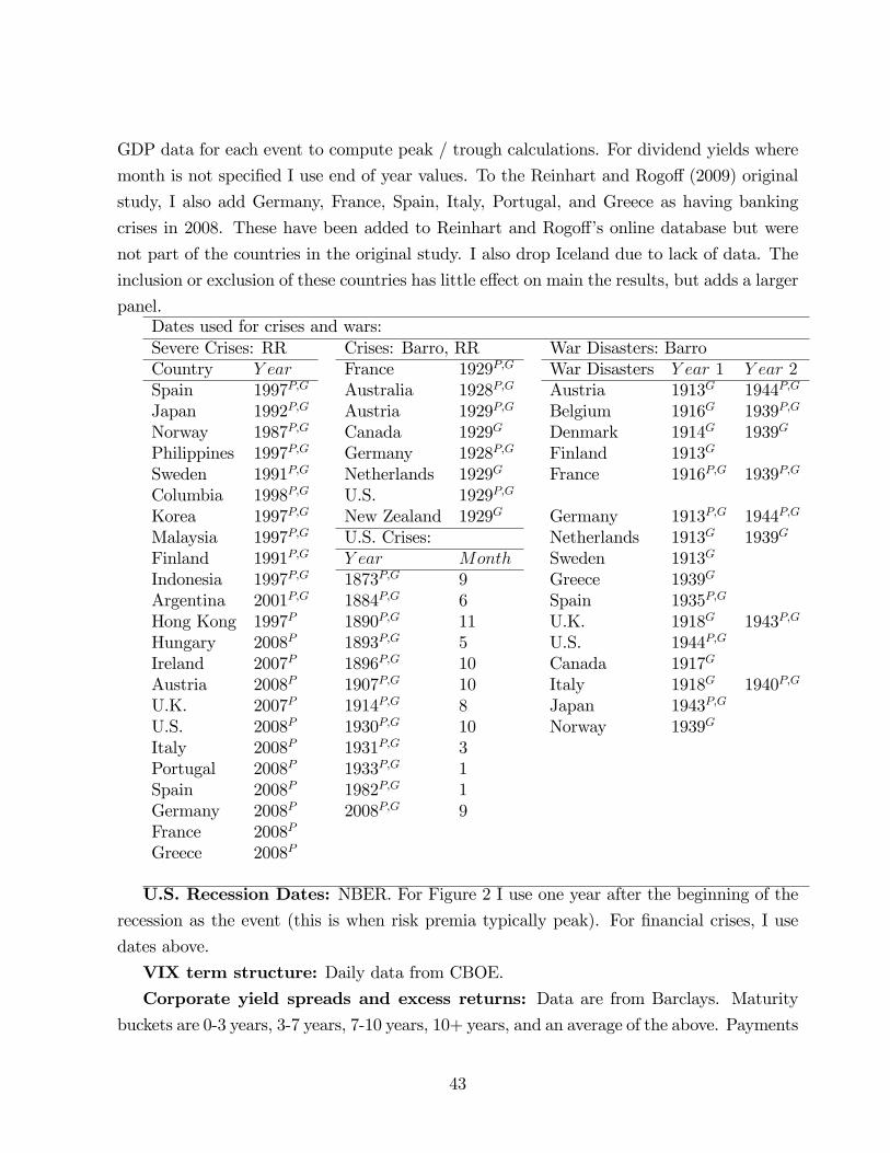
GDP data for each event to compute peak / trough calculations. For dividend yields where

month is not specified I use end of year values. To the Reinhart and Rogoff (2009) original

study, I also add Germany, France, Spain, Italy, Portugal, and Greece as having banking

crises in 2008. These have been added to Reinhart and Rogoff’s online database but were

not part of the countries in the original study. I also drop Iceland due to lack of data. The

inclusion or exclusion of these countries has little effect on main the results, but adds a larger

panel.Dates used for crises and wars:Severe Crises: RR Crises: Barro, RR War Disasters: BarroCountry Y ear France 1929P,G War Disasters Y ear 1 Y ear 2Spain 1997P,G Australia 1928P,G Austria 1913G 1944P,G

Japan 1992P,G Austria 1929P,G Belgium 1916G 1939P,G

Norway 1987P,G Canada 1929G Denmark 1914G 1939G

Philippines 1997P,G Germany 1928P,G Finland 1913G

Sweden 1991P,G Netherlands 1929G France 1916P,G 1939P,G

Columbia 1998P,G U.S. 1929P,G

Korea 1997P,G New Zealand 1929G Germany 1913P,G 1944P,G

Malaysia 1997P,G U.S. Crises: Netherlands 1913G 1939G

Finland 1991P,G Y ear Month Sweden 1913G

Indonesia 1997P,G 1873P,G 9 Greece 1939G

Argentina 2001P,G 1884P,G 6 Spain 1935P,G

Hong Kong 1997P 1890P,G 11 U.K. 1918G 1943P,G

Hungary 2008P 1893P,G 5 U.S. 1944P,G

Ireland 2007P 1896P,G 10 Canada 1917G

Austria 2008P 1907P,G 10 Italy 1918G 1940P,G

U.K. 2007P 1914P,G 8 Japan 1943P,G

U.S. 2008P 1930P,G 10 Norway 1939G

Italy 2008P 1931P,G 3Portugal 2008P 1933P,G 1Spain 2008P 1982P,G 1Germany 2008P 2008P,G 9France 2008P

Greece 2008P

U.S. Recession Dates: NBER. For Figure 2 I use one year after the beginning of therecession as the event (this is when risk premia typically peak). For financial crises, I use

dates above.

VIX term structure: Daily data from CBOE.

Corporate yield spreads and excess returns: Data are from Barclays. Maturity

buckets are 0-3 years, 3-7 years, 7-10 years, 10+ years, and an average of the above. Payments

43

for each bond are matched to the appropriate Treasury curve and the appropriate risk free

rate is subtracted off each. The yields are adjusted for optionality / callability. Excess

returns are over a portfolio of Treasury returns of matched maturity. Data are from 1989-

2012. I have each of these data separately for investment grade and high yield firms. Finally,

for daily corporate yield spreads I use data downloaded from FRED (1996-2012). These are

higher frequency but have a shorter sample. They behave similarly to the Barclays spreads

over the 1996-2012 period. The BofA Merrill Lynch Option-Adjusted Spreads (OASs) are

the calculated spreads between a computed OAS index of all investment grade bonds and

a spot Treasury curve. An OAS index is constructed using each constituent bond’s OAS,

weighted by market capitalization. Series names (BAMLC1A0C13Y, BAMLC2A0C35Y,

BAMLC3A0C57Y, BAMLC4A0C710Y, BAMLC7A0C1015Y, BAMLC8A0C15PY).

Moody’s Analytics EDF Data: Data includes 1-5 year annualized EDF (expecteddefault frequency) using average EDFs for panels of investment grade firms with between 330

and 570 firms per year. I also have analagous data for high yield firms. EDFs are computed

following a two step process. First, Moody’s constructs a default proxy using a structural

option-based model of default by modeling equity as a call option. These are then improved

upon by using the combined optimal forecast obtained statistically from using these default

proxies and other explanatory variables to forecast realized defaults. Moody’s KMV has the

largest empirical default database available which allows them to construct EDF measures

that are highly accurate. Moody’s constructs longer maturity EDFs by setting the forward

default rate equal to the forward default rate between years 4 and 5.

Historical Bond Data: Pulled from bond tables from the New York Times historical

issues for each recession and financial crisis after 1929 for which I do not already have bond

yield data. I use banking crisis dates (see above) and recession midpoint dates (i.e. the

month halfway between the peak and trough). I use the last available day of each month

and collect bond prices, coupon rates, and maturity dates, which I convert to yields. As much

as possible I try to use firms with multiple maturity bonds outstanding. I drop any yields

above 25% as these firms are close to default and will have a large influence on averages. I

then use government bond yields from the same table to compute a risk-free curve where

I just linearly fit points between maturities. When not enough government maturities are

available, I supplement these government yields with data on 3-month Treasury bills from

NBERMacro History (series M13029b) and data on long term government yields from FRED

(series LTGOVTBD). I then sort corporate yields by maturity, compute equal weighted

buckets by maturity (0-3 years, 5-7, 7-10, 10+) and subtract the closest possible government

yield from each bucket. I ensure that there are at least 10 bond yields in each bucket for

44

each date.

Equity yields: Figure 15 is from van Binsbergen et al. (2012b).

GDP and Consumption Data: GDP data are from Robert Barro’s webiste (see,

e.g., Barro et al. (2011)). When computing GDP growth rates around financial crises and

recessions, I subtract off the respective countries’long term economic growth rate, defined

as the linear trend in log per capita GDP.

Dividends: Real dividends are from Robert Shiller’s website. For the U.S. data, I

use the annual sum of this real dividend series to compute price dividend ratios (real price

divided by sum of previous year’s real dividend) which controls for seasonality in dividends.

Country Level Price and Dividend Yield Data: All indices for all countries arefrom Global Financial Data. All price series are real values of stock indices in U.S. dollars.

U.S. Market Excess Return: From Kenneth French’s website when possible. When

calculating monthly volatility of the stock market and “vol of vol,” however, I use daily

S&P500 observations from CRSP. I also pull the momentum, size and book-to-market

portoflios from Kenneth French’s website.

7.2 Solving the Term Structure of Risky Bonds, Equities, andVolatility

I show how to calculate prices and yields for risky bonds, equities, and volatility.

Throughout, I denote the SDF as

dΛ

Λ= −rdt− λdBt (32)

Where r is the risk free rate and λ = µ−rσis the instantaneous Sharpe ratio or “price of

risk.”Given these objects in the model, we can price any asset including corporate bonds

and dividend strips.

Asset prices are given by P (N)t = E

[Λt+N

Λtxt+N

]where xt+N represents the cash flow the

asset pays off at time t + N and P (N)t represents the price of this cash flow. I simulate

Λt+NΛt.using the formula ΛT

Λ0= exp

(∫ T0

(µΛ − 1

2σ2

Λ

)dt+

∫ T0σΛdBt

). I simulate the discount

rate and cash flow processes forward, creating 3,000 realizations of Λt+NΛt

and xt+N and then

take an average to find the price P (N)t .

Pricing formulas for various assets: Given the discount factor, pricing various assetssimply amounts to specifying their cash flow process. I will generally use lower case letters

to denote logs.

45

Risk free bonds: xt+N = 1. P (N)t = E

[Λt+N

Λt

]where N is years to maturity. I will define

risk free bond yields as y(N)t = − 1

Np

(N)t = − 1

Nln(P

(N)t

). In the model, the risk free term

structure is flat since the interest rate is constant.

Dividend Strips: xt+N = Dt+NDt. Define S

(N)t

D(N)t

= E[

Λt+NΛt

Dt+NDt

]as the price of the

aggregate dividend paying off in period N . I divide by current dividend for scale. Let

sd(N)t = ln

(S

(N)t

Dt

). The process for Dt+N

Dtis straightforward to simulate since it is given

direcly in the model by dYY.

Thus

ln

(S

(N)t

D(N)t

)= ln

(E

[exp

(∫ t+N

t

(µY,t − r −

1

2

(σ2 + λ2

t

))dt+

∫ t+N

t

(σ − λt) dBt

)])It is useful to decompose dividend strips into a growth component, a risk free component,

and a risk premium component. Define the following:

sd(N)t = N

(g

(N)t − y(N)

t − rp(N)t

)Where g

(N)t =

1

NEt

[ln

(Dt+N

Dt

)]Define ys

(N)t = − 1

Nsd

(N)t

Then ys(N)t = −g(N)

t + rp(N)t + y

(N)t

ef(N)t ≡ rp

(N)t − g(N)

t

The object ef(N)t (the “forward equity yield”) is useful since it is related to either risk

premia or growth expectations (see van Binsbergen et al. (2012b) who define and study this

object empirically).

VIX: xt+N =∫ t+Nt

σ2R,udu. VIX is the square root of the expected variance under the

risk neutral measure Q (where EQ (xt+N) = 1

E[

Λt+NΛt

]E [Λt+NΛt

xt+N

]). We can therefore simply

think of this as an asset paying the integrated variance as its cash flow. I specify the VIX

term structure for maturity N as

V IX2t,N =

1

NE

[Λt+N

Λt

xt+N

]=

exp (−rN)

NEQ

(∫ t+N

t

σ2R,udu

)Of course, as with equity yields, we can represent VIX as an expected variance component

and a variance risk premium. There are multiple ways to define the risk premium. In this

paper, I will use: rpvNt = V IXt,N −√

1NE(∫ t+N

tσ2R,udu

). Some papers instead define the

46

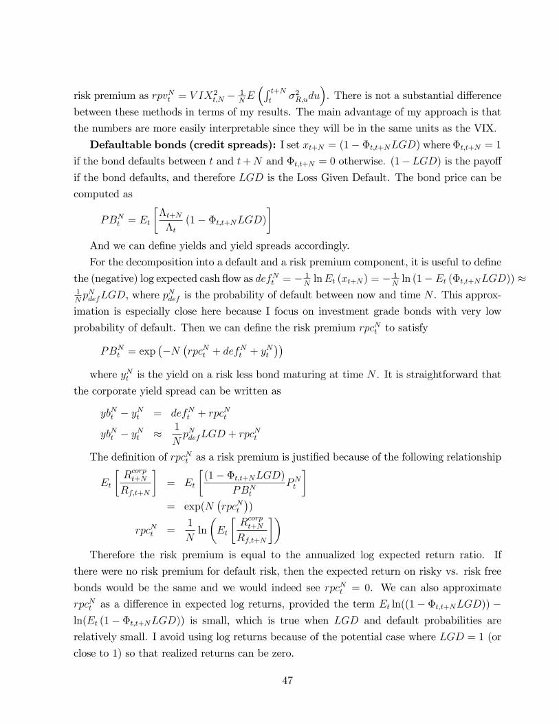
risk premium as rpvNt = V IX2t,N − 1

NE(∫ t+N

tσ2R,udu

). There is not a substantial difference

between these methods in terms of my results. The main advantage of my approach is that

the numbers are more easily interpretable since they will be in the same units as the VIX.

Defaultable bonds (credit spreads): I set xt+N = (1− Φt,t+NLGD) where Φt,t+N = 1

if the bond defaults between t and t+N and Φt,t+N = 0 otherwise. (1−LGD) is the payoff

if the bond defaults, and therefore LGD is the Loss Given Default. The bond price can be

computed as

PBNt = Et

[Λt+N

Λt

(1− Φt,t+NLGD)

]And we can define yields and yield spreads accordingly.

For the decomposition into a default and a risk premium component, it is useful to define

the (negative) log expected cash flow as defNt = − 1N

lnEt (xt+N) = − 1N

ln (1− Et (Φt,t+NLGD)) ≈1NpNdefLGD, where p

Ndef is the probability of default between now and time N . This approx-

imation is especially close here because I focus on investment grade bonds with very low

probability of default. Then we can define the risk premium rpcNt to satisfy

PBNt = exp

(−N

(rpcNt + defNt + yNt

))where yNt is the yield on a risk less bond maturing at time N . It is straightforward that

the corporate yield spread can be written as

ybNt − yNt = defNt + rpcNt

ybNt − yNt ≈ 1

NpNdefLGD + rpcNt

The definition of rpcNt as a risk premium is justified because of the following relationship

Et

[Rcorpt+N

Rf,t+N

]= Et

[(1− Φt,t+NLGD)

PBNt

PNt

]= exp(N

(rpcNt

))

rpcNt =1

Nln

(Et

[Rcorpt+N

Rf,t+N

])Therefore the risk premium is equal to the annualized log expected return ratio. If

there were no risk premium for default risk, then the expected return on risky vs. risk free

bonds would be the same and we would indeed see rpcNt = 0. We can also approximate

rpcNt as a difference in expected log returns, provided the term Et ln((1− Φt,t+NLGD)) −ln(Et (1− Φt,t+NLGD)) is small, which is true when LGD and default probabilities are

relatively small. I avoid using log returns because of the potential case where LGD = 1 (or

close to 1) so that realized returns can be zero.

47

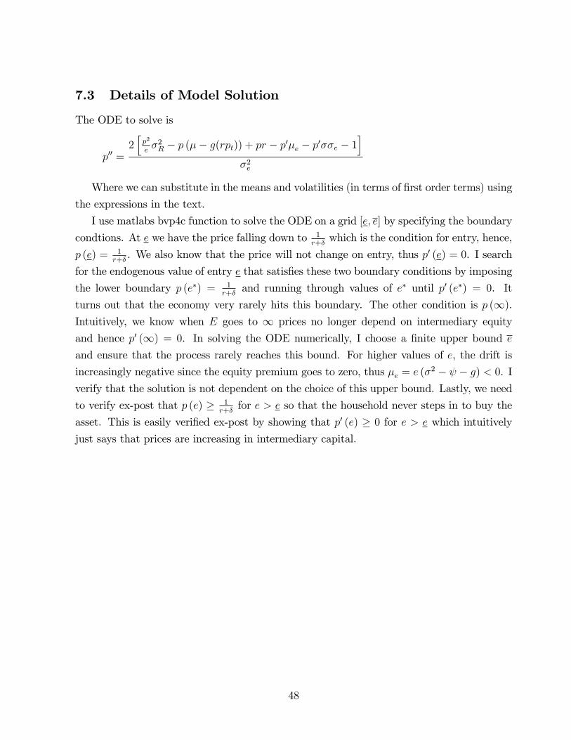
7.3 Details of Model Solution

The ODE to solve is

p′′ =2[p2

eσ2R − p (µ− g(rpt)) + pr − p′µe − p′σσe − 1

]σ2e

Where we can substitute in the means and volatilities (in terms of first order terms) using

the expressions in the text.

I use matlabs bvp4c function to solve the ODE on a grid [e, e] by specifying the boundary

condtions. At e we have the price falling down to 1r+δ

which is the condition for entry, hence,

p (e) = 1r+δ. We also know that the price will not change on entry, thus p′ (e) = 0. I search

for the endogenous value of entry e that satisfies these two boundary conditions by imposing

the lower boundary p (e∗) = 1r+δ

and running through values of e∗ until p′ (e∗) = 0. It

turns out that the economy very rarely hits this boundary. The other condition is p (∞).

Intuitively, we know when E goes to ∞ prices no longer depend on intermediary equity

and hence p′ (∞) = 0. In solving the ODE numerically, I choose a finite upper bound e

and ensure that the process rarely reaches this bound. For higher values of e, the drift is

increasingly negative since the equity premium goes to zero, thus µe = e (σ2 − ψ − g) < 0. I

verify that the solution is not dependent on the choice of this upper bound. Lastly, we need

to verify ex-post that p (e) ≥ 1r+δ

for e > e so that the household never steps in to buy the

asset. This is easily verified ex-post by showing that p′ (e) ≥ 0 for e > e which intuitively

just says that prices are increasing in intermediary capital.

48

8 Figures/Tables

49

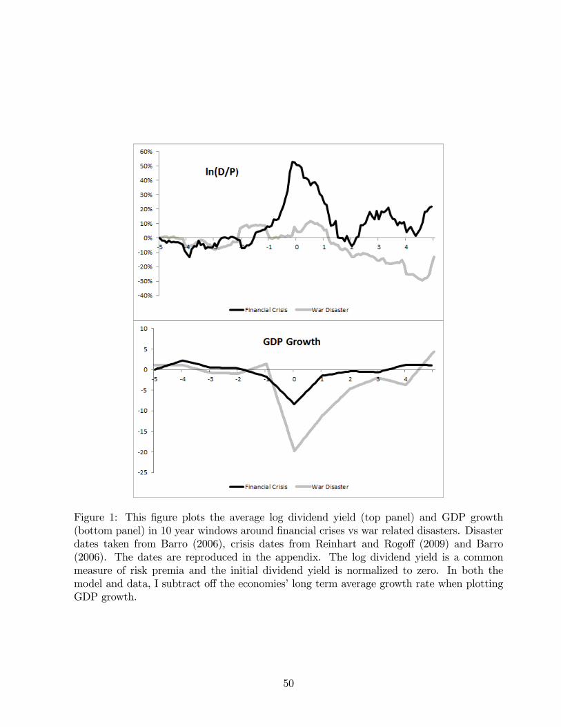
Figure 1: This figure plots the average log dividend yield (top panel) and GDP growth(bottom panel) in 10 year windows around financial crises vs war related disasters. Disasterdates taken from Barro (2006), crisis dates from Reinhart and Rogoff (2009) and Barro(2006). The dates are reproduced in the appendix. The log dividend yield is a commonmeasure of risk premia and the initial dividend yield is normalized to zero. In both themodel and data, I subtract off the economies’long term average growth rate when plottingGDP growth.

50

Figure 2: I split US recessions into those involving a financial crisis (black lines) and those notinvolving a financial crisis (gray lines). For non-financial recessions I use one year after thebeginning of recession dates marked as zero, as this is the typical peak for risk premia. Forfinancial recessions I use crisis dates from the appendix. I compare the two events in termsof risk premia as measured by the log dividend yield (upper left panel), the BaaAaa defaultspread (upper right panel), GDP growth (lower left panel), and stock market volatility (lowerright panel). I use a 10 year window centered around the event. Recession dates from NBER.See appendix for dates and data sources.

51

Figure 3: I provide a historical perspective of proxies for risk premia in the US from 1834-2012. Both panels plot the log dividend yield and BaaAaa spread from 1834-1919 as measuresof risk premia. In the top panel, shaded areas represent war related disasters or the beginningof wars. In the bottom panel, shaded areas indicate financial crises or periods of highfinancial distress. For the period 1834-1871, I use the consumption to price ratio instead ofthe dividend to price ratio since the dividend series does not extend back this far. I normalizethe consumption price ratio to have the same mean and standard deviation as the dividendprice ratio. In the later sample, these two series are very highly correlated.

52

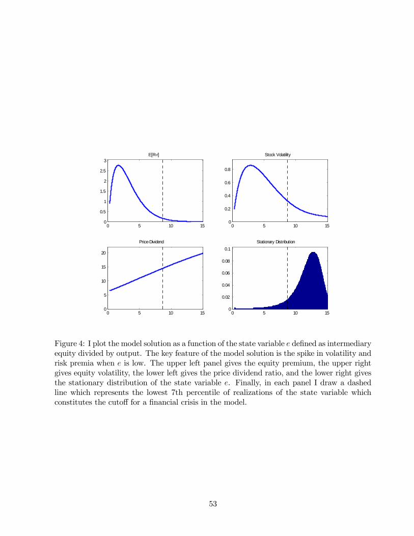
0 5 10 150

0.5

1

1.5

2

2.5

3E[R­r]

0 5 10 150

0.2

0.4

0.6

0.8

Stock Volatility

0 5 10 150

5

10

15

20

Price­Dividend

0 5 10 150

0.02

0.04

0.06

0.08

0.1Stationary Distribution

Figure 4: I plot the model solution as a function of the state variable e defined as intermediaryequity divided by output. The key feature of the model solution is the spike in volatility andrisk premia when e is low. The upper left panel gives the equity premium, the upper rightgives equity volatility, the lower left gives the price dividend ratio, and the lower right givesthe stationary distribution of the state variable e. Finally, in each panel I draw a dashedline which represents the lowest 7th percentile of realizations of the state variable whichconstitutes the cutoff for a financial crisis in the model.

53

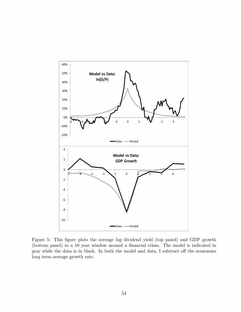
Figure 5: This figure plots the average log dividend yield (top panel) and GDP growth(bottom panel) in a 10 year window around a financial crises. The model is indicated ingray while the data is in black. In both the model and data, I subtract off the economieslong term average growth rate.

54

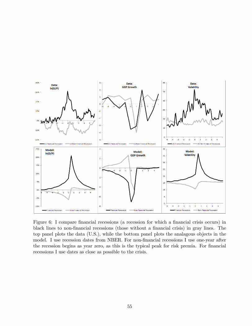
Figure 6: I compare financial recessions (a recession for which a financial crisis occurs) inblack lines to non-financial recessions (those without a financial crisis) in gray lines. Thetop panel plots the data (U.S.), while the bottom panel plots the analagous objects in themodel. I use recession dates from NBER. For non-financial recessions I use one-year afterthe recession begins as year zero, as this is the typical peak for risk premia. For financialrecessions I use dates as close as possible to the crisis.

55

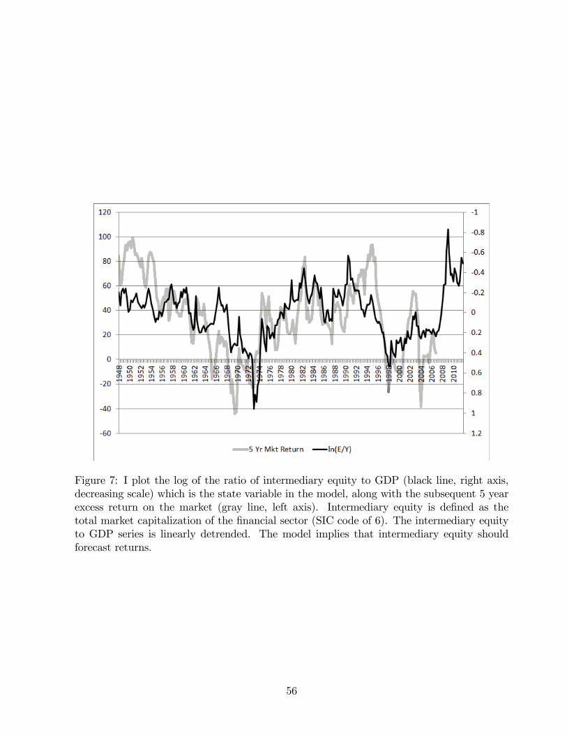
Figure 7: I plot the log of the ratio of intermediary equity to GDP (black line, right axis,decreasing scale) which is the state variable in the model, along with the subsequent 5 yearexcess return on the market (gray line, left axis). Intermediary equity is defined as thetotal market capitalization of the financial sector (SIC code of 6). The intermediary equityto GDP series is linearly detrended. The model implies that intermediary equity shouldforecast returns.

56

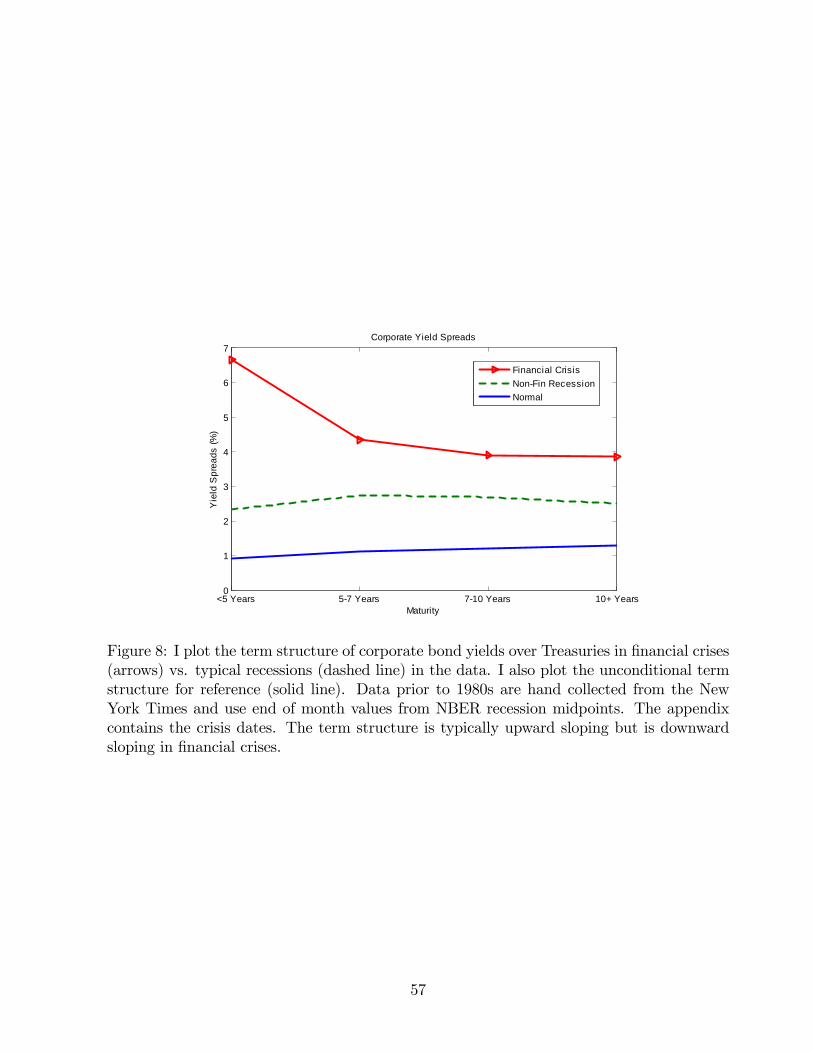
   <5 Years 5­7 Years 7­10 Years 10+ Years0

1

2

3

4

5

6

7

Maturity

Yie

ld S

prea

ds (%

)

Corporate Yield Spreads

Financial CrisisNon­Fin RecessionNormal

Figure 8: I plot the term structure of corporate bond yields over Treasuries in financial crises(arrows) vs. typical recessions (dashed line) in the data. I also plot the unconditional termstructure for reference (solid line). Data prior to 1980s are hand collected from the NewYork Times and use end of month values from NBER recession midpoints. The appendixcontains the crisis dates. The term structure is typically upward sloping but is downwardsloping in financial crises.

57

0 0.5 1 1.5 2 2.5 3 3.5 4 4.5 50

0.1

0.2

0.3

0.4

0.5

0.6

0.7

0.8

0.9

1

Y ears

Cris

is P

roba

bilit

ies 

by R

egim

e

N orm alD angerC ris is

Figure 9: I plot the term structure of crisis probabilities implied by the model, conditonalon the state of the economy. Each maturity corresponds to the probability of being in acrisis state at that point in time. Normal, danger, and crisis correspond to the current valueof intermediary equity to output, e, where normal is the 20th percentile and above, dangeris between the 7th and 20th percentile, and crisis is the bottom 7th percentile. In normaltimes the term structure slopes up since a crisis in the immediate future is highly unlikely,while in the long term it is higher. In contrast, when in a crisis, recovery next month is low,but is more likely in several years. This feature of the model helps me match key featuresof the term structure of risky assets in the data.

58

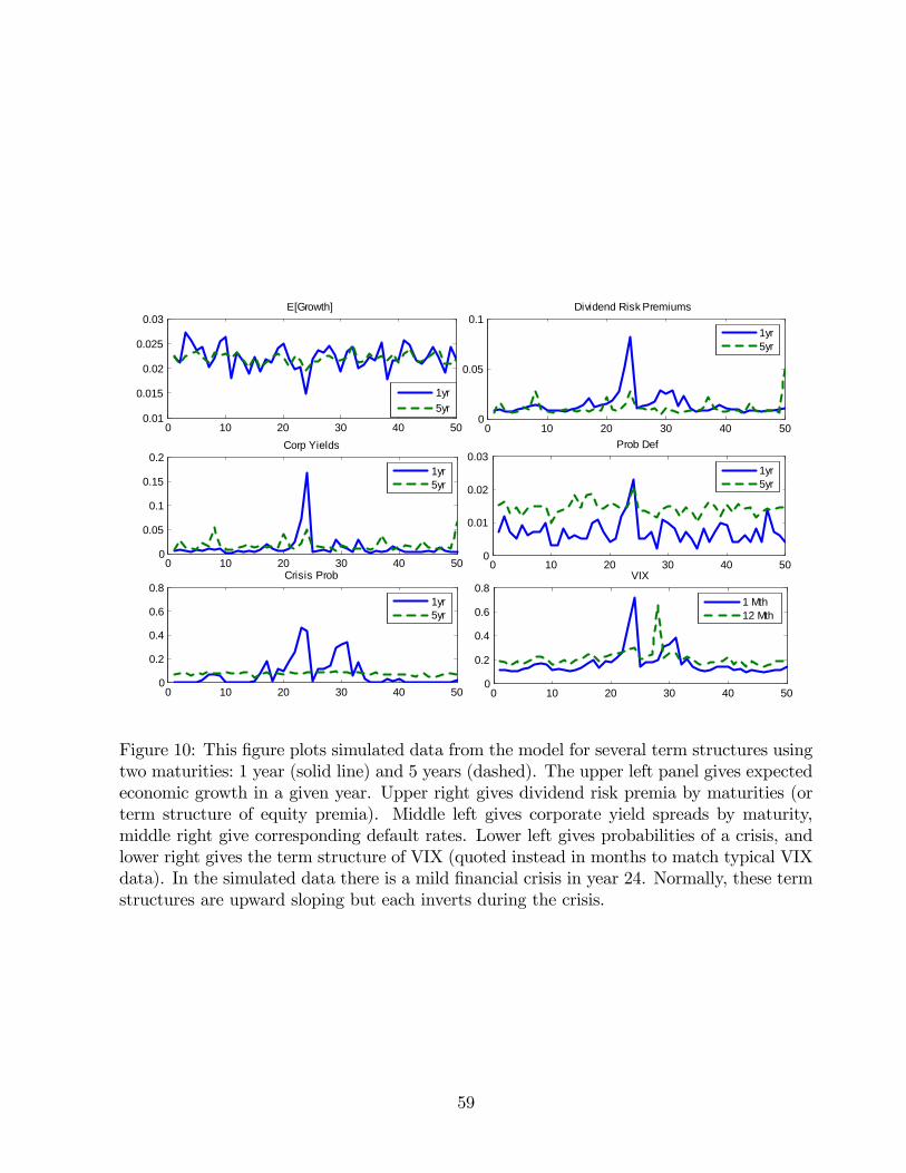
0 10 20 30 40 500.01

0.015

0.02

0.025

0.03E[Growth]

1yr5yr

0 10 20 30 40 500

0.05

0.1Dividend Risk Premiums

1yr5yr

0 10 20 30 40 500

0.05

0.1

0.15

0.2Corp Yields

1yr5yr

0 10 20 30 40 500

0.01

0.02

0.03Prob Def

1yr5yr

0 10 20 30 40 500

0.2

0.4

0.6

0.8Crisis Prob

1yr5yr

0 10 20 30 40 500

0.2

0.4

0.6

0.8VIX

1 Mth12 Mth

Figure 10: This figure plots simulated data from the model for several term structures usingtwo maturities: 1 year (solid line) and 5 years (dashed). The upper left panel gives expectedeconomic growth in a given year. Upper right gives dividend risk premia by maturities (orterm structure of equity premia). Middle left gives corporate yield spreads by maturity,middle right give corresponding default rates. Lower left gives probabilities of a crisis, andlower right gives the term structure of VIX (quoted instead in months to match typical VIXdata). In the simulated data there is a mild financial crisis in year 24. Normally, these termstructures are upward sloping but each inverts during the crisis.

59

Figure 11: I plot investment grade US corporate yield spreads of varying maturities. I usematurities between 0-3 years (black line) and above 10 years (gray line), but all resutls holdincluding intermediate maturities as well. The top panel plots the yield spreads in basispoints, the middle panel plots the risk premium component of yields in basis points, and thebottom panel plots the annualized probability of default based on Moody’s EDF data. Ineach panel, the lower thin line plots the slope of the term structure considered (long maturityminus short maturity). The plot suggests an inversion in yields during crisis times that ismainly due to risk premia. See appendix for details on the data.

60

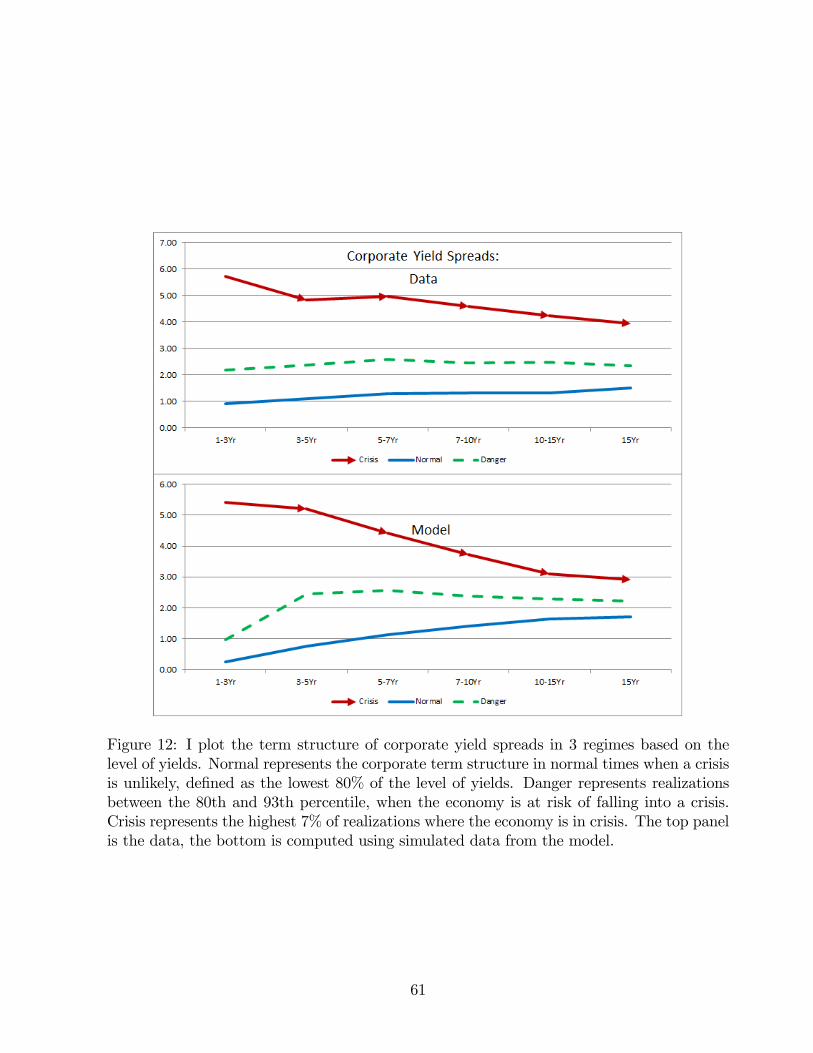
Figure 12: I plot the term structure of corporate yield spreads in 3 regimes based on thelevel of yields. Normal represents the corporate term structure in normal times when a crisisis unlikely, defined as the lowest 80% of the level of yields. Danger represents realizationsbetween the 80th and 93th percentile, when the economy is at risk of falling into a crisis.Crisis represents the highest 7% of realizations where the economy is in crisis. The top panelis the data, the bottom is computed using simulated data from the model.

61

1996 1998 2000 2002 2004 2006 2008 2010­50

0

50

100VIX

VIX3 VIX1 Slope

1996 1998 2000 2002 2004 2006 2008 2010­20

­10

0

10

20Risk Premium

VRP3 VRP1 Slope

1996 1998 2000 2002 2004 2006 2008 2010­20

0

20

40

60

80Expected Variance

E[Var1] E[Var3] Slope

Figure 13: The top panel plots the daily VIX term structure in the data for maturities 1month (thick gray line) and 3 months (black line), along with the slope of the term structure(thin lower line). The middle and lower panels decompose the VIX into a risk premiumcomponent (middle panel) and an expected variance component (lower panel). The expectedvariance is the square root of the expected integrated variance so that its units are consistentwith the VIX. I plot the term structure and slope for each of these. See paper for details onestimation.

62

Figure 14: I plot the VIX term structure in both the data and the model in 3 regimes. Thex-axis is in months. Normal represents the VIX term structure in normal times when a crisisis unlikely, defined as the lowest 80% of VIX realizations. Danger represents realizationsbetween the 80th and 93th percentile, when the economy is at risk of falling into a crisis.Crisis represents the highest 7% of realizations where the economy is in a crisis. The toppanel is the data, the bottom is computed using simulated data from the model.

63

Figure 15: The top panel corresponds to Figure 1 in van Binsbergen et al. (2012b). The figureplots equity yields of various maturities on the S&P 500. Equity yields are the forward yieldsof a claim to the dividend growth rate on the S&P 500 over n years, where n correspondsto the maturity. The bottom panel plots equity yield risk premia, as estimated by vanBinsbergen et al. (2012b), Figure 6. Both panels suggest that the equity yield curve andequity risk premium curve is typically upward sloping but slopes downward in the recentfinancial crisis.

64

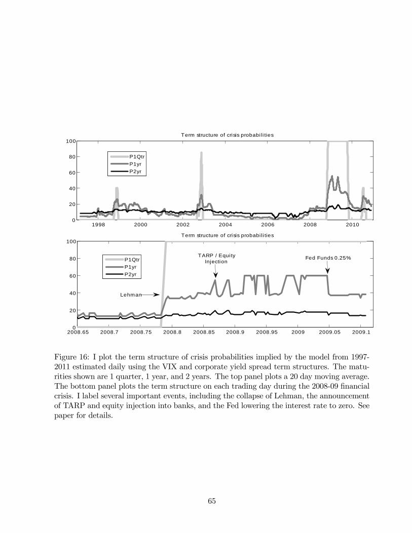
1998 2000 2002 2004 2006 2008 20100

20

40

60

80

100Term structure of crisis probabi li ties

P1QtrP1yrP2yr

2008.65 2008.7 2008.75 2008.8 2008.85 2008.9 2008.95 2009 2009.05 2009.10

20

40

60

80

100Term structure of crisis probabi li ties

P1QtrP1yrP2yr

TARP / EquityInjection

Fed Funds 0.25%

Lehman

Figure 16: I plot the term structure of crisis probabilities implied by the model from 1997-2011 estimated daily using the VIX and corporate yield spread term structures. The matu-rities shown are 1 quarter, 1 year, and 2 years. The top panel plots a 20 day moving average.The bottom panel plots the term structure on each trading day during the 2008-09 financialcrisis. I label several important events, including the collapse of Lehman, the announcementof TARP and equity injection into banks, and the Fed lowering the interest rate to zero. Seepaper for details.

65

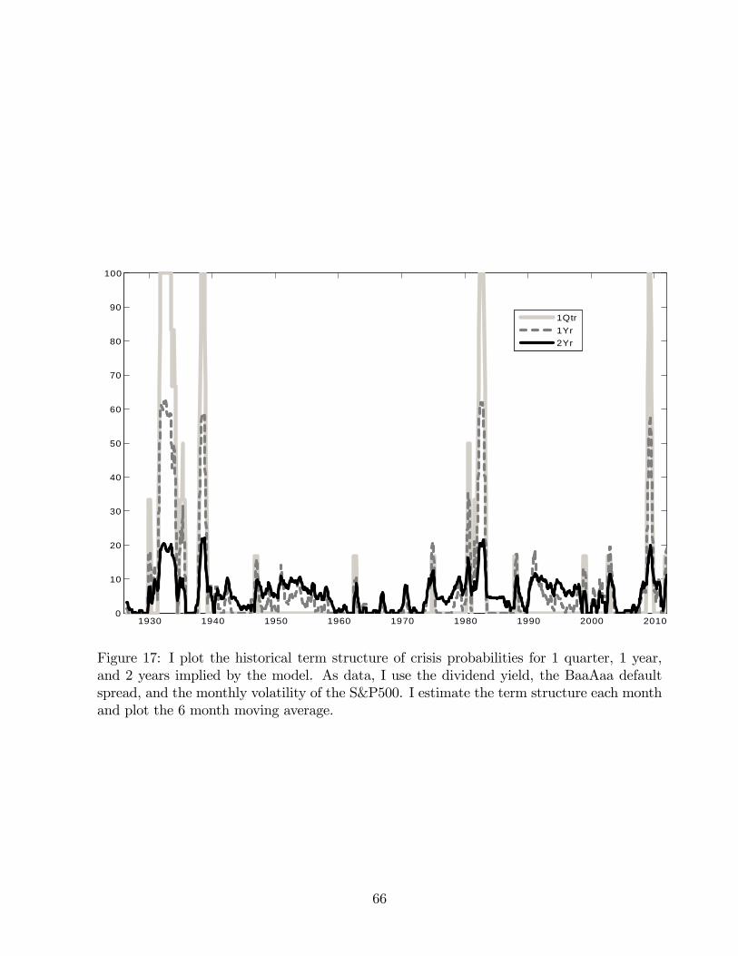
1930 1940 1950 1960 1970 1980 1990 2000 20100

10

20

30

40

50

60

70

80

90

100

1Qtr1Yr2Yr

Figure 17: I plot the historical term structure of crisis probabilities for 1 quarter, 1 year,and 2 years implied by the model. As data, I use the dividend yield, the BaaAaa defaultspread, and the monthly volatility of the S&P500. I estimate the term structure each monthand plot the 6 month moving average.

66

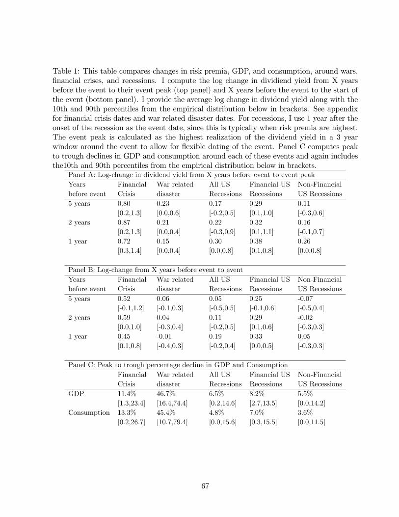
Table 1: This table compares changes in risk premia, GDP, and consumption, around wars,financial crises, and recessions. I compute the log change in dividiend yield from X yearsbefore the event to their event peak (top panel) and X years before the event to the start ofthe event (bottom panel). I provide the average log change in dividend yield along with the10th and 90th percentiles from the empirical distribution below in brackets. See appendixfor financial crisis dates and war related disaster dates. For recessions, I use 1 year after theonset of the recession as the event date, since this is typically when risk premia are highest.The event peak is calculated as the highest realization of the dividend yield in a 3 yearwindow around the event to allow for flexible dating of the event. Panel C computes peakto trough declines in GDP and consumption around each of these events and again includesthe10th and 90th percentiles from the empirical distribution below in brackets.

Panel A: Log-change in dividend yield from X years before event to event peakYears Financial War related All US Financial US Non-Financialbefore event Crisis disaster Recessions Recessions US Recessions5 years 0.80 0.23 0.17 0.29 0.11

[0.2,1.3] [0.0,0.6] [-0.2,0.5] [0.1,1.0] [-0.3,0.6]2 years 0.87 0.21 0.22 0.32 0.16

[0.2,1.3] [0.0,0.4] [-0.3,0.9] [0.1,1.1] [-0.1,0.7]1 year 0.72 0.15 0.30 0.38 0.26

[0.3,1.4] [0.0,0.4] [0.0,0.8] [0.1,0.8] [0.0,0.8]

Panel B: Log-change from X years before event to eventYears Financial War related All US Financial US Non-Financialbefore event Crisis disaster Recessions Recessions US Recessions5 years 0.52 0.06 0.05 0.25 -0.07

[-0.1,1.2] [-0.1,0.3] [-0.5,0.5] [-0.1,0.6] [-0.5,0.4]2 years 0.59 0.04 0.11 0.29 -0.02

[0.0,1.0] [-0.3,0.4] [-0.2,0.5] [0.1,0.6] [-0.3,0.3]1 year 0.45 -0.01 0.19 0.33 0.05

[0.1,0.8] [-0.4,0.3] [-0.2,0.4] [0.0,0.5] [-0.3,0.3]

Panel C: Peak to trough percentage decline in GDP and ConsumptionFinancial War related All US Financial US Non-FinancialCrisis disaster Recessions Recessions US Recessions

GDP 11.4% 46.7% 6.5% 8.2% 5.5%[1.3,23.4] [16.4,74.4] [0.2,14.6] [2.7,13.5] [0.0,14.2]

Consumption 13.3% 45.4% 4.8% 7.0% 3.6%[0.2,26.7] [10.7,79.4] [0.0,15.6] [0.3,15.5] [0.0,11.5]

67

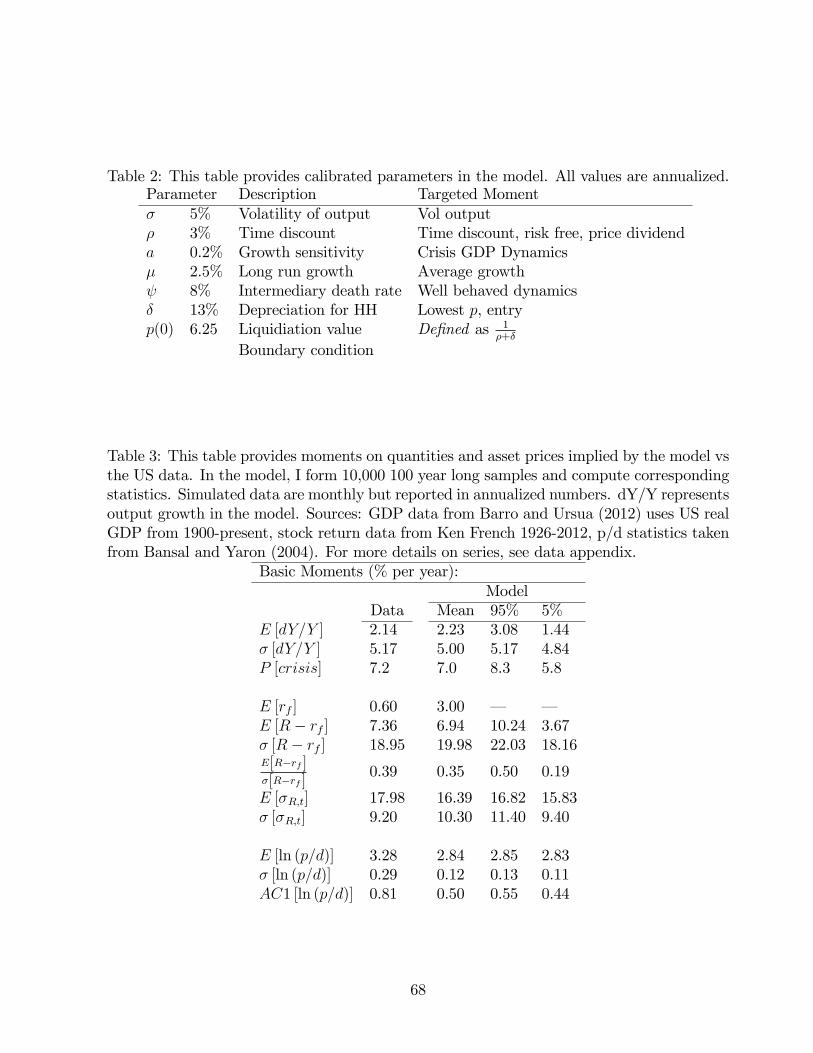
Table 2: This table provides calibrated parameters in the model. All values are annualized.Parameter Description Targeted Momentσ 5% Volatility of output Vol outputρ 3% Time discount Time discount, risk free, price dividenda 0.2% Growth sensitivity Crisis GDP Dynamicsµ 2.5% Long run growth Average growthψ 8% Intermediary death rate Well behaved dynamicsδ 13% Depreciation for HH Lowest p, entryp(0) 6.25 Liquidiation value Defined as 1

ρ+δ

Boundary condition

Table 3: This table provides moments on quantities and asset prices implied by the model vsthe US data. In the model, I form 10,000 100 year long samples and compute correspondingstatistics. Simulated data are monthly but reported in annualized numbers. dY/Y representsoutput growth in the model. Sources: GDP data from Barro and Ursua (2012) uses US realGDP from 1900-present, stock return data from Ken French 1926-2012, p/d statistics takenfrom Bansal and Yaron (2004). For more details on series, see data appendix.

Basic Moments (% per year):Model

Data Mean 95% 5%E [dY/Y ] 2.14 2.23 3.08 1.44σ [dY/Y ] 5.17 5.00 5.17 4.84P [crisis] 7.2 7.0 8.3 5.8

E [rf ] 0.60 3.00 – –E [R− rf ] 7.36 6.94 10.24 3.67σ [R− rf ] 18.95 19.98 22.03 18.16E[R−rf ]σ[R−rf ]

0.39 0.35 0.50 0.19

E [σR,t] 17.98 16.39 16.82 15.83σ [σR,t] 9.20 10.30 11.40 9.40

E [ln (p/d)] 3.28 2.84 2.85 2.83σ [ln (p/d)] 0.29 0.12 0.13 0.11AC1 [ln (p/d)] 0.81 0.50 0.55 0.44

68

Table 4: This table provides moments on the depth, duration, and distribution on outcomessurrounding financial crises. I create an artificial sample of crises in the model with the samenumber of crises as the data. I then calculate corresponding statistics over 10,000 of thesesamples. Panel C runs panel regressions to test for increases in annual dividend yields duringcrises, controlling for lagged annual dividend yields. Data on GDP are from GDP data fromBarro and Ursua (2012), data on real equities uses dates from Reinhardt and Rogoff (2009),data on dividend yields from Global Financial Data and Shiller (monthly, US).

Panel A: Crisis Severity (Peak to Trough Decline):Data Model

Loss Duration Loss DurationEquities -55.9% 3.4 yrs -40.2% 3.3 yrsGDP -11.4% 3.0 yrs -16.5% 4.5 yrs

Panel B: Distribution of GDP (Peak to Trough):Data Model

Loss Duration Loss Duration10% -1.3% 1.0 yr -9.5% 1.6 yrs90% -23.4% 5.0 yrs -24.9% 9.1 yrsMax -49.9% 15.0 yrs -40.9% 15.9 yrs

Panel C: Increase in Risk Premialn (d/p)i,t = αi + β1crisis,t + ρi ln (d/p)i,t−k + εi,t

Data Modelβ s.e. β s.e.

RR Crises 0.41 (0.08) 0.32 (0.00)US Crises 0.24 (0.07)

69

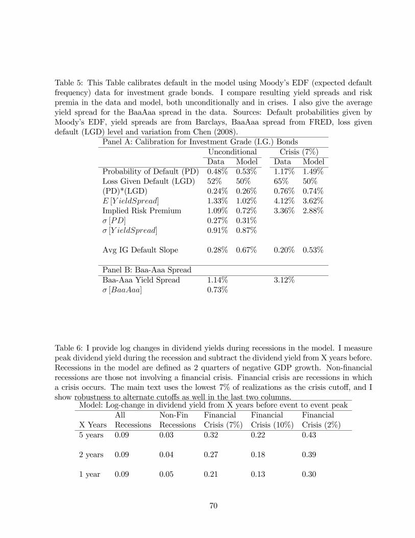
Table 5: This Table calibrates default in the model using Moody’s EDF (expected defaultfrequency) data for investment grade bonds. I compare resulting yield spreads and riskpremia in the data and model, both unconditionally and in crises. I also give the averageyield spread for the BaaAaa spread in the data. Sources: Default probabilities given byMoody’s EDF, yield spreads are from Barclays, BaaAaa spread from FRED, loss givendefault (LGD) level and variation from Chen (2008).

Panel A: Calibration for Investment Grade (I.G.) BondsUnconditional Crisis (7%)Data Model Data Model

Probability of Default (PD) 0.48% 0.53% 1.17% 1.49%Loss Given Default (LGD) 52% 50% 65% 50%(PD)*(LGD) 0.24% 0.26% 0.76% 0.74%E [Y ieldSpread] 1.33% 1.02% 4.12% 3.62%Implied Risk Premium 1.09% 0.72% 3.36% 2.88%σ [PD] 0.27% 0.31%σ [Y ieldSpread] 0.91% 0.87%

Avg IG Default Slope 0.28% 0.67% 0.20% 0.53%

Panel B: Baa-Aaa SpreadBaa-Aaa Yield Spread 1.14% 3.12%σ [BaaAaa] 0.73%

Table 6: I provide log changes in dividend yields during recessions in the model. I measurepeak dividend yield during the recession and subtract the dividend yield from X years before.Recessions in the model are defined as 2 quarters of negative GDP growth. Non-financialrecessions are those not involving a financial crisis. Financial crisis are recessions in whicha crisis occurs. The main text uses the lowest 7% of realizations as the crisis cutoff, and Ishow robustness to alternate cutoffs as well in the last two columns.

Model: Log-change in dividend yield from X years before event to event peakAll Non-Fin Financial Financial Financial

X Years Recessions Recessions Crisis (7%) Crisis (10%) Crisis (2%)5 years 0.09 0.03 0.32 0.22 0.43

2 years 0.09 0.04 0.27 0.18 0.39

1 year 0.09 0.05 0.21 0.13 0.30

70

Table 7: This table compares the predictive power of intermediary capital in the model vs thedata by running predictive regressions of returns on lagged intermediary equity In the data,I use the total market valuation of the financial sector divided by GDP, analagous to themodel. When forecasting asset returns, I include a linear time trend for intermediary equityas this variable is increasing over time. I compare performance to the log price-dividend ratioin the data. T-stats computed using Newey-West with lags depending on horizon. PanelB runs a cross-sectional asset pricing test using 35 portfolios (25 size and book to marketportfolios and 10 momentum portfolios) to test whether intermediary equity is “priced”inthe cross-section of asset returns. Shanken t-stats reported below. Data sources: Remkt andRefin are the market and financial sector excess returns, respectively. All stock returns arefrom Kenneth French’s website. Recorp is an excess corporate bond return from Barclaysconstructed as the return on maturities between 3 and 5 years. All data are from 1948-2012 except corporate bond returns which are from 1988-2012. See appendix for additionaldetails.

Panel A: Predicting Excess Returns: Ret+k = β1xt + β2t+ εt

Model: Data: Data:ln (et) ln (et) ln (P/D)

Return β t (β) R2 β t (β) R2 β t (β) R2

Remktt+1 -0.42 (-13.2) 3% -0.26 (-2.9) 2% -0.10 (-2.3) 1%Remktt+3 -0.39 (-14.4) 7% -0.27 (-3.4) 5% -0.11 (-2.5) 2%Remktt+12 -0.28 (-15.0) 21% -0.28 (-4.6) 17% -0.11 (-2.5) 8%Remktt+60 -0.10 (-14.9) 32% -0.27 (-6.8) 44% -0.13 (-3.9) 29%

Refint+12 -0.92 (-20.6) 51% -0.30 (-4.8) 20% -0.12 (-1.8) 7%Recorpt+12 -0.16 (-13.4) 32% -0.09 (-3.8) 17% -0.03 (-1.9) 10%

Panel B: Cross-Sectional Asset Pricing: E[Re] = a+ λfβf + εta mkt smb hml mom ln (et) AdjR2

Intermediary Model 5.96 0.63 0.43 49%t-stat (0.87) (0.34) (2.76)

Benchmark Model 7.55 0.15 1.45 3.53 13.91 86%t-stat (1.99) (0.04) (1.01) (2.08) (4.55)

71

Table 8: This table provides both unconditional moments and moments conditional on crisesepisodes implied by the model vs the US data. I focus on moments that reflect the dynamicsof risk premia, in particular that show that risk premia “spike”in crises but are temporary,as evidenced by lower autocorrelation of risk premia proxies and negative slope of the termstructure of risk premia during crises. Corp represents corportae yield spreads. Panel Bcomputes the persistence of dividend yields with a dummy for whether the economy is ina financial recession (ie a recession in which there is a financial crisis). I use two measuresof dividend yields: (1) raw log dividend yields, and (2) dividend yields with two breaks in1954, and 1994, following Lettau and van Niewerburgh (2008). T-stats are in parenthesis.The data appendix describes the various dates and sources of different series.

Panel A: Dynamics of Risk Premia (Annualized Numbers)Model Data

Unconditional Crisis Unconditional CrisisE [ln (p/d)] 2.80 2.21 3.20 2.30E [Corp] 1.02 3.62 1.33 4.12E [CorpSlope] 1.48 -2.50 0.24 -1.49E [V IX] 17.75 53.76 22.43 40.98E [V IXSlope] 2.31 -15.83 0.35 -6.21

Panel B: Persistence of dividend yields in financial crisisln(d/p)t+12 = a+ ρ ln(d/p)t + 1finρfin ln(d/p)t + εt+1

DataModel Two-Break No-Break

ρ 0.57 (39.5) 0.67 (9.3) 0.89 (18.5)ρfin -0.03 (-16.0) -0.31 (-2.0) -0.19 (-1.4)ρ+ ρfin 0.53 0.36 0.70

72

Table 9: I run predictive regressions of returns and dividend growth on lagged dividendyields. I include indicators for recessions (NBER dummies) which I split into recessionscontaining a financial crisis and ones that do not. I use two measures of dividend yields: (1)raw log dividend yields, and (2) dividend yields with two breaks in 1954, and 1994, followingLettau and van Niewerburgh (2008). Standard errors computed using Newey-West with 12lags. The dividend yield is defined as the sum of the last 12 monthly real dividends dividedby real price. Dividend growth is defined as the log change in the sum of the 12 monthlyreal dividiends. Data are from 1927-2012.

Panel A: Return predictability in crises and recessionsRt+1 − rf,t = a+ b ln(d/p)t + c1fin ln(d/p)t + d1non,fin ln(d/p)t + εt+1

a b c d Adj R2

Raw dp 0.18 0.12 6.9%(t-stat) (3.90) (2.69)Raw dp 0.18 0.11 0.27 -0.04 12.0%(t-stat) (4.21) (2.71) (1.77) -(0.74)Two Break dp 0.07 0.30 14.6%(t-stat) (4.17) (4.55)Two Break dp 0.07 0.21 0.29 0.26 17.2%(t-stat) (3.72) (3.27) (2.09) (1.85)

Panel A: Dividend growth predictability in crises and recessions

ln(dt+1

dt

)= a+ b ln(d/p)t + c1fin ln(d/p)t + d1non,fin ln(d/p)t + εt+1

a b c d Adj R2

Raw dp -0.01 -0.03 2.0%(t-stat) (-0.51) (-1.24)Raw dp -0.01 -0.03 0.12 0.02 8.6%(t-stat) (-0.37) (-1.37) (2.52) (0.93)Two Break dp 0.01 -0.09 6.6%(t-stat) (1.22) (-2.80)Two Break dp 0.01 -0.06 -0.13 0.06 9.4%(t-stat) (1.61) (-1.86) (-1.93) (0.71)

73