FINANCIAL CONTRACTIBILITY AND ASSETS’ HARDNESS:

INDUSTRIAL COMPOSITION AND GROWTH*

MATÍAS BRAUN

One salient characteristic of poorly developed capital markets is the excessive weight they give to the availability of hard assets in the allocation of financial funds. Where external finance contractibility is poor, higher proportions of assets that more easily remain with investors if the relationship breaks down are used in order to sustain external finance. Consistent with this view, I show that industries whose assets are relatively less tangible perform worse in terms of growth and contribution to GDP in countries with poorly developed financial systems. The impact is larger the more dependent an industry is on external finance. The effect is important (comparable to more traditional determinants of specialization and growth), and robust. Firm-level evidence also confirms finance as the link: leverage is less sensitive to tangibility in better-working capital markets.

JEL Classification: F0, G0, L6, O4 Keywords: Institutions, Financial Development, Collateral, Growth, Industrial Specialization, Incomplete Contracts. * I am very thankful to Philippe Aghion, Ricardo Caballero, Oliver Hart, Ricardo Hausmann, Dale Jorgenson, Rafael La Porta, Andrei Shleifer, Jeremy Stein, Andres Velasco, and to the participants in the seminars at Harvard University and Chile. I am especially grateful to Robert Barro for his constant support. All errors are mine. Comments are very welcome at: braun2@fas.harvard.edu.

1

I. INTRODUCTION

One key insight of the incomplete contracts view is that the existence of physical, nonhuman

assets is critical in holding a relationship together (Williamson [1985, 1998], Hart [1995]). These influence

the parties’ relative position in renegotiation through the threat of parting when contracts are incomplete.

The same can be thought of the entrepreneur-financier relationship (Hart and Moore [1994]) and be

extended to distinguish assets in general in terms of their ability to sustain external financing. One can

think of hard assets as those that would more easily shift to the investor’s control when this is set to happen

or the relationship breaks down, and soft assets as those that do not do this so easily. Real estate,

machinery, and the plant –tangible assets- are almost certainly harder than other more intangibles assets the

firm may have (such as goodwill, R&D, the human capital associated, organizational capital, and even

accounts receivables, cash, inventory or related investments). The higher the proportion of hard assets the

entrepreneur brings to the relationship, the higher the effective protection the outside investor has, and the

more likely the relationship will be stable and become feasible in the first place.

This paper shows that one important characteristic of poorly developed capital markets is the

excessive weight they give to the availability of hard assets in the allocation of financial funds. In the

context of agency and limited contractibility that characterizes the financier-entrepreneur relationship the

kind of assets a firm has is key in ensuring that the financier is protected and is, therefore, willing to

provide funds in the first place. Where external finance contractibility is poor and outside financiers are

weakly protected vis-à-vis the insiders –be because investors rights are unprotected, the monitoring or

screening technologies are less productive, or more generally because property rights are poorly defined or

enforced, all these typical characteristics of underdeveloped financial systems-, external finance demands a

higher proportion of tangible assets. Harder, tangible assets provide the security the environment does not.

The degree of external finance contractibility and the availability of hard assets are substitutes in the

sustainability of external financing. Of course, the substitution does not come for free, especially given that

not all activities or technologies are equally endowed in hard assets. Allocation inefficiencies are likely to

arise. In particular, where contractibility is poor, investment could be biased towards industries naturally

more endowed in hard assets.

2

The approach proposed consists in showing that industries that involve naturally little tangible

assets show worse economic outcomes –in terms of relative size and growth rates- where financial

development is poor. This relative to industries more generously endowed in those kinds of assets, or

relative to what they would have achieved in a more developed financial context. The median tangibility of

assets -that is net property, plant and equipment over total assets- for each industry from data for publicly

listed, U.S.-based companies measures the relative availability of hard assets. Bank credit to the private

sector measures external finance contractibility or financial development. Variation on these two indicators

provides identification for the empirical test based on a generalization of the difference-in-differences

methodology. A panel containing data for 28 manufacturing industrial segments in several countries is

used. The results are as expected. The effects are large, comparable with more traditional explanations of

industrial composition and growth. After controlling for other potential determinants, the share of total

manufacturing value added that comes from sectors with lower than median tangibility would be around

one third higher if a country’s financial system were in the highest quartile of development instead of in the

lowest quartile. Relative to tangible sectors (in the fourth quartile), intangible industries (first quartile)

grow around 1.1% faster under a developed financial system (fourth quartile) than in a less developed one

(first quartile). Both for industrial composition and growth the magnitude and significance of the estimated

effect appears to be larger for industries more dependent on external finance, linking the effects described

above directly to the differential access to external finance. Moreover, using firm-level data, one finds that

the traditional positive effect of tangibility on leverage is larger the lower the level of financial

development the firm faces. The results are robust to different measures of the key concepts, to a number of

omitted variables explanations, and to reverse causality.

The case that financial development matters for growth has been much strengthened in recent

years. Direct evidence on mechanisms through which finance matters, however, is still weak. This paper

aims at providing one such channel, while extending the evidence on the effects of the degree of capital

markets development on aggregate economic outcomes to industrial composition. It also advances in

characterizing what poor financial development means. Importantly, the empirical approach underscores a

source of exogenous variation for financing constraints –the tangibility of assets- that should prove useful

for future empirical work in financial economics. More broadly, the paper provides micro evidence of the

3

large effect institutions –in particular, the ability to write enforceable contracts and the protection of rights-

have on economic outcomes. It does this by demonstrating how the use of a –theoretically and empirically

sound- substitute to good institutions in the financial area appears to be more widespread where these

institutions are thought to be worse.

The paper relates closely to a number of literatures. The introduction focuses on the issues

concerning the real effects of financial development and corporate governance reform, while the conclusion

integrates the paper in a broader context. The literature relating to the links between a country’s degree of

financial development and its per capita income level and rate of growth is large and long dating. The

debate has also been heated; not only on the reason why finance would matter (Bagehot [1873] and Hicks

[1969]’s capital accumulation versus Schumpeter [1912]’s allocation views), but also on whether it matters

significantly or not (Robinson [1952] and Lucas [1988] on the negative side versus Bagehot and

Schumpeter on the positive one). The existence of a correlation was long ago documented (Cameron et. al.

[1967], Goldsmith [1969], and McKinnon [1973]), however correlation does not imply causality. Most

recently King and Levine [1993] showed that financial development and growth are not just

contemporaneously correlated, but the first anticipates the second in a cross-section of countries. The size

of the effect was shown to be large: a one standard deviation higher level of financial development –as

proxy primarily by measures related to the size of the banking sector and the stock market relative to the

economy- implies around one percentage point higher growth rates over long periods of time. Advances

have been made on addressing the potential endogeneity of the size of the financial system to future growth

prospects (Levine and Zervos [1998], and Beck, Levine and Loayza [2000]). The use of legal origins and

financier’s rights as instruments has been critical. The latest research has focused on identifying more

direct channels or mechanisms through which finance affects growth. This has been pursued in the cross-

country growth regressions setting (Beck et al. [2000]), using micro data (Rajan and Zingales [1998],

Wurgler [2000], and Love [2000]), and through the natural-experiment approach (Jayaratne and Strahan

[1996]).

Rajan and Zingales [1998], in particular, present evidence showing that sectors that are relatively

more in need of external finance grow disproportionably faster in countries with more developed financial

markets. This paper is particularly useful since it escapes the usual critiques to the cross-country

4

regressions approach (Mankiw [1995]) and provides evidence of a detailed mechanism through which

finance matters for aggregate outcomes.

Together these and other papers have made a strong case for financial development exerting a

causal and large effect on growth. The issue is far from settled, though. It is problematic to rely so much on

legal origins as instruments for financial development –as in the case of cross-country growth regressions

studies- when we are not really sure why they appear to be correlated with the degree of capital markets

sophistication and investors’ rights protection. Unfortunately, evidence coming from natural policy

experiments is always subject to criticism in terms of the endogeneity of adoption, and the extent to which

one can extrapolate the results. In terms of micro studies, the fact that most recent empirical research on the

effects of financial development hinges on the external finance dependence variable constructed by Rajan

and Zingales [1998] proves the importance of their methodological contribution. Indeed, we also follow

their lead in this paper. However, in terms of proving the role of finance, this constitutes its main weakness.

A different approach –one that does not rely exclusively on this variable- is needed to solidify previous

results. Ideally, the approach would also be consistent with that measure to validate it. This paper provides

such independent approach.

A parallel, influential strand in the literature provides evidence linking the legal environment to

corporate behavior, and to the degree of development of financial markets. La Porta, Lopez-de-Silanes,

Shleifer, and Vishny (henceforth LLSV) [1998] show that legal protection of outside investors varies

widely across countries and that this is related to the origins of the legal system. In particular, countries

with French legal origin seem to provide the worst protection, while those with common-law the best.

Furthermore, better protection has been found to be associated with larger and broader capital markets

(LLSV [1997]), higher corporate valuations (LLSV [1999]), higher dividend payouts and sensitivity to

investment opportunities (LLSV [2000b]), more extensive use of external finance for growing firms

(Demirguc-Kunt and Maksimovic [1998]), and even lower exposure of valuation to financial crisis

(Johnson et. al. [1999]).

This literature has highlighted the critical role that limiting the agency problem plays in

determining the access to external finance (Jensen and Meckling [1976]). In this context the incomplete

contracts framework becomes especially relevant (Williamson [1985, 1988], Grossman and Hart [1986],

5

Hart and Moore [1990], Hart [1995]). The view of securities shifts from them being merely collections of

cash flows (Modigliani and Miller [1958]) to being basically characterized by the rights they allocate to

their holders. These rights in the end pertain to the possibility of effectively shifting control over the assets.

It is this prospect what ultimately provides a reason for insiders or debtors to honor investors’ claims. The

environment in which the entrepreneur-financier relationship takes place importantly influences the actual

extent of these rights. The work by LLSV focuses on how well the rights of outside investors are legally

protected –by the rules themselves and their enforcement-. They argue that when the legal system does not

protect outside investors, corporate governance and external finance do not work well. Legal protection can

be thought of making the expropriation technology less efficient (LLSV [2000]). Although the law appears

to be critical, it is not the only way in which outside investors can protect themselves or the only variable

that affects the efficiency of the expropriation technology. Also, just limiting the supply of external finance

is not the only possible way-out when the legal environment does not provide enough protection or

importantly limits contractibility. This paper shows another possibility.

In the next section the idea that motivates the empirical work is discussed and a stylized model

developed. The measurement of the key concepts is pondered. Section III explains the empirical approach

and describes the data. Section IV contains the basic results in terms of industrial specialization and

growth. This is followed by more direct, firm-level evidence linking the results to the firm’s differential

access to external finance. Section VI concludes.

II. MOTIVATION AND MEASUREMENT

Consider an entrepreneur that has initial wealth or internal funds A and is considering undertaking

a project requiring a fixed investment I that yields the same income R ≥ I in every state of the world. The

entrepreneur has only one project that cannot be traded. When I ≥ A the entrepreneur must raise external

funds in the amount I-A to implement the positive net present value project. For notational simplicity we

assume that there is no time discounting. Both potential investors and the borrower are risk-neutral, and the

latter is protected by limited liability. Investors behave competitively so that they earn zero profit in

expectation. Investment consists of transforming the funds into assets with character 0 ≤≤τ 1. This is

verifiable1. τ is given by the technology of the project and any substitution causes income to become zero.

6

This parameter will relate to the outcome for the investor in the case the relationship breaks down. Taking

the perspective of the investor I call τ the assets’ hardness, and later identify it with tangibility.

Think of two periods. At t0 the external finance contract is signed and the investment is made. The

contract specifies that, in return for the funds, the entrepreneur will carry out the project and make a

payment P to the investor. Since the entrepreneur gets the whole expected net present value of the project,

he is always (weakly) better off maximizing the chance that the project goes ahead. Given his initial wealth

this implies the maximization of his external finance capacity. This is achieved by pledging all the income

to the investor, that is P=R. At t1 the project is completed, income accrues, assets wear-off, and payments

are made. There is uncertainty about the enforceability of the contract, which is resolved after the

investment is made but before the project is completed (say at t1/2). With probability 0 ≤≤ k 1 all

conditions are enforceable: the entrepreneur completes the project and makes the agreed payment.

However, with probability (1-k) the commitment of the entrepreneur to the project cannot be enforced. I

call k the degree of financial contractibility or investors’ protection, and later identify it with the level of

development of financial markets. The project yields nothing if not completed. The financier can complete

it by herself (without the entrepreneur) but to do so she needs to reinvest in restoring the assets that are lost

when the entrepreneur leaves. These soft assets add-up to a share (1- τ ) of the original investment. This

would leave the investor with R-(1- τ )I upon completion. Without loss of generality, suppose also that the

entrepreneur has all the (ex-post) bargaining power, so that this is exactly the outcome for the investor in a

renegotiation. One can think of soft assets as being specific to the entrepreneur and inalienable such as

human capital, or just with a value contingent on the entrepreneur staying such as organizational capital,

cumulated learning by doing, outstanding contracts, or clients. One need not necessarily assume that the

entrepreneur misappropriates, or even keeps them at all. Hard assets are simply those that more easily

remain with investors when the relationship breaks down.

Zero expected profit for the investors implies that the entrepreneur’s external finance capacity is

given by:

IkRD )1)(1( τ−−−= (1)

The interesting case is when the project’s income alone is not enough to ensure complete external funding.

It is easy to see that ceteris paribus borrowing capacity is increasing in both the degree of contractibility or

7

protection and the assets’ hardness. By reducing the agency costs associated with the external finance

relationship, both raise the amount financiers are willing to provide. Notice also that the dependence of

borrowing capacity on the quality of the assets is greater the lower contractibility is. Contractibility is all

the more important for projects involving softer assets because it is in those that financiers fare particularly

poorly in the event that assets become critical in determining their payoff:

0/2

<dkd

IDd

τ (2)

Now consider a measure 1/I continuum of entrepreneurs with the same class of projects indexed

by the hardness of the assets they involve (τ ). Their initial wealth is uniformingly distributed with support

[A , I+A]. Total investment (I T ) in this kind of projects or sector is, then, given by:

}1);1)(1(1min{ τπ −−−+−= krI T (3)

where π =1-A/I measures the share of investment needs that cannot be financed with internal funds (i.e.

external finance dependence), and r=R/I the project’s profitability. Since the net present value is positive,

the first best here amounts to getting each entrepreneur to carry out his project, that is I T =1. Notice that

when there is full contractibility (k=1), or assets are perfectly protective of investors (τ =1), the first best is

achieved regardless of the amount of internal funds available and the profitability of the project. In general,

however, under-investment will result. In what follows I focus on the intermediate case where 0<A<I-D,

meaning that some but not all entrepreneurs in the sector are credit constrained. The fact that the agency

issue cannot be solved completely –either contractually or through the use of hard assets- means that the

amount of assets allocated to each sector will depend on the availability of internal funds. If one assumes

these to be scarce relative to the investment needs, then too little amounts of resources will be allocated to

the productive sector and too much will go unused. Now observe that whenever contractibility is

incomplete, the assets’ differential hardness introduces an additional distortion. For any given level of

dependence on external finance, relatively more funds are channeled to sectors that involve harder assets,

despite the fact that we have assumed the projects to be otherwise identical.

It is clear from (3) that investment is increasing in the degree of contractibility and asset hardness,

and decreasing in external finance dependence: dlnIT/dk > 0 , dlnIT/dτ > 0 , and dlnIT/dπ < 0. The first

8

two limit the agency costs associated with the external finance relationship, while the availability of

internal funds substitutes for external funding altogether. Moreover,

0ln2

>dkd

Id T

π (4)

0ln2

<dkd

Id T

τ (5)

0ln3

<τπdkdd

Id T

(6)

That is, the poorer the contractibility the more harmful becomes being more dependent on external finance

(4), and relying on softer assets (5). The reason being simply that –by increasing the external finance

capacity- higher contractibility gradually allows projects to be financed and carried out despite being more

dependent on external funding and involving softer assets. Then, reducing the agency costs of external

finance further by having harder assets or relying more on internal funding, has an impact over a smaller

share of the projects or entrepreneurs when contractibility is relatively high. In addition to this diminishing

returns effect, when contractibility is high the odds that the assets’ quality will come into play in

determining the payment to outside investors are small, and therefore an increase in their hardness yields

modest improvements in the access to external finance. This is the manifestation of the fact that, for a given

level of external funds raised, the protection to the financier can be achieved through either improved

contractibility or the use of assets that more easily remain with investors if the relationship breaks down.

That is, the hardness of the underlying assets and the level of financial contractibility are substitutes in

sustaining external finance relationships. Finally, while relying on harder assets is more useful where

contractibility is poor, this is especially so the lower the share of investment needs that can be financed

with internal funds is (6), again a diminishing return feature.

More generally, with few or no modifications, equation (1) can be shown to accommodate a

number of financial frictions that link borrowing capacity to the quality of assets in the way implied by the

expression in (2). One can think of the agency issue in the provision of external finance to be primarily

related to the possibility that the borrower may choose an action that is not optimal from the point of view

of the project (such as exerting low effort, increasing its risk or favoring private benefits). In this hidden

action or moral hazard context, k would refer to the ability of observing and/or making verifiable either the

9

action itself or the signals they imply and upon which the contract could be made contingent. This ability

depends on, among others, the courts of law’s willingness or capacity to enforce (complex) contracts, and

the costs of acquiring relevant information. In a more general setting, in which investors instead of being

passive can invest in improving their control over borrowers’ actions, k may be seen as an index of the

degree of monitoring carried out. If the critical issue were one of asymmetric information about the quality

of projects, or the excellence or probity of entrepreneurs, then k would be the ex-post probability of the

desired feature, and could be related to the financial system’s ability to screen-out these differences. Here

the quality of information, and the existence of historical records on borrowers’ behavior –for instance-

would take center stage.

The general ability of the environment in supporting external finance relationships or the level of

financial contractibility is measured as each country’s degree of financial development, computed as the

relative size of the financial sector in the economy. Direct measures are hard to find. Moreover, using this

measure of financial development has advantages over employing more specific variables previously

shown to be correlated with it or to be related to the ability to raise external finance. In particular, it is

objective, inclusive, and outcome-based. It does not reflect opinions nor is biased because of researchers’

beliefs on what particular agency issue matters most. It is also dynamic: although it may not reflect exactly

what we would like at any point in time, long-term variations are not meaningless. Measures of financial

development are also available for a larger number of countries, and since they are cardinal -and not just

ordinal- there is more ample cross-country variation useful for identification purposes, and the

interpretation of the results is natural. Finally, recalling that one needs an index of the environment’s

capacity of supporting external finance relationships, a measure of the relative size of the financial system

that operates under this environment is precisely what one should use. Other more direct but limited

measures of contractibility and protection are also used to show that the results are indeed related to the

concepts explained above.

Unlike contractibility, which relates to the environment where the relationship takes place, τ is a

project (or sector)-specific characteristic. It could be termed the ability of assets to serve the role of

securing access to external finance under an incomplete contractual setting. More generally, it indexes the

(inverse of the) degree of exposure of a given sector to the agency issue. The level of tangibility -that is net

10

property, plant and equipment over total assets- seems to be a reasonable proxy for this. Tangibility has

been consistently shown to be positively associated to firms’ leverage using U.S. data and has become a

standard variable in the finance literature2. As documented by Rajan and Zingales [1995], this is mostly the

case in other wealthy countries as well. Moreover, when particular assets explicitly back external finance

contracts (i.e. they are explicitly pledged or collateralized), they usually coincide with tangible ones. And

within those assets explicitly collateralized, tangibles also typically command better terms for the debtor3.

On theoretical grounds, tangible assets also share many of the characteristics associated with

improved outcomes for investors when contracts turn out to be unenforceable or ask for the distribution of

the assets. This is especially so when referring to long term external financing. Unlike other assets, such as

accounts receivables and inventories, which are continuously converted into other –potentially softer-

assets during the normal course of operations, tangibles better allow to curb the transformation risk without

excessively limiting the entrepreneur’s flexibility or incurring high monitoring costs (Myers and Rajan

[1998]). Land, structures and most equipment are typically less specific to the firm or the industry, and

therefore can command higher salvage or liquidation values (Williamson [1988], Shleifer and Vishny

[1992]). Tangibles also depreciate more slowly, allowing investors to keep the ability to extract repayment

and facilitate funds at a longer term (Hart and Moore [1994]). If one takes the expropriation view of the

agency problem to the limit, then tangible assets are also typically more difficult to physically move and

conceal. Their being missing is easier to determine and verify ex-post, and their recovery more plausible

given their higher durability and that the recording of their transfer in public records is more commonly

required. Given our empirical approach, we do not need to pin-down exactly the capacity of a firm’s assets

to sustain external financing but only to devise a measure positively correlated with it to generate an index.

If one thinks that an important share of a firm’s value is related to the human capital associated with it, its

organizational structure, cumulated learning by doing, and so on, it is difficult to argue that these assets

would remain more easily in the investor’s side than tangibles would.

The recent literature on corporate governance reform has put great emphasis on the role legal rules

(and their enforcement) play in determining the ability of firms to raise external finance (LLSV [2000], for

instance). Legal protection of investors or creditors may mean the legal recognition and enforcement of

external finance contracts (i.e. the ability to reduce agency costs either directly through legally sanctioned

11

and enforced pecuniary and non-pecuniary punishment for breach, or indirectly by improving the

verifiability of the signals or actions the contracts are contingent on). But it has also been referred to the

narrower issue of how the law (both the rules and their enforcement) strikes the balance between the rights

of investors vis-à-vis insiders over the underlying assets whence the contract is breached or calls for the

distribution of the assets. The first concept is precisely what is meant by contractibility in this paper.

However, the second interpretation can be quite different in terms of predictions and policy implications

under some circumstances.

Above it was implicitly assumed that if the entrepreneur leaves the project, the underlying assets

(at least part of them) accrue in principle to the investor, and then their quality determines how they fare.

Under the first concept of legal protection, access to external finance improves as protection increases

because assets become less important. It is for this reason that the assets’ character matters less. However,

under the second interpretation assets would become more important as contractibility improves, while the

relevance of their hardness would depend on the bias protection has. Under this view contractibility is

extremely limited, so that borrowers only repay because financiers can make the threat of seizing the assets.

These will, then, matter more for getting access to external finance when the threat is more credible, that is

when investors’ protection is higher. Access to external funds improves because assets are more important.

If higher protection is associated with increased protection of hard assets vis-à-vis soft ones (hard-assets

biased), then one would expect relying on hard assets to be more important where protection is higher, and

not where is lower as in our setting. It is more natural to think that hard assets are similarly well protected

everywhere, and that differences in investors’ protection arise primarily with respect to softer ones, which

would be true if the costs of providing assets protection were increasing in their softness. But if this is the

case, the distinction between the two concepts of protection becomes conceptually more subtle, and its

relevance in terms of policy, unclear4. One could also take the implementation in this paper as a test of

these two views. The results favor the first –financial contractibility- interpretation.

III. METHODOLOGY AND DATA ISSUES

The methodology proposed consists in exploiting simultaneously cross-industry variation on

assets’ hardness and external finance dependence, and cross-country variation in contractibility. The key

industry characteristic is the level of tangibility as a proxy for each industry’s natural availability of assets

12

that serve well at protecting outside investors in an incomplete contracting setting. The basic country

characteristic is the level of financial development as a proxy for the degree of external finance

contractibility in each country. In the context of a generalized difference-in-differences approach,

exogenous industry-country variation on these two indicators provides identification to assess the

differential impact of contractibility or financial development on industries highly and poorly endowed in

hard assets. The outcome (i.e. dependent variable) is measured as the share of an industry’s value added in

the country’s gross domestic product, and as the real growth rate in an industry’s value added over time.

These variables are constructed essentially using data from UNIDO’s Indstat-3 [2001] database, which

provides a panel with data for as much as 28 manufacturing industries in each of several countries.

Each industry’s tangibility level is calculated as the median tangibility of all U.S.-based active

companies in the industry contained in Compustat’s Annual Industrial files in the 1986-1995 period.

Tangibility is defined as net property, plant and equipment divided by book value of assets. Since the

definition of industry segments is different in Compustat and Indstat, the former classification is matched to

the latter’s ISIC-3 28 segments. If there is any endogenous response of a firm’s tangibility level to financial

development, this is likely to be minor in respect to these relatively large, public firms facing one of the

most advanced and sophisticated capital markets. The tangibility index is based on the U.S. instead of

constructing one for each country also because of data availability. Conveniently this shields against

endogeneity issues at a country level. Using data for a period of 10 years smooths the measure. The

important proportion that the U.S. represents in the world’s total manufacturing activity also makes the

index relevant –i.e. it is the manner in which a large proportion of manufactures is actually produced-. In

this way one hopes to have identified the technical component –common to the industry in every country-

of an industry’s tangibility.

The measure is presented in Table I. Highly tangible industries include petroleum refineries, paper

and products, iron and steel, and industrial chemicals. The industries with the lowest level of tangibility are

pottery, china and earthenware, leather products, footwear except rubber or plastic, and wearing apparel.

An industry’s tangibility is very stable over time (the correlation between the measure for 1986-1995 and

the one for 1976-1985 and 1966-1975 is above 0.85), and across countries (based on the limited data we

have, the correlation with the measure for Japan, Germany and the U.K. is around 0.74, while the

13

correlation with a group of other countries in the sample is 0.71). It is also not importantly correlated with

other variables that might be relevant in explaining access to external finance (such as external finance

dependence, Tobin’s Q, and profitability). Moreover, the aggregation in industries seems granted given the

very high correlation of tangibility across firms within the same industrial segment. All these argue in favor

of the assumption that tangibility has a large technological component, and therefore the constructed

variable is a good instrument for ranking the industries’ relative availability of tangible assets in every

country. Tangibility is also measured in terms of the market value of assets and in terms of sales to check

the robustness of the results. Since the U.S. is used as the benchmark, the analysis and the inferences drawn

are made excluding the United States from the sample.

Inspection of average balance sheets reveals that for industries with tangibility above the median,

the share of tangible to total book assets is around 50%, while this is just one third for low tangibility

industries. The bulk of the difference in tangibility is accounted by intangibles and current assets, in

approximately the same proportion5.

Various measures of financial development have been used in the literature before. Credit to the

Private Sector by Deposit Money Banks (a.k.a. Private Credit) to GDP will serve as the basic measure here

for various reasons that make it more appropriate in the particular setting. First, by being an asset-side

balance sheet figure it focuses on the use of funds instead of the total availability of them. Second, it

excludes the quantity of money in circulation and the credit issued by the Central Bank, both difficult to

interpret as measuring financial development or contractibility in a monotonic way. Third, it isolates credit

issued to the private sector from that to the government and public enterprises, which may have additional

implicit guarantees. Among others, it has the drawback of being circumscribed to the banking sector alone.

This may be inappropriate given the important degree of substitutability of the services provided and

functions performed by other non-bank financial institutions respect to those of banks. However, the high

correlation between stock market and bank-based measures of financial development assures that this is not

a major problem in practice. Moreover, since the data used are not limited to publicly listed companies but

–in principle- include all companies in the manufacturing sector, banks are probably orders of magnitude

more relevant than the stock market as a source of external finance. Private credit over GDP has been used

extensively before. Along the way additional variables to proxy for external finance contractibility or

14

overall financiers’ protection will be introduced. All these are taken from Beck, Demirguc-Kunt, and

Levine [1999].

Following Rajan and Zingales [1998] in assuming that there is a technological component to an

industry’s external finance dependence (π ) that allows generating a ranking that will be maintained across

countries, their variable is used. The indicator aggregates of the ratio of capital expenditures minus cash

flow from operations to capital expenditures of firms for each industry6. Again, the data used to generate

the ranking come from U.S., publicly listed companies. Under the assumption that these firms face

relatively minor constraints to accessing external finance, their investment and the amount of external

finance they raise equal the desired quantities.

Do industries that are poorly endowed in tangible assets represent a disproportionately lower share

of GDP relative to more tangible industries in countries where the financial system is less developed? Is the

same true for industries more dependent on external finance? In order test this the industry’s value added

share in the country’s GDP is regressed on the interaction between industry tangibility and country

financial development, the interaction of external finance dependence and financial development, and other

control variables. The specification is as follows:

∑ ∑∑ +⋅+⋅+⋅⋅+

⋅⋅+⋅⋅+=

lji

mjmmilljk

kikk

jijiji

YXYX

ExtFinDepFinDevTangFinDevShareva

,,,,,

210,

εααα

ααα (7)

where i denotes countries and j stands for industries. Shareva is the mean share of the industry’s value

added in the country’s total manufacturing value added in the 1986-1995 period (computed from the Indstat

database) multiplied by the mean share of manufacturing in GDP during those years (taken from World

Development Indicators [2001]). FinDev is the level of financial development of the country where the

industry is located; Tang is the degree of tangibility of the industry, and ExtFinDep its dependence on

external finance. X represents country-specific variables, while Y stands for industry-specific ones. By

including both country and industry fixed effects one focus on the within country, between industries (or

within industries, between countries) variation of the data. The error term ε is allowed to be

heteroskedastic, and robust standard errors are reported. All control variables are averages over available

data for the years 1986 through 1995. The framework in section 2 implies that the estimated coefficient for

15

the interaction between tangibility and financial development (α1) is negative (see (5)), and that of the

external finance dependence-financial development one (α2) is positive (see (4)). This means that ceteris

paribus higher levels of financial development are associated with higher shares of low tangibility

industries relative to high tangibility ones, as well as higher shares of those more dependent on external

finance relative to the less so.

In explaining industrial composition one cares about controlling for industry, country, and

industry-country characteristics that may affect the patterns of specialization. Differences across countries,

which are common across industries, and industry differences common across countries are taken care of

when using country and industry fixed effects. However, countries vary in terms of the relative availability

of different resources, and industries vary in terms of the intensity with which each is used. The interaction

of these can potentially determine industrial composition. Data availability allows the definition of four

different resources: physical capital, human capital, natural resources, and raw labor. I normalize by labor

force -or population, depending on the original definition of the variable-, and focus the attention on the

first three factors. The sign of the coefficient for the interaction between a factor’s abundance in a country

and the intensity with which it is used by an industry should be positive. If so, a given industry would be

relatively larger in countries that are relatively more abundant in the factor that is used more intensively in

that industry.

Each country’s resources availability is measured as the logarithm of physical capital per worker,

the logarithm of the average number of years of formal education in the population, and the logarithm of

natural resources per capita. The first is based on aggregate investment series and comes from the Global

Development Network Growth Database, compiled and updated from the original sources by Easterly and

Sewadeh. The education variable comes from Barro and Lee [2000] and corresponds to the average figure

for 1985, 1990, and 1995. The indicator for natural resources is taken from World Bank’s Expanding the

Measure of Wealth publication, and includes minerals and fossil fuels, timber, non-timber forest benefits,

cropland, and pastureland, net of what is labeled as protected areas. Each industry’s factor utilization

intensity is measured with investment intensity, a wage-based index of human capital intensity, and a

dummy variable for natural resources intensity. Investment intensity corresponds to the median of the gross

fixed capital formation to value added ratio in the U.S. for the 1986-1995 period in each industry. The

16

index for human capital intensity is the median from 1986 to 1995 of the industry’s mean wage over that of

the whole manufacturing sector in the U.S. Both are computed from UNIDO’s dataset. Natural Resources

Intensity is a dummy variable that takes a value of 1 for the following industries (and 0 otherwise): Wood

products, except furniture; Paper and products; Petroleum refineries; Misc. petroleum and coal products;

other non-metallic mineral products; Iron and steel; and Non-ferrous metals.

If firms are affected primarily by the degree of financial contractibility of the country where they

are located -as implicitly shown by the related literature cited above- and this cannot be rapidly changed,

then this can give rise to comparative advantages. Just as countries may specialize in the sectors that use

more intensively relatively abundant factors, they might do so in the sectors that are more naturally

endowed in the kind of assets that serve better for allowing external finance relationships when the

environment does not provide enough security.

In terms of growth, the test involves showing that industries that are poorly endowed in tangible

assets grow disproportionately slower relative to more tangible industries in countries where the financial

system is less developed. Also, that the same is true for industries more dependent on external finance.

Industry growth is explained with the interaction between industry tangibility and financial development,

the interaction of external finance dependence and financial development, and other control variables. The

specification is as follows:

∑ ∑ +⋅+⋅++

⋅⋅+⋅⋅+=

l mjijmmillji

jijiji

YXShareva

ExtFinDepFinDevTangFinDevGrowth

,,,,3

210,

)0( εβββ

βββ (8)

Growth corresponds to the real growth rate in value added between 1985 and 1995. It is constructed

deflating Indstat’s change in local currency value added figures by each country’s producer prices index

from IMF’s International Financial Statistics [2001]. The value for all country variables corresponds to that

of 1985 (i.e. the initial year). Shareva(0) is the initial share of the industry in the total manufacturing value

added of the country where it is located. Again, both industry and country fixed effects are included, and

the error term ε is allowed to be heteroskedastic. The estimated coefficient for the interaction between

tangibility and financial development (β1) is expected to be negative (see (5)), and that of the external

finance dependence-financial development (β2) to be positive (see (4)). A negative coefficient for the initial

share in total value added (β3) implies conditional convergence.

17

For the estimation of (7) there are 1743 observations corresponding to 69 countries. The panel is

unbalanced due to the fact that not every industry has data in each country. Data for all the 28 industries are

available in 41 countries, and for 25 or more industries in 56. No industry has data from less than 53

countries. For (8) 919 observations corresponding to 37 countries are available. Data for all the 28

industries are available in 16 countries, and for 25 or more industries in 28. 25 industries have data from

more than 30 countries7.

IV. RESULTS

A first look at the data suggests that tangibility when associated with financial development may

go far in explaining industrial specialization and growth. Table II shows the differential performance of

high and low (above and below the median) tangibility industries in countries with high and low (above and

below the median) financial development. This is based on the residual contribution to GDP and the

residual real growth rate after accounting for country and industry fixed effects, and in the case of growth

also the initial share in total manufacturing value added. For clarity of exposition, the size of industries is

expressed relative to the sample average industry contribution to GDP (0.71%), while the average industry

growth (4.7%) is added to the residual growth rates. Highly tangible industries are relatively larger and

grow relatively faster than less tangible ones in countries with low financial development. In countries with

larger capital markets, the picture is exactly the opposite: low tangibility industries are larger and grow

faster than more tangible ones. The difference-in-differences shown are both statistically significant at a

level of 10%8.

Figures I and II anticipate the economic significance of the effect on the aggregate composition of

production. In Figure I industries are sorted by the tangibility index and plotted against the cumulative

share in total manufacturing value added for three representative countries: the United Kingdom (one of the

countries with the highest figure for Bank Credit to the Private Sector, 98.1%), Thailand (one of the most

financially-developed emerging economies, 60.8%), and Peru (among the least financially-developed

countries, 5.8%). While lower-than-median-tangibility industries represent altogether 54% of the total

manufacturing value added in the United Kingdom, they do 41% in Thailand, and only 33% in Peru. Figure

II plots the aggregate level of tangibility of the manufacturing sector (constructed as the weighted average

using the shares in the total manufacturing sector’s value added as weights) against the level of financial

18

development for all the countries for which there are data in all the 28 industries. There is a strong and

significantly negative relationship9. Countries not very dissimilar in terms of endowments and degree of

development (such as Argentina and Turkey compared to Portugal and Malaysia), present large differences

in the tangibility of their manufacturing sector correlated with their degree of financial development in the

way predicted.

A. Basic Results

The regression setting allows to generalize the results of the simple difference in differences

exercise of Table II by controlling for country and industry differences, and also for other effects that

potentially explain the within variation of the data. Furthermore, it does not rely on defining groups based

on the variables of interest but makes use of their whole variation, obtaining estimates for marginal

changes. The key prediction is tested by looking at the sign of the coefficient of the interaction term

between tangibility and financial development. This sign has the same interpretation as that of the simple

difference in differences figure. It answers the question: ceteris paribus, what is the effect of a change in

financial development on the size and growth rate of tangible industries relative to intangible ones?, or

what is the effect of a change in tangibility on the size and growth rate of an industry under high financial

development relative to the same under a less financially-developed setting? If the sign of the coefficient

for the interaction is negative, then an increase (reduction) in the level of financial development is

associated with a reduction (increase) in the size and growth rate of tangible relative to intangible

industries. In other words, an increase (reduction) in tangibility reduces (increases) the size and growth rate

of an industry located in a highly financially developed country in comparison to the same industry in a less

financially developed one.

Table III presents the basic results of the paper on the composition of the manufacturing sector or

specialization (Panel A), and industrial growth (Panel B). Begin with the results in the first column, panel

A for industrial composition. The coefficient of the interaction between external finance dependence and

financial development is significantly positive. This is in line with what was expected from (4), and with

the results Rajan and Zingales [1998] obtained for growth10. It suggests that industries that are more

dependent on external finance represent a disproportionately lower share of GDP relative to less dependent

industries in countries where the financial system is less developed. The coefficient of the interaction

19

between tangibility and financial development is significantly negative. Consistent with the main

hypothesis (see 5), this means that industries that are poorly endowed in tangible assets represent a

disproportionately lower share of GDP relative to more tangible industries in countries where the financial

system is less developed. Both estimates are highly significant (with p-values well below 1%). The

coefficients of the variables included to control for the effect of resources intensity of use and availability

also have the expected (positive) sign: industries that use intensively the resources that are abundant in the

economy are relatively larger than those that do not.

In terms of the growth regressions (first column, Panel B), the results also accord with the

hypothesis. As expected from (4) and (5) the coefficient of external finance dependence financial

development interaction is significantly positive, while the one of the tangibility financial development one

is significantly negative. Again, the estimates are highly significant. The magnitude of the effect associated

with external finance dependence is not significantly different to the one reported by Rajan and Zingales

[1998].

Therefore, the hypothesis on the signs of the coefficients associated with industry tangibility and

financial development -that constitutes the basic test- is not rejected by the data. Turn now to the relevance

and plausibility of the effects identified, based on the characteristics of each sample. Define high (low)

financial development as that of a country located in the first (fourth) quartile of private credit to GDP.

Similarly, high and low tangibility are defined as the level of an industry located in the first and fourth

quartile of tangibility, respectively. The results imply that, relative to a highly tangible industry, a less

tangible one accounts for a share of GDP 0.17 percentage points larger when located in a country with high

financial development instead of a low one. This differential effect amounts to around one fourth the

average industry size in the sample. The cumulative effect is considerable; lower than median tangibility

industries together would represent a share of manufacturing value added 34% higher (corresponding, on

average, to around 7 percentage points of GDP) if located in a highly developed financial system instead of

in a poorly developed one. Similarly, relative to a high tangibility industry, a low tangibility one grows 1.1

percentage points faster per annum if located in a high versus a low financial development context. This

differential effect is about one fourth the average industry growth rate in the sample.

20

The absolute size of the effect identified is, thus, economically relevant. How does it compare to

the effect of more traditional variables associated with either industrial composition? It corresponds to

around twice the differential effect the availability of physical capital has on relatively high physical-

capital-intensive industries versus low physical-capital-intensive ones.

B. Further Results and Robustness

Taking the regressions in column one as the benchmark, the result is checked for robustness to the

measure of financial development. These not only include relative size variables such as the stock market

total capitalization or liquid liabilities over GDP, but also the ratio of value traded in the stock market to

GDP, thought to be more particularly related to the depth or efficiency with which a financial system

operates. Also, variables not related just to the banking system are used. The following three columns in

Table III replicate the benchmark regressions for industrial composition and growth. The results accord

with what was expected: the choice of financial development indicator does not change the qualitative

results. In fact, the coefficient of the financial development-tangibility interaction is always of the expected

sign, and remains significant. The implied sizes of the effect are not statistically different than those of the

benchmark regressions except when both stock market variables are used in the composition regression and

when the stock market value traded variable is used for growth11. In these cases the effect is smaller12.

The last two columns in Table III check for the robustness of our measure of tangibility, now

expressing the book value of net property, plant and equipment first over the market value of assets, and

then over total sales13. We use the market value of assets –computed as book value of assets minus book

value of equity plus market value of equity- to take into account all the low tangibility assets that are

imperfectly or just not included in accounting books, such as the ability to seize growth opportunities, the

value of relationships, strategic position, etc. It is implicitly assumed that tangible assets are more easily

reproducible and therefore do not convey a larger value premium in the market. Sales is used as a different

measure of the value involved in the relationship in each industry, less subject to accounting differences

and market miss-valuation issues. The correlation between these new variables and the one based on book

value of assets is above 0.9 in both cases. This constitutes additional evidence in favor of the concept being

a meaningful way to sort industries by. The regression coefficients are again highly significant and negative

21

as expected. The implied effects are not statistically different than that of our benchmark regression at

conventional levels.

Do these results have really something to do with differential access to external finance, or is it

something else? The results were shown to be robust to different measures of financial development and

tangibility, however one could argue that all these could just be proxies for other country or industry

characteristics. The same aspects of a country’s environment and of an industry’s assets that make external

finance relationships easier to sustain, most probably also facilitate any trade relationship. In a deeper

sense, the results above constitute more generally evidence of the importance of institutions or

contractibility for industrial composition and growth. This is interesting, however the focus in this paper is

on identifying the firms’ financing possibilities as a channel for this. One way to test whether this is due to

finance or just something else is to compare the estimated effect between industries that are more

dependent on external finance and industries that are less so. If the hypothesis is correct, then we should

expect the coefficient of the financial development-tangibility interaction to be more negative for those

industries that are more dependent on external funding (see (6)). To implement a test on this I split the

sample in two according to whether the observations correspond to an industry that is above or below the

external dependence median. The first two columns of Table IV present the results. In both composition

and growth the point estimate of the coefficient associated to the sample more dependent on external

finance is more negative and more significant. For specialization it is statistically larger (in absolute terms)

at a 10% confidence level14. The same general conclusion is obtained if one forces the coefficients of the

other explanatory variables to be the same in both samples.

In the following two columns of Table IV evidence supporting that the results are indeed related to

the degree of protection outside investors enjoy or the degree of contractibility of external finance is

provided. To show this a two-stage least squares regressions is ran. In the first stage financial development

is explained with measures of the effective rights creditors enjoy -taken from the extension by Galindo and

Micco (1999) of LLSV (1998)’s variable multiplied by the rule of law index from Kaufmann et.al.(1999)-,

and the quality of accounting standards in each country (from Rajan and Zingales (1998)) (an all the other

regressors). The accounting variable is thought to be a proxy of the quality of the information available to

external investors and therefore the costs of monitoring and screening. The second stage corresponds to the

22

benchmark specification now using the predicted values from the first stage. Therefore, just the variation in

the degree of financial development that is explained by these environment variables is used. The

coefficient of the tangibility financial development interaction term is in each case negative –though not

significantly so in the growth regressions-, while the implied effects are not statistically different from the

benchmarks at conventional levels. The interpretation is as follows: in order to sustain external finance

relationships, harder assets can indeed substitute effective legal protection to outside creditors, and the

quality of information available. The result concerning creditors rights argues in favor of that variable

being a proxy not just for the balance of rights over the distribution of the assets but for the more general

concept of protection to financiers.

Is it likely that these results are driven by reverse causality? After all, this is a major cause of

concern in the related literature. It might be that the degree of financial development –through a demand

argument- is determined by the composition and relative expected growth performance of the different

sectors. In particular, in countries where –for other reasons- production and growth is concentrated in

industries with either little need for external funds or that rely on hard assets, financial markets would not

be as necessary. First, the analysis controlled for the traditional determinants of industrial composition and

growth (through the resource availability intensity of use interactions in the composition regressions, and

the initial size in the growth ones). Second, the data used corresponds just to the manufacturing sector that

is only a fraction of the economy. It is unlikely that the fact that a low tangibility industry that represents

more or less around half a percentage point of GDP can have a major impact in the degree of development

of the financial market. In other words, the effect found is large but implausible enough to have a sizable

impact on the size of the financial system; the variation in aggregate tangibility across countries is simply

too small compared to the variation in the relative size of the financial sectors (see Figure II). Then, given

that the results are based on industry as opposed to country-level data the reverse causality issue is at least

limited. Still, in the last column of Table IV financial development is instrumented with each country’s

legal origin, a characteristic largely predetermined but previously shown to be correlated with the size and

functioning of capital markets (La Porta et.al. [1997, 1998]). In both cases, the coefficient of the key

interaction variable is still negative, significant, and not statistically different from that of the benchmark

regression.

23

Different measures of financial development and tangibility have been used and the results found

to be robustly consistent with the basic hypothesis. Controls were included to ensure that the differential

size and growth performance of industries across countries was not driven by omitted variable bias.

However, the different measures of capital markets development and tangibility are not uncorrelated, and

one can never be entirely certain to have sufficiently controlled for other effects in the data. To come up

with an omitted variable explanation for the results identified above one needs simultaneously an omitted

variable strongly correlated with tangibility and an omitted variable strongly correlated with financial

development. Furthermore, the alternative has to speak to both industrial composition and growth, and be

also consistent with the sign of the external finance dependence interaction. Still, some possibilities are

checked in Table V.

Begin with industrial structure in the upper panel. First, tangibility may be negatively correlated

with volatility, and poor financial markets may not provide sufficient insurance commanding more volatile

industries to be relatively smaller. An index for industry technological volatility is created by computing

the standard deviation over the absolute value of the mean annual growth rate in value added using the

Indstat data for the U.S. This variable is added interacted with financial development in the benchmark

specification. Interestingly this insurance channel is indeed present: we get a significantly positive

coefficient for this new interaction, meaning that more volatile industries fare better in more developed

financial markets. However, it is independent from ours: the coefficient of the tangibility interaction is

virtually unchanged15. Second, it might be that tangible industries are more amenable to get direct or

indirect public sector support or involvement. If these political pressures are better resolved in richer

countries, the positive correlation between wealth and financial development might explain the results. In

column two, half the observations in the sample are kept: those corresponding to industries that in each

country employ a share of total manufacturing employment below the sample median (1.96%). If the

degree of political pressure or public sector involvement is increasing in the share of employment each

industry accounts for, the story would imply that there should be no significant effect of the financial

development tangibility interaction in this restricted sample. The estimated coefficient, however, is still

significantly negative and not significantly different from the benchmark.

24

Factor endowments are not the only potential determinant of industrial structure. For instance,

while sophisticated in terms of the production side, neoclassical trade models generally assume identical

homothetic preferences on the demand side. By using country fixed effects we have allowed the

manufacturing sector to be of different size with respect to the economy. However, it is possible for

differences in preferences to affect also the composition of manufactures. One possibility is that the level of

tangibility across industries is correlated with the income elasticity of demand for the goods produced by

the sector. Since the degree of financial development is correlated with income per capita, this might

explain the results. When one excludes the observations corresponding to countries below the lower and

above higher quartile of per capita GDP (at PPP) –and therefore limit the extent of preferences’ differences

in terms of income-, one still gets a point estimate for the tangibility financial development interaction that

-although not significant at conventional levels- is negative, and not significantly different to that of our

benchmark regression (see column three). Finally, the neoclassical model is not the only theory of

specialization. The most prominent alternative is based on industry-level economies of scale (Helpman

[1984], Helpman and Krugman [1985]). The fourth column of the upper panel of Table V uses the data

corresponding just to the countries with total GDP above the median, assumed to have sufficient internal

market size to allow significant production in all industries. The coefficient of the interaction is again

significantly negative and not statistically different from the benchmark result.

What about alternative explanations for the growth results? First, it might be the case that an

industry’s growth opportunities are negatively correlated with its tangibility and access to external finance

is more tightly linked to growth opportunities the more developed the financial system is. In a manner

analogous to the way tangibility was constructed from Compustat’s U.S.-based firms, Tobin’s Q concept is

used to proxy growth opportunities with the ratio of market to book value of assets (that is, book value of

assets minus book value of common equity plus market value of common equity all over book value of

assets). The correlation with the industry tangibility variable is negative but low: –0.136. When one adds

the financial development growth opportunities interaction to the regression it has no significant effect on

industry growth, while the coefficient for the tangibility financial development interaction remains virtually

unchanged. Second, it may be the case that more technologically advanced industries that –for many other

reasons- tend to be located in more developed countries are also less tangible. At least within the

25

manufacturing sector, it is not at all clear that less tangible industries are more technologically advanced

(see Table I). It is difficult to come up with an operational definition of technological advancement at the

industry level. However, if one thinks that those industries require a higher human capital input, once we

include a human capital intensity financial development interaction and a human capital availability

tangibility interaction, the size of the interaction of interest should diminish significantly. This is not the

case, as seen in column two of the lower panel of Table V. Third, it may be that financial development

proxies for initial per capita GDP or initial gross domestic investment, and wealthier countries or those that

invest more do so on the same kind of low tangibility industries because tangibility is correlated with some

other omitted industry variable. One story could be that as technologies mature, industries using those

migrate from developed to less-developed countries, and more tangible industries use more mature

technologies. Columns three and four dispose of this possibility.

The results for growth are also robust to the inclusion of the interaction between the initial relative

size of the industry with both tangibility and initial financial development. The results for industrial

composition are robust to the inclusion of the industry’s growth opportunities financial development

interaction, and to the technological advancement issue. Though not reported here, the results are also

robust to the inclusion of tangibility interacting with every other country-level explanatory variable, and to

the inclusion of financial development interacting with every other industry-level variable. This argues

against biases introduced by specification issues.

The variables used above are fairly standard in their corresponding literatures; the datasets are all

publicly available and have not been (to our knowledge) heavily attacked in terms of quality; and the

observations were selected solely on the basis of data availability. Still, it may be that, within the sample, a

few countries or industries are largely driving the results. This is not the case. The sample used has already

changed across the specifications due to different availability of the variables included, keeping the results

mostly unaltered. Though not reported here, the basic results are also robust to changes in the sample

countries (in terms of the level of financial development) and industries (in terms of tangibility and to the

exclusion of certain industries –in particular food, other manufactured products, sectors specified as

“other”, and petroleum refineries-), the time span and period used, and the level of aggregation of the

26

manufacturing sector (28 ISIC-3 or 79 ISIC-4 industries16). The same is true if one allows the disturbances

to be not just heteroskedastic but also clustered across industries or countries.

V. FIRM-LEVEL EVIDENCE

One would like to have even more direct evidence that the effect identified works through the

financing possibilities of the firms. This is difficult to show since there are little firm-level data, especially

for countries with poor financial development. Worldscope compiles data for large, publicly traded

companies for several countries. These are used to assess whether individual firms’ leverage levels behave

consistently with the hypothesis. This implies that the positive response of leverage to changes in

tangibility should be larger the lower the level of financial development or contractibility (see (2)). The

data are strongly biased against finding any effect. It comprises only large, publicly traded companies in

each country, arguably the ones less financially constrained, less affected by the local environment, with

lower monitoring and screening costs, and with better substitutes to tangibility.

Several factors have been used to explain leverage before. Studies have focused almost invariably

on samples comprising only rich, highly financially developed countries. The tangibility of a firm’s assets -

as a measure of the availability of easily collateralizable assets- shows up generally with significantly

positive coefficients and a large effect. The market to book value of assets ratio (a measure of Tobin’s Q),

assumed to be a proxy for growth opportunities, appears with a negative coefficient, consistent with firms

expecting high future growth giving preference to equity finance over debt finance to avoid passing up

investment opportunities (Myers [1977]). Although there are reasons to think that the size of a firm has an

ambiguous effect on leverage, it usually turns up to be positive and significant, and is therefore interpreted

as a proxy for the inverse of the probability of bankruptcy. The effect of profitability is also ambiguous, but

in general shows up negative, which is consistent with Myers and Majluf [1984].

In order to test the prediction one can regress leverage on tangibility, Tobin’s Q, the logarithm of

sales, profitability, and the interaction between tangibility and financial development. One focuses on the

within variation of the data by including both country and industry fixed effects. The tangibility coefficient

is expected to be positive, while the interaction coefficient to be negative so that, after controlling for the

other variables, the positive effect of tangibility on leverage is larger the lower the level of financial

development. That is, the availability of hard assets has a larger impact when financial contractibility or

27

creditors’ protection are poorer. Long term external financing is thought to be more in line with the large,

long lasting real effects identified in the previous section, so I focus on long-term debt. Results are

presented using both the book and market value of assets. Further tests are conducted to check the

robustness of the results using the market measure to limit the exposure to differences in accounting

practices across countries that are probably more acute for the assets side of the balance sheet17, and to

identify the differential effect of tangibility on leverage beyond its potential effect through market

valuation.

Long-term book leverage is simply long term debt over the book value of assets, long-term market

leverage is long term debt over book value of assets minus book value of equity plus market value of

equity, tangibility is measured as net property and equipment over total book value of assets, Tobin’s Q as

total assets less book value of equity plus market value of equity all divided by total assets, log(sales) as

the natural logarithm of total sales in thousands U.S. dollars, and profitability as operating income over

total book assets. All these firm-level variables are taken from Worldscope’s July 2000 CD-ROM and

correspond to the latest fiscal-year-end data available for each company at that date (mostly 1999). Only

firms in the manufacturing sector are included, while the 14 observations that present a profitability ratio

smaller than –1 are discarded. To avoid endogeneity issues and to smooth out short-term fluctuations,

financial development is measured as credit to the private sector by deposit money banks to GDP, averaged

over available data for the 1995-1999 period. This is taken from World Development Indicators [2001]18.

Equation (9) summarizes the approach:

∑ ∑ +⋅+⋅+⋅+⋅+⋅+

⋅⋅+⋅+=

l mkjikmmillkijkijkij

kijikijkij

YXofitsalesQ

TangFinDevTangLeverage

,,,,,,5,,4,,3

,,2,,10,,

Pr)ln( εβββββ

βββ (9)

where j stands for individual firms, i denotes countries, and k industries, X are country indicators, and Y

industry indicators. Again, the error term ε is allowed to be heteroskedastic, and robust standard errors are

reported. The estimate of β1 is expected to be positive, while that of β2 to be negative.

Table VI presents the results. The benchmark regression (that in column one) includes 6215 firms

located in 53 different countries, with a median number of 62 firms per country19. The coefficients are

estimated using both industry (at the 3-digit USSIC code level) and country fixed effects. In the first

column –which explains long-term market leverage- one sees that the traditional results obtain: each

28

coefficient has the usual sign, all are highly significant, and their size is approximately in line with previous

results. In particular, the coefficient of tangibility is large and very significant. The significantly negative

coefficient of the financial development tangibility interaction confirms the hypothesis: the positive effect

of tangibility on leverage is larger the less developed the financial system is. The magnitude is important: a

marginal increase in tangibility would increase the firm’s long-term leverage by 33% more if it were to be

located in a country in the fourth quartile instead of in the first quartile of financial development. Similar

results are obtained when computing leverage over the book value of assets (see column 2).

In the 2-stage least squares approach of columns three and four I use exclusively the variation in

the index of financial development that can be explained with either the index of effective creditors rights

or that of accounting standards. Again, a significantly negative coefficient for the financial development

tangibility term is obtained in both cases. The implied effect is now twice as large as before (around 66%).

The interpretation is that both the protection of creditors’ rights and the quality of information are indeed

behind the fact that leverage appears more sensitive to tangibility the lower the degree of financial

development.

In the last two columns leverage is explained with the traditional variables separately for firms

located in countries with a ratio of bank credit to the private sector above and below the sample median.

The overall picture suggests that the determinants of leverage are common across different environments,

giving some assurance that the effect identified is not the result of the correlation of tangibility with other

traditional firm-level variables. Again, the point estimates of tangibility indicate that its effect is much

larger in countries with poorly developed financial systems.

The qualitative results –and for the most part also the quantitative ones- in this section are also

robust to other measures of financial development and tangibility, and to the sample countries and

industries used.

VI. CONCLUDING REMARKS

I advanced in characterizing what poor financial development means and what are its

consequences beyond the understandable limitation in the availability of external finance. This paper

reinforces the literature on the effects of financial development for growth and corporate behavior, and

extends them to industrial composition, by providing a specific mechanism through which the degree of

29

capital markets’ development affects real outcomes. The relationship between the degree of contractibility

or investors’ protection and the hardness of firms’ assets is not any mechanism, however. It is one that is

consistent with –though without necessarily implying it- the evidence on the legal determinants of finance,

and one that has played a significant role in theories of the firm, industrial organization, financial structure,

business cycles, and financial crisis, among others. It provides evidence that is consistent with the effect of

finance –and more generally, institutions- on aggregate outcomes working through the allocation of

resources, and not just via their accumulation20. The evidence presented here supports paying attention to

the role and differential significance of the character of assets under diverse institutional settings for

understanding a number of issues. The empirical approach has also underscored a source of exogenous

variation for financing constraints that should prove useful in addressing empirical issues in the finance

literature –where its lack has caused much trouble21–.

Further research along these lines may shed light on a number of corporate finance issues. For

instance, internal capital markets could serve as a vehicle to enhance access to external finance through the

pooling of assets with different hardness. The seemingly higher incidence of business conglomerates in

countries with poorer financial development would be consistent with this. This view may also give a

different interpretation for the correlation between legal origins and the breadth and depth of financial

markets, and more general aggregate outcomes. It may be that common law tradition protects relatively

more activities intensive in non-tangible assets than in tangible ones with respect to civil law, as casual

evidence seems to indicate. This could be rooted in the fact that the English monarchy probably derived a

higher proportion of its wealth from intangibles –such as the sale of import and commercialization

monopolies- than land-rich French rulers, and therefore sought to protect them relatively more. It is easy to

imagine how this story could accommodate differences between legal systems so persistent in time22. This

explanation would also be consistent with the null correlation between legal origins and financial

development in the past (Rajan and Zingales [2001]) if economic activity then was characterized by a

higher level of tangibility than today (agriculture and early manufactures then versus services and

knowledge-intensive sectors today)23.

One can extract important policy implications for the corporate governance reform debate.

Improving the balance of rights that investors have vis-à-vis insiders when financial contracts are breached

30

or call for the distribution of the assets can bias the allocation of resources towards the sectors that use

more intensively the assets with enhanced protection. In improving the ability to sign, monitor, and enforce

contracts, however, there is no down side since this increases overall investment and also improves the

allocation. If countries with low indices of creditors rights can only achieve the former but not the latter,

the cross-country correlation between financial development and creditors’ protection does not directly

imply that increased protection is the optimal policy. In terms of the political economy of reform, one can

predict conflict to arise between sectors more intensive in hard assets and sectors less so, not only on the

need for reform, but also on the specific measures proposed.

The results presented do not relate solely to finance, however. Broader evidence on the large effect

institutions -the ability to contract and the protection of rights, in particular- have on economic outcomes is

provided. This is difficult to demonstrate in a macro context given the important multicollinearity in the

cross-country data, and the potential endogeneity of institutions. Very recently, Acemoglu et al. [2001,

2002] have used historical determinants of institutional differences for identification and verified that these

explain a large fraction of the cross-country differences in economic performance. Here I approach the

issue from a micro standpoint by showing how the use of a -theoretically and empirically sound- substitute

to good institutions in a particular area appears to be more widespread where these institutions are thought

to be worse. The effects are sizeable enough to show up also at the macro level. This approach may prove

useful to disaggregate and the further explore the details of the role of other institutions on economic

outcomes.

The magnitude of the results presented above calls for further exploring the idea in our

understanding of broader economic issues. On international trade the institutional environment –through

finance in this case- was shown to be a source of specialization similar in magnitude to the relative

endowment of factors. This would call for revisiting the way we model trade patterns. Kletzer and Bardhan

[1987], and Helpman and Grossman [1999, 2002] address some of these issues. On development

economics and growth, the dissimilar hardness of human capital, physical capital, and natural resources,

and between different technologies may contribute to the explanation of cross-country differences in factor

accumulation and total factor productivity, the composition of economic activity, and technology adoption.

We can also learn more about the role of finance and the contractual environment in the transition towards

31

industrialization first, then to a services economy, and finally to an information or knowledge-based one.

On macroeconomics and international finance, there is the need to assess the empirical relevance of

distinguishing -as a reading of Caballero and Krishnamurthy [2000] may suggest- between the differential

collateral-value assets have for locals and foreigners in our understanding of international financial crisis

and the nature of capital flows. On industrial organization, the role of an industry’s assets and a country’s

institutions on the size and likelihood of barriers to entry should be further explored.

Underlying assets take a central role in the credit channel theories of the business cycle (Bernanke

and Gertler [1989, 1990], Kiyotaki and Moore [1997]). Through their effect on the value of the assets

underlying the credit relationship shocks can persist, amplify, and spread out. The results in this paper –

particularly the size of the effects- in their selves provide independent evidence in favor of the likelihood of

these theories being an important piece in explaining business fluctuations. Moreover, one can expand

these theories to extract new testable implications both for different sectors of a given economy and across

different economies. The methodology used provides an identification strategy useful to further test and

explore in more detail the origins and implications of the credit channel view of the business cycle. Braun

and Larraín (2002) address this topic with favorable, consistent results.

This paper also adds to the scarce empirical evidence consistent with the incomplete contracts

framework (Rajan and Zingales [1998], Baker and Hubbard [2000, 2002], Kaplan and Stromberg [2001],

Kumar, Rajan and Zingales [2001]). It provides direct supporting evidence for one of the theory’s main

propositions: controlling for the degree of incomplete contractibility the assets underlying a relationship -

and their character- are critical for it to be sustainable.

HARVARD UNIVERSITY, DEPARTMENT OF ECONOMICS

32

REFERENCES

Acemoglu, Daron, Simon Johnson, and James A. Robinson, “Colonial Origins of Comparative Development: An Empirical Investigation”, American Economic Review, XCIX (2001), 1369-1401.

____, ____, and ____, “Reversal of Fortune: Geography and Institutions in the Making of the Modern World Income Distribution”, The Quarterly Journal of Economics, forthcoming (2002).

Aghion, Philippe, and Patrick Bolton, “An Incomplete Contracts Approach to Financial Contracting”, Review of Economic Studies, LIX (1992), 473-94.

____, and Jean Tirole, “Formal and Real Authority in Organizations”, Journal of Political Economy, CV (1997), 1-29.

Bagehot, Walter, Lombard Street, Homewood, IL, 1873. Reprint Wiley Investment Classics, 1999. Baker, George P., and Thomas N. Hubbard, “Make versus Buy in Trucking: Asset Ownership, Job Design,

and Information”, NBER Working Paper #8727 (2002). _____, and _____, “Contractibility and Asset Ownership: On-board Computers and Governance in U.S.

Trucking”, NBER Working Paper #7634 (2000). Barro, Robert and Jon-Wha Lee, “International Data on Educational Attainment: Updates and

Implications”, CID Working Paper # 42, April 2000. Beck, Thorsten, “Financial Dependence and International Trade”, World Bank Working Paper #2609,

2001. _____, Asli Demirguc-Kunt, and Ross Levine, “A New Database on Financial Development and

Structure”, World Bank 1999. _____, Ross Levine, and Norman Loayza, “Finance and the Sources of Growth”, Journal of Financial

Economics, LVIII (2000), 261-300. Bernanke, Ben and Mark Gertler, “Agency Costs, Collateral, and Business Fluctuations”, American

Economic Review, LXXIX (1989), 14-31. ____, and ____, “Financial Fragility and Economic Performance”, The Quarterly Journal of Economics,

CV (1990), 87-114. Braun, Matías and Borja Larraín, “The Credit Channel of the Business Cycle: International, Inter-industry

Evidence”, mimeo, 2002. Caballero, R. and A. Krishnamurthy, “International and Domestic Collateral Constraints in a Model of

Emerging Market Crisis”, MIT Department of Economics Working Paper No. 00-21, 2000. Cameron, R., O. Crisp, P. Hugh and R. Tilly eds., Banking in the Early Stages of Industrialization: A Study

in Comparative Economic History, New York, Oxford University Press, 1967. Standard and Poor’s Compustat Industrial Database, Accessed through Wharton Research Data Services. De Soto, Hernando, The Mystery of Capital: Why Capitalism Triumphs in the West and Fails Everywhere

Else, Basic Books, 2000. Demirguc-Kunt, Asli, and Vojislav Maksimovic, “Law, Finance, and Firm Growth”, Journal of Finance,

LIII (1998), 2107-37. Fazzari, Steven M., R. Glenn Hubbard, and Bruce C. Petersen. "Financing Constraints and Corporate

Investment." Brookings Papers on Economic Activity, Vol. 1 (1988), 141-195. Galindo, Arturo and Alejandro Micco, “Creditor Protection and Financial Cycles”, IADB Working Paper #

443, April 2001. Glaeser, Edward and Andrei Shleifer, “Legal Origins”, Harvard Institute of Economic Research Discussion

Paper # 1920, 2001. Goldsmith, R., Financial Structure and Development, New Haven, CT, Yale University Press, 1969. Grossman, Sanford and Oliver Hart, “The Costs and Benefits of Ownership: A Theory of Vertical and

Lateral Integration”, Journal of Political Economy, XCIV (1986), 691-719. Grossman, Gene and Elhanan Helpman, “Incomplete Contracts and Industrial Organization”, NBER

Working Paper #7303, August 1999. Grossman, Gene and Elhanan Helpman, “Outsourcing in a Global Economy”, NBER Working Paper

#8728, January 2002. Hall, Robert, “The Stock Market and Capital Accumulation”, NBER working paper # 7180, June 1999.

33

Harris, M. and A. Raviv, “The Theory of Capital Structure”, Journal of Finance, XLVI (1991), 297-355. Hart, Oliver D., Firms, Contracts, and Financial Structure. London: Oxford University Press, 1995. ______ and John Moore, “Default and Renegotiation: A Dynamic Model of Debt,” Quarterly Journal of

Economics CXIII (1998), 1–41. ____ and _____ , “Incomplete Contracts and Renegotiation”, Econometrica, LVI (1988), 755-785. ____, and ____, “Property Rights and the Nature of the Firm”, Journal of Political Economy, XCVIII

(1990), 1119-1158. ____, and ___, “A Theory of Debt based on the Inalienability of Human Capital”, The Quarterly Journal of

Economics, CIX (1994), 841-879. Helpman, Elhanan, “The Factor Content of Foreign Trade”, Economic Journal, XCIV (1984), 84-94. ______, and Paul Krugman, Market Structure and Foreign Trade, MIT Press, 1985. Hicks, J., A Theory of Economic History, Oxford, Clarendon Press, 1969. Holmstron, Bengt, and Jean Tirole, “Financial Intermediation, Loanable Funds, and the Real Sector”, The

Quarterly Journal of Economics, CXII (1997), 663-691. International Monetary Fund, “International Financial Statistics”, CD-ROM, 2001, Washington D.C. Jayaratne, Jith, and Philip E. Strahan, “The Finance-Growth nexus: Evidence from Bank Branch

Deregulation”, The Quarterly Journal of Economics, CXI (1996), 639-670. Jensen, Michael C., and William H. Meckling, “Theory of the firm: Managerial behavior, agency costs, and

ownership structure”, Journal of Financial Economics, III (1976), 305-360. Johnson, Simon, P. Boone, A. Breach and E. Friedman, “Corporate Governance in the Asian Financial

Crisis”, Journal of Financial Economic, LVIII (2000), 141-86. Kaplan, Steven, and Per Stromberg, “Venture Capitalists as Principals: Contracting, Screening, and

Monitoring”, NBER Working Paper # 8202, 2001. Kaufmann, Daniel, Aart Kraay and Pablo Zoido-Lobaton., “Aggregating Governance Indicators”, World

Bank Working Paper 2195, 1999. King, Robert G., and Ross Levine, “Finance and Growth: Schumpeter Might be Right”, The Quarterly

Journal of Economics, CVIII (1983), 717-37. Kiyotaki, Nobuhiro, and John Moore, “Credit Cycles”, Journal of Political Economy, CXV (1997), 211-48. Kletzer, Kenneth and Bardhan, Pranab, “Credit Markets and Patterns of International Trade”, Journal of

Development Economics, XXVII (1987), 57-70. Kumar, Krishna, Raghuram Rajan, and Luigi Zingales, “What determines Firm Size?”, mimeo, March

2001. La Porta, Rafael, Florencio Lopez-de-Silanes, Andrei Shleifer, and Robert Vishny, “Investor Protection and

Corporate Governance”, Journal of Financial Economic, LVIII (2000a), 3-27. ____, ____, ____, and ____, “Investor Protection and Corporate Valuation”, Harvard Institute of

Economics Research Paper No. 1882, October 1999. ____, ____, ____, and ____, “Law and Finance”, Journal of Political Economy, CVI (1998), 1113-55. ____, ____, ____, and ____, “Agency Problems and Dividend Policies Around the World”, Journal of

Finance, LV (2000b), 1-33. ____, ____, ____, and ____, “Legal Determinants of External Finance”, Journal of Finance, LII (1997),

1131-50. Leamer, Edward E., and James Levinsohn, "International Trade Theory: The Evidence," in Grossman and

Rogoff, eds., Handbook of International Economics, Volume 3 (1995), Amsterdam: North-Holland, 1139-94.

Levine, Ross, “Financial Development and Growth: Views and Agenda”, Journal of Economic Literature, XXXV (1997), 688-726.

_____, and Sara Zervos, “Stock Markets, Banks and Economic Growth”, American Economic Review, Vol. LXXXVIII (1998), 537-58.

Love, Inessa, “Financial Development and Financing Constraints: International Evidence from the Structural Investment Model”, mimeo, 2000.

Lucas, Robert, “On the Mechanisms of Economic Development”, Journal of Monetary Economics, XXII (1988), 3-42.

34

Mankiw, N. Gregory, “The Growth of Nations”, Brookings Papers on Economic Activity, I (1995), 275-326.

McKinnon, R., Money and Capital in Economic Development, Washington, DC, Brookings Institution, 1973.

Modigliani, Franco, and Merton Miller, “The Cost of Capital, Corporation Finance, and the Theory of Investment”, American Economic Review, XLVIII (1958), 261-297.

Myers, Stewart C., “The Determinants of Corporate Borrowing”, Journal of Financial Economics, V (1977), 147-175.

_____, and Nicholas S. Majluf, “Corporate Financing and Investment Decisions When Firms Have Information That Investors Do Not Have”, Journal of Financial Economics, XIII (1984), 187-221.

_____, and Raghuram Rajan, “The Paradox of Liquidity”, Quarterly Journal of Economics CXIII (1998), 733-771.

Petersen, Mitchell, and Raghuram Rajan, “The Benefits of Lending Relationships: Evidence from Small Business Data”, Journal of Finance, XLIX (1994), 3-37.

Rajan, Raghuram, and Luigi Zingales, “Financial Dependence and Growth”, American Economic Review, LXXXVIII (1998), 559-86.

________, and _________, “The Great Reversals: The Politics of Financial Development in the 20th Century”, NBER Working Paper #7178, March 2001.

_______, and ________, “What Do We Know about Capital Structure? Some Evidence from International Data”, Journal of Finance, L (1995), 1421-60.

____, and Andrew Winton, “Covenants and Collateral as Incentives to Monitor”, The Journal of Finance, L (1995), 1113-1146.

Robinson, Joan, ”The Generalization of the General Theory”, in The Rate of Interest and Other Essays, London, MacMillan, 1952.

Shleifer, Andrei, and Robert W. Vishny, “Liquidation Values and Debt Capacity: A Market Equilibrium Approach”, The Journal of Finance XLVII (1992), 1343-1366.

Schumpeter, J., The Theory of Economic Development, Cambridge, MA, Harvard University Press, 1934. Svaleryd, Helena, and Jonas Vlachos, “Financial Markets, the Pattern of Specialization and Comparative

Advantage. Evidence from OECD countries”, Stockholm School of Economics Working Paper, 2001.

UNIDO, “Industrial Statistics Database” (3 digit ISIC : CD-ROM), New York, 2001. World Bank, “World Development Indicators”, CD-ROM, 2001. ____, “Expanding the Measure of Wealth: Indicators of Environmentally Sustainable Development”, 1997. Thomson Financial, Worldscope Global, CD-ROM, July 2000. Wurgler, Jeffrey, “Financial Markets and the Allocation of Capital”, Journal of Financial Economics,

LVIII (2000), 187-214. Wynne, Jose, “Income Distribution as a Pattern of Trade”, mimeo, 2000. Williamson, Oliver E., The Economic Institutions of Capitalism, New York, NY, Free Press, 1985. Williamson, Oliver E., “Corporate Finance and Corporate Governance”, Journal of Finance, XLIII (1988),

567-592.

35

TABLES AND FIGURES

36

Table I Industry Variables

Industry Tangibility Physical

Capital

Intensity

Natural

Resources

Intensity

Human

Capital

Intensity

External Finance

Dependence

Market

Tangibility

Sales

Tangibility

Q Volatility

Beverages 0.2794 0.0620 0 1.1345 0.0772 0.2043 0.2566 1.3639 0.5516Fabricated metal products 0.2812 0.0531 0 0.9144 0.2371 0.2369 0.2162 1.1853 1.1017Food products 0.3777 0.0616 0 0.8117 0.1368 0.2293 0.2508 1.6897 0.3807Footwear, except rubber or plastic 0.1167 0.0181 0 0.5328 -0.0779 0.0978 0.0758 1.1907 2.7916Furniture, except metal 0.2630 0.0390 0 0.6984 0.2357 0.2127 0.1814 1.3346 0.9760Glass and products 0.3313 0.0899 0 1.0121 0.5285 0.2478 0.2731 1.2800 1.0952Industrial chemicals 0.4116 0.1237 0 1.4080 0.2050 0.2278 0.3959 1.5900 1.5228Iron and steel 0.4581 0.1017 1 1.2510 0.0871 0.3478 0.3806 1.1764 2.7818Leather products 0.0906 0.0324 0 0.6869 -0.1400 0.0682 0.0465 1.0705 5.9822Machinery, electric 0.2133 0.0765 0 1.0636 0.7675 0.1471 0.1820 1.3950 1.8167Machinery, except electrical 0.1825 0.0582 0 1.1187 0.4453 0.1337 0.1557 1.3896 1.4893Misc. petroleum and coal products 0.3038 0.0741 1 1.1531 0.3341 0.2044 0.2456 1.4606 1.5871Non-ferrous metals 0.3832 0.1012 1 1.0982 0.0055 0.2983 0.3781 1.1951 1.9756Other chemicals 0.1973 0.0597 0 1.2089 0.2187 0.0764 0.3337 2.4008 0.3799Other manufactured products 0.1882 0.0393 0 0.7553 0.4702 0.1317 0.1345 1.3171 1.2146Other non-metallic mineral products 0.4200 0.0684 1 0.9522 0.0620 0.3547 0.3801 1.1646 1.3524Paper and products 0.5579 0.1315 1 1.1392 0.1756 0.3473 0.4808 1.2782 1.4131Petroleum refineries 0.6708 0.1955 1 1.6558 0.0420 0.5262 0.6783 1.2537 2.0629Plastic products 0.3448 0.0883 0 0.8274 1.1401 0.2583 0.2345 1.1915 0.9237Pottery, china, earthenware 0.0745 0.0546 0 0.8041 -0.1459 0.0815 0.0480 1.0061 1.8528Printing and publishing 0.3007 0.0515 0 0.9339 0.2038 0.1531 0.2423 1.7366 1.0430Professional & scientific equipment 0.1511 0.0525 0 1.2341 0.9610 0.0839 0.1609 1.7210 2.3772Rubber products 0.3790 0.0656 0 0.9854 0.2265 0.2379 0.2870 1.4077 0.7759Textiles 0.3730 0.0726 0 0.6881 0.4005 0.3020 0.2531 1.1562 1.4237Tobacco 0.2208 0.0181 0 1.3539 -0.4512 0.0681 0.2164 2.2938 1.3542Transport equipment 0.2548 0.0714 0 1.3221 0.3069 0.2089 0.1791 1.2440 0.9242Wearing apparel, except footwear 0.1317 0.0189 0 0.5017 0.0286 0.1015 0.0766 1.3538 2.0325Wood products, except furniture 0.3796 0.0653 1 0.7409 0.2840 0.3086 0.2465 1.1183 1.5600

37

Table II Effect of Financial Development and Tangibility on Actual Industry Size and Growth Rate

The table is constructed based on the residuals of the share of industries’ value added in GDP and real growth rates obtained after regressing these on industry and country dummies, and in the case of growth also the initial share in total manufacturing value added. In panel A the residuals are presented in terms of the contribution to GDP of the average industry in the sample (0.7%). In panel B the average industry growth rate in the sample (4.7%) is added to the residuals. The four cells present the average figures depending on whether they correspond to industries located in countries with a value of bank credit to the private sector over GDP above or below the median, and industries with tangibility above or below the median. The number of observations used to compute these averages in each case is reported below.

A. Industry Relative Size

High Low

95.9% 104.6% -8.7%466 415

104.2% 95.2% 8.9%461 401

B. Industry Growth

High Low

4.4% 5.2% -0.8%248 205

5.1% 4.3% 0.8%253 213

-1.5%

Low

Difference -0.7% 0.9%

Difference

Country Initial Financial Development

Difference

Indu

stry

T

angi

bilit

y

High

Indu

stry

T

angi

bilit

y

Country Financial Development

-8.3% 9.4%

Difference

-17.7%

High

Low

38

Table III Industrial Composition and Growth Basic Results The specification in Panel A corresponds to that in (7). The dependent variable is the mean share of each ISIC-3 industry of the total manufacturing value added in each country computed from Unido’s Indstat-ISIC-3 (2001) database multiplied by the share of manufacturing value added in GDP from World Development Indicators (2001), both averaged over the 1986-1995 period. The specification in Panel B corresponds to that in (8). The dependent variable is the real (deflated using IFS producer price index) annual compounded value added growth rate of each ISIC-3 industry computed from Unido’s Indstat-ISIC-3 (2001) database in the 1986-1995 period. The independent variables are defined in the text. Columns one through four use Book Tangibility and vary the definition of Financial Development. Columns five and six use Credit to the Private Sector by Deposit Money Banks and vary the definition of Tangibility. Industry and country fixed effects are included in all regressions, coefficients not reported. Heteroskedasticity robust standard errors are reported below the coefficients. Significance (p-value): * 10%, ** 5%, *** 1%.

A. Industrial Composition

Variable

Bank Credit to the Private

Sector

Liquid

Liabilities

Stock Market

Capitalization

Stock Market

Value Traded

Market

Tangibility

Sales

Tangibility

0.0121 ** 0.0112 ** 0.0008 0.0005 0.0103 ** 0.0114 **0.0050 0.0051 0.0064 0.0065 0.0050 0.0049

0.0011 ** 0.0007 0.0009 * 0.0010 * 0.0011 ** 0.0010 **0.0004 0.0004 0.0005 0.0005 0.0004 0.0004

0.0022 0.0021 0.0011 0.0020 0.0017 0.00310.0015 0.0015 0.0022 0.0021 0.0015 0.0015

0.0106 *** 0.0087 *** 0.0078 *** 0.0242 *** 0.0110 *** 0.0100 ***0.0017 0.0020 0.0047 0.0055 0.0017 0.0017

-0.0247 *** -0.0201 *** -0.0103 ** -0.0289 *** -0.0243 *** -0.0253 ***0.0067 0.0064 0.0047 0.0104 0.0084 0.0072

R-squared = 0.4826 0.4802 0.4523 0.4633 0.4804 0.4824Number of obs = 1743 1743 1424 1452 1743 1743

B. Industry Growth

Variable

Bank Credit to the Private

Sector

Liquid

Liabilities

Stock Market

Capitalization

Stock Market

Value Traded

Market

Tangibility

Sales

Tangibility

-0.3708 *** -0.3569 *** -0.3661 *** -0.2448 *** -0.3707 *** -0.3690 ***0.0639 0.0651 0.0632 0.0752 0.0640 0.0644

0.0895 *** 0.0232 0.0348 -0.0685 0.0923 *** 0.0841 **0.0327 0.0272 0.0234 0.0732 0.0325 0.0330

-0.1900 *** -0.0884 * -0.0985 * -0.1643 ** -0.2306 *** -0.1949 ***0.0327 0.0490 0.0528 0.1079 0.0869 0.0669

R-squared = 0.4587 0.4502 0.5133 0.5476 0.4582 0.4587Number of obs = 919 919 ` 778 785 919 919

Initial Financial Development x IndustryTangibility

ln(Natural Resources per capita) x IndustryNatural Resources Intensity

ln(Schooling Years) x Industry HumanCapital Intensity

Financial Development x IndustryTangibility

ln(Physical Capital per worker) x IndustryPhysical Capital Intensity

Financial Development x Industry ExternalFinance Dependence

Initial Share of Industry of TotalManufacturing Value Added

Initial Financial Development x IndustryExternal Finance Dependence

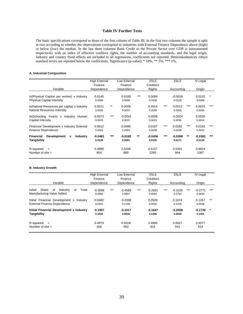
39

Table IV Further Tests The basic specifications correspond to those of the first column of Table III. In the first two columns the sample is split in two according to whether the observations correspond to industries with External Finance Dependence above (high) or below (low) the median. In the last three columns Bank Credit to the Private Sector over GDP is instrumented respectively with an index of effective creditors rights, the number of accounting standards, and the legal origin. Industry and country fixed effects are included in all regressions, coefficients not reported. Heteroskedasticity robust standard errors are reported below the coefficients. Significance (p-value): * 10%, ** 5%, *** 1%.

A. Industrial Composition

Variable

High External Finance

Dependence

Low External Finance

Dependence

2SLS Creditors

Rights

2SLS

Accounting

IV Legal

Origin

0.0145 0.0189 *** 0.0084 -0.0019 0.0132 *0.0089 0.0056 0.0106 0.0129 0.0068

0.0011 ** 0.0008 0.0014 *** 0.0013 *** 0.0015 ***0.0005 0.0007 0.0005 0.0006 0.0005

0.0073 *** -0.0018 0.0008 -0.0024 0.00200.0023 0.0022 0.0023 0.0035 0.0016

0.0012 0.0095 0.0167 *** 0.0182 *** 0.0192 ***0.0025 0.0063 0.0038 0.0038 0.0052

-0.0481 *** -0.0180 ** -0.0406 *** -0.0398 ** -0.0381 ***0.0129 0.0091 0.0130 0.0171 0.0134

R-squared = 0.4888 0.5206 0.5157 0.5341 0.4824Number of obs = 854 889 1265 844 1387

B. Industry Growth

Variable

High External Finance

Dependence

Low External Finance

Dependence

2SLS Creditors

Rights

2SLS

Accounting

IV Legal

Origin

-0.3098 *** -0.4588 *** -0.2681 *** -0.3105 *** -0.3771 ***0.0956 0.0857 0.0593 0.0754 0.0644

0.0482 -0.0398 0.0509 0.1674 0.1257 **0.0342 0.1189 0.0526 0.1238 0.0538

-0.1957 -0.1017 -0.1647 -0.2558 -0.1726 *0.1532 0.0916 0.1266 0.2636 0.1001

R-squared = 0.4973 0.5018 0.4685 0.6027 0.4577Number of obs = 456 463 815 641 919

ln(Physical Capital per worker) x IndustryPhysical Capital Intensity

ln(Natural Resources per capita) x IndustryNatural Resources Intensity

ln(Schooling Years) x Industry HumanCapital Intensity

Financial Development x Industry ExternalFinance Dependence

Financial Development x IndustryTangibility

Initial Share of Industry of TotalManufacturing Value Added

Initial Financial Development x IndustryExternal Finance Dependence

Initial Financial Development x IndustryTangibility

40

Table V Robustness The basic specifications correspond to those of the first column of Table III. In the first column of Panel A and all the columns of Panel B we add the interactions indicated in each case. In the second column of Panel A we drop the observations corresponding to industries representing more than 1.96% of the country’s total manufacturing employment (the sample median). In the third column of Panel A we drop the observations corresponding to industries located in countries in the first and fourth quartile of per capita GDP. In the fourth column we use only those observations corresponding to industries located in countries above the median of total GDP. Industry and country fixed effects are included in all regressions, coefficients not reported. Heteroskedasticity robust standard errors are reported below the coefficients. Significance (p-value): * 10%, ** 5%, *** 1%. A. Industrial Composition

Variable

Industry

Volatility

Low Political

Pressure

Intermediate Level of per capita GDP

Large Market

Size

0.0107 ** 0.0165 *** 0.0231 -0.01300.0051 0.0064 0.0144 0.0090

0.0010 ** 0.0003 0.0008 0.0016 ***0.0004 0.0004 0.0008 0.0005

0.0025 * -0.0014 0.0011 -0.00030.0015 0.0013 0.0037 0.0030

0.0116 *** 0.0025 ** 0.0076 * 0.0109 ***0.0019 0.0011 0.0042 0.0020

0.0013 **0.0006

-0.0215 *** -0.0203 ** -0.0151 -0.0157 **0.0073 0.0096 0.0117 0.0073

R-squared = 0.4837 0.4404 0.492 0.5397Number of obs = 1743 872 871 927

ln(Physical Capital per worker) x IndustryPhysical Capital Intensity

ln(Natural Resources per capita) x IndustryNatural Resources Intensity

ln(Schooling Years) x Industry Human CapitalIntensity

Financial Development x Industry ExternalFinance Dependence

Financial Development x Industry Volatility

Financial Development x Industry Tangibility

B. Industry Growth

Variable

Growth

Opportunities

Technological

Advancement

Initial per

capita GDP

Initial Investment

Rate

-0.3713 *** -0.3559 *** -0.3692 *** -0.3749 ***0.0638 0.0644 0.0639 0.0643

0.0866 *** 0.0899 *** 0.0894 *** 0.0894 ***0.0323 0.0328 0.0328 0.0326

-0.02970.0333

0.02020.0400

-0.02470.0553

0.00730.0282

-0.32070.3588

-0.1992 *** -0.2074 *** -0.2008 *** -0.1617 **0.0661 0.0771 0.0701 0.0676

R-squared = 0.4594 0.462 0.4588 0.4596Number of obs = 919 904 919 919

Initial Share of Industry of Total ManufacturingValue Added

Initial Financial Development x Industry ExternalFinance Dependence

Initial Financial Development x Industry Q

Initial Financial Development x Industry HumanCapital Intensity

Initial Financial Development x IndustryTangibility

Initial Investment Rate x Industry Tangibility

ln(Initial Schooling Years) x Industry Tangibility

ln(Initial per capita GDP) x Industry Tangibility

41

Table VI Firm Leverage Evidence The specification corresponds to that in (9). In columns one, three, four, five, and six the dependent variable is firms’ long-term market leverage, that is, long-term debt over book value of assets less book value of equity plus market value of equity. In column two the dependent variable is long-term debt over book value of assets. In the third and fourth columns Bank Credit to the Private Sector over GDP is instrumented respectively with an index of effective creditors rights and the number of accounting standards. In column five (six) only observations corresponding to firms located in countries with a ratio of private credit to GDP above (below) the sample median are included. Industry and country fixed effects are included in all regressions, coefficients not reported. Heteroskedasticity robust standard errors are reported below the coefficients. Significance (p-value): * 10%, ** 5%, *** 1%.

Variable

Long Term

Market

Leverage

Long Term

Book Leverage

2SLS

Creditors

Rights

2SLS

Accounting

High Financial

Development

Low Financial

Development

Tangibility 0.3378 *** 0.2880 *** 0.4623 *** 0.4850 *** 0.1941 *** 0.3183 ***0.0299 0.0313 0.0838 0.0810 0.0135 0.0314

Tobin's Q -0.0051 *** 0.0007 -0.0049 *** -0.0046 *** -0.0040 ** -0.0173 ***0.0020 0.0025 0.0019 0.0019 0.0017 0.0041

Ln(Sales) 0.0098 *** 0.0127 *** 0.0092 *** 0.0087 *** 0.0098 *** 0.0121 ***0.0010 0.0013 0.0010 0.0010 0.0010 0.0029

Profitability -0.1767 *** -0.1953 *** -0.1718 *** -0.1836 *** -0.1611 *** -0.1871 ***0.0175 0.0296 0.0175 0.0188 0.0186 0.0463

-0.1075 *** -0.0801 *** -0.2211 *** -0.2301 ***0.0236 0.0286 0.0775 0.0729

R-squared = 0.3115 0.1899 0.3111 0.3208 0.2633 0.4521Number of obs = 6215 6215 5848 5548 4955 1260

Financial Developmentx Tangibility

42

Figure I Manufacturing Sector Composition and Financial Development: 3 Cases

Figure II Aggregate Tangibility of the Manufacturing Sector and Financial Development

0

0.1

0.2

0.3

0.4

0.5

0.6

0.7

0.8

0.9

1

1 6 11 16 21 26Industries sorted by Tangibility (Low to High)

Cu

mm

ula

tive

Val

ue

Ad

ded

ThailandUnited KingdomPeru

Agg

rega

te_T

angi

bilit

y_of

_Man

uf

Private_Credit_over_GDP.022331 1.1353

.291216

.422177

ARG

AUS

AUT

BGDCAN

CHL

COL

DNK

ECU

SLVFIN

GHA

GRCGTM HND

IND

IDN

ITA JPN

KOR

MYS

NZL

NOR

PAK

PAN

PER

PHL

PRT

SAU

SEN

ZAF

ZWE

ESPSWE

THA

TUR

UGA

EGY

GBR

URY

VEN

43

APPENDIX

44

Table A-I Average Balance Sheets

The table presents average balance sheets using the data of active U.S.-based companies in Compustat’s Industrial database for the year 1995. The average is taken first within every industry and then across industries. The first column shows the overall average balance sheet, while columns two and three show the averages including just the firms in industries with book tangibility above and below the median, respectively.

All Firms High

Tangibility

Industries

Low

Tangibility

Industries

Difference Low v/s

High Tangibility

ASSETSCash and short-term investments 4.3% 3.6% 5.6% 2.0%Receivables 15.5% 14.8% 16.8% 2.0%Inventories 12.1% 10.8% 14.7% 3.9%Current assets - other 3.0% 2.6% 3.9% 1.2%Current assets - total 34.9% 31.8% 40.9% 9.1%Net property, plant & equipment 45.1% 51.0% 33.7% -17.4%Investment and advances - equity 4.2% 5.3% 2.2% -3.1%Investment and advances - other 2.4% 2.0% 3.0% 1.0%Intangibles 8.1% 5.3% 13.4% 8.1%Assets - other 5.3% 4.5% 6.8% 2.3%

LIABILITIESDebt in current liabilities 3.9% 3.3% 4.9% 1.6%Accounts payable 9.1% 9.1% 9.0% -0.2%Current liabilities - other 10.4% 9.1% 13.0% 3.8%Current liabilities - total 23.4% 21.6% 26.9% 5.3%Deferred taxes 4.5% 4.8% 3.8% -1.0%Long-term debt 26.1% 27.5% 23.3% -4.2%Liabilities - other 10.4% 10.7% 9.8% -0.8%Liabilities - total 64.3% 64.5% 63.8% -0.7%Common equity 34.5% 34.1% 35.4% 1.2%Shareholders equity - total 35.7% 35.5% 36.2% 0.7%

45

Table A-II Industrial Composition Sample

Country Number of

Industries

with Data

Country Number of

Industries

with Data

Industry Number of

Countries

with DataArgentina 28 Korea, Rep. 28 Beverages 66Australia 28 Malawi 23 Fabricated metal products 65Austria 28 Malaysia 28 Food products 69Bangladesh 28 Mauritius 27 Footwear, except rubber or plastic 57Belgium 19 Mexico 26 Furniture, except metal 60Bolivia 27 Nepal 21 Glass and products 58Botswana 18 Netherlands 27 Industrial chemicals 69Brazil 18 New Zealand 28 Iron and steel 66Burundi 27 Niger 7 Leather products 60Cameroon 25 Norway 28 Machinery, electric 60Canada 28 Pakistan 28 Machinery, except electrical 59Central African Republic 25 Panama 28 Misc. petroleum and coal products 53Chile 28 Papua New Guinea 25 Non-ferrous metals 58China 27 Paraguay 9 Other chemicals 60Colombia 28 Peru 28 Other manufactured products 64Congo, Rep. 16 Philippines 28 Other non-metallic mineral products 61Costa Rica 27 Portugal 28 Paper and products 68Denmark 28 Rwanda 7 Petroleum refineries 61Ecuador 28 Senegal 28 Plastic products 59Egypt, Arab Rep. 28 Sierra Leone 14 Pottery, china, earthenware 66El Salvador 28 South Africa 28 Printing and publishing 61Finland 28 Spain 28 Professional & scientific equipment 59France 26 Sri Lanka 27 Rubber products 61Ghana 28 Sweden 28 Textiles 69Greece 28 Thailand 28 Tobacco 66Guatemala 28 Trinidad and Tobago 26 Transport equipment 59Haiti 12 Tunisia 22 Wearing apparel, except footwear 61Honduras 28 Turkey 28 Wood products, except furniture 68India 28 Uganda 28Indonesia 28 United Kingdom 28Italy 28 Uruguay 28Jamaica 14 Venezuela 28Japan 28 Zambia 26Jordan 28 Zimbabwe 28Kenya 27

Variable # of Obs. Mean Std. Dev. Min MaxIndustry Value Added share of GDP 1743 0.0071292 0.0097662 -0.0042364 0.1152555

ln(Physical Capital per worker) 1743 9.346631 1.457672 5.784441 11.35078

Industry Physical Capital Intensity 1743 0.0697646 0.0369628 0.018056 0.1955499

ln(Natural Resources per capita) 1743 8.474001 0.8688306 6.733402 10.62474

Industry Natural Resources Intensity 1743 0.2495697 0.4328882 0 1

ln(Years of Education) 1743 1.649822 0.4967696 -0.2177415 2.434782

Industry Human Capital Intensity 1743 0.9993601 0.2723158 0.501737 1.65582

Credit to the Private Sector by Deposit Money Banks over GDP 1743 0.3552926 0.2617818 0.0223313 1.135299

Industry Tangibility 1743 0.3003901 0.1371717 0.074491 0.670836

Industry External Finance Dependence 1743 0.235937 0.3205729 -0.45116 1.140122

Liquid Liabilities over GDP 1743 0.4643626 0.2899575 0.0653742 1.810233

Stock Market Capitalization over GDP 1424 0.2726931 0.3156107 0.0075163 1.488477

Value Traded in the Stock Market over GDP 1452 0.0946794 0.1397575 0.0000884 0.6285858

Industry Market Tangibility 1743 0.2120837 0.1077033 0.0681114 0.5262105

Industry Sales Tangibility 1743 0.2513089 0.1345586 0.0465184 0.6783119

Effective Creditors Rights 1265 1.263956 0.8918789 0 3.704025

Accounting Standards 844 60.93009 13.08821 31 83

Industry Volatility 1743 1.585637 1.032271 0.3799427 5.982197

Real per capita GDP (PPP) 1743 5317.271 4848.975 483.1106 16802.84

GDP at Market Prices 1743 1.86E+11 4.74E+11 2.21E+08 3.44E+12

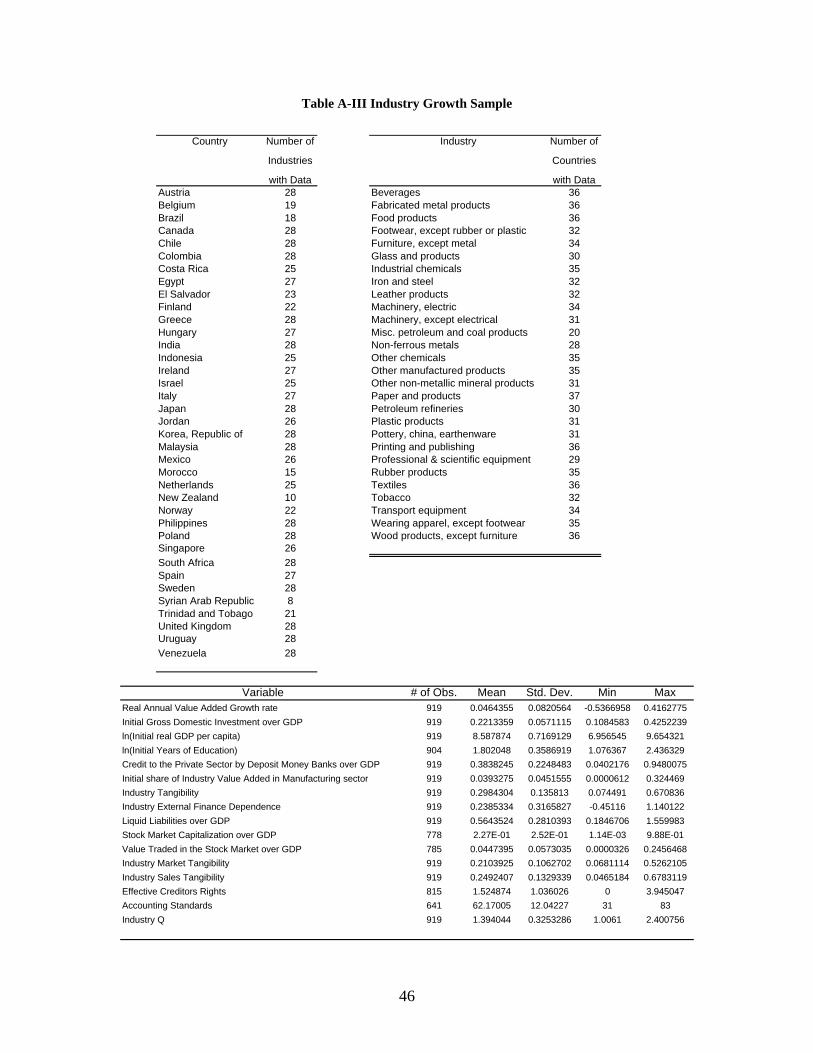
46

Table A-III Industry Growth Sample

Country Number of

Industries

with Data

Industry Number of

Countries

with DataAustria 28 Beverages 36Belgium 19 Fabricated metal products 36Brazil 18 Food products 36Canada 28 Footwear, except rubber or plastic 32Chile 28 Furniture, except metal 34Colombia 28 Glass and products 30Costa Rica 25 Industrial chemicals 35Egypt 27 Iron and steel 32El Salvador 23 Leather products 32Finland 22 Machinery, electric 34Greece 28 Machinery, except electrical 31Hungary 27 Misc. petroleum and coal products 20India 28 Non-ferrous metals 28Indonesia 25 Other chemicals 35Ireland 27 Other manufactured products 35Israel 25 Other non-metallic mineral products 31Italy 27 Paper and products 37Japan 28 Petroleum refineries 30Jordan 26 Plastic products 31Korea, Republic of 28 Pottery, china, earthenware 31Malaysia 28 Printing and publishing 36Mexico 26 Professional & scientific equipment 29Morocco 15 Rubber products 35Netherlands 25 Textiles 36New Zealand 10 Tobacco 32Norway 22 Transport equipment 34Philippines 28 Wearing apparel, except footwear 35Poland 28 Wood products, except furniture 36Singapore 26South Africa 28Spain 27Sweden 28Syrian Arab Republic 8Trinidad and Tobago 21United Kingdom 28Uruguay 28Venezuela 28

Variable # of Obs. Mean Std. Dev. Min MaxReal Annual Value Added Growth rate 919 0.0464355 0.0820564 -0.5366958 0.4162775

Initial Gross Domestic Investment over GDP 919 0.2213359 0.0571115 0.1084583 0.4252239

ln(Initial real GDP per capita) 919 8.587874 0.7169129 6.956545 9.654321

ln(Initial Years of Education) 904 1.802048 0.3586919 1.076367 2.436329

Credit to the Private Sector by Deposit Money Banks over GDP 919 0.3838245 0.2248483 0.0402176 0.9480075

Initial share of Industry Value Added in Manufacturing sector 919 0.0393275 0.0451555 0.0000612 0.324469

Industry Tangibility 919 0.2984304 0.135813 0.074491 0.670836

Industry External Finance Dependence 919 0.2385334 0.3165827 -0.45116 1.140122

Liquid Liabilities over GDP 919 0.5643524 0.2810393 0.1846706 1.559983

Stock Market Capitalization over GDP 778 2.27E-01 2.52E-01 1.14E-03 9.88E-01

Value Traded in the Stock Market over GDP 785 0.0447395 0.0573035 0.0000326 0.2456468

Industry Market Tangibility 919 0.2103925 0.1062702 0.0681114 0.5262105

Industry Sales Tangibility 919 0.2492407 0.1329339 0.0465184 0.6783119

Effective Creditors Rights 815 1.524874 1.036026 0 3.945047

Accounting Standards 641 62.17005 12.04227 31 83

Industry Q 919 1.394044 0.3253286 1.0061 2.400756

47

Table A-IV Firm Leverage Sample

Country Number of Firms with

Data

Country Number of Firms with

DataArgentina 23 Malaysia 169Australia 66 Mexico 48Austria 57 Morocco 4Belgium 55 Netherlands 94Brazil 91 New Zealand 17Canada 170 Norway 62Chile 36 Pakistan 71China 81 Peru 14Colombia 14 Philippines 36Czech Republic 33 Poland 39Denmark 91 Portugal 37Egypt, Arab Rep. 7 Russian Federation 4Finland 77 Singapore 85France 370 Slovak Republic 14Germany 388 South Africa 146Greece 87 Spain 59Hong Kong, China 139 Sri Lanka 8Hungary 17 Sweden 107India 263 Switzerland 101Indonesia 82 Taiwan, China 170Ireland 22 Thailand 118Israel 27 Turkey 55Italy 107 United Kingdom 598Japan 1,432 United States 223Jordan 2 Venezuela, RB 10Korea, Rep. 185 Zimbabwe 1Luxembourg 3

Variable Obs Mean Std. Dev. Min MaxLong-term Debt over Market Value of Assets 6215 0.1232163 0.1328564 0 1.081359

Long-term Debt over Book Value of Assets 6215 0.1365413 0.1558573 0 4.741825

Firm Tangibility 6215 0.353188 0.1806679 0 0.9705176

Tobin's Q 6215 1.536826 2.213763 0.1342066 97.67947

ln(sales) 6215 12.25745 1.880546 1.098612 18.98916

Profitability 6215 0.0450283 0.1076884 -0.8831435 0.7831048

Credit to the Private Sector by Deposit Money Banks over GDP 6215 1.102636 0.4811467 0.0999008 1.69693

Effective Creditors Rights 5848 1.845994 1.038537 0 3.945047

Accounting Standards 5548 66.56002 7.557877 36 83

48

ENDNOTES

1 i.e. contractible. In practice it is not uncommon to find that investors pay directly to the provider of the assets instead of letting the entrepreneur have the funds and buy them himself. 2 See, for instance, Harris and Raviv [1991]. 3 The other two main classes of assets that are usually collateralized explicitly are the accounts receivables and inventories. In comparison to property, plant, and equipment debt based on those assets typically finances a smaller share of their value, for a shorter period of time, and command higher interest rates. 4 This is not to say that the distinction is irrelevant. In terms of the allocation effect an improvement in contractibility and a soft-assets-biased increase in the protection balance of investors vis-à-vis borrowers’ rights may be similar. However, it would be interesting to know whether the improvement in the access to external finance in better functioning capital markets is due to the fact that dependence on assets diminishes altogether or because the ability to sustain relationships based on softer assets is enhanced. 5 These computations are available from the author upon request (see Appendix). 6 The correlation between the index of external finance dependence and the index of tangibility is 0.009, not significantly different than zero. Rajan and Zingales [1998] do not report the external finance dependence figure for the industrial chemicals industry (ISIC 351). We construct it as the average of the two sub-sectors reported by them: synthetic resins (3513) with external finance dependence of 0.16 and basic industrial chemicals excluding fertilizers (3511), with an index of 0.25. The results are robust to the exclusion of this sector. 7 The results are robust to restricting the samples to conform a balanced panel. The sample size for (7) is larger than for (8) because the computation of the growth rate requires data to be available simultaneously for two particular years (1985 and 1995). Summary statistics and additional sample description are available from the author upon request (see Appendix). 8 The p-values for the hypothesis that each difference-in-differences is equal to zero are 6.3% and 6.8%, respectively. 9 The simple correlation of -.058 is significantly negative (p-value 0.1%). This is not significantly different than the partial correlation obtained after controlling for the countries’ availability of resources. 10 Svalery and Vlachos [2001] and Beck [2001] obtain a similar result. 11 The implied size of the effects in Table III expressed as a proportion of the benchmark (column one), and the p-values corresponding to the hypothesis that each coefficient is equal to that of our benchmark regression (in parentheses) are, from column two to the right: Specialization: 0.86 (54.8%), 0.28 (1.8%), 0.24 (1.1%), 0.71 (54.7%), and 0.79 (35.9%); Growth: 0.53 (17,2%), 0.39 (22.6%), 0.13 (1.9%), 0.88 (91.9%), and 0.78 (46.2%). 12 This could mean that the underlying concept is measured with more noise than with banking variables (especially given the higher volatility of stock market measures) so that the attenuation bias is important. It is also possible that the marginal effect of having a more developed stock market in the outcomes of more and less tangible industries is actually smaller. Finally, the existence of an equity market may provide a –possibly limited- escape from the need to have hard assets to raise external finance. Although interesting, we do not explore the effect of the financial structure in this paper. 13 Again, these are computed using data from publicly listed, U.S.-based companies over the 1985-1995 period. 14 The p-values corresponding to the hypothesis that the coefficients are equal in each sample are: Specialization: 5.7%; Growth: 59.8%. In the following three columns of Table IV the size of the implied effect is directly comparable to our benchmarks. The p-values corresponding to the hypothesis that each coefficient is equal to that of our benchmark are: Specialization: 27.6%, 40.7%, and 37.1%; Growth: 85.9%, 80.8%, and 88.4%. 15 The p-values corresponding to the hypothesis that each coefficient of our financial development tangibility interaction in Table V (from column one to the right) is equal to that of our benchmark are: Specialization: 74.4%, 70.5%, 47.5%, and 36.1%; Growth: 92.1%, 86.4%, 91.1%, and 76.3%. 16 Data are available for a much larger number of countries using the ISIC-3 definition. This is why we use ISIC-3 instead of ISIC-4 in our analysis. 17 In any case, since the test pertains to cross-country differences in the effect of tangibility on leverage, this should not be of great concern. 18 The data for Taiwan are taken from Beck et al. [1999]. 19 Summary statistics and additional sample description are available from the author upon request (see Appendix). 20 On this, see also Beck et al. [2000] and Acemoglu et al. [2001, 2002]. 21 Just consider, for instance, the literature related to Fazzari, Hubbard, and Petersen [1988]’s attempt at identifying firms’ financing constraints. 22 For more on these issues, see Glaeser and Shleifer [2001], and Rajan and Zingales [2001]. 23 The analysis by Hall [1999] supports this at least for the post-war period and contingent on the endogenous investment hypothesis.

49