212 Frank Smets

Financial-asset Prices and Monetary Policy:Theory and Evidence

Frank Smets*

1. IntroductionThe monetary-policy environment over the past decade in industrial countries has

been increasingly characterised by low and stable inflation and often large movementsin the prices of equities, bonds and foreign exchange, or financial assets more broadly.While volatility in part reflects the nature of asset prices, driven primarily by revisionsin expectations of future returns, large movements raise questions about the appropriateresponse of monetary policy. In the past year, for instance, several central banks haveexpressed concern about such changes. In the United States, Chairman Greenspan raisedquestions about the large gains in stock prices and whether they had extended beyondlevels that are justifiable on the basis of economic fundamentals. In many formerly high-yielding bond markets such as in Italy and Spain, yields fell by several percentage points,often putting pressure on the respective central banks to relax policy rates. In theUnited Kingdom, the pound sterling appreciated by more than 15 per cent in effectiveterms from August 1996 to the beginning of 1997, giving rise to a lively debate betweenmarket observers and the central bank about the appropriate policy response.

The first part of this paper (Section 2) attempts to put these concerns in perspectiveby putting forward a common framework in which the optimal policy response tofinancial-asset prices can be analysed. Within the context of the central bank’s objectiveof price stability, the basic answer to the question raised is simple: the central bank’sresponse to unexpected changes in asset prices should depend on how these changesaffect the inflation outlook; if they imply a rise in the inflation forecast, policy shouldtighten and vice versa.1

The harder task is to determine how the inflation forecast is affected, as this requiresa structural model of the economy. Although the model developed in Section 2.1following Gerlach and Smets (1996) is simple, it does highlight two reasons whyunexpected asset-price movements may affect the inflation forecast. First, changes inasset prices may affect aggregate demand directly. For example, changes in asset pricesaffect household wealth and consumption expenditure, affect the ability of enterprisesto raise funds and thereby influence investment spending, and raise the value of collateralwhich affects the willingness of banks to lend. Similarly, sharp changes in exchange ratesaffect the demand for net exports. To the extent that there is no other information tosuggest that the movement in asset prices is warranted by the underlying fundamentals

* I thank Palle Andersen, Stefan Gerlach and Kostas Tsatsaronis for helpful comments and Gert Schnabelfor statistical support. The views expressed in this paper are solely my own and not necessarily those ofthe BIS.

1. The central role of the inflation forecast in inflation-targeting countries has been emphasised bySvensson (1997).

213Financial-asset Prices and Monetary Policy: Theory and Evidence

of the economy, the central bank may wish to offset such changes in order to avoidunnecessary output and price variability.

Second, asset prices are strongly influenced by expectations of future returns, whichin turn are related to expectations of future economic activity, inflation and monetarypolicy. Thus, even if their impact on aggregate demand is limited, they may containuseful information about current and future economic conditions. This information maybe used to improve the inflation forecast on which the direction of monetary policy isbased. The optimal policy response to asset prices for this reason will depend on theinformation contained in these prices. A number of authors have recently warned againstthe incorporation of asset prices in monetary-policy feedback rules (Fuhrer andMoore 1992; Woodford 1994). In the concluding part of Section 2.2, this criticism isbriefly discussed.

Since the early 1990s, a number of central banks have incorporated the exchange ratein their inflation-targeting framework by using a monetary conditions index (MCI) – thatis, a weighted average of a short-term interest rate and the exchange rate – as an operatingtarget. The analysis in Section 2 suggests that this idea could be extended to other assetprices that affect aggregate demand. In Section 3, I therefore discuss the advantages andpitfalls of setting monetary policy in terms of an MCI. Using an MCI is beneficial in termsof practicality and because it contributes to transparency about how the central bankintends to achieve its announced inflation target. There are, however, two potentiallyserious limitations which in part follow from the simplicity of the MCI concept. First, thepolicy focus on interest rates or exchange rates may need to vary over time, for example,depending on which sectors are the cause of inflationary pressures. Second, the MCIconcept ignores the potentially useful informational role of asset-price movementsmentioned above.

In Section 4, I analyse the monetary-policy response to financial-asset prices and, inparticular, the exchange rate in Australia and Canada. While the central banks of bothcountries have announced explicit inflation targets since the early 1990s, their views onhow to respond to unexplained exchange-rate movements differ. In contrast to the Bankof Canada which uses an MCI, the Reserve Bank of Australia has resisted systematicallyresponding to unexplained exchange-rate movements. In Section 4.1, I estimate a policyreaction function for both central banks over the period 1989–96 using a methodologyproposed by Clarida, Galí and Gertler (1997). The estimated parameters confirm thatwhile both central banks strongly respond to deviations of inflation from the announcedtarget, their short-term response to the exchange rate is indeed different. I also examinewhether the two central banks attach any weight to the long-term interest rate or thestock-market index in their short-run policy settings.

Finally, in Section 4.2, I examine whether, in accordance with the theoretical resultsof Section 2, differences in the sources of exchange-rate innovations can explain thedifferent policy response to unexpected exchange-rate movements in the two countries.If most of the exchange-rate innovations are related to changes in the real economy, itmay be optimal not to respond. In contrast, offsetting the effects of unexplainedexchange-rate changes on aggregate demand is optimal, if most of the shocks to theexchange rate are financial. Using a set of structural VAR models, I find some evidencethat terms-of-trade shocks are more important in Australia than in Canada, while the

214 Frank Smets

reverse is true for nominal shocks, in particular during the most recent period. Section 5concludes and suggests two other reasons why asset prices may play a role in monetary-policy formulation.

2. Financial Prices and Optimal Monetary Policy

2.1 A simple model

I start the analysis of the interaction between financial prices and monetary policy bydeveloping a stylised model of the economy. The model is an extension of that used byGerlach and Smets (1996) to analyse the optimal policy response to the exchange rate.In this paper I focus on a general asset price and demonstrate that the same principlesgovern the optimal response to any asset price whether it is an exchange rate, equityprices or bond prices. Although the model is very simple, it does capture the two mostimportant reasons why monetary authorities may want to respond to financial prices intheir pursuit of price stability. First, shocks to financial prices that are not driven byfundamentals may destabilise the economy through their effects on aggregate demand,in which case the central bank may want to offset them. Second, asset prices aredetermined by arbitrage equations in which expectations of future returns play animportant role. As a result, these prices may contain additional information about currentand future economic conditions that may be useful to the monetary authorities in theirstabilisation policy.

Equations (1) to (6) describe the economy:

p E p yt t t t ts= + −−1 γ ε( ) (1)

y r ft t t td= − + +α β ε (2)

f E f E d rt t t t t t tf= + − − ++

++

+ρ ρ ε1 11( ) (3)

d yt t+ =1 (4)

r R E p pt t t t t= − −+( )1 (5)

f F pt t t= − (6)

where all variables, except the interest rates, are in logarithms, and the constants havebeen normalised to zero.

Equation (1) is a simple Phillips curve which states that prices ( pt) are determined bylast period’s expectations of the current price level and the output gap ( yt – ε s

t ). Such arelationship can be derived in an economy where prices are determined as a mark-up overwages and wages are set one period in advance (Canzoneri and Henderson 1991).

According to Equation (2), aggregate demand depends negatively on the expected realinterest rate (rt) and positively on a real asset price ( ft). Different interpretations of ft arepossible. In what follows I will mainly think of ft as a real stock price. Equation (3) is

215Financial-asset Prices and Monetary Policy: Theory and Evidence

then a log-linear approximation of the arbitrage equation which requires the real returnon equities, which can be decomposed into the expected dividend yield and the expectedcapital gain, to equal the real riskless rate plus a time-varying risk premium (ε f

t ). Et xt+idenotes the expectation of variable x at time t + i, based on information available attime t. As discussed below, I allow for the fact that the information set of the asset-marketparticipants may be larger than that of the other agents in the economy. Expectationsbased on this larger information set are denoted by E+

t . According to Equation (4) theexpected real dividend on equities is proportional to output. Since stocks are claims onoutput, note that, for β = 1, Equation (2) then simply says that the share of demand in totalwealth is a function of the real interest rate.

Gerlach and Smets (1996) interpret ft as a real exchange rate. The parameter β thencaptures the effect of the real exchange rate on aggregate demand, which will depend on,for example, the size of the traded-goods sector. For ρ = 1, the arbitrage Equation (3)becomes

r E ft t t tf= ++

+( )∆ 1 ε . (3′)

This can then be interpreted as an uncovered interest-rate parity condition, provided theforeign interest rate and prices are normalised to be constant at zero. Finally, if dividendsare constant (i.e. dt = 0), then the real asset price can also be viewed as a real bond price.

Equations (5) and (6) define the expected real interest rate as the difference betweenthe nominal interest rate and the expected inflation rate over the period and the real assetprice as the difference between the nominal asset price (Ft) and the current price level.

The central bank sets the nominal interest rate to minimise the following intertemporalloss function,

E Lti

t ii

ρ +=

∞

∑0

where L y p pt t ts

t= − + −γ ε χ( ) ( )2 2 . (7)

The central bank cares about both deviations of output from potential and deviations ofprices from target. Two aspects of this loss function deserve to be highlighted. First, thecentral bank has no incentive to push output beyond its natural level (given by εs

t) and,as a result, is not subject to an inflation bias as in Barro and Gordon (1983). Second, theloss function implies that the central bank tries to stabilise the price level rather than theinflation rate. This is done for convenience, as targeting the inflation rate complicates thederivation of the optimal reaction function under asymmetric information withoutaffecting the main results. Moreover, I assume that the price target is constant over time.

Next, I discuss the assumptions regarding the information set available to the differentagents in the economy. First, all agents (the central bank, wage setters and financial-market participants) know the parameters and the distribution of the disturbances of themodel. Second, all agents observe last period’s realisation of the price level and output,and the current nominal interest rate and asset price. This assumption can be rationalisedin two ways. First, while asset prices are continually quoted in auction-like markets, thecollection of data on output and prices is more cumbersome and takes some time.Alternatively, in a dynamic model which would incorporate lags in the transmissionmechanism, it is future output and prices – by definition currently unobservable – ratherthan current output and prices that would enter the objective function.

216 Frank Smets

More controversially, I allow for the possibility that asset-market participants do havesome information on current output and prices. One justification is that asset-marketparticipants have financial incentives to acquire this information as their profits dependon how good their forecast of current and future returns is. For example, stock-marketanalysts have an incentive to gather detailed firm-level information to forecast corporateearnings. Such an argument is often made in favour of using asset prices rather thansurvey measures as indicators of private-sector expectations.

Finally, in order to derive the reaction function, I need to make assumptions about thestochastic processes driving the shocks to the economy. For simplicity, I assume that thesupply shock follows a random walk, the demand shock a first-order autoregressiveprocess and the financial shock a white-noise process, that is, εs

t = ε st--1 + ξ s

t, εdt = δεd

t--1 + ξ dt

and ε ft = ξ f

t, and that the shocks are mutually uncorrelated.

2.2 Optimal monetary policy

As shown in the Appendix, optimal monetary policy in this model results in settingthe perceived (or forecast) price level equal to its target. However, the actual equilibriumoutput and price level will differ from their targets to the extent that there are unexpectedexcess-demand shocks which the central bank fails to stabilise. This control problemarises from a lack of information concerning the current shocks affecting the output gapand consequently the price level.2

In the following two subsections, I discuss the central bank’s interest-rate reactionfunction which results in the achievement of the optimal price level.3 In the firstsubsection, it is assumed that the information set of the central bank and the asset-marketparticipants is the same. This allows me to focus on the implications of the role of theasset price in the monetary transmission mechanism for the optimal policy response toasset prices. In the second subsection, I investigate the implications of the informationalrole of asset prices by assuming that asset-market participants observe the currentdemand and supply shocks.

2.2.1 Asset prices and their role in the monetary transmissionmechanism

When asset markets do not contain additional information concerning current demandand supply shocks, the optimal reaction function is given by

R F E Ft t t td

ts

t td

ts= + − = + −− −

βα α

ε ε βα α

δε ε1 11 1( ) ( ) . (8)

2. These results are very similar to the results in Svensson (1996) who studies a (more realistic) dynamicmodel in which there is a one-period lag in both the Phillips curve and the aggregate-demand function. Inthat model actual output and inflation will deviate from their target levels because of shocks that occurduring the control lag.

3. The optimal reaction function is derived in the Appendix. In deriving Equations (8) to (15) a zero pricetarget is assumed.

217Financial-asset Prices and Monetary Policy: Theory and Evidence

In order to achieve the optimal price level, the central bank tightens policy rates inresponse to a rise in the asset price and perceived excess-demand shocks to the outputgap. In this case the perceived output gap is just a function of past supply and demandshocks. To understand the rationale behind this reaction function, note from Equations (1)and (2) that for given price expectations and holding the interest-rate and exchange-ratepath unchanged, excess-demand shocks will directly feed through into prices. Asmonetary policy affects prices through the effect of interest rates and asset prices onaggregate demand, it is optimal to change interest rates in such a way that the combinedeffect of the interest-rate and asset-price movements offsets the effect of the shocks to theoutput gap.

The equilibrium asset price and interest rate are then given by

Ft ts

td

tf* ( )

( ) ( )= − +

− +−

− ++

+− −α ρα ρ β

ε δα ρδ β

ε αα β

ε1 1

1 11 1 (9)

and

Rt ts

td

tf* ( )( )

( )

( )

( )= − − −

− ++ −

− ++

+− −1 1

1

1

11 1

β ρ θα ρ β

ε δ ρδα ρδ β

ε βα β

ε . (10)

On the basis of Equations (8) to (10) two observations can be made. First, Equation (8)highlights the asset price’s role in the transmission mechanism. If β = 0, i.e. the assetprice does not affect aggregate demand, then it drops out of the reaction function.Moreover, by rewriting Equation (8), the optimal reaction function can be interpreted asthe central bank setting a weighted average of the interest rate and the asset price – amonetary conditions index (MCI) – in response to perceived changes in the output gap:

α β δε εR F MCIt t t td

ts− = = −− −

*1 1 . (11)

If the asset price is the exchange rate, Equation (11) shows that the practice of settingmonetary policy in terms of a weighted average of the interest rate and the exchange rate,with the weights determined by their respective effects on aggregate demand, is optimalin this particular model (Gerlach and Smets 1996). More generally, an MCI should alsoinclude other asset prices such as long-term interest rates and stock prices that affectaggregate demand.

Second, Equations (10) and (11) are equivalent policy rules. This serves to highlighttwo misconceptions that sometimes arise in discussions about the usefulness of MCIs.First, using an MCI as the operating target does not imply an automatic reaction to allasset-price changes, as the response depends on the perceived output gap. In fact, if β = 1,the correlation between asset-price movements and the short-term interest rate will bezero in the case of supply shocks, negative in the case of demand shocks and positive inthe case of financial shocks. Second, by the same token, it is clear that using an MCI asthe operating target does not obviate the need to determine the source of the asset-priceshocks. Freedman (1994) emphasised that policy-makers who use an MCI as theoperating target need to make a distinction between shocks that affect the desired MCI(i.e. the left-hand side of Equation (11)), such as demand and supply shocks, and shocksthat do not, such as financial shocks.

218 Frank Smets

2.2.2 The informational role of asset prices

In this section, I investigate the implications of the informational role of asset pricesfor the optimal policy response. I therefore assume that asset-market participants haveinformation about current supply and demand shocks.4 In this case financial prices mayaffect policy rates through their effect on the perceived output gap.

In the Appendix I show how to solve for the optimal response to the asset price in twosteps. First, I postulate a particular form of the optimal interest-rate reaction function tothe asset price and calculate the equilibrium asset price that would be consistent with sucha reaction function. Given the expression of the asset price, I can then solve for thesignal-extraction problem of the central bank and calculate the optimal response to theasset price. As an illustration, I analyse here the special case when there are only twofundamental shocks to the economy: a permanent supply shock and a temporaryfinancial shock.

Consider first the case of β = 1. As can be seen from Equation (10), in this case it isoptimal for the central bank not to respond to supply shocks in the symmetric informationcase. The reason for this is that the rise in stock prices, in response to the improved supplyside of the economy, increases demand enough to close the output gap. Stock prices playan equilibrating role in response to supply shocks. In contrast, policy rates need to movestrongly in response to financial shocks.

Under asymmetric information, the optimal interest-rate reaction function is

R Ft t ts= − − −−

1 11

λα

λα

ε with λ α γ ρ σα γ ρ σ α γ σ

= + ++ + + +

( )( )

( )( ) ( )

1

1 1

2

2 2s

s f

. (12)

As 0 ≤ λ ≤ 1, it is clear from comparing Equations (8) and (12) that, when stockprices contain information about the current supply shock, the optimal policy responseto them will be reduced. In determining how much lower the response will be, the mostimportant factor is the ratio of the variance of supply shocks (σ 2

s ) relative to the varianceof financial shocks (σ 2

ƒ). This signal-to-noise ratio can be interpreted as an indicator ofthe information content of changes in stock prices. As financial shocks becomeincreasingly important, this ratio tends to zero and the informational role of the assetprice is lost and the optimal policy reaction function reverts to Equation (8). In contrast,if financial shocks to stock prices are rare, the central bank concludes that mostunexpected changes in stock prices are due to supply shocks. Since such movements inthe stock market are equilibrating the goods market, the central bank wants to accommodatethem. As λ → 1, the central bank no longer responds to changes in the stock market,which is the optimal response in the face of supply shocks.5 Thus, this example showsthat the informational role of asset prices may change the optimal response to asset pricesfrom firm leaning against the wind to complete laissez-faire.

4. I assume asset-market participants observe the current supply and demand shocks. This assumption ismade for convenience. Alternatively, one could assume that they only observe a noisy signal of theseshocks.

5. The basic insight is, of course, not new. For example, Boyer (1978) extends the classical Poole (1970)analysis to the question of optimal foreign-exchange market intervention.

219Financial-asset Prices and Monetary Policy: Theory and Evidence

Take now the case in which stock prices have no effect on aggregate demand (β = 0),so that it is never optimal to respond to stock prices in the symmetric information case.When current stock prices contain information about current supply shocks, the optimalreaction function becomes

R Ft t ts= − − −−

λα

λα

ε11 with λ ρσ

ρ α ρα ρ

σ α ρα ρ

σ= − +

−+ −

− +

s

s f

2

2 21 11

11 1

( ( ) )( )

( )( ( ) )

. (13)

Because rising equity prices signal positive supply shocks, which in turn lower theinflation forecast, it now becomes optimal to lower policy rates in response to a boomingstock market.

2.2.3 Conclusions

In this section, I have shown that the optimal monetary-policy response to changes inasset prices depends on their role in the monetary transmission mechanism and thesources of the shocks affecting them. Recently, a number of authors have criticised theuse of asset prices in feedback rules of monetary policy. This criticism has basically takentwo forms. The first set of arguments are a manifestation of the well-known Lucascritique. Fuhrer and Moore (1992), for example, analyse the implications of the use ofsimple feedback rules for monetary policy to various asset prices in an overlapping-contracts model and show that including the asset prices themselves in the reactionfunction can change the direction of the indicator properties. Woodford (1994) observesthat econometric evaluations on whether an asset price has good forecasting power maynot be relevant. On the one hand, it may not be desirable to base policy on an indicatorwhich has been found useful in forecasting inflation, because the forecasting ability maybe impaired by the very fact that the monetary authority responds to it. A specificexample of this phenomenon is analysed by Estrella (1996), who shows within a simplemodel that the ability of the slope of the term structure to forecast economic activity andinflation may disappear under a strict inflation-targeting rule. On the other hand, lowforecasting power may not justify ignoring an indicator if the absence of it simply meansthat the variable is already used by central banks in the conduct of policy.

The second form of criticism concerns the existence and uniqueness of equilibriawhen the central bank, in setting its policy rule, uses private-sector forecasts whichthemselves are based on expected monetary policy (Bernanke and Woodford 1996). Forexample, Fuhrer and Moore (1992) find that placing too much weight on asset prices inthe reaction function, may lead to instability as policy loses control of inflation.Similarly, Woodford (1994) and Bernanke and Woodford (1996) show that automaticmonetary-policy feedback from such indicators can create instability due to self-fulfilling expectations.

The analysis in these papers shows that automatic policy feedback from changes infinancial-asset prices and private-sector inflation forecasts may be dangerous. However,the use of a structural model to interpret observed changes in asset prices reduces the twopotential problems. First, the Lucas critique is not valid because the new information isevaluated within the context of the central bank’s structural model and not just on the

220 Frank Smets

basis of forecasting ability. Second, the potential for instability or non-existence ofequilibria is reduced because the response to asset prices is conditioned by the informationasset prices contain concerning the structural shocks to the economy and their implicationsfor the achievement of the central bank’s inflation objective. In particular, the use of astructural model allows the central bank to filter out how much of the movement in assetprices is due to the expected monetary-policy response so that the problem of ‘circularity’disappears (Bernanke and Woodford 1996, p. 3).

3. Advantages and Pitfalls of an MCI as anOperating Target

Recently, the Bank of Canada has formalised the role of the exchange rate in itsinflation-targeting framework by using a weighted average of a short-term interest rateand the exchange rate – an MCI – as an operating target.6 In the Canadian context, theinclusion of a short-term interest rate and an exchange rate in the MCI was motivated byresearch findings that inflationary pressures were largely determined by the output gapand that monetary policy affected the output gap mainly through the effects of theexchange rate and short-term interest rates on aggregate demand (Duguay 1994;Longworth and Poloz 1995). It was therefore natural to monitor a weighted average ofthe two, with the weights determined by their relative importance in affecting demand.

The analysis in Section 2.2 suggests that, more generally, the MCI could be extendedto include other asset prices that affect aggregate demand. Indeed, in research at theEuropean Monetary Institute a long-term interest rate was included on the grounds thatthese rates matter more for aggregate demand in many continental European countries(Banque de France 1996). Similarly, it could be argued that in Japan, where the effectsof equity prices on economic activity are shown to be stronger than in many othercountries, the MCI should include a stock-price index. In this section, I therefore discusssome of the advantages and pitfalls of setting monetary policy using an MCI. Most of thearguments that relate to an MCI which only includes the short-term interest rate and theexchange rate, also carry over to a broader MCI.

3.1 Advantages

One advantage of using an MCI as the operating target is that it is practical to formulatemonetary policy in terms of the financial-asset prices that matter in the transmissionprocess, because it is in general difficult to predict the response of asset markets tochanges in policy rates (Freedman 1994). Having a target for the MCI automaticallyachieves the desired monetary-policy stance in the presence of uncertainty about howfinancial markets will respond.

6. See Freedman (1994). Following the Bank of Canada, central banks in a number of countries – among themSweden, Finland, Iceland and Norway – have adopted MCIs. In contrast to Canada, however, the Nordiccountries use the MCI primarily as an ex post indicator of the stance of policy. Since October 1996, theReserve Bank of New Zealand also uses an MCI as the operating target. While the Bank of Canada onlyindicates the direction of its desired path, the Reserve Bank of New Zealand quantifies its desired path forboth components.

221Financial-asset Prices and Monetary Policy: Theory and Evidence

A second advantage is that it clarifies the central bank’s view of the monetarytransmission mechanism. This increased transparency may be more important in amonetary-policy strategy which does not rely on intermediate targets to communicatepolicy decisions. Moreover, announcing the desired path of monetary conditionsimproves the transparency of the intentions of the monetary authorities and by reducingfinancial-market volatility may make policy more effective.7

3.2 Pitfalls

Two sets of problems may reduce the desirability of using an MCI as the operatingtarget (Gerlach and Smets 1996). First, the concept of an MCI depends on a simple viewof the transmission mechanism which may only be a poor approximation of the actualworking of the economy. Second, its use presumes that most unexplained movements inasset prices are not related to the fundamentals of the underlying economy and thereforeneed to be stabilised. It therefore potentially underestimates the informational andequilibrating role of asset-price innovations. I discuss each of these arguments in turn.

The model on which the MCI concept is based may be deficient in a number of ways.First, monetary policy may affect inflation through transmission channels other thanthrough the output gap, for instance through the direct effect of exchange rates on importprices. Until recently, the Reserve Bank of New Zealand focused on this more directtransmission channel to control inflation (Grimes and Wong 1994). While such directprice effects are important, Freedman (1994) argues that they are best interpreted as onlyaffecting the price level and can hence be accommodated without necessarily triggeringongoing inflation. Stochastic simulations by Black, Macklem and Rose (1997) suggestthat controlling inflation through the output gap rather than through import prices maylead to higher inflation variability, but appears more appealing in terms of output,interest-rate and exchange-rate volatility.

A second problem arises from the assumed constancy of the demand elasticities. Theeffects of interest rates and exchange rates on aggregate demand may depend on thestructure of indebtedness of the economy. For example, in a country with a large foreigndebt, exchange-rate changes may have important wealth effects potentially offsetting thedirect effects on aggregate demand. Possibly even more important is the fact thatexchange-rate movements primarily affect the tradable-goods sector, while changes ininterest rates have a potentially stronger impact on non-tradable-goods sectors such asthe housing market. The model underlying a fixed-weight MCI assumes that resourcescan be shifted relatively easily from one sector to the other so that only the economy-wideoutput gap matters. In practice, inflationary pressures may arise from bottlenecks indifferent sectors at different times. In such a situation the weight on the relevant assetprice should shift (King 1997).

Finally, the lags with which the exchange rate and the interest rate affect aggregatedemand may be different. Indeed, simulations with macroeconometric models suggestthat exchange-rate changes have more immediate effects on real economic activity than

7. Similar arguments are used in favour of other instrument rules that quantify the link between the centralbank’s policy instrument and economic conditions; see Taylor (1996).

222 Frank Smets

changes in interest rates (Smets 1995). If so, changes in interest and exchange rates thatleave the MCI unaffected will change aggregate demand.

The second set of problems with the concept of an MCI relates to its neglect of thepotential informational and equilibrating role of asset-price innovations. As discussed inSection 2 and Gerlach and Smets (1996), the optimal weight on the exchange rate in theMCI will depend on its information content. When unexplained exchange-rate innovationsare primarily driven by underlying terms-of-trade shocks, then, depending on theparameters of the model, it may actually be optimal to respond to an appreciation byraising interest rates as the exchange rate signals a rise in the demand for home goodswhich may lead to inflationary pressures. On the other hand, if most innovations in theexchange rate are considered to be financial and related to changes in risk premia or thecredibility of monetary and fiscal policy, then the MCI weights as usually determined areoptimal. The central bank’s view on what drives unexpected changes in the exchange rateis thus important in deriving the optimal response and the implicit weight in an MCI. InSection 4.2 this is further explored to explain the different response to the exchange ratein Canada and Australia.8

This point also raises the general issue whether central banks know enough aboutasset-price determination to usefully target them in an MCI. Using an MCI presupposesthat the central bank knows what the equilibrium asset price should be. If this is not thecase, targeting a desired path for the MCI may hinder the equilibrating role of assetprices. For example, in the simple example of Section 2.2 with β = 1 and asymmetricinformation, if the central bank acts according to Equation (8), then the equilibrating roleof the response of equity prices to supply shocks would be undone by the monetary-policyresponse and output and price variability would be larger than under laissez-faire.

In practice, there appears to be a trade-off between avoiding letting financial shocksdestabilise the economy and the possibility that a policy response hinders the equilibratingrole of asset prices. When there is genuine uncertainty concerning what drives financialprices, the potential for asset-price misalignments to destabilise the economy will be adetermining factor. Thus, if the demand effects of changes in a particular asset price arelimited, the central bank’s bias will be not to interfere with the market. On the other hand,if unwarranted movements in the asset price can have strong and lasting effects on outputand prices, a policy of leaning against such changes may be cautious.

4. Financial-asset Prices and Monetary Policy in Australiaand Canada

4.1 Estimating a policy reaction function

Since the early 1990s both the Bank of Canada and the Reserve Bank of Australia havehad publicly announced explicit targets for inflation. The Bank of Canada announcedinflation-reduction bands in February 1991 and has, since 1995, been targeting the

8. For example, the view consistent with the analysis in Astley and Garrat (1996), that most exchange-rateinnovations are driven by real shocks, may partly explain why the Bank of England has rejected theusefulness of an MCI; see also King (1997).

223Financial-asset Prices and Monetary Policy: Theory and Evidence

inflation rate within a band of ±1 per cent around a midpoint target of 2 per cent. TheReserve Bank of Australia started publicly quantifying its inflation objective in 1993,announcing a target of 2–3 per cent on average over the course of the business cycle.However, while the Bank of Canada has incorporated the exchange rate in the inflation-targeting framework by using an MCI as the operating target, the Reserve Bank ofAustralia has resisted systematically responding to unexpected exchange-rate movements.9

9. Opinions about the usefulness of an MCI as an operating target also differ among other inflation-targetingcountries. While the Reserve Bank of New Zealand started using an MCI as the operating target at the endof 1996, the Bank of England firmly rejects it (King 1997).

10. Although the announcement of the inflation targets occurred in the early 1990s, in both countries thecommitment to low and stable inflation became gradually clear in the late 1980s when interest rates rosestrongly to undo the upward trend in inflation (Figure 1). In Canada, the appointment of John Crow toGovernor of the Bank of Canada in February 1987 marked a shift towards more emphasis on the goal ofprice stability. This shift was more gradual and less transparent in Australia (Debelle 1996).

Figure 1: The Policy Rate, Inflation and the Output Gap

-5

0

5

10

15

-5

0

5

10

15

-5

0

5

10

15

-5

0

5

10

15

Australia Canada

Policy rate

Output gap

Underlying inflation

Policy rate

Underlying inflation

Output gap

1990 1992 1994 1996 1990 1992 1994 1996

% %

In this Section I attempt to quantify the commitment to low inflation and test thedifferent attitude towards the exchange rate by estimating a policy reaction function forthe Bank of Canada and Reserve Bank of Australia over the period 1989–96, using themethodology proposed by Clarida, Galí and Gertler (1997).10 They assume that withineach operating period the central bank has a target for the nominal policy-controlledinterest rate, R*

t , which is based on the state of the economy. In particular, the targetdepends on perceived inflation and output,

224 Frank Smets

11. In contrast to Taylor (1993), Clarida, Gali and Gertler (1997) use expected inflation instead of actualinflation arguing that this makes it easier to disentangle the link between the estimated coefficients andthe central bank’s objectives. For example, it is not clear from the simple Taylor specification whether thecentral bank responds to the output gap independently of concerns about future inflation. In this paper, Iuse a centred annual inflation rate to capture the current trend inflation rate in Equation (14). The tworeasons for doing so are that using realised future inflation, first, reduces the already short sample period,and, second, leads to biased estimates because the current interest rate affects future inflation.

12. Clarida, Gali and Gertler (1997) interpret the significance of variables other than expected inflation in thepolicy reaction function as evidence in favour of other objectives than price stability (e.g.exchange-rate stability).

R R E E y yt t t t t t* ( [ | ] ) [ | ]= + − + −β π π γΩ Ω (14)

where R– is the equilibrium nominal interest rate, πt the trend inflation rate, π– the inflation

target and yt – y–t the current output gap.

This target rule is a generalisation of the type of simple interest-rate rules proposedby Taylor (1993).11 It can be derived as the optimal rule for a central bank that has aquadratic loss function over inflation and output in a model similar to that in Section 2(Svensson 1997). For this target rule to lead to an effective stabilisation of the inflationrate, β needs to be greater than one and γ positive, so that the real policy rate riseswhenever trend inflation is above target and/or output is above potential.

In order to derive the equation estimated in Table 1, three more steps are necessary.First, as discussed extensively in Lowe and Ellis at this conference, central banks tendto smooth changes in interest rates. This interest-rate smoothing is captured by assumingthat the actual rate partially adjusts to the target as follows:

R R Rt t t t= − + +−( ) *1 1ρ ρ ν (15)

where the parameter ρ captures the degree of interest-rate smoothing and vt reflects awhite-noise control error. Letting α ≡ R

–– βπ– and gapt = yt – y–t , and combining Equations

(14) and (15), the policy reaction becomes

∆ Ω ΩR E E gap Rt t t t t t t= − + + − +−( ) [ | ] [ | ]1 1ρ α β π γ ν . (16)

Second, in analogy with Equations (8) and (12) of the model in Section 2, I allow thepolicy rate to respond to contemporaneous changes in asset prices. Financial prices mayaffect current policy rates either because they have an independent impact on futureinflation or because they contain information about current trend inflation and the outputgap not captured in the instrument set.12 Adding asset prices to the reaction functionyields

∆ Ω Ω ∆R E E gap R xt t t t t t i iti

n

t= − + + − + +−=∑( ) [ | ] [ | ]1 1

1

ρ α β π γ ω ν (17)

where ωi is the response to the change in the ith financial variable. In Table 1, I considerthree such variables: a nominal trade-weighted exchange rate, a 10-year nominal bondyield and a broad stock-market index.

Finally, I eliminate the unobserved variables by rewriting the policy rule in terms ofrealised variables as follows:

∆ ∆R gap R xt t t t i iti

n

t= − + + − + +−=∑( )1 1

1

ρ α βπ γ ω ε (18)

where the error term εt ≡ –(1 – ρ)β(πt – E[πt|Ωt]) + γ(gapt – E[gapt|Ωt]+ vt.

225Financial-asset Prices and Monetary Policy: Theory and Evidence

Table 1: Financial Prices and the Policy Reaction Function inAustralia and Canada

Estimates of ∆Rt = (1 – ρ)α + βπt + γgapt – Rt–1+i=1Σ3ωi∆xit + εt

Country β γ ρ ω1 ω2 ω3 α π– r–

Model 1

Australia 2.83 0.35 0.60 — — — -0.00 2.2 4.5(0.37) (0.31) (0.11) — — — (0.00)

Canada 2.23 1.05 0.77 — — — 0.01 1.5 4.1(0.69) (0.72) (0.07) — — — (0.01)

Model 2

Australia 2.84 0.33 0.60 0.00 — — -0.00 2.2 4.5(0.36) (0.30) (0.11) (0.01) — — (0.00)

Canada 2.91 2.01 0.85 -0.22 — — -0.01 2.5 2.4(0.67) (0.90) (0.05) (0.05) — — (0.02)

Model 3

Australia 2.83 0.36 0.61 0.00 0.02 0.00 -0.00 2.2 4.5(0.37) (0.26) (0.10) (0.02) (0.15) (0.01) (0.00)

Canada 2.45 1.14 0.77 -0.14 -0.09 -0.06 0.01 1.6 4.0(0.52) (0.32) (0.04) (0.05) (0.11) (0.02) (0.01)

Model 4

Australia 3.09 — 0.54 — — — -0.00 2.3 4.4(0.25) — (0.09) — — — (0.00)

Canada 2.50 1.19 0.79 -0.14 — -0.06 0.00 1.7 3.9(0.55) (0.34) (0.03) (0.05) — (0.02) (0.01)

Model 5

Australia 2.84 0.26 0.60 — — — 0.00 2.0 3.9(0.33) (0.13) (0.10) — — — (0.00)

Canada 0.85 1.00 0.61 -0.15 — -0.06 0.06 2.2 6.4(0.27) (0.11) (0.04) (0.04) — (0.01) (0.00)

Notes: Estimates are obtained by GMM with correction for MA(3) autocorrelation. The optimal-weightingmatrix is obtained from the first-step two-stage non-linear least squares parameter estimates.The sample period is 1989:Q1–1996:Q3. In models 1 to 4, Rt is the day-to-day interest rate, πt is thecentred annual underlying inflation rate, gapt is the output gap using a HP(1 600) filter to generatethe potential-output series. The three asset prices are a nominal trade-weighted exchange rate, a10-year nominal government bond yield and a broad stock-market index. The instruments used arementioned in the text. Standard errors are shown in parentheses.

226 Frank Smets

Table 1 reports GMM estimates of Equation (18) using quarterly data over the period1989:Q1–1996:Q3.13 The instruments used are two lags of quarterly changes in theunderlying inflation rate, the log terms of trade, the policy rate and the three financialvariables, two lags in the output gap and the contemporaneous US interest rate, theUS/DM exchange rate, the 10-year bond yield and the S&P500 index. In the benchmarkmodel the output gap is calculated as the deviation of actual real GDP from a Hodrick-Prescott (λ = 1 600) generated potential output series (models 1 to 4 of Table 1). Inmodel 5 of Table 1, a quarterly interpolation of the OECD’s estimate of the output gapis used.

While the empirical model does not separately identify the inflation target π– and theequilibrium real rate r–, it does provide a relation between the two variables that isconditional upon α and β, which is given by π– = (r– – α) / (β –1). The second-to-lastcolumn of Table 1 gives the implied estimate of the inflation target, using the average realshort-term rate over the period 1973–96 as an estimate of the equilibrium real rate. Theaverage real rate over this period is 3.49 per cent in Canada and 4.04 per cent in Australia.The last column reports the implied estimate of the equilibrium real rate using themidpoint of the announced target band as an estimate of the inflation target (2 per centin Canada and 2.5 per cent in Australia).

In spite of the short sample, the results are quite promising. Model 4 in Table 1 showsthe results of the preferred specification. In both countries the parameter on trendinflation is significantly larger than one, indicating the commitment to stable inflationduring this period. Moreover, using the average real short rate over the period 1973–96as an estimate of the equilibrium real rate, the estimated inflation target is close to andnot significantly different from the midpoint of the announced inflation bands (2.3 per centin Australia and 1.7 per cent in Canada). The estimated response to the output gap isstrong and significant in Canada: policy rates are increased by more than 1 percentagepoint for every 1 percentage point increase of the output gap. In Australia, the responseis positive (about 0.33) but insignificant (see model 2).

The estimated responses to changes in the three financial variables (model 3), showthat, as expected, the Bank of Canada reduces policy rates significantly in response to anappreciation of the trade-weighted exchange rate. The implied estimated weight on theexchange rate (0.12) is about half the size of the announced weight of one-fourth. Moresurprisingly, changes in the stock-market index are also significant in the policy reactionfunction of the Bank of Canada. Moreover, the sign of the estimated elasticity suggeststhat policy rates were eased during the estimation period in response to a rise in the stockmarket. In light of the theoretical model of Section 2, this can be rationalised if a rise inthe stock market reflects positive supply developments which expand output and reduceinflation. An alternative and maybe more plausible explanation is that both the centralbank and the stock market respond to news about underlying inflation that is not capturedby the instrument set. In contrast, the Reserve Bank of Australia does not respond tochanges in any of the asset prices including the exchange rate.

13. Because the trend inflation rate is captured by a centred annual inflation rate, the composite error term hasan MA(3) representation with quarterly data. In this case the GMM estimator of the parameter vector isa two-step non-linear two-stage least squares estimator when the model is overidentified. See Hansen (1982)and Cumby, Huizinga and Obstfeld (1983).

227Financial-asset Prices and Monetary Policy: Theory and Evidence

The last model of Table 1 shows the effect of using the OECD’s estimate of the outputgap in the estimation of Equation (18). In the Australian case, the parameter estimateshardly change, but the policy response to the output gap is now significant. The estimateof the parameter γ implies that the Australian cash rate is raised by around 25 basis pointsfor every 1 per cent rise in output above the OECD’s estimate of potential. The Canadianresults are less robust to the alternative specification of the output gap: the parameter ontrend inflation drops to 0.85, not significantly different from 1, while the parameter onthe output gap remains strong and is quite precisely estimated. A 1 percentage point risein output above potential leads to a tightening of the interest rate by 1 percentage point.

4.2 Sources of exchange-rate variation and the policy response

Section 2 demonstrated that the source of unexplained exchange-rate movements andits implications for future inflation determine the optimal reaction coefficient tocontemporaneous exchange-rate shocks. If exchange-rate innovations mainly signalrelative shifts in the demand and supply of domestically produced goods, then the centralbank may want to accommodate or even reinforce such exchange-rate movements. Onthe other hand, if most exchange-rate innovations are financial, the central bank maywish to lean against them. In this Section I try to identify the sources of exchange-rateinnovations in Australia and Canada and analyse whether these can explain the differentattitude towards the exchange rate.

To investigate the sources of exchange-rate movements in both countries, I use a setof VAR models, each of which incorporates at a minimum both the nominal bilateralexchange rate against the US dollar and the relative GDP deflator vis-à-vis the UnitedStates.14 The structural shocks are identified using triangular long-run zero restrictions(Blanchard and Quah 1989). Long-run restrictions are favoured over short-run restrictionsfor two reasons. First, because I am interested in uncovering the source of the shocks ofthe contemporaneous innovations in the nominal exchange rate, it is more appealing notto impose any identification restrictions on the contemporaneous correlations. Second,my primary interest is to distinguish between real and nominal shocks for which the long-run restrictions are particularly suited.

Each model is estimated over two subperiods. The first subperiod, which starts afterthe breakdown of the Bretton Woods system and ends in the last quarter of 1989, has theadvantage of excluding the most recent period which was characterised by a shift inmonetary-policy regime which may have affected the source of exchange-rate shocks.The second subperiod, which starts in 1980 and ends in 1996, excludes the potentiallylarge effects of the two oil price shocks.15

For each of the models, Table 2 reports the percentage of contemporaneous and four-quarter-ahead forecast errors in the nominal exchange rate and of four- and eight-quarter-ahead forecast errors in relative prices that can be explained by the various shocks. Thisallows me to discuss the relative importance of the different sources of shocks to currentexchange-rate innovations and their contribution to the variability in relative prices oneto two years ahead.

14. All variables are included as log changes. See Table A1 for the relevant unit-root tests.

15. Because of the limited degrees of freedom, I could not split the total sample period in two.

228 Frank Smets

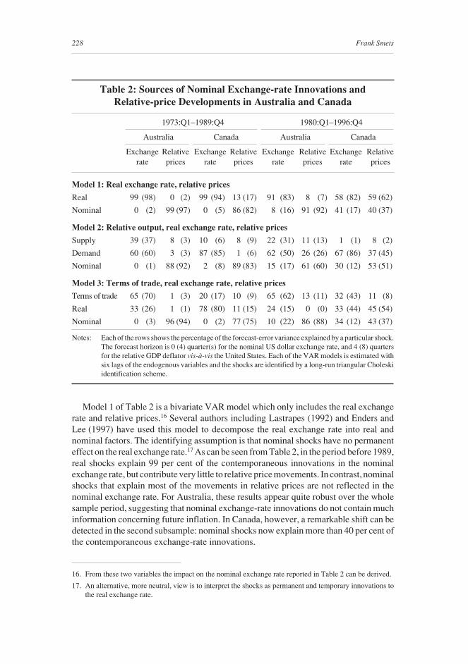
Model 1 of Table 2 is a bivariate VAR model which only includes the real exchangerate and relative prices.16 Several authors including Lastrapes (1992) and Enders andLee (1997) have used this model to decompose the real exchange rate into real andnominal factors. The identifying assumption is that nominal shocks have no permanenteffect on the real exchange rate.17 As can be seen from Table 2, in the period before 1989,real shocks explain 99 per cent of the contemporaneous innovations in the nominalexchange rate, but contribute very little to relative price movements. In contrast, nominalshocks that explain most of the movements in relative prices are not reflected in thenominal exchange rate. For Australia, these results appear quite robust over the wholesample period, suggesting that nominal exchange-rate innovations do not contain muchinformation concerning future inflation. In Canada, however, a remarkable shift can bedetected in the second subsample: nominal shocks now explain more than 40 per cent ofthe contemporaneous exchange-rate innovations.

Table 2: Sources of Nominal Exchange-rate Innovations andRelative-price Developments in Australia and Canada

1973:Q1–1989:Q4 1980:Q1–1996:Q4 Australia Canada Australia Canada

Exchange Relative Exchange Relative Exchange Relative Exchange Relativerate prices rate prices rate prices rate prices

Model 1: Real exchange rate, relative prices

Real 99 (98) 0 (2) 99 (94) 13 (17) 91 (83) 8 (7) 58 (82) 59 (62)

Nominal 0 (2) 99 (97) 0 (5) 86 (82) 8 (16) 91 (92) 41 (17) 40 (37)

Model 2: Relative output, real exchange rate, relative prices

Supply 39 (37) 8 (3) 10 (6) 8 (9) 22 (31) 11 (13) 1 (1) 8 (2)

Demand 60 (60) 3 (3) 87 (85) 1 (6) 62 (50) 26 (26) 67 (86) 37 (45)

Nominal 0 (1) 88 (92) 2 (8) 89 (83) 15 (17) 61 (60) 30 (12) 53 (51)

Model 3: Terms of trade, real exchange rate, relative prices

Terms of trade 65 (70) 1 (3) 20 (17) 10 (9) 65 (62) 13 (11) 32 (43) 11 (8)

Real 33 (26) 1 (1) 78 (80) 11 (15) 24 (15) 0 (0) 33 (44) 45 (54)

Nominal 0 (3) 96 (94) 0 (2) 77 (75) 10 (22) 86 (88) 34 (12) 43 (37)

Notes: Each of the rows shows the percentage of the forecast-error variance explained by a particular shock.The forecast horizon is 0 (4) quarter(s) for the nominal US dollar exchange rate, and 4 (8) quartersfor the relative GDP deflator vis-à-vis the United States. Each of the VAR models is estimated withsix lags of the endogenous variables and the shocks are identified by a long-run triangular Choleskiidentification scheme.

16. From these two variables the impact on the nominal exchange rate reported in Table 2 can be derived.

17. An alternative, more neutral, view is to interpret the shocks as permanent and temporary innovations tothe real exchange rate.

229Financial-asset Prices and Monetary Policy: Theory and Evidence

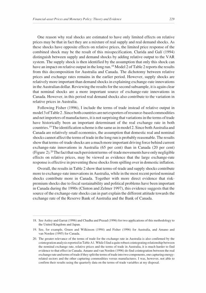
One reason why real shocks are estimated to have only limited effects on relativeprices may be that in fact they are a mixture of real supply and real demand shocks. Asthese shocks have opposite effects on relative prices, the limited price response of thecombined shock may be the result of this misspecification. Clarida and Galí (1994)distinguish between supply and demand shocks by adding relative output to the VARsystem. The supply shock is then identified by the assumption that only this shock canhave an impact on relative output in the long run.18 Model 2 of Table 2 reports the resultsfrom this decomposition for Australia and Canada. The dichotomy between relativeprices and exchange rates remains in the earlier period. However, supply shocks arerelatively more important than demand shocks in explaining exchange-rate innovationsin the Australian dollar. Reviewing the results for the second subsample, it is again clearthat nominal shocks are a more important source of exchange-rate innovations inCanada. However, in this period real demand shocks also contribute to the variation inrelative prices in Australia.

Following Fisher (1996), I include the terms of trade instead of relative output inmodel 3 of Table 2 . Since both countries are net exporters of resource-based commoditiesand net importers of manufactures, it is not surprising that variations in the terms of tradehave historically been an important determinant of the real exchange rate in bothcountries.19 The identification scheme is the same as in model 2. Since both Australia andCanada are relatively small economies, the assumption that domestic real and nominalshocks cannot affect the terms of trade in the long run is probably reasonable. The resultsshow that terms-of-trade shocks are a much more important driving force behind currentexchange-rate innovations in Australia (65 per cent) than in Canada (20 per cent)(Figure 2).20 The fact that such persistent terms-of-trade movements have only negligibleeffects on relative prices, may be viewed as evidence that the large exchange-rateresponse is effective in preventing these shocks from spilling over in domestic inflation.

Overall, the results in Table 2 show that terms-of-trade and supply shocks contributemore to exchange-rate innovations in Australia, while in the most recent period nominalshocks contribute more in Canada. Together with more direct evidence that risk-premium shocks due to fiscal sustainability and political problems have been importantin Canada during the 1990s (Clinton and Zelmer 1997), this evidence suggests that thesource of the exchange-rate shocks can in part explain the different attitude towards theexchange rate of the Reserve Bank of Australia and the Bank of Canada.

18. See Astley and Garrat (1996) and Chadha and Prasad (1996) for two applications of this methodology tothe United Kingdom and Japan.

19. See, for example, Gruen and Wilkinson (1994) and Fisher (1996) for Australia, and Amano andvan Norden (1995) for Canada.

20. The greater relevance of the terms of trade for the exchange rate in Australia is also confirmed by thecointegration analysis reported in Table A1. While I find a quite robust cointegrating relationship betweenthe nominal exchange rate, relative prices and the terms of trade in Australia, it is much harder to findevidence to that effect in Canada. Amano and van Norden (1996) do find cointegration between the realexchange rate and terms of trade if they split the terms of trade into two components, one capturing energy-related sectors and the other capturing commodities versus manufactures. I was, however, not able toconfirm their results using the quarterly data on the terms-of-trade variables at my disposal.

230 Frank Smets

5. ConclusionsThis paper consists of three sections. First, using a simple model and within the

context of the central bank’s objective of price stability, I discuss the optimal responseof monetary policy to unexpected changes in financial-asset prices. The main conclusionof this analysis is that the optimal response depends on how the asset-price movementaffects the central bank’s inflation forecast, which in turn depends on two factors: the roleof the asset price in the transmission mechanism and the typical information content ofinnovations in the asset price.

Second, I analysed the advantages and disadvantages of setting monetary policy interms of an MCI. While using an MCI as the operating target may be useful in terms ofpracticality and transparency when asset-price innovations are primarily driven byfinancial shocks, I have highlighted two potentially serious limitations which in partfollow from the simplicity of the MCI concept: first, the optimal weights are likely to varyover time, not least because interest rates and exchange rates affect the traded and non-traded goods sector differently; second, the MCI concept ignores the potentially usefulinformational and equilibrating role of asset-price innovations.

Figure 2: The Real Exchange Rate and the Terms of Trade

60

80

100

120

60

80

100

120

60

80

100

120

60

80

100

120

60

80

100

120

60

80

100

120

60

80

100

120

60

80

100

120

Real exchange rate

Terms of trade

Australia

Terms of trade

Real exchange rate

90 92 94 968886848280787674

Canada

Index Index

231Financial-asset Prices and Monetary Policy: Theory and Evidence

Third, I have estimated a policy reaction function for the Reserve Bank of Australiaand the Bank of Canada and found that while both central banks strongly respond todeviations of inflation from their announced target, their short-term response to theexchange rate differs. While the Bank of Canada, consistent with the idea of an MCI,systematically raises interest rates in response to a depreciation of the exchange rate, theReserve Bank of Australia does not respond. My analysis of the sources of exchange-rateinnovations in the two countries suggests that in part this can be explained by the greaterimportance of terms-of-trade shocks in Australia and, during the more recent period, ofnominal shocks in Canada.

In this paper I have focused on the role of asset prices in the central bank’s pursuit ofprice stability. There are at least two other reasons why asset prices may play a role inmonetary-policy formulation. First, the information in asset prices may be useful in thetactics of monetary policy. As much of the implementation of monetary policy is aboutcommunication and signalling, information from the financial markets about theexpected direction of policy may be useful to both assess the appropriateness of aparticular timing of policy actions and its effectiveness. Second, it is sometimessuggested that, to the extent that large and persistent asset-price misalignments may giverise to widespread financial instability, asset-price stability by itself should be animportant objective of the central bank (Goodhart 1995). Indeed, the experience of thelate 1980s, when many countries saw a sharp increase in the prices of real and financialassets which later proved to be unsustainable and led to large-scale losses in the bankingsector, shows that the misallocation costs due to such misalignments can be large. Bothof these issues deserve further attention in future research.

232 Frank Smets

21. The underlying assumption is that the price perception errors are independent of monetary-policybehaviour.

Appendix: Optimal Monetary Policy in the Model of Section 2.1Since the central bank does not observe current prices, I follow Canzoneri et al. (1983)

and Barro and Broadbent (1995) and assume that the central bank optimises the objectivefunction by picking the perceived price level. To implement this approach, I first derivethe contemporaneous price perception errors, and then rewrite the objective function (7)in terms of the perceived price level and the price perception errors.

Combining Equations (1) and (2) and rearranging, I express the price level as afunction of expectational variables, current observable variables and the excess-demandshock,

p E p E p p R Ft t t t t t t t td

ts= + − − + + − +− + ( ) ( ) /( )1 1 1γα γα γβ γ ε ε γβ . (A1)

Agents who use the current interest rate and asset price in making their current pricepredictions need estimate only the excess-demand disturbance, ε ε ε

t

xd

t

d

t

s= − , as theyeither know or can calculate all other terms on the right-hand side of Equation (8). Theircurrent price prediction is therefore

E p E p E p p R F Et t t t t t t t t t txd= + − − + + +− + ( ) /( )1 1 1γα γα γβ ε γβ (A2)

and, combining Equations (A1) and (A2), their price perception error is

p E p Et t t txd

t txd

t− = − + =( ) /( )ε ε γ γβ η1 . (A3)

Note that if agents observed current prices, they would be able to deduce fromEquation (A1) the current excess-demand shock, in which case the price perception errorwould be zero. If central banks do not observe current output and prices, they can stillpotentially extract information about the current excess-demand shock from the observedasset prices. Indeed, Equation (3) can be rewritten in nominal terms as

R F E F E yt t t t t t tf+ = + − ++

++ρ ρ ε1 1( ) . (3′′)

As the central bank does observe the left-hand side of Equation (3′′), it observes anoisy measure of the asset-market participants’ relevant expectations which may includeinformation about current output and prices. Below I discuss how that information canbe used to minimise the variance of ηt.

Optimal monetary policy

Equation (A3) can be used to rewrite the loss function in terms of the perceived currentprice level and a perception error,

L E p E p E p pt t t t t t t t t= + − + + −−( ) ( )η χ η12 2 . (A4)

Differentiating this expression with respect to Et pt yields,21

233Financial-asset Prices and Monetary Policy: Theory and Evidence

( )1 1+ = +−χ χE p E p pt t t t . (A5)

Imposing the rational-expectations condition, the equilibrium solution for the perceivedprice level is22

E p pt t = . (A6)

The central bank’s optimal policy is to equate the perceived price level to its target.

The associated equilibrium price and output level is then23

p pt t= + η (A7)

and

yt ts

t= +ε η γ/ . (A8)

The equilibrium output and price level differ from their targets to the extent that there areunexpected excess-demand shocks which the central bank cannot stabilise.

The next question is how the central bank should set the interest rate to achieve theoptimal price level. Combining Equations (1) and (2), taking the central bank’sexpectations and substituting for the equilibrium price level, the optimal reactionfunction in terms of the nominal interest rate is given by24

R F Et t t td

ts= + −β

α αε ε1

( ). (A9)

Policy interest rates will tighten in response to a perceived output gap and a rise in theasset price. Note that the size of the response to changes in the asset price depends on itsimpact on aggregate demand. If β = 0, i.e. the asset price does not play any role in thetransmission mechanism, then policy will not respond to movements in the asset price.However, Equation (A9) tells only part of the story. Since the asset price may containinformation about the current output gap, it may affect policy rates through its effect onperceived excess demand. Before turning to this case, I first solve for the equilibriumlevels of the interest rate and asset price under symmetric information.

Interest rates and asset prices under symmetric information

Next I derive the equilibrium level of the interest rate and the asset price when thefinancial market has no additional information on current output and prices. Equation(A9) becomes

R F E Ft t t td

ts

t td

ts= + − = + −− −

βα α

ε ε βα α

δε ε1 11 1( ( )) ( ) . (A10)

22. Note that here the assumption that wage setters also do not observe current output and prices is important.

23. In general, this need not be the case. For example, if the central bank targets the inflation rate, the priceforecast error will also depend on the past price perception error.

24. From here we assume that the price-level target is zero. Note that since current prices are not observed,neither the real interest rate nor the real stock price are known. In this case the perceived real interest rateand asset price equal the observed nominal interest rate and asset prices because the perceived price leveland expected inflation are zero.

234 Frank Smets

Moreover, using Equations (3), (4), (5) and (A7) and (A8) yields

F E F Rt t t t ts

tf= − + − ++ −ρ ρ ε ε1 11( ) . (A11)

Combining Equations (A10) and (A11) yields a first-order difference equation in thenominal asset price,

F E Ft t t td

ts

tf=

+−

++ + −

++

++ − −αρ

α βδ

α βε ρ α

α βε α

α βε1 1 1

1 1( )( ) . (A12)

Solving Equation (A12) forward yields the equilibrium solution given in Equations (9)and (10)

Asymmetric information and the policy response to asset prices

Now I assume that the financial-market participants do have information aboutcurrent output and prices, i.e. they observe the underlying supply and demand shocks.In this case the optimal response of policy rates is still governed by Equation (A9).However, this time there is a possibility that the asset price contains information aboutthe current excess-demand shock. I solve the optimal response to the asset price in twosteps. First, I postulate a particular form of the optimal interest-rate reaction function tothe asset price and calculate the equilibrium asset price that would be consistent with sucha reaction function. Given the expression of the asset price, I can then solve for the signal-extraction problem of the central bank and calculate the optimal response to the assetprice.

In this case I can rewrite the optimal reaction function

R F Et t td

ts

t td

ts= + − + −− −

1 1 11 1α α

δε εα

ξ ξ( ) ( ) . (A13)

The central bank estimates the current excess-demand shock using its knowledge of thecurrent asset price. I postulate that the signal-extraction function is of the form

E F E F Ft td

ts

t t t t ts

td( ) ( ) (

( )( ) ( )

)ξ ξ λ λ α ρα ρ β

ε δα ρδ β

ε− = − − = − − − +− +

+− +

−− −

1 11 11 1 (A14)

where λ is the response parameter that needs to be determined and Et– is the expectations

operator based on the information set which excludes the current asset price.

Going through the same procedure as before, the solution to a more complicated first-order forward-looking difference equation in Ft becomes

F E Ft t t td− = −

+ − − − ++ + − + + − − +

++ + − + − − − ++ +

− αδρ γβ α ρ α ρδ βγβ α β λ γβ α ρ α ρδ β

ξ

α γβ α β ρ ρ α ρ α ρ βγβ α β

( ) ( )( ( ) )

( )( ) ( ( ))( ( ) )

( )(( )( ) ) ( )( ( ) )

( )(

1 1 1

1 1 1 1

1 1 1 1

1 )) ( ( ))( ( ) )

( )

( )( ) ( ( ))

− + + − − +

+ ++ + − + + −

λ γβ α ρ α ρ βξ

α γβγβ α β λ γβ α ρ

ξ

1 1 1

1

1 1 1

ts

tf

. (A15)

235Financial-asset Prices and Monetary Policy: Theory and Evidence

Given this solution for the unexpected change in the asset price, I can now solve thesignal-extraction problem as follows,

− =− −

−

−

−λξ ξcov

var

( , )

( )td

ts

t t t

t t t

F E F

F E F . (A16)

This yields the following solution for λ ,

λ σ σ

α ρδ β σ α ρδα ρδ β σ α γβ

α β σ= +

− + + − +− + + +

+

a b

a bd s

d s f

2 2

2 2 2

11 1

11

( )( ( ) )

( )( )

(A17)

with a = + − − − +− +

δρ γβ ρ α δρ βα δρ β

( ) ( )( ( ) )( )

1 1 11

and b = + − + + − − − +− +

(( )( ) )( ) ( )( ( ) )( )

α β ρ ρ γβ ρ α ρ βα ρ β

1 1 1 11

.

Table A1: Statistics1973:Q1–1997:Q1

Phillips-Perron unit root tests Standard deviation Correlation

Australia Canada Australia Canada

Nominal US$ -1.43 -1.37 3.9 1.6 0.31exchange rate

Relative GDP deflator -1.41 -2.27 1.0 0.6 0.35

Terms of trade -2.45 -2.73 2.4 1.5 0.33

Johansen cointegration test

LR test Cointegrating equation (CE)

No CE At most Nominal Relative Termsone CE exchange prices of trade

rate

Australia 50** 11 1 -1.03 (0.13) 1.86 (0.26)

Canada 23 10 — — —

Notes: *(**) denotes rejection at 5(1) per cent significance level. All variables are in logs.

236 Frank Smets

ReferencesAmano, R. and S. van Norden (1995), ‘Terms of Trade and Real Exchange Rates: The Canadian

Evidence’, Journal of International Money and Finance, 14(1), pp. 83–104.

Astley, M.S. and A. Garrat (1996), ‘Interpreting Sterling Exchange Rate Movements’, Bank ofEngland Quarterly Bulletin, 36(4), pp. 394–404.

Banque de France (1996), ‘Les Indicateurs des Conditions Monetaires’, Bulletin de la Banque deFrance, 30, June, pp. 1–15.

Barro, R.J. and D.B. Gordon (1983), ‘Rules, Discretion and Reputation in a Model of MonetaryPolicy’, Journal of Monetary Economics, 12, pp. 101–120.

Bernanke, B. and M. Woodford (1996), ‘Inflation Forecasts and Monetary Policy’, mimeo.

Black, R., T. Macklem and D. Rose (1997), On Policy Rules for Price Stability, paper presentedat the Bank of Canada Conference, ‘Price Stability, Inflation Targets and Monetary Policy’,Ottawa, 3–5 May.

Blanchard, O. and D. Quah (1989), ‘The Dynamic Effects of Aggregate Demand and SupplyDisturbances’, American Economic Review, 79(4), pp. 655–673.

Boyer, R.S. (1978), ‘Optimal Foreign Exchange Market Intervention’, Journal of PoliticalEconomy, 86(8), pp. 1045–1055.

Broadbent, B. and R.J. Barro (1997), ‘Central Bank Preferences and Macroeconomic Equilibrium’,Journal of Monetary Economics, 39(1), pp. 17–43.

Canzoneri, M. and D.W. Henderson (1991), Monetary Policy in Interdependent Economies, MITPress, Cambridge, Massachusetts.

Canzoneri, M., D.W. Henderson and K.S. Rogoff (1983), ‘The Information Content of the InterestRate and Optimal Monetary Policy’, Quarterly Journal of Economics, 98(4), pp. 545--566.

Chadha, B. and E. Prasad (1996), ‘Real Exchange Rate Fluctuations and the Business Cycle:Evidence from Japan’, IMF Working Paper No. 96/132.

Clarida, R. and J. Galí (1994), ‘Sources of Real Exchange Rate Fluctuations: How Important areNominal Shocks?’, Carnegie-Rochester Conference Series on Public Policy, 41, pp. 1–56.

Clarida, R., J. Galí and M. Gertler (1997), ‘Monetary Policy Rules in Practice: Some InternationalEvidence’, mimeo.

Clinton, K. and M. Zelmer (1997), ‘Aspects of Canadian Monetary Policy Conduct in the 1990s:Dealing with Uncertainty’, in BIS, Implementation and Tactics of Monetary Policy,Conference Papers Vol. 3, pp. 169–199.

Cumby, R.E., J. Huizinga and M. Obstfeld (1983), ‘Two-Step Two-Stage Least Squares Estimationin Models with Rational Expectations’, Journal of Econometrics, 21(3), pp. 333–355.

Debelle, G. (1996), ‘The Ends of Three Small Inflations: Australia, New Zealand and Canada’,Canadian Public Policy, 22(1), pp. 56–78.

Duguay, P. (1994), ‘Empirical Evidence on the Strength of the Monetary Transmission Mechanismin Canada – an Aggregate Approach’, Journal of Monetary Economics, 33(1), pp. 39–61.

Enders, W. and B.S. Lee (1997), ‘Accounting for Real and Nominal Exchange Rate Movementsin the Post-Bretton Woods Period’, Journal of International Money and Finance, 16(2),pp. 233–254.

Estrella, A. (1996), ‘Why do Interest Rates Predict Macro Outcomes? A Unified Theory ofInflation, Output, Interest and Policy’, Federal Reserve Bank of New York Research PaperNo. 9717.

237Financial-asset Prices and Monetary Policy: Theory and Evidence

Fisher, L.A. (1996), ‘Sources of Exchange Rate and Price Level Fluctuations in Two CommodityExporting Countries: Australia and New Zealand’, Economic Record, 72(219), pp. 345--358.

Freedman, C. (1994), ‘The Use of Indicators and the Monetary Conditions Index in Canada’, inT.J.T. Balino and C. Cottarelli (eds), Frameworks for Monetary Stability – Policy Issues andCountry Experiences, IMF, Washington D.C., pp. 458–476.

Fuhrer, J. and G. Moore (1992), ‘Monetary Policy Rules and the Indicator Properties of AssetPrices’, Journal of Monetary Economics, 29(2), pp. 303–336.

Gerlach, S. and F. Smets (1996), ‘MCIs and Monetary Policy in Open Economies under FloatingRates’, mimeo.

Goodhart, C. (1995), ‘Price Stability and Financial Fragility’, in K. Sawamoto, Z. Nakajima andH. Taguchi (eds), Financial Stability in a Changing Environment, Macmillan, Basingtoke.

Grimes, A. and J. Wong (1994), ‘The Role of the Exchange Rate in New Zealand MonetaryPolicy’, in R. Glick and M. Hutchinson (eds), Exchange Rate Policy and Interdependence:Perspectives from the Pacific Basin, Cambridge University Press, New York.

Gruen, D.W.R. and J. Wilkinson, (1994), ‘Australia’s Real Exchange Rate: Is it Explained by theTerms of Trade or by Real Interest Differentials?’, Economic Record, 70(209), pp. 204–219.

Hansen, L. (1982), ‘Large Sample Properties of Generalised Method of Moments Estimators’,Econometrica, 50(4), pp. 1029–1054.

King, M. (1997), ‘Monetary Policy and the Exchange Rate’, Bank of England Quarterly Bulletin,37(2), pp. 225–227.

Lastrapes, W.D. (1992), ‘Sources of Fluctuations in Real and Nominal Exchange Rates’, Reviewof Economics and Statistics, 74(3), pp. 530–539.

Longworth, D. and S. Poloz (1995), ‘The Monetary Transmission Mechanism and PolicyFormulation in Canada: an Overview’, in BIS, Financial Structure and the Monetary PolicyTransmission Mechanism, March, pp. 312–323.

Lowe, P. and L. Ellis (1997), ‘The Smoothing of Official Interest Rates’, paper presented at thisconference.

Poole, W. (1970), ‘Optimal Choice of Monetary Policy Instruments in a Simple Stochastic MacroModel’, Quarterly Journal of Economics, 84(2), pp. 197–216.

Smets, F. (1995), ‘Central Bank Macroeconometric Models and the Monetary Policy TransmissionMechanism’, in BIS, Financial Structure and the Monetary Policy Transmission Mechanism,March, pp. 225–266.

Svensson, L.E.O. (1997), ‘Inflation Forecast Targeting: Implementing and Monitoring InflationTargets’, European Economic Review, 41(6), pp. 1111–1146.

Taylor, J.B. (1993), ‘Discretion versus Policy Rules in Practice’, Carnegie-Rochester ConferenceSeries on Public Policy, 39, pp. 195–214.

Taylor, J.B. (1996), ‘Policy Rules as a Means to a more Effective Monetary Policy’, Institute forMonetary and Economic Studies, Bank of Japan, Discussion Paper 96-E-12.

Woodford, M. (1994), ‘Nonstandard Indicators for Monetary Policy: Can their Usefulness beJudged from Forecasting Regressions?’ in N.G. Mankiw (ed.), Monetary Policy, Universityof Chicago Press, Chicago, pp. 95–115.