Final Revised Paper - Hydrology and Earth System Sciences

Hydrol. Earth Syst. Sci., 17, 5127–5139, 2013www.hydrol-earth-syst-sci.net/17/5127/2013/doi:10.5194/hess-17-5127-2013© Author(s) 2013. CC Attribution 3.0 License.

Hydrology and Earth System

SciencesO

pen Access

Large scale snow water equivalent status monitoring: comparison ofdifferent snow water products in the upper Colorado Basin

G. A. Artan 1, J. P. Verdin2, and R. Lietzow2

1ASRC Federal InuTeq LLC, US Geological Survey (USGS) Earth Resources Observation and Science (EROS) Center,Sioux Falls, SD, USA2USGS Earth Resources Observation and Science (EROS) Center, Sioux Falls, SD, USA

Correspondence to:G. A. Artan ([email protected])

Received: 6 February 2013 – Published in Hydrol. Earth Syst. Sci. Discuss.: 19 March 2013Revised: 4 November 2013 – Accepted: 19 November 2013 – Published: 18 December 2013

Abstract. We illustrate the ability to monitor the status ofsnow water content over large areas by using a spatiallydistributed snow accumulation and ablation model that usesdata from a weather forecast model in the upper ColoradoBasin. The model was forced with precipitation fields fromthe National Weather Service (NWS) Multi-sensor Precip-itation Estimator (MPE) and the Tropical Rainfall Measur-ing Mission (TRMM) data-sets; remaining meteorologicalmodel input data were from NOAA’s Global Forecast System(GFS) model output fields. The simulated snow water equiv-alent (SWE) was compared to SWEs from the Snow DataAssimilation System (SNODAS) and SNOwpack TELeme-try system (SNOTEL) over a region of the western US thatcovers parts of the upper Colorado Basin. We also com-pared the SWE product estimated from the special sensormicrowave imager (SSM/I) and scanning multichannel mi-crowave radiometer (SMMR) to the SNODAS and SNO-TEL SWE data-sets. Agreement between the spatial distri-butions of the simulated SWE with MPE data was high withboth SNODAS and SNOTEL. Model-simulated SWE withTRMM precipitation and SWE estimated from the passivemicrowave imagery were not significantly correlated spa-tially with either SNODAS or the SNOTEL SWE. Averagebasin-wide SWE simulated with the MPE and the TRMMdata were highly correlated with both SNODAS (r = 0.94andr = 0.64; d.f.= 14 – d.f. = degrees of freedom) and SNO-TEL (r = 0.93 andr = 0.68; d.f. = 14). The SWE estimatedfrom the passive microwave imagery was significantly corre-lated with the SNODAS SWE (r = 0.55, d.f. = 9,p = 0.05) butwas not significantly correlated with the SNOTEL-reportedSWE values (r = 0.45, d.f. = 9,p = 0.05).The results indicate

the applicability of the snow energy balance model for mon-itoring snow water content at regional scales when coupledwith meteorological data of acceptable quality. The two snowwater contents from the microwave imagery (SMMR andSSM/I) and the Utah Energy Balance forced with the TRMMprecipitation data were found to be unreliable sources formapping SWE in the study area; both data sets lacked dis-cernible variability of snow water content between sites asseen in the SNOTEL and SNODAS SWE data. This studywill contribute to better understanding the adequacy of datafrom weather forecast models, TRMM, and microwave im-agery for monitoring status of the snow water content.

1 Introduction

Every year large parts of the globe are seasonally covered bysnow; for example, each year as much as half of the landsurface in the Northern Hemisphere can be snow-covered(Robinson and Kukla, 1985). Most of the water supply forthose snow-covered areas comes from snowmelt runoff (Dalyet al., 2000; Schmugge et al., 2002; Tekeli et al., 2005); over60 % of the precipitation in the western US falls as snow(Serreze et al., 1999). In the upper Colorado Basin, 63 % ofprecipitation falls as snow (Fassnacht, 2006), and 70–80 % oftotal annual runoff comes from snowmelt (Daly et al., 2000;Schmugge et al., 2002). In the past few decades, some basinsin the US have seen historic floods that were induced andtriggered from spring rain-on-snow events during years ofabove average winter snowfall, such as the floods of the RedRiver of 2009 and 2010. Monitoring the status of snowpack

Published by Copernicus Publications on behalf of the European Geosciences Union.

5128 G. A. Artan et al.: Comparison of different snow water products in the upper Colorado Basin

during winter and spring is important to water resources anddisaster management entities.

Several methods have been used to monitor snowpack sta-tus: snow course surveys, remote sensing, and snow accumu-lation/ablation modeling. Worldwide, few areas have reliableground-observed snowpack status data collected regularly ona large scale. One exception is the western US, which is mon-itored by the SNOwpack TELemetry system (SNOTEL). Therepresentativeness of the snowpack characteristics estimatedeven from a data-extensive system such as SNOTEL is ques-tioned by some investigators (Daly et al., 2000; Molotch andBales, 2006).

Because of the limitations of the observational data,several snowpack status monitoring systems that rely onsnowmelt models (Pan et al., 2003; Watson et al., 2006)have been described in the literature: snowmelt models com-bined with remotely sensed data (Cline et al., 1998), remotelysensed data combined with observed snow data (Carroll,1995; Dressler et al., 2006), and models based solely onremote sensing methods (Bales et al., 2008; Schmugge etal., 2002; Tekeli et al., 2005). A system that utilizes as-similation of data (remotely sensed and in situ measured)and snow accumulation/ablation modeling is the NOAANational Operational Hydrologic Remote Sensing Center(NOHRC; NOHRC, 2004) Snow Data Assimilation System(SNODAS).

Efforts to monitor snowpack status for large areas fromremotely sensed data have mainly focused on snow coveredarea (SCA) mapping (Bales et al., 2008; Kelly et al., 2003;Robinson et al., 1993; Tekeli et al., 2005); however, the snowwater equivalent (SWE) status is what interests water re-sources and disaster risk managers the most. Despite theircoarse spatial resolution and known shortcomings (Kelly etal., 2003), passive microwave sensors like the scanning mul-tichannel microwave radiometer (SMMR) and the specialsensor microwave imager (SSM/I) have gained some accep-tance as tools to map SWE (Chen et al., 2001; Sun et al.,1996).

The objective of this study is to explore the possibility ofmonitoring the status of the snowpack at regional scales inreal time with models and data that are available in even themost data-scarce regions of the globe. The recent availabil-ity of precipitation data sets estimated from satellite-basedmethods (Janowiak et al., 2001; Joyce et al., 2004; Xie andArkin, 1997) and the upcoming Global Precipitation Mea-surement (GPM) offers an opportunity to model snow ac-cumulation and ablation processes on regional-scales evenfor data-parse areas. The specific aim of our study is to in-vestigate how SWE that is modeled (with coarse resolutionmeteorological data) and one that was estimated from pas-sive microwave sensor data compared with SWE values mea-sured by SNOTEL and estimated by SNODAS. We intro-duce a spatially distributed snow accumulation and ablationmodel that is forced with remotely sensed data and near-real-time meteorological data from forecast models. We compare

model-simulated SWE with the best available regional SWEdata sets. In the comparison, we include a SWE product es-timated from SSM/I and SMMR to substantiate how usefulthey are in lieu of snowmelt-predicted SWE products. Thisstudy will contribute to a better understanding of the ade-quacy of data from weather forecast models, TRMM, andmicrowave imagery for monitoring snow water status espe-cially in data-scarce regions of the world.

The snowmelt model we used is a spatially distributed ver-sion of the Utah Energy Balance (UEB) model (Tarboton andLuce, 1996). The UEB model has been applied successfullyto several basins from different parts of the world (Koivusaloand Heikinheimo, 1999; Schulz and de Jong, 2004; Watsonet al., 2006). We describe the model and data, and evaluatesimulated SWE values over a region of the western US thatcovers parts of the upper Colorado Basin.

2 Study site

Figure 1 depicts the geographic extent of the study area andof the SNOTEL sites that were used in the model verifica-tion. The area (43◦48′ N, 116◦06′ W) encompasses a model-ing domain of 1 504 800 km2. The area is rugged and strad-dles the Continental Divide and has a mean elevation of2203 m (σ = 517 m). The SNOTEL sites used for validationare mainly in the upper Colorado Basin. The average yearlyprecipitation that falls on the upper Colorado Basin, esti-mated from 39 SNOTEL stations, was 700 mm (± 184 mm)for the three water years of the study – 2006, 2007, and 2008.The area has a low (∼ 11 %) tree vegetation cover.

3 Model and data

SWE recorded from SNODAS and SNOTEL was comparedwith the SWE simulated by the UEB snowmelt model andSWE estimated from microwave imagery. In the followingsections, we describe the UEB snowmelt model, model inputdata sets, and the results of the SWE product intercompar-isons. Because the SNODAS system assimilates most of thereal-time recorded SWE data in the conterminous US, weassumed that the SNODAS SWE data were observed data.Although SNODAS SWE is the best regional-scale, spatiallydistributed SWE data available, we are not aware of a com-prehensive validation of the SWE estimated by the SNODASsystem. The snowmelt model was run for the period Decem-ber 2005–April 2008.

3.1 Snow accumulation and ablation model

The UEB model (Tarboton and Luce, 1996) was used for thiswork. The UEB model has been applied successfully to di-verse basins with good results (Koivusalo and Heikinheimo,1999; Schulz and de Jong, 2004; Watson et al., 2006). TheUEB model solves the snow energy balance at the surface

Hydrol. Earth Syst. Sci., 17, 5127–5139, 2013 www.hydrol-earth-syst-sci.net/17/5127/2013/

G. A. Artan et al.: Comparison of different snow water products in the upper Colorado Basin 5129

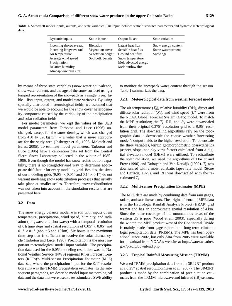
Table 1.Snowmelt model inputs, outputs, and state variables. The input includes static distributed parameters and dynamic meteorologicaldata.

Dynamic inputs Static inputs Output fluxes State variables

Incoming shortwave rad. Elevation Latent heat flux Snow energy contentIncoming longwave rad. Vegetation cover Sensible heat flux Snow water contentAir temperature Vegetation height Ground heat flux Snow ageAverage wind speed Soil bulk density Snow temperaturePrecipitation Melt advected energyRelative humidity Melt outflow fluxAtmospheric pressure

by means of three state variables (snow water equivalence,snow water content, and the age of the snow surface) using alumped representation of the snowpack as a single layer. Ta-ble 1 lists input, output, and model state variables. By usingspatially distributed meteorological fields, we assumed thatwe would be able to account for the snow cover heterogene-ity component caused by the variability of the precipitationand solar radiation fields.

For model parameters, we kept the values of the UEBmodel parameters from Tarboton and Luce (1996) un-changed, except for the snow density, which was changedfrom 450 to 320 kg m−3 – a value that is more appropri-ate for the study area (Josberger et al., 1996; Molotch andBales, 2005). To estimate model parameters, Tarboton andLuce (1996) have a calibration data set from the CentralSierra Snow Laboratory collected in the winter of 1985–1986. Even though the model has snow redistribution capa-bility, there is no straightforward way to determine appro-priate drift factor for every modeling grid. Besides, the sizesof our modeling grids (0.05◦ × 0.05◦ and 0.1◦ × 0.1◦) do notwarrant modeling snow redistribution processes that usuallytake place at smaller scales. Therefore, snow redistributionwas not taken into account in the simulation results that arepresented here.

3.2 Data

The snow energy balance model was run with inputs of airtemperature, precipitation, wind speed, humidity, and radi-ation (longwave and shortwave) with a temporal resolutionof 6 h time steps and spatial resolutions of 0.05◦

× 0.05◦ and0.1◦

× 0.1◦ (about 5 and 10 km). Six hours is the maximumtime step that is sufficient to resolve the solar diurnal cy-cle (Tarboton and Luce, 1996). Precipitation is the most im-portant meteorological model input variable. The precipita-tion data used for the 0.05◦ modeling resolution was the Na-tional Weather Service (NWS) regional River Forecast Cen-ters (RFCs)’s Multi-sensor Precipitation Estimator (MPE)data set, where the precipitation input for the 0.1◦ resolu-tion runs was the TRMM precipitation estimates. In the sub-sequent paragraphs, we describe model input meteorologicaldata and the data that were used to test simulated SWE ability

to monitor the snowpack water content through the season.Table 1 summarizes the data.

3.2.1 Meteorological data from weather forecast model

The air temperature (Ta), relative humidity (RH), direct anddiffuse solar radiation (Rs), and wind speed (U ) were fromthe NOAA Global Forecast System (GFS) model. To matchthe MPE resolution; theTa, RH, andRs were downscaledfrom their original 0.375◦ resolution grid to a 0.05◦ reso-lution grid. The downscaling algorithms rely on the topo-graphic data to downscale the coarse weather forecastingmodel’s output fields to the higher resolution. To downscalethe three variables, terrain geomorphometric characteristics(aspect, slope, and sky-view factor) calculated from a dig-ital elevation model (DEM) were utilized. To redistributethe solar radiation, we used the algorithms of Dozier andFrew (1990) and Dubayah and Van Katwijk (1992).Ta wasdownscaled with a moist adiabatic lapse rate model (Stoneand Carlson, 1979), and RH was downscaled with the re-estimatedTa.

3.2.2 Multi-sensor Precipitation Estimator (MPE)

The MPE data are made by combining data from rain gages,radars, and satellite sensors. The original format of MPE datais in the Hydrologic Rainfall Analysis Project (HRAP) gridformat and has an approximate spatial resolution of 4 km.Since the radar coverage of the mountainous areas of thewestern US is poor (Wood et al., 2003), especially duringthe winter, the MPE product west of the Continental Divideis mainly made from gage reports and long-term climato-logic precipitation data (PRISM). The MPE has been oper-ational since 2002, but only data from 2005 were availablefor download from NOAA’s website athttp://water.weather.gov/precip/download.php.

3.2.3 Tropical Rainfall Measuring Mission (TRMM)

We used TRMM precipitation data from the 3B42RT productat a 0.25◦ spatial resolution (Tian et al., 2007). The 3B42RTproduct is made by the combination of precipitation esti-mates from the TRMM microwave and infrared (IR) sensors.

www.hydrol-earth-syst-sci.net/17/5127/2013/ Hydrol. Earth Syst. Sci., 17, 5127–5139, 2013

http://water.weather.gov/precip/download.php

http://water.weather.gov/precip/download.php


Table 2. Locations of the SNOTEL station where simulated SWEand MI-estimated SWE were validated.

Station Station name Lat Long ElevationID

1 Brumley 39.08 −106.53 32312 Columbine Pass 38.42 −108.37 28653 Elk River 40.83 −106.97 26524 Lost Dog 40.80 −106.73 28415 Mccoy Park 39.60 −106.53 28906 Middle Fork Camp 39.78 −106.02 27257 Park Cone 39.82 −106.58 29268 Park Reservoir 39.03 −107.87 30369 Lone Cone 37.88 −108.18 292610 Elkhart Park 43.00 −109.75 286511 Battle Mountain 41.03 −107.25 226812 New Fork Lake 43.12 −109.93 254213 East Rim Divide 43.13 −110.20 241714 SandstoneRs 41.12 −107.17 248415 Hickerson Park 40.90 −109.95 278716 Trout Creek 40.73 −109.67 290117 Mosby Mtn 40.60 −109.88 289918 Lakefork #1 40.58 −110.43 317419 Loomis Park 43.17 −110.13 251220 Snider Basin 42.48 −110.52 245721 Kelley R. S. 42.27 −110.8 249322 Burro Mountain 39.87 −107.58 286523 Hams Fork 42.15 −110.67 239024 King’s Cabin 40.70 −109.53 265925 Lasal Mountain 38.47 −109.27 291426 Porphyry Creek 38.48 −106.33 328027 Slumgullion 37.98 −107.20 348728 Butte 38.88 −106.95 309729 Dry Lake 40.53 −106.77 256030 Gunsight Pass 43.37 −109.87 299331 Kendall R. S. 43.23 −110.02 235932 Stillwater Creek 40.22 −105.92 265833 Rock Creek 40.53 −110.68 240534 Indian Creek 42.30 −110.67 287335 Lizard Head Pass 37.78−107.92 310936 Spring Creek Divide 42.52 −110.65 274337 El Diente Peak 37.78 −108.02 304838 Townsend Creek 42.68 −108.88 265239 McClure Pass 39.12 −107.28 2896

The microwave sensor provides the main estimates, and theIR sensors provide coverage for areas with gaps in the mi-crowave precipitation estimates. Although the TRMM 3B42estimates are considered better than the 3B42RT product, the3B42 is not available in real time as the 3B42RT product is.The 3B42RT products are usually posted to the TRMM Website about 6 h after the event.

3.2.4 SWE from the microwave imagers

The SWE data sets estimated by microwave imagers that weused are from the Global Monthly EASE-Grid SWE Clima-tology (Armstrong et al., 2007). The EASE-Grid SWE data

660 661

Fig. 1. A shaded relief map of the study area and locations of theSNOTEL sites with an outline of the Colorado Basin and westernUS states.

sets are monthly average values downloaded from the Na-tional Snow and Ice Data Center Distributed Active ArchiveCenter (NSIDC,http://nsidc.org/data/), University of Col-orado at Boulder. The data are derived from the SMMRand selected SSM/Is. The EASE-Grid SWE data sets havea resolution of 25 km, about 0.25◦, but since the SSM/Idata used to produce the SWE are 19 and 37 GHz (the19 GHz imagery has a footprint of 69 km× 43 km), the ac-tual resolution of the SWE could be coarser than the nominal25 km. The microwave-based SWE (MI SWE) spans fromDecember 2005 to April 2007. Only data from December toApril were used in the intercomparison with the other SWEproducts.

3.2.5 SNOTEL

SNOTEL is an automated network of stations that recordsnow and meteorological variables in the western US andAlaska. SNOTEL is a Natural Resources Conservation Ser-vice (NRCS) network. Most SNOTEL sites are located athigher elevations. We downloaded SWE, precipitation, andair temperature data from the NRCS’s website (http://www.wcc.nrcs.usda.gov/snow). The data were recorded at 39 sta-tions located in the areas shown in Fig. 1 for the period Oc-tober 2005–September 2008 and summarized in Table 2.


http://nsidc.org/data/

http://www.wcc.nrcs.usda.gov/snow

http://www.wcc.nrcs.usda.gov/snow


Table 3.Source and resolution of meteorological and snow data.

Data Source Resolution Downscaling

Spatial Temporal

Ta, RH,Rs, U NOAA’s GFS Model 0.375◦ × 0.375◦ 6 h 0.05◦, 0.1◦

MPE NWS RFCs 4 km× 4 km 24 h 0.05◦, 0.1◦

TRMM NASA 0.25◦ × 0.25◦ 3 h 0.1◦

SWE (EASE-Grid) NSIDC 0.25◦ × 0.25◦ 24 h noneSWE,Ta SNOTEL Point data 24 h noneSWE (SNODAS) NOAA NOHRC 1 km× 1 km 24 h 0.05◦

3.2.6 SNODAS

SNODAS is an NOAA NOHRC SWE data set (NOHRC,2004). SNODAS is made by the assimilation of modeledSWE, remotely sensed SWE, and station-recorded SWEdata. The SNODAS data set covers the conterminous USat 1 km spatial resolution and 24 h temporal resolution. Al-though we will consider hereafter the SWE as observed,we are not aware of any extensive validation done on theSNODAS SWE data sets. Because SNODAS assimilates allavailable observed snow data, it is difficult to validate theaccuracy of the SNODAS product. Nevertheless, SNODAShas been used in several research studies and is the only pub-licly available large-scale SWE product. SNODAS data setswere downloaded from the NSIDC website (http://nsidc.org/data). Before comparing SNODAS with other data sets, theSNODAS data were re-gridded to 0.05, 0.1, and 0.25◦ resolu-tion from the native 1 km resolution. Table 3 summarizes thespatial and temporal resolutions of the meteorological andsnow data that were used in this study.

3.3 Performance indicators

For performance indicators, we used the percent of bias,coefficient of determination, total root mean square error(RMSE), and parameters that are based on the RMSE out-lined by Willmott (1982). Willmott (1982) decomposed theRMSE into the systematic error (RMSEs), which can be re-duced with small improvements in model parameters and in-put data, and unsystematic RMSE (RMSEu), which cannotbe reduced without extensive changes in the model structureand input data. The RMSE, RMSEs, and RMSEu parametersare defined (Willmott, 1982) as

RMSE =

[1

n

n∑i=1

(Pi − Oi)2

]1/2

,

RMSEs=

[1

n

n∑i=1

(Pi − Oi

)2]1/2

,

RMSEu=

[1

n

n∑i=1

(Pi − Pi

)2]1/2

,

wheren is the number of observations,Oi is the observedvalue,Pi is the predicted value, andPi =a · Oi + b. To de-scribe how much the model underestimates or overestimatesthe variable of interest, the percent bias was calculated ac-cording to

Bias = 100 ·

n∑i=1

Pi −

n∑i=1

Oi

n∑i=1

Oi

.

4 Results and discussion

4.1 Snowmelt model meteorological inputs

We tested the precipitation values reported by MPE andTRMM by comparing them to the precipitation valuesrecorded at the 39 SNOTEL stations shown in Fig. 1. Bycomparing gridded data of varying spatial scales and pointdata, there should not be an expectation of perfect agreementeven if both data are correct. We compared precipitation to-tals accumulated in the snow accumulation/ablation periodsof the three years of the simulation period – 1 January 2006–30 April 2006, 1 January 2007–30 April 2007, and 1 Jan-uary 2008–28 April 2008 (d.f. = 115). Both MPE and TRMMwere negatively biased against SNOTEL precipitation as il-lustrated in Fig. 2; on average the percent bias of the MPEper season for the 39 locations was−26 % with a mean andstandard deviation of−84± 110 mm, and for the TRMM thebias was−51 % (−164± 124 mm). The correlation betweenthe MPE and TRMM was even lower than the one the twodata sets had with SNOTEL data (r = 0.53). Higher propor-tions of the precipitation differences with SNOTEL sets weresystematic errors for both the TRMM (86 % of RMSE) andthe MPE data sets (77 % of RMSE), which means the datacould be improved with simpler correction schemes.

The large discrepancy of the MPE compared with SNO-TEL is difficult to explain even when the perils of compar-ing gridded precipitation with values from a single gage aretaken into account. The discrepancies could be due to thedifference between the methods used to calculate the MPEvalues east and west of the Continental Divide. The large


http://nsidc.org/data

http://nsidc.org/data


Fig. 2. Scatterplots of the total precipitation recorded at 39 SNO-TEL sites for the periods of 1 January 2006–30 April 2006, 1 Jan-uary 2007–30 April 2007, and 1 January 2008–28 April 2008 com-pared with precipitation estimates for the same locations from MPE(black) and TRMM (green).

magnitude of the discrepancy between some of the SNOTELstation-recorded precipitation and the MPE suggests that theMPE estimation needs to be improved. Our results on thebias direction, being inclined for underestimation, are in linewith what Habib et al. (2009) observed when they weightedprecipitation values from MPE against rain-gage-recordedprecipitation.

The GFS daily meanTa extracted from grid-cells was com-pared to SNOTEL-recordedTa from the 39 stations. TheGFSTa was created by averaging four 6 hTa. The compar-ison period was the same as the precipitation evaluation pe-riod – winter and spring – when theTa influences the snowprocess. The elevation at the 39 sites ranges from 2268 to3487 m. Figure 3 shows the plots of the average daily GFS-and SNOTEL-recordedTa for the 39 sites for the three sea-sons. GFSTa seasonally matches the SNOTEL-recordedTa(Fig. 3). TheTa of both GFS and SNOTEL were significantlycorrelated (R2 = 0.61, d.f. = 171), but the GFSTa were neg-atively biased versus theTa recorded at the SNOTEL sites.The bias between GFS and SNOTELTa was not correlatedwith elevation (Fig. 4). The negative bias of the GFSTa iscounterintuitive given that the SNOTEL sites are usually lo-cated at higher elevations than the surrounding terrain. Thepresence of a negative bias within all elevation bands sug-gests that the elevation correction applied to the original GFSdata was not the cause of the biases, but a systematic GFSunderestimation bias. Others have reported similar results ofnegative biases of weather forecast model air temperature inthe western US during the winter months (Pan et al., 2003).

4.2 Spatial intercomparisons of the SWE data sets

The SWE grids simulated with the UEB model and the SWEgrids estimated from MI were compared against SWE fromSNOTEL and SNODAS. While the SWE from the UEB sim-ulations and the SNODAS system had only a few grids withmissing data (grids over water bodies), the SWE estimatedfrom the MI data sets has a high number of pixels withmissing data. For example, MI-estimated SWE had missingdata in 40 % of the area for February 2007 (Fig. 5). Theevaluation of the SWE was done at the grids correspond-ing with the sites of the 39 SNOTEL sites shown in Fig. 1.The SNODAS grids used in the comparisons were upscaledfrom their native 1 km (∼ 0.01◦) resolution to grids with 0.05,0.10, and 0.025◦ resolution. Statistical indexes (correlationcoefficients, percent biases, RMSE, RMSEs, and RMSEu)were calculated at each of the 39 validation sites betweenthe SNODAS SWE and MI- and UEB-produced SWE. Ad-ditionally, to give a contextual frame-of-reference, the SWEproducts were compared to the SWE recorded at the 39 sitesby the SNOTEL system.

The average monthly SWE value recorded at the SNO-TEL sites was 259± 96 mm (mean± standard deviation) and240± 98 mm for the periods January 2006–April 2008 (UEBsimulations period) and January 2006–April 2007 (the pe-riod where MI-estimated SWE was available), respectively.Of the 39 sites, the SWEs simulated with the UEB were sig-nificantly correlated with the SNODAS SWE (p = 0.05) in38 and 25 sites for the MPE and TRMM precipitation, re-spectively (Fig. 7a). The SWE estimated from MI was notsignificantly correlated (p = 0.05) with the SNODAS SWEat 12 sites (Fig. 7a). The correlation between the SWE prod-ucts and the SNOTEL recorded SWE was significant at 39,27, and 2 sites for the UEB-MPE, UEB-TRMM, and MI-SWE products, respectively (Fig. 7b).

Figure 8a–f shows linear and box plots of the three SWEproducts contrasted with concurrent SNOTEL and SNODASSWE. The MI-estimated SWE consistently underestimatesthe SWE depicted by the SNODAS or the SNOTEL (Fig. 8c).The SWE simulated with the UEB model forced with TRMMdata for precipitation also consistently underpredicted theSWE most of the time (Fig. 8b). The SWE modeled withUEB driven with the MPE data was in good agreement withthe SNODAS and SNOTEL SWE values, except for one lo-cation that had an extremely large SWE value (Fig. 8d).

Given the large difference in precipitation and eleva-tion between the sites, it is fair to expect that SWEwould vary greatly between sites. Accumulated precipita-tion recorded by the SNOTEL network at 39 sites for thesnowmelt/accumulation months of 2006–2008 ranged from109 to 826 mm. The SWE simulated with the TRMM pre-cipitation (Fig. 7e) and MI-estimated SWE had a much nar-rower interquartile range than the SWE simulated with MPE(Fig. 8f). The process of upscaling by itself narrows the in-terquartile range as shown by the SNODAS data (Fig. 8d



Table 4.Statistical summary of the comparison between the SWE products and the SNOTEL data sets. The last row is the statistics summaryof comparison between the 0.05◦ resolution SNODAS and the point SNOTEL SWE.

Data set Mean± σ r2 Bias RMSE RMSEs RMSEu

Microwave 47± 33 0.20 −167 % 184 182 28UEB-TRMM 53± 57 0.46 −186 % 203 199 41UEB-MPE 146± 75 0.87 −37 % 107 102 32SNODAS 202± 98 0.96 −37 % 43 39 18

Table 5. Statistical summary of the evaluation of SWE products compared to the SNODAS product. The SNODAS product compared toeach product had the spatial and temporal resolution as the products (0.05, 0.10, and 0.25◦ resolution; daily or monthly).

Data set Mean± σ r2 Bias RMSE RMSEs RMSEu

Microwave 47± 33 0.30 −59 100 97 26UEB-TRMM 53± 57 0.58 −137 154 150 36UEB-MPE 146± 75 0.89 −56 67 62 24

1/1/2006 2/1/2006 3/1/2006 4/1/2006

Air

Te

mp

era

ture

(oC

)

-30

-20

-10

0

10

20

Date

12/1/2006 1/1/2007 2/1/2007 3/1/2007 4/1/2007

SNOTEL

GTS

12/1/2007 1/1/2008 2/1/2008 3/1/2008 4/1/2008

663 664 Fig. 3. Average daily forecasted GFS air temperature (dotted) and SNOTEL-recorded daily average temperature (solid line) at the 39 SNO-

TEL sites. GFS’s air temperatures were extracted from 0.05◦ resolution grids and an average of the 06:00, 12:00, 18:00 UTC, and thefollowing day 00:00 UTC forecasts.

Fig. 4. Bias of the GFS average daily air temperature from the airtemperature recorded at the SNOTEL sites and the sites’ elevations.

and f). We think that the lower variability of the TRMM-simulated SWE was in part due to the sub-optimal model gridresolution for modeling the snow accumulation/ablation pro-cesses in the study area (Artan et al., 2000; Blöschl, 1999)and the low accuracy of the TRMM 3B42RT product (seeFig. 2).

Tables 4 and 5 summarize the statistical indices of theSWE comparisons. Of the three SWE products, the SWEsimulated with UEB when forced with NOAA’s MPE precip-itation was the best performer. The TRMM-simulated SWEand MI-estimated SWE are not adept as site specific snow-pack monitoring tools.

Figure 8a–f shows the relationship between the elevationand the correlations the SNODAS-estimated SWE has withthe SWE predicted from the UEB or the SWE estimated fromthe MI imagery. The MI-estimated SWE products have a sig-nificant negative correlation (r =−0.45, d.f. = 37,p < 0.05)with the elevation value of the sites, but neither of the twoSWE simulated with UEB exhibited any relationship with el-evation (Fig. 8b and c). The MI provides better prediction of



Fig. 5. Average SWE for February 2007 predicted with the distributed UEB model, microwave imagery, and SNODAS. Over 40 % of thearea had missing data for the SWE data set estimates from the microwave imagery.

669 670

SNOTEL Locations

0 10 20 30 40

Corr

ela

tion C

oeffic

ient

-1.0

-0.5

0.0

0.5

1.0

SWE MPE

SWE-TRMM

SWE-MI

SNOTEL Locations

0 10 20 30 40

-1.0

-0.5

0.0

0.5

1.0

SWE MPE

SWE-TRMM

SWE-MI(A) (B)

Fig. 6. Correlation coefficients between the average seasonal(A) SNODAS SWE at various grid resolutions and(B) the SWE recorded bythe SNOTEL site at 39 sites in the upper Colorado Basin with the SWE estimate products from the MI imagery and UEB simulations.

SWE at lower elevation terrains. All three SWE products hadthe lowest skills in the southwestern part of the study area.

Among the three SWE data sets we evaluated to reproduceSWE values seen in the SNODAS and SNOTEL data sets, theperformance of the MI-estimated SWE was the worst in mostof the correlation metrics. The MI SWE had the lowest cor-relation with the SNODAS and SNOTEL SWE. Both the MI– estimated SWE and UEB-TRMM – simulated SWE hadrelatively large systematic errors. Both products also lack the

ability to differentiate sites with high snowfall from sites withsmall snowpack (see Fig. 7b and d). Furthermore, the skills ofthe MI-estimated SWE to reproduce the values recorded bySNOTEL and SNODAS were negatively correlated with theelevation. Other researchers have also reached similar con-clusions on the poor performance of MI-estimated SWE forthe mountainous western US; for example, Dong et al. (2005)found that in the western US, the complex nature of the ter-rain and climate causes a significant error in the estimation of



671 672

673

674

675

676

677

SNOTEL Station ID

0 10 20 30 40

SW

E (

mm

)

0

200

400

600

800Snotel

Snodas - 0.250

Microwave - SWE

SNOTEL Station ID

0 10 20 30 400

200

400

600

800Snotel

Snodas - 0.10

UEB-TRMM

SNOTEL Station ID

0 10 20 30 40

0

200

400

600

800Snotel

Snodas - 0.050

UEB-MPE

SNOTEL SNODAS-0.25 Microwave

SW

E (

mm

)

0

100

200

300

400

500

600

SNOTEL SNODAS-0.1 UEB-TRMM

0

100

200

300

400

500

600

SNOTEL SNODAS-0.05 UEB-MPE

0

100

200

300

400

500

600(D) (F)(B)

(A) (C) (E)

Fig. 7.Average SWE from SNOTEL and SNODAS for the winter and spring months compared with SWE estimated from(A) MI, (C) SWEpredicted with UEB when driven with TRMM precipitation, and(E) UEB forced with MPE precipitation. The SWE simulated with the UEBis for the period January 2006–April 2008, excluding the months from June to November.(B, D, F) are box plots of the data in the first threegraphs.

678 679

Elevation(m)

2200 2400 2600 2800 3000 3200 3400 3600

Corr

ela

tion C

oeff

icie

nt

-1.0

-0.8

-0.6

-0.4

-0.2

0.0

0.2

0.4

0.6

0.8

1.0

(A)

Elevation(m)

2200 2400 2600 2800 3000 3200 3400 3600

Corr

ela

tion C

oeff

icie

nt

-1.0

-0.5

0.0

0.5

1.0

(B)

Elevation(m)

2200 2400 2600 2800 3000 3200 3400 3600

Corr

ela

tion C

oeff

icie

nt

-1.0

-0.5

0.0

0.5

1.0

(C)R2 = 0.02

R2 = 0.12 R2 = 0.01

Fig. 8. Relationships between elevations and correlation between the three SWE products and SNODAS SWE plotted at the SNOTELsites. Correlation of the SWE estimated from microwave imagers(A), correlation of the SWE simulated with UEB forced with TRMMprecipitation data(B), and SWE simulated with the UEB with MPE as input precipitation data set(C).



680 681

682

Months Since Aug 2005

Aug Feb Aug Feb Aug Feb Aug

SW

E (

mm

)

0

100

200

300

400

500

SNOTEL

Microwave

SNODAS 0.25o



SW

E (

mm

)

0

100

200

300

400

500

SNOTEL UEB-TRMM

SNODAS 0.1o



SW

E (

mm

)

0

100

200

300

400

500

SNOTEL

UEB-MPE

SNODAS 0.05o

(A) (B)

(C)

Fig. 9.Time series plots of averaged SWE (at the 39 SNOTEL sites) from SNOTEL and SNODAS and(A) the microwave imagers,(B) sim-ulated with the UEB model with TRMM precipitation, and(C) modeled with UEB model and MPE precipitation.

SWE from microwave imagery. The low random error com-ponent, once the sources of the errors are fully known, shouldmake possible the improvement of the UEB-TRMM and Mi-estimated SWE product.

4.3 Temporal intercomparisons of the SWE data sets

The average SWE value at the 39 SNOTEL sites was calcu-lated at every time step (16 months of data for all productsexcept the MI-estimated SWE, which only had 11 monthsof data available) for the simulated and observed SWE datasets. Figure 9a–c shows the time series plots of the evolutionthrough the season of the average SWE in the study area fromSNOTEL, SNODAS, estimated from MI, and simulated bythe UEB. All of the SWE products displayed a similar evalu-ation of the SWE temporal pattern. The SWE estimated fromthe MI showed (Fig. 9a) an earlier start of the melt seasonthan either SNODAS or SNOTEL, but the snowpack simu-lated with the UEB model (Fig. 9b and c) showed a later startof the melt season than SNODAS. Although the SWE esti-mated from the MI has a monthly time step that makes it dif-ficult to accurately quantify the exact date of the start of themelt season, prediction of the start of the melt season of onemonth earlier by the MI will decrease the usefulness of theSWE-MI product for monitoring purposes. The SNODAS

SWE start of the melt period for two seasons (2005/2006 and2006/2007) was about two weeks earlier than SNOTEL’s.

Figure 10a–d presents the linear relationships between theaverage monthly values of the SWE products. The SWE es-timated from the MI was not significantly correlated withthe SNODAS SWE (Fig. 10a). But the SWE simulated withthe UEB models was in good agreement with the SNODAS-estimated SWE (Fig. 10b and c) with a clear linear relation-ship. The UEB-MPE-simulated SWE mostly captured theSNODAS SWE evolution through the season. Figure 10dshows the average area-wide SWE from the SNODAS andSNOTEL data sets. The striking feature of Fig. 10d is thegreat agreement between the two products in the three yearsof the comparison (16 months).

The later start of the melt season seen in the plots of UEB-simulated SWE (Fig. 9b and c) was due to the negative biasseen in model input air temperature (Fig. 4) and elucidatesthe effects of the errors in the input meteorological data onthe UEB-simulated SWE. To investigate the influence of thebias of the input air temperature, we re-ran the UEB-MPE byincreasing the air temperature from GFS by 2◦C for everymodel time step. The relationship of the simulated SWE im-proved compared with SWE simulated with original GFS airtemperature data (Fig. 11a and b). When the input air tem-perature increases from the GFS value, the snowmelt season



683 684

SNODAS-0.05o (mm)

0 100 200 300 400 500

UE

B-M

PE

SW

E (

mm

)

0

100

200

300

400

500

SNODAS-0.10o (mm)

0 100 200 300 400 500

UE

B-T

RM

MS

WE

(m

m)

-100

0

100

200

300

400

500

SNODAS-0.25o (mm)

0 100 200 300 400 500

MI

SW

E (

mm

)

0

100

200

300

400

500

SNOTEL (mm)

0 100 200 300 400 500

SN

OD

AS

SW

E (

mm

)

0

100

200

300

400

500

R2 = 0.89

RMSE = 67 mmBias = -28%

R2 = 0.58


R2 = 0.3


R2 = 0.96


(A) (B)

(C) (D)

Fig. 10.Averaged SWE (at the 39 SNOTEL sites) from the SNODAS and the(A) SWE estimated from the microwave imagers for December–May between January 2006 and April 2007;(B) SWE from the DisUEB with TRMM precipitation, and(C) DisUEB with MPE for Jan-uary 2006–April 2008.(D) Average SWE of the SNODAS and SNOTEL data sets for the period January 2006–April 2008.

685 686

687

SNODAS-0.05o (mm)

0 100 200 300 400 500

UE

B-M

PE

SW

E (

mm

)

0

100

200

300

400

500

SNODAS-0.05o (mm)

0 100 200 300 400 500

UE

B-M

PE

SW

E (

mm

)

0

100

200

300

400

500

R2 = 0.89


R2 = 0.94


Fig. 11.Scatterplots of average daily SWE (at the 39 SNOTEL sites) from the SNODAS and the(A) SWE from simulated with UEB and MPEprecipitation and the original GFS air temperature for January 2006–April 2008, and(B) SWE simulated with UEB and MPE precipitationand the original GFS air temperature increased by 2◦C.

starts earlier and with a faster rate of melt, which improvesthe performance of the simulated SWE.

Most of the time, the UEB model underestimated SWEcompared to the SWE values recorded at the SNOTEL sta-tions and SNODAS. Our findings, on the underestimation ofthe simulated SWE, are consistent with the findings of otherresearch on the underestimation biases of simulated SWE

in the mountainous western US (Pan et al., 2003). The un-derestimation of the simulated SWE was consistent with thenegative biases that MPE and TRMM precipitation data setshad when contrasted with SNOTEL precipitation recordedat a location inside the MPE or TRMM grid. Overall, theUEB-simulated SWE showed remarkable predictive skillscompared to the SWE predicted by the SNODAS, and the



agreement between the SNODAS- and SNOTEL-recordedSWE was marginal. Although the TRMM-simulated SWEhad low quantitative skills to predict snow water content itnevertheless had good qualitative skills to predict snow watergiven the high correlation it exhibited when compared withSNODAS time series data. The better correlation betweenSWE simulated with UEB-TRMM and SWE from SNODASand SNOTEL when time series basin-wide values were usedis due to seasonality of the precipitation occurrence beingcaptured by TRMM.

From a practical point of view, we found the MI-estimatedSWE and SWE simulated from TRMM data sets to be un-reliable sources for mapping SWE in the study area and tohave a large underestimation bias compared with the SNO-TEL SWE or the SWE estimated by the SNODAS system.Our results on the negative biases of the MI-estimated SWEare different from what Mote et al. (2003) reported. Mote etal. (2003) found that SWE estimated from SSM/I overpre-dicted during the melting period for five sites in the northernGreat Plains.

5 Conclusions

We presented a distributed snow accumulation and abla-tion model that is built on the UEB model that uses datafrom weather forecast models as forcing input. Besides theweather forecast model (GFS) data, the snowmelt model wasforced with two precipitation data sets: the NWS MPE andthe TRMM precipitation estimates. The model was run ata 0.050 and 0.100◦ resolution for the MPE and TRMM,respectively. We compared model-simulated SWE and MI-estimated SWE with co-located SWE data sets recorded bythe SNOTEL network or estimated by the SNODAS system.The SWE simulated by the UEB model was strongly corre-lated with the SWE estimated by SNODAS (R2 = 0.58 andR2 = 0.89 for model input precipitation as TRMM and MPE,respectively) and the SWE recorded by SNOTEL (R2 = 0.46andR2 = 0.87) when the seasonal average SWE values werecompared. The MI-estimated SWE was significantly corre-lated with the SNOTEL and not correlated with the SNODASSWE product (R2 of 0.3 and 0.2, respectively).

Both of the UEB-simulated and MI-estimated SWEs un-derestimated the SWE reported by the SNOTEL or SNODASsystems. The MI-estimated and the UEB-simulated SWEunderestimated the SWE values seen in the SNOTEL andSNODAS data sets and lacked a discernable variability be-tween sites seen in the SNOTEL and SNODAS SWE dataand were found to be unreliable sources for mapping SWEin the study area. In the future, we will evaluate the effectsof the parameterization of the snow albedo on the snowmeltprocesses by using remotely sensed snow albedo as input tothe model. Notwithstanding their experimental nature, sev-eral snow albedo products with near-global coverage arenow becoming available. Another area of future research is

quantifying the propagations of uncertainty of the input me-teorological data to the snow model output variables.

Acknowledgements.The authors would like to thankGabriel Senay, Lei Ji, and Thomas Adamson for helpfulcomments on an early draft of the manuscript. We also would liketo thank two anonymous referees for their constructive comments,which led to substantial improvements in the manuscript. The workof Guleid Artan was performed under USGS contract G13PC00028.

Edited by: A. Langousis

References

Armstrong, R. L., Brodzik, M. J., Knowles, K., and Savoie, M.:Global monthly EASE-Grid snow water equivalent climatology,National Snow and Ice Data Center, Digital media, Boulder, CO,2007.

Artan, G. A., Neale, C. M. U., and Tarboton, D. G.: Characteristiclength scale of input data in distributed models: Implications formodeling grid size, J. Hydrol., 227, 128–139, 2000.

Bales, R. C., Dressler, K. A., Imam, B., Fassnacht, S. R., andLampkin, D.: Fractional snow cover in the Colorado and RioGrande basins, 1995–2002, Water Resour. Res., 44, W01425,doi:10.1029/2006WR005377, 2008.

Blöschl, G.: Scaling issues in snow hydrology, Hydrol. Process., 13,2149–2175, doi:10.1029/2006WR005377, 1999.

Carroll, S. S.: Modeling measurement errors when estimating snowwater equivalent, J. Hydrol., 172, 247–260, 1995.

Chen, C. T., Nijssen, B., Guo, J., Tsang, L., Wood, A. W., Hwang, J.N., and Lettenmaier, D. P.: Passive microwave remote sensing ofsnow constrained by hydrological simulations, IEEE T. Geosci.Remote, 39, 1744–1756, 2001.

Cline, D. W., Bales, R. C., and Dozier, J.: Estimating the spatialdistribution of snow in mountain basins using remote sensing andenergy balance modeling, Water Resour. Res., 34, 1275–1285,1998.

Daly, S. F., Davis, R., Ochs, E., and Pangburn, T.: An approachto spatially distrubuted snow modelling of the sacramento andSan Joaquin basins, California, Hydrol. Process., 14, 3257–3271,2000.

Dong, J., Walker, J. P., and Houser, P. R.: Factors affecting remotelysensed snow water equivalent uncertainty, Remote Sens. Envi-ron., 97, 68–82, 2005.

Dozier, J. and Frew, J.: Rapid calculation of terrain parameters forradiation modeling from digital elevation data, IEEE T. Geosci.Remote, 28, 963–969, 1990.

Dressler, K. A., Leavesley, G. H., Bales, R. C., and Fassnacht, S. R.:Evaluation of gridded snow water equivalent and satellite snowcover products for mountain basins in a hydrologic model, Hy-drol. Process., 20, 673–688, 2006.

Dubayah, R. and Van Katwijk, V.: The topographic distribution ofannual incoming solar radiation in the Rio Grande River Basin,Geophys. Res. Lett., 19, 2231–2234, 1992.

Fassnacht, S. R.: Upper versus lower Colorado River sub-basinstreamflow: Characteristics, runoff estimation and model simu-lation, Hydrol. Process., 20, 2187–2205, 2006.


http://dx.doi.org/10.1029/2006WR005377

http://dx.doi.org/10.1029/2006WR005377


Habib, E., Larson, B. F., and Graschel, J.: Validation of NEXRADmultisensor precipitation estimates using an experimental denserain gauge network in south Louisiana, J. Hydrol., 373, 463–478,2009.

Janowiak, J. E., Joyce, R. J. and Yarosh, Y.: A real-time global half-hourly pixel-resolution infrared dataset and its applications, B.Am. Meteorol. Soc., 82, 205–217, 2001.

Josberger, E. G., Gloersen, P., Chang, A., and Rango, A.: The ef-fects of snowpack grain size on satellite passive microwave ob-servations from the Upper Colorado River Basin, J. Geophys.Res.-Oceans, 101, 6679–6688, 1996.

Joyce, R. J., Janowiak, J. E., Arkin, P. A., and Xie, P.: CMORPH: Amethod that produces global precipitation estimates from passivemicrowave and infrared data at high spatial and temporal resolu-tion, J. Hydrometeorol., 5, 487–503, 2004.

Kelly, R. E., Chang, A. T., Tsang, L., and Foster, J. L.: A prototypeAMSR-E global snow area and snow depth algorithm, IEEE T.Geosci. Remote, 41, 230–242, 2003.

Koivusalo, H. and Heikinheimo, M.: Surface energy exchange overa boreal snowpack: Comparison of two snow energy balancemodels, Hydrol. Process., 13, 2395–2408, 1999.

Molotch, N. P. and Bales, R. C.: Scaling snow observations from thepoint to the grid element: Implications for observation networkdesign, Water Resour. Res., 41, 1–16, 2005.

Molotch, N. P. and Bales, R. C.: SNOTEL representativeness inthe Rio Grande headwaters on the basis of physiographics andremotely sensed snow cover persistence, Hydrol. Process., 20,723–739, 2006.

Mote, T. L., Grandstein, A. J., Leathers, D. J., and Robinson, D. A.:A comparison of modeled, remotely sensed, and measured snowwater equivalent in the northern Great Plains, Water Resour. Res.,39, 1209, doi:10.1029/2002WR001782, 2003.

NOHRC – National Operational Hydrologic Remote Sensing Cen-ter: Snow Data Assimilation System (SNODAS) data products atNSIDC, National Snow and Ice Data Center, Boulder, Colorado,USA, 2004.

Pan, M., Sheffield, J., Wood, E. F., Mitchell, K. E., Houser, P. R.,Schaake, J. C., Robock, A., Lohmann, D., Cosgrove, B., Duan,Q., Luo, L., Higgins, R. W., Pinker, R. T., and Tarpley, J. D.:Snow process modeling in the North American Land Data As-similation System (NLDAS): 2. Evaluation of model simulatedsnow water equivalent, J. Geophys. Res.-Atmos., 108, 8850,doi:10.1029/2003JD003994, 2003.

Robinson, D. A. and Kukla, G.: Maximum surface albedo of sea-sonally snow-covered lands in the Northern Hemisphere, J. Clim.Appl. Meteorol., 24, 402–411, 1985.

Robinson, D. A., Dewey, K. F., and Heim Jr., R. R.: Global snowcover monitoring: an update, B. Am. Meteorol. Soc., 74, 1689–1696, 1993.

Schmugge, T. J., Kustas, W. P., Ritchie, J. C., Jackson, T. J., andRango, A.: Remote sensing in hydrology, Adv. Water Resour.,25, 1367–1385, 2002.

Schulz, O. and de Jong, C.: Snowmelt and sublimation: field ex-periments and modelling in the High Atlas Mountains of Mo-rocco, Hydrol. Earth Syst. Sci., 8, 1076–1089, doi:10.5194/hess-8-1076-2004, 2004.

Serreze, M. C., Clark, M. P., Armstrong, R. L., McGinnis, D. A.,and Pulwarty, R. S.: Characteristics of the western United Statessnowpack from snowpack telemetry (SNOTEL) data, Water Re-sour. Res., 35, 2145–2160, 1999.

Stone, P. and Carlson, J.: Atmospheric lapse rate regimes and theirparameterization, J. Atmos. Sci., 36, 415–423, 1979.

Sun, C., Neale, C. M. U., and McDonnell, J. J.: Snow wetness esti-mates of vegetated terrain from satellite passive microwave data,Hydrol. Process., 10, 1619–1628, 1996.

Tarboton, D. G. and Luce, C. H.: Utah Energy Balance Snow Accu-mulation and Melt Model (UEB): Computer model technical de-scription and users guide, Utah Water Research Laboratory andUSDA Forest Service Intermountain Research Station, Logan,Utah, 64 pp., 1996.

Tekeli, A. E., Akyürek, Z., Sorman, A. A., Sensoy, A., and Sorman,A. Ü.: Using MODIS snow cover maps in modeling snowmeltrunoff process in the eastern part of Turkey, Remote Sens. Envi-ron., 97, 216–230, 2005.

Tian, Y., Peters-Lidard, C. , Choudhury, B., and Garcia, M.: Mul-titemporal analysis of TRMM-based satellite precipitation prod-ucts for land data assimilation applications, J. Hydrometeorol.,8, 1165–1183, 2007.

Watson, F. G. R., Newman, W. B., Coughlan, J. C., and Garrott,R. A.: Testing a distributed snowpack simulation model againstspatial observations, J. Hydrol., 328, 453–466, 2006.

Willmott, C. J.: Some comments on the evaluation of model perfor-mance, B. Am. Meteorol. Soc., 63, 1309–1313, 1982.

Wood, V. T., Brown, R. A., and Vasiloff, S. V.: Improved detec-tion using negative elevation angles for mountaintop WSR-88Ds,Part II: Simulations of the three radars covering Utah, WeatherForecast., 18, 393–403, 2003.

Xie, P. and Arkin, P. A.: Global Precipitation: A 17-Year MonthlyAnalysis Based on Gauge Observations, Satellite Estimates, andNumerical Model Outputs, B. Am. Meteorol. Soc., 78, 2539–2558, 1997.


http://dx.doi.org/10.1029/2002WR001782

http://dx.doi.org/10.1029/2003JD003994

http://dx.doi.org/10.5194/hess-8-1076-2004

http://dx.doi.org/10.5194/hess-8-1076-2004

Documents

Final Revised Paper - Hydrology and Earth System Sciences