Embed Size (px)
Citation preview
Final Report-Vandenberg Air Force Base Diagnostic Tools for Performance Evaluation of Innovative In-
Situ Remediation Technologies at Chlorinated Solvent-Contaminated Sites
ESTCP Project ER-200318
July 2011 Michael Kavanaugh Rula Deeb Elisabeth Hawley Malcolm Pirnie, Inc.
Standard Form 298 (Rev. 8/98)
REPORT DOCUMENTATION PAGE
Prescribed by ANSI Std. Z39.18
Form Approved OMB No. 0704-0188
The public reporting burden for this collection of information is estimated to average 1 hour per response, including the time for reviewing instructions, searching existing data sources, gathering and maintaining the data needed, and completing and reviewing the collection of information. Send comments regarding this burden estimate or any other aspect of this collection of information, including suggestions for reducing the burden, to the Department of Defense, Executive Services and Communications Directorate (0704-0188). Respondents should be aware that notwithstanding any other provision of law, no person shall be subject to any penalty for failing to comply with a collection of information if it does not display a currently valid OMB control number. PLEASE DO NOT RETURN YOUR FORM TO THE ABOVE ORGANIZATION. 1. REPORT DATE (DD-MM-YYYY) 2. REPORT TYPE 3. DATES COVERED (From - To)
4. TITLE AND SUBTITLE 5a. CONTRACT NUMBER
5b. GRANT NUMBER
5c. PROGRAM ELEMENT NUMBER
5d. PROJECT NUMBER
5e. TASK NUMBER
5f. WORK UNIT NUMBER
6. AUTHOR(S)
7. PERFORMING ORGANIZATION NAME(S) AND ADDRESS(ES) 8. PERFORMING ORGANIZATION REPORT NUMBER
9. SPONSORING/MONITORING AGENCY NAME(S) AND ADDRESS(ES) 10. SPONSOR/MONITOR'S ACRONYM(S)
11. SPONSOR/MONITOR'S REPORT NUMBER(S)
12. DISTRIBUTION/AVAILABILITY STATEMENT
13. SUPPLEMENTARY NOTES
14. ABSTRACT
15. SUBJECT TERMS
16. SECURITY CLASSIFICATION OF: a. REPORT b. ABSTRACT c. THIS PAGE
17. LIMITATION OF ABSTRACT
18. NUMBER OF PAGES
19a. NAME OF RESPONSIBLE PERSON
19b. TELEPHONE NUMBER (Include area code)
INSTRUCTIONS FOR COMPLETING SF 298
1. REPORT DATE. Full publication date, including day, month, if available. Must cite at least the year and be Year 2000 compliant, e.g. 30-06-1998; xx-06-1998; xx-xx-1998.
2. REPORT TYPE. State the type of report, such as final, technical, interim, memorandum, master's thesis, progress, quarterly, research, special, group study, etc.
3. DATES COVERED. Indicate the time during which the work was performed and the report was written, e.g., Jun 1997 - Jun 1998; 1-10 Jun 1996; May - Nov 1998; Nov 1998.
4. TITLE. Enter title and subtitle with volume number and part number, if applicable. On classified documents, enter the title classification in parentheses.
5a. CONTRACT NUMBER. Enter all contract numbers as they appear in the report, e.g. F33615-86-C-5169.
5b. GRANT NUMBER. Enter all grant numbers as they appear in the report, e.g. AFOSR-82-1234.
5c. PROGRAM ELEMENT NUMBER. Enter all program element numbers as they appear in the report, e.g. 61101A.
5d. PROJECT NUMBER. Enter all project numbers as they appear in the report, e.g. 1F665702D1257; ILIR.
5e. TASK NUMBER. Enter all task numbers as they appear in the report, e.g. 05; RF0330201; T4112.
5f. WORK UNIT NUMBER. Enter all work unit numbers as they appear in the report, e.g. 001; AFAPL30480105.
6. AUTHOR(S). Enter name(s) of person(s) responsible for writing the report, performing the research, or credited with the content of the report. The form of entry is the last name, first name, middle initial, and additional qualifiers separated by commas, e.g. Smith, Richard, J, Jr.
7. PERFORMING ORGANIZATION NAME(S) AND ADDRESS(ES). Self-explanatory.
8. PERFORMING ORGANIZATION REPORT NUMBER. Enter all unique alphanumeric report numbers assigned by the performing organization, e.g. BRL-1234; AFWL-TR-85-4017-Vol-21-PT-2.
9. SPONSORING/MONITORING AGENCY NAME(S) AND ADDRESS(ES). Enter the name and address of the organization(s) financially responsible for and monitoring the work.
10. SPONSOR/MONITOR'S ACRONYM(S). Enter, if available, e.g. BRL, ARDEC, NADC.
11. SPONSOR/MONITOR'S REPORT NUMBER(S). Enter report number as assigned by the sponsoring/ monitoring agency, if available, e.g. BRL-TR-829; -215.
12. DISTRIBUTION/AVAILABILITY STATEMENT. Use agency-mandated availability statements to indicate the public availability or distribution limitations of the report. If additional limitations/ restrictions or special markings are indicated, follow agency authorization procedures, e.g. RD/FRD, PROPIN, ITAR, etc. Include copyright information.
13. SUPPLEMENTARY NOTES. Enter information not included elsewhere such as: prepared in cooperation with; translation of; report supersedes; old edition number, etc.
14. ABSTRACT. A brief (approximately 200 words) factual summary of the most significant information.
15. SUBJECT TERMS. Key words or phrases identifying major concepts in the report.
16. SECURITY CLASSIFICATION. Enter security classification in accordance with security classification regulations, e.g. U, C, S, etc. If this form contains classified information, stamp classification level on the top and bottom of this page.
17. LIMITATION OF ABSTRACT. This block must be completed to assign a distribution limitation to the abstract. Enter UU (Unclassified Unlimited) or SAR (Same as Report). An entry in this block is necessary if the abstract is to be limited.
Standard Form 298 Back (Rev. 8/98)

iv
TABLE OF CONTENTS
EXECUTIVE SUMMARY ...................................................................................................... ES-1
1.0 INTRODUCTION .............................................................................................................. 1
1.1 BACKGROUND .................................................................................................... 1
1.2 OBJECTIVE OF THE DEMONSTRATION ......................................................... 4
1.3 REGULATORY DRIVERS ................................................................................... 5
2.0 TECHNOLOGY ................................................................................................................. 6
2.1 TECHNOLOGY DESCRIPTION .......................................................................... 6
2.2 ADVANTAGES AND LIMITATIONS OF THE TECHNOLOGY ...................... 9
3.0 PERFORMANCE OBJECTIVES .................................................................................... 12
4.0 SITE DESCRIPTION ....................................................................................................... 14
4.1 SITE LOCATION AND HISTORY ..................................................................... 14
4.2 SITE GEOLOGY/HYDROGEOLOGY ............................................................... 14
4.3 CONTAMINANT DISTRIBUTION .................................................................... 15
5.0 TEST DESIGN ................................................................................................................. 18
5.1 CONCEPTUAL EXPERIMENTAL DESIGN ..................................................... 18
5.2 BASELINE CHARACTERIZATION .................................................................. 18
5.2.1 Background Concentrations ................................................................. 18 5.2.2 Aquifer Characterization ...................................................................... 19 5.2.3 Conceptual Site Model Review ............................................................ 19
5.3 DESIGN AND LAYOUT OF TECHNOLOGY COMPONENTS ...................... 19
5.3.1 Location and Construction of Well Transects ...................................... 19 5.3.2 Bromide Injection System Construction .............................................. 21
5.4 FIELD TESTING.................................................................................................. 23
5.4.1 Overall Schedule of Events .................................................................. 23 5.4.2 Bromide Injection ................................................................................ 26 5.4.3 Groundwater Elevation Measurements (Methods 1 and 4).................. 27
v
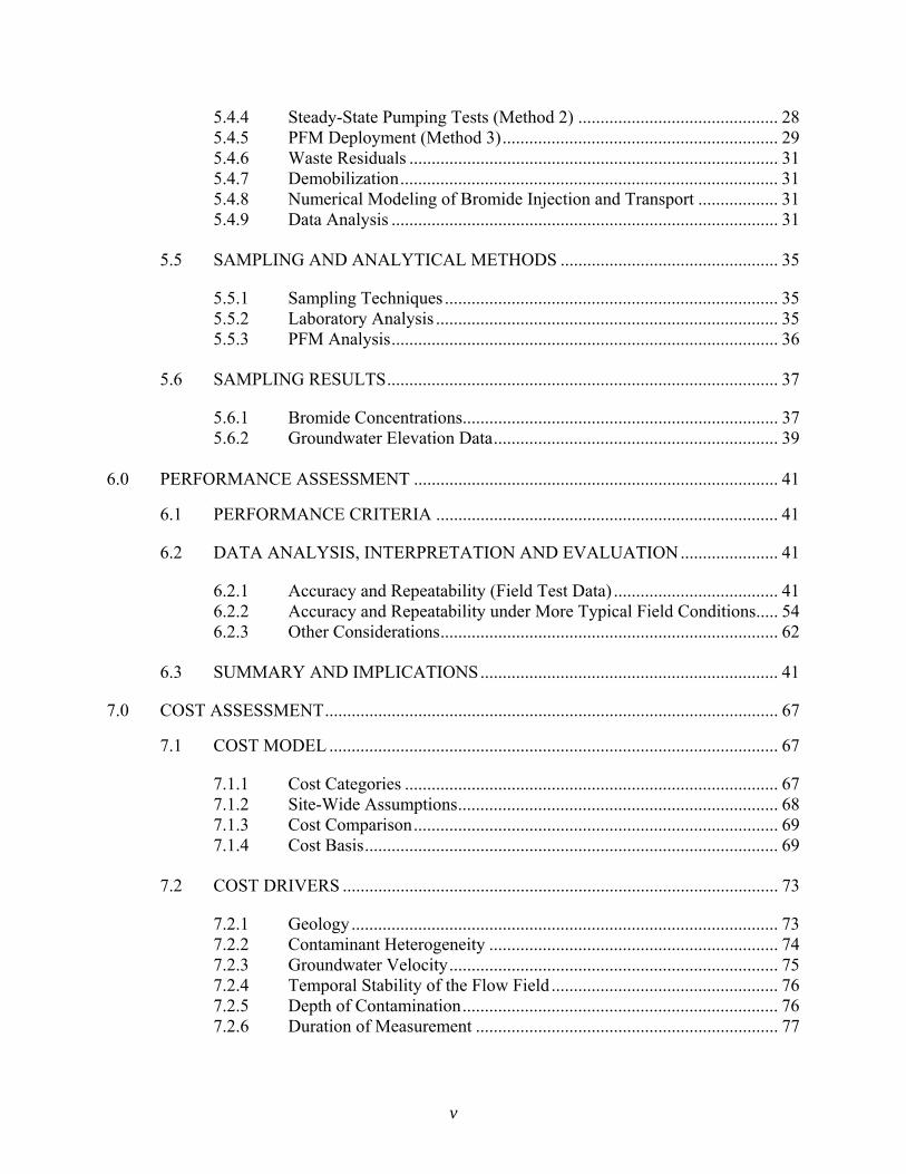
5.4.4 Steady-State Pumping Tests (Method 2) ............................................. 28 5.4.5 PFM Deployment (Method 3) .............................................................. 29 5.4.6 Waste Residuals ................................................................................... 31 5.4.7 Demobilization ..................................................................................... 31 5.4.8 Numerical Modeling of Bromide Injection and Transport .................. 31 5.4.9 Data Analysis ....................................................................................... 31
5.5 SAMPLING AND ANALYTICAL METHODS ................................................. 35
5.5.1 Sampling Techniques ........................................................................... 35 5.5.2 Laboratory Analysis ............................................................................. 35 5.5.3 PFM Analysis ....................................................................................... 36
5.6 SAMPLING RESULTS ........................................................................................ 37
5.6.1 Bromide Concentrations....................................................................... 37 5.6.2 Groundwater Elevation Data ................................................................ 39
6.0 PERFORMANCE ASSESSMENT .................................................................................. 41
6.1 PERFORMANCE CRITERIA ............................................................................. 41
6.2 DATA ANALYSIS, INTERPRETATION AND EVALUATION ...................... 41
6.2.1 Accuracy and Repeatability (Field Test Data) ..................................... 41 6.2.2 Accuracy and Repeatability under More Typical Field Conditions ..... 54 6.2.3 Other Considerations ............................................................................ 62
6.3 SUMMARY AND IMPLICATIONS ................................................................... 41
7.0 COST ASSESSMENT ...................................................................................................... 67
7.1 COST MODEL ..................................................................................................... 67
7.1.1 Cost Categories .................................................................................... 67 7.1.2 Site-Wide Assumptions ........................................................................ 68 7.1.3 Cost Comparison .................................................................................. 69 7.1.4 Cost Basis ............................................................................................. 69
7.2 COST DRIVERS .................................................................................................. 73
7.2.1 Geology ................................................................................................ 73 7.2.2 Contaminant Heterogeneity ................................................................. 74 7.2.3 Groundwater Velocity .......................................................................... 75 7.2.4 Temporal Stability of the Flow Field ................................................... 76 7.2.5 Depth of Contamination ....................................................................... 76 7.2.6 Duration of Measurement .................................................................... 77
vi
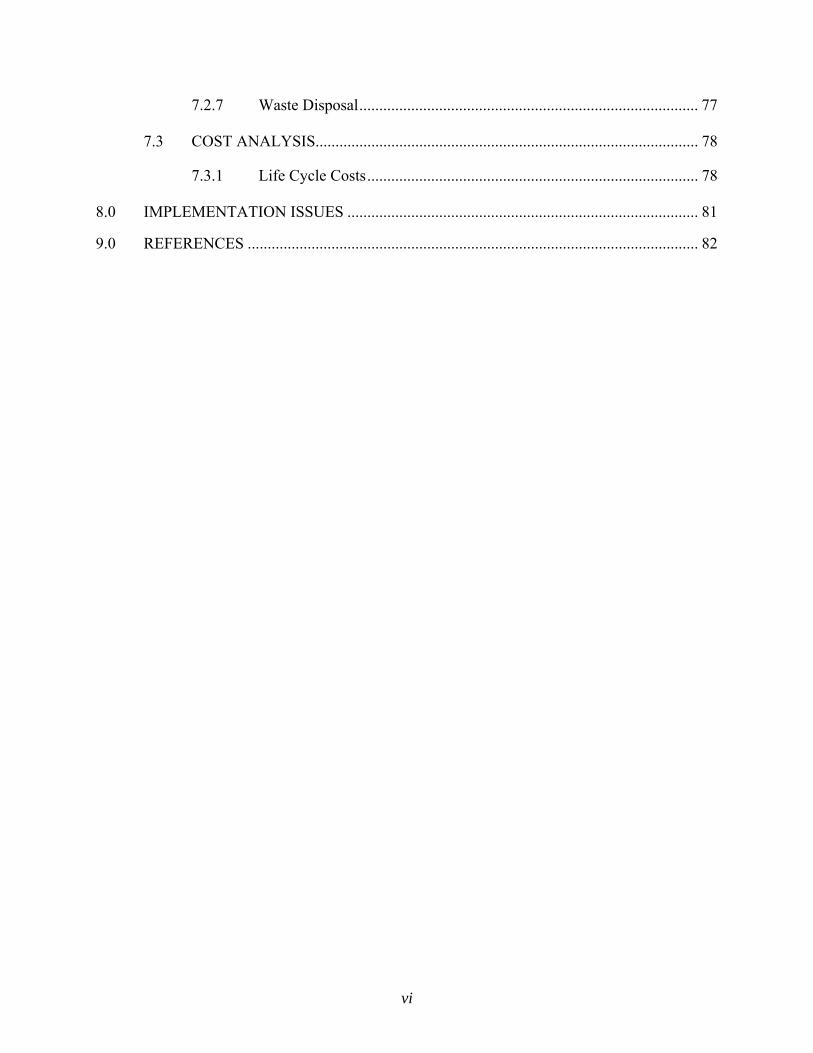
7.2.7 Waste Disposal ..................................................................................... 77
7.3 COST ANALYSIS................................................................................................ 78
7.3.1 Life Cycle Costs ................................................................................... 78
8.0 IMPLEMENTATION ISSUES ........................................................................................ 81
9.0 REFERENCES ................................................................................................................. 82
vii
LIST OF FIGURES
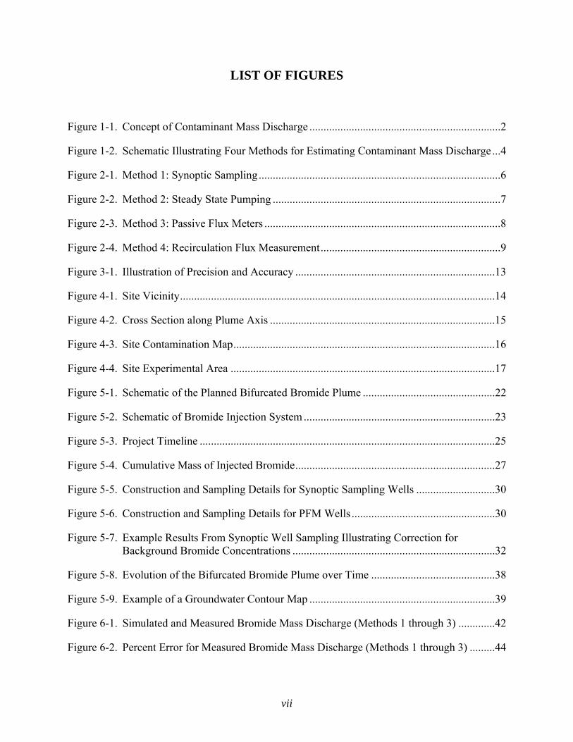
Figure 1-1. Concept of Contaminant Mass Discharge ....................................................................2
Figure 1-2. Schematic Illustrating Four Methods for Estimating Contaminant Mass Discharge ...4
Figure 2-1. Method 1: Synoptic Sampling ......................................................................................6
Figure 2-2. Method 2: Steady State Pumping .................................................................................7
Figure 2-3. Method 3: Passive Flux Meters ....................................................................................8
Figure 2-4. Method 4: Recirculation Flux Measurement ................................................................9
Figure 3-1. Illustration of Precision and Accuracy .......................................................................13
Figure 4-1. Site Vicinity ................................................................................................................14
Figure 4-2. Cross Section along Plume Axis ................................................................................15
Figure 4-3. Site Contamination Map .............................................................................................16
Figure 4-4. Site Experimental Area ..............................................................................................17
Figure 5-1. Schematic of the Planned Bifurcated Bromide Plume ...............................................22
Figure 5-2. Schematic of Bromide Injection System ....................................................................23
Figure 5-3. Project Timeline .........................................................................................................25
Figure 5-4. Cumulative Mass of Injected Bromide .......................................................................27
Figure 5-5. Construction and Sampling Details for Synoptic Sampling Wells ............................30
Figure 5-6. Construction and Sampling Details for PFM Wells ...................................................30
Figure 5-7. Example Results From Synoptic Well Sampling Illustrating Correction for Background Bromide Concentrations ........................................................................32
Figure 5-8. Evolution of the Bifurcated Bromide Plume over Time ............................................38
Figure 5-9. Example of a Groundwater Contour Map ..................................................................39
Figure 6-1. Simulated and Measured Bromide Mass Discharge (Methods 1 through 3) .............42
Figure 6-2. Percent Error for Measured Bromide Mass Discharge (Methods 1 through 3) .........44
viii
Figure 6-3. Cumulative Bromide Mass over Time at the EJ Transect ..........................................46
Figure 6-4. Simulated and Measured Bromide Mass Discharge (Method 2) at a Given Flowrate ......................................................................................................................49
Figure 6-5. Results of SSP Test #1, Day 157-249 (12/15/05 to 3/17/06) .....................................50
Figure 6-6. Results of SSP Test #3, Day 324-344 (5/31/06 to 6/20/06) .......................................51
Figure 6-7. Average Darcy Flux Estimates across the EJP Transect (Method 3) .........................52
Figure 6-8. Bromide Mass Discharge at Transect EJ Calculated as a Function of Well Spacing 57
Figure 6-9. Range of Potential Error as a Function of Well Spacing ...........................................58
Figure 6-10. Impact of Plume Heterogeneity on Bromide Mass Discharge Estimates .................63
Figure 7-1. Plan View Illustration of the Effect of Geologic Heterogeneity on Contaminant Flow Paths ..................................................................................................................74
Figure 7-2. Plan View Illustration of the Effect of Source Heterogeneity on Contaminant Flow Paths (Relatively Homogeneous Media) ....................................................................75
ix
LIST OF TABLES
Table 3-1. Performance Objectives .............................................................................................12
Table 5-1. Experimental Activities ..............................................................................................18
Table 5-2. Demonstration Schedule and Milestones ...................................................................24
Table 5-3. Passive Flux Meter Deployments at VAFB ...............................................................29
Table 5-4. Estimated Hydraulic Gradients, Calculated Darcy Flux and Average Linear Groundwater Velocities in S3 Aquifer at the EJ Transect .........................................40
Table 6-1. Simulated and Measured Bromide Mass Discharge ...................................................42
Table 6-2. Comparison of Measured and Simulated Extraction of Flow and Bromide During SSPs ............................................................................................................................48
Table 6-3. Subsets of Data Considered In Sensitivity Analysis of Method 1 (Synoptic Sampling) ...................................................................................................................55
Table 6-4. Performance of Mass Discharge Measurement Methods ...........................................66
Table 7-1. Comparison of Mass Discharge Measurement Method Cost Components ................78
APPENDICES
Appendix A: Simulation of Injection and Transport of Bromide at Vandenberg Air Force Base
Site 60
Appendix B: Post-Demonstration Testing of Recirculation Flux Measurement Method
Appendix C: Insights from Initial Research at Site 19, Vandenberg Air Force Base, CA
Appendix D: Hydraulic Testing Along EJP Transect
Appendix E: Points of Contact

x
ACRONYMS
% percent °C Degrees Celsius API American Petroleum Institute bgs below ground surface BTEX Benzene, Toluene, Ethylbenzene and Xylene CA California cm centimeters DNAPL Dense Non-Aqueous Phase Liquid DoD Department of Defense EPA Environmental Protection Agency ESTCP Environmental Security Technology Certification Program FRTR Federal Remediation Technology Roundtable ft feet g grams HPLC High Performance Liquid Chromatography in inch IPT Integral Pumping Test ITRC Interstate Technology Regulatory Council L Liter lbs pounds LDPE Low Density Polyethylene m meters MAPE Mean Absolute Percent Error mg milligrams min minute mL milliliter mm millimeter MNA Monitored Natural Attenuation MPE Measurement Percent Error MTBE Methyl Tertiary Butyl Ether O&M Operation and Maintenance PFM Passive Flux Meter PVC Polyvinyl Chloride RFM Recirculation Flux Measurement SERDP Strategic Environmental Research and Development Program SSP Steady-State Pumping U.S. United States UC University of California VAFB Vandenberg Air Force Base VOCs Volatile Organic Compounds
xi
ACKNOWLEDGEMENTS
This research was funded primarily by the Environmental Security Technology Certification Program (ESTCP). Seed funding for early characterization and other initial work was provided by the American Petroleum Institute (API). In addition, Geomatrix Consultants (Costa Mesa and Oakland, California (CA) provided monetary support and field assistance. This research was the result of efforts of many people from the following institutions:
• University of California at Davis (UC Davis) and UC Davis field site employees: Dr. Doug Mackay, Dr. Phil Kaiser, Dr. Mamie Nozawa-Inoue, Sunitha Gurushinge, Dr. Sham Goyal, Dr. Kate Scow, Irina Chakraborty, Madalena Velasco, Larry Justice, Max Justice, Veronica Morales, Anthony Parker and Chloe Lucado
• Murray Einarson, PG, CEG, CHG, AMEC/Geomatrix Consultants (formerly of Einarson & Associates)
• Malcolm Pirnie, Inc.: Dr. Michael C. Kavanaugh, Dr. Rula A. Deeb and Elisabeth L. Hawley
• University of Florida: Dr. Michael Annable, Dr. Kirk Hatfield
• Air Force Institute of Technology: Dr. Mark Goltz, Dr. Junqi Huang
• United States (U.S.) Environmental Protection Agency (EPA): Dr. Michael Brooks and Dr. Lynn Wood
The authors thank Vandenberg Air Force Base (VAFB) employees, especially Mike McElligott, Pablo Martinez, Andy Edwards, Ron MacLelland, Craig Nathe and Kathy Gerber. In addition, the authors thank staff from the Regional Water Quality Control Board, San Luis Obispo, CA especially Carol Kolb, Bill Meece, Kristina Seley and Linda Stone.
ES-1
EXECUTIVE SUMMARY
BACKGROUND
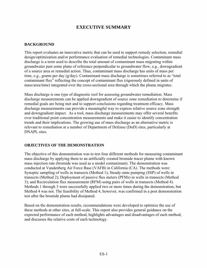
This report evaluates an innovative metric that can be used to support remedy selection, remedial design/optimization and/or performance evaluation of remedial technologies. Contaminant mass discharge is a term used to describe the total amount of contaminant mass migrating within groundwater past some plane of reference perpendicular to groundwater flow, e.g., downgradient of a source area or remedial action. Thus, contaminant mass discharge has units of mass per time, e.g., grams per day (g/day). Contaminant mass discharge is sometimes referred to as “total contaminant flux” reflecting the concept of contaminant flux (rigorously defined in units of mass/area/time) integrated over the cross-sectional area through which the plume migrates. Mass discharge is one type of diagnostic tool for assessing groundwater remediation. Mass discharge measurements can be applied downgradient of source zone remediation to determine if remedial goals are being met and to support conclusions regarding treatment efficacy. Mass discharge measurements can provide a meaningful way to express relative source zone strength and downgradient impact. As a tool, mass discharge measurements may offer several benefits over traditional point concentration measurements and make it easier to identify concentration trends and their implications. The growing use of mass discharge as an alternative metric is relevant to remediation at a number of Department of Defense (DoD) sites, particularly at DNAPL sites.
OBJECTIVES OF THE DEMONSTRATION
The objective of this demonstration was to test four different methods for measuring contaminant mass discharge by applying them to an artificially created bromide tracer plume with known mass injection rate (bromide was used as a model contaminant). The demonstration was conducted at Vandenberg Air Force Base (VAFB) in California (CA). The methods were: Synoptic sampling of wells in transects (Method 1); Steady-state pumping (SSP) of wells in transects (Method 2); Deployment of passive flux meters (PFMs) in wells in transects (Method 3); and Recirculation flux measurement (RFM) using pairs of wells in transects (Method 4). Methods 1 through 3 were successfully applied two or more times during the demonstration, but Method 4 was not. The feasibility of Method 4, however, was confirmed in a post demonstration test after the bromide plume had dissipated. Based on the demonstration results, recommendations were developed to optimize the use of these methods at other sites, at full-scale. This report also provides general guidance on the expected performance of each method, highlights advantages and disadvantages of each method, and discusses the relative costs of each technology.
ES-2
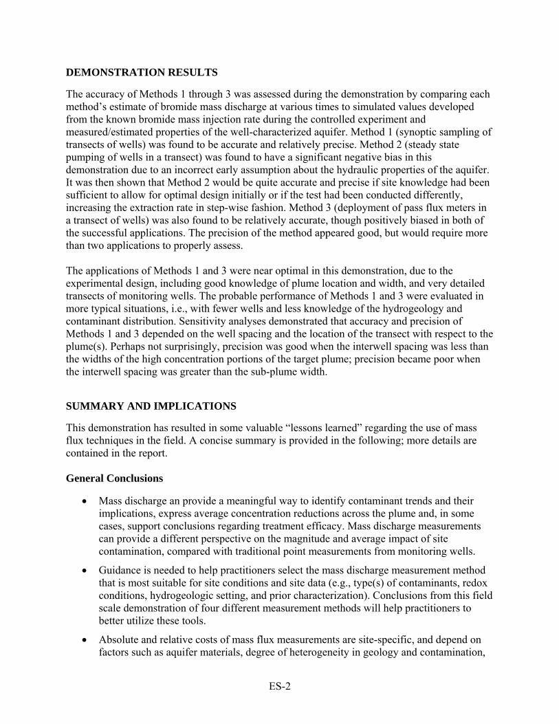
DEMONSTRATION RESULTS
The accuracy of Methods 1 through 3 was assessed during the demonstration by comparing each method’s estimate of bromide mass discharge at various times to simulated values developed from the known bromide mass injection rate during the controlled experiment and measured/estimated properties of the well-characterized aquifer. Method 1 (synoptic sampling of transects of wells) was found to be accurate and relatively precise. Method 2 (steady state pumping of wells in a transect) was found to have a significant negative bias in this demonstration due to an incorrect early assumption about the hydraulic properties of the aquifer. It was then shown that Method 2 would be quite accurate and precise if site knowledge had been sufficient to allow for optimal design initially or if the test had been conducted differently, increasing the extraction rate in step-wise fashion. Method 3 (deployment of pass flux meters in a transect of wells) was also found to be relatively accurate, though positively biased in both of the successful applications. The precision of the method appeared good, but would require more than two applications to properly assess. The applications of Methods 1 and 3 were near optimal in this demonstration, due to the experimental design, including good knowledge of plume location and width, and very detailed transects of monitoring wells. The probable performance of Methods 1 and 3 were evaluated in more typical situations, i.e., with fewer wells and less knowledge of the hydrogeology and contaminant distribution. Sensitivity analyses demonstrated that accuracy and precision of Methods 1 and 3 depended on the well spacing and the location of the transect with respect to the plume(s). Perhaps not surprisingly, precision was good when the interwell spacing was less than the widths of the high concentration portions of the target plume; precision became poor when the interwell spacing was greater than the sub-plume width.
SUMMARY AND IMPLICATIONS
This demonstration has resulted in some valuable “lessons learned” regarding the use of mass flux techniques in the field. A concise summary is provided in the following; more details are contained in the report. General Conclusions
• Mass discharge an provide a meaningful way to identify contaminant trends and their implications, express average concentration reductions across the plume and, in some cases, support conclusions regarding treatment efficacy. Mass discharge measurements can provide a different perspective on the magnitude and average impact of site contamination, compared with traditional point measurements from monitoring wells.
• Guidance is needed to help practitioners select the mass discharge measurement method that is most suitable for site conditions and site data (e.g., type(s) of contaminants, redox conditions, hydrogeologic setting, and prior characterization). Conclusions from this field scale demonstration of four different measurement methods will help practitioners to better utilize these tools.
• Absolute and relative costs of mass flux measurements are site-specific, and depend on factors such as aquifer materials, degree of heterogeneity in geology and contamination,
ES-3
depth of contamination, groundwater velocity, temporal stability of the flow field, duration of measurements, and waste treatment and disposal requirements. These site conditions, along with planned or ongoing remediation system design, determine the cost of wells required to measure mass flux and the associated sampling, analytical, and maintenance costs. Site conditions may also guide the choice of mass discharge measurement methods. A qualitative comparison of costs is presented in this report, because the costs of the field demonstration were not representative of typical full-scale site costs.
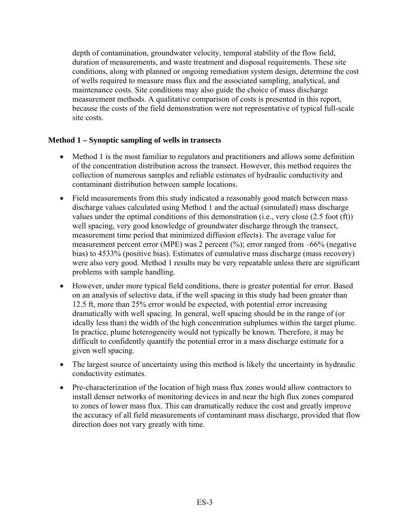
Method 1 – Synoptic sampling of wells in transects
• Method 1 is the most familiar to regulators and practitioners and allows some definition of the concentration distribution across the transect. However, this method requires the collection of numerous samples and reliable estimates of hydraulic conductivity and contaminant distribution between sample locations.
• Field measurements from this study indicated a reasonably good match between mass discharge values calculated using Method 1 and the actual (simulated) mass discharge values under the optimal conditions of this demonstration (i.e., very close (2.5 foot (ft)) well spacing, very good knowledge of groundwater discharge through the transect, measurement time period that minimized diffusion effects). The average value for measurement percent error (MPE) was 2 percent (%); error ranged from –66% (negative bias) to 4533% (positive bias). Estimates of cumulative mass discharge (mass recovery) were also very good. Method 1 results may be very repeatable unless there are significant problems with sample handling.
• However, under more typical field conditions, there is greater potential for error. Based on an analysis of selective data, if the well spacing in this study had been greater than 12.5 ft, more than 25% error would be expected, with potential error increasing dramatically with well spacing. In general, well spacing should be in the range of (or ideally less than) the width of the high concentration subplumes within the target plume. In practice, plume heterogeneity would not typically be known. Therefore, it may be difficult to confidently quantify the potential error in a mass discharge estimate for a given well spacing.
• The largest source of uncertainty using this method is likely the uncertainty in hydraulic conductivity estimates.
• Pre-characterization of the location of high mass flux zones would allow contractors to install denser networks of monitoring devices in and near the high flux zones compared to zones of lower mass flux. This can dramatically reduce the cost and greatly improve the accuracy of all field measurements of contaminant mass discharge, provided that flow direction does not vary greatly with time.
ES-4
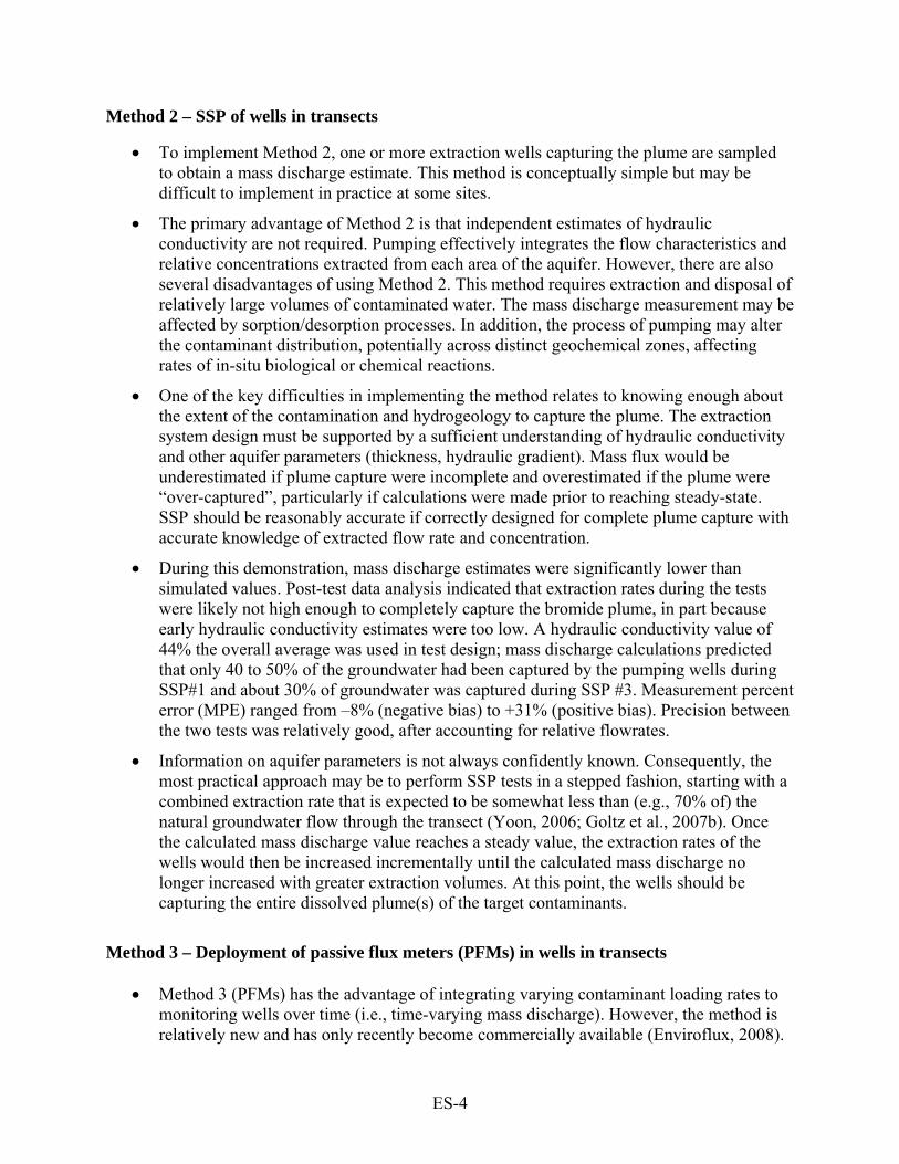
Method 2 – SSP of wells in transects
• To implement Method 2, one or more extraction wells capturing the plume are sampled to obtain a mass discharge estimate. This method is conceptually simple but may be difficult to implement in practice at some sites.
• The primary advantage of Method 2 is that independent estimates of hydraulic conductivity are not required. Pumping effectively integrates the flow characteristics and relative concentrations extracted from each area of the aquifer. However, there are also several disadvantages of using Method 2. This method requires extraction and disposal of relatively large volumes of contaminated water. The mass discharge measurement may be affected by sorption/desorption processes. In addition, the process of pumping may alter the contaminant distribution, potentially across distinct geochemical zones, affecting rates of in-situ biological or chemical reactions.
• One of the key difficulties in implementing the method relates to knowing enough about the extent of the contamination and hydrogeology to capture the plume. The extraction system design must be supported by a sufficient understanding of hydraulic conductivity and other aquifer parameters (thickness, hydraulic gradient). Mass flux would be underestimated if plume capture were incomplete and overestimated if the plume were “over-captured”, particularly if calculations were made prior to reaching steady-state. SSP should be reasonably accurate if correctly designed for complete plume capture with accurate knowledge of extracted flow rate and concentration.
• During this demonstration, mass discharge estimates were significantly lower than simulated values. Post-test data analysis indicated that extraction rates during the tests were likely not high enough to completely capture the bromide plume, in part because early hydraulic conductivity estimates were too low. A hydraulic conductivity value of 44% the overall average was used in test design; mass discharge calculations predicted that only 40 to 50% of the groundwater had been captured by the pumping wells during SSP#1 and about 30% of groundwater was captured during SSP #3. Measurement percent error (MPE) ranged from –8% (negative bias) to +31% (positive bias). Precision between the two tests was relatively good, after accounting for relative flowrates.
• Information on aquifer parameters is not always confidently known. Consequently, the most practical approach may be to perform SSP tests in a stepped fashion, starting with a combined extraction rate that is expected to be somewhat less than (e.g., 70% of) the natural groundwater flow through the transect (Yoon, 2006; Goltz et al., 2007b). Once the calculated mass discharge value reaches a steady value, the extraction rates of the wells would then be increased incrementally until the calculated mass discharge no longer increased with greater extraction volumes. At this point, the wells should be capturing the entire dissolved plume(s) of the target contaminants.
Method 3 – Deployment of passive flux meters (PFMs) in wells in transects
• Method 3 (PFMs) has the advantage of integrating varying contaminant loading rates to monitoring wells over time (i.e., time-varying mass discharge). However, the method is relatively new and has only recently become commercially available (Enviroflux, 2008).
ES-5
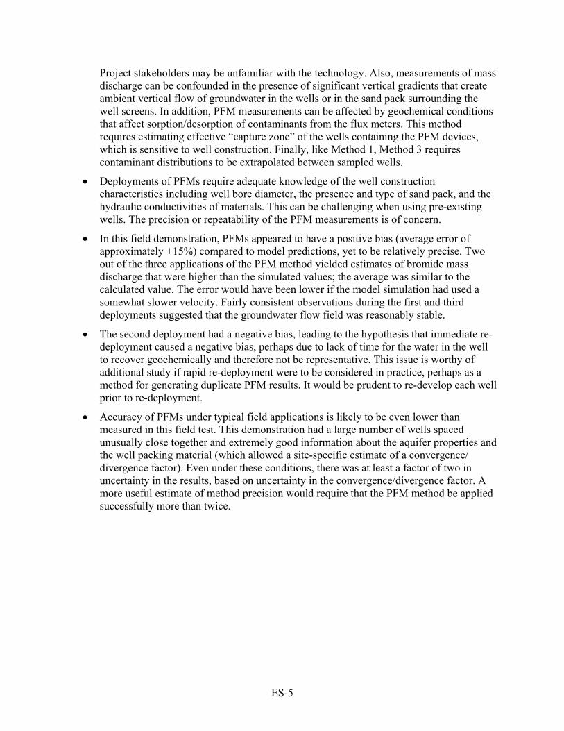
Project stakeholders may be unfamiliar with the technology. Also, measurements of mass discharge can be confounded in the presence of significant vertical gradients that create ambient vertical flow of groundwater in the wells or in the sand pack surrounding the well screens. In addition, PFM measurements can be affected by geochemical conditions that affect sorption/desorption of contaminants from the flux meters. This method requires estimating effective “capture zone” of the wells containing the PFM devices, which is sensitive to well construction. Finally, like Method 1, Method 3 requires contaminant distributions to be extrapolated between sampled wells.
• Deployments of PFMs require adequate knowledge of the well construction characteristics including well bore diameter, the presence and type of sand pack, and the hydraulic conductivities of materials. This can be challenging when using pre-existing wells. The precision or repeatability of the PFM measurements is of concern.
• In this field demonstration, PFMs appeared to have a positive bias (average error of approximately +15%) compared to model predictions, yet to be relatively precise. Two out of the three applications of the PFM method yielded estimates of bromide mass discharge that were higher than the simulated values; the average was similar to the calculated value. The error would have been lower if the model simulation had used a somewhat slower velocity. Fairly consistent observations during the first and third deployments suggested that the groundwater flow field was reasonably stable.
• The second deployment had a negative bias, leading to the hypothesis that immediate re-deployment caused a negative bias, perhaps due to lack of time for the water in the well to recover geochemically and therefore not be representative. This issue is worthy of additional study if rapid re-deployment were to be considered in practice, perhaps as a method for generating duplicate PFM results. It would be prudent to re-develop each well prior to re-deployment.
• Accuracy of PFMs under typical field applications is likely to be even lower than measured in this field test. This demonstration had a large number of wells spaced unusually close together and extremely good information about the aquifer properties and the well packing material (which allowed a site-specific estimate of a convergence/ divergence factor). Even under these conditions, there was at least a factor of two in uncertainty in the results, based on uncertainty in the convergence/divergence factor. A more useful estimate of method precision would require that the PFM method be applied successfully more than twice.
ES-6
Method 4 – RFM Technique
• Method 4, the RFM technique, is currently the least tested of the four methods at field-scale and the most difficult conceptually to set up, operate, and communicate results to stakeholders. Advantages include the method’s inherent integration of contaminant flux via groundwater extraction, similar to Method 2. Since the pumped water is reinjected, no disposal is required. Like Method 2, prior characterization of the plume and hydrogeology is needed to ensure capture. Also, mass discharge estimates may be affected by sorption/desorption. Finally, pumping may alter contaminant distribution, potentially across distinct geochemical zones, affecting in-situ biological or chemical reactions.
• Model simulations based on measured or estimated aquifer properties indicated that recirculation between adjacent injection/extraction wells could be achieved at relatively modest pumping rates (1 L/min). However, these pumping rates proved to not be sustainable during the field trials, probably due to operator error (e.g., failing to keep injection well and other parts of the system from clogging; incorrect location of the extraction pump intake within the extraction well).
• For the RFM technique to work at other field sites, hydraulic conductivity must be adequate to allow for recirculation of flow between the two wells of an injection/extraction well pair. Subsequent tests, detailed in Appendix D, determined that flow could be sustained if the injection well was frequently re-developed. Well spacing and pumping rate for an injection/extraction well pair should be determined based on modeling and estimated hydraulic conductivity values. Following RFM well installation, the model can be calibrated to actual water levels measured in the wells. Such preliminary testing would give confidence in experimental techniques, ability to achieve the necessary pumping rates, and usefulness of model simulations.
1
1.0 INTRODUCTION
This report evaluates the measurement of contaminant mass discharge, which is defined as the total amount of contaminant mass migrating within groundwater past some plane of reference perpendicular to groundwater flow. Four different methods for measuring contaminant mass discharge were tested at Vandenberg Air Force Base (VAFB), California (CA). Mass discharge is one type of innovative method that can be used to support remedial design efforts or to evaluate the performance of remedial technologies. Mass discharge is typically measured downgradient of a source area or area undergoing remedial action. It can be used as a diagnostic tool for assessing groundwater remediation. Similar demonstrations of mass discharge and other innovative diagnostic tools for remediation of chlorinated solvents were conducted at two other sites with different geologies: Fort Lewis, Washington, and Watervliet Arsenal, New York. The work at all three sites was conducted under the Environmental Security Technology Certification Program (ESTCP) Project ER-0318. An evaluation of the results of this work will also be presented in a separate ESTCP report discussing the broader implications of the results from the three sites considered as a whole, in the context of evaluating diagnostic tools.
1.1 BACKGROUND
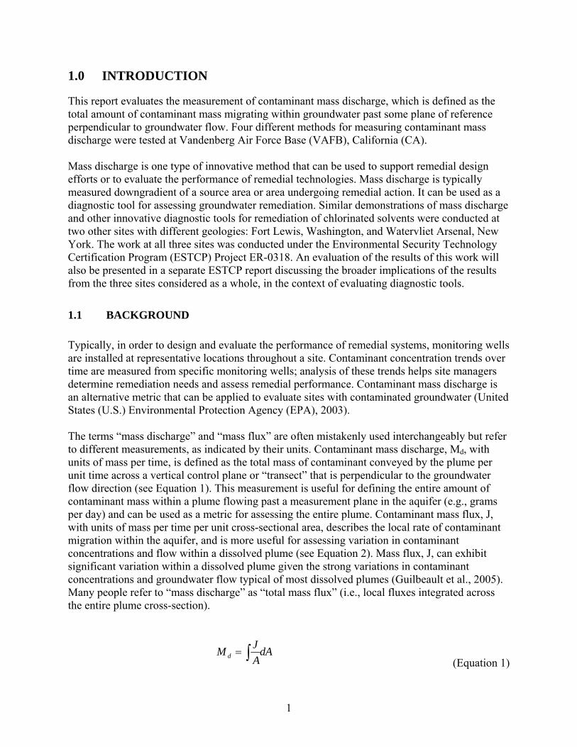
Typically, in order to design and evaluate the performance of remedial systems, monitoring wells are installed at representative locations throughout a site. Contaminant concentration trends over time are measured from specific monitoring wells; analysis of these trends helps site managers determine remediation needs and assess remedial performance. Contaminant mass discharge is an alternative metric that can be applied to evaluate sites with contaminated groundwater (United States (U.S.) Environmental Protection Agency (EPA), 2003). The terms “mass discharge” and “mass flux” are often mistakenly used interchangeably but refer to different measurements, as indicated by their units. Contaminant mass discharge, Md, with units of mass per time, is defined as the total mass of contaminant conveyed by the plume per unit time across a vertical control plane or “transect” that is perpendicular to the groundwater flow direction (see Equation 1). This measurement is useful for defining the entire amount of contaminant mass within a plume flowing past a measurement plane in the aquifer (e.g., grams per day) and can be used as a metric for assessing the entire plume. Contaminant mass flux, J, with units of mass per time per unit cross-sectional area, describes the local rate of contaminant migration within the aquifer, and is more useful for assessing variation in contaminant concentrations and flow within a dissolved plume (see Equation 2). Mass flux, J, can exhibit significant variation within a dissolved plume given the strong variations in contaminant concentrations and groundwater flow typical of most dissolved plumes (Guilbeault et al., 2005). Many people refer to “mass discharge” as “total mass flux” (i.e., local fluxes integrated across the entire plume cross-section).
dAAJM d ∫=
(Equation 1)
2
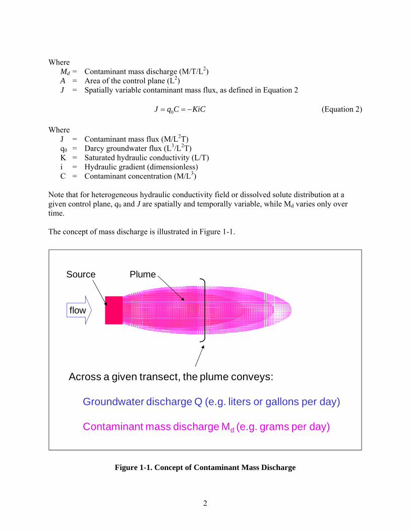
Where Md = Contaminant mass discharge (M/T/L2) A = Area of the control plane (L2) J = Spatially variable contaminant mass flux, as defined in Equation 2
KiCCqJ −== 0 (Equation 2) Where J = Contaminant mass flux (M/L2T) q0 = Darcy groundwater flux (L3/L2T) K = Saturated hydraulic conductivity (L/T) i = Hydraulic gradient (dimensionless) C = Contaminant concentration (M/L3) Note that for heterogeneous hydraulic conductivity field or dissolved solute distribution at a given control plane, q0 and J are spatially and temporally variable, while Md varies only over time. The concept of mass discharge is illustrated in Figure 1-1.
Across a given transect, the plume conveys:
Groundwater discharge Q (e.g. liters or gallons per day)
Contaminant mass discharge Md (e.g. grams per day)
Source Plume
flow
Figure 1-1. Concept of Contaminant Mass Discharge

3
Contaminant mass discharge is commonly measured downgradient of the source zone, as shown in Figure 1-1, but can also be used to assess contaminants migrating towards the source zone from upgradient, or to monitor processes occurring within large source zones. Mass discharge may be used as the primary metric of the significance or severity of a subsurface release or as one line of evidence in support of a conceptual site model or remedial objective. Contaminant mass discharge has been recognized as an important indicator of the severity or “strength” of a contaminant release (Feenstra et al., 1996; Einarson and Mackay, 2001; Rao et al., 2002). Thus, mass discharge measurements are increasingly being required by regulators overseeing partial dense non-aqueous phase liquid (DNAPL) source zone remediation or plume remediation to determine if remedial goals are being met and allow for remediation optimization (U.S. EPA, 2003; Interstate Technology Regulatory Council (ITRC), 2004). A significant advantage of estimating mass discharge in addition to point concentration measurements is that contamination trends and their implications may be more easily identified. For example, concentrations may decline at different rates in spatially distributed monitoring wells in response to upgradient treatment, making it difficult to quantify the overall effectiveness of treatment. Mass discharge provides a meaningful way to express average concentration reductions across the plume and support conclusions regarding treatment efficiency. Mass discharge measurements can provide a different perspective on the magnitude and average impact of site contamination. For example, high concentrations in one well may be recognized to be of minor significance if contaminant mass discharge from the site is low overall, i.e., only a small total mass of contaminant per unit time actually migrating with the groundwater. Risk posed by groundwater contamination is more closely related to the rate of contaminant mass migration than to the concentration in any particular point in the subsurface. The growing use of mass discharge as an alternative metric, particularly at DNAPL sites, has impacted the Department of Defense (DoD). In August 2001, an expert panel convened by Strategic Environmental Research and Development Program (SERDP) and ESTCP identified the highest priority research and development needs for evaluating DNAPL source zone remediation. One of the highest priorities listed by the panel was the continued development of contaminant mass discharge methods (Stroo et al., 2003). Despite the growing awareness of the importance of mass discharge as a site assessment parameter, there have not been any published comprehensive field comparisons of various measurement methods, especially at locations where the actual contaminant mass discharge is somehow independently known, allowing researchers to evaluate measurement accuracy. Moreover, work performed prior to this project suggested that (1) existing measurement methods for mass discharge required further evaluation; (2) new methods, or new variations on existing methods, were needed to overcome limitations of current methods; and (3) guidance was needed to help practitioners select the measurement method that was most appropriate for the hydrogeologic setting, contaminant type, and distribution (e.g., single vs. mixed contaminants, sorbing vs. nonsorbing contaminants, uniform vs. variable redox conditions).
4
1.2 OBJECTIVE OF THE DEMONSTRATION
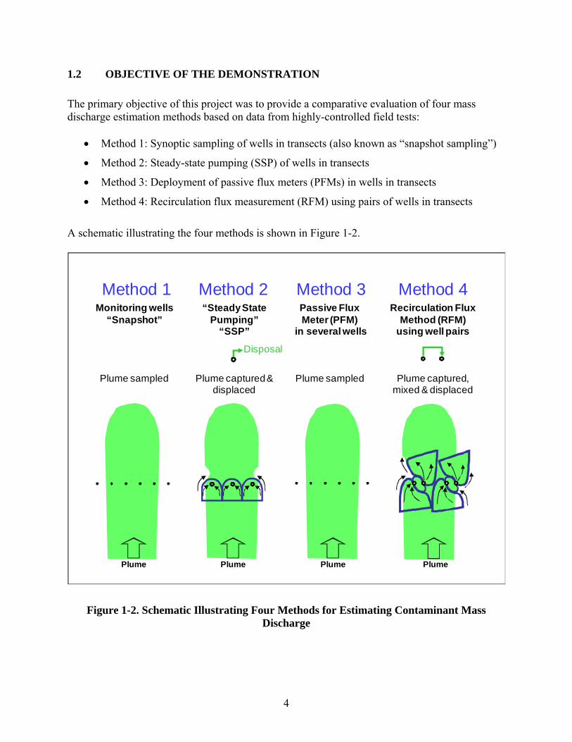
The primary objective of this project was to provide a comparative evaluation of four mass discharge estimation methods based on data from highly-controlled field tests:
• Method 1: Synoptic sampling of wells in transects (also known as “snapshot sampling”)
• Method 2: Steady-state pumping (SSP) of wells in transects
• Method 3: Deployment of passive flux meters (PFMs) in wells in transects
• Method 4: Recirculation flux measurement (RFM) using pairs of wells in transects
A schematic illustrating the four methods is shown in Figure 1-2.
Figure 1-2. Schematic Illustrating Four Methods for Estimating Contaminant Mass Discharge
Monitoring wells“Snapshot”
Plume sampled
Plume
“Steady State Pumping”
“SSP”
Plume captured & displaced
Plume
Passive Flux Meter (PFM)
in several wells
Plume sampled
Plume
Recirculation Flux Method (RFM)
using well pairs
Plume captured, mixed & displaced
Method 1 Method 2 Method 3 Method 4
Plume
Disposal
5
In addition, this project assessed the accuracy of each of the mass discharge estimation methods by comparing the result to the known rate of “contaminant” migration, i.e., the contaminant plume was a bromide tracer injected into the subsurface at a known rate as a model contaminant. The advantages, disadvantages, and costs of using each of the mass discharge estimation methods were also assessed. Results are summarized in this report in order to assist DoD site managers with the selection and implementation of mass discharge measurement methods at sites with different hydrogeologic conditions (e.g., soil types, aquifer thickness, groundwater flow rates) and contaminant distributions.
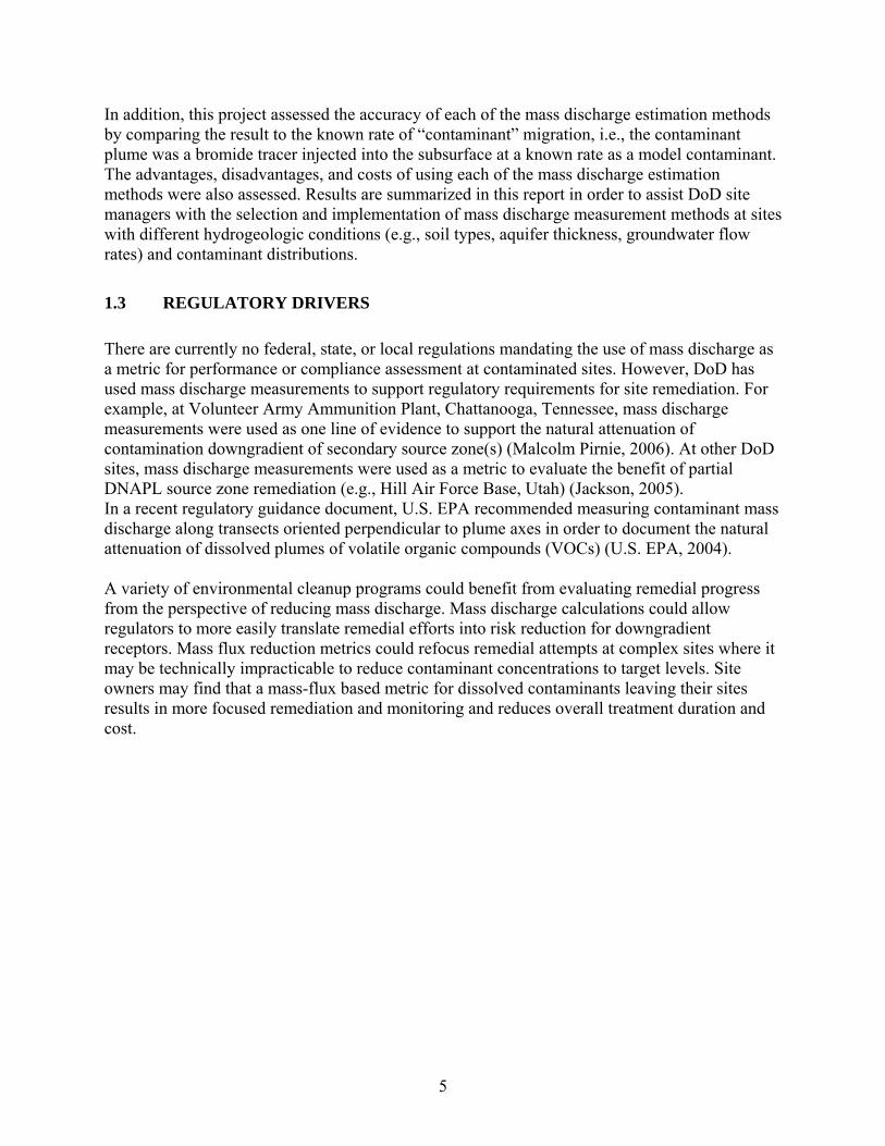
1.3 REGULATORY DRIVERS
There are currently no federal, state, or local regulations mandating the use of mass discharge as a metric for performance or compliance assessment at contaminated sites. However, DoD has used mass discharge measurements to support regulatory requirements for site remediation. For example, at Volunteer Army Ammunition Plant, Chattanooga, Tennessee, mass discharge measurements were used as one line of evidence to support the natural attenuation of contamination downgradient of secondary source zone(s) (Malcolm Pirnie, 2006). At other DoD sites, mass discharge measurements were used as a metric to evaluate the benefit of partial DNAPL source zone remediation (e.g., Hill Air Force Base, Utah) (Jackson, 2005). In a recent regulatory guidance document, U.S. EPA recommended measuring contaminant mass discharge along transects oriented perpendicular to plume axes in order to document the natural attenuation of dissolved plumes of volatile organic compounds (VOCs) (U.S. EPA, 2004). A variety of environmental cleanup programs could benefit from evaluating remedial progress from the perspective of reducing mass discharge. Mass discharge calculations could allow regulators to more easily translate remedial efforts into risk reduction for downgradient receptors. Mass flux reduction metrics could refocus remedial attempts at complex sites where it may be technically impracticable to reduce contaminant concentrations to target levels. Site owners may find that a mass-flux based metric for dissolved contaminants leaving their sites results in more focused remediation and monitoring and reduces overall treatment duration and cost.

6
2.0 TECHNOLOGY
2.1 TECHNOLOGY DESCRIPTION
Each of the four mass discharge estimation methods is described in this section. Method 1 refers to synoptic sampling of transects of single-level or multi-level wells, also known as “snapshot sampling” (Figure 2-1).
Figure 2-1. Method 1: Synoptic Sampling
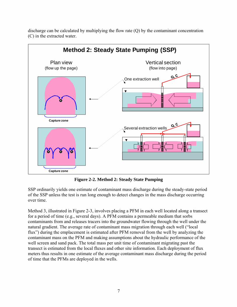
In Method 1, monitoring wells located along a transect are sampled using standard methods to get contaminant concentrations. Contaminant concentrations and estimates of hydraulic conductivity are then interpolated throughout the transect area and used to estimate mass per unit time migrating past the transect. Each sampling event provides a snapshot of mass discharge for a specific date and time. At sites where plume concentrations vary vertically, multilevel monitoring may provide more insight into the plume heterogeneity and more accurately estimate mass discharge. Method 2, SSP, illustrated in Figure 2-2, is conducted by pumping from one or more extraction wells located along a transect and measuring the total extraction rate and contaminant concentration in composite samples of the extracted groundwater. After pumping long enough to establish steady-state contaminant flowlines in the aquifer (as discussed later), contaminant mass
Plan view(flow up the page)
Vertical section(flow into page)
Method 1: Synoptic sampling of wells (“snapshot”)
Single-level monitoring wells
Multi-level monitoring wells or clusters
7
discharge can be calculated by multiplying the flow rate (Q) by the contaminant concentration (C) in the extracted water.
Figure 2-2. Method 2: Steady State Pumping
SSP ordinarily yields one estimate of contaminant mass discharge during the steady-state period of the SSP unless the test is run long enough to detect changes in the mass discharge occurring over time. Method 3, illustrated in Figure 2-3, involves placing a PFM in each well located along a transect for a period of time (e.g., several days). A PFM contains a permeable medium that sorbs contaminants from and releases tracers into the groundwater flowing through the well under the natural gradient. The average rate of contaminant mass migration through each well (“local flux”) during the emplacement is estimated after PFM removal from the well by analyzing the contaminant mass on the PFM and making assumptions about the hydraulic performance of the well screen and sand pack. The total mass per unit time of contaminant migrating past the transect is estimated from the local fluxes and other site information. Each deployment of flux meters thus results in one estimate of the average contaminant mass discharge during the period of time that the PFMs are deployed in the wells.
Plan view(flow up the page)
Vertical section(flow into page)
Method 2: Steady State Pumping (SSP)
Several extraction wells
One extraction well
Capture zone
Capture zone

8
Figure 2-3. Method 3: Passive Flux Meters
Method 4, illustrated in Figure 2-4, is a new monitoring approach not yet used in practice, called the RFM technique. The RFM technique uses pairs of extraction and injection wells located along a transect to induce groundwater flow between each well pair, recirculating the groundwater. The conceptually simplest application of this method is illustrated in plan view (one pair of single-screened injection and extraction wells, with recirculation occurring above ground). Figure 1-2 illustrated a more complex application of two pairs of single-screened wells, as two or more well pairs may be required to ensure capture of the entire plume width.
Plan view(flow up the page)
Vertical section(flow into page)
Method 3: Passive Flux Meters in wells (PFM)
PFM in single-level monitoring wells
PFM in multi-level monitoring wellsor clusters

9
Figure 2-4. Method 4: Recirculation Flux Measurement
Well pairs may also have multiple screens to cover shallow and deeper aquifers, as illustrated in the bottom vertical section in Figure 2-4. The dual-screened well approach may have regulatory advantages, since no water is pumped above ground (and thus no “reinjection” occurs). However, more equipment is needed within each well (e.g., packers, pump, tracer injection system, water sampling system). Regardless of the well configuration, the recirculation flow rates and concentrations in the recirculated water are measured. A published mathematical approach (Goltz et al., 2007a; Wheeldon, 2008) is then used to estimate the mass discharge through the transect. Each RFM application typically yields one estimate of contaminant mass discharge for a given date and time. Testing could be extended to yield a series of contaminant mass discharge estimates as the RFM operates.
2.2 ADVANTAGES AND LIMITATIONS OF THE TECHNOLOGY
Section 1.1 described several advantages of evaluating a site using contaminant mass discharge estimates instead of relying solely on conventional practices (i.e., evaluation based on individual point measurements of contaminant concentrations in monitoring wells over time). These include having a more significant indicator of the “strength” of contaminants being released to areas downgradient of the source area, an additional line of evidence to determine if remedial goals are being met, and an indicator of effectiveness of partial mass removal from the source area.
Dual-screened wells between screens are packers, pumps & tracer injection points
Plan view(of single-screened well pair)
Vertical section(with single screened wells)
Added tracer
Recirculated water
reinjectedinto regional
flowfield
Recirculation zone
Capture zone
Plume
Method 4: Recirculation Flux Measurement (RFM)
Single-screened wells
10
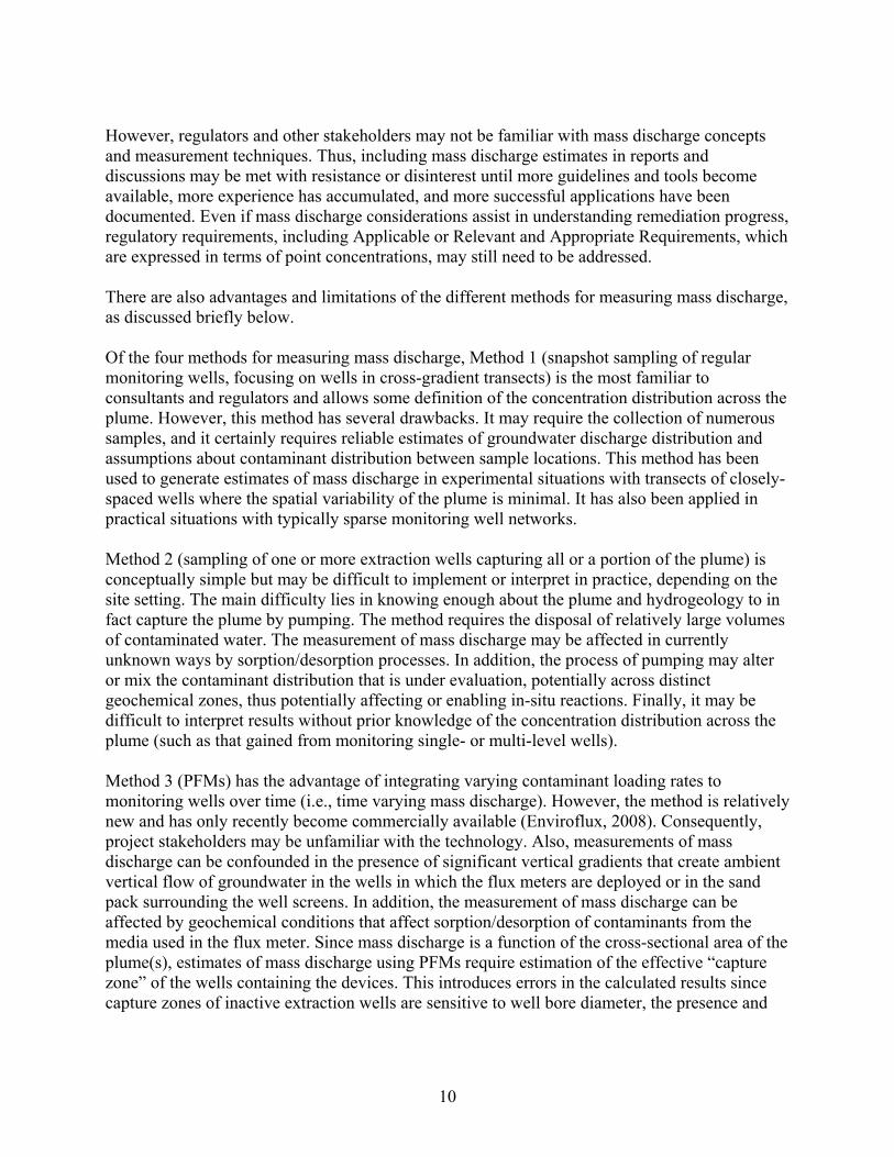
However, regulators and other stakeholders may not be familiar with mass discharge concepts and measurement techniques. Thus, including mass discharge estimates in reports and discussions may be met with resistance or disinterest until more guidelines and tools become available, more experience has accumulated, and more successful applications have been documented. Even if mass discharge considerations assist in understanding remediation progress, regulatory requirements, including Applicable or Relevant and Appropriate Requirements, which are expressed in terms of point concentrations, may still need to be addressed. There are also advantages and limitations of the different methods for measuring mass discharge, as discussed briefly below. Of the four methods for measuring mass discharge, Method 1 (snapshot sampling of regular monitoring wells, focusing on wells in cross-gradient transects) is the most familiar to consultants and regulators and allows some definition of the concentration distribution across the plume. However, this method has several drawbacks. It may require the collection of numerous samples, and it certainly requires reliable estimates of groundwater discharge distribution and assumptions about contaminant distribution between sample locations. This method has been used to generate estimates of mass discharge in experimental situations with transects of closely-spaced wells where the spatial variability of the plume is minimal. It has also been applied in practical situations with typically sparse monitoring well networks. Method 2 (sampling of one or more extraction wells capturing all or a portion of the plume) is conceptually simple but may be difficult to implement or interpret in practice, depending on the site setting. The main difficulty lies in knowing enough about the plume and hydrogeology to in fact capture the plume by pumping. The method requires the disposal of relatively large volumes of contaminated water. The measurement of mass discharge may be affected in currently unknown ways by sorption/desorption processes. In addition, the process of pumping may alter or mix the contaminant distribution that is under evaluation, potentially across distinct geochemical zones, thus potentially affecting or enabling in-situ reactions. Finally, it may be difficult to interpret results without prior knowledge of the concentration distribution across the plume (such as that gained from monitoring single- or multi-level wells). Method 3 (PFMs) has the advantage of integrating varying contaminant loading rates to monitoring wells over time (i.e., time varying mass discharge). However, the method is relatively new and has only recently become commercially available (Enviroflux, 2008). Consequently, project stakeholders may be unfamiliar with the technology. Also, measurements of mass discharge can be confounded in the presence of significant vertical gradients that create ambient vertical flow of groundwater in the wells in which the flux meters are deployed or in the sand pack surrounding the well screens. In addition, the measurement of mass discharge can be affected by geochemical conditions that affect sorption/desorption of contaminants from the media used in the flux meter. Since mass discharge is a function of the cross-sectional area of the plume(s), estimates of mass discharge using PFMs require estimation of the effective “capture zone” of the wells containing the devices. This introduces errors in the calculated results since capture zones of inactive extraction wells are sensitive to well bore diameter, the presence and

11
type of sand pack, and other factors. Finally, like Method 1, Method 3 requires contaminant distributions to be extrapolated between sampled wells. Method 4, the RFM technique, is currently the least tested of the four methods at field-scale and is conceptually the most difficult to set up, operate, and communicate results to stakeholders. However, like Method 2, this method integrates contaminant flux from the zone of groundwater extraction, eliminating the need to make assumptions about contaminant distribution between well locations, as required for Methods 1 and 3. Since the pumped water is reinjected, no disposal is required. This is a potentially significant advantage, assuming approval for reinjection can be obtained. Like Method 2, a key difficulty is in knowing enough about the plume and hydrogeology to be certain that all or the desired portion of the plume is in fact captured and extracted by the pumping. However, like Method 2, the measurement of mass discharge may be affected in currently unknown ways by sorption/desorption processes. In addition, the process of pumping may alter or mix the contaminant distribution that is under evaluation, potentially across distinct geochemical zones and thus potentially affecting or enabling in-situ reactions.
12
3.0 PERFORMANCE OBJECTIVES
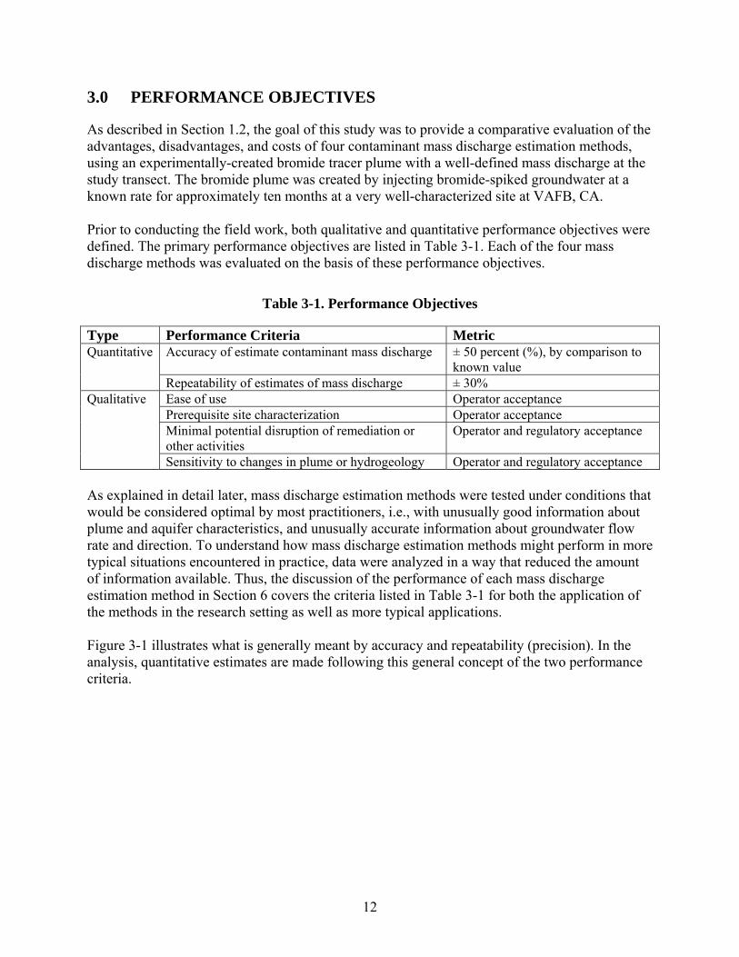
As described in Section 1.2, the goal of this study was to provide a comparative evaluation of the advantages, disadvantages, and costs of four contaminant mass discharge estimation methods, using an experimentally-created bromide tracer plume with a well-defined mass discharge at the study transect. The bromide plume was created by injecting bromide-spiked groundwater at a known rate for approximately ten months at a very well-characterized site at VAFB, CA. Prior to conducting the field work, both qualitative and quantitative performance objectives were defined. The primary performance objectives are listed in Table 3-1. Each of the four mass discharge methods was evaluated on the basis of these performance objectives.
Table 3-1. Performance Objectives
Type Performance Criteria Metric Quantitative Accuracy of estimate contaminant mass discharge ± 50 percent (%), by comparison to
known value Repeatability of estimates of mass discharge ± 30%
Qualitative Ease of use Operator acceptance Prerequisite site characterization Operator acceptance Minimal potential disruption of remediation or other activities
Operator and regulatory acceptance
Sensitivity to changes in plume or hydrogeology Operator and regulatory acceptance As explained in detail later, mass discharge estimation methods were tested under conditions that would be considered optimal by most practitioners, i.e., with unusually good information about plume and aquifer characteristics, and unusually accurate information about groundwater flow rate and direction. To understand how mass discharge estimation methods might perform in more typical situations encountered in practice, data were analyzed in a way that reduced the amount of information available. Thus, the discussion of the performance of each mass discharge estimation method in Section 6 covers the criteria listed in Table 3-1 for both the application of the methods in the research setting as well as more typical applications. Figure 3-1 illustrates what is generally meant by accuracy and repeatability (precision). In the analysis, quantitative estimates are made following this general concept of the two performance criteria.

13
Accurate, but not precise
Precise, but not accurate
Accuracy
Reference Value
Accuracy
Reference Value
PrecisionValue
Probability Density
Probability Density
Figure 3-1. Illustration of Precision and Accuracy
14
4.0 SITE DESCRIPTION
4.1 SITE LOCATION AND HISTORY
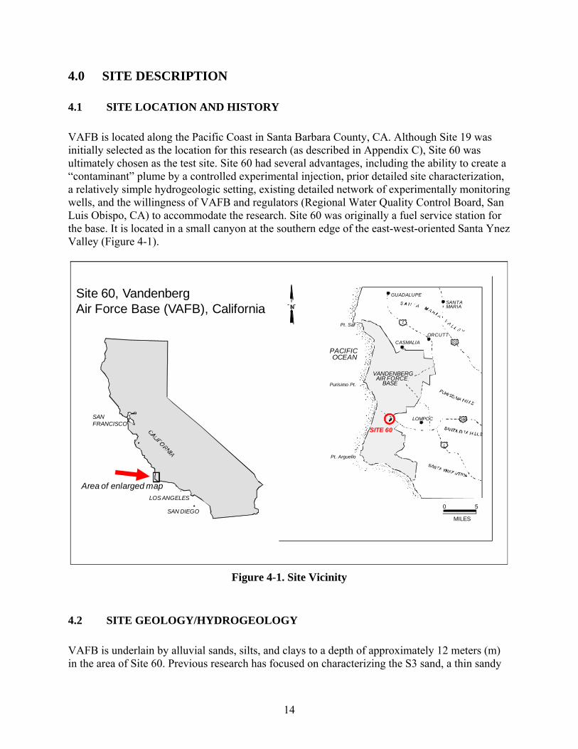
VAFB is located along the Pacific Coast in Santa Barbara County, CA. Although Site 19 was initially selected as the location for this research (as described in Appendix C), Site 60 was ultimately chosen as the test site. Site 60 had several advantages, including the ability to create a “contaminant” plume by a controlled experimental injection, prior detailed site characterization, a relatively simple hydrogeologic setting, existing detailed network of experimentally monitoring wells, and the willingness of VAFB and regulators (Regional Water Quality Control Board, San Luis Obispo, CA) to accommodate the research. Site 60 was originally a fuel service station for the base. It is located in a small canyon at the southern edge of the east-west-oriented Santa Ynez Valley (Figure 4-1).
Figure 4-1. Site Vicinity
4.2 SITE GEOLOGY/HYDROGEOLOGY
VAFB is underlain by alluvial sands, silts, and clays to a depth of approximately 12 meters (m) in the area of Site 60. Previous research has focused on characterizing the S3 sand, a thin sandy
SAN FRANCISCO
LOS ANGELES
SAN DIEGO
Area of enlarged map
101
SANTAMARIA
GUADALUPE
VANDENBERGAIR FORCE
BASE
ORCUTT
LOMPOC
CASMALIA
Pt. Arguello
PACIFICOCEAN
Purisimo Pt.
Pt. Sal
SITE 60
N
MILES
50
1
1
246
Site 60, Vandenberg Air Force Base (VAFB), California
15
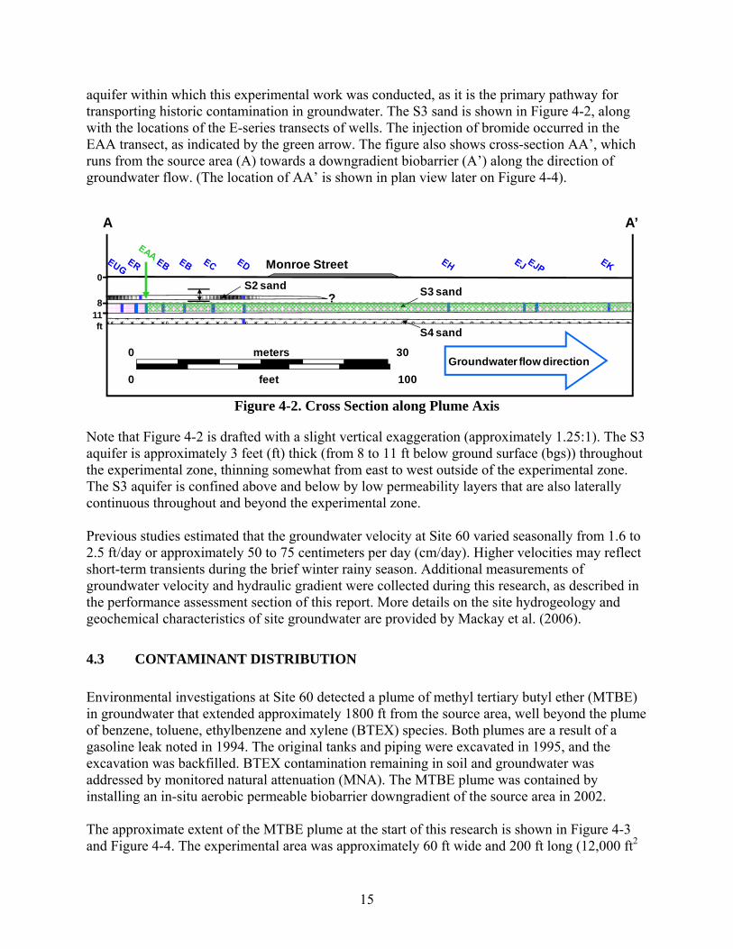
aquifer within which this experimental work was conducted, as it is the primary pathway for transporting historic contamination in groundwater. The S3 sand is shown in Figure 4-2, along with the locations of the E-series transects of wells. The injection of bromide occurred in the EAA transect, as indicated by the green arrow. The figure also shows cross-section AA’, which runs from the source area (A) towards a downgradient biobarrier (A’) along the direction of groundwater flow. (The location of AA’ is shown in plan view later on Figure 4-4).
0 feet 100
0 meters 30Groundwater flow direction
?
A’A
Monroe Street
S3 sandS2 sand
S4 sand
0
811ft
Figure 4-2. Cross Section along Plume Axis
Note that Figure 4-2 is drafted with a slight vertical exaggeration (approximately 1.25:1). The S3 aquifer is approximately 3 feet (ft) thick (from 8 to 11 ft below ground surface (bgs)) throughout the experimental zone, thinning somewhat from east to west outside of the experimental zone. The S3 aquifer is confined above and below by low permeability layers that are also laterally continuous throughout and beyond the experimental zone. Previous studies estimated that the groundwater velocity at Site 60 varied seasonally from 1.6 to 2.5 ft/day or approximately 50 to 75 centimeters per day (cm/day). Higher velocities may reflect short-term transients during the brief winter rainy season. Additional measurements of groundwater velocity and hydraulic gradient were collected during this research, as described in the performance assessment section of this report. More details on the site hydrogeology and geochemical characteristics of site groundwater are provided by Mackay et al. (2006).
4.3 CONTAMINANT DISTRIBUTION
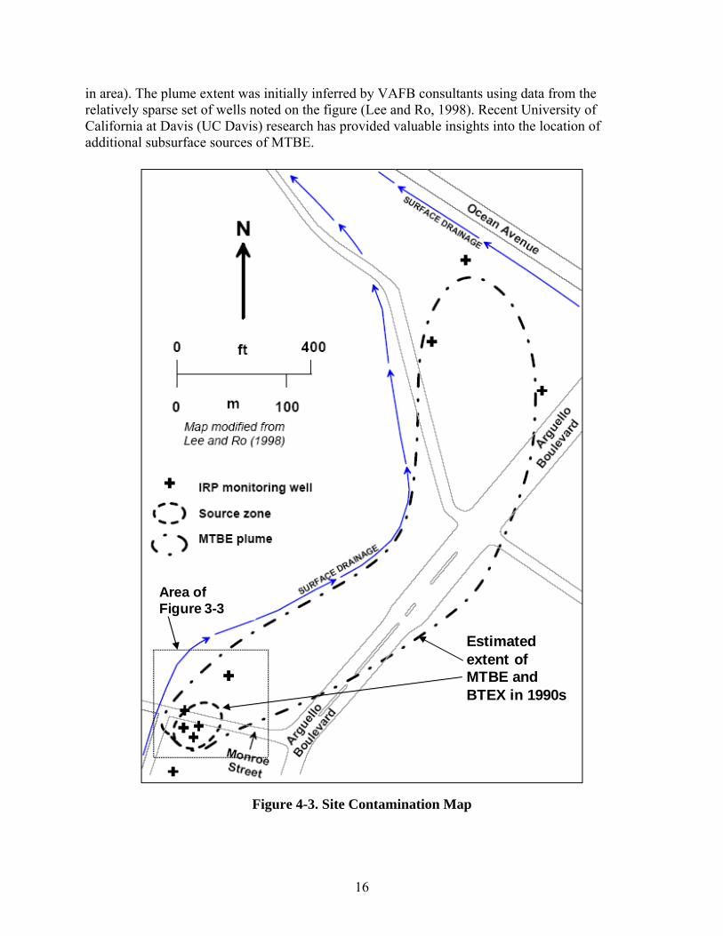
Environmental investigations at Site 60 detected a plume of methyl tertiary butyl ether (MTBE) in groundwater that extended approximately 1800 ft from the source area, well beyond the plume of benzene, toluene, ethylbenzene and xylene (BTEX) species. Both plumes are a result of a gasoline leak noted in 1994. The original tanks and piping were excavated in 1995, and the excavation was backfilled. BTEX contamination remaining in soil and groundwater was addressed by monitored natural attenuation (MNA). The MTBE plume was contained by installing an in-situ aerobic permeable biobarrier downgradient of the source area in 2002. The approximate extent of the MTBE plume at the start of this research is shown in Figure 4-3 and Figure 4-4. The experimental area was approximately 60 ft wide and 200 ft long (12,000 ft2
16
in area). The plume extent was initially inferred by VAFB consultants using data from the relatively sparse set of wells noted on the figure (Lee and Ro, 1998). Recent University of California at Davis (UC Davis) research has provided valuable insights into the location of additional subsurface sources of MTBE.
Estimated extent of MTBE andBTEX in 1990s
Area of Figure 3-3
Figure 4-3. Site Contamination Map
17
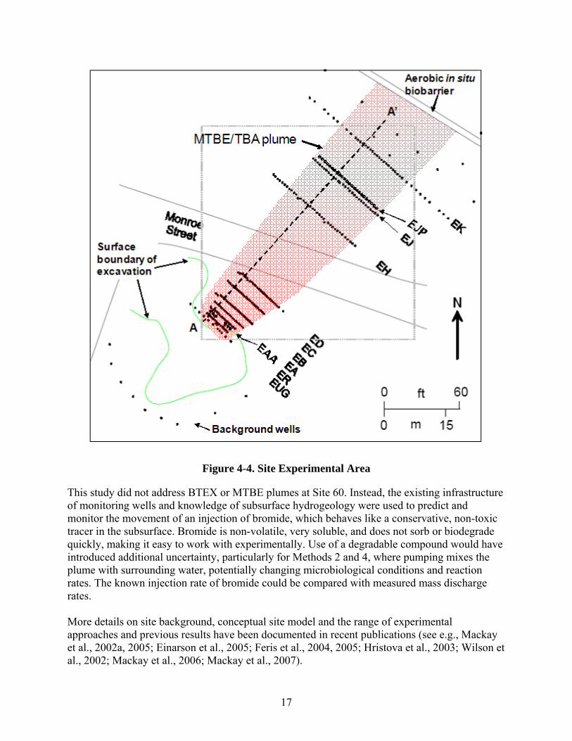
Figure 4-4. Site Experimental Area
This study did not address BTEX or MTBE plumes at Site 60. Instead, the existing infrastructure of monitoring wells and knowledge of subsurface hydrogeology were used to predict and monitor the movement of an injection of bromide, which behaves like a conservative, non-toxic tracer in the subsurface. Bromide is non-volatile, very soluble, and does not sorb or biodegrade quickly, making it easy to work with experimentally. Use of a degradable compound would have introduced additional uncertainty, particularly for Methods 2 and 4, where pumping mixes the plume with surrounding water, potentially changing microbiological conditions and reaction rates. The known injection rate of bromide could be compared with measured mass discharge rates. More details on site background, conceptual site model and the range of experimental approaches and previous results have been documented in recent publications (see e.g., Mackay et al., 2002a, 2005; Einarson et al., 2005; Feris et al., 2004, 2005; Hristova et al., 2003; Wilson et al., 2002; Mackay et al., 2006; Mackay et al., 2007).

18
5.0 TEST DESIGN
5.1 CONCEPTUAL EXPERIMENTAL DESIGN
In order to evaluate and compare the four mass discharge estimation techniques, a number of field activities were conducted, as summarized in Table 5-1. Each phase of work is described in the following sections.
Table 5-1: Experimental Activities
Work Phase Activities
Baseline characterization
Background bromide measurements
Aquifer characterization
Conceptual site model
Design and layout of experimental setup
Transect location and well installation
Bromide injection system construction
Field Testing
Bromide injection, followed by water-only injection
Groundwater elevation monitoring
Data collection Snapshot sampling (Method 1) Groundwater pumping (Methods 2 and 4) PFM deployment and retrieval (Method 3)
Data analysis Correction for background data Analysis of four methods Modeling
5.2 BASELINE CHARACTERIZATION
5.2.1 Background Concentrations
At most sites, the contaminant is likely present only within the plume under investigation. However, because a bromide tracer was used as a model contaminant at this site, and because bromide is naturally-occurring in groundwater, monitoring was conducted by the research team prior to the demonstration to characterize background levels.
19
Results indicated that the background concentration was low, on the order of 3 milligrams per liter (mg/L) bromide. The project team continued to monitor background concentrations during the demonstration. These results indicated that background bromide levels varied widely over time and space. In the nine samplings of the injection supply wells collected over the course of a year (from October 2005 to October 2006), background bromide levels ranged from 1 to 20 mg/L. Background bromide was also present in the water with which bromide was mixed prior to injection. 5.2.2 Aquifer Characterization
After additional wells were installed, each of the pumping wells was subjected to constant discharge hydraulic testing. A baseline set of groundwater elevation measurements was collected from extraction wells and nearby monitoring wells to represent pre-test hydraulic conditions. Next, pumping tests were performed sequentially in each of pumping wells. For each test, pressure transducers (Solinst Leveloggers™) were inserted into the pumping well and the two wells east of that pumping well. Time-drawdown data were collected from observation wells located at two different distances from the pumping well, facilitating the calculation of aquifer transmissivity using a steady-state, distance-drawdown, analytical solution. A complete discussion of the hydraulic testing program (including test methods, analytical solutions, and presentation of results) is included in Appendix D. 5.2.3 Conceptual Site Model Review
A third activity prior to experimental setup was a review of the conceptual site model. Due to previous detailed site characterization efforts, the site conceptual model was very refined at the beginning of the project. Site understanding, including existing geologic cross-sections and groundwater elevation contour maps, was used to plan the locations of tracer injection wells and additional monitoring wells.
5.3 DESIGN AND LAYOUT OF TECHNOLOGY COMPONENTS
5.3.1 Location and Construction of Well Transects
A number of injection and monitoring well transects were already in place at Site 60 prior to this research, as shown in Figure 4-2 (cross-sectional view) and Figure 4-4 (plan view). As this was a prior research study site, there were a large number of existing wells (a total of 19 wells screened in the S2 aquifer, 192 wells in the S3 aquifer, and 6 wells in the S4 aquifer). Transects are named as shown in Figure 4-4: EA, EB, EC, ED, EH, EJ, EK, ER, EAA’ and EUG. For this study, wells in the EJ transect were used (Method 1). In addition, an arc of 10 S3 wells had already been installed upgradient of the backfilled 1995 source excavation (Figure 4-4), which contained variable permeability backfill and extended at its deepest portions to the bottom of the S3 aquifer (Mackay et al., 2006). This arc of background wells was used to monitor the quality of groundwater (primarily, background bromide concentrations) flowing from the S3 aquifer into and through the backfill and subsequently back
20
into the S3 aquifer in the research area. The backfilled excavation is located just to the left of the area depicted in Figure 4-2. All of the existing wells used in this experiment had been installed using a low-cost direct push technique, described in detail previously (Mackay et al., 2006). In brief, a direct push rig was used to push/vibrate a continuous length of 20 ft of 1-inch (in) Schedule 40 steel (“black iron”) pipe, with a steel slip-fit “knock-off” tip first inserted into the bottom. Prior to use, both the inside and outside of the pipe were first cleaned of paint. After the pipe was vibrated into the subsurface to the desired depth, the tip was “knocked out” of the bottom of the pipe, and an appropriate length of 0.5-in Schedule 40 polyvinyl chloride (PVC) well screen and casing was inserted into the steel pipe to the bottom of the monitoring zone. All well screens were constructed of machine-slotted PVC with a slot size of 0.020 in. Wells installed to monitor the S3 sand had a slotted interval of three ft from a depth of 8 to 11 ft bgs, across the entire thickness of the S3 sand. The PVC well was held in place while the steel pipe was pulled up three ft, aligning its bottom with the top of the intended monitoring interval and exposing the well screen to the aquifer material. The steel pipe and PVC well inside it were then sawed off to a height of one ft above ground surface. The steel pipe was left in the ground to serve as a seal from the surface to the top of the monitored zone, preventing inadvertent short circuiting of flow from shallower permeable horizons. A new transect of 23 wells, the EJP transect, was installed specifically for this research project (see Figures 4-2 and 4-4 for EJP transect location). These wells were installed to facilitate hydraulic testing and use of mass discharge estimation Methods 2 through 4. Consequently, the wells were designed and installed to be as hydraulically efficient as possible. The slot size and sand pack were designed using water supply well methods (Driscoll, 1986). All wells were constructed of standard threaded, 1-in nominal schedule 40 PVC, with 3.5-foot slotted intervals (slot size 0.030 in) from a depth of 7.5 to 11 ft bgs, across the entire thickness of the S3 sand. The wells were installed inside of boreholes drilled to 11.5 ft bgs with a 4-in outside diameter solid-stem auger. All boreholes stayed open for a period of time sufficient to insert pre-assembled PVC wells and sand packs immediately after the augers were removed. Two-in diameter sand pack cartridges were installed over the slotted sections of PVC pipe prior to insertion in the boreholes. The cartridges were made by sewing polyester mesh “socks” which were then inverted, slid over each of the sections of slotted PVC, and attached at the bottom of the PVC well stock using nylon ties. The polyester mesh has the following specifications: 14.7 by 14.7 openings per inch, thread diameter of 0.0157 in, opening size of 0.0520 in, open area of 59%. The poly-mesh “socks” were then filled with Lonestar #3 graded sand, and the tops of the cartridges were secured with plastic ties. Number 3 sand was then added slowly from the surface to fill any remaining annular space between the sand pack cartridges and the borehole walls. Sand was added until the top of the sand pack in each well reached a depth of 7 ft bgs, approximately 0.5 ft above the top of the well screens. Thus the wells were surrounded with a coarse sand pack in an annulus between radii of 0.5 to 2.0 in. Bentonite chips were then added to the boreholes and hydrated to form annular seals. All wells were developed using a vented surge block and over-pumping methods (Driscoll, 1986). Development continued until water pumped from the wells was clear and sediment free.
21
To allow comparisons of mass discharge estimation methods, the EJ transect was used to estimate mass discharge using Method 1 and the new EJP transect (located five ft downgradient of Transect EJ) was used for Methods 2 through 4. There were two reasons why different transects were used for the different methods:
• Using a different set of wells for Method 1 enabled researchers to collect Method 1 measurements simultaneously with other methods, without interference. If the same set of wells were used, pumping methods could have changed contaminant distribution; flux meters would have prevented simultaneous synoptic sampling of the well during their deployment.
• Methods 2 through 4 required a different type of well than Method 1.
The simultaneous use of different transects for the different methods is not expected to affect the comparison. The EJ transect was located approximately 147 ft downgradient of the bromide injection wells; the EJP transect was only five ft further (153 ft downgradient of the injection wells). Therefore, based on the 5-ft distance and estimated groundwater velocity, bromide would be detected at the EJP transect only a few days later than the EJ transect, assuming no loss in bromide mass in the S3 aquifer (Appendix A). 5.3.2 Bromide Injection System Construction
Injection wells were spaced into two groups of three, in order to create a bifurcated bromide tracer plume as a more realistic representation of plumes commonly found at contaminated sites. (The plume is depicted schematically in Figure 5-1). Research over the last decade has shown that chlorinated solvents and other contaminated “plumes” are in fact often composed of a number of “subplumes” migrating alongside one another (e.g., Guilbeault et al., 2005). Plume bifurcation created a more complicated and realistic “target” for monitoring compared with a single, relatively uniform, plume. A schematic of the bromide injection system is shown in Figure 5-2. Groundwater was extracted from two background wells (locations shown in Figure 5-1), spiked with a small flow of concentrated bromide solution, and then re-injected into six individual wells in the EAA′ transect (Wells EAA′ 4, 5, 6 [Lane A] and Wells EAA′ 11, 12, 13 [Lane B]). Peristaltic pumps were installed to control groundwater extraction and total flow rate. Rotameters were installed to measure total rates and measure and balance split flow rates. A concentrated bromide solution was made by dissolving weighed masses of reagent grade potassium bromide into a measured volume of water. That spike solution was set up to be metered into the main water flow (Figure 5-2) using a high performance liquid chromatography (HPLC) pump. All equipment was already on site as it had been used in a previous experiment (Mackay et al., 2006). The only significant modification was the use of an HPLC pump for spiking in the current study since some operational problems had been observed in the prior work using a small peristaltic pump for spiking.
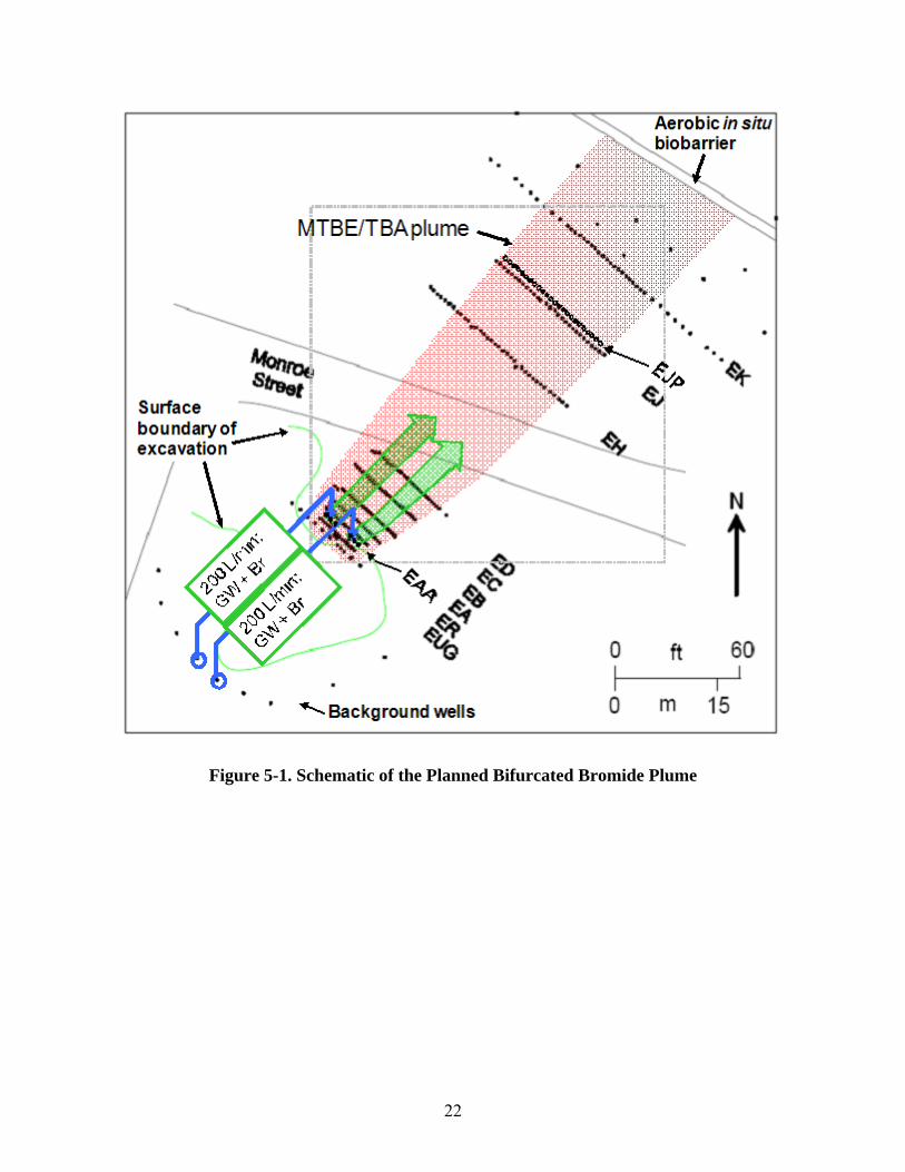
22
Figure 5-1. Schematic of the Planned Bifurcated Bromide Plume
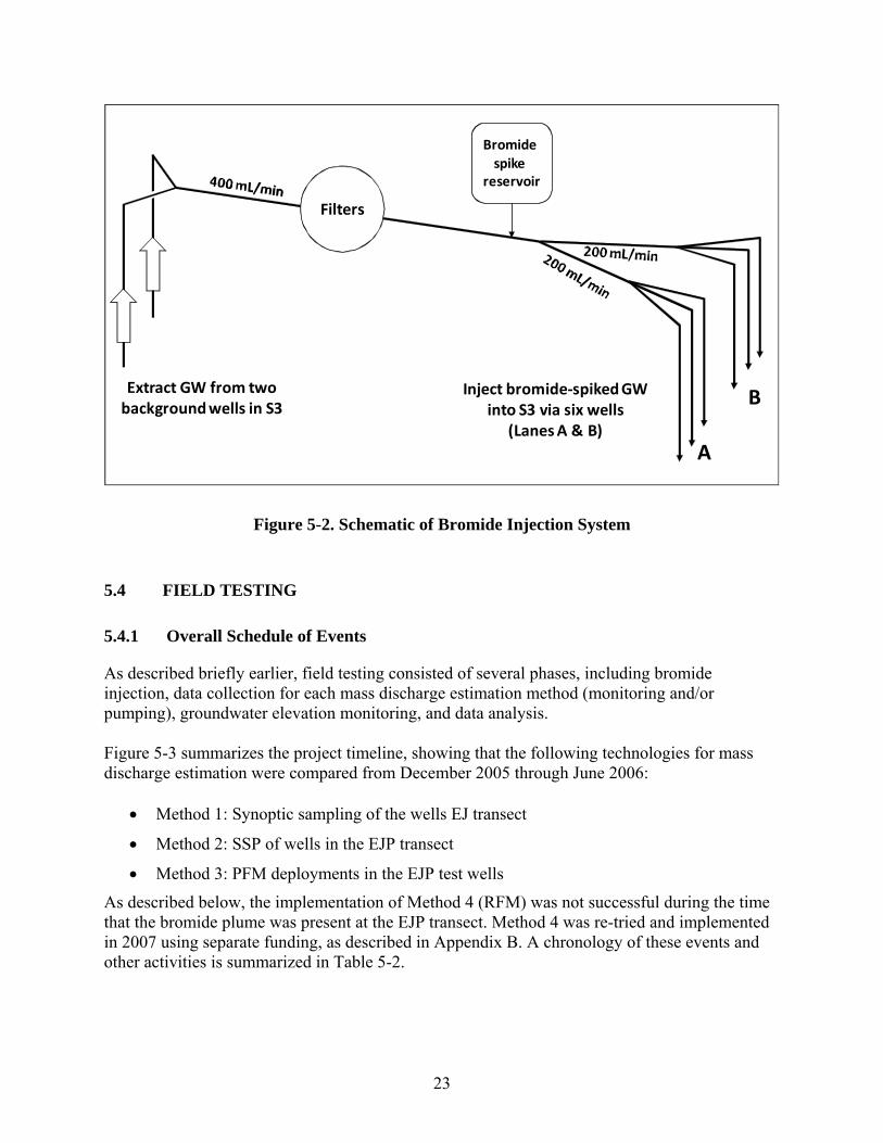
23
Figure 5-2. Schematic of Bromide Injection System
5.4 FIELD TESTING
5.4.1 Overall Schedule of Events
As described briefly earlier, field testing consisted of several phases, including bromide injection, data collection for each mass discharge estimation method (monitoring and/or pumping), groundwater elevation monitoring, and data analysis. Figure 5-3 summarizes the project timeline, showing that the following technologies for mass discharge estimation were compared from December 2005 through June 2006:
• Method 1: Synoptic sampling of the wells EJ transect
• Method 2: SSP of wells in the EJP transect
• Method 3: PFM deployments in the EJP test wells
As described below, the implementation of Method 4 (RFM) was not successful during the time that the bromide plume was present at the EJP transect. Method 4 was re-tried and implemented in 2007 using separate funding, as described in Appendix B. A chronology of these events and other activities is summarized in Table 5-2.
Extract GW from two backgroundwells in S3 B
A
Filters
Inject bromide‐spiked GW into S3 via six wells
(Lanes A & B)
Bromide spike
reservoir

24
Table 5-2. Demonstration Schedule and Milestones
Category Event Name Start Date Start Time End Date End Time Br Injection Br Injection Jul 11 2005 1:45 PM May 06 2006 9:17 AM
Water Only Injection May 06 2006 9:17 AM Aug 24 2006 7:56 AM Hydraulic Testing Pumping Tests Mar 24 2006 Mar 24 2006
Pumping Tests Mar 27 2006 Mar 27 2006 PFM Deployment PFM #1 and #2 Dec 06 2005 Dec 12 2005
PFM #3 Apr 21 2006 Apr 24 2006 Pumping SSP #1 Dec 15 2005 Mar 17 2006
Pump & Store (EK) Mar 18 2006 Jun 19 2006 SSP #2 Apr 07 2006 Apr 18 2006 SSP#3 (Sparse) May 31 2006 3:58 PM Jun 20 2006 11:00 AM
Synoptic (snapshot) sampling
Snap #01 (78 d) Sep 21 2005 Sep 30 2005 Snap #02 (107 d) Oct 25 2005 Oct 27 2005 Snap #03 (128 d) Nov 15 2005 Nov 18 2005 Snap #04 (160 d) Dec 19 2005 Dec 20 2005 Snap #05 (189 d) Jan 17 2006 Jan 18 2006 Snap #06 (218 d) Feb 13 2006 Feb 17 2006 Snap #07 (244 d) Mar 13 2006 Mar 13 2006 Snap #08 (342 d) Jun 19 2006 Jun 19 2006 Snap #09 (461 d) Oct 16 2006 Oct 16 2006 Snap #10 (582 d) Feb 13 2007 Feb 13 2007
Water Levels Site WL #1 May 09 2005 Site WL #2 Aug 16 2005 Site WL #3 Oct 13 2005 Site WL #4 Dec 14 2005 Site WL #5 Jan 12 2006 Site WL #6 Feb 22 2006 Site WL #7 Mar 17 2006 Site WL #8 Apr 20 2006 Site WL #9 May 18 2006 Site WL #10 Jul 11 2006 Site WL #11 Aug 29 2006 Site WL #12 Nov 13 2006 Site WL #13 Apr 02 2007
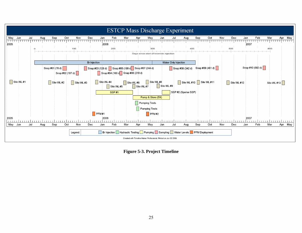
25
Figure 5-3. Project Timeline
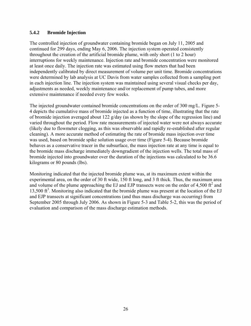
26
5.4.2 Bromide Injection
The controlled injection of groundwater containing bromide began on July 11, 2005 and continued for 299 days, ending May 6, 2006. The injection system operated consistently throughout the creation of the artificial bromide plume, with only short (1 to 2 hour) interruptions for weekly maintenance. Injection rate and bromide concentration were monitored at least once daily. The injection rate was estimated using flow meters that had been independently calibrated by direct measurement of volume per unit time. Bromide concentrations were determined by lab analysis at UC Davis from water samples collected from a sampling port in each injection line. The injection system was maintained using several visual checks per day, adjustments as needed, weekly maintenance and/or replacement of pump tubes, and more extensive maintenance if needed every few weeks. The injected groundwater contained bromide concentrations on the order of 300 mg/L. Figure 5-4 depicts the cumulative mass of bromide injected as a function of time, illustrating that the rate of bromide injection averaged about 122 g/day (as shown by the slope of the regression line) and varied throughout the period. Flow rate measurements of injected water were not always accurate (likely due to flowmeter clogging, as this was observable and rapidly re-established after regular cleaning). A more accurate method of estimating the rate of bromide mass injection over time was used, based on bromide spike solution usage over time (Figure 5-4). Because bromide behaves as a conservative tracer in the subsurface, the mass injection rate at any time is equal to the bromide mass discharge immediately downgradient of the injection wells. The total mass of bromide injected into groundwater over the duration of the injections was calculated to be 36.6 kilograms or 80 pounds (lbs). Monitoring indicated that the injected bromide plume was, at its maximum extent within the experimental area, on the order of 30 ft wide, 150 ft long, and 3 ft thick. Thus, the maximum area and volume of the plume approaching the EJ and EJP transects were on the order of 4,500 ft2 and 13,500 ft3. Monitoring also indicated that the bromide plume was present at the location of the EJ and EJP transects at significant concentrations (and thus mass discharge was occurring) from September 2005 through July 2006. As shown in Figure 5-3 and Table 5-2, this was the period of evaluation and comparison of the mass discharge estimation methods.

27
y = 121.53x
r2 = 0.9957
0
5000
10000
15000
20000
25000
30000
35000
40000
0 25 50 75 100 125 150 175 200 225 250 275 300
Mas
s (g
)
Days Elapsed7/11/05 5/5/067/11/05 5/5/06
Average injection rate =122 g/day
Figure 5-4. Cumulative Mass of Injected Bromide
In the figure, start and stop dates are noted at the ends of the x-axis. The solid line is a linear regression of the data, which results in an estimate of the average injection rate of approximately 122 g/day.
5.4.3 Groundwater Elevation Measurements (Methods 1 and 4)
Depth-to-water measurements were taken from approximately 50 site monitoring wells on 13 different occasions before, during, and after the bromide injection. Site-wide water level measurements were timed concurrent with site-wide groundwater sample collection, facilitating mass discharge estimation using Method 1. Depth-to-water measurements were made using a Slope Indicator water level meter that had been calibrated for the electrical conductivity of the groundwater in the S3 sand. Groundwater elevations in the wells were determined by subtracting depth-to-water measurements from the surveyed top-of-casing elevations for each well. These data were used to prepare groundwater contour maps, which were generated using the contouring software package Surfer Version 8.0 from Golden Software. Data were also used to calculate horizontal hydraulic gradients within the S3 sand in the study area. The hydraulic gradient in the vicinity of the EJP transect was calculated by measuring the slope of the piezometric surface. For example, if a 60-ft distance was measured between the 30-ft and 29-ft contours in the vicinity of the EJP transects, the calculated hydraulic gradient would be 1/60 ft/ft or 0.0167. These calculations were made 13 times to define horizontal hydraulic gradients within

28
the S3 sand in the vicinity of transects ED, EH, and EJ. The dates that the water levels were measured are listed in Table 5-2. Results are presented in Section 5.6.2. 5.4.4 Steady-State Pumping Tests (Method 2)
During SSP tests, groundwater was pumped simultaneously from wells in the EJP transect using peristaltic pumps. The eight pumps used during the SSP tests were Cole Parmer Masterflex® L/S Computerized Drive Pumps (Model # 7519-05), each equipped with four Model 7519-70 pump cartridges (thus each pump could extract water from four wells). Water was conveyed from the individual wells to the pump cartridges via 0.25-in outer diameter low density polyethylene (LDPE) tubing inserted into each of the wells. Inside each well, the ends of the tubing were suspended approximately 0.5 ft above the tops of the well screens to avoid inadvertently drawing the water table down below the top of the S3 sand. Effluent from the pump cartridges was conveyed through 0.25-in outer diameter LDPE tubing to an 11.4-L polyethylene mixing tank. The various tubes entered the mixing tank through water-tight nylon compression fittings threaded into a plexiglass lid that was attached to the mixing tank. The mixing tank rested on a mechanical stir plate which was operated continuously to keep the water in the tank well mixed. Water exited the mixing tank through a 0.75-in PVC pipe threaded into the wall of the tank. A rotameter-type flowmeter was used to measure flow of water in this pipe and a valved sampling port was installed to simplify collection of composite water samples from the mixing tank. Water exiting the mixing tank was directed into a 20-gallon (gal) plastic tub that held a sump pump. When the plastic tub filled with water, a float switch on the sump pump would turn the pump on, pumping the water to a nearby 3000-gal polyethylene storage container. Water contained in the storage container was periodically pumped out and disposed of by an Air Force environmental waste management contractor. During the tests, the pumps were adjusted to maintain the target composite extraction rate (estimated from prior assessments of the hydraulic properties of the S3 sand). The composite extraction rate was measured at approximately three-hour intervals using a 1-L glass graduated cylinder and stopwatch. In addition, the peristaltic pumps were operated and adjusted so that the extraction rates from individual wells in the EJP transect were as uniform as possible across the transect. Three-way valves mounted on a control rack between the pumps and the mixing tank facilitated measurement of the extraction rate from individual wells. This was done by diverting the flow (using the 3-way valves) from individual wells into a 50-milliliter (mL) graduated cylinder. Flow rates were measured by recording the time required to fill the graduated cylinder. Three SSP tests were performed during this study. The tests, referred to as SSP#1, SSP#2 and SSP#3, were performed between days 157 to 249, 270 to 281, and 324 to 344 of the experiment, respectively (Table 5-2 and Figure 5-3). During SSP#1, groundwater was simultaneously extracted from all 23 of the EJP wells for approximately 92 days at a target extraction rate of approximately 1.2 L/minute (min). SSP#2 was conducted in a manner similar to SSP#1 but for a period of 12 days. Unfortunately the bromide samples collected during SSP#2 were misplaced. Therefore, no analytical data for SSP#2 is presented in this report. SSP#3 began on April 7, 2006 and lasted 21 days. SSP#3 is referred to as the “Sparse SSP” test because only 6 of the EJP wells (EJP 2, 6, 10, 14, 18, and 22) were pumped. The target extraction rate during SSP#3 was also 1.2 L/min, but that total extraction rate could not be attained without lowering the water levels in the

29
wells below the elevation of the top of the S3 sand. Therefore, in SSP#3, the extraction rates in the six wells were reduced, resulting in a cumulative extraction rate for SSP#3 ranging from about 0.5 to 1.0 L/min. Extraction rates were quite variable during SSP#3, due to the frequent adjustments to the extraction rates in individual wells necessary to avoid excessive drawdown. 5.4.5 PFM Deployment (Method 3)
PFMs were constructed using well-established methods (see Annable et al., 2005 for details). Each PFM was 54 in. long, with resin packed from approximately 2 to 45 in. PFMs were inserted into the bottom of each well screen to capture contaminants throughout the saturated thickness of the aquifer. Because the screened interval of the wells was 42 in. long, a small portion of the PFM resin extended above the screened interval. However, when the upper section of the PFM resin was analyzed after deployment, results suggested it had been exposed to flow within the well casing; thus the entire PFM resin length was used in the calculations of Darcy velocity and local bromide mass flux. Passive flux meters were deployed three times in wells in the EJP transect as listed in Table 5-3. The first two deployments were conducted in December 2005 with very little time between them (one to two hours). The third deployment was conducted in April 2006.
Table 5-3. Passive Flux Meter Deployments at VAFB
Deployment Install Retrieve Duration (days)
Number of wells
PFMs with tracers
First 12/6/05 12/8/05 1.7 23 8 Second 12/8/05 12/12/05 3.9 11 0 Third 4/18/06 4/22/06 3.0 19 6
In order to minimize the total mass of pre-loaded PFM tracers (n-hexanol and n-heptanol) released to the aquifer during each deployment, only every third deployed PFM contained pre-loaded tracers. In all other wells, the sorbent was tracer-free. In this study the sorbent selected for bromide retention was Lewatit S 6328A resin. This resin also has the capacity to adsorb the alcohol tracers (n-hexanol and n-heptanol) used for quantifying Darcy velocity. Information on partitioning characteristics of Lewatit S 6328A has been published for use at a site containing phosphorous (Cho et al., 2007). The bromide mass that was captured by the resin in the flux meters was measured by extracting bromide from the resin following flux meter recovery. The captured mass for each flux meter was then used to estimate the local bromide flux (g/day per square meter of aquifer). The bromide mass discharge carried by the plume across the EJP transect was then estimated by integration over the known aquifer thickness across the width of the sampled portion of the transect using the known well spacing. It is important to note that the width of the aquifer sampled by Methods 1 and 3 are different. As shown in Figure 5-5, water drawn into the well during synoptic sampling likely arises from a width in the aquifer of about 1.2 in (assuming radial flow into the well during sampling). In contrast, Figure 5-6 shows that the width of the aquifer sampled by the PFM corresponds to the screened saturated thickness (approximately 41 in).
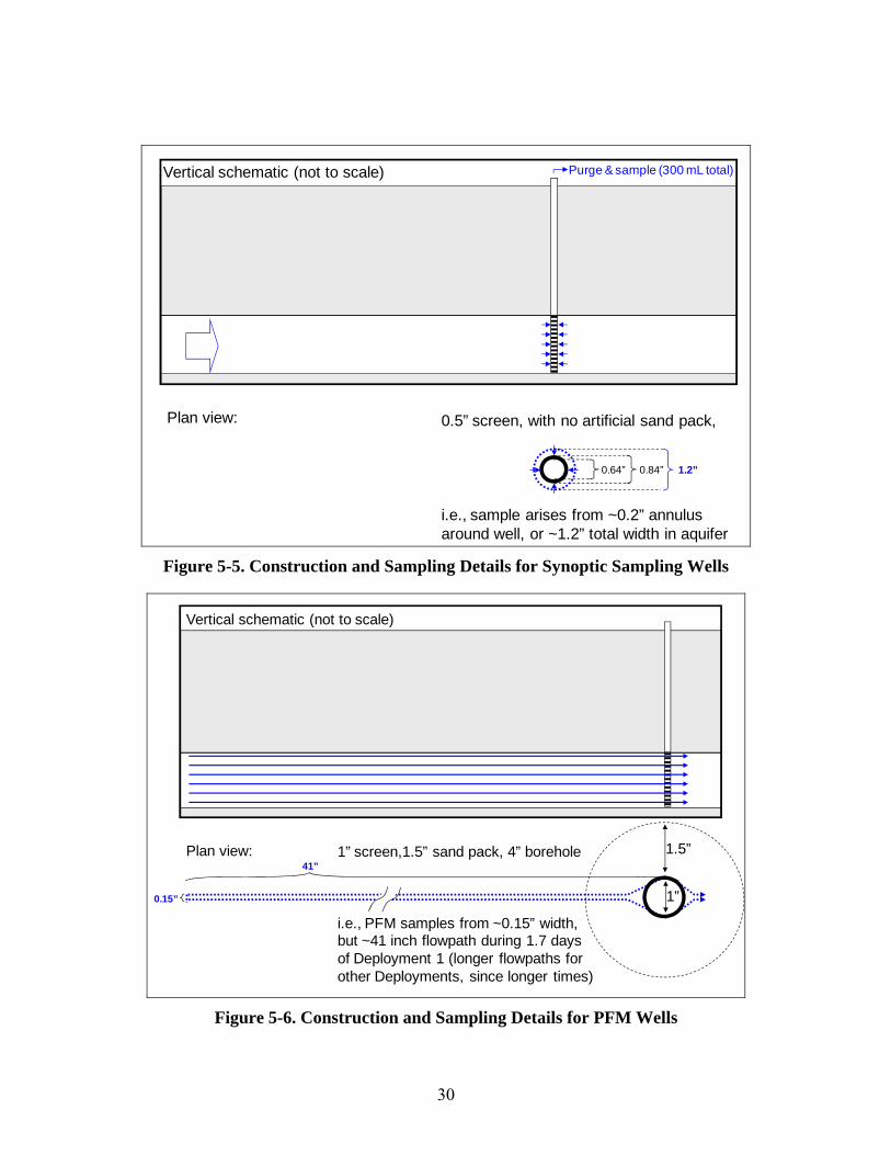
30
Vertical schematic (not to scale)
Plan view: 0.5” screen, with no artificial sand pack,
i.e., sample arises from ~0.2” annulusaround well, or ~1.2” total width in aquifer
Purge & sample (300 mL total)
0.64” 0.84” 1.2”
Figure 5-5. Construction and Sampling Details for Synoptic Sampling Wells
Vertical schematic (not to scale)
Plan view:
0.15”
41”1.5”
1”
1” screen,1.5” sand pack, 4” borehole
i.e., PFM samples from ~0.15” width, but ~41 inch flowpath during 1.7 days of Deployment 1 (longer flowpaths for other Deployments, since longer times)
Figure 5-6. Construction and Sampling Details for PFM Wells

31
5.4.6 Waste Residuals
Wastewater produced as part of the sampling processes was stored on site until it was hauled away for off-site treatment and disposal by VAFB contractors. Approximately 43 gallons of purge water was generated from the snapshot sampling at Transect EJ (based on approximately 540 samples and 300 mL of purge water per sample). This volume was insignificant compared with the amount of water generated during Method 2 trials. In the three SSP trials, a total of 51,600 gallons (~196,000 L) of extracted water was generated. 5.4.7 Demobilization
As requested by VAFB, all wells in the EA, EB, EC, ER, EAA′ and EUG transects were decommissioned in Fall 2006, and all wells in the ED transect were decommissioned in late Summer 2007; these are the wells grouped just south of Monroe Street, shown in Figure 4-4. Other wells, including the ARC background wells and transects north of Monroe Street were retained for continued research use at the site. The bromide injection system was retained for future research use at the site. 5.4.8 Numerical Modeling of Bromide Injection and Transport
Because the actual rate of bromide injection was not constant, another benchmark was needed as a comparison to the mass discharge estimates. The project team developed a transient, three-dimensional fate and transport model to simulate the injected bromide plumes. The model was constructed using detailed site data (including hydraulic conductivity, gradients, aquifer thickness, and background bromide concentrations) and accounted for the variable rate of bromide injection. The development and calibration of the model is described in Appendix A. That simulation, once calibrated to field data, provided a tool with which to estimate bromide mass discharge at any time and location during the field experiment. 5.4.9 Data Analysis
5.4.9.1 Correction for Background Concentrations
Using Method 1, no correction was needed for the background bromide concentrations measured within the injected plume since this was already accounted for in the injected bromide solution. However, wells on the ends of each transect were typically located beyond the width of the injected subplumes, i.e., the transect captured the entire width of the subplumes. Therefore, measured bromide concentrations in these wells were corrected to exclude background levels before calculating mass discharge. Corrections were made by examining each set of transect data, and excluding significant bromide detected on either side of the often clearly-defined plume. The difference in results is illustrated in Figure 5-7.
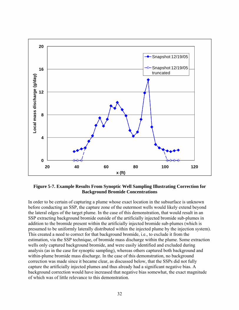
32
0
4
8
12
16
20
20 40 60 80 100 120
Loca
l mas
s di
scha
rge
(g/d
ay)
x (ft)
Snapshot 12/19/05
Snapshot 12/19/05 truncated
Figure 5-7. Example Results From Synoptic Well Sampling Illustrating Correction for Background Bromide Concentrations
In order to be certain of capturing a plume whose exact location in the subsurface is unknown before conducting an SSP, the capture zone of the outermost wells would likely extend beyond the lateral edges of the target plume. In the case of this demonstration, that would result in an SSP extracting background bromide outside of the artificially injected bromide sub-plumes in addition to the bromide present within the artificially injected bromide sub-plumes (which is presumed to be uniformly laterally distributed within the injected plume by the injection system). This created a need to correct for that background bromide, i.e., to exclude it from the estimation, via the SSP technique, of bromide mass discharge within the plume. Some extraction wells only captured background bromide, and were easily identified and excluded during analysis (as in the case for synoptic sampling), whereas others captured both background and within-plume bromide mass discharge. In the case of this demonstration, no background correction was made since it became clear, as discussed below, that the SSPs did not fully capture the artificially injected plumes and thus already had a significant negative bias. A background correction would have increased that negative bias somewhat, the exact magnitude of which was of little relevance to this demonstration.
33
PFMs detected mass discharge of background bromide and therefore required correction for background concentrations. Background mass discharge, i.e., the values corresponding to wells clearly outside the experimentally created bromide plumes, were excluded using the same method as described previously for synoptic sampling. Although the RFM technique was not successfully implemented, background bromide could have been accounted for using this same method. 5.4.9.2 Method 1 Analysis
To facilitate the calculation of bromide mass discharge using Method 1, measured (synoptic) values of bromide concentrations and hydraulic gradients were compiled for wells in the ED, EH, and EJ transects (Table 5-2 and Figure 5-3). Although the primary goal of this work was to implement all the methods at the EJ/EJP transects, Method 1 was easily implemented at all the transects as monitoring was conducted to track the development of the bromide plume. The aquifer thickness along each transect was defined using previously-collected characterization data. An average hydraulic conductivity assumed to be representative of the S3 sand was selected based on the results of the numerical model calibrated to extensive water level and bromide data. These parameters were compiled in a spreadsheet which was used to calculate the bromide mass discharge for each sampling event using the following equation:
AiKCMnd ⋅⋅⋅= ∑ Equation 3
Where
Md = Bromide mass discharge in the plume (g/day) C = Concentration of bromide in discrete samples (g/ft3) K = Measured hydraulic conductivity (ft/day) i = Measured horizontal hydraulic gradient (ft/ft) A = area (ft2)
5.4.9.3 Method 2 Analysis
Analysis of data using Method 2 is typically much simpler than Method 1. Assuming that pumping captures the entire plume, then the rate of mass extraction at steady state is simply equal to the contaminant mass discharge (Md) in the plume at the location of the transect of extraction wells. If an SSP captures only a portion of a plume, then the rate of mass extraction at steady state would be equal to the contaminant mass discharge in only the captured portion of the plume. During the SSP tests, the rate of mass extraction, or captured mass discharge, was calculated using Equation 4. Representative steady-state values of Ccomp and Qtotal were used in the calculations.
totalcompd QCM ⋅= (Equation 4) Where
Md = Contaminant mass discharge in the captured plume
34
Ccomp = Concentration of the target contaminant in a composite sample from the extraction system
Qtotal = Total rate of groundwater extraction 5.4.9.4 Method 3 Analysis
In addition to correcting for background concentrations, PFM data also required correction for convergence/divergence of flow through the well screen that is caused by the sand pack. The convergence/divergence factor (α3) for a well within a sandpack can be estimated using the following expression (Klammler et al., 2007a).
2
1
3
3
2
2
1
1
0
2
2
3
3
2
2
1
1
0
2
1
2
3
2
2
1
1
0
3
2
2
1
1
0
3
111111111111
8
⎟⎟⎠
⎞⎜⎜⎝
⎛⋅⎟⎟
⎠
⎞⎜⎜⎝
⎛−⋅⎟⎟
⎠
⎞⎜⎜⎝
⎛+⋅⎟⎟
⎠
⎞⎜⎜⎝
⎛−+⎟⎟
⎠
⎞⎜⎜⎝
⎛⋅⎟⎟
⎠
⎞⎜⎜⎝
⎛−⋅⎟⎟
⎠
⎞⎜⎜⎝
⎛−⋅⎟⎟
⎠
⎞⎜⎜⎝
⎛++⎟⎟
⎠
⎞⎜⎜⎝
⎛⋅⎟⎟
⎠
⎞⎜⎜⎝
⎛+⋅⎟⎟
⎠
⎞⎜⎜⎝
⎛−⋅⎟⎟
⎠
⎞⎜⎜⎝
⎛−+⎟⎟
⎠
⎞⎜⎜⎝
⎛+⋅⎟⎟
⎠
⎞⎜⎜⎝
⎛+⋅⎟⎟
⎠
⎞⎜⎜⎝
⎛+
=
rr
kk
kk
kk
rr
kk
kk
kk
rr
kk
kk
kk
kk
kk
kk
α
Where
α = Convergence/divergence factor k0 = Hydraulic conductivity of the aquifer k1 = Hydraulic conductivity of the sand pack k2 = Hydraulic conductivity of the well screen k3 = Hydraulic conductivity of sorbent r1 = Total rate of groundwater extraction r2 = Total rate of groundwater extraction
Values of α less than 1.0 mean that flow diverges into the well screen, as shown in Figure 5-6. Factors greater than 1.0 mean that flow converges into the well screen, i.e., from a width greater than the diameter of the well. Estimates for the hydraulic conductivity of the sand pack, k1, were 980 and 1938 m/day using respective empirical equations from Hazen (1892) and Kozeny (1953). The hydraulic conductivity of the sorbent, k3, was determined to be 200 m/day. The slotted PVC screen had an effective open area fraction of 0.0258. With this open area and accounting for wall effects that increase the local hydraulic conductivity, the screen hydraulic conductivity, k2, was calculated to be 10.5 m/day (see Klammler et al., 2007b). The hydraulic conductivity of the aquifer, k0, was assumed to be 13.8 m/day (45 ft/day, as estimated by numerical model calibration). Using these characteristics of the well construction and the two estimates for k1, two estimates were obtained for the convergence/divergence factor α3, i.e., 0.10 and 0.20. All additional flux calculations were adjusted using the average convergence/ divergence factor (0.15). Note that this factor is substantially lower than those employed in earlier studies (in which α3 typically ranged from 0.8 to 1.5, i.e., from moderate divergence to significant convergence of flow). This very low divergence factor appears to be a result of the unusually coarse sand pack used in EJP well construction. As illustrated in Figure 5-6, the implication of this low divergence factor is that the PFM sampled ambient groundwater flow from a width of only about 0.15 in, considerably less than that sampled by the synoptic sampling of the wells in the EJ transect (approximately 1.2 in, as illustrated in Figure 5-5).
35
5.4.9.5 Method 4 Analysis
To determine flux using the RFM technique, it is necessary to measure the fraction of flow from the injection well that enters the paired extraction well. This measurement is typically accomplished using a tracer test, where a tracer added to the injected water is measured at the extraction well (after reaching steady-state). Flux is then determined using the methods described in Huang et al. (2004) and Goltz et al. (2007b). Model simulations at VAFB indicated that based on the site hydrogeology, the tracer test would have to be run for more than a month before concentrations at the extraction well reached steady-state. In order to minimize the duration of the tracer test, two wells that were close to each other (wells EJ18P and EJ20P, which are five ft apart) were used for the test.
5.5 SAMPLING AND ANALYTICAL METHODS
5.5.1 Sampling Techniques
Groundwater samples were collected from monitoring wells and extraction wells. Groundwater was sampled using a cart outfitted with pumps and stainless steel tubing (Mackay et al., 2006). To collect a sample from a well, the stainless steel tubing on the cart was connected to the dedicated LDPE tubing left in each well, with the bottom end set 6 in. above the top of the well screens. Then 200 mL were purged at an extraction rate of 200 mL/min. Pumping at this rate resulted in approximately 6 in. of drawdown in the wells that stabilized after about 30 seconds. Once the drawdown in the well stabilized, stagnant water in the well casing above the screened interval no longer flowed into the sample intake tube. The purging rate was then decreased to 50 mL/min and an additional 100 mL were purged. After 300 mL total were purged, the well was sampled at 50 mL/min. Purging a total of 300 mL from the well was sufficient to recover samples that were vertically integrated over the monitored zone. Samples were collected in duplicate in pre-labeled 8 mL LDPE bottles without preservative (since bromide is a conservative tracer and is not subject to reactions). Samples were stored on site at room temperature before being packed into coolers with bubble wrap to prevent sample breakage during transport. Coolers were couriered or shipped to UC Davis, where they were stored at room temperature until analysis. Once at UC Davis, the samples were logged and analyzed for bromide and other parameters following procedures described in the following section. 5.5.2 Laboratory Analysis
Groundwater samples were analyzed for bromide in the HPLC laboratory of Dr. Sham Goyal, Department of Plant Sciences, UC Davis. Analyses were conducted by staff under the direction of Sunitha Gurushinge (through January 2006) or Dr. Mamie Nozawa-Inoue (from February 2006 through the end of the project). Bromide analyses are also available through commercial laboratories using standard methods. The chromatograph used to analyze bromide samples was equipped with an HPLC pump (ConstaMetric IIIG, LDC/Milton Roy, Riviera Beach, Florida), a self-regenerating suppressor
36
(ASRS-ULTRA-II, 4 millimeter (mm), operated at 100 milliamp, Dionex Corporation, Inc., Sunnyvale, CA), and an electrical conductivity detector (ED40, Dionex Corporation, Inc). The system was operated at room temperature (22±2 degrees Celsius (˚C)). The samples and standards were prepared by either filtering through 0.2-micron filter or centrifuged to remove the particulate matter, and the filtrates or the supernatants were injected using an automated sample injector (7126, Rheodyne) through a 7-microliter injection loop. Anions in the samples were separated on an IonPac AS22 analytical column (4 × 250 mm, Dionex Corporation, Inc., Sunnyvale, CA ) in tandem with an IonPac AG22 guard column (4 × 50 mm) with an eluent (4.5 mM Na2CO3/1.4 mM NaHCO3) at a flow rate of 1.5 mL/min. The detection range of the detector was 0 to 100 µS, and data were acquired by a Chromatopac integrator (C-R501, Shimadzu, Columbia, Maryland). For calibration, bromide standards (NaBr aqueous solution) in the range of 1 to 400 mg/L as Br- were used. Since a curve from 1 through 400 mg/L is slightly non-linear and bent downward, separate regression lines were drawn for lower (1 to 100 mg/L) and higher (100 to 400 mg/L) concentrations (R2=0.999). The calibration curve was made each day when running a set of samples using one or two replicates of the standards, and checked if there was any substantial difference from previous calibration results. The method detection limit was 0.29 mg/L (implying a practical quantification limit (PQL) of approximately 5 times that, or 1.5 mg/L), and the precision of 20 lab duplicate samples was 0.65% as a mean relative percent difference. 5.5.3 PFM Analysis
The PFM tracers (n-hexanol and n-heptanol) were pre-loaded on the PFM sorbents before deployment in 8 of the 23 flux meters used in the first deployment and 6 of the 18 used in the third deployment. Following deployment, PFMs were retrieved, segmented into four sections, and sub-sampled. All PFM analyses were conducted by Dr. Cho in the laboratory of Dr. Annable at the Department of Environmental Engineering Sciences, University of Florida. These analyses are currently not available at typical commercial laboratories; however, they are commercially available as described in Enviroflux’s website (Enviroflux, 2008). Bromide that had sorbed into the resin was extracted using potassium chloride (KCl). Each segment was homogenized and about 10 to 15 g of resin was transferred to pre-weighed 120-mL PVC bottles containing 100 mL of 2 molar KCl (Fisher Scientific). The samples were then rotated on a Glas-Col Rotator, set at 20% rotation speed, for 24 hrs, and then filtered through 0.45-micron glass fiber filters (Wattman Co). The filtered samples were taken in 2-mL analysis vial and analyzed for bromide (Br-) by an HPLC (Perkin Elmer series LC 200, Norwalk, Connecticut) with a ultraviolet (UV) detector at 205 nm. The HPLC system was equipped with an LC 235C Diode Array Detector, a series 200 LC Pump, and a series 200 Autosampler and was linked to an IBM-compatible PC loaded with with Turbochrom (version 4.01) software for acquisition, analysis interpretation and quantification. A Dionex IonPac column (Dionex Co., AS4A-SC, 4 × 250 mm) was used and the analyte Bromide was eluted with 12 millimolar (mM) Sodium Borate solution at a flow rate of 1 mL/min. A complete set of calibration standards (5 points, range 1 to 100 mg/L, R2=0.9999) were analyzed at the beginning of each day with a mid-range continuing calibration standard analyzed after every 25 samples. A matrix spike and a blank spike, and sample duplicates were analyzed with each daily sample set. The method detection limit was approximately 0.5 mg/L, and the precision of 10 lab duplicate samples was 1.50% as a mean relative percent difference.

37
The masses of PFM pre-loaded tracers (n-hexanol, n-heptanol, and n-octanol) remaining after deployment were recovered from the PFM sorbent using isopropyl alcohol. Approximately ten grams of the wet Lewatit resin (Lewatit S 6328 A, Sybron Chemicals Inc.) was transferred into 40-mL vials filled with 30 mL of isopropyl alcohol. The vials were rotated for 24 hours to extract the tracers from the resin and allowed to settle. The extracted samples were analyzed for the alcohol tracers using gas chromatography/flame ionization detector (GC/FID) (Autosystem XL; PerkinElmer, Wellesley, MA) with an autosampler. The Perkin Elmer GC system was linked to an IBM-compatible PC loaded with Turbochrom (version 4.01) software. A J&W Scientific DB-624 capillary column (30m X 0.53mm, 3um film thickness) was used. Ultra-high purity helium was used for carrier gas. Mixed calibration standard solution (5 points, R2=0.998) in range from 5 to 500 mg/L were prepared by diluting the stock standards and each calibration standard contained each of the three analytes. A quality assurance procedure was same as above. The method detection limit for three alcohol tracers was approximately 2 mg/L. The precision of 7 lab duplicate samples was 1.27% for n-hexanol, 1.70% for n-heptanol, and 3.61% for n-octanol as a mean relative percent difference. The Darcy flux was determined for various depth intervals of each deployed PFM based on the loss of pre-loaded tracer (n-hexanol or n-heptanol) from the PFM resin during the deployment period (Cho et al., 2007). For each PFM, the values for each analyzed vertical interval were averaged to generate an estimate for Darcy flux for each deployment location.
5.6 SAMPLING RESULTS
5.6.1 Bromide Concentrations
Bromide concentrations from each of the sampling events were compiled in a Microsoft Access database. Results are shown graphically in Figure 5-8. The top two frames of Figure 5-8 depict the growth of the bifurcated bromide plume (in essence two adjacent plumes) during the period of bromide injections, while the bottom two frames depict the gradual flushing of the bromide plumes out of the experimental area after the bromide injection ended. Note that after bromide addition ended, clean groundwater injection continued for an additional 110 days until August 24, 2006. This was done to maintain the artificial hydraulic gradient and groundwater velocity in the experimental area until the mass discharge data measurements were completed in July 2006 (Figure 5-3).

38
Figure 5-8. Evolution of the Bifurcated Bromide Plume over Time
This figure shows that the artificially created bromide plume was a well-defined target to evaluate mass discharge estimation methods (all applied at the EJ or EJP transect). The bromide plume had moderate spatial and temporal variability, a characteristic not likely to be known in practice for typical contaminant plumes. Thus, the bromide plume allowed for quantitative comparisons of mass discharge estimation methods, without the complexities expected at typical chlorinated solvent sites.
0 40ft
m0 10
STREET
MONROE
Bromide7/2006
04080120160200240280320360
Contours: 20, 80
mg/
L
0 40ft
m0 10
STREET
MONROE
Bromide9/2005
04080120160200240280320360
Contours:20, 80, 140, 200
mg/
L
0 40ft
m0 10
STREET
MONROE
Bromide6/2006
04080120160200240280320360
Contours:20, 80, 120
mg/
L0 40ft
m0 10
STREET
MONROE
Bromide3/2006
04 08 01 201 602 002 402 803 203 60
Contours:20, 80, 140, 200
log(
mg/
L)
EJ
ED
EJ
ED
EJ
ED
EJ
ED
EJP
a) 9/2005~70 days
b) 3/2006~250 days
c) 6/2006~343 days(~45 days)
d) 7/2006~373 days(~75 days)

39
5.6.2 Groundwater Elevation Data
An example groundwater contour map created from the January 16, 2005 groundwater elevation data is presented in Figure 5-9. Note: contour intervals are in feet above mean sea level. A summary of data extracted from figures such as this one, including hydraulic gradient, Darcy flux, and groundwater velocity, is presented in Table 5-4.
Figure 5-9. Example of a Groundwater Contour Map
32’
31’
30’29’

40
Table 5-4. Estimated Hydraulic Gradients, Calculated Darcy Flux and Average Linear Groundwater Velocities in S3 Aquifer at the EJ Transect
ft/day cm/day ft/day cm/day
10/13/2005 0.014 0.64 20 2.0 5910/13/2005 0.014 0.64 20 2.0 5910/13/2005 0.014 0.64 20 2.0 5912/14/2005 0.015 0.69 21 2.1 6412/14/2005 0.015 0.69 21 2.1 6412/19/2005 0.014 0.64 20 2.0 591/16/2006 0.015 0.68 21 2.0 622/13/2006 0.015 0.68 21 2.0 623/13/2006 0.015 0.68 21 2.0 623/13/2006 0.015 0.68 21 2.0 624/12/2006 0.015 0.68 21 2.0 624/20/2006 0.015 0.68 21 2.0 626/5/2006 0.013 0.59 18 1.8 546/16/2006 0.013 0.59 18 1.8 5411/13/2006 0.017 0.77 23 2.3 714/2/2007 0.015 0.69 21 2.1 64
Assumptions: K = 45 feet/day; ne = 0.33
Horizontal Gradient (i) at EJ
Date Gradient Meas.
Darcy Flux = K·i Groundwater velocity = K·i/ne
41
6.0 PERFORMANCE ASSESSMENT
6.1 PERFORMANCE CRITERIA
The performance of each of the methods for estimating mass discharge was evaluated using specific performance criteria discussed in Section 3 and listed in Table 6-1:
• Accuracy and repeatability (precision) of mass discharge estimates in field trials • Accuracy and repeatability of mass discharge estimates under more typical field
conditions • Other considerations (e.g., Ease of use, potential disruption of other activities,
prerequisite site characterization, sensitivity of results to changes in plume or hydrogeology)
In the following sections, results from each mass discharge estimation method are presented. Results are compared with a benchmark (numerical simulation results) to evaluate each method.
6.2 DATA ANALYSIS, INTERPRETATION AND EVALUATION
Four methods were tested in this project; however, only three methods yielded results. Method 4, the RFM method, could not be successfully implemented during this field experiment for the reasons discussed previously. Although Method 4 did not yield an estimate of bromide mass discharge, the field evaluation of the method yielded insights which are discussed later in this section. Bromide mass discharge estimates were successful using the other three methods (Methods 1, 2 and 3) at the EJ or EJP transect. Method 1, Synoptic sampling, was implemented at the EJ transect; Method 2, SSP, and Method 3, PFMs) were implemented at the EJP transect. Recall that the EJP transect is only five ft downgradient of the EJ transect (a few days travel time). A site-specific, calibrated, numerical model was used to predict the actual bromide mass discharge at each time and location. (Model simulations are discussed in detail in Appendix A). Results of each mass discharge estimate and simulated mass discharge estimates are shown in various figures throughout this section. 6.2.1 Accuracy and Repeatability (Field Test Data)
The accuracy of each mass discharge measurement method was assessed by comparing measured values with model predictions of actual bromide discharge. Note that the uncertainty in the model predictions has not been formally quantified but, based on the judgments of modelers familiar with this study, the 95% confidence interval for the model predictions is likely to be on the order of ±15%. Simulated and measured values for mass discharge are shown in Figure 6-1 and are also presented in Table 6-1, which shows the percent difference between measured and simulated values of bromide mass discharge. Since the simulated values are assumed accurate, the percent difference between the simulation and the measurement is taken as an estimate of the

42
measurement percent error (MPE). The mean absolute percent error (called here the MAPE) is also presented in Table 6-1.
0
20
40
60
80
100
120
140
160
180
0 100 200 300 400 500 600
Bromide Mass Discharge (g/day)
Days
Simulated
SSP
PFM
Synoptic Sampling
Figure 6-1. Simulated and Measured Bromide Mass Discharge (Methods 1 through 3)
Table 6-1. Simulated and Measured Bromide Mass Discharge
Meas Error (%) Absolute Error (%) Meas Error (%) Absolute
Error (%) Meas Error (%) Absolute Error (%)
80 52 18 -66%106 93 59 -37%128 111 80 -28%147 112 141 26% 26%155 109 88 -20% 20%160 126 143 14% 14% 60 -52% 52%190 126 122 -4% 4% 60 -53% 53%218 141 118 -16% 16% 50 -64% 64%237 136 51 -63% 63%244 133 115 -14% 14% 53 -60% 60%276 125 122 -2% 2%282 101 133 32% 32% 105 4% 4%330 142 55 -61% 61%342 130 135 3% 3% 45 -65% 65%461 6 43 589%582 0.4 18 4533%
2% 12% -60% 60% 15% 15%Sim= Simulated mass discharge flowing through Transect EJSSP= Steady State PumpingPFM= Passive Flux Meter; note estimate on day 155 considered an artifact, as discussed in text.Note: Days numbered from the start of controlled bromide injection -- July 11, 2005.Measurement error is assumed to be difference between simulated and measured value (expressed as percent of simulated value)Absolute error is the absolute value of the measurement error
SimPFM (Method 3)
MEAN FOR HIGHLIGHTED DAYS
Synoptic Sampling (Method 1) SSP (Method 2)Day
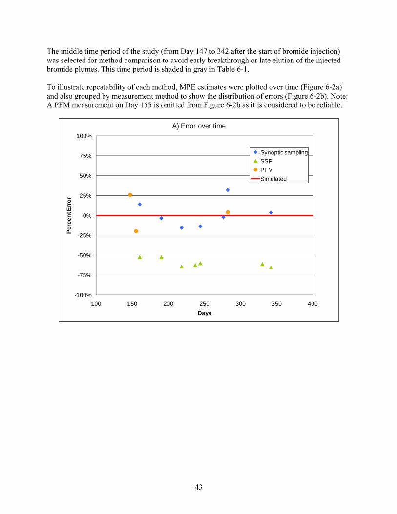
43
The middle time period of the study (from Day 147 to 342 after the start of bromide injection) was selected for method comparison to avoid early breakthrough or late elution of the injected bromide plumes. This time period is shaded in gray in Table 6-1. To illustrate repeatability of each method, MPE estimates were plotted over time (Figure 6-2a) and also grouped by measurement method to show the distribution of errors (Figure 6-2b). Note: A PFM measurement on Day 155 is omitted from Figure 6-2b as it is considered to be reliable.
-100%
-75%
-50%
-25%
0%
25%
50%
75%
100%
100 150 200 250 300 350 400
Perc
ent E
rror
Days
A) Error over time
Synoptic samplingSSPPFMSimulated
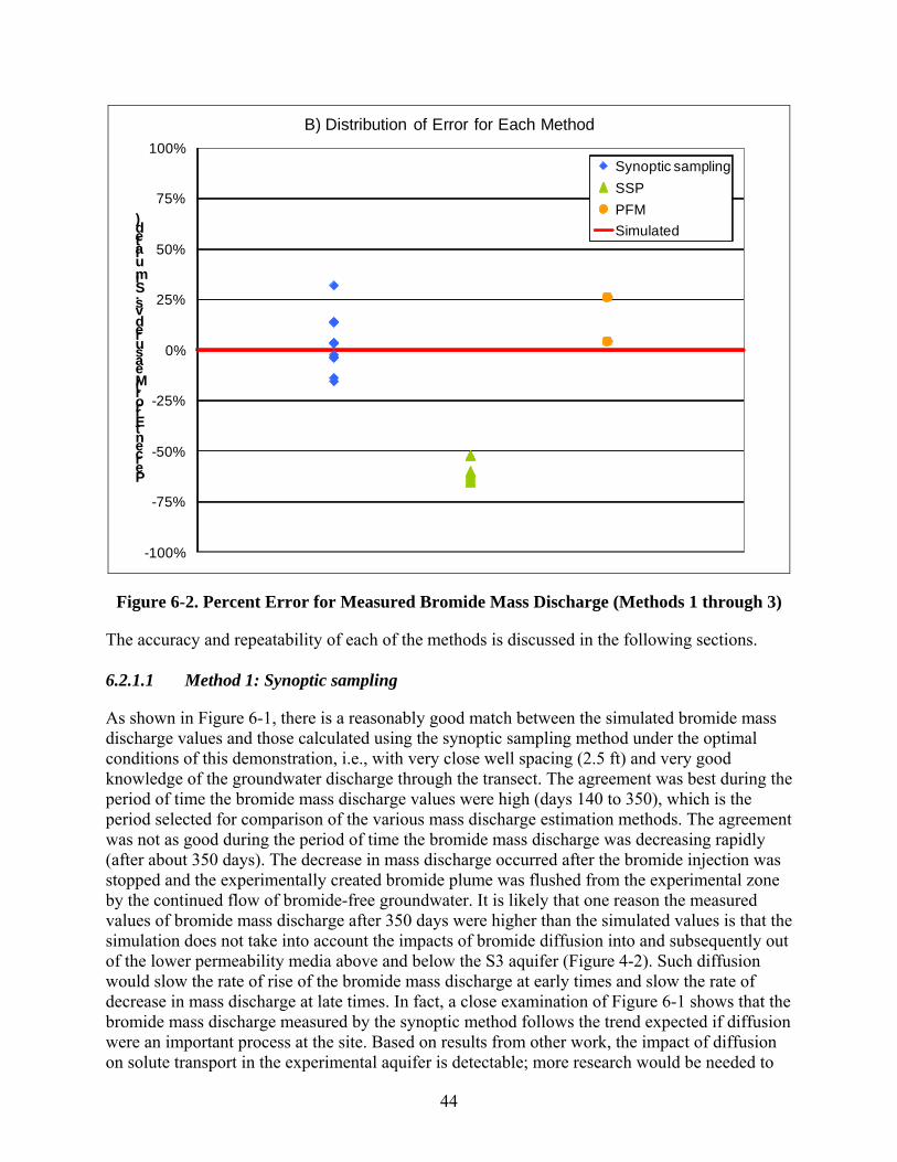
44
-100%
-75%
-50%
-25%
0%
25%
50%
75%
100%
Percent Error (Measured vs. Simulated)
B) Distribution of Error for Each Method
Synoptic samplingSSPPFMSimulated
Figure 6-2. Percent Error for Measured Bromide Mass Discharge (Methods 1 through 3)
The accuracy and repeatability of each of the methods is discussed in the following sections. 6.2.1.1 Method 1: Synoptic sampling
As shown in Figure 6-1, there is a reasonably good match between the simulated bromide mass discharge values and those calculated using the synoptic sampling method under the optimal conditions of this demonstration, i.e., with very close well spacing (2.5 ft) and very good knowledge of the groundwater discharge through the transect. The agreement was best during the period of time the bromide mass discharge values were high (days 140 to 350), which is the period selected for comparison of the various mass discharge estimation methods. The agreement was not as good during the period of time the bromide mass discharge was decreasing rapidly (after about 350 days). The decrease in mass discharge occurred after the bromide injection was stopped and the experimentally created bromide plume was flushed from the experimental zone by the continued flow of bromide-free groundwater. It is likely that one reason the measured values of bromide mass discharge after 350 days were higher than the simulated values is that the simulation does not take into account the impacts of bromide diffusion into and subsequently out of the lower permeability media above and below the S3 aquifer (Figure 4-2). Such diffusion would slow the rate of rise of the bromide mass discharge at early times and slow the rate of decrease in mass discharge at late times. In fact, a close examination of Figure 6-1 shows that the bromide mass discharge measured by the synoptic method follows the trend expected if diffusion were an important process at the site. Based on results from other work, the impact of diffusion on solute transport in the experimental aquifer is detectable; more research would be needed to
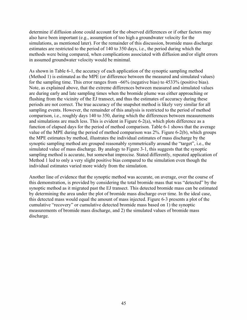
45
determine if diffusion alone could account for the observed differences or if other factors may also have been important (e.g., assumption of too high a groundwater velocity for the simulations, as mentioned later). For the remainder of this discussion, bromide mass discharge estimates are restricted to the period of 140 to 350 days, i.e., the period during which the methods were being compared, when complications associated with diffusion and/or slight errors in assumed groundwater velocity would be minimal. As shown in Table 6-1, the accuracy of each application of the synoptic sampling method (Method 1) is estimated as the MPE (or difference between the measured and simulated values) for the sampling time. This error ranges from –66% (negative bias) to 4533% (positive bias). Note, as explained above, that the extreme differences between measured and simulated values are during early and late sampling times when the bromide plume was either approaching or flushing from the vicinity of the EJ transect, and thus the estimates of accuracy during these periods are not correct. The true accuracy of the snapshot method is likely very similar for all sampling events. However, the remainder of this analysis is restricted to the period of method comparison, i.e., roughly days 140 to 350, during which the differences between measurements and simulations are much less. This is evident in Figure 6-2(a), which plots difference as a function of elapsed days for the period of method comparison. Table 6-1 shows that the average value of the MPE during the period of method comparison was 2%. Figure 6-2(b), which groups the MPE estimates by method, illustrates the individual estimates of mass discharge by the synoptic sampling method are grouped reasonably symmetrically around the “target”, i.e., the simulated value of mass discharge. By analogy to Figure 3-1, this suggests that the synoptic sampling method is accurate, but somewhat imprecise. Stated differently, repeated application of Method 1 led to only a very slight positive bias compared to the simulation even though the individual estimates varied more widely from the simulation. Another line of evidence that the synoptic method was accurate, on average, over the course of this demonstration, is provided by considering the total bromide mass that was “detected” by the synoptic method as it migrated past the EJ transect. This detected bromide mass can be estimated by determining the area under the plot of bromide mass discharge over time. In the ideal case, this detected mass would equal the amount of mass injected. Figure 6-3 presents a plot of the cumulative “recovery” or cumulative detected bromide mass based on 1) the synoptic measurements of bromide mass discharge, and 2) the simulated values of bromide mass discharge.
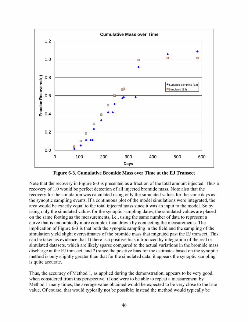
46
0.0
0.2
0.4
0.6
0.8
1.0
1.2
0 100 200 300 400 500 600
Frac
tion
Rec
over
ed (-
)
Days
Cumulative Mass over Time
Synoptic Sampling (EJ)
Simulated (EJ)
Figure 6-3. Cumulative Bromide Mass over Time at the EJ Transect
Note that the recovery in Figure 6-3 is presented as a fraction of the total amount injected. Thus a recovery of 1.0 would be perfect detection of all injected bromide mass. Note also that the recovery for the simulation was calculated using only the simulated values for the same days as the synoptic sampling events. If a continuous plot of the model simulations were integrated, the area would be exactly equal to the total injected mass since it was an input to the model. So by using only the simulated values for the synoptic sampling dates, the simulated values are placed on the same footing as the measurements, i.e., using the same number of data to represent a curve that is undoubtedly more complex than drawn by connecting the measurements. The implication of Figure 6-3 is that both the synoptic sampling in the field and the sampling of the simulation yield slight overestimates of the bromide mass that migrated past the EJ transect. This can be taken as evidence that 1) there is a positive bias introduced by integration of the real or simulated datasets, which are likely sparse compared to the actual variations in the bromide mass discharge at the EJ transect, and 2) since the positive bias for the estimates based on the synoptic method is only slightly greater than that for the simulated data, it appears the synoptic sampling is quite accurate. Thus, the accuracy of Method 1, as applied during the demonstration, appears to be very good, when considered from this perspective: if one were to be able to repeat a measurement by Method 1 many times, the average value obtained would be expected to be very close to the true value. Of course, that would typically not be possible; instead the method would typically be
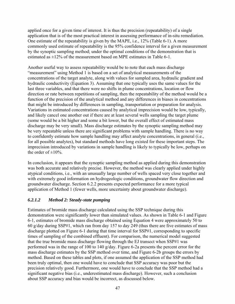
47
applied once for a given time of interest. It is thus the precision (repeatability) of a single application that is of the most practical interest in assessing performance of in-situ remediation. One estimate of the repeatability is given by the MAPE, i.e., 12% (Table 6-1). A more commonly used estimate of repeatability is the 95% confidence interval for a given measurement by the synoptic sampling method; under the optimal conditions of the demonstration that is estimated as ±12% of the measurement based on MPE estimates in Table 6-1. Another useful way to assess repeatability would be to note that each mass discharge “measurement” using Method 1 is based on a set of analytical measurements of the concentrations of the target analyte, along with values for sampled area, hydraulic gradient and hydraulic conductivity (Equation 3). Assuming that one typically uses the same values for the last three variables, and that there were no shifts in plume concentrations, location or flow direction or rate between repetitions of sampling, then the repeatability of the method would be a function of the precision of the analytical method and any differences in biases in concentrations that might be introduced by differences in sampling, transportation or preparation for analysis. Variations in estimated concentrations caused by analytical imprecision would be low, typically, and likely cancel one another out if there are at least several wells sampling the target plume (some would be a bit higher and some a bit lower, but the overall effect of estimated mass discharge may be very small). Mass discharge estimates by the synoptic sampling method may be very repeatable unless there are significant problems with sample handling. There is no way to confidently estimate how sample handling may affect analyte concentrations, in general (i.e., for all possible analytes), but standard methods have long existed for these important steps. The imprecision introduced by variations in sample handling is likely to typically be low, perhaps on the order of ±10%. In conclusion, it appears that the synoptic sampling method as applied during this demonstration was both accurate and relatively precise. However, the method was clearly applied under highly atypical conditions, i.e., with an unusually large number of wells spaced very close together and with extremely good information on hydrogeologic conditions, groundwater flow direction and groundwater discharge. Section 6.2.2 presents expected performance for a more typical application of Method 1 (fewer wells, more uncertainty about groundwater discharge). 6.2.1.2 Method 2: Steady-state pumping
Estimates of bromide mass discharge calculated using the SSP technique during this demonstration were significantly lower than simulated values. As shown in Table 6-1 and Figure 6-1, estimates of bromide mass discharge obtained using Equation 4 were approximately 50 to 60 g/day during SSP#1, which ran from day 157 to day 249 (thus there are five estimates of mass discharge plotted on Figure 6-1 during that time interval for SSP#1, corresponding to specific times of sampling of the combined effluent). For comparison, the numerical model suggested that the true bromide mass discharge flowing through the EJ transect when SSP#1 was performed was in the range of 100 to 140 g/day. Figure 6-2a presents the percent error for the mass discharge estimates by the SSP method over time, and Figure 6-2b groups the errors by method. Based on these tables and plots, if one assumed the application of the SSP method had been truly optimal, then one would have to conclude that SSP accuracy was poor but the precision relatively good. Furthermore, one would have to conclude that the SSP method had a significant negative bias (i.e., underestimated mass discharge). However, such a conclusion about SSP accuracy and bias would be incorrect, as discussed below.
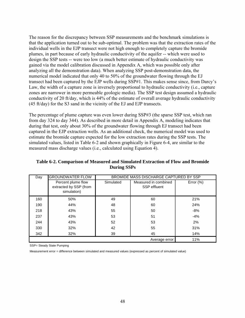
48
The reason for the discrepancy between SSP measurements and the benchmark simulations is that the application turned out to be sub-optimal. The problem was that the extraction rates of the individual wells in the EJP transect were not high enough to completely capture the bromide plumes, in part because of early hydraulic conductivity of the aquifer -- which were used to design the SSP tests -- were too low (a much better estimate of hydraulic conductivity was gained via the model calibration discussed in Appendix A, which was possible only after analyzing all the demonstration data). When analyzing SSP post-demonstration data, the numerical model indicated that only 40 to 50% of the groundwater flowing through the EJ transect had been captured by the EJP wells during SSP#1. This makes sense since, from Darcy’s Law, the width of a capture zone is inversely proportional to hydraulic conductivity (i.e., capture zones are narrower in more permeable geologic media). The SSP test design assumed a hydraulic conductivity of 20 ft/day, which is 44% of the estimate of overall average hydraulic conductivity (45 ft/day) for the S3 sand in the vicinity of the EJ and EJP transects. The percentage of plume capture was even lower during SSP#3 (the sparse SSP test, which ran from day 324 to day 344). As described in more detail in Appendix A, modeling indicates that during that test, only about 30% of the groundwater flowing through EJ transect had been captured in the EJP extraction wells. As an additional check, the numerical model was used to estimate the bromide capture expected for the low extraction rates during the SSP tests. The simulated values, listed in Table 6-2 and shown graphically in Figure 6-4, are similar to the measured mass discharge values (i.e., calculated using Equation 4).
Table 6-2. Comparison of Measured and Simulated Extraction of Flow and Bromide During SSPs
Day GROUNDWATER FLOWPercent plume flow
extracted by SSP (from simulation)
Simulated Measured in combined SSP effluent
Error (%)
160 50% 49 60 21%190 44% 48 60 24%218 43% 55 50 -8%237 43% 53 51 -4%244 43% 52 53 2%330 32% 42 55 31%342 32% 39 45 14%
Average error: 11%SSP= Steady State Pumping
Measurement error = difference between simulated and measured values (expressed as percent of simulated value)
BROMIDE MASS DISCHARGE CAPTURED BY SSP
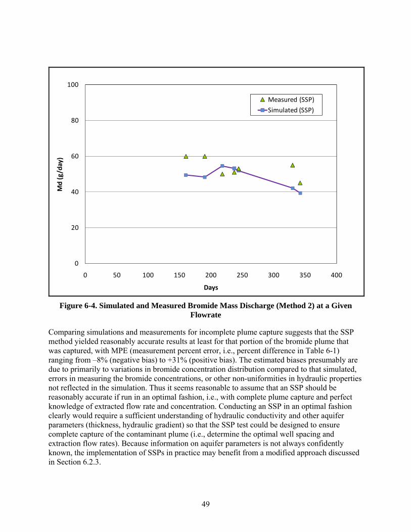
49
0
20
40
60
80
100
0 50 100 150 200 250 300 350 400
Md (g/day)
Days
Measured (SSP)
Simulated (SSP)
Figure 6-4. Simulated and Measured Bromide Mass Discharge (Method 2) at a Given
Flowrate
Comparing simulations and measurements for incomplete plume capture suggests that the SSP method yielded reasonably accurate results at least for that portion of the bromide plume that was captured, with MPE (measurement percent error, i.e., percent difference in Table 6-1) ranging from –8% (negative bias) to +31% (positive bias). The estimated biases presumably are due to primarily to variations in bromide concentration distribution compared to that simulated, errors in measuring the bromide concentrations, or other non-uniformities in hydraulic properties not reflected in the simulation. Thus it seems reasonable to assume that an SSP should be reasonably accurate if run in an optimal fashion, i.e., with complete plume capture and perfect knowledge of extracted flow rate and concentration. Conducting an SSP in an optimal fashion clearly would require a sufficient understanding of hydraulic conductivity and other aquifer parameters (thickness, hydraulic gradient) so that the SSP test could be designed to ensure complete capture of the contaminant plume (i.e., determine the optimal well spacing and extraction flow rates). Because information on aquifer parameters is not always confidently known, the implementation of SSPs in practice may benefit from a modified approach discussed in Section 6.2.3.
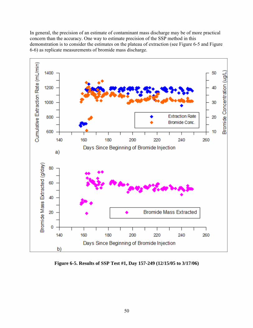
50
In general, the precision of an estimate of contaminant mass discharge may be of more practical concern than the accuracy. One way to estimate precision of the SSP method in this demonstration is to consider the estimates on the plateau of extraction (see Figure 6-5 and Figure 6-6) as replicate measurements of bromide mass discharge.
Figure 6-5. Results of SSP Test #1, Day 157-249 (12/15/05 to 3/17/06)
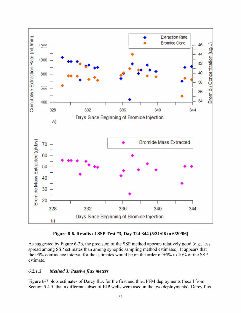
51
Figure 6-6. Results of SSP Test #3, Day 324-344 (5/31/06 to 6/20/06)
As suggested by Figure 6-2b, the precision of the SSP method appears relatively good (e.g., less spread among SSP estimates than among synoptic sampling method estimates). It appears that the 95% confidence interval for the estimates would be on the order of ±5% to 10% of the SSP estimate. 6.2.1.3 Method 3: Passive flux meters
Figure 6-7 plots estimates of Darcy flux for the first and third PFM deployments (recall from Section 5.4.5. that a different subset of EJP wells were used in the two deployments). Darcy flux
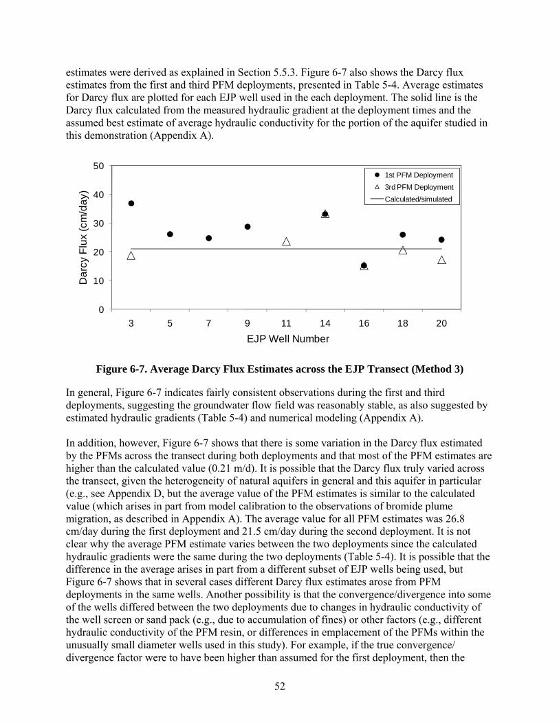
52
estimates were derived as explained in Section 5.5.3. Figure 6-7 also shows the Darcy flux estimates from the first and third PFM deployments, presented in Table 5-4. Average estimates for Darcy flux are plotted for each EJP well used in the each deployment. The solid line is the Darcy flux calculated from the measured hydraulic gradient at the deployment times and the assumed best estimate of average hydraulic conductivity for the portion of the aquifer studied in this demonstration (Appendix A).
0
10
20
30
40
50
3 5 7 9 11 14 16 18 20
Dar
cy F
lux
(cm
/day
)
EJP Well Number
1st PFM Deployment3rd PFM DeploymentCalculated/simulated
Figure 6-7. Average Darcy Flux Estimates across the EJP Transect (Method 3)
In general, Figure 6-7 indicates fairly consistent observations during the first and third deployments, suggesting the groundwater flow field was reasonably stable, as also suggested by estimated hydraulic gradients (Table 5-4) and numerical modeling (Appendix A). In addition, however, Figure 6-7 shows that there is some variation in the Darcy flux estimated by the PFMs across the transect during both deployments and that most of the PFM estimates are higher than the calculated value (0.21 m/d). It is possible that the Darcy flux truly varied across the transect, given the heterogeneity of natural aquifers in general and this aquifer in particular (e.g., see Appendix D, but the average value of the PFM estimates is similar to the calculated value (which arises in part from model calibration to the observations of bromide plume migration, as described in Appendix A). The average value for all PFM estimates was 26.8 cm/day during the first deployment and 21.5 cm/day during the second deployment. It is not clear why the average PFM estimate varies between the two deployments since the calculated hydraulic gradients were the same during the two deployments (Table 5-4). It is possible that the difference in the average arises in part from a different subset of EJP wells being used, but Figure 6-7 shows that in several cases different Darcy flux estimates arose from PFM deployments in the same wells. Another possibility is that the convergence/divergence into some of the wells differed between the two deployments due to changes in hydraulic conductivity of the well screen or sand pack (e.g., due to accumulation of fines) or other factors (e.g., different hydraulic conductivity of the PFM resin, or differences in emplacement of the PFMs within the unusually small diameter wells used in this study). For example, if the true convergence/ divergence factor were to have been higher than assumed for the first deployment, then the
53
estimated Darcy flux would have been lower (i.e., the flow estimated from tracer loss would have been attributed to a wider portion of the aquifer, thus implying a lower Darcy flux and groundwater velocity). Two out of the three applications of the PFM method yielded estimates of bromide mass discharge that were higher than the simulated values, as listed in Table 6-1 (e.g., +26%, deployment 1, and +4% deployment 3). Deployment 2, which yielded a result with considerable negative bias (-20%), was conducted immediately following the first deployment, which initially was thought might serve as a duplicate measurement. However, clearly the PFM re-deployment did not serve as a duplicate measurement. Based on the initially surprising results, it was hypothesized that immediate re-deployment caused the negative bias, perhaps due to lack of time for the water in the well to recover geochemically, thus leading to some of the groundwater sampled by the second deployment not being representative of the plume at that time. Although such immediate re-deployment of PFMs is not likely in practice, the results suggest that there would be issues worthy of more study if rapid re-deployment were to be considered in practice, or if a method for generating duplicate PFM results was desired. Ignoring the results from the second deployment, the results of the other two deployments suggest that, under the optimal conditions of application in the demonstration, the PFMs had an average error of approximately +15% (positive bias) compared to the model predictions. This, of course, assumes that the model predictions were perfectly accurate for the times of PFM deployment. The PFM and synoptic sampling measurements both were quite high compared to the simulated values during days 147 to 160 and also higher than the simulated value on day 282 (Figures 6-1 and 6-2, and Table 6-1). Since the synoptic estimates were on average very accurate, the discrepancies between simulated and measured values were suspected to be in part due to inaccuracy in the simulation. As discussed previously, if the simulation had used a somewhat slower velocity than assumed in Figure 6-1, then the spike in simulated concentration would have started from a higher base and thus would have been closer to the values measured by synoptic and PFM methods. Nevertheless, because further refinement of the simulation is beyond the scope of this project, it is assumed that the simulation presented in Figure 6-1 is accurate, which leads to the conclusion that the PFMs yield bromide mass discharge estimates which have a positive bias. Furthermore, if the Darcy flux estimates are interpreted as suggesting that too low of a convergence/ divergence factor was assumed for the first PFM deployment, then adjusting the convergence/ divergence factor (i.e., increasing it) to make the average estimated Darcy flux decrease to the calculated value (0.21 m/day) would cause the estimated bromide mass discharge for the first PFM deployment to decrease also (implying a lower positive bias if the convergence/divergence factor were somehow more accurately estimated for each deployment). In any case, this line of reasoning illustrates the sensitivity of the method’s mass discharge results to the assumption of the convergence/divergence factor. However, as mentioned above, it is often the precision (repeatability) of a single application of a mass discharge measurement method that is of the most interest. The average absolute error was 15% for the two reliable PFM measurements (Table 6-1). Considering the differences between measured and simulated values listed in Table 6-1 for the first and third deployments, the 95% confidence interval for a given measurement by the PFM method under the optimal conditions of

54
the demonstration would be estimated as ±22% of the measurement. A more useful estimate of method precision would require that the PFM method be applied successfully more than two times, but that was not possible during the demonstration. In conclusion, it appears that the PFM method as applied during this demonstration had a positive bias and yet was relatively precise. The method was clearly applied under highly atypical conditions, however. The factors that made PFM deployment atypically difficult during this demonstration was the unusually small diameter of the wells and the unusual method of well installation and completion. The factors that benefitted the accuracy of the PFM method were the use of a large number of wells spaced unusually close together and the availability of extremely good information about the properties of the aquifer and the packing material (which allowed a site specific estimate of the convergence/divergence factor needed to interpret the raw data from this method). The bromide mass discharge estimates in Figure 6-1, Figure 6-2 and Table 6-1 are based on an unusually low value for the divergence factor around the well screen and gravel pack (0.15). This divergence factor was calculated by members of the research team from measured characteristics of the aquifer and gravel pack and was considerably lower than would normally be assumed in the absence of such detailed, site-specific measurements (more typical values generally fall in the range 0.8 to 1.5). In Section 6.2.2, the probable performance of a more typical application of Method 3 is examined (fewer wells in which PFMs are deployed, more uncertainty about divergence factor). 6.2.1.4 Method 4: RFM technique
The RFM technique could not be applied under the conditions at Site 60, VAFB, during the period of this project. (For the results of subsequent application of the technique, see Appendix B). Although model simulations based on measured or estimated aquifer properties indicated that recirculation between adjacent injection/extraction wells could be achieved at relatively modest pumping rates (1 L/min), these pumping rates proved to be not sustainable during the field trials for reasons that were not clear, but probably included operator error (e.g., failing to keep injection well and other parts of the system from clogging; incorrect location of the extraction pump intake within the extraction well). Nevertheless, as discussed in Section 6.2.2, the failure of the RFM method during this field evaluation in the project period, i.e., 2005 to 2006, yielded insights that may help to guide future development and testing of the RFM technique. 6.2.2 Accuracy and Repeatability under More Typical Field Conditions
In this research, a very high sampling density (i.e., number of wells in a given cross sectional area of the aquifer, or number of samples taken during a given time interval) is used for each of the mass discharge methods compared to what typically would be done in practice. This was done intentionally to evaluate each of the methods under what presumably would have been nearly optimal conditions for their application to the experimentally produced bromide plume. With that approach, as presented in the prior sections, it was possible to make a reasonably clear comparison of advantages and disadvantages of the methods under the best of circumstances for each, given the hydrogeologic conditions at the test site and the width of the bromide plume. In this section is an examination of the impact on the estimates of bromide mass discharge by the methods if their sampling density had been less dense, i.e., if they had been applied in a more

55
typically feasible way (fewer wells for Methods 1 and 3 or shorter duration and fewer samples over time for Method 2). Each method is discussed separately below. 6.2.2.1 Method 1: Synoptic sampling
There were 29 wells in the EJ transect used to monitor the experimentally created bromide plume. The wells were spaced approximately 2.5 ft on average from each other along the transect (note that the actual interwell spacing ranged from 1.9 to 3.2 ft, but there were only two values at or near those low/high extremes, so the mean and standard deviation of the interwell spacing were 2.50 ft and 0.27 ft, respectively). As discussed previously, this very tight spacing allowed for reasonably accurate estimates of bromide mass discharge. An important question is what the accuracy and potential error would have been had a transect with fewer wells, i.e., wells spaced further apart (greater interwell spacing), been used. This was evaluated conceptually by examining subsets of the EJ well data collected during the demonstration, first assuming only every other well had existed, then assuming only every third well, then only every fourth well, then only every fifth well, then only every sixth well, and lastly only every seventh well. As shown in Table 6-3, this allowed for examination of the data as though the interwell spacing had ranged from approximately 2.5 ft (i.e., when all the wells in the transect were analyzed) to 17.6 ft (when only every seventh well was considered). As can be seen in Table 6-3, for subsets at a given interwell spacing of five ft and higher there were different sub-subsects (e.g., for 5-ft spacing, a subset with 15 and a subset with 14 wells; for 7.5-ft spacing, one sub-subset with nine wells and two sub-subsets with 10 wells; etc.). This was because the total number of wells was 29, a prime number not evenly divisible.
Table 6-3. Subsets of Data Considered In Sensitivity Analysis of Method 1 (Synoptic Sampling)
Average interwell spacing (ft) Number of different subsets with given spacing
Number of wells in each subset
2.5 1 29 5.0 2 15, 14 7.5 3 10, 10, 9 10.1 4 8, 7, 7, 7 12.6 5 6, 6, 6, 6, 5 15.1 6 5, 5, 5, 5, 5, 4 17.6 7 5, 4, 4, 4, 4, 4, 4 Using the approach described in Section 5.4.9, the bromide mass discharge was calculated for all 12 of the snapshot events and for all of the various subsets of data listed in Table 6-3. That is a total of 336 estimates of bromide mass discharge over the course of the demonstration, or 28 different estimates for each of the 12 snapshots. That approach allowed for a compilation of estimates that ranged from times when bromide mass discharge was low to times when it was high, and to examine the range of cases for each subset and snapshot that resulted from sampling of a variable bromide distribution with a fixed interwell spacing (i.e., sometimes the assumed subsets of wells sample the high bromide concentration zones and sometimes they don’t, depending on which subset of wells is used in a calculation).
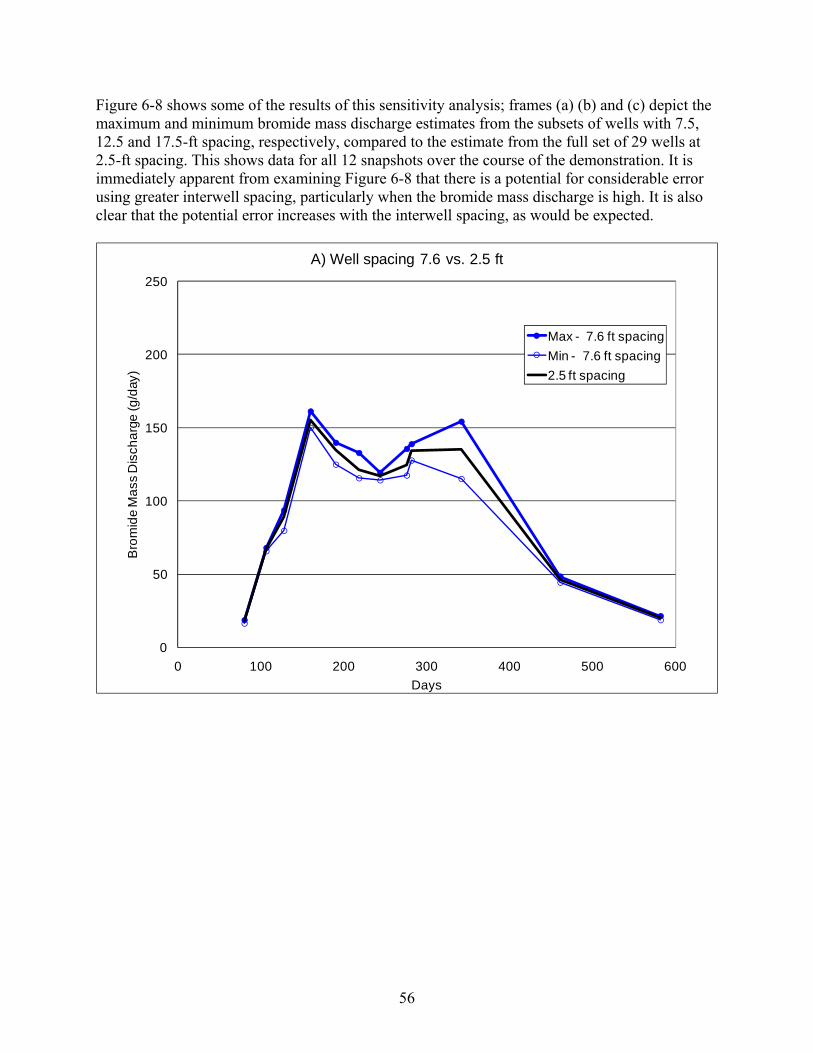
56
Figure 6-8 shows some of the results of this sensitivity analysis; frames (a) (b) and (c) depict the maximum and minimum bromide mass discharge estimates from the subsets of wells with 7.5, 12.5 and 17.5-ft spacing, respectively, compared to the estimate from the full set of 29 wells at 2.5-ft spacing. This shows data for all 12 snapshots over the course of the demonstration. It is immediately apparent from examining Figure 6-8 that there is a potential for considerable error using greater interwell spacing, particularly when the bromide mass discharge is high. It is also clear that the potential error increases with the interwell spacing, as would be expected.
0
50
100
150
200
250
0 100 200 300 400 500 600
Bro
mid
e M
ass
Dis
char
ge (g
/day
)
Days
A) Well spacing 7.6 vs. 2.5 ft
Max - 7.6 ft spacingMin - 7.6 ft spacing2.5 ft spacing

57
0
50
100
150
200
250
0 100 200 300 400 500 600
Bro
mid
e M
ass
Dis
char
ge (g
/day
)
Days
B) Well spacing 12.6 vs 2.5 ft
Max - 12.6 ft spacingMin - 12.6 ft spacing2.5 ft spacing
0
50
100
150
200
250
0 100 200 300 400 500 600
Bro
mid
e M
ass
Dis
char
ge (g
/day
)
Days
C) Well spacing 17.6 vs 2.5 ft
Max - 17.6 ft spacingMin - 17.6 ft spacing2.5 ft spacing
Figure 6-8. Bromide Mass Discharge at Transect EJ Calculated as a Function of Well
Spacing
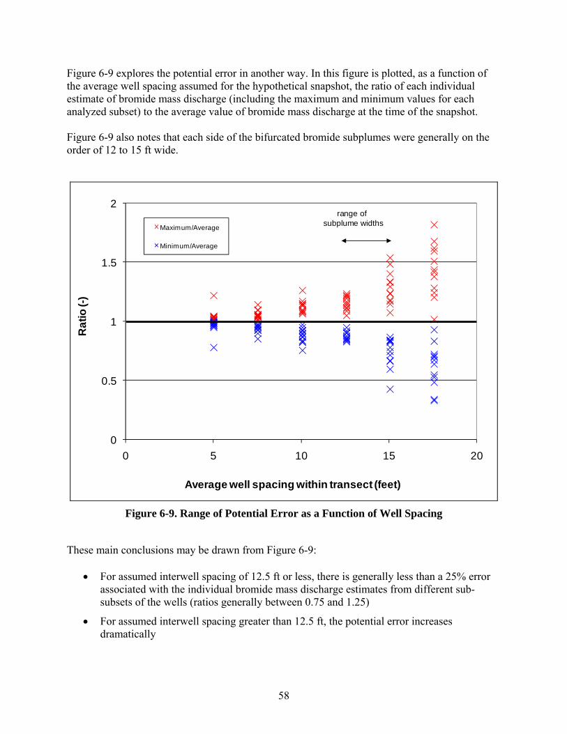
58
Figure 6-9 explores the potential error in another way. In this figure is plotted, as a function of the average well spacing assumed for the hypothetical snapshot, the ratio of each individual estimate of bromide mass discharge (including the maximum and minimum values for each analyzed subset) to the average value of bromide mass discharge at the time of the snapshot. Figure 6-9 also notes that each side of the bifurcated bromide subplumes were generally on the order of 12 to 15 ft wide.
0
0.5
1
1.5
2
0 5 10 15 20
Rat
io (-
)
Average well spacing within transect (feet)
Maximum/Average
Minimum/Average
range of subplume widths
Figure 6-9. Range of Potential Error as a Function of Well Spacing
These main conclusions may be drawn from Figure 6-9:
• For assumed interwell spacing of 12.5 ft or less, there is generally less than a 25% error associated with the individual bromide mass discharge estimates from different sub-subsets of the wells (ratios generally between 0.75 and 1.25)
• For assumed interwell spacing greater than 12.5 ft, the potential error increases dramatically

59
• For assumed interwell spacing greater than 12.5 ft, there are some subsets of the wells that still provide fairly accurate estimates of bromide mass discharge (i.e., ratios close to 1).
The main implication of Figures 6-8 and 6-9 is that one may expect less potential error in mass discharge estimation of a heterogeneous plume if the interwell spacing in the monitored transect is in the range of or ideally less than the width of the high concentration subplumes within the target plume. In practice the actual plume heterogeneity occurring at a scale finer than the available monitoring well spacing would not typically be known, so it may be difficult, in general, to confidently quantify the potential error in the mass discharge estimate for a given well spacing. However, this analysis suggests that the potential error should be less than ±25% if the well spacing is less than the width of the significant (i.e., high mass discharge) sub-plumes and the estimates of hydraulic conductivity (K), aquifer area sampled by each well (A=thickness*interwell spacing) and hydraulic gradient (i) (the other variables in Equation 3) are well defined. Clearly the latter assumption about knowledge of K, A and i is not typically the case. Hydraulic gradient and sampled aquifer area may typically be estimated with relatively low error, perhaps on the order of ±25% or less. Thus, since it is commonly realized that estimates of hydraulic conductivity are often in error by a factor of 10 or more, it appears that the largest source of uncertainty in contaminant mass discharge estimates by the snapshot method is likely to be the uncertainty in hydraulic conductivity. However it should be pointed out that accuracy may often be less important that precision in practice. For example, if the goal of measuring mass discharge is to determine if a remedial action has reduced the contaminant mass discharge by a desired amount, then it may be the percent difference between two measurements (before and after remediation) that is of primary practical importance. In that case, it does not matter if the methods are somewhat inaccurate as long as they are relatively precise or repeatable. If, for example, the method precision is ±25%, the method could be used with confidence to identify changes between two mass discharge estimates which are more than 50%. 6.2.2.2 Method 2: Steady-state pumping
As discussed above, the SSP tests performed during this field research project benefitted from a superior level of understanding of the plume position and aquifer properties not typically found at non-research sites. Still, inaccurate initial estimates of the hydraulic conductivity of the S3 sand during the planning stage of the experiment resulted in incomplete capture of the bromide plume because the pumping rates of individual wells in the transect were too low. This highlights one of the potential problems with the SSP method. A more general discussion of technical issues facing practitioners of this method follows. Incomplete capture of the plume, which leads to an underestimate of the contaminant mass flux, may occur for a number of reasons. First, the location (lateral and vertical) of the plume(s) may not be sufficiently defined. Thus, extraction wells may not be located to capture all of the contaminant mass flowing in the aquifer; however, this issue of sampling or capturing the significant portions of a plume also pertains to any mass discharge measurement method. Second, the location of the plume(s) may be accurately defined, but the actual capture zones of the extraction wells may be lower than calculated. This problem, which was a cause of
60
significant error during the experiment as discussed above, can occur if the Darcy flux in the aquifer is higher than estimated. Higher Darcy flux in the aquifer, resulting from more permeable sediments and/or greater hydraulic gradients than expected, results in smaller capture zones than predicted. With smaller capture zones, some of the contaminant mass discharge may therefore escape capture and quantification. Finally, incomplete capture of the plume(s) may occur if the extraction wells are not pumped long enough to fully capture the dissolved contaminants within the capture zones of the wells. Envision a dissolved plume located at the edge of a well’s capture zone. Pumping must continue long enough for the dissolved plume to be drawn into the well. For monitoring transects designed to have the fewest number of extraction wells possible (i.e., with the widest capture zones possible given the hydraulic properties of the aquifer, available drawdown, etc.), hydraulic capture of particles at the margins of the capture zone may take a considerable period of time (days, weeks or months). Mass discharge values calculated prior to capture of the contaminants flowing at the edge of the capture zone would therefore be erroneously low. “Over-capture” of the plume(s) can lead to overestimates of contaminant mass discharge if calculations are made prior to the well(s) reaching steady-state conditions. Envision a scenario in which the steady-state capture zone of a well extends a significant distance laterally beyond the edges of the dissolved plume(s). Initial pumping of the well will draw contaminants into the well from all sides at relatively high rates. Mass discharge values calculated using Equation 4 at this time would be relatively high. Over time, clean water bounding the dissolved plume(s) would be drawn into the well, reducing the average concentrations of the target analyte in the effluent. Accurate values of contaminant mass discharge could only be made once the clean water flowing along the lateral edges of the well’s capture zone had reached the well. As in the example above, this could take weeks or months for wells having large capture zones. Calculations made prior to this would be positively biased. After completion of the SSP tests in this demonstration, the research team asked itself how the tests could be improved to give more accurate results. Clearly, having accurate estimates of the hydraulic properties and gradients is important when designing the tests. If that knowledge is uncertain, then it is not possible to know before an SSP what the optimal SSP extraction rate would be to capture just the contaminant plume. As discussed above, pumping at rates higher than the optimal rate is undesirable because groundwater is then drawn into the pumping wells from downgradient and cross-gradient directions, which increases the time for the contaminant flowlines to reach steady-state conditions. Consequently, the best practical approach may be to perform SSP tests in a stepped fashion, starting with a combined extraction rate that is suspected to be somewhat less than the natural flow of groundwater through the transect (e.g., ~70% of the estimated natural flow of groundwater). This approach was discussed and recommended previously (Yoon, 2006; Goltz et al., 2007b). The wells would be pumped at that combined extraction rate and composite samples of the pumped water would be collected over time and analyzed for the target contaminant. Once the calculated mass discharge value reaches a steady value (which may not take long based on the tests performed in this study; see Figure 6-5 and Figure 6-6), the extraction rates of the wells would then be increased. Again, composite samples of the pumped water would be collected and analyzed, and the calculated mass discharge values plotted over time. Additional increases in pumping rates could be added until the calculated mass discharge using Equation 4 no longer increased as greater volumes of water are extracted. At that
61
point, the wells should be capturing the entire dissolved plume(s) of the target contaminants. In the future and under other funding, this more empirical method of performing SSP tests will be explored via computer simulations. 6.2.2.3 Method 3: Passive flux meters
Deployments of PFMs require adequate knowledge of the well construction characteristics including hydraulic conductivities of materials used and radial diameters. This is usually not difficult to obtain for wells constructed specifically for the PFM deployments but can be challenging for pre-existing wells. Thus higher uncertainty in convergence/divergence calculates are associated with such deployments. When integration of a transect of wells to calculate mass discharge is the objective of the PFM deployment, efforts to determine hydraulic characteristics of the well should be conducted including independent measurements of media properties. Deployments which focus on determination of relative spatial distribution of mass flux and comparison of pre and post-remedial may not require as high a degree of accuracy as studies which link mass discharge to site mass balance calculations. In PFM applications using pre-existing wells, the divergence assumption is probably the largest source of error. However divergence is not that sensitive to the aquifer hydraulic conductivity. Of more importance are the hydraulic conductivities of the sand pack, screen and PFM itself, all of which can be measured or estimated reasonably accurately for the materials prior to their emplacement in the subsurface. Based on measurements from this demonstration, the divergence/convergence factor was estimated to be in the range of 0.1 to 0.2; the average was used in the calculations. That implies that there might typically be at least a factor of two uncertainty in a careful estimate of the divergence/convergence factor, and thus a similar uncertainty in the contaminant mass discharge estimates arising solely from that assumption. Higher uncertainties would of course be expected if the well screen or sand pack properties of a pre-existing well were not accurately known, or if hydraulic properties changed due to siltation or precipitation within the sand pack or screen openings. In most practical applications, it is likely the precision or repeatability of the PFM measurements that is of most concern. The results suggest that the PFM measurements may be reasonably precise, but the general discussion above implies that precision could be affected by processes that alter the hydraulic conductivity of the sand pack, screen openings or PFM sorbent itself. Assuming that alteration of the PFM sorbent is not significant during a short deployment, the main concerns would be the alteration of the sand pack and screen openings. For this reason, it would seem prudent to re-develop a well prior to each PFM deployment, i.e., to ensure reasonably consistent hydraulic properties of the sand pack and screen for each deployment. 6.2.2.4 Method 4: RFM technique
Based on the experience of the researchers and lack of success with the RFM trial during the demonstration, insights for improvements to practical implementation of this method were gained. First and foremost, for the RFM technique to work, hydraulic conductivity must be adequate to allow for recirculation of flow between the two wells of an injection/extraction well pair. Based on hydraulic conductivity measurements at the site, modeling results indicated that recirculation at Site 60 could be achieved and that the technique could be successfully applied. The fact that the RFM application failed points to a number of possible causes: (1) conductivity

62
measurements were not accurate, (2) modeling was inappropriate, or (3) experimental techniques were improper. As standard flow modeling methods were used (e.g., MODFLOW) it is unlikely that the problems that were encountered were due to model application. More likely is that either local hydraulic conductivities near the wells were lower than the measured values that were assumed in the model, or that the experimental technique (e.g., well screen construction) was inadequate. In fact, it was later determined that the failure to sustain the flows during the field trial was likely due to errors on the part of the field team; in 2007, long after the period of this project, 1 L/min was sustained in recirculation between EJP well pairs by a new field researcher for different experimental reasons, who determined that frequent re-development of the injection well was needed to sustain the flow. Results of this additional work are reported in Appendix D. In any event, problems like these may be identified and overcome in future evaluations of the technique by conducting a relatively simple preliminary test. It is suggested that modeling first be used to determine well spacing and pumping rate for an injection/extraction well pair, based upon an estimated value of hydraulic conductivity (estimated using standard slug or pump test methods). The RFM wells (which may also serve as monitoring wells at the site) could be installed and a pump test conducted to ensure the modeled flow rates are obtainable, and that actual heads at the wells are similar to those simulated by the model. Such preliminary testing would give confidence that experimental techniques are adequate to achieve the necessary pumping rates and that the model is adequately simulating subsurface flow. With this confidence, the model can then be used to predict tracer breakthrough at the extraction well and design the evaluation. 6.2.3 Other Considerations
The dense grid of monitoring points along the EJ transect allowed examination of integration errors for the synoptic sampling method by performing a sensitivity analysis of the percent error as a function of data density. For assumed interwell spacing of 12.5 ft or less, there is generally less than a 25% error associated with the individual bromide mass discharge estimates from different sub-subsets of the wells (ratios generally between 0.75 and 1.25). For assumed interwell spacing greater than 12.5 ft, the potential error increases dramatically since the interwell spacing is on the order of or greater than the width of the high concentrations “subplumes” in this study. Figure 6-10 illustrates several cases that may arise when interwell spacing is greater than the width of the subplumes, taking a hypothetical example of four laterally separate subplumes. The figure shows that the wide spacing can affect what is measured by the synoptic or steady state pumping (SSP) method depending on the location of the wells relative to the subplumes.
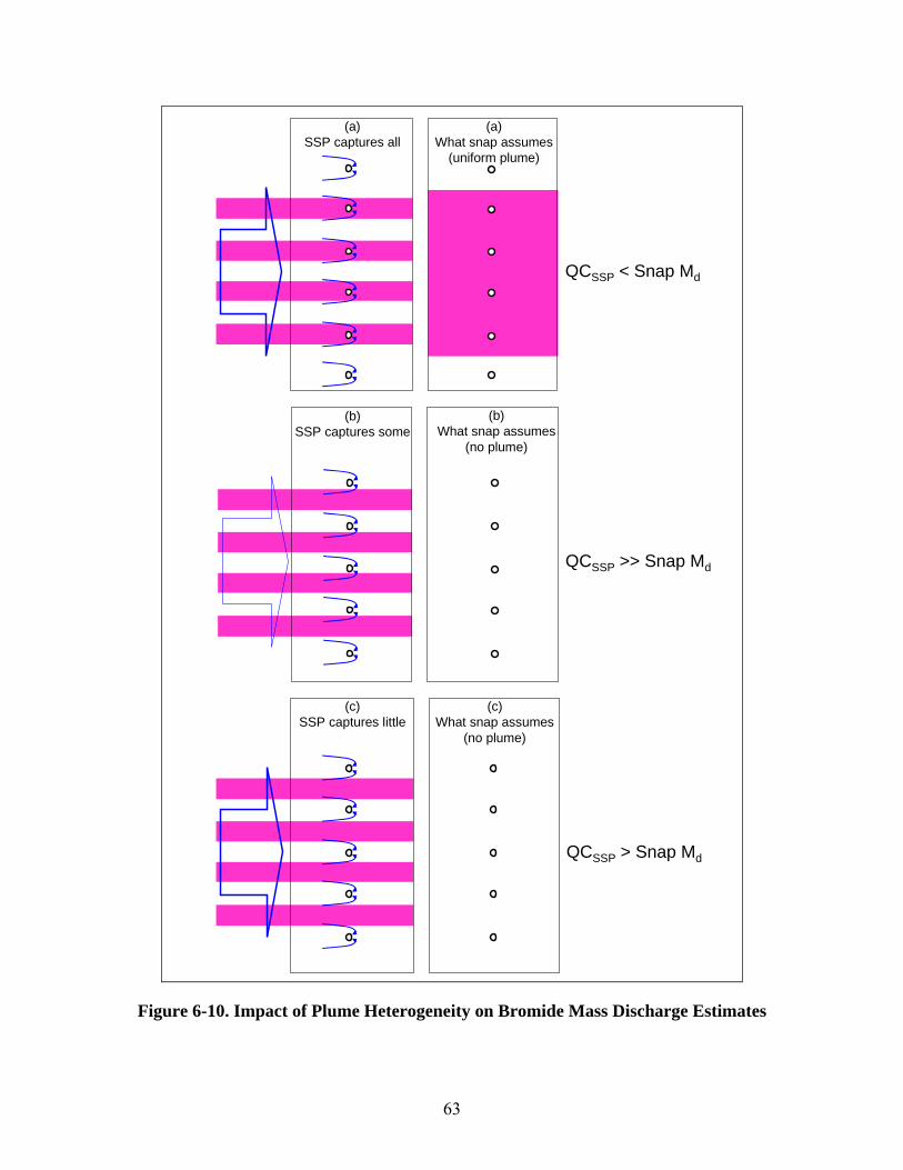
63
(a)SSP captures all
(a)What snap assumes
(uniform plume)
QCSSP < Snap Md
(b)SSP captures some
(b)What snap assumes
(no plume)
QCSSP >> Snap Md
(c)SSP captures little
(c)What snap assumes
(no plume)
QCSSP > Snap Md
Figure 6-10. Impact of Plume Heterogeneity on Bromide Mass Discharge Estimates
64
Illustrations of impacts of plume heterogeneity on mass discharge estimation by methods based on extended pumping (e.g. SSP) or brief/no pumping of wells (synoptic or “snap” sampling, or PFM deployment). In case (a), wells are within the individual subplumes and SSP captures some or all of each subplume. The synoptic result (“Snap Md”) would be much greater than the true mass discharge since the area between the subplumes would incorrectly be assumed to contain contaminant as shown. In case (b), wells are outside of each suplume, but SSP captures some of each subplume. In case (c), wells are outside each suplume, and SSP captures only a little of each subplume. For both cases (b) and (c), the reverse problem would occur in that the synoptic result would be zero since the snapshot sampling of the wells would not detect any contaminant. For application of the SSP method to the cases in Figure 6-10, the situation obviously depends on the rate at which the wells are pumped, and therefore the width of each well’s capture zone. Only the case in which the pumping rate is too low to capture all groundwater flowing within the full width spanned by all subplumes is hereby examined. Case (a) is the fortunate, perhaps rarely achieved, situation in which all contaminant mass discharge within each subplume is captured even though not all of the groundwater is captured within the full plume width. In this case, interestingly, the mass discharge estimated by the SSP method (“QCSSP”) is accurate but much lower than would be estimated by the synoptic method using the same wells pumped only briefly. In case (b), the SSP captures only a fraction of the total mass discharge and thus has a significant negative bias (the synoptic method, however, misses all subplumes). In case (c) the SSP captures even less of the subplumes. Note that increasing the assumed pumping rate (and thus the capture width for each well) would have no effect on the estimated mass discharge by the SSP method in case (a) whereas the estimated mass discharge would increase for the other two cases. This illustrates the complexity of applying either extended pumping methods (e.g., SSP) or brief/no pumping methods (e.g., synoptic sampling or PFM deployment) to heterogeneous plumes that have not be characterized in sufficient detail prior to attempting mass discharge estimation. Fortunately, in practice, integration errors such as illustrated in Figure 6-10 can be minimized by pre-characterizing the geology and solute distribution along the measurement transect(s) prior to installing the monitoring devices (e.g., point sampling wells, PFMs, wells for pumping methods, etc.). Pre-characterization of the location of high mass flux zones allows contractors to install denser networks of monitoring devices in and near the high flux zones compared to zones of lower mass flux. This can dramatically reduce the cost and greatly improve the accuracy of all field measurements of contaminant mass discharge, provided the flow direction does not vary greatly with time. Pre-characterizing the geology and solute distribution can be accomplished at many sites using inexpensive direct push sampling tools such as the Waterloo Groundwater Profiler, cone penetrometer testing, electrical conductivity profiling tools, and Membrane Interface Probe (see U.S. EPA, 2005).
6.3 SUMMARY AND IMPLICATIONS
The primary goal of this study was to evaluate the accuracy and precision of four methods for measuring contaminant mass discharge applied to an artificially created bromide plume: Method 1 (synoptic or “snapshot” sampling of transects of wells), Method 2 (steady state pumping of transects of wells), Method 3 (deployment of passive flux meters in transects of wells), and Method 4 (the recirculation flux method in pairs of wells in a transect). Method 4 was not
65
successfully implemented for bromide mass discharge estimation during the period of this project, as discussed earlier. The accuracy of estimated mass discharge values is a function of measurement errors (e.g., measurements of K, i, Q, C, etc.) and integration errors. Integration errors, also referred to as interpolation or aggregation errors, are difficult to define a priori and are a function of the geologic and plume heterogeneity (Li et al., 2007). The existence of known bromide mass discharge values at different locations and times in this study (via numerical modeling calibrated by many measured data) facilitated a more rigorous assessment of the mean absolute error than would have been possible at a site with an uncontrolled/unknown rate of mass loading. Table 6-4 compiles the overall results, though the reader is strongly advised to read the earlier portions of Section 6 to understand the strengths and limitations of this comparison.
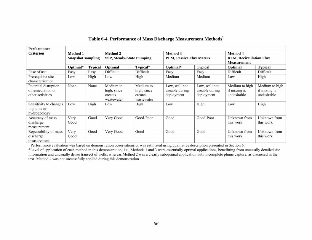
66
Table 6-4. Performance of Mass Discharge Measurement Methods1
Performance Criterion
Method 1 Snapshot sampling
Method 2 SSP, Steady-State Pumping
Method 3 PFM, Passive Flux Meters
Method 4 RFM, Recirculation Flux Measurement
Optimal* Typical Optimal Typical* Optimal* Typical Optimal Typical Ease of use Easy Easy Difficult Difficult Easy Easy Difficult Difficult Prerequisite site characterization
Low High Low High Medium Medium Low High
Potential disruption of remediation or other activities
None None Medium to high, since creates wastewater
Medium to high, since creates wastewater
Low, well not useable during deployment
Low, well not useable during deployment
Medium to high if mixing is undesirable
Medium to high if mixing is undesirable
Sensitivity to changes in plume or hydrogeology
Low High Low High Low High Low High
Accuracy of mass discharge measurement
Very Good
Good Very Good Good-Poor Good Good-Poor Unknown from this work
Unknown from this work
Repeatability of mass discharge measurement
Very Good
Good Very Good Good Good Good Unknown from this work
Unknown from this work
1 Performance evaluation was based on demonstration observations or was estimated using qualitative description presented in Section 6. *Level of application of each method in this demonstration; i.e., Methods 1 and 3 were essentially optimal applications, benefitting from unusually detailed site information and unusually dense transect of wells, whereas Method 2 was a clearly suboptimal application with incomplete plume capture, as discussed in the text. Method 4 was not successfully applied during this demonstration.

67
7.0 COST ASSESSMENT
This section summarizes cost data for conducting a full-scale mass discharge analysis using each of the four methods evaluated at VAFB. Unit costs from the field-scale demonstration are presented in this section for three of the four methods. In addition, there is a qualitative discussion of how these costs would change at a site with different conditions. This section can be used by remediation professionals to understand the cost components of performing a mass discharge analysis, estimate select unit costs and qualitatively understand the cost differential between the four mass discharge calculation methods as a function of site conditions.
7.1 COST MODEL
7.1.1 Cost Categories
Cost categories include design, capital, operation and maintenance (O&M) and demobilization costs. This list of cost categories was developed based on ESTCP and Federal Remediation Technology Roundtable (FRTR) guidelines (FRTR, 1998). (Other cost categories and activities suggested by these guidelines are not included because they relate to remedial technologies and are not applicable to diagnostic tools). Under each cost category, the following activities were identified as cost elements: Design costs
• Work plan preparation
• Modeling (remedial design)
• Site characterization
• Permitting
Capital costs
• Equipment mobilization and set-up
• Capital equipment purchase/rental
• Installation of monitoring wells
• Installation of extraction wells
• Installation of injection wells
• Modeling (performance verification)
O&M costs
• Training
• Sampling (field labor, equipment, materials)
• Laboratory analysis

68
• Data analysis and reporting
• Operational labor
• Maintenance
• Electricity
• Water treatment and/or disposal
Demobilization
• Equipment/treatment system demobilization
• Well decommissioning
Where possible, for each mass discharge measurement method, the costs of each activity were estimated using field demonstration data. However, in many cases, the costs of field demonstration were not representative of typical full-scale site costs. For example, much of the necessary site characterization work, installation of monitoring wells and other infrastructure had already been completed prior to this project. The density of monitoring wells was high, reflecting data quality needed during research and not limited by practical considerations. The site “contaminant” was bromide, and analyses were done by students and staff in an analytical laboratory, resulting in lower analytical costs that would typically be the case in practice. These conditions and other factors influence the extrapolation of the demonstration site cost data to other sites, as described in the following. 7.1.2 Site-Wide Assumptions
The demonstration site characteristics were described in Section 4. Key characteristics of the site are summarized below:
• The size of the demonstration site is approximately 0.25 acres (12,000 ft2 in area). The site is located approximately 15 miles from the nearest environmental service providers.
• The aquifer sediment is sandy, with a hydraulic conductivity of approximately 45 ft/day (13 m/day).
• The depth to groundwater is approximately five ft; the depth to the base of contamination (i.e., the depth of wells) is 11 ft.
• Approximately 80 lbs of “contaminant” (bromide tracer) were injected into the subsurface and spread out over a volume of approximately 13,500 ft3 (an aerial extent of 30 ft by 150 ft with a contaminated thickness of 3 ft).
• The bromide plume width was approximately 30 ft.
• The “contaminant” was highly mobile and did not sorb or biodegrade.
• Source(s) of contamination had already been identified, primary sources had been removed, and DNAPL was not present.
• There were no aboveground buildings or other structures that posed an obstacle to well placement or remedial system design.
69
• Site characterization (e.g., hydrogeology, nature and extent of contamination) had already been performed to a level of detail sufficient to design and implement a remediation system (which was completed by consultants to VAFB, in efforts unrelated to this research); however, additional wells and other infrastructure were needed for this research in order to allow detailed comparison of the mass discharge estimation methods.
7.1.3 Cost Comparison
Because the mass flux measurement techniques evaluated in this report are unique, there is no conventional technology to which they can be directly compared. The closest technique for comparing Method 1 is traditional groundwater monitoring. Many cost components of these two techniques are identical (e.g., cost of groundwater sample collection, laboratory analysis and depth-to-groundwater measurements). Depending on the site characteristics, Method 1 may require fewer or more wells than traditional groundwater monitoring. Sites with fairly narrow plumes may typically require fewer wells in a transect and thus are more obvious candidates for Method 1. However, the density of wells used in the Method 1 transect is typically greater than traditional monitoring well spacing. Well spacing must be on the order of the width of high concentration subplumes. At VAFB, a well spacing of approximately 12 ft apart resulted in mass discharge measurements that were accurate to within 25%. More heterogeneous sites would require tighter well spacing to achieve the same level of accuracy, which may or may not be needed depending on the goals of the mass discharge analysis. Activities that may make Method 1 more expensive than traditional monitoring include the cost of data analysis and reporting, which is likely to be a more significant effort than standard groundwater monitoring reports, but also provide additional insights not possible with traditional approaches. Actual reporting costs depend on the size of the project and stakeholder familiarity and acceptance of mass discharge measurement techniques. Finally, Method 1 requires a more detailed knowledge of hydraulic conductivity values throughout the aquifer in two dimensions at the location of the mass discharge transect. This is a one-time cost but can be substantial for sites with short remedial timeframes (on the order of 5 years). The overall cost effectiveness of Method 1 compared with traditional groundwater monitoring is site-specific. Cost drivers for selecting mass discharge analyses versus traditional groundwater monitoring methods are described in Section 7.2. A cost comparison of Method 1 with the other three mass discharge measurement methods is described in the following sections. 7.1.4 Cost Basis
Key assumptions, cost components and unit costs for each of the four mass discharge measurement methods are described in the following sections. 7.1.4.1 Design costs
Methods 1 through 4 all require some design, including any additional site characterization necessary for remedial design, modeling to demonstrate fate and transport/capture analysis, the preparation of a work plan, health and safety plan and obtaining necessary permits (e.g., well construction permits, waste discharge permits).
70
Site characterization had already been completed at a detailed level prior to the start of the project, including hydrogeology and the location and extent of “contamination”. Additional site characterization needed for Method 1 included hydraulic conductivity data to get a more accurate estimate of flow through different areas of the aquifer. These data was collected at VAFB by performing slug tests (typical cost is $855 per well, per R.S. Means guide). Alternatively, a dye tracer test could be used (cost on the order of $11,000, per R.S. Means guide). Method 3 required a similar level of characterization. In addition, if passive flux meters were to be installed at multiple depths in single-interval wells, vertical gradients would need to be measured. These costs are a function of the number of wells and would increase the cost of collecting depth-to-water measurements sitewide. In principle, Methods 2 and 4 were expected to require less detailed subsurface characterization of plume and plume anatomy, but in fact would have worked better during the research if more information had been considered prior to their evaluation. In essence, enough information would be needed in practice to tell where the target plume is and how wide the capture zones of the pumping methods will be. In general, Methods 2 and 4 would require a design and/or modeling of the extraction and/or reinjection system to ensure that capture is sufficient. At sites where such a system is part of the site remedy, this would not be an additional cost. At VAFB, the large number of closely-spaced wells were initially assumed to ensure capture for Method 2, but in fact after the field trials data analysis and modeling indicated that capture had not been complete. So clearly it would have been better if there had been more planning and model evaluation, and the same is likely to be true for application of Method 2 in practice. The cost of work plan preparation, quality assurance plan and a health and safety plan is expected to be about the same, regardless of the mass discharge measurement used. This was estimated to be approximately $10,000 to $15,000, based on professional judgment. Permitting costs for well construction were not applicable at VAFB, since direct push methods were used and regulators knew the wells were to be used only in research; however, they may be applicable on a per-well basis at other sites for Methods 1 through 4. Similarly, Methods 2 and 4 may require a permitting fee for wastewater discharge or reinjection. Like modeling, these costs may be incurred anyway as part of remedial design. 7.1.4.2 Capital costs
For Methods 1 through 4, capital costs include the cost of mobilization and set-up, equipment purchase and monitoring well installation. Capital costs associated with Method 2 and 4 include extraction well installation and possibly additional modeling for performance verification. Injection wells must also be installed for Method 4. The costs of mobilizing drilling equipment and installing wells were relatively inexpensive at VAFB. The shallow aquifer allowed for the installation of short (~12 ft), small-diameter wells, with drop tubes connected to peristaltic pumps for sampling or longer term groundwater extraction wells: 1.0-in diameter wells were used for Method 2, 3 and 4, installed using a solid-stem auger rig, while 0.5-in diameter wells were used for Method 1, installed using a direct push rig. The cost of installing approximately 30 wells was $5,930. In contrast, the cost of installing a
71
standard 2-in monitoring well to 12 ft deep can be approximately $9,000 per well, using the R.S. Means guide. The cost of installing a 6.0-in diameter, 9 gallons per minute extraction well, including a dedicated submersible pump, effluent collection tank and 50 ft of piping, is approximately $25,000 per well. The number of required monitoring and extraction wells is site-specific and can be based on modeling; however, Methods 1 and 3 will likely require more wells than Methods 2 and 4, yet Methods 2 and 4 may require more expensive wells than Methods 1 and 3. If vertical head gradients are present in the aquifer, wells will need to be multi-level for Methods 1 and 3. Baffles or other flow barriers will need to be installed for Method 3 if there are vertical head gradients (Enviroflux, 2008). For Method 2, additional equipment may need to be purchased and installed to treat the extracted groundwater. Method 4 is intended to involve reinjection of the extracted water without treatment, but if treatment were required by regulators it is possible this method would typically not be pursued. More Method 2 and 4, if extraction rates are based on model simulations, piezometers may need to be installed to compare groundwater elevations and head measurements to model-predicted values. However, these costs may already be incurred as part of remedial activities. For Method 3, flux meters will need to be purchased and inserted into groundwater monitoring wells. Model verification may be needed for Methods 2 and 4, particularly if the extraction system network is designed to be sparse. However, at a site where modeling has been performed as part of design, the model will already be set up and the level of effort needed to confirm that the wells are capturing the entire plume will be relatively minimal (e.g., $10,000). Installation of closer transects of extraction wells is also an advantage since the system will reach steady-state faster than if fewer wells are installed. At VAFB, detailed modeling was not conducted until after the field trials of Method 2; this post-hoc modeling helped understand why Method 2 was inaccurate during the trials, and overall the implication is that any pumping based method will benefit from as much initial characterization and modeling as possible. 7.1.4.3 O&M costs
O&M costs include the cost of training, groundwater monitoring (field labor, sampling supplies and equipment rental), analytical costs, data analysis and reporting, electricity (Methods 2 and 4), wastewater treatment system operations (Method 2), disposal of treated water (Method 2) and periodic maintenance costs. Training costs are not likely to be substantial for any method except Method 4. Method 3 may require some training (approximately eight hours for two field technicians) to illustrate the proper procedure for placing and retrieving the passive flux meters. Training will not likely be required for Methods 1 and 2. In addition, for Methods 2 and 4, labor rates for operations staff may be higher than standard field technician rates, due to the specialized nature of mass flux measurement and pumping test design. In the VAFB trial, the first deployment of flux meters was installed by the inventors of the method, providing several hours of training to field staff. Groundwater monitoring and depth-to-water measurements will be required for all four methods. The relative cost of these methods is a function of the number of sampling locations and the frequency of monitoring. It may seem that methods 1 and 3 are likely to have higher monitoring
72
costs than methods 2 and 4, because composite samples can be collected using methods 2 and 4. However, field staff do not know exactly when to collect samples during applications of methods 2 and 4 to allow optimal estimation of mass discharge. This means that almost certainly more samples will be acquired over time than turn out later to have been needed. Furthermore, if the extraction wells are not continually operating as part of a remediation strategy, it may be advisable to “step up” the total pumping rate of Method 2, as described in Section 6.2.2, and collect samples during each step. For these reasons, it may often be the case that Methods 2 and 4 would require more sample acquisition and analysis than Methods 1 or 3. As an example, in the field research conducted at VAFB, Method 1 required 29 samples (29 wells) to get a single estimate of mass discharge (although samples from only seven wells would have sufficed, according to Section 6.2.2) whereas the first application of Method 4 required 60 samples to understand the system performance, and ultimately recognize that the method had been inaccurate. Thus, the results suggest that it is not necessarily true that Method 2 and 4 would require fewer samples and therefore have lower analytical costs than Methods 1 and 3. Analytical costs will depend on the type of site contaminants. Unit cost quotes can be obtained from a variety of commercial laboratories or estimated using the R.S. Means guide. The exception is the analysis of passive flux meters after they have been deployed and retrieved from the field. Passive flux meters are typically sent back to the vendor for analysis at costs comparable to commercial laboratories. Passive flux meter analyses at VAFB were performed at the University of Florida. Data analysis to determine mass flux is a simple spreadsheet exercise for Methods 1 and 3, whereas data analysis for Methods 2 and 4 require model calibration and fitting. Thus, the data analysis costs of Methods 2 and 4 are likely to be higher than for Methods 1 and 3. The cost of reporting is likely to be similar for all methods. The absolute cost of this process will depend on the familiarity and acceptance of mass discharge estimation by stakeholders. Electricity usage for Methods 2 and 4, to power extraction well pumps, will be a function of remedial system design and can easily be calculated using R.S. Means guide or other data after sizing well pumps and any electricity needed for a treatment system. Method 1 does not require continuous electricity although power may be required during the short duration sampling of deeper wells. Method 3 requires no electricity unless the PFMs are withdrawn from the wells after deployment using a winch. Both Methods 2 and 4 may require wastewater treatment prior to discharge or reinjection. Treatment requirements and costs will be site-specific and may be required as part of remediation efforts. Similarly, disposal of treated water will be necessary for Method 2. During this demonstration At VAFB, extracted water was handled as described previously in Section 5.4.6. Periodic maintenance costs of monitoring wells would be needed for Methods 1 and 3. Additional maintenance costs of extraction system wells, well pumps and/or treatment system may be needed for Methods 2 and 4. Method 4 may require periodic redevelopment of the injection well if the method is run for a significant period of time (in the VAFB trial, the injection well tended to clog to the point that redevelopment was required to sustain the injection
73
rate). Standard costing assumptions could be used to estimate this; no maintenance costs were incurred at VAFB during field research. 7.1.4.4 Demobilization
Demobilization costs include the cost of well decommissioning and treatment system/equipment demobilization. Equipment demobilization costs at VAFB were not incurred for the wells used for comparison of the mass discharge estimation methods as those wells were retained for ongoing research at the . Equipment demobilization costs at other sites could be estimated based on vendor quotes or as a percentage of total system construction costs. A number of other wells were abandoned at VAFB after this research was complete, generally those used for injection and initial monitoring of the bromide tracer. The cost per well ranged from approximately $40 to $200, depending on the method used. (Some wells could be abandoned by removing the casings and filling the space with cement while others required over-drilling and tremmie grouting). Monitoring well decommissioning costs at other sites can be estimated from using vendor quotes or R.S. Means cost estimates.
7.2 COST DRIVERS
Cost drivers are site-specific and are a function of the several factors including aquifer materials, degree of heterogeneity in geology and contamination, depth of contamination, groundwater velocity, temporal stability of the flow field, duration of measurements, and waste treatment and disposal requirements. These site conditions, along with planned or ongoing remediation system design, determine the number and unit cost of wells required to measure mass flux and the associated sampling, analytical and maintenance costs. Site conditions may guide the choice of mass discharge measurement methods. 7.2.1 Geology
The type of aquifer materials and degree of geologic heterogeneity are clearly important factors controlling the cost and performance of the various mass discharge measurement methods. For example, costs for installing monitoring devices in fractured bedrock environments are greater than at sites located on unconsolidated sediments. Preferred flowpaths created by fractures in the rock would likely require greater subsurface characterization to ensure proper location of wells than would be the case for sites where groundwater flow is more homogeneous and isotropic. The issue of proper well location is discussed further in the following section. The degree of geologic heterogeneity exerts a strong control on the movement of groundwater and, therefore, dissolved contaminants in the subsurface, as illustrated in Figure 7-1. Geologic heterogeneity is therefore an important factor affecting the cost and performance of each of the mass discharge measurement methods. For example, the required density of monitoring points in a transect of multilevel wells could be influenced by geologic heterogeneity, as illustrated in Figure 7-1. While it is reasonable to expect that a denser grid of monitoring points would be necessary in strongly heterogeneous sedimentary deposits, it may not always be the case. For example, at sites where site characterization identifies buried channel deposits that are
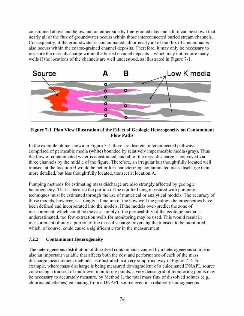
74
constrained above and below and on either side by fine-grained clay and silt, it can be shown that nearly all of the flux of groundwater occurs within those interconnected buried stream channels. Consequently, if the groundwater is contaminated, all or nearly all of the flux of contaminants also occurs within the coarse-grained channel deposits. Therefore, it may only be necessary to measure the mass discharge within the buried channel deposits – which may not require many wells if the locations of the channels are well understood, as illustrated in Figure 7-1.
Figure 7-1. Plan View Illustration of the Effect of Geologic Heterogeneity on Contaminant Flow Paths
In the example plume shown in Figure 7-1, there are discrete, interconnected pathways comprised of permeable media (white) bounded by relatively impermeable media (gray). Thus the flow of contaminated water is constrained, and all of the mass discharge is conveyed via three channels by the middle of the figure. Therefore, an irregular but thoughtfully located well transect at the location B would be better for characterizing contaminated mass discharge than a more detailed, but less thoughtfully located, transect at location A. Pumping methods for estimating mass discharge are also strongly affected by geologic heterogeneity. That is because the portion of the aquifer being measured with pumping techniques must be estimated through the use of numerical or analytical models. The accuracy of those models, however, is strongly a function of the how well the geologic heterogeneities have been defined and incorporated into the models. If the models over-predict the zone of measurement, which could be the case simply if the permeability of the geologic media is underestimated, too few extraction wells for monitoring may be used. This would result in measurement of only a portion of the mass discharge traversing the transect to be monitored, which, of course, could cause a significant error in the measurement. 7.2.2 Contaminant Heterogeneity
The heterogeneous distribution of dissolved contaminants caused by a heterogeneous source is also an important variable that affects both the cost and performance of each of the mass discharge measurement methods, as illustrated in a very simplified way in Figure 7-2. For example, where mass discharge is being measured downgradient of a chlorinated DNAPL source zone using a transect of multilevel monitoring points, a very dense grid of monitoring points may be necessary to accurately measure, by Method 1, the total mass flux of dissolved solutes (e.g., chlorinated ethenes) emanating from a DNAPL source even in a relatively homogeneous
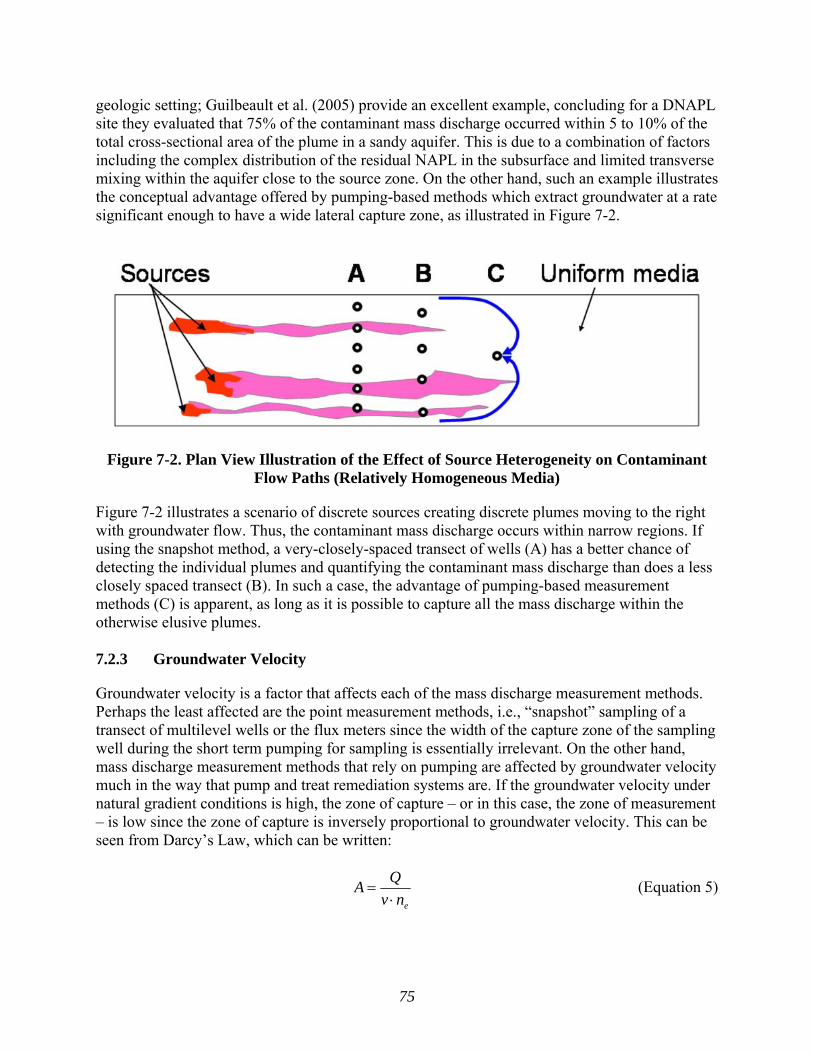
75
geologic setting; Guilbeault et al. (2005) provide an excellent example, concluding for a DNAPL site they evaluated that 75% of the contaminant mass discharge occurred within 5 to 10% of the total cross-sectional area of the plume in a sandy aquifer. This is due to a combination of factors including the complex distribution of the residual NAPL in the subsurface and limited transverse mixing within the aquifer close to the source zone. On the other hand, such an example illustrates the conceptual advantage offered by pumping-based methods which extract groundwater at a rate significant enough to have a wide lateral capture zone, as illustrated in Figure 7-2.
Figure 7-2. Plan View Illustration of the Effect of Source Heterogeneity on Contaminant
Flow Paths (Relatively Homogeneous Media)
Figure 7-2 illustrates a scenario of discrete sources creating discrete plumes moving to the right with groundwater flow. Thus, the contaminant mass discharge occurs within narrow regions. If using the snapshot method, a very-closely-spaced transect of wells (A) has a better chance of detecting the individual plumes and quantifying the contaminant mass discharge than does a less closely spaced transect (B). In such a case, the advantage of pumping-based measurement methods (C) is apparent, as long as it is possible to capture all the mass discharge within the otherwise elusive plumes. 7.2.3 Groundwater Velocity
Groundwater velocity is a factor that affects each of the mass discharge measurement methods. Perhaps the least affected are the point measurement methods, i.e., “snapshot” sampling of a transect of multilevel wells or the flux meters since the width of the capture zone of the sampling well during the short term pumping for sampling is essentially irrelevant. On the other hand, mass discharge measurement methods that rely on pumping are affected by groundwater velocity much in the way that pump and treat remediation systems are. If the groundwater velocity under natural gradient conditions is high, the zone of capture – or in this case, the zone of measurement – is low since the zone of capture is inversely proportional to groundwater velocity. This can be seen from Darcy’s Law, which can be written:
envQA⋅
= (Equation 5)

76
Where A = Cross-sectional area of the aquifer supplying water to the well Q = Extraction rate of the pumping well V = Groundwater tracer velocity ne = Effective porosity The relationship between the zone of measurement and the groundwater velocity can have significant practical consequences. For example, at sites with higher groundwater velocities, more pumping wells would be necessary to fully sample the contaminant plume. Alternatively, the extraction rate of the pumping wells can be increased to increase the size of the sampling zone (subject to the transmissivity of the aquifer and the efficiency of the extraction wells). However, this can have undesirable consequences such as increasing the time necessary for the system to reach steady-state conditions and creating a large volume of extracted water that may require on-site storage, treatment, and disposal. Finally, if the groundwater velocity is not constant in magnitude or direction over time, the aforementioned considerations become further complicated. The extraction wells may fully sample the plume some of the time but only sample a portion of it at other times. These fluctuations in the measured mass discharge could easily be mistaken for real fluctuations in mass discharge in the aquifer caused by temporal variations in the groundwater velocity. For these and other reasons, pumping techniques for measuring mass discharge must be based on accurate conceptual models of the subject sites. 7.2.4 Temporal Stability of the Flow Field
This is an important factor, affecting all methods of estimating contaminant mass discharge. For the methods involving samples from wells (snapshot sampling or PFM deployment), the wells may monitor distinctly different portions of a plume as the groundwater flow direction changes over time. Shifts in flow direction can also impact mass discharge measurement methods that are time integrated or rely on hydraulic capture of a portion of the contaminant plume. For example, the portion of the aquifer sampled while pumping a well (i.e., the capture zone of the well) is strongly a function of the direction of groundwater flow as well as the groundwater velocity. If the flow field changes over time, the well could be “sampling” a different part of the aquifer each time a measurement is made. During some sampling events the entire plume may be sampled. However, at other times, some portion of the plume may escape sampling, depending on the design of the sampling network and the magnitude of the variation in the groundwater flow field. Temporal stability of the flow field is clearly a factor that affects the cost and performance of the mass discharge measurement methods, especially those that rely on pumping of the aquifer to make a measurement, since the degree of capture by the extraction wells will vary with the groundwater velocity. So care must be taken to incorporate known or probable variations in flow directions and rates into the design and methods for interpretation of the mass discharge measurements. 7.2.5 Depth of Contamination
Measuring contaminant mass discharge at sites with deep groundwater would logically cost more money than making similar measurements at sites with shallow groundwater. This is due to the increased costs of installing monitoring devices to greater depths. There are other factors,
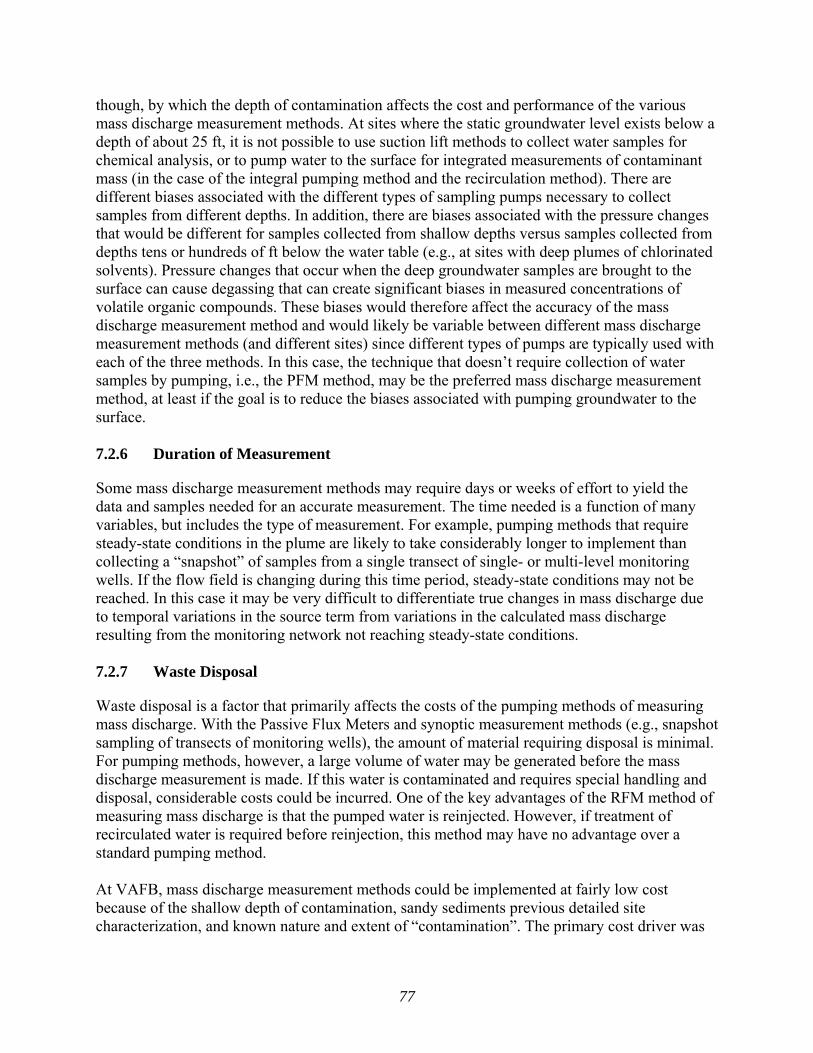
77
though, by which the depth of contamination affects the cost and performance of the various mass discharge measurement methods. At sites where the static groundwater level exists below a depth of about 25 ft, it is not possible to use suction lift methods to collect water samples for chemical analysis, or to pump water to the surface for integrated measurements of contaminant mass (in the case of the integral pumping method and the recirculation method). There are different biases associated with the different types of sampling pumps necessary to collect samples from different depths. In addition, there are biases associated with the pressure changes that would be different for samples collected from shallow depths versus samples collected from depths tens or hundreds of ft below the water table (e.g., at sites with deep plumes of chlorinated solvents). Pressure changes that occur when the deep groundwater samples are brought to the surface can cause degassing that can create significant biases in measured concentrations of volatile organic compounds. These biases would therefore affect the accuracy of the mass discharge measurement method and would likely be variable between different mass discharge measurement methods (and different sites) since different types of pumps are typically used with each of the three methods. In this case, the technique that doesn’t require collection of water samples by pumping, i.e., the PFM method, may be the preferred mass discharge measurement method, at least if the goal is to reduce the biases associated with pumping groundwater to the surface. 7.2.6 Duration of Measurement
Some mass discharge measurement methods may require days or weeks of effort to yield the data and samples needed for an accurate measurement. The time needed is a function of many variables, but includes the type of measurement. For example, pumping methods that require steady-state conditions in the plume are likely to take considerably longer to implement than collecting a “snapshot” of samples from a single transect of single- or multi-level monitoring wells. If the flow field is changing during this time period, steady-state conditions may not be reached. In this case it may be very difficult to differentiate true changes in mass discharge due to temporal variations in the source term from variations in the calculated mass discharge resulting from the monitoring network not reaching steady-state conditions. 7.2.7 Waste Disposal
Waste disposal is a factor that primarily affects the costs of the pumping methods of measuring mass discharge. With the Passive Flux Meters and synoptic measurement methods (e.g., snapshot sampling of transects of monitoring wells), the amount of material requiring disposal is minimal. For pumping methods, however, a large volume of water may be generated before the mass discharge measurement is made. If this water is contaminated and requires special handling and disposal, considerable costs could be incurred. One of the key advantages of the RFM method of measuring mass discharge is that the pumped water is reinjected. However, if treatment of recirculated water is required before reinjection, this method may have no advantage over a standard pumping method. At VAFB, mass discharge measurement methods could be implemented at fairly low cost because of the shallow depth of contamination, sandy sediments previous detailed site characterization, and known nature and extent of “contamination”. The primary cost driver was
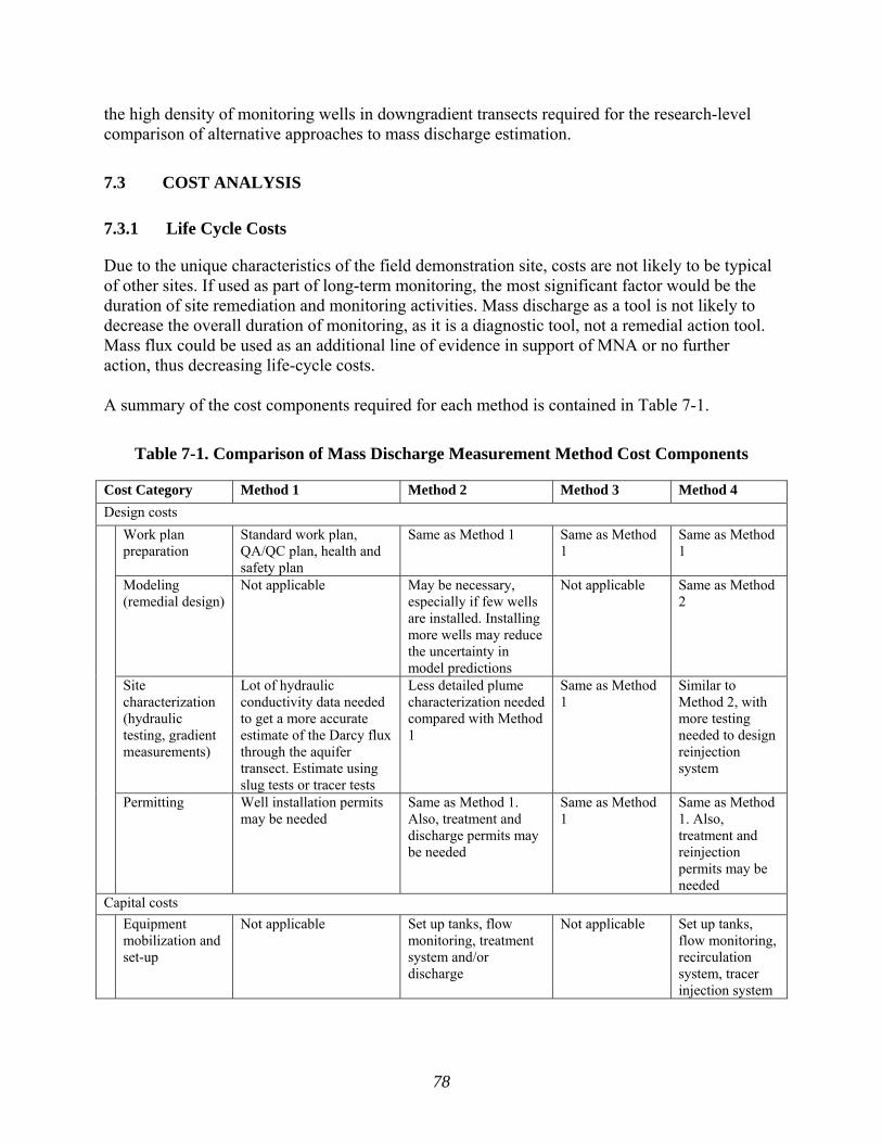
78
the high density of monitoring wells in downgradient transects required for the research-level comparison of alternative approaches to mass discharge estimation.
7.3 COST ANALYSIS
7.3.1 Life Cycle Costs
Due to the unique characteristics of the field demonstration site, costs are not likely to be typical of other sites. If used as part of long-term monitoring, the most significant factor would be the duration of site remediation and monitoring activities. Mass discharge as a tool is not likely to decrease the overall duration of monitoring, as it is a diagnostic tool, not a remedial action tool. Mass flux could be used as an additional line of evidence in support of MNA or no further action, thus decreasing life-cycle costs. A summary of the cost components required for each method is contained in Table 7-1.
Table 7-1. Comparison of Mass Discharge Measurement Method Cost Components
Cost Category Method 1 Method 2 Method 3 Method 4 Design costs
Work plan preparation
Standard work plan, QA/QC plan, health and safety plan
Same as Method 1 Same as Method 1
Same as Method 1
Modeling (remedial design)
Not applicable May be necessary, especially if few wells are installed. Installing more wells may reduce the uncertainty in model predictions
Not applicable Same as Method 2
Site characterization (hydraulic testing, gradient measurements)
Lot of hydraulic conductivity data needed to get a more accurate estimate of the Darcy flux through the aquifer transect. Estimate using slug tests or tracer tests
Less detailed plume characterization needed compared with Method 1
Same as Method 1
Similar to Method 2, with more testing needed to design reinjection system
Permitting Well installation permits may be needed
Same as Method 1. Also, treatment and discharge permits may be needed
Same as Method 1
Same as Method 1. Also, treatment and reinjection permits may be needed
Capital costs
Equipment mobilization and set-up
Not applicable Set up tanks, flow monitoring, treatment system and/or discharge
Not applicable Set up tanks, flow monitoring, recirculation system, tracer injection system

79
Cost Category Method 1 Method 2 Method 3 Method 4 Capital equipment
Not applicable Purchase extraction well pumps, holding tank, treatment or storage. Costs may be incurred anyway as part of remediation
Purchase flux meters
Same as Method 2
Monitoring well installation
Number and density are site-specific. Multi-level wells may be needed
Not applicable Same as Method 1. Larger diameter casings may be needed to house passive flux meters
Not applicable
Extraction well installation
Not applicable Sparse transects of extraction wells needed. Spacing is site-specific
Not applicable Same as Method 2
Injection well installation
Not applicable Not applicable Not applicable Number and spacing of injection wells is site-specific
Modeling (performance verification)
Possibly applicable to illustrate or interpret results
Modeling may be needed to demonstrate capture, particularly if well network is sparse
Same as Method 1
Same as Method 2
O&M costs Training Not applicable Not applicable Some training to
understand field methods
Necessary to understand concepts
Field sampling (labor, equipment rental, materials)
Standard monitoring costs. Number of samples is site-specific
Fewer sampling locations. Time-series data may be useful
Comparable to Method 1 (two trips to place and retrieve PFMs but less field time)
Same as Method 2
Analytical costs Standard analytical costs Same as Method 1. Likely will be fewer samples
Analysis of PFMs is not available at commercial laboratory. Ship to vendor for analysis
Same as Method 2
Data analysis and reporting
Cost of data analysis and reporting may be more than traditional monitoring since a discussion of groundwater flow rate must be included and more experienced staff are typically on the project team
Significant costs will be required for data analysis and modeling to determine whether or not capture is complete and refine system operation if necessary
Level of effort is likely between Method 1 and Method 2
Same as Method 2
Electricity Not applicable Extraction wells and treatment system energy requirements
Not applicable Same as Method 2

80
Cost Category Method 1 Method 2 Method 3 Method 4 Treatment, discharge and/or off-site disposal
Not applicable Site-specific treatment and discharge or off-site disposal costs. Costs may be incurred anyway as part of remediation
Not applicable Similar to Method 2 except treated water would be reinjected
Maintenance Standard maintenance costs for monitoring wells
Same as Method 1. In addition, maintenance of extraction wells and treatment system
Same as Method 1
Same as Method 2, also maintenance of reinjection wells
Demobilization
Equipment demobilization
Not applicable Demobilization of treatment system, holding tanks
Not applicable Same as Method 2
Well decommissioning
Standard monitoring well decommissioning costs
Fewer wells, higher unit cost
Same as Method 1
Similar to Method 2
81
8.0 IMPLEMENTATION ISSUES
There were no formal permits required for this work. However, as has been done in all previous projects at VAFB, work was conducted closely with the local regulators (Regional Water Quality Control Board, San Luis Obispo, CA) to identify issues of regulatory concern. This project did not present any. There were no emissions or residuals produced besides water created during the pumping method. Water produced during routine sampling of transects and by the pumping method was collected in storage tanks on site, periodically transferred to tanker trucks for conveyance to treatment facilities, both operated by TetraTech, Inc., consultants to the U.S. Air Force. There were no regulatory issues associated with this demonstration other than the requirement to provide regular update reports to VAFB and the Regional Water Quality Control Board. Wastewater generated as a result of this demonstration was collected and treated by consultants to VAFB and thus was not a regulatory issue for the research team. See earlier sections for discussion of stakeholders, their concerns, etc. All equipment used is readily available to practitioners, so procurement issues are routine. No proprietary technologies were used, except for the Flux meters (University of Florida, U.S. Patent No. 6,401,547). Scale-up issues are irrelevant as the evaluation was conducted at full-scale. The mass discharge estimation methods were customized to the demonstration site and plume scale, as would be true for any monitoring approach. Technology transfer activities will be coordinated by the prime contractor on this project, Malcolm Pirnie. To date, the results of this research have been presented in numerous conferences and professional short courses, and the inclusion in professional short course is sure to continue. Portions of this work will be submitted to peer-reviewed scientific journals and are expected to be accepted for publication. Results of this work will certainly be used by others involved in furthering the understanding and application of the contaminant mass discharge framework.
82
9.0 REFERENCES
Annable, M.D., K. Hatfield, J. Cho, H. Klammler, B.L. Parker, J.A. Cherry, P.S.C. Rao, 2005. Field-Scale Evaluation of the Passive Flux Meter for Simultaneous Measurement of Groundwater and Contaminant Fluxes. Environmental Science & Technology 39: 7194-7201.
Bockelmann, A., 2002. Natural Attenuation of Organic Contaminants: Integral Mass Flux Estimation and Reactive Transport Modeling in Heterogeneous Porous Media. Ph.D. Dissertation, University of Tubingen.
Bockelmann, A., T. Ptak, and G. Teutsch, 2001. An Analytical Quantification of Mass Fluxes and Natural Attenuation Rate Constants at a Former Gasworks Site. Journal of Contaminant Hydrology, 53, pp. 419-453.
Brooks, M.C., A.L. Wood, M.D. Annable, K. Hatfield, J. Cho, C. Holbert, P.S.C. Rao, C.G. Enfield, K. Lynch, and R.E. Smith, 2008. Changes in Contaminant Mass Discharge from DNAPL Source Mass Depletion: Evaluation at Two Field Sites. Submitted to Journal of Contaminant Hydrology.
Buscheck, T.E., N. Nijhawan, and K.T. O’Reilly, 2003. Mass Flux Estimates to Assist Remediation Decision-Making. Paper H-30, in: V.S. Magar and M.E. Kelley (Eds.), In-Situ and On-Site Bioremediation - 2003. Proceedings of the Seventh International In-Situ and On-Site Bioremediation Symposium. (Orlando, FL; June). ISBN 1-57477-139-6, Battelle Press, Columbus, OH, www.battelle.org/bookstore.
Cho, J., M.D. Annable, J.W. Jawitz, K. Hatfield, 2007. Passive Flux Meter Measurement of Water and Nutrient Flux in Porous Media. Journal of Environmental Quality, 36: 1266-1272.
Christ, J.A., M.N. Goltz and J. Huang, 1999. Development and Application of an Analytical Model to Aid Design and Implementation of In-Situ Remediation Technologies. Journal of Contaminant Hydrology 37(4-5): 295-317. April 15.
Driscoll, F.G. 1986. Groundwater and Wells, 2nd Edition. USFilter/Johnson Screens, St. Paul, MN.
Einarson, M.D., D.M. Mackay, N. R. de Sieyes, L. Jacobson, M. Noske, and L. Justice, 2005. Evaluation of Point Measurement and Pumping Techniques for Calculating Contaminant Mass Flux at a Nonsteady State MTBE Plume in California. Presented at National Ground Water Association Ground Water Summit Conference. San Antonio, Texas, April 25.
Einarson, M.D., D. M. Mackay, N. de Sieyes, A. Pappas, I. Wood, L. Jacobson, and L. Justice, 2004. Field Experiments on Impact of Ethanol on Natural Attenuation of BTEX and MTBE. Presented at American Petroleum Institute & National Ground Water Association Petroleum Hydrocarbons Conference, Baltimore, Maryland, August 17.
Einarson, M.D. and D.M. Mackay, 2001. Estimating Future Impacts of Groundwater Contamination. Environmental Science & Technology 35 (3): 66A-73A.

83
Enviroflux, 2008. Available online at www.enviroflux.com
Feenstra, S, J.; Cherry, A.; Parker, B. L., 1996. Conceptual Models for the Behavior of Dense Nonaqueous-Phase Liquids (DNAPLs) in the Subsurface. Dense Chlorinated Solvents and Other DNAPLs in Groundwater; J. F. Pankow, J. A. Cherry, Eds.; Waterloo Press: Portland, OR.
Feris, K., D Mackay, M Einarson, N de Sieyes, L Jacobson, L Justice, M Noske, K Hristova, and K Scow, 2005. Impacts of Ethanol and BTX on Microbial Populations, Processes, and Community Composition in a Sulfate-Reducing Contaminated Aquifer. Presented at Geologic Society of America (GSA) 2005 Annual Meeting, Salt Lake City, Utah, October 19.
Feris, K., K. Hristova, B. Gebreyesus, D. Mackay, and K. Scow, 2004. A Shallow BTEX and MTBE Contaminated Aquifer Supports a Diverse Microbial Community. Microbial Ecology 48(4): 589-600. December.
FRTR, 2008. Mass Flux Toolkit. Available online at www.frtr.gov/decisionsupport/DST_Tools/MASSFLUX.htm
FRTR, 1998. Guide to documenting and managing cost and performance information for remediation projects, Revised version. Federal Remediation Technologies Roundtable. October.
Goltz, M.N., J. Huang, M.E. Close, M. Flintoft, and L. Pang, 2007a. Use of tandem circulation wells to measure hydraulic conductivity without groundwater extraction, in review, Journal of Contaminant Hydrology.
Goltz, M.N., S. Kim, H. Yoon, J. Park, 2007b. Review of Groundwater Contaminant Mass Flux Measurement, Environmental Engineering Research, 12(4):176-193.
Guilbeault, M.A., B.L. Parker, and J.A. Cherry, 2005. Mass and flux distributions from DNAPL zones in sandy aquifers. Ground Water 43 (1): 70-86.
Hatfield, K., M.D. Annable, J. Cho, P.S.C. Rao, H. Klammler, 2004. A Direct Passive Method for Measuring Water and Contaminant Fluxes in Porous Media. Journal of Contaminant Hydrology Vol. 75, No. 3-4, pp. 155-181.
Hatfield, K., M. D. Annable, S. Kuhn. P.S.C. Rao, T. Campbell, 2002a. A new method for quantifying contaminant flux at hazardous waste sites. In Groundwater Quality: Natural and Enhanced Restoration of Groundwater Pollution (Proceedings of the Groundwater Quality 2001 Conference held at Sheffield, UK, June, 2001). S. F. Thornton and S. E. Oswald, editors. IAHS Publ. no. 275.
Hatfield, K., P.S.C. Rao, M.D. Annable, T.J., 2002b. Campbell. Device and Method for Measuring Fluid and Solute Fluxes in Flow Systems., U.S. Patent No. 6,401,547. June 11.
84
Hazen, A., 1892. Some physical properties of sands and gravels, with special reference to their use in filtration. 24th Annual Rep., Massachusetts State Board of Health, Pub. Doc. No. 34, 539–556.
Hristova, K., B. Gebreyesus, D. Mackay, and K. Scow, 2003. Naturally Occurring Bacteria Similar to the Methyl tert-Butyl Ether (MTBE)-Degrading Strain PM1 are Present in MTBE-Contaminated Aquifer. Applied and Environmental Microbiology, 69: 2616-2623.
Huang, J., M.E. Close, L. Pang, and M.N. Goltz, 2004. Innovative method to measure flux of dissolved contaminants in groundwater, Fourth International Conference on Remediation of Chlorinated and Recalcitrant Compounds, Monterey California, 24-27 May.
ITRC, 2004. Strategies for Monitoring the Performance of DNAPL Source Zone Remedies. Interstate Technology Regulatory Council.
Jackson, D., 2005. INTERA. Hill Air Force Base. Presented at the Groundwater Resources Association (GRA)’s 15th Symposium in the Series on Groundwater Contaminants: DNAPL Source Zone Characterization and Remediation.
Klammler, H., K. Hatfield, M. D. Annable, E Agyei, B. L. Parker, J. A. Cherry, and P. S. C. Rao, 2007a. General analytical treatment of the flow field relevant to the interpretation of passive flux meter measurements, Water Resources Research 43, W04407, doi:10.1029/2005WR004718.
Klammler, H., K. Hatfield, M.D. Annable, 2007b. Concepts for Measuring Horizontal Groundwater Flow Directions Using the Passive Flux Meter, Advances in Water Resources, 30 (4): 984-997.
Kozeny, 1953. Hydraulik: Ihre Grundlagen und praktische Anwendung. Springer-Verlag, Vienna.
Lee and Ro, 1998. Draft installation restoration program (IRP) Remedial Investigation Report for IRP Site 60, Vandenberg Air Force Base, California, Lee and Ro, Inc., City of Industry, CA.
Li, Betty K., Goovaerts, Pierre, and Abriola, Linda M., 2007. A geostatistical approach for quantification of contaminant mass discharge uncertainty using multilevel sampler measurements. Water Resources Research, 43 (W06436): 1-14.
Mackay, D. M., N. R. de Sieyes, M. D. Einarson, K. P. Feris, A. A. Pappas, I. A. Wood, L. Jacobson, L. G. Justice, M. N. Noske, J. T. Wilson, C. J. Adair, and K. M. Scow, 2007. Impact of Ethanol on Natural Attenuation of MTBE in a Normally Sulfate-Reducing Aquifer. Environmental Science and Technology, 41:6, 2015-2021.
Mackay, D. M., N. R. de Sieyes, M. D. Einarson, K. P. Feris, A. A. Pappas, I. A. Wood, L. Jacobson, L. G. Justice, M. N. Noske, K. M. Scow and J. T. Wilson, 2006. Impact of Ethanol on the Natural Attenuation of Benzene, Toluene and o-Xylene in a Normally Sulfate-Reducing Aquifer. Environmental Science and Technology, 40:19, 6123-6130.

85
Mackay, D. M., M. Einarson, C. M. Mok, N. de Sieyes, M. Noske, L. Justice, L. Jacobson, K. Feris, and K. Scow, 2005. Impacts of Ethanol on Natural Attenuation of BTEX and MTBE. Presented at meeting of ASTSWMO (Association of State and Territorial Solid Waste Management Officials) MTBE and Fuel Oxygenates Workgroup, Seattle, WA, March 16.
Mackay, D., I. Wood, R. Wilson, M. Einarson, P. Bennett, J. Huang, C. Henry, and M. Goltz. Estimation of Contaminant Mass Discharge in MTBE Plumes, 2002a. Presented at “2002 Petroleum Hydrocarbons and Organic Chemicals in Groundwater: 19th Annual Conference and Exposition”, National Ground Water Association and American Petroleum Institute, Atlanta, GA, November 6-8.
Mackay, D., R. Wilson, C. Naas, I. Wood, K. Scow, A. Smith, D. Ghandi, K. Hristova, B. Watanabe, and M. Einarson, 2002b. In-Situ Treatment of MTBE-Contaminated Groundwater at Two Sites in California. In “Groundwater Quality: Natural and Enhanced Restoration of Groundwater Pollution (Proceedings of the Groundwater Quality 2001 Conference held at Sheffield, UK, June, 2001). S. F. Thornton and S. E. Oswald, editors. IAHS Publ. no. 275.
Malcolm Pirnie, 2006. Mass Flux Analysis and Monitored Natural Attenuation Evaluation, North TNT Manufacturing Valley, Volunteer Army Ammunition Plant, Chattanooga, Tennessee. Prepared for U.S. Army Environmental Center, May.
McCarty, P.L., M.N. Goltz, G.D. Hopkins, M.E. Dolan, J.P. Allan, B.T. Kawakami, and T.J. Carrothers, 1998. Full-scale Evaluation of In-Situ Cometabolic Degradation of Trichloroethylene in Groundwater through Toluene Injection, Environmental Science and Technology, 32(1):88-100.
Newell, C.J., J.A. Conner, and D.L. Rowen, 2003. Groundwater Remediation Strategies Tool. American Petroleum Institute. Publication Number 4730. 80 pp.
Nichols, E.M., 2004. In a state of (mass) flux. Ground Water Monitoring and Remediation 24, no. 3: 4-8.
Nichols, E.M. and T. Roth, 2004. Flux redox -- Using mass flux to improve cleanup decisions. LUSTline Bulletin 46, March 2004.
Rao, P.S.C., J.W. Jawitz, C.G Enfield, R.W. Falta Jr., M.D. Annable, L. Wood, 2002. Technology integration for contaminated site remediation: clean-up goals and performance criteria. In Groundwater Quality: Natural and Enhanced Restoration of Groundwater Pollution (Proceedings of the Groundwater Quality 2001 Conference held at Sheffield, UK, June, 2001). S. F. Thornton and S. E. Oswald, editors. IAHS Publ. no. 275.
Semprini, L.; Kitanidis, P. K.; Kampbell, D. H.; Wilson, J. T., 1995.Water Resources Research 31 (4), 1051–1062.
Stroo, H.F., M. Unger, C.H. Ward, M.C. Kavanaugh, C. Vogel, A. Leeson, J.A. Marqusee, and B.P. Smith, 2003. Remediating chlorinated solvent source zones. Environmental Science and Technology, 37(11): 224A-230A.
86
U.S. EPA, 2005. Groundwater Sampling and Monitoring with Direct Push Technologies. Office of Solid Waste and Emergency Response (OSWER) No. 9200.1-51; EPA 540/R-04/005, pp. 67.
U.S. EPA, 2004. Performance Monitoring of MNA Remedies for VOCs in Ground Water. EPA/600/R-04/027. Office of Research and Development. Available at www.epa.gov/ada/download/reports/600R04027/600R04027_fm.pdf
U.S. EPA, 2003. The DNAPL Remediation Challenge: Is There a Case for Source Depletion. EPA/600/R-03/143.
Wheeldon, J. G., 2008. An Evaluation and Implementation Guide for Current Groundwater Mass Flux Measurement Practices. M.S. Thesis. Air Force Institute of Technology, Wright Patterson Air Force Base, Ohio. 122 pp.
Wilson, R. D., D. M. Mackay, and K. M. Scow, 2002. In-Situ MTBE Degradation Supported By Diffusive Oxygen Release. Environmental Science and Technology, 36(2): 190-199.
Yoon, H., 2006. Validation of methods to measure mass flux of a groundwater contaminant, AFIT/GES/ENV/06M-08, Department of the Air Force Air University, Wright-Patterson AFB, OH.
Appendix A
Simulation of Injection and Transport of Bromide at
Vandenberg Air Force Base Site 60
APPENDIX A
SIMULATION OF INJECTION AND TRANSPORT OF BROMIDE
AT VANDENBERG AFB SITE 60
An important objective of this demonstration was to compare results of contaminant mass
discharge estimation methods to known values. Ordinarily the true value of contaminant mass
discharge is not known, so various mass discharge estimation methods can only be compared to
one another. Creation of a dissolved plume with a known, controlled mass discharge of solutes is
easier said than done, however. As discussed above, we injected groundwater containing
dissolved bromide as our model “contaminant” at a target mass injection rate of 125 g/day. The
actual rate of mass injection was affected by variations in bromide concentration in our spiking
reservoir and the actual rate of injection. Twice-daily measurement of bromide concentrations
and injection rates at our injection wells suggested early on that the bromide mass injection rate
was not going to be as constant as we had hoped. Subsequent monitoring of bromide
concentrations along downgradient sampling transects confirmed that the rate of bromide
injection into the S3 sand had not been constant.
Because of this, we were not able to compare the field-generated mass discharge values to a
constant “control” value as intended, e.g., the target mass injection rate of 125 g/day.
Consequently, we developed a transient, three dimensional fate and transport model to simulate
our field experiment, in particular the variable rate of bromide injection. That simulation, once
calibrated to the unusually detailed data on site characteristics and bromide distribution over
time, provided us with a tool to estimate what the bromide mass discharge should have been
crossing any sampling transect at any time during the field experiment.
A.1. Code and GUI
The model we used was Modflow 96 with MT3D (using finite difference solver) used to
simulate the bromide transport. We used the software package Groundwater Vistas™ Version
5.07 Build 2 for pre-and post-processing.
A.2. Model Domain
The model domain is 560 ft long along the direction of groundwater flow and 370 ft wide in the
direction perpendicular to flow. Model boundaries extend 140 ft upgradient of the EA injection
wells and 250 ft downgradient of the EJP transect. The model domain extends 150 ft cross-
gradient of the footprint of the dissolved bromide plumes created during the experiment (Figure
A-1).
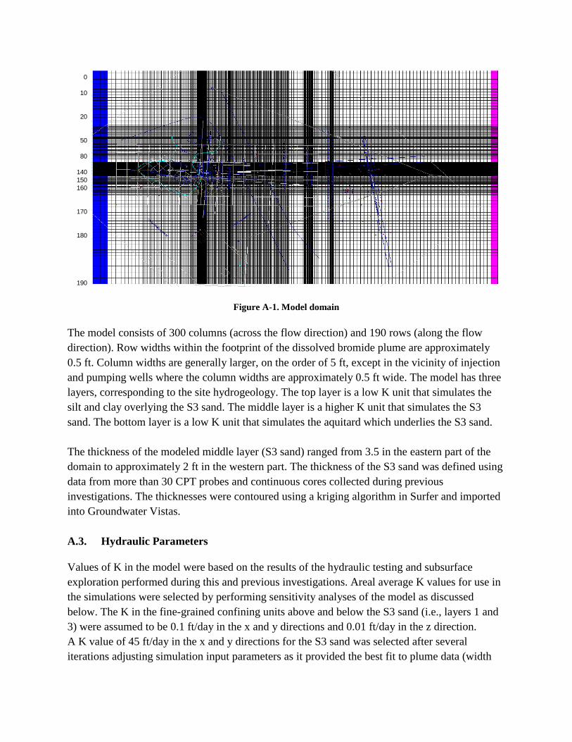
0
10
20
50
80
140
150
160
170
180
190
Figure A-1. Model domain
The model consists of 300 columns (across the flow direction) and 190 rows (along the flow
direction). Row widths within the footprint of the dissolved bromide plume are approximately
0.5 ft. Column widths are generally larger, on the order of 5 ft, except in the vicinity of injection
and pumping wells where the column widths are approximately 0.5 ft wide. The model has three
layers, corresponding to the site hydrogeology. The top layer is a low K unit that simulates the
silt and clay overlying the S3 sand. The middle layer is a higher K unit that simulates the S3
sand. The bottom layer is a low K unit that simulates the aquitard which underlies the S3 sand.
The thickness of the modeled middle layer (S3 sand) ranged from 3.5 in the eastern part of the
domain to approximately 2 ft in the western part. The thickness of the S3 sand was defined using
data from more than 30 CPT probes and continuous cores collected during previous
investigations. The thicknesses were contoured using a kriging algorithm in Surfer and imported
into Groundwater Vistas.
A.3. Hydraulic Parameters
Values of K in the model were based on the results of the hydraulic testing and subsurface
exploration performed during this and previous investigations. Areal average K values for use in
the simulations were selected by performing sensitivity analyses of the model as discussed
below. The K in the fine-grained confining units above and below the S3 sand (i.e., layers 1 and
3) were assumed to be 0.1 ft/day in the x and y directions and 0.01 ft/day in the z direction.
A K value of 45 ft/day in the x and y directions for the S3 sand was selected after several
iterations adjusting simulation input parameters as it provided the best fit to plume data (width

and breakthrough) of the alternatives examined. Numerical optimization was outside the scope of
the current project, but may be pursued in the future under other funding for reasons described
below. The Kv of the S3 sand in the model was assumed to be 4.5 ft/day.
The K in coarse grained artificial fill in source area in the model was assumed to be 200 ft/day in
the x, y, & z directions. This resulted in a good match to water levels and hydraulic gradients
measured in wells in the coarse-grained AF in the source area (SA). K values of 0.1 ft/day in x,
y, and z directions were used for the older, fine-grained fill in the SA.
A.4. Boundary Conditions
A.4.1. Perimeter boundaries
Model boundaries were based on measured site conditions. The upgradient boundary in the
model was a time-varying constant head boundary. Seventeen separate upgradient head values
were built into the upgradient constant head boundary condition. Those values were based on
variations in piezometric head measured throughout the period of the experiment in upgradient
monitoring well MW-1. A time-varying general head boundary was used in the model along the
downgradient edge of the test area. The specific time-varying general head boundaries were
defined based on extrapolation of heads at the downgradient limit of the model domain from
groundwater contour maps. A summary of sitewide hydraulic gradients calculated at various
times during the field experiment is presented in Table A-1. No-flow boundaries were used in the
model along the cross-gradient edges of domain.
Table A-1. Horizontal hydraulic gradients
D Transect H Transect J Transect
1 80 9/29/2005 10/13/2005 Whole site 14 0.015 0.014 0.014 Water levels near ED noisy
2 106 10/25/2005 10/13/2005 Whole site -12 NA 0.014 0.014 Water levels near ED noisy
3 128 11/16/2005 10/13/2005 Whole site -34 NA 0.014 0.014 Water levels near ED noisy
4 147 12/5/2005 12/14/2005 N of Monroe 9 NA 0.013 0.015
5 155 12/13/2005 12/14/2005 N of Monroe 1 NA 0.013 0.015
6 160 12/18/2005 12/19/2005 N of Monroe 1 NA 0.014 0.014
7 190 1/17/2006 1/16/2006 N of Monroe -1 NA 0.015 0.015 Data at ED noisy, used 2/13 data
8 218 2/14/2006 2/13/2006 N of Monroe -1 NA 0.015 0.015
9 237 3/5/2006 3/13/2006 N of Monroe 8 NA 0.015 0.015 Data at ED noisy, used 2/13 data
10 244 3/12/2006 3/13/2006 N of Monroe 1 NA 0.015 0.015
11 276 4/13/2006 4/12/2006 N of Monroe -1 NA 0.015 0.015
12 282 4/19/2006 4/20/2006 Whole site 1 NA 0.015 0.015
13 330 6/6/2006 6/5/2006 N of Monroe -1 NA 0.013 0.013
14 342 6/18/2006 6/16/2006 N of Monroe -2 NA 0.013 0.013 Data at ED noisy, used 2/13 data
15 461 10/15/2006 11/13/2006 Whole site 29 0.020 0.014 0.017
16 582 2/13/2007 4/2/2007 Whole site 48 0.015 0.013 0.015
Event CommentModel
Day
Sampling Date
for Synoptic
Sampling
Date Gradient
Meas.Area
Days Before (-) or
After (+) Sampling
Snapshot
Horiz. Gradient
A.4.2. Recharge
Recharge was simulated based on seasonal precipitation measured at the site during the field
experiment. An average value of 3.5 inches of precipitation per month was simulated during the
period from December 1, 2005 through April 31, 2006. In the model it was assumed that 80% of
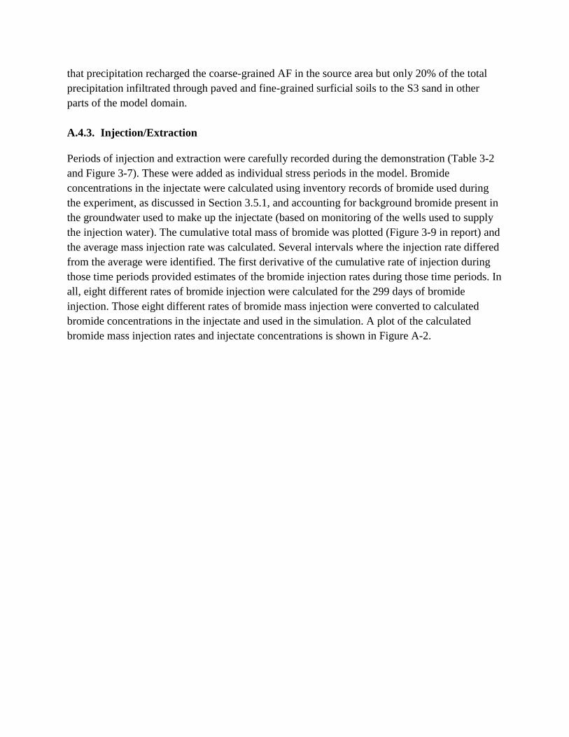
that precipitation recharged the coarse-grained AF in the source area but only 20% of the total
precipitation infiltrated through paved and fine-grained surficial soils to the S3 sand in other
parts of the model domain.
A.4.3. Injection/Extraction
Periods of injection and extraction were carefully recorded during the demonstration (Table 3-2
and Figure 3-7). These were added as individual stress periods in the model. Bromide
concentrations in the injectate were calculated using inventory records of bromide used during
the experiment, as discussed in Section 3.5.1, and accounting for background bromide present in
the groundwater used to make up the injectate (based on monitoring of the wells used to supply
the injection water). The cumulative total mass of bromide was plotted (Figure 3-9 in report) and
the average mass injection rate was calculated. Several intervals where the injection rate differed
from the average were identified. The first derivative of the cumulative rate of injection during
those time periods provided estimates of the bromide injection rates during those time periods. In
all, eight different rates of bromide injection were calculated for the 299 days of bromide
injection. Those eight different rates of bromide mass injection were converted to calculated
bromide concentrations in the injectate and used in the simulation. A plot of the calculated
bromide mass injection rates and injectate concentrations is shown in Figure A-2.
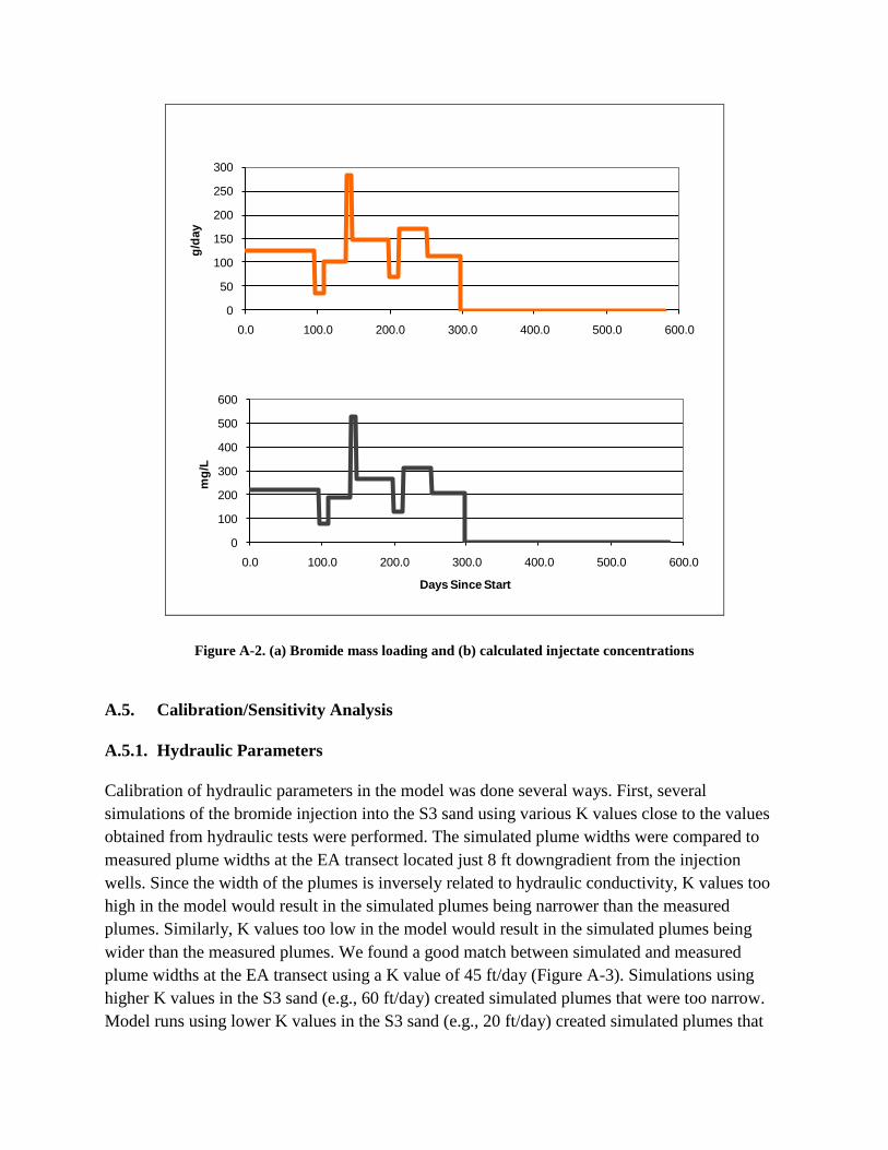
0
50
100
150
200
250
300
0.0 100.0 200.0 300.0 400.0 500.0 600.0
g/d
ay
Days Since Start
0
100
200
300
400
500
600
0.0 100.0 200.0 300.0 400.0 500.0 600.0
mg
/L
Days Since Start
Figure A-2. (a) Bromide mass loading and (b) calculated injectate concentrations
A.5. Calibration/Sensitivity Analysis
A.5.1. Hydraulic Parameters
Calibration of hydraulic parameters in the model was done several ways. First, several
simulations of the bromide injection into the S3 sand using various K values close to the values
obtained from hydraulic tests were performed. The simulated plume widths were compared to
measured plume widths at the EA transect located just 8 ft downgradient from the injection
wells. Since the width of the plumes is inversely related to hydraulic conductivity, K values too
high in the model would result in the simulated plumes being narrower than the measured
plumes. Similarly, K values too low in the model would result in the simulated plumes being
wider than the measured plumes. We found a good match between simulated and measured
plume widths at the EA transect using a K value of 45 ft/day (Figure A-3). Simulations using
higher K values in the S3 sand (e.g., 60 ft/day) created simulated plumes that were too narrow.
Model runs using lower K values in the S3 sand (e.g., 20 ft/day) created simulated plumes that
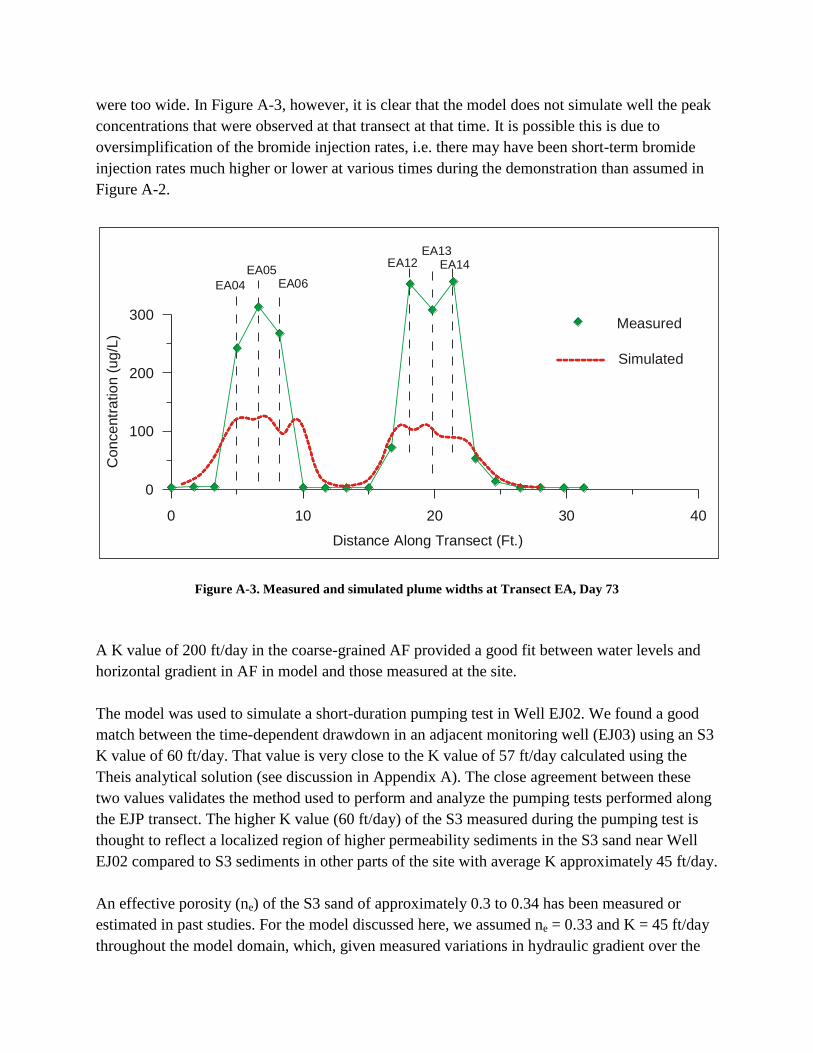
were too wide. In Figure A-3, however, it is clear that the model does not simulate well the peak
concentrations that were observed at that transect at that time. It is possible this is due to
oversimplification of the bromide injection rates, i.e. there may have been short-term bromide
injection rates much higher or lower at various times during the demonstration than assumed in
Figure A-2.
Figure A-3. Measured and simulated plume widths at Transect EA, Day 73
A K value of 200 ft/day in the coarse-grained AF provided a good fit between water levels and
horizontal gradient in AF in model and those measured at the site.
The model was used to simulate a short-duration pumping test in Well EJ02. We found a good
match between the time-dependent drawdown in an adjacent monitoring well (EJ03) using an S3
K value of 60 ft/day. That value is very close to the K value of 57 ft/day calculated using the
Theis analytical solution (see discussion in Appendix A). The close agreement between these
two values validates the method used to perform and analyze the pumping tests performed along
the EJP transect. The higher K value (60 ft/day) of the S3 measured during the pumping test is
thought to reflect a localized region of higher permeability sediments in the S3 sand near Well
EJ02 compared to S3 sediments in other parts of the site with average K approximately 45 ft/day.
An effective porosity (ne) of the S3 sand of approximately 0.3 to 0.34 has been measured or
estimated in past studies. For the model discussed here, we assumed ne = 0.33 and K = 45 ft/day
throughout the model domain, which, given measured variations in hydraulic gradient over the
EA04
EA05EA06
EA12EA13
EA14
0 10 20 30 40
Distance Along Transect (Ft.)
0
100
200
300
Co
nce
ntr
atio
n(u
g/L
)
Bromide Concentrations Along EA Transect -- Day 73.1
Simulated
Measured
Figure B-3. Measured and simulated plume widths at Transect EA; Day 73 (looking North)
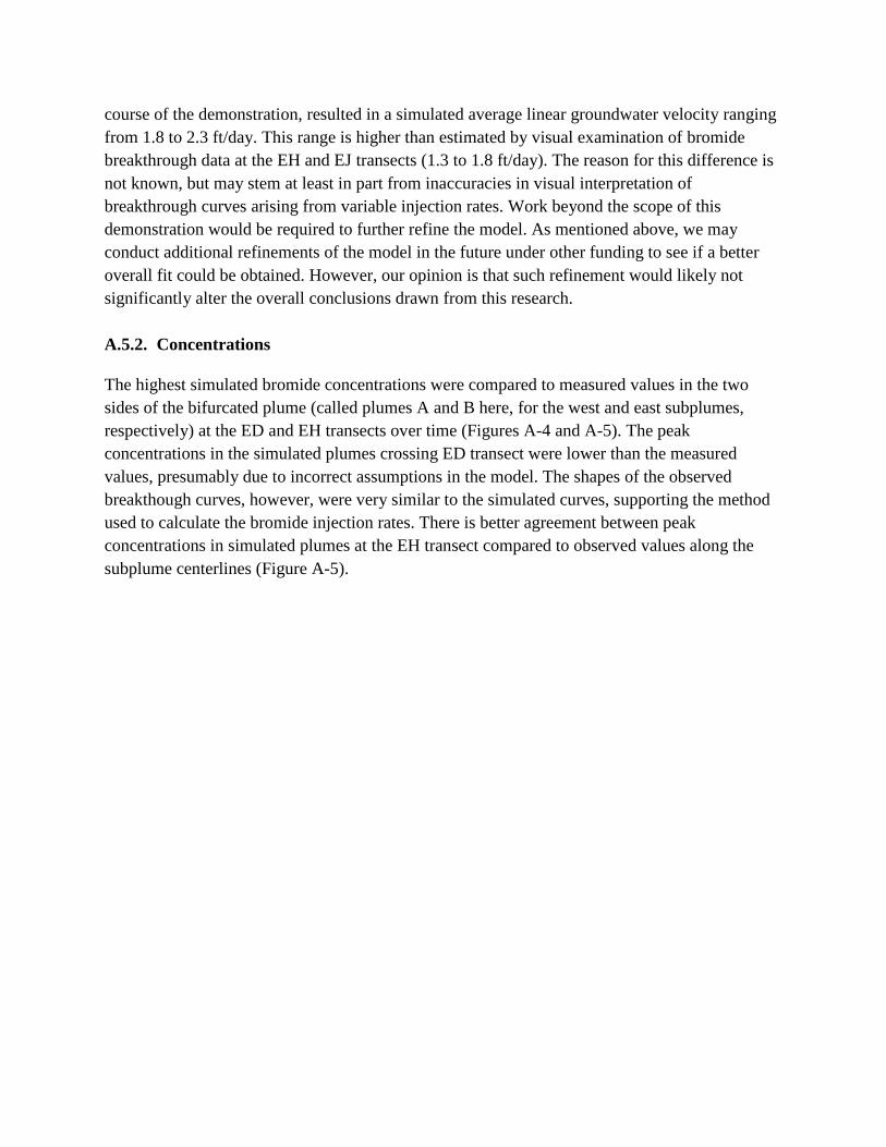
course of the demonstration, resulted in a simulated average linear groundwater velocity ranging
from 1.8 to 2.3 ft/day. This range is higher than estimated by visual examination of bromide
breakthrough data at the EH and EJ transects (1.3 to 1.8 ft/day). The reason for this difference is
not known, but may stem at least in part from inaccuracies in visual interpretation of
breakthrough curves arising from variable injection rates. Work beyond the scope of this
demonstration would be required to further refine the model. As mentioned above, we may
conduct additional refinements of the model in the future under other funding to see if a better
overall fit could be obtained. However, our opinion is that such refinement would likely not
significantly alter the overall conclusions drawn from this research.
A.5.2. Concentrations
The highest simulated bromide concentrations were compared to measured values in the two
sides of the bifurcated plume (called plumes A and B here, for the west and east subplumes,
respectively) at the ED and EH transects over time (Figures A-4 and A-5). The peak
concentrations in the simulated plumes crossing ED transect were lower than the measured
values, presumably due to incorrect assumptions in the model. The shapes of the observed
breakthough curves, however, were very similar to the simulated curves, supporting the method
used to calculate the bromide injection rates. There is better agreement between peak
concentrations in simulated plumes at the EH transect compared to observed values along the
subplume centerlines (Figure A-5).
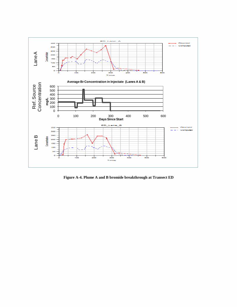
0
100
200
300
400
500
600
0 100 200 300 400 500 600
mg
/L
Days Since Start
Average Br Concentration in Injectate (Lanes A & B)
La
ne
AR
ef.
So
urc
e
Co
nce
ntr
atio
nL
an
e B
Figure A-4. Plume A and B bromide breakthrough at Transect ED
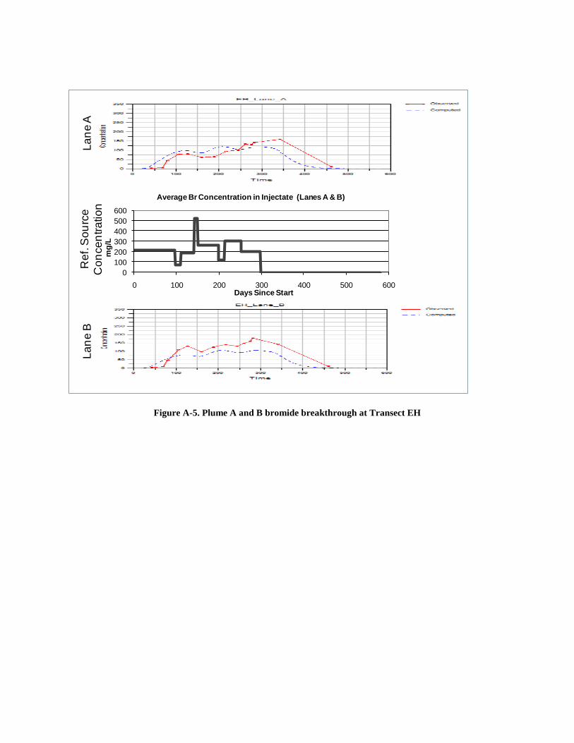
Figure A-5. Plume A and B bromide breakthrough at Transect EH
0
100
200
300
400
500
600
0 100 200 300 400 500 600
mg
/L
Days Since Start
Average Br Concentration in Injectate (Lanes A & B)
La
ne
BL
an
e A
Re
f. S
ou
rce
Co
nce
ntr
atio
n

Assumed dispersivity values of 11, 0.001, and 0.0001 (longitudinal, horizontal transverse, and
vertical transverse) provided good matches to plume widths (Figures A-6 and A-7) and
breakthrough at transect ED and EH (compare with Figures A-4 and A-5).
ED07
ED08
ED09 ED16
ED17
ED18
0 10 20 30 40
Distance Along Transect (Ft.)
0
100
200
300
Co
nce
ntr
atio
n(u
g/L
)
Bromide Concentrations Along ED Transect -- Day 461.4
Simulated
Measured
Figure B-6. Measured and simulated plume widths at Transect ED on Day 80 (looking North)
Figure A-6. Measured and simulated plume widths at Transect ED on Day 80
Simulated
Measured
EH16
EH17
EH18 EH24
EH25EH26
20 40 60 80
Distance Along Transect (ft.)
0
40
80
120
160
200
Co
ncen
tra
tion
(ug
/L)
Figure B-7. Measured and simulated plume widths at Transect EH on Day 244 (looking North)
Figure A-7. Measured and simulated plume widths at Transect EH on Day 244

A.5.3. Results and Mass Balance
A summary table of simulated mass discharge values versus mass discharge values measured
using the synoptic sampling method at Transects ED, EH, and EJ is listed in Table A-2 and
plotted in Figures A-8, A-9, and A-10, respectively. As can be seen in the plots, there is close
visual agreement between the simulated mass discharge values and those calculated using the
synoptic sampling method. The relationship between the two is examined more quantitatively in
Table A-2. As shown in that table, the percent error between the measured and simulated mass
discharge values for selected sampling events along Transects ED, EH, and EJ was 8%, 8%, and
2% (absolute errors of 13%, 20%, and 12%), respectively. Note that this comparison excludes
values during the breakthrough (rising) and elution (decreasing) periods of the bromide history;
the reason is to avoid comparisons that could be confounded by significant errors that could arise
from incorrect velocity, dispersion, or diffusion assumptions. Values used in the comparison are
highlighted in blue in Table A-2.
Table A-2. Mass discharge simulated and measured using synoptic
sampling method at Transects ED, EH and EJ
Sim Meas % Difference Sim Calc % Difference Sim Calc % Difference
80 121 113 -6.6% 67 54 -20.1% 52 18 -66.4%
106 114 100 -12.2% 112 97 -13.9% 93 59 -36.6%
128 93 114 23.1% 117 132 12.5% 111 80 -28.2%
160 161 160 -0.2% 113 146 29.4% 126 143 13.7%
190 145 136 -6.4% 137 157 15.0% 126 122 -3.7%
218 106 130 21.7% 141 124 -11.9% 141 118 -15.8%
244 149 149 0.4% 126 108 -14.5% 133 115 -14.0%
276 127 150 18.6% 125 134 6.5% 125 122 -2.4%
282 114 150 31.2% 113 140 23.6% 101 133 31.6%
342 25 7 -71.6% 112 170 52.4% 130 135 3.3%
461 0 9 3 20 6 43
582 0 0 0 0 0 18
Average difference for highlighted days 8% 8% 2%
Sim= Simulated mass discharge flowing through transect
EH EJDay
ED

0 100 200 300 400 500 600 700Days
0
40
80
120
160
200M
d (
gra
ms/d
ay)
Simulated
Synoptic Sampling Method
Figure B-8. Calculated and simulated bromide mass discharge crossing Transect ED
Figure A-8. Calculated and simulated bromide mass discharge crossing Transect ED
0 100 200 300 400 500 600 700Days
0
40
80
120
160
200
Md
(g
ram
s/d
ay)
Simulated
Synoptic Sampling Method
Figure B-9. Calculated and simulated bromide mass discharge crossing Transect EH
Figure A-9. Calculated and simulated bromide mass discharge crossing Transect EH
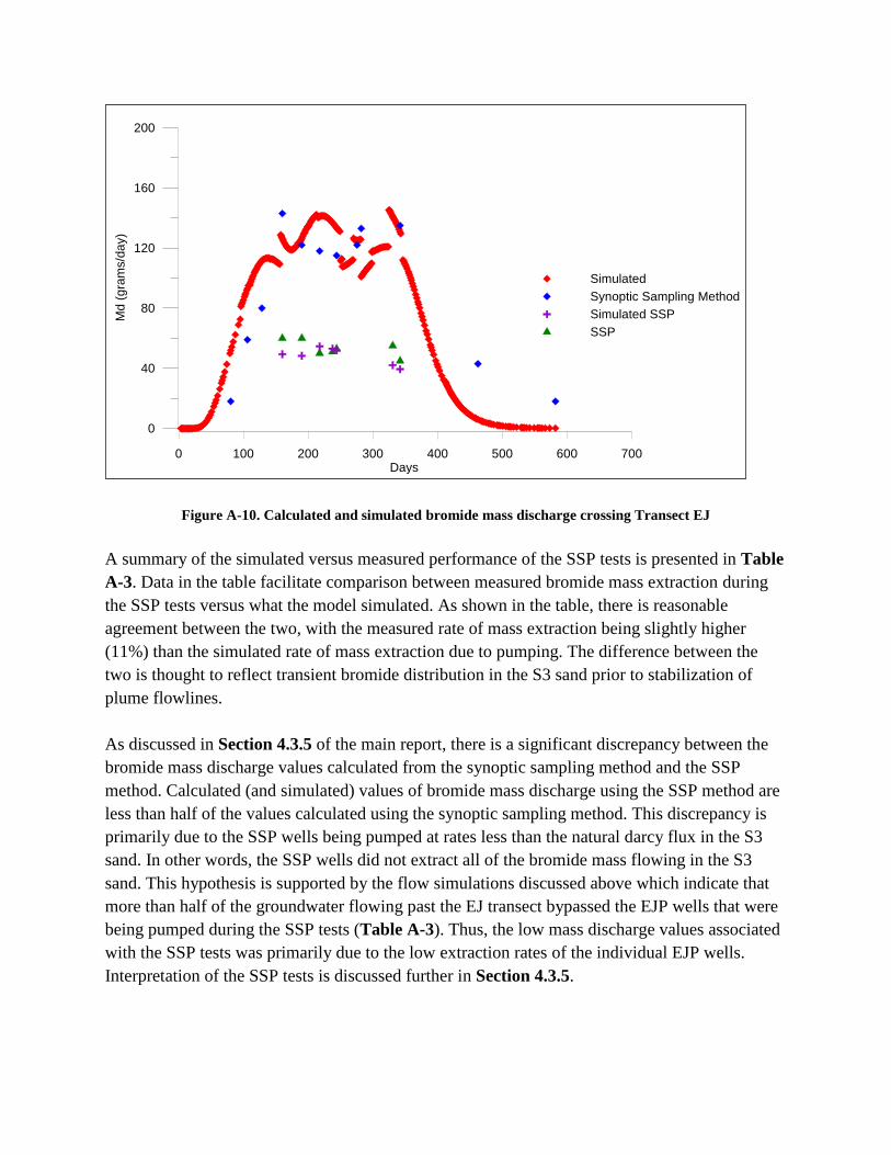
0 100 200 300 400 500 600 700Days
0
40
80
120
160
200M
d (
gra
ms/d
ay)
Simulated
Synoptic Sampling Method
Simulated SSP
SSP
Figure B-10. Calculated and simulated bromide mass discharge crossing Transect EJ
Figure A-10. Calculated and simulated bromide mass discharge crossing Transect EJ
A summary of the simulated versus measured performance of the SSP tests is presented in Table
A-3. Data in the table facilitate comparison between measured bromide mass extraction during
the SSP tests versus what the model simulated. As shown in the table, there is reasonable
agreement between the two, with the measured rate of mass extraction being slightly higher
(11%) than the simulated rate of mass extraction due to pumping. The difference between the
two is thought to reflect transient bromide distribution in the S3 sand prior to stabilization of
plume flowlines.
As discussed in Section 4.3.5 of the main report, there is a significant discrepancy between the
bromide mass discharge values calculated from the synoptic sampling method and the SSP
method. Calculated (and simulated) values of bromide mass discharge using the SSP method are
less than half of the values calculated using the synoptic sampling method. This discrepancy is
primarily due to the SSP wells being pumped at rates less than the natural darcy flux in the S3
sand. In other words, the SSP wells did not extract all of the bromide mass flowing in the S3
sand. This hypothesis is supported by the flow simulations discussed above which indicate that
more than half of the groundwater flowing past the EJ transect bypassed the EJP wells that were
being pumped during the SSP tests (Table A-3). Thus, the low mass discharge values associated
with the SSP tests was primarily due to the low extraction rates of the individual EJP wells.
Interpretation of the SSP tests is discussed further in Section 4.3.5.
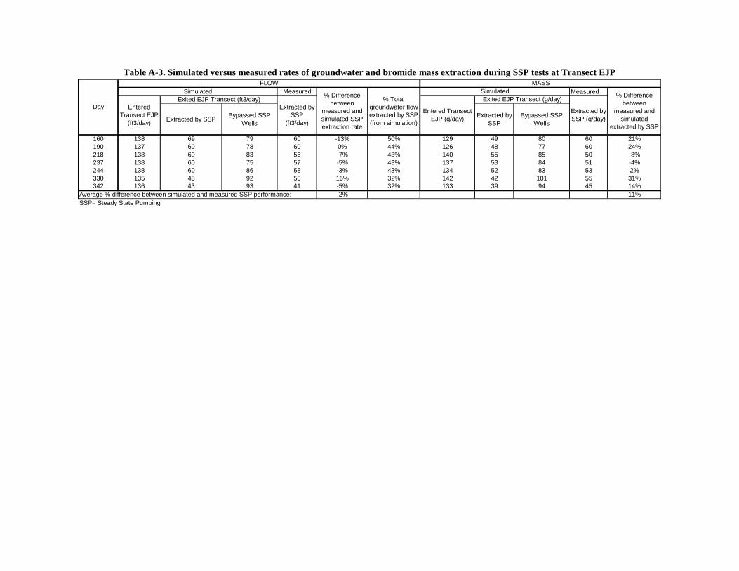
Table A-3. Simulated versus measured rates of groundwater and bromide mass extraction during SSP tests at Transect EJP
Measured Measured
Extracted by SSPBypassed SSP
Wells
Extracted by
SSP
Bypassed SSP
Wells
160 138 69 79 60 -13% 50% 129 49 80 60 21%
190 137 60 78 60 0% 44% 126 48 77 60 24%
218 138 60 83 56 -7% 43% 140 55 85 50 -8%
237 138 60 75 57 -5% 43% 137 53 84 51 -4%
244 138 60 86 58 -3% 43% 134 52 83 53 2%
330 135 43 92 50 16% 32% 142 42 101 55 31%
342 136 43 93 41 -5% 32% 133 39 94 45 14%
Average % difference between simulated and measured SSP performance: -2% 11%
SSP= Steady State Pumping
% Difference
between
measured and
simulated SSP
extraction rate
Simulated
Exited EJP Transect (g/day)
Extracted by
SSP
(ft3/day)
Entered
Transect EJP
(ft3/day)
Exited EJP Transect (ft3/day)
Entered Transect
EJP (g/day)
Day
MASSFLOW
Simulated
% Total
groundwater flow
extracted by SSP
(from simulation)
Extracted by
SSP (g/day)
% Difference
between
measured and
simulated
extracted by SSP
Appendix B
Post-Demonstration Testing of Recirculation Flux Measurement
Method
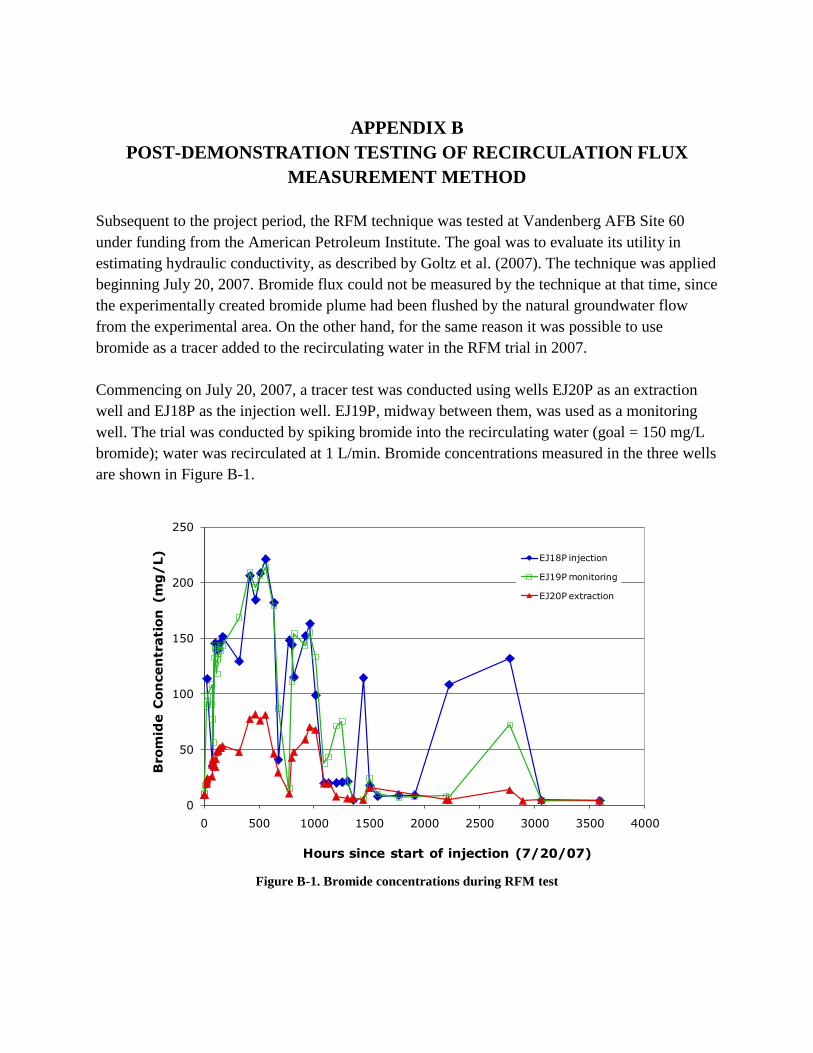
APPENDIX B
POST-DEMONSTRATION TESTING OF RECIRCULATION FLUX
MEASUREMENT METHOD
Subsequent to the project period, the RFM technique was tested at Vandenberg AFB Site 60
under funding from the American Petroleum Institute. The goal was to evaluate its utility in
estimating hydraulic conductivity, as described by Goltz et al. (2007). The technique was applied
beginning July 20, 2007. Bromide flux could not be measured by the technique at that time, since
the experimentally created bromide plume had been flushed by the natural groundwater flow
from the experimental area. On the other hand, for the same reason it was possible to use
bromide as a tracer added to the recirculating water in the RFM trial in 2007.
Commencing on July 20, 2007, a tracer test was conducted using wells EJ20P as an extraction
well and EJ18P as the injection well. EJ19P, midway between them, was used as a monitoring
well. The trial was conducted by spiking bromide into the recirculating water (goal = 150 mg/L
bromide); water was recirculated at 1 L/min. Bromide concentrations measured in the three wells
are shown in Figure B-1.
0
50
100
150
200
250
0 500 1000 1500 2000 2500 3000 3500 4000
Bro
mid
e C
on
cen
trati
on
(m
g/
L)
Hours since start of injection (7/20/07)
EJ18P injection
EJ19P monitoring
EJ20P extraction
Figure B-1. Bromide concentrations during RFM test

Ideally, a constant concentration of bromide would have been injected at EJ18P, and steady-state
concentrations observed in the water extracted at EJ20P. Unfortunately, due to operational
difficulties, bromide concentrations at both the injection and extraction wells varied in time.
However, it was possible to identify several periods (100 to 170 hours, 415 to 560 hours, and 770
to 960 hours) where steady-state injection and extraction concentrations appear to have been
obtained. Based on concentration measurements made during these three “steady-state” periods,
it was determined that approximately 37% of the water extracted at well EJ20P originated at well
EJ18P (termed “interflow”). Using this value of interflow between the two wells, and assuming
two-dimensional flow between the wells, model analysis estimated an aquifer hydraulic
conductivity of 154 ft/d (47 m/d). Note that this is significantly greater than the hydraulic
conductivity of 45 ft/d (12.8 m/d) estimated from the hydraulic testing described in Appendix A.
The reasons for the discrepancy are not known, but one likelihood is that the hydraulic
conductivity heterogeneity within the S3 sand is sufficient to confound the interpretation of the
results we gained from our non-ideal application of the RFM technique. More work would be
needed to conduct a more ideal trial of the method, and thus to evaluate its applicability for
estimating hydraulic conductivity at this or other sites.

Appendix C
Insights from Initial Research at Site 19, Vandenberg Air Force
Base, CA
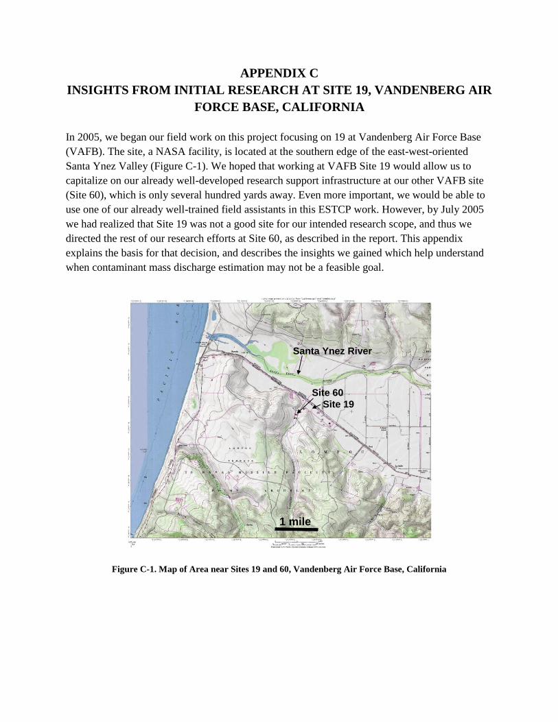
APPENDIX C
INSIGHTS FROM INITIAL RESEARCH AT SITE 19, VANDENBERG AIR
FORCE BASE, CALIFORNIA
In 2005, we began our field work on this project focusing on 19 at Vandenberg Air Force Base
(VAFB). The site, a NASA facility, is located at the southern edge of the east-west-oriented
Santa Ynez Valley (Figure C-1). We hoped that working at VAFB Site 19 would allow us to
capitalize on our already well-developed research support infrastructure at our other VAFB site
(Site 60), which is only several hundred yards away. Even more important, we would be able to
use one of our already well-trained field assistants in this ESTCP work. However, by July 2005
we had realized that Site 19 was not a good site for our intended research scope, and thus we
directed the rest of our research efforts at Site 60, as described in the report. This appendix
explains the basis for that decision, and describes the insights we gained which help understand
when contaminant mass discharge estimation may not be a feasible goal.
Santa Ynez River
1 mile
Site 60
Site 19
Figure D-1. Map of area near Sites 19 and 60 at
Vandenberg AFB, CA
Figure C-1. Map of Area near Sites 19 and 60, Vandenberg Air Force Base, California
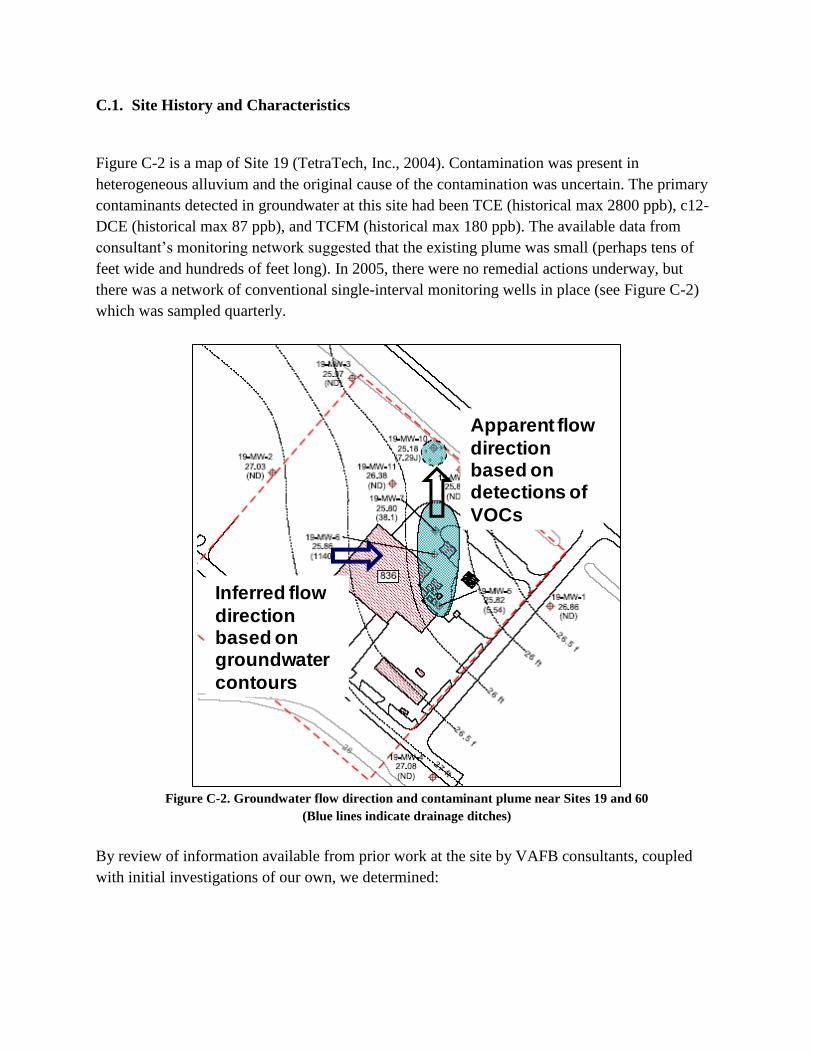
C.1. Site History and Characteristics
Figure C-2 is a map of Site 19 (TetraTech, Inc., 2004). Contamination was present in
heterogeneous alluvium and the original cause of the contamination was uncertain. The primary
contaminants detected in groundwater at this site had been TCE (historical max 2800 ppb), c12-
DCE (historical max 87 ppb), and TCFM (historical max 180 ppb). The available data from
consultant’s monitoring network suggested that the existing plume was small (perhaps tens of
feet wide and hundreds of feet long). In 2005, there were no remedial actions underway, but
there was a network of conventional single-interval monitoring wells in place (see Figure C-2)
which was sampled quarterly.
Apparent flow
direction based on detections of
VOCs
Inferred flow
direction based on groundwater
contours
Figure C-2. Groundwater flow direction and contaminant plume near Sites 19 and 60
(Blue lines indicate drainage ditches)
By review of information available from prior work at the site by VAFB consultants, coupled
with initial investigations of our own, we determined:
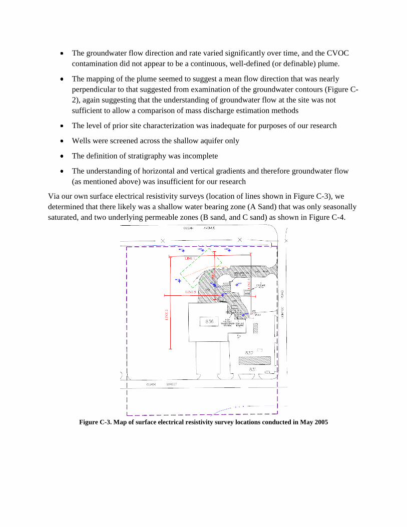
The groundwater flow direction and rate varied significantly over time, and the CVOC
contamination did not appear to be a continuous, well-defined (or definable) plume.
The mapping of the plume seemed to suggest a mean flow direction that was nearly
perpendicular to that suggested from examination of the groundwater contours (Figure C-
2), again suggesting that the understanding of groundwater flow at the site was not
sufficient to allow a comparison of mass discharge estimation methods
The level of prior site characterization was inadequate for purposes of our research
Wells were screened across the shallow aquifer only
The definition of stratigraphy was incomplete
The understanding of horizontal and vertical gradients and therefore groundwater flow
(as mentioned above) was insufficient for our research
Via our own surface electrical resistivity surveys (location of lines shown in Figure C-3), we
determined that there likely was a shallow water bearing zone (A Sand) that was only seasonally
saturated, and two underlying permeable zones (B sand, and C sand) as shown in Figure C-4.
Figure C-3. Map of surface electrical resistivity survey locations conducted in May 2005
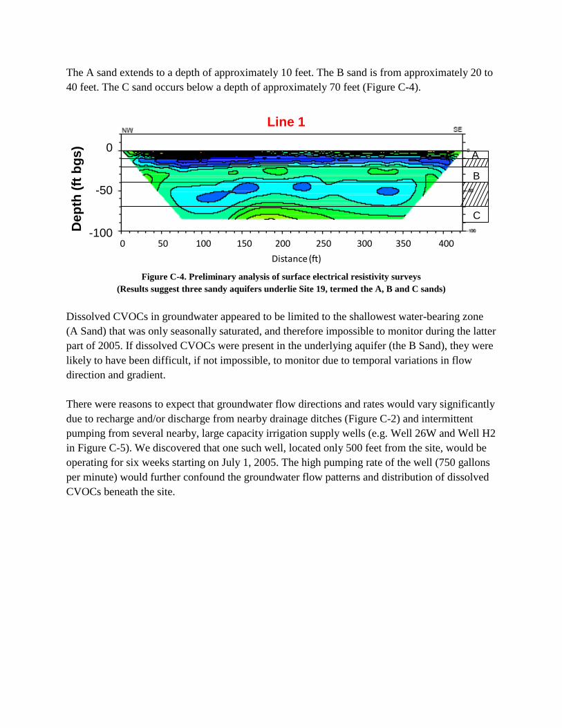
The A sand extends to a depth of approximately 10 feet. The B sand is from approximately 20 to
40 feet. The C sand occurs below a depth of approximately 70 feet (Figure C-4).
A
B
C
A
B
C
Line 1
0
-50
-100De
pth
(ft
bg
s)
Figure D-4. Preliminary analysis of surface electrical resistivity surveys suggest 3
sandy aquifers underlie Site 19, which we term the A, B and C sands.
0 50 100 150 200 250 300 350 400
Distance (ft)
Figure C-4. Preliminary analysis of surface electrical resistivity surveys
(Results suggest three sandy aquifers underlie Site 19, termed the A, B and C sands)
Dissolved CVOCs in groundwater appeared to be limited to the shallowest water-bearing zone
(A Sand) that was only seasonally saturated, and therefore impossible to monitor during the latter
part of 2005. If dissolved CVOCs were present in the underlying aquifer (the B Sand), they were
likely to have been difficult, if not impossible, to monitor due to temporal variations in flow
direction and gradient.
There were reasons to expect that groundwater flow directions and rates would vary significantly
due to recharge and/or discharge from nearby drainage ditches (Figure C-2) and intermittent
pumping from several nearby, large capacity irrigation supply wells (e.g. Well 26W and Well H2
in Figure C-5). We discovered that one such well, located only 500 feet from the site, would be
operating for six weeks starting on July 1, 2005. The high pumping rate of the well (750 gallons
per minute) would further confound the groundwater flow patterns and distribution of dissolved
CVOCs beneath the site.
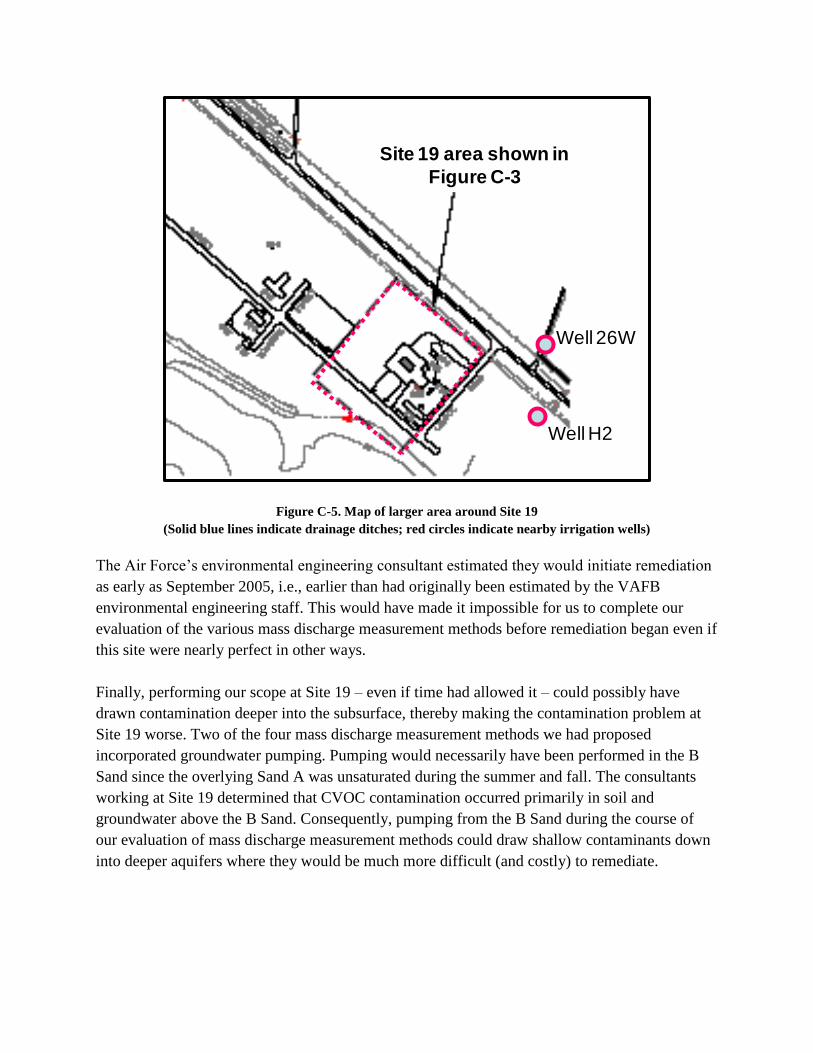
Well 26W
Well H2
Site 19 area shown in
Figure C-3
Figure C-5. Map of larger area around Site 19
(Solid blue lines indicate drainage ditches; red circles indicate nearby irrigation wells)
The Air Force’s environmental engineering consultant estimated they would initiate remediation
as early as September 2005, i.e., earlier than had originally been estimated by the VAFB
environmental engineering staff. This would have made it impossible for us to complete our
evaluation of the various mass discharge measurement methods before remediation began even if
this site were nearly perfect in other ways.
Finally, performing our scope at Site 19 – even if time had allowed it – could possibly have
drawn contamination deeper into the subsurface, thereby making the contamination problem at
Site 19 worse. Two of the four mass discharge measurement methods we had proposed
incorporated groundwater pumping. Pumping would necessarily have been performed in the B
Sand since the overlying Sand A was unsaturated during the summer and fall. The consultants
working at Site 19 determined that CVOC contamination occurred primarily in soil and
groundwater above the B Sand. Consequently, pumping from the B Sand during the course of
our evaluation of mass discharge measurement methods could draw shallow contaminants down
into deeper aquifers where they would be much more difficult (and costly) to remediate.

C.2. Advantages of shifting research to Site 60 Vandenberg AFB
Performing the evaluation at VAFB Site 60 allowed us to safely compare all four methods of
measuring contaminant mass discharge, including pumping techniques that would have created
an unacceptable risk of cross-contamination at Site 19.
The comparisons were performed under much more controlled conditions at VAFB Site 60 than
would have been possible at Site 19. This was due to the high level of understanding of the
subsurface conditions that our team already had at Site 60 and the existing detailed grid of
monitoring points already in place at the site. In addition, we perform a continuous injection of a
non-reactive tracer at Site 60 to provide a much-needed control for the experiment. The results of
each mass discharge measurement method were therefore compared to the mass discharge of the
tracer in order to estimate the absolute accuracy and precision of each method, not just the
similarity of the methods to one another. We reasoned that this would result in a technically-
superior, more rigorous comparison of the methods than would have been possible if the
comparison was performed at Site 19.
We could easily and inexpensively install additional wells or devices we might need for
conducting or evaluating the pumping-based mass discharge estimation methods.
We had a dedicated field team stationed at Site 60 that was familiar with the injection and
monitoring systems at the site, so startup would be much smoother than would be the case at any
other site.
C.3. Value to be derived from preliminary work at Site 19 Vandenberg AFB
Our experience working at Site 19 gave us practical insights to add to our final report (Section 4)
regarding the conditions and prerequisite site characterization necessary to successfully
implement each of the four mass discharge measurement methods.
Appendix D
Hydraulic Testing Along EJP Transect

APPENDIX D
HYDRAULIC TESTING ALONG EJP TRANSECT
Hydraulic tests were performed in each of the wells in the EJP (i.e., Wells EJ01P through EJ23P)
in the spring of 2006. Prior to performing the constant discharge tests, water levels were
measured in all of the pumping wells (i.e., the fully-screened “P” wells and many nearby
monitoring wells in order to establish baseline, pre-test conditions. Next, pumping tests were
performed sequentially in each of the fully screened wells in the EJP transect. Prior to starting
each of the tests, pressure transducers (Solinst Leveloggers™) were inserted into the pumping
well and the two “P” wells east of the pumping well (e.g., Wells EJ03P and EJ04P in the test
where Well EJ02P was pumped). Collection of time-drawdown data in observation wells located
at two different distances from the pumping well facilitated calculation of aquifer transmissivity
using a steady-state, distance-drawdown analytical solution (i.e., analytical method described by
Thiem [1906]). Following insertion of the pressure transducers, water levels were monitored and
allowed to return to baseline levels before starting the extraction tests.
The wells were pumped at constant rates using a peristaltic pump equipped with a 3/8 inch-OD
polyethylene suction tube. Flow rates were measured using a graduated cylinder and stop watch.
Groundwater pumped from the aquifer was stored on site. Pumping rates during the tests ranged
from 80 to 2,880 mL/min (Table D-1). Because of the short distance between the static water
levels (piezometric heads) in the pumping wells and the top of the S3 sand (approximately 1.5 to
2.5 feet, depending on the well), care was taken to ensure that water levels in the pumping wells
never dropped below the top of the S3 sand. Allowing the water level in the S3 sand to drop
below the top of the unit would have complicated analysis of the data by creating a condition that
was transitional between a confined and unconfined system. To avoid this, the end of the suction
tube was always placed at a depth above the top of the well screens (which is coincident with or
above the top of the S3 sand). That way, the well would dewater and water levels would not
inadvertently be drawn below the top of the S3 sand. This happened several times during the
testing program. When it did, the test was terminated and the aquifer was allowed to recover.
The test was then repeated at a lower extraction rate. Table D-1 presents a summary of pertinent
data for the constant discharge pumping tests.
Using the pressure transducers and data logger, water levels in the wells were measured and
recorded at one second intervals during the tests. At the end of each day, the electronic data were
downloaded to a computer and drawdown values were calculated in a spreadsheet by subtracting
the water pressure measured by the pressure transducers (converted to feet of water) from the
starting, pre-test water level.
The electronic data files were then exported into an aquifer test analysis program (Waterloo
Hydrogeologic AquiferTest Pro Version 3.5) to simplify the data analysis. The analytical
solutions deemed most appropriate for the test data are the Theis solution (Theis, 1935) and the
Cooper-Jacob approximation method for confined aquifers (Cooper and Jacob, 1946). Both
analytical solutions are appropriate for the S3 sand, which is hydraulically confined by
approximately 7 to 8 feet of silt and clay. Both analytical solutions can be used to calculate
aquifer transmissivity using data from the pumping well and the observation wells. However,
aquifer coefficients calculated using data from observation wells are considered to be more
accurate than those using data from pumping wells due to (1) additional head losses in the
pumping wells caused by high entrance velocities and (2) mathematical sensitivity of the
analytical solutions to the distance term in both the Theis and Cooper-Jacob equations
(Kruseman and de Ridder, 1989). In addition, values of aquifer storativity cannot be determined
using data from pumping wells; time-drawdown data in observation wells are necessary for
calculating aquifer storage coefficients. When the Cooper-Jacob curve-matching method was
used, early drawdown data were ignored if they violated the assumptions of the Cooper-Jacob
approximation technique. This was done following the method described by Driscoll (1986).
Finally, times when casing storage became insignificant were calculated for each test. This was
done using the technique described by Schafer (1978). Time-drawdown data collected before
times when casing storage became insignificant (15 to 20 seconds in the worst cases) were
omitted from the subsequent curve-matching analyses.
During the specific capacity tests and the constant discharge pumping tests, drawdown in the
pumping wells and observation wells (pumping tests only) reached quasi-steady state conditions
after just a few minutes. Marked slowdown in the rate of drawdown in the wells, in particular the
pumping wells, was also apparent in log-log plots of data used in the Theis analyses and in the
semi-log plots of data used in the Cooper-Jacob analyses. In confined aquifers, this condition is
most often due to a positive hydraulic boundary such as aquifer recharge. In the tests performed
in the study area, however, there were no sources of hydraulic recharge during the tests. Rather,
the “recharge” condition indicated in the pumping test data is simply the result of the cones of
depression expanding to the point at which the rate of groundwater extraction was matched by
the natural volumetric flux of groundwater being captured by the pumped well. This recharge
condition violates the assumptions of both the Theis and Cooper-Jacob analytical solutions.
Fortunately, the time when the drawdown data begin to show the effects of recharge caused by
ambient aquifer flow can be easily identified in log-log and semi-log plots of the time-drawdown
data. Only time-drawdown data collected prior to the onset of the “recharge condition” were
therefore used in the analyses. Finally, even though several pumping tests were performed in
several wells where drawdown data were collected in two observation wells located at different
distances from the pumping well, only two data sets, from the tests performed in Wells EJ02P
and EJ08P, were appropriate for performing distance-drawdown analyses. This was because the
amount of drawdown in the wells furthest from the pumping wells (i.e., 5 feet away) usually did
not show sufficient drawdown to exceed the threshold resolution of the pressure transducers used
to record the pressure changes in the wells.
Table D-1 lists key data, assumptions, results, and comments from the pumping tests performed
during this study. Output plots of the curve-matching analyses performed using the AquiferTest
Pro® software are included at the end of this Appendix. Those plots show log-log time-
drawdown data and Theis curve match points for the pumping well and the two wells
immediately to the east of the pumping well. The aquifer coefficients calculated by the software
program are shown at the bottom of the plots. Those values are the source of the aquifer
coefficients listed on Table D-1.
Note that there are several values of hydraulic conductivity highlighted in pink in Table D-1.
Those values are considered to be the most reliable estimates of K because of the quality of the
data used to perform the analyses (e.g., amount of drawdown, compliance with assumptions of
the analytical method, etc.). There are several tests listed in Table D-1 that are not considered to
be representative of the hydraulic properties of the S3 sand, even though K values were
calculated and are listed in Table D-1. Those tests, the results of which yielded lower estimates
of K, are thought to be negatively biased because the wells were pumped at very low rates which
did not adequately stress the S3 sand aquifer.
References
Cooper, H.H.Jr. and C.E. Jacob. 1946. A generalized graphical method for evaluating formation constants
and summarizing well field history. Transactions, American Geophysical Union 27, no. 4.
Driscoll, F.G. 1986. Groundwater and Wells. Edited by Driscoll, F.G. Second ed. Minneapolis: Johnson
Division. 1089 pp.
Kruseman, G.P. and N.A. de Ridder. 1990. Analysis and Evaluation of Pumping Test Data. Second ed.:
International Institute for Land Reclamation and Improvement. 377 pp.
Schafer, D.C. 1978. Casing storage can affect pumping test data. Johnson Drillers' Journal, no. Jan/Feb.
Theis, C.V. 1935. The relation between the lowering of the piezometric surface and the rate and duration
of discharge of a well using ground water storage. Transactions, American Geophysical Union: 518-
524.
Thiem, G. 1906. Hydrologische methoden. Leipzig. 56 pp.
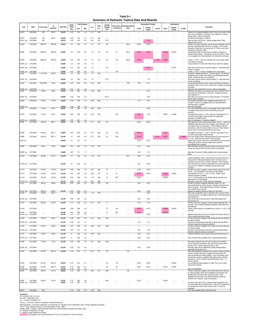
Sec Min TheisCooper-
JacobCJ DD Theis
Cooper-
JacobCJ DD
EJ01P 3/24/2006 180 68.47 EJ01P 4.42 194 3.2 0.17 168 -- -- -- -- -- -- -- -- -- Reason for increased drawdown after 100 sec not known. Most
likely due to variability in extraction rate. Opposite of casing
storage effect. Data not analyzed.
EJ01P 3/24/2006 180 68.47 EJ02P 4.42 194 3.2 0.17 168 -- -- -- -- -- -- -- -- -- Not enough drawdown to analyze.
EJ01P_rec 3/24/2006 NA EJ01P 4.42 146 2.4 NA NA 30 (?) -- -- -- 0.76 -- -- -- -- Slow recovery until 30 sec. Casing storage effect? Data
analyzed after 30 sec.
EJ02P 3/24/2006 2880.00 1095.55 EJ02P 4.3 294 4.9 1.6 172 64 -- None 28.00 32.00 -- -- -- -- Schafer calculation suggests casing storage negligable after 64
seconds. Used data after that time in analysis. Low K value
because of head loss in pumping well (?). Theis curve match
insensitive to late-time data.
EJ02P 3/24/2006 2880.00 1095.55 EJ03P 4.3 294 4.9 1.6 172 64 21 None 57.00 74.00 -- 0.0043 0.0022 -- Analyzed data after 64 seconds per Schafer calculation of
casing storage effects. Comparison of late time data to Theis
curve suggests late time drawdown not reduced by recharge.
EJ02P 3/24/2006 2880.00 1095.55 EJ04P 4.47 294 4.9 1.6 172 50 143 None 48.00 -- 74.00 0.0042 -- -- t when u < 0.05 = 143 sec, therefore can't use Cooper Jacob
time-distance analysis.
EJ02P_rec 3/24/2006 -- -- EJ02P 4.3 230 3.8 1.6 -- -- -- -- -- -- -- -- -- -- Large oscilation in water level after 20 sec. Data not useable.
EJ02P_rec 3/24/2006 -- -- EJ03P 4.3 230 3.8 1.6 -- 60 -- -- -- 59.00 -- -- 0.0041 -- Slow early recovery due to casing storage (?). Used data after
60 sec in analysis.
EJ02P_rec 3/24/2006 -- -- EJ04P 4.47 230 3.8 1.6 -- -- 143 -- -- -- -- -- -- -- t when u < 0.05 = 143 sec, therefore can't use analysis.
EJ03P 3/24/2006 11/10/1901 258.67 EJ03P 4.3 294 4.9 1.9 246 -- -- -- -- -- -- -- -- -- Drawdown stopped abruptly at 1.9 feet at approx. 30 seconds.
Suggests pump intake at that depth and well dewatered after
30 sec. Drawdown data not analyzable.
EJ03P_rec 3/24/2006 -- -- EJ03P 4.3 236 3.9 1.9 -- 15 (?) -- -- -- 1.10 -- -- -- -- Slow early recovery due to casing storage (?). Used data after
15 sec in analysis.
EJ04P 3/24/2006 5/29/1900 57.06 EJ04P 4.47 296 4.9 0.34 280 -- -- 100 1.50 2.10 -- -- -- -- Low pumping rate didn't stress aquifer significantly. Reduced
drawdown after 100 sec due to natural flux in aquifer (recharge
boundary).
EJ04P_rec 3/24/2006 -- -- EJ04P 4.47 30 0.5 -- -- -- -- -- -- -- -- -- -- -- Recovery only monitored for 30 sec. Data not analyzable.
EJ05P 3/24/2006 180.00 68.47 EJ05P 4.45 296 4.9 1.99 286 -- -- -- -- 0.22 -- -- -- -- Significant drawdown in pumping well at low extraction rate. V.
small amount of drawdown in obs well. Suggests pumping
well inefficient (?).
EJ05P_rec 3/24/2006 -- -- EJ05P 4.45 378 6.3 -- -- 95 (?) -- -- -- 0.33 -- -- -- -- Slow early time recovery due to casing storage (?). Data after
90 sec used in analysis.
EJ06P 3/24/2006 370.00 140.75 EJ06P 4.58 296 4.9 0.62 286 -- -- -- 1.70 3.50 -- -- -- -- Poor quality drawdown data. Suggests pumping rate not
constant. Theis curve suggests late time data affected by
recharge (flow in aquifer).
EJ06P_rec -- EJ06P 4.58 108 1.8 -- -- -- -- -- -- -- -- -- -- -- Data not analyzable
EJ07P 3/24/2006 170.00 64.67 EJ07P 4.75 296 4.9 0.92 292 -- -- -- -- 0.59 -- -- -- -- Low rate of drawdown early in test possibly due to adjustments
to extraction rate (suction tube of peristaltic pump not
primed?).
EJ07P 3/24/2006 170.00 64.67 EJ09P 4.67 296 4.9 0.92 292 -- 255 -- 5.80 7.00 -- 0.0007 0.0006 -- Calculated time when u < 0.05 = 255 sec. Calculated K & S
not valid using Cooper Jacob method. No significant
drawdown in EJ08P (why?).
EJ07P_rec 3/24/2006 -- -- EJ07P 4.75 98 1.6 -- -- -- -- -- -- -- -- -- -- -- Data not analyzable. Transducer slipped?
EJ08P 3/27/2006 1525.00 580.11 EJ08P 4.64 294 4.9 0.77 262 53 -- -- 29.00 29.00 -- -- -- -- Calculated time when well storage ended = 53 sec. Used time
drawdown data after that time in Cooper Jacob analysis. Low
calculated K due to well losses(?). Theis analysis relatively
insensitive to late-time data. Shape of curve in Theis analysis
doesn't point to recharge affecting late time data.
EJ08P 3/27/2006 1525.00 580.11 EJ09P 4.67 294 4.9 0.77 262 53 160 -- 29.00 -- -- 0.02 -- -- Calculated time when u < 0.05 = 160 sec. Calculated K & S
not valid using Cooper Jacob method.
EJ08P 3/27/2006 1525.00 580.11 EJ10P 4.7 294 4.9 0.77 262 53 630 -- 41.00 -- 61.00 0.0077 -- 0.0060 Can't use Cooper Jacob method because not long enough for
u < 0.05. Used late time date for Theis analysis.
EJ08_rec -- EJ08P 4.7 84 1.4 -- -- -- -- -- 16.00 27.00 -- -- -- -- Rapid initial recovery likely due to discharge from pump tubing.
"Recharge" at end of recovery likely due to ambient
groundwater flow in aquifer.
EJ09P 3/27/2006 80.00 30.43 EJ09P 4.67 294 4.9 0.35 278 -- -- -- 0.70 0.80 -- -- -- -- Slow drawdown during early part of test may be due to pump
tubing not being primed. Obs well data not analyzable.
EJ09P_rec 3/27/2006 -- -- EJ09P 4.67 70 1.2 -- -- -- -- -- 1.40 1.70 -- -- -- -- Slow rate of recovery initially possibly due to casing storage
effect.
EJ10P 3/27/2006 250.00 95.10 EJ10P 4.7 296 4.9 1.42 278 -- -- 130+- 0.39 0.45 -- -- -- --Delayed drawdown early in test likely due to pump tubing not
being primed. Reduced drawdown late in test likely due to
recharge caused by flow in aquifer (based on Theis analysis).
EJ10P_rec 3/27/2006 -- -- EJ10P 4.7 336 5.6 -- -- -- -- -- 0.61 0.68 -- -- -- -- Slow recovery may be due to discharge from pump tube after
pump shut off. Reason for delayed recovery late in test
unknown.
EJ11P 3/27/2006 510.00 194.00 EJ11P 4.88 296 4.9 0.37 284 70 -- -- 15.00 15.00 -- -- -- -- Schafer calculation suggests casing storage insignificant after
70 sec.. Low calculated K may be due to well losses.
EJ11P 3/27/2006 510.00 194.00 EJ12P 5.02 296 4.9 0.39 272 70 81 -- 27.00 29.00 -- 0.0034 0.0030 -- Calculated time when u < 0.05 = 81 sec. Cooper Jacob
analysis therefore unreliable.
EJ11P 3/27/2006 510.00 194.00 EJ13P 5.05 296 4.9 1.13 196 70 324 -- 34.00 -- -- 0.0054 -- -- t for u < 0.05 too large to use Cooper Jacob methods. Few
data points for Theis analysis.
EJ11P_rec 3/27/2006 -- -- EJ11P 4.88 116 1.9 0.37 284 -- -- -- -- -- -- -- -- -- Recovery in less than 15 sec. Data not analyzable.
EJ12P 3/27/2006 260.00 98.90 EJ12P 5.02 296 4.9 0.39 272 160 -- -- 5.00 6.00 -- -- -- -- Schafer calculation suggests drawdown data up to 160
seconds affected by casing storage. Therefore used late time
data in analysis. Theis analysis doesn't identify "recharge"
from ambient flow in aquifer.
EJ12P_rec 3/27/2006 260.00 98.90 EJ12P 5.02 296 4.9 -- -- -- -- -- 3.20 3.00 Reason for delayed recovery at late time not known.
EJ13P 3/27/2006 180.00 68.47 5.05 296 4.9 1.13 196 -- -- -- -- 0.90 -- -- -- -- Slow rate of drawdown early in test likely due to pump tubing
not being primed. Increased drawdown late in test likely due to
flow adjustment.
EJ13P_rec 3/27/2006 -- -- EJ13P 5.05 240 4.0 -- -- -- -- -- 0.50 0.50 -- -- -- -- Slow initial rate of recovery due to water discharging from
pump tubing (?).
EJ14P 3/27/2006 520.00 197.81 EJ14P 5.17 296 4.9 0.37 264 77 17.00 17.30 Schafer calculation suggests casing storage negligible after 77
seconds. Theis analysis relatively insensitive since early time
data ignored.
EJ14P 3/27/2006 -- -- EJ15P 4.98 296 4.9 -- -- 77 125 -- 28.50 30.70 -- 0.0060 0.0053 -- Cooper Jacob analysis not reliable since t when u < 0.05 = 125
seconds.
EJ14P 3/27/2006 -- -- EJ16P 4.87 296 4.9 -- -- 77 500 -- 30.00 -- -- 0.0015 -- --
EJ14P_rec 3/27/2006 -- -- EJ14P 5.17 127 2.1 -- -- -- -- -- -- 13.00 -- -- -- -- Rapid recovery early on due to recharge from pump tubing (?).
Theis method insensitive to data.
EJ15P 3/27/2006 180.00 68.47 EJ15P 4.98 292 4.9 0.44 288 300 -- -- -- -- -- -- -- -- Schafer calculation suggests that all data during test affected
by casing storage.
EJ15P_rec 3/27/2006 -- -- EJ15P 4.98 102 1.7 -- -- -- -- -- 1.40 1.70 -- -- -- -- Recovery may have been slow due to casing storage effects,
therefore negatively biasing calculated K.
EJ16P 3/27/2006 220.00 83.69 EJ16P 4.87 296 4.9 0.86 230 >300 -- -- -- -- -- -- -- -- Schafer calculation suggests that all data during test affected
by casing storage.
EJ16P_rec 3/27/2006 -- -- EJ16P 4.87 170 2.8 -- -- -- -- -- 1.00 1.00 -- -- -- -- Recovery may have been slow due to casing storage effects,
therefore negatively biasing calculated K.
EJ17P 3/27/2006 100.00 38.04 EJ17P 5 294 4.9 0.69 294 -- -- -- 0.42 0.47 -- -- -- -- Delayed drawdown due to pump tubing not being primed (?).
EJ17P_rec 3/27/2006 -- -- EJ17P 5 206 3.4 -- -- -- -- -- 0.66 0.64 -- -- -- -- Early recovery slow, possibly due to casing storage effects.
EJ18P 3/27/2006 110.00 41.84 EJ18P 5.22 296 4.9 0.47 258 >300 -- -- -- -- -- -- -- -- Slow early response may be due to suction line not being
primed. Reduced drawdown near end of test may be due to
ambient flow in aqufer supplying water to well.
EJ18P_rec 3/27/2006 - - EJ18P 5.22 170 2.8 -- -- -- -- -- 0.92 0.95 -- -- -- -- Recovery data may be affected by casing storage effects,
especially during early time.
EJ19P 3/27/2006 810.00 308.12 EJ19P 5.19 304 5.1 0.57 60 55 -- 55 -- -- -- -- -- -- Slow early drawdown possibly due to suction tubing not being
primed. Schafer calculation suggests that data before 55
seconds affected by casing storage. Lack of drawdown after
55 seconds, however, suggests that steady-state conditions
reached (i.e., flow in aquifer matched extraction rate). Try
Thiem analysis.
EJ19P 3/27/2006 810.00 308.12 EJ20P 5.15 304 5.1 -- -- 55 115 -- 48.00 40.00 -- -- 0.0064 -- No recharge boundary apparent in data. Poor curve match
using Theis method.
EJ19P 3/27/2006 810.00 308.12 EJ21P 5.12 304 5.1 -- -- 55 60 52.00 53.00 -- 0.0013 0.0045
EJ19P_rec 3/27/2006 -- -- EJ19P 5.19 130 2.2 -- -- -- -- -- -- -- -- -- -- -- Data not analyzable.
EJ20P 3/27/2006 350.00 133.14 EJ20P 5.15 296 4.9 0.84 214 >300 -- 100 -- -- -- -- -- -- Schafer calculation suggests that all data during test affected
by casing storage. Slow rate of drawdown during early time
possibly due to suction tube not being primed. Slow
drawdown at end of test may reflect recharge caused by
ambient flow in aquifer. Data not analyzed.
EJ20P 3/27/2006 350.00 133.14 EJ21P 5.12 296 4.9 -- -- >300 -- -- 25.00 -- -- 0.0054 -- --
EJ20P_rec 3/27/2006 -- -- EJ20P 5.15 262 4.4 -- -- -- -- -- -- -- -- -- -- -- If recovery rate after 100 sec reflects aquifer properties, why
the more rapid rate of recovery prior to 100 sec? Possibly due
to recharge from water within suction tube (?). Data not
analyzed.
EJ21P 3/27/2006 NA 5.12 292 4.9 0.22 292 Don't have reliable value of extraction rate.
Explanation
Q = extraction rate in mL/min
Obs well = observation well
smax = maximum drawdown (ft)
Timemax = time when maximum drawdown measured (seconds)
Recharge Bndry = time when drawdown curve flattened out, indicating cone of depression was no longer expanding (seconds)
Theis = Theis analytical solution for confined aquifers (Theis, 1948)
Cooper-Jacob = Cooper & Jacob analytical solution for confined aquifers (Cooper and Jacob, 1954)
K = hydraulic conductivity in ft./day
S = aquifer storage coefficient (unitless)
value judged to be the best estimate of K or S in the S3 sand in vicinity of the test
Test Duration
Test Date Q (mL/min)Q
(gal/day)Obs Well
Static
DTW
(GL)
Table D-1
Summary of Hydraulic Testing Data And Results
smax
Time
smax
Casing
storage
(sec)
Recharge Bndry
(sec)Comment
Time when u
< 0.05 (sec)
Calculated K (ft/day) Calculated S
Pumping Test Analyses VAFB Site 60
Well EJ01P
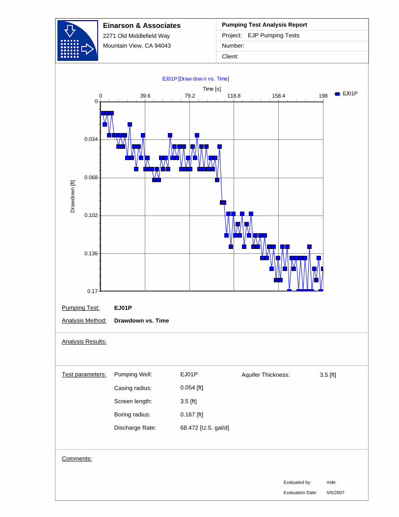
Einarson & Associates2271 Old Middlefield Way
Mountain View, CA 94043
Project:
Number:
Client:
EJP Pumping Tests
Pumping Test Analysis Report
EJ01P
EJ01P [Draw dow n vs. Time]
Time [s]198158.4118.879.239.60
Dra
wdo
wn
[ft]
0.17
0.136
0.102
0.068
0.034
0
Comments:
EJ01PPumping Well:
Discharge Rate: 68.472 [U.S. gal/d]
Casing radius:
0.167 [ft]
Screen length: 3.5 [ft]
Boring radius:
0.054 [ft]
Test parameters:
EJ01P
Analysis Method: Drawdown vs. Time
Aquifer Thickness: 3.5 [ft]
Analysis Results:
Evaluated by:
Evaluation Date:
mde
5/5/2007
Pumping Test:
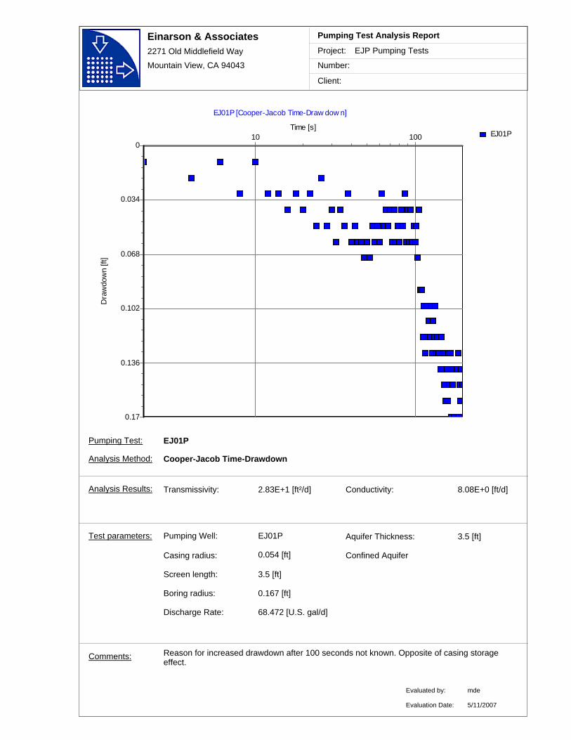
Einarson & Associates2271 Old Middlefield Way
Mountain View, CA 94043
Project:
Number:
Client:
EJP Pumping Tests
Pumping Test Analysis Report
EJ01P
EJ01P [Cooper-Jacob Time-Draw dow n]
Time [s]10 100
Dra
wdo
wn
[ft]
0.17
0.136
0.102
0.068
0.034
0
Transmissivity: 2.83E+1 [ft²/d]
Reason for increased drawdown after 100 seconds not known. Opposite of casing storage effect.
Conductivity: 8.08E+0 [ft/d]
Comments:
EJ01PPumping Well:
Discharge Rate: 68.472 [U.S. gal/d]
Casing radius:
0.167 [ft]
Screen length: 3.5 [ft]
Boring radius:
0.054 [ft]
Test parameters:
EJ01P
Analysis Method: Cooper-Jacob Time-Drawdown
Aquifer Thickness: 3.5 [ft]
Analysis Results:
Evaluated by:
Evaluation Date:
mde
Confined Aquifer
5/11/2007
Pumping Test:

Einarson & Associates2271 Old Middlefield Way
Mountain View, CA 94043
Project:
Number:
Client:
EJP Pumping Tests
Pumping Test Analysis Report
EJ01P
EJ01Prec [Draw dow n vs. Time]
Time [s]146116.887.658.429.2
Dra
wdo
wn
[ft]
0.75
0.6
0.45
0.3
0.15
Comments:
EJ01PPumping Well:
Discharge Rate: 68.472 [U.S. gal/d]
Casing radius:
0.167 [ft]
Screen length: 3.5 [ft]
Boring radius:
0.054 [ft]
Test parameters:
EJ01Prec
Analysis Method: Drawdown vs. Time
Aquifer Thickness: 3.5 [ft]
Analysis Results:
Evaluated by:
Evaluation Date: 5/6/2007
Pumping Test:
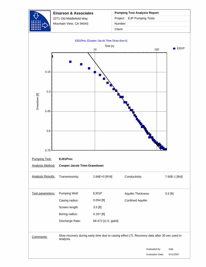
Einarson & Associates2271 Old Middlefield Way
Mountain View, CA 94043
Project:
Number:
Client:
EJP Pumping Tests
Pumping Test Analysis Report
EJ01P
EJ01Prec [Cooper-Jacob Time-Draw dow n]
Time [s]10 100
Dra
wdo
wn
[ft]
0.75
0.6
0.45
0.3
0.15
Transmissivity: 2.66E+0 [ft²/d]
Slow recovery during early time due to casing effect (?). Recovery data after 30 sec used in analysis.
Conductivity: 7.60E-1 [ft/d]
Comments:
EJ01PPumping Well:
Discharge Rate: 68.472 [U.S. gal/d]
Casing radius:
0.167 [ft]
Screen length: 3.5 [ft]
Boring radius:
0.054 [ft]
Test parameters:
EJ01Prec
Analysis Method: Cooper-Jacob Time-Drawdown
Aquifer Thickness: 3.5 [ft]
Analysis Results:
Evaluated by:
Evaluation Date:
mde
Confined Aquifer
5/11/2007
Pumping Test:

Pumping Test Analyses VAFB Site 60
Well EJ02P

Einarson & Associates2271 Old Middlefield Way
Mountain View, CA 94043
Project:
Number:
Client:
EJP Pumping Tests
Pumping Test Analysis Report
EJ02PEJ03PEJ04P
EJ02P [Draw dow n vs. Time]
Time [s]294235.2176.4117.658.8
Dra
wdo
wn
[ft]
1.6
1.28
0.96
0.64
0.32
Comments:
EJ02PPumping Well:
Discharge Rate: 1095.55 [U.S. gal/d]
Casing radius:
0.167 [ft]
Screen length: 3.5 [ft]
Boring radius:
0.054 [ft]
Test parameters:
EJ02P
Analysis Method: Drawdown vs. Time
Aquifer Thickness: 3.5 [ft]
Analysis Results:
Evaluated by:
Evaluation Date:
mde
5/6/2007
Pumping Test:
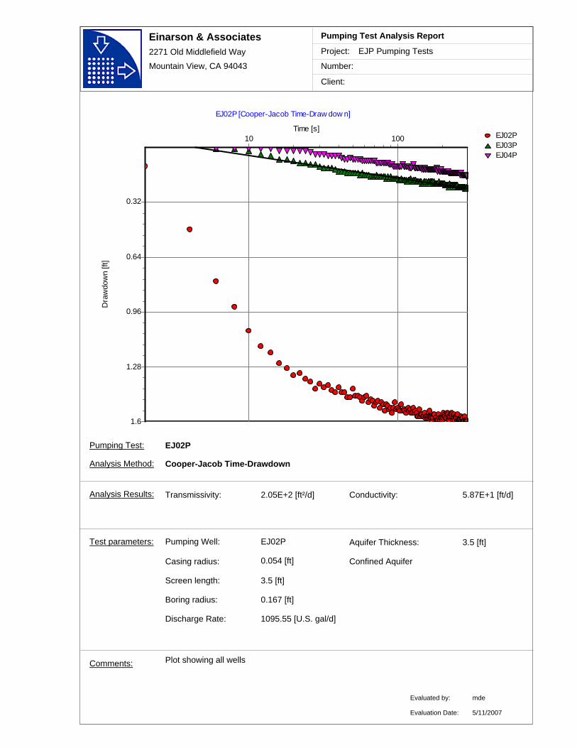
Einarson & Associates2271 Old Middlefield Way
Mountain View, CA 94043
Project:
Number:
Client:
EJP Pumping Tests
Pumping Test Analysis Report
EJ02PEJ03PEJ04P
EJ02P [Cooper-Jacob Time-Draw dow n]
Time [s]10 100
Dra
wdo
wn
[ft]
1.6
1.28
0.96
0.64
0.32
Transmissivity: 2.05E+2 [ft²/d]
Plot showing all wells
Conductivity: 5.87E+1 [ft/d]
Comments:
EJ02PPumping Well:
Discharge Rate: 1095.55 [U.S. gal/d]
Casing radius:
0.167 [ft]
Screen length: 3.5 [ft]
Boring radius:
0.054 [ft]
Test parameters:
EJ02P
Analysis Method: Cooper-Jacob Time-Drawdown
Aquifer Thickness: 3.5 [ft]
Analysis Results:
Evaluated by:
Evaluation Date:
mde
Confined Aquifer
5/11/2007
Pumping Test:

Einarson & Associates2271 Old Middlefield Way
Mountain View, CA 94043
Project:
Number:
Client:
EJP Pumping Tests
Pumping Test Analysis Report
EJ02PEJ03PEJ04P
EJ02P [Cooper-Jacob Time-Draw dow n]
Time [s]10 100
Dra
wdo
wn
[ft]
1.6
1.28
0.96
0.64
0.32
Transmissivity: 1.14E+2 [ft²/d]
Analysis of pumping well data after 64 sec (casing storage)
Conductivity: 3.24E+1 [ft/d]
Comments:
EJ02PPumping Well:
Discharge Rate: 1095.55 [U.S. gal/d]
Casing radius:
0.167 [ft]
Screen length: 3.5 [ft]
Boring radius:
0.054 [ft]
Test parameters:
EJ02P
Analysis Method: Cooper-Jacob Time-Drawdown
Aquifer Thickness: 3.5 [ft]
Analysis Results:
Evaluated by:
Evaluation Date:
mde
Confined Aquifer
5/11/2007
Pumping Test:
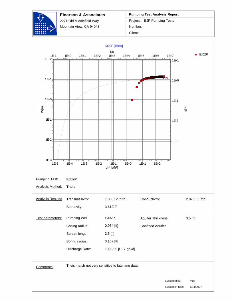
Einarson & Associates2271 Old Middlefield Way
Mountain View, CA 94043
Project:
Number:
Client:
EJP Pumping Tests
Pumping Test Analysis Report
EJ02P
EJ02P [Theis]
t/r² [s/ft²]1E-5 1E-4 1E-3 1E-2 1E-1 1E+0 1E+1 1E+2
1/u1E-1 1E+0 1E+1 1E+2 1E+3 1E+4 1E+5 1E+6 1E+7
W(u
)
1E-3
1E-2
1E-1
1E+0
1E+1
1E+2
s [ft]
1E-3
1E-2
1E-1
1E+0
1E+1
THEIS
Transmissivity: 1.00E+2 [ft²/d]
Theis match not very sensitive to late time data.
Conductivity: 2.87E+1 [ft/d]
Storativity: 3.61E-7
Comments:
EJ02PPumping Well:
Discharge Rate: 1095.55 [U.S. gal/d]
Casing radius:
0.167 [ft]
Screen length: 3.5 [ft]
Boring radius:
0.054 [ft]
Test parameters:
EJ02P
Analysis Method: Theis
Aquifer Thickness: 3.5 [ft]
Analysis Results:
Evaluated by:
Evaluation Date:
mde
Confined Aquifer
5/11/2007
Pumping Test:
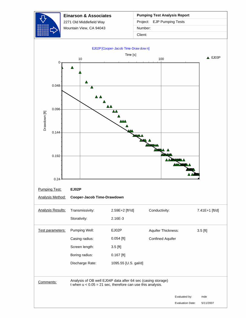
Einarson & Associates2271 Old Middlefield Way
Mountain View, CA 94043
Project:
Number:
Client:
EJP Pumping Tests
Pumping Test Analysis Report
EJ03P
EJ02P [Cooper-Jacob Time-Draw dow n]
Time [s]10 100
Dra
wdo
wn
[ft]
0.24
0.192
0.144
0.096
0.048
0
Transmissivity: 2.59E+2 [ft²/d]
Analysis of OB well EJ04P data after 64 sec (casing storage)t when u < 0.05 = 21 sec, therefore can use this analysis.
Conductivity: 7.41E+1 [ft/d]
Storativity: 2.16E-3
Comments:
EJ02PPumping Well:
Discharge Rate: 1095.55 [U.S. gal/d]
Casing radius:
0.167 [ft]
Screen length: 3.5 [ft]
Boring radius:
0.054 [ft]
Test parameters:
EJ02P
Analysis Method: Cooper-Jacob Time-Drawdown
Aquifer Thickness: 3.5 [ft]
Analysis Results:
Evaluated by:
Evaluation Date:
mde
Confined Aquifer
5/11/2007
Pumping Test:
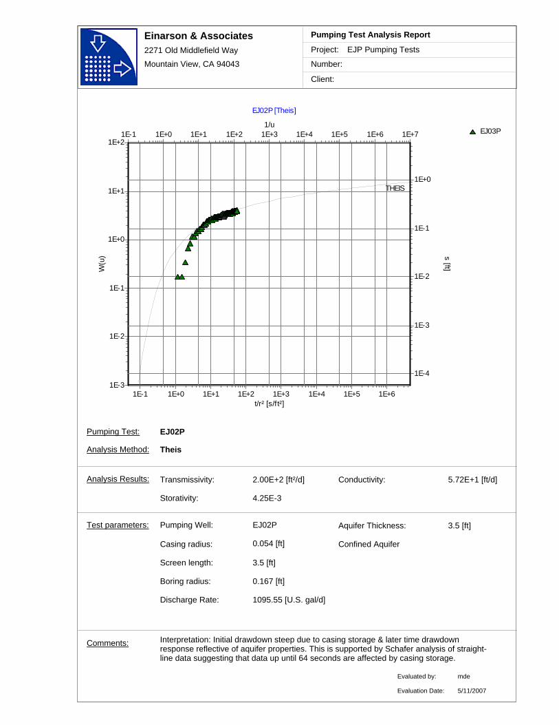
Einarson & Associates2271 Old Middlefield Way
Mountain View, CA 94043
Project:
Number:
Client:
EJP Pumping Tests
Pumping Test Analysis Report
EJ03P
EJ02P [Theis]
t/r² [s/ft²]1E-1 1E+0 1E+1 1E+2 1E+3 1E+4 1E+5 1E+6
1/u1E-1 1E+0 1E+1 1E+2 1E+3 1E+4 1E+5 1E+6 1E+7
W(u
)
1E-3
1E-2
1E-1
1E+0
1E+1
1E+2
s [ft]
1E-4
1E-3
1E-2
1E-1
1E+0THEIS
Transmissivity: 2.00E+2 [ft²/d]
Interpretation: Initial drawdown steep due to casing storage & later time drawdown response reflective of aquifer properties. This is supported by Schafer analysis of straight-line data suggesting that data up until 64 seconds are affected by casing storage.
Conductivity: 5.72E+1 [ft/d]
Storativity: 4.25E-3
Comments:
EJ02PPumping Well:
Discharge Rate: 1095.55 [U.S. gal/d]
Casing radius:
0.167 [ft]
Screen length: 3.5 [ft]
Boring radius:
0.054 [ft]
Test parameters:
EJ02P
Analysis Method: Theis
Aquifer Thickness: 3.5 [ft]
Analysis Results:
Evaluated by:
Evaluation Date:
mde
Confined Aquifer
5/11/2007
Pumping Test:
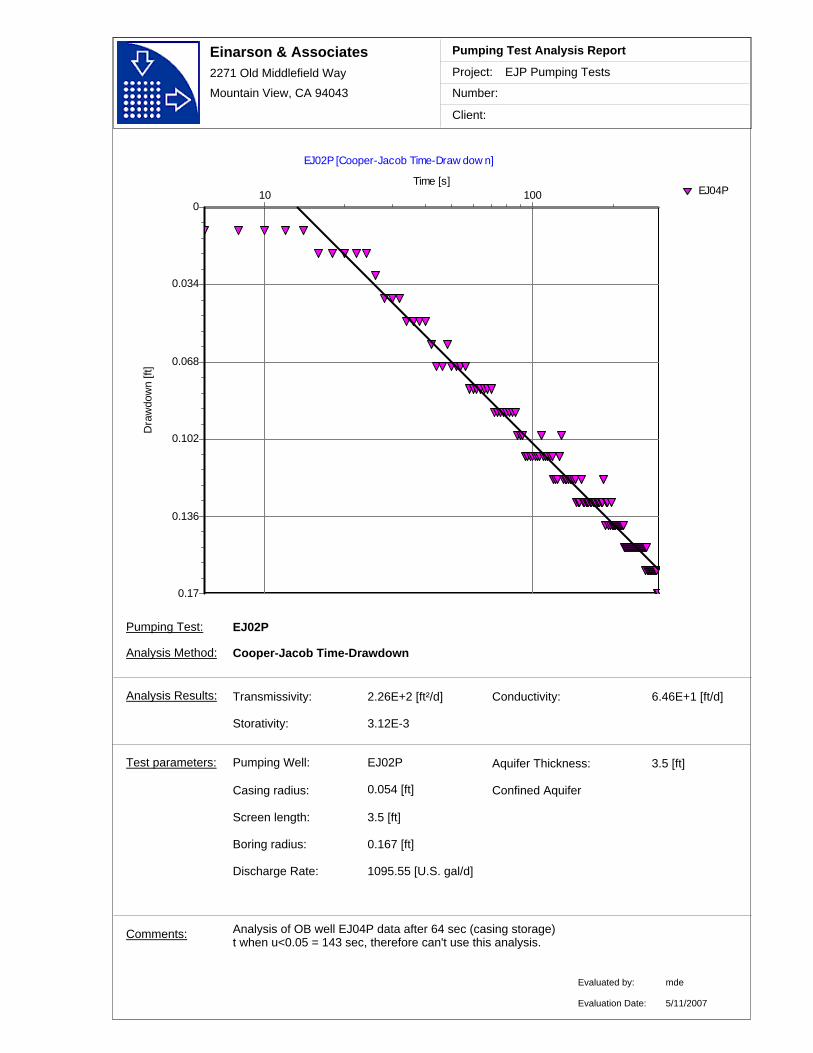
Einarson & Associates2271 Old Middlefield Way
Mountain View, CA 94043
Project:
Number:
Client:
EJP Pumping Tests
Pumping Test Analysis Report
EJ04P
EJ02P [Cooper-Jacob Time-Draw dow n]
Time [s]10 100
Dra
wdo
wn
[ft]
0.17
0.136
0.102
0.068
0.034
0
Transmissivity: 2.26E+2 [ft²/d]
Analysis of OB well EJ04P data after 64 sec (casing storage)t when u<0.05 = 143 sec, therefore can't use this analysis.
Conductivity: 6.46E+1 [ft/d]
Storativity: 3.12E-3
Comments:
EJ02PPumping Well:
Discharge Rate: 1095.55 [U.S. gal/d]
Casing radius:
0.167 [ft]
Screen length: 3.5 [ft]
Boring radius:
0.054 [ft]
Test parameters:
EJ02P
Analysis Method: Cooper-Jacob Time-Drawdown
Aquifer Thickness: 3.5 [ft]
Analysis Results:
Evaluated by:
Evaluation Date:
mde
Confined Aquifer
5/11/2007
Pumping Test:
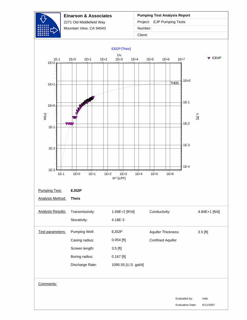
Einarson & Associates2271 Old Middlefield Way
Mountain View, CA 94043
Project:
Number:
Client:
EJP Pumping Tests
Pumping Test Analysis Report
EJ04P
EJ02P [Theis]
t/r² [s/ft²]1E-1 1E+0 1E+1 1E+2 1E+3 1E+4 1E+5 1E+6
1/u1E-1 1E+0 1E+1 1E+2 1E+3 1E+4 1E+5 1E+6 1E+7
W(u
)
1E-3
1E-2
1E-1
1E+0
1E+1
1E+2
s [ft]
1E-4
1E-3
1E-2
1E-1
1E+0THEIS
Transmissivity: 1.69E+2 [ft²/d] Conductivity: 4.84E+1 [ft/d]
Storativity: 4.18E-3
Comments:
EJ02PPumping Well:
Discharge Rate: 1095.55 [U.S. gal/d]
Casing radius:
0.167 [ft]
Screen length: 3.5 [ft]
Boring radius:
0.054 [ft]
Test parameters:
EJ02P
Analysis Method: Theis
Aquifer Thickness: 3.5 [ft]
Analysis Results:
Evaluated by:
Evaluation Date:
mde
Confined Aquifer
5/11/2007
Pumping Test:
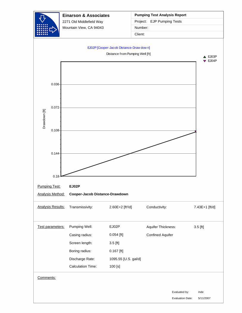
Einarson & Associates2271 Old Middlefield Way
Mountain View, CA 94043
Project:
Number:
Client:
EJP Pumping Tests
Pumping Test Analysis Report
EJ03PEJ04P
EJ02P [Cooper-Jacob Distance-Draw dow n]
Distance from Pumping Well [f t]
Dra
wdo
wn
[ft]
0.18
0.144
0.108
0.072
0.036
Transmissivity: 2.60E+2 [ft²/d] Conductivity: 7.43E+1 [ft/d]
Comments:
EJ02PPumping Well:
Discharge Rate: 1095.55 [U.S. gal/d]
Casing radius:
0.167 [ft]
Screen length: 3.5 [ft]
Boring radius:
0.054 [ft]
Calculation Time: 100 [s]
Test parameters:
EJ02P
Analysis Method: Cooper-Jacob Distance-Drawdown
Aquifer Thickness: 3.5 [ft]
Analysis Results:
Evaluated by:
Evaluation Date:
mde
Confined Aquifer
5/11/2007
Pumping Test:
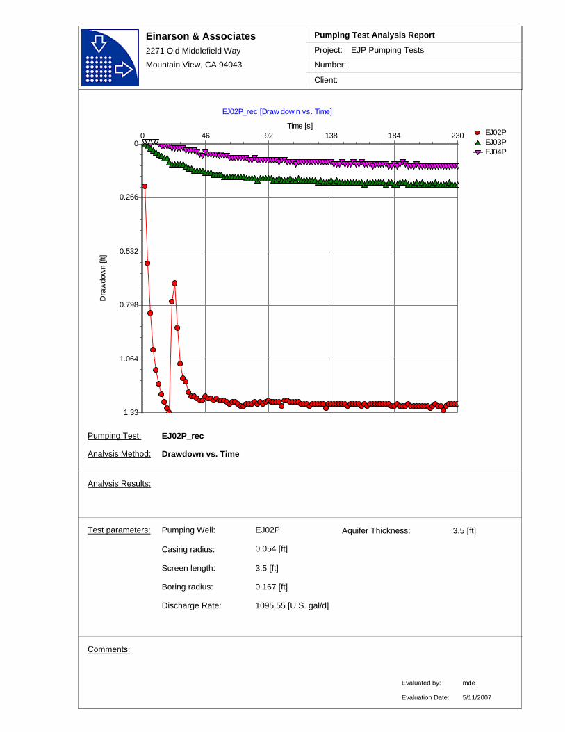
Einarson & Associates2271 Old Middlefield Way
Mountain View, CA 94043
Project:
Number:
Client:
EJP Pumping Tests
Pumping Test Analysis Report
EJ02PEJ03PEJ04P
EJ02P_rec [Draw dow n vs. Time]
Time [s]23018413892460
Dra
wdo
wn
[ft]
1.33
1.064
0.798
0.532
0.266
0
Comments:
EJ02PPumping Well:
Discharge Rate: 1095.55 [U.S. gal/d]
Casing radius:
0.167 [ft]
Screen length: 3.5 [ft]
Boring radius:
0.054 [ft]
Test parameters:
EJ02P_rec
Analysis Method: Drawdown vs. Time
Aquifer Thickness: 3.5 [ft]
Analysis Results:
Evaluated by:
Evaluation Date:
mde
5/11/2007
Pumping Test:
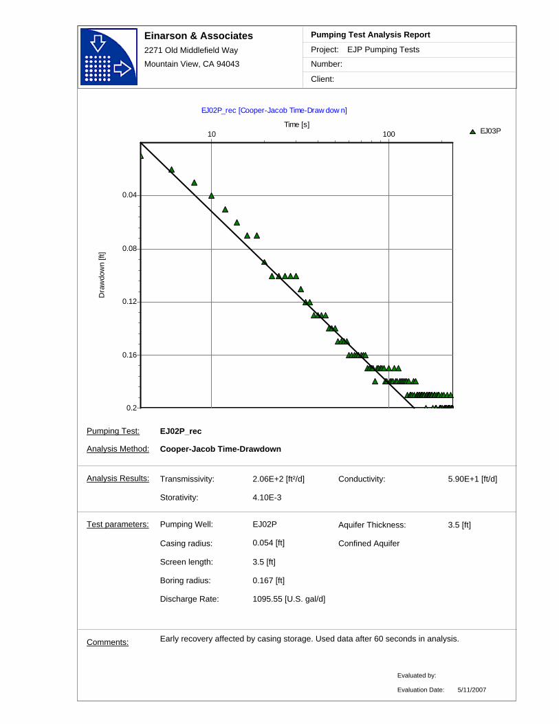
Einarson & Associates2271 Old Middlefield Way
Mountain View, CA 94043
Project:
Number:
Client:
EJP Pumping Tests
Pumping Test Analysis Report
EJ03P
EJ02P_rec [Cooper-Jacob Time-Draw dow n]
Time [s]10 100
Dra
wdo
wn
[ft]
0.2
0.16
0.12
0.08
0.04
Transmissivity: 2.06E+2 [ft²/d]
Early recovery affected by casing storage. Used data after 60 seconds in analysis.
Conductivity: 5.90E+1 [ft/d]
Storativity: 4.10E-3
Comments:
EJ02PPumping Well:
Discharge Rate: 1095.55 [U.S. gal/d]
Casing radius:
0.167 [ft]
Screen length: 3.5 [ft]
Boring radius:
0.054 [ft]
Test parameters:
EJ02P_rec
Analysis Method: Cooper-Jacob Time-Drawdown
Aquifer Thickness: 3.5 [ft]
Analysis Results:
Evaluated by:
Evaluation Date:
Confined Aquifer
5/11/2007
Pumping Test:

Pumping Test Analyses
VAFB Site 60
Well EJ03P
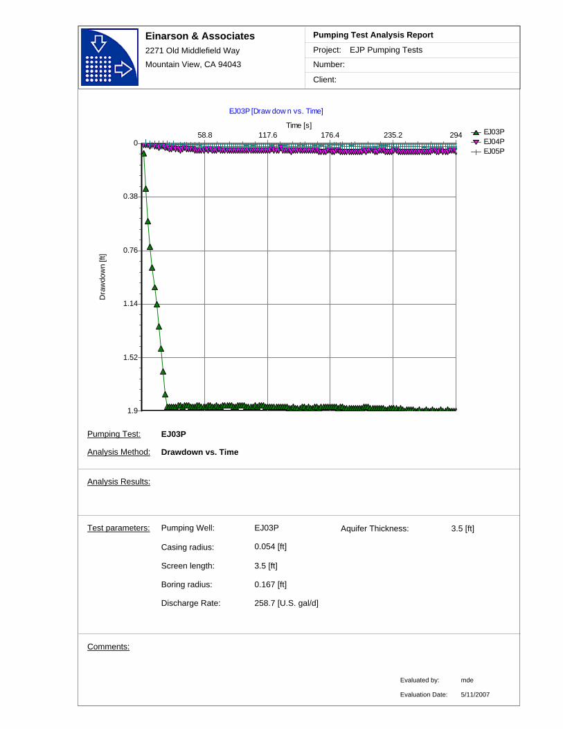
Einarson & Associates2271 Old Middlefield Way
Mountain View, CA 94043
Project:
Number:
Client:
EJP Pumping Tests
Pumping Test Analysis Report
EJ03PEJ04PEJ05P
EJ03P [Draw dow n vs. Time]
Time [s]294235.2176.4117.658.8
Dra
wdo
wn
[ft]
1.9
1.52
1.14
0.76
0.38
0
Comments:
EJ03PPumping Well:
Discharge Rate: 258.7 [U.S. gal/d]
Casing radius:
0.167 [ft]
Screen length: 3.5 [ft]
Boring radius:
0.054 [ft]
Test parameters:
EJ03P
Analysis Method: Drawdown vs. Time
Aquifer Thickness: 3.5 [ft]
Analysis Results:
Evaluated by:
Evaluation Date:
mde
5/11/2007
Pumping Test:
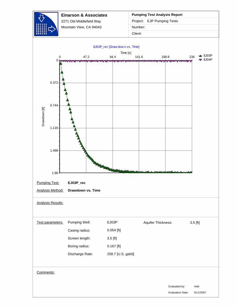
Einarson & Associates2271 Old Middlefield Way
Mountain View, CA 94043
Project:
Number:
Client:
EJP Pumping Tests
Pumping Test Analysis Report
EJ03PEJ04P
EJ03P_rec [Draw dow n vs. Time]
Time [s]236188.8141.694.447.20
Dra
wdo
wn
[ft]
1.86
1.488
1.116
0.744
0.372
0
Comments:
EJ03PPumping Well:
Discharge Rate: 258.7 [U.S. gal/d]
Casing radius:
0.167 [ft]
Screen length: 3.5 [ft]
Boring radius:
0.054 [ft]
Test parameters:
EJ03P_rec
Analysis Method: Drawdown vs. Time
Aquifer Thickness: 3.5 [ft]
Analysis Results:
Evaluated by:
Evaluation Date:
mde
5/11/2007
Pumping Test:
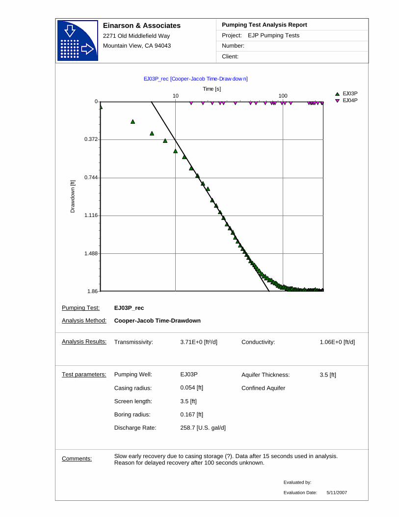
Einarson & Associates2271 Old Middlefield Way
Mountain View, CA 94043
Project:
Number:
Client:
EJP Pumping Tests
Pumping Test Analysis Report
EJ03PEJ04P
EJ03P_rec [Cooper-Jacob Time-Draw dow n]
Time [s]10 100
Dra
wdo
wn
[ft]
1.86
1.488
1.116
0.744
0.372
0
Transmissivity: 3.71E+0 [ft²/d]
Slow early recovery due to casing storage (?). Data after 15 seconds used in analysis. Reason for delayed recovery after 100 seconds unknown.
Conductivity: 1.06E+0 [ft/d]
Comments:
EJ03PPumping Well:
Discharge Rate: 258.7 [U.S. gal/d]
Casing radius:
0.167 [ft]
Screen length: 3.5 [ft]
Boring radius:
0.054 [ft]
Test parameters:
EJ03P_rec
Analysis Method: Cooper-Jacob Time-Drawdown
Aquifer Thickness: 3.5 [ft]
Analysis Results:
Evaluated by:
Evaluation Date:
Confined Aquifer
5/11/2007
Pumping Test:

Pumping Test Analyses
VAFB Site 60
Well EJ04P
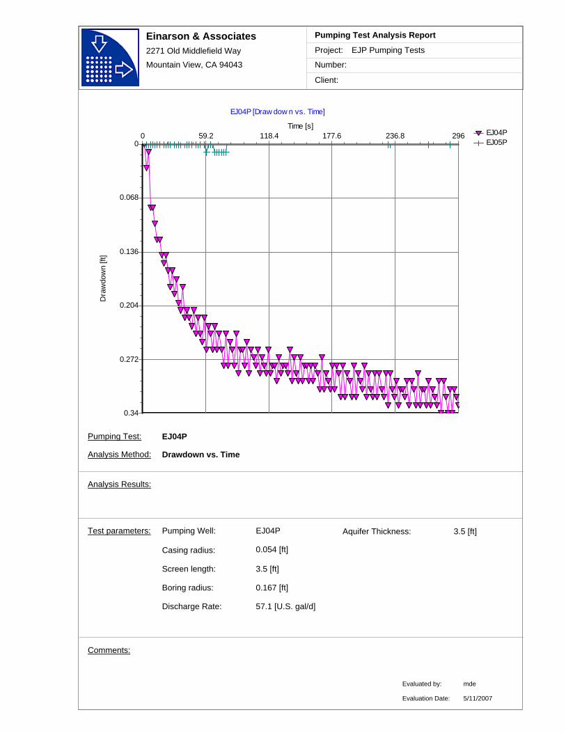
Einarson & Associates2271 Old Middlefield Way
Mountain View, CA 94043
Project:
Number:
Client:
EJP Pumping Tests
Pumping Test Analysis Report
EJ04PEJ05P
EJ04P [Draw dow n vs. Time]
Time [s]296236.8177.6118.459.20
Dra
wdo
wn
[ft]
0.34
0.272
0.204
0.136
0.068
0
Comments:
EJ04PPumping Well:
Discharge Rate: 57.1 [U.S. gal/d]
Casing radius:
0.167 [ft]
Screen length: 3.5 [ft]
Boring radius:
0.054 [ft]
Test parameters:
EJ04P
Analysis Method: Drawdown vs. Time
Aquifer Thickness: 3.5 [ft]
Analysis Results:
Evaluated by:
Evaluation Date:
mde
5/11/2007
Pumping Test:
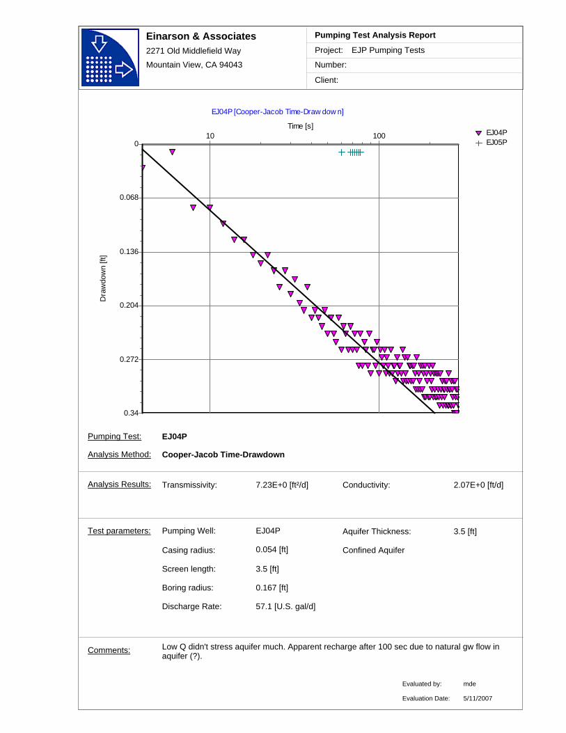
Einarson & Associates2271 Old Middlefield Way
Mountain View, CA 94043
Project:
Number:
Client:
EJP Pumping Tests
Pumping Test Analysis Report
EJ04PEJ05P
EJ04P [Cooper-Jacob Time-Draw dow n]
Time [s]10 100
Dra
wdo
wn
[ft]
0.34
0.272
0.204
0.136
0.068
0
Transmissivity: 7.23E+0 [ft²/d]
Low Q didn't stress aquifer much. Apparent recharge after 100 sec due to natural gw flow in aquifer (?).
Conductivity: 2.07E+0 [ft/d]
Comments:
EJ04PPumping Well:
Discharge Rate: 57.1 [U.S. gal/d]
Casing radius:
0.167 [ft]
Screen length: 3.5 [ft]
Boring radius:
0.054 [ft]
Test parameters:
EJ04P
Analysis Method: Cooper-Jacob Time-Drawdown
Aquifer Thickness: 3.5 [ft]
Analysis Results:
Evaluated by:
Evaluation Date:
mde
Confined Aquifer
5/11/2007
Pumping Test:

Einarson & Associates2271 Old Middlefield Way
Mountain View, CA 94043
Project:
Number:
Client:
EJP Pumping Tests
Pumping Test Analysis Report
EJ04PEJ05P
EJ04P [Theis]
t/r² [s/ft²]1E+0 1E+1 1E+2 1E+3 1E+4 1E+5 1E+6 1E+7
1/u1E-1 1E+0 1E+1 1E+2 1E+3 1E+4 1E+5 1E+6 1E+7
W(u
)
1E-3
1E-2
1E-1
1E+0
1E+1
1E+2
s [ft]
1E-3
1E-2
1E-1
1E+0
1E+1
THEIS
Transmissivity: 5.39E+0 [ft²/d]
Ignored later data since assumed to be affected by recharge (natural flow in aquifer).
Conductivity: 1.54E+0 [ft/d]
Storativity: 8.69E-4
Comments:
EJ04PPumping Well:
Discharge Rate: 57.1 [U.S. gal/d]
Casing radius:
0.167 [ft]
Screen length: 3.5 [ft]
Boring radius:
0.054 [ft]
Test parameters:
EJ04P
Analysis Method: Theis
Aquifer Thickness: 3.5 [ft]
Analysis Results:
Evaluated by:
Evaluation Date:
mde
Confined Aquifer
5/11/2007
Pumping Test:
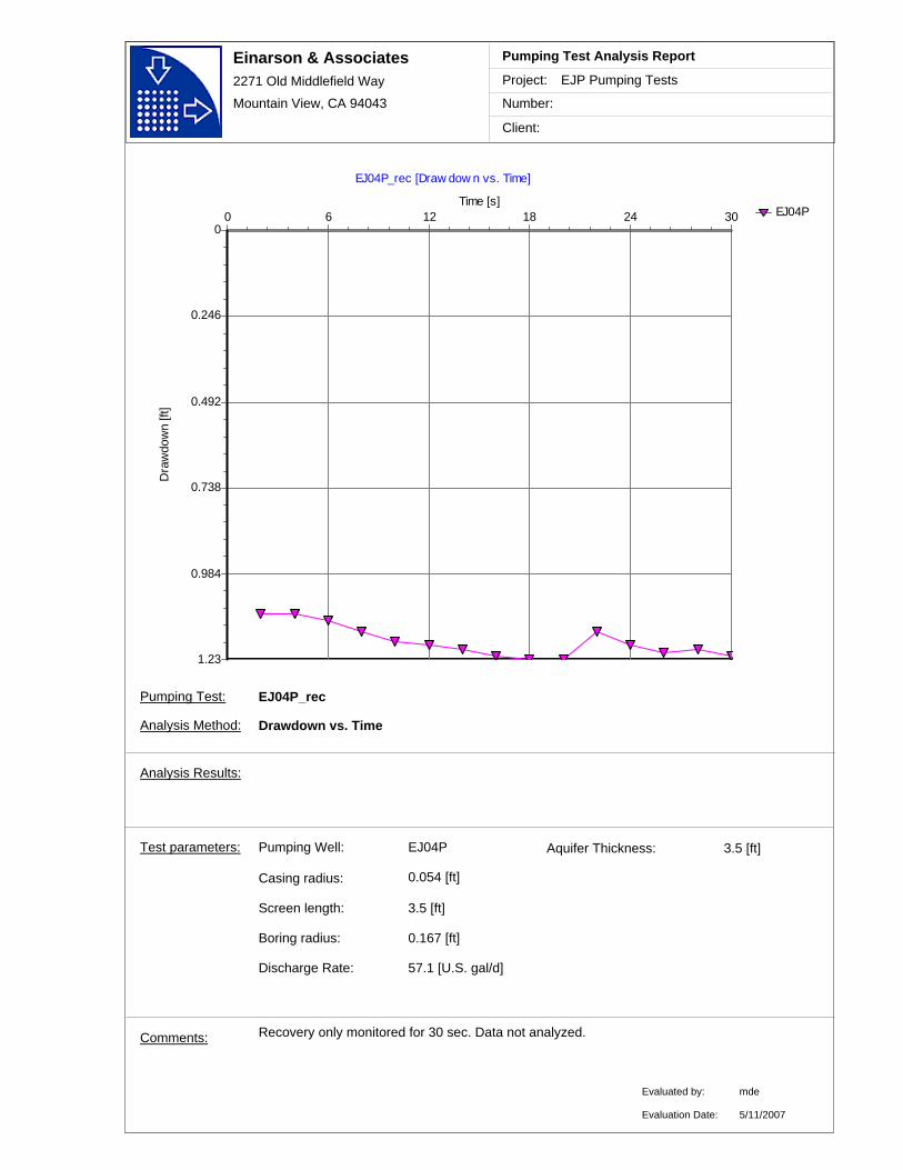
Einarson & Associates2271 Old Middlefield Way
Mountain View, CA 94043
Project:
Number:
Client:
EJP Pumping Tests
Pumping Test Analysis Report
EJ04P
EJ04P_rec [Draw dow n vs. Time]
Time [s]3024181260
Dra
wdo
wn
[ft]
1.23
0.984
0.738
0.492
0.246
0
Recovery only monitored for 30 sec. Data not analyzed. Comments:
EJ04PPumping Well:
Discharge Rate: 57.1 [U.S. gal/d]
Casing radius:
0.167 [ft]
Screen length: 3.5 [ft]
Boring radius:
0.054 [ft]
Test parameters:
EJ04P_rec
Analysis Method: Drawdown vs. Time
Aquifer Thickness: 3.5 [ft]
Analysis Results:
Evaluated by:
Evaluation Date:
mde
5/11/2007
Pumping Test:

Pumping Test Analyses
VAFB Site 60
Well EJ05P
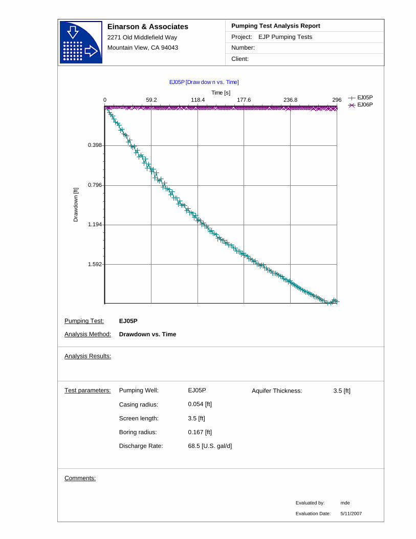
Einarson & Associates2271 Old Middlefield Way
Mountain View, CA 94043
Project:
Number:
Client:
EJP Pumping Tests
Pumping Test Analysis Report
EJ05PEJ06P
EJ05P [Draw dow n vs. Time]
Time [s]296236.8177.6118.459.20
Dra
wdo
wn
[ft]
1.592
1.194
0.796
0.398
Comments:
EJ05PPumping Well:
Discharge Rate: 68.5 [U.S. gal/d]
Casing radius:
0.167 [ft]
Screen length: 3.5 [ft]
Boring radius:
0.054 [ft]
Test parameters:
EJ05P
Analysis Method: Drawdown vs. Time
Aquifer Thickness: 3.5 [ft]
Analysis Results:
Evaluated by:
Evaluation Date:
mde
5/11/2007
Pumping Test:
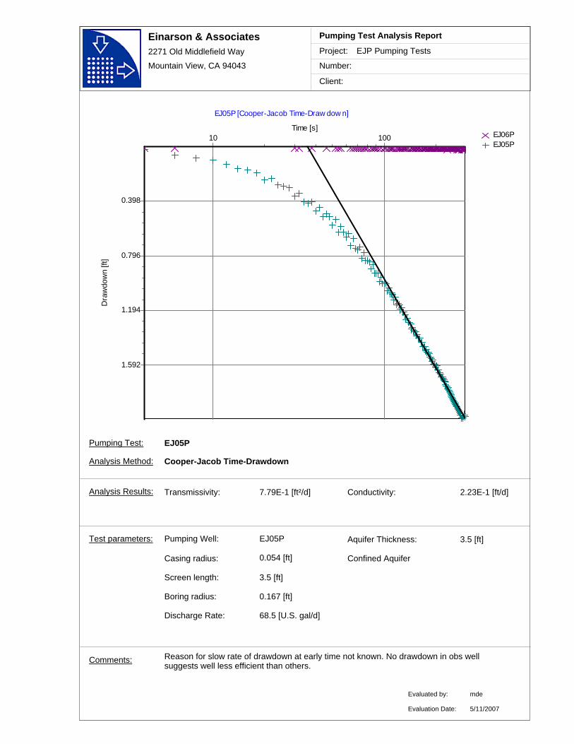
Einarson & Associates2271 Old Middlefield Way
Mountain View, CA 94043
Project:
Number:
Client:
EJP Pumping Tests
Pumping Test Analysis Report
EJ06PEJ05P
EJ05P [Cooper-Jacob Time-Draw dow n]
Time [s]10 100
Dra
wdo
wn
[ft]
1.592
1.194
0.796
0.398
Transmissivity: 7.79E-1 [ft²/d]
Reason for slow rate of drawdown at early time not known. No drawdown in obs well suggests well less efficient than others.
Conductivity: 2.23E-1 [ft/d]
Comments:
EJ05PPumping Well:
Discharge Rate: 68.5 [U.S. gal/d]
Casing radius:
0.167 [ft]
Screen length: 3.5 [ft]
Boring radius:
0.054 [ft]
Test parameters:
EJ05P
Analysis Method: Cooper-Jacob Time-Drawdown
Aquifer Thickness: 3.5 [ft]
Analysis Results:
Evaluated by:
Evaluation Date:
mde
Confined Aquifer
5/11/2007
Pumping Test:
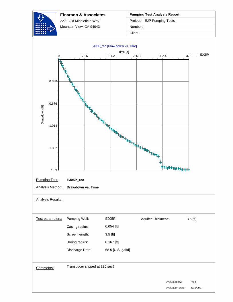
Einarson & Associates2271 Old Middlefield Way
Mountain View, CA 94043
Project:
Number:
Client:
EJP Pumping Tests
Pumping Test Analysis Report
EJ05P
EJ05P_rec [Draw dow n vs. Time]
Time [s]378302.4226.8151.275.60
Dra
wdo
wn
[ft]
1.69
1.352
1.014
0.676
0.338
Transducer slipped at 290 sec? Comments:
EJ05PPumping Well:
Discharge Rate: 68.5 [U.S. gal/d]
Casing radius:
0.167 [ft]
Screen length: 3.5 [ft]
Boring radius:
0.054 [ft]
Test parameters:
EJ05P_rec
Analysis Method: Drawdown vs. Time
Aquifer Thickness: 3.5 [ft]
Analysis Results:
Evaluated by:
Evaluation Date:
mde
5/11/2007
Pumping Test:
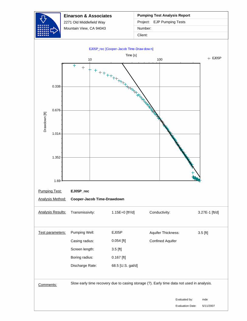
Einarson & Associates2271 Old Middlefield Way
Mountain View, CA 94043
Project:
Number:
Client:
EJP Pumping Tests
Pumping Test Analysis Report
EJ05P
EJ05P_rec [Cooper-Jacob Time-Draw dow n]
Time [s]10 100
Dra
wdo
wn
[ft]
1.69
1.352
1.014
0.676
0.338
Transmissivity: 1.15E+0 [ft²/d]
Slow early time recovery due to casing storage (?). Early time data not used in analysis.
Conductivity: 3.27E-1 [ft/d]
Comments:
EJ05PPumping Well:
Discharge Rate: 68.5 [U.S. gal/d]
Casing radius:
0.167 [ft]
Screen length: 3.5 [ft]
Boring radius:
0.054 [ft]
Test parameters:
EJ05P_rec
Analysis Method: Cooper-Jacob Time-Drawdown
Aquifer Thickness: 3.5 [ft]
Analysis Results:
Evaluated by:
Evaluation Date:
mde
Confined Aquifer
5/11/2007
Pumping Test:

Pumping Test Analyses
VAFB Site 60
Well EJ06P
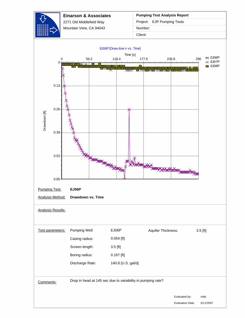
Einarson & Associates2271 Old Middlefield Way
Mountain View, CA 94043
Project:
Number:
Client:
EJP Pumping Tests
Pumping Test Analysis Report
EJ06PEJ07PEJ08P
EJ06P [Draw dow n vs. Time]
Time [s]296236.8177.6118.459.20
Dra
wdo
wn
[ft]
0.65
0.52
0.39
0.26
0.13
0
Drop in head at 145 sec due to variability in pumping rate? Comments:
EJ06PPumping Well:
Discharge Rate: 140.8 [U.S. gal/d]
Casing radius:
0.167 [ft]
Screen length: 3.5 [ft]
Boring radius:
0.054 [ft]
Test parameters:
EJ06P
Analysis Method: Drawdown vs. Time
Aquifer Thickness: 3.5 [ft]
Analysis Results:
Evaluated by:
Evaluation Date:
mde
5/11/2007
Pumping Test:

Einarson & Associates2271 Old Middlefield Way
Mountain View, CA 94043
Project:
Number:
Client:
EJP Pumping Tests
Pumping Test Analysis Report
EJ07PEJ06PEJ08P
EJ06P [Cooper-Jacob Time-Draw dow n]
Time [s]10 100
Dra
wdo
wn
[ft]
0.65
0.52
0.39
0.26
0.13
0
Transmissivity: 1.19E+1 [ft²/d] Conductivity: 3.40E+0 [ft/d]
Comments:
EJ06PPumping Well:
Discharge Rate: 140.8 [U.S. gal/d]
Casing radius:
0.167 [ft]
Screen length: 3.5 [ft]
Boring radius:
0.054 [ft]
Test parameters:
EJ06P
Analysis Method: Cooper-Jacob Time-Drawdown
Aquifer Thickness: 3.5 [ft]
Analysis Results:
Evaluated by:
Evaluation Date:
mde
Confined Aquifer
5/11/2007
Pumping Test:
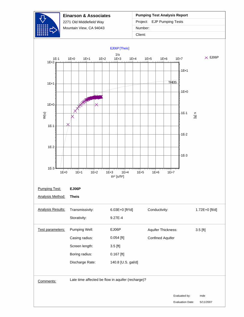
Einarson & Associates2271 Old Middlefield Way
Mountain View, CA 94043
Project:
Number:
Client:
EJP Pumping Tests
Pumping Test Analysis Report
EJ06P
EJ06P [Theis]
t/r² [s/ft²]1E+0 1E+1 1E+2 1E+3 1E+4 1E+5 1E+6 1E+7
1/u1E-1 1E+0 1E+1 1E+2 1E+3 1E+4 1E+5 1E+6 1E+7
W(u
)
1E-3
1E-2
1E-1
1E+0
1E+1
1E+2
s [ft]
1E-3
1E-2
1E-1
1E+0
1E+1
THEIS
Transmissivity: 6.03E+0 [ft²/d]
Late time affected be flow in aquifer (recharge)?
Conductivity: 1.72E+0 [ft/d]
Storativity: 9.27E-4
Comments:
EJ06PPumping Well:
Discharge Rate: 140.8 [U.S. gal/d]
Casing radius:
0.167 [ft]
Screen length: 3.5 [ft]
Boring radius:
0.054 [ft]
Test parameters:
EJ06P
Analysis Method: Theis
Aquifer Thickness: 3.5 [ft]
Analysis Results:
Evaluated by:
Evaluation Date:
mde
Confined Aquifer
5/11/2007
Pumping Test:
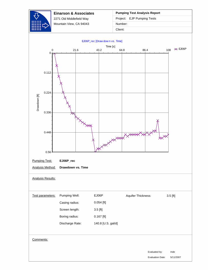
Einarson & Associates2271 Old Middlefield Way
Mountain View, CA 94043
Project:
Number:
Client:
EJP Pumping Tests
Pumping Test Analysis Report
EJ06P
EJ06P_rec [Draw dow n vs. Time]
Time [s]10886.464.843.221.60
Dra
wdo
wn
[ft]
0.56
0.448
0.336
0.224
0.112
0
Comments:
EJ06PPumping Well:
Discharge Rate: 140.8 [U.S. gal/d]
Casing radius:
0.167 [ft]
Screen length: 3.5 [ft]
Boring radius:
0.054 [ft]
Test parameters:
EJ06P_rec
Analysis Method: Drawdown vs. Time
Aquifer Thickness: 3.5 [ft]
Analysis Results:
Evaluated by:
Evaluation Date:
mde
5/11/2007
Pumping Test:
Pumping Test Analyses
VAFB Site 60
Well EJ07P

Einarson & Associates2271 Old Middlefield Way
Mountain View, CA 94043
Project:
Number:
Client:
EJP Pumping Tests
Pumping Test Analysis Report
EJ07PEJ08PEJ09P
EJ07P [Draw dow n vs. Time]
Time [s]296236.8177.6118.459.20
Dra
wdo
wn
[ft]
0.92
0.736
0.552
0.368
0.184
0
Comments:
EJ07PPumping Well:
Discharge Rate: 64.7 [U.S. gal/d]
Casing radius:
0.167 [ft]
Screen length: 3.5 [ft]
Boring radius:
0.054 [ft]
Test parameters:
EJ07P
Analysis Method: Drawdown vs. Time
Aquifer Thickness: 3.5 [ft]
Analysis Results:
Evaluated by:
Evaluation Date:
mde
5/11/2007
Pumping Test:
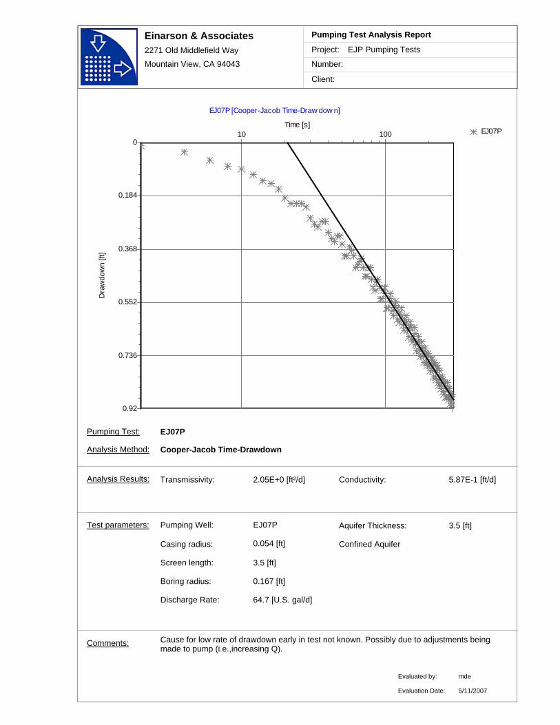
Einarson & Associates2271 Old Middlefield Way
Mountain View, CA 94043
Project:
Number:
Client:
EJP Pumping Tests
Pumping Test Analysis Report
EJ07P
EJ07P [Cooper-Jacob Time-Draw dow n]
Time [s]10 100
Dra
wdo
wn
[ft]
0.92
0.736
0.552
0.368
0.184
0
Transmissivity: 2.05E+0 [ft²/d]
Cause for low rate of drawdown early in test not known. Possibly due to adjustments being made to pump (i.e.,increasing Q).
Conductivity: 5.87E-1 [ft/d]
Comments:
EJ07PPumping Well:
Discharge Rate: 64.7 [U.S. gal/d]
Casing radius:
0.167 [ft]
Screen length: 3.5 [ft]
Boring radius:
0.054 [ft]
Test parameters:
EJ07P
Analysis Method: Cooper-Jacob Time-Drawdown
Aquifer Thickness: 3.5 [ft]
Analysis Results:
Evaluated by:
Evaluation Date:
mde
Confined Aquifer
5/11/2007
Pumping Test:

Einarson & Associates2271 Old Middlefield Way
Mountain View, CA 94043
Project:
Number:
Client:
EJP Pumping Tests
Pumping Test Analysis Report
EJ09P
EJ07P [Cooper-Jacob Time-Draw dow n]
Time [s]10 100
Dra
wdo
wn
[ft]
0.08
0.064
0.048
0.032
0.016
0
Transmissivity: 2.45E+1 [ft²/d]
Cause for low rate of drawdown early in test not known. Possibly due to adjustments being made to pump (i.e.,increasing Q). Calculated time for u < 0.05 = 255 sec. Therefore calculated K & S not valid.
Conductivity: 7.01E+0 [ft/d]
Storativity: 5.79E-4
Comments:
EJ07PPumping Well:
Discharge Rate: 64.7 [U.S. gal/d]
Casing radius:
0.167 [ft]
Screen length: 3.5 [ft]
Boring radius:
0.054 [ft]
Test parameters:
EJ07P
Analysis Method: Cooper-Jacob Time-Drawdown
Aquifer Thickness: 3.5 [ft]
Analysis Results:
Evaluated by:
Evaluation Date:
mde
Confined Aquifer
5/11/2007
Pumping Test:

Einarson & Associates2271 Old Middlefield Way
Mountain View, CA 94043
Project:
Number:
Client:
EJP Pumping Tests
Pumping Test Analysis Report
EJ09P
EJ07P [Theis]
t/r² [s/ft²]1E-1 1E+0 1E+1 1E+2 1E+3 1E+4 1E+5 1E+6
1/u1E-1 1E+0 1E+1 1E+2 1E+3 1E+4 1E+5 1E+6 1E+7
W(u
)
1E-3
1E-2
1E-1
1E+0
1E+1
1E+2
s [ft]
1E-4
1E-3
1E-2
1E-1
1E+0
THEIS
Transmissivity: 2.01E+1 [ft²/d] Conductivity: 5.75E+0 [ft/d]
Storativity: 7.13E-4
Comments:
EJ07PPumping Well:
Discharge Rate: 64.7 [U.S. gal/d]
Casing radius:
0.167 [ft]
Screen length: 3.5 [ft]
Boring radius:
0.054 [ft]
Test parameters:
EJ07P
Analysis Method: Theis
Aquifer Thickness: 3.5 [ft]
Analysis Results:
Evaluated by:
Evaluation Date:
mde
Confined Aquifer
5/11/2007
Pumping Test:
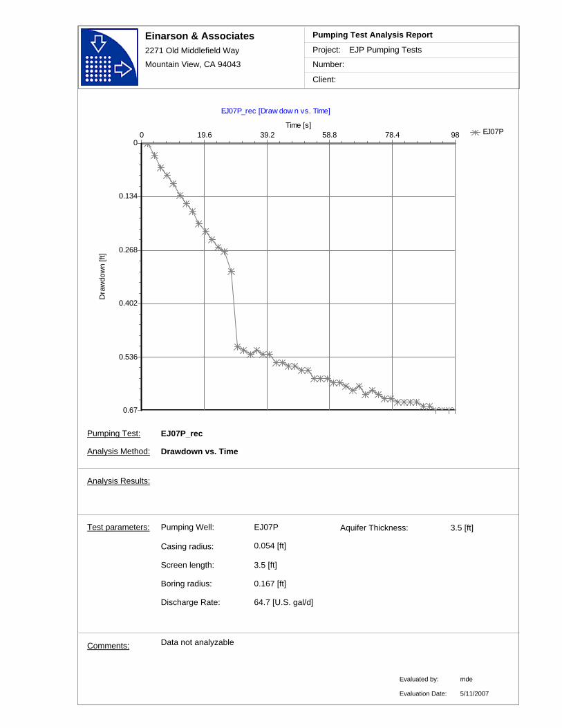
Einarson & Associates2271 Old Middlefield Way
Mountain View, CA 94043
Project:
Number:
Client:
EJP Pumping Tests
Pumping Test Analysis Report
EJ07P
EJ07P_rec [Draw dow n vs. Time]
Time [s]9878.458.839.219.60
Dra
wdo
wn
[ft]
0.67
0.536
0.402
0.268
0.134
0
Data not analyzableComments:
EJ07PPumping Well:
Discharge Rate: 64.7 [U.S. gal/d]
Casing radius:
0.167 [ft]
Screen length: 3.5 [ft]
Boring radius:
0.054 [ft]
Test parameters:
EJ07P_rec
Analysis Method: Drawdown vs. Time
Aquifer Thickness: 3.5 [ft]
Analysis Results:
Evaluated by:
Evaluation Date:
mde
5/11/2007
Pumping Test:
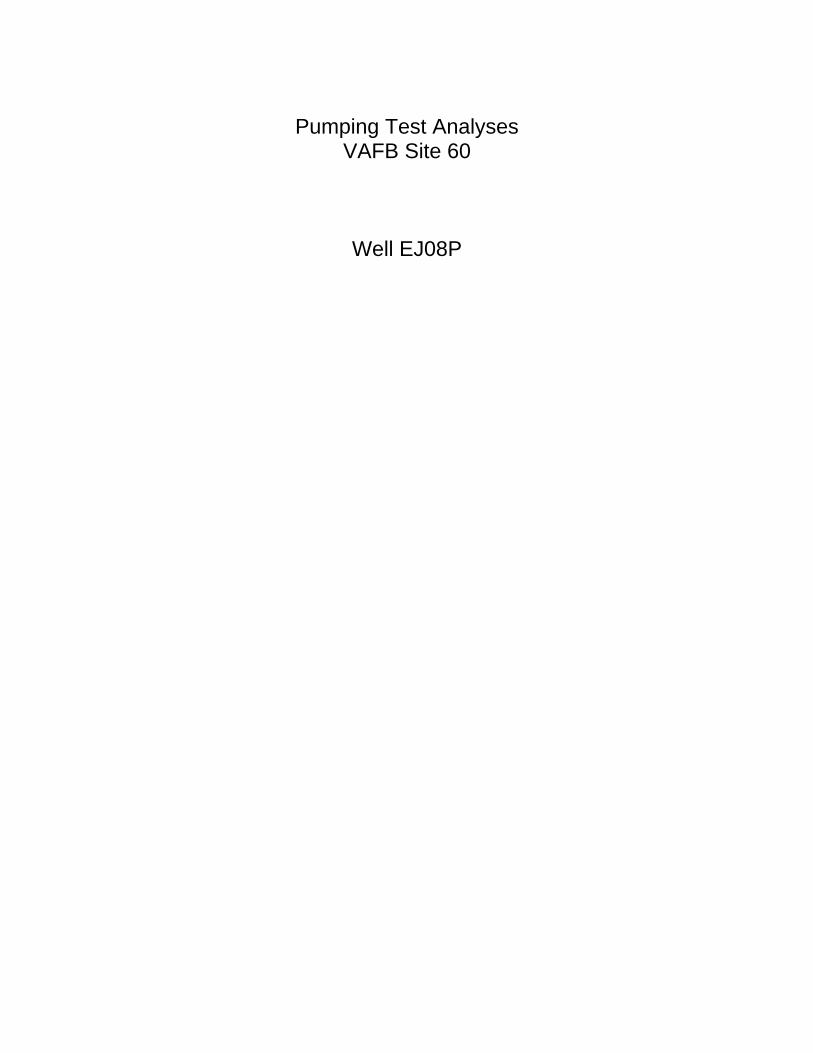
Pumping Test Analyses
VAFB Site 60
Well EJ08P
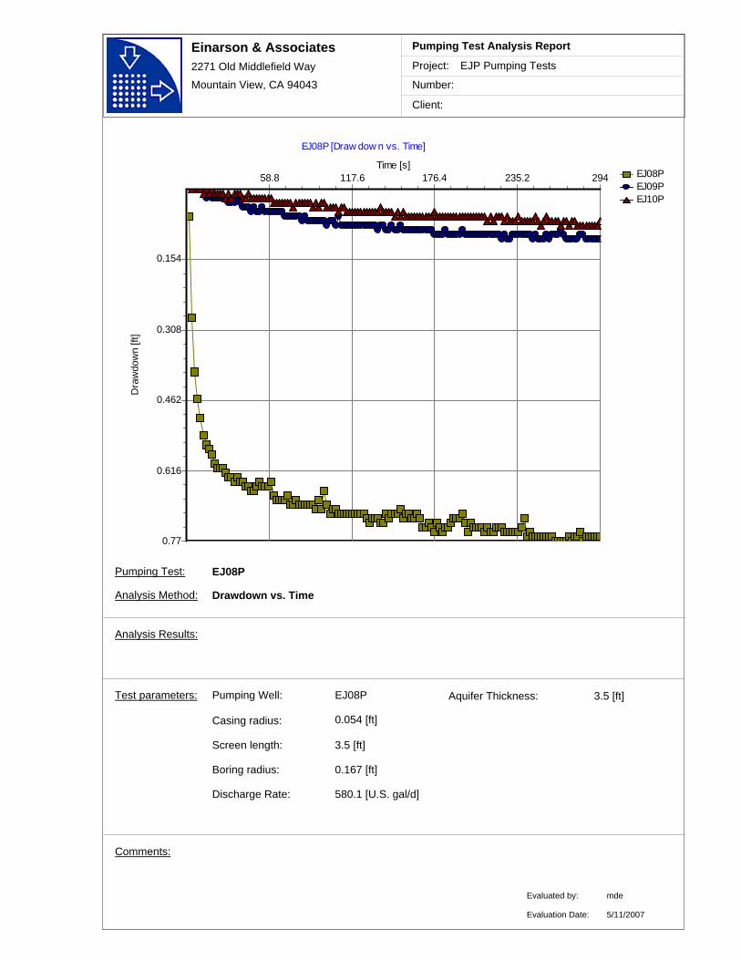
Einarson & Associates2271 Old Middlefield Way
Mountain View, CA 94043
Project:
Number:
Client:
EJP Pumping Tests
Pumping Test Analysis Report
EJ08PEJ09PEJ10P
EJ08P [Draw dow n vs. Time]
Time [s]294235.2176.4117.658.8
Dra
wdo
wn
[ft]
0.77
0.616
0.462
0.308
0.154
Comments:
EJ08PPumping Well:
Discharge Rate: 580.1 [U.S. gal/d]
Casing radius:
0.167 [ft]
Screen length: 3.5 [ft]
Boring radius:
0.054 [ft]
Test parameters:
EJ08P
Analysis Method: Drawdown vs. Time
Aquifer Thickness: 3.5 [ft]
Analysis Results:
Evaluated by:
Evaluation Date:
mde
5/11/2007
Pumping Test:

Einarson & Associates2271 Old Middlefield Way
Mountain View, CA 94043
Project:
Number:
Client:
EJP Pumping Tests
Pumping Test Analysis Report
EJ08P
EJ08P [Cooper-Jacob Time-Draw dow n]
Time [s]10 100
Dra
wdo
wn
[ft]
0.77
0.616
0.462
0.308
0.154
Transmissivity: 1.01E+2 [ft²/d]
early drawdown affected by casing storage. Shafer method suggests data before 53 seconds affected by casing storage. Therefore analyzed data after that time.
Conductivity: 2.90E+1 [ft/d]
Comments:
EJ08PPumping Well:
Discharge Rate: 580.1 [U.S. gal/d]
Casing radius:
0.167 [ft]
Screen length: 3.5 [ft]
Boring radius:
0.054 [ft]
Test parameters:
EJ08P
Analysis Method: Cooper-Jacob Time-Drawdown
Aquifer Thickness: 3.5 [ft]
Analysis Results:
Evaluated by:
Evaluation Date:
mde
Confined Aquifer
5/11/2007
Pumping Test:
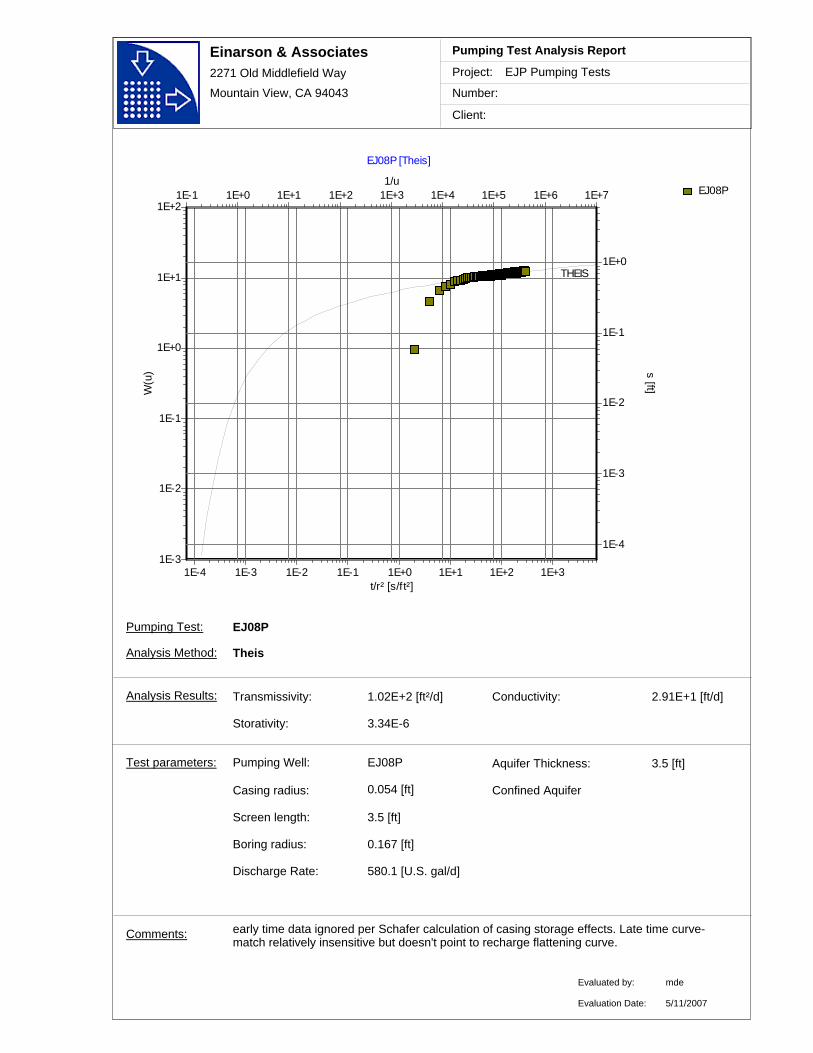
Einarson & Associates2271 Old Middlefield Way
Mountain View, CA 94043
Project:
Number:
Client:
EJP Pumping Tests
Pumping Test Analysis Report
EJ08P
EJ08P [Theis]
t/r² [s/ft²]1E-4 1E-3 1E-2 1E-1 1E+0 1E+1 1E+2 1E+3
1/u1E-1 1E+0 1E+1 1E+2 1E+3 1E+4 1E+5 1E+6 1E+7
W(u
)
1E-3
1E-2
1E-1
1E+0
1E+1
1E+2
s [ft]
1E-4
1E-3
1E-2
1E-1
1E+0THEIS
Transmissivity: 1.02E+2 [ft²/d]
early time data ignored per Schafer calculation of casing storage effects. Late time curve-match relatively insensitive but doesn't point to recharge flattening curve.
Conductivity: 2.91E+1 [ft/d]
Storativity: 3.34E-6
Comments:
EJ08PPumping Well:
Discharge Rate: 580.1 [U.S. gal/d]
Casing radius:
0.167 [ft]
Screen length: 3.5 [ft]
Boring radius:
0.054 [ft]
Test parameters:
EJ08P
Analysis Method: Theis
Aquifer Thickness: 3.5 [ft]
Analysis Results:
Evaluated by:
Evaluation Date:
mde
Confined Aquifer
5/11/2007
Pumping Test:
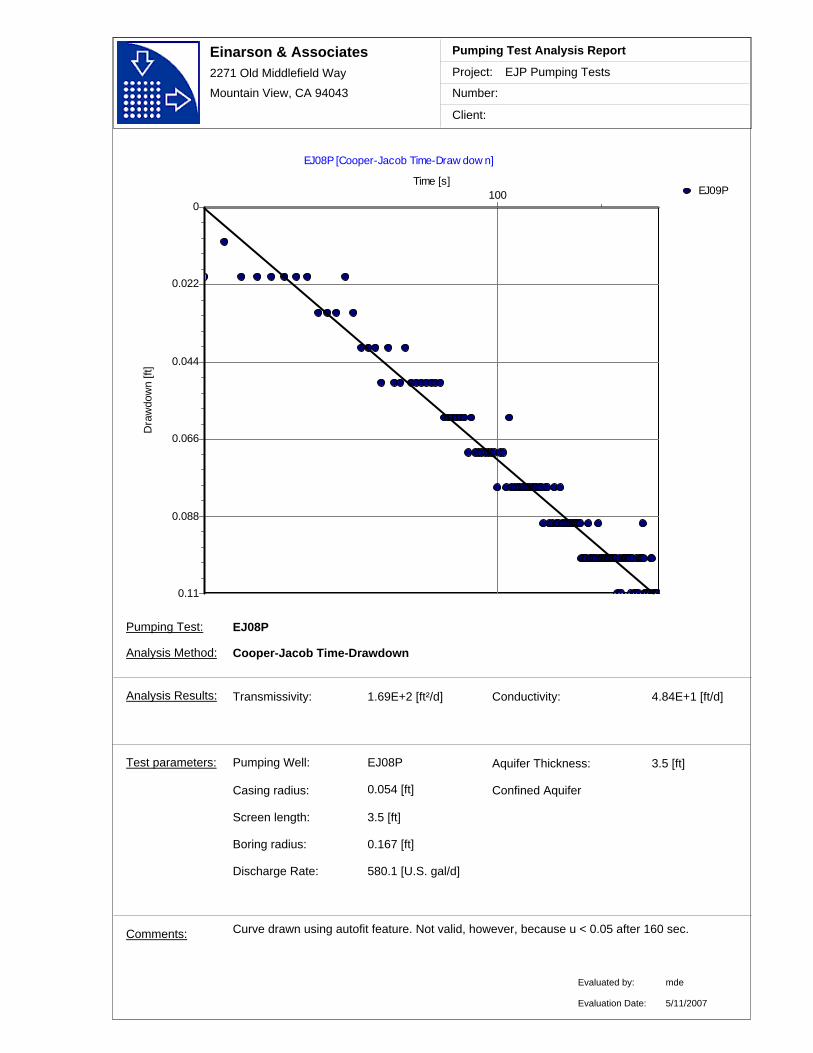
Einarson & Associates2271 Old Middlefield Way
Mountain View, CA 94043
Project:
Number:
Client:
EJP Pumping Tests
Pumping Test Analysis Report
EJ09P
EJ08P [Cooper-Jacob Time-Draw dow n]
Time [s]100
Dra
wdo
wn
[ft]
0.11
0.088
0.066
0.044
0.022
0
Transmissivity: 1.69E+2 [ft²/d]
Curve drawn using autofit feature. Not valid, however, because u < 0.05 after 160 sec.
Conductivity: 4.84E+1 [ft/d]
Comments:
EJ08PPumping Well:
Discharge Rate: 580.1 [U.S. gal/d]
Casing radius:
0.167 [ft]
Screen length: 3.5 [ft]
Boring radius:
0.054 [ft]
Test parameters:
EJ08P
Analysis Method: Cooper-Jacob Time-Drawdown
Aquifer Thickness: 3.5 [ft]
Analysis Results:
Evaluated by:
Evaluation Date:
mde
Confined Aquifer
5/11/2007
Pumping Test:
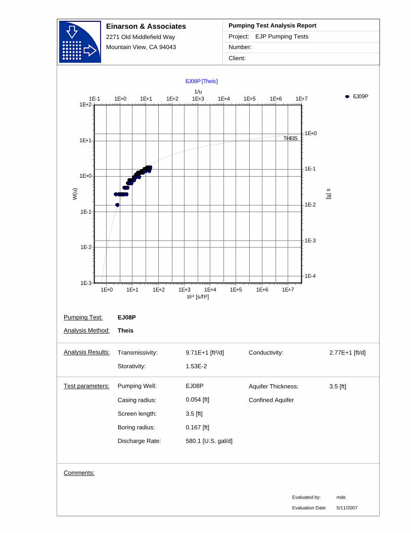
Einarson & Associates2271 Old Middlefield Way
Mountain View, CA 94043
Project:
Number:
Client:
EJP Pumping Tests
Pumping Test Analysis Report
EJ09P
EJ08P [Theis]
t/r² [s/ft²]1E+0 1E+1 1E+2 1E+3 1E+4 1E+5 1E+6 1E+7
1/u1E-1 1E+0 1E+1 1E+2 1E+3 1E+4 1E+5 1E+6 1E+7
W(u
)
1E-3
1E-2
1E-1
1E+0
1E+1
1E+2
s [ft]
1E-4
1E-3
1E-2
1E-1
1E+0THEIS
Transmissivity: 9.71E+1 [ft²/d] Conductivity: 2.77E+1 [ft/d]
Storativity: 1.53E-2
Comments:
EJ08PPumping Well:
Discharge Rate: 580.1 [U.S. gal/d]
Casing radius:
0.167 [ft]
Screen length: 3.5 [ft]
Boring radius:
0.054 [ft]
Test parameters:
EJ08P
Analysis Method: Theis
Aquifer Thickness: 3.5 [ft]
Analysis Results:
Evaluated by:
Evaluation Date:
mde
Confined Aquifer
5/11/2007
Pumping Test:

Einarson & Associates2271 Old Middlefield Way
Mountain View, CA 94043
Project:
Number:
Client:
EJP Pumping Tests
Pumping Test Analysis Report
EJ10P
EJ08P [Theis]
t/r² [s/ft²]1E+0 1E+1 1E+2 1E+3 1E+4 1E+5 1E+6 1E+7
1/u1E-1 1E+0 1E+1 1E+2 1E+3 1E+4 1E+5 1E+6 1E+7
W(u
)
1E-3
1E-2
1E-1
1E+0
1E+1
1E+2
s [ft]
1E-4
1E-3
1E-2
1E-1
1E+0
THEIS
Transmissivity: 1.44E+2 [ft²/d] Conductivity: 4.10E+1 [ft/d]
Storativity: 7.65E-3
Comments:
EJ08PPumping Well:
Discharge Rate: 580.1 [U.S. gal/d]
Casing radius:
0.167 [ft]
Screen length: 3.5 [ft]
Boring radius:
0.054 [ft]
Test parameters:
EJ08P
Analysis Method: Theis
Aquifer Thickness: 3.5 [ft]
Analysis Results:
Evaluated by:
Evaluation Date:
mde
Confined Aquifer
5/11/2007
Pumping Test:

Einarson & Associates2271 Old Middlefield Way
Mountain View, CA 94043
Project:
Number:
Client:
EJP Pumping Tests
Pumping Test Analysis Report
EJ09PEJ10P
EJ08P [Cooper-Jacob Distance-Draw dow n]
Distance from Pumping Well [f t]
Dra
wdo
wn
[ft]
0.08
0.064
0.048
0.032
0.016
0
Transmissivity: 2.13E+2 [ft²/d] Conductivity: 6.09E+1 [ft/d]
Storativity: 5.97E-3
Comments:
EJ08PPumping Well:
Discharge Rate: 580.1 [U.S. gal/d]
Casing radius:
0.167 [ft]
Screen length: 3.5 [ft]
Boring radius:
0.054 [ft]
Calculation Time: 100 [s]
Test parameters:
EJ08P
Analysis Method: Cooper-Jacob Distance-Drawdown
Aquifer Thickness: 3.5 [ft]
Analysis Results:
Evaluated by:
Evaluation Date:
mde
Confined Aquifer
5/11/2007
Pumping Test:
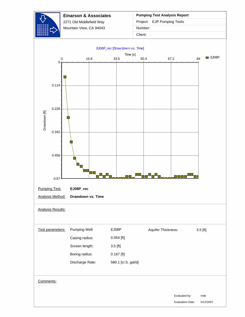
Einarson & Associates2271 Old Middlefield Way
Mountain View, CA 94043
Project:
Number:
Client:
EJP Pumping Tests
Pumping Test Analysis Report
EJ08P
EJ08P_rec [Draw dow n vs. Time]
Time [s]8467.250.433.616.80
Dra
wdo
wn
[ft]
0.57
0.456
0.342
0.228
0.114
0
Comments:
EJ08PPumping Well:
Discharge Rate: 580.1 [U.S. gal/d]
Casing radius:
0.167 [ft]
Screen length: 3.5 [ft]
Boring radius:
0.054 [ft]
Test parameters:
EJ08P_rec
Analysis Method: Drawdown vs. Time
Aquifer Thickness: 3.5 [ft]
Analysis Results:
Evaluated by:
Evaluation Date:
mde
5/12/2007
Pumping Test:

Einarson & Associates2271 Old Middlefield Way
Mountain View, CA 94043
Project:
Number:
Client:
EJP Pumping Tests
Pumping Test Analysis Report
EJ08P
EJ08P_rec [Cooper-Jacob Time-Draw dow n]
Time [s]10
Dra
wdo
wn
[ft]
0.57
0.456
0.342
0.228
0.114
0
Transmissivity: 9.45E+1 [ft²/d]
not sure reason for rapid recovery during early time. Could be discharge from pump tubing. Full recovery by approx. 25 sec.
Conductivity: 2.70E+1 [ft/d]
Comments:
EJ08PPumping Well:
Discharge Rate: 580.1 [U.S. gal/d]
Casing radius:
0.167 [ft]
Screen length: 3.5 [ft]
Boring radius:
0.054 [ft]
Test parameters:
EJ08P_rec
Analysis Method: Cooper-Jacob Time-Drawdown
Aquifer Thickness: 3.5 [ft]
Analysis Results:
Evaluated by:
Evaluation Date:
mde
Confined Aquifer
5/12/2007
Pumping Test:

Einarson & Associates2271 Old Middlefield Way
Mountain View, CA 94043
Project:
Number:
Client:
EJP Pumping Tests
Pumping Test Analysis Report
EJ08P
EJ08P_rec [Theis]
t/r² [s/ft²]1E+0 1E+1 1E+2 1E+3 1E+4 1E+5 1E+6 1E+7
1/u1E-1 1E+0 1E+1 1E+2 1E+3 1E+4 1E+5 1E+6 1E+7
W(u
)
1E-3
1E-2
1E-1
1E+0
1E+1
1E+2
s [ft]
1E-3
1E-2
1E-1
1E+0
1E+1
THEIS
Transmissivity: 1.59E+1 [ft²/d]
Fast recovery early on may be due to recharge from pump tubing. Rapid recovery overall likely due to "recharge" caused by natural flow in aquifer.
Conductivity: 4.53E+0 [ft/d]
Storativity: 1.17E-3
Comments:
EJ08PPumping Well:
Discharge Rate: 580.1 [U.S. gal/d]
Casing radius:
0.167 [ft]
Screen length: 3.5 [ft]
Boring radius:
0.054 [ft]
Test parameters:
EJ08P_rec
Analysis Method: Theis
Aquifer Thickness: 3.5 [ft]
Analysis Results:
Evaluated by:
Evaluation Date:
mde
Confined Aquifer
5/12/2007
Pumping Test:
Pumping Test Analyses
VAFB Site 60
Well EJ09P

Einarson & Associates2271 Old Middlefield Way
Mountain View, CA 94043
Project:
Number:
Client:
EJP Pumping Tests
Pumping Test Analysis Report
EJ09PEJ10P
EJ09P [Draw dow n vs. Time]
Time [s]294235.2176.4117.658.8
Dra
wdo
wn
[ft]
0.35
0.28
0.21
0.14
0.07
Comments:
EJ09PPumping Well:
Discharge Rate: 30.4 [U.S. gal/d]
Casing radius:
0.167 [ft]
Screen length: 3.5 [ft]
Boring radius:
0.054 [ft]
Test parameters:
EJ09P
Analysis Method: Drawdown vs. Time
Aquifer Thickness: 3.5 [ft]
Analysis Results:
Evaluated by:
Evaluation Date:
mde
5/12/2007
Pumping Test:
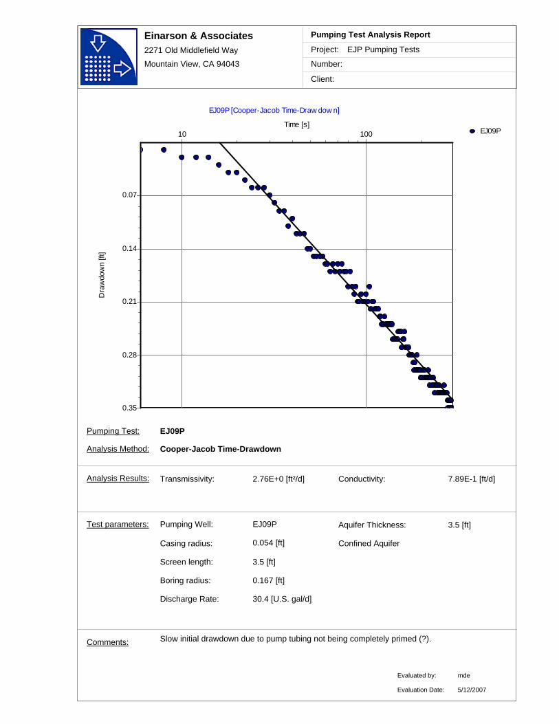
Einarson & Associates2271 Old Middlefield Way
Mountain View, CA 94043
Project:
Number:
Client:
EJP Pumping Tests
Pumping Test Analysis Report
EJ09P
EJ09P [Cooper-Jacob Time-Draw dow n]
Time [s]10 100
Dra
wdo
wn
[ft]
0.35
0.28
0.21
0.14
0.07
Transmissivity: 2.76E+0 [ft²/d]
Slow initial drawdown due to pump tubing not being completely primed (?).
Conductivity: 7.89E-1 [ft/d]
Comments:
EJ09PPumping Well:
Discharge Rate: 30.4 [U.S. gal/d]
Casing radius:
0.167 [ft]
Screen length: 3.5 [ft]
Boring radius:
0.054 [ft]
Test parameters:
EJ09P
Analysis Method: Cooper-Jacob Time-Drawdown
Aquifer Thickness: 3.5 [ft]
Analysis Results:
Evaluated by:
Evaluation Date:
mde
Confined Aquifer
5/12/2007
Pumping Test:
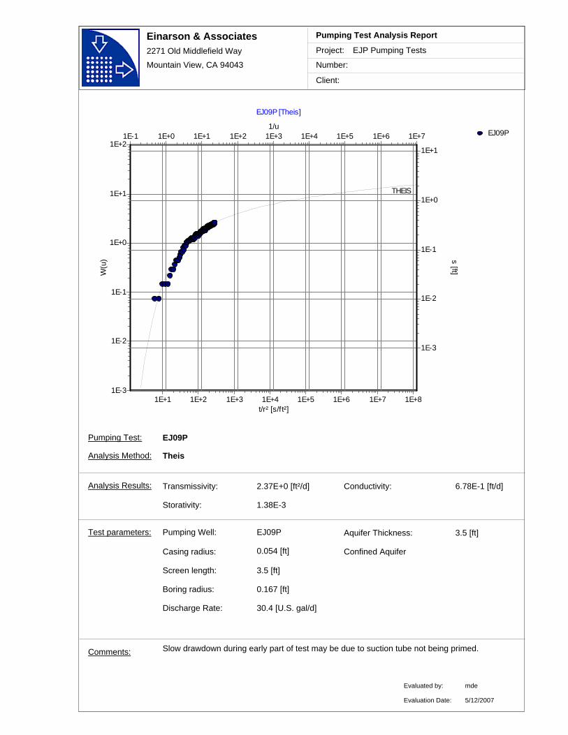
Einarson & Associates2271 Old Middlefield Way
Mountain View, CA 94043
Project:
Number:
Client:
EJP Pumping Tests
Pumping Test Analysis Report
EJ09P
EJ09P [Theis]
t/r² [s/ft²]1E+1 1E+2 1E+3 1E+4 1E+5 1E+6 1E+7 1E+8
1/u1E-1 1E+0 1E+1 1E+2 1E+3 1E+4 1E+5 1E+6 1E+7
W(u
)
1E-3
1E-2
1E-1
1E+0
1E+1
1E+2
s [ft]
1E-3
1E-2
1E-1
1E+0
1E+1
THEIS
Transmissivity: 2.37E+0 [ft²/d]
Slow drawdown during early part of test may be due to suction tube not being primed.
Conductivity: 6.78E-1 [ft/d]
Storativity: 1.38E-3
Comments:
EJ09PPumping Well:
Discharge Rate: 30.4 [U.S. gal/d]
Casing radius:
0.167 [ft]
Screen length: 3.5 [ft]
Boring radius:
0.054 [ft]
Test parameters:
EJ09P
Analysis Method: Theis
Aquifer Thickness: 3.5 [ft]
Analysis Results:
Evaluated by:
Evaluation Date:
mde
Confined Aquifer
5/12/2007
Pumping Test:
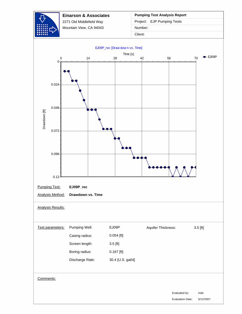
Einarson & Associates2271 Old Middlefield Way
Mountain View, CA 94043
Project:
Number:
Client:
EJP Pumping Tests
Pumping Test Analysis Report
EJ09P
EJ09P_rec [Draw dow n vs. Time]
Time [s]70564228140
Dra
wdo
wn
[ft]
0.12
0.096
0.072
0.048
0.024
0
Comments:
EJ09PPumping Well:
Discharge Rate: 30.4 [U.S. gal/d]
Casing radius:
0.167 [ft]
Screen length: 3.5 [ft]
Boring radius:
0.054 [ft]
Test parameters:
EJ09P_rec
Analysis Method: Drawdown vs. Time
Aquifer Thickness: 3.5 [ft]
Analysis Results:
Evaluated by:
Evaluation Date:
mde
5/12/2007
Pumping Test:

Einarson & Associates2271 Old Middlefield Way
Mountain View, CA 94043
Project:
Number:
Client:
EJP Pumping Tests
Pumping Test Analysis Report
EJ09P
EJ09P_rec [Cooper-Jacob Time-Draw dow n]
Time [s]10
Dra
wdo
wn
[ft]
0.12
0.096
0.072
0.048
0.024
0
Transmissivity: 6.02E+0 [ft²/d]
Delayed recovery possibly due to casing storage effect.
Conductivity: 1.72E+0 [ft/d]
Comments:
EJ09PPumping Well:
Discharge Rate: 30.4 [U.S. gal/d]
Casing radius:
0.167 [ft]
Screen length: 3.5 [ft]
Boring radius:
0.054 [ft]
Test parameters:
EJ09P_rec
Analysis Method: Cooper-Jacob Time-Drawdown
Aquifer Thickness: 3.5 [ft]
Analysis Results:
Evaluated by:
Evaluation Date:
mde
Confined Aquifer
5/12/2007
Pumping Test:

Einarson & Associates2271 Old Middlefield Way
Mountain View, CA 94043
Project:
Number:
Client:
EJP Pumping Tests
Pumping Test Analysis Report
EJ09P
EJ09P_rec [Theis]
t/r² [s/ft²]1E+0 1E+1 1E+2 1E+3 1E+4 1E+5 1E+6 1E+7
1/u1E-1 1E+0 1E+1 1E+2 1E+3 1E+4 1E+5 1E+6 1E+7
W(u
)
1E-3
1E-2
1E-1
1E+0
1E+1
1E+2
s [ft]
1E-4
1E-3
1E-2
1E-1
1E+0THEIS
Transmissivity: 4.97E+0 [ft²/d] Conductivity: 1.42E+0 [ft/d]
Storativity: 1.33E-3
Comments:
EJ09PPumping Well:
Discharge Rate: 30.4 [U.S. gal/d]
Casing radius:
0.167 [ft]
Screen length: 3.5 [ft]
Boring radius:
0.054 [ft]
Test parameters:
EJ09P_rec
Analysis Method: Theis
Aquifer Thickness: 3.5 [ft]
Analysis Results:
Evaluated by:
Evaluation Date:
mde
Confined Aquifer
5/12/2007
Pumping Test:
Pumping Test Analyses
VAFB Site 60
Well EJ010P
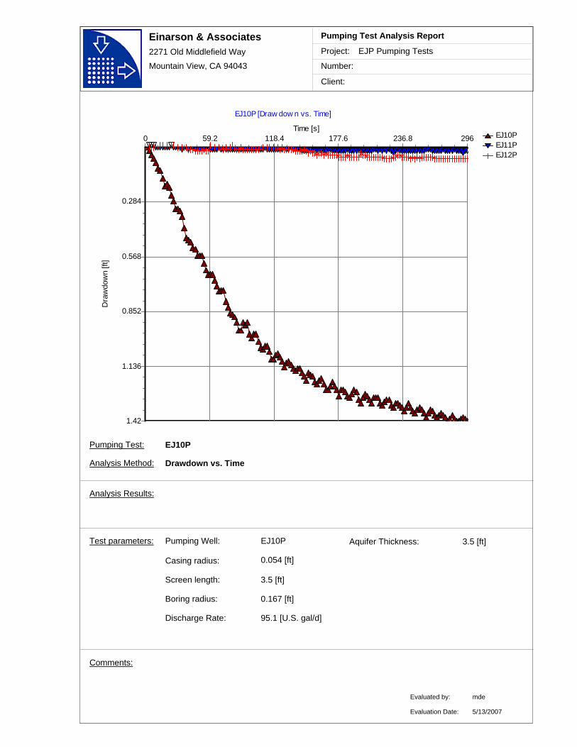
Einarson & Associates2271 Old Middlefield Way
Mountain View, CA 94043
Project:
Number:
Client:
EJP Pumping Tests
Pumping Test Analysis Report
EJ10PEJ11PEJ12P
EJ10P [Draw dow n vs. Time]
Time [s]296236.8177.6118.459.20
Dra
wdo
wn
[ft]
1.42
1.136
0.852
0.568
0.284
Comments:
EJ10PPumping Well:
Discharge Rate: 95.1 [U.S. gal/d]
Casing radius:
0.167 [ft]
Screen length: 3.5 [ft]
Boring radius:
0.054 [ft]
Test parameters:
EJ10P
Analysis Method: Drawdown vs. Time
Aquifer Thickness: 3.5 [ft]
Analysis Results:
Evaluated by:
Evaluation Date:
mde
5/13/2007
Pumping Test:

Einarson & Associates2271 Old Middlefield Way
Mountain View, CA 94043
Project:
Number:
Client:
EJP Pumping Tests
Pumping Test Analysis Report
EJ10PEJ11PEJ12P
EJ10P [Cooper-Jacob Time-Draw dow n]
Time [s]10 100
Dra
wdo
wn
[ft]
1.42
1.136
0.852
0.568
0.284
Transmissivity: 1.58E+0 [ft²/d]
Delayed drawdown early in test likely due to pump tubing not being primed. Reduced drawdown late in test likely due to recharge caused by flow in aquifer (based on Theis analysis).
Conductivity: 4.51E-1 [ft/d]
Comments:
EJ10PPumping Well:
Discharge Rate: 95.1 [U.S. gal/d]
Casing radius:
0.167 [ft]
Screen length: 3.5 [ft]
Boring radius:
0.054 [ft]
Test parameters:
EJ10P
Analysis Method: Cooper-Jacob Time-Drawdown
Aquifer Thickness: 3.5 [ft]
Analysis Results:
Evaluated by:
Evaluation Date:
mde
Confined Aquifer
5/13/2007
Pumping Test:

Einarson & Associates2271 Old Middlefield Way
Mountain View, CA 94043
Project:
Number:
Client:
EJP Pumping Tests
Pumping Test Analysis Report
EJ10P
EJ10P [Theis]
t/r² [s/ft²]1E+1 1E+2 1E+3 1E+4 1E+5 1E+6 1E+7 1E+8
1/u1E-1 1E+0 1E+1 1E+2 1E+3 1E+4 1E+5 1E+6 1E+7
W(u
)
1E-3
1E-2
1E-1
1E+0
1E+1
1E+2
s [ft]
1E-3
1E-2
1E-1
1E+0
1E+1THEIS
Transmissivity: 1.38E+0 [ft²/d]
Delayed drawdown early in test likely due to pump tubing not being primed. Reduced drawdown late in test likely due to recharge caused by flow in aquifer.
Conductivity: 3.93E-1 [ft/d]
Storativity: 1.14E-3
Comments:
EJ10PPumping Well:
Discharge Rate: 95.1 [U.S. gal/d]
Casing radius:
0.167 [ft]
Screen length: 3.5 [ft]
Boring radius:
0.054 [ft]
Test parameters:
EJ10P
Analysis Method: Theis
Aquifer Thickness: 3.5 [ft]
Analysis Results:
Evaluated by:
Evaluation Date:
mde
Confined Aquifer
5/13/2007
Pumping Test:
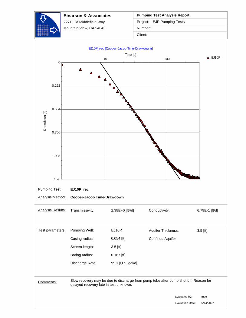
Einarson & Associates2271 Old Middlefield Way
Mountain View, CA 94043
Project:
Number:
Client:
EJP Pumping Tests
Pumping Test Analysis Report
EJ10P
EJ10P_rec [Cooper-Jacob Time-Draw dow n]
Time [s]10 100
Dra
wdo
wn
[ft]
1.26
1.008
0.756
0.504
0.252
0
Transmissivity: 2.38E+0 [ft²/d]
Slow recovery may be due to discharge from pump tube after pump shut off. Reason for delayed recovery late in test unknown.
Conductivity: 6.79E-1 [ft/d]
Comments:
EJ10PPumping Well:
Discharge Rate: 95.1 [U.S. gal/d]
Casing radius:
0.167 [ft]
Screen length: 3.5 [ft]
Boring radius:
0.054 [ft]
Test parameters:
EJ10P_rec
Analysis Method: Cooper-Jacob Time-Drawdown
Aquifer Thickness: 3.5 [ft]
Analysis Results:
Evaluated by:
Evaluation Date:
mde
Confined Aquifer
5/14/2007
Pumping Test:

Einarson & Associates2271 Old Middlefield Way
Mountain View, CA 94043
Project:
Number:
Client:
EJP Pumping Tests
Pumping Test Analysis Report
EJ10P
EJ10P_rec [Theis]
t/r² [s/ft²]1E+0 1E+1 1E+2 1E+3 1E+4 1E+5 1E+6 1E+7
1/u1E-1 1E+0 1E+1 1E+2 1E+3 1E+4 1E+5 1E+6 1E+7
W(u
)
1E-3
1E-2
1E-1
1E+0
1E+1
1E+2
s [ft]
1E-3
1E-2
1E-1
1E+0
1E+1
THEIS
Transmissivity: 2.14E+0 [ft²/d]
Slow recovery may be due to discharge from pump tube after pump shut off. Reason for delayed recovery late in test unknown.
Conductivity: 6.11E-1 [ft/d]
Storativity: 6.56E-4
Comments:
EJ10PPumping Well:
Discharge Rate: 95.1 [U.S. gal/d]
Casing radius:
0.167 [ft]
Screen length: 3.5 [ft]
Boring radius:
0.054 [ft]
Test parameters:
EJ10P_rec
Analysis Method: Theis
Aquifer Thickness: 3.5 [ft]
Analysis Results:
Evaluated by:
Evaluation Date:
mde
Confined Aquifer
5/14/2007
Pumping Test:
Pumping Test Analyses
VAFB Site 60
Well EJ011P

Einarson & Associates2271 Old Middlefield Way
Mountain View, CA 94043
Project:
Number:
Client:
EJP Pumping Tests
Pumping Test Analysis Report
EJ11PEJ12PEJ13P
EJ11P [Draw dow n vs. Time]
Time [s]296236.8177.6118.459.20
Dra
wdo
wn
[ft]
0.37
0.296
0.222
0.148
0.074
Comments:
EJ11PPumping Well:
Discharge Rate: 194 [U.S. gal/d]
Casing radius:
0.167 [ft]
Screen length: 3.5 [ft]
Boring radius:
0.054 [ft]
Test parameters:
EJ11P
Analysis Method: Drawdown vs. Time
Aquifer Thickness: 3.5 [ft]
Analysis Results:
Evaluated by:
Evaluation Date:
mde
5/14/2007
Pumping Test:
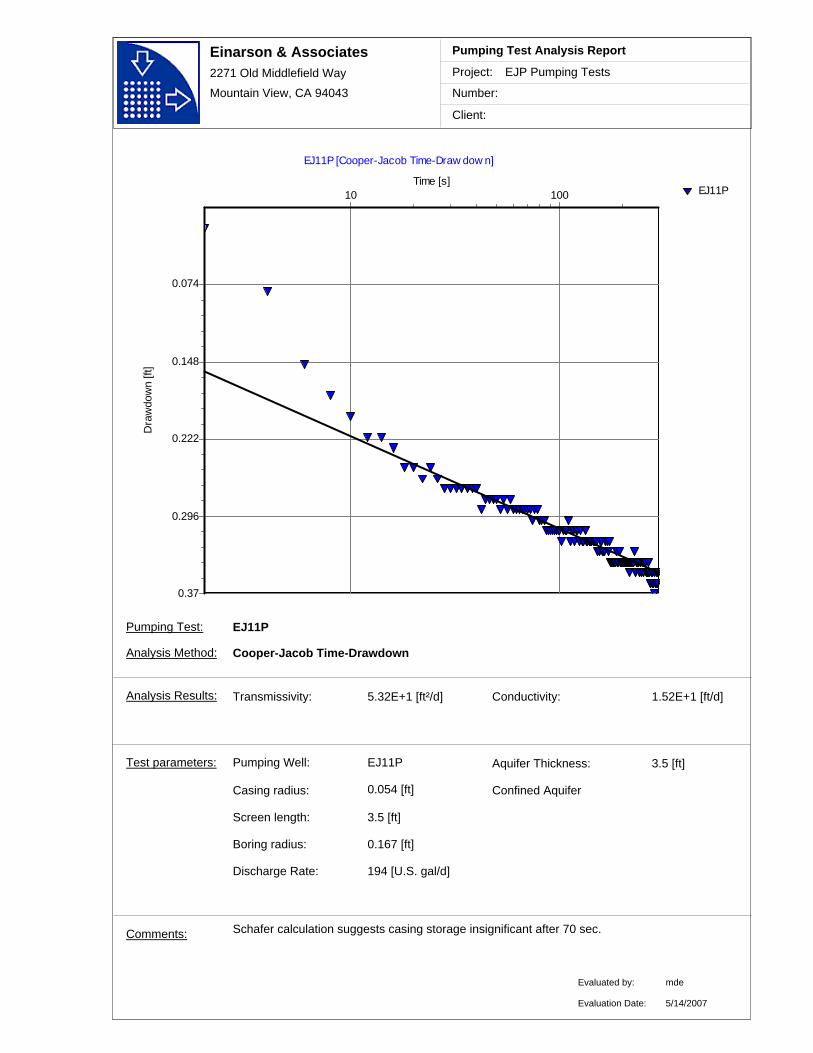
Einarson & Associates2271 Old Middlefield Way
Mountain View, CA 94043
Project:
Number:
Client:
EJP Pumping Tests
Pumping Test Analysis Report
EJ11P
EJ11P [Cooper-Jacob Time-Draw dow n]
Time [s]10 100
Dra
wdo
wn
[ft]
0.37
0.296
0.222
0.148
0.074
Transmissivity: 5.32E+1 [ft²/d]
Schafer calculation suggests casing storage insignificant after 70 sec.
Conductivity: 1.52E+1 [ft/d]
Comments:
EJ11PPumping Well:
Discharge Rate: 194 [U.S. gal/d]
Casing radius:
0.167 [ft]
Screen length: 3.5 [ft]
Boring radius:
0.054 [ft]
Test parameters:
EJ11P
Analysis Method: Cooper-Jacob Time-Drawdown
Aquifer Thickness: 3.5 [ft]
Analysis Results:
Evaluated by:
Evaluation Date:
mde
Confined Aquifer
5/14/2007
Pumping Test:

Einarson & Associates2271 Old Middlefield Way
Mountain View, CA 94043
Project:
Number:
Client:
EJP Pumping Tests
Pumping Test Analysis Report
EJ11P
EJ11P [Theis]
t/r² [s/ft²]1E-2 1E-1 1E+0 1E+1 1E+2 1E+3 1E+4 1E+5
1/u1E-1 1E+0 1E+1 1E+2 1E+3 1E+4 1E+5 1E+6 1E+7
W(u
)
1E-3
1E-2
1E-1
1E+0
1E+1
1E+2
s [ft]
1E-4
1E-3
1E-2
1E-1
1E+0
THEIS
Transmissivity: 5.13E+1 [ft²/d]
early time data ignored since Schafer calculation suggests due to casing storage.
Conductivity: 1.46E+1 [ft/d]
Storativity: 4.64E-5
Comments:
EJ11PPumping Well:
Discharge Rate: 194 [U.S. gal/d]
Casing radius:
0.167 [ft]
Screen length: 3.5 [ft]
Boring radius:
0.054 [ft]
Test parameters:
EJ11P
Analysis Method: Theis
Aquifer Thickness: 3.5 [ft]
Analysis Results:
Evaluated by:
Evaluation Date:
mde
Confined Aquifer
5/14/2007
Pumping Test:

Einarson & Associates2271 Old Middlefield Way
Mountain View, CA 94043
Project:
Number:
Client:
EJP Pumping Tests
Pumping Test Analysis Report
EJ12P
EJ11P [Cooper-Jacob Time-Draw dow n]
Time [s]10 100
Dra
wdo
wn
[ft]
0.08
0.064
0.048
0.032
0.016
0
Transmissivity: 1.02E+2 [ft²/d]
Schafer calculation suggests casing storage insignificant after 70 sec. Calculated time when u < 0.05 = 81 sec.
Conductivity: 2.90E+1 [ft/d]
Storativity: 3.01E-3
Comments:
EJ11PPumping Well:
Discharge Rate: 194 [U.S. gal/d]
Casing radius:
0.167 [ft]
Screen length: 3.5 [ft]
Boring radius:
0.054 [ft]
Test parameters:
EJ11P
Analysis Method: Cooper-Jacob Time-Drawdown
Aquifer Thickness: 3.5 [ft]
Analysis Results:
Evaluated by:
Evaluation Date:
mde
Confined Aquifer
5/14/2007
Pumping Test:
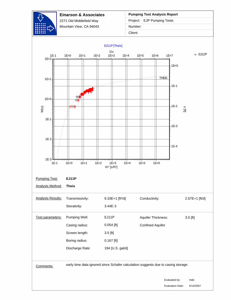
Einarson & Associates2271 Old Middlefield Way
Mountain View, CA 94043
Project:
Number:
Client:
EJP Pumping Tests
Pumping Test Analysis Report
EJ12P
EJ11P [Theis]
t/r² [s/ft²]1E-1 1E+0 1E+1 1E+2 1E+3 1E+4 1E+5 1E+6
1/u1E-1 1E+0 1E+1 1E+2 1E+3 1E+4 1E+5 1E+6 1E+7
W(u
)
1E-3
1E-2
1E-1
1E+0
1E+1
1E+2
s [ft]
1E-4
1E-3
1E-2
1E-1
1E+0
THEIS
Transmissivity: 9.33E+1 [ft²/d]
early time data ignored since Schafer calculation suggests due to casing storage.
Conductivity: 2.67E+1 [ft/d]
Storativity: 3.44E-3
Comments:
EJ11PPumping Well:
Discharge Rate: 194 [U.S. gal/d]
Casing radius:
0.167 [ft]
Screen length: 3.5 [ft]
Boring radius:
0.054 [ft]
Test parameters:
EJ11P
Analysis Method: Theis
Aquifer Thickness: 3.5 [ft]
Analysis Results:
Evaluated by:
Evaluation Date:
mde
Confined Aquifer
5/14/2007
Pumping Test:
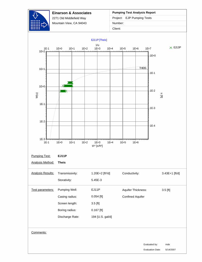
Einarson & Associates2271 Old Middlefield Way
Mountain View, CA 94043
Project:
Number:
Client:
EJP Pumping Tests
Pumping Test Analysis Report
EJ13P
EJ11P [Theis]
t/r² [s/ft²]1E-1 1E+0 1E+1 1E+2 1E+3 1E+4 1E+5 1E+6
1/u1E-1 1E+0 1E+1 1E+2 1E+3 1E+4 1E+5 1E+6 1E+7
W(u
)
1E-3
1E-2
1E-1
1E+0
1E+1
1E+2
s [ft]
1E-4
1E-3
1E-2
1E-1
1E+0
THEIS
Transmissivity: 1.20E+2 [ft²/d] Conductivity: 3.43E+1 [ft/d]
Storativity: 5.45E-3
Comments:
EJ11PPumping Well:
Discharge Rate: 194 [U.S. gal/d]
Casing radius:
0.167 [ft]
Screen length: 3.5 [ft]
Boring radius:
0.054 [ft]
Test parameters:
EJ11P
Analysis Method: Theis
Aquifer Thickness: 3.5 [ft]
Analysis Results:
Evaluated by:
Evaluation Date:
mde
Confined Aquifer
5/14/2007
Pumping Test:
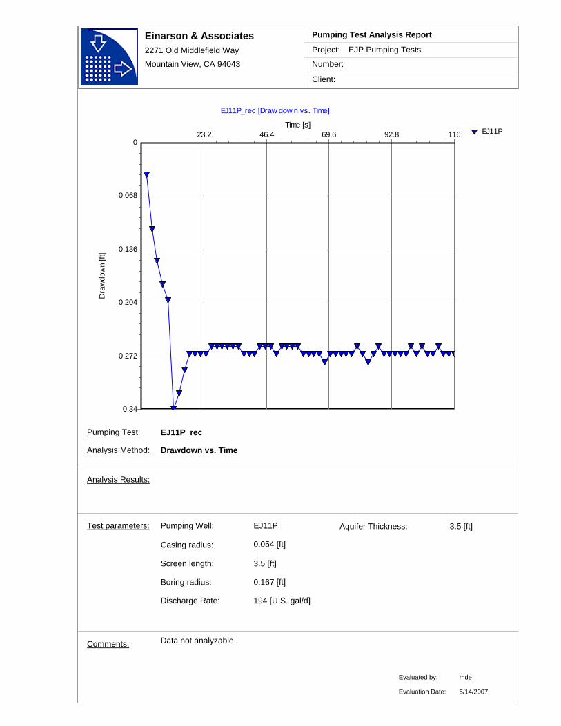
Einarson & Associates2271 Old Middlefield Way
Mountain View, CA 94043
Project:
Number:
Client:
EJP Pumping Tests
Pumping Test Analysis Report
EJ11P
EJ11P_rec [Draw dow n vs. Time]
Time [s]11692.869.646.423.2
Dra
wdo
wn
[ft]
0.34
0.272
0.204
0.136
0.068
0
Data not analyzableComments:
EJ11PPumping Well:
Discharge Rate: 194 [U.S. gal/d]
Casing radius:
0.167 [ft]
Screen length: 3.5 [ft]
Boring radius:
0.054 [ft]
Test parameters:
EJ11P_rec
Analysis Method: Drawdown vs. Time
Aquifer Thickness: 3.5 [ft]
Analysis Results:
Evaluated by:
Evaluation Date:
mde
5/14/2007
Pumping Test:

Pumping Test Analyses
VAFB Site 60
Well EJ012P
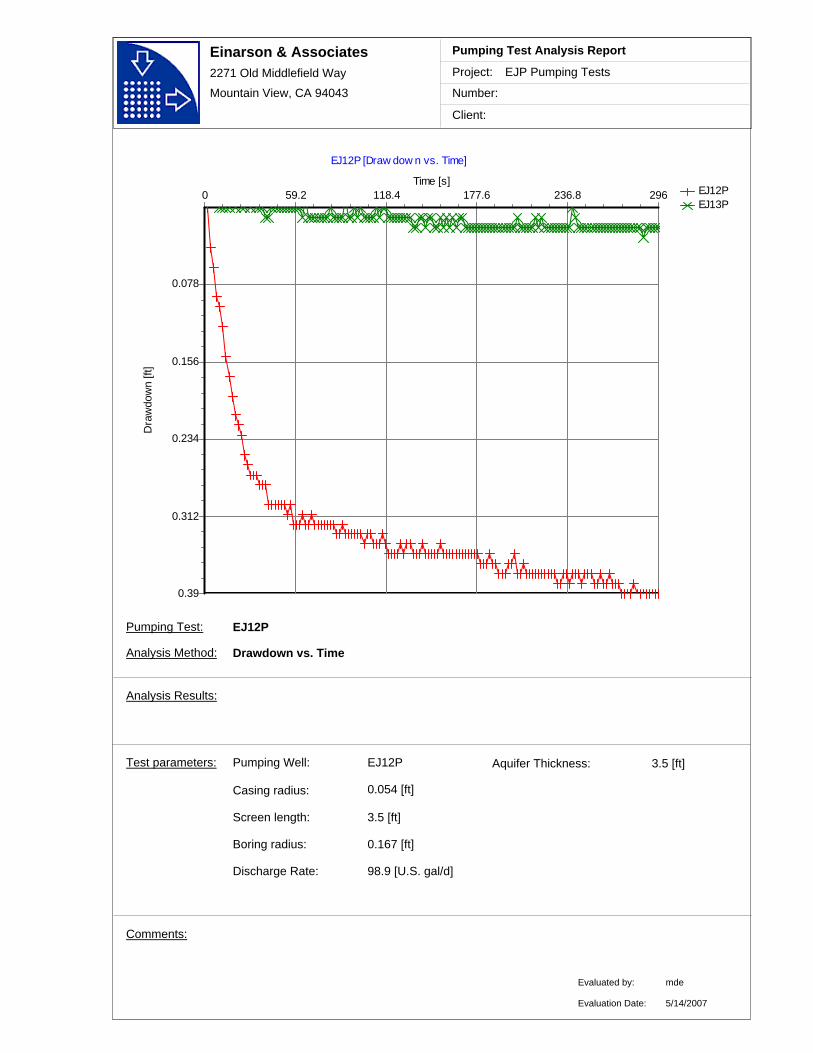
Einarson & Associates2271 Old Middlefield Way
Mountain View, CA 94043
Project:
Number:
Client:
EJP Pumping Tests
Pumping Test Analysis Report
EJ12PEJ13P
EJ12P [Draw dow n vs. Time]
Time [s]296236.8177.6118.459.20
Dra
wdo
wn
[ft]
0.39
0.312
0.234
0.156
0.078
Comments:
EJ12PPumping Well:
Discharge Rate: 98.9 [U.S. gal/d]
Casing radius:
0.167 [ft]
Screen length: 3.5 [ft]
Boring radius:
0.054 [ft]
Test parameters:
EJ12P
Analysis Method: Drawdown vs. Time
Aquifer Thickness: 3.5 [ft]
Analysis Results:
Evaluated by:
Evaluation Date:
mde
5/14/2007
Pumping Test:
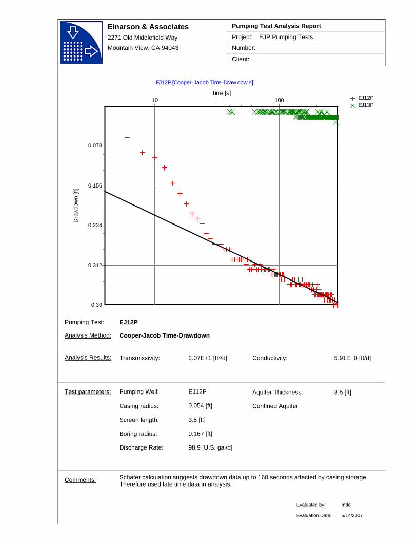
Einarson & Associates2271 Old Middlefield Way
Mountain View, CA 94043
Project:
Number:
Client:
EJP Pumping Tests
Pumping Test Analysis Report
EJ12PEJ13P
EJ12P [Cooper-Jacob Time-Draw dow n]
Time [s]10 100
Dra
wdo
wn
[ft]
0.39
0.312
0.234
0.156
0.078
Transmissivity: 2.07E+1 [ft²/d]
Schafer calculation suggests drawdown data up to 160 seconds affected by casing storage. Therefore used late time data in analysis.
Conductivity: 5.91E+0 [ft/d]
Comments:
EJ12PPumping Well:
Discharge Rate: 98.9 [U.S. gal/d]
Casing radius:
0.167 [ft]
Screen length: 3.5 [ft]
Boring radius:
0.054 [ft]
Test parameters:
EJ12P
Analysis Method: Cooper-Jacob Time-Drawdown
Aquifer Thickness: 3.5 [ft]
Analysis Results:
Evaluated by:
Evaluation Date:
mde
Confined Aquifer
5/14/2007
Pumping Test:

Einarson & Associates2271 Old Middlefield Way
Mountain View, CA 94043
Project:
Number:
Client:
EJP Pumping Tests
Pumping Test Analysis Report
EJ12P
EJ12P [Theis]
t/r² [s/ft²]1E-1 1E+0 1E+1 1E+2 1E+3 1E+4 1E+5 1E+6
1/u1E-1 1E+0 1E+1 1E+2 1E+3 1E+4 1E+5 1E+6 1E+7
W(u
)
1E-3
1E-2
1E-1
1E+0
1E+1
1E+2
s [ft]
1E-4
1E-3
1E-2
1E-1
1E+0THEIS
Transmissivity: 1.70E+1 [ft²/d]
Early time data ignored because Schafer analysis suggests due to casing storage.
Conductivity: 4.86E+0 [ft/d]
Storativity: 2.03E-4
Comments:
EJ12PPumping Well:
Discharge Rate: 98.9 [U.S. gal/d]
Casing radius:
0.167 [ft]
Screen length: 3.5 [ft]
Boring radius:
0.054 [ft]
Test parameters:
EJ12P
Analysis Method: Theis
Aquifer Thickness: 3.5 [ft]
Analysis Results:
Evaluated by:
Evaluation Date:
mde
Confined Aquifer
5/14/2007
Pumping Test:
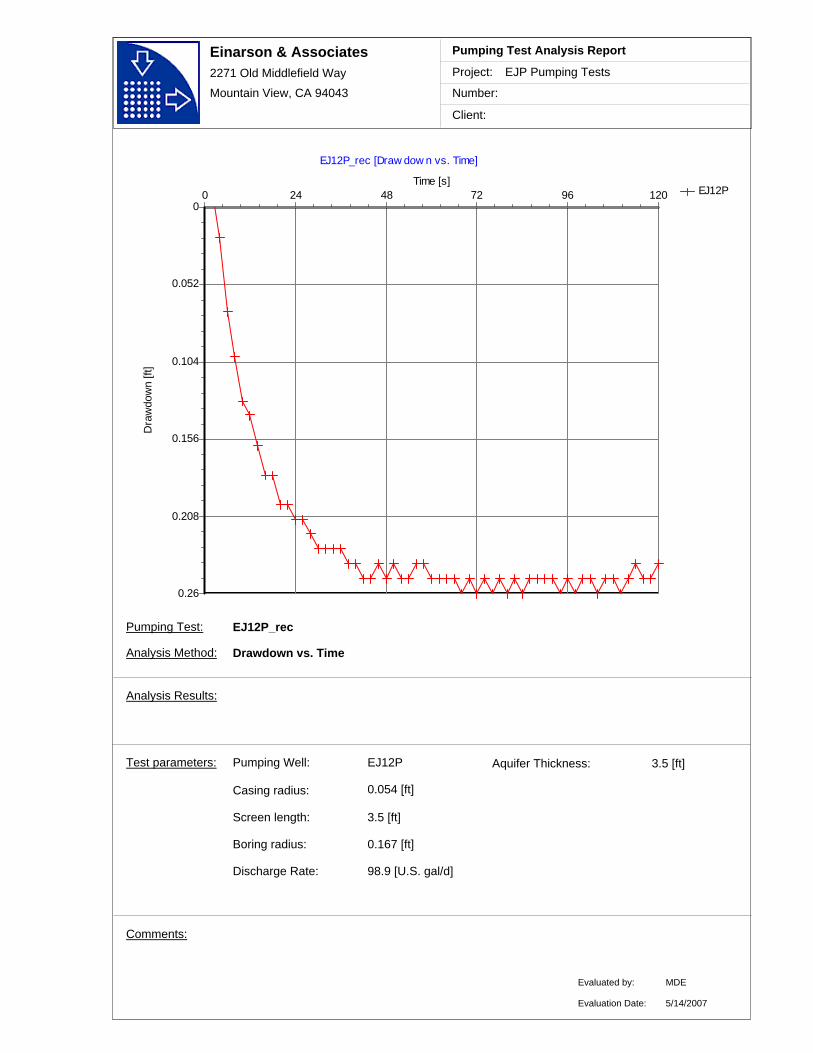
Einarson & Associates2271 Old Middlefield Way
Mountain View, CA 94043
Project:
Number:
Client:
EJP Pumping Tests
Pumping Test Analysis Report
EJ12P
EJ12P_rec [Draw dow n vs. Time]
Time [s]120967248240
Dra
wdo
wn
[ft]
0.26
0.208
0.156
0.104
0.052
0
Comments:
EJ12PPumping Well:
Discharge Rate: 98.9 [U.S. gal/d]
Casing radius:
0.167 [ft]
Screen length: 3.5 [ft]
Boring radius:
0.054 [ft]
Test parameters:
EJ12P_rec
Analysis Method: Drawdown vs. Time
Aquifer Thickness: 3.5 [ft]
Analysis Results:
Evaluated by:
Evaluation Date:
MDE
5/14/2007
Pumping Test:
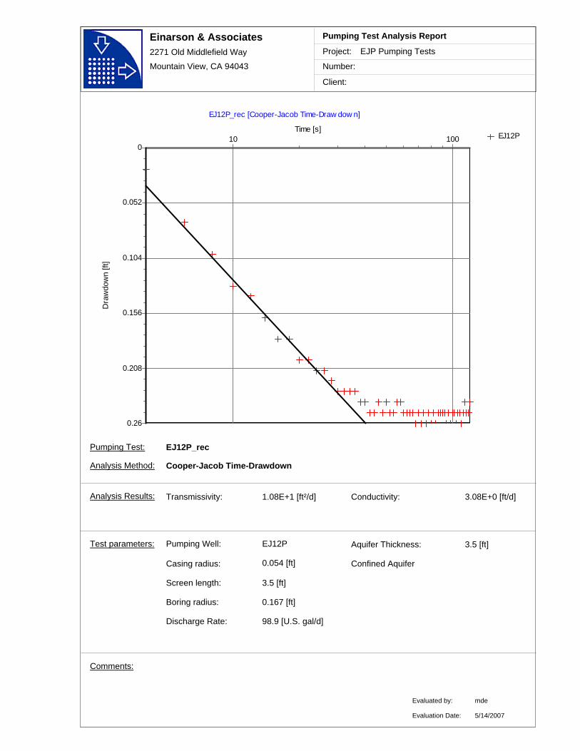
Einarson & Associates2271 Old Middlefield Way
Mountain View, CA 94043
Project:
Number:
Client:
EJP Pumping Tests
Pumping Test Analysis Report
EJ12P
EJ12P_rec [Cooper-Jacob Time-Draw dow n]
Time [s]10 100
Dra
wdo
wn
[ft]
0.26
0.208
0.156
0.104
0.052
0
Transmissivity: 1.08E+1 [ft²/d] Conductivity: 3.08E+0 [ft/d]
Comments:
EJ12PPumping Well:
Discharge Rate: 98.9 [U.S. gal/d]
Casing radius:
0.167 [ft]
Screen length: 3.5 [ft]
Boring radius:
0.054 [ft]
Test parameters:
EJ12P_rec
Analysis Method: Cooper-Jacob Time-Drawdown
Aquifer Thickness: 3.5 [ft]
Analysis Results:
Evaluated by:
Evaluation Date:
mde
Confined Aquifer
5/14/2007
Pumping Test:

Einarson & Associates2271 Old Middlefield Way
Mountain View, CA 94043
Project:
Number:
Client:
EJP Pumping Tests
Pumping Test Analysis Report
EJ12P
EJ12P_rec [Theis]
t/r² [s/ft²]1E+0 1E+1 1E+2 1E+3 1E+4 1E+5 1E+6 1E+7
1/u1E-1 1E+0 1E+1 1E+2 1E+3 1E+4 1E+5 1E+6 1E+7
W(u
)
1E-3
1E-2
1E-1
1E+0
1E+1
1E+2
s [ft]
1E-4
1E-3
1E-2
1E-1
1E+0THEIS
Transmissivity: 1.10E+1 [ft²/d]
Reason for delayed recovery late in test not known.
Conductivity: 3.15E+0 [ft/d]
Storativity: 8.72E-4
Comments:
EJ12PPumping Well:
Discharge Rate: 98.9 [U.S. gal/d]
Casing radius:
0.167 [ft]
Screen length: 3.5 [ft]
Boring radius:
0.054 [ft]
Test parameters:
EJ12P_rec
Analysis Method: Theis
Aquifer Thickness: 3.5 [ft]
Analysis Results:
Evaluated by:
Evaluation Date:
mde
Confined Aquifer
5/14/2007
Pumping Test:

Pumping Test Analyses
VAFB Site 60
Well EJ013P

Einarson & Associates2271 Old Middlefield Way
Mountain View, CA 94043
Project:
Number:
Client:
EJP Pumping Tests
Pumping Test Analysis Report
EJ13PEJ14PEJ15P
EJ13P [Draw dow n vs. Time]
Time [s]296236.8177.6118.459.20
Dra
wdo
wn
[ft]
1.13
0.904
0.678
0.452
0.226
0
Comments:
EJ13PPumping Well:
Discharge Rate: 68.5 [U.S. gal/d]
Casing radius:
0.167 [ft]
Screen length: 3.5 [ft]
Boring radius:
0.054 [ft]
Test parameters:
EJ13P
Analysis Method: Drawdown vs. Time
Aquifer Thickness: 3.5 [ft]
Analysis Results:
Evaluated by:
Evaluation Date:
mde
5/14/2007
Pumping Test:
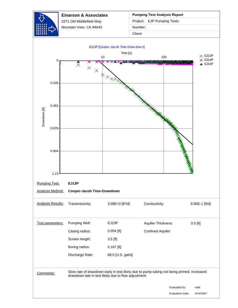
Einarson & Associates2271 Old Middlefield Way
Mountain View, CA 94043
Project:
Number:
Client:
EJP Pumping Tests
Pumping Test Analysis Report
EJ13PEJ14PEJ15P
EJ13P [Cooper-Jacob Time-Draw dow n]
Time [s]10 100
Dra
wdo
wn
[ft]
1.13
0.904
0.678
0.452
0.226
0
Transmissivity: 3.08E+0 [ft²/d]
Slow rate of drawdown early in test likely due to pump tubing not being primed. Increased drawdown late in test likely due to flow adjustment.
Conductivity: 8.80E-1 [ft/d]
Comments:
EJ13PPumping Well:
Discharge Rate: 68.5 [U.S. gal/d]
Casing radius:
0.167 [ft]
Screen length: 3.5 [ft]
Boring radius:
0.054 [ft]
Test parameters:
EJ13P
Analysis Method: Cooper-Jacob Time-Drawdown
Aquifer Thickness: 3.5 [ft]
Analysis Results:
Evaluated by:
Evaluation Date:
mde
Confined Aquifer
5/14/2007
Pumping Test:
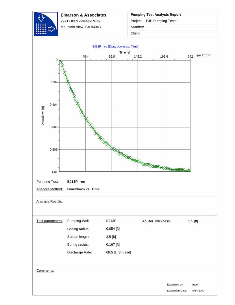
Einarson & Associates2271 Old Middlefield Way
Mountain View, CA 94043
Project:
Number:
Client:
EJP Pumping Tests
Pumping Test Analysis Report
EJ13P
EJ13P_rec [Draw dow n vs. Time]
Time [s]242193.6145.296.848.4
Dra
wdo
wn
[ft]
1.01
0.808
0.606
0.404
0.202
0
Comments:
EJ13PPumping Well:
Discharge Rate: 68.5 [U.S. gal/d]
Casing radius:
0.167 [ft]
Screen length: 3.5 [ft]
Boring radius:
0.054 [ft]
Test parameters:
EJ13P_rec
Analysis Method: Drawdown vs. Time
Aquifer Thickness: 3.5 [ft]
Analysis Results:
Evaluated by:
Evaluation Date:
mde
5/14/2007
Pumping Test:

Einarson & Associates2271 Old Middlefield Way
Mountain View, CA 94043
Project:
Number:
Client:
EJP Pumping Tests
Pumping Test Analysis Report
EJ13P
EJ13P_rec [Cooper-Jacob Time-Draw dow n]
Time [s]10 100
Dra
wdo
wn
[ft]
1.01
0.808
0.606
0.404
0.202
0
Transmissivity: 1.93E+0 [ft²/d]
Slow recovery initially due to recharge from pump tubing (?)
Conductivity: 5.52E-1 [ft/d]
Comments:
EJ13PPumping Well:
Discharge Rate: 68.5 [U.S. gal/d]
Casing radius:
0.167 [ft]
Screen length: 3.5 [ft]
Boring radius:
0.054 [ft]
Test parameters:
EJ13P_rec
Analysis Method: Cooper-Jacob Time-Drawdown
Aquifer Thickness: 3.5 [ft]
Analysis Results:
Evaluated by:
Evaluation Date:
mde
Confined Aquifer
5/14/2007
Pumping Test:

Einarson & Associates2271 Old Middlefield Way
Mountain View, CA 94043
Project:
Number:
Client:
EJP Pumping Tests
Pumping Test Analysis Report
EJ13P
EJ13P_rec [Theis]
t/r² [s/ft²]1E+0 1E+1 1E+2 1E+3 1E+4 1E+5 1E+6 1E+7
1/u1E-1 1E+0 1E+1 1E+2 1E+3 1E+4 1E+5 1E+6 1E+7
W(u
)
1E-3
1E-2
1E-1
1E+0
1E+1
1E+2
s [ft]
1E-3
1E-2
1E-1
1E+0
1E+1
THEIS
Transmissivity: 1.90E+0 [ft²/d] Conductivity: 5.42E-1 [ft/d]
Storativity: 6.85E-4
Comments:
EJ13PPumping Well:
Discharge Rate: 68.5 [U.S. gal/d]
Casing radius:
0.167 [ft]
Screen length: 3.5 [ft]
Boring radius:
0.054 [ft]
Test parameters:
EJ13P_rec
Analysis Method: Theis
Aquifer Thickness: 3.5 [ft]
Analysis Results:
Evaluated by:
Evaluation Date:
mde
Confined Aquifer
5/14/2007
Pumping Test:

Pumping Test Analyses
VAFB Site 60
Well EJ014P

Einarson & Associates2271 Old Middlefield Way
Mountain View, CA 94043
Project:
Number:
Client:
EJP Pumping Tests
Pumping Test Analysis Report
EJ14PEJ15PEJ16P
EJ14P [Draw dow n vs. Time]
Time [s]296236.8177.6118.459.20
Dra
wdo
wn
[ft]
0.37
0.296
0.222
0.148
0.074
Comments:
EJ14PPumping Well:
Discharge Rate: 197.8 [U.S. gal/d]
Casing radius:
0.167 [ft]
Screen length: 3.5 [ft]
Boring radius:
0.054 [ft]
Test parameters:
EJ14P
Analysis Method: Drawdown vs. Time
Aquifer Thickness: 3.5 [ft]
Analysis Results:
Evaluated by:
Evaluation Date:
mde
5/14/2007
Pumping Test:

Einarson & Associates2271 Old Middlefield Way
Mountain View, CA 94043
Project:
Number:
Client:
EJP Pumping Tests
Pumping Test Analysis Report
EJ14P
EJ14P [Cooper-Jacob Time-Draw dow n]
Time [s]10 100
Dra
wdo
wn
[ft]
0.37
0.296
0.222
0.148
0.074
Transmissivity: 6.05E+1 [ft²/d]
Schafer calculation suggests casing storage negligible after 77 second.
Conductivity: 1.73E+1 [ft/d]
Comments:
EJ14PPumping Well:
Discharge Rate: 197.8 [U.S. gal/d]
Casing radius:
0.167 [ft]
Screen length: 3.5 [ft]
Boring radius:
0.054 [ft]
Test parameters:
EJ14P
Analysis Method: Cooper-Jacob Time-Drawdown
Aquifer Thickness: 3.5 [ft]
Analysis Results:
Evaluated by:
Evaluation Date:
mde
Confined Aquifer
5/14/2007
Pumping Test:
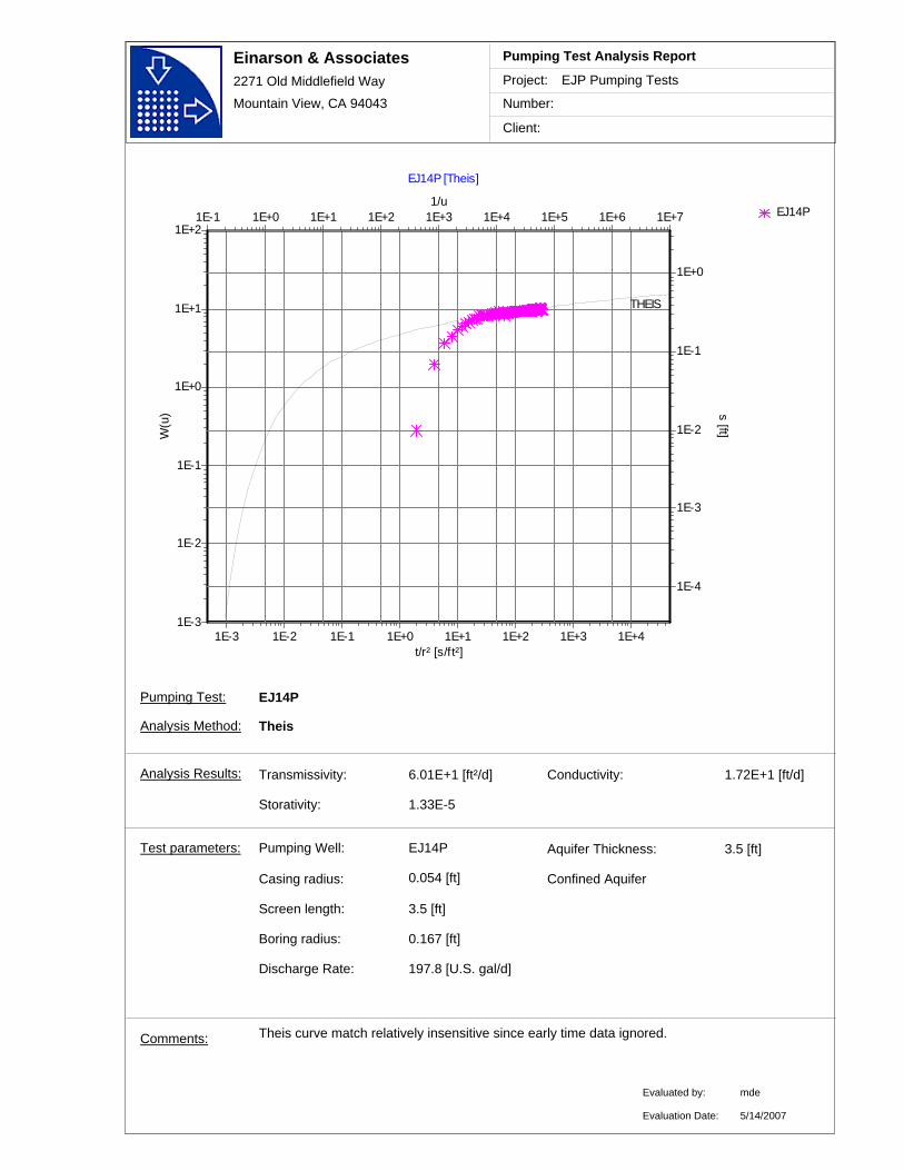
Einarson & Associates2271 Old Middlefield Way
Mountain View, CA 94043
Project:
Number:
Client:
EJP Pumping Tests
Pumping Test Analysis Report
EJ14P
EJ14P [Theis]
t/r² [s/ft²]1E-3 1E-2 1E-1 1E+0 1E+1 1E+2 1E+3 1E+4
1/u1E-1 1E+0 1E+1 1E+2 1E+3 1E+4 1E+5 1E+6 1E+7
W(u
)
1E-3
1E-2
1E-1
1E+0
1E+1
1E+2
s [ft]
1E-4
1E-3
1E-2
1E-1
1E+0
THEIS
Transmissivity: 6.01E+1 [ft²/d]
Theis curve match relatively insensitive since early time data ignored.
Conductivity: 1.72E+1 [ft/d]
Storativity: 1.33E-5
Comments:
EJ14PPumping Well:
Discharge Rate: 197.8 [U.S. gal/d]
Casing radius:
0.167 [ft]
Screen length: 3.5 [ft]
Boring radius:
0.054 [ft]
Test parameters:
EJ14P
Analysis Method: Theis
Aquifer Thickness: 3.5 [ft]
Analysis Results:
Evaluated by:
Evaluation Date:
mde
Confined Aquifer
5/14/2007
Pumping Test:

Einarson & Associates2271 Old Middlefield Way
Mountain View, CA 94043
Project:
Number:
Client:
EJP Pumping Tests
Pumping Test Analysis Report
EJ15P
EJ14P [Cooper-Jacob Time-Draw dow n]
Time [s]10 100
Dra
wdo
wn
[ft]
0.06
0.048
0.036
0.024
0.012
0
Transmissivity: 1.08E+2 [ft²/d]
Schafer calculation suggests casing storage negligible after 77 seconds. Time when u < 0.05 = 125 seconds.
Conductivity: 3.07E+1 [ft/d]
Storativity: 5.32E-3
Comments:
EJ14PPumping Well:
Discharge Rate: 197.8 [U.S. gal/d]
Casing radius:
0.167 [ft]
Screen length: 3.5 [ft]
Boring radius:
0.054 [ft]
Test parameters:
EJ14P
Analysis Method: Cooper-Jacob Time-Drawdown
Aquifer Thickness: 3.5 [ft]
Analysis Results:
Evaluated by:
Evaluation Date:
mde
Confined Aquifer
5/14/2007
Pumping Test:
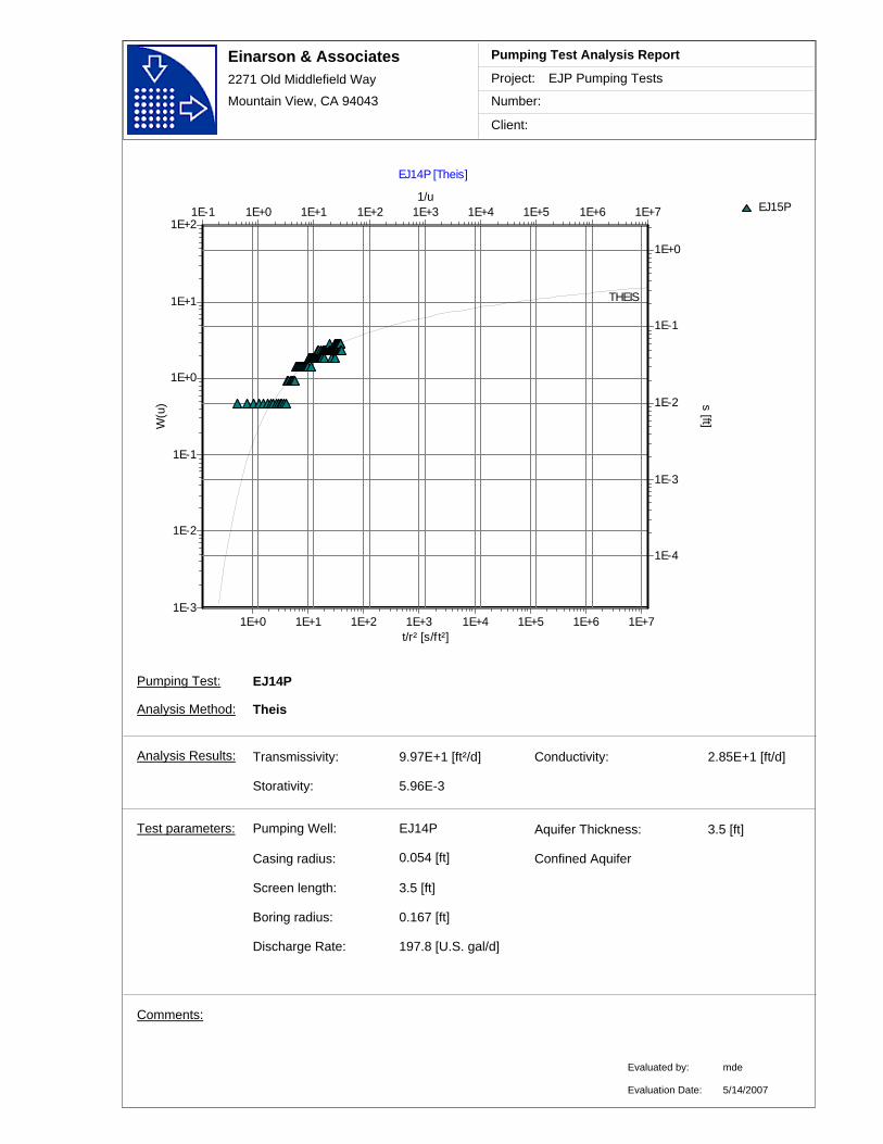
Einarson & Associates2271 Old Middlefield Way
Mountain View, CA 94043
Project:
Number:
Client:
EJP Pumping Tests
Pumping Test Analysis Report
EJ15P
EJ14P [Theis]
t/r² [s/ft²]1E+0 1E+1 1E+2 1E+3 1E+4 1E+5 1E+6 1E+7
1/u1E-1 1E+0 1E+1 1E+2 1E+3 1E+4 1E+5 1E+6 1E+7
W(u
)
1E-3
1E-2
1E-1
1E+0
1E+1
1E+2
s [ft]
1E-4
1E-3
1E-2
1E-1
1E+0
THEIS
Transmissivity: 9.97E+1 [ft²/d] Conductivity: 2.85E+1 [ft/d]
Storativity: 5.96E-3
Comments:
EJ14PPumping Well:
Discharge Rate: 197.8 [U.S. gal/d]
Casing radius:
0.167 [ft]
Screen length: 3.5 [ft]
Boring radius:
0.054 [ft]
Test parameters:
EJ14P
Analysis Method: Theis
Aquifer Thickness: 3.5 [ft]
Analysis Results:
Evaluated by:
Evaluation Date:
mde
Confined Aquifer
5/14/2007
Pumping Test:
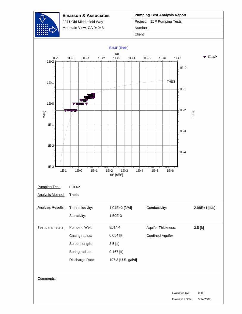
Einarson & Associates2271 Old Middlefield Way
Mountain View, CA 94043
Project:
Number:
Client:
EJP Pumping Tests
Pumping Test Analysis Report
EJ16P
EJ14P [Theis]
t/r² [s/ft²]1E-1 1E+0 1E+1 1E+2 1E+3 1E+4 1E+5 1E+6
1/u1E-1 1E+0 1E+1 1E+2 1E+3 1E+4 1E+5 1E+6 1E+7
W(u
)
1E-3
1E-2
1E-1
1E+0
1E+1
1E+2
s [ft]
1E-4
1E-3
1E-2
1E-1
1E+0
THEIS
Transmissivity: 1.04E+2 [ft²/d] Conductivity: 2.98E+1 [ft/d]
Storativity: 1.50E-3
Comments:
EJ14PPumping Well:
Discharge Rate: 197.8 [U.S. gal/d]
Casing radius:
0.167 [ft]
Screen length: 3.5 [ft]
Boring radius:
0.054 [ft]
Test parameters:
EJ14P
Analysis Method: Theis
Aquifer Thickness: 3.5 [ft]
Analysis Results:
Evaluated by:
Evaluation Date:
mde
Confined Aquifer
5/14/2007
Pumping Test:

Einarson & Associates2271 Old Middlefield Way
Mountain View, CA 94043
Project:
Number:
Client:
EJP Pumping Tests
Pumping Test Analysis Report
EJ14P
EJ14P_rec [Draw dow n vs. Time]
Time [s]128102.476.851.225.60
Dra
wdo
wn
[ft]
0.28
0.224
0.168
0.112
0.056
0
Comments:
EJ14PPumping Well:
Discharge Rate: 197.8 [U.S. gal/d]
Casing radius:
0.167 [ft]
Screen length: 3.5 [ft]
Boring radius:
0.054 [ft]
Test parameters:
EJ14P_rec
Analysis Method: Drawdown vs. Time
Aquifer Thickness: 3.5 [ft]
Analysis Results:
Evaluated by:
Evaluation Date:
mde
5/14/2007
Pumping Test:
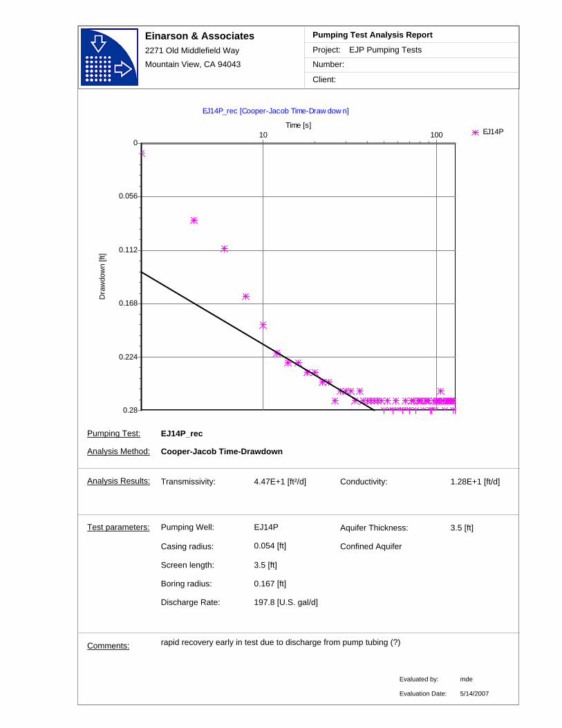
Einarson & Associates2271 Old Middlefield Way
Mountain View, CA 94043
Project:
Number:
Client:
EJP Pumping Tests
Pumping Test Analysis Report
EJ14P
EJ14P_rec [Cooper-Jacob Time-Draw dow n]
Time [s]10 100
Dra
wdo
wn
[ft]
0.28
0.224
0.168
0.112
0.056
0
Transmissivity: 4.47E+1 [ft²/d]
rapid recovery early in test due to discharge from pump tubing (?)
Conductivity: 1.28E+1 [ft/d]
Comments:
EJ14PPumping Well:
Discharge Rate: 197.8 [U.S. gal/d]
Casing radius:
0.167 [ft]
Screen length: 3.5 [ft]
Boring radius:
0.054 [ft]
Test parameters:
EJ14P_rec
Analysis Method: Cooper-Jacob Time-Drawdown
Aquifer Thickness: 3.5 [ft]
Analysis Results:
Evaluated by:
Evaluation Date:
mde
Confined Aquifer
5/14/2007
Pumping Test:

Pumping Test Analyses
VAFB Site 60
Well EJ015P

Einarson & Associates2271 Old Middlefield Way
Mountain View, CA 94043
Project:
Number:
Client:
EJP Pumping Tests
Pumping Test Analysis Report
EJ15PEJ16PEJ17P
EJ15P [Draw dow n vs. Time]
Time [s]292233.6175.2116.858.4
Dra
wdo
wn
[ft]
0.44
0.352
0.264
0.176
0.088
0
Suspect 16 & 17 are reversed. Comments:
EJ15PPumping Well:
Discharge Rate: 68.5 [U.S. gal/d]
Casing radius:
0.167 [ft]
Screen length: 3.5 [ft]
Boring radius:
0.054 [ft]
Test parameters:
EJ15P
Analysis Method: Drawdown vs. Time
Aquifer Thickness: 3.5 [ft]
Analysis Results:
Evaluated by:
Evaluation Date:
mde
5/14/2007
Pumping Test:
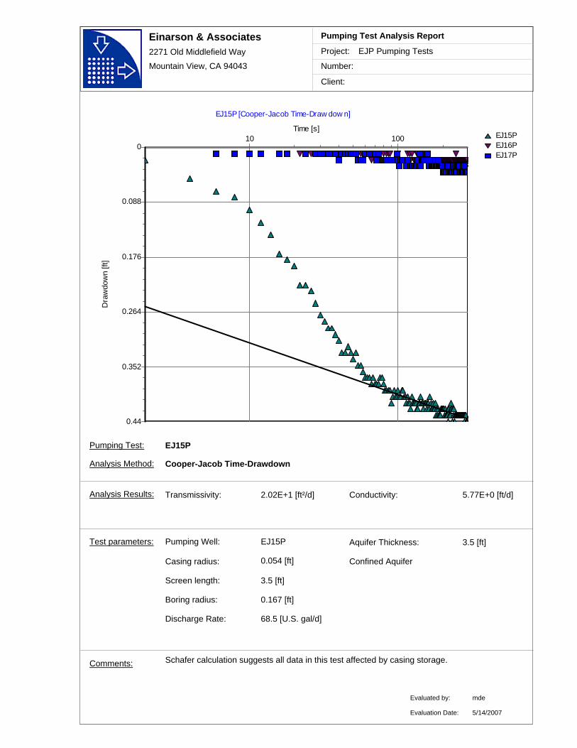
Einarson & Associates2271 Old Middlefield Way
Mountain View, CA 94043
Project:
Number:
Client:
EJP Pumping Tests
Pumping Test Analysis Report
EJ15PEJ16PEJ17P
EJ15P [Cooper-Jacob Time-Draw dow n]
Time [s]10 100
Dra
wdo
wn
[ft]
0.44
0.352
0.264
0.176
0.088
0
Transmissivity: 2.02E+1 [ft²/d]
Schafer calculation suggests all data in this test affected by casing storage.
Conductivity: 5.77E+0 [ft/d]
Comments:
EJ15PPumping Well:
Discharge Rate: 68.5 [U.S. gal/d]
Casing radius:
0.167 [ft]
Screen length: 3.5 [ft]
Boring radius:
0.054 [ft]
Test parameters:
EJ15P
Analysis Method: Cooper-Jacob Time-Drawdown
Aquifer Thickness: 3.5 [ft]
Analysis Results:
Evaluated by:
Evaluation Date:
mde
Confined Aquifer
5/14/2007
Pumping Test:
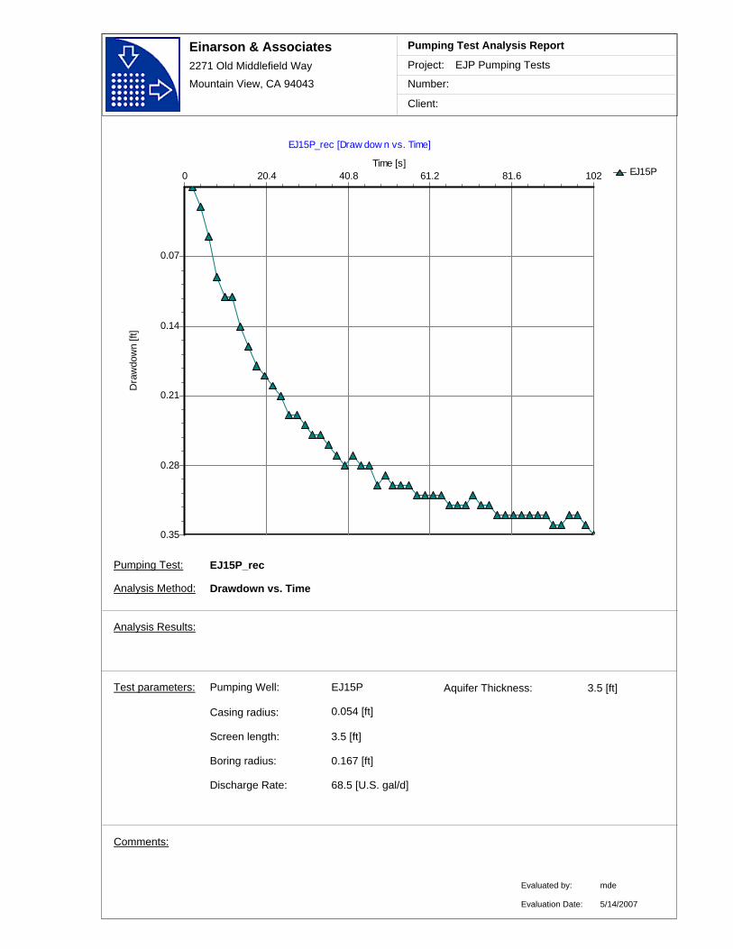
Einarson & Associates2271 Old Middlefield Way
Mountain View, CA 94043
Project:
Number:
Client:
EJP Pumping Tests
Pumping Test Analysis Report
EJ15P
EJ15P_rec [Draw dow n vs. Time]
Time [s]10281.661.240.820.40
Dra
wdo
wn
[ft]
0.35
0.28
0.21
0.14
0.07
Comments:
EJ15PPumping Well:
Discharge Rate: 68.5 [U.S. gal/d]
Casing radius:
0.167 [ft]
Screen length: 3.5 [ft]
Boring radius:
0.054 [ft]
Test parameters:
EJ15P_rec
Analysis Method: Drawdown vs. Time
Aquifer Thickness: 3.5 [ft]
Analysis Results:
Evaluated by:
Evaluation Date:
mde
5/14/2007
Pumping Test:
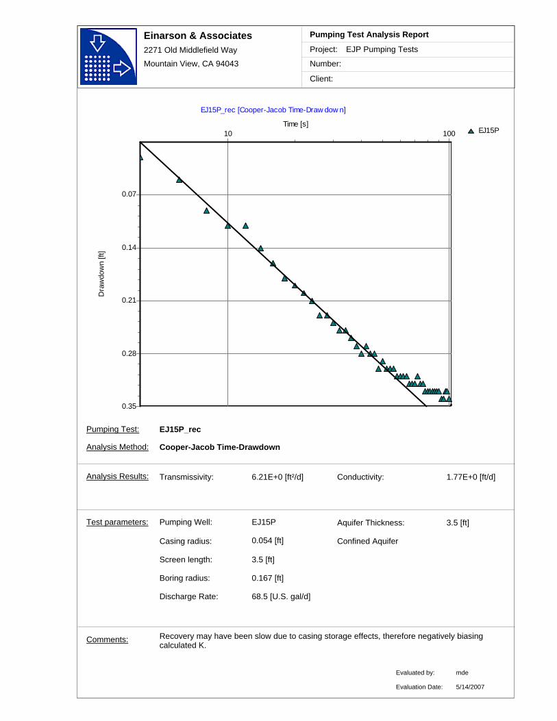
Einarson & Associates2271 Old Middlefield Way
Mountain View, CA 94043
Project:
Number:
Client:
EJP Pumping Tests
Pumping Test Analysis Report
EJ15P
EJ15P_rec [Cooper-Jacob Time-Draw dow n]
Time [s]10 100
Dra
wdo
wn
[ft]
0.35
0.28
0.21
0.14
0.07
Transmissivity: 6.21E+0 [ft²/d]
Recovery may have been slow due to casing storage effects, therefore negatively biasing calculated K.
Conductivity: 1.77E+0 [ft/d]
Comments:
EJ15PPumping Well:
Discharge Rate: 68.5 [U.S. gal/d]
Casing radius:
0.167 [ft]
Screen length: 3.5 [ft]
Boring radius:
0.054 [ft]
Test parameters:
EJ15P_rec
Analysis Method: Cooper-Jacob Time-Drawdown
Aquifer Thickness: 3.5 [ft]
Analysis Results:
Evaluated by:
Evaluation Date:
mde
Confined Aquifer
5/14/2007
Pumping Test:
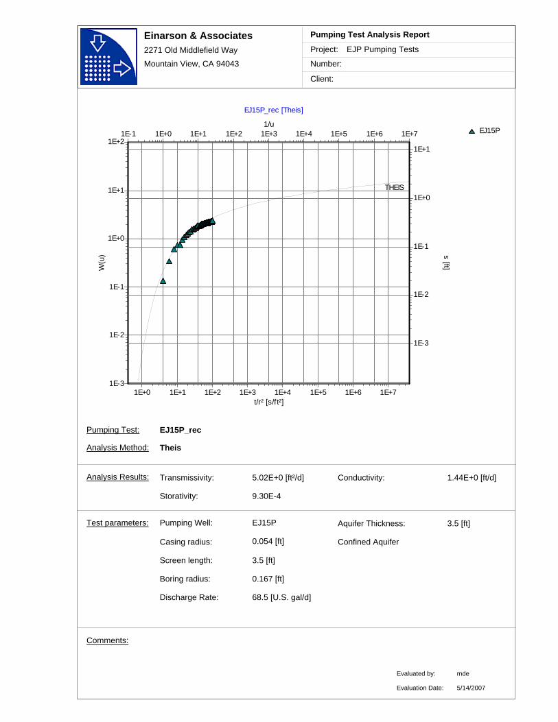
Einarson & Associates2271 Old Middlefield Way
Mountain View, CA 94043
Project:
Number:
Client:
EJP Pumping Tests
Pumping Test Analysis Report
EJ15P
EJ15P_rec [Theis]
t/r² [s/ft²]1E+0 1E+1 1E+2 1E+3 1E+4 1E+5 1E+6 1E+7
1/u1E-1 1E+0 1E+1 1E+2 1E+3 1E+4 1E+5 1E+6 1E+7
W(u
)
1E-3
1E-2
1E-1
1E+0
1E+1
1E+2
s [ft]
1E-3
1E-2
1E-1
1E+0
1E+1
THEIS
Transmissivity: 5.02E+0 [ft²/d] Conductivity: 1.44E+0 [ft/d]
Storativity: 9.30E-4
Comments:
EJ15PPumping Well:
Discharge Rate: 68.5 [U.S. gal/d]
Casing radius:
0.167 [ft]
Screen length: 3.5 [ft]
Boring radius:
0.054 [ft]
Test parameters:
EJ15P_rec
Analysis Method: Theis
Aquifer Thickness: 3.5 [ft]
Analysis Results:
Evaluated by:
Evaluation Date:
mde
Confined Aquifer
5/14/2007
Pumping Test:

Pumping Test Analyses
VAFB Site 60
Well EJ016P
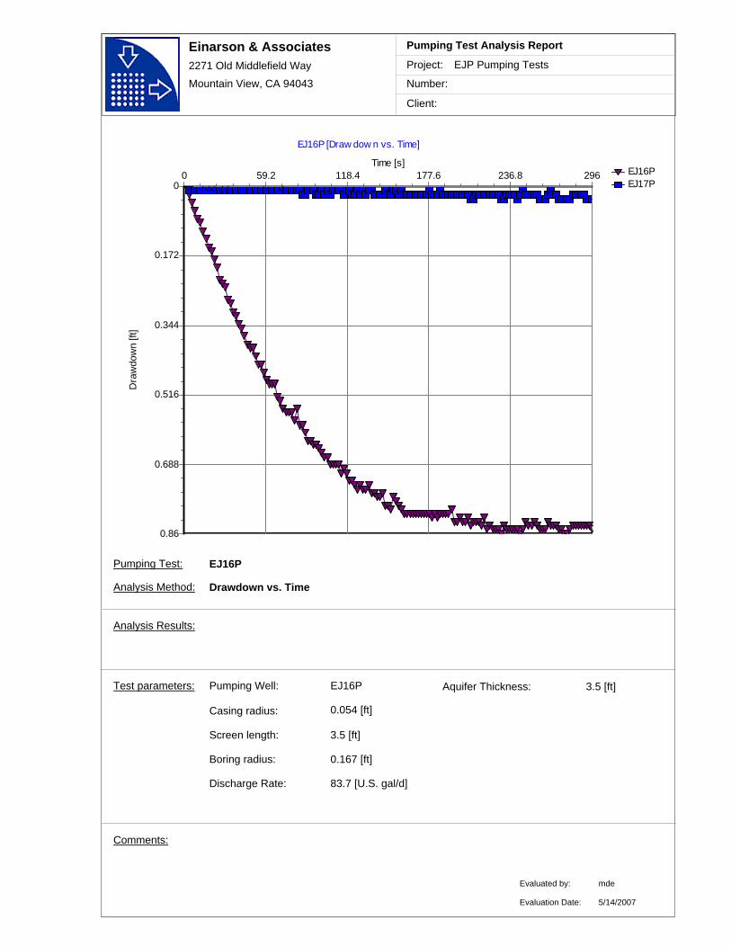
Einarson & Associates2271 Old Middlefield Way
Mountain View, CA 94043
Project:
Number:
Client:
EJP Pumping Tests
Pumping Test Analysis Report
EJ16PEJ17P
EJ16P [Draw dow n vs. Time]
Time [s]296236.8177.6118.459.20
Dra
wdo
wn
[ft]
0.86
0.688
0.516
0.344
0.172
0
Comments:
EJ16PPumping Well:
Discharge Rate: 83.7 [U.S. gal/d]
Casing radius:
0.167 [ft]
Screen length: 3.5 [ft]
Boring radius:
0.054 [ft]
Test parameters:
EJ16P
Analysis Method: Drawdown vs. Time
Aquifer Thickness: 3.5 [ft]
Analysis Results:
Evaluated by:
Evaluation Date:
mde
5/14/2007
Pumping Test:
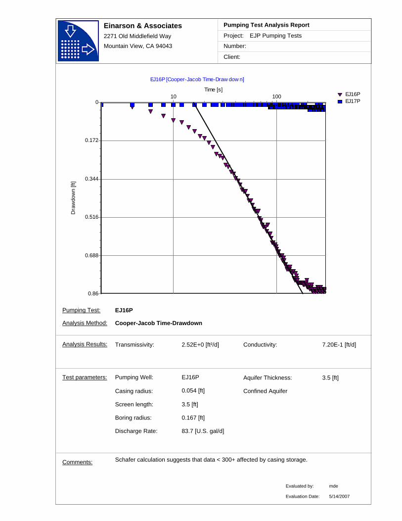
Einarson & Associates2271 Old Middlefield Way
Mountain View, CA 94043
Project:
Number:
Client:
EJP Pumping Tests
Pumping Test Analysis Report
EJ16PEJ17P
EJ16P [Cooper-Jacob Time-Draw dow n]
Time [s]10 100
Dra
wdo
wn
[ft]
0.86
0.688
0.516
0.344
0.172
0
Transmissivity: 2.52E+0 [ft²/d]
Schafer calculation suggests that data < 300+ affected by casing storage.
Conductivity: 7.20E-1 [ft/d]
Comments:
EJ16PPumping Well:
Discharge Rate: 83.7 [U.S. gal/d]
Casing radius:
0.167 [ft]
Screen length: 3.5 [ft]
Boring radius:
0.054 [ft]
Test parameters:
EJ16P
Analysis Method: Cooper-Jacob Time-Drawdown
Aquifer Thickness: 3.5 [ft]
Analysis Results:
Evaluated by:
Evaluation Date:
mde
Confined Aquifer
5/14/2007
Pumping Test:

Einarson & Associates2271 Old Middlefield Way
Mountain View, CA 94043
Project:
Number:
Client:
EJP Pumping Tests
Pumping Test Analysis Report
EJ16P
EJ16P_rec [Cooper-Jacob Time-Draw dow n]
Time [s]10 100
Dra
wdo
wn
[ft]
0.68
0.544
0.408
0.272
0.136
0
Transmissivity: 3.51E+0 [ft²/d]
Recovery may have been slow due to casing storage effects, therefore negatively biasing calculated K.
Conductivity: 1.00E+0 [ft/d]
Comments:
EJ16PPumping Well:
Discharge Rate: 83.7 [U.S. gal/d]
Casing radius:
0.167 [ft]
Screen length: 3.5 [ft]
Boring radius:
0.054 [ft]
Test parameters:
EJ16P_rec
Analysis Method: Cooper-Jacob Time-Drawdown
Aquifer Thickness: 3.5 [ft]
Analysis Results:
Evaluated by:
Evaluation Date:
mde
Confined Aquifer
5/14/2007
Pumping Test:

Einarson & Associates2271 Old Middlefield Way
Mountain View, CA 94043
Project:
Number:
Client:
EJP Pumping Tests
Pumping Test Analysis Report
EJ16P
EJ16P_rec [Theis]
t/r² [s/ft²]1E+0 1E+1 1E+2 1E+3 1E+4 1E+5 1E+6 1E+7
1/u1E-1 1E+0 1E+1 1E+2 1E+3 1E+4 1E+5 1E+6 1E+7
W(u
)
1E-3
1E-2
1E-1
1E+0
1E+1
1E+2
s [ft]
1E-3
1E-2
1E-1
1E+0
1E+1
THEIS
Transmissivity: 3.60E+0 [ft²/d] Conductivity: 1.03E+0 [ft/d]
Storativity: 7.29E-4
Comments:
EJ16PPumping Well:
Discharge Rate: 83.7 [U.S. gal/d]
Casing radius:
0.167 [ft]
Screen length: 3.5 [ft]
Boring radius:
0.054 [ft]
Test parameters:
EJ16P_rec
Analysis Method: Theis
Aquifer Thickness: 3.5 [ft]
Analysis Results:
Evaluated by:
Evaluation Date:
mde
Confined Aquifer
5/14/2007
Pumping Test:

Pumping Test Analyses
VAFB Site 60
Well EJ017P
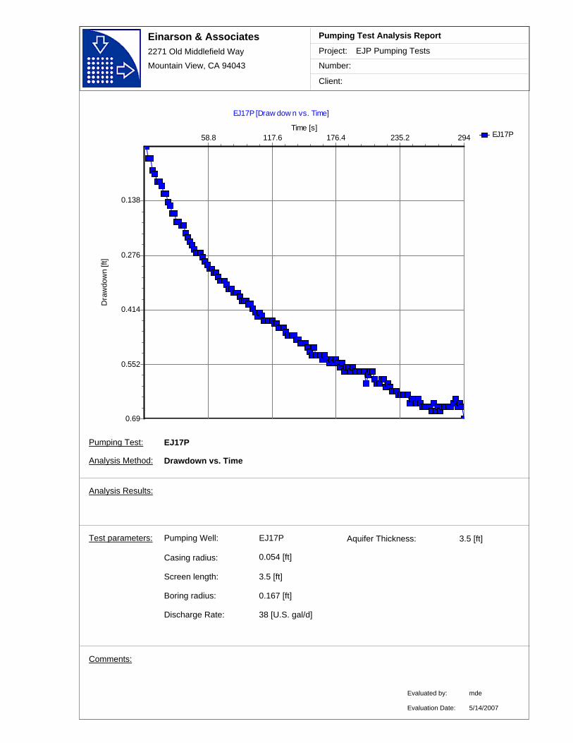
Einarson & Associates2271 Old Middlefield Way
Mountain View, CA 94043
Project:
Number:
Client:
EJP Pumping Tests
Pumping Test Analysis Report
EJ17P
EJ17P [Draw dow n vs. Time]
Time [s]294235.2176.4117.658.8
Dra
wdo
wn
[ft]
0.69
0.552
0.414
0.276
0.138
Comments:
EJ17PPumping Well:
Discharge Rate: 38 [U.S. gal/d]
Casing radius:
0.167 [ft]
Screen length: 3.5 [ft]
Boring radius:
0.054 [ft]
Test parameters:
EJ17P
Analysis Method: Drawdown vs. Time
Aquifer Thickness: 3.5 [ft]
Analysis Results:
Evaluated by:
Evaluation Date:
mde
5/14/2007
Pumping Test:
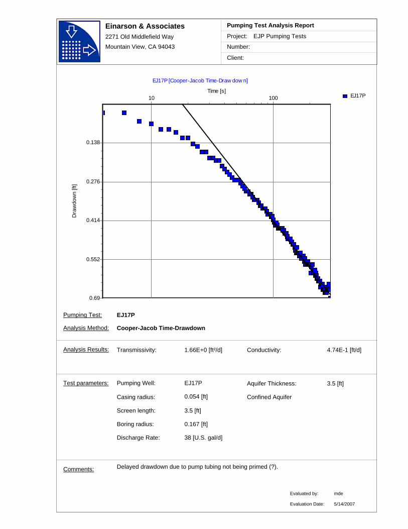
Einarson & Associates2271 Old Middlefield Way
Mountain View, CA 94043
Project:
Number:
Client:
EJP Pumping Tests
Pumping Test Analysis Report
EJ17P
EJ17P [Cooper-Jacob Time-Draw dow n]
Time [s]10 100
Dra
wdo
wn
[ft]
0.69
0.552
0.414
0.276
0.138
Transmissivity: 1.66E+0 [ft²/d]
Delayed drawdown due to pump tubing not being primed (?).
Conductivity: 4.74E-1 [ft/d]
Comments:
EJ17PPumping Well:
Discharge Rate: 38 [U.S. gal/d]
Casing radius:
0.167 [ft]
Screen length: 3.5 [ft]
Boring radius:
0.054 [ft]
Test parameters:
EJ17P
Analysis Method: Cooper-Jacob Time-Drawdown
Aquifer Thickness: 3.5 [ft]
Analysis Results:
Evaluated by:
Evaluation Date:
mde
Confined Aquifer
5/14/2007
Pumping Test:

Einarson & Associates2271 Old Middlefield Way
Mountain View, CA 94043
Project:
Number:
Client:
EJP Pumping Tests
Pumping Test Analysis Report
EJ17P
EJ17P [Theis]
t/r² [s/ft²]1E+1 1E+2 1E+3 1E+4 1E+5 1E+6 1E+7 1E+8
1/u1E-1 1E+0 1E+1 1E+2 1E+3 1E+4 1E+5 1E+6 1E+7
W(u
)
1E-3
1E-2
1E-1
1E+0
1E+1
1E+2
s [ft]
1E-3
1E-2
1E-1
1E+0
1E+1
THEIS
Transmissivity: 1.48E+0 [ft²/d]
Delayed drawdown due to pump tubing not being primed (?).
Conductivity: 4.24E-1 [ft/d]
Storativity: 8.49E-4
Comments:
EJ17PPumping Well:
Discharge Rate: 38 [U.S. gal/d]
Casing radius:
0.167 [ft]
Screen length: 3.5 [ft]
Boring radius:
0.054 [ft]
Test parameters:
EJ17P
Analysis Method: Theis
Aquifer Thickness: 3.5 [ft]
Analysis Results:
Evaluated by:
Evaluation Date:
mde
Confined Aquifer
5/14/2007
Pumping Test:
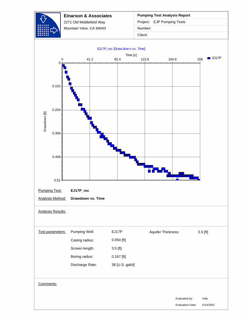
Einarson & Associates2271 Old Middlefield Way
Mountain View, CA 94043
Project:
Number:
Client:
EJP Pumping Tests
Pumping Test Analysis Report
EJ17P
EJ17P_rec [Draw dow n vs. Time]
Time [s]206164.8123.682.441.20
Dra
wdo
wn
[ft]
0.51
0.408
0.306
0.204
0.102
0
Comments:
EJ17PPumping Well:
Discharge Rate: 38 [U.S. gal/d]
Casing radius:
0.167 [ft]
Screen length: 3.5 [ft]
Boring radius:
0.054 [ft]
Test parameters:
EJ17P_rec
Analysis Method: Drawdown vs. Time
Aquifer Thickness: 3.5 [ft]
Analysis Results:
Evaluated by:
Evaluation Date:
mde
5/14/2007
Pumping Test:
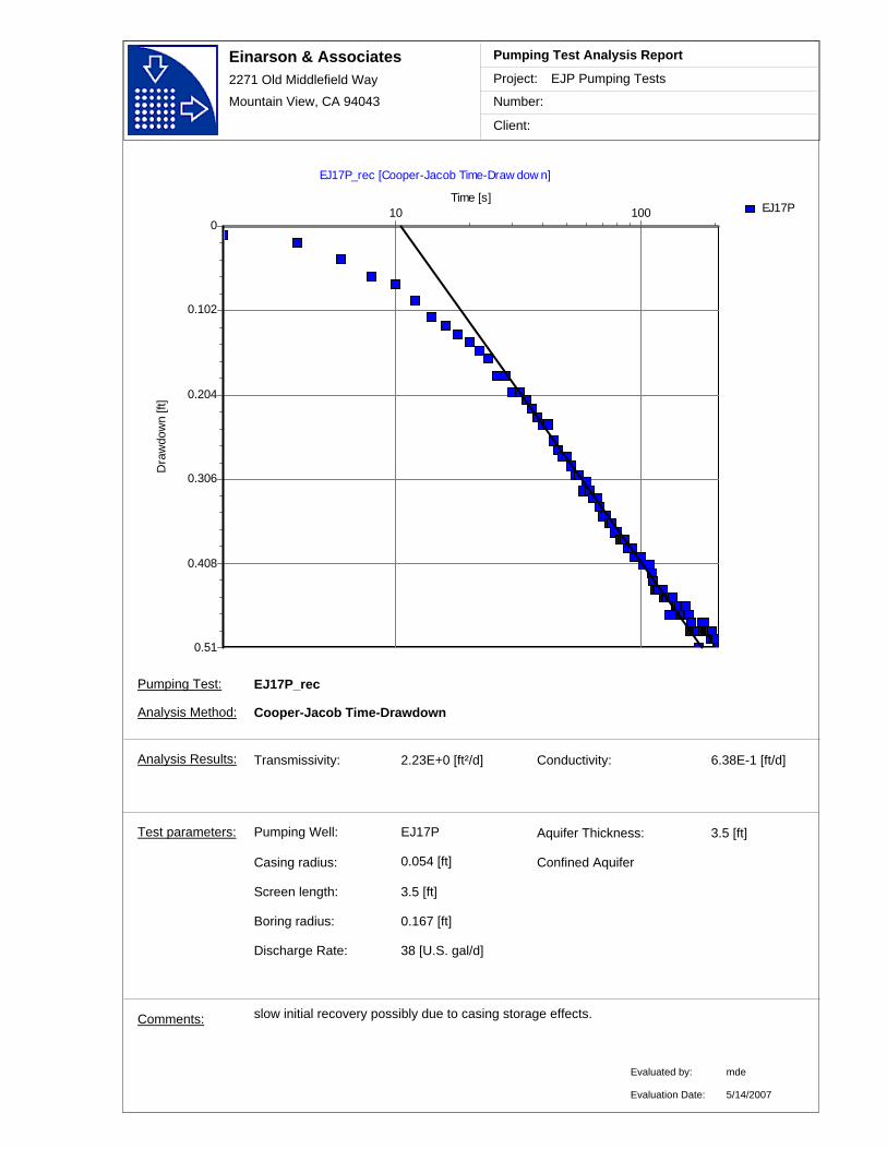
Einarson & Associates2271 Old Middlefield Way
Mountain View, CA 94043
Project:
Number:
Client:
EJP Pumping Tests
Pumping Test Analysis Report
EJ17P
EJ17P_rec [Cooper-Jacob Time-Draw dow n]
Time [s]10 100
Dra
wdo
wn
[ft]
0.51
0.408
0.306
0.204
0.102
0
Transmissivity: 2.23E+0 [ft²/d]
slow initial recovery possibly due to casing storage effects.
Conductivity: 6.38E-1 [ft/d]
Comments:
EJ17PPumping Well:
Discharge Rate: 38 [U.S. gal/d]
Casing radius:
0.167 [ft]
Screen length: 3.5 [ft]
Boring radius:
0.054 [ft]
Test parameters:
EJ17P_rec
Analysis Method: Cooper-Jacob Time-Drawdown
Aquifer Thickness: 3.5 [ft]
Analysis Results:
Evaluated by:
Evaluation Date:
mde
Confined Aquifer
5/14/2007
Pumping Test:
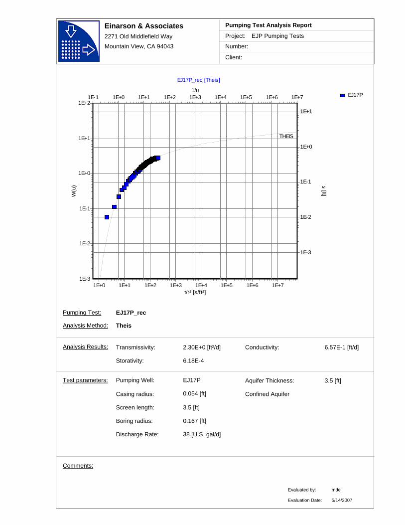
Einarson & Associates2271 Old Middlefield Way
Mountain View, CA 94043
Project:
Number:
Client:
EJP Pumping Tests
Pumping Test Analysis Report
EJ17P
EJ17P_rec [Theis]
t/r² [s/ft²]1E+0 1E+1 1E+2 1E+3 1E+4 1E+5 1E+6 1E+7
1/u1E-1 1E+0 1E+1 1E+2 1E+3 1E+4 1E+5 1E+6 1E+7
W(u
)
1E-3
1E-2
1E-1
1E+0
1E+1
1E+2
s [ft]
1E-3
1E-2
1E-1
1E+0
1E+1
THEIS
Transmissivity: 2.30E+0 [ft²/d] Conductivity: 6.57E-1 [ft/d]
Storativity: 6.18E-4
Comments:
EJ17PPumping Well:
Discharge Rate: 38 [U.S. gal/d]
Casing radius:
0.167 [ft]
Screen length: 3.5 [ft]
Boring radius:
0.054 [ft]
Test parameters:
EJ17P_rec
Analysis Method: Theis
Aquifer Thickness: 3.5 [ft]
Analysis Results:
Evaluated by:
Evaluation Date:
mde
Confined Aquifer
5/14/2007
Pumping Test:
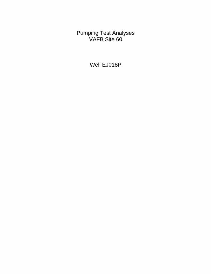
Pumping Test Analyses
VAFB Site 60
Well EJ018P
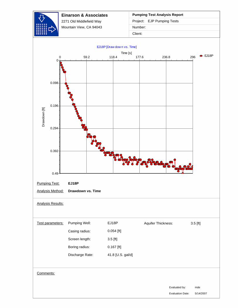
Einarson & Associates2271 Old Middlefield Way
Mountain View, CA 94043
Project:
Number:
Client:
EJP Pumping Tests
Pumping Test Analysis Report
EJ18P
EJ18P [Draw dow n vs. Time]
Time [s]296236.8177.6118.459.20
Dra
wdo
wn
[ft]
0.49
0.392
0.294
0.196
0.098
0
Comments:
EJ18PPumping Well:
Discharge Rate: 41.8 [U.S. gal/d]
Casing radius:
0.167 [ft]
Screen length: 3.5 [ft]
Boring radius:
0.054 [ft]
Test parameters:
EJ18P
Analysis Method: Drawdown vs. Time
Aquifer Thickness: 3.5 [ft]
Analysis Results:
Evaluated by:
Evaluation Date:
mde
5/14/2007
Pumping Test:

Einarson & Associates2271 Old Middlefield Way
Mountain View, CA 94043
Project:
Number:
Client:
EJP Pumping Tests
Pumping Test Analysis Report
EJ18P
EJ18P [Cooper-Jacob Time-Draw dow n]
Time [s]10 100
Dra
wdo
wn
[ft]
0.49
0.392
0.294
0.196
0.098
0
Transmissivity: 2.50E+0 [ft²/d]
Schafer calculation suggests all data are affected by casing storage. Slow early response may be due to suction line not being primed. Reduced drawdown near end of test may be due to ambient flow in aqufer supplying water to well.
Conductivity: 7.15E-1 [ft/d]
Comments:
EJ18PPumping Well:
Discharge Rate: 41.8 [U.S. gal/d]
Casing radius:
0.167 [ft]
Screen length: 3.5 [ft]
Boring radius:
0.054 [ft]
Test parameters:
EJ18P
Analysis Method: Cooper-Jacob Time-Drawdown
Aquifer Thickness: 3.5 [ft]
Analysis Results:
Evaluated by:
Evaluation Date:
mde
Confined Aquifer
5/14/2007
Pumping Test:

Einarson & Associates2271 Old Middlefield Way
Mountain View, CA 94043
Project:
Number:
Client:
EJP Pumping Tests
Pumping Test Analysis Report
EJ18P
EJ18P_rec [Cooper-Jacob Time-Draw dow n]
Time [s]10 100
Dra
wdo
wn
[ft]
0.39
0.312
0.234
0.156
0.078
Transmissivity: 3.35E+0 [ft²/d]
Slow response during early recovery possibly due to casing storage.
Conductivity: 9.58E-1 [ft/d]
Comments:
EJ18PPumping Well:
Discharge Rate: 41.8 [U.S. gal/d]
Casing radius:
0.167 [ft]
Screen length: 3.5 [ft]
Boring radius:
0.054 [ft]
Test parameters:
EJ18P_rec
Analysis Method: Cooper-Jacob Time-Drawdown
Aquifer Thickness: 3.5 [ft]
Analysis Results:
Evaluated by:
Evaluation Date:
mde
Confined Aquifer
5/14/2007
Pumping Test:
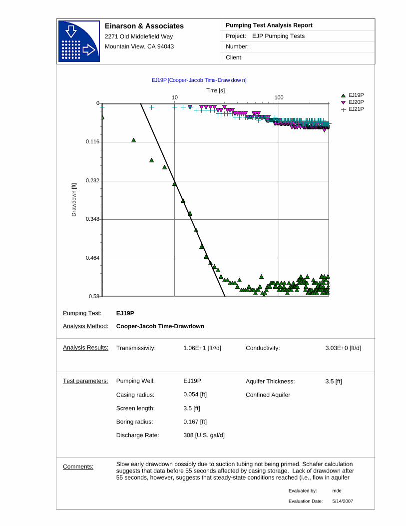
Einarson & Associates2271 Old Middlefield Way
Mountain View, CA 94043
Project:
Number:
Client:
EJP Pumping Tests
Pumping Test Analysis Report
EJ19PEJ20PEJ21P
EJ19P [Cooper-Jacob Time-Draw dow n]
Time [s]10 100
Dra
wdo
wn
[ft]
0.58
0.464
0.348
0.232
0.116
0
Transmissivity: 1.06E+1 [ft²/d]
Slow early drawdown possibly due to suction tubing not being primed. Schafer calculation suggests that data before 55 seconds affected by casing storage. Lack of drawdown after 55 seconds, however, suggests that steady-state conditions reached (i.e., flow in aquifer
Conductivity: 3.03E+0 [ft/d]
Comments:
EJ19PPumping Well:
Discharge Rate: 308 [U.S. gal/d]
Casing radius:
0.167 [ft]
Screen length: 3.5 [ft]
Boring radius:
0.054 [ft]
Test parameters:
EJ19P
Analysis Method: Cooper-Jacob Time-Drawdown
Aquifer Thickness: 3.5 [ft]
Analysis Results:
Evaluated by:
Evaluation Date:
mde
Confined Aquifer
5/14/2007
Pumping Test:
Einarson & Associates2271 Old Middlefield Way
Mountain View, CA 94043
Project:
Number:
Client:
EJP Pumping Tests
Pumping Test Analysis Report
EJ18P
EJ18P_rec [Theis]
t/r² [s/ft²]1E+0 1E+1 1E+2 1E+3 1E+4 1E+5 1E+6 1E+7
1/u1E-1 1E+0 1E+1 1E+2 1E+3 1E+4 1E+5 1E+6 1E+7
W(u
)
1E-3
1E-2
1E-1
1E+0
1E+1
1E+2
s [ft]
1E-3
1E-2
1E-1
1E+0
1E+1
THEIS
Transmissivity: 3.21E+0 [ft²/d] Conductivity: 9.17E-1 [ft/d]
Storativity: 7.48E-4
Comments:
EJ18PPumping Well:
Discharge Rate: 41.8 [U.S. gal/d]
Casing radius:
0.167 [ft]
Screen length: 3.5 [ft]
Boring radius:
0.054 [ft]
Test parameters:
EJ18P_rec
Analysis Method: Theis
Aquifer Thickness: 3.5 [ft]
Analysis Results:
Evaluated by:
Evaluation Date:
mde
Confined Aquifer
5/14/2007
Pumping Test:

Pumping Test Analyses
VAFB Site 60
Well EJ019P
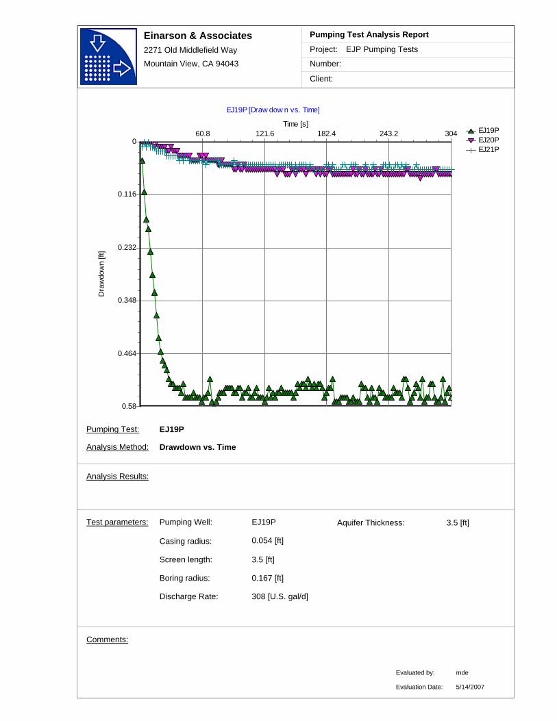
Einarson & Associates2271 Old Middlefield Way
Mountain View, CA 94043
Project:
Number:
Client:
EJP Pumping Tests
Pumping Test Analysis Report
EJ19PEJ20PEJ21P
EJ19P [Draw dow n vs. Time]
Time [s]304243.2182.4121.660.8
Dra
wdo
wn
[ft]
0.58
0.464
0.348
0.232
0.116
0
Comments:
EJ19PPumping Well:
Discharge Rate: 308 [U.S. gal/d]
Casing radius:
0.167 [ft]
Screen length: 3.5 [ft]
Boring radius:
0.054 [ft]
Test parameters:
EJ19P
Analysis Method: Drawdown vs. Time
Aquifer Thickness: 3.5 [ft]
Analysis Results:
Evaluated by:
Evaluation Date:
mde
5/14/2007
Pumping Test:
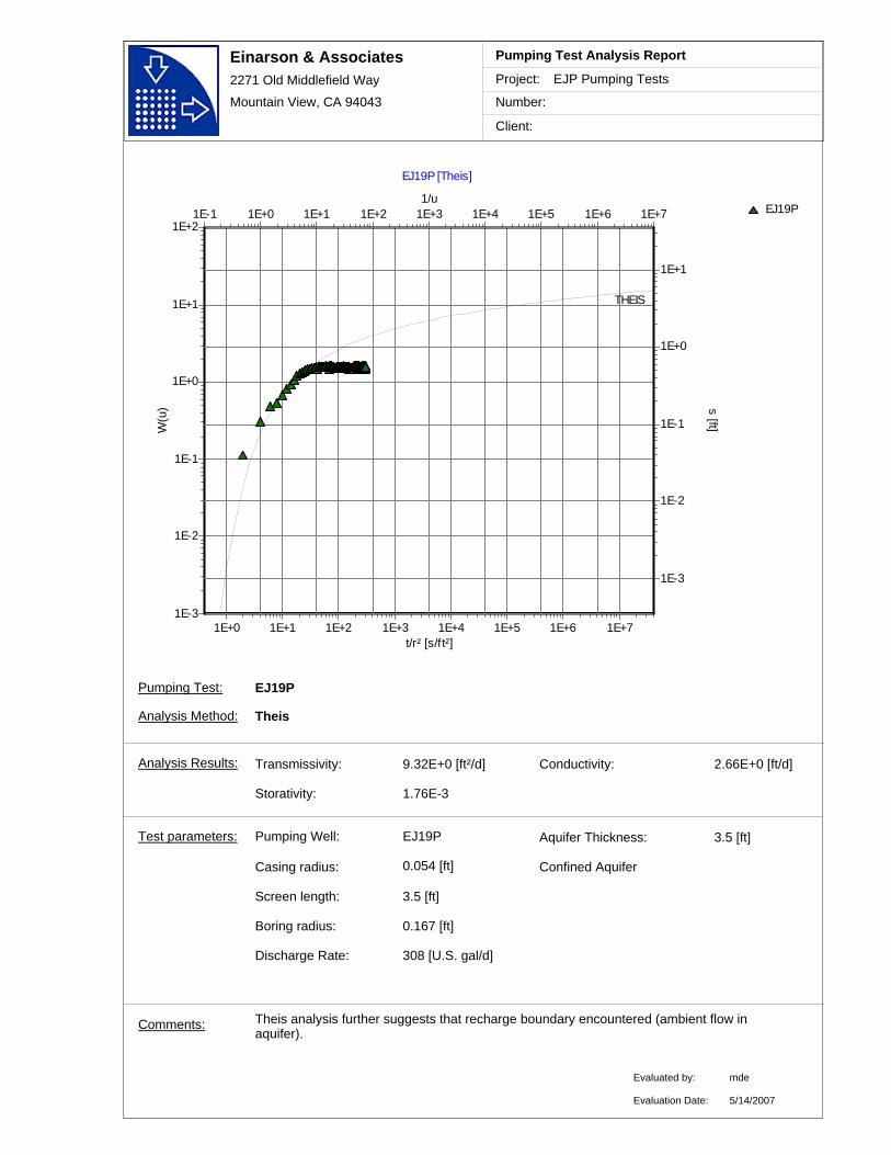
Einarson & Associates2271 Old Middlefield Way
Mountain View, CA 94043
Project:
Number:
Client:
EJP Pumping Tests
Pumping Test Analysis Report
EJ19P
EJ19P [Theis]
t/r² [s/ft²]1E+0 1E+1 1E+2 1E+3 1E+4 1E+5 1E+6 1E+7
1/u1E-1 1E+0 1E+1 1E+2 1E+3 1E+4 1E+5 1E+6 1E+7
W(u
)
1E-3
1E-2
1E-1
1E+0
1E+1
1E+2
s [ft]
1E-3
1E-2
1E-1
1E+0
1E+1
THEIS
Transmissivity: 9.32E+0 [ft²/d]
Theis analysis further suggests that recharge boundary encountered (ambient flow in aquifer).
Conductivity: 2.66E+0 [ft/d]
Storativity: 1.76E-3
Comments:
EJ19PPumping Well:
Discharge Rate: 308 [U.S. gal/d]
Casing radius:
0.167 [ft]
Screen length: 3.5 [ft]
Boring radius:
0.054 [ft]
Test parameters:
EJ19P
Analysis Method: Theis
Aquifer Thickness: 3.5 [ft]
Analysis Results:
Evaluated by:
Evaluation Date:
mde
Confined Aquifer
5/14/2007
Pumping Test:
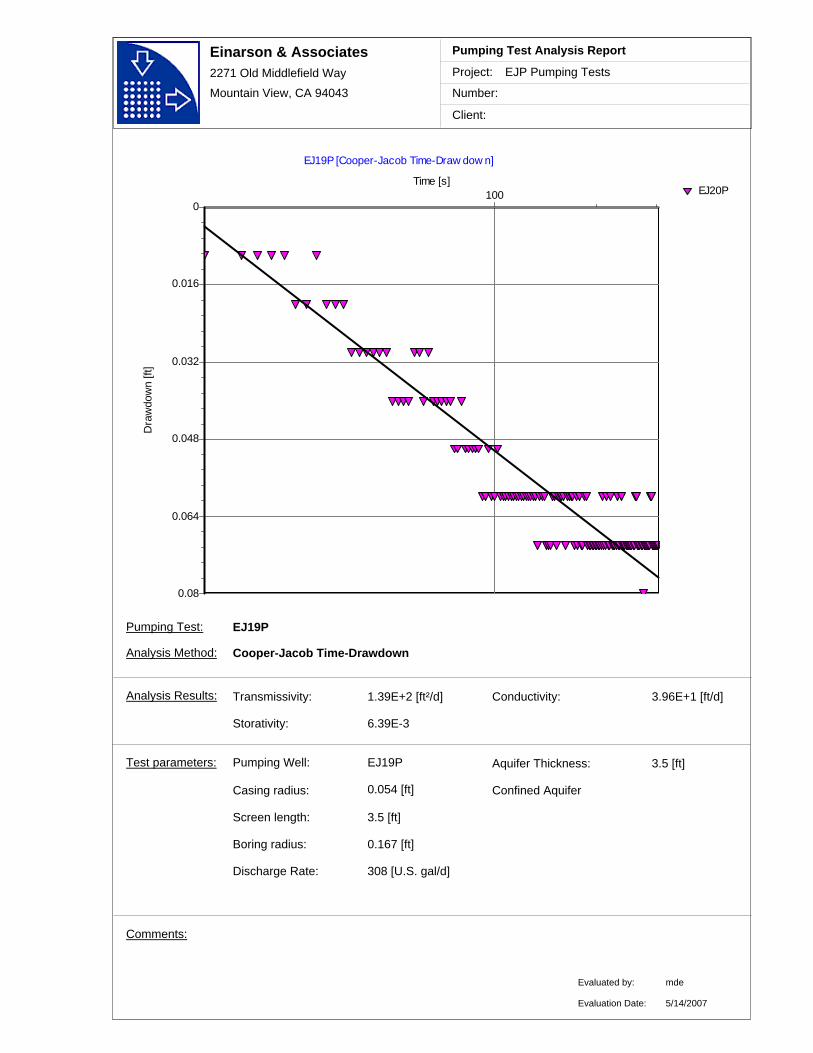
Einarson & Associates2271 Old Middlefield Way
Mountain View, CA 94043
Project:
Number:
Client:
EJP Pumping Tests
Pumping Test Analysis Report
EJ20P
EJ19P [Cooper-Jacob Time-Draw dow n]
Time [s]100
Dra
wdo
wn
[ft]
0.08
0.064
0.048
0.032
0.016
0
Transmissivity: 1.39E+2 [ft²/d] Conductivity: 3.96E+1 [ft/d]
Storativity: 6.39E-3
Comments:
EJ19PPumping Well:
Discharge Rate: 308 [U.S. gal/d]
Casing radius:
0.167 [ft]
Screen length: 3.5 [ft]
Boring radius:
0.054 [ft]
Test parameters:
EJ19P
Analysis Method: Cooper-Jacob Time-Drawdown
Aquifer Thickness: 3.5 [ft]
Analysis Results:
Evaluated by:
Evaluation Date:
mde
Confined Aquifer
5/14/2007
Pumping Test:
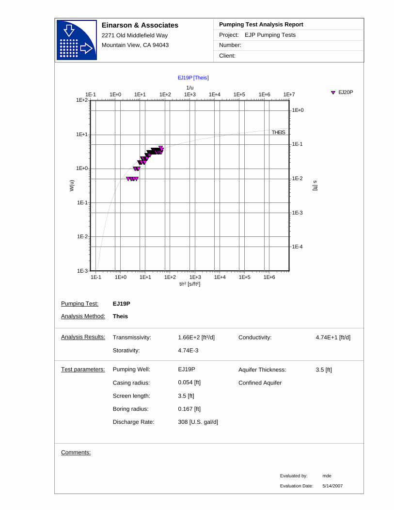
Einarson & Associates2271 Old Middlefield Way
Mountain View, CA 94043
Project:
Number:
Client:
EJP Pumping Tests
Pumping Test Analysis Report
EJ20P
EJ19P [Theis]
t/r² [s/ft²]1E-1 1E+0 1E+1 1E+2 1E+3 1E+4 1E+5 1E+6
1/u1E-1 1E+0 1E+1 1E+2 1E+3 1E+4 1E+5 1E+6 1E+7
W(u
)
1E-3
1E-2
1E-1
1E+0
1E+1
1E+2
s [ft]
1E-4
1E-3
1E-2
1E-1
1E+0
THEIS
Transmissivity: 1.66E+2 [ft²/d] Conductivity: 4.74E+1 [ft/d]
Storativity: 4.74E-3
Comments:
EJ19PPumping Well:
Discharge Rate: 308 [U.S. gal/d]
Casing radius:
0.167 [ft]
Screen length: 3.5 [ft]
Boring radius:
0.054 [ft]
Test parameters:
EJ19P
Analysis Method: Theis
Aquifer Thickness: 3.5 [ft]
Analysis Results:
Evaluated by:
Evaluation Date:
mde
Confined Aquifer
5/14/2007
Pumping Test:
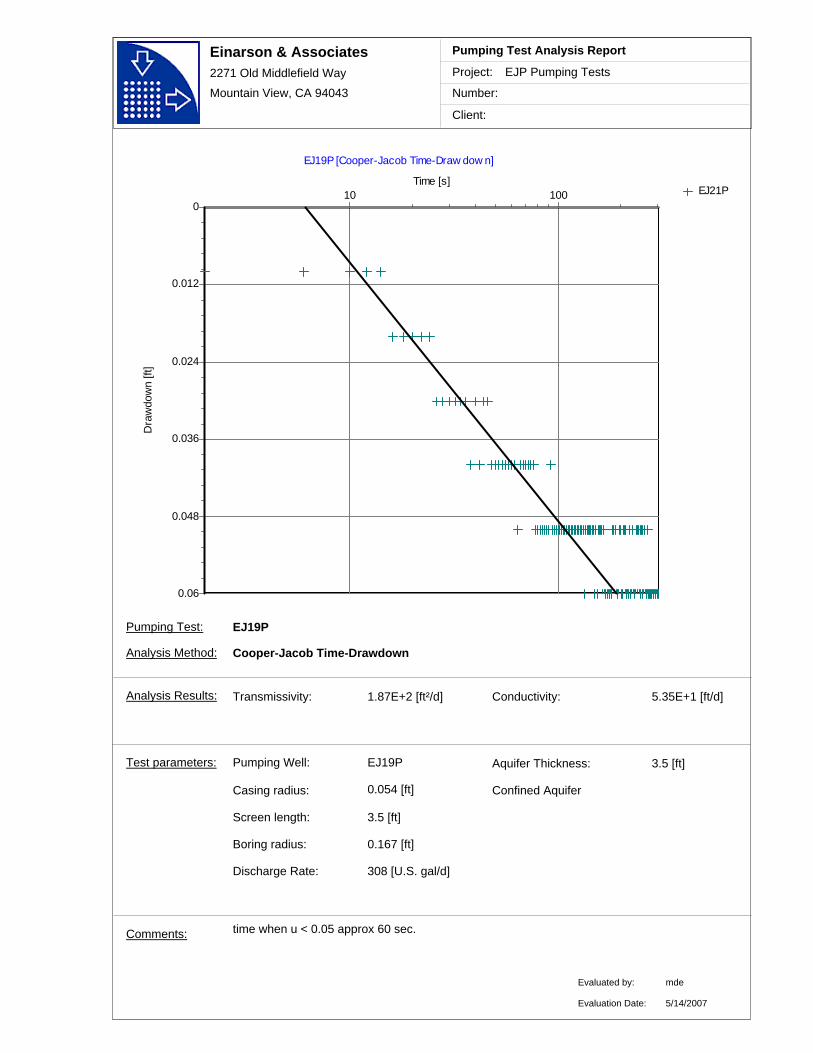
Einarson & Associates2271 Old Middlefield Way
Mountain View, CA 94043
Project:
Number:
Client:
EJP Pumping Tests
Pumping Test Analysis Report
EJ21P
EJ19P [Cooper-Jacob Time-Draw dow n]
Time [s]10 100
Dra
wdo
wn
[ft]
0.06
0.048
0.036
0.024
0.012
0
Transmissivity: 1.87E+2 [ft²/d]
time when u < 0.05 approx 60 sec.
Conductivity: 5.35E+1 [ft/d]
Comments:
EJ19PPumping Well:
Discharge Rate: 308 [U.S. gal/d]
Casing radius:
0.167 [ft]
Screen length: 3.5 [ft]
Boring radius:
0.054 [ft]
Test parameters:
EJ19P
Analysis Method: Cooper-Jacob Time-Drawdown
Aquifer Thickness: 3.5 [ft]
Analysis Results:
Evaluated by:
Evaluation Date:
mde
Confined Aquifer
5/14/2007
Pumping Test:

Einarson & Associates2271 Old Middlefield Way
Mountain View, CA 94043
Project:
Number:
Client:
EJP Pumping Tests
Pumping Test Analysis Report
EJ21P
EJ19P [Theis]
t/r² [s/ft²]1E-1 1E+0 1E+1 1E+2 1E+3 1E+4 1E+5 1E+6
1/u1E-1 1E+0 1E+1 1E+2 1E+3 1E+4 1E+5 1E+6 1E+7
W(u
)
1E-3
1E-2
1E-1
1E+0
1E+1
1E+2
s [ft]
1E-4
1E-3
1E-2
1E-1
1E+0
THEIS
Transmissivity: 1.82E+2 [ft²/d] Conductivity: 5.19E+1 [ft/d]
Storativity: 1.31E-3
Comments:
EJ19PPumping Well:
Discharge Rate: 308 [U.S. gal/d]
Casing radius:
0.167 [ft]
Screen length: 3.5 [ft]
Boring radius:
0.054 [ft]
Test parameters:
EJ19P
Analysis Method: Theis
Aquifer Thickness: 3.5 [ft]
Analysis Results:
Evaluated by:
Evaluation Date:
mde
Confined Aquifer
5/14/2007
Pumping Test:
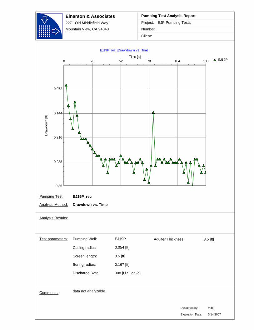
Einarson & Associates2271 Old Middlefield Way
Mountain View, CA 94043
Project:
Number:
Client:
EJP Pumping Tests
Pumping Test Analysis Report
EJ19P
EJ19P_rec [Draw dow n vs. Time]
Time [s]1301047852260
Dra
wdo
wn
[ft]
0.36
0.288
0.216
0.144
0.072
data not analyzable. Comments:
EJ19PPumping Well:
Discharge Rate: 308 [U.S. gal/d]
Casing radius:
0.167 [ft]
Screen length: 3.5 [ft]
Boring radius:
0.054 [ft]
Test parameters:
EJ19P_rec
Analysis Method: Drawdown vs. Time
Aquifer Thickness: 3.5 [ft]
Analysis Results:
Evaluated by:
Evaluation Date:
mde
5/14/2007
Pumping Test:

Pumping Test Analyses
VAFB Site 60
Well EJ020P

Einarson & Associates2271 Old Middlefield Way
Mountain View, CA 94043
Project:
Number:
Client:
EJP Pumping Tests
Pumping Test Analysis Report
EJ20PEJ21PEJ22P
EJ20P [Draw dow n vs. Time]
Time [s]296236.8177.6118.459.20
Dra
wdo
wn
[ft]
0.85
0.68
0.51
0.34
0.17
0
Comments:
EJ20PPumping Well:
Discharge Rate: 133 [U.S. gal/d]
Casing radius:
0.167 [ft]
Screen length: 3.5 [ft]
Boring radius:
0.054 [ft]
Test parameters:
EJ20P
Analysis Method: Drawdown vs. Time
Aquifer Thickness: 3.5 [ft]
Analysis Results:
Evaluated by:
Evaluation Date:
mde
5/14/2007
Pumping Test:
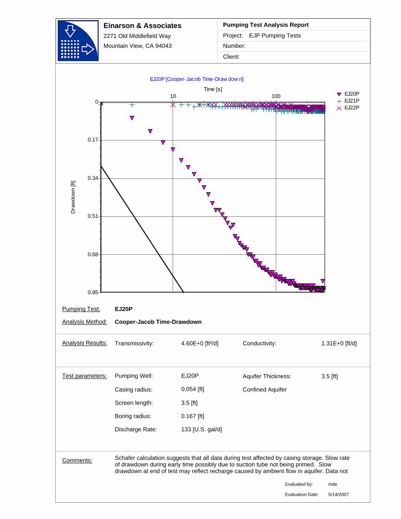
Einarson & Associates2271 Old Middlefield Way
Mountain View, CA 94043
Project:
Number:
Client:
EJP Pumping Tests
Pumping Test Analysis Report
EJ20PEJ21PEJ22P
EJ20P [Cooper-Jacob Time-Draw dow n]
Time [s]10 100
Dra
wdo
wn
[ft]
0.85
0.68
0.51
0.34
0.17
0
Transmissivity: 4.60E+0 [ft²/d]
Schafer calculation suggests that all data during test affected by casing storage. Slow rate of drawdown during early time possibly due to suction tube not being primed. Slow drawdown at end of test may reflect recharge caused by ambient flow in aquifer. Data not
Conductivity: 1.31E+0 [ft/d]
Comments:
EJ20PPumping Well:
Discharge Rate: 133 [U.S. gal/d]
Casing radius:
0.167 [ft]
Screen length: 3.5 [ft]
Boring radius:
0.054 [ft]
Test parameters:
EJ20P
Analysis Method: Cooper-Jacob Time-Drawdown
Aquifer Thickness: 3.5 [ft]
Analysis Results:
Evaluated by:
Evaluation Date:
mde
Confined Aquifer
5/14/2007
Pumping Test:
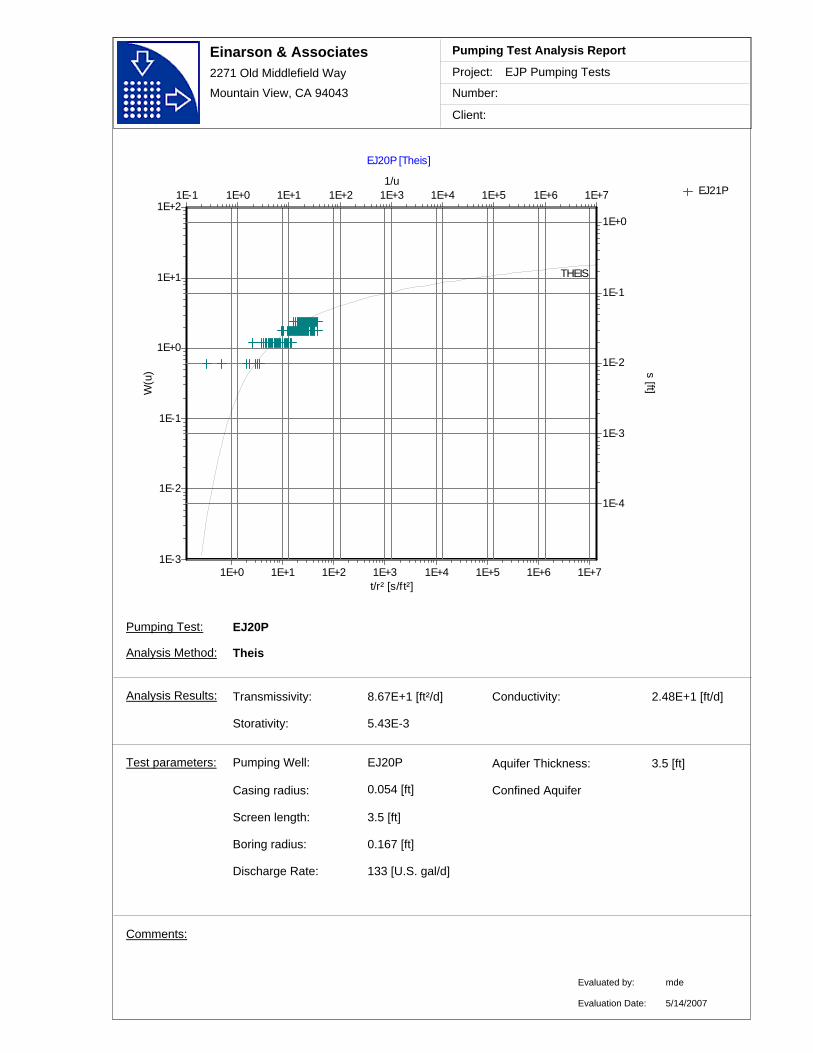
Einarson & Associates2271 Old Middlefield Way
Mountain View, CA 94043
Project:
Number:
Client:
EJP Pumping Tests
Pumping Test Analysis Report
EJ21P
EJ20P [Theis]
t/r² [s/ft²]1E+0 1E+1 1E+2 1E+3 1E+4 1E+5 1E+6 1E+7
1/u1E-1 1E+0 1E+1 1E+2 1E+3 1E+4 1E+5 1E+6 1E+7
W(u
)
1E-3
1E-2
1E-1
1E+0
1E+1
1E+2
s [ft]
1E-4
1E-3
1E-2
1E-1
1E+0
THEIS
Transmissivity: 8.67E+1 [ft²/d] Conductivity: 2.48E+1 [ft/d]
Storativity: 5.43E-3
Comments:
EJ20PPumping Well:
Discharge Rate: 133 [U.S. gal/d]
Casing radius:
0.167 [ft]
Screen length: 3.5 [ft]
Boring radius:
0.054 [ft]
Test parameters:
EJ20P
Analysis Method: Theis
Aquifer Thickness: 3.5 [ft]
Analysis Results:
Evaluated by:
Evaluation Date:
mde
Confined Aquifer
5/14/2007
Pumping Test:
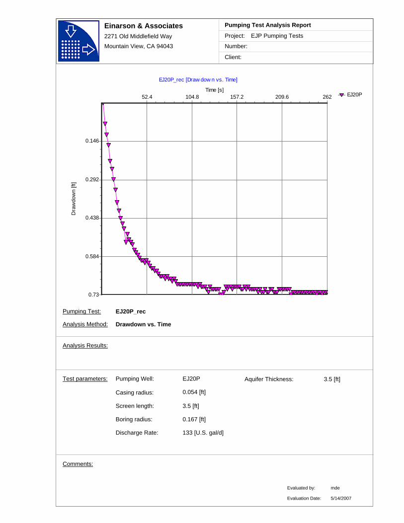
Einarson & Associates2271 Old Middlefield Way
Mountain View, CA 94043
Project:
Number:
Client:
EJP Pumping Tests
Pumping Test Analysis Report
EJ20P
EJ20P_rec [Draw dow n vs. Time]
Time [s]262209.6157.2104.852.4
Dra
wdo
wn
[ft]
0.73
0.584
0.438
0.292
0.146
Comments:
EJ20PPumping Well:
Discharge Rate: 133 [U.S. gal/d]
Casing radius:
0.167 [ft]
Screen length: 3.5 [ft]
Boring radius:
0.054 [ft]
Test parameters:
EJ20P_rec
Analysis Method: Drawdown vs. Time
Aquifer Thickness: 3.5 [ft]
Analysis Results:
Evaluated by:
Evaluation Date:
mde
5/14/2007
Pumping Test:
Pumping Test Analyses
VAFB Site 60
Well EJ021P


Appendix E
Points of Contact
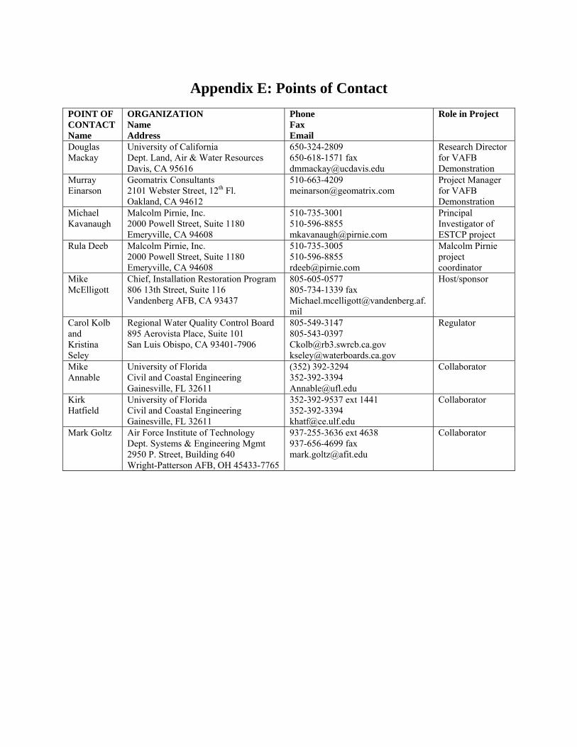
Appendix E: Points of Contact POINT OF CONTACT Name
ORGANIZATION Name Address
Phone Fax Email
Role in Project
Douglas Mackay
University of California Dept. Land, Air & Water Resources Davis, CA 95616
650-324-2809 650-618-1571 fax [email protected]
Research Director for VAFB Demonstration
Murray Einarson
Geomatrix Consultants 2101 Webster Street, 12th Fl. Oakland, CA 94612
510-663-4209 [email protected]
Project Manager for VAFB Demonstration
Michael Kavanaugh
Malcolm Pirnie, Inc. 2000 Powell Street, Suite 1180 Emeryville, CA 94608
510-735-3001 510-596-8855 [email protected]
Principal Investigator of ESTCP project
Rula Deeb Malcolm Pirnie, Inc. 2000 Powell Street, Suite 1180 Emeryville, CA 94608
510-735-3005 510-596-8855 [email protected]
Malcolm Pirnie project coordinator
Mike McElligott
Chief, Installation Restoration Program 806 13th Street, Suite 116 Vandenberg AFB, CA 93437
805-605-0577 805-734-1339 fax [email protected]
Host/sponsor
Carol Kolb and Kristina Seley
Regional Water Quality Control Board 895 Aerovista Place, Suite 101 San Luis Obispo, CA 93401-7906
805-549-3147 805-543-0397 [email protected] [email protected]
Regulator
Mike Annable
University of Florida Civil and Coastal Engineering Gainesville, FL 32611
(352) 392-3294 352-392-3394 [email protected]
Collaborator
Kirk Hatfield
University of Florida Civil and Coastal Engineering Gainesville, FL 32611
352-392-9537 ext 1441 352-392-3394 [email protected]
Collaborator
Mark Goltz Air Force Institute of Technology Dept. Systems & Engineering Mgmt 2950 P. Street, Building 640 Wright-Patterson AFB, OH 45433-7765
937-255-3636 ext 4638 937-656-4699 fax [email protected]
Collaborator