Final Report Spatial and Temporal Variations in Mixing ... · Spatial and Temporal Variations in Mixing Height in Houston ... maximum backscatter gradient at the top of the ... Data

1

Final Report

Spatial and Temporal Variations in Mixing Height in Houston

TNRCC Project F-20

Christoph Senff1,2, Robert Banta2, Lisa Darby2, Wayne Angevine1,3,

Allen White1,2, Carl Berkowitz4 , Christopher Doran4

1CIRES, University of Colorado

2NOAA Environmental Technology Laboratory 3NOAA Aeronomy Laboratory

4Pacific Northwest National Laboratory

2

1. Introduction

Mixed layer height is an important meteorological parameter that affects near-surface

atmospheric pollutant concentrations since it determines the volume of air into which pollutants

and their precursors are emitted. The Houston area is characterized by a considerable spatial

variability of mixed layer height due to its coastal location and due to variations in land use.

Marine boundary layers are typically only several hundred meters deep and their depth does not

vary much over the course of the day. The mixed layer height over land, however, exhibits a

strong diurnal cycle and typically peaks in the afternoon at depths of up to 2 km or more. The

temporal evolution and spatial distribution of mixed layer height depends on many factors,

including the synoptic conditions, local circulation patterns, cloud cover, and surface

characteristics. For example, the heat island effect associated with large metropolitan areas, such

as Houston, is known to enhance mixed layer depth. Also, the sea breeze circulation is likely to

have a significant impact on the boundary layer depth evolution in the Houston area by advecting

marine air from Galveston Bay or the Gulf of Mexico over land.

The objective of this project is to characterize the temporal and spatial variations of mixed

layer height in the Houston area during the Texas 2000 Air Quality Study. A secondary goal is to

document the relationship between mixed layer depth and boundary layer ozone concentrations.

To address these objectives we use data collected with various instruments during the Texas

2000 Air Quality Study in August and September of 2000. The focus of this project is on the

August 23rd - September 1st time period. A more comprehensive analysis encompassing all days

of the Texas 2000 campaign for which data are available will be undertaken as part of a follow-

up study funded under TNRCC Project F-2.

In section 2 of this report we describe the data analysis approach we have used to address the

objectives of this project, in section 3 we present our findings for each day of the August 23rd -

September 1st time period, and in section 4 we summarize the main results and conclusions.

2. Data analysis

To determine the temporal evolution and spatial distribution of the mixed layer depth in the

Houston area during the Texas 2000 study we have used data gathered with the NOAA/ETL

airborne ozone lidar, the Texas 2000 wind profiler network, and radio sondes launched during

the Texas 2000 study. The wind profiler and radio sonde data provide information on the

3

temporal evolution of mixed layer depth at fixed, land-based locations. The airborne lidar yields

information on the spatial variability of boundary layer height, in particular the contrast between

land areas, Galveston Bay and the Gulf of Mexico.

Boundary layer height is determined from radio sonde data by inspecting the potential

temperature profile and finding the altitude of the temperature inversion capping the boundary

layer. Typically, in a well-mixed boundary layer, the potential temperature is nearly constant

with height. At the top of the mixed layer, in the inversion layer, the potential temperature

increases sharply with altitude. In the free troposphere above the inversion layer, the atmosphere

is usually stably stratified, i.e. the potential temperature increases with altitude, but the positive

lapse rate is smaller than in the inversion layer. We chose the “middle” altitude of the inversion

layer as an estimate for boundary layer depth. In cases where the potential temperature sounding

was inconclusive in terms of locating the inversion layer we looked for a significant decrease in

the water vapor mixing ratio sounding to find the inversion layer. As an example, Figure 1

shows a potential temperature sounding recorded in the late afternoon on August 26th, 2000 at

the Downtown Houston site. The sharp increase in potential temperature in the inversion layer is

clearly visible. In this case the boundary layer was determined to be 1660 m deep.

Wind profiler mixing depths are based on evidence that the profile of the refractive index

structure function parameter exhibits a peak at the top of the boundary layer. With the

backscattered clear air signal being proportional to the refractive index structure function

parameter, the profiler method of detecting mixing depth relies on finding a local maximum in

the backscatter profiles. Figure 2 shows an example of mixed layer depth retrieval from

backscatter data recorded with the Houston Southwest profiler during the daytime on August

28th, 2000. The mixed layer height estimates were determined by manual selection of the

reflectivity maxima and are indicated by the green “x”s in figure 2.

The lidar retrieval of boundary layer height is based on detecting the gradient in the lidar

backscatter signal associated with the decrease in aerosol backscatter often found in the

transition zone from the mixed layer to the overlying free troposphere. To objectively locate the

maximum backscatter gradient at the top of the boundary layer we apply a wavelet analysis

technique to each lidar signal profile. Outliers in the resulting time series of mixed layer depth

are removed using a simple consensus algorithm. Figure 3 shows a 30-minute time height cross

section of aerosol backscatter measured with the airborne lidar on August 28th, 2000. The sharp

4

decrease of aerosol backscatter near the top of the boundary layer is clearly visible. Overlaid as

a black line is the mixed layer depth estimate retrieved from the lidar data.

During the Texas 2000 Air Quality study radio sondes were launched at the Downtown

Houston, La Marque and Wharton sites at 3-hour intervals on some days and at 6-hour or greater

intervals on other days. For the wind profiler retrieval of mixed layer height we used data from

five profilers located at La Marque, Houston Southwest, Ellington Field, Wharton, and Liberty.

The temporal resolution of the profiler estimates of mixed layer depth is 30 minutes. The

airborne lidar estimates of boundary layer depth are derived at a resolution of 10 s, which

translates to a horizontal resolution of about 600 m.

Radio sondes provide a “snapshot” of the state of the atmosphere as they ascend. Therefore,

the mixing height determined from radio sonde data represents a point measurement in space and

time. Wind profilers and lidars, on the other hand, yield temporal and spatial averages of

boundary layer height. This has to be kept in mind when comparing mixing height estimates

from radio sondes with those of wind profilers or lidars. A particular radio sonde may fly

through an updraft or downdraft, thus yielding significantly higher or lower values for mixing

height than the remote sensors. The wind profiler and lidar techniques work well under a variety

of atmospheric conditions and intercomparison studies have shown good agreement between the

two methods. However, there are certain circumstances that place limitations on these

techniques. Enhancements of wind profiler reflectivity can also be caused by scattering from

clouds, precipitation, insects, birds, or ground clutter and may be mistaken as the reflectivity

peak associated with the boundary layer top. The effect of clouds can be accounted for by

deploying next to the wind profiler a ceilometer, which indicates the occurrence of clouds and

measures cloud base height (see Figure 2). The airborne lidar retrieval of mixed layer depth is

also affected by clouds: the strong lidar signal increase due to cloud top backscatter can be

misinterpreted as the backscatter gradient at the top of the mixed layer and cause a high bias in

the lidar retrieval of boundary layer depth. The lidar method may also be of limited use when

the contrast between aerosol backscatter in the free troposphere and the mixed layer is not very

pronounced. A reduced backscatter contrast could be due to advection of air with high aerosol

loading at altitudes just above the boundary layer. Another reason could be that the mixed layer

is growing into the previous’ day polluted residual layer which may have similar backscatter

characteristics as the newly evolving boundary layer.

5

A secondary objective of this project is to study the relationship between mixed layer depth

and boundary layer ozone concentrations. Since the airborne lidar measures vertical profiles of

ozone and mixing depth, it is the instrument of choice to address this task.

3. Results

In this section we present the results of our research on the temporal and spatial

characteristics of boundary layer height in the Houston area for August 23rd through September

1st, 2000. Data on mixing depth collected with the wind profilers and radio sondes were

available on all of the days of the above time period, albeit the coverage is sparse on August 23rd

and 24th. The airborne lidar was flown every day of the episode except on August 23rd, 24th, and

August 27th. For each of the above days the following data products (if available) are shown:

1. Daytime forward trajectories derived from the wind profiler data (see e.g. figure 4)

Wind profiler forward trajectories are plotted as a sequence of arrows and are overlaid on

a map of the Houston area. Each arrow represents the path traveled by an air parcel in

one hour. A time stamp indicating the start time of each hourly segment is plotted next to

each arrow. To calculate the trajectories the wind profiler measurements were first

averaged vertically between 200 and 1000 m altitude. Then they were averaged spatially

with the data from each profiler being weighted according to the inverse of the distance

between the starting point of each trajectory segment and the respective profiler location.

If a flow reversal occurred on a particular day, the starting point of the trajectory was

chosen so that flow reversal was centered over the Houston/Ship Channel area.

2. Time series of boundary layer depth retrieved from wind profiler and radio sonde data

(see e.g. figure 9)

Time series of daytime wind profiler boundary layer depths are shown as lines color-

coded according to profiler location. Boundary layer heights derived from radio sonde

data are plotted as diamond-shaped symbols, again color-coded according to radio sonde

launch site. Acronyms used for site locations are:

LM - La Marque

EL - Ellington

6

HS - Houston Southwest

HD - Houston Downtown

WH - Wharton

LB - Liberty

3. Planview plots of boundary layer depth measured with the airborne lidar (see e.g. figure

10)

The mixed layer depth retrieved with the airborne lidar is color coded according to

altitude, plotted along the flight track of the lidar aircraft, and overlaid on a map of the

Houston area. In some cases the lidar data are broken up into shorter segments, which

are presented as separate planview plots of boundary layer depth. This was done in order

to minimize distortions due to temporal changes when plotting the spatial distribution of

boundary layer depth.

Following are - in chronological order - descriptions of the findings for each of the 10 days that

were investigated. Days with similar flow patterns and boundary layer height characteristics are

grouped together and discussed in the same section.

3.1 August 23rdand 24th

On August 23rd the early morning flow was onshore from the southeast, followed by a period

of northeasterly winds, and then a switch to an easterly wind direction (figure 4). Time series of

mixing height measured with the Houston Southwest profiler (the only profiler from which

boundary layer height estimates were available on August 23rd) and soundings from the three

radio sonde sites are depicted in figure 5. The airborne lidar did not fly on this day. The

boundary layer height was remarkably similar across the greater Houston area - from La Marque

in the southeast to Wharton in the northwest. Also, the boundary layer was very shallow

throughout the day, never exceeding 1000 m. The weather in the Houston area on August 23rd

was characterized by mostly cloudy conditions and thunderstorms that moved through the area in

the afternoon and produced light rain showers. This weather pattern explains the shallow and

uniform boundary layer depth measured in the Houston area and may also be responsible for the

shifts in the flow pattern that occurred around 7:00 and 11:00 CST.

7

The flow pattern on August 24th (figure 6) shows southeasterly, onshore flow in the early

morning, followed by light-wind conditions during the middle of the day, after which the winds

shifted to an east-southeasterly direction and increased in speed with the onset of the sea breeze.

This flow pattern is very similar to the ones observed on August 25th and 26th (see discussion in

section 3.2). The reason why we grouped the 24th together with the 23rd is that the weather

patterns were similar with thunderstorms in the area and several stations in the Houston vicinity

reporting precipitation. However, the cloud cover on the 24th was not as extensive as on the 23rd.

The lidar was not flown on this day, and only very limited boundary layer depth measurements

from the wind profilers and radio sondes are available (figure 7). Consequently, a discussion of

the mixing height variations is not useful.

3.2 August 25thand 26th

The flow patterns on August 25th (figure 8) and 26th (figure 11) were similar and were

characterized by southerly winds in the early morning hours, followed by weak winds between

about 7:00 and 11:00 CST, and then a switch to easterly, onshore flow with the onset of the sea

breeze. On August 25th the afternoon winds veered from an east-northeasterly to an east-

southeasterly direction while on August 26th the onshore flow was from the southeast.

The time series of wind profiler and radio sonde derived boundary layer depths (figures 9 and

12) show a similar temporal evolution of mixing heights on both days. After a steady growth

through the middle of the day mixing heights at all locations (with the exception of Wharton on

August 26th) decreased in the afternoon. As the sea breeze became established in the early

afternoon, mixing heights declined due to the advection of marine air with shallow mixing

depths. It appears that the sea breeze onset occurred slightly earlier on August 25th. The mixing

heights on August 25th started to decrease between 12:00 and 13:00 CST while on August 26th

the beginning of the decline in mixing depth was observed between 13:00 and 14:00 CST. As a

result, the boundary layer reached slightly greater depths on the 26th than on the 25th. The wind

profiler and radio sonde data show a strong south-to-north increase of boundary layer depth. At

La Marque, located closest to the Gulf of Mexico, the mixing height was substantially lower than

at the other sites, which are all located farther north at greater distances away from the Gulf

shore. The Downtown Houston and Wharton sites, at the northwestern edge of the network,

recorded the largest afternoon boundary layer depths. The August 25th measurements at Liberty,

8

at the same latitude as Wharton, seem not to fit into this picture, but the closer proximity of the

Liberty site to Galveston Bay may explain the shallower boundary layer depths measured there.

Planview plots of boundary layer depth retrieved with the airborne lidar for the flights on

August 25th and 26th are shown in figures 10 and 13, respectively. During the times the lidar

data were taken (12:10 - 15:57 CST on August 25th and 12:31 - 14:59 CST on August 26th) the

mixed layer depth as measured with the profilers and sondes did not change by much. Therefore,

figures 10 and 13 provide a “snapshot” of the spatial distribution of mixed layer depth, i.e. the

observed variations in mixed layer depth are primarily due to spatial differences rather than

temporal changes over the course of the flight. The lidar data confirm the south-to-north

gradient in boundary layer height evident from the profiler and sonde measurements and also

show an increase in boundary layer depth from east to west. Over the Gulf of Mexico, the

southern portion of Galveston Bay, and the immediate coastal areas, mixed layer depths ranged

from 400 to about 900 m. At the northern end of Galveston Bay we found mixing depths of

1000 to 1600 m, while over the Houston urban area the boundary layer height was around 1800

m. Farther west and north a deeper mixed layer was observed reaching depths of up to 2100 m

on August 25th and up to 2300 m on August 26th.

It appears that because of the early onset of onshore flow on August 25th and 26th the

temporal evolution and spatial distribution of boundary layer height in the Houston area was

dominated by advection of marine air with shallow mixing depths. Local differences in surface

characteristics did not have a significant impact on boundary layer heights. For example, we did

not find any evidence of enhanced mixing depths over the Houston urban area due to the heat

island effect. As a result, the spatial distribution of peak mixing depths essentially becomes a

function of distance to the coast of the Gulf of Mexico and Galveston Bay, with the boundary

layer growing deeper with increasing distance from shore.

3.3 August 27thand 28th

On August 27th and 28th the flow was onshore all day (see figures 14 and 16). The flow

pattern was remarkably similar with the trajectory on the two days being essentially the same.

The wind was from the south in the early morning and gradually veered to the southeast during

the middle of the day. The profiler and radio sonde mixing depth time series for August 27th and

28th (figures 15 and 17) and the planview plots of the lidar mixing depth measurements for

9

August 28th (figures 18, 19, and 20 – no flight on August 27th) show a spatial distribution of

boundary layer height that is similar in many ways to the situation on August 25th and 26th. Due

to the persistent onshore flow all day, the boundary layer depth evolution is strongly influenced

by advection of marine air from the Gulf of Mexico and Galveston Bay. Again, the data show a

significant southeast-to-northwest gradient in mixing depth with the mixed layer becoming

deeper with increasing distance from shore.

Similar to the previous two days, the mixing depths at La Marque are significantly lower than

at the other sites, due to the proximity of the La Marque site to the coast. Also, mixing depths

are highest at Downtown Houston and Wharton, the sites farthest to the northwest, in particular

in the afternoon (see figures 15 and 17). This could be explained by the fact that the marine air

is gradually modified as it is advected inland, taking on more continental air mass characteristics

including greater mixing depth the farther it penetrates inland.

The lidar measurements from the first portion of the August 28th flight (12:06 - 13:15 CST,

figure 18) clearly support this assessment. Low mixing depths of 400 to 800 m were found over

the Gulf of Mexico and the northern end of Galveston Bay, while mixing depths of around 2000

m were measured west and northwest of downtown Houston. The lidar measurements from the

second part of the flight (13:15 - 15:11 CST, figure 19) confirm the existence of strong spatial

gradients in mixing depth in the vicinity of Galveston Bay. Over a distance of about 40 km to

the west and northwest of the Baytown and La Porte areas the mixing depth increased by up to

1500 m. North of the Houston urban area the lidar data show a localized enhancement of the

boundary layer depth with peak values reaching 2500 m. This appears to indicate that a deeper

boundary layer developed over the Houston urban area and was transported to the north by the

large-scale onshore flow. During the remainder of the flight (15:15 - 18:00 CST, figure 20) the

airborne lidar mapped out the Houston urban and Ship Channel pollution plume that had been

transported to the Conroe vicinity. It appears that the influence of the marine air advected by the

onshore flow did not reach that far north, allowing the mixed layer there to grow to depths of up

to 2800 m.

3.4 August 29th - August 31st

The flow pattern on August 29th through 31st (figures 21, 26, and 31) was different from the

days discussed previously in that the wind blew from a westerly direction or offshore in the

10

morning, then became light and variable around the middle of the day, before the winds turned to

the southeast and accelerated with the onset of the sea breeze. Among these three days the flow

patterns on August 30th and 31st were very similar with morning offshore flow from a

northwesterly direction and a fairly weak sea breeze in the afternoon, while on August 29th the

morning offshore winds were from the southwest and the sea breeze winds were stronger than on

August 30th and 31st. As a consequence of the morning offshore flow pattern, the spatial

distribution of mixing depth prior to the onset of the sea breeze was much more homogeneous

than on August 25th - 28th. The profiler and radio sonde time series (figures 22, 27, and 32) show

that the mixing depths at all sites were very similar until the sea breeze developed in the

afternoon. In particular, the La Marque boundary layer depths, which on the days discussed

previously were substantially lower, did not differ significantly from the mixing heights at the

other sites prior to the onset of the sea breeze. After the switch to onshore flow the mixing

depths dropped or stayed level as the sea breeze front passed through. At several sites (La

Marque on all three days, Ellington and Houston Southwest on August 29th) the decrease in

boundary layer depth is large and very sudden. The timing and magnitude of the decrease in

boundary layer depth is again dependent on the distance to the shore, with the La Marque mixing

depth dropping first and very sharply, followed by Ellington and Houston Southwest (on August

30th and 31st the Houston Southwest boundary layer depth stayed rather level after the sea breeze

front passage). The other sites (all farther north) are less impacted with the mixing depths

staying fairly constant throughout the afternoon. For the Wharton and Downtown Houston sites

the exact timing and the magnitude of the change in boundary layer depth cannot be assessed as

the measurements are based on radio sondes that were launched three hours apart. In the late

afternoon, after the passage of the sea breeze front, the spatial distribution of boundary layer

depths again shows the familiar southeast-to-northwest gradient (see figures 22, 27, and 32 at

17:00 CST).

The lidar mixing depth planview plots from the first flight segments on August 29th (11:22 -

14:31 CST, figure 23) and on August 30th (12:28 - 14:54 CST, figure 28) also show the relatively

homogeneous mixing depth distribution prior to the sea breeze onset. Apart from areas over the

middle of Galveston Bay and offshore over the Gulf of Mexico, mixing depths in the Houston

vicinity ranged from about 1300 to 1700 m on August 29th and from approximately 1000 to 1400

m on August 30th. Boundary layer depth measurements from the mid-day portion of the flight on

11

August 31st are not available because the contrast in aerosol loading between the boundary layer

and overlying residual layer was too poor to infer mixing depth estimates from the lidar data.

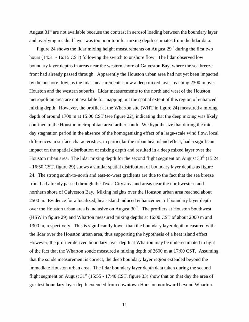
Figure 24 shows the lidar mixing height measurements on August 29th during the first two

hours (14:31 - 16:15 CST) following the switch to onshore flow. The lidar observed low

boundary layer depths in areas near the western shore of Galveston Bay, where the sea breeze

front had already passed through. Apparently the Houston urban area had not yet been impacted

by the onshore flow, as the lidar measurements show a deep mixed layer reaching 2300 m over

Houston and the western suburbs. Lidar measurements to the north and west of the Houston

metropolitan area are not available for mapping out the spatial extent of this region of enhanced

mixing depth. However, the profiler at the Wharton site (WHT in figure 24) measured a mixing

depth of around 1700 m at 15:00 CST (see figure 22), indicating that the deep mixing was likely

confined to the Houston metropolitan area farther south. We hypothesize that during the mid-

day stagnation period in the absence of the homogenizing effect of a large-scale wind flow, local

differences in surface characteristics, in particular the urban heat island effect, had a significant

impact on the spatial distribution of mixing depth and resulted in a deep mixed layer over the

Houston urban area. The lidar mixing depth for the second flight segment on August 30th (15:24

- 16:50 CST, figure 29) shows a similar spatial distribution of boundary layer depths as figure

24. The strong south-to-north and east-to-west gradients are due to the fact that the sea breeze

front had already passed through the Texas City area and areas near the northwestern and

northern shore of Galveston Bay. Mixing heights over the Houston urban area reached about

2500 m. Evidence for a localized, heat-island induced enhancement of boundary layer depth

over the Houston urban area is inclusive on August 30th. The profilers at Houston Southwest

(HSW in figure 29) and Wharton measured mixing depths at 16:00 CST of about 2000 m and

1300 m, respectively. This is significantly lower than the boundary layer depth measured with

the lidar over the Houston urban area, thus supporting the hypothesis of a heat island effect.

However, the profiler derived boundary layer depth at Wharton may be underestimated in light

of the fact that the Wharton sonde measured a mixing depth of 2600 m at 17:00 CST. Assuming

that the sonde measurement is correct, the deep boundary layer region extended beyond the

immediate Houston urban area. The lidar boundary layer depth data taken during the second

flight segment on August 31st (15:55 - 17:40 CST, figure 33) show that on that day the area of

greatest boundary layer depth extended from downtown Houston northward beyond Wharton.

12

Compared to the previous two days the afternoon mixing depths in the Houston vicinity are

significantly higher on August 31st ranging from 2500 m near the Galveston Bay shore and over

the southwestern suburbs to more than 3000 m over and north of downtown Houston.

Lidar measurements taken during the third flight segment on August 29th (16:15 - 18:00 CST,

figure 25) indicate that with the inland progression of the sea breeze front mixing depths

decreased significantly north and west of Galveston Bay, in particular over the Houston urban

area, where mixing depths dropped to around 1500 m. The corresponding planview plots of

boundary layer depth on August 30th (16:50 - 18:24 CST, figure 30) and August 31st (17:40 -

18:24 CST, figure 34) also show the expansion of the area of decreasing mixing heights due to

the sea breeze. However, the inland progress of the sea breeze is much slower than on August

29th.

Even though the flow patterns on August 30th and 31st were very similar, the afternoon

boundary layer in the Houston vicinity west of Galveston Bay was about 600 – 1000 m deeper

on the 31st than on the 30th (see figures 27, 29, 32, and 33). At the same time peak ozone

concentrations at the surface and aloft in the Houston urban and Ship Channel areas were lower

on August 31st than on August 30th. In the absence of any evidence for different emission

characteristics on these two days we hypothesize that the differences in peak ozone levels are

directly related to the differences in boundary layer depth. Figure 35 shows potential

temperature profiles from the 5:00 CST morning and 17:00 CST afternoon soundings at

downtown Houston on August 30th and 31st. These soundings indicate that the substantially

higher boundary layer heights on August 31st are due to the fact that the boundary layer was

about 2 °C warmer than on the previous day. Without the presence of a strong inversion aloft,

this small increase in temperature caused the boundary layer to grow to 2800 m compared to

2200 m on August 30th.

Figures 36 and 37 show time-height cross section of ozone mixing ratio measured with the

airborne lidar during 20-minute flight segments flown near Ellington Field on August 30th and

August 31st approximately around the same time in the afternoon. Both ozone cross sections

show very concentrated ozone plumes extending from the surface to the top of the boundary

layer. The vertically averaged ozone concentrations in the plume core are about 195 ppbv on

August 30th and around 145 ppbv on August 31st. Using the sharp gradient of ozone

concentration near the top of the plumes as an indicator of mixing depth the mixing height

13

estimates are about 1700 m for the August 30th plume and around 2600 m for the August 31st

plume, which is in good agreement with the other boundary layer depth measurements presented

above. By providing a larger volume for the pollutants to disperse in, the deeper mixed layer

likely is the main reason for the lower ozone concentrations observed in the August 31st pollution

plume. Assuming that the dilution process is linear, a lower mixing depth of 1700 m on August

31st would have translated into an average ozone concentration in the plume core of around 220

ppbv. This means that the total mass of ozone contained in the plume was greater on the 31st, but

the ozone was diluted more in the vertical.

3.5 September 1st

The flow on September 1st was from the west in the morning veering to a southwesterly

direction around the middle of the day (figure 38). Contrary to the previous three days, a flow

reversal and the establishment of a sea breeze was not observed. The time series of profiler and

radio sonde derived boundary layer depths (figure 39) indicate a spatially very homogeneous

distribution of mixing heights in the morning. Just as for the previous three days this can be

attributed to the westerly offshore flow. Mixing heights remained very shallow throughout the

morning, reaching depths of only 650 to 900 m by 11:30 CST. After 11:30 CST the boundary

layer started growing more rapidly, eventually reaching a depth of about 3300 m at Wharton with

lesser mixing depths at the other sites. The early morning potential temperature sounding at

Wharton shown in figure 40 helps to explain this behavior. A very strong temperature inversion

below 700 m suppressed boundary layer growth until the temperature had reached 309 °K or 36

°C. As the boundary layer warmed further it grew into less stable ambient air allowing for more

rapid growth, especially above 1700 m where the air was nearly neutrally stratified. The drop in

mixing height at La Marque after 13:00 CST (figure 39) could be explained by the advection of

Gulf of Mexico air to the La Marque site after the winds shifted to the southwest. The afternoon

drops in mixing height observed with the Houston Southwest and Liberty profilers are

questionable as an afternoon decrease in boundary layer depth at inland sites is not consistent

with the radio sonde and lidar data (figures 40 and 43).

The planview plot of lidar mixing heights for the first flight segment on September 1st (09:30

- 12:21 CST, figure 41) confirms that mixing heights were very shallow (800 m or less) before

11:30 CST and rather uniform across the Houston area. The lidar measurements during the

14

second flight segment (12:22 - 15:13 CST, figure 42) show still rather low mixing heights over

the Houston urban area and the western shore of Galveston Bay. Boundary layer depths east of

Galveston Bay were even lower (1100 m or less) because of advection of low mixing heights

from Galveston Bay. North of a line from Houston Intercontinental Airport (IAH in figure 42) to

Port Arthur the lidar data show a sharp south-to-north gradient in boundary layer depth with

mixing heights approaching 2500 m at the northernmost flight legs. This gradient in mixing

height is likely due to a slight south-to-north increase in boundary layer temperature. According

to the 12:00 CST surface temperature observations (not shown), the Houston urban area

experienced temperatures around 36 to 38 °C while temperatures north of Houston ranged from

about 38 to 40 °C. The slightly warmer temperatures north of Houston caused the boundary

layer to break through the inversion earlier and to start growing rapidly while mixing heights

farther south were still suppressed (see figure 40). The lidar boundary layer depth measurements

from the third flight segment (15:14 - 15:50 CST, figure 43) clearly show the effect of advection

of lower mixing heights from Galveston Bay to the east. Downwind or east of the Bay mixing

heights of less than 1200 m were observed while upwind or west of the Bay boundary layer

depths reached 2300 m.

4. Conclusions

The results of our research can be summarized as follows:

1. Mixing height measurements using radio sonde, wind profiler, and airborne lidar data

were generally in good agreement.

2. Under onshore flow conditions the temporal and spatial variability of mixed layer depth

in the Houston area is dominated by the advection of marine air from the Gulf of Mexico

or Galveston Bay where the boundary layer is typically only 400 to 700 m deep. As a

result, the mixing depth shows a characteristic southeast to northwest gradient, where the

boundary layer height increases with increasing distance from shore. Locations further

away form the coast experience deeper mixing layers because the marine air is either

15

gradually modified as it is advected inland or because the local mixed layer had more

time to grow to larger depths before being replaced by marine air.

3. Under offshore flow conditions the mixed layer depth distribution tends to be more

homogeneous compared to onshore flow conditions because marine air with shallow

mixing depths is not transported onshore.

4. When the winds become light and variable, particularly around the middle of the day

during the rapid-growth phase of the mixed layer, local differences in surface

characteristics can express themselves and result in mixing depth variations over

relatively small spatial scales. One such example is the possible enhancement of the

mixing depth over the Houston urban area due to the heat island effect. One light-wind

case (August 29th) provided evidence for a heat-island induced enhancement of mixing

depth over the Houston urban area while in two other cases (August 30th and 31st) the

evidence was inconclusive.

5. In the presence of a strong, low-level temperature inversion and a near-neutrally stratified

atmosphere aloft, the boundary layer can grow very rapidly once it has broken through

the inversion, and then mixing height correlates very strongly with boundary layer

temperature. Under these conditions mixing depths inland are likely to be greater than in

coastal areas, because temperatures in the Houston area typically increase with distance

away from the Gulf and Galveston Bay shores.

6. A limited case study of the relationship between boundary layer depth and mixed layer

ozone concentration provided evidence that a deeper mixed layer led to reduced ozone

concentrations by diluting pollutants in a larger volume of air.

16

Figure 1: Potential temperature sounding at Downtown Houston on August 26th, 17:00 CST.

zi = 1660 m

17

Figure 2: Time height cross section of radar reflectivity measured on August 28th with the Houston Southwest profiler. Mixed layer depth estimates are indicated by green “x”s. Blue crosses denote cloud base height measurements from a collocated ceilometer.

18

Figure 3: Time-height cross section of aerosol backscatter measured with the airborne lidar in the early afternoon on August 28th, 2000. The black line represents the lidar retrieved boundary layer depth estimate. This figure provides a snapshot of the spatial distribution of mixed layer depth: over the Gulf of Mexico (18:11 – 18:18 UTC) the boundary layer was shallow, whereas the mixed layer depth increased rapidly as the lidar aircraft flew away from the coast towards Houston (18:18 – 18:33 UTC).

19

Figure 4: Wind profiler forward trajectories for August 23rd, 02:00 - 18:00 CST.

20

Figure 5: Time series of mixing depth on August 23rd derived from wind profiler and radio sonde measurements.

21

Figure 6: Wind profiler forward trajectories for August 24th, 02:00 - 18:00 CST.

22

Figure 7: Time series of mixing depth on August 24th derived from wind profiler and radio sonde measurements.

23


24


25

Figure 10: Planview plot of mixing depth derived from airborne lidar data for August 25th.

26


27


28

Figure 13: Planview plot of mixing depth derived from airborne lidar data for August 26th.

29


30


31


32


33

Figure 18: Planview plot of mixing depth derived from airborne lidar data for August 28th, first flight segment.

34

Figure 19: Planview plot of mixing depth derived from airborne lidar data for August 28th, second flight segment.

35

Figure 20: Planview plot of mixing depth derived from airborne lidar data for August 28th, third flight segment.

36


37


38


39


40


41


42


43


44


45


46

Figure 31: Wind profiler forward trajectories for August 31st, 08:00 - 24:00 CST.

47

Figure 32: Time series of mixing depth on August 31st derived from wind profiler and radio sonde measurements.

48

Figure 33: Planview plot of mixing depth derived from airborne lidar data for August 31st, second flight segment.

49

Figure 34: Planview plot of mixing depth derived from airborne lidar data for August 31st, third flight segment.

50

Figure 35: Potential temperature morning and afternoon soundings at Downtown Houston on August 30th and August 31st.

zi = 2200 m

zi = 2800 m

51

Figure 36: Time height cross section of ozone mixing ratio measured with the airborne lidar on August 30th during a 20-min flight segment flown in the vicinity of Ellington Field.

52

Figure 37: Time height cross section of ozone mixing ratio measured with the airborne lidar on August 31st during a 20-min flight segment flown in the vicinity of Ellington Field.

53

Figure 38: Wind profiler forward trajectories for September 1st, 08:00 - 20:00 CST.

54

Figure 39: Time series of mixing depth on September 1st derived from wind profiler and radio sonde measurements.

55

Figure 40: Potential temperature sounding at Wharton on September 1st, 5:00 CST.

56

Figure 41: Planview plot of mixing depth derived from airborne lidar data for September 1st, first flight segment.

57

Figure 42: Planview plot of mixing depth derived from airborne lidar data for September 1st, second flight segment.

58

Figure 43: Planview plot of mixing depth derived from airborne lidar data for September 1st, third flight segment.

Documents

Final Report Spatial and Temporal Variations in Mixing ... · Spatial and Temporal Variations in Mixing Height in Houston ... maximum backscatter gradient at the top of the ... Data