AFRL-AFOSR-JP-TR-2016-0102

Study of solar energetic particles (SEPs) using largely separated spacecraft

Jinhye ParkKYUNG HEE UNIVERSITY, RESEARCH AND UNIVERSITY-INDUSTRY CORPORATION

Final Report10/29/2016

DISTRIBUTION A: Distribution approved for public release.

AF Office Of Scientific Research (AFOSR)/ IOAArlington, Virginia 22203

Air Force Research Laboratory

Air Force Materiel Command

a. REPORT

Unclassified

b. ABSTRACT

Unclassified

c. THIS PAGE

Unclassified

REPORT DOCUMENTATION PAGE Form ApprovedOMB No. 0704-0188

The public reporting burden for this collection of information is estimated to average 1 hour per response, including the time for reviewing instructions, searching existing   data sources, gathering and maintaining the data needed, and completing and reviewing the collection of information. Send comments regarding this burden estimate or   any other aspect of this collection of information, including suggestions for reducing the burden, to Department of Defense, Executive Services, Directorate (0704-0188).   Respondents should be aware that notwithstanding any other provision of law, no person shall be subject to any penalty for failing to comply with a collection of information   if it does not display a currently valid OMB control number.PLEASE DO NOT RETURN YOUR FORM TO THE ABOVE ORGANIZATION.1. REPORT DATE (DD-MM-YYYY)     16-12-2016

2. REPORT TYPEFinal

3. DATES COVERED (From - To)01 Sep 2013 to 31 Aug 2016

4. TITLE AND SUBTITLEStudy of solar energetic particles (SEPs) using largely separated spacecraft

5a.  CONTRACT NUMBER

5b.  GRANT NUMBERFA2386-13-1-4066

5c.  PROGRAM ELEMENT NUMBER61102F

6. AUTHOR(S)Jinhye Park

5d.  PROJECT NUMBER

5e.  TASK NUMBER

5f.  WORK UNIT NUMBER

7. PERFORMING ORGANIZATION NAME(S) AND ADDRESS(ES)KYUNG HEE UNIVERSITY, RESEARCH AND UNIVERSITY-INDUSTRY CORPORATIONKYUNG HEE UNIV, 1 SEOCHEON-DONG GIHEUGYEONGGI-DO, 446-701 KR

8. PERFORMING ORGANIZATIONREPORT NUMBER

9. SPONSORING/MONITORING AGENCY NAME(S) AND ADDRESS(ES)AOARDUNIT 45002APO AP 96338-5002

10. SPONSOR/MONITOR'S ACRONYM(S)AFRL/AFOSR IOA

11. SPONSOR/MONITOR'S REPORTNUMBER(S)

AFRL-AFOSR-JP-TR-2016-0102      12. DISTRIBUTION/AVAILABILITY STATEMENTA DISTRIBUTION UNLIMITED: PB Public Release

13. SUPPLEMENTARY NOTES

14. ABSTRACTSolar energetic particles (SEPs) are one of the main activities in terms of space weather forecast. SEPscould affect commercial airlines, HF communication, satellite launch, extra-vehicular activity fromspace stations, and manned space flight missions. In this study, we investigate the source regions andthe characteristics of SEPs using multiple spacecraft data, Solar TErrestrial RElations ObservatoryAhead (STEREO-A), Behind (STEREO-B) and Solar Dynamics Observatory (SDO)/Solar andHeliospheric Observatory (SOHO)/Geostationary Operational Environmental Satellites (GOES).

15. SUBJECT TERMSsolar wind, AOARD, solar physics, CME

16. SECURITY CLASSIFICATION OF: 17. LIMITATION OFABSTRACT

SAR

18. NUMBEROFPAGES 23     

19a.  NAME OF RESPONSIBLE PERSONMAH, MISOON

19b.  TELEPHONE NUMBER (Include area code)042-511-2001

Standard Form 298 (Rev. 8/98)Prescribed by ANSI Std. Z39.18

Page 1 of 1FORM SF 298

12/16/2016https://livelink.ebs.afrl.af.mil/livelink/llisapi.dll

Final Report for AOARD Grant FA2386-13-1-4066

“Study of solar energetic particles (SEPs) using largely separated spacecraft”

31. Dec. 2016

Jinhye Park (PI): - e-mail address : jinhye@khu.ac.kr - Institution : Department of Astronomy and Space Science, Kyung Hee University - Mailing Address : Department of Astronomy and Space Science, Kyung Hee University

1732, Deogyeong-daero, Giheung-gu, Yongin-si, Gyeonggi-do, Republic of Korea - Phone : +82-31-201-3874 - Fax : +82-31-204-8122

Yong-Jae Moon (Co-PIs): - e-mail address : moonyj@khu.ac.kr - Institution : Department of Astronomy and Space Science, Kyung Hee University - Mailing Address : Department of Astronomy and Space Science, Kyung Hee University

1732, Deogyeong-daero, Giheung-gu, Yongin-si, Gyeonggi-do, Republic of Korea - Phone : +82-31-201-3807 - Fax : +82-31-204-8122

Period of Performance: 09/01/2013 – 08/31/2016

Abstract

Solar energetic particles are one of important phenomena in the Sun. They are mainly accelerated by magnetic field reconnections of flares and CME-driven shocks so that the characteristics of SEPs are strongly associated with physical quantities of related solar activities. In addition, SEPs are a major component in terms of space weather. In the present study, we examine the relationships between SEPs and related solar activities: EUV (Extreme-ultraviolet) waves, flares and CMEs. From spacecraft largely separated, we observe SEPs and related solar activities with multiple points of view. The major results of the present study are as follows. 1) SEP onset times and SEP peak fluxes at 1 AU are significantly associated with EUV wave arrival times and EUV wave speeds at the photospheric magnetic footpoints of spacecraft connecting open magnetic field lines. This result supports that EUV waves reflect the lateral expansion of CME-driven shocks in corona region. 2) On the study of the dependence of SEP on CME and flare parameters, SEP occurrence probabilities and SEP peak fluxes increase with CME speed, CME angular width, flare peak flux, flare impulsive time and source longitude from east to west. 3) On the study of SEPs using 3-dimensional CME parameters

obtained from multiple spacecraft, there are positive correlations between SEP peak fluxes and CME speeds as well as angular widths. The highest association with SEP peak fluxes is found in longitudinal separation angles from magnetic footpoints of spacecraft to SEP source longitudes.

1. Introduction Solar energetic particles (SEPs) are one of the main solar activities in that SEPs can affect commercial airlines, HF communication, satellite launch, extra-vehicular activity from space stations, and manned space flight missions. SEPs are accelerated by flare reconnections and CME-driven shocks. The characteristics of SEPs depend on their solar sources (Reames 1999, 2013; Kallenrode 2003). Impulsive SEP events, having short durations of several hours, are associated with impulsive flares. They are electron rich and have enhanced 3He/4He and Fe/O ratios in contrast to nominal coronal values. Also, they are generally distributed within a narrow propagation cone. Gradual SEP events are associated with gradual X-ray flares and type II and type IV radio emission. They are produced by wide and fast CME-driven shocks (Gopalswamy 2003) and have a broad range of source longitudes (Kahler 1994; Reames 1999). Gradual events show typical coronal abundances and are proton rich in contrast to impulsive events. Many events have characteristics of both gradual and impulsive events due to a combination of both flare-and shock-associated particles (Cane et al. 2006). Surprisingly, some of these appear to have poor magnetic connection to the associated flare sites, suggesting that flare-accelerated particles can be distributed over wide angles in interplanetary space either by efficient cross-field transport in interplanetary space or by ejection of flare particles into an expanding source, for example, a CME shock, near the Sun (Wiedenbeck et al. 2013; Dresing et al. 2014). EUV waves are generated in solar eruptions (Thompson & Myers 2009; Warmuth 2010). They show up as faint fronts moving with velocities up to 1000 km/s, with large dimming regions in their wakes. It has been generally accepted that they track the outer edge of a CME at the Sun (Veronig et al. 2010; Patsourakos & Vourlidas 2009; Rouillard et al. 2012). Whether this edge is a wave front (Thompson et al. 1999; Patsourakos & Vourlidas 2009, Kozarev et al. 2011) or the rim of the region affected by magnetic reconfiguration associated with the CME (Cheng et al. 2012; Attrill et al. 2007) is often not resolvable. Since released SEPs follow magnetic fields as long as interplanetary scattering is not a dominant effect, it is reasonable to assume that there may be a relationship between the time that the EUV wave crosses the spacecraft connection point at the Sun and the arrival time of SEPs at the connected spacecraft. If the EUV wave front indicates triggering reconnections, then SEPs may be released from the reconnection site. Alternatively if the EUV wave is the skirt of the CME-associated shock it should give a good indication of the time when the edge of the shock reached the connecting field line. The main motivation of this study is to see if a relationship between SEPs and EUV waves exists by considering as many events with widely separated SEPs. The purpose of the present study is to understand SEPs and related solar activities observed by largely separated spacecraft. It makes possible to look for connections between widely distributed SEPs and related solar activities. In particular, the Stonyhurst heliographic images with 5 minutes cadence from STEREO/EUVI and SDO/AIA give us a complete 360° view of the evolving solar EUV waves, which is considered as the lateral expansions of CME-driven shocks. We also all sources of sympathetic flaring that may produce the wide longitudinal spread of SEPs. The paper is structured as follows. We describe data and analysis in Section 2. In Section 3, we describe the results of three main topics: 1) Relationship between SEP and EUV wave properties, 2) SEPs depending on CME and flare parameters and 3) SEPs depending on 3-dimensional CMEs obtained from multiple-spacecraft observations. The summary and conclusion are given in the last section.

2. Data and Analysis For the study of SEP onset time and EUV wave onset time, we use 12 SEP events between 2010 August and 2012 January (Table 1). We obtain electron fluxes from the Solar Electron Proton Telescope (SEPT; Müller-Mellin et al. 2008) on STEREO averaged over 5 minutes in four low-energy channels (55–65 keV, 105–125 keV, 195–225 keV, and 335–375 keV) and from the High Energy Telescope (HET; von Rosenvinge et al. 2008) in three energy channels (0.7–1.4 MeV, 1.4–2.8 MeV, and 2.8–4.0 MeV). In addition, we obtain the ACE Electron, Proton, and Alpha Monitor (EPAM; Gold et al. 1998) averaged over 5 minutes in four energy channels (38–53 keV, 53–103 keV, 103–175 keV, and 175–315 keV) and the SOHO Electron Proton and Helium Instrument (EPHIN; Müller-Mellin et al. 1995) in two channels (0.67–3.0 MeV and 2.64–10.4 MeV). Proton fluxes are from the Low Energy Telescope (LET; Mewaldt et al. 2008) on STEREO averaged over 10 minutes in three energy channels (1.8–3.6 MeV, 4–6 MeV, and 6–10 MeV), from HET in four high-energy channels (13.6–15.1 MeV, 20.8–23.8 MeV, 29.5–33.4 MeV, and 40.0–60.0 MeV), the Energetic and Relativistic Nuclei and Electron instrument (ERNE; Torsti et al. 1995) on SOHO averaged over 10 minutes in seven channels (1.90–3.06 MeV, 3.06–5.12 MeV, 5.12–8.69 MeV, 8.69–14.9 MeV, 12.6–20.8 MeV, 19.4–32.2 MeV, and 32.2–57.5 MeV). For the study of SEP peak flux and EUV wave arrival time, we investigate 16 SEP events from 2010 August and 2013 May (Table 2). We use LET (Mewaldt et al. 2008) on STEREO averaged over 10 minutes in the 6–10 MeV proton channel or by ERNE (Torsti et al. 1995) on SOHO averaged over 10 minutes in the 6–10 MeV proton channel. For the study of solar proton events depending on flare and CME parameters, we use the NOAA SPE list (http://swpc.noaa.gov/ftpdir/indices/SPE.txt) from 1997 to 2011 and the information of their related CMEs observed by the Solar and Heliospheric Observatory mission (SOHO) Large Angle and Spectrometric Coronagraph (LASCO) (Brueckner et al., 1995). The CME linear speeds and angular widths are taken from the SOHO LASCO CME online catalog (http://cdaw.gsfc.nasa.gov/ CME_list/) (Gopalswamy et al., 2009). Flare information is taken from the NOAA National Geophysical Data Center (NGDC) Geostationary Operational Environmental Satellite (GOES) X-ray flare catalog (http://www. ngdc.noaa.gov/ngdc.html). Table 1. The Solar Sources of the 12 SEP Events (Park et al. 2013).

For the study of SEPs using 3-dimensional CME parameters, we examine 18 SEPs from 2010 to 2013, which are detected by LET (Mewaldt et al. 2008) on STEREO averaged over 10 minutes in the 6–10 MeV proton channel and/or by ERNE (Torsti et al. 1995) on SOHO averaged over 10 minutes in the 6–10 MeV proton channel (Table 3). We use the GOES flare list (http://solar-center.stanford.edu/SID/activities/PickFlare.html), the SOHO LASCO CME catalogue (http://cdaw.gsfc.nasa.gov/CME_list), and the SECCHI-A and B CME lists (http://secchi.nrl.navy.mil/cactus). To obtain radial CME parameters, we use STEREO CME Analysis Tool (StereoCAT), which is provided by NASA CCMC (http://ccmc.gsfc.nasa.gov/analysis/stereo/). In the StereoCAT, the radial CME parameters are measured by two coronagraphs out of three coronagraphs: SOHO/LASCO C3, STEREO-A, and B SECCHI COR2 images. Table 2. The Solar Sources of the SEP Events (Park et al. 2015).

Table 3. The properties of flares and CMEs associated with 18 SEP events. VL is 2D CME speed and VR is 3D CME speed. AWL is 2D angular width and VR is 3D angular width.

2.1 SEP onset time and peak flux We look at the flux profiles from low- to high-energy bands to get a crude estimate of the onset time after the solar eruption associated with the event. Then, we plotted the data around the time at which the flux increase occurred. We identify the three earliest consecutive times with increasing flux and mark the first of the three as its SEP onset time. If the data were very noisy and there were no three consecutive times with increasing flux, we double the time over which the data were averaged until an enhancement time emerged. The peak times and peak fluxes are chosen as the points at the top of the of the steep flux rise, which appeared just after the solar eruption. 2.2 Photospheric magnetic footpoints of spacecraft The interplanetary magnetic field emanates from the footpoints of coronal holes and streamers. Potential field source surface (PFSS) models give a good approximation of the magnetic field up to 2.5 Rsun and can be used to trace back the sources of the interplanetary field in the ecliptic plane at 2.5 Rsun (Neugebauer et al. 1998). Further out the field is stretched by the solar wind to form the Parker spiral, and so depends on the solar wind speed. The connection points of the spacecraft are obtained using synoptic magnetic field and ecliptic-plane PFSS extrapolations from the GONG website (http://gong.nso.edu/data/magmap/pfss.html). The gif images provided by the site have been rotated to Stonyhurst co-ordinates. The original connection points for Earth, STEREO-A and STEREO-B longitudes shown on the plots do not account for the Parker spiral. Therefore we move the connection points at 2.5 Rsun, westward according to the solar wind speed observed at the time of the events using the equation, Ø0 = DΩ/Vw + Ø where Ø, Ø0 are the spacecraft and solar longitudes, D is the distance to the Sun, Vw is the solar wind speed, and Ω is the solar rotation rate. 2.3 EUV wave arrival time and speed at photospheric magnetic footpoints of spacecraft For obtaining EUV wave arrival times and speeds, we use the full-Sun difference image created by combining STB/EUVI 195Å, SDO/AIA 193Å, and STA/EUVI 195Å images (Figure 1). From the source region to the three footpoints, the lines along which the EUV wave speeds and arrival times were estimated. The distance traveled is computed by considering a great circle trajectory to account for projection effects. EUV wave arrival times and speeds are determined by linear extrapolation of the EUV wavefront in the running ratio spacetime images to the footpoint site. There are several significant sources of uncertainty with EUV wave properties. They depend strongly on the applicability and accuracy of the PFSS extrapolations and the Parker spiral formula for pinpointing the footpoints of the connecting field lines. A feel for the reliability of the positions can best be obtained

by looking at the PFSS extrapolations and the spacecraft connecting points for the individual events. Times to sites close to the EUV wave source are accurate to within 5 minutes, and to more distance sites accurate to 10 minutes.

Figure 1. 2010 August 14 source region and EUV wave: (a) GONG synoptic magnetic field with PFSS ecliptic plane field lines traced back to their source. White and red crosses mark the longitudes of STB, Earth, and STA at 2.5R⊙. The photospheric footpoints of the connecting field lines are marked by orange crosses. Connecting footpoints are deduced by tracing the field lines from the white crosses to the Sun. Green/red indicates positive/negative open fields. The source region is enclosed by a white square. (b) Full Sun ratio image at the times given. This is a composite of STB 195 Å, SDO 193 Å, and STA 194 Å images. The dashed line indicates the position of the space–time image below. (c) Running ratio space–time image along the line in (b). The white number is the approximate wave speed calculated by manually choosing the start and end positions of the wave (Park et. al., 2013).

3. Results and Discussion 3.1 Relationship between SEP and EUV wave properties 3.1.1 SEP onset time and EUV wave arrival time (Park et al. 2013) To examine the relationship between EUV waves and SEP onset times, we need an offset time against which we can compare the SEP onset times at the spacecraft and EUV arrival times at the photospheric magnetic field connection points of the spacecraft. There are three natural choices: flare, CME, and type III radio burst times. Figures 2-3 show the relationships between the EUV wave travel times to the connecting footpoints (EUV arrival time – solar event time) and the SEP travel time (SEP onset time – solar event time). All cases have moderate correlation coefficients, stronger in the electron groups. Our result shows that the correlation coefficients between the two parameters are between 0.60 and 0.69. The highest correlation value is for electrons when the CME time is used. The averages of the slopes and offsets are 1.1 and 40.7 minutes for electrons and 2.2 and 131.8 minutes for protons, respectively. The results support the idea that EUV waves trace the release sites of SEPs, which is consistent with previous studies that suggested that SEPs are accelerated by large coronal shock waves (Kocharov et al. 1994; Torsti et al. 1998; Krucker et al. 1999; Vainio & Khan 2004; Rouillard et al. 2012).

Figure 2. Relationship between EUV-flare time Figure 3. Relationship between EUV-CME time

and SEP-flare time: (a) electron and (b) proton. The error bars represents the number of degradations. The dashed line is a linear least squares fit to the data. In the figure, r means a correlation coefficient and the p-value is the probability that r = 0. (Park et al. 2013)

and SEP-CME time: (a) electron and (b) proton. The error bars represents the number of degradations. The dashed line is a linear least squares fit to the data. In the figure, r means a correlation coefficient and the p-value is the probability that r = 0. (Park et al. 2013)

3.1.2 SEP peak flux and EUV wave speed (Park et al. 2015)

The speeds of EUV waves (Ve) seen in the low corona give a direct measure of their energies. The point is that if the wave speeds exceed the magnetosonic speeds in the corona, then the waves are shocks that can accelerate particles. Therefore, we examine the relationship between the wave speeds and the SEP fluxes. Figure 4a shows the relationship between log10 SEP peak flux and EUV wave speed. The equation of the linear regression is described as

I=I0exp(0.01 ×Ve) (1)

where I0 = 0.06 cm-1 s-1 sr-1 MeV-1 with a correlation coefficient of 0.66 ± 0.16. It shows that there is a definite tendency for the fluxes to increase with the EUV wave speeds. It is seen that EUV wave speeds around 200 km s−1 are associated with the widest range of SEP peak fluxes and that the SEP peak fluxes increase by three orders of magnitude in the range from 200 to 600 km s−1. The energy spectra in gradual SEP events are well represented by power laws (Ellison & Ramaty 1985; Lee 2005). Now we examine the association between the EUV wave speeds and the two-point power-law spectral indices of SEP events, which are obtained at the proton peak fluxes in the SOHO/ERNE 20.8–26.0 MeV and 34.8–40.5 MeV and the STEREO/HET 20.8–23.8 MeV and 35.5–40.5 MeV channels. Only 14 spectral indices are obtained from the 24 cases because the other events do not extend to such high energies and they lack continuous flux profiles to determine the peak fluxes. In Figure 4b, the equation of the linear fitting is described as

γ = 0.21×10-2 Ve - 3.62 (2) The correlation coefficient is 0.41 ± 0.26 between the two quantities. The spectral indices become harder with increasing EUV wave speeds. We also find a weak correlation between the γ and I, as shown in Figure 4c. These results imply that faster waves are related to the acceleration of SEPs of higher fluxes and energies and suggest that EUV wave speeds represent the strengths of the lateral coronal disturbances in CME-driven shocks. In Figure 5a we show the relationship between the CME linear speeds and the SEP peak fluxes for the 16 events. If SEP events were observed by more than two instruments, we selected the highest flux among them. The correlation coefficient is 0.66 ± 0.20, which is similar to ones found in previous studies (Park et al. 2012; Kahler & Vourlidas 2014). In the case of EUV wave speeds using the same data set, the correlation coefficient is 0.75. The results show that both the CME speeds and the EUV wave speeds are associated with SEP peak fluxes. Figure 5b shows the relationship between CME speeds and EUV wave speeds for the 16 events. The correlation coefficient (r = 0.52 ± 0.23) is meaningful even though the direct comparison of EUV and CME characteristics is difficult because it is not easy to trace CME speeds in the high coronal region along the directions of the EUV wave propagations in the low coronal region.

Figure 4. Relationships between SEPs and the EUV waves: (a) 6–10 MeV proton peak fluxes vs. wave speeds for 24 cases, (b) two-point power-law spectral indices vs. wave speeds for 14 cases, and (c) 6–10 MeV proton peak fluxes vs. two-point power-law spectral indices. The spectral indices of SEP events were obtained at the proton peak fluxes in the SOHO/ERNE 20.8–26.0 MeV and 34.8–40.5 MeV and STEREO/HET 20.8–23.8 MeV and 35.5–40.5 MeV channels. The dashed lines are linear least-squares fits to the data. In each figure, r is the correlation coefficient and p is the p-value. (Park et al. 2015)

Figure 5. Relationship between SEPs, EUV waves, and CME linear speeds for 16 events: (a) CME linear speed vs. 6–10 MeV proton peak flux, and (b) CME linear speed vs. EUV wave speed. The dashed line is a linear least-squares fit to the data. In the figure, r is the correlation coefficient and p is the p-value (Park et al. 2015).

3.2 Dependence on SEPs on CME and flare parameters (Park et al. 2014)

3.2.1 SEP occurrence probability To examine SPE occurrence probabilities, we consider four solar eruption parameters: flare peak flux, source longitude, CME linear speed, and angular width. The previous studies (Park et al., 2010, 2012) showed that it is extremely rare that SPEs are generated by narrow (< 120°) and slow (< 400 km s-1) CMEs as well as weak flares (< C1 class). We exclude the events generated by relatively weak solar eruptions, which are only two from 1996 to 2011, and do not consider events whose source regions are behind the limb. Accordingly, we use 67 SPEs and 490 solar eruptions, which meet the criteria of the parameters as follows: flare peak flux ≥ C1 class, CMEs linear speed ≥ 400 km s-1, angular width ≥ 120◦, and front source longitude (−90° ≤ L ≤ 90°).

For the regression between solar eruption parameters and SPE peak flux, we use five solar eruption parameters associated with the observed SPEs. The parameters are flare peak flux, source longitude, impulsive time, CME linear speed, and angular width. In this case, we exclude two events because the events have unusual long impulsive times (2.66 h and 1.76 h) which are significantly larger than 1.39, mean (0.55) plus 2 times standard deviation (0.42). For the regression, we use 65 SPEs and their associated eruptions.

Our results have shown that the SPE occurrence probabilities are strongly dependent on flare and CME parameters and the distinct contrasts of the probabilities are seen according to the quantitative ranges of the parameters (Tables 4 and 5). The highest probabilities have been found in the subgroups of fast full halo CMEs (55.3%) and partial halo CMEs (42.9%) associated with strong flares from the western region. The probability is also high for the subgroup of slow full halo CMEs associated with strong flares from the western region (31.6%). Noticeably, the SPE probabilities are nearly 0% for eight subgroups. As shown in Table 4, slow full halo CMEs from the eastern region have no SPE. As for the partial halo CMEs in Table 5, all eastern events have no SPE and western slow CMEs have only one SPE. These results show that CME linear speed, angular width, and source longitude are the most important parameters to control SPE occurrences. This is understood by that wide and fast CMEs can form piston-driven shocks, which is the main mechanism to accelerate SPEs. The importance of source longitude and angular width can be interpreted by the sub-Earth point, which is directly linked to the Earth by the Parker spiral magnetic fields. Our results are the same line with Kahler and Reames (2003) and Gopalswamy et al. (2008). Kahler and Reames (2003) found that CMEs having w ide angular widths are mostly fast (V ≥ 900km s-1) and associated with SPEs. They noted that CMEs with narrow angular widths are unsuitable to form CME-driven shocks accelerating SPEs. Gopalswamy et al. (2008) also showed that the SPE occurrences increase with CME linear speeds and angular widths. They found that some CMEs with DH type II bursts as coronal shock signatures are not associated with SPEs, mainly because of poor connectivity or it is possible that the shocks with the bursts are too weak to accelerate SPEs (Shen et al., 2007).

Table 4. SPE Occurrence Probability Depending on Flare Peak Flux, Longitude, and CME Linear Speed (Slow CME: 400 km/s ≤ V < 1000 km/s and Fast CME: V ≥ 1000 km/s) for Full Halo CMEs (Park et al. 2014).

Table 5. SPE Occurrence Probability Depending on Flare Peak Flux, Longitude, and CME Linear Speed (Slow CME: 400 km/s ≤ V < 1000 km/s and Fast CME: V ≥ 1000 km/s) for Partial Halo CMEs (Park et al. 2014).

3.2.2 Predicted SEP peak flux using flare and CME parameters We present the relationships between the observed and the predicted SPE peak fluxes using the multiple regression method combining the solar eruption parameters (flare peak flux, longitude, impulsive time, CME linear speed, and angular width) for 20 subgroups whose criteria are given in Table 6. In case that all of the events are associated with full halo CMEs, we only consider four parameters except for the angular width (Park et al. 2014). When we take into account the impulsive times, short duration (T < 0.4 h) and long duration (T ≥ 0.4 h), the correlation coefficients between the observed and the predicted SPE peak fluxes are 0.59 for the short-duration case and 0.78 for the long-duration case. For the long-duration case, the correlation coefficients are 0.95 for the eastern events and 0.73 for the western events. Noticeably, the coefficient for the eastern long-duration events is significantly high. The slope of the linear fitting (0.90) is close to 1.0.

Table 6. The Results of Multiple Regressions of SPE Peak Fluxes and Associated Solar Eruption Parameters for 20 Subgroups (Park et al. 2014).

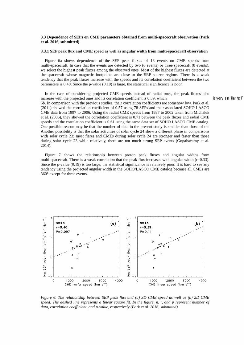
3.3 Dependence of SEPs on CME parameters obtained from multi-spacecraft observation (Park et al. 2016, submitted) 3.3.1 SEP peak flux and CME speed as well as angular width from multi-spacecraft observation Figure 6a shows dependence of the SEP peak fluxes of 18 events on CME speeds from multi-spacecraft. In case that the events are detected by two (6 events) or three spacecraft (8 events), we select the highest peak fluxes among the observed ones. Most of the highest fluxes are detected at the spacecraft whose magnetic footpoints are close to the SEP source regions. There is a weak tendency that the peak fluxes increase with the speeds and its correlation coefficient between the two parameters is 0.40. Since the p-value (0.10) is large, the statistical significance is poor. In the case of considering projected CME speeds instead of radial ones, the peak fluxes also increase with the projected ones and its correlation coefficient is 0.39, which is very sim ilar to F 6b. In comparison with the previous studies, their correlation coefficients are somehow low. Park et al. (2011) showed the correlation coefficient of 0.57 using 78 SEPs and their associated SOHO LASCO CME data from 1997 to 2006. Using the radial CME speeds from 1997 to 2002 taken from Michalek et al. (2006), they showed the correlation coefficient is 0.71 between the peak fluxes and radial CME speeds and the correlation coefficient is 0.61 using the same data set of SOHO LASCO CME catalog. One possible reason may be that the number of data in the present study is smaller than those of the Another possibility is that the solar activities of solar cycle 24 show a different phase in comparisons with solar cycle 23; most flares and CMEs during solar cycle 24 are stronger and faster than those during solar cycle 23 while relatively, there are not much strong SEP events (Gopalswamy et al. 2014). Figure 7 shows the relationship between proton peak fluxes and angular widths from multi-spacecraft. There is a weak correlation that the peak flux increases with angular width (r=0.33). Since the p-value (0.19) is too large, the statistical significance is relatively poor. It is hard to see any tendency using the projected angular width in the SOHO/LASCO CME catalog because all CMEs are 360° except for three events.

Figure 6. The relationship between SEP peak flux and (a) 3D CME speed as well as (b) 2D CME speed. The dashed line represents a linear square fit. In the figure, n, r, and p represent number of data, correlation coefficient, and p-value, respectively (Park et al. 2016, submitted).

Figure 7. The relationship between SEP peak flux and 3D CME angular width (Park et al., 2016, submitted).

3.3.2 Relationship between SEP peak flux and longitudinal separation angle

The magnetic foopoints of SOHO are estimated between 45 and 65° considering solar wind speeds between around 300 and 800 km s−1 using Parker spiral field equation. The magnetic footpoints of STEREO-A and B are calculated in the range of 140 to 200° and 10 to -90°, respectively. All 17 measurements whose magnetic footpoints are located inside the CME angular widths (in-boundary), have SEP enhancements but about 40% of the measurements (14/37) whose footpoints are located outside (out-boundary), have no SEP enhancement. Figure 8 shows that the relationship between the SEP peak fluxes and their longitudinal separation angles (|θs|) for 40 measurements of 18 SEP events. There is a noticeable anti-correlation (r=-0.62) between the two parameters. As shown in the figure, the proton peak fluxes decrease with |θs|. The enhancements (filled circles in Fig. 4), which are much close to source region, have higher fluxes than the out-boundary enhancements (open circles in Figure 4). In the range of 40 to 80°, such a dependence are not much different between the proton enhancements associated with in-boundary and out-boudnary.

Figure 8. The relationship between the absolute value of longitudinal angular separation (|θS |) and the SEP peak flux. Filled circles represent that the magnetic footpoints of spacecraft are located inside the longitudinal boundaries of 3D angular width. Open circles represent that the magnetic footprints of spacecraft are located outside the longitudinal boundaries of 3D angular width (Park et al. 2016, submitted).

Figure 9. Proton peak flux as a function of 3D CME speed and longitudinal angular separation (θS). The red and green bar represent SEP peak fluxes associated with in-boundary and out-boundary of 3D angular widths, respectively (Park et al. 2016, submitted)

Figure 9 shows the SEP peak fluxes as a function of radial CME speed and θs. As shown in the figure, most strong SEP events are associated with very fast CMEs whose radial CMEs are closer to zero within the radial angular widths, which means that most of proton fluxes are generated near the CME source regions (or CME nose). This fact implies that most of the proton fluxes are generated near the CME noses rather than their flanks. It is also noted that several events far from their source regions have still noticeable proton flux enhancements, which may be contributed by proton fluxes generated near the CME flank regions. The above results have shown that the proton peak fluxes are dependent on 3D CME parameters: radial speed, angular width, and longitudinal angular separation. In the case of CME-driven shocks, the Alfven Mach number, which indicates the strength of a shock, can be described by VR/VA where VA is the Alfven speed. This equation implies that the faster the CME speed is, the stronger its associated shock is. The angular width of a CME seems to be associated with the volume of shock-forming regions. Thus we expect that the number of proton particles accelerated by the CME piston driven shocks have a tendency to increase with angular width. The angular separation is directly linked to the magnetic field connectivity of the spacecraft. Our results, for the first time, demonstrate that 3D CME physical parameters are very important for the generation of energetic proton particles in the corona.

4. Summary and Conclusion (Park et al. 2013, 2014, 2015; 2016 submitted) The genesis of EUV waves has been under debate: are they MHD waves, coronal disturbances, wave-like motion, or a hybrid combination (Patsourakos & Vourlidas 2012; Liu & Ofman 2014)? Another important issue is whether EUV waves are associated with SEP events, and if so, is it because those waves act to accelerate the SEPs, or because the waves are signatures of CME-driven shocks that produce SEPs? The present study has investigated the relationships between SEP events observed by multiple spacecraft and their associated EUV waves. By combining observations from SDO and STEREO instruments with high temporal and spatial resolution, we have been able to measure the propagation of EUV waves across the Sun. We have considered EUV wave propagation from their source regions to the photospheric magnetic footpoints of the spacecraft, by assuming Parker spiral fields from the spacecraft to the source surface at 2.5 and then potential field source surface extrapolation to the photosphere. In the analysis we have made the following comparisons: SEP onset time versus EUV wave arrival time, SEP peak fluxes versus EUV wave speeds and two-point power-law spectral indices of SEP events versus EUV wave speeds. The results have shown associations between the SEP events and the EUV waves. The main results are as follows.

1) We have considered an offset time using flare, CME, and type III radio burst times against which we can compare the SEP onset and EUV arrival times. SEP onset times are significantly associated with EUV wave arrival times. Our result shows that the correlation coefficients between the two parameters are between 0.60 and 0.69. The results support the idea that EUV waves trace the release sites of SEPs, which is consistent with previous studies that suggested that SEPs are accelerated by large coronal shock waves (Kocharov et al. 1994; Torsti et al. 1998; Krucker et al. 1999; Vainio & Khan 2004; Rouillard et al. 2012).

2) We found that the 6–10 MeV SEP peak fluxes increase with the EUV wave speeds measured along the direction from the source regions to the footpoints of the spacecraft. It is also seen that the proton spectral indices measured at higher energies become harder with the EUV wave speeds. These results imply that faster waves are related to the acceleration of SEPs of higher fluxes and energies and suggest that EUV wave speeds represent the strengths of the lateral coronal disturbances in CME-driven shocks.

We have investigated the SEP events depending on both flare and CME parameters (flare peak flux, source longitude, flare impulsive time, CME linear speed and angular width). We have estimated the SPE occurrence probabilities as well as the relationships between the observed and the predicted SPE peak fluxes on the param eters. We have also examined SEP events depending on 3-dimensional CME parameters (speed, angular width and longitudinal separation angle) obtained from multi-spacecraft observations. The studies are to scientifically examine the relationship between SEP characteristics and flare as well as CME and to practically use the results as a way of the SEP forecast. The main results are follows.

1) Three highest probabilities are found for the following subgroups: full halo (55.3%) and fast partial halo (42.9%) CMEs associated with strong flares from the western region, and slow full halo CMEs associated with strong flares from the western region (31.6%). It is noted that the events whose SPE probabilities are nearly 0% belong to the following subgroups: slow and fast partial halo CMEs from the eastern region, slow partial halo CMEs from the western region, and slow full halo CMEs from the eastern region. These results show that important parameters to control SPE occurrences are CME linear speed, angular width, and source longitude, which can be understood by the piston-driven shock formation of fast CMEs and magnetic field connectivity from the source site to the Earth. 2) We have investigated the relationships between the observe and predicted SPE peak fluxes by the multiple regression method using the five combined parameters: flare peak flux, flare impulsive time, source longitude, CME linear speed and angular width. In this case, the correlation coefficient is 0.62. The whole data were divided into the 20 subgroups according to the flare and the CME parameters, and we have examined the relationships between the

observed and the predicted SPE peak fluxes for the subgroups. In terms of the SPE peak flux prediction, the best result is found for the set of four subgroups using the impulsive time (T ≥ 0.4 h and T < 0.4 h) and the source longitude (east and west). Its correlation coefficients are between 0.59 and 0.95.

3) There is a positive correlation between SEP peak flux and angular width, which is more evident than the relationship between SEP peak flux and projected angular width. There is a noticeable anti-correlation (r=-0.62) between SEP peak flux and longitudinal separation angle for 40 measurements of 18 SEP events.

Reference Attrill, G. D. R., Harra, L. K., van Driel-Gesztelyi, L., & Démoulin, P. 2007, ApJL, 656, L101 Brueckner, G. E., Howard, R. A. , Koomen, M. J. , et al. 1995, Sol. Phys., 162(1–2), 357–402 Cane, H. V., Mewaldt, R. A., Cohen, C. M. S., & von Rosenvinge, T. T. 2006, JGRA, 111, 6 Cheng, X., Zhang, J., Olmedo, O., et al. 2012, ApJL, 745, L5 Dresing, N., Gómez-Herrero, R., Heber, B., et al. 2014, A&A, 567, A27 Ellison, D. C., & Ramaty, R. 1985, ApJ, 298, 400 Gold, R. E., Krimigis, S. M., Hawkins, S. E., III., et al. 1998, SSRv, 86, 541 Gopalswamy, N., Akiyama, S., Yashiro, S., et al. 2014, Geophys. Res. Lett., 41, 2673 Gopalswamy, N., Yashiro, S., Michalek, G., et al. 2009, Earth Moon Planets, 104, 295–313, doi:10.1007/s11038-008-9282-7. Gopalswamy, N., Yashiro, S., Akiyama, S., et al. 2008, Annales Geophysicae, 26, 3033 Gopalswamy, N. 2003, GeoRL, 30, 8013 Kahler, S. W., & Reames, D. V. 2003, ApJ, 584, 1063 Kahler, S. 1994, ApJ, 428, 837 Kahler, S. W., & Vourlidas, A. 2014, ApJ, 784, 47 Kallenrode, M.-B. 2003, JPhG, 29, 965 Kocharov, L. G., Lee, J. W., Zirin, H., et al. 1994, SoPh, 155, 149 Kozarev, K. A., Korreck, K. E., Lobzin, V. V., Weber, M. A., & Schwadron, N. A. 2011, ApJL, 733, L25 Krucker, S., Larson, D. E., Lin, R. P., & Thompson, B. J. 1999, ApJ, 519, 864 Lee, M. A. 2005, ApJS, 158, 38 Liu, W., & Ofman, L. 2014, SoPh, 289, 3233 Mewaldt, R. A., Cohen, C. M. S., Cook, W. R., et al. 2008, SSRv, 136, 285 Müller-Mellin, R., Böttcher, S., Falenski, J., et al. 2008, SSRv, 136, 363 Müller-Mellin, R., Kunow, H., Fleißner, V., et al. 1995, SoPh, 162, 483 Neugebauer, M., Forsyth, R. J., Galvin, A. B., et al. 1998, JGR, 103, 14587 Park, J., Innes, D. E., Bucik, R., Moon, Y.-J., & Kahler, S. W. 2015, ApJ, 808, 3 Park, J., & Moon, Y.-J. 2014, Journal of Geophysical Research (Space Physics), 119, 9456 Park, J., Innes, D. E., Bucik, R., & Moon, Y.-J. 2013, ApJ, 779, 184 Park, J., Moon, Y.-J., & Gopalswamy, N. 2012, JGRA, 117, 8108 Patsourakos, S., & Vourlidas, A. 2009, ApJL, 700, L182 Patsourakos, S., & Vourlidas, A. 2012, SoPh, 281, 187 Reames, D. V. 1999, SSRv, 90, 413 Reames, D. V. 2013, SSRv, 175, 53 Rouillard, A. P., Sheeley, N. R., Tylka, A., et al. 2012, ApJ, 752, 44 Shen, C., Wang, Y., Ye, P., et al. 2007, Astrophys. J., 670(1), 849–856 Thompson, B. J., & Myers, D. C. 2009, ApJS, 183, 225 Thompson, B. J., Gurman, J. B., Neupert, W. M., et al. 1999, ApJL, 517, L151 Torsti, J., Anttila, A., Kocharov, L., et al. 1998, GeoRL, 25, 2525 Torsti, J., Valtonen, E., Lumme, M., et al. 1995, SoPh, 162, 505 Vainio, R., & Khan, J. I. 2004, ApJ, 600, 451 Veronig, A. M., Muhr, N., Kienreich, I. W., Temmer, M., & Vršnak, B. 2010, ApJL, 716, L57 von Rosenvinge, T. T., Reames, D. V., Baker, R., et al. 2008, SSRv, 136, 391 Warmuth, A. 2010, AdSpR, 45, 527 Wiedenbeck, M. E., Mason, G. M., Cohen, C. M. S., et al. 2013, ApJ, 762, 54

List of Publications and Significant Collaborations that resulted from your AOARD supported project: In standard format showing authors, title, journal, issue, pages, and date, for each category list the following: a) papers published in peer-reviewed journals,

Park, Jinhye, Innes, D. E., Bucik, R., Moon, Y.-J., and Kahler, S. W., Study of solar energetic particle associations with coronal extreme-ultraviolet waves., The Astrophysical Journal, 808:3 (10pp), 2015 July 20 Park, Jinhye, Innes, D. E., Bucik, R., and Moon, Y.-J., The source regions of solar energetic particles detected by widely separated spacecraft, The Astrophysical Journal, 779:184 (15pp), 2013 December 20 Park, Jinhye and Moon, Y.-J., What flare and CME parameters control the occurrence of solar proton events?, Journal of Geophysical Research: Space Physics, 119, 9456-9463, 2014 December, 23

b) conference presentations without papers,

Park, Jinhye, Moon, Y.-J., and Lee, Harim, Dependence of solar energetic particles on 3-dimensional CME parameters, AOGS, Beijing, China, 2016 Park, Jinhye, Youn, Saepoom, and Moon, Y.-J., Dependence of solar proton events on their associated activities solar and interplanetary type II radio burst, flare, and CME, April, 2016

Park, Jinhye, Innes, D. E., Bucik, R., Moon, Y.-J., and Kahler, S. W, Study of solar energetic particle associations with extreme-ultraviolet waves, APSPM, Seoul Korea, November 2015 Park, Jinhye, Moon, Y.-J., and Lee, Harim, Dependence of solar proton peak flux on 3-dimensional CME parameter, KASI, Seoul, Korea, April 2015 Park, Jinhye, Innes, D. E., Bucik, R., Moon, Y.-J., and Kahler, S. W, Study of solar energetic particle associations with solar eruptions, Space science review meeting, AFRL, Kirtland AFB, NM, USA, January 2015 Park, Jinhye, Innes, D. E., Bucik, R., Moon, Y.-J., and Kahler, S. W, The study of solar energetic protons associated with EUV waves, SPD, Boston, MA, USA, June 2014 Park, Jinhye, Innes, D. E., Bucik, R., Moon, Y.-J., A study of the relationship between solar energetic particles and EUV waves, AGU, San Francisco, CA, USA, December 2013

c) manuscripts submitted but not yet published,

Park, Jinhye, Moon, Y.-J., and Lee, Harim, Dependence of solar energetic particles on CME parameters from multi-spacecraft, The Astrophysical Journal, submitted, 2016

d) provide a list any interactions with industry or with Air Force Research Laboratory scientists or

significant collaborations that resulted from this work.

Kahler, S. W, Air Force Research Laboratory, Space Vehicles Directorate, 3550 Aberdeen Avenue, Kirtland AFB, NM 87117, USA Innes, D. E, Max Planck Institute for Solar System Research, Justus-von-Liebig-Weg 3, D-37077, Göttingen, Germany

Bucik, R, Max Planck Institute for Solar System Research, Justus-von-Liebig-Weg 3, D-37077, Göttingen, Germany

Attachments: Publications a), b) and c) listed above if possible. DD882: As a separate document, please complete and sign the inventions disclosure form. Important Note: If the work has been adequately described in refereed publications, submit an abstract as described above and refer the reader to your above List of Publications for details. If a full report needs to be written, then submission of a final report that is very similar to a full length journal article will be sufficient in most cases. This document may be as long or as short as needed to give a fair account of the work performed during the period of performance. There will be variations depending on the scope of the work. As such, there is no length or formatting constraints for the final report. Keep in mind the amount of funding you received relative to the amount of effort you put into the report. For example, do not submit a $300k report for $50k worth of funding; likewise, do not submit a $50k report for $300k worth of funding. Include as many charts and figures as required to explain the work.