Embed Size (px)
Citation preview

May 30, 2000
Final Report:
Improving the Accuracy of Mixing Depth Predictionsfrom the Mesoscale Meteorological Model MM5
CARB Contract Number: 96-319
Prepared for
Jim Pederson, Project OfficerCalifornia Air Resources Board and the California Environmental Protection Agency
Prepared by
Kirankumar V. Alapaty, Principal Investigator (MCNC)(919) 248-9253; [email protected]
Nelson L. Seaman, Co-Principal Investigator (The Pennsylvania State University)
Environmental ProgramsMCNC–North Carolina Supercomputing CenterP.O. Box 12889Research Triangle Park, NC 27709-2889

Improving the Accuracy of Mixing Depth Predictions from the Mesoscale Meteorological Model MM5
ii
Disclaimer
The statements and conclusions in this report are those of the Contractor and not necessarily those of theCalifornia Air Resources Board. The mention of commercial products, their source, or their use in connectionwith material reported herein is not to be construed as actual or implied endorsement of such products.
Acknowledgments
We would like to thank the Project Officer, Mr. Jim Pederson, for his help at various stages of this project.We also extend our thanks to Ms. Liz Niccum, Dr. Ned Nikolov, Dr. David Stauffer, Dr. Aijun Xiu, Mr. DonOlerud, and Mr. Glenn Hunter for their help during this project.
This report was submitted in fulfillment of ARB Contract Number 96-319 titled “Improving the Accuracyof Mixing Depth Predictions from the Mesoscale Meteorological Model MM5,” by MCNC-North CarolinaSupercomputing Center under the sponsorship of the California Air Resources Board. Work was completed asof May 30, 2000.

Improving the Accuracy of Mixing Depth Predictions from the Mesoscale Meteorological Model MM5
iii
Table of Contents
Disclaimer ........................................................................................................................................................... ii
Acknowledgments .............................................................................................................................................. ii
Abstract ............................................................................................................................................................... 1
Executive Summary ........................................................................................................................................... 2
1. Introduction................................................................................................................................................... 5
2. Project Objectives ......................................................................................................................................... 8
3. Investigation of Causes of Overestimated Mixed-Layer Depths and Testing of Improvements......... 8
3.1 One-Dimensional Model Simulations ................................................................................................... 8
3.1.1 Model Description ................................................................................................................... 8
3.1.2 Land Surface Parameterization Schemes................................................................................. 9
3.1.3 Surface-Layer Formulation .................................................................................................... 10
3.1.4 Mixed-Layer Formulations .................................................................................................... 10
3.1.5 Experimental Design and Analysis of Observational Data.................................................... 12
3.1.6 Effect of Uncertainty in Soil Moisture Availability............................................................... 15
3.1.7 Effects of Using Different Mixed-Layer Formulations.......................................................... 20
3.1.8 Role of 3-D Processes on Temperature ................................................................................. 22
3.1.9 Variability Due to Different Mixed-Layer Height Calculations ............................................ 22
3.2 Development and Testing of New Techniques to Improve the Mixed-Layer Depths Estimations ..... 27
3.2.1 Surface Data Assimilation Technique........................................................................................ 27
3.2.2 A Technique to Improve the Surface Latent Heat Fluxes...................................................... 34
3.3 Three-Dimensional Model Simulations............................................................................................... 42
3.3.1 Hypotheses and Work Plan.................................................................................................... 42
3.3.2 Model Description ................................................................................................................. 49
3.3.3 Methodology.......................................................................................................................... 49
3.3.4 Case Description.................................................................................................................... 50
3.3.5 Results of Experiments .......................................................................................................... 55
4. Summary...................................................................................................................................................... 74
5. Future Research .......................................................................................................................................... 76
References ......................................................................................................................................................... 77
Glossary of Symbols......................................................................................................................................... 80

Improving the Accuracy of Mixing Depth Predictions from the Mesoscale Meteorological Model MM5
1
AbstractThis research work was initiated to determine modeling aspects that control the accuracy of the estimated
mixed-layer depths over central California, calculated by meteorological models. Most importantly, wefocused on surface and large-scale atmospheric process representations and studied their effects in controllingthe growth of the daytime boundary layer over this region.
First, using a 1-D boundary layer model, we studied and improved the representation of surface processes.We developed a technique to facilitate the assimilation of surface data into the model without damaging themodeled mixed-layer structures. We then demonstrated that the modeled boundary layer predictions areimproved and are closer to the observations when using this technique. Next we developed and tested aformulation to improve the estimation of surface latent heat fluxes; it allows the vegetation component to beincluded explicitly in the land surface parameterization. We found that this formulation improved modeledsurface fluxes and thus improved boundary layer predictions. These two new methods need further testing in a3-D mesoscale model.
Second, using the Mesoscale Model, Version 5 (MM5) with a nested-grid configuration, we studied theinteractions of large-scale processes with the growth of the boundary layer.. We performed several sensitivitystudies to understand the interactions of processes and to weed out insignificant aspects of modelconfigurations. We found that increasing model vertical resolution from 32 to 62 layers did not lead to asignificant skill increase in the model estimations. Inclusion of a large outer domain covering the East PacificRidge helped to yield better model solutions in the inner domains. Removal of analysis nudging in coarserdomains in the lowest 1.5 km also improved the model solutions in the innermost domain in which no nudgingwas performed. Boundary layer initialization over the marine environment did not much improve the modelsolutions. Finally, application of a physically robust boundary layer scheme resulted in further improvementsin the model predictions compared to a simple boundary layer scheme. Thus, we found that an enhanced modelconfiguration did lead to improved mixed-layer predictions over central California.

Improving the Accuracy of Mixing Depth Predictions from the Mesoscale Meteorological Model MM5
2
Executive Summary
BACKGROUND
Accurate meteorological information is needed to support air quality modeling, which is used to predict
future air quality, determine the effects from control of emissions, and formulate the State implementation
plans for attaining federal standards for ozone and particulate matter. Ambient pollutant concentrations are
sensitive to the mixing depth; therefore, this depth must be correctly characterized for reliable air quality
modeling results. Meteorological models that both simulate the thermodynamics of the atmosphere and utilize
meteorological observations can better characterize the spatial and temporal variability of mixing depth, winds,
and other variables needed in the air quality model, compared to what can be done using diagnostic modeling
of the observations. The objective of this study was to improve the accuracy of the mixing depth estimates
generated by the meteorological, state-of-the-science model widely known as MM5 and used by the ARB.
This model simulates the physical processes and assimilates information from meteorological measurements.
MM5 was demonstrated, in developing the State Implementation Plan for Ozone, to reproduce the significant
flow features in areas of complex terrain with finer detail than would be expected from the spacing of the
available observations. However, MM5 overestimated the mixing depth when used with limited observations.
METHODS
We investigated the numerical and physical processes in the model that affect estimation of mixing depth
and potential sources of inaccuracy in mixed-layer depths over central California, when simulated by a
standard formulation of the meteorological model MM5. Study of the representation of surface processes,
using a 1-D boundary layer model to identify factors influencing daytime mixed-layer depths resulted in the
development and testing of two new methodologies to improve boundary layer predictions. One improvement
is a new technique for assimilating observations of the surface layer into the model, while maintaining
consistent thermodynamic relationships and modeled mixed-layer structures. The other improvement allows
explicit representation of the latent heat flux from vegetation, within the land surface parameterization, thereby
improving the estimates of total latent heat flux and the partition of available energy between latent and
sensible heat. These two new methods will require further testing in a 3-D mesoscale model.
Next, using the Mesoscale Model, Version 5 (MM5) with a nested-grid configuration, we studied the
effects of large-scale atmospheric processes on the growth of the boundary layer. Several sensitivity studies
were performed to understand process interactions and identify the significant and insignificant aspects of
model configurations. These studies focused on the effects of (1) large-scale dynamics and thermodynamics,

Improving the Accuracy of Mixing Depth Predictions from the Mesoscale Meteorological Model MM5
3
(2) vertical resolution, (3) initializing the marine atmospheric boundary layer, (4) mesoscale circulations in the
Sacramento Valley, (5) different boundary-layer turbulence parameterizations, and (6) use of a
four-dimensional data assimilation strategy.
RESULTS
Our new formulation to perform consistent adjustment of ground temperature, along with the assimilation
of temperature and water vapor mixing ratio in the surface layer, mixed layer, and free atmosphere, led to very
significant improvements in the simulated boundary layer depth and its structures. Using a 1-D model,
assimilation of surface temperature observations can be used successfully to adjust for uncertainties in surface
characteristics, such as soil moisture specifications and inaccuracies in boundary layer parameterizations.
Using the same 1-D model, we also developed and tested a new formulation that introduces vegetative effects
into the equation that is being used in MM5 for estimating surface latent heat fluxes. This formulation uses
many surface and vegetation parameters, as do other sophisticated land surface schemes. But the new
formulation takes a diagnostic approach, providing many advantages over prognostic approaches.
We found that increasing MM5 model vertical resolution from 32 to 62 layers did not lead to
a significant skill increase in the model estimations. Inclusion of a large outer domain, covering
the East Pacific Ridge, helped to yield better model solutions in the inner domains. Removal of
analysis nudging in coarser domains in the lowest 1.5 kilometers also helped the model solutions
in the innermost domain in which no nudging was performed. Boundary layer initialization over
the marine environment did not significantly improve the model solutions. Finally, application
of a physically robust boundary layer scheme resulted in further improvements in the model
predictions, compared to a simple boundary layer scheme.
CONCLUSIONS
Results obtained from the 1-D model simulations indicated very good improvement in the boundary layer
predictions using the two new methodologies. We have demonstrated that an enhanced MM5 model
configuration improved mixed-layer predictions over central California and confirmed that a vertical resolution
of 32 layers was adequate. To further improve boundary layer predictions over the central California region,
particularly for use in air pollution modeling studies, it is highly desirable that the new formulations developed
in this study be implemented and tested rigorously in MM5. Because the 1-D model results were very

Improving the Accuracy of Mixing Depth Predictions from the Mesoscale Meteorological Model MM5
4
encouraging, we anticipate that the implementation of the new formulations in MM5 will lead to better
predictions of mixed-layer depths.

Improving the Accuracy of Mixing Depth Predictions from the Mesoscale Meteorological Model MM5
5
1. Introduction
Measured ozone concentrations at the surface during the summer in California’s San Joaquin Valley (SJV)often exceed the limits set by the Federal government. To better understand the meteorological and chemicalcharacteristics of the atmosphere and air quality over central California, the California Air Resources Board(CARB) has undertaken extensive observational and modeling studies of the meteorological influences on airquality over the San Joaquin Valley (SJV) region. Special observation programs capable of providingatmospheric data with dense horizontal and temporal resolution are vital for better understanding of thecomplex mesoscale circulations. For example, the San Joaquin Valley Air Quality Study (SJVAQS) and theAtmospheric Utility Signatures, Predictions, and Experiments (AUSPEX) project were conductedsimultaneously in summer 1990 and provided excellent upper-air coverage as well as a fine-scale network ofsurface observations (Ranzieri and Thuillier 1991). However, such special field programs are very expensiveto operate even for limited periods. Therefore, numerical dynamical modeling has become a very importantmethod for providing a comparatively inexpensive means to study mesoscale atmospheric structures and tosupply quality meteorological inputs for air chemistry models.
During the summer months, especially during episodes of high ozone concentrations, mixing depths in theSan Joaquin Valley of California are known to be quite low compared to those of other semi-arid parts of thewestern United States. These shallow mixing depths occur in conjunction with maximum surface temperaturesthat often exceed 35-40 °C. In contrast, it is common in this season for many other inland semi-arid areasthroughout the West to have similar temperatures, but with convectively unstable boundary layers exceeding 3kilometers (km) in depth. These deep mixed layers are normal for areas as close to the SJV as the MojaveDesert and Nevada. However, at the same time, mixing depths for convectively unstable boundary layers in theSJV can be as low as 400-800 meters (m). Because these low mixing depths have important implications forunderstanding air quality in the SJV and the specific mechanisms responsible for them are unclear, thisphenomenon has significant scientific and practical importance.
It is well known that shallow mixing depths tend to reduce ventilation and thereby concentrate pollutantsnear the surface. In the SJV, unlike the Los Angeles Basin, the capping inversion above the mixed layer tendsto be quite weak, often no more than 1 °C. Meanwhile, a very strong, shallow capping inversion (oftenexceeding 15 °C) is typically found upwind over the Pacific Ocean and in coastal regions only a few hundredkilometers away. Therefore, there are important questions regarding the origin of the shallow boundary layersin the SJV. Are they due to inland advection of the marine mixed layer? Are they due to local or evensynoptic-scale circulations? Finding clear answers to these questions is important because of their implicationsfor regional air quality in that area.
Numerical dynamical modeling is a key tool used for answering such questions. For example, under theSJVAQS/AUSPEX Regional Modeling Adaptation Project (SARMAP) study, the rich SJVAQS/AUSPEXobservational database was used with the SARMAP Mesoscale Model (SMM) (Seaman et al., 1995; Seamanand Stauffer, 1995) to simulate circulation features over California and surrounding states and to providemeteorological data to the SARMAP Air Quality Model (SAQM) (Chang et al., 1996). The SMM is anadvanced version of the Penn State University/National Center for Atmospheric Research (PSU/NCAR)Mesoscale Model (MM5), developed by Seaman et al. (1995). Two primary objectives of the SARMAP studywere to better understand the meteorology of the high-ozone episodes and to establish the viability of the

Improving the Accuracy of Mixing Depth Predictions from the Mesoscale Meteorological Model MM5
6
MM5–Four-Dimensional Data Assimilation (FDDA) system. The study included statistical evaluations of theSMM/MM5 and its ability to simulate specific mesoscale structures of the wind and thermal fields.
One of the main findings of Seaman et al. (1995) is that the SMM/MM5 system overestimates the depth ofthe mixed layer. In the innermost nested domain (4-km horizontal resolution), which covers central California,estimated depths of the atmospheric boundary layer (ABL) during the period 1200 UTC August 2 through1200 UTC August 7, 1990, were found to have a mean error of +343 m. At individual grid points (e.g., overthe southern SJV), the estimated error in the ABL depth was found to be as high as 900 m. It was also foundthat applying special thermal sounding data in addition to the regular analysis nudging reduced the mean errorin the estimated depths to 139 m. These results pertain to the simulations where Blackadar's nonlocal-closurescheme was used to represent the convective boundary layer (CBL) processes. Seaman et al. (1995) furtherfound that use of the turbulent kinetic energy (1.5-order closure) scheme to represent the ABL processes hastwo advantages compared to Blackadar's scheme: (1) the opportunity exists to assimilate the surface-layertemperatures in the SMM/MM5 modeling system, and (2) estimated ABL depths with the 1.5-order scheme arebetter than those obtained using Blackadar's scheme.
Realistic representation of ABL processes is very important because they control the dynamic,thermodynamic, and chemical states of the lower troposphereWhen meteorological model predictions are usedto drive an air quality modeling system, errors resulting from the inaccurate specification of boundary layerparameters can adversely affect the resultant concentrations of simulated atmospheric pollutants (Sistla et al.1996, Russell and Dennis 2000). For example, a poor simulation of ABL depth can adversely influence otherturbulence processes, such as the upward eddy-transport of surface emissions and fumigation of elevatedpollutants to the surface. These errors in turn can affect the nonlinearity of the chemical system and hence theconcentrations of secondary chemical species. Alapaty and Mathur (1998) showed that differences in theestimated depths of the mixed layer resulting from several local- and nonlocal-closure ABL schemes resultedin large differences among the simulated concentrations of various atmospheric chemical pollutants.
Another important component of ABL modeling is the realistic representation of land surfacecharacteristics and associated processes. The effects of uncertainty in the specification of surfacecharacteristics on simulated ABL processes and structure are widely recognized, and have been reviewed bymany researchers (e.g., Alapaty et al., 1997a; Niyogi et al., 1999). Several studies (e.g., Pleim and Xiu 1995,Alapaty et al. 1997a, Niyogi et al. 1999) have pointed out that uncertainty in the representation of surfacecharacteristics and turbulent processes can lead to serious prediction errors, mainly in the temperature andmoisture fields within the ABL, while errors in the predicted dynamic fields (Alapaty et al.1997a) are lesssignificant. In an effort to reduce modeling errors, several sophisticated soil-vegetation parameterizationschemes have been developed that provide fairly realistic representations of land surface-atmosphere exchangeprocesses in meteorological models. However, using these comprehensive schemes require specifying manyinput variables, some of which may be poorly known (e.g., soil porosity).
Lack of specific input data has been a major hindrance in the ability to use complex soil-vegetationschemes with a high degree of confidence in 3-D meteorological models. For example, Lakhtakia (1999) useda sophisticated land surface scheme, the Biosphere Atmosphere Transfer Scheme (BATS) (Dickinson et al.1993), and a very simple moisture flux scheme to perform numerical simulations using a regional climatemodel. It was found that simulation results obtained using the simple scheme were superior to those obtainedusing BATS due in part to the uncertainty in the specification of surface parameters. Such results clearlydemonstrate the gross effects of uncertainties in the specification of surface characteristics. Moreover, proper

Improving the Accuracy of Mixing Depth Predictions from the Mesoscale Meteorological Model MM5
7
specification of soil moisture in meteorological models can be particularly important, even for short-rangeweather forecasts, because it can have a large nonlinear influence on the surface sensible and latent heat fluxes(Niyogi et al. 1999) and thus on the kinetic energy of the turbulent eddies. However, because observed soilmoisture data are not routinely available, errors in initial estimates used in meteorological models can bedifficult to detect and correct.
Errors in the ABL predictions can also result from deficiencies and/or assumptions used in various ABLparameterizations. For example, Alapaty et al. (1997b) studied the performance of several local- and nonlocal-closure ABL schemes using a 1-D model. They found that near-surface turbulent fluxes predicted by each ofthe ABL schemes differed from one another by a maximum of about 22%, even though the formulation used torepresent the surface-layer processes was the same. These differences arose from differing ways ofrepresenting subgrid-scale vertical mixing processes. They also found that vertical profiles of predicteddynamic and thermodynamic parameters from each of the ABL schemes differed from the others, particularlyduring daytime growth of the ABL.
Similarly, as mentioned earlier, the SARMAP study (Ranzieri and Thuiller 1991) involving 3-D numericalsimulations using the nonhydrostatic MM5 found that the depth of the mixed layer was overestimated incentral California (mean error +343 m). They noted that a low–level capping inversion is a characteristicfeature of the thermal structure of the summertime CBL over central California during periods having poor airquality. This capping inversion is often so weak that it is difficult to define its altitude unambiguously. In thesesituations, accurate representation of mesoscale processes in a model is crucial, particularly those influencingthe growth of the ABL, because modest errors can easily erode the inversion, resulting in unrealisticdevelopment of deep mixed layers as reported by Seaman et al. (1995). It was also found that assimilatingspecial mesoscale thermal sounding data reduced the mean error in the estimated ABL depths to 139 m.However, at certain sounding locations (e.g., over the southern SJV), this approach failed and the estimatederror in the depth of the ABL was found to be over 80%. To alleviate these types of prediction errors,Ruggiero et al. (1996) studied the effects of frequent intermittent assimilation of surface observations using anobjective analysis in an intermittent technique. They found that their simple technique improved mesoscaleanalyses and forecasts. Recently, Lohmann et al. (1999) performed 1-D simulations using a simple relaxationassimilation technique to improve their model simulations. A disadvantage in their method is the uncertainty inspecifying the relaxation time scale.
In general, modeled ABL processes can be affected by (1) the accuracy of the initial conditions andspecified parameters, (2) the type of formulation used to represent surface processes, (3) the formulation usedfor turbulent mixing processes, (4) the vertical resolution of the model, and (5) the effective simulation ofmesoscale and large-scale dynamics. Despite progress in reducing errors associated with each of these factors,it remains difficult to prevent significant errors in all cases. As discussed above, such errors can havedamaging effects in subsequent air pollution modeling. There is a need to develop improved data assimilationtechniques for thermodynamic variables to further alleviate prediction errors in the ABL. We hypothesized thatsimulation errors in the ABL could be reduced if the measured or analyzed temperature and moisture data inthe surface layer could be assimilated in a way that causes little disruption of the model’s physical processeswithin the ABL, but instead focuses the corrective measures at the surface, which strongly controls the naturalevolution of the ABL.
The goal of the research work we undertook for the CARB project described in this report was to gain abetter understanding of the various aspects that control the accuracy of the estimated mixed-layer depths in a

Improving the Accuracy of Mixing Depth Predictions from the Mesoscale Meteorological Model MM5
8
meteorological model such as MM5. The project’s results can be used to increase the accuracy and usefulnessof meteorological models for studying and improving air quality in California and elsewhere.
2. Project Objectives
This project had two major objectives:
1. To determine factors that influence the growth of a CBL
2. To suggest, develop, and test methodologies that lead to increased accuracy in central California CBLdepths simulated by meteorological models
To accomplish these objectives, we chose three modeling pathways: (1) study the influence of varioussurface and boundary layer parameters on the accuracy of simulated mixed-layer depths, (2) develop and testnew methodologies that control the error growth in the simulated mixed-layer depths, and (3) study howvarious aspects of modeling large-scale flow affect CBL depths during a summer period in central California.We accomplished objectives 1 and 2 using a 1-D boundary layer model and objective 3 using a 3-Dmeteorological model.
3. Investigation of Causes of Overestimated Mixed-Layer Depths and Testing of Improvements
To accomplish the objectives of this research project, we performed extensive 1-D and 3-D modelsimulations. Details are given in the following sections.
3.1 One-Dimensional Model Simulations
The objectives of the 1-D modeling study are (1) to illustrate how uncertainty present in the specificationof surface characteristics and ABL parameterizations affects the simulated ABL structures, and (2) todemonstrate the feasibility of a new technique that allows continuous data assimilation of surface observationsto improve the boundary layer predictions. To accomplish these objectives, we performed several numericalsimulations using a 1-D soil-vegetation ABL model developed by Alapaty et al. (1997b).
3.1.1 Model Description
The 1-D model of Alapaty et al. (1997b) uses advanced local and nonlocal boundary layer formulations torealistically represent turbulent processes of the ABL with an efficiency suitable for use in 3-D models. Forthis study the model was configured with 35 vertical layers between the surface and ~5000 m altitude. Itpredicts the wind (eastward and northward components), temperature, and mixing ratio of water vapor. The1-D model provides the option to specify externally the horizontal advection of all prognostic variables. Theuser can select from various turbulence schemes and soil-vegetation interaction formulations; however, wedescribe below only the physical parameterization schemes that were used in this study. For further details,refer to Alapaty et al. (1997b).

Improving the Accuracy of Mixing Depth Predictions from the Mesoscale Meteorological Model MM5
9
3.1.2 Land Surface Parameterization Schemes
In this study we chose two types of formulations to estimate the surface latent heat fluxes: (1) a diagnosticformulation suggested by Carlson and Boland (1978), which is available in MM5; and (2) the soil-vegetationparameterization scheme suggested by Noilhan and Planton (1989) and Jacquemin and Noilhan (1990). In boththe formulations there are two soil layers, representing surface and subsurface processes; the first layer is0.01 m thick and the second is 1 m thick. The prognostic equations used to calculate the temperatures and soilmoisture contents of these two layers are shown in Eqs. 1–6; the temperature tendency equations (1 and 2) arebased on a force-restore method and are the same in both formulations.
The rate of change of the mean soil temperature of layer 1 can be written as
)(2
)( 211
gghfhfnTg TTLSRCt
T−−−−=
∂
∂
τπ
(1)
where Tg1 and Tg2 are the temperatures of layers 1 and 2; CT is the inverse of the thermal capacity of aparticular soil type; Rn is the net radiation at the surface; Shf and Lhf are the surface sensible and latent heatfluxes; and τ is the number of seconds in a day. The mean temperature of layer 2 is given by (Blackadar 1976):
τ)( 212 ggg TT
t
T −=
∂
∂(2)
The first formulation used to estimate surface kinematic latent heat flux, suggested by Carlson and Boland(1978), can be written as
( )
ha
a
a
vagvsahf
z
z
K
zkun
qTqkuML
Φ−
+
−=
λ
λ *
* )( (3)
where Ma is the soil moisture availability, k the von Karman constant, u* the friction velocity, qvs the saturatedwater vapor mixing ratio at temperature Tg, qva the water vapor mixing ratio of air in the lowest layer of themodel, za the altitude of the lowest level in the model, Ka the background molecular diffusivity, λz the depth
of the molecular layer, and Φh the nondimensional stability parameter for heat. In the Carlson and Bolandformulation, Ma is generally specified as a constant.
The second, more detailed formulation to estimate surface latent heat fluxes was suggested by Noilhan andPlanton (1989). In this formulation prognostic equations for the soil moisture of the two layers are given as
)()( 12
1
11geqggg
w
g WWC
EPd
C
t
W−−−=
∂
∂
τρ(4)
2
2 )(
d
EEP
t
W
w
trggg
ρ−−
=∂
∂(5)

Improving the Accuracy of Mixing Depth Predictions from the Mesoscale Meteorological Model MM5
10
where Wg1 and Wg2 are the volumetric soil moisture contents of the two soil layers, C1 and C2 are soil moisturecoefficients (see Noilhan and Planton 1989), ρw is the density of liquid water, d1 and d2 are the layerthicknesses, Pg is the flux of liquid water reaching the soil surface, Eg is the evaporation flux at the soil surface,Wgeq is the layer 1 soil moisture when gravity balances the capillary forces, and Etr is the transpiration flux. Thewater content on the wet parts of the canopy due to rainfall and/or dew formation on the foliage is representedby Wr. The prognostic equation for Wr is based on Deardorff's (1978) formulation and can be written as
rrrcr REPV
t
W−−=
∂∂
)( (6)
where Vc is the vegetation cover in fractional units, Pr is the precipitation rate at the top of the vegetation, andEr is the evaporation rate from the wet parts of the canopy, and Rr is the runoff rate from canopy interceptionreservoir. The total kinematic latent heat flux (E) into the atmosphere’s surface layer is the sum of bare groundevaporation, transpiration from plant canopies, and evaporation from wet parts of the canopy (due to dewformation and/or rainfall interception). This can be written as
E = (Eg + Etr + Er )/ρa (7)
where ρa is the air density at the surface. The two land surface schemes differ in that the Carlson and Boland(1978) formulation uses constant moisture availability (Ma is a function of land use type), while moistureavailability is a prognostic variable (Wg1 and Wg2) in the Noilhan and Planton (1989) scheme.
A simple surface radiation model is used in the 1-D ABL model. Net radiation at the surface is calculatedas the sum of incoming solar radiation absorbed at the surface, atmospheric longwave back-scatteringradiation, and outgoing longwave surface radiation. The solar radiation reaching the surface is a function ofsolar zenith angle, surface albedo, and atmospheric turbidity. Surface albedo is computed as the sum ofminimum albedo with a solar zenith angle of zero and albedo changes due to the variation in the solar zenithangle (Idso et al. 1975; Pleim and Xiu 1995). Upward and downward longwave radiation are calculated assuggested by Grell et al. (1994), as functions of soil emissivity, ground temperature, atmospheric longwaveemissivity, and atmospheric temperatures.
3.1.3 Surface-Layer Formulation
The lower boundary layer (surface layer) is parameterized based on similarity theory suggested by Moninand Yaglom (1971) using the nondimensional stability parameters Φm, Φh, and Φq for momentum, heat, andmoisture, respectively. Turbulent kinematic sensible heat fluxes are computed using the relationship given by
**θuShf =
where u* is friction velocity and θ* is the scale for temperature, while the turbulent kinematic latent heat fluxesare estimated using either Eq. 3 or 7.
3.1.4 Mixed-Layer Formulations
In this study, we used two different mixed-layer formulations: (1) an ABL scheme based on turbulentkinetic energy and its dissipation rate (E-ε) (a local-closure model); and (2) a combination of the Asymmetric

Improving the Accuracy of Mixing Depth Predictions from the Mesoscale Meteorological Model MM5
11
Convective Model (ACM) (a nonlocal-closure model) and a K-theory-based scheme (a local-closure model).These two different mixed–layer formulations are described briefly below.
3.1.4.1 Turbulent Kinetic Energy (E-ε) Scheme
The prognostic equations used in this scheme to explicitly calculate the turbulent kinetic energy (E) and itsdissipation rate (ε) are those suggested by Mellor and Yamada (1974) and as used by Alapaty et al. (1997b).This scheme is often called a 1.5-order closure scheme in which the unknown terms in the prognosticequations are parameterized in terms of local gradients of dynamic and thermodynamic parameters. Thecoefficient of vertical eddy diffusivity for momentum is calculated from the ratio of E and ε. Surface-layersimilarity profiles (Businger et al. 1971) are used for obtaining boundary conditions for the prognosticequations for E and ε, while for the mixed layer the E-ε scheme is used. For further details, the reader isreferred to Alapaty et al. (1997b). The coefficients of eddy diffusivity for momentum and heat, Km and Kh, canbe written as
ε
23Ec
Km = (8)
)/(
)/(
Lz
LzKK
h
mmh Φ
Φ= (9)
where c3 is an empirical constant (Detering and Etling 1985), Φm and Φh are nondimensional functions formomentum and heat (Businger et al. 1971), z is altitude, and L is Monin-Obukhov length.
3.1.4.2 Asymmetric Convective Model and K-Theory-Based Scheme (ACM-BKTScheme)
The ACM is based on Blackadar’s nonlocal-closure scheme (Blackadar 1979), which is based on theassumption that turbulent mixing is isotropic (i.e., symmetric) in the ABL. Noting that the observationalevidence and large-eddy simulation modeling results of the mixing processes in a convective boundary layer(Schumann, 1989) are essentially asymmetric (i.e., turbulence is anisotropic), Pleim and Chang (1992)modified this model by adding asymmetry in the vertical mixing processes. However, the ACM can be usedonly during convective conditions in the ABL. For other stability regimes, a K-theory-based approach is usedto represent the turbulence processes. We refer to this combination as the ACM-BKT scheme.
Asymmetric Convective Model: Turbulent mixing in the ABL for any dynamic or thermodynamicvariable, S, can be written as
∑=
∆=∂
∂ N
jijj
i ttMSt
S
1
),( (10)
where i and j are indices for different model layers, N is the number of layers, the elements in the matrix Mrepresent mass mixing rates, t is time, and ∆t is the diffusion time step. Only a few pathways that represent thedominant mixing scales in the CBL are considered, resulting in a very sparse transilient matrix that can besolved numerically. Specifically, upward transport originates in the bottom-most layer and goes to all CBLlayers above. Downward transport goes from each layer to the next lower layer. This simulates rapid upward

Improving the Accuracy of Mixing Depth Predictions from the Mesoscale Meteorological Model MM5
12
transport from the surface layer by buoyant plumes and more gradual compensatory subsidence. Thecalculation of the matrix elements is based on the conservation of sensible heat flux in the vertical direction. IfMu and Md represent upward mixing and downward mixing rates, respectively, then Eq. 10 can be rewritten as
i
iidiidiu
i SMSMSMt
S
σσ
∆∆
+−=∂
∂ +++
1111 (11)
where ∆σ is the relative mass in or thickness of cell i in a numerical model. The upward and downwardmixing rates are estimated using the sensible heat flux. See Pleim and Chang (1992), Pleim and Xiu (1995),and Alapaty et al. (1997b) for details and performance tests of the ACM.
K-theory-based scheme: Because the ACM represents only the convective mixing in the ABL, weconsider the formulations suggested by Businger et al. (1971) and Hass et al. (1991) to represent the turbulentprocesses in the stable boundary layer (we refer to this as the BKT scheme). This type of formulation has beensuccessfully used to represent turbulent mixing in the ABL (see for example, Chang et al. 1987; Hass etal.1991). The coefficient of vertical eddy diffusivity, Kz, for the surface layer is
)/(*
Lz
zkuK
hz Φ
= (12)
while for the stable or neutral mixed layer, it is
)/(
12
*
Lzh
zzku
Kh
z Φ
−
= for h/L ≥ -10 (13)
where h is the depth of the boundary layer. In the free atmosphere, turbulent mixing is parameterized using theformulation suggested by Blackadar (1979) in which vertical eddy diffusivities are functions of the Richardsonnumber and wind shear in the vertical. This formulation can be written as
( )c
icoz R
RRkSKK
−+= 2
λ (14)
where Ko is the background value (1 m2 s-1), S is the vertical wind shear, l is the characteristic turbulent lengthscale (100 m), Rc is the critical Richardson number, and Ri is the Richardson number:
zS
gR v
vi ∂
Θ∂Θ
=2
where g is the acceleration due to gravity and Θv is virtual potential temperature.
3.1.5 Experimental Design and Analysis of Observational Data
We performed several 1-D simulations to investigate and delineate the effects of ABL modeling errors(1) the effects of uncertainty in soil moisture availability, (2) the variability due to different mixed-layer

Improving the Accuracy of Mixing Depth Predictions from the Mesoscale Meteorological Model MM5
13
formulations, (3) the effects of horizontal advection of temperature, and (4) the variability due to differentmixed-layer height calculations. Two additional experiments (5 and 6) were performed to test a new techniquefor assimilation of surface data in the ABL (test 5) and the combined effect of the data assimilation and changein the soil moisture availability (test 6). For these simulations we used the observational data from two fieldexperiments, the SJVAQS (Blumenthal et al. 1993), and the First International Satellite Land SurfaceClimatology Project (ISLSCP) Field Experiment (FIFE) (Sellers et al. 1992). All numerical experiments werebegun shortly after sunrise and ran for 13 h. A brief analysis of the observational data is given below.
3.1.5.1 Analysis of Buttonwillow, CA, Observational Data
From the SJVAQS, we selected observational data for Buttonwillow, CA (35o24’47’’ N, 119o28’20’’ W) inthe southern SJV. These data include vertical profiles of eastward and northward winds, virtual potentialtemperature, and water vapor mixing ratio for various times throughout the day starting from 0700 PDT 3August 1990. These profiles are shown in Fig. 1. The wind profiles (Figs. 1a and 1b) from 0700 to 1900 PDTindicate that the top of the ABL appears to be around 1200 m. Both wind components show vertical windshear, indicating that the ABL may not have well-mixed layers, even during convective conditions. The virtualpotential temperature (Θv) profile (Fig. 1c) does not vary much between 0700 and 1000 PDT. Notice that the
Θv profile at 1300 PDT indicates warming of the atmosphere from the surface to the 2000 m altitude, even
though there is a negligible vertical gradient only up to ~500 m altitude. The presence of warming in the layersabove 500 m (the approximate top of the ABL at this time) may be due to either adiabatic sinking of the airmass associated with the east Pacific high-pressure system or advection of warmer air into this region below2000 m. By 1600 PDT, the top of the ABL seems to have grown to around 1000 m altitude, as indicated by theΘv profile. Again, the effect of a large-scale process can be seen in the 1600 PDT profile farther aloft,
although more weakly than before. By 1900 PDT, the mixed layer has grown to about 1200 m beforestabilizing due to sensible heat flux divergence at the surface an hour or so before sunset. It also can be seenthat the capping inversion above the CBL is rather weak in the afternoon observed soundings. Verticalvariations in the mixing ratio of water vapor (Fig. 1d) also indicate, in general, the presence of unmixed layersin the ABL throughout the observational period.
In summary, the maximum depth of the ABL at Buttonwillow appears to reach about 1200 m during thelate afternoon on this day. The temperature is well mixed, but the winds and water vapor mixing ratio are not.There is a warming in the layers above the daytime ABL, especially between 1000 and 1300 PDT, with a weakafternoon capping inversion. Obviously, simulating these kinds of ABL structures using a 1-D model isdifficult. However, we consider this case to delineate how uncertainties in different processes affect the ABLstructures and to study the effect of data assimilation in the ABL.

Improving the Accuracy of Mixing Depth Predictions from the Mesoscale Meteorological Model MM5
14
-10 -5 0 5 100
500
1000
1500
2000
2500
3000
07001000
13001600
1900
Eastward Wind Velocity (m s-1)
Alti
tude
AG
L (m
)
(a)
-10 -5 0 5 100
500
1000
1500
2000
2500
3000
07001000
13001600
1900
Northward Wind Velocity (m s-1)A
ltitu
de A
GL
(m)
(b)
295 300 305 310 315 3200
500
1000
1500
2000
2500
3000
07001000
13001600
1900
Virtual Potential Temperature (K)
Alti
tude
AG
L (m
)
(c)
0 5 10 150
500
1000
1500
2000
2500
3000
07001000
13001600
1900
Water Vapor Mixing Ratio (g kg-1)
Alti
tude
AG
L (m
)
(d)
Figure 1. Temporal variation of “observed” (a) eastward wind velocity, (b) westward wind velocity, (c)virtual potential temperature, and (d) water vapor mixing ratio at the Buttonwillow, CA for 3 August1990 during SARMAP. All times in legends are PDT.

Improving the Accuracy of Mixing Depth Predictions from the Mesoscale Meteorological Model MM5
15
3.1.5.2 Analysis of FIFE Data
We also considered a data set from the FIFE measurements made on a “Golden Day” (i.e., a period duringwhich turbulent mixing processes are the only dominating mechanism in the ABL). Initial meteorologicalconditions (0700 LT 6 June 1987) over the FIFE site in Manhattan, KS, indicated the presence of remnants ofa nocturnal low-level jet located about 500 m above ground level (not shown). Up to about 500 m AGL, thewater vapor mixing ratio showed very weak vertical gradients in this case. Virtual potential temperatureindicated stable lapse rates particularly below 700 m altitude. Observations at later time periods during thedaytime evolution revealed that the nocturnal jet had dissipated, leading to uniform winds within the ABL.Observed water vapor mixing ratio and virtual potential temperature profiles at intervals during the daytimeindicated the presence of well-mixed layers in the ABL. A more detailed description can be found in Alapatyet al. (1997a,b).
3.1.6 Effect of Uncertainty in Soil Moisture Availability
In the SARMAP mesoscale meteorology study over California, Seaman et al. (1995) found that thesimulated daytime maxima of the surface air temperatures (35 m AGL) during the 2-7 August 1990 episodewere about 1-2 K warmer than in the observations (2 m AGL). Superadiabatic lapse rates are commonlypresent in the surface layer during convective conditions over land, so the projection of model-predictedtemperatures at 35 m AGL to an altitude of 2 m AGL would likely yield even higher simulated surfacetemperatures. Because surface-layer temperature fields are not assimilated in the simulations, prediction errorsfor the surface-layer temperatures potentially can be linked to uncertainty in the soil moisture availabilityparameter.
For example, Alapaty et al. (1995) used a hydrostatic 3-D model, the MM4 (Anthes et al., 1987), toprovide meteorological (winds and thermodynamic) information to the U.S. Environmental ProtectionAgency’s Regional Oxidant Model (ROM). The modeled domain covered the eastern United States andsimulations were performed for the period July 29-August 5, 1988, during which much of the region was undera severe drought. In these simulations, Blackadar's nonlocal-closure scheme was used to represent the CBLmixing processes along with default moisture availabilities for climatologically average summer conditions.They then compared the MM4-generated mixed-layer depths and those obtained by analyzing the standardobservations for the eight days. It was found that area-averaged mixed-layer depths over different regions ofthe eastern United States were underpredicted in MM4 by as much as 50% compared to the diagnosticallydetermined mixed-layer depths. They also found that surface temperatures were underpredicted for the entiresimulation period and concluded that the default soil moisture availability (Ma) used in the experiment was notappropriate for the drought conditions. This positive feedback between soil moisture modulations in sensibleheating and ABL depths has been confirmed in many other studies (e.g., Niyogi et al. 1997, 1999).
In the agricultural and grazing regions of central California, the vegetation (excluding irrigated farmland)is under high water stress during most of the summer months. For example, virtually no rainfall occurred overthe San Joaquin Valley and Coast Ranges during the SARMAP episodes, while only a few showers occurredover the high ridges of the Sierras. Hence, the SARMAP case of 2-7 August 1990 provides an opportunity tostudy the interactive role of soil moisture uncertainty for central California and its surrounding regions. Forthis purpose we performed several 1-D model simulations to study how variations in soil moisture availabilityaffected the ABL depth in the SJV, as described in the sections below.

Improving the Accuracy of Mixing Depth Predictions from the Mesoscale Meteorological Model MM5
16
3.1.6.1 Simulation of ABL Structure over Buttonwillow, CA (SARMAP Case)
In their SARMAP study, Seaman et al. (1995) used soil moisture availability values for each land use typethat were reduced to half of those generally used in the MM5 (Grell et al. 1994) because of the extremedryness of the SJV during the summer. In the present analysis, we believe that this kind of uniform reductionof moisture availability across all land use types is unlikely to be optimal. For example, in an observationalstudy of the SJV, Pederson et al. (1995) found maximum latent heat fluxes to be about 400 W m−2 for some ofthe observation sites. Thus, we believe that soil moisture availability values may need to be more carefullyselected for the SARMAP region while recognizing that nonirrigated vegetation in California and surroundingregions remains under high water stress.
To study the effects of soil moisture uncertainties on the structures of the ABL, we performed twonumerical simulations with the 1-D model utilizing the observational data available for the Buttonwillow site(a site in the southwest SJV dominated by grasslands). The starting time of the simulations is 1400 UTC/0700PDT 3 August 1990. In these simulations we used the ACM to represent convective mixing in the ABL andthe BKT scheme to represent diffusion/mixing processes during the nonconvective conditions in the ABL asdescribed earlier. In the first simulation (referred to as “SMA1”), the soil moisture availability value used inthe study of Seaman et al. (1995) was considered (Ma=0.075). The second simulation (referred to as “SMA2”)used the standard value of soil moisture availability generally used in the MM5 for summertime agriculturalland (Ma=0.15). Figures 2a and 2b show the temporal variation of modeled turbulent sensible and latent heatfluxes in the SMA1 and SMA2 cases. Because the SMA1 soil moisture availability is lower than the SMA2value by exactly half, latent heat fluxes are larger in SMA2 by about 200 W m−2. Consistent with this response,turbulent sensible heat fluxes are reduced in the SMA2 by about 100 W m−2 (Fig. 2a). Predicted virtualpotential temperature (Θv) profiles at 1600 PDT in SMA1 and SMA2, together with the Θv observations, areshown in Fig. 2c. In SMA2, the predicted Θv below 1000 m altitude is closer to the observations, while theSMA1 Θv is warmer by about 2 K. Notice that surface-layer temperature is well predicted in SMA2 eventhough the depth of the ABL remains overpredicted (as indicated by the simulated inversion just above1700 m). The estimated maximum depths of the boundary layer (Fig. 2d) in SMA1 and SMA2 are about 2200and 1750 m, respectively; this difference reflects the effects of increased soil moisture availability.Additionally, simulated mixing ratio profiles (not shown) followed the variations in the latent heat fluxes, withSMA2 having higher values than SMA1. These results are consistent with those reported in Alapaty et al.(1997b).
Clearly, the observed maximum depth (~1200 m at 1900 PDT) of the ABL for Buttonwillow was notcaptured in either SMA1 or SMA2. In addition, the mixed-layer depth in these experiments is much greaterthan that simulated by Seaman et al. (1995) for the Buttonwillow

Improving the Accuracy of Mixing Depth Predictions from the Mesoscale Meteorological Model MM5
17
-50
0
50
100
150
200
250
300
350
6 8 10 12 14 16 18 20 22
SMA1 SMA2
Tu
rbu
len
t S
ensi
ble
Hea
t F
lux
(W m-2
)
Hour (PDT)
(a)
0
50
100
150
200
250
300
350
400
6 8 10 12 14 16 18 20 22
SMA1 SMA2
Tur
bule
nt L
aten
t Hea
t Flu
x (W
m-2
)
Hour (PDT)
(b)
305 310 315 320 3250
500
1000
1500
2000
2500
3000
3500
4000
Obs SMA1 SMA2
Virtual Potential Temperature (K)
Alti
tude
AG
L (m
)
(16 PDT)
(c)
0
500
1000
1500
2000
2500
6 8 10 12 14 16 18 20 22
"Obs" SMA1 SMA2
Dep
th o
f AB
L (m
)
Hour (PDT)
(d)
Figure 2. Effects of uncertainty in the specification of soil moisture availability for the SARMAPcase: Temporal variation of (a) predicted turbulent sensible heat flux, (b) predicted turbulent latentheat flux, (c) predicted and observed virtual potential temperature at 1600 PDT, and (d) predicteddepth of the ABL.

Improving the Accuracy of Mixing Depth Predictions from the Mesoscale Meteorological Model MM5
18
case, in the same episode. However, comparing SMA2 and SMA1 results shows that the soil moisturevariability is a critical factor for improving model performance. To further explore the impact of soil moisturevariability, we performed additional 1-D simulations using observational data from the FIFE site. Note thatfrom here onwards, SMA1 is also referred to as the control run.
3.1.6.2 Simulation of ABL Structure over Manhattan, KS (FIFE Case)
The FIFE site was located near Manhattan, KS, covering a 15×15-km area where tall grass prairie was thepredominant vegetation. We selected measurements from 6 June 1987, one of the five FIFE intensive fieldcampaigns (Sellers et al. 1992), for the model simulations. During this intensive observing period, specialefforts were made to measure various meteorological, hydrological, and biophysical parameters. Thisparticular day was characterized by almost-clear sky and weak advection conditions, so boundary layerprocesses dominated the atmospheric profile. We performed three simulations using the 1-D model for 13 hstarting from 1200 UTC 6 June 1987. These three cases utilized two different latent heat flux formulations:
FSMA1: The soil moisture availability was reduced by 50 % as in SMA1 (control run) in Section3.1.6.1
FSMA2: The soil moisture availability was the same as that used in SMA2 in Section 3.1.6.1
FNPJ: An interactive soil-vegetation parameterization suggested by Noilhan and Planton (1989) andJacquemin and Noilhan (1990) was used
In all of the above simulations, we again used the ACM-BKT scheme to represent the CBL mixing. Thetemporal variation in the predicted and observed fluxes of sensible and latent heat are shown in Figures 3a and3b, while profiles of the predicted and observed virtual temperature at 17 CDT are shown in Figure 3c.Observed heat fluxes, available at 30-min intervals, were estimated using the eddy correlation (covariance)method. Sensible heat fluxes in SMA1 are the highest, while those obtained in FNPJ and FSMA2 are closer tothe observations. An opposite trend can be seen with the latent heat fluxes (Fig. 3b), where fluxes are highestin FNPJ and lowest in FSMA1. The much larger values of observed surface latent heat flux (relative to thesensible heat flux) for 6 June 1987 (Bowen ratio about 0.3) are consistent with the improvement of the modelresults in FSMA2 versus FSMA1. In fact, the data strongly suggest that the optimal moisture availability forthis case should be more moist than the MM5 summer default value for agricultural land used in FSMA2.Similarly, FNPJ and FSMA2 provide better predictions of the virtual potential temperature, compared toFSMA1; as an example, we show the model predictions at 17 CDT (Fig. 3c). The observed depths of the ABLwere obtained from SODAR measurements and are compared with the respective modeled values (Fig. 3d).Again, FNPJ and FSMA2 give better predictions of ABL depths. Note that in all the experiments a warmerboundary layer is simulated than exists in the observations, which is related to the overprediction of thesensible heat fluxes when the moisture availability is too low. Consistent with the SARMAP case, these resultsalso confirm that modulating surface characteristics such as the soil moisture can lead to improved simulationresults.

Improving the Accuracy of Mixing Depth Predictions from the Mesoscale Meteorological Model MM5
19
-100
0
100
200
300
400
6 8 10 12 14 16 18 20 22
ObsFSMA1
FSMA2FNPJ
Tu
rbu
len
t S
ensi
ble
Hea
t F
lux
(W m-2
)
Hour (CDT)
(a)
0
100
200
300
400
500
6 8 10 12 14 16 18 20 22
ObsFSMA1
FSMA2FNPJ
Tur
bule
nt L
aten
t Hea
t Flu
x (W
m-2
)
Hour (CDT)
(b)
302 304 306 308 310 312 3140
500
1000
1500
2000
ObsFSMA1
FSMA2FNPJ
Virtual Potential Temperature (K)
Alti
tude
AG
L (m
)
(17 CDT)
(c)
0
500
1000
1500
2000
2500
6 8 10 12 14 16 18 20 22
Obs (SODAR)FSMA1
FSMA2FNPJ
Dep
th o
f AB
L (m
)
Hour (CDT)
(d)
Figure 3. Evaluation of turbulent latent heat flux formulations for the FIFE case: Temporalvariation of predicted and observed (a) turbulent sensible heat flux, (b) turbulent latent heat flux,(c) virtual potential temperature at 1600 PDT, and (d) depth of the ABL.

Improving the Accuracy of Mixing Depth Predictions from the Mesoscale Meteorological Model MM5
20
Note that direct measurements of several surface characteristics required for use in the FNPJ (or to adjust soilmoisture for departures from seasonal climatology in the case of MM5) are available for the FIFE site for onlya short period, and such measurements are not routinely available in most regions for use in a 3-D model.Thus, ABL modeling errors due to soil moisture uncertainty can be large. Methods similar to that proposed byAlapaty and Niyogi (1999) can help reduce these types of errors. And as pointed out by Ruggiero et al. (1996),surface-layer data assimilation also can help to minimize such ABL modeling errors.
3.1.7 Effects of Using Different Mixed-Layer Formulations
Dynamic and thermodynamic profiles within the ABL result from the complex interactions among surfaceheating, buoyant plumes, shear across the boundary layer, and entrainment in the interfacial layer. Predictionerrors may arise from the uncertainty present in the prescribed constants and/or assumptions related to thesimplification of the turbulence closure problem. Seaman et al. (1995) found that using a turbulent kineticenergy (TKE) scheme instead of Blackadar’s nonlocal-closure scheme resulted in a slight improvement inpredicted ABL depths. However, in their TKE scheme, dissipation of TKE was obtained diagnostically. In ourcase study, we used a TKE scheme (referred to as the E-ε scheme, described in Section 3.1.4.1) in whichdissipation of TKE is prognostically determined (e.g., Alapaty et al.1997b). We performed one numericalsimulation using the E-ε scheme and a second simulation using the ACM-BKT scheme to study the effects ofmixed-layer formulation on ABL structure; Buttonwillow, California observational data and the soil moisturevalues used in SMA1 were utilized in both simulations.
Figures 4a and 4b show the temporal variation in sensible and latent heat fluxes as predicted by the E-εand ACM-BKT schemes. Sensible heat fluxes in both simulations are very similar until the afternoon, whenthe E-ε scheme predicts sensible fluxes about 40 W m−2 higher than those from the ACM-BKT scheme. Latentheat fluxes from the ACM-BKT scheme show a compensating increase compared to the E-ε scheme fluxes.Although the afternoon sensible heat fluxes are higher with the E-ε scheme, the predicted maximum depth ofthe ABL (Fig. 4c) is lower than with the ACM-BKT scheme.
There are several reasons for greater growth of the ABL with the ACM-BKT scheme despite weakerfluxes of sensible heat. First, in the ACM-BKT scheme the depth of the ABL depends directly on the surfacelayer’s virtual potential temperature (a warmer surface layer therefore leads to a deeper boundary layer).Second, it has been found (Pleim and Chang 1992, Alapaty et al. 1997b) that the nonlocal mixing in the ACM-BKT scheme causes a rapid erosion of temperature inversion, leading to faster growth of the ABL; this isclearly evident near noon in Fig. 4c. Also, a deeper ABL entrains potentially warmer air into itself, leading tofurther warming. In the ACM-BKT scheme the calculation of sensible heat flux depends on the temperaturegradient across the surface, thus a warmer surface layer leads to lower sensible heat fluxes. Finally, the ABLcollapses about an hour earlier in the evening with the ACM-BKT scheme than with the E-ε scheme. Thisresult agrees with Shafran et al. (2000), who noted that a mixing depth diagnosed as a function of the surface-layer virtual potential temperature stabilizes soon after the surface sensible heat flux becomes negative in thelate afternoon, even though turbulent mixing may continue for some time.

Improving the Accuracy of Mixing Depth Predictions from the Mesoscale Meteorological Model MM5
21
-100
0
100
200
300
400
6 8 10 12 14 16 18 20 22
E-εε ACM
Tu
rbu
len
t S
ensi
ble
Hea
t F
lux
(W m-2
)
Hour (PDT)
(a)
0
50
100
150
200
6 8 10 12 14 16 18 20 22
E-ε ACM
Tur
bule
nt L
aten
t Hea
t Flu
x (W
m-2
)
Hour (PDT)
(b)
0
500
1000
1500
2000
2500
6 8 10 12 14 16 18 20 22
"Obs" E−ε ACM
Dep
th o
f AB
L (m
)
Hour (PDT)
(c)
295 300 305 310 315 320 325 3300
1000
2000
3000
4000
5000
Obs E-ε ACM
Virtual Potential Temperature (K)
Alti
tude
AG
L (m
)
(07 PDT)
(d)
Figure 4. Effects of turbulent mixing formulations for the SARMAP case: Temporal variationof (a) predicted turbulent sensible heat flux, (b) predicted turbulent latent heat flux, (c) predicteddepth of the ABL, and (d) predicted and observed virtual potential temperature at 0700 PDT.“ACM” in the legends is short for “ACM-BKT”.

Improving the Accuracy of Mixing Depth Predictions from the Mesoscale Meteorological Model MM5
22
The vertical profiles of virtual potential temperature predicted by the E-ε and ACM-BKT schemes are showntogether with corresponding observations in Figs. 4d through 4h. The conditions at 0700 PDT shown in Fig.4d indicate the presence of a stable boundary layer. At 1000 PDT (Fig. 4e), the CBL has not grown above150 m altitude in either the observations or the simulations. As described earlier, the observed atmosphericlayers between 600 and 2000 m were warmed, probably by one or more large-scale processes between 1000and 1300 PDT (Fig. 1), but these 3-D processes are not modeled in this simulation. Therefore, predicted meanABL potential temperatures at 1300 PDT (Fig. 4f) indicate well-mixed layers in both the E-ε and ACM-BKTsimulations that are deeper than observed, even though the temperatures below 200 m in the E-ε experimentnearly match the observed temperatures. Note that the ACM-BKT scheme predicts a warmer and deeper ABLthroughout the afternoon, relative to the E-ε scheme (Figs. 4g and 4h). In general, then, the E-ε scheme showsrelatively better agreement with the observed surface-layer temperatures than does the ACM-BKT scheme.
3.1.8 Role of 3-D Processes on Temperature
The near-stationary summertime East Pacific Ridge is often associated with the large-scale circulationsthat lead to subsidence and adiabatic heating of the air over California. This compressional heating, which isgreatest in the first few kilometers above the ground, contributes to stable inversion conditions and cansuppress the growth rates of the ABL. The general effect of this heating is replicated in the 1-D model byspecifying a positive temperature tendency profile in the atmospheric column. Analysis of the lowertroposphere temperature data indicated a warming of the atmosphere of about 4 K between 600 m and 2000 mAGL from 0700 to 1600 PDT 3 August 1990. Therefore, we specified an equivalent warming contribution tothe tendency profile, using a heating rate at 600 m AGL that decreased linearly with height to zero at 2200 maltitude. Two numerical simulations were performed using the E-ε and ACM-BKT schemes to study howsubsidence-like heating affects ABL growth. These simulations are referred to as “HADV.”
Figure 5a shows the modeled sensible heat fluxes in SMA1 (control run) and HADV with both the E-εand ACM-BKT schemes. The addition of the specified subsidence-like warming led to slightly reducedsensible heat fluxes and a corresponding small increase in the latent heat fluxes (Fig. 5b) in HADV.Consistently, the mean virtual potential temperature of the ABL (Fig. 5c) in HADV indicates 1.5 to 2 Kwarmer temperatures than in SMA1, mostly due to entrainment of the warmer mid-level air. The mid-levelwarming resulted in marginally lower boundary layer depths compared to those in SMA1 (Fig. 5d) with boththe E-ε and ACM-BKT schemes. This is because turbulent mixing in HADV is weaker than in SMA1, leadingto slightly shallower boundary layers.
3.1.9 Variability Due to Different Mixed-Layer Height Calculations
When applying the ACM-BKT scheme, we used two different methods to calculate the depth of the ABL.The first method is the same as that used in the MM5: the ABL depth is defined as the altitude at which thevirtual potential temperature of the air becomes the same as that of the air in the surface layer. The secondmethod is based on the bulk Richardson number criterion

Improving the Accuracy of Mixing Depth Predictions from the Mesoscale Meteorological Model MM5
23
300 305 310 315 320 325 3300
1000
2000
3000
4000
5000
Obs E-εε ACM
Virtual Potential Temperature (K)
Alt
itu
de
AG
L (
m)
(10 PDT)
(e)
305 310 315 320 325 3300
1000
2000
3000
4000
5000
Obs E-ε ACM
Virtual Potential Temperature (K)
Alti
tude
AG
L (m
)
(13 PDT)
(f)
305 310 315 320 325 3300
1000
2000
3000
4000
5000
Obs E-ε ACM
Virtual Potential Temperature (K)
Alti
tude
AG
L (m
)
(16 PDT)
(g)
305 310 315 320 325 3300
1000
2000
3000
4000
5000
Obs E-ε ACM
Virtual Potential Temperature (K)
Alti
tude
AG
L (m
)
(19 PDT)
(h)
Figure 4 (contd.). Effects of turbulent mixing formulations for the SARMAP case (continued):Temporal variation of predicted and observed virtual potential temperature at (e) 1000 PDT, (f)1300 PDT, (g) 1600 PDT, and (h) 1900 PDT.

Improving the Accuracy of Mixing Depth Predictions from the Mesoscale Meteorological Model MM5
24
-100
0
100
200
300
400
6 8 10 12 14 16 18 20 22
E−ε−ε (SMA1)E−ε−ε (HADV)
ACM (SMA1)ACM (HADV)
Tu
rbu
len
t S
ensi
ble
Hea
t F
lux
(W m-2
)
Hour (PDT)
(a)
0
50
100
150
200
250
6 8 10 12 14 16 18 20 22
E−ε (SMA1)E−ε (HADV)
ACM (SMA1)ACM (HADV)
Tur
bule
nt L
aten
t Hea
t Flu
x (W
m-2
)
Hour (PDT)
(b)
305 310 315 320 325 3300
500
1000
1500
2000
2500
3000
3500
4000
ObsE−ε (SMA1)E−ε (HADV)
ACM (SMA1)ACM (HADV)
Virtual Potential Temperature (K)
Alti
tude
AG
L (m
)
(c)
(16 PDT)
0
500
1000
1500
2000
2500
6 8 10 12 14 16 18 20 22
"Obs"E−ε (SMA1)E−ε (HADV)
ACM (SMA1)ACM (HADV)
Dep
th o
f AB
L (m
)
Hour (PDT)
(d)
Figure 5. Effects of horizontal advection of warm air in the SARMAP case: Temporal variation of (a)predicted turbulent sensible heat flux, (b) predicted turbulent latent heat flux, (c) predicted and observedvirtual potential temperature at 1600 PDT, and (d) predicted depth of the ABL. “ACM” in the legendsis short for “ACM-BKT”.

Improving the Accuracy of Mixing Depth Predictions from the Mesoscale Meteorological Model MM5
25
suggested by Holtslag et al. (1990). In this method, the bulk Richardson number (Rib) is calculated for everymodel level, always starting from the lowest level. Then the vertical level at which the Rib exceeds the critical
Richardson number (0.25) is diagnosed to be the top of the mixed layer. The bulk Richardson number can bewritten as
[ ][ ])()(
)(22 zvzu
zgzR
v
vsvib +Θ
Θ−Θ= (15)
where z is the altitude, Θv is the virtual potential temperature at that altitude, Θvs is the virtual potential
temperature of the surface layer, vΘ is the average of the virtual potential temperature of the surface layer and
a layer at altitude z, and u and v are the eastward and northward components of the horizontal wind. Forexample, if Rib for levels 15 and 16 are 0.31 and 0.18 respectively, then the ABL top lies in between the
altitudes of these two levels. Since the altitudes of all model levels are known, we linearly interpolate theheight field at which Rib is exactly 0.25. This linearly interpolated height is considered to be the height of the
ABL above ground level.
As stated earlier, Seaman et al. (1995) found that assimilation of surface-layer data is difficult withBlackadar’s nonlocal-closure scheme. This is because the calculation of the ABL depth in this scheme reliesdirectly on the surface-layer temperature (the first method described above); any change in the surface-layertemperature due to data assimilation often resulted in dramatic spurious changes in the depth of the ABL. Thealternative Holtslag et al. (1990) formulation for ABL depth is attractive for alleviating this problem because itdoes not emphasize a dependence on surface temperature, but instead relies on the nonlocal difference in thevirtual potential temperature and vertical wind shear.
We performed numerical simulations to delineate the effects of using these two diagnostic methods forcalculating ABL depth. In Fig. 6, simulation results from Holtslag’s method are designated “HOLTSLAG”while the results obtained from SMA1 are designated “MM5-ACM-PBLHT.” Figures 6a and 6b, which showthe estimated sensible and latent heat fluxes, reveal only marginal differences between the two techniques.Figure 6c shows that the differences in the virtual potential temperature profiles predicted by the two methodsare also minor. Figure 6d shows that the diagnosed ABL depths from the two methods are only marginallydifferent. Overall, Hotlslag’s formulation estimates a slightly deeper boundary layer than the method used inthe Blackadar PBL in MM5. This is because the ACM scheme, in general, (1) simulates weak superadiabaticlapse rates in the surface layer (as does the Blackadar scheme), leading to ABL depth estimates similar to thosefrom other methods that define the altitude of the temperature inversion’s base as the depth of the ABL; and(2) does not account for the turbulent mixing due to vertical wind shear in the ABL. These two factors areimplicitly taken into account by Holtslag’s method, which typically calculates the top of the boundary layer inthe neighborhood of the top of the interfacial (inversion) layers.

Improving the Accuracy of Mixing Depth Predictions from the Mesoscale Meteorological Model MM5
26
-50
0
50
100
150
200
250
300
350
6 8 10 12 14 16 18 20 22
ACM (MM5-ACM-PBLHT)ACM (HOLTSLAG)
Tu
rbu
len
t S
ensi
ble
Hea
t F
lux
(W m-2
)
Hour (PDT)
(a)
0
50
100
150
200
6 8 10 12 14 16 18 20 22
ACM (MM5-ACM-PBLHT)ACM (HOLTSLAG)
Tur
bule
nt L
aten
t Hea
t Flu
x (W
m-2
)
Hour (PDT)
(b)
310 312 314 316 318 320 322 324 3260
1000
2000
3000
4000
5000
ObsACM (MM5-ACM-PBLHT)ACM (HOLTSLAG)
Virtual Potential Temperature (K)
Alti
tude
AG
L (m
)
(16 PDT)
(c)
0
500
1000
1500
2000
2500
6 8 10 12 14 16 18 20 22
"Obs"ACM (MM5-ACM-PBLHT)ACM (HOLTSLAG)
Dep
th o
f AB
L (m
)
Hour (PDT)
(d)
Figure 6. Effects of mixed-layer depth calculation formulations for the SARMAP case: Temporalvariation of (a) predicted turbulent sensible heat flux, (b) predicted turbulent latent heat flux, (c)predicted and observed virtual potential temperature at 1600 PDT, and (d) predicted depth of theABL. “ACM” in the legends is short for “ACM-BKT”.

Improving the Accuracy of Mixing Depth Predictions from the Mesoscale Meteorological Model MM5
27
3.2 Development and Testing of New Techniques to Improve theMixed-Layer Depths Estimations
The results in the previous sections indicate that, even for 1-D processes, considerable errors can becaused by uncertainties in parameter settings and formulations. These problems can be alleviated by improvingthe existing formulations and also by making use of surface observations in the data assimilation techniques.We present here two new methodologies that can help reduce errors in the estimated mixed-layer depths. Thefirst is a method to assimilate surface data without damaging representation of ABL features. The second is atechnique to improve prediction of latent heat flux by implicitly including evapotranspiration from both soiland vegetation.
3.2.1 Surface Data Assimilation Technique
In this section we describe a nudging technique that can reduce errors in surface flux estimates byassimilating surface observations into the model solutions. The modeling study of Seaman et al. (1995)indicated that four-dimensional data assimilation (FDDA) of surface-temperature data could reduce modelerrors because predicted ground/skin and surface-layer temperatures control turbulent heat fluxes in the CBL.However, their study further concluded that assimilation of surface-temperature data is difficult usingBlackadar’s nonlocal-closure scheme because (1) the estimated mixed-layer depths are directly linked withsurface-layer temperatures, and (2) computation of mixing rates is based on the temperatures of the lowest twolayers. Thus, any error in adjusting the surface temperature when using Blackadar’s scheme can directlyinfluence the depth of the mixing layer as well as the mixing within it. The approach we took was toassimilate the observational data and adjust the temperature and mixing ratio in the surface layer accordingly.In doing this we also simplified the data assimilation procedure used in MM5. To maintain consistency wethen calculated the fluxes that would be needed to effect that rate of change in surface temperature andhumidity and then adjusted the ground skin temperature to be consistent with the revised rates of sensible andlatent heat fluxes.
Description of Technique
To nudge prognostic variables in the ABL and the free atmosphere in our 1-D model, we simplified theFDDA scheme used in the MM5 (Seaman et al. 1995). Furthermore, we converted changes in temperature andwater-vapor mixing ratio caused by the assimilation of surface-layer data to the respective fluxes for use inadjusting the ground/skin temperature, so that the air temperature and water vapor mixing ratio are consistent.This new procedure not only maintains the thermodynamic balance but may also provide an improved groundtemperature prediction. Following the data assimilation procedure that is used in the 3-D version of the MM5(Stauffer and Seaman 1990), a simplified assimilation formulation for use in 1-D models can be written as
)ˆ(),,( αασαα
α −+=∂∂
GtFt
(16)
where α is a prognostic variable for which observations are available, t is time, F is the forcing termrepresenting the effects of all physical processes modeled in the single column model, σ is the verticalcoordinate, Gα is the nudging factor (magnitude) for α, and α̂ is an analyzed value obtained from observationsfor α. For more details, refer to Stauffer and Seaman (1990).

Improving the Accuracy of Mixing Depth Predictions from the Mesoscale Meteorological Model MM5
28
The proposed adjustment of the ground/skin temperature due to the assimilation of surface data needs
further explanation. For brevity, consider the assimilation of surface-layer temperature. Let t/T FS ∂∂ be the
rate of change of the surface-layer temperature due to nudging. Then the turbulent sensible heat flux, FSH (W
m-2), required to change the surface-layer temperature in a time interval ∆t by ( t/T FS ∂∂ •∆t) due to nudging
can be written as
( ) ( ) ztTCt
zttTCH F
SpF
SpFS ∆∂∂=
∆∆
∆•∂∂= // ρρ (17)
where ρ is the density of the air in the lowest layer of the model, Cp is the specific heat of air at constant
pressure, and ∆z is the thickness of the lowest model layer. Similarly, if t/q FS ∂∂ is the rate of change of the
surface-layer water vapor mixing ratio due to nudging, then the turbulent latent heat flux, FH λ (W m-2),
required to change the surface-layer mixing ratio in a time interval ∆t by ( t/q FS ∂∂ •∆t) due to nudging can be
written as
( ) ( ) ztqLt
zttqLH F
SFS
F ∆∂∂=∆∆
∆•∂∂= .// ρρλ (18)
where L is the latent heat due to condensation. Because direct ground/skin temperature observations are notgenerally available (unless they are estimated from clear-sky surface radiances), the above relationships wereused to adjust the ground temperature tendency. The adjusted tendency of ground/skin temperature includingthe assimilation of surface-layer temperature and moisture can be written as
FFssmn
gg HHHHHR
t
TC λλ −−−−−=
∂
∂(19)
where Cg is the thermal capacity of the soil slab per unit area, Rn is the net radiation reaching the ground, Hm
is the soil heat flux, Hs is the turbulent sensible heat flux, and λH is the turbulent latent heat flux. This
procedure can be extended to any 3-D model, making assimilation of surface observations (temperature andwater vapor mixing ratio) feasible in a meteorological model.
Testing of Data Assimilation Technique
We tested the data assimilation technique using special observational data. The data available at 3-hourintervals were interpolated in time and height to the model layers. Here we present the results of experimentsthat include (1) assimilation of temperature, wind, and water vapor mixing ratio data for the ABL and the freeatmosphere; and (2) physically consistent adjustment of skin/ground temperature. The weights used fornudging were the same as the standard values used in the MM5 (Grell et al. 1994). Special observational data(winds, temperature, and mixing ratio) available at 3-hour intervals at Buttonwillow,California, wereinterpolated to the 1-D model’s vertical layers. These data were then linearly interpolated in time for everymodel time step at all layers for use in the continuous assimilation scheme. Results obtained using the dataassimilation scheme are shown in Figs. 7a through 7h; we refer to this case as “FDDA.”

Improving the Accuracy of Mixing Depth Predictions from the Mesoscale Meteorological Model MM5
29
Figures 7a and 7b show the sensible and latent heat fluxes predicted in SMA1 (control run) and in FDDAusing the E-ε and ACM-BKT schemes. As a result of data assimilation, sensible heat fluxes in FDDA arelower than in SMA1 with both of the ABL schemes. Estimated latent heat fluxes (Fig. 7b) in FDDA with theE-ε and ACM-BKT schemes are very close to each other and both are significantly less than in SMA1. Thus,the effect on the surface latent heating is not simply a “mirror image” of the response to changes in sensibleheating as found in the earlier experiments. The assimilation technique dramatically reduced the predicteddepths of the ABL with both ABL schemes (Fig. 7c). However, compared to the ACM-BKT, the E-ε schemewith FDDA provides better predictions of the ABL depth. For example, at 1600 PDT, the E-ε schemeapproximates the observed ABL depth (~900 m) very closely, but even with data assimilation, the ACM-BKTscheme overpredicts the ABL depth by ~300 m. Furthermore, the timing of the collapse of the ABL is bettersimulated by the E-ε scheme. Predicted virtual potential temperature profiles with the E-ε and ACM-BKTschemes and corresponding observations are shown in Figs. 7d through 7h.
At all observational time periods, both the E-ε and the ACM-BKT predictions are very close to theobservations. However, the E-ε scheme shows greater improvement in general than does the ACM-BKTscheme. Thus, consistent adjustment of ground temperature along with the assimilation of ABL and freeatmosphere data can lead to improved mixed-layer simulations. Two features stand out from these results:(1) independent of mixed-layer formulation, data assimilation consistently improves the model predictions; and(2) despite data assimilation, minor differences persist between the simulation results, which can be attributed(in this case) primarily to differences between the mixed-layer formulations (since all other formulations arethe same).
At this stage it was not clear whether improvements in the simulated ABL structures in the FDDA casewere due to assimilation of data into the surface-layer, the mixed-layer, or both. To determine the relativecontribution of surface-layer assimilation and associated ground temperature adjustment to the overallimprovements in the simulated ABL structures, we performed another case study in which surface-layerassimilation and associated ground temperature adjustment were omitted (in contrast to the previous case,FDDA). Results obtained from this new case are referred to as “NOSFC.” Figure 8a shows the verticalvariation of virtual potential temperature at 1600 PDT and Fig. 8b shows the temporal evolution of the ABLdepth obtained using the ACM-BKT scheme. It is evident omitting surface-layer assimilation and adjustmentof ground temperature over predicted the temperature and depth of the ABL (Fig. 8a and 8b) as compared tothe FDDA simulation and observations. We also found that sensible heat fluxes at the surface wereconsistently higher in NOSFC than in FDDA. Results from this case study indicate that surface-layerassimilation and associated ground temperature adjustment indeed help reduce ABL modeling errors.

Improving the Accuracy of Mixing Depth Predictions from the Mesoscale Meteorological Model MM5
30
-100
0
100
200
300
400
6 8 10 12 14 16 18 20 22
E-εε (SMA1)E−ε−ε (FDDA)
ACM (SMA1)ACM (FDDA)
Tu
rbu
len
t S
ensi
ble
Hea
t F
lux
(W m-2
)
Hour (PDT)
(a)
0
50
100
150
200
6 8 10 12 14 16 18 20 22
E−ε (SMA1)E−ε (FDDA)
ACM (SMA1)ACM (FDDA)
Tur
bule
nt L
aten
t Hea
t Flu
x (W
m-2
)
Hour (PDT)
(b)
0
500
1000
1500
2000
2500
6 8 10 12 14 16 18 20 22
"Obs"E−ε (SMA1)E−ε (FDDA)
ACM (SMA1)ACM (FDDA)(c)
Dep
th o
f AB
L (m
)
Hour (PDT)295 300 305 310 315 320 325 330
0
1000
2000
3000
4000
5000
Obs E-ε ACM
Virtual Potential Temperature (K)
Alti
tude
AG
L (m
)
(07 PDT)
(d)
Figure 7. Effects of data assimilation of the boundary layer (including the free atmosphere) for theSARMAP case: Temporal variation of (a) predicted turbulent sensible heat flux, (b) predicted turbulentlatent heat flux, (c) predicted depth of the ABL, and (d) predicted and observed virtual potentialtemperature at 0700 PDT. “ACM” in the legends is short for “ACM-BKT”.

Improving the Accuracy of Mixing Depth Predictions from the Mesoscale Meteorological Model MM5
31
300 305 310 315 320 325 3300
1000
2000
3000
4000
5000
Obs E−ε−ε ACM
Virtual Potential Temperature (K)
Alt
itu
de
AG
L (
m)
(10 PDT)
(e)
305 310 315 320 325 3300
1000
2000
3000
4000
5000
Obs E−ε ACM
Virtual Potential Temperature (K)
Alti
tude
AG
L (m
)
(13 PDT)
(f)
305 310 315 320 325 3300
1000
2000
3000
4000
5000
Obs E−ε ACM
Virtual Potential Temperature (K)
Alti
tude
AG
L (m
)
(16 PDT)
(g)
305 310 315 320 325 3300
1000
2000
3000
4000
5000
Obs E−ε ACM
Virtual Potential Temperature (K)
Alti
tude
AG
L (m
)
(19 PDT)
(h)
Figure 7 (contd). Effects of data assimilation of the boundary layer (including the free atmosphere)for the SARMAP case (continued): Vertical variation of predicted and observed virtual potentialtemperature at (e) 1000 PDT, (f) 1300 PDT, (g) 1600 PDT, and (h) 1900 PDT.

Improving the Accuracy of Mixing Depth Predictions from the Mesoscale Meteorological Model MM5
32
Finally, we investigated how the simulated ABL is affected by the combination of data assimilation andincreased soil moisture availability. We performed two more simulations with the soil moisture availabilityvalues used in SMA2 (recall that SMA2 soil moisture values are double those of SMA1). In the firstsimulation we used the E-ε scheme and in the second we used the ACM-BKT scheme. Results from theprevious FDDA simulations are now referred to as “SMA1+FDDA1,” and results from the new simulationsare referred to as “SMA2+FDDA2.” Figure 9a shows the modeled ABL depths in SMA2, SMA1+FDDA1,and SMA2+FDDA2 using the E-ε scheme, and Figure 9b shows corresponding results obtained using theACM-BKT scheme. Increased soil moisture availability led to increased latent heat fluxes (not shown),resulting in relatively shallower ABL depths in both of the new simulations. The ACM-BKT–modeled ABLdepth at 1600 PDT is now closer to the observed value of about 900 m. Thus, in this case, increased soilmoisture availability has a more direct effect on the ACM-BKT simulation than on the E-ε results, which arealready close to the observed ABL depths.
Figure 8. Effects of exclusion of surface layer assimilation and associated ground temperatureadjustment for the SARMAP case: (a) Vertical variation of predicted and observed virtualpotential temperature at 1600 PDT, and (b) Temporal variation of the predicted depth of the ABLusing the ACM-BKT scheme.
305 310 315 320 325 3300
1000
2000
3000
4000
5000
Obs ACM (FDDA) ACM (NOSFC)
Virtual Potential Temperature (K)
Alt
itu
de
AG
L (
m)
(16 PDT)
(a)
0
500
1000
1500
2000
2500
6 8 10 12 14 16 18 20 22
"Obs" ACM (FDDA) ACM (NOSFC)
Dep
th o
f AB
L (m
)
Hour (PDT)
(b)

Improving the Accuracy of Mixing Depth Predictions from the Mesoscale Meteorological Model MM5
33
Figure 9. Combined effects of increased soil moisture availability and data assimilation of theboundary layer (including the free atmosphere) for the SARMAP case: Temporal variation of thepredicted depth of the ABL using (a) the E-ε scheme and (b) the ACM-BKT scheme.
0
500
1000
1500
2000
2500
6 8 10 12 14 16 18 20 22
"Obs"SMA2
SMA1+FDDA1SMA2+FDDA2
Dep
th o
f A
BL
(m
)
Hour (PDT)
(E−ε−ε)
(a)
0
500
1000
1500
2000
2500
6 8 10 12 14 16 18 20 22
"Obs"
SMA2
SMA1+FDDA1
SMA2+FDDA2
Dep
th o
f AB
L (m
)Hour (PDT)
(b)
(ACM)

Improving the Accuracy of Mixing Depth Predictions from the Mesoscale Meteorological Model MM5
34
In summary, the effects of data assimilation are modulated slightly by the type of boundary layer closurescheme used and by variations in the soil moisture availability used in a simulation. Data assimilation is quiteeffective for correcting ABL errors due to uncertainties in representing physical processes. These results haveimportant implications for representing land surface processes in meteorological models that maintain constantsoil moisture availability over an entire simulation period.
3.2.2 A Technique to Improve the Surface Latent Heat Fluxes
From the above results it is clear that surface soil moisture specification strongly influences boundary layerpredictions. To further reduce errors in the surface flux estimation, we present a technique to reduce theuncertainty in specification of soil moisture.
In the MM5 Version 2.7 modeling system, the surface latent heat fluxes are estimated using a simplescheme suggested by Carlson and Boland (1978) as described by Eq. 3 in Section 3.1.2. In this method, soilmoisture availability (Ma) is held constant for each land use category irrespective of flood or droughtconditions in MM5. It has two values, one for the warm versus cold season. Thus, there is no directdependency on the transient nature of the canopy respiration or on the diurnal variations in the moisturecontent of the soil. To introduce the effects of evapotranspiration into this formulation, we developed amethodology based on a statistical index called the water deficit index. For convenience, we repeat Eq. 3 here:
( )
ha
a
a
vagvsahf
z
z
K
zkun
qTqkuML
Φ−
+
−=
λ
λ *
* )(
To introduce the vegetative influences on Ma, the soil moisture availability index, we created a newformulation that allows variability in Ma according to the vegetation conditions. This can be written as
( ))5.0(* WDIaa eMM −= (20)
where *aM is the modified soil moisture availability and WDI is the water deficit index as defined by Moran et
al. (1994). The closure problem in the above formulation is the specification of WDI using available surfacecharacteristic data and empirical formulations. WDI can be estimated from the formulation:
p
a
E
EWDI −= 1 (21)
where Ea and Ep are total actual evaporation and total potential evaporation from the soil as well as fromtranspiring canopies. When Ea becomes equal to Ep, then WDI is zero, reflecting a zero deficit for the watersupply. When WDI is zero, canopies can transpire at their maximum potential. On the other hand, when Ea
becomes zero, then WDI is unity, reflecting a large water deficit.
To define or estimate WDI we must specify actual and potential evaporation in terms of the evaporation fromvegetation and from soil. The components of these two parameters are given as

Improving the Accuracy of Mixing Depth Predictions from the Mesoscale Meteorological Model MM5
35
Ea = Eav + Eas and Ep = Epv + Eps
where Eav is actual evapotranspiration from vegetation, Eas is actual evaporation from bare soil, Epv is potentialevapotranspiration from vegetation (i.e., the maximum evaporation from the freely transpiring canopies), andEps is potential evaporation from bare soil. We made use of various formulations that exist in the literature toestimate these unknown variables. Using the Penman-Monteith equations, Eav can be written as:
[ ]
+++∆
−+∆
=
ah
avbst
ah
aaspnv
av
r
rrrr
eTeCR
E)(
)(.
λγ
ρ
δ (22)
where δ is a shielding factor, ∆ is the ratio of the change in saturation vapor pressure (es) to the change inambient air temperature (Classius-Claperyron equation), Rnv is net radiation reaching the vegetation, ea isactual vapor pressure, rah is aerodynamic resistance for heat, γ is the psychrometric constant, rst is stomatalresistance, rlb is leaf boundary resistance, and rav is aerodynamic resistance for water vapor. The shieldingfactor can be written as:
).exp(1 LAIξδ −−=
where ξ is vegetation cover and LAI is leaf area index. The leaf boundary resistance can be estimated as:
UAr w
lb
λ=
where wλ is average leaf width and A is a constant )/ are units( ms , and U is the mean horizontal wind
speed.
Similarly, the actual evaporation from soil can be written as
( ) [ ]
++∆
−+−∆
−=
ah
avsoil
ah
asspns
as
r
rrr
eTeCGR
E)(
)(.
)1(γ
ρ
δ (23)
where Rns is net radiation reaching bare soil, G is soil heat flux, and rsoil is soil surface resistance. Following theformulations suggested by Grace et al. (1981), expressions for various unknown terms are given below:
rav = 0.93 rah ; rah = ram + 6.26(u*)-2/3
−
+
−
=Uk
z
dzn
Uk
z
dzn
r ooam
λλ
6.12

Improving the Accuracy of Mixing Depth Predictions from the Mesoscale Meteorological Model MM5
36
where d is displacement height, zo is roughness length, k is the Von Karman constant, and U is meanhorizontal wind speed. The displacement height can be written as
( )[ ]25.01)1.1( LAICnhd d+= λ
where h is mean height of the vegetation and Cd is mean drag coefficient for leaves. Following the SimpleBiospheric model formulation (Sellers et al., 1986) , the soil surface resistance (rsoil) can be written as:
rsoil = exp(8.206-4.255Ws)
where Ws is soil moisture, to be determined. The net radiation reaching vegetation and the soil surface can bewritten as:
Rnv = Rnet [1-exp(-0.7LAI)] and Rns = Rnet - R nv
where Rnet is the net radiation.
The equation for the potential evaporation from the vegetation can be written as
[ ]
+∆
−+∆
=γ
ρ
δ ah
aaspnv
pv
r
eTeCR
E
)(.
(24)
and from bare soil it is
( ) [ ]
+∆
−+−∆
−=γ
ρ
δ ah
asspns
ps
r
eTeCGR
E
)(.
)1( (25)
We made use of the formulation suggested by Taconet et al. (1986) to estimate the stomatal resistance:
+
+
+=
LAI
LAI
W
W
QQC
Qrr
s
wiltsst
5.012.12
max1
maxmin (26)
where Wwilt is soil moisture during wilting conditions, Qmax is maximum radiation reaching the ground, Q isradiation reaching the ground at a given instant, and rsmin is minimum stomatal resistance. Now the problemnarrows down to the estimation of soil moisture, Ws. There are two ways to solve this problem. The first is theprognostic equation for solving soil moisture. This procedure is very common in many current land surfacemodels. However, there are two problems with this approach. First, it is usually very expensive because verysmall time steps are required to solve the soil moisture prognostic equation. Second, uncertainty is present inthe input data and in other data estimated using empirical formulations. To avoid these problems, we chose touse the second method for estimating soil moisture: an empirical relation. This approach is common in the

Improving the Accuracy of Mixing Depth Predictions from the Mesoscale Meteorological Model MM5
37
literature. Thus, we considered a formulation similar to that suggested by Mahfouf (1991) to estimate the soilmoisture. This can be written as:
RHTW as 06.031.095.114 −−= (27)
where Ta is air temperature and RH is relative humidity of the air in the surface layer. The constants in theabove equation are obtained from a regression curve fit using data from the Environment and ClimaticObservations NETwork (ECONET) observations database; these data are being collected continuously by theState Climate Office of North Carolina. The above equation is the main closure to the problem considered inour approach. Now that all unknown variables are specified or estimated, WDI can be written as
p
a
E
EWDI −= 1
ty)(Uncertain O
ty)(Uncertain O=
Note that several empirical formulations, constants, and parameters are used in the above series ofequations. Thus, there is a lot of uncertainty in various parametric estimations of Ea and Ep. Because similarkinds of uncertainty exist in both the formulations and all of the related equations for Ea and Ep, we believe thatthe uncertainty in the specification of surface characteristics is minimized in this type of parameterization.Once WDI is estimated, the modified soil moisture availability can be calculated as
]5.0exp[.* WDIMM aa −=
Since WDI ranges from 0 to 1, the value of the second part of the right hand side of the above equation rangesfrom about 0.6 to 1.6. This kind of equation assumes that the uncertainty in the Ma estimation is well between40% of the higher end (overprediction) and 60% of the lower end (underprediction). For example, consider agrid cell covered with forest. Then, for this grid cell the Ma is 0.3 for summer and 0.7 for winter. With the
new formulation the *aM can be between 0.18 and 0.48 for summer while for winter it can be between 0.42
and 1.12. Since, *aM =1.0 means that the air at the surface is at its saturation level, any value above 1.0 does
not have any physical meaning. Thus, the values of *aM are restricted to range from 0.0 to 1.0. Thus, using
this new formulation, the Eq. 3 is rewritten as:
( )
ha
a
a
vagvsahf
z
z
K
zkun
qTqkuML
Φ−
+
−=
λ
λ *
** )(
To investigate whether the above new parameterization scheme for soil moisture improves the surfacelatent heat fluxes, we performed three 1-D simulations using the formulations and data from the earliersimulations. We used the FIFE data to provide initial conditions and to verify the modeled results. In each ofthe three simulations, we used a different method of estimating the surface latent heat fluxes: (1) the standardMM5 method as described by Eq. 3, (2) the new method just described in this section, and (3) the Noilhan andPlanton (1989) method. Preliminary results are described below.
Figure 10 contrasts the surface latent heat fluxes observed with those predicted using the three differentmethods. Observations are denoted by “OBS,” modeled values obtained from using the standard MM5

Improving the Accuracy of Mixing Depth Predictions from the Mesoscale Meteorological Model MM5
38
method by “OLD,” those obtained from using the new method by “NEW,” and those from the Noilhan andPlanton (1989) method by “NPJ.” As expected, predicted latent heat fluxes from OLD are lower than in theobservations, while those from NPJ are higher. There is reasonable agreement between the observations andNEW. Also note that latent heat fluxes from NEW are higher than those from OLD, indicating that modulationof soil moisture availability seems to improve model predictions. Figure 11 shows observed and predictedsurface sensible heat fluxes. It seems that all of the methods (OLD, NEW, and NPJ) overestimated sensibleheat fluxes. The pattern is the reverse of that for latent heat fluxes: OLD results in the highest values whileNPJ results in lower values than with the other methods. Sensible heat fluxes obtained from NEW are veryclose to the NPJ results. We think that the soil properties (e.g., heat capacity) prescribed in the 1-D model maynot be suitable for the FIFE site. This issue needs further attention.
Observed and predicted virtual potential temperatures (Θv) at 1400 CDT are shown in Figure 12. Becausethe sensible heat fluxes are overpredicted in all simulations, predicted Θv is higher than in the observations.Consistently, results from NEW and NPJ are much closer to the observations than the OLD results. Observedand modeled water vapor mixing ratios at 1400 CDT are shown in Figure 13. The NEW predicted mixingratios are very close to the observations.
In NPJ, the soil moisture is explicitly predicted for the two soil layers. NEW, on the other hand, does notdo explicit estimation. However, it does have an empirical equation for the soil moisture based on a regressioncurve fit using the ECONET data. It is interesting to compare the soil moistures predicted by these twomethods. Figure 14 shows the temporal variation of modeled soil moisture from NPJ and from NEW. In NPJ,soil layer 1 responds to diurnal changes; soil layer 2 acts as a reservoir, so its diurnal changes are expected tobe small. The soil moisture estimated from NEW (denoted by NEW_SM) acts like that for soil layer 2 in NPJ,and the magnitudes of these two are comparable. The original formulation (OLD) does not contain vegetativeeffects. NEW, however, does contain these effects, so the temporal variation of soil moisture in NEW can beconsidered to be similar to the variation in NPJ’s root zone moisture (i.e., soil layer 2 moisture).
0
100
200
300
400
500
6 8 10 12 14 16 18 20 22
OBS OLD NEW NPJ
Tur
bule
nt L
aten
t Hea
t Flu
x (W
/m2 )
Local Time (h)

Improving the Accuracy of Mixing Depth Predictions from the Mesoscale Meteorological Model MM5
39
Figure 10. Comparison of observed surface latent heat flux with simulations using three soil moistureformulations.. OBS: observations; OLD: standard MM5 method; NEW: WDI method; NPJ: Noilhan-Plantonmethod.
Figure 11. Comparison of observed sensible heat flux with simulations using three soil moistureformulations.. OBS: observations; OLD: standard MM5 method; NEW: WDI method; NPJ: Noilhan-Plantionmethod.
-100
-50
0
50
100
150
200
250
6 8 10 12 14 16 18 20 22
OBS OLD NEW NPJ
Tur
bule
nt S
ensi
ble
Hea
t Flu
x (W
/m2 )
Local Time (h)

Improving the Accuracy of Mixing Depth Predictions from the Mesoscale Meteorological Model MM5
40
Figure 12. Vertical variation of virtual potential temperature at 1400 CDT. OBS: observations; OLD:standard MM5 method; NEW: WDI method; NPJ: Noilhan-Plantion method.
Figure 13. Vertical variation of water vapor mixing ratio at 1400 CDT. OBS: observations; OLD: standardMM5 method; NEW: WDI method; NPJ: Noilhan-Plantion method.
300 302 304 306 308 3100
500
1000
1500
2000
OBS OLD NEW NPJ
Virtual Potential Temperature (K)
Alti
tude
AG
L (m
)
(14 CDT)
0 2 4 6 8 100
500
1000
1500
2000
OBS OLD NEW NPJ
Water Vapor Mixing Ratio (gm/kg)
Alti
tude
AG
L (m
)
(14 CDT)
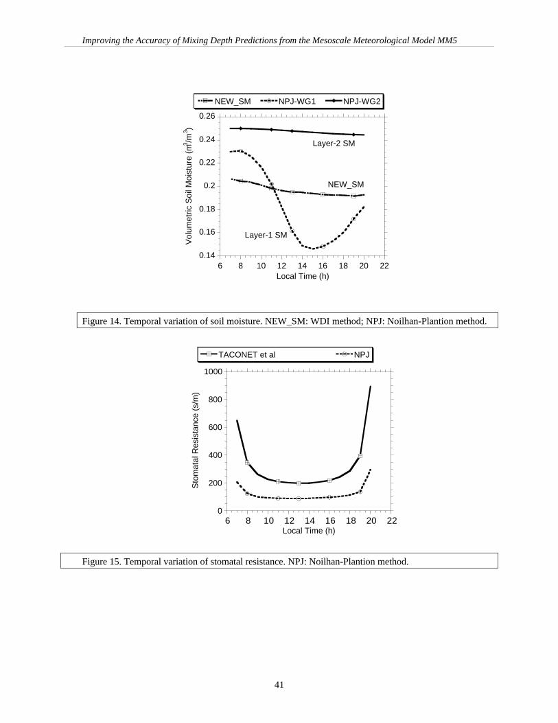
Improving the Accuracy of Mixing Depth Predictions from the Mesoscale Meteorological Model MM5
41
Figure 14. Temporal variation of soil moisture. NEW_SM: WDI method; NPJ: Noilhan-Plantion method.
Figure 15. Temporal variation of stomatal resistance. NPJ: Noilhan-Plantion method.
0.14
0.16
0.18
0.2
0.22
0.24
0.26
6 8 10 12 14 16 18 20 22
NEW_SM NPJ-WG1 NPJ-WG2
Vol
umet
ric S
oil M
oist
ure
(m3 /m
3 )
Local Time (h)
Layer-1 SM
Layer-2 SM
NEW_SM
0
200
400
600
800
1000
6 8 10 12 14 16 18 20 22
TACONET et al NPJ
Sto
mat
al R
esis
tanc
e (s
/m)
Local Time (h)

Improving the Accuracy of Mixing Depth Predictions from the Mesoscale Meteorological Model MM5
42
These preliminary results are very encouraging and showed some improvement in the model predictions.To illustrate the effects of uncertainty, we show in Figure 15 the estimated stomatal resistance (Rs) from twodifferent methods. This figure shows the temporal variation in Rs estimated by Teconet et al. (1986) and alsofrom NPJ. Both formulations are based on observational evidence for different geographic regions. The figureshows that the type of formulation chosen in a scheme can result in different outcomes, thus contributing touncertainty in the model estimates.
The method we have developed is designed to suppress the effects of uncertainty in the model estimationof various surface characteristics and processes. We are investigating how various formulations affect theestimation of WDI and hence the surface latent heat fluxes. We are currently conducting more simulations andsensitivity tests and will present the results at a later date.
3.3 Three-Dimensional Model Simulations
We now move to the three-dimensional model simulations we used to study the effects of various physicaland dynamical processes that control the depths of the mixed layers over central California.
Results from prior 3-D numerical investigations have indicated that many mesoscale meteorologicalmodels have difficulty simulating the very shallow mixing depths often found in the SJV. For example, asnoted in Section 1, Seaman et al. (1995) found that MM5 overpredicted afternoon mixing depths during two ofthe SJVAQS/AUSPEX cases by over 300 m (Figure 16). Although this result is not unique to MM5, theperformance of this model is of particular interest because it has been adopted by CARB as the primarymeteorological model for use in numerical air quality studies in California. Here we use MM5 (1) to study the3-D physical and dynamical causes of the shallow mixing depths in the SJV, and (2) to determine whatmodeling options might correct errors in prior MM5 simulations of the SJV mixed-layer depths.
In this section we first present a statement of work based on hypotheses concerning the shallow SJVmixing depths and the causes of previous 3-D modeling errors. Next, we give a brief overview of the 3-DMM5 version used in the study, followed by a discussion of the experimental methodology we used to testthese hypotheses. Finally, we describe the cases used in this study and the results obtained from the varioussimulations.
3.3.1 Hypotheses and Work Plan
We began the project by following the original Statement of Work (as documented in CARB Contract 96-319 with NCSC), which required us to examine the effects of large-scale dynamics and of model verticalresolution. As the work progressed, however, evaluation of the first few experiments suggested that additionalprocesses might be important for explaining the occurrences of low mixing depths over the SJV. We thereforeexpanded the Work Plan (at no additional cost) in order to include several new experiments designed toinvestigate the following issues: (1) the role of the initial structure of the marine atmospheric boundary layer(MABL), (2) the role of mesoscale circulations in the Sacramento Valley, (3) the influence of the type of

Improving the Accuracy of Mixing Depth Predictions from the Mesoscale Meteorological Model MM5
43
Figure 16. Mixed-layer depth (m) simulated by the MM5 at 0000 UTC 6 August 19990 in the 4-km domaindescribed by Seaman et al. (1995), Experiment 7 in this report. Contour interval is 200 m. Observations fromupper-air network (Fig. 17) are shown in italics.

Improving the Accuracy of Mixing Depth Predictions from the Mesoscale Meteorological Model MM5
44
boundary-layer turbulence parameterization used in the numerical model, and (4) the influence of four-dimensional data assimilation (FDDA) in the 36-km and 12-km domains. The goals of this 3-D modeling studywere to identify the most important physical processes that contribute to shallow SJV mixing depths and tolearn what numerical configurations and methods are necessary to successfully simulate those processes forthis region. The expanded list of hypotheses and experiments appear in Sections 3.3.1.1 through 3.3.1.6.
3.3.1.1 Experiment 1: Effects of Large-Scale Dynamics and Thermodynamics
We hypothesized that strengthening of the large-scale subsidence associated with the Northeast PacificRidge may be an important factor contributing to the shallow mixing depths observed in the SJV duringepisodes of poor air quality. The Pacific Ridge is a quasi-stationary climatological feature that is verypersistent during the summer months and is responsible for the well-known very strong inversion layer thatcaps the MABL off the coast of California (Ahrens 1993). When the ridge shifts toward the east, 500-mbheights rise over the interior of California. It is likely that this height rise is accompanied by increasedsynoptic-scale subsidence. The enhanced subsidence over California is hypothesized to contribute to broadadiabatic warming of the middle levels of the troposphere, thereby acting to prevent growth of the convectivelyunstable mixed layer and resulting in much-reduced ventilation of pollutants. This proposed mechanism maybe an active contributor to the shallow mixing depths in the area of interest, but the absence of such an extremeresponse over larger areas of the western United States strongly suggests that it cannot be the only process atwork.
In order for a numerical model to correctly simulate the changes in the ridge position and intensity, andthus the changes in the synoptic-scale subsidence, the outer model domain may need to include most or all ofthe region covered by the ridge. In earlier experiments reported by Seaman et al. (1995), the largest domaincovered an area of only 1944 x 1944 km, using a 36-km mesh. In Experiment 1, we test the hypothesis that thedynamics of the ridge may be important in simulating the subsidence over the SJV by adding an outer domainhaving a 108-km mesh and covering an area of 4860 x 6480 km.
3.3.1.2 Experiment 2: Effects of Vertical Resolution
In the original MM5 experiments performed by Seaman et al. (1995), the model was configured with 30layers in the vertical direction. While this is completely adequate for many purposes, it is hypothesized that theresolution used in the vicinity of the mixed-layer top was too coarse to adequately resolve weak cappinginversions in that study (layer thicknesses in the lowest kilometer had averaged ~120-150 m). Therefore,Experiment 2 explores the impact of resolution by increasing the number of layers to 62, which allows thelayer thickness to be only 40 m throughout the first kilometer above ground.
Better resolution not only allows more accurate treatment of the inversion layer in the SJV, it may alsoimprove the model's representation of the transverse-vertical valley breeze circulation. The mesoscale valleybreeze flowing up the sides of the mountain ranges flanking the SJV should induce a compensating subsidencecirculation over the valley. This mesoscale subsidence has the potential of reinforcing the synoptic-scalesubsidence, thus creating a regional maximum of downward motion and adiabatic heating over the SJV. It ishypothesized that superposition of the synoptic and mesoscale subsidences could explain the low mixingdepths found in this region.

Improving the Accuracy of Mixing Depth Predictions from the Mesoscale Meteorological Model MM5
45
3.3.1.3 Experiment 3: Effects Due to Initialization of the Marine AtmosphericBoundary Layer
In the summertime, air originating over the ocean in the MABL is advected inland through the SanFrancisco Bay area and other gaps in the Coast Range mountains. It then is modified by surface heating as ittravels southward into the SJV. As for most limited-area models, initialization of the MM5 variable fields inreal cases requires the use of background global meteorological fields. In these 1990 cases, we used fieldsanalyzed by the National Center for Environmental Predictions (NCEP). Over the ocean, where data are verysparse, these analyses rely mostly on short-range predictions generated by the most recent run of the NCEPglobal spectral model. Because the global model has relatively coarse vertical resolution and rather simpleboundary layer physics, it often does not accurately represent the thermal and moisture structure of the MABL.Therefore, we hypothesized that errors in the initial offshore MABL structure used in MM5 experiments couldadversely affect simulations of the inland modification of that marine air mass, and hence lead to errors in thepredicted SJV mixing depths.
To test this hypothesis, we corrected the thermal and moisture structure of the MM5's MABL at the initialtime, rather than allowing the MM5 to generate the MABL structure completely on its own. This was thoughtto be important because the physical processes that generate the shallow MABL act rather slowly, requiring~24-48 h to create a fully developed cold MABL. The logistics for this initialization are relativelystraightforward because Penn State already had developed a marine boundary layer initialization (MBLI)technique, based on climatology and case-specific observations, for use over the Eastern Pacific Ocean(Leidner et al. 2000).
3.3.1.4 Experiment 4: Effects of Mesoscale Circulations in the Sacramento Valley
One of the more important mesoscale circulations affecting airflow into the SJV is found in theSacramento River delta area, where the strong marine inflow through the San Francisco Bay diverges into twoseparate branches. One branch heads southeastward into the SJV, while the other branch turns north-northwestward up the Sacramento Valley. These two flows are forced by two thermally induced low-pressurecenters in the vicinities of Bakersfield and Redding, CA. We hypothesized that the accuracy of the model-simulated mass fluxes into these two valleys is dependent on the accuracy with which this split flow isrepresented by the model.
During the numerical experiments conducted by Seaman et al. (1995), the northern boundary of the 4-kmdomain was located just north of the city of Sacramento near 39.0 N (Figure 17). However, while this locationfor the 4-km boundary placed the Sacramento Delta within the 4-km domain, the location of the thermal lownear Redding was farther north in the 12-km domain. That means that an artificial (numerical) interface wasinterposed between the region of the flow divergence and one of the low-pressure centers driving thismesoscale circulation. Consequently, there was considerable opportunity for the introduction of model-inducederrors in the meteorological simulations.

Improving the Accuracy of Mixing Depth Predictions from the Mesoscale Meteorological Model MM5
46
Figure 17. Location of special upper-air measurement sites for SJVAQS/AUSPEX. Circles representradiosondes, triangle represent Doppler acoustic sounders, and boxes represent profilers. Data from these sitesare used for model verification only and are not assimilated in any of the experiments.

Improving the Accuracy of Mixing Depth Predictions from the Mesoscale Meteorological Model MM5
47
As a corollary to the hypothesis expressed above for this experiment, we believed that a consistent treatment ofthe split flow requires that both thermal lows be included within the 4-km domain. This is done easily byextending the domain northward above Redding to about 40.2 N, as shown in Figure 18.
3.3.1.5 Experiment 5: Effects of Boundary-Layer Turbulence Parameterization
In the original experiments of Seaman et al. (1995), the Blackadar nonlocal turbulence scheme was used torepresent boundary layer processes (Zhang and Anthes 1982). However, as seen in the 1-D model simulationsand tests by Shafran et al. (2000), the Blackadar-type schemes have a bias toward overpredicting the depth ofconvectively unstable boundary layers, even when capped by a moderate inversion (2-6 °C). Therefore, weanticipate that after replacing the Blackadar scheme by a 1.5-order parameterization that explicitly predictsturbulent kinetic energy (TKE) and produces very low bias for boundary-layer depths (Shafran et al. 2000)MM5 would be better able to simulate the shallow mixing depths found in the SJV.
3.3.1.6 Experiment 6: Effects Due to Four-Dimensional Data Assimilation Strategy
It is well known that data assimilation strategies can have important influences on both numerical modelsolutions and analyses. In the case of the FDDA strategy used by Seaman et al. (1995), the solutions on the 36-km and 12-km domains were nudged toward synoptic-scale analyses from the top of the domain at 100 mbdownward to the top of the boundary layer. However, that strategy may have had unexpected consequences. Inparticular, during the nocturnal period when only a shallow stable boundary layer exists, this FDDA strategycaused the layers in and above the vicinity of the daytime mixed-layer top (the interfacial layer) to be forcedtoward those synoptic-scale analyses. In the case of layers above the surface, the analyses are based on theNational Weather Service standard synoptic observations spaced at roughly 400 km. However, these data donot provide sufficient horizontal or vertical resolution to accurately represent the stable layer capping mixed-layer growth and none exist over the SJV. (The special SJVAQS/AUSPEX data are not used to createanalyses for model initialization or for analysis nudging.
We hypothesized that this FDDA strategy may have resulted in an unintended smoothing of any mesoscalemid-level stable layer that develops in MM5, thus weakening resistance to boundary-layer growth during thedaytime. The direct effect of this smoothing occurs on the 36-km and 12-km domains where the analysisnudging is performed. However, the 12-km solutions are used to provide lateral boundary conditions to the 4-km domain (which is the primary domain used to study SJV phenomena). Therefore, it is possible that the lossof accuracy in the 12-km domain due to the nudging strategy of Seaman et al. (1995) could have indirectlydegraded the accuracy of the 4-km solutions as the influence of the boundary conditions was advected throughthe domain during the model integrations.
Based on earlier FDDA work by Shafran et al. (2000), Experiment 6 is designed to test this hypothesis byremoving all analysis nudging below 1.5 km AGL (unless, of course, the boundary layer is deeper than1.5 km). This approach should prevent unintended weakening of any mid-level stable layer generated bymesoscale circulations or by other processes. No nudging toward

Improving the Accuracy of Mixing Depth Predictions from the Mesoscale Meteorological Model MM5
48
Figure 18. Terrain (m) for the large innermost 4-km mesh used in Exps. 1-4. Contour interval is 100 m. Heavyhorizontal line shows location of a cross section through Fresno. Dashed line makrs location of the smaller 4-km domain used in Epxs. 5-7 (see Table 1).

Improving the Accuracy of Mixing Depth Predictions from the Mesoscale Meteorological Model MM5
49
any of the special SJVAQS/AUSPEX observations is performed in this study. Furthermore, no analysisnudging is used on the 4-km domain, so that FDDA is felt on the innermost domain only through the lateralboundaries supplied from the 12-km grid. This approach is used so that the model's physical and dynamicalprocesses are free to develop mesoscale circulations on the 4-km inner mesh without imposing the influence ofany artificial forcing terms.
3.3.2 Model Description
The numerical model used in this study is the 3-D nonhydrostatic MM5 (Dudhia 1993, Grell et al. 1994).The MM5 is a nested-grid primitive-equation model written in the terrain-following nondimensionalizedpressure vertical coordinate (sigma). For efficiency, MM5 uses a split semi-implicit temporal integrationscheme. Prognostic equations predict the 3-D wind components (u, v, and w), temperature (T), water vapormixing ratio (qv), and the perturbation pressure (p'). The perturbation pressure is the departure from atemporally invariant reference-state pressure described by Dudhia (1993).
A surface energy budget equation predicts the ground temperature (Tg) and includes the effects ofinsolation, atmospheric path length, water vapor, cloud cover, and longwave radiation (Zhang and Anthes1982). Surface physical characteristics of albedo, roughness length, moisture availability, emissivity, andthermal inertia are defined as a function of land use for 14 categories via a look-up table. The land usedefinitions over California were made using a 1-km database supplied by the Desert Research Institute.Radiation flux divergence at each layer is calculated using a full column broadband two-stream scheme(Dudhia 1989). Additional model physics include explicit prognostic equations for mixing ratios of cloudwater/ice (qc) and rain/snow (qr), but without mixed-phase microphysics (Dudhia 1989). Subgrid deepconvection is parameterized using the scheme of Kain and Fritsch (1990).
Turbulent processes are represented in this study using either of two parameterizations. The first is a 1.5-order TKE-predicting scheme described by Shafran et al. (2000). The second is a Blackadar nonlocal-closurescheme (Zhang and Anthes 1982), which had been used in the experiments reported by Seaman et al. (1995).As mentioned earlier, Shafran et al. (2000) demonstrated that the 1.5-order TKE scheme produces lower biasesfor simulations of mixed-layer depth, so it is used in most of the experiments reported here.
3.3.3 Methodology
We conducted a series of seven experiments to learn how SJV mixing depths are influenced by thefollowing factors: synoptic-scale dynamics, vertical resolution, MABL initial conditions, mesoscalecirculations, boundary-layer physics, and FDDA. All experiments were performed for the four-day high-pollution episode that occurred from 2-6 August 1990 that was observed during the SJVAQS/AUSPEX. Theinitial and boundary conditions on the outermost model domain were specified from the NCEP global spectral-model analyses. Initial conditions for inner nested domains were obtained by interpolation, while the MM5solutions from the next coarser grid were used to provide the conditions at the lateral grid-interfaces. Table 1summarizes the experimental conditions.
Table 1. Experimental conditions for the MM5.
ExperNo. MBLI
No. ofDomains
Expanded4-km
Domain
FDDAbelow1.5 km
PBLType
No. ofLayers

Improving the Accuracy of Mixing Depth Predictions from the Mesoscale Meteorological Model MM5
50
1 Yes 4 Yes No TKE 62
2 Yes 4 Yes No TKE 32
3 No 4 Yes No TKE 32
4 No 3 Yes No TKE 32
5 No 3 No No TKE 32
6 No 3 No Yes TKE 32
7 No 3 No Yes BLKDR 32
All experiments used three model domains having mesh sizes of 36 km, 12 km, and 4 km, andExperiments 1-3 used a fourth 108-km domain of 46 x 61 points (Figure 19). The 36-km domain had 55 x 55points and the 12-km domain had 79 x 55 points. Two different sizes of 4-km domain were used in the study.The larger grid had 151 x 121 points and was used for Experiments 1-4; the terrain for these four experimentsis shown in Figure 18. A smaller 4-km grid of 118 x 100 points was used in Experiments 5-7, the area of whichis indicated by the dashed lines in Figure 18. This smaller 4-km domain included the entire SJV, but omittedthe upper Sacramento Valley to the north and had its western boundary closer to the coastline.
3.3.4 Case Description
The early August period of 1990 was fairly characteristic of the summertime climatology for Californiaand of conditions associated with high levels of ozone. At the beginning of the episode (1200 UTC 2 August),a 500-mb ridge lay off the California coast with a maximum height of 591 dam centered several hundredkilometers southwest of Oakland (Seaman et al. 1995). During the episode the height maximum graduallyintensified to 599 dam and shifted slowly northeastward over the western United States, until it reachedsouthwestern Idaho on 7 August 1990. The intensification of the ridge and its movement over land during theperiod of most severe air pollution (5-6 August) are consistent with increased synoptic-scale subsidence andwarming (temperatures rose about +3 °C at 500 dam over California-Nevada during the episode). However,since the subsidence rate in large anticyclones is only on the order of 1-5 cm s-1, there are no observations forvertical velocity. Therefore, a numerical model provides the best means of estimating the evolution ofsubsidence as the episode proceeds.
As is typical for summertime, cool marine boundary-layer air is advected onshore due to the pressuregradients induced by intense heating over the interior of California. This marine air is rapidly modified due tothe daytime surface sensible heat flux and eddy transport in the convectively unstable boundary layer.Normally, as marine boundary-layer air is heated, the mixed layer should grow in depth. In this region, theheating occurs rapidly as the column of marine air experiences advection, so it is appropriate to follow theeffects of the thermal

Improving the Accuracy of Mixing Depth Predictions from the Mesoscale Meteorological Model MM5
51
Figure 19. Mesoscale model nested domains showing the 108-km resolution outermost mesh. Boxes showlocations of nested 36-km, 12-km, and large 4-km domains.

Improving the Accuracy of Mixing Depth Predictions from the Mesoscale Meteorological Model MM5
52
modification in a Lagrangian reference frame. To demonstrate the effects of this air mass modification, weexamined observed thermal soundings obtained at five stations for a day during SJVAQS/ AUSPEX. Thesestations lie along a line running roughly east-northeast from Oakland, or approximately perpendicular to theCalifornia coastline and parallel to the mean wind direction in this area (for reference see Figure 17). We chosethe stations at Oakland (OAK), Livermore (LI2), Brentwood (BRE), Stockton (STO), and Pardee Reservoir(PAR) because they are more or less free from obvious terrain influences and are representative of soundingsthroughout the SJV.
We analyzed the depth of the convectively unstable mixed layer from the observed temperature profilesusing the following conventions. First, the average temperature of the two lowest levels in the sounding wascalculated. For convectively unstable boundary layers over land, this gave a representative temperature for theatmospheric surface layer. However, if the sounding showed that the surface layer was strongly superadiabatic,then we replaced the surface-layer temperature with the temperature at the top of the superadiabatic layer plus1.5 C. This averaged surface-layer parcel was then lifted dry adiabatically until it reached the point aloft whereit intersected the sounding. We found that this intersection generally coincided with the base of the stable layercapping the mixed layer, even if that stable layer was fairly weak. For our purposes, this level was defined asthe top of the mixed layer.
Figure 20 shows an example of temperature profiles observed at Oakland on August 5 as the high-ozoneepisode in the SJV was approaching its peak intensity. The soundings at 0400 and 1000 LST both show ashallow marine layer of about 290-300 m, capped by a very strong inversion of 15 °C, which is about normalfor this part of the California coast in summer. The marine-layer depth at this coastal station actually developsa minimum during the afternoons (not shown), when the sea breeze reaches its maximum intensity and causesnet horizontal divergence in the cool air at the shoreline. The horizontal divergence, in turn, causes theinversion base to fall. The continuous inflow of marine air during this flow pattern keeps the boundary layer atOakland rather cool and shallow throughout the diurnal cycle. Although there is no sounding available at thissite at 1600 LST on 5 August, examination of the days before and after suggest that the mixed-layer depth atOakland generally remained about 300 m at this time of day.
Meanwhile, Figure 21 shows temperature profiles on 5 August at Livermore, which is only about 35 kminland from Oakland. The temperature profiles from the nocturnal hours (0100 and 0400 LST) have very coolsurface temperatures capped by a strong inversion at about 300 m AGL, similar to those found in the coastalsoundings at Oakland. Thus, in the absence of surface sensible heating, the marine layer is advected this farinland at night with very little modification. However, examination of the soundings at 1000 and 1600 LSTreveals that the surface is heated rapidly during the daytime, reaching almost 36 °C by 1600 LST (0000 UTC 6August). Nevertheless, on this afternoon the depth of the mixed layer remains only ~370 m. Above the top ofthe mixed layer, the 1600 LST sounding at Livermore is only weakly stable for another 700 m, but that issufficient to prevent penetration by boundary-layer eddies. It should also be noted that the advective time scalefor marine air to travel from Oakland to Livermore, assuming a mean speed of only 5 m s-1, is about 2 h. Thisemphasizes how rapidly the shallow column of marine air undergoes heating as it travels to Livermore.

Improving the Accuracy of Mixing Depth Predictions from the Mesoscale Meteorological Model MM5
53
Figure 20. Observed temperature sounding © at Oakland on 5 August 1990. Times are given as localstandard time.

Improving the Accuracy of Mixing Depth Predictions from the Mesoscale Meteorological Model MM5
54
Figure 21. Observed temperature soundings (C) at Livermore on 5 August 1990. Times are given as localstandard time.

Improving the Accuracy of Mixing Depth Predictions from the Mesoscale Meteorological Model MM5
55
From the observations shown for Oakland and Livermore, it seems easy to assume that a much deeper mixedlayer must lie only a short distance farther inland, where the effects of surface sensible heating would haveacted longer on the rapidly modifying marine air. The next available inland sounding site is at Brentwood,which lies about 55 km east of Oakland (Figure 22). Again, cool temperatures in the shallow nocturnalboundary layer rise rapidly following sunrise. By 1600 LST, the surface temperature has climbed to amaximum of 39.5 °C. However, despite this very high temperature, the mixed-layer depth at this time is only~500 m AGL. Even though the capping inversion is only about 1 °C, notice that the air above that level isclearly stable. Thus, despite the hot surface temperature, the afternoon boundary layer remains shallow becausethe air only a few hundred meters above is potentially even hotter.
In the center of the northern SJV about 85 km from Oakland lies Stockton, for which the temperatureprofiles on 5 August are shown in Figure 23. The same cool nocturnal low-level temperatures also are foundlying below a strong nocturnal inversion at this site. Again, as daytime temperatures reach their maximum of35.5 °C at 1600 LST, the boundary layer is capped by still warmer air farther aloft. The mixed-layer depth atthis time is only 390 m and the inversion layer is the strongest found at any of the four inland stationsexamined.
Lastly, the temperature profiles for 5 August for the easternmost site at Pardee Reservoir, 135 km fromOakland, are shown in Figure 24. This site lies in the western foothills of the Sierra Nevada Mountains ~350 mabove sea level. Because of the distance from the coast and the elevation, there is no indication of the verystrong nocturnal inversion noted at Stockton and westward (see 0100 and 0400 profiles), and minimum surfacetemperatures before sunrise remain above 21 °C. By 1600 LST (0000 UTC 6 August), however, the surfacetemperature at Pardee Reservoir has reached a maximum of 40 °C. At this site the afternoon mixed-layer depthis 780 m AGL, with a 2-3 °C capping inversion.
3.3.5 Results of Experiments
3.3.5.1 Numerical Factors Influencing Mixing-Depth Simulations
Our examination of the MM5 model results began with an evaluation of Experiment 1. Notice from Table1 that Experiment 1 was designed to include all of the factors that were hypothesized to make a positivecontribution toward accurate simulation of the shallow mixed layers found in the SJV (also see Section 2).Therefore, the goal of Experiment 1 was to learn whether the mesoscale model, with improved physics,enhanced grid configurations, and better initialization and FDDA, could more accurately simulate the depth ofthe mixed layer in the SJV during episodes having poor air quality. If this experiment were successful, thencomparisons with the other six experiments would allow us to identify the most important factors contributingto this result.
First, we examine the influence of the MBLI during the 12-h dynamic initialization phase of Experiment 1using Figures 25 and 26. These figures show a west-east cross section of potential temperature,θ , on the 4-kmdomain. The section is located along Bakersfield. In Figure 25, the cross section shows the θ -field at 1200UTC 2 August 1990, at the beginning of the 12-h dynamic.
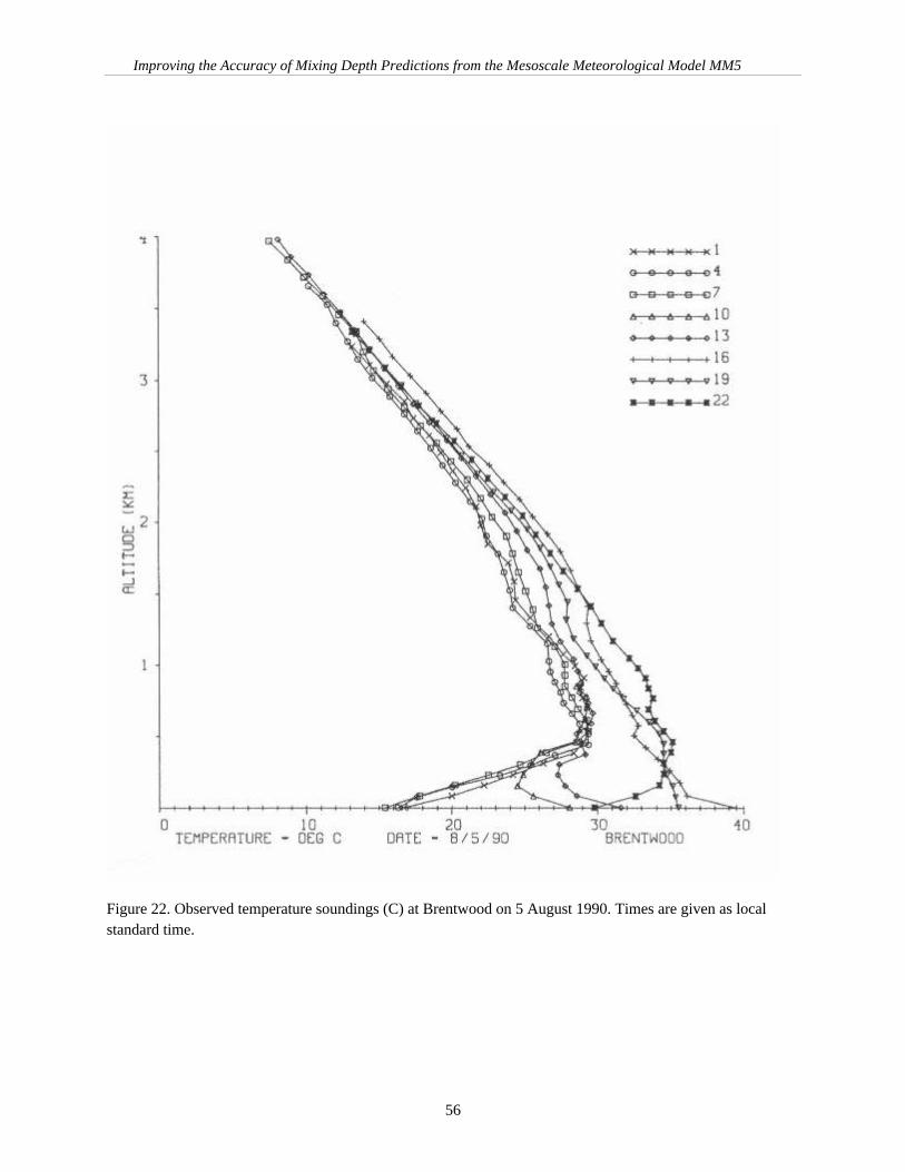
Improving the Accuracy of Mixing Depth Predictions from the Mesoscale Meteorological Model MM5
56
Figure 22. Observed temperature soundings (C) at Brentwood on 5 August 1990. Times are given as localstandard time.

Improving the Accuracy of Mixing Depth Predictions from the Mesoscale Meteorological Model MM5
57
Figure 23. Observed temperature soundings (C) at Stockton on 5 August 1990. Times are given as localstandard time.

Improving the Accuracy of Mixing Depth Predictions from the Mesoscale Meteorological Model MM5
58
Figure 24. Observed temperature soundings (C) at Pardee Reservoir on 5 August 1990. Times are given aslocal standard time.

Improving the Accuracy of Mixing Depth Predictions from the Mesoscale Meteorological Model MM5
59
Figure 25. Vertical cross section of the MM5 initial potential temperature (K) below 700 mb for Exp. 1 on the4-km domain at 1200 UTC 2 August 1990, before application of the MBLI dynamic initialization. Location isalong the Bakersfiled. Isentrope interval is 1 K.

Improving the Accuracy of Mixing Depth Predictions from the Mesoscale Meteorological Model MM5
60
Figure 26. Vertical cross section of the MM5 potential temperature (K) below 700 mb for Exp. 1 on the 4-kmdomain at 0000 UTC 3 August 1990, after the 12-h application of the MBLI dynamic initialization. Locationof the cross section is shown in Figure 18. Isentrope interval is 1 K.

Improving the Accuracy of Mixing Depth Predictions from the Mesoscale Meteorological Model MM5
61
initialization period over which the MBLI is applied. Notice that it reveals a shallow stable MABL confinedbelow 1000 mb over the ocean (left side of the figure). By the end of the 12-h MBLI period, Figure 26indicates that the MABL has become approximately moist adiabatic and is far less stable. As noted in Section2, this more realistic MABL structure may contribute to the shallow inland mixed-layer depths, butdetermination of that contribution must await examination of the other sensitivity experiments. Notice thatFigure 26 also shows that the afternoon mixed-layer depth at 0000 UTC, 3 August (1600 LST) has grown to~1125 m in the center of the SJV. Most of the remaining model evaluations concentrate on the second andthird days following the MBLI period (0000 UTC 5-6 August), when the high-ozone episode was buildingtoward its maximum intensity and mixed-layer depths over land were becoming steadily lower.
Figures 27 and 28 show that, 72 h after the end of the dynamic initialization, the horizontal solutions fortemperature and wind over the Sacramento Valley and SJV are realistic for this case. In Figure 27, the surface-layer temperature at 0000 UTC 6 August (approximately the time of the peak of the high-ozone episode)shows maximums of 35 °C in the SJV and 41 °C in the Sacramento Valley. Figure 28 indicates that the modelreproduces the divergent wind flow commonly observed east of San Francisco Bay and the 2-5m s-1 divergentnorthwesterly low-level winds in the SJV. The latter is the typical response caused by superposition of twotypes of mesoscale forcing: (1) northwesterly mean flow in the SJV due to the thermal low-pressure centernear Bakersfield, and (2) low-level divergence caused by two independent valley breezes induced by theheated mountain ranges flanking the valley. Thus, these figures indicate that the basic wind and temperaturepatterns are consistent with observations and with results of previous modeling studies (e.g., Seaman et al.1995).
Next, Figure 29 shows the horizontal distribution of mixed-layer depth simulated by MM5 in Experiment1 at 0000 UTC 6 August (1600 LST 5 August) 1990. This figure can be compared to the observations andMM5 results from Experiment 7 performed by Seaman et al. (1995), which are shown in Figure 16. It isapparent upon examination of Figures 16 and 29 that the mixed-layer depths simulated over the SJV inExperiment 1 are generally lower than in Experiment 7. However, the complexity of the pattern makes it verydifficult to draw objective conclusions. Therefore, we performed a statistical analysis of the mean error (ME)and mean absolute error (MAE), as defined by Stauffer and Seaman (1990), on the simulated mixed-layerdepths for the experiments (Table 2).
Table 2 shows that the ME (a measure of the bias) in Experiment 1 is only 56 m, compared to 304 m inExperiment 7. The large positive ME in Experiment 7, which implies that the MM5-simulated meteorologycontributes to significant overdilution of pollutants when used to drive an air chemistry model, was the primarymotivation at CARB to conduct the present study.

Improving the Accuracy of Mixing Depth Predictions from the Mesoscale Meteorological Model MM5
62
Figure 27. MM5-simulated surface-layer temperature (C) at 10 m AGL for Exp. 1 on the large 4-kmdomain at 0000 UTC 6 August 1990 (72 h after the MBLI period). Isotherm interval is 2 C.

Improving the Accuracy of Mixing Depth Predictions from the Mesoscale Meteorological Model MM5
63
Figure 28. MM5-simulated surface-layer winds (m/s) at 10 m AGL for Exp. 1 on the large 4-km domain at0000 UTC 6 August 1990 (72 h after the MBLI period). Isotach interval is 5 m/s.

Improving the Accuracy of Mixing Depth Predictions from the Mesoscale Meteorological Model MM5
64
Figure 29. Mixed-layer depth (m) simulated by the MM5 at 0000 UTC 6 August 1990 in the 4-km domainfor Exp. 1. Contour interval is 200 m.

Improving the Accuracy of Mixing Depth Predictions from the Mesoscale Meteorological Model MM5
65
Table 2. Errors in model-predicted mixed-layer depths (model minus observations) for upper-air sites in theSJV at 0000 UTC 6 August (1600 LST 5 August) 1990.
Station ID
Obs'dMixed-LayerDepth (m)
Exp. 1
Error (m)
Exp. 2
Error (m)
Exp. 3
Error (m)
Exp. 4
Error (m)
Exp. 5a
Error (m)
Exp. 6
Error (m)
Exp. 7
Error (m)
PTB 140 +30 +10 +0 +10 +20 +80 OAK 290 -90 -140 -110 -110 -100 -75 LI2 370 +20 +0 +0 -170 +10 +200 BRE 500 +120 -100 -50 +450 +110 +320 ALT 590 -190 -220 -210 -210 -15 +210 STO 390 +210 +60 +190 -290 +240 +490 PAR 780 -190 -130 -100 -680 +145 +30 WOO 440 +60 +60 +50 -290 +200 +410 ANG 400 +120 +30 +200 -220 +50 +410 MRG 340 +60 +60 +40 +40 +80 +270 CRO 370 +350 +210 +280 +190 +380 +530 PA2 220 +355 +180 -20 +600 +460 +580 ORO 560 -60 +50 +300 -380 +190 +415 MAR 780 +200 -400 -240 -130 -55 +90 MAD 800 -130 -390 -580 -200 +80 +200 KIN 170 +210 +150 +70 +100 +215 +430 THR 410 +230 +5 -30 +0 +300 +530 TUL 630 +200 -50 -60 -190 +210 +380 VIS 310 +340 -120 -80 +270 +470 +920 DEV 680 -105 +70 -80 -600 -40 +90 DEL 720 +90 -220 -410 -130 +50 +190 BUT 850 -190 -250 -540 -460 -250 -70ME (m) -- +56 -52 -63 -109 +125 +304MAE (m) -- 161 132 165 260 167 317
a The results of Experiment 5 had been lost by the time of this writing. The experiment is being performed asecond time in order to obtain the missing statistical data and complete the table.b ME = mean error, MAE = mean absolute error.
Station ID’s are listed in geographical order from north to south.

Improving the Accuracy of Mixing Depth Predictions from the Mesoscale Meteorological Model MM5
66
The reduction of this bias by nearly 82% in Experiment 1 is a very significant improvement in model skill. Atthe same time, the MAE (a measure of the average size of the individual errors) in Experiment 7 has beenreduced by half in Experiment 1, from 317 m to 161 m. Considering that the model's vertical resolution is 40 mand the accuracy with which the observations can be used to estimate mixed-layer depth is imperfect, theseresults appear to be very reasonable.
Further examination of the statistics in Table 2 reveals some very important information. Experiment 2 isidentical to Experiment 1 except that the vertical resolution is reduced in the first kilometer so that the totalnumber of layers is 32 instead of 62 (Table 1). However, despite the loss of vertical resolution, Experiment 2actually produced slightly more accurate results than Experiment1 and had the lowest errors of any of theexperiments in the study (ME = -52 m and MAE = 132 m). Also, the sign of the ME changed from positive tonegative, meaning that Experiment 2 somewhat underestimated the depth of the mixed layer. Although theimprovement in skill found for Experiment 2 compared to Experiment 1 is probably not statisticallysignificant, this result is important nevertheless because it means that very high vertical resolution in the modelis unnecessary to obtain accurate simulations of the SJV boundary -layer structurre and the related mesoscalecirculations.
Next, comparison of Experiments 2 and 3 allowed isolation of the model's sensitivity to the MBLI over thePacific Ocean. Table 2 shows that the removal of the MBLI in Experiment 3 caused the ME and MAE tobecome slightly degraded, but the amount is so small that this technique is probably unnecessary for most airquality studies in the SJV. This result is consistent with the observational evidence presented in Figures 20-24,which demonstrated that the cool marine air is modified very rapidly as it is advected onshore, so that themarine layer retains little of its original structure in the daytime once it reaches the SJV. However, comparisonof the statistics from Experiments 3 and 4 reveals that there is a significant loss of accuracy when the 108-kmoutermost domain is removed. In fact, the ME in Experiment 4 is –109 m, meaning that for this case the modelsignificantly underestimated the mixed-layer depth across the 4-km grid when the large-scale dynamics of theEast Pacific Ridge were not contained fully within the outermost 108-km domain. The implication is that thesubsidence induced by the large-scale dynamics was inaccurate (possibly overestimated) in this experiment.While an impact due to the size of the outer domain was not unexpected, it is surprising that its exclusioncaused such a serious underestimate of this key variable. It cannot be assumed that the sign of the error wouldbe the same in all cases, but it appears that use of a larger outer domain can be a valuable factor to ensure thatthe dynamics of the anticyclone are simulated well and are consistent with other scales of motion.
Comparison of Experiments 4 and 6 reveals a large shift of the ME from negative (-109 m) to positive(+125 m). Although results of Experiment 5 have been lost (they are being re-created), it is very likely thatmost of this large change in the ME can be traced to the inclusion of the FDDA strategy in Experiment 6. Thatis, when the analysis-nudging performed on the 12-km grid (and on the coarser domains) was allowed to pushthe model solutions toward the synoptic-scale analyses below 1500 m AGL (above the mixed layer) inExperiment 6, the mesoscale influences on the capping inversion above the boundary layer was weakened.Subsequently, horizontal advection carried the degraded (smoothed) mid-level thermal field into the 4-kmdomain, where it presented less inhibition to the growth of the SJV convectively unstable daytime mixed layerin this experiment.
Finally, comparison of statistics from Experiments 6 and 7 demonstrates the influence of changing themodel's turbulence representation from the 1.5-order TKE scheme to the Blackadar nonlocal-closure scheme.Consistent with the results of Shafran et al. (2000), use of the Blackadar scheme in Experiment 7 caused a very

Improving the Accuracy of Mixing Depth Predictions from the Mesoscale Meteorological Model MM5
67
large increase in the positive bias for the mixed-layer depth (from +125 m to +304 m). In the Midwest U.S.cases studied by Shafran et al., however, a moderate subsidence inversion of 2-6 °C capped the convectivelyunstable boundary layer and may have helped reduce the magnitude of mixing-depth errors that could develop.In the August 1990 SJV case, on the other hand, Figures 20-24 showed that the capping inversion was oftenrather weak in the afternoons, so that this case presents a more difficult prediction problem for both turbulenceschemes. In this challenging situation, the 1.5-order TKE scheme clearly performed rather well for this keyvariable.
3.3.5.2 Physical Processes Leading to Shallow Mixed-Layer Depths
Having determined the numerical requirements necessary for a mesoscale model such as MM5 toaccurately simulate the occurrence of shallow mixing depths in the SJV, we next considered what might be thephysical causes of those conditions. Examination of the 62-layer Experiment 1 provides an excellentopportunity to identify the dominant physical processes. First, Figure 30 shows the TKE in the cross sectionthrough Fresno at 0000 UTC 5 August 1990 (1600 LST 4 August), during the period when the upper-levelridge is moving onshore over California. As anticipated, the TKE is small over the ocean, where the upwellingof cool water along the coast prevents strong surface sensible heat fluxes. Over land, however, the TKE showsthe approximate depth of the convectively unstable mixed layer. The maximum TKE in the SJV is about2.7 J kg-1 at this time. Notice that the large TKE values extend well above the inland Coast Range, wherevalley breezes directed up the east and west slopes converge and develop a strong buoyant plume of upwardvertical velocities. It is not uncommon to find vertical motions reaching +1-2 m s-1 in this convergence zoneover the mountain peaks (not shown). At the same time, Figure 31 shows the potential temperature, θ, alongthe cross section, with the mixed-layer top indicated as a heavy dashed line. The depth of the mixed layer inthe SJV at 0000 UTC 5 August ranges from about 700 m to 1000 m.
Over the following 24 h, in response to continued subsidence aloft, the isentropic surfaces and the mixed-layer depths are forced downward. First, Figure 32 shows that the TKE is very nearly as intense in the SJV at0000 UTC 6 August (1600 LST 5 August) as on the previous day, with a maximum of 2.6 J kg-1. The strongturbulence is consistent with the hot surface temperatures that are persistent during the episode. However,Figure 33 reveals that the mixed-layer depth in the cross section over the SJV at this time is as low as 450 m.
To better understand this change, compare the height of the 316 K and 312 K isentropic surfaces in thecross sections on these two afternoons (Figures 31 and 33). Over the ocean at the western boundary of thecross section (~200 km offshore), where mesoscale circulations associated with the California orographyshould be negligible, the 316 K isentrope is at virtually

Improving the Accuracy of Mixing Depth Predictions from the Mesoscale Meteorological Model MM5
68
Figure 30. Vertical corss section of MM5 turbulent kinetic energy (J/kg) below 700 mb in Exp. 1 on the 4-kmdomain at 0000 UTC 5 August 1990 (48 h after end of dynamic initialization). Location of the cross section isshown in Figure 18. Contour interval is 0.5 J/kg.

Improving the Accuracy of Mixing Depth Predictions from the Mesoscale Meteorological Model MM5
69
Figure 31. Vertical cross section of the MM5 potential temperature (K) below 700 mb in Exp.1 on the 4-kmdomain at 0000 UTC 5 August 1990 (48 h after the end of dynamic initialization). Location of the crosssection is shown in Figure 18. Isentrope interval is 1 K. Dashed line indicates the top of the mixed layer.

Improving the Accuracy of Mixing Depth Predictions from the Mesoscale Meteorological Model MM5
70
Figure 32. Vertical cross section of MM5 turbulent kinetic energy (J/kg) below 700 mb in Exp. 1 on the 4-kmdomain at 0000 UTC 6 August 1990 (72 h after dynamic initialization). Location of the cross section is shownin Figure 18. Contour interval is 0.5 J/kg.

Improving the Accuracy of Mixing Depth Predictions from the Mesoscale Meteorological Model MM5
71
Figure 33. Vertical cross section of the MM5 potential temperature (K) below 700 mb in the Exp. 1 on the 4-km domain at 0000 UTC 6 August 1990 (72 h after end of dynamic initialization). Location of the crosssection is shown in Figure 18. Isentrope interval is 1 K. Dashed line indicates the top of the mixed-layer.

Improving the Accuracy of Mixing Depth Predictions from the Mesoscale Meteorological Model MM5
72
the same height on both days. Meanwhile the 312 K and 308 K isotherms between 900 and 800 mb havesubsided about 435-440 m (see Table 3). The subsidence experienced in this area should be due almost entirelyto the 3-D dynamics in the East Pacific Ridge. The 24-h local adiabatic warming in the layer is equivalent to adaily mean subsidence of about -0.51 cm s-1.
Table 3. Change of heights of MM5-simulated isentropic surfaces (m) over the Pacific Ocean and over the SJVbetween 0000 UTC 5 and 6 August 1990 in Experiment 1. Values are calculated along the cross section shown
in Figure 18. Potential Temperature (K) 200 km West of CA Coast San Joaquin Valley
316 +50 -565
312 -435 -730
308 -440 -380
304 -330 ---
Notice in the figures that the isentropic surfaces slope downward from west to east (toward land). Table 3also indicates that the subsidence in the cross section over the SJV is maximized for the 312 K surface, whichis forced downward by 730 m over the 24-h period; this is equivalent to a daily mean rate of -0.85 cm s-1 overthe valley. The stronger downward motion, compared to the oceanic region, represents the subsidence forcedby the return branch of the mesoscale valley breeze circulation. Figure 33 suggests that the subsidencecomponent due to the valley breeze is most intense in the central and eastern portions of the SJV, where theisentropic surfaces have dropped most rapidly. Of course, the mesoscale-induced subsidence should reach amaximum in the late afternoon when the upslope flow along the flanks of the mountain ranges is most intense,and then it should disappear at night. Thus, the mean mesoscale contribution over the valley (about -0.35 cm s-
1) must substantially underestimate the total rate during the afternoon. Because the mesoscale subsidenceshould be maximized over the SJV at about the same time as the daily maximum in surface heating, thecombined subsidence-induced adiabatic heating aloft (synoptic plus mesoscale) should contribute significantlyto raising temperatures directly above the convective boundary layer, thereby resulting in the especially lowmixing depths in the valley.
Finally, Figure 34 shows the isentropic cross section from Experiment 6 at 0000 UTC 6 August (sametime as in Figure 33). Recall that Experiment 6 does not include the large outermost domain (108-km mesh) orthe large 4-km mesh and does not remove the analysis-nudging FDDA from the region below 1.5 km AGL(see Table 1). The sensitivity evaluation suggested that this set of conditions in Experiment 6 is less suitablefor predicting shallow mixed-layer depths in the SJV. Figure 34 provides additional insight into this conclusion. In particular note that the 312 K isentropic surface in Experiment 6 does not slope downward from the oceantoward the SJV. This suggests that the mesoscale valley breeze is ineffective or has been neutralized in its roleof reinforcing the synoptic-scale subsidence. However, examination of the model results confirms that thevalley breeze in Experiment 6 develops in a realistic manner (not shown). Therefore, the most reasonableexplanation for the result shown in

Improving the Accuracy of Mixing Depth Predictions from the Mesoscale Meteorological Model MM5
73
Figure 34. Vertical cross section of the MM5 potential temperature (K) below 700 mb in Exp. 6 on the 4-kmdomain at 0000 UTC 6 August (72 h after end of dynamic initialization). Location of the cross section isshown in Figure 18. Isentrope interval is 1 K. Dashed line indicates the top of the mixed-layer.

Improving the Accuracy of Mixing Depth Predictions from the Mesoscale Meteorological Model MM5
74
Figure 33 is that the poor analysis-nudging strategy used in this experiment acts to damp out the cumulativemultiday impact of the mesoscale mountain-valley circulation on temperatures aloft in this region, ashypothesized in Section 3.3.1.6.
4. Summary
We followed two modeling strategies to determine reasons for the overestimation ofmixed-layer depths by the mesoscale model MM5 over the central California region. In the firststrategy, we performed sensitivity studies to understand the nature of some of the ABL errors anddeveloped new techniques to improve the ABL simulation, using a 1-D model. When a simple landsurface parameterization was used, simulation results for the Buttonwillow and FIFE sites indicated that achange of soil moisture availability by a factor of two led to large changes in simulated temperatures andmixing depths. Use of different mixed-layer formulations led to only minor differences between thesimulations. However, the TKE-ε scheme performed better than the ACM-BKT scheme in predicting thesurface features, as well as the ABL depth. Simulation results obtained by including a specified warming torepresent the 3-D thermodynamics, due to synoptic–scale subsidence, also showed variability, depending onthe type of mixed-layer schemes used in the simulations. Moreover, simulation results indicated that twodifferent diagnostic methods of estimating the boundary layer depth yielded similar results in simulating thestructures of the boundary layer. All these experiments indicated the presence of errors, with no assurance thata particular set of formulations can consistently provide accurate ABL structures.
Our new formulation to perform consistent adjustment of ground temperature, along with theassimilation of temperature and water vapor mixing ratio in the surface layer, mixed layer, andfree atmosphere, led to very significant improvements in the simulated boundary layer depth andits structures. These results indicated that assimilation of the surface-layer data is possible whenground temperature is adjusted to reflect the changes in the surface-layer thermodynamic fieldsdue to the data assimilation. Thus, we have shown that assimilation of surface temperatureobservations can be used successfully to adjust for uncertainties in surface characteristics, such assoil moisture specifications and inaccuracies in boundary layer parameterizations. This result hasfavorable implications for a number of data assimilation applications, including the developmentof improved meteorological conditions for air pollution modeling and meteorological analysis.
Another component of improvements in the model formulations is the proper estimation ofsurface latent heat fluxes, which control the mixed-layer depths. Our new formulation introducesvegetative effects in the equation that is being used in MM5 for estimating surface latent heatfluxes. This formulation uses many surface and vegetation parameters, as other sophisticatedland surface schemes do. But the new formulation takes a diagnostic approach, providing twoadvantages over prognostic approaches; the diagnostic approach (1) is computationallyinexpensive, and (2) controls or limits uncertainty present in the input data depicting surface andvegetation characteristics. Preliminary results obtained from the 1-D model simulationsindicated very good improvement in the boundary layer predictions using this new methodology.Further research is in progress.
In the second modeling strategy, we performed several numerical simulations, using differentconfigurations of MM5. Our first step was to determine the numerical conditions that allow

Improving the Accuracy of Mixing Depth Predictions from the Mesoscale Meteorological Model MM5
75
accurate simulation of the low mixed-layer depths in the SJV. The following are the mostimportant findings of the numerical sensitivity experiments:
• No significant difference in skill was found when the number of layers was increased from 32to 62 layers (higher resolution in the lowest km). Therefore, we conclude that the lessexpensive model configuration with 32 layers is quite adequate to generate accuratesimulations of the mixed-layer depth in the SJV.
• Use of an outer domain large enough to include most of the East Pacific Ridge is valuable forensuring that the dynamics of the anticyclone are simulated well and are consistent with otherscales of motion influencing the model solutions in the SJV.
• Removal of analysis nudging in the region below 1.5 km AGL on the coarser domainsimproved the simulations of mixed-layer depth on the 4-km grid (even though that domaindid not directly use any FDDA).
• The 1.5-order TKE-predicting turbulence scheme (Shafran et al. 2000) provided much moreaccurate simulations of mixed-layer depth than were possible when using the Blackadarnonlocal-closure scheme (Zhang and Anthes 1982).
The second step was to determine the physical and dynamical processes responsible for theunusually shallow boundary-layer heights found in the SJV during episodes of poor air quality.The following are the most important conclusions deduced from the sensitivity experimentresults:
• Widespread subsidence is induced by the synoptic-scale East Pacific Ridge and acts acrossthe entire 4-km domain, especially when the ridge builds eastward over land as the 2-6August 1990 episode proceeds. This synoptic-scale subsidence averages about -0.5 cm s-1
and acts continuously throughout the diurnal cycle. While it is an important factor producingadiabatic heating in the middle troposphere, this alone cannot explain the shallow mixingdepths in the SJV. Otherwise, similar shallow mixing depths would be found in nearbystrongly heated inland regions of the western United States during the same episodes.
• Strong surface sensible-heat fluxes lead to rapid modification of cool marine air as it isadvected inland by the regional scale pressure gradient. This heating causes surface potentialtemperatures to approach those above the capping inversion within just a few hours and overdistances of less than 100 km from the coast. Therefore, the shallow SJV mixing depthscannot be explained as a remnant of the marine atmospheric boundary layer.
• Synoptic-scale subsidence is reinforced over the SJV by the return branch of the mesoscaleupslope valley breeze. The induced mesoscale subsidence produces enhanced adiabaticwarming in the region above the convectively unstable boundary layer over land. Thismesoscale subsidence has a daily average of about -0.35 cm s-1 on 5-6 August 1990.However, since the valley breeze is driven by the diurnal heating cycle, it should beconsiderably stronger during the afternoon hours, thereby contributing to especially lowmixing depths at the time of maximum daily heating over the SJV.

Improving the Accuracy of Mixing Depth Predictions from the Mesoscale Meteorological Model MM5
76
• Since very high concentrations of ozone do not occur every day during the summer, it islikely that the mixed-layer depths in the SJV become especially shallow primarily when thesynoptic-scale and mesoscale subsidence mechanisms both exceed average values, as whenthe East Pacific Ridge shifts onshore.
5. Future Research
To further improve boundary layer predictions over the central California region, particularlyto benefit air pollution modeling studies, it is highly desirable that the new formulations wedeveloped in this study be implemented and tested rigorously in MM5. Because the 1-D modelresults were very encouraging, we anticipate that the implementation of these new formulationswill lead to better predictions of mixed-layer depths.

Improving the Accuracy of Mixing Depth Predictions from the Mesoscale Meteorological Model MM5
77
References
Ahrens, C.D., 1993: Essentials of Meteorology. West Publishing Co., 437 pp.
Alapaty, K., D.T. Olerud, K. Schere and A.F. Hanna, 1995: Sensitivity of Regional Oxidant Model Predictionsto Diagnostic and Prognostic Meteorological Fields. J. Appl. Meteor., 34, 1787-1801.
Alapaty, K., S. Raman, and D.S. Niyogi, 1997a: Uncertainty in the specification of surface characteristics: Acase study of prediction errors in the boundary layer. Bound.-Layer Meteor., 82, 473-500.
Alapaty, K., J.E. Pleim, S. Raman, D.S. Niyogi, and D.W. Byun, 1997b: Simulation of atmospheric boundarylayer processes using local- and nonlocal-closure schemes. J. Appl. Meteorol., 36, 214-233.
Alapaty, K., and R. Mathur, 1998: Effects of atmospheric boundary layer mixing representations on verticaldistribution of passive and reactive tracers. Meteorol. and Atmos. Phy., 69, 101-118.
Alapaty, K., and D.S. Niyogi, 1999: A Study to Improve the Existing MM5 Land-Surface Scheme usingStatistical Indices. The Ninth PSU/NCAR Mesoscale Model Users’ Workshop, pp 12, 23-25 June 1999,Boulder, Colorado, USA.
Anthes, R.A., E.-Y. Hsie, and Y.-H. Kuo, 1987: Description of the Penn State/NCAR Mesoscale ModelVersion 4 (MM4). NCAR Tech. Note, NCAR/TN-282+STR, 66 pp.
Blackadar, A.K, 1976: Modeling the nocturnal boundary layer. Preprints, Third Symposium on AtmosphericTurbulence, Diffusion and Air Quality, Raleigh, Amer. Meteor. Soc., 46-49.
Blackadar, A.K., 1979: Modeling pollutant transfer during daytime convection. Preprints, 4th Symposium onTurbulence, Diffusion and Air Pollution, Reno, Amer. Meteor., Soc., 443-447.
Blumenthal, D.L., et al.1993: Field program plan for the San Joaquin Valley air quality study (SJVAQS) andthe atmospheric utility signatures, predictions, and experiments program. [Available from The Valley AirPollution Study Agency, Sacramento, CA.]
Businger, J.A., J.C. Wyngaard, Y. Izumi and E.F. Bradley, 1971: Flux-profile relationship in the atmosphericsurface layer. J. Atmos. Sci., 28, 181-189.
Carlson, T.N., and F.E. Boland, 1978: Analysis of urban-rural canopy using a surface heat flux/temperaturemodel. J. Appl. Meteor., 17, 998-1013.
Chang, J.S., R.A. Brost, I.S.A. Isaken, S. Madronich, P. Middleton, W.R. Stockwell, and C.J. Walcek, 1987:A three-dimensional Eulerian acid deposition model: Physical concepts and formulation. J. Geophys. Res.,92, 14681-14700.
Deardorff, J., 1978: Efficient prediction of ground surface temperature and moisture, with inclusion of a layerof vegetation. J. Geophys. Res., 83, 1889-1903.
Detering, H.W., and D. Etling, 1985: Application of E-ε turbulence model to the atmospheric boundary layer.Bound.-Layer Meteor., 33, 113-133.
Dickinson, R.E., Kennedy, P.J., Henderson-Sellers, A., 1993: Biosphere-Atmosphere Transfer Scheme(BATS) - Version 1E as coupled to the NCAR Community Climate Model. NCAR Tech. NoteNCAR/TN-387+STR, National Center for Atmospheric Research, Boulder, CO, 72 pp.
Dudhia, J., 1989: Numerical study of convection observed during the winter monsoon experiment using amesoscale two-dimensional model. J. Atmos. Sci., 46, 3077-3107.
Dudhia, J., 1993: A nonhydrostatic version of the Penn State-NCAR Mesoscale Model: Validation tests andsimulation of an Atlantic cyclone and cold front. Mon. Wea. Rev., 121, 1493-1513.
Grell G. A., J. Dudhia, and D. R. Stuaffer, 1994: A description of the fifth – generation Penn State / NCARmesoscale model (MM5), NCAR TN – 398+STR, 138 pp.

Improving the Accuracy of Mixing Depth Predictions from the Mesoscale Meteorological Model MM5
78
Hass, H., H.J. Jacobs, M. Memmesheimer, A. Ebel, and J.S. Chang, 1991: Simulation of a wet deposition casein Europe using the European Acid Deposition Model (EURAD). In Air Pollution Modeling and itsApplications VIII, Plenum Press, New York, 205-213.
Holtslag, A.A.A., E.I.F. de Bruijn, and H.-L. Pan, 1990: A high resolution air mass transformation model forshort-range weather forecasting. Mon. Wea. Rev., 118, 1561- 1575.
Idso, S., R. Jackson, B. Kimball, and F. Nakayama, 1975: The dependence of bare soil albedo on soil watercontent. J. Appl. Meteor. , 14, 109-113.
Jacquemin, B., and J. Noilhan, 1990: Sensitivity study and validation of land surface parameterization usingthe HAPEX-MOBILHY data set. Bound.-Layer Meteor., 52, 93-134.
Kain, J.S., and J.M. Fritsch, 1990: A one-dimensional entraining/detraining plume model and its application inconvective parameterization. J. Atmos. Sci., 47, 2784-2802.
Lakhtakia, M.N., 1999: Multiple-Storm Simulations: A First Step to Regional Climate Modeling. The NinthPSU/NCAR Mesoscale Model Users’ Workshop, pp 194, 23-25 June 1999, Boulder, Colorado, USA.
Leidner, S.M., D.R. Stauffer, and N.L. Seaman, 2000: Improving short-term numerical weather predictions inthe California coastal zone by dynamic initialization of the marine boundary layer. Submitted to Mon.Wea. Rev., 128, 39 pp.
Lohmann, U., N. McFarlane, L. Levkov, K. Abdella, and F. Albers, 1999: Comparing different cloud schemesof a single column model by using mesoscale forcing and nudging technique. J. Clim., 12, 438-461.
Mahfouf J., 1991, Analysis of soil moisture from near - surface parameters: a feasibility study, J. Appl.Meteor., 30, 1534 - 1551.
Mellor, G.L., and T. Yamada, 1974: A hierarchy of turbulence closure models for planetary boundary layers. J.Atmos. Sci., 31, 1791-1806.
Monin, A.S., and A.M. Yaglom, 1971: Statistical Fluid Mechanics. Vol. I, MIT Press, 468-504.
Niyogi D., S. Raman, K. Alapaty K., and J. Han, 1997: A dynamic statistical experiment for atmosphericinteractions, Environ. Model. Assess., 2, 209 – 225.
Niyogi D., S. Raman, and K. Alapaty, 1999: Uncertainty in specification of surface characteristics, Part II:Hierarchy of interaction – explicit statistical analysis, Bound.-Layer Meteor., 91, 341 – 366.
Noilhan, J., and S. Planton, 1989: A simple parameterization of land surface processes for meteorologicalmodels. Mon. Wea. Rev., 117, 536-549.
Pederson, J.R., et al.1995: California Ozone Depostion Experiment: Methods, Results, and Opportunities.Atmos. Envi., 29, 3115-3132.
Pleim, J.E., and A. Xiu, 1995: Development and testing of a surface flux planetary boundary layer model withexplicit soil moisture parameterization for applications in mesoscale models. J. Appl. Meteor., 34, 16-32.
Pleim, J.E., and J.S. Chang, 1992: A non-local closure model for vertical mixing in the convective boundarylayer. Atmos. Environ., 26A, 965-981.
Ranzieri, A. J., and R. Thuiller, 1991: San Joaquin Valley Air Quality Study (SJVAQS) and AtmosphericUtility Signatures, Predictions and Experiments (AUSPEX): A collaborative model program. Preprints,84th Annual Meeting and Exhibition of A&WMA, Vancouver, BC, Canada, A&WMA, 1-27.
Ruggiero, F.H., K.D. Sashegyi, R.V. Madala, and S. Raman, 1996: The Use of Surface Observations in Four-Dimensional Data Assimilation in a Mesoscale Model, Mon. Wea. Rev., 124, 1018 - 1033.
Russell, A. G., and R. Dennis, 2000: NARSTO critical review of photochemical models and modeling, Atmos.Environ., 34, in press.
Schumann, U., 1989: Large-eddy simulation of turbulent diffusion with chemical reactions in the convectiveboundary layer. Atmos. Environ., 23, 1-15.

Improving the Accuracy of Mixing Depth Predictions from the Mesoscale Meteorological Model MM5
79
Seaman, N.L., D.R. Stauffer, and A.M. Lario-Gibbs, 1995: A multiscale Four-Dimensional Data AssimilationSystem Applied to in the San Joaquin Valley during SARMAP. Part I: Modeling Design and BasicPerformance Characteristics. J. Appl. Meteor., 34, 1739-1754.
Sellers P. J., F. G. Hall, G. Asrar, D. E. Strebel, and R. E. Murphy. 1992: An overview of the FirstInternational Satellite Land Surface Climatology Project (ISLSCP) Field Experiment (FIFE). J. Geophys.Res., 97, 18,345-18,371.
Shafran, P.C., N. L. Seaman, and G. A. Gayno, 2000: Evaluation of numerical predictions of boundary – layerstructure during the Lake Michigan Ozone Study (LMOS). J. Appl. Meteor., 39, 412-426.
Sistla G., N. Zhou, W. Hao, J. –K. Ku, S. T. Rao, R. Bornstein, F. Freedman, and P. Thunis, 1996: Effects ofuncertainties in meteorological inputs on Urban Airshed Model predictions and ozone control strategies,Atmos. Environ., 30, 2011 – 2025.
Stauffer, D.R., and N.L. Seaman, 1990: Use of four-dimensional data assimilation in a limited area mesoscalemodel. Part I: Experiments with synoptic-scale data. Mon. Wea. Rev., 118, 1250-1277.
Stauffer, D. R., N. L. Seaman, and F. S. Binkowski, 1991: Use of four – dimensional data assimilation in alimited-area mesoscale model. Part II: Effects of data assimilation in the planetary boundary layer, Mon.Wea. Rev., 119, 734 – 754.
Zhang, D. L., and R. A. Anthes, 1982: A high resolution model of the planetary boundary layer: Sensitivitytests and comparisons with SESAME-79 data, J. Appl. Meteor., 21, 1594 – 1609.

Improving the Accuracy of Mixing Depth Predictions from the Mesoscale Meteorological Model MM5
80
Glossary of Symbols
A ConstantC1, C2 Soil moisture coefficientsCd Mean drag coefficient for leavesCp Specific heat of air at constant pressure
CT Inverse of the thermal capacity of a particular soil typed Displacement heightd1, d2 Model’s layer 1 and 2 thicknessesE Total kinematic latent heat flux or turbulent kinetic energyea Actual vapor pressureEa , Ep Total actual evaporation and total potential evaporationEas Actual evaporation from bare soilEav Actual evapotranspiration from vegetationEg Evaporation flux at the soil surfaceEps Potential evaporation from bare soilEpv Potential evapotranspiration from vegetationEr Evaporation rate from the wet parts of the canopyEtr Transpiration fluxF Forcing term representing the effects of all physical processesG Soil heat fluxg Acceleration due to gravityGα Nudging factor (magnitude) for αh Depth of atmospheric boundary layer or height of the vegetationk Von Karman constantKa Background molecular diffusivityKm , Kh Coefficients of eddy diffusivity for momentum and heatKo Background vertical eddy diffusivity in the free atmosphereKz Coefficient of vertical eddy diffusivity for heat, momentum, and moisture in stable boundary
layer.LAI Leaf area indexLhf Turbulent latent heat fluxM Mass mixing ratesMa Soil moisture availability
*aM Modified soil moisture availability
Pg Flux of liquid water reaching the soil surfacePr Precipitation rate at the top of the vegetationQ Radiation reaching the ground at a given instantQmax Maximum radiation reaching the groundqva Water vapor mixing ratio of air in the lowest layer of the modelqvs Saturated water vapor mixing ratiorah Aerodynamic resistance for heatrav Aerodynamic resistance for water vapor

Improving the Accuracy of Mixing Depth Predictions from the Mesoscale Meteorological Model MM5
81
Rc Critical Richardson numberRi Richardson numberrlb Leaf boundary resistanceRn , Rns Net radiation reaching the surfaceRns Radiation reaching bare soilRnv Radiation reaching the vegetationRr Runoff rate from canopy interception reservoir.rsmin Minimum stomatal resistancersoil Soil surface resistancerst Stomatal resistanceS Vertical wind shearShf Turbulent sensible heat fluxt TimeTg1 Temperature of first soil layerTg2 Temperature of second soil layeru* Friction velocity
U Mean horizontal wind speedVc , ξ Vegetation cover in fractional unitsWDI Water deficit indexWg1,Wg2 Volumetric soil moisture contents of the two soil layers,Wgeq Layer 1 soil moisture when gravity balances the capillary forcesWr Water content on the wet parts of the canopy due to rainfall and/or dew formation
on the foliageWs Soil moistureWwilt Soil moisture during wilting conditionsza Altitude of the lowest level in the modelzo Roughness length
λz Depth of the molecular layer
τ Number of seconds in a dayΦh Nondimensional stability parameter for heatΘv Virtual potential temperature
ι Characteristic turbulent length scaleθ* Scale for temperature
wλ Average leaf width
α̂ Analyzed value obtained from observations for α∆σ, ∆z Relative mass in or thickness of a grid cell∆t Diffusion time stepρw Density of liquid waterε Dissipation rate of turbulent kinetic energyα Prognostic variable for which observations are availableγ Psychrometric constant∆ Ratio of the change in saturation vapor pressure (es)δ Shielding factorσ Vertical coordinate


![Verification of a model for estimating maximum depth of ... · mixing(plottedagainstdepth)inabasicequation^]. Figures1and2arediagramsofthegeometricrepresentations ... maximumdepth;](https://img.dokumen.tips/doc/110x75/5b0104727f8b9ab9598baaf7/verification-of-a-model-for-estimating-maximum-depth-of-plottedagainstdepthinabasicequation.jpg)