MS-E2177 Seminar on Case Studies in Operations Research

Final report:Disaggregation of electricity data

Client: Fortum

Project manager:Mihail Douhaniarismihail.douhaniaris@aalto.fi

Team members:Samuel Marisa, Matias Peljo, Johan Salmelin

May 26, 2017

Contents

Contents 1

1. Introduction 4

1.1 Background . . . . . . . . . . . . . . . . . . . . . . . . . . . . . . . . . 4

1.2 Objectives . . . . . . . . . . . . . . . . . . . . . . . . . . . . . . . . . . 4

2. Literature review 5

2.1 Supervised and unsupervised methods . . . . . . . . . . . . . . . . . . 6

2.1.1 Supervised electricity disaggregation . . . . . . . . . . . . . . 7

2.1.2 Unsupervised electricity disaggregation . . . . . . . . . . . . . 8

2.2 Open source in electricity disaggregation . . . . . . . . . . . . . . . . 9

3. Theory 12

3.1 Hidden Markov Models . . . . . . . . . . . . . . . . . . . . . . . . . . . 12

3.2 Factorial Hidden Markov Models . . . . . . . . . . . . . . . . . . . . . 12

3.3 Markov Indian Buffet Process . . . . . . . . . . . . . . . . . . . . . . . 13

3.4 Nonparametric Factorial Hidden Markov Model . . . . . . . . . . . . 15

4. Data 16

4.1 Fortum datasets . . . . . . . . . . . . . . . . . . . . . . . . . . . . . . . 16

4.1.1 Consumption dataset . . . . . . . . . . . . . . . . . . . . . . . . 16

4.1.2 Boiler dataset . . . . . . . . . . . . . . . . . . . . . . . . . . . . 17

4.2 Synthetic testing datasets . . . . . . . . . . . . . . . . . . . . . . . . . 17

5. Implementation 19

5.1 NFHMM Inference Algorithm . . . . . . . . . . . . . . . . . . . . . . . 19

5.2 Non-Intrusive Load Monitoring Toolkit . . . . . . . . . . . . . . . . . 21

6. Results 23

1

Contents

6.1 Validation with generated dataset . . . . . . . . . . . . . . . . . . . . 23

6.2 Performance comparison using NILMTK . . . . . . . . . . . . . . . . 25

6.3 Disaggregating Fortum datasets . . . . . . . . . . . . . . . . . . . . . 29

7. Discussion 41

Bibliography 45

2

Abbreviations

ARS Adaptive Rejection Sampling

CFHMM Conditional Factorial Hidden Markov Model

CFHSMM Conditional Factorial Hidden Semi-Markov Model

CO Combinatorial Optimization

FFBS Forward-Filtering Backward-Sampling

FHMM Factorial Hidden Markov Model

FHSMM Factorial Hidden Semi-Markov Model

HMM Hidden Markov Model

IBP Indian Buffet Process

MIBP Markov Indian Buffet Process

NFHMM Nonparametric Factorial Hidden Markov Model

NILM Non-Intrusive Load Monitoring

NILMTK Non-intrusive Load Monitoring Toolkit

REDD Reference Energy Disaggregation Data Set

3

1. Introduction

1.1 Background

Electricity disaggregation, or Non-Intrusive Load Monitoring (NILM), is the pro-

cess of separating the total electrical load of a single household into appliance spe-

cific loads. It is used as an alternative to the intrusive monitoring of each appliance

via individual device load meters, which can be expensive for energy companies to

deploy on a large scale. Electricity disaggregation methods together with the in-

creasing number of available household smart meters have the potential to allow

energy companies to gain insights into customer electricity usage behaviour.

Fortum is a Finnish leading clean energy company which provides its customers

with electricity, heating and cooling as well as smart solutions. Fortum operates in

both energy generation and sales in the Nordic and Baltic countries, Russia, Poland

and India. It has access to vast amounts of energy consumption data and is inter-

ested in evaluating whether these datasets could be used to build new products

and services. Specifically, Fortum is interested in understanding the possibilities

and limitations of currently available power disaggregation technologies.

1.2 Objectives

In this project, our high-level objective is to study electricity disaggregation meth-

ods, seeking to help Fortum understand the possibilities and limitations of cur-

rently available electricity disaggregation technologies. Additionally, we develop

and implement a proof of concept electricity disaggregation model seeking to test

and demonstrate how Fortum could utilize their own consumption data.

4

2. Literature review

Electricity disaggregation was proposed by George Hart in the late 1980s and has

been an active area of research since the 1990s (Hart, 1992). Hart’s work focused

on detecting individual appliances based on the changes in the aggregate electric-

ity consumption signal. In these so-called event-based methods, events are first

detected and then classified based on the transient event characteristics. Based on

classification, the events are assigned to different devices by keeping track of their

operation. Expanding on Hart’s work, algorithms using more advanced event clas-

sification methods such as neural networks and Support Vector Machines, have

been explored (Roos et al., 1994; Farinaccio and Zmeureanu, 1999; Onoda et al.,

2002).

Approaches that utilize high frequency electricity consumption data with sam-

pling rates from tens of Hz up to several MHz have been also explored (Prudenzi,

2002). In these methods, the household consumption is disaggregated into individ-

ual appliances based on the different orders of harmonics present in the electrical

noise of the household electricity consumption. High sampling frequency meth-

ods allow for higher disaggregation precision and are able to identify more distinct

appliances than methods based on low sampling frequency data (Armel, 2011).

However, the main drawback of such disaggregation methods is the high cost and

installation effort of the electrical sensors providing the data.

Recently, there has been increasing interest in model-based methods that move

away from the standard event-based framework (Kim et al., 2011; Kolter and

Jaakkola, 2012; Parson et al., 2011). These model-based methods refer to a family

of methods which maintain an explicit representation of the entire system state,

instead of modelling individual events. The underlying assumption of these models

is that the electrical signal is the output of a stochastic system. Particularly, with

the increasing number of available smart meter data, model-based methods that

utilize low frequency electricity consumption data in the range of 1 Hz or lower

5

Literature review

have attracted the interest of researchers (Kim et al., 2011). A useful framework

for model-based low frequency disaggregation is Factorial Hidden Markov Mod-

els (FHMM), in which each household’s electricity consumption is modelled as a

parallel Markov chain evolving independently in time.

In the following sections, we review some of the more promising methods that

have been used in electricity disaggregation in recent publications. Additionally,

we introduce a fundamental classification of disaggregation methods based on the

requirements of the available training data for each method: supervised and unsu-

pervised methods. Lastly, we describe why and how an open source energy disag-

gregation toolkit was needed and developed to speed up progress of energy disag-

gregation research.

2.1 Supervised and unsupervised methods

Disaggregation methods can be classified based on the type of data used in the dis-

aggregation algorithm. All disaggregation methods take an aggregated electricity

signal as input with the aim of decomposing, or disaggregating, the input signal

into individual appliances’ signals as accurately as possible. However, the way the

model parameters are obtained differ between disaggregation methods.

Supervised disaggregation methods require the labelled ground truth data to de-

termine the model parameters and to disaggregate new aggregated signals. This

ground truth training data can be obtained by installing sensors and monitoring

each appliance separately. Supervised learning methods usually require the train-

ing data for each household separately in order to work well. The drawback is that

such training data can be expensive or difficult to obtain (Zoha et al., 2012).

Because of the limitations of supervised methods, there has been interest in un-

supervised approaches in recent years (Kim et al., 2011; Parson et al., 2014; Jia

et al., 2015; Zhao et al., 2016). Unlike supervised learning, unsupervised learning

does not require appliance-level training data from households. In its most pure

form, unsupervised learning does not require any prior knowledge of appliances

in the household, and in some cases not even the number of appliances is known

(Jia et al., 2015). Consequently, methods that utilize unsupervised learning are

not able to assign labels to each disaggregated appliance, because there is no prior

information about the names of appliances. Therefore, some labelling process is

6

Literature review

required to join the disaggregated data and the names of the appliances together.

2.1.1 Supervised electricity disaggregation

This section describes different fully and semi-supervised approaches for the en-

ergy disaggregation problem proposed in the literature. Zoha et al. (2012) divides

supervised approaches into two categories: optimization and pattern recognition

based methods.

Optimization based methods compare the feature vector of an unknown load to

feature vectors of known loads stored in a database and then attempt to minimize

the error between them. There are several approaches to the optimization prob-

lem, such as integer programming (Suzuki et al., 2008) and genetic algorithms

(Baranski and Voss, 2004). One optimization approach implemented in the Non-

Intrusive Load Monitoring Toolkit (NILMTK) is combinatorial optimization which

is discussed in the following chapter.

Pattern recognition methods contain several different approaches ranging from

Artificial Neural Networks (ANN) and Hidden Markov Models (HMM) to Support

Vector Machines (SVM) and Bayesian approaches. For example, small neural net-

works have been applied on NILM since the mid 90s when Roos et al. (1994) in-

troduced a NILM method that analyses the load current and voltage in detail. A

more recent method introduces an ANN approach that can recognize appliances in

real-time provided that training is done for every appliance (Ruzzelli et al. 2010).

Altrabasi et al. (2016) developed a low-complexity supervised method using k-

means clustering and SVM to disaggregate low-sampling rate data. The FHMM

approach implemented in NILMTK belongs to this category and the method will

be described in more detail the following chapter.

An alternative approach to fully supervised methods involves manipulating the

aggregated smart-meter data so that the load signatures of appliances can be de-

tected separately. This is enabled by turning on each appliance sequentially while

keeping others turned off. Such an approach is often called semi-supervised, be-

cause the installation and use of device-specific sensors is avoided. Alternatively,

researchers have studied semi-supervised models which can utilize existing la-

belled appliance datasets to process the aggregate signal, but the results are not

comparable to methods using household specific datasets. One such example is

discussed by Parson et al. (2004) in which a semi-supervised approach is used for

7

Literature review

the disaggregation of household electricity consumption. Parson et al. use a super-

vised learning method for an existing labeled appliance specific dataset, which in

turn is tuned by an unsupervised learning method over the aggregate data. Thus,

the household specific appliance level measurements are avoided.

2.1.2 Unsupervised electricity disaggregation

In this section, we describe unsupervised electricity disaggregation methods that

have been published in the last decade. A widely used approach to model the elec-

tricity disaggregation problem is the Hidden Markov Model (HMM). In HMMs, a

Markov chain with hidden states evolves in time according to its state transition

probabilities. The hidden states cannot be observed directly, but the states gener-

ate observations that depend on the state via emission probabilities. An extension

of HMMs, Factorial Hidden Markov Models (FHMM), model each appliance as a

parallel HMM (Ghahramani and Jordan, 1997). Each HMM emits an output and

the observed aggregate signal is a function of these outputs. In additive FHMMs

the observation is the sum of the outputs of HMMs.

There are several different variants of FHMMs in the literature. Kolter and

Jaakkola (2012) developed a convex quadratic programming relaxation of the in-

ference problem by assuming that appliances do not change state simultaneously.

Kim et al. (2011) explore and evaluate the performance of four HMM variants:

FHMM, Factorial Hidden semi-Markov Model (FHSMM), Conditional Factorial

Hidden Markov Model (CFHMM) and combination of FHSMM and CFHMM, CFHSMM.

CFHMM extends FHMM to include additional features, such as time of day and

appliance dependencies, whereas FHSMM extends FHMM to model the state oc-

cupancy durations in a more sophisticated way. As a combination of the previous

two methods, CFHSMM outperforms the other three methods in the paper. John-

son and Willsky (2013) introduce explicit-duration Hierarchical Dirichlet Process

Hidden semi-Markov Model (HDP-HSMM) to utilize the advantages of Bayesian

nonparametric methods and the semi-Markov property. Jia et al. (2015) represent

a fully unsupervised NILM framework using Nonparametric FHMM (NFHMM).

This method uses the Indian Buffet Process as a prior to resolve the problem of a

possibly infinite number of appliances in FHMM.

In addition to HMM-based methods, other unsupervised approaches, such as

methods based on Graph Signal Processing (GSP), Dynamic Time Warping (DTW)

8

Literature review

and Deep Learning have been developed. Zhao et al. (2016) introduce a fully un-

supervised event-based GSP method which, in contrast to conventional signal pro-

cessing approaches, embedded the structure of signals onto a graph. The algorithm

applied adaptive thresholding, signal clustering and pattern matching for solving

the disaggregation problem. Liao et al. (2014) propose an unsupervised disaggre-

gation algorithm based on DTW for low-sampling rate data. After detecting events,

DTW matches events using a nonlinear mapping of an event window to another

by minimizing the distance between them via dynamic programming. Lange and

Bergés (2016) develop an unsupervised Deep Learning method for high-frequency

power disaggregation. Their approach identifies additive subcomponents of the

aggregate signal in an unsupervised way by training a neural network. After iden-

tification, the electricity disaggregation is regarded as a non-linear filtering of the

current signal.

2.2 Open source in electricity disaggregation

The problem of developing the optimal disaggregation method is not the only ma-

jor problem researchers in the field of electricity disaggregation are tackling with.

According to Batra et al. (2014), three additional problems impede progress in the

field. The first pertains to the data used: Researchers have analyzed and developed

methods usually with a single dataset which may not be comparable to the datasets

used by other researchers and may not even be accessible to them. Collecting, pro-

cessing and organizing data to produce datasets with suitable quality for NILM

research is costly. The second problem arises when researchers try to evaluate the

performance of a new disaggregation method. Access to reference implementations

of previously developed methods is required in order for comparative analysis and

benchmarking of new methods to be feasible. The third problem arises when re-

searchers conduct such analysis or benchmarking or have already published the

results. The exact benchmarking methods must be known and preferably identical

across researchers for a straightforward comparison of different studies.

These three major problems inspired a team of researchers to develop an open

source toolkit to help address these challenges. Consequently, Batra et al. (2014)

published the Non-intrusive Load Monitoring Toolkit (NILMTK). The toolkit was

designed specifically to lower the barrier for researchers to implement new dis-

9

Literature review

aggregation algorithms and facilitate the comparative analysis of different algo-

rithms across diverse data sets. The toolkit was released under the Apache 2.0

licence allowing anyone to use and extend the toolkit for any purpose. This drasti-

cally lowers the need for researchers to reinvent the wheel when faced with one or

more of the aforementioned problems. Since the toolkit was published in GitHub, it

has been forked 117 times, although the rate of further development of the toolkit

has diminished.

The toolkit is essentially a collection of Python modules designed to be utilized

by scripts or interactively via iPython notebooks. The modules include parsers

for a range of public datasets such as REDD (Kolter and Johnson, 2011) as well

as a collection of functions for the preprocessing and statistical description of the

data. The modules also include a number of reference benchmark disaggregation

algorithms as well as functions for computing disaggregation accuracy metrics.

Python was chosen because it offers a vast set of libraries supporting both machine

learning research and the deployment of such research as web applications. The

toolkit requires that datasets are described with rich metadata which conforms to

the NILM Metadata specification. These datasets are then converted to the HDF5

format for more effective use. Some effort has also been put into enabling the

convenient use of the toolkit even when the datasets are very large.

However, the toolkit is still at an early stage in which it is useful merely for

researchers. It cannot perform any out-of-the-box disaggregation without sub-

metered data. That is because the set of reference disaggregation algorithm im-

plementations include only supervised algorithms. However, the unsupervised

NFHMM algorithm developed in this research project is already a major step to-

ward extending the toolkit.

The first notable benchmark algorithm implemented in NILMTK is combinato-

rial optimization (CO). In essence, during the training period the model learns the

total number of appliances and the consumption levels of each appliance. During

disaggregation it then tries to solve the optimization problem of minimizing the

difference between the sum of predicted appliance states and observed aggregate

with respect to the appliance levels.

The second notable benchmark algorithm implemented in NILMTK is a one di-

mensional factorial hidden Markov model (FHMM). During training the algorithm

constructs an independent Markov chain for each appliance. Then in disaggre-

10

Literature review

gation it uses these parallel Markov models and exact inference to find the most

likely state combination. The next chapter describes the FHMM in more detail.

More information on NILMTK and some iPython notebooks that demonstrate

how NILMTK can be used are available in the original publication by Batra et al.

(2014).

11

3. Theory

3.1 Hidden Markov Models

Hidden Markov models (HMM) are widely used in modeling discrete time series

data. The HMM models the system as a hidden Markov chain, Z1, . . . , ZT , with

each Zt having N possible states. The hidden Markov chain evolves over time ac-

cording to a N × N state transition matrix W. The states of the Markov chain

cannot be observed directly, but at each time step t the hidden chain generates

observation Yt from a likelihood model F that is parametrized by a state depen-

dent parameter θZt . Figure 3.1 illustrates the HMM as a graphical model. Using

the previous assumptions, we can now determine a probability distribution over

observations Yt, t = 1, . . . , T , by p(Y1, ..., YT , Z1, ..., ZT ) =∏Tt=1 p(Zt|Zt−1)p(Yt|Zt) =∏T

t=1WZt,Zt−1F (Yt; θZt), whereWZt,Zt−1 is the element of the state transition matrix

W corresponding to the transition Zt−1 → Zt

Figure 3.1. The graphical model of the Hidden Markov Model.

3.2 Factorial Hidden Markov Models

The HMM is not the most effective way to model appliances in a household: the

hidden Markov chain would need to take every combination of the states of appli-

ances as states, which would lead into an extremely large transition matrix W.

12

Theory

Instead, the hidden states can be represented in a factored form. The FHMM mod-

els the system as K parallel hidden Markov chains Z(k)1 , ..., Z

(k)T , k = 1, ...,K, where

each chain generates an output at time step t using some state dependent likeli-

hood model. The observation Yt is then a function of these outputs (Ghahramani

and Jordan, 1997). The graphical model of FHMM is shown in figure 3.2. In the

case of electricity disaggregation, the natural choice is additive FHMM, i.e. the

observation Yt is the sum of the outputs of each chain at time step t. Each of the

markov chains evolves independently according to its state transition matrix W(k),

and each chain (appliance) is assumed to operate between only two states, either

ON or OFF, leading to K 2× 2 state transition matrices W(k).

Figure 3.2. The graphical model of the Factorial Hidden Markov Model. Each of the K parallelhidden Markov chains models a single appliance.

3.3 Markov Indian Buffet Process

Griffiths and Ghahramani introduced a prior probability distribution for nonpara-

metric Bayesian factor models called the Indian Buffet Process (IBP) (2006). The

IBP defines a probability distribution over infinite-dimensional binary matrices Z,

where each element znk denotes whether datapoint n has feature k or not. A full

description of the model and a culinary metaphor for the Markov dynamics of the

IBP can be found in the original paper.

The data points in IBP are fully exchangeable, meaning that the features do not

follow Markov dynamics. The Markov Indian Buffet Process (MIBP) is an exten-

sion of the IBP in which each column of the binary matrix Z evolves according to

13

Theory

a Markov process. In time series settings, Z has T rows (time steps) and poten-

tially infinite columns (latent features). In the MIBP each column k of Z evolves

according to the transition matrix

W(k) =

1− µk µk

1− bk bk

,

where W(k)ij = p(zt+1,k = j|zt,k = i). Each column is initialized with a zero state

z0k = 0. Then, the state of kth appliance follows Bernoulli(µ1−zt−1,kk b

zt−1,k

k ). Finally,

a prior distribution is placed on µk ∼ Beta(α/K, 1), bk ∼ Beta(γ, δ), where K is the

number of features. In the infinite limit the distribution of the equivalence class of

Z is

limK→∞

p([Z]) =αK+e−αHT

Π2T−1h=0 Kh!

ΠK+

k=1

(c01k − 1)!c00k !Γ(γ + δ)Γ(δ + c10k )Γ(γ + c11k )

(c00k + c01k )!Γ(γ)Γ(δ)Γ(γ + δ + c10k + c11k ),

where Ht is the t’th harmonic number, cijk , i, j = 0, 1 is the number of transitions

from state i to state j in the column k and K+ gives the number of columns that

contain at least one nonzero entry, which also indicates the effective dimension of

the model (van Gael, 2011). The equivalence class of Z, [Z], is defined as the left-

ordered form of the binary matrix Z in which the columns are sorted in decreasing

order, by binary number representation (Griffiths and Ghahramani, 2006).

The above theoretical description of the MIBP cannot be directly used for infer-

ence in infinite FHMM models. However, the stick breaking representation of the

IBP is also applicable to the MIBP which provides a distribution law for the order

statistics of the appliance state transition parameters µk (Teh et al., 2007). Let

µ(k) be the decreasing ordering of variables µk, µ(1) > µ(2) > . . .. Then, µ(k) has the

following distribution

p(µ(1)) = αµα−1(1) I(0 ≤ µ(1) ≤ 1)

p(µ(k)|µ(k−1) = αµ−α(k−1)µα−1(k) I(0 ≤ µ(k) ≤ µ(k−1)).

The variables bk are all independent draws from their prior Beta(γ, δ) distribu-

tion which is independent of K. As such, b(k) also has the same Beta(γ, δ) dis-

tribution. This representation makes it possible to use slice sampling and Gibbs

sampling for inference, as is shown in section 5.

14

Theory

3.4 Nonparametric Factorial Hidden Markov Model

The Nonparametric Factorial Hidden Markov Model (NFHMM) uses the MIBP as

the stochastic model and can be effectively used in unsupervised electricity dis-

aggregation. Because of the nonparametric nature of the MIBP, the number of

appliances in the household does not have to be known in advance. Instead, the

number of appliances is obtained in inference, together with the binary states of

each electrical appliance.

The full Bayesian model used in unsupervised electricity disaggregation intro-

duces a base distributionH from which parameters θk are sampled for each Markov

chain, representing the power profile of each device in the household. The parame-

ters θk are assumed to be normally distributedN (µθ, σ2θ). Then, the observed signal

Y is generated from the model as emission Y = Zθ+ ε, where ε is the measurement

noise drawn from N (′, σε). The graphical model of NFHMM is shown in figure 3.3

in plate notation.

Figure 3.3. The graphical model of the Nonparametric Factorial Hidden Markov Model used in un-supervised electricity disaggregation.

15

4. Data

The data in this project is comprised of three different datasets described below.

The data is from Fortum’s pilot elasticity of demand programme. The first two

datasets are actual 1 Hz smart meter data from Fortum pilot customer households,

whereas the third dataset is a simple synthetic datasets used for testing.

4.1 Fortum datasets

4.1.1 Consumption dataset

The consumption dataset contains the phase specific consumption of 100 Fortum

pilot customer households over three weeks in March 2016. The dataset was de-

livered in 430 CSV files containing a million rows each, totalling 12 GB in storage

size. A sample of a consumption file is given in table 4.1.

Table 4.1. Fortum consumption dataset example. The DeviceId defines the building, TypeId thephase and DataValue the current in Amperes.

DeviceId TypeId ValueTimeStamp DataValue

1 1 2016-03-04 21:19:47 4.5

1 3 2016-03-04 21:19:47 9.7

1 2 2016-03-04 21:19:47 1

1 1 2016-03-04 21:19:48 4.5

1 2 2016-03-04 21:19:48 0.7

1 3 2016-03-04 21:19:48 9.7

1 1 2016-03-04 21:19:49 0.7

16

Data

4.1.2 Boiler dataset

The boiler dataset contains the phase specific consumption of 66 Fortum pilot cus-

tomer households participating in Fortum’s Virtual Power Plant (VPP) demand

response program over a one month period in fall 2016. In VPP the participat-

ing households’ water heater boilers are remote controlled by Fortum according to

the real time supply and demand imbalance in the grid. In addition to the elec-

tricity consumption data of the participating households, the dataset contains the

timestamps of each household’s boiler switch commands. The boiler dataset is used

in validating the implemented disaggregation model and examining its ability to

detect boiler loads from the aggregate data.

The boiler dataset is divided into CSV files with a single file for each household

(66 files, 168M lines, 7.5 GB). An example of a consumption data file is given in

table 4.2.

Table 4.2. Fortum boiler dataset example. The time is given in UTC, active power in kW, and thecurrents for the three phases I1, I2 and I3 in Amperes.

DataItemTime ActivePower I1 I2 I3

15/10/16 00:00:00 4.333 0.091 7.578 11.172

15/10/16 00:00:01 4.955 2.799 7.577 11.168

15/10/16 00:00:02 5.017 2.982 7.655 11.177

15/10/16 00:00:03 5.421 2.964 7.641 12.969

15/10/16 00:00:04 5.419 2.922 7.622 13.019

15/10/16 00:00:05 5.819 2.922 7.622 14.762

15/10/16 00:00:06 5.744 2.884 7.597 14.494

The boiler command data was given in a single CSV file. The format of the file is

shown in table 4.3. In addition to the remote commands, the boilers are controlled

by their thermostats, resulting in situations where a boiler is switched on or off

before a remote command.

4.2 Synthetic testing datasets

During the development of the NFHMM, it was useful to have testing data with

perfect information of device specific consumption i.e. the ground truth data. Such

17

Data

Table 4.3. Fortum boiler command dataset example. The boilers are commanded to switch on (1) orswitch off (-1).

DeviceId CommandTimeStamp Command

1 2016-10-15 04:00:01.567 -1

1 2016-10-15 21:00:01.910 1

1 2016-10-16 04:00:00.457 -1

1 2016-10-16 21:00:00.543 1

1 2016-10-17 04:00:01.373 -1

1 2016-10-17 20:59:59.637 1

1 2016-10-18 04:00:01.570 -1

data is not available from Fortum, and open source datasets are unnecessarily

large and complex for the early testing phase. Thus we generated our own chunks

of data with four different devices for testing the model with and without added

noise. This data was then used in model testing and refinement, so that the model

output could be compared to the ground truth.

The first synthetic dataset covered a virtual house over 48 hours with 0.1 Hz

sampling rate and perfect information (17k lines, < 1 MB storage space). The

second synthetic dataset covered two virtual houses over 14 days with 0.1 Hz sam-

pling rate and some generated measurement noise (121k lines, 5 MB). The format

of such synthetic datafiles is given in table 4.4.

Table 4.4. Synthetic testing dataset example. The “aggregate” column is the sum of the device con-sumptions.

timestampelectric

space heater

electric

ovenfridge light aggregate

01/03/16 02:00:10 1000 0 500 0 1500

01/03/16 02:00:20 1000 0 500 0 1500

01/03/16 02:00:30 1000 0 500 0 1500

01/03/16 02:00:40 1000 0 500 0 1500

01/03/16 02:00:50 1000 0 500 0 1500

01/03/16 02:01:00 1000 0 0 0 1000

01/03/16 02:01:10 1000 0 0 0 1000

18

5. Implementation

5.1 NFHMM Inference Algorithm

The model parameters of NFHMM are obtained by an approximate inference method.

Instead of assigning fixed values to variables, the NFHMM inference algorithm

samples variables from their posterior distributions. Gibbs sampling is a com-

monly used and easily implemented method for sampling variables from their joint

distribution. In Gibbs sampling, the variables are updated sequentially after being

sampled from the distribution that is obtained by conditioning on the rest of the

variables. The first few samples are discarded as the warm up period, after the

method samples approximately from the joint distribution of the variables. The

order statistics of µ(k) in the stick breaking representation, described in the theory

section, enables the use of slice sampling (Teh et al., 2007). Hence, the inference

algorithm of NFHMM is based on the combination of slice sampling and Gibbs

sampling. Slice sampling allows the adaptive truncation of the size of the model.

The iterative NFHMM inference algorithm takes the observations as input and

follows the steps described in Teh et al. (2007) and Jia et al. (2015):

Input

Aggregate electricity consumption data Y .

Initialization

Initialize Z, µ, b, θ and select iteration number IterNum.

Iteration loop

while IterNum > 0 do

1. Sample slice variable s from p(s|rest) = 1µ∗1{0 ≤ s ≤ µ

∗},

where µ∗ = min{1,mink:∃t,zt,k=1 µ(k)}.

19

Implementation

2. Expand representation of Z, µ, b, θ.

Let K∗ be the maximal index with µ(k) > s and K† be an index such that

all active appliances have index k < K†. If K∗ ≥ K† zero columns are

expanded to Z until K∗ < K†. The stick lengths µ(k) for the new columns

are drawn from p(µ(k)|µ(k−1), z:,>k = 0) ∝ exp(α∑N

i=11i (1−µ(k))

i)µα−1(k) (1−

µ(k))N1{0 ≤ µ(k) ≤ µ(k−1)} with Adaptive Rejection Sampling (ARS),

while the remaining parameters are drawn from their respective prior

distributions.

3. Sample Z from p(z:,k|rest) ∝ p(Y |Z, θ)p(s|Z, µ)p(z:,k|θ, b) using a blocked

Gibbs sampler and Forward Filtering Backward Sampling (FFBS). The

slice variable s ensures that the columns of Z for which µ(k) < s are zero

columns. After sampling, delete any zero columns k < K∗ of Z and their

corresponding parameters.

4. Sample θk from p(θk|rest) ∼ N (σ2θ;p(µθσ2θ

+ 1σ2ε

∑t zt,k(Yt−

∑i 6=k zt,iθi)), σ

2θ,p),

where σ2θ;p = ( 1σ2θ

+∑

t zt,k1σ2ε)−1.

5. Sample µ(k) from p(µ(k)|rest) ∝ (1 − µ(k))c00(k)µ

c01(k)−1

(k) 1{µ(k+1) ≤ µ(k) ≤

µ(k−1)} using ARS.

6. Sample b(k) from p(b(k)|rest) ∝ (1− b(k))c10(k)

+δ−1bc11(k)

+γ−1(k) .

7. Sample hyperparameters α, δ, γ, µθ, σ2θ , σ2ε from their posterior distribu-

tions.

8. IterNum← IterNum - 1.

Output

Binary matrix Z and device power levels θ.

Step 7 of the while loop requires imposing appropriate conjugate prior distribu-

tions to the hyperparameters. In this project work, however, a heuristic is used

for sampling σε based on the median of the first order differences of Y − Zθ. Ad-

ditionally, the output is by default only a sample of the last iteration, drawn from

the approximate joint distribution of the parameters. In order to obtain maximum

likelihood estimates, the likelihoods of Z and θ need to be evaluated and stored for

each iteration.

20

Implementation

5.2 Non-Intrusive Load Monitoring Toolkit

In order to explore and use our datasets with NILMTK they had to be reorganized

according to the NILM metadata specification. We developed a script to reorganize

the data from Fortum’s consumption dataset such that data from each meter (three

for current and one for total power) was its own CSV file with a very simple format.

Additionally metadata was developed for Fortum’s consumption dataset and the

two synthetic datasets according to NILM Metadata specification version 0.2. The

metadata allows NILMTK to process and organize the data for the disaggregation

problem. Then dataset converters were implemented in NILMTK for the three

datasets to convert the CSV data into the HDF5 format used by NILMTK to store

data internally. Finally, a wrapper for the NFHMM algorithm implemented in R

was developed for NILMTK to be able to utilize it through the toolkit for instance

to explore its performance against datasets and disaggregation algorithms already

adapted or implemented for the toolkit.

The current implementation of the NFHMM wrapper makes testing and com-

paring the algorithm with NILMTK datasets and benchmark algorithms possible

but not ideal. The wrapper iterates through the data-to-be-disaggregated in large

chunks and forwards them one by one to the actual NFHMM algorithm for dis-

aggregation. Three parameters are forwarded along with the data chunk: initial

guess of the number of appliances, the sigma epsilon heuristic parameter and the

number of sampling iterations. Because the non-deterministic disaggregation pro-

cess may get stuck in infinite loops in cases of bad input heuristic parameters,

the wrapper will terminate the process if the execution takes too long. It also at-

tempts to finish the disaggregation process five times before giving up with the

chunk. This design makes it possible to apply the algorithm for even big datasets

rather conveniently. The data chunk and disaggregated appliance time series are

communicated through a simple file-based interface using the pandas library at

the NILMTK end. The wrapper as well as the algorithm were adjusted to display

helpful messages to facilitate the monitoring of progress. This is useful, because

as each chunk is disaggregated independently with no learning going on across

chunks, it is important that each chunk is big enough to represent each appliance

properly, which might make each chunk take several minutes of processing time.

The comparison of supervised against unsupervised algorithms is nontrivial. For

21

Implementation

instance, as NFHMM estimates the number of appliances and their consump-

tion patterns entirely, no found appliance consumption pattern can directly be

compared with those from supervised algorithms. Most comparison functions in

NILMTK require that the number of time series is identical to the number of me-

ters in the metadata which led to the simplification in the current implementation

of the NFHMM wrapper in NILMTK to completely disregard any found excess ap-

pliances. Also, in the current implementation, there is no attempt to match the

found patterns with the ground truth patterns such as to facilitate automatic nu-

meric analysis of disaggregation accuracy. Thus computing f-scores, for example,

with NILMTK to compare performance can be misleading and unfruitful.

More information and examples on how to utilize the toolkit with the described

extensions is available online at https://github.com/smarisa/nilmtk. The snippet

below gives a rough Python script outline on how data from Fortum can be disag-

gregated using our NFHMM algorithm with NILMTK:

# Convert the CSV data from a directory into HDF5 format

convert_fortum(’data/fortum_test’, ’data/fortum_test/fortum_test.h5’)

# Open the dataset and disaggregate it using NFHMM

dataset = DataSet(’data/fortum_test/fortum_test.h5’)

nfhmm = NFHMMDisaggregator()

output = HDFDataStore(’output.h5’, ’w’)

nfhmm.disaggregate(dataset.buildings[1].elec.mains(), output,

max_appliances=10)

output.close()

# Plot the disaggregation results into a PNG file

results = DataSet(’output.h5’)

ax = results.buildings[1].elec.plot()

ax.set_title("NFHMM disaggregation results")

plt.savefig(’results.png’)

plt.clf()

22

6. Results

6.1 Validation with generated dataset

We validate the accuracy of the algorithm by comparing the output of the algorithm

with the electrical signals in the synthetic dataset. The validation is easily carried

out with the synthetic dataset, because all the individual electrical appliances’ sig-

nals and power levels are known, as well as the noise in their aggregate signal. We

use two error metrics to calculate the error in the real aggregate signal and the

obtained aggregate signal. The mean absolute error (MAE) is defined as

MAE =1

NΣTt=1|yt − εt − Ztθ|.

The mean absolute percentage error is defined as

MAPE =1

NΣTt=1|

yt − εt − Ztθyt

|.

Figure 6.1 shows the synthetic input data used to validate the NFHMM algo-

rithm. The input data consists of 23 minutes of electrical measurements with low

noise, εt ∼ N (0, 10). The shown aggregate signal is the sum of the individual appli-

ances’ signals. Figure 6.2 shows the separate electrical appliances present in the

input data.

The output of the NFHMM algorithm is shown in figure 6.3 and 6.4. The mean

absolute error of the NFHMM output aggregate signal is MAE = 76.0 and the mean

absolute percentage error is MAPE = 0.13. The output aggregate signal matches

the input quite well, and the individual electrical appliances’ consumption signals

seem reasonable. The main difference in the input and output individual appliance

signals is the “mirroring” of the signals corresponding to the oven and the heater

signals in the input data. In the input data the oven signal is a two-event on-

off signal, and the heater signal is periodic throughout the whole time series. In

23

Results

Figure 6.1. The synthetic aggregate signal used as input for the NFHMM algorithm.

the output signals this behaviour is reversed, because the signal corresponding

to the input oven signal is periodic in the middle of the time-series, whereas the

signal corresponding to the input heater signal stops being periodic in the same

time frame. Additionally, the power levels of the appliances corresponding to light,

fridge and heater are slightly overestimated, whereas the appliance corresponding

to oven is underestimated. The real and computed values of the power levels are

shown in table 6.1.

Table 6.1. The real and computed appliance power levels.

Real Computed

Light 200 294

Fridge 500 881

Heater 1000 1287

Oven 2000 1578

Because the NFHMM algorithm is not deterministic, it is possible for the algo-

rithm to converge to a local optimum where the extracted number of appliances is

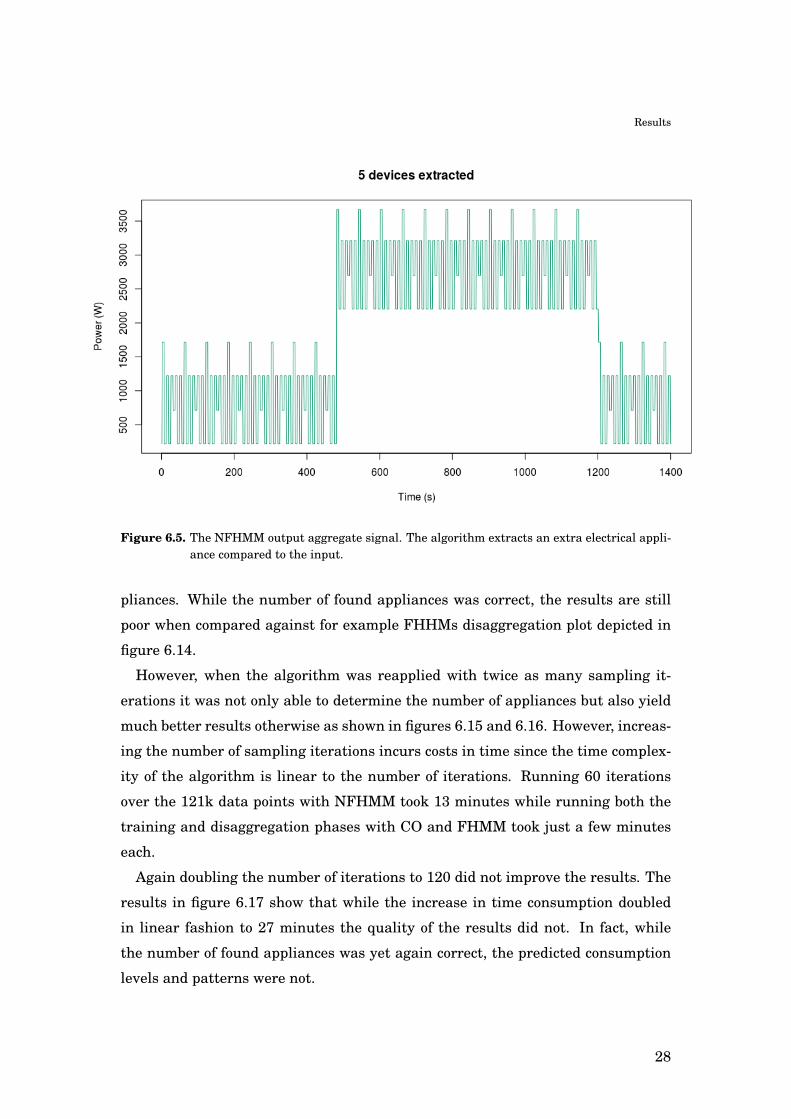
not the same as in the input. An example of such a case is shown in figure 6.5 and

24

Results

Figure 6.2. The separate electrical appliances present in the input of the NFHMM algorithm.

6.6.

We also tested the disaggregation accuracy of the NFHMM algorithm using the

same generated data, but with noise εt ∼ N (0, 100). The noisy input data is shown

in figure 6.7.

The NFHMM output for the noisier input data is shown in figures 6.8 and 6.9. As

seen in the figures, the algorithm seems to be quite robust and is able to estimate

the noise and produce sensible results, even with high noise. The output aggregate

signal errors are somewhat higher, MAE = 96.6 and MAPE = 0.16. Additionally,

the added noise makes the NFHMM algorithm more prone to converge to a local

optimum, and required several runs to produce a sensible result.

6.2 Performance comparison using NILMTK

NILMTK’s CO and FHMM implementations can be used to benchmark the disag-

gregation performance of the developed NFHMM algorithm. Using a script we de-

veloped (comparison.py), NILMTK can be used to train the supervised algorithms

and apply them to disaggregate the data. In this comparison, we ran the script

25

Results

Figure 6.3. The NFHMM output aggregate signal. The algorithm is able to extract the correct num-ber of electrical appliances in the household.

with two synthetic datasets in turn. In the first dataset only one building exists so

it was wholly used for both training and disaggregation and in the second dataset

the first building was used for training and the second for disaggregation. Exam-

ples of the two datasets are shown in figures 6.10 and 6.11, whereas the wiring

hierarchy of the two synthetic datasets is shown in figure 6.12. NILMTK’s plotting

and metrics functionality were used to generate the results.

In the case of the first dataset, where the same data was used for both training

and disaggregation, the supervised CO and FHMM algorithms performed excel-

lently. With the second dataset, where there was some difference between the

training and disaggregation datasets, some error began to appear in their perfor-

mance. However, the NFHMM algorithm did not reach the level of either super-

vised algorithm using such perfect data as can be read from table 6.2.

It should be noted that the comparison of supervised against unsupervised algo-

rithms with perfect or near perfect data is unfair. The limitations of the current

implementation of the NILMTK integration must also be noted. As explained in

chapter 5, NFHMM is sometimes unable to correctly determine the number of ap-

pliances and the current implementation of the NFHMM wrapper in NILMTK sim-

26

Results

Figure 6.4. The NFHMM output of the individual electrical appliances’ consumption.

ply disregards any found excess appliances and compares just the first four of the

found appliances against the ground truth. This makes simple f-score comparison

unflattering and thus complicates comparison.

However, during testing we found that when the frequency and number of data

points is sufficiently high, the algorithm tends to find the correct number of devices

with suitable heuristic parameter values. To explore performance with different

parameter combinations, three parameters were varied: The sigma epsilon heuris-

tic parameter (HP), the number of sampling iterations (SI) and the sampling period

or data frequency (SP). The NFHMM columns of the table 6.2 describe the best of

six runs with different parameter combinations. The parameter combination that

produced the best results for dataset 1 was 20, 120, 10 and the best for dataset 2

was 10, 60, 10, respectively. It should be noted that the process is not deterministic

and much computing resources would be required to produce a good distribution

of results to yield confidence in the optimality of any parameter combination for a

dataset.

Figure 6.13 provides an example of a NFHMM disaggregation result in a case

where the algorithm managed to correctly divide the consumption among four ap-

27

Results

Figure 6.5. The NFHMM output aggregate signal. The algorithm extracts an extra electrical appli-ance compared to the input.

pliances. While the number of found appliances was correct, the results are still

poor when compared against for example FHHMs disaggregation plot depicted in

figure 6.14.

However, when the algorithm was reapplied with twice as many sampling it-

erations it was not only able to determine the number of appliances but also yield

much better results otherwise as shown in figures 6.15 and 6.16. However, increas-

ing the number of sampling iterations incurs costs in time since the time complex-

ity of the algorithm is linear to the number of iterations. Running 60 iterations

over the 121k data points with NFHMM took 13 minutes while running both the

training and disaggregation phases with CO and FHMM took just a few minutes

each.

Again doubling the number of iterations to 120 did not improve the results. The

results in figure 6.17 show that while the increase in time consumption doubled

in linear fashion to 27 minutes the quality of the results did not. In fact, while

the number of found appliances was yet again correct, the predicted consumption

levels and patterns were not.

28

Results

Figure 6.6. The NFHMM output of the individual electrical appliances’ consumption, where thealgorithm has extracted an extra appliance.

6.3 Disaggregating Fortum datasets

The implemented NFHMM algorithm was used to disaggregate the data given by

Fortum. Figure 6.18 shows a 20 minute segment of a Fortum pilot customer house-

hold electricity consumption.

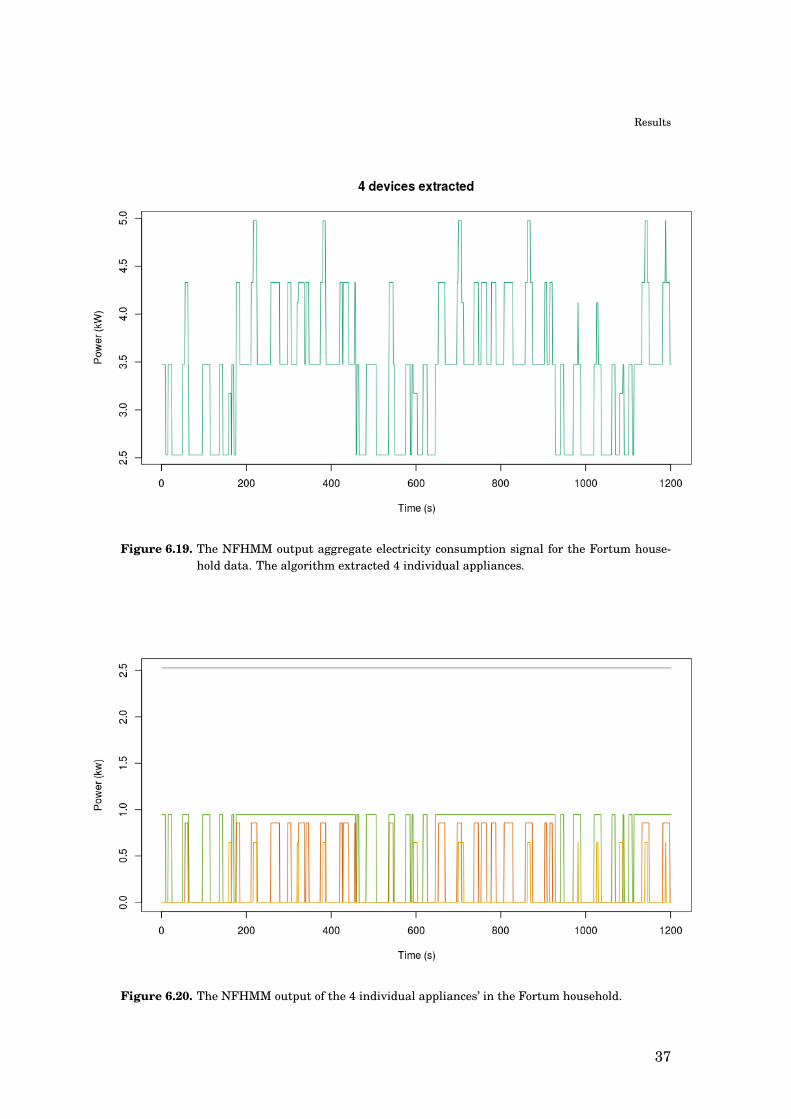
The NFHMM algorithm was run for 200 iterations resulting in 4 extracted ap-

pliances. The output aggregate signal is shown in figure 6.19 and the individual

appliances’ consumption is shown in figure 6.20.

On some runs the NFHMM algorithm converged to a solution with 3 appliances.

An example of such an output aggregate signal and the individual appliances’ sig-

nals is shown in figures 6.21 and 6.22.

We also used the NFHMM algorithm to disaggregate a segment from a Fortum

pilot customer household containing a boiler switch event. Figure 6.23 shows the

data that was used, containing a roughly 3 kW boiler switch-on event at the 700

second mark.

The NFHMM algorithm was run again for 200 iterations resulting now in 5 ex-

tracted appliances. The NFHMM output aggregate signal is shown in figure 6.24,

29

Results

Figure 6.7. The generated noisy aggregate signal used as input of the NFHMM algorithm.

and the individual appliance consumptions are shown in figure 6.25. The algo-

rithm extracted a 2.89 kW appliance, which can be seen in figure 6.25. The boiler

switch-on event is detected and maintained quite well, however, the appliance cor-

responding to the boiler is also detected as being active before the switch-on event,

for very short durations.

30

Results

Figure 6.8. The NFHMM output aggregate signal for the noisier input. The algorithm is still ableto extract the correct number of electrical appliances.

Figure 6.9. The NFHMM output of the individual electrical appliances’ consumption for the noisierinput.

31

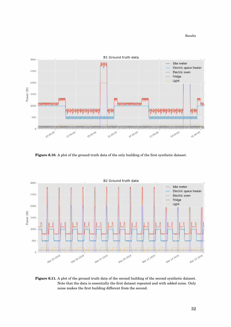
Results

Figure 6.10. A plot of the ground truth data of the only building of the first synthetic dataset.

Figure 6.11. A plot of the ground truth data of the second building of the second synthetic dataset.Note that the data is essentially the first dataset repeated and with added noise. Onlynoise makes the first building different from the second.

32

Results

Figure 6.12. A graph depicting the wiring hierarchy of the meters in all buildings of the two syn-thetic datasets.

Table 6.2. F-scores of the algorithms with both datasets.

Appliance Dataset 1 (perfect) Dataset 2 (noisy)

Method CO FHMM NFHMM CO FHMM NFHMM

Light 1.00 1.00 0.6 0.96 0.97 0.9

Fridge 1.00 1.00 0.8 0.95 0.98 0.5

Electric

oven1.00 1.00 0.7 1.00 1.00 0.5

Electric

space heater1.00 1.00 0.7 1.00 1.00 0.9

33

Results

Figure 6.13. Disaggregation result from a run which successfully determined the number of appli-ances but failed to otherwise produce clean results.

Figure 6.14. Disaggregation results using the implementation of FHMM available in NILMTK. Bycomparing this plot with the ground truth depicted in figure 6.10 one can visuallyaffirm the results depicted in table 6.2 and conclude that FHMM was able to performexcellently with this dataset.

34

Results

Figure 6.15. Disaggregation result from a run with twice as many sampling iterations as in the rundepicted in figure 6.13.

Figure 6.16. Disaggregation accuracy plot corresponding to figure 6.15. However, note that the va-lidity of the accuracy plot is not good because the mapping of disaggregated applianceconsumption time series to these four appliances was done simply in sequential order.This is why the values presented in table 6.2 were manually adjusted.

35

Results

Figure 6.17. NFHMM disaggregation results with 120 sampling iterations.

Figure 6.18. The Fortum pilot customer household electricity consumption that was disaggregatedwith the fully unsupervised NFHMM algorithm.

36

Results

Figure 6.19. The NFHMM output aggregate electricity consumption signal for the Fortum house-hold data. The algorithm extracted 4 individual appliances.

Figure 6.20. The NFHMM output of the 4 individual appliances’ in the Fortum household.

37

Results

Figure 6.21. The NFHMM output aggregate electricity consumption signal for the Fortum house-hold data. The algorithm extracted 3 individual appliances.

Figure 6.22. The NFHMM output of the 3 individual appliances in the Fortum household.

38

Results

Figure 6.23. The Fortum pilot customer household electricity consumption containing a boilerswitch-on event.

Figure 6.24. The NFHMM output aggregate electricity consumption signal for the Fortum house-hold data containing a boiler switch-on event. The algorithm extracted 4 individualappliances in addition to the boiler.

39

Results

Figure 6.25. The NFHMM output of the individual components for the Fortum pilot customer house-hold containing a boiler switch-on event.

40

7. Discussion

In this report, we provided a literature review of different NILM methods and a

studied fully unsupervised NFHMM disaggregation algorithm introduced by Jia et

al. (2015) in more detail. We examined shortly the performance of NFHMM algo-

rithm and compared it to performance of some supervised algorithms implemented

in NILMTK. Although it is difficult to compare the performance of unsupervised

methods to that of supervised methods, it appeared that supervised methods out-

performed clearly our implementation of NFHMM. For an unsupervised method

our implementation of NFHMM performed well in some situations, but the fre-

quently occurred convergence to local optima made it too unreliable to be operated

as a disaggregation tool as such, which is mainly due to the limitations of the

NFHMM model. Next, we discuss shortly how the implemented model could be

improved without using labelled appliance-level training data from each house-

hold.

There is room for improvement in both the implementation as well as the used

NFHMM model. There were some workarounds that we had to do because of lim-

ited time. Firstly, not all the hyperparameters were sampled from their correct

posterior distributions. The conjugate priors were omitted and the likelihood func-

tions were used as posterior distributions. Additionally, σε was sampled with a

heuristic as stated in Chapter 5. These workarounds might have affected the con-

vergence of the algorithm and through that the disaggregation results and possibly

better results would have been obtained using the correct posterior distributions.

Secondly, there were some problems using the ars() function of R that performs

the ARS to a given log-concave function. The problems occurred when the initial

points were chosen badly for certain function with certain bounds, which made the

ars() function to do some infinite loops. There were also problems in satisfying

the log-concavity requirement of the function, but this was caused by R’s rounding

errors of certain type of large sums which actually made the functions non-log-

41

Discussion

concave.

The third improvement for implementation would be applying the multi-state

designation to NFHMM as in (Jia et al., 2015). This would consider appliances

with multiple different states. However, this simple procedure was out of the scope

of this report.

The NFHMM model itself could be improved as well. It seems that the NFHMM

cannot find always the global optimum. The algorithm inevitably converges some-

times to local optima or alternatively, the global optimum is not reached after

reasonable amount of iterations. The Markov assumption of NFHMM is a ma-

jor limitation in the model: it assumes that the state of appliance depend only on

the previous state. However, the appliances usually have their typical signatures

which include the state durations. The boiler switch-on event detection in Chapter

6 is a clear example of this limitation. While the real boiler event is recognized

correctly, NFHMM finds some excessive short-period boiler events before the real

event, which are wrong and unreasonable. This behaviour could be avoided by

adding a semi-markovian property to the model. The semi-markov property would

consider the state durations of appliances, which would improve the disaggrega-

tion accuracy. The “mirroring” effect described in Chapter 6 would be suppressed

as well by the semi-markov property.

In addition to the state durations, other features could be added to the model

too. This could be done using approaches similar to CFHMM introduced by Kim et

al. (2011). Most appliances have the typical time of day when used, so adding time

of day as an additional feature could improve the accuracy. However, additional

features make the model even more complicated which might make the algorithm

slower.

One advantage of the Bayesian nonparametric property of NFHMM is that NFHMM

finds the number of appliances adaptively so that the prior information of number

of appliances is not required. Although NFHMM outperformed some other FHMM

models using AIC or BIC as a criterion for the number of appliances in the publica-

tion by Jia et al., we thought that it would be useful sometimes that the user could

set the number of appliances to the algorithm (2015). Then user could compare the

disaggregation results of different number of appliances chosen as an argument.

Our NFHMM implementation could be improved by at least adding upper bound

to number of appliances so that NFHMM would not detect over 10 appliances. A

42

Discussion

large number of appliances in the model makes NFHMM quite slow and often it is

not important to detect all small appliances.

The last problematic property of NFHMM that we found is that the power lev-

els of appliances can be negative. Usually, this is not the case (unless there are

batteries or solar panels in the household) and restricting the power levels to only

positive values could be realistic. Namely, we noticed that our implementation of

NFHMM produced negative power levels in some rare situations. This could be

easily avoided by setting constraints to power level, but setting constraints affects

convergence to optimal solution as well and in our experiments the convergence

became worse after adding constraints.

The datasets used in our development and analysis in this project have been two

very simple synthetic datasets. These datasets might not compare well with real

world datasets but because performance level achieved by our implementation of

the NFHMM algorithm is still relatively modest the characteristics of the data rel-

ative to the real world data in this stage is not essential. If more resources would

have been available for this project and the performance of the algorithm was much

improved, we would have proceeded to generate incrementally more complex and

real world like synthetic datasets for testing. Eventually, we would have moved on

to use highly submetered publicly available real world datasets for final refinement

and tuning and validated the model with any adequately submetered data avail-

able from Fortum. The original unmetered datasets provided would have become

the target of our focus only after these stages of refinement and validation would

have been completed to high standards.

Regarding the performance comparison it must be again noted that the CO and

FHMM implementations used in the NILMTK comparison had an unfair advan-

tage at this testing phase. The datasets were perfect or near perfect and the data

used for training and disaggregation were similar to an extent which is rare with

real world data. Consequently, one should not conclude based on this compari-

son alone that the NFHMM algorithm or other unsupervised algorithms could not

be improved and refined such as to be any match for the supervised algorithms.

Collecting enough real world data from a wide enough variety of households and

appliances to give supervised algorithms a clear advantage is costly. In addition,

we believe that the NFHMM model could be developed to become semi-supervised

and utilize any available submetered data or other relevant data regarding the

43

Discussion

target of disaggregation.

Due to the difficulty of reaching good results with the test data, we did not use

many of the features that NILMTK had to offer. NILMTK would have been more

useful had we been able to reach higher performance levels that would have in-

spired us to fully implement it using Python into NILMTK instead of just imple-

menting a wrapper in order to conveniently test it with the various public datasets

adapted for NILMTK. The statistical analysis and benchmarking functions imple-

mented in NILMTK would have been more relevant at that phase.

Regarding the future, we believe Fortum should first study the commercial busi-

ness potential of an imaginary high performing unsupervised disaggregation algo-

rithms. If these seem attractive, then effort should be directed to further develop

the algorithm as outlined earlier in this chapter. We believe that by following the

path we outlined, it should be possible to reach much more promising results in

about 400 hours of further research, and possibly even a performance level suit-

able for production with about another similar batch of work.

All in all, it seems that the disaggregation problem is certainly not trivial. The

unsupervised methods have produced some promising results, but the performance

is not yet comparable to performance of supervised methods. Supervised methods

require the expensive training data, which in turn hampers their use. In the fu-

ture, our implementation of NFHMM could be probably improved so that it would

disaggregate the loads fairly well, however before committing to such a project, it

should be evaluated whether developments in smart metering technology are likely

to make it feasible to submeter a vast proportion of household appliances such as

to make investing into a supervised approach more reasonable.

44

Bibliography

Altrabalsi, H., Stankovic, V., Liao, J., and Stankovic, L. (2016). “Low-complexity energy

disaggregation using appliance load modelling”, AIMS Energy, vol. 4, pp. 884–905

http://www.aimspress.com/article/10.3934/energy.2016.1.1

Armel, C. K., Gupta A., Shrimali G., and Albert A.(2012). “Is disaggregation the holy

grail of energy efficiency? The case of electricity”, Energy Policy

http://dx.doi.org/10.1016/j.enpol.2012.08.062

Baranski, M., and Voss, J. (2004). “Genetic algorithm for pattern detection in NIALM

systems”, 2004 IEEE International Conference on Systems, Man and Cybernetics, 10–13 Oct

2004, The Hague, Netherlands

https://doi.org/10.1109/ICSMC.2004.1400878

Batra, N., Kelly, J., Parson, O., Dutta, H., Knottenbelt, W., Rogers, A., Singh, A. and Sri-

vastava, M. (2014). “NILMTK: an open source toolkit for non-intrusive load monitoring”,

Proceedings of the 5th international conference on Future energy systems

https://arxiv.org/abs/1404.3878

Farinaccio, L., and Zmeureanu, R. (1999). “Using a pattern recognition approach to dis-

aggregate the total electricity consumption in a house into the major end-uses”, Energy and

Buildings, vol. 30, no. 3, pp. 245–259

https://doi.org/10.1016/S0378-7788(99)00007-9

Ghahramani, Z., and Jordan, M. I. (1997). “Factorial Hidden Markov Models”, Machine

Learning, vol. 29, pp. 245–273

https://doi.org/10.1023/A:1007425814087

Griffiths, T. L., and Ghahramani, Z. (2006). “Infinite latent feature models and the in-

dian buffet process”, Advances in Neural Information Processing Systems, vol. 18, pp. 475–482

http://mlg.eng.cam.ac.uk/zoubin/papers/ibp-nips05.pdf

Hart, G. (1992). “Nonintrusive appliance load monitoring”, Proceedings of the IEEE, vol.

80, no. 122, pp. 1870–1891

45

Bibliography

Jia, R., Gao, Y., and Spanos, C. J. (2015). “A fully unsupervised non-intrusive load monitoring

framework”, IEEE International Conference on Smart Grid Communications, 2–5 Nov 2015,

Miami, FL, USA

https://doi.org/10.1109/SmartGridComm.2015.7436411

Johnson, M. J., and Willsky, A. (2012). “The Hierarchical Dirichlet Process Hidden Semi-

Markov Model”, arXiv

https://arxiv.org/abs/1203.3485

Kim, H., Marwah, M., Arlitt, M., Lyon, G., and Han, J. (2011). “Unsupervised disaggre-

gation of low frequency power measurements”, Proceedings of the SIAM International

Conference on Data Mining

http://dx.doi.org/10.1137/1.9781611972818.64

Kolter, J. Z., and Jaakkola, T. (2012). “Approximate Inference in Additive Factorial HMMs with

Application to Energy Disaggregation”, Proceedings of the Fifteenth International Conference

on Artificial Intelligence and Statistics, vol. 22, pp. 1472–1482

http://proceedings.mlr.press/v22/zico12/zico12.pdf

Kolter, J. Z. and Johnson, M. J. (2011). “REDD: A public data set for energy disaggregation

research”. Proceedings of 1st KDD Workshop on Data Mining Applications in Sustainability,

San Diego, CA, USA.

http://redd.csail.mit.edu/kolter-kddsust11.pdf

Lange, H., and Bergés, M. (2016). “The Neural Energy Decoder: Energy Disaggregation

by Combining Binary Subcomponents”, Proceedings of the 3rd International Workshop on

Non-Intrusive Load Monitoring

http://nilmworkshop.org/2016/proceedings/Paper_ID19.pdf

Liao, J., Elafoudi, G., Stankovic, L., and Stankovic, V. (2014). “Power disaggregation for

low-sampling rate data”, 2nd International Non-Intrusive Appliance Load Monitoring Work-

shop, Austin, TX, USA

http://nilmworkshop.org/2014/proceedings/liao_power.pdf

Onoda, T., Murata H., Ratsch, G., and Muller, K. (2002) “Experimental analysis of sup-

port vector machines with different kernels based on non-intrusive monitoring data”, Neural

Networks, vol. 3, pp. 2186–2191

Parson, O., Ghosh, S., Weal, M., and Rogers, A. (2011). “Using Hidden Markov Models

for iterative non-intrusive appliance monitoring”, Neural Information Processing Systems

Workshop on Machine Learning for Sustainability

http://eprints.soton.ac.uk/id/eprint/272990

46

Bibliography

Parson, O., Ghosh, S., Weal, M., and Rogers, A. (2014). “An unsupervised training method for

non-intrusive appliance load monitoring”, Artificial Intelligence, vol. 217, pp. 1–19

https://doi.org/10.1016/j.artint.2014.07.010

Prudenzi A. (2002). “A neuron nets based procedure for identifying domestic appliances

pattern-of-use from energy recordings at meter panel”, IEEE Power Engineering Society Winter

Meeting, 27–31 Jan 2002, New York, NY, USA

https://doi.org/10.1109/PESW.2002.985144

Roos, J., Lane, I., Botha E., and Hancke G. (1994). “Using neural networks for non-intrusive

monitoring of industrial electrical loads”, Proceedings of the Instrumentation and Measurement

Technology Conference, 10–12 May 1994, Hamamatsu, Japan

https://doi.org/10.1109/IMTC.1994.351862

Ruzzelli, A. G., Nicolas, C., Schoofs, A., and O’Hare, G. M. (2010). “Real-time recognition

and profiling of appliances through a single electricity sensor”, 2010 7th Annual IEEE Com-

munications Society Conference on Sensor Mesh and Ad Hoc Communications and Networks,

21–25 Jun 2010, Boston, MA, USA

https://doi.org/10.1109/SECON.2010.5508244

Suzuki, K., Inagaki, S., Suzuki, T., Nakamura, H., and Ito, K. (2008). “Nonintrusive ap-

pliance load monitoring based on integer programming”, SICE Annual Conference, 20–22 Aug

2008, Tokyo, Japan

https://doi.org/10.1109/SICE.2008.4655131

Teh, Y. W., Grür, D., and Ghahramani, Z. (2007). “Stick-breaking construction for the In-

dian buffet process”, Proceedings of the Eleventh International Conference on Artificial

Intelligence and Statistics, vol. 2, pp. 556–563

http://proceedings.mlr.press/v2/teh07a/teh07a.pdf

Van Gael, J. (2011). “Bayesian Nonparametric Hidden Markov Models”, Doctoral disser-

tation, University of Cambridge

Zhao, B., Stankovic, L., and Stankovic, V. (2016). “On a training-less solution for non-

intrusive appliance load monitoring using graph signal processing”, IEEE Access, vol. 4, pp.

1784–1799

https://doi.org/10.1109/ACCESS.2016.2557460

Zoha, A., Gluhak, A., Imran, M. A., and Rajasegarar S. (2012). “Non-intrusive load moni-

toring approaches for disaggregated energy sensing: A survey”, Sensors, vol. 12, 16838–16866

https://dx.doi.org/10.3390%2Fs121216838

47

Appendix A: Self-evaluation of project work

Herein we present a brief self-evaluation of our performance in the project. The

first three paragraphs focus on our project related practices and project manage-

ment. The following paragraph relates the realized effort against the allocated

budget. Finally, the last paragraph describes the achievements we are especially

satisfied of as well as the areas where we feel the project did not go as ideally as

we would have hoped and provides some words of hindsight.

We employed few clear project management or teamwork practices. Because

neither the client nor we understood nor were able to estimate the feasibility of

the project, we decided to try to apply an incremental approach to how the goals

and objectives of the project were formed. In addition to the fact that the project

topic was outside both our and our client’s know-how area, we had two further

challenges. Firstly, only two of our team members were from the same department

and knew each other in advance. This required us to explore how to best interact

in order to maximize the productivity of the team. Secondly, all members were

busy and had more or less long periods of travelling abroad during the course of

the project which increased the difficulty of scheduling and coordination.

Consequently two more major decisions were made. First, it was decided that

we try to book enough work sessions from all of our calendars as early as possible

such as to ensure that we are able to follow our plans and do not have to work much

individually. In addition to trying to work as much with the whole team in person,

we also decided Mihail to be the project manager. This meant that he would carry

out the scheduling and coordination work as well as lead the communication and

interaction with other project stakeholders. Mihail was chosen primarily because

he worked for Fortum already and was in the best position to perform in the role.

The project manager also had a more leading role in opponent work as well as in

all course related formalities. We tried to keep frequent enough contact with the

client to ensure we share a similar understanding of project goals and are able to

48

Appendix A: Self-evaluation of project work

manage expectations.

Overall, we think our chosen practices worked fairly well. Thanks to the fre-

quent live work sessions we were able to achieve progress almost every week and

in the end we more than met the allocated work budget. Our work provided a good

review and prototype that we believe will bring the client valuable insight into

the problem we studied. Our team members were able to take initiatives on their

own and the teamwork atmosphere was pleasant, constructive and fruitful without

almost any pressure or direction from peers or the project manager.

The allocated effort for the project was 5 ECTS or 135 hours. Due to the good

motivation levels among team members and our commitment to keep scheduling

and contributing actively in live work sessions we were able to keep the pace of

work good and steady. We believe most members contributed rather equally to the

project. Over the duration of the whole course Samuel had used a tool to track his

time use and the data indicates the following totals in hours for the months from

Jan to May: 12, 35, 47, 29, 21. The total, 144 hours, slightly exceeds the course

budget.

We believe that the project was successful in providing a case study of recent ad-

vances in electricity disaggregation methods. The project work serves as a useful

reference for the client for developing further their vision on energy disaggregation

services. NILMTK proved to be quite extensive for the scope of this project and

would have been more suitable for a bigger project. Nevertheless, we managed to

get the supervised methods working and the toolkit was useful for benchmarking.

That being said, the comparison to supervised methods was quite difficult to carry

out and we feel the implemented comparisons were somewhat unfair towards the

unsupervised method, especially considering its tremendous practical advantages

over the supervised ones. Given more resources, a more fair comparison scheme

could have been devised. Even though the implemented NFHMM model is not

ready to be used for out-of-the-box disaggregation as such, we are satisfied by the

implementation as a proof of concept for completely unsupervised electricity dis-

aggregation, and believe that it lowers the threshold for the client to continue its

development.

49