Embed Size (px)
Citation preview

FINAL REPORT
DEVELOPMENT OF AN INVENTORY OF MATERIALS POTENTIALLY
SENSITIVE TO AMBIENT ATMOSPHERIC ACIDITY IN THE
SOUTH COAST AIR BASIN
Contract No A6-079-32 VRC Project No 1058
Prepared by
Yuji Horie PhD Arthur Shrope
Valley Research Corporation 15904 Strathern Street Suite 22
Van Nuys California 91406
and
Richard Ellefsen PhD San Jose State University
Department of Geography One Washington Square
San Jose California 95192
Prepared for
California Air Resources Board Research Division
1800 15th Street Sacramento California 95814
March 1989
DISCLAIMER
The statements and conclusions in this report are those of the Contractor and not necessarily those of the State Air Resources Board The mention of commercial products the source of their use in connection with material reported herein is not to be construed as actual or implied endorsement of such products
4
C 0272bull 1 1)1 2 J Rec101emmiddots Accesuan No~- REPORT NOIREPORT DOCUMENTATION
PAGE - ARBR-89 399 PB89224604
bull rte bullna Subtbullt1 bull Development of an Inventory of Materials Potentiall i s Recort Cate
Sensitive to Ambient Atmospheric Acidity in the South Coast March 1989 Air Basin ~
7 Autnor1s1 Yuji Horie
9 Perlarmnbull Orsanrenon Name ano Addbull 10 Pro1ect1 Tasawo Unit No
Valley Research Corporation 11 Contrac11Cl or Gralll1G) He
15904 Strathern Street Suite 20 (C) A6-079-32Van Nuys CA 91406 (Gl
12 SOOMenflC o Name ano Addbull 13 Tyoe at Reoon 6 ~ ~
AIR RESOURCES BOARD RESEARCH DIVISION Final J_ 0 BOX 2815 1
SACRAMENTO CA 95812 I 15 SuaD1e Notes
lL Abancl CUfflll zoa
The ~ontractors developed an inventory of exposed materials for residential and nonshyresidential buildings and nonbuildings The inventory of the residential buildin~middotwas developed by conducting telephone surveys of 1200 households and field surveys of-200 households The inventory of multi-family residential buildings and nonresidentialmiddotshybuildings was conducted by aerial photo analysis The inventory of nonbuildingmiddot materials (infrastructure) was developed by conducting a limited survey and by using engineering calculations The investigators extrapolated the inventory to the entire SoCAB using the building-count method
Materials inventory Acid Deposition
gt ldent1fien100en-poundndeo Terms
Air Pollution South Coast Air Basin
C COSATI FlefdGIOUO
1L AvaOliilY Stat9nWM 19 SealfflY Clan t This ReOOfftRelease Unlimited Available from National Technical Information Service 5285 Port Royal Roa~n-------------------Sor i n a f i e 1 d VA 221 61 20 scum c1an Thibull Pa 22 Pnce
tA ai
ABSTRACT
This study demonstrates a methodology which permits the development of a comprehensive inventory of materials-in-place in an urban region within a practical scope of work and with verified reliability This methodology has been successfully applied to produce an inventory for the South Coast Air Basin of potentially susceptible materials exposed to the urban atmosphere It involves separate treatment of three types of facilities with specific protocols for each type The three types of facilities in which almost middotall of the susceptible materials are found are (1) single-family residences (SFRs) (2) non-residential buildings and multiple-unit residential buildings collectively called non-single-family residences (NSFRs) (3) structures other than buildings collectively called Infrastructures
Out _of two and a quarter mi 11 ion SFR parce1s recorded in the tax assessor data bases in the SoCAB a representative sample of 1200 households were selected and surveyed by telephone regarding exterior surface materials of buildings and ground covers Subsequently a field survey of 200 houses selected from those surveyed by telephone was conducted to make detailed on-site measurements of all exterior material-finishes For NSFRs out of 3855 tax assessor mapbooks over the SoCAB 30 mapbooks were selected and the corresponding regions were examined using aerial photographic method With a camera system mounted on a light aircraft a total of 2000 low altitude oblique photographs were taken and analyzed to evaluate exposed material surfaces of 1429 NSFR parcels selected from those in the 30 study sites Materials associated with infrastructures such as highways railroads channelized waterways and power distribution networks were quantified by estimating three basic quantities the total miles of infrastructure facilities the number of material-bearing items associated with the facilities and the material factors for such items Estimates of the three quantities were made either by conducting a special survey (for highways) by taking on-site measurements of a few selected items of each type or by obtaining enumeration statistics from appropriate data source organizations
Based on these three separate analyses a reliable highly resolved comprehensive inventory of materials-in-place was developed for the entire SoCAB region
TABLE OF CONTENTS
Section Page
List of Figures iii
List of Tables iv
Glossary vii
LO INTRODUCTION 1-1
11 Background and Study Objective 1-1 12 Summary of Findings 1-2
121 SFR Survey Findings 1-3 122 NSFR Survey Findings 1-4 123 Infrastructure Survey Findings 1-6
20 OUTLINE OF STUDY APPROACH 2-1
21 Review of Earlier Studies 2-1 22 Present Study Approach 2-3
221 Sampling Frame 2-4 222 Survey Design 2-5
2221 SFR Survey Design 2-7
2222 NSFR Survey Design 2-9
2223 Infrastructure Survey Design 2-16 223 Measurement System 2-19
30 SINGLE FAMILY RESIDENCES (SFRs) 3-1
31 General 3-1 32 Telephone Questionnaire Survey 3-1
32 l Sample Selection for Questionnaire Survey 3-2 322 Questionnaire Design and Testing 3-5 323 Survey Execution 3-7
33 Field Survey 3-9 331 Development of Survey Protocol 3-11 332 Field Survey Execution 3-13 333 Data Reduction and Encoding 3-16 334 Reliability of Field Survey Data 3-18
34 Materials in SFR Parcels 3-22 341 Comparison of Field and Questionnaire Survey Results 3-23
i
TABLE OF CONTENTS
Section Page
342 Materials-in-Place for Field Surveyed Houses 3-31 343 Basinwide Inventory of Materials Associated with SFRS 3-39
40 NON-SINGLE FAMILY RESIDENCES (NSFRs) 4-1
41 General 4-1 42 Airphoto Method 4-3
421 Nature of the Study Sites 4-3 422 Photographic System 4-8 423 Other Supporting Materials 4-12
43 Development of NSFR Data Base 4-15 431 Parcel File 4-15 432 Building File 4-21
44 Materials in NSFR Parcels 4-26 441 Materials-in-Place for NSFRs in Building File Sample 4-26 442 Basinwide Inventory of Materials Associated with NSFRs 4-34
50 INFRASTRUCTURES 5-1
51 General 5-1 ( 52 Materials in Highways 5-1
521 Items Associated with State Highways 5-4 522 Items Associated with Surface Streets 5-4 523 Basinwide Inventory of Materials in Highways 5-11
53 Materials in Other Infrastructures 5-12
60 CONCLUSIONS AND RECOMMENDATIONS 6-1
61 Conclusions 6-1 62 Reliability of Estimates 6-4 63 Recommendations 6-10
631 Recommendations for Prospective Data Base User 6-10 632 Recommendations for Future Studies 6-15
70 REFERENCES 7-1
Appendix A Telephone Questionnaire Appendix B Material-Finish Codes Appendix C Field Worksheet Example Appendix D Instructions for Field Worksheet Appendix E Conventions for Field Data Reduction Appendix F Field Survey Coding Sheet Appendix G Material Factors for Enumeration Items Appendix H General Instructions for NSFR Parcel File and Revisions Appendix I Street Survey Form Appendix J Basinwide Material Surface by Infrastructure Type
LIST OF FIGURES
Figure No Title Page
3-1 Locations of 200 Houses Examined In The Field Survey 3-10
4-1 Locations of the 30 Sites in the SoCAB 4-4
4-2 Vertical Photograph of a Segment of the Pasadena Site 4-~5
4-3 Enviro-Pod Mounting 4-10
4-4 Photograph of Camera 4-11
4-5 A Black and White Copy of the Full Color Enviro-Pod Photograph 4-13
4-6 A segment of a Cadastral Map of Pasadena 4-14
4-7 Guide to Use of Branching Key in Identifying Building Materials 4-24
5-1 Locations of Special Street Survey Sites 5-7
6-1 Required Sample Size versus Probability of Finding Items 6-9
Ill
(
LIST OF TABLES
Table No Title Page
2-1 Number of Mapbooks and Parcels by Use Type 2-6
2-2 Number of Samples Allocated to Each of the 13 Strata Used for Questionnaire and Field Surveys 2-8
2-3 Summary Features of 18 Candidate Sets for LA County 2-13
2-4 Numbers and Types of Land Parcels in the Study Set and in LA County 2-15
2-5 Numbers and Types of Land Parcels in the Study Set and in Composite County 2-16
2-6 Total Miles of Road by Type and Numbers of Selected Survey Routes for Each Type 2-18
3-1 Comparison of SFR Size Distributions for Houses with Listed Phone Numbers Versus All Houses for the SoCAB 3-3
3-2 Allocation of Survey Houses for the Telephone Questionnaire Survey 3-4
3-3 Summary Results of Telephone Interviewing 3-8
3-4 Summary Results of Field Survey - 3-15
3-5 Test House 1 - Single Story with Detached Garage 3-19
3-6 Test House 2 - Single Story with Attached Garage 3-20
3-7 Test House 3 - Two Story with Detached Garage 3-21
3-8 Rating Response Reliabilities for Questionnaire Items 3-24
3-9 Configuration Characteristics of the Questionnaire Surveyed Houses 3-25
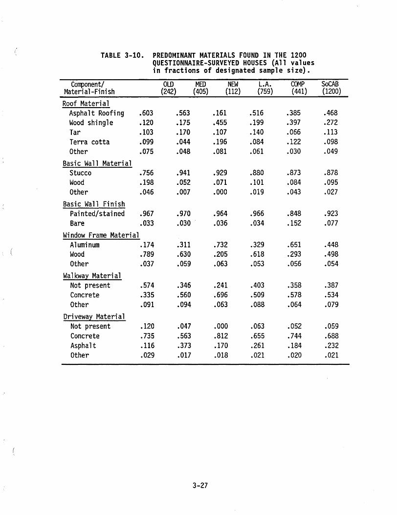
3-10 Predominant Materials Found in the 1200 Questionnaire Surveyed Houses 3-27
3-11 Comparison of House Mixes Depicted by the Questionnaire Survey and the Field Survey at County- and Basin-Wide Level 3-29
3-12 Comparison of House Mixes Depicted by the Questionnaire Survey and the Field Survey at Age Strata Level 3-30
3-13 Mean Exposed Surface Areas by Category in SFR Strata 3-32 3-14 Mean Exposed Surface Areas by Material-Finish Building Primary 3-34
3-15 Mean Exposed Surface Areas by Material-Finish Parcel Total 3-35 3-16 Number of Houses with the Stated Material-Finish 3-37
3-17 Mean Exposed Surface Areas by Material-Finish in House Component 3-38 3-18 Mean Painted Surfaces by Material 3-39 3-19 Basin Total Exposed Surface Areas by Material-Finish for SFR Strata 3-41
iv
LIST OF TABLES
Table No Title Page
3-20 Basin Total Painted Surface Areas by Material in SFR Strata 3-42
3-21 Number of Enumeration Items by Type in SFR Strata 3-43
3-22 Material-Finish Surface Areas for SFR Enumeration Items 3-44
3-23 Basin Total Exposed Surface Areas of Enumeration Items in SFRs 3-44
4-1 Site Area and Number of Parcels per Site 4--6
4-2 Site Groups Among the 30 Study Sites 4-7
4-3 Summary Results of Parcel File Data NSFR Parcels 4-18
4-4 Mean Values of Major Features of Buildings NSFR Parcels 4-20
4-5 Number of Clusters and Parcels with Buildings 4-22
4-6 NSFR Mean Exposed Surface Areas by Material-Finish LA County 4-28
4-7 NSFR Mean Exposed Surface Areas by Material-Finish Composite County 4-30
4-8 NSFR Mean Exposed Surface Areas by Material-Finish Construction Types 4-32
4-9 Mean Exposed Surface Areas by NSFR Parcel Component 4-34
4-10 Estimated Numbers of NSFR Parcels with Buildings 4-36
4-11 Basin Total Exposed Surface Areas by Material-Finish LA County 4-37
4-12 Basin Total Exposed Surface Areas by aterial-Finish Composite County 4-39
4-13 Material-Finish Surface Areas for NSFR Enumeration Items 4-40
4-14 Total Exposed Surface Areas NSFR Enumeration Items 4--41
5-1 Road Miles by Functional Class in the SoCAB 5-2 5-2 Total Road Miles by Type and County 5-3
5-3 Numbers of Enumeration Items State Highways 5-5
5-4 Summary of Routes Selected for the Special Street Survey 5-6
5-5 Summary Results of the Street Survey 5-9
5-6 Number of Enumeration Items by Road Type 5-10
5-7 Total Exposed Material Surfaces of Items Associated with Highways 5-11
5-8 Enumeration Items of Power Transmission Network 5-13
5-9 Total Miles of Railroad and Channelized Waterway 5-14
5-10 Total Exposed Material Surfaces Other Infrastructures 5-15
V
LIST OF TABLES
Table No Title Page
6-1 Summary of Material-Finish Inventory in the SoCAB 6-3 6-2 Sampling Errors in Basinwide Material Surface Areas
of Selected Material-Finishes for SFRs 6-6 6-3 Sampling Errors in Basinwide Material Surface Areas
of Selected Material-Finishes for NSFRs 6-7 6-4 Mean and Total Exposed Surface Areas by Materialshy
Finish for SFR Parcels in Orange County 6-13 6-5 Total Exposed Surface Areas by NSFR Use-Type
in Orange County 6-14
vi
GLOSSARY
AGR Agricultural parcel
ARB California Air Resources Board
CALTRANS California Department of Transportation
CBD Central Business District
Cluster A collection of contiguous NSFR parcels that share a common building or building complex
COMP Composite County that consists of counties of Orange Riverside and San Bernardino
COL Collector streets in urban area
EPA Environmental Protection Agency
EPRI Electric Power Research Institute
HPMS Highway Performanc~ Monitoring System a major data base managed by CALTRANS
HWY Highways and surface streets
LMFR Large multi-family residential parcel having 5 or more dwelling units
LNR Large non-residential parcel that includes balance of NR excluding those found in SNR
LOC Local streets in urban area
MA Minor arterial streets in urban area
Mapbook Highest hierarchical unit used by tax assessors to indicate geographical location of a parcel
MED Time period for buildings built in years between 1946 and 1964
MFR Multi-family residential parcel having triplex or more dwelling units
MH Mobile homes
MJC Major collector streets in rural area
MJR Major properties identified by Los Angeles tax assessor office
NAPAP National Acid Precipitation Assessment Program
NEW Time period for buildings built in 1965 or later years
NR Non-residential parcel
vii
NSFR Non-single family residential parcel that includes all parcelsother than SFRs
OI Other infrastructures that include railroads waterways and power distribution networks
channelized
OLD Time period for buildings built in 1945 or prior years
PA Principal arterial streets in urban area
Parcel Basic land plot used by tax assessors
RCOND Residential condominium
SFR Single family residential parcel that includes single detached house and duplex
SJSU San Jose State University
SMFR Small multi-familyand fourplex
residential parcel that includes triplex
SNR Small non-residential parceleries parking lots etc
such as service stations nursshy
SoCAB Californias South Coast Air Basin that consists of OrangeCounty and portions of three other counties Los AngelesRiverside and San Bernardino
UNK Parcel with unknown use
VAC Vacant parcel
VRC Valley Research Corporation
10 INTRODUCTION
11 BACKGROUND AND STUDY OBJECTIVE
The Kapiloff Acid Deposition Act of 1982 mandates the Air Resources Board (ARB) to conduct a comprehensive research program to determine the nature extent and potential effects of acid deposition in California Part of this far reaching effort is the need to accurately assess the economic impact that acid deposition has upon materials in place To make such an assessment possible ARB has sponsored a series of research projects which are aimed to obtain the following information
Material Damage Functions to quantify marginal rates of material deterioration (eg metal corrosion and paint erosion) due to air po11 uti on
Materials Inventory to quantify and characterize materials-in-place which are exposed to ambient air and
Replacement Costs to quantify marginal costs of replacing at an accelerated rate items containing those materials which are susceptible to acid deposition
The present study is concerned with deve1 oping a reliable comprehensive inventory of materials-in-place A previous ARB-contract study (Murray et al 1985) developed a preliminary inventory of several economically significant materials in place in the South Coast Air Basin (SoCAB) The study however was limited with respect to the level of detail and the number and types of materials considered Therefore the main objective of this study is to develop for the SoCAB an improved more comprehensive inventory of materials that are potentially susceptible to damage from atmospheric acid deposition
Although it is a part of the overall study of assessing the economic impact of acid deposition upon materials the scope of this study is not limited to only those materials which are being investigated under the ARB-sponsored materials damage studies or those which will be examined under a forthcoming economic assessment study Since it is not wise to presume
1-1
economic loss due to acid deposition in the basin occurs predominantly in one type of material rather than another this inventory study aims to characterize a11 types of materials that are present in significant quantity and are potentially susceptible to damage by acid deposition~
Further the inventory deve1oped under this study sped fies not only what amounts and types of materi a 1 s are in use but a 1 so what types of facilities and what structural components the materials are used for The rate of damage to a material due to acid deposition may depend in part on how and where in the facility the material is used In addition the replacement cost for a material may partially depend on the type of facilities in which the material is used
Because of the importance of knowing the types of facilities as well as the types and amounts of materials-in-places this study is designed to quantify materials-in-place in relation to specific types of facilities There are three main types of faci 1 i ti es in which the great majority of materials are found
1 Single Family Residences (SFRs) including single detached houses and duplexes
2 Non-Single Family Residences (NSFRs) including multi-family resshyidences and non~residential buildings and
3 Infra-Structures including roadways electrical distribution netshyworks railroads and channelized waterwayso
12 SUMMARY OF FINDINGS
The most important result of this study is probably the demonstration of a methodology which permits the development of a comprehensive inventory of materials-in-place in an urban region within a practical scope of work and with verified reliability
Here facilities mean any man-made material bearing complexes such as residential buildings (including various associated minor structres) commercial buildings industrial plants institutional complexes highshyways surface streets railroads channelized waterways and transmission and distribution towers
1-2
This methodology has been successfully applied to produce an inventory for the South Coast Air Basin of potentially susceptible materials exposed to the urban atmosphere It involves separate treatment of three types of facilities with specific protoco 1 s for each type The three types of facilities in which almost all of the susceptible materials are found are 1) single-family residences SFRs) (2) non-residential buildings and multiple-unit residential buildings collectively called non-single-family residences (NSFRs) (3) structures other than buildings collectively called Infrastructures
For each of these types of faci 1 i ti es VRC devised and app1 i ed an appropriate sampling frame and a corresponding inventory procedure These developments are fully described in Chapter 20 and further details regarding the execution of the surveys as well as brief summaries of the results are reported in Chapters 30 40 and 50 Highlights of VRC 1 s experience and findings in preparing the subject inventory are set forth in the following paragraphs
121 SFR SURVEY FINDINGS
bull Out of two and a quarter million SFR parcels in the SoCAB 3825 SFR households with listed telephone numbers were selected by a stratified random sampling method
bull Of the 3825 households a telephone questionnaire survey on exterior surface materials of buildings and ground covers was attempted for 2095 households and completed on 1200 households a completion rate of 57 percent
bull Of the 1200 househo1ds so surveyed 259 houses were se 1 ected as target houses for a subsequent field survey The field survey was completed on 176 target houses (68 percent completion rate) and 24 substitute houses which were selected from houses having the same structural features as target houses in the immediate neighborhood In all the survey was completed on 200 houses
bull Comparisons between questionnaire responses and field observation results indicate that the questionnaire-responses are reliable for questions about presence or absence of features questions on building configuration and questions on materials used for chimneys garage walls and ground cover
bull Re 1 i abi 1 i ty of the fie1 d survey was examined by comparing survey results on three test houses for which two survey teams of two surveyors each made on-site measurements twice first separately by
1-3
each team and second jointly by both teams The comparison revealed that relative measurement errors were within 10 to 20 percent for major components For some material-finishes the two teams identified them differently indicating that misidentification of material-finishes can in some instances be a primary source of errors
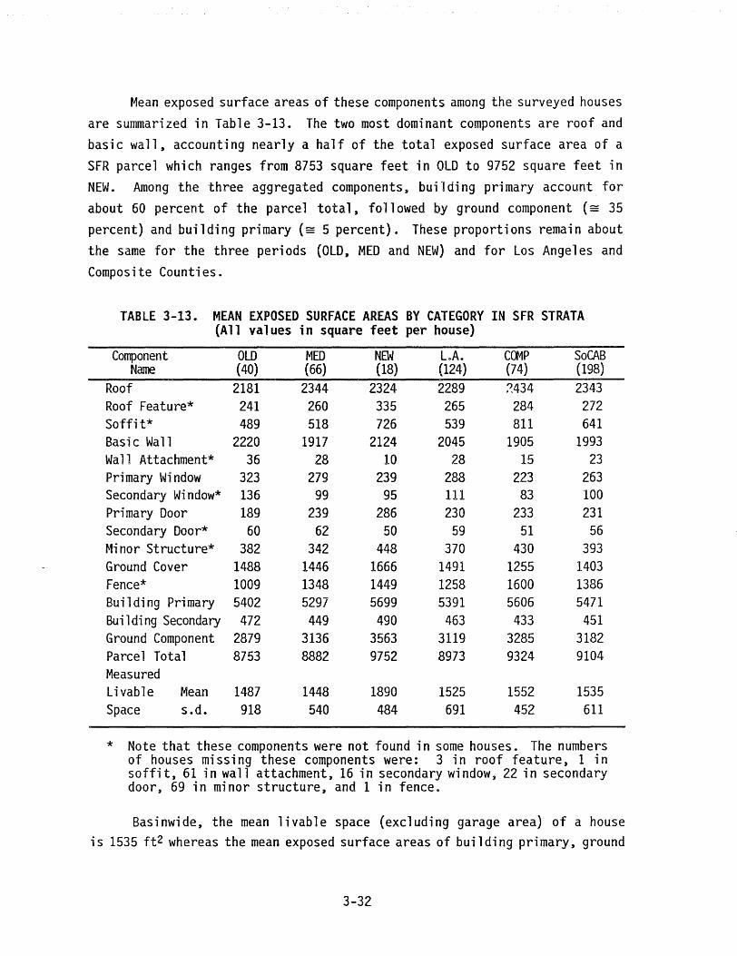
e The mean l i vab1e space of the 198 houses (2 houses were later excluded from the data base is 1500 ft2 whereas the mean tota1 building exterior surface area is 5500 ft2 and the mean total exposed surface area of SFR parcels is 9100 ft2
bull Of the building primary surface of 5500 ft2 roofs account for 43 percent basic walls for 36 percent soffits for 12 percent and walls and doors for 9 percenta
bull Houses in Los Ange1es County were examined separate1y for OLD (pre-1946) MED 1946-1964) and NEW post-1964) Houses in NEW have the largest livable space (1900 ft2) the highest proportion of two-story houses (50 percent) and the least proportion of detached garages (11 percent) Conversely houses in MED have the least livable space (1450 ft2) and the least proportion of two-story houses (8 percent)o Houses in OLD have the highest proportion of detached garages (80 percent)o
bull As to exterior surface materials houses in NEW have the largest amounts of bare concrete (for ground cover) painted stucco (for wall) block and chain link (for fence) and painted wood (for trim eave etco)o Conversely house in MED have the least amounts of bare concrete and painted wooda Houses in OLD have the least amount of block but have the largest amount of brick
bull As to roofing materials houses in OLD have the largest amount of asphalt roofing (ioe shingle) but the least amount of tar On the other hand houses in NEW have the least amount of asphalt roofing but the largest amount of terracotta (iea Spanish tile) Houses in MED have the largest amount of wood shingleo
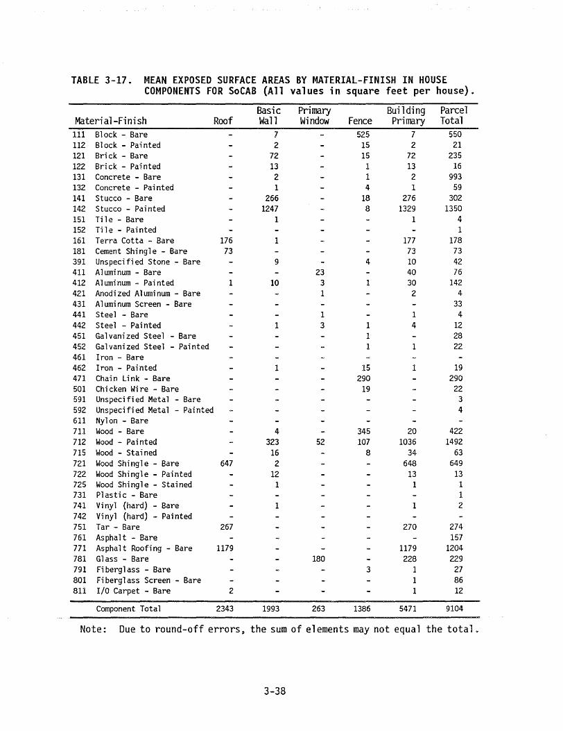
bull Total exposed material surfaces associated with SFRs in the SoCAB are estimated to be 20 bi 11 ion ft2 of which the most common material-finish is painted wood (16 percent) followed by painted stucco (15 percent) bare asphalt (13 percent) bare concrete (11 percent) bare wood shingle (7 percent) and bare block 6 percent)o
bull Basin total painted surface is estimated to be 71 billion ft2 of which the preponderant material is wood (47 percent) followed by stucco (43 percent) aluminum (5 percent and concrete (2 percent)
1202 NSFR Survey Findings
bull Out of 3855 tax assessor mapbooks over the SoCAB 30 mapbooks were selected representing sites to be examined using the aerial photographic method (hereafter called airphoto method) Of the 30 mapbooks 20 were in Los Angeles County and 10 in Composite County
1-4
which consists of Orange County and SoCAB portions of Riverside and San Bernardino County
bull Using the Enviro-Pod camera system mounted on a light aircraft a tota1 of 2000 1ow altitude ob1 i que photographs were taken and analyzed to evaluate exposed material surfaces of NSFRs in the 30 mapbook areas
bull Of 12235 NSFR parcels contained in the 30 mapbooks in the parcel file phase 6348 parcels were analyzed with respect to building height and size and ground cover materials In the building file phase 1429 parcels selected from those in the parcel file were analyzed in detail using low altitude oblique airphotos and cadastral maps
bull Among the eight NSFR use-types (SMFR LMFR RCOND SNR LNR MJR UNK VAC) examined for Los Angeles County VAC exhibited the highest proportion (53 percent) of parcels without buildings followed by SNR with 39 percent The average percentage of no-building parcels in Los Ange1 es County is 9 5 percent In Composite County such no-building parcels account for 27 percent of all NSFR parcels with the three highest percentages 87 for VAC 49 for UNK and 29 for AGR
bull For parce 1 s with bui 1 dings the construction type of dominant bui 1 ding in each parcel was identified wooden post lintel (Wood) masonry (Masonry) concrete (Concrete) or steel reinforced frame (Frame) 11 Wood 11 is the most numerous accounting for 64 percent and 69 percent respectively in Los Angeles and Composite Counties Frame is the 1 east numerous composing on1 y 6 percent and 2 percent of NSFR parce 1 s in Los Angeles and Composite Counties
bull In terms of floor space per parcel 11 Wood 11 is the smallest having 7200 ft2 and 13000 ft2 in the two counties whereas 11 Frame 11 is the 1 argest (46000 ft2) in Los Ange1es County and 11 Concrete 11 is the largest (33000 ft2) in Composite County
bull Compared to SFRs NSFRs have considerably greater exposed material surfaces except for VAC and MH whose surface areas are smaller than the SFRs 9100 ft2 41000 ft2 for MJR to 14000 ft2 for SMFR in Los Angeles County and 41000 ft2 for UNK to 17000 ft2 for RCOND in Composite County
bull The mean exposed surface of NSFR parce 1 s in Composite County is considerably greater than that for Los Angeles County 27000 ft2 vs 18000 ft2 In Composite County ground cover accounts for the most (10050 ft2) followed by Roof 8900 ft2) and Wall (7100 ft2) In Los Ange 1es County Roof accounts for the most (7000 ft2) fa11 owed by Ground Cover (5700 ft2) and Wall (5200 ft2)
bull In the SoCAB the total number of NSFR parcels with buildings is estimated to be 810000 Basin total exposed surfaces of these NSFRs are estimated to be 145 billion ft2 as compared to 205 billion ft2 for all SFRs NSFRs in Los Angeles County have 84 billion ft2 and those in Composite County 61 billion ft2
1-5
bull The preponderant materi a 1 s are aspha 1 t roofing (35 percent25 percent in Los Angeles and Composite Counties) bare asphalt (1828) painted stucco (1414) and bare concrete (148)
123 INFRASTRUCTURE FINDINGS
bull Materials associated with highways and other infrastructures such as railroads~ channelized waterways and power transmissiondistribution networks were estimated from the number of material-bearing items in those infrastructure facilities and the material factors which were determined by taking detailed measurements on a few typical items of each type
bull The numbers of materi a 1-beari ng items for surface streets were estimated by conducting a special street survey for a total of 47 survey routes covering 282 miles whereas those for state highways were obtained from CALTRANS local district office in Los Angeles
bull In the SoCAB the total exposed material surfaces (excluding road surface) associated with highways are estimated to be lo6 billion ft2 of which the predominant materials is concrete (87 percent) and The rest are unspecified meta1 ( 6 percent) chain link fence ( 5 percent) galvanized steel (1 percent) and steel (Oo6 percent)o
bull The total exposed material surfaces associated with other i nfrastrucshytures are estimated to be 006 billion ft2~ of which the predominant materials are bare wood (48 percent) and concrete (26 percent)o The remain_ing materials are galvanized steel (13 percent) chain link fence (8 percent) and steel (5 percent)
1-6
20 OUTLINE OF STUDY APPROACH
Prior to the present study several material inventory studies have been conducted in the US Northeast and Midwest Canada and the SoCAB Al though each contributed significantly to the development of materials inventory methodology these earlier studies invariably failed to produce a reliable comprehensive inventory of materials-in-place By incorporating lessons from the failures of the earlier studies this study has advanced the state-of-the-art inventory methodology so as to generate a reliable comprehensive inventory of materials-in-place in the SoCAB
This section critically reviews earlier inventory studies and then discusses the sampling frames survey designs and measurement schemes which were used for quantifying materials associated with single family residences (SFRs) non-single family residences (NSFRs) including all types of buildings other than those inSFR parcels and infrastructures (IRs) including roads railroads power distribution systems and channelized waterways
21 REVIEW OF EARLIER STUDIES
While the science of corrosion and other material damage processes has been developed over many years the materials inventory question has received detailed and systematic study only recently Among studies conducted since the late seventies the following paragraphs outline the five major studies on materials inventory
EPA Study McFadden and Koontz (1980) made the first systematic study of materials inventory They used as the primary data source fire insurance maps covering the study area Unfortunately these maps appear to have been outdated leading to unreliable estimates and probably gross under-estimates of the most sensitive but sparsely distributed materials such as galvanized steel and marble
EPRI Study For the Greater Boston area Stankunas et al (1983) used small (100 ft x 100 ft) land area samples which intersected building boundaries Unfortunately they worked with an unstratified sample creating excessive variance and many vacant sites (49) having zero material content
2-1
Accardi ng to Daum and Li pferd 1984) who reanalyzed the study data the results were incorrectly extrapolated to apply to the entire metropolitan area
ARB Study Murray et al (1985) attempted an inventory in SoCAB but had difficulties with i nsuffi ci ent fie1d observations and thus with the subsequent extrapolation However this work did generate the semi na1
suggestion of using census-tract-average building age and family income as predictor variables for residential housing materials
CANADIAN Study The Leman Group (1985) carried out a pilot inventory effort in Toronto using land area as an extrapolation basis The study utilized aerial photographs in developing a gridded urban terrain map and paid special attention to architectural details for NSFR buildings However the statistical basis for themiddotir approach has not been verified nor have any sampling or extrapolation errors been estimated
NAPAP Study Merry and LaPotin (1985) carried out a series of building surveys for two New England cities (Portland and New Haven) and two midwest cities (Pittsburgh and Cincinnati) Their surveys were based on the use of a stratified systematic unaligned random sample using strata defined on the basis of both USGS land use categories and census data (Rosenfield 1984 and 1985) However as the 1985 NAPAP Assessment developed it became apparent that a building-count basis was preferable to a land area basis for extrapolating to unsampled areas (Daum et al 1986)
This review of the earlier studies indicates that there is yet no established methodology that can adequately treat all important aspects of surveying mapping and extrapolating materials-in-place to a large geographshyical region like SoCAB The methods based on pre-existing data like census housing statistics and fire insurance maps suffer from the fact that these data do not cover the entire population of buildings and other important structures On the other hand the methods based on footprints (land-area samples) suffer from the inefficiency associated with many empty cells if the footprints are small and from sampling bias associated with multiple buildings in a cell if large footprints are used Furthermore results of the land-based survey cannot be readily extrapolated to unsampled areaso
2-2
22 PRESENT STUDY APPROACH
A deficiency of all the studies reviewed above appears to lie in the weakness of the sampling frames on which the survey designs and measurement schemes were based This deficiency probably resulted from optimistic assumptions regarding their survey designs and measurement schemes For example the NAPAP study (Merry and LaPotin 1985) assumed that materials found within a sample of randomly placed footprints would provide both a representative mix and representative quantities of different materials in place However it was found that such an assumption was unsupported by the survey data they gathered Later their land-based data were converted into building-related data in order to allow for extrapolation to the study region (Daum et al 1986)
Another deficiency lies in the incompleteness of their observational data For example Murray et al (1985)surveyed 90 houses in the SoCAB by taking pictures of only the fronts of their houses then generated observational data of materials-in-place based on the pictures and field notes taken at the sites No on-site measurements were taken except the distance between the photographers position and the house Deducing from the pictures both dimensions of and materials present at various components of the house is quite imprecise particularly for unseen areas like the back of the house and structures in the backyard
By learning from the deficiencies and shortcomings of earlier materials inventory studies this study has focused its efforts on the following three areas
Sampling Frame Since materials are present as a part of a facility containing them rather than by themselves we define separate frames for different types of facilities namely SFRs NSFRs and Infrastrucshytures
Survey Design For the three sampling frames separate surveys are designed in a rigorous manner so that a representative sample is drawn from each sampling frame and
Measurement System Recognizing known limitations of quantifying and characterizing materi a 1s-i n-p1ace the most appropriate measurement system is devised for each concei vab1e assemb1age of material s-i n-p lace
2-3
More detailed discussions of each of the above three areas are given in subsections that follow
221 SAMPLING FRAME
Success in any survey-oriented study depends 1 a rge 1 y on a proper definition of the sampling frame for the survey The NAPAP study (Merry and LaPotin 1985) used a land area as the sampling frame that is a unit of land area which they called a footprint was considered as a basic sampling unit and was selected in a random manner from the entire study area This study area was divided into a few sub-areas having a similar housing density Unfortunatelyi the amounts of materials found in a footprint are not readily comparab1 e to quantities and types of materials associated with common facilities like houses and roads for which reliable statistics are available
The previous ARB study (Murray et al 1985) used census tracts of the Census of Housing as the samp1 i ng frame Unfortunately the census data relate to housing units and not buildings Furthermore they do not include non-residential buildings Since most data on materials are associated with buildings rather than with housing units the census data do not provide a good sampling frame for this study
For these reasons the authors sought a better sampling frame to be used for this study After reviewing various data sources it was found that land parcels used in tax assessor records have better attributes as a sampling frame for surveying SFRs and NSFRs than other known data sources In particular tax assessor records have the following desirable attributes
All-Inclusive Sampling Frame All buildings and structures except those associated with infrastructures belong to certain land parcels uniquely Thus the records provide all-inclusive sampling frames for materials associated with SFRs and NSFRs
Readily Available Data Bases All four counties composing the SoCAB have computerized data bases of tax assessor records and make them available for public useo Similar availability is expected in other metropolitan areas in Californiao
2-4
Ready Population Characteristics Assessor records provide not only counts of SFRs and NSFRs but also types of SFRs and NSFRs and in some cases (eg Los Angeles County) physical dimensions and age of buildings (ie year built) Therefore they can be used to elaborate a survey design for SFR and NSFR surveys
Because of these attributes this study used tax assessor records of the four counties as a sampling frame for both SFR and NSFR surveys which were conducted under this study
222 SURVEY DESIGN
VRC purchased a full assessor data base from each of the four counties composing the SoCAB Los Angeles Orange Riverside and San Bernardino In total 74 volumes of 2400-foot magnetic tapes containing over 3 million assessor records were subjected to data processing Since data formats and parcel classification schemes differ somewhat from one county to another a series of data cornpacti on and standardization operations were performed on the ori gi nal assessor records so as to obtain a manageable and inter-comparable data base for this study (see Interim Report by Horie and Shrope (1987) for more detailed discussion)
Three major data files were created from the tax assessor data bases
Mapbook-Stat All land parcel records in the assessor data base were classified into a few VRC-defined use categories and then reduced to summary statistics of parcel counts by use category at mapbook level (Every assessor record is identified by mapbook page number and parcel number)
SFR Mini-Universe A systematic IO-percent sampling of all SFR parcels was made to create SFR Mini -Uni verse This mini -uni verse carries detailed data on every sampled SFR including the owners name the street address the city the year built (Los Angeles County only) the total livable space (Los Angeles County only) and the full parcel identification number (hereafter called parcel ID) and
NSFR Full-Universe Some 300 data items of each NSFR parcel record in the assessor data base were reduced to only two data items parcel ID and VRC-defined use type A full universe of NSFRs in the SoCAB is retained in this file by the two data items
( Table 2-1 presents summary counts of mapbooks and parcels by use type
in the SoCAB The number of parcels in each county is already adjusted to
2-5
the SoCAB portion of that county Use types in the table are
SFR
MFR SMFR LMFR
RCOND NR
SNR LNR MJR
MH AGR VAC UNK
=
= = = = = = = = = = = =
Single family residential parcel (single detached house and duplex)Multi-family residential parcel (triRlex or more units)Small MFR that includes triplex and fourplexLar9e MFR that includes parcels of 5 or more unitsRes1dential condominiumNon-residential parcelSmall NR such as service stations nurseries parking lots etcoLarge NR that includes balance of NR excluding those found in SNRMajor properties identified by Los Angeles tax assessor office Mobile homeAgricultural parcelVacant lotParee1 with unknown use
TABLE 2-1 NUMBER OF MAPBOOKS AND PARCELS BY USE TYPE IN EACH COUNTY OF THE SoCAB (as of June 1 1986)
Use San Type Los Angeles Orange Riverside Bernardino SoCAB
Mapbooks SFR
2942 1414872
344 434013
388 159827
231 240278
3905 2248990
MFR 129000 26152 2658 5711 168521 SMFR LMFR RCOND NR SNR LNR MJR MH
f67954~61246 41559
167825 25559l
(119604 (22662 55000
20~267 38685
3884
735 8570
24839
4718 25859
681
67279 240939
84404 AGR VAC
0 126680
526 38782
9757 92952
2597 73884
12880 332298
UNK 3027 110 6609 1051 10797
Total 1937963 562419 305947 354779 3161108 Percent of SoCAB 613 1L8 97 112 100
Note Numerals in parenthesis are of sub-categories used only for Los Angeles County Residential condominiums which had the same street address and were listed consecutively in the Los Angeles county assessor data base were reduced to a single parcel This process yielded 39 condominium units per a colffilon parcel This correction factor was applied to condominiums in the other three counties as well
All agricultural type parcels in Los Angeles County are included in SNR category
Mobile homes are not assigned parcel numbers in the assessor data base These counts were obtained either from assessor office or from buried-in records in the assessor data base they represent mobile homes and IlQ1 assessed parcels
2-6
According to the table there are 316 million parcels in the SoCAB of which 225 million parcels (71) are SFRs The balance is 091 million NSFRs which consist of various parcel uses such as multi-dwelling units (MFRs and RCONDs) non-residential parcels (NRs) mobile homes (MHs) and vacant parcels (VACs parcels for new development renewal or simply idled lots) A few parcels are for agricultural (AGR) and unknown (UNK) uses
Among the four counties constituting the SoCAB Los Angeles County accounts for 61 percent of the basin total followed by the counties of Orange (18) San Bernardino (11) and Riverside (10) Since Los Angeles County data are more detailed in use type than those of other counties both SFR and NSFR surveys were designed and implemented separately for Los Angeles and for the other three counties Hereinafter the three counties are collectively designated as Composite County
2221 SFR Survey Design
Although the population (in a statistical sense) of SFRs is much greater than the NSFR population the former is expected to be more homogeneous in both building sizes and construction materials than the latter Based on this assumption the smaller number of survey samples was assigned to SFRs rather than NSFRs On the other hand higher accuracy in both identifying the types and determining the amounts of exterior materials was sought for SFRs than for NSFRs As discussed in Section 223 - Measurement System it was considered that accurate measurements can not be expected in a SFR field survey without physically entering each target property after first obtaining permission from the owner or occupant of the property To ensure obtaining permission from a11 fie 1d survey houses a screening survey ( a telephone questionnaire on building features) was applied to the greater number of houses prior to the field survey Another purpose of this questionnaire survey was to ensure that houses used for the field survey were indeed representative of the SFR population
A two-stage stratified random sampling method was applied separately to the SFR populations of Los Angeles County and of Composite County Since the SFR universe of 235 million parcels was too large to be handled effectively the SFR Mini-Universe consisting of 141000 records for Los
2-7
Angeles County and 84000 records for Composite County was used to select survey samples To take advantage of both the higher cost effectiveness associated with questionnaire surveys and the higher accuracy associated with field surveys VRC decided first to conduct a telephone questionnaire survey for 1200 randomly selected houses and then to do a field survey for 200 houses which would be a subset of the 1200 surveyed houses
By analyzing SFR records of Los Angeles County which contain data on year built and total livable spaceu distributions of SFRs with respect to house size and age were examined so as to determine an appropriate stratification of the SFR population This analysis and our general knowledge of house sizes and construction materials led to the eleven SFR strata as presented in Table 2-20
TABLE 2-2 NUMBER OF SAMPLES ALLOCATED TO EACH OF THE 13 STRATA USED FOR QUESTIONNAIRE AND FIELD SURVEYS
Percent Samples Samples County Tine House Size Parcels of Basin in in Stratum Period in Sq Ft in 1000 Total T Survey Fe Survey
Los Angeles County ls415 629 755 126 1 OLD-Smal l lt1946 lt1000 129 57 69 12
2 OLD-Medium lt1946 1001-2000 185 82 99 16
3 OLD-Large lt1946 gt2000 129 57 69 12
4 MED-Small 1946-1964 lt1000 113 5 0 60 10
5 MED-Medium 1946-1964 1001-2000 373 166 199 33
60 MED-Large 1946-1964 gt2000 275 122 146 24
7 NEW-Smal 1 1965-1986 lt2000 118 53 63 11
8 NEW-Large 1965-1986 gt2000 93 41 50 8
ComQosite Countl 834 371 445 74 9 Orange all year all sizes 434 193 232 39
10 Riverside all year all sizes 160 71 85 14
11 San Bernardino all year all sizes 240 107 128 21
200SoCAB Total 2249 100 1200
2-8
SFRs in Los Angeles County were first classified into three time periods OLD (pre-1946) MED (1946-1964) and NEW (post-1964) These periods were considered to coincide with times around which major changes in construction methods or materials took place
The number of houses built during the MED period is by far the largest among the three periods ( see Table 2-2) bull This is in agreement with our knowledge of the great housing boom in the fifties It is apparent that the average size of pre-1946 SFRs is quite small (around 1200 square feet) whereas that of post-1964 SFRs is considerably larger (around 1900 square feet) Because of this trend toward larger houses in recent years only two size categories are used for the post-1964 period 2000 square feet or less and over 2000 square feet
Assessor records in Orange Riverside and San Bernardi no counties include neither year built nor total livable feet Therefore all SFRs in each of these counties are grouped to form their own stratum SFRs in Los Angeles County are grouped into 8 strata according to their age and size whereas those in Composite County were grouped into 3 strata according to their counties In total 11 strata are used for conducting both the telephone questionnaire survey of 1200 SFRs and the field survey of 200 SFRs
2222 NSFR Survey Design
Unlike SFR records in Los Angeles County assessor records for NSFRs do not provide either age or size data for the NSFR parcels in any county In addition NSFRs are more variable than SFRs in size and types of construction materials Therefore to quantify materials associated with NSFRs data gathering efforts must take precedence over analysis of existing data However conventional field and questionnaire survey methods do not seem likely to meet the increased data needs at an affordable cost
In this study a remote sensing technique called airphoto analysis has been applied to gather NSFR data at an affordable cost Ai rphoto analysis is a subjective technique evolved through military applications From photographs taken at various altitudes and angles an experienced photo-analyst interprets the image of each designated object to estimate its
2-9
physical dimensions structural characteristics and the types and amounts of materials used in their exterior surfaces
Initially VRC considered selecting 30 study sites of approximately 1 square kilometer each for airphoto analysisc However 30 mapbook areas were used instead because exact counts of NSFRs by use category are avai lab middot1 e at mapbook level (through Mapbook-Stat file which has been generated from the assessor data bases) Since there are 2942 and 963 mapbooks respectively in Los Angeles and Composite Counties an optimal selection of 30 mapbooks is not a simple task
To ensure that NSFRs in the sample would be representative of the NSFR population in the SoCAB the following criteria were considered in selecting 30 mapbooks
l The number of NSFR parce1s in the sample shou1d be as 1arge as possible
2 Use-type mix in the samp1e should resemble that of the NSFR population
3o Selection of the sample should be made as objectively as possible and
4o The sample so selected must be reasonable and practical for airphoto work
Since parcel use categories in the Los Angeles County assessor data are more numerous and specific than those of the Composite County data selections of rnapbooks for Los Angeles and Composite counties were made separatemiddotly 20 mapbooks from Los Angel es County and 10 mapbooks from Composite County o
However the same methodo1ogy was app1i ed to se1ect mapbooks for the two sub-regi ans The methodology used is rather complex and is described in detail in the interim report (Horie and Shrope 1987) In essence a combination of objective and subjective selection methods was devised and employed The objective selections were made using the following three performance indices to evaluate 6000 sets of 20 (for Los Angeles) or 10 (for Composite) randomly selected mapbooks
2-10
Pllmiddot = SUMk Pkj PklJ
PI2middot = SUMk Pkj Pk PkJ
PI3 middot = SUMk Pkj Pk (wknkj)J
where Pk = proportion of parcels with the k-th use type
Pkj = proportion of parcels with the k-th use type in the j-th set
nkj = the number of parcels with the k-th use type in the j-th set and
Wk = the weight for the exterior surface of the k-th use type (1 for SMFR 3 for LMFR and RCOND 2 for SNR 4 for LNR and 6 for MJR)
In determining the best set for the aerial photography mission the following steps were taken
STEP 1 - Selection of NSFR-Rich Mapbooks Mapbooks in Los Angles County were ranked according to proportion of NSFR parcels in the mapbook whereas those in Composite County were ranked according to the number of NSFR parcels in the mapbook Then only the highest-ranking mapbooks were considered for selection This screening reduced the number of mapbooks for consideration from 2942 to 886 in Los Angeles County and from 963 to 262 in Composite County (The reason for using different screening criteria for the two sub-regions is that while Los Angeles County mapbooks contain similar numbers of land parcels about 1000) mapbooks in Composite County vary greatly in their numbers of land parcels
STEP 2 - Evaluation of Sample Sets of 20 and 10 Mapbooks A total of 6000 sets of 20 (or 10 for Composite County) mapbooks were generated using three different sampling methods simple random sampling stratified random sampling and weight-stratified random samp1i ng Then these sets were ranked in three different ways according to values of three different performance indices which are all designed to measure the closeness of use-type mix (excluding vacant and unknown-use parcels) in the set to that of the NSFR population in the subregion
2-11
STEP 3 - Selection of Candidate Sets The fifty top-ranked sets in each of the three performance indices were listed for all three sampling methods for closer scrutinyo (The top fifty sets selected by the simple random sampling method were considerably different from those by the stratified random sampling method whereas those by the second and third methods are rather similar to each other) After visual scrutiny of these high-ranked sets 18 sets which ranked consistently high in all indices and all sampling methods were selected as candidate sets for Los Angeles County Similarly 14 sets ranked consistently high were selected as candidate sets for Composite County
STEP 4 - Final Determination of Study Sets for Los Angeles and Composite Counties Noteworthy features of each mapbook included in the candidate sets were identified by examining aerial at1ases of Los Ange1es and Orange counties Thomas Bros maps with mapbook boundaries on them and the numbers and use types of NSFR parcelso These identified features were then summarized for each randidate set as indicated in Table 2-30 (A similar table was prepared for Composite County as wello) For mapbooks in Riverside and San Bernardino counties for which an aerial atlas was unavailable VRC staff physically visited the mapbook areas and evaluated their appropriateness as study sites By reviewing the summary tables and other evaluation materials the authors and two ARB scientists jointly selected Set 1549 to be a study set for Los Angeles County and Set 2533 to be a study set for Composite Countyo
In this final determination step the following desirable features and undesirable features of each candidate set were subjectively evaluated
Desirable Features
bull The number of NSFR parcels is large
bull The number of LNR and MJR parcels is large
bull the set contains at least one major central business district (CBO)o
bull The set contains at least one regional commercial centero
bull The set contains at least one major shopping center
Undesirable
bull The set contains a large institution like university and governmentalcomplexe
bull The set contains excessive open space like preservation area and undeveloped land area
bull The set contains a major transportation center like airport rail head and harbor
2-12
TABLE 2-3 SUMMARY FEATURES OF 18 CANDIDATE SETS FOR LOS ANGELES COUNTY
Method Rank Set Number by PI
1-2-3
Number of LNRs
NSFRs amp MAJs
LA CBD
Number of Mapbooks inwith
Other Regional Shopping Large Excessive CBD Commercial Center Institu- Open
Core tions Space
Trans-portationCenter
Restricted Airspace
METHOD 1 Simple Random Sampling 1713
730 149 83
128 465
1-2-8 2-1-1 3-3-4 6-4-5 10-5-2 9-22-4
4417 ~539 4732 4133 5310 5286
1862 2324 1905 1707 2131 2309
1 0 0 0 1 1
1 2 0 1 0 2
2 0 4 1 4 1
0 1 1 0 1 0
1 0 2 0 0 0
1 1 1 1 3 3
2 1 0 1 l 0
0 2 0 2 0 1
N I
w
METHOD 2
1492 1817 1345 571
1272 710
Stratified Random Sampling
1-2-2 5263 2216 1 2-1-1 5408 2146 0 8-6-3 5419 2267 0
3-10-17 5372 2191 0 14-4-8 5638 2257 0
5-15-12 5571 2303 0
1 2 1 1 3 1
5 2 2 1 1 2
0 0 1 0 0 0
1 0 0 1 1 1
3 1 1 1 3 2
2 0 0 0 0 2
4 0 0 0 1 1
METHOD 3 Weighted Stratified Random Sampling 187
1549 1038 1124 1698 1634
1-1-1 2-2-8 3-3-2 5-9-5 7-4-13 12-20-3
6109 5910 5619 6037 5972 5760
2541 2533 2255 2570 2433 2348
0 0 0 0 0 0
0 1 1 1 2 0
3 1 2 4 4 4
1 0 1 1 1 1
0 0 0 1 0 0
1 0 2 0 1 1
2 0 2 0 0 1
3 0 4 1 0 1
Performance indices This set was selected as the study set for Los Angeles County
bull The set extends over restricted airspace where airphoto flights can not be made
Considering these des i rab 1 e and undes i rab 1 e f eatures a11 candi date sets except Set 1549 were eliminated A similar screening method was applied to candidate sets for Composite County before deciding on mapbooks of Set 2533 as study sites
Table 2-4 presents the numbers and types of land parcels in the study set and those in Los Angeles County As seen from this table the use-type mix in the study set is in exce11 ent agreement with that of Los Ange1 es County
It should also be noted that the proportion of NSFR use-types to the total number of land parcels in the set is considerably higher than that of Los Angeles County as a whole (42 vso 18)0 Since land parcels of vacant (VAC) and unknown use (UNK) were assumed to contain little material with economic significance these parcel types were not taken into account in this survey design However materials in these parcels are taken into account both in actual survey and analysis phaseso
Table 2-5 presents a similar land parcel summary for the study set for Composite County In selecting this study set minor use-types of mobile home (MH) and agriculture (AGR) as well as VAC and UNK were not consideredo These use-types appear to be treated somewhat differently from one county to another Here again the use-type mix of the study set is in exce11 ent agreement with that of entire Composite Countyo
2-14
TABLE 2-4 NUMBERS AND TYPES OF LAND PARCELS IN THE NSFR STUDY SET (1549) AND IN LOS ANGELES COUNTY
Sub- Total Mapbook SMFR LMFR RCOND SNR LNR MJR total Parcels
2321 57 114 6 15 99 5 296 632 2353 110 141 23 9 125 6 414 847 4016 72 106 11 13 109 8 319 536 4135 62 56 1 20 51 145 335 569 4252 90 172 8 7 61 6 344 1083 4337 57 65 19 14 133 4 292 744 5189 29 14 0 5 59 1 108 360 5283 71 4 0 10 94 2 181 646 5695 52 30 14 16 37 22 171 430 5746 63 48 13 43 156 13 336 692 5807 100 57 17 7 101 14 296 707 6102 4 0 0 52 235 3 294 359 6132 10 10 0 69 235 28 352 902 6251 45 48 0 24 62 5 184 716 7101 29 15 113 5 30 0 192 798 7271 40 61 0 29 15 144 289 385 8026 67 6 12 23 157 6 271 1007 8104 48 42 2 27 102 3 224 523 8139 74 83 7 51 215 33 463 647 8743 0 4 531 5 9 0 549 1357
Set Total 1080 1076 777 444 2085 448 5910 13958 Set Mix 183 182 132 075 353 076 100
LA Total 68 61 42 26 120 23 340 1885 LA Mix 200 179 124 076 353 068 100
All values in thousands
This total does not include 55000 mobile homes which are not contained in the assessor data base
2-15
TABLE 2-5 NUMBERS AND TYPES OF LAND PARCELS IN NSFR STUDY SET (2533) AND IN COMPOSITE COUNTY
Sub- Total CountyMapbook MFR RCOND NR total Parcels
OR 22 112 18 218 348 1798
OR 70 139 65 266 470 3855
OR 84 179 173 313 665 3859
OR 129 125 113 67 305 1402
OR 133 157 8 140 305 2159
OR 298 80 109 150 339 859
RV 219 69 9 41 119 1106
SB 141 21 10 415 446 1586
SB 154 89 26 149 264 3156
SB 1011 26 225 362 613 1654
Set Total 997 756 2121 3874 21434
Set Mix e257 195 548 LOO
Orange 262 203 387 852 5625
Riverside 27 7 86 120 3060
San Bernardino 57 47 259 363 3549
Composite Total 346 257 732 1335 12234
Composite Mix 0259 193 548 100
All values in hundreds
2223 Infrastructure Survey Design
Economically significant materials exposed to ambient air are found not only in SFRs and NSFRs but also in infrastructures such as highways surface streets power distribution networks channelized waterways and railroadso Unlike materials associated with buildings many of the materials found in infrastructures occur principally in repetitive standard forms and spaced at regular intervals as in light standards along streets and highwayso
2-16
Therefore surveys for infrastructures focused on quantifying both infrastructure facilities by type and materials and material-bearing items associated with each type
Basinwide miles of various types of roads are compiled in Table 2-6 using the statistics presented in the Highway Performance Monitoring System (HPMS) data summary (CALTRANS 1984) In the table road miles in the SoCAB portion of each county are estimated by applying estimated urban and rural fractions to the reported road miles for that county
For state highways which are under CALTRANS 1 jurisdiction no survey was necessary because re 1 i ab1 e counts of materi a 1-beari ng items (eg freeway signs and light poles) were available from the CALTRANS District 7 in Los Angeles However counts of material-bearing items on surface streets are not readily available Therefore a special street survey was designed to obtain data on such materi a 1-beari ng i terns for various types of surface streets The numbers of survey routes selected for each road type are indicated in Table 2-6 The largest number of survey routes is needed for urban local streets for two reasons
1 The road miles of urban local are by far the greatest among all road types and
2 A survey route for urban local can be only 1 to 2 miles long in a continuous stretch while those for arterials and collectors can be 5 to 50 miles long
As indicated the in the table a total of 47 survey routes were selected for five different road types 3 for pri nci pa1 arterial 3 for mi nor arterial 10 for urban collector 30 for urban local and 1 for rural collector No survey was done for rural local because the number of material-bearing items to be found there was not expected to be significant Although the number of survey routes differs from one road type to another it was planned that the cumulative total miles of the survey routes would be in the range of 30 to 60 miles for each road type to be surveyed
2-17
TABLE 2-6 TOTAL MILES OF ROAD BY TYPE IN EACH COUNTY AND NUMBER OF SELECTED SURVEY ROUTES FOR EACH ROAD TYPE (After CALTRANS 1983)
Road Type Los Angelesa Orangeh Riversidec San Bernardinod SoCAB
State Highwar
Princi pal Arterial
Mi nor Arterial
Urban Collector
Urban Local
Rural Collectorf
Rural Local
457
2211 (2)
1929 (1)
2015 7)
10516 10)
139
225
163
579 (1)
606 (1)
347 (1)
3274 (9)
72
231
332
129
267
278 (1)
1443 (5)
649 (1)
1156
180
280
507 (1)
410 (1)
1984 (6)
155
299
1132
3199 (3)
3309 (3)
3050 (10)
17217 (30)
1015 (1)
1911
Total 17492 5272 4250 3815 30829 (20) (12) (7) (8) (47)
Note Numerals in parenthesis indicate the number of se 1 ected survey routes
a Include 100 of urban road and 10 of rural road
b Include 100 of urban road and 100 of rural road
c Include 90 of urban road and 50 of rural road
d Include 90 of urban road and 10 of rural road
e Include urban interstate and other freeway and rural interstate principal arterial and minor arterialo
f Include major collector and minor collectoro
2-18
For other infrastructures such as power distribution networks railroads and channelized waterways no systematic survey was conducted Instead the numbers of material-bearing items in these infrastructures were estimated by indirect methods such as contacting a data source organization and reading an appropriate map showing locations of such infrastructures
223 MEASUREMENT SYSTEM
To develop a reliable inventory of materials-in-place requires accurate inventories of facilities by type and of the types and amounts of materials in those facilities Using the tax assessor data bases as previously explained VRC determined the sizes and characteristics of the statistical populations of SFRs and NSFRs and to a lesser degree of state highways and surface streets In the NAPAP study (Merry and LaPotin 1985) these facility populations were estimated from survey results whereas in the previous ARB study (Murray et al 1985) a surrogate population of housing units was used instead
There are so many types of materi a 1 s and materi a 1-beari ng items in various facilities that no single method of measurement can be used effectively in quantifying materials-in-place under all situations Therefore a cogent measurement system was needed for effectively classifying and quantifying materials found in surveyed facilities Since none of the earlier studies produced such a system VRC developed a completely new measurement system
Full specification determinations
of materials-in-place requires the following
(i) material type
(ii) surface finish
(iii) dimensions of exposed surfaces
(iv) building component in which the materials are found
(v) facility in which the materials are found
To make such determinations for even a single window may require over 100 measurements of dimensions of numerous elements such as window casings
2-19
frames panes seal ants screens screen frames splines security bars awning shades and awning supports It was impractical to make such detailed measurements repetitively for each element of a11 surveyed facilities Instead this study devised a measurement system that enabled us to determine types and amounts of material s-i n-pmiddot1 ace with satisfactory accuracy in an efficient mannero
Under this system materials-in-place are first classified according to the types of material-bearing elements or items
Primary Element - For primary elements such as basic sections of wall roof ground cover and fence and gross surfaces of window door chimney etc both the dimensions and material types are determined either by on-site measurements (for SFRs) or remote sensing techniques (for NSFRs) bull Secondary Element - For secondary elements such as gutters~ window frames~ window ~anes window screens window screen frames security door frames etco the quantities of identified materials are calculated from the dimensions of corresponding primary elements (eg window frame and pane from the dimension of window casing) according to a formula which VRC derived from test cases Enumeration Item-middot Enumeration items such as air conditioning units antennas sky lights light poles street signs etc are first c1ass i fi ed into proper categories and then ta11 i ed The types and amounts of materials contained in a given category of enumeration items are computed using the standard material factors for that category which VRC derived from test cases
For primary elements both identification of material-finishes and actual measurements of all dimensions are implemented rigorously We spurn any guessing in favor of actual identification of material type and actual measurements of a11 key dimensions of each e1ement either by direct inspection or by examining a photographic image In both the NAPAP study and the ARB study the field work involved some degree of guesswork primarily because the field surveyors never entered the property being surveyed o This procedure can leave many materials undetected especially in backyardso
In this study all surveyed SFRs were observed by field surveyors who physically inspected both front and rear aspects of the properties after obtaining permission from the owners or residentso From a pilot study it became evident that any guessing regarding unseen sides of the property
2-20
introduced unacceptable errors in identifying the types of material present and in quantifying the areas of their exposed surfaces
For secondary elements such as those found in windows our efforts were focused on i dent i fyi ng the types of materials used rather than taking detailed masurements of the minute dimensions of all the substructures The reasons for omitting detailed measurements of such secondary elements are twofold
1 Avoiding routine repetitive measurements of many identical subshystructure elements allows field surveyors to focus their efforts on recording key dimensions of buildings and other essential features of the property and on identifying material types present in both primary and secondary elements and
2 The field survey of a target house can thus be completed in an expedient manner normally less than 2 hours
The second reason was important for this study because particularly in a large metropolitan area like the SoCAB property owners do not like to leave their houses while strangers are taking measurements
Simple enumeration without on-site measurement of similar or identical items such as air conditioning units and light poles also speeds up a material inventory survey More important many enumeration items can not be measured accurately in a routine survey activity For example antennas on rooftops or light poles can not be easily accessed for detailed measurements during a casual visit For enumeration items VRC measured in detail for a few test cases (usually 2 to 5) and considered the findings to be typical for observed but unmeasured items of the same type
2-21
30 SINGLE FAMILY RESIDENCES
31 GENERAL
Among al 1 use-types considered SFRs are by far the most numerous accounting for over two thirds of all land parcels in the SoCAB (see Table 2-1) Therefore to develop a reliable inventory of materials-in-place in the basin it is crucial to account accurately for all materials associated with the SFR population To ensure an accurate accounting VRC conducted two surveys
1 Telephone Questionnaire Survey of 1200 randomly selected SFRs and
2 Field Survey of 200 SFRs which were selected from those surveyed in 1
The purpose of the field survey was to make an accurate account of all types of materials present in surveyed SFR parcels while the primary purpose of the telephone questionnaire survey was to obtain a larger more representative sample of the SFR population
Section 32 of this report discusses the questionnaire survey while Section 33 describes all phases of the field survey protocol development survey execution and data reduction Section 34discusses analyses of the survey-generated data and presents predictive equations derived for materials associated with the SFR population
32 TELEPHONE QUESTIONNAIRE SURVEY
For the first time ever in material inventory studies VRC has used a telephone questionnaire survey as a means of gathering data on materi a 1s present in SFR parcels By taking advantage of the greater flexibility and cost effectiveness of the telephone questionnaire approach VRC has surveyed 1200 houses se1ected randomly from tax assessor records in four counties composing the SoCAB All earlier studies depended on field surveys of only a few hundred houses in any one study area Considering the great diversity in ages and configurations of existing buildings a sample of this magnitude appears to be necessary to ensure that the proportions of houses in the sample
3-1
having detached garages second stories fences and other noteworthy features are indeed representative of the SFR population
321 SAMPLE SELECTION FOR QUESTIONNAIRE SURVEY
From the SFR Mini -Uni verse which is a ten percent samp 1e of the basinwide SFR population an initial list of 10530 SFR owners was generated according to a stratified random sampling method Then using appropriate telephone directories telephone numbers were identified for 3823 of these households from the names and street addresses Telephone numbers of the remaining households could not be readily identified mainly because they were unlisted A smaller fraction of identified listings were unsuitable for the survey because of name-only listings corporate owners and owners who reside outside of the study region
A question was raised as to whether these unlisted phone numbers had introduced any significant bias into the sample To examine this potential bias due to unlisted phone numbers distributions of SFR sizes in each of three periods (pre-1946~ 1946-1964 post-1964) were computed separately for all houses and for houses with identified phone numbers in Los Angeles County for which year built and total livable space data are available
Table 3-1 presents comparisons of SFR size distributions in each period for houses with listed phone number versus all houses Frequency density va1ues of houses with phones and a11 houses in each size range are 31 in genera1
in reasonable agreement differences between them appear to be within a norma1
sample variation Therefore it was judged that use of SFRs with listed phone numbers would not cause any significant bias in the sample
In the table it should also be noted that medians for houses with listed phone numbers occurred in the same size ranges as those for all houses in three periods These coincidental occurrences of the two medians in the same size range may provide further evidence that the use of SFRs with listed phone numbers would not cause a significant bias in the survey sample As mentioned earlier a trend toward 1arger houses in recent years is exemplified in the shift of the medians from 1001-1500 square feet in Period 1 to 1251-1500 square feet in Period 2 and to 1751-2000 square feet in Period 3
3-2
TABLE 3-1 COMPARISON OF SFR SIZE DISTRIBUTIONS FOR HOUSES WITH LISTED PHONE NUMBERS VERSUS ALL HOUSES FOR THE SoCAB
Square Footage Pre-1946 wPhone All Houses
1946-1964 wPhone All Houses
1965-1986 wPhone All Houses
750 or Less 047 073 019 029 003 004
751 to 1000 171 218 081 120 011 016
1001 to 1250 279 254 227 261 046 055
1251 to 1500 146 164 247 229 127 146
1501 to 1750 116 096 172 159 165 177
1751 to 2000 069 064 095 082 154 156
2001 to 2500 085 059 097 074 281 234
2501 to 3000 034 030 040 028 124 122
3001 to 4000 040 028 021 014 078 071
4001 or More 014 014 002 004 011 016
Sample Size 656 2135 1323 3669 370 1016
---median for houses with 1 i sted phone numbers
--median for all houses
Table 3-2 provides the numbers of SFRs initially sampled houses with listed phone numbers and target number of complete interviews for each of the eleven strata The target numbers of complete interviews are calculated in proportion to each stratum I s share of the basi nwi de SFR population Los Angeles County accounts for 63 percent of the SFR population and Composite County for 37 percent Among the eight age-size strata in Los Ange1 es County MED-medium cell (ie medium sized SFRs of Period 2) gets the largest sample allocation 296 or 247 percent of the target total Among the three strata in Composite County Orange County cell gets the largest allocation 232 or 193 percent
3-3
TABLE 3-2 ALLOCATION OF SURVEY HOUSES TO LOS ANGELES AND COMPOSITE COUNTY STRATA FOR THE TELEPHONE QUESTIONNAIRE SURVEY
I SFRs TargetInitially Houses Percent of No of
CountyStratum Yr-Built Sq Ft Sampled wPhone Total Interviews
Los Angeles County 1o OLD-Sma11 Pre-1946 lt1000 621 143 57 69
2 OLD-Medium Pre-1946 1001-1500 892 279 802 99
3 OLD-Large Pre-1946 gt1500 622 234 57 69
4 MED-Smal 1 1946-1964 lt1000 546 132 50 60
5 MED-Medium 1946-1964 1001-1500 1797 627 166 199
6 MED-Large 1946-1964 gt1500 1326 564 122 146
7 NEW-Small 1965-1986 lt2000 566 187 5 3 63
80 NEW-Large 1965-1986 gt2000 450 183 4 1 50
Los Angeles Total 6820 2349 629 755
Comeosite Count~ 9 Orange all year all sizes 1930 817 l9o3 232
10 Riverside all year all sizes 710 293 7ol 85
IL San Bernardino all year all sizes 1070 364 107 128
Composite Total 3710 1474 371 445
Grand Total 10530 3823 1000 1200
3-4
Imiddot
322 QUESTIONNAIRE DESIGN AND TESTING
To elicit factual information regarding exterior materials at selected home sites VRC designed a questionnaire to be used in the telephone survey Wording and phrasing of the questions were carefully considered and reconsidered so as to avoid alarming respondents and to reassure them as to the legitimacy of the telephone contact thereby encouraging them to answer candidly Subjects covered by the questionnaire were the following
bull General Information including questions on livable square footage year built number of stories and type of garage
bull Roof including questions for main house and detached garage on roof material roof slope eaves rain gutters and downspouts the number and types of chimneys and other roof-attachments such as TV antennas skylights and evaporative coolers
bull Windows including questions for each side of the house on the number and type of windows window screens security bars awnings and window frame materials
bull Doors including questions for each side of the house on the number and type of doors door materials and screen doors
bull Walls including questions for house and garage on main wall materials on all sides except the front and on the garage door
bull Front wall including questions middoton the types of materials and their proportions in the front wall
bull Fence including questions on the types materials and dimensions of fences
bull Other items such as carport patios walkways pools spas and pool decks and presence or absence of outdoor accessories such as sheds gazebos satellite dishes and air conditioning units
Si nee telephone i ntervi ewi ng is more art than science only highly experienced telephone interviewers were allowed to conduct the interviews Ms Eve Fielder Director of the UCLAs Survey Research Center thoroughly briefed each interviewer as to the objectives and scope of the interviews Having a good understanding of the purpose of the questions being asked the interviewer could readily judge the reasonableness of each response and engage in clarifying dialogue to resolve awkward or unsound responses thereby enhancing the quality of the interview
3-5
I
VRC tested the survey questionnaire by conducting pilot surveys of single-family residences in Los Angeles County Results of the first round revealed the following
1 Of the 40 attempts
14 interviews were completed
10 refused (3 involved female interviewers while 7 were male)
1 interviewee terminated mid-way
7 had either disconnected telephones or wrong addresses and 8 non-connects
2 Male interviewers were less successful than their female countershyparts It seems likely that the male projects a more threatening image as perceived by persons responding to detailed questions about their homes
3 A few unsuitable question sequences and a few ambiguous questions were identifiede
4 On balance the questionnaire and protocols appeared to work well
In a second round only female interviewers participated and a revised questionnaire was used Results of this round were
1 Of the 34 attempts
14 interviews were completed
2 refused
0 terminated
1 wrong address and
17 non-connects (as before limited attempts)
2 Respondents seemed sensitive to direct questions dealing with security bars on windows (question sequence later revised)
3 Interviewers experienced some di ffi culti es with the sequence of questions dealing with target materials on the front of the house (question sequence later revised)
As a further check four sites with completed interviews were selected for ground-truthing This involved a VRC staff member going to the site with the questionnaire to check the validity of the interview Except for the 3rd problem (with the sequence of questions) in each case the interview was found to be gathering the intended information
3-6
(
Based on the information gained in this second round VRC again revised the questionnaire The final version of the questionnaire is provided in Appendix A
323 SURVEY EXECUTION
About a half dozen interviewers were recruited for this survey mostly from those associated with the UCLAs Survey Research Center The interviewers were instructed as to the purpose of the survey and provided with a list of answers to anticipated questions and concerns which might be raised by interviewees Although these interviewers were all veterans with five to ten years of experience they raised numerous questions and concerns about unexpected cases for which their common sense judgment did not provide a ready solution
Concerns raised by interviewees were answered directly by VRC staff members whereas those of interviewers were handled by the survey coordinator The concern most frequently raised by interviewees was about authenticity of the survey that is the real purpose of this study Many residents obviously had difficulty accepting that detailed questions on their hou~es were indeed related to air po11 ut ion problems By telephone and by mail VRC staff explained to them how air pollution can cause deterioration of paint and other exposed materials
The questions which caused most difficulty to interviewers turned out to be those on fences and ground cover materials Nearly all interviewers complained about their difficulties in dealing with unusual fence set-ups and material combinations On the other hand many interviewees had difficulty in providing accurate answers regarding square-footage of walkways driveways pools spas and decks etc
Table 3-3 presents a summary of telephone interview results The overall completion rate was 57 percent The 18-percent refusal rate seems reasonable considering the complexity of the questionnaire and the unease of residents on being asked about their homes The remaining non-responses (25 percent) were caused by a variety of reasons including non-working numbers and inability to contact even after five attempts
3-7
TABLE 3-3 SUMMARY RESULTS OF TELEPHONE INTERVIEWING
T t N Atterrpted Succes_sful Refusa1s U _ Response RefusalCounty arge 0 bull Interviews Interv1ews neon Rate RateStratum Interv1 ews (A) (B) (C) nected (BA) (CA)
Los Angeles Count1
L OLD-Small 69 141 74 21 46 Oo52 Ool5
2 OLD-Medium 99 162 99 18 45 061 011
3 OLD-Large 69 104 69 18 17 066 017
4 MED-Small 60 96 61 11 24 Oo64 011
5 MED-Medium 199 357 199 74 84 056 021
6 MED-Large 146 237 145 48 44 061 Oo20
lo NEW-Small 63 134 62 13 59 Oo46 OolO
8 NEW-Large 50 90 50 19 21 Oo56 Oo2l
Sub-Total 755 1321 759 222 340 057 017
Com~osite County 9 Orange 232 399 225 92 82 Oo56 023
lOo Riverside 85 156 84 16 56 Oo54 010
11 San Berndn 128 219 132 42 45 Oo60 019
Sub-Total 445 774 441 150 183 Oo57 Ool9
Grand Total 1200 2095 1200 372 523 Oo57 018
3-8
The number of completed interviews in each of the 11 strata is generally in good agreement with the target number assigned to that stratum although small differences between the two numbers occurred in some strata (eg 5 too many in OLD-Small and 7 too few in Orange County) These discrepancies were due to three causes
1 In some cases interviews were reassigned to other interviewers to allow attempts at other times of day and other days
2 Different interviewers targeting separate parts of the list for a given stratum did not al ways know when the target number was reached and
3 In some cases questionnaires initially judged complete were found not to be so
Results of the questionnaire survey are discussed in Section 3 4 together with those of the field survey
33 FIELD SURVEY
From among the 1200 houses in the completed questionnaire survey 200 were selected as a subsample for the field survey according to a stratified random sampling method The distribution of the 200 samples over the eleven strata is the same as that for the questionnaire survey (see Table 2-2 for exact sample allocations) VRC considered these as final sampling points and thus did not relinquish any of them unless there was absolutely no practical way to obtain frommiddotthem permission to enter for field measurements Locations of these 200 houses are shown in Figure 3-1
Prior to undertaking a field survey all field surveyors reviewed the completed questionnaires for the target houses and transcribed all pertinent data from these houses onto a specially designed coding sheet This review and transcription exercise produced a long list of material types that would be encountered in the field survey To f ami l i ari ze themse1ves with the comp 1ex typology of materi a 1s a11 field surveyors were assigned to test the procedures and their skills at a few houses which were selected from homes of the staff members surveyors and their acquaintances
3-9
LOS ANGELES
_1--SAN BERNARDINO -----a
bull _f _
bullbull
I
f)
bull
bull
bull
bullbullbull
I bull
bull 11 20 30 11111111111 1
Scale I bullIIbullbull
Figure 3-1 Locations of 200 Houses Examined in the Field Surveyc
3-10
331 DEVELOPMENT OF SURVEY PROTOCOL
To conduct a field survey on materials-in-place in selected SFR parcels VRC recruited four co11 ege students (2 from UCLA and 2 from Stanford University) These students were all in natural science majors and junior year to ensure that they would be available throughout the survey period (ie June through September 1988) and that they were adequately skilled in geometrical calculations
To familiarize them with types of materials and structures present in SFRs a11 students were first assigned to work on the completed questionnaires from the questionnaire survey Together the students and VRC staff developed a long list of materials used in roofs walls windows doors fences and ground covers There were surprisingly many materials which were reported in the questionnaires but were not readily classifiable in generic terms
In particular there were many unfamiliar materials reported as roofing materials For example steel concrete aluminum decratile etc were reported in the questionnaires To determine what generic materials they represented VRC staff visited some of the houses reporting those materials and then contacted roofing contractors and hardware stores to inquire about Through this exercise the students and staff came to realize how many new roofing materials there were and how easily they could be misclassified For example a new roofing material made of asphalt composite on aluminum base can easily be misjudged to be terracotta or Spanish tile Another is a concrete shingle which simulates wood shingle To a lesser degree similar situations exist with new materials used for window screens garage doors regular and screen doors and wall surfaces
From the findings regarding the numerous materi a 1 s used in roofs wa11 s doors etc VRC developed a list of generic materials and finishes used for various components of SFRs and NSFRs as shown in Appendix B To ensure that this list would be workable under various SFR situations it was left
An optical range finder is a device to measure distance to the object of interest by optical focusing The accuracy is said to be 1 to 3 percent at distances from 25 feet to 100 feet This was verified by comparing readings by the range finder with tape measurements of the distances A survey protractor is a hand-held device with a bubble level to measure a zenith or azimuth angle of the object of interest This device was used to measure the slopes of roofs
3-11
open-ended at the start of the field survey with space to insert additional materials and finishesG
Two survey teams of two students each were formed to conduct a field survey on 200 selected SFRs Each team accompanied by a VRC staff member was sent to two houses as a training exercise to acquire basic survey skills and develop survey protoco 1 s Physical measurements were made for every detail of the houses using the following tools yardstick tape measure optical range finder survey protractor camera and field worksheet
The field worksheet shown in Appendix C was evolved from experience gained from field measurements of the training houses After a few trials and false starts we settled on a simple hand-drawn house plan with detailed dimensions of house components and notes about materials present there to record all basic inform~tion concerning the house Details about individual components and accessories were recorded in loosely formatted tables which were designed separately for roof accessories windows doors wall accessories and other accessories The last page of the worksheet was used to draw the parcel boundaries fences and any other noteworthy features except for the house itself These procedures were formalized in Instructions for Field Worksheet 11 (see Appendix D) and were followed by every surveyor
As an alternative method measurements based on photographs of the house were also attempted However it quickly became evident that photo-intershypretation by untrained persons led to frequent misclassification or gross omissions of materials in ground covers minor structures and unseen sides of the house In addition reviewing photo-prints turned out to be a clumsy method for making quantitative measurements of minute details of the house In this study photographs of all surveyed houses were taken as confirmatory evidence that the right houses were surveyed and that materi a 1 s were correct1 y identified by field surveyors
As discussed in Section 223 - Measurement System field measurements were made differently for
1 Quantitative items requiring identification of materials and measurements of all relevant dimensions
3-12
2 Deductive items requiring identification of materials and measureshyments of perimeters only and
3 Enumeration items requiring classification only
Examples of Type 1 items are materials found in roofs walls windows doors mi nor structures and ground covers Examples of Type 2 i terns are latticeworks of windows window screens screen doors and metal trims on eaves and doors Examples of Type 3 items are air conditioning units antennas light fixtures solar panels and skylights
In calculating surface areas from original measurements it was decided that exposed surface area would be determined for all identified materials except screens and chainlink fences For the latter apparent surface area (eg single side area of a screen or a chainlink in stretched condition) was computed Thus the exposed surface of the frame material of a window screen was computed for both sides of the frame whereas a single side of the screen area was computed for the screen material bull We believed that replacement costs of screens and chainlinks would be more readily relatable to area in square feet than would linear feet of metal or fiberglass wire or square feet of the wire surfaces
332 FIELD SURVEY EXECUTION
Unlike the previous ARB study (Murray et al 1985) and the NAPAP study (Merry and LaPotin 1985) all field measurements in this study were made by physically entering both the front and back yards of every target house (However we did not climb the roof or visit second story of any house) To enter the property for measurements VRC survey teams had to obtain permission from the owner or other resident of every target house
To increase the chance of obtaining permission a cogent survey procedure was developed and observed throughout the field survey
Letter Notice About a week in advance of any actual visits to target houses an ARB letter was mailed to all affected residents This letter expressed ARB I s appreciation of their cooperation with the questionnaire survey and solicits similar cooperation for that forth coming field survey It also explained that the surveys would wear photo-identifishycation cards and carry copies of the letter
3-13
Entry Permission Upon arrival at a target house surveyors were required to seek permission to enter by expl ai ni ng the purpose of their visit and what measurements they want to make If no one was at the house they were required to revisit the house twice before giving up Should permission be denied either by refusal or by continued absence of the resident the surveyors were then allowed to select and survey a substitute house in the immediate neighborhood which was in all structural aspects equivalent to the target house If no such house was found a replacement residence was drawn randomly from among questionnaire-surveyed houses in the same stratum
Field Measurement Upon entering the property one surveyor measured a11 key dimensions of house components mi nor structures if any ground covers and fences while the other sketched the configuration of the house and minor structures and recorded key dimensions and materials identifiedo For individual components all noteworthy items found were recorded by material finish type X-Y dimensions and the numbers of the items (see Appendix C)c
Photo-Identification Upon completion of the survey surveyors expressed their thanks to the residento Before leaving the site they photographed the house Upon deve1opment of the photopri nt they recorded the house ID number the survey team number and the date of the survey on the back of the print
After two to three weeks of training in June 1988 two survey teams of two students each initiated the field survey in July For one survey trip each team was assigned about five target houses in a compact geographical area If at any house the resident was absent that house was to be revisited at a later time on the same day or on another day As the surveyors learned how to develop a quick rapport with the residents of target housesj their rate of success in obtaining permission to enter their target houses increased reducing the need of substituting equivalent houses or having new target houses assigned Overall field measurements were conducted for 176 target houses and 24 substitute houses
Table 3-4 summarizes results of the field visit outcomes In total field visits were made to 259 target houses for which we had completed questionnaires Of these attempts successfu 1 field measurements were performed for 176 target houses and 24 substituted houseso The completion rate for target houses alone was 68 percento With the substituted houses the overall completion rate is raised to 77 percent Among the factors which helped achieve these high completion rates we may identify the following
3-14
1 Residents visited by the surveyors had been previously interviewed in the telephone questionnaire survey
2 The letter of notification was mailed just a few days in advance of the visits
3 Surveyors were well trained to dress and behave properly and
4 No target house was dropped until at least three unfruitful visits had been made
TABLE 3-4 SUMMARY RESULTS OF FIELD SURVEY
Target No 11 Atterrpted I Corrpl etes I Corrpl etes Corrpletion OverallCounty of Corrp1et~s Houses on Ta1et on Substitute Rate RateStratum (A) House B) House (C) (BA) (B+C)A Los Angeles County 1 OLD-Sma11 12 23 11 1 478 522
2 OLD-Medium 16 21 16 1 762 810
3 OLD-large 12 17 12 0 706 706
4 MED-Small 10 12 9 1 750 833
5 MED-Medium 33 40 27 6 675 825
6 MED-Large 24 32 23 1 718 750
7 NEW-Small 11 14 8 2 571 714
8 NEW-Large 8 8 6 2 750 100
Sub-Total 126 167 112 14 670 754
Composite County 9 Orange 39 46 35 3 761 826
10 Riverside 14 20 10 4 500 700
11 San Berndn 21 26 19 3 731 846
Sub-Total 74 92 64 10 696 804
Grand Total 200 259 176 24 680 772
3-15
333 DATA REDUCTION AND ENCODING
While quantities recorded in field worksheets are item names material types finishes and basic dimensions of individual items data required by the objectives of this project are material-finish surfaces in specified components such as roof basic wall and window For most measured items this transformation from raw data in the field worksheets to material-finish surfaces were done in a straightforward manner However some measured items were found to require rather elaborate data reduction schemes
For example there are three different types of eaves Smooth (S) -those without any exposed beams underneath Open (0) - those with open exposed beams underneath and Boxed (B) - those with undersides compmiddotletely boxed in Since it is rather redundant to measure the width and height of exposed beams for every case surveyors used a cryptic note like 10A0 in the field worksheet (see Appendix C) This means that the eave is 1 foot wide without facing rising (or sloped) and with open beams Conventions used to compute the exposed surfaces are
Soffit = Length x Width x 2
Facing = Length x Facing With x 2 x Roof Factor
where the roof factor is given by a reciprocal of cosine of the roof angle
Conventions like the above were derived and used for ca lcul ati ng exposed surfaces of gutters downspouts fences doors door screens windows and window screens as we11 These conventions were derived from deta i1 edo
measurements of specific houses those of hardware-store specimens and experience gained through the field survey All conventions used to reduce field worksheet data to material-finish surfaces are compiled and presented in Appendix E In the appendix definitions of terms used are also given
To make a concise yet comprehensive presentation of all calculated material surfaces in a single record a cogent data coding system was devised This data coding system has the following features
3-16
Hierarchical - In every record data are organized in a hierarchical order first parcel summary data then component summary data and finally individual material-finish data
Comprehensive - Every house is fully described by summary data and deta i1 ed materi a 1-fi ni sh data for a11 recognized components of the house roof roof features roof accessories bullbullbull ground cover area ground accessories and fences
Built-in Redundancy - For every component the total area and total number of material-finish combinations are given and must be matched with the consequent data of individual material-finish combinations found in that component
The third feature provided an effective means of detecting and correcting a11 encoding errors and data i nconsi stenci es In the second feature VRC also introduced the concepts of 11 primary elements and secondary e 1 ements II for windows and doors Primary e 1 ements were considered to be essential for integrity of the house whereas secondary elements are not For example panes and casings are essential parts of a window and thus are included in primary window elements On the other hand screens and awnings emp 1aced on the window a re opt i ona1 and thus were inc 1 uded in secondary window elementsmiddot Similar distinctions were made for items associated with doors
A full data coding sheet is given in Appendix F This coding sheet is organized as follows
Parcel Summary - including parcel ID reported and measured livable space building footprint number of buildings and number of stories
Component Summary - including total exposed area of and total number of material-finish combinations found in the component and
Material-Finish - including either material-finish and its exposed area or accessory type size and the number depending upon whether the item is quantitative or enumerative type
The types of components listed in the coding sheet are roof roof feature (eg chimney and gutter) roof accessory (eg solar panel and TV antenna) basic wall primary window secondary window (eg screens security bar and awning) primary door secondary door (eg screen door and security bar) wall attachment (eg downspouts and attached water heater
3-17
casing) soffit (eaves and underneath surface) minor structure (eogc patio and shed) ground cover (eg walkway and garage pavement) ground accessory (eg climatic unit and pool heater) and fence
It should be noted that the number of buildings is given in the parcel summary whereas materi a 1-fi ni shes in different bui 1 dings ( e g i detached garage and main house) are entered collectively to relevant components such as roof basic wall primary window and primary door In this way a single record covers all material-finish combinations found in the parcel
334 RELIABILITY OF FIELD SURVEY DATA
Several material inventory field surveys have been conducted elsewhere (eg Merry and LaPotin 1985 Murray et al 1985) However none of these field surveys addressed uncertainties involved in such surveys other than sampling errors Since accurate identification and quantification of a great variety of material-finishes in field can never be a simple matter VRC conducted a special case study to test the reliability of in-field determinations of material types and material-finish surfaces
Two survey teams Red and Bl ue 11 were sent at different times to three test houses House 1 - single story with detached garage House 2 - single story attached house and House 3 - two story with detached garage Each team first conducted in-field measurements of the three test houses independent of the other team Then both teams jointly surveyed the three houses to obtain the most accurate measurements of material-finishes in those houses In this joint measurement members of the two teams reviewed their previous findings and discussed their differences in detail arguing pro and con on procedures interpretations classification etc Subsequently they jointly re-evaluated the disputed items endeavoring to achieve agreement on each item
By the data reduction and coding procedures discussed in the preceding section raw measurement data for the three houses were a11 reduced to material-finish surfaceso Results for Test Houses 1 2 and 3 are summarized in Tables 3-5 3-6 and 3-7 respectively These tables list all material finishes identified by Red and Blue teams and their surface areas in square
3-18
------ ------ ------ ------ ------ ---------------------------
TABLE 3-5 TEST HOUSE 1 - SINGLE STORY WITH DETACHED GARAGE
Dif Dif Category Red Blue Diff Actual Red Blue Building Footprint 1 326 1787 7 1982 3 10 Building Primary 5701 5955 4 6510 12 9 Parcel Tital 9848 10723 8 11141 12 4
Asphalt Shingle 2531 2336 8 2653 5 12 Painted Wood 1131 1785 33 1533 22 16 Painted Aluminum 9 0 100 9 0 100 Painted Stucco 1943 1990 2 2065 6 4 Ba1re Galv Stael 20 8 60 19 5 58 Bare Al 11mi num 62 47 24 65 s 28 Bara Brick 76 64 16 98 22 35
a Glass 231 231 0 231 0 0 ~-
Stained Wood 20 21 5 21 5 0 Aluminum Screen 19 18 5 19 0 5 Fiberglass Screen 87 85 2 86 1 1 Painted IYon 26 23 10 28 7 4 B~Ye Concrete 2137 1989 14 2376 10 16
( l BaYe Block 1020 1467 30 141 9 28 3 Painted Salv Steel 3 27 89 27 89 0 TaY 162 225 28 168 4 34 Chain Link Fence 32 45 29 44 27 2 Bare Wood 162 210 23 168 4 25 Painted Steel 0 9 100 5 100 44 Unspecified Stone 117 143 18 107 9 34
of Matl-Finish 19 19 0 20 5 5
100 X ABSCRed - Blue) Larger of Red or Blue 100 X ABS(Red - Actual) Actual
3-19
-------------------- ------ ------ ------ ------
TABLE 3-6 TEST HOUSE 2 - SINGLE STORY WITH ATTACHED GARAGE
Category Red Blue
Building Footprint 1734 1793 Building PrimaYy 5344 5690 Parcel Total 12017 12079
Tar 2242 2320 Painted Wood 2125 1891 Painted Stucco 1805 1910 Baye BYick 826 453 Glass 159 155 Bare Aluminum 51 52 Fiberglass Screen 94 86
- Painted Iron 15 14 Stained Wood 485 0 Canvas 572 524 Bare Concrete 2101 2700 I0 Carpet 240 240 Bare Block 1023 1090 Chain Link Fence 279 280 Painted Galv Steal 0 0 Bare Galv Steel 0 8 Bare Wood 0 350
Matl-Finisih 14 15
100 X ABS(Red - Blue) LaYger of 100 X ABS(Red - Actual) Actual
Diff Actual 3 2335 6 5866 1 13187
3 2565 11 2032
5 2082 44 791
3 159 2 51 9 94 7 12
100 0 8 660
22 2860 0 240 6 924 0 293 0 14
100 0 100 410
7 15
Red or Blue
Dif Dif Red Blue
------ -------26 23
9 3 9 8
13 10 5 7
13 8 4 42 0 3 0 2 0 9
25 17
13 21 27 6
0 0 11 18
5 4 100
100 15
7 0
3-20 I
--------------------
TABLE 3-7 TEST HOUSE 3 - TWO STORY WITH DETACHED GARAGE
Dif Dif Category Red Blue Diff Actual Red Blue ------ ------ ------ ------ ------ -------Building Footprint 1714 1703 1 1968 13 13 Building Primary 6355 6612 4 662~ 4 0 Parcel Total 13481 15030 10 14910 10 1
Wood Shingle 1418 1464 3 1626 13 10 Asphalt Roll 0 60 100 64 100 6 Bare Gbulllv Steel 94 106 11 119 21 11 Painted Galv Steel 133 150 11 86 55 74 Painted Wood 2060 2518 18 1223 68 106 Painted Stucco 3355 3611 7 3715 10 3
61bullbullmiddot 480 356 14 552 13 1 Bare Aluminum 66 55 17 71 7 23 Fiberglass Screen 506 483 4 477 6 2 Bare Brick 468 220 53 543 14 59 Painted Steal 61 65 6 63 3 3 Paintbulld Aluminum 1B7 616 70 595 69 4 Chbullin Link Fence 205 400 49 45 356 789 Bare Asphalt 1605 1630 2 1832 12 11 Bare Wood 442 1216 64 1034 57 18
I ( Bara Blockmiddotmiddot 494 718 31 763 35 6
Bare Concrete 1240 1160 6 1397 11 17 Tile 467 0 100 0 Bare Stone 200 0 100 0 Tar 0 0 0 695 100 100
tt Matl-Finish 18 17 6 17 6 0
100 X ABS(Red - Blue) Larger of Red or Blue 100 X ABS(Red - Actual) Actual
feet In addition to individual material-finish data parcel totals are indicated by building footprint building primary (excluding secondary elements in windows and doors) parcel total (including all material-bearing items in the parcel except for enumeration items) and the number of material-finish combinationso Results of the joint measurement are listed in a column designated as Actual
Results of this test study indicate that percent differences between the two teams are less than 10 percent in parcel summary variables around 20 percent in material-finishes over 500 square feet and up to 100 percent in those less than 500 square feet Major causes of these differences appear to be misclassification of certain items into similar material-finish categories and omission of items in small quantity such as painted steel found in a fuse boxo
34 MATERIALS IN SFR PARCELS
This section discusses results of the telephone questionnaire survey and the field survey For the latter~ all survey results were further reduced to exposed surface areas by materi a 1-fi ni sh combinations In the first subsection Section 341 results of the telephone questionnaire survey are discussed and compared with those of the field survey Quantitative estimates of material-finish combinations in individual sampling strata and in aggregated strata are discussed in the second subsection whereas predictive equations to extrapolate the survey results to the basinwide SFR population and its sub-populations are discussed in the third subsection Section 3430
3-22
341 COMPARISON OF FIELD AND QUESTIONNAIRE SURVEY RESULTS
With a large sample of 1200 houses the telephone questionnaire survey would yield more robust estimates of proportions of houses with certain materials or features than the field survey whose sample size is only 200 On the other hand the questionnaire survey is subject to potential response errors which we have been able to measure using data compiled in the field survey during visits to some of the surveyed houses
By comparing questionnaire responses and on-site i denti fi cation of material-bearing items for individual houses we classified questionnaire questions into three categories
Reliable Those questions which yielded responses in good agreement with on-site identifications of the subject items or material-finishes asked Marginal Those with responses in fair agreement with on-site identifications of the subject items or material-finishes and Unre1 i ab1 e Those with responses in poor agreement with on-site identifications of the subject items or material-finishes
To classify the questions in this manner we chose the most reliable subset of 151 houses from those surveyed by the questionnaire and field surveys As previously explained 24 of the houses surveyed were substituted houses (ie not belonging to the set initially started) Of the 176 target houses surveyed for 25 houses on-site measurements were 1 imited to the fronts and sides on1 y because their residents dee1 i ned to permit entry to their backyards For the remaining 151 (= 200 - 24 - 25) houses surveyors at the site filled out the same questionnaire as used in the questionnaire surveyo
By comparing questionnaire responses and surveyors answers to each questionnaire item for the 151 houses the reliability of questionnaire responses to various items was rated as follows
Reliable if the responses and the surveyors answers agreed in more than 85 percent of all cases Marginal if the responses and the answers agreed in 60 percent to 85 percent of all cases and Unreliable if the responses and the answers agreed in less than 60 percent of all cases
3-23
Table 3-8 lists questionnaire items whose reliability ratings are judged to be 11 reliable 11
11 marginal 11 or 11 unreliable 11 Those rated 11 reliable 11 includebull
general house features such as the number of stories garage type and size roof slope and the number of chimneys presence or absence of accessories such as those on roof (eogo TV antenna) window (eg awning) door (eego screen) and ground (eogo pool and walkway)and basic building materials such as those used for garages chimneys walkways driveways and carports
Basic materials that elicit responses not reliable are those used for main house wa11 s raquo roofs gutters and downspouts windows window frames patios front walls and fenceso In particularraquo responses for front walls and fences were rated 11 unreliable~ Other items rated 11 unreliable 11 are gutter coverage (around roof line) numbers of downspouts windows and doors window size door type fence type and areas of front wall materialso
TABLE 3-8 RATING RESPONSE RELIABILITIES FOR QUESTIONNAIRE ITEMS
Response Reliability Questionnaire Items Percent Correct)
Reliable (85-100)
Marginal (60-85)
Unreliable 60)
stories garage type and size roof slope chimneys chimney material~ P roof accessoshyries P window accessories P screen door garage wall material P carport carport material P walkway walkway material driveshyway material P pool or spa~ P door accessories
roof material eave width P gutter and downspout gutter ampdownspout material window frame material basic wall material proporshytion of windows and doors in front wall patio material
gutter coverage downspouts windows window size doors door type front wall material by area fence type fence material
P indicates presence of the stated element
3-24
This grouping of questionnaire items according to the reliability scale seems to indicate a limitation of the questionnaire survey often people can correctly answer questions about obvious features of their houses but not about details In view of this limitation we used only those items whose responses were considered trustworthy for characterizing the SFR population
Table 3-9 summarizes characteristics of building configurations for houses in each of the three periods (OLD MED and NEW) and in Los Angeles and Composite counties The proportion of two-story houses is considerably higher in NEW (post-1964) than OLD (pre-1946) and MED (1946-1964) Similarly the proportion of attached garages is the highest in NEW followed by MED and then by OLD As to roof slope sloped houses dominate in all three periods As to chimneys houses without chimneys dropped dramatically from 42 percent in OLD to 35 percent in MED and to 8 percent in NEW
TABLE 3-9 CONFIGURATION CHARACTERISTICS OF THE 1200 QUESTIONNAIRE-SURVEYED HOUSES (All values in fractions of designated sample size)
( Questionnaire OLD MED NEW LA C04P SoCAB Items (242) (405) (112) 759) (441) (1200)
Number of Stories 1 - story house 864 953 580 870 810 847 2 - story house 136 047 420 130 190 153
Garage Type Attached 195 574 911 503 823 621 Detached 730 396 062 453 136 336 No Garage 075 030 027 044 041 043
House Roof Slope Sloped 735 869 884 828 930 866 Flat 116 030 071 064 025 049 Both 149 101 045 108 045 085
Number of Chimne~s None 422 348 080 332 177 275 One 570 612 875 631 778 685 Two 008 040 045 037 045 040
3-25
Since the population growth in the SoCAB has been faster in Composite County than in Los Angel es County in the last 10 to 20 years houses in Composite County are in general newer than those in Los Angeles County Because of this Composite County has higher proportions of two-story houses and houses with attached garages and chimneys as compared to Los Ange1 es County
Table 3-10 provides a summary of predominant materials found in various components of the 1200 surveyed houses As anticipated this table exhibits marked changes over time in materials used for roofs and window frames As to roofing material asphalt composite shingles dominated in OLD and MED periods whereas in NEW wood shingles became a dominant material followed by terracotta which increased markedly as compared to the earlier periodso Wood window frame which was dominant in OLD and MED periods was almost entirely replaced by aluminum frame in NEW period
On the other hand materials used for basic wa11 s walkways and driveways remained nearly the same throughout the three periods except for wood in walls which was more common in OLD than in MED and NEW periodse Another noticeable change is a steady decrease in houses without walkways or driveways o
Composite County whose houses are newer than those in Los Angel es County tended to have higher proportions of houses with wood shingle and terracotta roofs and with aluminum window frames
The limited reliability of data from the questionnaire survey suggests that a material inventory should be based chiefly on data gathered in the field survey However the sample size in the field survey was much smaller than in the questionnaire survey raising the question whether the field survey sample adequately represents the SFR population To answer this question Tables 3-11 and 3-12 show the proportions of houses with particular features or materials as found in the field survey and the questionnaire survey at basinwide and age strata levels respectively
3-26
( TABLE 3-10 PREDOMINANT MATERIALS FOUND IN THE 1200
QUESTIONNAIRE-SURVEYED HOUSES (All values in fractions of designated sample size)
Component OLD MED NEW LA CQ1P SoCAB Material-Finish (242) (405) (112) (759) (441) (1200)
Roof Materi a 1 Asphalt Roofing Wood shingle Tar
603
120
103
563
175
170
161
455
107
516
199
140
385
397
066
468
272
113 Terracotta 099 044 196 084 122 098 Other 075 048 081 061 030 049
Basic Wall Stucco
Material 756 941 929 880 873 878
Wood 198 052 071 101 084 095 Other 046 007 000 019 043 027
Basic Wall Finish Paintedstained Bare
967 bull033
970
030 964 036
966
034 848 152
923
077
Window Frame Material Aluminum Wood
174
789 311 630
732
205 329 618
651
293 448 498
Other 037 059 063 053 056 054
Walkway Material Not present Concrete
574
335 346 560
241
696 403 509
358
578 387 534
Other 091 094 063 088 064 079
Drivewa~ Material Not present Concrete
120
735 047 0563
000
812 063 655
052
744 059 688
Asphalt Other
116
029 373 017
170
018 261 021
184
020 232 021
3-27
Table 3-11 compares house proportions found in the field survey vso those in the questionnaire survey at basin- and county-wide levels Proportions of houses with two stories detached garages and particular roof and wall materials in the field survey sample are essentially the same as those in the questionnaire survey sample Although there are noticeable differences in incidence of sloping roofs between the two survey samples these differences appear to be well within sampling errorso
Table 3-12 shows the same comparisons as Table 3-11 but at a lower level namely in each of the three periods (except for Composite County whose data could not be disaggregated by time periods) Even at this level house proportions in the two survey samples are generally in fairly good agreement (Agreement should not be expected to be as good in cases like the comparison for new houses where the field survey sample was quite small =- only l8o)
Based on the comparisons discussed above it can be said that the field survey sample is adequately representative of the SFR population at basinshyand county-wide l eve1s However at time period 1evel its representativeness is marginalraquo requiring some caution in using the field survey data at that level
3-28
TABLE 3-11 COMPARISON OF HOUSE MIXES DEPICTED BY THE QUESTIONNAIRE SURVEY AND THE FIELD SURVEY AT COUNTY- AND BASIN-WIDE LEVEL (All values in fractions of designated sample size)
Questionnaire Survey Field SurveyQuestionnaire Los Angeles CCJ1P SoCAB Los Angeles CJi1P SoCAB
Items 759) (441) (1200) (124) (74 (198) Number of Stories
1 - story house 87 81 85 83 85 84 2 - story house 13 19 15 17 15 16
Garage Ttee Attached 50 82 62 50 86 63 Detached 45 14 34 46 14 034 No garage OS 04 04 04 00 03
House Roof Sloee Sloped 83 93 87 80 96 86 Flat 06 03 05 04 00 03 Both bull 11 04 08 16 04 11
Roof Material Asphalt roofing 52 38 47 51 38 47
( Wood shingle 20 40 27 17 39 25 Tar 14 07 11 17 07 13 Terracotta 08 12 10 09 15 11 Other 06 03 OS 06 01 04
Basic Wall Material Stucco 88 87 88 85 90 87 Wood 10 08 09 13 07 11 Other 02 04 03 02 03 02
A1though a11 200 houses were surveyed in the fie1d survey two houses which had undergone major remodeling after they were interviewed in the questionnaire survey were deleted from the original sample of 200 These two houses belonged to Stratum 1 (OLD-Small) and Stratum 4 (MED-Small)
3-29
TABLE 3-12 COMPARISON OF HOUSE MIXES DEPICTED BY THE QUESTIONNAIRE SURVEY AND THE FIELD SURVEY AT AGE STRATA LEVEL (All values in fractions of designated sample size)
Questionnaire Survey Field SurveyQuestionnaire OLD MED NEW COMP OLD MED NEW COMP
Items (242) (405) (112) (441) (40) (66) (18) (74)
Number of Stories 1 - story house 86 95 58 81 82 c92 50 85 2 - story house cl4 05 42 19 18 08 50 15
Garage TYQe Attached 20 57 91 82 15 60 89 86 Detached 73 AO 06 14 80 35 11 14 No garage 07 03 03 04 05 05 00 00
House Roof Sloee Sloped 73 87 88 93 J5 083 78 96 Fmiddotlat 12 03 07 03 05 02 11 00 Both 15 010 05 04 20 15 011 004
Roof Material Asphalt roofing 60 56 16 038 072 42 39 038 Wood shingle 12 ol8 045 40 03 023 28 039 Tar 010 ol7 oll 07 003 029 005 07 Terracotta 10 04 20 ol2 15 03 011 01 Other 08 05 08 03 07 03 11 01
Basic Wall Material Stucco 75 94 93 87 70 92 89 90 Wood 020 05 07 09 027 06 11 07 Other 05 01 00 04 003 02 00 003
3-30
342 MATERIALS-IN-PLACE FOR FIELD-SURVEYED HOUSES
Although detailed data on materials found in the 198 houses in the field survey are all recorded in the field-survey data base (the data format is described in Appendix F) a useful summary of the data is not simple because there are multiple levels of many variables subregions LA and Composite) SFR strata by age and size house components such as roof wall window and door item types such as basic attachment accessory and enumeration material types such as stucco wood asphalt composite and steel and finish types such as bare painted and galvanized
Because of the complexity of the data only salient features of materi a 1-fi ni shes in the surveyed houses are discussed in this section Detailed computer-generated statistics have been submitted to ARB for review and use by professionals who may be interested in such data
Exposed materi a 1middot surfaces of a house and associated i terns in a SFR parcel are classified into the following simple categories
bull Roof bull Roof Feature chimney eave facing and gutter)
bull Soffit bull Basic Wall bull Primary Window bull Secondary Window (window screen awning and security bar)
bull Primary Door bull Secondary Door (screen door and security door) bull Wall Attachment downspout attached shed water heater box) bull Ground Cover (driveway walkway planter box deck and any other
thing that is neither soil nor grass) bull Minor Structure patio detached shed gazebo and carport)
bull Fence
and three aggregated categories
bull Building Primary including roof soffit basic wall primary window and primary door
bull Building Secondary including roof feature secondary window secondshyary door and wall attachment
bull Ground Component including ground cover minor structure and fence
3-31
Mean exposed surface areas of these components among the surveyed houses are summarized in Table 3-13 The two most dominant components are roof and basic wallgt accounting nearly a half of the total exposed surface area of a SFR parcel which ranges from 8753 square feet in OLD to 9752 square feet in NEW Among the three aggregated components building primary account for
about 60 percent of the parcel totalgt fo 11 owed by ground component (= 35
percent) and building primary= 5 percent)G These proportions remain about the same for the three periods (OLDgt MED and NEW) and for Los Angeles and Composite Counties
TABLE 3-13 MEAN EXPOSED SURFACE AREAS BY CATEGORY IN SFR STRATA All values in square feet per house)
ComponentName
OLD (40)
MED (66)
NEW (18)
LA (124)
CQ1P (74)
SoCAB (198)
Roof 2181 2344 2324 2289 ~434 2343 Roof Feature 241 260 335 265 284 272 Soffit 489 518 726 539 811 641 Basic Wall 2220 1917 2124 2045 1905 1993 Wall Attachment 36 28 10 28 15 23 Primary Window 323 279 239 288 223 263 Secondary Window 136 99 95 111 83 100 Primary Door 189 239 286 230 233 231 Secondary Door 60 62 50 59 51 56 Minor Structure 382 342 448 370 430 393 Ground Cover 1488 1446 1666 1491 1255 1403 Fence 1009 1348 1449 1258 1600 1386 Building Primary 5402 5297 5699 5391 5606 5471 Building Secondary 472 449 490 463 433 451 Ground Component 2879 3136 3563 3119 3285 3182 Paree1 Tota1 8753 8882 9752 8973 9324 9104 Measured Livable Mean 1487 1448 1890 1525 1552 1535 Space sd 918 540 484 691 452 611
Note that these components were not found in some houses The numbers of houses missing these components were 3 in roof featuregt 1 in soffitgt 61 in wall attachmentgt 16 in secondary window 22 in secondarydoorgt 69 in minor structuregt and 1 in fenceo
Basinwidegt the mean livable space (excluding garage area) of a house is 1535 ft2 whereas the mean exposed surface areas of building primarygt ground
3-32
component and parcel total are respectively 5471 3182 and 9104 ft2 These exposed surface areas are considerably greater than those reported elsewhere (Murray et al 1985 Host 1985) Thus while Table 3-13 shows total building primary areas averaging from about 5300 to 5700 square foot per house the previous ARB study (Murray et al 1985) estimated the total exposed surface area to be about 1300 ft2 for houses in low income areas of the SoCAB 2000 ft2 for medium income areas and 2500 ft2 for high income areas The NAPAP study (Host 1985) estimated it to be 2823 ft2 for Portland (Maine) 3479 ft 2
for New Haven 2735 ft2 for Pittsburgh and 3247 ft2 for Cincinnati
The small values reported in these two studies appear to be caused primarily by exclusion of roof materials (except for those used for gutters) in their calculations The present study has compiled exposed surfaces of all economically significant materials including roof materials as well as those on ground within the property boundary
Tab1 e 3-14 provides detai 1 ed accounts of exposed surface areas by material-finish for building primary ie the sum of roof soffit basic wall primary window and primary door elements In all six SFR strata examined the two preponderant materials are wood and stucco Painted and bare stucco account respectively for about 25 percent and 5 percent of the total exposed surface in SoCAB The sum of painted and stained wood accounts for 20 percent of the total exposed surface while wood shingle (bare) accounts for another 12 percen~ Material mixes among the three periods and between Los Angeles and Composite in general remained about the same except for particular materi a 1 s such as a 1 umi num and wood shingles which were more abundant in NEW and MED than in OLD
Table 3-15 shows the same material-finish areas as Table 3-14 but for parcel total which includes building secondary and ground components as well as building primary As compared to material areas for building primary those for parcel total showed considerably more earthy materials (s~ch as block brick and concrete) used for ground cover and metallic materials (such as aluminum steel iron and chain link) and wood and fiberglass used for building secondary Total exposed surface areas range from 8753 ft2 in OLD to 9752 ft2 in NEW with SoCAB average 9104 ft2 These exposed areas are approximately 3500 ft2 greater than those of building primary whose basin average is 5471 ft2
3-33
TABLE 3-14 MEAN EXPOSED SURFACE AREAS BY MATERIAL-FINISH FOR BUILDING PRIMARY IN SIX SFR STRATA All values in square feet per house)
OLD MED NEW LA COMP SoCAB Material-Finish (40) (66) (18) (124) (74) (198)
111 Block - Bare 3 44 8 6 7 112 Block - Painted 5 3 3 1 2 121 Brick - Bare 138 53 59 81 56 72 122 Brick - Painted 6 28 10 18 4 13 131 Concrete - Bare 1 1 1 4 2 132 Concrete - Painted 1 1 2 1 1 1 141 Stucco - Bare 232 128 255 180 437 276 142 Stucco - Painted 1296 1482 1514 1427 1165 1329 151 Tile - Bare 2 1 1 152 Tile - Painted 161 Terra Cotta - Bare 221 406 130 256 177 181 Cement Shingle - Bare 128 41 125 73 391 Unspecified Stone - Bare 9 9 13 10 11 10 411 Aluminum - Bare 26 35 71 38 44 40 412 Aluminum - Painted 26 51 28 40 15 30 421 Anodized Aluminum - Bare 1 1 1 3 2 431 Aluminum Screen - Bare 441 Steel - Bare 1 1 1 1 442 Steel - Painted 8 5 5 2 4 451 Galvanized Steel - Bare 452 Galvanized Steel - Painted 1 6 1 1 461 Iron~ Bare 462 Iron - Painted 2 2 1 1 471 Chain Link - Bare 501 Chicken Wire - Bare 591 Unspecified Metal - Bare 592 Unspecified Metal - Painted 611 Nylon - Bare 711 Wood - Bare 39 6 10 25 20 712 Wood - Painted 1103 887 1093 987 1118 1036 715 Wood - Stained 26 11 18 17 62 34 721 Wood Shingle - Bare 688 676 464 956 648 722 Wood Shingle - Painted 63 20 13 725 Wood Shingle - Stained 4 2 1 731 Plastic - Bare 741 Vinyl (hard) - Bare 11 2 1 742 Vinyl (hard) - Painted 751 Tar - Bare 172 415 199 305 210 270 761 Asphalt - Bare 771 Asphalt Roofing - Bare 1655 1256 1031 1353 889 1179 781 Glass - Bare 232 231 250 235 216 228 791 Fiberglass - Bare 3 1 1 1 801 Fiberglass Screen - Bare 1 1 1 1 811 I0 Carpet - Bare 6 2 1
Total Area 5402 5297 5699 5391 5606 5471
Note Due to round-off errors the elements may not equal the total
3-34
TABLE 3-15 MEAN EXPOSED SURFACE AREAS BY MATERIAL-FINISH FOR PARCEL TOTAL IN SIX SFR STRATA (All values in square feet per house)
OLD MED NEW LA COv1P SoCAB Materi a1-Fini sh (40) (66) (18) (124) (74) (198)
111 Block - Bare 314 624 791 559 536 550 112 Block - Painted 43 22 45 32 1 21 121 Brick - Bare 416 198 201 268 179 235 122 Brick - painted 10 32 17 22 7 16 131 Concrete - Bare 1028 897 1388 1011 962 993 132 Concrete - Painted 88 78 21 74 36 59 141 Stucco - Bare 239 132 263 186 497 302 142 Stucco - Painted 1338 1496 1528 1451 1181 1350 151 Tile - Bare 4 7 3 4 4 152 Tile - Painted 9 1 1 161 Terra Cotta - Bare 229 406 133 255 178 181 Cement Shingle - Bare 129 41 125 73 391 Unspecified Stone - Bare 39 34 41 37 23 32 411 Aluminum - Bare 78 70 118 80 67 76 412 Aluminum - Painted 130 174 84 147 133 142 421 Anodized Aluminum - Bare 2 3 3 3 5middot 4 431 Aluminum Screen - Bare 43 47 13 40 20 33 441 Steel - Bare 1 2 2 7 4 442 Steel Painted 19 12 15 14 7 12 451 Galvanized Steel - Bare 36 35 14 32 22 28
11 ( 452 Galvani zed Steel - Painted 25 28 17 26 15 22
461 Iron - Bare 462 Iron - Painted 20 22 22 22 14 19 471 Chain Link - Bare 260 250 364 270 325 290 501 Chicken Wire - Bare 6 11 8 9 44 22 591 Unspecified Metal - Bare 1 5 4 4 1 3 592 Unspecified Metal - Painted 5 5 5 5 2 4 611 Nylon - Bare 1 711 Wood - Bare 335 314 240 310 610 422 712 Wood - Painted 1492 1264 1605 1388 1667 1492 715 Wood - Stained 75 28 101 54 77 63 721 Wood Shingle - Bare 688 676 466 957 649 722 Wood Shingle - Painted 64 21 13 725 Wood Shingle - Stained 4 2 1 731 Plastic - Bare 5 2 1 741 Vinyl (hard) - Bare 2 11 3 2 742 Vinyl (hard) - Painted 751 Tar - Bare 172 426 199 311 212 274 761 Asphalt - Bare 46 318 60 194 98 157 771 Asphalt Roofing - Bare 1688 1284 1068 1384 903 1204 781 Glass - Bare 234 231 254 236 217 229 791 Fiberglass - Bare 32 39 17 33 16 27 801 Fiberglass Screen - Bare 94 79 98 87 87 86 811 I0 Carpet - Bare 8 10 40 13 7 12
Total Area 8753 8882 9752 8973 9324 9104
Note Due to round-off errors the sum of elements may not equal the total
3-35
Mean exposed areas of i ndi vi dua1 materi a 1-fi ni shes may have very different stati sti cal reliability because of the different numbers of non-zero cases included in the means Table 3-16 shows the number of data points from which for each material-finish an estimate of the parcel total exposed surface area is derived (see Table 3-15) Although a11 198 houses were surveyed many houses turned out not to have particular material-finishes Indeed only painted wood and bare glass were found in all the houses all other material-finish combinations were absent from at least some houses For example cement shingle was found in only four of the 198 houses whereas bare aluminum was found in 185 Yet their mean exposed surface areas were nearly the same 73 ft2 for cement shingle versus 76 ft2 for bare aluminum The mean for the latter would be a much more reliable estimate than that for the former because of the larger number of data points (185 as compared to
4)
Table 3-17 provides a breakdown of exposed surface areas by component as well as material-finish It indicates that materials associated with roofs wa11 s windows and fences are di sti nctmiddotly different For windows glass painted wood and bare aluminum are the preponderant materials whereas for roofraquo asphalt shingle wood shingle tar and terra cotta are preponderanL For walls painted stucco is preponderant by far followed by painted wood and bare stucco For fence bare block bare and painted wood and chain link are the preponderant materials
Table 3-18 shows mean areas of painted surfaces by material For all three periods (OLD MED and NEW) stucco and wood are by far the preponderant painted materials It is noteworthy that painted metals such as aluminum and steel are nearly as abundant as painted earthy materials such as block brick and concrete In terms of the ratio of total painted surface to total exposed surface houses in OLD have a slightly higher ratio than those in MED and NEW (37 vs 35) Similarly houses in Los Angeles County have a higher proportion of painted surface than those in Composite County (36 vs 33)
To illustrate this point imagine that a house lacking the above two materials were not included in the survey sample Then the mean for cement shingle might decrease drastically say to 45 ft while the mean for bare aluminum would remain practically unchanged
3-36
TABLE 3-16 NUMBER OF HOUSES WITH THE STATED MATERIAL-FINISH IN PARCEL TOTAL BY SFR STRATA
OLD MED NEW LA COMP SoCAB Material-Finish (40) (66) (18) (124) (74) (198)
111 Block - Bare 29 55 16 100 52 152 112 Block - Painted 6 8 2 16 2 18 121 Brick - Bare 22 55 12 89 49 138 122 Brick Painted 3 8 4 15 3 18 131 Concrete - Bare 40 63 17 120 69 189 132 Concrete - Painted 18 14 3 35 9 44 141 Stucco - Bare 6 6 3 15 20 35 142 Stucco - Painted 30 60 15 105 56 161 151 Tile - Bare 5 1 6 2 8 152 Tile - Painted 1 1 1 161 Terra Cotta - Bare 6 4 10 9 19 181 Cement Shingle - Bare 1 1 3 4 391 Unspecified Stone - Bare 7 9 4 20 8 28 411 Aluminum - Bare 37 63 18 118 67 185 412 Aluminum - Painted 28 55 10 93 52 145 421 Anodized Aluminum - Bare 5 8 2 15 15 30 431 Aluminum Screen - Bare 24 42 7 73 28 101 441 Steel - Bare 2 5 7 5 12 442 Steel - Painted 15 21 5 41 14 55 451 Galvanized Steel - Bare 17 34 6 57 26 83 452 Galvanized Steel - Painted 17 32 5 54 19 73
I 461 Iron - Bare 1 1 1 462 Iron - Painted 15 16 6 37 17 54 471 Chain Link - Bare 24 31 9 64 23 87 501 Chicken Wire - Bare 2 4 1 7 4 11 591 Unspecified Metal - Bare 1 3 1 5 3 8 592 Unspecified Metal - Painted 3 4 2 9 5 14 611 Nylon - Bare 1 1 1 711 Wood - Bare 26 43 8 77 55 132 712 Wood - Painted 40 66 18 124 74 198 715 Wood - Stained 21 24 6 51 26 77 721 Wood Shingle - Bare 17 5 22 28 50 722 Wood Shingle - Painted 1 1 1 725 Wood Shingle - Stained 1 1 1 731 Plastic - Bare 1 1 2 2 741 Vinyl (hard) - Bare 2 1 1 1 2 742 Vinyl (hard) - Painted 1 1 1 2 751 Tar - Bare 6 15 2 23 8 31 761 Asphalt - Bare 2 29 3 34 14 48 771 Asphalt Roofing - Bare 32 53 10 85 34 119 781 Glass - Bare 40 66 18 124 74 198 791 Fiberglass - Bare 4 14 2 20 5 25 801 Fiberglass Screen - Bare 35 57 18 110 70 180 811 I0 Carpet - Bare 2 3 4 9 4 13
3-37
TABLE 3-17 MEAN EXPOSED SURFACE AREAS BY MATERIAL-FINISH IN HOUSE COMPONENTS FOR SoCAB (All values in square feet per house)
Material-Finish Roof Basic Wall
PrimaryWindow Fence
BuildingPrimary
Parcel Total
111 Block - Bare 7 525 7 550 112 Block - Painted 2 15 2 21 121 Brick - Bare 72 15 72 235 122 Brick - Painted 13 1 13 16 131 Concrete - Bare 2 1 2 993 132 Concrete - Painted 1 4 1 59 141 Stucco - Bare 266 18 276 302 142 Stucco - Painted 1247 8 1329 1350 151 Tile - Bare 1 1 4 152 Tile - Painted 1 161 Terra Cotta - Bare 176 1 177 178 181 Cement Shingle - Bare 73 73 73 391 Unspecified Stone - Bare 9 4 10 42 411 Aluminum - Bare 23 40 76 412 Aluminum - Painted 1 10 3 1 30 142 421 Anodized Aluminum - Bare 1 2 4
431 Aluminum Screen - Bare 33 441 Steel - Bare 1 1 4
442 Steel - Painted 1 3 1 4 12 451 Galvanized Steel - Bare 1 28 452 Galvanized Steel - Painted 1 1 22 461 Iron - Bare 462 Iron - Painted 1 15 1 19 471 Chain Link - Bare 290 290 501 Chicken Wire - Bare 19 22 591 Unspecified Metal - Bare 3 592 Unspecified Metal - Painted 4 611 Nylon - Bare 711 Wood - Bare 4 345 20 422 712 Wood - Painted 323 52 107 1036 1492 715 Wood - Stained 16 8 34 63 721 Wood Shingle - Bare 647 2 648 649 722 Wood Shingle - Painted 12 13 13 725 Wood Shingle - Stained 1 1 1 731 Plastic - Bare 1 741 Vinyl (hard) - Bare 1 1 2 742 Vinyl (hard) - Painted 751 Tar - Bare 267 270 274 761 Asphalt - Bare 157 771 Asphalt Roofing - Bare 1179 1179 1204 781 Glass - Bare 180 228 229 791 Fiberglass - Bare 3 1 27 801 Fiberglass Screen - Bare 1 86 811 I0 Carpet - Bare 2 1 12
Component Total 2343 1993 263 1386 5471 9104
Note Due to round-off errors the sum of e 1 ements may not equal the tota 1 o
3-38
TABLE 3-18 MEAN PAINTED SURFACES BY MATERIAL FOR PARCEL TOTAL IN SFR STRATA (All values in square feet per house)
OLD MED NEW LA CG1P SoCAB Material 40) (66) (18) (124) (74) (198)
Block 43 22 45 32 1 21 Brick 10 32 17 22 7 16 Concrete 88 78 21 74 36 59 Stucco 1388 1496 1528 1451 1181 1350 Tile 9 1 1 Aluminum 130 174 84 147 133 142 Steel 19 12 15 14 7 12 Galvanized Steel 25 28 17 26 15 22 Iron 20 22 22 22 14 19 Unspecified Metal 5 5 5 5 2 4 Wood 1492 1264 1605 1388 1667 1492 Wood Shingle 64 21 13
Painted Total 3248 3133 3368 3203 3063 3151
Parcel Total 8753 8882 9752 8973 9324 9104
Only painted materials are listed Materials never painted are terra cotta cement shingle unspecified stone anodized aluminum aluminum screen chain link chicken wire nylon plastic vinyl asphaltasphalt shingle glass fiberglass fiberglass screen and I0 carpet
343 BASINWIDE INVENTORY OF MATERIALS ASSOCIATED WITH SFRs
Since this study used land parcels as a basic survey unit the basinwide SFR population has been accurately computed using tax assessor records of the four counties composing the SoCAB This provides a much firmer basis for scaling up the survey results to the entire SoCAB than the previous ARB study (Murray et al 1985) and the NAPAP study (Merry and LaPotin 1985) The ARB used census tracts for housing as a basic survey unit However the number of housing units does not indicate the number of buildings or land parcels in view of the prevalence of multi-dwelling units such as duplexes triplexes apartments and condominiums The NAPAP study used a fixed-size land area (called a footprint) as a basic sampling unit Therefore the survey results obtained by sampling the footprints had to be used to estimate the number of buildings as well as the types and amounts of materials-in-place
3-39
In this study basin totals of exposed surface areas of any material-finishes are estimated as a product of the number of SFR parcels in the SoCAB and the mean surface areas per SFR) of those material-finisheso Of course the survey samples are assumed to be representative of the bas i nwi de SFR population (This representativeness assumption has been discussed in Section 34 1)
Table 3-19 provides a summary of the basinwide inventory of all materi a 1-fi ni shes found in SFRs c (Although not included there far more comprehensive inventories have been compiled in computer-generated tables submitted to ARB) Since there are 225 million SFR parcels in the SoCAB all exposed surface areas in the table are expressed in million square feet In the SoCAB there are about twenty billion square feet of exposed material surfaces of a11 types of items (except for enumeration items for which separate estimates are made and discussed later in this section)o OLD MED and NEW periods of Los Angeles County account respectively for 19 33 and 10 percent of the basin total while Composite County accounts for 38 percento
In the SoCAB wood stucco concrete asphalt shingle and block are the five preponderant materials Their combined total (including painted and stained as well as bare) accounts for 68 percent of all exposed material surfaces Table 3-20 shows total painted surface areas by material In the SoCAB wood and stucco account for respectively 47 and 43 percent of the total painted material surface Painted metals such as aluminum steel and iron account for 6 percent and earthy materials such as block brick and concrete account for another 2 percent of the total painted material surface which in turn amounts to 35 percent of the total exposed surface area of all material-finish combinations
3-40
TABLE 3-19 BASIN TOTAL EXPOSED SURFACE AREAS BY MATERIAL-FINISH FOR SFR STRATA (All values in 106 ft2)
OLD MED NEW LA COMP SoCAB Material-Finish (443) (761) (211) (1415) (834) (2249)
111 Block - Bare 139 489 167 791 447 1237 112 Block - Painted 19 17 9 45 1 47 121 Brick - Bare 184 151 42 379 149 529 122 Brick - painted 4 24 4 31 6 37 131 Concrete - Bare 455 683 293 1431 802 2233 132 Concrete - Painted 39 59 4 103 30 133 141 Stucco - Bare 106 100 55 263 414 679 142 Stucco - Painted 593 1138 322 2053 985 3036 151 Tile - Bare 3 1 4 3 7 152 Tile - Painted 2 2 2 161 Terra Cotta - Bare 101 86 188 213 400 181 Cement Shingle - Bare 57 58 104 164 391 Unspecified Stone - Bare 17 26 9 52 19 71 411 Aluminum - Bare 35 53 25 113 56 170 412 Aluminum - Painted 58 132 18 208 111 319 421 Anodized Aluminum - Bare 1 2 1 4 5 9 431 Aluminum Screen - Bare 19 36 3 57 17 74 441 Steel - Bare 1 2 3 6 9 442 Steel - Painted 8 9 3 20 6 26 451 Galvanized Steel - Bare 16 27 3 45 18 63 452 Galvanized Steel - Painted 11 21 4 37 13 50
( 461 Iron - Bare 462 Iron - Painted 9 17 5 31 12 43 471 Chain Link - Bare 115 190 77 382 271 653 501 Chicken Wire - Bare 3 8 2 13 37 50 591 Unspecified Metal - Bare 1 4 1 6 1 7 592 Unspecified Metal - Painted 2 4 1 7 2 9 611 Nylon - Bare 1 1 1 711 Wood - Bare 148 239 51 439 509 948 712 Wood - Painted 661 962 339 1964 1390 3354 715 Wood - Stained 33 21 21 76 64 140 721 Wood Shingle - Bare 524 143 659 798 1457 722 Wood Shingle - Painted 28 28 28 725 Wood Shingle - Stained 2 3 3 731 Plastic - Bare 2 3 3 741 Vinyl (hard) - Bare 2 2 4 4 742 Vinyl (hard) - Painted 751 Tar - Bare 76 324 42 440 177 617 761 Asphalt - Bare 20 242 13 275 82 357 771 Asphalt Roofing - Bare 748 977 225 1950 753 2703 781 Glass - Bare 104 176 54 334 181 515 791 Fiberglass - Bare 14 30 4 47 13 60 801 Fiberglass Screen - Bare 42 60 21 123 73 196 811 I0 Carpet - Bare 4 8 8 18 6 24
Total Area 3878 6759 2058 12697 7776 20474
Number of parcels in thousands Note Due to round-off errors the sum of elements may not equal
the total
3-41
TABLE 3-20 BASIN TOTAL PAINTED SURFACES BY MATERIAL IN SFR STRATA (All values in 106 ft2) 0
OLD MED NEW LA CG1P SoCAB Material (443) (761) (211) (1415) (834) (2249)
Block 19 17 9 45 1 47 Brick 4 24 4 31 6 37 Concrete 39 59 4 103 30 133 Stucco 593 1138 322 2053 985 3036 Ti le 2 2 2 Aluminum 58 132 18 208 111 319 Steel 8 9 3 20 6 26 Galvanized Steel 11 21 4 37 13 50 Iron 9 17 5 31 12 43 Unspecified metal 2 4 1 7 2 9 Wood 661 962 339 1964 1390 3354 Wood Shingle 28 28 28
Painted Total 1432 2383 711 4529 2556 7084
All Finishes 3878 6759 2058 12~697 7776 20474
Note Due to round-off errors the sum of elements may not equal the total
Number of Parcels in thousands
Table 3-21 shows the numbers of enumeration items by type for SFR stratae The table also indicates the average number per house for each item type The most numerous item is light fixtures (18 items per house) followed by medium size antennas (051 items per house) and circular roof vents (038 i terns per house) Table 3-22 summarizes material -finish areas for these enumeration items These values were arrived at only after elaborate measurements were made for test cases in the field or items of the same type at hardware stores A more complete list of all types of enumeration items encountered in this study is given in Appendix G
3-42
TABLE 3-21 NUMBER OF ENUMERATION ITEMS BY TYPE IN SFR STRATA
OLD MED NEW LA C04P SoCAB Item (40) (66) (18) (124) (74) (198)
Antenna - Large Total Counts 1 6 2 9 12 21 Nohouse 03 09 11 07 16 11
Antenna - Medium Total Counts 25 39 5 69 31 100 Nohouse 63 59 28 56 42 51
Antenna - Small Total Counts 9 12 3 24 12 36 Naohouse 23 18 ol7 ol9 16 18
Circular Roof Vent Total Counts 14 29 4 47 28 75 Nohouse 35 44 22 038 38 38
Evaporative Cooler Total Counts 1 6 0 7 2 9 Nohouse 03 09 00 06 03 05
Light Fixture
Total Counts 61 110 48 219 132 351 Nohouse 153 167 267 177 178 177
Pool Plumbing Total Counts 3 5 5 13 7 20 Nohouse 08 08 28 10 09 10
Roof and Ground AC Total Counts 5 13 6 24 29 53 Nohouse 12 20 33 19 39 27
Sate11 i te Di sh Total Counts 0 1 1 2 2 4 Nohouse 00 02 06 02 03 02
Skylight Total Counts 1 5 0 6 9 15 Nohouse 03 08 00 05 12 08
Solar Panel Total Counts 8 9 2 19 24 43 Nohouse 20 14 11 15 32 22
Wall AC Total Counts 16 27 1 44 13 57 Nohouse 40 41 06 35 18 29
3-43
TABLE 3-22 MATERIAL-FINISH SURFACE AREAS FOR ENUMERATION ITEMS ASSOCIATED WITH SFRs (All values in square feet per item)
Galv Painted Bare Painted Enurreration Item Steel Steel AlLDTiinum Aluminum Copper Glass Plastic
Antenna - Large 5 2 3 2 Antenna - MedillTI 26 3o2 Antenna - Small LO 0 8 Circular Roof Vent 51 Evaporative Cooler 5L8 Light Fixture 02 LO Pool Plumbing 530 406 Roof ampGround AC 436 Satel middot1 ite Di sh 4o7 566 Sky Light 100 Solar Panel 30 0 34 240 Wa11 AC Unit 137
By combining Tables 3-21 and 3-22 VRC estimated basin total exposed surface areas by material-finish~ as shown in Table 3-230 Although these surface areas are in genera1 much sma11 er than those of non-enumeration i terns for three material-finishes the exposed areas so estimated are larger than those of non-enumeration items 67 million ft2 vs 26 million ft2 for painted steel 3 million ft2 vs none for bare copper and 11 million ft2 vs 3 million ft2 for bare plastic
TABLE 3-23 BASIN TOTAL EXPOSED SURFACE AREAS OF ENUMERATION ITEMS IN SFRs (All values in 106 ft2)
OLD MED NEW LA COMP SoCAB Material-Finish (443) (761) (211) (1415) (834) (2249)
Galvanized Steel - Bare L7 33 0 5 56 34 9o0 Steel - Painted 101 212 72 374 299 673 Aluminum - Bare 10 18 0 3 31 17 48 Aluminum - Painted 08 07 L6 14 30 Cooper - Bare 04 006 04 14 13 27 Glass - Bare 07 13 06 25 L5 4o0 Plastic - Bare 23 32 05 59 51 110
Number of parcels in thousands
3-44
1 (
40 NON-SINGLE FAMILY RESIDENCES (NSFRs)
41 GENERAL
Unlike SFRs non-single family residence (NSFR) buildings vary greatly in both sizes and usages making the survey design and on-site measurements more difficult than those for SFRs As discussed in Section 2222 VRC elaborated the survey design by delineating NSFR use types and the number of NSFRs in each use type from tax assessor records of the four counties and by carefully selecting study sites from the 20 mapbook areas in Los Angeles County and the 10 mapbook areas in Composite County These study sites were selected so that their NSFR parcels (13958 in LA and 21432 in Composite) collectively mimic the use-type mixes of the two counties
Both the previous ARB study (Murray et al 1985) and the NAPAP study (Merry and LaPotin 1985) were very sketchy about NSFRs The previous ARB study made indirect measurements of construction materials through use of the Sanborn maps of selected buildings and the MacRae Industrial Directory Unfortunately the Sanborn maps (primarily used for fire insurance assessment) were often outdated (eg 10 years old) and were not available for a11
buildings The NAPAP study which used footprint as a basic sampling unit ended up with so few non-residential samples that they could not draw any meaningful interpretation for the nonresidential building population as a whole
Recognizing the difficulty of doing on-site observation of NSFRs and the futility of indirect measurements through existing maps such as the Sanborn maps VRC and its sub-contractor the San Jose State University (SJSU) decided to undertake an innovative method of airphoto analysis for identifying and quantifying materials associated with NSFRs We term this method the Airphoto Method because it is based on techniques of airphoto analysis developed through numerous military applications The airphoto method is an integrated method of airphoto taking material identification through structural categorization and quantitative measurements of features appearshying on air photographs through use of supporting information such as cadastra l maps showing the study objects
4-1
This method was selected for the non-SFRs because the advantages it afforded far outweighed the marginal disadvantage of not making direct observations in the field of each inventoried buildingo The advantages of the method are
bull Far more buildings could be examined on aerial photographs than would be possible by visiting each sample structure in the field measurements of construction materials and features were made of a total of approximately 2000 buildings sitting on 899 parcels Field visits by automobile to each parcel in each of the thirty sites -selected from throughout the South Coast Air Basin (SoCAB) in locations ranging from Van Nuys in the northwestern part to Riverside in the eastern end of the Basin to Anaheim in the southeast - would have constituted an unacceptably large task0
bull Aerial photographs present a synoptic view of buildings one that is unattainable from the ground In addition to being able to see roof materials and featuresJ eog air conditioners and vents that a ground-based observer cannot see (especially on flat roofs of buildings with parapets)~ the observer of the air photograph can readily see other features on the ground that may be hidden to the field worker (such as doors and windows at the rear on a building located within a large piece of fenced property that a field worker could enter only with special permission)e
bull Mensuration (measurement) of building dimensions is readily and accurate 1 y accomp1 i shed from the photographs The sea 1 e of the photographs is standard thus for example one millimeter on the photograph equals one meter on the ground at a scale of 11000
Making measurements from photographs obviates the need for the common time-consuming ground task of using a tape measure
bull All selected buildings may be observed from the photographs in a clinical manner without the need for gaining information from the owner of a structure Indeedraquo identifying and contacting owners of non-single family residences is a difficult task in itself
4-2
(
The obvious disadvantages of using aerial photographs as a data source are the i nabi 1 i ty to see and measure features that are too sma11 to be discerned on the photograph and to make positive identification of building materials that are so similar in appearance that distinction cannot be made without personally visiting the building Fortunately few of these unresolvable identifications exist because the photo interpreter is able to use supporting information (see discussion of the branching key) that resolves most confusion At the levels of generalization employed in the project discrete types of building materials can be readily identified
42 AIRPHOTO METHOD
The actual inventorying of building materials was preceded by several steps ranging from site selection through photo mission flying to photo interpretation Each is described below
421 NATURE OF THE TEST SITES
Measurements of building materi a 1 s were made on randomly se 1 ected parcels from thirty sites 1 ocated throughout the South Coast Air Basin (Figure 4-1) areas of all sites and numbers of parcels in each are given in Table 4-1 Twenty of the sites are in Los Angeles County six are in Orange County three in San Bernardino County and one is in Riverside County each is a map book from tax assessor records They range in area from five (El Segundo Glendale East Los Angeles West Hollywood and El Monte) in Los Angeles County at 07 square kilometers to Buena Park at 79 square kilometers The sites are representative of the type of diversity found in the SoCAB some contain segments of centers of separate small towns long since coalesced into the broad urban matrix Others are drawn from more recently built areas some of these are largely residential some are nearly all industrial A segment of the vertical air photograph of the Pasadena site (Figure 4-2) represents the type of land uses found in the sites Commercial industrial and apartment buildings can be seen in the photograph
Analysis of the genera 1 i zed 1and uses found in the sites suggests placement of all of the sites within three broad groups (Table 4-2) The basis for distinguishing the groups is the percent of NSFR parcels falling
4-3
bull bull bull
LOS ANGELES
bull l__1--SAN BERNARDINO--- I I
_f bull bull I bull bull bullbull bull bullbullbull bull
W-ltamp-E s
8 10 10 30 11111111111 1
Scale I bullIIbullbull
Figure 4-1 Location of the Thirty Sites in the South Coast Air Basin
4-4
J Ibull middotmiddot ~ ~
-Jli
Figure 4-2 Vertical photograph of a segment of the Pasadena site Comnercial industrial and apartment houses may be identified
A cadastral map (Figure 4-6) of part of the same area may be compared both contain part of curving Sierra Madre Boulevard
4-5
TABLE 4-1 SITE AREA AND NUMBER OF PARCELS PER SITE
Area of Number of Parcels Mapbook Site Site km2 SFRs NSFRs Total
Los Angeles County 2321 Van Nuys L3 312 320 632 2353 North Hollywood L2 406 441 847 4016 Inglewood 11 181 355 536 4135 El Segundo Oo7 176 393 569 4252 Culver City Ll 716 367 1083 4337 West Hollywood 07 379 365 744 5181 East Los Angeles Oo7 225 135 360 5283 San GabrielRosemead Ll 424 222 646 5695 Glendale Oe7 232 198 430 5746 Pasadena Ll 324 368 692 5807 Montrose Oo9 374 333 707 6102 Gardena L3 30 329 359 6132 Compton 2o5 432 470 902 6251 Downey Ll 500 216 716 7101 Paramount LI 563 235 798 7271 Long Beach Ll 69 316 385 8026 Santa Fe Springs 206 669 338 1007 8104 El Monte Oo7 267 256 523 8139 Whittier 008 162 485 647 8743 West Covina Ll 723 634 1357
Sub-Total 229 7164 6776 13940 Average LI 358 339 697
ComEosite Countl OR 022 La Habra 3o2 1414 384 1798 OR 070 Buena Park 79 3332 523 3855 OR 089 East Garden Grove 5o3 3129 730 3859 OR 129 Anaheim 27 1075 327 1402 OR 133 West Garden Grove 32 1806 353 2159 OR 298 La Habra 09 455 404 859 RV 219 Riverside 27 792 314 1106 SB 0141 Colton 58 581 1005 1586 SB 0154 San Bernardino North 69 2721 435 3156 SB 1011 Ontario 58 670 984 1654
Sub-Total 185 15975 5459 21434 Average 62 1598 546 2143
TOTAL SITES 414 23139 12235 35374
4-6
TABLE 4-2 SITE GROUPS AMONG THE THIRTY STUDY SITES
NSFR Percent SiteGroup Parcels NSFRs
SFR Dominated Sites Buena Park 523 13 6 San Bernardino North 435 138 West Garden Grove 353 164 East Garden Grove 730 189 La Habra Anaheim
(Pb 22) 384 327
214 233
Riverside 314 284 Paramount 235 294 Downey Santa Fe Springs Culver City San GabrielRosemead Average
216 338 367 722 369
302 336 339 344 248
Intermediate Sites East Los Angeles Glendale
135 198
375 460
West Covina 634 467
r ( La Habra Montrose
(mb 298) 404 333
470 471
El Monte 256 489 West Hollywood Van Nuys
365 320
491 506
North Hollywood Compton
441 470
521 521
Pasadena 368 532 Ontario 984 595 Colton 1005 634 Average 409 502
NSFR Dominated Sites Inglewood El Segundo
355 393
662 691
Whittier 485- 75-0 Long Beach Gardena
316 329
821 916
Average 376 768
All Sites 12235 445
Percent of NSFR parcels to the total number of parcels in the mapbook
Average of individual NSFR percentages
4-7
in either the broad class of SFRs or NSFRs as based on functional classification assigned to parcels by the tax assessors of each of the counties a more discrete separation is possible within Los Angeles County but distinctions among subdivisions of the two groups for the combined sites are obscured by the more generalized land-use classification used by the other counties
SFR land use dominates in the first of the three groups of sites with an average for the twelve sites of 25 percentc At the other end of the scale five of the sites are dominantly NSFR with an average of 77 percent NSFR The intermediate class consisting of thirteen of the sites shows an approximate balance between SFR and NSFR land use None of the sites are purely one of the two land-use classes The principal reason that these sites are not homogenous regions is that the boundaries of the tax assessors map books are not intended to enclose homogeneous reJions Rather they are major streets and boulevards that are readily recognizable as boundaries by the public being served Acommon case is where commerci a 1 1 and usesraquo or apartment houses face a bounding boulevard Other land uses within the map book area are industries in some cases multiple family residences in some~ and single family residences in others remaining uses are scattered throughout the sites
422 PHOTOGRAPHIC SYSTEM
A necessary step before beginning the taking of Envi ro-Pod ob1 i que aerial photographs was a visit to each of the thirty sites to locate relative landmarks to use during the photo mission In addition to ground visits l ow-1 evel flights were made over several of these to take hand-held photographs to compare with ground observations These were used in the early phase of learning to identify building materials on the Enviro-Pod photographs
The Enviro-Pod camera system The Environmental Protection Agency office in Denver contributed to the project by lending a camera system and providing an expert to direct the operationo Mro Dennis Nelson brought the camera system with him from Denver for the 10-day photography session in August 1987
4-8
The Enviro-Pod camera system is unique in that it provides for taking systematic oblique photo coverage of large areas (Most oblique photographs are single pictures of a site) For each of the thirty sites predetermined flight lines (approximately 15 kilometers apart) were drawn on large scale maps and followed during the actual flying mission in a few instances not a11 p1anned flight 1i nes could be fo11 owed because of 1oca1 air traffic restrictions near airports The width of the flight lines followed was great enough to allow for sufficient sidelap an intervalometer (which released the shutter at set intervals) inside the aircraft was set to allow ample overlap For most of the sites flight lines following the four cardinal compass directions were flown flight lines were from East to West West to East North to South and South to North) Atotal of approximately 2000 exposures were made seven rolls of 200 foot long Aero Ektachrome 2448 film were used Picture size is 70 by 200 millimeters a single role of film allows 300 exposures Film and developing were contributed by the High Altitude Program at NASAs Ames Research Center at Moffett Field in Mountain View
The camera mounted in the Envi ro-Pod was an Air Force K85A reconnaissance model belonging to the Environmental Protection Agency It was mounted at a 45 degree angle in the Enviro-Pod camera mount (see Figure 4-3) The Pod was mounted on the underside of the fuselage on a Cessna 182 aircraft hired at Mid Field Aviation located at the Apple Valley Airport near Victorville in the Mojave Desert The panning lens of the camera may be seen in the upper part of Figure 4-4 the 45 degree downward look of the camera through a glass port is seen in the lower photograph
Flying the mission A period of ten days was required to complete the mission excessive cloud cover precluded flying on one of the days Dennis Nelsons time was contributed by EPA while the project paid his food and lodging The missions were flown with a hired pilot at the controls of the aircraft Dennis Nelson operating the camera and Richard Ellefsen navigating the flight lines over the sites As the camera mount has space for only one obliquely directed camera the crew had to land at several different general aviation fields in the area to remove the camera with its exposed roll of film and replace it with a camera that had been pre-loaded before beginning
4-9
Figure 4-3 The above photograph shows the Envi ro-Pod prepared for mounting on the bottom of the fuselage of the aircraft On the left side bottomraquo may be seen the 45deg angled mount for a camera the vertical camera can be mounted in the compartment on the right The lower panel shows the Enviro-Pod in its mounted configuration note the support straps connected to the seat rails inside the
4-10
Figure 4-4 The upper panel shows the front of the camera with its panning lens the lower shows the camera in the 45deg angle bay
4-11
the days flying This necessitated the task of removing the Enviro-Pod each time from the aircraft and then remounting it after changing cameraso
Film Processing Upon completion of the flying mission the film was brought to NASAs Ames Research Center for processing The processed 200
foot long rolls were then taken to the Remote Sensing Laboratory at San Jose State University where each scene was identified relative to the mission planning flight lines for each site cut into individuamiddot1 exposures and mounted
in transparent plastic jackets for use by the interpreters
The Enviro-Pod photographs The pictures were all taken at the FAA minimum allowed flying altitude of 1000 feet (with a normal 80 mm focal length lens) This combination produced pictures that had the major attributes of (1) showing all of the walls of the sample buildings plus roofs and other features (the 45deg angle of the camera is optimum to negate any possible masking by nearby buildings) (2) sufficiently large enough scale
(about 15000 at a photograph 1 s center) to make necessary distinctions and identifications and (3) excellent resolution to aid in identifying building material so The example (Figure 4-5) of West Hollywood even in this degraded half=toned form demonstrates the high quality of the pictures the original full color transparencies viewed over a professional quality light table and with sharp optical magnification provide a high level of detailed information
423 OTHER SUPPORTING MATERIAL
The project purchased from an aerial photography firm copies of black and white vertical air photographs of each of the thirty map book areas (see
example in Figure 4-2) These were essential for making building perimeter measurements required to calculate areas Scale of the pictures was approximately 13500 detail was sufficient for all needs
Copies of the cadastra l maps of the sites were used to make measurements of the parcels the cadastral map (Figure 4-6) covers approximately the same area of Pasadena as seen in Figure 4-2 Used in conjunction with the vertical photographs and the oblique Enviro-Pod pictures the analysts were able to make all the required measurements
4-12
Figure 4-5 A black and white copy of the full col or Envi ro-Pod photograph The covered area is at the northern end of the West Hollywood site the major street is Santa Monica Boulevard The view is looking northward and comes from one of the north-south flight lines Note the detail of the roof features and that building height can be readily determined by counting stories
4-13
u L l
~ ~ BLVD ~I ~-~t- --~--~ _-~__ __ 1 ltb _ ~ 9-()l 63~ 6087for Idpound~1HSr~ - rr e-- ~
~Tl- 6sect - w) -
middot middot I _J 60 ~--------L--~------------1 -middot --- _ 3BO J9 - I~~Qmiddot
i ~ V ~ t i ~ u--1LJ 97Q)v ~ 86 -J 1i ~- W ~bull)-i---1-U ~ _reg___ s ~949W I fo~_ Ji-- JmicroJ-1 35 I ~ 3 2J ~
f)~ ~
1 -C P7r ---Joo 10- -~ 73 1-SO I I b bullr- bull1514- or i I t- 1gto-ia5 ~ 98 ~ N bull I
-1~ ~ ~0Jt 5(7 S99bull11c 1~=~ degr 11T CC QJ) lbullbull-34 ~ ~ ~- V _ QJ QJ C I ~deg I bull10() ~=-- ~ - middot C s- SshyJ t() I-~ e Jtl-1-~ n 0 -r- I Icl-_ j74 44 ii I 84 ~ 99 V 0 u-v-- for ltl QJ
a LL s-33 reg ~ 28 ~- 1-~-+-----=~-middot Ilt) Jmiddot_bullmiddot ~ 2 - s 0 -_(cJbullN 8948pound 4 i72~~ -~ 10lt-middot1 +- C C
- )100 0 - C83I fI amp 75 iJ -s--1- ltl bullmiddotmiddot--1 middotPlaquo70SO $0 I 100 C C V
32 regi QJ V Sshy-~ t~ iOll t frac12J- r- E QJ c QJ
311 I V 0 f) -- - QJ~ I~ 82 ~ IG87$ 71~~1
g T I
70 ltJ35
---~ $(7
-7g_~ _---- ~
77
69 4U
~- 78 f-3_~ ~ u--
68 ~ t
l~(JJ
_)- r-
79
~ 67 fjtj
15-tlt42 311
80 -~ 50
~-31
45 79 ~ Q- I 30
o- I
c6JP degI ~ __ -middot ~ ~-middot ~ ~ bull Ill ~
~ ~~ L29 -~ ~~ $
~ fj ~~- 0~ rv ( 0~~ ~ ut gto
60
-t-LNUT Rbull~7848 L --- -
~ ~ - ti middot ST l l
~
r - w bull bull_- _ ~ 260
I)
~ V w w = = rm ---middotmiddot 8PP -__~-~N ~9bull50pound
5F )C) RY ~
ltl ltS f) E 5() S- QJ ltS ltS
f) s- s- sshy ~ 7tf v n tt ltS 0 0~ ~ C QJ bull- ~
~ __~t~ ltl c +- f)o U f) C 0 Q-shyl4J6
ltl +- u- - - N 4Ptl-f6Y - -0 +-
+- f) 0IrI ~g 0 f) 0 s- -- V
f) ltS r r 0 QJ 0~ QJ c shy81
l(j E v f) v ~ ~
middotla tn s- r ~ QJ QJ QJ QJ~r~ ~ ~~middot~ ~
vgtf)E~ ~middot~ 5S 750~ 11 bull --
0 0 bullshylt u z C
degI 11T
QJ sshy 0
bull-LL
ST ~ CF 104S
I~w ((z) g~I 0J l 1 I
I

DISCLAIMER
The statements and conclusions in this report are those of the Contractor and not necessarily those of the State Air Resources Board The mention of commercial products the source of their use in connection with material reported herein is not to be construed as actual or implied endorsement of such products
4
C 0272bull 1 1)1 2 J Rec101emmiddots Accesuan No~- REPORT NOIREPORT DOCUMENTATION
PAGE - ARBR-89 399 PB89224604
bull rte bullna Subtbullt1 bull Development of an Inventory of Materials Potentiall i s Recort Cate
Sensitive to Ambient Atmospheric Acidity in the South Coast March 1989 Air Basin ~
7 Autnor1s1 Yuji Horie
9 Perlarmnbull Orsanrenon Name ano Addbull 10 Pro1ect1 Tasawo Unit No
Valley Research Corporation 11 Contrac11Cl or Gralll1G) He
15904 Strathern Street Suite 20 (C) A6-079-32Van Nuys CA 91406 (Gl
12 SOOMenflC o Name ano Addbull 13 Tyoe at Reoon 6 ~ ~
AIR RESOURCES BOARD RESEARCH DIVISION Final J_ 0 BOX 2815 1
SACRAMENTO CA 95812 I 15 SuaD1e Notes
lL Abancl CUfflll zoa
The ~ontractors developed an inventory of exposed materials for residential and nonshyresidential buildings and nonbuildings The inventory of the residential buildin~middotwas developed by conducting telephone surveys of 1200 households and field surveys of-200 households The inventory of multi-family residential buildings and nonresidentialmiddotshybuildings was conducted by aerial photo analysis The inventory of nonbuildingmiddot materials (infrastructure) was developed by conducting a limited survey and by using engineering calculations The investigators extrapolated the inventory to the entire SoCAB using the building-count method
Materials inventory Acid Deposition
gt ldent1fien100en-poundndeo Terms
Air Pollution South Coast Air Basin
C COSATI FlefdGIOUO
1L AvaOliilY Stat9nWM 19 SealfflY Clan t This ReOOfftRelease Unlimited Available from National Technical Information Service 5285 Port Royal Roa~n-------------------Sor i n a f i e 1 d VA 221 61 20 scum c1an Thibull Pa 22 Pnce
tA ai
ABSTRACT
This study demonstrates a methodology which permits the development of a comprehensive inventory of materials-in-place in an urban region within a practical scope of work and with verified reliability This methodology has been successfully applied to produce an inventory for the South Coast Air Basin of potentially susceptible materials exposed to the urban atmosphere It involves separate treatment of three types of facilities with specific protocols for each type The three types of facilities in which almost middotall of the susceptible materials are found are (1) single-family residences (SFRs) (2) non-residential buildings and multiple-unit residential buildings collectively called non-single-family residences (NSFRs) (3) structures other than buildings collectively called Infrastructures
Out _of two and a quarter mi 11 ion SFR parce1s recorded in the tax assessor data bases in the SoCAB a representative sample of 1200 households were selected and surveyed by telephone regarding exterior surface materials of buildings and ground covers Subsequently a field survey of 200 houses selected from those surveyed by telephone was conducted to make detailed on-site measurements of all exterior material-finishes For NSFRs out of 3855 tax assessor mapbooks over the SoCAB 30 mapbooks were selected and the corresponding regions were examined using aerial photographic method With a camera system mounted on a light aircraft a total of 2000 low altitude oblique photographs were taken and analyzed to evaluate exposed material surfaces of 1429 NSFR parcels selected from those in the 30 study sites Materials associated with infrastructures such as highways railroads channelized waterways and power distribution networks were quantified by estimating three basic quantities the total miles of infrastructure facilities the number of material-bearing items associated with the facilities and the material factors for such items Estimates of the three quantities were made either by conducting a special survey (for highways) by taking on-site measurements of a few selected items of each type or by obtaining enumeration statistics from appropriate data source organizations
Based on these three separate analyses a reliable highly resolved comprehensive inventory of materials-in-place was developed for the entire SoCAB region
TABLE OF CONTENTS
Section Page
List of Figures iii
List of Tables iv
Glossary vii
LO INTRODUCTION 1-1
11 Background and Study Objective 1-1 12 Summary of Findings 1-2
121 SFR Survey Findings 1-3 122 NSFR Survey Findings 1-4 123 Infrastructure Survey Findings 1-6
20 OUTLINE OF STUDY APPROACH 2-1
21 Review of Earlier Studies 2-1 22 Present Study Approach 2-3
221 Sampling Frame 2-4 222 Survey Design 2-5
2221 SFR Survey Design 2-7
2222 NSFR Survey Design 2-9
2223 Infrastructure Survey Design 2-16 223 Measurement System 2-19
30 SINGLE FAMILY RESIDENCES (SFRs) 3-1
31 General 3-1 32 Telephone Questionnaire Survey 3-1
32 l Sample Selection for Questionnaire Survey 3-2 322 Questionnaire Design and Testing 3-5 323 Survey Execution 3-7
33 Field Survey 3-9 331 Development of Survey Protocol 3-11 332 Field Survey Execution 3-13 333 Data Reduction and Encoding 3-16 334 Reliability of Field Survey Data 3-18
34 Materials in SFR Parcels 3-22 341 Comparison of Field and Questionnaire Survey Results 3-23
i
TABLE OF CONTENTS
Section Page
342 Materials-in-Place for Field Surveyed Houses 3-31 343 Basinwide Inventory of Materials Associated with SFRS 3-39
40 NON-SINGLE FAMILY RESIDENCES (NSFRs) 4-1
41 General 4-1 42 Airphoto Method 4-3
421 Nature of the Study Sites 4-3 422 Photographic System 4-8 423 Other Supporting Materials 4-12
43 Development of NSFR Data Base 4-15 431 Parcel File 4-15 432 Building File 4-21
44 Materials in NSFR Parcels 4-26 441 Materials-in-Place for NSFRs in Building File Sample 4-26 442 Basinwide Inventory of Materials Associated with NSFRs 4-34
50 INFRASTRUCTURES 5-1
51 General 5-1 ( 52 Materials in Highways 5-1
521 Items Associated with State Highways 5-4 522 Items Associated with Surface Streets 5-4 523 Basinwide Inventory of Materials in Highways 5-11
53 Materials in Other Infrastructures 5-12
60 CONCLUSIONS AND RECOMMENDATIONS 6-1
61 Conclusions 6-1 62 Reliability of Estimates 6-4 63 Recommendations 6-10
631 Recommendations for Prospective Data Base User 6-10 632 Recommendations for Future Studies 6-15
70 REFERENCES 7-1
Appendix A Telephone Questionnaire Appendix B Material-Finish Codes Appendix C Field Worksheet Example Appendix D Instructions for Field Worksheet Appendix E Conventions for Field Data Reduction Appendix F Field Survey Coding Sheet Appendix G Material Factors for Enumeration Items Appendix H General Instructions for NSFR Parcel File and Revisions Appendix I Street Survey Form Appendix J Basinwide Material Surface by Infrastructure Type
LIST OF FIGURES
Figure No Title Page
3-1 Locations of 200 Houses Examined In The Field Survey 3-10
4-1 Locations of the 30 Sites in the SoCAB 4-4
4-2 Vertical Photograph of a Segment of the Pasadena Site 4-~5
4-3 Enviro-Pod Mounting 4-10
4-4 Photograph of Camera 4-11
4-5 A Black and White Copy of the Full Color Enviro-Pod Photograph 4-13
4-6 A segment of a Cadastral Map of Pasadena 4-14
4-7 Guide to Use of Branching Key in Identifying Building Materials 4-24
5-1 Locations of Special Street Survey Sites 5-7
6-1 Required Sample Size versus Probability of Finding Items 6-9
Ill
(
LIST OF TABLES
Table No Title Page
2-1 Number of Mapbooks and Parcels by Use Type 2-6
2-2 Number of Samples Allocated to Each of the 13 Strata Used for Questionnaire and Field Surveys 2-8
2-3 Summary Features of 18 Candidate Sets for LA County 2-13
2-4 Numbers and Types of Land Parcels in the Study Set and in LA County 2-15
2-5 Numbers and Types of Land Parcels in the Study Set and in Composite County 2-16
2-6 Total Miles of Road by Type and Numbers of Selected Survey Routes for Each Type 2-18
3-1 Comparison of SFR Size Distributions for Houses with Listed Phone Numbers Versus All Houses for the SoCAB 3-3
3-2 Allocation of Survey Houses for the Telephone Questionnaire Survey 3-4
3-3 Summary Results of Telephone Interviewing 3-8
3-4 Summary Results of Field Survey - 3-15
3-5 Test House 1 - Single Story with Detached Garage 3-19
3-6 Test House 2 - Single Story with Attached Garage 3-20
3-7 Test House 3 - Two Story with Detached Garage 3-21
3-8 Rating Response Reliabilities for Questionnaire Items 3-24
3-9 Configuration Characteristics of the Questionnaire Surveyed Houses 3-25
3-10 Predominant Materials Found in the 1200 Questionnaire Surveyed Houses 3-27
3-11 Comparison of House Mixes Depicted by the Questionnaire Survey and the Field Survey at County- and Basin-Wide Level 3-29
3-12 Comparison of House Mixes Depicted by the Questionnaire Survey and the Field Survey at Age Strata Level 3-30
3-13 Mean Exposed Surface Areas by Category in SFR Strata 3-32 3-14 Mean Exposed Surface Areas by Material-Finish Building Primary 3-34
3-15 Mean Exposed Surface Areas by Material-Finish Parcel Total 3-35 3-16 Number of Houses with the Stated Material-Finish 3-37
3-17 Mean Exposed Surface Areas by Material-Finish in House Component 3-38 3-18 Mean Painted Surfaces by Material 3-39 3-19 Basin Total Exposed Surface Areas by Material-Finish for SFR Strata 3-41
iv
LIST OF TABLES
Table No Title Page
3-20 Basin Total Painted Surface Areas by Material in SFR Strata 3-42
3-21 Number of Enumeration Items by Type in SFR Strata 3-43
3-22 Material-Finish Surface Areas for SFR Enumeration Items 3-44
3-23 Basin Total Exposed Surface Areas of Enumeration Items in SFRs 3-44
4-1 Site Area and Number of Parcels per Site 4--6
4-2 Site Groups Among the 30 Study Sites 4-7
4-3 Summary Results of Parcel File Data NSFR Parcels 4-18
4-4 Mean Values of Major Features of Buildings NSFR Parcels 4-20
4-5 Number of Clusters and Parcels with Buildings 4-22
4-6 NSFR Mean Exposed Surface Areas by Material-Finish LA County 4-28
4-7 NSFR Mean Exposed Surface Areas by Material-Finish Composite County 4-30
4-8 NSFR Mean Exposed Surface Areas by Material-Finish Construction Types 4-32
4-9 Mean Exposed Surface Areas by NSFR Parcel Component 4-34
4-10 Estimated Numbers of NSFR Parcels with Buildings 4-36
4-11 Basin Total Exposed Surface Areas by Material-Finish LA County 4-37
4-12 Basin Total Exposed Surface Areas by aterial-Finish Composite County 4-39
4-13 Material-Finish Surface Areas for NSFR Enumeration Items 4-40
4-14 Total Exposed Surface Areas NSFR Enumeration Items 4--41
5-1 Road Miles by Functional Class in the SoCAB 5-2 5-2 Total Road Miles by Type and County 5-3
5-3 Numbers of Enumeration Items State Highways 5-5
5-4 Summary of Routes Selected for the Special Street Survey 5-6
5-5 Summary Results of the Street Survey 5-9
5-6 Number of Enumeration Items by Road Type 5-10
5-7 Total Exposed Material Surfaces of Items Associated with Highways 5-11
5-8 Enumeration Items of Power Transmission Network 5-13
5-9 Total Miles of Railroad and Channelized Waterway 5-14
5-10 Total Exposed Material Surfaces Other Infrastructures 5-15
V
LIST OF TABLES
Table No Title Page
6-1 Summary of Material-Finish Inventory in the SoCAB 6-3 6-2 Sampling Errors in Basinwide Material Surface Areas
of Selected Material-Finishes for SFRs 6-6 6-3 Sampling Errors in Basinwide Material Surface Areas
of Selected Material-Finishes for NSFRs 6-7 6-4 Mean and Total Exposed Surface Areas by Materialshy
Finish for SFR Parcels in Orange County 6-13 6-5 Total Exposed Surface Areas by NSFR Use-Type
in Orange County 6-14
vi
GLOSSARY
AGR Agricultural parcel
ARB California Air Resources Board
CALTRANS California Department of Transportation
CBD Central Business District
Cluster A collection of contiguous NSFR parcels that share a common building or building complex
COMP Composite County that consists of counties of Orange Riverside and San Bernardino
COL Collector streets in urban area
EPA Environmental Protection Agency
EPRI Electric Power Research Institute
HPMS Highway Performanc~ Monitoring System a major data base managed by CALTRANS
HWY Highways and surface streets
LMFR Large multi-family residential parcel having 5 or more dwelling units
LNR Large non-residential parcel that includes balance of NR excluding those found in SNR
LOC Local streets in urban area
MA Minor arterial streets in urban area
Mapbook Highest hierarchical unit used by tax assessors to indicate geographical location of a parcel
MED Time period for buildings built in years between 1946 and 1964
MFR Multi-family residential parcel having triplex or more dwelling units
MH Mobile homes
MJC Major collector streets in rural area
MJR Major properties identified by Los Angeles tax assessor office
NAPAP National Acid Precipitation Assessment Program
NEW Time period for buildings built in 1965 or later years
NR Non-residential parcel
vii
NSFR Non-single family residential parcel that includes all parcelsother than SFRs
OI Other infrastructures that include railroads waterways and power distribution networks
channelized
OLD Time period for buildings built in 1945 or prior years
PA Principal arterial streets in urban area
Parcel Basic land plot used by tax assessors
RCOND Residential condominium
SFR Single family residential parcel that includes single detached house and duplex
SJSU San Jose State University
SMFR Small multi-familyand fourplex
residential parcel that includes triplex
SNR Small non-residential parceleries parking lots etc
such as service stations nursshy
SoCAB Californias South Coast Air Basin that consists of OrangeCounty and portions of three other counties Los AngelesRiverside and San Bernardino
UNK Parcel with unknown use
VAC Vacant parcel
VRC Valley Research Corporation
10 INTRODUCTION
11 BACKGROUND AND STUDY OBJECTIVE
The Kapiloff Acid Deposition Act of 1982 mandates the Air Resources Board (ARB) to conduct a comprehensive research program to determine the nature extent and potential effects of acid deposition in California Part of this far reaching effort is the need to accurately assess the economic impact that acid deposition has upon materials in place To make such an assessment possible ARB has sponsored a series of research projects which are aimed to obtain the following information
Material Damage Functions to quantify marginal rates of material deterioration (eg metal corrosion and paint erosion) due to air po11 uti on
Materials Inventory to quantify and characterize materials-in-place which are exposed to ambient air and
Replacement Costs to quantify marginal costs of replacing at an accelerated rate items containing those materials which are susceptible to acid deposition
The present study is concerned with deve1 oping a reliable comprehensive inventory of materials-in-place A previous ARB-contract study (Murray et al 1985) developed a preliminary inventory of several economically significant materials in place in the South Coast Air Basin (SoCAB) The study however was limited with respect to the level of detail and the number and types of materials considered Therefore the main objective of this study is to develop for the SoCAB an improved more comprehensive inventory of materials that are potentially susceptible to damage from atmospheric acid deposition
Although it is a part of the overall study of assessing the economic impact of acid deposition upon materials the scope of this study is not limited to only those materials which are being investigated under the ARB-sponsored materials damage studies or those which will be examined under a forthcoming economic assessment study Since it is not wise to presume
1-1
economic loss due to acid deposition in the basin occurs predominantly in one type of material rather than another this inventory study aims to characterize a11 types of materials that are present in significant quantity and are potentially susceptible to damage by acid deposition~
Further the inventory deve1oped under this study sped fies not only what amounts and types of materi a 1 s are in use but a 1 so what types of facilities and what structural components the materials are used for The rate of damage to a material due to acid deposition may depend in part on how and where in the facility the material is used In addition the replacement cost for a material may partially depend on the type of facilities in which the material is used
Because of the importance of knowing the types of facilities as well as the types and amounts of materials-in-places this study is designed to quantify materials-in-place in relation to specific types of facilities There are three main types of faci 1 i ti es in which the great majority of materials are found
1 Single Family Residences (SFRs) including single detached houses and duplexes
2 Non-Single Family Residences (NSFRs) including multi-family resshyidences and non~residential buildings and
3 Infra-Structures including roadways electrical distribution netshyworks railroads and channelized waterwayso
12 SUMMARY OF FINDINGS
The most important result of this study is probably the demonstration of a methodology which permits the development of a comprehensive inventory of materials-in-place in an urban region within a practical scope of work and with verified reliability
Here facilities mean any man-made material bearing complexes such as residential buildings (including various associated minor structres) commercial buildings industrial plants institutional complexes highshyways surface streets railroads channelized waterways and transmission and distribution towers
1-2
This methodology has been successfully applied to produce an inventory for the South Coast Air Basin of potentially susceptible materials exposed to the urban atmosphere It involves separate treatment of three types of facilities with specific protoco 1 s for each type The three types of facilities in which almost all of the susceptible materials are found are 1) single-family residences SFRs) (2) non-residential buildings and multiple-unit residential buildings collectively called non-single-family residences (NSFRs) (3) structures other than buildings collectively called Infrastructures
For each of these types of faci 1 i ti es VRC devised and app1 i ed an appropriate sampling frame and a corresponding inventory procedure These developments are fully described in Chapter 20 and further details regarding the execution of the surveys as well as brief summaries of the results are reported in Chapters 30 40 and 50 Highlights of VRC 1 s experience and findings in preparing the subject inventory are set forth in the following paragraphs
121 SFR SURVEY FINDINGS
bull Out of two and a quarter million SFR parcels in the SoCAB 3825 SFR households with listed telephone numbers were selected by a stratified random sampling method
bull Of the 3825 households a telephone questionnaire survey on exterior surface materials of buildings and ground covers was attempted for 2095 households and completed on 1200 households a completion rate of 57 percent
bull Of the 1200 househo1ds so surveyed 259 houses were se 1 ected as target houses for a subsequent field survey The field survey was completed on 176 target houses (68 percent completion rate) and 24 substitute houses which were selected from houses having the same structural features as target houses in the immediate neighborhood In all the survey was completed on 200 houses
bull Comparisons between questionnaire responses and field observation results indicate that the questionnaire-responses are reliable for questions about presence or absence of features questions on building configuration and questions on materials used for chimneys garage walls and ground cover
bull Re 1 i abi 1 i ty of the fie1 d survey was examined by comparing survey results on three test houses for which two survey teams of two surveyors each made on-site measurements twice first separately by
1-3
each team and second jointly by both teams The comparison revealed that relative measurement errors were within 10 to 20 percent for major components For some material-finishes the two teams identified them differently indicating that misidentification of material-finishes can in some instances be a primary source of errors
e The mean l i vab1e space of the 198 houses (2 houses were later excluded from the data base is 1500 ft2 whereas the mean tota1 building exterior surface area is 5500 ft2 and the mean total exposed surface area of SFR parcels is 9100 ft2
bull Of the building primary surface of 5500 ft2 roofs account for 43 percent basic walls for 36 percent soffits for 12 percent and walls and doors for 9 percenta
bull Houses in Los Ange1es County were examined separate1y for OLD (pre-1946) MED 1946-1964) and NEW post-1964) Houses in NEW have the largest livable space (1900 ft2) the highest proportion of two-story houses (50 percent) and the least proportion of detached garages (11 percent) Conversely houses in MED have the least livable space (1450 ft2) and the least proportion of two-story houses (8 percent)o Houses in OLD have the highest proportion of detached garages (80 percent)o
bull As to exterior surface materials houses in NEW have the largest amounts of bare concrete (for ground cover) painted stucco (for wall) block and chain link (for fence) and painted wood (for trim eave etco)o Conversely house in MED have the least amounts of bare concrete and painted wooda Houses in OLD have the least amount of block but have the largest amount of brick
bull As to roofing materials houses in OLD have the largest amount of asphalt roofing (ioe shingle) but the least amount of tar On the other hand houses in NEW have the least amount of asphalt roofing but the largest amount of terracotta (iea Spanish tile) Houses in MED have the largest amount of wood shingleo
bull Total exposed material surfaces associated with SFRs in the SoCAB are estimated to be 20 bi 11 ion ft2 of which the most common material-finish is painted wood (16 percent) followed by painted stucco (15 percent) bare asphalt (13 percent) bare concrete (11 percent) bare wood shingle (7 percent) and bare block 6 percent)o
bull Basin total painted surface is estimated to be 71 billion ft2 of which the preponderant material is wood (47 percent) followed by stucco (43 percent) aluminum (5 percent and concrete (2 percent)
1202 NSFR Survey Findings
bull Out of 3855 tax assessor mapbooks over the SoCAB 30 mapbooks were selected representing sites to be examined using the aerial photographic method (hereafter called airphoto method) Of the 30 mapbooks 20 were in Los Angeles County and 10 in Composite County
1-4
which consists of Orange County and SoCAB portions of Riverside and San Bernardino County
bull Using the Enviro-Pod camera system mounted on a light aircraft a tota1 of 2000 1ow altitude ob1 i que photographs were taken and analyzed to evaluate exposed material surfaces of NSFRs in the 30 mapbook areas
bull Of 12235 NSFR parcels contained in the 30 mapbooks in the parcel file phase 6348 parcels were analyzed with respect to building height and size and ground cover materials In the building file phase 1429 parcels selected from those in the parcel file were analyzed in detail using low altitude oblique airphotos and cadastral maps
bull Among the eight NSFR use-types (SMFR LMFR RCOND SNR LNR MJR UNK VAC) examined for Los Angeles County VAC exhibited the highest proportion (53 percent) of parcels without buildings followed by SNR with 39 percent The average percentage of no-building parcels in Los Ange1 es County is 9 5 percent In Composite County such no-building parcels account for 27 percent of all NSFR parcels with the three highest percentages 87 for VAC 49 for UNK and 29 for AGR
bull For parce 1 s with bui 1 dings the construction type of dominant bui 1 ding in each parcel was identified wooden post lintel (Wood) masonry (Masonry) concrete (Concrete) or steel reinforced frame (Frame) 11 Wood 11 is the most numerous accounting for 64 percent and 69 percent respectively in Los Angeles and Composite Counties Frame is the 1 east numerous composing on1 y 6 percent and 2 percent of NSFR parce 1 s in Los Angeles and Composite Counties
bull In terms of floor space per parcel 11 Wood 11 is the smallest having 7200 ft2 and 13000 ft2 in the two counties whereas 11 Frame 11 is the 1 argest (46000 ft2) in Los Ange1es County and 11 Concrete 11 is the largest (33000 ft2) in Composite County
bull Compared to SFRs NSFRs have considerably greater exposed material surfaces except for VAC and MH whose surface areas are smaller than the SFRs 9100 ft2 41000 ft2 for MJR to 14000 ft2 for SMFR in Los Angeles County and 41000 ft2 for UNK to 17000 ft2 for RCOND in Composite County
bull The mean exposed surface of NSFR parce 1 s in Composite County is considerably greater than that for Los Angeles County 27000 ft2 vs 18000 ft2 In Composite County ground cover accounts for the most (10050 ft2) followed by Roof 8900 ft2) and Wall (7100 ft2) In Los Ange 1es County Roof accounts for the most (7000 ft2) fa11 owed by Ground Cover (5700 ft2) and Wall (5200 ft2)
bull In the SoCAB the total number of NSFR parcels with buildings is estimated to be 810000 Basin total exposed surfaces of these NSFRs are estimated to be 145 billion ft2 as compared to 205 billion ft2 for all SFRs NSFRs in Los Angeles County have 84 billion ft2 and those in Composite County 61 billion ft2
1-5
bull The preponderant materi a 1 s are aspha 1 t roofing (35 percent25 percent in Los Angeles and Composite Counties) bare asphalt (1828) painted stucco (1414) and bare concrete (148)
123 INFRASTRUCTURE FINDINGS
bull Materials associated with highways and other infrastructures such as railroads~ channelized waterways and power transmissiondistribution networks were estimated from the number of material-bearing items in those infrastructure facilities and the material factors which were determined by taking detailed measurements on a few typical items of each type
bull The numbers of materi a 1-beari ng items for surface streets were estimated by conducting a special street survey for a total of 47 survey routes covering 282 miles whereas those for state highways were obtained from CALTRANS local district office in Los Angeles
bull In the SoCAB the total exposed material surfaces (excluding road surface) associated with highways are estimated to be lo6 billion ft2 of which the predominant materials is concrete (87 percent) and The rest are unspecified meta1 ( 6 percent) chain link fence ( 5 percent) galvanized steel (1 percent) and steel (Oo6 percent)o
bull The total exposed material surfaces associated with other i nfrastrucshytures are estimated to be 006 billion ft2~ of which the predominant materials are bare wood (48 percent) and concrete (26 percent)o The remain_ing materials are galvanized steel (13 percent) chain link fence (8 percent) and steel (5 percent)
1-6
20 OUTLINE OF STUDY APPROACH
Prior to the present study several material inventory studies have been conducted in the US Northeast and Midwest Canada and the SoCAB Al though each contributed significantly to the development of materials inventory methodology these earlier studies invariably failed to produce a reliable comprehensive inventory of materials-in-place By incorporating lessons from the failures of the earlier studies this study has advanced the state-of-the-art inventory methodology so as to generate a reliable comprehensive inventory of materials-in-place in the SoCAB
This section critically reviews earlier inventory studies and then discusses the sampling frames survey designs and measurement schemes which were used for quantifying materials associated with single family residences (SFRs) non-single family residences (NSFRs) including all types of buildings other than those inSFR parcels and infrastructures (IRs) including roads railroads power distribution systems and channelized waterways
21 REVIEW OF EARLIER STUDIES
While the science of corrosion and other material damage processes has been developed over many years the materials inventory question has received detailed and systematic study only recently Among studies conducted since the late seventies the following paragraphs outline the five major studies on materials inventory
EPA Study McFadden and Koontz (1980) made the first systematic study of materials inventory They used as the primary data source fire insurance maps covering the study area Unfortunately these maps appear to have been outdated leading to unreliable estimates and probably gross under-estimates of the most sensitive but sparsely distributed materials such as galvanized steel and marble
EPRI Study For the Greater Boston area Stankunas et al (1983) used small (100 ft x 100 ft) land area samples which intersected building boundaries Unfortunately they worked with an unstratified sample creating excessive variance and many vacant sites (49) having zero material content
2-1
Accardi ng to Daum and Li pferd 1984) who reanalyzed the study data the results were incorrectly extrapolated to apply to the entire metropolitan area
ARB Study Murray et al (1985) attempted an inventory in SoCAB but had difficulties with i nsuffi ci ent fie1d observations and thus with the subsequent extrapolation However this work did generate the semi na1
suggestion of using census-tract-average building age and family income as predictor variables for residential housing materials
CANADIAN Study The Leman Group (1985) carried out a pilot inventory effort in Toronto using land area as an extrapolation basis The study utilized aerial photographs in developing a gridded urban terrain map and paid special attention to architectural details for NSFR buildings However the statistical basis for themiddotir approach has not been verified nor have any sampling or extrapolation errors been estimated
NAPAP Study Merry and LaPotin (1985) carried out a series of building surveys for two New England cities (Portland and New Haven) and two midwest cities (Pittsburgh and Cincinnati) Their surveys were based on the use of a stratified systematic unaligned random sample using strata defined on the basis of both USGS land use categories and census data (Rosenfield 1984 and 1985) However as the 1985 NAPAP Assessment developed it became apparent that a building-count basis was preferable to a land area basis for extrapolating to unsampled areas (Daum et al 1986)
This review of the earlier studies indicates that there is yet no established methodology that can adequately treat all important aspects of surveying mapping and extrapolating materials-in-place to a large geographshyical region like SoCAB The methods based on pre-existing data like census housing statistics and fire insurance maps suffer from the fact that these data do not cover the entire population of buildings and other important structures On the other hand the methods based on footprints (land-area samples) suffer from the inefficiency associated with many empty cells if the footprints are small and from sampling bias associated with multiple buildings in a cell if large footprints are used Furthermore results of the land-based survey cannot be readily extrapolated to unsampled areaso
2-2
22 PRESENT STUDY APPROACH
A deficiency of all the studies reviewed above appears to lie in the weakness of the sampling frames on which the survey designs and measurement schemes were based This deficiency probably resulted from optimistic assumptions regarding their survey designs and measurement schemes For example the NAPAP study (Merry and LaPotin 1985) assumed that materials found within a sample of randomly placed footprints would provide both a representative mix and representative quantities of different materials in place However it was found that such an assumption was unsupported by the survey data they gathered Later their land-based data were converted into building-related data in order to allow for extrapolation to the study region (Daum et al 1986)
Another deficiency lies in the incompleteness of their observational data For example Murray et al (1985)surveyed 90 houses in the SoCAB by taking pictures of only the fronts of their houses then generated observational data of materials-in-place based on the pictures and field notes taken at the sites No on-site measurements were taken except the distance between the photographers position and the house Deducing from the pictures both dimensions of and materials present at various components of the house is quite imprecise particularly for unseen areas like the back of the house and structures in the backyard
By learning from the deficiencies and shortcomings of earlier materials inventory studies this study has focused its efforts on the following three areas
Sampling Frame Since materials are present as a part of a facility containing them rather than by themselves we define separate frames for different types of facilities namely SFRs NSFRs and Infrastrucshytures
Survey Design For the three sampling frames separate surveys are designed in a rigorous manner so that a representative sample is drawn from each sampling frame and
Measurement System Recognizing known limitations of quantifying and characterizing materi a 1s-i n-p1ace the most appropriate measurement system is devised for each concei vab1e assemb1age of material s-i n-p lace
2-3
More detailed discussions of each of the above three areas are given in subsections that follow
221 SAMPLING FRAME
Success in any survey-oriented study depends 1 a rge 1 y on a proper definition of the sampling frame for the survey The NAPAP study (Merry and LaPotin 1985) used a land area as the sampling frame that is a unit of land area which they called a footprint was considered as a basic sampling unit and was selected in a random manner from the entire study area This study area was divided into a few sub-areas having a similar housing density Unfortunatelyi the amounts of materials found in a footprint are not readily comparab1 e to quantities and types of materials associated with common facilities like houses and roads for which reliable statistics are available
The previous ARB study (Murray et al 1985) used census tracts of the Census of Housing as the samp1 i ng frame Unfortunately the census data relate to housing units and not buildings Furthermore they do not include non-residential buildings Since most data on materials are associated with buildings rather than with housing units the census data do not provide a good sampling frame for this study
For these reasons the authors sought a better sampling frame to be used for this study After reviewing various data sources it was found that land parcels used in tax assessor records have better attributes as a sampling frame for surveying SFRs and NSFRs than other known data sources In particular tax assessor records have the following desirable attributes
All-Inclusive Sampling Frame All buildings and structures except those associated with infrastructures belong to certain land parcels uniquely Thus the records provide all-inclusive sampling frames for materials associated with SFRs and NSFRs
Readily Available Data Bases All four counties composing the SoCAB have computerized data bases of tax assessor records and make them available for public useo Similar availability is expected in other metropolitan areas in Californiao
2-4
Ready Population Characteristics Assessor records provide not only counts of SFRs and NSFRs but also types of SFRs and NSFRs and in some cases (eg Los Angeles County) physical dimensions and age of buildings (ie year built) Therefore they can be used to elaborate a survey design for SFR and NSFR surveys
Because of these attributes this study used tax assessor records of the four counties as a sampling frame for both SFR and NSFR surveys which were conducted under this study
222 SURVEY DESIGN
VRC purchased a full assessor data base from each of the four counties composing the SoCAB Los Angeles Orange Riverside and San Bernardino In total 74 volumes of 2400-foot magnetic tapes containing over 3 million assessor records were subjected to data processing Since data formats and parcel classification schemes differ somewhat from one county to another a series of data cornpacti on and standardization operations were performed on the ori gi nal assessor records so as to obtain a manageable and inter-comparable data base for this study (see Interim Report by Horie and Shrope (1987) for more detailed discussion)
Three major data files were created from the tax assessor data bases
Mapbook-Stat All land parcel records in the assessor data base were classified into a few VRC-defined use categories and then reduced to summary statistics of parcel counts by use category at mapbook level (Every assessor record is identified by mapbook page number and parcel number)
SFR Mini-Universe A systematic IO-percent sampling of all SFR parcels was made to create SFR Mini -Uni verse This mini -uni verse carries detailed data on every sampled SFR including the owners name the street address the city the year built (Los Angeles County only) the total livable space (Los Angeles County only) and the full parcel identification number (hereafter called parcel ID) and
NSFR Full-Universe Some 300 data items of each NSFR parcel record in the assessor data base were reduced to only two data items parcel ID and VRC-defined use type A full universe of NSFRs in the SoCAB is retained in this file by the two data items
( Table 2-1 presents summary counts of mapbooks and parcels by use type
in the SoCAB The number of parcels in each county is already adjusted to
2-5
the SoCAB portion of that county Use types in the table are
SFR
MFR SMFR LMFR
RCOND NR
SNR LNR MJR
MH AGR VAC UNK
=
= = = = = = = = = = = =
Single family residential parcel (single detached house and duplex)Multi-family residential parcel (triRlex or more units)Small MFR that includes triplex and fourplexLar9e MFR that includes parcels of 5 or more unitsRes1dential condominiumNon-residential parcelSmall NR such as service stations nurseries parking lots etcoLarge NR that includes balance of NR excluding those found in SNRMajor properties identified by Los Angeles tax assessor office Mobile homeAgricultural parcelVacant lotParee1 with unknown use
TABLE 2-1 NUMBER OF MAPBOOKS AND PARCELS BY USE TYPE IN EACH COUNTY OF THE SoCAB (as of June 1 1986)
Use San Type Los Angeles Orange Riverside Bernardino SoCAB
Mapbooks SFR
2942 1414872
344 434013
388 159827
231 240278
3905 2248990
MFR 129000 26152 2658 5711 168521 SMFR LMFR RCOND NR SNR LNR MJR MH
f67954~61246 41559
167825 25559l
(119604 (22662 55000
20~267 38685
3884
735 8570
24839
4718 25859
681
67279 240939
84404 AGR VAC
0 126680
526 38782
9757 92952
2597 73884
12880 332298
UNK 3027 110 6609 1051 10797
Total 1937963 562419 305947 354779 3161108 Percent of SoCAB 613 1L8 97 112 100
Note Numerals in parenthesis are of sub-categories used only for Los Angeles County Residential condominiums which had the same street address and were listed consecutively in the Los Angeles county assessor data base were reduced to a single parcel This process yielded 39 condominium units per a colffilon parcel This correction factor was applied to condominiums in the other three counties as well
All agricultural type parcels in Los Angeles County are included in SNR category
Mobile homes are not assigned parcel numbers in the assessor data base These counts were obtained either from assessor office or from buried-in records in the assessor data base they represent mobile homes and IlQ1 assessed parcels
2-6
According to the table there are 316 million parcels in the SoCAB of which 225 million parcels (71) are SFRs The balance is 091 million NSFRs which consist of various parcel uses such as multi-dwelling units (MFRs and RCONDs) non-residential parcels (NRs) mobile homes (MHs) and vacant parcels (VACs parcels for new development renewal or simply idled lots) A few parcels are for agricultural (AGR) and unknown (UNK) uses
Among the four counties constituting the SoCAB Los Angeles County accounts for 61 percent of the basin total followed by the counties of Orange (18) San Bernardino (11) and Riverside (10) Since Los Angeles County data are more detailed in use type than those of other counties both SFR and NSFR surveys were designed and implemented separately for Los Angeles and for the other three counties Hereinafter the three counties are collectively designated as Composite County
2221 SFR Survey Design
Although the population (in a statistical sense) of SFRs is much greater than the NSFR population the former is expected to be more homogeneous in both building sizes and construction materials than the latter Based on this assumption the smaller number of survey samples was assigned to SFRs rather than NSFRs On the other hand higher accuracy in both identifying the types and determining the amounts of exterior materials was sought for SFRs than for NSFRs As discussed in Section 223 - Measurement System it was considered that accurate measurements can not be expected in a SFR field survey without physically entering each target property after first obtaining permission from the owner or occupant of the property To ensure obtaining permission from a11 fie 1d survey houses a screening survey ( a telephone questionnaire on building features) was applied to the greater number of houses prior to the field survey Another purpose of this questionnaire survey was to ensure that houses used for the field survey were indeed representative of the SFR population
A two-stage stratified random sampling method was applied separately to the SFR populations of Los Angeles County and of Composite County Since the SFR universe of 235 million parcels was too large to be handled effectively the SFR Mini-Universe consisting of 141000 records for Los
2-7
Angeles County and 84000 records for Composite County was used to select survey samples To take advantage of both the higher cost effectiveness associated with questionnaire surveys and the higher accuracy associated with field surveys VRC decided first to conduct a telephone questionnaire survey for 1200 randomly selected houses and then to do a field survey for 200 houses which would be a subset of the 1200 surveyed houses
By analyzing SFR records of Los Angeles County which contain data on year built and total livable spaceu distributions of SFRs with respect to house size and age were examined so as to determine an appropriate stratification of the SFR population This analysis and our general knowledge of house sizes and construction materials led to the eleven SFR strata as presented in Table 2-20
TABLE 2-2 NUMBER OF SAMPLES ALLOCATED TO EACH OF THE 13 STRATA USED FOR QUESTIONNAIRE AND FIELD SURVEYS
Percent Samples Samples County Tine House Size Parcels of Basin in in Stratum Period in Sq Ft in 1000 Total T Survey Fe Survey
Los Angeles County ls415 629 755 126 1 OLD-Smal l lt1946 lt1000 129 57 69 12
2 OLD-Medium lt1946 1001-2000 185 82 99 16
3 OLD-Large lt1946 gt2000 129 57 69 12
4 MED-Small 1946-1964 lt1000 113 5 0 60 10
5 MED-Medium 1946-1964 1001-2000 373 166 199 33
60 MED-Large 1946-1964 gt2000 275 122 146 24
7 NEW-Smal 1 1965-1986 lt2000 118 53 63 11
8 NEW-Large 1965-1986 gt2000 93 41 50 8
ComQosite Countl 834 371 445 74 9 Orange all year all sizes 434 193 232 39
10 Riverside all year all sizes 160 71 85 14
11 San Bernardino all year all sizes 240 107 128 21
200SoCAB Total 2249 100 1200
2-8
SFRs in Los Angeles County were first classified into three time periods OLD (pre-1946) MED (1946-1964) and NEW (post-1964) These periods were considered to coincide with times around which major changes in construction methods or materials took place
The number of houses built during the MED period is by far the largest among the three periods ( see Table 2-2) bull This is in agreement with our knowledge of the great housing boom in the fifties It is apparent that the average size of pre-1946 SFRs is quite small (around 1200 square feet) whereas that of post-1964 SFRs is considerably larger (around 1900 square feet) Because of this trend toward larger houses in recent years only two size categories are used for the post-1964 period 2000 square feet or less and over 2000 square feet
Assessor records in Orange Riverside and San Bernardi no counties include neither year built nor total livable feet Therefore all SFRs in each of these counties are grouped to form their own stratum SFRs in Los Angeles County are grouped into 8 strata according to their age and size whereas those in Composite County were grouped into 3 strata according to their counties In total 11 strata are used for conducting both the telephone questionnaire survey of 1200 SFRs and the field survey of 200 SFRs
2222 NSFR Survey Design
Unlike SFR records in Los Angeles County assessor records for NSFRs do not provide either age or size data for the NSFR parcels in any county In addition NSFRs are more variable than SFRs in size and types of construction materials Therefore to quantify materials associated with NSFRs data gathering efforts must take precedence over analysis of existing data However conventional field and questionnaire survey methods do not seem likely to meet the increased data needs at an affordable cost
In this study a remote sensing technique called airphoto analysis has been applied to gather NSFR data at an affordable cost Ai rphoto analysis is a subjective technique evolved through military applications From photographs taken at various altitudes and angles an experienced photo-analyst interprets the image of each designated object to estimate its
2-9
physical dimensions structural characteristics and the types and amounts of materials used in their exterior surfaces
Initially VRC considered selecting 30 study sites of approximately 1 square kilometer each for airphoto analysisc However 30 mapbook areas were used instead because exact counts of NSFRs by use category are avai lab middot1 e at mapbook level (through Mapbook-Stat file which has been generated from the assessor data bases) Since there are 2942 and 963 mapbooks respectively in Los Angeles and Composite Counties an optimal selection of 30 mapbooks is not a simple task
To ensure that NSFRs in the sample would be representative of the NSFR population in the SoCAB the following criteria were considered in selecting 30 mapbooks
l The number of NSFR parce1s in the sample shou1d be as 1arge as possible
2 Use-type mix in the samp1e should resemble that of the NSFR population
3o Selection of the sample should be made as objectively as possible and
4o The sample so selected must be reasonable and practical for airphoto work
Since parcel use categories in the Los Angeles County assessor data are more numerous and specific than those of the Composite County data selections of rnapbooks for Los Angeles and Composite counties were made separatemiddotly 20 mapbooks from Los Angel es County and 10 mapbooks from Composite County o
However the same methodo1ogy was app1i ed to se1ect mapbooks for the two sub-regi ans The methodology used is rather complex and is described in detail in the interim report (Horie and Shrope 1987) In essence a combination of objective and subjective selection methods was devised and employed The objective selections were made using the following three performance indices to evaluate 6000 sets of 20 (for Los Angeles) or 10 (for Composite) randomly selected mapbooks
2-10
Pllmiddot = SUMk Pkj PklJ
PI2middot = SUMk Pkj Pk PkJ
PI3 middot = SUMk Pkj Pk (wknkj)J
where Pk = proportion of parcels with the k-th use type
Pkj = proportion of parcels with the k-th use type in the j-th set
nkj = the number of parcels with the k-th use type in the j-th set and
Wk = the weight for the exterior surface of the k-th use type (1 for SMFR 3 for LMFR and RCOND 2 for SNR 4 for LNR and 6 for MJR)
In determining the best set for the aerial photography mission the following steps were taken
STEP 1 - Selection of NSFR-Rich Mapbooks Mapbooks in Los Angles County were ranked according to proportion of NSFR parcels in the mapbook whereas those in Composite County were ranked according to the number of NSFR parcels in the mapbook Then only the highest-ranking mapbooks were considered for selection This screening reduced the number of mapbooks for consideration from 2942 to 886 in Los Angeles County and from 963 to 262 in Composite County (The reason for using different screening criteria for the two sub-regions is that while Los Angeles County mapbooks contain similar numbers of land parcels about 1000) mapbooks in Composite County vary greatly in their numbers of land parcels
STEP 2 - Evaluation of Sample Sets of 20 and 10 Mapbooks A total of 6000 sets of 20 (or 10 for Composite County) mapbooks were generated using three different sampling methods simple random sampling stratified random sampling and weight-stratified random samp1i ng Then these sets were ranked in three different ways according to values of three different performance indices which are all designed to measure the closeness of use-type mix (excluding vacant and unknown-use parcels) in the set to that of the NSFR population in the subregion
2-11
STEP 3 - Selection of Candidate Sets The fifty top-ranked sets in each of the three performance indices were listed for all three sampling methods for closer scrutinyo (The top fifty sets selected by the simple random sampling method were considerably different from those by the stratified random sampling method whereas those by the second and third methods are rather similar to each other) After visual scrutiny of these high-ranked sets 18 sets which ranked consistently high in all indices and all sampling methods were selected as candidate sets for Los Angeles County Similarly 14 sets ranked consistently high were selected as candidate sets for Composite County
STEP 4 - Final Determination of Study Sets for Los Angeles and Composite Counties Noteworthy features of each mapbook included in the candidate sets were identified by examining aerial at1ases of Los Ange1es and Orange counties Thomas Bros maps with mapbook boundaries on them and the numbers and use types of NSFR parcelso These identified features were then summarized for each randidate set as indicated in Table 2-30 (A similar table was prepared for Composite County as wello) For mapbooks in Riverside and San Bernardino counties for which an aerial atlas was unavailable VRC staff physically visited the mapbook areas and evaluated their appropriateness as study sites By reviewing the summary tables and other evaluation materials the authors and two ARB scientists jointly selected Set 1549 to be a study set for Los Angeles County and Set 2533 to be a study set for Composite Countyo
In this final determination step the following desirable features and undesirable features of each candidate set were subjectively evaluated
Desirable Features
bull The number of NSFR parcels is large
bull The number of LNR and MJR parcels is large
bull the set contains at least one major central business district (CBO)o
bull The set contains at least one regional commercial centero
bull The set contains at least one major shopping center
Undesirable
bull The set contains a large institution like university and governmentalcomplexe
bull The set contains excessive open space like preservation area and undeveloped land area
bull The set contains a major transportation center like airport rail head and harbor
2-12
TABLE 2-3 SUMMARY FEATURES OF 18 CANDIDATE SETS FOR LOS ANGELES COUNTY
Method Rank Set Number by PI
1-2-3
Number of LNRs
NSFRs amp MAJs
LA CBD
Number of Mapbooks inwith
Other Regional Shopping Large Excessive CBD Commercial Center Institu- Open
Core tions Space
Trans-portationCenter
Restricted Airspace
METHOD 1 Simple Random Sampling 1713
730 149 83
128 465
1-2-8 2-1-1 3-3-4 6-4-5 10-5-2 9-22-4
4417 ~539 4732 4133 5310 5286
1862 2324 1905 1707 2131 2309
1 0 0 0 1 1
1 2 0 1 0 2
2 0 4 1 4 1
0 1 1 0 1 0
1 0 2 0 0 0
1 1 1 1 3 3
2 1 0 1 l 0
0 2 0 2 0 1
N I
w
METHOD 2
1492 1817 1345 571
1272 710
Stratified Random Sampling
1-2-2 5263 2216 1 2-1-1 5408 2146 0 8-6-3 5419 2267 0
3-10-17 5372 2191 0 14-4-8 5638 2257 0
5-15-12 5571 2303 0
1 2 1 1 3 1
5 2 2 1 1 2
0 0 1 0 0 0
1 0 0 1 1 1
3 1 1 1 3 2
2 0 0 0 0 2
4 0 0 0 1 1
METHOD 3 Weighted Stratified Random Sampling 187
1549 1038 1124 1698 1634
1-1-1 2-2-8 3-3-2 5-9-5 7-4-13 12-20-3
6109 5910 5619 6037 5972 5760
2541 2533 2255 2570 2433 2348
0 0 0 0 0 0
0 1 1 1 2 0
3 1 2 4 4 4
1 0 1 1 1 1
0 0 0 1 0 0
1 0 2 0 1 1
2 0 2 0 0 1
3 0 4 1 0 1
Performance indices This set was selected as the study set for Los Angeles County
bull The set extends over restricted airspace where airphoto flights can not be made
Considering these des i rab 1 e and undes i rab 1 e f eatures a11 candi date sets except Set 1549 were eliminated A similar screening method was applied to candidate sets for Composite County before deciding on mapbooks of Set 2533 as study sites
Table 2-4 presents the numbers and types of land parcels in the study set and those in Los Angeles County As seen from this table the use-type mix in the study set is in exce11 ent agreement with that of Los Ange1 es County
It should also be noted that the proportion of NSFR use-types to the total number of land parcels in the set is considerably higher than that of Los Angeles County as a whole (42 vso 18)0 Since land parcels of vacant (VAC) and unknown use (UNK) were assumed to contain little material with economic significance these parcel types were not taken into account in this survey design However materials in these parcels are taken into account both in actual survey and analysis phaseso
Table 2-5 presents a similar land parcel summary for the study set for Composite County In selecting this study set minor use-types of mobile home (MH) and agriculture (AGR) as well as VAC and UNK were not consideredo These use-types appear to be treated somewhat differently from one county to another Here again the use-type mix of the study set is in exce11 ent agreement with that of entire Composite Countyo
2-14
TABLE 2-4 NUMBERS AND TYPES OF LAND PARCELS IN THE NSFR STUDY SET (1549) AND IN LOS ANGELES COUNTY
Sub- Total Mapbook SMFR LMFR RCOND SNR LNR MJR total Parcels
2321 57 114 6 15 99 5 296 632 2353 110 141 23 9 125 6 414 847 4016 72 106 11 13 109 8 319 536 4135 62 56 1 20 51 145 335 569 4252 90 172 8 7 61 6 344 1083 4337 57 65 19 14 133 4 292 744 5189 29 14 0 5 59 1 108 360 5283 71 4 0 10 94 2 181 646 5695 52 30 14 16 37 22 171 430 5746 63 48 13 43 156 13 336 692 5807 100 57 17 7 101 14 296 707 6102 4 0 0 52 235 3 294 359 6132 10 10 0 69 235 28 352 902 6251 45 48 0 24 62 5 184 716 7101 29 15 113 5 30 0 192 798 7271 40 61 0 29 15 144 289 385 8026 67 6 12 23 157 6 271 1007 8104 48 42 2 27 102 3 224 523 8139 74 83 7 51 215 33 463 647 8743 0 4 531 5 9 0 549 1357
Set Total 1080 1076 777 444 2085 448 5910 13958 Set Mix 183 182 132 075 353 076 100
LA Total 68 61 42 26 120 23 340 1885 LA Mix 200 179 124 076 353 068 100
All values in thousands
This total does not include 55000 mobile homes which are not contained in the assessor data base
2-15
TABLE 2-5 NUMBERS AND TYPES OF LAND PARCELS IN NSFR STUDY SET (2533) AND IN COMPOSITE COUNTY
Sub- Total CountyMapbook MFR RCOND NR total Parcels
OR 22 112 18 218 348 1798
OR 70 139 65 266 470 3855
OR 84 179 173 313 665 3859
OR 129 125 113 67 305 1402
OR 133 157 8 140 305 2159
OR 298 80 109 150 339 859
RV 219 69 9 41 119 1106
SB 141 21 10 415 446 1586
SB 154 89 26 149 264 3156
SB 1011 26 225 362 613 1654
Set Total 997 756 2121 3874 21434
Set Mix e257 195 548 LOO
Orange 262 203 387 852 5625
Riverside 27 7 86 120 3060
San Bernardino 57 47 259 363 3549
Composite Total 346 257 732 1335 12234
Composite Mix 0259 193 548 100
All values in hundreds
2223 Infrastructure Survey Design
Economically significant materials exposed to ambient air are found not only in SFRs and NSFRs but also in infrastructures such as highways surface streets power distribution networks channelized waterways and railroadso Unlike materials associated with buildings many of the materials found in infrastructures occur principally in repetitive standard forms and spaced at regular intervals as in light standards along streets and highwayso
2-16
Therefore surveys for infrastructures focused on quantifying both infrastructure facilities by type and materials and material-bearing items associated with each type
Basinwide miles of various types of roads are compiled in Table 2-6 using the statistics presented in the Highway Performance Monitoring System (HPMS) data summary (CALTRANS 1984) In the table road miles in the SoCAB portion of each county are estimated by applying estimated urban and rural fractions to the reported road miles for that county
For state highways which are under CALTRANS 1 jurisdiction no survey was necessary because re 1 i ab1 e counts of materi a 1-beari ng items (eg freeway signs and light poles) were available from the CALTRANS District 7 in Los Angeles However counts of material-bearing items on surface streets are not readily available Therefore a special street survey was designed to obtain data on such materi a 1-beari ng i terns for various types of surface streets The numbers of survey routes selected for each road type are indicated in Table 2-6 The largest number of survey routes is needed for urban local streets for two reasons
1 The road miles of urban local are by far the greatest among all road types and
2 A survey route for urban local can be only 1 to 2 miles long in a continuous stretch while those for arterials and collectors can be 5 to 50 miles long
As indicated the in the table a total of 47 survey routes were selected for five different road types 3 for pri nci pa1 arterial 3 for mi nor arterial 10 for urban collector 30 for urban local and 1 for rural collector No survey was done for rural local because the number of material-bearing items to be found there was not expected to be significant Although the number of survey routes differs from one road type to another it was planned that the cumulative total miles of the survey routes would be in the range of 30 to 60 miles for each road type to be surveyed
2-17
TABLE 2-6 TOTAL MILES OF ROAD BY TYPE IN EACH COUNTY AND NUMBER OF SELECTED SURVEY ROUTES FOR EACH ROAD TYPE (After CALTRANS 1983)
Road Type Los Angelesa Orangeh Riversidec San Bernardinod SoCAB
State Highwar
Princi pal Arterial
Mi nor Arterial
Urban Collector
Urban Local
Rural Collectorf
Rural Local
457
2211 (2)
1929 (1)
2015 7)
10516 10)
139
225
163
579 (1)
606 (1)
347 (1)
3274 (9)
72
231
332
129
267
278 (1)
1443 (5)
649 (1)
1156
180
280
507 (1)
410 (1)
1984 (6)
155
299
1132
3199 (3)
3309 (3)
3050 (10)
17217 (30)
1015 (1)
1911
Total 17492 5272 4250 3815 30829 (20) (12) (7) (8) (47)
Note Numerals in parenthesis indicate the number of se 1 ected survey routes
a Include 100 of urban road and 10 of rural road
b Include 100 of urban road and 100 of rural road
c Include 90 of urban road and 50 of rural road
d Include 90 of urban road and 10 of rural road
e Include urban interstate and other freeway and rural interstate principal arterial and minor arterialo
f Include major collector and minor collectoro
2-18
For other infrastructures such as power distribution networks railroads and channelized waterways no systematic survey was conducted Instead the numbers of material-bearing items in these infrastructures were estimated by indirect methods such as contacting a data source organization and reading an appropriate map showing locations of such infrastructures
223 MEASUREMENT SYSTEM
To develop a reliable inventory of materials-in-place requires accurate inventories of facilities by type and of the types and amounts of materials in those facilities Using the tax assessor data bases as previously explained VRC determined the sizes and characteristics of the statistical populations of SFRs and NSFRs and to a lesser degree of state highways and surface streets In the NAPAP study (Merry and LaPotin 1985) these facility populations were estimated from survey results whereas in the previous ARB study (Murray et al 1985) a surrogate population of housing units was used instead
There are so many types of materi a 1 s and materi a 1-beari ng items in various facilities that no single method of measurement can be used effectively in quantifying materials-in-place under all situations Therefore a cogent measurement system was needed for effectively classifying and quantifying materials found in surveyed facilities Since none of the earlier studies produced such a system VRC developed a completely new measurement system
Full specification determinations
of materials-in-place requires the following
(i) material type
(ii) surface finish
(iii) dimensions of exposed surfaces
(iv) building component in which the materials are found
(v) facility in which the materials are found
To make such determinations for even a single window may require over 100 measurements of dimensions of numerous elements such as window casings
2-19
frames panes seal ants screens screen frames splines security bars awning shades and awning supports It was impractical to make such detailed measurements repetitively for each element of a11 surveyed facilities Instead this study devised a measurement system that enabled us to determine types and amounts of material s-i n-pmiddot1 ace with satisfactory accuracy in an efficient mannero
Under this system materials-in-place are first classified according to the types of material-bearing elements or items
Primary Element - For primary elements such as basic sections of wall roof ground cover and fence and gross surfaces of window door chimney etc both the dimensions and material types are determined either by on-site measurements (for SFRs) or remote sensing techniques (for NSFRs) bull Secondary Element - For secondary elements such as gutters~ window frames~ window ~anes window screens window screen frames security door frames etco the quantities of identified materials are calculated from the dimensions of corresponding primary elements (eg window frame and pane from the dimension of window casing) according to a formula which VRC derived from test cases Enumeration Item-middot Enumeration items such as air conditioning units antennas sky lights light poles street signs etc are first c1ass i fi ed into proper categories and then ta11 i ed The types and amounts of materials contained in a given category of enumeration items are computed using the standard material factors for that category which VRC derived from test cases
For primary elements both identification of material-finishes and actual measurements of all dimensions are implemented rigorously We spurn any guessing in favor of actual identification of material type and actual measurements of a11 key dimensions of each e1ement either by direct inspection or by examining a photographic image In both the NAPAP study and the ARB study the field work involved some degree of guesswork primarily because the field surveyors never entered the property being surveyed o This procedure can leave many materials undetected especially in backyardso
In this study all surveyed SFRs were observed by field surveyors who physically inspected both front and rear aspects of the properties after obtaining permission from the owners or residentso From a pilot study it became evident that any guessing regarding unseen sides of the property
2-20
introduced unacceptable errors in identifying the types of material present and in quantifying the areas of their exposed surfaces
For secondary elements such as those found in windows our efforts were focused on i dent i fyi ng the types of materials used rather than taking detailed masurements of the minute dimensions of all the substructures The reasons for omitting detailed measurements of such secondary elements are twofold
1 Avoiding routine repetitive measurements of many identical subshystructure elements allows field surveyors to focus their efforts on recording key dimensions of buildings and other essential features of the property and on identifying material types present in both primary and secondary elements and
2 The field survey of a target house can thus be completed in an expedient manner normally less than 2 hours
The second reason was important for this study because particularly in a large metropolitan area like the SoCAB property owners do not like to leave their houses while strangers are taking measurements
Simple enumeration without on-site measurement of similar or identical items such as air conditioning units and light poles also speeds up a material inventory survey More important many enumeration items can not be measured accurately in a routine survey activity For example antennas on rooftops or light poles can not be easily accessed for detailed measurements during a casual visit For enumeration items VRC measured in detail for a few test cases (usually 2 to 5) and considered the findings to be typical for observed but unmeasured items of the same type
2-21
30 SINGLE FAMILY RESIDENCES
31 GENERAL
Among al 1 use-types considered SFRs are by far the most numerous accounting for over two thirds of all land parcels in the SoCAB (see Table 2-1) Therefore to develop a reliable inventory of materials-in-place in the basin it is crucial to account accurately for all materials associated with the SFR population To ensure an accurate accounting VRC conducted two surveys
1 Telephone Questionnaire Survey of 1200 randomly selected SFRs and
2 Field Survey of 200 SFRs which were selected from those surveyed in 1
The purpose of the field survey was to make an accurate account of all types of materials present in surveyed SFR parcels while the primary purpose of the telephone questionnaire survey was to obtain a larger more representative sample of the SFR population
Section 32 of this report discusses the questionnaire survey while Section 33 describes all phases of the field survey protocol development survey execution and data reduction Section 34discusses analyses of the survey-generated data and presents predictive equations derived for materials associated with the SFR population
32 TELEPHONE QUESTIONNAIRE SURVEY
For the first time ever in material inventory studies VRC has used a telephone questionnaire survey as a means of gathering data on materi a 1s present in SFR parcels By taking advantage of the greater flexibility and cost effectiveness of the telephone questionnaire approach VRC has surveyed 1200 houses se1ected randomly from tax assessor records in four counties composing the SoCAB All earlier studies depended on field surveys of only a few hundred houses in any one study area Considering the great diversity in ages and configurations of existing buildings a sample of this magnitude appears to be necessary to ensure that the proportions of houses in the sample
3-1
having detached garages second stories fences and other noteworthy features are indeed representative of the SFR population
321 SAMPLE SELECTION FOR QUESTIONNAIRE SURVEY
From the SFR Mini -Uni verse which is a ten percent samp 1e of the basinwide SFR population an initial list of 10530 SFR owners was generated according to a stratified random sampling method Then using appropriate telephone directories telephone numbers were identified for 3823 of these households from the names and street addresses Telephone numbers of the remaining households could not be readily identified mainly because they were unlisted A smaller fraction of identified listings were unsuitable for the survey because of name-only listings corporate owners and owners who reside outside of the study region
A question was raised as to whether these unlisted phone numbers had introduced any significant bias into the sample To examine this potential bias due to unlisted phone numbers distributions of SFR sizes in each of three periods (pre-1946~ 1946-1964 post-1964) were computed separately for all houses and for houses with identified phone numbers in Los Angeles County for which year built and total livable space data are available
Table 3-1 presents comparisons of SFR size distributions in each period for houses with listed phone number versus all houses Frequency density va1ues of houses with phones and a11 houses in each size range are 31 in genera1
in reasonable agreement differences between them appear to be within a norma1
sample variation Therefore it was judged that use of SFRs with listed phone numbers would not cause any significant bias in the sample
In the table it should also be noted that medians for houses with listed phone numbers occurred in the same size ranges as those for all houses in three periods These coincidental occurrences of the two medians in the same size range may provide further evidence that the use of SFRs with listed phone numbers would not cause a significant bias in the survey sample As mentioned earlier a trend toward 1arger houses in recent years is exemplified in the shift of the medians from 1001-1500 square feet in Period 1 to 1251-1500 square feet in Period 2 and to 1751-2000 square feet in Period 3
3-2
TABLE 3-1 COMPARISON OF SFR SIZE DISTRIBUTIONS FOR HOUSES WITH LISTED PHONE NUMBERS VERSUS ALL HOUSES FOR THE SoCAB
Square Footage Pre-1946 wPhone All Houses
1946-1964 wPhone All Houses
1965-1986 wPhone All Houses
750 or Less 047 073 019 029 003 004
751 to 1000 171 218 081 120 011 016
1001 to 1250 279 254 227 261 046 055
1251 to 1500 146 164 247 229 127 146
1501 to 1750 116 096 172 159 165 177
1751 to 2000 069 064 095 082 154 156
2001 to 2500 085 059 097 074 281 234
2501 to 3000 034 030 040 028 124 122
3001 to 4000 040 028 021 014 078 071
4001 or More 014 014 002 004 011 016
Sample Size 656 2135 1323 3669 370 1016
---median for houses with 1 i sted phone numbers
--median for all houses
Table 3-2 provides the numbers of SFRs initially sampled houses with listed phone numbers and target number of complete interviews for each of the eleven strata The target numbers of complete interviews are calculated in proportion to each stratum I s share of the basi nwi de SFR population Los Angeles County accounts for 63 percent of the SFR population and Composite County for 37 percent Among the eight age-size strata in Los Ange1 es County MED-medium cell (ie medium sized SFRs of Period 2) gets the largest sample allocation 296 or 247 percent of the target total Among the three strata in Composite County Orange County cell gets the largest allocation 232 or 193 percent
3-3
TABLE 3-2 ALLOCATION OF SURVEY HOUSES TO LOS ANGELES AND COMPOSITE COUNTY STRATA FOR THE TELEPHONE QUESTIONNAIRE SURVEY
I SFRs TargetInitially Houses Percent of No of
CountyStratum Yr-Built Sq Ft Sampled wPhone Total Interviews
Los Angeles County 1o OLD-Sma11 Pre-1946 lt1000 621 143 57 69
2 OLD-Medium Pre-1946 1001-1500 892 279 802 99
3 OLD-Large Pre-1946 gt1500 622 234 57 69
4 MED-Smal 1 1946-1964 lt1000 546 132 50 60
5 MED-Medium 1946-1964 1001-1500 1797 627 166 199
6 MED-Large 1946-1964 gt1500 1326 564 122 146
7 NEW-Small 1965-1986 lt2000 566 187 5 3 63
80 NEW-Large 1965-1986 gt2000 450 183 4 1 50
Los Angeles Total 6820 2349 629 755
Comeosite Count~ 9 Orange all year all sizes 1930 817 l9o3 232
10 Riverside all year all sizes 710 293 7ol 85
IL San Bernardino all year all sizes 1070 364 107 128
Composite Total 3710 1474 371 445
Grand Total 10530 3823 1000 1200
3-4
Imiddot
322 QUESTIONNAIRE DESIGN AND TESTING
To elicit factual information regarding exterior materials at selected home sites VRC designed a questionnaire to be used in the telephone survey Wording and phrasing of the questions were carefully considered and reconsidered so as to avoid alarming respondents and to reassure them as to the legitimacy of the telephone contact thereby encouraging them to answer candidly Subjects covered by the questionnaire were the following
bull General Information including questions on livable square footage year built number of stories and type of garage
bull Roof including questions for main house and detached garage on roof material roof slope eaves rain gutters and downspouts the number and types of chimneys and other roof-attachments such as TV antennas skylights and evaporative coolers
bull Windows including questions for each side of the house on the number and type of windows window screens security bars awnings and window frame materials
bull Doors including questions for each side of the house on the number and type of doors door materials and screen doors
bull Walls including questions for house and garage on main wall materials on all sides except the front and on the garage door
bull Front wall including questions middoton the types of materials and their proportions in the front wall
bull Fence including questions on the types materials and dimensions of fences
bull Other items such as carport patios walkways pools spas and pool decks and presence or absence of outdoor accessories such as sheds gazebos satellite dishes and air conditioning units
Si nee telephone i ntervi ewi ng is more art than science only highly experienced telephone interviewers were allowed to conduct the interviews Ms Eve Fielder Director of the UCLAs Survey Research Center thoroughly briefed each interviewer as to the objectives and scope of the interviews Having a good understanding of the purpose of the questions being asked the interviewer could readily judge the reasonableness of each response and engage in clarifying dialogue to resolve awkward or unsound responses thereby enhancing the quality of the interview
3-5
I
VRC tested the survey questionnaire by conducting pilot surveys of single-family residences in Los Angeles County Results of the first round revealed the following
1 Of the 40 attempts
14 interviews were completed
10 refused (3 involved female interviewers while 7 were male)
1 interviewee terminated mid-way
7 had either disconnected telephones or wrong addresses and 8 non-connects
2 Male interviewers were less successful than their female countershyparts It seems likely that the male projects a more threatening image as perceived by persons responding to detailed questions about their homes
3 A few unsuitable question sequences and a few ambiguous questions were identifiede
4 On balance the questionnaire and protocols appeared to work well
In a second round only female interviewers participated and a revised questionnaire was used Results of this round were
1 Of the 34 attempts
14 interviews were completed
2 refused
0 terminated
1 wrong address and
17 non-connects (as before limited attempts)
2 Respondents seemed sensitive to direct questions dealing with security bars on windows (question sequence later revised)
3 Interviewers experienced some di ffi culti es with the sequence of questions dealing with target materials on the front of the house (question sequence later revised)
As a further check four sites with completed interviews were selected for ground-truthing This involved a VRC staff member going to the site with the questionnaire to check the validity of the interview Except for the 3rd problem (with the sequence of questions) in each case the interview was found to be gathering the intended information
3-6
(
Based on the information gained in this second round VRC again revised the questionnaire The final version of the questionnaire is provided in Appendix A
323 SURVEY EXECUTION
About a half dozen interviewers were recruited for this survey mostly from those associated with the UCLAs Survey Research Center The interviewers were instructed as to the purpose of the survey and provided with a list of answers to anticipated questions and concerns which might be raised by interviewees Although these interviewers were all veterans with five to ten years of experience they raised numerous questions and concerns about unexpected cases for which their common sense judgment did not provide a ready solution
Concerns raised by interviewees were answered directly by VRC staff members whereas those of interviewers were handled by the survey coordinator The concern most frequently raised by interviewees was about authenticity of the survey that is the real purpose of this study Many residents obviously had difficulty accepting that detailed questions on their hou~es were indeed related to air po11 ut ion problems By telephone and by mail VRC staff explained to them how air pollution can cause deterioration of paint and other exposed materials
The questions which caused most difficulty to interviewers turned out to be those on fences and ground cover materials Nearly all interviewers complained about their difficulties in dealing with unusual fence set-ups and material combinations On the other hand many interviewees had difficulty in providing accurate answers regarding square-footage of walkways driveways pools spas and decks etc
Table 3-3 presents a summary of telephone interview results The overall completion rate was 57 percent The 18-percent refusal rate seems reasonable considering the complexity of the questionnaire and the unease of residents on being asked about their homes The remaining non-responses (25 percent) were caused by a variety of reasons including non-working numbers and inability to contact even after five attempts
3-7
TABLE 3-3 SUMMARY RESULTS OF TELEPHONE INTERVIEWING
T t N Atterrpted Succes_sful Refusa1s U _ Response RefusalCounty arge 0 bull Interviews Interv1ews neon Rate RateStratum Interv1 ews (A) (B) (C) nected (BA) (CA)
Los Angeles Count1
L OLD-Small 69 141 74 21 46 Oo52 Ool5
2 OLD-Medium 99 162 99 18 45 061 011
3 OLD-Large 69 104 69 18 17 066 017
4 MED-Small 60 96 61 11 24 Oo64 011
5 MED-Medium 199 357 199 74 84 056 021
6 MED-Large 146 237 145 48 44 061 Oo20
lo NEW-Small 63 134 62 13 59 Oo46 OolO
8 NEW-Large 50 90 50 19 21 Oo56 Oo2l
Sub-Total 755 1321 759 222 340 057 017
Com~osite County 9 Orange 232 399 225 92 82 Oo56 023
lOo Riverside 85 156 84 16 56 Oo54 010
11 San Berndn 128 219 132 42 45 Oo60 019
Sub-Total 445 774 441 150 183 Oo57 Ool9
Grand Total 1200 2095 1200 372 523 Oo57 018
3-8
The number of completed interviews in each of the 11 strata is generally in good agreement with the target number assigned to that stratum although small differences between the two numbers occurred in some strata (eg 5 too many in OLD-Small and 7 too few in Orange County) These discrepancies were due to three causes
1 In some cases interviews were reassigned to other interviewers to allow attempts at other times of day and other days
2 Different interviewers targeting separate parts of the list for a given stratum did not al ways know when the target number was reached and
3 In some cases questionnaires initially judged complete were found not to be so
Results of the questionnaire survey are discussed in Section 3 4 together with those of the field survey
33 FIELD SURVEY
From among the 1200 houses in the completed questionnaire survey 200 were selected as a subsample for the field survey according to a stratified random sampling method The distribution of the 200 samples over the eleven strata is the same as that for the questionnaire survey (see Table 2-2 for exact sample allocations) VRC considered these as final sampling points and thus did not relinquish any of them unless there was absolutely no practical way to obtain frommiddotthem permission to enter for field measurements Locations of these 200 houses are shown in Figure 3-1
Prior to undertaking a field survey all field surveyors reviewed the completed questionnaires for the target houses and transcribed all pertinent data from these houses onto a specially designed coding sheet This review and transcription exercise produced a long list of material types that would be encountered in the field survey To f ami l i ari ze themse1ves with the comp 1ex typology of materi a 1s a11 field surveyors were assigned to test the procedures and their skills at a few houses which were selected from homes of the staff members surveyors and their acquaintances
3-9
LOS ANGELES
_1--SAN BERNARDINO -----a
bull _f _
bullbull
I
f)
bull
bull
bull
bullbullbull
I bull
bull 11 20 30 11111111111 1
Scale I bullIIbullbull
Figure 3-1 Locations of 200 Houses Examined in the Field Surveyc
3-10
331 DEVELOPMENT OF SURVEY PROTOCOL
To conduct a field survey on materials-in-place in selected SFR parcels VRC recruited four co11 ege students (2 from UCLA and 2 from Stanford University) These students were all in natural science majors and junior year to ensure that they would be available throughout the survey period (ie June through September 1988) and that they were adequately skilled in geometrical calculations
To familiarize them with types of materials and structures present in SFRs a11 students were first assigned to work on the completed questionnaires from the questionnaire survey Together the students and VRC staff developed a long list of materials used in roofs walls windows doors fences and ground covers There were surprisingly many materials which were reported in the questionnaires but were not readily classifiable in generic terms
In particular there were many unfamiliar materials reported as roofing materials For example steel concrete aluminum decratile etc were reported in the questionnaires To determine what generic materials they represented VRC staff visited some of the houses reporting those materials and then contacted roofing contractors and hardware stores to inquire about Through this exercise the students and staff came to realize how many new roofing materials there were and how easily they could be misclassified For example a new roofing material made of asphalt composite on aluminum base can easily be misjudged to be terracotta or Spanish tile Another is a concrete shingle which simulates wood shingle To a lesser degree similar situations exist with new materials used for window screens garage doors regular and screen doors and wall surfaces
From the findings regarding the numerous materi a 1 s used in roofs wa11 s doors etc VRC developed a list of generic materials and finishes used for various components of SFRs and NSFRs as shown in Appendix B To ensure that this list would be workable under various SFR situations it was left
An optical range finder is a device to measure distance to the object of interest by optical focusing The accuracy is said to be 1 to 3 percent at distances from 25 feet to 100 feet This was verified by comparing readings by the range finder with tape measurements of the distances A survey protractor is a hand-held device with a bubble level to measure a zenith or azimuth angle of the object of interest This device was used to measure the slopes of roofs
3-11
open-ended at the start of the field survey with space to insert additional materials and finishesG
Two survey teams of two students each were formed to conduct a field survey on 200 selected SFRs Each team accompanied by a VRC staff member was sent to two houses as a training exercise to acquire basic survey skills and develop survey protoco 1 s Physical measurements were made for every detail of the houses using the following tools yardstick tape measure optical range finder survey protractor camera and field worksheet
The field worksheet shown in Appendix C was evolved from experience gained from field measurements of the training houses After a few trials and false starts we settled on a simple hand-drawn house plan with detailed dimensions of house components and notes about materials present there to record all basic inform~tion concerning the house Details about individual components and accessories were recorded in loosely formatted tables which were designed separately for roof accessories windows doors wall accessories and other accessories The last page of the worksheet was used to draw the parcel boundaries fences and any other noteworthy features except for the house itself These procedures were formalized in Instructions for Field Worksheet 11 (see Appendix D) and were followed by every surveyor
As an alternative method measurements based on photographs of the house were also attempted However it quickly became evident that photo-intershypretation by untrained persons led to frequent misclassification or gross omissions of materials in ground covers minor structures and unseen sides of the house In addition reviewing photo-prints turned out to be a clumsy method for making quantitative measurements of minute details of the house In this study photographs of all surveyed houses were taken as confirmatory evidence that the right houses were surveyed and that materi a 1 s were correct1 y identified by field surveyors
As discussed in Section 223 - Measurement System field measurements were made differently for
1 Quantitative items requiring identification of materials and measurements of all relevant dimensions
3-12
2 Deductive items requiring identification of materials and measureshyments of perimeters only and
3 Enumeration items requiring classification only
Examples of Type 1 items are materials found in roofs walls windows doors mi nor structures and ground covers Examples of Type 2 i terns are latticeworks of windows window screens screen doors and metal trims on eaves and doors Examples of Type 3 items are air conditioning units antennas light fixtures solar panels and skylights
In calculating surface areas from original measurements it was decided that exposed surface area would be determined for all identified materials except screens and chainlink fences For the latter apparent surface area (eg single side area of a screen or a chainlink in stretched condition) was computed Thus the exposed surface of the frame material of a window screen was computed for both sides of the frame whereas a single side of the screen area was computed for the screen material bull We believed that replacement costs of screens and chainlinks would be more readily relatable to area in square feet than would linear feet of metal or fiberglass wire or square feet of the wire surfaces
332 FIELD SURVEY EXECUTION
Unlike the previous ARB study (Murray et al 1985) and the NAPAP study (Merry and LaPotin 1985) all field measurements in this study were made by physically entering both the front and back yards of every target house (However we did not climb the roof or visit second story of any house) To enter the property for measurements VRC survey teams had to obtain permission from the owner or other resident of every target house
To increase the chance of obtaining permission a cogent survey procedure was developed and observed throughout the field survey
Letter Notice About a week in advance of any actual visits to target houses an ARB letter was mailed to all affected residents This letter expressed ARB I s appreciation of their cooperation with the questionnaire survey and solicits similar cooperation for that forth coming field survey It also explained that the surveys would wear photo-identifishycation cards and carry copies of the letter
3-13
Entry Permission Upon arrival at a target house surveyors were required to seek permission to enter by expl ai ni ng the purpose of their visit and what measurements they want to make If no one was at the house they were required to revisit the house twice before giving up Should permission be denied either by refusal or by continued absence of the resident the surveyors were then allowed to select and survey a substitute house in the immediate neighborhood which was in all structural aspects equivalent to the target house If no such house was found a replacement residence was drawn randomly from among questionnaire-surveyed houses in the same stratum
Field Measurement Upon entering the property one surveyor measured a11 key dimensions of house components mi nor structures if any ground covers and fences while the other sketched the configuration of the house and minor structures and recorded key dimensions and materials identifiedo For individual components all noteworthy items found were recorded by material finish type X-Y dimensions and the numbers of the items (see Appendix C)c
Photo-Identification Upon completion of the survey surveyors expressed their thanks to the residento Before leaving the site they photographed the house Upon deve1opment of the photopri nt they recorded the house ID number the survey team number and the date of the survey on the back of the print
After two to three weeks of training in June 1988 two survey teams of two students each initiated the field survey in July For one survey trip each team was assigned about five target houses in a compact geographical area If at any house the resident was absent that house was to be revisited at a later time on the same day or on another day As the surveyors learned how to develop a quick rapport with the residents of target housesj their rate of success in obtaining permission to enter their target houses increased reducing the need of substituting equivalent houses or having new target houses assigned Overall field measurements were conducted for 176 target houses and 24 substitute houses
Table 3-4 summarizes results of the field visit outcomes In total field visits were made to 259 target houses for which we had completed questionnaires Of these attempts successfu 1 field measurements were performed for 176 target houses and 24 substituted houseso The completion rate for target houses alone was 68 percento With the substituted houses the overall completion rate is raised to 77 percent Among the factors which helped achieve these high completion rates we may identify the following
3-14
1 Residents visited by the surveyors had been previously interviewed in the telephone questionnaire survey
2 The letter of notification was mailed just a few days in advance of the visits
3 Surveyors were well trained to dress and behave properly and
4 No target house was dropped until at least three unfruitful visits had been made
TABLE 3-4 SUMMARY RESULTS OF FIELD SURVEY
Target No 11 Atterrpted I Corrpl etes I Corrpl etes Corrpletion OverallCounty of Corrp1et~s Houses on Ta1et on Substitute Rate RateStratum (A) House B) House (C) (BA) (B+C)A Los Angeles County 1 OLD-Sma11 12 23 11 1 478 522
2 OLD-Medium 16 21 16 1 762 810
3 OLD-large 12 17 12 0 706 706
4 MED-Small 10 12 9 1 750 833
5 MED-Medium 33 40 27 6 675 825
6 MED-Large 24 32 23 1 718 750
7 NEW-Small 11 14 8 2 571 714
8 NEW-Large 8 8 6 2 750 100
Sub-Total 126 167 112 14 670 754
Composite County 9 Orange 39 46 35 3 761 826
10 Riverside 14 20 10 4 500 700
11 San Berndn 21 26 19 3 731 846
Sub-Total 74 92 64 10 696 804
Grand Total 200 259 176 24 680 772
3-15
333 DATA REDUCTION AND ENCODING
While quantities recorded in field worksheets are item names material types finishes and basic dimensions of individual items data required by the objectives of this project are material-finish surfaces in specified components such as roof basic wall and window For most measured items this transformation from raw data in the field worksheets to material-finish surfaces were done in a straightforward manner However some measured items were found to require rather elaborate data reduction schemes
For example there are three different types of eaves Smooth (S) -those without any exposed beams underneath Open (0) - those with open exposed beams underneath and Boxed (B) - those with undersides compmiddotletely boxed in Since it is rather redundant to measure the width and height of exposed beams for every case surveyors used a cryptic note like 10A0 in the field worksheet (see Appendix C) This means that the eave is 1 foot wide without facing rising (or sloped) and with open beams Conventions used to compute the exposed surfaces are
Soffit = Length x Width x 2
Facing = Length x Facing With x 2 x Roof Factor
where the roof factor is given by a reciprocal of cosine of the roof angle
Conventions like the above were derived and used for ca lcul ati ng exposed surfaces of gutters downspouts fences doors door screens windows and window screens as we11 These conventions were derived from deta i1 edo
measurements of specific houses those of hardware-store specimens and experience gained through the field survey All conventions used to reduce field worksheet data to material-finish surfaces are compiled and presented in Appendix E In the appendix definitions of terms used are also given
To make a concise yet comprehensive presentation of all calculated material surfaces in a single record a cogent data coding system was devised This data coding system has the following features
3-16
Hierarchical - In every record data are organized in a hierarchical order first parcel summary data then component summary data and finally individual material-finish data
Comprehensive - Every house is fully described by summary data and deta i1 ed materi a 1-fi ni sh data for a11 recognized components of the house roof roof features roof accessories bullbullbull ground cover area ground accessories and fences
Built-in Redundancy - For every component the total area and total number of material-finish combinations are given and must be matched with the consequent data of individual material-finish combinations found in that component
The third feature provided an effective means of detecting and correcting a11 encoding errors and data i nconsi stenci es In the second feature VRC also introduced the concepts of 11 primary elements and secondary e 1 ements II for windows and doors Primary e 1 ements were considered to be essential for integrity of the house whereas secondary elements are not For example panes and casings are essential parts of a window and thus are included in primary window elements On the other hand screens and awnings emp 1aced on the window a re opt i ona1 and thus were inc 1 uded in secondary window elementsmiddot Similar distinctions were made for items associated with doors
A full data coding sheet is given in Appendix F This coding sheet is organized as follows
Parcel Summary - including parcel ID reported and measured livable space building footprint number of buildings and number of stories
Component Summary - including total exposed area of and total number of material-finish combinations found in the component and
Material-Finish - including either material-finish and its exposed area or accessory type size and the number depending upon whether the item is quantitative or enumerative type
The types of components listed in the coding sheet are roof roof feature (eg chimney and gutter) roof accessory (eg solar panel and TV antenna) basic wall primary window secondary window (eg screens security bar and awning) primary door secondary door (eg screen door and security bar) wall attachment (eg downspouts and attached water heater
3-17
casing) soffit (eaves and underneath surface) minor structure (eogc patio and shed) ground cover (eg walkway and garage pavement) ground accessory (eg climatic unit and pool heater) and fence
It should be noted that the number of buildings is given in the parcel summary whereas materi a 1-fi ni shes in different bui 1 dings ( e g i detached garage and main house) are entered collectively to relevant components such as roof basic wall primary window and primary door In this way a single record covers all material-finish combinations found in the parcel
334 RELIABILITY OF FIELD SURVEY DATA
Several material inventory field surveys have been conducted elsewhere (eg Merry and LaPotin 1985 Murray et al 1985) However none of these field surveys addressed uncertainties involved in such surveys other than sampling errors Since accurate identification and quantification of a great variety of material-finishes in field can never be a simple matter VRC conducted a special case study to test the reliability of in-field determinations of material types and material-finish surfaces
Two survey teams Red and Bl ue 11 were sent at different times to three test houses House 1 - single story with detached garage House 2 - single story attached house and House 3 - two story with detached garage Each team first conducted in-field measurements of the three test houses independent of the other team Then both teams jointly surveyed the three houses to obtain the most accurate measurements of material-finishes in those houses In this joint measurement members of the two teams reviewed their previous findings and discussed their differences in detail arguing pro and con on procedures interpretations classification etc Subsequently they jointly re-evaluated the disputed items endeavoring to achieve agreement on each item
By the data reduction and coding procedures discussed in the preceding section raw measurement data for the three houses were a11 reduced to material-finish surfaceso Results for Test Houses 1 2 and 3 are summarized in Tables 3-5 3-6 and 3-7 respectively These tables list all material finishes identified by Red and Blue teams and their surface areas in square
3-18
------ ------ ------ ------ ------ ---------------------------
TABLE 3-5 TEST HOUSE 1 - SINGLE STORY WITH DETACHED GARAGE
Dif Dif Category Red Blue Diff Actual Red Blue Building Footprint 1 326 1787 7 1982 3 10 Building Primary 5701 5955 4 6510 12 9 Parcel Tital 9848 10723 8 11141 12 4
Asphalt Shingle 2531 2336 8 2653 5 12 Painted Wood 1131 1785 33 1533 22 16 Painted Aluminum 9 0 100 9 0 100 Painted Stucco 1943 1990 2 2065 6 4 Ba1re Galv Stael 20 8 60 19 5 58 Bare Al 11mi num 62 47 24 65 s 28 Bara Brick 76 64 16 98 22 35
a Glass 231 231 0 231 0 0 ~-
Stained Wood 20 21 5 21 5 0 Aluminum Screen 19 18 5 19 0 5 Fiberglass Screen 87 85 2 86 1 1 Painted IYon 26 23 10 28 7 4 B~Ye Concrete 2137 1989 14 2376 10 16
( l BaYe Block 1020 1467 30 141 9 28 3 Painted Salv Steel 3 27 89 27 89 0 TaY 162 225 28 168 4 34 Chain Link Fence 32 45 29 44 27 2 Bare Wood 162 210 23 168 4 25 Painted Steel 0 9 100 5 100 44 Unspecified Stone 117 143 18 107 9 34
of Matl-Finish 19 19 0 20 5 5
100 X ABSCRed - Blue) Larger of Red or Blue 100 X ABS(Red - Actual) Actual
3-19
-------------------- ------ ------ ------ ------
TABLE 3-6 TEST HOUSE 2 - SINGLE STORY WITH ATTACHED GARAGE
Category Red Blue
Building Footprint 1734 1793 Building PrimaYy 5344 5690 Parcel Total 12017 12079
Tar 2242 2320 Painted Wood 2125 1891 Painted Stucco 1805 1910 Baye BYick 826 453 Glass 159 155 Bare Aluminum 51 52 Fiberglass Screen 94 86
- Painted Iron 15 14 Stained Wood 485 0 Canvas 572 524 Bare Concrete 2101 2700 I0 Carpet 240 240 Bare Block 1023 1090 Chain Link Fence 279 280 Painted Galv Steal 0 0 Bare Galv Steel 0 8 Bare Wood 0 350
Matl-Finisih 14 15
100 X ABS(Red - Blue) LaYger of 100 X ABS(Red - Actual) Actual
Diff Actual 3 2335 6 5866 1 13187
3 2565 11 2032
5 2082 44 791
3 159 2 51 9 94 7 12
100 0 8 660
22 2860 0 240 6 924 0 293 0 14
100 0 100 410
7 15
Red or Blue
Dif Dif Red Blue
------ -------26 23
9 3 9 8
13 10 5 7
13 8 4 42 0 3 0 2 0 9
25 17
13 21 27 6
0 0 11 18
5 4 100
100 15
7 0
3-20 I
--------------------
TABLE 3-7 TEST HOUSE 3 - TWO STORY WITH DETACHED GARAGE
Dif Dif Category Red Blue Diff Actual Red Blue ------ ------ ------ ------ ------ -------Building Footprint 1714 1703 1 1968 13 13 Building Primary 6355 6612 4 662~ 4 0 Parcel Total 13481 15030 10 14910 10 1
Wood Shingle 1418 1464 3 1626 13 10 Asphalt Roll 0 60 100 64 100 6 Bare Gbulllv Steel 94 106 11 119 21 11 Painted Galv Steel 133 150 11 86 55 74 Painted Wood 2060 2518 18 1223 68 106 Painted Stucco 3355 3611 7 3715 10 3
61bullbullmiddot 480 356 14 552 13 1 Bare Aluminum 66 55 17 71 7 23 Fiberglass Screen 506 483 4 477 6 2 Bare Brick 468 220 53 543 14 59 Painted Steal 61 65 6 63 3 3 Paintbulld Aluminum 1B7 616 70 595 69 4 Chbullin Link Fence 205 400 49 45 356 789 Bare Asphalt 1605 1630 2 1832 12 11 Bare Wood 442 1216 64 1034 57 18
I ( Bara Blockmiddotmiddot 494 718 31 763 35 6
Bare Concrete 1240 1160 6 1397 11 17 Tile 467 0 100 0 Bare Stone 200 0 100 0 Tar 0 0 0 695 100 100
tt Matl-Finish 18 17 6 17 6 0
100 X ABS(Red - Blue) Larger of Red or Blue 100 X ABS(Red - Actual) Actual
feet In addition to individual material-finish data parcel totals are indicated by building footprint building primary (excluding secondary elements in windows and doors) parcel total (including all material-bearing items in the parcel except for enumeration items) and the number of material-finish combinationso Results of the joint measurement are listed in a column designated as Actual
Results of this test study indicate that percent differences between the two teams are less than 10 percent in parcel summary variables around 20 percent in material-finishes over 500 square feet and up to 100 percent in those less than 500 square feet Major causes of these differences appear to be misclassification of certain items into similar material-finish categories and omission of items in small quantity such as painted steel found in a fuse boxo
34 MATERIALS IN SFR PARCELS
This section discusses results of the telephone questionnaire survey and the field survey For the latter~ all survey results were further reduced to exposed surface areas by materi a 1-fi ni sh combinations In the first subsection Section 341 results of the telephone questionnaire survey are discussed and compared with those of the field survey Quantitative estimates of material-finish combinations in individual sampling strata and in aggregated strata are discussed in the second subsection whereas predictive equations to extrapolate the survey results to the basinwide SFR population and its sub-populations are discussed in the third subsection Section 3430
3-22
341 COMPARISON OF FIELD AND QUESTIONNAIRE SURVEY RESULTS
With a large sample of 1200 houses the telephone questionnaire survey would yield more robust estimates of proportions of houses with certain materials or features than the field survey whose sample size is only 200 On the other hand the questionnaire survey is subject to potential response errors which we have been able to measure using data compiled in the field survey during visits to some of the surveyed houses
By comparing questionnaire responses and on-site i denti fi cation of material-bearing items for individual houses we classified questionnaire questions into three categories
Reliable Those questions which yielded responses in good agreement with on-site identifications of the subject items or material-finishes asked Marginal Those with responses in fair agreement with on-site identifications of the subject items or material-finishes and Unre1 i ab1 e Those with responses in poor agreement with on-site identifications of the subject items or material-finishes
To classify the questions in this manner we chose the most reliable subset of 151 houses from those surveyed by the questionnaire and field surveys As previously explained 24 of the houses surveyed were substituted houses (ie not belonging to the set initially started) Of the 176 target houses surveyed for 25 houses on-site measurements were 1 imited to the fronts and sides on1 y because their residents dee1 i ned to permit entry to their backyards For the remaining 151 (= 200 - 24 - 25) houses surveyors at the site filled out the same questionnaire as used in the questionnaire surveyo
By comparing questionnaire responses and surveyors answers to each questionnaire item for the 151 houses the reliability of questionnaire responses to various items was rated as follows
Reliable if the responses and the surveyors answers agreed in more than 85 percent of all cases Marginal if the responses and the answers agreed in 60 percent to 85 percent of all cases and Unreliable if the responses and the answers agreed in less than 60 percent of all cases
3-23
Table 3-8 lists questionnaire items whose reliability ratings are judged to be 11 reliable 11
11 marginal 11 or 11 unreliable 11 Those rated 11 reliable 11 includebull
general house features such as the number of stories garage type and size roof slope and the number of chimneys presence or absence of accessories such as those on roof (eogo TV antenna) window (eg awning) door (eego screen) and ground (eogo pool and walkway)and basic building materials such as those used for garages chimneys walkways driveways and carports
Basic materials that elicit responses not reliable are those used for main house wa11 s raquo roofs gutters and downspouts windows window frames patios front walls and fenceso In particularraquo responses for front walls and fences were rated 11 unreliable~ Other items rated 11 unreliable 11 are gutter coverage (around roof line) numbers of downspouts windows and doors window size door type fence type and areas of front wall materialso
TABLE 3-8 RATING RESPONSE RELIABILITIES FOR QUESTIONNAIRE ITEMS
Response Reliability Questionnaire Items Percent Correct)
Reliable (85-100)
Marginal (60-85)
Unreliable 60)
stories garage type and size roof slope chimneys chimney material~ P roof accessoshyries P window accessories P screen door garage wall material P carport carport material P walkway walkway material driveshyway material P pool or spa~ P door accessories
roof material eave width P gutter and downspout gutter ampdownspout material window frame material basic wall material proporshytion of windows and doors in front wall patio material
gutter coverage downspouts windows window size doors door type front wall material by area fence type fence material
P indicates presence of the stated element
3-24
This grouping of questionnaire items according to the reliability scale seems to indicate a limitation of the questionnaire survey often people can correctly answer questions about obvious features of their houses but not about details In view of this limitation we used only those items whose responses were considered trustworthy for characterizing the SFR population
Table 3-9 summarizes characteristics of building configurations for houses in each of the three periods (OLD MED and NEW) and in Los Angeles and Composite counties The proportion of two-story houses is considerably higher in NEW (post-1964) than OLD (pre-1946) and MED (1946-1964) Similarly the proportion of attached garages is the highest in NEW followed by MED and then by OLD As to roof slope sloped houses dominate in all three periods As to chimneys houses without chimneys dropped dramatically from 42 percent in OLD to 35 percent in MED and to 8 percent in NEW
TABLE 3-9 CONFIGURATION CHARACTERISTICS OF THE 1200 QUESTIONNAIRE-SURVEYED HOUSES (All values in fractions of designated sample size)
( Questionnaire OLD MED NEW LA C04P SoCAB Items (242) (405) (112) 759) (441) (1200)
Number of Stories 1 - story house 864 953 580 870 810 847 2 - story house 136 047 420 130 190 153
Garage Type Attached 195 574 911 503 823 621 Detached 730 396 062 453 136 336 No Garage 075 030 027 044 041 043
House Roof Slope Sloped 735 869 884 828 930 866 Flat 116 030 071 064 025 049 Both 149 101 045 108 045 085
Number of Chimne~s None 422 348 080 332 177 275 One 570 612 875 631 778 685 Two 008 040 045 037 045 040
3-25
Since the population growth in the SoCAB has been faster in Composite County than in Los Angel es County in the last 10 to 20 years houses in Composite County are in general newer than those in Los Angeles County Because of this Composite County has higher proportions of two-story houses and houses with attached garages and chimneys as compared to Los Ange1 es County
Table 3-10 provides a summary of predominant materials found in various components of the 1200 surveyed houses As anticipated this table exhibits marked changes over time in materials used for roofs and window frames As to roofing material asphalt composite shingles dominated in OLD and MED periods whereas in NEW wood shingles became a dominant material followed by terracotta which increased markedly as compared to the earlier periodso Wood window frame which was dominant in OLD and MED periods was almost entirely replaced by aluminum frame in NEW period
On the other hand materials used for basic wa11 s walkways and driveways remained nearly the same throughout the three periods except for wood in walls which was more common in OLD than in MED and NEW periodse Another noticeable change is a steady decrease in houses without walkways or driveways o
Composite County whose houses are newer than those in Los Angel es County tended to have higher proportions of houses with wood shingle and terracotta roofs and with aluminum window frames
The limited reliability of data from the questionnaire survey suggests that a material inventory should be based chiefly on data gathered in the field survey However the sample size in the field survey was much smaller than in the questionnaire survey raising the question whether the field survey sample adequately represents the SFR population To answer this question Tables 3-11 and 3-12 show the proportions of houses with particular features or materials as found in the field survey and the questionnaire survey at basinwide and age strata levels respectively
3-26
( TABLE 3-10 PREDOMINANT MATERIALS FOUND IN THE 1200
QUESTIONNAIRE-SURVEYED HOUSES (All values in fractions of designated sample size)
Component OLD MED NEW LA CQ1P SoCAB Material-Finish (242) (405) (112) (759) (441) (1200)
Roof Materi a 1 Asphalt Roofing Wood shingle Tar
603
120
103
563
175
170
161
455
107
516
199
140
385
397
066
468
272
113 Terracotta 099 044 196 084 122 098 Other 075 048 081 061 030 049
Basic Wall Stucco
Material 756 941 929 880 873 878
Wood 198 052 071 101 084 095 Other 046 007 000 019 043 027
Basic Wall Finish Paintedstained Bare
967 bull033
970
030 964 036
966
034 848 152
923
077
Window Frame Material Aluminum Wood
174
789 311 630
732
205 329 618
651
293 448 498
Other 037 059 063 053 056 054
Walkway Material Not present Concrete
574
335 346 560
241
696 403 509
358
578 387 534
Other 091 094 063 088 064 079
Drivewa~ Material Not present Concrete
120
735 047 0563
000
812 063 655
052
744 059 688
Asphalt Other
116
029 373 017
170
018 261 021
184
020 232 021
3-27
Table 3-11 compares house proportions found in the field survey vso those in the questionnaire survey at basin- and county-wide levels Proportions of houses with two stories detached garages and particular roof and wall materials in the field survey sample are essentially the same as those in the questionnaire survey sample Although there are noticeable differences in incidence of sloping roofs between the two survey samples these differences appear to be well within sampling errorso
Table 3-12 shows the same comparisons as Table 3-11 but at a lower level namely in each of the three periods (except for Composite County whose data could not be disaggregated by time periods) Even at this level house proportions in the two survey samples are generally in fairly good agreement (Agreement should not be expected to be as good in cases like the comparison for new houses where the field survey sample was quite small =- only l8o)
Based on the comparisons discussed above it can be said that the field survey sample is adequately representative of the SFR population at basinshyand county-wide l eve1s However at time period 1evel its representativeness is marginalraquo requiring some caution in using the field survey data at that level
3-28
TABLE 3-11 COMPARISON OF HOUSE MIXES DEPICTED BY THE QUESTIONNAIRE SURVEY AND THE FIELD SURVEY AT COUNTY- AND BASIN-WIDE LEVEL (All values in fractions of designated sample size)
Questionnaire Survey Field SurveyQuestionnaire Los Angeles CCJ1P SoCAB Los Angeles CJi1P SoCAB
Items 759) (441) (1200) (124) (74 (198) Number of Stories
1 - story house 87 81 85 83 85 84 2 - story house 13 19 15 17 15 16
Garage Ttee Attached 50 82 62 50 86 63 Detached 45 14 34 46 14 034 No garage OS 04 04 04 00 03
House Roof Sloee Sloped 83 93 87 80 96 86 Flat 06 03 05 04 00 03 Both bull 11 04 08 16 04 11
Roof Material Asphalt roofing 52 38 47 51 38 47
( Wood shingle 20 40 27 17 39 25 Tar 14 07 11 17 07 13 Terracotta 08 12 10 09 15 11 Other 06 03 OS 06 01 04
Basic Wall Material Stucco 88 87 88 85 90 87 Wood 10 08 09 13 07 11 Other 02 04 03 02 03 02
A1though a11 200 houses were surveyed in the fie1d survey two houses which had undergone major remodeling after they were interviewed in the questionnaire survey were deleted from the original sample of 200 These two houses belonged to Stratum 1 (OLD-Small) and Stratum 4 (MED-Small)
3-29
TABLE 3-12 COMPARISON OF HOUSE MIXES DEPICTED BY THE QUESTIONNAIRE SURVEY AND THE FIELD SURVEY AT AGE STRATA LEVEL (All values in fractions of designated sample size)
Questionnaire Survey Field SurveyQuestionnaire OLD MED NEW COMP OLD MED NEW COMP
Items (242) (405) (112) (441) (40) (66) (18) (74)
Number of Stories 1 - story house 86 95 58 81 82 c92 50 85 2 - story house cl4 05 42 19 18 08 50 15
Garage TYQe Attached 20 57 91 82 15 60 89 86 Detached 73 AO 06 14 80 35 11 14 No garage 07 03 03 04 05 05 00 00
House Roof Sloee Sloped 73 87 88 93 J5 083 78 96 Fmiddotlat 12 03 07 03 05 02 11 00 Both 15 010 05 04 20 15 011 004
Roof Material Asphalt roofing 60 56 16 038 072 42 39 038 Wood shingle 12 ol8 045 40 03 023 28 039 Tar 010 ol7 oll 07 003 029 005 07 Terracotta 10 04 20 ol2 15 03 011 01 Other 08 05 08 03 07 03 11 01
Basic Wall Material Stucco 75 94 93 87 70 92 89 90 Wood 020 05 07 09 027 06 11 07 Other 05 01 00 04 003 02 00 003
3-30
342 MATERIALS-IN-PLACE FOR FIELD-SURVEYED HOUSES
Although detailed data on materials found in the 198 houses in the field survey are all recorded in the field-survey data base (the data format is described in Appendix F) a useful summary of the data is not simple because there are multiple levels of many variables subregions LA and Composite) SFR strata by age and size house components such as roof wall window and door item types such as basic attachment accessory and enumeration material types such as stucco wood asphalt composite and steel and finish types such as bare painted and galvanized
Because of the complexity of the data only salient features of materi a 1-fi ni shes in the surveyed houses are discussed in this section Detailed computer-generated statistics have been submitted to ARB for review and use by professionals who may be interested in such data
Exposed materi a 1middot surfaces of a house and associated i terns in a SFR parcel are classified into the following simple categories
bull Roof bull Roof Feature chimney eave facing and gutter)
bull Soffit bull Basic Wall bull Primary Window bull Secondary Window (window screen awning and security bar)
bull Primary Door bull Secondary Door (screen door and security door) bull Wall Attachment downspout attached shed water heater box) bull Ground Cover (driveway walkway planter box deck and any other
thing that is neither soil nor grass) bull Minor Structure patio detached shed gazebo and carport)
bull Fence
and three aggregated categories
bull Building Primary including roof soffit basic wall primary window and primary door
bull Building Secondary including roof feature secondary window secondshyary door and wall attachment
bull Ground Component including ground cover minor structure and fence
3-31
Mean exposed surface areas of these components among the surveyed houses are summarized in Table 3-13 The two most dominant components are roof and basic wallgt accounting nearly a half of the total exposed surface area of a SFR parcel which ranges from 8753 square feet in OLD to 9752 square feet in NEW Among the three aggregated components building primary account for
about 60 percent of the parcel totalgt fo 11 owed by ground component (= 35
percent) and building primary= 5 percent)G These proportions remain about the same for the three periods (OLDgt MED and NEW) and for Los Angeles and Composite Counties
TABLE 3-13 MEAN EXPOSED SURFACE AREAS BY CATEGORY IN SFR STRATA All values in square feet per house)
ComponentName
OLD (40)
MED (66)
NEW (18)
LA (124)
CQ1P (74)
SoCAB (198)
Roof 2181 2344 2324 2289 ~434 2343 Roof Feature 241 260 335 265 284 272 Soffit 489 518 726 539 811 641 Basic Wall 2220 1917 2124 2045 1905 1993 Wall Attachment 36 28 10 28 15 23 Primary Window 323 279 239 288 223 263 Secondary Window 136 99 95 111 83 100 Primary Door 189 239 286 230 233 231 Secondary Door 60 62 50 59 51 56 Minor Structure 382 342 448 370 430 393 Ground Cover 1488 1446 1666 1491 1255 1403 Fence 1009 1348 1449 1258 1600 1386 Building Primary 5402 5297 5699 5391 5606 5471 Building Secondary 472 449 490 463 433 451 Ground Component 2879 3136 3563 3119 3285 3182 Paree1 Tota1 8753 8882 9752 8973 9324 9104 Measured Livable Mean 1487 1448 1890 1525 1552 1535 Space sd 918 540 484 691 452 611
Note that these components were not found in some houses The numbers of houses missing these components were 3 in roof featuregt 1 in soffitgt 61 in wall attachmentgt 16 in secondary window 22 in secondarydoorgt 69 in minor structuregt and 1 in fenceo
Basinwidegt the mean livable space (excluding garage area) of a house is 1535 ft2 whereas the mean exposed surface areas of building primarygt ground
3-32
component and parcel total are respectively 5471 3182 and 9104 ft2 These exposed surface areas are considerably greater than those reported elsewhere (Murray et al 1985 Host 1985) Thus while Table 3-13 shows total building primary areas averaging from about 5300 to 5700 square foot per house the previous ARB study (Murray et al 1985) estimated the total exposed surface area to be about 1300 ft2 for houses in low income areas of the SoCAB 2000 ft2 for medium income areas and 2500 ft2 for high income areas The NAPAP study (Host 1985) estimated it to be 2823 ft2 for Portland (Maine) 3479 ft 2
for New Haven 2735 ft2 for Pittsburgh and 3247 ft2 for Cincinnati
The small values reported in these two studies appear to be caused primarily by exclusion of roof materials (except for those used for gutters) in their calculations The present study has compiled exposed surfaces of all economically significant materials including roof materials as well as those on ground within the property boundary
Tab1 e 3-14 provides detai 1 ed accounts of exposed surface areas by material-finish for building primary ie the sum of roof soffit basic wall primary window and primary door elements In all six SFR strata examined the two preponderant materials are wood and stucco Painted and bare stucco account respectively for about 25 percent and 5 percent of the total exposed surface in SoCAB The sum of painted and stained wood accounts for 20 percent of the total exposed surface while wood shingle (bare) accounts for another 12 percen~ Material mixes among the three periods and between Los Angeles and Composite in general remained about the same except for particular materi a 1 s such as a 1 umi num and wood shingles which were more abundant in NEW and MED than in OLD
Table 3-15 shows the same material-finish areas as Table 3-14 but for parcel total which includes building secondary and ground components as well as building primary As compared to material areas for building primary those for parcel total showed considerably more earthy materials (s~ch as block brick and concrete) used for ground cover and metallic materials (such as aluminum steel iron and chain link) and wood and fiberglass used for building secondary Total exposed surface areas range from 8753 ft2 in OLD to 9752 ft2 in NEW with SoCAB average 9104 ft2 These exposed areas are approximately 3500 ft2 greater than those of building primary whose basin average is 5471 ft2
3-33
TABLE 3-14 MEAN EXPOSED SURFACE AREAS BY MATERIAL-FINISH FOR BUILDING PRIMARY IN SIX SFR STRATA All values in square feet per house)
OLD MED NEW LA COMP SoCAB Material-Finish (40) (66) (18) (124) (74) (198)
111 Block - Bare 3 44 8 6 7 112 Block - Painted 5 3 3 1 2 121 Brick - Bare 138 53 59 81 56 72 122 Brick - Painted 6 28 10 18 4 13 131 Concrete - Bare 1 1 1 4 2 132 Concrete - Painted 1 1 2 1 1 1 141 Stucco - Bare 232 128 255 180 437 276 142 Stucco - Painted 1296 1482 1514 1427 1165 1329 151 Tile - Bare 2 1 1 152 Tile - Painted 161 Terra Cotta - Bare 221 406 130 256 177 181 Cement Shingle - Bare 128 41 125 73 391 Unspecified Stone - Bare 9 9 13 10 11 10 411 Aluminum - Bare 26 35 71 38 44 40 412 Aluminum - Painted 26 51 28 40 15 30 421 Anodized Aluminum - Bare 1 1 1 3 2 431 Aluminum Screen - Bare 441 Steel - Bare 1 1 1 1 442 Steel - Painted 8 5 5 2 4 451 Galvanized Steel - Bare 452 Galvanized Steel - Painted 1 6 1 1 461 Iron~ Bare 462 Iron - Painted 2 2 1 1 471 Chain Link - Bare 501 Chicken Wire - Bare 591 Unspecified Metal - Bare 592 Unspecified Metal - Painted 611 Nylon - Bare 711 Wood - Bare 39 6 10 25 20 712 Wood - Painted 1103 887 1093 987 1118 1036 715 Wood - Stained 26 11 18 17 62 34 721 Wood Shingle - Bare 688 676 464 956 648 722 Wood Shingle - Painted 63 20 13 725 Wood Shingle - Stained 4 2 1 731 Plastic - Bare 741 Vinyl (hard) - Bare 11 2 1 742 Vinyl (hard) - Painted 751 Tar - Bare 172 415 199 305 210 270 761 Asphalt - Bare 771 Asphalt Roofing - Bare 1655 1256 1031 1353 889 1179 781 Glass - Bare 232 231 250 235 216 228 791 Fiberglass - Bare 3 1 1 1 801 Fiberglass Screen - Bare 1 1 1 1 811 I0 Carpet - Bare 6 2 1
Total Area 5402 5297 5699 5391 5606 5471
Note Due to round-off errors the elements may not equal the total
3-34
TABLE 3-15 MEAN EXPOSED SURFACE AREAS BY MATERIAL-FINISH FOR PARCEL TOTAL IN SIX SFR STRATA (All values in square feet per house)
OLD MED NEW LA COv1P SoCAB Materi a1-Fini sh (40) (66) (18) (124) (74) (198)
111 Block - Bare 314 624 791 559 536 550 112 Block - Painted 43 22 45 32 1 21 121 Brick - Bare 416 198 201 268 179 235 122 Brick - painted 10 32 17 22 7 16 131 Concrete - Bare 1028 897 1388 1011 962 993 132 Concrete - Painted 88 78 21 74 36 59 141 Stucco - Bare 239 132 263 186 497 302 142 Stucco - Painted 1338 1496 1528 1451 1181 1350 151 Tile - Bare 4 7 3 4 4 152 Tile - Painted 9 1 1 161 Terra Cotta - Bare 229 406 133 255 178 181 Cement Shingle - Bare 129 41 125 73 391 Unspecified Stone - Bare 39 34 41 37 23 32 411 Aluminum - Bare 78 70 118 80 67 76 412 Aluminum - Painted 130 174 84 147 133 142 421 Anodized Aluminum - Bare 2 3 3 3 5middot 4 431 Aluminum Screen - Bare 43 47 13 40 20 33 441 Steel - Bare 1 2 2 7 4 442 Steel Painted 19 12 15 14 7 12 451 Galvanized Steel - Bare 36 35 14 32 22 28
11 ( 452 Galvani zed Steel - Painted 25 28 17 26 15 22
461 Iron - Bare 462 Iron - Painted 20 22 22 22 14 19 471 Chain Link - Bare 260 250 364 270 325 290 501 Chicken Wire - Bare 6 11 8 9 44 22 591 Unspecified Metal - Bare 1 5 4 4 1 3 592 Unspecified Metal - Painted 5 5 5 5 2 4 611 Nylon - Bare 1 711 Wood - Bare 335 314 240 310 610 422 712 Wood - Painted 1492 1264 1605 1388 1667 1492 715 Wood - Stained 75 28 101 54 77 63 721 Wood Shingle - Bare 688 676 466 957 649 722 Wood Shingle - Painted 64 21 13 725 Wood Shingle - Stained 4 2 1 731 Plastic - Bare 5 2 1 741 Vinyl (hard) - Bare 2 11 3 2 742 Vinyl (hard) - Painted 751 Tar - Bare 172 426 199 311 212 274 761 Asphalt - Bare 46 318 60 194 98 157 771 Asphalt Roofing - Bare 1688 1284 1068 1384 903 1204 781 Glass - Bare 234 231 254 236 217 229 791 Fiberglass - Bare 32 39 17 33 16 27 801 Fiberglass Screen - Bare 94 79 98 87 87 86 811 I0 Carpet - Bare 8 10 40 13 7 12
Total Area 8753 8882 9752 8973 9324 9104
Note Due to round-off errors the sum of elements may not equal the total
3-35
Mean exposed areas of i ndi vi dua1 materi a 1-fi ni shes may have very different stati sti cal reliability because of the different numbers of non-zero cases included in the means Table 3-16 shows the number of data points from which for each material-finish an estimate of the parcel total exposed surface area is derived (see Table 3-15) Although a11 198 houses were surveyed many houses turned out not to have particular material-finishes Indeed only painted wood and bare glass were found in all the houses all other material-finish combinations were absent from at least some houses For example cement shingle was found in only four of the 198 houses whereas bare aluminum was found in 185 Yet their mean exposed surface areas were nearly the same 73 ft2 for cement shingle versus 76 ft2 for bare aluminum The mean for the latter would be a much more reliable estimate than that for the former because of the larger number of data points (185 as compared to
4)
Table 3-17 provides a breakdown of exposed surface areas by component as well as material-finish It indicates that materials associated with roofs wa11 s windows and fences are di sti nctmiddotly different For windows glass painted wood and bare aluminum are the preponderant materials whereas for roofraquo asphalt shingle wood shingle tar and terra cotta are preponderanL For walls painted stucco is preponderant by far followed by painted wood and bare stucco For fence bare block bare and painted wood and chain link are the preponderant materials
Table 3-18 shows mean areas of painted surfaces by material For all three periods (OLD MED and NEW) stucco and wood are by far the preponderant painted materials It is noteworthy that painted metals such as aluminum and steel are nearly as abundant as painted earthy materials such as block brick and concrete In terms of the ratio of total painted surface to total exposed surface houses in OLD have a slightly higher ratio than those in MED and NEW (37 vs 35) Similarly houses in Los Angeles County have a higher proportion of painted surface than those in Composite County (36 vs 33)
To illustrate this point imagine that a house lacking the above two materials were not included in the survey sample Then the mean for cement shingle might decrease drastically say to 45 ft while the mean for bare aluminum would remain practically unchanged
3-36
TABLE 3-16 NUMBER OF HOUSES WITH THE STATED MATERIAL-FINISH IN PARCEL TOTAL BY SFR STRATA
OLD MED NEW LA COMP SoCAB Material-Finish (40) (66) (18) (124) (74) (198)
111 Block - Bare 29 55 16 100 52 152 112 Block - Painted 6 8 2 16 2 18 121 Brick - Bare 22 55 12 89 49 138 122 Brick Painted 3 8 4 15 3 18 131 Concrete - Bare 40 63 17 120 69 189 132 Concrete - Painted 18 14 3 35 9 44 141 Stucco - Bare 6 6 3 15 20 35 142 Stucco - Painted 30 60 15 105 56 161 151 Tile - Bare 5 1 6 2 8 152 Tile - Painted 1 1 1 161 Terra Cotta - Bare 6 4 10 9 19 181 Cement Shingle - Bare 1 1 3 4 391 Unspecified Stone - Bare 7 9 4 20 8 28 411 Aluminum - Bare 37 63 18 118 67 185 412 Aluminum - Painted 28 55 10 93 52 145 421 Anodized Aluminum - Bare 5 8 2 15 15 30 431 Aluminum Screen - Bare 24 42 7 73 28 101 441 Steel - Bare 2 5 7 5 12 442 Steel - Painted 15 21 5 41 14 55 451 Galvanized Steel - Bare 17 34 6 57 26 83 452 Galvanized Steel - Painted 17 32 5 54 19 73
I 461 Iron - Bare 1 1 1 462 Iron - Painted 15 16 6 37 17 54 471 Chain Link - Bare 24 31 9 64 23 87 501 Chicken Wire - Bare 2 4 1 7 4 11 591 Unspecified Metal - Bare 1 3 1 5 3 8 592 Unspecified Metal - Painted 3 4 2 9 5 14 611 Nylon - Bare 1 1 1 711 Wood - Bare 26 43 8 77 55 132 712 Wood - Painted 40 66 18 124 74 198 715 Wood - Stained 21 24 6 51 26 77 721 Wood Shingle - Bare 17 5 22 28 50 722 Wood Shingle - Painted 1 1 1 725 Wood Shingle - Stained 1 1 1 731 Plastic - Bare 1 1 2 2 741 Vinyl (hard) - Bare 2 1 1 1 2 742 Vinyl (hard) - Painted 1 1 1 2 751 Tar - Bare 6 15 2 23 8 31 761 Asphalt - Bare 2 29 3 34 14 48 771 Asphalt Roofing - Bare 32 53 10 85 34 119 781 Glass - Bare 40 66 18 124 74 198 791 Fiberglass - Bare 4 14 2 20 5 25 801 Fiberglass Screen - Bare 35 57 18 110 70 180 811 I0 Carpet - Bare 2 3 4 9 4 13
3-37
TABLE 3-17 MEAN EXPOSED SURFACE AREAS BY MATERIAL-FINISH IN HOUSE COMPONENTS FOR SoCAB (All values in square feet per house)
Material-Finish Roof Basic Wall
PrimaryWindow Fence
BuildingPrimary
Parcel Total
111 Block - Bare 7 525 7 550 112 Block - Painted 2 15 2 21 121 Brick - Bare 72 15 72 235 122 Brick - Painted 13 1 13 16 131 Concrete - Bare 2 1 2 993 132 Concrete - Painted 1 4 1 59 141 Stucco - Bare 266 18 276 302 142 Stucco - Painted 1247 8 1329 1350 151 Tile - Bare 1 1 4 152 Tile - Painted 1 161 Terra Cotta - Bare 176 1 177 178 181 Cement Shingle - Bare 73 73 73 391 Unspecified Stone - Bare 9 4 10 42 411 Aluminum - Bare 23 40 76 412 Aluminum - Painted 1 10 3 1 30 142 421 Anodized Aluminum - Bare 1 2 4
431 Aluminum Screen - Bare 33 441 Steel - Bare 1 1 4
442 Steel - Painted 1 3 1 4 12 451 Galvanized Steel - Bare 1 28 452 Galvanized Steel - Painted 1 1 22 461 Iron - Bare 462 Iron - Painted 1 15 1 19 471 Chain Link - Bare 290 290 501 Chicken Wire - Bare 19 22 591 Unspecified Metal - Bare 3 592 Unspecified Metal - Painted 4 611 Nylon - Bare 711 Wood - Bare 4 345 20 422 712 Wood - Painted 323 52 107 1036 1492 715 Wood - Stained 16 8 34 63 721 Wood Shingle - Bare 647 2 648 649 722 Wood Shingle - Painted 12 13 13 725 Wood Shingle - Stained 1 1 1 731 Plastic - Bare 1 741 Vinyl (hard) - Bare 1 1 2 742 Vinyl (hard) - Painted 751 Tar - Bare 267 270 274 761 Asphalt - Bare 157 771 Asphalt Roofing - Bare 1179 1179 1204 781 Glass - Bare 180 228 229 791 Fiberglass - Bare 3 1 27 801 Fiberglass Screen - Bare 1 86 811 I0 Carpet - Bare 2 1 12
Component Total 2343 1993 263 1386 5471 9104
Note Due to round-off errors the sum of e 1 ements may not equal the tota 1 o
3-38
TABLE 3-18 MEAN PAINTED SURFACES BY MATERIAL FOR PARCEL TOTAL IN SFR STRATA (All values in square feet per house)
OLD MED NEW LA CG1P SoCAB Material 40) (66) (18) (124) (74) (198)
Block 43 22 45 32 1 21 Brick 10 32 17 22 7 16 Concrete 88 78 21 74 36 59 Stucco 1388 1496 1528 1451 1181 1350 Tile 9 1 1 Aluminum 130 174 84 147 133 142 Steel 19 12 15 14 7 12 Galvanized Steel 25 28 17 26 15 22 Iron 20 22 22 22 14 19 Unspecified Metal 5 5 5 5 2 4 Wood 1492 1264 1605 1388 1667 1492 Wood Shingle 64 21 13
Painted Total 3248 3133 3368 3203 3063 3151
Parcel Total 8753 8882 9752 8973 9324 9104
Only painted materials are listed Materials never painted are terra cotta cement shingle unspecified stone anodized aluminum aluminum screen chain link chicken wire nylon plastic vinyl asphaltasphalt shingle glass fiberglass fiberglass screen and I0 carpet
343 BASINWIDE INVENTORY OF MATERIALS ASSOCIATED WITH SFRs
Since this study used land parcels as a basic survey unit the basinwide SFR population has been accurately computed using tax assessor records of the four counties composing the SoCAB This provides a much firmer basis for scaling up the survey results to the entire SoCAB than the previous ARB study (Murray et al 1985) and the NAPAP study (Merry and LaPotin 1985) The ARB used census tracts for housing as a basic survey unit However the number of housing units does not indicate the number of buildings or land parcels in view of the prevalence of multi-dwelling units such as duplexes triplexes apartments and condominiums The NAPAP study used a fixed-size land area (called a footprint) as a basic sampling unit Therefore the survey results obtained by sampling the footprints had to be used to estimate the number of buildings as well as the types and amounts of materials-in-place
3-39
In this study basin totals of exposed surface areas of any material-finishes are estimated as a product of the number of SFR parcels in the SoCAB and the mean surface areas per SFR) of those material-finisheso Of course the survey samples are assumed to be representative of the bas i nwi de SFR population (This representativeness assumption has been discussed in Section 34 1)
Table 3-19 provides a summary of the basinwide inventory of all materi a 1-fi ni shes found in SFRs c (Although not included there far more comprehensive inventories have been compiled in computer-generated tables submitted to ARB) Since there are 225 million SFR parcels in the SoCAB all exposed surface areas in the table are expressed in million square feet In the SoCAB there are about twenty billion square feet of exposed material surfaces of a11 types of items (except for enumeration items for which separate estimates are made and discussed later in this section)o OLD MED and NEW periods of Los Angeles County account respectively for 19 33 and 10 percent of the basin total while Composite County accounts for 38 percento
In the SoCAB wood stucco concrete asphalt shingle and block are the five preponderant materials Their combined total (including painted and stained as well as bare) accounts for 68 percent of all exposed material surfaces Table 3-20 shows total painted surface areas by material In the SoCAB wood and stucco account for respectively 47 and 43 percent of the total painted material surface Painted metals such as aluminum steel and iron account for 6 percent and earthy materials such as block brick and concrete account for another 2 percent of the total painted material surface which in turn amounts to 35 percent of the total exposed surface area of all material-finish combinations
3-40
TABLE 3-19 BASIN TOTAL EXPOSED SURFACE AREAS BY MATERIAL-FINISH FOR SFR STRATA (All values in 106 ft2)
OLD MED NEW LA COMP SoCAB Material-Finish (443) (761) (211) (1415) (834) (2249)
111 Block - Bare 139 489 167 791 447 1237 112 Block - Painted 19 17 9 45 1 47 121 Brick - Bare 184 151 42 379 149 529 122 Brick - painted 4 24 4 31 6 37 131 Concrete - Bare 455 683 293 1431 802 2233 132 Concrete - Painted 39 59 4 103 30 133 141 Stucco - Bare 106 100 55 263 414 679 142 Stucco - Painted 593 1138 322 2053 985 3036 151 Tile - Bare 3 1 4 3 7 152 Tile - Painted 2 2 2 161 Terra Cotta - Bare 101 86 188 213 400 181 Cement Shingle - Bare 57 58 104 164 391 Unspecified Stone - Bare 17 26 9 52 19 71 411 Aluminum - Bare 35 53 25 113 56 170 412 Aluminum - Painted 58 132 18 208 111 319 421 Anodized Aluminum - Bare 1 2 1 4 5 9 431 Aluminum Screen - Bare 19 36 3 57 17 74 441 Steel - Bare 1 2 3 6 9 442 Steel - Painted 8 9 3 20 6 26 451 Galvanized Steel - Bare 16 27 3 45 18 63 452 Galvanized Steel - Painted 11 21 4 37 13 50
( 461 Iron - Bare 462 Iron - Painted 9 17 5 31 12 43 471 Chain Link - Bare 115 190 77 382 271 653 501 Chicken Wire - Bare 3 8 2 13 37 50 591 Unspecified Metal - Bare 1 4 1 6 1 7 592 Unspecified Metal - Painted 2 4 1 7 2 9 611 Nylon - Bare 1 1 1 711 Wood - Bare 148 239 51 439 509 948 712 Wood - Painted 661 962 339 1964 1390 3354 715 Wood - Stained 33 21 21 76 64 140 721 Wood Shingle - Bare 524 143 659 798 1457 722 Wood Shingle - Painted 28 28 28 725 Wood Shingle - Stained 2 3 3 731 Plastic - Bare 2 3 3 741 Vinyl (hard) - Bare 2 2 4 4 742 Vinyl (hard) - Painted 751 Tar - Bare 76 324 42 440 177 617 761 Asphalt - Bare 20 242 13 275 82 357 771 Asphalt Roofing - Bare 748 977 225 1950 753 2703 781 Glass - Bare 104 176 54 334 181 515 791 Fiberglass - Bare 14 30 4 47 13 60 801 Fiberglass Screen - Bare 42 60 21 123 73 196 811 I0 Carpet - Bare 4 8 8 18 6 24
Total Area 3878 6759 2058 12697 7776 20474
Number of parcels in thousands Note Due to round-off errors the sum of elements may not equal
the total
3-41
TABLE 3-20 BASIN TOTAL PAINTED SURFACES BY MATERIAL IN SFR STRATA (All values in 106 ft2) 0
OLD MED NEW LA CG1P SoCAB Material (443) (761) (211) (1415) (834) (2249)
Block 19 17 9 45 1 47 Brick 4 24 4 31 6 37 Concrete 39 59 4 103 30 133 Stucco 593 1138 322 2053 985 3036 Ti le 2 2 2 Aluminum 58 132 18 208 111 319 Steel 8 9 3 20 6 26 Galvanized Steel 11 21 4 37 13 50 Iron 9 17 5 31 12 43 Unspecified metal 2 4 1 7 2 9 Wood 661 962 339 1964 1390 3354 Wood Shingle 28 28 28
Painted Total 1432 2383 711 4529 2556 7084
All Finishes 3878 6759 2058 12~697 7776 20474
Note Due to round-off errors the sum of elements may not equal the total
Number of Parcels in thousands
Table 3-21 shows the numbers of enumeration items by type for SFR stratae The table also indicates the average number per house for each item type The most numerous item is light fixtures (18 items per house) followed by medium size antennas (051 items per house) and circular roof vents (038 i terns per house) Table 3-22 summarizes material -finish areas for these enumeration items These values were arrived at only after elaborate measurements were made for test cases in the field or items of the same type at hardware stores A more complete list of all types of enumeration items encountered in this study is given in Appendix G
3-42
TABLE 3-21 NUMBER OF ENUMERATION ITEMS BY TYPE IN SFR STRATA
OLD MED NEW LA C04P SoCAB Item (40) (66) (18) (124) (74) (198)
Antenna - Large Total Counts 1 6 2 9 12 21 Nohouse 03 09 11 07 16 11
Antenna - Medium Total Counts 25 39 5 69 31 100 Nohouse 63 59 28 56 42 51
Antenna - Small Total Counts 9 12 3 24 12 36 Naohouse 23 18 ol7 ol9 16 18
Circular Roof Vent Total Counts 14 29 4 47 28 75 Nohouse 35 44 22 038 38 38
Evaporative Cooler Total Counts 1 6 0 7 2 9 Nohouse 03 09 00 06 03 05
Light Fixture
Total Counts 61 110 48 219 132 351 Nohouse 153 167 267 177 178 177
Pool Plumbing Total Counts 3 5 5 13 7 20 Nohouse 08 08 28 10 09 10
Roof and Ground AC Total Counts 5 13 6 24 29 53 Nohouse 12 20 33 19 39 27
Sate11 i te Di sh Total Counts 0 1 1 2 2 4 Nohouse 00 02 06 02 03 02
Skylight Total Counts 1 5 0 6 9 15 Nohouse 03 08 00 05 12 08
Solar Panel Total Counts 8 9 2 19 24 43 Nohouse 20 14 11 15 32 22
Wall AC Total Counts 16 27 1 44 13 57 Nohouse 40 41 06 35 18 29
3-43
TABLE 3-22 MATERIAL-FINISH SURFACE AREAS FOR ENUMERATION ITEMS ASSOCIATED WITH SFRs (All values in square feet per item)
Galv Painted Bare Painted Enurreration Item Steel Steel AlLDTiinum Aluminum Copper Glass Plastic
Antenna - Large 5 2 3 2 Antenna - MedillTI 26 3o2 Antenna - Small LO 0 8 Circular Roof Vent 51 Evaporative Cooler 5L8 Light Fixture 02 LO Pool Plumbing 530 406 Roof ampGround AC 436 Satel middot1 ite Di sh 4o7 566 Sky Light 100 Solar Panel 30 0 34 240 Wa11 AC Unit 137
By combining Tables 3-21 and 3-22 VRC estimated basin total exposed surface areas by material-finish~ as shown in Table 3-230 Although these surface areas are in genera1 much sma11 er than those of non-enumeration i terns for three material-finishes the exposed areas so estimated are larger than those of non-enumeration items 67 million ft2 vs 26 million ft2 for painted steel 3 million ft2 vs none for bare copper and 11 million ft2 vs 3 million ft2 for bare plastic
TABLE 3-23 BASIN TOTAL EXPOSED SURFACE AREAS OF ENUMERATION ITEMS IN SFRs (All values in 106 ft2)
OLD MED NEW LA COMP SoCAB Material-Finish (443) (761) (211) (1415) (834) (2249)
Galvanized Steel - Bare L7 33 0 5 56 34 9o0 Steel - Painted 101 212 72 374 299 673 Aluminum - Bare 10 18 0 3 31 17 48 Aluminum - Painted 08 07 L6 14 30 Cooper - Bare 04 006 04 14 13 27 Glass - Bare 07 13 06 25 L5 4o0 Plastic - Bare 23 32 05 59 51 110
Number of parcels in thousands
3-44
1 (
40 NON-SINGLE FAMILY RESIDENCES (NSFRs)
41 GENERAL
Unlike SFRs non-single family residence (NSFR) buildings vary greatly in both sizes and usages making the survey design and on-site measurements more difficult than those for SFRs As discussed in Section 2222 VRC elaborated the survey design by delineating NSFR use types and the number of NSFRs in each use type from tax assessor records of the four counties and by carefully selecting study sites from the 20 mapbook areas in Los Angeles County and the 10 mapbook areas in Composite County These study sites were selected so that their NSFR parcels (13958 in LA and 21432 in Composite) collectively mimic the use-type mixes of the two counties
Both the previous ARB study (Murray et al 1985) and the NAPAP study (Merry and LaPotin 1985) were very sketchy about NSFRs The previous ARB study made indirect measurements of construction materials through use of the Sanborn maps of selected buildings and the MacRae Industrial Directory Unfortunately the Sanborn maps (primarily used for fire insurance assessment) were often outdated (eg 10 years old) and were not available for a11
buildings The NAPAP study which used footprint as a basic sampling unit ended up with so few non-residential samples that they could not draw any meaningful interpretation for the nonresidential building population as a whole
Recognizing the difficulty of doing on-site observation of NSFRs and the futility of indirect measurements through existing maps such as the Sanborn maps VRC and its sub-contractor the San Jose State University (SJSU) decided to undertake an innovative method of airphoto analysis for identifying and quantifying materials associated with NSFRs We term this method the Airphoto Method because it is based on techniques of airphoto analysis developed through numerous military applications The airphoto method is an integrated method of airphoto taking material identification through structural categorization and quantitative measurements of features appearshying on air photographs through use of supporting information such as cadastra l maps showing the study objects
4-1
This method was selected for the non-SFRs because the advantages it afforded far outweighed the marginal disadvantage of not making direct observations in the field of each inventoried buildingo The advantages of the method are
bull Far more buildings could be examined on aerial photographs than would be possible by visiting each sample structure in the field measurements of construction materials and features were made of a total of approximately 2000 buildings sitting on 899 parcels Field visits by automobile to each parcel in each of the thirty sites -selected from throughout the South Coast Air Basin (SoCAB) in locations ranging from Van Nuys in the northwestern part to Riverside in the eastern end of the Basin to Anaheim in the southeast - would have constituted an unacceptably large task0
bull Aerial photographs present a synoptic view of buildings one that is unattainable from the ground In addition to being able to see roof materials and featuresJ eog air conditioners and vents that a ground-based observer cannot see (especially on flat roofs of buildings with parapets)~ the observer of the air photograph can readily see other features on the ground that may be hidden to the field worker (such as doors and windows at the rear on a building located within a large piece of fenced property that a field worker could enter only with special permission)e
bull Mensuration (measurement) of building dimensions is readily and accurate 1 y accomp1 i shed from the photographs The sea 1 e of the photographs is standard thus for example one millimeter on the photograph equals one meter on the ground at a scale of 11000
Making measurements from photographs obviates the need for the common time-consuming ground task of using a tape measure
bull All selected buildings may be observed from the photographs in a clinical manner without the need for gaining information from the owner of a structure Indeedraquo identifying and contacting owners of non-single family residences is a difficult task in itself
4-2
(
The obvious disadvantages of using aerial photographs as a data source are the i nabi 1 i ty to see and measure features that are too sma11 to be discerned on the photograph and to make positive identification of building materials that are so similar in appearance that distinction cannot be made without personally visiting the building Fortunately few of these unresolvable identifications exist because the photo interpreter is able to use supporting information (see discussion of the branching key) that resolves most confusion At the levels of generalization employed in the project discrete types of building materials can be readily identified
42 AIRPHOTO METHOD
The actual inventorying of building materials was preceded by several steps ranging from site selection through photo mission flying to photo interpretation Each is described below
421 NATURE OF THE TEST SITES
Measurements of building materi a 1 s were made on randomly se 1 ected parcels from thirty sites 1 ocated throughout the South Coast Air Basin (Figure 4-1) areas of all sites and numbers of parcels in each are given in Table 4-1 Twenty of the sites are in Los Angeles County six are in Orange County three in San Bernardino County and one is in Riverside County each is a map book from tax assessor records They range in area from five (El Segundo Glendale East Los Angeles West Hollywood and El Monte) in Los Angeles County at 07 square kilometers to Buena Park at 79 square kilometers The sites are representative of the type of diversity found in the SoCAB some contain segments of centers of separate small towns long since coalesced into the broad urban matrix Others are drawn from more recently built areas some of these are largely residential some are nearly all industrial A segment of the vertical air photograph of the Pasadena site (Figure 4-2) represents the type of land uses found in the sites Commercial industrial and apartment buildings can be seen in the photograph
Analysis of the genera 1 i zed 1and uses found in the sites suggests placement of all of the sites within three broad groups (Table 4-2) The basis for distinguishing the groups is the percent of NSFR parcels falling
4-3
bull bull bull
LOS ANGELES
bull l__1--SAN BERNARDINO--- I I
_f bull bull I bull bull bullbull bull bullbullbull bull
W-ltamp-E s
8 10 10 30 11111111111 1
Scale I bullIIbullbull
Figure 4-1 Location of the Thirty Sites in the South Coast Air Basin
4-4
J Ibull middotmiddot ~ ~
-Jli
Figure 4-2 Vertical photograph of a segment of the Pasadena site Comnercial industrial and apartment houses may be identified
A cadastral map (Figure 4-6) of part of the same area may be compared both contain part of curving Sierra Madre Boulevard
4-5
TABLE 4-1 SITE AREA AND NUMBER OF PARCELS PER SITE
Area of Number of Parcels Mapbook Site Site km2 SFRs NSFRs Total
Los Angeles County 2321 Van Nuys L3 312 320 632 2353 North Hollywood L2 406 441 847 4016 Inglewood 11 181 355 536 4135 El Segundo Oo7 176 393 569 4252 Culver City Ll 716 367 1083 4337 West Hollywood 07 379 365 744 5181 East Los Angeles Oo7 225 135 360 5283 San GabrielRosemead Ll 424 222 646 5695 Glendale Oe7 232 198 430 5746 Pasadena Ll 324 368 692 5807 Montrose Oo9 374 333 707 6102 Gardena L3 30 329 359 6132 Compton 2o5 432 470 902 6251 Downey Ll 500 216 716 7101 Paramount LI 563 235 798 7271 Long Beach Ll 69 316 385 8026 Santa Fe Springs 206 669 338 1007 8104 El Monte Oo7 267 256 523 8139 Whittier 008 162 485 647 8743 West Covina Ll 723 634 1357
Sub-Total 229 7164 6776 13940 Average LI 358 339 697
ComEosite Countl OR 022 La Habra 3o2 1414 384 1798 OR 070 Buena Park 79 3332 523 3855 OR 089 East Garden Grove 5o3 3129 730 3859 OR 129 Anaheim 27 1075 327 1402 OR 133 West Garden Grove 32 1806 353 2159 OR 298 La Habra 09 455 404 859 RV 219 Riverside 27 792 314 1106 SB 0141 Colton 58 581 1005 1586 SB 0154 San Bernardino North 69 2721 435 3156 SB 1011 Ontario 58 670 984 1654
Sub-Total 185 15975 5459 21434 Average 62 1598 546 2143
TOTAL SITES 414 23139 12235 35374
4-6
TABLE 4-2 SITE GROUPS AMONG THE THIRTY STUDY SITES
NSFR Percent SiteGroup Parcels NSFRs
SFR Dominated Sites Buena Park 523 13 6 San Bernardino North 435 138 West Garden Grove 353 164 East Garden Grove 730 189 La Habra Anaheim
(Pb 22) 384 327
214 233
Riverside 314 284 Paramount 235 294 Downey Santa Fe Springs Culver City San GabrielRosemead Average
216 338 367 722 369
302 336 339 344 248
Intermediate Sites East Los Angeles Glendale
135 198
375 460
West Covina 634 467
r ( La Habra Montrose
(mb 298) 404 333
470 471
El Monte 256 489 West Hollywood Van Nuys
365 320
491 506
North Hollywood Compton
441 470
521 521
Pasadena 368 532 Ontario 984 595 Colton 1005 634 Average 409 502
NSFR Dominated Sites Inglewood El Segundo
355 393
662 691
Whittier 485- 75-0 Long Beach Gardena
316 329
821 916
Average 376 768
All Sites 12235 445
Percent of NSFR parcels to the total number of parcels in the mapbook
Average of individual NSFR percentages
4-7
in either the broad class of SFRs or NSFRs as based on functional classification assigned to parcels by the tax assessors of each of the counties a more discrete separation is possible within Los Angeles County but distinctions among subdivisions of the two groups for the combined sites are obscured by the more generalized land-use classification used by the other counties
SFR land use dominates in the first of the three groups of sites with an average for the twelve sites of 25 percentc At the other end of the scale five of the sites are dominantly NSFR with an average of 77 percent NSFR The intermediate class consisting of thirteen of the sites shows an approximate balance between SFR and NSFR land use None of the sites are purely one of the two land-use classes The principal reason that these sites are not homogenous regions is that the boundaries of the tax assessors map books are not intended to enclose homogeneous reJions Rather they are major streets and boulevards that are readily recognizable as boundaries by the public being served Acommon case is where commerci a 1 1 and usesraquo or apartment houses face a bounding boulevard Other land uses within the map book area are industries in some cases multiple family residences in some~ and single family residences in others remaining uses are scattered throughout the sites
422 PHOTOGRAPHIC SYSTEM
A necessary step before beginning the taking of Envi ro-Pod ob1 i que aerial photographs was a visit to each of the thirty sites to locate relative landmarks to use during the photo mission In addition to ground visits l ow-1 evel flights were made over several of these to take hand-held photographs to compare with ground observations These were used in the early phase of learning to identify building materials on the Enviro-Pod photographs
The Enviro-Pod camera system The Environmental Protection Agency office in Denver contributed to the project by lending a camera system and providing an expert to direct the operationo Mro Dennis Nelson brought the camera system with him from Denver for the 10-day photography session in August 1987
4-8
The Enviro-Pod camera system is unique in that it provides for taking systematic oblique photo coverage of large areas (Most oblique photographs are single pictures of a site) For each of the thirty sites predetermined flight lines (approximately 15 kilometers apart) were drawn on large scale maps and followed during the actual flying mission in a few instances not a11 p1anned flight 1i nes could be fo11 owed because of 1oca1 air traffic restrictions near airports The width of the flight lines followed was great enough to allow for sufficient sidelap an intervalometer (which released the shutter at set intervals) inside the aircraft was set to allow ample overlap For most of the sites flight lines following the four cardinal compass directions were flown flight lines were from East to West West to East North to South and South to North) Atotal of approximately 2000 exposures were made seven rolls of 200 foot long Aero Ektachrome 2448 film were used Picture size is 70 by 200 millimeters a single role of film allows 300 exposures Film and developing were contributed by the High Altitude Program at NASAs Ames Research Center at Moffett Field in Mountain View
The camera mounted in the Envi ro-Pod was an Air Force K85A reconnaissance model belonging to the Environmental Protection Agency It was mounted at a 45 degree angle in the Enviro-Pod camera mount (see Figure 4-3) The Pod was mounted on the underside of the fuselage on a Cessna 182 aircraft hired at Mid Field Aviation located at the Apple Valley Airport near Victorville in the Mojave Desert The panning lens of the camera may be seen in the upper part of Figure 4-4 the 45 degree downward look of the camera through a glass port is seen in the lower photograph
Flying the mission A period of ten days was required to complete the mission excessive cloud cover precluded flying on one of the days Dennis Nelsons time was contributed by EPA while the project paid his food and lodging The missions were flown with a hired pilot at the controls of the aircraft Dennis Nelson operating the camera and Richard Ellefsen navigating the flight lines over the sites As the camera mount has space for only one obliquely directed camera the crew had to land at several different general aviation fields in the area to remove the camera with its exposed roll of film and replace it with a camera that had been pre-loaded before beginning
4-9
Figure 4-3 The above photograph shows the Envi ro-Pod prepared for mounting on the bottom of the fuselage of the aircraft On the left side bottomraquo may be seen the 45deg angled mount for a camera the vertical camera can be mounted in the compartment on the right The lower panel shows the Enviro-Pod in its mounted configuration note the support straps connected to the seat rails inside the
4-10
Figure 4-4 The upper panel shows the front of the camera with its panning lens the lower shows the camera in the 45deg angle bay
4-11
the days flying This necessitated the task of removing the Enviro-Pod each time from the aircraft and then remounting it after changing cameraso
Film Processing Upon completion of the flying mission the film was brought to NASAs Ames Research Center for processing The processed 200
foot long rolls were then taken to the Remote Sensing Laboratory at San Jose State University where each scene was identified relative to the mission planning flight lines for each site cut into individuamiddot1 exposures and mounted
in transparent plastic jackets for use by the interpreters
The Enviro-Pod photographs The pictures were all taken at the FAA minimum allowed flying altitude of 1000 feet (with a normal 80 mm focal length lens) This combination produced pictures that had the major attributes of (1) showing all of the walls of the sample buildings plus roofs and other features (the 45deg angle of the camera is optimum to negate any possible masking by nearby buildings) (2) sufficiently large enough scale
(about 15000 at a photograph 1 s center) to make necessary distinctions and identifications and (3) excellent resolution to aid in identifying building material so The example (Figure 4-5) of West Hollywood even in this degraded half=toned form demonstrates the high quality of the pictures the original full color transparencies viewed over a professional quality light table and with sharp optical magnification provide a high level of detailed information
423 OTHER SUPPORTING MATERIAL
The project purchased from an aerial photography firm copies of black and white vertical air photographs of each of the thirty map book areas (see
example in Figure 4-2) These were essential for making building perimeter measurements required to calculate areas Scale of the pictures was approximately 13500 detail was sufficient for all needs
Copies of the cadastra l maps of the sites were used to make measurements of the parcels the cadastral map (Figure 4-6) covers approximately the same area of Pasadena as seen in Figure 4-2 Used in conjunction with the vertical photographs and the oblique Enviro-Pod pictures the analysts were able to make all the required measurements
4-12
Figure 4-5 A black and white copy of the full col or Envi ro-Pod photograph The covered area is at the northern end of the West Hollywood site the major street is Santa Monica Boulevard The view is looking northward and comes from one of the north-south flight lines Note the detail of the roof features and that building height can be readily determined by counting stories
4-13
u L l
~ ~ BLVD ~I ~-~t- --~--~ _-~__ __ 1 ltb _ ~ 9-()l 63~ 6087for Idpound~1HSr~ - rr e-- ~
~Tl- 6sect - w) -
middot middot I _J 60 ~--------L--~------------1 -middot --- _ 3BO J9 - I~~Qmiddot
i ~ V ~ t i ~ u--1LJ 97Q)v ~ 86 -J 1i ~- W ~bull)-i---1-U ~ _reg___ s ~949W I fo~_ Ji-- JmicroJ-1 35 I ~ 3 2J ~
f)~ ~
1 -C P7r ---Joo 10- -~ 73 1-SO I I b bullr- bull1514- or i I t- 1gto-ia5 ~ 98 ~ N bull I
-1~ ~ ~0Jt 5(7 S99bull11c 1~=~ degr 11T CC QJ) lbullbull-34 ~ ~ ~- V _ QJ QJ C I ~deg I bull10() ~=-- ~ - middot C s- SshyJ t() I-~ e Jtl-1-~ n 0 -r- I Icl-_ j74 44 ii I 84 ~ 99 V 0 u-v-- for ltl QJ
a LL s-33 reg ~ 28 ~- 1-~-+-----=~-middot Ilt) Jmiddot_bullmiddot ~ 2 - s 0 -_(cJbullN 8948pound 4 i72~~ -~ 10lt-middot1 +- C C
- )100 0 - C83I fI amp 75 iJ -s--1- ltl bullmiddotmiddot--1 middotPlaquo70SO $0 I 100 C C V
32 regi QJ V Sshy-~ t~ iOll t frac12J- r- E QJ c QJ
311 I V 0 f) -- - QJ~ I~ 82 ~ IG87$ 71~~1
g T I
70 ltJ35
---~ $(7
-7g_~ _---- ~
77
69 4U
~- 78 f-3_~ ~ u--
68 ~ t
l~(JJ
_)- r-
79
~ 67 fjtj
15-tlt42 311
80 -~ 50
~-31
45 79 ~ Q- I 30
o- I
c6JP degI ~ __ -middot ~ ~-middot ~ ~ bull Ill ~
~ ~~ L29 -~ ~~ $
~ fj ~~- 0~ rv ( 0~~ ~ ut gto
60
-t-LNUT Rbull~7848 L --- -
~ ~ - ti middot ST l l
~
r - w bull bull_- _ ~ 260
I)
~ V w w = = rm ---middotmiddot 8PP -__~-~N ~9bull50pound
5F )C) RY ~
ltl ltS f) E 5() S- QJ ltS ltS
f) s- s- sshy ~ 7tf v n tt ltS 0 0~ ~ C QJ bull- ~
~ __~t~ ltl c +- f)o U f) C 0 Q-shyl4J6
ltl +- u- - - N 4Ptl-f6Y - -0 +-
+- f) 0IrI ~g 0 f) 0 s- -- V
f) ltS r r 0 QJ 0~ QJ c shy81
l(j E v f) v ~ ~
middotla tn s- r ~ QJ QJ QJ QJ~r~ ~ ~~middot~ ~
vgtf)E~ ~middot~ 5S 750~ 11 bull --
0 0 bullshylt u z C
degI 11T
QJ sshy 0
bull-LL
ST ~ CF 104S
I~w ((z) g~I 0J l 1 I
I

TABLE OF CONTENTS
Section Page
342 Materials-in-Place for Field Surveyed Houses 3-31 343 Basinwide Inventory of Materials Associated with SFRS 3-39
40 NON-SINGLE FAMILY RESIDENCES (NSFRs) 4-1
41 General 4-1 42 Airphoto Method 4-3
421 Nature of the Study Sites 4-3 422 Photographic System 4-8 423 Other Supporting Materials 4-12
43 Development of NSFR Data Base 4-15 431 Parcel File 4-15 432 Building File 4-21
44 Materials in NSFR Parcels 4-26 441 Materials-in-Place for NSFRs in Building File Sample 4-26 442 Basinwide Inventory of Materials Associated with NSFRs 4-34
50 INFRASTRUCTURES 5-1
51 General 5-1 ( 52 Materials in Highways 5-1
521 Items Associated with State Highways 5-4 522 Items Associated with Surface Streets 5-4 523 Basinwide Inventory of Materials in Highways 5-11
53 Materials in Other Infrastructures 5-12
60 CONCLUSIONS AND RECOMMENDATIONS 6-1
61 Conclusions 6-1 62 Reliability of Estimates 6-4 63 Recommendations 6-10
631 Recommendations for Prospective Data Base User 6-10 632 Recommendations for Future Studies 6-15
70 REFERENCES 7-1
Appendix A Telephone Questionnaire Appendix B Material-Finish Codes Appendix C Field Worksheet Example Appendix D Instructions for Field Worksheet Appendix E Conventions for Field Data Reduction Appendix F Field Survey Coding Sheet Appendix G Material Factors for Enumeration Items Appendix H General Instructions for NSFR Parcel File and Revisions Appendix I Street Survey Form Appendix J Basinwide Material Surface by Infrastructure Type
LIST OF FIGURES
Figure No Title Page
3-1 Locations of 200 Houses Examined In The Field Survey 3-10
4-1 Locations of the 30 Sites in the SoCAB 4-4
4-2 Vertical Photograph of a Segment of the Pasadena Site 4-~5
4-3 Enviro-Pod Mounting 4-10
4-4 Photograph of Camera 4-11
4-5 A Black and White Copy of the Full Color Enviro-Pod Photograph 4-13
4-6 A segment of a Cadastral Map of Pasadena 4-14
4-7 Guide to Use of Branching Key in Identifying Building Materials 4-24
5-1 Locations of Special Street Survey Sites 5-7
6-1 Required Sample Size versus Probability of Finding Items 6-9
Ill
(
LIST OF TABLES
Table No Title Page
2-1 Number of Mapbooks and Parcels by Use Type 2-6
2-2 Number of Samples Allocated to Each of the 13 Strata Used for Questionnaire and Field Surveys 2-8
2-3 Summary Features of 18 Candidate Sets for LA County 2-13
2-4 Numbers and Types of Land Parcels in the Study Set and in LA County 2-15
2-5 Numbers and Types of Land Parcels in the Study Set and in Composite County 2-16
2-6 Total Miles of Road by Type and Numbers of Selected Survey Routes for Each Type 2-18
3-1 Comparison of SFR Size Distributions for Houses with Listed Phone Numbers Versus All Houses for the SoCAB 3-3
3-2 Allocation of Survey Houses for the Telephone Questionnaire Survey 3-4
3-3 Summary Results of Telephone Interviewing 3-8
3-4 Summary Results of Field Survey - 3-15
3-5 Test House 1 - Single Story with Detached Garage 3-19
3-6 Test House 2 - Single Story with Attached Garage 3-20
3-7 Test House 3 - Two Story with Detached Garage 3-21
3-8 Rating Response Reliabilities for Questionnaire Items 3-24
3-9 Configuration Characteristics of the Questionnaire Surveyed Houses 3-25
3-10 Predominant Materials Found in the 1200 Questionnaire Surveyed Houses 3-27
3-11 Comparison of House Mixes Depicted by the Questionnaire Survey and the Field Survey at County- and Basin-Wide Level 3-29
3-12 Comparison of House Mixes Depicted by the Questionnaire Survey and the Field Survey at Age Strata Level 3-30
3-13 Mean Exposed Surface Areas by Category in SFR Strata 3-32 3-14 Mean Exposed Surface Areas by Material-Finish Building Primary 3-34
3-15 Mean Exposed Surface Areas by Material-Finish Parcel Total 3-35 3-16 Number of Houses with the Stated Material-Finish 3-37
3-17 Mean Exposed Surface Areas by Material-Finish in House Component 3-38 3-18 Mean Painted Surfaces by Material 3-39 3-19 Basin Total Exposed Surface Areas by Material-Finish for SFR Strata 3-41
iv
LIST OF TABLES
Table No Title Page
3-20 Basin Total Painted Surface Areas by Material in SFR Strata 3-42
3-21 Number of Enumeration Items by Type in SFR Strata 3-43
3-22 Material-Finish Surface Areas for SFR Enumeration Items 3-44
3-23 Basin Total Exposed Surface Areas of Enumeration Items in SFRs 3-44
4-1 Site Area and Number of Parcels per Site 4--6
4-2 Site Groups Among the 30 Study Sites 4-7
4-3 Summary Results of Parcel File Data NSFR Parcels 4-18
4-4 Mean Values of Major Features of Buildings NSFR Parcels 4-20
4-5 Number of Clusters and Parcels with Buildings 4-22
4-6 NSFR Mean Exposed Surface Areas by Material-Finish LA County 4-28
4-7 NSFR Mean Exposed Surface Areas by Material-Finish Composite County 4-30
4-8 NSFR Mean Exposed Surface Areas by Material-Finish Construction Types 4-32
4-9 Mean Exposed Surface Areas by NSFR Parcel Component 4-34
4-10 Estimated Numbers of NSFR Parcels with Buildings 4-36
4-11 Basin Total Exposed Surface Areas by Material-Finish LA County 4-37
4-12 Basin Total Exposed Surface Areas by aterial-Finish Composite County 4-39
4-13 Material-Finish Surface Areas for NSFR Enumeration Items 4-40
4-14 Total Exposed Surface Areas NSFR Enumeration Items 4--41
5-1 Road Miles by Functional Class in the SoCAB 5-2 5-2 Total Road Miles by Type and County 5-3
5-3 Numbers of Enumeration Items State Highways 5-5
5-4 Summary of Routes Selected for the Special Street Survey 5-6
5-5 Summary Results of the Street Survey 5-9
5-6 Number of Enumeration Items by Road Type 5-10
5-7 Total Exposed Material Surfaces of Items Associated with Highways 5-11
5-8 Enumeration Items of Power Transmission Network 5-13
5-9 Total Miles of Railroad and Channelized Waterway 5-14
5-10 Total Exposed Material Surfaces Other Infrastructures 5-15
V
LIST OF TABLES
Table No Title Page
6-1 Summary of Material-Finish Inventory in the SoCAB 6-3 6-2 Sampling Errors in Basinwide Material Surface Areas
of Selected Material-Finishes for SFRs 6-6 6-3 Sampling Errors in Basinwide Material Surface Areas
of Selected Material-Finishes for NSFRs 6-7 6-4 Mean and Total Exposed Surface Areas by Materialshy
Finish for SFR Parcels in Orange County 6-13 6-5 Total Exposed Surface Areas by NSFR Use-Type
in Orange County 6-14
vi
GLOSSARY
AGR Agricultural parcel
ARB California Air Resources Board
CALTRANS California Department of Transportation
CBD Central Business District
Cluster A collection of contiguous NSFR parcels that share a common building or building complex
COMP Composite County that consists of counties of Orange Riverside and San Bernardino
COL Collector streets in urban area
EPA Environmental Protection Agency
EPRI Electric Power Research Institute
HPMS Highway Performanc~ Monitoring System a major data base managed by CALTRANS
HWY Highways and surface streets
LMFR Large multi-family residential parcel having 5 or more dwelling units
LNR Large non-residential parcel that includes balance of NR excluding those found in SNR
LOC Local streets in urban area
MA Minor arterial streets in urban area
Mapbook Highest hierarchical unit used by tax assessors to indicate geographical location of a parcel
MED Time period for buildings built in years between 1946 and 1964
MFR Multi-family residential parcel having triplex or more dwelling units
MH Mobile homes
MJC Major collector streets in rural area
MJR Major properties identified by Los Angeles tax assessor office
NAPAP National Acid Precipitation Assessment Program
NEW Time period for buildings built in 1965 or later years
NR Non-residential parcel
vii
NSFR Non-single family residential parcel that includes all parcelsother than SFRs
OI Other infrastructures that include railroads waterways and power distribution networks
channelized
OLD Time period for buildings built in 1945 or prior years
PA Principal arterial streets in urban area
Parcel Basic land plot used by tax assessors
RCOND Residential condominium
SFR Single family residential parcel that includes single detached house and duplex
SJSU San Jose State University
SMFR Small multi-familyand fourplex
residential parcel that includes triplex
SNR Small non-residential parceleries parking lots etc
such as service stations nursshy
SoCAB Californias South Coast Air Basin that consists of OrangeCounty and portions of three other counties Los AngelesRiverside and San Bernardino
UNK Parcel with unknown use
VAC Vacant parcel
VRC Valley Research Corporation
10 INTRODUCTION
11 BACKGROUND AND STUDY OBJECTIVE
The Kapiloff Acid Deposition Act of 1982 mandates the Air Resources Board (ARB) to conduct a comprehensive research program to determine the nature extent and potential effects of acid deposition in California Part of this far reaching effort is the need to accurately assess the economic impact that acid deposition has upon materials in place To make such an assessment possible ARB has sponsored a series of research projects which are aimed to obtain the following information
Material Damage Functions to quantify marginal rates of material deterioration (eg metal corrosion and paint erosion) due to air po11 uti on
Materials Inventory to quantify and characterize materials-in-place which are exposed to ambient air and
Replacement Costs to quantify marginal costs of replacing at an accelerated rate items containing those materials which are susceptible to acid deposition
The present study is concerned with deve1 oping a reliable comprehensive inventory of materials-in-place A previous ARB-contract study (Murray et al 1985) developed a preliminary inventory of several economically significant materials in place in the South Coast Air Basin (SoCAB) The study however was limited with respect to the level of detail and the number and types of materials considered Therefore the main objective of this study is to develop for the SoCAB an improved more comprehensive inventory of materials that are potentially susceptible to damage from atmospheric acid deposition
Although it is a part of the overall study of assessing the economic impact of acid deposition upon materials the scope of this study is not limited to only those materials which are being investigated under the ARB-sponsored materials damage studies or those which will be examined under a forthcoming economic assessment study Since it is not wise to presume
1-1
economic loss due to acid deposition in the basin occurs predominantly in one type of material rather than another this inventory study aims to characterize a11 types of materials that are present in significant quantity and are potentially susceptible to damage by acid deposition~
Further the inventory deve1oped under this study sped fies not only what amounts and types of materi a 1 s are in use but a 1 so what types of facilities and what structural components the materials are used for The rate of damage to a material due to acid deposition may depend in part on how and where in the facility the material is used In addition the replacement cost for a material may partially depend on the type of facilities in which the material is used
Because of the importance of knowing the types of facilities as well as the types and amounts of materials-in-places this study is designed to quantify materials-in-place in relation to specific types of facilities There are three main types of faci 1 i ti es in which the great majority of materials are found
1 Single Family Residences (SFRs) including single detached houses and duplexes
2 Non-Single Family Residences (NSFRs) including multi-family resshyidences and non~residential buildings and
3 Infra-Structures including roadways electrical distribution netshyworks railroads and channelized waterwayso
12 SUMMARY OF FINDINGS
The most important result of this study is probably the demonstration of a methodology which permits the development of a comprehensive inventory of materials-in-place in an urban region within a practical scope of work and with verified reliability
Here facilities mean any man-made material bearing complexes such as residential buildings (including various associated minor structres) commercial buildings industrial plants institutional complexes highshyways surface streets railroads channelized waterways and transmission and distribution towers
1-2
This methodology has been successfully applied to produce an inventory for the South Coast Air Basin of potentially susceptible materials exposed to the urban atmosphere It involves separate treatment of three types of facilities with specific protoco 1 s for each type The three types of facilities in which almost all of the susceptible materials are found are 1) single-family residences SFRs) (2) non-residential buildings and multiple-unit residential buildings collectively called non-single-family residences (NSFRs) (3) structures other than buildings collectively called Infrastructures
For each of these types of faci 1 i ti es VRC devised and app1 i ed an appropriate sampling frame and a corresponding inventory procedure These developments are fully described in Chapter 20 and further details regarding the execution of the surveys as well as brief summaries of the results are reported in Chapters 30 40 and 50 Highlights of VRC 1 s experience and findings in preparing the subject inventory are set forth in the following paragraphs
121 SFR SURVEY FINDINGS
bull Out of two and a quarter million SFR parcels in the SoCAB 3825 SFR households with listed telephone numbers were selected by a stratified random sampling method
bull Of the 3825 households a telephone questionnaire survey on exterior surface materials of buildings and ground covers was attempted for 2095 households and completed on 1200 households a completion rate of 57 percent
bull Of the 1200 househo1ds so surveyed 259 houses were se 1 ected as target houses for a subsequent field survey The field survey was completed on 176 target houses (68 percent completion rate) and 24 substitute houses which were selected from houses having the same structural features as target houses in the immediate neighborhood In all the survey was completed on 200 houses
bull Comparisons between questionnaire responses and field observation results indicate that the questionnaire-responses are reliable for questions about presence or absence of features questions on building configuration and questions on materials used for chimneys garage walls and ground cover
bull Re 1 i abi 1 i ty of the fie1 d survey was examined by comparing survey results on three test houses for which two survey teams of two surveyors each made on-site measurements twice first separately by
1-3
each team and second jointly by both teams The comparison revealed that relative measurement errors were within 10 to 20 percent for major components For some material-finishes the two teams identified them differently indicating that misidentification of material-finishes can in some instances be a primary source of errors
e The mean l i vab1e space of the 198 houses (2 houses were later excluded from the data base is 1500 ft2 whereas the mean tota1 building exterior surface area is 5500 ft2 and the mean total exposed surface area of SFR parcels is 9100 ft2
bull Of the building primary surface of 5500 ft2 roofs account for 43 percent basic walls for 36 percent soffits for 12 percent and walls and doors for 9 percenta
bull Houses in Los Ange1es County were examined separate1y for OLD (pre-1946) MED 1946-1964) and NEW post-1964) Houses in NEW have the largest livable space (1900 ft2) the highest proportion of two-story houses (50 percent) and the least proportion of detached garages (11 percent) Conversely houses in MED have the least livable space (1450 ft2) and the least proportion of two-story houses (8 percent)o Houses in OLD have the highest proportion of detached garages (80 percent)o
bull As to exterior surface materials houses in NEW have the largest amounts of bare concrete (for ground cover) painted stucco (for wall) block and chain link (for fence) and painted wood (for trim eave etco)o Conversely house in MED have the least amounts of bare concrete and painted wooda Houses in OLD have the least amount of block but have the largest amount of brick
bull As to roofing materials houses in OLD have the largest amount of asphalt roofing (ioe shingle) but the least amount of tar On the other hand houses in NEW have the least amount of asphalt roofing but the largest amount of terracotta (iea Spanish tile) Houses in MED have the largest amount of wood shingleo
bull Total exposed material surfaces associated with SFRs in the SoCAB are estimated to be 20 bi 11 ion ft2 of which the most common material-finish is painted wood (16 percent) followed by painted stucco (15 percent) bare asphalt (13 percent) bare concrete (11 percent) bare wood shingle (7 percent) and bare block 6 percent)o
bull Basin total painted surface is estimated to be 71 billion ft2 of which the preponderant material is wood (47 percent) followed by stucco (43 percent) aluminum (5 percent and concrete (2 percent)
1202 NSFR Survey Findings
bull Out of 3855 tax assessor mapbooks over the SoCAB 30 mapbooks were selected representing sites to be examined using the aerial photographic method (hereafter called airphoto method) Of the 30 mapbooks 20 were in Los Angeles County and 10 in Composite County
1-4
which consists of Orange County and SoCAB portions of Riverside and San Bernardino County
bull Using the Enviro-Pod camera system mounted on a light aircraft a tota1 of 2000 1ow altitude ob1 i que photographs were taken and analyzed to evaluate exposed material surfaces of NSFRs in the 30 mapbook areas
bull Of 12235 NSFR parcels contained in the 30 mapbooks in the parcel file phase 6348 parcels were analyzed with respect to building height and size and ground cover materials In the building file phase 1429 parcels selected from those in the parcel file were analyzed in detail using low altitude oblique airphotos and cadastral maps
bull Among the eight NSFR use-types (SMFR LMFR RCOND SNR LNR MJR UNK VAC) examined for Los Angeles County VAC exhibited the highest proportion (53 percent) of parcels without buildings followed by SNR with 39 percent The average percentage of no-building parcels in Los Ange1 es County is 9 5 percent In Composite County such no-building parcels account for 27 percent of all NSFR parcels with the three highest percentages 87 for VAC 49 for UNK and 29 for AGR
bull For parce 1 s with bui 1 dings the construction type of dominant bui 1 ding in each parcel was identified wooden post lintel (Wood) masonry (Masonry) concrete (Concrete) or steel reinforced frame (Frame) 11 Wood 11 is the most numerous accounting for 64 percent and 69 percent respectively in Los Angeles and Composite Counties Frame is the 1 east numerous composing on1 y 6 percent and 2 percent of NSFR parce 1 s in Los Angeles and Composite Counties
bull In terms of floor space per parcel 11 Wood 11 is the smallest having 7200 ft2 and 13000 ft2 in the two counties whereas 11 Frame 11 is the 1 argest (46000 ft2) in Los Ange1es County and 11 Concrete 11 is the largest (33000 ft2) in Composite County
bull Compared to SFRs NSFRs have considerably greater exposed material surfaces except for VAC and MH whose surface areas are smaller than the SFRs 9100 ft2 41000 ft2 for MJR to 14000 ft2 for SMFR in Los Angeles County and 41000 ft2 for UNK to 17000 ft2 for RCOND in Composite County
bull The mean exposed surface of NSFR parce 1 s in Composite County is considerably greater than that for Los Angeles County 27000 ft2 vs 18000 ft2 In Composite County ground cover accounts for the most (10050 ft2) followed by Roof 8900 ft2) and Wall (7100 ft2) In Los Ange 1es County Roof accounts for the most (7000 ft2) fa11 owed by Ground Cover (5700 ft2) and Wall (5200 ft2)
bull In the SoCAB the total number of NSFR parcels with buildings is estimated to be 810000 Basin total exposed surfaces of these NSFRs are estimated to be 145 billion ft2 as compared to 205 billion ft2 for all SFRs NSFRs in Los Angeles County have 84 billion ft2 and those in Composite County 61 billion ft2
1-5
bull The preponderant materi a 1 s are aspha 1 t roofing (35 percent25 percent in Los Angeles and Composite Counties) bare asphalt (1828) painted stucco (1414) and bare concrete (148)
123 INFRASTRUCTURE FINDINGS
bull Materials associated with highways and other infrastructures such as railroads~ channelized waterways and power transmissiondistribution networks were estimated from the number of material-bearing items in those infrastructure facilities and the material factors which were determined by taking detailed measurements on a few typical items of each type
bull The numbers of materi a 1-beari ng items for surface streets were estimated by conducting a special street survey for a total of 47 survey routes covering 282 miles whereas those for state highways were obtained from CALTRANS local district office in Los Angeles
bull In the SoCAB the total exposed material surfaces (excluding road surface) associated with highways are estimated to be lo6 billion ft2 of which the predominant materials is concrete (87 percent) and The rest are unspecified meta1 ( 6 percent) chain link fence ( 5 percent) galvanized steel (1 percent) and steel (Oo6 percent)o
bull The total exposed material surfaces associated with other i nfrastrucshytures are estimated to be 006 billion ft2~ of which the predominant materials are bare wood (48 percent) and concrete (26 percent)o The remain_ing materials are galvanized steel (13 percent) chain link fence (8 percent) and steel (5 percent)
1-6
20 OUTLINE OF STUDY APPROACH
Prior to the present study several material inventory studies have been conducted in the US Northeast and Midwest Canada and the SoCAB Al though each contributed significantly to the development of materials inventory methodology these earlier studies invariably failed to produce a reliable comprehensive inventory of materials-in-place By incorporating lessons from the failures of the earlier studies this study has advanced the state-of-the-art inventory methodology so as to generate a reliable comprehensive inventory of materials-in-place in the SoCAB
This section critically reviews earlier inventory studies and then discusses the sampling frames survey designs and measurement schemes which were used for quantifying materials associated with single family residences (SFRs) non-single family residences (NSFRs) including all types of buildings other than those inSFR parcels and infrastructures (IRs) including roads railroads power distribution systems and channelized waterways
21 REVIEW OF EARLIER STUDIES
While the science of corrosion and other material damage processes has been developed over many years the materials inventory question has received detailed and systematic study only recently Among studies conducted since the late seventies the following paragraphs outline the five major studies on materials inventory
EPA Study McFadden and Koontz (1980) made the first systematic study of materials inventory They used as the primary data source fire insurance maps covering the study area Unfortunately these maps appear to have been outdated leading to unreliable estimates and probably gross under-estimates of the most sensitive but sparsely distributed materials such as galvanized steel and marble
EPRI Study For the Greater Boston area Stankunas et al (1983) used small (100 ft x 100 ft) land area samples which intersected building boundaries Unfortunately they worked with an unstratified sample creating excessive variance and many vacant sites (49) having zero material content
2-1
Accardi ng to Daum and Li pferd 1984) who reanalyzed the study data the results were incorrectly extrapolated to apply to the entire metropolitan area
ARB Study Murray et al (1985) attempted an inventory in SoCAB but had difficulties with i nsuffi ci ent fie1d observations and thus with the subsequent extrapolation However this work did generate the semi na1
suggestion of using census-tract-average building age and family income as predictor variables for residential housing materials
CANADIAN Study The Leman Group (1985) carried out a pilot inventory effort in Toronto using land area as an extrapolation basis The study utilized aerial photographs in developing a gridded urban terrain map and paid special attention to architectural details for NSFR buildings However the statistical basis for themiddotir approach has not been verified nor have any sampling or extrapolation errors been estimated
NAPAP Study Merry and LaPotin (1985) carried out a series of building surveys for two New England cities (Portland and New Haven) and two midwest cities (Pittsburgh and Cincinnati) Their surveys were based on the use of a stratified systematic unaligned random sample using strata defined on the basis of both USGS land use categories and census data (Rosenfield 1984 and 1985) However as the 1985 NAPAP Assessment developed it became apparent that a building-count basis was preferable to a land area basis for extrapolating to unsampled areas (Daum et al 1986)
This review of the earlier studies indicates that there is yet no established methodology that can adequately treat all important aspects of surveying mapping and extrapolating materials-in-place to a large geographshyical region like SoCAB The methods based on pre-existing data like census housing statistics and fire insurance maps suffer from the fact that these data do not cover the entire population of buildings and other important structures On the other hand the methods based on footprints (land-area samples) suffer from the inefficiency associated with many empty cells if the footprints are small and from sampling bias associated with multiple buildings in a cell if large footprints are used Furthermore results of the land-based survey cannot be readily extrapolated to unsampled areaso
2-2
22 PRESENT STUDY APPROACH
A deficiency of all the studies reviewed above appears to lie in the weakness of the sampling frames on which the survey designs and measurement schemes were based This deficiency probably resulted from optimistic assumptions regarding their survey designs and measurement schemes For example the NAPAP study (Merry and LaPotin 1985) assumed that materials found within a sample of randomly placed footprints would provide both a representative mix and representative quantities of different materials in place However it was found that such an assumption was unsupported by the survey data they gathered Later their land-based data were converted into building-related data in order to allow for extrapolation to the study region (Daum et al 1986)
Another deficiency lies in the incompleteness of their observational data For example Murray et al (1985)surveyed 90 houses in the SoCAB by taking pictures of only the fronts of their houses then generated observational data of materials-in-place based on the pictures and field notes taken at the sites No on-site measurements were taken except the distance between the photographers position and the house Deducing from the pictures both dimensions of and materials present at various components of the house is quite imprecise particularly for unseen areas like the back of the house and structures in the backyard
By learning from the deficiencies and shortcomings of earlier materials inventory studies this study has focused its efforts on the following three areas
Sampling Frame Since materials are present as a part of a facility containing them rather than by themselves we define separate frames for different types of facilities namely SFRs NSFRs and Infrastrucshytures
Survey Design For the three sampling frames separate surveys are designed in a rigorous manner so that a representative sample is drawn from each sampling frame and
Measurement System Recognizing known limitations of quantifying and characterizing materi a 1s-i n-p1ace the most appropriate measurement system is devised for each concei vab1e assemb1age of material s-i n-p lace
2-3
More detailed discussions of each of the above three areas are given in subsections that follow
221 SAMPLING FRAME
Success in any survey-oriented study depends 1 a rge 1 y on a proper definition of the sampling frame for the survey The NAPAP study (Merry and LaPotin 1985) used a land area as the sampling frame that is a unit of land area which they called a footprint was considered as a basic sampling unit and was selected in a random manner from the entire study area This study area was divided into a few sub-areas having a similar housing density Unfortunatelyi the amounts of materials found in a footprint are not readily comparab1 e to quantities and types of materials associated with common facilities like houses and roads for which reliable statistics are available
The previous ARB study (Murray et al 1985) used census tracts of the Census of Housing as the samp1 i ng frame Unfortunately the census data relate to housing units and not buildings Furthermore they do not include non-residential buildings Since most data on materials are associated with buildings rather than with housing units the census data do not provide a good sampling frame for this study
For these reasons the authors sought a better sampling frame to be used for this study After reviewing various data sources it was found that land parcels used in tax assessor records have better attributes as a sampling frame for surveying SFRs and NSFRs than other known data sources In particular tax assessor records have the following desirable attributes
All-Inclusive Sampling Frame All buildings and structures except those associated with infrastructures belong to certain land parcels uniquely Thus the records provide all-inclusive sampling frames for materials associated with SFRs and NSFRs
Readily Available Data Bases All four counties composing the SoCAB have computerized data bases of tax assessor records and make them available for public useo Similar availability is expected in other metropolitan areas in Californiao
2-4
Ready Population Characteristics Assessor records provide not only counts of SFRs and NSFRs but also types of SFRs and NSFRs and in some cases (eg Los Angeles County) physical dimensions and age of buildings (ie year built) Therefore they can be used to elaborate a survey design for SFR and NSFR surveys
Because of these attributes this study used tax assessor records of the four counties as a sampling frame for both SFR and NSFR surveys which were conducted under this study
222 SURVEY DESIGN
VRC purchased a full assessor data base from each of the four counties composing the SoCAB Los Angeles Orange Riverside and San Bernardino In total 74 volumes of 2400-foot magnetic tapes containing over 3 million assessor records were subjected to data processing Since data formats and parcel classification schemes differ somewhat from one county to another a series of data cornpacti on and standardization operations were performed on the ori gi nal assessor records so as to obtain a manageable and inter-comparable data base for this study (see Interim Report by Horie and Shrope (1987) for more detailed discussion)
Three major data files were created from the tax assessor data bases
Mapbook-Stat All land parcel records in the assessor data base were classified into a few VRC-defined use categories and then reduced to summary statistics of parcel counts by use category at mapbook level (Every assessor record is identified by mapbook page number and parcel number)
SFR Mini-Universe A systematic IO-percent sampling of all SFR parcels was made to create SFR Mini -Uni verse This mini -uni verse carries detailed data on every sampled SFR including the owners name the street address the city the year built (Los Angeles County only) the total livable space (Los Angeles County only) and the full parcel identification number (hereafter called parcel ID) and
NSFR Full-Universe Some 300 data items of each NSFR parcel record in the assessor data base were reduced to only two data items parcel ID and VRC-defined use type A full universe of NSFRs in the SoCAB is retained in this file by the two data items
( Table 2-1 presents summary counts of mapbooks and parcels by use type
in the SoCAB The number of parcels in each county is already adjusted to
2-5
the SoCAB portion of that county Use types in the table are
SFR
MFR SMFR LMFR
RCOND NR
SNR LNR MJR
MH AGR VAC UNK
=
= = = = = = = = = = = =
Single family residential parcel (single detached house and duplex)Multi-family residential parcel (triRlex or more units)Small MFR that includes triplex and fourplexLar9e MFR that includes parcels of 5 or more unitsRes1dential condominiumNon-residential parcelSmall NR such as service stations nurseries parking lots etcoLarge NR that includes balance of NR excluding those found in SNRMajor properties identified by Los Angeles tax assessor office Mobile homeAgricultural parcelVacant lotParee1 with unknown use
TABLE 2-1 NUMBER OF MAPBOOKS AND PARCELS BY USE TYPE IN EACH COUNTY OF THE SoCAB (as of June 1 1986)
Use San Type Los Angeles Orange Riverside Bernardino SoCAB
Mapbooks SFR
2942 1414872
344 434013
388 159827
231 240278
3905 2248990
MFR 129000 26152 2658 5711 168521 SMFR LMFR RCOND NR SNR LNR MJR MH
f67954~61246 41559
167825 25559l
(119604 (22662 55000
20~267 38685
3884
735 8570
24839
4718 25859
681
67279 240939
84404 AGR VAC
0 126680
526 38782
9757 92952
2597 73884
12880 332298
UNK 3027 110 6609 1051 10797
Total 1937963 562419 305947 354779 3161108 Percent of SoCAB 613 1L8 97 112 100
Note Numerals in parenthesis are of sub-categories used only for Los Angeles County Residential condominiums which had the same street address and were listed consecutively in the Los Angeles county assessor data base were reduced to a single parcel This process yielded 39 condominium units per a colffilon parcel This correction factor was applied to condominiums in the other three counties as well
All agricultural type parcels in Los Angeles County are included in SNR category
Mobile homes are not assigned parcel numbers in the assessor data base These counts were obtained either from assessor office or from buried-in records in the assessor data base they represent mobile homes and IlQ1 assessed parcels
2-6
According to the table there are 316 million parcels in the SoCAB of which 225 million parcels (71) are SFRs The balance is 091 million NSFRs which consist of various parcel uses such as multi-dwelling units (MFRs and RCONDs) non-residential parcels (NRs) mobile homes (MHs) and vacant parcels (VACs parcels for new development renewal or simply idled lots) A few parcels are for agricultural (AGR) and unknown (UNK) uses
Among the four counties constituting the SoCAB Los Angeles County accounts for 61 percent of the basin total followed by the counties of Orange (18) San Bernardino (11) and Riverside (10) Since Los Angeles County data are more detailed in use type than those of other counties both SFR and NSFR surveys were designed and implemented separately for Los Angeles and for the other three counties Hereinafter the three counties are collectively designated as Composite County
2221 SFR Survey Design
Although the population (in a statistical sense) of SFRs is much greater than the NSFR population the former is expected to be more homogeneous in both building sizes and construction materials than the latter Based on this assumption the smaller number of survey samples was assigned to SFRs rather than NSFRs On the other hand higher accuracy in both identifying the types and determining the amounts of exterior materials was sought for SFRs than for NSFRs As discussed in Section 223 - Measurement System it was considered that accurate measurements can not be expected in a SFR field survey without physically entering each target property after first obtaining permission from the owner or occupant of the property To ensure obtaining permission from a11 fie 1d survey houses a screening survey ( a telephone questionnaire on building features) was applied to the greater number of houses prior to the field survey Another purpose of this questionnaire survey was to ensure that houses used for the field survey were indeed representative of the SFR population
A two-stage stratified random sampling method was applied separately to the SFR populations of Los Angeles County and of Composite County Since the SFR universe of 235 million parcels was too large to be handled effectively the SFR Mini-Universe consisting of 141000 records for Los
2-7
Angeles County and 84000 records for Composite County was used to select survey samples To take advantage of both the higher cost effectiveness associated with questionnaire surveys and the higher accuracy associated with field surveys VRC decided first to conduct a telephone questionnaire survey for 1200 randomly selected houses and then to do a field survey for 200 houses which would be a subset of the 1200 surveyed houses
By analyzing SFR records of Los Angeles County which contain data on year built and total livable spaceu distributions of SFRs with respect to house size and age were examined so as to determine an appropriate stratification of the SFR population This analysis and our general knowledge of house sizes and construction materials led to the eleven SFR strata as presented in Table 2-20
TABLE 2-2 NUMBER OF SAMPLES ALLOCATED TO EACH OF THE 13 STRATA USED FOR QUESTIONNAIRE AND FIELD SURVEYS
Percent Samples Samples County Tine House Size Parcels of Basin in in Stratum Period in Sq Ft in 1000 Total T Survey Fe Survey
Los Angeles County ls415 629 755 126 1 OLD-Smal l lt1946 lt1000 129 57 69 12
2 OLD-Medium lt1946 1001-2000 185 82 99 16
3 OLD-Large lt1946 gt2000 129 57 69 12
4 MED-Small 1946-1964 lt1000 113 5 0 60 10
5 MED-Medium 1946-1964 1001-2000 373 166 199 33
60 MED-Large 1946-1964 gt2000 275 122 146 24
7 NEW-Smal 1 1965-1986 lt2000 118 53 63 11
8 NEW-Large 1965-1986 gt2000 93 41 50 8
ComQosite Countl 834 371 445 74 9 Orange all year all sizes 434 193 232 39
10 Riverside all year all sizes 160 71 85 14
11 San Bernardino all year all sizes 240 107 128 21
200SoCAB Total 2249 100 1200
2-8
SFRs in Los Angeles County were first classified into three time periods OLD (pre-1946) MED (1946-1964) and NEW (post-1964) These periods were considered to coincide with times around which major changes in construction methods or materials took place
The number of houses built during the MED period is by far the largest among the three periods ( see Table 2-2) bull This is in agreement with our knowledge of the great housing boom in the fifties It is apparent that the average size of pre-1946 SFRs is quite small (around 1200 square feet) whereas that of post-1964 SFRs is considerably larger (around 1900 square feet) Because of this trend toward larger houses in recent years only two size categories are used for the post-1964 period 2000 square feet or less and over 2000 square feet
Assessor records in Orange Riverside and San Bernardi no counties include neither year built nor total livable feet Therefore all SFRs in each of these counties are grouped to form their own stratum SFRs in Los Angeles County are grouped into 8 strata according to their age and size whereas those in Composite County were grouped into 3 strata according to their counties In total 11 strata are used for conducting both the telephone questionnaire survey of 1200 SFRs and the field survey of 200 SFRs
2222 NSFR Survey Design
Unlike SFR records in Los Angeles County assessor records for NSFRs do not provide either age or size data for the NSFR parcels in any county In addition NSFRs are more variable than SFRs in size and types of construction materials Therefore to quantify materials associated with NSFRs data gathering efforts must take precedence over analysis of existing data However conventional field and questionnaire survey methods do not seem likely to meet the increased data needs at an affordable cost
In this study a remote sensing technique called airphoto analysis has been applied to gather NSFR data at an affordable cost Ai rphoto analysis is a subjective technique evolved through military applications From photographs taken at various altitudes and angles an experienced photo-analyst interprets the image of each designated object to estimate its
2-9
physical dimensions structural characteristics and the types and amounts of materials used in their exterior surfaces
Initially VRC considered selecting 30 study sites of approximately 1 square kilometer each for airphoto analysisc However 30 mapbook areas were used instead because exact counts of NSFRs by use category are avai lab middot1 e at mapbook level (through Mapbook-Stat file which has been generated from the assessor data bases) Since there are 2942 and 963 mapbooks respectively in Los Angeles and Composite Counties an optimal selection of 30 mapbooks is not a simple task
To ensure that NSFRs in the sample would be representative of the NSFR population in the SoCAB the following criteria were considered in selecting 30 mapbooks
l The number of NSFR parce1s in the sample shou1d be as 1arge as possible
2 Use-type mix in the samp1e should resemble that of the NSFR population
3o Selection of the sample should be made as objectively as possible and
4o The sample so selected must be reasonable and practical for airphoto work
Since parcel use categories in the Los Angeles County assessor data are more numerous and specific than those of the Composite County data selections of rnapbooks for Los Angeles and Composite counties were made separatemiddotly 20 mapbooks from Los Angel es County and 10 mapbooks from Composite County o
However the same methodo1ogy was app1i ed to se1ect mapbooks for the two sub-regi ans The methodology used is rather complex and is described in detail in the interim report (Horie and Shrope 1987) In essence a combination of objective and subjective selection methods was devised and employed The objective selections were made using the following three performance indices to evaluate 6000 sets of 20 (for Los Angeles) or 10 (for Composite) randomly selected mapbooks
2-10
Pllmiddot = SUMk Pkj PklJ
PI2middot = SUMk Pkj Pk PkJ
PI3 middot = SUMk Pkj Pk (wknkj)J
where Pk = proportion of parcels with the k-th use type
Pkj = proportion of parcels with the k-th use type in the j-th set
nkj = the number of parcels with the k-th use type in the j-th set and
Wk = the weight for the exterior surface of the k-th use type (1 for SMFR 3 for LMFR and RCOND 2 for SNR 4 for LNR and 6 for MJR)
In determining the best set for the aerial photography mission the following steps were taken
STEP 1 - Selection of NSFR-Rich Mapbooks Mapbooks in Los Angles County were ranked according to proportion of NSFR parcels in the mapbook whereas those in Composite County were ranked according to the number of NSFR parcels in the mapbook Then only the highest-ranking mapbooks were considered for selection This screening reduced the number of mapbooks for consideration from 2942 to 886 in Los Angeles County and from 963 to 262 in Composite County (The reason for using different screening criteria for the two sub-regions is that while Los Angeles County mapbooks contain similar numbers of land parcels about 1000) mapbooks in Composite County vary greatly in their numbers of land parcels
STEP 2 - Evaluation of Sample Sets of 20 and 10 Mapbooks A total of 6000 sets of 20 (or 10 for Composite County) mapbooks were generated using three different sampling methods simple random sampling stratified random sampling and weight-stratified random samp1i ng Then these sets were ranked in three different ways according to values of three different performance indices which are all designed to measure the closeness of use-type mix (excluding vacant and unknown-use parcels) in the set to that of the NSFR population in the subregion
2-11
STEP 3 - Selection of Candidate Sets The fifty top-ranked sets in each of the three performance indices were listed for all three sampling methods for closer scrutinyo (The top fifty sets selected by the simple random sampling method were considerably different from those by the stratified random sampling method whereas those by the second and third methods are rather similar to each other) After visual scrutiny of these high-ranked sets 18 sets which ranked consistently high in all indices and all sampling methods were selected as candidate sets for Los Angeles County Similarly 14 sets ranked consistently high were selected as candidate sets for Composite County
STEP 4 - Final Determination of Study Sets for Los Angeles and Composite Counties Noteworthy features of each mapbook included in the candidate sets were identified by examining aerial at1ases of Los Ange1es and Orange counties Thomas Bros maps with mapbook boundaries on them and the numbers and use types of NSFR parcelso These identified features were then summarized for each randidate set as indicated in Table 2-30 (A similar table was prepared for Composite County as wello) For mapbooks in Riverside and San Bernardino counties for which an aerial atlas was unavailable VRC staff physically visited the mapbook areas and evaluated their appropriateness as study sites By reviewing the summary tables and other evaluation materials the authors and two ARB scientists jointly selected Set 1549 to be a study set for Los Angeles County and Set 2533 to be a study set for Composite Countyo
In this final determination step the following desirable features and undesirable features of each candidate set were subjectively evaluated
Desirable Features
bull The number of NSFR parcels is large
bull The number of LNR and MJR parcels is large
bull the set contains at least one major central business district (CBO)o
bull The set contains at least one regional commercial centero
bull The set contains at least one major shopping center
Undesirable
bull The set contains a large institution like university and governmentalcomplexe
bull The set contains excessive open space like preservation area and undeveloped land area
bull The set contains a major transportation center like airport rail head and harbor
2-12
TABLE 2-3 SUMMARY FEATURES OF 18 CANDIDATE SETS FOR LOS ANGELES COUNTY
Method Rank Set Number by PI
1-2-3
Number of LNRs
NSFRs amp MAJs
LA CBD
Number of Mapbooks inwith
Other Regional Shopping Large Excessive CBD Commercial Center Institu- Open
Core tions Space
Trans-portationCenter
Restricted Airspace
METHOD 1 Simple Random Sampling 1713
730 149 83
128 465
1-2-8 2-1-1 3-3-4 6-4-5 10-5-2 9-22-4
4417 ~539 4732 4133 5310 5286
1862 2324 1905 1707 2131 2309
1 0 0 0 1 1
1 2 0 1 0 2
2 0 4 1 4 1
0 1 1 0 1 0
1 0 2 0 0 0
1 1 1 1 3 3
2 1 0 1 l 0
0 2 0 2 0 1
N I
w
METHOD 2
1492 1817 1345 571
1272 710
Stratified Random Sampling
1-2-2 5263 2216 1 2-1-1 5408 2146 0 8-6-3 5419 2267 0
3-10-17 5372 2191 0 14-4-8 5638 2257 0
5-15-12 5571 2303 0
1 2 1 1 3 1
5 2 2 1 1 2
0 0 1 0 0 0
1 0 0 1 1 1
3 1 1 1 3 2
2 0 0 0 0 2
4 0 0 0 1 1
METHOD 3 Weighted Stratified Random Sampling 187
1549 1038 1124 1698 1634
1-1-1 2-2-8 3-3-2 5-9-5 7-4-13 12-20-3
6109 5910 5619 6037 5972 5760
2541 2533 2255 2570 2433 2348
0 0 0 0 0 0
0 1 1 1 2 0
3 1 2 4 4 4
1 0 1 1 1 1
0 0 0 1 0 0
1 0 2 0 1 1
2 0 2 0 0 1
3 0 4 1 0 1
Performance indices This set was selected as the study set for Los Angeles County
bull The set extends over restricted airspace where airphoto flights can not be made
Considering these des i rab 1 e and undes i rab 1 e f eatures a11 candi date sets except Set 1549 were eliminated A similar screening method was applied to candidate sets for Composite County before deciding on mapbooks of Set 2533 as study sites
Table 2-4 presents the numbers and types of land parcels in the study set and those in Los Angeles County As seen from this table the use-type mix in the study set is in exce11 ent agreement with that of Los Ange1 es County
It should also be noted that the proportion of NSFR use-types to the total number of land parcels in the set is considerably higher than that of Los Angeles County as a whole (42 vso 18)0 Since land parcels of vacant (VAC) and unknown use (UNK) were assumed to contain little material with economic significance these parcel types were not taken into account in this survey design However materials in these parcels are taken into account both in actual survey and analysis phaseso
Table 2-5 presents a similar land parcel summary for the study set for Composite County In selecting this study set minor use-types of mobile home (MH) and agriculture (AGR) as well as VAC and UNK were not consideredo These use-types appear to be treated somewhat differently from one county to another Here again the use-type mix of the study set is in exce11 ent agreement with that of entire Composite Countyo
2-14
TABLE 2-4 NUMBERS AND TYPES OF LAND PARCELS IN THE NSFR STUDY SET (1549) AND IN LOS ANGELES COUNTY
Sub- Total Mapbook SMFR LMFR RCOND SNR LNR MJR total Parcels
2321 57 114 6 15 99 5 296 632 2353 110 141 23 9 125 6 414 847 4016 72 106 11 13 109 8 319 536 4135 62 56 1 20 51 145 335 569 4252 90 172 8 7 61 6 344 1083 4337 57 65 19 14 133 4 292 744 5189 29 14 0 5 59 1 108 360 5283 71 4 0 10 94 2 181 646 5695 52 30 14 16 37 22 171 430 5746 63 48 13 43 156 13 336 692 5807 100 57 17 7 101 14 296 707 6102 4 0 0 52 235 3 294 359 6132 10 10 0 69 235 28 352 902 6251 45 48 0 24 62 5 184 716 7101 29 15 113 5 30 0 192 798 7271 40 61 0 29 15 144 289 385 8026 67 6 12 23 157 6 271 1007 8104 48 42 2 27 102 3 224 523 8139 74 83 7 51 215 33 463 647 8743 0 4 531 5 9 0 549 1357
Set Total 1080 1076 777 444 2085 448 5910 13958 Set Mix 183 182 132 075 353 076 100
LA Total 68 61 42 26 120 23 340 1885 LA Mix 200 179 124 076 353 068 100
All values in thousands
This total does not include 55000 mobile homes which are not contained in the assessor data base
2-15
TABLE 2-5 NUMBERS AND TYPES OF LAND PARCELS IN NSFR STUDY SET (2533) AND IN COMPOSITE COUNTY
Sub- Total CountyMapbook MFR RCOND NR total Parcels
OR 22 112 18 218 348 1798
OR 70 139 65 266 470 3855
OR 84 179 173 313 665 3859
OR 129 125 113 67 305 1402
OR 133 157 8 140 305 2159
OR 298 80 109 150 339 859
RV 219 69 9 41 119 1106
SB 141 21 10 415 446 1586
SB 154 89 26 149 264 3156
SB 1011 26 225 362 613 1654
Set Total 997 756 2121 3874 21434
Set Mix e257 195 548 LOO
Orange 262 203 387 852 5625
Riverside 27 7 86 120 3060
San Bernardino 57 47 259 363 3549
Composite Total 346 257 732 1335 12234
Composite Mix 0259 193 548 100
All values in hundreds
2223 Infrastructure Survey Design
Economically significant materials exposed to ambient air are found not only in SFRs and NSFRs but also in infrastructures such as highways surface streets power distribution networks channelized waterways and railroadso Unlike materials associated with buildings many of the materials found in infrastructures occur principally in repetitive standard forms and spaced at regular intervals as in light standards along streets and highwayso
2-16
Therefore surveys for infrastructures focused on quantifying both infrastructure facilities by type and materials and material-bearing items associated with each type
Basinwide miles of various types of roads are compiled in Table 2-6 using the statistics presented in the Highway Performance Monitoring System (HPMS) data summary (CALTRANS 1984) In the table road miles in the SoCAB portion of each county are estimated by applying estimated urban and rural fractions to the reported road miles for that county
For state highways which are under CALTRANS 1 jurisdiction no survey was necessary because re 1 i ab1 e counts of materi a 1-beari ng items (eg freeway signs and light poles) were available from the CALTRANS District 7 in Los Angeles However counts of material-bearing items on surface streets are not readily available Therefore a special street survey was designed to obtain data on such materi a 1-beari ng i terns for various types of surface streets The numbers of survey routes selected for each road type are indicated in Table 2-6 The largest number of survey routes is needed for urban local streets for two reasons
1 The road miles of urban local are by far the greatest among all road types and
2 A survey route for urban local can be only 1 to 2 miles long in a continuous stretch while those for arterials and collectors can be 5 to 50 miles long
As indicated the in the table a total of 47 survey routes were selected for five different road types 3 for pri nci pa1 arterial 3 for mi nor arterial 10 for urban collector 30 for urban local and 1 for rural collector No survey was done for rural local because the number of material-bearing items to be found there was not expected to be significant Although the number of survey routes differs from one road type to another it was planned that the cumulative total miles of the survey routes would be in the range of 30 to 60 miles for each road type to be surveyed
2-17
TABLE 2-6 TOTAL MILES OF ROAD BY TYPE IN EACH COUNTY AND NUMBER OF SELECTED SURVEY ROUTES FOR EACH ROAD TYPE (After CALTRANS 1983)
Road Type Los Angelesa Orangeh Riversidec San Bernardinod SoCAB
State Highwar
Princi pal Arterial
Mi nor Arterial
Urban Collector
Urban Local
Rural Collectorf
Rural Local
457
2211 (2)
1929 (1)
2015 7)
10516 10)
139
225
163
579 (1)
606 (1)
347 (1)
3274 (9)
72
231
332
129
267
278 (1)
1443 (5)
649 (1)
1156
180
280
507 (1)
410 (1)
1984 (6)
155
299
1132
3199 (3)
3309 (3)
3050 (10)
17217 (30)
1015 (1)
1911
Total 17492 5272 4250 3815 30829 (20) (12) (7) (8) (47)
Note Numerals in parenthesis indicate the number of se 1 ected survey routes
a Include 100 of urban road and 10 of rural road
b Include 100 of urban road and 100 of rural road
c Include 90 of urban road and 50 of rural road
d Include 90 of urban road and 10 of rural road
e Include urban interstate and other freeway and rural interstate principal arterial and minor arterialo
f Include major collector and minor collectoro
2-18
For other infrastructures such as power distribution networks railroads and channelized waterways no systematic survey was conducted Instead the numbers of material-bearing items in these infrastructures were estimated by indirect methods such as contacting a data source organization and reading an appropriate map showing locations of such infrastructures
223 MEASUREMENT SYSTEM
To develop a reliable inventory of materials-in-place requires accurate inventories of facilities by type and of the types and amounts of materials in those facilities Using the tax assessor data bases as previously explained VRC determined the sizes and characteristics of the statistical populations of SFRs and NSFRs and to a lesser degree of state highways and surface streets In the NAPAP study (Merry and LaPotin 1985) these facility populations were estimated from survey results whereas in the previous ARB study (Murray et al 1985) a surrogate population of housing units was used instead
There are so many types of materi a 1 s and materi a 1-beari ng items in various facilities that no single method of measurement can be used effectively in quantifying materials-in-place under all situations Therefore a cogent measurement system was needed for effectively classifying and quantifying materials found in surveyed facilities Since none of the earlier studies produced such a system VRC developed a completely new measurement system
Full specification determinations
of materials-in-place requires the following
(i) material type
(ii) surface finish
(iii) dimensions of exposed surfaces
(iv) building component in which the materials are found
(v) facility in which the materials are found
To make such determinations for even a single window may require over 100 measurements of dimensions of numerous elements such as window casings
2-19
frames panes seal ants screens screen frames splines security bars awning shades and awning supports It was impractical to make such detailed measurements repetitively for each element of a11 surveyed facilities Instead this study devised a measurement system that enabled us to determine types and amounts of material s-i n-pmiddot1 ace with satisfactory accuracy in an efficient mannero
Under this system materials-in-place are first classified according to the types of material-bearing elements or items
Primary Element - For primary elements such as basic sections of wall roof ground cover and fence and gross surfaces of window door chimney etc both the dimensions and material types are determined either by on-site measurements (for SFRs) or remote sensing techniques (for NSFRs) bull Secondary Element - For secondary elements such as gutters~ window frames~ window ~anes window screens window screen frames security door frames etco the quantities of identified materials are calculated from the dimensions of corresponding primary elements (eg window frame and pane from the dimension of window casing) according to a formula which VRC derived from test cases Enumeration Item-middot Enumeration items such as air conditioning units antennas sky lights light poles street signs etc are first c1ass i fi ed into proper categories and then ta11 i ed The types and amounts of materials contained in a given category of enumeration items are computed using the standard material factors for that category which VRC derived from test cases
For primary elements both identification of material-finishes and actual measurements of all dimensions are implemented rigorously We spurn any guessing in favor of actual identification of material type and actual measurements of a11 key dimensions of each e1ement either by direct inspection or by examining a photographic image In both the NAPAP study and the ARB study the field work involved some degree of guesswork primarily because the field surveyors never entered the property being surveyed o This procedure can leave many materials undetected especially in backyardso
In this study all surveyed SFRs were observed by field surveyors who physically inspected both front and rear aspects of the properties after obtaining permission from the owners or residentso From a pilot study it became evident that any guessing regarding unseen sides of the property
2-20
introduced unacceptable errors in identifying the types of material present and in quantifying the areas of their exposed surfaces
For secondary elements such as those found in windows our efforts were focused on i dent i fyi ng the types of materials used rather than taking detailed masurements of the minute dimensions of all the substructures The reasons for omitting detailed measurements of such secondary elements are twofold
1 Avoiding routine repetitive measurements of many identical subshystructure elements allows field surveyors to focus their efforts on recording key dimensions of buildings and other essential features of the property and on identifying material types present in both primary and secondary elements and
2 The field survey of a target house can thus be completed in an expedient manner normally less than 2 hours
The second reason was important for this study because particularly in a large metropolitan area like the SoCAB property owners do not like to leave their houses while strangers are taking measurements
Simple enumeration without on-site measurement of similar or identical items such as air conditioning units and light poles also speeds up a material inventory survey More important many enumeration items can not be measured accurately in a routine survey activity For example antennas on rooftops or light poles can not be easily accessed for detailed measurements during a casual visit For enumeration items VRC measured in detail for a few test cases (usually 2 to 5) and considered the findings to be typical for observed but unmeasured items of the same type
2-21
30 SINGLE FAMILY RESIDENCES
31 GENERAL
Among al 1 use-types considered SFRs are by far the most numerous accounting for over two thirds of all land parcels in the SoCAB (see Table 2-1) Therefore to develop a reliable inventory of materials-in-place in the basin it is crucial to account accurately for all materials associated with the SFR population To ensure an accurate accounting VRC conducted two surveys
1 Telephone Questionnaire Survey of 1200 randomly selected SFRs and
2 Field Survey of 200 SFRs which were selected from those surveyed in 1
The purpose of the field survey was to make an accurate account of all types of materials present in surveyed SFR parcels while the primary purpose of the telephone questionnaire survey was to obtain a larger more representative sample of the SFR population
Section 32 of this report discusses the questionnaire survey while Section 33 describes all phases of the field survey protocol development survey execution and data reduction Section 34discusses analyses of the survey-generated data and presents predictive equations derived for materials associated with the SFR population
32 TELEPHONE QUESTIONNAIRE SURVEY
For the first time ever in material inventory studies VRC has used a telephone questionnaire survey as a means of gathering data on materi a 1s present in SFR parcels By taking advantage of the greater flexibility and cost effectiveness of the telephone questionnaire approach VRC has surveyed 1200 houses se1ected randomly from tax assessor records in four counties composing the SoCAB All earlier studies depended on field surveys of only a few hundred houses in any one study area Considering the great diversity in ages and configurations of existing buildings a sample of this magnitude appears to be necessary to ensure that the proportions of houses in the sample
3-1
having detached garages second stories fences and other noteworthy features are indeed representative of the SFR population
321 SAMPLE SELECTION FOR QUESTIONNAIRE SURVEY
From the SFR Mini -Uni verse which is a ten percent samp 1e of the basinwide SFR population an initial list of 10530 SFR owners was generated according to a stratified random sampling method Then using appropriate telephone directories telephone numbers were identified for 3823 of these households from the names and street addresses Telephone numbers of the remaining households could not be readily identified mainly because they were unlisted A smaller fraction of identified listings were unsuitable for the survey because of name-only listings corporate owners and owners who reside outside of the study region
A question was raised as to whether these unlisted phone numbers had introduced any significant bias into the sample To examine this potential bias due to unlisted phone numbers distributions of SFR sizes in each of three periods (pre-1946~ 1946-1964 post-1964) were computed separately for all houses and for houses with identified phone numbers in Los Angeles County for which year built and total livable space data are available
Table 3-1 presents comparisons of SFR size distributions in each period for houses with listed phone number versus all houses Frequency density va1ues of houses with phones and a11 houses in each size range are 31 in genera1
in reasonable agreement differences between them appear to be within a norma1
sample variation Therefore it was judged that use of SFRs with listed phone numbers would not cause any significant bias in the sample
In the table it should also be noted that medians for houses with listed phone numbers occurred in the same size ranges as those for all houses in three periods These coincidental occurrences of the two medians in the same size range may provide further evidence that the use of SFRs with listed phone numbers would not cause a significant bias in the survey sample As mentioned earlier a trend toward 1arger houses in recent years is exemplified in the shift of the medians from 1001-1500 square feet in Period 1 to 1251-1500 square feet in Period 2 and to 1751-2000 square feet in Period 3
3-2
TABLE 3-1 COMPARISON OF SFR SIZE DISTRIBUTIONS FOR HOUSES WITH LISTED PHONE NUMBERS VERSUS ALL HOUSES FOR THE SoCAB
Square Footage Pre-1946 wPhone All Houses
1946-1964 wPhone All Houses
1965-1986 wPhone All Houses
750 or Less 047 073 019 029 003 004
751 to 1000 171 218 081 120 011 016
1001 to 1250 279 254 227 261 046 055
1251 to 1500 146 164 247 229 127 146
1501 to 1750 116 096 172 159 165 177
1751 to 2000 069 064 095 082 154 156
2001 to 2500 085 059 097 074 281 234
2501 to 3000 034 030 040 028 124 122
3001 to 4000 040 028 021 014 078 071
4001 or More 014 014 002 004 011 016
Sample Size 656 2135 1323 3669 370 1016
---median for houses with 1 i sted phone numbers
--median for all houses
Table 3-2 provides the numbers of SFRs initially sampled houses with listed phone numbers and target number of complete interviews for each of the eleven strata The target numbers of complete interviews are calculated in proportion to each stratum I s share of the basi nwi de SFR population Los Angeles County accounts for 63 percent of the SFR population and Composite County for 37 percent Among the eight age-size strata in Los Ange1 es County MED-medium cell (ie medium sized SFRs of Period 2) gets the largest sample allocation 296 or 247 percent of the target total Among the three strata in Composite County Orange County cell gets the largest allocation 232 or 193 percent
3-3
TABLE 3-2 ALLOCATION OF SURVEY HOUSES TO LOS ANGELES AND COMPOSITE COUNTY STRATA FOR THE TELEPHONE QUESTIONNAIRE SURVEY
I SFRs TargetInitially Houses Percent of No of
CountyStratum Yr-Built Sq Ft Sampled wPhone Total Interviews
Los Angeles County 1o OLD-Sma11 Pre-1946 lt1000 621 143 57 69
2 OLD-Medium Pre-1946 1001-1500 892 279 802 99
3 OLD-Large Pre-1946 gt1500 622 234 57 69
4 MED-Smal 1 1946-1964 lt1000 546 132 50 60
5 MED-Medium 1946-1964 1001-1500 1797 627 166 199
6 MED-Large 1946-1964 gt1500 1326 564 122 146
7 NEW-Small 1965-1986 lt2000 566 187 5 3 63
80 NEW-Large 1965-1986 gt2000 450 183 4 1 50
Los Angeles Total 6820 2349 629 755
Comeosite Count~ 9 Orange all year all sizes 1930 817 l9o3 232
10 Riverside all year all sizes 710 293 7ol 85
IL San Bernardino all year all sizes 1070 364 107 128
Composite Total 3710 1474 371 445
Grand Total 10530 3823 1000 1200
3-4
Imiddot
322 QUESTIONNAIRE DESIGN AND TESTING
To elicit factual information regarding exterior materials at selected home sites VRC designed a questionnaire to be used in the telephone survey Wording and phrasing of the questions were carefully considered and reconsidered so as to avoid alarming respondents and to reassure them as to the legitimacy of the telephone contact thereby encouraging them to answer candidly Subjects covered by the questionnaire were the following
bull General Information including questions on livable square footage year built number of stories and type of garage
bull Roof including questions for main house and detached garage on roof material roof slope eaves rain gutters and downspouts the number and types of chimneys and other roof-attachments such as TV antennas skylights and evaporative coolers
bull Windows including questions for each side of the house on the number and type of windows window screens security bars awnings and window frame materials
bull Doors including questions for each side of the house on the number and type of doors door materials and screen doors
bull Walls including questions for house and garage on main wall materials on all sides except the front and on the garage door
bull Front wall including questions middoton the types of materials and their proportions in the front wall
bull Fence including questions on the types materials and dimensions of fences
bull Other items such as carport patios walkways pools spas and pool decks and presence or absence of outdoor accessories such as sheds gazebos satellite dishes and air conditioning units
Si nee telephone i ntervi ewi ng is more art than science only highly experienced telephone interviewers were allowed to conduct the interviews Ms Eve Fielder Director of the UCLAs Survey Research Center thoroughly briefed each interviewer as to the objectives and scope of the interviews Having a good understanding of the purpose of the questions being asked the interviewer could readily judge the reasonableness of each response and engage in clarifying dialogue to resolve awkward or unsound responses thereby enhancing the quality of the interview
3-5
I
VRC tested the survey questionnaire by conducting pilot surveys of single-family residences in Los Angeles County Results of the first round revealed the following
1 Of the 40 attempts
14 interviews were completed
10 refused (3 involved female interviewers while 7 were male)
1 interviewee terminated mid-way
7 had either disconnected telephones or wrong addresses and 8 non-connects
2 Male interviewers were less successful than their female countershyparts It seems likely that the male projects a more threatening image as perceived by persons responding to detailed questions about their homes
3 A few unsuitable question sequences and a few ambiguous questions were identifiede
4 On balance the questionnaire and protocols appeared to work well
In a second round only female interviewers participated and a revised questionnaire was used Results of this round were
1 Of the 34 attempts
14 interviews were completed
2 refused
0 terminated
1 wrong address and
17 non-connects (as before limited attempts)
2 Respondents seemed sensitive to direct questions dealing with security bars on windows (question sequence later revised)
3 Interviewers experienced some di ffi culti es with the sequence of questions dealing with target materials on the front of the house (question sequence later revised)
As a further check four sites with completed interviews were selected for ground-truthing This involved a VRC staff member going to the site with the questionnaire to check the validity of the interview Except for the 3rd problem (with the sequence of questions) in each case the interview was found to be gathering the intended information
3-6
(
Based on the information gained in this second round VRC again revised the questionnaire The final version of the questionnaire is provided in Appendix A
323 SURVEY EXECUTION
About a half dozen interviewers were recruited for this survey mostly from those associated with the UCLAs Survey Research Center The interviewers were instructed as to the purpose of the survey and provided with a list of answers to anticipated questions and concerns which might be raised by interviewees Although these interviewers were all veterans with five to ten years of experience they raised numerous questions and concerns about unexpected cases for which their common sense judgment did not provide a ready solution
Concerns raised by interviewees were answered directly by VRC staff members whereas those of interviewers were handled by the survey coordinator The concern most frequently raised by interviewees was about authenticity of the survey that is the real purpose of this study Many residents obviously had difficulty accepting that detailed questions on their hou~es were indeed related to air po11 ut ion problems By telephone and by mail VRC staff explained to them how air pollution can cause deterioration of paint and other exposed materials
The questions which caused most difficulty to interviewers turned out to be those on fences and ground cover materials Nearly all interviewers complained about their difficulties in dealing with unusual fence set-ups and material combinations On the other hand many interviewees had difficulty in providing accurate answers regarding square-footage of walkways driveways pools spas and decks etc
Table 3-3 presents a summary of telephone interview results The overall completion rate was 57 percent The 18-percent refusal rate seems reasonable considering the complexity of the questionnaire and the unease of residents on being asked about their homes The remaining non-responses (25 percent) were caused by a variety of reasons including non-working numbers and inability to contact even after five attempts
3-7
TABLE 3-3 SUMMARY RESULTS OF TELEPHONE INTERVIEWING
T t N Atterrpted Succes_sful Refusa1s U _ Response RefusalCounty arge 0 bull Interviews Interv1ews neon Rate RateStratum Interv1 ews (A) (B) (C) nected (BA) (CA)
Los Angeles Count1
L OLD-Small 69 141 74 21 46 Oo52 Ool5
2 OLD-Medium 99 162 99 18 45 061 011
3 OLD-Large 69 104 69 18 17 066 017
4 MED-Small 60 96 61 11 24 Oo64 011
5 MED-Medium 199 357 199 74 84 056 021
6 MED-Large 146 237 145 48 44 061 Oo20
lo NEW-Small 63 134 62 13 59 Oo46 OolO
8 NEW-Large 50 90 50 19 21 Oo56 Oo2l
Sub-Total 755 1321 759 222 340 057 017
Com~osite County 9 Orange 232 399 225 92 82 Oo56 023
lOo Riverside 85 156 84 16 56 Oo54 010
11 San Berndn 128 219 132 42 45 Oo60 019
Sub-Total 445 774 441 150 183 Oo57 Ool9
Grand Total 1200 2095 1200 372 523 Oo57 018
3-8
The number of completed interviews in each of the 11 strata is generally in good agreement with the target number assigned to that stratum although small differences between the two numbers occurred in some strata (eg 5 too many in OLD-Small and 7 too few in Orange County) These discrepancies were due to three causes
1 In some cases interviews were reassigned to other interviewers to allow attempts at other times of day and other days
2 Different interviewers targeting separate parts of the list for a given stratum did not al ways know when the target number was reached and
3 In some cases questionnaires initially judged complete were found not to be so
Results of the questionnaire survey are discussed in Section 3 4 together with those of the field survey
33 FIELD SURVEY
From among the 1200 houses in the completed questionnaire survey 200 were selected as a subsample for the field survey according to a stratified random sampling method The distribution of the 200 samples over the eleven strata is the same as that for the questionnaire survey (see Table 2-2 for exact sample allocations) VRC considered these as final sampling points and thus did not relinquish any of them unless there was absolutely no practical way to obtain frommiddotthem permission to enter for field measurements Locations of these 200 houses are shown in Figure 3-1
Prior to undertaking a field survey all field surveyors reviewed the completed questionnaires for the target houses and transcribed all pertinent data from these houses onto a specially designed coding sheet This review and transcription exercise produced a long list of material types that would be encountered in the field survey To f ami l i ari ze themse1ves with the comp 1ex typology of materi a 1s a11 field surveyors were assigned to test the procedures and their skills at a few houses which were selected from homes of the staff members surveyors and their acquaintances
3-9
LOS ANGELES
_1--SAN BERNARDINO -----a
bull _f _
bullbull
I
f)
bull
bull
bull
bullbullbull
I bull
bull 11 20 30 11111111111 1
Scale I bullIIbullbull
Figure 3-1 Locations of 200 Houses Examined in the Field Surveyc
3-10
331 DEVELOPMENT OF SURVEY PROTOCOL
To conduct a field survey on materials-in-place in selected SFR parcels VRC recruited four co11 ege students (2 from UCLA and 2 from Stanford University) These students were all in natural science majors and junior year to ensure that they would be available throughout the survey period (ie June through September 1988) and that they were adequately skilled in geometrical calculations
To familiarize them with types of materials and structures present in SFRs a11 students were first assigned to work on the completed questionnaires from the questionnaire survey Together the students and VRC staff developed a long list of materials used in roofs walls windows doors fences and ground covers There were surprisingly many materials which were reported in the questionnaires but were not readily classifiable in generic terms
In particular there were many unfamiliar materials reported as roofing materials For example steel concrete aluminum decratile etc were reported in the questionnaires To determine what generic materials they represented VRC staff visited some of the houses reporting those materials and then contacted roofing contractors and hardware stores to inquire about Through this exercise the students and staff came to realize how many new roofing materials there were and how easily they could be misclassified For example a new roofing material made of asphalt composite on aluminum base can easily be misjudged to be terracotta or Spanish tile Another is a concrete shingle which simulates wood shingle To a lesser degree similar situations exist with new materials used for window screens garage doors regular and screen doors and wall surfaces
From the findings regarding the numerous materi a 1 s used in roofs wa11 s doors etc VRC developed a list of generic materials and finishes used for various components of SFRs and NSFRs as shown in Appendix B To ensure that this list would be workable under various SFR situations it was left
An optical range finder is a device to measure distance to the object of interest by optical focusing The accuracy is said to be 1 to 3 percent at distances from 25 feet to 100 feet This was verified by comparing readings by the range finder with tape measurements of the distances A survey protractor is a hand-held device with a bubble level to measure a zenith or azimuth angle of the object of interest This device was used to measure the slopes of roofs
3-11
open-ended at the start of the field survey with space to insert additional materials and finishesG
Two survey teams of two students each were formed to conduct a field survey on 200 selected SFRs Each team accompanied by a VRC staff member was sent to two houses as a training exercise to acquire basic survey skills and develop survey protoco 1 s Physical measurements were made for every detail of the houses using the following tools yardstick tape measure optical range finder survey protractor camera and field worksheet
The field worksheet shown in Appendix C was evolved from experience gained from field measurements of the training houses After a few trials and false starts we settled on a simple hand-drawn house plan with detailed dimensions of house components and notes about materials present there to record all basic inform~tion concerning the house Details about individual components and accessories were recorded in loosely formatted tables which were designed separately for roof accessories windows doors wall accessories and other accessories The last page of the worksheet was used to draw the parcel boundaries fences and any other noteworthy features except for the house itself These procedures were formalized in Instructions for Field Worksheet 11 (see Appendix D) and were followed by every surveyor
As an alternative method measurements based on photographs of the house were also attempted However it quickly became evident that photo-intershypretation by untrained persons led to frequent misclassification or gross omissions of materials in ground covers minor structures and unseen sides of the house In addition reviewing photo-prints turned out to be a clumsy method for making quantitative measurements of minute details of the house In this study photographs of all surveyed houses were taken as confirmatory evidence that the right houses were surveyed and that materi a 1 s were correct1 y identified by field surveyors
As discussed in Section 223 - Measurement System field measurements were made differently for
1 Quantitative items requiring identification of materials and measurements of all relevant dimensions
3-12
2 Deductive items requiring identification of materials and measureshyments of perimeters only and
3 Enumeration items requiring classification only
Examples of Type 1 items are materials found in roofs walls windows doors mi nor structures and ground covers Examples of Type 2 i terns are latticeworks of windows window screens screen doors and metal trims on eaves and doors Examples of Type 3 items are air conditioning units antennas light fixtures solar panels and skylights
In calculating surface areas from original measurements it was decided that exposed surface area would be determined for all identified materials except screens and chainlink fences For the latter apparent surface area (eg single side area of a screen or a chainlink in stretched condition) was computed Thus the exposed surface of the frame material of a window screen was computed for both sides of the frame whereas a single side of the screen area was computed for the screen material bull We believed that replacement costs of screens and chainlinks would be more readily relatable to area in square feet than would linear feet of metal or fiberglass wire or square feet of the wire surfaces
332 FIELD SURVEY EXECUTION
Unlike the previous ARB study (Murray et al 1985) and the NAPAP study (Merry and LaPotin 1985) all field measurements in this study were made by physically entering both the front and back yards of every target house (However we did not climb the roof or visit second story of any house) To enter the property for measurements VRC survey teams had to obtain permission from the owner or other resident of every target house
To increase the chance of obtaining permission a cogent survey procedure was developed and observed throughout the field survey
Letter Notice About a week in advance of any actual visits to target houses an ARB letter was mailed to all affected residents This letter expressed ARB I s appreciation of their cooperation with the questionnaire survey and solicits similar cooperation for that forth coming field survey It also explained that the surveys would wear photo-identifishycation cards and carry copies of the letter
3-13
Entry Permission Upon arrival at a target house surveyors were required to seek permission to enter by expl ai ni ng the purpose of their visit and what measurements they want to make If no one was at the house they were required to revisit the house twice before giving up Should permission be denied either by refusal or by continued absence of the resident the surveyors were then allowed to select and survey a substitute house in the immediate neighborhood which was in all structural aspects equivalent to the target house If no such house was found a replacement residence was drawn randomly from among questionnaire-surveyed houses in the same stratum
Field Measurement Upon entering the property one surveyor measured a11 key dimensions of house components mi nor structures if any ground covers and fences while the other sketched the configuration of the house and minor structures and recorded key dimensions and materials identifiedo For individual components all noteworthy items found were recorded by material finish type X-Y dimensions and the numbers of the items (see Appendix C)c
Photo-Identification Upon completion of the survey surveyors expressed their thanks to the residento Before leaving the site they photographed the house Upon deve1opment of the photopri nt they recorded the house ID number the survey team number and the date of the survey on the back of the print
After two to three weeks of training in June 1988 two survey teams of two students each initiated the field survey in July For one survey trip each team was assigned about five target houses in a compact geographical area If at any house the resident was absent that house was to be revisited at a later time on the same day or on another day As the surveyors learned how to develop a quick rapport with the residents of target housesj their rate of success in obtaining permission to enter their target houses increased reducing the need of substituting equivalent houses or having new target houses assigned Overall field measurements were conducted for 176 target houses and 24 substitute houses
Table 3-4 summarizes results of the field visit outcomes In total field visits were made to 259 target houses for which we had completed questionnaires Of these attempts successfu 1 field measurements were performed for 176 target houses and 24 substituted houseso The completion rate for target houses alone was 68 percento With the substituted houses the overall completion rate is raised to 77 percent Among the factors which helped achieve these high completion rates we may identify the following
3-14
1 Residents visited by the surveyors had been previously interviewed in the telephone questionnaire survey
2 The letter of notification was mailed just a few days in advance of the visits
3 Surveyors were well trained to dress and behave properly and
4 No target house was dropped until at least three unfruitful visits had been made
TABLE 3-4 SUMMARY RESULTS OF FIELD SURVEY
Target No 11 Atterrpted I Corrpl etes I Corrpl etes Corrpletion OverallCounty of Corrp1et~s Houses on Ta1et on Substitute Rate RateStratum (A) House B) House (C) (BA) (B+C)A Los Angeles County 1 OLD-Sma11 12 23 11 1 478 522
2 OLD-Medium 16 21 16 1 762 810
3 OLD-large 12 17 12 0 706 706
4 MED-Small 10 12 9 1 750 833
5 MED-Medium 33 40 27 6 675 825
6 MED-Large 24 32 23 1 718 750
7 NEW-Small 11 14 8 2 571 714
8 NEW-Large 8 8 6 2 750 100
Sub-Total 126 167 112 14 670 754
Composite County 9 Orange 39 46 35 3 761 826
10 Riverside 14 20 10 4 500 700
11 San Berndn 21 26 19 3 731 846
Sub-Total 74 92 64 10 696 804
Grand Total 200 259 176 24 680 772
3-15
333 DATA REDUCTION AND ENCODING
While quantities recorded in field worksheets are item names material types finishes and basic dimensions of individual items data required by the objectives of this project are material-finish surfaces in specified components such as roof basic wall and window For most measured items this transformation from raw data in the field worksheets to material-finish surfaces were done in a straightforward manner However some measured items were found to require rather elaborate data reduction schemes
For example there are three different types of eaves Smooth (S) -those without any exposed beams underneath Open (0) - those with open exposed beams underneath and Boxed (B) - those with undersides compmiddotletely boxed in Since it is rather redundant to measure the width and height of exposed beams for every case surveyors used a cryptic note like 10A0 in the field worksheet (see Appendix C) This means that the eave is 1 foot wide without facing rising (or sloped) and with open beams Conventions used to compute the exposed surfaces are
Soffit = Length x Width x 2
Facing = Length x Facing With x 2 x Roof Factor
where the roof factor is given by a reciprocal of cosine of the roof angle
Conventions like the above were derived and used for ca lcul ati ng exposed surfaces of gutters downspouts fences doors door screens windows and window screens as we11 These conventions were derived from deta i1 edo
measurements of specific houses those of hardware-store specimens and experience gained through the field survey All conventions used to reduce field worksheet data to material-finish surfaces are compiled and presented in Appendix E In the appendix definitions of terms used are also given
To make a concise yet comprehensive presentation of all calculated material surfaces in a single record a cogent data coding system was devised This data coding system has the following features
3-16
Hierarchical - In every record data are organized in a hierarchical order first parcel summary data then component summary data and finally individual material-finish data
Comprehensive - Every house is fully described by summary data and deta i1 ed materi a 1-fi ni sh data for a11 recognized components of the house roof roof features roof accessories bullbullbull ground cover area ground accessories and fences
Built-in Redundancy - For every component the total area and total number of material-finish combinations are given and must be matched with the consequent data of individual material-finish combinations found in that component
The third feature provided an effective means of detecting and correcting a11 encoding errors and data i nconsi stenci es In the second feature VRC also introduced the concepts of 11 primary elements and secondary e 1 ements II for windows and doors Primary e 1 ements were considered to be essential for integrity of the house whereas secondary elements are not For example panes and casings are essential parts of a window and thus are included in primary window elements On the other hand screens and awnings emp 1aced on the window a re opt i ona1 and thus were inc 1 uded in secondary window elementsmiddot Similar distinctions were made for items associated with doors
A full data coding sheet is given in Appendix F This coding sheet is organized as follows
Parcel Summary - including parcel ID reported and measured livable space building footprint number of buildings and number of stories
Component Summary - including total exposed area of and total number of material-finish combinations found in the component and
Material-Finish - including either material-finish and its exposed area or accessory type size and the number depending upon whether the item is quantitative or enumerative type
The types of components listed in the coding sheet are roof roof feature (eg chimney and gutter) roof accessory (eg solar panel and TV antenna) basic wall primary window secondary window (eg screens security bar and awning) primary door secondary door (eg screen door and security bar) wall attachment (eg downspouts and attached water heater
3-17
casing) soffit (eaves and underneath surface) minor structure (eogc patio and shed) ground cover (eg walkway and garage pavement) ground accessory (eg climatic unit and pool heater) and fence
It should be noted that the number of buildings is given in the parcel summary whereas materi a 1-fi ni shes in different bui 1 dings ( e g i detached garage and main house) are entered collectively to relevant components such as roof basic wall primary window and primary door In this way a single record covers all material-finish combinations found in the parcel
334 RELIABILITY OF FIELD SURVEY DATA
Several material inventory field surveys have been conducted elsewhere (eg Merry and LaPotin 1985 Murray et al 1985) However none of these field surveys addressed uncertainties involved in such surveys other than sampling errors Since accurate identification and quantification of a great variety of material-finishes in field can never be a simple matter VRC conducted a special case study to test the reliability of in-field determinations of material types and material-finish surfaces
Two survey teams Red and Bl ue 11 were sent at different times to three test houses House 1 - single story with detached garage House 2 - single story attached house and House 3 - two story with detached garage Each team first conducted in-field measurements of the three test houses independent of the other team Then both teams jointly surveyed the three houses to obtain the most accurate measurements of material-finishes in those houses In this joint measurement members of the two teams reviewed their previous findings and discussed their differences in detail arguing pro and con on procedures interpretations classification etc Subsequently they jointly re-evaluated the disputed items endeavoring to achieve agreement on each item
By the data reduction and coding procedures discussed in the preceding section raw measurement data for the three houses were a11 reduced to material-finish surfaceso Results for Test Houses 1 2 and 3 are summarized in Tables 3-5 3-6 and 3-7 respectively These tables list all material finishes identified by Red and Blue teams and their surface areas in square
3-18
------ ------ ------ ------ ------ ---------------------------
TABLE 3-5 TEST HOUSE 1 - SINGLE STORY WITH DETACHED GARAGE
Dif Dif Category Red Blue Diff Actual Red Blue Building Footprint 1 326 1787 7 1982 3 10 Building Primary 5701 5955 4 6510 12 9 Parcel Tital 9848 10723 8 11141 12 4
Asphalt Shingle 2531 2336 8 2653 5 12 Painted Wood 1131 1785 33 1533 22 16 Painted Aluminum 9 0 100 9 0 100 Painted Stucco 1943 1990 2 2065 6 4 Ba1re Galv Stael 20 8 60 19 5 58 Bare Al 11mi num 62 47 24 65 s 28 Bara Brick 76 64 16 98 22 35
a Glass 231 231 0 231 0 0 ~-
Stained Wood 20 21 5 21 5 0 Aluminum Screen 19 18 5 19 0 5 Fiberglass Screen 87 85 2 86 1 1 Painted IYon 26 23 10 28 7 4 B~Ye Concrete 2137 1989 14 2376 10 16
( l BaYe Block 1020 1467 30 141 9 28 3 Painted Salv Steel 3 27 89 27 89 0 TaY 162 225 28 168 4 34 Chain Link Fence 32 45 29 44 27 2 Bare Wood 162 210 23 168 4 25 Painted Steel 0 9 100 5 100 44 Unspecified Stone 117 143 18 107 9 34
of Matl-Finish 19 19 0 20 5 5
100 X ABSCRed - Blue) Larger of Red or Blue 100 X ABS(Red - Actual) Actual
3-19
-------------------- ------ ------ ------ ------
TABLE 3-6 TEST HOUSE 2 - SINGLE STORY WITH ATTACHED GARAGE
Category Red Blue
Building Footprint 1734 1793 Building PrimaYy 5344 5690 Parcel Total 12017 12079
Tar 2242 2320 Painted Wood 2125 1891 Painted Stucco 1805 1910 Baye BYick 826 453 Glass 159 155 Bare Aluminum 51 52 Fiberglass Screen 94 86
- Painted Iron 15 14 Stained Wood 485 0 Canvas 572 524 Bare Concrete 2101 2700 I0 Carpet 240 240 Bare Block 1023 1090 Chain Link Fence 279 280 Painted Galv Steal 0 0 Bare Galv Steel 0 8 Bare Wood 0 350
Matl-Finisih 14 15
100 X ABS(Red - Blue) LaYger of 100 X ABS(Red - Actual) Actual
Diff Actual 3 2335 6 5866 1 13187
3 2565 11 2032
5 2082 44 791
3 159 2 51 9 94 7 12
100 0 8 660
22 2860 0 240 6 924 0 293 0 14
100 0 100 410
7 15
Red or Blue
Dif Dif Red Blue
------ -------26 23
9 3 9 8
13 10 5 7
13 8 4 42 0 3 0 2 0 9
25 17
13 21 27 6
0 0 11 18
5 4 100
100 15
7 0
3-20 I
--------------------
TABLE 3-7 TEST HOUSE 3 - TWO STORY WITH DETACHED GARAGE
Dif Dif Category Red Blue Diff Actual Red Blue ------ ------ ------ ------ ------ -------Building Footprint 1714 1703 1 1968 13 13 Building Primary 6355 6612 4 662~ 4 0 Parcel Total 13481 15030 10 14910 10 1
Wood Shingle 1418 1464 3 1626 13 10 Asphalt Roll 0 60 100 64 100 6 Bare Gbulllv Steel 94 106 11 119 21 11 Painted Galv Steel 133 150 11 86 55 74 Painted Wood 2060 2518 18 1223 68 106 Painted Stucco 3355 3611 7 3715 10 3
61bullbullmiddot 480 356 14 552 13 1 Bare Aluminum 66 55 17 71 7 23 Fiberglass Screen 506 483 4 477 6 2 Bare Brick 468 220 53 543 14 59 Painted Steal 61 65 6 63 3 3 Paintbulld Aluminum 1B7 616 70 595 69 4 Chbullin Link Fence 205 400 49 45 356 789 Bare Asphalt 1605 1630 2 1832 12 11 Bare Wood 442 1216 64 1034 57 18
I ( Bara Blockmiddotmiddot 494 718 31 763 35 6
Bare Concrete 1240 1160 6 1397 11 17 Tile 467 0 100 0 Bare Stone 200 0 100 0 Tar 0 0 0 695 100 100
tt Matl-Finish 18 17 6 17 6 0
100 X ABS(Red - Blue) Larger of Red or Blue 100 X ABS(Red - Actual) Actual
feet In addition to individual material-finish data parcel totals are indicated by building footprint building primary (excluding secondary elements in windows and doors) parcel total (including all material-bearing items in the parcel except for enumeration items) and the number of material-finish combinationso Results of the joint measurement are listed in a column designated as Actual
Results of this test study indicate that percent differences between the two teams are less than 10 percent in parcel summary variables around 20 percent in material-finishes over 500 square feet and up to 100 percent in those less than 500 square feet Major causes of these differences appear to be misclassification of certain items into similar material-finish categories and omission of items in small quantity such as painted steel found in a fuse boxo
34 MATERIALS IN SFR PARCELS
This section discusses results of the telephone questionnaire survey and the field survey For the latter~ all survey results were further reduced to exposed surface areas by materi a 1-fi ni sh combinations In the first subsection Section 341 results of the telephone questionnaire survey are discussed and compared with those of the field survey Quantitative estimates of material-finish combinations in individual sampling strata and in aggregated strata are discussed in the second subsection whereas predictive equations to extrapolate the survey results to the basinwide SFR population and its sub-populations are discussed in the third subsection Section 3430
3-22
341 COMPARISON OF FIELD AND QUESTIONNAIRE SURVEY RESULTS
With a large sample of 1200 houses the telephone questionnaire survey would yield more robust estimates of proportions of houses with certain materials or features than the field survey whose sample size is only 200 On the other hand the questionnaire survey is subject to potential response errors which we have been able to measure using data compiled in the field survey during visits to some of the surveyed houses
By comparing questionnaire responses and on-site i denti fi cation of material-bearing items for individual houses we classified questionnaire questions into three categories
Reliable Those questions which yielded responses in good agreement with on-site identifications of the subject items or material-finishes asked Marginal Those with responses in fair agreement with on-site identifications of the subject items or material-finishes and Unre1 i ab1 e Those with responses in poor agreement with on-site identifications of the subject items or material-finishes
To classify the questions in this manner we chose the most reliable subset of 151 houses from those surveyed by the questionnaire and field surveys As previously explained 24 of the houses surveyed were substituted houses (ie not belonging to the set initially started) Of the 176 target houses surveyed for 25 houses on-site measurements were 1 imited to the fronts and sides on1 y because their residents dee1 i ned to permit entry to their backyards For the remaining 151 (= 200 - 24 - 25) houses surveyors at the site filled out the same questionnaire as used in the questionnaire surveyo
By comparing questionnaire responses and surveyors answers to each questionnaire item for the 151 houses the reliability of questionnaire responses to various items was rated as follows
Reliable if the responses and the surveyors answers agreed in more than 85 percent of all cases Marginal if the responses and the answers agreed in 60 percent to 85 percent of all cases and Unreliable if the responses and the answers agreed in less than 60 percent of all cases
3-23
Table 3-8 lists questionnaire items whose reliability ratings are judged to be 11 reliable 11
11 marginal 11 or 11 unreliable 11 Those rated 11 reliable 11 includebull
general house features such as the number of stories garage type and size roof slope and the number of chimneys presence or absence of accessories such as those on roof (eogo TV antenna) window (eg awning) door (eego screen) and ground (eogo pool and walkway)and basic building materials such as those used for garages chimneys walkways driveways and carports
Basic materials that elicit responses not reliable are those used for main house wa11 s raquo roofs gutters and downspouts windows window frames patios front walls and fenceso In particularraquo responses for front walls and fences were rated 11 unreliable~ Other items rated 11 unreliable 11 are gutter coverage (around roof line) numbers of downspouts windows and doors window size door type fence type and areas of front wall materialso
TABLE 3-8 RATING RESPONSE RELIABILITIES FOR QUESTIONNAIRE ITEMS
Response Reliability Questionnaire Items Percent Correct)
Reliable (85-100)
Marginal (60-85)
Unreliable 60)
stories garage type and size roof slope chimneys chimney material~ P roof accessoshyries P window accessories P screen door garage wall material P carport carport material P walkway walkway material driveshyway material P pool or spa~ P door accessories
roof material eave width P gutter and downspout gutter ampdownspout material window frame material basic wall material proporshytion of windows and doors in front wall patio material
gutter coverage downspouts windows window size doors door type front wall material by area fence type fence material
P indicates presence of the stated element
3-24
This grouping of questionnaire items according to the reliability scale seems to indicate a limitation of the questionnaire survey often people can correctly answer questions about obvious features of their houses but not about details In view of this limitation we used only those items whose responses were considered trustworthy for characterizing the SFR population
Table 3-9 summarizes characteristics of building configurations for houses in each of the three periods (OLD MED and NEW) and in Los Angeles and Composite counties The proportion of two-story houses is considerably higher in NEW (post-1964) than OLD (pre-1946) and MED (1946-1964) Similarly the proportion of attached garages is the highest in NEW followed by MED and then by OLD As to roof slope sloped houses dominate in all three periods As to chimneys houses without chimneys dropped dramatically from 42 percent in OLD to 35 percent in MED and to 8 percent in NEW
TABLE 3-9 CONFIGURATION CHARACTERISTICS OF THE 1200 QUESTIONNAIRE-SURVEYED HOUSES (All values in fractions of designated sample size)
( Questionnaire OLD MED NEW LA C04P SoCAB Items (242) (405) (112) 759) (441) (1200)
Number of Stories 1 - story house 864 953 580 870 810 847 2 - story house 136 047 420 130 190 153
Garage Type Attached 195 574 911 503 823 621 Detached 730 396 062 453 136 336 No Garage 075 030 027 044 041 043
House Roof Slope Sloped 735 869 884 828 930 866 Flat 116 030 071 064 025 049 Both 149 101 045 108 045 085
Number of Chimne~s None 422 348 080 332 177 275 One 570 612 875 631 778 685 Two 008 040 045 037 045 040
3-25
Since the population growth in the SoCAB has been faster in Composite County than in Los Angel es County in the last 10 to 20 years houses in Composite County are in general newer than those in Los Angeles County Because of this Composite County has higher proportions of two-story houses and houses with attached garages and chimneys as compared to Los Ange1 es County
Table 3-10 provides a summary of predominant materials found in various components of the 1200 surveyed houses As anticipated this table exhibits marked changes over time in materials used for roofs and window frames As to roofing material asphalt composite shingles dominated in OLD and MED periods whereas in NEW wood shingles became a dominant material followed by terracotta which increased markedly as compared to the earlier periodso Wood window frame which was dominant in OLD and MED periods was almost entirely replaced by aluminum frame in NEW period
On the other hand materials used for basic wa11 s walkways and driveways remained nearly the same throughout the three periods except for wood in walls which was more common in OLD than in MED and NEW periodse Another noticeable change is a steady decrease in houses without walkways or driveways o
Composite County whose houses are newer than those in Los Angel es County tended to have higher proportions of houses with wood shingle and terracotta roofs and with aluminum window frames
The limited reliability of data from the questionnaire survey suggests that a material inventory should be based chiefly on data gathered in the field survey However the sample size in the field survey was much smaller than in the questionnaire survey raising the question whether the field survey sample adequately represents the SFR population To answer this question Tables 3-11 and 3-12 show the proportions of houses with particular features or materials as found in the field survey and the questionnaire survey at basinwide and age strata levels respectively
3-26
( TABLE 3-10 PREDOMINANT MATERIALS FOUND IN THE 1200
QUESTIONNAIRE-SURVEYED HOUSES (All values in fractions of designated sample size)
Component OLD MED NEW LA CQ1P SoCAB Material-Finish (242) (405) (112) (759) (441) (1200)
Roof Materi a 1 Asphalt Roofing Wood shingle Tar
603
120
103
563
175
170
161
455
107
516
199
140
385
397
066
468
272
113 Terracotta 099 044 196 084 122 098 Other 075 048 081 061 030 049
Basic Wall Stucco
Material 756 941 929 880 873 878
Wood 198 052 071 101 084 095 Other 046 007 000 019 043 027
Basic Wall Finish Paintedstained Bare
967 bull033
970
030 964 036
966
034 848 152
923
077
Window Frame Material Aluminum Wood
174
789 311 630
732
205 329 618
651
293 448 498
Other 037 059 063 053 056 054
Walkway Material Not present Concrete
574
335 346 560
241
696 403 509
358
578 387 534
Other 091 094 063 088 064 079
Drivewa~ Material Not present Concrete
120
735 047 0563
000
812 063 655
052
744 059 688
Asphalt Other
116
029 373 017
170
018 261 021
184
020 232 021
3-27
Table 3-11 compares house proportions found in the field survey vso those in the questionnaire survey at basin- and county-wide levels Proportions of houses with two stories detached garages and particular roof and wall materials in the field survey sample are essentially the same as those in the questionnaire survey sample Although there are noticeable differences in incidence of sloping roofs between the two survey samples these differences appear to be well within sampling errorso
Table 3-12 shows the same comparisons as Table 3-11 but at a lower level namely in each of the three periods (except for Composite County whose data could not be disaggregated by time periods) Even at this level house proportions in the two survey samples are generally in fairly good agreement (Agreement should not be expected to be as good in cases like the comparison for new houses where the field survey sample was quite small =- only l8o)
Based on the comparisons discussed above it can be said that the field survey sample is adequately representative of the SFR population at basinshyand county-wide l eve1s However at time period 1evel its representativeness is marginalraquo requiring some caution in using the field survey data at that level
3-28
TABLE 3-11 COMPARISON OF HOUSE MIXES DEPICTED BY THE QUESTIONNAIRE SURVEY AND THE FIELD SURVEY AT COUNTY- AND BASIN-WIDE LEVEL (All values in fractions of designated sample size)
Questionnaire Survey Field SurveyQuestionnaire Los Angeles CCJ1P SoCAB Los Angeles CJi1P SoCAB
Items 759) (441) (1200) (124) (74 (198) Number of Stories
1 - story house 87 81 85 83 85 84 2 - story house 13 19 15 17 15 16
Garage Ttee Attached 50 82 62 50 86 63 Detached 45 14 34 46 14 034 No garage OS 04 04 04 00 03
House Roof Sloee Sloped 83 93 87 80 96 86 Flat 06 03 05 04 00 03 Both bull 11 04 08 16 04 11
Roof Material Asphalt roofing 52 38 47 51 38 47
( Wood shingle 20 40 27 17 39 25 Tar 14 07 11 17 07 13 Terracotta 08 12 10 09 15 11 Other 06 03 OS 06 01 04
Basic Wall Material Stucco 88 87 88 85 90 87 Wood 10 08 09 13 07 11 Other 02 04 03 02 03 02
A1though a11 200 houses were surveyed in the fie1d survey two houses which had undergone major remodeling after they were interviewed in the questionnaire survey were deleted from the original sample of 200 These two houses belonged to Stratum 1 (OLD-Small) and Stratum 4 (MED-Small)
3-29
TABLE 3-12 COMPARISON OF HOUSE MIXES DEPICTED BY THE QUESTIONNAIRE SURVEY AND THE FIELD SURVEY AT AGE STRATA LEVEL (All values in fractions of designated sample size)
Questionnaire Survey Field SurveyQuestionnaire OLD MED NEW COMP OLD MED NEW COMP
Items (242) (405) (112) (441) (40) (66) (18) (74)
Number of Stories 1 - story house 86 95 58 81 82 c92 50 85 2 - story house cl4 05 42 19 18 08 50 15
Garage TYQe Attached 20 57 91 82 15 60 89 86 Detached 73 AO 06 14 80 35 11 14 No garage 07 03 03 04 05 05 00 00
House Roof Sloee Sloped 73 87 88 93 J5 083 78 96 Fmiddotlat 12 03 07 03 05 02 11 00 Both 15 010 05 04 20 15 011 004
Roof Material Asphalt roofing 60 56 16 038 072 42 39 038 Wood shingle 12 ol8 045 40 03 023 28 039 Tar 010 ol7 oll 07 003 029 005 07 Terracotta 10 04 20 ol2 15 03 011 01 Other 08 05 08 03 07 03 11 01
Basic Wall Material Stucco 75 94 93 87 70 92 89 90 Wood 020 05 07 09 027 06 11 07 Other 05 01 00 04 003 02 00 003
3-30
342 MATERIALS-IN-PLACE FOR FIELD-SURVEYED HOUSES
Although detailed data on materials found in the 198 houses in the field survey are all recorded in the field-survey data base (the data format is described in Appendix F) a useful summary of the data is not simple because there are multiple levels of many variables subregions LA and Composite) SFR strata by age and size house components such as roof wall window and door item types such as basic attachment accessory and enumeration material types such as stucco wood asphalt composite and steel and finish types such as bare painted and galvanized
Because of the complexity of the data only salient features of materi a 1-fi ni shes in the surveyed houses are discussed in this section Detailed computer-generated statistics have been submitted to ARB for review and use by professionals who may be interested in such data
Exposed materi a 1middot surfaces of a house and associated i terns in a SFR parcel are classified into the following simple categories
bull Roof bull Roof Feature chimney eave facing and gutter)
bull Soffit bull Basic Wall bull Primary Window bull Secondary Window (window screen awning and security bar)
bull Primary Door bull Secondary Door (screen door and security door) bull Wall Attachment downspout attached shed water heater box) bull Ground Cover (driveway walkway planter box deck and any other
thing that is neither soil nor grass) bull Minor Structure patio detached shed gazebo and carport)
bull Fence
and three aggregated categories
bull Building Primary including roof soffit basic wall primary window and primary door
bull Building Secondary including roof feature secondary window secondshyary door and wall attachment
bull Ground Component including ground cover minor structure and fence
3-31
Mean exposed surface areas of these components among the surveyed houses are summarized in Table 3-13 The two most dominant components are roof and basic wallgt accounting nearly a half of the total exposed surface area of a SFR parcel which ranges from 8753 square feet in OLD to 9752 square feet in NEW Among the three aggregated components building primary account for
about 60 percent of the parcel totalgt fo 11 owed by ground component (= 35
percent) and building primary= 5 percent)G These proportions remain about the same for the three periods (OLDgt MED and NEW) and for Los Angeles and Composite Counties
TABLE 3-13 MEAN EXPOSED SURFACE AREAS BY CATEGORY IN SFR STRATA All values in square feet per house)
ComponentName
OLD (40)
MED (66)
NEW (18)
LA (124)
CQ1P (74)
SoCAB (198)
Roof 2181 2344 2324 2289 ~434 2343 Roof Feature 241 260 335 265 284 272 Soffit 489 518 726 539 811 641 Basic Wall 2220 1917 2124 2045 1905 1993 Wall Attachment 36 28 10 28 15 23 Primary Window 323 279 239 288 223 263 Secondary Window 136 99 95 111 83 100 Primary Door 189 239 286 230 233 231 Secondary Door 60 62 50 59 51 56 Minor Structure 382 342 448 370 430 393 Ground Cover 1488 1446 1666 1491 1255 1403 Fence 1009 1348 1449 1258 1600 1386 Building Primary 5402 5297 5699 5391 5606 5471 Building Secondary 472 449 490 463 433 451 Ground Component 2879 3136 3563 3119 3285 3182 Paree1 Tota1 8753 8882 9752 8973 9324 9104 Measured Livable Mean 1487 1448 1890 1525 1552 1535 Space sd 918 540 484 691 452 611
Note that these components were not found in some houses The numbers of houses missing these components were 3 in roof featuregt 1 in soffitgt 61 in wall attachmentgt 16 in secondary window 22 in secondarydoorgt 69 in minor structuregt and 1 in fenceo
Basinwidegt the mean livable space (excluding garage area) of a house is 1535 ft2 whereas the mean exposed surface areas of building primarygt ground
3-32
component and parcel total are respectively 5471 3182 and 9104 ft2 These exposed surface areas are considerably greater than those reported elsewhere (Murray et al 1985 Host 1985) Thus while Table 3-13 shows total building primary areas averaging from about 5300 to 5700 square foot per house the previous ARB study (Murray et al 1985) estimated the total exposed surface area to be about 1300 ft2 for houses in low income areas of the SoCAB 2000 ft2 for medium income areas and 2500 ft2 for high income areas The NAPAP study (Host 1985) estimated it to be 2823 ft2 for Portland (Maine) 3479 ft 2
for New Haven 2735 ft2 for Pittsburgh and 3247 ft2 for Cincinnati
The small values reported in these two studies appear to be caused primarily by exclusion of roof materials (except for those used for gutters) in their calculations The present study has compiled exposed surfaces of all economically significant materials including roof materials as well as those on ground within the property boundary
Tab1 e 3-14 provides detai 1 ed accounts of exposed surface areas by material-finish for building primary ie the sum of roof soffit basic wall primary window and primary door elements In all six SFR strata examined the two preponderant materials are wood and stucco Painted and bare stucco account respectively for about 25 percent and 5 percent of the total exposed surface in SoCAB The sum of painted and stained wood accounts for 20 percent of the total exposed surface while wood shingle (bare) accounts for another 12 percen~ Material mixes among the three periods and between Los Angeles and Composite in general remained about the same except for particular materi a 1 s such as a 1 umi num and wood shingles which were more abundant in NEW and MED than in OLD
Table 3-15 shows the same material-finish areas as Table 3-14 but for parcel total which includes building secondary and ground components as well as building primary As compared to material areas for building primary those for parcel total showed considerably more earthy materials (s~ch as block brick and concrete) used for ground cover and metallic materials (such as aluminum steel iron and chain link) and wood and fiberglass used for building secondary Total exposed surface areas range from 8753 ft2 in OLD to 9752 ft2 in NEW with SoCAB average 9104 ft2 These exposed areas are approximately 3500 ft2 greater than those of building primary whose basin average is 5471 ft2
3-33
TABLE 3-14 MEAN EXPOSED SURFACE AREAS BY MATERIAL-FINISH FOR BUILDING PRIMARY IN SIX SFR STRATA All values in square feet per house)
OLD MED NEW LA COMP SoCAB Material-Finish (40) (66) (18) (124) (74) (198)
111 Block - Bare 3 44 8 6 7 112 Block - Painted 5 3 3 1 2 121 Brick - Bare 138 53 59 81 56 72 122 Brick - Painted 6 28 10 18 4 13 131 Concrete - Bare 1 1 1 4 2 132 Concrete - Painted 1 1 2 1 1 1 141 Stucco - Bare 232 128 255 180 437 276 142 Stucco - Painted 1296 1482 1514 1427 1165 1329 151 Tile - Bare 2 1 1 152 Tile - Painted 161 Terra Cotta - Bare 221 406 130 256 177 181 Cement Shingle - Bare 128 41 125 73 391 Unspecified Stone - Bare 9 9 13 10 11 10 411 Aluminum - Bare 26 35 71 38 44 40 412 Aluminum - Painted 26 51 28 40 15 30 421 Anodized Aluminum - Bare 1 1 1 3 2 431 Aluminum Screen - Bare 441 Steel - Bare 1 1 1 1 442 Steel - Painted 8 5 5 2 4 451 Galvanized Steel - Bare 452 Galvanized Steel - Painted 1 6 1 1 461 Iron~ Bare 462 Iron - Painted 2 2 1 1 471 Chain Link - Bare 501 Chicken Wire - Bare 591 Unspecified Metal - Bare 592 Unspecified Metal - Painted 611 Nylon - Bare 711 Wood - Bare 39 6 10 25 20 712 Wood - Painted 1103 887 1093 987 1118 1036 715 Wood - Stained 26 11 18 17 62 34 721 Wood Shingle - Bare 688 676 464 956 648 722 Wood Shingle - Painted 63 20 13 725 Wood Shingle - Stained 4 2 1 731 Plastic - Bare 741 Vinyl (hard) - Bare 11 2 1 742 Vinyl (hard) - Painted 751 Tar - Bare 172 415 199 305 210 270 761 Asphalt - Bare 771 Asphalt Roofing - Bare 1655 1256 1031 1353 889 1179 781 Glass - Bare 232 231 250 235 216 228 791 Fiberglass - Bare 3 1 1 1 801 Fiberglass Screen - Bare 1 1 1 1 811 I0 Carpet - Bare 6 2 1
Total Area 5402 5297 5699 5391 5606 5471
Note Due to round-off errors the elements may not equal the total
3-34
TABLE 3-15 MEAN EXPOSED SURFACE AREAS BY MATERIAL-FINISH FOR PARCEL TOTAL IN SIX SFR STRATA (All values in square feet per house)
OLD MED NEW LA COv1P SoCAB Materi a1-Fini sh (40) (66) (18) (124) (74) (198)
111 Block - Bare 314 624 791 559 536 550 112 Block - Painted 43 22 45 32 1 21 121 Brick - Bare 416 198 201 268 179 235 122 Brick - painted 10 32 17 22 7 16 131 Concrete - Bare 1028 897 1388 1011 962 993 132 Concrete - Painted 88 78 21 74 36 59 141 Stucco - Bare 239 132 263 186 497 302 142 Stucco - Painted 1338 1496 1528 1451 1181 1350 151 Tile - Bare 4 7 3 4 4 152 Tile - Painted 9 1 1 161 Terra Cotta - Bare 229 406 133 255 178 181 Cement Shingle - Bare 129 41 125 73 391 Unspecified Stone - Bare 39 34 41 37 23 32 411 Aluminum - Bare 78 70 118 80 67 76 412 Aluminum - Painted 130 174 84 147 133 142 421 Anodized Aluminum - Bare 2 3 3 3 5middot 4 431 Aluminum Screen - Bare 43 47 13 40 20 33 441 Steel - Bare 1 2 2 7 4 442 Steel Painted 19 12 15 14 7 12 451 Galvanized Steel - Bare 36 35 14 32 22 28
11 ( 452 Galvani zed Steel - Painted 25 28 17 26 15 22
461 Iron - Bare 462 Iron - Painted 20 22 22 22 14 19 471 Chain Link - Bare 260 250 364 270 325 290 501 Chicken Wire - Bare 6 11 8 9 44 22 591 Unspecified Metal - Bare 1 5 4 4 1 3 592 Unspecified Metal - Painted 5 5 5 5 2 4 611 Nylon - Bare 1 711 Wood - Bare 335 314 240 310 610 422 712 Wood - Painted 1492 1264 1605 1388 1667 1492 715 Wood - Stained 75 28 101 54 77 63 721 Wood Shingle - Bare 688 676 466 957 649 722 Wood Shingle - Painted 64 21 13 725 Wood Shingle - Stained 4 2 1 731 Plastic - Bare 5 2 1 741 Vinyl (hard) - Bare 2 11 3 2 742 Vinyl (hard) - Painted 751 Tar - Bare 172 426 199 311 212 274 761 Asphalt - Bare 46 318 60 194 98 157 771 Asphalt Roofing - Bare 1688 1284 1068 1384 903 1204 781 Glass - Bare 234 231 254 236 217 229 791 Fiberglass - Bare 32 39 17 33 16 27 801 Fiberglass Screen - Bare 94 79 98 87 87 86 811 I0 Carpet - Bare 8 10 40 13 7 12
Total Area 8753 8882 9752 8973 9324 9104
Note Due to round-off errors the sum of elements may not equal the total
3-35
Mean exposed areas of i ndi vi dua1 materi a 1-fi ni shes may have very different stati sti cal reliability because of the different numbers of non-zero cases included in the means Table 3-16 shows the number of data points from which for each material-finish an estimate of the parcel total exposed surface area is derived (see Table 3-15) Although a11 198 houses were surveyed many houses turned out not to have particular material-finishes Indeed only painted wood and bare glass were found in all the houses all other material-finish combinations were absent from at least some houses For example cement shingle was found in only four of the 198 houses whereas bare aluminum was found in 185 Yet their mean exposed surface areas were nearly the same 73 ft2 for cement shingle versus 76 ft2 for bare aluminum The mean for the latter would be a much more reliable estimate than that for the former because of the larger number of data points (185 as compared to
4)
Table 3-17 provides a breakdown of exposed surface areas by component as well as material-finish It indicates that materials associated with roofs wa11 s windows and fences are di sti nctmiddotly different For windows glass painted wood and bare aluminum are the preponderant materials whereas for roofraquo asphalt shingle wood shingle tar and terra cotta are preponderanL For walls painted stucco is preponderant by far followed by painted wood and bare stucco For fence bare block bare and painted wood and chain link are the preponderant materials
Table 3-18 shows mean areas of painted surfaces by material For all three periods (OLD MED and NEW) stucco and wood are by far the preponderant painted materials It is noteworthy that painted metals such as aluminum and steel are nearly as abundant as painted earthy materials such as block brick and concrete In terms of the ratio of total painted surface to total exposed surface houses in OLD have a slightly higher ratio than those in MED and NEW (37 vs 35) Similarly houses in Los Angeles County have a higher proportion of painted surface than those in Composite County (36 vs 33)
To illustrate this point imagine that a house lacking the above two materials were not included in the survey sample Then the mean for cement shingle might decrease drastically say to 45 ft while the mean for bare aluminum would remain practically unchanged
3-36
TABLE 3-16 NUMBER OF HOUSES WITH THE STATED MATERIAL-FINISH IN PARCEL TOTAL BY SFR STRATA
OLD MED NEW LA COMP SoCAB Material-Finish (40) (66) (18) (124) (74) (198)
111 Block - Bare 29 55 16 100 52 152 112 Block - Painted 6 8 2 16 2 18 121 Brick - Bare 22 55 12 89 49 138 122 Brick Painted 3 8 4 15 3 18 131 Concrete - Bare 40 63 17 120 69 189 132 Concrete - Painted 18 14 3 35 9 44 141 Stucco - Bare 6 6 3 15 20 35 142 Stucco - Painted 30 60 15 105 56 161 151 Tile - Bare 5 1 6 2 8 152 Tile - Painted 1 1 1 161 Terra Cotta - Bare 6 4 10 9 19 181 Cement Shingle - Bare 1 1 3 4 391 Unspecified Stone - Bare 7 9 4 20 8 28 411 Aluminum - Bare 37 63 18 118 67 185 412 Aluminum - Painted 28 55 10 93 52 145 421 Anodized Aluminum - Bare 5 8 2 15 15 30 431 Aluminum Screen - Bare 24 42 7 73 28 101 441 Steel - Bare 2 5 7 5 12 442 Steel - Painted 15 21 5 41 14 55 451 Galvanized Steel - Bare 17 34 6 57 26 83 452 Galvanized Steel - Painted 17 32 5 54 19 73
I 461 Iron - Bare 1 1 1 462 Iron - Painted 15 16 6 37 17 54 471 Chain Link - Bare 24 31 9 64 23 87 501 Chicken Wire - Bare 2 4 1 7 4 11 591 Unspecified Metal - Bare 1 3 1 5 3 8 592 Unspecified Metal - Painted 3 4 2 9 5 14 611 Nylon - Bare 1 1 1 711 Wood - Bare 26 43 8 77 55 132 712 Wood - Painted 40 66 18 124 74 198 715 Wood - Stained 21 24 6 51 26 77 721 Wood Shingle - Bare 17 5 22 28 50 722 Wood Shingle - Painted 1 1 1 725 Wood Shingle - Stained 1 1 1 731 Plastic - Bare 1 1 2 2 741 Vinyl (hard) - Bare 2 1 1 1 2 742 Vinyl (hard) - Painted 1 1 1 2 751 Tar - Bare 6 15 2 23 8 31 761 Asphalt - Bare 2 29 3 34 14 48 771 Asphalt Roofing - Bare 32 53 10 85 34 119 781 Glass - Bare 40 66 18 124 74 198 791 Fiberglass - Bare 4 14 2 20 5 25 801 Fiberglass Screen - Bare 35 57 18 110 70 180 811 I0 Carpet - Bare 2 3 4 9 4 13
3-37
TABLE 3-17 MEAN EXPOSED SURFACE AREAS BY MATERIAL-FINISH IN HOUSE COMPONENTS FOR SoCAB (All values in square feet per house)
Material-Finish Roof Basic Wall
PrimaryWindow Fence
BuildingPrimary
Parcel Total
111 Block - Bare 7 525 7 550 112 Block - Painted 2 15 2 21 121 Brick - Bare 72 15 72 235 122 Brick - Painted 13 1 13 16 131 Concrete - Bare 2 1 2 993 132 Concrete - Painted 1 4 1 59 141 Stucco - Bare 266 18 276 302 142 Stucco - Painted 1247 8 1329 1350 151 Tile - Bare 1 1 4 152 Tile - Painted 1 161 Terra Cotta - Bare 176 1 177 178 181 Cement Shingle - Bare 73 73 73 391 Unspecified Stone - Bare 9 4 10 42 411 Aluminum - Bare 23 40 76 412 Aluminum - Painted 1 10 3 1 30 142 421 Anodized Aluminum - Bare 1 2 4
431 Aluminum Screen - Bare 33 441 Steel - Bare 1 1 4
442 Steel - Painted 1 3 1 4 12 451 Galvanized Steel - Bare 1 28 452 Galvanized Steel - Painted 1 1 22 461 Iron - Bare 462 Iron - Painted 1 15 1 19 471 Chain Link - Bare 290 290 501 Chicken Wire - Bare 19 22 591 Unspecified Metal - Bare 3 592 Unspecified Metal - Painted 4 611 Nylon - Bare 711 Wood - Bare 4 345 20 422 712 Wood - Painted 323 52 107 1036 1492 715 Wood - Stained 16 8 34 63 721 Wood Shingle - Bare 647 2 648 649 722 Wood Shingle - Painted 12 13 13 725 Wood Shingle - Stained 1 1 1 731 Plastic - Bare 1 741 Vinyl (hard) - Bare 1 1 2 742 Vinyl (hard) - Painted 751 Tar - Bare 267 270 274 761 Asphalt - Bare 157 771 Asphalt Roofing - Bare 1179 1179 1204 781 Glass - Bare 180 228 229 791 Fiberglass - Bare 3 1 27 801 Fiberglass Screen - Bare 1 86 811 I0 Carpet - Bare 2 1 12
Component Total 2343 1993 263 1386 5471 9104
Note Due to round-off errors the sum of e 1 ements may not equal the tota 1 o
3-38
TABLE 3-18 MEAN PAINTED SURFACES BY MATERIAL FOR PARCEL TOTAL IN SFR STRATA (All values in square feet per house)
OLD MED NEW LA CG1P SoCAB Material 40) (66) (18) (124) (74) (198)
Block 43 22 45 32 1 21 Brick 10 32 17 22 7 16 Concrete 88 78 21 74 36 59 Stucco 1388 1496 1528 1451 1181 1350 Tile 9 1 1 Aluminum 130 174 84 147 133 142 Steel 19 12 15 14 7 12 Galvanized Steel 25 28 17 26 15 22 Iron 20 22 22 22 14 19 Unspecified Metal 5 5 5 5 2 4 Wood 1492 1264 1605 1388 1667 1492 Wood Shingle 64 21 13
Painted Total 3248 3133 3368 3203 3063 3151
Parcel Total 8753 8882 9752 8973 9324 9104
Only painted materials are listed Materials never painted are terra cotta cement shingle unspecified stone anodized aluminum aluminum screen chain link chicken wire nylon plastic vinyl asphaltasphalt shingle glass fiberglass fiberglass screen and I0 carpet
343 BASINWIDE INVENTORY OF MATERIALS ASSOCIATED WITH SFRs
Since this study used land parcels as a basic survey unit the basinwide SFR population has been accurately computed using tax assessor records of the four counties composing the SoCAB This provides a much firmer basis for scaling up the survey results to the entire SoCAB than the previous ARB study (Murray et al 1985) and the NAPAP study (Merry and LaPotin 1985) The ARB used census tracts for housing as a basic survey unit However the number of housing units does not indicate the number of buildings or land parcels in view of the prevalence of multi-dwelling units such as duplexes triplexes apartments and condominiums The NAPAP study used a fixed-size land area (called a footprint) as a basic sampling unit Therefore the survey results obtained by sampling the footprints had to be used to estimate the number of buildings as well as the types and amounts of materials-in-place
3-39
In this study basin totals of exposed surface areas of any material-finishes are estimated as a product of the number of SFR parcels in the SoCAB and the mean surface areas per SFR) of those material-finisheso Of course the survey samples are assumed to be representative of the bas i nwi de SFR population (This representativeness assumption has been discussed in Section 34 1)
Table 3-19 provides a summary of the basinwide inventory of all materi a 1-fi ni shes found in SFRs c (Although not included there far more comprehensive inventories have been compiled in computer-generated tables submitted to ARB) Since there are 225 million SFR parcels in the SoCAB all exposed surface areas in the table are expressed in million square feet In the SoCAB there are about twenty billion square feet of exposed material surfaces of a11 types of items (except for enumeration items for which separate estimates are made and discussed later in this section)o OLD MED and NEW periods of Los Angeles County account respectively for 19 33 and 10 percent of the basin total while Composite County accounts for 38 percento
In the SoCAB wood stucco concrete asphalt shingle and block are the five preponderant materials Their combined total (including painted and stained as well as bare) accounts for 68 percent of all exposed material surfaces Table 3-20 shows total painted surface areas by material In the SoCAB wood and stucco account for respectively 47 and 43 percent of the total painted material surface Painted metals such as aluminum steel and iron account for 6 percent and earthy materials such as block brick and concrete account for another 2 percent of the total painted material surface which in turn amounts to 35 percent of the total exposed surface area of all material-finish combinations
3-40
TABLE 3-19 BASIN TOTAL EXPOSED SURFACE AREAS BY MATERIAL-FINISH FOR SFR STRATA (All values in 106 ft2)
OLD MED NEW LA COMP SoCAB Material-Finish (443) (761) (211) (1415) (834) (2249)
111 Block - Bare 139 489 167 791 447 1237 112 Block - Painted 19 17 9 45 1 47 121 Brick - Bare 184 151 42 379 149 529 122 Brick - painted 4 24 4 31 6 37 131 Concrete - Bare 455 683 293 1431 802 2233 132 Concrete - Painted 39 59 4 103 30 133 141 Stucco - Bare 106 100 55 263 414 679 142 Stucco - Painted 593 1138 322 2053 985 3036 151 Tile - Bare 3 1 4 3 7 152 Tile - Painted 2 2 2 161 Terra Cotta - Bare 101 86 188 213 400 181 Cement Shingle - Bare 57 58 104 164 391 Unspecified Stone - Bare 17 26 9 52 19 71 411 Aluminum - Bare 35 53 25 113 56 170 412 Aluminum - Painted 58 132 18 208 111 319 421 Anodized Aluminum - Bare 1 2 1 4 5 9 431 Aluminum Screen - Bare 19 36 3 57 17 74 441 Steel - Bare 1 2 3 6 9 442 Steel - Painted 8 9 3 20 6 26 451 Galvanized Steel - Bare 16 27 3 45 18 63 452 Galvanized Steel - Painted 11 21 4 37 13 50
( 461 Iron - Bare 462 Iron - Painted 9 17 5 31 12 43 471 Chain Link - Bare 115 190 77 382 271 653 501 Chicken Wire - Bare 3 8 2 13 37 50 591 Unspecified Metal - Bare 1 4 1 6 1 7 592 Unspecified Metal - Painted 2 4 1 7 2 9 611 Nylon - Bare 1 1 1 711 Wood - Bare 148 239 51 439 509 948 712 Wood - Painted 661 962 339 1964 1390 3354 715 Wood - Stained 33 21 21 76 64 140 721 Wood Shingle - Bare 524 143 659 798 1457 722 Wood Shingle - Painted 28 28 28 725 Wood Shingle - Stained 2 3 3 731 Plastic - Bare 2 3 3 741 Vinyl (hard) - Bare 2 2 4 4 742 Vinyl (hard) - Painted 751 Tar - Bare 76 324 42 440 177 617 761 Asphalt - Bare 20 242 13 275 82 357 771 Asphalt Roofing - Bare 748 977 225 1950 753 2703 781 Glass - Bare 104 176 54 334 181 515 791 Fiberglass - Bare 14 30 4 47 13 60 801 Fiberglass Screen - Bare 42 60 21 123 73 196 811 I0 Carpet - Bare 4 8 8 18 6 24
Total Area 3878 6759 2058 12697 7776 20474
Number of parcels in thousands Note Due to round-off errors the sum of elements may not equal
the total
3-41
TABLE 3-20 BASIN TOTAL PAINTED SURFACES BY MATERIAL IN SFR STRATA (All values in 106 ft2) 0
OLD MED NEW LA CG1P SoCAB Material (443) (761) (211) (1415) (834) (2249)
Block 19 17 9 45 1 47 Brick 4 24 4 31 6 37 Concrete 39 59 4 103 30 133 Stucco 593 1138 322 2053 985 3036 Ti le 2 2 2 Aluminum 58 132 18 208 111 319 Steel 8 9 3 20 6 26 Galvanized Steel 11 21 4 37 13 50 Iron 9 17 5 31 12 43 Unspecified metal 2 4 1 7 2 9 Wood 661 962 339 1964 1390 3354 Wood Shingle 28 28 28
Painted Total 1432 2383 711 4529 2556 7084
All Finishes 3878 6759 2058 12~697 7776 20474
Note Due to round-off errors the sum of elements may not equal the total
Number of Parcels in thousands
Table 3-21 shows the numbers of enumeration items by type for SFR stratae The table also indicates the average number per house for each item type The most numerous item is light fixtures (18 items per house) followed by medium size antennas (051 items per house) and circular roof vents (038 i terns per house) Table 3-22 summarizes material -finish areas for these enumeration items These values were arrived at only after elaborate measurements were made for test cases in the field or items of the same type at hardware stores A more complete list of all types of enumeration items encountered in this study is given in Appendix G
3-42
TABLE 3-21 NUMBER OF ENUMERATION ITEMS BY TYPE IN SFR STRATA
OLD MED NEW LA C04P SoCAB Item (40) (66) (18) (124) (74) (198)
Antenna - Large Total Counts 1 6 2 9 12 21 Nohouse 03 09 11 07 16 11
Antenna - Medium Total Counts 25 39 5 69 31 100 Nohouse 63 59 28 56 42 51
Antenna - Small Total Counts 9 12 3 24 12 36 Naohouse 23 18 ol7 ol9 16 18
Circular Roof Vent Total Counts 14 29 4 47 28 75 Nohouse 35 44 22 038 38 38
Evaporative Cooler Total Counts 1 6 0 7 2 9 Nohouse 03 09 00 06 03 05
Light Fixture
Total Counts 61 110 48 219 132 351 Nohouse 153 167 267 177 178 177
Pool Plumbing Total Counts 3 5 5 13 7 20 Nohouse 08 08 28 10 09 10
Roof and Ground AC Total Counts 5 13 6 24 29 53 Nohouse 12 20 33 19 39 27
Sate11 i te Di sh Total Counts 0 1 1 2 2 4 Nohouse 00 02 06 02 03 02
Skylight Total Counts 1 5 0 6 9 15 Nohouse 03 08 00 05 12 08
Solar Panel Total Counts 8 9 2 19 24 43 Nohouse 20 14 11 15 32 22
Wall AC Total Counts 16 27 1 44 13 57 Nohouse 40 41 06 35 18 29
3-43
TABLE 3-22 MATERIAL-FINISH SURFACE AREAS FOR ENUMERATION ITEMS ASSOCIATED WITH SFRs (All values in square feet per item)
Galv Painted Bare Painted Enurreration Item Steel Steel AlLDTiinum Aluminum Copper Glass Plastic
Antenna - Large 5 2 3 2 Antenna - MedillTI 26 3o2 Antenna - Small LO 0 8 Circular Roof Vent 51 Evaporative Cooler 5L8 Light Fixture 02 LO Pool Plumbing 530 406 Roof ampGround AC 436 Satel middot1 ite Di sh 4o7 566 Sky Light 100 Solar Panel 30 0 34 240 Wa11 AC Unit 137
By combining Tables 3-21 and 3-22 VRC estimated basin total exposed surface areas by material-finish~ as shown in Table 3-230 Although these surface areas are in genera1 much sma11 er than those of non-enumeration i terns for three material-finishes the exposed areas so estimated are larger than those of non-enumeration items 67 million ft2 vs 26 million ft2 for painted steel 3 million ft2 vs none for bare copper and 11 million ft2 vs 3 million ft2 for bare plastic
TABLE 3-23 BASIN TOTAL EXPOSED SURFACE AREAS OF ENUMERATION ITEMS IN SFRs (All values in 106 ft2)
OLD MED NEW LA COMP SoCAB Material-Finish (443) (761) (211) (1415) (834) (2249)
Galvanized Steel - Bare L7 33 0 5 56 34 9o0 Steel - Painted 101 212 72 374 299 673 Aluminum - Bare 10 18 0 3 31 17 48 Aluminum - Painted 08 07 L6 14 30 Cooper - Bare 04 006 04 14 13 27 Glass - Bare 07 13 06 25 L5 4o0 Plastic - Bare 23 32 05 59 51 110
Number of parcels in thousands
3-44
1 (
40 NON-SINGLE FAMILY RESIDENCES (NSFRs)
41 GENERAL
Unlike SFRs non-single family residence (NSFR) buildings vary greatly in both sizes and usages making the survey design and on-site measurements more difficult than those for SFRs As discussed in Section 2222 VRC elaborated the survey design by delineating NSFR use types and the number of NSFRs in each use type from tax assessor records of the four counties and by carefully selecting study sites from the 20 mapbook areas in Los Angeles County and the 10 mapbook areas in Composite County These study sites were selected so that their NSFR parcels (13958 in LA and 21432 in Composite) collectively mimic the use-type mixes of the two counties
Both the previous ARB study (Murray et al 1985) and the NAPAP study (Merry and LaPotin 1985) were very sketchy about NSFRs The previous ARB study made indirect measurements of construction materials through use of the Sanborn maps of selected buildings and the MacRae Industrial Directory Unfortunately the Sanborn maps (primarily used for fire insurance assessment) were often outdated (eg 10 years old) and were not available for a11
buildings The NAPAP study which used footprint as a basic sampling unit ended up with so few non-residential samples that they could not draw any meaningful interpretation for the nonresidential building population as a whole
Recognizing the difficulty of doing on-site observation of NSFRs and the futility of indirect measurements through existing maps such as the Sanborn maps VRC and its sub-contractor the San Jose State University (SJSU) decided to undertake an innovative method of airphoto analysis for identifying and quantifying materials associated with NSFRs We term this method the Airphoto Method because it is based on techniques of airphoto analysis developed through numerous military applications The airphoto method is an integrated method of airphoto taking material identification through structural categorization and quantitative measurements of features appearshying on air photographs through use of supporting information such as cadastra l maps showing the study objects
4-1
This method was selected for the non-SFRs because the advantages it afforded far outweighed the marginal disadvantage of not making direct observations in the field of each inventoried buildingo The advantages of the method are
bull Far more buildings could be examined on aerial photographs than would be possible by visiting each sample structure in the field measurements of construction materials and features were made of a total of approximately 2000 buildings sitting on 899 parcels Field visits by automobile to each parcel in each of the thirty sites -selected from throughout the South Coast Air Basin (SoCAB) in locations ranging from Van Nuys in the northwestern part to Riverside in the eastern end of the Basin to Anaheim in the southeast - would have constituted an unacceptably large task0
bull Aerial photographs present a synoptic view of buildings one that is unattainable from the ground In addition to being able to see roof materials and featuresJ eog air conditioners and vents that a ground-based observer cannot see (especially on flat roofs of buildings with parapets)~ the observer of the air photograph can readily see other features on the ground that may be hidden to the field worker (such as doors and windows at the rear on a building located within a large piece of fenced property that a field worker could enter only with special permission)e
bull Mensuration (measurement) of building dimensions is readily and accurate 1 y accomp1 i shed from the photographs The sea 1 e of the photographs is standard thus for example one millimeter on the photograph equals one meter on the ground at a scale of 11000
Making measurements from photographs obviates the need for the common time-consuming ground task of using a tape measure
bull All selected buildings may be observed from the photographs in a clinical manner without the need for gaining information from the owner of a structure Indeedraquo identifying and contacting owners of non-single family residences is a difficult task in itself
4-2
(
The obvious disadvantages of using aerial photographs as a data source are the i nabi 1 i ty to see and measure features that are too sma11 to be discerned on the photograph and to make positive identification of building materials that are so similar in appearance that distinction cannot be made without personally visiting the building Fortunately few of these unresolvable identifications exist because the photo interpreter is able to use supporting information (see discussion of the branching key) that resolves most confusion At the levels of generalization employed in the project discrete types of building materials can be readily identified
42 AIRPHOTO METHOD
The actual inventorying of building materials was preceded by several steps ranging from site selection through photo mission flying to photo interpretation Each is described below
421 NATURE OF THE TEST SITES
Measurements of building materi a 1 s were made on randomly se 1 ected parcels from thirty sites 1 ocated throughout the South Coast Air Basin (Figure 4-1) areas of all sites and numbers of parcels in each are given in Table 4-1 Twenty of the sites are in Los Angeles County six are in Orange County three in San Bernardino County and one is in Riverside County each is a map book from tax assessor records They range in area from five (El Segundo Glendale East Los Angeles West Hollywood and El Monte) in Los Angeles County at 07 square kilometers to Buena Park at 79 square kilometers The sites are representative of the type of diversity found in the SoCAB some contain segments of centers of separate small towns long since coalesced into the broad urban matrix Others are drawn from more recently built areas some of these are largely residential some are nearly all industrial A segment of the vertical air photograph of the Pasadena site (Figure 4-2) represents the type of land uses found in the sites Commercial industrial and apartment buildings can be seen in the photograph
Analysis of the genera 1 i zed 1and uses found in the sites suggests placement of all of the sites within three broad groups (Table 4-2) The basis for distinguishing the groups is the percent of NSFR parcels falling
4-3
bull bull bull
LOS ANGELES
bull l__1--SAN BERNARDINO--- I I
_f bull bull I bull bull bullbull bull bullbullbull bull
W-ltamp-E s
8 10 10 30 11111111111 1
Scale I bullIIbullbull
Figure 4-1 Location of the Thirty Sites in the South Coast Air Basin
4-4
J Ibull middotmiddot ~ ~
-Jli
Figure 4-2 Vertical photograph of a segment of the Pasadena site Comnercial industrial and apartment houses may be identified
A cadastral map (Figure 4-6) of part of the same area may be compared both contain part of curving Sierra Madre Boulevard
4-5
TABLE 4-1 SITE AREA AND NUMBER OF PARCELS PER SITE
Area of Number of Parcels Mapbook Site Site km2 SFRs NSFRs Total
Los Angeles County 2321 Van Nuys L3 312 320 632 2353 North Hollywood L2 406 441 847 4016 Inglewood 11 181 355 536 4135 El Segundo Oo7 176 393 569 4252 Culver City Ll 716 367 1083 4337 West Hollywood 07 379 365 744 5181 East Los Angeles Oo7 225 135 360 5283 San GabrielRosemead Ll 424 222 646 5695 Glendale Oe7 232 198 430 5746 Pasadena Ll 324 368 692 5807 Montrose Oo9 374 333 707 6102 Gardena L3 30 329 359 6132 Compton 2o5 432 470 902 6251 Downey Ll 500 216 716 7101 Paramount LI 563 235 798 7271 Long Beach Ll 69 316 385 8026 Santa Fe Springs 206 669 338 1007 8104 El Monte Oo7 267 256 523 8139 Whittier 008 162 485 647 8743 West Covina Ll 723 634 1357
Sub-Total 229 7164 6776 13940 Average LI 358 339 697
ComEosite Countl OR 022 La Habra 3o2 1414 384 1798 OR 070 Buena Park 79 3332 523 3855 OR 089 East Garden Grove 5o3 3129 730 3859 OR 129 Anaheim 27 1075 327 1402 OR 133 West Garden Grove 32 1806 353 2159 OR 298 La Habra 09 455 404 859 RV 219 Riverside 27 792 314 1106 SB 0141 Colton 58 581 1005 1586 SB 0154 San Bernardino North 69 2721 435 3156 SB 1011 Ontario 58 670 984 1654
Sub-Total 185 15975 5459 21434 Average 62 1598 546 2143
TOTAL SITES 414 23139 12235 35374
4-6
TABLE 4-2 SITE GROUPS AMONG THE THIRTY STUDY SITES
NSFR Percent SiteGroup Parcels NSFRs
SFR Dominated Sites Buena Park 523 13 6 San Bernardino North 435 138 West Garden Grove 353 164 East Garden Grove 730 189 La Habra Anaheim
(Pb 22) 384 327
214 233
Riverside 314 284 Paramount 235 294 Downey Santa Fe Springs Culver City San GabrielRosemead Average
216 338 367 722 369
302 336 339 344 248
Intermediate Sites East Los Angeles Glendale
135 198
375 460
West Covina 634 467
r ( La Habra Montrose
(mb 298) 404 333
470 471
El Monte 256 489 West Hollywood Van Nuys
365 320
491 506
North Hollywood Compton
441 470
521 521
Pasadena 368 532 Ontario 984 595 Colton 1005 634 Average 409 502
NSFR Dominated Sites Inglewood El Segundo
355 393
662 691
Whittier 485- 75-0 Long Beach Gardena
316 329
821 916
Average 376 768
All Sites 12235 445
Percent of NSFR parcels to the total number of parcels in the mapbook
Average of individual NSFR percentages
4-7
in either the broad class of SFRs or NSFRs as based on functional classification assigned to parcels by the tax assessors of each of the counties a more discrete separation is possible within Los Angeles County but distinctions among subdivisions of the two groups for the combined sites are obscured by the more generalized land-use classification used by the other counties
SFR land use dominates in the first of the three groups of sites with an average for the twelve sites of 25 percentc At the other end of the scale five of the sites are dominantly NSFR with an average of 77 percent NSFR The intermediate class consisting of thirteen of the sites shows an approximate balance between SFR and NSFR land use None of the sites are purely one of the two land-use classes The principal reason that these sites are not homogenous regions is that the boundaries of the tax assessors map books are not intended to enclose homogeneous reJions Rather they are major streets and boulevards that are readily recognizable as boundaries by the public being served Acommon case is where commerci a 1 1 and usesraquo or apartment houses face a bounding boulevard Other land uses within the map book area are industries in some cases multiple family residences in some~ and single family residences in others remaining uses are scattered throughout the sites
422 PHOTOGRAPHIC SYSTEM
A necessary step before beginning the taking of Envi ro-Pod ob1 i que aerial photographs was a visit to each of the thirty sites to locate relative landmarks to use during the photo mission In addition to ground visits l ow-1 evel flights were made over several of these to take hand-held photographs to compare with ground observations These were used in the early phase of learning to identify building materials on the Enviro-Pod photographs
The Enviro-Pod camera system The Environmental Protection Agency office in Denver contributed to the project by lending a camera system and providing an expert to direct the operationo Mro Dennis Nelson brought the camera system with him from Denver for the 10-day photography session in August 1987
4-8
The Enviro-Pod camera system is unique in that it provides for taking systematic oblique photo coverage of large areas (Most oblique photographs are single pictures of a site) For each of the thirty sites predetermined flight lines (approximately 15 kilometers apart) were drawn on large scale maps and followed during the actual flying mission in a few instances not a11 p1anned flight 1i nes could be fo11 owed because of 1oca1 air traffic restrictions near airports The width of the flight lines followed was great enough to allow for sufficient sidelap an intervalometer (which released the shutter at set intervals) inside the aircraft was set to allow ample overlap For most of the sites flight lines following the four cardinal compass directions were flown flight lines were from East to West West to East North to South and South to North) Atotal of approximately 2000 exposures were made seven rolls of 200 foot long Aero Ektachrome 2448 film were used Picture size is 70 by 200 millimeters a single role of film allows 300 exposures Film and developing were contributed by the High Altitude Program at NASAs Ames Research Center at Moffett Field in Mountain View
The camera mounted in the Envi ro-Pod was an Air Force K85A reconnaissance model belonging to the Environmental Protection Agency It was mounted at a 45 degree angle in the Enviro-Pod camera mount (see Figure 4-3) The Pod was mounted on the underside of the fuselage on a Cessna 182 aircraft hired at Mid Field Aviation located at the Apple Valley Airport near Victorville in the Mojave Desert The panning lens of the camera may be seen in the upper part of Figure 4-4 the 45 degree downward look of the camera through a glass port is seen in the lower photograph
Flying the mission A period of ten days was required to complete the mission excessive cloud cover precluded flying on one of the days Dennis Nelsons time was contributed by EPA while the project paid his food and lodging The missions were flown with a hired pilot at the controls of the aircraft Dennis Nelson operating the camera and Richard Ellefsen navigating the flight lines over the sites As the camera mount has space for only one obliquely directed camera the crew had to land at several different general aviation fields in the area to remove the camera with its exposed roll of film and replace it with a camera that had been pre-loaded before beginning
4-9
Figure 4-3 The above photograph shows the Envi ro-Pod prepared for mounting on the bottom of the fuselage of the aircraft On the left side bottomraquo may be seen the 45deg angled mount for a camera the vertical camera can be mounted in the compartment on the right The lower panel shows the Enviro-Pod in its mounted configuration note the support straps connected to the seat rails inside the
4-10
Figure 4-4 The upper panel shows the front of the camera with its panning lens the lower shows the camera in the 45deg angle bay
4-11
the days flying This necessitated the task of removing the Enviro-Pod each time from the aircraft and then remounting it after changing cameraso
Film Processing Upon completion of the flying mission the film was brought to NASAs Ames Research Center for processing The processed 200
foot long rolls were then taken to the Remote Sensing Laboratory at San Jose State University where each scene was identified relative to the mission planning flight lines for each site cut into individuamiddot1 exposures and mounted
in transparent plastic jackets for use by the interpreters
The Enviro-Pod photographs The pictures were all taken at the FAA minimum allowed flying altitude of 1000 feet (with a normal 80 mm focal length lens) This combination produced pictures that had the major attributes of (1) showing all of the walls of the sample buildings plus roofs and other features (the 45deg angle of the camera is optimum to negate any possible masking by nearby buildings) (2) sufficiently large enough scale
(about 15000 at a photograph 1 s center) to make necessary distinctions and identifications and (3) excellent resolution to aid in identifying building material so The example (Figure 4-5) of West Hollywood even in this degraded half=toned form demonstrates the high quality of the pictures the original full color transparencies viewed over a professional quality light table and with sharp optical magnification provide a high level of detailed information
423 OTHER SUPPORTING MATERIAL
The project purchased from an aerial photography firm copies of black and white vertical air photographs of each of the thirty map book areas (see
example in Figure 4-2) These were essential for making building perimeter measurements required to calculate areas Scale of the pictures was approximately 13500 detail was sufficient for all needs
Copies of the cadastra l maps of the sites were used to make measurements of the parcels the cadastral map (Figure 4-6) covers approximately the same area of Pasadena as seen in Figure 4-2 Used in conjunction with the vertical photographs and the oblique Enviro-Pod pictures the analysts were able to make all the required measurements
4-12
Figure 4-5 A black and white copy of the full col or Envi ro-Pod photograph The covered area is at the northern end of the West Hollywood site the major street is Santa Monica Boulevard The view is looking northward and comes from one of the north-south flight lines Note the detail of the roof features and that building height can be readily determined by counting stories
4-13
u L l
~ ~ BLVD ~I ~-~t- --~--~ _-~__ __ 1 ltb _ ~ 9-()l 63~ 6087for Idpound~1HSr~ - rr e-- ~
~Tl- 6sect - w) -
middot middot I _J 60 ~--------L--~------------1 -middot --- _ 3BO J9 - I~~Qmiddot
i ~ V ~ t i ~ u--1LJ 97Q)v ~ 86 -J 1i ~- W ~bull)-i---1-U ~ _reg___ s ~949W I fo~_ Ji-- JmicroJ-1 35 I ~ 3 2J ~
f)~ ~
1 -C P7r ---Joo 10- -~ 73 1-SO I I b bullr- bull1514- or i I t- 1gto-ia5 ~ 98 ~ N bull I
-1~ ~ ~0Jt 5(7 S99bull11c 1~=~ degr 11T CC QJ) lbullbull-34 ~ ~ ~- V _ QJ QJ C I ~deg I bull10() ~=-- ~ - middot C s- SshyJ t() I-~ e Jtl-1-~ n 0 -r- I Icl-_ j74 44 ii I 84 ~ 99 V 0 u-v-- for ltl QJ
a LL s-33 reg ~ 28 ~- 1-~-+-----=~-middot Ilt) Jmiddot_bullmiddot ~ 2 - s 0 -_(cJbullN 8948pound 4 i72~~ -~ 10lt-middot1 +- C C
- )100 0 - C83I fI amp 75 iJ -s--1- ltl bullmiddotmiddot--1 middotPlaquo70SO $0 I 100 C C V
32 regi QJ V Sshy-~ t~ iOll t frac12J- r- E QJ c QJ
311 I V 0 f) -- - QJ~ I~ 82 ~ IG87$ 71~~1
g T I
70 ltJ35
---~ $(7
-7g_~ _---- ~
77
69 4U
~- 78 f-3_~ ~ u--
68 ~ t
l~(JJ
_)- r-
79
~ 67 fjtj
15-tlt42 311
80 -~ 50
~-31
45 79 ~ Q- I 30
o- I
c6JP degI ~ __ -middot ~ ~-middot ~ ~ bull Ill ~
~ ~~ L29 -~ ~~ $
~ fj ~~- 0~ rv ( 0~~ ~ ut gto
60
-t-LNUT Rbull~7848 L --- -
~ ~ - ti middot ST l l
~
r - w bull bull_- _ ~ 260
I)
~ V w w = = rm ---middotmiddot 8PP -__~-~N ~9bull50pound
5F )C) RY ~
ltl ltS f) E 5() S- QJ ltS ltS
f) s- s- sshy ~ 7tf v n tt ltS 0 0~ ~ C QJ bull- ~
~ __~t~ ltl c +- f)o U f) C 0 Q-shyl4J6
ltl +- u- - - N 4Ptl-f6Y - -0 +-
+- f) 0IrI ~g 0 f) 0 s- -- V
f) ltS r r 0 QJ 0~ QJ c shy81
l(j E v f) v ~ ~
middotla tn s- r ~ QJ QJ QJ QJ~r~ ~ ~~middot~ ~
vgtf)E~ ~middot~ 5S 750~ 11 bull --
0 0 bullshylt u z C
degI 11T
QJ sshy 0
bull-LL
ST ~ CF 104S
I~w ((z) g~I 0J l 1 I
I

(
LIST OF TABLES
Table No Title Page
2-1 Number of Mapbooks and Parcels by Use Type 2-6
2-2 Number of Samples Allocated to Each of the 13 Strata Used for Questionnaire and Field Surveys 2-8
2-3 Summary Features of 18 Candidate Sets for LA County 2-13
2-4 Numbers and Types of Land Parcels in the Study Set and in LA County 2-15
2-5 Numbers and Types of Land Parcels in the Study Set and in Composite County 2-16
2-6 Total Miles of Road by Type and Numbers of Selected Survey Routes for Each Type 2-18
3-1 Comparison of SFR Size Distributions for Houses with Listed Phone Numbers Versus All Houses for the SoCAB 3-3
3-2 Allocation of Survey Houses for the Telephone Questionnaire Survey 3-4
3-3 Summary Results of Telephone Interviewing 3-8
3-4 Summary Results of Field Survey - 3-15
3-5 Test House 1 - Single Story with Detached Garage 3-19
3-6 Test House 2 - Single Story with Attached Garage 3-20
3-7 Test House 3 - Two Story with Detached Garage 3-21
3-8 Rating Response Reliabilities for Questionnaire Items 3-24
3-9 Configuration Characteristics of the Questionnaire Surveyed Houses 3-25
3-10 Predominant Materials Found in the 1200 Questionnaire Surveyed Houses 3-27
3-11 Comparison of House Mixes Depicted by the Questionnaire Survey and the Field Survey at County- and Basin-Wide Level 3-29
3-12 Comparison of House Mixes Depicted by the Questionnaire Survey and the Field Survey at Age Strata Level 3-30
3-13 Mean Exposed Surface Areas by Category in SFR Strata 3-32 3-14 Mean Exposed Surface Areas by Material-Finish Building Primary 3-34
3-15 Mean Exposed Surface Areas by Material-Finish Parcel Total 3-35 3-16 Number of Houses with the Stated Material-Finish 3-37
3-17 Mean Exposed Surface Areas by Material-Finish in House Component 3-38 3-18 Mean Painted Surfaces by Material 3-39 3-19 Basin Total Exposed Surface Areas by Material-Finish for SFR Strata 3-41
iv
LIST OF TABLES
Table No Title Page
3-20 Basin Total Painted Surface Areas by Material in SFR Strata 3-42
3-21 Number of Enumeration Items by Type in SFR Strata 3-43
3-22 Material-Finish Surface Areas for SFR Enumeration Items 3-44
3-23 Basin Total Exposed Surface Areas of Enumeration Items in SFRs 3-44
4-1 Site Area and Number of Parcels per Site 4--6
4-2 Site Groups Among the 30 Study Sites 4-7
4-3 Summary Results of Parcel File Data NSFR Parcels 4-18
4-4 Mean Values of Major Features of Buildings NSFR Parcels 4-20
4-5 Number of Clusters and Parcels with Buildings 4-22
4-6 NSFR Mean Exposed Surface Areas by Material-Finish LA County 4-28
4-7 NSFR Mean Exposed Surface Areas by Material-Finish Composite County 4-30
4-8 NSFR Mean Exposed Surface Areas by Material-Finish Construction Types 4-32
4-9 Mean Exposed Surface Areas by NSFR Parcel Component 4-34
4-10 Estimated Numbers of NSFR Parcels with Buildings 4-36
4-11 Basin Total Exposed Surface Areas by Material-Finish LA County 4-37
4-12 Basin Total Exposed Surface Areas by aterial-Finish Composite County 4-39
4-13 Material-Finish Surface Areas for NSFR Enumeration Items 4-40
4-14 Total Exposed Surface Areas NSFR Enumeration Items 4--41
5-1 Road Miles by Functional Class in the SoCAB 5-2 5-2 Total Road Miles by Type and County 5-3
5-3 Numbers of Enumeration Items State Highways 5-5
5-4 Summary of Routes Selected for the Special Street Survey 5-6
5-5 Summary Results of the Street Survey 5-9
5-6 Number of Enumeration Items by Road Type 5-10
5-7 Total Exposed Material Surfaces of Items Associated with Highways 5-11
5-8 Enumeration Items of Power Transmission Network 5-13
5-9 Total Miles of Railroad and Channelized Waterway 5-14
5-10 Total Exposed Material Surfaces Other Infrastructures 5-15
V
LIST OF TABLES
Table No Title Page
6-1 Summary of Material-Finish Inventory in the SoCAB 6-3 6-2 Sampling Errors in Basinwide Material Surface Areas
of Selected Material-Finishes for SFRs 6-6 6-3 Sampling Errors in Basinwide Material Surface Areas
of Selected Material-Finishes for NSFRs 6-7 6-4 Mean and Total Exposed Surface Areas by Materialshy
Finish for SFR Parcels in Orange County 6-13 6-5 Total Exposed Surface Areas by NSFR Use-Type
in Orange County 6-14
vi
GLOSSARY
AGR Agricultural parcel
ARB California Air Resources Board
CALTRANS California Department of Transportation
CBD Central Business District
Cluster A collection of contiguous NSFR parcels that share a common building or building complex
COMP Composite County that consists of counties of Orange Riverside and San Bernardino
COL Collector streets in urban area
EPA Environmental Protection Agency
EPRI Electric Power Research Institute
HPMS Highway Performanc~ Monitoring System a major data base managed by CALTRANS
HWY Highways and surface streets
LMFR Large multi-family residential parcel having 5 or more dwelling units
LNR Large non-residential parcel that includes balance of NR excluding those found in SNR
LOC Local streets in urban area
MA Minor arterial streets in urban area
Mapbook Highest hierarchical unit used by tax assessors to indicate geographical location of a parcel
MED Time period for buildings built in years between 1946 and 1964
MFR Multi-family residential parcel having triplex or more dwelling units
MH Mobile homes
MJC Major collector streets in rural area
MJR Major properties identified by Los Angeles tax assessor office
NAPAP National Acid Precipitation Assessment Program
NEW Time period for buildings built in 1965 or later years
NR Non-residential parcel
vii
NSFR Non-single family residential parcel that includes all parcelsother than SFRs
OI Other infrastructures that include railroads waterways and power distribution networks
channelized
OLD Time period for buildings built in 1945 or prior years
PA Principal arterial streets in urban area
Parcel Basic land plot used by tax assessors
RCOND Residential condominium
SFR Single family residential parcel that includes single detached house and duplex
SJSU San Jose State University
SMFR Small multi-familyand fourplex
residential parcel that includes triplex
SNR Small non-residential parceleries parking lots etc
such as service stations nursshy
SoCAB Californias South Coast Air Basin that consists of OrangeCounty and portions of three other counties Los AngelesRiverside and San Bernardino
UNK Parcel with unknown use
VAC Vacant parcel
VRC Valley Research Corporation
10 INTRODUCTION
11 BACKGROUND AND STUDY OBJECTIVE
The Kapiloff Acid Deposition Act of 1982 mandates the Air Resources Board (ARB) to conduct a comprehensive research program to determine the nature extent and potential effects of acid deposition in California Part of this far reaching effort is the need to accurately assess the economic impact that acid deposition has upon materials in place To make such an assessment possible ARB has sponsored a series of research projects which are aimed to obtain the following information
Material Damage Functions to quantify marginal rates of material deterioration (eg metal corrosion and paint erosion) due to air po11 uti on
Materials Inventory to quantify and characterize materials-in-place which are exposed to ambient air and
Replacement Costs to quantify marginal costs of replacing at an accelerated rate items containing those materials which are susceptible to acid deposition
The present study is concerned with deve1 oping a reliable comprehensive inventory of materials-in-place A previous ARB-contract study (Murray et al 1985) developed a preliminary inventory of several economically significant materials in place in the South Coast Air Basin (SoCAB) The study however was limited with respect to the level of detail and the number and types of materials considered Therefore the main objective of this study is to develop for the SoCAB an improved more comprehensive inventory of materials that are potentially susceptible to damage from atmospheric acid deposition
Although it is a part of the overall study of assessing the economic impact of acid deposition upon materials the scope of this study is not limited to only those materials which are being investigated under the ARB-sponsored materials damage studies or those which will be examined under a forthcoming economic assessment study Since it is not wise to presume
1-1
economic loss due to acid deposition in the basin occurs predominantly in one type of material rather than another this inventory study aims to characterize a11 types of materials that are present in significant quantity and are potentially susceptible to damage by acid deposition~
Further the inventory deve1oped under this study sped fies not only what amounts and types of materi a 1 s are in use but a 1 so what types of facilities and what structural components the materials are used for The rate of damage to a material due to acid deposition may depend in part on how and where in the facility the material is used In addition the replacement cost for a material may partially depend on the type of facilities in which the material is used
Because of the importance of knowing the types of facilities as well as the types and amounts of materials-in-places this study is designed to quantify materials-in-place in relation to specific types of facilities There are three main types of faci 1 i ti es in which the great majority of materials are found
1 Single Family Residences (SFRs) including single detached houses and duplexes
2 Non-Single Family Residences (NSFRs) including multi-family resshyidences and non~residential buildings and
3 Infra-Structures including roadways electrical distribution netshyworks railroads and channelized waterwayso
12 SUMMARY OF FINDINGS
The most important result of this study is probably the demonstration of a methodology which permits the development of a comprehensive inventory of materials-in-place in an urban region within a practical scope of work and with verified reliability
Here facilities mean any man-made material bearing complexes such as residential buildings (including various associated minor structres) commercial buildings industrial plants institutional complexes highshyways surface streets railroads channelized waterways and transmission and distribution towers
1-2
This methodology has been successfully applied to produce an inventory for the South Coast Air Basin of potentially susceptible materials exposed to the urban atmosphere It involves separate treatment of three types of facilities with specific protoco 1 s for each type The three types of facilities in which almost all of the susceptible materials are found are 1) single-family residences SFRs) (2) non-residential buildings and multiple-unit residential buildings collectively called non-single-family residences (NSFRs) (3) structures other than buildings collectively called Infrastructures
For each of these types of faci 1 i ti es VRC devised and app1 i ed an appropriate sampling frame and a corresponding inventory procedure These developments are fully described in Chapter 20 and further details regarding the execution of the surveys as well as brief summaries of the results are reported in Chapters 30 40 and 50 Highlights of VRC 1 s experience and findings in preparing the subject inventory are set forth in the following paragraphs
121 SFR SURVEY FINDINGS
bull Out of two and a quarter million SFR parcels in the SoCAB 3825 SFR households with listed telephone numbers were selected by a stratified random sampling method
bull Of the 3825 households a telephone questionnaire survey on exterior surface materials of buildings and ground covers was attempted for 2095 households and completed on 1200 households a completion rate of 57 percent
bull Of the 1200 househo1ds so surveyed 259 houses were se 1 ected as target houses for a subsequent field survey The field survey was completed on 176 target houses (68 percent completion rate) and 24 substitute houses which were selected from houses having the same structural features as target houses in the immediate neighborhood In all the survey was completed on 200 houses
bull Comparisons between questionnaire responses and field observation results indicate that the questionnaire-responses are reliable for questions about presence or absence of features questions on building configuration and questions on materials used for chimneys garage walls and ground cover
bull Re 1 i abi 1 i ty of the fie1 d survey was examined by comparing survey results on three test houses for which two survey teams of two surveyors each made on-site measurements twice first separately by
1-3
each team and second jointly by both teams The comparison revealed that relative measurement errors were within 10 to 20 percent for major components For some material-finishes the two teams identified them differently indicating that misidentification of material-finishes can in some instances be a primary source of errors
e The mean l i vab1e space of the 198 houses (2 houses were later excluded from the data base is 1500 ft2 whereas the mean tota1 building exterior surface area is 5500 ft2 and the mean total exposed surface area of SFR parcels is 9100 ft2
bull Of the building primary surface of 5500 ft2 roofs account for 43 percent basic walls for 36 percent soffits for 12 percent and walls and doors for 9 percenta
bull Houses in Los Ange1es County were examined separate1y for OLD (pre-1946) MED 1946-1964) and NEW post-1964) Houses in NEW have the largest livable space (1900 ft2) the highest proportion of two-story houses (50 percent) and the least proportion of detached garages (11 percent) Conversely houses in MED have the least livable space (1450 ft2) and the least proportion of two-story houses (8 percent)o Houses in OLD have the highest proportion of detached garages (80 percent)o
bull As to exterior surface materials houses in NEW have the largest amounts of bare concrete (for ground cover) painted stucco (for wall) block and chain link (for fence) and painted wood (for trim eave etco)o Conversely house in MED have the least amounts of bare concrete and painted wooda Houses in OLD have the least amount of block but have the largest amount of brick
bull As to roofing materials houses in OLD have the largest amount of asphalt roofing (ioe shingle) but the least amount of tar On the other hand houses in NEW have the least amount of asphalt roofing but the largest amount of terracotta (iea Spanish tile) Houses in MED have the largest amount of wood shingleo
bull Total exposed material surfaces associated with SFRs in the SoCAB are estimated to be 20 bi 11 ion ft2 of which the most common material-finish is painted wood (16 percent) followed by painted stucco (15 percent) bare asphalt (13 percent) bare concrete (11 percent) bare wood shingle (7 percent) and bare block 6 percent)o
bull Basin total painted surface is estimated to be 71 billion ft2 of which the preponderant material is wood (47 percent) followed by stucco (43 percent) aluminum (5 percent and concrete (2 percent)
1202 NSFR Survey Findings
bull Out of 3855 tax assessor mapbooks over the SoCAB 30 mapbooks were selected representing sites to be examined using the aerial photographic method (hereafter called airphoto method) Of the 30 mapbooks 20 were in Los Angeles County and 10 in Composite County
1-4
which consists of Orange County and SoCAB portions of Riverside and San Bernardino County
bull Using the Enviro-Pod camera system mounted on a light aircraft a tota1 of 2000 1ow altitude ob1 i que photographs were taken and analyzed to evaluate exposed material surfaces of NSFRs in the 30 mapbook areas
bull Of 12235 NSFR parcels contained in the 30 mapbooks in the parcel file phase 6348 parcels were analyzed with respect to building height and size and ground cover materials In the building file phase 1429 parcels selected from those in the parcel file were analyzed in detail using low altitude oblique airphotos and cadastral maps
bull Among the eight NSFR use-types (SMFR LMFR RCOND SNR LNR MJR UNK VAC) examined for Los Angeles County VAC exhibited the highest proportion (53 percent) of parcels without buildings followed by SNR with 39 percent The average percentage of no-building parcels in Los Ange1 es County is 9 5 percent In Composite County such no-building parcels account for 27 percent of all NSFR parcels with the three highest percentages 87 for VAC 49 for UNK and 29 for AGR
bull For parce 1 s with bui 1 dings the construction type of dominant bui 1 ding in each parcel was identified wooden post lintel (Wood) masonry (Masonry) concrete (Concrete) or steel reinforced frame (Frame) 11 Wood 11 is the most numerous accounting for 64 percent and 69 percent respectively in Los Angeles and Composite Counties Frame is the 1 east numerous composing on1 y 6 percent and 2 percent of NSFR parce 1 s in Los Angeles and Composite Counties
bull In terms of floor space per parcel 11 Wood 11 is the smallest having 7200 ft2 and 13000 ft2 in the two counties whereas 11 Frame 11 is the 1 argest (46000 ft2) in Los Ange1es County and 11 Concrete 11 is the largest (33000 ft2) in Composite County
bull Compared to SFRs NSFRs have considerably greater exposed material surfaces except for VAC and MH whose surface areas are smaller than the SFRs 9100 ft2 41000 ft2 for MJR to 14000 ft2 for SMFR in Los Angeles County and 41000 ft2 for UNK to 17000 ft2 for RCOND in Composite County
bull The mean exposed surface of NSFR parce 1 s in Composite County is considerably greater than that for Los Angeles County 27000 ft2 vs 18000 ft2 In Composite County ground cover accounts for the most (10050 ft2) followed by Roof 8900 ft2) and Wall (7100 ft2) In Los Ange 1es County Roof accounts for the most (7000 ft2) fa11 owed by Ground Cover (5700 ft2) and Wall (5200 ft2)
bull In the SoCAB the total number of NSFR parcels with buildings is estimated to be 810000 Basin total exposed surfaces of these NSFRs are estimated to be 145 billion ft2 as compared to 205 billion ft2 for all SFRs NSFRs in Los Angeles County have 84 billion ft2 and those in Composite County 61 billion ft2
1-5
bull The preponderant materi a 1 s are aspha 1 t roofing (35 percent25 percent in Los Angeles and Composite Counties) bare asphalt (1828) painted stucco (1414) and bare concrete (148)
123 INFRASTRUCTURE FINDINGS
bull Materials associated with highways and other infrastructures such as railroads~ channelized waterways and power transmissiondistribution networks were estimated from the number of material-bearing items in those infrastructure facilities and the material factors which were determined by taking detailed measurements on a few typical items of each type
bull The numbers of materi a 1-beari ng items for surface streets were estimated by conducting a special street survey for a total of 47 survey routes covering 282 miles whereas those for state highways were obtained from CALTRANS local district office in Los Angeles
bull In the SoCAB the total exposed material surfaces (excluding road surface) associated with highways are estimated to be lo6 billion ft2 of which the predominant materials is concrete (87 percent) and The rest are unspecified meta1 ( 6 percent) chain link fence ( 5 percent) galvanized steel (1 percent) and steel (Oo6 percent)o
bull The total exposed material surfaces associated with other i nfrastrucshytures are estimated to be 006 billion ft2~ of which the predominant materials are bare wood (48 percent) and concrete (26 percent)o The remain_ing materials are galvanized steel (13 percent) chain link fence (8 percent) and steel (5 percent)
1-6
20 OUTLINE OF STUDY APPROACH
Prior to the present study several material inventory studies have been conducted in the US Northeast and Midwest Canada and the SoCAB Al though each contributed significantly to the development of materials inventory methodology these earlier studies invariably failed to produce a reliable comprehensive inventory of materials-in-place By incorporating lessons from the failures of the earlier studies this study has advanced the state-of-the-art inventory methodology so as to generate a reliable comprehensive inventory of materials-in-place in the SoCAB
This section critically reviews earlier inventory studies and then discusses the sampling frames survey designs and measurement schemes which were used for quantifying materials associated with single family residences (SFRs) non-single family residences (NSFRs) including all types of buildings other than those inSFR parcels and infrastructures (IRs) including roads railroads power distribution systems and channelized waterways
21 REVIEW OF EARLIER STUDIES
While the science of corrosion and other material damage processes has been developed over many years the materials inventory question has received detailed and systematic study only recently Among studies conducted since the late seventies the following paragraphs outline the five major studies on materials inventory
EPA Study McFadden and Koontz (1980) made the first systematic study of materials inventory They used as the primary data source fire insurance maps covering the study area Unfortunately these maps appear to have been outdated leading to unreliable estimates and probably gross under-estimates of the most sensitive but sparsely distributed materials such as galvanized steel and marble
EPRI Study For the Greater Boston area Stankunas et al (1983) used small (100 ft x 100 ft) land area samples which intersected building boundaries Unfortunately they worked with an unstratified sample creating excessive variance and many vacant sites (49) having zero material content
2-1
Accardi ng to Daum and Li pferd 1984) who reanalyzed the study data the results were incorrectly extrapolated to apply to the entire metropolitan area
ARB Study Murray et al (1985) attempted an inventory in SoCAB but had difficulties with i nsuffi ci ent fie1d observations and thus with the subsequent extrapolation However this work did generate the semi na1
suggestion of using census-tract-average building age and family income as predictor variables for residential housing materials
CANADIAN Study The Leman Group (1985) carried out a pilot inventory effort in Toronto using land area as an extrapolation basis The study utilized aerial photographs in developing a gridded urban terrain map and paid special attention to architectural details for NSFR buildings However the statistical basis for themiddotir approach has not been verified nor have any sampling or extrapolation errors been estimated
NAPAP Study Merry and LaPotin (1985) carried out a series of building surveys for two New England cities (Portland and New Haven) and two midwest cities (Pittsburgh and Cincinnati) Their surveys were based on the use of a stratified systematic unaligned random sample using strata defined on the basis of both USGS land use categories and census data (Rosenfield 1984 and 1985) However as the 1985 NAPAP Assessment developed it became apparent that a building-count basis was preferable to a land area basis for extrapolating to unsampled areas (Daum et al 1986)
This review of the earlier studies indicates that there is yet no established methodology that can adequately treat all important aspects of surveying mapping and extrapolating materials-in-place to a large geographshyical region like SoCAB The methods based on pre-existing data like census housing statistics and fire insurance maps suffer from the fact that these data do not cover the entire population of buildings and other important structures On the other hand the methods based on footprints (land-area samples) suffer from the inefficiency associated with many empty cells if the footprints are small and from sampling bias associated with multiple buildings in a cell if large footprints are used Furthermore results of the land-based survey cannot be readily extrapolated to unsampled areaso
2-2
22 PRESENT STUDY APPROACH
A deficiency of all the studies reviewed above appears to lie in the weakness of the sampling frames on which the survey designs and measurement schemes were based This deficiency probably resulted from optimistic assumptions regarding their survey designs and measurement schemes For example the NAPAP study (Merry and LaPotin 1985) assumed that materials found within a sample of randomly placed footprints would provide both a representative mix and representative quantities of different materials in place However it was found that such an assumption was unsupported by the survey data they gathered Later their land-based data were converted into building-related data in order to allow for extrapolation to the study region (Daum et al 1986)
Another deficiency lies in the incompleteness of their observational data For example Murray et al (1985)surveyed 90 houses in the SoCAB by taking pictures of only the fronts of their houses then generated observational data of materials-in-place based on the pictures and field notes taken at the sites No on-site measurements were taken except the distance between the photographers position and the house Deducing from the pictures both dimensions of and materials present at various components of the house is quite imprecise particularly for unseen areas like the back of the house and structures in the backyard
By learning from the deficiencies and shortcomings of earlier materials inventory studies this study has focused its efforts on the following three areas
Sampling Frame Since materials are present as a part of a facility containing them rather than by themselves we define separate frames for different types of facilities namely SFRs NSFRs and Infrastrucshytures
Survey Design For the three sampling frames separate surveys are designed in a rigorous manner so that a representative sample is drawn from each sampling frame and
Measurement System Recognizing known limitations of quantifying and characterizing materi a 1s-i n-p1ace the most appropriate measurement system is devised for each concei vab1e assemb1age of material s-i n-p lace
2-3
More detailed discussions of each of the above three areas are given in subsections that follow
221 SAMPLING FRAME
Success in any survey-oriented study depends 1 a rge 1 y on a proper definition of the sampling frame for the survey The NAPAP study (Merry and LaPotin 1985) used a land area as the sampling frame that is a unit of land area which they called a footprint was considered as a basic sampling unit and was selected in a random manner from the entire study area This study area was divided into a few sub-areas having a similar housing density Unfortunatelyi the amounts of materials found in a footprint are not readily comparab1 e to quantities and types of materials associated with common facilities like houses and roads for which reliable statistics are available
The previous ARB study (Murray et al 1985) used census tracts of the Census of Housing as the samp1 i ng frame Unfortunately the census data relate to housing units and not buildings Furthermore they do not include non-residential buildings Since most data on materials are associated with buildings rather than with housing units the census data do not provide a good sampling frame for this study
For these reasons the authors sought a better sampling frame to be used for this study After reviewing various data sources it was found that land parcels used in tax assessor records have better attributes as a sampling frame for surveying SFRs and NSFRs than other known data sources In particular tax assessor records have the following desirable attributes
All-Inclusive Sampling Frame All buildings and structures except those associated with infrastructures belong to certain land parcels uniquely Thus the records provide all-inclusive sampling frames for materials associated with SFRs and NSFRs
Readily Available Data Bases All four counties composing the SoCAB have computerized data bases of tax assessor records and make them available for public useo Similar availability is expected in other metropolitan areas in Californiao
2-4
Ready Population Characteristics Assessor records provide not only counts of SFRs and NSFRs but also types of SFRs and NSFRs and in some cases (eg Los Angeles County) physical dimensions and age of buildings (ie year built) Therefore they can be used to elaborate a survey design for SFR and NSFR surveys
Because of these attributes this study used tax assessor records of the four counties as a sampling frame for both SFR and NSFR surveys which were conducted under this study
222 SURVEY DESIGN
VRC purchased a full assessor data base from each of the four counties composing the SoCAB Los Angeles Orange Riverside and San Bernardino In total 74 volumes of 2400-foot magnetic tapes containing over 3 million assessor records were subjected to data processing Since data formats and parcel classification schemes differ somewhat from one county to another a series of data cornpacti on and standardization operations were performed on the ori gi nal assessor records so as to obtain a manageable and inter-comparable data base for this study (see Interim Report by Horie and Shrope (1987) for more detailed discussion)
Three major data files were created from the tax assessor data bases
Mapbook-Stat All land parcel records in the assessor data base were classified into a few VRC-defined use categories and then reduced to summary statistics of parcel counts by use category at mapbook level (Every assessor record is identified by mapbook page number and parcel number)
SFR Mini-Universe A systematic IO-percent sampling of all SFR parcels was made to create SFR Mini -Uni verse This mini -uni verse carries detailed data on every sampled SFR including the owners name the street address the city the year built (Los Angeles County only) the total livable space (Los Angeles County only) and the full parcel identification number (hereafter called parcel ID) and
NSFR Full-Universe Some 300 data items of each NSFR parcel record in the assessor data base were reduced to only two data items parcel ID and VRC-defined use type A full universe of NSFRs in the SoCAB is retained in this file by the two data items
( Table 2-1 presents summary counts of mapbooks and parcels by use type
in the SoCAB The number of parcels in each county is already adjusted to
2-5
the SoCAB portion of that county Use types in the table are
SFR
MFR SMFR LMFR
RCOND NR
SNR LNR MJR
MH AGR VAC UNK
=
= = = = = = = = = = = =
Single family residential parcel (single detached house and duplex)Multi-family residential parcel (triRlex or more units)Small MFR that includes triplex and fourplexLar9e MFR that includes parcels of 5 or more unitsRes1dential condominiumNon-residential parcelSmall NR such as service stations nurseries parking lots etcoLarge NR that includes balance of NR excluding those found in SNRMajor properties identified by Los Angeles tax assessor office Mobile homeAgricultural parcelVacant lotParee1 with unknown use
TABLE 2-1 NUMBER OF MAPBOOKS AND PARCELS BY USE TYPE IN EACH COUNTY OF THE SoCAB (as of June 1 1986)
Use San Type Los Angeles Orange Riverside Bernardino SoCAB
Mapbooks SFR
2942 1414872
344 434013
388 159827
231 240278
3905 2248990
MFR 129000 26152 2658 5711 168521 SMFR LMFR RCOND NR SNR LNR MJR MH
f67954~61246 41559
167825 25559l
(119604 (22662 55000
20~267 38685
3884
735 8570
24839
4718 25859
681
67279 240939
84404 AGR VAC
0 126680
526 38782
9757 92952
2597 73884
12880 332298
UNK 3027 110 6609 1051 10797
Total 1937963 562419 305947 354779 3161108 Percent of SoCAB 613 1L8 97 112 100
Note Numerals in parenthesis are of sub-categories used only for Los Angeles County Residential condominiums which had the same street address and were listed consecutively in the Los Angeles county assessor data base were reduced to a single parcel This process yielded 39 condominium units per a colffilon parcel This correction factor was applied to condominiums in the other three counties as well
All agricultural type parcels in Los Angeles County are included in SNR category
Mobile homes are not assigned parcel numbers in the assessor data base These counts were obtained either from assessor office or from buried-in records in the assessor data base they represent mobile homes and IlQ1 assessed parcels
2-6
According to the table there are 316 million parcels in the SoCAB of which 225 million parcels (71) are SFRs The balance is 091 million NSFRs which consist of various parcel uses such as multi-dwelling units (MFRs and RCONDs) non-residential parcels (NRs) mobile homes (MHs) and vacant parcels (VACs parcels for new development renewal or simply idled lots) A few parcels are for agricultural (AGR) and unknown (UNK) uses
Among the four counties constituting the SoCAB Los Angeles County accounts for 61 percent of the basin total followed by the counties of Orange (18) San Bernardino (11) and Riverside (10) Since Los Angeles County data are more detailed in use type than those of other counties both SFR and NSFR surveys were designed and implemented separately for Los Angeles and for the other three counties Hereinafter the three counties are collectively designated as Composite County
2221 SFR Survey Design
Although the population (in a statistical sense) of SFRs is much greater than the NSFR population the former is expected to be more homogeneous in both building sizes and construction materials than the latter Based on this assumption the smaller number of survey samples was assigned to SFRs rather than NSFRs On the other hand higher accuracy in both identifying the types and determining the amounts of exterior materials was sought for SFRs than for NSFRs As discussed in Section 223 - Measurement System it was considered that accurate measurements can not be expected in a SFR field survey without physically entering each target property after first obtaining permission from the owner or occupant of the property To ensure obtaining permission from a11 fie 1d survey houses a screening survey ( a telephone questionnaire on building features) was applied to the greater number of houses prior to the field survey Another purpose of this questionnaire survey was to ensure that houses used for the field survey were indeed representative of the SFR population
A two-stage stratified random sampling method was applied separately to the SFR populations of Los Angeles County and of Composite County Since the SFR universe of 235 million parcels was too large to be handled effectively the SFR Mini-Universe consisting of 141000 records for Los
2-7
Angeles County and 84000 records for Composite County was used to select survey samples To take advantage of both the higher cost effectiveness associated with questionnaire surveys and the higher accuracy associated with field surveys VRC decided first to conduct a telephone questionnaire survey for 1200 randomly selected houses and then to do a field survey for 200 houses which would be a subset of the 1200 surveyed houses
By analyzing SFR records of Los Angeles County which contain data on year built and total livable spaceu distributions of SFRs with respect to house size and age were examined so as to determine an appropriate stratification of the SFR population This analysis and our general knowledge of house sizes and construction materials led to the eleven SFR strata as presented in Table 2-20
TABLE 2-2 NUMBER OF SAMPLES ALLOCATED TO EACH OF THE 13 STRATA USED FOR QUESTIONNAIRE AND FIELD SURVEYS
Percent Samples Samples County Tine House Size Parcels of Basin in in Stratum Period in Sq Ft in 1000 Total T Survey Fe Survey
Los Angeles County ls415 629 755 126 1 OLD-Smal l lt1946 lt1000 129 57 69 12
2 OLD-Medium lt1946 1001-2000 185 82 99 16
3 OLD-Large lt1946 gt2000 129 57 69 12
4 MED-Small 1946-1964 lt1000 113 5 0 60 10
5 MED-Medium 1946-1964 1001-2000 373 166 199 33
60 MED-Large 1946-1964 gt2000 275 122 146 24
7 NEW-Smal 1 1965-1986 lt2000 118 53 63 11
8 NEW-Large 1965-1986 gt2000 93 41 50 8
ComQosite Countl 834 371 445 74 9 Orange all year all sizes 434 193 232 39
10 Riverside all year all sizes 160 71 85 14
11 San Bernardino all year all sizes 240 107 128 21
200SoCAB Total 2249 100 1200
2-8
SFRs in Los Angeles County were first classified into three time periods OLD (pre-1946) MED (1946-1964) and NEW (post-1964) These periods were considered to coincide with times around which major changes in construction methods or materials took place
The number of houses built during the MED period is by far the largest among the three periods ( see Table 2-2) bull This is in agreement with our knowledge of the great housing boom in the fifties It is apparent that the average size of pre-1946 SFRs is quite small (around 1200 square feet) whereas that of post-1964 SFRs is considerably larger (around 1900 square feet) Because of this trend toward larger houses in recent years only two size categories are used for the post-1964 period 2000 square feet or less and over 2000 square feet
Assessor records in Orange Riverside and San Bernardi no counties include neither year built nor total livable feet Therefore all SFRs in each of these counties are grouped to form their own stratum SFRs in Los Angeles County are grouped into 8 strata according to their age and size whereas those in Composite County were grouped into 3 strata according to their counties In total 11 strata are used for conducting both the telephone questionnaire survey of 1200 SFRs and the field survey of 200 SFRs
2222 NSFR Survey Design
Unlike SFR records in Los Angeles County assessor records for NSFRs do not provide either age or size data for the NSFR parcels in any county In addition NSFRs are more variable than SFRs in size and types of construction materials Therefore to quantify materials associated with NSFRs data gathering efforts must take precedence over analysis of existing data However conventional field and questionnaire survey methods do not seem likely to meet the increased data needs at an affordable cost
In this study a remote sensing technique called airphoto analysis has been applied to gather NSFR data at an affordable cost Ai rphoto analysis is a subjective technique evolved through military applications From photographs taken at various altitudes and angles an experienced photo-analyst interprets the image of each designated object to estimate its
2-9
physical dimensions structural characteristics and the types and amounts of materials used in their exterior surfaces
Initially VRC considered selecting 30 study sites of approximately 1 square kilometer each for airphoto analysisc However 30 mapbook areas were used instead because exact counts of NSFRs by use category are avai lab middot1 e at mapbook level (through Mapbook-Stat file which has been generated from the assessor data bases) Since there are 2942 and 963 mapbooks respectively in Los Angeles and Composite Counties an optimal selection of 30 mapbooks is not a simple task
To ensure that NSFRs in the sample would be representative of the NSFR population in the SoCAB the following criteria were considered in selecting 30 mapbooks
l The number of NSFR parce1s in the sample shou1d be as 1arge as possible
2 Use-type mix in the samp1e should resemble that of the NSFR population
3o Selection of the sample should be made as objectively as possible and
4o The sample so selected must be reasonable and practical for airphoto work
Since parcel use categories in the Los Angeles County assessor data are more numerous and specific than those of the Composite County data selections of rnapbooks for Los Angeles and Composite counties were made separatemiddotly 20 mapbooks from Los Angel es County and 10 mapbooks from Composite County o
However the same methodo1ogy was app1i ed to se1ect mapbooks for the two sub-regi ans The methodology used is rather complex and is described in detail in the interim report (Horie and Shrope 1987) In essence a combination of objective and subjective selection methods was devised and employed The objective selections were made using the following three performance indices to evaluate 6000 sets of 20 (for Los Angeles) or 10 (for Composite) randomly selected mapbooks
2-10
Pllmiddot = SUMk Pkj PklJ
PI2middot = SUMk Pkj Pk PkJ
PI3 middot = SUMk Pkj Pk (wknkj)J
where Pk = proportion of parcels with the k-th use type
Pkj = proportion of parcels with the k-th use type in the j-th set
nkj = the number of parcels with the k-th use type in the j-th set and
Wk = the weight for the exterior surface of the k-th use type (1 for SMFR 3 for LMFR and RCOND 2 for SNR 4 for LNR and 6 for MJR)
In determining the best set for the aerial photography mission the following steps were taken
STEP 1 - Selection of NSFR-Rich Mapbooks Mapbooks in Los Angles County were ranked according to proportion of NSFR parcels in the mapbook whereas those in Composite County were ranked according to the number of NSFR parcels in the mapbook Then only the highest-ranking mapbooks were considered for selection This screening reduced the number of mapbooks for consideration from 2942 to 886 in Los Angeles County and from 963 to 262 in Composite County (The reason for using different screening criteria for the two sub-regions is that while Los Angeles County mapbooks contain similar numbers of land parcels about 1000) mapbooks in Composite County vary greatly in their numbers of land parcels
STEP 2 - Evaluation of Sample Sets of 20 and 10 Mapbooks A total of 6000 sets of 20 (or 10 for Composite County) mapbooks were generated using three different sampling methods simple random sampling stratified random sampling and weight-stratified random samp1i ng Then these sets were ranked in three different ways according to values of three different performance indices which are all designed to measure the closeness of use-type mix (excluding vacant and unknown-use parcels) in the set to that of the NSFR population in the subregion
2-11
STEP 3 - Selection of Candidate Sets The fifty top-ranked sets in each of the three performance indices were listed for all three sampling methods for closer scrutinyo (The top fifty sets selected by the simple random sampling method were considerably different from those by the stratified random sampling method whereas those by the second and third methods are rather similar to each other) After visual scrutiny of these high-ranked sets 18 sets which ranked consistently high in all indices and all sampling methods were selected as candidate sets for Los Angeles County Similarly 14 sets ranked consistently high were selected as candidate sets for Composite County
STEP 4 - Final Determination of Study Sets for Los Angeles and Composite Counties Noteworthy features of each mapbook included in the candidate sets were identified by examining aerial at1ases of Los Ange1es and Orange counties Thomas Bros maps with mapbook boundaries on them and the numbers and use types of NSFR parcelso These identified features were then summarized for each randidate set as indicated in Table 2-30 (A similar table was prepared for Composite County as wello) For mapbooks in Riverside and San Bernardino counties for which an aerial atlas was unavailable VRC staff physically visited the mapbook areas and evaluated their appropriateness as study sites By reviewing the summary tables and other evaluation materials the authors and two ARB scientists jointly selected Set 1549 to be a study set for Los Angeles County and Set 2533 to be a study set for Composite Countyo
In this final determination step the following desirable features and undesirable features of each candidate set were subjectively evaluated
Desirable Features
bull The number of NSFR parcels is large
bull The number of LNR and MJR parcels is large
bull the set contains at least one major central business district (CBO)o
bull The set contains at least one regional commercial centero
bull The set contains at least one major shopping center
Undesirable
bull The set contains a large institution like university and governmentalcomplexe
bull The set contains excessive open space like preservation area and undeveloped land area
bull The set contains a major transportation center like airport rail head and harbor
2-12
TABLE 2-3 SUMMARY FEATURES OF 18 CANDIDATE SETS FOR LOS ANGELES COUNTY
Method Rank Set Number by PI
1-2-3
Number of LNRs
NSFRs amp MAJs
LA CBD
Number of Mapbooks inwith
Other Regional Shopping Large Excessive CBD Commercial Center Institu- Open
Core tions Space
Trans-portationCenter
Restricted Airspace
METHOD 1 Simple Random Sampling 1713
730 149 83
128 465
1-2-8 2-1-1 3-3-4 6-4-5 10-5-2 9-22-4
4417 ~539 4732 4133 5310 5286
1862 2324 1905 1707 2131 2309
1 0 0 0 1 1
1 2 0 1 0 2
2 0 4 1 4 1
0 1 1 0 1 0
1 0 2 0 0 0
1 1 1 1 3 3
2 1 0 1 l 0
0 2 0 2 0 1
N I
w
METHOD 2
1492 1817 1345 571
1272 710
Stratified Random Sampling
1-2-2 5263 2216 1 2-1-1 5408 2146 0 8-6-3 5419 2267 0
3-10-17 5372 2191 0 14-4-8 5638 2257 0
5-15-12 5571 2303 0
1 2 1 1 3 1
5 2 2 1 1 2
0 0 1 0 0 0
1 0 0 1 1 1
3 1 1 1 3 2
2 0 0 0 0 2
4 0 0 0 1 1
METHOD 3 Weighted Stratified Random Sampling 187
1549 1038 1124 1698 1634
1-1-1 2-2-8 3-3-2 5-9-5 7-4-13 12-20-3
6109 5910 5619 6037 5972 5760
2541 2533 2255 2570 2433 2348
0 0 0 0 0 0
0 1 1 1 2 0
3 1 2 4 4 4
1 0 1 1 1 1
0 0 0 1 0 0
1 0 2 0 1 1
2 0 2 0 0 1
3 0 4 1 0 1
Performance indices This set was selected as the study set for Los Angeles County
bull The set extends over restricted airspace where airphoto flights can not be made
Considering these des i rab 1 e and undes i rab 1 e f eatures a11 candi date sets except Set 1549 were eliminated A similar screening method was applied to candidate sets for Composite County before deciding on mapbooks of Set 2533 as study sites
Table 2-4 presents the numbers and types of land parcels in the study set and those in Los Angeles County As seen from this table the use-type mix in the study set is in exce11 ent agreement with that of Los Ange1 es County
It should also be noted that the proportion of NSFR use-types to the total number of land parcels in the set is considerably higher than that of Los Angeles County as a whole (42 vso 18)0 Since land parcels of vacant (VAC) and unknown use (UNK) were assumed to contain little material with economic significance these parcel types were not taken into account in this survey design However materials in these parcels are taken into account both in actual survey and analysis phaseso
Table 2-5 presents a similar land parcel summary for the study set for Composite County In selecting this study set minor use-types of mobile home (MH) and agriculture (AGR) as well as VAC and UNK were not consideredo These use-types appear to be treated somewhat differently from one county to another Here again the use-type mix of the study set is in exce11 ent agreement with that of entire Composite Countyo
2-14
TABLE 2-4 NUMBERS AND TYPES OF LAND PARCELS IN THE NSFR STUDY SET (1549) AND IN LOS ANGELES COUNTY
Sub- Total Mapbook SMFR LMFR RCOND SNR LNR MJR total Parcels
2321 57 114 6 15 99 5 296 632 2353 110 141 23 9 125 6 414 847 4016 72 106 11 13 109 8 319 536 4135 62 56 1 20 51 145 335 569 4252 90 172 8 7 61 6 344 1083 4337 57 65 19 14 133 4 292 744 5189 29 14 0 5 59 1 108 360 5283 71 4 0 10 94 2 181 646 5695 52 30 14 16 37 22 171 430 5746 63 48 13 43 156 13 336 692 5807 100 57 17 7 101 14 296 707 6102 4 0 0 52 235 3 294 359 6132 10 10 0 69 235 28 352 902 6251 45 48 0 24 62 5 184 716 7101 29 15 113 5 30 0 192 798 7271 40 61 0 29 15 144 289 385 8026 67 6 12 23 157 6 271 1007 8104 48 42 2 27 102 3 224 523 8139 74 83 7 51 215 33 463 647 8743 0 4 531 5 9 0 549 1357
Set Total 1080 1076 777 444 2085 448 5910 13958 Set Mix 183 182 132 075 353 076 100
LA Total 68 61 42 26 120 23 340 1885 LA Mix 200 179 124 076 353 068 100
All values in thousands
This total does not include 55000 mobile homes which are not contained in the assessor data base
2-15
TABLE 2-5 NUMBERS AND TYPES OF LAND PARCELS IN NSFR STUDY SET (2533) AND IN COMPOSITE COUNTY
Sub- Total CountyMapbook MFR RCOND NR total Parcels
OR 22 112 18 218 348 1798
OR 70 139 65 266 470 3855
OR 84 179 173 313 665 3859
OR 129 125 113 67 305 1402
OR 133 157 8 140 305 2159
OR 298 80 109 150 339 859
RV 219 69 9 41 119 1106
SB 141 21 10 415 446 1586
SB 154 89 26 149 264 3156
SB 1011 26 225 362 613 1654
Set Total 997 756 2121 3874 21434
Set Mix e257 195 548 LOO
Orange 262 203 387 852 5625
Riverside 27 7 86 120 3060
San Bernardino 57 47 259 363 3549
Composite Total 346 257 732 1335 12234
Composite Mix 0259 193 548 100
All values in hundreds
2223 Infrastructure Survey Design
Economically significant materials exposed to ambient air are found not only in SFRs and NSFRs but also in infrastructures such as highways surface streets power distribution networks channelized waterways and railroadso Unlike materials associated with buildings many of the materials found in infrastructures occur principally in repetitive standard forms and spaced at regular intervals as in light standards along streets and highwayso
2-16
Therefore surveys for infrastructures focused on quantifying both infrastructure facilities by type and materials and material-bearing items associated with each type
Basinwide miles of various types of roads are compiled in Table 2-6 using the statistics presented in the Highway Performance Monitoring System (HPMS) data summary (CALTRANS 1984) In the table road miles in the SoCAB portion of each county are estimated by applying estimated urban and rural fractions to the reported road miles for that county
For state highways which are under CALTRANS 1 jurisdiction no survey was necessary because re 1 i ab1 e counts of materi a 1-beari ng items (eg freeway signs and light poles) were available from the CALTRANS District 7 in Los Angeles However counts of material-bearing items on surface streets are not readily available Therefore a special street survey was designed to obtain data on such materi a 1-beari ng i terns for various types of surface streets The numbers of survey routes selected for each road type are indicated in Table 2-6 The largest number of survey routes is needed for urban local streets for two reasons
1 The road miles of urban local are by far the greatest among all road types and
2 A survey route for urban local can be only 1 to 2 miles long in a continuous stretch while those for arterials and collectors can be 5 to 50 miles long
As indicated the in the table a total of 47 survey routes were selected for five different road types 3 for pri nci pa1 arterial 3 for mi nor arterial 10 for urban collector 30 for urban local and 1 for rural collector No survey was done for rural local because the number of material-bearing items to be found there was not expected to be significant Although the number of survey routes differs from one road type to another it was planned that the cumulative total miles of the survey routes would be in the range of 30 to 60 miles for each road type to be surveyed
2-17
TABLE 2-6 TOTAL MILES OF ROAD BY TYPE IN EACH COUNTY AND NUMBER OF SELECTED SURVEY ROUTES FOR EACH ROAD TYPE (After CALTRANS 1983)
Road Type Los Angelesa Orangeh Riversidec San Bernardinod SoCAB
State Highwar
Princi pal Arterial
Mi nor Arterial
Urban Collector
Urban Local
Rural Collectorf
Rural Local
457
2211 (2)
1929 (1)
2015 7)
10516 10)
139
225
163
579 (1)
606 (1)
347 (1)
3274 (9)
72
231
332
129
267
278 (1)
1443 (5)
649 (1)
1156
180
280
507 (1)
410 (1)
1984 (6)
155
299
1132
3199 (3)
3309 (3)
3050 (10)
17217 (30)
1015 (1)
1911
Total 17492 5272 4250 3815 30829 (20) (12) (7) (8) (47)
Note Numerals in parenthesis indicate the number of se 1 ected survey routes
a Include 100 of urban road and 10 of rural road
b Include 100 of urban road and 100 of rural road
c Include 90 of urban road and 50 of rural road
d Include 90 of urban road and 10 of rural road
e Include urban interstate and other freeway and rural interstate principal arterial and minor arterialo
f Include major collector and minor collectoro
2-18
For other infrastructures such as power distribution networks railroads and channelized waterways no systematic survey was conducted Instead the numbers of material-bearing items in these infrastructures were estimated by indirect methods such as contacting a data source organization and reading an appropriate map showing locations of such infrastructures
223 MEASUREMENT SYSTEM
To develop a reliable inventory of materials-in-place requires accurate inventories of facilities by type and of the types and amounts of materials in those facilities Using the tax assessor data bases as previously explained VRC determined the sizes and characteristics of the statistical populations of SFRs and NSFRs and to a lesser degree of state highways and surface streets In the NAPAP study (Merry and LaPotin 1985) these facility populations were estimated from survey results whereas in the previous ARB study (Murray et al 1985) a surrogate population of housing units was used instead
There are so many types of materi a 1 s and materi a 1-beari ng items in various facilities that no single method of measurement can be used effectively in quantifying materials-in-place under all situations Therefore a cogent measurement system was needed for effectively classifying and quantifying materials found in surveyed facilities Since none of the earlier studies produced such a system VRC developed a completely new measurement system
Full specification determinations
of materials-in-place requires the following
(i) material type
(ii) surface finish
(iii) dimensions of exposed surfaces
(iv) building component in which the materials are found
(v) facility in which the materials are found
To make such determinations for even a single window may require over 100 measurements of dimensions of numerous elements such as window casings
2-19
frames panes seal ants screens screen frames splines security bars awning shades and awning supports It was impractical to make such detailed measurements repetitively for each element of a11 surveyed facilities Instead this study devised a measurement system that enabled us to determine types and amounts of material s-i n-pmiddot1 ace with satisfactory accuracy in an efficient mannero
Under this system materials-in-place are first classified according to the types of material-bearing elements or items
Primary Element - For primary elements such as basic sections of wall roof ground cover and fence and gross surfaces of window door chimney etc both the dimensions and material types are determined either by on-site measurements (for SFRs) or remote sensing techniques (for NSFRs) bull Secondary Element - For secondary elements such as gutters~ window frames~ window ~anes window screens window screen frames security door frames etco the quantities of identified materials are calculated from the dimensions of corresponding primary elements (eg window frame and pane from the dimension of window casing) according to a formula which VRC derived from test cases Enumeration Item-middot Enumeration items such as air conditioning units antennas sky lights light poles street signs etc are first c1ass i fi ed into proper categories and then ta11 i ed The types and amounts of materials contained in a given category of enumeration items are computed using the standard material factors for that category which VRC derived from test cases
For primary elements both identification of material-finishes and actual measurements of all dimensions are implemented rigorously We spurn any guessing in favor of actual identification of material type and actual measurements of a11 key dimensions of each e1ement either by direct inspection or by examining a photographic image In both the NAPAP study and the ARB study the field work involved some degree of guesswork primarily because the field surveyors never entered the property being surveyed o This procedure can leave many materials undetected especially in backyardso
In this study all surveyed SFRs were observed by field surveyors who physically inspected both front and rear aspects of the properties after obtaining permission from the owners or residentso From a pilot study it became evident that any guessing regarding unseen sides of the property
2-20
introduced unacceptable errors in identifying the types of material present and in quantifying the areas of their exposed surfaces
For secondary elements such as those found in windows our efforts were focused on i dent i fyi ng the types of materials used rather than taking detailed masurements of the minute dimensions of all the substructures The reasons for omitting detailed measurements of such secondary elements are twofold
1 Avoiding routine repetitive measurements of many identical subshystructure elements allows field surveyors to focus their efforts on recording key dimensions of buildings and other essential features of the property and on identifying material types present in both primary and secondary elements and
2 The field survey of a target house can thus be completed in an expedient manner normally less than 2 hours
The second reason was important for this study because particularly in a large metropolitan area like the SoCAB property owners do not like to leave their houses while strangers are taking measurements
Simple enumeration without on-site measurement of similar or identical items such as air conditioning units and light poles also speeds up a material inventory survey More important many enumeration items can not be measured accurately in a routine survey activity For example antennas on rooftops or light poles can not be easily accessed for detailed measurements during a casual visit For enumeration items VRC measured in detail for a few test cases (usually 2 to 5) and considered the findings to be typical for observed but unmeasured items of the same type
2-21
30 SINGLE FAMILY RESIDENCES
31 GENERAL
Among al 1 use-types considered SFRs are by far the most numerous accounting for over two thirds of all land parcels in the SoCAB (see Table 2-1) Therefore to develop a reliable inventory of materials-in-place in the basin it is crucial to account accurately for all materials associated with the SFR population To ensure an accurate accounting VRC conducted two surveys
1 Telephone Questionnaire Survey of 1200 randomly selected SFRs and
2 Field Survey of 200 SFRs which were selected from those surveyed in 1
The purpose of the field survey was to make an accurate account of all types of materials present in surveyed SFR parcels while the primary purpose of the telephone questionnaire survey was to obtain a larger more representative sample of the SFR population
Section 32 of this report discusses the questionnaire survey while Section 33 describes all phases of the field survey protocol development survey execution and data reduction Section 34discusses analyses of the survey-generated data and presents predictive equations derived for materials associated with the SFR population
32 TELEPHONE QUESTIONNAIRE SURVEY
For the first time ever in material inventory studies VRC has used a telephone questionnaire survey as a means of gathering data on materi a 1s present in SFR parcels By taking advantage of the greater flexibility and cost effectiveness of the telephone questionnaire approach VRC has surveyed 1200 houses se1ected randomly from tax assessor records in four counties composing the SoCAB All earlier studies depended on field surveys of only a few hundred houses in any one study area Considering the great diversity in ages and configurations of existing buildings a sample of this magnitude appears to be necessary to ensure that the proportions of houses in the sample
3-1
having detached garages second stories fences and other noteworthy features are indeed representative of the SFR population
321 SAMPLE SELECTION FOR QUESTIONNAIRE SURVEY
From the SFR Mini -Uni verse which is a ten percent samp 1e of the basinwide SFR population an initial list of 10530 SFR owners was generated according to a stratified random sampling method Then using appropriate telephone directories telephone numbers were identified for 3823 of these households from the names and street addresses Telephone numbers of the remaining households could not be readily identified mainly because they were unlisted A smaller fraction of identified listings were unsuitable for the survey because of name-only listings corporate owners and owners who reside outside of the study region
A question was raised as to whether these unlisted phone numbers had introduced any significant bias into the sample To examine this potential bias due to unlisted phone numbers distributions of SFR sizes in each of three periods (pre-1946~ 1946-1964 post-1964) were computed separately for all houses and for houses with identified phone numbers in Los Angeles County for which year built and total livable space data are available
Table 3-1 presents comparisons of SFR size distributions in each period for houses with listed phone number versus all houses Frequency density va1ues of houses with phones and a11 houses in each size range are 31 in genera1
in reasonable agreement differences between them appear to be within a norma1
sample variation Therefore it was judged that use of SFRs with listed phone numbers would not cause any significant bias in the sample
In the table it should also be noted that medians for houses with listed phone numbers occurred in the same size ranges as those for all houses in three periods These coincidental occurrences of the two medians in the same size range may provide further evidence that the use of SFRs with listed phone numbers would not cause a significant bias in the survey sample As mentioned earlier a trend toward 1arger houses in recent years is exemplified in the shift of the medians from 1001-1500 square feet in Period 1 to 1251-1500 square feet in Period 2 and to 1751-2000 square feet in Period 3
3-2
TABLE 3-1 COMPARISON OF SFR SIZE DISTRIBUTIONS FOR HOUSES WITH LISTED PHONE NUMBERS VERSUS ALL HOUSES FOR THE SoCAB
Square Footage Pre-1946 wPhone All Houses
1946-1964 wPhone All Houses
1965-1986 wPhone All Houses
750 or Less 047 073 019 029 003 004
751 to 1000 171 218 081 120 011 016
1001 to 1250 279 254 227 261 046 055
1251 to 1500 146 164 247 229 127 146
1501 to 1750 116 096 172 159 165 177
1751 to 2000 069 064 095 082 154 156
2001 to 2500 085 059 097 074 281 234
2501 to 3000 034 030 040 028 124 122
3001 to 4000 040 028 021 014 078 071
4001 or More 014 014 002 004 011 016
Sample Size 656 2135 1323 3669 370 1016
---median for houses with 1 i sted phone numbers
--median for all houses
Table 3-2 provides the numbers of SFRs initially sampled houses with listed phone numbers and target number of complete interviews for each of the eleven strata The target numbers of complete interviews are calculated in proportion to each stratum I s share of the basi nwi de SFR population Los Angeles County accounts for 63 percent of the SFR population and Composite County for 37 percent Among the eight age-size strata in Los Ange1 es County MED-medium cell (ie medium sized SFRs of Period 2) gets the largest sample allocation 296 or 247 percent of the target total Among the three strata in Composite County Orange County cell gets the largest allocation 232 or 193 percent
3-3
TABLE 3-2 ALLOCATION OF SURVEY HOUSES TO LOS ANGELES AND COMPOSITE COUNTY STRATA FOR THE TELEPHONE QUESTIONNAIRE SURVEY
I SFRs TargetInitially Houses Percent of No of
CountyStratum Yr-Built Sq Ft Sampled wPhone Total Interviews
Los Angeles County 1o OLD-Sma11 Pre-1946 lt1000 621 143 57 69
2 OLD-Medium Pre-1946 1001-1500 892 279 802 99
3 OLD-Large Pre-1946 gt1500 622 234 57 69
4 MED-Smal 1 1946-1964 lt1000 546 132 50 60
5 MED-Medium 1946-1964 1001-1500 1797 627 166 199
6 MED-Large 1946-1964 gt1500 1326 564 122 146
7 NEW-Small 1965-1986 lt2000 566 187 5 3 63
80 NEW-Large 1965-1986 gt2000 450 183 4 1 50
Los Angeles Total 6820 2349 629 755
Comeosite Count~ 9 Orange all year all sizes 1930 817 l9o3 232
10 Riverside all year all sizes 710 293 7ol 85
IL San Bernardino all year all sizes 1070 364 107 128
Composite Total 3710 1474 371 445
Grand Total 10530 3823 1000 1200
3-4
Imiddot
322 QUESTIONNAIRE DESIGN AND TESTING
To elicit factual information regarding exterior materials at selected home sites VRC designed a questionnaire to be used in the telephone survey Wording and phrasing of the questions were carefully considered and reconsidered so as to avoid alarming respondents and to reassure them as to the legitimacy of the telephone contact thereby encouraging them to answer candidly Subjects covered by the questionnaire were the following
bull General Information including questions on livable square footage year built number of stories and type of garage
bull Roof including questions for main house and detached garage on roof material roof slope eaves rain gutters and downspouts the number and types of chimneys and other roof-attachments such as TV antennas skylights and evaporative coolers
bull Windows including questions for each side of the house on the number and type of windows window screens security bars awnings and window frame materials
bull Doors including questions for each side of the house on the number and type of doors door materials and screen doors
bull Walls including questions for house and garage on main wall materials on all sides except the front and on the garage door
bull Front wall including questions middoton the types of materials and their proportions in the front wall
bull Fence including questions on the types materials and dimensions of fences
bull Other items such as carport patios walkways pools spas and pool decks and presence or absence of outdoor accessories such as sheds gazebos satellite dishes and air conditioning units
Si nee telephone i ntervi ewi ng is more art than science only highly experienced telephone interviewers were allowed to conduct the interviews Ms Eve Fielder Director of the UCLAs Survey Research Center thoroughly briefed each interviewer as to the objectives and scope of the interviews Having a good understanding of the purpose of the questions being asked the interviewer could readily judge the reasonableness of each response and engage in clarifying dialogue to resolve awkward or unsound responses thereby enhancing the quality of the interview
3-5
I
VRC tested the survey questionnaire by conducting pilot surveys of single-family residences in Los Angeles County Results of the first round revealed the following
1 Of the 40 attempts
14 interviews were completed
10 refused (3 involved female interviewers while 7 were male)
1 interviewee terminated mid-way
7 had either disconnected telephones or wrong addresses and 8 non-connects
2 Male interviewers were less successful than their female countershyparts It seems likely that the male projects a more threatening image as perceived by persons responding to detailed questions about their homes
3 A few unsuitable question sequences and a few ambiguous questions were identifiede
4 On balance the questionnaire and protocols appeared to work well
In a second round only female interviewers participated and a revised questionnaire was used Results of this round were
1 Of the 34 attempts
14 interviews were completed
2 refused
0 terminated
1 wrong address and
17 non-connects (as before limited attempts)
2 Respondents seemed sensitive to direct questions dealing with security bars on windows (question sequence later revised)
3 Interviewers experienced some di ffi culti es with the sequence of questions dealing with target materials on the front of the house (question sequence later revised)
As a further check four sites with completed interviews were selected for ground-truthing This involved a VRC staff member going to the site with the questionnaire to check the validity of the interview Except for the 3rd problem (with the sequence of questions) in each case the interview was found to be gathering the intended information
3-6
(
Based on the information gained in this second round VRC again revised the questionnaire The final version of the questionnaire is provided in Appendix A
323 SURVEY EXECUTION
About a half dozen interviewers were recruited for this survey mostly from those associated with the UCLAs Survey Research Center The interviewers were instructed as to the purpose of the survey and provided with a list of answers to anticipated questions and concerns which might be raised by interviewees Although these interviewers were all veterans with five to ten years of experience they raised numerous questions and concerns about unexpected cases for which their common sense judgment did not provide a ready solution
Concerns raised by interviewees were answered directly by VRC staff members whereas those of interviewers were handled by the survey coordinator The concern most frequently raised by interviewees was about authenticity of the survey that is the real purpose of this study Many residents obviously had difficulty accepting that detailed questions on their hou~es were indeed related to air po11 ut ion problems By telephone and by mail VRC staff explained to them how air pollution can cause deterioration of paint and other exposed materials
The questions which caused most difficulty to interviewers turned out to be those on fences and ground cover materials Nearly all interviewers complained about their difficulties in dealing with unusual fence set-ups and material combinations On the other hand many interviewees had difficulty in providing accurate answers regarding square-footage of walkways driveways pools spas and decks etc
Table 3-3 presents a summary of telephone interview results The overall completion rate was 57 percent The 18-percent refusal rate seems reasonable considering the complexity of the questionnaire and the unease of residents on being asked about their homes The remaining non-responses (25 percent) were caused by a variety of reasons including non-working numbers and inability to contact even after five attempts
3-7
TABLE 3-3 SUMMARY RESULTS OF TELEPHONE INTERVIEWING
T t N Atterrpted Succes_sful Refusa1s U _ Response RefusalCounty arge 0 bull Interviews Interv1ews neon Rate RateStratum Interv1 ews (A) (B) (C) nected (BA) (CA)
Los Angeles Count1
L OLD-Small 69 141 74 21 46 Oo52 Ool5
2 OLD-Medium 99 162 99 18 45 061 011
3 OLD-Large 69 104 69 18 17 066 017
4 MED-Small 60 96 61 11 24 Oo64 011
5 MED-Medium 199 357 199 74 84 056 021
6 MED-Large 146 237 145 48 44 061 Oo20
lo NEW-Small 63 134 62 13 59 Oo46 OolO
8 NEW-Large 50 90 50 19 21 Oo56 Oo2l
Sub-Total 755 1321 759 222 340 057 017
Com~osite County 9 Orange 232 399 225 92 82 Oo56 023
lOo Riverside 85 156 84 16 56 Oo54 010
11 San Berndn 128 219 132 42 45 Oo60 019
Sub-Total 445 774 441 150 183 Oo57 Ool9
Grand Total 1200 2095 1200 372 523 Oo57 018
3-8
The number of completed interviews in each of the 11 strata is generally in good agreement with the target number assigned to that stratum although small differences between the two numbers occurred in some strata (eg 5 too many in OLD-Small and 7 too few in Orange County) These discrepancies were due to three causes
1 In some cases interviews were reassigned to other interviewers to allow attempts at other times of day and other days
2 Different interviewers targeting separate parts of the list for a given stratum did not al ways know when the target number was reached and
3 In some cases questionnaires initially judged complete were found not to be so
Results of the questionnaire survey are discussed in Section 3 4 together with those of the field survey
33 FIELD SURVEY
From among the 1200 houses in the completed questionnaire survey 200 were selected as a subsample for the field survey according to a stratified random sampling method The distribution of the 200 samples over the eleven strata is the same as that for the questionnaire survey (see Table 2-2 for exact sample allocations) VRC considered these as final sampling points and thus did not relinquish any of them unless there was absolutely no practical way to obtain frommiddotthem permission to enter for field measurements Locations of these 200 houses are shown in Figure 3-1
Prior to undertaking a field survey all field surveyors reviewed the completed questionnaires for the target houses and transcribed all pertinent data from these houses onto a specially designed coding sheet This review and transcription exercise produced a long list of material types that would be encountered in the field survey To f ami l i ari ze themse1ves with the comp 1ex typology of materi a 1s a11 field surveyors were assigned to test the procedures and their skills at a few houses which were selected from homes of the staff members surveyors and their acquaintances
3-9
LOS ANGELES
_1--SAN BERNARDINO -----a
bull _f _
bullbull
I
f)
bull
bull
bull
bullbullbull
I bull
bull 11 20 30 11111111111 1
Scale I bullIIbullbull
Figure 3-1 Locations of 200 Houses Examined in the Field Surveyc
3-10
331 DEVELOPMENT OF SURVEY PROTOCOL
To conduct a field survey on materials-in-place in selected SFR parcels VRC recruited four co11 ege students (2 from UCLA and 2 from Stanford University) These students were all in natural science majors and junior year to ensure that they would be available throughout the survey period (ie June through September 1988) and that they were adequately skilled in geometrical calculations
To familiarize them with types of materials and structures present in SFRs a11 students were first assigned to work on the completed questionnaires from the questionnaire survey Together the students and VRC staff developed a long list of materials used in roofs walls windows doors fences and ground covers There were surprisingly many materials which were reported in the questionnaires but were not readily classifiable in generic terms
In particular there were many unfamiliar materials reported as roofing materials For example steel concrete aluminum decratile etc were reported in the questionnaires To determine what generic materials they represented VRC staff visited some of the houses reporting those materials and then contacted roofing contractors and hardware stores to inquire about Through this exercise the students and staff came to realize how many new roofing materials there were and how easily they could be misclassified For example a new roofing material made of asphalt composite on aluminum base can easily be misjudged to be terracotta or Spanish tile Another is a concrete shingle which simulates wood shingle To a lesser degree similar situations exist with new materials used for window screens garage doors regular and screen doors and wall surfaces
From the findings regarding the numerous materi a 1 s used in roofs wa11 s doors etc VRC developed a list of generic materials and finishes used for various components of SFRs and NSFRs as shown in Appendix B To ensure that this list would be workable under various SFR situations it was left
An optical range finder is a device to measure distance to the object of interest by optical focusing The accuracy is said to be 1 to 3 percent at distances from 25 feet to 100 feet This was verified by comparing readings by the range finder with tape measurements of the distances A survey protractor is a hand-held device with a bubble level to measure a zenith or azimuth angle of the object of interest This device was used to measure the slopes of roofs
3-11
open-ended at the start of the field survey with space to insert additional materials and finishesG
Two survey teams of two students each were formed to conduct a field survey on 200 selected SFRs Each team accompanied by a VRC staff member was sent to two houses as a training exercise to acquire basic survey skills and develop survey protoco 1 s Physical measurements were made for every detail of the houses using the following tools yardstick tape measure optical range finder survey protractor camera and field worksheet
The field worksheet shown in Appendix C was evolved from experience gained from field measurements of the training houses After a few trials and false starts we settled on a simple hand-drawn house plan with detailed dimensions of house components and notes about materials present there to record all basic inform~tion concerning the house Details about individual components and accessories were recorded in loosely formatted tables which were designed separately for roof accessories windows doors wall accessories and other accessories The last page of the worksheet was used to draw the parcel boundaries fences and any other noteworthy features except for the house itself These procedures were formalized in Instructions for Field Worksheet 11 (see Appendix D) and were followed by every surveyor
As an alternative method measurements based on photographs of the house were also attempted However it quickly became evident that photo-intershypretation by untrained persons led to frequent misclassification or gross omissions of materials in ground covers minor structures and unseen sides of the house In addition reviewing photo-prints turned out to be a clumsy method for making quantitative measurements of minute details of the house In this study photographs of all surveyed houses were taken as confirmatory evidence that the right houses were surveyed and that materi a 1 s were correct1 y identified by field surveyors
As discussed in Section 223 - Measurement System field measurements were made differently for
1 Quantitative items requiring identification of materials and measurements of all relevant dimensions
3-12
2 Deductive items requiring identification of materials and measureshyments of perimeters only and
3 Enumeration items requiring classification only
Examples of Type 1 items are materials found in roofs walls windows doors mi nor structures and ground covers Examples of Type 2 i terns are latticeworks of windows window screens screen doors and metal trims on eaves and doors Examples of Type 3 items are air conditioning units antennas light fixtures solar panels and skylights
In calculating surface areas from original measurements it was decided that exposed surface area would be determined for all identified materials except screens and chainlink fences For the latter apparent surface area (eg single side area of a screen or a chainlink in stretched condition) was computed Thus the exposed surface of the frame material of a window screen was computed for both sides of the frame whereas a single side of the screen area was computed for the screen material bull We believed that replacement costs of screens and chainlinks would be more readily relatable to area in square feet than would linear feet of metal or fiberglass wire or square feet of the wire surfaces
332 FIELD SURVEY EXECUTION
Unlike the previous ARB study (Murray et al 1985) and the NAPAP study (Merry and LaPotin 1985) all field measurements in this study were made by physically entering both the front and back yards of every target house (However we did not climb the roof or visit second story of any house) To enter the property for measurements VRC survey teams had to obtain permission from the owner or other resident of every target house
To increase the chance of obtaining permission a cogent survey procedure was developed and observed throughout the field survey
Letter Notice About a week in advance of any actual visits to target houses an ARB letter was mailed to all affected residents This letter expressed ARB I s appreciation of their cooperation with the questionnaire survey and solicits similar cooperation for that forth coming field survey It also explained that the surveys would wear photo-identifishycation cards and carry copies of the letter
3-13
Entry Permission Upon arrival at a target house surveyors were required to seek permission to enter by expl ai ni ng the purpose of their visit and what measurements they want to make If no one was at the house they were required to revisit the house twice before giving up Should permission be denied either by refusal or by continued absence of the resident the surveyors were then allowed to select and survey a substitute house in the immediate neighborhood which was in all structural aspects equivalent to the target house If no such house was found a replacement residence was drawn randomly from among questionnaire-surveyed houses in the same stratum
Field Measurement Upon entering the property one surveyor measured a11 key dimensions of house components mi nor structures if any ground covers and fences while the other sketched the configuration of the house and minor structures and recorded key dimensions and materials identifiedo For individual components all noteworthy items found were recorded by material finish type X-Y dimensions and the numbers of the items (see Appendix C)c
Photo-Identification Upon completion of the survey surveyors expressed their thanks to the residento Before leaving the site they photographed the house Upon deve1opment of the photopri nt they recorded the house ID number the survey team number and the date of the survey on the back of the print
After two to three weeks of training in June 1988 two survey teams of two students each initiated the field survey in July For one survey trip each team was assigned about five target houses in a compact geographical area If at any house the resident was absent that house was to be revisited at a later time on the same day or on another day As the surveyors learned how to develop a quick rapport with the residents of target housesj their rate of success in obtaining permission to enter their target houses increased reducing the need of substituting equivalent houses or having new target houses assigned Overall field measurements were conducted for 176 target houses and 24 substitute houses
Table 3-4 summarizes results of the field visit outcomes In total field visits were made to 259 target houses for which we had completed questionnaires Of these attempts successfu 1 field measurements were performed for 176 target houses and 24 substituted houseso The completion rate for target houses alone was 68 percento With the substituted houses the overall completion rate is raised to 77 percent Among the factors which helped achieve these high completion rates we may identify the following
3-14
1 Residents visited by the surveyors had been previously interviewed in the telephone questionnaire survey
2 The letter of notification was mailed just a few days in advance of the visits
3 Surveyors were well trained to dress and behave properly and
4 No target house was dropped until at least three unfruitful visits had been made
TABLE 3-4 SUMMARY RESULTS OF FIELD SURVEY
Target No 11 Atterrpted I Corrpl etes I Corrpl etes Corrpletion OverallCounty of Corrp1et~s Houses on Ta1et on Substitute Rate RateStratum (A) House B) House (C) (BA) (B+C)A Los Angeles County 1 OLD-Sma11 12 23 11 1 478 522
2 OLD-Medium 16 21 16 1 762 810
3 OLD-large 12 17 12 0 706 706
4 MED-Small 10 12 9 1 750 833
5 MED-Medium 33 40 27 6 675 825
6 MED-Large 24 32 23 1 718 750
7 NEW-Small 11 14 8 2 571 714
8 NEW-Large 8 8 6 2 750 100
Sub-Total 126 167 112 14 670 754
Composite County 9 Orange 39 46 35 3 761 826
10 Riverside 14 20 10 4 500 700
11 San Berndn 21 26 19 3 731 846
Sub-Total 74 92 64 10 696 804
Grand Total 200 259 176 24 680 772
3-15
333 DATA REDUCTION AND ENCODING
While quantities recorded in field worksheets are item names material types finishes and basic dimensions of individual items data required by the objectives of this project are material-finish surfaces in specified components such as roof basic wall and window For most measured items this transformation from raw data in the field worksheets to material-finish surfaces were done in a straightforward manner However some measured items were found to require rather elaborate data reduction schemes
For example there are three different types of eaves Smooth (S) -those without any exposed beams underneath Open (0) - those with open exposed beams underneath and Boxed (B) - those with undersides compmiddotletely boxed in Since it is rather redundant to measure the width and height of exposed beams for every case surveyors used a cryptic note like 10A0 in the field worksheet (see Appendix C) This means that the eave is 1 foot wide without facing rising (or sloped) and with open beams Conventions used to compute the exposed surfaces are
Soffit = Length x Width x 2
Facing = Length x Facing With x 2 x Roof Factor
where the roof factor is given by a reciprocal of cosine of the roof angle
Conventions like the above were derived and used for ca lcul ati ng exposed surfaces of gutters downspouts fences doors door screens windows and window screens as we11 These conventions were derived from deta i1 edo
measurements of specific houses those of hardware-store specimens and experience gained through the field survey All conventions used to reduce field worksheet data to material-finish surfaces are compiled and presented in Appendix E In the appendix definitions of terms used are also given
To make a concise yet comprehensive presentation of all calculated material surfaces in a single record a cogent data coding system was devised This data coding system has the following features
3-16
Hierarchical - In every record data are organized in a hierarchical order first parcel summary data then component summary data and finally individual material-finish data
Comprehensive - Every house is fully described by summary data and deta i1 ed materi a 1-fi ni sh data for a11 recognized components of the house roof roof features roof accessories bullbullbull ground cover area ground accessories and fences
Built-in Redundancy - For every component the total area and total number of material-finish combinations are given and must be matched with the consequent data of individual material-finish combinations found in that component
The third feature provided an effective means of detecting and correcting a11 encoding errors and data i nconsi stenci es In the second feature VRC also introduced the concepts of 11 primary elements and secondary e 1 ements II for windows and doors Primary e 1 ements were considered to be essential for integrity of the house whereas secondary elements are not For example panes and casings are essential parts of a window and thus are included in primary window elements On the other hand screens and awnings emp 1aced on the window a re opt i ona1 and thus were inc 1 uded in secondary window elementsmiddot Similar distinctions were made for items associated with doors
A full data coding sheet is given in Appendix F This coding sheet is organized as follows
Parcel Summary - including parcel ID reported and measured livable space building footprint number of buildings and number of stories
Component Summary - including total exposed area of and total number of material-finish combinations found in the component and
Material-Finish - including either material-finish and its exposed area or accessory type size and the number depending upon whether the item is quantitative or enumerative type
The types of components listed in the coding sheet are roof roof feature (eg chimney and gutter) roof accessory (eg solar panel and TV antenna) basic wall primary window secondary window (eg screens security bar and awning) primary door secondary door (eg screen door and security bar) wall attachment (eg downspouts and attached water heater
3-17
casing) soffit (eaves and underneath surface) minor structure (eogc patio and shed) ground cover (eg walkway and garage pavement) ground accessory (eg climatic unit and pool heater) and fence
It should be noted that the number of buildings is given in the parcel summary whereas materi a 1-fi ni shes in different bui 1 dings ( e g i detached garage and main house) are entered collectively to relevant components such as roof basic wall primary window and primary door In this way a single record covers all material-finish combinations found in the parcel
334 RELIABILITY OF FIELD SURVEY DATA
Several material inventory field surveys have been conducted elsewhere (eg Merry and LaPotin 1985 Murray et al 1985) However none of these field surveys addressed uncertainties involved in such surveys other than sampling errors Since accurate identification and quantification of a great variety of material-finishes in field can never be a simple matter VRC conducted a special case study to test the reliability of in-field determinations of material types and material-finish surfaces
Two survey teams Red and Bl ue 11 were sent at different times to three test houses House 1 - single story with detached garage House 2 - single story attached house and House 3 - two story with detached garage Each team first conducted in-field measurements of the three test houses independent of the other team Then both teams jointly surveyed the three houses to obtain the most accurate measurements of material-finishes in those houses In this joint measurement members of the two teams reviewed their previous findings and discussed their differences in detail arguing pro and con on procedures interpretations classification etc Subsequently they jointly re-evaluated the disputed items endeavoring to achieve agreement on each item
By the data reduction and coding procedures discussed in the preceding section raw measurement data for the three houses were a11 reduced to material-finish surfaceso Results for Test Houses 1 2 and 3 are summarized in Tables 3-5 3-6 and 3-7 respectively These tables list all material finishes identified by Red and Blue teams and their surface areas in square
3-18
------ ------ ------ ------ ------ ---------------------------
TABLE 3-5 TEST HOUSE 1 - SINGLE STORY WITH DETACHED GARAGE
Dif Dif Category Red Blue Diff Actual Red Blue Building Footprint 1 326 1787 7 1982 3 10 Building Primary 5701 5955 4 6510 12 9 Parcel Tital 9848 10723 8 11141 12 4
Asphalt Shingle 2531 2336 8 2653 5 12 Painted Wood 1131 1785 33 1533 22 16 Painted Aluminum 9 0 100 9 0 100 Painted Stucco 1943 1990 2 2065 6 4 Ba1re Galv Stael 20 8 60 19 5 58 Bare Al 11mi num 62 47 24 65 s 28 Bara Brick 76 64 16 98 22 35
a Glass 231 231 0 231 0 0 ~-
Stained Wood 20 21 5 21 5 0 Aluminum Screen 19 18 5 19 0 5 Fiberglass Screen 87 85 2 86 1 1 Painted IYon 26 23 10 28 7 4 B~Ye Concrete 2137 1989 14 2376 10 16
( l BaYe Block 1020 1467 30 141 9 28 3 Painted Salv Steel 3 27 89 27 89 0 TaY 162 225 28 168 4 34 Chain Link Fence 32 45 29 44 27 2 Bare Wood 162 210 23 168 4 25 Painted Steel 0 9 100 5 100 44 Unspecified Stone 117 143 18 107 9 34
of Matl-Finish 19 19 0 20 5 5
100 X ABSCRed - Blue) Larger of Red or Blue 100 X ABS(Red - Actual) Actual
3-19
-------------------- ------ ------ ------ ------
TABLE 3-6 TEST HOUSE 2 - SINGLE STORY WITH ATTACHED GARAGE
Category Red Blue
Building Footprint 1734 1793 Building PrimaYy 5344 5690 Parcel Total 12017 12079
Tar 2242 2320 Painted Wood 2125 1891 Painted Stucco 1805 1910 Baye BYick 826 453 Glass 159 155 Bare Aluminum 51 52 Fiberglass Screen 94 86
- Painted Iron 15 14 Stained Wood 485 0 Canvas 572 524 Bare Concrete 2101 2700 I0 Carpet 240 240 Bare Block 1023 1090 Chain Link Fence 279 280 Painted Galv Steal 0 0 Bare Galv Steel 0 8 Bare Wood 0 350
Matl-Finisih 14 15
100 X ABS(Red - Blue) LaYger of 100 X ABS(Red - Actual) Actual
Diff Actual 3 2335 6 5866 1 13187
3 2565 11 2032
5 2082 44 791
3 159 2 51 9 94 7 12
100 0 8 660
22 2860 0 240 6 924 0 293 0 14
100 0 100 410
7 15
Red or Blue
Dif Dif Red Blue
------ -------26 23
9 3 9 8
13 10 5 7
13 8 4 42 0 3 0 2 0 9
25 17
13 21 27 6
0 0 11 18
5 4 100
100 15
7 0
3-20 I
--------------------
TABLE 3-7 TEST HOUSE 3 - TWO STORY WITH DETACHED GARAGE
Dif Dif Category Red Blue Diff Actual Red Blue ------ ------ ------ ------ ------ -------Building Footprint 1714 1703 1 1968 13 13 Building Primary 6355 6612 4 662~ 4 0 Parcel Total 13481 15030 10 14910 10 1
Wood Shingle 1418 1464 3 1626 13 10 Asphalt Roll 0 60 100 64 100 6 Bare Gbulllv Steel 94 106 11 119 21 11 Painted Galv Steel 133 150 11 86 55 74 Painted Wood 2060 2518 18 1223 68 106 Painted Stucco 3355 3611 7 3715 10 3
61bullbullmiddot 480 356 14 552 13 1 Bare Aluminum 66 55 17 71 7 23 Fiberglass Screen 506 483 4 477 6 2 Bare Brick 468 220 53 543 14 59 Painted Steal 61 65 6 63 3 3 Paintbulld Aluminum 1B7 616 70 595 69 4 Chbullin Link Fence 205 400 49 45 356 789 Bare Asphalt 1605 1630 2 1832 12 11 Bare Wood 442 1216 64 1034 57 18
I ( Bara Blockmiddotmiddot 494 718 31 763 35 6
Bare Concrete 1240 1160 6 1397 11 17 Tile 467 0 100 0 Bare Stone 200 0 100 0 Tar 0 0 0 695 100 100
tt Matl-Finish 18 17 6 17 6 0
100 X ABS(Red - Blue) Larger of Red or Blue 100 X ABS(Red - Actual) Actual
feet In addition to individual material-finish data parcel totals are indicated by building footprint building primary (excluding secondary elements in windows and doors) parcel total (including all material-bearing items in the parcel except for enumeration items) and the number of material-finish combinationso Results of the joint measurement are listed in a column designated as Actual
Results of this test study indicate that percent differences between the two teams are less than 10 percent in parcel summary variables around 20 percent in material-finishes over 500 square feet and up to 100 percent in those less than 500 square feet Major causes of these differences appear to be misclassification of certain items into similar material-finish categories and omission of items in small quantity such as painted steel found in a fuse boxo
34 MATERIALS IN SFR PARCELS
This section discusses results of the telephone questionnaire survey and the field survey For the latter~ all survey results were further reduced to exposed surface areas by materi a 1-fi ni sh combinations In the first subsection Section 341 results of the telephone questionnaire survey are discussed and compared with those of the field survey Quantitative estimates of material-finish combinations in individual sampling strata and in aggregated strata are discussed in the second subsection whereas predictive equations to extrapolate the survey results to the basinwide SFR population and its sub-populations are discussed in the third subsection Section 3430
3-22
341 COMPARISON OF FIELD AND QUESTIONNAIRE SURVEY RESULTS
With a large sample of 1200 houses the telephone questionnaire survey would yield more robust estimates of proportions of houses with certain materials or features than the field survey whose sample size is only 200 On the other hand the questionnaire survey is subject to potential response errors which we have been able to measure using data compiled in the field survey during visits to some of the surveyed houses
By comparing questionnaire responses and on-site i denti fi cation of material-bearing items for individual houses we classified questionnaire questions into three categories
Reliable Those questions which yielded responses in good agreement with on-site identifications of the subject items or material-finishes asked Marginal Those with responses in fair agreement with on-site identifications of the subject items or material-finishes and Unre1 i ab1 e Those with responses in poor agreement with on-site identifications of the subject items or material-finishes
To classify the questions in this manner we chose the most reliable subset of 151 houses from those surveyed by the questionnaire and field surveys As previously explained 24 of the houses surveyed were substituted houses (ie not belonging to the set initially started) Of the 176 target houses surveyed for 25 houses on-site measurements were 1 imited to the fronts and sides on1 y because their residents dee1 i ned to permit entry to their backyards For the remaining 151 (= 200 - 24 - 25) houses surveyors at the site filled out the same questionnaire as used in the questionnaire surveyo
By comparing questionnaire responses and surveyors answers to each questionnaire item for the 151 houses the reliability of questionnaire responses to various items was rated as follows
Reliable if the responses and the surveyors answers agreed in more than 85 percent of all cases Marginal if the responses and the answers agreed in 60 percent to 85 percent of all cases and Unreliable if the responses and the answers agreed in less than 60 percent of all cases
3-23
Table 3-8 lists questionnaire items whose reliability ratings are judged to be 11 reliable 11
11 marginal 11 or 11 unreliable 11 Those rated 11 reliable 11 includebull
general house features such as the number of stories garage type and size roof slope and the number of chimneys presence or absence of accessories such as those on roof (eogo TV antenna) window (eg awning) door (eego screen) and ground (eogo pool and walkway)and basic building materials such as those used for garages chimneys walkways driveways and carports
Basic materials that elicit responses not reliable are those used for main house wa11 s raquo roofs gutters and downspouts windows window frames patios front walls and fenceso In particularraquo responses for front walls and fences were rated 11 unreliable~ Other items rated 11 unreliable 11 are gutter coverage (around roof line) numbers of downspouts windows and doors window size door type fence type and areas of front wall materialso
TABLE 3-8 RATING RESPONSE RELIABILITIES FOR QUESTIONNAIRE ITEMS
Response Reliability Questionnaire Items Percent Correct)
Reliable (85-100)
Marginal (60-85)
Unreliable 60)
stories garage type and size roof slope chimneys chimney material~ P roof accessoshyries P window accessories P screen door garage wall material P carport carport material P walkway walkway material driveshyway material P pool or spa~ P door accessories
roof material eave width P gutter and downspout gutter ampdownspout material window frame material basic wall material proporshytion of windows and doors in front wall patio material
gutter coverage downspouts windows window size doors door type front wall material by area fence type fence material
P indicates presence of the stated element
3-24
This grouping of questionnaire items according to the reliability scale seems to indicate a limitation of the questionnaire survey often people can correctly answer questions about obvious features of their houses but not about details In view of this limitation we used only those items whose responses were considered trustworthy for characterizing the SFR population
Table 3-9 summarizes characteristics of building configurations for houses in each of the three periods (OLD MED and NEW) and in Los Angeles and Composite counties The proportion of two-story houses is considerably higher in NEW (post-1964) than OLD (pre-1946) and MED (1946-1964) Similarly the proportion of attached garages is the highest in NEW followed by MED and then by OLD As to roof slope sloped houses dominate in all three periods As to chimneys houses without chimneys dropped dramatically from 42 percent in OLD to 35 percent in MED and to 8 percent in NEW
TABLE 3-9 CONFIGURATION CHARACTERISTICS OF THE 1200 QUESTIONNAIRE-SURVEYED HOUSES (All values in fractions of designated sample size)
( Questionnaire OLD MED NEW LA C04P SoCAB Items (242) (405) (112) 759) (441) (1200)
Number of Stories 1 - story house 864 953 580 870 810 847 2 - story house 136 047 420 130 190 153
Garage Type Attached 195 574 911 503 823 621 Detached 730 396 062 453 136 336 No Garage 075 030 027 044 041 043
House Roof Slope Sloped 735 869 884 828 930 866 Flat 116 030 071 064 025 049 Both 149 101 045 108 045 085
Number of Chimne~s None 422 348 080 332 177 275 One 570 612 875 631 778 685 Two 008 040 045 037 045 040
3-25
Since the population growth in the SoCAB has been faster in Composite County than in Los Angel es County in the last 10 to 20 years houses in Composite County are in general newer than those in Los Angeles County Because of this Composite County has higher proportions of two-story houses and houses with attached garages and chimneys as compared to Los Ange1 es County
Table 3-10 provides a summary of predominant materials found in various components of the 1200 surveyed houses As anticipated this table exhibits marked changes over time in materials used for roofs and window frames As to roofing material asphalt composite shingles dominated in OLD and MED periods whereas in NEW wood shingles became a dominant material followed by terracotta which increased markedly as compared to the earlier periodso Wood window frame which was dominant in OLD and MED periods was almost entirely replaced by aluminum frame in NEW period
On the other hand materials used for basic wa11 s walkways and driveways remained nearly the same throughout the three periods except for wood in walls which was more common in OLD than in MED and NEW periodse Another noticeable change is a steady decrease in houses without walkways or driveways o
Composite County whose houses are newer than those in Los Angel es County tended to have higher proportions of houses with wood shingle and terracotta roofs and with aluminum window frames
The limited reliability of data from the questionnaire survey suggests that a material inventory should be based chiefly on data gathered in the field survey However the sample size in the field survey was much smaller than in the questionnaire survey raising the question whether the field survey sample adequately represents the SFR population To answer this question Tables 3-11 and 3-12 show the proportions of houses with particular features or materials as found in the field survey and the questionnaire survey at basinwide and age strata levels respectively
3-26
( TABLE 3-10 PREDOMINANT MATERIALS FOUND IN THE 1200
QUESTIONNAIRE-SURVEYED HOUSES (All values in fractions of designated sample size)
Component OLD MED NEW LA CQ1P SoCAB Material-Finish (242) (405) (112) (759) (441) (1200)
Roof Materi a 1 Asphalt Roofing Wood shingle Tar
603
120
103
563
175
170
161
455
107
516
199
140
385
397
066
468
272
113 Terracotta 099 044 196 084 122 098 Other 075 048 081 061 030 049
Basic Wall Stucco
Material 756 941 929 880 873 878
Wood 198 052 071 101 084 095 Other 046 007 000 019 043 027
Basic Wall Finish Paintedstained Bare
967 bull033
970
030 964 036
966
034 848 152
923
077
Window Frame Material Aluminum Wood
174
789 311 630
732
205 329 618
651
293 448 498
Other 037 059 063 053 056 054
Walkway Material Not present Concrete
574
335 346 560
241
696 403 509
358
578 387 534
Other 091 094 063 088 064 079
Drivewa~ Material Not present Concrete
120
735 047 0563
000
812 063 655
052
744 059 688
Asphalt Other
116
029 373 017
170
018 261 021
184
020 232 021
3-27
Table 3-11 compares house proportions found in the field survey vso those in the questionnaire survey at basin- and county-wide levels Proportions of houses with two stories detached garages and particular roof and wall materials in the field survey sample are essentially the same as those in the questionnaire survey sample Although there are noticeable differences in incidence of sloping roofs between the two survey samples these differences appear to be well within sampling errorso
Table 3-12 shows the same comparisons as Table 3-11 but at a lower level namely in each of the three periods (except for Composite County whose data could not be disaggregated by time periods) Even at this level house proportions in the two survey samples are generally in fairly good agreement (Agreement should not be expected to be as good in cases like the comparison for new houses where the field survey sample was quite small =- only l8o)
Based on the comparisons discussed above it can be said that the field survey sample is adequately representative of the SFR population at basinshyand county-wide l eve1s However at time period 1evel its representativeness is marginalraquo requiring some caution in using the field survey data at that level
3-28
TABLE 3-11 COMPARISON OF HOUSE MIXES DEPICTED BY THE QUESTIONNAIRE SURVEY AND THE FIELD SURVEY AT COUNTY- AND BASIN-WIDE LEVEL (All values in fractions of designated sample size)
Questionnaire Survey Field SurveyQuestionnaire Los Angeles CCJ1P SoCAB Los Angeles CJi1P SoCAB
Items 759) (441) (1200) (124) (74 (198) Number of Stories
1 - story house 87 81 85 83 85 84 2 - story house 13 19 15 17 15 16
Garage Ttee Attached 50 82 62 50 86 63 Detached 45 14 34 46 14 034 No garage OS 04 04 04 00 03
House Roof Sloee Sloped 83 93 87 80 96 86 Flat 06 03 05 04 00 03 Both bull 11 04 08 16 04 11
Roof Material Asphalt roofing 52 38 47 51 38 47
( Wood shingle 20 40 27 17 39 25 Tar 14 07 11 17 07 13 Terracotta 08 12 10 09 15 11 Other 06 03 OS 06 01 04
Basic Wall Material Stucco 88 87 88 85 90 87 Wood 10 08 09 13 07 11 Other 02 04 03 02 03 02
A1though a11 200 houses were surveyed in the fie1d survey two houses which had undergone major remodeling after they were interviewed in the questionnaire survey were deleted from the original sample of 200 These two houses belonged to Stratum 1 (OLD-Small) and Stratum 4 (MED-Small)
3-29
TABLE 3-12 COMPARISON OF HOUSE MIXES DEPICTED BY THE QUESTIONNAIRE SURVEY AND THE FIELD SURVEY AT AGE STRATA LEVEL (All values in fractions of designated sample size)
Questionnaire Survey Field SurveyQuestionnaire OLD MED NEW COMP OLD MED NEW COMP
Items (242) (405) (112) (441) (40) (66) (18) (74)
Number of Stories 1 - story house 86 95 58 81 82 c92 50 85 2 - story house cl4 05 42 19 18 08 50 15
Garage TYQe Attached 20 57 91 82 15 60 89 86 Detached 73 AO 06 14 80 35 11 14 No garage 07 03 03 04 05 05 00 00
House Roof Sloee Sloped 73 87 88 93 J5 083 78 96 Fmiddotlat 12 03 07 03 05 02 11 00 Both 15 010 05 04 20 15 011 004
Roof Material Asphalt roofing 60 56 16 038 072 42 39 038 Wood shingle 12 ol8 045 40 03 023 28 039 Tar 010 ol7 oll 07 003 029 005 07 Terracotta 10 04 20 ol2 15 03 011 01 Other 08 05 08 03 07 03 11 01
Basic Wall Material Stucco 75 94 93 87 70 92 89 90 Wood 020 05 07 09 027 06 11 07 Other 05 01 00 04 003 02 00 003
3-30
342 MATERIALS-IN-PLACE FOR FIELD-SURVEYED HOUSES
Although detailed data on materials found in the 198 houses in the field survey are all recorded in the field-survey data base (the data format is described in Appendix F) a useful summary of the data is not simple because there are multiple levels of many variables subregions LA and Composite) SFR strata by age and size house components such as roof wall window and door item types such as basic attachment accessory and enumeration material types such as stucco wood asphalt composite and steel and finish types such as bare painted and galvanized
Because of the complexity of the data only salient features of materi a 1-fi ni shes in the surveyed houses are discussed in this section Detailed computer-generated statistics have been submitted to ARB for review and use by professionals who may be interested in such data
Exposed materi a 1middot surfaces of a house and associated i terns in a SFR parcel are classified into the following simple categories
bull Roof bull Roof Feature chimney eave facing and gutter)
bull Soffit bull Basic Wall bull Primary Window bull Secondary Window (window screen awning and security bar)
bull Primary Door bull Secondary Door (screen door and security door) bull Wall Attachment downspout attached shed water heater box) bull Ground Cover (driveway walkway planter box deck and any other
thing that is neither soil nor grass) bull Minor Structure patio detached shed gazebo and carport)
bull Fence
and three aggregated categories
bull Building Primary including roof soffit basic wall primary window and primary door
bull Building Secondary including roof feature secondary window secondshyary door and wall attachment
bull Ground Component including ground cover minor structure and fence
3-31
Mean exposed surface areas of these components among the surveyed houses are summarized in Table 3-13 The two most dominant components are roof and basic wallgt accounting nearly a half of the total exposed surface area of a SFR parcel which ranges from 8753 square feet in OLD to 9752 square feet in NEW Among the three aggregated components building primary account for
about 60 percent of the parcel totalgt fo 11 owed by ground component (= 35
percent) and building primary= 5 percent)G These proportions remain about the same for the three periods (OLDgt MED and NEW) and for Los Angeles and Composite Counties
TABLE 3-13 MEAN EXPOSED SURFACE AREAS BY CATEGORY IN SFR STRATA All values in square feet per house)
ComponentName
OLD (40)
MED (66)
NEW (18)
LA (124)
CQ1P (74)
SoCAB (198)
Roof 2181 2344 2324 2289 ~434 2343 Roof Feature 241 260 335 265 284 272 Soffit 489 518 726 539 811 641 Basic Wall 2220 1917 2124 2045 1905 1993 Wall Attachment 36 28 10 28 15 23 Primary Window 323 279 239 288 223 263 Secondary Window 136 99 95 111 83 100 Primary Door 189 239 286 230 233 231 Secondary Door 60 62 50 59 51 56 Minor Structure 382 342 448 370 430 393 Ground Cover 1488 1446 1666 1491 1255 1403 Fence 1009 1348 1449 1258 1600 1386 Building Primary 5402 5297 5699 5391 5606 5471 Building Secondary 472 449 490 463 433 451 Ground Component 2879 3136 3563 3119 3285 3182 Paree1 Tota1 8753 8882 9752 8973 9324 9104 Measured Livable Mean 1487 1448 1890 1525 1552 1535 Space sd 918 540 484 691 452 611
Note that these components were not found in some houses The numbers of houses missing these components were 3 in roof featuregt 1 in soffitgt 61 in wall attachmentgt 16 in secondary window 22 in secondarydoorgt 69 in minor structuregt and 1 in fenceo
Basinwidegt the mean livable space (excluding garage area) of a house is 1535 ft2 whereas the mean exposed surface areas of building primarygt ground
3-32
component and parcel total are respectively 5471 3182 and 9104 ft2 These exposed surface areas are considerably greater than those reported elsewhere (Murray et al 1985 Host 1985) Thus while Table 3-13 shows total building primary areas averaging from about 5300 to 5700 square foot per house the previous ARB study (Murray et al 1985) estimated the total exposed surface area to be about 1300 ft2 for houses in low income areas of the SoCAB 2000 ft2 for medium income areas and 2500 ft2 for high income areas The NAPAP study (Host 1985) estimated it to be 2823 ft2 for Portland (Maine) 3479 ft 2
for New Haven 2735 ft2 for Pittsburgh and 3247 ft2 for Cincinnati
The small values reported in these two studies appear to be caused primarily by exclusion of roof materials (except for those used for gutters) in their calculations The present study has compiled exposed surfaces of all economically significant materials including roof materials as well as those on ground within the property boundary
Tab1 e 3-14 provides detai 1 ed accounts of exposed surface areas by material-finish for building primary ie the sum of roof soffit basic wall primary window and primary door elements In all six SFR strata examined the two preponderant materials are wood and stucco Painted and bare stucco account respectively for about 25 percent and 5 percent of the total exposed surface in SoCAB The sum of painted and stained wood accounts for 20 percent of the total exposed surface while wood shingle (bare) accounts for another 12 percen~ Material mixes among the three periods and between Los Angeles and Composite in general remained about the same except for particular materi a 1 s such as a 1 umi num and wood shingles which were more abundant in NEW and MED than in OLD
Table 3-15 shows the same material-finish areas as Table 3-14 but for parcel total which includes building secondary and ground components as well as building primary As compared to material areas for building primary those for parcel total showed considerably more earthy materials (s~ch as block brick and concrete) used for ground cover and metallic materials (such as aluminum steel iron and chain link) and wood and fiberglass used for building secondary Total exposed surface areas range from 8753 ft2 in OLD to 9752 ft2 in NEW with SoCAB average 9104 ft2 These exposed areas are approximately 3500 ft2 greater than those of building primary whose basin average is 5471 ft2
3-33
TABLE 3-14 MEAN EXPOSED SURFACE AREAS BY MATERIAL-FINISH FOR BUILDING PRIMARY IN SIX SFR STRATA All values in square feet per house)
OLD MED NEW LA COMP SoCAB Material-Finish (40) (66) (18) (124) (74) (198)
111 Block - Bare 3 44 8 6 7 112 Block - Painted 5 3 3 1 2 121 Brick - Bare 138 53 59 81 56 72 122 Brick - Painted 6 28 10 18 4 13 131 Concrete - Bare 1 1 1 4 2 132 Concrete - Painted 1 1 2 1 1 1 141 Stucco - Bare 232 128 255 180 437 276 142 Stucco - Painted 1296 1482 1514 1427 1165 1329 151 Tile - Bare 2 1 1 152 Tile - Painted 161 Terra Cotta - Bare 221 406 130 256 177 181 Cement Shingle - Bare 128 41 125 73 391 Unspecified Stone - Bare 9 9 13 10 11 10 411 Aluminum - Bare 26 35 71 38 44 40 412 Aluminum - Painted 26 51 28 40 15 30 421 Anodized Aluminum - Bare 1 1 1 3 2 431 Aluminum Screen - Bare 441 Steel - Bare 1 1 1 1 442 Steel - Painted 8 5 5 2 4 451 Galvanized Steel - Bare 452 Galvanized Steel - Painted 1 6 1 1 461 Iron~ Bare 462 Iron - Painted 2 2 1 1 471 Chain Link - Bare 501 Chicken Wire - Bare 591 Unspecified Metal - Bare 592 Unspecified Metal - Painted 611 Nylon - Bare 711 Wood - Bare 39 6 10 25 20 712 Wood - Painted 1103 887 1093 987 1118 1036 715 Wood - Stained 26 11 18 17 62 34 721 Wood Shingle - Bare 688 676 464 956 648 722 Wood Shingle - Painted 63 20 13 725 Wood Shingle - Stained 4 2 1 731 Plastic - Bare 741 Vinyl (hard) - Bare 11 2 1 742 Vinyl (hard) - Painted 751 Tar - Bare 172 415 199 305 210 270 761 Asphalt - Bare 771 Asphalt Roofing - Bare 1655 1256 1031 1353 889 1179 781 Glass - Bare 232 231 250 235 216 228 791 Fiberglass - Bare 3 1 1 1 801 Fiberglass Screen - Bare 1 1 1 1 811 I0 Carpet - Bare 6 2 1
Total Area 5402 5297 5699 5391 5606 5471
Note Due to round-off errors the elements may not equal the total
3-34
TABLE 3-15 MEAN EXPOSED SURFACE AREAS BY MATERIAL-FINISH FOR PARCEL TOTAL IN SIX SFR STRATA (All values in square feet per house)
OLD MED NEW LA COv1P SoCAB Materi a1-Fini sh (40) (66) (18) (124) (74) (198)
111 Block - Bare 314 624 791 559 536 550 112 Block - Painted 43 22 45 32 1 21 121 Brick - Bare 416 198 201 268 179 235 122 Brick - painted 10 32 17 22 7 16 131 Concrete - Bare 1028 897 1388 1011 962 993 132 Concrete - Painted 88 78 21 74 36 59 141 Stucco - Bare 239 132 263 186 497 302 142 Stucco - Painted 1338 1496 1528 1451 1181 1350 151 Tile - Bare 4 7 3 4 4 152 Tile - Painted 9 1 1 161 Terra Cotta - Bare 229 406 133 255 178 181 Cement Shingle - Bare 129 41 125 73 391 Unspecified Stone - Bare 39 34 41 37 23 32 411 Aluminum - Bare 78 70 118 80 67 76 412 Aluminum - Painted 130 174 84 147 133 142 421 Anodized Aluminum - Bare 2 3 3 3 5middot 4 431 Aluminum Screen - Bare 43 47 13 40 20 33 441 Steel - Bare 1 2 2 7 4 442 Steel Painted 19 12 15 14 7 12 451 Galvanized Steel - Bare 36 35 14 32 22 28
11 ( 452 Galvani zed Steel - Painted 25 28 17 26 15 22
461 Iron - Bare 462 Iron - Painted 20 22 22 22 14 19 471 Chain Link - Bare 260 250 364 270 325 290 501 Chicken Wire - Bare 6 11 8 9 44 22 591 Unspecified Metal - Bare 1 5 4 4 1 3 592 Unspecified Metal - Painted 5 5 5 5 2 4 611 Nylon - Bare 1 711 Wood - Bare 335 314 240 310 610 422 712 Wood - Painted 1492 1264 1605 1388 1667 1492 715 Wood - Stained 75 28 101 54 77 63 721 Wood Shingle - Bare 688 676 466 957 649 722 Wood Shingle - Painted 64 21 13 725 Wood Shingle - Stained 4 2 1 731 Plastic - Bare 5 2 1 741 Vinyl (hard) - Bare 2 11 3 2 742 Vinyl (hard) - Painted 751 Tar - Bare 172 426 199 311 212 274 761 Asphalt - Bare 46 318 60 194 98 157 771 Asphalt Roofing - Bare 1688 1284 1068 1384 903 1204 781 Glass - Bare 234 231 254 236 217 229 791 Fiberglass - Bare 32 39 17 33 16 27 801 Fiberglass Screen - Bare 94 79 98 87 87 86 811 I0 Carpet - Bare 8 10 40 13 7 12
Total Area 8753 8882 9752 8973 9324 9104
Note Due to round-off errors the sum of elements may not equal the total
3-35
Mean exposed areas of i ndi vi dua1 materi a 1-fi ni shes may have very different stati sti cal reliability because of the different numbers of non-zero cases included in the means Table 3-16 shows the number of data points from which for each material-finish an estimate of the parcel total exposed surface area is derived (see Table 3-15) Although a11 198 houses were surveyed many houses turned out not to have particular material-finishes Indeed only painted wood and bare glass were found in all the houses all other material-finish combinations were absent from at least some houses For example cement shingle was found in only four of the 198 houses whereas bare aluminum was found in 185 Yet their mean exposed surface areas were nearly the same 73 ft2 for cement shingle versus 76 ft2 for bare aluminum The mean for the latter would be a much more reliable estimate than that for the former because of the larger number of data points (185 as compared to
4)
Table 3-17 provides a breakdown of exposed surface areas by component as well as material-finish It indicates that materials associated with roofs wa11 s windows and fences are di sti nctmiddotly different For windows glass painted wood and bare aluminum are the preponderant materials whereas for roofraquo asphalt shingle wood shingle tar and terra cotta are preponderanL For walls painted stucco is preponderant by far followed by painted wood and bare stucco For fence bare block bare and painted wood and chain link are the preponderant materials
Table 3-18 shows mean areas of painted surfaces by material For all three periods (OLD MED and NEW) stucco and wood are by far the preponderant painted materials It is noteworthy that painted metals such as aluminum and steel are nearly as abundant as painted earthy materials such as block brick and concrete In terms of the ratio of total painted surface to total exposed surface houses in OLD have a slightly higher ratio than those in MED and NEW (37 vs 35) Similarly houses in Los Angeles County have a higher proportion of painted surface than those in Composite County (36 vs 33)
To illustrate this point imagine that a house lacking the above two materials were not included in the survey sample Then the mean for cement shingle might decrease drastically say to 45 ft while the mean for bare aluminum would remain practically unchanged
3-36
TABLE 3-16 NUMBER OF HOUSES WITH THE STATED MATERIAL-FINISH IN PARCEL TOTAL BY SFR STRATA
OLD MED NEW LA COMP SoCAB Material-Finish (40) (66) (18) (124) (74) (198)
111 Block - Bare 29 55 16 100 52 152 112 Block - Painted 6 8 2 16 2 18 121 Brick - Bare 22 55 12 89 49 138 122 Brick Painted 3 8 4 15 3 18 131 Concrete - Bare 40 63 17 120 69 189 132 Concrete - Painted 18 14 3 35 9 44 141 Stucco - Bare 6 6 3 15 20 35 142 Stucco - Painted 30 60 15 105 56 161 151 Tile - Bare 5 1 6 2 8 152 Tile - Painted 1 1 1 161 Terra Cotta - Bare 6 4 10 9 19 181 Cement Shingle - Bare 1 1 3 4 391 Unspecified Stone - Bare 7 9 4 20 8 28 411 Aluminum - Bare 37 63 18 118 67 185 412 Aluminum - Painted 28 55 10 93 52 145 421 Anodized Aluminum - Bare 5 8 2 15 15 30 431 Aluminum Screen - Bare 24 42 7 73 28 101 441 Steel - Bare 2 5 7 5 12 442 Steel - Painted 15 21 5 41 14 55 451 Galvanized Steel - Bare 17 34 6 57 26 83 452 Galvanized Steel - Painted 17 32 5 54 19 73
I 461 Iron - Bare 1 1 1 462 Iron - Painted 15 16 6 37 17 54 471 Chain Link - Bare 24 31 9 64 23 87 501 Chicken Wire - Bare 2 4 1 7 4 11 591 Unspecified Metal - Bare 1 3 1 5 3 8 592 Unspecified Metal - Painted 3 4 2 9 5 14 611 Nylon - Bare 1 1 1 711 Wood - Bare 26 43 8 77 55 132 712 Wood - Painted 40 66 18 124 74 198 715 Wood - Stained 21 24 6 51 26 77 721 Wood Shingle - Bare 17 5 22 28 50 722 Wood Shingle - Painted 1 1 1 725 Wood Shingle - Stained 1 1 1 731 Plastic - Bare 1 1 2 2 741 Vinyl (hard) - Bare 2 1 1 1 2 742 Vinyl (hard) - Painted 1 1 1 2 751 Tar - Bare 6 15 2 23 8 31 761 Asphalt - Bare 2 29 3 34 14 48 771 Asphalt Roofing - Bare 32 53 10 85 34 119 781 Glass - Bare 40 66 18 124 74 198 791 Fiberglass - Bare 4 14 2 20 5 25 801 Fiberglass Screen - Bare 35 57 18 110 70 180 811 I0 Carpet - Bare 2 3 4 9 4 13
3-37
TABLE 3-17 MEAN EXPOSED SURFACE AREAS BY MATERIAL-FINISH IN HOUSE COMPONENTS FOR SoCAB (All values in square feet per house)
Material-Finish Roof Basic Wall
PrimaryWindow Fence
BuildingPrimary
Parcel Total
111 Block - Bare 7 525 7 550 112 Block - Painted 2 15 2 21 121 Brick - Bare 72 15 72 235 122 Brick - Painted 13 1 13 16 131 Concrete - Bare 2 1 2 993 132 Concrete - Painted 1 4 1 59 141 Stucco - Bare 266 18 276 302 142 Stucco - Painted 1247 8 1329 1350 151 Tile - Bare 1 1 4 152 Tile - Painted 1 161 Terra Cotta - Bare 176 1 177 178 181 Cement Shingle - Bare 73 73 73 391 Unspecified Stone - Bare 9 4 10 42 411 Aluminum - Bare 23 40 76 412 Aluminum - Painted 1 10 3 1 30 142 421 Anodized Aluminum - Bare 1 2 4
431 Aluminum Screen - Bare 33 441 Steel - Bare 1 1 4
442 Steel - Painted 1 3 1 4 12 451 Galvanized Steel - Bare 1 28 452 Galvanized Steel - Painted 1 1 22 461 Iron - Bare 462 Iron - Painted 1 15 1 19 471 Chain Link - Bare 290 290 501 Chicken Wire - Bare 19 22 591 Unspecified Metal - Bare 3 592 Unspecified Metal - Painted 4 611 Nylon - Bare 711 Wood - Bare 4 345 20 422 712 Wood - Painted 323 52 107 1036 1492 715 Wood - Stained 16 8 34 63 721 Wood Shingle - Bare 647 2 648 649 722 Wood Shingle - Painted 12 13 13 725 Wood Shingle - Stained 1 1 1 731 Plastic - Bare 1 741 Vinyl (hard) - Bare 1 1 2 742 Vinyl (hard) - Painted 751 Tar - Bare 267 270 274 761 Asphalt - Bare 157 771 Asphalt Roofing - Bare 1179 1179 1204 781 Glass - Bare 180 228 229 791 Fiberglass - Bare 3 1 27 801 Fiberglass Screen - Bare 1 86 811 I0 Carpet - Bare 2 1 12
Component Total 2343 1993 263 1386 5471 9104
Note Due to round-off errors the sum of e 1 ements may not equal the tota 1 o
3-38
TABLE 3-18 MEAN PAINTED SURFACES BY MATERIAL FOR PARCEL TOTAL IN SFR STRATA (All values in square feet per house)
OLD MED NEW LA CG1P SoCAB Material 40) (66) (18) (124) (74) (198)
Block 43 22 45 32 1 21 Brick 10 32 17 22 7 16 Concrete 88 78 21 74 36 59 Stucco 1388 1496 1528 1451 1181 1350 Tile 9 1 1 Aluminum 130 174 84 147 133 142 Steel 19 12 15 14 7 12 Galvanized Steel 25 28 17 26 15 22 Iron 20 22 22 22 14 19 Unspecified Metal 5 5 5 5 2 4 Wood 1492 1264 1605 1388 1667 1492 Wood Shingle 64 21 13
Painted Total 3248 3133 3368 3203 3063 3151
Parcel Total 8753 8882 9752 8973 9324 9104
Only painted materials are listed Materials never painted are terra cotta cement shingle unspecified stone anodized aluminum aluminum screen chain link chicken wire nylon plastic vinyl asphaltasphalt shingle glass fiberglass fiberglass screen and I0 carpet
343 BASINWIDE INVENTORY OF MATERIALS ASSOCIATED WITH SFRs
Since this study used land parcels as a basic survey unit the basinwide SFR population has been accurately computed using tax assessor records of the four counties composing the SoCAB This provides a much firmer basis for scaling up the survey results to the entire SoCAB than the previous ARB study (Murray et al 1985) and the NAPAP study (Merry and LaPotin 1985) The ARB used census tracts for housing as a basic survey unit However the number of housing units does not indicate the number of buildings or land parcels in view of the prevalence of multi-dwelling units such as duplexes triplexes apartments and condominiums The NAPAP study used a fixed-size land area (called a footprint) as a basic sampling unit Therefore the survey results obtained by sampling the footprints had to be used to estimate the number of buildings as well as the types and amounts of materials-in-place
3-39
In this study basin totals of exposed surface areas of any material-finishes are estimated as a product of the number of SFR parcels in the SoCAB and the mean surface areas per SFR) of those material-finisheso Of course the survey samples are assumed to be representative of the bas i nwi de SFR population (This representativeness assumption has been discussed in Section 34 1)
Table 3-19 provides a summary of the basinwide inventory of all materi a 1-fi ni shes found in SFRs c (Although not included there far more comprehensive inventories have been compiled in computer-generated tables submitted to ARB) Since there are 225 million SFR parcels in the SoCAB all exposed surface areas in the table are expressed in million square feet In the SoCAB there are about twenty billion square feet of exposed material surfaces of a11 types of items (except for enumeration items for which separate estimates are made and discussed later in this section)o OLD MED and NEW periods of Los Angeles County account respectively for 19 33 and 10 percent of the basin total while Composite County accounts for 38 percento
In the SoCAB wood stucco concrete asphalt shingle and block are the five preponderant materials Their combined total (including painted and stained as well as bare) accounts for 68 percent of all exposed material surfaces Table 3-20 shows total painted surface areas by material In the SoCAB wood and stucco account for respectively 47 and 43 percent of the total painted material surface Painted metals such as aluminum steel and iron account for 6 percent and earthy materials such as block brick and concrete account for another 2 percent of the total painted material surface which in turn amounts to 35 percent of the total exposed surface area of all material-finish combinations
3-40
TABLE 3-19 BASIN TOTAL EXPOSED SURFACE AREAS BY MATERIAL-FINISH FOR SFR STRATA (All values in 106 ft2)
OLD MED NEW LA COMP SoCAB Material-Finish (443) (761) (211) (1415) (834) (2249)
111 Block - Bare 139 489 167 791 447 1237 112 Block - Painted 19 17 9 45 1 47 121 Brick - Bare 184 151 42 379 149 529 122 Brick - painted 4 24 4 31 6 37 131 Concrete - Bare 455 683 293 1431 802 2233 132 Concrete - Painted 39 59 4 103 30 133 141 Stucco - Bare 106 100 55 263 414 679 142 Stucco - Painted 593 1138 322 2053 985 3036 151 Tile - Bare 3 1 4 3 7 152 Tile - Painted 2 2 2 161 Terra Cotta - Bare 101 86 188 213 400 181 Cement Shingle - Bare 57 58 104 164 391 Unspecified Stone - Bare 17 26 9 52 19 71 411 Aluminum - Bare 35 53 25 113 56 170 412 Aluminum - Painted 58 132 18 208 111 319 421 Anodized Aluminum - Bare 1 2 1 4 5 9 431 Aluminum Screen - Bare 19 36 3 57 17 74 441 Steel - Bare 1 2 3 6 9 442 Steel - Painted 8 9 3 20 6 26 451 Galvanized Steel - Bare 16 27 3 45 18 63 452 Galvanized Steel - Painted 11 21 4 37 13 50
( 461 Iron - Bare 462 Iron - Painted 9 17 5 31 12 43 471 Chain Link - Bare 115 190 77 382 271 653 501 Chicken Wire - Bare 3 8 2 13 37 50 591 Unspecified Metal - Bare 1 4 1 6 1 7 592 Unspecified Metal - Painted 2 4 1 7 2 9 611 Nylon - Bare 1 1 1 711 Wood - Bare 148 239 51 439 509 948 712 Wood - Painted 661 962 339 1964 1390 3354 715 Wood - Stained 33 21 21 76 64 140 721 Wood Shingle - Bare 524 143 659 798 1457 722 Wood Shingle - Painted 28 28 28 725 Wood Shingle - Stained 2 3 3 731 Plastic - Bare 2 3 3 741 Vinyl (hard) - Bare 2 2 4 4 742 Vinyl (hard) - Painted 751 Tar - Bare 76 324 42 440 177 617 761 Asphalt - Bare 20 242 13 275 82 357 771 Asphalt Roofing - Bare 748 977 225 1950 753 2703 781 Glass - Bare 104 176 54 334 181 515 791 Fiberglass - Bare 14 30 4 47 13 60 801 Fiberglass Screen - Bare 42 60 21 123 73 196 811 I0 Carpet - Bare 4 8 8 18 6 24
Total Area 3878 6759 2058 12697 7776 20474
Number of parcels in thousands Note Due to round-off errors the sum of elements may not equal
the total
3-41
TABLE 3-20 BASIN TOTAL PAINTED SURFACES BY MATERIAL IN SFR STRATA (All values in 106 ft2) 0
OLD MED NEW LA CG1P SoCAB Material (443) (761) (211) (1415) (834) (2249)
Block 19 17 9 45 1 47 Brick 4 24 4 31 6 37 Concrete 39 59 4 103 30 133 Stucco 593 1138 322 2053 985 3036 Ti le 2 2 2 Aluminum 58 132 18 208 111 319 Steel 8 9 3 20 6 26 Galvanized Steel 11 21 4 37 13 50 Iron 9 17 5 31 12 43 Unspecified metal 2 4 1 7 2 9 Wood 661 962 339 1964 1390 3354 Wood Shingle 28 28 28
Painted Total 1432 2383 711 4529 2556 7084
All Finishes 3878 6759 2058 12~697 7776 20474
Note Due to round-off errors the sum of elements may not equal the total
Number of Parcels in thousands
Table 3-21 shows the numbers of enumeration items by type for SFR stratae The table also indicates the average number per house for each item type The most numerous item is light fixtures (18 items per house) followed by medium size antennas (051 items per house) and circular roof vents (038 i terns per house) Table 3-22 summarizes material -finish areas for these enumeration items These values were arrived at only after elaborate measurements were made for test cases in the field or items of the same type at hardware stores A more complete list of all types of enumeration items encountered in this study is given in Appendix G
3-42
TABLE 3-21 NUMBER OF ENUMERATION ITEMS BY TYPE IN SFR STRATA
OLD MED NEW LA C04P SoCAB Item (40) (66) (18) (124) (74) (198)
Antenna - Large Total Counts 1 6 2 9 12 21 Nohouse 03 09 11 07 16 11
Antenna - Medium Total Counts 25 39 5 69 31 100 Nohouse 63 59 28 56 42 51
Antenna - Small Total Counts 9 12 3 24 12 36 Naohouse 23 18 ol7 ol9 16 18
Circular Roof Vent Total Counts 14 29 4 47 28 75 Nohouse 35 44 22 038 38 38
Evaporative Cooler Total Counts 1 6 0 7 2 9 Nohouse 03 09 00 06 03 05
Light Fixture
Total Counts 61 110 48 219 132 351 Nohouse 153 167 267 177 178 177
Pool Plumbing Total Counts 3 5 5 13 7 20 Nohouse 08 08 28 10 09 10
Roof and Ground AC Total Counts 5 13 6 24 29 53 Nohouse 12 20 33 19 39 27
Sate11 i te Di sh Total Counts 0 1 1 2 2 4 Nohouse 00 02 06 02 03 02
Skylight Total Counts 1 5 0 6 9 15 Nohouse 03 08 00 05 12 08
Solar Panel Total Counts 8 9 2 19 24 43 Nohouse 20 14 11 15 32 22
Wall AC Total Counts 16 27 1 44 13 57 Nohouse 40 41 06 35 18 29
3-43
TABLE 3-22 MATERIAL-FINISH SURFACE AREAS FOR ENUMERATION ITEMS ASSOCIATED WITH SFRs (All values in square feet per item)
Galv Painted Bare Painted Enurreration Item Steel Steel AlLDTiinum Aluminum Copper Glass Plastic
Antenna - Large 5 2 3 2 Antenna - MedillTI 26 3o2 Antenna - Small LO 0 8 Circular Roof Vent 51 Evaporative Cooler 5L8 Light Fixture 02 LO Pool Plumbing 530 406 Roof ampGround AC 436 Satel middot1 ite Di sh 4o7 566 Sky Light 100 Solar Panel 30 0 34 240 Wa11 AC Unit 137
By combining Tables 3-21 and 3-22 VRC estimated basin total exposed surface areas by material-finish~ as shown in Table 3-230 Although these surface areas are in genera1 much sma11 er than those of non-enumeration i terns for three material-finishes the exposed areas so estimated are larger than those of non-enumeration items 67 million ft2 vs 26 million ft2 for painted steel 3 million ft2 vs none for bare copper and 11 million ft2 vs 3 million ft2 for bare plastic
TABLE 3-23 BASIN TOTAL EXPOSED SURFACE AREAS OF ENUMERATION ITEMS IN SFRs (All values in 106 ft2)
OLD MED NEW LA COMP SoCAB Material-Finish (443) (761) (211) (1415) (834) (2249)
Galvanized Steel - Bare L7 33 0 5 56 34 9o0 Steel - Painted 101 212 72 374 299 673 Aluminum - Bare 10 18 0 3 31 17 48 Aluminum - Painted 08 07 L6 14 30 Cooper - Bare 04 006 04 14 13 27 Glass - Bare 07 13 06 25 L5 4o0 Plastic - Bare 23 32 05 59 51 110
Number of parcels in thousands
3-44
1 (
40 NON-SINGLE FAMILY RESIDENCES (NSFRs)
41 GENERAL
Unlike SFRs non-single family residence (NSFR) buildings vary greatly in both sizes and usages making the survey design and on-site measurements more difficult than those for SFRs As discussed in Section 2222 VRC elaborated the survey design by delineating NSFR use types and the number of NSFRs in each use type from tax assessor records of the four counties and by carefully selecting study sites from the 20 mapbook areas in Los Angeles County and the 10 mapbook areas in Composite County These study sites were selected so that their NSFR parcels (13958 in LA and 21432 in Composite) collectively mimic the use-type mixes of the two counties
Both the previous ARB study (Murray et al 1985) and the NAPAP study (Merry and LaPotin 1985) were very sketchy about NSFRs The previous ARB study made indirect measurements of construction materials through use of the Sanborn maps of selected buildings and the MacRae Industrial Directory Unfortunately the Sanborn maps (primarily used for fire insurance assessment) were often outdated (eg 10 years old) and were not available for a11
buildings The NAPAP study which used footprint as a basic sampling unit ended up with so few non-residential samples that they could not draw any meaningful interpretation for the nonresidential building population as a whole
Recognizing the difficulty of doing on-site observation of NSFRs and the futility of indirect measurements through existing maps such as the Sanborn maps VRC and its sub-contractor the San Jose State University (SJSU) decided to undertake an innovative method of airphoto analysis for identifying and quantifying materials associated with NSFRs We term this method the Airphoto Method because it is based on techniques of airphoto analysis developed through numerous military applications The airphoto method is an integrated method of airphoto taking material identification through structural categorization and quantitative measurements of features appearshying on air photographs through use of supporting information such as cadastra l maps showing the study objects
4-1
This method was selected for the non-SFRs because the advantages it afforded far outweighed the marginal disadvantage of not making direct observations in the field of each inventoried buildingo The advantages of the method are
bull Far more buildings could be examined on aerial photographs than would be possible by visiting each sample structure in the field measurements of construction materials and features were made of a total of approximately 2000 buildings sitting on 899 parcels Field visits by automobile to each parcel in each of the thirty sites -selected from throughout the South Coast Air Basin (SoCAB) in locations ranging from Van Nuys in the northwestern part to Riverside in the eastern end of the Basin to Anaheim in the southeast - would have constituted an unacceptably large task0
bull Aerial photographs present a synoptic view of buildings one that is unattainable from the ground In addition to being able to see roof materials and featuresJ eog air conditioners and vents that a ground-based observer cannot see (especially on flat roofs of buildings with parapets)~ the observer of the air photograph can readily see other features on the ground that may be hidden to the field worker (such as doors and windows at the rear on a building located within a large piece of fenced property that a field worker could enter only with special permission)e
bull Mensuration (measurement) of building dimensions is readily and accurate 1 y accomp1 i shed from the photographs The sea 1 e of the photographs is standard thus for example one millimeter on the photograph equals one meter on the ground at a scale of 11000
Making measurements from photographs obviates the need for the common time-consuming ground task of using a tape measure
bull All selected buildings may be observed from the photographs in a clinical manner without the need for gaining information from the owner of a structure Indeedraquo identifying and contacting owners of non-single family residences is a difficult task in itself
4-2
(
The obvious disadvantages of using aerial photographs as a data source are the i nabi 1 i ty to see and measure features that are too sma11 to be discerned on the photograph and to make positive identification of building materials that are so similar in appearance that distinction cannot be made without personally visiting the building Fortunately few of these unresolvable identifications exist because the photo interpreter is able to use supporting information (see discussion of the branching key) that resolves most confusion At the levels of generalization employed in the project discrete types of building materials can be readily identified
42 AIRPHOTO METHOD
The actual inventorying of building materials was preceded by several steps ranging from site selection through photo mission flying to photo interpretation Each is described below
421 NATURE OF THE TEST SITES
Measurements of building materi a 1 s were made on randomly se 1 ected parcels from thirty sites 1 ocated throughout the South Coast Air Basin (Figure 4-1) areas of all sites and numbers of parcels in each are given in Table 4-1 Twenty of the sites are in Los Angeles County six are in Orange County three in San Bernardino County and one is in Riverside County each is a map book from tax assessor records They range in area from five (El Segundo Glendale East Los Angeles West Hollywood and El Monte) in Los Angeles County at 07 square kilometers to Buena Park at 79 square kilometers The sites are representative of the type of diversity found in the SoCAB some contain segments of centers of separate small towns long since coalesced into the broad urban matrix Others are drawn from more recently built areas some of these are largely residential some are nearly all industrial A segment of the vertical air photograph of the Pasadena site (Figure 4-2) represents the type of land uses found in the sites Commercial industrial and apartment buildings can be seen in the photograph
Analysis of the genera 1 i zed 1and uses found in the sites suggests placement of all of the sites within three broad groups (Table 4-2) The basis for distinguishing the groups is the percent of NSFR parcels falling
4-3
bull bull bull
LOS ANGELES
bull l__1--SAN BERNARDINO--- I I
_f bull bull I bull bull bullbull bull bullbullbull bull
W-ltamp-E s
8 10 10 30 11111111111 1
Scale I bullIIbullbull
Figure 4-1 Location of the Thirty Sites in the South Coast Air Basin
4-4
J Ibull middotmiddot ~ ~
-Jli
Figure 4-2 Vertical photograph of a segment of the Pasadena site Comnercial industrial and apartment houses may be identified
A cadastral map (Figure 4-6) of part of the same area may be compared both contain part of curving Sierra Madre Boulevard
4-5
TABLE 4-1 SITE AREA AND NUMBER OF PARCELS PER SITE
Area of Number of Parcels Mapbook Site Site km2 SFRs NSFRs Total
Los Angeles County 2321 Van Nuys L3 312 320 632 2353 North Hollywood L2 406 441 847 4016 Inglewood 11 181 355 536 4135 El Segundo Oo7 176 393 569 4252 Culver City Ll 716 367 1083 4337 West Hollywood 07 379 365 744 5181 East Los Angeles Oo7 225 135 360 5283 San GabrielRosemead Ll 424 222 646 5695 Glendale Oe7 232 198 430 5746 Pasadena Ll 324 368 692 5807 Montrose Oo9 374 333 707 6102 Gardena L3 30 329 359 6132 Compton 2o5 432 470 902 6251 Downey Ll 500 216 716 7101 Paramount LI 563 235 798 7271 Long Beach Ll 69 316 385 8026 Santa Fe Springs 206 669 338 1007 8104 El Monte Oo7 267 256 523 8139 Whittier 008 162 485 647 8743 West Covina Ll 723 634 1357
Sub-Total 229 7164 6776 13940 Average LI 358 339 697
ComEosite Countl OR 022 La Habra 3o2 1414 384 1798 OR 070 Buena Park 79 3332 523 3855 OR 089 East Garden Grove 5o3 3129 730 3859 OR 129 Anaheim 27 1075 327 1402 OR 133 West Garden Grove 32 1806 353 2159 OR 298 La Habra 09 455 404 859 RV 219 Riverside 27 792 314 1106 SB 0141 Colton 58 581 1005 1586 SB 0154 San Bernardino North 69 2721 435 3156 SB 1011 Ontario 58 670 984 1654
Sub-Total 185 15975 5459 21434 Average 62 1598 546 2143
TOTAL SITES 414 23139 12235 35374
4-6
TABLE 4-2 SITE GROUPS AMONG THE THIRTY STUDY SITES
NSFR Percent SiteGroup Parcels NSFRs
SFR Dominated Sites Buena Park 523 13 6 San Bernardino North 435 138 West Garden Grove 353 164 East Garden Grove 730 189 La Habra Anaheim
(Pb 22) 384 327
214 233
Riverside 314 284 Paramount 235 294 Downey Santa Fe Springs Culver City San GabrielRosemead Average
216 338 367 722 369
302 336 339 344 248
Intermediate Sites East Los Angeles Glendale
135 198
375 460
West Covina 634 467
r ( La Habra Montrose
(mb 298) 404 333
470 471
El Monte 256 489 West Hollywood Van Nuys
365 320
491 506
North Hollywood Compton
441 470
521 521
Pasadena 368 532 Ontario 984 595 Colton 1005 634 Average 409 502
NSFR Dominated Sites Inglewood El Segundo
355 393
662 691
Whittier 485- 75-0 Long Beach Gardena
316 329
821 916
Average 376 768
All Sites 12235 445
Percent of NSFR parcels to the total number of parcels in the mapbook
Average of individual NSFR percentages
4-7
in either the broad class of SFRs or NSFRs as based on functional classification assigned to parcels by the tax assessors of each of the counties a more discrete separation is possible within Los Angeles County but distinctions among subdivisions of the two groups for the combined sites are obscured by the more generalized land-use classification used by the other counties
SFR land use dominates in the first of the three groups of sites with an average for the twelve sites of 25 percentc At the other end of the scale five of the sites are dominantly NSFR with an average of 77 percent NSFR The intermediate class consisting of thirteen of the sites shows an approximate balance between SFR and NSFR land use None of the sites are purely one of the two land-use classes The principal reason that these sites are not homogenous regions is that the boundaries of the tax assessors map books are not intended to enclose homogeneous reJions Rather they are major streets and boulevards that are readily recognizable as boundaries by the public being served Acommon case is where commerci a 1 1 and usesraquo or apartment houses face a bounding boulevard Other land uses within the map book area are industries in some cases multiple family residences in some~ and single family residences in others remaining uses are scattered throughout the sites
422 PHOTOGRAPHIC SYSTEM
A necessary step before beginning the taking of Envi ro-Pod ob1 i que aerial photographs was a visit to each of the thirty sites to locate relative landmarks to use during the photo mission In addition to ground visits l ow-1 evel flights were made over several of these to take hand-held photographs to compare with ground observations These were used in the early phase of learning to identify building materials on the Enviro-Pod photographs
The Enviro-Pod camera system The Environmental Protection Agency office in Denver contributed to the project by lending a camera system and providing an expert to direct the operationo Mro Dennis Nelson brought the camera system with him from Denver for the 10-day photography session in August 1987
4-8
The Enviro-Pod camera system is unique in that it provides for taking systematic oblique photo coverage of large areas (Most oblique photographs are single pictures of a site) For each of the thirty sites predetermined flight lines (approximately 15 kilometers apart) were drawn on large scale maps and followed during the actual flying mission in a few instances not a11 p1anned flight 1i nes could be fo11 owed because of 1oca1 air traffic restrictions near airports The width of the flight lines followed was great enough to allow for sufficient sidelap an intervalometer (which released the shutter at set intervals) inside the aircraft was set to allow ample overlap For most of the sites flight lines following the four cardinal compass directions were flown flight lines were from East to West West to East North to South and South to North) Atotal of approximately 2000 exposures were made seven rolls of 200 foot long Aero Ektachrome 2448 film were used Picture size is 70 by 200 millimeters a single role of film allows 300 exposures Film and developing were contributed by the High Altitude Program at NASAs Ames Research Center at Moffett Field in Mountain View
The camera mounted in the Envi ro-Pod was an Air Force K85A reconnaissance model belonging to the Environmental Protection Agency It was mounted at a 45 degree angle in the Enviro-Pod camera mount (see Figure 4-3) The Pod was mounted on the underside of the fuselage on a Cessna 182 aircraft hired at Mid Field Aviation located at the Apple Valley Airport near Victorville in the Mojave Desert The panning lens of the camera may be seen in the upper part of Figure 4-4 the 45 degree downward look of the camera through a glass port is seen in the lower photograph
Flying the mission A period of ten days was required to complete the mission excessive cloud cover precluded flying on one of the days Dennis Nelsons time was contributed by EPA while the project paid his food and lodging The missions were flown with a hired pilot at the controls of the aircraft Dennis Nelson operating the camera and Richard Ellefsen navigating the flight lines over the sites As the camera mount has space for only one obliquely directed camera the crew had to land at several different general aviation fields in the area to remove the camera with its exposed roll of film and replace it with a camera that had been pre-loaded before beginning
4-9
Figure 4-3 The above photograph shows the Envi ro-Pod prepared for mounting on the bottom of the fuselage of the aircraft On the left side bottomraquo may be seen the 45deg angled mount for a camera the vertical camera can be mounted in the compartment on the right The lower panel shows the Enviro-Pod in its mounted configuration note the support straps connected to the seat rails inside the
4-10
Figure 4-4 The upper panel shows the front of the camera with its panning lens the lower shows the camera in the 45deg angle bay
4-11
the days flying This necessitated the task of removing the Enviro-Pod each time from the aircraft and then remounting it after changing cameraso
Film Processing Upon completion of the flying mission the film was brought to NASAs Ames Research Center for processing The processed 200
foot long rolls were then taken to the Remote Sensing Laboratory at San Jose State University where each scene was identified relative to the mission planning flight lines for each site cut into individuamiddot1 exposures and mounted
in transparent plastic jackets for use by the interpreters
The Enviro-Pod photographs The pictures were all taken at the FAA minimum allowed flying altitude of 1000 feet (with a normal 80 mm focal length lens) This combination produced pictures that had the major attributes of (1) showing all of the walls of the sample buildings plus roofs and other features (the 45deg angle of the camera is optimum to negate any possible masking by nearby buildings) (2) sufficiently large enough scale
(about 15000 at a photograph 1 s center) to make necessary distinctions and identifications and (3) excellent resolution to aid in identifying building material so The example (Figure 4-5) of West Hollywood even in this degraded half=toned form demonstrates the high quality of the pictures the original full color transparencies viewed over a professional quality light table and with sharp optical magnification provide a high level of detailed information
423 OTHER SUPPORTING MATERIAL
The project purchased from an aerial photography firm copies of black and white vertical air photographs of each of the thirty map book areas (see
example in Figure 4-2) These were essential for making building perimeter measurements required to calculate areas Scale of the pictures was approximately 13500 detail was sufficient for all needs
Copies of the cadastra l maps of the sites were used to make measurements of the parcels the cadastral map (Figure 4-6) covers approximately the same area of Pasadena as seen in Figure 4-2 Used in conjunction with the vertical photographs and the oblique Enviro-Pod pictures the analysts were able to make all the required measurements
4-12
Figure 4-5 A black and white copy of the full col or Envi ro-Pod photograph The covered area is at the northern end of the West Hollywood site the major street is Santa Monica Boulevard The view is looking northward and comes from one of the north-south flight lines Note the detail of the roof features and that building height can be readily determined by counting stories
4-13
u L l
~ ~ BLVD ~I ~-~t- --~--~ _-~__ __ 1 ltb _ ~ 9-()l 63~ 6087for Idpound~1HSr~ - rr e-- ~
~Tl- 6sect - w) -
middot middot I _J 60 ~--------L--~------------1 -middot --- _ 3BO J9 - I~~Qmiddot
i ~ V ~ t i ~ u--1LJ 97Q)v ~ 86 -J 1i ~- W ~bull)-i---1-U ~ _reg___ s ~949W I fo~_ Ji-- JmicroJ-1 35 I ~ 3 2J ~
f)~ ~
1 -C P7r ---Joo 10- -~ 73 1-SO I I b bullr- bull1514- or i I t- 1gto-ia5 ~ 98 ~ N bull I
-1~ ~ ~0Jt 5(7 S99bull11c 1~=~ degr 11T CC QJ) lbullbull-34 ~ ~ ~- V _ QJ QJ C I ~deg I bull10() ~=-- ~ - middot C s- SshyJ t() I-~ e Jtl-1-~ n 0 -r- I Icl-_ j74 44 ii I 84 ~ 99 V 0 u-v-- for ltl QJ
a LL s-33 reg ~ 28 ~- 1-~-+-----=~-middot Ilt) Jmiddot_bullmiddot ~ 2 - s 0 -_(cJbullN 8948pound 4 i72~~ -~ 10lt-middot1 +- C C
- )100 0 - C83I fI amp 75 iJ -s--1- ltl bullmiddotmiddot--1 middotPlaquo70SO $0 I 100 C C V
32 regi QJ V Sshy-~ t~ iOll t frac12J- r- E QJ c QJ
311 I V 0 f) -- - QJ~ I~ 82 ~ IG87$ 71~~1
g T I
70 ltJ35
---~ $(7
-7g_~ _---- ~
77
69 4U
~- 78 f-3_~ ~ u--
68 ~ t
l~(JJ
_)- r-
79
~ 67 fjtj
15-tlt42 311
80 -~ 50
~-31
45 79 ~ Q- I 30
o- I
c6JP degI ~ __ -middot ~ ~-middot ~ ~ bull Ill ~
~ ~~ L29 -~ ~~ $
~ fj ~~- 0~ rv ( 0~~ ~ ut gto
60
-t-LNUT Rbull~7848 L --- -
~ ~ - ti middot ST l l
~
r - w bull bull_- _ ~ 260
I)
~ V w w = = rm ---middotmiddot 8PP -__~-~N ~9bull50pound
5F )C) RY ~
ltl ltS f) E 5() S- QJ ltS ltS
f) s- s- sshy ~ 7tf v n tt ltS 0 0~ ~ C QJ bull- ~
~ __~t~ ltl c +- f)o U f) C 0 Q-shyl4J6
ltl +- u- - - N 4Ptl-f6Y - -0 +-
+- f) 0IrI ~g 0 f) 0 s- -- V
f) ltS r r 0 QJ 0~ QJ c shy81
l(j E v f) v ~ ~
middotla tn s- r ~ QJ QJ QJ QJ~r~ ~ ~~middot~ ~
vgtf)E~ ~middot~ 5S 750~ 11 bull --
0 0 bullshylt u z C
degI 11T
QJ sshy 0
bull-LL
ST ~ CF 104S
I~w ((z) g~I 0J l 1 I
I

LIST OF TABLES
Table No Title Page
6-1 Summary of Material-Finish Inventory in the SoCAB 6-3 6-2 Sampling Errors in Basinwide Material Surface Areas
of Selected Material-Finishes for SFRs 6-6 6-3 Sampling Errors in Basinwide Material Surface Areas
of Selected Material-Finishes for NSFRs 6-7 6-4 Mean and Total Exposed Surface Areas by Materialshy
Finish for SFR Parcels in Orange County 6-13 6-5 Total Exposed Surface Areas by NSFR Use-Type
in Orange County 6-14
vi
GLOSSARY
AGR Agricultural parcel
ARB California Air Resources Board
CALTRANS California Department of Transportation
CBD Central Business District
Cluster A collection of contiguous NSFR parcels that share a common building or building complex
COMP Composite County that consists of counties of Orange Riverside and San Bernardino
COL Collector streets in urban area
EPA Environmental Protection Agency
EPRI Electric Power Research Institute
HPMS Highway Performanc~ Monitoring System a major data base managed by CALTRANS
HWY Highways and surface streets
LMFR Large multi-family residential parcel having 5 or more dwelling units
LNR Large non-residential parcel that includes balance of NR excluding those found in SNR
LOC Local streets in urban area
MA Minor arterial streets in urban area
Mapbook Highest hierarchical unit used by tax assessors to indicate geographical location of a parcel
MED Time period for buildings built in years between 1946 and 1964
MFR Multi-family residential parcel having triplex or more dwelling units
MH Mobile homes
MJC Major collector streets in rural area
MJR Major properties identified by Los Angeles tax assessor office
NAPAP National Acid Precipitation Assessment Program
NEW Time period for buildings built in 1965 or later years
NR Non-residential parcel
vii
NSFR Non-single family residential parcel that includes all parcelsother than SFRs
OI Other infrastructures that include railroads waterways and power distribution networks
channelized
OLD Time period for buildings built in 1945 or prior years
PA Principal arterial streets in urban area
Parcel Basic land plot used by tax assessors
RCOND Residential condominium
SFR Single family residential parcel that includes single detached house and duplex
SJSU San Jose State University
SMFR Small multi-familyand fourplex
residential parcel that includes triplex
SNR Small non-residential parceleries parking lots etc
such as service stations nursshy
SoCAB Californias South Coast Air Basin that consists of OrangeCounty and portions of three other counties Los AngelesRiverside and San Bernardino
UNK Parcel with unknown use
VAC Vacant parcel
VRC Valley Research Corporation
10 INTRODUCTION
11 BACKGROUND AND STUDY OBJECTIVE
The Kapiloff Acid Deposition Act of 1982 mandates the Air Resources Board (ARB) to conduct a comprehensive research program to determine the nature extent and potential effects of acid deposition in California Part of this far reaching effort is the need to accurately assess the economic impact that acid deposition has upon materials in place To make such an assessment possible ARB has sponsored a series of research projects which are aimed to obtain the following information
Material Damage Functions to quantify marginal rates of material deterioration (eg metal corrosion and paint erosion) due to air po11 uti on
Materials Inventory to quantify and characterize materials-in-place which are exposed to ambient air and
Replacement Costs to quantify marginal costs of replacing at an accelerated rate items containing those materials which are susceptible to acid deposition
The present study is concerned with deve1 oping a reliable comprehensive inventory of materials-in-place A previous ARB-contract study (Murray et al 1985) developed a preliminary inventory of several economically significant materials in place in the South Coast Air Basin (SoCAB) The study however was limited with respect to the level of detail and the number and types of materials considered Therefore the main objective of this study is to develop for the SoCAB an improved more comprehensive inventory of materials that are potentially susceptible to damage from atmospheric acid deposition
Although it is a part of the overall study of assessing the economic impact of acid deposition upon materials the scope of this study is not limited to only those materials which are being investigated under the ARB-sponsored materials damage studies or those which will be examined under a forthcoming economic assessment study Since it is not wise to presume
1-1
economic loss due to acid deposition in the basin occurs predominantly in one type of material rather than another this inventory study aims to characterize a11 types of materials that are present in significant quantity and are potentially susceptible to damage by acid deposition~
Further the inventory deve1oped under this study sped fies not only what amounts and types of materi a 1 s are in use but a 1 so what types of facilities and what structural components the materials are used for The rate of damage to a material due to acid deposition may depend in part on how and where in the facility the material is used In addition the replacement cost for a material may partially depend on the type of facilities in which the material is used
Because of the importance of knowing the types of facilities as well as the types and amounts of materials-in-places this study is designed to quantify materials-in-place in relation to specific types of facilities There are three main types of faci 1 i ti es in which the great majority of materials are found
1 Single Family Residences (SFRs) including single detached houses and duplexes
2 Non-Single Family Residences (NSFRs) including multi-family resshyidences and non~residential buildings and
3 Infra-Structures including roadways electrical distribution netshyworks railroads and channelized waterwayso
12 SUMMARY OF FINDINGS
The most important result of this study is probably the demonstration of a methodology which permits the development of a comprehensive inventory of materials-in-place in an urban region within a practical scope of work and with verified reliability
Here facilities mean any man-made material bearing complexes such as residential buildings (including various associated minor structres) commercial buildings industrial plants institutional complexes highshyways surface streets railroads channelized waterways and transmission and distribution towers
1-2
This methodology has been successfully applied to produce an inventory for the South Coast Air Basin of potentially susceptible materials exposed to the urban atmosphere It involves separate treatment of three types of facilities with specific protoco 1 s for each type The three types of facilities in which almost all of the susceptible materials are found are 1) single-family residences SFRs) (2) non-residential buildings and multiple-unit residential buildings collectively called non-single-family residences (NSFRs) (3) structures other than buildings collectively called Infrastructures
For each of these types of faci 1 i ti es VRC devised and app1 i ed an appropriate sampling frame and a corresponding inventory procedure These developments are fully described in Chapter 20 and further details regarding the execution of the surveys as well as brief summaries of the results are reported in Chapters 30 40 and 50 Highlights of VRC 1 s experience and findings in preparing the subject inventory are set forth in the following paragraphs
121 SFR SURVEY FINDINGS
bull Out of two and a quarter million SFR parcels in the SoCAB 3825 SFR households with listed telephone numbers were selected by a stratified random sampling method
bull Of the 3825 households a telephone questionnaire survey on exterior surface materials of buildings and ground covers was attempted for 2095 households and completed on 1200 households a completion rate of 57 percent
bull Of the 1200 househo1ds so surveyed 259 houses were se 1 ected as target houses for a subsequent field survey The field survey was completed on 176 target houses (68 percent completion rate) and 24 substitute houses which were selected from houses having the same structural features as target houses in the immediate neighborhood In all the survey was completed on 200 houses
bull Comparisons between questionnaire responses and field observation results indicate that the questionnaire-responses are reliable for questions about presence or absence of features questions on building configuration and questions on materials used for chimneys garage walls and ground cover
bull Re 1 i abi 1 i ty of the fie1 d survey was examined by comparing survey results on three test houses for which two survey teams of two surveyors each made on-site measurements twice first separately by
1-3
each team and second jointly by both teams The comparison revealed that relative measurement errors were within 10 to 20 percent for major components For some material-finishes the two teams identified them differently indicating that misidentification of material-finishes can in some instances be a primary source of errors
e The mean l i vab1e space of the 198 houses (2 houses were later excluded from the data base is 1500 ft2 whereas the mean tota1 building exterior surface area is 5500 ft2 and the mean total exposed surface area of SFR parcels is 9100 ft2
bull Of the building primary surface of 5500 ft2 roofs account for 43 percent basic walls for 36 percent soffits for 12 percent and walls and doors for 9 percenta
bull Houses in Los Ange1es County were examined separate1y for OLD (pre-1946) MED 1946-1964) and NEW post-1964) Houses in NEW have the largest livable space (1900 ft2) the highest proportion of two-story houses (50 percent) and the least proportion of detached garages (11 percent) Conversely houses in MED have the least livable space (1450 ft2) and the least proportion of two-story houses (8 percent)o Houses in OLD have the highest proportion of detached garages (80 percent)o
bull As to exterior surface materials houses in NEW have the largest amounts of bare concrete (for ground cover) painted stucco (for wall) block and chain link (for fence) and painted wood (for trim eave etco)o Conversely house in MED have the least amounts of bare concrete and painted wooda Houses in OLD have the least amount of block but have the largest amount of brick
bull As to roofing materials houses in OLD have the largest amount of asphalt roofing (ioe shingle) but the least amount of tar On the other hand houses in NEW have the least amount of asphalt roofing but the largest amount of terracotta (iea Spanish tile) Houses in MED have the largest amount of wood shingleo
bull Total exposed material surfaces associated with SFRs in the SoCAB are estimated to be 20 bi 11 ion ft2 of which the most common material-finish is painted wood (16 percent) followed by painted stucco (15 percent) bare asphalt (13 percent) bare concrete (11 percent) bare wood shingle (7 percent) and bare block 6 percent)o
bull Basin total painted surface is estimated to be 71 billion ft2 of which the preponderant material is wood (47 percent) followed by stucco (43 percent) aluminum (5 percent and concrete (2 percent)
1202 NSFR Survey Findings
bull Out of 3855 tax assessor mapbooks over the SoCAB 30 mapbooks were selected representing sites to be examined using the aerial photographic method (hereafter called airphoto method) Of the 30 mapbooks 20 were in Los Angeles County and 10 in Composite County
1-4
which consists of Orange County and SoCAB portions of Riverside and San Bernardino County
bull Using the Enviro-Pod camera system mounted on a light aircraft a tota1 of 2000 1ow altitude ob1 i que photographs were taken and analyzed to evaluate exposed material surfaces of NSFRs in the 30 mapbook areas
bull Of 12235 NSFR parcels contained in the 30 mapbooks in the parcel file phase 6348 parcels were analyzed with respect to building height and size and ground cover materials In the building file phase 1429 parcels selected from those in the parcel file were analyzed in detail using low altitude oblique airphotos and cadastral maps
bull Among the eight NSFR use-types (SMFR LMFR RCOND SNR LNR MJR UNK VAC) examined for Los Angeles County VAC exhibited the highest proportion (53 percent) of parcels without buildings followed by SNR with 39 percent The average percentage of no-building parcels in Los Ange1 es County is 9 5 percent In Composite County such no-building parcels account for 27 percent of all NSFR parcels with the three highest percentages 87 for VAC 49 for UNK and 29 for AGR
bull For parce 1 s with bui 1 dings the construction type of dominant bui 1 ding in each parcel was identified wooden post lintel (Wood) masonry (Masonry) concrete (Concrete) or steel reinforced frame (Frame) 11 Wood 11 is the most numerous accounting for 64 percent and 69 percent respectively in Los Angeles and Composite Counties Frame is the 1 east numerous composing on1 y 6 percent and 2 percent of NSFR parce 1 s in Los Angeles and Composite Counties
bull In terms of floor space per parcel 11 Wood 11 is the smallest having 7200 ft2 and 13000 ft2 in the two counties whereas 11 Frame 11 is the 1 argest (46000 ft2) in Los Ange1es County and 11 Concrete 11 is the largest (33000 ft2) in Composite County
bull Compared to SFRs NSFRs have considerably greater exposed material surfaces except for VAC and MH whose surface areas are smaller than the SFRs 9100 ft2 41000 ft2 for MJR to 14000 ft2 for SMFR in Los Angeles County and 41000 ft2 for UNK to 17000 ft2 for RCOND in Composite County
bull The mean exposed surface of NSFR parce 1 s in Composite County is considerably greater than that for Los Angeles County 27000 ft2 vs 18000 ft2 In Composite County ground cover accounts for the most (10050 ft2) followed by Roof 8900 ft2) and Wall (7100 ft2) In Los Ange 1es County Roof accounts for the most (7000 ft2) fa11 owed by Ground Cover (5700 ft2) and Wall (5200 ft2)
bull In the SoCAB the total number of NSFR parcels with buildings is estimated to be 810000 Basin total exposed surfaces of these NSFRs are estimated to be 145 billion ft2 as compared to 205 billion ft2 for all SFRs NSFRs in Los Angeles County have 84 billion ft2 and those in Composite County 61 billion ft2
1-5
bull The preponderant materi a 1 s are aspha 1 t roofing (35 percent25 percent in Los Angeles and Composite Counties) bare asphalt (1828) painted stucco (1414) and bare concrete (148)
123 INFRASTRUCTURE FINDINGS
bull Materials associated with highways and other infrastructures such as railroads~ channelized waterways and power transmissiondistribution networks were estimated from the number of material-bearing items in those infrastructure facilities and the material factors which were determined by taking detailed measurements on a few typical items of each type
bull The numbers of materi a 1-beari ng items for surface streets were estimated by conducting a special street survey for a total of 47 survey routes covering 282 miles whereas those for state highways were obtained from CALTRANS local district office in Los Angeles
bull In the SoCAB the total exposed material surfaces (excluding road surface) associated with highways are estimated to be lo6 billion ft2 of which the predominant materials is concrete (87 percent) and The rest are unspecified meta1 ( 6 percent) chain link fence ( 5 percent) galvanized steel (1 percent) and steel (Oo6 percent)o
bull The total exposed material surfaces associated with other i nfrastrucshytures are estimated to be 006 billion ft2~ of which the predominant materials are bare wood (48 percent) and concrete (26 percent)o The remain_ing materials are galvanized steel (13 percent) chain link fence (8 percent) and steel (5 percent)
1-6
20 OUTLINE OF STUDY APPROACH
Prior to the present study several material inventory studies have been conducted in the US Northeast and Midwest Canada and the SoCAB Al though each contributed significantly to the development of materials inventory methodology these earlier studies invariably failed to produce a reliable comprehensive inventory of materials-in-place By incorporating lessons from the failures of the earlier studies this study has advanced the state-of-the-art inventory methodology so as to generate a reliable comprehensive inventory of materials-in-place in the SoCAB
This section critically reviews earlier inventory studies and then discusses the sampling frames survey designs and measurement schemes which were used for quantifying materials associated with single family residences (SFRs) non-single family residences (NSFRs) including all types of buildings other than those inSFR parcels and infrastructures (IRs) including roads railroads power distribution systems and channelized waterways
21 REVIEW OF EARLIER STUDIES
While the science of corrosion and other material damage processes has been developed over many years the materials inventory question has received detailed and systematic study only recently Among studies conducted since the late seventies the following paragraphs outline the five major studies on materials inventory
EPA Study McFadden and Koontz (1980) made the first systematic study of materials inventory They used as the primary data source fire insurance maps covering the study area Unfortunately these maps appear to have been outdated leading to unreliable estimates and probably gross under-estimates of the most sensitive but sparsely distributed materials such as galvanized steel and marble
EPRI Study For the Greater Boston area Stankunas et al (1983) used small (100 ft x 100 ft) land area samples which intersected building boundaries Unfortunately they worked with an unstratified sample creating excessive variance and many vacant sites (49) having zero material content
2-1
Accardi ng to Daum and Li pferd 1984) who reanalyzed the study data the results were incorrectly extrapolated to apply to the entire metropolitan area
ARB Study Murray et al (1985) attempted an inventory in SoCAB but had difficulties with i nsuffi ci ent fie1d observations and thus with the subsequent extrapolation However this work did generate the semi na1
suggestion of using census-tract-average building age and family income as predictor variables for residential housing materials
CANADIAN Study The Leman Group (1985) carried out a pilot inventory effort in Toronto using land area as an extrapolation basis The study utilized aerial photographs in developing a gridded urban terrain map and paid special attention to architectural details for NSFR buildings However the statistical basis for themiddotir approach has not been verified nor have any sampling or extrapolation errors been estimated
NAPAP Study Merry and LaPotin (1985) carried out a series of building surveys for two New England cities (Portland and New Haven) and two midwest cities (Pittsburgh and Cincinnati) Their surveys were based on the use of a stratified systematic unaligned random sample using strata defined on the basis of both USGS land use categories and census data (Rosenfield 1984 and 1985) However as the 1985 NAPAP Assessment developed it became apparent that a building-count basis was preferable to a land area basis for extrapolating to unsampled areas (Daum et al 1986)
This review of the earlier studies indicates that there is yet no established methodology that can adequately treat all important aspects of surveying mapping and extrapolating materials-in-place to a large geographshyical region like SoCAB The methods based on pre-existing data like census housing statistics and fire insurance maps suffer from the fact that these data do not cover the entire population of buildings and other important structures On the other hand the methods based on footprints (land-area samples) suffer from the inefficiency associated with many empty cells if the footprints are small and from sampling bias associated with multiple buildings in a cell if large footprints are used Furthermore results of the land-based survey cannot be readily extrapolated to unsampled areaso
2-2
22 PRESENT STUDY APPROACH
A deficiency of all the studies reviewed above appears to lie in the weakness of the sampling frames on which the survey designs and measurement schemes were based This deficiency probably resulted from optimistic assumptions regarding their survey designs and measurement schemes For example the NAPAP study (Merry and LaPotin 1985) assumed that materials found within a sample of randomly placed footprints would provide both a representative mix and representative quantities of different materials in place However it was found that such an assumption was unsupported by the survey data they gathered Later their land-based data were converted into building-related data in order to allow for extrapolation to the study region (Daum et al 1986)
Another deficiency lies in the incompleteness of their observational data For example Murray et al (1985)surveyed 90 houses in the SoCAB by taking pictures of only the fronts of their houses then generated observational data of materials-in-place based on the pictures and field notes taken at the sites No on-site measurements were taken except the distance between the photographers position and the house Deducing from the pictures both dimensions of and materials present at various components of the house is quite imprecise particularly for unseen areas like the back of the house and structures in the backyard
By learning from the deficiencies and shortcomings of earlier materials inventory studies this study has focused its efforts on the following three areas
Sampling Frame Since materials are present as a part of a facility containing them rather than by themselves we define separate frames for different types of facilities namely SFRs NSFRs and Infrastrucshytures
Survey Design For the three sampling frames separate surveys are designed in a rigorous manner so that a representative sample is drawn from each sampling frame and
Measurement System Recognizing known limitations of quantifying and characterizing materi a 1s-i n-p1ace the most appropriate measurement system is devised for each concei vab1e assemb1age of material s-i n-p lace
2-3
More detailed discussions of each of the above three areas are given in subsections that follow
221 SAMPLING FRAME
Success in any survey-oriented study depends 1 a rge 1 y on a proper definition of the sampling frame for the survey The NAPAP study (Merry and LaPotin 1985) used a land area as the sampling frame that is a unit of land area which they called a footprint was considered as a basic sampling unit and was selected in a random manner from the entire study area This study area was divided into a few sub-areas having a similar housing density Unfortunatelyi the amounts of materials found in a footprint are not readily comparab1 e to quantities and types of materials associated with common facilities like houses and roads for which reliable statistics are available
The previous ARB study (Murray et al 1985) used census tracts of the Census of Housing as the samp1 i ng frame Unfortunately the census data relate to housing units and not buildings Furthermore they do not include non-residential buildings Since most data on materials are associated with buildings rather than with housing units the census data do not provide a good sampling frame for this study
For these reasons the authors sought a better sampling frame to be used for this study After reviewing various data sources it was found that land parcels used in tax assessor records have better attributes as a sampling frame for surveying SFRs and NSFRs than other known data sources In particular tax assessor records have the following desirable attributes
All-Inclusive Sampling Frame All buildings and structures except those associated with infrastructures belong to certain land parcels uniquely Thus the records provide all-inclusive sampling frames for materials associated with SFRs and NSFRs
Readily Available Data Bases All four counties composing the SoCAB have computerized data bases of tax assessor records and make them available for public useo Similar availability is expected in other metropolitan areas in Californiao
2-4
Ready Population Characteristics Assessor records provide not only counts of SFRs and NSFRs but also types of SFRs and NSFRs and in some cases (eg Los Angeles County) physical dimensions and age of buildings (ie year built) Therefore they can be used to elaborate a survey design for SFR and NSFR surveys
Because of these attributes this study used tax assessor records of the four counties as a sampling frame for both SFR and NSFR surveys which were conducted under this study
222 SURVEY DESIGN
VRC purchased a full assessor data base from each of the four counties composing the SoCAB Los Angeles Orange Riverside and San Bernardino In total 74 volumes of 2400-foot magnetic tapes containing over 3 million assessor records were subjected to data processing Since data formats and parcel classification schemes differ somewhat from one county to another a series of data cornpacti on and standardization operations were performed on the ori gi nal assessor records so as to obtain a manageable and inter-comparable data base for this study (see Interim Report by Horie and Shrope (1987) for more detailed discussion)
Three major data files were created from the tax assessor data bases
Mapbook-Stat All land parcel records in the assessor data base were classified into a few VRC-defined use categories and then reduced to summary statistics of parcel counts by use category at mapbook level (Every assessor record is identified by mapbook page number and parcel number)
SFR Mini-Universe A systematic IO-percent sampling of all SFR parcels was made to create SFR Mini -Uni verse This mini -uni verse carries detailed data on every sampled SFR including the owners name the street address the city the year built (Los Angeles County only) the total livable space (Los Angeles County only) and the full parcel identification number (hereafter called parcel ID) and
NSFR Full-Universe Some 300 data items of each NSFR parcel record in the assessor data base were reduced to only two data items parcel ID and VRC-defined use type A full universe of NSFRs in the SoCAB is retained in this file by the two data items
( Table 2-1 presents summary counts of mapbooks and parcels by use type
in the SoCAB The number of parcels in each county is already adjusted to
2-5
the SoCAB portion of that county Use types in the table are
SFR
MFR SMFR LMFR
RCOND NR
SNR LNR MJR
MH AGR VAC UNK
=
= = = = = = = = = = = =
Single family residential parcel (single detached house and duplex)Multi-family residential parcel (triRlex or more units)Small MFR that includes triplex and fourplexLar9e MFR that includes parcels of 5 or more unitsRes1dential condominiumNon-residential parcelSmall NR such as service stations nurseries parking lots etcoLarge NR that includes balance of NR excluding those found in SNRMajor properties identified by Los Angeles tax assessor office Mobile homeAgricultural parcelVacant lotParee1 with unknown use
TABLE 2-1 NUMBER OF MAPBOOKS AND PARCELS BY USE TYPE IN EACH COUNTY OF THE SoCAB (as of June 1 1986)
Use San Type Los Angeles Orange Riverside Bernardino SoCAB
Mapbooks SFR
2942 1414872
344 434013
388 159827
231 240278
3905 2248990
MFR 129000 26152 2658 5711 168521 SMFR LMFR RCOND NR SNR LNR MJR MH
f67954~61246 41559
167825 25559l
(119604 (22662 55000
20~267 38685
3884
735 8570
24839
4718 25859
681
67279 240939
84404 AGR VAC
0 126680
526 38782
9757 92952
2597 73884
12880 332298
UNK 3027 110 6609 1051 10797
Total 1937963 562419 305947 354779 3161108 Percent of SoCAB 613 1L8 97 112 100
Note Numerals in parenthesis are of sub-categories used only for Los Angeles County Residential condominiums which had the same street address and were listed consecutively in the Los Angeles county assessor data base were reduced to a single parcel This process yielded 39 condominium units per a colffilon parcel This correction factor was applied to condominiums in the other three counties as well
All agricultural type parcels in Los Angeles County are included in SNR category
Mobile homes are not assigned parcel numbers in the assessor data base These counts were obtained either from assessor office or from buried-in records in the assessor data base they represent mobile homes and IlQ1 assessed parcels
2-6
According to the table there are 316 million parcels in the SoCAB of which 225 million parcels (71) are SFRs The balance is 091 million NSFRs which consist of various parcel uses such as multi-dwelling units (MFRs and RCONDs) non-residential parcels (NRs) mobile homes (MHs) and vacant parcels (VACs parcels for new development renewal or simply idled lots) A few parcels are for agricultural (AGR) and unknown (UNK) uses
Among the four counties constituting the SoCAB Los Angeles County accounts for 61 percent of the basin total followed by the counties of Orange (18) San Bernardino (11) and Riverside (10) Since Los Angeles County data are more detailed in use type than those of other counties both SFR and NSFR surveys were designed and implemented separately for Los Angeles and for the other three counties Hereinafter the three counties are collectively designated as Composite County
2221 SFR Survey Design
Although the population (in a statistical sense) of SFRs is much greater than the NSFR population the former is expected to be more homogeneous in both building sizes and construction materials than the latter Based on this assumption the smaller number of survey samples was assigned to SFRs rather than NSFRs On the other hand higher accuracy in both identifying the types and determining the amounts of exterior materials was sought for SFRs than for NSFRs As discussed in Section 223 - Measurement System it was considered that accurate measurements can not be expected in a SFR field survey without physically entering each target property after first obtaining permission from the owner or occupant of the property To ensure obtaining permission from a11 fie 1d survey houses a screening survey ( a telephone questionnaire on building features) was applied to the greater number of houses prior to the field survey Another purpose of this questionnaire survey was to ensure that houses used for the field survey were indeed representative of the SFR population
A two-stage stratified random sampling method was applied separately to the SFR populations of Los Angeles County and of Composite County Since the SFR universe of 235 million parcels was too large to be handled effectively the SFR Mini-Universe consisting of 141000 records for Los
2-7
Angeles County and 84000 records for Composite County was used to select survey samples To take advantage of both the higher cost effectiveness associated with questionnaire surveys and the higher accuracy associated with field surveys VRC decided first to conduct a telephone questionnaire survey for 1200 randomly selected houses and then to do a field survey for 200 houses which would be a subset of the 1200 surveyed houses
By analyzing SFR records of Los Angeles County which contain data on year built and total livable spaceu distributions of SFRs with respect to house size and age were examined so as to determine an appropriate stratification of the SFR population This analysis and our general knowledge of house sizes and construction materials led to the eleven SFR strata as presented in Table 2-20
TABLE 2-2 NUMBER OF SAMPLES ALLOCATED TO EACH OF THE 13 STRATA USED FOR QUESTIONNAIRE AND FIELD SURVEYS
Percent Samples Samples County Tine House Size Parcels of Basin in in Stratum Period in Sq Ft in 1000 Total T Survey Fe Survey
Los Angeles County ls415 629 755 126 1 OLD-Smal l lt1946 lt1000 129 57 69 12
2 OLD-Medium lt1946 1001-2000 185 82 99 16
3 OLD-Large lt1946 gt2000 129 57 69 12
4 MED-Small 1946-1964 lt1000 113 5 0 60 10
5 MED-Medium 1946-1964 1001-2000 373 166 199 33
60 MED-Large 1946-1964 gt2000 275 122 146 24
7 NEW-Smal 1 1965-1986 lt2000 118 53 63 11
8 NEW-Large 1965-1986 gt2000 93 41 50 8
ComQosite Countl 834 371 445 74 9 Orange all year all sizes 434 193 232 39
10 Riverside all year all sizes 160 71 85 14
11 San Bernardino all year all sizes 240 107 128 21
200SoCAB Total 2249 100 1200
2-8
SFRs in Los Angeles County were first classified into three time periods OLD (pre-1946) MED (1946-1964) and NEW (post-1964) These periods were considered to coincide with times around which major changes in construction methods or materials took place
The number of houses built during the MED period is by far the largest among the three periods ( see Table 2-2) bull This is in agreement with our knowledge of the great housing boom in the fifties It is apparent that the average size of pre-1946 SFRs is quite small (around 1200 square feet) whereas that of post-1964 SFRs is considerably larger (around 1900 square feet) Because of this trend toward larger houses in recent years only two size categories are used for the post-1964 period 2000 square feet or less and over 2000 square feet
Assessor records in Orange Riverside and San Bernardi no counties include neither year built nor total livable feet Therefore all SFRs in each of these counties are grouped to form their own stratum SFRs in Los Angeles County are grouped into 8 strata according to their age and size whereas those in Composite County were grouped into 3 strata according to their counties In total 11 strata are used for conducting both the telephone questionnaire survey of 1200 SFRs and the field survey of 200 SFRs
2222 NSFR Survey Design
Unlike SFR records in Los Angeles County assessor records for NSFRs do not provide either age or size data for the NSFR parcels in any county In addition NSFRs are more variable than SFRs in size and types of construction materials Therefore to quantify materials associated with NSFRs data gathering efforts must take precedence over analysis of existing data However conventional field and questionnaire survey methods do not seem likely to meet the increased data needs at an affordable cost
In this study a remote sensing technique called airphoto analysis has been applied to gather NSFR data at an affordable cost Ai rphoto analysis is a subjective technique evolved through military applications From photographs taken at various altitudes and angles an experienced photo-analyst interprets the image of each designated object to estimate its
2-9
physical dimensions structural characteristics and the types and amounts of materials used in their exterior surfaces
Initially VRC considered selecting 30 study sites of approximately 1 square kilometer each for airphoto analysisc However 30 mapbook areas were used instead because exact counts of NSFRs by use category are avai lab middot1 e at mapbook level (through Mapbook-Stat file which has been generated from the assessor data bases) Since there are 2942 and 963 mapbooks respectively in Los Angeles and Composite Counties an optimal selection of 30 mapbooks is not a simple task
To ensure that NSFRs in the sample would be representative of the NSFR population in the SoCAB the following criteria were considered in selecting 30 mapbooks
l The number of NSFR parce1s in the sample shou1d be as 1arge as possible
2 Use-type mix in the samp1e should resemble that of the NSFR population
3o Selection of the sample should be made as objectively as possible and
4o The sample so selected must be reasonable and practical for airphoto work
Since parcel use categories in the Los Angeles County assessor data are more numerous and specific than those of the Composite County data selections of rnapbooks for Los Angeles and Composite counties were made separatemiddotly 20 mapbooks from Los Angel es County and 10 mapbooks from Composite County o
However the same methodo1ogy was app1i ed to se1ect mapbooks for the two sub-regi ans The methodology used is rather complex and is described in detail in the interim report (Horie and Shrope 1987) In essence a combination of objective and subjective selection methods was devised and employed The objective selections were made using the following three performance indices to evaluate 6000 sets of 20 (for Los Angeles) or 10 (for Composite) randomly selected mapbooks
2-10
Pllmiddot = SUMk Pkj PklJ
PI2middot = SUMk Pkj Pk PkJ
PI3 middot = SUMk Pkj Pk (wknkj)J
where Pk = proportion of parcels with the k-th use type
Pkj = proportion of parcels with the k-th use type in the j-th set
nkj = the number of parcels with the k-th use type in the j-th set and
Wk = the weight for the exterior surface of the k-th use type (1 for SMFR 3 for LMFR and RCOND 2 for SNR 4 for LNR and 6 for MJR)
In determining the best set for the aerial photography mission the following steps were taken
STEP 1 - Selection of NSFR-Rich Mapbooks Mapbooks in Los Angles County were ranked according to proportion of NSFR parcels in the mapbook whereas those in Composite County were ranked according to the number of NSFR parcels in the mapbook Then only the highest-ranking mapbooks were considered for selection This screening reduced the number of mapbooks for consideration from 2942 to 886 in Los Angeles County and from 963 to 262 in Composite County (The reason for using different screening criteria for the two sub-regions is that while Los Angeles County mapbooks contain similar numbers of land parcels about 1000) mapbooks in Composite County vary greatly in their numbers of land parcels
STEP 2 - Evaluation of Sample Sets of 20 and 10 Mapbooks A total of 6000 sets of 20 (or 10 for Composite County) mapbooks were generated using three different sampling methods simple random sampling stratified random sampling and weight-stratified random samp1i ng Then these sets were ranked in three different ways according to values of three different performance indices which are all designed to measure the closeness of use-type mix (excluding vacant and unknown-use parcels) in the set to that of the NSFR population in the subregion
2-11
STEP 3 - Selection of Candidate Sets The fifty top-ranked sets in each of the three performance indices were listed for all three sampling methods for closer scrutinyo (The top fifty sets selected by the simple random sampling method were considerably different from those by the stratified random sampling method whereas those by the second and third methods are rather similar to each other) After visual scrutiny of these high-ranked sets 18 sets which ranked consistently high in all indices and all sampling methods were selected as candidate sets for Los Angeles County Similarly 14 sets ranked consistently high were selected as candidate sets for Composite County
STEP 4 - Final Determination of Study Sets for Los Angeles and Composite Counties Noteworthy features of each mapbook included in the candidate sets were identified by examining aerial at1ases of Los Ange1es and Orange counties Thomas Bros maps with mapbook boundaries on them and the numbers and use types of NSFR parcelso These identified features were then summarized for each randidate set as indicated in Table 2-30 (A similar table was prepared for Composite County as wello) For mapbooks in Riverside and San Bernardino counties for which an aerial atlas was unavailable VRC staff physically visited the mapbook areas and evaluated their appropriateness as study sites By reviewing the summary tables and other evaluation materials the authors and two ARB scientists jointly selected Set 1549 to be a study set for Los Angeles County and Set 2533 to be a study set for Composite Countyo
In this final determination step the following desirable features and undesirable features of each candidate set were subjectively evaluated
Desirable Features
bull The number of NSFR parcels is large
bull The number of LNR and MJR parcels is large
bull the set contains at least one major central business district (CBO)o
bull The set contains at least one regional commercial centero
bull The set contains at least one major shopping center
Undesirable
bull The set contains a large institution like university and governmentalcomplexe
bull The set contains excessive open space like preservation area and undeveloped land area
bull The set contains a major transportation center like airport rail head and harbor
2-12
TABLE 2-3 SUMMARY FEATURES OF 18 CANDIDATE SETS FOR LOS ANGELES COUNTY
Method Rank Set Number by PI
1-2-3
Number of LNRs
NSFRs amp MAJs
LA CBD
Number of Mapbooks inwith
Other Regional Shopping Large Excessive CBD Commercial Center Institu- Open
Core tions Space
Trans-portationCenter
Restricted Airspace
METHOD 1 Simple Random Sampling 1713
730 149 83
128 465
1-2-8 2-1-1 3-3-4 6-4-5 10-5-2 9-22-4
4417 ~539 4732 4133 5310 5286
1862 2324 1905 1707 2131 2309
1 0 0 0 1 1
1 2 0 1 0 2
2 0 4 1 4 1
0 1 1 0 1 0
1 0 2 0 0 0
1 1 1 1 3 3
2 1 0 1 l 0
0 2 0 2 0 1
N I
w
METHOD 2
1492 1817 1345 571
1272 710
Stratified Random Sampling
1-2-2 5263 2216 1 2-1-1 5408 2146 0 8-6-3 5419 2267 0
3-10-17 5372 2191 0 14-4-8 5638 2257 0
5-15-12 5571 2303 0
1 2 1 1 3 1
5 2 2 1 1 2
0 0 1 0 0 0
1 0 0 1 1 1
3 1 1 1 3 2
2 0 0 0 0 2
4 0 0 0 1 1
METHOD 3 Weighted Stratified Random Sampling 187
1549 1038 1124 1698 1634
1-1-1 2-2-8 3-3-2 5-9-5 7-4-13 12-20-3
6109 5910 5619 6037 5972 5760
2541 2533 2255 2570 2433 2348
0 0 0 0 0 0
0 1 1 1 2 0
3 1 2 4 4 4
1 0 1 1 1 1
0 0 0 1 0 0
1 0 2 0 1 1
2 0 2 0 0 1
3 0 4 1 0 1
Performance indices This set was selected as the study set for Los Angeles County
bull The set extends over restricted airspace where airphoto flights can not be made
Considering these des i rab 1 e and undes i rab 1 e f eatures a11 candi date sets except Set 1549 were eliminated A similar screening method was applied to candidate sets for Composite County before deciding on mapbooks of Set 2533 as study sites
Table 2-4 presents the numbers and types of land parcels in the study set and those in Los Angeles County As seen from this table the use-type mix in the study set is in exce11 ent agreement with that of Los Ange1 es County
It should also be noted that the proportion of NSFR use-types to the total number of land parcels in the set is considerably higher than that of Los Angeles County as a whole (42 vso 18)0 Since land parcels of vacant (VAC) and unknown use (UNK) were assumed to contain little material with economic significance these parcel types were not taken into account in this survey design However materials in these parcels are taken into account both in actual survey and analysis phaseso
Table 2-5 presents a similar land parcel summary for the study set for Composite County In selecting this study set minor use-types of mobile home (MH) and agriculture (AGR) as well as VAC and UNK were not consideredo These use-types appear to be treated somewhat differently from one county to another Here again the use-type mix of the study set is in exce11 ent agreement with that of entire Composite Countyo
2-14
TABLE 2-4 NUMBERS AND TYPES OF LAND PARCELS IN THE NSFR STUDY SET (1549) AND IN LOS ANGELES COUNTY
Sub- Total Mapbook SMFR LMFR RCOND SNR LNR MJR total Parcels
2321 57 114 6 15 99 5 296 632 2353 110 141 23 9 125 6 414 847 4016 72 106 11 13 109 8 319 536 4135 62 56 1 20 51 145 335 569 4252 90 172 8 7 61 6 344 1083 4337 57 65 19 14 133 4 292 744 5189 29 14 0 5 59 1 108 360 5283 71 4 0 10 94 2 181 646 5695 52 30 14 16 37 22 171 430 5746 63 48 13 43 156 13 336 692 5807 100 57 17 7 101 14 296 707 6102 4 0 0 52 235 3 294 359 6132 10 10 0 69 235 28 352 902 6251 45 48 0 24 62 5 184 716 7101 29 15 113 5 30 0 192 798 7271 40 61 0 29 15 144 289 385 8026 67 6 12 23 157 6 271 1007 8104 48 42 2 27 102 3 224 523 8139 74 83 7 51 215 33 463 647 8743 0 4 531 5 9 0 549 1357
Set Total 1080 1076 777 444 2085 448 5910 13958 Set Mix 183 182 132 075 353 076 100
LA Total 68 61 42 26 120 23 340 1885 LA Mix 200 179 124 076 353 068 100
All values in thousands
This total does not include 55000 mobile homes which are not contained in the assessor data base
2-15
TABLE 2-5 NUMBERS AND TYPES OF LAND PARCELS IN NSFR STUDY SET (2533) AND IN COMPOSITE COUNTY
Sub- Total CountyMapbook MFR RCOND NR total Parcels
OR 22 112 18 218 348 1798
OR 70 139 65 266 470 3855
OR 84 179 173 313 665 3859
OR 129 125 113 67 305 1402
OR 133 157 8 140 305 2159
OR 298 80 109 150 339 859
RV 219 69 9 41 119 1106
SB 141 21 10 415 446 1586
SB 154 89 26 149 264 3156
SB 1011 26 225 362 613 1654
Set Total 997 756 2121 3874 21434
Set Mix e257 195 548 LOO
Orange 262 203 387 852 5625
Riverside 27 7 86 120 3060
San Bernardino 57 47 259 363 3549
Composite Total 346 257 732 1335 12234
Composite Mix 0259 193 548 100
All values in hundreds
2223 Infrastructure Survey Design
Economically significant materials exposed to ambient air are found not only in SFRs and NSFRs but also in infrastructures such as highways surface streets power distribution networks channelized waterways and railroadso Unlike materials associated with buildings many of the materials found in infrastructures occur principally in repetitive standard forms and spaced at regular intervals as in light standards along streets and highwayso
2-16
Therefore surveys for infrastructures focused on quantifying both infrastructure facilities by type and materials and material-bearing items associated with each type
Basinwide miles of various types of roads are compiled in Table 2-6 using the statistics presented in the Highway Performance Monitoring System (HPMS) data summary (CALTRANS 1984) In the table road miles in the SoCAB portion of each county are estimated by applying estimated urban and rural fractions to the reported road miles for that county
For state highways which are under CALTRANS 1 jurisdiction no survey was necessary because re 1 i ab1 e counts of materi a 1-beari ng items (eg freeway signs and light poles) were available from the CALTRANS District 7 in Los Angeles However counts of material-bearing items on surface streets are not readily available Therefore a special street survey was designed to obtain data on such materi a 1-beari ng i terns for various types of surface streets The numbers of survey routes selected for each road type are indicated in Table 2-6 The largest number of survey routes is needed for urban local streets for two reasons
1 The road miles of urban local are by far the greatest among all road types and
2 A survey route for urban local can be only 1 to 2 miles long in a continuous stretch while those for arterials and collectors can be 5 to 50 miles long
As indicated the in the table a total of 47 survey routes were selected for five different road types 3 for pri nci pa1 arterial 3 for mi nor arterial 10 for urban collector 30 for urban local and 1 for rural collector No survey was done for rural local because the number of material-bearing items to be found there was not expected to be significant Although the number of survey routes differs from one road type to another it was planned that the cumulative total miles of the survey routes would be in the range of 30 to 60 miles for each road type to be surveyed
2-17
TABLE 2-6 TOTAL MILES OF ROAD BY TYPE IN EACH COUNTY AND NUMBER OF SELECTED SURVEY ROUTES FOR EACH ROAD TYPE (After CALTRANS 1983)
Road Type Los Angelesa Orangeh Riversidec San Bernardinod SoCAB
State Highwar
Princi pal Arterial
Mi nor Arterial
Urban Collector
Urban Local
Rural Collectorf
Rural Local
457
2211 (2)
1929 (1)
2015 7)
10516 10)
139
225
163
579 (1)
606 (1)
347 (1)
3274 (9)
72
231
332
129
267
278 (1)
1443 (5)
649 (1)
1156
180
280
507 (1)
410 (1)
1984 (6)
155
299
1132
3199 (3)
3309 (3)
3050 (10)
17217 (30)
1015 (1)
1911
Total 17492 5272 4250 3815 30829 (20) (12) (7) (8) (47)
Note Numerals in parenthesis indicate the number of se 1 ected survey routes
a Include 100 of urban road and 10 of rural road
b Include 100 of urban road and 100 of rural road
c Include 90 of urban road and 50 of rural road
d Include 90 of urban road and 10 of rural road
e Include urban interstate and other freeway and rural interstate principal arterial and minor arterialo
f Include major collector and minor collectoro
2-18
For other infrastructures such as power distribution networks railroads and channelized waterways no systematic survey was conducted Instead the numbers of material-bearing items in these infrastructures were estimated by indirect methods such as contacting a data source organization and reading an appropriate map showing locations of such infrastructures
223 MEASUREMENT SYSTEM
To develop a reliable inventory of materials-in-place requires accurate inventories of facilities by type and of the types and amounts of materials in those facilities Using the tax assessor data bases as previously explained VRC determined the sizes and characteristics of the statistical populations of SFRs and NSFRs and to a lesser degree of state highways and surface streets In the NAPAP study (Merry and LaPotin 1985) these facility populations were estimated from survey results whereas in the previous ARB study (Murray et al 1985) a surrogate population of housing units was used instead
There are so many types of materi a 1 s and materi a 1-beari ng items in various facilities that no single method of measurement can be used effectively in quantifying materials-in-place under all situations Therefore a cogent measurement system was needed for effectively classifying and quantifying materials found in surveyed facilities Since none of the earlier studies produced such a system VRC developed a completely new measurement system
Full specification determinations
of materials-in-place requires the following
(i) material type
(ii) surface finish
(iii) dimensions of exposed surfaces
(iv) building component in which the materials are found
(v) facility in which the materials are found
To make such determinations for even a single window may require over 100 measurements of dimensions of numerous elements such as window casings
2-19
frames panes seal ants screens screen frames splines security bars awning shades and awning supports It was impractical to make such detailed measurements repetitively for each element of a11 surveyed facilities Instead this study devised a measurement system that enabled us to determine types and amounts of material s-i n-pmiddot1 ace with satisfactory accuracy in an efficient mannero
Under this system materials-in-place are first classified according to the types of material-bearing elements or items
Primary Element - For primary elements such as basic sections of wall roof ground cover and fence and gross surfaces of window door chimney etc both the dimensions and material types are determined either by on-site measurements (for SFRs) or remote sensing techniques (for NSFRs) bull Secondary Element - For secondary elements such as gutters~ window frames~ window ~anes window screens window screen frames security door frames etco the quantities of identified materials are calculated from the dimensions of corresponding primary elements (eg window frame and pane from the dimension of window casing) according to a formula which VRC derived from test cases Enumeration Item-middot Enumeration items such as air conditioning units antennas sky lights light poles street signs etc are first c1ass i fi ed into proper categories and then ta11 i ed The types and amounts of materials contained in a given category of enumeration items are computed using the standard material factors for that category which VRC derived from test cases
For primary elements both identification of material-finishes and actual measurements of all dimensions are implemented rigorously We spurn any guessing in favor of actual identification of material type and actual measurements of a11 key dimensions of each e1ement either by direct inspection or by examining a photographic image In both the NAPAP study and the ARB study the field work involved some degree of guesswork primarily because the field surveyors never entered the property being surveyed o This procedure can leave many materials undetected especially in backyardso
In this study all surveyed SFRs were observed by field surveyors who physically inspected both front and rear aspects of the properties after obtaining permission from the owners or residentso From a pilot study it became evident that any guessing regarding unseen sides of the property
2-20
introduced unacceptable errors in identifying the types of material present and in quantifying the areas of their exposed surfaces
For secondary elements such as those found in windows our efforts were focused on i dent i fyi ng the types of materials used rather than taking detailed masurements of the minute dimensions of all the substructures The reasons for omitting detailed measurements of such secondary elements are twofold
1 Avoiding routine repetitive measurements of many identical subshystructure elements allows field surveyors to focus their efforts on recording key dimensions of buildings and other essential features of the property and on identifying material types present in both primary and secondary elements and
2 The field survey of a target house can thus be completed in an expedient manner normally less than 2 hours
The second reason was important for this study because particularly in a large metropolitan area like the SoCAB property owners do not like to leave their houses while strangers are taking measurements
Simple enumeration without on-site measurement of similar or identical items such as air conditioning units and light poles also speeds up a material inventory survey More important many enumeration items can not be measured accurately in a routine survey activity For example antennas on rooftops or light poles can not be easily accessed for detailed measurements during a casual visit For enumeration items VRC measured in detail for a few test cases (usually 2 to 5) and considered the findings to be typical for observed but unmeasured items of the same type
2-21
30 SINGLE FAMILY RESIDENCES
31 GENERAL
Among al 1 use-types considered SFRs are by far the most numerous accounting for over two thirds of all land parcels in the SoCAB (see Table 2-1) Therefore to develop a reliable inventory of materials-in-place in the basin it is crucial to account accurately for all materials associated with the SFR population To ensure an accurate accounting VRC conducted two surveys
1 Telephone Questionnaire Survey of 1200 randomly selected SFRs and
2 Field Survey of 200 SFRs which were selected from those surveyed in 1
The purpose of the field survey was to make an accurate account of all types of materials present in surveyed SFR parcels while the primary purpose of the telephone questionnaire survey was to obtain a larger more representative sample of the SFR population
Section 32 of this report discusses the questionnaire survey while Section 33 describes all phases of the field survey protocol development survey execution and data reduction Section 34discusses analyses of the survey-generated data and presents predictive equations derived for materials associated with the SFR population
32 TELEPHONE QUESTIONNAIRE SURVEY
For the first time ever in material inventory studies VRC has used a telephone questionnaire survey as a means of gathering data on materi a 1s present in SFR parcels By taking advantage of the greater flexibility and cost effectiveness of the telephone questionnaire approach VRC has surveyed 1200 houses se1ected randomly from tax assessor records in four counties composing the SoCAB All earlier studies depended on field surveys of only a few hundred houses in any one study area Considering the great diversity in ages and configurations of existing buildings a sample of this magnitude appears to be necessary to ensure that the proportions of houses in the sample
3-1
having detached garages second stories fences and other noteworthy features are indeed representative of the SFR population
321 SAMPLE SELECTION FOR QUESTIONNAIRE SURVEY
From the SFR Mini -Uni verse which is a ten percent samp 1e of the basinwide SFR population an initial list of 10530 SFR owners was generated according to a stratified random sampling method Then using appropriate telephone directories telephone numbers were identified for 3823 of these households from the names and street addresses Telephone numbers of the remaining households could not be readily identified mainly because they were unlisted A smaller fraction of identified listings were unsuitable for the survey because of name-only listings corporate owners and owners who reside outside of the study region
A question was raised as to whether these unlisted phone numbers had introduced any significant bias into the sample To examine this potential bias due to unlisted phone numbers distributions of SFR sizes in each of three periods (pre-1946~ 1946-1964 post-1964) were computed separately for all houses and for houses with identified phone numbers in Los Angeles County for which year built and total livable space data are available
Table 3-1 presents comparisons of SFR size distributions in each period for houses with listed phone number versus all houses Frequency density va1ues of houses with phones and a11 houses in each size range are 31 in genera1
in reasonable agreement differences between them appear to be within a norma1
sample variation Therefore it was judged that use of SFRs with listed phone numbers would not cause any significant bias in the sample
In the table it should also be noted that medians for houses with listed phone numbers occurred in the same size ranges as those for all houses in three periods These coincidental occurrences of the two medians in the same size range may provide further evidence that the use of SFRs with listed phone numbers would not cause a significant bias in the survey sample As mentioned earlier a trend toward 1arger houses in recent years is exemplified in the shift of the medians from 1001-1500 square feet in Period 1 to 1251-1500 square feet in Period 2 and to 1751-2000 square feet in Period 3
3-2
TABLE 3-1 COMPARISON OF SFR SIZE DISTRIBUTIONS FOR HOUSES WITH LISTED PHONE NUMBERS VERSUS ALL HOUSES FOR THE SoCAB
Square Footage Pre-1946 wPhone All Houses
1946-1964 wPhone All Houses
1965-1986 wPhone All Houses
750 or Less 047 073 019 029 003 004
751 to 1000 171 218 081 120 011 016
1001 to 1250 279 254 227 261 046 055
1251 to 1500 146 164 247 229 127 146
1501 to 1750 116 096 172 159 165 177
1751 to 2000 069 064 095 082 154 156
2001 to 2500 085 059 097 074 281 234
2501 to 3000 034 030 040 028 124 122
3001 to 4000 040 028 021 014 078 071
4001 or More 014 014 002 004 011 016
Sample Size 656 2135 1323 3669 370 1016
---median for houses with 1 i sted phone numbers
--median for all houses
Table 3-2 provides the numbers of SFRs initially sampled houses with listed phone numbers and target number of complete interviews for each of the eleven strata The target numbers of complete interviews are calculated in proportion to each stratum I s share of the basi nwi de SFR population Los Angeles County accounts for 63 percent of the SFR population and Composite County for 37 percent Among the eight age-size strata in Los Ange1 es County MED-medium cell (ie medium sized SFRs of Period 2) gets the largest sample allocation 296 or 247 percent of the target total Among the three strata in Composite County Orange County cell gets the largest allocation 232 or 193 percent
3-3
TABLE 3-2 ALLOCATION OF SURVEY HOUSES TO LOS ANGELES AND COMPOSITE COUNTY STRATA FOR THE TELEPHONE QUESTIONNAIRE SURVEY
I SFRs TargetInitially Houses Percent of No of
CountyStratum Yr-Built Sq Ft Sampled wPhone Total Interviews
Los Angeles County 1o OLD-Sma11 Pre-1946 lt1000 621 143 57 69
2 OLD-Medium Pre-1946 1001-1500 892 279 802 99
3 OLD-Large Pre-1946 gt1500 622 234 57 69
4 MED-Smal 1 1946-1964 lt1000 546 132 50 60
5 MED-Medium 1946-1964 1001-1500 1797 627 166 199
6 MED-Large 1946-1964 gt1500 1326 564 122 146
7 NEW-Small 1965-1986 lt2000 566 187 5 3 63
80 NEW-Large 1965-1986 gt2000 450 183 4 1 50
Los Angeles Total 6820 2349 629 755
Comeosite Count~ 9 Orange all year all sizes 1930 817 l9o3 232
10 Riverside all year all sizes 710 293 7ol 85
IL San Bernardino all year all sizes 1070 364 107 128
Composite Total 3710 1474 371 445
Grand Total 10530 3823 1000 1200
3-4
Imiddot
322 QUESTIONNAIRE DESIGN AND TESTING
To elicit factual information regarding exterior materials at selected home sites VRC designed a questionnaire to be used in the telephone survey Wording and phrasing of the questions were carefully considered and reconsidered so as to avoid alarming respondents and to reassure them as to the legitimacy of the telephone contact thereby encouraging them to answer candidly Subjects covered by the questionnaire were the following
bull General Information including questions on livable square footage year built number of stories and type of garage
bull Roof including questions for main house and detached garage on roof material roof slope eaves rain gutters and downspouts the number and types of chimneys and other roof-attachments such as TV antennas skylights and evaporative coolers
bull Windows including questions for each side of the house on the number and type of windows window screens security bars awnings and window frame materials
bull Doors including questions for each side of the house on the number and type of doors door materials and screen doors
bull Walls including questions for house and garage on main wall materials on all sides except the front and on the garage door
bull Front wall including questions middoton the types of materials and their proportions in the front wall
bull Fence including questions on the types materials and dimensions of fences
bull Other items such as carport patios walkways pools spas and pool decks and presence or absence of outdoor accessories such as sheds gazebos satellite dishes and air conditioning units
Si nee telephone i ntervi ewi ng is more art than science only highly experienced telephone interviewers were allowed to conduct the interviews Ms Eve Fielder Director of the UCLAs Survey Research Center thoroughly briefed each interviewer as to the objectives and scope of the interviews Having a good understanding of the purpose of the questions being asked the interviewer could readily judge the reasonableness of each response and engage in clarifying dialogue to resolve awkward or unsound responses thereby enhancing the quality of the interview
3-5
I
VRC tested the survey questionnaire by conducting pilot surveys of single-family residences in Los Angeles County Results of the first round revealed the following
1 Of the 40 attempts
14 interviews were completed
10 refused (3 involved female interviewers while 7 were male)
1 interviewee terminated mid-way
7 had either disconnected telephones or wrong addresses and 8 non-connects
2 Male interviewers were less successful than their female countershyparts It seems likely that the male projects a more threatening image as perceived by persons responding to detailed questions about their homes
3 A few unsuitable question sequences and a few ambiguous questions were identifiede
4 On balance the questionnaire and protocols appeared to work well
In a second round only female interviewers participated and a revised questionnaire was used Results of this round were
1 Of the 34 attempts
14 interviews were completed
2 refused
0 terminated
1 wrong address and
17 non-connects (as before limited attempts)
2 Respondents seemed sensitive to direct questions dealing with security bars on windows (question sequence later revised)
3 Interviewers experienced some di ffi culti es with the sequence of questions dealing with target materials on the front of the house (question sequence later revised)
As a further check four sites with completed interviews were selected for ground-truthing This involved a VRC staff member going to the site with the questionnaire to check the validity of the interview Except for the 3rd problem (with the sequence of questions) in each case the interview was found to be gathering the intended information
3-6
(
Based on the information gained in this second round VRC again revised the questionnaire The final version of the questionnaire is provided in Appendix A
323 SURVEY EXECUTION
About a half dozen interviewers were recruited for this survey mostly from those associated with the UCLAs Survey Research Center The interviewers were instructed as to the purpose of the survey and provided with a list of answers to anticipated questions and concerns which might be raised by interviewees Although these interviewers were all veterans with five to ten years of experience they raised numerous questions and concerns about unexpected cases for which their common sense judgment did not provide a ready solution
Concerns raised by interviewees were answered directly by VRC staff members whereas those of interviewers were handled by the survey coordinator The concern most frequently raised by interviewees was about authenticity of the survey that is the real purpose of this study Many residents obviously had difficulty accepting that detailed questions on their hou~es were indeed related to air po11 ut ion problems By telephone and by mail VRC staff explained to them how air pollution can cause deterioration of paint and other exposed materials
The questions which caused most difficulty to interviewers turned out to be those on fences and ground cover materials Nearly all interviewers complained about their difficulties in dealing with unusual fence set-ups and material combinations On the other hand many interviewees had difficulty in providing accurate answers regarding square-footage of walkways driveways pools spas and decks etc
Table 3-3 presents a summary of telephone interview results The overall completion rate was 57 percent The 18-percent refusal rate seems reasonable considering the complexity of the questionnaire and the unease of residents on being asked about their homes The remaining non-responses (25 percent) were caused by a variety of reasons including non-working numbers and inability to contact even after five attempts
3-7
TABLE 3-3 SUMMARY RESULTS OF TELEPHONE INTERVIEWING
T t N Atterrpted Succes_sful Refusa1s U _ Response RefusalCounty arge 0 bull Interviews Interv1ews neon Rate RateStratum Interv1 ews (A) (B) (C) nected (BA) (CA)
Los Angeles Count1
L OLD-Small 69 141 74 21 46 Oo52 Ool5
2 OLD-Medium 99 162 99 18 45 061 011
3 OLD-Large 69 104 69 18 17 066 017
4 MED-Small 60 96 61 11 24 Oo64 011
5 MED-Medium 199 357 199 74 84 056 021
6 MED-Large 146 237 145 48 44 061 Oo20
lo NEW-Small 63 134 62 13 59 Oo46 OolO
8 NEW-Large 50 90 50 19 21 Oo56 Oo2l
Sub-Total 755 1321 759 222 340 057 017
Com~osite County 9 Orange 232 399 225 92 82 Oo56 023
lOo Riverside 85 156 84 16 56 Oo54 010
11 San Berndn 128 219 132 42 45 Oo60 019
Sub-Total 445 774 441 150 183 Oo57 Ool9
Grand Total 1200 2095 1200 372 523 Oo57 018
3-8
The number of completed interviews in each of the 11 strata is generally in good agreement with the target number assigned to that stratum although small differences between the two numbers occurred in some strata (eg 5 too many in OLD-Small and 7 too few in Orange County) These discrepancies were due to three causes
1 In some cases interviews were reassigned to other interviewers to allow attempts at other times of day and other days
2 Different interviewers targeting separate parts of the list for a given stratum did not al ways know when the target number was reached and
3 In some cases questionnaires initially judged complete were found not to be so
Results of the questionnaire survey are discussed in Section 3 4 together with those of the field survey
33 FIELD SURVEY
From among the 1200 houses in the completed questionnaire survey 200 were selected as a subsample for the field survey according to a stratified random sampling method The distribution of the 200 samples over the eleven strata is the same as that for the questionnaire survey (see Table 2-2 for exact sample allocations) VRC considered these as final sampling points and thus did not relinquish any of them unless there was absolutely no practical way to obtain frommiddotthem permission to enter for field measurements Locations of these 200 houses are shown in Figure 3-1
Prior to undertaking a field survey all field surveyors reviewed the completed questionnaires for the target houses and transcribed all pertinent data from these houses onto a specially designed coding sheet This review and transcription exercise produced a long list of material types that would be encountered in the field survey To f ami l i ari ze themse1ves with the comp 1ex typology of materi a 1s a11 field surveyors were assigned to test the procedures and their skills at a few houses which were selected from homes of the staff members surveyors and their acquaintances
3-9
LOS ANGELES
_1--SAN BERNARDINO -----a
bull _f _
bullbull
I
f)
bull
bull
bull
bullbullbull
I bull
bull 11 20 30 11111111111 1
Scale I bullIIbullbull
Figure 3-1 Locations of 200 Houses Examined in the Field Surveyc
3-10
331 DEVELOPMENT OF SURVEY PROTOCOL
To conduct a field survey on materials-in-place in selected SFR parcels VRC recruited four co11 ege students (2 from UCLA and 2 from Stanford University) These students were all in natural science majors and junior year to ensure that they would be available throughout the survey period (ie June through September 1988) and that they were adequately skilled in geometrical calculations
To familiarize them with types of materials and structures present in SFRs a11 students were first assigned to work on the completed questionnaires from the questionnaire survey Together the students and VRC staff developed a long list of materials used in roofs walls windows doors fences and ground covers There were surprisingly many materials which were reported in the questionnaires but were not readily classifiable in generic terms
In particular there were many unfamiliar materials reported as roofing materials For example steel concrete aluminum decratile etc were reported in the questionnaires To determine what generic materials they represented VRC staff visited some of the houses reporting those materials and then contacted roofing contractors and hardware stores to inquire about Through this exercise the students and staff came to realize how many new roofing materials there were and how easily they could be misclassified For example a new roofing material made of asphalt composite on aluminum base can easily be misjudged to be terracotta or Spanish tile Another is a concrete shingle which simulates wood shingle To a lesser degree similar situations exist with new materials used for window screens garage doors regular and screen doors and wall surfaces
From the findings regarding the numerous materi a 1 s used in roofs wa11 s doors etc VRC developed a list of generic materials and finishes used for various components of SFRs and NSFRs as shown in Appendix B To ensure that this list would be workable under various SFR situations it was left
An optical range finder is a device to measure distance to the object of interest by optical focusing The accuracy is said to be 1 to 3 percent at distances from 25 feet to 100 feet This was verified by comparing readings by the range finder with tape measurements of the distances A survey protractor is a hand-held device with a bubble level to measure a zenith or azimuth angle of the object of interest This device was used to measure the slopes of roofs
3-11
open-ended at the start of the field survey with space to insert additional materials and finishesG
Two survey teams of two students each were formed to conduct a field survey on 200 selected SFRs Each team accompanied by a VRC staff member was sent to two houses as a training exercise to acquire basic survey skills and develop survey protoco 1 s Physical measurements were made for every detail of the houses using the following tools yardstick tape measure optical range finder survey protractor camera and field worksheet
The field worksheet shown in Appendix C was evolved from experience gained from field measurements of the training houses After a few trials and false starts we settled on a simple hand-drawn house plan with detailed dimensions of house components and notes about materials present there to record all basic inform~tion concerning the house Details about individual components and accessories were recorded in loosely formatted tables which were designed separately for roof accessories windows doors wall accessories and other accessories The last page of the worksheet was used to draw the parcel boundaries fences and any other noteworthy features except for the house itself These procedures were formalized in Instructions for Field Worksheet 11 (see Appendix D) and were followed by every surveyor
As an alternative method measurements based on photographs of the house were also attempted However it quickly became evident that photo-intershypretation by untrained persons led to frequent misclassification or gross omissions of materials in ground covers minor structures and unseen sides of the house In addition reviewing photo-prints turned out to be a clumsy method for making quantitative measurements of minute details of the house In this study photographs of all surveyed houses were taken as confirmatory evidence that the right houses were surveyed and that materi a 1 s were correct1 y identified by field surveyors
As discussed in Section 223 - Measurement System field measurements were made differently for
1 Quantitative items requiring identification of materials and measurements of all relevant dimensions
3-12
2 Deductive items requiring identification of materials and measureshyments of perimeters only and
3 Enumeration items requiring classification only
Examples of Type 1 items are materials found in roofs walls windows doors mi nor structures and ground covers Examples of Type 2 i terns are latticeworks of windows window screens screen doors and metal trims on eaves and doors Examples of Type 3 items are air conditioning units antennas light fixtures solar panels and skylights
In calculating surface areas from original measurements it was decided that exposed surface area would be determined for all identified materials except screens and chainlink fences For the latter apparent surface area (eg single side area of a screen or a chainlink in stretched condition) was computed Thus the exposed surface of the frame material of a window screen was computed for both sides of the frame whereas a single side of the screen area was computed for the screen material bull We believed that replacement costs of screens and chainlinks would be more readily relatable to area in square feet than would linear feet of metal or fiberglass wire or square feet of the wire surfaces
332 FIELD SURVEY EXECUTION
Unlike the previous ARB study (Murray et al 1985) and the NAPAP study (Merry and LaPotin 1985) all field measurements in this study were made by physically entering both the front and back yards of every target house (However we did not climb the roof or visit second story of any house) To enter the property for measurements VRC survey teams had to obtain permission from the owner or other resident of every target house
To increase the chance of obtaining permission a cogent survey procedure was developed and observed throughout the field survey
Letter Notice About a week in advance of any actual visits to target houses an ARB letter was mailed to all affected residents This letter expressed ARB I s appreciation of their cooperation with the questionnaire survey and solicits similar cooperation for that forth coming field survey It also explained that the surveys would wear photo-identifishycation cards and carry copies of the letter
3-13
Entry Permission Upon arrival at a target house surveyors were required to seek permission to enter by expl ai ni ng the purpose of their visit and what measurements they want to make If no one was at the house they were required to revisit the house twice before giving up Should permission be denied either by refusal or by continued absence of the resident the surveyors were then allowed to select and survey a substitute house in the immediate neighborhood which was in all structural aspects equivalent to the target house If no such house was found a replacement residence was drawn randomly from among questionnaire-surveyed houses in the same stratum
Field Measurement Upon entering the property one surveyor measured a11 key dimensions of house components mi nor structures if any ground covers and fences while the other sketched the configuration of the house and minor structures and recorded key dimensions and materials identifiedo For individual components all noteworthy items found were recorded by material finish type X-Y dimensions and the numbers of the items (see Appendix C)c
Photo-Identification Upon completion of the survey surveyors expressed their thanks to the residento Before leaving the site they photographed the house Upon deve1opment of the photopri nt they recorded the house ID number the survey team number and the date of the survey on the back of the print
After two to three weeks of training in June 1988 two survey teams of two students each initiated the field survey in July For one survey trip each team was assigned about five target houses in a compact geographical area If at any house the resident was absent that house was to be revisited at a later time on the same day or on another day As the surveyors learned how to develop a quick rapport with the residents of target housesj their rate of success in obtaining permission to enter their target houses increased reducing the need of substituting equivalent houses or having new target houses assigned Overall field measurements were conducted for 176 target houses and 24 substitute houses
Table 3-4 summarizes results of the field visit outcomes In total field visits were made to 259 target houses for which we had completed questionnaires Of these attempts successfu 1 field measurements were performed for 176 target houses and 24 substituted houseso The completion rate for target houses alone was 68 percento With the substituted houses the overall completion rate is raised to 77 percent Among the factors which helped achieve these high completion rates we may identify the following
3-14
1 Residents visited by the surveyors had been previously interviewed in the telephone questionnaire survey
2 The letter of notification was mailed just a few days in advance of the visits
3 Surveyors were well trained to dress and behave properly and
4 No target house was dropped until at least three unfruitful visits had been made
TABLE 3-4 SUMMARY RESULTS OF FIELD SURVEY
Target No 11 Atterrpted I Corrpl etes I Corrpl etes Corrpletion OverallCounty of Corrp1et~s Houses on Ta1et on Substitute Rate RateStratum (A) House B) House (C) (BA) (B+C)A Los Angeles County 1 OLD-Sma11 12 23 11 1 478 522
2 OLD-Medium 16 21 16 1 762 810
3 OLD-large 12 17 12 0 706 706
4 MED-Small 10 12 9 1 750 833
5 MED-Medium 33 40 27 6 675 825
6 MED-Large 24 32 23 1 718 750
7 NEW-Small 11 14 8 2 571 714
8 NEW-Large 8 8 6 2 750 100
Sub-Total 126 167 112 14 670 754
Composite County 9 Orange 39 46 35 3 761 826
10 Riverside 14 20 10 4 500 700
11 San Berndn 21 26 19 3 731 846
Sub-Total 74 92 64 10 696 804
Grand Total 200 259 176 24 680 772
3-15
333 DATA REDUCTION AND ENCODING
While quantities recorded in field worksheets are item names material types finishes and basic dimensions of individual items data required by the objectives of this project are material-finish surfaces in specified components such as roof basic wall and window For most measured items this transformation from raw data in the field worksheets to material-finish surfaces were done in a straightforward manner However some measured items were found to require rather elaborate data reduction schemes
For example there are three different types of eaves Smooth (S) -those without any exposed beams underneath Open (0) - those with open exposed beams underneath and Boxed (B) - those with undersides compmiddotletely boxed in Since it is rather redundant to measure the width and height of exposed beams for every case surveyors used a cryptic note like 10A0 in the field worksheet (see Appendix C) This means that the eave is 1 foot wide without facing rising (or sloped) and with open beams Conventions used to compute the exposed surfaces are
Soffit = Length x Width x 2
Facing = Length x Facing With x 2 x Roof Factor
where the roof factor is given by a reciprocal of cosine of the roof angle
Conventions like the above were derived and used for ca lcul ati ng exposed surfaces of gutters downspouts fences doors door screens windows and window screens as we11 These conventions were derived from deta i1 edo
measurements of specific houses those of hardware-store specimens and experience gained through the field survey All conventions used to reduce field worksheet data to material-finish surfaces are compiled and presented in Appendix E In the appendix definitions of terms used are also given
To make a concise yet comprehensive presentation of all calculated material surfaces in a single record a cogent data coding system was devised This data coding system has the following features
3-16
Hierarchical - In every record data are organized in a hierarchical order first parcel summary data then component summary data and finally individual material-finish data
Comprehensive - Every house is fully described by summary data and deta i1 ed materi a 1-fi ni sh data for a11 recognized components of the house roof roof features roof accessories bullbullbull ground cover area ground accessories and fences
Built-in Redundancy - For every component the total area and total number of material-finish combinations are given and must be matched with the consequent data of individual material-finish combinations found in that component
The third feature provided an effective means of detecting and correcting a11 encoding errors and data i nconsi stenci es In the second feature VRC also introduced the concepts of 11 primary elements and secondary e 1 ements II for windows and doors Primary e 1 ements were considered to be essential for integrity of the house whereas secondary elements are not For example panes and casings are essential parts of a window and thus are included in primary window elements On the other hand screens and awnings emp 1aced on the window a re opt i ona1 and thus were inc 1 uded in secondary window elementsmiddot Similar distinctions were made for items associated with doors
A full data coding sheet is given in Appendix F This coding sheet is organized as follows
Parcel Summary - including parcel ID reported and measured livable space building footprint number of buildings and number of stories
Component Summary - including total exposed area of and total number of material-finish combinations found in the component and
Material-Finish - including either material-finish and its exposed area or accessory type size and the number depending upon whether the item is quantitative or enumerative type
The types of components listed in the coding sheet are roof roof feature (eg chimney and gutter) roof accessory (eg solar panel and TV antenna) basic wall primary window secondary window (eg screens security bar and awning) primary door secondary door (eg screen door and security bar) wall attachment (eg downspouts and attached water heater
3-17
casing) soffit (eaves and underneath surface) minor structure (eogc patio and shed) ground cover (eg walkway and garage pavement) ground accessory (eg climatic unit and pool heater) and fence
It should be noted that the number of buildings is given in the parcel summary whereas materi a 1-fi ni shes in different bui 1 dings ( e g i detached garage and main house) are entered collectively to relevant components such as roof basic wall primary window and primary door In this way a single record covers all material-finish combinations found in the parcel
334 RELIABILITY OF FIELD SURVEY DATA
Several material inventory field surveys have been conducted elsewhere (eg Merry and LaPotin 1985 Murray et al 1985) However none of these field surveys addressed uncertainties involved in such surveys other than sampling errors Since accurate identification and quantification of a great variety of material-finishes in field can never be a simple matter VRC conducted a special case study to test the reliability of in-field determinations of material types and material-finish surfaces
Two survey teams Red and Bl ue 11 were sent at different times to three test houses House 1 - single story with detached garage House 2 - single story attached house and House 3 - two story with detached garage Each team first conducted in-field measurements of the three test houses independent of the other team Then both teams jointly surveyed the three houses to obtain the most accurate measurements of material-finishes in those houses In this joint measurement members of the two teams reviewed their previous findings and discussed their differences in detail arguing pro and con on procedures interpretations classification etc Subsequently they jointly re-evaluated the disputed items endeavoring to achieve agreement on each item
By the data reduction and coding procedures discussed in the preceding section raw measurement data for the three houses were a11 reduced to material-finish surfaceso Results for Test Houses 1 2 and 3 are summarized in Tables 3-5 3-6 and 3-7 respectively These tables list all material finishes identified by Red and Blue teams and their surface areas in square
3-18
------ ------ ------ ------ ------ ---------------------------
TABLE 3-5 TEST HOUSE 1 - SINGLE STORY WITH DETACHED GARAGE
Dif Dif Category Red Blue Diff Actual Red Blue Building Footprint 1 326 1787 7 1982 3 10 Building Primary 5701 5955 4 6510 12 9 Parcel Tital 9848 10723 8 11141 12 4
Asphalt Shingle 2531 2336 8 2653 5 12 Painted Wood 1131 1785 33 1533 22 16 Painted Aluminum 9 0 100 9 0 100 Painted Stucco 1943 1990 2 2065 6 4 Ba1re Galv Stael 20 8 60 19 5 58 Bare Al 11mi num 62 47 24 65 s 28 Bara Brick 76 64 16 98 22 35
a Glass 231 231 0 231 0 0 ~-
Stained Wood 20 21 5 21 5 0 Aluminum Screen 19 18 5 19 0 5 Fiberglass Screen 87 85 2 86 1 1 Painted IYon 26 23 10 28 7 4 B~Ye Concrete 2137 1989 14 2376 10 16
( l BaYe Block 1020 1467 30 141 9 28 3 Painted Salv Steel 3 27 89 27 89 0 TaY 162 225 28 168 4 34 Chain Link Fence 32 45 29 44 27 2 Bare Wood 162 210 23 168 4 25 Painted Steel 0 9 100 5 100 44 Unspecified Stone 117 143 18 107 9 34
of Matl-Finish 19 19 0 20 5 5
100 X ABSCRed - Blue) Larger of Red or Blue 100 X ABS(Red - Actual) Actual
3-19
-------------------- ------ ------ ------ ------
TABLE 3-6 TEST HOUSE 2 - SINGLE STORY WITH ATTACHED GARAGE
Category Red Blue
Building Footprint 1734 1793 Building PrimaYy 5344 5690 Parcel Total 12017 12079
Tar 2242 2320 Painted Wood 2125 1891 Painted Stucco 1805 1910 Baye BYick 826 453 Glass 159 155 Bare Aluminum 51 52 Fiberglass Screen 94 86
- Painted Iron 15 14 Stained Wood 485 0 Canvas 572 524 Bare Concrete 2101 2700 I0 Carpet 240 240 Bare Block 1023 1090 Chain Link Fence 279 280 Painted Galv Steal 0 0 Bare Galv Steel 0 8 Bare Wood 0 350
Matl-Finisih 14 15
100 X ABS(Red - Blue) LaYger of 100 X ABS(Red - Actual) Actual
Diff Actual 3 2335 6 5866 1 13187
3 2565 11 2032
5 2082 44 791
3 159 2 51 9 94 7 12
100 0 8 660
22 2860 0 240 6 924 0 293 0 14
100 0 100 410
7 15
Red or Blue
Dif Dif Red Blue
------ -------26 23
9 3 9 8
13 10 5 7
13 8 4 42 0 3 0 2 0 9
25 17
13 21 27 6
0 0 11 18
5 4 100
100 15
7 0
3-20 I
--------------------
TABLE 3-7 TEST HOUSE 3 - TWO STORY WITH DETACHED GARAGE
Dif Dif Category Red Blue Diff Actual Red Blue ------ ------ ------ ------ ------ -------Building Footprint 1714 1703 1 1968 13 13 Building Primary 6355 6612 4 662~ 4 0 Parcel Total 13481 15030 10 14910 10 1
Wood Shingle 1418 1464 3 1626 13 10 Asphalt Roll 0 60 100 64 100 6 Bare Gbulllv Steel 94 106 11 119 21 11 Painted Galv Steel 133 150 11 86 55 74 Painted Wood 2060 2518 18 1223 68 106 Painted Stucco 3355 3611 7 3715 10 3
61bullbullmiddot 480 356 14 552 13 1 Bare Aluminum 66 55 17 71 7 23 Fiberglass Screen 506 483 4 477 6 2 Bare Brick 468 220 53 543 14 59 Painted Steal 61 65 6 63 3 3 Paintbulld Aluminum 1B7 616 70 595 69 4 Chbullin Link Fence 205 400 49 45 356 789 Bare Asphalt 1605 1630 2 1832 12 11 Bare Wood 442 1216 64 1034 57 18
I ( Bara Blockmiddotmiddot 494 718 31 763 35 6
Bare Concrete 1240 1160 6 1397 11 17 Tile 467 0 100 0 Bare Stone 200 0 100 0 Tar 0 0 0 695 100 100
tt Matl-Finish 18 17 6 17 6 0
100 X ABS(Red - Blue) Larger of Red or Blue 100 X ABS(Red - Actual) Actual
feet In addition to individual material-finish data parcel totals are indicated by building footprint building primary (excluding secondary elements in windows and doors) parcel total (including all material-bearing items in the parcel except for enumeration items) and the number of material-finish combinationso Results of the joint measurement are listed in a column designated as Actual
Results of this test study indicate that percent differences between the two teams are less than 10 percent in parcel summary variables around 20 percent in material-finishes over 500 square feet and up to 100 percent in those less than 500 square feet Major causes of these differences appear to be misclassification of certain items into similar material-finish categories and omission of items in small quantity such as painted steel found in a fuse boxo
34 MATERIALS IN SFR PARCELS
This section discusses results of the telephone questionnaire survey and the field survey For the latter~ all survey results were further reduced to exposed surface areas by materi a 1-fi ni sh combinations In the first subsection Section 341 results of the telephone questionnaire survey are discussed and compared with those of the field survey Quantitative estimates of material-finish combinations in individual sampling strata and in aggregated strata are discussed in the second subsection whereas predictive equations to extrapolate the survey results to the basinwide SFR population and its sub-populations are discussed in the third subsection Section 3430
3-22
341 COMPARISON OF FIELD AND QUESTIONNAIRE SURVEY RESULTS
With a large sample of 1200 houses the telephone questionnaire survey would yield more robust estimates of proportions of houses with certain materials or features than the field survey whose sample size is only 200 On the other hand the questionnaire survey is subject to potential response errors which we have been able to measure using data compiled in the field survey during visits to some of the surveyed houses
By comparing questionnaire responses and on-site i denti fi cation of material-bearing items for individual houses we classified questionnaire questions into three categories
Reliable Those questions which yielded responses in good agreement with on-site identifications of the subject items or material-finishes asked Marginal Those with responses in fair agreement with on-site identifications of the subject items or material-finishes and Unre1 i ab1 e Those with responses in poor agreement with on-site identifications of the subject items or material-finishes
To classify the questions in this manner we chose the most reliable subset of 151 houses from those surveyed by the questionnaire and field surveys As previously explained 24 of the houses surveyed were substituted houses (ie not belonging to the set initially started) Of the 176 target houses surveyed for 25 houses on-site measurements were 1 imited to the fronts and sides on1 y because their residents dee1 i ned to permit entry to their backyards For the remaining 151 (= 200 - 24 - 25) houses surveyors at the site filled out the same questionnaire as used in the questionnaire surveyo
By comparing questionnaire responses and surveyors answers to each questionnaire item for the 151 houses the reliability of questionnaire responses to various items was rated as follows
Reliable if the responses and the surveyors answers agreed in more than 85 percent of all cases Marginal if the responses and the answers agreed in 60 percent to 85 percent of all cases and Unreliable if the responses and the answers agreed in less than 60 percent of all cases
3-23
Table 3-8 lists questionnaire items whose reliability ratings are judged to be 11 reliable 11
11 marginal 11 or 11 unreliable 11 Those rated 11 reliable 11 includebull
general house features such as the number of stories garage type and size roof slope and the number of chimneys presence or absence of accessories such as those on roof (eogo TV antenna) window (eg awning) door (eego screen) and ground (eogo pool and walkway)and basic building materials such as those used for garages chimneys walkways driveways and carports
Basic materials that elicit responses not reliable are those used for main house wa11 s raquo roofs gutters and downspouts windows window frames patios front walls and fenceso In particularraquo responses for front walls and fences were rated 11 unreliable~ Other items rated 11 unreliable 11 are gutter coverage (around roof line) numbers of downspouts windows and doors window size door type fence type and areas of front wall materialso
TABLE 3-8 RATING RESPONSE RELIABILITIES FOR QUESTIONNAIRE ITEMS
Response Reliability Questionnaire Items Percent Correct)
Reliable (85-100)
Marginal (60-85)
Unreliable 60)
stories garage type and size roof slope chimneys chimney material~ P roof accessoshyries P window accessories P screen door garage wall material P carport carport material P walkway walkway material driveshyway material P pool or spa~ P door accessories
roof material eave width P gutter and downspout gutter ampdownspout material window frame material basic wall material proporshytion of windows and doors in front wall patio material
gutter coverage downspouts windows window size doors door type front wall material by area fence type fence material
P indicates presence of the stated element
3-24
This grouping of questionnaire items according to the reliability scale seems to indicate a limitation of the questionnaire survey often people can correctly answer questions about obvious features of their houses but not about details In view of this limitation we used only those items whose responses were considered trustworthy for characterizing the SFR population
Table 3-9 summarizes characteristics of building configurations for houses in each of the three periods (OLD MED and NEW) and in Los Angeles and Composite counties The proportion of two-story houses is considerably higher in NEW (post-1964) than OLD (pre-1946) and MED (1946-1964) Similarly the proportion of attached garages is the highest in NEW followed by MED and then by OLD As to roof slope sloped houses dominate in all three periods As to chimneys houses without chimneys dropped dramatically from 42 percent in OLD to 35 percent in MED and to 8 percent in NEW
TABLE 3-9 CONFIGURATION CHARACTERISTICS OF THE 1200 QUESTIONNAIRE-SURVEYED HOUSES (All values in fractions of designated sample size)
( Questionnaire OLD MED NEW LA C04P SoCAB Items (242) (405) (112) 759) (441) (1200)
Number of Stories 1 - story house 864 953 580 870 810 847 2 - story house 136 047 420 130 190 153
Garage Type Attached 195 574 911 503 823 621 Detached 730 396 062 453 136 336 No Garage 075 030 027 044 041 043
House Roof Slope Sloped 735 869 884 828 930 866 Flat 116 030 071 064 025 049 Both 149 101 045 108 045 085
Number of Chimne~s None 422 348 080 332 177 275 One 570 612 875 631 778 685 Two 008 040 045 037 045 040
3-25
Since the population growth in the SoCAB has been faster in Composite County than in Los Angel es County in the last 10 to 20 years houses in Composite County are in general newer than those in Los Angeles County Because of this Composite County has higher proportions of two-story houses and houses with attached garages and chimneys as compared to Los Ange1 es County
Table 3-10 provides a summary of predominant materials found in various components of the 1200 surveyed houses As anticipated this table exhibits marked changes over time in materials used for roofs and window frames As to roofing material asphalt composite shingles dominated in OLD and MED periods whereas in NEW wood shingles became a dominant material followed by terracotta which increased markedly as compared to the earlier periodso Wood window frame which was dominant in OLD and MED periods was almost entirely replaced by aluminum frame in NEW period
On the other hand materials used for basic wa11 s walkways and driveways remained nearly the same throughout the three periods except for wood in walls which was more common in OLD than in MED and NEW periodse Another noticeable change is a steady decrease in houses without walkways or driveways o
Composite County whose houses are newer than those in Los Angel es County tended to have higher proportions of houses with wood shingle and terracotta roofs and with aluminum window frames
The limited reliability of data from the questionnaire survey suggests that a material inventory should be based chiefly on data gathered in the field survey However the sample size in the field survey was much smaller than in the questionnaire survey raising the question whether the field survey sample adequately represents the SFR population To answer this question Tables 3-11 and 3-12 show the proportions of houses with particular features or materials as found in the field survey and the questionnaire survey at basinwide and age strata levels respectively
3-26
( TABLE 3-10 PREDOMINANT MATERIALS FOUND IN THE 1200
QUESTIONNAIRE-SURVEYED HOUSES (All values in fractions of designated sample size)
Component OLD MED NEW LA CQ1P SoCAB Material-Finish (242) (405) (112) (759) (441) (1200)
Roof Materi a 1 Asphalt Roofing Wood shingle Tar
603
120
103
563
175
170
161
455
107
516
199
140
385
397
066
468
272
113 Terracotta 099 044 196 084 122 098 Other 075 048 081 061 030 049
Basic Wall Stucco
Material 756 941 929 880 873 878
Wood 198 052 071 101 084 095 Other 046 007 000 019 043 027
Basic Wall Finish Paintedstained Bare
967 bull033
970
030 964 036
966
034 848 152
923
077
Window Frame Material Aluminum Wood
174
789 311 630
732
205 329 618
651
293 448 498
Other 037 059 063 053 056 054
Walkway Material Not present Concrete
574
335 346 560
241
696 403 509
358
578 387 534
Other 091 094 063 088 064 079
Drivewa~ Material Not present Concrete
120
735 047 0563
000
812 063 655
052
744 059 688
Asphalt Other
116
029 373 017
170
018 261 021
184
020 232 021
3-27
Table 3-11 compares house proportions found in the field survey vso those in the questionnaire survey at basin- and county-wide levels Proportions of houses with two stories detached garages and particular roof and wall materials in the field survey sample are essentially the same as those in the questionnaire survey sample Although there are noticeable differences in incidence of sloping roofs between the two survey samples these differences appear to be well within sampling errorso
Table 3-12 shows the same comparisons as Table 3-11 but at a lower level namely in each of the three periods (except for Composite County whose data could not be disaggregated by time periods) Even at this level house proportions in the two survey samples are generally in fairly good agreement (Agreement should not be expected to be as good in cases like the comparison for new houses where the field survey sample was quite small =- only l8o)
Based on the comparisons discussed above it can be said that the field survey sample is adequately representative of the SFR population at basinshyand county-wide l eve1s However at time period 1evel its representativeness is marginalraquo requiring some caution in using the field survey data at that level
3-28
TABLE 3-11 COMPARISON OF HOUSE MIXES DEPICTED BY THE QUESTIONNAIRE SURVEY AND THE FIELD SURVEY AT COUNTY- AND BASIN-WIDE LEVEL (All values in fractions of designated sample size)
Questionnaire Survey Field SurveyQuestionnaire Los Angeles CCJ1P SoCAB Los Angeles CJi1P SoCAB
Items 759) (441) (1200) (124) (74 (198) Number of Stories
1 - story house 87 81 85 83 85 84 2 - story house 13 19 15 17 15 16
Garage Ttee Attached 50 82 62 50 86 63 Detached 45 14 34 46 14 034 No garage OS 04 04 04 00 03
House Roof Sloee Sloped 83 93 87 80 96 86 Flat 06 03 05 04 00 03 Both bull 11 04 08 16 04 11
Roof Material Asphalt roofing 52 38 47 51 38 47
( Wood shingle 20 40 27 17 39 25 Tar 14 07 11 17 07 13 Terracotta 08 12 10 09 15 11 Other 06 03 OS 06 01 04
Basic Wall Material Stucco 88 87 88 85 90 87 Wood 10 08 09 13 07 11 Other 02 04 03 02 03 02
A1though a11 200 houses were surveyed in the fie1d survey two houses which had undergone major remodeling after they were interviewed in the questionnaire survey were deleted from the original sample of 200 These two houses belonged to Stratum 1 (OLD-Small) and Stratum 4 (MED-Small)
3-29
TABLE 3-12 COMPARISON OF HOUSE MIXES DEPICTED BY THE QUESTIONNAIRE SURVEY AND THE FIELD SURVEY AT AGE STRATA LEVEL (All values in fractions of designated sample size)
Questionnaire Survey Field SurveyQuestionnaire OLD MED NEW COMP OLD MED NEW COMP
Items (242) (405) (112) (441) (40) (66) (18) (74)
Number of Stories 1 - story house 86 95 58 81 82 c92 50 85 2 - story house cl4 05 42 19 18 08 50 15
Garage TYQe Attached 20 57 91 82 15 60 89 86 Detached 73 AO 06 14 80 35 11 14 No garage 07 03 03 04 05 05 00 00
House Roof Sloee Sloped 73 87 88 93 J5 083 78 96 Fmiddotlat 12 03 07 03 05 02 11 00 Both 15 010 05 04 20 15 011 004
Roof Material Asphalt roofing 60 56 16 038 072 42 39 038 Wood shingle 12 ol8 045 40 03 023 28 039 Tar 010 ol7 oll 07 003 029 005 07 Terracotta 10 04 20 ol2 15 03 011 01 Other 08 05 08 03 07 03 11 01
Basic Wall Material Stucco 75 94 93 87 70 92 89 90 Wood 020 05 07 09 027 06 11 07 Other 05 01 00 04 003 02 00 003
3-30
342 MATERIALS-IN-PLACE FOR FIELD-SURVEYED HOUSES
Although detailed data on materials found in the 198 houses in the field survey are all recorded in the field-survey data base (the data format is described in Appendix F) a useful summary of the data is not simple because there are multiple levels of many variables subregions LA and Composite) SFR strata by age and size house components such as roof wall window and door item types such as basic attachment accessory and enumeration material types such as stucco wood asphalt composite and steel and finish types such as bare painted and galvanized
Because of the complexity of the data only salient features of materi a 1-fi ni shes in the surveyed houses are discussed in this section Detailed computer-generated statistics have been submitted to ARB for review and use by professionals who may be interested in such data
Exposed materi a 1middot surfaces of a house and associated i terns in a SFR parcel are classified into the following simple categories
bull Roof bull Roof Feature chimney eave facing and gutter)
bull Soffit bull Basic Wall bull Primary Window bull Secondary Window (window screen awning and security bar)
bull Primary Door bull Secondary Door (screen door and security door) bull Wall Attachment downspout attached shed water heater box) bull Ground Cover (driveway walkway planter box deck and any other
thing that is neither soil nor grass) bull Minor Structure patio detached shed gazebo and carport)
bull Fence
and three aggregated categories
bull Building Primary including roof soffit basic wall primary window and primary door
bull Building Secondary including roof feature secondary window secondshyary door and wall attachment
bull Ground Component including ground cover minor structure and fence
3-31
Mean exposed surface areas of these components among the surveyed houses are summarized in Table 3-13 The two most dominant components are roof and basic wallgt accounting nearly a half of the total exposed surface area of a SFR parcel which ranges from 8753 square feet in OLD to 9752 square feet in NEW Among the three aggregated components building primary account for
about 60 percent of the parcel totalgt fo 11 owed by ground component (= 35
percent) and building primary= 5 percent)G These proportions remain about the same for the three periods (OLDgt MED and NEW) and for Los Angeles and Composite Counties
TABLE 3-13 MEAN EXPOSED SURFACE AREAS BY CATEGORY IN SFR STRATA All values in square feet per house)
ComponentName
OLD (40)
MED (66)
NEW (18)
LA (124)
CQ1P (74)
SoCAB (198)
Roof 2181 2344 2324 2289 ~434 2343 Roof Feature 241 260 335 265 284 272 Soffit 489 518 726 539 811 641 Basic Wall 2220 1917 2124 2045 1905 1993 Wall Attachment 36 28 10 28 15 23 Primary Window 323 279 239 288 223 263 Secondary Window 136 99 95 111 83 100 Primary Door 189 239 286 230 233 231 Secondary Door 60 62 50 59 51 56 Minor Structure 382 342 448 370 430 393 Ground Cover 1488 1446 1666 1491 1255 1403 Fence 1009 1348 1449 1258 1600 1386 Building Primary 5402 5297 5699 5391 5606 5471 Building Secondary 472 449 490 463 433 451 Ground Component 2879 3136 3563 3119 3285 3182 Paree1 Tota1 8753 8882 9752 8973 9324 9104 Measured Livable Mean 1487 1448 1890 1525 1552 1535 Space sd 918 540 484 691 452 611
Note that these components were not found in some houses The numbers of houses missing these components were 3 in roof featuregt 1 in soffitgt 61 in wall attachmentgt 16 in secondary window 22 in secondarydoorgt 69 in minor structuregt and 1 in fenceo
Basinwidegt the mean livable space (excluding garage area) of a house is 1535 ft2 whereas the mean exposed surface areas of building primarygt ground
3-32
component and parcel total are respectively 5471 3182 and 9104 ft2 These exposed surface areas are considerably greater than those reported elsewhere (Murray et al 1985 Host 1985) Thus while Table 3-13 shows total building primary areas averaging from about 5300 to 5700 square foot per house the previous ARB study (Murray et al 1985) estimated the total exposed surface area to be about 1300 ft2 for houses in low income areas of the SoCAB 2000 ft2 for medium income areas and 2500 ft2 for high income areas The NAPAP study (Host 1985) estimated it to be 2823 ft2 for Portland (Maine) 3479 ft 2
for New Haven 2735 ft2 for Pittsburgh and 3247 ft2 for Cincinnati
The small values reported in these two studies appear to be caused primarily by exclusion of roof materials (except for those used for gutters) in their calculations The present study has compiled exposed surfaces of all economically significant materials including roof materials as well as those on ground within the property boundary
Tab1 e 3-14 provides detai 1 ed accounts of exposed surface areas by material-finish for building primary ie the sum of roof soffit basic wall primary window and primary door elements In all six SFR strata examined the two preponderant materials are wood and stucco Painted and bare stucco account respectively for about 25 percent and 5 percent of the total exposed surface in SoCAB The sum of painted and stained wood accounts for 20 percent of the total exposed surface while wood shingle (bare) accounts for another 12 percen~ Material mixes among the three periods and between Los Angeles and Composite in general remained about the same except for particular materi a 1 s such as a 1 umi num and wood shingles which were more abundant in NEW and MED than in OLD
Table 3-15 shows the same material-finish areas as Table 3-14 but for parcel total which includes building secondary and ground components as well as building primary As compared to material areas for building primary those for parcel total showed considerably more earthy materials (s~ch as block brick and concrete) used for ground cover and metallic materials (such as aluminum steel iron and chain link) and wood and fiberglass used for building secondary Total exposed surface areas range from 8753 ft2 in OLD to 9752 ft2 in NEW with SoCAB average 9104 ft2 These exposed areas are approximately 3500 ft2 greater than those of building primary whose basin average is 5471 ft2
3-33
TABLE 3-14 MEAN EXPOSED SURFACE AREAS BY MATERIAL-FINISH FOR BUILDING PRIMARY IN SIX SFR STRATA All values in square feet per house)
OLD MED NEW LA COMP SoCAB Material-Finish (40) (66) (18) (124) (74) (198)
111 Block - Bare 3 44 8 6 7 112 Block - Painted 5 3 3 1 2 121 Brick - Bare 138 53 59 81 56 72 122 Brick - Painted 6 28 10 18 4 13 131 Concrete - Bare 1 1 1 4 2 132 Concrete - Painted 1 1 2 1 1 1 141 Stucco - Bare 232 128 255 180 437 276 142 Stucco - Painted 1296 1482 1514 1427 1165 1329 151 Tile - Bare 2 1 1 152 Tile - Painted 161 Terra Cotta - Bare 221 406 130 256 177 181 Cement Shingle - Bare 128 41 125 73 391 Unspecified Stone - Bare 9 9 13 10 11 10 411 Aluminum - Bare 26 35 71 38 44 40 412 Aluminum - Painted 26 51 28 40 15 30 421 Anodized Aluminum - Bare 1 1 1 3 2 431 Aluminum Screen - Bare 441 Steel - Bare 1 1 1 1 442 Steel - Painted 8 5 5 2 4 451 Galvanized Steel - Bare 452 Galvanized Steel - Painted 1 6 1 1 461 Iron~ Bare 462 Iron - Painted 2 2 1 1 471 Chain Link - Bare 501 Chicken Wire - Bare 591 Unspecified Metal - Bare 592 Unspecified Metal - Painted 611 Nylon - Bare 711 Wood - Bare 39 6 10 25 20 712 Wood - Painted 1103 887 1093 987 1118 1036 715 Wood - Stained 26 11 18 17 62 34 721 Wood Shingle - Bare 688 676 464 956 648 722 Wood Shingle - Painted 63 20 13 725 Wood Shingle - Stained 4 2 1 731 Plastic - Bare 741 Vinyl (hard) - Bare 11 2 1 742 Vinyl (hard) - Painted 751 Tar - Bare 172 415 199 305 210 270 761 Asphalt - Bare 771 Asphalt Roofing - Bare 1655 1256 1031 1353 889 1179 781 Glass - Bare 232 231 250 235 216 228 791 Fiberglass - Bare 3 1 1 1 801 Fiberglass Screen - Bare 1 1 1 1 811 I0 Carpet - Bare 6 2 1
Total Area 5402 5297 5699 5391 5606 5471
Note Due to round-off errors the elements may not equal the total
3-34
TABLE 3-15 MEAN EXPOSED SURFACE AREAS BY MATERIAL-FINISH FOR PARCEL TOTAL IN SIX SFR STRATA (All values in square feet per house)
OLD MED NEW LA COv1P SoCAB Materi a1-Fini sh (40) (66) (18) (124) (74) (198)
111 Block - Bare 314 624 791 559 536 550 112 Block - Painted 43 22 45 32 1 21 121 Brick - Bare 416 198 201 268 179 235 122 Brick - painted 10 32 17 22 7 16 131 Concrete - Bare 1028 897 1388 1011 962 993 132 Concrete - Painted 88 78 21 74 36 59 141 Stucco - Bare 239 132 263 186 497 302 142 Stucco - Painted 1338 1496 1528 1451 1181 1350 151 Tile - Bare 4 7 3 4 4 152 Tile - Painted 9 1 1 161 Terra Cotta - Bare 229 406 133 255 178 181 Cement Shingle - Bare 129 41 125 73 391 Unspecified Stone - Bare 39 34 41 37 23 32 411 Aluminum - Bare 78 70 118 80 67 76 412 Aluminum - Painted 130 174 84 147 133 142 421 Anodized Aluminum - Bare 2 3 3 3 5middot 4 431 Aluminum Screen - Bare 43 47 13 40 20 33 441 Steel - Bare 1 2 2 7 4 442 Steel Painted 19 12 15 14 7 12 451 Galvanized Steel - Bare 36 35 14 32 22 28
11 ( 452 Galvani zed Steel - Painted 25 28 17 26 15 22
461 Iron - Bare 462 Iron - Painted 20 22 22 22 14 19 471 Chain Link - Bare 260 250 364 270 325 290 501 Chicken Wire - Bare 6 11 8 9 44 22 591 Unspecified Metal - Bare 1 5 4 4 1 3 592 Unspecified Metal - Painted 5 5 5 5 2 4 611 Nylon - Bare 1 711 Wood - Bare 335 314 240 310 610 422 712 Wood - Painted 1492 1264 1605 1388 1667 1492 715 Wood - Stained 75 28 101 54 77 63 721 Wood Shingle - Bare 688 676 466 957 649 722 Wood Shingle - Painted 64 21 13 725 Wood Shingle - Stained 4 2 1 731 Plastic - Bare 5 2 1 741 Vinyl (hard) - Bare 2 11 3 2 742 Vinyl (hard) - Painted 751 Tar - Bare 172 426 199 311 212 274 761 Asphalt - Bare 46 318 60 194 98 157 771 Asphalt Roofing - Bare 1688 1284 1068 1384 903 1204 781 Glass - Bare 234 231 254 236 217 229 791 Fiberglass - Bare 32 39 17 33 16 27 801 Fiberglass Screen - Bare 94 79 98 87 87 86 811 I0 Carpet - Bare 8 10 40 13 7 12
Total Area 8753 8882 9752 8973 9324 9104
Note Due to round-off errors the sum of elements may not equal the total
3-35
Mean exposed areas of i ndi vi dua1 materi a 1-fi ni shes may have very different stati sti cal reliability because of the different numbers of non-zero cases included in the means Table 3-16 shows the number of data points from which for each material-finish an estimate of the parcel total exposed surface area is derived (see Table 3-15) Although a11 198 houses were surveyed many houses turned out not to have particular material-finishes Indeed only painted wood and bare glass were found in all the houses all other material-finish combinations were absent from at least some houses For example cement shingle was found in only four of the 198 houses whereas bare aluminum was found in 185 Yet their mean exposed surface areas were nearly the same 73 ft2 for cement shingle versus 76 ft2 for bare aluminum The mean for the latter would be a much more reliable estimate than that for the former because of the larger number of data points (185 as compared to
4)
Table 3-17 provides a breakdown of exposed surface areas by component as well as material-finish It indicates that materials associated with roofs wa11 s windows and fences are di sti nctmiddotly different For windows glass painted wood and bare aluminum are the preponderant materials whereas for roofraquo asphalt shingle wood shingle tar and terra cotta are preponderanL For walls painted stucco is preponderant by far followed by painted wood and bare stucco For fence bare block bare and painted wood and chain link are the preponderant materials
Table 3-18 shows mean areas of painted surfaces by material For all three periods (OLD MED and NEW) stucco and wood are by far the preponderant painted materials It is noteworthy that painted metals such as aluminum and steel are nearly as abundant as painted earthy materials such as block brick and concrete In terms of the ratio of total painted surface to total exposed surface houses in OLD have a slightly higher ratio than those in MED and NEW (37 vs 35) Similarly houses in Los Angeles County have a higher proportion of painted surface than those in Composite County (36 vs 33)
To illustrate this point imagine that a house lacking the above two materials were not included in the survey sample Then the mean for cement shingle might decrease drastically say to 45 ft while the mean for bare aluminum would remain practically unchanged
3-36
TABLE 3-16 NUMBER OF HOUSES WITH THE STATED MATERIAL-FINISH IN PARCEL TOTAL BY SFR STRATA
OLD MED NEW LA COMP SoCAB Material-Finish (40) (66) (18) (124) (74) (198)
111 Block - Bare 29 55 16 100 52 152 112 Block - Painted 6 8 2 16 2 18 121 Brick - Bare 22 55 12 89 49 138 122 Brick Painted 3 8 4 15 3 18 131 Concrete - Bare 40 63 17 120 69 189 132 Concrete - Painted 18 14 3 35 9 44 141 Stucco - Bare 6 6 3 15 20 35 142 Stucco - Painted 30 60 15 105 56 161 151 Tile - Bare 5 1 6 2 8 152 Tile - Painted 1 1 1 161 Terra Cotta - Bare 6 4 10 9 19 181 Cement Shingle - Bare 1 1 3 4 391 Unspecified Stone - Bare 7 9 4 20 8 28 411 Aluminum - Bare 37 63 18 118 67 185 412 Aluminum - Painted 28 55 10 93 52 145 421 Anodized Aluminum - Bare 5 8 2 15 15 30 431 Aluminum Screen - Bare 24 42 7 73 28 101 441 Steel - Bare 2 5 7 5 12 442 Steel - Painted 15 21 5 41 14 55 451 Galvanized Steel - Bare 17 34 6 57 26 83 452 Galvanized Steel - Painted 17 32 5 54 19 73
I 461 Iron - Bare 1 1 1 462 Iron - Painted 15 16 6 37 17 54 471 Chain Link - Bare 24 31 9 64 23 87 501 Chicken Wire - Bare 2 4 1 7 4 11 591 Unspecified Metal - Bare 1 3 1 5 3 8 592 Unspecified Metal - Painted 3 4 2 9 5 14 611 Nylon - Bare 1 1 1 711 Wood - Bare 26 43 8 77 55 132 712 Wood - Painted 40 66 18 124 74 198 715 Wood - Stained 21 24 6 51 26 77 721 Wood Shingle - Bare 17 5 22 28 50 722 Wood Shingle - Painted 1 1 1 725 Wood Shingle - Stained 1 1 1 731 Plastic - Bare 1 1 2 2 741 Vinyl (hard) - Bare 2 1 1 1 2 742 Vinyl (hard) - Painted 1 1 1 2 751 Tar - Bare 6 15 2 23 8 31 761 Asphalt - Bare 2 29 3 34 14 48 771 Asphalt Roofing - Bare 32 53 10 85 34 119 781 Glass - Bare 40 66 18 124 74 198 791 Fiberglass - Bare 4 14 2 20 5 25 801 Fiberglass Screen - Bare 35 57 18 110 70 180 811 I0 Carpet - Bare 2 3 4 9 4 13
3-37
TABLE 3-17 MEAN EXPOSED SURFACE AREAS BY MATERIAL-FINISH IN HOUSE COMPONENTS FOR SoCAB (All values in square feet per house)
Material-Finish Roof Basic Wall
PrimaryWindow Fence
BuildingPrimary
Parcel Total
111 Block - Bare 7 525 7 550 112 Block - Painted 2 15 2 21 121 Brick - Bare 72 15 72 235 122 Brick - Painted 13 1 13 16 131 Concrete - Bare 2 1 2 993 132 Concrete - Painted 1 4 1 59 141 Stucco - Bare 266 18 276 302 142 Stucco - Painted 1247 8 1329 1350 151 Tile - Bare 1 1 4 152 Tile - Painted 1 161 Terra Cotta - Bare 176 1 177 178 181 Cement Shingle - Bare 73 73 73 391 Unspecified Stone - Bare 9 4 10 42 411 Aluminum - Bare 23 40 76 412 Aluminum - Painted 1 10 3 1 30 142 421 Anodized Aluminum - Bare 1 2 4
431 Aluminum Screen - Bare 33 441 Steel - Bare 1 1 4
442 Steel - Painted 1 3 1 4 12 451 Galvanized Steel - Bare 1 28 452 Galvanized Steel - Painted 1 1 22 461 Iron - Bare 462 Iron - Painted 1 15 1 19 471 Chain Link - Bare 290 290 501 Chicken Wire - Bare 19 22 591 Unspecified Metal - Bare 3 592 Unspecified Metal - Painted 4 611 Nylon - Bare 711 Wood - Bare 4 345 20 422 712 Wood - Painted 323 52 107 1036 1492 715 Wood - Stained 16 8 34 63 721 Wood Shingle - Bare 647 2 648 649 722 Wood Shingle - Painted 12 13 13 725 Wood Shingle - Stained 1 1 1 731 Plastic - Bare 1 741 Vinyl (hard) - Bare 1 1 2 742 Vinyl (hard) - Painted 751 Tar - Bare 267 270 274 761 Asphalt - Bare 157 771 Asphalt Roofing - Bare 1179 1179 1204 781 Glass - Bare 180 228 229 791 Fiberglass - Bare 3 1 27 801 Fiberglass Screen - Bare 1 86 811 I0 Carpet - Bare 2 1 12
Component Total 2343 1993 263 1386 5471 9104
Note Due to round-off errors the sum of e 1 ements may not equal the tota 1 o
3-38
TABLE 3-18 MEAN PAINTED SURFACES BY MATERIAL FOR PARCEL TOTAL IN SFR STRATA (All values in square feet per house)
OLD MED NEW LA CG1P SoCAB Material 40) (66) (18) (124) (74) (198)
Block 43 22 45 32 1 21 Brick 10 32 17 22 7 16 Concrete 88 78 21 74 36 59 Stucco 1388 1496 1528 1451 1181 1350 Tile 9 1 1 Aluminum 130 174 84 147 133 142 Steel 19 12 15 14 7 12 Galvanized Steel 25 28 17 26 15 22 Iron 20 22 22 22 14 19 Unspecified Metal 5 5 5 5 2 4 Wood 1492 1264 1605 1388 1667 1492 Wood Shingle 64 21 13
Painted Total 3248 3133 3368 3203 3063 3151
Parcel Total 8753 8882 9752 8973 9324 9104
Only painted materials are listed Materials never painted are terra cotta cement shingle unspecified stone anodized aluminum aluminum screen chain link chicken wire nylon plastic vinyl asphaltasphalt shingle glass fiberglass fiberglass screen and I0 carpet
343 BASINWIDE INVENTORY OF MATERIALS ASSOCIATED WITH SFRs
Since this study used land parcels as a basic survey unit the basinwide SFR population has been accurately computed using tax assessor records of the four counties composing the SoCAB This provides a much firmer basis for scaling up the survey results to the entire SoCAB than the previous ARB study (Murray et al 1985) and the NAPAP study (Merry and LaPotin 1985) The ARB used census tracts for housing as a basic survey unit However the number of housing units does not indicate the number of buildings or land parcels in view of the prevalence of multi-dwelling units such as duplexes triplexes apartments and condominiums The NAPAP study used a fixed-size land area (called a footprint) as a basic sampling unit Therefore the survey results obtained by sampling the footprints had to be used to estimate the number of buildings as well as the types and amounts of materials-in-place
3-39
In this study basin totals of exposed surface areas of any material-finishes are estimated as a product of the number of SFR parcels in the SoCAB and the mean surface areas per SFR) of those material-finisheso Of course the survey samples are assumed to be representative of the bas i nwi de SFR population (This representativeness assumption has been discussed in Section 34 1)
Table 3-19 provides a summary of the basinwide inventory of all materi a 1-fi ni shes found in SFRs c (Although not included there far more comprehensive inventories have been compiled in computer-generated tables submitted to ARB) Since there are 225 million SFR parcels in the SoCAB all exposed surface areas in the table are expressed in million square feet In the SoCAB there are about twenty billion square feet of exposed material surfaces of a11 types of items (except for enumeration items for which separate estimates are made and discussed later in this section)o OLD MED and NEW periods of Los Angeles County account respectively for 19 33 and 10 percent of the basin total while Composite County accounts for 38 percento
In the SoCAB wood stucco concrete asphalt shingle and block are the five preponderant materials Their combined total (including painted and stained as well as bare) accounts for 68 percent of all exposed material surfaces Table 3-20 shows total painted surface areas by material In the SoCAB wood and stucco account for respectively 47 and 43 percent of the total painted material surface Painted metals such as aluminum steel and iron account for 6 percent and earthy materials such as block brick and concrete account for another 2 percent of the total painted material surface which in turn amounts to 35 percent of the total exposed surface area of all material-finish combinations
3-40
TABLE 3-19 BASIN TOTAL EXPOSED SURFACE AREAS BY MATERIAL-FINISH FOR SFR STRATA (All values in 106 ft2)
OLD MED NEW LA COMP SoCAB Material-Finish (443) (761) (211) (1415) (834) (2249)
111 Block - Bare 139 489 167 791 447 1237 112 Block - Painted 19 17 9 45 1 47 121 Brick - Bare 184 151 42 379 149 529 122 Brick - painted 4 24 4 31 6 37 131 Concrete - Bare 455 683 293 1431 802 2233 132 Concrete - Painted 39 59 4 103 30 133 141 Stucco - Bare 106 100 55 263 414 679 142 Stucco - Painted 593 1138 322 2053 985 3036 151 Tile - Bare 3 1 4 3 7 152 Tile - Painted 2 2 2 161 Terra Cotta - Bare 101 86 188 213 400 181 Cement Shingle - Bare 57 58 104 164 391 Unspecified Stone - Bare 17 26 9 52 19 71 411 Aluminum - Bare 35 53 25 113 56 170 412 Aluminum - Painted 58 132 18 208 111 319 421 Anodized Aluminum - Bare 1 2 1 4 5 9 431 Aluminum Screen - Bare 19 36 3 57 17 74 441 Steel - Bare 1 2 3 6 9 442 Steel - Painted 8 9 3 20 6 26 451 Galvanized Steel - Bare 16 27 3 45 18 63 452 Galvanized Steel - Painted 11 21 4 37 13 50
( 461 Iron - Bare 462 Iron - Painted 9 17 5 31 12 43 471 Chain Link - Bare 115 190 77 382 271 653 501 Chicken Wire - Bare 3 8 2 13 37 50 591 Unspecified Metal - Bare 1 4 1 6 1 7 592 Unspecified Metal - Painted 2 4 1 7 2 9 611 Nylon - Bare 1 1 1 711 Wood - Bare 148 239 51 439 509 948 712 Wood - Painted 661 962 339 1964 1390 3354 715 Wood - Stained 33 21 21 76 64 140 721 Wood Shingle - Bare 524 143 659 798 1457 722 Wood Shingle - Painted 28 28 28 725 Wood Shingle - Stained 2 3 3 731 Plastic - Bare 2 3 3 741 Vinyl (hard) - Bare 2 2 4 4 742 Vinyl (hard) - Painted 751 Tar - Bare 76 324 42 440 177 617 761 Asphalt - Bare 20 242 13 275 82 357 771 Asphalt Roofing - Bare 748 977 225 1950 753 2703 781 Glass - Bare 104 176 54 334 181 515 791 Fiberglass - Bare 14 30 4 47 13 60 801 Fiberglass Screen - Bare 42 60 21 123 73 196 811 I0 Carpet - Bare 4 8 8 18 6 24
Total Area 3878 6759 2058 12697 7776 20474
Number of parcels in thousands Note Due to round-off errors the sum of elements may not equal
the total
3-41
TABLE 3-20 BASIN TOTAL PAINTED SURFACES BY MATERIAL IN SFR STRATA (All values in 106 ft2) 0
OLD MED NEW LA CG1P SoCAB Material (443) (761) (211) (1415) (834) (2249)
Block 19 17 9 45 1 47 Brick 4 24 4 31 6 37 Concrete 39 59 4 103 30 133 Stucco 593 1138 322 2053 985 3036 Ti le 2 2 2 Aluminum 58 132 18 208 111 319 Steel 8 9 3 20 6 26 Galvanized Steel 11 21 4 37 13 50 Iron 9 17 5 31 12 43 Unspecified metal 2 4 1 7 2 9 Wood 661 962 339 1964 1390 3354 Wood Shingle 28 28 28
Painted Total 1432 2383 711 4529 2556 7084
All Finishes 3878 6759 2058 12~697 7776 20474
Note Due to round-off errors the sum of elements may not equal the total
Number of Parcels in thousands
Table 3-21 shows the numbers of enumeration items by type for SFR stratae The table also indicates the average number per house for each item type The most numerous item is light fixtures (18 items per house) followed by medium size antennas (051 items per house) and circular roof vents (038 i terns per house) Table 3-22 summarizes material -finish areas for these enumeration items These values were arrived at only after elaborate measurements were made for test cases in the field or items of the same type at hardware stores A more complete list of all types of enumeration items encountered in this study is given in Appendix G
3-42
TABLE 3-21 NUMBER OF ENUMERATION ITEMS BY TYPE IN SFR STRATA
OLD MED NEW LA C04P SoCAB Item (40) (66) (18) (124) (74) (198)
Antenna - Large Total Counts 1 6 2 9 12 21 Nohouse 03 09 11 07 16 11
Antenna - Medium Total Counts 25 39 5 69 31 100 Nohouse 63 59 28 56 42 51
Antenna - Small Total Counts 9 12 3 24 12 36 Naohouse 23 18 ol7 ol9 16 18
Circular Roof Vent Total Counts 14 29 4 47 28 75 Nohouse 35 44 22 038 38 38
Evaporative Cooler Total Counts 1 6 0 7 2 9 Nohouse 03 09 00 06 03 05
Light Fixture
Total Counts 61 110 48 219 132 351 Nohouse 153 167 267 177 178 177
Pool Plumbing Total Counts 3 5 5 13 7 20 Nohouse 08 08 28 10 09 10
Roof and Ground AC Total Counts 5 13 6 24 29 53 Nohouse 12 20 33 19 39 27
Sate11 i te Di sh Total Counts 0 1 1 2 2 4 Nohouse 00 02 06 02 03 02
Skylight Total Counts 1 5 0 6 9 15 Nohouse 03 08 00 05 12 08
Solar Panel Total Counts 8 9 2 19 24 43 Nohouse 20 14 11 15 32 22
Wall AC Total Counts 16 27 1 44 13 57 Nohouse 40 41 06 35 18 29
3-43
TABLE 3-22 MATERIAL-FINISH SURFACE AREAS FOR ENUMERATION ITEMS ASSOCIATED WITH SFRs (All values in square feet per item)
Galv Painted Bare Painted Enurreration Item Steel Steel AlLDTiinum Aluminum Copper Glass Plastic
Antenna - Large 5 2 3 2 Antenna - MedillTI 26 3o2 Antenna - Small LO 0 8 Circular Roof Vent 51 Evaporative Cooler 5L8 Light Fixture 02 LO Pool Plumbing 530 406 Roof ampGround AC 436 Satel middot1 ite Di sh 4o7 566 Sky Light 100 Solar Panel 30 0 34 240 Wa11 AC Unit 137
By combining Tables 3-21 and 3-22 VRC estimated basin total exposed surface areas by material-finish~ as shown in Table 3-230 Although these surface areas are in genera1 much sma11 er than those of non-enumeration i terns for three material-finishes the exposed areas so estimated are larger than those of non-enumeration items 67 million ft2 vs 26 million ft2 for painted steel 3 million ft2 vs none for bare copper and 11 million ft2 vs 3 million ft2 for bare plastic
TABLE 3-23 BASIN TOTAL EXPOSED SURFACE AREAS OF ENUMERATION ITEMS IN SFRs (All values in 106 ft2)
OLD MED NEW LA COMP SoCAB Material-Finish (443) (761) (211) (1415) (834) (2249)
Galvanized Steel - Bare L7 33 0 5 56 34 9o0 Steel - Painted 101 212 72 374 299 673 Aluminum - Bare 10 18 0 3 31 17 48 Aluminum - Painted 08 07 L6 14 30 Cooper - Bare 04 006 04 14 13 27 Glass - Bare 07 13 06 25 L5 4o0 Plastic - Bare 23 32 05 59 51 110
Number of parcels in thousands
3-44
1 (
40 NON-SINGLE FAMILY RESIDENCES (NSFRs)
41 GENERAL
Unlike SFRs non-single family residence (NSFR) buildings vary greatly in both sizes and usages making the survey design and on-site measurements more difficult than those for SFRs As discussed in Section 2222 VRC elaborated the survey design by delineating NSFR use types and the number of NSFRs in each use type from tax assessor records of the four counties and by carefully selecting study sites from the 20 mapbook areas in Los Angeles County and the 10 mapbook areas in Composite County These study sites were selected so that their NSFR parcels (13958 in LA and 21432 in Composite) collectively mimic the use-type mixes of the two counties
Both the previous ARB study (Murray et al 1985) and the NAPAP study (Merry and LaPotin 1985) were very sketchy about NSFRs The previous ARB study made indirect measurements of construction materials through use of the Sanborn maps of selected buildings and the MacRae Industrial Directory Unfortunately the Sanborn maps (primarily used for fire insurance assessment) were often outdated (eg 10 years old) and were not available for a11
buildings The NAPAP study which used footprint as a basic sampling unit ended up with so few non-residential samples that they could not draw any meaningful interpretation for the nonresidential building population as a whole
Recognizing the difficulty of doing on-site observation of NSFRs and the futility of indirect measurements through existing maps such as the Sanborn maps VRC and its sub-contractor the San Jose State University (SJSU) decided to undertake an innovative method of airphoto analysis for identifying and quantifying materials associated with NSFRs We term this method the Airphoto Method because it is based on techniques of airphoto analysis developed through numerous military applications The airphoto method is an integrated method of airphoto taking material identification through structural categorization and quantitative measurements of features appearshying on air photographs through use of supporting information such as cadastra l maps showing the study objects
4-1
This method was selected for the non-SFRs because the advantages it afforded far outweighed the marginal disadvantage of not making direct observations in the field of each inventoried buildingo The advantages of the method are
bull Far more buildings could be examined on aerial photographs than would be possible by visiting each sample structure in the field measurements of construction materials and features were made of a total of approximately 2000 buildings sitting on 899 parcels Field visits by automobile to each parcel in each of the thirty sites -selected from throughout the South Coast Air Basin (SoCAB) in locations ranging from Van Nuys in the northwestern part to Riverside in the eastern end of the Basin to Anaheim in the southeast - would have constituted an unacceptably large task0
bull Aerial photographs present a synoptic view of buildings one that is unattainable from the ground In addition to being able to see roof materials and featuresJ eog air conditioners and vents that a ground-based observer cannot see (especially on flat roofs of buildings with parapets)~ the observer of the air photograph can readily see other features on the ground that may be hidden to the field worker (such as doors and windows at the rear on a building located within a large piece of fenced property that a field worker could enter only with special permission)e
bull Mensuration (measurement) of building dimensions is readily and accurate 1 y accomp1 i shed from the photographs The sea 1 e of the photographs is standard thus for example one millimeter on the photograph equals one meter on the ground at a scale of 11000
Making measurements from photographs obviates the need for the common time-consuming ground task of using a tape measure
bull All selected buildings may be observed from the photographs in a clinical manner without the need for gaining information from the owner of a structure Indeedraquo identifying and contacting owners of non-single family residences is a difficult task in itself
4-2
(
The obvious disadvantages of using aerial photographs as a data source are the i nabi 1 i ty to see and measure features that are too sma11 to be discerned on the photograph and to make positive identification of building materials that are so similar in appearance that distinction cannot be made without personally visiting the building Fortunately few of these unresolvable identifications exist because the photo interpreter is able to use supporting information (see discussion of the branching key) that resolves most confusion At the levels of generalization employed in the project discrete types of building materials can be readily identified
42 AIRPHOTO METHOD
The actual inventorying of building materials was preceded by several steps ranging from site selection through photo mission flying to photo interpretation Each is described below
421 NATURE OF THE TEST SITES
Measurements of building materi a 1 s were made on randomly se 1 ected parcels from thirty sites 1 ocated throughout the South Coast Air Basin (Figure 4-1) areas of all sites and numbers of parcels in each are given in Table 4-1 Twenty of the sites are in Los Angeles County six are in Orange County three in San Bernardino County and one is in Riverside County each is a map book from tax assessor records They range in area from five (El Segundo Glendale East Los Angeles West Hollywood and El Monte) in Los Angeles County at 07 square kilometers to Buena Park at 79 square kilometers The sites are representative of the type of diversity found in the SoCAB some contain segments of centers of separate small towns long since coalesced into the broad urban matrix Others are drawn from more recently built areas some of these are largely residential some are nearly all industrial A segment of the vertical air photograph of the Pasadena site (Figure 4-2) represents the type of land uses found in the sites Commercial industrial and apartment buildings can be seen in the photograph
Analysis of the genera 1 i zed 1and uses found in the sites suggests placement of all of the sites within three broad groups (Table 4-2) The basis for distinguishing the groups is the percent of NSFR parcels falling
4-3
bull bull bull
LOS ANGELES
bull l__1--SAN BERNARDINO--- I I
_f bull bull I bull bull bullbull bull bullbullbull bull
W-ltamp-E s
8 10 10 30 11111111111 1
Scale I bullIIbullbull
Figure 4-1 Location of the Thirty Sites in the South Coast Air Basin
4-4
J Ibull middotmiddot ~ ~
-Jli
Figure 4-2 Vertical photograph of a segment of the Pasadena site Comnercial industrial and apartment houses may be identified
A cadastral map (Figure 4-6) of part of the same area may be compared both contain part of curving Sierra Madre Boulevard
4-5
TABLE 4-1 SITE AREA AND NUMBER OF PARCELS PER SITE
Area of Number of Parcels Mapbook Site Site km2 SFRs NSFRs Total
Los Angeles County 2321 Van Nuys L3 312 320 632 2353 North Hollywood L2 406 441 847 4016 Inglewood 11 181 355 536 4135 El Segundo Oo7 176 393 569 4252 Culver City Ll 716 367 1083 4337 West Hollywood 07 379 365 744 5181 East Los Angeles Oo7 225 135 360 5283 San GabrielRosemead Ll 424 222 646 5695 Glendale Oe7 232 198 430 5746 Pasadena Ll 324 368 692 5807 Montrose Oo9 374 333 707 6102 Gardena L3 30 329 359 6132 Compton 2o5 432 470 902 6251 Downey Ll 500 216 716 7101 Paramount LI 563 235 798 7271 Long Beach Ll 69 316 385 8026 Santa Fe Springs 206 669 338 1007 8104 El Monte Oo7 267 256 523 8139 Whittier 008 162 485 647 8743 West Covina Ll 723 634 1357
Sub-Total 229 7164 6776 13940 Average LI 358 339 697
ComEosite Countl OR 022 La Habra 3o2 1414 384 1798 OR 070 Buena Park 79 3332 523 3855 OR 089 East Garden Grove 5o3 3129 730 3859 OR 129 Anaheim 27 1075 327 1402 OR 133 West Garden Grove 32 1806 353 2159 OR 298 La Habra 09 455 404 859 RV 219 Riverside 27 792 314 1106 SB 0141 Colton 58 581 1005 1586 SB 0154 San Bernardino North 69 2721 435 3156 SB 1011 Ontario 58 670 984 1654
Sub-Total 185 15975 5459 21434 Average 62 1598 546 2143
TOTAL SITES 414 23139 12235 35374
4-6
TABLE 4-2 SITE GROUPS AMONG THE THIRTY STUDY SITES
NSFR Percent SiteGroup Parcels NSFRs
SFR Dominated Sites Buena Park 523 13 6 San Bernardino North 435 138 West Garden Grove 353 164 East Garden Grove 730 189 La Habra Anaheim
(Pb 22) 384 327
214 233
Riverside 314 284 Paramount 235 294 Downey Santa Fe Springs Culver City San GabrielRosemead Average
216 338 367 722 369
302 336 339 344 248
Intermediate Sites East Los Angeles Glendale
135 198
375 460
West Covina 634 467
r ( La Habra Montrose
(mb 298) 404 333
470 471
El Monte 256 489 West Hollywood Van Nuys
365 320
491 506
North Hollywood Compton
441 470
521 521
Pasadena 368 532 Ontario 984 595 Colton 1005 634 Average 409 502
NSFR Dominated Sites Inglewood El Segundo
355 393
662 691
Whittier 485- 75-0 Long Beach Gardena
316 329
821 916
Average 376 768
All Sites 12235 445
Percent of NSFR parcels to the total number of parcels in the mapbook
Average of individual NSFR percentages
4-7
in either the broad class of SFRs or NSFRs as based on functional classification assigned to parcels by the tax assessors of each of the counties a more discrete separation is possible within Los Angeles County but distinctions among subdivisions of the two groups for the combined sites are obscured by the more generalized land-use classification used by the other counties
SFR land use dominates in the first of the three groups of sites with an average for the twelve sites of 25 percentc At the other end of the scale five of the sites are dominantly NSFR with an average of 77 percent NSFR The intermediate class consisting of thirteen of the sites shows an approximate balance between SFR and NSFR land use None of the sites are purely one of the two land-use classes The principal reason that these sites are not homogenous regions is that the boundaries of the tax assessors map books are not intended to enclose homogeneous reJions Rather they are major streets and boulevards that are readily recognizable as boundaries by the public being served Acommon case is where commerci a 1 1 and usesraquo or apartment houses face a bounding boulevard Other land uses within the map book area are industries in some cases multiple family residences in some~ and single family residences in others remaining uses are scattered throughout the sites
422 PHOTOGRAPHIC SYSTEM
A necessary step before beginning the taking of Envi ro-Pod ob1 i que aerial photographs was a visit to each of the thirty sites to locate relative landmarks to use during the photo mission In addition to ground visits l ow-1 evel flights were made over several of these to take hand-held photographs to compare with ground observations These were used in the early phase of learning to identify building materials on the Enviro-Pod photographs
The Enviro-Pod camera system The Environmental Protection Agency office in Denver contributed to the project by lending a camera system and providing an expert to direct the operationo Mro Dennis Nelson brought the camera system with him from Denver for the 10-day photography session in August 1987
4-8
The Enviro-Pod camera system is unique in that it provides for taking systematic oblique photo coverage of large areas (Most oblique photographs are single pictures of a site) For each of the thirty sites predetermined flight lines (approximately 15 kilometers apart) were drawn on large scale maps and followed during the actual flying mission in a few instances not a11 p1anned flight 1i nes could be fo11 owed because of 1oca1 air traffic restrictions near airports The width of the flight lines followed was great enough to allow for sufficient sidelap an intervalometer (which released the shutter at set intervals) inside the aircraft was set to allow ample overlap For most of the sites flight lines following the four cardinal compass directions were flown flight lines were from East to West West to East North to South and South to North) Atotal of approximately 2000 exposures were made seven rolls of 200 foot long Aero Ektachrome 2448 film were used Picture size is 70 by 200 millimeters a single role of film allows 300 exposures Film and developing were contributed by the High Altitude Program at NASAs Ames Research Center at Moffett Field in Mountain View
The camera mounted in the Envi ro-Pod was an Air Force K85A reconnaissance model belonging to the Environmental Protection Agency It was mounted at a 45 degree angle in the Enviro-Pod camera mount (see Figure 4-3) The Pod was mounted on the underside of the fuselage on a Cessna 182 aircraft hired at Mid Field Aviation located at the Apple Valley Airport near Victorville in the Mojave Desert The panning lens of the camera may be seen in the upper part of Figure 4-4 the 45 degree downward look of the camera through a glass port is seen in the lower photograph
Flying the mission A period of ten days was required to complete the mission excessive cloud cover precluded flying on one of the days Dennis Nelsons time was contributed by EPA while the project paid his food and lodging The missions were flown with a hired pilot at the controls of the aircraft Dennis Nelson operating the camera and Richard Ellefsen navigating the flight lines over the sites As the camera mount has space for only one obliquely directed camera the crew had to land at several different general aviation fields in the area to remove the camera with its exposed roll of film and replace it with a camera that had been pre-loaded before beginning
4-9
Figure 4-3 The above photograph shows the Envi ro-Pod prepared for mounting on the bottom of the fuselage of the aircraft On the left side bottomraquo may be seen the 45deg angled mount for a camera the vertical camera can be mounted in the compartment on the right The lower panel shows the Enviro-Pod in its mounted configuration note the support straps connected to the seat rails inside the
4-10
Figure 4-4 The upper panel shows the front of the camera with its panning lens the lower shows the camera in the 45deg angle bay
4-11
the days flying This necessitated the task of removing the Enviro-Pod each time from the aircraft and then remounting it after changing cameraso
Film Processing Upon completion of the flying mission the film was brought to NASAs Ames Research Center for processing The processed 200
foot long rolls were then taken to the Remote Sensing Laboratory at San Jose State University where each scene was identified relative to the mission planning flight lines for each site cut into individuamiddot1 exposures and mounted
in transparent plastic jackets for use by the interpreters
The Enviro-Pod photographs The pictures were all taken at the FAA minimum allowed flying altitude of 1000 feet (with a normal 80 mm focal length lens) This combination produced pictures that had the major attributes of (1) showing all of the walls of the sample buildings plus roofs and other features (the 45deg angle of the camera is optimum to negate any possible masking by nearby buildings) (2) sufficiently large enough scale
(about 15000 at a photograph 1 s center) to make necessary distinctions and identifications and (3) excellent resolution to aid in identifying building material so The example (Figure 4-5) of West Hollywood even in this degraded half=toned form demonstrates the high quality of the pictures the original full color transparencies viewed over a professional quality light table and with sharp optical magnification provide a high level of detailed information
423 OTHER SUPPORTING MATERIAL
The project purchased from an aerial photography firm copies of black and white vertical air photographs of each of the thirty map book areas (see
example in Figure 4-2) These were essential for making building perimeter measurements required to calculate areas Scale of the pictures was approximately 13500 detail was sufficient for all needs
Copies of the cadastra l maps of the sites were used to make measurements of the parcels the cadastral map (Figure 4-6) covers approximately the same area of Pasadena as seen in Figure 4-2 Used in conjunction with the vertical photographs and the oblique Enviro-Pod pictures the analysts were able to make all the required measurements
4-12
Figure 4-5 A black and white copy of the full col or Envi ro-Pod photograph The covered area is at the northern end of the West Hollywood site the major street is Santa Monica Boulevard The view is looking northward and comes from one of the north-south flight lines Note the detail of the roof features and that building height can be readily determined by counting stories
4-13
u L l
~ ~ BLVD ~I ~-~t- --~--~ _-~__ __ 1 ltb _ ~ 9-()l 63~ 6087for Idpound~1HSr~ - rr e-- ~
~Tl- 6sect - w) -
middot middot I _J 60 ~--------L--~------------1 -middot --- _ 3BO J9 - I~~Qmiddot
i ~ V ~ t i ~ u--1LJ 97Q)v ~ 86 -J 1i ~- W ~bull)-i---1-U ~ _reg___ s ~949W I fo~_ Ji-- JmicroJ-1 35 I ~ 3 2J ~
f)~ ~
1 -C P7r ---Joo 10- -~ 73 1-SO I I b bullr- bull1514- or i I t- 1gto-ia5 ~ 98 ~ N bull I
-1~ ~ ~0Jt 5(7 S99bull11c 1~=~ degr 11T CC QJ) lbullbull-34 ~ ~ ~- V _ QJ QJ C I ~deg I bull10() ~=-- ~ - middot C s- SshyJ t() I-~ e Jtl-1-~ n 0 -r- I Icl-_ j74 44 ii I 84 ~ 99 V 0 u-v-- for ltl QJ
a LL s-33 reg ~ 28 ~- 1-~-+-----=~-middot Ilt) Jmiddot_bullmiddot ~ 2 - s 0 -_(cJbullN 8948pound 4 i72~~ -~ 10lt-middot1 +- C C
- )100 0 - C83I fI amp 75 iJ -s--1- ltl bullmiddotmiddot--1 middotPlaquo70SO $0 I 100 C C V
32 regi QJ V Sshy-~ t~ iOll t frac12J- r- E QJ c QJ
311 I V 0 f) -- - QJ~ I~ 82 ~ IG87$ 71~~1
g T I
70 ltJ35
---~ $(7
-7g_~ _---- ~
77
69 4U
~- 78 f-3_~ ~ u--
68 ~ t
l~(JJ
_)- r-
79
~ 67 fjtj
15-tlt42 311
80 -~ 50
~-31
45 79 ~ Q- I 30
o- I
c6JP degI ~ __ -middot ~ ~-middot ~ ~ bull Ill ~
~ ~~ L29 -~ ~~ $
~ fj ~~- 0~ rv ( 0~~ ~ ut gto
60
-t-LNUT Rbull~7848 L --- -
~ ~ - ti middot ST l l
~
r - w bull bull_- _ ~ 260
I)
~ V w w = = rm ---middotmiddot 8PP -__~-~N ~9bull50pound
5F )C) RY ~
ltl ltS f) E 5() S- QJ ltS ltS
f) s- s- sshy ~ 7tf v n tt ltS 0 0~ ~ C QJ bull- ~
~ __~t~ ltl c +- f)o U f) C 0 Q-shyl4J6
ltl +- u- - - N 4Ptl-f6Y - -0 +-
+- f) 0IrI ~g 0 f) 0 s- -- V
f) ltS r r 0 QJ 0~ QJ c shy81
l(j E v f) v ~ ~
middotla tn s- r ~ QJ QJ QJ QJ~r~ ~ ~~middot~ ~
vgtf)E~ ~middot~ 5S 750~ 11 bull --
0 0 bullshylt u z C
degI 11T
QJ sshy 0
bull-LL
ST ~ CF 104S
I~w ((z) g~I 0J l 1 I
I
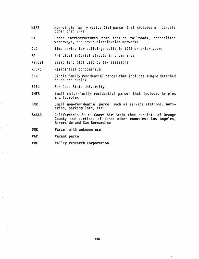