Final report BFP to CE2030-v3 - Bureau du plan

1

REPORT

Long term energy and emissions’ projections

for Belgium with the PRIMES model

Addressed to the COMMISSION ENERGY 2030

September 2006

Federal Planning Bureau Economic analyses and forecasts

Kunstlaan 47-49 Avenue des Arts 47-49 B-1000 Brussel-Bruxelles Tel.: (02)507.73.11 Fax: (02)507.73.73 E-mail: [email protected] URL: http://www.plan.be

Report

2

This report is written by

Danielle Devogelaer & Dominique Gusbin

Report

3

Table of contents

I. Introduction.....................................................................................................................................................7 II. Methodology ...................................................................................................................................................9

A. The PRIMES model ...................................................................................................................................9 B. The scenarios ............................................................................................................................................10

1. Baseline.................................................................................................................................................10 2. Sensitivity analysis .............................................................................................................................10 3. Alternative or policy scenarios.........................................................................................................10

III. Baseline......................................................................................................................................................13 A. Hypotheses ...............................................................................................................................................13

1. International fuel prices.....................................................................................................................13 a. Recent evolution ............................................................................................................................13 b. Forecasts ..........................................................................................................................................14 c. Price forecasts used in the baseline.............................................................................................14

2. Economic activity and demography ...............................................................................................15 3. Transport activity ...............................................................................................................................16 4. Other hypotheses................................................................................................................................17 5. Greenhouse gases other than energy related CO2 ........................................................................17 6. Policy context ......................................................................................................................................18

B. Results .......................................................................................................................................................19 1. Primary energy demand....................................................................................................................19 2. Production of electricity ....................................................................................................................21 3. Final energy demand .........................................................................................................................23 4. Energy related CO2 emissions ..........................................................................................................26

IV. Sensitivity analysis ..................................................................................................................................29 1. Primary energy demand....................................................................................................................30 2. Production of electricity ....................................................................................................................31 3. Final energy demand .........................................................................................................................31

V. Alternative scenarios ...................................................................................................................................35 A. Definition ..................................................................................................................................................35 B. Marginal abatement cost ........................................................................................................................36 C. Analysis of the impact of the alternative scenarios and variants....................................................38

1. Belgian reduction of energy CO2 emissions by -15% ...................................................................38 a. Primary energy demand...............................................................................................................38

i General........................................................................................................................................38 ii Coupled analysis.......................................................................................................................39

Bpk15 vs. Bpk15n...........................................................................................................................39 Bpk15s vs. Bpk15ns .......................................................................................................................40

b. Electricity and steam generation.................................................................................................41 i General........................................................................................................................................41 ii Coupled analysis.......................................................................................................................43


iii Cost implications.......................................................................................................................44 c. Final energy demand ....................................................................................................................46



iii Cost implications.......................................................................................................................48 d. CO2 emissions by sector................................................................................................................54

Report

4

e. Sensitivity analysis on prices .......................................................................................................54 i Bpk15h vs. Bpk15nh .................................................................................................................55

Primary energy demand...............................................................................................................55 Electricity production....................................................................................................................56 Final energy demand ....................................................................................................................57

2. Belgian reduction of energy CO2 emissions by -30%....................................................................57 a. Primary energy demand...............................................................................................................58



b. Electricity and steam generation.................................................................................................60 i General........................................................................................................................................60 ii Coupled analysis.......................................................................................................................62


iii Cost implications.......................................................................................................................63 c. Final energy demand ....................................................................................................................65



iii Cost implications.......................................................................................................................67 d. CO2 emissions by sector................................................................................................................71 e. Sensitivity analysis on prices .......................................................................................................72

i Bpk30h vs. Bpk30nh .................................................................................................................72 Primary energy demand...............................................................................................................73 Electricity production....................................................................................................................74 Final energy demand ....................................................................................................................75

3. Comparison of CO2 reduction scenarios: key findings ................................................................75 a. CO2 reduction options...................................................................................................................75 b. Total and sectoral CO2 emissions................................................................................................77 c. Electricity generation ....................................................................................................................82 d. Final energy consumption............................................................................................................83 e. Average power and heat production costs ...............................................................................85 f. Energy costs for the final consumers..........................................................................................86

VI. Conclusion ................................................................................................................................................87 Annexes....................................................................................................................................................................91

A. International price forecasts for fuels used in the scenarios for the Commission 2030: clarification .........................................................................................................................................................91 B. Definition of the indicators used in the PRIMES analyses ...............................................................93 C. Details on the design of the alternative scenarios..............................................................................95 D. Detailed scenario results ........................................................................................................................97 E. Sensitivity analyses: some more results.............................................................................................117 F. The PRIMES model in a nutshell ........................................................................................................125 G. Energy savings in the PRIMES model: potentials, modelling and interpretation of results....127

i Introduction .............................................................................................................................127 ii Modelling energy consumption and savings in PRIMES ................................................127 iii Interpretation of PRIMES results .........................................................................................128 iv References.................................................................................................................................128

VII. List of references ....................................................................................................................................129

Report

5

List of figures

Figure 1: Brent oil spot prices in US dollars and euros per barrel.................................................................14 Figure 2: Comparison of international energy prices present baseline vs. scenarios in the PP95, 1990-2030 ($05/boe) ................................................................................................................................................15 Figure 3: Composition of the primary energy demand, baseline (ktoe).......................................................20 Figure 4: Composition of the electricity generation, baseline (%) .................................................................22 Figure 5: Sectoral composition of final energy demand, baseline (ktoe)......................................................24 Figure 6: Fuel composition of final energy demand, baseline (ktoe) ............................................................25 Figure 7: Changes in CO2 emissions compared to 1990 levels .......................................................................27 Figure 8: Comparison forecasts international energy prices for baseline and price variants (1990-2030)...................................................................................................................................................................................29 Figure 9: Primary energy related indicators for the higher-oil-higher-gas variant, evolution, difference with the baseline (%) ..........................................................................................................................30 Figure 10: Electricity production related indicators for the higher-oil-higher-gas variant, evolution, difference with the baseline (%) ..........................................................................................................................31 Figure 11: Changes in sectoral final energy demand for the higher-oil-higher-gas variant, evolution, difference with the baseline (%) ..........................................................................................................................32 Figure 12: Primary energy related indicators for the Bpk15 and Bpk15n scenarios, year 2030, difference with the baseline (%) ..........................................................................................................................39 Figure 13: Primary energy related indicators for the Bpk15s and Bpk15ns scenarios, year 2030, difference with the baseline (%) ..........................................................................................................................40 Figure 14: Electricity production related indicators for the Bpk15 and Bpk15n scenarios, year 2030, difference with the baseline (%) ..........................................................................................................................43 Figure 15: Electricity production related indicators for the Bpk15s and Bpk15ns scenarios, year 2030, difference with the baseline (%) ................................................................................................................44 Figure 16: Average production costs of electricity and steam in the -15% reduction cases, difference from unconstrained cases in 2030 (%) ................................................................................................................46 Figure 17: Changes in sectoral final energy demand for the Bpk15 and Bpk15n scenarios, year 2030, difference with the baseline (%) ..........................................................................................................................47 Figure 18: Changes in sectoral final energy demand for the Bpk15s and Bpk15ns scenarios, year 2030, difference with the baseline (%) ................................................................................................................48 Figure 19: Energy related costs in industry in the -15% reduction cases, difference from baseline in 2030 (%) 50 Figure 20 : Energy related costs in the tertiary sector in the -15% reduction cases, difference from baseline in 2030 (%)................................................................................................................................................51 Figure 21: Energy related costs in the residential sector in the -15% reduction cases, difference from baseline in 2030 (%)................................................................................................................................................52 Figure 22: Costs in transport in the -15% reduction cases, difference from baseline in 2030 (%) ............53 Figure 23: Primary energy related indicators for the Bpk15h and Bpk15nh scenarios, year 2030, difference with the baseline (%) ..........................................................................................................................55 Figure 24: Electricity production related indicators for the Bpk15h and Bpk15nh scenarios, year 2030, difference with the baseline (%) ................................................................................................................56 Figure 25: Changes in sectoral final energy demand for the Bpk15h and Bpk15nh scenarios, year 2030, difference with the baseline (%) ................................................................................................................57 Figure 26: Primary energy related indicators for the BPK30 and Bpk30n scenarios, year 2030, difference with the baseline (%) ..........................................................................................................................59 Figure 27: Primary energy related indicators for the Bpk30s and Bpk30ns scenarios, year 2030, difference with the baseline (%) ..........................................................................................................................60 Figure 28: Electricity production related indicators for the Bpk30 and Bpk30n scenarios, year 2030, difference with the baseline (%) ..........................................................................................................................62

Report

6

Figure 29: Electricity production related indicators for the Bpk30s and Bpk30ns scenarios, year 2030, difference with the baseline (%)...........................................................................................................................63 Figure 30: Average production costs of electricity and steam in the -30% reduction cases, difference from unconstrained cases in 2030 (%) ................................................................................................................65 Figure 31: Changes in sectoral final energy demand for the Bpk30 and Bpk30n scenarios, year 2030, difference with the baseline (%)...........................................................................................................................66 Figure 32: Changes in sectoral final energy demand for the Bpk30s and Bpk30ns scenarios, year 2030, difference with the baseline (%) ................................................................................................................67 Figure 33: Energy related costs in industry in the -30% reduction cases, difference from baseline in 2030 (%) 68 Figure 34: Energy related costs in the tertiary sector in the -30% reduction cases, difference from baseline in 2030 (%)................................................................................................................................................69 Figure 35: Energy related costs in the residential sector in the -30% reduction cases, difference from baseline in 2030 (%)................................................................................................................................................70 Figure 36: Costs in transport in the -30% reduction cases, difference from baseline in 2030 (%) ............71 Figure 37: Primary energy related indicators for the Bpk30h and Bpk30nh scenarios, year 2030, difference with the baseline (%)...........................................................................................................................73 Figure 38: Electricity production related indicators for the Bpk30h and Bpk30nh scenarios, year 2030, difference with the baseline (%) ................................................................................................................74 Figure 39: Changes in sectoral final energy demand for the Bpk30h and Bpk30nh scenarios, year 2030, difference with the baseline (%) ................................................................................................................75 Figure 40: Total energy related CO2 emissions, comparison, period 1990-2030 (Mt) ...........................78 Figure 41: Energy related CO2 emissions in the power and steam sector and energy branch (Mt) ........79 Figure 42: Energy related CO2 emissions in industry (Mt) .............................................................................80 Figure 43: Energy related CO2 emissions in the tertiary and residential sectors (Mt) ...............................81 Figure 44: Energy related CO2 emissions in the transport sector (Mt)..........................................................81 Figure 45: Electricity generation (GWh) .......................................................................................................82 Figure 46: Final energy demand (ktoe) .........................................................................................................84 Figure 47: Average power and heat production costs vs. CO2 emissions in the year 2030 .................85 Figure 48: Total energy related costs of final consumers per unit of GDP vs. CO2 emissions in the year 2030 86

Report

7

I. Introduction

In the Royal Decree de dato December 6, 2005 (published in the Belgian Official Journal1 of December 19, 2005) the installation of a Commission Energy 2030 was officialised: the Commission is made up of a number of Belgian and foreign experts who will carefully scrutinize the energy future of Belgium on a long term horizon (2030). In order to fulfil this task, it was decided to start from a quantitative, scientific base. Because of the long expertise in modelling and analysing of long term energy projections, the Federal Planning Bureau (FPB) was asked to take up the task of providing the Commission with the necessary input. This input will subsequently be studied by the Commission, as well as complemented with analyses and other activities executed in its bosom.

This report aims at gathering the work carried out by the FPB in the above framework. The heart of the analysis of the Belgian energy outlook to 2030 is provided by a set of energy scenarios. These scenarios provide a quantitative basis for the analysis of environmental, energy and economic challenges Belgium will be faced with in the coming years. Doing so, the analysis gives a valuable input to the report the Commission Energy 2030 has to deliver to M. Verwilghen, the federal Minister of Energy.

However, numbers do not tell the whole story and modelling tools have their limitations. Consequently, this quantitative analysis needs to be (and is in most cases) complemented and enlarged by additional analyses carried out by experts within the Commission or by other relevant studies. All the more so that, given the strict timing of the study, only a limited number of energy policy options and environmental or economic challenges have been examined in detail. The FPB is fully aware of these limitations. As such, the focus of the analysis is put on policy options in the power generation sector, as was specifically requested by the Commission Energy 20302.

In this overall context, it is worth noting that, in parallel with this study, the FPB has completed another study for M. Tobback, the federal Minister of Environment. The principal objective of this study is to elaborate on and analyse greenhouse gas (GHG) emission reduction scenarios in Belgium to 2020 and 2050. This study was conceived in the light of the international preliminary climate discussions in which Belgium is involved for the period after 2012 as new commitments have to be formulated for this period. Belgium has expressed its wish to properly prepare itself for these new discussion rounds and wants to secure itself by quantitatively estimating the consequences different GHG emission reductions have on an environmental and socio-economic level.

Main differences between the two studies (the present one and the study for Minister Tobback) can be found in the divergence in time horizon (2030 vs. 2020 for the energy outlook) and the general framework that is used to perform the analyses. The latter can be shown by two illustrating examples: - While the present study, on the specific request of the Commission Energy 2030, investigates some

options concerning a nuclear come-back, the study for the Minister of Environment precludes the use of nuclear energy and subscribes itself within the legal framework of the Law holding the progressive phase-out of nuclear energy for industrial electricity production;

- The perspective concerning emission reductions followed in both studies is different. The present study chooses to look at it on a national stand-alone basis and to deal with energy related CO2 emissions only: Belgium needs to reduce its energy CO2 emissions by 15% and 30% compared to the CO2 emissions achieved in the year 1990. The study for Minister Tobback, on the other hand,

1 Belgisch Staatsblad, Moniteur Belge, Belgisches Staatsblatt 2 This choice results also from the limitations of the model to cope, in an exhaustive manner, with the cost impacts of specific

options in the demand side.

Report

8

subscribes itself in a European system that leads to equalisation of marginal costs of the reduction constraint imposed on all GHG by 2020.

At the start of the study, it is important to pinpoint that a number of hypotheses as well as policy scenarios and variants were defined by the Commission Energy 2030 in collaboration and after discussion with the DG Energy from the FPS Economy, SMEs, Self-Employed and Energy and with the Federal Planning Bureau (FPB). As such, decisions on potentials of renewable energy sources, deployment of nuclear energy and carbon capture and storage were debated and decided on within this working group.

The present report starts with a short description of the PRIMES model, the model that was used in order to generate the quantitative results, and the scenarios discussed (chapter II), and by the main hypotheses used for the analysis (chapter III.A). After that, results of the baseline (or reference scenario) are being described (chapter III.B), followed by the outcome of a price sensitivity analysis (chapter IV). Next, a number of alternative scenarios are presented and analysed in chapter V. Chapter VI contains the main conclusions.

Report

9

II. Methodology

A. The PRIMES model

In this study, the PRIMES model is used in order to quantitatively examine the energy outlook of Belgium in the period 2005-2030. For the analysing of PRIMES projections, one starts from a baseline scenario in which recent policy and current trends are being taken up. Next to the baseline, sensitivity analyses and/or policy scenarios are defined in order to study the effect of uncertainty existing around one parameter and scrutinize the impact of a different policy on the national energy system respectively.

PRIMES then generates long term energy and emissions’ projections (horizon 2030) on the supranational (European) and national (e.g. Belgian) level. For a number of years, European Commission’s DG TREN makes use of the PRIMES model in order to elaborate energy projections for the EU25, next to individual nation’s projections. The PRIMES model is being developed and managed in the University of Athens (NTUA) by a team under the coordination of Prof. P. Capros. For some of the hypotheses, the NTUA makes use of the output of other universities or scientific institutions, like for example international energy prices (on the basis of POLES, supplemented by the world energy model PROMETHEUS and revised by a number of experts) and the modelling of the transport activity (on the basis of SCENES, a European transport network model).

PRIMES is a modelling system that simulates a market equilibrium solution for energy supply and demand in the European Union (EU) member states. The model determines the equilibrium by finding the prices of each energy form such that the quantity producers find best to supply match the quantity consumers wish to use. The equilibrium is static (within each time period) but repeated in a time-forward path, under dynamic relationships. PRIMES can be run with perfect foresight3; the model is behavioural but also represents in an explicit and detailed way the available energy demand and supply technologies and pollution abatement technologies. The system reflects considerations about market economics, industry structure, energy/environmental policies and regulation. These are conceived so as to influence market behaviour of energy system agents. The modular structure of PRIMES reflects a distribution of decision making among agents that decide individually about their supply, demand, combined supply and demand, and prices. Then the market integrating part of PRIMES simulates market clearing. PRIMES is a general purpose model. It is conceived for forecasting, scenario construction and policy impact analysis. It covers a medium to long-term horizon. It is modular and allows either for a unified model use or for partial use of modules to support specific energy studies.

More information about the PRIMES model is provided in annex F. A more elaborate description of the PRIMES model can be found in “The PRIMES Energy System Model, Summary Description” by NTUA4.

3 PRIMES is run with perfect foresight in this study. 4 Downloadable via http://www.e3mlab.ntua.gr/, the model is run at NTUA.

Report

10

B. The scenarios

1. Baseline

The baseline (or reference scenario) simulates current trends and policies as implemented in Belgium by the end of 2004. While informing about the development of policy relevant indicators such as the renewables shares in 2010, the baseline does not assume that indicative targets, as set out in the Directives, will be necessarily met. The numerical values for these indicators are outcomes of the modelling; they reflect implemented policies rather than targets. This also applies for CO2 emissions. The baseline thus describes what the Belgian energy future could look like if no additional actions are taken.

In addition to its role as reference projection, the baseline also serves as a standard for sensitivity analyses and alternative scenarios, next to which they can be placed in order to measure the impact of a change in one exogenous variable or a different policy setting respectively.

2. Sensitivity analysis

Sensitivity analyses study the effect one single exogenous parameter can have on the energy system. Traditionally, this single exogenous parameter is a variable around which a lot of uncertainty exists, like e.g. international fuel prices or the growth of the (inter)national economy. With the exception of this one parameter, the baseline setting is not touched upon and hypotheses and presumed trends are identical to the ones reported in the baseline.

This study performs sensitivity analyses on fuel prices.

3. Alternative or policy scenarios

Policy or alternative scenarios are different from sensitivity analyses in that the former do entail a new policy setting and philosophy. Not a single one, but a whole mindset of variables is changed compared to the baseline. Such a setup makes it possible to examine -among other things- the achievement of energy or environmental policy targets. Issues such as renewable energy sources, nuclear energy, energy efficiency, alternative fuels in transport or climate change can then be studied with reference to the baseline.

The evolution of the Belgian energy system described in the baseline accounts for policies and measures implemented by the end of 2004. Needless to say that additional policies and measures having an impact on energy developments are likely to occur in the coming years in order to cope with three important issues: climate change, the security of our future energy supply and the competitiveness of our economy. These policies and measures can either be additional or constitute changes in current energy policy orientations.

This study is not aimed at covering all possible alternatives in terms of energy policy options or climate change strategies. Its objective is to shed light on the above issues through a limited set of alternative or policy scenarios that nevertheless cover a large range of possibilities. As regards the climate change issue, all alternative scenarios introduce constraints on energy related carbon dioxide emissions at the horizon 2030 (CO2 is the principal GHG in Belgium). Further to discussion within the Commission Energy 2030, it was decided to consider two targets, namely reductions in energy related CO2 emissions of 15% and 30% in 2030 from 1990 levels. Concerning specific policy options, the Commission Energy 2030 has asked to examine the repercussions that a come-back of nuclear on the electricity scene would generate for Belgium. Finally, given the large uncertainty associated to the commercial availability and technical feasibility of the promising CO2 emission reduction technology

Report

11

of carbon capture and storage, it was proposed to subdivide the scenarios into two categories: those that include this technology as a possible option and those that do not.

Report

12

Report

13

III. Baseline

For the baseline, the reference scenario that was published by the DG TREN in 20065 and that also includes Belgian projections is being used. The same reference scenario was also chosen as baseline in the study for Minister Tobback (cf. Introduction). This baseline gives a coherent view of the long term evolution of the Belgian energy system. It is based on a number of hypotheses on the demographic and economic context (activity of the sectors, international fuel prices …) and on the existing policy measures on energy, transport and environment. Recent trends and structural changes are assumed to continue. This baseline thus enables to pinpoint the long term challenges in the fields of energy, transport and environment, as well as to identify the actions that have to be taken in order to solve potential problems. The baseline then examines what could happen if no new action in the field of energy, climate or transport is installed. It also allows to evaluate the impact of new propositions or alternative policy measures on the evolution of the Belgian energy system and its emissions6.

A. Hypotheses

The hypotheses used relate to a number of variables like international fuel prices, the economy, demography, the transport activity and the implemented policy measures. They are described briefly below. More information, in particular on assumptions that are not Belgium specific but relate to the European policy context or international framework, can be found in the DG TREN publication of May 2006.

1. International fuel prices

a. Recent evolution

Over the last years, the international energy prices have embarked on an impressive growth path. The prices of oil are a good example7. Starting in the mid eighties until the end of the nineties, the Brent crude oil price fluctuated around 20 dollars per barrel. By the turn of the century, this situation changed drastically. For the first time in years, the price of the Brent reached a level of more than 30 dollars per barrel. In 2002 the situation looked like it was going to normalize, but this turned out to be an illusion. The price of crude oil continued its upward journey to reach record heights in 2005 of 55$. Today, values of 70$ per barrel are common.

5 European Commission, Directorate-General for Energy and Transport, European Energy and Transport, Trends to 2030-update

2005, prepared by NTUA with the PRIMES model, May 2006. 6 The PRIMES model focuses on energy related CO2 emissions. 7 Furthermore they play the role of catalyst as oil and gas prices are coupled. In other words, the price of gas follows the

evolution of the price of oil, although with some delay.

Report

14

Figure 1: Brent oil spot prices in US dollars and euros per barrel

Source: Thomson Datastream

b. Forecasts

Given these recent sound fluctuations, the exercise of drawing up international energy price projections then becomes subject to a strong sense of insecurity (and disagreement) amongst the experts. To illustrate this point, a table is cited in which the long term projections for oil prices in nominal terms ($2000) according to a number of renowned sources are being given. The strongly diverging figures are telling.

Table 1: Comparison of long term oil price projections according to different institutions ($2000)

Source 2010 2020 2030 IEA 22 26 29 EIA 23.3 25.1 EC 27.7 33.4 40.3 OPEC 19.3 19.3 IEEJ 24 27 CGES 20.5 15.1

Source: IEA, World Energy Outlook 2004, p.529

c. Price forecasts used in the baseline

In order to make up the PRIMES’ baseline, the hypotheses of the future fuel prices of figure 2 are being used. This figure is produced by the University of Athens (NTUA) with the use of POLES 8 and PROMETHEUS (also a NTUA model) and has been revised by a number of experts9. Assumptions on fuel prices are higher than the projections elaborated in the years before 2004 (see table 1). In fact, they take

8 The POLES model is a global sectoral model of the world energy system. The development of the POLES model has been

partially funded under the Joule II and Joule III programmes of DG XII of the European Commission. Since 1997 the model has been fully operational and can produce detailed long-term (2030) world energy and CO2 emission outlooks with demand, supply and price projections by main region. The model splits the world into 26 regions. For the model design see the model reference manual: POLES 2.2. European Commission, DG XII, December 1996.

9 For a more elaborate description on the modelling of oil and gas prices and the energy price outlook, see annex A.

Report

15

into account the rather high price levels seen up to mid 2005 (when the modelling of the baseline started). For comparison, oil prices in this baseline are similar to those used in the DG RTD funded WETO-H2 project (World Energy and Technology Outlook), but slightly higher than those used in the 2005 IEA World Energy Outlook. In order to take the uncertainty on the energy prices into account, the baseline is complemented with a price variant in which the oil and gas prices are considerably higher than in the baseline. This variant will be discussed in part IV (Sensitivity analysis).

In order to further underline the uncertainty associated with price forecasts, they are depicted together with the ones taken from a publication of the FPB on long term energy forecasts for Belgium which appeared in 2004, named PP95 (‘refPP95’): oil and gas prices of the new run are obviously higher than the ones used in the PP95.

Figure 2: Comparison of international energy prices present baseline vs. scenarios in the PP95, 1990-2030 ($05/boe)

0

10

20

30

40

50

60

70

1990 1995 2000 2005 2010 2015 2020 2025 2030

$05/

boe

Oil-baseline Gas-baseline Coal-baseline

Oil-ref PP95 Gas-ref PP95 Coal-ref PP95

Gas-HGP sc PP95

Source: NTUA (2005), PP95

refPP95: reference scenario in the PP95

HGP sc PP95: High Gas Price scenario in the PP95

2. Economic activity and demography

Next to hypotheses on price, hypotheses on the evolution of the national macro-economic situation and on demography are indispensable10. In table 2, absolute values of these indicators are given next to the annual growth rate of a couple of key variables of the Belgian economy. First, projections of the total number of people living on Belgian soil and the average household size for the period 2000-2030 are given, followed by the GDP and the average household revenue. After, value added is depicted, divided per (sub)sector. The table concludes with the hypotheses on the Belgian iron and steel production according to the 2 production processes: these are expressed in kton.

10 Demographic and macroeconomic assumptions are described more extensively in NTUA (2005). The principal sources of

these hypotheses are Eurostat, Global Urban Observatory and Statistics Unit of UN-HABITAT, Economic and Financial Affairs DG of the European Commission, Member States’ stability programmes and the results of the GEM-E3 and PRIMES models.

Report

16

Table 2: Macro-economic assumptions for Belgium, 2000-2030

2000 2010 2020 2030 '90-'00 '00-'10 '10-'20 '20-'30

Annual % Change

Population (in Million) 10.246 10.554 10.790 10.984 0.3 0.3 0.2 0.2 Household size (inhabitants per

household) 2.42 2.28 2.16 2.08 -0.6 -0.6 -0.5 -0.4 Gross Domestic Product (in MEuro'00) 247924 302858 370146 431665 2.2 2.0 2.0 1.5 Household Income (in Euro'00/capita) 12904 14887 17226 19396 1.8 1.4 1.5 1.2 SECTORAL VALUE ADDED (in

MEuro'00) 231229 280534 339665 393763 2.0 2.0 1.9 1.5 Industry 46407 53371 62492 71457 1.7 1.4 1.6 1.3

iron and steel 2630 2714 2753 2757 -3.1 0.3 0.1 0.0 non ferrous metals 1028 1295 1436 1477 -0.4 2.3 1.0 0.3 chemicals 9553 12219 14866 17565 4.5 2.5 2.0 1.7 non metallic minerals 2134 2125 2455 2691 0.2 0.0 1.5 0.9 paper, pulp and printing 3268 3927 4672 5345 1.1 1.9 1.8 1.4 food, drink and tobacco 5137 6107 7011 7764 -0.1 1.7 1.4 1.0 engineering 16236 18257 21593 25114 2.4 1.2 1.7 1.5 textiles 2587 2232 2200 2194 -0.3 -1.5 -0.1 0.0 other industries 3835 4495 5507 6548 2.8 1.6 2.1 1.7

Construction 11622 13123 14985 16653 1.4 1.2 1.3 1.1 Tertiary 162581 203552 250349 292506 2.2 2.3 2.1 1.6

market services 62659 78140 96924 115204 3.6 2.2 2.2 1.7 non market services 52285 64005 75402 81171 1.5 2.0 1.7 0.7 trade 43967 57722 74027 92013 1.1 2.8 2.5 2.2 agriculture 3669 3685 3997 4118 3.7 0.0 0.8 0.3

Energy sector and others 8509 7936 8762 9553 2.0 -0.7 1.0 0.9 INDUSTRIAL PRODUCTION iron and steel (in ktn) 11636 11924 12040 11970 0.2 0.2 0.1 -0.1

integrated steelworks 8910 8376 8250 7846 -1.5 -0.6 -0.2 -0.5 electric processing 2726 3548 3790 4124 10.0 2.7 0.7 0.8

Source: NTUA (2005)

3. Transport activity

The projections for the transport activity are being depicted in table 3. The figures were generated by the SCENES model, a European transport network model. The transport of people as well as goods keeps growing in the period 2000-2030, but at a slower pace than in the period 1990-2000.

Report

17

Table 3: Projections of the transport activity in Belgium, 2000-2030

2000 2010 2020 2030 '90-'00 '00-'10 '10-'20 '20-'30

Annual % Change

Transport activity

Passenger transport activity (Gpkm) 135.8 155.6 173.1 189.1 2.0 1.4 1.1 0.9

Public road transport 13.2 13.0 12.1 11.3 2.0 -0.1 -0.7 -0.6

Private cars 106.3 121.7 135.5 147.6 1.8 1.4 1.1 0.9

Motorcycles 1.0 1.2 1.4 1.5 -1.6 1.4 1.4 1.2

Rail 8.6 9.4 9.9 10.3 1.7 0.9 0.5 0.4

Aviation 6.5 10.0 13.8 17.9 8.2 4.4 3.3 2.6

Freight transport activity (Gtkm) 65.9 78.9 92.1 103.5 3.2 1.8 1.6 1.2

Trucks 51.0 62.1 74.0 84.2 4.1 2.0 1.8 1.3

Rail 7.7 7.8 8.0 8.1 -0.9 0.2 0.2 0.2

Inland navigation 7.2 9.1 10.2 11.2 2.8 2.3 1.1 1.0

Travel per person (km per capita) 13258 14742 16039 17218 1.7 1.1 0.8 0.7 Freight activity per unit of GDP

(tkm/000 Euro'00) 266 261 249 240 1.0 -0.2 -0.5 -0.4 Source: SCENES model (information received from NTUA) Gpkm: billion of passenger-kilometres Gtkm: billion of ton-kilometres

4. Other hypotheses

Some other hypotheses were necessary in order to run the different scenarios. - The number of degree-days is assumed to be fixed over the entire projection period and equals the

number reached in the year 2000 (i.e. 2097 degree-days, 16.5 equivalent). - The discount rate plays an important role within the PRIMES model. It is a crucial element in the

determination of investment decisions by economic agents regarding energy using equipment. Three (real) rates are currently used within the model. The first, used mostly for large utilities, is set at 8%; the second, used for large industrial and commercial entities, is set at 12%; the third, used for households in determining their spending on transport and household equipment, is set at 17.5%.

- The emission factors used in the calculation of energy emissions are the following (expressed in ton CO2 per toe): 3.941 for coal, 2.872 for gasoline, 3.069 for gasoil and 2.336 for natural gas.

- The most recent energy balances used in order to draw up the baseline date from 2004. - As regards renewable energy sources, the Commission Energy 2030 looked into the issue of

achievable contributions in the Belgian energy system by 2030. Potentials were provided for wind power and solar photovoltaics (PV). These potentials represent reasonable maximum achievable “technical” potentials at the horizon 2030. These are the following: 2026 MW for on-shore wind, 3800 MW for off-shore wind and 10000 MW for solar PV. Supply cost curves are associated to all three power technologies to account for cost increases according to the level of capacity installed. These increases reflect e.g. additional costs related to less favourable production sites or additional investments required in the electricity grid to absorb the increase in renewable capacities. As far as biomass is concerned, no limit is put on its supply on the Belgian territory (total supply combines domestic production and imports). However, a supply cost curve is associated to biomass reflecting supply cost increases when the demand for biomass rises (see J. De Ruyck, Renewable energies, September 2006).

5. Greenhouse gases other than energy related CO2

The present study only focuses on energy related CO2 emissions (as PRIMES is an energy model). Energy related CO2 emissions, however, are not the only damaging emissions in the biosphere: there

Report

18

also exist other greenhouse gases (GHG). Knowledge of the amount and appearance of those other GHG is crucial since general (international) objectives on emission reductions are defined in terms of total GHG. Next to energy CO2, GHG consist of non-energy CO2 (emitted through industrial processes, fugitive and waste), methane (CH4), nitrous oxide (N2O) and fluorinated gases (HFC, PFC and SF6). Together, these GHG other than energy related CO2 account for approximately 21% of the total, since energy CO2 makes up 92% of the total of CO2 emissions and total CO2 emissions take up a share of 85.5% in the GHG (see National Climate Commission, Fourth National Communication on Climate Change, 2006).

It is also important to be more specific about what is meant by energy related CO2 emissions in this study. According to the Eurostat statistical convention on which the PRIMES model is based, aviation bunkers are included in the final energy consumption of transport whereas maritime bunkers are not. Maritime bunkers are put into the export category of the energy balances. The rationale behind this choice comes from the fact that this consumption has, in most cases, no link with the economic activity of the country. Consequently, CO2 emissions from aviation bunkers are included in the analysis whereas those from maritime bunkers are not. From an environmental perspective, the consumption of maritime bunkers is however crucial as it is a major contributor to climate change. In 1990, the base year for the Kyoto Protocol, maritime bunkers represented no less than 10% of total GHG emissions in Belgium (i.e. comparable to the contribution of agriculture). Furthermore, its consumption follows an increasing trend: + 80% between 1990 and 2004.

Both aviation and maritime bunkers are excluded from the scope of the Kyoto Protocol. Nevertheless, there is some question of them being part of the game in future GHG reduction commitments. The exclusion of maritime bunkers in the analysis should therefore be borne in mind when discussing the results of the different scenarios.

6. Policy context

The baseline includes agreed policies addressing economic actors as known by the end of 2004. It presumes that all current policies and those in the process of being implemented at the end of 2004 will continue in the future. However, in the baseline, it is not assumed that the indicative targets, as set out in various EC Directives, will necessarily be met. The numerical values for these indicators are outcomes of the modelling; they reflect implemented policies rather than targets. - The establishment of an emission trading regime in Europe is included in the baseline assuming a

permit price of 5 €’00/t CO2 for those sectors covered by the EU Emission Trading Scheme (ETS). - The baseline integrates effects from the restructuring of markets through the liberalisation of

electricity and gas in the EU, which proceeds in line with EC Directives (e.g. decreases in producers’ mark-ups and in regulated transport and distribution tariffs). Liberalisation is assumed to be fully implemented in the period to 2010.

- Concerning the use of biofuels in transport, it is assumed that Belgium will follow EU rules sooner or later. The impact of blending gasoline and diesel with biofuels on final consumer prices is assumed to be negligible, since higher fuel production costs will probably be offset by tax reductions scheduled to be implemented on these fuel blends.

- On transport, the baseline assumes that the targets agreed for 2008 with the car industry on the reduction of specific CO2 emissions for new cars11 are achieved without assuming a further strengthening of targets thereafter.

- The Law on the progressive phase-out of nuclear energy is taken up in the baseline. The baseline, in other words, takes into account the decommissioning of nuclear power plants once they turn 40,

11 The voluntary agreement reached between the European Commission and the European automobile industry on specific

CO2 emissions from new cars (followed in 1999 by similar agreements with Korean and Japanese car manufacturers).

Report

19

conform the Law on the progressive phase-out of nuclear energy for industrial electricity production which was consented on January 31, 200312.

- The system on green and heat certificates is part of the baseline. In agreement with the European Directive on the promotion of electricity generation from renewable energy sources, the Belgian Regions have decided to make use of green certificates. Concerning the combined heat and power (CHP), the Regions have fixed regional objectives in order to stimulate the production of electricity on the basis of CHP.

B. Results

1. Primary energy demand

The primary energy demand (also referred to as gross inland consumption or GIC), an indicator that describes a nation’s total energy consumption and that consists of primary production (energy sources that are exploited on the nation’s soil, e.g. wind and hydro) and net import (energy sources that are imported by the country, e.g. oil), follows an inverse U-shaped path. In 2000, a total gross inland consumption (GIC) of 57 Mtoe is reached. After 2000 a slow growth is set in (0.5% per year) to reach a peak in 2010 of 60 Mtoe. During the period 2010-2020 the indicator declines at a rhythm of -0.3% annually, followed by a further decrease in the next decennium (-0.5% yearly). In 2030 the GIC reaches 55 Mtoe.

The evolution of primary energy demand should be interpreted with caution, though, at least at the end of the projection period when the share of nuclear decreases steadily. The decreasing trend does not only reflect overall improvements in energy efficiency (both at final energy demand level and energy transformation level) but also the impact of the statistical convention used since many years for nuclear heat. According to this statistical convention, an average efficiency of 33% is given to nuclear power plants in order to calculate the primary energy requirements corresponding to nuclear electricity. Given that current and future fossil fuel based power plants as well as those using renewable energy sources have conversion efficiencies considerably higher than 33%, the progressive retirement of nuclear plants translates into comparatively lower primary energy inputs.

12 Belgian Official Journal (Belgisch Staatsblad, Moniteur Belge or Belgisches Staatsblatt), February 28, 2003, pp. 9879-9880. This law was already announced in the governing agreement of July 7, 1999.

Report

20

Figure 3: Composition of the primary energy demand, baseline (ktoe)

0

10000

20000

30000

40000

50000

60000

70000

2000 2005 2010 2015 2020 2025 2030

Solids Oil Natural gas Nuclear Electricity Renewable energy forms

Source: PRIMES

Next to the evolution of the GIC, it is also interesting to study its composition. Oil is head of the class during the entire period. In 2000, the dominance of oil is crystal clear, in 2030 it still ranks first in the fuel order, but the relative relations between the different energy sources have shuffled. Especially the “dash for gas” is threatening the strong position of oil, leading to an almost equal share of the two fuels in the GIC at the end of the projection period (oil: 38%, natural gas: 35%).

From 2015 onwards, nuclear energy is being phased out because of the law stipulating the progressive retirement of nuclear plants after a lifetime of 40 years13. Whereas the gross inland consumption of nuclear energy still reaches 12 Mtoe in 2000, it disappears from the GIC scene by 2030. Solid fuels start off from a position of 8 Mtoe in 2000, then loose weight to only reach 5 Mtoe in 2015, but after that, they start to rise again towards the end of the projection period to arrive at 11 Mtoe. Together with natural gas, these solids fill up the gap left by the nuclear void.

Renewable energy sources follow a spectacular growth path, mainly during the first projection period (2000-2010) when their consumption climbs by 6% per year. In 2030, it then reaches a level of approximately 3 Mtoe.

Still remaining: a small level of electricity that is being imported14. This imported electricity sharply increases during the first decennium (2000-2010), to decrease again in the 2 subsequent periods. In the end, a level is obtained that comes close to the level at which it all started (325 ktoe).

13 See the law on the progressive phase-out of nuclear energy for industrial electricity production, Belgian Official Journal,

February 28, 2003. 14 The new version of PRIMES (that is used in order to perform the present analysis) integrates a country-by-country

modelling which focuses on the dynamics of the energy system within a country, while considering trade in fuels between countries. The analysis has fully taken into account the economic opportunities of electricity and gas trade within the EU Internal Energy Market as well as the engineering and operating constraints of the European transmission system as this evolves in relation to the completion of new interconnectors as planned in the context of the Trans-European Energy Networks. The extension and stabilization of the UCTE system has also been considered. The endogenous treatment of electricity and gas imports and exports is a new feature of the PRIMES model (PRIMES ver.2005).

Report

21

The table below gives an overall picture of the evolution of the primary energy demand in the baseline. It also describes the evolution of several indicators, namely the energy intensity of the GDP (i.e. GIC divided by the GDP), the primary energy consumption per capita and the import dependency (i.e. the share of net imports in the GIC).

Table 4: Primary energy demand and related indicators

2000 2010 2020 2030 10//00 (%)

20//10 (%)

30//20(%)

Gross inland consumption (Mtoe) 57.2 60.4 58.3 55.4 0.5 -0.3 -0.5 - Solids 8.2 6.4 5.2 11.5 -2.5 -2.1 8.3 - Oil 21.9 23.4 22.4 21.2 0.6 -0.4 -0.5 - Natural gas 13.4 15.5 18.9 19.5 1.6 1.9 0.3 - Nuclear 12.4 12.9 9.0 0.0 0.4 -3.6 - - Electricity 0.4 0.6 0.4 0.3 5.2 -3.2 -3.2 - Renewable energy forms 0.9 1.5 2.3 2.9 5.9 4.4 2.2 Energy intensity of the GDP (toe/M€’00)

230.6 199.3 157.5 128.4 -1.4 -2.3 -2.0

GIC/capita (toe/inhabitant) 5.6 5.7 5.4 5.1 0.2 -0.6 -0.7 Import dependency (%) 77.7 78.2 82.4 95.3

Source: PRIMES //: average annual growth rate

2. Production of electricity

A second indicator of interest is the generation of electricity. As for the previous indicator, we first look at the evolution of the total production, and then we turn to the structure or composition of this parameter.

The production of electricity is mounting throughout the entire projection period. During the first period (2000-2010) it increases at 1.3% per annum, reaching a total of 94 TWh by the year 2010 (in 2000, it was still 82.6 TWh). During the next decennium this increase keeps pace and the production of electricity grows at 1.1% per annum. It is only in the last period that the pace of growth will slow down and reach 0.7% per year: in 2030 then, 112 TWh of electricity will be generated.

The generation capacity is provided by nuclear power stations, renewable units (especially hydro and wind) and thermal production units (including biomass). In 2000, the supremacy of nuclear electricity is still obvious: 48 TWh is being generated by nuclear power stations. Thermal units take up the rest of the national production (34 TWh), as renewables only stand for 0.5 TWh. At the end of the projection period, this situation changes considerably. Because of the nuclear phase-out, nuclear power disappears from the electricity scene, which, in turn, forces the thermal units to catch up for the difference: in 2030 they will account for 106 TWh. Generation through renewables will also increase: spectacularly during the first period (‘00-’10) at a rate of 20,4% per year; followed by more modest percentages (3,1% and 4,1% per annum respectively) in the next decennia. In 2030, renewables will provide 6 TWh of electricity.

Figure 4 complements the above analysis per category of power production units; it shows the evolution of electricity generation in the baseline according to the different energy forms, namely nuclear energy, natural gas and RES (incl. biomass). The balance gives the share of coal.

Report

22

Figure 4: Composition of the electricity generation, baseline (%)

0

10

20

30

40

50

60

70

2000 2005 2010 2015 2020 2025 2030

RES Natural gas Nuclear

Source: PRIMES

The evolution of the electricity production and fuel mix described above can be complemented by the presentation of several indicators that enlarge the scope of the analysis.

Table 5: Indicators related to the production of electricity in the baseline

2000 2010 2020 2030 Efficiency of thermal electricity production (%)

37.1 42.1 55.1 52.6

Net import ratio (1) (%) 4.97 7.10 4.74 3.27 % of electricity from CHP 7.9 14.3 18.5 18.2 Share of non fossil fuels in electricity production (%)

60.3 58.5 42.3 11.8

Installed power capacity (GW) 14.9 16.8 19.6 23.0 Carbon intensity (t CO2/GWh) 246 212 213 395 Electricity (final demand) per capita (kWh/capita)

7566 8618 9265 9583

Source: PRIMES (1): Net import of electricity divided by total electricity supply.

The evolution of the average efficiency of thermal electricity production is closely related to the technology mix. The remarkable increase in 2000-2020 has to do with the investments in combined cycle gas turbines (CCGT) that are characterised by high conversion efficiencies (close to 60% for new generation), while the slight decrease in 2020-2030 comes from the progression of supercritical coal power plants in the power technology mix; this technology has a lower conversion efficiency than CCGT (around 50%).

The significant penetration of coal based power plants beyond 2020 also helps to explain the jump in the carbon intensity and in the CO2 emission index in 2030.

The share of non fossil fuels in electricity production combines two elements: nuclear on the one hand, renewable energy sources on the other. The share of nuclear electricity decreases steadily further to

Report

23

the decommissioning of nuclear plants after an operating lifetime of 40 years. On the contrary, the share of renewable energy sources goes up: representing only 2% in 2000, it reaches almost 12% in 2030. Similarly, the share of CHP in electricity generation goes up steadily up to 2020 after which it stabilises at 18% for the next 10 years.

The installed power capacity increases by 54% in 2000-2030. This increase is required to meet the growth in electricity consumption. However, the power capacity increases at a higher pace than electricity demand. One reason is the decrease in net electricity imports; another is the decrease in the average utilisation rate of electrical capacities: in 2000, it was close to 63%; in 2030, it is estimated to be 55%15. The evolution of electricity imports and exports is determined endogenously by the model16 given a certain number of assumptions regarding the declared strategy of the neighbouring countries. The progressive decrease in net electricity imports in 2005-2030 results, among other things, from the decline of surplus capacities in France and Germany. In 2030, net electricity imports are projected to be slightly less than 4 TWh.

3. Final energy demand

The final energy demand is the demand for the different end forms of energy (e.g. gasoline) by different consumers (e.g. the transport sector). Traditionally, one makes a distinction between the final energy demand by sector (or consumer) and the final energy demand by fuel (or energy form).

15 The decrease in average utilisation rate (i.e. generation/(installed capacity x 8760 hours)) is due to the higher share of power

capacities based on intermittent energy sources. 16 The new version of PRIMES used for this scenario analysis includes a set of improvements notably in the electricity and

steam sub-model where optimal flow analysis and investment expansion over a set of regional electricity markets are explicitly modelled, see also footnote 6.

Report

24

Figure 5: Sectoral composition of final energy demand, baseline (ktoe)

0

5000

10000

15000

20000

25000

30000

35000

40000

45000

2000 2005 2010 2015 2020 2025 2030

Transport

Tertiary

Residential

Industry

Source: PRIMES

Taking a look at each sector separately we can conclude that the largest end consumer of energy in 2000 is also the largest consumer in 2030: the industry is consuming the biggest part of the final energy demand. Nevertheless, it can be noticed that the final industrial energy demand in 2030 shows a status quo with demand in 2000. This is due to the energy intensive industries that constantly diminish their final energy demand.

During the first decennium, the residential sector gains territory: every year, its final energy demand increases with 0.9% on average. After 2010, final demand stabilizes and between 2020 and 2030, a slight decrease in final energy demand can be noted.

The transport sector, on the other hand, continues to satisfy her energy appetite by an enlarged consumption. Its final demand grows in the period 2000-2010; it keeps on growing in 2010-2020 but at a slower pace and finally stabilizes in the last decennium. This causes the transport sector to maintain its second place in the final energy consumption (11 Mtoe in 2030).

The tertiary sector consumes the least energy, but shows the strongest growth. During the 3 decennia under consideration, it grows on average at 1.5%, 1.2% and 0.6% per annum, reaching a final energy demand of 6 Mtoe in 2030.

The table below describes the evolution of the final energy consumption in each sector, the changes in the sectoral share in the total final energy demand and the increment/decrease in consumption between 2000 and 2030 (in ktoe and in %).

Report

25

Table 6: Evolution of the final energy demand in the baseline (per sector)

2000 2010 2020 2030 Increment 2000-2030 ktoe share ktoe share ktoe share ktoe share ktoe % Industry 13769 37% 13993 35% 14102 34% 13851 34% 82 1% Residential 9465 26% 10311 26% 10314 25% 10008 24% 543 6% Tertiary 4158 11% 4848 12% 5446 13% 5763 14% 1605 39% Transport 9662 26% 10816 27% 11336 28% 11308 28% 1645 17% Total 37055 39968 41197 40930 3876 10%

Source: PRIMES

Next to a subdivision of the final energy demand into consuming sectors, there also exists a subdivision in fuels.

Figure 6: Fuel composition of final energy demand, baseline (ktoe)

0

5000

10000

15000

20000

25000

30000

35000

40000

45000

2000 2005 2010 2015 2020 2025 2030

Solids Oil Gas Electricity Heat (from CHP and District Heating) Other

Source: PRIMES

Taken this subdivision, we see that oil is the fuel that is the most consumed. Although its pole position, the demand for oil does not change much during the whole projection period: the consumption level in 2000 is identical to the level in 2030 (16 Mtoe in 2000 and in 2030) causing its relative share in the final energy demand to shrink from 43% down to 39%.

Natural gas and electricity, on the other hand, are in for a climb: natural gas reaches 11 Mtoe in 2030, electricity 9 Mtoe. Both of them are able to raise their relative share during the projection period: natural gas climbs from 26 to 28%, electricity grows from 18 to 22%.

Solid fuels have become much less popular and plunge from 3 Mtoe in 2000 to somewhat less than 2 Mtoe in 2030, leading to a relative share of 5% of final demand. The decrease is mainly due to the iron and steel sector (production decreases in integrated steelworks).

Heat use increases fast: in 2000, heat demand was only 1 Mtoe, in 2030, it already climbed up to 1.6 Mtoe.

Report

26

The consumption of RES more than triples in the period 2000-2030. The major share of the increase can be subscribed to biofuels: its demand reaches slightly more than 700 ktoe in 2030, which equals 8% of total gasoline and diesel consumption in transport.

The table below describes the evolution of the final energy consumption per fuel, the changes in the share of each fuel in the total final energy demand and the increment/decrease in consumption between 2000 and 2030 (in ktoe and in %).

Table 7: Evolution of the final energy demand in the baseline (per fuel)

2000 2010 2020 2030 Increment 2000-2030 ktoe share ktoe share ktoe share ktoe share ktoe % Solids 3373 9% 2453 6% 2143 5% 1907 5% -1466 -43% Oil 16038 43% 17497 44% 17003 41% 16091 39% 54 0% Nat. Gas 9615 26% 10312 26% 11052 27% 11300 28% 1686 18% Electricity 6667 18% 7822 20% 8597 21% 9052 22% 2385 36% Other 1362 4% 1883 5% 2402 6% 2580 6% 1218 89% Total 37055 39968 41197 40930 3876 10%

Source: PRIMES “Other” includes heat and RES

4. Energy related CO2 emissions

Using different forms of energy to satisfy the final energy demand is not an action without consequences: the consumption of most of these energy vectors initiates a harmful effect on the environment in the form of greenhouse gas emissions. A national energy consumption pattern as described in the previous paragraphs will have a negative impact in terms of polluting greenhouse gas emissions. In the output of the PRIMES run, only the energy related CO2 emissions get calculated. In what follows, their evolution is discussed.

In the year 2000, a total of 114.7 Mt of CO2 emissions was registered. Every year this amount grows further, first rather slowly (0.1% per annum in the period 2000-2020), then very fast (at a yearly rate of 1.8% in the period 2020-2030). Remarkable is that the biggest CO2 pollutant in 2000 (namely, industry) passes on her bad reputation to the sectors of electricity production and transport, which, from 2020 onwards, take the lead in polluting. The electricity production emits 23.5 Mt of CO2 in 2000, a figure which more than doubles by 2030 (to 52.4 Mt). Transport takes in the second place with 31.3 Mt in 2030, while industry still reaches a value of 23.5 Mt in 2030, meaning a decrease compared to the year 2000 (when the level was up to 29.1 Mt). In 2030, households exhaust 18.3 Mt in CO2 emissions, while the tertiary sector is the smallest polluter at 10.2 Mt of CO2 emissions. The residential sector declined its emissions by 1.7 Mt compared to 2000, the tertiary sector did the opposite and gained 2 Mt.

In the context of the Kyoto Protocol and of current discussions on reduction targets for the post-2012 period, it is also useful to present the evolutions described above in another perspective, namely in comparison with 1990 emission figures (1990 is the base year for CO2 emissions in the Kyoto Protocol). The graph below shows the differences in CO2 emissions compared to 1990, by sector category and for the total energy-related CO2 emissions. The key messages are the following:

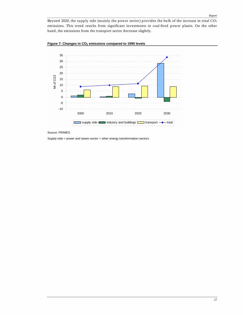
Given the current policies and measures and assumptions underlying the baseline, total energy-related CO2 emissions will increase by 32% in 2030 compared to 1990. The increase is particularly sharp beyond 2020, while CO2 emissions are in the range of 8 to 11% above the 1990 level in the period 2000-2020.

Up to 2020, the increase mainly comes from the transport sector. By contrast, CO2 emissions from industry and buildings (i.e. residential and tertiary sectors) decline steadily.

Report

27

Beyond 2020, the supply side (mainly the power sector) provides the bulk of the increase in total CO2 emissions. This trend results from significant investments in coal-fired power plants. On the other hand, the emissions from the transport sector decrease slightly.

Figure 7: Changes in CO2 emissions compared to 1990 levels

-10

-5

0

5

10

15

20

25

30

35

2000 2010 2020 2030

Mt o

f CO

2

supply side industry and buildings transport total

Source: PRIMES

Supply side = power and steam sector + other energy transformation sectors

Report

28

Report

29

IV. Sensitivity analysis

Next to the baseline, a sensitivity analysis is performed on “international energy prices”, more specifically, on the prices for oil, gas and coal. In this analysis, a coupled evolution of oil and gas is assumed. The rationale behind this price analysis is that in this ‘higher-oil-higher-gas’ variant energy prices are pushed upwards by a strong economic growth in China, India and other Asian countries in development (+10% compared to the baseline) and oil and gas reserves are less abundant than they are presumed to be in the baseline. In other words, oil and gas reserves will be depleted sooner, which will initiate a rise in prices. The ‘alternative’ (-Soaring) and ‘baseline’ (-Base) prices for oil, gas and coal are depicted in figure 8.

Figure 8: Comparison forecasts international energy prices for baseline and price variants (1990-2030)

Apr. 2006 E3mlab - NTUA 22

Oil-Soaring

Oil-Base

Gas-Medium

Gas-Soaring

Gas-Base

Coal-Soaring

Coal-Base

0

20

40

60

80

100

120

1990 1995 2000 2005 2010 2015 2020 2025 2030

$ of

2005

per

barr

el o

f oi

l equ

ival

ent

Source: NTUA

The higher oil and gas prices assumption will have immediate repercussions on the indicators described for the baseline as common economics dictate that a price rise will cause a decrease in demand. A decrease in demand (a lower consumption) entails a decrease in emissions, except when a ‘fuel switch’ takes place which can upset the situation. This fuel switch occurs when another, more competitive fuel (rendered more competitive because of the new price situation) will take the place of a more expensive fuel (oil or gas), but that this cheaper fuel in itself is more polluting (e.g. coal). Even in the generation of electricity, this fuel switch caused by higher prices can play: the electricity fuel mix will change in the sense that coal will, where possible, take the place of the more expensive fuels. Some parameters that will experience an impact from the higher fuel prices are shown in the graphs below. On the X-axis, the evolution throughout the projection period is depicted; on the Y-axis, the difference with the baseline expressed in percentages is being shown.

Report

30

1. Primary energy demand

Figure 9: Primary energy related indicators for the higher-oil-higher-gas variant, evolution, difference with the baseline (%)

Source: PRIMES (*): expressed in percentage points

Figure 9 presents a couple of general energy indicators. Starting with the net import of energy, this will, due to higher fuel prices, shrink. In 2030, a decrease in net imports of 3% can be noted, which in fact hides 2 opposite movements: on the one hand, the net imports of oil and gas will shrivel (respectively with -6% and -11% in 2030); on the other hand, more coal will be imported (a rise of 22% in 2030). Summed up, this leads to a total impact in net imports of -3%. The decrease in net imports will have an influence on the primary energy demand, which will in its turn slightly decline (with -1.2% in 2030). This modest decrease is due to the partial substitution of the net imports by an increase in primary production (more specifically, in renewable energy sources).

The price variant will lead to a complementary decrease in the energy intensity of the GDP (in the baseline, one could already notice a yearly decline in the energy intensity) and it will bring along a lessened national dependence on strategically sensitive import.

The need for gas declines as a result of the less competitive prices: by the end of the projection period, gas demand decreases by more than 10% compared to the baseline.

CO2 emissions are lower in 2010, but carefully climb above the baseline level in 2020 and 2030 (0.8% in 2020 and 0.4% in 2030). This is the result of the emissions being subject to an opposite movement: on the one hand, a lower energy consumption which puts a downward pressure on the emissions (the dominant effect in 2010), on the other hand, the higher consumption of coal in the price variant replacing the expensive gas. Since coal emits more CO2 per unit output than gas does, this movement pulls the emissions back up again. The relative strength of these effects changes through time and it is only from 2020 onwards that the use of more polluting coal gets the upper hand and that CO2 emissions are slightly higher compared with the baseline.

Finally, we see that the share of renewable energy sources in the gross national consumption is slightly higher than the baseline level, in 2010 only 0.1 percentage points, in 2020 and 2030 the difference boils down to 0.6 and 0.8 percentage points respectively.

-1.7-0.9

-0.3

5.3

-2.0

0.1

-2.6

-1.1 -0.8

-9.8

0.8 0.6

-2.6

-1.2 -0.8

-10.4

0.4 0.8

-12.0

-10.0

-8.0

-6.0

-4.0

-2.0

0.0

2.0

4.0

6.0

8.0

2010 -1.7 -0.9 -0.3 5.3 -2.0 0.1 2020 -2.6 -1.1 -0.8 -9.8 0.8 0.6 2030 -2.6 -1.2 -0.8 -10.4 0.4 0.8

Net imports of energy Energy intensity of GDP Import dependency (*) Total gas needs CO2 emissionsRenewables share in

GIC (*)

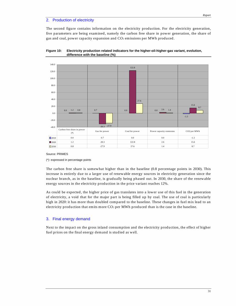
Report

31

2. Production of electricity

The second figure contains information on the electricity production. For the electricity generation, five parameters are being examined, namely the carbon free share in power generation, the share of gas and coal, power capacity expansion and CO2 emissions per MWh produced.

Figure 10: Electricity production related indicators for the higher-oil-higher-gas variant, evolution, difference with the baseline (%)

Source: PRIMES

(*): expressed in percentage points

The carbon free share is somewhat higher than in the baseline (0.8 percentage points in 2030). This increase is entirely due to a larger use of renewable energy sources in electricity generation since the nuclear branch, as in the baseline, is gradually being phased out. In 2030, the share of the renewable energy sources in the electricity production in the price variant reaches 12%.

As could be expected, the higher price of gas translates into a lower use of this fuel in the generation of electricity, a void that for the major part is being filled up by coal. The use of coal is particularly high in 2020: it has more than doubled compared to the baseline. These changes in fuel mix lead to an electricity production that emits more CO2 per MWh produced than is the case in the baseline.

3. Final energy demand

Next to the impact on the gross inland consumption and the electricity production, the effect of higher fuel prices on the final energy demand is studied as well.

0.0 0.7 0.0 0.0

-1.3

1.2

-30.3

122.8

2.6

15.6

0.8

-27.9

27.6

1.48.7

-40.0

-20.0

0.0

20.0

40.0

60.0

80.0

100.0

120.0

140.0

2010 0.0 0.7 0.0 0.0 -1.3

2020 1.2 -30.3 122.8 2.6 15.6

2030 0.8 -27.9 27.6 1.4 8.7

Carbon free share in power (*) Gas for power Coal for power Power capacity extension CO2 per MWh

Report

32

Figure 11: Changes in sectoral final energy demand for the higher-oil-higher-gas variant, evolution, difference with the baseline (%)

Source: PRIMES

All the end sectors undergo an impact from the higher energy prices as higher prices lower demand. The effect is highest in the residential sector, shrinking its consumption by almost 6% relative to the baseline by the end of the projection period. Industry and transport, on the other hand, seem to be the least affected. This can be attributed to, in the case of industry, the limited medium term flexibility for structural changes and to important efficiency gains already reached in the baseline. The low impact on final transport demand then is due to the high motor fuel taxes which curb the impact of higher oil import prices.

-0.5-1.7 -1.6 -1.5-1.1

-4.9-3.8

-2.6-2.1

-5.7 -5.2

-0.5

-25.0

-20.0

-15.0

-10.0

-5.0

0.0

2010 -0.5 -1.7 -1.6 -1.5

2020 -1.1 -4.9 -3.8 -2.6

2030 -2.1 -5.7 -5.2 -0.5

changes in final energy demand-industry

changes in final energy demand-residential

changes in final energy demand-tertiary

changes in final energy demand- transport

Report

33

Box 1: An alternative price variant

Another possible price variant that will not be discussed in this study, though, is an analysis in which oil prices are still assumed to be high, but the evolution of the gas prices does no longer follow the oil price progression. Gas nevertheless shows a slight price increase (as is shown in figure 8 as ‘Gas Medium’). This ‘higher-oil-medium-gas-price variant’ starts from the same hypotheses as the previous variant (stronger GDP growth in the East and smaller oil and gas reserves), but introduces a relatively slower growth in the gas price compared to oil (but still stays above the level obtained in the baseline). This variant allows to test the hypothesis that the most nearby suppliers of gas in Europe (Russia, Iran and the Caspian Sea) could sell their gas at a price slightly under the price determined by the market fundamentals so as to maintain a share in this region of the world.

Main lessons to be drawn from this variant is that at more moderate gas prices (but still skyrocketing oil prices), total gas needs will be higher than in the baseline (and much higher than in the higher-oil-higher-gas variant). This can be subscribed to the relative price proportions (gas is far less expensive than oil). Nonetheless, gas is slightly more expensive than in the baseline, which leads to a small decrease in primary energy demand. This lower primary energy consumption combined with a further penetration of natural gas will entail lower CO2 emissions.

When it comes to electricity production, coal is more competitive than gas so coal is the preferred fuel, gas occupies the second place. This leads to a power generation sector that is somewhat more polluting than the baseline power sector (but less polluting than the higher-oil-higher-gas variant).

Due to the higher energy prices, final demand is being reduced, although not as drastically as in the higher-oil-higher-gas variant. This can be explained by the moderate gas prices in the higher-oil-medium-gas variant which limit the impact on energy consumption. Interesting to remark is that the demand reduction in the transport sector is exactly identical to the higher-oil-higher-gas variant, due to the fact that this sector does not consume natural gas and that the price hypotheses for oil are the same as the ones described in the higher-oil-higher-gas variant.

Report

34

Report

35

V. Alternative scenarios

A. Definition

Next to an obligatory baseline and a sensitivity analysis on international fuel prices to take into account the uncertainty surrounding future energy prices, the FPB was also asked to study the impact of a number of alternative scenarios. Alternative scenarios are constructed in order to investigate a particular policy line or policy measures of which one wants to know the impact on the national energy system and its emissions. These alternative scenarios differ from sensitivity analyses in that they do not study the effect one single exogenous parameter has on the outcome, rather the whole context of the scenario is being changed. In this way, through the definition of the alternative scenario, a new policy background is chosen, in such a way different from the baseline that it becomes possible to compare the two scenarios (reference and alternative) and to investigate how a different outset (as stipulated in the alternative scenario) can change the national energy and emission system.

Further to the request of the Commission Energy 2030, three main policy issues are put forward in this report and assessed in different combinations: first, the impact of a CO2 emission constraint is being studied17, second, the reappearance of nuclear on the electricity scene will be scrutinized, third, the uncertainty related to the availability of a particular emission reduction technology, namely carbon capture and storage, is assessed. A detailed description of the way the scenarios were designed and of the rationale behind these choices is provided in annex C.

Finally, the alternative scenarios are complemented with a sensitivity analysis on soaring oil and gas prices (identical to the one tested on the baseline). This adds up to 12 new scenarios and associated variants.

17 The emission constraint is achieved in modelling the energy economy so as to obtain equal marginal abatement costs across

the sectors.

Report

36

Box 2: Definition of alternative scenarios and sensitivity analyses on the alternative scenarios

Alternative: - Bpk15: scenario in which Belgium reduces its energy CO2 emissions by 15% in 2030 compared to

the 1990 level, decommissioning of nuclear plants takes place and CCS is available in the period 2020-2030

- Bpk15n: scenario in which Belgium reduces its energy CO2 emissions by 15% in 2030 compared to the 1990 level, lifetime extension of existing nuclear plants + possibility of having 1 new nuclear unit of 1700 MW after 2020 and CCS is available in the period 2020-2030

- Bpk15s: scenario in which Belgium reduces its energy CO2 emissions by 15% in 2030 compared to the 1990 level, decommissioning of nuclear plants and CCS is not available in the period 2020-2030

- Bpk15ns: scenario in which Belgium reduces its energy CO2 emissions by 15% in 2030 compared to the 1990 level, lifetime extension of existing nuclear plants + possibility of having 1 new nuclear unit of 1700 MW after 2020 and CCS is not available in the period 2020-2030

Sensitivity analysis: - Bpk15h: scenario in which Belgium reduces its energy CO2 emissions by 15% in 2030 compared to

the 1990 level, coupled with soaring oil and gas prices, CCS is available in the period 2020-2030 - Bpk15nh: scenario in which Belgium reduces its energy CO2 emissions by 15% in 2030 compared to

the 1990 level, lifetime extension of existing nuclear plants + possibility of having 1 new nuclear unit of 1700 MW after 2020 coupled with soaring oil and gas prices, CCS is available in the period 2020-2030

Alternative: - Bpk30: scenario in which Belgium reduces its energy CO2 emissions by 30% in 2030 compared to

the 1990 level, decommissioning of nuclear plants takes place and CCS is available in the period 2020-2030

- Bpk30n: scenario in which Belgium reduces its energy CO2 emissions by 30% in 2030 compared to the 1990 level, lifetime extension of existing nuclear plants + possibility of having 1 new nuclear unit of 1700 MW after 2020 and CCS is available in the period 2020-2030

- Bpk30s: scenario in which Belgium reduces its energy CO2 emissions by 30% in 2030 compared to the 1990 level, decommissioning of nuclear plants and CCS is not available in the period 2020-2030

- Bpk30ns: scenario in which Belgium reduces its energy CO2 emissions by 30% in 2030 compared to the 1990 level, lifetime extension of existing nuclear plants + possibility of having 1 new nuclear unit of 1700 MW after 2020 and CCS is not available in the period 2020-2030

Sensitivity analysis: - Bpk30h: scenario in which Belgium reduces its energy CO2 emissions by 30% in 2030 compared to

the 1990 level, coupled with soaring oil and gas prices, CCS is available in the period 2020-2030 - Bpk30nh: scenario in which Belgium reduces its energy CO2 emissions by 30% in 2030 compared to

the 1990 level, lifetime extension of existing nuclear plants + possibility of having 1 new nuclear unit of 1700 MW after 2020 coupled with soaring oil and gas prices, CCS is available in the period 2020-2030

B. Marginal abatement cost

Given the growth in energy related CO2 emissions in the baseline (+32% in 2030 compared to 1990), the imposition of emission reduction constraints requires additional effort to be undertaken by economic agents over the projection period. In the PRIMES modelling approach, this is reflected by the marginal abatement cost (or carbon value) which is equal to the shadow variable of the emission constraint. Following the introduction of a carbon value (CV), the producers and consumers of energy

Report

37

adjust their behaviour to emit less CO2 emissions. The resulting changes in the energy system represent the least-cost solution for achieving the constraint. By construction, the marginal abatement costs are equal among the sectors.

The carbon value reflects the degree of ease or difficulty in achieving the constraint on emissions; it depends not only on the constraint itself but also on the number, potential and costs of the reduction options accounted for in the analysis.

The above statement is illustrated in the following table which gives the marginal abatement costs associated with the two constraints on CO2 emissions considered in the study (-15% and -30%), according to the presence or not of two particular CO2 reduction options in the power sector, namely nuclear energy and carbon capture and storage (CCS). To make the figures more “telling” by themselves, the carbon values are also expressed in $ per barrel of oil equivalent.

Table 8: Carbon values associated to the different emission reduction scenarios, year 2030

Bpk15 Bpk15n Bpk15s Bpk15ns Bpk30 Bpk30n Bpk30s Bpk30ns in €/t CO2 123 60 524 105 320 186 2150 490 in $/bbl 47 23 202 40 123 71 827 188

Source: PRIMES

The carbon value required to reduce the energy related CO2 emissions of Belgium by 15% in 2030 at 1990 level range from 60 to 524 € per ton of CO2 reduced. The lowest value corresponds to the scenario where both nuclear energy and CCS are made available as energy technology options (Bpk15n). The corresponding figure of 60 €/tCO2 is equivalent to one third of current oil price (i.e. around 70$ per barrel). On the other hand, if both options are not made available (BPk15s), the CV climbs dramatically to reach three times the current oil price. The other two reduction scenarios show similar carbon values, in the range of 100-120 €/tCO2.

A doubling of the emission constraint, from -15% to -30% in 2030 compared to 1990 levels, leads to more than a doubling of the marginal abatement cost. With CCS, the CV is roughly multiplied by three; without CCS, it is multiplied by a factor of four or more. The ranking of CV’s according to the scenario is the same as for the -15% reduction cases. It is interesting to notice that the CV’s required to achieve a 30% reduction of energy related CO2 emissions in 2030 with nuclear energy and/or CCS as possible options, are lower than the CV estimated for the 15% reduction case in the absence of the these two options. This result underlines the role of the power generation sector for responding to the introduction of CO2 emission reduction constraints either through the use of CCS or through the abrogation of the law of 2003 on the use of nuclear power generation. However, it does not address a wider range of policy strategies that exist in the final demand sectors and in the power sector.

Table 8 also shows that the selected constraints on CO2 emissions could entail relatively high costs to the society. Having noted that, it is important to stress that (1) the analysis only copes with energy related CO2 emissions, (2) the abatement costs can be (partially) compensated by reductions in other costs through appropriate policy measures (e.g. labour charges), and (3) the benefits of taking appropriate actions to reduce the negative impacts of climate change are not taken into account. In other words, the estimated carbon values should not be interpreted as costs of policy implementation but rather as an indicator of the relative difficulty of achieving the constraints. As regards the focus on energy related CO2 emissions, it is reasonable to think that at such high carbon values, options aimed at reducing non-CO2 greenhouse gases and the resort to flexible mechanisms under the Kyoto Protocol or to the EU Emission Trading Scheme (ETS) will be less costly than certain domestic actions focusing on CO2 emissions alone.

In what follows, the main results of the alternative scenarios will be discussed.

Report

38

C. Analysis of the impact of the alternative scenarios and variants

The analysis of the impact of a change in policy is quantitatively calculated with the use of the PRIMES model and focalises on the consequences on the Belgian energy system. The analysis takes place along two lines: first, a more general overview of the evolution and structure of the major energy indicators for all scenarios will be provided through the use of comprehensive tables, second, a selection of energy indicators will be presented through the format of coupled analyses, meaning that two alternative scenarios or variants will be jointly analysed and their impact relative to the baseline will be unfold. The latter (the coupled analyses) all describe the changes with respect to the baseline and for the year 2030, unless stated otherwise. Where relevant, the cost implications for the different sectors are also examined.

In order to facilitate the comparison with other parts of the report, the same type of graphs and tables are constructed and presented in each section.

1. Belgian reduction of energy CO2 emissions by -15%

This part details all scenarios in which the CO2 emission reduction obligation boils down to a decrease on the Belgian territory of the energy CO2 emissions with 15% in 2030 compared to the energy CO2 emission level obtained in 1990.

a. Primary energy demand

i General

The table below shows the total evolution (expressed in average annual growth rate) for the period 2000-2030 and the structure of the primary energy demand or gross inland consumption (GIC) for the year 2030 of, on the one hand, the baseline, on the other hand, the four -15% reduction scenarios.

Table 9: Primary energy demand, comparison baseline vs. -15% reduction scenarios, year 2030 (%)

Baseline Bpk15 Bpk15n Bpk15s Bpk15ns Average annual growth rate 2000-2030 -0.1 -0.3 0.2 -0.8 0.1 Structure of GIC (%) - Coal 20.8 13.9 3.0 1.7 2.5 - Oil 38.6 38.0 33.6 39.0 33.1 - Natural gas 35.3 39.9 29.5 48.3 29.5 - Nuclear 0.0 0.0 27.4 0.0 27.9 - RES 5.3 8.2 6.5 11.0 7.0

Source: PRIMES

Looking at this table, it immediately becomes clear that, in order to reach the -15% reduction in energy CO2 emissions, not only a fuel switch is necessary, but also a reduction in primary energy demand is indispensable. The alternative scenario in which the CO2 reduction technology CCS is not available and nuclear decommissioning is in place (Bpk15s) is the hardest hit with an average primary demand reduction rate of -0.8% per year. Nuclear power erases this demand reduction and even leads to small annual demand increases: this evolution, however, has to do with the statistical convention related to nuclear energy (cf. supra).

Within the composition of the GIC, coal suffers most from the reduction constraint: its representation within the GIC shrinks considerably in the Bpk15 cases; when nuclear is added and/or when CCS is not available; its percentage shrivels even further. Turning to natural gas, we see that in the case in which nuclear power and CCS are no parts of the reduction alternatives, its share jumps to almost half

Report

39

the GIC. This is due to the fact that one cannot turn to nuclear in this alternative and coal without the CCS option is not interesting to use due to its high carbon content. With nuclear, the share of gas remains around 30%. Last, the CO2 reduction of -15% translates into a higher use of renewable energy sources: the RES’s share floats between 7 and 11% of the GIC.

ii Coupled analysis

In this section, different scenarios are being pairwisely discussed, the first being the comparison between a scenario in which a -15% reduction will be reached by 2030 with nuclear phase-out and a scenario with the same reduction target but in which the lifetime of existing nuclear plants will be prolonged up to 60 years and new nuclear investment in one additional power plant is made possible.

Bpk15 vs. Bpk15n

This joint analysis between Bpk15 and Bpk15n can be seen as a study of the relative impact the nuclear option (decommissioning versus extension of plant operating lifetime to 60 years and possibility to invest in an additional unit of 1700 MW) has on primary energy related indicators for the year 2030, both subject to the CO2 emission constraint of having to reduce the energy CO2 emissions on Belgian soil by 15% in 2030 compared to 1990. The joint analysis also constitutes a deepening of the general analysis on the individual scenarios presented in table 9.

Figure 12: Primary energy related indicators for the Bpk15 and Bpk15n scenarios, year 2030, difference with the baseline (%)

Source: PRIMES

(*): expressed in percentage points

The net import of energy18 for both scenarios will be lower than in the baseline, even much lower when nuclear energy is allowed back in the game. The fact that there is less import is due to the rather severe constraint that 15% of the energy CO2 emissions has to be eliminated, what is translated into a serious dip in the energy consumption (hence, because of the lack of fossil fuel resources in Belgium, in import). Coal is victim number one of the -15% reduction constraint because it exhausts the most CO2 per unit of output. In the case of ‘nuclear allowed’ (Bpk15n) even less coal is needed, especially

18 According to Eurostat convention, this excludes the import of uranium.

-7.4-5.4

-2.5

6.9

-35.7

2.9

-21.3

8.7

-25.7

-9.3

-35.7

1.2

-60.0

-50.0

-40.0

-30.0

-20.0

-10.0

0.0

10.0

20.0

BPK15 -7.4 -5.4 -2.5 6.9 -35.7 2.9

BPK15n -21.3 8.7 -25.7 -9.3 -35.7 1.2

Net imports of energy Energy intensity ofGDP

Import dependency (*) Total gas needs CO2 emissionsRenewables share in

GIC (*)

Report

40

for the production of electricity. The latter will also employ less natural gas; nuclear after all seems to be more competitive than coal or gas when a constraint on CO2 emissions is imposed. As a consequence, the indicator for import dependency will plunge in both cases, much lower though in the Bpk15n-case.

The gas needs are higher in the case of nuclear decommissioning. This is due to the fact that CO2

emissions have to be reduced, nuclear is being phased out, coal emits more CO2 per unit of output than gas and there is only a limited potential of some renewable energy sources available, so the only refuge is being provided by gas. 7% more gas will be consumed compared with the baseline, whilst gas needs are approximately 9% lower when nuclear is an option. CO2 emissions will in both cases fall 36% under the baseline level: this is the translation of the 15% reduction compared with 1990, the starting point of both scenarios.

The share of renewable energy sources in the gross inland consumption is higher in both cases than the baseline level, although the non-nuclear scenario registers a higher renewables’ share. In absolute terms, the share of RES reaches 8.1% of the GIC in 2030 in the Bpk15-scenario, whereas it only arrives at 6.5% in the Bpk15n-scenario (in the baseline, it is 5.2%).

Bpk15s vs. Bpk15ns

This coupled analysis investigates the two cases in which the novel emission reduction technology CCS is not used during the entire projection period (2000-2030) because this technology option is not assumed to be commercially viable at the stated carbon value and/or within the time frame studied. Overall, the changes in primary energy indicators compared to the baseline are more outspoken when CCS is not included in the analysis (cf. figure 12 vs. figure 13).

Figure 13: Primary energy related indicators for the Bpk15s and Bpk15ns scenarios, year 2030, difference with the baseline (%)

Source: PRIMES (*): expressed in percentage points

-21.7-19.6

-4.8

9.7

-35.7

5.7

-23.6

6.7

-26.6

-10.8

-35.7

1.8

-60.0

-50.0

-40.0

-30.0

-20.0

-10.0

0.0

10.0

20.0

BPK15s -21.7 -19.6 -4.8 9.7 -35.7 5.7

BPK15ns -23.6 6.7 -26.6 -10.8 -35.7 1.8



GIC (*)

Report

41

Without CCS and with the nuclear phase-out in place, we see that renewable energy sources take off significantly. No less than 67% more renewable energy sources are deployed in the primary production of this variant. This adds up to a representation in the gross inland consumption of 10.9% (compared to 5.2% in the baseline). Because of the CO2 emission constraint and the lack of CCS, the use of coal and, although to a lesser extent, oil is penalised: therefore, 93% less coal is being imported, 14% less oil, hence the strong dip in net imports. Gas on the other hand is consumed more than in the baseline and pulls the net import figure slightly up. The nuclear allowed scenario also shows a decline in both coal and oil import, but this time, even gas is less used (and imported). Nonetheless, the Bpk15ns scenario has a higher total GIC: this can be explained by the higher share of nuclear.

The lower net imports of energy entail a lower import dependency. Total gas needs are higher compared to the baseline in the nuclear decommissioning scenario without CCS, lower in the nuclear allowed scenario. This is because gas is the only refuge in the non-nuclear case (next to RES), whilst in the nuclear allowed scenario, nuclear is more competitive and outprices gas.

The share of renewables in the GIC is never higher than in the Bpk15s case: at a rate of almost 6 percentage points above the baseline, approximately 11% of the primary energy demand is being covered by renewable energy sources. Biomass and wind take up the lion’s share, but also the appearance of solar PVs is worth noting and is much more significant than in the baseline (almost 6 times higher in 2030).

b. Electricity and steam generation

i General

Turning to electricity and steam generation, the following tables show some light on the discussion.

Table 10: Power generation, comparison, year 2030 (%)

Baseline Bpk15 Bpk15n Bpk15s Bpk15ns Average annual growth rate 2000-2030 1.0 1.0 1.3 0.9 1.4 Structure of electricity generation - Nuclear 0.0 0.0 51.9 0.0 50.9 - RES 11.8 22.7 19.5 28.3 20.3 - Fossil fuels 88.2 77.3 28.6 71.7 28.8

Source: PRIMES

Power generation in the baseline grows by 1% on average each year, the alternative scenarios show higher growth rates provided nuclear is taken into account as an energy policy option. This is due to the privileged use of electricity in the CO2 reduction scenarios, especially in industry where more electricity will be consumed to the detriment of fossil fuels (e.g. in the iron and steel sector). In the cases where nuclear is a part of the generation park, electricity consumption, hence production, growth rates are highest. In these scenarios, nuclear represents more than half of the power production by 2030, nibbling market share away from fossil fuel based plants. Renewable energy sources profit from the CO2 reduction constraint: in the alternative scenarios, their share (almost) doubles compared to the baseline.

The reduction effort of the power and steam sector is assessed keeping the levels of net electricity imports equal to those calculated endogenously in the baseline. In other words, we do not consider the possibility to achieve reductions in CO2 emissions through an increase in electricity imports and, hence, a decrease in electricity production on the national territory.

Report

42

Table 11: Installed power capacity, comparison, year 2030 (MW)

Baseline Bpk15 Bpk15n Bpk15s Bpk15ns Installed power capacity 22999 25524 27539 29998 27912 - Nuclear 0 0 7775 0 7775 - Wind onshore 1388 2045 1976 2058 2045 - Wind offshore 1019 3800 3791 3800 3800 - Solar PV 209 209 209 5903 209 - Biomass 1310 1568 1413 1631 1575 - Coal fired 7054 3940 0 0 0 - Gas fired 11240 12142 11704 12562 11834

Source: PRIMES

Digging somewhat deeper into power generation, we come up with the figures for the installed power capacity. It immediately becomes clear that the reduction scenarios go hand in hand with an expansion of the installed power capacity. When the nuclear option is included (Bpk15n and Bpk15ns), the increase in power capacity results mainly from the increase in the demand for electricity. When nuclear is phased out (Bpk15 and Bpk15s), the increment in capacity is due to higher shares of intermittent RES in the production park: additional capacity is needed to cope with relatively low availability factors of wind power and solar PV. Investments in wind turbines (on- and off-shore) become primordial: all alternative scenarios but the Bpk15n use the maximum potential of on- and off-shore wind by the end of the projection period. Also, more biomass is used than in the baseline. Coal, on the other hand, has completely vanished. Only exception is the Bpk15 scenario as coal, with the CCS option open, remains the only alternative next to gas as nuclear is being phased out. When CCS cannot be implemented, though, we see a spectacular surge in the use of solar PV. Although solar PV does not seem to be commercially viable in the other scenarios, the absence of other alternatives in the Bpk15s case obliges them to make their appearance in the future generation park.

The relative role of CO2 reduction options in the power and steam sector is analysed further in section V.C.3.a.

Report

43

ii Coupled analysis

Bpk15 vs. Bpk15n

Figure 14: Electricity production related indicators for the Bpk15 and Bpk15n scenarios, year 2030, difference with the baseline (%)

Source: PRIMES

The coupled analysis on electricity production with CCS possible shows a large impact of the nuclear come-back on the generation park. First of all, the carbon free share in power production is much higher when nuclear is allowed. For one, this is due to the fact that nuclear power is seen as a non-carbon emitting energy source (hence it is not penalized by placing a carbon tax on energy fuels). Second, the share of renewable energy sources in electricity generation in both scenarios is much higher compared to the baseline: in the Bpk15 scenario, it reaches almost 23%, in the Bpk15n case, it is 20%. This underwrites the thesis that nuclear and renewable energy sources are substitutes for fossil fuels, but that they do not form substitutes for one another. The appearance of nuclear does not, in other words, preclude the upsurge of RES.

Natural gas, on the other hand, is used more when Belgium has to answer to post-2012 CO2 constraints without the use of nuclear. When new nuclear investments are allowed and the lifetime of existing plants can be extended, much less gas is needed to produce electricity. In this last scenario, coal even disappears completely from the power scene by the end of the projection period. These changed production patterns translate into a considerably cleaner power generation: without nuclear, almost 70% less CO2 per MWh produced is being emitted, with nuclear a further reduction becomes possible (-76.4%).

11.018.8

-45.6

12.3

-69.1

59.6

-32.1

-100.0

-7.5

-76.4

-150.0

-100.0

-50.0

0.0

50.0

100.0

BPK15 11.0 18.8 -45.6 12.3 -69.1

BPK15n 59.6 -32.1 -100.0 -7.5 -76.4


Report

44

Bpk15s vs. Bpk15ns

Figure 15: Electricity production related indicators for the Bpk15s and Bpk15ns scenarios, year 2030, difference with the baseline (%)

Source: PRIMES

Electricity production in these two non-CCS scenarios diverges strongly from the baseline. The carbon free share in power generation in both cases is (much) higher than in the baseline due to the preferred (read: less costly with the introduction of a carbon value) utilization of non carbon containing energy fuels like RES and nuclear power. The first scenario (Bpk15s) still uses a lot of gas in order to keep the lights on, the second (Bpk15ns) severely reduces its use of gas in favour of nuclear and renewables. Coal is completely abolished when CCS is not available, due to the high exhaustion rate and the carbon value that is subsequently raised on the use of this fuel. Power generation becomes cleaner compared to the baseline, especially in the second scenario. It is nevertheless noticeable that the Bpk15s case possesses, in the ranking order of all -15% reduction scenarios under discussion, the most polluting power generation sector: CCS, in other words, enables the electricity sector to produce in a much less polluting way.

iii Cost implications

The impact of a CO2 emission reduction constraint on the costs of electricity and steam generation is estimated in this section through changes in average production costs. Average production cost is defined as the total cost of electricity and steam supply divided by total electricity and steam production. This cost indicator includes all (energy) costs related to electricity and steam generation in power plants (electricity only and CHP) as well as in industrial and refinery boilers; they also include costs for transmission, distribution and net electricity imports.

The average production costs are only illustrative of the impacts on the costs of the power and heat supply sector. They do not represent the full costs related to the implementation of CO2 reduction policies. Indeed, the imposition of carbon values induces changes in behaviour, fuels and technologies (whose costs are reflected in the average production cost) but does not involve any policies needed to realise these changes.

Table 12 and figure 16 below compare the evolution of the average production costs in the baseline and in the different -15% reduction scenarios.

16.5

51.3

-100.0

34.1

-44.7

59.4

-30.2

-100.0

-5.6

-71.6

-150.0

-100.0

-50.0

0.0

50.0

100.0

BPK15s 16.5 51.3 -100.0 34.1 -44.7

BPK15ns 59.4 -30.2 -100.0 -5.6 -71.6


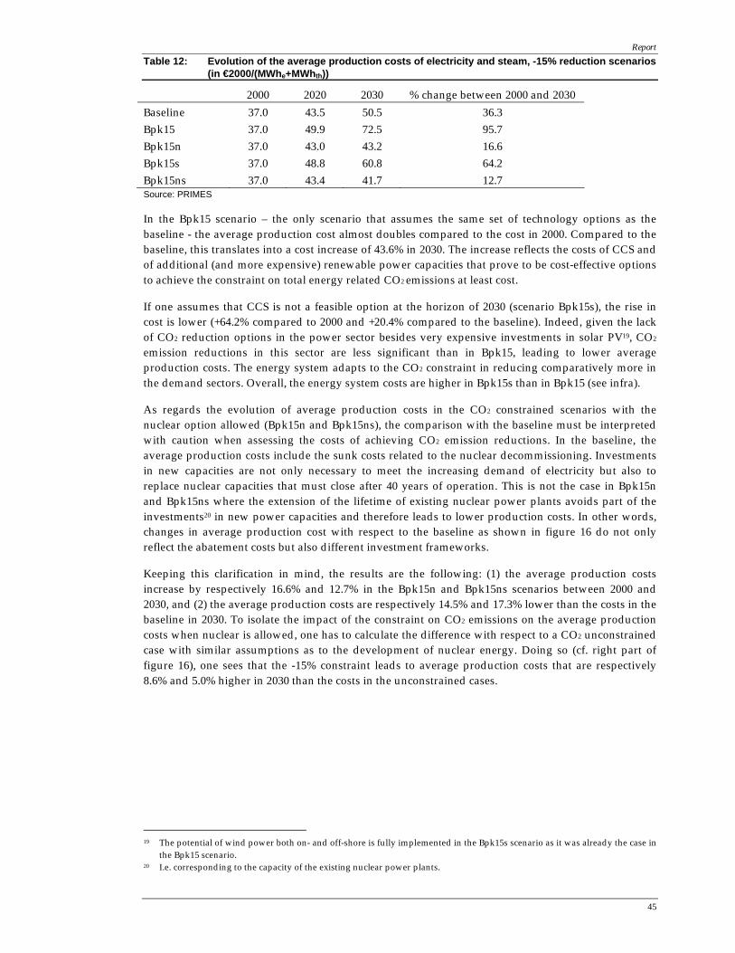
Report

45

Table 12: Evolution of the average production costs of electricity and steam, -15% reduction scenarios (in €2000/(MWhe+MWhth))

2000 2020 2030 % change between 2000 and 2030 Baseline 37.0 43.5 50.5 36.3 Bpk15 37.0 49.9 72.5 95.7 Bpk15n 37.0 43.0 43.2 16.6 Bpk15s 37.0 48.8 60.8 64.2 Bpk15ns 37.0 43.4 41.7 12.7 Source: PRIMES

In the Bpk15 scenario – the only scenario that assumes the same set of technology options as the baseline - the average production cost almost doubles compared to the cost in 2000. Compared to the baseline, this translates into a cost increase of 43.6% in 2030. The increase reflects the costs of CCS and of additional (and more expensive) renewable power capacities that prove to be cost-effective options to achieve the constraint on total energy related CO2 emissions at least cost.

If one assumes that CCS is not a feasible option at the horizon of 2030 (scenario Bpk15s), the rise in cost is lower (+64.2% compared to 2000 and +20.4% compared to the baseline). Indeed, given the lack of CO2 reduction options in the power sector besides very expensive investments in solar PV19, CO2

emission reductions in this sector are less significant than in Bpk15, leading to lower average production costs. The energy system adapts to the CO2 constraint in reducing comparatively more in the demand sectors. Overall, the energy system costs are higher in Bpk15s than in Bpk15 (see infra).

As regards the evolution of average production costs in the CO2 constrained scenarios with the nuclear option allowed (Bpk15n and Bpk15ns), the comparison with the baseline must be interpreted with caution when assessing the costs of achieving CO2 emission reductions. In the baseline, the average production costs include the sunk costs related to the nuclear decommissioning. Investments in new capacities are not only necessary to meet the increasing demand of electricity but also to replace nuclear capacities that must close after 40 years of operation. This is not the case in Bpk15n and Bpk15ns where the extension of the lifetime of existing nuclear power plants avoids part of the investments20 in new power capacities and therefore leads to lower production costs. In other words, changes in average production cost with respect to the baseline as shown in figure 16 do not only reflect the abatement costs but also different investment frameworks.

Keeping this clarification in mind, the results are the following: (1) the average production costs increase by respectively 16.6% and 12.7% in the Bpk15n and Bpk15ns scenarios between 2000 and 2030, and (2) the average production costs are respectively 14.5% and 17.3% lower than the costs in the baseline in 2030. To isolate the impact of the constraint on CO2 emissions on the average production costs when nuclear is allowed, one has to calculate the difference with respect to a CO2 unconstrained case with similar assumptions as to the development of nuclear energy. Doing so (cf. right part of figure 16), one sees that the -15% constraint leads to average production costs that are respectively 8.6% and 5.0% higher in 2030 than the costs in the unconstrained cases.

19 The potential of wind power both on- and off-shore is fully implemented in the Bpk15s scenario as it was already the case in

the Bpk15 scenario. 20 I.e. corresponding to the capacity of the existing nuclear power plants.

Report

46

Figure 16: Average production costs of electricity and steam in the -15% reduction cases, difference from unconstrained cases in 2030 (%)

-20,0

0,0

20,0

40,0

60,0

80,0

100,0

Bpk15 43,6

Bpk15n -14,5 8,6

Bpk15s 20,4

Bpk15ns -17,3 5,0

from baseline from CO2 unconstrained case w ith nuclear

Source: PRIMES

c. Final energy demand

i General

In analogy with the baseline and the sensitivity analysis, the analysis of the GIC and the electricity production is followed by a study on the final energy demand.

Table 13: Final energy demand, comparison, year 2030 (%)

Base Bpk15 Bpk15n Bpk15s Bpk15ns Average annual growth rate 2000-2030 0.3 0.1 0.2 -0.4 0.2 Structure of FED - Solids 5 2 3 1 2 - Oil 39 39 39 38 38 - Gas 28 28 27 26 27 - Electricity 22 24 25 27 26 - Heat 4 4 4 4 4 - Other 2 3 2 4 3

Source: PRIMES

First thing that pops out of this table is the fact that the average annual final energy demand growth rate in the -15% reduction scenarios is lower than in the baseline. In the Bpk15s scenario, it even becomes negative. Next to supply side contributions, significant final energy demand reductions are thus essential when a CO2 constraint is installed, all the more so when supply side CO2 reduction options are limited. When it comes to the fuel structure of the final energy demand, table 13 shows that fuel switching plays a smaller role for CO2 reduction at the final energy level than in primary energy demand as strong shifts towards less carbon intensive energy forms already take place in the baseline. The most significant changes from the baseline are (1) the decline and demise of the solid fuels (2) the upsurge of electricity. The expiration of solid fuels is due to the penalisation of CO2 exhaustion, and since coal is a large CO2 emitter, its use consequently shrinks. The introduction of a carbon value hurts electricity relatively less (compared to fossil fuels), hence its larger share.

Report

47

ii Coupled analysis

Bpk15 vs. Bpk15n

Figure 17: Changes in sectoral final energy demand for the Bpk15 and Bpk15n scenarios, year 2030, difference with the baseline (%)

Source: PRIMES

This graph proves, next to the table above, that the installation of a -15% constraint leads to a dip in the final energy demand. The difference between the two alternative scenarios (Bpk15 and Bpk15n) is worth noting: without the nuclear option, efforts on the demand side are far more significant, especially in the industry and tertiary. These two sectors have to give in 10% of their final consumption relative to the baseline. As no change in value added is assumed in the CO2 constraint scenarios (compared to baseline), this means that the energy intensity21 of industry and the tertiary sector decreases by 10% in 2030 compared to the baseline. Two main factors contribute to the decrease in the final energy consumption of industry: (1) a partial switch from integrated steelworks to electric arc furnaces in the iron and steel sector (40%), and (2) a further increase in the energy efficiency (60%). The decline recorded in the tertiary and residential sectors is due, on the one hand, to a decrease in the demand for energy services and, on the other hand, to further improvements in the efficiency of heating devices and electric appliances.

Transport responds the least to the -15% reduction constraint. A high level of taxation on transport fuels combined with low price elasticities recorded in this sector cause the impact of the carbon values required in the -15% reduction cases to be rather small. The reduction by 2.3% in final energy demand of transport results mainly from a decrease in transport activity (both passengers and freight) and an increase of the energy efficiency of airplanes22. The energy efficiency of other vehicles remains almost unchanged as well as the fuel mix. It is worth underlining here that the share of biofuels in transport is an exogenous policy parameter in PRIMES. In all alternative scenarios, the share of biofuels is assumed to follow a similar trend than in the baseline, i.e. 2.1% in 2010, 6.4% in 2020 and 8% in 2030.

21 Final energy consumption on value added. 22 The responsiveness of the aviation sector to price increases is higher than that of the other transport modes.

-10.0-9.0

-10.0

-2.3

-5.3

-3.0-1.6

0.4

-25.0

-20.0

-15.0

-10.0

-5.0

0.0

BPK15 -10.0 -9.0 -10.0 -2.3

BPK15n -5.3 -3.0 -1.6 0.4



changes in final energy demand- tertiary

changes in final energy demand-transport

Report

48

With nuclear power in place, final demand decreases are more moderate as more significant CO2 emission reductions take place in the power supply sector. However, the general pattern of changes is similar to that in Bpk15.

Bpk15s vs. Bpk15ns

Figure 18: Changes in sectoral final energy demand for the Bpk15s and Bpk15ns scenarios, year 2030, difference with the baseline (%)

Source: PRIMES

If CCS is not assumed to be a commercially or technically viable option by 2030, moderate final consumption changes in the scenario with nuclear can be noticed, but the Bpk15s scenario notes a sharp decline of the final energy demand in all the end sectors. Without both CCS and nuclear, the demand side has to carry a relatively big part of the CO2 emission reduction burden, with reductions as high as almost a quarter of the final energy consumption (e.g. tertiary sector) compared to the baseline. The determinants of the changes in the level of final energy consumption are the same as the ones cited in Bpk15; they, however, intensify their role.


The imposition of a CO2 emission reduction constraint has an impact on the energy related costs of the final demand sectors. The impact results from changes in consumer behaviour, production processes and technology choices triggered by the carbon values in order to adjust to the constraints. To assess the cost implications on the demand side, several cost indicators are considered.

For industry and the tertiary sector, the cost indicators are the energy related costs per toe consumed (in €2000/toe) and the energy related costs per unit of value added23. The energy costs include both the costs related to energy equipment (capital and O&M24) and those related to fuel purchases. In the residential sector, the assessment is made via the energy related costs per toe consumed (in €2000/toe) and the energy related expenditures per household (in €2000). The cost implications in the transport sector are provided by the total cost per passenger-kilometre (pkm) and per ton-kilometre (tkm) travelled (in €2000/pkm or tkm). The former indicator relates to passenger transport, the latter to

23 €2000 energy related costs per million €2000 value added. 24 I.e. operation and maintenance costs

-20.9-22.0

-23.7

-12.7

-8.6

-5.7

-3.5

-1.7

-25.0

-20.0

-15.0

-10.0

-5.0

0.0

BPK15s -20.9 -22.0 -23.7 -12.7

BPK15ns -8.6 -5.7 -3.5 -1.7

changes in final energy demand- industry



changes in final energy demand- transport

Report

49

freight transport. The total cost comprises the fuel costs, the energy equipment costs and the non-energy costs (e.g. infrastructure costs) that are important factors in transport.

By construction, all above cost indicators include the changes in costs in the power and steam sector. Indeed, changes in average production costs are transferred to electricity prices paid by the final consumers, affecting the total energy costs of the final demand sectors25.

As already stressed in the section on the power and steam generation, the computed cost indicators do not represent the full costs related to the implementation of the reduction policies. They are only indicative of the relative difficulty of achieving the reduction constraints.

Before moving to the analysis of the cost implications of CO2 emission constraints for the demand sectors, it is worth noting that, in the baseline, energy related costs per toe consumed increase in all sectors over the period 2000-2030. This trend is notably due to the rise in energy prices (oil, natural gas, electricity, etc.) making the fuel purchases more expensive for the final consumers. The costs related to energy equipments are also moving up over the projection period. Overall, the (energy) cost increase ranges from 24% in industry to 63% in the residential sector. The evolution of the energy related costs per unit of value added or per household shows different patterns. In industry, these costs represent a declining trend. In other words, the rate of increase in energy related costs is lower than the rate of increase in value added. In the tertiary sector, the energy related costs per unit of value added remain roughly constant between 2000 and 2030. Finally, in the residential sector, the energy related expenditures per household increase but at a lower pace than the energy related costs per unit of toe consumed.

When a constraint is imposed on the emissions of CO2, energy related costs increase further compared to the baseline, reflecting the impact of the carbon value. The size of the impacts depends on the sector and on the reduction scenario.

Table 14 and figure 19 give the results for industry according to the different -15% reduction cases. The cost implications for the tertiary sector are provided in table 15 and figure 20. The results for the residential sector are reported in table 16 and figure 21. And finally, the impacts on the costs of transport are summarised in table 17 and figure 22.

25 In PRIMES, the pricing of electricity follows the Ramsey-Boiteux principle, which is close to average cost pricing. The

principle is interpreted as a regime of regulated monopoly for new technologies, but also as a result of long-run equilibrium of monopolistic competition in case of mature technologies. The selling price of electricity that each consumer faces is then derived by adding transport and distribution costs, mark-ups and taxes. This price setting mechanism may lead to electricity prices that are considerably different from current market prices.

Report

50

Table 14: Evolution of energy related costs in industry, -15% reduction scenarios

2000 2020 2030 % change between 2000 and 2030 Energy related costs per toe consumed (in €2000/toe) Baseline 537 581 664 24 Bpk15 537 767 970 81 Bpk15n 537 663 734 37 Bpk15s 537 1077 1324 146 Bpk15ns 537 727 789 47 Energy related costs per unit of value added (*) Baseline 159 131 129 -19 Bpk15 159 158 169 6 Bpk15n 159 143 135 -16 Bpk15s 159 192 203 27 Bpk15ns 159 150 140 -12

Source: PRIMES (*) in €2000 energy related costs per thousand €2000 value added

Irrespective of the sector, the lowest cost impacts are recorded in the CO2 reduction scenarios that include the nuclear option (Bpk15n and Bpk15ns). This is explained by two related factors. First, the reduction effort in the demand side is comparatively smaller in the scenarios with nuclear (but higher in the power and steam sector) than in the scenarios with nuclear decommissioning. Second, electricity prices26 which constitute one element of the energy costs reach lower levels in the scenarios with nuclear than in the others (see supra). The latter factor is however less relevant for the transport sector whose consumption is dominated by oil products.

Figure 19: Energy related costs in industry in the -15% reduction cases, difference from baseline in 2030 (%)

0

20

40

60

80

100

Bpk15 46 31

Bpk15n 10 5

Bpk15s 99 58

Bpk15ns 19 9

Energy related costs per toe consumed

Energy related costs per unit of value added

Source: PRIMES

The cost increase is particularly dramatic in the Bpk15s scenario in all sectors but transport (between +146% and +169% in 2030 compared to 2000 and between +64% and +99% compared to the baseline). Due to limited and expensive reduction options on top of those already implemented in the Bpk15

26 Which are related to the average costs of electricity production.

Report

51

scenario, most of the reduction effort is transferred to the demand sectors with a non negligible impact on the energy related costs.

Table 15: Evolution of energy related costs in the tertiary sector, -15% reduction scenarios

2000 2020 2030 % change between 2000 and 2030 Energy related costs per toe consumed (in €2000/toe) Baseline 817 914 1071 31 Bpk15 817 1139 1496 83 Bpk15n 817 1006 1110 36 Bpk15s 817 1623 2061 152 Bpk15ns 817 1079 1170 43 Energy related costs per unit of value added (*) Baseline 21 20 21 1 Bpk15 21 23 27 27 Bpk15n 21 21 22 3 Bpk15s 21 28 31 48 Bpk15ns 21 22 22 6


Looking at the energy related costs per unit of value added or per household, the differences with respect to the baseline reflect the impact on the energy related costs of the sectors as the evolution of value added and number of households is the same in all scenarios. The differences in energy related costs (from the baseline) are systematically lower than the differences in energy related costs per toe consumed. Indeed, the increase in costs per toe leads to lower consumption levels so that the rise in the former factor is partly counterbalanced by the decline in the latter27.

Figure 20 : Energy related costs in the tertiary sector in the -15% reduction cases, difference from baseline in 2030 (%)

0

20

40

60

80

100

Bpk15 40 26

Bpk15n 4 2

Bpk15s 92 47

Bpk15ns 9 5



Source: PRIMES

27 Following the formula C = Q x C/Q.

Report

52

In relative terms, the cost implications of the -15% reduction constraint are comparable in industry and the tertiary sector. They are however comparatively less important in the residential sector. For instance, the difference from baseline in the residential sector of energy related costs per toe consumed is 64% in the Bpk15s scenario, compared to about 100% in industry and the tertiary sector.

Table 16 : Evolution of energy related costs in the residential sector, -15% reduction scenarios

2000 2020 2030 % change between 2000 and 2030 Energy related costs per toe consumed (in €2000/toe) Baseline 962 1305 1572 63 Bpk15 962 1551 2018 110 Bpk15n 962 1422 1640 71 Bpk15s 962 2083 2585 169 Bpk15ns 962 1509 1720 79 Energy related expenditures per household (in €2000) Baseline 2150 2695 2979 39 Bpk15 2150 2971 3483 62 Bpk15n 2150 2823 3018 40 Bpk15s 2150 3375 3825 78 Bpk15ns 2150 2917 3073 43

Source: PRIMES

Figure 21: Energy related costs in the residential sector in the -15% reduction cases, difference from baseline in 2030 (%)

0

20

40

60

80

100

Bpk15 28 17

Bpk15n 4 1

Bpk15s 64 28

Bpk15ns 9 3


Energy related expenditures per household

Source: PRIMES

In general, the effects of the -15% emission constraint on the cost indicators for transport are less significant than the impact on the costs of the other final demand sectors. This result is explained by the low responsiveness of the sector28 to price increases (i.e. low price elasticity and high share of taxes in the end-user prices) and by the relatively less important share of fuel costs in the total cost of transport. The imposition of carbon values changes first of all the priority among fuels and does not generate a significant impact on the allocation of transport activity among the different modes nor on

28 With the exception of the aviation sector.

Report

53

the demand for mobility. Doing so would require other policy strategies than those solely based on fuel prices.

Table 17: Cost evolution in transport, -15% reduction scenarios

2000 2020 2030 % change between 2000 and 2030 Total cost per pkm travelled (in €/pkm) Baseline 0.26 0.26 0.29 11 Bpk15 0.26 0.27 0.29 14 Bpk15n 0.26 0.27 0.29 11 Bpk15s 0.26 0.29 0.32 22 Bpk15ns 0.26 0.27 0.29 13 Total cost per tkm travelled (in €/tkm) Baseline 0.32 0.33 0.35 10 Bpk15 0.32 0.34 0.35 11 Bpk15n 0.32 0.33 0.34 9 Bpk15s 0.32 0.37 0.40 25 Bpk15ns 0.32 0.34 0.35 10

Source: PRIMES

The evolution of the total cost of transport is similar for passenger and freight transport, irrespective of the scenario. It is also comparable in the baseline and in the -15% reduction scenarios with the exception of the Bpk15s scenario. Again, the CO2 reduction limitations in the power and steam sector in Bpk15s enhance the reduction effort in the demand sectors including transport with a direct impact on the costs of the sector.

Compared to the baseline, the total cost per pkm and tkm travelled in 2030 in the -15% reduction cases increases only slightly (less than 2%) except in the Bpk15s scenario where it increases by 10 to 14%, depending on the transport activity.

Figure 22: Costs in transport in the -15% reduction cases, difference from baseline in 2030 (%)

-5

0

5

10

15

20

Bpk15 2 1

Bpk15n 0 -1

Bpk15s 10 14

Bpk15ns 1 0

Total cost per pkm travelled Total cost per tkm travelled

Source: PRIMES

Report

54

d. CO2 emissions by sector

Other indicators of interest are the sectoral CO2 emissions indicators. Whereas the total CO2 emissions are the same in 2030 in all -15% reduction scenarios, the allocation of emissions among sectors may vary from one scenario to another. The table below describes these CO2 emissions in absolute values (Mt) for the year 2030 for the main sectors. The electricity and steam generation sector has two inputs, though, reflecting a subdivision between net emitted emissions and captured emissions (through the use of the CCS technology, denominated CO2 emissions captured).

Table 18: CO2 emissions by sector, comparison, year 2030 (Mt)

Baseline Bpk15 Bpk15n Bpk15s Bpk15ns Electricity and steam generation - Net emissions 52.4 12.4 8.9 27.0 12.8 - CO2 emissions captured 0.0 31.7 4.0 0.0 0.0 Industry 23.5 17.7 19.1 12.8 17.1 Residential 18.3 16.1 16.9 12.0 15.9 Tertiary 10.2 9.2 9.7 7.4 9.4 Transport 31.3 30.6 31.5 27.3 30.8

Source: PRIMES

The availability of nuclear power and/or CCS has a large impact on the power generation emissions. Compared to the baseline, the power generation emissions are at least 4 times smaller than the baseline emissions. When nuclear is being phased out, CCS takes care of three quarters of the power generation reduction; otherwise its contribution drops to one third. Table 18 also shows that the lower the reduction possibilities in the electricity and steam sector, the higher the reductions implemented in the final demand sectors.

e. Sensitivity analysis on prices

After the discussion on the alternative scenarios, this section deals with what happens if international energy prices are higher than expected in the baseline (see graph 8). This section only describes the coupled analyses (and not the general analysis) as to put the finger on the difference the changing of one parameter (here: the international energy prices) has on the scenario in which we are interested.

Report

55

i Bpk15h vs. Bpk15nh

The graphs below show the same scenarios as the Bpk15 and Bpk15n alternative scenarios, but this time, adjusted for the higher oil and gas prices.

Primary energy demand

Figure 23: Primary energy related indicators for the Bpk15h and Bpk15nh scenarios, year 2030, difference with the baseline (%)

Source: PRIMES

This graph is quite similar to figure 12, the difference being the scale of changes and the total gas needs in the Bpk15h variant. Total gas needs in the sensitivity analysis on Bpk15 decrease by 3.2% (whereas they increased by 6.9% in the Bpk15 scenario), meaning that at these soaring prices, gas becomes too expensive and is replaced by other fuels where possible. For the rest, the effect on the import of fossil fuels, hence the import dependency indicator becomes somewhat more outspoken compared to the previous alternative scenarios. CO2 emissions, on the other hand, remain constant due to the obligatory -15% reduction and plunge in both cases by 36% compared to the baseline. The share of renewable energy sources in the gross inland consumption will be slightly higher (0.3 and 0.5 percentage points respectively relative to Bpk15 and Bpk15n) to compensate for the loss in gas.

-10.0-7.2

-2.9 -3.2

-36.0

3.2

-25.1

5.7

-27.0

-14.5

-35.8

1.7

-50.0

-40.0

-30.0

-20.0

-10.0

0.0

10.0

20.0

BPK15h -10.0 -7.2 -2.9 -3.2 -36.0 3.2

BPK15nh -25.1 5.7 -27.0 -14.5 -35.8 1.7

Net imports of energyEnergy intensity of

GDPImport dependency (*) Total gas needs CO2 emissions

Renewables share in GIC (*)

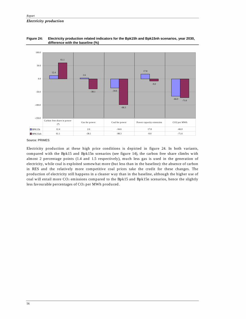
Report

56

Electricity production

Figure 24: Electricity production related indicators for the Bpk15h and Bpk15nh scenarios, year 2030, difference with the baseline (%)

Source: PRIMES

Electricity production at these high price conditions is depicted in figure 24. In both variants, compared with the Bpk15 and Bpk15n scenarios (see figure 14), the carbon free share climbs with almost 2 percentage points (1.4 and 1.5 respectively), much less gas is used in the generation of electricity, while coal is exploited somewhat more (but less than in the baseline): the absence of carbon in RES and the relatively more competitive coal prices take the credit for these changes. The production of electricity still happens in a cleaner way than in the baseline, although the higher use of coal will entail more CO2 emissions compared to the Bpk15 and Bpk15n scenarios, hence the slightly less favourable percentages of CO2 per MWh produced.

12.42.6

-34.6

17.8

-66.0

61.1

-38.1

-98.3

-9.0

-71.6

-150.0

-100.0

-50.0

0.0

50.0

100.0

BPK15h 12.4 2.6 -34.6 17.8 -66.0

BPK15nh 61.1 -38.1 -98.3 -9.0 -71.6


Report

57

Final energy demand

Figure 25: Changes in sectoral final energy demand for the Bpk15h and Bpk15nh scenarios, year 2030, difference with the baseline (%)

Source: PRIMES

Soaring fuel prices coupled with the -15% restriction do make a difference in the final energy demand: energy is considerably less consumed in all end sectors, not only compared to the baseline but also compared to Bpk15 and Bpk15n. The transport sector again is the least affected by the price increases in both cases. This can be subscribed to the fact that the latter already has to support relatively high fuel levies; additional price rises caused by the soaring oil prices then do not have a proportionally equal impact on this sector. The other sectors do carry the weight of the higher prices. Nuclear production seems to lessen the impact on the final energy consumption, although even in this case, sacrifices on the demand side have to be made. Compared to the Bpk15 and Bpk15n scenarios, final demand reductions are more significant to compensate for the higher CO2 emissions in the power sector.

2. Belgian reduction of energy CO2 emissions by -30%

This part details all scenarios in which the CO2 reduction constraint boils down to a reduction on the Belgian territory of the energy CO2 emissions with 30% compared to the energy CO2 emission level obtained in 1990. As in the previous part, the analysis consists of 2 components: first, a rather general overview of the energy indicator is given for the baseline and the alternative scenarios, second, different scenarios and variants are being pairwisely analysed and discussed.

-10.2

-12.2

-13.7

-4.3

-6.5-7.9

-5.3

-2.6

-25.0

-20.0

-15.0

-10.0

-5.0

0.0

BPK15h -10.2 -12.2 -13.7 -4.3

BPK15nh -6.5 -7.9 -5.3 -2.6





Report

58

a. Primary energy demand

i General

Table 19: Primary energy demand, comparison baseline vs. -30% reduction scenarios, year 2030 (%)

Baseline Bpk30 Bpk30n Bpk30s Bpk30ns Average annual growth rate 2000-2030 -0.1 -0.4 0.1 -1.2 -0.2 Structure of GIC (%) - Coal 20.8 12.5 3.1 0.8 1.3 - Oil 38.6 36.8 32.6 37.1 31.4 - Natural gas 35.3 41.5 29.0 48.8 28.2 - Nuclear 0.0 0.0 28.2 0.0 30.5 - RES 5.3 9.2 7.1 13.3 8.7

Source: PRIMES

With a more strict reduction constraint in place, an immediate impact on the average annual growth rate of the GIC can be noticed. This growth rate becomes negative in all scenarios, except when both nuclear and CCS are available (Bpk30n). In all other cases, primary energy consumption has to be reduced year after year in order to satisfy the -30% constraint. Turning to the structure of the primary demand, we see that coal almost disappears from the GIC landscape, while renewable energy sources take in a higher share than is the case in the baseline and in the -15% reduction scenarios.

ii Coupled analysis

The coupled analyses presented below give the opportunity to detail the general analysis shown in table 19.

Bpk30 vs. Bpk30n

The first coupled analysis compares two scenarios in which the energy CO2 emissions on Belgian soil decline by no less than 30%. The first scenario studies the impact such a reduction has in terms of the national energy system and its emissions, the second couples this same analysis with the fact that nuclear is allowed back in the energy playing field (prolongation of lifetime of existing plants and possibility of one new investment). Analysing these two scenarios together makes it possible to distinct the relative impact nuclear energy could have in pulling down the energy CO2 emission level to such an ambitious level (-30% in 2030 compared to 1990).

Report

59

Figure 26: Primary energy related indicators for the Bpk30 and Bpk30n scenarios, year 2030, difference with the baseline (%)

Source: PRIMES

This graph shows that at the ambitious reduction target of -30% for Belgium, CO2 emissions have to decline by 47% compared to the baseline. In order to reach this goal, both variants carry on in a different way. In the Bpk30 scenario, net imports of energy are much lower than in the baseline, due in the first place to a fall in coal (-46%) and oil (-14%) consumption. Gas imports are approximately 6.5% higher, but are not able to make up for the difference. Total net imports then will be around 12% lower, which will have an effect on the import dependency indicator. The share of renewable energy sources in the primary consumption reaches 9.2%, almost 4 percentage points higher than the baseline (and 1.1 percentage point higher than the Bpk15 scenario).

The (re)appearance of nuclear energy in the Bpk30n scenario shows a different picture. First, net imports drop with about one quarter compared to the baseline. This is basically due to a serious cutback in the consumption of polluting fossil fuels (coal, oil and gas). Even gas is not needed as much as in the baseline (almost 14% less overall consumption). This blank is filled in by a prolonged production and new investment in nuclear energy and more renewable energy sources that together make up for the difference29. The part of RES in the GIC climbs spectacularly: over the projection period, it goes from 1.5% in 2000 up to 7% by 2030, being 1.8 percentage points higher than the 2030 baseline figure.

Bpk30s vs. Bpk30ns

This analysis studies the impact on the primary energy needs when the CCS technology is no part of the emission reduction package for the -30% constraint.

29 They even entail a bigger GIC which is 5.5% higher than the baseline GIC (for the major part due to the accounting

convention on nuclear primary energy), while at the same time becoming less dependent of import.

-11.6-9.3

-3.4

6.5

-47.2

3.9

-24.7

5.5

-26.9

-13.5

-47.0

1.8

-60.0

-50.0

-40.0

-30.0

-20.0

-10.0

0.0

10.0

20.0

BPK30 -11.6 -9.3 -3.4 6.5 -47.2 3.9

BPK30n -24.7 5.5 -26.9 -13.5 -47.0 1.8



GIC (*)

Report

60

Figure 27: Primary energy related indicators for the Bpk30s and Bpk30ns scenarios, year 2030, difference with the baseline (%)

Source: PRIMES

Without the CO2 mitigating technology CCS and nuclear conform the law on the nuclear phase-out, the most striking effect of the -30% constraint is the free fall in the primary energy consumption: 29.2% fewer primary energy is consumed in 2030. This is in the first place caused by the dramatic drop in coal consumption: as coal emits the most CO2 per unit of output and since CCS provides a technological solution to capture and store the CO2 emitted by a.o. coal plants, the absence of the CCS technology will translate in a quasi vanishing of the solid energy fuels from the Belgian energy stage. Above that, fewer oil and gas makes it to Belgium. Consequently, this has an impact on the total net imports and the import dependency indicator. To fill up part of the void, more renewables are put into place (the share of RES climbs by 8 percentage points, reaching a high of 13.2% of the GIC). With nuclear (Bpk30ns), the same story goes, but even less gas is imported and consumed, while on the other hand the share of renewables stays 3.4 percentage points above the baseline level, representing 8.6% of the GIC.

b. Electricity and steam generation

i General

The impact of the ambitious -30% constraint on power generation is undeniable, proof delivered by the tables below.

Table 20: Power generation, comparison, year 2030 (%)

Baseline Bpk30 Bpk30n Bpk30s Bpk30ns Average annual growth rate 2000-2030 1.0 1.2 1.5 0.8 1.5 Structure of electricity generation (%) - Nuclear 0.0 0.0 49.4 0.0 49.5 - RES 11.8 22.7 17.9 32.8 22.3 - Fossil fuels 88.2 77.3 32.7 67.2 28.2

Source: PRIMES

Remarkable are the higher production growth rates relative to the baseline (the exception being the Bpk30s scenario). This can be explained by the partial substitution in the demand sectors of fossil fuels

-31.3-29.2

-6.6-2.4

-46.9

8.0

-33.0

-2.3

-30.1

-22.1

-47.1

3.4

-60.0

-50.0

-40.0

-30.0

-20.0

-10.0

0.0

10.0

20.0

BPK30s -31.3 -29.2 -6.6 -2.4 -46.9 8.0

BPK30ns -33.0 -2.3 -30.1 -22.1 -47.1 3.4



GIC (*)

Report

61

by electricity, the latter’s price being less affected by the carbon value than the former. High shares of RES are reached in the -30% reduction scenarios which allow to replace a significant part of the fossil fuels.

Table 21: Installed power capacity, comparison, year 2030 (MW)

Baseline Bpk30 Bpk30n Bpk30s Bpk30ns Installed power capacity (MW) 22999 28592 29029 32367 31913 - Nuclear 0 0 7775 0 7775 - Wind onshore 1388 2049 2045 2049 2049 - Wind offshore 1019 3800 3800 3800 3800 - Solar PV 209 2477 209 9880 3792 - Biomass 1310 1587 1345 1570 1518 - Coal fired 7054 3706 837 0 0 - Gas fired 11240 12434 11823 11844 11992

Source: PRIMES

An expansion of power capacity is expected in all -30% reduction cases, compared to the baseline. If nuclear can be exploited, the maximum potential assumed in the study is installed. As in the -15% reduction scenarios, the -30% restriction brings on a maximum of on- and off-shore wind parks all along with the use of solar PVs skyrocketing. The major difference between the -15% and -30% reduction scenarios exactly lies in the extended development of solar PV. In the Bpk30s scenario (i.e. neither nuclear nor CCS is available), the power capacity of solar PV is very close to the assumed maximum potential of 10 TW. Coal is being abandoned if CCS is no part of the emission reduction package as being too polluting.

Report

62

ii Coupled analysis

Bpk30 vs. Bpk30n

Figure 28: Electricity production related indicators for the Bpk30 and Bpk30n scenarios, year 2030, difference with the baseline (%)

Source: PRIMES

This graph further demonstrates the significant changes taking place in the generation landscape. For the Bpk30 scenario, an enlarged use of renewables and gas can be noted, while coal looses almost half of its volume. Things are different when nuclear is available: the carbon free share (for the major part driven by nuclear) surges and gas and coal are much less exploited in power generation (compared to both the baseline and the Bpk30 scenario). Both scenarios hold a remarkably cleaner power production, emitting over 80% less CO2 per MWh produced.

11.0

29.0

-49.1

27.3

-82.7

55.5

-29.3

-92.8

-0.2

-88.8

-150.0

-100.0

-50.0

0.0

50.0

100.0

BPK30 11.0 29.0 -49.1 27.3 -82.7

BPK30n 55.5 -29.3 -92.8 -0.2 -88.8


Report

63

Bpk30s vs. Bpk30ns

Figure 29: Electricity production related indicators for the Bpk30s and Bpk30ns scenarios, year 2030, difference with the baseline (%)

Source: PRIMES

Without CCS, two things immediately become clear: the complete absence of coal in electricity generation and the less negative reduction figures for CO2 emissions per MWh produced. As stated above, without CCS the use of coal is completely abolished as being too polluting. In the Bpk30s scenario, the share of renewables then goes up significantly, representing almost a third of power production by 2030. Next to renewable energy sources, hydrogen fuel cells come into play, standing for 13.1% of electricity production. The rest of the generation (around half) is being provided by natural gas. In the Bpk30ns scenario, fuel cells no longer appear, nuclear power provides almost half of the electricity, next to 28.2% supplied by fossil fuel plants (practically all natural gas plants) and 22.3% of renewable energy sources. Electricity production will, without the use of CCS, be more polluting than the other alternatives (Bpk30 and Bpk30n), but still be better off than in the baseline (without any CO2 emission reduction constraint).


In the same way as for the -15% CO2 constraint scenarios, the impact of the -30% reduction cases on the costs of electricity and steam generation is estimated through changes in average production costs.

Table 22 and figure 30 below compare the evolution of the average production costs in the baseline and in the different -30% reduction scenarios.

21.012.8

-100.0

45.7

-58.1

60.0

-29.6

-100.0

13.8

-74.1

-150.0

-100.0

-50.0

0.0

50.0

100.0

BPK30s 21.0 12.8 -100.0 45.7 -58.1

BPK30ns 60.0 -29.6 -100.0 13.8 -74.1


Report

64

Table 22: Evolution of the average production costs of electricity and steam, -30% reduction scenarios (in €2000/(MWhe+MWhth))

2000 2020 2030 % change between 2000 and 2030 Baseline 37.0 43.5 50.5 36.3 Bpk30 37.0 62.2 83.1 124.3 Bpk30n 37.0 49.2 51.0 37.7 Bpk30s 37.0 72.3 93.9 153.6 Bpk30ns 37.0 46.5 45.7 23.3 Source: PRIMES

In the Bpk30 scenario – the only scenario that assumes the same set of technology options as in the baseline - the average production cost more than doubles compared to the cost in 2000 (+124.3%). Compared to the baseline, this translates into a cost increase of 64.6% in 2030. The increase reflects the costs of CCS and of additional (and more expensive) renewable power capacities that prove to be cost-effective options to satisfy the constraint on total energy related CO2 emissions at least cost. The average production costs are higher compared to the Bpk15 scenario because more power plants are equipped with CCS and more investments in solar PV are realised.

If one assumes that CCS is not a feasible option at the horizon of 2030 (scenario Bpk30s), the rise in cost is even higher (+153.6% compared to 2000 and +86.0% compared to the baseline). This trend is different from the one obtained in the Bpk15s scenario. Now, the strength of the constraint on energy related CO2 emissions requires important investments in expensive solar PVs30, investments that are close to the maximum potential, leading to higher average production costs in spite of the fact that CO2 emission reductions in the power and steam sector are lower than in Bpk30. Here again, the energy system adapts to the CO2 constraint in reducing comparatively more in the demand sectors.

As regards the evolution of average production costs in the CO2 constrained scenarios with the nuclear option allowed (Bpk30n and Bpk30ns), the comparison with the baseline must be interpreted with caution when assessing the costs of achieving CO2 emission reductions (see section V.C.1.b.iii). The changes in average production cost with respect to the baseline depicted in figure 30 do not only reflect the impact of the CO2 constraint on the costs of the power and steam sector but also the different investment frameworks.

Keeping this clarification in mind, the results are the following: (1) the average production costs increase by respectively 37.7% and 23.3% in the Bpk30n and Bpk30ns scenarios between 2000 and 2030, and (2) the average production costs are respectively 1.0% higher and 9.5% lower than the costs in the baseline in 2030. To isolate the impact of the constraint on CO2 emissions on the average production costs when nuclear is allowed, one has to calculate the difference with respect to a CO2 unconstrained case with similar assumptions as to the development of nuclear energy. Doing so (cf. right part of figure 30), one sees that the -30% constraint leads to average production costs that are respectively 28.3% and 14.9% higher in 2030 than the costs in the unconstrained cases.

30 The potential of wind power both on- and off-shore is already fully implemented in the Bpk15 and Bpk15s scenarios.

Report

65

Figure 30: Average production costs of electricity and steam in the -30% reduction cases, difference from unconstrained cases in 2030 (%)

-20,0

0,0

20,0

40,0

60,0

80,0

100,0

Bpk30 64,6

Bpk30n 1,0 28,3

Bpk30s 86,0

Bpk30ns -9,5 14,9

from baseline from CO2 unconstrained case w ith nuclear

Source: PRIMES

c. Final energy demand

i General

The final energy demand is also affected by the more strict CO2 emission reduction constraint: it is considerably reduced compared to the baseline and even shows lower growth rates (and levels) than those reported in the -15% reduction cases.

Table 23: Final energy demand, comparison, year 2030 (%)

Baseline Bpk30 Bpk30n Bpk30s Bpk30ns Average annual growth rate 2000-2030 0.3 -0.2 0.0 -0.9 -0.3 Structure of FED - Solids 5 1 2 1 1 - Oil 39 38 38 36 37 - Gas 28 26 26 23 24 - Electricity 22 27 28 31 31 - Heat 4 4 4 4 4 - Other 2 4 4 5 4

Source: PRIMES

All the -30% reduction scenarios have to hand in part of their final consumption, the Bpk30s scenario being hurt the most. The same conclusion as in the -15% cases can be drawn: solids have to give up most of their final demand share since coal is far less used, electricity takes on a major part and renewable energy sources (denominated as “other” in table 23) come into play (doubling their share in all the alternative scenarios).

Report

66

ii Coupled analysis

Bpk30 vs. Bpk30n

Looking closer at the different scenarios through the coupled analysis, more specific conclusions can be drawn.

Figure 31: Changes in sectoral final energy demand for the Bpk30 and Bpk30n scenarios, year 2030, difference with the baseline (%)

Source: PRIMES

Relatively larger reductions in the final demand are attained compared to the -15% constraint scenarios. Because of the more severe restriction of energy CO2 emissions in the Bpk30 and Bpk30n scenarios, the demand side has to lower its final energy consumption by considerably higher percentages. The drop is implemented through a reinforcement of the measures described in the section on the -15% reduction scenarios, namely a decrease in the demand for energy services and in transport activity, improvements in the energy efficiency of equipments and a shift away from the integrated steelworks in the iron and steel sector at the benefit of electric arc furnaces.

-16.7 -16.6-17.9

-7.1

-12.3

-9.7

-8.2

-5.0

-25.0

-20.0

-15.0

-10.0

-5.0

0.0

BPK30 -16.7 -16.6 -17.9 -7.1

BPK30n -12.3 -9.7 -8.2 -5.0





Report

67

Bpk30s vs. Bpk30ns

Figure 32: Changes in sectoral final energy demand for the Bpk30s and Bpk30ns scenarios, year 2030, difference with the baseline (%)31

Source: PRIMES

Final energy demand really tumbles down in these 2 variants. Even when nuclear energy is used to produce electricity, final consumption is significantly lower than in the baseline. The scenario in which no nuclear and no CCS are taken up (Bpk30s) exhibits a major impact on the demand side. Even the traditionally least affected sector of transport has to give in more than a fourth of its final demand, the tertiary sector being the most hurt with a cutback in its final consumption of approximately 41%.


The imposition of a -30% reduction constraint on CO2 emissions has significant impact on the energy related costs of the final demand sectors. The impact results from changes in consumer behaviour, production processes and technology choices triggered by the carbon values in order to adjust to the constraints. To assess the cost implications on the demand side, we have considered the same cost indicators as those defined in the section on the -15% reduction scenarios.

Again, the computed cost indicators do not represent the full costs related to the implementation of the reduction policies. They are only indicative of the relative difficulty to achieve the reduction constraints.

Table 24 and figure 33 give the results for industry according to the different -30% reduction cases. The cost implications for the tertiary sector are provided in table 25 and figure 34. The results for the residential sector are reported in table 26 and figure 35. Finally, the impacts on the costs of transport are summarised in table 27 and figure 36.

31 Attention has to be paid to the fact that the scale is different than the one used for the previous final energy demand

exercises.

-29.7

-36.3

-40.7

-26.2

-19.4 -19.9-18.4

-12.0

-45.0

-40.0

-35.0

-30.0

-25.0

-20.0

-15.0

-10.0

-5.0

0.0

BPK30s -29.7 -36.3 -40.7 -26.2

BPK30ns -19.4 -19.9 -18.4 -12.0





Report

68

Table 24: Evolution of energy related costs in industry, -30% reduction scenarios

2000 2020 2030 % change between 2000 and 2030 Energy related costs per toe consumed (in €2000/toe) Baseline 537 581 664 24 Bpk30 537 1002 1257 134 Bpk30n 537 814 930 73 Bpk30s 537 2197 2888 438 Bpk30ns 537 1029 1174 119 Energy related costs per unit of value added (*) Baseline 159 131 129 -19 Bpk30 159 190 203 27 Bpk30n 159 164 158 -1 Bpk30s 159 335 393 147 Bpk30ns 159 187 184 15


Figure 33: Energy related costs in industry in the -30% reduction cases, difference from baseline in 2030 (%)

050

100150200250300350400

Bpk30 89 58

Bpk30n 40 23

Bpk30s 335 206

Bpk30ns 77 43



Source: PRIMES

Overall, the evolution pattern of cost indicators in the different scenarios and changes with respect to the baseline are similar to those underlined in the cost analysis of the -15% reduction cases. There are two main differences, however. First, the scale of the changes is much more significant. For instance, the energy related costs per toe consumed can be multiplied by up to six between 2000 and 2030 (tertiary sector and Bpk30s scenario) whereas the increase is at most 170% in the -15% reduction cases (domestic sector and Bpk15s scenario). As regards the increase from the baseline in 2030, it ranges from 24% to 365% for the energy costs per toe consumed, depending on the scenario and the sector, from 21% and 206% for the energy costs per unit of value added in the tertiary sector and industry and from 12% to 104% for the energy costs per household. The highest figures correspond to the Bpk30s scenario that is characterised by an important emission reduction effort in the demand sectors.

Report

69

Table 25: Evolution of energy related costs in the tertiary sector, -30% reduction scenarios

2000 2020 2030 % change between 2000 and 2030 Energy related costs per toe consumed (in €2000/toe) Baseline 817 914 1071 31 Bpk30 817 1513 1983 143 Bpk30n 817 1214 1412 73 Bpk30s 817 3727 4979 509 Bpk30ns 817 1561 1823 123 Energy related costs per unit of value added (*) Baseline 21 20 21 1 Bpk30 21 28 32 53 Bpk30n 21 24 26 22 Bpk30s 21 51 58 178 Bpk30ns 21 28 29 40


The second major difference between the -15% and -30% reduction cases is the weakening of the role of nuclear energy in moderating the cost increases in the demand sectors provided the CCS option is made available in the power and steam sector.

Figure 34: Energy related costs in the tertiary sector in the -30% reduction cases, difference from baseline in 2030 (%)

050

100

150200250300

350400

Bpk30 85 52

Bpk30n 32 21

Bpk30s 365 176

Bpk30ns 70 39



Source: PRIMES

Report

70

Table 26: Evolution of energy related costs in the residential sector, -30% reduction scenarios

2000 2020 2030 % change between 2000 and 2030 Energy related costs per toe consumed (in €2000/toe) Baseline 962 1305 1572 63 Bpk30 962 1957 2527 163 Bpk30n 962 1647 1954 103 Bpk30s 962 3834 5026 423 Bpk30ns 962 2016 2354 145 Energy related expenditures per household (in €2000) Baseline 2150 2695 2979 39 Bpk30 2150 3384 3997 86 Bpk30n 2150 3051 3344 56 Bpk30s 2150 5102 6066 182 Bpk30ns 2150 3331 3577 66

Source: PRIMES

Figure 35: Energy related costs in the residential sector in the -30% reduction cases, difference from baseline in 2030 (%)

0

50

100

150

200

250

300

Bpk30 61 34

Bpk30n 24 12

Bpk30s 220 104

Bpk30ns 50 20


Energy related expenditures per household

Source: PRIMES

Report

71

Table 27: Cost evolution in transport, -30% reduction scenarios

2000 2020 2030 % change between 2000 and 2030 Total cost per pkm travelled (in €/pkm) Baseline 0.26 0.26 0.29 11 Bpk30 0.26 0.28 0.30 16 Bpk30n 0.26 0.27 0.30 15 Bpk30s 0.26 0.39 0.44 71 Bpk30ns 0.26 0.29 0.31 21 Total cost per tkm travelled (in €/tkm) Baseline 0.32 0.33 0.35 10 Bpk30 0.32 0.36 0.37 18 Bpk30n 0.32 0.34 0.36 13 Bpk30s 0.32 0.54 0.61 94 Bpk30ns 0.32 0.37 0.39 24

Source: PRIMES

Figure 36: Costs in transport in the -30% reduction cases, difference from baseline in 2030 (%)

0

20

40

60

80

100

Bpk30 5 8

Bpk30n 3 3

Bpk30s 54 76

Bpk30ns 9 13

Total cost per pkm travelled Total cost per tkm travelled

Source: PRIMES

d. CO2 emissions by sector

Finally, sectoral CO2 emissions are scrutinised.

Report

72

Table 28: CO2 emissions by sector, comparison, year 2030 (Mt)

Baseline Bpk30 Bpk30n Bpk30s Bpk30ns Electricity and steam generation - Net emissions 52.4 6.5 3.2 18.6 12.7 - CO2 emissions captured 0.0 39.7 14.6 0.0 0.0 Industry 23.5 12.8 14.0 9.7 11.5 Residential 18.3 13.7 14.8 8.3 11.5 Tertiary 10.2 8.2 8.8 5.5 7.4 Transport 31.3 29.0 29.8 23.0 27.5

Source: PRIMES

The large impact CCS has on the power generation emissions is telling. When CCS is available, it is used to capture a major part of the emissions. For the rest, industry and the residential sector deliver most of the work: they substantially reduce their emission level.

e. Sensitivity analysis on prices

After the discussion on the -30% reduction scenarios, this section deals with what happens if international energy prices are higher than expected in the baseline (see graph 8). This section only describes the coupled analyses (and not the general analysis) as to put the finger on the difference the changing of one parameter (here: the international energy prices) has on the scenarios in which we are interested.

i Bpk30h vs. Bpk30nh

When we take the exact same conditions as in the Bpk30 and Bpk30n scenarios and add higher energy prices, the following graphs result.

Report

73

Primary energy demand

Figure 37: Primary energy related indicators for the Bpk30h and Bpk30nh scenarios, year 2030, difference with the baseline (%)

Source: PRIMES

The same trends as in the Bpk30 and Bpk30n coupled analysis on primary consumption (figure 26) can be observed, although more explicit. The impact of the higher prices is particularly noticeable in the net imports indicator and in the total gas needs, which are (significantly) lower than in the baseline, even lower than in the Bpk30 and Bpk30n scenarios. The 2 phenomena can be jointly explained as, due to the higher fuel prices, the nation adapts to a smaller and/or less costly gross inland consumption. In the first case (Bpk30h), more expensive fuels will be substituted (although substitution options are scarce) and/or eliminated. Substitution takes place between fossil fuels and RES: solids and oil will be imported less; the amount of imported natural gas will stay approximately equal (but is significantly lower than in the Bpk30 and Bpk30n scenarios). The share of renewables in the gross inland consumption then will be higher (this is for the most part due to wind and biomass, but solar energy is also consumed more). Elimination takes place through a dip in the GIC: the primary consumption of energy will decline by 10% when the post-2012 constraint of -30% is installed simultaneously with skyrocketing energy prices. In the second variant (Bpk30nh), the declining imports caused by the soaring prices are for the major part replaced by nuclear energy. Even gas is less needed because of the competitive nuclear power. Next to nuclear, wind and biomass are being called upon. These renewable sources are consumed more (2 percentage points higher than in the baseline), even marginally more than in the Bpk30n scenario.

-12.8-10.0

-3.4

0.5

-47.0

3.8

-26.5

4.4

-27.5

-17.6

-47.4

2.0

-60.0

-50.0

-40.0

-30.0

-20.0

-10.0

0.0

10.0

20.0

BPK30h -12.8 -10.0 -3.4 0.5 -47.0 3.8

BPK30nh -26.5 4.4 -27.5 -17.6 -47.4 2.0




Report

74

Electricity production

Figure 38: Electricity production related indicators for the Bpk30h and Bpk30nh scenarios, year 2030, difference with the baseline (%)

Source: PRIMES

The same pattern as in the Bpk30 and Bpk30n alternative scenarios repeats itself. When nuclear is being phased out, gas is used more in the production of electricity; coal is exploited less, although its share in electricity production still reaches almost 25%. With nuclear part of the generation park, the share of coal plunges to 5.5%, a quarter of the production will be filled in by gas, 50.1% will be nuclear and around 18% will be generated by renewable sources. The changed fuel mix will lead to a power production that emits not nearly as much CO2 per MWh produced as the baseline.

10.720.0

-39.7

20.4

-81.5

56.6

-35.7

-85.3

1.1

-88.0

-120.0

-100.0

-80.0

-60.0

-40.0

-20.0

0.0

20.0

40.0

60.0

80.0

BPK30h 10.7 20.0 -39.7 20.4 -81.5

BPK30nh 56.6 -35.7 -85.3 1.1 -88.0


Report

75

Final energy demand

Figure 39: Changes in sectoral final energy demand for the Bpk30h and Bpk30nh scenarios, year 2030, difference with the baseline (%)

Source: PRIMES

Relative to the Bpk30 and Bpk30n scenarios as well as the baseline, final demand differences are most outspoken for the residential and tertiary sector. These two sectors will have to undergo the largest adaptations in their final consumption patterns because of the new high prices. Transport and industry linger: transport because of the existence of high fuel taxes, industry because of the already important energy efficiencies obtained in the baseline and the rather small medium term flexibility for structural changes.

3. Comparison of CO2 reduction scenarios: key findings

The previous analyses have described the impact the two CO2 emission reduction constraints (respectively -15% and -30%) implied in terms of some major energy indicators. In general, we could say that a more severe reduction constraint (-30% versus -15%) translates into more pronounced values on these indicators, hence has a larger impact on the national energy system. In order to follow this road further and to carefully pinpoint the differences in effect caused by the different constraints, this section extends the analysis and puts the two constraints (meaning: the alternative scenarios linked to each constraint) next to one another.

a. CO2 reduction options

In the following table, the relative contribution of CO2 reduction options (or measures) in the different scenarios is being summarised through the use of a selection of indicators. CO2 reduction options are grouped into four broad categories: energy savings, carbon free production technologies or energy forms, cogeneration of heat and electricity (CHP) and carbon capture and storage (CCS).

-16.5

-18.0

-19.7

-7.5

-12.4 -12.9

-10.7

-4.2

-25.0

-20.0

-15.0

-10.0

-5.0

0.0

BPK30h -16.5 -18.0 -19.7 -7.5

BPK30nh -12.4 -12.9 -10.7 -4.2





Report

76

Table 29: Contribution of CO2 reduction options in the -15% and -30% constraint, year 2030, difference from baseline (except for CHP and CCS where absolute figures are shown)

Bpk15 Bpk15n Bpk15s Bpk15ns Bpk30 Bpk30n Bpk30s Bpk30ns

Energy savings Final energy demand 3117 1081 7893 2161 5802 3717 13068 7086

(ktoe) of which

industry 1387 738 2896 1189 2309 1704 4117 2680

residential 896 297 2198 574 1660 975 3637 1988

tertiary 578 90 1364 203 1033 474 2345 1062

transport 256 -43 1435 195 801 563 2968 1356

Fuel input elec/steam 1101 10685 4579 10525 279 9494 5653 10588

Nuclear (MW) 0 7775 0 7775 0 7775 0 7775 RES for electricity wind on 657 588 670 657 661 657 661 661

(MW) wind off 2781 2772 2781 2781 2781 2781 2781 2781

solar PV 0 0 5694 0 2268 0 9671 3583

biomass 258 103 321 265 277 35 259 207

CHP1 14.3% 16.3% 14.5% 15.0% 12.8% 9.6% 14.1% 12.4% RES in FED (ktep) 118 14 277 13 460 368 428 295

CCS2 72% 31% 0% 0% 86% 82% 0% 0%

CV (€/t CO2) 123 60 524 105 320 186 2150 490 Source: PRIMES 1 share of electricity produced in CHP units 2 share of (gross) CO2 emissions from electricity and steam production that is captured with the CCS technology

The comparison of the -15% with the -30% scenarios unravels some major differences, more specifically in the energy savings made in the final energy demand, in the installation of solar PVs, in the CHP used for electricity production, in the use of renewable energy sources in the final demand sectors and finally, in the amount of CO2 emissions captured and stored.

Final energy savings are much larger in the -30% scenarios. This is due to the fact that, given the stricter reduction target and higher carbon values needed to meet it, it becomes cost-effective for the demand side to put in more effort. These enlarged efforts are translated into larger energy savings. Compared to the final energy consumption recorded in the baseline, energy savings represent 3 to 19% in 2030 in the -15% reduction scenarios and 9 to 32% in the -30% reduction cases.

Converted to the sector level, we see that industry and the residential sector are the largest contributors to energy savings in absolute terms. In relative terms32, however, the contribution of industry, the tertiary and the residential sectors are comparable for a given scenario whereas transport contributes far less in all -15% reduction cases. To illustrate this statement, we calculate that energy savings in the Bpk15 scenario represent about 10% of the final energy consumption in all sectors but transport where they are estimated at 2%. Moving from 15% to 30% for the emission reductions, energy savings increase proportionally more in transport than in the other sectors. In other words, when the CO2 emission reduction constraint becomes more stringent, transport has to come up with a larger relative effort whereas proportionally less stress is put on the other sectors, especially in the scenarios where CCS is not included. A deeper insight into the kind of energy savings is provided in section V.C.3.d below.

Fuel savings in the power and steam generation sector relate to the consumption of fossil fuels and biomass in thermal power plants. The imposition of carbon values has effects on fuel choices in the

32 I.e. taking into account the shares of the sector in the total final energy demand (cf. III.B.3).

Report

77

power and steam sector. These effects are however highly sensitive to the availability of nuclear and/or CCS. As expected, fuel savings are the highest in the scenarios including the nuclear option and the lowest in the scenarios where CCS is assumed to be available but where nuclear power plants are decommissioned.

Turning to carbon free power production technologies, we see that when nuclear is an option (extended lifetime and/or new investment), either in the -15% or in the -30% case, the maximum assumed capacity is used for production. Also, both CO2 reduction constraints lead to the maximum (assumed) potentials of wind power, be it on- or off-shore and irrespective of the scenario33.

The use of solar PVs, on the other hand, is much larger in the -30% scenarios. This can be subscribed to the fact that the -30% reduction entails a larger carbon value, and that at this new carbon value, solar PVs become commercially attractive. More remarkable is the result of the Bpk30s scenario where the maximum (assumed) capacity is almost reached. The constraints on CO2 emissions lead also to additional investments in biomass-fired power plants, that are comparable in all scenarios except the ones where nuclear and CCS are accounted for.

Surprisingly, the share of combined heat and power in electricity production34 is lower in all CO2 reduction scenarios than the share projected in the baseline in 2030 (i.e. 18%). Moreover, CHP seems to reach smaller shares in electricity production in the -30% reduction scenarios than in the -15% reduction cases. It should be recalled that fossil fuel inputs (CHP uses mainly natural gas in the baseline) become more expensive in the alternative scenarios due to the carbon values imposed on fossil fuel consumption in relation to the carbon content of fuels and the global level of CO2 reduction aimed at. Furthermore, the electric capacity of CHP units is usually below 300 MW so that CCS is not applicable to them. The combination of the above two factors explains the decrease in the share of CHP especially when the CVs are the highest: the role of CHP in limiting CO2 emissions (through better conversion efficiencies) is partly overruled by unfavourable gas prices and CO2 emissions that cannot be reduced at the source in the present state and expected development of the CCS technology.

In this connection, the table above underlines the significant role CCS could play in achieving the CO2 reduction constraints if it becomes available and reliable by 2020. Furthermore, the CCS technology is far more exploited in the -30% cases due to the stricter constraint and the subsequent higher carbon value which has an effect on its relative price.

Finally, the use of renewable energy sources (mainly biomass and solar thermal) in the final energy demand is higher than in the baseline and significantly higher in the -30% scenarios than in the -15% reduction cases. Nevertheless, their share in final energy demand remains small: it is estimated to be at most 4%.

b. Total and sectoral CO2 emissions

This section aims at further illustrating the differences between scenarios in the development of energy related CO2 emissions (see also previous sections on this issue).

The different outset of the alternative scenarios leads to different paths to arrive at the -15%/-30% reductions. This is what is depicted in the following graph: Figure 40 shows how each alternative scenario arrives at its final reduction target (-15% or -30%).

33 To be more precise, the maximum potential is reached in all scenarios but the Bpk15n scenario where there is a small gap of

about 50 MW of onshore wind between the capacity installed and the maximum potential. 34 CHP relates here mainly to industrial CHP, the possible development of micro cogeneration in the residential sector is

beyond the scope of the present analysis.

Report

78

Figure 40: Total energy related CO2 emissions, comparison, period 1990-2030 (Mt)

60

80

100

120

140

160

1990 1995 2000 2005 2010 2015 2020 2025 2030

Bpk15 Bpk15n Bpk15s Bpk15ns Bpk30

Bpk30n Bpk30s Bpk30ns Baseline

Source: PRIMES

This graph demonstrates that the respective reduction targets are being reached in a smoother way when nuclear and/or CCS are part of the electricity generation options than when they are not. The most drastic road to reduction seems to be to exclude both options from the CO2 emissions reduction package: a large dive in the period 2010-2020 can then be noted, followed by a small increase in emissions during the next decennium.

The evolution of energy related CO2 emissions in the different sectors may also differ strongly according to the scenario. This is illustrated in the following graphs, each representing a specific sector.

Report

79

Figure 41: Energy related CO2 emissions in the power and steam sector and energy branch (Mt)

0

20

40

60

80

1990 1995 2000 2005 2010 2015 2020 2025 2030



Source: PRIMES

The graph on the power and steam sector underlines the role played by this sector in the reduction effort required to achieve the CO2 constraints imposed on the Belgian energy system. It illustrates the impact CO2 free production technologies (nuclear and RES) and CO2 abatement devices may have on the emissions of the sector.

First, when looking at the evolution in the Bpk15s and Bpk30s scenarios (i.e. without nuclear and CCS), one can see the significant contribution of renewable energy sources: CO2 emissions in the Bpk15s and Bpk30s scenarios are significantly lower than in the baseline. More precisely, emissions follow a U-curve: they first decrease over 2005 and 2020 and then increase over 2020-2030. In 2030, the emissions of the power and steam sector are above the level of 1990 (respectively +24% and +36%) but close to the level recorded in 2000. The difference between these two scenarios is however significant in terms of marginal abatement costs. The additional reduction achieved in the Bpk30s scenario compared to Bpk15s comes from expensive solar photovoltaics as all the assumed potential of wind power is already realised in the -15% reduction case.

Second, the graph shows that nuclear power and/or CCS allow for additional reductions. In these cases, CO2 emissions in the power and steam sector decrease steadily to reach emission levels below the 1990 level. Up to 2025, nuclear power and CCS act more or less as substitutes in the reduction effort whereas nuclear allows for some additional reductions in the period 2025-2030.

Finally, when neither nuclear nor CCS are considered as possible options, emission reductions achieved in 2030 compared to the baseline are roughly half the reductions achieved otherwise.

Report

80

Figure 42: Energy related CO2 emissions in industry (Mt)

0

10

20

30

40

1 2 3 4 5 6 7 8 9



Source: PRIMES

The response of industry to the introduction of emission reduction constraints is a further reduction of its CO2 emissions compared to the baseline. Indeed, already in the baseline, the emissions of industry are lower than the level of 1990 (-20% in 2030). The largest emission reductions occur in the Bpk30s scenario which records the highest carbon value. In this particular case, CO2 emissions are 67% below the 1990 level. By contrast to the other final demand sectors (see infra), emission reductions in industry do not come primarily from cuts in energy requirements but also from changes in the fuel mix towards the use of less carbon intensive fuels (e.g. electricity) as a result of changes in production processes. The principal example of such changes is the iron and steel sector where the share of electric arc furnaces increases at the expense of integrated steelworks using coal as a fuel.

Report

81

Figure 43: Energy related CO2 emissions in the tertiary and residential sectors (Mt)

10

20

30

40

1 2 3 4 5 6 7 8 9



Source: PRIMES

The responsiveness of the tertiary and residential sectors to CO2 emission constraints is comparable to that of industry. More precisely, the percentages of decline in emissions from baseline levels recorded in each scenario are similar in either sectors (or group of sectors). However, the bulk of reduction in the residential and tertiary sectors occurs mainly from changes in consumer’s behaviour (leading to a lower demand for energy services) and from the adoption of more efficient technologies. Shifts in the fuel mix do not contribute much to emission reductions as the share of less carbon intensive energy forms (electricity and natural gas) is already high in the baseline.

Figure 44: Energy related CO2 emissions in the transport sector (Mt)

20

25

30

35

1990 1995 2000 2005 2010 2015 2020 2025 2030



Source: PRIMES

Report

82

The development of CO2 emissions in the transport sector shows very contrasting trends according to the scenario. Up to a carbon value of around 200 € per ton CO2, carbon dioxide emissions from transport are not significantly reduced compared to baseline. Due to the existence of high consumption taxes on transport fuels, the additional energy cost faced by consumers brought along by the implementation of a carbon value does not alter much the overall energy use costs in this sector and, hence, the consumption and emission patterns. Consequently, CO2 emissions in 2030 remain within a range of 32 to 39% above the 1990 emission level in scenarios Bpk15, Bpk15n, Bpk15ns, Bpk30n (the increase is 39% in the baseline).

When the emission constraint becomes more strict (-30%) and/or reduction possibilities are limited or rather expensive in the power supply sector (e.g. Bpk15s), CO2 emission savings become larger. The largest savings occur in scenario Bpk30s and correspond to a CV of 2 150 €/t CO2 which is equivalent to more than ten times the current price of a barrel of crude oil. In this case, CO2 emissions return to the level of 1990 in 2030.

Consumers react to the introduction of the emission constraints by reducing overall transport activity (passengers and freight), shifting towards less energy intensive transport modes and adopting more efficient vehicle technologies. Changes in the fuel mix are, however, very limited. Thus, emission reductions in transport go hand in hand with a decline in energy requirements.

The implementation of strong specific policies aimed at promoting (further) the use of low or zero carbon fuel emissions in transport (hydrogen, biofuels, etc.) or at changing the mobility patterns, should have an impact on the cost-effectiveness of CO2 reductions in transport, they are, nevertheless, out of the scope of the present analysis.

c. Electricity generation

As already stressed in previous sections, constraints on CO2 emissions have an impact on the level of electricity production. Furthermore, the impact depends on the limit imposed on the emissions, on the availability of carbon free or carbon abatement technologies and on the relative costs between these technologies and electricity saving measures on the demand side.

Figure 45: Electricity generation (GWh)

80000

90000

100000

110000

120000

130000

2000 2005 2010 2015 2020 2025 2030



Source: PRIMES

The first message the graph provides is that CO2 emission constraints lead in general to an increase in the production of electricity compared to baseline. It is only when both nuclear and CCS are not part

Report

83

of the power generation park that electricity generation declines with respect to the baseline. The highest increase is 15% above the baseline (Bpk30n and Bpk30ns). The highest decrease is 7.4% below the baseline (Bpk30s). The two figures hold for the year 2030.

As regards the strength of the constraint, one sees that in general the higher the constraint the higher the electricity generation. The only exception occurs in the scenarios without nuclear and CCS where electricity production is lower in the Bpk30s case than in Bpk15s.

The availability (and costs) of carbon free or carbon abatement technologies in the power sector plays also a significant role in the development of electricity production. Provided they are passed on to the final consumers, lower average production costs recorded in the reduction scenarios with nuclear (compared to the scenarios without nuclear) lead to an increase in the demand for electricity which replaces fossil fuels and therefore contributes to emission reductions on the demand side. The increase is moderate in the residential and tertiary sectors (approximately one fourth of the total increase in demand) but significant in industry where shifts towards electricity offer the largest possibilities especially in the iron and steel and chemical sector: around 90% of the additional electricity demand comes from these two sectors.

Although increases in electricity production are also observed in some reduction cases without nuclear, the picture is slightly different. The jump in electricity demand is then only driven by industry (mainly the iron and steel and chemical industry) whereas the demand for electricity declines in the tertiary and residential sectors compared to baseline. For the latter sectors, electricity savings prove to be more cost-effective than fuel switching in favour of electricity. The net effect on electricity demand (and production) is an increase when CCS is available in the power sector; it is a decrease, on the other hand, when this technology does not belong to the reduction package (Bpk15s and Bpk30s).

d. Final energy consumption

The evolution of final energy demand in the CO2 constraint cases is roughly similar to the evolution of CO2 emissions in the demand sectors35 described in section V.C.3.b. This feature illustrates the statement according to which the response of the demand side to the introduction of emission reduction constraints is above all a reduction in energy consumption. Changes in the fuel mix generally play a less significant role.

35 More accurately, the development of CO2 emissions is driven by the evolution of final energy consumption.

Report

84

Figure 46: Final energy demand (ktoe)

20000

30000

40000

50000

2000 2005 2010 2015 2020 2025 2030



Source: PRIMES

In what follows, the final energy demand discrepancies between the different scenarios are further analysed in order to display the sectoral impacts. First, the residential and tertiary sectors are examined. The adoption of more efficient technologies and a reduced demand for energy services are the key drivers in the residential and tertiary sectors. The evolution of these two indicators compared to the baseline is given in the following table for the year 2030. Useful energy demand reflects the demand for energy services and includes the demand for heating, cooling, electric appliances and lighting. A reduction in useful energy demand takes place through changes in consumers’ behaviour (e.g. reduction of inside temperature or stand-by electricity consumption) and better insulation. Energy efficiency is an index that measures the improvement in energy efficiency of equipments and appliances compared to the baseline (=100).

Table 30: Useful energy demand and energy efficiency, year 2030, difference from baseline

Baseline Bpk15 Bpk15n Bpk15s Bpk15ns Bpk30 Bpk30n Bpk30s Bpk30ns

Residential

Useful energy demand (ktoe) 9909 -6,8% -1,5% -16,3% -3,0% -12,2% -6,0% -26,8% -13,1%

Energy efficiency (baseline=100) 100 3,0% 1,7% 8,7% 3,3% 6,5% 4,9% 13,7% 10,2%

Tertiary

Useful energy demand (ktoe) 4615 -8,8% -1,0% -19,4% -2,7% -14,8% -6,4% -30,7% -14,8%

Energy efficiency (baseline=100) 100 1,4% 0,6% 5,6% 0,9% 3,8% 2,0% 16,8% 4,5%

Source: PRIMES

In the transport sector, energy savings originate primarily from reductions in transport activity focusing on the most energy intensive modes of transport (e.g. aviation). The table bellow illustrates the changes in total passenger and freight transport activities compared to the baseline for the year 2030.

Report

85

Table 31: Total passenger and freight transport activities, year 2030, difference from baseline

Baseline Bpk15 Bpk15n Bpk15s Bpk15ns Bpk30 Bpk30n Bpk30s Bpk30ns Passenger transport activity (Gpkm)

189 -3,7% -1,8% -12,3% -3,1% -8,4% -5,2% -23,5% -11,6%

Freight transport activity (Gtkm)

104 -5,0% -2,6% -14,5% -4,2% -10,4% -6,8% -22,9% -13,8%

Source: PRIMES Gpkm: billion of passenger-kilometres Gtkm: billion of ton-kilometres

Finally, the decline in total energy demand of industry is largely due to the significant restructuring in the iron and steel sector (see the table below) but also to additional energy intensity gains in other industrial sectors.

Table 32: Structure of the production of iron & steel, year 2030

Baseline Bpk15 Bpk15n Bpk15s Bpk15ns Bpk30 Bpk30n Bpk30s Bpk30ns Integrated steelworks 65% 43% 49% 14% 40% 17% 26% 2% 9% Electric processing 35% 57% 51% 86% 60% 83% 74% 98% 91%

Source: PRIMES

e. Average power and heat production costs

The graph below provides a comprehensive picture of the changes in average power and heat production costs according to the constraints on CO2 emissions and the policy options in the power and heat sector.

Figure 47: Average power and heat production costs vs. CO2 emissions in the year 2030

0

20

40

60

80

100

120

140

160


CO

2 (M

t)

0,00

10,00

20,00

30,00

40,00

50,00

60,00

70,00

80,00

90,00

100,00

Ave

rage

pro

duct

ion

cost

(eur

o/M

Whe

+MW

hth)

Total CO2 Average pow er and heat production costs CO2 pow er and heat sector

Source: PRIMES

Report

86

Keeping in mind the remarks made in sections V.C.1.b.iii and V.C.2.b.iii concerning the lower average production costs recorded in most scenarios with nuclear compared to baseline36, constraints on CO2 emissions may lead to significant cost increases in the power and heat sector. The average production costs increase with the level of the constraint (they are higher in the -15% reduction cases than in the -30% reduction scenarios). They are above all very sensitive to the policy options taken into account. They are the lowest when both nuclear and CCS are made available to the sector, and the highest otherwise. Furthermore, in these latter cases (Bpk15s and Bpk30s), CO2 emission reductions are comparatively lower than in the other reduction scenarios.

f. Energy costs for the final consumers

To compare the impact of the CO2 constraints on the energy costs born by the demand side, an overall cost indicator is constructed. This indicator gives the total energy related costs of final consumers per unit of GDP (%). It gives a global picture of the cost implications of CO2 reduction constraints on the demand side. It includes the changes in electricity prices which, in the PRIMES model, are related to changes in average production costs.

Figure 48: Total energy related costs of final consumers per unit of GDP vs. CO2 emissions in the year 2030

0

20

40

60

80

100

120

140

160


CO

2 (M

t)

0,00

5,00

10,00

15,00

20,00

25,00

30,00

35,00

Cos

ts a

s %

of G

DP

Total CO2 Final consumer energy costs CO2 final sectors

Source: PRIMES

The energy related costs of final consumers increase with the constraint on total CO2 emissions. Furthermore, the additional costs depend directly on the reductions achieved on the demand side, but are significantly higher in the Bpk30s scenario: this scenario experiences the highest reduction effort, both in physical and financial terms.

36 The savings in sunk costs the power sector takes advantage of when the operating lifetime of existing power plants could be

extended to 60 years (as assumed in the scenarios with nuclear) more than counterbalance the CO2 abatement costs.

Report

87

VI. Conclusion

At the end of this report, it is time to draw some conclusions based on the analyses undertaken in this study.

In the baseline which reflects the evolution of the Belgian energy system under current policies and trends, energy demand decreases slightly (-0.1% per year in 2000-2030) whereas GDP grows at a pace of 1.9% per year, leading to significant improvements in energy intensity. However, at the same time, the structure of energy demand changes markedly: in 2030, fossil fuels represent about 95% of the country energy requirements (respectively 21%, 38% and 35% for coal, oil and natural gas), the remaining 5% being provided by renewable energy sources. Given the limited domestic energy resources (mainly wind, solar and biomass) compared to total energy requirements, Belgium relies more and more on imports with the associated concern on the security of energy supply. Furthermore and despite the trends of energy demand, the predominant role of fossil fuels makes the CO2 emissions increase significantly over 2000-2030. In 2030, energy related CO2 emissions are 32% above the 1990 level.

A different evolution of world energy prices generates some changes in the future evolution of the Belgian energy system. In the higher-oil-higher-gas variant, world oil, gas and coal prices are 71%, 64% and 32% higher respectively, in constant terms, than in the baseline in 2030. These higher prices result, on the one hand, in further improvements in energy intensity but, on the other hand, in a deterioration of the carbon intensity of the system. Indeed, this variant leads to higher coal consumption at the detriment of natural gas, essentially in the power and steam generation sector. This evolution puts less stress on the security of energy supply (coal supplies are better allocated among world regions than are gas supplies). Finally, the shift towards a more carbon intensive energy form (coal) cancels the effect of energy savings so that the development of CO2 emissions in this price variant is similar to that of the baseline.

In this study, the FPB was asked to examine different scenarios from various energy policy angles. More precisely, the repercussions of constraints on energy related CO2 emissions on the development of the Belgian energy system were analysed in different (policy) contexts, reflecting different levels of reductions and different policies or technological developments in the power generation sector. The policy scenarios were defined by the Commission Energy 2030 in collaboration and after discussion with the DG Energy from the Ministry of Economy and with the FPB. Two emission constraints were analysed: reductions of energy CO2 emissions by -15% and -30% in 2030 compared to 1990. For each emission constraint, four policy scenarios were defined according to whether or not CO2 reduction options in power generation include nuclear power and carbon capture and storage.

The key findings for the policy scenarios examined are the following:

First, some policy scenarios include the possibility of turning back the clock on the nuclear decommissioning decision, hence, leaving the nuclear option open37. Although the results of these scenarios seem promising as a tool to reach CO2 emission reductions at low energy related system costs, promoting the use of nuclear has to be carefully considered and nuanced with reflections on the functioning of the electricity market, safety, nuclear waste, decommissioning and public acceptance.

As regards the first element, namely the functioning of the internal electricity market, it is worth coming back to the methodology underlying the assessment of the energy related costs of final

37 Nevertheless, the baseline and a number of policy scenarios depart from the hypothesis that a nuclear phase-out will take

place, all along the lines of the Law on the progressive phase-out of nuclear energy as published in the Belgian Official Journal (February 28, 2003).

Report

88

consumers. In the PRIMES model, the pricing of electricity is close to average cost pricing (i.e. follows the Ramsey-Boiteux principle), whereas in a fully competitive electricity market, electricity prices are equal to the marginal production costs. In both cases, the nuclear option as described in the study will lead to lower (marginal and average) production costs and, provided these cost reductions are passed on to the final consumers, to lower overall energy related costs. However, the current situation as regards electricity prices seems to be far from these theoretical considerations and to depend more on balances of power between market operators. For instance, a recent study of the French Ministry of Industry has shown that electricity prices in France are determined by the (high) German electricity prices rather than by the (low) production costs due to nuclear. Therefore, the conclusions concerning the relatively lower total energy related costs of final consumers when nuclear power is an option must be interpreted with caution as they are not likely to hold in the situation prevailing on the today electricity markets. Appropriate policies towards a better functioning of the electricity markets are necessary to “realise” the benefits assessed for the demand side.

The analysis of the other factors related to nuclear power is beyond the scope of this study. Nevertheless, it is clear that public acceptance of nuclear energy will be influenced by the implementation of legal provisions on waste management, the actual cost of decommissioning38 as well as by the development of new reactor designs incorporating improved levels of safety.

Second, the study of the alternative scenarios has enlightened the merits of the carbon capture and storage technology. Although in an explorative study phase and still extremely costly, this technology proofs to have a potentially big impact on the reduction of energy CO2 emissions and related costs. Especially in the most stringent CO2 emission constraint scenarios, the CCS technology can bring breathing space and is able to lower power generation emissions by more than 80%. It is therefore of utmost importance that the research on and the commercialisation of this technology is being continued and speeded up and that all issues related to this technology will be coped with. The horizon of 2020 can become within reach only with the aid of a sustained R&D investment programme.

Third, throughout the analyses, it became crystal clear that a trade-off in reduction efforts takes place between the electricity and steam generation sector and the demand sectors. More specifically, we see that if electricity generation is less flexible in terms of CO2 reduction options (e.g. in the absence of specific policies directed towards nuclear power, CCS or more RES), the demand side has to carry a far larger reduction burden. The final demand sectors, in other words, have to undertake much larger consumption reductions in the case of a power generation sector that is not able to exploit the full range of reduction options.

Among the final demand sectors, the transport sector seems to be the last sector that has to come up with profound reduction efforts (only in the Bpk30s case, transport is hit hard). This is because of the sector’s low sensitivity to price increases and the relatively small share of fuel costs in the total cost of transport. This result is in line with the view of a number of experts according to which the costs to reduce CO2 emissions are highest in this particular sector. Nevertheless, when all other reduction options are exhausted (more particularly, in the power generation sector and the other final demand sectors), transport has to take a share in the reduction effort, at a very high price.

The scenario analysis has pointed out the comparatively higher marginal abatement costs required in order to achieve larger reduction levels in the demand sectors. Given the inertia of the systems that give rise to energy consumption (e.g. consumption patterns or lifetime of the buildings stock in the residential and tertiary sectors, land use policies or mobility behaviours in transport, structure of industrial production in industry), the costs involved are high in the absence of specific policies some of which were analysed in the study for Minister Tobback. In other words, an appropriate institutional and policy framework might reduce the costs of implementing the energy savings identified in the

38 The cost of decommissioning is included in the cost data of nuclear power plants, but is subject to large uncertainties.

Report

89

demand sectors or facilitate a number of changes that goes beyond those already realised39. For instance, the implementation of a policy specifically aimed at promoting renewable energy sources could result in higher potentials than defined in these scenarios (e.g. wind, biofuels).

Coming to the power generation sector, we see that, the moment a reduction constraint comes into play, this sector will deploy the maximum (assumed) potential of wind energy. Already in the -15% reduction scenarios, the entire capacity of wind energy (both on- and off-shore) is exploited. Other renewable energy sources are also called upon: we see that solar PVs, although they are branded as being a very expensive technology at the moment, will be exploited if all other CO2 reduction options are constrained or depleted. To be noted, however, is that a power sector resulting from this generation structure (being a structure based on many renewable energy sources) entails additional investments in generation capacities and a non negligible impact on the transport and/or distribution network. The first effect is quantified in the study whereas the technical and economic challenges related to large amounts of intermittent wind and solar put on the network are beyond the scope of our analysis.

Fourth, there is the issue of security of energy supply40. This general term in fact encompasses three concepts41: there is (1) the short term security of supply (or system reliability), covering everything that has to do with the capability of the energy industry to satisfy the demand at any time and to get electricity to the final consumers in a proper way (no black-outs, no net interruptions), (2) the long-term security of supply which is measured through sufficient investments in the system and (3) the security of energy inputs.

The study with the PRIMES model inherently takes care of a number of aspects related to the security of energy supply, whereas other issues are not covered. First, the permanent physical disruption that can occur when an energy source is exhausted is coped with in the analysis. Oil and gas supplies on the Belgian territory are compatible with available oil and gas reserves worldwide and with the demands in other world regions or countries; the relationship between these two indicators determines the world or regional energy prices (POLES model) which are an input for PRIMES. Second, the provision of sufficient investments in the electricity sector is being covered through the model. These investments are simulated as to follow electricity demand up close which leads to the fact that sufficient generation capacities will be available at all times. On the other hand, temporary physical disruptions or erratic fluctuations in the price of energy products, the consequences of which can be significant both for consumers and the economy in general are beyond the scope of the analysis. These can result from a geopolitical crisis or from structural supply difficulties (i.e. related to transport networks or power generation capacities).

Although the security of energy inputs has a broader scope, it can be examined through the indicator import dependency. This indicator measures the share of energy imports in the total energy supplies of a country42. Turning to the results, we see that the dependency on imports becomes sky high in the baseline by the year 2030 (95.3% compared to 77.7% in 2000) because of the large use of fossil fuels, the decommissioning of nuclear power and the moderate penetration of renewable energy sources. Imposing a carbon constraint then effects the consumption, hence the supply and import, of the different fuels. We see that the -15% and -30% reduction scenarios are able to lower this import dependency somewhat and that the higher the constraint on CO2 emissions, the higher the decline in import dependency. This is explained through a more significant penetration of renewable energy sources. Another important factor is nuclear power: import dependency turns out to be the lowest in the scenarios in which the nuclear option is available (around 67%).

39 Cf. annex G on Energy savings in the PRIMES model. 40 European Commission, Green Paper: Towards a European strategy for the security of energy supply, 2001. 41 For more information, see Devogelaer D. and D. Gusbin, Een kink in de kabel: de kosten van een storing in de

stroomvoorziening, FPB, WP 18-04, September 2004. 42 It is important to underline that, according to Eurostat statistical convention, the import of uranium for nuclear power

production is not included in the energy imports.

Report

90

Nevertheless, the reader should beware of drawing conclusions too soon based on the import dependency indicator. First, when looking at drastic reductions in dependency when nuclear energy is part of the game, one has to bear in mind that nuclear energy can only bring (part of) a solution for security of energy supply in one particular sector: power generation. Supply problems in the transport sector for instance cannot be solved through an extended use of nuclear power; for this sector, access to oil is the major challenge. We then plead for a broad and open approach of the security of supply issue, as to avoid that the discussion strands on only one aspect of the problem, be it one interpretation, one sector or one energy source.

This statement is further reinforced by the fact that Belgium cannot rely on domestic fossil fuel resources and that the resources in the EU are steadily declining. In other words, energy self-sufficiency is an utopia; the actual challenge is rather to secure our energy supplies and to manage properly our supply dependence. The realisation of these objectives has to go through a number of policy actions (in Belgium and in the EU) including limiting the growth of energy consumption, the development of renewable energy sources, the availability of sufficient stocks, the completion of the internal energy markets, the extension of the number of transport routes for natural gas (i.e. diversification of supply routes from producing to consuming regions) and a permanent dialogue with the energy producing countries.

Although the impact of the constraints on the national energy system does require major changes in consumer behaviour, production processes and technology choices, and lead, in some scenarios, to significant cost increases, it can nevertheless be mitigated through the use of some other instruments, not taken up in this study though. Some of them are listed below:

! Reduction in other greenhouse gases emissions: in this study, only the energy CO2 emissions are being modelled, and the constraint was put on this specific source of pollution. Most (inter)national conventions, however (e.g. Kyoto), do specify their reduction objectives in terms of total greenhouse gases. If it is less costly to reduce the other GHG, it is recommended to first cut down these other GHG before turning to the energy CO2 emissions. Also, flexible mechanisms and the European Emission Trading System can bring some additional room to reduce the costs of achieving the emission reduction constraints.

! Compensation policies (cf. the analysis with HERMES in the study for Minister Tobback): the costly impact on society of installing a carbon value can be mitigated through the recurring effect of investing the higher state revenues in societal benefits like employment (e.g. through the lowering of labour taxes). In this way, society pays for a better environment (through the carbon value) and gains a healthier nation (through an increase in employment triggered by lower labour taxes). The enjoying of these two benefits is called a “double dividend”.

! Long-term environmental gains: although the constraints seem stringent, installing them in a timely fashion benefits the climate (climate mitigation) before large climate changes have taken place and had the chance to destroy or pollute large parts of our environmental heritage. Taking action now lowers the future negative effects which one way or another have to be paid at some time in the future. Avoiding them brings along a cost or change in society as we know it, but keeps us from incurring even higher costs and detrimental effects linked to non-action.

Finally, this study does not pretend to be exhaustive in any way. The FPB is fully aware that the scenario choices do not cover all possible emission reduction options, let alone all climate mitigating opportunities and that the broad range of impacts is only partially assessed. Despite these shortcomings, the study provides a sound and coherent quantitative basis and therefore a valuable input to the Commission Energy 2030 when it comes to developing thoughts as to the Belgian energy future.

Report

91

Annexes

A. International price forecasts for fuels used in the scenarios for the Commission 2030: clarification

Modelling of oil and gas supply and prices in the POLES model: key elements of the underlying methodology

(Source: LEPII-EPE December 2005)

A key feature of the POLES model is its detailed simulation module for the oil and gas discovery and development process, which is in particular essential to the endogenous process of international oil and gas prices determination. In broad terms, the logic used in order to model oil and gas supply and price is based on the following sequence: - The Ultimate Recoverable Resources (URR) is derived from the USGS estimates, but are modified

over the projection period in order to account for the impact of increasing recovery rates (which are assumed to be dependent on the oil and gas prices).

- Discoveries depend on the drilling effort (also oil and gas price dependent) and the reserves are equal to the total discoveries minus the past cumulative production.

- For all regions except the Gulf, the production depends on a price dependent “reserve on production” or R/P ratio.

- The international prices depends, in the case of oil on the world R/P ratio (including non conventional oil), and for gas on regional R/P ratios as well as of an indexation term to the oil price.

In this process, the driving exogenous hypothesis is related to the URR estimate at the beginning of the simulation. The uncertainty concerning this set of hypotheses is quite high as testifies the long-lasting controversy between ‘optimists’ and ‘pessimists’ concerning oil and gas resources. In order to produce the Baseline projection, a relatively optimistic view on oil and gas resource availability has been adopted. It is based on a set hypothesis which corresponds to an increase of 30% of the US Geological Survey's median view (50%probability): this results in oil recoverable resources of around 3 300 billion barrels at the beginning of the simulation.

A principal feature of the POLES model is that it estimates international prices for oil, gas and coal, based on an explicit description of the fundamentals of each international market and a detailed representation of the reserve and resource constraints.

The model calculates a single world price; the oil market is described as “one great pool”. It depends in the short-term on variations in the rate of utilisation of capacity in the Gulf countries and, more importantly, in the medium and long-term on the average Reserve-to-Production ratio across the world.

The price of gas is calculated for each regional market; the price depends on the demand, domestic production and supply capacity in each market. There is some linkage to oil prices in the short-term, but in the long-term, the main driver of price is the variation in the average Reserve-to-Production ratio of the core suppliers of each main regional market. As this ratio decreases for natural gas as well as for oil, gas prices follow an upward trend that is similar in the long-term to that of oil.

The price of coal is also estimated for each regional market as the average price of the key suppliers on each market, weighted by their market shares. The average price of the key suppliers is derived from variations in mining and operating costs (that are a function of the increase in per capita GDP and of a

Report

92

productivity trend) and from the capital and transport costs (both depending on the simulated production increases, as compared to a "normal" expansion rate of production capacity).

The energy price outlook in the baseline scenario

(Source: LEPII-EPE & NTUA)

The energy prices calculated in the Baseline reflect a situation in which no strong supply constraints are supposed to be felt at least in the period to 2020. At the beginning of the simulation period, the decline in the oil price to 45 $05/bl until 2015 reflects a situation of relatively abundant supply due to competition among key producers. After that date, when the production of the Gulf and OPEC regions has to expand more rapidly to keep pace with world demand, the oil price increases steadily and attains 58 $05/bl in 2030, a level that is higher than the one reached in 2005, under particularly tense supply conditions.

These changes reflect the built-in dynamic processes in the model: in the short run, oil prices depend on changes in global oil demand and on the productive capacities of the Gulf countries, considered as the "swing producers" in the oil market. In the longer run, oil prices are likely to be influenced to a greater extent by the "fundamentals", i. e. the relative dynamics of oil demand and of available reserves, which is measured by the variations in the R/P ratio.

While the oil market is fairly integrated at a global level (“one great pool”), this is not the case for gas and coal, the markets of which still show a strong regional basis. The main reason for these regional differentiations is the high transport cost of gas and coal, relative to their production cost. Although the development of LNG transport facilities will introduce some degree of trade-off between the regional gas markets, the price differentials are not expected to fully disappear over the next 30 years under the baseline assumptions for energy prices.

For gas, the R/P ratio in 2000 is significantly different from one region to the other, from about 18 years in the American market to more than 100 years for the European market. While the decline in R/P ratio explains the rise in gas prices in the projection, it has to be noted that the hierarchy in R/P by region doesn’t explain the hierarchy in price levels as the latter indeed depends of the structure of supply of each market: the Asian market with the highest proportion of LNG supply has the highest price level and the American market which is mostly continental the lowest, while Europe is in an intermediate position for both features.

The European gas price dynamics remains quite parallel to that of oil price until 2025, while later the gap widens with a lower increase for the gas price. During all the period it stays in the middle of the range between American and Asian markets prices.

In a very different profile, coal prices on the three markets converge at the end of the period at a level of 15 €05/boe, about one fourth of the oil price.

This trend in the prices of oil and gas create a structural cost advantage for coal. Resources of coal are much larger than of oil and gas; they are dispersed and often located in large consuming countries. Consequently, the absolute increase in coal price, expressed in terms of oil equivalent, is expected to be less than for hydrocarbons. In the baseline, coal prices roughly double from the current level, which is similar to the relative change expected for oil.

93

B. Definition of the indicators used in the PRIMES analyses

Table 33: List of the indicators and their definition used in the analysis of the PRIMES results

Lexicon of indicators

Indicator Description Unit

Primary energy needs Net imports of energy Sum of the imports of solids, oil (consisting of crude oil and feedstocks and oil products), natural gas and electricity minus the sum of their exports ktoe

Energy intensity of GDP Gross Inland Consumption divided by GDP toe/MEUR'00

Import dependency Share of Net Imports of energy in the Gross Inland Consumption (defined as the sum of Primary Production and Net Imports) %

Total gas needs Total national gas requirements or gross inland consumption of natural gas ktoe

CO2 emissions Energy related CO2 emissions Mt of CO2

Renewables share in GIC Share of renewable energy forms in the Gross Inland Consumption %

Power generation Carbon free share in power Share in power generation of energy forms which do not emit CO2 while producing power %

Gas for power Electricity generated on the basis of gas GWh

Coal for power Electricity generated on the basis of coal GWh

Power capacity extension Expansion of national power capacity from 2005 on (cumulative) MWe

CO2 per MWh CO2 emitted per MWh produced tCO2/MWh

Sectors

Industry Changes in final energy demand Change in the industrial energy demand compared to the baseline ktoe

Residential Changes in final energy demand Change in the final energy demand of households compared to the baseline ktoe

Tertiary Changes in final energy demand Change in the final energy demand of the tertiary sector compared to the baseline ktoe

Transport Changes in final energy demand Change in the energy demand of the transport activity compared to the baseline ktoe

94

Report

95

C. Details on the design of the alternative scenarios

The design of the different scenarios was defined by the Commission Energy 2030 further to discussions with the FPB, the CES (KULeuven) and the Energy Directorate of the Ministry of Economy.

• Constraints on energy related CO2 emissions

According to the Kyoto Protocol of December 1997, the European Community should reduce its greenhouse gas (GHG) emissions by 8% in the period 2008-2012 relative to 1990. This target was translated into Member States’ commitments; for Belgium the commitment is a reduction of 7,5% below the level of 1990. The GHG covered by the Kyoto Protocol are CO2 (energy and non-energy related emissions), methane, nitrous oxyde and fluorinated gases.

Given the long term effects of climate change, climate policy will not stop in 2012. Discussions are now underway at international, European, national and regional level in order to assess and subsequently define post-2012 commitments.

The analysis performed with the use of the PRIMES model places itself in this larger context and focuses on the repercussions that the introduction of emission constraints in the long term (2030) would generate on the Belgian energy system. Given that the analysis of GHG emissions other than energy related CO2 emissions is outside the scope of the PRIMES model, the emission constraints for Belgium are treated as if they apply only to energy related CO2 emissions. Consequently, they are only indicative of the required changes in the energy system and as such, cannot be interpreted as possible post-2012 targets.

Two emissions constraints are considered in the analysis, reflecting two degrees of reinforcement of the Kyoto commitment in 2008-2012. The first constraint is a reduction by 15% of the energy related CO2 emissions in 2030 relative to the level of the year 1990; the second one is a reduction by 30% of energy related CO2 emissions in 2030 relative to the level of the year 1990. Furthermore, the constraints are to be met on the Belgian territory as the use of flexible mechanisms falls outside the scope of the analysis.

• Come-back of nuclear energy for electricity production

The come-back of nuclear power is defined along the following assumptions as regards costs, timing and production capacities:

1. The lifetime of the existing nuclear plants can be extended up to 60 years. For the newest units (Tihange 2 and 3, Doel 3 and 4), it is assumed that such an extension does not entail any additional investments. The older units, on the other hand, do need extra investments when their operational time is to be prolonged: the lifetime of the Tihange 1 nuclear power unit can be extended up to a maximum of 60 years provided an investment cost that equals 25% of the cost of a newly built plant, while the Doel 1&2 units can be upgraded to 60 years at an investment cost of 30% of a newly built unit (due to the older technology).

2. On top of that, the model can decide to invest in one additional nuclear unit after 2020 with a capacity of 1700 MW. The overnight cost for this newly built unit is set at 1800 €/kW installed.

The come-back of nuclear power is however not only a question of economics and the economics of downstream nuclear activities still entail uncertainties. The nuclear option is promising if a

Report

96

satisfactory and transparent solution can be found to the question of safety and nuclear waste management, and this at a reasonable cost. Opinion surveys recently undertaken by the European Commission confirm this statement. They show a.o. that a clear policy for the management of nuclear waste would significantly enhance public attitudes towards the use of nuclear power. It is therefore important for the EU to ensure that Member States take decisions as regards safe disposal within a reasonable time and with future generations in mind. According to most experts, permanent deep disposal is the best-known solution for the long-term management of radioactive waste. Research into the technology of radioactive waste management has not yet resulted in a practicable alternative to geological disposal. However, research should be continued to give future generations access to new technologies for the treatment of radioactive waste - such as transmutation - in the hope that in due course waste can be significantly reduced. Concerning safety, technology is constantly on the cutting edge and new types of reactors putting safety as one of the top priorities are in the phase of implementation. On top of that, the European Commission has proposed a package of three measures covering nuclear safety and the decommissioning of obsolete installations, the management of radioactive waste and trade in nuclear materials with Russia.

• Carbon Capture and Storage (CCS)

CCS is a novel and promising technological option used to reduce carbon dioxide emissions. More specifically, CCS is a procedure in which CO2 is captured while it is being produced, e.g. when coal or natural gas are being burnt. Afterwards, the CO2 is transported and stored in a permanent way in e.g. old coal mines or deep rock formations.

This technology is essentially aimed at large (above 300 MW) electricity production plants1. The deployment of CCS poses technological, scientific as well as financial challenges for producers and consumers. Leaving aside the economics of CCS which are crucial but coped with in the quantitative analysis with PRIMES 2 (although large uncertainties on costs are to be borne in mind), there are major R&D and demonstration gaps to be bridged over the next few years if CCS technologies are to be developed in time for their potential to be realised. These gaps relate to the three components of CCS, namely CO2 capture technologies, CO2 transport over long distances and CO2 storage facilities. The public acceptance and environmental acceptability of CCS remains an issue as well. An overview of carbon capture and storage and more detailed information about the challenges associated with this technology can be found in the following reports: - IEA, Energy Technology Perspectives: Scenarios & Strategies to 2050, 2006 - Devogelaer D., D. Gusbin, D. Bassilière, F. Bossier, I. Bracke, F. Thiery, A. Henry and N. Gouzée,

Het klimaatbeleid na 2012: Analyse van scenario’s voor emissiereductie tegen 2020 en 2050, Federaal Planbureau, Rapport in opdracht van de federale Minister van Leefmilieu, 2006

Given this overall context, it has been decided to consider two sets of scenarios: one set in which it is assumed that CCS would become technically and commercially available in the period 2020-2030, another set in which this CO2 abatement technology is not taken up as part of the CO2 reduction options.

1 CCS is also envisaged in hydrogen production plants. 2 The technico-economic data of CCS used in the PRIMES analysis are principally based on Tzimas E. et all (2005). The

economic assessment of CCS presented in this paper leads to the conclusion that the introduction of CCS technologies in Europe in 2020 will result in an increase in the production cost of electricity of 30-55% depending on the electricity generation technology used. The cost of capture is the highest among the three cost components (capture, transport and storage), it lies in the range of 20-40 € per ton CO2 avoided; the cost of CO2 transport is estimated at 1 to 4 € per ton CO2 and the cost of storage is within the range of 1-3 € per ton CO2 stored.

Report

97

D. Detailed scenario results

BELGIUM: Baseline Summary Energy Balance

1990 2000 2010 2020 2030 00//90 10//00 20//10 30//20Annual % Change

Primary Production (ktoe) 12528 13471 14450 11344 2908 0,7 0,7 -2,4 -12,7Fossil fuels 1094 193 0 0 0 -15,9Nuclear 10707 12422 12926 9004 0 1,5 0,4 -3,6Renew able energy sources 727 856 1524 2340 2908 1,6 5,9 4,4 2,2

Hydro 23 39 39 39 39 5,6 0,0 0,0 0,0Biomass & Waste 701 810 1241 1932 2292 1,4 4,4 4,5 1,7Wind 1 1 221 312 483 7,9 67,3 3,5 4,5Solar and others 2 5 22 57 83 10,0 16,5 9,9 3,9

Net Imports (ktoe) 38857 48547 51783 53238 59052 2,3 0,6 0,3 1,0Solids 9492 7566 6388 5171 11485 -2,2 -1,7 -2,1 8,3Oil 21468 27331 29160 28688 27780 2,4 0,6 -0,2 -0,3Natural gas 8217 13278 15617 18932 19463 4,9 1,6 1,9 0,3Electricity -320 372 618 448 325 5,2 -3,2 -3,2

Gross Inland Consumption (ktoe) 47257 57168 60354 58280 55429 1,9 0,5 -0,3 -0,5Solids 10244 8200 6388 5171 11485 -2,2 -2,5 -2,1 8,3Oil 17730 21949 23281 22386 21249 2,2 0,6 -0,4 -0,5Natural gas 8169 13369 15617 18932 19463 5,0 1,6 1,9 0,3Nuclear 10707 12422 12926 9004 0 1,5 0,4 -3,6Electricity -320 372 618 448 325 5,2 -3,2 -3,2Renew able energy forms 727 856 1524 2340 2908 1,6 5,9 4,4 2,2

as % in Gross Inland ConsumptionSolids 21,7 14,3 10,6 8,9 20,7Oil 37,5 38,4 38,6 38,4 38,3Natural gas 17,3 23,4 25,9 32,5 35,1Nuclear 22,7 21,7 21,4 15,4 0,0Renew able energy forms 1,5 1,5 2,5 4,0 5,2

Fuel Inputs for Thermal Power & Steam Generation (ktoe) 6839 7876 8343 10215 17282 1,4 0,6 2,0 5,4Solids 3879 3030 2781 2126 8906 -2,4 -0,9 -2,6 15,4Oil 318 172 141 134 123 -6,0 -2,0 -0,5 -0,8Gas 2239 4186 4732 7001 7012 6,5 1,2 4,0 0,0Biomass & Waste 403 488 689 954 1241 1,9 3,5 3,3 2,7Other (hydrogen,…) 0 0 0 0 0

Fuel Input in other transformation processes (ktoe) 35153 40739 37200 36665 35307 1,5 -0,9 -0,1 -0,4Energy Branch Consumption (ktoe) 2310 2370 2334 2216 2161 0,3 -0,2 -0,5 -0,3Non-Energy Uses (ktoe) 2739 5814 5337 5097 5043 7,8 -0,9 -0,5 -0,1Final Energy Demand (ktoe) 31355 37055 39968 41197 40930 1,7 0,8 0,3 -0,1by sector

Industry 11944 13769 13993 14102 13851 1,4 0,2 0,1 -0,2Residential 8337 9465 10311 10314 10008 1,3 0,9 0,0 -0,3Tertiary 3370 4158 4848 5446 5763 2,1 1,5 1,2 0,6Transport 7704 9662 10816 11336 11308 2,3 1,1 0,5 0,0

by fuel Solids 3783 3373 2453 2143 1907 -1,1 -3,1 -1,3 -1,2Oil 14734 16038 17497 17003 16091 0,9 0,9 -0,3 -0,5Gas 6993 9615 10312 11052 11300 3,2 0,7 0,7 0,2Electricity 4986 6667 7822 8597 9052 2,9 1,6 0,9 0,5Heat (from CHP and District Heating) 566 1046 1369 1529 1605 6,3 2,7 1,1 0,5Other 293 316 514 873 975 0,8 5,0 5,4 1,1

CO2 Emissions (Mt of CO2) 105,9 114,7 115,9 117,0 139,9 0,8 0,1 0,1 1,8Pow er generation/District heating 22,4 23,5 23,4 25,9 52,4 0,5 -0,1 1,0 7,3Energy Branch 5,3 5,3 4,7 4,5 4,2 0,0 -1,2 -0,5 -0,7Industry 29,3 29,1 26,1 24,9 23,5 -0,1 -1,1 -0,4 -0,6Residential 18,7 20,0 20,8 19,8 18,3 0,7 0,4 -0,5 -0,8Tertiary 7,5 8,2 9,4 10,1 10,2 0,9 1,5 0,7 0,2Transport 22,6 28,6 31,5 31,9 31,3 2,4 1,0 0,1 -0,2CO2 Emissions Index (1990=100) 100,0 108,3 109,5 110,5 132,2

Source: PRIMES

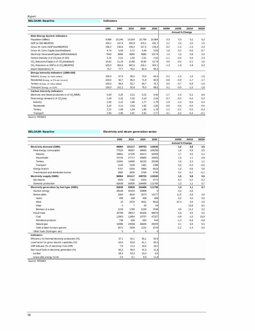
Report

98

BELGIUM: Baseline Indicators

1990 2000 2010 2020 2030 00//90 10//00 20//10 30//20Annual % Change

Main Energy System IndicatorsPopulation (Million) 9,968 10,246 10,554 10,790 10,984 0,3 0,3 0,2 0,2GDP (in 000 MEUR'00) 200,1 247,9 302,9 370,1 431,7 2,2 2,0 2,0 1,5Gross Inl. Cons./GDP (toe/MEUR'00) 236,2 230,6 199,3 157,5 128,4 -0,2 -1,4 -2,3 -2,0Gross Inl. Cons./Capita (toe/inhabitant) 4,74 5,58 5,72 5,40 5,05 1,6 0,2 -0,6 -0,7Electricity Generated/Capita (kWh/inhabitant) 7043 8066 8900 9685 10174 1,4 1,0 0,8 0,5Carbon intensity (t of CO2/toe of GIC) 2,24 2,01 1,92 2,01 2,52 -1,1 -0,4 0,4 2,3CO2 Emissions/Capita (t of CO2/inhabitant) 10,62 11,19 10,98 10,84 12,74 0,5 -0,2 -0,1 1,6CO2 Emissions to GDP (t of CO2/MEUR'00) 529,0 462,6 382,6 316,1 324,1 -1,3 -1,9 -1,9 0,3Import Dependency % 75,7 77,7 78,2 82,4 95,3Energy intensity indicators (1990=100)Industry (Energy on Value added) 100,0 97,5 86,0 73,9 63,4 -0,2 -1,3 -1,5 -1,5Residential (Energy on Priv ate Income) 100,0 92,7 85,0 71,9 60,9 -0,8 -0,9 -1,7 -1,7Tertiary (Energy on Value added) 100,0 99,5 92,7 84,7 76,7 0,0 -0,7 -0,9 -1,0Transport (Energy on GDP) 100,0 101,2 92,8 79,5 68,0 0,1 -0,9 -1,5 -1,6Carbon Intensity indicatorsElectricity and Steam production (t of CO2/MWh) 0,29 0,25 0,21 0,21 0,40 -1,7 -1,5 -0,1 6,6Final energy demand (t of CO2/toe) 2,49 2,32 2,20 2,10 2,04 -0,7 -0,5 -0,4 -0,3

Industry 2,46 2,12 1,86 1,77 1,70 -1,5 -1,3 -0,5 -0,4Residential 2,24 2,11 2,02 1,92 1,82 -0,6 -0,4 -0,5 -0,5Tertiary 2,22 1,96 1,94 1,85 1,78 -1,2 -0,1 -0,5 -0,4Transport 2,94 2,96 2,91 2,81 2,77 0,1 -0,2 -0,4 -0,1

BELGIUM: Baseline Electricity and steam generation sector

2000 2010 2020 2030 10//00 20//10 30//20Annual % Change

Electricity demand (GWh) 86964 101117 109703 115530 1,5 0,8 0,5Final energy consumption 77525 90957 99969 105258 1,6 0,9 0,5

Industry 39861 47105 49472 50059 1,7 0,5 0,1Households 23734 27717 30883 33553 1,6 1,1 0,8Tertiary 12491 14606 18133 20248 1,6 2,2 1,1Transport 1440 1529 1481 1398 0,6 -0,3 -0,6

Energy branch 5757 6334 5966 6523 1,0 -0,6 0,9Transmission and distribution losses 3682 3826 3769 3749 0,4 -0,2 -0,1

Electricity supply (GWh) 86964 101117 109703 115530 1,5 0,8 0,5Net imports 4325 7182 5204 3774 5,2 -3,2 -3,2Domestic production 82639 93935 104499 111756 1,3 1,1 0,7

Electricity generation by fuel type (GWh) 82639 93935 104499 111756 1,3 1,1 0,7Nuclear energy 48148 50103 34898 0 0,4 -3,6Renew ables 1693 4816 9273 13177 11,0 6,8 3,6

Hydro 459 458 458 458 0,0 0,0 0,0Wind 15 2570 3631 5616 67,3 3,5 4,5Solar 0 7 25 54 13,8 8,2Biomass & w aste 1219 1780 5159 7048 3,9 11,2 3,2

Fossil fuels 32798 39017 60328 98579 1,8 4,5 5,0Coal 12903 11854 10757 47227 -0,8 -1,0 15,9Petroleum products 738 648 592 544 -1,3 -0,9 -0,8Natural gas 16086 24058 46848 49229 4,1 6,9 0,5Coke & blast-furnace gasses 3071 2458 2131 1579 -2,2 -1,4 -3,0

Other fuels (hydrogen, etc) 0 0 0 0IndicatorsEfficiency for thermal electricity production (%) 37,1 42,1 55,1 52,6Load factor for gross electric capacities (%) 63,0 63,6 61,1 55,5CHP indicator (% of electricity from CHP) 7,9 14,3 18,5 18,2Non fossil fuels in electricity generation (%) 60,3 58,5 42,3 11,8 - nuclear 58,3 53,3 33,4 0,0 - renew able energy forms 2,0 5,1 8,9 11,8

Source: PRIMES

Source: PRIMES

Report

99

BELGIUM: Higher-oil-higher-gas price variant Summary Energy Balance

1990 2000 2010 2020 2030 00//90 10//00 20//10 30//20Annual % Change

Primary Production (ktoe) 12528 13471 14497 11693 3336 0.7 0.7 -2.1 -11.8Fossil fuels 1094 193 0 0 0 -15.9Nuclear 10707 12422 12926 9004 0 1.5 0.4 -3.6Renew able energy sources 727 856 1570 2689 3336 1.6 6.3 5.5 2.2

Hydro 23 39 39 39 39 5.6 0.0 0.0 0.0Biomass & Waste 701 810 1261 2211 2614 1.4 4.5 5.8 1.7Wind 1 1 246 368 545 7.9 69.1 4.1 4.0Solar and others 2 5 24 71 138 10.0 17.3 11.5 6.9

Net Imports (ktoe) 38857 48547 50921 51872 57523 2.3 0.5 0.2 1.0Solids 9492 7566 6399 7732 13945 -2.2 -1.7 1.9 6.1Oil 21468 27331 27463 26622 25815 2.4 0.0 -0.3 -0.3Natural gas 8217 13278 16441 17071 17438 4.9 2.2 0.4 0.2Electricity -320 372 618 447 324 5.2 -3.2 -3.2

Gross Inland Consumption (ktoe) 47257 57168 59793 57650 54758 1.9 0.4 -0.4 -0.5Solids 10244 8200 6399 7732 13945 -2.2 -2.4 1.9 6.1Oil 17730 21949 21838 20706 19715 2.2 -0.1 -0.5 -0.5Natural gas 8169 13369 16441 17071 17438 5.0 2.1 0.4 0.2Nuclear 10707 12422 12926 9004 0 1.5 0.4 -3.6Electricity -320 372 618 447 324 5.2 -3.2 -3.2Renew able energy forms 727 856 1570 2689 3336 1.6 6.3 5.5 2.2

as % in Gross Inland ConsumptionSolids 21.7 14.3 10.7 13.4 25.5Oil 37.5 38.4 36.5 35.9 36.0Natural gas 17.3 23.4 27.5 29.6 31.8Nuclear 22.7 21.7 21.6 15.6 0.0Renew able energy forms 1.5 1.5 2.6 4.7 6.1

Fuel Inputs for Thermal Power & Steam Generation (ktoe) 6839 7876 8416 10865 17925 1.4 0.7 2.6 5.1Solids 3879 3030 2781 4673 11418 -2.4 -0.9 5.3 9.3Oil 318 172 144 114 100 -6.0 -1.7 -2.3 -1.3Gas 2239 4186 4801 4996 5132 6.5 1.4 0.4 0.3Biomass & Waste 403 488 689 1082 1275 1.9 3.5 4.6 1.7Other (hydrogen,…) 0 0 0 0 0

Fuel Input in other transformation processes (ktoe) 35153 40739 35198 34303 33149 1.5 -1.5 -0.3 -0.3Energy Branch Consumption (ktoe) 2310 2370 2243 2143 2106 0.3 -0.5 -0.5 -0.2Non-Energy Uses (ktoe) 2739 5814 5288 5007 4937 7.8 -0.9 -0.5 -0.1Final Energy Demand (ktoe) 31355 37055 39482 40043 39706 1.7 0.6 0.1 -0.1by sector

Industry 11944 13769 13928 13947 13554 1.4 0.1 0.0 -0.3Residential 8337 9465 10132 9810 9436 1.3 0.7 -0.3 -0.4Tertiary 3370 4158 4772 5241 5466 2.1 1.4 0.9 0.4Transport 7704 9662 10650 11045 11250 2.3 1.0 0.4 0.2

by fuel Solids 3783 3373 2473 2207 1911 -1.1 -3.1 -1.1 -1.4Oil 14734 16038 16482 15741 14962 0.9 0.3 -0.5 -0.5Gas 6993 9615 10763 10948 10930 3.2 1.1 0.2 0.0Electricity 4986 6667 7867 8606 9045 2.9 1.7 0.9 0.5Heat (from CHP and District Heating) 566 1046 1363 1529 1612 6.3 2.7 1.2 0.5Other 293 316 534 1011 1247 0.8 5.4 6.6 2.1

CO2 Emissions (Mt of CO2) 105.9 114.7 113.6 117.9 140.6 0.8 -0.1 0.4 1.8Pow er generation/District heating 22.4 23.5 23.5 31.2 57.8 0.5 0.0 2.8 6.4Energy Branch 5.3 5.3 4.3 4.0 3.8 0.0 -2.1 -0.5 -0.6Industry 29.3 29.1 25.6 24.2 22.3 -0.1 -1.3 -0.6 -0.8Residential 18.7 20.0 20.1 18.3 16.6 0.7 0.0 -0.9 -1.0Tertiary 7.5 8.2 9.2 9.5 9.5 0.9 1.2 0.4 -0.1Transport 22.6 28.6 31.0 30.7 30.5 2.4 0.8 -0.1 0.0CO2 Emissions Index (1990=100) 100.0 108.3 107.3 111.4 132.8

Source: PRIMES

Report

100

BELGIUM: Higher-oil-higher-gas price variant Indicators

1990 2000 2010 2020 2030 00//90 10//00 20//10 30//20Annual % Change

Main Energy System IndicatorsPopulation (Million) 9.968 10.246 10.554 10.790 10.984 0.3 0.3 0.2 0.2GDP (in 000 MEUR'00) 200.1 247.9 302.9 370.1 431.7 2.2 2.0 2.0 1.5Gross Inl. Cons./GDP (toe/MEUR'00) 236.2 230.6 197.4 155.7 126.9 -0.2 -1.5 -2.3 -2.0Gross Inl. Cons./Capita (toe/inhabitant) 4.74 5.58 5.67 5.34 4.99 1.6 0.2 -0.6 -0.7Electricity Generated/Capita (kWh/inhabitant) 7043 8066 8944 9723 10193 1.4 1.0 0.8 0.5Carbon intensity (t of CO2/toe of GIC) 2.24 2.01 1.90 2.05 2.57 -1.1 -0.5 0.7 2.3CO2 Emissions/Capita (t of CO2/inhabitant) 10.62 11.19 10.76 10.93 12.80 0.5 -0.4 0.2 1.6CO2 Emissions to GDP (t of CO2/MEUR'00) 529.0 462.6 375.0 318.5 325.6 -1.3 -2.1 -1.6 0.2Import Dependency % 75.7 77.7 77.8 81.6 94.5Energy intensity indicators (1990=100)Industry (Energy on Value added) 100.0 97.5 85.6 73.1 62.1 -0.2 -1.3 -1.6 -1.6Residential (Energy on Priv ate Income) 100.0 92.7 83.5 68.4 57.4 -0.8 -1.0 -2.0 -1.7Tertiary (Energy on Value added) 100.0 99.5 91.2 81.5 72.7 0.0 -0.9 -1.1 -1.1Transport (Energy on GDP) 100.0 101.2 91.3 77.5 67.7 0.1 -1.0 -1.6 -1.3Carbon Intensity indicatorsElectricity and Steam production (t of CO2/MWh) 0.29 0.25 0.21 0.25 0.44 -1.7 -1.5 1.7 5.7Final energy demand (t of CO2/toe) 2.49 2.32 2.17 2.07 1.99 -0.7 -0.6 -0.5 -0.4

Industry 2.46 2.12 1.84 1.73 1.64 -1.5 -1.4 -0.6 -0.5Residential 2.24 2.11 1.98 1.87 1.76 -0.6 -0.6 -0.6 -0.6Tertiary 2.22 1.96 1.92 1.82 1.73 -1.2 -0.2 -0.5 -0.5Transport 2.94 2.96 2.91 2.78 2.72 0.1 -0.2 -0.5 -0.2

BELGIUM: Higher-oil-higher-gas price variant Electricity and steam generation sector

2000 2010 2020 2030 10//00 20//10 30//20Annual % Change

Electricity demand (GWh) 86964 101578 110109 115730 1.6 0.8 0.5Final energy consumption 77525 91478 100067 105170 1.7 0.9 0.5

Industry 39861 47253 50114 50773 1.7 0.6 0.1Households 23734 28075 30714 33479 1.7 0.9 0.9Tertiary 12491 14604 17750 19569 1.6 2.0 1.0Transport 1440 1546 1490 1349 0.7 -0.4 -1.0

Energy branch 5757 6256 6273 6817 0.8 0.0 0.8Transmission and distribution losses 3682 3844 3769 3743 0.4 -0.2 -0.1

Electricity supply (GWh) 86964 101578 110109 115730 1.6 0.8 0.5Net imports 4325 7181 5203 3773 5.2 -3.2 -3.2Domestic production 82639 94397 104907 111957 1.3 1.1 0.7

Electricity generation by fuel type (GWh) 82639 94397 104907 111957 1.3 1.1 0.7Nuclear energy 48148 50103 34898 0 0.4 -3.6Renew ables 1693 5110 10681 14095 11.7 7.7 2.8

Hydro 459 458 458 458 0.0 0.0 0.0Wind 15 2864 4283 6332 69.1 4.1 4.0Solar 0 7 25 54 13.8 8.2Biomass & w aste 1219 1780 5915 7251 3.9 12.8 2.1

Fossil fuels 32798 39184 59327 97862 1.8 4.2 5.1Coal 12903 11854 23969 60245 -0.8 7.3 9.7Petroleum products 738 651 594 545 -1.2 -0.9 -0.9Natural gas 16086 24220 32630 35493 4.2 3.0 0.8Coke & blast-furnace gasses 3071 2460 2134 1579 -2.2 -1.4 -3.0

Other fuels (hydrogen, etc) 0 0 0 0IndicatorsEfficiency for thermal electricity production (%) 37.1 41.9 51.6 50.4Load factor for gross electric capacities (%) 63.0 63.9 60.3 54.9CHP indicator (% of electricity from CHP) 7.9 13.2 19.3 18.6Non fossil fuels in electricity generation (%) 60.3 58.5 43.4 12.6 - nuclear 58.3 53.1 33.3 0.0 - renew able energy forms 2.0 5.4 10.2 12.6

Source: PRIMES

Source: PRIMES

Report

101

BELGIUM: Bpk15 Summary Energy Balance

1990 2000 2010 2020 2030 00//90 10//00 20//10 30//20Annual % Change



Net Imports (ktoe) 38857 48547 49960 49723 54693 2.3 0.3 0.0 1.0Solids 9492 7566 3963 1973 7250 -2.2 -6.3 -6.7 13.9Oil 21468 27331 28503 27318 26316 2.4 0.4 -0.4 -0.4Natural gas 8217 13278 16876 19985 20804 4.9 2.4 1.7 0.4Electricity -320 372 618 447 324 5.2 -3.2 -3.2

Gross Inland Consumption (ktoe) 47257 57168 58610 55571 52419 1.9 0.2 -0.5 -0.6Solids 10244 8200 3963 1973 7250 -2.2 -7.0 -6.7 13.9Oil 17730 21949 22624 21016 19785 2.2 0.3 -0.7 -0.6Natural gas 8169 13369 16876 19985 20804 5.0 2.4 1.7 0.4Nuclear 10707 12422 12926 9004 0 1.5 0.4 -3.6Electricity -320 372 618 447 324 5.2 -3.2 -3.2Renew able energy forms 727 856 1603 3146 4256 1.6 6.5 7.0 3.1


Fuel Inputs for Thermal Power & Steam Generation (ktoe) 6839 7876 7839 10020 16181 1.4 0.0 2.5 4.9Solids 3879 3030 778 1 5762 -2.4 -12.7 -48.0 134.9Oil 318 172 72 566 155 -6.0 -8.4 23.0 -12.1Gas 2239 4186 6250 8260 8756 6.5 4.1 2.8 0.6Biomass & Waste 403 488 740 1193 1508 1.9 4.3 4.9 2.4Other (hydrogen,…) 0 0 0 0 0

Fuel Input in other transformation processes (ktoe) 35153 40739 36251 34413 32945 1.5 -1.2 -0.5 -0.4Energy Branch Consumption (ktoe) 2310 2370 2273 2162 2171 0.3 -0.4 -0.5 0.0Non-Energy Uses (ktoe) 2739 5814 5365 5126 5072 7.8 -0.8 -0.5 -0.1Final Energy Demand (ktoe) 31355 37055 38872 38404 37813 1.7 0.5 -0.1 -0.2by sector

Industry 11944 13769 13568 12893 12464 1.4 -0.1 -0.5 -0.3Residential 8337 9465 9999 9569 9112 1.3 0.5 -0.4 -0.5Tertiary 3370 4158 4689 5082 5186 2.1 1.2 0.8 0.2Transport 7704 9662 10616 10860 11051 2.3 0.9 0.2 0.2


CO2 Emissions (Mt of CO2) 105.9 114.7 107.1 95.8 90.0 0.8 -0.7 -1.1 -0.6Pow er generation/District heating 22.4 23.5 18.8 15.1 12.4 0.5 -2.2 -2.2 -1.9Energy Branch 5.3 5.3 4.7 4.1 3.9 0.0 -1.2 -1.4 -0.6Industry 29.3 29.1 23.9 19.2 17.7 -0.1 -2.0 -2.1 -0.8Residential 18.7 20.0 19.8 17.7 16.1 0.7 -0.1 -1.1 -0.9Tertiary 7.5 8.2 9.0 9.2 9.2 0.9 1.0 0.3 0.0Transport 22.6 28.6 30.9 30.5 30.6 2.4 0.8 -0.1 0.1CO2 Emissions Index (1990=100) 100.0 108.3 101.1 90.5 85.0

Source: PRIMES

Report

102

BELGIUM: Bpk15 Indicators

1990 2000 2010 2020 2030 00//90 10//00 20//10 30//20Annual % Change

Main Energy System IndicatorsPopulation (Million) 9.968 10.246 10.554 10.790 10.984 0.3 0.3 0.2 0.2GDP (in 000 MEUR'00) 200.1 247.9 302.9 370.1 431.7 2.2 2.0 2.0 1.5Gross Inl. Cons./GDP (toe/MEUR'00) 236.2 230.6 193.5 150.1 121.4 -0.2 -1.7 -2.5 -2.1Gross Inl. Cons./Capita (toe/inhabitant) 4.74 5.58 5.55 5.15 4.77 1.6 0.0 -0.8 -0.8Electricity Generated/Capita (kWh/inhabitant) 7043 8066 9172 10068 10198 1.4 1.3 0.9 0.1Carbon intensity (t of CO2/toe of GIC) 2.24 2.01 1.83 1.72 1.72 -1.1 -0.9 -0.6 0.0CO2 Emissions/Capita (t of CO2/inhabitant) 10.62 11.19 10.14 8.88 8.19 0.5 -1.0 -1.3 -0.8CO2 Emissions to GDP (t of CO2/MEUR'00) 529.0 462.6 353.5 258.7 208.4 -1.3 -2.7 -3.1 -2.1Import Dependency % 75.7 77.7 77.5 80.4 92.8Energy intensity indicators (1990=100)Industry (Energy on Value added) 100.0 97.5 83.4 67.6 57.1 -0.2 -1.6 -2.1 -1.7Residential (Energy on Priv ate Income) 100.0 92.7 82.4 66.7 55.4 -0.8 -1.2 -2.1 -1.8Tertiary (Energy on Value added) 100.0 99.5 89.6 79.0 69.0 0.0 -1.0 -1.3 -1.3Transport (Energy on GDP) 100.0 101.2 91.0 76.2 66.5 0.1 -1.1 -1.8 -1.4Carbon Intensity indicatorsElectricity and Steam production (t of CO2/MWh) 0.29 0.25 0.17 0.12 0.10 -1.7 -3.7 -3.2 -2.2Final energy demand (t of CO2/toe) 2.49 2.32 2.15 1.99 1.95 -0.7 -0.8 -0.7 -0.2


BELGIUM: Bpk15 Electricity and steam generation sector

2000 2010 2020 2030 10//00 20//10 30//20Annual % Change


Industry 39861 50003 54113 53550 2.3 0.8 -0.1Households 23734 28094 30708 31894 1.7 0.9 0.4Tertiary 12491 14523 17462 18003 1.5 1.9 0.3Transport 1440 1539 1477 1301 0.7 -0.4 -1.3

Energy branch 5757 5868 6166 7311 0.2 0.5 1.7Transmission and distribution losses 3682 3956 3906 3729 0.7 -0.1 -0.5




Fossil fuels 32798 41557 57814 86537 2.4 3.4 4.1Coal 12903 3300 4 25707 -12.7 -49.2 141.5Petroleum products 738 378 2664 751 -6.5 21.6 -11.9Natural gas 16086 35420 53013 58500 8.2 4.1 1.0Coke & blast-furnace gasses 3071 2459 2132 1579 -2.2 -1.4 -3.0


Source: PRIMES

Source: PRIMES

Report

103

BELGIUM: Bpk15n Summary Energy Balance

1990 2000 2010 2020 2030 00//90 10//00 20//10 30//20Annual % Change

Primary Production (ktoe) 12528 13471 14529 16362 20311 0.7 0.8 1.2 2.2Fossil fuels 1094 193 0 0 0 -15.9Nuclear 10707 12422 12926 13476 16399 1.5 0.4 0.4 2.0Renew able energy sources 727 856 1603 2886 3913 1.6 6.5 6.1 3.1


Net Imports (ktoe) 38857 48547 50032 48614 46456 2.3 0.3 -0.3 -0.5Solids 9492 7566 4165 2448 1821 -2.2 -5.8 -5.2 -2.9Oil 21468 27331 28373 27308 26666 2.4 0.4 -0.4 -0.2Natural gas 8217 13278 16876 18411 17644 4.9 2.4 0.9 -0.4Electricity -320 372 618 448 325 5.2 -3.2 -3.2

Gross Inland Consumption (ktoe) 47257 57168 58682 58674 60236 1.9 0.3 0.0 0.3Solids 10244 8200 4165 2448 1821 -2.2 -6.6 -5.2 -2.9Oil 17730 21949 22494 21006 20135 2.2 0.2 -0.7 -0.4Natural gas 8169 13369 16876 18411 17644 5.0 2.4 0.9 -0.4Nuclear 10707 12422 12926 13476 16399 1.5 0.4 0.4 2.0Electricity -320 372 618 448 325 5.2 -3.2 -3.2Renew able energy forms 727 856 1603 2886 3913 1.6 6.5 6.1 3.1


Fuel Inputs for Thermal Power & Steam Generation (ktoe) 6839 7876 7914 7533 6597 1.4 0.0 -0.5 -1.3Solids 3879 3030 979 0 0 -2.4 -10.7Oil 318 172 16 11 10 -6.0 -21.3 -3.1 -1.8Gas 2239 4186 6179 6414 5313 6.5 4.0 0.4 -1.9Biomass & Waste 403 488 740 1108 1275 1.9 4.3 4.1 1.4Other (hydrogen,…) 0 0 0 0 0

Fuel Input in other transformation processes (ktoe) 35153 40739 36099 34723 33566 1.5 -1.2 -0.4 -0.3Energy Branch Consumption (ktoe) 2310 2370 2275 2157 2121 0.3 -0.4 -0.5 -0.2Non-Energy Uses (ktoe) 2739 5814 5364 5120 5072 7.8 -0.8 -0.5 -0.1Final Energy Demand (ktoe) 31355 37055 38874 39761 39850 1.7 0.5 0.2 0.0by sector



CO2 Emissions (Mt of CO2) 105.9 114.7 107.4 100.6 90.0 0.8 -0.7 -0.7 -1.1Pow er generation/District heating 22.4 23.5 19.3 15.7 8.9 0.5 -2.0 -2.0 -5.5Energy Branch 5.3 5.3 4.7 4.2 3.9 0.0 -1.3 -1.1 -0.6Industry 29.3 29.1 23.9 21.6 19.1 -0.1 -2.0 -1.0 -1.3Residential 18.7 20.0 19.8 18.4 16.9 0.7 -0.1 -0.7 -0.9Tertiary 7.5 8.2 9.0 9.6 9.7 0.9 1.0 0.6 0.2Transport 22.6 28.6 30.9 31.1 31.5 2.4 0.8 0.1 0.1CO2 Emissions Index (1990=100) 100.0 108.3 101.5 95.1 85.0

Source: PRIMES

Report

104

BELGIUM: Bpk15n Indicators

1990 2000 2010 2020 2030 00//90 10//00 20//10 30//20Annual % Change

Main Energy System IndicatorsPopulation (Million) 9.968 10.246 10.554 10.790 10.984 0.3 0.3 0.2 0.2GDP (in 000 MEUR'00) 200.1 247.9 302.9 370.1 431.7 2.2 2.0 2.0 1.5Gross Inl. Cons./GDP (toe/MEUR'00) 236.2 230.6 193.8 158.5 139.5 -0.2 -1.7 -2.0 -1.3Gross Inl. Cons./Capita (toe/inhabitant) 4.74 5.58 5.56 5.44 5.48 1.6 0.0 -0.2 0.1Electricity Generated/Capita (kWh/inhabitant) 7043 8066 9178 10162 11153 1.4 1.3 1.0 0.9Carbon intensity (t of CO2/toe of GIC) 2.24 2.01 1.83 1.71 1.49 -1.1 -0.9 -0.7 -1.4CO2 Emissions/Capita (t of CO2/inhabitant) 10.62 11.19 10.18 9.33 8.19 0.5 -0.9 -0.9 -1.3CO2 Emissions to GDP (t of CO2/MEUR'00) 529.0 462.6 354.7 271.8 208.5 -1.3 -2.6 -2.6 -2.6Import Dependency % 75.7 77.7 77.5 74.8 69.6Energy intensity indicators (1990=100)Industry (Energy on Value added) 100.0 97.5 83.4 70.8 60.1 -0.2 -1.6 -1.6 -1.6Residential (Energy on Priv ate Income) 100.0 92.7 82.5 69.1 59.1 -0.8 -1.2 -1.8 -1.6Tertiary (Energy on Value added) 100.0 99.5 89.7 81.9 75.5 0.0 -1.0 -0.9 -0.8Transport (Energy on GDP) 100.0 101.2 91.0 77.8 68.3 0.1 -1.1 -1.6 -1.3Carbon Intensity indicatorsElectricity and Steam production (t of CO2/MWh) 0.29 0.25 0.17 0.12 0.06 -1.7 -3.5 -3.2 -6.5Final energy demand (t of CO2/toe) 2.49 2.32 2.15 2.03 1.94 -0.7 -0.8 -0.6 -0.5


BELGIUM: Bpk15n Electricity and steam generation sector

2000 2010 2020 2030 10//00 20//10 30//20Annual % Change



Energy branch 5757 5919 5848 6456 0.3 -0.1 1.0Transmission and distribution losses 3682 3957 3955 4114 0.7 0.0 0.4


Electricity generation by fuel type (GWh) 82639 96869 109644 122505 1.6 1.2 1.1Nuclear energy 48148 50103 52234 63561 0.4 0.4 2.0Renew ables 1693 5142 14371 23880 11.7 10.8 5.2


Fossil fuels 32798 41625 43040 35064 2.4 0.3 -2.0Coal 12903 4160 0 0 -10.7Petroleum products 738 80 59 50 -20.0 -2.9 -1.7Natural gas 16086 34925 40848 33435 8.1 1.6 -2.0Coke & blast-furnace gasses 3071 2459 2132 1579 -2.2 -1.4 -3.0


Source: PRIMES

Source: PRIMES

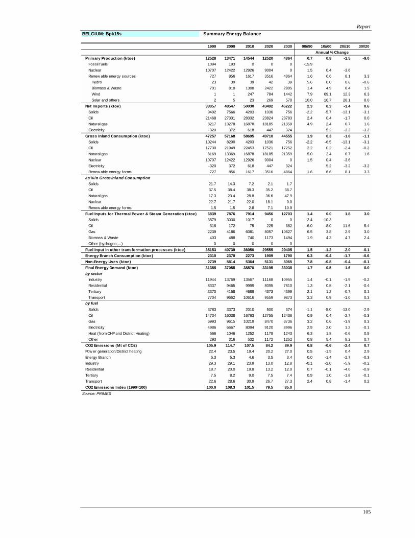
Report

105

BELGIUM: Bpk15s Summary Energy Balance

1990 2000 2010 2020 2030 00//90 10//00 20//10 30//20Annual % Change


Hydro 23 39 39 42 39 5.6 0.0 0.6 -0.6Biomass & Waste 701 810 1308 2422 2805 1.4 4.9 6.4 1.5Wind 1 1 247 784 1442 7.9 69.1 12.3 6.3Solar and others 2 5 23 269 578 10.0 16.7 28.1 8.0

Net Imports (ktoe) 38857 48547 50030 43492 46222 2.3 0.3 -1.4 0.6Solids 9492 7566 4203 1036 756 -2.2 -5.7 -13.1 -3.1Oil 21468 27331 28332 23824 23783 2.4 0.4 -1.7 0.0Natural gas 8217 13278 16878 18185 21359 4.9 2.4 0.7 1.6Electricity -320 372 618 447 324 5.2 -3.2 -3.2

Gross Inland Consumption (ktoe) 47257 57168 58695 49710 44555 1.9 0.3 -1.6 -1.1Solids 10244 8200 4203 1036 756 -2.2 -6.5 -13.1 -3.1Oil 17730 21949 22453 17521 17252 2.2 0.2 -2.4 -0.2Natural gas 8169 13369 16878 18185 21359 5.0 2.4 0.7 1.6Nuclear 10707 12422 12926 9004 0 1.5 0.4 -3.6Electricity -320 372 618 447 324 5.2 -3.2 -3.2Renew able energy forms 727 856 1617 3516 4864 1.6 6.6 8.1 3.3


Fuel Inputs for Thermal Power & Steam Generation (ktoe) 6839 7876 7914 9456 12703 1.4 0.0 1.8 3.0Solids 3879 3030 1017 0 0 -2.4 -10.3Oil 318 172 75 225 382 -6.0 -8.0 11.6 5.4Gas 2239 4186 6081 8057 10827 6.5 3.8 2.9 3.0Biomass & Waste 403 488 740 1173 1494 1.9 4.3 4.7 2.4Other (hydrogen,…) 0 0 0 0 0

Fuel Input in other transformation processes (ktoe) 35153 40739 36050 29555 29405 1.5 -1.2 -2.0 -0.1Energy Branch Consumption (ktoe) 2310 2370 2273 1909 1790 0.3 -0.4 -1.7 -0.6Non-Energy Uses (ktoe) 2739 5814 5364 5131 5065 7.8 -0.8 -0.4 -0.1Final Energy Demand (ktoe) 31355 37055 38870 33195 33038 1.7 0.5 -1.6 0.0by sector

Industry 11944 13769 13567 11168 10955 1.4 -0.1 -1.9 -0.2Residential 8337 9465 9999 8095 7810 1.3 0.5 -2.1 -0.4Tertiary 3370 4158 4689 4373 4399 2.1 1.2 -0.7 0.1Transport 7704 9662 10616 9559 9873 2.3 0.9 -1.0 0.3

by fuel Solids 3783 3373 2010 500 374 -1.1 -5.0 -13.0 -2.9Oil 14734 16038 16763 12755 12436 0.9 0.4 -2.7 -0.3Gas 6993 9615 10219 8470 8736 3.2 0.6 -1.9 0.3Electricity 4986 6667 8094 9120 8996 2.9 2.0 1.2 -0.1Heat (from CHP and District Heating) 566 1046 1252 1178 1243 6.3 1.8 -0.6 0.5Other 293 316 532 1172 1252 0.8 5.4 8.2 0.7

CO2 Emissions (Mt of CO2) 105.9 114.7 107.5 84.2 89.9 0.8 -0.6 -2.4 0.7Pow er generation/District heating 22.4 23.5 19.4 20.2 27.0 0.5 -1.9 0.4 2.9Energy Branch 5.3 5.3 4.6 3.5 3.4 0.0 -1.4 -2.7 -0.3Industry 29.3 29.1 23.8 13.0 12.8 -0.1 -2.0 -5.9 -0.2Residential 18.7 20.0 19.8 13.2 12.0 0.7 -0.1 -4.0 -0.9Tertiary 7.5 8.2 9.0 7.5 7.4 0.9 1.0 -1.8 -0.1Transport 22.6 28.6 30.9 26.7 27.3 2.4 0.8 -1.4 0.2CO2 Emissions Index (1990=100) 100.0 108.3 101.5 79.5 85.0

Source: PRIMES

Report

106

BELGIUM: Bpk15s Indicators

1990 2000 2010 2020 2030 00//90 10//00 20//10 30//20Annual % Change

Main Energy System IndicatorsPopulation (Million) 9.968 10.246 10.554 10.790 10.984 0.3 0.3 0.2 0.2GDP (in 000 MEUR'00) 200.1 247.9 302.9 370.1 431.7 2.2 2.0 2.0 1.5Gross Inl. Cons./GDP (toe/MEUR'00) 236.2 230.6 193.8 134.3 103.2 -0.2 -1.7 -3.6 -2.6Gross Inl. Cons./Capita (toe/inhabitant) 4.74 5.58 5.56 4.61 4.06 1.6 0.0 -1.9 -1.3Electricity Generated/Capita (kWh/inhabitant) 7043 8066 9173 10209 9924 1.4 1.3 1.1 -0.3Carbon intensity (t of CO2/toe of GIC) 2.24 2.01 1.83 1.69 2.02 -1.1 -0.9 -0.8 1.8CO2 Emissions/Capita (t of CO2/inhabitant) 10.62 11.19 10.18 7.80 8.19 0.5 -0.9 -2.6 0.5CO2 Emissions to GDP (t of CO2/MEUR'00) 529.0 462.6 354.8 227.4 208.3 -1.3 -2.6 -4.4 -0.9Import Dependency % 75.7 77.7 77.5 77.6 90.5Energy intensity indicators (1990=100)Industry (Energy on Value added) 100.0 97.5 83.4 58.5 50.2 -0.2 -1.6 -3.5 -1.5Residential (Energy on Priv ate Income) 100.0 92.7 82.4 56.4 47.5 -0.8 -1.2 -3.7 -1.7Tertiary (Energy on Value added) 100.0 99.5 89.6 68.0 58.5 0.0 -1.0 -2.7 -1.5Transport (Energy on GDP) 100.0 101.2 91.0 67.1 59.4 0.1 -1.1 -3.0 -1.2Carbon Intensity indicatorsElectricity and Steam production (t of CO2/MWh) 0.29 0.25 0.17 0.16 0.22 -1.7 -3.4 -0.6 3.0Final energy demand (t of CO2/toe) 2.49 2.32 2.15 1.82 1.80 -0.7 -0.8 -1.6 -0.1

Industry 2.46 2.12 1.76 1.17 1.17 -1.5 -1.8 -4.0 0.0Residential 2.24 2.11 1.98 1.63 1.54 -0.6 -0.7 -1.9 -0.6Tertiary 2.22 1.96 1.92 1.71 1.69 -1.2 -0.2 -1.1 -0.2Transport 2.94 2.96 2.91 2.80 2.76 0.1 -0.2 -0.4 -0.1

BELGIUM: Bpk15s Electricity and steam generation sector

2000 2010 2020 2030 10//00 20//10 30//20Annual % Change

Electricity demand (GWh) 86964 103994 115352 112773 1.8 1.0 -0.2Final energy consumption 77525 94113 106049 104606 2.0 1.2 -0.1

Industry 39861 49963 55551 52643 2.3 1.1 -0.5Households 23734 28090 32151 33634 1.7 1.4 0.5Tertiary 12491 14521 16847 16982 1.5 1.5 0.1Transport 1440 1539 1500 1347 0.7 -0.3 -1.1

Energy branch 5757 5927 5319 4449 0.3 -1.1 -1.8Transmission and distribution losses 3682 3954 3984 3718 0.7 0.1 -0.7

Electricity supply (GWh) 86964 103994 115352 112773 1.8 1.0 -0.2Net imports 4325 7182 5201 3770 5.2 -3.2 -3.2Domestic production 82639 96813 110151 109003 1.6 1.3 -0.1

Electricity generation by fuel type (GWh) 82639 96813 110151 109003 1.6 1.3 -0.1Nuclear energy 48148 50103 34898 0 0.4 -3.6Renew ables 1693 5308 18167 30883 12.1 13.1 5.4

Hydro 459 458 486 458 0.0 0.6 -0.6Wind 15 2871 9119 16763 69.1 12.3 6.3Solar 0 7 2357 5541 79.5 8.9Biomass & w aste 1219 1972 6205 8121 4.9 12.1 2.7

Fossil fuels 32798 41402 57085 78120 2.4 3.3 3.2Coal 12903 4323 0 0 -10.4Petroleum products 738 396 1193 2041 -6.0 11.7 5.5Natural gas 16086 34224 53838 74492 7.8 4.6 3.3Coke & blast-furnace gasses 3071 2459 2055 1586 -2.2 -1.8 -2.6


Source: PRIMES

Source: PRIMES

Report

107

BELGIUM: Bpk15ns Summary Energy Balance

1990 2000 2010 2020 2030 00//90 10//00 20//10 30//20Annual % Change



Net Imports (ktoe) 38857 48547 49967 47301 45124 2.3 0.3 -0.5 -0.5Solids 9492 7566 4073 1954 1448 -2.2 -6.0 -7.1 -2.9Oil 21468 27331 28271 26541 25993 2.4 0.3 -0.6 -0.2Natural gas 8217 13278 17005 18359 17358 4.9 2.5 0.8 -0.6Electricity -320 372 618 448 325 5.2 -3.2 -3.2

Gross Inland Consumption (ktoe) 47257 57168 58631 57538 59131 1.9 0.3 -0.2 0.3Solids 10244 8200 4073 1954 1448 -2.2 -6.8 -7.1 -2.9Oil 17730 21949 22392 20238 19462 2.2 0.2 -1.0 -0.4Natural gas 8169 13369 17005 18359 17358 5.0 2.4 0.8 -0.6Nuclear 10707 12422 12926 13477 16399 1.5 0.4 0.4 2.0Electricity -320 372 618 448 325 5.2 -3.2 -3.2Renew able energy forms 727 856 1617 3064 4139 1.6 6.6 6.6 3.1





by fuel Solids 3783 3373 2010 1169 910 -1.1 -5.0 -5.3 -2.5Oil 14734 16038 16763 15409 14826 0.9 0.4 -0.8 -0.4Gas 6993 9615 10216 10538 10485 3.2 0.6 0.3 -0.1Electricity 4986 6667 8098 9220 10177 2.9 2.0 1.3 1.0Heat (from CHP and District Heating) 566 1046 1252 1332 1384 6.3 1.8 0.6 0.4Other 293 316 532 892 988 0.8 5.4 5.3 1.0

CO2 Emissions (Mt of CO2) 105.9 114.7 107.1 96.2 89.9 0.8 -0.7 -1.1 -0.7Pow er generation/District heating 22.4 23.5 19.0 15.9 12.8 0.5 -2.1 -1.8 -2.1Energy Branch 5.3 5.3 4.6 4.0 3.8 0.0 -1.4 -1.4 -0.5Industry 29.3 29.1 23.8 19.1 17.1 -0.1 -2.0 -2.2 -1.1Residential 18.7 20.0 19.8 17.6 15.9 0.7 -0.1 -1.1 -1.0Tertiary 7.5 8.2 9.0 9.2 9.4 0.9 1.0 0.3 0.2Transport 22.6 28.6 30.9 30.4 30.8 2.4 0.8 -0.2 0.1CO2 Emissions Index (1990=100) 100.0 108.3 101.1 90.9 84.9

Source: PRIMES

Report

108

BELGIUM: Bpk15ns Indicators

1990 2000 2010 2020 2030 00//90 10//00 20//10 30//20Annual % Change



BELGIUM: Bpk15ns Electricity and steam generation sector

2000 2010 2020 2030 10//00 20//10 30//20Annual % Change









Source: PRIMES

Source: PRIMES

Report

109

BELGIUM: Bpk30 Summary Energy Balance

1990 2000 2010 2020 2030 00//90 10//00 20//10 30//20Annual % Change



Net Imports (ktoe) 38857 48547 51118 47206 52219 2.3 0.5 -0.8 1.0Solids 9492 7566 5036 2119 6258 -2.2 -4.0 -8.3 11.4Oil 21468 27331 28553 25335 24910 2.4 0.4 -1.2 -0.2Natural gas 8217 13278 16912 19305 20727 4.9 2.4 1.3 0.7Electricity -320 372 618 447 324 5.2 -3.2 -3.2

Gross Inland Consumption (ktoe) 47257 57168 59789 53341 50299 1.9 0.4 -1.1 -0.6Solids 10244 8200 5036 2119 6258 -2.2 -4.8 -8.3 11.4Oil 17730 21949 22674 19032 18379 2.2 0.3 -1.7 -0.3Natural gas 8169 13369 16912 19305 20727 5.0 2.4 1.3 0.7Nuclear 10707 12422 12926 9004 0 1.5 0.4 -3.6Electricity -320 372 618 447 324 5.2 -3.2 -3.2Renew able energy forms 727 856 1623 3434 4611 1.6 6.6 7.8 3.0


Fuel Inputs for Thermal Power & Steam Generation (ktoe) 6839 7876 8961 11026 17003 1.4 1.3 2.1 4.4Solids 3879 3030 1846 830 5404 -2.4 -4.8 -7.7 20.6Oil 318 172 298 627 475 -6.0 5.6 7.7 -2.7Gas 2239 4186 6078 8414 9787 6.5 3.8 3.3 1.5Biomass & Waste 403 488 740 1155 1338 1.9 4.2 4.6 1.5Other (hydrogen,…) 0 0 0 0 0

Fuel Input in other transformation processes (ktoe) 35153 40739 36317 31549 30830 1.5 -1.1 -1.4 -0.2Energy Branch Consumption (ktoe) 2310 2370 2302 2157 2174 0.3 -0.3 -0.6 0.1Non-Energy Uses (ktoe) 2739 5814 5362 5137 5080 7.8 -0.8 -0.4 -0.1Final Energy Demand (ktoe) 31355 37055 38848 35357 35128 1.7 0.5 -0.9 -0.1by sector

Industry 11944 13769 13560 11879 11542 1.4 -0.2 -1.3 -0.3Residential 8337 9465 9989 8637 8348 1.3 0.5 -1.4 -0.3Tertiary 3370 4158 4683 4663 4731 2.1 1.2 0.0 0.1Transport 7704 9662 10616 10178 10507 2.3 0.9 -0.4 0.3

by fuel Solids 3783 3373 2011 679 458 -1.1 -5.0 -10.3 -3.9Oil 14734 16038 16765 13846 13448 0.9 0.4 -1.9 -0.3Gas 6993 9615 10256 9226 9082 3.2 0.6 -1.1 -0.2Electricity 4986 6667 8033 9196 9463 2.9 1.9 1.4 0.3Heat (from CHP and District Heating) 566 1046 1251 1206 1242 6.3 1.8 -0.4 0.3Other 293 316 532 1203 1435 0.8 5.4 8.5 1.8

CO2 Emissions (Mt of CO2) 105.9 114.7 111.5 76.0 73.8 0.8 -0.3 -3.8 -0.3Pow er generation/District heating 22.4 23.5 23.3 6.0 6.5 0.5 -0.1 -12.7 0.8Energy Branch 5.3 5.3 4.6 3.7 3.6 0.0 -1.4 -2.2 -0.3Industry 29.3 29.1 23.9 14.5 12.8 -0.1 -2.0 -4.9 -1.2Residential 18.7 20.0 19.8 15.0 13.7 0.7 -0.1 -2.7 -0.9Tertiary 7.5 8.2 9.0 8.3 8.2 0.9 1.0 -0.8 -0.2Transport 22.6 28.6 30.9 28.5 29.0 2.4 0.8 -0.8 0.2CO2 Emissions Index (1990=100) 100.0 108.3 105.4 71.8 69.8

Source: PRIMES

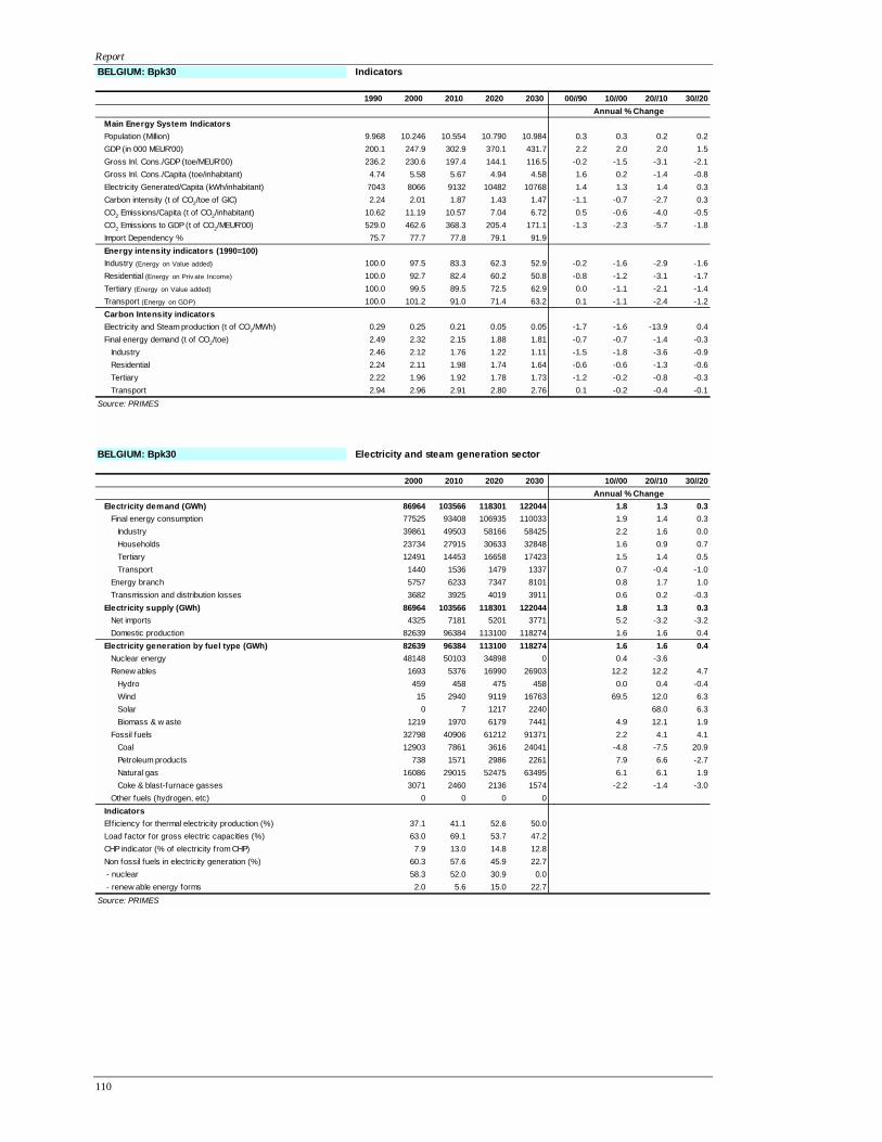
Report

110

BELGIUM: Bpk30 Indicators

1990 2000 2010 2020 2030 00//90 10//00 20//10 30//20Annual % Change

Main Energy System IndicatorsPopulation (Million) 9.968 10.246 10.554 10.790 10.984 0.3 0.3 0.2 0.2GDP (in 000 MEUR'00) 200.1 247.9 302.9 370.1 431.7 2.2 2.0 2.0 1.5Gross Inl. Cons./GDP (toe/MEUR'00) 236.2 230.6 197.4 144.1 116.5 -0.2 -1.5 -3.1 -2.1Gross Inl. Cons./Capita (toe/inhabitant) 4.74 5.58 5.67 4.94 4.58 1.6 0.2 -1.4 -0.8Electricity Generated/Capita (kWh/inhabitant) 7043 8066 9132 10482 10768 1.4 1.3 1.4 0.3Carbon intensity (t of CO2/toe of GIC) 2.24 2.01 1.87 1.43 1.47 -1.1 -0.7 -2.7 0.3CO2 Emissions/Capita (t of CO2/inhabitant) 10.62 11.19 10.57 7.04 6.72 0.5 -0.6 -4.0 -0.5CO2 Emissions to GDP (t of CO2/MEUR'00) 529.0 462.6 368.3 205.4 171.1 -1.3 -2.3 -5.7 -1.8Import Dependency % 75.7 77.7 77.8 79.1 91.9Energy intensity indicators (1990=100)Industry (Energy on Value added) 100.0 97.5 83.3 62.3 52.9 -0.2 -1.6 -2.9 -1.6Residential (Energy on Priv ate Income) 100.0 92.7 82.4 60.2 50.8 -0.8 -1.2 -3.1 -1.7Tertiary (Energy on Value added) 100.0 99.5 89.5 72.5 62.9 0.0 -1.1 -2.1 -1.4Transport (Energy on GDP) 100.0 101.2 91.0 71.4 63.2 0.1 -1.1 -2.4 -1.2Carbon Intensity indicatorsElectricity and Steam production (t of CO2/MWh) 0.29 0.25 0.21 0.05 0.05 -1.7 -1.6 -13.9 0.4Final energy demand (t of CO2/toe) 2.49 2.32 2.15 1.88 1.81 -0.7 -0.7 -1.4 -0.3


BELGIUM: Bpk30 Electricity and steam generation sector

2000 2010 2020 2030 10//00 20//10 30//20Annual % Change



Energy branch 5757 6233 7347 8101 0.8 1.7 1.0Transmission and distribution losses 3682 3925 4019 3911 0.6 0.2 -0.3




Fossil fuels 32798 40906 61212 91371 2.2 4.1 4.1Coal 12903 7861 3616 24041 -4.8 -7.5 20.9Petroleum products 738 1571 2986 2261 7.9 6.6 -2.7Natural gas 16086 29015 52475 63495 6.1 6.1 1.9Coke & blast-furnace gasses 3071 2460 2136 1574 -2.2 -1.4 -3.0


Source: PRIMES

Source: PRIMES

Report

111

BELGIUM: Bpk30n Summary Energy Balance

1990 2000 2010 2020 2030 00//90 10//00 20//10 30//20Annual % Change



Net Imports (ktoe) 38857 48547 50035 46492 44476 2.3 0.3 -0.7 -0.4Solids 9492 7566 4324 1652 1822 -2.2 -5.4 -9.2 1.0Oil 21468 27331 28268 26046 25499 2.4 0.3 -0.8 -0.2Natural gas 8217 13278 16824 18346 16831 4.9 2.4 0.9 -0.9Electricity -320 372 618 447 325 5.2 -3.2 -3.2

Gross Inland Consumption (ktoe) 47257 57168 58699 56882 58451 1.9 0.3 -0.3 0.3Solids 10244 8200 4324 1652 1822 -2.2 -6.2 -9.2 1.0Oil 17730 21949 22390 19744 18968 2.2 0.2 -1.2 -0.4Natural gas 8169 13369 16824 18346 16831 5.0 2.3 0.9 -0.9Nuclear 10707 12422 12926 13485 16399 1.5 0.4 0.4 2.0Electricity -320 372 618 447 325 5.2 -3.2 -3.2Renew able energy forms 727 856 1617 3207 4107 1.6 6.6 7.1 2.5


Fuel Inputs for Thermal Power & Steam Generation (ktoe) 6839 7876 7918 8219 7789 1.4 0.1 0.4 -0.5Solids 3879 3030 1139 0 762 -2.4 -9.3Oil 318 172 16 7 475 -6.0 -21.1 -7.4 51.6Gas 2239 4186 6025 7114 5442 6.5 3.7 1.7 -2.6Biomass & Waste 403 488 738 1098 1109 1.9 4.2 4.0 0.1Other (hydrogen,…) 0 0 0 0 0

Fuel Input in other transformation processes (ktoe) 35153 40739 35976 32661 31651 1.5 -1.2 -1.0 -0.3Energy Branch Consumption (ktoe) 2310 2370 2275 2168 2150 0.3 -0.4 -0.5 -0.1Non-Energy Uses (ktoe) 2739 5814 5364 5134 5085 7.8 -0.8 -0.4 -0.1Final Energy Demand (ktoe) 31355 37055 38871 37424 37213 1.7 0.5 -0.4 -0.1by sector


by fuel Solids 3783 3373 2010 943 617 -1.1 -5.0 -7.3 -4.1Oil 14734 16038 16761 14876 14027 0.9 0.4 -1.2 -0.6Gas 6993 9615 10220 9893 9549 3.2 0.6 -0.3 -0.4Electricity 4986 6667 8093 9306 10373 2.9 2.0 1.4 1.1Heat (from CHP and District Heating) 566 1046 1253 1277 1304 6.3 1.8 0.2 0.2Other 293 316 533 1129 1343 0.8 5.4 7.8 1.7

CO2 Emissions (Mt of CO2) 105.9 114.7 107.6 85.4 74.2 0.8 -0.6 -2.3 -1.4Pow er generation/District heating 22.4 23.5 19.5 9.2 3.2 0.5 -1.8 -7.2 -10.1Energy Branch 5.3 5.3 4.6 4.0 3.6 0.0 -1.4 -1.5 -0.8Industry 29.3 29.1 23.8 17.0 14.0 -0.1 -2.0 -3.3 -1.9Residential 18.7 20.0 19.8 16.6 14.8 0.7 -0.1 -1.8 -1.1Tertiary 7.5 8.2 9.0 8.8 8.8 0.9 1.0 -0.2 0.0Transport 22.6 28.6 30.9 29.8 29.8 2.4 0.8 -0.4 0.0CO2 Emissions Index (1990=100) 100.0 108.3 101.7 80.6 70.1

Source: PRIMES

Report

112

BELGIUM: Bpk30n Indicators

1990 2000 2010 2020 2030 00//90 10//00 20//10 30//20Annual % Change



BELGIUM: Bpk30n Electricity and steam generation sector

2000 2010 2020 2030 10//00 20//10 30//20Annual % Change



Energy branch 5757 5956 6674 7498 0.3 1.1 1.2Transmission and distribution losses 3682 3954 4069 4282 0.7 0.3 0.5



Hydro 459 458 458 458 0.0 0.0 0.0Wind 15 2871 9119 16763 69.1 12.3 6.3Solar 0 7 25 54 13.8 8.2Biomass & w aste 1219 1967 5749 5701 4.9 11.3 -0.1

Fossil fuels 32798 41430 46131 42089 2.4 1.1 -0.9Coal 12903 4842 0 3393 -9.3Petroleum products 738 79 39 2296 -20.0 -6.8 50.2Natural gas 16086 34050 43959 34820 7.8 2.6 -2.3Coke & blast-furnace gasses 3071 2459 2133 1579 -2.2 -1.4 -3.0


Source: PRIMES

Source: PRIMES

Report

113

BELGIUM: Bpk30s Summary Energy Balance

1990 2000 2010 2020 2030 00//90 10//00 20//10 30//20Annual % Change



Net Imports (ktoe) 38857 48547 50953 37332 40597 2.3 0.5 -3.1 0.8Solids 9492 7566 5064 237 302 -2.2 -3.9 -26.4 2.4Oil 21468 27331 28361 21045 20983 2.4 0.4 -2.9 0.0Natural gas 8217 13278 16910 15602 18987 4.9 2.4 -0.8 2.0Electricity -320 372 618 447 324 5.2 -3.2 -3.2

Gross Inland Consumption (ktoe) 47257 57168 59624 43947 39247 1.9 0.4 -3.0 -1.1Solids 10244 8200 5064 237 302 -2.2 -4.7 -26.4 2.4Oil 17730 21949 22482 14743 14452 2.2 0.2 -4.1 -0.2Natural gas 8169 13369 16910 15602 18987 5.0 2.4 -0.8 2.0Nuclear 10707 12422 12926 9004 0 1.5 0.4 -3.6Electricity -320 372 618 447 324 5.2 -3.2 -3.2Renew able energy forms 727 856 1623 3914 5181 1.6 6.6 9.2 2.8


Fuel Inputs for Thermal Power & Steam Generation (ktoe) 6839 7876 8799 8497 11629 1.4 1.1 -0.3 3.2Solids 3879 3030 1874 0 0 -2.4 -4.7Oil 318 172 102 0 0 -6.0 -5.1 -43.0 -5.0Gas 2239 4186 6083 6255 7886 6.5 3.8 0.3 2.3Biomass & Waste 403 488 740 1066 1347 1.9 4.3 3.7 2.4Other (hydrogen,…) 0 0 0 1177 2396

Fuel Input in other transformation processes (ktoe) 35153 40739 36092 26629 28193 1.5 -1.2 -3.0 0.6Energy Branch Consumption (ktoe) 2310 2370 2299 1693 1590 0.3 -0.3 -3.0 -0.6Non-Energy Uses (ktoe) 2739 5814 5362 5115 5037 7.8 -0.8 -0.5 -0.2Final Energy Demand (ktoe) 31355 37055 38853 27764 27863 1.7 0.5 -3.3 0.0by sector

Industry 11944 13769 13560 9539 9734 1.4 -0.2 -3.5 0.2Residential 8337 9465 9991 6647 6371 1.3 0.5 -4.0 -0.4Tertiary 3370 4158 4684 3396 3418 2.1 1.2 -3.2 0.1Transport 7704 9662 10616 8182 8340 2.3 0.9 -2.6 0.2

by fuel Solids 3783 3373 2011 228 202 -1.1 -5.0 -19.5 -1.2Oil 14734 16038 16766 10240 10067 0.9 0.4 -4.8 -0.2Gas 6993 9615 10253 6062 6523 3.2 0.6 -5.1 0.7Electricity 4986 6667 8039 8945 8592 2.9 1.9 1.1 -0.4Heat (from CHP and District Heating) 566 1046 1252 991 1076 6.3 1.8 -2.3 0.8Other 293 316 532 1298 1403 0.8 5.4 9.3 0.8

CO2 Emissions (Mt of CO2) 105.9 114.7 111.0 66.8 74.3 0.8 -0.3 -5.0 1.1Pow er generation/District heating 22.4 23.5 22.8 14.6 18.6 0.5 -0.3 -4.4 2.4Energy Branch 5.3 5.3 4.6 6.1 9.3 0.0 -1.4 2.9 4.2Industry 29.3 29.1 23.9 9.1 9.7 -0.1 -2.0 -9.2 0.7Residential 18.7 20.0 19.8 8.5 8.3 0.7 -0.1 -8.0 -0.3Tertiary 7.5 8.2 9.0 5.6 5.5 0.9 1.0 -4.7 -0.1Transport 22.6 28.6 30.9 22.8 23.0 2.4 0.8 -3.0 0.1CO2 Emissions Index (1990=100) 100.0 108.3 104.9 63.1 70.2

Source: PRIMES

Report

114

BELGIUM: Bpk30s Indicators

1990 2000 2010 2020 2030 00//90 10//00 20//10 30//20Annual % Change

Main Energy System IndicatorsPopulation (Million) 9.968 10.246 10.554 10.790 10.984 0.3 0.3 0.2 0.2GDP (in 000 MEUR'00) 200.1 247.9 302.9 370.1 431.7 2.2 2.0 2.0 1.5Gross Inl. Cons./GDP (toe/MEUR'00) 236.2 230.6 196.9 118.7 90.9 -0.2 -1.6 -4.9 -2.6Gross Inl. Cons./Capita (toe/inhabitant) 4.74 5.58 5.65 4.07 3.57 1.6 0.1 -3.2 -1.3Electricity Generated/Capita (kWh/inhabitant) 7043 8066 9137 9965 9422 1.4 1.3 0.9 -0.6Carbon intensity (t of CO2/toe of GIC) 2.24 2.01 1.86 1.52 1.89 -1.1 -0.7 -2.0 2.2CO2 Emissions/Capita (t of CO2/inhabitant) 10.62 11.19 10.52 6.19 6.76 0.5 -0.6 -5.2 0.9CO2 Emissions to GDP (t of CO2/MEUR'00) 529.0 462.6 366.6 180.4 172.1 -1.3 -2.3 -6.8 -0.5Import Dependency % 75.7 77.7 77.8 74.3 88.7Energy intensity indicators (1990=100)Industry (Energy on Value added) 100.0 97.5 83.3 50.0 44.6 -0.2 -1.6 -5.0 -1.1Residential (Energy on Priv ate Income) 100.0 92.7 82.4 46.3 38.7 -0.8 -1.2 -5.6 -1.8Tertiary (Energy on Value added) 100.0 99.5 89.6 52.8 45.5 0.0 -1.1 -5.1 -1.5Transport (Energy on GDP) 100.0 101.2 91.0 57.4 50.2 0.1 -1.1 -4.5 -1.3Carbon Intensity indicatorsElectricity and Steam production (t of CO2/MWh) 0.29 0.25 0.21 0.12 0.16 -1.7 -1.8 -5.0 2.7Final energy demand (t of CO2/toe) 2.49 2.32 2.15 1.66 1.67 -0.7 -0.7 -2.6 0.1

Industry 2.46 2.12 1.76 0.95 1.00 -1.5 -1.8 -6.0 0.5Residential 2.24 2.11 1.98 1.29 1.30 -0.6 -0.6 -4.2 0.1Tertiary 2.22 1.96 1.92 1.64 1.61 -1.2 -0.2 -1.5 -0.2Transport 2.94 2.96 2.91 2.79 2.75 0.1 -0.2 -0.4 -0.1

BELGIUM: Bpk30s Electricity and steam generation sector

2000 2010 2020 2030 10//00 20//10 30//20Annual % Change

Electricity demand (GWh) 86964 103616 112716 107255 1.8 0.8 -0.5Final energy consumption 77525 93478 104016 99909 1.9 1.1 -0.4

Industry 39861 49509 53840 51843 2.2 0.8 -0.4Households 23734 27959 34423 32281 1.7 2.1 -0.6Tertiary 12491 14472 14223 14472 1.5 -0.2 0.2Transport 1440 1537 1529 1314 0.7 -0.1 -1.5

Energy branch 5757 6210 4799 3798 0.8 -2.5 -2.3Transmission and distribution losses 3682 3928 3901 3547 0.6 -0.1 -0.9

Electricity supply (GWh) 86964 103616 112716 107255 1.8 0.8 -0.5Net imports 4325 7181 5199 3766 5.2 -3.2 -3.2Domestic production 82639 96434 107517 103488 1.6 1.1 -0.4

Electricity generation by fuel type (GWh) 82639 96434 107517 103488 1.6 1.1 -0.4Nuclear energy 48148 50103 34898 0 0.4 -3.6Renew ables 1693 5377 22156 33898 12.2 15.2 4.3


Fossil fuels 32798 40955 50463 69591 2.2 2.1 3.3Coal 12903 7982 0 0 -4.7 -100.0Petroleum products 738 538 2 1 -3.1 -43.0 -5.0Natural gas 16086 29975 43848 55545 6.4 3.9 2.4Coke & blast-furnace gasses 3071 2460 0 472 -2.2 -100.0


Source: PRIMES

Source: PRIMES

Report

115

BELGIUM: Bpk30ns Summary Energy Balance

1990 2000 2010 2020 2030 00//90 10//00 20//10 30//20Annual % Change



Net Imports (ktoe) 38857 48547 49969 41925 39588 2.3 0.3 -1.7 -0.6Solids 9492 7566 4059 1012 683 -2.2 -6.0 -13.0 -3.9Oil 21468 27331 28277 23731 23415 2.4 0.3 -1.7 -0.1Natural gas 8217 13278 17016 16734 15166 4.9 2.5 -0.2 -1.0Electricity -320 372 618 447 325 5.2 -3.2 -3.2

Gross Inland Consumption (ktoe) 47257 57168 58620 52579 54136 1.9 0.3 -1.1 0.3Solids 10244 8200 4059 1012 683 -2.2 -6.8 -13.0 -3.9Oil 17730 21949 22398 17429 16884 2.2 0.2 -2.5 -0.3Natural gas 8169 13369 17016 16734 15166 5.0 2.4 -0.2 -1.0Nuclear 10707 12422 12926 13476 16399 1.5 0.4 0.4 2.0Electricity -320 372 618 447 325 5.2 -3.2 -3.2Renew able energy forms 727 856 1603 3480 4680 1.6 6.5 8.1 3.0




Industry 11944 13769 13569 11331 11171 1.4 -0.1 -1.8 -0.1Residential 8337 9465 9999 8254 8020 1.3 0.5 -1.9 -0.3Tertiary 3370 4158 4689 4464 4701 2.1 1.2 -0.5 0.5Transport 7704 9662 10616 9645 9952 2.3 0.9 -1.0 0.3

by fuel Solids 3783 3373 2010 503 327 -1.1 -5.0 -12.9 -4.2Oil 14734 16038 16751 12883 12439 0.9 0.4 -2.6 -0.4Gas 6993 9615 10191 8404 8120 3.2 0.6 -1.9 -0.3Electricity 4986 6667 8094 9533 10490 2.9 2.0 1.7 1.0Heat (from CHP and District Heating) 566 1046 1253 1176 1198 6.3 1.8 -0.6 0.2Other 293 316 574 1194 1270 0.8 6.2 7.6 0.6

CO2 Emissions (Mt of CO2) 105.9 114.7 107.0 80.4 74.0 0.8 -0.7 -2.8 -0.8Pow er generation/District heating 22.4 23.5 19.0 16.2 12.7 0.5 -2.1 -1.6 -2.3Energy Branch 5.3 5.3 4.6 3.5 3.4 0.0 -1.4 -2.7 -0.4Industry 29.3 29.1 23.7 12.8 11.5 -0.1 -2.0 -6.0 -1.1Residential 18.7 20.0 19.8 13.3 11.5 0.7 -0.1 -3.9 -1.5Tertiary 7.5 8.2 9.0 7.6 7.4 0.9 1.0 -1.7 -0.3Transport 22.6 28.6 30.9 27.0 27.5 2.4 0.8 -1.3 0.2CO2 Emissions Index (1990=100) 100.0 108.3 101.1 75.9 69.9

Source: PRIMES

Report

116

BELGIUM: Bpk30ns Indicators

1990 2000 2010 2020 2030 00//90 10//00 20//10 30//20Annual % Change



BELGIUM: Bpk30ns Electricity and steam generation sector

2000 2010 2020 2030 10//00 20//10 30//20Annual % Change









Source: PRIMES

Source: PRIMES

117

E. Sensitivity analyses: some more results

In what follows, some more sensitivity analyses are presented taking the form of coupled analyses in which an alternative scenario is put next to its higher price variant. To be noted is that higher prices not only have an impact on the different indicators, but also on the carbon value that is associated with the scenario: the carbon value (CV) of the Bpk15 scenario boils down to 123€/tCO2, while the CV of the Bpk15h variant reaches only 98€/tCO2. This is because at soaring fuel prices, part of the carbon value effect is already satisfied as carbon values, in the end, raise polluting fuel prices in order to change consumer behaviour. When fuel prices are raised “on their own” (because of e.g. international conditions), this price raising/consumption deterring effect already takes place and hence, allows the carbon value attached to the variant to become somewhat lower.

Bpk15 vs. Bpk15h

The effect that higher fuel prices initiate on the Bpk15 scenario is very similar to the one the hohg-variant induced on the baseline.

Belgian reduction of energy CO2 emissions by 15%, Relative impact of soaring prices, year 2030

-7.4-5.4

-2.5

6.9

-35.7

2.9

-10.0-7.2

-2.9 -3.2

-36.0

3.2

-60.0

-50.0

-40.0

-30.0

-20.0

-10.0

0.0

10.0

20.0

BPK15 -7.4 -5.4 -2.5 6.9 -35.7 2.9

BPK15h -10.0 -7.2 -2.9 -3.2 -36.0 3.2




Source: PRIMES

Report

118


11.018.8

-45.6

12.3

-69.1

12.42.6

-34.6

17.8

-66.0

-150.0

-100.0

-50.0

0.0

50.0

100.0

BPK15 11.0 18.8 -45.6 12.3 -69.1

BPK15h 12.4 2.6 -34.6 17.8 -66.0

Carbon free share in power (*)

Gas for power Coal for power Power capacity extension CO2 per MWh

Source: PRIMES


-10.0-9.0

-10.0

-2.3

-10.2

-12.2

-13.7

-4.3

-25.0

-20.0

-15.0

-10.0

-5.0

0.0

BPK15 -10.0 -9.0 -10.0 -2.3

BPK15h -10.2 -12.2 -13.7 -4.3





Source: PRIMES

Report

119

Bpk15n vs. Bpk15nh

Belgian reduction of energy CO2 emissions by 15%, Relative impact of soaring prices when nuclear allowed, year 2030

-21.3

8.7

-25.7

-9.3

-35.7

1.2

-25.1

5.7

-27.0

-14.5

-35.8

1.7

-60.0

-50.0

-40.0

-30.0

-20.0

-10.0

0.0

10.0

20.0

BPK15n -21.3 8.7 -25.7 -9.3 -35.7 1.2

BPK15nh -25.1 5.7 -27.0 -14.5 -35.8 1.7




Source: PRIMES


59.6

-32.1

-100.0

-7.5

-76.4

61.1

-38.1

-98.3

-9.0

-71.6

-150.0

-100.0

-50.0

0.0

50.0

100.0

BPK15n 59.6 -32.1 -100.0 -7.5 -76.4

BPK15nh 61.1 -38.1 -98.3 -9.0 -71.6



Source: PRIMES

Report

120


-5.3

-3.0-1.6

0.4

-6.5-7.9

-5.3

-2.6

-25.0

-20.0

-15.0

-10.0

-5.0

0.0

BPK15n -5.3 -3.0 -1.6 0.4

BPK15nh -6.5 -7.9 -5.3 -2.6





Source: PRIMES

Report

121

Bpk30 vs. Bpk30h

Trends that become obvious when comparing the Bpk30 and the Bpk30h cases are similar to the effect discerned in comparing the hohg-variant and the baseline. Also in this exercise, the carbon value is lower in the Bpk30h variant (266€/tCO2) than in the Bpk30 scenario (320€/tCO2).


-11.6-9.3

-3.4

6.5

-47.2

3.9

-12.8-10.0

-3.4

0.5

-47.0

3.8

-60.0

-50.0

-40.0

-30.0

-20.0

-10.0

0.0

10.0

20.0

BPK30 -11.6 -9.3 -3.4 6.5 -47.2 3.9

BPK30h -12.8 -10.0 -3.4 0.5 -47.0 3.8




Source: PRIMES


11.0

29.0

-49.1

27.3

-82.7

10.720.0

-39.7

20.4

-81.5

-150.0

-100.0

-50.0

0.0

50.0

100.0

BPK30 11.0 29.0 -49.1 27.3 -82.7

BPK30h 10.7 20.0 -39.7 20.4 -81.5



Source: PRIMES

Report

122


-16.7 -16.6-17.9

-7.1

-16.5

-18.0

-19.7

-7.5

-25.0

-20.0

-15.0

-10.0

-5.0

0.0

BPK30 -16.7 -16.6 -17.9 -7.1

BPK30h -16.5 -18.0 -19.7 -7.5





Source: PRIMES

Report

123

Bpk30n vs. Bpk30nh


-24.7

5.5

-26.9

-13.5

-47.0

1.8

-26.5

4.4

-27.5

-17.6

-47.4

2.0

-60.0

-50.0

-40.0

-30.0

-20.0

-10.0

0.0

10.0

20.0

BPK30n -24.7 5.5 -26.9 -13.5 -47.0 1.8

BPK30nh -26.5 4.4 -27.5 -17.6 -47.4 2.0




Source: PRIMES


55.5

-29.3

-92.8

-0.2

-88.8

56.6

-35.7

-85.3

1.1

-88.0

-150.0

-100.0

-50.0

0.0

50.0

100.0

BPK30n 55.5 -29.3 -92.8 -0.2 -88.8

BPK30nh 56.6 -35.7 -85.3 1.1 -88.0



Source: PRIMES

Report

124


-12.3

-9.7-8.2

-5.0

-12.4 -12.9

-10.7

-4.2

-25.0

-20.0

-15.0

-10.0

-5.0

0.0

BPK30n -12.3 -9.7 -8.2 -5.0

BPK30nh -12.4 -12.9 -10.7 -4.2





Source: PRIMES

Report

125

F. The PRIMES model in a nutshell

The PRIMES model was developed under research projects funded by the European Commission Joule programme. The design was influenced by the previous generation of energy models (EFOM, MIDAS and MEDEE). The PRIMES model was developed to make energy projections, evaluate scenarios and analyse the impact of energy policy measures. The PRIMES model can be used to simulate trends in supply, demand, prices and emissions of pollutants for the various fuels, taking account of the fact that international energy prices and macroeconomic variables (GDP, disposable income, inflation, interest rates and so forth) are incorporated exogenously.

PRIMES is a partial equilibrium model because changes in the energy supply and prices and constraints on the emission of pollutants cannot in turn influence the economic sphere. PRIMES is a market-driven model which simultaneously simulates a balance between supply and demand both at European level and for the 15 countries individually. Equilibrium is reached when prices ensure a balance between demand and supply for the different forms of energy. Convergence towards equilibrium occurs iteratively. Based on an estimate of the prices for the various forms of energy, PRIMES provides an initial estimate of demand. This determines the requisite capacity and level of the various forms of energy. The choice of production technology is then determined endogenously on a "least production costs" basis. PRIMES calculates the production costs which, after duties are added, provide an initial estimate of energy prices. Prices are then compared to the previous iteration and the convergence process terminates once they are sufficiently close. If not, a fresh estimate of demand is made and the back coupling process continues.

Demand comprises a series of non-linear equations. The model for final energy demand for energy is based on a bottom-up approach (engineering approach), but includes a minimisation of energy users' costs. The model uses a detailed sector breakdown, allowing for 24 different energy forms.

The model distinguishes between 9 branches of activity in the industrial sector. Each segment is broken down into different sub sectors (some 30 sub sectors in all, including recycling); at the sub sector level, various kinds of energy use are distinguished according to the production process (blast-furnaces, electrical furnaces, electrolysis, etc.).

For the residential sector, 5 different types of buildings are distinguished according to the heating system used (central heating, partial central heating, electric heating, district heating and independent gas heating). In addition to the type of heating, the model also considers three kinds of household energy use: hot water, cooking and specific electricity use. Household demand depends on different variables, including disposable household income, the number of degree-days, the type of heating system, and parameters that reflect the technology and features of the house insulation.

Within the tertiary sector, a distinction is made between the commercial sector, the non-market sector and trade services. Various types of energy use are considered, according to the technology used. The model also considers energy consumption for the agricultural sector separately.

PRIMES distinguishes between passenger and freight transport. Four means of transport are considered: air, rail, road and sea. For road passenger transport, a distinction is made between public transport (buses) and private transport (cars and motorcycles). Between six and ten different technologies are considered for cars, trucks and buses. A lesser number of technologies is considered for rail, air and sea transport. The total transport volume is determined by the growth in income and GDP. The distribution among the various forms of transport depends on their relative prices, which are in turn influenced by the technology of new investments and the existing fleet.

Report

126

The energy supply in PRIMES consists primarily of three modules for electricity and steam generation, oil refining and other transformation sectors. To accommodate the demand curves, the module for electricity and steam generation determines the choice of the production processes, the extension and decommissioning of the required means of production and the choice of fuel. The model takes account of a large number of technologies for electricity production (by combining the various technologies, fuels, sizes and forms, a choice of more than 900 power stations is possible). Particular attention is focused on the combined heat and power production, renewable energy sources and new forms of energy. Refineries operate nationally, but capacity, market share and prices are determined by competition at European level.

For primary energy, the model determines the optimum share of imports and domestic production to be able to meet demand. The model considers the global petroleum market as being exogenous.

A key feature of the model is a tariff module ensuring a balance between demand and supply. This module calculates the revenue that the sector requires (on the basis of total expenses and other accounting expenses) and allocates charges to users in accordance with the Ramsey pricing principle. The consumer price is then deduced by adding distribution and transport costs, margins and duties.

More details about the PRIMES model can be found on the following web site: http://www.e3mlab.ntua.gr/downloads.php

Report

127

G. Energy savings in the PRIMES model: potentials, modelling and interpretation of results

i Introduction

Detailed technological models, often based on bottom-up approaches, points to the existence of energy saving potentials that may be achieved without extra cost to the energy system (i.e. fuel savings more than counterbalance the additional investment costs associated to the purchase of more efficient equipments). However, there is no evidence in real evolution (i.e. energy consumption statistics) about the realisation of such cost-efficient energy saving potential: this is often referred to as the efficiency gap.

Microeconomic analyses suggest that the gap can be explained by specific conditions prevailing in the markets (e.g. lack of information) and by the differentiated behaviour of economic agents. This issue is underlined in the recent report: the Stern Review “The Economics of Climate Change”: “…Even where measures to reduce emissions are cost-effective, there may be barriers preventing action. These include a lack of reliable information, transaction costs, and behavioural and organisational inertia. The impact of these barriers can be most clearly seen in the frequent failure to realise the potential for cost-effective energy efficiency measures”.

ii Modelling energy consumption and savings in PRIMES

The PRIMES model not only represents a detailed set of technologies for the transformation and consumption of energy but also models market mechanisms and the behaviour of economic agents. The latter feature is particularly relevant when modelling the decisions of households as regards investments and level of energy consumption (i.e. intensity of use of equipment): decisions depend both on technological and behavioural components. Technological components are necessary to capture the physical constraints on energy use and savings, while behavioural components are necessary to explain consumer expectations and their influence on equipment choice as well as to explain the influence of energy prices on energy consumption. The dynamic of equipment penetration and replacement is also driven by the capital turnover.

Based on studies made by Ecofys and the Wuppertal Institute for the European Commission, the PRIMES model specifies, for each “use/technology” pair, an ultimate energy saving potential that corresponds to the use of the best available technology.

However, as underlined above, the fraction of the ultimate energy saving potential that will be implemented by the model depends not only on (fuel) prices and (equipment) costs but also on behavioural indicators. One of these behavioural indicators is the discount rate. Based on empirical observations, small consumers use high subjective discount rates whereas industry uses comparatively lower discount rates. More precisely, the following figures are used in PRIMES: 8% for large utilities, 12% for industrial and commercial activities and 17.5% for household’s investments. Higher discount rates mimic the fact that most households opt for short payback periods.

The presence of behavioural indicators explains why all the cost-efficient energy saving potential is not implemented and why significant fuel price increases are required to realise it: price signals alone may be too muted to have a significant impact (Stern Review, 2006). Appropriate policies and measures are required to remove existing market barriers and imperfections that impede the efficient use of energy and make price signals work properly, and to shape consumers’ behaviour towards more energy savings. Relevant policies and measures include regulatory measures (e.g. minimum standards for buildings and appliances), financial measures but also information and education. However, these policies and measures have a cost, a cost for the public finances and for the

Report

128

consumers. The analysis of the economic impact of these policy instruments would require fully capturing cost elements that are sometimes difficult to estimate and that are presently outside the scope of the PRIMES model.

Of course, it is possible to evaluate, with the PRIMES model, the impact of targeted actions that improve the perception of energy consumers of energy costs by changing the behavioural parameters so that more efficient solutions are chosen despite of higher initial costs. That is what has been done in the scenarios “with additional measures” in the study for Minister Tobback and in the “energy efficiency” scenarios for DG TREN. However, the evaluation is limited to the impacts on the energy system, the emissions and the energy related costs; it does not provide a complete representation of the economic effects.

iii Interpretation of PRIMES results

As stressed in the report (but also in the various reports drafted by NTUA for the European Commission), the carbon values do not represent costs of policy implementation, they are only indicative of the relative difficulty of achieving targets. The carbon values represent the marginal abatement costs for CO2 reductions of -15% and -30% in 2030 compared to the 1990 level, i.e. the cost of the last ton reduced in order to achieve the reduction objectives. In the scenarios without nuclear and CCS, the flexibility of the power and steam generation sector to respond to CO2 constraints becomes narrow (essentially some further development of RES up to the limits set) and some changes are rather expensive (solar PV). Consequently, the focus is more on the demand side where, given the inertia of the system (reflected through appropriate behavioural indicators), higher carbon values are required in the absence of specific policies. High carbon values simply reflect the higher costs involved in the different sectors.

This result can be seen as an overestimation of the actual cost of energy savings if one expects appropriate policies to take place in order to remove market failures and barriers to behavioural change. But it is most probably not if policy makers do not take strong action now to that effect.

iv References

- The PRIMES energy system model: short description (http://www.e3mlab.ntua.be)

- European Energy and Transport: Scenarios on key drivers, European Commission - DG TREN, September 2004.

- European Energy and Transport: Scenarios on energy efficiency and renewables, European Commission - DG TREN, January 2007.

- Stern Review, The Economics of Climate Change, December 2006. (http://www.hm-treasury.gov.uk/independent_reviews/stern_review_economics_climate_change/ sternreview_index.cfm)

Report

129

VII. List of references

Belgian Official Journal, Law on the progressive phase-out of nuclear energy for industrial electricity production, pp. 9879-9880, February 28, 2003

De Ruyck J., Renewable energies, document prepared for the Commission Energy 2030, September 2006

Devogelaer D. and D. Gusbin, Een kink in de kabel: de kosten van een storing in de stroomvoorziening, Federaal Planbureau, Working Paper 18-04, September 2004

Devogelaer D., D. Gusbin, D. Bassilière, F. Bossier, I. Bracke, F. Thiery, A. Henry and N. Gouzée, Het klimaatbeleid na 2012: Analyse van scenario’s voor emissiereductie tegen 2020 en 2050, Federaal Planbureau, Rapport in opdracht van de federale Minister van Leefmilieu, July 2006

European Commission, DG TREN, Green Paper: Towards a European strategy for the security of energy supply, 2001

European Commission, DG TREN, European Energy and Transport, Scenario on key drivers, prepared by NTUA with the PRIMES model, September 2004

European Commission, DG TREN, European Energy and Transport, Trends to 2030 – update 2005, prepared by NTUA with the PRIMES model, May 22, 2006

Federal Public Service Health, Food Chain Safety and Environment, Fourth National Communication on Climate Change under the UNFCCC, Belgium, January 2006

Gusbin D. and B. Hoornaert, Energievooruitzichten voor België tegen 2030, Federaal Planbureau, Planning Paper 95, January 2004

IEA, Energy Technology Perspectives: Scenarios & Strategies to 2050, 2006

NTUA, The PRIMES Energy System Model, Summary Description

Tzimas E. and S.D. Peteves, The impact of carbon sequestration on the production cost of electricity and hydrogen from coal and natural-gas technologies in Europe in the medium term, Energy 30, pp. 2672-2689, 2005

Documents

Final report BFP to CE2030-v3 - Bureau du plan