State University of New York at Buffalo Department of Mechanical and Aerospace Engineering MAE566 System Identification Spring Semester – 2007

Final Project Report System Identification Approach in Signature verification Qiushi Fu Baro Hyun

1

Abstract This report will present an investigation into one of the common used biometrics, personal signatures. From the perspective of system identification, the signature dynamics will be studied, and two novel verification algorithms will be discussed in details. They are spectral analysis and correlation method. We verified our algorithms using both public dataset and private dataset. The result will be shown and compared. Furthermore, two unfinished algorithms will also be proposed.

Index 1 Introduction...................................................................................................................... 3 2 Previous work .................................................................................................................. 4 3 Methodology.................................................................................................................... 5

3.1 Data acquisition ........................................................................................................ 5 3.2 Data preprocessing.................................................................................................... 5 3.3 Model of handwriting ............................................................................................... 6 3.4 Frequency domain verification ................................................................................. 7

3.4.1 feature extraction ............................................................................................... 7 3.4.2 Decision making ................................................................................................ 9 3.4.3 Result ............................................................................................................... 11 3.4.4 Discussion ........................................................................................................ 11

3.5 Time domain verification - Correlation .................................................................. 12 3.5.1 Preprocessing ................................................................................................... 12 3.5.2 Reference envelope.......................................................................................... 13 3.5.3. Signature Verification..................................................................................... 13 3.5.4 Results.............................................................................................................. 15

4 Further investigation ...................................................................................................... 17 4.1 Piecewise AR Model............................................................................................... 18 4.2 Moving AR model .................................................................................................. 20 4.3 Discussion ............................................................................................................... 20

5 Real data experiment...................................................................................................... 20 6 Conclusion ..................................................................................................................... 21 Reference .......................................................................................................................... 22 Appendix A....................................................................................................................... 23

2

1 Introduction Handwritten signature verification is the process of confirming the identity of a user using the handwritten signature of the user as a form of behavioral biometrics [1][2]. Automatic handwritten signature verification has been studied for decades. Many early research attempts were reviewed in the survey papers [3]. The main advantage that signature verification has over other forms of biometric technologies, such as fingerprints or voice verification, is that handwritten signature is already the most widely accepted biometric for identity verification in our society for years. The long history of trust of signature verification means that people are very willing to accept a signature-based biometric authentication system [4]. Automatic signature verification can be divided into two main areas depending on what data acquisition method is used: offline and online signature verification. In offline signature verification, the signature is on a document and is scanned to obtain its digital image representation. Online signature verification uses special hardware, such as a pressure-sensitive digitizing tablet, to record the pen tip movements during writing. In addition to the shape, the dynamics of writing are also captured in online signatures, which is not present in the image representation and it is more unique and more difficult to forge. The application areas of the two are naturally different: online signature verification includes verification in credit card purchases, authorization of computer users for accessing sensitive data, while offline signature verification is used to verify signatures on bank checks and documents. [3] [5] Like in other biometric verification systems, first, users are enrolled to the system by providing references. Later when a user presents a signature that is claimed to be a particular individual, the system compares this signature with the reference signatures for that individual. If the dissimilarity exceeds a certain threshold, the signature is rejected. While many different features and matching algorithms have been used to compare two signatures, the use of frequency domain system identification methods has not been thoroughly explored. In this project, since the online signature data are essentially time series, we will test the effectiveness of such methods for signature verification. The aim of this project is to apply the system identification technique to the analysis of the well known personal signature characteristics. Section 2 begins by introducing

3

previous works. Then the rapid handwriting model will be constructed. In section 3, two fully developed methods will be discussed, and in section 4, some current study will be talked about. In the last section, We will make a conclusion.

2 Previous work Signature verification systems are different both in their feature selection and their decision making methodologies. The features can be categorized in two types: global and local. Global features are those related to the signature as a whole, including the average signing speed, the signature bounding box, and signing duration. Frequency domain feature studied in this work are also examples of global features. Local features on the other hand are extracted at each point or segment along the trajectory of the signature. Examples of local features include distance and curvature change between successive points on the signature trajectory and our piecewise AR model. The decision methodology depends on whether global or local features are used. Even the signatures of the same person may have different signing durations due to the variability in signing speed. The advantage of global features is that there are a fixed number of measurements per signature, regardless of the signature length, making the comparison easier. When local features are used, one needs to use methods which are suitable to compare feature vectors which have different size. [5] The use of frequency domain system identification method for online signature verification has not been extensively considered as it studies this problem in a quite different perspective, though some relative techniques have been proposed. In [6], the signature is normalized to a fixed length vector of 1024 complex numbers that encodes the x and y coordinates of the points on the signature trajectory. Performing FFT, 15 Fourier descriptors with largest magnitude were chosen to be the feature. The system is tested using very small signature dataset (8 genuine signatures of the same user and 152 forgeries provided by 19 forgers), achieving 2.5% error rate. In [5], the authors also use the Fourier Transform, and proposed alternatives for the preprocessing, normalization and matching stages. The system is tested on a large database (dataset of around 1500 signatures collected from 94 subjects), and achieved 10% equal error rate for verification. In our project, while Fourier transform is also used, we explored this area more deeply on different types of normalization, feature extraction and decision making method adapted

4

from system identification. The system is tested using another large dataset of 1600 signatures.

3 Methodology

3.1 Data acquisition Signature database is available on the internet. Signature verification competition 2004 (SVC2004) provided a well designed database which is constructed using WACOM Intuos tablet and includes 40 sets of Chinese and English signature data. Each of them contains 20 genuine signature and 20 skilled forgeries with full information including position, orientation and pressure. The data has been normalized in some level and is almost ready for directly being used by researchers though we don’t know much about their collection [4]. The original data has seven columns :

X-coordinate - scaled cursor position along the x-axis Y-coordinate - scaled cursor position along the y-axis Time stamp - system time at which the event was posted Button status - current button status (0 for pen-up and 1 for pen-down) Azimuth - clockwise rotation of cursor about the z-axis Altitude - angle upward toward the positive z-axis Pressure - adjusted state of the normal pressure

The position coordinates X, Y , speed V, and the pressure P are the most reliable dynamic features while azimuth and altitude have relative high standard deviations [9]. So we will only use the first two columns of the data which are x and y coordinates, and the last one which is the pressure information. The sampling time is 0.01s.

3.2 Data preprocessing The basic data is preprocessed by following steps:

1. Scale the X,Y signal to the range of [0,1], using the maxim and minimum of the signal. This is only for convenience, since the original data has been made invariant to scaling.

2. Translate the center of the signature to origin by removing the mean of each coordinate profile.

5

3. Scale the pressure signal to the range of [0,1], by dividing each point by 1023 which is the upper limit of the tablet.

4. Compute the polar coordinates ( , )r θ , to remove the rotation of the signature and combine the information of X,Y profile. Removing the rotation is not necessary for this dataset since the original signal has been processed so that rotation has been very small. But this is one way to make use of both x and y information.

5. Compute the velocity V by subtracting neighboring points. A sample plot is shown in figure1 (from user 15 genuine signature 1). Further normalization is performed in the later stage and will be introduced in the following part.

0 50 100 150 200 250 300-0.5

0

0.5

1

Pt. #

x pr

ofile

0 50 100 150 200 250 300-1

-0.5

0

0.5

Pt. #

y pr

ofile

0 50 100 150 200 250 3000

0.5

1

Pt. #

p pr

ofile

0 50 100 150 200 250 3000

0.2

0.4

0.6

0.8

Pt. #

r pro

file

0 50 100 150 200 250 3000

0.5

1

Pt. #

v pr

ofile

-0.8 -0.6 -0.4 -0.2 0 0.2 0.4 0.6-1

-0.5

0

0.5

x

y

Figure 1 sample plot of data after basic preprocessing

3.3 Model of handwriting Motions controlled by sensory feedback are generally slow and precise. Both opposing muscles (called the agonist and the antagonist) for a particular degree of freedom are active together, and their ratio is controlled consciously. But not all body motions are controlled by sensory feedback. Those motions that do not involve sensory feedback are called ballistic motions. They are generally rapid, practiced motions whose accuracy increases with speed. People could improve the performance of ballistic motions by practicing.

6

In rapid handwriting, the individual muscle forces are not determined by simple feedback but are rather predetermined by the brain [7]. These forces are not only predetermined but are given strictly in terms of only two magnitude and duration. Based on the ballistic model, a simple simulator was made by Vredenbregt and Koster [8], containing two pairs of mechanically coupled DC motors moving a stylus. The energy was supplied by voltage pulses of constant amplitude and variable duration deduced from the envelope of measured electromyograms, which simulate the nervous stimuli responsible for movement initiation. The oscillation exists in the form of spring forces arising from the stiffness of the unexcited opposing muscle, and a viscous damping term representing the various fluids surrounding the muscles. Most significantly, perturbations in the excitation gave rise to natural-looking distortions in the resulting pattern and the ballistic model has been proved relatively accurate. As we can see, rapid handwriting can be modeled as such, it is actually a very complicated system and it is difficult to obtain the input signal of the muscle motion for a signature verification system. But if the signature production is a ballistic motion which is predetermined, we can assume that for each genuine signature, the input signal and system should be the same one with certain perturbations. The information of the input and system is invisible to the forgers, hence is difficult to forge. The signature verification problem then can be studied as a fault detection problem in the perspective of system identification with unknown but identical input and system structure.

3.4 Frequency domain verification

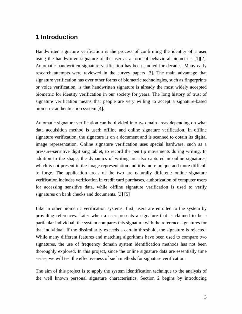
3.4.1 feature extraction To avoid dealing with unknown input and system, we want to solve this problem blindly using only output information. Spectrum analysis is useful here since it is not necessary to know the input information. The output of the signature dynamics can be assumed as a result of coupled oscillations in the horizontal and vertical directions, superimposed on a rightward (leftward) constant velocity horizontal sweep. [10] This structure can be easily obtained by performing Discrete Fourier Transformation (DFT). Using y coordinates profile as an example:

1

2 /

0( ) ( ) , 0,1,..., 1

Nj kt N

tF k y t e k Nπ

−−

=

= =∑ −

7

where y(t) is the y-profile, N is the number of points in the signature, and the F(k) are the DFT of y(t). We assumed that personal signature has unique frequency information and DFT could help us to extract this information by providing the power spectrum of the signature which is defined as the magnitude of F(k). In order to make comparison of the spectrum, we normalized the spectrum using total energy as shown in the following formulas

/ 2 1

0

( ) ( )* ( ( ))

( )

( ) ( ) / , 0,1,..., / 2 1

N

k

E k F k conj F k

E E k

N k E k E k N

−

=

=

=

= = −

∑

where E(k) constitute the Fourier spectrum of the signal, E is the total energy, and N(k) is the normalized spectrum. In online signature verification, timing information is very important. If the user signs signature in twice the size but in the same amount of time compared to his/her usual signature, the normalized spectrum will be the same, if the user signs signature in its usual size but in twice the time, the resolution will be doubled, the component energies will be shifted to double the frequency values compared to the usual signature and matching will be failed. However, people have found that a person signs his/her signature in roughly the same amount of time each time independent of size (within normal size variations), small speed differences will only shift the component energies by a small amount, and does not affect the matching significantly [5]. Meanwhile, forgers usually take significantly longer to sign and spectral difference could be observed. On the other hand different timings bring another problem. The formula of computing the interval between frequency components of DFT is

1s N Ts

ω =×

The natural variations within genuine signatures of the same user almost never have equal lengths. This variation will results in varying frequency components after performing DFT which will cause inconvenience in comparison. To solve this problem, we applied zero padding to each signature to make them have same length of 1024 points See Figure 2. Zero padding is heavily used in the assumption of time limited signal, which is true in this case since signature is finite duration non periodic signal. It can interpolate the

8

spectrum and improve the apparent spectrum resolution. With padding, the spectrum could have same frequency samples to compare as we need.

0 50 100 150 200 250 300-1

-0.5

0

0.5

1

0 200 400 600 800 1000 1200-1

-0.5

0

0.5

1

Figure 2 sample y signal before (left) and after (left) zero padding.

3.4.2 Decision making The user supplies 5 reference signatures to enroll to the system which are used to measure the variation within his/her signatures, so as to set user-specific thresholds for accepting or rejecting a candidate signature. After zero padding and DFT, the spectrum of each signature could be obtained. A sample plot of the spectral analysis is shown in figure 3. The lines represents the envelop that is formed using the maximum, mean, minimum energy at each sample frequency among the reference signatures. The dots represent the energy of the candidate signature.

Figure 3

Sample plot of spectral analysis. The left one is a genuine signature and the right one is a forgery. Though it is quite challenging to determine the decision boundary no matter what feature is used when you only have such a few references, feature selection is very important to make better verification. We tried several different methods.

9

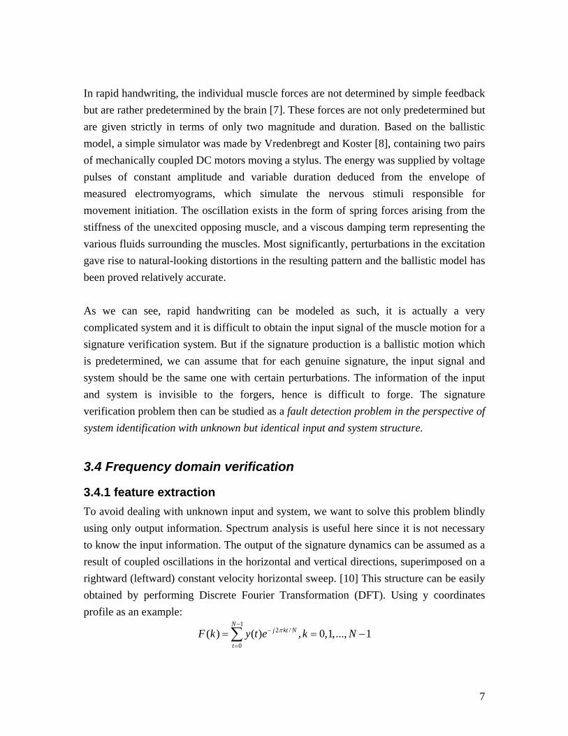
1. The first one is to choose the most consistent frequencies as features. To measure the consistency, we used the following formula.

max( ( )) min( ( ))( )

2 ( ( ))1, 2,3, 4,5 0,1,..., 1

i i

i

N k N kC kmean N k

i k N

−=

×

= = −

Where C(k) is the consistency measurement at each sample frequency, Ni(k) is the normalized energy of the i th reference signature at the corresponding frequency. 2. The second option is to choose the dominant frequencies as features. The dominant frequencies are chosen using the energy. Those frequencies that have large average magnitude are considered as dominant. 3. The third option is to choose the worst outsiders no mater at what frequencies they are. The outsiders are those frequencies of candidate signature that fall out of the envelop formed by the reference signatures. Also, we have several output signals to be considered: the coordinate profile X, Y, pressure P, velocity V, and polar magnitude r. After a certain number, m, of features are chosen, we can evaluated the candidate signature by using weighting factor. Let be the variance measurement of the j th feature of the candidate signature

je

( ) ( ( ))

| |( ( ))

c j i jj

i j

N k mean N ke

mean N k−

=

where is the normalized energy of the j th feature, we can define the evaluation of the candidate signature as the weighted sum of the ratio of actual variance and consistency of all features.

( )c jN k

1

( )( )

mj

cj j

ef W

C k=

= ∑

W(x) is a weighting function which can be arbitrarily defined. Basically, the larger is, the more it is weighted. In our work, we use a simple one / ( )je C k j

1

3( 1) ,( )

0, 1x x

W xx

⎧ − >= ⎨

≤⎩

If cf is above a threshold, the signature is a forgery.

10

3.4.3 Result We used the whole dataset to test our system. By tuning the threshold of decision, the best performance (achieve Equal Error Rate, EER where the False Acceptance Rate ‘FAR’ is equal to the false Rejection Rate ‘FRR’, )of each method is shown in table 1. Result of individual signatures is in appendix. The number of feature m=20.

Table 1 Result comparison Method III

signal y p r v threshold 450 450 350 70

frr 0.2667 0.28 0.2733 0.285 far 0.2575 0.2788 0.285 0.2913

Method I signal y p r v

threshold 160 250 200 230 frr 0.31 0.2983 0.3083 0.3217 far 0.2962 0.285 0.3063 0.315

Method II signal y p r v

threshold 25 60 60 36 frr 0.3333 0.2383 0.26 0.2883 far 0.325 0.2375 0.2563 0.2875

3.4.4 Discussion

We can see that the best performance was given by using dominant frequencies in pressure signal as features, using outsiders of the y profile is also good. However, the difference among all methods is not very large. The overall performance is about 28% EER, which is not as good as we expect. This may be due to the simple decision making scheme. A better weighting function or a user specific threshold may be defined to improve the system. Another reason may be that the forgeries are all skilled forgeries. In literature, two forgery types have been defined: a skilled forgery is signed by a person who has had access to a genuine signature for practice. A random forgery is signed without having any information about the signature of the person whose signature is forged. By observing the individual performance of each signature, we found that the complexity of the signature, and the character of the signature (Chinese or English) do not affect the performance of the spectral analysis method.

11

The spectral analysis method can be considered as using a rectangular window function on a periodic signal. The rectangular window function is a high resolution, low dynamic range window which could minimize the leakage, but it also cause discontinuity at the beginning and the end of the signal. We tried several other types of window function including Hann window, Bartlett window, and Nuttall window, but the overall performance is heavily weakened by the leakage. Also, we tried double the signal length by repeating the signal, it didn’t work well neither.

3.5 Time domain verification - Correlation Assuming that all genuine signatures have consistent feature, in other words consecutive performance of signature-writing is not far different to each other, correlation of the signature would be a good way to distinguish forgeries out of genuine ones.

Figure 4 Correlation obtained from generic time-domain function.

The figure above shows the quick view of deriving correlation of a generic time-domain function. S(w) represents the spectral density while R(w) represents the correlation function. If the complex conjugate of the same function is taken, it will result as a auto-correlation while if other function is taken it will result in cross-correlation. One thing to notice is that the function that is subject to take the complex conjugate is the one that is subject to have the time delay in the definition of time-domain correlation function.

3.5.1 Preprocessing In order to have comparable results, preprocessing of the data is necessary.

1. Normalization of the scale By normalizing the scale to a certain fixed large value, the comparison between the reference and sample signature would be easier. If the normalization is done by the maximum magnitude of each sample signature it will lose the relative magnitude information with respect to the reference signature, so this should be avoided. 2. Remove the translational mean (only for x,y coordinate) 3. Zero-padding When cross-correlation is considered the two objective signatures should have a same length of data. Zero-padding technique may change the correlation result, especially the magnitude, however, the oscillating nature of the data still remains constant. 4. Implementing a window function

12

For a real data that has a limited length with a different magnitude at the end points, taking the discrete fourier transform would cause a leakage due to the discontinuity. For this aspect, a window function has been implemented to the data so it can have less leakage. Three different window functions, Hanning, Laplace-Gauss and Kaiser-Bessel window, have been implemented and since the difference of the results is not significant, Kaiser-Bessel window was used for entire data.

3.5.2 Reference envelope There are five genuine reference signatures. A reference envelope is constructed by five corresponding auto-correlation and ten cross-correlation of the reference signatures. There is supposed to be 20 cross-correlations, however, half of them are mirror images so they are not considered.

Figure 5 reference auto, cross-correlation and the envelope.

The envelope is constructed by taking the minimum and maximum value of the reference correlation at each data point. The more genuine signature is consistence in its feature, the less the area inside the envelope.

3.5.3. Signature Verification Now, to identify a sample signature whether if it is genuine or fraudulent, the cross-correlation with respect to the five reference signature will be compared to the reference envelope that we had constructed earlier. The following figure shows the abstract idea of our verification process.

13

Figure 6 verification idea

If the signature is genuine, the five cross-correlations will be located inside the envelope, or somewhere near by, while if it is a forgery the characteristic of the cross-correlation curve will be different.

Figure 7 envelope and cross-correlation of fraudulent sign

As shown above, which the red oscillating plot indicates the cross-correlation of a fraudulent signature, the number of points that are located inside the reference envelope is far less than the genuine signature. The ratio of the number of valid points to the total number of data points will give the percentage. Note that the range where the difference of the minimum and the maximum of the envelope is very small, this process will not be activated. Since we have five reference signatures, we will have five percentages and based on this percentage figure a decision should be made whether the sample is real or fake. This certain threshold percentage is set between 85% and 98% in this approach. (threshold 1) The second threshold is the number of cross-correlation that exceeded threshold 1. Once again, since we have five reference signatures, threshold 2 should be some number between zero to five. For our case this has set to three. In other words, if three or more

14

sample cross-correlations have exceeded threshold 1, this sample signature will be identified as a genuine, otherwise a forgery.

3.5.4 Results Using the SVC data, which has 800 signatures in total, several results were obtained using this method with different threshold 1 value. The same FAR and FRR convention is given in the following table.

Table 2 Result table. Threshold 2 = 3.

For the pressure information case, the best performance is obtained when the threshold 1 is set to 98%. Based on the fact that the champion results of SVC competition had a result of about 10% for both case, this result is quite satisfactory. When the threshold is set to the lowest value, 85%, FAR is the largest while FRR is the smallest. As the threshold increases FAR gradually decreases while FRR increases. This makes sense since higher threshold will cause a relatively larger false rejection rate and lower false acceptance rate. This nature remains constant for y coordinate case. However as the threshold gets higher, FAR drops down to zero while FRR increases drastically. This infers that the genuine signature has poor consistency in its y coordinate information and for the fraudulent signature it does not quite match with the genuine y coordinate information. Therefore, the pressure information is more consistent than the y-coordinate information. The following figure shows one of the good performance example:

15

Figure 8 signature verification for signature No.2 using pressure information

The black dashed line represents the reference envelope. The yellow line is the two of the genuine sample signal cross-correlations with respect to the five reference signature while the red line represents the forgery sample signature. Yellow lines are located inside the envelope for most of the case and the overall size of the envelope is quite narrow so based on this fact we can say that this signature is quite consistent. For the red lines, even though they have similar slope compared to the genuine ones, the magnitude is quite different so eventually located outside of the envelope. The following figure is the result of the same signature, but with different information: y-coordinate.

Figure 9 signature verification for signature No.2 using y-coordinate information

As we can see from the figure, the size of the envelope is larger than the pressure case, indicating that it has less consistency, so even most of the red lines are located inside the envelope. However, on the other side of the correlation plot, the difference between the genuine and forgery is significant, eventually resulting in a good performance.

16

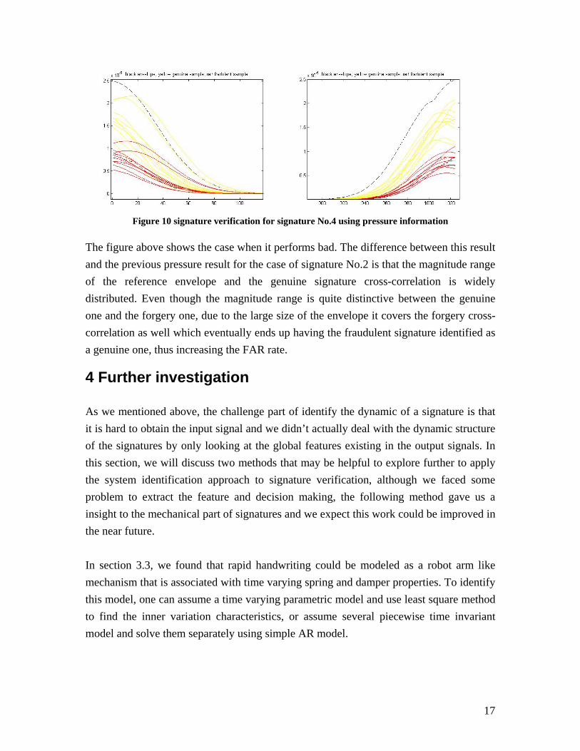
Figure 10 signature verification for signature No.4 using pressure information

The figure above shows the case when it performs bad. The difference between this result and the previous pressure result for the case of signature No.2 is that the magnitude range of the reference envelope and the genuine signature cross-correlation is widely distributed. Even though the magnitude range is quite distinctive between the genuine one and the forgery one, due to the large size of the envelope it covers the forgery cross-correlation as well which eventually ends up having the fraudulent signature identified as a genuine one, thus increasing the FAR rate.

4 Further investigation As we mentioned above, the challenge part of identify the dynamic of a signature is that it is hard to obtain the input signal and we didn’t actually deal with the dynamic structure of the signatures by only looking at the global features existing in the output signals. In this section, we will discuss two methods that may be helpful to explore further to apply the system identification approach to signature verification, although we faced some problem to extract the feature and decision making, the following method gave us a insight to the mechanical part of signatures and we expect this work could be improved in the near future. In section 3.3, we found that rapid handwriting could be modeled as a robot arm like mechanism that is associated with time varying spring and damper properties. To identify this model, one can assume a time varying parametric model and use least square method to find the inner variation characteristics, or assume several piecewise time invariant model and solve them separately using simple AR model.

17

4.1 Piecewise AR Model Prior to discussing the identification, we first normalize the signature invariant to timing. Though the feature may be lost, it’s much easier to compare signatures with same length and it also enriches the information of the signature. Simple linear interpolation to 1024 points is used. However, we may use some other techniques to eliminate those signatures that are much longer than the references and only consider the ones that have similar length. See Figure 11. The segmentation of the signature can be solved in two ways: uniform segmentation and dynamic segmentation. Uniform segmentation could be simply done by dividing the signal equally. The only thing we considered is the number of segments which should satisfy, as much as possible, a number of competing constraints. In order to obtain approximate stationarity for the local AR models the segment size should be small. On the other hand, the number of samples used to estimate the coefficients needs to be large enough to ensure consistent parameter estimation. In our project, each signature was divided uniformly into 8 segments, each segment with 128 points. Figure 12

Figure 11 Signature after and before interpolation

Though uniform segmentation is easy, it has its own drawback. It can not reflect the signature dynamics accurately, some dramatic change were observed in position and pressure profile and will affect the result heavily. We tried another segmentation method which is truly based on the local characteristic of the signature. Dynamic segmentation is done by scanning the acceleration profile of the signature. The signature is divided where the acceleration of the pen tip is above a certain threshold. This method is good to obtain nice local behavior, but suffered from having different number of segments among different signature for a same user, even among genuine ones. See figure 5, compare with

18

figure4 (they are from same signature), the right one clearly shows that the segmentation is based on the strokes of the signature.

Figure 12

Sample segmentation on same y profile. Left one is uniform, right one is dynamic After segmentation, each local system can be identified using low order AR model. In our project, we used 2nd order AR model. Using y profile as an example, the model is 1 2( ) ( 1) ( 2)i i i i i 3iy k a y k a y k a= − + − +

Where ( )iy k is the y signal in i th segment. Using least square method, [ ]0 1 2T

i i ia a a can be identified. The feature vector is

11 21 1

12 21 2

m

m

a a aa a a⎡ ⎤⎢ ⎥⎣ ⎦

3ia are discard since they are the offset of the model. Figure 13 shows an example plot of using y profile with dynamic segmentation. 2ia

Figure 13 parameter comparison

19

4.2 Moving AR model An extension of piecewise AR model is to use a moving window to truncate data and only make parameter estimation within the window, in our project, we tested a window with size 128. The model is still a 2nd order AR model, with [ ]0 1 2

Ti i ia a a to be

identified. An example plot of for a set of 40 signatures that are claimed to be the same person is shown in Figure 14.

2ia

4.3 Discussion Due to the limitation of time, we didn’t find the matching algorithm to detect the forgery. The result is promising as we can see the difference between genuine and forgery, though it’s not very large. Higher order model could be used to improve the result. Especially when using dynamic segmentation, each segment could be assumed as an impulse response of a spring-mass-damper system (maybe nonlinear) with certain initial condition. Then ERA and other algorithms could be used to identify the subsystems.

Figure 14, blue ones are genuine, red ones are forgery.

5 Real data experiment To complete this report, we finally got some real world data by ourselves to test our algorithm. The data was collected using WACOM FAVO digitizing table and had to be done manually, so we were only able to get a small set of signatures. We totally collected

20

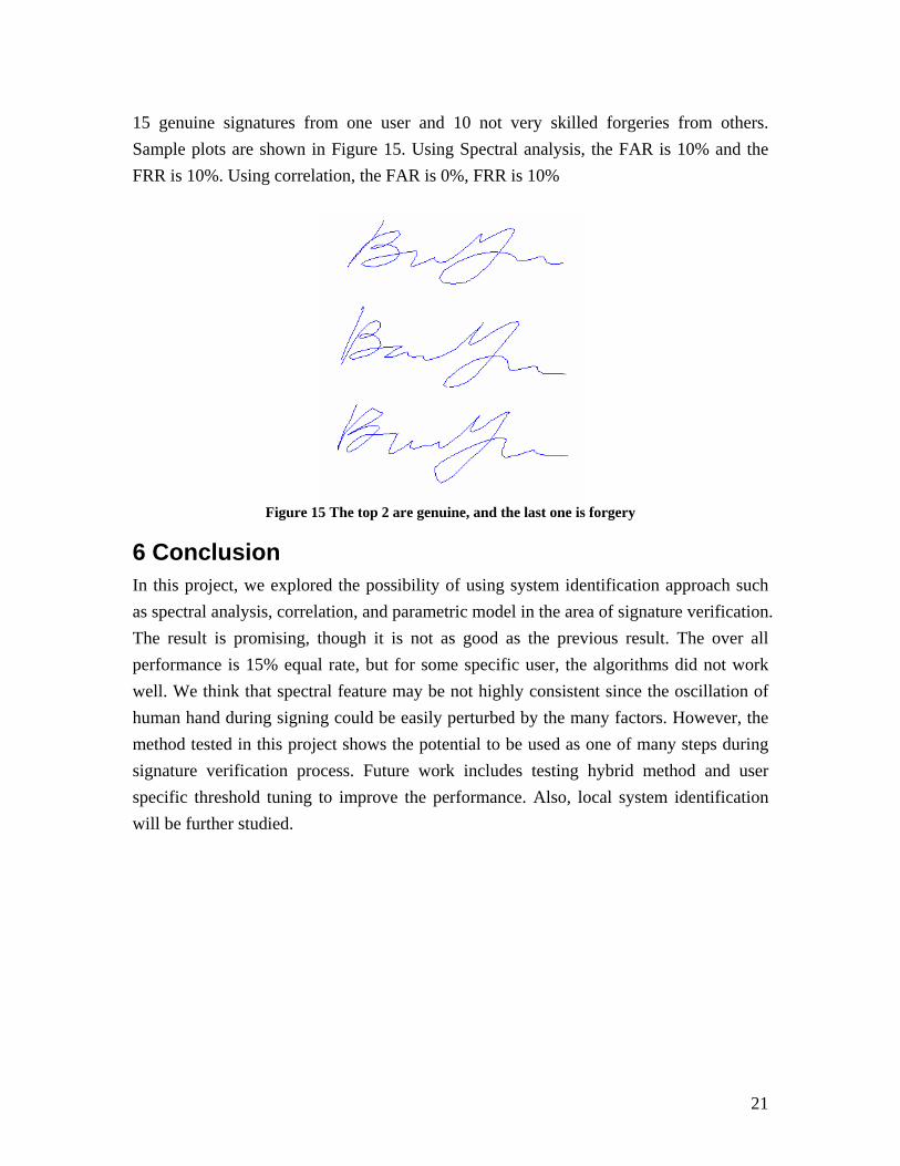
15 genuine signatures from one user and 10 not very skilled forgeries from others. Sample plots are shown in Figure 15. Using Spectral analysis, the FAR is 10% and the FRR is 10%. Using correlation, the FAR is 0%, FRR is 10%

Figure 15 The top 2 are genuine, and the last one is forgery

6 Conclusion In this project, we explored the possibility of using system identification approach such as spectral analysis, correlation, and parametric model in the area of signature verification. The result is promising, though it is not as good as the previous result. The over all performance is 15% equal rate, but for some specific user, the algorithms did not work well. We think that spectral feature may be not highly consistent since the oscillation of human hand during signing could be easily perturbed by the many factors. However, the method tested in this project shows the potential to be used as one of many steps during signature verification process. Future work includes testing hybrid method and user specific threshold tuning to improve the performance. Also, local system identification will be further studied.

21

Reference 1. Vishvjit S. Nalwa, “Automatic On-Line Signature Verification” 2. A.K. Jain, F.D. Griess, and S.D. Connell, “On-line signature verification” 3. F. Leclerc and R. Plamondon, “Automatic signature verification: the state of the

art 1989-1993” 4. Dit-Yan Yeung, Hong Chang, Yimin Xiong, Susan George, Ramanujan Kashi,

Takashi Matsumoto, and Gerhard Rigoll, “SVC2004: First International Signature Verification Competition”

5. Alisher Kholmatov and Berrin Yanikoglu, “Fourier Descriptors for On-line Signature Verification”

6. C Lam, D Kamins and K Zimmermann, “Signature recognition through spectral analysis”

7. N. M. Herbst and C. N. Liu , “Automatic Signature Verification Based on Accelerometry”

8. J. Vredenbregt and W. G. Koster, “Analysis and Synthesis of Handwriting” 9. Hansheng Lei and Venu Govindaraju, “A Comparative Study on the Consistency

of Features in On-line Signature verification” 10. Orly Stettinerl and Dan Chazan, “A Statistical Parametric Model for Recognition

and Synthesis of Handwriting”

22

Appendix A Screen shot of all 40 users’ genuine signatures

2000 4000 6000 8000 100002000

4000

6000

8000

2000 4000 6000 8000 100002000

4000

6000

8000

2000 4000 6000 8000 100002000

4000

6000

8000

2000 4000 6000 8000 100002000

4000

6000

8000

0 2000 4000 6000 8000 100002000

4000

6000

8000

2000 4000 6000 8000 100004000

5000

6000

7000

2000 4000 6000 80002000

4000

6000

8000

2000 4000 6000 8000 100002000

4000

6000

8000

0 2000 4000 6000 80002000

4000

6000

8000

2000 4000 6000 8000 100000

5000

10000

2000 3000 4000 5000 6000 70002000

3000

4000

5000

2000 4000 6000 8000 100000

2000

4000

6000

2000 4000 6000 80005000

5500

6000

6500

2000 3000 4000 5000 6000 70004000

5000

6000

7000

0 5000 10000 150003000

4000

5000

6000

3000 4000 5000 6000 7000 80003000

4000

5000

6000

0 2000 4000 6000 8000 100002000

4000

6000

8000

0 5000 10000 150002000

4000

6000

8000

4000 5000 6000 7000 80000

2000

4000

6000

5000 6000 7000 8000 9000 100003000

4000

5000

6000

2000 4000 6000 8000 100002000

4000

6000

8000

2000 4000 6000 8000 100002000

4000

6000

8000

0 5000 10000 150000

5000

10000

0 2000 4000 6000 8000 100002000

4000

6000

8000

1000 2000 3000 4000 50005000

6000

7000

8000

3000 4000 5000 6000 70002000

4000

6000

8000

2000 4000 6000 8000 10000 120002000

4000

6000

8000

2000 4000 6000 8000 100002000

4000

6000

8000

3000 4000 5000 6000 7000 80006000

7000

8000

9000

4000 5000 6000 7000 80004000

4500

5000

5500

4000 5000 6000 7000 8000 90002000

4000

6000

8000

2000 4000 6000 8000 100000

5000

10000

2000 4000 6000 8000 100004000

6000

8000

2000 4000 6000 8000 100002000

4000

6000

8000

2000 4000 6000 8000 100002000

4000

6000

5500 6000 6500 7000 7500 80004000

5000

6000

7000

4000 5000 6000 7000 80004000

5000

6000

7000

6000 7000 8000 90004000

5000

6000

7000

2000 4000 6000 8000 10000 120002000

4000

6000

8000

0 5000 10000 150000

5000

10000

23