Embed Size (px)
Citation preview

Final-Placement BRDF Editing
Aner Ben-Artzi
Submitted in partial fulfillment of theRequirements for the degree
of Doctor of Philosophyin the Graduate School of Arts and Sciences
COLUMBIA UNIVERSITY
2007

c© 2007
Aner Ben-ArtziAll Rights Reserved
Abstract
Final-Placement BRDF Editing
Aner Ben-Artzi
The scene descriptions of computer-generated worlds include the geometry and lo-
cation of objects, the lighting configuration, and the material properties of object sur-
faces. Material properties can often be described with the Bi-directional Reflectance
Distribution Function (BRDF). The BRDF is a function that encodes the way light
interacts with a surface, giving rise to different material perceptions, such as wood,
metal, or plastic. Using traditional rendering techniques it is not possible to mod-
ify the BRDF of a complex scene while rendering it at interactive rates. Therefore,
BRDFs are often chosen in simplified scenarios, and only later rendered in their final
placement within a scene with complex geometry and lighting. This can lead to unex-
pected results since the appearance of objects depends on the interaction of lighting,
geometry, and materials. In this thesis, I discuss how to use precomputation-based
rendering techniques to allow for interactive rendering of changing BRDFs in scenes
with complex lighting and geometry, including cast shadows and global illumination.
This new capability allows artists and designers to choose the material properties of
objects based on accurate feedback so they can have confidence that their decisions are
well-informed. Final-placement decision making has been shown for lighting design,
and this work is inspired by such precomputed radiance transfer (PRT) for interac-
tive relighting. Linear rendering via a dot-product is introduced for BRDF editing in
direct, complex lighting with cast shadows. This requires a new linear BRDF repre-
sentation that is useful for both editing and rendering. For BRDF editing with global
illumination, the image is no longer linear in the BRDFs of the scene. Therefore a

new bilinear reflection operator is introduced to enable precomputing a polynomial
representation that captures the higher-order interactions of editable BRDFs. Opti-
mizations for both the precomputation and rendering phases are presented. The final
render-time operation is a per-pixel dot-product whose complexity is independent of
geometric and lighting complexity, as these aspects of the scene are fixed. Runtime
improvements including curve-switching, object freezing, and incremental rendering
are used to improve rendering performance without loss of quality.
CONTENTS
Part I BRDFs: Then and Now 2
1. Introduction . . . . . . . . . . . . . . . . . . . . . . . . . . . . . . . . . . . 3
1.1 A Walkthrough with the Phong BRDF . . . . . . . . . . . . . . . . . 5
1.2 Current State of the Art . . . . . . . . . . . . . . . . . . . . . . . . . 6
1.3 Organization and Contributions . . . . . . . . . . . . . . . . . . . . . 8
2. Previous Work . . . . . . . . . . . . . . . . . . . . . . . . . . . . . . . . . 10
2.1 BRDF Representations . . . . . . . . . . . . . . . . . . . . . . . . . . 10
2.2 BRDF Editing . . . . . . . . . . . . . . . . . . . . . . . . . . . . . . . 14
2.3 Precomputed Radiance Transfer (PRT) . . . . . . . . . . . . . . . . . 16
2.4 Global Illumination . . . . . . . . . . . . . . . . . . . . . . . . . . . . 18
3. A New Editable and Renderable Representation . . . . . . . . . . . . . . . 19
3.1 Cook-Torrance: an analytic BRDF example . . . . . . . . . . . . . . 22
3.2 Ashikhmin-Shirley: an anisotropic analytic BRDF . . . . . . . . . . . 23
3.3 Making use of the quotient BRDF . . . . . . . . . . . . . . . . . . . . 25
3.3.1 Ashikhmin-Shirley with Fresnel edits in 2 factors . . . . . . . 25
3.3.2 Anisotropy with 1 Factor . . . . . . . . . . . . . . . . . . . . . 27
3.4 Other Analytic and Hybrid BRDFs . . . . . . . . . . . . . . . . . . . 27
3.5 Measured/Factored BRDFs . . . . . . . . . . . . . . . . . . . . . . . 28
Part II Interactive BRDF Editing Beyond Simple Lighting 32
4. Interactive Rendering in Complex Lighting . . . . . . . . . . . . . . . . . . 33
4.1 Method Overview . . . . . . . . . . . . . . . . . . . . . . . . . . . . . 33
4.2 Environment Map Precomputation . . . . . . . . . . . . . . . . . . . 37
4.2.1 Computing Overlaps . . . . . . . . . . . . . . . . . . . . . . . 37
4.2.2 Initial Approach . . . . . . . . . . . . . . . . . . . . . . . . . 40
4.2.3 Our Algorithm . . . . . . . . . . . . . . . . . . . . . . . . . . 41
4.2.4 Two Factor BRDFs . . . . . . . . . . . . . . . . . . . . . . . . 44
4.2.5 Use of Daubechies 4 Wavelets . . . . . . . . . . . . . . . . . . 45
4.3 BRDF Editing Results . . . . . . . . . . . . . . . . . . . . . . . . . . 47
4.3.1 Real-time Edits . . . . . . . . . . . . . . . . . . . . . . . . . . 47
4.3.2 Precomputation Numbers . . . . . . . . . . . . . . . . . . . . 51
5. Bilinear Rendering Operators for BRDF Editing . . . . . . . . . . . . . . . 53
5.1 Theory of BRDF Editing in Global Illumination . . . . . . . . . . . . 53
5.1.1 Basic Framework using the bilinear K operator . . . . . . . . 55
5.1.2 Polynomial Representation for Multi-Bounce . . . . . . . . . . 57
5.2 Managing Complexity . . . . . . . . . . . . . . . . . . . . . . . . . . 61
5.2.1 Low-Frequency BRDF approximations . . . . . . . . . . . . . 62
5.2.2 Diffuse approximation for further bounces . . . . . . . . . . . 64
5.2.3 Slower Decay of BRDF Series . . . . . . . . . . . . . . . . . . 68
5.2.4 Equivalent Albedo . . . . . . . . . . . . . . . . . . . . . . . . 69
6. Interactive Rendering with Global Illumination . . . . . . . . . . . . . . . 72
6.1 Implementation . . . . . . . . . . . . . . . . . . . . . . . . . . . . . . 73
6.1.1 Monte Carlo Precomputation . . . . . . . . . . . . . . . . . . 73
ii
6.1.2 Rendering in Real Time . . . . . . . . . . . . . . . . . . . . . 77
6.1.3 Extensions . . . . . . . . . . . . . . . . . . . . . . . . . . . . . 80
6.2 Global Illumination Results . . . . . . . . . . . . . . . . . . . . . . . 82
6.2.1 Editing and Visual effects . . . . . . . . . . . . . . . . . . . . 82
6.2.2 Precomputation Times and Memory Usage . . . . . . . . . . . 85
6.2.3 Rendering Speed . . . . . . . . . . . . . . . . . . . . . . . . . 87
Part III New Concepts Applicable to BRDF Editing and More 88
7. Temporal Coherence for Real-Time Precomputed Rendering . . . . . . . . 90
7.1 Use in BRDF editing . . . . . . . . . . . . . . . . . . . . . . . . . . . 92
7.2 Use in Relighting . . . . . . . . . . . . . . . . . . . . . . . . . . . . . 94
8. Visibility Coherence for Precomputation . . . . . . . . . . . . . . . . . . . 97
8.1 Use in BRDF Editing . . . . . . . . . . . . . . . . . . . . . . . . . . . 98
8.2 Use in Offline Still and Animation Rendering . . . . . . . . . . . . . . 98
8.3 Introduction . . . . . . . . . . . . . . . . . . . . . . . . . . . . . . . . 99
8.4 Background . . . . . . . . . . . . . . . . . . . . . . . . . . . . . . . . 101
8.5 Preliminaries . . . . . . . . . . . . . . . . . . . . . . . . . . . . . . . 103
8.6 Algorithm Components . . . . . . . . . . . . . . . . . . . . . . . . . . 104
8.6.1 Estimating Visibility . . . . . . . . . . . . . . . . . . . . . . . 105
8.6.2 Correcting Visibility Estimates . . . . . . . . . . . . . . . . . 108
8.7 Analyzing Possible Component Combinations . . . . . . . . . . . . . 109
8.7.1 The Scenes . . . . . . . . . . . . . . . . . . . . . . . . . . . . 110
8.7.2 Correctness Analysis (Scanline vs. Grid) . . . . . . . . . . . . 111
8.7.3 Performance Analysis . . . . . . . . . . . . . . . . . . . . . . . 112
8.7.4 Discussion of Analysis . . . . . . . . . . . . . . . . . . . . . . 115
iii

8.8 Optimizations and Implementation . . . . . . . . . . . . . . . . . . . 116
8.8.1 Optimized Algorithm . . . . . . . . . . . . . . . . . . . . . . . 117
8.8.2 Implementation . . . . . . . . . . . . . . . . . . . . . . . . . . 120
8.8.3 Time and Memory Considerations . . . . . . . . . . . . . . . . 123
8.9 Other Considerations . . . . . . . . . . . . . . . . . . . . . . . . . . . 125
9. User Interface for 1D Function Editing . . . . . . . . . . . . . . . . . . . . 127
9.1 Empirical Definition of Helper Functions . . . . . . . . . . . . . . . . 130
9.2 Smoothness and Layered operators . . . . . . . . . . . . . . . . . . . 131
9.3 Use in BRDF Editing and Other Graphics Applications . . . . . . . . 131
Part IV Conclusion 133
10. Conclusion . . . . . . . . . . . . . . . . . . . . . . . . . . . . . . . . . . . . 134
10.1 Final-Placement . . . . . . . . . . . . . . . . . . . . . . . . . . . . . . 134
10.2 Theoretical Framework with Few Assumptions . . . . . . . . . . . . . 135
10.3 Complement to Relighting . . . . . . . . . . . . . . . . . . . . . . . . 136
10.4 Continuous Editing and Discrete Choices . . . . . . . . . . . . . . . . 137
11. Future Directions . . . . . . . . . . . . . . . . . . . . . . . . . . . . . . . . 138
11.1 Higher-Complexity Functions . . . . . . . . . . . . . . . . . . . . . . 138
11.2 Practical Extensions . . . . . . . . . . . . . . . . . . . . . . . . . . . 139
11.3 Advantages of Precomputation-based Rendering . . . . . . . . . . . . 141
References . . . . . . . . . . . . . . . . . . . . . . . . . . . . . . . . . . . . . . 142
iv

LIST OF TABLES
4.1 Daubechies 4 Coefficients . . . . . . . . . . . . . . . . . . . . . . . . . 45
4.2 Timings and Memory for Complex Lighting . . . . . . . . . . . . . . 52
5.1 Table of Notation for Chapters 5 and 6 . . . . . . . . . . . . . . . . . 55
6.1 Timings and Storage for Global Illumination . . . . . . . . . . . . . . 86
7.1 Didactic Example of Incremental vs. Non-Linear . . . . . . . . . . . . 93
8.1 Percentage of Shadow-Rays Traced . . . . . . . . . . . . . . . . . . . 112
8.2 Visibility Timings . . . . . . . . . . . . . . . . . . . . . . . . . . . . . 113
8.3 Shadow-Ray Timings . . . . . . . . . . . . . . . . . . . . . . . . . . . 123
v

LIST OF FIGURES
1.1 Teatray with Cloth . . . . . . . . . . . . . . . . . . . . . . . . . . . . 4
1.2 Edit in Complex Lighting . . . . . . . . . . . . . . . . . . . . . . . . 6
1.3 Edit in Point Lighting . . . . . . . . . . . . . . . . . . . . . . . . . . 6
1.4 Edit without Shadows . . . . . . . . . . . . . . . . . . . . . . . . . . 7
3.1 Edit of Phong Curve . . . . . . . . . . . . . . . . . . . . . . . . . . . 21
3.2 Specularity Edit on Pearls . . . . . . . . . . . . . . . . . . . . . . . . 22
3.3 Fresnel Edit on Stems . . . . . . . . . . . . . . . . . . . . . . . . . . 23
3.4 Anisotropic Edit on Teapot . . . . . . . . . . . . . . . . . . . . . . . 25
3.5 McCool Edit on Cloth . . . . . . . . . . . . . . . . . . . . . . . . . . 29
3.6 Factored BRDF Edits . . . . . . . . . . . . . . . . . . . . . . . . . . 30
3.7 Measured BRDF Edits . . . . . . . . . . . . . . . . . . . . . . . . . . 31
4.1 Light-Bands Overlaps . . . . . . . . . . . . . . . . . . . . . . . . . . . 38
4.2 Triangle-Range Overlap . . . . . . . . . . . . . . . . . . . . . . . . . 38
4.3 Point vs. Area Samples . . . . . . . . . . . . . . . . . . . . . . . . . . 42
4.4 Teatray Results . . . . . . . . . . . . . . . . . . . . . . . . . . . . . . 48
4.5 Earrings Results . . . . . . . . . . . . . . . . . . . . . . . . . . . . . . 49
5.1 Rendering Operators . . . . . . . . . . . . . . . . . . . . . . . . . . . 54
5.2 BRDF Polynomial . . . . . . . . . . . . . . . . . . . . . . . . . . . . 54
5.3 Comparison of Bounce Resolution . . . . . . . . . . . . . . . . . . . . 60

5.4 Exponential Growth wrt BRDF Bases . . . . . . . . . . . . . . . . . 61
5.5 BRDF Edits in Cornell Box . . . . . . . . . . . . . . . . . . . . . . . 65
5.6 Errors in Simpler Approximations . . . . . . . . . . . . . . . . . . . . 66
6.1 Interior Design Session . . . . . . . . . . . . . . . . . . . . . . . . . . 72
6.2 Light Paths . . . . . . . . . . . . . . . . . . . . . . . . . . . . . . . . 75
6.3 Vase with Flowers . . . . . . . . . . . . . . . . . . . . . . . . . . . . . 82
6.4 Room Closeup . . . . . . . . . . . . . . . . . . . . . . . . . . . . . . . 84
6.5 Two-Bounce Glossy Edits . . . . . . . . . . . . . . . . . . . . . . . . 85
7.1 Incremental BRDF Editing . . . . . . . . . . . . . . . . . . . . . . . . 94
7.2 Incremental Relighting . . . . . . . . . . . . . . . . . . . . . . . . . . 95
8.1 Fast Visibility Ground Truth Comparisons . . . . . . . . . . . . . . . 98
8.2 Domino Scene Comparing Visibility Calculations . . . . . . . . . . . . 99
8.3 Voronoi Regions . . . . . . . . . . . . . . . . . . . . . . . . . . . . . . 104
8.4 Grid-Based Evaluation . . . . . . . . . . . . . . . . . . . . . . . . . . 106
8.5 Warping Blockers . . . . . . . . . . . . . . . . . . . . . . . . . . . . . 106
8.6 Light-space Flooding . . . . . . . . . . . . . . . . . . . . . . . . . . . 108
8.7 Shapes and Bunny Ground Truth Comparisons . . . . . . . . . . . . 110
8.8 Error Analysis of Visibility Coherence Components . . . . . . . . . . 111
8.9 Plant Comparisons of Visibility Algorithms . . . . . . . . . . . . . . . 117
9.1 Y-Translation . . . . . . . . . . . . . . . . . . . . . . . . . . . . . . . 128
9.2 X-Translation . . . . . . . . . . . . . . . . . . . . . . . . . . . . . . . 129
9.3 Y-Amplification . . . . . . . . . . . . . . . . . . . . . . . . . . . . . . 130
9.4 X-Amplificaiton . . . . . . . . . . . . . . . . . . . . . . . . . . . . . . 130
vii

Acknowledgments
To my advisor, Ravi, thank you for carrying me through these five years and helping
me come out on the other side with a body of work that I can be proud of. Your
example was a high bar to reach for, and I got farther for stretching to reach it.
To Eitan Grinspun, thank you for your support and encouragement and friendship.
You added a constant light1 to my time at Columbia.
To Ryan Overbeck, Kevin Egan – my coauthors and lab mates – thank you for
the chats, the lunches, and your support. Without you, this work would not be what
it is today. Everyday I’d come into the lab, the first thing I did was check to see if
you were around.
To Shree Nayar and Peter Belhumeur, thank you for always having the time to
listen, and presenting me with excellent role models. To Fredo Durand and Szymon
Rusinkiewicz, thank you for sharing your wisdom and experience on our projects
together. And thank you to all four for sharing your time to be on my committee
and participate in my final step on this journey.
To Jason Lawrence, thank you for visits to Princeton that I always looked forward
to, and a ‘snazzy’ time editing text hours before the deadline.
To my parents, Dalia and Itai, thank you for raising me to believe that what I
envision for my future will one day be my present. This thesis and doctoral degree
seemed so far away at one time, and now they’re a reality. You’ve given me everything
I need to be successful.
To my wife Nicole, thank you for your constant support and being my cheerleader
every day.
1 literally and figuratively
viii

1
This thesis is dedicated to my wife, Nicole, and to our future life together.

Part I
BRDFS: THEN AND NOW

3
1. INTRODUCTION
Computer graphics develops tools for skilled artists, designers, and engineers to create
images based on the building blocks of geometry, material properties, and lighting.
Interactive (versus offline) design of these scene components allows users not only to
converge on a goal more quickly, but also to explore the design space and discover
new effects. Material properties are often expressed as the bi-directional reflectance
distribution function (BRDF), defined in (Nicodemus et al., 1977). While lighting
design and geometric modeling have analogs in the real world, it is not usually pos-
sible to continuously edit material properties. However, in a computer simulated
world, editing BRDFs has no fundamental distinction from editing other aspects of
a scene (such as lighting or geometry), and is equally important in contributing to
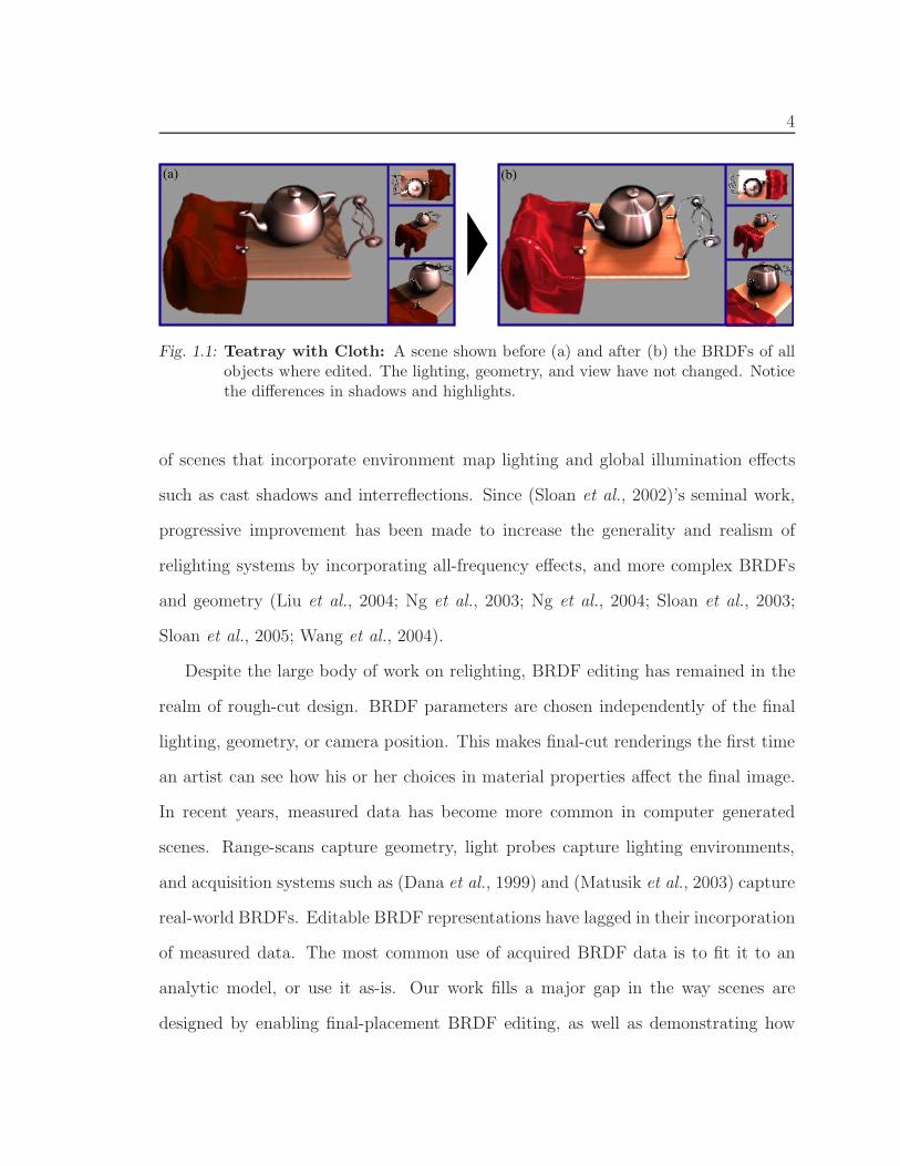
the final scene appearance. Figure 1.11 shows the same scene, illuminated by the
same environment map, with different BRDFs. Notice how the choice of materials
affects the mood of the arrangement. Also, the materials have to be selected in their
final-placement since aspects such as the elongation of specularities and shadow shape
result from an interaction of all three aspects of scene appearance : lighting, geometry,
and materials.
Lighting design has been an active field of research for photorealistic rendering
since its introduction in (Nimeroff et al., 1994) and (Dobashi et al., 1995). More
recent work by (Sloan et al., 2002) has rekindled an interest in real-time relighting
1 All images of 3D scenes in this thesis are rendered with systems implemented for this work,except where explicitly stated for ground-truth comparisons.
4
(a) (b)
Fig. 1.1: Teatray with Cloth: A scene shown before (a) and after (b) the BRDFs of allobjects where edited. The lighting, geometry, and view have not changed. Noticethe differences in shadows and highlights.
of scenes that incorporate environment map lighting and global illumination effects
such as cast shadows and interreflections. Since (Sloan et al., 2002)’s seminal work,
progressive improvement has been made to increase the generality and realism of
relighting systems by incorporating all-frequency effects, and more complex BRDFs
and geometry (Liu et al., 2004; Ng et al., 2003; Ng et al., 2004; Sloan et al., 2003;
Sloan et al., 2005; Wang et al., 2004).
Despite the large body of work on relighting, BRDF editing has remained in the
realm of rough-cut design. BRDF parameters are chosen independently of the final
lighting, geometry, or camera position. This makes final-cut renderings the first time
an artist can see how his or her choices in material properties affect the final image.
In recent years, measured data has become more common in computer generated
scenes. Range-scans capture geometry, light probes capture lighting environments,
and acquisition systems such as (Dana et al., 1999) and (Matusik et al., 2003) capture
real-world BRDFs. Editable BRDF representations have lagged in their incorporation
of measured data. The most common use of acquired BRDF data is to fit it to an
analytic model, or use it as-is. Our work fills a major gap in the way scenes are
designed by enabling final-placement BRDF editing, as well as demonstrating how

1.1. A WALKTHROUGH WITH THE PHONG BRDF 5
measured BRDF data can be edited and used without resorting to parametric fits.
With the use of our real-time rendering system, images such as the one shown in
Figure 1.1 can be updated as the user edits the BRDFs of scene objects. Updates
include all-frequency complex lighting and accurate cast shadows. The cloth in Figure
1.1 uses a measured BRDF that is never fit to any analytic model, yet can still be
edited intuitively. Previous methods were only able to render such scenes in simple
lighting or without cast shadows, greatly limiting their usefulness for determining the
BRDFs’ influence on the appearance.
1.1 A Walkthrough with the Phong BRDF
We seek to edit BRDFs in their final placement on objects already arranged in a scene,
lit by complex illumination. With this ability, we provide control over an important
component of appearance: material properties. More powerful than simply selecting
a pre-existing material, the designer has the freedom to adjust the BRDF to simulate
novel materials. This can include fine-tuning a measured dataset, exploring variations
of analytic models, venturing outside the analytic form of those models, or designing
a new BRDF from scratch. Let’s begin with an example that must be similar to
one of the first explorations of BRDF space in computer graphics, and which should
be familiar to anyone who has worked with computer-generated scenes: choosing a
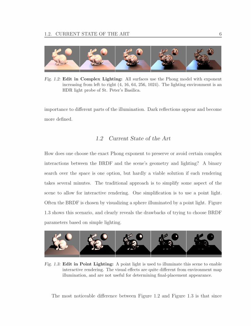
Phong exponent. Figure 1.2 shows a scene illuminated by an environment map, with
increasing Phong exponent; ranging exponentially from 4 to 1024. Each of these
images would take several minutes to render with traditional ray-tracing.
Many interesting effects occur in this scene: The objects appear to become darker
resulting from the localization of very bright points, due to the narrower Phong lobe.
Shadow lines appear and disappear as the Phong lobe narrows, giving different relative
1.2. CURRENT STATE OF THE ART 6
Fig. 1.2: Edit in Complex Lighting: All surfaces use the Phong model with exponentincreasing from left to right (4, 16, 64, 256, 1024). The lighting environment is anHDR light probe of St. Peter’s Basilica.
importance to different parts of the illumination. Dark reflections appear and become
more defined.
1.2 Current State of the Art
How does one choose the exact Phong exponent to preserve or avoid certain complex
interactions between the BRDF and the scene’s geometry and lighting? A binary
search over the space is one option, but hardly a viable solution if each rendering
takes several minutes. The traditional approach is to simplify some aspect of the
scene to allow for interactive rendering. One simplification is to use a point light.
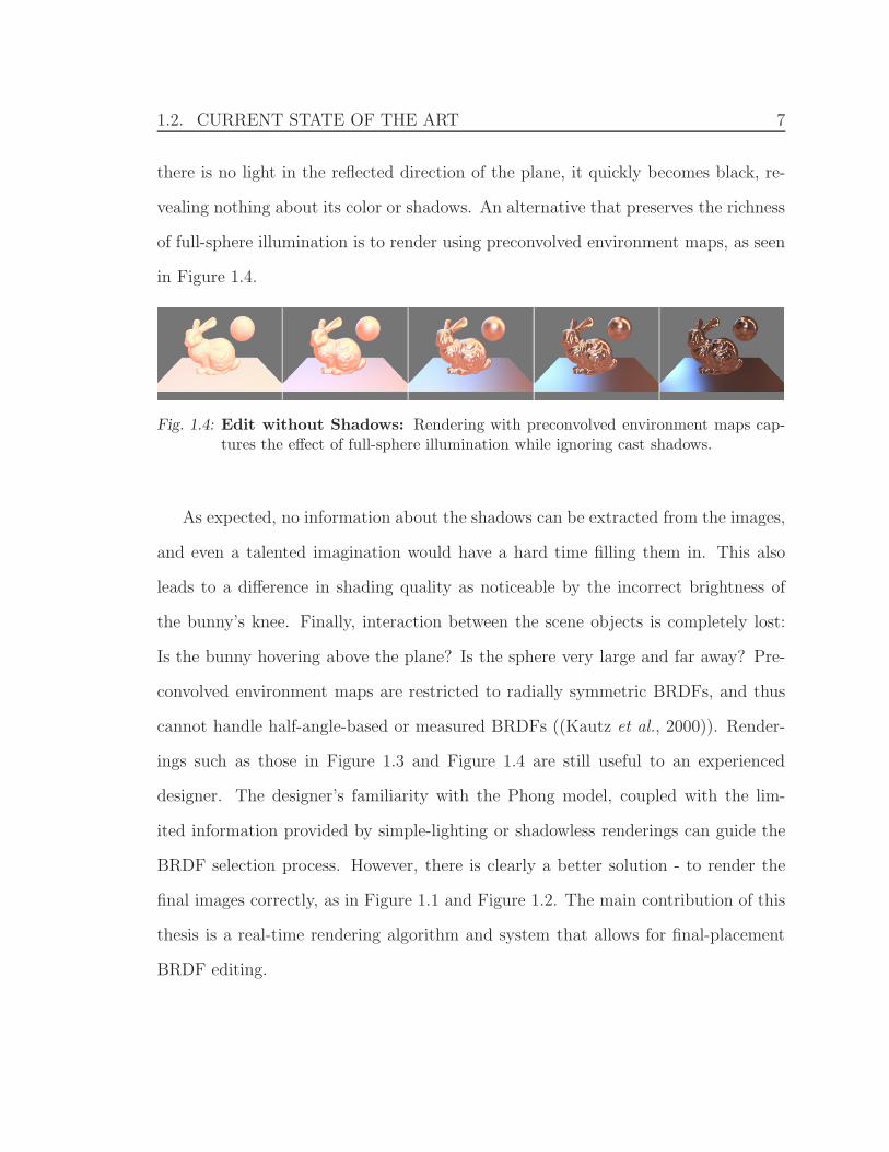
Often the BRDF is chosen by visualizing a sphere illuminated by a point light. Figure
1.3 shows this scenario, and clearly reveals the drawbacks of trying to choose BRDF
parameters based on simple lighting.
Fig. 1.3: Edit in Point Lighting: A point light is used to illuminate this scene to enableinteractive rendering. The visual effects are quite different from environment mapillumination, and are not useful for determining final-placement appearance.
The most noticeable difference between Figure 1.2 and Figure 1.3 is that since
1.2. CURRENT STATE OF THE ART 7
there is no light in the reflected direction of the plane, it quickly becomes black, re-
vealing nothing about its color or shadows. An alternative that preserves the richness
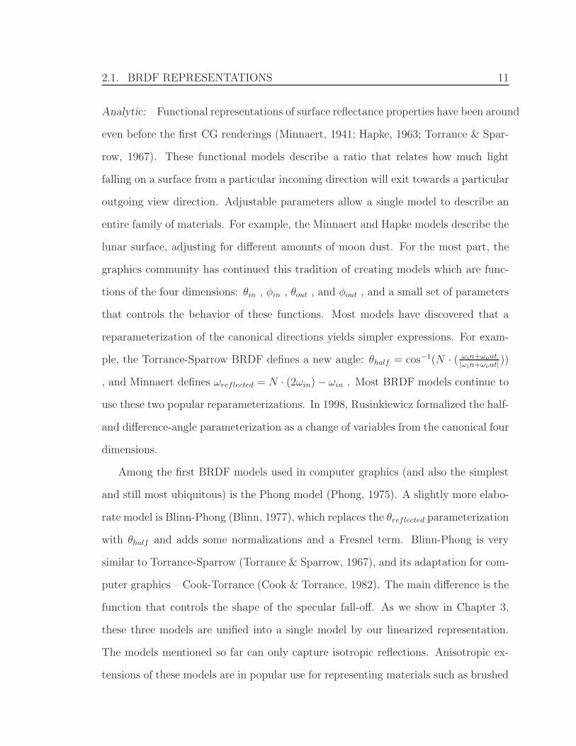
of full-sphere illumination is to render using preconvolved environment maps, as seen
in Figure 1.4.
Fig. 1.4: Edit without Shadows: Rendering with preconvolved environment maps cap-tures the effect of full-sphere illumination while ignoring cast shadows.
As expected, no information about the shadows can be extracted from the images,
and even a talented imagination would have a hard time filling them in. This also
leads to a difference in shading quality as noticeable by the incorrect brightness of
the bunny’s knee. Finally, interaction between the scene objects is completely lost:
Is the bunny hovering above the plane? Is the sphere very large and far away? Pre-
convolved environment maps are restricted to radially symmetric BRDFs, and thus
cannot handle half-angle-based or measured BRDFs ((Kautz et al., 2000)). Render-
ings such as those in Figure 1.3 and Figure 1.4 are still useful to an experienced
designer. The designer’s familiarity with the Phong model, coupled with the lim-
ited information provided by simple-lighting or shadowless renderings can guide the
BRDF selection process. However, there is clearly a better solution - to render the
final images correctly, as in Figure 1.1 and Figure 1.2. The main contribution of this
thesis is a real-time rendering algorithm and system that allows for final-placement
BRDF editing.

1.3. ORGANIZATION AND CONTRIBUTIONS 8
1.3 Organization and Contributions
This thesis is organized into four parts as follows:
Part I provides a motivation, background information, and introduction to a new
BRDF representation which will be used in Part II. Chapter 2 provides a history
of related work. The most recommended background readings are given in each sec-
tion. Chapter 3 introduces a new BRDF representation, which is used for interactive
editing. It linearizes the often non-linear nature of BRDF edits. This representation
is useful for editing as well as rendering operations, minimizing the need to convert
between representations at run-time. It is designed to respect the long history of
analytic BRDF models, as well as include support for data-driven representations.
Part II is the main contribution of this thesis, describing how to edit BRDFs
in complex lighting, and then in global illumination, fulfilling the promise of final-
placement BRDF editing. Chapter 4 discusses how to use the representation intro-
duced in Chapter 3 for real-time BRDF editing with complex lighting and shadows.
Chapter 5 introduces a bilinear operator framework to describe the reflection equa-
tion. This framework enables us to describe the higher-order effects of BRDF changes
on a scene when global illumination is considered. Chapter 6 uses the bilinear oper-
ator framework introduced in Chapter 5 in an interactive BRDF editing system that
takes into account interreflections for true global illumination rendering.
Part III goes into more detail on novel concepts that have applicability for both
BRDF editing (as used in Part II), as well as other rendering applications. Chapter
7 discusses an improvement to the dot-product operation which is at the heart of
precomputation-based rendering. Using temporal coherence, higher quality rendering
can be achieved at the same cost. This speedup is applicable to both BRDF editing
and relighting systems. Chapter 8 discusses how to calculate direct-lighting visibility

1.3. ORGANIZATION AND CONTRIBUTIONS 9
from an environment map more efficiently. This process is used for speeding up
the precomputation stage of real-time editing methods, as well as offline rendering.
Chapter 9 introduces a new set of operations to manipulate the shape of 1D functions.
Editing 1D functions is at the heart of many graphics-related operations, including
the BRDF editing discussed in Part II, and adjusting other 1D behavior such as
animation paths and exposure curves.
Part IV provides a brief conclusion and discussion on future directions for the
work. Chapter 10 highlights some important conclusions of the work presented in this
thesis. Chapter 11 is a discussion of immediate, mid-term, and long-term extensions
for this work.

10
2. PREVIOUS WORK
The work in this thesis draws together several areas within rendering that have had
separate histories. Section 2.1 discusses BRDF representations, which have often been
developed with little consideration for interactive BRDF editing (Section 2.2). Section
2.3 talks about precomputed radiance transfer (PRT), which has been used to enable
real-time relighting. PRT techniques are the forerunners to the precomputation-based
rendering used in Chapter 4 for BRDF editing. Section 2.4 highlights some of the
relevant works in global illumination that serve as the backdrop for the methods
introduced in Chapter 6.
2.1 BRDF Representations
The BRDF was formally defined as a ratio between incoming irradiance and outgoing
radiance by (Nicodemus et al., 1977). It can also be thought of as a probability
distribution function which describes the way an incoming light ray is likely to be
scattered by the surface into outgoing light rays. Throughout this thesis, I will use
the notation ρ(ωin, ωout) for the BRDF, where ωin is the incoming light direction, and
ωout is the outgoing view direction. A direction can be represented as a unit cartesian
vector: ω ≡ (x, y, z) or in spherical coordinates1: ω ≡ (θ, φ).
1 This document uses the graphics convention that θ is the elevation angle, and should not beconfused with the mathematical community’s notation that chooses φ for that role.
2.1. BRDF REPRESENTATIONS 11
Analytic: Functional representations of surface reflectance properties have been around
even before the first CG renderings (Minnaert, 1941; Hapke, 1963; Torrance & Spar-
row, 1967). These functional models describe a ratio that relates how much light
falling on a surface from a particular incoming direction will exit towards a particular
outgoing view direction. Adjustable parameters allow a single model to describe an
entire family of materials. For example, the Minnaert and Hapke models describe the
lunar surface, adjusting for different amounts of moon dust. For the most part, the
graphics community has continued this tradition of creating models which are func-
tions of the four dimensions: θin , φin , θout , and φout , and a small set of parameters
that controls the behavior of these functions. Most models have discovered that a
reparameterization of the canonical directions yields simpler expressions. For exam-
ple, the Torrance-Sparrow BRDF defines a new angle: θhalf = cos−1(N · ( ωin+ωout|ωin+ωout|))
, and Minnaert defines ωreflected = N · (2ωin)− ωin . Most BRDF models continue to
use these two popular reparameterizations. In 1998, Rusinkiewicz formalized the half-
and difference-angle parameterization as a change of variables from the canonical four
dimensions.
Among the first BRDF models used in computer graphics (and also the simplest
and still most ubiquitous) is the Phong model (Phong, 1975). A slightly more elabo-
rate model is Blinn-Phong (Blinn, 1977), which replaces the θreflected parameterization
with θhalf and adds some normalizations and a Fresnel term. Blinn-Phong is very
similar to Torrance-Sparrow (Torrance & Sparrow, 1967), and its adaptation for com-
puter graphics – Cook-Torrance (Cook & Torrance, 1982). The main difference is the
function that controls the shape of the specular fall-off. As we show in Chapter 3,
these three models are unified into a single model by our linearized representation.
The models mentioned so far can only capture isotropic reflections. Anisotropic ex-
tensions of these models are in popular use for representing materials such as brushed

2.1. BRDF REPRESENTATIONS 12
metal. The Ward model (Ward, 1992) and Ashikhmin-Shirley BRDF (Ashikhmin &
Shirley, 2000) add a parameter that allows (indirect) control of the eccentricity of the
highlight. Their main difference is the choice of highlight direction, with Ward using
ωreflected and Ashikhmin-Shirley using ωhalf .2
A single material is often represented as the sum of several BRDFs. Most com-
monly, a diffuse layer and a specular layer are summed, each one being represented
with some function of (ωi, ωo). Each analytic BRDF model has a small set of pa-
rameters that can be adjusted to control the material properties represented by the
model. Throughout this work, I will refer to these parameters as user-controlled vari-
ables(UCV). BRDF design and editing with these models amounts to adjusting these
0D parameters, usually with a slider or color picker. Examples of such UCVs are Ks
– a scalar for the specular component of the material, n or σ – a scalar that controls
the width of the specular highlights, and αd – a color value that multiplies the diffuse
component. In this thesis, I assume that user interfaces already exist to control the
behavior of analytic BRDFs, and that the values of these UCVs will be passed to the
rendering engine from these interfaces.
Measured BRDFs: Analytic BRDF models are restricted to representing behavior
that fits some prescribed form. However, real-world materials deviate from these ideal
forms (sometimes slightly, sometimes greatly). To better represent real materials,
their reflectance properties can be measured, and those measurements are either used
directly (Matusik et al., 2003), or fit to one or more analytic forms (Ward, 1992;
Lafortune et al., 1997). BRDF measurements can be achieved with a controlled setup
and a gonioreflectometer or digital camera. The incoming and outgoing directions are
controlled via light and camera placement, and measurements are tabulated into a 4D
2 Interestingly enough, the Ashikhmin-Shirley paper is titled ”An Anisotropic Phong BRDFmodel”, even though Phong is associated with θreflected.
2.1. BRDF REPRESENTATIONS 13
dataset. (Dana et al., 1999; Matusik et al., 2003) captured a database of materials
with such a setup.
Instead of fitting the data to a model, the 4D/3D data may be factored into
2D or 1D tabulated sets for direct use in rendering applications via table lookups
(Kautz & McCool, 1999; McCool et al., 2001). These factored representations of-
ten use the Rusinkiewicz (Rusinkiewicz, 1998b) reparameterization to improve data
coherence along the chosen dimensions. High quality measurements such as those
made by (Matusik et al., 2003) have lead to an interest in higher quality factorization
techniques (Lawrence et al., 2004). Such measured datasets can be used without
fitting to analytic functions in order to preserve the real-world nuances in the data.
(Ashikhmin et al., 2000) described a hybrid BRDF that uses a 2D map for variation
along the half-angle dimensions, but an analytic expression for variation along other
dimensions (difference-, view-, and light-directions). For the highest-quality offline
renderings, the 4D measured data is used directly3. (Lawrence et al., 2006) have
shown that lower dimensional factors can be extracted with low reconstruction error.
Despite recent advancements in BRDF measurements, analytic models such as
Blinn-Phong (Blinn, 1977) and Cook-Torrance (Cook & Torrance, 1982) are still very
popular in many applications due to their simplicity and adequate accuracy for many
applications.
3 However, interpolation between the available measurements is not trivial.
2.2. BRDF EDITING 14
2.2 BRDF Editing
Parametric models can be easily edited (under point source lighting) by simply moving
sliders for their parameters, and such software is available for research (Rusinkiewicz,
1998a) and production (Maya, 3DMax). Abstractions can be used on top of a model’s
parameters to make material editing more intuitive. The simplest example is to cre-
ate a shininess parameter on top of the Phong model, which may be linked to the
exponent non-linearly and additionally control a normalization parameter simultane-
ously. These types of edits rely on the GPU pipeline to provide interactive feedback.
Shadowing techniques may be used to enhance the rendered results. However, GPU
speed depends on the number of lights, complexity of the shadow technique, number
of vertices (and pixels), and BRDF complexity. As these burdens increase, the GPU
renderings slow down, and quickly fall out of the interactive regime. Specifically, for
complex BRDFs that make use of modern shader capability, interactive rates cannot
be maintained for more than a few lights when per-pixel calculations are performed
in Phong-style shading. In our current work, we respect the existing history for edit-
ing analytic BRDFs, and our techniques are compatible with current popular user
interfaces.
Preconvolved environment maps (Ramamoorthi & Hanrahan, 2002) are able to
render arbitrary BRDFs under complex lighting, but only in the low-frequency do-
main. The preconvolution step is quick, and may be combined with live editing of
BRDFs. (Colbert et al., 2006) uses preconvolved environment maps and fits to the
Ward model (Ward, 1992) for editing BRDFs that can be represented by that model.
Any method based on preconvolved environment maps is limited to renderings with-
out cast shadows. As seen in Chapter 1(Figure 1.4), this is a large drawback when
attempting to make decisions about the choice of BRDF parameters.
2.2. BRDF EDITING 15
Previous work has not focused much on real-time editing of data-driven reflectance.
(Ashikhmin et al., 2000) use GPU-base rendering with 2D maps, which can be edited
using standard image-editing software. However, this approach is not always intuitive
for deriving new physically-based BRDFs, and these methods suffer from the same
limitations as analytic GPU-based rendering. In this work, we introduce a more in-
tuitive editing technique of measured data, based on 1D factors. Our representation
can be used with GPU shaders for simple lighting scenarios (Chapter 3). We also
describe a new real-time rendering system that can render using this representation
in real-time under complex illumination, including cast shadows, and even include
full global illumination.
For specific applications like car paint design, specialized systems (Ershov et al.,
2001) have been developed to allow edits of a custom designed BRDF model. They
quote near-interactive frame-rates (1-6fps), but like GPU approaches suffer from de-
graded speed as the BRDF becomes more complex, and do not demonstrate general
complex illumination. To our knowledge commercial systems allow users to specify
weights for a linear combination of pre-defined materials [PEARL], while viewing
the results in a static scene under complex illumination. However, a few pre-defined
materials do not suffice for many applications: (Matusik et al., 2003) cites a require-
ment for 45 linear basis materials to allow good reconstruction of materials from their
database.
2.3. PRECOMPUTED RADIANCE TRANSFER (PRT) 16
2.3 Precomputed Radiance Transfer (PRT)
The linearity of light transport has been leveraged in a large body of work on relight-
ing. Beginning with (Nimeroff et al., 1994), lighting could be edited by representing
the user’s input as a linear combination of lighting functions that can be combined to
generate a relit image. More recently, precomputed radiance transfer (PRT) for static
scenes (Sloan et al., 2002) has rekindled an interest in basis projections of editable
lighting. This, and subsequent work later enabled changing view (Sloan et al., 2003)
and some dynamic geometry (Sloan et al., 2005; Zhou et al., 2005), but are all lim-
ited to low-frequency effects due to the choice of spherical harmonics as the basis for
lighting. Editing within a restricted family of BRDFs is possible with (Sloan et al.,
2002), but only for low-frequency, radially symmetric Phong-like models.
Since a material designer wants to preserve the full richness of effects in the BRDF
and lighting while editing, we focus instead on all-frequency wavelet-based approaches
(Ng et al., 2003). We build on PRT ideas for static scenes (Sloan et al., 2002; Ng
et al., 2003). While those methods focus on lighting design with fixed BRDFs, we
focus on BRDF editing, with fixed lighting. We are inspired by a body of recent
work that underscores the importance of interreflections in relighting (Hasan et al.,
2006; Wang et al., 2004; Kontkanen et al., 2006). All these approaches exploit the
linearity of relighting with respect to light intensity, even when global illumination
is taken into account. In contrast, BRDF editing is fundamentally nonlinear when
global illumination is considered. While recent advances allow for changing view
and lighting (Sloan et al., 2003; Wang et al., 2004; Ng et al., 2004), they require
a precomputed factorization or tabulation of the BRDF, that can neither be edited
continuously, nor recomputed in real-time.
It is also important to note some differences that make BRDF editing a funda-
2.3. PRECOMPUTED RADIANCE TRANSFER (PRT) 17
mentally harder problem than relighting. The BRDF lobe at a given pixel is affected
by all of the: lighting, view, and geometry (surface normal). This is why we must
fix these quantities, while relighting methods can sometimes factor shadowing effects
from material properties (Ng et al., 2004). Some flexibility for viewpoint change is
possible in both relighting (Liu et al., 2004; Wang et al., 2004) and our method if
one uses an incident-outgoing factorization, but that is accurate and editable only
for a limited class of diffuse-like materials or components. Moreover, for material
design, the final image is not even linearly related to the BRDF if global illumination
is considered, which is why we focus on all-frequency direct lighting.
Most previous PRT methods precompute a linear light transport vector at each
image location, taking advantage of the linearity of light. We extend this concept to
a general tensor of coefficients for a high-dimensional polynomial. The idea of going
from linear to quadratic or cubic precomputed models has also begun to be explored in
physical simulation (Barbic & James, 2005) but in the context of differential equations
and model dimensionality reduction. In the context of real-time rendering, (Sun &
Mukherjee, 2006) precompute with a larger product of functions, leading to an N -part
multiplication at runtime. Each function is still precomputed independently, and the
runtime calculations are still linear in any of the individual functions.
2.4. GLOBAL ILLUMINATION 18
2.4 Global Illumination
Our precomputation method for global illumination effects in Chapter 6 is inspired
by offline global illumination algorithms, such as Monte Carlo path tracing (Kajiya,
1986). We have also been able to adapt finite element radiosity (Cohen & Wallace,
1993), although we found meshing and complexity issues difficult to deal with for our
complex scenes, and do not discuss it further. By basing the precomputation on path
tracing, the quality of our renderings are limited (or unbounded) in the same way as
rendering a single off-line image of the scene.
Global illumination techniques usually require the BRDF to be fixed, and use it
for importance sampling or hierarchy construction—we develop extensions that are
independent of the BRDF, and allow real-time editing. In effect, we precompute a
symbolic representation of the image, which can be evaluated at runtime with poly-
nomials in the user-specified BRDF values, to obtain the final intensity.
Sequin and Smyrl (Sequin & Smyrl, 1989) also precomputes a symbolic represen-
tation of the final image for recursive ray tracing—but not full global illumination.
Phong shading can be evaluated at runtime, allowing later changes to surface pa-
rameters, while reflected and refracted contributions are handled with pointers to
sub-expressions. In contrast, we seek to simulate complex lighting and full global
illumination, with many possible illumination paths. Therefore, we cannot afford to
store or sum all subexpressions. Instead, we show that the final symbolic expression
is a polynomial and only precompute its coefficients. We also allow editing of general
parametric and measured BRDFs.
In Chapter 5, we extend Arvo’s (Arvo et al., 1994) linear operators for global
illumination. Using that operator notation, it is possible to express the radiance due
to multiple bounces without explicitly writing cumbersome nested integrals.

19
3. A NEW EDITABLE AND RENDERABLE REPRESENTATION
Editing BRDFs is a more structured process than editing images, lighting, or geom-
etry. BRDFs have understandable behaviors that are coupled with known physical
phenomena, and this is clearly visible in the structure of functional models such as
Cook-Torrance (Cook & Torrance, 1982) and Ward (Ward, 1992). In short, not all
4D functions are BRDFs. To express this, we use the following representation for
BRDFs:
ρ(ωi, ωo) = fqρq(ωi, ωo))fo(γo(ωo))fA(γA(ωi, ωo))fB(γB(ωi, ωo)), (3.1)
where the γs are 1D reparameterizations of the canonical directions1, and the fs are
1D functions that describes how the BRDF varies along their respective γ. Common
choices for γ are θhalf , θreflected, and θdiff . fo is dependent only on the view direction,
ωo. One might expect a similar term utilizing only ωo, such as (fin(γin(ωi))). However,
because there is only one view for a given pixel/image and many lighting directions,
ωo and ωi are not treated symmetrically. The focus of this work is to recognize
and address the complexity of realistic lighting environments, and any dependence of
the BRDF on ωi is captured in fA or fB. ρq is the quotient BRDF which contains
more general, but uneditable variation in the BRDF. A common example of ρq is
the geometric-attenuation-factor (GAF). fq is the 0D quotient factor which may be
edited, but is independent of the canonical directions (implicitly or explicitly). A
1 The canonical directions are θin, φin, θout, and φout as defined in (Nicodemus et al., 1977).
20
common example of fq is a scaling factor that depends on the model’s parameters,
but not ωin nor ωout.
2D parameterizations are reasonable to consider, such as the 2D microfacet distri-
bution maps in (Ashikhmin et al., 2000). However, inspection of these maps reveals
that they exhibit variation only along 1D for realistic isotropic BRDFs. Anisotropic
BRDFs will be shown to fit into the form of equation 3.1 with a proper choice of
γ’s. In addition, we will show in Section 3.5 that editing 1D functions is much more
intuitive. 2D editing via image-editing software is inappropriate for BRDFs that are
typically much more constrained than a general 2D function. It is important to note
that many BRDF models describe a sum of terms, such as diffuse-plus-specular. In
this work, we consider each of these terms to be its own BRDF, and handle summa-
tion in the trivial manner of adding the final radiances that result from each term.
A longer list of editable factors (fC ,fD,... ) might be considered, but BRDFs rarely
exhibit interesting behavior which a user may wish to edit, along more than two pa-
rameterizations (not including γo ). Furthermore, we have not found a case where
more factors are needed.
The benefits of this representation are three-fold. First, it is general enough
to encompass all commonly used analytic BRDF models, as well as factored mea-
sured BRDF data. Second, it allows for intuitive editing by exposing the variations
along different directions as understandable 1D functions. In Chapter 9, we will
demonstrate our system for editing these 1D functions. Finally, and perhaps most
importantly, it can be used in our real-time rendering systems, described in Part II.
As a simple example of how our representation can be applied to an analytic model,
consider the scaled Phong model we used to generate Figures 1.3-1.4:√
ncosn(θr).
The parameterization γA(ωi, ωo) = θr is the angle between the reflected light and
the view direction. The curve fA(γA) = cosn(γA) , is controlled by the ‘parameter’

21
n. To avoid confusion with the curve parameterization, we will refer to an analytic
parameter, such as the Phong exponent, as a user-controlled variable or UCV. The
unchanging quotient BRDF, ρq , is 1 in this case, or the traditional cosine falloff,
max(0, θin) , if we wish to consider that as part of the BRDF. Finally, the quotient
factor, fq , is the scaling term that we added to keep the images from becoming too
dark as the exponent increased:√
n . The other two factors ( fB and fo ) are not
used, and set to unity. Figure 3.1 shows the 1D factor (with fq). Notice the y-scale
of each graph. In some cases it will be more convenient to show the 1D factors with
the scale factor. The y-scale label should make it clear when this is the case.
θ-reflectedn=4
π 4 π 2
2
00
θ-reflectedn=16
π 4 π 2
4
00
θ-reflectedn=256
π 4 π 2
16
00
θ-reflectedn=1024
π 4 π 2
32
00
θ-reflectedn=64
π 4 π 2
8
00
Fig. 3.1: Edit of Phong Curve: 1D factor of the Phong model used in Figures 2-4 withthe exponent set to 4, 16, 64, 256, and 1024.
For purely functional models like the Phong example in Figure 3.1, the curves
shown are only used by our rendering system, and not revealed to the user. The
standard slider controls are available to the user, and they in turn determine the 1D
function by direct evaluation of the BRDF model. The next four sections (3.1, 3.2,
3.3, and 3.4) describe in more detail how common analytic models fit into our repre-
sentation. Section 3.5 shows how revealing these curves to direct user manipulation
allows measured data to be edited.
3.1. COOK-TORRANCE: AN ANALYTIC BRDF EXAMPLE 22
3.1 Cook-Torrance: an analytic BRDF example
Like many analytic BRDFs, the Cook-Torrance model [1982] is already in the desired
form presented in equation 3.1. The specular term of CT is:
ρCT = sFn,e(θd)G(ωi, ωo)Dσ(θh)
π(ωi ·N)(ωo ·N), (3.2)
where N is the surface normal. The user-controlled variables are n (index of
refraction), e (extinction coefficient), σ (mean slope distribution), and s (specular
term scalar). The first two UCVs control the shape of the Fresnel term, F (θd) , while
σ controls the shape of the slope distribution function, G(ωi, ωo) , often taken to
be the Beckmann distribution. The geometric attenuation factor, G(ωi, ωo), and the
denominator are fixed for all values of the UCVs, and form the quotient brdf, ρq .
This BRDF requires two 1D factors: fA = D(θh) and fB = F (θd) . The corresponding
parameterizations are: the theta components of the half-difference parameterization:
γA = θh(ωi, ωo) and γB = θd(ωi, ωo) . The quotient factor, fq , is sπ
.
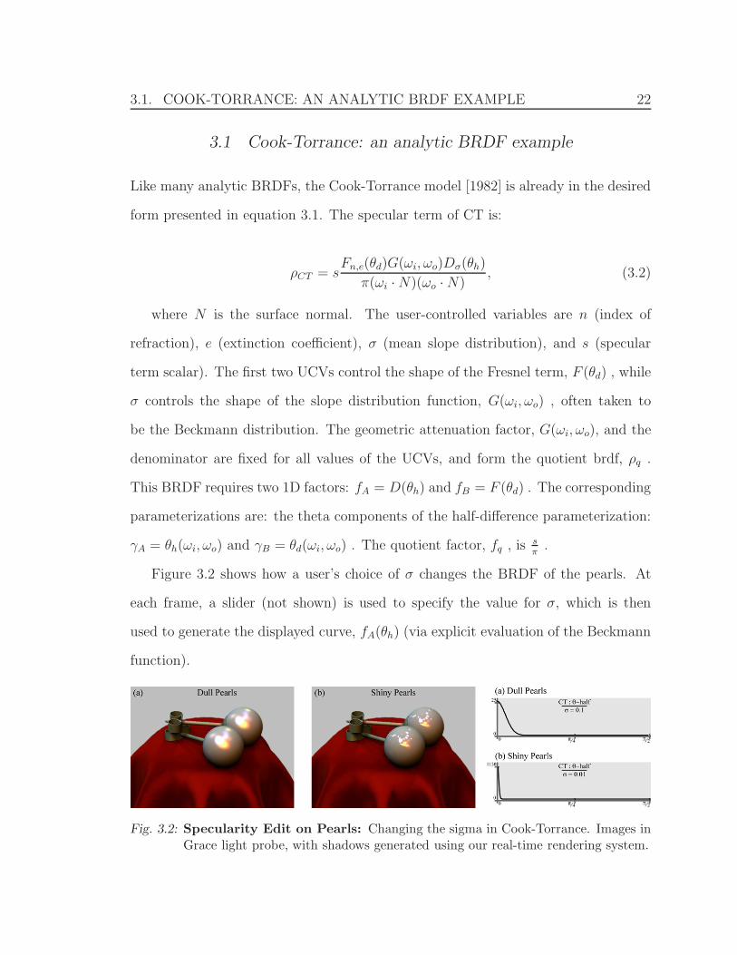
Figure 3.2 shows how a user’s choice of σ changes the BRDF of the pearls. At
each frame, a slider (not shown) is used to specify the value for σ, which is then
used to generate the displayed curve, fA(θh) (via explicit evaluation of the Beckmann
function).
Fig. 3.2: Specularity Edit on Pearls: Changing the sigma in Cook-Torrance. Images inGrace light probe, with shadows generated using our real-time rendering system.
3.2. ASHIKHMIN-SHIRLEY: AN ANISOTROPIC ANALYTIC BRDF 23
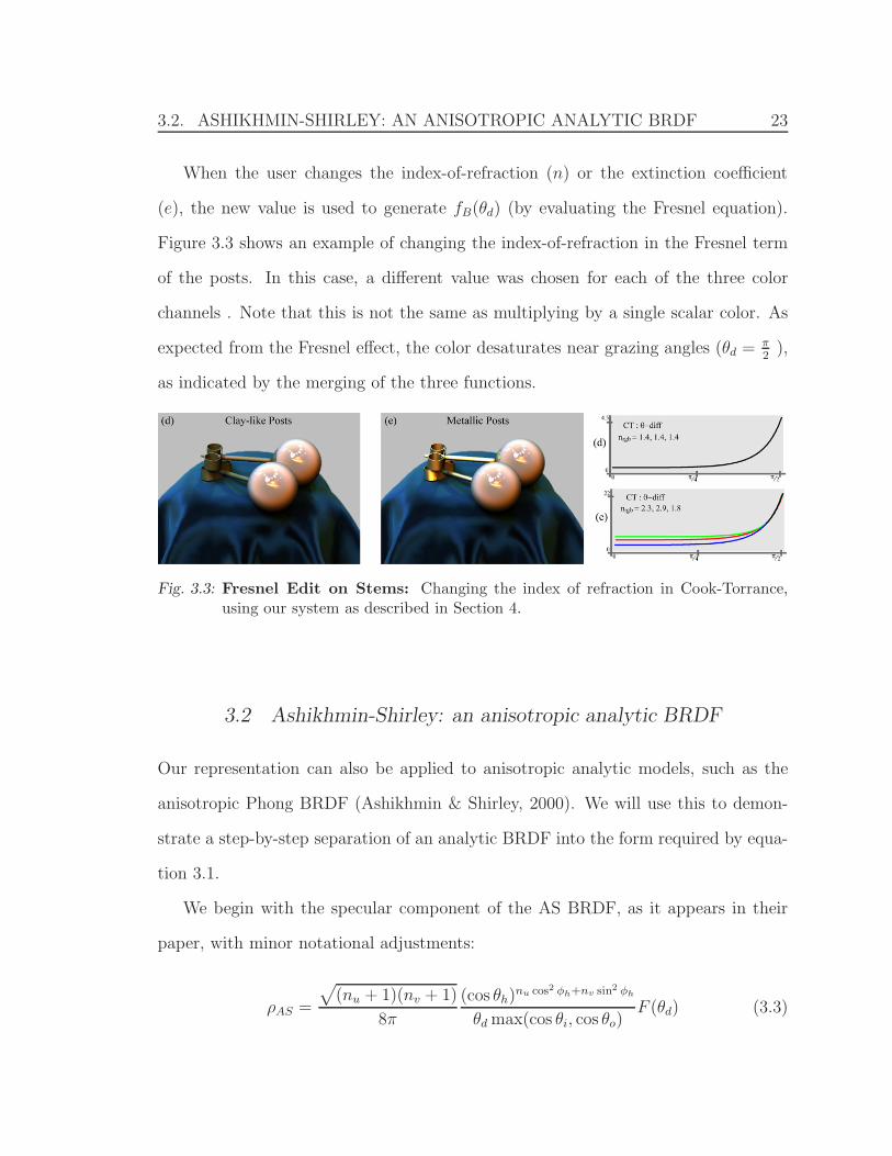
When the user changes the index-of-refraction (n) or the extinction coefficient
(e), the new value is used to generate fB(θd) (by evaluating the Fresnel equation).
Figure 3.3 shows an example of changing the index-of-refraction in the Fresnel term
of the posts. In this case, a different value was chosen for each of the three color
channels . Note that this is not the same as multiplying by a single scalar color. As
expected from the Fresnel effect, the color desaturates near grazing angles (θd = π2
),
as indicated by the merging of the three functions.
Fig. 3.3: Fresnel Edit on Stems: Changing the index of refraction in Cook-Torrance,using our system as described in Section 4.
3.2 Ashikhmin-Shirley: an anisotropic analytic BRDF
Our representation can also be applied to anisotropic analytic models, such as the
anisotropic Phong BRDF (Ashikhmin & Shirley, 2000). We will use this to demon-
strate a step-by-step separation of an analytic BRDF into the form required by equa-
tion 3.1.
We begin with the specular component of the AS BRDF, as it appears in their
paper, with minor notational adjustments:
ρAS =
√(nu + 1)(nv + 1)
8π
(cos θh)nu cos2 φh+nv sin2 φh
θd max(cos θi, cos θo)F (θd) (3.3)
3.2. ASHIKHMIN-SHIRLEY: AN ANISOTROPIC ANALYTIC BRDF 24
The first step is to identify the UCVs of the model: nu and nv . These are similar
to the exponent in the Phong model, but having two controls allows for anisotropic
highlights. Next, we find the smallest subexpression that contains all instances of all
UCVs:√
nu + 1√
nv + 1(cos θh)nu cos2 φh+nv sin2 φh (3.4)
The rest of the BRDF becomes ρq . Next, we find fq by factoring out any subex-
pression that does not rely on the canonical directions: fq =√
nu + 1√
nv + 1. Then,
we try to factor the remaining expression into factors, each of which is defined for
some 1D parameterizations, γ . Note that once we find these factors, the same UCV
cannot appear in more than one factor. A simple identity for exponents allows us to
do exactly that (we name them α and β):
fα = (cos θh)nu cos2 φh (3.5)
fβ = (cos θh)nv sin2 φh (3.6)
The final step is to identify the 1D parameterization of all angle-dependent values.
We must find an expression that does not involve the user-controlled variables, so we
eventually obtain
γα = cos−1((cosθh)
cos2 φh
); fα(γα) = cosnu γα (3.7)
γβ = cos−1((cosθh)
sin2 φh
); fβ(γα) = cosnv γβ (3.8)
The inverse-cosine was added because it is useful to think of the γs as angles that
range from 0 to π2
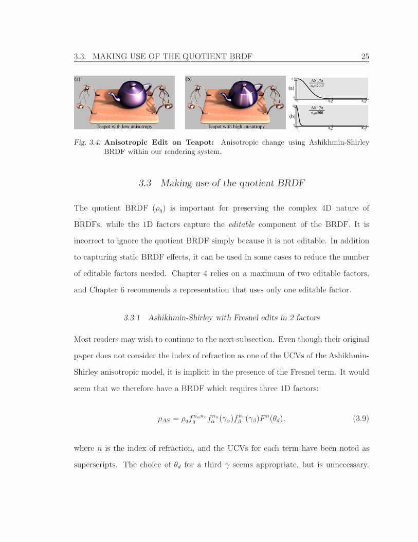
, but is not strictly necessary. The teapot in Figure 1.1 and Figure
3.4 uses this Ashikhmin-Shirley BRDF.
3.3. MAKING USE OF THE QUOTIENT BRDF 25
Fig. 3.4: Anisotropic Edit on Teapot: Anisotropic change using Ashikhmin-ShirleyBRDF within our rendering system.
3.3 Making use of the quotient BRDF
The quotient BRDF (ρq) is important for preserving the complex 4D nature of
BRDFs, while the 1D factors capture the editable component of the BRDF. It is
incorrect to ignore the quotient BRDF simply because it is not editable. In addition
to capturing static BRDF effects, it can be used in some cases to reduce the number
of editable factors needed. Chapter 4 relies on a maximum of two editable factors,
and Chapter 6 recommends a representation that uses only one editable factor.
3.3.1 Ashikhmin-Shirley with Fresnel edits in 2 factors
Most readers may wish to continue to the next subsection. Even though their original
paper does not consider the index of refraction as one of the UCVs of the Ashikhmin-
Shirley anisotropic model, it is implicit in the presence of the Fresnel term. It would
seem that we therefore have a BRDF which requires three 1D factors:
ρAS = ρqfnunvq fnu
α (γα)fnvβ (γβ)F
n(θd), (3.9)
where n is the index of refraction, and the UCVs for each term have been noted as
superscripts. The choice of θd for a third γ seems appropriate, but is unnecessary.
3.3. MAKING USE OF THE QUOTIENT BRDF 26
Expand F n(θd) according to the Schlick approximation (1994):
ρAS = ρqfnunvq fnu
α fnvβ (Rn + (1− Rn)(1− cos θd)
5), (3.10)
where Rn = (n− 1)2/(n + 1)2. Distributing ρq and fq gives us:
ρAS = fnuα fnv
β (ρqfnunvq Rn + ρqf
nunvq (1−Rn)(1− cos θd)
5), (3.11)
We now absorb the terms from the Schlick approximation to define fnunvnq1 ≡ fnunv
q Rn,
and fnunvnq2 ≡ fnunv
q (1−Rn), and ρq2 ≡ ρq(1−cos θd)5. This leaves us with a two-term
definition for ρAS which shares the same editable factors among both terms:
ρAS = ρqfq1fαfβ + ρq2fq2fαfβ (3.12)
This sharing of fαfβ is useful since the user need not try to keep the two terms ’in
sync’ by editing a factor of one, and then editing a factor of the other to match. The
practice of representing a BRDF as a sum of terms is acceptable under the following
conditions: First, the number of UCVs, or unique editable factors should not increase
to make the model unwieldy for editing. Second, when considering each UCV or
editable factor independently, any relationship between terms must be explicit so
that changes in one term automatically trigger corresponding changes in the other.
This condition of explicit dependence is what we have in 9. Finally, the number of
terms should be small (1-4) since simultaneous editing of many terms may eventually
slow down the rendering engine. This is true of our complex lighting system, as well
as GPU shaders where multi-pass rendering is common, but should be limited to a
few passes. The same technique shown above for capturing the Fresnel term without
introducing a new θd factor, can be used for other BRDF models.
3.4. OTHER ANALYTIC AND HYBRID BRDFS 27
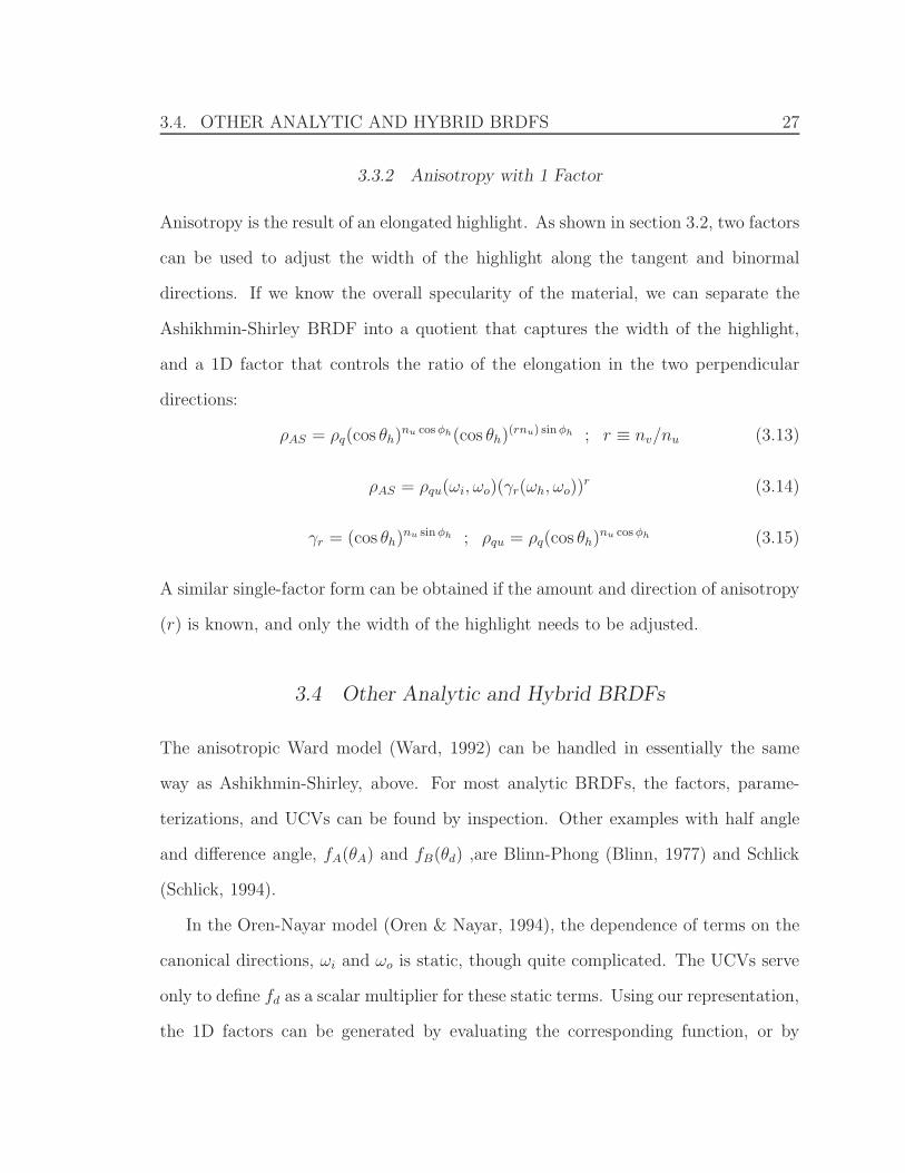
3.3.2 Anisotropy with 1 Factor
Anisotropy is the result of an elongated highlight. As shown in section 3.2, two factors
can be used to adjust the width of the highlight along the tangent and binormal
directions. If we know the overall specularity of the material, we can separate the
Ashikhmin-Shirley BRDF into a quotient that captures the width of the highlight,
and a 1D factor that controls the ratio of the elongation in the two perpendicular
directions:
ρAS = ρq(cos θh)nu cos φh(cos θh)
(rnu) sinφh ; r ≡ nv/nu (3.13)
ρAS = ρqu(ωi, ωo)(γr(ωh, ωo))r (3.14)
γr = (cos θh)nu sinφh ; ρqu = ρq(cos θh)
nu cos φh (3.15)
A similar single-factor form can be obtained if the amount and direction of anisotropy
(r) is known, and only the width of the highlight needs to be adjusted.
3.4 Other Analytic and Hybrid BRDFs
The anisotropic Ward model (Ward, 1992) can be handled in essentially the same
way as Ashikhmin-Shirley, above. For most analytic BRDFs, the factors, parame-
terizations, and UCVs can be found by inspection. Other examples with half angle
and difference angle, fA(θA) and fB(θd) ,are Blinn-Phong (Blinn, 1977) and Schlick
(Schlick, 1994).
In the Oren-Nayar model (Oren & Nayar, 1994), the dependence of terms on the
canonical directions, ωi and ωo is static, though quite complicated. The UCVs serve
only to define fd as a scalar multiplier for these static terms. Using our representation,
the 1D factors can be generated by evaluating the corresponding function, or by
3.5. MEASURED/FACTORED BRDFS 28
explicitly tabulating the values through direct manipulation of the curves we have
shown. In this way, any BRDF can be made into a hybrid between functional and
data-driven. For example, the Oren-Nayar model can be separated into two factors
using θin and θout as the parameterizations. The lack of UCVs defined over these
factors does not preclude the original functions from being manipulated to generate
new effects.
Ashikhmin et al. (2000) presented a hybrid BRDF model similar to Cook-Torrance
that had a functional expression for all but the half-angle dependence. That factor
was tabulated explicitly as a 2D map. Most plausible BRDFs required only a 1D
map of θh, or two 1D factors: fA(θh) and fB(φh). Our model can use these tabulated
factors without requiring an analytic expression. Editing would occur directly on the
curves.
3.5 Measured/Factored BRDFs
We can use the same idea as seen in hybrid BRDFs to edit purely measured reflectance
data. Isotropic factored BRDFs can be manipulated, by editing curves corresponding
to each of the factors. We consider editing the recent homomorphic factorization
(HF) of (McCool et al., 2001). Specifically, the factorization is:
ρHF � P ′(ωi)Q′(ωh)P
′(ωo) = ρqP (θi)Q(θh)P (θo), (3.16)
where for isotropic BRDFs, we are really editing 1D curves P and Q. (If the 2D
terms are not symmetric because of noise or mild anisotropy, we can absorb that in
the quotient, ρq ). Figure 1.1 and Figure 3.5 use (McCool et al., 2001)’s data for red
velvet (factored from the CURET database (Dana et al., 1999)). Figure 3.5 only edits
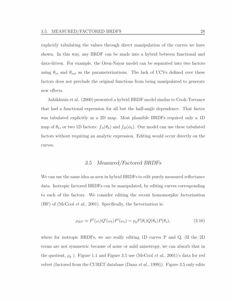
3.5. MEASURED/FACTORED BRDFS 29
the P term, and therefore maintains the same feel of cloth (though a different type).
Figure 1.1 shows the result of also editing the Q term, thus changing the quality to
a more plastic appearance.
Fig. 3.5: McCool Edit on Cloth: Editing measured red velvet with freehand changes tothe P factor of Homomorphic Factorized data.
We now consider fitting arbitrary, high-resolution measured BRDFs to our repre-
sentation. Many dimensionality reduction techniques have been proposed for factoring
measured BRDF data (Leung & Malik, 2001; Chen et al., 2002; Vasilescu & Terzopou-
los, 2004). However, not all methods of factorization are amenable to our editable
representation. (Lawrence et al., 2004) introduced a method using non-negative ma-
trix factorization (NMF), to extract 1D factors with low reconstruction error. We
collaborated with them on continued work in that area, and have now shown that all
of the BRDFs from the database of (Matusik et al., 2003) can be well approximated
with the four 1D factors: θhalf , φhalf , θdiff , and φdiff . By using the Ruseinkewicz
reparameterization, and a modified constrained least-squares (SACLS) method, the
factors extracted have the desired property of non-negativity. SACLS is also able to
separate the diffuse and specular terms of BRDFs that contain both. Unlike with
general dimensionality reduction techniques, only a single set of factors is needed for
each term, as opposed to a low-order sum of products. All of these properties mean
that the extracted factors are meaningful as trends in the BRDF. The φ factors are
3.5. MEASURED/FACTORED BRDFS 30
mostly constant, and the θ factors often resemble those of analytic models, such as
Cook-Torrance. The added benefits of using real-world data is noticeable in the small
variations from the clean lines of the analytic models - capturing the details of the
acquired material’s reflectance properties. Other irregular variations that don’t align
with any of the parameterizations can be absorbed in the quotient BRDF. We have
found that the φ factors are rarely useful for editing, and absorb those into the quo-
tient BRDF as well, leaving only the two θ factors. Having fewer factors also makes
editing more intuitive, much like an abundance of UCVs in analytic models can be
overwhelming. The factored BRDFs are then in the following form:
ρfactored = ρd + ρs; ρd = ρqdGd(θi)Hd(θo); ρs = ρqsGs(θd)Hs(θh) (3.17)
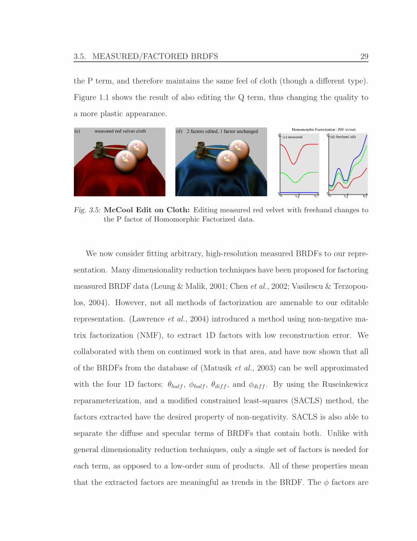
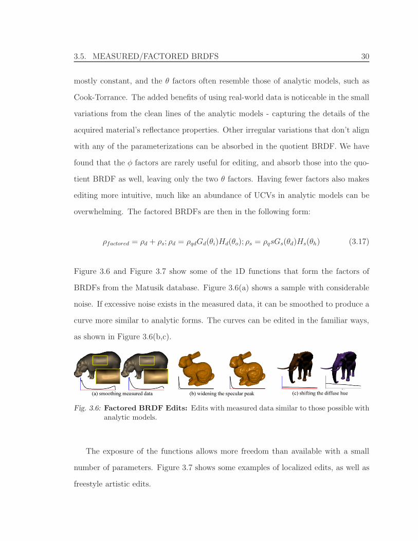
Figure 3.6 and Figure 3.7 show some of the 1D functions that form the factors of
BRDFs from the Matusik database. Figure 3.6(a) shows a sample with considerable
noise. If excessive noise exists in the measured data, it can be smoothed to produce a
curve more similar to analytic forms. The curves can be edited in the familiar ways,
as shown in Figure 3.6(b,c).
Fig. 3.6: Factored BRDF Edits: Edits with measured data similar to those possible withanalytic models.
The exposure of the functions allows more freedom than available with a small
number of parameters. Figure 3.7 shows some examples of localized edits, as well as
freestyle artistic edits.
3.5. MEASURED/FACTORED BRDFS 31
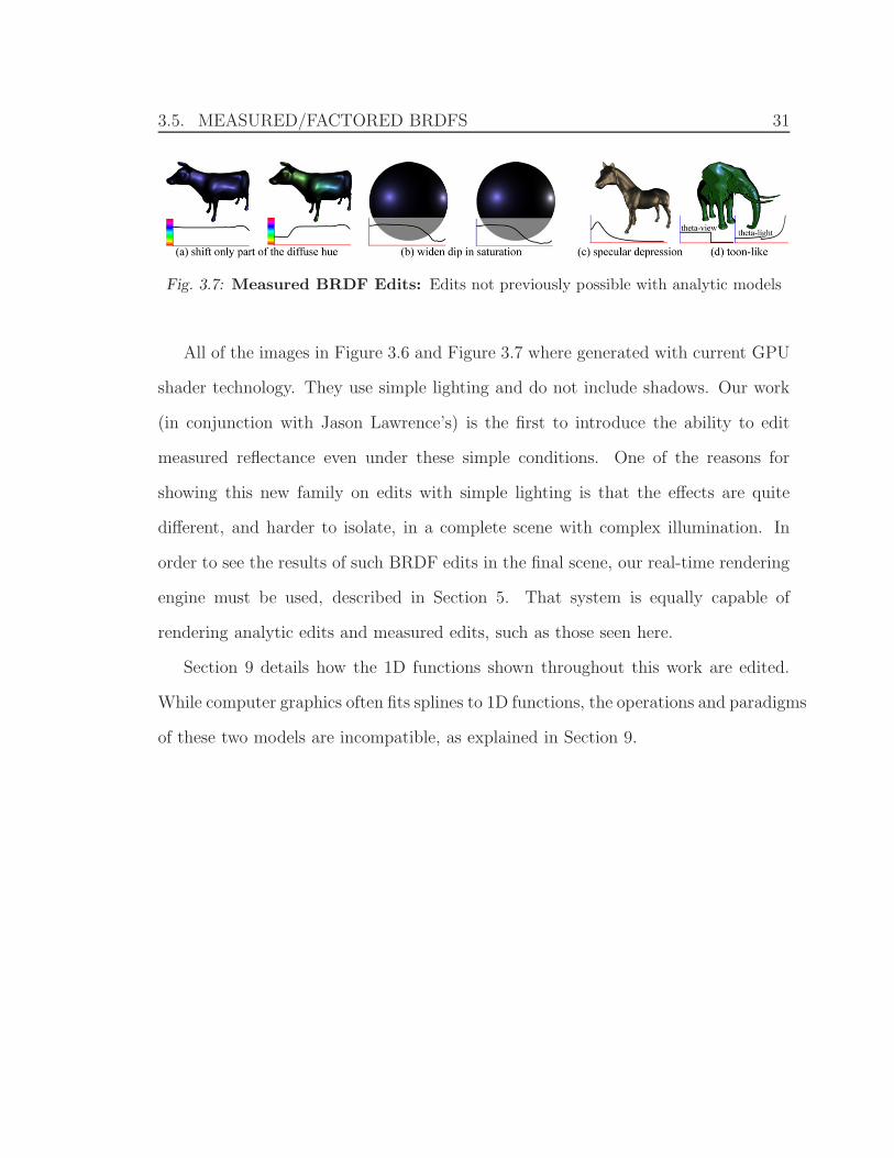
Fig. 3.7: Measured BRDF Edits: Edits not previously possible with analytic models
All of the images in Figure 3.6 and Figure 3.7 where generated with current GPU
shader technology. They use simple lighting and do not include shadows. Our work
(in conjunction with Jason Lawrence’s) is the first to introduce the ability to edit
measured reflectance even under these simple conditions. One of the reasons for
showing this new family on edits with simple lighting is that the effects are quite
different, and harder to isolate, in a complete scene with complex illumination. In
order to see the results of such BRDF edits in the final scene, our real-time rendering
engine must be used, described in Section 5. That system is equally capable of
rendering analytic edits and measured edits, such as those seen here.
Section 9 details how the 1D functions shown throughout this work are edited.
While computer graphics often fits splines to 1D functions, the operations and paradigms
of these two models are incompatible, as explained in Section 9.

Part II
INTERACTIVE BRDF EDITING BEYOND SIMPLE
LIGHTING
33
4. INTERACTIVE RENDERING IN COMPLEX LIGHTING
4.1 Method Overview
We use a precomputed approach to calculate all of the static scene-data and factor
out the user-editable parts for render-time multiplication. Precomputed approaches
to rendering rely on the linearity of the output image with respect to the editable
inputs. In relighting, the exit radiance at a point is linearly dependant on the radiance
of the lighting environment. We express this as follows:
R(x) =∑
i
Ti(x)Li = T(x) · L (4.1)
where the radiance of each light basis, Li , is weighted according to its contribution
to the point being rendered, Ti(x) , and added to the contributions of all the other
lights. This formulation assumes fixed geometry, material properties, and view. The
natural 2D basis of the lighting – pixels in the environment map – is usually converted
to some other orthonormal basis such 2D wavelets or spherical harmonics. As long
as the transport vector, T(x) , is also converted to the same orthonormal basis, the
dot-product in equation 4.1 will remain valid. The transport vector encodes all of
the static scene data which affects how much any given light contributes to the exit
radiance at x . Notice that the lighting vector, L , is common to all locations in the
scene. If it had to be recomputed at each frame, for each pixel/vertex, the rendering
operation would not proceed in real-time.
4.1. METHOD OVERVIEW 34
For BRDF editing, we wish to express our rendering operation as a similar dot-
product, which we arrive at in equation 4.7, but replace the lighting vector with a
user-editable BRDF vector. We assume fixed geometry, lighting, and view. In this
chapter, we only render using direct lighting, since the image is not linearly dependent
on the BRDF when considering interreflections. To express the outgoing radiance at
a point, in the view direction , R(x, ωo) , we begin with the reflection equation:
R(x, ωo) =
∫
Ω4π
L(x, ωi)V (x, ωi), ρ(ωi, ωo)S(ωi, ωo)dωi, (4.2)
where L is the lighting 1, V is the binary visibility function, and ρ is the BRDF, all
expressed in the local coordinate-frame. In this frame, the BRDF is the same at each
point, allowing edits of a single BRDF to be used over the whole surface. For now,
S is the cosine-falloff term, max(cos θi, 0), but later it will include arbitrary (static)
functions of the light and view directions, as expressed in the quotient BRDF, ρq ,
from equation 3.1.
Just as in Chapter 3, we consider a single term of a BRDF. A sum of terms (such
as diffuse-like and specular lobes) can be handled separately and summed 2 . Spatial
variation is currently handled with a texture for any term that simply multiplies the
corresponding image pixels. Editing spatial weights of the terms through texture
painting is a natural extension, but we do not address it here. Different objects can
have different BRDFs, and are treated independently. Finally, every operation is
performed 3 times, once for each color channel. Our final scenes show a variety of
materials, with complex multi-term BRDFs, color variations, and texturing.
We begin by substituting our representation from equation 3.1 into 4.2, with fB
1 We use environment maps as a convenient source of complex lighting for our sample scenes, butthe mathematical development and our rendering system can handle arbitrary local lighting as well.
2 Since this is simply a summation, they can also be edited simultaneously – such as modifyingtheir relative weights to conserve energy
4.1. METHOD OVERVIEW 35
absorbed into ρq to simplify the exposition. (We later factor it out again, and deal
formally with the two-factor version.)
R(x, ωo) = fqfo(γo(ωo))
∫
Ω4π
L(x, ωi)V (x, ωi)S(ωi, ωo)fA(γA(ωi, ωo))dωi (4.3)
where we have absorbed ρq (now containting fB ) and max(0, cos θi) into S . As in
standard precomputation techniques, we define the equivalent of a transport function,
L′, as the product of all the fixed data:
L′(x, ωi, ωo) = L(x, ωi)V (x, ωi)S(ωi, ωo). (4.4)
We use the name L′ to suggest that it is a modified version of the lighting (specific
to each location’s visibility, normal, and static function). We now take the important
step of expressing the BRDF factor (fA) as a linear combination of J basis functions,
bj : The basis functions 3 we choose are 1D Daubechies4 wavelets. Recall that γA is
a 1D parameterization, enabling us to use a 1D basis to discretize fA . Forming a
discrete representation of the full 4D BRDF would substantially increase the system’s
memory requirements, making its implementation unfeasible. We will see later some
of the benefits of using Daub4 over other 1D bases, such as 1D Haar or box functions.
Substituting equations 5.4 and 4.4 in equation 4.2, and pulling values not depen-
dent on ωi outside the integral,
R(x, ωi) = fqfo(γo(ωo))∑
j
cj
∫
Ω4π
L′(x, ωi, ωo)bj(γA(ωi, ωo))dωi. (4.5)
Using the fixed viewpoint assumption (ωo = ωo(x)), we define the light transport
3 We use the term basis functions loosely. We only need a set of functions whose linear combinationapproximates the BRDF. Specifically we do not make any extra assumptions about orthogonality.
4.1. METHOD OVERVIEW 36
coefficients Tj(x), to be
Tj(x) =
∫
Ω4π
L′(x, ωi, ωo(x))bj(γA(ωi, ωo(x)))dωi. (4.6)
With a fixed view, fo is just a texture that multiplies the final image(fo(γo(ωo(x))) =
fo(x) ), and fq is a single scale factor over the whole image. We do not consider these
lighting-independent factors further, as applying them to the final images is trivial.
Substituting equation 4.6 into equation 4.5 allows us to express the outgoing radiance
at a point x, in the direction ωo(x), as the following dot-product:
R(x, ωo(x)) =∑
j
cjTj(x) = c ·T(x). (4.7)
Equation 4.7 has the same form as precomputed relighting methods, except that we
use BRDF coefficients cj , instead of lighting coefficients. The user will manipulate
the BRDF, either by editing curves (Chapter 4 ), or by varying analytic parameters.
The 1D functions thus generated are then converted to the wavelet basis to obtain
the coefficient vector c . The dot-product in equation 4.7 is then performed at each
location x, corresponding to each pixel in the image.

4.2. ENVIRONMENT MAP PRECOMPUTATION 37
4.2 Environment Map Precomputation
We now consider the precomputation step, described by equation 4.6. It will be con-
venient to treat each pixel separately in what follows, so we can drop the dependence
on spatial location x. To emphasize this, we write L′(x, ωi, ωo(x)) = L′(ωi), where
both x and ωo(x) are fixed for a given pixel. We rewrite equation 4.6 with the above
notational adjustments:
Tj =
∫
Ω4π
L′(ωi)bj(γ(ωi))dωi. (4.8)
Equation 4.8 takes the form of a projection. The lighting function, L′, is being
projected onto the jth basis function. The 1D wavelet basis functions bj , that are
used for rendering, are better replaced with box functions for precomputation, since
this makes the projection sparser and more efficient. It is a simple matter of using
the fast wavelet transform to convert box coefficients to Daubechies4 coefficients at
the end of precomputation, before rendering. Figure 4.1 shows examples of the bands
formed by these box functions, when visualized on the sphere of incoming directions.
4.2.1 Computing Overlaps
This section details how we compute the overlaps Δm,j between the triangle light m
and BRDF bin j, as introduced in equation 4.12. See Figure 4.1(c) for an example
using γ = θr.
First, we consider the overlap between a planar triangle and a region bordered by
horizontal lines in the plane. In this case, the vertical or y-coordinate is the relevant
parameter (e.g. θr ). The key idea is that we only need this parameter at each vertex,
which is known, given that a light’s vertex represents a particular value of ωi.
4.2. ENVIRONMENT MAP PRECOMPUTATION 38
θ-half(Blinn-Phong)
θ-reflected(Phong)
θ-half/θ-light(Homomorphic Factorization)
θ-half/θ-diff(Cook-Torrance)
α/β(Ashikhmin-
Shirley)
θh=0
θr=0
below the horizon (n.l<0)
α=0
θL=0
{
θh band
θd band
43% of overlaps the 7th
θr band, .327
326 ππ θ << r
{
(a) (b)
(d) (f)
(c)
(e)
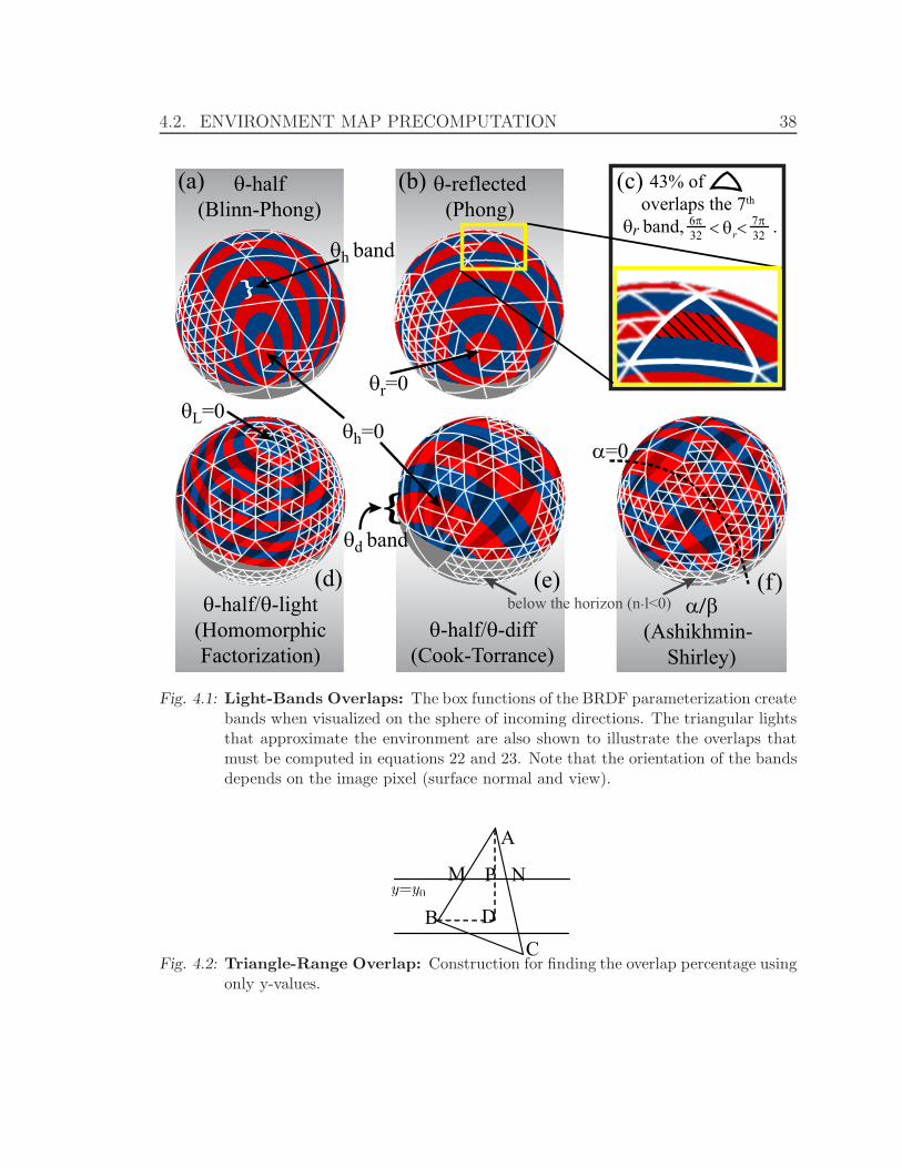
Fig. 4.1: Light-Bands Overlaps: The box functions of the BRDF parameterization createbands when visualized on the sphere of incoming directions. The triangular lightsthat approximate the environment are also shown to illustrate the overlaps thatmust be computed in equations 22 and 23. Note that the orientation of the bandsdepends on the image pixel (surface normal and view).
A
B C
M N
D
P 0y y=
Fig. 4.2: Triangle-Range Overlap: Construction for finding the overlap percentage usingonly y-values.

4.2. ENVIRONMENT MAP PRECOMPUTATION 39
The fraction of the area of δABC above a line y = y0 is given by:
δAMN
δABC=
sin A|AM ||AN |sin A|AB||AC| =
|AM ||AN ||AB||AC| (4.9)
We construct δABD so that yD = yB . By similar triangles, and an analogous
construction for the right half, we find that the fraction depends only on the y values
(γ values) of the vertices:
AM
AB=
AP
AD=
yA − y0
yA − yB
;δAMN
δABC=
(yA − y0)2)
(yA − yb)(yA − yC). (4.10)
We compute the percentage above and below the boundary lines of a band to find
the overlap within the band. It is important to be able to calculate the overlaps
based on a single coordinate because our parameterizations are 1D, and there is no
notion of ’x’ values for the vertices of triangular lights. Even in the simple Phong
parameterization, γ = θr, a perpendicular axis (possibly φr ) does not exist, and
would be ambiguous to define.
The remaining question is what to do when the assumption of local linearity
in the parameterization breaks down (as it will for example, near the pole of the
parameterization, causing the lines of constant γ to be curved, relative to the triangle.)
To account for this, we simply subdivide a triangle into four smaller triangles. If the
fractions of the area, added up from these four, agree with the coarser calculation
to some tolerance, we consider the parameterization locally linear and stop there.
Otherwise, we subdivide again recursively. Figure 4.1 shows the original subdivision
of the lighting environment for one image pixel, and the reader may wish to find large
triangles that would require subdivision, and smaller ones that would not.
4.2. ENVIRONMENT MAP PRECOMPUTATION 40
4.2.2 Initial Approach
We now describe two simple ideas which seem like a straightforward solution, but
turn out to be inappropriate for BRDF editing. In standard PRT, equation 4.8
simply involves a spherical harmonic or wavelet transform, where projection onto the
basis is a well-studied operation. In our case, the box functions bj use a different
parameterization than the lighting, with γ implicitly depending on the local view
direction, and therefore changing for each pixel. As seen in Figure 4.1, the box
functions form highly irregular projections onto the sphere of lighting directions. To
address this issue, one might imagine making a change of variables so that the lighting
and the integral are also specified over the domain of γ, where bj is a well-behaved
box-function:
Tj =
∫ 1
o
L′(γ−1(ωi))bj(γ)∣∣Jac(γ−1)
∣∣ dγ, (Initial.1)
where Jac is the Jacobian necessary for a multi-dimensional change-of-variables. It
turns out that most parameterizations, γ, are not invertible, so Initial.1 cannot be
evaluated analytically. Moreover, we do not want be restricted to a subclass of map-
pings that are invertible, and whose Jacobian can be written explicitly. Hence, we
discretize equation 4.8 directly, without reparameterizing.
The straightforward approach for discretization is to reduce the continuous en-
vironment map into point samples. We can select a number of incoming directions,
such as with structured importance sampling (Agarwal et al., 2003), and replace the
environment map with a light for each of these directions. The radiance of the solid
angle around each light is preintegrated, and attributed to the directional light, thus
allowing it to act as proxy for the illumination of its neighboring directions. Equation
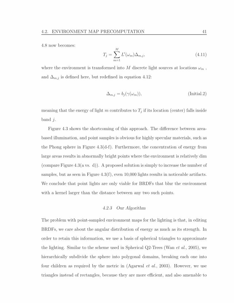
4.2. ENVIRONMENT MAP PRECOMPUTATION 41
4.8 now becomes:
Tj =
M∑
m=1
L′(ωm)Δm,j , (4.11)
where the environment is transformed into M discrete light sources at locations ωm ,
and Δm,j is defined here, but redefined in equation 4.12:
Δm,j = bj(γ(ωm)), (Initial.2)
meaning that the energy of light m contributes to Tj if its location (center) falls inside
band j.
Figure 4.3 shows the shortcoming of this approach. The difference between area-
based illumination, and point samples is obvious for highly specular materials, such as
the Phong sphere in Figure 4.3(d-f). Furthermore, the concentration of energy from
large areas results in abnormally bright points where the environment is relatively dim
(compare Figure 4.3(a vs. d)). A proposed solution is simply to increase the number of
samples, but as seen in Figure 4.3(f), even 10,000 lights results in noticeable artifacts.
We conclude that point lights are only viable for BRDFs that blur the environment
with a kernel larger than the distance between any two such points.
4.2.3 Our Algorithm
The problem with point-sampled environment maps for the lighting is that, in editing
BRDFs, we care about the angular distribution of energy as much as its strength. In
order to retain this information, we use a basis of spherical triangles to approximate
the lighting. Similar to the scheme used in Spherical Q2-Trees (Wan et al., 2005), we
hierarchically subdivide the sphere into polygonal domains, breaking each one into
four children as required by the metric in (Agarwal et al., 2003). However, we use
triangles instead of rectangles, because they are more efficient, and also amenable to
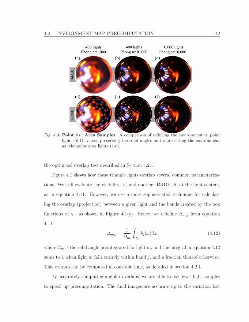
4.2. ENVIRONMENT MAP PRECOMPUTATION 42
Fig. 4.3: Point vs. Area Samples: A comparison of reducing the environment to pointlights (d-f), versus preserving the solid angles and representing the environmentas triangular area lights (a-c).
the optimized overlap test described in Section 4.2.1.
Figure 4.1 shows how these triangle lights overlap several common parameteriza-
tions. We still evaluate the visibility, V , and quotient BRDF, S, at the light centers,
as in equation 4.11. However, we use a more sophisticated technique for calculat-
ing the overlap (projection) between a given light and the bands created by the box
functions of γ , as shown in Figure 4.1(c). Hence, we redefine Δm,j from equation
4.11:
Δm,j =1
Ωm
∫
Ωm
bj(ω)dω (4.12)
where Ωm is the solid angle preintegrated for light m, and the integral in equation 4.12
sums to 1 when light m falls entirely within band j, and a fraction thereof otherwise.
This overlap can be computed in constant time, as detailed in section 4.2.1.
By accurately computing angular overlaps, we are able to use fewer light samples
to speed up precomputation. The final images are accurate up to the variation lost
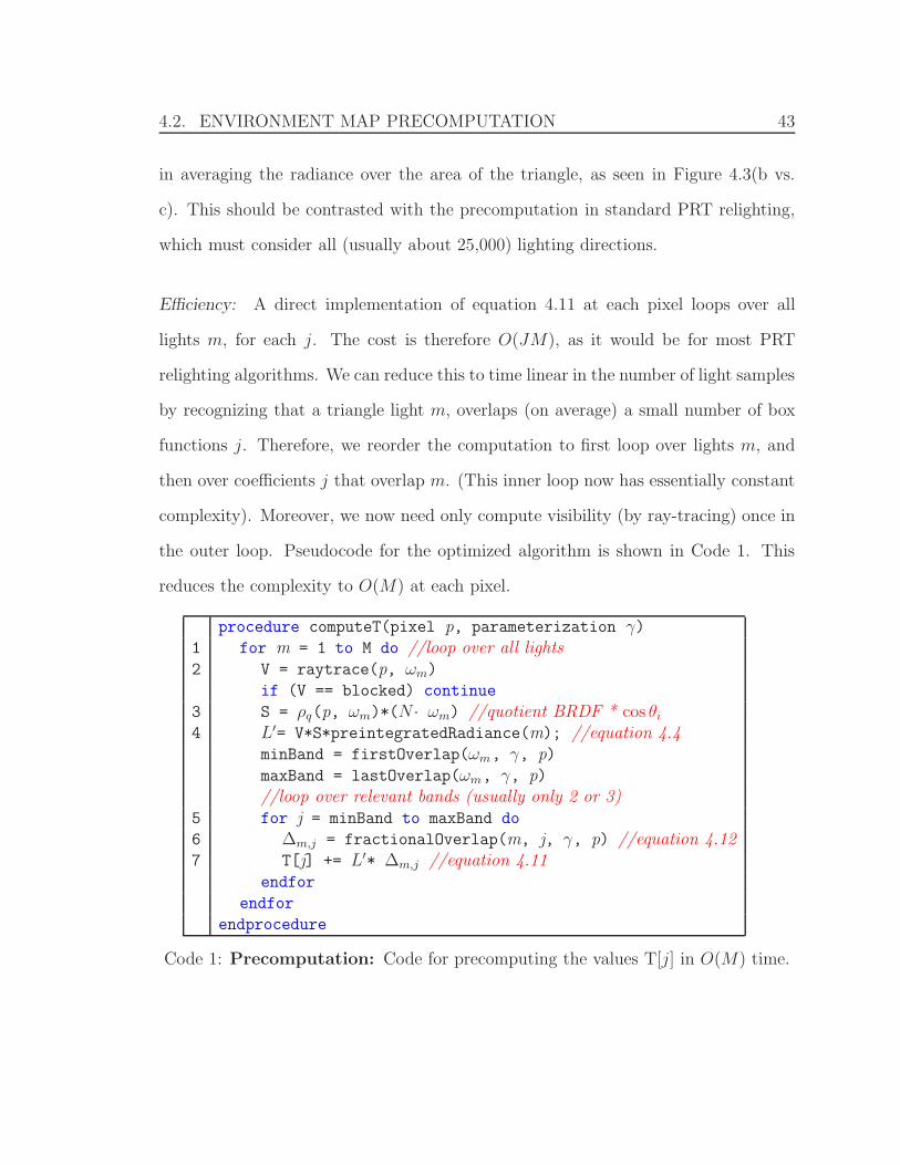
4.2. ENVIRONMENT MAP PRECOMPUTATION 43
in averaging the radiance over the area of the triangle, as seen in Figure 4.3(b vs.
c). This should be contrasted with the precomputation in standard PRT relighting,
which must consider all (usually about 25,000) lighting directions.
Efficiency: A direct implementation of equation 4.11 at each pixel loops over all
lights m, for each j. The cost is therefore O(JM), as it would be for most PRT
relighting algorithms. We can reduce this to time linear in the number of light samples
by recognizing that a triangle light m, overlaps (on average) a small number of box
functions j. Therefore, we reorder the computation to first loop over lights m, and
then over coefficients j that overlap m. (This inner loop now has essentially constant
complexity). Moreover, we now need only compute visibility (by ray-tracing) once in
the outer loop. Pseudocode for the optimized algorithm is shown in Code 1. This
reduces the complexity to O(M) at each pixel.
procedure computeT(pixel p, parameterization γ)1 for m = 1 to M do //loop over all lights2 V = raytrace(p, ωm)
if (V == blocked) continue
3 S = ρq(p, ωm)*(N · ωm) //quotient BRDF * cos θi
4 L′= V*S*preintegratedRadiance(m); //equation 4.4minBand = firstOverlap(ωm, γ, p)maxBand = lastOverlap(ωm, γ, p)//loop over relevant bands (usually only 2 or 3)
5 for j = minBand to maxBand do
6 Δm,j = fractionalOverlap(m, j, γ, p) //equation 4.127 T[j] += L′* Δm,j //equation 4.11
endfor
endfor
endprocedure
Code 1: Precomputation: Code for precomputing the values T[j] in O(M) time.
4.2. ENVIRONMENT MAP PRECOMPUTATION 44
4.2.4 Two Factor BRDFs
We now detail the extension to two different curves and parameterizations for editing.
We use the fact that a user can only edit one curve at a time, making the other
curve temporarily ‘dormant’. Each curve or factor is approximated with a set of box
functions. Using a 2-factor form of equation 5.4 through the derivations in Section
4.1, we arrive at a quadratic form of equation 4.7,
R =∑
j
cAj
∑
k
cBk Ujk = (cB)TUcA, (4.13)
where cA and cB are the coefficient vectors for the two curves, fA and fB , as in
equation 3.1. The vector T has been replaced with the matrix U, defined by the 2D
form of equation 4.8:
Ujk =
∫
Ω4π
L′(ωi)bj(γA(ωi))bj(γB(ωi))dωi. (4.14)
Recalling that equation 4.14 takes the form of a projection, we note that U is
a projection of the lighting onto the (non-orthogonal) axes of γA and γB4 . The
discrete form is analogous to equation 4.11,
Ujk =M∑
m=1
L′(ωm)(Δm,jΔm,k) (4.15)
As in the one-curve case, we loop first over all the lights, and then find the overlapping
bands for each parameterization.
The quadratic form in equation 4.13 cannot currently be evaluated directly in real-
time. Instead, either the left or the right matrix-vector multiplication is evaluated in
4 For the case of γA = θi and γB = φi, U is the lighting, modulated by V and S

4.2. ENVIRONMENT MAP PRECOMPUTATION 45
a run-time precomputation step we call curve switching. Let us say the user chooses
curve A (Figure 4.5(a):Pearls θh ) . Using the (temporarily fixed) values of cB for the
’dormant’ curve (Figure 4.5(f):Pearls θd ), we compute
TA = (cB)TU; R = TA · cA, (4.16)
where TA is the transport coefficient vector for standard 1D curve editing of curve
A, given the fixed value of curve B. While not real-time, it takes only a few seconds
to compute TA (shown in Table 4.2), making it a viable part of an interactive editing
session. The second part of equation 4.16 to compute the actual image is the standard
rendering dot-product, and one can now edit the first curve with real-time feedback.
At some point, the user decides to switch curves, fixing cA while editing cB. The
system now computes TB = UcA , which again takes only a few seconds.
4.2.5 Use of Daubechies 4 Wavelets
low-pass= [d1 d2 d3 d4]
high-pass= [d4 –d3 d2 –d1]
d1= 0.4829629131445341
d2= 0.8365163037378077
d3= 0.2241438680420134 d4= -0.1294095225512603
Tab. 4.1: Daubechies 4 Coefficients: Coefficients used for filtering primal band coeffi-cients to wavelet coefficients.
The low-pass and high-pass filter coefficients for Daubechies 4 (Daubecies, 1988)
wavelets we used are shown on the right. Like the Haar basis, Daub4 wavelets are
orthonormal. Unlike Haar, they are designed for C1, not just C0 continuity.
To obtain the Daub4 coefficients of the user’s input curve, we first discretize it
4.2. ENVIRONMENT MAP PRECOMPUTATION 46
using the box basis functions. It is important to integrate over the domain of each
box function (as opposed to taking point samples) in order to avoid popping artifacts
during edits. So at each frame, the following operation happens once for each edited
curve:
cj =
∫ jπ2J
(j−1)π2J
bj(γ)f(γ)dγ, (4.17)
where we’ve assumed γ ∈ [0, π2], as it usually is.
Using column vectors, we use the synthesis matrix for Daub4, SD4 , to write the
wavelet transformed versions of cA and cB :
cAD4 = SD4c
A; cBD4 = SD4c
B (4.18)
To find the properly transformed U , UD4 , we refer to equation 4.13:
R = (cBD4)
TUD4cAD4;UD4 = S−T
D4US−1D4 = SD4UST
D4, (4.19)
where the last equality uses the fact that the Daubechies 4 synthesis matrix is or-
thonormal. Therefore, we must use the standard 2D transform of the matrix U,
which first uses the 1D transform to convert the rows, and then uses it to convert
the columns (or vice-versa). Though the non-standard 2D transform often provides
better compression, it is not applicable for our use.
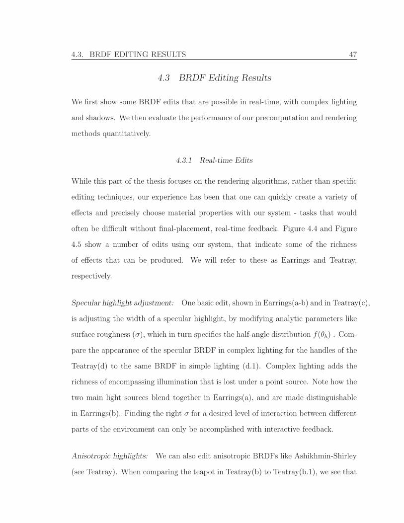
4.3. BRDF EDITING RESULTS 47
4.3 BRDF Editing Results
We first show some BRDF edits that are possible in real-time, with complex lighting
and shadows. We then evaluate the performance of our precomputation and rendering
methods quantitatively.
4.3.1 Real-time Edits
While this part of the thesis focuses on the rendering algorithms, rather than specific
editing techniques, our experience has been that one can quickly create a variety of
effects and precisely choose material properties with our system - tasks that would
often be difficult without final-placement, real-time feedback. Figure 4.4 and Figure
4.5 show a number of edits using our system, that indicate some of the richness
of effects that can be produced. We will refer to these as Earrings and Teatray,
respectively.
Specular highlight adjustment: One basic edit, shown in Earrings(a-b) and in Teatray(c),
is adjusting the width of a specular highlight, by modifying analytic parameters like
surface roughness (σ), which in turn specifies the half-angle distribution f(θh) . Com-
pare the appearance of the specular BRDF in complex lighting for the handles of the
Teatray(d) to the same BRDF in simple lighting (d.1). Complex lighting adds the
richness of encompassing illumination that is lost under a point source. Note how the
two main light sources blend together in Earrings(a), and are made distinguishable
in Earrings(b). Finding the right σ for a desired level of interaction between different
parts of the environment can only be accomplished with interactive feedback.
Anisotropic highlights: We can also edit anisotropic BRDFs like Ashikhmin-Shirley
(see Teatray). When comparing the teapot in Teatray(b) to Teatray(b.1), we see that
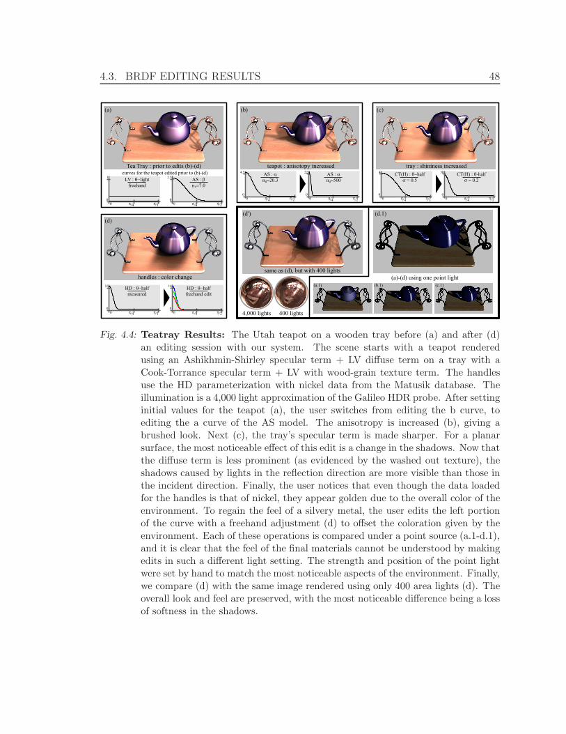
4.3. BRDF EDITING RESULTS 48
(b)
teapot : anisotopy increasedAS : αnu=20.3
π 4 π 2
4.5
00
AS : αnu=500
π 4 π 2
22
00
(a)
Tea Tray : prior to edits (b)-(d)
LV : θ−lightfreehand
π 4 π 1
1
00
AS : βnv=7.0
π 4 π 2
2.5
00
(c)
tray : shininess increasedCT(H) : θ−half
σ = 0.5
π 4 π 2
4
00
CT(H) : θ-halfσ = 0.2
π 4 π 2
30
00
(d)
handles : color change
HD : θ−halfmeasured
π 4 π 1
16
00
HD : θ−halffreehand edit
π 4 π 2
16
00
(d’)
same as (d), but with 400 lights
(d.1)
(a.1) (b.1) (c.1)
curves for the teapot edited prior to (b)-(d)
(a)-(d) using one point light
4,000 lights 400 lights
Fig. 4.4: Teatray Results: The Utah teapot on a wooden tray before (a) and after (d)an editing session with our system. The scene starts with a teapot renderedusing an Ashikhmin-Shirley specular term + LV diffuse term on a tray with aCook-Torrance specular term + LV with wood-grain texture term. The handlesuse the HD parameterization with nickel data from the Matusik database. Theillumination is a 4,000 light approximation of the Galileo HDR probe. After settinginitial values for the teapot (a), the user switches from editing the b curve, toediting the a curve of the AS model. The anisotropy is increased (b), giving abrushed look. Next (c), the tray’s specular term is made sharper. For a planarsurface, the most noticeable effect of this edit is a change in the shadows. Now thatthe diffuse term is less prominent (as evidenced by the washed out texture), theshadows caused by lights in the reflection direction are more visible than those inthe incident direction. Finally, the user notices that even though the data loadedfor the handles is that of nickel, they appear golden due to the overall color of theenvironment. To regain the feel of a silvery metal, the user edits the left portionof the curve with a freehand adjustment (d) to offset the coloration given by theenvironment. Each of these operations is compared under a point source (a.1-d.1),and it is clear that the feel of the final materials cannot be understood by makingedits in such a different light setting. The strength and position of the point lightwere set by hand to match the most noticeable aspects of the environment. Finally,we compare (d) with the same image rendered using only 400 area lights (d). Theoverall look and feel are preserved, with the most noticeable difference being a lossof softness in the shadows.
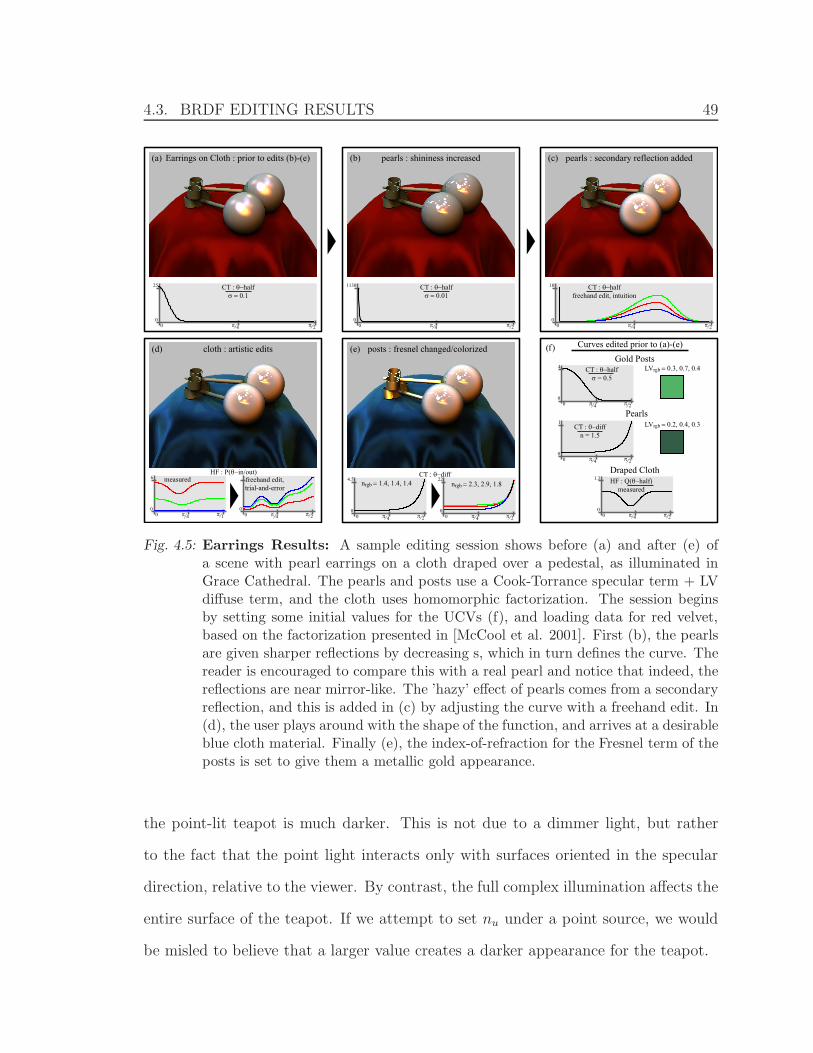
4.3. BRDF EDITING RESULTS 49
CT : θ−halfσ = 0.1
π 4 π 2
25
00
Earrings on Cloth : prior to edits (b)-(e)(a)
CT : θ−halfσ = 0.01
π 4 π 2
1130
00
pearls : shininess increased(b)
CT : θ−halffreehand edit, intuition
π 4 π 2
10
00
pearls : secondary reflection added(c)
HF : P(θ−in/out)
π 4 π 1
6
00 π 4 π 2
00
measured freehand edit,trial-and-error
cloth : artistic edits(d)
CT : θ−diff
π 4 π 2
4.5
00 π 4 π 2
22
00
nrgb = 1.4, 1.4, 1.4 nrgb = 2.3, 2.9, 1.8
posts : fresnel changed/colorized(e)
CT : θ−halfσ = 0.5
π 4 π 2
4
00
Gold PostsLVrgb = 0.3, 0.7, 0.4
LVrgb = 0.2, 0.4, 0.3
π 4 π 2
1
00
CT : θ−diffn = 1.5
Pearls
HF : Q(θ−half)measured
π 4 π 2
1.3
00
Draped Cloth
Curves edited prior to (a)-(e)(f)
Fig. 4.5: Earrings Results: A sample editing session shows before (a) and after (e) ofa scene with pearl earrings on a cloth draped over a pedestal, as illuminated inGrace Cathedral. The pearls and posts use a Cook-Torrance specular term + LVdiffuse term, and the cloth uses homomorphic factorization. The session beginsby setting some initial values for the UCVs (f), and loading data for red velvet,based on the factorization presented in [McCool et al. 2001]. First (b), the pearlsare given sharper reflections by decreasing s, which in turn defines the curve. Thereader is encouraged to compare this with a real pearl and notice that indeed, thereflections are near mirror-like. The ’hazy’ effect of pearls comes from a secondaryreflection, and this is added in (c) by adjusting the curve with a freehand edit. In(d), the user plays around with the shape of the function, and arrives at a desirableblue cloth material. Finally (e), the index-of-refraction for the Fresnel term of theposts is set to give them a metallic gold appearance.
the point-lit teapot is much darker. This is not due to a dimmer light, but rather
to the fact that the point light interacts only with surfaces oriented in the specular
direction, relative to the viewer. By contrast, the full complex illumination affects the
entire surface of the teapot. If we attempt to set nu under a point source, we would
be misled to believe that a larger value creates a darker appearance for the teapot.

4.3. BRDF EDITING RESULTS 50
Retroreflection and the Fresnel effect: Earrings(e) shows how changing the index of
refraction at each color channel generates a new set of curves for f(θd) , according
to the Fresnel equation. Values of f(θd) near θd = 0 control retroreflection, since the
view and light directions are close to each other. As seen in the separate RGB curves,
the color distinction is large near this part of the curve, and dissipates as θd grows.
This will give the desired Fresnel effect of desaturating the color of lights near grazing
angles.
Interaction of Materials and Shadows: Shadows can often depend on the material
properties, since a diffuse BRDF draws lighting energy from a different area than a
glossy BRDF. In Teatray(c), we edit the tray’s material from diffuse to glossy, which
also allows us to create different shadowing effects. Notice that occluding geometry
in the reflection direction is now much more important to the creation of shadows
than in the diffuse case, Teatray(b).
Artistic edits: We can also go beyond physically-based BRDFs, to create flexible
artistic effects. Earrings(c) shows how intuition about a secondary reflection can be
used to edit a portion of a curve otherwise specified by the user’s choice of σ. In
Earrings(d), we used trial-and-error to manipulate a curve loaded from factored data
in order to design a desirable material. A simpler type of artistic license is used on
the handles in Teatray(d), where we compensate for the color of the environment to
force the silver appearance.
4.3. BRDF EDITING RESULTS 51
4.3.2 Precomputation Numbers
Table 4.2 analyzes the time and memory usage for the precomputation phase, for the
Earring and Teatray scenes, itemized for each object. Since each pixel is treated sep-
arately, the totals are proportional to the number of pixels, and would be comparable
for any scene with the same (512x512) image resolution. These tests were run on an
Intel Xeon 3.2Ghz 64bit processor with 8GB of RAM.
We proceed from left to right in Table 4.2. For each object, we show the BRDF
model used. In many cases we use a sum of diffuse and specular lobes, such as LV +
CT for the posts, and LV + AS for the teapot. We typically use 128 or 256 bands
to accurately represent specularities. In some cases, lower resolutions of 32 or 64
are used for in HD or CT representations. For two-curve models, the time to switch
curves for editing is only one or two seconds.
To reduce storage of the transport coefficient vectors and matrices, we zero out
values below a small threshold and do not store them explicitly. Unlike relighting, we
must be much more careful about compression since the BRDF is visualized directly,
and we are able to achieve compression rates of only 5:1 - 6:1 (and only about 2:1
in some cases). Even so, our final storage requirements, while large (hundreds of
megabytes), are comparable with all-frequency relighting PRT methods. Most of the
storage is for two-curve BRDF models, where we must store transport matrices U at
each pixel (for example, AS in teapot, CT in pearls and HF in cloth). The storage
for transport vectors from one-curve BRDF models like LV is usually much smaller.
We separate the precomputation time into visibility and our precomputation. The
visibility is precomputed once for the scene, using a standard ray-tracer. The band-
light triangle overlap and fixed BRDF shading computations are performed as per
Code 1. The time for both computations is approximately linear in the number of
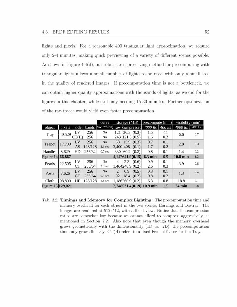
4.3. BRDF EDITING RESULTS 52
lights and pixels. For a reasonable 400 triangular light approximation, we require
only 2-4 minutes, making quick previewing of a variety of different scenes possible.
As shown in Figure 4.4(d), our robust area-preserving method for precomputing with
triangular lights allows a small number of lights to be used with only a small loss
in the quality of rendered images. If precomputation time is not a bottleneck, we
can obtain higher quality approximations with thousands of lights, as we did for the
figures in this chapter, while still only needing 15-30 minutes. Further optimization
of the ray-tracer would yield even faster precomputation.
storage (MB) precompute (min) visibility (min) object pixels model bands
curve switching raw compressed 4000 lts 400 lts 4000 lts 400 lts
LV 256 NA 121 36.3 (0.3) 1.5 0.2 Tray 40,529
CT(H) 256 NA 243 121.5 (0.5) 1.6 0.3 6.6 0.7
LV 256 NA 53 15.9 (0.3) 0.7 0.1 Teapot 17,709 AS 128/128 2.1 sec 3,400 408 (0.1) 1.7 0.2
2.8 0.3
Handles 8,629 HD 256/32 0.7 sec 330 60.2 (0.2) 0.8 0.1 1.4 0.2
Figure 14 66,867 4,147641.9 (0.15) 6.3 min 0.9 10.8 min 1.2
LV 256 NA 4 2.3 (0.6) 0.9 0.1 Pearls 22,505 CT 256/64 2.3 sec 1,464248.9 (0.2) 2.6 0.3
3.9 0.5
LV 256 NA 2 0.9 (0.5) 0.3 0.1 Posts 7,626 CT 256/64 0.3 sec 92 18.4 (0.2) 0.8 0.2
1.3 0.2
Cloth 98,890 HF 128/128 1.8 sec 1,186260.9 (0.2) 6.3 0.8 18.8 2.1
Figure 15 129,021 2,748531.4 (0.19) 10.9 min 1.5 24 min 2.8
Tab. 4.2: Timings and Memory for Complex Lighting: The precomputation time andmemory overhead for each object in the two scenes, Earrings and Teatray. Theimages are rendered at 512x512, with a fixed view. Notice that the compressionratios are somewhat low because we cannot afford to compress aggressively, asmentioned in Section 7.2. Also note that even though the memory overheadgrows geometrically with the dimensionality (1D vs. 2D), the precomputationtime only grows linearly. CT(H) refers to a fixed Fresnel factor for the Tray.
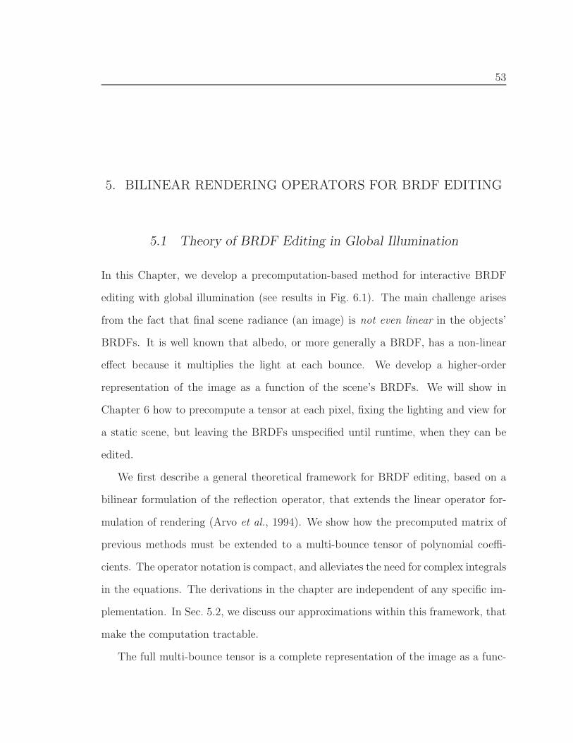
53
5. BILINEAR RENDERING OPERATORS FOR BRDF EDITING
5.1 Theory of BRDF Editing in Global Illumination
In this Chapter, we develop a precomputation-based method for interactive BRDF
editing with global illumination (see results in Fig. 6.1). The main challenge arises
from the fact that final scene radiance (an image) is not even linear in the objects’
BRDFs. It is well known that albedo, or more generally a BRDF, has a non-linear
effect because it multiplies the light at each bounce. We develop a higher-order
representation of the image as a function of the scene’s BRDFs. We will show in
Chapter 6 how to precompute a tensor at each pixel, fixing the lighting and view for
a static scene, but leaving the BRDFs unspecified until runtime, when they can be
edited.
We first describe a general theoretical framework for BRDF editing, based on a
bilinear formulation of the reflection operator, that extends the linear operator for-
mulation of rendering (Arvo et al., 1994). We show how the precomputed matrix of
previous methods must be extended to a multi-bounce tensor of polynomial coeffi-
cients. The operator notation is compact, and alleviates the need for complex integrals
in the equations. The derivations in the chapter are independent of any specific im-
plementation. In Sec. 5.2, we discuss our approximations within this framework, that
make the computation tractable.
The full multi-bounce tensor is a complete representation of the image as a func-
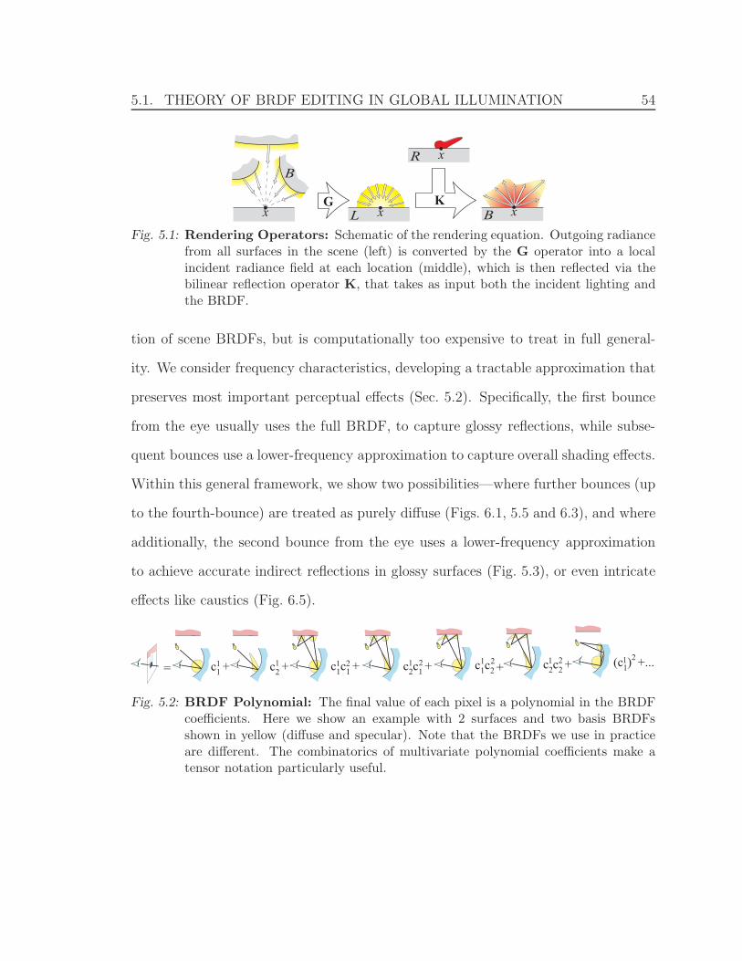
5.1. THEORY OF BRDF EDITING IN GLOBAL ILLUMINATION 54
x x
x
xG K
B
BL
R
Fig. 5.1: Rendering Operators: Schematic of the rendering equation. Outgoing radiancefrom all surfaces in the scene (left) is converted by the G operator into a localincident radiance field at each location (middle), which is then reflected via thebilinear reflection operator K, that takes as input both the incident lighting andthe BRDF.
tion of scene BRDFs, but is computationally too expensive to treat in full general-
ity. We consider frequency characteristics, developing a tractable approximation that
preserves most important perceptual effects (Sec. 5.2). Specifically, the first bounce
from the eye usually uses the full BRDF, to capture glossy reflections, while subse-
quent bounces use a lower-frequency approximation to capture overall shading effects.
Within this general framework, we show two possibilities—where further bounces (up
to the fourth-bounce) are treated as purely diffuse (Figs. 6.1, 5.5 and 6.3), and where
additionally, the second bounce from the eye uses a lower-frequency approximation
to achieve accurate indirect reflections in glossy surfaces (Fig. 5.3), or even intricate
effects like caustics (Fig. 6.5).
= c1 + c2 + c2c1 + c2c2 + (c1)2
+... c1c2 + c1c1 + 1 1 1 2 1 2 1 2 1 2 1
Fig. 5.2: BRDF Polynomial: The final value of each pixel is a polynomial in the BRDFcoefficients. Here we show an example with 2 surfaces and two basis BRDFsshown in yellow (diffuse and specular). Note that the BRDFs we use in practiceare different. The combinatorics of multivariate polynomial coefficients make atensor notation particularly useful.

5.1. THEORY OF BRDF EDITING IN GLOBAL ILLUMINATION 55
B(x, ωo) Outgoing radiance (image)E(x, ωo) Emissive radiance of light sourcesL(x, ωi) Local incident radianceR(x, ωi, ωo) BRDFs of all points in the sceneTN(x, ωo) Precomputed multi-bounce tensorρm(ωi, ωo) BRDF of object mbmj (ωi, ωo) Basis function j for the BRDF of object m
Hm(x) Spatial weight map or texture for object mG Linear geometric operator
G : B(x, ωo) �→ L(y, ωi)(GB)(x, ω) ≡ B(x′(x, ω),−ω)
K(R) Reflection operator (equation 5.2)cmj BRDF coefficients (equation 5.4)
dm Equivalent albedo of object m (section 5.2.4)
dz Product of albedos dm
�Xi Light path with contribution f( �Xi)F i
jn Tensor coefficient after freezing BRDFsJ Number of BRDF bases (usually 64 or 128)M Number of objects (M ∼ 5)W Total basis functions (W = JM ∼ 500)
Z Number of terms for diffuse dz (Z ∼ 64)
Tab. 5.1: Table of Notation for Chapters 5 and 6: This table give the notation used fordeveloping the global illumination solution to BRDF editin, presented in Chapters5 and 6
5.1.1 Basic Framework using the bilinear K operator
We begin by writing the rendering equation (Kajiya, 1986) as a linear operator equa-
tion, similar to (Arvo et al., 1994):
B = E + K(R)GB, (5.1)
where B(x, ωo) is the outgoing surface radiance, E(x, ωo) is the emission and G is the
linear geometric operator that converts the outgoing radiance from distant surfaces to
a local incident radiance field as in (Arvo et al., 1994). Figure 5.1 shows a schematic,

5.1. THEORY OF BRDF EDITING IN GLOBAL ILLUMINATION 56
and Table 5.1 summarizes notation.
Arvo et al. (1994) define K as a linear reflection operator on the local incident
radiance field L. In our first departure from previous representations, we make explicit
K’s dependence on the BRDFs R of scene objects. We write K as a bilinear operator
that takes an additional input R(x, ωi, ωo) which describes the BRDF at each point
in the scene and is the kernel of integration in K,
K : L(x, ωi), R(x, ωi, ωo) �→ B(x, ωo)
(K(R)L)(x, ωo)≡∫
Ω2π
R(x, ωi, ωo)L(x, ωi) cos θidωi. (5.2)
Note that K is bilinear, or linear with respect to both inputs—incident lighting L,
and the BRDFs of objects in the scene R. That is, for scalars a and b,
K(aR1 + bR2)L = aK(R1)L + bK(R2)L
K(R) (aL1 + bL2) = aK(R)L1 + bK(R)L2. (5.3)
We now seek to relate R (and hence K) to editable BRDFs of individual objects.
We assume there are M objects in the scene, and for now that each object has a single
BRDF. Let object m have1 BRDF ρm. We assume the BRDF can be represented as
a linear combination of functions over the domain (ωi, ωo),
ρm(ωi, ωo) =J∑
j=1
cmj bm
j (ωi, ωo). (5.4)
The BRDF basis functions b could be spherical harmonics, wavelets or any other
linear basis. We follow previous BRDF editing methods (Ben-Artzi et al., 2006b;
1 We use superscripts to denote some property of the function, and parentheses for explicitlyraising to a power, so ρ2 is the second in a series, whereas (ρ)2 is ρ squared.
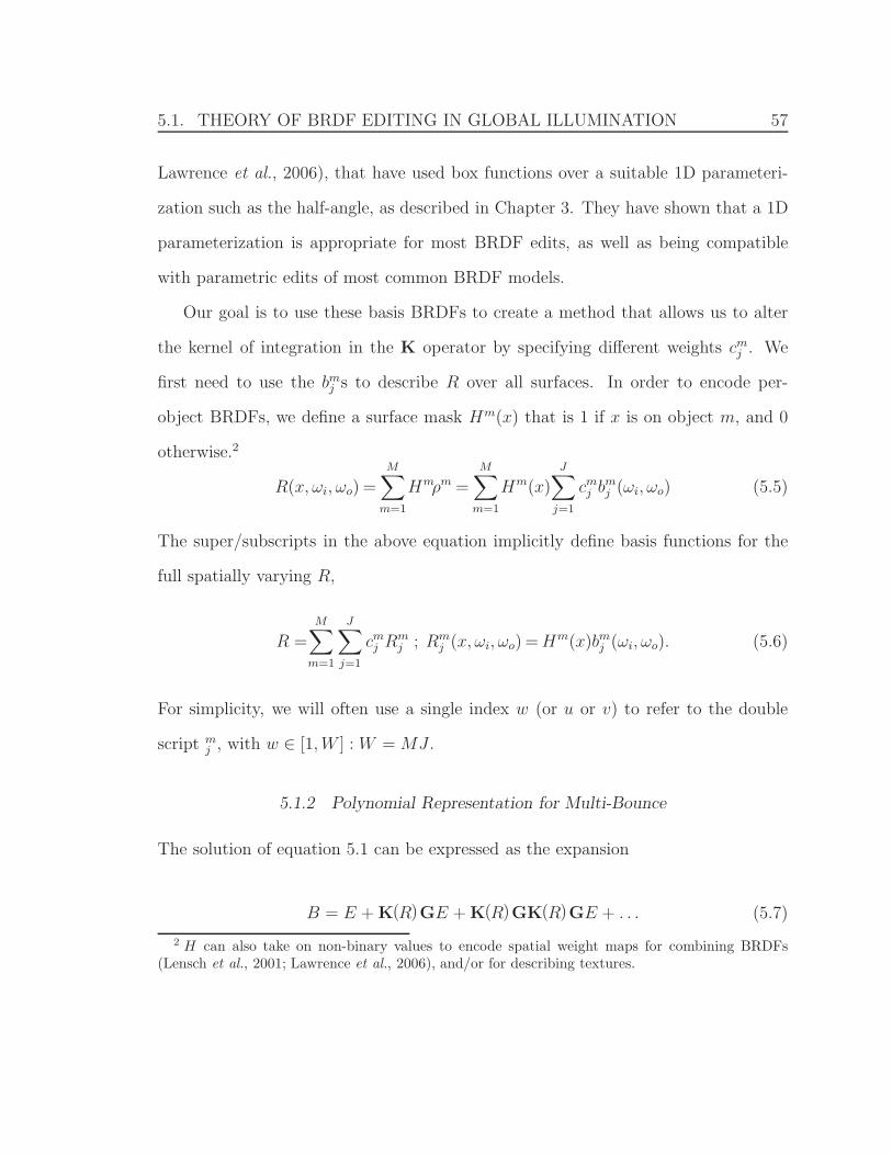
5.1. THEORY OF BRDF EDITING IN GLOBAL ILLUMINATION 57
Lawrence et al., 2006), that have used box functions over a suitable 1D parameteri-
zation such as the half-angle, as described in Chapter 3. They have shown that a 1D
parameterization is appropriate for most BRDF edits, as well as being compatible
with parametric edits of most common BRDF models.
Our goal is to use these basis BRDFs to create a method that allows us to alter
the kernel of integration in the K operator by specifying different weights cmj . We
first need to use the bmj s to describe R over all surfaces. In order to encode per-
object BRDFs, we define a surface mask Hm(x) that is 1 if x is on object m, and 0
otherwise.2
R(x, ωi, ωo) =M∑
m=1
Hmρm =M∑
m=1
Hm(x)J∑
j=1
cmj bm
j (ωi, ωo) (5.5)
The super/subscripts in the above equation implicitly define basis functions for the
full spatially varying R,
R =
M∑
m=1
J∑
j=1
cmj Rm
j ; Rmj (x, ωi, ωo) = Hm(x)bm
j (ωi, ωo). (5.6)
For simplicity, we will often use a single index w (or u or v) to refer to the double
script mj , with w ∈ [1, W ] : W = MJ .
5.1.2 Polynomial Representation for Multi-Bounce
The solution of equation 5.1 can be expressed as the expansion
B = E + K(R)GE + K(R)GK(R)GE + . . . (5.7)
2 H can also take on non-binary values to encode spatial weight maps for combining BRDFs(Lensch et al., 2001; Lawrence et al., 2006), and/or for describing textures.
5.1. THEORY OF BRDF EDITING IN GLOBAL ILLUMINATION 58
where each term N has an intuitive interpretation, as corresponding to N bounces of
light from source(s) to viewer.
All current relighting methods rely on the linearity of B with respect to E. Previ-
ous BRDF editing methods also take advantage of the linearity of the 1-bounce term
in B (i.e., K(R)GE) with respect to K (and hence with respect to R), requiring them
to render using only direct lighting.
However, this linearity no longer applies for BRDF editing with global illumination
because the operator K(R) is applied multiple times. Even for 2-bounce reflections,
the system becomes quadratic, and must be represented with a quadratic multivari-
able polynomial in the cws. The N -bounce solution is an order N polynomial. We
now show how to extend the general PRT approach to these polynomial equations.
We start by considering 2-bounce reflection,
B2 = K(R)GK(R)GE (5.8)
= K(∑
u
cuRu)GK(∑
v
cvRv)GE (5.9)
=∑
u
cu
(
K(Ru)G∑
v
cv
(K(Rv)GE
))
(5.10)
=∑
u
∑
v
cucvK(Ru)GK(Rv)GE. (5.11)
The bilinear nature of K is crucial here. We use the linearity of K with respect to the
BRDF to get equation 5.10, and the linearity of K and G with respect to radiance
to get equation 5.11.
For BRDF editing, the coefficients (cu and cv) become the variables of our com-
putation. The fixed quantities for precomputation are the basis BRDF distributions
(Ru and Rv), that depend only on the parameterizations of the various BRDFs. G
and E are also known, defined by the geometry and lighting of the scene, respectively.
5.1. THEORY OF BRDF EDITING IN GLOBAL ILLUMINATION 59
We precompute a 2-bounce transport function T 2uv and calculate B2 as
T 2uv = K(Ru)GK(Rv)GE
B2 =∑
u
∑
v
T 2uvcucv. (5.12)
Most generally, T 2uv and B2 are defined over all spatial locations and view direc-
tions. In practice, since we fix the view, T 2uv(x, ωo(x)) is an order 2 tensor (that is, a
matrix for 2-bounce reflection) at each pixel. B2(x, ωo(x)) at each pixel is a quadratic
polynomial in the variables c, with coefficients given by T 2. When evaluated, it be-
comes the radiance function for the scene due to light that has reflected off exactly 2
surfaces. More explicitly,
B2 = T11(c1)2 + T12c1c2 + . . . Tuvcucv + . . . T
WW(c
W)2. (5.13)
Figure 5.2 illustrates such polynomials for paths of length 1 and 2. All 1- and 2-
term combinations of the BRDFs are possible, including repetitions of the same basis
function, as in T11(c11)
2, since concave objects can reflect onto themselves. Following
the same logic, the N -bounce energy is
BN =∑
wN
∑
wN−1
. . .∑
w1
TNwN wN−1...w1
cwNcwN−1
. . . cw1, (5.14)
where T N is an order N tensor for each pixel, whose size varies with the number of
objects and BRDF basis functions per object. We are evaluating a multi-variable,
degree N polynomial where each w runs over all W values (all basis functions). The
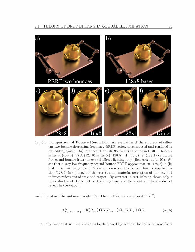
5.1. THEORY OF BRDF EDITING IN GLOBAL ILLUMINATION 60
a) b)
c) d) e) f)PBRT two bounces 128x8 bases
128x8 16x8 128x1 Direct Fig. 5.3: Comparison of Bounce Resolution: An evaluation of the accuracy of differ-
ent two-bounce decreasing-frequency BRDF series, precomputed and rendered inour editing system. (a) Full resolution BRDFs rendered offline in PBRT—hence aseries of (∞,∞) (b) A (128, 8) series (c) (128, 8) (d) (16, 8) (e) (128, 1) or diffusefor second bounce from the eye (f) Direct lighting only (Ben-Artzi et al. 06). Wesee that a very low-frequency second-bounce BRDF approximation (128, 8) in (b)and (c) is essentially exact. Moreover, even a diffuse second bounce approxima-tion (128, 1) in (e) provides the correct shiny material perception of the tray andindirect reflections of tray and teapot. By contrast, direct lighting shows only ablack shadow of the teapot on the shiny tray, and the spout and handle do notreflect in the teapot.
variables of are the unknown scalar c’s. The coefficients are stored in T N ,
TNwN wN−1···w1
= K(RwN)GK(RwN−1
)G...K(Rw1)GE. (5.15)
Finally, we construct the image to be displayed by adding the contributions from
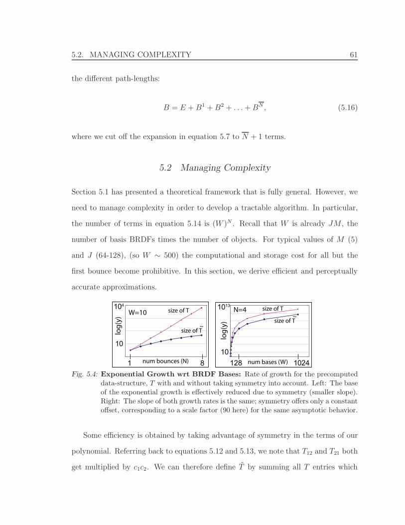
5.2. MANAGING COMPLEXITY 61
the different path-lengths:
B = E + B1 + B2 + . . . + BN , (5.16)
where we cut off the expansion in equation 5.7 to N + 1 terms.
5.2 Managing Complexity
Section 5.1 has presented a theoretical framework that is fully general. However, we
need to manage complexity in order to develop a tractable algorithm. In particular,
the number of terms in equation 5.14 is (W )N . Recall that W is already JM , the
number of basis BRDFs times the number of objects. For typical values of M (5)
and J (64-128), (so W ∼ 500) the computational and storage cost for all but the
first bounce become prohibitive. In this section, we derive efficient and perceptually
accurate approximations.
10
104
1 8
log(
y)
num bounces (N)
W=10
128 1024num bases (W)
log(
y)
N=4
10
1013size of T size of T
size of T~
size of T~
Fig. 5.4: Exponential Growth wrt BRDF Bases: Rate of growth for the precomputeddata-structure, T with and without taking symmetry into account. Left: The baseof the exponential growth is effectively reduced due to symmetry (smaller slope).Right: The slope of both growth rates is the same; symmetry offers only a constantoffset, corresponding to a scale factor (90 here) for the same asymptotic behavior.
Some efficiency is obtained by taking advantage of symmetry in the terms of our
polynomial. Referring back to equations 5.12 and 5.13, we note that T12 and T21 both
get multiplied by c1c2. We can therefore define T by summing all T entries which
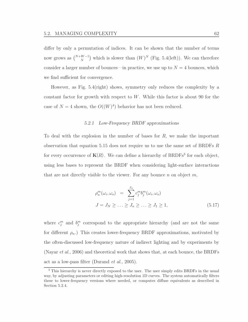
5.2. MANAGING COMPLEXITY 62
differ by only a permutation of indices. It can be shown that the number of terms
now grows as(
N+W−1N
)which is slower than (W )N (Fig. 5.4(left)). We can therefore
consider a larger number of bounces—in practice, we use up to N = 4 bounces, which
we find sufficient for convergence.
However, as Fig. 5.4(right) shows, symmetry only reduces the complexity by a
constant factor for growth with respect to W . While this factor is about 90 for the
case of N = 4 shown, the O((W )4) behavior has not been reduced.
5.2.1 Low-Frequency BRDF approximations
To deal with the explosion in the number of bases for R, we make the important
observation that equation 5.15 does not require us to use the same set of BRDFs R
for every occurrence of K(R) . We can define a hierarchy of BRDFs3 for each object,
using less bases to represent the BRDF when considering light-surface interactions
that are not directly visible to the viewer. For any bounce n on object m,
ρmn (ωi, ωo) =
Jn∑
j=1
cmj bm
j (ωi, ωo)
J = JN ≥ . . . ≥ Jn ≥ . . . ≥ J1 ≥ 1, (5.17)
where cmj and bm
j correspond to the appropriate hierarchy (and are not the same
for different ρn.) This creates lower-frequency BRDF approximations, motivated by
the often-discussed low-frequency nature of indirect lighting and by experiments by
(Nayar et al., 2006) and theoretical work that shows that, at each bounce, the BRDFs
act as a low-pass filter (Durand et al., 2005).
3 This hierarchy is never directly exposed to the user. The user simply edits BRDFs in the usualway, by adjusting parameters or editing high-resolution 1D curves. The system automatically filtersthese to lower-frequency versions where needed, or computes diffuse equivalents as described inSection 5.2.4.
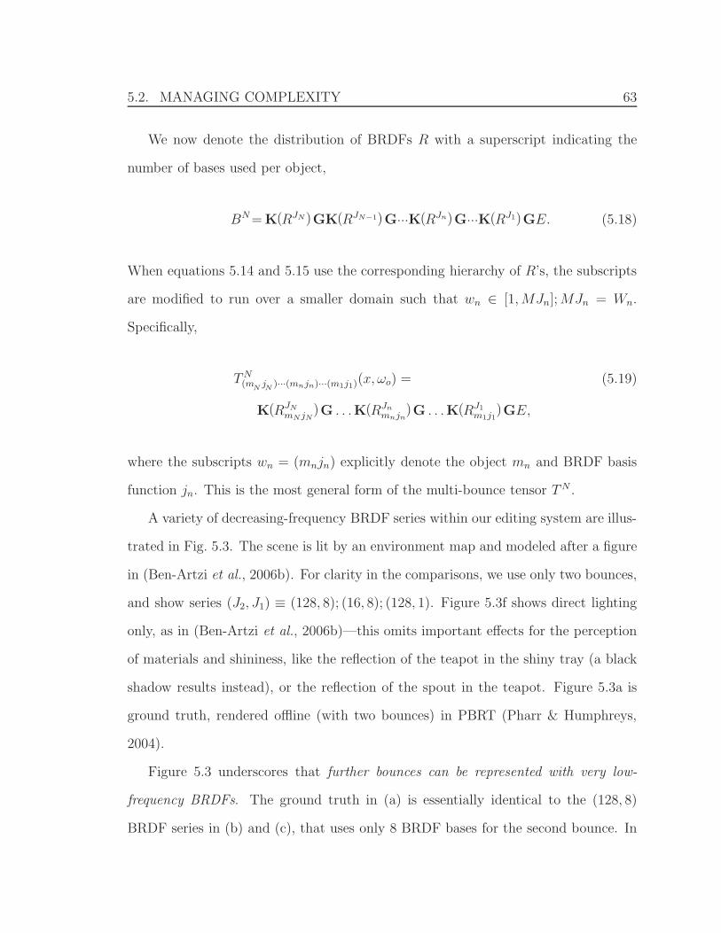
5.2. MANAGING COMPLEXITY 63
We now denote the distribution of BRDFs R with a superscript indicating the
number of bases used per object,
BN = K(RJN)GK(RJN−1)G...K(RJn)G...K(RJ1)GE. (5.18)
When equations 5.14 and 5.15 use the corresponding hierarchy of R’s, the subscripts
are modified to run over a smaller domain such that wn ∈ [1, MJn]; MJn = Wn.
Specifically,
T N(m
NjN
)···(mnjn)···(m1j1)(x, ωo) = (5.19)
K(RJNmN jN
)G . . .K(RJnmnjn
)G . . .K(RJ1m1j1
)GE,
where the subscripts wn = (mnjn) explicitly denote the object mn and BRDF basis
function jn. This is the most general form of the multi-bounce tensor T N .
A variety of decreasing-frequency BRDF series within our editing system are illus-
trated in Fig. 5.3. The scene is lit by an environment map and modeled after a figure
in (Ben-Artzi et al., 2006b). For clarity in the comparisons, we use only two bounces,
and show series (J2, J1) ≡ (128, 8); (16, 8); (128, 1). Figure 5.3f shows direct lighting
only, as in (Ben-Artzi et al., 2006b)—this omits important effects for the perception
of materials and shininess, like the reflection of the teapot in the shiny tray (a black
shadow results instead), or the reflection of the spout in the teapot. Figure 5.3a is
ground truth, rendered offline (with two bounces) in PBRT (Pharr & Humphreys,
2004).
Figure 5.3 underscores that further bounces can be represented with very low-
frequency BRDFs. The ground truth in (a) is essentially identical to the (128, 8)
BRDF series in (b) and (c), that uses only 8 BRDF bases for the second bounce. In
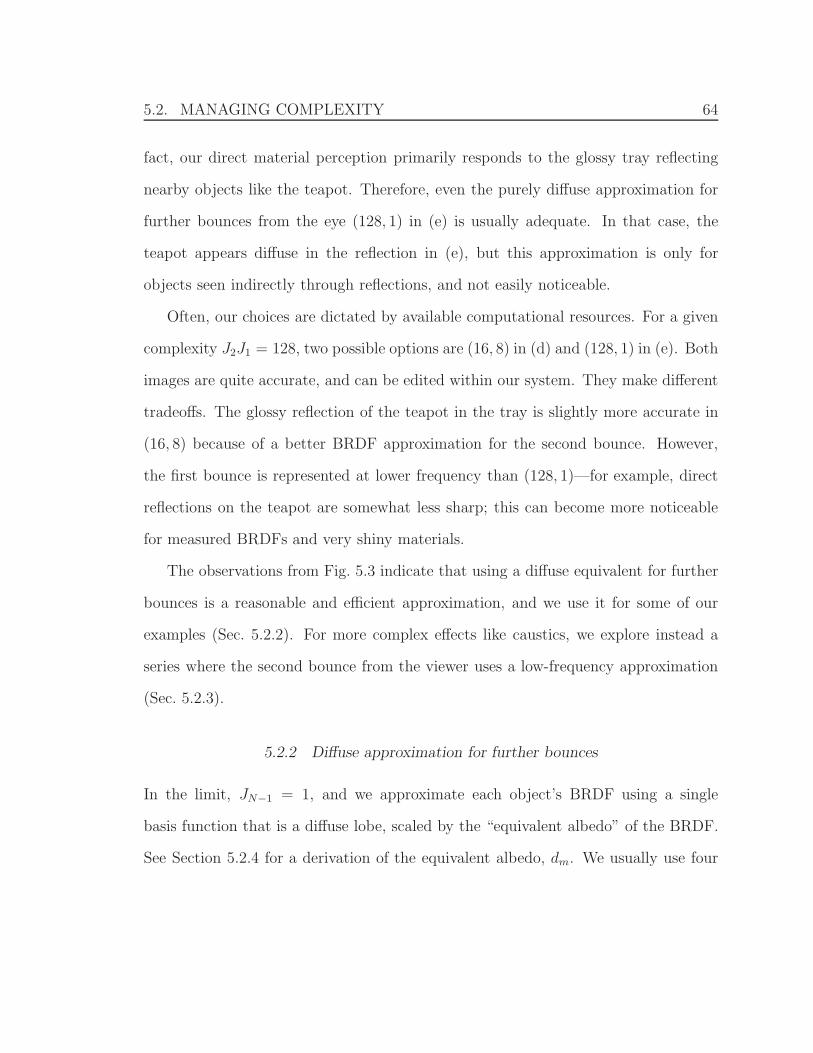
5.2. MANAGING COMPLEXITY 64
fact, our direct material perception primarily responds to the glossy tray reflecting
nearby objects like the teapot. Therefore, even the purely diffuse approximation for
further bounces from the eye (128, 1) in (e) is usually adequate. In that case, the
teapot appears diffuse in the reflection in (e), but this approximation is only for
objects seen indirectly through reflections, and not easily noticeable.
Often, our choices are dictated by available computational resources. For a given
complexity J2J1 = 128, two possible options are (16, 8) in (d) and (128, 1) in (e). Both
images are quite accurate, and can be edited within our system. They make different
tradeoffs. The glossy reflection of the teapot in the tray is slightly more accurate in
(16, 8) because of a better BRDF approximation for the second bounce. However,
the first bounce is represented at lower frequency than (128, 1)—for example, direct
reflections on the teapot are somewhat less sharp; this can become more noticeable
for measured BRDFs and very shiny materials.
The observations from Fig. 5.3 indicate that using a diffuse equivalent for further
bounces is a reasonable and efficient approximation, and we use it for some of our
examples (Sec. 5.2.2). For more complex effects like caustics, we explore instead a
series where the second bounce from the viewer uses a low-frequency approximation
(Sec. 5.2.3).
5.2.2 Diffuse approximation for further bounces
In the limit, JN−1 = 1, and we approximate each object’s BRDF using a single
basis function that is a diffuse lobe, scaled by the “equivalent albedo” of the BRDF.
See Section 5.2.4 for a derivation of the equivalent albedo, dm. We usually use four
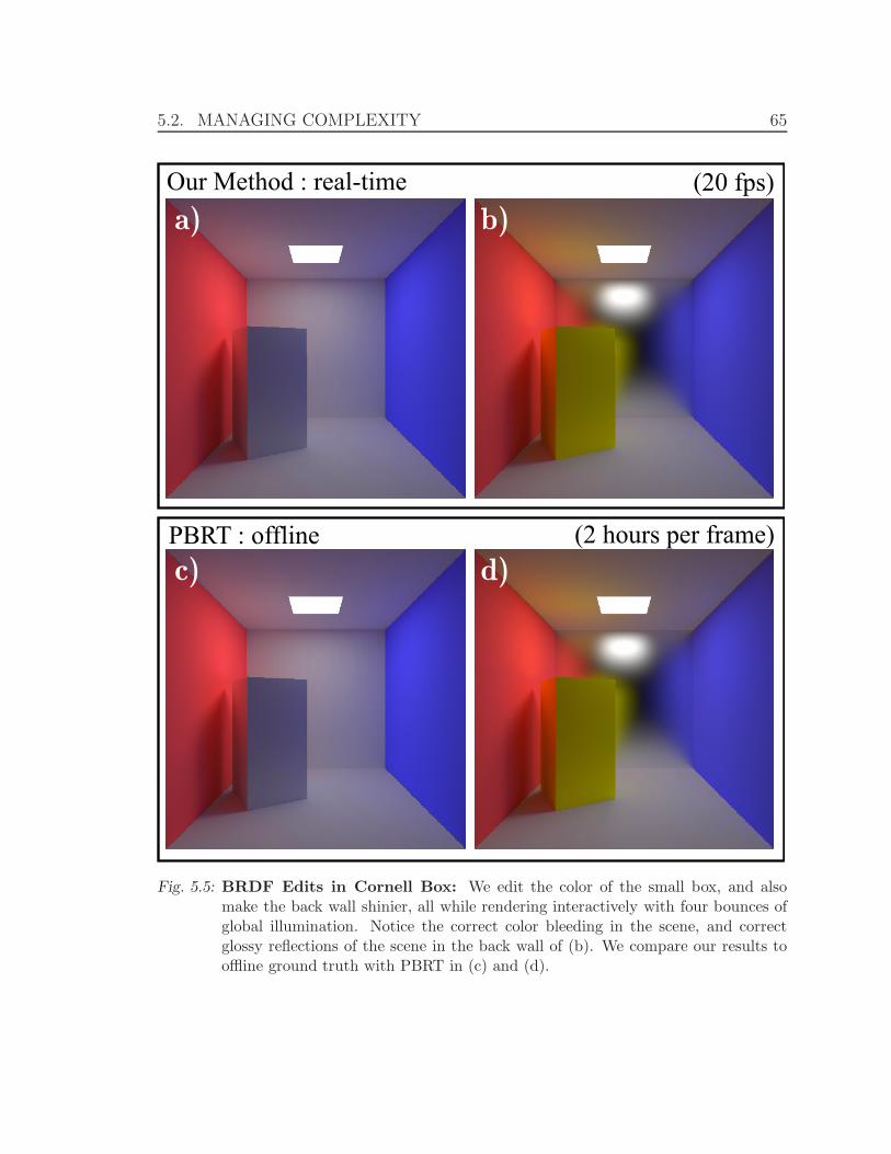
5.2. MANAGING COMPLEXITY 65
Our Method : real-timea)
c)
b)
d)PBRT : offline (2 hours per frame)
(20 fps)
Fig. 5.5: BRDF Edits in Cornell Box: We edit the color of the small box, and alsomake the back wall shinier, all while rendering interactively with four bounces ofglobal illumination. Notice the correct color bleeding in the scene, and correctglossy reflections of the scene in the back wall of (b). We compare our results tooffline ground truth with PBRT in (c) and (d).
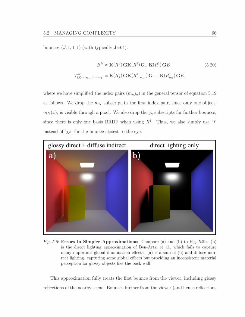
5.2. MANAGING COMPLEXITY 66
bounces (J, 1, 1, 1) (with typically J=64).
BN ≈K(RJ)GK(R1)G...K(R1)GE (5.20)
TN(j)(mN−1)···(m1) = K(RJ
j )GK(R1mN−1
)G . . .K(R1m1
)GE,
where we have simplified the index pairs (mnjn) in the general tensor of equation 5.19
as follows. We drop the mN subscript in the first index pair, since only one object,
mN (x), is visible through a pixel. We also drop the jn subscripts for further bounces,
since there is only one basis BRDF when using R1. Thus, we also simply use ‘j’
instead of ‘jN ’ for the bounce closest to the eye.
direct lighting onlyglossy direct + diffuse indirect
a) b)
Fig. 5.6: Errors in Simpler Approximations: Compare (a) and (b) to Fig. 5.5b. (b)is the direct lighting approximation of Ben-Artzi et al., which fails to capturemany important global illumination effects. (a) is a sum of (b) and diffuse indi-rect lighting, capturing some global effects but providing an inconsistent materialperception for glossy objects like the back wall.
This approximation fully treats the first bounce from the viewer, including glossy
reflections of the nearby scene. Bounces further from the viewer (and hence reflections
5.2. MANAGING COMPLEXITY 67
of objects not seen directly) are treated as diffuse. The complexity at each pixel
reduces from O((W )N) to O(J(M)N ). We will later see how this reduces further to
O(J) for rendering, since we edit only one object or material at a time.
Evaluation: Figures 5.5a and 5.5b are produced with our system. In (a), all surfaces
are diffuse, while in (b) we edit the back wall to make it a glossy material, and
change the color of the inner box to yellow. It is clear our method enables perception
of material appearance, because objects correctly reflect other nearby objects (see
the glossy interreflections of the room in the back wall in (b)), while also accurately
preserving global effects like color bleeding onto the large inner box. We compare
to ground truth using offline path tracing with PBRT in Figs. 5.5c and 5.5d, which
confirms the accuracy of the approximation.
By contrast, Fig. 5.6b shows the direct lighting approximation of (Ben-Artzi et al.,
2006b) for the configuration in Fig. 5.5b. Not only is it missing a lot of energy, but
it also lacks the reflections of the room in the back wall, which makes it difficult to
assess the desired glossiness while editing.
Note that our method treats the first bounce from the eye with the full BRDF to
get glossy reflections of nearby objects,
B ≈ E + K(RJ)GE + K(RJ)G
N∑
N=2
(K(R1)G
)N−1E.
Figure 5.6a compares to an alternative coarser approximation we originally tried using
our framework. This simply adds a diffuse indirect solution to the full direct lighting
result. It is essentially a series (1, 1, 1, 1) for the indirect illumination, and therefore
5.2. MANAGING COMPLEXITY 68
the most efficient technique,
B ≈ E + K(RJ)GE + K(R1)G
N∑
N=2
(K(R1)G
)N−1E,
where the main difference is that K(R1) is used instead of K(RJ) for the leftmost op-
erator of the multiple-bounce terms. Figure 5.6a is clearly better than direct lighting
only—some global illumination is usually better than none.
However, a comparison with Fig. 5.5b shows that while further bounces can be ap-
proximated as diffuse, the first bounce from the eye does need the full high-frequency
BRDF. Unlike our method, Fig. 5.6a gives an inconsistent material appearance of the
back wall, that may be difficult to interpret while editing. While the direct reflection
of the light source is glossy, the indirect reflections of the room appear diffuse.
5.2.3 Slower Decay of BRDF Series
Treating later bounces as diffuse works well in most scenes (see Figs. 6.1, 5.3e, 5.5
and 6.3). However, in some configurations like concave curved reflectors, higher fre-
quency indirect effects like caustics are visually important (Durand et al., 2005).
To handle such challenging situations, we need to reduce the BRDF frequencies
more slowly, using more (8-16) basis functions for the second bounce from the eye.
(Cases where even the third or higher bounces away from the eye need to be high-
frequency are quite rare, though our general framework does not preclude taking
them into account.) We compensate for the extra memory cost either by reducing
the number of bases for the first bounce (Fig. 5.3d) or by using fewer bounces (Fig. 6.5
has only two bounces).
We have already seen an example of using 8 BRDF basis functions for the second
bounce in Fig. 5.3(b-d), that gives a more accurate reflection of the teapot in the
5.2. MANAGING COMPLEXITY 69
shiny tray. In practice, our editing system also includes diffuse approximations for
the third and fourth bounces to augment the series in Fig. 5.3 (see table 6.1). An
even more challenging example is Fig. 6.5, that involves caustic effects. In this case,
we use 16 BRDF basis functions for the second bounce, with a BRDF series of the
form (J, J/4) ≡ (64, 16).
5.2.4 Equivalent Albedo
We choose the equivalent albedo to match the average BRDF value, or more exactly,
the output power for a uniform incident radiance field. This also corresponds formally
to choosing the best perturbed K operator, as in (Arvo et al., 1994). In other words,
d =1
π
∫ ∫ρ(ωi, ωo) cos θi cos θo dωidωo (5.21)
=1
π
∑
j
cj
∫ ∫ρq(ωi, ωo)bj(γ(ωi, ωo)) cos θi cos θo dωi, dωo.
The term in the integral now depends only on known quantities—the quotient BRDFs
and the basis functions, and can therefore be evaluated by dense Monte Carlo sam-
pling (this needs to be done only once for a given parameterization, not even for each
scene). Call this ej . Finally, at run-time, we simply need to compute
d =1
π
∑
j
cjej, (5.22)
with the predetermined ej and the dynamically chosen cj.
Note that the quotient BRDF must be included in equation 5.22 for energy con-
servation.
This section describes how we approximate a BRDF with an energy-conserving
equivalent diffuse BRDF. (Arvo et al., 1994) introduced a norm for the reflectance
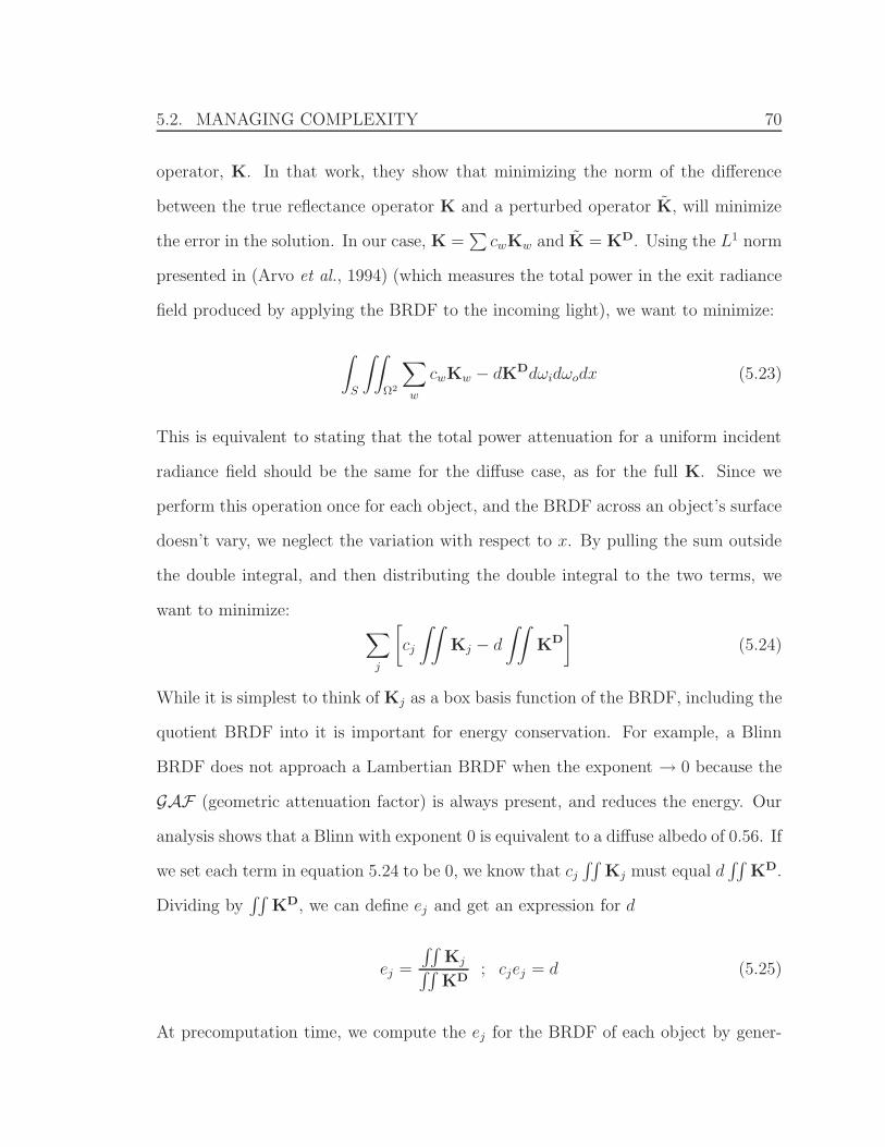
5.2. MANAGING COMPLEXITY 70
operator, K. In that work, they show that minimizing the norm of the difference
between the true reflectance operator K and a perturbed operator K, will minimize
the error in the solution. In our case, K =∑
cwKw and K = KD. Using the L1 norm
presented in (Arvo et al., 1994) (which measures the total power in the exit radiance
field produced by applying the BRDF to the incoming light), we want to minimize:
∫
S
∫∫
Ω2
∑
w
cwKw − dKDdωidωodx (5.23)
This is equivalent to stating that the total power attenuation for a uniform incident
radiance field should be the same for the diffuse case, as for the full K. Since we
perform this operation once for each object, and the BRDF across an object’s surface
doesn’t vary, we neglect the variation with respect to x. By pulling the sum outside
the double integral, and then distributing the double integral to the two terms, we
want to minimize:∑
j
[cj
∫∫Kj − d
∫∫KD
](5.24)
While it is simplest to think of Kj as a box basis function of the BRDF, including the
quotient BRDF into it is important for energy conservation. For example, a Blinn
BRDF does not approach a Lambertian BRDF when the exponent → 0 because the
GAF (geometric attenuation factor) is always present, and reduces the energy. Our
analysis shows that a Blinn with exponent 0 is equivalent to a diffuse albedo of 0.56. If
we set each term in equation 5.24 to be 0, we know that cj
∫∫Kj must equal d
∫∫KD.
Dividing by∫∫
KD, we can define ej and get an expression for d
ej =
∫∫Kj∫∫KD
; cjej = d (5.25)
At precomputation time, we compute the ej for the BRDF of each object by gener-

5.2. MANAGING COMPLEXITY 71
ating several thousand light and view direction using the path-tracer’s Monte Carlo
method. At run-time, we compute d, given the user-defined cj. This gives us the
albedo of a diffuse object that would reflect the same percentage of incoming radi-
ance as the user-defined BRDF. This technique can be generalized to approximations
with more than a single basis function.
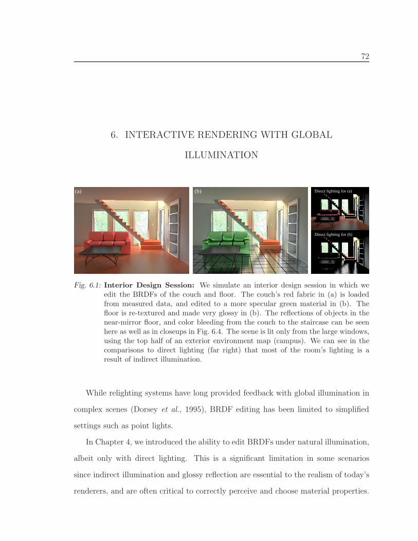
72
6. INTERACTIVE RENDERING WITH GLOBAL
ILLUMINATION
(a) (b) Direct lighting for (a)
Direct lighting for (b)
Fig. 6.1: Interior Design Session: We simulate an interior design session in which weedit the BRDFs of the couch and floor. The couch’s red fabric in (a) is loadedfrom measured data, and edited to a more specular green material in (b). Thefloor is re-textured and made very glossy in (b). The reflections of objects in thenear-mirror floor, and color bleeding from the couch to the staircase can be seenhere as well as in closeups in Fig. 6.4. The scene is lit only from the large windows,using the top half of an exterior environment map (campus). We can see in thecomparisons to direct lighting (far right) that most of the room’s lighting is aresult of indirect illumination.
While relighting systems have long provided feedback with global illumination in
complex scenes (Dorsey et al., 1995), BRDF editing has been limited to simplified
settings such as point lights.
In Chapter 4, we introduced the ability to edit BRDFs under natural illumination,
albeit only with direct lighting. This is a significant limitation in some scenarios
since indirect illumination and glossy reflection are essential to the realism of today’s
renderers, and are often critical to correctly perceive and choose material properties.
6.1. IMPLEMENTATION 73
For precomputation (Sec. 6.1.1), we show how Monte Carlo path tracing can be
extended to precompute the multi-bounce tensors needed. For rendering (Sec. 6.1.2),
since only one object’s BRDF is edited at a time, we show that the tensor can be
reduced to a few vector dot products at each pixel, whose coefficients can be computed
in a very fast runtime preprocess. Our results show a variety of BRDF edits, with
interactive feedback rendered with global illumination.
6.1 Implementation
We now describe our implementation, starting with our precomputation method
(Sec. 6.1.1), followed by the rendering algorithm (Sec. 6.1.2), and some practical
extensions (Sec. 6.1.3).
6.1.1 Monte Carlo Precomputation
We need to precompute the tensors defined by equation 5.19 at each pixel. The
important special case for diffuse approximation in further bounces is given by equa-
tion 5.20. Recall that the K operators involve integrals over the hemisphere, which
means that each TN(x) requires nested (high-dimensional) integrals over ray paths.
This is similar to traditional global illumination.
We adapt Monte Carlo path tracing (Kajiya, 1986) for precomputation because
of its flexibility, ease of implementation and negligible memory overhead.
Each value in the different tensors can be seen as a separate integral over the
space of paths. However, it is easier and more similar to traditional path tracing to
sample path space for all integrals at the same time. We generate random paths, and
for each path update the appropriate tensor integrals. We must modify three basic
aspects of the path tracer. First, we cannot generate rays by sampling the BRDF
6.1. IMPLEMENTATION 74
(since it is unknown). Second, we must add each path’s contribution to the correct
tensor element, as opposed to simply contributing to the final pixel radiance. Third,
we must compute the contribution of each path using basis BRDFs.
Consider a given path �X from a point on a light source ( ) to the eye (e), that
passes through points xN , xN−1, . . . , x1 on objects mN , mN−1, . . . , m1, as illustrated in
Fig. 6.2.
Sampling path space: According to Monte Carlo theory, any random sampling can
be used to generate new directions when building up the path. We follow standard
path tracing and generate rays recursively from the eye. We sample the light source
at each bounce to generate all path lengths.
Path tracers usually importance sample the BRDF to select a new direction at
each intersection. Unfortunately, we have no knowledge of the final BRDF. We can-
not sample according to the basis BRDFs either because they will be combined with
arbitrary weights at runtime. The simplest approach would be to sample the cosine-
weighted hemisphere uniformly, but this would yield high variance when sharp spec-
ular lobes are used. Instead, we take advantage of the general form of typical BRDFs
and sample according to a mixture of 70% diffuse, and 30% high-gloss (Blinn exponent
of 200). This places more importance on specular directions and enables low-noise
results for the full range of glossy to near-mirror BRDFs in a practical editing session.
Tensor update: For each random path, we need to accumulate a contribution to
the appropriate tensor element. In effect, we are computing coefficients in a symbolic
polynomial representation of the basis BRDFs (in the spirit of symbolic rendering by
(Sequin & Smyrl, 1989)). In our case, we have chosen bases that do not overlap, and
therefore a given path requires updating exactly one tensor element. The j index
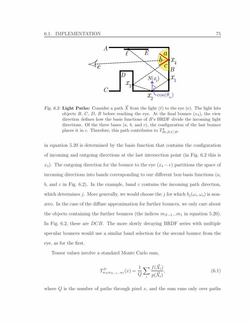
6.1. IMPLEMENTATION 75
x1
x2
x3
x4�
e
A
B
C
D
E abc
N(x2)
cos(θin)
Fig. 6.2: Light Paths: Consider a path �X from the light (�) to the eye (e). The light hitsobjects B, C, D, B before reaching the eye. At the final bounce (x4), the viewdirection defines how the basis functions of B’s BRDF divide the incoming lightdirections. Of the three bases (a, b, and c), the configuration of the last bounceplaces it in c. Therefore, this path contributes to T 4
Bc,D,C,B.
in equation 5.20 is determined by the basis function that contains the configuration
of incoming and outgoing directions at the last intersection point (in Fig. 6.2 this is
x4). The outgoing direction for the bounce to the eye (x4− e) partitions the space of
incoming directions into bands corresponding to our different box-basis functions (a,
b, and c in Fig. 6.2). In the example, band c contains the incoming path direction,
which determines j. More generally, we would choose the j for which bj(ωi, ωo) is non-
zero. In the case of the diffuse approximation for further bounces, we only care about
the objects containing the further bounces (the indices mN−1...m1 in equation 5.20).
In Fig. 6.2, these are DCB. The more slowly decaying BRDF series with multiple
specular bounces would use a similar band selection for the second bounce from the
eye, as for the first.
Tensor values involve a standard Monte Carlo sum,
TNwNwN−1...w1
(x) =1
Q
∑
i
f( �Xi)
p( �Xi), (6.1)
where Q is the number of paths through pixel x, and the sum runs only over paths
6.1. IMPLEMENTATION 76
�Xi that correspond to the specific subscripts (bands and objects) in T N . f( �Xi) is the
contribution of �Xi, and p( �Xi) is the probability of generating it.
Path Contribution: In standard path tracing, the path contribution f( �Xi) is the
direct visible lighting at x1, multiplied by the product of BRDFs (corresponding to
K) and cosine terms at each intersection (the visibility in G is already considered
when creating valid paths). In our case, we must instead multiply by the appropriate
basis BRDFs.
For the first bounce from the eye, we use
bj(e, xN , xN−1) = bmN (xN )j (ωi, ωo) cos θi, (6.2)
where ωi(xN , xN−1) and θi(xN , xN−1) depend on the direction of the incident ray,
and ωo(e, xN) on the outgoing view direction. For the slowly decaying series, a very
similar form can be used for the second bounce from the eye, simply considering a
lower-frequency bj(xN , xN−1, xN−2). For the other bounces, we use the single diffuse
basis:
D(xn, xn−1) =1
πcos(θi(xn, xn−1)). (6.3)
Finally, f( �X) is a product of the terms at each bounce. For the diffuse approximation
for further bounces, this is
f( �X) = bmN (xN )j (ωi, ωo)D(xN−1, xN−2) . . .D(x1, )E( ). (6.4)
Optimizations: Our precomputation is essentially the same complexity as rendering
a single image with MCPT. Moreover, many standard path tracing optimizations can
still be applied. For example, we have adapted irradiance caching (Ward et al.,
6.1. IMPLEMENTATION 77
1988)—instead of generating paths that terminate at the light source, we find the
direct lighting at the last surface point x1. We cache the irradiance in a preprocess
that samples visibility on a grid within each triangle.
6.1.2 Rendering in Real Time
We now focus on the runtime rendering computation for each pixel. For compactness
of notation, this subsection will deal primarily with the diffuse approximation for
further bounces, but more slowly decaying series use very similar methods, and are
discussed briefly at the end.
To simplify notation, we denote the tensor as T Njz (x), where the single “super-
index” z is a short-hand for writing out mN−1...m1 in equation 5.20 (viewed as an
index, z ∈ [1, Z = (M)N−1]). Similarly, we also denote the product of diffuse equiva-
lents dm of each object by dz,
z ≡ {mN−1, · · · , mn, · · · , m1}
dz ≡ dmN−1dmN−2
· · · dmn · · · dm2dm1 . (6.5)
Note that z represents a list of indices, while dz is a single number, corresponding to
the product of the albedos dm.
Finally, we can adapt equation 5.14 for rendering,
BN(x) =
J∑
j=1
Z∑
z=1
TNjz (x) cjdz. (6.6)
During the edit, the user specifies the BRDF coefficients cj (either directly by editing
a curve, or implicitly by editing a parametric model). The diffuse equivalents d
(and hence dz) are then computed as described in Section 5.2.4. Finding the cj and
6.1. IMPLEMENTATION 78
dz occurs once per frame for the whole image. Using the precomputed T Njz (x), the
double summation in equation 6.6 must now be evaluated at each pixel.
Object Freezing: Equation 6.6 requires O(JZ) operations per pixel. On modern
hardware, this is fast, but still not real-time (requiring a couple of seconds per update).
To reduce complexity, we observe that a user edits the BRDF of only one object at a
time. We use a run-time precomputation that performs the bulk of the calculations
in Equation 6.6 by temporarily “freezing” the BRDFs of the remaining objects.
Recall that dz represents a multi-variable polynomial in the d’s of the objects in
the scene. For example, if we have z = {1, 3, 2, 1, 5, 3}, dz = (d1)2d2(d3)
2d5. However,
if all but one of the d’s are fixed, this becomes just a single-variable polynomial in the
unfrozen d of the object being edited. For example, if all but object 1 are “frozen”,
we can define a constant A = d2(d3)2d5, so that dz becomes a simple quadratic
polynomial, dz = A · (d1)2 in only the edited variable d1.
To implement this scheme more formally, we need a helper function n(z, i) that
tells us how many times a given edited object i appears in z. In the above example,
n(z, i) = 2 (for i = 1) that tells us dz is a quadratic polynomial in di alone. We
can also define the constant A more formally as A = dz/(di)n. Finally, we compute
at run-time a new tensor of coefficients at each pixel, where each row represents a
single-variable polynomial in di,
F ijn(x) =
∑
N
∑
z
⎧⎪⎨
⎪⎩
n(z, i) = n : 0
n(z, i) = n : TNjz (x) dz
(di)n
(6.7)
6.1. IMPLEMENTATION 79
Our real-time rendering step is now a direct evaluation of
B(x) =
N−1∑
n=0
(di)n
J∑
j=1
cjFijn(x). (6.8)
For each power (di)n, we simply evaluate a dot-product cjFj, essentially as in a
standard linear PRT formulation.
The computation in equation 6.7 requires O(JZ) operations per pixel, comparable
to simply evaluating equation 6.6 directly once. This requires a short (usually 5-10
seconds) mode switch each time the user begins editing a different object. The real-
time rendering in equation 6.8 is now O(J) (the number of bounces N is a small
constant, usually four.)
Two further optimizations are possible. In a practical editing session, the coeffi-
cients cj change slowly from frame to frame, especially if we transform into a wavelet
representation. This temporal coherence can be directly exploited using the incre-
mental wavelet rendering method described in (Ben-Artzi et al., 2006b). Finally, if
we are rendering a pixel of an object that is not being edited, the cj do not change
at all. (Note however, that the object’s appearance will still be affected because of
global illumination.) This makes it possible to further precompute V in =
∑j F i
jncj ,
reducing the cost to evaluating a simple polynomial in di.
Slower Decaying Series: We briefly describe the generalization to more slowly de-
caying series, as in Sec. 5.2.3. The general rendering operation of Equation 6.6 is
now best described as a triple-summation, since we are dealing with three distinct
representations of R: RJN , RJN−1, and R1.
BN(x) =
JN∑
j=1
MJN−1∑
w=1
Z∑
z=1
TNjwz(x) cj cwdz, (6.9)
6.1. IMPLEMENTATION 80
with cw denoting the lower-frequency BRDF coefficients for the second bounce (JN−1
bases on each of the M objects).
Object freezing is a bit more difficult, theoretically requiring the creation of a
three-dimensional F ijkn, where j ∈ [1, JN ], k ∈ [1, JN−1], n ∈ [0, N−2]. In practice, we
think of the j as one dimension, and k′ ≡ kn as the other.
6.1.3 Extensions
We briefly describe two important practical extensions.
Objects with Fixed BRDFs: Large scenes can contain many small objects that
cause an exponential increase in memory requirements. Such scenes usually do not
require editing the BRDFs of all objects. When designing the materials in a room,
one typically does not want to change the BRDFs of small “placeholder” objects like
books or toys. We extend our algorithm by implementing the ability to fix the BRDFs
of certain objects at precomputation. Note that their shading is still updated, based
on global illumination from other surfaces. This should also not be confused with
run-time object freezing above, which occurs temporarily during an editing session.
In precomputation, instead of using diffuse equivalents D or BRDF bases b, we
must use the full known BRDF ρm(ωi, ωo) cos θi for reflections from fixed object m.
Rendering is unchanged for editable objects, since there are no new BRDF bases. For
the fixed object, we still use T Nz (x) and multiply by the diffuse albedos of editable
objects. However, the BRDF bases (and index j) need not be considered. In Fig. 6.1,
the table and its legs have fixed BRDFs.
Spatial Weight Maps: So far, we have focused on BRDF effects. Spatial variation
can be handled with textures to modulate the BRDF over an object’s surface. If we do
6.1. IMPLEMENTATION 81
not seek to edit them, the textures can be directly incorporated into the BRDF basis
functions (as the multiplicative Hm(x) terms in equation 5.5). Finally, while we have
discussed a single BRDF per object for clarity, our framework and implementation
can handle multiple co-located BRDFs for each object. If we also seek to modify the
spatial blending of BRDFs, as we do for the floor in Fig. 6.1, we can simply modulate
the directly viewed surfaces in image-space by the multiplicative spatial blending
weights (weight maps) or texture. For global illumination, we are concerned only
with the low-frequency behavior of the weight maps or textures, and we modulate
the diffuse equivalent albedos by the average value of the weight map for each BRDF
layer.
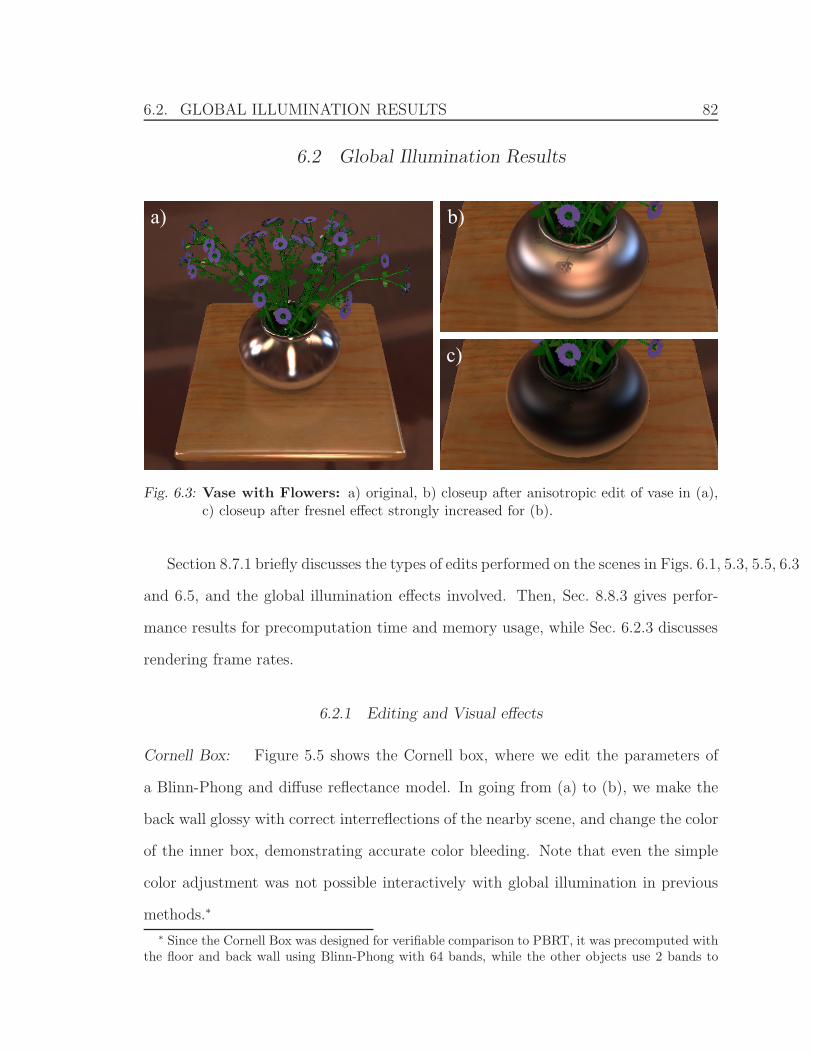
6.2. GLOBAL ILLUMINATION RESULTS 82
6.2 Global Illumination Results
a) b)
c)
Fig. 6.3: Vase with Flowers: a) original, b) closeup after anisotropic edit of vase in (a),c) closeup after fresnel effect strongly increased for (b).
Section 8.7.1 briefly discusses the types of edits performed on the scenes in Figs. 6.1, 5.3, 5.5, 6.3
and 6.5, and the global illumination effects involved. Then, Sec. 8.8.3 gives perfor-
mance results for precomputation time and memory usage, while Sec. 6.2.3 discusses
rendering frame rates.
6.2.1 Editing and Visual effects
Cornell Box: Figure 5.5 shows the Cornell box, where we edit the parameters of
a Blinn-Phong and diffuse reflectance model. In going from (a) to (b), we make the
back wall glossy with correct interreflections of the nearby scene, and change the color
of the inner box, demonstrating accurate color bleeding. Note that even the simple
color adjustment was not possible interactively with global illumination in previous
methods.∗
∗ Since the Cornell Box was designed for verifiable comparison to PBRT, it was precomputed withthe floor and back wall using Blinn-Phong with 64 bands, while the other objects use 2 bands to

6.2. GLOBAL ILLUMINATION RESULTS 83
Teatray: Figure 5.3 shows a teatray scene. The teapot has a Cook-Torrance BRDF
with specular and diffuse components, and the handles and tray a Blinn-Phong model.
While only a single set of BRDFs for the objects is shown in Fig. 5.3 for brevity, we
can freely edit the teapot, tray and handles in real-time, using any of the BRDF series
shown in the figure (extended to three or four bounces).
Vase: Figure 6.3 shows a variety of flexible BRDFs possible within our system. The
flowers are diffuse, while the stems are a diffuse+specular BRDF to enable a glossy
coating. The table has diffuse and specular BRDFs, with the diffuse shown textured
in Fig. 6.3. The vase uses a diffuse and a specular layer. The specular BRDF is an
Ashikhmin-Shirley BRDF with fixed exponent of 225, but adjustable ratio to adjust
the direction and amount of anisotropy (see Section 3.3.2). A second specular layer
allows for edits to the Fresnel term. Section 3.3.1 describes how to enable Fresnel
control for any BRDF via a second additive layer.†
Room: Figure 6.1 shows one potential application of our system to design interiors.
In this case, indirect light is critical, since a large part of the scene, like the back wall
and much of the couch, would be black with direct lighting only. Most of the indirect
illumination is low-frequency, so we use our diffuse approximation for further bounces.
We only use three bounces, with a BRDF series (64, 1, 1), since we found that the
fourth bounce contributed relatively little to the qualitative appearance of the scene.
This is a complex scene with 8 objects (6 editable), environment lighting from
the windows, and a variety of materials including measured reflectance and textures,
which can all be edited. Our system renders interactive feedback with global illu-
represent a pure diffuse BRDF with editable albedo.† The glossy layers of the stems and table use 64 bands. The Ashikhmin-Shirley layers of the vase
use 256 bands. All diffuse layers use 2 bands.
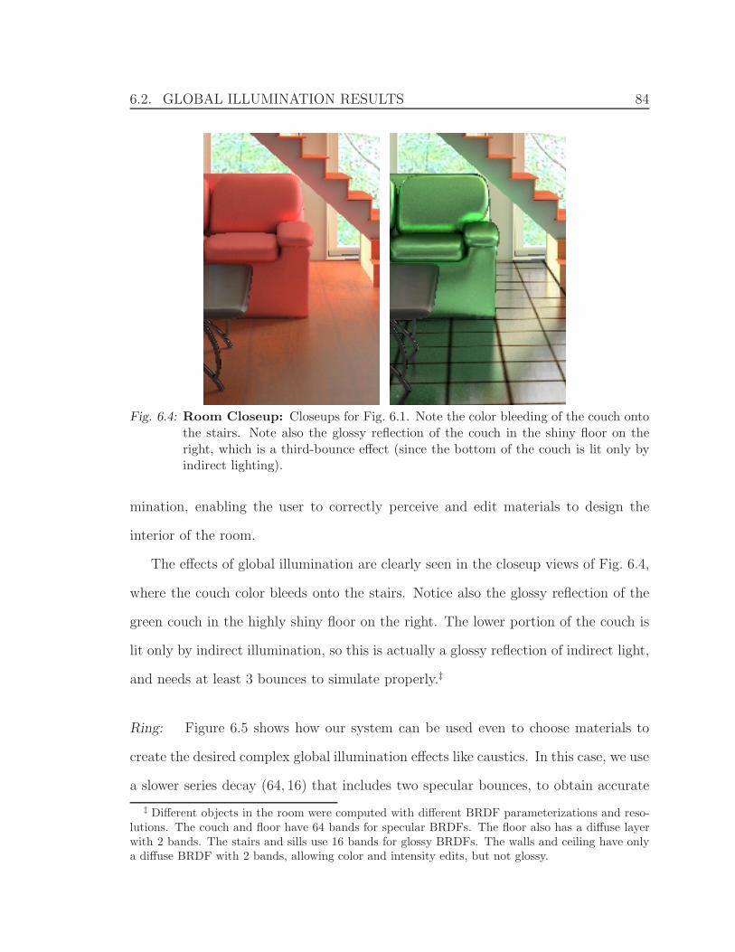
6.2. GLOBAL ILLUMINATION RESULTS 84
Fig. 6.4: Room Closeup: Closeups for Fig. 6.1. Note the color bleeding of the couch ontothe stairs. Note also the glossy reflection of the couch in the shiny floor on theright, which is a third-bounce effect (since the bottom of the couch is lit only byindirect lighting).
mination, enabling the user to correctly perceive and edit materials to design the
interior of the room.
The effects of global illumination are clearly seen in the closeup views of Fig. 6.4,
where the couch color bleeds onto the stairs. Notice also the glossy reflection of the
green couch in the highly shiny floor on the right. The lower portion of the couch is
lit only by indirect illumination, so this is actually a glossy reflection of indirect light,
and needs at least 3 bounces to simulate properly.‡
Ring: Figure 6.5 shows how our system can be used even to choose materials to
create the desired complex global illumination effects like caustics. In this case, we use
a slower series decay (64, 16) that includes two specular bounces, to obtain accurate
‡ Different objects in the room were computed with different BRDF parameterizations and reso-lutions. The couch and floor have 64 bands for specular BRDFs. The floor also has a diffuse layerwith 2 bands. The stairs and sills use 16 bands for glossy BRDFs. The walls and ceiling have onlya diffuse BRDF with 2 bands, allowing color and intensity edits, but not glossy.
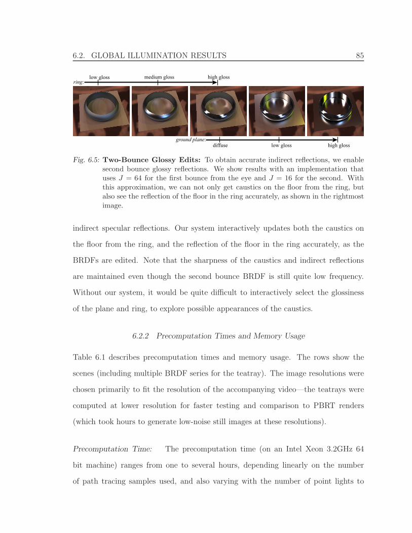
6.2. GLOBAL ILLUMINATION RESULTS 85
low glossring:
high gloss
diffuseground plane:
high glosslow gloss
medium gloss
Fig. 6.5: Two-Bounce Glossy Edits: To obtain accurate indirect reflections, we enablesecond bounce glossy reflections. We show results with an implementation thatuses J = 64 for the first bounce from the eye and J = 16 for the second. Withthis approximation, we can not only get caustics on the floor from the ring, butalso see the reflection of the floor in the ring accurately, as shown in the rightmostimage.
indirect specular reflections. Our system interactively updates both the caustics on
the floor from the ring, and the reflection of the floor in the ring accurately, as the
BRDFs are edited. Note that the sharpness of the caustics and indirect reflections
are maintained even though the second bounce BRDF is still quite low frequency.
Without our system, it would be quite difficult to interactively select the glossiness
of the plane and ring, to explore possible appearances of the caustics.
6.2.2 Precomputation Times and Memory Usage
Table 6.1 describes precomputation times and memory usage. The rows show the
scenes (including multiple BRDF series for the teatray). The image resolutions were
chosen primarily to fit the resolution of the accompanying video—the teatrays were
computed at lower resolution for faster testing and comparison to PBRT renders
(which took hours to generate low-noise still images at these resolutions).
Precomputation Time: The precomputation time (on an Intel Xeon 3.2GHz 64
bit machine) ranges from one to several hours, depending linearly on the number
of path tracing samples used, and also varying with the number of point lights to
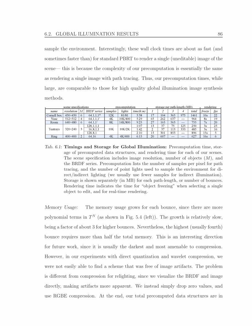
6.2. GLOBAL ILLUMINATION RESULTS 86
sample the environment. Interestingly, these wall clock times are about as fast (and
sometimes faster than) for standard PBRT to render a single (uneditable) image of the
scene— this is because the complexity of our precomputation is essentially the same
as rendering a single image with path tracing. Thus, our precomputation times, while
large, are comparable to those for high quality global illumination image synthesis
methods.
scene specifications precomputation storage per path-length (MB) rendering
name resolution M BRDF series samples lights time(h:m) 1 2 3 4 total freeze fps
Cornell box 450×450 6 64,1,1,1* 12K 81/81 5:58 17 104 365 975 1461 10s 22 Vase 512×512 4 64,1,1,1† 4K 10K/400 5:29 65 262 637 — 964 8s 19 Room 640×480 6 64,1,1‡ 8K 14K/800 9:25 27 165 563 — 755 7s 20
128,1,1,1 1:07 13 37 75 125 250 3s 25 16,8,1,1 1:42 2 37 113 333 485 3s 16 Teatrays 320×240 3
128,8,1
10K 10K/2K
2:10 13 301 853 — 896 15s 5 Ring 400×400 2 64,16 4K 4K/400 6:15 20 607 — — 627 16s 6
Tab. 6.1: Timings and Storage for Global Illumination: Precomputation time, stor-age of precomputed data structures, and rendering time for each of our scenes.The scene specification includes image resolution, number of objects (M), andthe BRDF series. Precomputation lists the number of samples per pixel for pathtracing, and the number of point lights used to sample the environment for di-rect/indirect lighting (we usually use fewer samples for indirect illumination).Storage is shown separately (in MB) for each path-length, or number of bounces.Rendering time indicates the time for “object freezing” when selecting a singleobject to edit, and for real-time rendering.
Memory Usage: The memory usage grows for each bounce, since there are more
polynomial terms in T N (as shown in Fig. 5.4 (left)). The growth is relatively slow,
being a factor of about 3 for higher bounces. Nevertheless, the highest (usually fourth)
bounce requires more than half the total memory. This is an interesting direction
for future work, since it is usually the darkest and most amenable to compression.
However, in our experiments with direct quantization and wavelet compression, we
were not easily able to find a scheme that was free of image artifacts. The problem
is different from compression for relighting, since we visualize the BRDF and image
directly, making artifacts more apparent. We instead simply drop zero values, and
use RGBE compression. At the end, our total precomputed data structures are in
6.2. GLOBAL ILLUMINATION RESULTS 87
the range of several hundred MB. While this is large, it is comparable, for instance,
to all-frequency relighting approaches on similar resolution images.
Note that the storage sizes shown in Table 6.1 are larger than the theoretical
runtime memory requirements. Due to our object freezing step, only the smaller F ijn
in equation 6.7 needs to be in main memory. We can avoid preloading all of the data
at the cost of higher object-switch times.
In comparing the different BRDF series for the teatray, (128, 8, 1) requires the
most memory, because of the extra factor of 8 for second bounce BRDF bases (as
opposed to (16, 8, 1, 1) and (128, 1, 1, 1)). To keep memory consumption reasonable,
we limit to 3 bounces rather than 4 as with the other series. These numbers are
comparable to the ring, that also uses 16 bases in the second bounce. (We similarly
limit the number of bounces in the ring to two (64, 16)).
6.2.3 Rendering Speed
For simplicity, we pursue a purely software implementation, although the simple dot-
product form of equation 6.8 indicates that GPU implementations, similar to those
recently developed for relighting should also be applicable.
As can be seen in the video and the last column of table 6.1, our software method
achieves frame rates of 15-25fps on most scenes. The time for “object-freezing” when
we switch from one object to another for editing is about 5-10 seconds, and isn’t
disruptive to typical editing sessions, as seen in the video. The rendering and mode
switch times are somewhat larger when there are more BRDF bases for the second
bounce (one teatray example and ring), on account of the additional complexity.
However, they are still interactive, and our video demonstrates interactive editing of
the ring scene. In summary, our results and video for the first time show practical
real-time BRDF editing, as interactive feedback is rendered with global illumination.

Part III
NEW CONCEPTS APPLICABLE TO BRDF EDITING
AND MORE
89
The general theoretical framework presented in Part II can be improved with
several orthogonal developments presented in this part. These concepts merit an
independent discussion because they are easily beneficial to BRDF editing, as well
as other applications in computer graphics. Chapter 7 will introduce an improve-
ment of the standard dot-product performed at each pixel during rendering in a
precomputation-based context. The improvement relies on the temporal coherence
of inputs from frame to frame, without being specific to the meaning encoded in the
input vectors. Chapter 8 presents a fast method for computing visibility of a lighting
environment. This calculation is a necessary step to shading surface illuminate by
environment maps. It is also required by the precomputation steps discussed in Part
II. Instead of casting shadow rays to 100’s of sample points in an environment map,
the visibility function can constructed with an accurate prediction of about 90% of
the shadow rays. This gain is achieved by relying on the spatial coherence of visibil-
ity in typical scenes. Chapter 9 presents a novel function editing framework. This
method of editing 1D functions is utilized as the user interface for editing 1D BRDF
factors as described in Part II. The operations described in Chapter 9 can be equally
applied to any graphics application that requires editing 1D functions, such as the
curves tool in image-editing software, and time-dependent parameters in animations.
90
7. TEMPORAL COHERENCE FOR REAL-TIME
PRECOMPUTED RENDERING
In Part II, Sections 4.1 and 6.1.2 phrase the real-time rendering operation as a dot-
product at each pixel. One of the vectors of the dot-product is constant throughout
the editing session, but unique to each pixel. The other vector changes from frame-
to-frame, but is uniform across all pixels of an object. The methods described in this
chapter are equally applicable to any operation which has this same nature for the
two vectors of a dot-product. For a concrete application, we will describe it in terms
of equation 4.7 in Section 4.1.
Recall that Chapter 4 described how to obtain the transport vector T, and vector
of function coefficients c, required by equation 4.7. The number of elements in the
dot-product T · c , can be quite large, and when performed at each pixel, modern
CPUs may not be able to render this in real-time. A common solution is to transform
both vectors into a wavelet basis, and then use a non-linear wavelet approximation
that makes these vectors sparse,
Riperfect = T · ci
perfect (7.1)
Rieffective = T · ci
effective (7.2)
where cieffective is the representation of ci
perfect after approximation, and Rieffective is
the effective (approximate) image displayed. This method has two drawbacks for
91
us. First, we cannot compress as aggressively as relighting methods, which never
directly visualize the lighting 1 . We need to keep many more terms in cieffective ,
since both lighting and BRDF retain all frequencies. Second, the standard non-linear
wavelet approximation, by definition ignores small coefficients, often giving the user
no feedback when small adjustments are made to the BRDF.
We note that c tends to change by small amounts between frames, since the user
is continuously editing the 1D curve that defines it. We take advantage of this by
rendering the current frame i, using the change cidiff relative to the previous frame
i− 1,
cidiff = ci
perfect − ci−1effective (7.3)
The c’s of consecutive frames tend to be more similar when they are coefficients of
a wavelet basis. In interactive editing, one is usually making local modifications to the
curve, so cidiff has only a few nonzero wavelet coefficients, even when ci
perfect would
need many terms for accurate approximation. We must also consider occasional cases
where cidiff has more nonzero wavelet terms than we can afford to use in a single
frame. This happens when the user makes drastic changes that affect the entire curve
(such as a uniform scaling). To handle these situations within our framework, we use
a standard non-linear wavelet approximation, cidiff , of ci
diff . For most frames, cidiff
will be equal to cidiff , but allowing for approximation makes our system robust when
large changes occur (or if the wavelet budget is very small).
1 Relighting implicitly assumes the BRDF is lower frequency than the lighting (no near-mirror),thus being more forgiving of lighting approximations.
7.1. USE IN BRDF EDITING 92
Our final equations for incremental rendering then become:
Rieffective = Ri−1
effective + T · cidiff (7.4)
cieffective = ci−1
effective + cidiff , (7.5)
where we make explicit that the final radiance, Rieffective may not be exact. Equation
7.5 shows how we keep track of the cieffective , so that ci+1
diff can be calculated in the
next frame, per equation 7.3. Note that the expensive operation here is the (per-pixel)
dot-product (T · cdiff ) just as in standard (non-incremental) PRT rendering.
Even though we never explicitly calculate the dot-product in equation 7.2, our
incremental updates in equation 7.4 effectively give the same result. The main dif-
ference is that our ceffective are not approximated with a predetermined budget, but
rather can get arbitrarily close (and often equal) to cperfect. Table 7.1 uses equations
7.3-7.5 to compute successive frames of a didactic editing session.
Incremental wavelet rendering addresses the issues mentioned at the start of this
chapter. Since work is focused only in the local region where the user is chang-
ing the BRDF, our system almost always renders reference-quality images. In rare
cases, when the region of change is large, and cannot be exactly captured in a single
incremental update, our system automatically continues to refine the image using
equations 7.4 and 7.5 until ceffective equals cperfect.
7.1 Use in BRDF editing
Rendering is real-time, at about 25fps, and with rapid interactive switching between
curves if the user desires. We typically use 30 wavelet coefficients for each frame. Our
incremental rendering algorithm ensures essentially reference-quality images while
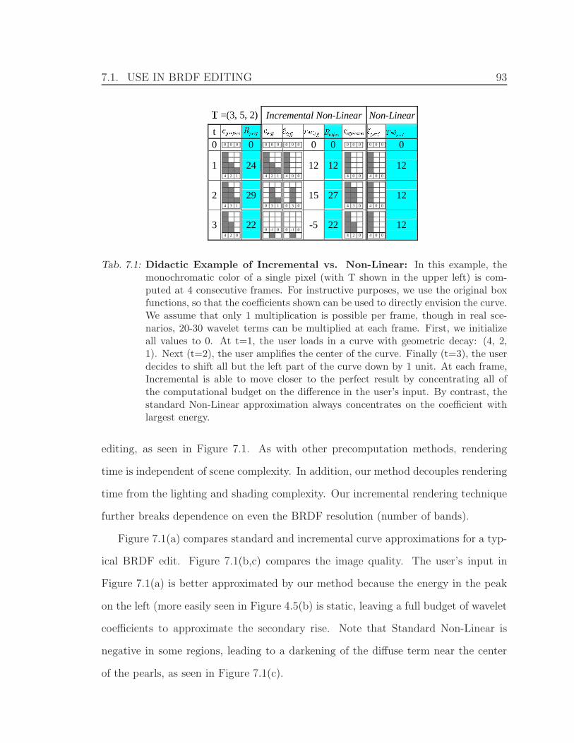
7.1. USE IN BRDF EDITING 93
T =(3, 5, 2) Incremental Non-Linear Non-Linear
t perfectc perfR diffc diffc�
diffT c�i effecR effectivec
perfc� perfT c�i
0 0 0 0 0 0 0 0 0 0 0 0 0 0 0 0 0 0 0 0
1
4 2 1 24
4 2 1
4 0 0
12 12 4 0 0
4 0 0
12
2 4 3 1
29 0 3 1
0 3 0
15 27 4 3 0
4 0 0
12
3 4 2 0
22
0 -1 0
0 -1 0
-5 22
4 2 0
4 0 0
12
Tab. 7.1: Didactic Example of Incremental vs. Non-Linear: In this example, themonochromatic color of a single pixel (with T shown in the upper left) is com-puted at 4 consecutive frames. For instructive purposes, we use the original boxfunctions, so that the coefficients shown can be used to directly envision the curve.We assume that only 1 multiplication is possible per frame, though in real sce-narios, 20-30 wavelet terms can be multiplied at each frame. First, we initializeall values to 0. At t=1, the user loads in a curve with geometric decay: (4, 2,1). Next (t=2), the user amplifies the center of the curve. Finally (t=3), the userdecides to shift all but the left part of the curve down by 1 unit. At each frame,Incremental is able to move closer to the perfect result by concentrating all ofthe computational budget on the difference in the user’s input. By contrast, thestandard Non-Linear approximation always concentrates on the coefficient withlargest energy.
editing, as seen in Figure 7.1. As with other precomputation methods, rendering
time is independent of scene complexity. In addition, our method decouples rendering
time from the lighting and shading complexity. Our incremental rendering technique
further breaks dependence on even the BRDF resolution (number of bands).
Figure 7.1(a) compares standard and incremental curve approximations for a typ-
ical BRDF edit. Figure 7.1(b,c) compares the image quality. The user’s input in
Figure 7.1(a) is better approximated by our method because the energy in the peak
on the left (more easily seen in Figure 4.5(b) is static, leaving a full budget of wavelet
coefficients to approximate the secondary rise. Note that Standard Non-Linear is
negative in some regions, leading to a darkening of the diffuse term near the center
of the pearls, as seen in Figure 7.1(c).
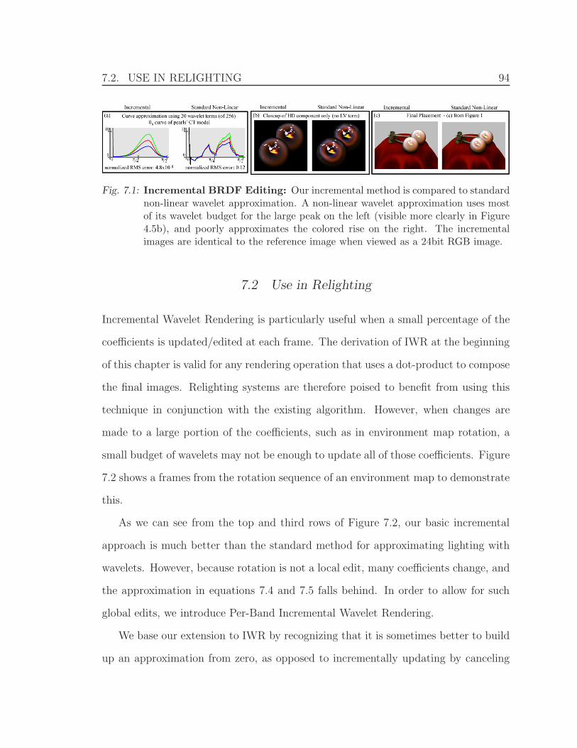
7.2. USE IN RELIGHTING 94
Fig. 7.1: Incremental BRDF Editing: Our incremental method is compared to standardnon-linear wavelet approximation. A non-linear wavelet approximation uses mostof its wavelet budget for the large peak on the left (visible more clearly in Figure4.5b), and poorly approximates the colored rise on the right. The incrementalimages are identical to the reference image when viewed as a 24bit RGB image.
7.2 Use in Relighting
Incremental Wavelet Rendering is particularly useful when a small percentage of the
coefficients is updated/edited at each frame. The derivation of IWR at the beginning
of this chapter is valid for any rendering operation that uses a dot-product to compose
the final images. Relighting systems are therefore poised to benefit from using this
technique in conjunction with the existing algorithm. However, when changes are
made to a large portion of the coefficients, such as in environment map rotation, a
small budget of wavelets may not be enough to update all of those coefficients. Figure
7.2 shows a frames from the rotation sequence of an environment map to demonstrate
this.
As we can see from the top and third rows of Figure 7.2, our basic incremental
approach is much better than the standard method for approximating lighting with
wavelets. However, because rotation is not a local edit, many coefficients change, and
the approximation in equations 7.4 and 7.5 falls behind. In order to allow for such
global edits, we introduce Per-Band Incremental Wavelet Rendering.
We base our extension to IWR by recognizing that it is sometimes better to build
up an approximation from zero, as opposed to incrementally updating by canceling
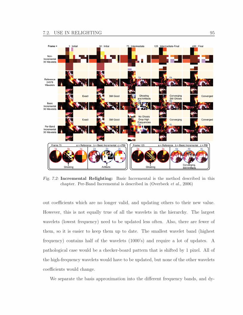
7.2. USE IN RELIGHTING 95
Fig. 7.2: Incremental Relighting: Basic Incremental is the method described in thischapter. Per-Band Incremental is described in (Overbeck et al., 2006)
out coefficients which are no longer valid, and updating others to their new value.
However, this is not equally true of all the wavelets in the hierarchy. The largest
wavelets (lowest frequency) need to be updated less often. Also, there are fewer of
them, so it is easier to keep them up to date. The smallest wavelet band (highest
frequency) contains half of the wavelets (1000’s) and require a lot of updates. A
pathological case would be a checker-board pattern that is shifted by 1 pixel. All of
the high-frequency wavelets would have to be updated, but none of the other wavelets
coefficients would change.
We separate the basis approximation into the different frequency bands, and dy-

7.2. USE IN RELIGHTING 96
namically decide which bands to treat incrementally, and which ones to treat tradi-
tionally. As seen in the bottom row of Figure 7.2, zeroing out the high frequencies
and only updating the lower ones successfully produces an approximation without
artifacts that is still better than the standard wavelet approximation (top row). The
details of selecting how to treat each band, and how many coefficient updates to
allocate to it can be found in (Overbeck et al., 2006).
97
8. VISIBILITY COHERENCE FOR PRECOMPUTATION
Over the past decade, environment maps have increased in popularity as a source for
realistic, complex lighting. Today, they are common in computer graphics workflows
due to the ease of acquisition and representation. This chapter addresses the problem
of efficiently calculating shadows from environment map lighting. Since accurate ren-
dering of shadows from environment maps requires hundreds of samples, the expensive
computation is determining visibility from each pixel to each light direction, such as
by ray-tracing. We show that coherence in both spatial and angular domains can be
used to reduce the number of shadow rays that need to be traced. Specifically, we
use a coarse-to-fine evaluation of the image, predicting visibility by reusing visibility
calculations from four nearby pixels that have already been evaluated. This simple
method allows us to explicitly mark regions of uncertainty in the prediction. By only
tracing rays in these and neighboring directions, we are able to reduce the number
of shadow rays traced by up to a factor of 20 while maintaining error rates below
0.01%. Figure 8.3 shows how a high-dynamic range environment map is partitioned
into areas, with visibility calculated at the centroid of each area. Figure 8.5 shows
how visibility information from one pixel may be leveraged to predict visibility of the
lighting at a nearby pixel. Our method uses a unanimous vote from 4 neighboring
pixels to determine visibility of lights in the environment. Where consensus is not
reached, explicit ray-tracing is triggered. For more details, please refer to (Ben-Artzi
et al., 2006a)
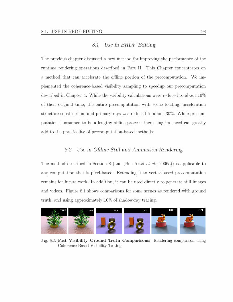
8.1. USE IN BRDF EDITING 98
8.1 Use in BRDF Editing
The previous chapter discussed a new method for improving the performance of the
runtime rendering operations described in Part II. This Chapter concentrates on
a method that can accelerate the offline portion of the precomputation. We im-
plemented the coherence-based visibility sampling to speedup our precomputation
described in Chapter 4. While the visibility calculations were reduced to about 10%
of their original time, the entire precomputation with scene loading, acceleration
structure construction, and primary rays was reduced to about 30%. While precom-
putation is assumed to be a lengthy offline process, increasing its speed can greatly
add to the practicality of precomputation-based methods.
8.2 Use in Offline Still and Animation Rendering
The method described in Section 8 (and (Ben-Artzi et al., 2006a)) is applicable to
any computation that is pixel-based. Extending it to vertex-based precomputation
remains for future work. In addition, it can be used directly to generate still images
and videos. Figure 8.1 shows comparisons for some scenes as rendered with ground
truth, and using approximately 10% of shadow-ray tracing.
Fig. 8.1: Fast Visibility Ground Truth Comparisons: Rendering comparison usingCoherence Based Visibility Testing
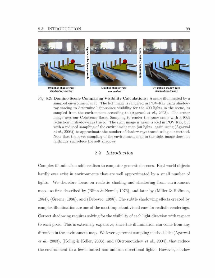
8.3. INTRODUCTION 99
appr
oxim
atel
y eq
ual q
ualit
y
appr
oxim
atel
y eq
ual w
ork
60 million shadow rays standard ray-tracing
6 million shadow rays our method
7½ million shadow rays standard ray-tracing
Fig. 8.2: Domino Scene Comparing Visibility Calculations: A scene illuminated by asampled environment map. The left image is rendered in POV-Ray using shadow-ray tracing to determine light-source visibility for the 400 lights in the scene, assampled from the environment according to (Agarwal et al., 2003). The centerimage uses our Coherence-Based Sampling to render the same scene with a 90%reduction in shadow-rays traced. The right image is again traced in POV Ray, butwith a reduced sampling of the environment map (50 lights, again using (Agarwalet al., 2003)) to approximate the number of shadow-rays traced using our method.Note that the lower sampling of the environment map in the right image does notfaithfully reproduce the soft shadows.
8.3 Introduction
Complex illumination adds realism to computer-generated scenes. Real-world objects
hardly ever exist in environments that are well approximated by a small number of
lights. We therefore focus on realistic shading and shadowing from environment
maps, as first described by (Blinn & Newell, 1976), and later by (Miller & Hoffman,
1984), (Greene, 1986), and (Debevec, 1998). The subtle shadowing effects created by
complex illumination are one of the most important visual cues for realistic renderings.
Correct shadowing requires solving for the visibility of each light direction with respect
to each pixel. This is extremely expensive, since the illumination can come from any
direction in the environment map. We leverage recent sampling methods like (Agarwal
et al., 2003), (Kollig & Keller, 2003), and (Ostromoukhov et al., 2004), that reduce
the environment to a few hundred non-uniform directional lights. However, shadow
8.3. INTRODUCTION 100
testing for all sources at each pixel is still the bottleneck in a conventional raytracer
or other renderer.
In this chapter, we show how to calculate the visibility function efficiently by
exploiting coherence in both the angular and spatial dimensions. We recognize that
the expensive operation when lighting with complex illumination is the tracing of
secondary shadow-rays. Thus, in our method, we trace all primary eye-rays and
cull only shadow-rays, whenever possible. Our method is closest to that of (Agrawala
et al., 2000), who exploited coherence in the visibility of an area light source to reduce
the number of shadow-rays cast. We adapt their method to environment maps, and
show that modifications to both the spatial sharing and angular sharing of visibility
information are required for accurate and efficient visibility sampling in the context
of environment lighting. The salient differences from area lighting are the lack of
a well-defined boundary, lack of locality, and lack of efficient uniform sampling for
environment lighting. By addressing all of these points, we demonstrate, for the first
time, how coherence-based visibility sampling can be used for full-sphere illumination.
We identify two important components of an algorithm estimating visibility by
reusing previously calculated visibility, and explicitly tracing new shadow-rays to
correct errors in the estimate. By correctly sharing information among pixels, as well
as light directions, we show that accurate visibility predictions can be achieved by
tracing only about 10% of the shadow-rays that would normally be required by a
standard raytracer without loss in accuracy, as shown in Figure 8.2. Working source
code, data, animations, and scripts to recreate all images are available onine at the
address listed at the end of this chapter.
8.4. BACKGROUND 101
8.4 Background
Previous work describes coherence-based methods for rendering scenes illuminated
by point or area lights. Most of these techniques find image-space discontinuities and
share visibility or shading information within regions bounded by discontinuities, thus
reducing the number of primary eye rays (and recursively, the number of shadow-rays).
We discuss some of these methods below, and discover that image-space radiance
interpolation is not well-suited for complex illumination. Furthermore, an efficient
method cannot rely on the presence of a light boundary, the locality of the light(s),
nor the ability to uniformly sample the lighting. When these assumptions are broken,
existing methods often degenerate to an exhaustive raytracing for both eye- and
shadow-rays.
(Guo, 1998) was able to efficiently render a scene lit by area light sources by
finding radiance discontinuities in image-space. A sparse grid of primary rays was fully
evaluated, and radiance discontinuities were discovered by comparing the results of
these calculations. The rest of the image pixels are bilinearly interpolated, thus culling
the actual primary and secondary rays for those pixels. Unlike area light sources,
environment map illumination produces continuous gradients instead of discoverable
discontinuities. The method used by (Guo, 1998) would incorrectly interpolate large
regions of the scene that in fact have smooth, yet complex variations in radiance.
(Bala et al., 2003) also interpolate radiance in image-space, but determine the
regions of interpolation by examining the visibility of lights. Each pixel is classified
as empty, simple, or complex, depending on whether it contains 0, 1, or more discon-
tinuities of light visibility. Only complex pixels are fully evaluated. When rendering
images illuminated by a sampled environment map, nearly every pixel becomes com-
plex. This is due to the presence of hundereds of light sources, several of which exhibit
8.4. BACKGROUND 102
a change in visibility when moving from one pixel to the next.
(Hart et al., 1999) demonstrated an analytic integration method for calculating
irradiance due to area light sources. They find all light-blocker pairs, exploiting
coherence of these pairings between nearby pixels. The lights are then clipped against
the blocker(s) to produce an emissive polygon corresponding to the visible section of
the light source. The light-blocker pairs are discovered using uniform sampling of the
solid angle subtended by the area light source, taking advantage of the light’s locality.
For an environment map which subtends the entire sphere of directions, this method
degenerates to brute-force visibility sampling.
(Agrawala et al., 2000) achieve their speedup by assuming that visibility of the
light source is similar for adjacent pixels. They determine visibility of regularly spaced
samples of the area light source, and then share that visibility information with the
subsequent pixel of the scanline order. Errors are corrected by explicitly tracing
new shadow-rays to light samples that lie along visibility boundaries (and recursively
flooding the shadow traces when errors are detected). Locality of the area light source
and a well-defined edge ensured that the number of samples was small, and boundaries
were well-defined.
Our work also relates to much recent effort on real-time rendering of static scenes
illuminated by environment maps. Precomputed radiance transfer methods such as
(Ng et al., 2003) and (Sloan et al., 2002) have a different goal of compactly repre-
senting and reusing the results of exhaustive calculations. They perform a lengthy
precomputation step during which standard raytracing is used to compute the radi-
ance transferred to all parts of a static scene. In contrast, we focus on computing the
visibility of an arbitrary scene more efficiently. PRT methods may benefit from using
our algorithm in the raytracer they employ for the precomputation stage.
8.5. PRELIMINARIES 103
8.5 Preliminaries
In this section, we briefly desctibe how our method relates to rendering engines that
solve the reflection equation. The exit radiance at a point, x, in the direction ω0, is
given by
L(x, ω0) =
∫
Ω
fr(ω, ω0)L(ω)V (x, ω)(ω · n)dω,
where x is a location in the scene with a BRDF of fr, n is the normal, and ω
is a direction in the upper hemisphere, Ω2π. V (x, ω) is the 4D, binary visibility
function of the scene. The light-space of each location, x, is the set of directions
in the upper hemisphere, Ω, centered at x. V (x, ω) assigns to each direction in the
light-space of x, a binary value indicating whether occluding geometry exists in that
direction, or not. (Agarwal et al., 2003) demonstrated that the integral above can
be approximated with an explicit sum over a set of well-chosen directions {ωi}, with
associated regions or cells, as shown in Figure 8.3 right. An efficient approximation
of several hundred directional lights can be found for most environment maps, and
we assume that such a technique has been used. Often, the hardest part of solving
for L(x, ω0) is computing the visibility term, V (x, ω). Our work concentrates on
making this visibility calculation more efficient. Any system which can substitute its
computation of V (x, ω) in the above equation can make use of the methods described
in this chapter. We demonstrate that a sparse set of samples in {x} × {ω} can be
used to reconstruct V (x, ω) with a high degree of accuracy.
Given a set of directional lights, we partition the set of all directions into regions
that are identified with each light, as seen in Figure 8.3 right. This is done by
uniformly sampling a unit disk and projecting each sample onto the unit sphere to
obtain a direction. The sample is then assigned the ID (visualized as a color) of the
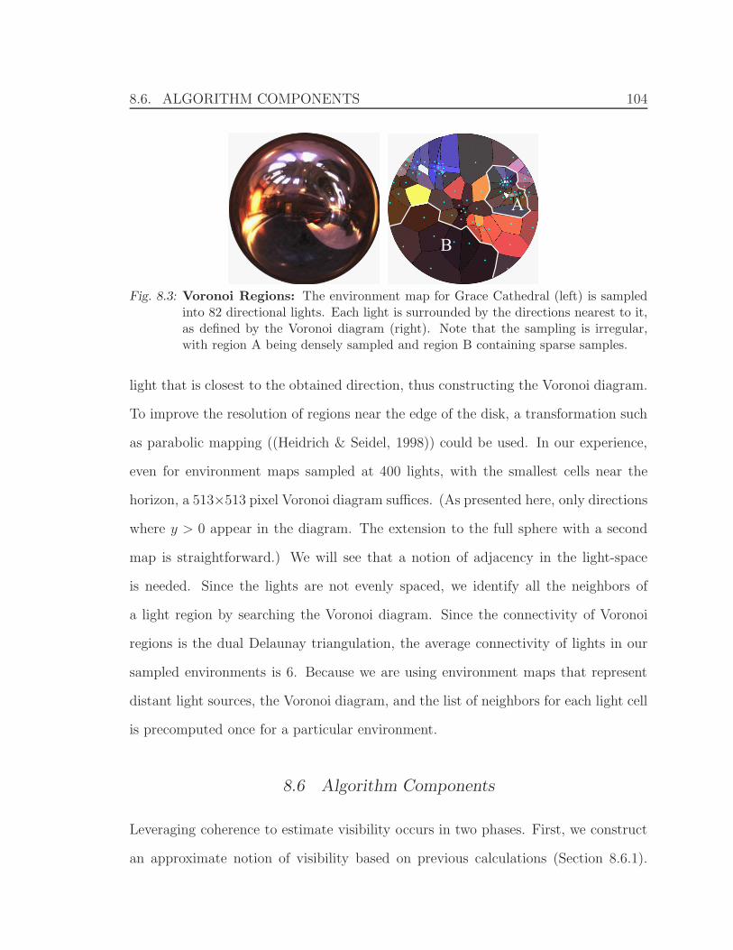
8.6. ALGORITHM COMPONENTS 104
A
B
Fig. 8.3: Voronoi Regions: The environment map for Grace Cathedral (left) is sampledinto 82 directional lights. Each light is surrounded by the directions nearest to it,as defined by the Voronoi diagram (right). Note that the sampling is irregular,with region A being densely sampled and region B containing sparse samples.
light that is closest to the obtained direction, thus constructing the Voronoi diagram.
To improve the resolution of regions near the edge of the disk, a transformation such
as parabolic mapping ((Heidrich & Seidel, 1998)) could be used. In our experience,
even for environment maps sampled at 400 lights, with the smallest cells near the
horizon, a 513×513 pixel Voronoi diagram suffices. (As presented here, only directions
where y > 0 appear in the diagram. The extension to the full sphere with a second
map is straightforward.) We will see that a notion of adjacency in the light-space
is needed. Since the lights are not evenly spaced, we identify all the neighbors of
a light region by searching the Voronoi diagram. Since the connectivity of Voronoi
regions is the dual Delaunay triangulation, the average connectivity of lights in our
sampled environments is 6. Because we are using environment maps that represent
distant light sources, the Voronoi diagram, and the list of neighbors for each light cell
is precomputed once for a particular environment.
8.6 Algorithm Components
Leveraging coherence to estimate visibility occurs in two phases. First, we construct
an approximate notion of visibility based on previous calculations (Section 8.6.1).
8.6. ALGORITHM COMPONENTS 105
Then we must clean up this estimate by identifying and correcting regions that may
have been predicted incorrectly (Section 8.6.2). In this section, we present several
choices for compoennts that provide these functions. The next section (Secion 8.7)
will analyze the possible combinations to determine the best algorthim for both cor-
rectness and efficiency. For the rest of the discussion we will refer to a pixel, and the
scene location intersected by an eye-ray through that pixel, interchangeably.
8.6.1 Estimating Visibility
Our goal is to reuse the points of geometry that represent intersections between
shadow-rays and objects in the scene. To predict the visibility at one spatial loca-
tion, we consider the occluding geometry discovered while calculating visibility at
nearby locations, thus taking advantage of spatial coherence. We must choose which
previously evaluated pixels will be most helpful when attempting to reuse visibility
information. We explore the options of scanline and grid-based pixel evaluations.
Scanline Ordering (S)
When evaluating the pixels in scanline order, we use the previous pixel on the scanline,
as well as the two pixels directly above them, on the previous scanline. The reasoning
behind this is that visibility changes very little from pixel to pixel, and thus using the
immediate neighbors gives a good first approximation to the visibility at the current
pixel.
Grid-based Ordering (G)
Scanline ordering has the notable limitation that all of the previously evaluated pixels
come from the same general direction (up, and to the left). Therefore, we present an
alternative which always allows us to reuse visibility from 4 previously evaluated pixels
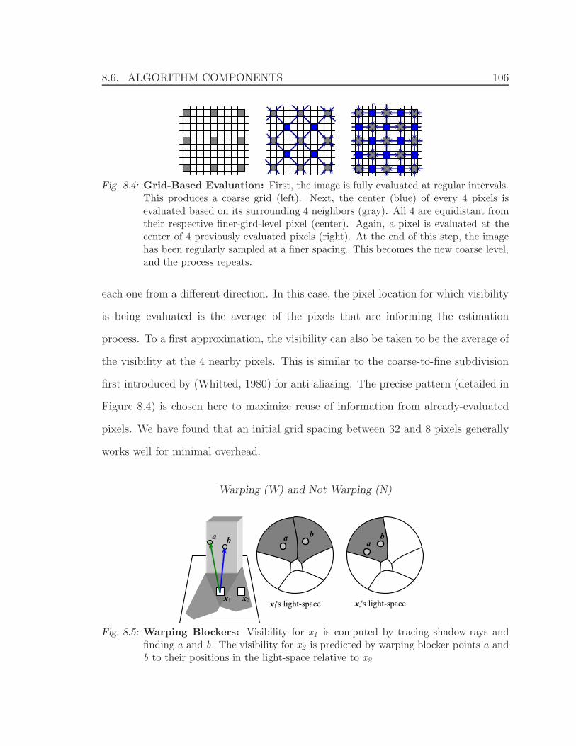
8.6. ALGORITHM COMPONENTS 106
Fig. 8.4: Grid-Based Evaluation: First, the image is fully evaluated at regular intervals.This produces a coarse grid (left). Next, the center (blue) of every 4 pixels isevaluated based on its surrounding 4 neighbors (gray). All 4 are equidistant fromtheir respective finer-gird-level pixel (center). Again, a pixel is evaluated at thecenter of 4 previously evaluated pixels (right). At the end of this step, the imagehas been regularly sampled at a finer spacing. This becomes the new coarse level,and the process repeats.
each one from a different direction. In this case, the pixel location for which visibility
is being evaluated is the average of the pixels that are informing the estimation
process. To a first approximation, the visibility can also be taken to be the average of
the visibility at the 4 nearby pixels. This is similar to the coarse-to-fine subdivision
first introduced by (Whitted, 1980) for anti-aliasing. The precise pattern (detailed in
Figure 8.4) is chosen here to maximize reuse of information from already-evaluated
pixels. We have found that an initial grid spacing between 32 and 8 pixels generally
works well for minimal overhead.
Warping (W) and Not Warping (N)
x1 x2
a b a b
x 's light-space1 x 's light-space2
a b
Fig. 8.5: Warping Blockers: Visibility for x1 is computed by tracing shadow-rays andfinding a and b. The visibility for x2 is predicted by warping blocker points a andb to their positions in the light-space relative to x2
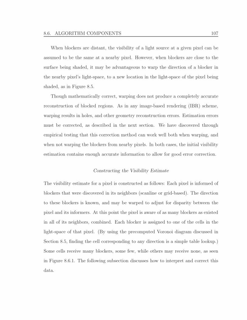
8.6. ALGORITHM COMPONENTS 107
When blockers are distant, the visibility of a light source at a given pixel can be
assumed to be the same at a nearby pixel. However, when blockers are close to the
surface being shaded, it may be advantageous to warp the direction of a blocker in
the nearby pixel’s light-space, to a new location in the light-space of the pixel being
shaded, as in Figure 8.5.
Though mathematically correct, warping does not produce a completely accurate
reconstruction of blocked regions. As in any image-based rendering (IBR) scheme,
warping results in holes, and other geometry reconstruction errors. Estimation errors
must be corrected, as described in the next section. We have discovered through
empirical testing that this correction method can work well both when warping, and
when not warping the blockers from nearby pixels. In both cases, the initial visibility
estimation contains enough accurate information to allow for good error correction.
Constructing the Visibility Estimate
The visibility estimate for a pixel is constructed as follows: Each pixel is informed of
blockers that were discovered in its neighbors (scanline or grid-based). The direction
to these blockers is known, and may be warped to adjust for disparity between the
pixel and its informers. At this point the pixel is aware of as many blockers as existed
in all of its neighbors, combined. Each blocker is assigned to one of the cells in the
light-space of that pixel. (By using the precomputed Voronoi diagram discussed in
Section 8.5, finding the cell corresponding to any direction is a simple table lookup.)
Some cells receive many blockers, some few, while others may receive none, as seen
in Figure 8.6.1. The following subsection discusses how to interpret and correct this
data.
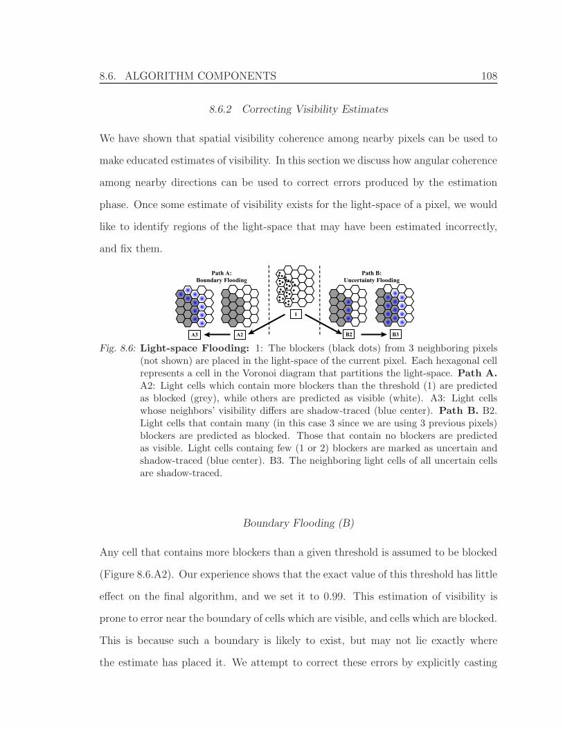
8.6. ALGORITHM COMPONENTS 108
8.6.2 Correcting Visibility Estimates
We have shown that spatial visibility coherence among nearby pixels can be used to
make educated estimates of visibility. In this section we discuss how angular coherence
among nearby directions can be used to correct errors produced by the estimation
phase. Once some estimate of visibility exists for the light-space of a pixel, we would
like to identify regions of the light-space that may have been estimated incorrectly,
and fix them.
Path A: Boundary Flooding
A2A3 B3
1
B2
Path B: Uncertainty Flooding
Fig. 8.6: Light-space Flooding: 1: The blockers (black dots) from 3 neighboring pixels(not shown) are placed in the light-space of the current pixel. Each hexagonal cellrepresents a cell in the Voronoi diagram that partitions the light-space. Path A.A2: Light cells which contain more blockers than the threshold (1) are predictedas blocked (grey), while others are predicted as visible (white). A3: Light cellswhose neighbors’ visibility differs are shadow-traced (blue center). Path B. B2.Light cells that contain many (in this case 3 since we are using 3 previous pixels)blockers are predicted as blocked. Those that contain no blockers are predictedas visible. Light cells containg few (1 or 2) blockers are marked as uncertain andshadow-traced (blue center). B3. The neighboring light cells of all uncertain cellsare shadow-traced.
Boundary Flooding (B)
Any cell that contains more blockers than a given threshold is assumed to be blocked
(Figure 8.6.A2). Our experience shows that the exact value of this threshold has little
effect on the final algorithm, and we set it to 0.99. This estimation of visibility is
prone to error near the boundary of cells which are visible, and cells which are blocked.
This is because such a boundary is likely to exist, but may not lie exactly where
the estimate has placed it. We attempt to correct these errors by explicitly casting

8.7. ANALYZING POSSIBLE COMPONENT COMBINATIONS 109
shadow-rays in the directions that lie along a boundary (Figure 8.6.A3). Wherever
the shadow-ray indicates that an error had been made in the estimation stage, we
recursively shadow trace all the adjacent regions. This process continues until all
shadow-rays report back in agreement with the estimate.
Uncertainty Flooding (U)
Instead of guessing that boundaries are prone to error, we can use a more explicit
measure of when we are uncertain of the visibility constructed by the estimation phase.
Cells that contain many (4 in grid-based, 3 in scanline) blockers are considered blocked
because all of the informing pixels agree that it is blocked. Similarly, cells without any
blockers are considered visible. Whenever the neighbor pixels disagree on the visibility
for any cell of the light-space (indicated by a small number of blockers), we mark it
as uncertain (Figure 8.6.B2). We explicitly trace shadow-rays for these regions, and
flood outwards, recursively tracing more shadow-rays when the estimation disagrees
with the shadow-ray (Figure 8.6.B3).
8.7 Analyzing Possible Component Combinations
So far, we have developed four variations of the first phase: estimating visibility. We
can use scanline evaluation (S) or grid-based evaluation (G), and for each of these, we
may choose to warp (W) or not warp (N) the blockers from nearby pixels. We have also
developed two variations for the second phase: correcting the estimate. We can trace
shadow-rays at the visibility boundaries (B) or at the explicitly marked uncertainty
regions (U). We performed comprehensive evaluations of all eight possibilities, and
will now present the findings of the components’ usefulness, both on their own, and
as they interact with the other variations.
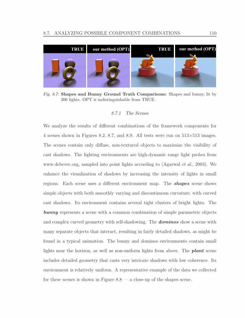
8.7. ANALYZING POSSIBLE COMPONENT COMBINATIONS 110
TRUE our method (OPT)TRUE our method (OPT)
Fig. 8.7: Shapes and Bunny Ground Truth Comparisons: Shapes and bunny, lit by200 lights. OPT is indistinguishable from TRUE.
8.7.1 The Scenes
We analyze the results of different combinations of the framework components for
4 scenes shown in Figures 8.2, 8.7, and 8.9. All tests were run on 513×513 images.
The scenes contain only diffuse, non-textured objects to maximize the visibility of
cast shadows. The lighting environments are high-dynamic range light probes from
www.debevec.org, sampled into point lights according to (Agarwal et al., 2003). We
enhance the visualization of shadows by increasing the intensity of lights in small
regions. Each scene uses a different environment map. The shapes scene shows
simple objects with both smoothly varying and discontinuous curvature, with curved
cast shadows. Its environment contains several tight clusters of bright lights. The
bunny represents a scene with a common combination of simple parametric objects
and complex curved geometry with self-shadowing. The dominos show a scene with
many separate objects that interact, resulting in fairly detailed shadows, as might be
found in a typical animation. The bunny and dominos environments contain small
lights near the horizon, as well as non-uniform lights from above. The plant scene
includes detailed geometry that casts very intricate shadows with low coherence. Its
environment is relatively uniform. A representative example of the data we collected
for these scenes is shown in Figure 8.8 — a close-up of the shapes scene.
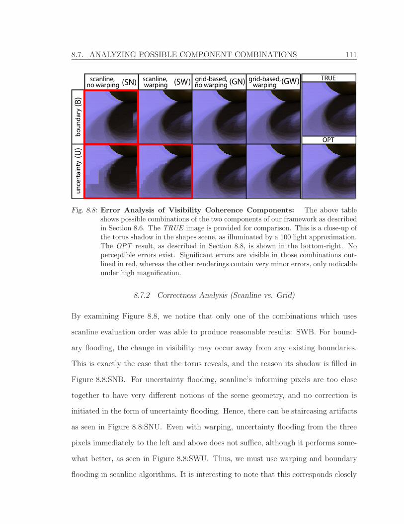
8.7. ANALYZING POSSIBLE COMPONENT COMBINATIONS 111
scanline, no warping
scanline, warping
grid-based,no warping
grid-based,warping(SN) (SW) (GN) (GW)
un
cert
ain
tyb
ou
nd
ary
(U)
(B)
TRUE
OPT
Fig. 8.8: Error Analysis of Visibility Coherence Components: The above tableshows possible combinations of the two components of our framework as describedin Section 8.6. The TRUE image is provided for comparison. This is a close-up ofthe torus shadow in the shapes scene, as illuminated by a 100 light approximation.The OPT result, as described in Section 8.8, is shown in the bottom-right. Noperceptible errors exist. Significant errors are visible in those combinations out-lined in red, whereas the other renderings contain very minor errors, only noticableunder high magnification.
8.7.2 Correctness Analysis (Scanline vs. Grid)
By examining Figure 8.8, we notice that only one of the combinations which uses
scanline evaluation order was able to produce reasonable results: SWB. For bound-
ary flooding, the change in visibility may occur away from any existing boundaries.
This is exactly the case that the torus reveals, and the reason its shadow is filled in
Figure 8.8:SNB. For uncertainty flooding, scanline’s informing pixels are too close
together to have very different notions of the scene geometry, and no correction is
initiated in the form of uncertainty flooding. Hence, there can be staircasing artifacts
as seen in Figure 8.8:SNU. Even with warping, uncertainty flooding from the three
pixels immediately to the left and above does not suffice, although it performs some-
what better, as seen in Figure 8.8:SWU. Thus, we must use warping and boundary
flooding in scanline algorithms. It is interesting to note that this corresponds closely
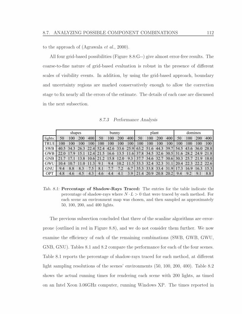
8.7. ANALYZING POSSIBLE COMPONENT COMBINATIONS 112
to the approach of (Agrawala et al., 2000).
All four grid-based possibilities (Figure 8.8:G--) give almost error-free results. The
coarse-to-fine nature of grid-based evaluation is robust in the presence of different
scales of visibility events. In addition, by using the grid-based approach, boundary
and uncertainty regions are marked conservatively enough to allow the correction
stage to fix nearly all the errors of the estimate. The details of each case are discussed
in the next subsection.
8.7.3 Performance Analysis
shapes bunny plant dominos
21
lights:TRUESWBGWBGNBGWUGNUOPT
5010040.522.021.710.49.44.8
10010034.317.917.110.78.84.6
20010026.315.113.811.08.34.5
40010022.412.410.611.37.54.3
5010052.4
.521.29.18.14.6
10010042.616.615.89.47.74.4
20010033.613.512.010.27.24.1
40010025.911.69.3
11.56.73.9
5010063.237.837.733.335.321.4
10010051.634.534.632.433.820.9
20010044.332.632.732.333.420.8
40010039.730.530.631.131.920.2
5010054.531.630.320.417.39.4
10010043.628.225.722.316.99.2
20010036.024.921.922.216.39.1
40010028.821.818.022.615.38.8
Tab. 8.1: Percentage of Shadow-Rays Traced: The entries for the table indicate thepercentage of shadow-rays where N ·L > 0 that were traced by each method. Foreach scene an environment map was chosen, and then sampled as approximately50, 100, 200, and 400 lights.
The previous subsection concluded that three of the scanline algorithms are error-
prone (outlined in red in Figure 8.8), and we do not consider them further. We now
examine the efficiency of each of the remaining combinations (SWB, GWB, GWU,
GNB, GNU). Tables 8.1 and 8.2 compare the performance for each of the four scenes.
Table 8.1 reports the percentage of shadow-rays traced for each method, at different
light sampling resolutions of the scenes’ environments (50, 100, 200, 400). Table 8.2
shows the actual running times for rendering each scene with 200 lights, as timed
on an Intel Xeon 3.06GHz computer, running Windows XP. The times reported in

8.7. ANALYZING POSSIBLE COMPONENT COMBINATIONS 113
shapes bunny plant dominosec speedup sec speedup sec speedup sec speedup
primary rays only (EYE) 4.0 N/A 4.0 N/A 4.4 N/A 4.2 N/Aground truth (TRUE) 75.3 1.0 80.8 1.0 152.3 1.0 124.9 1.0scanline, warping, boundary (SWB) 34.9 2.2 54.8 1.5 120.3 1.3 67.1 1.9grid-based, warping, boundary (GWB) 25.2 3.0 36.7 2.2 113.2 1.3 55.7 2.2grid-based, no warping, boundary (GNB) 16.8 4.5 23.2 3.5 95.1 1.6 35.4 3.5grid-based, warping, uncertainty (GWU) 19.6 3.8 30.6 2.6 109.0 1.3 47.1 2.6grid-based, no warping, uncertainty (GNU) 11.2 6.7 16.7 4.8 94.7 1.6 23.8 5.2optimized algorithm (OPT) 7.1 10.5 10.7 7.6 58.3 2.6 14.7 8.5
environments sampled at 200 lights
Tab. 8.2: Visibility Timings: The wall-clock timings for the full rendering with 200lights, shown here, are related to, but not equivalent to the reduction in work asmeasured in shadow-rays traced (see Table 8.1).
Table 8.2 include the (relatively small) time for the initial setup of the raytracer and
tracing just the EYE rays for each pixel, as well as performing the diffuse shading
calculation. The errors in the five remaining algorithms are generally small (<0.1%)
either when measured as absolute mispredictions, or when viewed as the resulting
color shift in the image. All of these algorithms enable significant reductions in the
number of shadow-rays traced, with negligible loss in quality.
To Warp or Not to Warp
The motivation for warping blockers into the local frame of a pixel is that it may
produce a better approximation of the occluding scene geometry. This turns out
to be counterproductive for non-uniformly distributed samples of the light-space.
Consider Figure 8.3 right . When the blockers in an area of densely sampled lights
(region A), are warped onto an area of sparse lights (region B), large cells in region B
that are mostly visible may receive a large number of blockers, clustered in a corner of
the cell. These would be incorrectly estimated as blocked. Symmetrically, if warping
occurs form a sparse region to a dense one, cells that are actually blocked may not
receive any blockers and be erroneously estimated as visible. When the spacing of
8.7. ANALYZING POSSIBLE COMPONENT COMBINATIONS 114
the light samples is not uniform, warping can introduce more errors in the visibility
estimation, requiring more work to be done in the correction phase.
When comparing GWU with GNU and GWB with GNB, Table 8.1 shows that
the non-warping algorithms perform slightly better for all but the plant scene. When
comparing the warping algorithms (GWB, GWU) to the equivalent non-warping
algorithms (GNB, GNU) in Table 8.2, we can see a significant speedup in the wall-
clock timings. Not warping requires fewer instructions since a simple count of the
blockers in each cell suffices, whereas warping must perform the 3D transformation
of the blockers and project them into the new cells. One additional advantage of not
warping is that we eliminate the dependence on accurate depth information for the
blockers. This can be useful when rendering engines optimize the intersection test of
shadow-rays by stopping as soon as an intersection is found, without discovering the
true depth of the closest blocker. (To obtain controlled comparisions, we did not turn
on this optimization.)
Boundary Flooding vs. Uncertainty Flooding
Since the illumination from an environment map spans the entire sphere, many visi-
bility boundaries can exist, resulting in flooding to most of the lights when boundary
flooding is used. Uncertainty flooding has the advantage of being restricted to those
areas which are visible at some neighboring pixels, and blocked at others. It is par-
ticularly well suited to combat the sampling discrepancies described in the previous
subsection (see Section 8.7.3 and Figure 8.3). When under- or over-sampling of the
light-space occurs, some cells in that region receive few (1-3) blockers, and trigger
explicit shadow traces for their neighbors. Marking cells as uncertain is equivalent
to finding image-space discontinuities for individual shadows. If such a discontinu-
ity passes through the area surrounded by the informing pixels, that light is marked
8.7. ANALYZING POSSIBLE COMPONENT COMBINATIONS 115
as uncertain in the current pixel. In essence, uncertainty flooding concentrates on
regions with image-space discontinuities, while boundary flooding concentrates on
light-space discontinuities.
Looking at Table 8.1, we see that in all cases, uncertainty flooding performs about
twice as well as the corresponding boundary flooding algorithm, at the lower resolu-
tions. In particular, the first row (shapes50), shows GWB doing 22% of the work and
GWU doing only 10%. Similarly, GNB does 22% of the work, while GNU does only
9%. This indicates that marking boundaries as regions that require shadow-tracing
is an overly-conservative estimate. In our experience, not all visibility boundaries are
error-prone.
Since the work done by boundary flooding is proportional to the area of the light-
space occupied by boundaries, its performance is strongly dependent on the sampling
rate of the environment. Notice that for shapes, bunny, and dominos, boundary
flooding algorithms degrade by a factor of 2 as the light resolution is decreased from
400 to 50. On the other hand, the performance of algorithms based on uncertainty
flooding is relatively independent of the number of lights.
8.7.4 Discussion of Analysis
The examples shown in Figure 8.8 indicate that scanline evaluation order is much
more constrained than grid-based. This is primarily because the small increments
as the scanline progresses are sensitive to the scale of changes that may occur in
visibility. We see in the results outlined in red in Figure 8.8, that a missed visibility
event propagates along the scanline until some other event triggers its correction via
flooding. It is instructive to compare GWB and SWB in Table 8.1, and notice that
GWB is more efficient by about a factor of 2 for most cases. One reason for this
is that scanline must consider the lights near the horizon as part of a boundary.
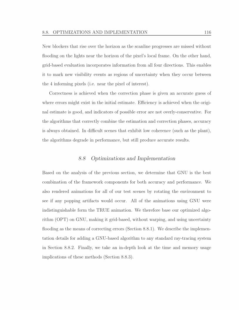
8.8. OPTIMIZATIONS AND IMPLEMENTATION 116
New blockers that rise over the horizon as the scanline progresses are missed without
flooding on the lights near the horizon of the pixel’s local frame. On the other hand,
grid-based evaluation incorporates information from all four directions. This enables
it to mark new visibility events as regions of uncertainty when they occur between
the 4 informing pixels (i.e. near the pixel of interest).
Correctness is achieved when the correction phase is given an accurate guess of
where errors might exist in the initial estimate. Efficiency is achieved when the origi-
nal estimate is good, and indicators of possible error are not overly-conservative. For
the algorithms that correctly combine the estimation and correction phases, accuracy
is always obtained. In difficult scenes that exhibit low coherence (such as the plant),
the algorithms degrade in performance, but still produce accurate results.
8.8 Optimizations and Implementation
Based on the analysis of the previous section, we determine that GNU is the best
combination of the framework components for both accuracy and performance. We
also rendered animations for all of our test scenes by rotating the environment to
see if any popping artifacts would occur. All of the animations using GNU were
indistinguishable form the TRUE animation. We therefore base our optimized algo-
rithm (OPT) on GNU, making it grid-based, without warping, and using uncertainty
flooding as the means of correcting errors (Section 8.8.1). We describe the implemen-
tation details for adding a GNU-based algorithm to any standard ray-tracing system
in Section 8.8.2. Finally, we take an in-depth look at the time and memory usage
implications of these methods (Section 8.8.3).
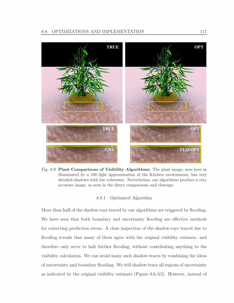
8.8. OPTIMIZATIONS AND IMPLEMENTATION 117
TRUE
TRUE OPT
OPT
GNU FLO-OPT
Fig. 8.9: Plant Comparisons of Visibility Algorithms: The plant image, seen here asilluminated by a 100 light approximation of the Kitchen environment, has verydetailed shadows with low coherence. Nevertheless, our algorithms produce a veryaccurate image, as seen in the direct comparisons and closeups.
8.8.1 Optimized Algorithm
More than half of the shadow-rays traced by our algorithms are triggered by flooding.
We have seen that both boundary and uncertainty flooding are effective methods
for correcting prediction errors. A close inspection of the shadow-rays traced due to
flooding reveals that many of them agree with the original visibility estimate, and
therefore only serve to halt further flooding, without contributing anything to the
visibility calculation. We can avoid many such shadow-traces by combining the ideas
of uncertainty and boundary flooding. We still shadow-trace all regions of uncertainty
as indicated by the original visibility estimate (Figure 8.6.A2). However, instead of
8.8. OPTIMIZATIONS AND IMPLEMENTATION 118
flooding to all neighbors (typically 6) of a cell whose shadow-trace disagrees with the
estimate, we only flood to those neighboring cells that also disagree with the shadow-
trace result. This means that for uncertainty regions that lie on a border, we only
flood onto one side of the border; trying to find where it truly lies. This optimization
reduces the number of flood-triggered traces by about 40%. For complex shadows,
small artifacts are introduced by this method, as may be visible in the Figure 8.9:OPT
close-up, but we feel that the performance gain is worth the slight difference in image
quality. Since animations are more sensitive to small differences, we recommend that
this optimization only be used for stills, and omitted in animations. (A comparison
of these animations for the shapes scene is available online at the address listed at
the end of this chapter.)
In an effort to further reduce the number of shadow-rays traced due to flooding,
we note that half of the image pixels are contained in the finest grid — when the
initial estimate is informed by a pixel’s immediate neighbors. If all 4 neighbors agree
on the visibility of a particular light, the center pixel can only disagree if there is a
shadow discontinuity smaller than a single pixel passing through it. Since the image
cannot resolve elements smaller than a single pixel, we ignore these sub-pixel shadow
discontinuities and turn off flooding altogether at the grid’s finest level only (FLO).
We still rely on error correction due to explicit uncertainty marking. This reduces the
total number of shadow-rays required to calculate the image by about 25%, without
adding any noticeable artifacts to the final image, as seen in the Figure 8.9:FLO-OPT
close-up. This optimization also is safe for animations, as its effects are only noticeable
at a sub-pixel level. Sub-pixel sampling for antialiasing is a popular method employed
by many rendering engines. When such a feature is used in conjunction with our
method, the highest resolution of sampling should be considered to be the native
image resolution for the purposes of defining the grid.
8.8. OPTIMIZATIONS AND IMPLEMENTATION 119
Our optimized algorithm (OPT) uses the above two methods of restricting flood-
ing; flooding only to neighbors that disagree with the shadow-ray, and not flooding
at the finest grid level. The high quality of OPT can be seen in Figures 8.2, 8.8, 8.7,
and 8.9. The close-ups in Figure 8.8 and Figure 8.9 reveal that OPT produces images
nearly indistinguishable from the ground-truth (TRUE). Even on the stress-test pro-
vided by the plant scene (Figure 8.9), OPT has only a 0.4% error rate, as measured in
actual shadow-ray prediction errors. The error rate for OPT on the bunny is 0.0026%,
meaning only 1 in 38,000 shadow-rays disagree from ground-truth. In terms of visual
quality of the images OPT produces accurate results for all the scenes. As visualized
in the final images, these errors produce rendering that are nearly identical to the
true images when viewed as standard 24 bit RGB images. Adding the above two op-
timizations typically leads to a 50% reduction in the number of shadow-rays traces,
when compared to GNU. As reported in Table 8.1, this can result in a factor of 20
improvement in efficiency over standard visibility testing in ray-tracers. In Table 8.2,
the timings show that as OPT’s performance improves, shadow-tracing is no longer
the bottleneck for rendering. In the shapes scene, tracing the primary eye rays (4.0
seconds) takes longer than adding complex shadows to the scene (3.1 seconds).
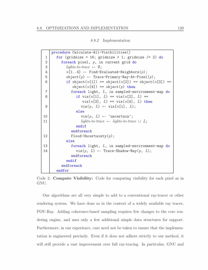
8.8. OPTIMIZATIONS AND IMPLEMENTATION 120
8.8.2 Implementation
procedure Calculate-All-Visibilities()
1 for (gridsize = 16; gridsize > 1; gridsize /= 2) do
2 foreach pixel, p, in current grid do
3 lights-to-trace ← ∅;4 n[1..4] ← Find-Evaluated-Neighbors(p);5 object(p) ← Trace-Primary-Ray-At-Pixel(p);6 if object(n[1]) == object(n[2]) == object(n[3]) ==
object(n[4]) == object(p) then
7 foreach light, L, in sampled-environment-map do
8 if vis(n[1], L) == vis(n[2], L) ==
vis(n[3], L) == vis(n[4], L) then
9 vis(p, L) ← vis[n[1], L);else
10 vis(p, L) ← ‘uncertain’;
11 lights-to-trace ← lights-to-trace ∪ L;endif
endforeach
12 Flood-Uncertainty(p);else
13 foreach light, L, in sampled-environment-map do
14 vis(p, L) ← Trace-Shadow-Ray(p, L);endforeach
endif
endforeach
endfor
Code 2: Compute Visibility: Code for computing visibility for each pixel as inGNU.
Our algorithms are all very simple to add to a conventional ray-tracer or other
rendering system. We have done so in the context of a widely available ray tracer,
POV-Ray. Adding coherence-based sampling requires few changes to the core ren-
dering engine, and uses only a few additional simple data structures for support.
Furthermore, in our experience, care need not be taken to ensure that the implemen-
tation is engineered precisely. Even if it does not adhere strictly to our method, it
will still provide a vast improvement over full ray-tracing. In particular, GNU and

8.8. OPTIMIZATIONS AND IMPLEMENTATION 121
OPT are very simple to implement. For each pixel, once the 4 nearby pixels are
identified in the grid-based evaluation, a simple check of agreement for each light is
performed. If all 4 pixels agree that a light is blocked or visible, it is predicted as
blocked or visible, respectively. When the 4 pixels do not agree on a particular light,
it is shadow-traced, with possible flooding to neighboring lights. If the optimizations
are used, only neighbors whose prediction disagrees with the shadow-trace are traced,
and no flooding to neighbors is performed at the final grid level. Code for GNU is
shown in procedure Calculate-All-Visibilities (Code 2).
Lines 1–4 describe the use of grid-based evaluation as shown in Figure 8.4. To
prime this process, the coarsest level of the grid is evaluated at a scale of 16 pixels,
which we found to be suitable for all of the scenes we tested. For each of these pixels
(<0.5% of the image), all shadow-rays are traced. This is comparable to the priming
for scanline which requires the top row and left column to be fully evaluated ( 0.4% for
513x513 images). In lines 5 and 6, we perform a sanity check to make sure that only
visibility calculations relating to the same scene object are used for estimation. We
have found that there is a significant loss in coherence when the informing pixels are
not on the same object as the current pixel. We therefore fully shadow-trace around
these silhouette edges to determine visibility. For very complex scenes such as the
plant in Figure 8.9, explicitly tracing in this situation traces 7% of the shadow-rays.
For average scenes like those in Figure 8.2 and Figure 8.7, this results in about 1–3%
of the shadow-rays.
In lines 7–11, the initial rough estimate of visibility is formed as shown in Figure 8.6
steps 1 and A2. In line 12, the error correction phase is called, as described in
Section 8.6.2, and diagrammed in Figure 8.6.A3. The pseudocode for this is shown
in Flood-Uncertainty(Code 3).
When Flood-Uncertainty is called, the set lights-to-trace contains all those lights
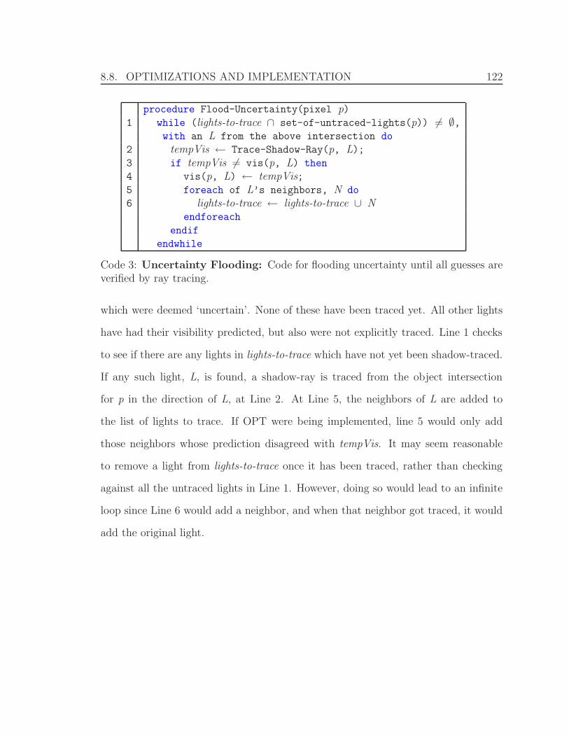
8.8. OPTIMIZATIONS AND IMPLEMENTATION 122
procedure Flood-Uncertainty(pixel p)1 while (lights-to-trace ∩ set-of-untraced-lights(p)) = ∅,
with an L from the above intersection do
2 tempVis ← Trace-Shadow-Ray(p, L);3 if tempVis = vis(p, L) then
4 vis(p, L) ← tempVis;5 foreach of L’s neighbors, N do
6 lights-to-trace ← lights-to-trace ∪ Nendforeach
endif
endwhile
Code 3: Uncertainty Flooding: Code for flooding uncertainty until all guesses areverified by ray tracing.
which were deemed ‘uncertain’. None of these have been traced yet. All other lights
have had their visibility predicted, but also were not explicitly traced. Line 1 checks
to see if there are any lights in lights-to-trace which have not yet been shadow-traced.
If any such light, L, is found, a shadow-ray is traced from the object intersection
for p in the direction of L, at Line 2. At Line 5, the neighbors of L are added to
the list of lights to trace. If OPT were being implemented, line 5 would only add
those neighbors whose prediction disagreed with tempVis. It may seem reasonable
to remove a light from lights-to-trace once it has been traced, rather than checking
against all the untraced lights in Line 1. However, doing so would lead to an infinite
loop since Line 6 would add a neighbor, and when that neighbor got traced, it would
add the original light.
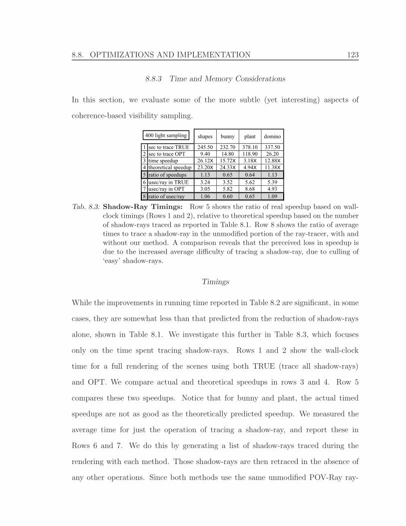
8.8. OPTIMIZATIONS AND IMPLEMENTATION 123
8.8.3 Time and Memory Considerations
In this section, we evaluate some of the more subtle (yet interesting) aspects of
coherence-based visibility sampling.
400 light sampling shapes bunny plant domino
1 sec to trace TRUE 245.50 232.70 378.10 337.50 2 sec to trace OPT 9.40 14.80 118.90 26.20 3 time speedup 26.12X 15.72X 3.18X 12.88X 4 theoretical speedup 23.20X 24.33X 4.94X 11.38X 5 ratio of speedups 1.13 0.65 0.64 1.13 6 usec/ray in TRUE 3.24 3.52 5.62 5.39 7 usec/ray in OPT 3.05 5.82 8.68 4.93 8 ratio of usec/ray 1.06 0.60 0.65 1.09
Tab. 8.3: Shadow-Ray Timings: Row 5 shows the ratio of real speedup based on wall-clock timings (Rows 1 and 2), relative to theoretical speedup based on the numberof shadow-rays traced as reported in Table 8.1. Row 8 shows the ratio of averagetimes to trace a shadow-ray in the unmodified portion of the ray-tracer, with andwithout our method. A comparison reveals that the perceived loss in speedup isdue to the increased average difficulty of tracing a shadow-ray, due to culling of‘easy’ shadow-rays.
Timings
While the improvements in running time reported in Table 8.2 are significant, in some
cases, they are somewhat less than that predicted from the reduction of shadow-rays
alone, shown in Table 8.1. We investigate this further in Table 8.3, which focuses
only on the time spent tracing shadow-rays. Rows 1 and 2 show the wall-clock
time for a full rendering of the scenes using both TRUE (trace all shadow-rays)
and OPT. We compare actual and theoretical speedups in rows 3 and 4. Row 5
compares these two speedups. Notice that for bunny and plant, the actual timed
speedups are not as good as the theoretically predicted speedup. We measured the
average time for just the operation of tracing a shadow-ray, and report these in
Rows 6 and 7. We do this by generating a list of shadow-rays traced during the
rendering with each method. Those shadow-rays are then retraced in the absence of
any other operations. Since both methods use the same unmodified POV-Ray ray-
8.8. OPTIMIZATIONS AND IMPLEMENTATION 124
tracing engine, this is a very controlled experiment. We notice that not all shadow-
rays are equally expensive. In particular, shadow-rays that are not occluded generally
need to perform only the bounding box intersection test. When a ray intersects an
object, or grazes the silhouette of an object, an exact point of intersection must be
discovered (or proven non-existent). In our algorithm, we optimize away many of the
‘easy’ shadow tests, tracing primarily the ‘difficult’ shadow-rays. Hence, the average
time to trace a shadow-ray in OPT can exceed that in TRUE. Row 8 of Table 8.3
shows the ratio of the average time per ray when all rays are traced (TRUE), versus
the average time to trace only rays needed by OPT. A comparison to Row 5 reveals
that the perceived loss in speedup is due to the increased average difficulty of tracing
a shadow-ray. We also see that the actual computational overhead of our algorithm
is negligible. For the shapes and domino scenes, we achieve the theoretical speedups
as predicted in Table 8.1.
We performed a similar analysis of timings for algorithms that include warping. In
those algorithms, some extra time ( 20%) is expended on operations such as blocker
retrieval and warping, and light-cell identification through lookup in the Voronoi
diagram. The added overhead is partially due to cache misses in the memory. The
net performance of the grid-based warping algorithms is still a significant gain over
standard ray tracing in most cases, as seen in Table 8.2.
Memory
The grid-based algorithms that use warping store all blocker points for reuse. The
memory usage for 200 lights, for a 513x513 image, corresponds to approximately
160MB, assuming 20 bytes per blocker. When memory usage is important, an addi-
tional 3% of the pixels can be traced to split the image into independent blocks of
64x64. The peak memory usage will then be approximately 2.5MB. This compares
8.9. OTHER CONSIDERATIONS 125
favorably with the size of the geometry for complex scenes, such as the bunny model.
For algorithms that do not warp, such as OPT, the memory consumption can
be significantly reduced. In this case, we do not need to store information about the
blocker, but simply need one bit for storing past visibility calculations. In these cases,
for 200 lights in a 513×513 image, memory usage can be reduced to 5MB. If we were
to use independent blocks of 64×64, as discussed above, the memory consumption
can be reduced to a very insignificant 100KB.
8.9 Other Considerations
When strong coherence exists in the visibility function, as in most scenes, efficient
evaluation can be achieved using very simple coherence-based methods. It is im-
portant to couple predictions based on coherence with an appropriate measure for
discovering areas of possible error. IBR uses the techniques of warping and splatting
to recreate geometry. After experimenting with splatting (not discussed here), we
determined that too much information must be gathered to attempt a highly detailed
reconstruction. We were encouraged to start with a rough approximation, and work
to create appropriate error-correcting functionality. This approach is aided by the fact
that in a ray-tracing environment we can benefit from the added ability to introduce
new samples wherever we believe they are needed. A good measure of uncertainty
guarantees that even scenes with weak coherence, such as the plant, will be rendered
accurately, though at a lower prediction rate. It is important to remember that our
method is only as accurate as the sampling of the environment map. If tiny objects
exist in the scene such that all shadow-rays miss them, the lighting must be sampled
more densly to produce the cast shadows from such objects. It is also possible to
create a scene that fools our method into believing that all predictions are correct,

8.9. OTHER CONSIDERATIONS 126
when they are not. This would require an unnatural collusion between the geometry,
lighting, camera position, and image resolution. If there is concern that such a grid of
objects exists in the scene, boundary and uncertainty flooding can be used. While we
tested our method with many types of objects, we did not experiment with particle
objects that cast shadows, such as hail. We expect real-world scenes with gravity and
solid objects to be rendered accuratly with our method.
The algorithm we presented considers the prediction of each shadow-ray to be
equally important. In real scenes, some lights contain more energy than others, and
the cosine fall-off term gives further importance to particular lights. It is straight-
forward to consider a scheme that catalogs the lights with the most energy for each
possible normal direction, and treats those lights specially. Specifically, such lights
tend to be small, and thus are more likely to be mispredicted. Adding boundary
flooding for only these high-energy lights ensures higher fidelity in the final image.
Besides the differing energy of shadow-rays, we saw in Section 6.3.1 that some shadow-
rays are more expensive to trace than others. Unfortunately, the work required to
trace a ray seems to be inversely proportional to the predictability of its path. This
is understandable, and may be used in the future to set a theoretical lower bound for
coherence-based ray-tracing.
Our algorithm also considered accuracy to be much more important than efficiency.
We presented methods of combining and optimizing the components in a way that
often sacrifices efficiency to maintain accuracy. It may be possible to achieve higher
speedups if some tolerance for errors exists. We saw in Section 8.8.1 that restricting
the flooding can improve performance at the cost of some error. An adjustable level
of such flood-restriction may provide more control for accuracy/efficiency tradeoff.
However, one must be careful of a naive implementation that would result in unwanted
poping artifacts, or other large fluctuations in the image.

127
9. USER INTERFACE FOR 1D FUNCTION EDITING
Section 3 introduced 1D functions as factors of BRDFs, per equation 1. Sections
3.3 and 3.4 introduced the ability to edit these functions directly, without relying on
UCV-driven functions. In this chapter, we explain our system for function editing
used throughout this work.
One-dimensional functions are distinct from plane curves in several important
ways. First, a function can have only one value in the range for every value in
the domain. Second, a function’s smoothness and other intrinsic characteristics are
independent of its representation. Third, the values of a function are of primary
importance and these inform the shape, while with splines, the shape is often primary,
defining the values as a consequence. Finally, the types of edits on a function form a
different paradigm than splines. Whereas splines use controls such as ’set the location’
or ’set the tangent’ of a point on the curve, functions use such notions as ’amplify’ and
’translate’. For these reasons, we choose to avoid the temptation of fitting splines to
our functions, and instead develop a set of higher-order operations designed to work
well with 1D functions. Extensions of these to 2D remains for future research.
The two main tools we use for editing functions are Amplify and Translate. Instead
of operating on control points, we operate on regions of the function (i.e. intervals of
the domain). Each operator defines a primary region in which the operation is applied
uniformly, and secondary regions in which the operator’s strength diminishes until
its effect is non-existent. Outside of any of the regions of influence for an operation,
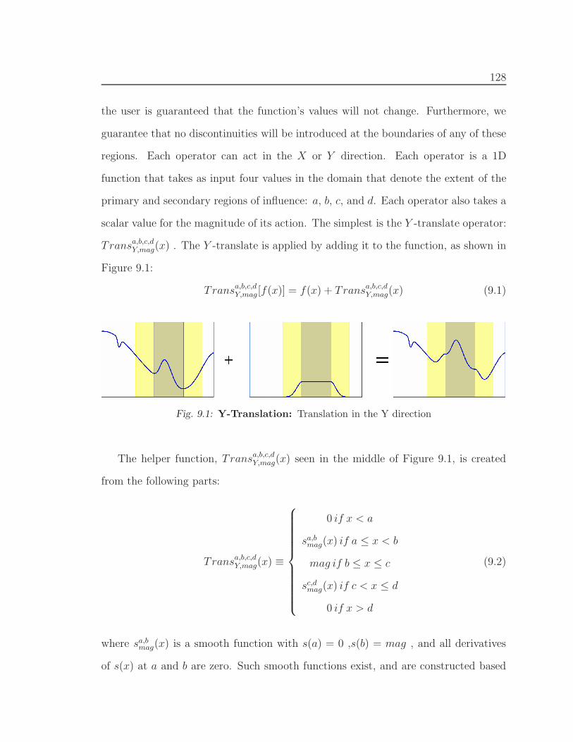
128
the user is guaranteed that the function’s values will not change. Furthermore, we
guarantee that no discontinuities will be introduced at the boundaries of any of these
regions. Each operator can act in the X or Y direction. Each operator is a 1D
function that takes as input four values in the domain that denote the extent of the
primary and secondary regions of influence: a, b, c, and d. Each operator also takes a
scalar value for the magnitude of its action. The simplest is the Y -translate operator:
Transa,b,c,dY,mag(x) . The Y -translate is applied by adding it to the function, as shown in
Figure 9.1:
Transa,b,c,dY,mag[f(x)] = f(x) + Transa,b,c,d
Y,mag(x) (9.1)
Fig. 9.1: Y-Translation: Translation in the Y direction
The helper function, Transa,b,c,dY,mag(x) seen in the middle of Figure 9.1, is created
from the following parts:
Transa,b,c,dY,mag(x) ≡
⎧⎪⎪⎪⎪⎪⎪⎪⎪⎪⎪⎨
⎪⎪⎪⎪⎪⎪⎪⎪⎪⎪⎩
0 if x < a
sa,bmag(x) if a ≤ x < b
mag if b ≤ x ≤ c
sc,dmag(x) if c < x ≤ d
0 if x > d
(9.2)
where sa,bmag(x) is a smooth function with s(a) = 0 ,s(b) = mag , and all derivatives
of s(x) at a and b are zero. Such smooth functions exist, and are constructed based
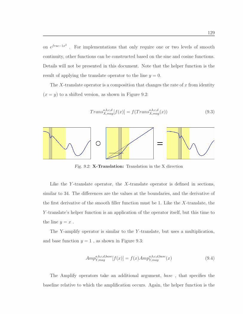
129
on efrac−1x2. For implementations that only require one or two levels of smooth
continuity, other functions can be constructed based on the sine and cosine functions.
Details will not be presented in this document. Note that the helper function is the
result of applying the translate operator to the line y = 0.
The X-translate operator is a composition that changes the rate of x from identity
(x = y) to a shifted version, as shown in Figure 9.2:
Transa,b,c,dX,mag[f(x)] = f(Transa,b,c,d
X,mag(x)) (9.3)
Fig. 9.2: X-Translation: Translation in the X direction
Like the Y -translate operator, the X-translate operator is defined in sections,
similar to 34. The differences are the values at the boundaries, and the derivative of
the first derivative of the smooth filler function must be 1. Like the X-translate, the
Y -translate’s helper function is an application of the operator itself, but this time to
the line y = x .
The Y-amplify operator is similar to the Y -translate, but uses a multiplication,
and base function y = 1 , as shown in Figure 9.3:
Ampa,b,c,d,baseY,mag [f(x)] = f(x)Ampa,b,c,d,base
Y,mag (x) (9.4)
The Amplify operators take an additional argument, base , that specifies the
baseline relative to which the amplification occurs. Again, the helper function is the
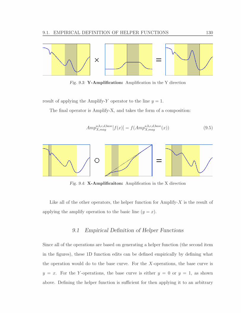
9.1. EMPIRICAL DEFINITION OF HELPER FUNCTIONS 130
Fig. 9.3: Y-Amplification: Amplification in the Y direction
result of applying the Amplify-Y operator to the line y = 1.
The final operator is Amplify-X, and takes the form of a composition:
Ampa,b,c,d,baseX,mag [f(x)] = f(Ampa,b,c,d,base
X,mag (x)) (9.5)
Fig. 9.4: X-Amplificaiton: Amplification in the X direction
Like all of the other operators, the helper function for Amplify-X is the result of
applying the amplify operation to the basic line (y = x).
9.1 Empirical Definition of Helper Functions
Since all of the operations are based on generating a helper function (the second item
in the figures), these 1D function edits can be defined empirically by defining what
the operation would do to the base curve. For the X-operations, the base curve is
y = x. For the Y -operations, the base curve is either y = 0 or y = 1, as shown
above. Defining the helper function is sufficient for then applying it to an arbitrary
9.2. SMOOTHNESS AND LAYERED OPERATORS 131
1D function through addition, multiplication, or compositing, as described in the
previous section.
9.2 Smoothness and Layered operators
The number of times the result of an operation is differentiable is the min of the orig-
inal function’s continuity and the helper function’s continuity. It is possible to build
helper functions which are infinitely differentiable (smooth), and therefore applying
the operation does not introduce any discontinuities to the original function. This
has the obvious exception when the operation has a degenerate condition, such as
zero-width regions of influence. The invariance of continuity can be proven using the
chain-rule of differentiation for the X operations (function compositions), and by the
linearity of the derivative operator for the Y operators (adds and multiplies).
Often, both Amplify or both Translate operators are applied ’simultaneously’.
For example, when moving a portion of the function along a diagonal, there is a
component of Translate-X and Translate-Y . This can be represented as a layering
of operators. It is important to apply the Y operator first. Otherwise, it will not
be applied to the correct portion of the function since the X operators change the
regions of influence.
While it is theoretically possible to continue layering operations, periodically, it
may be beneficial to collapse the edited function into a new function by evaluating it
explicitly.
9.3 Use in BRDF Editing and Other Graphics Applications
The operations described in Section 9 are natural to most processes that make use of
1D functions. Most previous edits of 1D functions have been performed with splines,

9.3. USE IN BRDF EDITING AND OTHER GRAPHICS APPLICATIONS 132
but the unpredictable nature of a spline’s shape as control point get close requires a
lot of ’counter-editing’ to correct for undesirable fluctuations. Image editing software
uses 1D functions to define color correction and gamma curves. Animation designers
use 1D functions to describe the speed of objects along their 3D path. All of the edits
we have shown in Part I operate on 1D functions, and use the operators described
above. Any scalar value that varies with time is a 1D function.

Part IV
CONCLUSION

134
10. CONCLUSION
This work has presented a new capability to render scenes interactively with complex
materials, geometry, and lighting (including global illumination) while the user adjusts
the material properties of objects in the scene. This final-placement BRDF editing is
imperative anywhere choices for BRDFs must be made based on how such decisions
affect the appearance of objects and their surroundings.
10.1 Final-Placement
Traditional workflows for choosing and editing BRDFs have used simplified visualiza-
tions, such as spheres lit by a point light. After a material is created in this way, it is
stored to be passed into an offline renderer at final frame-generation. The image(s) is
then examined, and different choices can be made for the materials, based on how they
affect the appearance of the final scene. In most cases, the final-placement appear-
ance of a material is quite different from the simplified visualization. Special effects
houses tend to adjust for this difference by placing disembodied lights, or making
local tweaks to the material – ultimately leading to the desired shot-by-shot look, but
sacrificing consistency and reproducibility. The ideal situation is to be able to choose
the materials based on visualizations of the final scene(s). This is the capability pro-
vided by the current work, with a tradeoff for flexibility of other scene parameters
(such as lighting and viewpoint). This means that the design process must still be
iterative - alternating between lighting and material design, but is no longer based on
10.2. THEORETICAL FRAMEWORK WITH FEW ASSUMPTIONS 135
an iterative cycle (with a long offline rendering step) while in the mode of designing
the scene’s materials.
10.2 Theoretical Framework with Few Assumptions
Part II presents a precomputation-based framework for interactive BRDF editing.
The precomputation step is founded on a standard path-tracer, and therefore inher-
its the generality of Monte Carlo path-tracing. Generating the precomputation data
is very similar to rendering a single frame. The main difference is not the operations
performed, but how the results are accumulated. In traditional rendering, the results
of many samples at a pixel are accumulated into a single color. With the BRDF
editing framework, each sample’s result is accumulated into the appropriate bin of a
high-dimensional tensor at each pixel. The rendering engine’s task is to weight these
bins appropriately and collapse their stored values into a single color at runtime. The
implication is that the final quality of the rendered images are as good as the offline
path-tracer can produce for a single frame. While more samples may be needed to
achieve the same signal-to-noise ratio, there is no inherent limitation in the quality
achievable by the renderers presented in Part II. Two important qualifications exist.
First, the precomputed data takes up much more storage than a single frame, and the
resolution of the image and BRDF factors is limited in practice to fit the resources
available. Second, intra-pixel integrations such as anti-aliasing and motion blur can-
not be directly applied without further theoretical scaffolding. It is important to note
that the practical limitations of storage are not limitations of the framework, and the
same theoretical mechanisms will be useful for more accurate implementations as
computing resources improve.

10.3. COMPLEMENT TO RELIGHTING 136
10.3 Complement to Relighting
A similar ‘final-placement’ approach has already been developed for lighting design.
Precomputation-based relighting has enabled artists and engineers to interactively
manipulate the complex lighting of a scene, while receiving feedback on how these
edits affect the final scene with shadows, complex geometry, and complex materials.
Just as relighting requires fixing the geometry and materials of the scene, BRDF
Editing is the complementary solution that requires fixing the geometry and lighting,
while leaving BRDFs unspecified until render-time. Just as relighting systems origi-
nally made restrictive assumptions on the nature of the source illumination (requiring
a 2D environment map), so must BRDF Editing restrict the editing operation from
acting on the full 4D space in which BRDFs live. This work has recommended edit-
ing a set of 1D factors that span the space of ”editable” behavior for each material.
Relighting has advanced to allow near-field illumination changes, using aggressive
compression. Unlike any of the relighting works that rely on an approximating basis
(such as spherical harmonics) or aggressive compression, the work presented here is
able to faithfully render the full nature of a BRDF, up to the degree of discretization
of the 1D factors. In Chapter 7, we discussed how the temporal coherence developed
for BRDF editing can be used in relighting to recapture the full 2D representation
without resorting to compression that may lose many important characteristics of the
lighting. Chapter 3 introduced the quotient BRDF, which is vital to maintaining a
full representation of the BRDF while editing some 1D aspect of its behavior.

10.4. CONTINUOUS EDITING AND DISCRETE CHOICES 137
10.4 Continuous Editing and Discrete Choices
BRDF Editing is unlike geometric or lighting design in that there is no good real-world
analogue to the process. While geometric tools try to mimic the act of clay modeling
or manufacturing processes, it is rare that one can change the material of an object
by directly interacting with it. Some exceptions to this are sanding and painting, but
these operations are often long and difficult to reverse. In addition, even situations
that present alternate choices for materials (such as choosing a tile for a new floor),
offer discrete choices. In the virtual setting, BRDF editing is a first-order operation
(not a byproduct of some other action), and editing can be accomplished along a
continuous spectrum. Even the seemingly continuous realm of paint colors does not
afford one the option to continuously vary the color of a wall or car (since applying a
new paint must be done to the whole surface uniformly.) Therefore, BRDF Editing
opens up a new mode of appearance design that has not been previously accessible
in real-world settings. This possibility is accompanied by the challenge of finding
appropriate cognitive actions for achieving the desired edits. Chapter 9 presented an
initial system for editing 1D functions that represent material behavior along some
parameterized direction. This has been shown to allow for a wide variety of edits,
but does not purport to be a final solution.
138
11. FUTURE DIRECTIONS
This thesis (and the related published works) has introduced the first general BRDF
editing framework for final-placement material design. The BRDF is just one of many
material representations — the most complex of which is the 8D BSSRDF. There
are two major directions for extending the current work in the future. First, more
complex representations such as BTFs and BSSRDFs may be analyzed to produce
similar material editing applications. Second, refinements and practical extensions to
the current BRDF framework can be added to make the work applicable in a broader
range of applications.
11.1 Higher-Complexity Functions
The BRDF is a local approximation to a more complex set of interactions between
light and scene objects. More complex behaviors such as those arising from nor-
mal/bump/displacement -maps and finally fully 6D BTFs cannot be edited in the
current framework. It should be noted that many of these effects can be included into
the precomputations as described in Part II, but will not be editable at runtime. One
hurdle to creating an interactive editing system that admits these higher-complexity
material attributes is that even offline editing of such effects has not been well stud-
ied. Just as BRDF editing does not have a real-world analog, BTFs present an even
tougher challenge when it comes to developing useful editing paradigms. The most
likely manifestation of these editing operations will require finding a representation
11.2. PRACTICAL EXTENSIONS 139
built up from low-dimensional factors, each of which can be easily edited by a human
user. This is similar to the editable BRDF representation introduced in Chapter 3.
Just as that representation includes a complex but non-editable component (the quo-
tient BRDF), so will higher-complexity functions likely include some fixed component
and some editable terms.
Subsurface scattering and transparencies with editable index-of-refraction are other
examples of departures from the local, opaque assumption of BRDFs. A more imme-
diate extension of the BRDFs used in this thesis is editable anisotropy shape. While
Chapter 3 describes how to edit parametric anisotropy, recent work ((Lawrence et al.,
2006)) suggests that anisotropic highlights of real-world materials are not oval. Con-
trolling this shape is a task that has not been explored offline nor interactively. Future
work in BRDF editing may incorporate such highlight-shape adjustments, once more
data is captured to determine the variety of this phenomena in the real world.
11.2 Practical Extensions
The work presented in this thesis is demonstrates practical implementations of the
theoretical framework developed in Chapter 5. Extending the implementation to ac-
count for production workflows would add to the practicality of the method. Very
little compression is recommended in this thesis. Preliminary experiments with stan-
dard compression methods (e.g. non-linear wavelet) for both inter- and intra-pixel
data has shown that artifacts quickly become noticeable in the regime of BRDF edit-
ing. An examination of Table 6.1 shows that the last bounce of global illumination
precomputations requires the most storage. However, that bounce also contributes
the least to the quality of the image, and is generally smooth due to the smoothing ef-
fect of multiple reflections. Therefore, a compression scheme that allows for constant
11.2. PRACTICAL EXTENSIONS 140
importance-to-storage ratios across bounces would seem a fruitful avenue of future
research.
One advantage of the absence of compression is that the precomputed data can be
passed directly to the render. This suggests a progressive precomputation that allows
users to begin working with coarse/noisy data very quickly, while a background pro-
cess continues to add precomputation data in order to refine the renderings through-
out an editing session.
Another extension that would allow the techniques proposed in this thesis to better
integrate with current production workflows is the ability to precompute on a short
animated sequence. Digital artists today work often with a turntable animation where
either the lighting or camera make a 360◦ rotation around a scene, while attributes
are adjusted. The capability to precompute on a similar preset animation would
no-doubt require the use of some compression, since storing many frames with the
footprints described in previous sections would not be practical. In addition, it is
more natural to perform such precomputation and compression on vertices instead of
pixels, as is currently the case.
Extending the pixel-based precomputation methods described in this thesis to
vertex-based would provide several advantages. (The precomputations in Sections
4.2, 6.1.1, and Chapter 8 are all pixel-based) While these methods assume a fixed
viewpoint, and therefore would not allow scene walkthroughs even with a vertex-
based extension, other operations can be enabled by computing directly on the scene’s
geometry. Besides the aforementioned per-vertex compression, changes in image res-
olution, camera zoom and field-of-view, as well as camera rotation (without change
in position) would be possible with vertex-bound precomputed data.
11.3. ADVANTAGES OF PRECOMPUTATION-BASED RENDERING 141
11.3 Advantages of Precomputation-based Rendering
The ‘holy grail’ of real-time rendering is to be able to edit any aspect of a scene
and rerender the image in less than 30ms. GPUs and programable shaders approach
this problem by increasing the speed and versatility of the scanline-shade pipeline
for rendering. However complex lighting and global illumination are not part of
this pipeline. In addition hardware-based rendering speed is proportional to the
complexity of the input data. Modern scenes with millions of polygons, hundreds of
lights, and hundreds of shaders continue to require more computation power than the
industry can supply. In contrast, precomputation-based rendering (that fixes some
aspect of the scene) can be decoupled from the complexity of many scene components.
For example, the work presented in this thesis renders at the same speed regardless
of geometric and lighting complexity of the scene. Similarly, relighting is decoupled
from the material complexity, and interactive camera motion techniques (radiosity
and (surface) light-fields) are decoupled from the material and lighting complexity.
A more restricted problem is the ‘holy-grail’ of interactive design. This problem
recognizes that scenes do not change arbitrarily, but must be able to change accord-
ing the will of a human designer. With the introduction of BRDF editing in this
work, there is an opportunity now to combine the three design scenarios (relight-
ing, camera motion, BRDF editing) into an iterative system that fixes two, while
allowing interactive design of the third. The ‘holy grail’ will not be achieved with a
brute-force approach, but by partitioning the problem into manageable subproblems.
A worthwhile direction of future work is to be able to quickly convert between the
representations needed for each type of editing operation, to unite them into an inter-
active rendering experience that gives the user control over any of: lighting, materials,
or camera, but not necessarily simultaneously.
REFERENCES
Agarwal, Sameer, Ramamoorthi, Ravi, Belongie, Serge, & Jensen, Henrik Wann.2003. Structured importance sampling of environment maps. Acm transactionson graphics, 22(3), 605–612.
Agrawala, Maneesh, Ramamoorthi, Ravi, Heirich, Alan, & Moll, Laurent. 2000 (July).Efficient image-based methods for rendering soft shadows. Pages 375–384 of:Proceedings of acm siggraph 2000. Computer Graphics Proceedings, AnnualConference Series.
Arvo, James, Torrance, Kenneth, & Smits, Brian. 1994. A framework for the anal-ysis of error in global illumination algorithms. Computer graphics, 28(AnnualConference Series), 75–84.
Ashikhmin, Michael, & Shirley, Peter. 2000. An anisotropic phong brdf model. J.graph. tools, 5(2), 25–32.
Ashikhmin, Michael, Premoze, Simon, & Shirley, Peter. 2000. A mirofacet-basedBRDF generator. Pages 65–74 of: Siggraph 00.
Bala, Kavita, Walter, Bruce J., & Greenberg, Donald P. 2003. Combining edgesand points for interactive high-quality rendering. Acm transactions on graphics,22(3), 631–640.
Barbic, James, & James, Doug. 2005. Real-time subspace integration of St. Venant-Kirchoff deformable models. Acm transactions on graphics (siggraph 2005),24(3), 982–990.
Ben-Artzi, Aner, Ramamoorthi, Ravi, & Agrawala, Maneesh. 2006a. Efficient shad-ows from sampled environment maps. journal of graphics tools, 11(1), 13–36.
Ben-Artzi, Aner, Overbeck, Ryan, & Ramamoorthi, Ravi. 2006b. Real-time BRDFediting in complex lighting. Acm transactions on graphics (siggraph 06), 25(3),945–954.
Blinn, James F. 1977. Models of light reflection for computer synthesized pictures.Pages 192–198 of: Siggraph ’77: Proceedings of the 4th annual conference oncomputer graphics and interactive techniques. New York, NY, USA: ACM Press.
REFERENCES 143
Blinn, James F., & Newell, Martin E. 1976. Texture and reflection in computergenerated images. Communications of the acm, 19(10), 542–547.
Chen, Wei-Chao, Bouguet, Jean-Yves, Chu, Michael H., & Grzeszczuk, Radek. 2002.Light field mapping: efficient representation and hardware rendering of surfacelight fields. Acm trans. graph., 21(3), 447–456.
Cohen, Michael F., & Wallace, John R. 1993. Radiosity and realistic image synthesis.Academic Press.
Colbert, Mark, Pattanaik, Sumanta, & Krivanek, Jaroslav. 2006. Brdf-shop: Creatingphysically correct bidirectional reflectance distribution functions. Ieee comput.graph. appl., 26(1), 30–36.
Cook, Robert, & Torrance, Kenneth. 1982. A reflectance model for computer graphics.Acm transactions on graphics, 1(1), 7–24.
Dana, Kristin J., van Ginneken, Bram, Nayar, Shree K., & Koenderink, Jan J. 1999.Reflectance and texture of real-world surfaces. Acm transactions on graphics,18(1), 1–34.
Daubecies, Ingrid. 1988. Orthonormal bases of compactly cupported wavelets. Com-munications of pure and applied math, 41(0).
Debevec, Paul. 1998 (July). Rendering synthetic objects into real scenes. Pages 189–198 of: Proceedings of siggraph 98. Computer Graphics Proceedings, AnnualConference Series.
Dobashi, Yoshinori, Kaneda, Kazufumi, Nakatani, Hideki, & Yamashita, Hideo. 1995.A quick rendering method using basis functions for interactive lighting design.Computer graphics forum, 14(3), 229–240.
Dorsey, Julie, Arvo, James, & Greenberg, Donald. 1995. Interactive design of complextime dependent lighting. Ieee computer graphics and applications, 15(2), 26–36.
Durand, Fredo, Holzschuch, Nicolas, Soler, Cyril, Chan, Eric, & Sillion, Francois X.2005. A frequency analysis of light transport. Acm transactions on graphics(siggraph 05), 24(3), 1115–1126.
Ershov, Sergey, Kolchin, Konstantin, & Myszkowski, Karol. 2001. Rendering pearles-cent appearance based on paint-composition modelling. Pages 227–238 of:Chalmers, A., & Rhyne, T.-M. (eds), EG 2001 proceedings, vol. 20(3). BlackwellPublishing.
Greene, Ned. 1986. Environment mapping and other applications of world projections.Ieee computer graphics & applications, 6(11), 21–29.
REFERENCES 144
Guo, Baining. 1998 (July). Progressive radiance evaluation using directional coher-ence maps. Pages 255–266 of: Proceedings of siggraph 98. Computer GraphicsProceedings, Annual Conference Series.
Hapke, Bruce W. 1963. A theoretical photometric function of the lunar surface.Journal of geophysical research 68, 15, 4571–4586.
Hart, David, Dutre, Philip, & Greenberg, Donald P. 1999 (Aug.). Direct illuminationwith lazy visibility evaluation. Pages 147–154 of: Proceedings of siggraph 99.Computer Graphics Proceedings, Annual Conference Series.
Hasan, Milos;, Pellacini, Fabio, & Bala, Kavita. 2006. Direct-to-indirect transfer forcinematic relighting. 1089–1097.
Heidrich, Wolfgang, & Seidel, Hans-Peter. 1998 (Aug.). View-independent environ-ment maps. Pages 39–46 of: 1998 siggraph / eurographics workshop on graphicshardware.
Kajiya, James T. 1986. The rendering equation. Pages 143–150 of: Siggraph ’86:Proceedings of the 13th annual conference on computer graphics and interactivetechniques. New York, NY, USA: ACM Press.
Kautz, Jan, & McCool, Michael. 1999. Interactive rendering with arbitrary BRDFsusing separable approximations. Pages 247–260 of: Eurographics rendering work-shop 99.
Kautz, Jan, Vázquez, Pere-Pau, Heidrich, Wolfgang, & Seidel, Hans-Peter.2000. Unified approach to prefiltered environment maps. Pages 185–196 of:Proceedings of the eurographics workshop on rendering techniques 2000. London,UK: Springer-Verlag.
Kollig, Thomas, & Keller, Alexander. 2003 (June). Efficient illumination by highdynamic range images. Pages 45–51 of: Eurographics symposium on rendering:14th eurographics workshop on rendering.
Kontkanen, Janne, Turquin, Emmanuel, Holzschuch, Nicolas, & Sillion, Francois.2006. Wavelet radiance transport for interactive indirect lighting. In: Euro-graphics symposium on rendering.
Lafortune, Eric P. F., Foo, Sing-Choong, Torrance, Kenneth E., & Greenberg, Don-ald P. 1997. Non-linear approximation of reflectance functions. Pages 117–126of: Siggraph ’97: Proceedings of the 24th annual conference on computer graphicsand interactive techniques. New York, NY, USA: ACM Press/Addison-WesleyPublishing Co.
REFERENCES 145
Lawrence, Jason, Rusinkiewicz, Szymon, & Ramamoorthi, Ravi. 2004. EfficientBRDF importance sampling using a factored representation. Acm transactionson graphics (siggraph 2004), 23(3).
Lawrence, Jason, Ben-Artzi, Aner, DeCoro, Christopher, Matusik, Wojciech, Pfister,Hanspeter, Ramamoorthi, Ravi, & Rusinkiewicz, Szymon. 2006. Inverse shadetrees for non-parametric material representation and editing. 735–745.
Lensch, Hendrik P. A., Kautz, Jan, Goesele, Michael, Heidrich, Wolfgang, & Seidel,Hans-Peter. 2001 (June). Image-based reconstruction of spatially varying mate-rials. Pages 103–114 of: Rendering techniques 2001: 12th eurographics workshopon rendering.
Leung, Thomas, & Malik, Jitendra. 2001. Representing and recognizing the visualappearance of materials using three-dimensional textons. Int. j. comput. vision,43(1), 29–44.
Liu, Xinguo, Sloan, Peter-Pike, Shum, Heung-Yeung, & Snyder, John. 2004. All-frequency precomputed radiance transfer for glossy objects. Pages 337–344 of:Eurographics symposium on rendering.
Matusik, Wojciech, Pfister, Hanspeter, Brand, Matt, & McMillan, Leonard. 2003. Adata-driven reflectance model. Acm trans. graph., 22(3), 759–769.
McCool, Michael D., Ang, Jason, & Ahmad, Anis. 2001. Homomorphic factoriza-tion of brdfs for high-performance rendering. Pages 171–178 of: Siggraph ’01:Proceedings of the 28th annual conference on computer graphics and interactivetechniques. New York, NY, USA: ACM Press.
Miller, Gene S., & Hoffman, C. Robert. 1984 (July). Illumination and reflectionmaps: Simulated objects in simulated and real environments. In: Course notesfor advanced computer graphics animation in siggraph 84.
Minnaert, Marcel. 1941. The reciprocity principle in lunar photometry. Astrophysicaljournal, 93, 403–401.
Nayar, Shree K., Krishnan, Gurunandan, Grossberg, Michael D., & Raskar, Ramesh.2006. Fast separation of direct and global components of a scene using highfrequency illumination. Acm trans. graph., 25(3), 935–944.
Ng, Ren, Ramamoorthi, Ravi, & Hanrahan, Pat. 2003. All-frequency shadows usingnon-linear wavelet lighting approximation. Acm transactions on graphics, 22(3),376–381.
Ng, Ren, Ramamoorthi, Ravi, & Hanrahan, Pat. 2004. Triple product wavelet inte-grals for all-frequency relighting. Acm transactions on graphics (siggraph 2004),23(3), 475–485.
REFERENCES 146
Nicodemus, F. E., Richmond, J. C., Hsia, J. J., Ginsberg, I. W., & Limperis, T. 1977.Geometric considerations and nomenclature for reflectance. National Bureau ofStandards (US).
Nimeroff, Jeffry S., Simoncelli, Eero, & Dorsey, Julie. 1994. Efficient Re-renderingof Naturally Illuminated Environments. Pages 359–373 of: Fifth eurographicsworkshop on rendering. Darmstadt, Germany: Springer-Verlag.
Oren, Michael, & Nayar, Shree. 1994. Generalization of lambert’s reflectance model.Pages 239–246 of: Siggraph 94.
Ostromoukhov, Victor, Donohue, Charles, & Jodoin, Pierre-Marc. 2004. Fast hier-archical importance sampling with blue noise properties. Acm transactions ongraphics, 23(3), 488–495.
Overbeck, Ryan, Ben-Artzi, Aner, Ramamoorthi, Ravi, & Grinspun, Eitan. 2006.Exploiting Temporal Coherence for Incremental All-Frequency Relighting. In:Eurographics symposium on rendering.
Pharr, Matt, & Humphreys, Greg. 2004. Physically based rendering: From theory toimplementation. Morgan Kaufmann.
Phong, Bui Tuong. 1975. Illumination for computer generated pictures. Commun.acm, 18(6), 311–317.
Ramamoorthi, Ravi, & Hanrahan, Pat. 2002. Frequency space environment maprendering. Acm transactions on graphics (siggraph 02 proceedings), 21(3), 517–526.
Rusinkiewicz, Szymon. 1998a. bv: brdf viewer. In: graph-ics.stanford.edu/ smr/brdf/bv.
Rusinkiewicz, Szymon. 1998b. A new change of variables for efficient BRDF repre-sentation. Pages 11–22 of: Eurographics rendering workshop 98.
Schlick, Christophe. 1994. An inexpensive BRDF model for physically-based render-ing. Computer graphics forum, 13(3), 233–246.
Sequin, Carlo H., & Smyrl, Eliot K. 1989. Parameterized ray-tracing. Pages 307–314of: Siggraph ’89: Proceedings of the 16th annual conference on computer graphicsand interactive techniques. New York, NY, USA: ACM Press.
Sloan, Peter-Pike, Kautz, Jan, & Snyder, John. 2002. Precomputed radiance transferfor real-time rendering in dynamic, low-frequency lighting environments. Pages527–536 of: Siggraph ’02: Proceedings of the 29th annual conference on computergraphics and interactive techniques. New York, NY, USA: ACM Press.
REFERENCES 147
Sloan, Peter-Pike, Hall, Jesse, Hart, John, & Snyder, John. 2003. Clustered principalcomponents for precomputed radiance transfer. Acm trans. graph., 22(3), 382–391.
Sloan, Peter-Pike, Luna, Ben, & Snyder, John. 2005. Local, deformable precomputedradiance transfer. Acm trans. graph., 24(3), 1216–1224.
Sun, Weifeng, & Mukherjee, Amar. 2006. Generalized wavelet product integral forrendering dynamic glossy objects. 955–966.
Torrance, Kenneth, & Sparrow, Ephraim. 1967. Theory for off-specular reflectionfrom roughened surfaces. JOSA, 57(9), 1105–1114.
Vasilescu, M. Alex O., & Terzopoulos, Demetri. 2004. Tensortextures: multilinearimage-based rendering.
Wan, Liang, Wong, Tien-Tsin, & Leung, Chi-Sing. 2005. Spherical q2-tree for sam-pling dynamic environment sequences. Pages 21–30 of: Rendering techniques.
Wang, Rui, Tran, John, & Luebke, David. 2004. All-frequency relighting of non-diffuseobjects using separable BRDF approximation. Pages 345–354 of: Eurographicssymposium on rendering.
Ward, Greg. 1992. Measuring and modeling anisotropic reflection. Pages 265–272 of:Siggraph 1992.
Ward, Gregory J., Rubinstein, Francis M., & Clear, Robert D. 1988. A ray tracingsolution for diffuse interreflection. Pages 85–92 of: Siggraph ’88: Proceedingsof the 15th annual conference on computer graphics and interactive techniques.New York, NY, USA: ACM Press.
Whitted, Turner. 1980. An improved illumination model for shaded display. Com-munications of the acm, 23(6), 343–349.
Zhou, Kun, Hu, Yaohua, Lin, Stephen, Guo, Baining, & Shum, Heung-Yeung. 2005.Precomputed shadow fields for dynamic scenes. 1196–1201.

i

vi

2

32

88

133

142