FINAL For Spinoff Wednesday SYM-AM-17-034 4-20-17

Acquisition Research Program Graduate School of Business & Public Policy Naval Postgraduate School

SYM-AM-17-057

Proceedings of the

Fourteenth Annual Acquisition Research

Symposium

Wednesday Sessions Volume I

Acquisition Research: Creating Synergy for Informed Change

April 26–27, 2017

Published March 31, 2017

Approved for public release; distribution is unlimited.

Prepared for the Naval Postgraduate School, Monterey, CA 93943.

Acquisition Research Program: Creating Synergy for Informed Change - 240 -

Empirical Cost Estimation Tool (PMS 320)

Johnathan C. Mun—is a research professor at NPS and teaches executive seminars in quantitative risk analysis, decision sciences, real options, simulation, portfolio optimization, and other related concepts. He received his PhD in finance and economics from Lehigh University. He is considered a leading world expert on risk analysis and real options analysis. Dr. Mun has authored 12 books and is the founder and CEO of Real Options Valuation Inc. [[email protected]]

Thomas J. Housel—specializes in valuing intellectual capital, knowledge management, telecommunications, information technology, value-based business process reengineering, and knowledge value measurement in profit and non-profit organizations. He is a tenured full professor for the Information Sciences (Systems) Department at NPS. He has conducted over 80 knowledge value added (KVA) projects within the non-profit, Department of Defense (DoD) sector for the Army, Navy, and Marines. Dr. Housel also completed over 100 KVA projects in the private sector. The results of these projects provided substantial performance improvement strategies and tactics for core processes throughout DoD organizations and private sector companies. [[email protected]]

Introduction This research project pertains to the identification, review, and potential development

of existing and alternative ship cost modeling methodologies. Most ship cost modeling has been traditionally weight-based. This approach drives the U.S. Navy decision makers to acquire smaller ships that require custom-designed shipboard components.

Current, and future, Department of Defense (DoD) acquisition budgeting processes require identifying, modeling, and estimating the costs of shipbuilding. The purpose of this research project is to determine if there is a more accurate way to empirically predict and model ship acquisition costs. The cost modeling tool developed in this study is intended to support development of ship cost forecasts. The proof of concept example for using this cost modeling tool included herein will provide a roadmap for other new ship acquisition cost modeling. The outcome of this research will likely increase cost savings.

The focus of this research is a comprehensive review of the most promising cost modeling methodologies. Notional cost data, or rough order of magnitude values, will be collected or generated to support this review of the cost methodologies. These data will be generated by the researchers using archival cost data from ship maintenance projects of various destroyer (i.e., DDG) acquisitions. We will identify these extrapolations, and we will use the resulting notional data to help evaluate the efficacy of the various cost models. This approach allows readers and study sponsors to see the various types of cost models, approaches, and sample data variables that are required to run the cost models and to examine sample results, as well as review the pros and cons of each approach. This study may require a follow-on project if there is a method that is of interest or that the sponsors feel might be applicable for a given ship acquisition context. The required data variables as well as sample results will be listed in the report, so the sponsors will know what to expect prior to engaging in any new research project. A follow-on study would allow us to obtain real-life cost data that could be plugged into the desired cost model.

The selected cost model will likely include the standard parametric models, nonparametric methods, systems dynamics based on project management task-based schedule and cost models; semiparametric Monte Carlo simulation models; curve fitting, time-series, and cross sectional models; nonlinear models, and so forth that have proven useful in forecasting costs in other acquisition contexts.


The Theory of Predictive Modeling in Cost

Different Types of Forecasting Techniques

The review of standard forecasting logic, in what follows, is useful in understanding the foundations of the various cost modeling techniques assessed in this study. Generally, forecasting can be divided into quantitative and qualitative approaches. Qualitative forecasting is used when little to no reliable historical, contemporaneous, or comparable data exist. Several qualitative methods exist such as the Delphi or expert opinion approach (a consensus-building forecast by field experts, marketing experts, or internal staff members), management assumptions (target growth rates set by senior management), as well as market research or external data or polling and surveys (data obtained through third-party sources, industry and sector indexes, or active market research). These estimates can be either single-point estimates (an average consensus) or a set of prediction values (a distribution of predictions). The latter can be entered into the Risk Simulator software tool, used in this study, as a custom distribution and the resulting predictions can be simulated; that is, running a nonparametric simulation using the prediction data points as the custom distribution. This approach can leverage experts’ knowledge by combining it with available quantitative data to arrive at more reliable ship building cost estimates.

Expert knowledge can be leveraged using the software by including qualitative estimates with quantitative analysis techniques. We provide several ship cost modeling case examples that are designed to demonstrate how the various cost modeling tools can be used in estimating ship building costs. That will also be helpful in learning how to apply the Risk Simulator software to develop more robust ship building cost estimates. The appendix provides a quick review of the quantitative methodologies that are available in the software.

Case Application: DDG 51 FLT III This section provides a detailed illustration of the proposed integrated cost

estimation modeling approach. As this is only an illustration, and due to a lack of proprietary data for this first phase of the analysis, the input assumptions are only high-level approximations based on publicly available information and publicly available subject matter expert estimates. Therefore, the results generated are not designed to be used in any specific decision making. Nonetheless, the approach presented has proven to be robust and valid, and with the correct input assumptions, can be rerun to generate accurate and reliable ship cost estimates. Information and data were obtained via publicly available sources and were collected, collated, and used in an integrated risk-based cost and schedule modeling methodology. The objective of this case study was to develop a comprehensive cost modeling strategy and approach, and as such, notional data were used. Specifically, we used the Arleigh Burke Class Guided Missile Destroyer DDG 51 Flight I, Flight II, Flight IIA, and Flight III (Figure 1) as a basis for the cost and schedule assumptions, but the modeling approach is extensible to all other ship building cost contexts within the U.S. Navy.


Overview of DDG 51 Flight III

DoD Spending on the Aegis Destroyer in FY 2012–2014

Figure 2 shows some sample acquisition budgets for DDG 51 Aegis destroyers from FY 2012 through FY 2016. The comprehensive DoD budget was downloaded and analyzed in the current research.

DoD Spending and Procurement for FY 2012–2014


High-Level Shipbuilding Process

Figure 3 shows the high-level process flow of building ship hulls and sections.

High-Level Process Flow (Hull and Sections)

Information, Communication, and Technology Subprocess

Figure 4 shows the ship’s subprocess for information, communication, and technology (ICT).

Subprocess for Information, Communication, and Technology (ICT)


Weapons System Subprocess

Figure 5 shows the ship’s subprocess for weapons systems.

Subprocess for Weapons Systems

SPY-6 Radar System

Figure 6 shows the ship’s radar subsystem’s process.

SPY-6 Radar System and Rework


DoD Extras: Electronic Warfare, Decoys, Extra Capabilities

Figure 7 shows the ship’s Electronic Warfare, Decoys, and Extra Capabilities subprocesses.

Subprocesses and Examples of DoD Extras

Risk-Based Schedule and Cost Process Modeling Figures 8 illustrates how the project management tasks are incorporated into the

Project Economics Analysis Toolkit (PEAT) software application. It includes all the high-level tasks required to build the ship along with their attendant costs with one million simulation trials that provide the possible distributions of the costing data. The parallel development of tasks 20–25 is where the ship’s various subsystems are incorporated into the cost and schedule model.

Input Assumptions


Similarly, using the cost and schedule modeling approach, we can zoom into various tasks and model each task in more detail. This permits us to use the results by reinserting the more detailed data values back into the more comprehensive model as required to improve accuracy. For instance, Figure 9 shows the ship’s weapons subsystem, with Figure 10 showing its cost and schedule assumptions. This model’s result can be inserted back into Task 23 in the comprehensive model (Figure 5).

Weapons Subsystem Process Development

Weapons Subsystem Cost and Schedule Assumptions


Critical Success Factors in Cost and Schedule Estimates

Tornado analysis is a powerful analytical tool that captures the model’s sensitivity to fluctuations in the critical success factors values for cost and schedule. This is done by identifying the static impacts of each variable on the outcome of the model; that is, the tool automatically perturbs each variable in the model a preset amount, captures the fluctuation on the model’s forecast or final result, and lists the resulting perturbations ranked from the most significant to the least. Figures 11 and 12 illustrate the application of a tornado analysis. Tornado analysis answers the question: “What are the critical success drivers that affect the model’s output the most?”

Tornado Analysis of Critical Success Factors (Cost Factors)

Tornado Analysis of Critical Success Factors (Schedule Factors)


Risk-Based Schedule and Cost Process Simulation

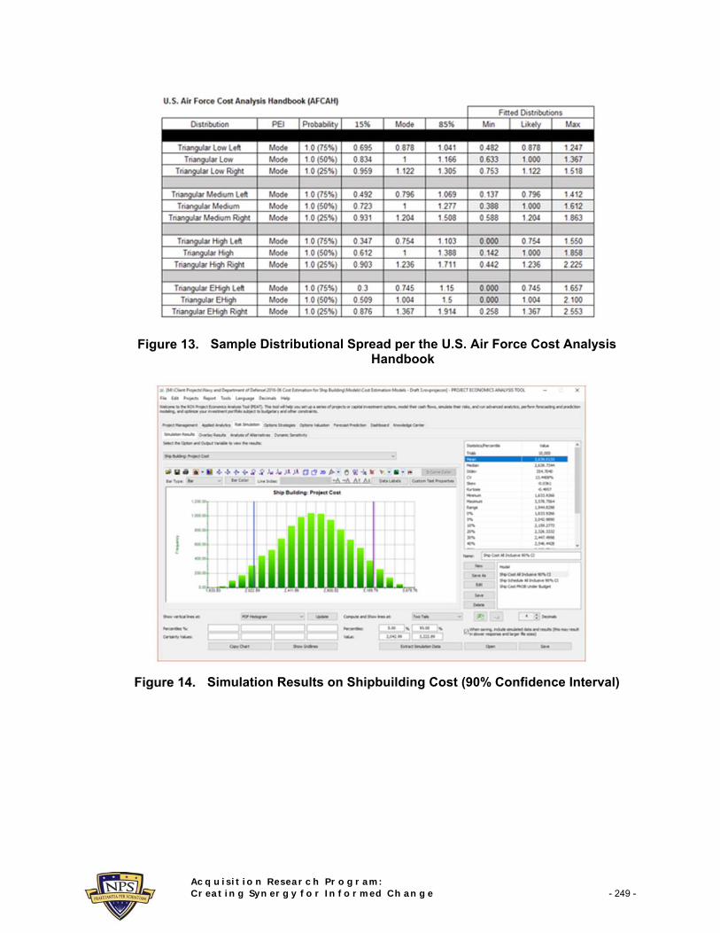
Next, the Monte Carlo Risk Simulation capability of the tool was used to create artificial futures by generating hundreds of thousands of sample paths of outcomes and analyzing their prevalent characteristics. In the Monte Carlo simulation process, triangular distributions (i.e., best-case, most-likely case, and worst-case scenarios) were used on the previously identified critical inputs. Figure 13 shows the values for a sample distributional spread used in Monte Carlo Risk Simulations per the Air Force Cost Analysis Handbook (AFCAH). These probability spreads were applied to each of the task’s cost and schedule inputs, and each of the tasks was simulated tens of thousands to hundreds of thousands of trials.

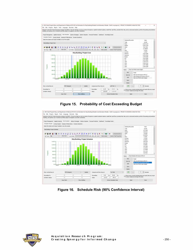
Figure 14 shows a sample representation of the results from the simulation process. For instance, the figure shows a 90% confidence interval for the total acquisition cost of a full-complement ship (fully built ship delivered after tests and sea trials, complete with ICTS, weapons systems, electrical systems, SPY-6 radar, and other add-ons). The 90% confidence interval pegs the total acquisition costs to be between $2.0 billion and $3.2 billion for a single ship. Clearly, these results are only for illustration purposes and are not meant to be definitive. Figure 15 shows the probability that there will be a budget overrun. For instance, if the acquisition budget is $2.2 billion, then we see that there is an approximately 12% probability of the cost coming in at or under budget, which means that there is an 88% probability of a budget overrun, with a mean or average actual acquisition cost of $2.6 billion.

Similarly, Figure 16 shows the total schedule from the initial contracting phase to delivery of the ship, complete with all subsystems installed and tested. The 90% confidence interval pegs the total schedule at between 110 and 146 weeks, averaging at 127 weeks.

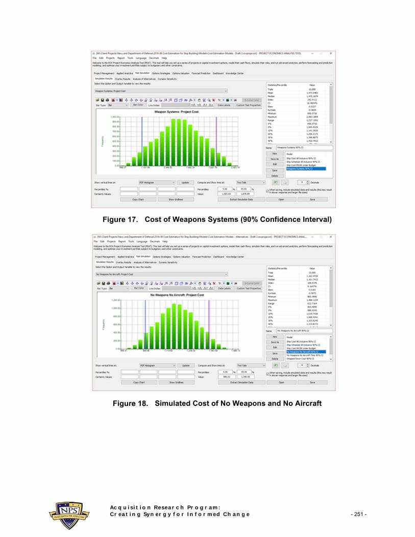
Alternatively, the modeling approach allows us to look at the ship’s subsystems. For example, Figure 17 shows the 90% confidence interval for weapons systems costs ($1.1 to $1.8 billion), while Figure 18 shows modeling the cost of building the ship without any subsystems. Each individual system or combinations of systems can be similarly modeled and analyzed (Figure 19), or overlaid on one another, as shown in Figures 20, 21, and 22. The probability distributions in these three figures allow you to compare how one system’s cost and uncertainties compare to one another. Finally, Figure 23 shows how the individual task’s schedule and cost elements impact and are correlated to each other, by way of dynamic sensitivity analysis.


Sample Distributional Spread per the U.S. Air Force Cost Analysis Handbook

Simulation Results on Shipbuilding Cost (90% Confidence Interval)


Probability of Cost Exceeding Budget

Schedule Risk (90% Confidence Interval)


Cost of Weapons Systems (90% Confidence Interval)

Simulated Cost of No Weapons and No Aircraft


Simulated Cost of Stripped-Down Ship Build

Comparative Analysis of Ship Configurations


Overlay of Simulated Probability Distributions (Subsystems)

Overlay of Simulated Probability Distributions (All Subsystems)


Dynamic Sensitivities of Stripped-Down Ship Build

Parametric Cost Models With Historical Data

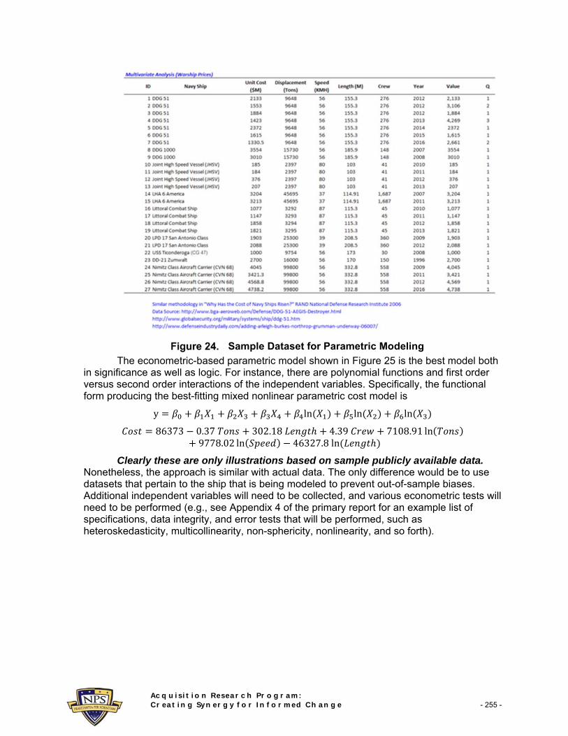
A complementary approach to generate additional input cost assumptions includes the use of parametric modeling. To run parametric models, historical data is first required. Figure 24 shows an example dataset obtained via various defense agencies’ publicly available information. The dataset shows various ship types, the unit costs (in millions), displacement in tons, speed, length, crew size, and year the ships were delivered.

Parametric models were developed and tested using simple multiple regression analysis, nonlinear regression, and econometric models. For instance, the following shows a simple linear parametric regression model and its results, where the functional form tested was

X

11837 0.10 80.44 55.56 6.09

Although the model looks good, with statistically significant p-values (e.g., 0.0097) that are lower than the standard 0.05 or 0.10 significance cutoffs and coefficients of determination (R-squared) that are relatively high at 82.60%, the model is flawed. For instance, the coefficient for displacement is negative, which defies conventional logic, where typically the heavier the ship, the higher the cost. This means the model’s specification is incorrect and another model is required. Figure 25 shows a mixed nonlinear parametric model with the following specification:

ln ln

40271 3351 ln 3952 ln 26.37 2.18

This model makes slightly more sense in that tonnage and speed have a positive relationship to cost and their effects are nonlinear. However, some of the other independent variables such as crew and length still show negative effects, albeit all modeled variables have the statistical significance of low p-values and a higher adjusted R-squared coefficient.


Sample Dataset for Parametric Modeling

The econometric-based parametric model shown in Figure 25 is the best model both in significance as well as logic. For instance, there are polynomial functions and first order versus second order interactions of the independent variables. Specifically, the functional form producing the best-fitting mixed nonlinear parametric cost model is

y ln ln ln

86373 0.37 302.18 4.39 7108.91 ln9778.02 ln 46327.8ln

Clearly these are only illustrations based on sample publicly available data. Nonetheless, the approach is similar with actual data. The only difference would be to use datasets that pertain to the ship that is being modeled to prevent out-of-sample biases. Additional independent variables will need to be collected, and various econometric tests will need to be performed (e.g., see Appendix 4 of the primary report for an example list of specifications, data integrity, and error tests that will be performed, such as heteroskedasticity, multicollinearity, non-sphericity, nonlinearity, and so forth).


Parametric Model With Nonlinear Regression

Parametric Probability Distribution and Curve Fitting

Another powerful cost modeling approach is distributional fitting; that is, how does an analyst or engineer determine which distribution to use for a particular task’s input cost or schedule variable? What are the relevant distributional parameters? If no historical data exist, we can make assumptions about the variables in question using the qualitative Delphi method, where a group of subject matter experts are tasked with estimating the behavior of each variable. Then, these values can be used as the variable’s input parameters (e.g., uniform distribution with extreme values between 0.5 and 1.2). When testing is not possible (e.g., a new or novel weapon subsystem), management can still make estimates of potential outcomes and provide the best-case, most-likely case, and worst-case scenarios, whereupon a triangular or custom distribution can be created.

However, if reliable historical data are available, distributional fitting can be accomplished. Assuming that historical patterns hold and that history tends to repeat itself, then historical data can be used to find the best-fitting distribution with their relevant parameters to better define the variables to be simulated. Figure 26 illustrates a distributional-fitting example of the costs shown previously (Figure 24).

The null hypothesis (Ho) being tested is such that the fitted distribution is the same distribution as the population from which the sample data to be fitted came. Thus, if the computed p-value is lower than a critical alpha level (typically .10 or .05), then the distribution is the wrong distribution. Conversely, the higher the p-value, the better the distribution fits the data. Roughly, you can think of p-value as a percentage explained, that is, if the p-value is 0.9849 (Figure 26), then setting a normal distribution with a mean of 1990 and a standard deviation of 1290 explains about 98.49% of the variation in the data, indicating an especially good fit. The results from the Risk Simulator software also rank all the selected distributions and how well they fit the data. The fitted distribution can now be


set up to run a simulation. The results from the simulation (tens to hundreds of thousands of simulation trials can be run) can be interpreted accurately (Figure 27).

Parametric Monte Carlo Simulation Model Distributional Fitting

Parametric Simulated Cost Results


Conclusions and Next Step Recommendations Based on this preliminary analysis and review of the alternatives, we conclude that

the risk-based cost and schedule simulations as well as parametric econometric models can be applied to modeling the cost of current and future U.S. Navy warships. It is evident in the analysis that any cost modeling must also include schedule risk because schedule delays can cause significant cost creep and budget overruns. Using the project process diagrams and task-based cost modeling coupled with Monte Carlo simulations to account for uncertainties in input assumptions and estimates and risks of overruns, a comprehensive methodology was developed.

We therefore recommend the following:

Collect and use actual cost data and develop more accurate cost estimates going forward in order to better calibrate the inputs based on real-life conditions. (We can provide suggestions on how to generate a database and methods to capture said required data.)

Use the Risk Simulator–based simulated probability distributions to determine how well the vendors are performing (e.g., running at 92% efficiency, etc.), thus creating a common set of agreed upon performance metrics for the organization.

Use control charts (based on simulated results) to determine if processes and tasks are in-control or out-of-control over time.

Identify critical success factors to start collecting cost and schedule data for more accurate estimates.

Incorporate learning curves and synergies when more than one ship is on order and the unit cost per ship would be lower.

The next phase of this research will focus on collecting actual cost and schedule data from a specific ship with subject matter experts’ inputs to obtain the qualitative values. The resulting simulations will provide an alternative to the existing cost and schedule forecasting models that can be compared for accuracy over the course of the ship build. If complete archival cost and schedule data are available for a specific ship build along with the forecasted costs and schedule, this data can be applied to the ship cost model forecasting approaches suggested by the current study for purposes of comparison to the existing models that were used during the ship build.

References Brown, A., & Neu, W. (2008). Naval surface ship design optimization for affordability: Phase

I.

Congressional Budget Office. (2015, October). An analysis of the Navy’s Fiscal Year 2016 shipbuilding plan. Retrieved from https://www.cbo.gov/sites/default/files/114th-congress-2015-2016/reports/50926-Shipbuilding.pdf

Deegan, C. (2005). NAVSEA Cost Estimation Handbook. Washington, DC: Naval Sea Systems Command.

Deschamps, L., & Greenwell, C. (n.d.). Integrating cost estimating with the ship design process.

Cost Assessment Data Enterprise (CADE). (2014). Joint agency cost schedule risk and uncertainty handbook (CSRUH). Retrieved from http://cade.osd.mil/cade/CSRUH.aspx

Kaluzny, B. L., Barbici, S., Berg, G., Chiomento, R., Derpanis, D., Jonsson, U., & Ramaroson, F. (2011). An application of data mining algorithms for shipbuilding cost


estimation. Journal of Cost Analysis and Parametrics, 4(1), 2–30. doi:10.1080/1941658X.2011.585336

Lee, U. (2014). Improving the parametric method of cost estimating relationships of naval ships (Master’s thesis). Cambridge, MA: Massachusetts Institute of Technology.

Miroyannis, A. (2006). Estimation of ship construction costs (Master’s thesis). Cambridge, MA: Massachusetts Institute of Technology.

Mislick, G. K., & Nussbaum, D. A. (2015). Cost estimation: Methods and tools. Hoboken, NJ: Wiley.

Moore, G. W., & White, E. D. (2005). A regression approach for estimating procurement cost. Journal of Public Procurement, 5(2), 187–209.

Mulligan, R. F. (2008, September 1). A simple model for estimating newbuilding costs. Maritime Economics & Logistics 10(3), 310–321.

Mun, J. (2015). Modeling risk: Applying Monte Carlo risk simulation, strategic real options, stochastic forecasting, portfolio optimization, data analytics, business intelligence, and decision modeling. Dexter, MI: Thompson-Shore.

Mun, J. (2016). Real options analysis: Tools and techniques. Dexter, MI: Thompson-Shore.

Naval Sea Systems Command (NAVSEA). (2015). Cost estimating. In SUPSHIP Operations Manual (SOM) (NAVSEA S0300-B2-MAN-010; ch. 6). Washington, DC: Department of the Navy.

Ross, J. M. (n.d.). A practical approach for ship construction cost estimating. Retrieved from http://ds-t.com/trade_shows-cd/ProteusEngineeringCOMPITPaper2004.pdf

Smith, M. B. (2008). Updating MIT’s cost estimation model for shipbuilding (Master’s thesis). Cambridge, MA: Massachusetts Institute of Technology.

SPAR Associates. (2015). Independent cost estimating services [Presentation]. Retrieved from http://www.sparusa.com/Presentations/Independent%20Cost%20Estimating%20Services-Overview.pdf

Truver, S. C. (2001, January–February). Navy develops product oriented design and construction cost model: PODAC emerges as critical element in achieving operationally superior, affordable naval forces. Program Manager, 38–41.

Walcott, J. (2012). Budget Office questions Navy shipbuilding cost estimates. Bloomberg. Retrieved from http://www.bloomberg.com/news/articles/2012-07-25/budget-office-questions-navy-shipbuilding-cost-estimate


Appendix: Most Common Forecast and Predictive Modeling Techniques ARIMA. Autoregressive integrated moving average (ARIMA, also known as

Box–Jenkins ARIMA) is an advanced econometric modeling technique. ARIMA looks at historical time-series data and performs back-fitting optimization routines to account for historical autocorrelation (the relationship of a variable’s values over time, that is, how a variable’s data is related to itself over time). It accounts for the stability of the data to correct for the nonstationary characteristics of the data, and it learns over time by correcting its forecasting errors. Think of ARIMA as an advanced multiple regression model, where time-series variables are modeled and predicted using its historical data as well as other time-series explanatory variables. Advanced knowledge in econometrics is typically required to build good predictive models using this approach. Suitable for time-series and mixed-panel data (not applicable for cross-sectional data).

Auto-ARIMA. The Auto-ARIMA module automates some of the traditional ARIMA modeling by automatically testing multiple permutations of model specifications and returns the best-fitting model. Running the Auto-ARIMA module is like running regular ARIMA forecasts; the differences being that the required P, D, Q inputs in ARIMA are no longer required and that different combinations of these inputs are automatically run and compared. Suitable for time-series and mixed-panel data (not applicable for cross-sectional data).

Basic Econometrics. Econometrics refers to a branch of business analytics, modeling, and forecasting techniques for modeling the behavior or forecasting certain business, economic, finance, physics, manufacturing, operations, and any other variables. Running Basic Econometrics models is similar to regular regression analysis except that the dependent and independent variables are allowed to be modified before a regression is run. Suitable for all types of data.

Basic Auto Econometrics. This methodology is similar to basic econometrics, but thousands of linear, nonlinear, interacting, lagged, and mixed variables are automatically run on your data to determine the best-fitting econometric model that describes the behavior of the dependent variable. It is useful for modeling the effects of the variables and for forecasting future outcomes, while not requiring the analyst to be an expert econometrician. Suitable for all types of data.

Combinatorial Fuzzy Logic. Fuzzy sets deal with approximate rather than accurate binary logic. Fuzzy values are between 0 and 1. This weighting schema is used in a combinatorial method to generate the optimized time-series forecasts. Suitable for time-series only.

Custom Distributions. Using Risk Simulator, expert opinions can be collected and a customized distribution can be generated. This forecasting technique comes in handy when the dataset is small, the Delphi method is used, or the goodness-of-fit is bad when applied to a distributional fitting routine. Suitable for all types of data.

GARCH. The generalized autoregressive conditional heteroskedasticity (GARCH) model is used to model historical and forecast future volatility levels of a marketable security (e.g., stock prices, commodity prices, oil prices, etc.). The dataset has to be a time series of raw price levels. GARCH will first convert the prices into relative returns and then run an internal optimization to


fit the historical data to a mean-reverting volatility term structure, while assuming that the volatility is heteroskedastic in nature (changes over time according to some econometric characteristics). Several variations of this methodology are available in Risk Simulator, including EGARCH, EGARCH-T, GARCH-M, GJR-GARCH, GJR-GARCH-T, IGARCH, and T-GARCH. Suitable for time-series data only. This technique can be used with cost data in the current ship costs context by forecasting ship cost volatility.

J-Curve. The J-curve, or exponential growth curve, is one where the growth of the next period depends on the current period’s level and the increase is exponential. This phenomenon means that over time, the values will increase significantly, from one period to another. This model is typically used in forecasting biological growth and chemical reactions over time. Suitable for time-series data only. It can be used in the current cost context by forecasting cost growth data.

Markov Chains. A Markov chain exists when the probability of a future state depends on a previous state and when linked together forms a chain that reverts to a long-run steady state level. This approach is typically used to forecast the market share of two competitors. The required inputs are the starting probability of a customer in the first state returning to the same state in the next period, versus the probability of switching to a competitor’s state in the next state. Suitable for time-series data only.

Maximum Likelihood on Logit, Probit, and Tobit. Maximum likelihood estimation (MLE) is used to forecast the probability of something occurring given some independent variables. For instance, MLE is used to predict if a credit line or debt will default given the obligor’s characteristics (30 years old, single, salary of $100,000 per year, and total credit card debt of $10,000), or the probability a patient will have lung cancer if the person is a male between the ages of 50 and 60, smokes five packs of cigarettes per month or year, and so forth. In these circumstances, the dependent variable is limited (i.e., limited to being binary 1 and 0 for default/die and no default/live, or limited to integer values such as 1, 2, 3, etc.) and the desired outcome of the model is to predict the probability of an event occurring. Traditional regression analysis will not work in these situations (the predicted probability is usually less than zero or greater than one, and many of the required regression assumptions are violated, such as independence and normality of the errors, and the errors will be fairly large). Suitable for cross-sectional data only.

Multivariate Regression. Multivariate regression is used to model the relationship structure and characteristics of a certain dependent variable as it depends on other independent exogenous variables. Using the modeled relationship, we can forecast the future values of the dependent variable. The accuracy and goodness-of-fit for this model can also be determined. Linear and nonlinear models can be fitted in the multiple regression analysis. Suitable for all types of data.

Neural Network. This method creates artificial neural networks, nodes, and neurons inside software algorithms for the purposes of forecasting time-series variables using pattern recognition. Suitable for time-series data only.

Nonlinear Extrapolation. In this methodology, the underlying structure of the data to be forecasted is assumed to be nonlinear over time. For instance, a


dataset such as 1, 4, 9, 16, 25 is considered to be nonlinear (these data points are from a squared function). Suitable for time-series data only.

S-Curves. The S-curve, or logistic growth curve, starts off like a J-curve, with exponential growth rates. Over time, the environment becomes saturated (e.g., market saturation, competition, overcrowding), the growth slows, and the forecast value eventually ends up at a saturation or maximum level. The S-curve model is typically used in forecasting market share or sales growth of a new product from market introduction until maturity and decline, population dynamics, and other naturally occurring phenomenon. Suitable for time-series data only.

Spline Curves. Sometimes there are missing values in a time-series dataset. For instance, interest rates for years 1 to 3 may exist, followed by years 5 to 8, and then year 10. Spline curves can be used to interpolate the missing years’ interest rate values based on the data that exist. Spline curves can also be used to forecast or extrapolate values of future time periods beyond the time period of available data. The data can be linear or nonlinear. Suitable for time-series data only.

Stochastic Process Forecasting. Sometimes variables are stochastic and cannot be readily predicted using traditional means. Nonetheless, most financial, economic, and naturally occurring phenomena (e.g., motion of molecules through the air) follow a known mathematical law or relationship. Although the resulting values are uncertain, the underlying mathematical structure is known and can be simulated using Monte Carlo risk simulation. The processes supported in Risk Simulator include Brownian motion random walk, mean-reversion, jump-diffusion, and mixed processes, useful for forecasting nonstationary time-series variables. Suitable for time-series data only.

Time-Series Analysis and Decomposition. In well-behaved time-series data (typical examples include sales revenues and cost structures of large corporations), the values tend to have up to three elements: a base value, trend, and seasonality. Time-series analysis uses these historical data and decomposes them into these three elements, and recomposes them into future forecasts. In other words, this forecasting method, like some of the others described, first performs a back-fitting (backcast) of historical data before it provides estimates of future values (forecasts). Suitable for time-series data only.

Trendlines. This method fits various curves such as linear, nonlinear, moving average, exponential, logarithmic, polynomial, and power functions on existing historical data. Suitable for time-series data only.

Acquisition Research Program Graduate School of Business & Public Policy Naval Postgraduate School 555 Dyer Road, Ingersoll Hall Monterey, CA 93943

www.acquisitionresearch.net

Documents

FINAL For Spinoff Wednesday SYM-AM-17-034 4-20-17