Filtering and forecasting with misspecified ARCH … of Econometrics 52 (1992) 61-90. North-Holland Filtering and forecasting with misspecified ARCH models I Getting the right variance

Journal of Econometrics 52 (1992) 61-90. North-Holland

Filtering and forecasting with misspecified ARCH models I

Getting the right variance with the wrong model

Daniel B. Nelson* NBER and UnicSersity of Chicago, Chicago, IL 60637, USA

This paper investigates the properties of the conditional covariance estimates generated by a misspecified ARCH model. For example, suppose that we observe a diffusion process at discrete time intervals of length h. For each h, we use a GARCH(l,l) model to estimate the instantaneous conditional covariance matrix of the diffusion. Under mild regularity conditions, the difference between these conditional covariance estimates and the true conditional covari- ante converges to zero in probability as h JO. Many other ARCH models (for example, Exponential ARCH) have similar consistency properties. This may well account for the success of ARCH models in short-term forecasting using high-frequency data, since even misspecihed ARCH models can produce ‘good’ estimates of volatility.

1. Introduction

Most theories of asset pricing, for example the CAPM of Sharpe (1964) and Lintner (19651, the option pricing formula of Black and Scholes (19731, and the arbitrage pricing theory of Ross (1976), relate required returns on assets to their variances and covariances. An enormous literature in empirical

*I would like to thank Stuart Ethier, Dean Foster, Leo Kadanoff, G. Andrew Karolyi, Albert Kyle, Franz Palm, G. William Schwert, an editor (Robert Engle), two anonymous referees, participants at the 1989 NBER Summer Institute, the 1990 Conference on Statistical Models for Financial Volatility, the 1990 Paris ARCH conference, and at workshops at Northwestern, Queen’s University, the University of Chicago, and the University of Wisconsin at Madison for helpful comments. The usual disclaimer regarding errors applies. The Center for Research in Security Prices provided research support.

0304-4076/92/$05.00 0 1992-Elsevier Science Publishers B.V. All rights reserved

62 D. Nelson, Filtering and forecasting with misspecified ARCH models

finance has explored the nature of this relation between risk and return. This literature has made it clear that the variability of returns and the degree of co-movement between assets change stochastically over time. Practical experience (as in the October stock market crashes of 1929, 1987, and 1989) points to the same conclusion. This realization has lead many researchers to recast asset pricing theory in terms of the conditional variances and covari- antes of returns. [See, for example, Engle, Ng, and Rothschild (19901, Harvey (1989), Hull and White (1987), Merton (19731, Shanken (19901, and Wiggins (1987j.l

Researchers have examined the time series behavior of stock market volatility for other reasons as well: for example, Schwert (1989) investigates the connection between macroeconomic variables and market volatility. The nature of market volatility changes has also entered into public policy debates on financial market regulation, margin requirements, transactions taxes, etc. [See, e.g., Hardouvelis (19881, Hsieh and Miller (1990), Summers and Summers (19891, and the Summer 1988 issue of the Journal of Economic Perspectiues.]

Since the seminal work of Engle (1982), ARCH models have become one of the most widely used means of modelling changing conditional variances.’ As are all statistical models, ARCH models are at best a rough approxima- tion to reality, and in applied work a misspecified model will inevitably be chosen. If we are concerned with accurately measuring conditional variances and covariances, it is important to ask how well a misspecified ARCH model can approximate the true structure of conditional heteroskedasticity in a time series.

This paper examines the ability of a misspecified ARCH model to estimate the conditonal covariance matrix of a stochastic process. To anticipate the results below, ARCH models are remarkably robust to certain types of misspecification. In particular, if the process is well approximated by a di$u- sion, broad classes of ARCH models provide consistent (in a sense developed below) estimates of the conditional covariances. The ARCH models may seriously misspecify both the conditional mean of the process and the dynamic behavior of the conditional variances. In fact, the misspecification can be so severe that the ARCH models would make no sense as data- generating processes and may make terrible medium and long-term forecasts - without affecting the consistency of the one-step-ahead conditional covariance estimates. As we will see, however, this robustness does not extend to all ARCH models, and it breaks down altogether to the extent that the process is not well approximated by a diffusion.

‘The survey of applications of ARCH in finance by Bollerslev, Chou, and Kroner (1992) lists several hundred papers on ARCH in finance, most dated 1989 and after.

D. Nelson, Filtering and forecasting with misspecijied ARCH models 63

1.1. The initial setup

Define the II X 1 diffusion process {X,) by the stochastic integral equation

X, =X0 + j’,u( X,) ds + jfL?‘/‘( X,) dW,, 0 0

(1.1)

where (W,) is an n x 1 standard Brownian motion, and p(. > and 01/2(.l are continuous functions from R” into R” and into the space of n X n matrices, respectively. Under mild moment conditions [see Arnold (1973)l fl(X,> = 0*/*(X,> .L?‘/2(Xr)l and ,LL(X~) are, respectively, the instantaneous conditional covariance matrix and instantaneous conditional mean (per unit of time) of increments in the {X,) process. X0 is assumed random with probability measure u0 independent of (W,), of <m.

In applications, {X,) might include asset prices and other state variables describing an economy. Some elements of {X,) may never be directly observable. Others, we assume, are observable, but only at discrete time intervals of length h. For example, our model may define the stock price process in continuous time, while we observe only stock prices at discrete intervals of length h. Formally, we partition X, as [Xi:,,, Xi,, :n,l)‘, where X,:,,, consists of the first q elements of X, (observable at intervals of length h) and X q+, :n, I consists of the last IZ - q elements (which are never observable).2 We partition p and 0 accordingly.

For each t, our goal is to estimate 0, :q,, :4 (X,) (the instantaneous covari- ante of the increments in the observable variables X, :4 f given t and the history up to time t of the (X,) process) given the smaller information set

{t,X1:q,0,X1:q,h,X1:q,2h,...,X1:q,h[t/h] ) (i.e., the time index and the past observed values of X, :4,1). Under these assumptions, 0, :q,, ,,(X,> is unobservable since X,+ 1 :n , is unobservable, and unless t is an integer multiple of h, X,lq:r.is as well - i.e., L!,:,,,:, (X,1 is a conditional covariance matrix, but is condmonal on a larger information set than is possessed by the econometrician.

1.2. Consistent filters: A definition

In our examples, we generate conditional covariance estimates {,8, :q, 1 :q,t) with a sequence of ARCH models, whose coefficients may depend on h. We say that a given sequence of ARCH conditional covariance estimates

{h’,:q,l:q,t)hJ,, P rovides a consistent jifter for the {LZ, :q,, :q, ,) if for each

‘Similarly, in our notation, A, , , is the (i - j)th element of the matrix function A, at time t, and L is the ith element of t‘hk vector function b, at time t. Where A, can be written as ACX,), we use the notations interchangeably.

64 D. Nelson, Filtering and forecasting with m&specified ARCH models

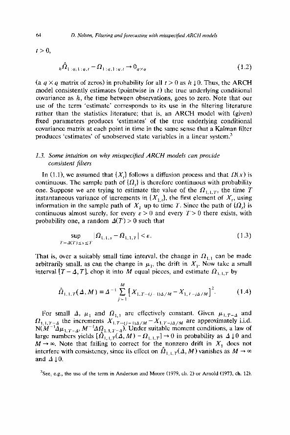
t > 0,

h A 1 :q.l :q,, - 01 :q,l :q,1 + oqxq

(a q X q matrix of zeros) in probability for all t > 0 as h J. 0. Thus, the ARCH model consistently estimates (pointwise in t) the true underlying conditional covariance as h, the time between observations, goes to zero. Note that our use of the term ‘estimate’ corresponds to its use in the filtering literature rather than the statistics literature; that is, an ARCH model with (given) fixed parameters produces ‘estimates’ of the true underlying conditional covariance matrix at each point in time in the same sense that a Kalman filter produces ‘estimates’ of unobserved state variables in a linear system.3

1.3. Some intuition on why misspecij‘ied ARCH models can provide consistent jilters

In (1.11, we assumed that (X,} follows a diffusion process and that 62(x> is continuous. The sample path of {n,} is therefore continuous with probability one. Suppose we are trying to estimate the value of the L!,,,,,, the time T instantaneous variance of increments in {X, ,I, the first element of X,, using information in the sample path of X, up to’time T. Since the path of (0,) is continuous almost surely, for every E > 0 and every T > 0 there exists, with probability one, a random A(T) > 0 such that

sup If4,1,s-f4,1,TI <&.

T-A(T)sssT (1.3)

That is, over a suitably small time interval, the change in a,,, can be made arbitrarily small, as can the change in pr, the drift in X,. Now take a small interval [T - A, T], chop it into M equal pieces, and estimate 0 ,, ,, T by

h l,l,T(A,M) =A-’ IE [Xl.~-~j-l~~/~-Xl,~-jA/~]2~ (1.4) j=l

For small A, pL1 and L2,,, are effectively constant. Given ~r,~_~ and R l,l,T_d the increments X,,T_(j_ljd,M -X1,T_jd,M are approximately i.i.d. NW’&,,,-,, M-‘A$,,,.-, ). Under suitable moment conditions, a law of large numbers yields [fl,,,,,(A, M) - L2,,,,, I + 0 in probability as A 4 0 and M + ~0. Note that failing to correct for the nonzero drift in X, does not interfere with consistency, since its effect on h,, JA, M) vanishes as M + a, and A JO.

‘See, e.g., the use of the term in Anderson and Moore (1979, ch. 2) or Arnold (1973, ch. 12).


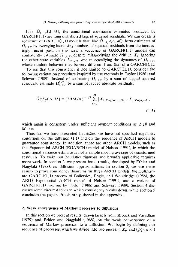
Like fi ,,i,r(A, Ml, the c on i ional cl t covariance estimates produced by GARCH(1, 1) are long distributed lags of squared residuals. We can create a sequence of GARCH(1, 1) models that, like &,,,,.(A, Ml, form estimates of R ,, ,, r by averaging increasing numbers of squared residuals from the increasingly recent past. In this way, a sequence of GARCH(1, 1) models can consistently estimate 0,. ,,r, despite misspecifying the drift in Xi, ignoring the other state variables XZtn,r, and misspecifying the dynamics of O,,i,r, whose random behavior may be very different from that of a GARCH(1, 1).

To see that this consistency is not limited to GARCH(1, 11, consider the following estimation procedure inspired by the methods in Taylor (1986) and Schwert (1989): Instead of estimating Oi,,,r by a sum of lagged squared residuals, estimate 0 , , i’fT by a sum of lagg ed absolute residuals:

h;‘fT(A,M) E (2AM/T)p”2 E IX*,T-(j-l)d/M-X1,T-,~/MI' 9 .

j=l

(1.5)

which again is consistent under sufficient moment conditions as A J. 0 and M + co.

Thus far, we have presented heuristics: we have not specified regularity conditions on the diffusion (1.1) and on the sequence of ARCH models to guarantee consistency. In addition, there are other ARCH models, such as the Exponential ARCH (EGARCH) model of Nelson (1991), in which the conditional variance estimate is not a simple moving average of transformed residuals. To make our heuristics rigorous and broadly applicable requires more work. In section 2, we present basic results, developed by Ethier and Nagylaki (19X8), on diffusion approximations. In section 3, we use these results to prove consistency theorems for three ARCH models: the multivariate GARCH(l,l> process of Bollerslev, Engle, and Wooldridge (19881, the AR(l) Exponential ARCH model of Nelson (19911, and a variant of GARCH(l,l) inspired by Taylor (1986) and Schwert (1989). Section 4 dis- cusses some circumstances in which consistency breaks down, while section 5 concludes the paper. Proofs are gathered in the appendix.

2. Weak convergence of Markov processes to diffusions

In this section we present results, drawn largely from Stroock and Varadhan (1979) and Ethier and Nagylaki (1988), on the weak convergence of a sequence of Markov processes to a diffusion. We begin by defining our sequence of processes, which we divide into two pieces: &XI} and &x}, n x 1


and m X 1 vector processes, respectively.4 {hXt} and {,Y,) will be random step functions taking jumps at times h, 2h, 3h, and so on. In the convergence results below, we present sufficient conditions for IhXt} =$ IX,}, where {X,} is a solution of (1.1) and =j denotes weak convergence. In the applications in section 3, IhXIl represents the underlying stochastic system generating the data, while &Ytl represents the difference between the true conditional covariance matrix of IhXtl and the estimate generated by an ARCH model. The conditions below will be used in section 3 to guarantee that for every t > 0, hY, converges in probability to an m x 1 vector of zeros as h JO - i.e., that for each t > 0, our conditional covariance estimator is consistent as h JO.

Formally, let D([O, to>, R” X R”) be the space of functions from [O, co) into R” x R” that are right continuous with finite left limits (RCLL). D is a metric space when endowed with the Skorohod metric [see Ethier and Kurtz (1986, ch. 3) for formal definitions]. For each h > 0, let h~kh be the information set at time kh - i.e., the c-algebra generated by

hX0,hXh,hX2h,. . . ,,,Xkh and hYo,hY,,,hYZh,. . . ,hYk,,. Let B(R” X R”) denote the Bore1 sets on R” x R”, and let vh be a probability measure on (R”, B(R” x R”)). For each h > 0, let IIh<x, y, . ) be a transition function on R” x R” - i.e.:

(a) n,(x, y, . > is a probability measure on CR” x R”, B(R” X R”)) for all (x, y) E R” x R”.

(b) II,<., . , r) is B(R” X Rm) measurable for all r~ B(R” X Rm).

Let P,, be the probability measure on D([O, m>, R” X R”) such that

P,[(,X,,,,Y,) or] =~,,(r) forany TgB(R”XR”), (2.1)

hK,xt~hyt) = LXkh~hYkh)~ khst<(k+l)h] =I, (2.2)

almost surely under Ph for all k 2 0 and all r E B( R” x R") .

41n our notation, &,XJ refers to ,,X, as a random function of time - i.e., it refers to the ,,XI process. On the other hand, ,,X, (without the curly brackets) refers to the value that the IhX,) process takes at a particular time t.

D. Nelson, Filtering and forecasting with misspecified ARCH models 67

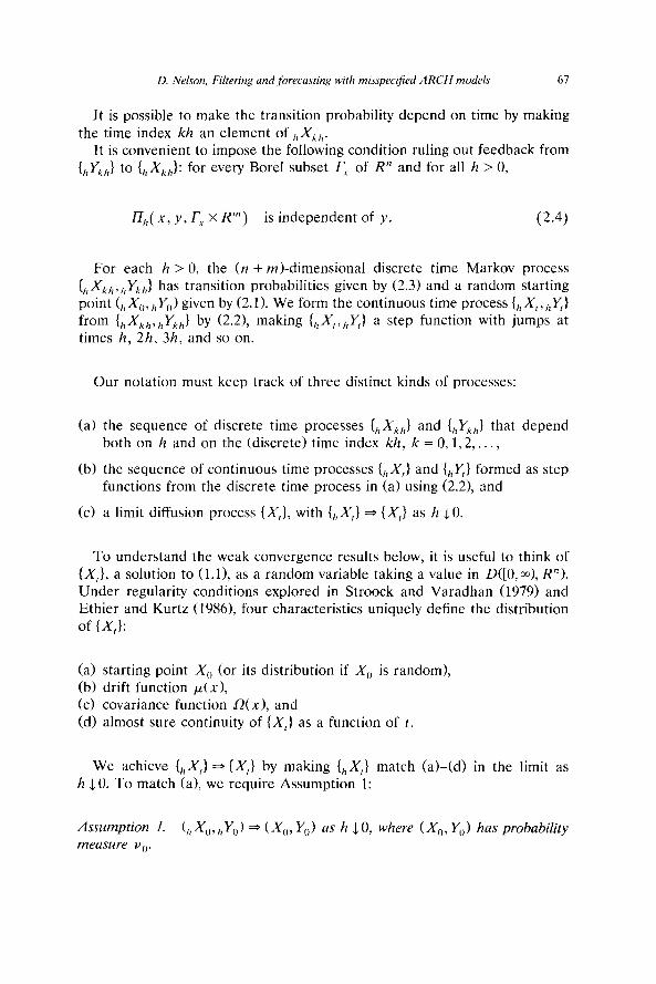
It is possible to make the transition probability depend on time by making the time index kh an element of ,,Xkh.

It is convenient to impose the following condition ruling out feedback from {,IYkh} to IhXk,,}: for every Bore1 subset r, of R” and for all h > 0,

D,?( X, y , r, x R’,) is independent of y. (2.4)

For each h > 0, the (n + m&dimensional discrete time Markov process

(hXkh,lr k/l Y } has transition probabilities given by (2.3) and a random starting point (,lX,),hYO) given by (2.1). We form the continuous time process (hXr,,ZY}

from (1, xkh> /I kh Y 1 by (2.2), making IhXI, IZY) a step function with jumps at times h, 2h, 3h, and so on.

Our notation must keep track of three distinct kinds of processes:

(a) the sequence of discrete time processes (hXk,J and (hYk,,) that depend both on h and on the (discrete) time index kh, k = 0,1,2,. . ,

(b) the sequence of continuous time processes (hXf} and (I,Y,) formed as step functions from the discrete time process in (a> using (2.2), and

Cc) a limit diffusion process IX,), with IhX,) * (X,} as h LO.

To understand the weak convergence results below, it is useful to think of (X,), a solution to (l.l), as a random variable taking a value in D([O,m), R”). Under regularity conditions explored in Stroock and Varadhan (1979) and Ethier and Kurtz (1986), four characteristics uniquely define the distribution of (PC,):

(a) starting point X,, (or its distribution if X,, is random), (b) drift function p(x), Cc) covariance function L?(x), and Cd) almost sure continuity of IX,) as a function of t.

We achieve (hX,) * (X,1 by making (,,X,} match (a)-(d) in the limit as h JO. To match (a), we require Assumption 1:

Assumption 1. Ch X,,, hY,,) 3 (Xc,, Y,,> as h 10, where (X0, Y,)> has probability measure vg.

68 D. Nelson, Filtering and forecasting with misspecifed ARCH models

Next, we require that the discrete analogues of j_~ and 0, ph and fihY are well-defined for all (x, y) E R”+“:

(2.5)

nh(x) =‘+(h&+,,h -,xkh>

(2.6)

where the expectations in (2.5M2.6) are taken under Ph.5 ph and ah are independent of y by (2.4). Next, define the norm of a 9 x r real matrix A as

1 1 l/2

IlAll = c c 4, . i=l,q j=l,r

To match (b)-(c) in the limit as h JO, we require:

Assumption 2. For every r~ > 0,

lim sup IlL!,(x) -fl(x)II=O, h Jo llX/lS?J

(2.7)

(2.8)

P-9)

where kL(. 1 and fX. ) are continuous.

Assumption 2 requires ph and 0, to converge uniformly on every bounded subset of R”, which is much less restrictive than uniform convergence on R”.

The following fourth moment condition guarantees sample path continuity of the limit process [see Arnold (1973, p. 40) and Nelson (1990a, theorem 2.211, and so matches (d) in the limit as h 5 0:

Assumption 3. For every 77 > 0 and all i = 1,. . . , n,

lim sup h-‘E (,XL Ck+,jh - h Jo IIXllS?

I hxi,khj4(hXkh =x] =O. (2.10)

‘(2.6) defines O,(x) as an uncentered conditional second moment. None of our results would be altered by using the centered moments instead [i.e., by replacing ChXllCk+,) -,,Xhk) with (hXh(k+,)-hXhk-h~h(hXhk)) in (2.6)1, since the difference between the centered and uncentered second moments vanishes as h 10.

D. Nelson, Filtering and forecasting with misspecifed ARCH models 69

Finally, (a)-(d) must completely characterize the distribution of {X,}:

Assumption 4. There is a distributionally unique solution to (l.l).’

Theorem 2.1 (Stroock- Varadhan >. Under Assumptions 1-4, {,X,1 * (X,1 as h JO.

We next turn to {jIyf}. First, for every 6 > 0, h > 0, and (x, y) E R”+“, let the following conditional expectations be well-defined:

c,,.a(x>~) ~hh-SE[h~k+,)h-hYkhl,,Xkh=X,/,Ykh=Y

d,,.,(x,y) =h-‘E[(,&+,,,, -I&,)

‘I, (2.11)

%&+l)h - hYHJ’LXk/2 =x,,y,, =y].

Assumption 5. For some 6, 0 < 6 < 1, and for every 77 > 0,

(2.12)

where .for all x E R”, c(x, 0) = 0, and

(2.13)

(2.14)

While the drift and conditional second moment of the increments in {hXkh} are O(h), Assumption 5 guarantees that the drift and (uncentered) second moment of the increments in (hYk,J are O(h’) and o(h’>, respectively. This has two important implications: first, IhY} operates on a faster time scale than &Xl}, since the drift (and possibly the variance) per unit of time of&Y) grow at a faster rate (as h 5 0) than the drift and variance per unit of time of &XI}. This implies that if IhYt) mean-reverts to a vector of zeros, it does so with increasing speed as h JO. Second, as h JO the drift of IhYr) [which is O(h’)] dominates the variance of {hY) [which is o(h’)]. This allows us to approximate the behavior of IhY,) by a deterministic differential equation.

‘See Ethier and Kurtz (1986, pp. 290-291) for formal definitions. Several sets of sufficient conditions for Assumption 4 are summarized in appendix A of Nelson (1990a).


The next assumption assures that this differential equation is well-behaved, pulling ihYt} back to a vector of zeros:

Assumption 6. For each x E R”, y E R”, define the differential equation

dY(t,x,y)/dt=c(x,Y(t,x,y)), (2.15)

with initial condition

Y(O, x, Y) =Y. (2.16)

Then Omx, is a globally asymptotically stable solution of (2.15)-(2.16) for bounded values of x, y - i.e., for every TJ > 0,

lim I’m /;;,,, IIWj x7 Y) II = 0.7 (2.17)

Finally, we require a Lyapunov condition which guarantees that &Y,} does not diverge to infinity in finite time:’

Assumption 7. There exists a nonnegative function p(x, y, h), twice differentiable in x and y, and a positive function NT, h) such that

lim liminf hi0 ,Kx’,i&sP(X~Y~h) =co, (2.18) rl_”

limsup limsup A(q, h) < a, ?l-+m hLO

(2.19)

limsup E[p(,&,hY”,h)] ccoT hLO

(2.20)

and for every 77 > 0,

lim sup sup h10

h-‘EIL)(hx~k+l)h,h~k+l)h,h)

Kx’, Y’NS7,

-P(x, Y,h)l,Jk/, =x,,y,, =Y] -h(T,h)p(x,y,h) 10. (2.21)

‘It is often possible to verify Assumption 6 without solving (2.1%(2.16). For example, the following Lyapunov condition suffices: There is a nonnegative V(x, y), bounded on compact tx, y) sets and differentiable in y, functions ~(7) and g(x), and a d > 0 such that for each

N > 0, inf, d R s N ~(7) > 0, info d IIxI, B ,, g(x) > 0, Ilull’s < V(x, y), and for each n > 0 and all

Y eR”‘> suP,,,,,.~K(7))1/(X,Y)+(~T/(x,Y)/aY)”c(x,Y)sO.

‘This condition also guarantees that (X,} does not explode in finite time, but this was already implied by Assumption 4 [see Stroock and Varadhan (1979, ch. lo)].


Theorem 2.2 ( Ethier-Nagylaki). Let Assumptions l-7 hold. Then

/ZK-)Ot7lx, in probability as h JO for euery t > 0. (2.22)

3. Examples of consistent ARCH filters

In this section, we prove filter consistency for three ARCH models [multivariate GARCH(1, 11, AR(l) EGARCH, and the Taylor-Schwert model1 when (1.1) generates IhXr) - i.e., we let {X,1 be a solution to (1.11, and then

define for all t 2 0, hXI = XLr,hI.h where [t/h] is the integer part of t/h. We then expand these results to allow lhXtl to be generated by a stochastic difference equation.

3.1. Multivariate GARCH(1, 1)

In the multivariate GARCH(l, 1) model of Bollerslev, Engle, and Wooldridge (19881, conditional covariance estimates are formed by the

recursion

vech [ h4 :y,I :cr.(k+I)h] = K + & vech[,fir :4,1 :q.lJ

+ h-‘%vech hii :,.kh& :,,,,I y [ (3.1)

where vech( .> stacks the columns of the lower portion of a symmetric matrix. W,, B,, and A,, are i(q + 1)q X ;Cq + 1)q matrices. The {,[, :4 khl in (3.1) are fitted residuals obtained using the (possibly misspec’ified) drift n +/stlX!ft17,fl, :q. I :q,kh)I

htl :q,kh ‘hX1 :q,(k+l)h -hX1 :q,kh -h ‘~h(hxkh.h’l :q.l :q,kh).

(3.2)

For some 6, 0 < S < 1, let wh, A,, B,, and ,&A(‘, .I satisfy

6, = o(h-“2),9

W, =o(h6),

I-B,-A,=o(h’),

A,=h’A+o(h*),

(3.3)

(3.4)

(3.5)

(3.6)

‘f(x, y, h) = O(h”) means that for every positive finite r), there is a A t 0 such that

lim sup SUP h-Yllf(x,y,h)ll<A. h 10 IKx’, y’)II<q

That is, hdYf is uniformly bounded in h for bounded (x, y). If A = 0, then we say that f(x, y, h) = o(h9.

72 D. Nelson, Filtering and forecasting with misspecijied ARCH models

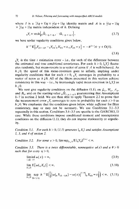
where I is a t<q + 1)q X i(q + l)q identity matrix and A is a +Cq + 1)q X $(q + l)q matrix independent of h. Defining

hYt =vech[,& :q.l :q,t - fi, :q,l :,,t]>

we have under regularity conditions given below,

(3.7)

h-r E[,&+rjh - hYkhlhXkh =x,,,Ykh =y] = -hs-‘A +y + O(1).

(3.8)

hYt is the time t estimation error - i.e., the vech of the difference between the estimated and true conditional covariances. For each h > 0, ihYt) fluctu- ates randomly, but mean-reverts to a vector of zeros if A is well-behaved. As h JO, the speed of this mean-reversion goes to infinity, implying under regularity conditions that for each t > 0, ,,Y, converges in probability to a vector of zeros as h JO. All of the filters presented in this section achieve consistency in this way - i.e., by increasingly rapid mean reversion in &Yt} as h JO.

We next give regularity condition; on the diffusion (l.l), on ji,,, W,, A,, and B,, and on the starting value hfil :q,l :q,o g uaranteeing that Assumptions

l-7 in section 2 hold. We are then able to apply Theorem 2.2 to prove that the measurement error hy1 converges to zero in probability for each t > 0 as h J 0. We emphasize that the conditions given below, while suficient for filter consistency, may or may not be necessary. We use Conditions 3.1-3.3 repeatedly in this section. Conditions 3.4-3.5 are specific to the GARCH(1, 1) case. While these conditions impose conditional moment and nonexplosion conditions on the diffusion (1.11, they do not impose stationarity or ergodic- ity.

Condition 3.1. For each h > 0, (1.1) generates {hXr} and satisfies Assumptions 1, 3, and 4 of section 2.

Condition 3.2. For some E > 0, limsup, 1 0 EljhYO)l’+’ < ~0.

Condition 3.3. There is a twice differentiable, nonnegatiue w(x) and a 8 > 0 such that for every > 0, 77

lim sup h-’ E( [ Iw(hXck+ljh) -W(X) I”?,x,, =x]) < m, (3.11) h Jo IIxll5?1


and there is a h > 0 for all x E R”,

SAW(X). (3.12)

We use Conditions 3.2-3.3Ato verify Assumption 7. Condition 3.2 is trivially

satisfied ifhfil:q,l:q,O and hflnl:q,I:q.O are nonrandom and independent of h. Though Condition 3.3 looks formidable, it is often easy to verify, since verifying Assumption 4 usually involves a condition close to Condition 3.3. [See the examples and discussion in Nelson (1990a, esp. app. A).]

Condition 3.4. For every 17 > 0, there is an F > 0 such that for every i, j, 1 I

i, j 2 4,

lim sup h-’ h Jo IIXIII?

) - n;,j(x)12+Pl/lx~),=X] =O,

(3.13)

lim sup h- ’ h J” llxll4lJ

E[(,X;,~,+,,h-n,(4+~l,,X,h=.] =O. (3.14)

Condition 3.5. W,, A,, and B, satisfy (3.3)-(3.5). Alf the eigenvalues of A have strictly positive real parts.

The differential equation of Assumption 6 is now

dY/dt = -A. Y, (3.15)

which has the unique solution Y, = exp( -At)Y, where exp(. ) is the matrix exponential. Condition 3.5 assures that Y satisfies Assumption 6 [Hochstadt (197511.

Theorem 3.1. Let Conditions 3.1-3.5 hold. Then for each t > 0, Il,yll+ 0 in probability as h JO.

The GARCH model is misspecified, since it is not the true data-generating process. Nevertheless, it achieves filter consistency as h JO. The GARCH filter need not be heavily parameterized, regardless of how high q (the dimension of X, :4,r) is. For example, let (Y be a positive number, set

fi,,=Oqxl, A,,=h ‘/*al B, = (1 - h’/*Cy)I, and W,, = 0, where ‘I’ and ‘0’ are $(q + 1)s x $(q + 1)q identity and zero matrices, respectively. Under Condi- tions 3.1-3.5, this defines a consistent filter for 10, :4,1 :4,1}.

Under (3.3)-(3.5), A,, + Bh converge to an identity matrix as h -10. This also holds for GARCH models considered as data-generating processes


converging to a diffusion limit [Nelson (1990a)l and is consistent with findings in the empirical ARCH literature. For example, Baillie and Bollerslev (1989) estimated univariate GARCH(l, 1) models on exchange rate data for several currencies using various sampling intervals. The estimated values of A, + B, using daily data were very close to one, less so using weekly data. Using monthly data, A,, + B, were much less than one.” In interpreting results from ARCH models fit to high-frequency data, it is important to remember that values of A, + B, close to one do not necessarily indicate nonstationarity - i.e., even for a sequence of covariance-stationary GARCH(1, 1) models converging to a covariance-stationary diffusion limit, A,, + B, converge to an identity matrix as h JO.”

Caution is required in applying our results when the parameters of the ARCH model (i.e., bh, W,, A,,, and B,) are random, as they are when they are estimated, for example by quasi-maximum likelihood. There are reasons to believe that our results apply when W,,, A,, and B, are estimated and the data are generated by a diffusion: first, because the class of consistent filters in Theorem 3.1 is very broad, and second, because better conditional covari- ante estimates should produce higher quasi-likelihoods. This heuristic is not a proof, however.

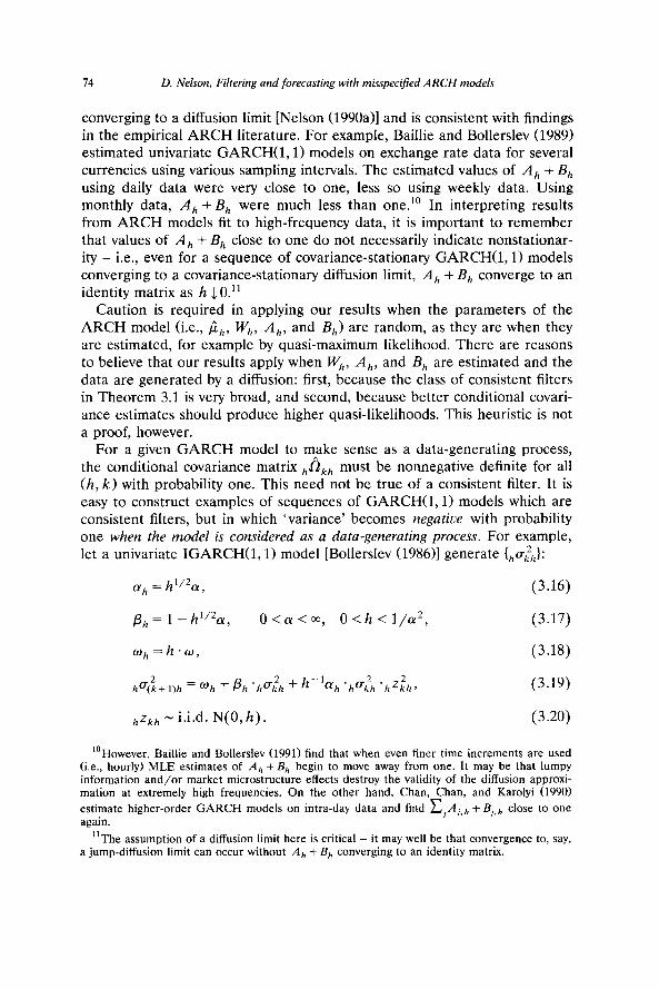
For a given GARCH model to make sense as a data-generating process, the conditional covariance matrix hOnkh must be nonnegative definite for all (h, k) with probability one. This need not be true of a consistent filter. It is easy to construct examples of sequences of GARCH(1, 1) models which are consistent filters, but in which ‘variance’ becomes negative with probability one when the model is considered as a data-generating process. For example, let a univariate IGARCH(1, 1) model [Bollerslev (1986)l generate &u$:

cy,, = h”*a,

Ph = 1 - h1’2cx, O<CY<~, O<h<l/a*,

w -h.w, h-

h”$+l)h ~~~~~~~~~~~~~~~~~~~~~~~~~~~~

h =kh - i.i.d. N(0, h).

(3.16)

(3.17)

(3.18)

(3.19)

(3.20)

“However, Baillie and Bollerslev (1991) find that when even finer time increments are used (i.e., hourly) MLE estimates of A, + B, begin to move away from one. It may be that lumpy information and/or market microstructure effects destroy the validity of the diffusion approxi- mation at extremely high frequencies. On the other hand, Chan, Chart, and Karolyi (1990)

estimate higher-order GARCH models on intra-day data and find C,A,.A + Bj,h close to one again.

“The assumption of a diffusion limit here is critical - it may well be that convergence to, say, a jump-diffusion limit can occur without A, + B, converging to an identity matrix.

D. Nelson, Filtering and forecasting with misspecified ARCH models 7.5

When w 2 0, huih remains nonnegative with probability one for all (h, k), and the process has a well-defined diffusion limit [Nelson (1990a)l. For each h and k we can define ,,tkh zhzkh .,,a,, and write

(3.21)

When w < 0, however, (3.16)~(3.20) imply that for every h, {,aiJ eventually becomes negative (for large k) with probability one and remains negative forever [Nelson (1990b)l. Clearly such a model yields unacceptable long-term forecasts if we insist on interpreting {hu,,?h) as a conditional variance! Never- theless, (3.16)~(3.19) define a consistent filter, even when w < 0.

The misspecification in the conditional mean and covariance processes permitted by Theorem 3.1 is even wider. For example, while the true drift per unit of time p(x) is bounded for bounded values of X, (3.3) permits the drift per unit of time jib assumed in the ARCH mode1 to explode to infinity as h JO. Next, we have ignored the state variables X,+ 1 :n, ,. As a final example of the ways in which the ARCH mode1 may misspecify the data-generating mechanism yet still provide consistent filtering, suppose we replace the vech operators in (3.1) with ordinary vet operators: we could then create hbl :4,1 :q,r matrices that are asymmetric with probability one for all (h, t>,

and yet are consistent filters.12

3.2. AR(I) EGARCH

As a discrete time data-generating process, the AR(l) Exponential ARCH model is given by

hX I,kh =hx I,(k- I)h +h’~~~h(h~,.(k~,)h,,,~k2h,~~) +hZkh’hukhl

(3.22)

‘4 hq2k+Uh) = ln(huk’h) -Ph .h ’ [‘n(huk’,) -ah]

+ Oh ‘h’kh + ?%[I ,~Zkhl -m +‘*I, (3.23)

h’kh - i.i.d. N(0, h), (3.24)

m = E[Ih-1/2hzkhI] = (2/rr)“2. (3.25)

“This distinction between the behavior of a model as a filter and its behavior as a data-generating process is found in linear models as well. For example, a stationary series that has been exponentially smoothed remains stationary. As a data-generating process, however, an exponential smoothing model corresponds to an ARIMACO, 1,l) model, which is nonstationary [Granger and Newbold (1986)].


Nelson (1990a) shows that if ~~ + p uniformly on compacts,

&=/3+0(l), ah=c-u+o(l),

eh = e + o(l), Yh=Y+o(l)? (3.26)

if the starting values hXO and lmhai> converge in distribution, and if p satisfies fairly mild regularity conditions, then as h J 0, the sequence of step function processes {hXI,t,hu:}h I 0 g enerated by (3.22)-(3.26) and (2.2) converge weakly to the diffusion13

dX,,, = P(X,, $, t) dr + a, dw,,,, (3.27)

dln(a:) = -p(ln($) - Ly) dt + dW,,,, (3.28)

where W, f and W, t are one-dimensional Brownian motions with no drift and with ’

%,,I = 1 0

0 82-t (1 -&)y 2 dt. 1 (3.29)

But suppose, once again, that the data are generated by (1.1) and that a misspecified EGARCH model is used to produce an estimate of the true underlying conditional variance process {a,, ,(X,)}. We generate fitted {,&,‘,} recursively by (3.23) with some ,,&i, and generate (hikh) by

?. hZkh- h [

X 1,kh -hXl,(k-l,h -h ‘bh(hX(k-I)h,h’k:,, kh)] /h6kh.

(3.30)

When the model is misspecified, Ihikh} is neither i.i.d. nor N(0, h). The requirements we place on ch, Ph, (Y,,, oh, and yh to achieve consistent filtering are much weaker than (3.26): for some 6, 0 < 6 < 1, we require

/I,, = o( h-“2) (3.31)

& = o(h’-‘), (3.32)

ah& = o(h’-‘), (3.33)

oh = o(@r)/2), (3.34)

yh=y~hS-‘~2+o(hs-1~2) where y>O. (3.35)

13This diffusion is employed in the options pricing models of Hull and White (1987) and Wiggins (1987).

D. Nelson, Filfering and forecasting with misspecified ARCH models 77

Defining the measurement error

(3.36)

=y.m.[exp(-y/2)-1]. (3.37)

The drift per unit of time in {hYkh} is approximately hsP’ . c(x, y). By (3.37), this drift explodes to + co ( -m) whenever ,,Ykh is below (above) zero, causing the measurement error to mean-revert to zero with increasing speed and vanish in the limit as h JO. The differential equation of Assumption 6 is

dY/dt = y .rn. [exp( -Y/2) - I], (3.38)

which is globally asymptotically stable when y > 0. Condition 3.6 replaces Condition 3.4:

Condition 3.6. For euery 77 > 0, there is an F > 0 such that

lim SUP hp’ E Iln(fi,,,(h+k+,,h h 1” l/X/l~~

[ 1) -ln(~,,,(x))12+FIhX,h =x]

= 0. (3.39)

Theorem 3.2. Let (3.31)~(3.36) and Conditions 3.1-3.3 and 3.6 hold. Then ,,yt + 0 in probability for ecery t > 0 as h JO.

As was the case with GARCH(1, l), the effect of misspecification in the conditional mean washes out of the conditional variance as h JO. This is in accord with experience from estimated ARCH models. For example, Nelson (1991) fit an EGARCH model to daily stock index returns computed two different ways: first, using capital gains, and second, using including dividends and a (crude) adjustment for the riskless interest rate. Since dividends and riskless interest rates are almost entirely predictable one day ahead, their inclusion in the returns series amounts to a perturbation in the conditional mean of the capital gains series. The inclusion or exclusion of dividends and riskless rates made virtually no difference in the fitted conditional variances of the two series, which had nearly identical in-sample means and variances and a correlation of approximately 0.9996. Considering our results, this is not

78 D. Nelson, Filtering and forecasting with misspeci’ed ARCH models

surprising. l4 Similarly, Schwert (1990) found that neglecting dividends made little difference in stock volatility estimates even in monthly data. Note also that (3.23) and (3.32) imply an approach to a unit root in (ln(,,~$J) as h JO. As in the GARCH(1, 1) case, this holds for the model both as a filter and as a data-generating process and does not necessarily imply nonstationarity.15

3.3. The Taylor-Schwert variant

Univariate GARCH(1, 1) creates its estimate of the conditional variance as a distributed lag of squared residuals. An equally natural procedure is to estimate the conditional standard deviation using a distributed lag of absolute residuals. Taylor (1986) employed this method to estimate conditional variances for several financial time series. Schwert (1989) used a closely related procedure, generating conditional standard deviations with a 12th- order moving average of absolute residuals. We follow Taylor (1986) by using an AR(l). As a data-generating process, the system is

hX 1,kh =hX,,(k-,)h +h.~h(hX,,(k-,,,,hak,,,kh) +hZkh’hukh,

(3.40)

h*(k+ 1)h =mh +&, ‘,a,, +hh”2ahihZkhihffk/,, (3.41)

h~kh - i.i.d. N(0, h) (3.42)

where wh, Ph, and cxh are nonnegative, and the distribution u,(x, a) of

IX h l,O,h~O} converges to a limit vo(x, a) as h JO. The (hX,,,,hct} are formed using (2.2).16

The properties of the procedure as a filter are similar to GARCH(1, 1). Let hXl,r consist of the first element of hXt: as in the EGARCH case, define an initial value h$,, and define ihikh} and {,bkh} by (3.30) and (3.41). Again,

14Merton (1980) demonstrated the near-irrelevance of the mean as h JO when the variance is constant.

“Once again, this is in accord with the empirical literature - compare, for example, the AR parameters generated in Nelson (1991) using daily data and in Glosten, Jagannathan, and Runkle (1989) using monthly data. See also Priestley (1981, section 3.7.2) for a related discussion of passage to continuous time in the linear AR(l) model. Sims (1984) uses a related result to explain the martingale-like behavior of asset prices and interest rates.

16Higgins and Bera (1989) nest the Taylor-Schwert model and GARCH in a class of ‘NARCH’ (nonlinear ARCH) models. They make v,” a distributed lag of absolute residuals each raised to the 26 power. The Taylor-Schwert model corresponds to S = i, while univariate GARCH sets 6 = 1.


define m = (2/7r) l/2 For some 6 with 0 < 6 < 1, let .

6J h = o(@),

(Y), = hs, + o(h’) with LY > 0,

ph = 1 -/zs,.m +0(P),

jib = 0(h-“2).

Defining

the differential equation (2.15) is

dY= -a.m.Ydt,

(3.43)

(3.44)

(3.45)

(3.46)

(3.47)

(3.48)

which satisfies Assumption 6.”

Condition 3.7. For er;ery 77 > 0, there is an E > 0 such that

lim sup h-l E (@i;-(,X,,+,,,)) -fii!;(~))I’+‘~~x~~ =x] =o. h Jo lIXlI~7J I

(3.49)

Theorem 3.3. Under (3.43H3.46) and Conditions 3.1-3.3 and 3.7, hyt --) 0 in probability as h JO for ecery t > 0.

3.4. A generalization: From diffusions to near-difSusions

Thus far we have generated &X,1 by the stochastic integral equation (1.1) observed at intervals of length h. This can be generalized: it is not necessary that IhXt} is generated by a diffusion, though it is essential that the sequence

17Considered as a data-generating process, the model’s diffusion limit is also similar to GARCH(l,l)‘s. An application of Theorem 2.1 shows that if LJ~ --4 yO as h JO, wh = hw, (Y,, = h”2a, oh = 1 - h1j2a. m - Bh, with w and a nonnegative, and if CL(.) satisfies minimal regularity conditions, (hX,,,,h , CT ) converges weakly to the solution of

dX,,,=CL(X,,,,u~,tf)df+u,ddW,,,,

du, = (w -Bq)dt +a(1 -tnz)‘%, dW,,,,

as h JO, where {IV,,,} and (W,,,) are independent Brownian motions.


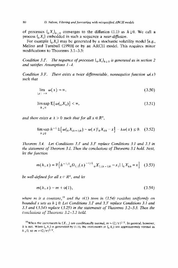
of processes Ih X,}, 1 a converges to the diffusion (1.1) as h JO. We call a process (hXt} embedded in such a sequence a near-difision.

For example IhXt) may be generated by a stochastic volatility model [e.g., Melino and Turnbull (199011 or by an ARCH model. This requires minor modifications to Theorems 3.1-3.3:

Condition 3.1’. The sequence of processes {,,Xt},, 1 0 is generated as in section 2 and satisfies Assumptions l-4.

Condition 3.3’. There exists a twice differentiable, nonnegatme function w(x) such that

lim w(x) = 03, Il.l+m

(3.50)

lim sup E[ w(,X,,)] < co, hia

(3.51)

and there exists a A > 0 such that for all x E R”,

limsup h-‘E[o(,X,,+,,, hLO

) -ti(X)/hXk/, =x] -Am(x) 10. (3.52)

Theorem 3.4. Let Conditions 3.1’ and 3.3’ replace Conditions 3.1 and 3.3 in the statement of Theorem 3.1. Then the conclusions of Theorems 3.1 hold. Next, let the function

m(h,x) = E[h-‘/Zh~,,,(x)-“2~,,X,,o+~,r, -x11 IhxkhEx] (3.53)

be well-defined for all x E R”, and let

m(h,x) =m+o(l), (3.54)

where m is a constant,” and the o(1) term in (3.54) vanishes uniformly on bounded x sets as h 1 0. Let Conditions 3.1’ and 3.3’ replace Conditions 3.1 and 3.3 and (3.54) replace (3.25) in the statements of Theorems 3.2-3.3. Then the conclusions of Theorems 3.2-3.3 hold.

“When the increments in (X,,,) are conditionally normal, M = (2/n)‘/‘. In general, however, it is not. When (hX,) is generated by (l.l), the increments in (hX,) are approximately normal as

h JO, so m = (2/7r)‘j2.


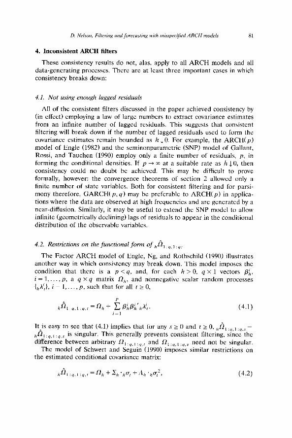
4. Inconsistent ARCH filters

These consistency results do not, alas, apply to all ARCH models and all data-generating processes. There are at least three important cases in which consistency breaks down:

4.1. Not using enough lagged residuals

All of the consistent filters discussed in the paper achieved consistency by (in effect) employing a law of large numbers to extract covariance estimates from an infinite number of lagged residuals. This suggests that consistent filtering will break down if the number of lagged residuals used to form the covariance estimates remain bounded as h JO. For example, the ARCH(p) model of Engle (1982) and the seminonparametric (SNP) model of Gallant, Rossi, and Tauchen (1990) employ only a finite number of residuals, p, in forming the conditional densities. If p + x at a suitable rate as h JO, then consistency could no doubt be achieved. This may be difficult to prove formally, however: the convergence theorems of section 2 allowed only a finite number of state variables. Both for consistent filtering and for parsimony therefore, GARCH(p, 4) may be preferable to ARCH(p) in applications where the data are observed at high frequencies and are generated by a near-diffusion. Similarly, it may be useful to extend the SNP model to allow infinite (geometrically declining) lags of residuals to appear in the conditional distribution of the observable variables.

4.2. Restrictions on the functional form of h&, : 4,, :4,

The Factor ARCH model of Engle, Ng, and Rothschild (1990) illustrates another way in which consistency may break down. This model imposes the condition that there is a p < 4, and, for each h > 0, q x 1 vectors pj,, i=l , . . . , p, a q X q matrix L!,,, and nonnegative scalar random processes lhh;), i = l,..., p, such that for all t 2 0,

h A 1 :q,l :q,, = fib + 5 pj,&‘,h’~. (4.1) i=l

It&is easy to see that (4.1) implies that for any s 2 0 and t 2 0, ,$?I, :4,1 :4,f -

h”nl:q,l:q,s is singular. This generally prevents consistent filtering, since the difference between arbitrary a, :q,, :4,1 and 0, :y, 1 :4,s need not be singular.

The model of Schwert and Seguin (1990) imposes similar restrictions on the estimated conditional covariance matrix:


where a,,, Zh, and A,, are q X q symmetric matrices and {hat2} is the conditional variance of returns on a market index. (4.2) constrains the q(q + 1)/2 distinct elements of hfi, :4,, :4,1 to lie in a one-dimensional sub- space of Rq(q+‘)/2 fo r all t. When q > 1, consistency breaks down if the model is misspecified.

Restrictions on conditional covariances matrices such as those imposed by Engle, Ng, and Rothschild (1990) and Schwert and Seguin (1990) are useful because they achieve parsimony. This considerable virtue comes with a price, namely the loss of consistency when the model is misspecified.

4.3. Failure of the near-dij$sion assumption

Consider again the 8 ,, ,,JA, M) discussed in the introduction, but with {X,, ,) generated by a continuous time Poisson process instead of the diffusion (1.1). The sample paths of IX,,,) are (almost surely) step functions with a finite numb$r of steps over any finite time interval. For almost every t therefore, R ,,,,T(A, Ml -+ 0 in probability as A JO and M+ ~0. Yet the instantaneous conditional variance in the increments in IX, ,) is nonnegative, so A ,, ,, ,(A, M) does not consisiently estimate L?,, t,r. Similarly, if {X,} is a jump-diffusion, consistency for 0, : q, 1 : 4, T generated by misspecified ARCH models breaks down, since except in the immediate aftermath of a jump, the ARCH models effectively ignore the contribution of the jump component to the instantaneous covariance matrix.”

The near-diffusion assumption is crucial for two reasons: first, it guarantees that the increments in {X,) are small over small time intervals (i.e., they are not too thick-tailed). Second, it guarantees that 0, changes by only small amounts over small time intervals. These two conditions effectively allowed us to apply laws of large numbers in estimating 0,. When these two assumptions break down, so, in general, does consistency. Unfortunately, so too will consistency for the other procedures commonly used for estimating time-varying conditional variances and covariances [e.g., Beckers (19831, Cox and Rubinstein (198.5, sect. 6.1), French, Schwert, and Stambaugh (1987), Fama and MacBeth (1973), Schwert (1989), Taylor (1986)1.20

“The situation is not quite so bleak if the jumps occur in R, : 4, 1 : 4,, but not in X, : 4, ,. Recall

that our consistency results did not assume hfil:q,,:q,O=hR, :4 tzq,a, which is why we had

h h 1:q.l:q.r -hfh:q,l:q,I-+oqxq in probability for positive t. As far as the filtering problem is

concerned, a jump in R, .y, 1 :y., essentially resets the clock back to time 0, when $, _, :9.a

and J4 :y.l :4 a were not equal. If the probability of a jump in &, : 4,1 : y,l at any given t equals

zero, then the consistency results of sections 2 and 3 should still hold - i.e., hf?J, :4 , :4 1 - . *~l.4.1:q.l~oyxq in probability (again, pointwise) at t. Of course, hh, :9 1 :4 , will not

converge to St :y,I :y,l when t is a jump point, but the probability of this at an); fixed t equals zero.

2”The method in Bates (1991) may be an exception.


The possibility of large jumps in asset prices plays an important role in some asset pricing theories. For example, in a regime of fixed exchange rates, there is typically a large probability of no change in the exchange rate over a small interval and a small probability of a large move due to a currency revaluation. [See, for example, Krasker’s (1980) discussion of the ‘peso problem’.] While the diffusion assumption is commonly made in asset pricing models, it is not without its dangers even apart from the peso problem: we know, for example, that asset prices cannot literally follow diffusion processes: markets are not always open (they are typically closed on evenings, weekends, and holidays), stocks do not trade at every instant even when the markets are open (leading to discrete price changes when they do trade), prices change in discrete units ($th’s for most stocks), stocks in portfolios trade nonsynchronously, and prices are observed sometimes at the bid and sometimes at the asked. These and other facts of market microstructure make the diffusion assumption, if pushed too far, unrealistic.” Even if we could correct for such market microstructure considerations, it might be that ‘true’ underlying asset prices do not change smoothly - as in the peso problem. Information may arrive in a lumpy manner better characterized by a mixed jump-diffusion process.

Our results are relevant to the extent that the estimation error becomes small for h large enough that market microstructure problems haven’t destroyed the approximate validity of our diffusion assumption. Whether this is actually true is an open question. The usual large-sample asymptotics employed in time series analysis suffer from a similar defect: it is almost always unrealistic to assume that parameters (or hyperparameters in a random coefficients model) remain fixed forever - i.e., as the sample period and sample size T goes to infinity. If taken literally, the notion of consistency breaks down. Nevertheless, large-T consistency is a useful concept, partly because it imposes discipline in the choice of parameter estimators. Similarly, small-h consistency may help impose a useful discipline on the choice of ARCH models.

5. Conclusion

Traditionally, econometricians have regarded heteroskedasticity mainly as an obstacle to the efficient estimation of regression parameters. In recent years, however, financial economists have stressed that the behavior of conditional variances and covariances is important in and of itself. Unfortu-

“Similar warnings are in order when diffusion models are applied in almost any field. For example, Brownian motion is often used by physicists to model particle motion, even though a particle cannot literally follow a Brownian motion: Brownian sample paths have unbounded variation almost surely, so a particle following a Brownian motion would, with probability one, travel an infinite distance in a finite time period, a physical impossibility.


nately, traditional linear time series models are simply not capable of modelling dynamic conditional variances and covariances in a natural way. ARCH models have greatly expanded the ability of econometricians to model heteroskedastic time series, particularly financial time series.

If the near-diffusion assumption is approximately valid for high-frequency financial time series, our results may explain some features of estimated ARCH models: first, the tendency to find ‘persistent’ volatility (e.g., IGARCH) when using high-frequency (e.g., daily) data, second, the small influence of misspecification in the conditional mean on the estimated conditional variance, and third, estimated models (especially in the multivariate case) that do not make sense as data-generating processes (i.e., in which the conditional covariance matrix loses nonnegative definiteness with positive probability).

Our results should be reassuring to users of ARCH models and suggest a reason for the forecasting success of ARCH: If the process generating prices is (approximately) a diffusion, then there is so much information about conditional second moments at high frequencies that even a misspecified model can be a consistent filter. This does not suggest, however, that the econometrician should be indifferent as to which ARCH model to use: a consistent filter may be a very poor long-term forecaster, and there may be considerable differences in the efficiency of different ARCH filters. These issues remain for future work.

Appendix

Proof of Theorem 2.1. See Ethier and Kurtz (1986, ch. 7, theorem 4.1) or Nelson (1990a, theorem 2.2).

Proof of Theorem 2.2. This theorem is a special case of Ethier and Nagylaki (1988, theorem 2.1). There are a few changes in notation: we have set Ed, 6,, XN(k>, Y”‘(k), and ZN(k) in Ethier and Nagylaki equal to h, h’, hXkh, ,,Ykh, (hXkh,hYkh, kh), respectively. By our (2.41, Ethier and Nagylaki’s h(x, y) function [see their (2.1)-(2.211 is a vector of zeros. Our Theorem 2.2 now directly follows by Ethier and Nagylaki (1988, theorem 2.1). Q.E.D.

In proving the theorems in section 3, we need the following lemma:

Lemma A.1. Let {~,)IO,TI be generated by the stochastic integral equation

(A-1)

D. Nelson, Filtering and forecasting with misspecijed ARCH models 85

where 5” is fixed, (W,) is a q x 1 standard Brownian motion, m( . , . > and A(., . > are continuous, (q X l)- and (q x q)-valued functions, respectively, and where (A.1) has a unique weak-sense solution. Next, let g(t) be a q X 1 function satisfying

g(t) = o( t’/*) as t JO. (A.4

Then,

(A.3)

Further, let f(S, t) be a continuous function from Rq+’ into R’. Let there exist an F > 0 such that

(A.41

Then if Z N NCO,, ,, A(&, O>>,

f’,:: E[f(t-“*(& -g(t) -&‘),t)] =E[f(Z,O)l cco. (A.51

Proof of Lemma A.1. Once we prove (A.3), (A.51 follows directly by Billingsley (1986, theorem 25.7, corollary a and theorem 25.12, corollary). To prove (A.3), note that by (A.2), tt’/“g(t) + 0 as t JO. Next, rewrite (A.l) as

t-‘/*(~,-~o) = t-1/2A1/2(&,0)~ + t”“‘21;‘m(is,s) ds

+t~‘/2~~~[,l’/2(~~,s) -A”2(~,~,0)] dW,. (A.6)

Since tC “*W, N N(0, I> and t- ‘/*g(t) + 0,, l as t JO, (A.3) follows if the last two terms on the right-hand side of (A.6) converge in probability to zero as t JO. The middle term is

‘m(ls,s)ds It’/* max Im(lS,.s)l, OlSll

(A.71

which converges to a vector of zeros in probability as t JO. Next, consider the


last term. Define

(A.8)

The proof of (A.3) is complete if t -1/2Z converges in probability to a vector I of zeros as t JO. Letting I(.) be an indicator function, we have

The second term on the right-hand side of (A.9) vanishes in probability as t J 0 since

)i; E[ t-’ ~Z(llZ,ll 2 1)15,,] = Oqxq (A.lO)

[Arnold (1973, p. 40, formula (a))]. Since A is continuous, the first term also vanishes [Arnold (1973, p. 40, formula (b))l. Q.E.D.

Proof of Theorem 3.1. We need only verify Assumptions l-7. Condition 3.1 includes Assumptions 1, 3, and 4. Assumption 3 and (1.1) directly imply Assumption 2 [see Arnold (1973, p. 40)]. Define

h-1/2 htl :q,(k+l)h =h-1’2[hX1 :q,(k+l)h -hX1 :q.kh

(A.ll)

Applying Condition 3.4 and Lemma A.1 we have for all x E R”+“,

h-1’2htl:q,(k+l)h~hXkh =‘] =j N(“& :q.l :q(‘)), (A.12)

as h JO. By Condition 3.4 and Lemma A.l, the conditional absolute moments

of h-?,5, :q,k,, (given hXkh =x> of order less than 4 + e converge to the corresponding moments of a N(0, R, :q, 1 ,,(x>). It is then easy to derive c(y) = -A .y and d(y) = 0, as required by Assumption 5. The differential equation of Assumption 6 is dY/dt = -A ‘y with unique solution Y, = exp(-At)Y, [see, e.g., Hochstadt (197511. The solution is globally asymptotically stable if the eigenvalues of A have strictly positive real parts. To verify


Assumption 7, define G(y) = y’y . [l - exp( -y’y)] and

p(x,y) = 1 +w(x) t-NY). (A.13)

(2.18) is immediate and Condition 3.2 implies (2.20). Condition 3.3 implies

lim sup SUP h JO

h-‘+~(,J~~+,)h) -~(xhzXkh =x,/Y/c/z =Y] Kx’, y’)lllq

-hw( x) 5 0, (A.14)

SO to verify (2.21) it suffices that there is a A(n, h) satisfying (2.19) such that for every 7j > 0,

lim sup sup hJO

h-’ E[$(hYi,(k+l)h) - !J+(Y)lhxkh =x,hykh =y]

IIW, Y’)lJII

-eLw + !b( Y)] IO. (A.15)

Using (1.1) and (3.1)-(3.2), we have

Y h (k+l)h =hYkh +hDkh +hNkh, (A.16)

where h D,, and h Nkh are, respectively, drift and noise terms defined by

hDkh = E[hI;k+,,h -hykhb?4h] 3 (A.17)

t,Nkt, -hyk+l)h -hYkh -hDkh. (A.18)

Condition 3.4 guarantees that hDkh is well-defined and that the conditional variance of hNkh is bounded in compact regions of the state space. By Conditions 3.1, 3.4, and 3.5,

lim sup h Lo Il(x’,y’)IIs~

h-1 E[+(hy,ck+,,,) - $(Y)lhXkh =x>hykh =Y]

[0( 1) + 0( h2’-I)]. (A.19)


Since the eigenvalues of A have strictly positive real parts, -(&,G/ay)Ay is negative for y # 0, X I. Hence, the first term on the right-hand side of (A.191 dominates the second term (since it diverges to -w) except in a shrinking neighborhood of y = 0, X 1 (i.e., in neighborhoods of the form 11 y II I K. h* for K > 0 and 0 < A < min{l - 6,6)). In this shrinking neighborhood of

Y =Omx,, &,l~/ay + 0 and a’r,!J’/ay Jy’ + 0, so the right-hand side of (A.19) is uniformly bounded on compacts, diverging to - ~0 except at y = 0, X ,. (A.151 can therefore be satisfied with a h(n, h) satisfying (2.19). (2.21) now follows directly. Q.E.D.

Proof of Theorem 3.2. Assumptions l-4 follow directly from Conditions 3.1-3.3. The proof that Assumptions 5 and 7 hold closely follows the proof of Theorem 3.1, with Condition 3.6 taking the place of Condition 3.4. The differential equation of Assumption 6 is dY/dt = y . m * [exp( - Y/2) - 11, with solution

Y,=2.ln(l-exp[-ym.t/2]+exp[+(Y0-ymt)]), (A.20)

which satisfies Assumption 6 as long as y > 0. Q.E.D.

Proofs of Theorems 3.3 and 3.4. Nearly identical to the proofs of Theorem 3.1 and Theorems 3.1-3.3, respectively. Q.E.D.

References

Anderson, B.D.0 Arnold, L., 1973,

NY)

and J.B. Moore, 1979, Optimal filtering (Prentice Hall, Englewood Cliffs, NJ). Stochastic differential equations: Theory and applications (Wiley, New York,

_._,. Baillie, R.T. and T. Bollerslev, 1989, The message in daily exchange rates: A conditional

variance tale, Journal of Business and Economic Statistics 7, 297-305. Baillie, R.T. and T. Bollerslev, 1990, Intra-day and inter-market volatility in foreign exchange

rates, Review of Economic Studies 58, 565-585. Bates, D.S., 1991, The crash of ‘87: Was it expected? The evidence from options markets,

Journal of Finance 46, 1009-1044. Beckers. S., 1983, Variances of security price returns based on high, low, and closing prices,

Journal ‘of Business 56, 97-112. Billingsley, P., 1986, Probability and measure, 2nd ed. (Wiley, New York, NY). Black, F. and M. Scholes, 1973, The pricing of options and corporate liabilities, Journal of

Political Economy 81, 637-654. Bollerslev, T., 1986, Generalized autoregressive conditional heteroskedasticity, Journal of

Econometrics 31, 307-327. Bollerslev, T., R.Y. Chou, and K. Kroner, 1992, ARCH modeling in finance: A review of the

theory and empirical evidence, Journal of Econometrics, this issue. Bollerslev, T., R.F. Engle, and J.M. Wooldridge, 1988, A capital asset pricing model with time

varying covariances, Journal of Political Economy 96, 116-131. Chan, K., K.C. Chan, and G.A. Karolyi, 1991, Intraday volatility in the stock index and stock

index futures markets, Review of Financial Studies, forthcoming.


Cox, J. and M. Rubinstein, 1985, Options markets (Prentice Hall, Englewood Cliffs, NJ). Engle, R.F., 1982, Autoregressive conditional heteroskedasticity with estimates of the variance of

United Kingdom inflation, Econometrica 50, 987-1008. Engle, R.F. and T. Bollerslev, 1986, Modelling the persistence of conditional variances, Econo-

metric Reviews 5, l-50. Engle, R.F., V. Ng, and M. Rothschild, 1990, Asset pricing with a factor ARCH covariance

structure: Empirical estimates for Treasury bills, Journal of Econometrics 45, 213-238. Ethier, S.N. and T.G. Kurtz, 1986, Markov processes: Characterization and convergence (Wiley,

New York, NY). Ethier, S.N. and T. Nagylaki, 1988, Diffusion approximations of markov chains with two time

scales and applications to population genetics, II, Advances in Applied Probability 20, 525-545.

Fama, E.F. and J.D. MacBeth, 1973, Risk, return, and equilibrium: Empirical tests, Journal of Political Economy 81, 607-636.

French, K.R., G.W. Schwert, and R.F. Stambaugh, 1987, Expected stock returns and volatility, Journal of Financial Economics 19, 3-29.

Gallant, A.R., P.E. Rossi, and G. Tauchen, 1990, Stock prices and volume, Manuscript (University of Chicago, Chicago, IL).

Glosten, L.R., R. Jagannathan, and D. Runkle, 1989, Relationship between the expected value and the volatility of the nominal excess return on stocks, Manuscript (Northwestern Univer- sity, Evanston, IL).

Granger, C.W.J. and P. Newbold, 1986, Forecasting economic time series, 2nd ed. (Academic Press, New York, NY).

Hardouvelis, G.A., 1990, Margin requirements, volatility, and the transitory component of stock prices, American Economic Review 80, 736-762.

Harvey, C.R., 1989, Time-varying conditional covariances in tests of asset pricing models, Journal of Financial Economics 24, 289-318.

Higgins, M.L. and A.K. Bera, 1989, A class of nonlinear ARCH models, International Economic Review, forthcoming.

Hochstadt, H., 1975, Differential equations: A modern approach (Dover Press, New York, NY). Hsieh, D.A. and M.H. Miller, 1990, Margin regulation and stock market volatility, Journal of

Finance 45, 3-30. Hull, J. and A. White, 1987, The pricing of options on assets with stochastic volatilities, Journal

of Finance 42, 281-300. Krasker, W.S., 1980, The peso problem in testing for efficiency of foreign exchange markets,

Journal of Monetary Economics 6, 269-276. Lintner, J., 1965, The valuation of risky assets and the selection of risky investments in stock

portfolios and capital budgets, Review of Economics and Statistics 47, 13-37. Melino, A. and S. Turnbull, 1990, Pricing foreign currency options with stochastic volatility,

Journal of Econometrics 45, 239-266. Merton, R.C., 1973, An intertemporal capital asset pricing model, Econometrica 41, 867-887. Merton, R.C., 1980, On estimating the expected return on the market, Journal of Financial

Economics 8, 323-361,

Nelson, D.B., 1990a, ARCH models as diffusion approximations, Journal of Econometrics 45, 7-39.

Nelson, D.B., 1990b, Stationarity and persistence in the GARCHfl, 1) model, Econometric Theorv 6. 318-334.

Nelson, D.B:, 1991, Conditional heteroskedasticity in asset returns: A new approach, Economet- rica 59, 347-370.

Priestley, M.B., 1981, Spectral analysis and time series (Academic Press, London). Ross, S., 1976, The arbitrage theory of capital asset pricing, Journal of Economic Theory 13,

341-360. Schwert, G.W., 1989, Why does stock market volatility change over time?, Journal of Finance 44,

1115-1154. Schwert, G.W., 1990, Indexes of U.S. stock prices, Journal of Business 63, 399-426. Schwert, G.W. and P.J. Seguin, 1990, Heteroskedasticity in stock returns, Journal of Finance 45,

1129-1156.

90 D. Nelson, Filtering and forecasting with misspecijied ARCH models

Shanken, J., 1990, Intertemporal asset pricing: An empirical investigation, Journal of Economet- rics 45, 99-120.

Sharpe, W., 1964, Capital asset prices: A theory of market equilibrium under conditions of risk, Journal of Finance 19, 425-442.

Sims, C., 1984, Martingale-like behavior of asset prices and interest rates, Manuscript (Univer- sity of Minnesota, Minneapolis, MN).

Stroock, D.W. and S.R.S. Varadhan, 1979, Multidimensional diffusion processes (Springer Verlag, Berlin).

Summers, L.H. and V.P. Summers, 1989, When financial markets work too well: A cautious case for a securities transactions tax, Journal of Financial Services Research 3, 261-286.

Taylor, S., 1986, Modeling financial time series (Wiley, New York, NY). Wiggins, J.B., 1987, Option values under stochastic volatility: Theory and empirical estimates,

Journal of Financial Economics 19. 351-372.

Documents

Filtering and forecasting with misspecified ARCH … of Econometrics 52 (1992) 61-90. North-Holland Filtering and forecasting with misspecified ARCH models I Getting the right variance