Film thickness variation about a T-junction

Film thickness variation about a T-junction

G. Conte, B.J. Azzopardi *

Multiphase Flow Research Group, School of Chemical, Environmental and Mining Engineering,

University of Nottingham, University Park, Nottingham NG7 2RD, UK

Received 20 March 2002; received in revised form 22 October 2002

Abstract

The division of gas/liquid flow at a large diameter T-junction has been studied experimentally. The

misdistribution of the phases has been quantified for horizontal semi-annular flow. Film thickness varia-

tions about the circumference of the inlet and outlet pipes have been obtained using conductivity tech-niques. In addition, liquid depth profiles within the junction have been measured. The data have been

compared with available theoretical models.

� 2003 Elsevier Science Ltd. All rights reserved.

Keywords: Gas/liquid; T-junctions; Horizontal; Phase separation; Film thickness

1. Introduction

Multiphase flow, primarily liquid–gas flow, exists in chemical, power, oil/gas production and oilrefining plants. These flow are very complex. However, observation has shown that when suchflows divide at T-junctions there is an added level of complexity with an almost inevitable mal-distribution of the phases (Azzopardi, 1999). Though Leonardo da Vinci first recorded thecomplex behaviour of fluids at T-junctions in the 16th century, it was not until 1973 when work byOranje (1973) on gas pipelines first showed a maldistribution of phases. Oranje noticed thatcondensate in gas lines did not appear equally at all terminal points on branched pipelines.The maldistribution which occurs when a gas/liquid flow divides at a T-junctions can have both

negative and positive consequences. On the negative side, the maldistribution can result in a fall inefficiency in downstream equipment. There is anecdotal evidence to support this. A bank of fourair-cooled heat exchangers (fin–fan coolers) was operated in parallel as condensers. The feed

International Journal of Multiphase Flow 29 (2003) 305–328www.elsevier.com/locate/ijmulflow

*Corresponding author. Tel.: +44-115-951-4150; fax: +44-115-951-4115.

E-mail address: [email protected] (B.J. Azzopardi).

0301-9322/03/$ - see front matter � 2003 Elsevier Science Ltd. All rights reserved.

PII: S0301-9322(02)00130-1

mail to: [email protected]

arrived partially condensed at the inlet manifold connecting the exchangers. This consisted of aseries of side pipes off a main header, i.e., a series of dividing junctions. In operation the fourthexchanger significantly underperformed. Simple laboratory trials using four pipes connecting theinlet and outlet headers quantified the routes taken by the two phases and showed that the firstthree side arms each took approximately 30% of the gas and �10% of the liquid. The final pipereceived most of the liquid. It then became obvious why the fourth condenser was underper-forming; it was overwhelmed with liquid.Another example of phase maldistribution has been reported from offshore platforms in the

UK North Sea. Here, it had been decided to install two main (phase) vessel separators in parallel.This would enable production to continue albeit at a reduced level if there was a need formaintenance or modification of a separator. To ensure an even split of the phases, an impactingT-junction was employed, i.e., one in which both outlet pipes were at right angles to the inlet.When the system was started up it was found that one separator received most of the gas whilstthe other got most of the liquid. Inspection of the pipework upstream of the junction showed thata bend had been positioned at the worst possible place. This bend was centrifuging the phases andpresenting each outlet with substantially one phase.A more positive note has been struck recently by Azzopardi et al. (2002). They designed a

pipework partial separator incorporating a T-junction to replace a conventional vessel separator.The feed to this unit was the partially flashed product stream of from a high-pressure liquid phasechemical reactor. This had to be separated into gas and liquid before being fed into a distillationcolumn. Phase separation was necessary to prevent liquid being carried up the column and soreducing its efficiency. The design, based on an intimate knowledge of multiphase flow and phaseseparation at T-junctions, was installed on a hydrocarbon plant in the North of England and isoperating successfully.There have been a large number of studies of the phase split. Azzopardi (1999), in a very

comprehensive review, records 78 papers that provide experimental data. Of these 12 also mea-sured drops across the junction. However, there are only a very limited number of papers, whichprovide information about the details of the flow at the inlet and outlets of the T-junction. Davisand Fungtamasan (1990); Lemonnier and Hervieu (1991) and Suu (1992) have mapped the voidfraction distribution about the cross-section of the pipes. These studies have used junctionsmounted on a vertical main pipe. The flow pattern approaching the junction was bubbly. Scottet al. (2001) used a conductivity technique to study the flow structure in the side arm of aT-junction with a vertical main pipe in the flow pattern is churn. Peng et al. (1998) have measuredcross-sectional averaged void fraction in the three horizontal legs of a T-junction into which astratified flow is introduced. There are no studies that provide information on the phase distri-bution within the junction itself.As noted by Azzopardi (1999), phase split mechanism at T-junctions is strongly dependent on

flow pattern. In the case of horizontal annular flow, this is characterised by the distribution of thefilm around the pipe, the entrained fraction, the drop size distribution and the local fluxes of liquidin the film and as drops. Azzopardi and Whalley (1982) suggested that fluids would be diverted orotherwise according to the local momentum fluxes. Film and gas have low momentum fluxeswhilst that of the drops is much higher. Therefore, the drops would carry on past the junction.Attention must be directed to the characterisation of the film. There is evidence in the literaturethat scale has a strong effect on the film distribution around the pipe circumference, Azzopardi

306 G. Conte, B.J. Azzopardi / International Journal of Multiphase Flow 29 (2003) 305–328

and Rea (1999). In fact, models developed for small pipes do not apply to larger ones. This isprobably due to the mechanism which provided liquid at the top of the pipe against the drainingaction of gravity being different in small and large diameter pipes.These models require information about the film flow variation about the inlet pipe. Secondary

flow in the gas phase, pumping action in the disturbance waves and entrainment /deposition havebeen suggested as the mechanisms which balance the draining effect of gravity and maintain theliquid film at the top of the pipe. James et al. (1987); Fukano and Ousaka (1989); Fisher andPearce (1993) and Hurlburt and Newell (2000) hvave presented models. Roberts et al. (1997) andAzzopardi and Rea (1999) have used the models of Fukano and Ousaka and Hurlburt and Ne-well, respectively, to model phase split at T-junctions. Generally, for larger pipes the film is seen tobe less symmetric with a stratified layer at the bottom and a thin film around the top. This hasbeen described as semi-annular by Kimpland et al. (1992).The diameters of pipelines in the oil/gas production industry are usually in the range 0.1–1 m.

They handle gas superficial velocities in the range 0–20 m/s and liquid superficial velocities of0–2.5 m/s. Wu et al. (1987) and Williams et al. (1996) are the only sources of circumferentialvariation of film thickness in industrial sized pipes. The former used a 0.2 m diameter pipeline, 280m long operating with natural gas and gas condensate. Williams et al. (1996) studied air/waterflows in a 0.0953 m internal diameter pipe.In this paper flow split data for (semi) annular flow approaching a horizontal T-junction of

0.127 m diameter are presented. For these inlet conditions, film thicknesses around the pipecircumference in all three legs of the junction have been measured. The liquid depth variationwithin the junction itself has also been obtained. For the same inlet flow rates data of phase splitwere also obtained. Measurements are reported which characterise the film distribution aroundthe junction, within the T-junction, in the inlet and outlet pipes, and upstream of the T-junctionnear the mixing section. The effect of gas and liquid inlet flow rates and of the phase split areconsidered.

2. Experimental arrangement

2.1. Flow facility

The apparatus employed in the experiments reported here is the same as that used by Robertset al. (1995) and Rea and Azzopardi (2001). The arrangement is shown schematically in Fig. 1. Airis drawn from the laboratory by a centrifugal fan and the airflow rate adjusted by use of a bypassand measured further downstream by an orifice plate. Water is drawn from the large storage tankby one of two centrifugal pumps and the flow rate was monitored by either one of three calibratedrotameters, for smaller flow rates or by a turbine meter for much larger flow rates. The water thenenters the main flow pipe through a porous wall section.The T-junction was positioned 3.5 m downstream of the mixer. There is a further 3.5 of 0.127 m

diameter tubing, which is followed by a 120� bend. Beyond the bend is a further 0.5 m of piping,containing a butterfly valve, which leads to a cyclone. The side arm consists of 1.5 of 0.127m-diameter tubing leading to another butterfly valve and a second cyclone. The T-junctions usedin the present experiments had a main bore and side arm both 0.127 m in diameter and was

G. Conte, B.J. Azzopardi / International Journal of Multiphase Flow 29 (2003) 305–328 307

machined from an acrylic resin block with the outside machined to a square cross-section(0:2� 0:2 m) to minimise refraction problems during observation. It had carefully machinedsharp corners so as to eliminate the radius of curvature as a possible variable in the experimentsand had flanges at the three ends so as to mate with the rest of the test section piping.The air and water leaving the test section are separated in the two cyclones. Calibrated venturi

meters or orifice plates on top of the cyclones are used to measure the airflow rate. The water flowrate is determined by diverting the flow from either cyclone to a weigh tank mounted on a cali-brated load cell and measuring the timed discharge.

2.2. Film thickness measurement

In a recent comprehensive review of measurement methods for film thickness, Clark (2002)identified that the most widely used techniques are based on the different impedance of the twomedia. When the liquid is conductive, such as water with dissolved salts as in the presentexperiments, this is predominantly conductance.Conductance probes are defined as the arrangement of two electrodes, extremities of a circuit,

which is closed by the liquid film bridging between them. Three probe configurations have beenused for film thickness measurement in pipes. These are needle probes, parallel wires and flushmounted pins.Needle probe: This method relies on the contact made between an electrode mounted flush with

the pipe surface and the tip of a needle which could be moved across the pipe diameter passingthrough the fixed electrode. When the tip of the needle is at or below the gas–liquid interface, acurrent will flow. As the film is wavy the needle tip will be in the water intermittently. The sta-tistical description of film thickness is built up by positioning the needle tip at a series of distancesfrom the wall and determining the fraction of time that the circuit is completed. The advantage ofthis method is that it is very precise, does not require calibration and is applicable to a wide range

Fig. 1. Schematic of flow facility.


of thickness. Furthermore, it is a very localised measurement. On the other hand, it can be quiteintrusive for thin films and it is particularly laborious to operate.Parallel wires: In this approach, the electrodes are two parallel thin wires, Miya et al. (1971);

Brown et al. (1978) and Koskie et al. (1989). These are stretched across a channel or along chordsof the pipe or protrude from the wall supported only at one end. As the film thickness increases,the surface area of electrode increases and the resistance decreases. The output depends on thegeometrical dimensions and on the conductivity of the liquid. The film thickness/output rela-tionship is obtained by calibration. The response of this system is fairly linear and can be used forthick films. It is less reliable for thin films because of its intrusive nature, i.e., the formation of ameniscus due to surface tension effects. The method is most useful film heights in stratified andslug flow.Flush mounted pins: The method is used for very thin films, typically up to 2 mm. Electrodes are

pins mounted flush with the pipe surface linked in a circuit to a neighbouring, similar electrode.The method is non-intrusive but the response is non-linear. The range of film thickness that can behandled depends on the size and spacing of the electrodes. However, the greater the spacing, themore averaged is the result over space. Design is based on a compromise between the range ofoperability and local character of the measurement.A composite type, a combination of the flush mounted and wire probes was used by Kim and

Kang (1990). In their design, the resistance is measured between a needle, which is always im-mersed in the liquid, and a flush mounted electrode. They show that this design is the best forminimising the averaging effect on wave height measurements due to the area of activity of theother arrangements.The types of probe employed in this study were chosen on the basis of the characteristics de-

scribed above and visual observations of the flow regime in the inlet pipe. A semi-annular flowwas observed with a thick film at the pipe bottom, and a much thinner film at the top. Therefore,wire probes were used at the pipe bottom and flush mounted probes at the top.

2.3. Parallel wire test section for height measurements at the pipe bottom

The method employed for the measurement of film thickness at the bottom of the pipe is thesame employed by Rea and Azzopardi (2001), Fig. 2. Five pairs of stainless steel wires arestretched along chords of the pipe cross-section. The spacing between the two wires of each pair isof 5 mm and the distance between each pair is 25 mm, with the central pair placed symmetricallyabout a vertical diameter. 0.33 mm diameter wires are stretched across an acrylic resin ring 25 mmdeep. Plastic screws at each end keep the wires taught. The top 15 mm of the wires were insulatedto prevent errors being caused by the liquid film at the top of the pipe.The electronic circuit to apply voltage and is subsequent filtering is the same as used by Rea and

Azzopardi (2001). Signals from five probes could be obtained simultaneously. After filtering, thesewere fed to a PC equipped with an A/D converter card (Data Translation, DT-VPI). Gains wereadjusted to obtain optimal operation in the expected range of heights. Data processing was partlycarried out using HP-Vee 4.0 by Hewlett-Packard.The system was calibrated by mounting the ring containing the probes between two short pieces

of acrylic resin pipe. The ends were sealed with transparent plates and scales were placed on each.


Water was added or removed via a small hole. The cylinder was mounted horizontally and theliquid height measured.Calibration of the probes at the periphery of the pipe cross-section proved more difficult. The

curvature of the pipe caused a difference in height of �6.4 and 2.1 mm between the bottom of thetwo electrodes for the most external (A and E) and intermediate (B and D) probes, respectively,Fig. 2. Furthermore, the shape of the film during calibration was flat as opposed to the curvedinterface expected under annular flow conditions. However, it is expected that the electrode im-mersed the least in the liquid would control the resistance across the two electrodes. Hence,calibration was made for the height at the outer electrode.Because the electrical conductivity of water was seen to vary with temperature and salt con-

centration the calibration was carried out with solutions of de-ionised water and sodium chlorideof three different conductivities in the expected range for steps of �50 lS/cm. This permitted acalibration curve to be produced for each probe correct for the conductivity of the liquid beingused.

2.4. Flush mounted pin probes for thickness measurements at the pipe top and their calibration

Two electrode spacings were incorporated into the same test section, Fig. 3. Electrodes werepositioned 5 or 10 mm apart. This corresponded to angles of 4.5� or 9� subtended at the pipe axis.The pins were made from 1.5 mm diameter, stainless steel rods to avoid problems of corrosion.They were located at one end of a 190 mm long section of acrylic resin pipe, 20 mm from theflange and mounted flush to the internal surface of the pipe.

Fig. 2. Sketch of the test section for film thickness measurement at the bottom of pipe (the harp) used near the mixing

section and in the three legs of the T-junction.


Pairs of pins, from the series mounted around the pipe were selected by using a set of switches.This was arranged in such a way that intermediate electrodes could belong to two probes in se-quence, one with a spacing of 5 mm and the other of 10 mm. The sequence is shown in Fig. 3 (1–1;2–1; 2–2; 3–2; 3–3. . .6–6). The three groups of three pins at the very top of the section, 30� apart,were used in the same way but each group was used independently, with no coupling of pinsbelonging to different groups.Calibration was carried out using slots machined out of an acrylic resin cylinder with the same

diameter as the test section. At one end, a length of 60 mm, the cylinder was notched progressivelyfor steps of 51�, cutting 0.3, 0.5, 1, 1.5, 2.25, 3 and 5 mm off the original surface, Fig. 4. The testsection was blanked off at the end opposite the pins. The machined insert was inserted and the gapfilled with water of known conductivity and rotated in a stepwise manner to present each filmthickness to all electrode pairs. The exact film thickness was determined by use of feeler gauges.Calibration data was obtained for a range of specific conductivities. The conductivity of the tapwater in the rig was monitored continuously and this value was used to produce an interpolatedfilm thickness/resistance relationship.Fig. 5 shows example calibration curves for the two probe spacings. The curve for 5 mm

spacing is much steeper for small thickness and becomes quite flat for thicknesses over 1.5 mm.Conversely, although less linear and with a smaller initial slope for very thin films, the calibrationcurve for 10 mm spacing allows measurement to be made with a good degree of confidence up to2.5 mm. The calibration curves were fitted with polynomial equations third to fifth order for threeconductivities.

Fig. 3. Cross-section view of the test section for film thickness measurements at the top of the pipe (the pins-ring).

Linear dimensions are in mm.


2.5. Measurements of liquid heights within the T-junction

A third test section was designed and constructed to measure film heights within the T-junction.Stainless steel wires were fitted in the locations shown in Fig. 6. The spacing between the pairs ofelectrodes was 5 mm and the probes were 25 mm apart in the radial direction. To avoid theproblems experienced with the probes far from the vertical diameter, where the two wires havedifferent lengths due to the pipe curvature, the wires were aligned along the pipe axis except for

Fig. 4. Top view of the calibration slot for the flush mounted probes test section. The darker shade is the original

cylinder, the lighter shade is the upper part of the slot after cutting. Linear dimensions are in mm.

Fig. 5. Calibration curves for flush mounted pin probes showing signal plateau and the effect of electrodes spacing.

Conductivity ¼ 600 lS/cm.


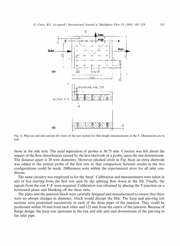
those in the side arm. The axial separation of probes is 36.75 mm. Concern was felt about theimpact of the flow disturbances caused by the first electrode of a probe, upon the one downstream.The distance apart is 20 wire diameters. However (dashed circle in Fig. 8(a)) an extra electrodewas added to the central probe of the first row so that comparison between results in the twoconfigurations could be made. Differences were within the experimental error for all inlet con-ditions.The same circuitry was employed as for the �harp�. Calibration and measurements were taken in

sets of five starting from the first row seen by the splitting flow down to the 5th. Finally, thesignals from the row F–F were acquired. Calibration was obtained by placing the T-junction on ahorizontal plane and blanking off the three exits.The pipes and the junction block were carefully designed and manufactured to ensure that there

were no abrupt changes in diameter, which would disrupt the film. The harp and pin-ring testsections were positioned successively in each of the three pipes of the junction. They could bepositioned within 10 mm from each other and 125 mm from the centre of the junction. Because offlange design, the harp was upstream in the run and side arm and downstream of the pin-ring inthe inlet pipe.

Fig. 6. Plan (a) and side section (b) views of the test section for film height measurements in the T. Dimensions are in

mm.


Tap water, which was used in the experiments, was found to have a conductivity between 500and 650 lS/cm. If not replaced the water quickly became fouled and mineral deposits begun toshow, particularly on the wires. To avoid large variations of conductivity within the same ex-perimental run and to reduce fouling of the electrodes, fresh water was fed continuously to thestorage tank and discharged to drain. Within twenty minutes of start-up, the conductivity wasseen to settle out to a constant value with fluctuations <1%. Conductivity was checkedthroughout each session of experiments by collecting water �6 m downstream of the measuringstation. The conductivities determined during the measurement were used to interpolate betweenthe calibration curves to obtain the signal/film thickness relationship. Calibrations were repeatedperiodically without any cleaning of the electrodes. It was observed that the variations of thecalibration curves caused changes in the film thicknesses, which were well within experimentalerror. The largest discrepancy recorded was 3.5%. From the gradient of the signal/film thicknesscurve and the accuracy of the signal measurement the uncertainty in film thickness at the top ofthe pipe is about 10%. The value for thicker films at the pipe bottom is much lower.

3. Results

3.1. Inlet conditions and phase split

The inlet flow rates at which data were taken are shown in Fig. 7. Also shown are the flowpattern transition lines from the model of Taitel and Dukler (1976). The conditions employedwere chosen so as to be in annular flow and were the maximum flow rates achievable with the flowfacility.Phase split data have been obtained for these inlet conditions. Different fractions of the flow

were diverted through the side arm by altering the degree of closure of the butterfly valves on the

Fig. 7. Flow pattern map showing were data were taken.


two downstream legs. Fig. 8 shows the split as fraction of incoming liquid emerging through theside arm versus the corresponding gas fraction. The data show characteristics similar to thoseobtained by Rea and Azzopardi (2001) on the same equipment and by other researchers in smallerdiameter junctions, e.g., Buell et al. (1994), for similar flow rates. The split is characterised bypredominantly gas take off. Less than 20% of the liquid is taken off until the gas taken off exceeds80%. Thereafter, the liquid take off increases sharply. There is some effect of inlet liquid flow rate,an increase in the liquid superficial velocity decreasing the fractional liquid take off. The effect ofgas superficial velocity is much smaller.

3.2. Film thickness results from harp and pin-ring test sections

One of the first tests to be carried out was to compare the present film thickness data with thoseobtained by Williams et al. (1996) in a pipe with a similar diameter. His data were obtained on a0.095 m diameter pipe at a distance of 260 D from the mixing section for gas superficialvelocity ¼ 31:7 m/s and liquid superficial velocity ¼ 0:12 m/s. This can be compared data from thepresent experiments (gas superficial velocity ¼ 28:1 m/s, liquid superficial velocity ¼ 0:14 m/s).Fig. 9 shows that the results match fairly well, although the data fromWilliams et al. is lower thanthose obtained in the present measurements. This can be attributed partly to the difference in inletconditions particularly in gas flow rate and scale effects. Furthermore, the data from Williamset al. are taken at a distance from the feed of 260 D against the 23 D of the present work. Thismight indicate that the flow was not fully developed in the present experiments. Confirmation thatthe flow is developing is provided in Fig. 10. This shows the film thickness distribution about the

Fig. 8. Phase split at T-junction.


pipe circumference at two distances from the mixer. The liquid is introduced uniformly and theflow develops to a more stratified distribution.Film thickness measurements were taken for the same inlet conditions as the phase split data.

The results are plotted as film thickness/pipe diameter. Logarithmic plots are used to cope with thelarge range of values. The abscissa is the angular position of the probes and the convention is anti-clockwise for the observer travelling with the direction of the flow. Fig. 11 shows the data from allthree pipes of the T-junction for one set of inlet conditions and one particular phase split. Thethickness of the liquid film at the inlet increases noticeably after about 120�. The film distribution

Fig. 9. Circumferential variation of dimensionless film thickness- comparison between data from present work (Gas

superficially velocity ¼ 28:1 m/s, liquid superficial velocity ¼ 0:136 m/s, pipe diameter ¼ 0:127 m) against data ofWilliams et al. (1996) (Gas superficially velocity ¼ 31:7 m/s, liquid superficial velocity ¼ 0:127 m/s, pipe diameter ¼0:095 m).

Fig. 10. Film thickness distribution about pipe circumference showing the development of film profile from a section

close to the feed to a section before the T-junction. Gas superficial velocity ¼ 16:5 m/s, liquid superficial velocity ¼ 0:28m/s.


is generally symmetrical. It was observed that the split of the phases did not significantly influ-ence the film distribution upstream of the junction, at a plane 125 mm (1 diameter) from the centreof the junction. The run data shows a small amount of asymmetry, not surprising given the pull ofthe side arm. The most interesting structures are seen in the sidearm data. The liquid in the filmhits the downstream corner and because of its momentum climbs on the pipe wall causing thethicker film observed between 100� and 150� on the run leg curve. Because of the convention, thedownstream corner of the T, in the side arm is located at the other end of the graph,�250�. There,it can be seen that the film is significantly thicker than it was at the inlet.The effect of phase split on the film distribution for this case can be seen in Fig. 12 for small,

medium and large gas take off, for the three legs. Fig. 12(a), shows that no effect of the split of thephases is fed back to the inlet film distribution, even very close to the upstream corner of thejunction (0.5 D). The film is quite symmetrical and the sudden thinning of the liquid is very visiblefrom the bottom towards the top. The film is approximately constant over the next 40� and dropsagain towards the very top.Fig. 12(b) shows the film distribution in the side arm. There, two areas of locally thicker film

were observed through the transparent wall of the pipe. They are also visible in the film thicknessresults. At the downstream corner of the T-junction, part of the film was seen flowing as a thickrivulet (peak between 200� and 250�), slowly moving towards the bottom of the side arm. Becauseof its momentum, the remaining film climbed up the wall at the entrance to the side arm againstgravity and, for high liquid flow rates or large take off of liquid, flowed around the entire pipecircumference. This film moving in the circumferential direction joined the liquid diverted at theupstream corner of the junction to form a ridge of liquid (peak between 100� and 150�) fromwhich droplets were entrained in the gas stream. The film thickness at the bottom of the pipetowards its centre was seen to be very small, with the central probe nearly dry for some conditions.Also, there is a smaller, secondary peak moving towards the top of the pipe as the take off de-creases (peak between 250� and 300�). In this section of the pipe circumference, the film is ob-served to become thicker as the diverted fraction increases. This secondary peak is due to theopposing forces of gravity and momentum of the liquid entering the side in the circumferential

Fig. 11. Film thickness distribution in the three legs of the T-junction. Gas superficial velocity ¼ 24:5 m/s, liquid su-perficial velocity ¼ 0:28 m/s; gas fractional take off ¼ 0:52, liquid fractional take off ¼ 0:16.


direction. This would also explain why the location of this maximum is closer to the pipe bottomwhen more liquid turns into the side arm. It is reasonable to assume that the velocity of the liquidclimbing up to the wall of the side arm is related to its velocity at the inlet. Hence, this does notvary with split ratio and nor does the related driving force towards the pipe top. When a largervolume of liquid is forced on the wall of the downstream corner in the side arm, the action ofgravity to drain the liquid is stronger and the maximum moves closer to the bottom. It could beexpected that the velocity of the gas has a strong component in the circumferential direction tooand, as the fraction of diverted gas increases monotonically with the fraction of liquid, the drag ofthe gas should increase its effect against gravity. However, experiments suggest that the effect ofgravity also overcomes the circumferential drag.Fig. 12(c) shows the results in the run arm. The thickness at the bottom of the run outlet is seen

to decrease as the diverted fraction increases. This trend is reversed towards the downstreamcorner, in the run arm. In fact, the wire probe at the side of the central one, in the direction of theside arm, already shows a larger thickness for a larger diverted fraction. There is a small butdistinct trend of liquid thickening with diverted fraction is evident. Also in this case, the film

Fig. 12. Effect of phase split on film thickness about the T-junction. Gas superficial velocity ¼ 24:5 m/s, liquidsuperficial velocity ¼ 0:28 m/s. (a) inlet; (b) side outlet; (c) run outlet. Each 12.5 cm from its centre.


exhibited a circumferential component of motion. This is due to the turning of the film towardsthe side arm which occurs at the junction. For this reason, when the diverted fraction increases,although less liquid enters the run outlet the film climbing up the wall is thicker because the lateralcomponent of the film velocity is of larger magnitude. Furthermore, the decrease of gas axialvelocity in the run due to the larger gas diversion, forces the thin film to slow down and hencebecome thicker and drain at the bottom, as was observed further down the run arm.The data collected can be used to understand the variation of film distribution with gas and

liquid superficial velocities. Fig. 13 shows data for a constant liquid superficial velocity of 0.14 m/sand gas superficial velocities of 16.5, 23.0 and 28.1 m/s. In the inlet leg, Fig. 13(a), the distributionof film thickness does not change significantly in the range of flow rates investigated in dis-agreement with other findings (Rea and Azzopardi, 2001; Paras et al., 1994). A small trend can beseen in the film becoming thicker towards the top and slightly thinner at the bottom when liquid

Fig. 13. Dimensionless film thickness distribution around pipe circumference for a constant liquid superficial velocity

of 0.14 m/s: (a) inlet; (b) side arm outlet.


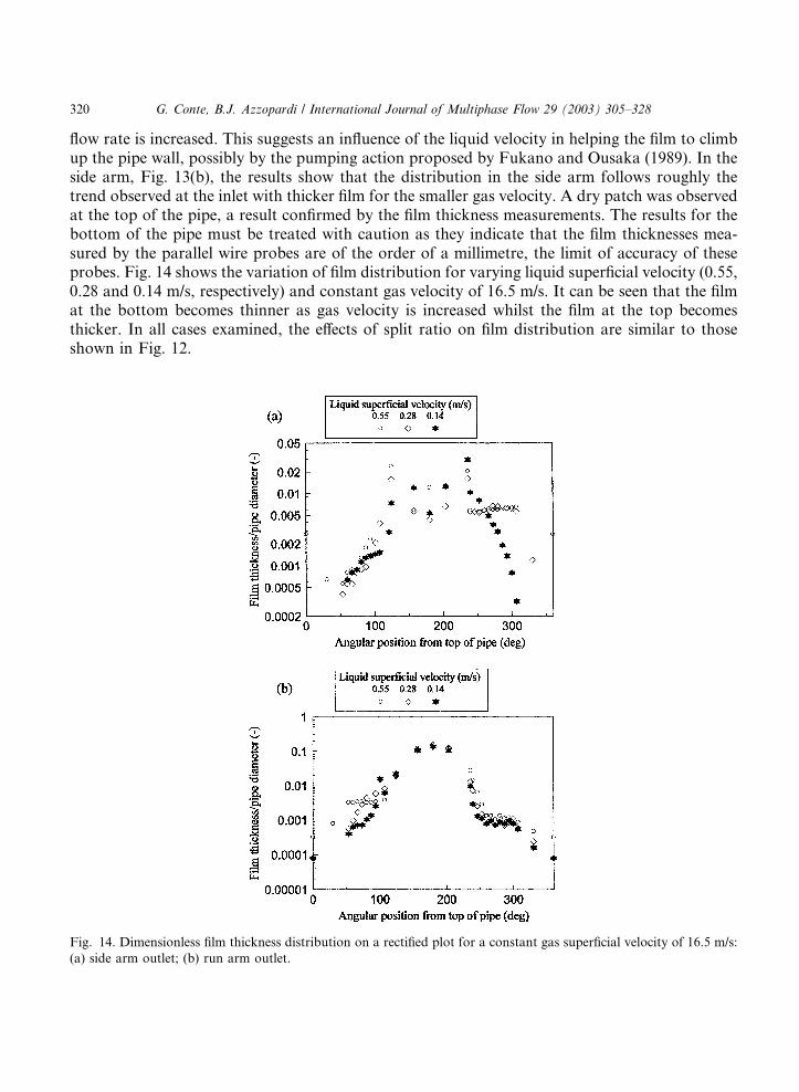
flow rate is increased. This suggests an influence of the liquid velocity in helping the film to climbup the pipe wall, possibly by the pumping action proposed by Fukano and Ousaka (1989). In theside arm, Fig. 13(b), the results show that the distribution in the side arm follows roughly thetrend observed at the inlet with thicker film for the smaller gas velocity. A dry patch was observedat the top of the pipe, a result confirmed by the film thickness measurements. The results for thebottom of the pipe must be treated with caution as they indicate that the film thicknesses mea-sured by the parallel wire probes are of the order of a millimetre, the limit of accuracy of theseprobes. Fig. 14 shows the variation of film distribution for varying liquid superficial velocity (0.55,0.28 and 0.14 m/s, respectively) and constant gas velocity of 16.5 m/s. It can be seen that the filmat the bottom becomes thinner as gas velocity is increased whilst the film at the top becomesthicker. In all cases examined, the effects of split ratio on film distribution are similar to thoseshown in Fig. 12.

Fig. 14. Dimensionless film thickness distribution on a rectified plot for a constant gas superficial velocity of 16.5 m/s:

(a) side arm outlet; (b) run arm outlet.


3.3. Film thicknesses within the T-junction

Because of the large number of stations at which measurements have been made within theT-junction, it is convenient to use a simple code identifying the rows and columns of the matrix ofpositions. Fig. 15 indicates the code. Typical results for one set of inlet flow rates and one split areshown in Fig. 16. This is a view from the inlet of the T-junction. Data from F1, 2, 4, 5 are notshown, as they are not line with other stations from the ‘‘same’’ columns. Of particular interest arethe values from stations just in the side arm where the results indicate a film climbing up the sidesof the pipe with a depression at the centre of the side arm where the liquid is draining away. This isevident in Fig. 17, which provides a view from the side opposite the side arm. There is very lit-tle change in the liquid level along the centre of the main pipe. For other inlet conditions,the same plot can show either a peak or a depression. For row C, slight variations corre-sponding to the centre of the T can cause either a peak or a trough. The liquid slowing down toturn in the side arm causes a thicker film. On the other hand, the film tends to become thin-ner because of its removal through the side arm. Row D remains unchanged up to few centi-metres past the upstream corner and then flows down because of the absence of the pipe wall.The liquid level increases again towards the run arm, usually to a slightly lower height. Simi-lar behaviour is observed for row E. However, because of the film climbing on the down-stream corner of the T-junction, the liquid level after the junction is higher than upstream of it(points E2 and E4). Finally, row F presents the features discussed in the results from the harp testsection.To appreciate the effect of different split conditions, it can be significant to plot for low, medium

and high gas take off, the film contour along the side arm, Fig. 18(row 3) and along the main pipe,

Fig. 15. Top view of the T-block fitted with wire probes showing the location of probes at the knots of the net. The

distance between two consecutive rows of letters (A–F) is of 25 mm. The distance between two columns of numbers

(1–5) is 36.75 mm except for the probes on row F which are spaced at 25 mm. The dotted lines show the contours of the

T. Arrows indicate the direction of flow.


Fig. 16. Film distribution results at the bottom. View from inlet section. Gas superficial velocity ¼ 24:5 m/s, liquidsuperficial velocity ¼ 0:28 m/s; gas fractional take off ¼ 0:54, liquid fractional take off ¼ 0:11.

Fig. 17. Film distribution results at the bottom. View from mean pipe axial vertical plane. Gas superficial

velocity ¼ 16:5 m/s, liquid superficial velocity ¼ 0:28 m/s; gas fractional take off ¼ 0:57, liquid fractional takeoff ¼ 0:08.

Fig. 18. Film distribution along row 3, towards side arm, for the three splits. Gas superficial velocity ¼ 28:1 m/s, liquidsuperficial velocity ¼ 0:14 m/s. The flow is entering the plane of the plot.


Fig. 19(row C). Those figures are for the highest inlet gas superficial velocity and are chosen asgiving the most interesting trends. The contour of the pipe has not been represented to the use thedifferent scale of abscissa and ordinate to magnify the differences observed. In most cases, pointC3 shows a relative maximum, in the plot along the side arm direction, Fig. 18. This is in fact theeffect of the film slowing down in proximity of a dividing streamline for the liquid. A similar effectcan be often observed in a plot along the main direction, Fig. 19. Again, no clear trend can be seenfrom the results in dependence of phases split, probably due to the narrow range of take offexamined. The other flow rates showed less strong trends with take off.As with the results of the harp/pin test sections, it is interesting to compare results obtained for

similar split and for either a constant gas or constant liquid superficial velocity, varying superficialvelocity of the other phase. Figs. 20 and 21 show the results along side arm direction and main

Fig. 20. Film distribution along row 3, towards side arm, for a constant inlet gas superficial velocity of 16.5 m/s. Main

flow is entering the plane of the plot.

Fig. 19. Film distribution along row C towards run outlet for the three splits. Gas superficial velocity ¼ 28:1 m/s, liquidsuperficial velocity ¼ 0:14 m/s. The flow is entering the plane of the plot, towards the side arm. Main flow is from left toright.


Fig. 21. Film distribution along row C towards run outlet for a constant inlet gas superficial velocity of 16.5 m/s.

Fig. 22. Film distribution along row 3 along side arm for a constant liquid superficial velocity of 0.14 m/s. The flow is

towards the side arm. Main flow is entering the plane of the plot.

Fig. 23. Film distribution along row C towards run outlet arm for a constant liquid superficial velocity of 0.14 m/s.


pipe direction for cases for constant gas and varying liquid superficial velocities and 72–79% gastaken off. No general trend can be established and both for the plot along the run and side armdirection, variations are quite small. The largest liquid flow rate appears qualitatively differentfrom the other two. The effect of the inlet gas superficial velocity can be seen in Figs. 22 and 23.These consider data for fractional gas take off in the range 0.44–0.46 and fraction liquid take off inthe range 0.13–0.15. They show a clear trend with a thinner film for increasing liquid velocity. Thisis in agreement with the findings of the measurements at the inlet to the T-junction. In this case, itis the results from the run at the largest inlet gas superficial velocity, which are the most different.

4. Comparison with models

The present experimental data have been used to validate models for the prediction of film flowvariation around the pipe circumference and of the phase split. Two levels of model are con-sidered. The first is essentially one-dimensional and uses the ideas of Hurlburt and Newell (2000)for horizontal annular flow and those of Azzopardi and Whalley (1982) and Azzopardi (1989) forthe phase split at the T-junction. Full details can be found in Conte (2000); Wren et al. (inpreparation). The second approach uses a three dimensional Computational Fluid Dynamicsmodel for the gas/drop flow and an integral boundary layer model for the film. Full details aregiven in Adechy and Issa (submitted for publication).The models give a reasonable prediction of the film thickness variation upstream of the

T-junction. Fig. 24 shows the comparison of the Hurlburt and Newell (2000) model with theexperimental data described above. The original model shows an unphysical cusp at the bottomcentre. This is removed in the modified version produced by Conte (2000); Wren et al. (inpreparation) who added a term to account for it. However, even the modified model underpredictsthe film thickness at the bottom and over predicts that at the top. The predictions of Adechy andIssa (submitted for publication) give film thicknesses that are larger than those measured, i.e.,

Fig. 24. Circumferential variation of film thickness upstream of the T-junction. Present experimental data and model of

Hurlburt and Newell (2000) (original) and modification of Conte (2000).


predicted ¼ 18:7 mm, measured ¼ 14:9 mm at the bottom and predicted ¼ 0:46 mm,measured ¼ 0:027 mm at �30� from the top. When the film thickness variation around the sidearm is considered, Fig. 25, it can be seen that the model correctly predicts two peaks in the filmthickness. However, though the position of one is correctly predicted, the film thickness at thepeak is about 100% too thick. The film thickness at the second peak is correctly predicted.However, it is shown to occur at a position 70� lower that found experimentally.The models give reasonable predictions of the phase split. The results of Adechy and Issa

(submitted for publication) show a lower slope than the experimental data. Those of the model ofAzzopardi (1989) using the modification of the Hurlburt and Newell (2000) model for the inletcircumferential film variation show the correct absolute values of split and pick up some of thetrends with inlet gas and liquid flow rates. More detailed comparisons are given in Wren et al. (inpreparation).

5. Conclusions

From the material presented above it can be concluded:

1. The phase split of semi-annular flow at a large diameter T-junction is liquid dominated. Lessthan 20% of the liquid is taken off for 80% gas take off.

2. The liquid at the entry to the T-junction is concentrated in the bottom 30% of the pipe with athin film on the remaining, top part of the pipe.

3. The film thickness distribution just inside the side arm is characterised by two peaks at �120�and �230� from the top of the pipe.

4. The film distributions are not sensitive to take off up to 80% gas take off and to gas and liquidinlet flow rate.

Fig. 25. Circumferential variation of film thickness in side arm. Present experimental data and prediction of Adechy

and Issa (submitted for publication).


Acknowledgements

This work was funded by EPSRC, Grant GR/K82741. The authors would like to thanks Dr. R.Issa and Mr. D. Adechy (Imperial College), Dr. L.C. Daniels (Hyprotech Ltd), Mr. P. Gramme(Norsk Hydro) and Mr. D. Dick (BP) for their helpful comments.

References

Adechy, D., Issa, R.I. Modelling of annular flow through pipes and T-junctions. Computers and Fluids, submitted for

publication.

Azzopardi, B.J., 1989. The split of annular-mist flows at vertical and horizontal Ts. In: Proceedings of 8th International

Conference on Offshore Mechanics and Arctic Engineering V. ASME, pp. 389–395.

Azzopardi, B.J., 1999. Phase separation at T-junctions. Multiphase Science and Technology 11, 223–329.

Azzopardi, B.J., Whalley, P.B., 1982. The effect of flow pattern on two-phase flow in a T-junction. Int. J. Multiphase

Flow 8, 481–507.

Azzopardi, B.J., Rea, S., 1999. Modelling the split of horizontal annular flow at a T-junction. Transaction of the

Institution of Chemical Engineers 77A, 713–720.

Azzopardi, B.J., Colman, D.A., Nicholson, D., 2002. Plant application of a T-junction as a partial phase separator.

Transaction of the Institution of Chemical Engineers 80A, 87–96.

Brown, R.C., Andreussi, P., Zanelli, S., 1978. The use of parallel wire probes for measurment of film thickness in

annular gas–liquid flows. Canandian Journal of Chemical Engineering 56, 754–757.

Buell, J.R., Soliman, H.M., Sims, G.E., 1994. Two-phase pressure drop and phase distribution at a horizontal

T-junction. Int. J. Multiphase Flow 20, 819–836.

Clark, W.W., 2002. Liquid film thickness measurement. Multiphase Science and Technology 14, 1–74.

Conte, G., 2000. An experimental study for the characterisation of gas/liquid flow splitting at T-junctions. Ph.D. thesis,

University of Nottingham.

Davis, M.R., Fungtamasan, B., 1990. Two-phase flow through pipe junctions. Int. J. Multiphase Flow 16, 799–

817.

Fisher, S.A., Pearce, D.L., 1993. An annular flow model for predicting liquid carryover into austenitic superheaters. Int.

J. Multiphase Flow 19, 295–307.

Fukano, T., Ousaka, A., 1989. Prediction of the circumferential distribution of film thickness in horizontal and near-

horizontal gas–liquid annular flow. Int. J. Multiphase Flow 15, 403–419.

Hurlburt, E.T., Newell, T.A., 2000. Prediction of the circumferential film thickness distribution in horizontal annular

gas–liquid flow. Journal of Fluids Engineering 122, 1–7.

James, P.W., Wilkes, N.S., Conkie, W., Burns, A., 1987. Developments in the modelling of horizontal annular two-

phase flow. Int. J. Multiphase Flow 13, 173–198.

Kim, M., Kang, H., 1990. The development of a flush-wire probe and calibration technique for measuring liquid film

thickness. ASME Winter Annual Meeting, Dallas, FED 99, HTD 155, pp. 31–138.

Kimpland, R.H., Lahey, R.T., Azzopardi, B.J., Soliman, H.M., 1992. A contribution to the prediction of phase

separation in branching conduits. Chemical Engineering Communications 111, 79–105.

Koskie, J.E., Mudawar, I., Tiederman, W.G., 1989. Parallel-wire probes for measurement of thick liquid films. Int. J.

Multiphase Flow 15, 521–530.

Lemonnier, H., Hervieu, E., 1991. Theoretical modelling and experimental investigation of single-phase and two-phase

division at a tee junction. Nuclear Engineering and Design 125, 201–213.

Miya, M., Woodmansee, D.E., Hanratty, T.J., 1971. A model of roll waves in gas liquid flow. Chemical Engineering

Science 26, 1915–1931.

Oranje, L., 1973. Condensate behaviour in gas pipelines is predictable. Oil and Gas Journal 71, 39–44.

Paras, S.V., Vlachos, N.A., Karabelas, A.J., 1994. Liquid layer characteristics in stratified-atomization flow. Int. J.

Multiphase Flow 20, 939–956.


Peng, F., Shoukri, M., Ballyk, J.D., 1998. An experimental investigation of stratified steam-water flow in T-junctions.

Proceedings of 3rd International Conference on Multiphase Flow, CD ROM, #569.

Rea, S., Azzopardi, B.J., 2001. The split of horizontal stratified flow at a T-junction. Transaction of the Institution of

Chemical Engineers 79A, 470–476.

Roberts, P.A., Azzopardi, B.J., Hibberd, S., 1995. The split of horizontal semi-annular flow at a large diameter

T-junction. Int. J. Multiphase Flow 21, 455–466.

Roberts, P.A., Azzopardi, B.J., Hibberd, S., 1997. The split of horizontal annular flow at a T-junction. Chemical

Engineering Science 52, 3441–3453.

Scott, A.H., Das, P.K., Azzopardi, B.J., Wren, E., 2001. The effect of side arm length on the split of two-phase flow at a

vertical T-junction. European Two-Phase Flow Group Meeting, Aveiro, Portugal, 18–20 June.

Suu, T., 1992. Air–water two-phase flow through a pipe junction effect of the Reynolds number on the local void

fraction distribution. JSME International Journal Ser. II 35, 76–81.

Taitel, Y., Dukler, A.E., 1976. A model for predicting flow regime transitions in horizontal and near-horizontal gas–

liquid flow. American Institute of Chemical Engineers 22, 47–55.

Williams, L.R., Dykhno, L.A., Hanratty, T.J., 1996. Droplet flux distribution and entrainment in horizontal gas liquid

flows. Int. J. Multiphase Flow 22, 1–18.

Wren, E., Conte, G., Azzopardi, B.J. Modelling the split of gas/liquid flow at a T-junction: the effect of side arm

orientation, in preparation.

Wu, H.L., Pots, B.F.M., Hollenberg, J.F., Meerhoff, R., 1987. Flow pattern transitions in two-phase gas/condensate

flow at high pressure in an 8-inch horizontal pipe. In: Proceedings of 3rd International Conference on Multi-phase

Flow. BHRA, pp. 13–21.


Documents

Film thickness variation about a T-junction