Filling in the MIMO Matrix - sandv. · PDF filecreating and controlling time records with a “seamless ... • Quality of the multi-channel test data to be used for ... Filling in

www.SandV.com8 SOUND & VIBRATION/SEPTEMBER 2011

There is currently quite a bit of interest in using field data as much as possible for performing multi-shaker laboratory simula-tions. With the introduction of MIL-STD-810G in 2008, and es-pecially Method 525, Time Waveform Replication, multi-shaker replication tests are being attempted and performed more than ever. As with any multi-exciter test, it is important to characterize the entire test configuration, including shakers, amplifiers, fix-tures, transducers and cables before starting the test. To minimize test errors, especially if long time records are being used, system characterization should be updated during the test, perhaps every control loop. Also, even though the purpose of the test is carefully reproducing time waveforms from field measurements, the control process may take place in the time domain, the frequency domain or both. We show here the development of a unique approach to creating and controlling time records with a “seamless” transition from block to block.

Although multi-shaker testing has been attempted for over 40 years, it is only in the past 8 to 10 years that the correct combina-tion of instrumentation, computers and software have become available to make this technique a reality. In the absence of a set of comprehensive “multi-exciter test specifications,” many orga-nizations have tried to take the advice of MIL-STD-810 and use measured or borrowed field vibration data to create a laboratory simulation. Some recent reports1,2 have indicated that when using actual measured field vibration for multi-exciter simulation, care must be taken to assure good phase and coherence duplication, or unexpected results may occur. So it is up to the test engineers to assure that they have taken into account or at least considered:

Quality of the multi-channel test data to be used for replica-•tionBoundary condition differences, field to lab•Number and location of lab shakers•Test lab fixturing arrangement and possible effect on system •dynamicsControl approach to be implemented – square, rectangular, •over-determined, etc.Position and number of control transducers•Approach to error analysis for proof of performance•

Time Waveform ReplicationAs discussed in Reference 3, time waveform replication (TWR)

is a vibration control method whose goal is to cause the response time history at one or more control points to agree with a prespeci-fied vector of waveforms while using one or more exciters. TWR control is typically performed at least partially in the frequency domain. But since the main goal of TWR is to recreate a series of time waveforms as closely as possible, its performance is usually evaluated in the time domain.

Figure 1 shows an overlay of the Reference and actual Control waveforms present at Control point 3 in the 4 shaker test described here. In this case, the Control was so good that it is very hard to distinguish between the Control (white) and Reference (blue) traces. This figure shows the first 100 milliseconds of the 4-second records that were used. Note that the peak values shown refer to the entire 4-second record.

Figure 2 shows an error display in percent of peak value for the same Control location 3, but this time for the entire 4-second record. Note that one point approaches 0.4%, and a second exceeds 0.3%. But for most of the record the peak error never exceeds 0.2%.

When performing TWR control, the Reference and Control re-sponse time histories are typically longer than an FFT block. So an indirect convolution method using overlap and add is typically used for Control and Drive signal generation.

TWR Control ApproachWhile in the frequency domain, the product of two spectra or

of a spectrum and a frequency response function, can be taken by direct multiplication. Performing an “equivalent” operation in the time domain, requires the use of convolution.4,5 The Control approach described here uses indirect linear convolution between the measured inverse impulse response of the system under test and the Reference and Error time histories. The use of overdeter-

Filling in the MIMO MatrixPart 2 – Time Waveform Replication Tests Using Field DataMarcos Underwood, Russ Ayres, and Tony Keller, Spectral Dynamics, Inc., San Jose, California

Figure 1. Overlay of Reference and Control waveforms (expanded).

Figure 2. Control error as percentage of peak value shown over full 4-second waveform.

Figure 3. Test setup for acquiring and controlling field data.

www.SandV.com DYNAMIC TESTING REFERENCE ISSUE 9

Figure 4. Control PSDs at four plate corners during field data acquisition phase: (a) 1,1; (b) 2,2; (c) 3,3; (d) 4,4.

Figure 5. Control coherence and phase for MIMO random test shown in Figure 4: (a&c) 1,2; (b&d) 2,3


mined TWR Control is possible with the use of I/O transformations, although this technique was not used in the tests described here. Generally, TWR Control performance is determined by the quality of the system under test and the accuracy of the measured inverse frequency response (impedance) matrix.

Adaptive ControlAdaptive Control is a patented method [Patent # 5,299,459], that

updates the impedance matrix (system model) of virtually every control loop using actual Response and Drive signals. This can minimize the time it takes to match the Reference and Response time histories or spectra. This approach can also be used to update the actual Drive signals in real-time while the test is running to reduce Control errors during a TWR test. Without this capability, Drives are only updated between test sequences or at the start of the test in TWR applications. This approach can simulate and control nonlinear and time-varying environments to a much higher degree of accuracy than using traditional techniques. For example, if the

Figure 6. Response PSDs at locations: (a) 5, (b) 6, (c) 7 and (d) 8 for Test A.

Figure 7. Four-second Reference and Control waveforms.

test system includes bolted joints or oil flow, which can change dynamic properties with time, only adaptive control can assure a successful test completion.

Considerations for using Field DataBefore attempting to run any multi-exciter TWR test, it is always

good practice to see how good a match there is between the avail-able field data, the goals and objectives of the TWR test and the test facilities at your disposal. At a minimum, the dynamic capa-bilities of the multi-exciter test system, in terms of load capacity, force rating, bandwidth, acceleration, velocity and displacement capability should match or exceed the test objectives. In addition, the test article’s dynamic response characteristics must be compat-ible with the field data.

Is the measured data complete and a good match for the sampling rate and record length parameters of the test control system? Or will resampling be required? Were the field transducers mounted at locations and orientations that will exist and be available in the Lab? Or will the apparatus and fixturing required to mount the test article to the exciters actually eliminate some field mea-surement locations? Test article dynamic response characteristics must be compatible with the measured field data, and boundary conditions encountered in the field should be satisfied as closely as possible during the lab test. Unless care is taken to understand the dynamic response of the test article when mounted in the test platform configuration, the resulting TWR could be a severe overt-est or even an undertest.

Using Field Data in a Multi-Exciter TWR TestTest A – MIMO Random Control with Zero Coherence Between

Control Points. We present several examples of recording “field” data and using these data to create time waveform records and then to replicate the data on a four-shaker system. In the first example (Test A), the boundary conditions (BC) between the field setup and the test lab simulation are exactly matched. In another case (Test C), they are not matched, but the lab test is still required to


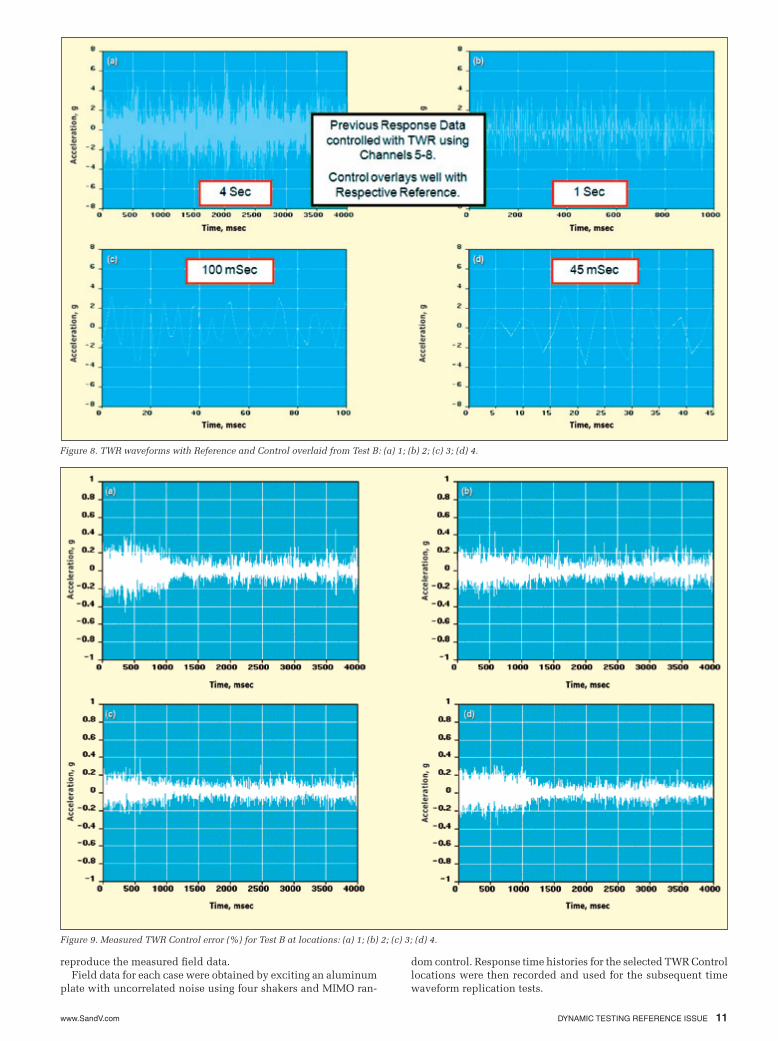
Figure 8. TWR waveforms with Reference and Control overlaid from Test B: (a) 1; (b) 2; (c) 3; (d) 4.

Figure 9. Measured TWR Control error (%) for Test B at locations: (a) 1; (b) 2; (c) 3; (d) 4.

reproduce the measured field data.Field data for each case were obtained by exciting an aluminum

plate with uncorrelated noise using four shakers and MIMO ran-

dom control. Response time histories for the selected TWR Control locations were then recorded and used for the subsequent time waveform replication tests.


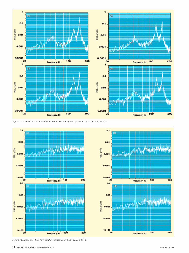
Figure 11. Response PSDs for Test B at locations: (a) 1; (b) 2; (c) 3; (d) 4.

Figure 10. Control PSDs derived from TWR time waveforms of Test B: (a) 1; (b) 2; (c) 3; (d) 4.


Figure 12. Nuts loosened toward end of Test B.

Figure 13. Control PSDs for Test C with loosened nuts: (a) 1,1 (b) 2,2; (c) 3,3; (d) 4,4.

Figure 3 shows the test setup for controlling the four corners of a lightly damped plate and measuring four field data Responses at four arbitrary locations inboard from the Control locations.

Note that in addition to the eight mounted accelerometers, a loose book was placed on the plate to simulate system time variability during the test. Since the test data used for TWR often exceeded 6 g, quite a bit of book motion was experienced during the TWR test. The first phase of the test controlling the four corners was done at a nominal Control level of 1 g rms. This means that, besides having instantaneous acceleration values at the response points that exceeded 5 g, the corners would sometimes also exceed 1 g. This would cause book motion also during the acquisition phase

of getting the field data. The Control PSDs experienced during the first-step MIMO random Control are seen in Figure 4. As can be seen, Control was quite good even in the presence of several resonances; this will be shown later.

For Test A, the Control coherence was set to zero. This produces completely random phase relationships between Control locations.The coherence for all six upper off-diagonal matrix terms was controlled to zero, resulting in random phase between all Control points for this incoherent situation. While controlling to these parameters, the response PSDs for the auxiliary points, 5 through 8, were also measured. These are seen in Figure 6.

While controlling the four corners of the plate with MIMO random excitation, time histories of the four Response locations, 5 thru 8, were recorded to disk. Since stationary data were being recorded, we decided that 4-second time blocks would be sufficient for performing subsequent TWR tests. This also corresponds to one block of the 200 Hz MIMO random test performed with 800 Control lines. A typical 4-second TWR signal from this test showing both Reference and Control is seen in Figure 7.

In Figure 7, the instantaneous accelerations at the TWR Control points can easily exceed 6 or 7 g. Therefore, the nonlinearizing loose book on the plate becomes a critical factor in terms of the need for adaptive Control. Summary, Test A.: MIMO Random Control at locations 1, 2, 3 and 4. Response measurements at locations 5, 6, 7 and 8. Time histories of all channels recorded.

Test B – TWR Control Using Time Records from Test A. In Figure 8, the four channels of time waveforms collected during Test A and used as the basis of Test B are shown. Different record lengths are shown for each controlled channel to illustrate the excellent over-lay between the Reference (desired) and actual Control waveforms. At this point in the testing, the system boundary conditions were considered to be the same for both the MIMO random test when waveforms were recorded and the subsequent TWR test.

Figure 9 shows the accuracy achieved in the first TWR test and that most errors are less than 0.2% after a few iterations. The error definition used here is instantaneous Control error normalized to peak acceleration. This is quite a stringent definition, compared


Figure 14. Resulting Control coherence and phase during Test C: (a) 1,2 coherence; (b) 2,3 coherence; (c) 1,2 phase; (d) 2,3 phase

Figure15. Measured Responses taken during Test C: (a) 5; (b) 6; (c) 7; (d) 8.


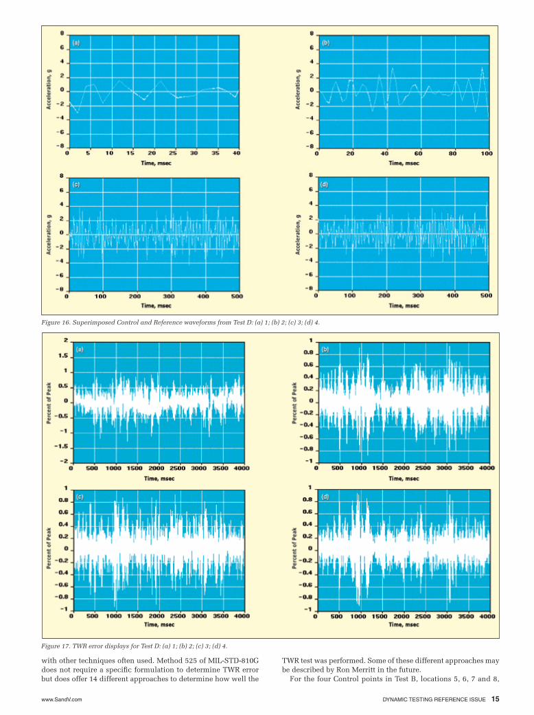
Figure 16. Superimposed Control and Reference waveforms from Test D: (a) 1; (b) 2; (c) 3; (d) 4.

Figure 17. TWR error displays for Test D: (a) 1; (b) 2; (c) 3; (d) 4.

with other techniques often used. Method 525 of MIL-STD-810G does not require a specific formulation to determine TWR error but does offer 14 different approaches to determine how well the

TWR test was performed. Some of these different approaches may be described by Ron Merritt in the future.

For the four Control points in Test B, locations 5, 6, 7 and 8,


Figure 18. PSDs of Control TWR waveforms for Test D: (a) 1; (b) 2; (c) 3; (d) 4.

Figure 19. PSDs during TWR of Test D for auxiliary locations: (a) 1; (b) 2; (c) 3; (d) 4.


those of Figure 10 taken during Test B (tight MIMO acquisition, tight TWR control), than those of Figure 15 taken during Test C (loose MIMO acquisition, loose MIMO control). A slight increase in Q is noted, but there are not as many obvious spikes in all four channels as previously.

Finally, Figure 19 shows the “reciprocity” locations 1 thru 4 dur-ing the TWR control of Test D; it bears a closer similarity to Figure 11 (no spikes) than Figure 13 (many spikes). Although there are spikes in Figure 19 at the same frequencies as in Figure 13, they are at reduced amplitudes.

ConclusionsTWR control performance while employing the field Response •data discussed here was very good; waveform errors were less than 1% in virtually all cases.Comparing Reference and Control waveforms during TWR test-•ing is an extremely sensitive procedure, much more so than, for example, comparing PSD levels. So extra precautions should be taken to assure that factors such as loose connections or slapping are not present during the test.The use of adaptive Control during TWR testing is very effec-•tive in addressing time-varying and nonlinear characteristics in the test setup.Satisfying field boundary conditions in the lab as much as pos-•sible may have the largest single effect on assuring a quality laboratory simulation.More work needs to be done on selecting a range of acceptable •error metrics when performing TWR tests. However, the point-to-point error comparison used in this article is the most severe.When performing error analysis after a TWR test, it is advan-•tageous to observe results in both the time and the frequency domains. Although our goal is to match the time histories as closely as possible, some results, especially on highly resonant structures, may offer more meaningful comparisons as PSDs. This is evident in Figures 18 and 19.Measuring and comparing nonControl points in the field and •in the lab during TWR tests will help assure a quality TWR simulation.

References1. Lamparelli, Marc, Underwood, Marcos, Ayres, Russell, and Keller,

Tony, “An Application of ED Shakers to High Kurtosis Replication,” ESTECH2009, 55th Annual meeting of the IEST, Schaumburg, IL, May 4-7, 2009.

2. Underwood, Marcos, Ayres, Russell, and Keller, Tony, “Filling in the MIMO Matrix, Using Measured Data to run a Multi-Actuator/Multi-Axis Vibration Test,” presented at the 80th Shock & Vibration Symposium, San Diego, CA, October 26-29, 2009.

3. MIL-STD-810G – Test Method Standard for Environmental Engineering Considerations and Laboratory Tests, http://www.dtc.army.mil/publica-tions/MIL-STD-810G.pdf, October 31, 2008, Method 525, Time Waveform Replication.

4. Chang, David K., Analysis of Linear Systems, Addison-Wesley, 1959.5. Schwartz, Mischa, Information Transmission, Modulation and Noise,

McGraw-Hill Electrical and Electronic Engineering Series, 1959.

power spectral densities were created and are shown in Figure 10.

During Test B, locations 1, 2, 3 and 4 (which were the Control points for Test A but are Response locations for Test B) were also analyzed and are shown in Figure 11. Due to reciprocity, the ex-cellent Control results in replicating the Responses at locations 5, 6, 7 and 8 and the nearly linear behavior of the test system, these agree quite well with those shown in Figure 4.

Near the end of Test B, it was noted that some unexplained spikes were appearing in the data, especially in the frequency domain representations. An investigation was done, and it was discovered that at the shaker 3 attachment to the plate, the set of attachment nuts had vibrated loose. In effect, this was providing a fifth excita-tion to the plate but in the form of nonrepetitive shocks. This had the result of exciting the plate resonances to an even higher degree than the random excitation, creating a non-zero coherence with respect to location 3 and introducing a noncontrollable spectrum source. This definitely introduces a sense of realism into an other-wise very clean test. The connection involved here is highlighted in Figure 12. The realization that the single loosened nut added a completely new dynamic into the TWR test led to the creation of additional tests that are described next.

Test C – MIMO RandomTest Performed with Shaker 3 Attach-ment Nuts Loosened. The next test performed was done to see the effects of running another controlled MIMO random test, this time with the loose connection at Shaker 3. Figure 13 shows the Control situation for Test C. Note that the Control levels are all very close to 1 g rms. But at the Control location nearest shaker 3, additional spikes, not coming directly from the (linear) shakers are contribut-ing to the measurements. Since these are not linearly related to the complex set of Drive vectors being created, they fall outside the system definition in the spectral density matrix. So the resulting Control coherence is also affected at these “spike” frequencies (see Figure 14). The Response PSDs of locations 5 thru 8 were also measured during Test C and are shown in Figure 15.

In addition to the impacts imparted at shaker 3 during Test C, due to the loosened connection, the lack of a secure tiedown at that location also removed some natural damping imparted by the normally tight connection. This results in a slightly higher Q in the plate responses, as shown in Figure 15. During Test C with the untightened condition at shaker 3, a new set of time waveforms was recorded. This led to Test D.

Test D: TWR Test Performed on Retightened Structure Using Waveforms Recorded During Test C. The final test was performed using a set of boundary conditions, (connections tightened at all 4 shakers), which was different from the boundary conditions that existed when the data were taken during Test C. With these dif-ferent sets of boundary conditions between Test C and Test D, the TWR Control, although quite good, was not as good as that seen during Tests A and B. Examples of the four waveforms replicated during the final test are shown in Figure 16.

The poorer boundary condition match in Test D resulted in an increased error during TWR (see Figure 17). But the PSDs measured during the TWR done in Test D (Figure 18), look much more like The author may be reached at: [email protected].

Documents

Filling in the MIMO Matrix - sandv. · PDF filecreating and controlling time records with a “seamless ... • Quality of the multi-channel test data to be used for ... Filling in