Embed Size (px)
Citation preview

Competitive Balance
Chapter 5
FIFTH EDITION
The Economics of Sports
MICHAEL A. LEEDS | PETER VON ALLMEN

Copyright ©2014 Pearson Education, Inc. All rights reserved. 5-2
Competitive Balance
• The term means different things to different people
– Close competition every year, with the difference
between the best and worst teams being relatively small
– Regular turnover in the winner of the league’s
championship
• More generally, it means degree of parity within a
league

Copyright ©2014 Pearson Education, Inc. All rights reserved. 5-3
Learning Objectives
• Understand why owners and fans care about
competitive balance
• Be able to use and interpret the different measures
of competitive balance
• Describe and compare the tools that leagues use
to promote competitive balance and the limitations
of those tools.

Copyright ©2014 Pearson Education, Inc. All rights reserved. 5-4
5.1 Desire for Competitive Balance
• Fans and owners alike have a conflicted
relationship with competitive balance
• On any given day, seeing one’s team win is
preferable to seeing it lose
• But an uninterrupted string of wins is dull

Copyright ©2014 Pearson Education, Inc. All rights reserved. 5-5
The Fans’ Perspective
• A game with an uncertain outcome is much more
exciting than a foregone conclusion
• Table 5.1 shows that from 1950 to 1958
attendance for both the Yankees and the entire
American League either stagnated or fell because
of Yankees dominance
• Evidence suggests that in many sports, fans
prefer a game where the home team has a 60-
70% chance of winning

Copyright ©2014 Pearson Education, Inc. All rights reserved. 5-6
Table 5.1
Copyright ©2014 Pearson Education, Inc. All rights reserved. 5-7
The Owners’ Perspective
• Competitive balance matters to owners because it
matters to fans
• Leagues adopt policies to promote competitive
balance because they enhance fan demand
• Leagues restrict team behavior if it leads to teams
that are too strong or too weak (see Table 5.1)
• Balance is hard to achieve if some teams maximize
wins while others maximize profits

Copyright ©2014 Pearson Education, Inc. All rights reserved. 5-8
Effect of Market Size
• There is considerable debate over the impact of
market size on competitive balance
• There are three primary sources of disagreement
– How to measure of success
• During playoffs or regular season?
– How to characterize market size
• Market size has become more important with the advent of
broadcasting
Copyright ©2014 Pearson Education, Inc. All rights reserved. 5-9
Effect of Market Size (cont.)
• The third point of disagreement is how to measure
the impact of policies, such as revenue sharing
• Profit-maximizing leagues do not want total balance –
they want big-market teams to win more
• At minimum, more populous locations will win the
league championship more frequently
• Figure 5.1 shows an additional win is more valuable in
a larger market, so the optimum number of wins is
greater

Copyright ©2014 Pearson Education, Inc. All rights reserved. 5-10
Figure 5.1

Copyright ©2014 Pearson Education, Inc. All rights reserved. 5-11
The Effect of
Diminishing Returns
• The impact of another unit of a variable input (when added
to a fixed input) eventually falls
– This effect limits the desire of teams to stockpile – and pay –
star players
– And promotes competitive balance
• Drew Brees has limited value to a team that has Tom
Brady
– Brees adds little to wins, attendance, or revenue
– The added cost exceeds the added benefit
– Other teams can use him more effectively

Copyright ©2014 Pearson Education, Inc. All rights reserved. 5-12
Is Perfect Balance Profit Maximizing?
• Winning has a bigger impact
in a larger market
– It adds more to gate, media,
and venue revenue
– MRwins higher in big cities
• Profit-maximizing leagues and
competitive balance may be
incompatible
– Big cities will win more unless
MCwins is also higher
MR, MC
MRsmall MRlarge
MC
Wins

Copyright ©2014 Pearson Education, Inc. All rights reserved. 5-13
A History of
Competitive Balance
• Yankee dominance of MLB is not new
– Appeared in 15 World Series between 1947 and 1964
• The LA Lakers and San Antonio Spurs won 9 of 13 NBA
championships between 1999 and 2011
• The Montreal Canadiens won 10 Stanley Cups in the NHL
between 1965 and 1979
– They were succeeded by NY Islander and Edmonton Oiler
dynasties in the 1980s
• The NFL is more balanced, but the Browns and Lions have
never been in a Super Bowl

Copyright ©2014 Pearson Education, Inc. All rights reserved. 5-14
Competitive Balance in Soccer from
2000-01 to 2011-12
• In England’s Premier League
– Manchester United, Chelsea, and Arsenal have won 11 times
• In Germany’s Bundesliga
– Bayern Munich and Borussia Dortmund have won 9 times
• In Italy’s Serie A
– AC Milan, Inter Milan, and Juventus have won 11 times
• In Spain’s La Liga
– FC Barcelona and Real Madrid have won 10 times
Copyright ©2014 Pearson Education, Inc. All rights reserved. 5-15
5.2 Measuring Competitive Balance
• Within-Season Balance (Variation)
– Compares teams within a season—across a league
– A low dispersion of team winning percentages means that the
teams are evenly matched
• Between-Season Balance (Variation)
– Compares winners (champions) across time
– Some leagues have the same champions year after year
• Regular turnover is preferred

Copyright ©2014 Pearson Education, Inc. All rights reserved. 5-16
Within-Season Variation (1)
• We could use the standard deviation of winning percentage
– The standard deviation gives the dispersion of performance
by teams
– It is the square root of the average squared deviation from
the mean
– See formula on p. 159
• The mean performance is always .5 as there are a winner and a
loser in every game

Copyright ©2014 Pearson Education, Inc. All rights reserved. 5-17
Application
• In 2011, the standard deviation in the American League
was 0.067
– The typical winning percentage varies by 0.067 from the
mean
• The standard deviation in the National League was 0.054,
about three-fourths that of the American League.
– The National Leagues was more balanced

Copyright ©2014 Pearson Education, Inc. All rights reserved. 5-18
Within-Season Variation (cont.)
• We cannot compare the standard deviation across leagues
or across seasons with a different number of games
• As the number of matches rises, winning percentages
cluster around the mean
– If teams are evenly matched, then the probability of success
in any game is close to .5
• We can apply the binomial distribution
• In a short season, a lucky team can have all wins and an
unlucky team no wins
• The league can look unbalanced in a short season

Copyright ©2014 Pearson Education, Inc. All rights reserved. 5-19
Within-Season Variation (cont.)
– We need a better measure
– We compare a league’s standard deviation to the standard
deviation that would result if teams were evenly matched
– The “ideal” standard deviation occurs when each team has a
50% chance of winning a given game
• The better measure is the ratio of the actual to the ideal
standard deviation
– R = sA/sI
Copyright ©2014 Pearson Education, Inc. All rights reserved. 5-20
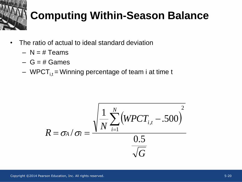
Computing Within-Season Balance
• The ratio of actual to ideal standard deviation
– N = # Teams
– G = # Games
– WPCTi,t = Winning percentage of team i at time t
G
WPCTN
R
N
i
ti
IA5.0
500.1
/
2
1
,
ss

Copyright ©2014 Pearson Education, Inc. All rights reserved. 5-21
Interpreting the Ratio
• The ratio R gives a standardized measure
– Actual and ideal standard deviation fall as G rises
– We can now compare leagues and seasons with a different
number of games
– The formula appears on p. 161
• As a rule, R > 1
• If R = 1, the league is completely balanced
– Outcomes are effectively randomly determined
• As R rises, balance worsens
Copyright ©2014 Pearson Education, Inc. All rights reserved. 5-22
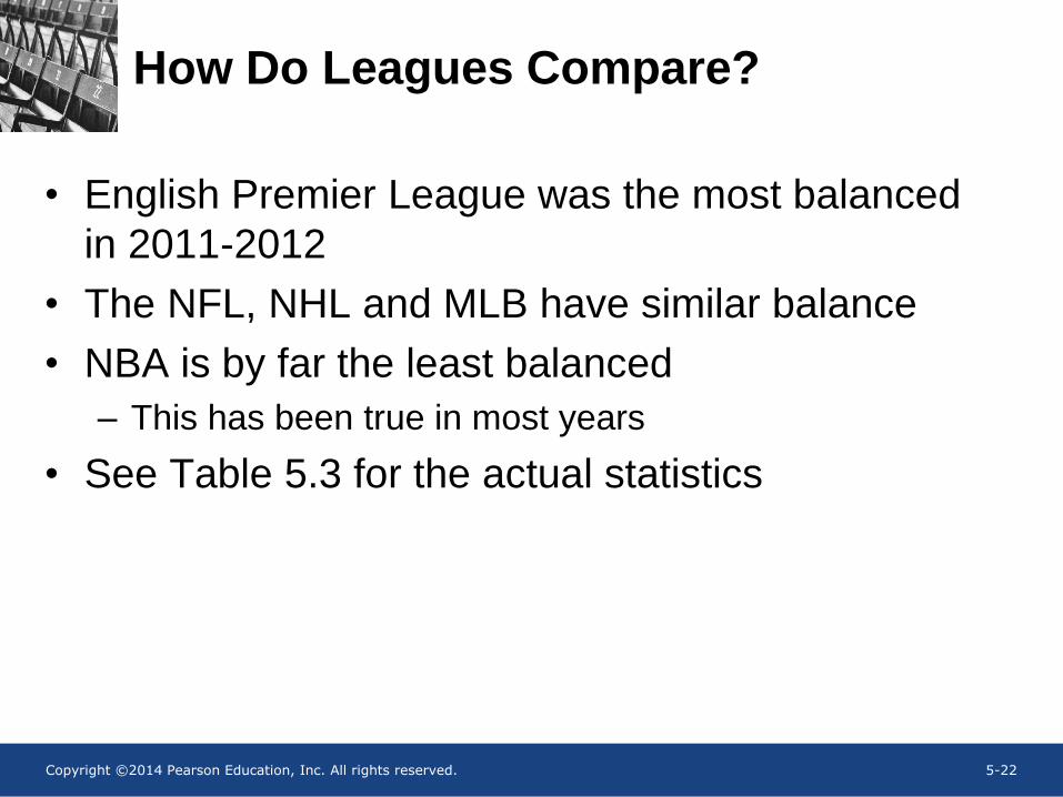
How Do Leagues Compare?
• English Premier League was the most balanced
in 2011-2012
• The NFL, NHL and MLB have similar balance
• NBA is by far the least balanced
– This has been true in most years
• See Table 5.3 for the actual statistics

Copyright ©2014 Pearson Education, Inc. All rights reserved. 5-23
Table 5.3
Copyright ©2014 Pearson Education, Inc. All rights reserved. 5-24
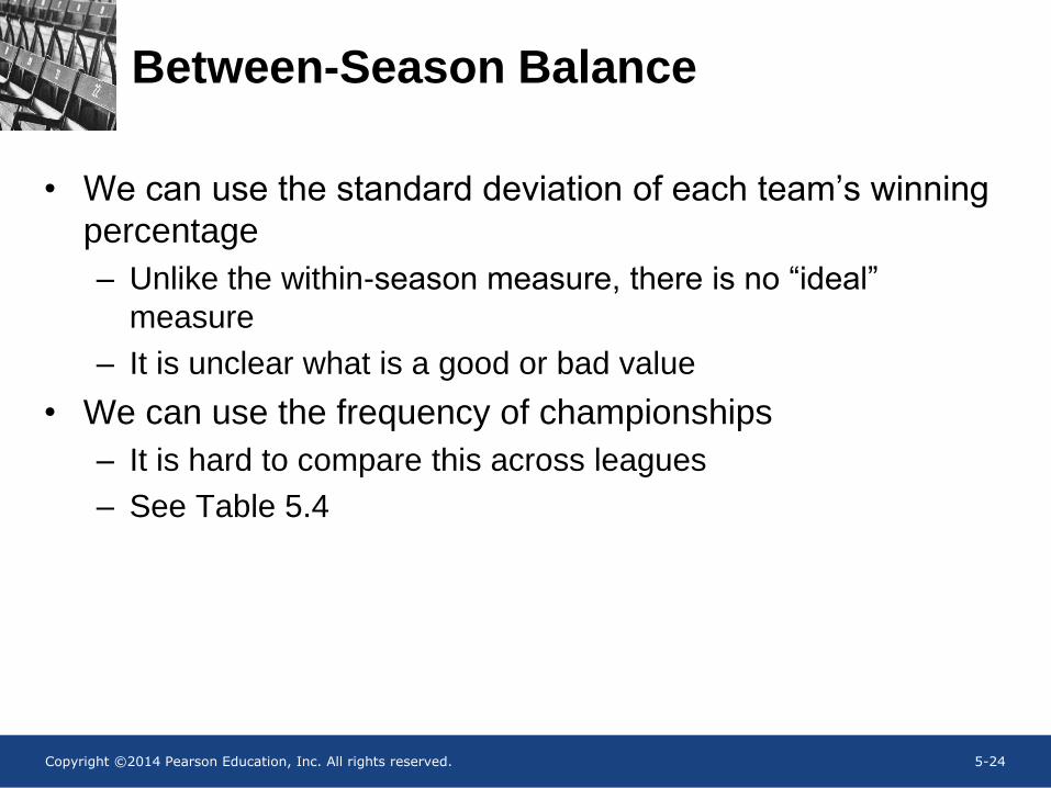
Between-Season Balance
• We can use the standard deviation of each team’s winning
percentage
– Unlike the within-season measure, there is no “ideal”
measure
– It is unclear what is a good or bad value
• We can use the frequency of championships
– It is hard to compare this across leagues
– See Table 5.4
Copyright ©2014 Pearson Education, Inc. All rights reserved. 5-25
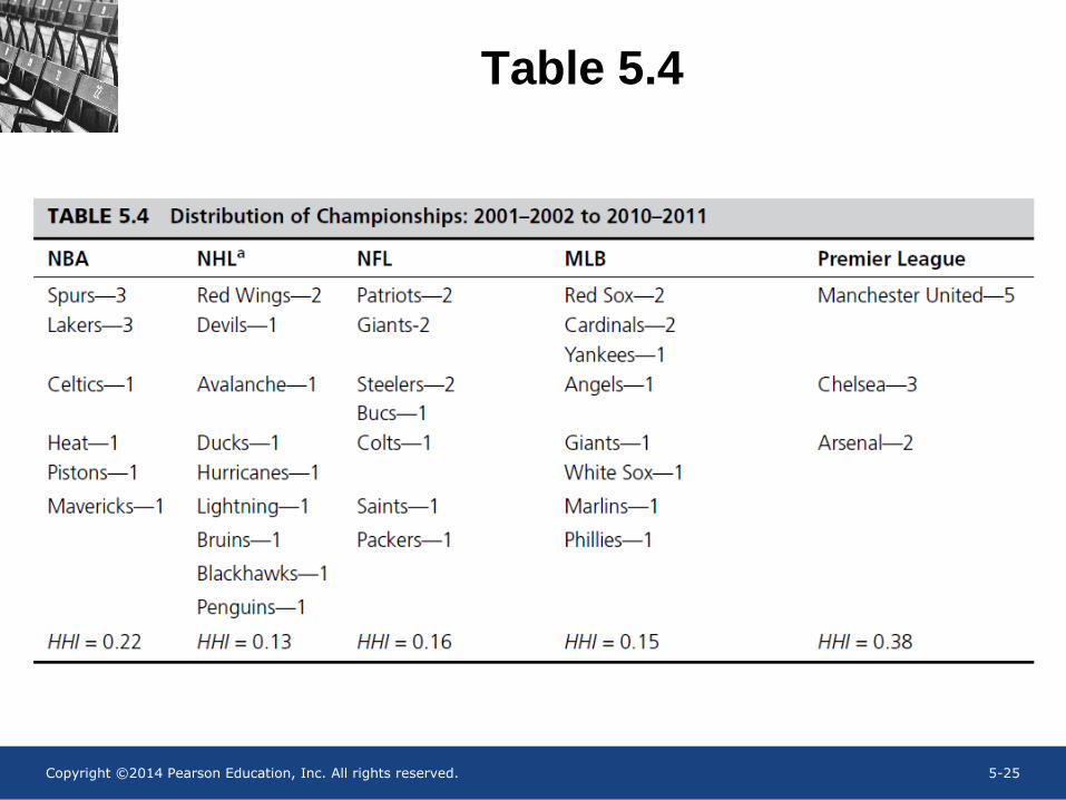
Table 5.4

Copyright ©2014 Pearson Education, Inc. All rights reserved. 5-26
The Herfindahl-Hirschman Index
• HHI measures the concentration of championships
• In industrial organization, it measures monopoly power
• Let ci = #championships by team i
– T = #teams; N = #Years
– If HHI=1, one team always wins
– If HHI=1/N and N>T, complete competitive balance
– If HHI=1/T and N<T, complete competitive balance
• See p. 164 for computations; What if the league had 10 teams?
T
i
i
N
cHHI
1
2

Copyright ©2014 Pearson Education, Inc. All rights reserved. 5-27
Applying the HHI to Sports
• See Table 5.4
• the HHI for the Premier League is far greater than for
any other league
• the HHI for the NBA is also large
• the HHI for the NHL, NFL, and MLB are substantially
smaller
• the HHI for the NHL is the smallest, indicating that the
league was most balanced in the first decade of the
21st century

Copyright ©2014 Pearson Education, Inc. All rights reserved. 5-28
Illustrating Competitive Imbalance
• The Lorenz Curve measures inequality in a population
– It is typically used to measure income inequality
– We use it to measure inequality in winning
• Line up NBA teams by wins in 2010-2011 (p. 164)
– 1230 games were played, so population = 1230
– The 3 weakest teams (the lowest decile) won 58 games
• 58 games correspond to 4.7 % of 1230
• Thus, the bottom 10% accounted for 4.7% of wins
• The next 10% accounted for 5.8% and so on
• The top 10% accounted for 14.7% of wins
– Figure 5.2 presents the results

Copyright ©2014 Pearson Education, Inc. All rights reserved. 5-29
The Lorenz Curve for the NBA
• Red line shows perfect balance
– Adding 10% more teams adds 10% more wins
• Blue line shows reality
– Bottom 10% wins less than 10%
• Sags below red line
– As we add better teams, blue curve catches up
– At 100% of teams, we account for 100% of wins
• The farther the blue line sags, the greater the inequality
0
0.2
0.4
0.6
0.8
1
1.2
0 0.1 0.2 0.3 0.4 0.5 0.6 0.7 0.8 0.9 1
Copyright ©2014 Pearson Education, Inc. All rights reserved. 5-30
5.3 Altering Competitive Balance
• All the major North American sports leagues have
developed policies to promote competitive balance
– Revenue sharing
– Salary caps and luxury taxes
– Reverse-order draft
• Players claim that the policies merely depress
overall salaries
• This section explores the policies’ effect on
competitive balance

Copyright ©2014 Pearson Education, Inc. All rights reserved. 5-31
The Invariance Principle
• Free agency allows a player to go to the team that offers
the best employment terms
– Players sell their services to the highest bidder
• Owners claim that free agency is incompatible with
competitive balance
– Economic theory suggests otherwise
• Markets direct resources to the most productive uses
– Property rights do not affect the flow of resources
– They affect only who gets paid for them
– Simon Rottenberg (1956) first applied the principle to sports
Copyright ©2014 Pearson Education, Inc. All rights reserved. 5-32
How the Invariance Theorem Works
• In 2012 Albert Pujols was more valuable to the LA Angels than to the St. Louis Cardinals in terms of revenue
• With free agency
• The Angels paid Pujols to move to LA
• Without free agency
• The Angels would pay the Cardinals for the “rights” to Pujols
• Pujols moves in both cases—the use of the resource is unaffected
• The only difference is who gets paid
• The reserve clause did not prevent player movement
• In 1920 Red Sox sold Babe Ruth to Yankees
• Connie Mack twice sold off championship teams in Philadelphia
Copyright ©2014 Pearson Education, Inc. All rights reserved. 5-33
With Transaction Costs…
• The Invariance principle breaks down if there are large
costs to making transactions
• Benefits that do not exceed transaction costs are not
realized
• Transactions costs could have prevented the Angels from
pursuing Pujols
Copyright ©2014 Pearson Education, Inc. All rights reserved. 5-34
Revenue Sharing
• MLB, NBA, NFL, and NHL share network TV revenue
equally
• NFL extensively shares all sources of revenue
– Teams keep only 60% of home gate revenue
– Huge TV package dwarfs other sources
• MLB shares 31% of local revenue (minus “expenses”)
– Central (non-local) revenue also goes disproportionately to
teams in 15 smallest markets
– They will have to spend this revenue on players

Copyright ©2014 Pearson Education, Inc. All rights reserved. 5-35
Revenue Sharing (cont.)
• The NBA is expected to vastly increase sharing
– Teams will share up to 50% of local revenue (minus
“expenses”)
• The NHL transfers income to teams
– In bottom 15 smallest media markets
– If the market has a base population under 2 million

Copyright ©2014 Pearson Education, Inc. All rights reserved. 5-36
Revenue Sharing (cont.)
• Revenue sharing equalizes revenue across teams
• Goal is to reduce incentive of big teams to pursue talent
• This will not work if
– Sharing shifts down MR of a win for all teams equally – big-
market teams still have higher MR
– Teams that receive revenue do not spend their added
revenue on talent
• Some teams might pursue profit over wins

Copyright ©2014 Pearson Education, Inc. All rights reserved. 5-37
Salary Caps
• NBA, NFL, and NHL all have salary caps (not MLB)
– Salary caps are neither a salary limit nor a cap
• They set a band on salaries: both upper and lower limits to payrolls (not individual salaries)
• Take qualifying revenue (QR) of league
– Not all revenue “qualifies”
– Definition varies from league to league
• Players get a defined share of the QR
• Divide total player share by # of teams
• Add & subtract a fudge factor (5-20%) to get the bounds
Copyright ©2014 Pearson Education, Inc. All rights reserved. 5-38
NFL Example
• Players receive
– 55% of national broadcast revenue
– 45% of NFL Ventures (merchandising) revenue
– 40% of aggregate local revenues
• Each team must spend at least 89% of the cap
• Overall, players must receive at least 95%

Copyright ©2014 Pearson Education, Inc. All rights reserved. 5-39
Hard Caps and Soft Caps
• The NFL has a hard cap – Sets a firm limit on salaries without exceptions
• The NBA has a soft cap with many exceptions – Mid-level exception
• Team can sign 1 player to the league average salary
• Even if it is over the limit
– Rookie exception
• Team can sign a rookie to his first contract
• Even if it is over the limit
– Larry Bird exception
• Named for former Celtics great who was its first beneficiary
• Team can re-sign a player who is already on its roster
• Even if it is over the limit

Copyright ©2014 Pearson Education, Inc. All rights reserved. 5-40
The NBA and Soft Caps
• All the exceptions have undermined the cap
• This has led to further rules
– The NBA now caps individual salaries as well
– The NBA has a luxury tax to prevent teams from abusing the
exceptions
• This has nothing to do with luxury boxes
• Teams pay a tax that increases for every $5 million over the cap
• A team $15 million over the cap must pay a $37.5 million tax

Copyright ©2014 Pearson Education, Inc. All rights reserved. 5-41
MLB’s Luxury Tax
• Tax starts at 17.5% for first-time offenders
– Threshold is $178 million in 2011-2013
– Rises to $189 million in 2014
• Tax rises with the number of abuses
• NY Yankees have paid the tax every year

Copyright ©2014 Pearson Education, Inc. All rights reserved. 5-42
The Reverse-Order Entry Draft
• Ideally, it levels out talent over time
• Teams select new players according to their order of
finish in the previous season
– Weakest teams get the first choice of new talent
– Strongest teams get the last choice

Copyright ©2014 Pearson Education, Inc. All rights reserved. 5-43
What Was the Point of the Draft?
• Did teams just want to keep salaries low?
• Was is a cynical move by weak teams?
– Eagles’ owner Bert Bell proposed the draft
– The Eagles happened to have the NFL’s worst record
• Was it an idealistic move?
– The NY Giants & Chicago Bears agreed to the draft
– They were the dominant teams & had the most to lose
– Tim Mara (Giants owner): “People come to see
competition…. We could give [it to] them only if the teams
had some sort of equality.”
Copyright ©2014 Pearson Education, Inc. All rights reserved. 5-44
Weaknesses of the Draft
• It can lead to “tanking”
– Teams lose intentionally to improve draft position
– That is why the NBA has a draft “lottery”
• Under a lottery
– The weakest team has the best chance of choosing first
– But it might not
• It works only if teams can identify talent

Copyright ©2014 Pearson Education, Inc. All rights reserved. 5-45
Identifying Talent: Moneyball
• Billy Beane, the Oakland A’s general manager, found
underrated players
• He saw that teams
– Overrated physical skills
– Underrated on-base percentage
• Using different criteria in player selection kept his small
market team competitive
• Other teams eventually caught on
– A’s have fallen on hard times as a result