Embed Size (px)
Citation preview

PNNL-21678
Prepared for the U.S. Department of Energy under Contract DE-AC05-76RL01830
Side-by-Side Field Evaluation of Highly Insulating Windows in the PNNL Lab Homes FINAL REPORT SW Widder MC Baechler GB Parker NN Bauman August 2012


PNNL-21678
Side-by-Side Field Evaluation of Highly Insulating Windows in the PNNL Lab Homes
FINAL REPORT
SH Widder MC Baechler
GB Parker NN Bauman
August 2012
Prepared for
the U.S. Department of Energy
under Contract DE-AC05-76RL01830
Pacific Northwest National Laboratory
Richland, Washington 99352


iii
Abstract
To examine the energy, air leakage, and thermal comfort performance of highly insulating windows, a
field evaluation was undertaken in a matched pair of all-electric, factory-built “Lab Homes” located on
the Pacific Northwest National Laboratory (PNNL) campus in Richland, Washington. The “baseline”
Lab Home A was retrofitted with “standard” double-pane clear aluminum-frame slider windows and patio
doors, while the “experimental” Lab Home B was retrofitted with Jeld-Wen® triple-pane vinyl-frame
slider windows and patio doors with a U-factor of 0.2 and solar heat gain coefficient of 0.19. To assess
the window, the building shell air leakage, energy use, and interior temperatures of each home were
compared during the 2012 winter heating and summer cooling seasons. The measured energy savings in
Lab Home B averaged 5,821 watt-hours per day (Wh/day) during the heating season and 6,518 Wh/day
during the cooling season. The overall whole-house energy savings of Lab Home B compared to Lab
Home A are 11.6% ± 1.53% for the heating season and 18.4% ± 2.06% for the cooling season for
identical occupancy conditions with no window coverings deployed. Extrapolating these energy savings
numbers based on typical average heating degree days and cooling degree days per year yields an
estimated annual energy savings of 12.2%, or 1,784 kWh/yr. The data show that highly insulating
windows are an effective energy-saving measure that should be considered for high-performance new
homes and in existing retrofits. However, the cost effectiveness of the measure, as determined by the
simple payback period, suggests that highly insulating window costs continue to make windows difficult
to justify on a cost basis alone. Additional reductions in costs via improvements in manufacturing and/or
market penetration that continue to drive down costs will make highly insulating windows much more
viable as a cost-effective energy efficiency measure. This study also illustrates that highly insulating
windows have important impacts on peak load, occupant comfort, and condensation potential, which are
not captured in the energy savings calculation. More consistent and uniform interior temperature
distributions suggest that highly insulated windows, as part of a high performance building envelope, may
enable more centralized duct design and downsized HVAC systems. Shorter, more centralized duct
systems and smaller HVAC systems could yield additional cost savings, making highly insulating
windows more cost effective as part of a package of new construction or retrofit measures which achieve
significant reductions in home energy use.

v
Executive Summary
Improving the insulation and solar heat gain characteristics of a home’s windows has the potential to
significantly improve the home’s overall thermal performance by reducing heat loss (in the winter), and
cooling loss and solar heat gain (in the summer) through the windows. A high-quality installation will
also minimize or reduce air leakage through the building envelope, decreasing infiltration and thus
contributing to reduced heat loss in the winter and cooling loss in the summer. These improvements all
contribute to decreasing overall annual home energy use. In addition to improvements in energy
efficiency, highly insulating windows can have important impacts on occupant comfort by minimizing or
eliminating the cold draft many residents experience at or near window surfaces that are at a noticeably
lower temperature than the room air temperature. Although not measured in this experiment, highly
insulating windows (triple-pane in this experiment) also have the potential to significantly reduce the
noise transmittance through windows compared to standard double-pane windows. Energy efficiency
measures, such as highly insulating windows, also have the potential to decrease peak energy use in a
home, which can lead to measurable peak load decreases for a utility service territory if implemented on a
large scale.
High-performance windows now feature triple-pane glass, double low-e coatings, and vinyl insulated
frames to achieve U-factors as low as 0.21, as compared to double-pane clear glass windows with a U-
factor of 0.67, which are common in existing homes across the United States. The highly insulating
windows (as they will be referred to in this document) are now available from several manufacturers and
show promise to yield considerable energy savings and thermal comfort improvements in homes.
To examine the energy, air leakage, and thermal comfort performance of highly insulating windows, a
field evaluation was undertaken in a matched pair of “Lab Homes” located on the Pacific Northwest
National Laboratory (PNNL) campus in Richland, Washington, during the winter heating and summer
cooling seasons in 2012. The heating season data were taken from February 3 to April 13, 2012, and the
cooling season data was taken from July 6, 2012 to August 18, 2012. In this field test, the energy savings
from highly insulating windows in the experimental home (Lab Home B) were compared to those of the
standard double-pane clear glass windows in the baseline home (Lab Home A).
In addition to the improved energy and thermal comfort performance, highly insulating windows
must prove to be cost-effective compared to baseline, clear glass, windows to enable significant market
penetration. Based on measured and modeled energy savings, as well as installed cost data from window
manufacturers, the cost-effectiveness of windows in new construction and retrofit scenarios was
examined.
The PNNL Lab Homes
The Lab Homes are factory-built,2 all-electric, and nearly 1,500 ft
2 with 3 bedrooms/2 bathrooms and
have approximately 196 ft2 of window area. The homes were fully instrumented to collect energy end-
use and environmental data. One of the homes (Lab Home A—the baseline home) was retrofit with
“standard” double-pane clear aluminum-frame slider windows and patio doors typically found in many
1 The U factor is the inverse of R value, with units of Btu/ft
2·°F·h, a represents the rate of heat transfer through a
material. 2 The homes were built at the Marlette Industries factory in Hermiston, Oregon.

vi
existing homes built in the decades of the 1960s through 1980s throughout the Pacific Northwest (PNW)
region and across the country.1 The other home (Lab Home B—the experimental home) was retrofit with
Jeld-Wen® triple-pane vinyl-frame slider windows and patio doors. The retrofit windows’ characteristics
are given in Table S.1. The homes are identical in every way except for the windows, including
simulated occupancy and weather variations. Thus, all variations in energy use and temperature
distributions are directly a result of the difference in window performance. This type of side-by-side
experiment provides a degree of accuracy and precision in the results that pre-/post-assessments do not
afford.
Table S.1. Window Performance Characteristics of the Windows in Lab Home A (Standard Retrofit
Windows and Patio Doors), and Lab Home B (Highly Insulating Windows and Patio Doors)
Retrofit in the Lab Homes
Value
Lab Home A
Standard Retrofit Windows
Lab Home B
Highly Insulating Retrofit Windows
Windows Patio Doors Windows Patio Doors
U-factor 0.68 0.66 0.20 0.20
SHGC(a)
0.7 0.66 0.19 0.19
VT(b)
0.73 0.71 0.36 0.37
(a) Solar heat gain coefficient
(b) Visible transmittance
Results
To assess the performance of the retrofit highly insulating windows compared to the retrofit baseline
windows, the building shell air leakage, energy use and interior temperatures of the homes were
compared. A 95% confidence interval is calculated to quantify error about each measured value,
assuming a normal distribution and based on a two-tailed student’s t-statistic. Statistical significance of
measured differences is determined using a t-test, based on the calculated 95% confidence intervals.
Building Shell Air Leakage
Building shell air leakage was measured prior to and after the windows retrofit to determine whether
there was any difference in the windows or installation techniques. Prior to the windows retrofit and after
the metering equipment and sensors were installed in the homes, the blower door test results show the air
leakage of the two homes to be statistically the same, with 95% confidence. The homes are both fairly
tight, which is typical of the manufactured housing industry in the PNW. Lab Home A has leakage of
657.6 ± 27.8 cubic feet/minute (cfm) at 50 Pascals depressurization (cfm50) and Lab Home B has an air
leakage of 701.4 ± 26.7 cfm50. These values correspond to 0.15 ± 0.01 natural air changes per hour
(ACHn) in Lab Home A and 0.16 ± 0.01 ACHn in Lab Home B.
The windows in Lab Home B were retrofitted by the general contractor (GC) with technical
assistance and materials (foam sealant and window drain mat material) provided by Jeld-Wen® Inc. The
Jeld-Wen® Inc staff ensured installation was in accordance with the documented recommendations by
1 These double-pane clear windows are typical of many windows installed in homes across the country in the late
60s through the late 90s. They were also the 2006-2012 Federal Housing and Urban Development (HUD)-mandated
nationwide minimum code for manufactured housing (see http://www.gpo.gov/fdsys/pkg/CFR-2003-title24-
vol1/content-detail.html).

vii
Jeld-Wen® Inc for their windows. The windows in Lab Home A were retrofitted by the same GC staff
using standard caulking technique and no special flashing or additional materials.
In Lab Home B, air leakage, as characterized by the cfm50 depressurization with respect to the
outside, decreased 46.4 ± 34.9 cfm50 or 6.9%. Conversely, air leakage in Lab Home A increased 50.3 ±
34.1 cfm50. While the error is large in comparison to the magnitude of the change, the overall impact of
these changes was statistically significant. This decrease in air leakage in Lab Home B is attributed
primarily to the quality of the retrofit given that the air leakage (AL) rating of the highly insulating
windows and patio doors (AL = 0.3 cfm/ft2) is greater than the factory-supplied windows and patio doors
(AL=0.1 cfm/ft2).
1 This is therefore compelling evidence of the positive impact of the installation of the
retrofit windows on home air leakage.
Prior to initiating the summer cooling season experiment, the air leakage in both homes was retested
to determine the persistence of improved air leakage resulting from the windows installation. The
measured air leakage was 660.1 ± 21.2 cfm50 in Lab Home A and 622.9 ± 21.9 cfm50 in Lab Home B.
These numbers show that the statistically significant difference in air leakage between Lab Home A and
Lab Home B was maintained, with the leakage in Lab Home B being less than Lab Home A. However,
the values have decreased slightly in both homes, as shown in Table S.2.
Table S.2. Building Shell Leakage in the Baseline and Experimental Homes Before Window Retrofits,
After Window Retrofits, and Prior to Initiation of the Summer Experiment
Baseline Home Error Experimental Home Error
Null Data
cfm25 477.4 30.4 478.5 30.5
cfm50 638.5 27.8 681.1 26.7
ACH50 3.07 0.13 3.28 0.13
ACHn 0.14 0.01 0.15 0.01
Post-Windows Install
cfm25 446.9 19.0 372.8 15.7
cfm50 690.8 24.6 639.3 22.5
ACH50 3.32 0.12 3.08 0.11
ACHn 0.15 0.01 0.14 0.01
Prior to Summer Experiment
cfm25 432.8 17.7 401.8 26.3
cfm50 660.1 21.2 622.9 21.9
ACH50 3.18 0.10 3.00 0.11
ACHn 0.15 0.005 0.14 0.005
Whole-House Energy Savings
The measured energy savings in Lab Home B averaged 5,821 watt-hours per day (Wh/day) during the
heating season and 6,518 Wh/day during the cooling season. The overall whole-house energy savings of
1 The AL rating of the retrofit windows in Lab Home A is unknown because this attribute was not included in the
windows certification data the manufacturer provided to PNNL.

viii
Lab Home B compared to Lab Home A are 11.6% ± 1.53% for the heating season and 18.4 ± 2.06% for
the cooling season. Extrapolating these energy savings numbers based typical average heating degree
days (HDD) and cooling degree days (CDD) for Pasco, Washington per year yields an estimated annual
energy savings of 12.2%, or 1,784 kWh/yr.
Table S.3. Average Daily Energy Use and Energy Savings in the Heating Season and Cooling Season
Average Daily
Energy Use (Wh)
Average Daily
Energy Savings (Wh)
Average Daily
Energy Savings (%)
Heating
Season
Lab Home A (Baseline) 47,599 5,821 ± 1,054 11.6 ± 1.53
Lab Home B (Experimental) 41,896
Cooling
Season
Lab Home A (Baseline) 35,572 6,518 ± 842 18.4 ± 2.06
Lab Home B (Experimental) 29,055
In addition to increasing the thermal performance windows, low-e coatings1 also affect the solar heat
gain through the windows. The highly insulating windows installed in Lab Home B have a very low solar
heat gain coefficient (SHGC) compared to the clear glass windows in Lab Home A, as shown in Table
S.1, which was found to decrease the solar insolation measured on the inside of window by 83.2% in Lab
Home B compared to Lab Home A. An analysis of the whole-house energy use in watt-hours (Wh)
versus solar insolation in watts per square meter (W/m2) for Lab Home A and Lab Home B revealed that
increased solar insolation decreased whole-house energy use in the winter and increased whole-house
energy use in the summer. The difference in solar heat gain also affects the whole-house energy savings.
Data analysis of whole-house energy savings on overcast days showed energy savings for Lab Home B
compared to Lab Home A of 14.6% ± 1.86%, while the energy savings on clear days are 8.9% ± 1.42%.
In the summer, days are much more consistently sunny in Richland, Washington, so the impact of solar
insolation cannot be as clearly observed. However, the energy savings appear to be more correlated to
outdoor air temperatures, with higher temperatures yielding higher savings. Also, the high savings
observed in the cooling season (18.4% ± 2.06%) indicate that both the low U-factor and low SHGC are
contributing to savings during the hot summer days.
Energy Modeling
A representative EnergyPlus model was created for the Lab Homes to compare modeled savings from
the highly insulating windows to measured results. The EnergyPlus analysis run with typical weather
data for the nearby Pasco, Washington, airport station shows average whole-building energy savings in
Lab Home B from the highly insulating windows to be 13.9% during the heating and cooling season
experimental periods (February 2012 to April 2012 and July to August 2012). These results agree fairly
well with measured data, which indicated savings of 11.6 ± 1.53% in Lab Home B compared to Lab
Home A in the heating season and 18.4% ± 2.06% in the cooling season. The EnergyPlus model was also
used to predict annual savings from the highly insulating windows using typical occupancy patterns and
thermostat set points. The EnergyPlus model predicts 13.2% annual savings, or 1,370 kWh/yr.
1 Low-emittance (low-e) coatings are microscopically thin, virtually invisible, metal or metallic oxide layers
deposited on a window surface primarily to reduce the heat loss through the glass by suppressing radiative heat flow.
The principal mechanism of heat transfer in multilayer glazing is thermal radiation from a warm pane of glass to a
cooler pane. Coating a glass surface with a low-e material and facing that coating into the gap between the glass
layers of multi-pane windows blocks a significant amount of this radiant heat transfer, thus lowering the total heat
flow through the window.

ix
Peak Load Reduction
Another impact of reduced energy use that is important to mention from a utility and resource
planning perspective is the ability to reduce peak load. In the heating season, the daily peak power
observed in Lab Home B was 33.9% ± 0.6% less than the peak power observed in Lab Home A. During
the heating season, the peak load in both homes occurred during the evening hours after sunset. In the
cooling season, the peak power use occurred in the afternoon and early evening hours each day, which
corresponds with typical utility peaks. The peak power measured in Lab Home B was 24.7% ± 0.1% less
than Lab Home A in the cooling season. Although there is no direct financial benefit to most residential
customers of a utility for peak reduction (customers with time-of-use rates notwithstanding), this
significant reduction in peak power can be of benefit to the utility depending upon the time of the utility
or system peak.
Thermal Comfort
In addition to yielding energy savings, the highly insulating windows in Lab Home B exhibited much
more consistent indoor temperatures than Lab Home A. For example, on a sunny day in February, the
average indoor temperatures in the kitchen of Lab Home A reached a balmy 84°F, while Lab Home B
reached only 78°F, within 3°F of the 75°F thermostat set point. The average outside temperature on this
day was 39°F. This could cause a comfort problem for any occupants at home during this time, even
during these cold winter months.
In the summer, comfort problems also were observed. Measured indoor temperatures reached 73°F
on several days in Lab Home A, indicating that the heat pump is undersized for the load on this home
with clear glass windows and no window coverings, while the heat pump in Lab Home B (also with no
window coverings) was able to maintain a temperature of 70°F on most days, which was consistent with
the 70°F thermostat set point. Also, the temperature rise in Lab Home A caused increased overcooling in
some rooms with the shortest duct runs, where temperatures as cool as 63°F were observed. The outdoor
temperature typically reached 90 to 100°F during the cooling season experimental period.
The window surface temperatures also affect comfort in the home felt by occupants, particularly in
the winter. A window with a colder surface temperature is noticeable to an occupant (near the window
area) even though the room dry bulb temperature may be at a comfortable level, due to convective and
radiative heat transfer from the occupant to the cooler air near the window or cooler window surface
temperatures. This effect is apparent in the Lab Homes, as illustrated by the dramatically cooler window
surface temperatures observed in Lab Home A (baseline home) of as low as 50°F recorded on the west-
facing living room window. In the Lab Home B (experimental home), the highly insulating window’s
surface temperature never dropped below 60°F—the lowest temperature measured on the same window.
When considering the average interior glass surface temperature measurement of all the windows over
this period, a difference of 7°F is observed, with an average interior glass surface temperature of 68.7 ±
0.05°F in the baseline home compared to 75.7 ± 0.04°F (almost exactly the interior thermostat set point)
in the experimental home.
Mean radiant temperature (MRT) is also a measured proxy for thermal comfort/discomfort resulting
from the radiant heat exchange between an occupant (a body) and surrounding surface temperatures such
as the surface temperature of a window or a wall. Each Lab Home has two MRT sensors: one located in
the master bedroom and one in the northwest corner of the living room. The average indoor MRT in Lab

x
Home A and Lab Home B was determined after the windows retrofit over a 1-week time period when the
outside temperature averaged 49°F, with a maximum of 65 °F and a minimum of 35 °F.
The average MRT in Lab Home A during the nighttime period during the week when radiant heat loss
was most extreme was 79.0 ± 0.02°F in both the master bedroom and the living room compared to an
average room temperature of 80.2 ± 0.11°F. The average MRT of both the living room and master
bedroom was 1.63 ± 0.01°F lower than the average interior room temperature in Lab Home A. The
maximum MRT recorded in Lab Home A was 86.3°F and the minimum MRT was 77.0°F.
In contrast, in Lab Home B the average MRT in the living room and master bedroom was 1.64 ±
0.01°F lower than the average room temperature of 80.4 ± 0.01°F in the living room and master bedroom.
The maximum MRT recorded in Lab Home B was 81.7°F and the minimum MRT was 77.7°F. Overall,
the average nighttime MRT in Lab Home B was slightly warmer than the average MRT in Lab Home A
during the nighttime periods when radiant heat loss is most extreme, but the difference was small. The
very small temperature differences between the room temperature and MRT in Lab Home B compared to
the larger difference in Lab Home A, as well as the higher average MRT in Lab Home B, suggest the
highly insulating windows can provide a noticeably greater comfort level for occupants. Also, the MRT
in Lab Home B was much more consistent, varying only 4.9°F, while Lab Home A varied 9.2°F.
Condensation/Moisture on Windows
Condensation on windows is of concern to homeowners and can be a health issue because moisture
can lead to mold growth. A direct measurement was not made of condensation or moisture on windows
in either Lab Home A or Lab Home B.1 However, using the windows’ inside surface temperature
measurements allowed a calculation of the potential for condensation to form on the windows. An
interior window temperature as low as 50°F was recorded in Lab Home A, while the lowest interior
window temperature was 60°F in Lab Home B. With these temperatures and an average interior room
temperature of 75°F, the relative humidity of the air in Lab Home B would have to exceed 70% to cause
condensation on the highly insulating windows, while a relative humidity of 40% or more would cause
condensation on the double-pane windows in Lab Home A. However, condensation was not a concern
due to the dry climate in Richland. The average measured relative humidity in the heating season was
20.7%, with a maximum of 31.7%, in Lab Home A, and it was 21.7%, with a maximum of 28.1% in Lab
Home B. During the cooling season, similarly low indoor relative humidities were observed. In addition,
the warm interior glass temperature measurements do not cause concerns related to the potential for
condensation.
Analysis of Window Cost
While the highly insulating windows show significant energy savings compared to the baseline
windows, the capital cost of windows must also be considered to determine the cost-effectiveness of
highly insulating windows as an energy efficiency measure. The capital cost of highly insulating
windows, as delivered, was used to determine the cost effectiveness of windows in a retrofit scenario. An
incremental cost, compared to code minimum windows2, was also considered for new construction or if
windows are being replaced for another reason (e.g., safety, functionality, aesthetics). In the incremental
1 Humidity to represent occupants and occupant activity was not generated in the Lab Homes for this experiment.
2 Minimum code for the State of Washington Climate Zone 1 is 0.32 U-factor and 0.40 SHGC.

xi
cost scenario, installation cost is not included and only the cost difference between code minimum and
highly insulating (triple-pane) windows is used.
Windows cost data for highly insulating windows and sliding glass doors in small quantities for
retrofit were obtained from the U.S. Department of Energy (DOE) Windows Volume Purchase Program.1
These costs ranged from $25/ft2 to $46/ft
2, with an average cost of $34/ft
2. This agrees well with the
quoted cost of the windows—$25/ft2—that were installed in the Lab Homes. These numbers include
installation and materials costs, which were estimated at $3/ft2 based on observed retrofit of the windows
at the Lab Homes. Therefore, the total installed cost for the highly insulating windows and sliding glass
doors in Lab Home B was estimated to be $4,900 to $9,000. Based on these costs and the modeled
annual savings of 1,370 kWh/yr, the payback period (PBP) for highly insulating windows ranges from 30
to 55 years. Using the extrapolated measured data to estimate annual savings, a savings of 1,784 kWh/yr,
the PBP ranges from 23 to 42 years.
If the highly insulating windows were installed in a new home or windows are already being replaced
for another reason (i.e., safety, operability, aesthetics), the incremental cost of the windows over a code
minimum window should be considered and installation costs can be ignored. The incremental cost of
highly insulating windows is estimated to be approximately $3.87/ft2 and ranges from $1.59/ft
2 to
$5.85/ft2. Using the average value, the total incremental cost for highly insulating windows is estimated
to be $1,372 for a home with the same window area as the Lab Homes (195.7 ft2). Based on the modeled
incremental annual energy savings of highly insulating windows over code minimum windows of 363
kWh, the PBP is 32 years.
Conclusion
The side-by-side assessment in the PNNL Lab Homes demonstrates that highly insulating windows
show considerable energy savings when compared to double-pane clear glass windows. These energy
savings may also contribute to reduced peak energy load, especially in the cooling season, if implemented
on a large scale. Highly insulating windows show more consistent interior temperature distributions and
improved thermal comfort because interior glass surface temperatures are much closer to interior dry bulb
temperatures. Increased glass surface temperatures in the winter could also decrease the risk of
condensation and mold issues in regions where high humidity exists. Based on windows cost data
available from manufacturers via the Windows Volume Purchase Program and a local cost of electricity,
highly insulating windows have a simple PBP of 23 to 55 years. The range is primarily due to the large
variability in primary window costs.
These data suggest that highly insulating windows are an effective energy-saving measure that should
be considered for high-performance new homes and in existing retrofits. However, the cost effectiveness
of the measure, as determined by the simple PBP, suggests that highly insulating window costs continue
to make windows difficult to justify on a cost effectiveness basis alone. Additional reductions in costs via
improvements in manufacturing and/or market penetration that continue to drive down costs will make
highly insulating windows much more viable as a cost-effective energy efficiency measure. This study
also illustrates that highly insulating windows have important impacts on peak load, occupant comfort,
1 The window vendors selected for estimating costs from the qualified vendors in the DOE High Performance
Windows Volume Purchase Program were vendors who offered both sliders and patio doors and who sold products
in the PNW. An average cost per square foot across the multiple sizes of highly insulating windows for Lab Home
B was determined from these windows suppliers.

xii
and condensation potential, which are not captured in the energy savings calculation. In addition, more
consistent and uniform interior temperature distributions suggest that highly insulated windows, as part of
a high performance building envelope, may enable more centralized duct design and downsized HVAC
systems. Shorter, more centralized duct systems and smaller HVAC systems could yield additional cost
savings, making highly insulating windows more cost effective as part of a package of new construction
or retrofit measures which achieve significant reductions in home energy use.
xiii
Acknowledgments
This project was funded by the U.S. Department of Energy, Energy Efficiency and Renewable Energy
Building America Program (Eric Werling/David Lee, Program Managers) and Emerging Technology
Windows R&D Program (Marc LaFrance, Program Manager); the Bonneville Power Administration
(Kacie Bedney, Project Manager); and the U.S. Department of Energy, Office of Electricity Delivery and
Energy Reliability (Dan Ton, Program Manager). Additional support was provided by Battelle Memorial
Institute; Northwest Energy Works (Tom Hews/Brady Peeks); Washington State University Extension
Energy Program (Ken Eklund/Emily Salzberg); GE Appliances (Dave Najewicz); Tri Cities Research
District (Diahann Howard); the City of Richland, Washington (Bob Hammond); and Jeld Wen®, Inc.
(Ray Garris/Mike Westfall).
Other stakeholders on this project include the U.S. Department of Energy Pacific Northwest Site
Office, Northwest Energy Efficiency Alliance, the Energy Trust of Oregon, and Marlette Industries.
PNNL staff significantly contributing to this project include facilities, operations, contracting, and
financial staff: Raul Carreno, Garret Hyatt, Sheena Kanyid, David Koontz, Bob Turner, Ray Sadesky,
T.R. Hensyel, Jim Bixler, Vicki Stephens, Sam Martinez and Jamie Spangle; media relations staff: Annie
Haas, Franny White, Dawn Zimmerman, Megan Neer, Tim Ledbetter, and Kevin Kautzky; editor: Susan
Ennor; management staff: Evan Jones, Sean McDonald, Mark Morgan, Todd Samuel, Sriram
Somasundaram, Terry Brog, Rob Pratt and Gary Spanner; and technical staff: Vrushali Mendon, Susan
Sande, Jeremy Blanchard, Eric Richman, Susan Loper, Michael Kintner-Meyer, Michael Baechler, and
Laura Van Kolck (student intern).
The authors also acknowledge the technical support provided by Greg Sullivan, Principal, Efficiency
Solutions, LLC, Richland, Washington, for specification development, occupancy simulation
development, metering, and data collection.


xv
Acronyms and Abbreviations
°C degree(s) Centigrade or Celsius
°F degree(s) Fahrenheit
A ampere(s)
ACH50 air changes per hour at 50 Pascals depressurization
ACHn natural air changes per hour
AL air leakage
AML Atmospheric Measurement Lab
ARRA American Recovery and Reinvestment Act of 2009
ASTM ASTM International, formerly the American Society for Testing and Materials
BPA Bonneville Power Administration
BTP Buildings Technology Program
Btu British thermal unit(s)
Btu/(h·°F·ft²) British thermal unit per hour, degree Farenheit, square foot (feet)
CDD cooling degree days
cfm cubic feet per minute
cfm25 cubic feet per minute at 25 Pascals depressurization
cfm50 cubic feet per minute at 50 Pascals depressurization
COM common
CT current transformers
DAC digital-to-analog converter
DNP3 Distributed Network Protocol 3
DOE U.S. Department of Energy
DOE/OE DOE Office of Electricity Delivery & Energy Reliability
ELA effective leakage area
EMC electromagnetic compatibility
ER electric resistance
fc footcandle(s)
ft foot(feet)
ft2 square foot(feet)
GC general contractor
GFI Ground Fault Interrupter
HDD heating degree days
HP heat pump
hr hour(s)
HSPF Heating Seasonal Performance Factor
HUD U.S. Department of Housing and Urban Development
HVAC heating, ventilating and air conditioning

xvi
IEC International Electrotechnical Commission
IECC International Energy Conservation Code
in. or ” inch(es)
IP internet protocol
IR infrared
IT information technology
kW kilowatt(s)
lb pound(s)
low-e low-emisivity
mA milliampere(s)
MRT mean radiant temperature
MW megawatt
NE northeast
NEC National Electric Code
NEW Northwest Energy Works
NFRC National Fenestration Rating Council
NREL National Renewable Energy Laboratory
Pa pascal(s)
PBP payback period
PNNL Pacific Northwest National Laboratory
PNW Pacific Northwest
R thermal resistance (ft²·°F·h/Btu)
R&D research and development
RH relative humidity
RTU remote terminal unit
S second(s)
SEER Seasonal Energy Efficiency Ratio
SHGC solar heat gain coefficient
SMTP Simple Mail Transfer Protocol
SRAM static random access memory
TCP/IP Transmission Control Protocol/Internet Protocol
TI/C Technology Innovation Council
TMY typical meteorological year
U overall heat transfer coefficient (Btu/(h·°F·ft²))
VT visible transmittance
W watt(s)
Wh watt-hour(s)
W/m2 watt(s) per square meter
WSU Washington State University

xvii
Contents
Abstract ................................................................................................................................................. iii
Executive Summary .............................................................................................................................. v
Acknowledgments ................................................................................................................................. xiii
Acronyms and Abbreviations ............................................................................................................... xv
1.0 Introduction .................................................................................................................................. 1.1
1.1 Project Scope ................................................................................................................... 1.1
1.2 Report Contents and Organization ....................................................................................... 1.2
2.0 Project Background ................................................................................................................. 2.1
2.1 Development, Expansion, and Relevance of the Field Evaluation Project .......................... 2.1
2.2 Background and History of Building Research in Manufactured Housing ..................... 2.3
3.0 The PNNL Lab Homes ................................................................................................................. 3.1
3.1 Construction Features and Siting of the Lab Homes ............................................................ 3.1
3.2 Metering, Monitoring, and Experimental Plan ..................................................................... 3.4
3.2.1 Metering and Monitoring Approach .......................................................................... 3.4
4.0 Testing Protocol ............................................................................................................................ 4.1
4.1 Post-Siting Testing of the Homes .................................................................................... 4.2
4.1.1 IR Testing .................................................................................................................. 4.2
4.1.2 Building Shell Air Leakage ....................................................................................... 4.2
4.1.3 Duct Leakage and Pressure Mapping ........................................................................ 4.2
4.1.4 Ventilation Fan Flow Rate ........................................................................................ 4.3
4.1.5 Heat Pump Performance ............................................................................................ 4.3
4.2 Post-Siting Instrumentation Installation and Data Collection Protocols ......................... 4.3
4.3 Float, HVAC, and Full-System Null Testing ....................................................................... 4.3
4.4 Windows Retrofit ................................................................................................................. 4.4
4.5 Initiation of Windows Field Evaluation ............................................................................... 4.6
4.6 Energy Modeling .................................................................................................................. 4.8
4.7 Cost Effectiveness ................................................................................................................ 4.8
5.0 Results ..................................................................................................................................... 5.1
5.1 Data Analysis ....................................................................................................................... 5.1
5.2 Lab Homes Thermal Characteristics .................................................................................... 5.1
5.2.1 Infrared Testing ......................................................................................................... 5.1
5.2.2 Pre-Windows-Retrofit Building Shell Air Leakage .................................................. 5.3
5.2.3 Duct Leakage and Pressure Mapping ................................................................... 5.4
5.2.4 Ventilation Fan Flow Rate ................................................................................... 5.5
5.3 Heat Pump and Air Handler Performance ............................................................................ 5.5
5.4 Pre-Windows-Retrofit Null Testing ..................................................................................... 5.6
xviii
5.5 Post-Windows-Retrofit Building Shell Air Leakage ............................................................ 5.7
5.6 Post-Windows Retrofit HVAC and Whole-House Energy Performance ............................. 5.8
5.6.1 Thermostat Set Points ................................................................................................ 5.9
5.6.2 Winter Heating Season Results ................................................................................. 5.9
5.6.3 Summer Cooling Season Results .............................................................................. 5.9
5.6.4 Dependence on Outdoor Air Temperature and Solar Insolation ............................... 5.11
5.6.5 Average Annual Savings ........................................................................................... 5.22
5.7 Interior Temperature Distributions ....................................................................................... 5.23
5.8 Thermal Comfort and Condensation .................................................................................... 5.25
5.9 Peak Load ............................................................................................................................. 5.28
5.10 Energy Modeling .................................................................................................................. 5.29
5.11 Cost Effectiveness of Highly Insulating Windows .............................................................. 5.31
6.0 Conclusions .................................................................................................................................. 6.1
7.0 References .................................................................................................................................... 1

xix
Figures
3.1 Floor Plan of the Lab Homes as Constructed ......................................................................... 3.1
3.2 Lab Home B and Lab Home A after Setup During Final Site Preparation ................................. 3.3
3.3 North Side and North and West Sides of Lab Home A............................................................... 3.3
3.4 West and South Sides of Lab Home B ........................................................................................ 3.4
3.5 South Side of Lab Home B ......................................................................................................... 3.4
4.1 NFRC Certification Label for Jeld-Wen® Highly Insulating Windows Installed in Lab
Home B ....................................................................................................................................... 4.5
5.1 Baseline and Experimental Homes Exterior Side/Endwall Corner Thermal Images .................. 5.2
5.2 Thermal Image of Experimental Home East End Wall from the Master Bedroom. ................... 5.2
5.3 Comparison of Cumulative HVAC Energy Use of Lab Home A Versus Lab Home B ............. 5.7
5.4 Relative Daily Whole House Energy Consumption of Lab Home A and Lab Home B
Scaled Based on CDD for Each Day During the Summer Experiment ............................... 5.11
5.5 Whole-House Energy Use and Whole-House Energy Savings Versus Outdoor Air
Temperature ......................................................................................................................... 5.12
5.6 Daily Whole-House Energy Savings Due to Highly Insulating Windows for Overcast,
Clear, Partly Cloudy, and Dusty Conditions ............................................................................... 5.13
5.7 Whole-House Energy Use and Indoor Temperature for the Experimental Home and the
Baseline Home on a Sunny Day .................................................................................................. 5.14
5.8 Cumulative Energy Use of Lab Home B Versus Lab Home A on a Sunny Day ........................ 5.15
5.9 Whole-House Energy Use and Indoor Temperature for the Experimental Home and the
Baseline Home on a Cloudy Day ................................................................................................ 5.16
5.10 Cumulative Energy Use of Lab Home B Versus Lab Home A on a Cloudy Day ...................... 5.16
5.11 Whole-House Energy Use in Lab Home A Versus Solar Insolation for the Heating Season ..... 5.17
5.12 Whole-House Energy Use in Lab Home B Versus Solar Insolation for the Heating Season5.17
5.13 Whole-House Energy Use in Lab Home A and Lab Home B Versus Solar Insolation for the
Cooling Season............................................................................................................................ 5.18
5.14 Whole-House Energy Savings in Lab Home B as Compared to Lab Home A in the Cooling
Season Versus Solar Insolation Through the Window in Lab Home A ............................... 5.18
5.15 Whole House Energy Savings in Lab Home B as Compared to Lab Home A in the Cooling
Season Versus Outdoor Air Temperature ................................................................................... 5.19
5.16 Hourly Average Whole-House Energy Use and Indoor Temperature for Lab Home B and
Lab Home A and Outdoor Air Temperature on a Hot Day ......................................................... 5.20
5.17 Cumulative Energy Use of Lab Home B Versus Lab Home A on a Hot Day ............................ 5.20
5.18 Cumulative Energy Use of Lab Home B Versus Lab Home A on a Milder Day ....................... 5.21
5.19 Hourly Average Whole-House Energy Use and Indoor Temperature for the Experimental
Home and the Baseline Home and Outdoor Air Temperature on a Mild Day ..................... 5.22
5.20 Interior Temperature Distribution for Lab Home A and Lab Home B on a Sunny Day ............. 5.23
5.21 Whole House Energy Use in Lab Home A on a Hot Day with HVAC, Occupancy, and
Lighting Loads Disaggregated .................................................................................................... 5.24

xx
5.22 Interior Temperature Distribution for Lab Home A and Lab Home B on a Hot Day ................. 5.25
5.23 Interior Window Temperatures and Dew Point Temperatures Based on a 75°F Interior Air
Temperature in the Baseline Home from March 11 Through 17, 2012 ...................................... 5.26
5.24 Interior Window Temperatures and Dew Point Temperatures Based on a 75°F Interior Air
Temperature in the Experimental Home from March 11 Through 17, 2012 .............................. 5.26
5.25 Average Indoor Air Temperature and Mean Radiant Temperature in Lab Home A and Lab
Home B ....................................................................................................................................... 5.27
5.26 Average Hourly Power Use for Lab Home A and Lab Home B and the Bonneville Power
Administration Load Curve During a 1-Week Period from July 6 to July 13, 2012 .................. 5.29
5.27 Modeled and Measured HVAC Energy Use for Lab Home A .................................................... 5.30
5.28 Modeled and Measured HVAC Energy Use for Lab Home B ............................................ 5.30
5.29 Modeled and Measured Energy Savings ..................................................................................... 5.31
5.30 Window Cost Data for R-5 Sliders, Casements, and Double-Hung from the DOE Windows
Volume Purchase Program. ......................................................................................................... 5.33
5.31 Cost Data, Excluding Outliers, for All Window Types from the Windows Volume Purchase
Program ....................................................................................................................................... 5.34
5.32 Simple PBP for R-5 Windows for a Retrofit or in an Incremental Cost Scenario ...................... 5.35
Tables
2.1 2009 International Energy Conservation Code (IECC) Requirements for Climate Zone 5 ........ 2.2
3.1 Electrical Points Monitored ......................................................................................................... 3.5
3.2 Temperature and Environmental Points Monitored .................................................................... 3.5
4.1 Window Performance Characteristics of the Factory-Installed, Baseline Retrofit, and
Highly Insulating Retrofit Windows and Patio Doors Installed in the Lab Homes .................... 4.6
4.2 Timeline and Summary of Operating Parameters During the Data Collection Period ............... 4.7
4.3 2009 Washington State Energy Requirements for Climate Zone 1 ............................................ 4.9
5.1 Building Envelope Air Leakage of Baseline and Experimental Home As-Received and
Sited ........................................................................................................................................... 5.3
5.2 Building Envelope Leakage as Measured by Blower Door Tests in the Baseline and
Experimental Home with Metering Equipment Installed............................................................ 5.3
5.3 Duct Leakage Measurements in Lab Home A and Lab Home B ................................................ 5.4
5.4 Duct Distribution System Performance, Static Pressure and Flows in Baseline Lab Home A
and Experimental Lab Home B ................................................................................................... 5.5
5.5 Flow Rate of Bath and Whole-House Ventilation Exhaust Fans Measured in the Baseline
and Experimental Homes ............................................................................................................ 5.5
5.6 Heat Pump Temperature Differential Across the Coil ................................................................ 5.6
5.7 Air Handler Flow and Static Operating Pressure ........................................................................ 5.6
5.8 Building Shell Leakage in the Baseline and Experimental Homes After Window Retrofits ...... 5.7

xxi
5.9 Building Envelope Leakage as Measured by Blower Door Tests in the Baseline and
Experimental Home Prior to Initiation of Summer Cooling Season Experiments ...................... 5.8
5.10 Average Heating Season Energy Savings and 95% Confidence Interval from Highly
Insulating Windows in Different Operating Scenarios: With and Without Occupancy
Simulation and in HP Versus ER Heating Modes ....................................................................... 5.9
5.11 Average Energy Savings and 95% Confidence Interval from Highly Insulating Windows in
Different Operating Scenarios: With and Without Simulated Equipment Loads and With
Blinds .......................................................................................................................................... 5.10


1.1
1.0 Introduction
As utility and governmental programs and regulations continue to drive reduced energy use in new
and existing site-built and manufactured homes, new energy efficient technologies and measures are
necessary to cost-effectively achieve energy-reduction goals. The Bonneville Power Administration
(BPA) and the U.S. Department of Energy (DOE) have identified highly insulating windows, with U-
factors around 0.2, as a key technology that could play an important role in the next phase of energy
efficiency improvements in the residential sector.
Pacific Northwest National Laboratory (PNNL) proposed a joint-funded research project to the BPA
Request for Offers 1515 in the spring of 2010. Under the PNNL proposal, joint funding was provided by
the DOE Buildings Technology Program (BTP) Envelope and Windows research and development
(R&D). The initial $200K proposal was to demonstrate the energy performance of highly insulating
windows retrofitted in a matched pair of single-wide manufactured homes leased/rented for
approximately 1 year. With additional joint funding (see additional background in Section 2.0) and the
agreement of BPA and DOE/BTP, the windows demonstration experiment was re-scoped to take place in
a matched pair of double-wide manufactured “Lab Homes” located side-by-side on the PNNL campus in
Richland, Washington1—one served as the baseline, the other as the experimental home. After arriving
on the PNNL campus, the homes were null tested for a short time period to verify similar construction
and energy use before retrofitting the baseline home with double-pane, clear, metal-frame windows
typical of existing homes and the other experimental home with highly insulating (U-factor2 of 0.22 or
lower, equivalent to ~R-5) triple-pane windows. The highly insulating windows were selected from a
window manufacturer that is participating in the DOE volume purchase program for highly insulating
windows.3
1.1 Project Scope
The field evaluation included winter and summer experiments; the former was conducted for a period
of 70 days from February 3 to April 13, 2012, during the heating season, and the latter was conducted for
a period 43 days from July 6 to August 18, 2012, during the cooling season. The evaluation compared the
energy and comfort performance of highly insulating windows to those of baseline windows in the two
identical (except for the windows), all electric, side-by-side Lab Homes. Occupancy in each home was
simulated to represent loads from inhabitants and associated lighting loads. No window coverings were
installed or used for the heating season experiment or the majority of the cooling season experiment.
Measured data obtained with simulated occupancy and lighting loads, with no window coverings,
represents the primary data that are used for comparison of heating and cooling seasons and for
comparison with the EnergyPlus model (see Section 5.10) used to predict annual savings. For the final
weeks of the summer study period, sensitivity experiments were conducted; they included the impact of
equipment loads and blinds on window performance.
1 http://labhomes.pnnl.gov
2 The rate of heat loss through a window assembly is indicated in terms of the U-factor. The lower the U-factor, the
greater a window's resistance to heat flow and the better its insulating properties. 3 www.windowsvolumepurchase.org

1.2
1.2 Report Contents and Organization
This report describes the results of testing highly insulating, triple-pane, R-5 windows in the
experimental home and double-pane, clear glass windows in the baseline home for a period of 70 days
during the heating season and 39 days during the cooling season in 2012. The impact of highly insulating
windows and quality installation was investigated based on measured air leakage of the home before and
after installation of the windows for the experiment. The whole-house and heating, ventilation, and air
conditioning (HVAC) electrical energy savings derived from the installation of highly insulating windows
are presented, including impacts on peak load energy reductions. The ensuing sections provide project
background relative to the development, expansion, and relevance of the Lab Homes field evaluation
project and an overview of the history of building research in manufactured homes (Section 2.0). An
overview of the PNNL Lab Homes—their construction features and siting and the associated metering,
monitoring, and experimental plan—is provided in Section 3.0. The testing protocol is described in
Section 4.0, followed by results, conclusions, and recommendations in Sections 5.0, 6.0, and 7.0,
respectively. Section 8.0 contains the reference list and appendixes contain information that supplements
the main text.

2.1
2.0 Project Background
The field research documented in this report developed beyond its initially proposed field evaluation,
expanding its scope and relevance and building upon the history of building research in manufactured
housing, as described below.
2.1 Development, Expansion, and Relevance of the Field Evaluation Project
After the project was awarded, additional joint funding became available from DOE to expand the
capabilities of undertaking residential retrofit research and smart grid-enabled residential technologies
beyond the highly insulating windows demonstration. The additional funding was provided through the
American Recovery and Reinvestment Act (ARRA) funds allocated to DOE’s Building America Program
and from DOE’s Office of Electricity Delivery and Energy Reliability (OE) smart grid appliances R&D
program. The scope of the ARRA project is to undertake field demonstrations of a portfolio of new and
emerging retrofit technologies in the residential building sector.1 The scope of the DOE/OE smart grid
R&D program is to undertake a demonstration of smart grid-enabled appliances and technologies.
As indicated previously, with the additional joint funding and agreement of BPA and DOE/BTP, the
windows demonstration experiment was re-scoped to take place in a matched pair of double-wide
manufactured “Lab Homes” located side-by-side on the PNNL campus in Richland, Washington.2 As the
expanded project was developed, it became a joint effort among many agencies and partners contributing
more than $1M to the establishment of the Lab Homes at PNNL. The partners include the following:
DOE/BTP (ARRA, Building America, Envelope and Windows R&D)
BPA
DOE/OE
PNNL Facilities
Battelle Memorial Institute
GE Appliances
Tri Cities Research District
City of Richland, Washington, Energy Services
Northwest Energy Works (NEW)
Washington State University Extension Energy Program
Jeld-Wen®, Inc.
1 Additional retrofit technologies will be evaluated in the Lab Homes under a broad-based R&D demonstration
program in these homes at the conclusion of the highly insulating windows demonstration project. Therefore, the
pair of homes will remain at the PNNL campus for these experiments for an additional 5 to 7 years beyond the end
of the highly insulating windows demonstration project. 2 http://labhomes.pnnl.gov

2.2
Improving the insulation and solar heat gain characteristics of a home’s windows has the potential to
significantly improve the home’s building envelope and overall thermal performance by reducing heat
loss (in the winter) and cooling loss and solar heat gain (in the summer) through the windows. A high-
quality installation will also minimize or reduce air leakage through the window cavity, thereby
contributing to reduced heat loss in the winter and reduced cooling loss in the summer. These changes
decrease overall yearly home energy use and increase occupant comfort.
The outcome of this field evaluation has relevance to the recent activity by BPA to develop new
specifications for high-performance manufactured homes that go beyond today’s ENERGY STAR
specifications. This activity is designed to obtain deep energy savings in the manufactured housing sector
in the Pacific Northwest (PNW). The approach is designed to 1) develop a set of specifications for the
construction of manufactured homes that address all aspects of home energy use,2) develop a new market
for high-performance manufactured homes, and 3) provide large, cost-effective electric savings to the
region. The draft specifications were presented to the Regional Technical Forum in April 2012.1 The
proposed specifications included a recommendation for U-factor = 0.22 windows, the same U-factor as
that of the windows being evaluated under this project, and a maximum air infiltration of 0.21 air
changes/hour (natural) (ACHn). Therefore, the data from the field evaluation can be of value to the
ongoing regional dialog and analysis required for the adoption of the high-performance manufactured
home specifications.
The results are also relevant to residential retrofit programs being implemented across the nation.
Windows are a key aspect of the building envelope, accounting for approximately 10 to 13% of an
average home’s energy use (EIA 2009; DOE 2011). This is because of the low thermal resistance of
typical windows found in existing home or installed in most new homes today. Table 2.1 lists the typical
insulation characteristics of several building envelope components in climate zone 5, which is where the
Lab Homes are located, and illustrates the dramatic difference between the isolative qualities of windows
versus other building envelope components, such as walls.
Table 2.1. 2009 International Energy Conservation Code (IECC) Requirements for Climate Zone 5
Building Component R-Value
Wall Insulation R-20
Ceiling Insulation R-38
Window Insulation ~R-3
Windows are also an area with high potential for significant improvements in energy efficiency. The
U.S. Energy Information Administration estimates there are more than 100 million homes in the United
States with single- or double-pane clear glass (2009). High-performance windows decrease heat transfer
through the window by as much as 70% over double-pane clear glass windows.2
1 See http://www.nwcouncil.org/energy/rtf/meetings/2012/04/.
2 Based on an assumed U-factor of 0.67 for double-pane clear glass and 0.2 for triple-pane, low-e (high-
performance) windows.

2.3
2.2 Background and History of Building Research in Manufactured Housing
In 2002, the BPA demonstrated multiple technologies in a zero-energy manufactured home. The
2002 project involved the demonstration, promotion, and monitoring of two manufactured homes: a zero-
energy manufactured home, and a base (Housing and Urban Development [HUD]-code) home. The BPA
partnered with the Nez Perce Tribe, the Washington State University (WSU) Extension Energy Program,
and the DOE’s Building America Industrialized Housing Partnership as well as a number of industry
partners.
The zero-energy manufactured home used innovative energy-saving technologies and building
practices, such as ENERGY STAR lighting, appliances, and windows; a heat-recovery, whole-house
ventilation system; Icynene wall insulation; a solar water heating system; and a heat pump that extracts
heat from the crawlspace. It also incorporated a renewable energy system—4.2 kW of photovoltaic
panels on the roof—that converts the sun’s energy into electricity. The base home is a typical
manufactured home built to Super Good Cents and ENERGY STAR standards.
In addition, there is a nationwide ENERGY STAR qualified manufactured home program.1 To
qualify as an ENERGY STAR home, a manufactured home is required to be substantially more energy
efficient than a comparable HUD-code home. This includes not only the thermal envelope, but also the
estimate of total energy use for space heating, space cooling, and water heating. ENERGY STAR has
developed pre-approved design packages of energy features that meet or exceed the ENERGY STAR
requirements. For each climate region, pre-approved ENERGY STAR design packages are provided.
The variety of packages gives the manufacturer fairly wide latitude in deciding how to design an
ENERGY STAR qualified home. A package contains requirements for several features that must be used
together to qualify as an ENERGY STAR qualified manufactured home. All the packages are roughly
equivalent in energy terms. That is, applied to the same home, each package will result in approximately
the same total energy use.
The federal government is currently undertaking rulemaking to improve the energy efficiency of
current HUD-code manufactured homes.2 As part of that rulemaking, multiple scenarios are being
evaluated for cost-effectively improving the building shell of the manufactured home. Among the
measures being analyzed are highly insulating windows. These analyses are being done across multiple
climate zones.
The DOE/BTP is undertaking a number of R&D and demonstration projects on envelopes and
windows focused almost exclusively on site-built homes.3 The focal point for all subprogram elements is
the goal of advancing technologies that contribute to net zero-energy buildings. Specifically, DOE’s
Residential and Commercial Buildings Integration subprograms have identified the building shell and
window needs for reducing home energy use by 30 to 50% (compared to the 2009 energy codes for new
homes and pre-retrofit energy use for existing homes). Overall, highly insulating windows can become
one of the key technologies in the building shell and contribute to DOE’s goals for reduced energy use.
1 See http://www.energystar.gov/index.cfm?c=bldrs_lenders_raters.pt_builder_manufactured.
2 See http://www.energycodes.gov/status/mfg_housing.stm
3 See http://www1.eere.energy.gov/buildings/building_america/index.html
2.4
In fact, studies suggest that advanced highly insulating windows have the technical potential to just
about completely offset the current 4 quads of net energy use attributed to windows. In any given
building energy simulation, results show that improved windows and shell measures are key to achieving
DOE’s whole-building energy goals.
Equipment loads and humidity were not simulated during the winter or most of the summer study
period. The impact of the windows on interior dry bulb temperature distributions, glass surface
temperature, and mean radiant temperature are presented to characterize thermal comfort impacts.
In this final report, PNNL evaluates the cost effectiveness of highly insulating windows as an energy
efficiency measure for new and existing homes and makes recommendations for integrating highly
insulating windows into the manufactured homes industry, utilities, and the retrofit industry.

3.1
3.0 The PNNL Lab Homes
The project began with specification of the homes and procurement of the homes on the PNNL
campus. The construction features and siting of the PNNL Lab Homes is described in Section 3.1. After
arriving at PNNL, the double-wide homes were sited and alterations began. The most significant
alterations included rewiring to accommodate 42 independent and controllable circuits in each home and
installation of electrical, temperature, and environmental sensors throughout each home. The final
specifications to which the two homes were constructed and altered are given in Appendix A and the
specification process is described in more detail in the report that documents the winter experiment
(Parker et al. 2012). After the homes were procured, PNNL procured highly insulating (U-factor = 0.20–
0.22) windows and sliding glass doors for retrofit in Lab Home B (the experimental home), and standard
windows and sliding glass doors for retrofit in Lab Home A (the baseline home). The highly insulating
windows were specified by Jeld-Wen®, a window manufacturer that is a participant in the DOE Windows
Volume Purchase Program for high-performance windows and is based in Portland, Oregon. The
standard windows (double-pane clear with aluminum frame) were specified and installed in Lab Home B
to represent windows commonly found in existing homes.
3.1 Construction Features and Siting of the Lab Homes
The matched pair of Lab Homes were constructed at a Marlette® Homes manufacturing plant in
Hermiston, Oregon, during the time period from August 11 through August 23, 2011. The homes are
both HUD-code Marlette Value Edition Model #2856B with the options identified in the specifications
given in Appendix A. The thermal calculations provided by the manufacturer show a heat transfer
coefficient of 345.36 Btu/hr ft2 °F. The floor plan of the homes as constructed is shown in Figure 3.1.
Figure 3.1. Floor Plan of the Lab Homes as Constructed
Features of the 1,493-ft2 double-wide 3-bedroom/2-bathroom homes that are relevant to the highly
insulating windows evaluation include the following:
W/H

3.2
all-electric
window area: 195.7 ft2 or ~13% of the floor area
frame: 2 in. 6 in. walls; 2 in. 10 in. floor and ceiling
insulation: R-22 floors (with belly wrap), R-11 walls; R-22 vaulted ceiling, R-4.2 exterior ducts
heating/cooling: non-setback central thermostat-controlled ducted 2.5-ton heat pump; 13 Seasonal
Energy Efficiency Ratio (SEER)/8.0 Heating Seasonal Performance Factor (HSPF) with single-speed
air handler, three 5 kW electrical elements, plus alternative heating provided by Cadet Model
#RMC151W 120V fan wall heaters with individual thermostats1
underfloor HVAC ducting
lighting: 100% incandescent
6-in. (overhang) vented eaves all around
bath fans, kitchen range hood, and whole-house exhaust fan
wood (SmartSide®2) panel siding
carpet + vinyl flooring
vented crawlspace with Rapid Wall 2-in. thick expanded polystyrene foam-backed aluminum with R-
9 insulation value with access panels
exterior access foam-core door to water heater.
The homes were placed 90 ft apart on the PNNL campus in a flat, open area with no buildings or trees
near them that would create shade on the homes during any time of the year. The homes were oriented in
an east/west direction with the main entry doors to the living room facing north. This orientation resulted
in one sliding glass patio door facing west and the other sliding glass patio door facing south. The homes
were sited such that neither house shades the other or is affected by the other home’s prevailing wind
shadow.
The homes are surrounded by irrigated grass with gravel driveways on the east end and a gravel
walkway all around each home. The homes are adjacent to an irrigated alfalfa field to the east.
Figure 3.2, Figure 3.3, Figure 3.4, and Figure 3.5 show the homes as they are currently sited. Appendix B
contains additional photos of the exterior and interior of the homes.
1 Note that the locations of the Cadet wall heaters are not shown in Figure 3.1. These heaters were not used/not
activated during any part of the highly insulating windows winter evaluation. 2 Registered trademark of Louisiana-Pacific Corporation, Binghamton, New York.

3.3
Figure 3.2. Lab Home B (foreground) and Lab Home A (background) after Setup During Final Site
Preparation
Figure 3.3. North Side and North and West Sides of Lab Home A (Baseline Home)

3.4
Figure 3.4. West and South Sides of Lab Home B (Experimental Home)
Figure 3.5. South Side of Lab Home B (Experimental Home)
3.2 Metering, Monitoring, and Experimental Plan
The windows performance evaluation relied on a tiered approach to performance and evaluation in
the Lab Homes. The approach was designed to generate a multilevel performance evaluation whereby
each level was used to aggregate to the next highest level (component, to building system, and then whole
building) to arrive at the net impact. A major advantage of this approach is the ability to implement a
“check-sum” methodology during the evaluation; i.e., the sum of the end-use parts compared to the
expected/metered whole with a capability to drill down to the individual component level.
3.2.1 Metering and Monitoring Approach
The approach to the metering included metering and system-control activities taking place at both the
electrical panel and at the end-use or point of use. Monitoring was broken into electrical (Table 3.1) and

3.5
temperature/other (Table 3.2). Each table highlights the performance metric (the equipment/system being
monitored), the monitoring method and/or point, the monitored variables, and the data application.
Table 3.1. Electrical Points Monitored
Performance
Metric
Monitoring
Method/Points
Monitored
Variables Data Application
Whole Building
Energy Use
Electrical panel
mains
kW, amps, volts Comparison and difference calculations between
homes of
power profiles
time-series energy use
differences and savings
HVAC Energy
Use (heat pump)
Panel metering
compressor
kW, amps, volts Comparison and difference calculations between
systems of
power profiles
time-series energy use
differences and savings
Panel metering air
handling unit
kW, amps, volts
End-use metering
condensing unit (CU)
fan/controls
kW, amps, volts
HVAC Energy
Use (ventilation)
Panel metering of 3
ventilation breakers
(2 bathroom and
whole-house fans)
kW, amps, volts Comparison and difference calculations between
systems of
power profiles
time-series energy use
differences and savings
Water Heating Panel metering of
water heater breakers
kW, amps, volts Comparison and difference calculations between
systems of
power profiles
time-series energy use
differences and savings
Appliances and
Lighting
Panel metering of all
appliance and
lighting breakers
kW, amps, volts Comparison and difference calculations.
Table 3.2. Temperature and Environmental Points Monitored
Performance
Metric Monitoring Method/Points Monitored Variables Data Application
Space
Temperatures
13 Ceiling-hung
thermocouples/1–2 sensors
per room/area, and 1 HVAC
duct supply temperature per
home
Temp. °F Comparison and difference calculations
between homes of:
temperature profiles
time-series temperature changes
2 mean radiant sensors per
home (main living area,
master bedroom)
Temp. °F
Space Relative
Humidity (RH)
2 percent-relative-humidity
sensors per home (main
living area, hall outside of
bathroom)
% RH Comparison and difference calculations
between homes of:
RH profiles
time-series RH changes

3.6
Table 3.2. (contd)
Performance
Metric Monitoring Method/Points Monitored Variables Data Application
Glass Surface
Temperatures
22 thermocouples (2 sensors
per window interior/exterior
center of glass); west
window with 6 sensors
Temp. °F Comparison and difference calculations
between homes of:
temperature profiles
time-series temperature changes
Through-Glass
Solar
Radiation
1 pyranometer sensor per
home trained on west-facing
window
Watts/m2
Comparison and difference calculations
between homes of:
profiles by window and location
Meteorological
Station
Package station mounted on
Lab Home B
Temp. °F
Humidity %
Wind speed m/s
Wind direction
Barometric pressure
mm
Rainfall, inches
Analytical application to quantify setting
and develop routines for application to
other climate zones
All metering was done using Campbell® Scientific data loggers and matching sensors. Two Campbell
data loggers were installed in each home, one allocated to electrical measurements and one to temperature
and other data collection. Data from all sensors were collected via cellular modems that were
individually connected to each of the loggers. The polling computer located in the metering lab on the
PNNL campus connected to each logger using Campbell Scientific software.
Initially, data were collected at tight intervals (starting at 1-minute integration) to make sure all
systems and equipment were operating as expected—both within each home and in comparison home-to-
home. These 1-minute data have been supplemented with 15-minute and 1-hour data to afford different
analysis activities.
In a parallel effort, occupancy in the homes was simulated via programmed access to a custom-
designed breaker panel (one per home) using motorized breakers. These breakers were programmed to
activate connected loads on schedules to simulate human occupancy. The occupancy simulation schedule
is included in Appendix C. Technical information about the controllable breaker panel, the Campbell
data logger, and relevant sensors is included in Appendix D.
3.2.1.1 Electrical Measurements
In each home, all 42 panel electrical breakers were monitored for amperage and voltage. The
resulting data were used to calculate apparent and real power (kVA/kW). All data were captured at 1-
minute intervals by the Campbell Scientific data logger.
3.2.1.2 Temperature and Environmental Sensors
Space Temperature. To provide for maximum flexibility for existing and future experiments,
identical networks of temperature sensors were deployed in both homes. Each defined area of the home
(individual rooms, hallway, and open living areas) had at least one thermocouple; a total of 13 space

3.7
temperature thermocouples were installed per home. All temperature measurements were taken with type
T thermocouples at 1-minute intervals by the Campbell data logger.
Glass Surface Temperature. All seven windows and two sliding glass doors in each home were
instrumented with surface-mount type T thermocouples in a center-of-glass position on both the interior
and exterior surfaces. The west-facing 46-in. 52-in. window in each home was instrumented with three
thermocouples to capture variance in temperature from the center of glass to the window edge and frame.
A total of 22 window/sliding glass door surface temperature thermocouples were installed per home.
Mean Radiant Temperature. To estimate thermal comfort, mean radiant temperature (MRT) sensors
were installed in each home. One was located in the living room in the northwest corner (facing the west
window and the north sliding glass door) and the other was located in the master bedroom facing the
north window. These devices, also known as black-globe temperature sensors, use a thermistor inside a
6-in. hollow black copper sphere to measure incident radiant temperature. This measurement becomes a
proxy for thermal comfort/discomfort resulting from the radiant heat exchange between an occupant and
surrounding (e.g., window) surface temperatures.
Relative Humidity. Two humidity sensors were installed in each home, one in the living area and one
in the hallway. The data from these sensors were collected and compared to verify that comparable
humidity profiles were present in each home.
Transmitted Solar Radiation. Through-glass transmission of solar radiation was measured with a
thermopile pyranometer. Each home was instrumented with one solar pyranometer facing the west
window. The pyranometers were installed identically (height and distance from the window) in each
home to provide a measure of comparative transmitted solar radiation.
Light Level Measurements. Measurements of light level were taken by PNNL staff in each home
before and after the windows retrofit prior to the start of the winter experiment (see Appendix F). The
instrument used was a Konica Minolta T-10 illuminance meter with detachable head, cable, and
connector.


4.1
4.0 Testing Protocol
The metering and data collection approach for the highly insulating windows demonstration was
designed to make sure that the performance data collected in the windows experiment would reflect only
the performance impact of the windows retrofitted in the two homes and that all other variables that
would affect the performance would be identical in the two homes. The experimental testing protocol is
summarized below in chronological order of implementation. The details of the testing and the schedule
and duration of each test follow.
1. Post-Siting Testing of the Homes. After the homes were sited and modified, but before the
instrumentation was installed, PNNL, NEW and WSU-Extension Energy staff conducted blower door
tests, duct testing, and infrared (IR) scans. These tests were conducted to determine qualitatively the
comparative construction and setup of the two homes.
2. Post Instrumentation Installation Testing. After post-setup testing of the Lab Homes, PNNL
instrumented both of the manufactured homes with appropriate monitoring, sensors, and data
collection/archiving equipment used to determine the comparative energy performance of the two
homes. After equipment installation, the homes were blower door tested to determine building shell
air leakage, and penetrations due to the instrumentation were sealed to bring the homes to a
statistically identical level of air tightness. The HVAC (heat pump) operation and performance in
each home were also ascertained.
3. Float Null Testing. Temperatures were monitored in both homes in a float null case (no heating,
cooling, lighting, etc., loads enabled) to determine any differences in the homes as delivered and set
up.
4. HVAC Null Testing. Temperatures, whole-house energy use, and HVAC energy use were monitored
in both homes in an HVAC system-enabled null case with identical thermostat set points in both
homes to determine any differences in whole-house or HVAC system performance.
5. Full-System Null Testing. Both homes were monitored in a full-system activation null case that
included operating the HVAC systems (heat pumps) at identical thermostat set points and identical
occupancy simulation in both homes to determine any differences in systems performance.
6. Windows Retrofit and Initiate Experiments. Once the homes were full-system null tested, the
windows winter and summer experiments were initiated. The original (factory-supplied) windows in
Lab Home A were retrofitted with double-pane, clear, aluminum-frame windows and the windows in
Lab Home B were retrofitted with the Jeld-Wen® Inc triple-pane, argon gas-filled,1 low-e coated
windows. Performance testing included monitoring of the following:
whole-building energy use
HVAC-specific energy use
multiple interior zone/space temperature measurement
interior relative humidity measurement (two locations)
1 Window manufacturers fill the sealed gap in multi-pane windows with an inert gas such as argon to reduce the
conduction of heat between panes and thus increase the overall U-factor of the window assembly.

4.2
window surface temperatures – interior/exterior center-of-glass measurements
window solar irradiation (solar radiation transmittance)
MRT (black body) measurement (two locations).
The testing undertaken, the retrofit windows specifications, and post-windows retrofit testing protocol
for the Lab Homes are described in detail below. The data derived from the testing are presented in
Section 5.0.
4.1 Post-Siting Testing of the Homes
After siting the Lab Homes, extensive baseline testing was conducted to verify similar construction,
envelope leakage, duct leakage, ventilation fan flow rates, and heat pump operation between the homes.
These physical parameters were evaluated by PNNL, with assistance from the WSU-Extension Energy
Program and NEW, using industry standard methods and protocols, as described in the following
sections.
4.1.1 IR Testing
Similar construction and thermal performance was evaluated from the interior and exterior using a
Fluke Ti32 IR camera. Scans were recorded in the Fluke proprietary .is2 file format with descriptive
vocal annotations to locate the image in the proper home and location within the home.
4.1.2 Building Shell Air Leakage
Air leakage through the building shell was quantified in both homes using a Minneapolis Blower
Door Model 3 and DG-700 digital pressure gauge in accordance with ASTM E779, Standard Test Method
for Determining Air Leakage Rate by Fan Pressurization (ASTM 2010) and manufacturer
recommendations. The accuracy of the blower door test is 3% of the reading, as stated in manufacturer’s
literature (The Energy Conservatory 2012). All reported blower door values have been adjusted based on
the density of air using the correction factors supplied in the Blower Door Operation Manual (The
Energy Conservatory 2012). The air leakage was measured before the start of the winter experiment and
again before the start of the summer experiment.
4.1.3 Duct Leakage and Pressure Mapping
Duct leakage was measured using a Minneapolis Duct Blaster Series B fan and DG-700 digital
pressure gauge supplied by The Energy Conservatory. The test was conducted according to the protocol
defined in the duct blaster operating manual (The Energy Conservatory 2011). The accuracy of the duct
blaster fan is 3% of the measurement, as stated in the manufacturer’s literature (The Energy Conservatory
2011). Distribution of the duct system was also characterized in each home by measuring the flow
through each supply register using an Exhaust Fan Flow Meter from The Energy Conservatory (The
Energy Conservatory 2010).

4.3
4.1.4 Ventilation Fan Flow Rate
Flow rates of the whole-house ventilation fan and two bathroom exhaust fans were measured using an
Exhaust Fan Flow Meter and DG-700 digital pressure gauge from The Energy Conservatory. The stated
accuracy of the Exhaust Fan Flow Meter is 10% of the reading (The Energy Conservatory 2010).
4.1.5 Heat Pump Performance
The performance of both homes’ heat pumps was verified by measuring the temperature differential
across the coil in both homes when heating was called for. This was done during the baseline testing
prior to the start of the winter windows experiment using a small digital readout thermometer.
Temperature sensor accuracy was not verified and measurement error is not known for this device. The
heat pump was allowed to run for at least 20 minutes prior to taking readings and the supply air
temperature was taken immediately downstream from the indoor coil.
Flow through the air handler was also measured using an Energy Conservatory TrueFlow air handler
flow meter and DG-700 digital pressure gauge. The accuracy of the combined system is ± 7% of the
reading, as stated in manufacturer literature (The Energy Conservatory 2006). For this measurement, the
duct system pressure tap was placed in the duct at the north entryway register to obtain system operating
pressure readings and Plate 20 was used in the air handler. The automated procedure in the DG-700
gauge was used to obtain corrected airflow readings directly.
4.2 Post-Siting Instrumentation Installation and Data Collection Protocols
All metering equipment, data loggers, and indoor and outdoor sensors were installed and
commissioned prior to initiating null testing. Data from all sensors were collected via four data
acquisition systems, one for environmental sensors and one for energy sensors in each home. Data were
downloaded using Internet Protocol cellular modems. A polling computer, located in the metering lab on
the PNNL campus, was connected to each logger using Campbell Scientific software. Data were
recorded at 1-minute, 15-minute, and hourly intervals. One-minute data were used for all analysis to
capture any short-duration changes in energy use within the home—for example from a heating element
cycling on—and to limit error introduced from averaging over longer time periods. Data were averaged
over 15-minute intervals.
The metering equipment is described in Section 5.0; equipment specifications are given in Appendix
D.
4.3 Float, HVAC, and Full-System Null Testing
Baseline null testing was performed prior to the windows retrofits by comparing the whole-house
energy use given identical operating conditions. Null testing was performed for 8 days from January 16
through 23, 2012, with the thermostat set point increased by 5°F increments in each home (identically)
from 60°F on the first day to 85°F on the last day of testing. This was done to verify the identical
performance of the homes over a range of interior temperatures and indoor/outdoor temperature

4.4
differentials. During the null tests, the homes were operated identically in heat pump and electric
resistance modes. Null testing was not undertaken prior to the summer experiment.
4.4 Windows Retrofit
The homes as received from the factory came with Kinro Series 1500 windows and two Kinro Series
1600 sliding glass doors (patio doors). The windows were horizontal sliders with double glaze, argon-
filled, low-e 036 coating, and vinyl frames.1 The sliding glass patio doors were also vinyl-framed,
double-glazed, and argon-filled with low-e 036 coating. The factory windows provided were selected to
meet the HUD overall building shell thermal performance criteria for manufactured homes in the climate
zone of Richland, Washington.2
In Lab Home B, the factory-supplied slider windows and two patio doors were replaced by Jeld-
Wen® Premium Energy Saver-MAX-K slider vinyl windows and patio doors.3 These vinyl-frame
windows are triple-pane, argon/krypton-filled with low-e coatings on both inside glass surfaces. In
addition, these windows have a Jeld-Wen®’s low-e3-366 coating, which comprises three layers of silver
particles instead of two for increased insulation performance and decreased solar heat gain. A photo of
the National Fenestration Rating Council (NFRC) label from one of the windows installed in the
experimental home is included in Figure 4.1.
1 The window in the master bathroom was retrofitted with a single-hung window because that was the window type
supplied by the factory. The Jeld-Wen® retrofit window, however, was not frosted as is the case for the retrofitted
window in Lab Home A (see footnote on next page). 2 See http://www.gpo.gov/fdsys/pkg/CFR-2001-title24-vol1/content-detail.html.
3 Note that the retrofitted window in the master bathroom was a single-hung (non-frosted) window because a single-
pane window was the factory-supplied window in the home (see Figure 4.1).

4.5
Figure 4.1. NFRC Certification Label for Jeld-Wen® Highly Insulating Windows Installed in Lab
Home B
The Jeld-Wen® highly insulating windows were installed by the primary general contractor (GC) for
the Lab Homes procurement with guidance provided onsite by Jeld-Wen®-trained installers and
according to the documented instructions provided by Jeld-Wen® on each window for retrofitting its
windows. Installation included removal of the existing window, installation of a drain mat with self-
sticking felt and foam moisture barrier on the sill plate, installation of the new highly insulating windows
squarely in the opening, and sealing around the window with preformed rolled foam and caulk. See
Appendix E for more details and photos of the Lab Home B windows retrofit.
In Lab Home A, windows were installed that are representative of a large percentage of existing home
construction in the PNW region and across much of the country. The windows are double-pane, clear
glass aluminum-frame sliders.1 The windows were installed by the GC with no special training or
assistance, to represent a “typical” installation.2 Installation included removal of the existing windows,
insertion of the new double-pane clear windows, and caulking of the opening.3
Table 4.1 provides the specifications for the factory-supplied windows, the baseline retrofit windows
in Lab Home A and the highly insulating retrofit windows in Lab Home B. As can be seen in Table 4.1,
1 The retrofit master bathroom window in Lab Home A (see Figure 4.1) is a single-hung frosted (privacy) glass
window with the same specifications and from the same manufacturer as the other retrofit windows in Lab Home A
given that the single-hung window was the window type installed at the factory. 2 The windows retrofitted in Lab Home A could only approximate a representation of windows in typical existing
homes given that the windows were new, the caulking was fresh, and the windows were installed in a new home
without the effects of aging. 3 The Lab Homes were constructed without an air barrier because an air barrier was not a requirement in the
specifications, nor was one required to meet the HUD code thermal performance.

4.6
the U-factor of the windows and patio doors in Lab Home B is ~70% less than that of the standard
windows in Lab Home B. Also the low-e coatings of the windows in Lab Home B significantly decrease
the solar heat gain coefficient (SHGC) by ~77% compared to the standard double-pane clear windows
and patio doors. The visible transmittance (VT) of the highly insulating windows is approximately half
that of the double-pane clear windows in Lab Home A.
Table 4.1. Window Performance Characteristics of the Factory-Installed, Baseline Retrofit, and Highly
Insulating Retrofit Windows and Patio Doors Installed in the Lab Homes
Value
Lab Homes A & B
Factory Installed Windows
Baseline Lab Home A
Standard Retrofit Windows
Experimental Lab Home B
Highly Insulating Retrofit Windows
Windows Patio Doors Windows Patio Doors Windows Patio Doors
U-factor 0.31 0.29 0.68 0.66 0.20 0.20
SHGC 0.3 0.31 0.7 0.66 0.19 0.19
VT 0.56 0.59 0.73 0.71 0.36 0.37
The possible impact of reduced interior light levels in Lab Home B from the reduced VT of the highly
insulating windows was measured. Light levels were measured in both homes prior to and after the
windows retrofit. The measurements and the results are described in Appendix F.
4.5 Initiation of Windows Field Evaluation
After the highly insulating and standard windows were installed in Lab Home B and Lab Home A,
respectively, the air leakage of the two homes was again measured with a blower door test to determine
air leakage changes and differences due to the windows retrofit. The homes were then set up identically
for data collection of the energy use and thermal performance and to characterize savings and comfort
impacts of the highly insulating windows compared to the standard windows during the heating and the
cooling season.
As part of the experimental plan, the homes were operated identically in a variety of scenarios to
understand the importance of different variables. Specifically, the impact of occupancy loads, heating
system type (heat pump and electric resistance heat with central distribution system), and use of interior
blinds (summer experiment only) were each evaluated. A timeline of the operating parameters and
scenarios exercised during the data collection period are listed in Table 4.2.

4.7
Table 4.2. Timeline and Summary of Operating Parameters During the Data Collection Period
Activity Start Date End Date
WINTER EXPERIMENT
Air leakage testing 11/15/2012 11/15/2012
Post-metering air leakage testing 1/11/2012 1/16/2012
Null testing 1/17/2012 1/23/2012
Windows installation 1/24/2012 1/25/2012
Post-windows leakage testing 1/27/2012 1/27/2012
Post-windows heating system only (HP) 2/4/2012 2/10/2012
Windows with lighting and occupancy (ER) 2/11/2012 3/1/2012
MRT and solar implemented 3/1/2012 3/7/2012
Windows with lighting and occupancy (HP) 3/7/2012 3/7/2012
Switch to 80°F set point (HP) 3/8/2012 3/8/2012
End winter data collection 4/13/2012 4/13/2012
SUMMER EXPERIMENT
Air leakage testing, setup 7/3/2012 7/3/2012
Summer data collection with lighting and occupancy 7/4/2012 7/18/2012
Implement appliance schedule for additional sensible load 7/19/2012 8/5/2012
Implement blinds closed 24 hrs/day 8/6/2012 8/13/2012
Implement blinds closed at night (9pm – 9am) 8/14/2012 8/15/2012
Implement blinds closed during the day (9am – 9pm) 8/16/2012 8/17/2012
End summer season data collection 8/18/2012 8/18/2012
As shown in Table 4.2, the thermostat set points were set at 75°F early in the study period and at 80°F
later in the study period to maximize the indoor/outdoor temperature difference as outdoor average
temperatures began to increase toward the end of winter. The set point during the cooling season
experiment was maintained at 70°F.
The field evaluation was run with and without simulated occupancy. The field evaluation was also
performed with all appliances disabled to minimize any possible differences in appliance performance
that might influence the heating of the homes. When run under simulated occupancy, the homes were run
identically using the protocols described in Appendix C. For the heating season experiment and the
majority of the cooling season experiment the homes were operated with no equipment or latent loads, but
with people-related occupancy, simulated by 60-W light bulbs in each of the bedrooms, and with
simulated lighting loads. After sufficient summer data were collected for comparison to heating season
data, equipment loads (e.g. appliances and other equipment) were simulated using the wall-mounted space
heaters and controlled via the electrical panel. These additional sensible loads were used to determine the
impact of the equipment loads on whole-house and HVAC energy use.
All interior window coverings (vinyl blinds) in both Lab Homes were removed to ensure that the
homes were identically configured and operated for the heating season experiment and the majority of the
cooling season experiment. During the final 3 weeks of the cooling season experiment, sensitivity
experiments were conducted to investigate the impact of blinds on the energy-savings results. Blinds
were closed for 24 hours per day to determine the maximum impact on the measured savings from the
highly insulating windows. Also, anecdotal observation by the research team has noted that homeowners

4.8
frequently keep blinds closed 24 hours per day in the summer for shading and privacy reasons. Thus, it is
believed that this configuration is representative of a scenario that could be experienced in occupied
homes.
4.6 Energy Modeling
The energy analysis for the Lab Homes was carried out using the EnergyPlus energy simulation
engine. EnergyPlus is a whole-building detailed energy simulation engine capable of carrying out
calculations at the hourly and sub-hourly level. It is the successor of powerful building energy modeling
programs DOE-2 and BLAST. It combines the strong points of both prior programs and adds some more
of its own. It is one of the most powerful whole-building energy modeling programs available today and
is publicly available.1 The model requires a text input file (.idf) with information about the building and a
weather file (.epw) to generate an annual energy simulation.
EnergyPlus lacks a graphical user interface and the building information is input to the program
through a text input file. Because EnergyPlus lacks a graphical user interface, OpenStudio,2 developed by
the National Renewable Energy Laboratory (NREL), is used to specify building geometry. OpenStudio
allows the user to visualize and modify building geometry and creates an EnergyPlus input file (.idf) for
the whole building. It was desirable to use OpenStudio’s graphical abilities while still maintaining the
freedom of using all of EnergyPlus’ mechanical systems capability. In order to accomplish this, the
building geometry was created in OpenStudio and exported in the form of an idf. The idf was then
modified directly in EnergyPlus to model all of the mechanical systems.
Building geometry, envelope leakage parameters, internal gains, and HVAC equipment
characteristics were specified to be consistent with the experimental parameters. Detailed input for the
EnergyPlus input parameters are included in Appendix G.
To do an annual simulation, EnergyPlus needs weather data in form of an .epw file. NREL developed
and maintains weather files for over 1200 locations in the United States.3 The closest typical
meteorological year (TMY) site available is Pasco, Washington (airport), and it was used for energy
simulation.
Energy use for the high-performance windows test was recorded from February 3, 2012 to April 13,
2012 and from July 6 to August 18, 2012. The ‘runperiod’ field in EnergyPlus was set to this exact
period for comparison. Additional runs were conducted to get the annual energy savings from using the
high-performance windows.
4.7 Cost Effectiveness
While windows may have a significant impact on whole-house energy use, the cost of windows
compared to the value of the achieved savings is also important to consider when evaluating the
1 http://apps1.eere.energy.gov/buildings/energyplus/
2 http://apps1.eere.energy.gov/buildings/energyplus/openstudio_suite.cfm
3
http://apps1.eere.energy.gov/buildings/energyplus/cfm/weather_data3.cfm/region=4_north_and_central_america_w
mo_region_4/country=1_usa/cname=USA#WA

4.9
effectiveness of windows as an energy efficiency measure. Windows have traditionally been perceived as
a high-cost measure, such that the savings on a homeowner’s utility bill will take years or even decades to
recoup upfront costs. There are many ways to calculate cost effectiveness. In this report, the cost
effectiveness of highly insulating windows is determined using the simple payback period (PBP), which
describes the number of years it will take to payback the capital investment in the measure using non-
discounted energy savings, as shown in the following equation:
The capital cost of highly insulating windows, including installation costs, was used to determine the
cost effectiveness of windows in a retrofit scenario. An incremental cost was also considered for new
construction or if windows are being replaced for another reason (e.g., safety, functionality, aesthetics).
In the incremental cost scenario, installation cost is not included and only the cost difference between
code minimum and highly insulating (triple-pane) windows is used. The code minimum window is
determined based on the 2009 Washington State Energy Code requirements for climate zone 1, shown
below in Table 4.3 (Washington State Building Code Council 2009). Also, the incremental case
considers the incremental savings of highly insulating windows over code minimum windows, as
modeled in EnergyPlus.
Table 4.3. 2009 Washington State Energy Requirements for Climate Zone 1
Metric Value
U-factor 0.32
SHGC 0.40


5.1
5.0 Results
Evaluation results relative to data analysis, the thermal performance of the Lab Homes, heat pumps
and air handlers, pre-windows-retrofit null testing, post-windows-retrofit building shell air leakage, post-
windows retrofit HVAC and whole-house energy performance, peak load, energy modeling, and highly
insulating windows retrofit cost effectiveness are described in the following sections.
5.1 Data Analysis
Data were averaged over 15-minute intervals and hourly and daily time-steps for data visualization
and trends analysis. Data analysis was performed using Microsoft Excel and R statistical software. The
error around each variable was calculated as the instrument error specific to each measurement
instrument, if available, plus the 95% confidence interval around the geometric mean (average) value,
assuming a normal distribution about the mean and based on a two-tailed student’s t-statistic. Data were
checked for completeness and accuracy prior to use in the analysis. Error analysis was only conducted on
relevant data. Statistical significance of measured differences is determined using a t-test, based on the
calculated 95% confidence intervals.
5.2 Lab Homes Thermal Characteristics
After the Lab Homes were set up on the PNNL campus and prior to the installation of the metering
equipment and sensors, a home energy assessment was conducted on both homes to verify similar
construction as built and sited. The results of these tests are given below.
5.2.1 Infrared Testing
Thermal imaging with an IR camera showed very similar thermal characteristics of the floor, ceiling,
and exterior walls in both homes. However, the images can only be compared qualitatively due to
differences in the interior temperature of each home. The baseline home average interior temperature was
between 74.1 and 74.8°F, while the experimental home’s average interior temperature ranged between
71.6 and 71.8°F. The exterior scans on the experimental home were taken from 7:09 pm to 7:18 pm,
while those on the baseline home were taken between 7:50 pm and 7:58 pm. The night sky was clear, and
the outside temperature was 22°F during the scans. The time difference allowed the baseline home’s
outer surfaces to cool longer than the outside of the experimental home. Figure 5.1 shows two images of
the baseline and experimental homes from the outside. Each image has a box drawn on it with the
maximum, average, and minimum temperature in the box; however, conclusions should not be drawn
from the temperature differentials presented in the images, as explained above. In Figure 5.1, the
increased thermal conductivity of the studs is evident, shown as brighter vertical lines on the wall. Heat
also appears to be escaping from the top of the wall at the joint where the wall meets the ceiling.

5.2
Figure 5.1. Baseline (left) and Experimental (right) Homes Exterior Side/Endwall Corner Thermal
Images
Other thermal images indicate infiltration at electrical outlets and building joints, and inconsistency in
wall insulation. The exterior scans indicate increased heat transfer at the joints between the ceiling and
floor as well as above the windows where a solid structural heater exists (see Figure 5.1). Also, the
temperature of the wall surface on each home varies as if there are inconsistencies in the insulation. This
insulation inconsistency is particularly evident in the east- and west-facing end walls, as shown in
Figure 5.2. In this image, insulation appears to not be in contact with this interior wall in the master
bedroom near the foot of the wall, as indicated by the greater than 10°F temperature differential. This
insulation inconsistency is probably caused by movement and slumping of the R-11 batt insulation, which
does not completely fill the 2 x 6 stud cavity and may not be well-attached. Much of this movement may
have occurred during transportation of the homes from the factory to the site.
Figure 5.2. Thermal Image of Experimental Home East End Wall from the Master Bedroom. This
image was taken with a FLIR b60 IR camera; image resolution is that of the instrument.
The scans focused mainly on the walls and joints. Where the ceiling and floors were included in
scans they appear to be much more consistent in temperature across the assembly than the walls.

5.3
5.2.2 Pre-Windows-Retrofit Building Shell Air Leakage
Blower door tests were conducted after siting of the homes to document air leakage of the homes as
procured from the manufacturer and after installation of the metering equipment, but prior to the retrofit
of the windows, to verify all penetrations were adequately sealed in both homes and that they had near-
identical air leakage. It is important that both homes have similar air leakage, because the amount of air
leakage will affect HVAC energy use in each home. Differences in air leakage will thus confound
determination of energy savings due to the highly insulating windows in Lab Home B.
As received, the two homes exhibited very similar building envelope leakage, within 30 cubic feet per
minute at 50 Pascals depressurization (cfm50) of each other. Lab Home A had a measured ACHn of 0.14
and Lab Home B had a measured ACHn of 0.14, as shown in Table 5.1.
Table 5.1. Building Envelope Air Leakage of Baseline and Experimental Home As-Received and Sited
(prior to metering installation)
Parameter
Lab Home A
Baseline Home
Lab Home B
Experimental Home
Average Value Average Value
cfm25(a)
410.8 417.6
cfm50 625.3 653.9
ACH50(b)
3.01 3.15
ACHn 0.14 0.15
(a) Cubic feet per minute at 25 Pascals depressurization
(b) Air changes per hour at 50 Pascals depressurization
After installation of metering equipment, the homes were retested for similar air leakage, because the
installation of metering equipment required minor penetrations of the building envelope, which could
increase leakage. After slight additional air sealing was performed, the blower door test results showed
the air leakage of the two homes is statistically the same, with 95% confidence. The homes are both
fairly tight, which is typical of the manufactured housing industry in the PNW. The baseline home has
leakage of 0.14 ± 0.01 ACHn and the experimental home has leakage of 0.15 ± 0.01 ACHn. Detailed air
leakage test results are given in Table 5.2.
Table 5.2. Building Envelope Leakage as Measured by Blower Door Tests in the Baseline and
Experimental Home with Metering Equipment Installed
Parameter
Lab Home A
Baseline Home Lab Home B
Experimental Home
Average Value ± Error
Average Value ± Error
cfm25 477.4 30.4 478.5 30.5
cfm50 638.5 27.8 681.1 26.7
ACH50 3.07 0.13 3.28 0.13
ACHn(a)
0.14 0.01 0.15 0.01
(a) n = 21.5, based on single-story home in climate zone 3, minimal shielding

5.4
5.2.3 Duct Leakage and Pressure Mapping
Duct leakage and distribution performance was characterized in each home prior to the start of the
winter experiment to verify similar performance. As shown in Table 5.3, Lab Home A has duct leakage
of 203 ± 6 cfm at 25 Pascals (cfm25) depressurization with respect to the house and duct leakage to
outside1 of 70 ± 2 cfm25 depressurization with respect to outside (cfm25 to out), while Lab Home B has
duct leakage of 197 ± 6 cfm25 and duct leakage to outside of 57 ± cfm25 to out. Overall duct leakage
was shown to be reasonably similar between the two homes, with Lab Home A slightly leakier than Lab
Home B but within measurement error. For duct leakage to the outside, Lab Home A is leakier than Lab
Home B by approximately 10 cfm25 to out, which is statistically significant. This may indicate greater
leakage from the belly into the crawlspace in Lab Home A. However, much care was taken to maintain
the integrity of the belly pan in the manufactured homes in their original condition because extensive duct
sealing and penetration of the belly could introduce additional leakage. This additional leakage could
increase the difference between the homes, rather than make the homes air and duct leakage more similar
it. Also, 10 cfm25 to out is still a small difference and is not expected to significantly affect the measured
energy performance. Thus, the team did not take measures to reduce the duct leakage in Lab Home A to
make it statistically the same as Lab Home B. The duct systems were tested in the homes as sited at
PNNL and the ducting has not been modified since then.
Table 5.3. Duct Leakage Measurements in Lab Home A and Lab Home B
Measured Parameter
Baseline Lab Home A Experimental Lab Home B
Value Error Value Error
Total Duct Leakage, near 25 Pa (cfm) 203 6.09 197 5.91
Total Duct Leakage, near 50 Pa (cfm) 311 9.33 304 9.12
Duct Leakage to Outside, near 25 Pa (cfm) 70 2.1 57 1.71
Duct Leakage to Outside, near 50 Pa (cfm) 104 3.12 83 2.49
The distribution system in each home also showed reasonably similar performance, with higher flow
rates for supply registers near the air handler and lower flow rates farther away, as shown in Table 5.4.
These results indicated that all ducts are connected and there are no large problems with the duct work.
Error is not calculated for these static pressure and fan flows and their relative magnitude of concern and
precise values are not necessary.
1 Duct leakage to outside quantifies the amount of air leakage from the duct work that exfiltrates to outside the
building’s air barrier (usually the same as the thermal boundary). Because some of the duct work is located in
conditioned space, air that leaks out of the ducts is not “lost,” because it is still (unintentionally) heating, cooling, or
ventilating a conditioned space. Duct leakage that is outside the conditioned space causes heated or cooled air to be
wasted and is more important than duct leakage inside the conditioned space. That is why it is calculated separately.

5.5
Table 5.4. Duct Distribution System Performance, Static Pressure and Flows in Baseline Lab Home A
and Experimental Lab Home B
Location
Baseline Lab Home A Experimental Lab Home B
Static Pressure
(Pa) Flow (cfm)
Static Pressure
(Pa) Flow (cfm)
Living Room (northwest corner) 5.2 60 2.7 54
North Entryway 25.2 124 25.7 120
Bedroom 1 25.9 124 28.0 138
Bedroom 2 25.7 124 28.8 129
Master Bath (northeast corner) 26.1 103 28.2 116
Master Bedroom (southeast corner) 4.0 73 3.7 100
Hall Bath 50.9 176 61.0 172
Utility Room 2.2 62 5.1 65
Kitchen 14.8 92 10.7 85
Dining Room (southwest corner) 3.0 90 1.8 69
Total Flow, sum of register flows - 1028 - 1048
Average Static Pressure and Register Flow 18.3 103 19.6 105
5.2.4 Ventilation Fan Flow Rate
Flow rates of the whole-house ventilation fan and two bathroom exhaust fans were measured prior to
the start of the winter experiment. Measurements showed very similar flow rates, which were lower than
their rated value as shown in Table 5.5. The bathroom fans were rated as 50 cfm and the whole-house fan
was rated as 90 cfm. These values were taken from the manufactured home manufacturer literature.1.
Table 5.5. Flow Rate of Bath and Whole-House Ventilation Exhaust Fans Measured in the Baseline and
Experimental Homes
Ventilation Fan
Baseline Lab Home A
(cfm)
Experimental Lab Home B
(cfm)
Hall Bath Fan, Broan 655 38 41
Whole-House Fan, Active Ventilation EC-25 49 50
Master Bath Fan, Broan 655 35 39
5.3 Heat Pump and Air Handler Performance
The performance of both homes’ heat pumps was verified during null testing, which occurred prior to
the start of the winter experiment, by measuring the temperature differential across the coil in both homes
when heating was called for. The measured temperature differential using a hand-held thermometer was
1 Telephone call to Larry Burdette and Mike Boylan, Marlette Industries, by Greg Sullivan, Efficiency Solutions,
December 20, 2011, confirming rated fan flows.

5.6
very similar for both homes, which suggests similar performance of the units. Error is not provided on
these readings because the accuracy of the thermometer is not known.
Table 5.6. Heat Pump Temperature Differential Across the Coil
Measurement
Baseline Lab Home A Experimental Lab Home B
Return Air Temp.
(°F)
Supply Air Temp
(°F)
Return Air Temp.
(°F)
Supply Air Temp.
(°F)
Air Temperature in Home and
Downstream from Coil
74.45 96.35 71.7 94.3
Temperature Rise across Indoor Coil
in Heating Mode (°F)
21.9 22.6
Air flow across the coil was also measured to assess adequate and similar fan performance. As
shown in Table 5.7, the measured flow rate through the air handler is statistically similar for Lab Home A
and Lab Home B.
Table 5.7. Air Handler Flow and Static Operating Pressure
Measurement
Baseline Home
Lab Home A
Experimental
Lab Home B
Air Handler Flow Measurement, TrueFlow Plate (cfm) 927 ± 65 875 ± 61
Normal System Operating Pressure (Pa) 27.2 27.0
5.4 Pre-Windows-Retrofit Null Testing
After instrumentation and the baseline assessments were completed in both Lab Homes, null testing
was performed to compare energy-use information over several days. Null testing with no occupancy or
moisture generation showed exceptionally similar energy use between the two homes, within 0.5% ±
0.5% over the 6-day period. Figure 5.3 shows a comparison of energy use between the experimental
home (Lab Home A) and the baseline home (Lab Home B), for 1 day of the null test. The black 45-
degree line indicates perfect agreement. This chart is indicative of the agreement observed on the other
days of null testing.

5.7
Figure 5.3. Comparison of Cumulative HVAC Energy Use of Lab Home A (Baseline Home; x-axis)
Versus Lab Home B (Experimental Home; y-axis)
5.5 Post-Windows-Retrofit Building Shell Air Leakage
Building shell air leakage was measured after the windows retrofit in the two homes to characterize
the impact of the two installation techniques. Table 5.8 shows the null-test building leakage values, the
building leakage after windows installation, and the difference achieved by the different installation
practices. In the experimental home, air leakage, as characterized by the cfm50 depressurization with
respect to the outside value, decreased by 46.4 ± 34.9 cfm50. Conversely, air leakage in the baseline
home increased 50.3 ± 34.1 cfm50. While the error is large in comparison to the magnitude of the
change, the overall impact of these changes was statistically significant. The improved installation
technique of the highly insulating windows in Lab Home B in comparison to the typical installation of
the baseline windows in Lab Home A caused the experimental home to be measurably tighter, if only
slightly so, than the baseline home.
Table 5.8. Building Shell Leakage in the Baseline and Experimental Homes After Window Retrofits
Baseline Home Error Experimental Home Error
Null Data
cfm25 477.4 30.4 478.5 30.5
cfm50 638.5 27.8 681.1 26.7
ACH50 3.07 0.13 3.28 0.13
ACHn 0.14 0.01 0.15 0.01
Post-Windows Install
cfm25 446.9 19.0 372.8 15.7
cfm50 690.8 24.6 639.3 22.5
ACH50 3.32 0.12 3.08 0.11
ACHn 0.15 0.01 0.14 0.01
y = 0.994xR² = 0.9993
0
5,000
10,000
15,000
20,000
25,000
30,000
35,000
40,000
45,000
50,000
0 5,000 10,000 15,000 20,000 25,000 30,000 35,000 40,000 45,000 50,000
Lab
Ho
me
B (
Wat
t-h
ou
rs)
Lab Home A (Watt-hrs)
Lab Homes Null Testing: 1-22-12

5.8
Table 5.8. (contd)
Baseline Home Error Experimental Home Error
Difference
cfm25 -30.4 -11.4 -105.7 -14.8
cfm50 52.3 -3.2 -41.8 -4.3
ACH50 0.25 -0.02 -0.20 -0.02
ACHn 0.01 0.00 -0.01 0.00
Prior to initiation of the summer, cooling season experiments, the air leakage of each home was
retested, to ensure that any activity that occurred in the homes between the winter and summer
experiments had not altered the building envelopes significantly. The measured blower door results
showed the air leakage of the two homes was not significantly altered from the winter to the summer
experiments. The difference between Lab Home A and Lab Home B was maintained and the measured
blower door reading for each home in the winter and the summer is statistically the same, with 95%
confidence. The baseline home has leakage of 0.15 ± 0.01 ACHn and the experimental home has leakage
of 0.14 ± 0.01 ACHn, as shown in Table 5.9. Note that these blower door values (and all reported blower
door values) have been adjusted based on air density to allow for an accurate comparison.
Table 5.9. Building Envelope Leakage as Measured by Blower Door Tests in the Baseline and
Experimental Home Prior to Initiation of Summer Cooling Season Experiments
Parameter
Baseline Lab Home A Experimental Lab Home B
Average Value ± Error
Average Value ± Error
cfm25 432.8 17.7 401.8 26.3
cfm50 660.1 21.1 622.9 21.9
ACH50 3.18 0.10 3.00 0.11
ACHn(a)
0.15 0.005 0.14 0.005
(a) n = 21.5, based on single-story home in climate zone 3, minimal shielding
5.6 Post-Windows Retrofit HVAC and Whole-House Energy Performance
After retrofitting the highly insulating and baseline windows, the experiment began in earnest. Data
were collected from February 3 to April 13, 2012, to describe the energy and thermal performance of the
windows in the heating season and July 6 to August 18, 2012, to characterize performance during the
cooling season.
During both the winter heating and summer cooling season experiments, data were collected over a
range of temperature and operational scenarios. To assess the performance of the highly insulating
windows compared to the baseline windows, energy use and interior and glass surface temperatures were
compared daily. Comparison shows significant whole-house energy savings and comfort improvement in
the Lab Home with the highly insulating windows (Lab Home B). The overall whole-house savings are
11.6% ± 1.53% in the heating season and 18.4% ± 2.06% in the cooling season.

5.9
5.6.1 Thermostat Set Points
The thermostat set point was changed to maintain a sufficient temperature differential between
indoors and outdoors to drive heating system use. Changing the thermostat set point was also successful
at maintaining a fairly uniform average temperature differential between indoors and outdoors on a daily
basis. The average difference between the indoor and outdoor temperatures was 69.9°F; the maximum
and minimum temperature differentials were 75.7°F and 63.3°F, respectively. During the cooling season,
the thermostat set point was maintained at 70°F, which resulted in an average daily difference between
the indoor and outdoor temperatures of 8.6°F. The maximum average daily temperature differential in the
cooling season was 16.2°F and the minimum was 2.1°F. While not observed in the average daily
temperature differentials, significant temperature differentials were observed in the heat of the day, when
temperatures regularly reached over 100°F.
5.6.2 Winter Heating Season Results
During the heating season study period, the Lab Homes were operated in a number of configurations
including with and without occupancy simulation, in heat pump (HP) and electric resistance (ER) heating
modes, and at two different interior thermostat set points. Comparing the periods without occupancy
simulation to comparable periods after occupancy simulation was introduced, the savings decrease
approximately 2.5% when occupancy is introduced, as shown in Table 5.10. This decrease is logical,
because you would expect increased energy use of equivalent magnitudes from the identical occupancy
simulations in both homes and the resulting decrease in energy savings. However, this difference is not
statistically significant due to the variation in savings based on other factors, such as outdoor air
temperature and solar insolation.
Table 5.10. Average Heating Season Energy Savings and 95% Confidence Interval from Highly
Insulating Windows in Different Operating Scenarios: With and Without Occupancy
Simulation and in HP Versus ER Heating Modes
Operating Scenario
Average
Savings (Wh)
95% Confidence
Interval
(Wh)
Average
Savings (%)
95% Confidence
Interval
(%)
Without Occupancy Simulation 9,392 4,611 14.3 5.23
With Occupancy Simulation 4,420 1,025 11.7 2.08
HP Mode (with occupancy simulation) 7,137 2,348 10.4 2.96
ER Mode (with occupancy simulation) 4,420 1,023 11.7 2.08
When comparing savings from periods when the HP mode was providing heating versus ER mode, no
statistically significant difference was observed. In HP mode, the ER elements were still enabled and
cycled to provide heating during extremely cold periods.
5.6.3 Summer Cooling Season Results
During the cooling season, the homes were first operated with simulated lighting and occupancy
(sensible heat from occupants), but with no simulated appliance loads. This is consistent with the

5.10
operating regime for the majority of the heating season. Simulated equipment loads were added and
interior blinds were drawn in both homes. As observed in the heating season data, additional load in both
homes decreased the percentage savings by 2.9%, comparing the percentage savings with and without
simulated equipment loads, however the reduction in the magnitude of energy savings was not statistical
different.
Table 5.11. Average Energy Savings and 95% Confidence Interval from Highly Insulating Windows in
Different Operating Scenarios: With and Without Simulated Equipment Loads and With
Blinds
Operating Scenario
Average
Savings
(Wh)
95% Confidence
Interval
(Wh)
Average
Savings
(%)
95% Confidence
Interval
(%)
With Occupancy Simulation 6,518 842 18.4 2.06
With Occupancy& Equipment Simulation 5,443 244 15.5 0.67
With Blinds Closed 24 Hours/Day 2,831 1,161 7.1 2.58
The drawinf of blinds in the cooling season decreased the percentage of savings by 46%. Blinds were
implemented in addition to lighting, occupancy, and equipment related loads, so the savings from the
simulated equipment period are compared to the period with blinds closed for 24 hours per day to
determine the impact. The overall whole house energy use scaled based on cooling degree day (CDD)1
with and without blinds drawn was compared to determine the impact of blinds on the whole-house
energy use. In this case the period without blinds in Lab Home A was compared to the period with blinds
drawn in Lab Home A and similarly in Lab Home B. While the blinds reduce energy use in the homes, as
shown in Figure 5.4, the difference in each home is not statistically significant.
1 Cooling degree days are calculated as the average daily temperature, in °F, minus 65°F.

5.11
Figure 5.4. Relative Daily Whole House Energy Consumption of Lab Home A and Lab Home B Scaled
Based on CDD (Wh/CDD) for Each Day During the Summer Experiment. The period with
equipment simulation is identified by the green rectangle and the period with blinds closed 24
hours per day is indicated by the shaded purple rectangle.
5.6.4 Dependence on Outdoor Air Temperature and Solar Insolation
Savings were also analyzed with respect to daily weather variation, including outdoor air temperature
and degree of cloud cover. In the heating season, the magnitude of whole-house energy savings showed
significant dependence on weather patterns.
Energy use of the baseline and experimental homes both show a linear dependence on outdoor air
temperature, as shown in Figure 5.5. In the figure, Lab Home A (blue diamonds) exhibits slightly greater
average energy use (higher points) than Lab Home B (red squares). Figure 5.5 also depicts greater
temperature dependence of heating season energy use versus cooling season. This is expected due to
lower efficiency of the heating system, which employed electric resistance strip heat as well as the heat
pump during the heating season.
-
500
1,000
1,500
2,000
2,500
3,000
3,500
4,000
4,500
Re
lati
ve E
ne
rgy
Co
nsu
mp
tio
n [
Wh
/CD
D]
Lab B Lab A
Equipment Simulation Blinds Closed24 hrs/day

5.12
Figure 5.5. Whole-House Energy Use (Wh/day; left axis) and Whole-House Energy Savings (%; right
axis) Versus Outdoor Air Temperature (°F)
However, the whole-house energy savings do not show the temperature dependence that the whole-
house energy use does. This suggests that actual measured savings are dependent on other variables in
addition to outdoor temperature, principally solar insolation, which complicates the relationship between
savings and outdoor air temperature. During the heating season, the impact of solar insolation is
illustrated by the dependence of the variability and extent of savings on the degree of cloud cover. Over
the study period, most days were either overcast or clear. These classifications are based on data recorded
visually and verified by weatherunderground.com historical information. Figure 5.6 shows the savings
achieved on each day grouped with respect to these two weather extremes. Days that were difficult to
place into one of these categories (i.e., widespread dust) were omitted from the analysis, but are included
in Figure 5.6 as separate data series. There is no relevance to the horizontal ordering of data. When
depicted this way, one can see that, during the heating season, the majority of high-savings days are
overcast days (green triangles), while the majority of low-savings days are clear (blue diamonds). The
average savings achieved on overcast days is 14.6% ± 1.86%, while the average savings on clear days is
8.9% ± 1.42% during the heating season experiment. The average savings and error are indicated in the
figure by solid and dashed lines, respectively.
The decreased savings observed on clear days is due to solar heat gain, which offsets some heating
system energy use in the winter months. Because the baseline windows are not low-e coated and have a
much higher SHGC, the baseline home is able to take advantage of the incident solar heat and offset more
of the heating system energy use on sunny days.
-5.0%
0.0%
5.0%
10.0%
15.0%
20.0%
25.0%
30.0%
-
10,000
20,000
30,000
40,000
50,000
60,000
70,000
80,000
90,000
30 40 50 60 70 80 90
Wh
ole
Ho
use
En
erg
y Sa
vin
gs
Wh
ole
Ho
use
En
erg
y U
se (
kWh
/day
)
Outdoor Air Temperature (F)

5.13
Figure 5.6. Daily Whole-House Energy Savings Due to Highly Insulating Windows for Overcast (green
triangles), Clear (blue diamonds), Partly Cloudy (red squares), and Dusty (purple circles)
Conditions. Blue and green solid lines indicate average savings, with 95% confidence
interval indicated by the dashed lines.
The effect of solar heat gain on heating system operation is clearly seen in Figure 5.7, which shows a
representative time series of whole-house energy use for the experimental home and the baseline home on
a clear, sunny day in the winter. Data from February 12, 2012, are shown with the Lab Homes in HP
mode with a 75°F set point and no occupancy. The outside average temperature on this day was 39°F.
This graph is illustrative and conclusions shown in this graph are applicable to other similar sunny days.
The significant decrease in energy use in the middle of the day is due to solar heating and is
experienced in both homes. However, the thermal properties and high SHGC (0.7) of the windows in the
baseline home (blue line) take full advantage of this effect and the heat pump does not have to cycle on
from 9:00 am until 8:00 pm. The heat pump in the experimental home (red line) is engaged until
approximately 10:00 am and is only off until 6:00 pm. Although the heat pump in the experimental home
cycles less frequently throughout the night, which achieves a significant level of savings, some of this
decreased energy use is negated by increased heat pump operation during the day.
-5%
0%
5%
10%
15%
20%
25%D
aily
Wh
ole
Ho
use
En
erg
y Sa
vin
gs
Clear
Partly Cloudy
Overcast
Widespread Dust

5.14
Figure 5.7. Whole-House Energy Use and Indoor Temperature for the Experimental Home (blue and
green lines) and the Baseline Home (red and purple lines) on a Sunny Day
Not obvious from Figure 5.7 is the magnitude of energy use. Figure 5.8 compares the cumulative
energy use of Lab Home A to that of Lab Home B on the same day. A whole-house savings of 9.6% is
achieved on this cold, sunny day (the 45° red line represents equal energy use by the two homes). The
impact of solar heat gain is evident in Figure 5.8 as well. The first change in slope just before Lab Home
A consumes 40,000 Wh corresponds to 8:00 am when the heat pump turns off in Lab Home A, but
remains on until 9:00 am in Lab Home B. Thus, the line trends back towards the red line of equal energy
use (losing savings). At 9:00 am, the slope of the blue line runs parallel the red line for a period, which
corresponds to the middle of the day when the heating system is off in both homes. Just before
50,000 Wh on the x-axis, the slope of the blue line changes again when the heat pump in Lab Home B
turns on again and remains off in Lab Home A. Additional savings are “lost” until the heat pump in Lab
Home A turns on again and the superior thermal properties of the highly insulating windows in Lab Home
B provide additional savings in the evening via decreased heat pump energy use.
This hypothesis is confirmed by observing the energy use and thermal performance of the two homes
on cloudy days in the winter. On cloudy days, whole-house energy savings for Lab Home B compared to
Lab Home A of 14.6% ± 1.86% are observed, due to the reduced impact of solar heating. Similar
graphics to those presented above for a sunny day are presented in Figure 5.9 and Figure 5.10 for cloudy
days. Data from February 13, 2012, are shown with the Lab Homes in HP mode with a 75°F set point
and no occupancy. The outside average temperature on this day was 40°F. Figure 5.9 is illustrative and
conclusions shown in this graph are applicable to other similar cloudy days. Without the impact of solar
heat gain, the heat pump operates fairly consistently throughout the day in both homes, as shown in
Figure 5.9.
70
72
74
76
78
80
82
84
0
2,000
4,000
6,000
8,000
10,000
12,000
14,000
16,000
18,000
20,000
12:00 AM 4:00 AM 8:00 AM 12:00 PM 4:00 PM 8:00 PM 12:00 AM
Ind
oo
r Te
mp
era
ture
(F)
Wh
ole
Ho
use
En
erg
y C
on
sum
pti
on
(Wat
ts)
Time
A B Indoor Temp A Indoor Temp B
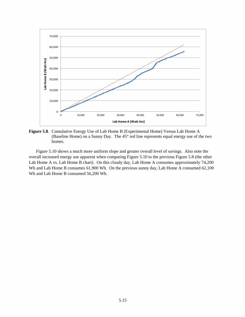
5.15
Figure 5.8. Cumulative Energy Use of Lab Home B (Experimental Home) Versus Lab Home A
(Baseline Home) on a Sunny Day. The 45° red line represents equal energy use of the two
homes.
Figure 5.10 shows a much more uniform slope and greater overall level of savings. Also note the
overall increased energy use apparent when comparing Figure 5.10 to the previous Figure 5.8 (the other
Lab Home A vs. Lab Home B chart). On this cloudy day, Lab Home A consumes approximately 74,200
Wh and Lab Home B consumes 61,900 Wh. On the previous sunny day, Lab Home A consumed 62,100
Wh and Lab Home B consumed 56,200 Wh.
0
10,000
20,000
30,000
40,000
50,000
60,000
70,000
0 10,000 20,000 30,000 40,000 50,000 60,000 70,000
Lab
Ho
me
B (
Wat
t-h
rs)
Lab Home A (Watt-hrs)

5.16
Figure 5.9. Whole-House Energy Use and Indoor Temperature for the Experimental Home (blue and
green lines) and the Baseline Home (red and purple lines) on a Cloudy Day
Figure 5.10. Cumulative Energy Use of Lab Home B (Experimental Home) Versus Lab Home A
(Baseline Home) on a Cloudy Day. The 45° red line represents equal energy use of the two
homes.
This relationship between energy use and solar insolation in the winter is further illustrated by
Figure 5.11 and Figure 5.12, which depict daily whole-house energy use in watt-hours versus solar
insolation in watts per square meter (W/m2) for Lab Home A and Lab Home B, respectively. In both
70
72
74
76
78
80
82
84
0
2,000
4,000
6,000
8,000
10,000
12,000
14,000
16,000
18,000
20,000
12:00 AM 4:00 AM 8:00 AM 12:00 PM 4:00 PM 8:00 PM 12:00 AM
Ind
oo
r Te
mp
era
ture
(F)
Wh
ole
Ho
use
En
erg
y C
on
sum
pti
on
(Wat
ts)
Time
A B Indoor Temp A Indoor Temp B
0
10,000
20,000
30,000
40,000
50,000
60,000
70,000
80,000
0 10,000 20,000 30,000 40,000 50,000 60,000 70,000 80,000
Lab
Ho
me
B (
Wat
t-h
rs)
Lab Home A (Watt-hrs)

5.17
homes, increased solar insolation decreased whole-house energy use. However, the difference in solar
heat gain can clearly be seen by comparing the x-axes of the two charts. The measured solar insolation
through the window is 83.2% ± 1.2% less through the low-e coated windows in Lab Home B than through
the clear glass windows in Lab Home A.1
Figure 5.11. Whole-House Energy Use in Lab Home A Versus Solar Insolation for the Heating Season
Figure 5.12. Whole-House Energy Use in Lab Home B Versus Solar Insolation for the Heating Season
1 Note that the solar heat gain measurement reported here is in situ and does not represent or replicate the
measurement of the SHGC measurement that takes place in a highly controlled laboratory environment to certify a
window. However, the magnitude of the solar insolation reduction is consistent with the magnitude of the difference
in SHGC of the windows in Lab Homes A (SHGC=0.7) compared to the windows in Lab Home B (SHGC=0.19).
0
10,000
20,000
30,000
40,000
50,000
60,000
70,000
80,000
0 20 40 60 80 100
Lab
Ho
me
A W
ho
le H
ou
se E
ne
rgy
Co
nsu
mp
tio
n
(Wh
/day
)
Solar Insolation Through Window (W/m^2)
0
10,000
20,000
30,000
40,000
50,000
60,000
70,000
80,000
0 5 10 15
Lab
Ho
me
B W
ho
le H
ou
se E
ne
rgy
Co
nsu
mp
tio
n (
(Wh
/day
)
Solar Insolation Through Window (W/m^2)

5.18
However, during the cooling season, sunny days were much more common, which made regression
based on solar insolation difficult, as can be seen by the concentration of high solar heat gain observations
in Figure 5.13., which plots whole-house energy use versus solar insolation for both Lab Home A and
Lab Home B, respectively.
Figure 5.13. Whole-House Energy Use in Lab Home A (left) and Lab Home B (right) Versus Solar
Insolation for the Cooling Season
Energy use and energy savings in the cooling season, appear to be much more related to outdoor air
temperature, due to the relatively consistent solar insolation, as shown in Figure 5.14 and Figure 5.15,
which plot energy savings with respect to solar insolation as measured in Lab Home A and whole-house
energy savings for Lab Home B with respect to Lab Home A.
Figure 5.14. Whole-House Energy Savings in Lab Home B as Compared to Lab Home A in the Cooling
Season Versus Solar Insolation Through the Window in Lab Home A
0
5,000
10,000
15,000
20,000
25,000
30,000
35,000
40,000
45,000
50,000
0 50 100 150 200
La
b H
om
e A
Wh
ole
Ho
use
En
erg
y C
on
sum
pti
on
(W
h/
CD
D)
Solar Insolation Through Window (W/m^2)
0
5,000
10,000
15,000
20,000
25,000
30,000
35,000
40,000
45,000
50,000
0 5 10 15 20 25
La
b H
om
e B
Wh
ole
Ho
use
En
erg
y C
on
sum
pti
on
(W
h/
CD
D)
Solar Insolation Through Window (W/m^2)
0%
5%
10%
15%
20%
25%
50 70 90 110 130 150
Lab
Ho
me
Wh
ole
Ho
use
En
erg
y Sa
vin
gs (
%)
Solar Insolation Through Window (W/m^2)

5.19
Figure 5.15. Whole House Energy Savings in Lab Home B as Compared to Lab Home A in the Cooling
Season Versus Outdoor Air Temperature
The dependence of energy use and energy savings on outdoor air temperature is illustrated by
comparing two representative days, July 10, 2012 and July 16, 2012, both periods when the homes were
operated with occupancy and lighting loads, but no equipment loads. July 10 was much hotter than July
16; the average daily outdoor air temperature was 84.4 °F and the maximum temperature in the afternoon
was 95 °F. Figure 5.16 shows the whole-house energy use in Lab Home A (blue) and Lab Home B (red),
as well as interior temperatures in both homes (purple and green lines) and outdoor air temperature
(turquoise line). Whole-house energy use tracks well with outdoor air temperature, as expected, but is
reduced in Lab Home B compared to Lab Home A. Unlike, the winter season, energy savings occur at a
similar rate throughout the day, as can be seen from the consistent slope of cumulative energy use in Lab
Home B versus Lab Home A, the blue line in Figure 5.17. On this hot, sunny day, Lab Home A used
39,631 Wh of energy and Lab Home B used 31,093 Wh, a savings of 21.5% in Lab Home B.
0%
5%
10%
15%
20%
25%
70 75 80 85 90
Lab
Ho
me
Wh
ole
Ho
use
En
erg
y Sa
vin
gs (
%)
Average Daily Outdoor Air Temperature (°F)

5.20
Figure 5.16. Hourly Average Whole-House Energy Use and Indoor Temperature for Lab Home B
(Experimental Home; blue and green lines) and Lab Home A (Baseline Home; red and
purple lines) and Outdoor Air Temperature on a Hot Day
Figure 5.17. Cumulative Energy Use of Lab Home B (Experimental Home) Versus Lab Home A
(Baseline Home) on a Hot Day. The 45° red line represents equal energy use of the two
homes.
60
65
70
75
80
85
90
95
100
0
500
1,000
1,500
2,000
2,500
3,000
3,500
12:00 AM 4:00 AM 8:00 AM 12:00 PM 4:00 PM 8:00 PM 12:00 AM
Ind
oo
r Te
mp
era
ture
(F)
Wh
ole
Ho
use
En
erg
y U
se (
Wat
ts)
Time
A B Indoor Temp A Indoor Temp B Outdoor Temp
0
5,000
10,000
15,000
20,000
25,000
30,000
35,000
40,000
0 5,000 10,000 15,000 20,000 25,000 30,000 35,000 40,000
Lab
Ho
me
B (
Wat
t-h
rs)
Lab Home A (Watt-hrs)

5.21
The savings and energy use on July 10 can be compared to a day with milder daily average outdoor
air temperature of 72.1°F and an afternoon peak of 83°F observed on July 16. As heat transmission, and
thus energy use, is dependent on the temperature difference between indoors and out, significantly greater
savings are observed on hotter days. A cumulative energy use plot of whole house energy use in Lab
Home B versus Lab Home A (Figure 5.18) still shows consistent savings throughout the day, but the
slope of the line is much closer to 1 (the red 45° line, representative equal energy use in both homes). On
July 16, Lab Home A used 27,512 Wh of energy and Lab Home B used 24,603 Wh, resulting in total
daily energy savings of 10.6% in Lab Home B.
Figure 5.18. Cumulative Energy Use of Lab Home B (Experimental Home) Versus Lab Home A
(Baseline Home) on a Milder Day (daily average outdoor air temperature of 72.1 °F). The
45° red line represents equal energy use of the two homes.
Due to the small difference in average temperature between indoors and out (2.1 °F), the whole-house
energy use in both Lab Home A and Lab Home B is much less tied to outdoor air temperature because the
HVAC energy use is significantly reduced. As shown in Figure 5.19, more variability in occupancy and
lighting loads are more visible in the whole-house energy use due to the HVAC load being less dominant.
0
5,000
10,000
15,000
20,000
25,000
30,000
0 5,000 10,000 15,000 20,000 25,000 30,000
Lab
Ho
me
B (
Wat
t-h
rs)
Lab Home A (Watt-hrs)

5.22
Figure 5.19. Hourly Average Whole-House Energy Use and Indoor Temperature for the Experimental
Home (blue and green lines) and the Baseline Home (red and purple lines) and Outdoor Air
Temperature on a Mild Day
5.6.5 Average Annual Savings
Measured data were extrapolated to estimate annual energy savings based on the heating degree days
(HDD – base 65 °F) and cooling degree days (CDD – base 65 F°). Energy savings, in kilowatt-hours,
were scaled based on HDD and then extrapolated to total annual heating season savings based on the
number of HDD in a typical year (TMY3 file) in Pasco, Washington. A similar analysis was done for
cooling savings measured during the summer experimental period and typical CDD in the TMY3 file.
This calculation is shown in the following equations:
60
65
70
75
80
85
90
95
100
0
500
1,000
1,500
2,000
2,500
3,000
3,500
12:00 AM 4:00 AM 8:00 AM 12:00 PM 4:00 PM 8:00 PM 12:00 AM
Ind
oo
r Te
mp
era
ture
(F)
Wh
ole
Ho
use
En
erg
y U
se (
Wat
ts)
Time
A B Indoor Temp A Indoor Temp B Outdoor Temp

5.23
Summing the estimated annual average heating and cooling savings, 12.2% annual savings are
expected based on the measured data, or 1,784 kWh. However, because the HDD/CDD data do not
explicitly account for the incident solar radiation these savings are considered to be conservative.
5.7 Interior Temperature Distributions
In addition, the impact of performance of the highly insulating windows on indoor temperature
distribution within the homes cannot be discounted. Indoor temperature in the kitchen of each home is
shown in Figure 5.7 and Figure 5.9 for the heating season for sunny and cloudy days, respectively. As
can be seen by the purple line in Figure 5.7, Lab Home B maintains a much more consistent indoor
temperature throughout the day due to both the low U-factor and low SHGC (0.19) of the windows. In
heating-only mode, interior temperatures in the baseline home climb to almost 84°F, as illustrated by the
green line in Figure 5.7. This would clearly cause a comfort problem for any occupants home during this
time, even during days with cold outdoor temperatures. This elevated temperature is seen in all areas of
the baseline home, while the experimental home maintains a much more consistent temperature profile, as
shown in Figure 5.20. The interior temperature distribution in both homes on cloudy days are much more
uniform, as illustrated in Figure 5.9 by the purple and green lines for Lab Home A and Lab Home B,
respectively. Lab Home B maintains a slightly higher indoor temperature due to the improved thermal
performance and lower SHGC of the highly insulating windows.
Figure 5.20. Interior Temperature Distribution for Lab Home A (left) and Lab Home B (right) on a
Sunny Day
Comparing Figure 5.19 and Figure 5.16 in the previous section, the impact of increased outdoor air
temperature on interior temperature distributions and comfort is also apparent during the cooling season.
Indoor temperature in the kitchen of each home is shown in Figure 5.16 and Figure 5.19 for the heating
season for hot and mild summer days, respectively. On hot days, Lab Home A is not able to maintain the
thermostat set point during the hottest part of the day, as illustrated by the green line in Figure 5.16. Note
that equipment loads are not exercised on this day, which would further exacerbate the problem. The heat
pump is already operating at 100% capacity for several hours a day even in this reduced occupancy
scenario (no equipment), as shown in Figure 5.21 between the hours of 2:00 pm and 7:00 pm. As can be
seen by the purple line in Figure 5.16, Lab Home B maintains the thermostat set point and, thus, a much
more consistent indoor temperature throughout the day due to both the low U-factor and low SHGC
70
71
72
73
74
75
76
77
78
79
80
81
82
83
84
85
0 1 2 3 4 5 6 7 8 9 10 11 12 13 14 15 16 17 18 19 20 21 22 23
Inte
rio
r Te
mp
era
ture
(F)
Hour
70
71
72
73
74
75
76
77
78
79
80
81
82
83
84
85
0 1 2 3 4 5 6 7 8 9 10 11 12 13 14 15 16 17 18 19 20 21 22 23
Hour
TC_KitSp(Deg F)
TC_DinSp(Deg F)
TC_LivSpWestIn(Deg F)
TC_LivEntry(Deg F)
TC_HallSp(Deg F)
TC_WBedSp(Deg F)
TC_EBedSp(Deg F)
TC_UtilitySp(Deg F)
TC_BathSp(Deg F)
TC_MBathSp(Deg F)
TC_MBedSp(Deg F)
Average
Set Point

5.24
(0.19) of the windows. Also, in Lab Home B, the heat pump continues to cycle throughout the day and
appears to have additional capacity to accommodate warmer days or increased internal loads.
Figure 5.21. Whole House Energy Use in Lab Home A on a Hot Day (July 10) with HVAC, Occupancy,
and Lighting Loads Disaggregated
This increased temperature is seen in all areas of the home in the baseline home, while the
experimental home maintains a much more consistent temperature profile, as shown in Figure 5.22. Also,
Figure 5.22 shows overcooling occurring in some rooms in both homes, probably due to the thermostat
location (in the hallway adjacent to the kitchen in both homes). Temperatures as low as 64°F are
observed in both Lab Home A and B in the rooms closest to the air handler and, thus, receiving the most
air (the bathroom, west bedroom, and east bedroom) due to shorter duct runs. However, more extreme
local temperature variations (lower lows and higher highs) are evident in Lab Home A due to the
increased localized heat gain through the windows and the subsequent increased need for cooling.
0
1000
2000
3000
4000
5000
6000
7000
8000
Ener
gy C
on
sum
pti
on
[W
]
Time
Mains
HVAC
Occupancy
Lighting
Equipment

5.25
Figure 5.22. Interior Temperature Distribution for Lab Home A (left) and Lab Home B (right) on a
Hot Day
On milder days, both Lab Home A and Lab Home B are able to maintain the 70°F thermostat set
point, as illustrated in Figure 5.19 by the purple and green lines for Lab Home A and Lab Home B,
respectively.
5.8 Thermal Comfort and Condensation
The increased thermal performance of highly insulating windows can also affect the health of a home.
Poorly insulating windows, such as the double-pane clear glass windows installed in the baseline home
(Lab Home A), can cause condensation to form on the window, which over time can contribute to mold
growth on the window sill. While condensation was not observed with the low relative humidity in the
homes, the thermal performance of the double-pane clear windows clearly indicated a potential for
condensation during the heating season.
Figure 5.23 shows the interior temperature of all window surfaces in the baseline home (Lab Home
A) and Figure 5.24 shows the interior temperature of all window surfaces in the experimental home (Lab
Home B) during the period from March 11 through 17, 2012. The average outdoor air temperature during
this period was 49 °F, with a high of 65 °F and a low of 35 °F. As the figures show, the interior window
temperature of the coolest window reaches 50°F on the west-facing dining room window in the baseline
home, while the same window in the experimental home does not dip below 60°F. With these
temperatures and an interior room temperature of 75°F in both homes, the relative humidity of the air in
the experimental home would have to exceed 70% to cause condensation on the highly insulating
windows, while a minimum of 40% relative humidity in the baseline would cause condensation and
potential mold problems with the windows.1 For reference, the average relative humidity in the baseline
home (Lab Home A) was 20.7%, with a maximum of 31.7%, and the average relative humidity observed
in the experimental home (Lab Home B) was 21.7%, with a maximum of 28.1%.
1 Based on data from a psychrometric chart.
60
62
64
66
68
70
72
74
76
78
80
0 1 2 3 4 5 6 7 8 9 10 11 12 13 14 15 16 17 18 19 20 21 22 23
Inte
rio
r Te
mp
era
ture
(F)
Hour
60
62
64
66
68
70
72
74
76
78
80
0 1 2 3 4 5 6 7 8 9 1011121314151617181920212223
Inte
rio
r Te
mp
era
ture
(F)
Hour
TC_KitSp(Deg F)
TC_DinSp(Deg F)
TC_LivSpWestIn(Deg F)
TC_LivEntry(Deg F)
TC_WBedSp(Deg F)
TC_UtilitySp(Deg F)
TC_MBedSp(Deg F)
TC_MBathSp(Deg F)
TC_EBedSp(Deg F)
TC_BathSp(Deg F)
Lab Home A Average Interior Temperature (F)
Set Point

5.26
Figure 5.23. Interior Window Temperatures and Dew Point Temperatures Based on a 75°F Interior Air
Temperature in the Baseline Home from March 11 Through 17, 2012
Figure 5.24. Interior Window Temperatures and Dew Point Temperatures Based on a 75°F Interior Air
Temperature in the Experimental Home from March 11 Through 17, 2012
35
40
45
50
55
60
65
70
75
80
85
90
95
100
3/11/2012 3/12/2012 3/13/2012 3/14/2012 3/15/2012 3/16/2012 3/17/2012
Tem
pe
ratu
re (F
)
TC_KitWIn(Deg F)
TC_DinSldrIn(Deg F)
TC_DinWCntrIn(Deg F)
TC_DinWSUpIn(Deg F)
TC_DinWNDwnIn(Deg F)
TC_LivSldrIn(Deg F)
TC_LivWIn(Deg F)
TC_WBedWIn(Deg F)
TC_EBedWIn(Deg F)
TC_MBedWIn(Deg F)
TC_MBathWIn(Deg F)
Outdoor Air Temperature (F)
40% RH
50% RH
60% RH
70% RH
35
40
45
50
55
60
65
70
75
80
85
90
95
100
3/11/2012 3/12/2012 3/13/2012 3/14/2012 3/15/2012 3/16/2012 3/17/2012
Tem
pe
ratu
re (F
)
TC_KitWIn(Deg F)
TC_DinSldrIn(Deg F)
TC_DinWCntrIn(Deg F)
TC_DinWSUpIn(Deg F)
TC_DinWNDwnIn(Deg F)
TC_LivSldrIn(Deg F)
TC_LivWIn(Deg F)
TC_WBedWIn(Deg F)
TC_EBedWIn(Deg F)
TC_MBedWIn(Deg F)
TC_MBathWIn(Deg F)
Outdoor Air Temperature (F)
50% RH
60% RH
60% RH
70% RH

5.27
Figure 5.23 and Figure 5.24 also depict the difference in average interior glass surface temperature in
the two homes. The average interior glass surface temperature measurement of all the windows over this
period was 68.7 ± 0.05°F in Lab Home A compared to 75.7 ± 0.04°F in Lab Home B, nearly 7°F cooler.
The colder window surface temperatures also affect comfort felt by occupants in the home. A window
with a colder surface temperature will cause rooms to feel colder than the measured dry bulb temperature
would suggest.
The MRT also was monitored in two locations in each Lab Home during the period from March 11
through 17, 2012. In Figure 5.25, the average indoor air temperature and MRT are plotted for both the
homes.
Figure 5.25. Average Indoor Air Temperature (solid line) and Mean Radiant Temperature (dotted line)
in Lab Home A (blue) and Lab Home B (red)
During the same week, the average MRT in Lab Home A during the nighttime period when radiant
heat loss was most extreme was 79.0 ± 0.02°F in both the master bedroom and the living room compared
to an average room temperature of 80.2 ± 0.11°F. The average MRT of both the living area and master
bedroom was 1.63 ± 0.01°F lower than the average interior room temperature in Lab Home A. The
maximum MRT recorded in Lab Home A during the winter experiment was 86.3°F and the minimum
MRT was 77.0°F.
76
78
80
82
84
86
3/11/2012 3/12/2012 3/13/2012 3/14/2012 3/15/2012 3/16/2012 3/17/2012
Ave
rage
Inte
rio
r an
d M
ean
Rad
ian
t Te
mp
era
ture
(F)
Lab Home A Average MRT (F) Lab Home B Average MRT (F)
Lab Home A Average Interior Temperature (F) Lab Home B Average Interior Temperature (F)

5.28
In contrast, in Lab Home B, the average MRT in the living area and master bedroom was 1.64 ±
0.01°F lower than the average room temperature of 80.4 ± 0.01°F in the living area and master bedroom.
The maximum MRT recorded in Lab Home B was 81.7°F and the minimum MRT was 77.7°F. Overall,
the average nighttime MRT in Lab Home B was slightly warmer than the average MRT in Lab Home A
during the nighttime periods when radiant heat loss is most extreme. The very small temperature
differences between the room temperature and MRT in Lab Home B compared to the larger difference in
Lab Home A, as well as the higher average MRT in Lab Home B, suggest the highly insulating windows
can provide a greater comfort level for occupants. Also, the MRT in Lab Home B was much more
consistent, varying only 4.9°F, while Lab Home A varied 9.2°F. MRT and surface glass temperatures
were not assessed in the summer cooling season experiment, since thermal comfort is an issue primarily
in the winter heating season.
5.9 Peak Load
Another impact of reduced energy use that is important to mention from a utility and resource
planning perspective is the ability to reduce peak load (kW). Figure 5.26 depicts peak load impacts due to
installation of the highly insulating windows in the experimental home over a representative 1-week time
period in the summer. The impact on peak load is significantly more than the average daily energy
savings, reducing the peak power consumed on an hourly basis in the home with highly insulating
windows (Lab Home B) by 24.7% ± 0.1% over the entire cooling experiment study period. This is
because the peak load reduction represents a maximum real-time savings, rather than an average savings.
Peak power savings occur, typically, between 10:00 am and 6:00 pm when the system demand is highest.

5.29
Figure 5.26. Average Hourly Power Use for Lab Home A (blue) and Lab Home B (red) and the
Bonneville Power Administration Load Curve During a 1-Week Period from July 6 to July
13, 2012 (Note: the Bonneville Power Administration data is for the same days in 2011
since 2012 data was not available).
Peak load savings were also measured in the heating season. Average hourly peak savings for the
heating season were 33.9 ± 0.6%. However, these savings occurred in the nighttime hours when outdoor
air temperatures were coldest, which does not typically correspond with utility peak demand periods, as
shown by the grey dashed line in Figure 5.26. The grey line shows the load curve, in megawatts (MW),
for the Bonneville Power Administration service territory, for July 6 through July 13, 2011, since 2012
data was not available.1 While the load shape changes in the winter months, peaks still occur during the
day, which juxtaposes the winter heating season peaks observed in the Lab Homes.
5.10 Energy Modeling
An EnergyPlus model was created for the Lab Homes to compare modeled savings from the highly
insulating windows to measured results. The EnergyPlus analysis shows average whole-building energy
savings in Lab Home B from the highly insulating windows to be 13.9% during the simulation period
(February to April 2012 and from July to August 2012). Part of the savings is due to the slightly tighter
1 Bonneville Power Administration peak load data was obtained from the Federal Energy Regulatory Commission
Form 714 for respondent 122, available at http://www.ferc.gov/docs-filing/forms/form-714/data.asp.
0
1,000
2,000
3,000
4,000
5,000
6,000
7,000
8,000
0
500
1,000
1,500
2,000
2,500
3,000
3,500
4,000
7/6/2012 7/7/2012 7/8/2012 7/9/2012 7/10/2012 7/11/2012 7/12/2012
BPA
Ho
url
y Lo
ad P
rofi
le (M
W)
Ave
rage
Ho
url
y Po
wer
Use
(W)

5.30
envelope of Lab Home B achieved as part of the windows retrofit (see Section 5.2.2). The general trends
in energy use and savings are comparable to the measured data, which indicated observed savings of 11.6
± 1.53% in Lab Home B compared to Lab Home A in the heating season and 18.4% ± 2.06% in the
cooling season, with an average of 15%.
Figure 5.27. Modeled and Measured HVAC Energy Use for Lab Home A (Baseline Home)
Figure 5.28. Modeled and Measured HVAC Energy Use for Lab Home B (Experimental Home)
0
10,000
20,000
30,000
40,000
50,000
60,000
70,000
80,000
90,000
20 30 40 50 60 70 80 90 100 Wh
ole
Ho
use
En
erg
y C
on
sum
pti
on
[W
-h/d
ay]
Outdoor Air Temperature [F]
Labhome A modeled Labhome A measured
0
10,000
20,000
30,000
40,000
50,000
60,000
70,000
80,000
20 30 40 50 60 70 80 90 100 Wh
ole
Ho
use
En
erg
y C
on
sum
pti
on
[W
-h/d
ay]
Outdoor Air Temperature [F]
Labhome B modeled Labhome B measured

5.31
Figure 5.29. Modeled and Measured Energy Savings
Figure 5.27 and Figure 5.28 show the modeled and measured whole-house energy use compared to
outdoor air temperature for Lab Home A and Lab Home B, respectively. Figure 5.29 shows the modeled
and measured energy savings compared to outdoor air temperature of Lab Home B with respect to Lab
Home A.
The modeled results correspond well with the measured data. However, the EnergyPlus models
underpredict the energy use as compared to the measured data in both homes. The modeled average
annual energy use for Lab Home A is 28,537 Wh and 24,784 Wh for Lab Home B, which results in
13.2%, or 1,370 kWh, annual energy savings from the highly insulating windows for Lab Home B with a
cooling season set point of 75°F and a heating set point of 72°F and typical internal gains schedules, as
described in Appendix G. This annual energy savings model typifies the savings that highly insulating
windows would achieve in an average home, including an impact on envelope leakage. While this
number is similar to the calculated annual savings based on measured data reported in Section 5.6, the
model needs to undergo a more robust calibration before it can be used to accurately predict annual
energy performance and savings or extrapolate findings to other climates. Future work will involve using
onsite weather data in the energy simulation and matching daily load profiles exactly for the heating and
cooling seasons.
5.11 Cost Effectiveness of Highly Insulating Windows
The energy savings achieved by highly insulating windows in the PNNL Lab Homes have
demonstrated the potential of this technology to significantly improve the energy efficiency of homes.
However, the viability of highly insulating windows as an energy efficiency measure depends not only on
their energy saving potential, but also their costs.
-10%
-5%
0%
5%
10%
15%
20%
25%
30%
20 30 40 50 60 70 80 90 100 Wh
ole
Ho
use
En
erg
y Sa
vin
gs %
Outdoor Air Temperature [F]
Savings % modeled Savings % measured

5.32
For the calculation of simple PBP, annual energy savings as determined by the EnergyPlus model as
well as the extrapolated annual energy savings reported in Section 5.6 are used. In the EnergyPlus model,
set points and occupancy parameters that typify existing homes in the United States are used to represent
the energy savings, and thus cost effectiveness results, a typical homeowner could expect to see. In many
cases, these assumed parameters were the same or similar to those exercised in the Lab Homes during the
experimental periods (lighting and occupancy schedules, interior set points). See Section 5.10 and
Appendix G for more information on this representative annual model. The annual savings determined by
the annual savings model are 1,370 kWh per year or 13.2% in Lab Home B compared to Lab Home A.
The estimated annual savings extrapolated based on the measured data and typical HDD and CDD are
1,784 kWh/yr or 12.2%.
The annual utility bill cost savings are determined by multiplying the annual energy savings in kWh
by the national average cost of electricity of 11.8¢/kWh (EIA 2012). This results in an annual savings of
$162/yr for the modeled annual savings and $211/yr for the measured annual savings estimate.
The costs of purchasing the highly insulating windows was obtained from the window distributor as
$6,243 or $32/ft21
. However, window costs are highly variable and, thus, these costs were compared with
other manufacturers and other windows types, to ensure the costs were representative of the range of
window costs observed in the retrofit market. A delivered (to the PNW) cost range for highly insulating
slider windows and patio glass doors in small quantities for retrofit was obtained from the vendors in the
DOE Windows Volume Purchase Program who sell a product line of sliders and patio doors.2 However,
costs were considered for casements and double-hung windows as well, for comparison. These costs are
highly variable and range from $10/ft2 to $100/ft
2. Although manufacturers were asked for data
representing delivered costs (not including installation), it is assumed that higher costs represent window
costs which include installation costs. Plotting the data, to identify any trends, yielded no clear
differentiation or relationship, as shown in Figure 5.30. In all cases, several high outliers are observed.
Because we do not know the degree of customization or complexity of each product in this data set, it is
assumed that these three outliers (indicated by red circles) are specialty windows that are not
representative of average R-5 window costs.
1 This price was obtained from the invoice from the local window supplier for the specified windows and sliding
glass doors 2 The window vendors selected for estimating costs from the qualified vendors in the Windows Volume Purchase
Program were vendors who offered horizontal sliders and patio doors and who sold or delivered products in the
Pacific Northwest. An average cost per square foot across the multiple sizes of windows in Lab Home B was
determined.

5.33
Figure 5.30. Window Cost Data for R-5 Sliders (top), Casements (middle), and Double-Hung
(bottom) from the DOE Windows Volume Purchase Program. Red circles indicate
outliers assumed to have a high degree of customization that were excluded from the
analysis.
Excluding the outliers, the average cost of all the costs data for all three types of R-5 windows is
$31/ft2. All the data also show a similar small break near the average, as indicated in Figure 5.31. To
$0.00
$10.00
$20.00
$30.00
$40.00
$50.00
$60.00
$70.00
$80.00
0 5 10 15 20 25
Cost ($/ft^2)
$0.00
$10.00
$20.00
$30.00
$40.00
$50.00
$60.00
$70.00
$80.00
$90.00
0 5 10 15 20 25 30
Cost ($/ft^2)
$0.00
$10.00
$20.00
$30.00
$40.00
$50.00
$60.00
$70.00
0 5 10 15 20 25 30
Cost ($/ft^2)

5.34
arrive at a lower estimate of delivered cost, without installation, the lower half of the data was averaged,
yielding an average of $22/ft2. To arrive at a higher bound the upper half of the data was also averaged,
arriving at an average of $43/ft2. While this reduces some of the extreme variability observed in the
window cost data obtained from the Windows Volume Purchase Program, it is thought to be
representative of average costs for R-5 windows and sliding glass doors.
Figure 5.31. Cost Data, Excluding Outliers, for All Window Types from the Windows Volume
Purchase Program
In addition to the delivered cost of the window, primary windows must be installed by a qualified
contractor. However, costs for installing the highly insulating windows for Lab Home B were not
provided as a separate cost to PNNL by the GC because these costs were included in the fixed-price bid
for the package of work undertaken by the GC. Installation and materials costs were estimated at $3/ft2
based on observed retrofitting of the windows by subcontractors at the Lab Homes. Therefore, the total
installed cost for the windows and sliding glass doors in Lab Home B was estimated to range from $4,900
to $9,000 or $25/ft2 to $46/ft
2 and $35/ft
2 based on the bid for the windows installed in the Lab Homes
obtained from windows distributor. This range is consistent with the cost for retrofitting double-pane,
clear glass, aluminum-frame windows with triple-pane, low-E, vinyl-framed windows listed in the
National Residential Efficiency Measures Database, maintained by the National Renewable Energy
Laboratory of $21/ft2 to $55/ft
2, with an average of $33/ft
2 (NREL 2012).
Based on these costs and a modeled annual savings of 1,370 kWh/yr, the simple PBP ranges from 30
to 55 years, as shown in Figure 5.32. Using, instead, the annual energy savings estimate based on
extrapolated measured data of 1,784 kWh/yr, the simple PBP ranges from 23 to 42 years.
$0.00
$10.00
$20.00
$30.00
$40.00
$50.00
$60.00
Cost ($/ft^2)
Sliders Casements Double Hung
Lower Half
Upper Half

5.35
Figure 5.32. Simple PBP for R-5 Windows for a Retrofit or in an Incremental Cost Scenario. Costs
considered are the actual windows costs as retrofit in the Lab Homes, a high, average,
and low cost estimate based on data in the DOE Windows Volume Purchase Program;
and incremental cost over code minimum windows. Modeled and an estimate of
annual energy savings are calculated.
These primary window costs are appropriate for a retrofit scenario, but an incremental cost scenario
should be considered for new construction or if windows are being replaced for another reason (e.g.,
safety, functionality, aesthetics). In the incremental cost scenario, installation cost is not included and
only the cost difference between code minimum and highly insulating (triple-pane) windows is used. The
costs of code minimum windows (as delivered) were obtained from National Residential Efficiency
Measures Database (NREL 2012). The incremental cost of highly insulating windows over code
minimum windows ranged from $1.59/ft2 to $5.84/ft
2, with an average of $3.87/ft
2. Installation and
material costs were not included in the incremental cost estimate, resulting in total incremental costs for
highly insulating windows and sliding glass doors in Lab Home B is estimated to be $1,372, based on an
average cost of $27/ft2 and the average cost of R-5 windows of $34/ft
2. Based on a modeled incremental
annual energy savings of 363 kWh/yr, the simple PBP is 32 years.
0
10
20
30
40
50
60
Actaul Window Costs
High Cost Estimate
Average Cost Estimate
Low Cost Estimate
Incremental Cost Over
Code
Minimum
Sim
ple
PB
P (
yrs)
Modeled Estimated Annual Savings
Measured Data Estimated Annual Savings


6.1
6.0 Conclusions
This experiment used two side-by-side Lab Homes on the PNNL campus to measure the potential
energy savings, thermal comfort impacts, and cost effectiveness of highly insulating triple-pane windows
(and patio doors) in the experimental home compared to the baseline home equipped with standard
double-pane windows (and patio doors), the latter representing windows in many existing homes across
the PNW and much of the United States. Testing was conducted during the 2011-2012 winter heating
and summer cooling seasons. The design of this field experiment in the Lab Homes was unique to the
PNW. The experiment removed as many variables as possible that commonly affect other similar types
of field experiments by having a nearly identical pair of homes, as verified by the null testing and by
simulating occupancy identically in the two homes. The homes were oriented identically, experienced the
same weather, had the same interior furnishings and equipment, and were operated identically during the
experiments. Thus, the only differences between the two homes were the windows themselves (their
inherent thermal properties) plus any impact from the windows’ installation.
To verify similar performance prior to retrofitting the windows, the homes were initially null tested
prior to the windows retrofit to verify similar construction and energy performance. Air leakage, duct
leakage, ventilation fan flow, and heat pump performance testing was performed on both homes to
compare the construction of both homes’ envelope and their HVAC performance. This testing found the
homes to be statistically the same, with blower door readings of 638.5 ± 27.8 cfm50 in Lab Home A and
681.1 ± 26.7 cfm50 in Lab Home B. For additional testing results see Section 1.0. Thermal imaging of
the homes’ envelopes also revealed similar construction, although some insulation settling had occurred
in both homes—slightly more in Lab Home A than Lab Home B. After baseline testing confirmed nearly
identical construction of the homes during a null test prior to the winter experiment, the energy use of the
two homes was compared to verify similar energy performance. During this null test, no occupancy was
simulated and the homes were operated in HP mode with the thermostat set point varied from 50°F to
85°F on a daily basis. Whole-house energy use was shown to be similar within 0.5% ± 0.5% during the 6
days of null testing.
The air leakage of both homes was also measured after the windows were retrofitted, to determine the
impact of the difference in air leakage inherent to the windows and the quality of the window installation.
The blower door measurements after the windows were retrofitted showed an increase of 50.3 ± 34.1
cfm50 in air leakage in Lab Home A; this increase in air leakage is attributed to the combined effects of
the air leakage of the window and air leakage around the window cavity resulting from the installation of
the window. The air leakage of Lab Home B decreased by 46.4 ± 34.9 cfm50 or 6.9% after the windows
were retrofitted; this decrease in air leakage is primarily due to the quality of the installation because the
air leakage of the highly insulating windows is similar to that of the factory-supplied windows, as
certified in a laboratory test. This is strong evidence of how important it is to properly install/retrofit
windows.
The data from the heating season and cooling season show significant whole-house energy savings
and comfort improvement in Lab Home B. The overall whole-house energy savings in Lab Home B with
the highly insulating windows are 11.6% ± 1.53% compared to Lab Home A during the heating season
and 18.4% ± 2.06% during the cooling season. The largest difference in energy performance between the
homes was a result of solar insolation (solar heat gain) given the significant difference in SHGC of the
windows in Lab Home A (0.7) compared to Lab Home B (0.19). The dependence on solar insolation and

6.2
solar heat gain was observed in the heating season by the lower savings seen in Lab Home B as compared
to Lab Home A on sunny days versus cloudy days. On sunny days, for almost any home, solar heat gain
through windows contributes enough heat to the home that the heating systems may even turn off, even
though the outdoor temperature is well below the thermostat set point for the home. Given that neither
home deployed window coverings, this condition was expected and observed more often in Lab Home A
(with high SHGC windows); measured average whole-house indoor temperatures often increased 5 to
10°F above the set point of the heating system thermostat due to solar heating. In Lab Home B,
temperatures remained much more consistent, but the heating system was required to turn on to supply
heat much sooner in the evening, while Lab Home A could typically coast well into the late evening
before needing to call for heat. Overall, the low SHGC of the windows in Lab Home B showed energy
savings on sunny days of 8.9% ± 1.42% compared to the baseline home Lab Home A.
On cloudy winter days, the difference in the SHGC of the windows, and thus the solar heat gain
contribution, is not as evident. Data showed that both homes maintained average interior temperatures
near the thermostat set points throughout the day and that the heating systems were operating to maintain
that set point throughout the day. The heat pumps in both homes cycle, as would be expected, and they
cycle less frequently in the afternoon when outdoor temperatures are the warmest. On overcast days, the
average whole-house energy savings from the windows is 14.6% ± 1.86%.
However, due to the frequency of sunny days in the summer experimental period, the energy use and
energy savings appeared to be more related to outdoor air temperature, which is a function of the highly
insulating windows’ lower U-factor. The U-factor of the highly insulating windows and patio doors in
the experimental home (Lab Home B) is ~70% lower than that of the standard windows in the baseline
home (Lab Home A) and the SHGC of the highly insulating windows in the experimental home is ~77%
compared to the standard windows and patio doors in the baseline home. Due to the high energy savings
observed in the summer period, it is assumed that the lower U-factor as well as the low SHGC are both
affecting savings. These heating and cooling season savings are reported with no window coverings
deployed. A sensitivity analysis deploying interior blinds in both the homes reduced energy savings in
Lab Home B compared to Lab Home A by 46%, but did not significantly affect energy use in the homes.
However, this could be due to the short period of data collection for sensitivity study resulting in high
error about the mean, because visual interpretation of the data suggests lower energy use would be
observed.
In addition to significant overall energy savings, the highly insulating windows also reduced the peak
load in Lab Home B by 33.9% during the heating season and 24.7% during the cooling season during two
representative 1-week periods. The heating season peak load in both homes occurred during the evening
hours after sunset and thus does not correspond with utility peak loads. However, the cooling season
peak occurs in the afternoon and early evening, which corresponds directly with national utility peaks.
Thus, energy efficiency measures such as windows can serve as an important peak reduction measure as
well in the cooling season. Although there is currently no direct financial benefit to most residential
customers of an electric utility for peak load reduction, this significant reduction in peak power can be of
benefit to the utility depending upon the time of the utility or system peak.
In addition to the energy savings and peak load reduction potential of highly insulating windows, the
thermal comfort implications of more uniform temperature distributions in Lab Home B compared to Lab
Home A cannot be discounted. In addition, the highly insulating windows in Lab Home B enabled the
maintenance of the average interior temperature near the thermostat set point throughout the day, while

6.3
elevated temperatures were observed in Lab Home A. During the heating season, the high SHGC in the
baseline windows resulted in overheating of the interior space despite the cold outdoor air temperatures.
In the cooling season, the heat pump was unable to keep up with the cooling load caused by the high
outdoor air temperature, high solar heat gain, and limited internal gains. If full occupancy schedules had
been used, internal gains would increase, further exaggerating the effects of an undersized heat pump and
potentially resulting in uncomfortably warm interior temperatures.
The window surface temperatures also affect the comfort felt by occupants in the home. A window
with a colder surface temperature will cause the occupant to feel colder near the window due to the lower
window surface temperature than the measured dry bulb room temperature would suggest. This effect is
partially illustrated by the dramatically cooler window surface temperatures observed in the baseline
home of as low as 50°F compared to the experimental home where the window surface temperature never
dropped below 60°F. Overall, the average nighttime MRT in Lab Home B was slightly warmer than the
average MRT in Lab Home A. Also, Lab Home A exhibited higher high temperatures and lower low
temperatures as measured by the MRT.
Cold interior glass surface temperatures can also affect the health and durability of a home, in
addition to its comfort. Cold glass surface temperatures can cause condensation on the inside of the glass
and frame, which in time can lead to mold and rot. This experiment did not directly measure the presence
of condensation on the windows, nor was additional humidity from occupancy introduced into either
home for this experiment. However, window condensation is a common occurrence in most homes
during the heating season, and can be of concern to residents. In climates with elevated relative humidity
levels such as in the PNW coastal climate, or in residences with significant interior moisture generation,
window condensation on interior window surfaces would likely occur. At an average outdoor
temperature of 49°F, an interior window temperature was recorded as low as 50°F in Lab Home A, while
the lowest interior window temperature recorded was 60°F in Lab Home B.1 With these temperatures and
an average interior room temperature of 75°F, the relative humidity of the air in Lab Home B would have
to exceed 70% to cause condensation on the highly insulating performance windows, while a 40% relative
humidity would cause condensation on the double-pane windows in Lab Home B. For reference, during
the study period, the average relative humidity in Lab Home A was 20.7% and the maximum was 31.7%;
the average relative humidity in Lab Home B was 21.7% and the maximum was 28.1%.
EnergyPlus models were created to extrapolate measured energy savings during the study period to an
entire year. The modeled results generated using EnergyPlus compare fairly well to the measured energy
use and savings. The model shows 13.9% savings over the study period, from February to April and July
to August 2012, and predicts 13.15%, or 1,370 kWh, annual energy savings. This is as compared to
estimated annual savings based on the measured data, extrapolated based on typical annual HDD and
CDD, of 1,784 kWh or 12.2%. Future work will involve using real weather data in the energy simulation
and matching daily load profiles exactly for the heating and cooling seasons to create a calibrated model
that represents the actual observed savings for heating and cooling seasons. This calibrated model can
then be used to extrapolate the measured savings to different climate zones to predict performance of the
high-performance windows regionally or nationally. Annual measured data and savings will also be
1 The highly insulating windows in Lab Home B have sealed cavities with desiccant material to eliminate any
(visible) condensation on inside surfaces of the glass. As noted, the overall insulating properties of the window will
minimize the potential for condensation on the interior-facing glass surface even with very cold outdoor
temperatures.

6.4
compared to other modeling software, particularly the SEEM (Simple Energy Efficiency Model)
simulation tool,1 which is used in the PNW for determining measure cost and benefits for utility energy
efficiency programs.
Measured energy savings of highly insulating windows in the PNNL Lab Homes exhibits significant
energy savings. However, the cost of highly insulating windows must be considered when determined the
viability of them as an energy efficiency measure. The cost for the highly insulating windows to retrofit
these homes is highly variable, so multiple cost scenarios were considered. However, even the low-cost
scenario, an installed cost of $25/ft2, and the extrapolated measured data to estimate annual energy
savings, 1,784 kWh/yr, resulted in a PBP of 23 years. The PBP ranged as high as 55 years. This
indicates that retrofitting highly insulating windows is still difficult from a cost-effectiveness perspective,
due to the high capital cost of windows. However, the study also illustrated that the windows provide
additional non-quantifiable benefits, such as increased comfort levels, reduced peak load, and decreased
condensation potential.
These data suggest that highly insulating windows are an effective energy-saving measure that should
be considered for high-performance new homes and in existing retrofits. However, the cost effectiveness
of the measure, as determined by the simple PBP, suggests that highly insulating window costs continue
to make windows difficult to justify on a cost basis alone. Additional reductions in costs via
improvements in manufacturing and/or market penetration that continue to drive down costs will make
highly insulating windows much more viable as a cost-effective energy efficiency measure. In addition,
this study illustrates that highly insulating windows have important impacts on peak load, occupant
comfort, and condensation potential, which are not captured in the energy savings calculation. More
consistent and uniform interior temperature distributions suggest that highly insulated windows, as part of
a high performance building envelope, may enable more centralized duct design and downsized HVAC
systems. Shorter, more centralized duct systems and smaller HVAC systems could yield additional cost
savings, making highly insulating windows more cost effective as part of a package of new construction
or retrofit measures which achieve significant reductions in home energy use.
1 A Simple Energy Efficiency Model. http://www.nwcouncil.org/energy/rtf/measures/support/SEEM/Default.asp

1
7.0 References
ASTM International. 2010. Standard Test Method for Determining Air Leakage Rate by Fan
Pressurization. ASTM Standard E779-10, West Conshohocken, Pennsylvania.
Energy Information Administration (EIA). 2009. Residential Energy Consumption Survey. Available at:
http://www.eia.gov/consumption/residential/index.cfm
Energy Information Administration (EIA). 2012. Electricity Explained: Factors Affecting Electricity
Prices. Available at:
http://www.eia.gov/energyexplained/index.cfm?page=electricity_factors_affecting_prices
Hendron R and C Engebrecht. 2010. Building America House Simulation Protocols. National
Renewable Energy Laboratory. Golden, Colorado. Available at:
http://apps1.eere.energy.gov/buildings/publications/pdfs/building_america/house_simulation_revised.pdf
The Energy Conservatory. 2006. TrueFlow Air Handler Flow Meter Operation Manual. Minneapolis,
Minnesota. Available at: http://www.energyconservatory.com/download/tfman.pdf
The Energy Conservatory. 2010. Exhaust Fan Flow Meter Operation Manual. Minneapolis, Minnesota.
Available at: http://www.energyconservatory.com/download/boxman.pdf
The Energy Conservatory. 2011. Minneapolis Duct Blaster Operation Manual. Minneapolis,
Minnesota. Available at: http://www.energyconservatory.com/download/dbmanual.pdf
The Energy Conservatory. 2012. Minneapolis Blower Door Operation Manual for Model 3 and Model 4
Systems. Minneapolis, Minnesota. Available at:
http://www.energyconservatory.com/download/bdmanual.pdf
National Renewable Energy Laboratory (NREL). 2012. National Residential Efficiency Measures
Database. Available at: http://www.nrel.gov/ap/retrofits/measures.cfm?gId=1&ctId=47&scId=558
Parker GP, SH Widder, and NN Bauman. 2012. Field Evaluation of Highly Insulating Windows in the
Lab Homes: Winter Experiment. PNNL-21524, Pacific Northwest National Laboratory, Richland,
Washington.
Washington State Building Code Council. 2009. 2009 Washington State Energy Code: Chapter 51-11
WAC. Olympia, Washington. Available at: https://fortress.wa.gov/ga/apps/sbcc/File.ashx?cid=1096
U.S. Department of Energy (DOE). 2011. Buildings Energy Data Book. Available at:
http://buildingsdatabook.eren.doe.gov/.