Embed Size (px)
Citation preview

Department of Applied Mechanics Division of Fluid Dynamics CHALMERS UNIVERSITY OF TECHNOLOGY Gothenburg, Sweden 2014
Fibre modelling in venturi flow and disc refiner Implementation and development of models
for turbulent fibre suspension flow Master’s thesis in Engineering Mathematics and Computational Science SIMON INGELSTEN

MASTER’S THESIS IN ENGINEERING MATHEMATICS AND COMPUTATIONAL SCIENCE
Fibre modelling in venturi flow and disc refiner Implementation and development of models for
turbulent fibre suspension flow
Master’s thesis 2015:23
SIMON INGELSTEN
Department of Applied Mechanics
Division of Fluid Dynamics
CHALMERS UNIVERSITY OF TECHNOLOGY Gothenburg, Sweden 2015

Fibre modelling in venturi flow and disc refiner
Implementation and development of models for turbulent fibre suspension flow
SIMON INGELSTEN
© SIMON INGELSTEN, 2015
Master’s thesis 2015:23
ISSN 1652-8557
Department of Applied Mechanics
Division of Fluid Dynamics
Chalmers University of Technology
SE-412 96 Gothenburg
Sweden
Telephone +46 (0)31-772 1000
Cover:
Instantaneous picture from simulation in a pipe connected to a channel with a
backwards facing step used for fibre model validation. Volumes show areas where
the effective viscosity in the Bingham model is larger than 50 times the viscosity
of water. The volumes are coloured by pressure.


v
Abstract
As a part of a larger project in developing a new technology for increased energy
efficiency in the pulp and paper industry a model for turbulent fibre suspension flow was
needed. The model was also desired to be suitable for applications alongside additional
multiphase flow models to study cavitation in fibre suspension flows. Two models with
different levels of complexity were studied. A relatively simple model was the Bingham
model where a fibre suspension is described as a non-Newtonian fluid. The model acts
through modification of the viscous stresses, as the suspension viscosity is computed as a
function of shear rate. A more complex model, denoted the ODF model, was
implemented by modifying the viscous stress tensor with additional stresses computed
from the orientation distribution of suspended fibres. A model for the orientation
distribution function (ODF) was proposed and developed within the thesis work and used
to construct explicit expressions for the additional stress tensor components as functions
of the flow field with the use of Fourier series.
Both fibre models were implemented to Fluent through user-defined functions (UDF)
written in C programming language. The models were validated and the best performing
parameter setting was identified by performing simulations of turbulent fibre suspension
flow and comparing the results to experimental data from literature. Both fibre models
resembled experimental data fairly well and had a reasonable computational cost. In
comparison the performances of the models were roughly similar. Although both models
showed potential the Bingham model gave slightly better resemblance of the
experimental data was at the same time fairly simple to implement. In addition the ODF
model was judged still needing further and more rigorous study. The Bingham model was
therefore identified as the better and more reliable model at the current stage.
Further validation of the chosen model, i.e. the Bingham model, was made by using it in
an example application. A simplified model of a disc refiner was used and the fibre
suspension flow was simulated with the Bingham model. The simulation yielded results
to be expected and that resembled results from literature.
Key words: Fibre modelling, Fibre suspension rheology, Bingham model, Fibre
orientation distribution, Computational fluid dynamics, Energy efficiency, Disc refiner


vii
Thesis Layout
This thesis work is based on the following research papers that have been submitted for
publication in conferences and journals.
Modelling of Turbulent Fibre Suspension Flow – A State of the Art CFD
Analysis, Simon Ingelsten, Anton Lundberg, Vijay Shankar, Lars-Olof
Landström, Örjan Johansson, submitted to the conference, 11th International
Conference on Advances in Fluid Mechanics, 5 - 7 September 2016, Ancona,
Italy
Virtual Modelling of Turbulent Fibre Flow in a Low Consistency Refiner for a
Sustainable and Energy Efficient Process, Simon Ingelsten, Anton Lundberg,
Vijay Shankar, Lars-Olof Landström, Örjan Johansson, submitted to the
conference, 13th International Conference of Numerical Analysis and Applied
Mathematics, 23-29 September, Rhodes, Greece


ix
Acknowledgements
This Master’s thesis is part of the E2MPi (Energy Efficiency in Mechanical Pulp) project
carried out by ÅF-Industry AB in collaboration with ÅForsk, Energimyndigheten, Luleå
University of Technology, Holmen, SCA and Stora Enso. Examiner for the thesis is
Srdjan Sasic at Chalmers University of Technology.
First of all, I would like to thank everyone who has made this thesis possible. I would like
to thank my supervisor Vijay Shankar for assigning the exciting project to me and for
guiding me along the way. I would like to thank my colleague Anton Lundberg who have
been a great support and help throughout my thesis work. I would like to thank Lars-Olof
Landström for providing the original idea for the project.
I would also like to hand out a giant thank you to my family who always supports me, to
my friends who always keep my feet at the ground and to my girlfriend Louise who
always believes in me and treats me like I could to anything.

xi
Contents
1 Introduction ................................................................................................................. 1
2 Aim ............................................................................................................................. 3
2.1 Desired model features ........................................................................................ 3
2.2 Limitations .......................................................................................................... 4
3 Theory ......................................................................................................................... 5
3.1 Fluid mechanics .................................................................................................. 5
3.1.1 Reynolds averaged Navier-Stokes .............................................................. 6
3.1.2 Large eddy simulations ............................................................................... 8
3.1.3 Detached Eddy Simulations ........................................................................ 9
3.1.4 Courant-Friedrich-Lewy condition ........................................................... 10
3.2 Fibre suspensions and fibre modelling .............................................................. 10
3.2.1 Bingham viscoplastic fluid model ............................................................. 11
3.2.2 Fibre orientation distribution ..................................................................... 12
3.3 Experimental measurements of fibre suspensions............................................. 13
3.3.1 Fibre suspension flow over a backwards facing step. ............................... 13
3.3.2 Fibre suspension flow in rectangular channel ........................................... 15
3.4 Disc refiners ...................................................................................................... 16
4 Method ...................................................................................................................... 17
4.1 Fibre modelling ................................................................................................. 17
4.1.1 Bingham model ......................................................................................... 18
4.1.2 ODF model ................................................................................................ 19
4.2 Comparison with experiments by Claesson et al (2012) ................................... 27
4.2.1 Mesh creation and fitting geometry .......................................................... 28
4.2.2 Grid independence study ........................................................................... 30
4.2.3 Simulations with the Bingham model ....................................................... 31
4.2.4 Simulations with the ODF model .............................................................. 31
4.3 Comparison with experiments by Xu & Aidun (2005) ..................................... 33
4.4 Disc refiner application ..................................................................................... 35
4.4.1 Mesh .......................................................................................................... 35
4.4.2 Simulations ................................................................................................ 36
5 Results ....................................................................................................................... 39

5.1 Comparison with experiments by Claesson et al. (2012) .................................. 39
5.1.1 Simulations with pure water ...................................................................... 40
5.1.2 Grid independence study ........................................................................... 41
5.1.3 Simulations with the Bingham model ....................................................... 43
5.1.4 Simulations with the ODF model .............................................................. 52
5.1.5 Comparison between the respective models ............................................. 66
5.2 Comparison with experiments by Xu & Aidun (2005) ..................................... 68
5.3 Disc refiner application ..................................................................................... 70
6 Discussion ................................................................................................................. 75
6.1 Error sources ..................................................................................................... 75
6.2 Fibre models ...................................................................................................... 77
6.2.1 Bingham model ......................................................................................... 77
6.2.2 ODF model ................................................................................................ 78
6.2.3 Comparison of fibre models ...................................................................... 80
6.3 Disc refiner application ..................................................................................... 80
6.4 Future work ....................................................................................................... 80
6.4.1 Bingham model ......................................................................................... 81
6.4.2 ODF model ................................................................................................ 81
7 Conclusion ................................................................................................................ 83
References ......................................................................................................................... 85
1
1
Introduction
Production of energy makes up for a significant part of the emission of greenhouse gases
and in Europe the use and supply of energy, transport excluded, made up for of all
such emissions in 2012 (European Commission, 2014). The Intergovernmental Panel on
Climate Change (IPCC) have reported that greenhouse gas emissions caused by humans
do have a significant effect on the climate system, and that emission levels now are the
highest in our history (IPCC, 2014). Overall energy efficiency in the world is thus
important for minimising climate changes caused by human activities. In a report from
the Swedish Energy Agency (Swedish Energy Agency, 2014) it can be read that the pulp
and paper industry makes up for about of the total energy consumption in the
Swedish industrial sector. Developing methods for increased energy efficiency within the
pulp and paper industry is thus a highly relevant area of research for contributing to
increased overall energy efficiency in Sweden and, in extension, the world.
This Master’s thesis is part of a larger project carried out by ÅF-Industry AB in
collaboration with ÅForsk, Energimyndigheten, Luleå University of Technology,
Holmen, SCA and Stora Enso. The project focuses on the development of a new
technology for increased energy efficiency in the process of refining wood fibres in the
pulp and paper industry. A new technology has been proposed by Johansson &
Landström (2010) in which the concept of flow induced cavitation is put to use. Their
idea is based on using the collapse of intentionally induced cavitation bubbles for the
fibrillation stage, instead of the commonly used and highly energy demanding disc
refiners (Illikainen et al., 2007; Rajabi Nasab et al., 2014).
In another project, carried out by ÅF-Industry AB in collaboration with Volvo Car
Corporation, a method for shape optimisation with the use computational fluid dynamics
(CFD) was developed (Lundberg et al., 2015). In the first phase of the present project a
method to optimise venturi shape in cavitating flows over a set of geometrical parameters
was developed from the methodology (Lundberg et al., 2014). The optimisation was then
applied for the shape of a venturi using simulations of pure water (Frenander et al., 2015).
To further validate and improve the venturi design, prior to the construction of a physical
prototype, simulations of fibre suspension flows were needed and a suitable fibre model
was thus desired.
Fibre suspensions exhibit complex rheology, which is governed by contact forces
between fibres. The rheological properties are also strongly dependent on concentration,

fibre properties and flow regime (Kerekes, 2006). Modelling of fibre suspension flow can
grow very complex, especially if micro-scale physical phenomena are to be resolved.
Macro-scale models of relatively simple types do exist but may provide limited accuracy
and be restricted to certain regimes with regards to flow rate and fibre concentration. The
wide span in complexity serve to illustrate that choosing and applying a fibre model that
is both efficient and sufficiently accurate is far from trivial. To identify a fibre model
suitable for the scope of the main project a study to choose and, if possible, further
develop one or more fibre models was thus desired. Such a study was conducted and is
described in this Master’s thesis.
3
2
Aim
The aim of this Master’s thesis was to deliver a fibre suspension model suitable for
engineering simulations of turbulent flow. More specifically the model should be suitable
for use in simulations on the venturi geometry designed in the main project. To satisfy the
aim models should be evaluated with respect to accuracy, complexity and to what extent
they provide necessary features for the simulations in mind. After evaluating existing
modelling approaches a set of suitable models should be chosen for implementation and,
if possible, further development. The models should be validated by comparing simulated
results with experimental data, preferably for benchmark flow cases and cases containing
features similar to the venturi. As an example application, the model should also to be
used to simulate the flow in a simplified disc refiner. The sub-tasks that needed to be
completed in order to fulfil the aim are listed below, namely
evaluation of available fibre models,
choice of suitable fibre models,
further development and implementation of fibre models,
validation with experimental data to identify the best model,
application on simplified disc refiner.
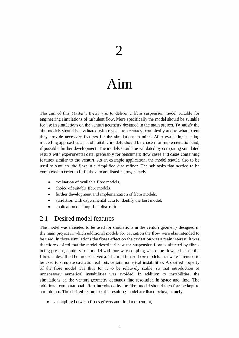
2.1 Desired model features
The model was intended to be used for simulations in the venturi geometry designed in
the main project in which additional models for cavitation the flow were also intended to
be used. In those simulations the fibres effect on the cavitation was a main interest. It was
therefore desired that the model described how the suspension flow is affected by fibres
being present, contrary to a model with one-way coupling where the flows effect on the
fibres is described but not vice versa. The multiphase flow models that were intended to
be used to simulate cavitation exhibits certain numerical instabilities. A desired property
of the fibre model was thus for it to be relatively stable, so that introduction of
unnecessary numerical instabilities was avoided. In addition to instabilities, the
simulations on the venturi geometry demands fine resolution in space and time. The
additional computational effort introduced by the fibre model should therefore be kept to
a minimum. The desired features of the resulting model are listed below, namely
a coupling between fibres effects and fluid momentum,

4
minimal introduction of additional numerical instability,
minimal introduction of additional computational cost.
2.2 Limitations
Since fluid flow with fibres is a very complex physical situation, there are many
uncertainties with respect to modelling and the reliability of numerical solutions. The
implementation itself can also grow difficult if the models are complex. This thesis work
mainly focused on modelling how turbulent fibre suspension flows behave as a collective
result of fibres being present. Detailed description and information of fibres as individual
particles was outside the scope of the work. Since fibre suspension rheology is strongly
dependent on concentration and properties of the fibres the modelling in this work was
limited those suspensions of the type of interest. The type was softwood fibres with mass
concentration around .
For the simulations needed to validate the fibre models the computational resources were
limited to single laptop workstation with a 4 core CPU. The number of simulations that
could be performed to study the fibre models was thus limited. Implementation of the
fibre models were intended for the ANSYS Fluent software (ANSYS Inc. (b), 2013). The
models available were therefore limited to those having possible implementation through
so-called user defined functions (UDF) written in C programming language. All work
conduced within the thesis was also made without performing any physical experiments.
Experimental data for validation was therefore limited to the one available in literature.

5
3
Theory
Theory relevant for the thesis work is presented in this section. First fluid mechanics and
turbulence modelling is covered, followed by theory on fibre suspensions in general and
on fibre modelling in more detail. Literature with experimental data intended for the
validation of fibre models is then presented. Finally a short introduction to the concept of
disc refiners is given.
3.1 Fluid mechanics
The theory of fluid mechanics is centred on equations governing conservation of mass,
momentum and energy. The governing equation for conservation for mass, called the
continuity equation, reads in tensor notation (Davidson, 2014)
(3.1)
where is fluid density, is velocity and is spatial direction. From this point and on
all flows will be considered incompressible, implying that . Equation (3.1)
then gives
(3.2)
where , and are the velocities in the Cartesian -, - and -coordinates,
respectively. In Equation (3.2) Einstein’s summation convention for the tensor notation,
i.e. that indices appearing twice in the same term are summed over, was explicitly shown.
The equation governing conservation of linear momentum reads (Davidson, 2014)
(3.3)
where are the stress tensor and the body force acting on the fluid. The stress tensor
may be decomposed into normal stresses and shear stresses, also known as pressure and
viscous stresses, respectively, as (Davidson, 2014)

6
(3.4)
where is the unit tensor and is the viscous stress tensor. The constitutive law for
Newtonian incompressible viscous fluids reads (Davidson, 2014)
(
) (3.5)
where is the dynamic viscosity of the fluid and , the symmetric part of the velocity
gradient tensor, is called the strain rate tensor. Combination of Equation (3.3), Equation
(3.4) and Equation (3.5) gives the transport equation for linear momentum, called the
Navier-Stokes equation (Davidson, 2014):
(3.6)
Equation (3.6) may be discretised and solved directly. However, very high resolution in
space and time is usually needed to correctly resolve a turbulent flow field. Instead,
turbulence modelling is often employed to reduce the computational resources needed.
Models relevant for this work are described below.
3.1.1 Reynolds averaged Navier-Stokes
It is preferable for many turbulent flows to decompose the instantaneous velocity and
pressure fields into their time-averaged components, assumed steady, and their
fluctuating parts. By decomposing velocity and pressure as
(3.7)
(3.8)
where denotes time averaging and denotes fluctuation, and then time-average the
Navier-Stokes equation (3.6) the Reynolds Averaged Navier-Stokes equation (RANS) is
obtained, reading (Davidson, 2014)
( )
(
) (3.9)
The time-averaged incompressible continuity equation reads
(3.10)
which together with the original continuity equation (3.1) gives
(3.11)

7
The last term in the RANS equation
, called the Reynolds stress tensor, is unknown
and needs to be modelled for the system of equations governing the fluid flow to be
closed.
The Boussinesq assumption
In many turbulence models used for solving the RANS equation the so-called Boussinesq
assumption is used. The unknown Reynolds stresses are then modelled as diffusion-like
transport by introducing a turbulent viscosity, or eddy viscosity, . This is called the
Boussinesq assumption and reads (Davidson, 2014)
(
) (3.12)
The turbulent viscosity needs to be computed with some model. Such models are
described below.
The model
In the model the turbulent viscosity is computed from the turbulent kinetic energy
and the turbulent dissipation as (Davidson, 2014)
(3.13)
where is a model constant. and are obtained by solving the modelled transport
equation for the respective quantities, reading (Davidson, 2014)
*(
)
+ (3.14)
*(
)
+
(3.15)
where , , are are model constants and the production term for turbulent
kinetic energy reads
(
)
(3.16)
The model
In the model the turbulent viscosity is computed from the turbulent kinetic energy
and the so-called specific dissipation rate as (Davidson, 2015)
(3.17)

8
where the specific dissipation is related to the turbulent kinetic energy and the turbulent
dissipation rate through a constant as
(3.18)
The quantities and are obtained from solving the modelled transport equation for ,
i.e. Equation (3.14), and the modelled transport equation for reading (Davidson, 2015)
*(
)
+
( )
(3.19)
where , and are model constants.
The SST model
Two main weaknesses of the model are over-prediction of shear stress in adverse
pressure gradient flows and the need of near-wall modification. While the model is
better than the model in adverse pressure gradient flows it depends on the free
stream value of . A solution can be the SST model, which combines the models
and behaves like the model near walls and like the model in the outer region.
(Davidson, 2014)
Using the relation between and from Equation (3.18), using that and
assuming the modelled transport equation for , i.e. Equation (3.15), is
reformulated to an equation for as (Davidson, 2014)
*(
)
+
(
)
(3.20)
where and are model constants derived from the model constants of the and the
models. The SST model switches smoothly between coefficients for the
model and the model with the use of a blending function employed
in the computation of .
3.1.2 Large eddy simulations
If a flow needs to be resolved in both space in time, the Navier-Stokes equations may be
filtered, i.e. volume averaged, so that large turbulent scales are resolved but small
turbulent scales, called sub-grid scales (SGS), are modelled. This is called large eddy
simulation (LES). In this case the pressure and velocity fields, respectively, are
decomposed into their volume averages, or filtered quantities, and SGS fluctuations as
⟨ ⟩ (3.21)
⟨ ⟩ (3.22)
where ⟨ ⟩ denotes volume average and denotes sub-grid fluctuation. Using the
composition and volume averaging the Navier-Stokes equation (3.6) yields the filtered
Navier-Stokes equation (Davidson, 2014),

9
⟨ ⟩
⟨ ⟩
⟨ ⟩
⟨ ⟩
⟨ ⟩
(3.23)
and the filtered incompressible continuity equation
⟨ ⟩
(3.24)
The SGS stresses in the filtered Navier-Stokes equation, reading (Davidson, 2014)
⟨ ⟩ ⟨ ⟩⟨ ⟩ (3.25)
are unknown and needs to be modelled to close the system of equations for the fluid flow.
The Smagorinsky-Lilly model
The SGS stresses in the filtered Navier-Stokes equation may be modelled by the
Boussinesq assumption, similarly to the RANS models in Section 3.1.1, as (Davidson,
2014)
(
⟨ ⟩
⟨ ⟩
) ⟨ ⟩ (3.26)
where is called the SGS viscosity and needs to be computed using some model. A
common model used is the Smagorinsky-Lilly model, which is available for the LES
model in Fluent, where the SGS viscosity is computed as (ANSYS Inc. (a), 2013)
|⟨ ⟩| (3.27)
with
|⟨ ⟩| √ ⟨ ⟩⟨ ⟩ (3.28)
and with denoting the mixing length for sub-grid scales, computed as
(3.29)
where is the von Kármán constant, is the distance to the closest wall, is the
Smagorinsky constant and is the local grid scale.
3.1.3 Detached Eddy Simulations
Detached Eddy Simulations (DES) uses a combination of LES and the unsteady version
of RANS, called URANS, to capture the boundary layer with RANS and the detached
eddies away from the boundary layer using LES (Davidson, 2014). DES based on two-
equation turbulence models, e.g. and , switches between RANS mode and
LES mode by switching the method used to calculate the turbulent length scale and the

10
dissipation as. For instance, in DES with the model the quantities are computed
as (Davidson, 2014)
(
) (3.30)
(
) (3.31)
where the first arguments in the minimum and maximum operators, respectively,
correspond to RANS mode and the second arguments correspond to LES mode.
3.1.4 Courant-Friedrich-Lewy condition
A conditions which is often preferred to satisfy in transient CFD-simulations is the
Courant-Friedrich-Lewy condition. The dimensionless CFL number is defined as (Tu et
al., 2013)
(3.32)
where is velocity, the time step and the local grid size. The CFL condition states
that must be satisfied to guarantee stability in numerical solutions. A CFL number
corresponds to a case where fluid particles travel one cell per time step (Davidson,
2014) .
3.2 Fibre suspensions and fibre modelling
Fibre suspensions exhibit complex rheology and a range of physical phenomena influence
the flow pattern with varying significance depending on the fibre concentration, fibre
length and flow regime (Kerekes, 2006). Various non-dimensional numbers have been
defined in literature characterise fibre suspensions with respect to concentration. A
commonly used number, called the crowding number, is the average number of fibres in
the volume of a sphere swept by a fibre length, calculated as (Kerekes, 2006)
(
)
(3.33)
where is volume concentration of fibres, fibre length and fibre diameter. Fibre
suspensions are associated with a yield stress, which varies in magnitude from suspension
to suspension, that has to be exceeded for the network of fibres yield and for the
suspension to behave as a fluid contrary to something more similar to an elastic solid
(Andersson et al., 1999). Fibre suspensions also have the tendency to form flocs, i.e. local
concentration of fibres sticking together through mechanical inter-fibre forces, that can be
important for the suspension rheology (Derakhshandeh et al., 2011). Flocculation occurs,
for instance, in flows with decaying turbulence which also is the most common
flocculating flow in papermaking processes (Kerekes, 2006).
11
The flow regime and the flow pattern near solid boundaries can be of importance for fibre
suspension rheology. Pipe flow may be used as an illustrative example. At low velocity
fibres move in a plug formation in the centre of the pipe, with almost no relative motion
between fibres, while a clear water annulus can be observed close to the wall (Fock et al.,
2011). With increasing velocity the annulus becomes turbulent and increases in size and
starts mixing the fibres more and more until a fully turbulent flow is attained for the
whole pipe cross section (Derakhshandeh et al., 2011). In the turbulent regime the
rheology of pulp suspensions is close to the one of Newtonian fluids and they are
therefore often referred to as “fluidized” (Bennington & Kerekes, 1996).
When it comes to modelling of fibre suspensions, different modelling approaches exist
with wide differences in complexity, accuracy and computational effort needed. Models
span from detailed description of individual fibres, modelled as chains of linked segments
tracked individually in the fluid flow field (Lindström & Uesaka, 2008), (Andric et al.,
2013), to modelling of the fibre suspension as a single fluid with non-Newtonian
rheology (Ford et al., 2006), (Fock et al., 2010). The coupling between fibre orientation
distribution and fluid momentum has also been used in the modelling of fibre suspension
flow (Yang et al., 2013), (Krochak et al., 2009), (Moosaie & Manhart, 2013). Modelling
approaches relevant for this thesis are presented below.
3.2.1 Bingham viscoplastic fluid model
A macroscopic approach to model fibre suspension rheology is to use the non-Newtonian
Bingham viscoplastic fluid model. In the model the suspension is associated with a yield
stress which is the shear stress that must be exceeded to initiate flow. If the yield stress
is not exceeded the material will behave as solid. If the yield stress is exceeded, on the
other hand, the material behaves like a Newtonian fluid. (Irgens, 2014)
The relationship between shear stress and shear rate can be summarised as (Irgens, 2014)
{
( )
( ) [
| |]
(3.34)
where is the consistency index and is the shear rate, defined as
√ (3.35)
A sketch of the relationship between stress and shear rate for the Bingham viscoplastic
fluid model can be seen in Figure 3.1.

12
Figure 3.1: Relationship between shear stress and shear rate for the Bingham
viscoplastic fluid model. Figure from the main project report (Lundberg et al., 2015).
The rheology of a Bingham viscoplastic fluid may be expressed in the relationship
between shear rate and effective viscosity is the fluid as (Irgens, 2014)
( ) {
(3.36)
where is the maximum shear stress in the fluid.
3.2.2 Fibre orientation distribution
Fibres a suspension can be described by their distribution with regards to position and
orientation in space, with the probability density function (pdf) ( ) (Zhang, 2014).
The pdf ( ) describes the probability to find a fibre with position between and
with orientation vector between and at time . The evolution of may be
described by a transport equation, called a Fokker-Planck equation, as (Zhang, 2014)
( ) (3.37)
where and are the gradient operators in rotational space and translational space,
respectively. The flux densities in Equation (3.37) are defined as (Zhang, 2014)
( ) ( ) ( ) (3.38)
( ) ( ) ( ) (3.39)
where and are called the rotational and translational drift coefficients, respectively,
and represents collective rotational and translational motion, respectively, of fibres in the
suspension. If fibre concentration is homogeneous the distribution is uniform with respect
position, since the probability of finding a fibre is the same for all positions, and is a
non-uniform distribution solely for fibre orientation.
A coupling between the fibre orientation distribution function, from here on denoted the
ODF, ( ) and the fluid momentum equations can be introduced through a constitutive

13
equation for viscous stresses in the suspension. Assuming high aspect ratio rigid fibres
the stresses in the fibre suspension are (Shaqfeh & Fredrickson, 1990)
(
) (3.40)
where is called the additional viscosity due to presence of fibres. The tensors and
are the second and fourth order statistical moments of the fibre orientation
distribution:
⟨ ⟩ (3.41)
⟨ ⟩ (3.42)
where ⟨ ⟩ denotes averaging with respect to the orientation distribution and is the
orientation vector of a fibre.
3.3 Experimental measurements of fibre suspensions
Data from experimental measurements of fibre suspension flows was used to validate
simulations with the fibre models. In this section two articles on experimental
measurements are covered. The first article provides experimental data from fibre
suspension flow in a channel with a backwards facing step, a flow case featuring
recirculating flow and decaying turbulence, much like the venturi geometry in the main
project (Lundberg et al., 2015). The second article is on the turbulent fibre suspension
flow in a rectangular channel where turbulent boundary layers are of importance for the
flow. Graphical data from experimental measurements in the literature shown in this
section were read graphically using a Matlab script that was created for the purpose. In
short, the Matlab script was designed in a way so that the user may click on points of
plotted data in a coordinate system and then save them to a data file.
3.3.1 Fibre suspension flow over a backwards facing step.
Claesson et al (2012) studied the flow of fibre suspensions over a backward facing step
using Laser Doppler Anemometry (LDA). In the experiments the flow entered from a
circular pipe with diameter which was expanded and connected to a quadratic
channel with side . A backwards facing step was created by inserting a block at the
entrance of the quadratic channel. Two different step heights, and , were
used. Mass concentrations , , and were used and the pulp was fully
bleached never-dried kraft pulp provided by Södra Cell Värö in Sweden.
Instantaneous velocities were measured for flows with all different concentrations and at
two free stream velocities, and . For free steam velocity and
mass consistency the profiles of mean streamwise velocity and turbulent intensity
were shown in the article. Turbulent intensity was defined as the average velocity
fluctuation magnitude normalised by bulk velocity computed as

14
√
( )
(3.43)
where is the number of instantaneous measurements, the instantaneous streamwise
velocity in measurement and the mean streamwise velocity. The bulk velocity
was taken as the mean streamwise velocity at the step and at height . The
recirculation zone for all flow cases were visualized by the level curve . For step
height , profiles of mean streamwise velocity for mass concentration and
free stream velocity can be seen in Figure 3.2 and corresponding profiles of
turbulent intensity can be seen in Figure 3.3. The peak in turbulent intensity that can be
seen, roughly at the height of the step, is referred to as the mixing layer in Claesson et al.
(2012). The recirculation zones can be seen in Figure 3.4 for mass concentrations ,
and for pure water, both for step height .
Figure 3.2: Mean streamwise velocity profiles for fibre suspension with free stream
velocity and mass consistency read graphically from experimental data in
Claesson et al. (2012).
Figure 3.3: Turbulent intensity profiles for fibre suspension with free stream velocity
and mass consistency read graphically from experimental data in Claesson
et al. (2012).

15
Figure 3.4: Recirculation zones as the level curve of mean streamwise velocity
for free stream velocity read graphically from experimental data in Claesson et
al. (2012).
3.3.2 Fibre suspension flow in rectangular channel
Xu & Aidun (2005) measured velocity and turbulent intensity for turbulent fibre
suspension flow with different mass concentrations and flow rates in a rectangular
channel. Measurements were made using pulsed ultrasonic Doppler velocimetry (PUDV).
Cellulose wood fibres, with average length and diameter and ,
respectively, were used and mass concentrations ranged from to . The fibres
were assumed to have the same density as water in the experiments, since they were
totally soaked, so that mass concentration and volume concentration were equal.
Inlet velocities used ranged from to and the corresponding Reynolds
number based on pure water ranged from to . The rectangular channel was
wide, high and long and measurements were made close
to the outlet. Mean velocities and turbulent intensities were plotted along the height-
direction in the channel. As a result of the measurements an empirical relation for the
velocity profile in the channel was found as
( )
(
) (3.44)
where is wall distance, is channel height, and are non-dimensional wall
distance and velocity, respectively. The coefficient was called the wake coefficient,
defined as
(3.45)
where is the Reynolds number, the fibre number density and the fibre half-length.
The authors came to the conclusion that the higher the flow rate the lower the effect of
fibre concentration is on the velocity profiles. For sufficiently high flow rate velocity
profiles of pure water and fibre suspensions were practically the same.

16
3.4 Disc refiners
In mechanical pulping processes so-called disc refiners are used to process cellulose
fibres mechanically between rotating discs patterned with bars and grooves. Fibre
suspension enters at the centre of the refining discs and is then forced towards the
periphery by centrifugal forces and the fibres are processed by passing over the bars and
through the grooves. A rotating disc is called rotor, a non-rotating disc is called stator and
the distance between rotor and stator is called gap clearance. In low consistency refining,
meaning where the fibre consistency or mass concentration is below the gap
clearance can have length on the same order as a few fibre diameters. (Rajabi Nasab et
al., 2014)
A sketch of the disc refiner concept is shown in Figure 3.5. In the figure the sizes of gap
clearance and bars have been exaggerated for comprehensibility. In reality the bars and
the grooves between them have width and height on the scale of a few millimetres (Rajabi
Nasab et al., 2014).
Figure 3.5: Sketch of disc refiner showing the concept of inlet and rotor movement
(left),the concept of bars on the disc (middle) and the concept of stator and rotor discs
(right). The size of gap clearance and bars are exaggerated.
𝜔
17
4
Method
In this section the methodology for the thesis work is presented. In summary, the work
consisted of conducting a literature survey providing a theoretical background and an
overview of fibre modelling. Two approaches for modelling were chosen for
implementation and, if possible, further development and the models were implemented
in Fluent. The models were then validated using experimental data from literature. In the
validation the models were optimised, in the sense that the best parameter setting was
identified, using data from the flow over a backwards facing step. The models were then
further validated using data from the flow in a rectangular channel. All simulations were
performed using Fluent (ANSYS Inc. (b), 2013) and all mesh creation was made in
ANSA (BETA CAE Systems S.A., 2014). After the validation one of the models were
used to simulate the flow in a simplified disc refiner. The disc refiner simulation was
performed as an example application for the fibre models and since it was of interest as a
relevant flow case for pulp and paper industry.
4.1 Fibre modelling
Two fibre models, denoted the Bingham model and the ODF model, were implemented.
The Bingham model was to a large part an implementation of modelling that can be
found in literature, while the ODF model was mainly developed within this thesis. Both
models effectively act as single-phase flow models in the sense that the Navier-Stokes
equations are solved for a single phase with some modification of the viscous stress
tensor. The single-phase property supposedly enhances the numerical stability of the
models which was considered a desired property. The models were implemented in
Fluent through so-called user-defined functions (UDF) which are sub-routines to the
Fluent solver written in C programming language.
As discussed in Section 3.2 the rheology of fibre suspensions depend on many factors.
Fibres of interest for the project were softwood fibres from pine and spruce, being a type
of fibres commonly used in Swedish paper mills. Softwood pulp fibres have length on the
millimetre scale and diameter on the order of tens of microns giving aspect ratio
(Derakhshandeh et al., 2011). Fibre suspensions with mass concentration around
were mainly considered for modelling.

18
4.1.1 Bingham model
A method to numerically model fibre suspension flow with the Bingham viscoplastic
fluid model was used by Fock et al. (2010). In this thesis work the implementation of the
Bingham model followed a similar methodology. The yield stress for the suspension was
computed using the empirical relation (Fock et al., 2010; Derakhshandeh et al., 2011;
Kerekes, 2006)
(4.1)
where and are model constants, varying from suspension to suspension, and is the
mass concentration, or mass consistency, of fibres. In the theoretical case for a Bingham
viscoplastic fluid the effective viscosity is infinite for shear stress levels below the yield
stress, which was stated in Equation (3.36). In a numerical model this may be
approximated by assigning a large value to the viscosity for low shear rates and vary it
linearly with shear rates corresponding to stress levels exceeding yield stress. That
methodology, however, gives a discontinuity in the derivative which may cause
numerical issues. Fock et al. (2010) used the Herschel-Bulkley model in Fluent to
compute suspension viscosity as (ANSYS Inc. (b), 2013)
{
(
)
(4.2)
where is called consistency index which they set to the viscosity of water, is called
critical strain rate, corresponding to the limit case were fluid shear stress equals the yield
stress, and is computed as
(4.3)
where they set the constant to a large value. Equation (4.2) was used to compute the
viscosity of the fibre suspension for the Bingham model also in this thesis work. It can
observed that the derivative of the viscosity with respect to shear rate yields
|
(4.4)
and is thus continuous, which also corresponds to a continuous derivative . A
comparison between the numerical model for the viscosity with discontinuous derivative
and the modified version in the Herschel-Bulkley model is illustrated in Figure 4.1.

19
Figure 4.1: Illustration of the difference between discontinuous derivative (left) and
continuous derivative (right) in the relationship between shear stress and shear rate in the
fluid. Figures from the main project report (Lundberg et al., 2015).
The Herschel-Bulkley model in Fluent is not available for use in simulation of turbulent
flows. In addition, according to Fock et al. (2010) the Bingham model is only valid for
flows with low shear rates. In this work, however, the desired fibre model needed to be
used also for simulations of turbulent fibre suspension flow. It was therefore decided to
implement the model anyway and use validation with experimental data to evaluate if the
use may be justified or not. To make it possible to use the model alongside turbulence
models in Fluent the suspension viscosity was instead computed in each cell from
Equation (4.2) using a UDF. In the flow model described in Fock et al. (2010) an
additional transport equation was introduced to account for local variations in fibre mass
concentration , reading
(
) (4.5)
where is fibre concentration diffusivity. In this thesis work, however, this transport was
excluded. In the main project the model was tested for simulation in the designed venturi
geometry. Both the case of homogenous concentration in the whole domain and the case
of non-homogeneous inlet concentration together with the use of Equation (4.5) was
tested. It was found that both cases yielded practically the same simulation results
(Lundberg et al., 2015). Solving Equation (4.5) would therefore solely raise the
computational cost and it was therefore concluded that the fibre concentration may and
should be treated as homogeneous in this work.
4.1.2 ODF model
With intent to implement the coupling between fibre orientation and fluid momentum,
described in Section 3.2.2, a model for the fibre orientation distribution function (ODF)
was developed. The model was then used contrary to solving the probability transport
from the Fokker-Planck equation (3.37). The modelled ODF was then used to construct
explicit expressions for the fibre stresses
as a function of the flow field prior to
simulations. Using the model no additional transport equation to the momentum and
continuity equations needs to be solved. The idea behind the model was to use a statistical
model for the ODF for an arbitrary flow field. Expressions for the orientation tensors,
20
needed to compute the fibre stresses, may then be constructed by computing the
components numerically for the set of possible flow fields and fit a regression model the
results. The model and its implementation are described below.
Modelling of the orientation distribution function
Lin et al. (2005) studied the ODF numerically in turbulent boundary layer flow and found
that fibres aligned with the flow streamlines. Lin et al. (2011) numerically studied
turbulent fibre suspension flow through an axisymmetric contraction and found that fibres
aligned with flow direction, a result which was also validated with experimental data. In
addition Lin et. al (2011) found that higher aspect ratio fibres aligned faster with flow
direction and that turbulence had a randomising effect on the ODF, which increased in
significance with the turbulent intensity of the flow. Olson et al. (2004) numerically
studied the ODF for fibre suspension flowing in a planar contraction and found that fibres
aligned in the flow direction, which was validated by experimental data. Similar
numerical results for fibre suspension flow in a planar contraction were obtained by
Krochak et al. (2009). Lin et al. (2012) simulated the ODF in a round turbulent jet of fibre
suspension and found alignment with flow direction also in that flow, with more
alignment for higher aspect ratio fibres. In summary, studies have shown that in turbulent
flows suspended fibres align with flow direction and the alignment increases with aspect
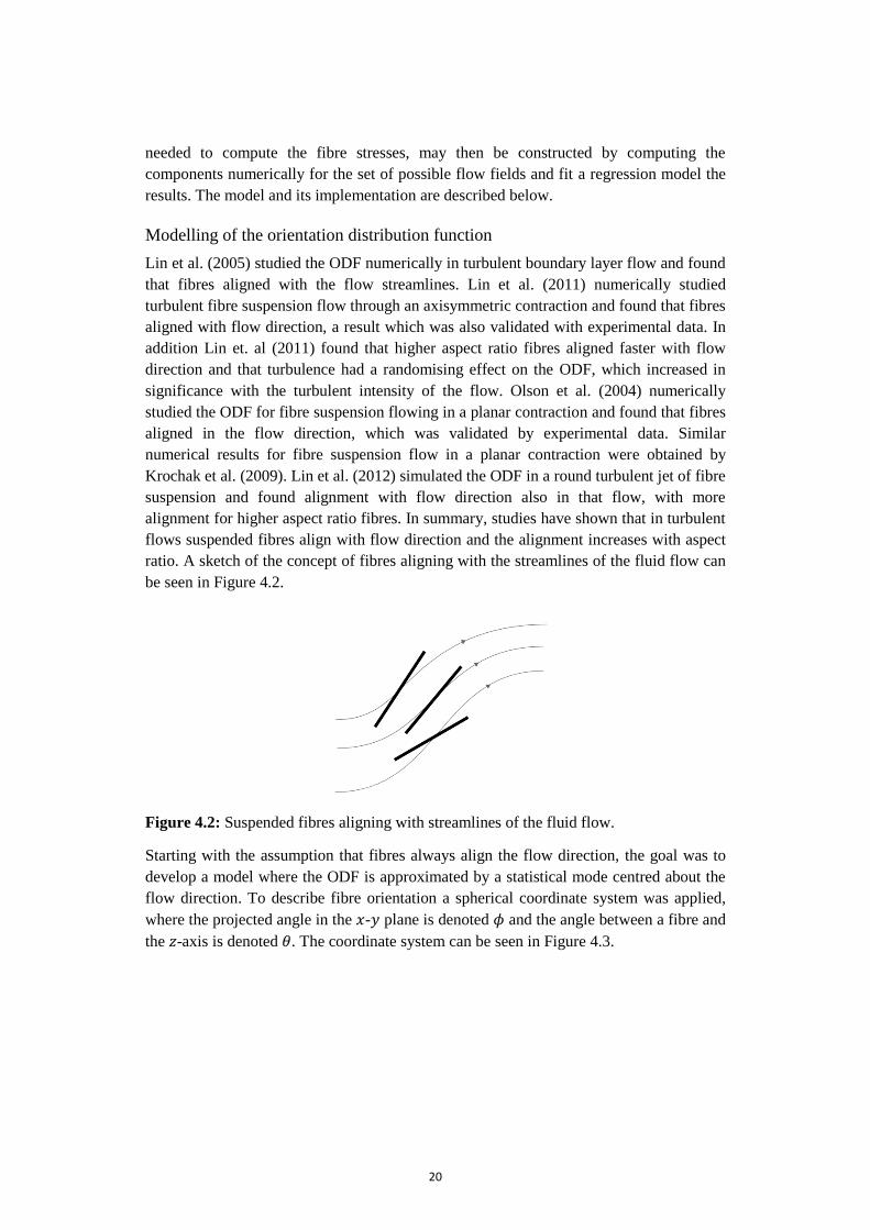
ratio. A sketch of the concept of fibres aligning with the streamlines of the fluid flow can
be seen in Figure 4.2.
Figure 4.2: Suspended fibres aligning with streamlines of the fluid flow.
Starting with the assumption that fibres always align the flow direction, the goal was to
develop a model where the ODF is approximated by a statistical mode centred about the
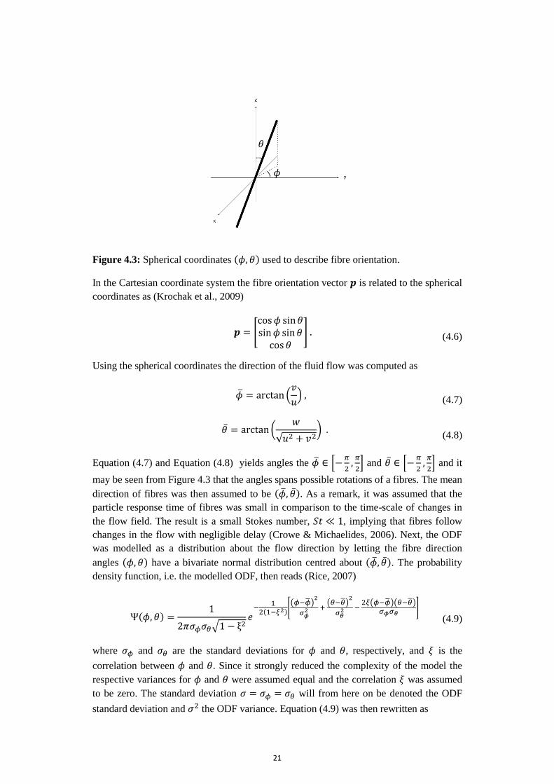
flow direction. To describe fibre orientation a spherical coordinate system was applied,
where the projected angle in the - plane is denoted and the angle between a fibre and
the -axis is denoted . The coordinate system can be seen in Figure 4.3.
21
Figure 4.3: Spherical coordinates ( ) used to describe fibre orientation.
In the Cartesian coordinate system the fibre orientation vector is related to the spherical
coordinates as (Krochak et al., 2009)
[
] (4.6)
Using the spherical coordinates the direction of the fluid flow was computed as
(
) (4.7)
(
√ )
(4.8)
Equation (4.7) and Equation (4.8) yields angles the *
+ and *
+ and it
may be seen from Figure 4.3 that the angles spans possible rotations of a fibres. The mean
direction of fibres was then assumed to be ( ). As a remark, it was assumed that the
particle response time of fibres was small in comparison to the time-scale of changes in
the flow field. The result is a small Stokes number, , implying that fibres follow
changes in the flow with negligible delay (Crowe & Michaelides, 2006). Next, the ODF
was modelled as a distribution about the flow direction by letting the fibre direction
angles ( ) have a bivariate normal distribution centred about ( ). The probability
density function, i.e. the modelled ODF, then reads (Rice, 2007)
( )
√
( )[( )
( )
( )( )
]
(4.9)
where and are the standard deviations for and , respectively, and is the
correlation between and . Since it strongly reduced the complexity of the model the
respective variances for and were assumed equal and the correlation was assumed
to be zero. The standard deviation will from here on be denoted the ODF
standard deviation and the ODF variance. Equation (4.9) was then rewritten as
𝜃
𝜙

22
( ) ( ) ( ) (4.10)
where ( ) and ( ) are the respective marginal distributions of and reading
( )
√
( )
(4.11)
( )
√
( )
(4.12)
It can be observed that Equation (4.11) and Equation (4.12) are the probability density
functions for and being independently normally distributed random variables (Rice,
2007). In other words,
( ) (4.13)
( ) (4.14)
A visualisation of the modelled ODF is shown in Figure 4.4. The choice of ODF standard
deviation is discussed below.
Figure 4.4: Fibre orientation distribution function (ODF) modelled as a bivariate normal
distribution with zero correlation.
ODF standard deviation
A possible choice of ODF standard deviation was to set it constant and assume it to be
homogeneous throughout the flow. Another possibility was that it rather would depend on
the flow in some way. It therefore was assumed that the ODF standard deviation should
increase with the magnitude of turbulent velocity fluctuations, inspired by the results
from Lin et al. (2011). The ODF standard deviation was thus assumed to vary with
turbulent intensity , computed from the turbulent kinetic energy as
√
(4.15)

23
where is the bulk velocity for the flow. Being a simple form of variation, a linear
function was used relate the ODF standard deviation to the turbulent intensity. The ODF
standard deviation was then computed as
(4.16)
where is the slope of the linear function. A minimum value was also introduced
to prevent the fibres to perfectly align assuming it being non-realistic. Above the
minimum varies linearly according to Equation (4.16).
A priori computation of fibre orientation tensors
The fibre orientation tensors of second and fourth order, respectively, can be computed
from the integrals (Yang et al., 2013)
∮ ( ) (4.17)
∮ ( )
(4.18)
where is component of the fibre orientation vector and the integrals are taken over
all possible rotations. It should be remarked that general second and fourth order tensors
have and components, respectively. However, it can be seen that because
of symmetries has unique components and has unique components. Now,
since the modelled ODF is known for an arbitrary flow field the fibre orientation tensors
and may be computed numerically for all possible flow directions prior to
simulations. Explicit expressions for all tensor components as functions of and may
then be constructed by fitting a regression model to the computed values and the
expressions can be used to compute the tensor components as functions of the flow field
in simulations. For instance, components of the second order orientation tensor could be
computed from Equation (4.17) for given flow direction ( ) as
∬ ( ) ( ) (∫ ( ) ( ) ) (∫ ( ) ( ) )
( ) ( ) (4.19)
where ( ) and ( ) denotes the - and -parts, respectively, of the combined fibre
direction vectors according to
( ) ( ) (4.20)
All components and can be computed analogously. Note that the reason ( )
and ( ) are functions of the flow direction coordinates and , respectively, is since
the marginal distribution functions and are determined by those coordinates.
For series of discrete values *
+ and *
+, and for given ODF standard
deviation , ( ) and ( ) were computed as described for all unique components of

24
the fibre orientation tensors by numerical integration of Equation (4.17) and Equation
(4.18). As regression model to construct explicit expressions for the tensor components
Fourier series expansions then was applied, approximating ( ) and ( ) as (Nordling
& Österman, 2006)
( ) ( )
∑ (
)
(4.21)
( ) ( )
∑ (
)
(4.22)
where is length of the intervals for and , respectively, i.e. . The number of
terms needed in the sums and , respectively, was only up to to obtain
approximations that resembled the computed values very well. The expressions for the
orientation tensor components constructed by multiplying ( ) and ( ). In Figure 4.5
the numerically computed values and the fitted Fourier series can be seen for the fourth
order orientation tensor component as an example. In Figure 4.6 the same tensor
component, ( ) ( ), is shown in 2-D. It can be observed that the Fourier
series expressions practically match the computed values. Similar good agreement was
found for all components and and for the range of used.
Figure 4.5: Computed values( ) and Fourier series value (--) of ( ) (left) and ( )
(right) for the fourth order orientation tensor component . ODF standard deviation
.

25
Figure 4.6: Component of the fourth order orientation tensor computed from
numerical integration (left) and Fourier series expression (right) with ODF standard
deviation
A Matlab script was used to compute the components of the fibre orientation tensors. In
addition to computing and fitting of Fourier series the script also printed the expressions
in C programming language to the Matlab console so that they could be copied directly
into a Fluent UDF source code. For the case of non-homogeneous ODF standard
deviation local values of the orientation tensor components were computed using linear
interpolation. Fourier series expressions were constructed as described for a series
discrete values of as
(4.23)
and a total of discrete values were used. The local values the orientation tensor
components were then computed using linear interpolation between constructed
expressions. The maximum value was used and was chosen as a value to cover
an upper bound on with a certain margin. The value was based on results on the ODF in
the literature (Lin et al., 2005; Lin et al., 2011; Olson et al., 2004; Lin et al., 2012;
Kerekes, 2006). As a remark, the fibres of interest for this thesis work were of larger
aspect ratio than the ones in the mentioned literature which should reduce the maximum
value of further.
Coupling to fluid momentum
Using the constitutive equation for viscous stresses in a fibre suspension, Equation (3.40),
the ODF was effectively coupled to the fluid momentum equations by an anisotropic
modification of the viscous stress tensor through an additional fibre stress tensor
as
(
) (4.24)
which leads to a modified version of the incompressible Navier-Stokes equation (3.6)
reading (Yang et al., 2013)

26
[
( ) ] (4.25)
The body force term was left out by Yang et al. (2013) but can, if desired, be included
by adding it on the right hand side of Equation (4.25). Additional viscosity due to
presence of fibres for a semi-dilute suspension of rigid slender ellipsoids was
computed by using a relation derived by Shaqfeh & Fredrickson (1990) reading
* (
) ( (
)) +
(4.26)
where is the number of fibres per unit volume, the fibre half-length and the volume
fraction of fibres. Shaqfeh & Fredrickson (1990) defined semi-dilute concentration as the
regime where and . Following, for completeness, it is motivated that
this was the case for fibre suspensions of interest within this work. The volume
concentration can be computed as the number of fibres per unit volume times volume of a
fibre, i.e.
(
)
(4.27)
where it was used that the aspect ratio . An expression for as a function of
and can then be obtained from Equation (4.27) as
(4.28)
An expression for was also be derived using Equation (4.28) as
(4.29)
Assuming then for and for .
In other words for fibres with aspect ratio suspensions with volume
concentration up to can be considered semi-dilute. If the aspect ratio is smaller the
upper limit on is even larger. The concentration regime thus covers up fibre
suspensions of interest and it was considered justified to use the expression for as
stated in Equation (4.26). Equation (4.26) was also rewritten to a function of and
using Equation (4.28) as
* (
) ( (
)) +
(4.30)
Since information on either and or and may be missing in some cases the model
may contain uncertainties. It was therefore decided to introduce a constant, called , to
27
account for this. The constant was introduced in the expression for additional
viscosity due to fibres and Equation (4.30) was thus modified as
* (
) ( (
)) +
(4.31)
Implementation in Fluent
A total of 4 UDF:s where used to implement the ODF model in Fluent. The methodology
of the implementation was to compute the components of the orientation tensors from
constructed expressions and use them to compute the components of the fibre stress
tensor
. Then the divergence of the stresses, the last term in Equation (4.25), was added
to the momentum equation in the respective directions as source terms. To store variables
a total of 9 so-called user-defined scalars (UDS) in Fluent were used. UDS are additional
transport equations for scalar variables defined by the user. UDS variables were allocated
to store variables since Fluent automatically computes the gradient of each UDS variable,
which were needed to compute the divergence of
. Solution of the transport equations
for the UDS variables, however, was deactivated. The first UDF executes at the
beginning of each iteration and its actions are listed below, namely
computes the mean direction angles and from the flow field according to
Equation (4.7) and Equation (4.8),
computes ODF standard deviation (homogeneous or non-homogeneous).
computes the components of the orientation tensors and ,
computes the unique components of the fibre stress tensor
in Equation
(4.24) and stores in the 6 first UDS variables,
obtains the gradient of the 6 first UDS variables,
computes divergence
from the last term in Equation (4.25) in the three
momentum equations and stores in the remaining 3 UDS variables.
The remaining 3 UDFs adds the 3 last UDS variables as momentum sources in the x-, y-,
and z-directions, respectively.
4.2 Comparison with experiments by Claesson et al (2012)
Data obtained from experimental measurements of fibre suspension flow in a channel
with a backwards facing step obtained by Claesson et al. (Claesson et al., 2012) was used
to validate the fibre models. The aim was identify the best performing settings and which
parameters gave significant impact on the simulated results for the respective models. The
experiments were considered suitable for the project since the flow geometry includes a
recirculation zone after a sudden change in flow geometry, a flow characteristic relevant
for the flow in the venturi nozzle. In addition pulp from a Swedish paper mill was used,
which was the type of fibres of main interest for this work.

28
The first step consisted of creating a mesh to resemble experimental conditions
sufficiently accurate in geometry and the second step consisted of simulations with fibre
models. All simulations were made with the step height . This was made mainly
since the most amount of data was available for the case. All simulations were performed
using DES with SST turbulence model, the main reason being that the simulations
on the venturi geometry were intended to be performed using the same turbulence model.
The model is also accurate as a large part of the turbulence is resolved and not modelled.
Since the simulations were performed to validate the fibre models it was preferred to
minimise the sources of additional modelling errors as, for instance, turbulence
modelling. Gravity was therefore also accounted for in the simulations. Simulations were
carried out assuming isothermal conditions at temperature . The properties of water
were then viscosity and density (Mörtstedt &
Hellsten, 2010). The time step was chosen sufficiently small to satisfy the CFL condition
in the mesh. Inlet velocity was used in all simulations. The flow was
simulated until stabilised and then averaged over about . The turbulence was assumed
to be sufficient for the fibre concentration to be homogeneous and was used
for the fibre models.
4.2.1 Mesh creation and fitting geometry
A first version mesh for the backwards facing step flow case was created. Simulations
were then carried out for pure water with the same flow conditions as in the experimental
measurements in Claesson et al. (2012). The computed and experimental recirculation
zones were compared graphically the mesh was updated modified by increasing the
geometry detail level. The process was repeated until good agreement with experimental
data was found and in total three versions were created. All three meshes consisted of
polyhedral cells and were constructed with boundary layers and cell sizes suitable for
DES. A symmetry boundary was used at the channel centre line with respect to the
spanwise direction, effectively reducing the number of cells in half.
Mesh version 1
Version 1 of the mesh consisted of a simple 3-D geometry of a backwards facing step
flow. The mesh had a channel inlet with rectangular cross section of height and
width and at downstream distance from the inlet the flow encounters the
step. The distance from the inlet to the step was to allow for the flow to develop. The
mesh consisted of around cells and can be seen in Figure 4.7. Simulations with
water on version 1 of the mesh resulted in poor resemblance with the experimental
recirculation zone. More detail on the results is presented in Section 5.1.1.

29
Figure 4.7: Backwards facing step mesh version 1.
Mesh version 2
A second version mesh was created by modifying version 1 and taking the flow before
the step into account in higher detail. In the experiments performed by Claesson et al.
(2012) the step was created by inserting a block with dimensions
in a quadratic channel with the side . Mesh version 1 was therefore
modified to a quadratic channel encountering an obstacle downstream of the
inlet. The distance from the inlet to the step, i.e. the expansion, was the same as for
version 1. The mesh consisted of about 208.000 cells and can be seen in Figure 4.8.
Simulations with water on the version 2 mesh produced results showing great
improvement from the version 1 mesh. However, it was decided to increase the geometry
detail further to resemble the experimental recirculation zone for water more closely. The
results are presented in Section 5.1.1.
Figure 4.8: Backwards facing step mesh version 2.

30
Mesh version 3
In Claesson et al. (2012) the channel upstream of the step was not rectangular, but a pipe
with circular cross section that was expanded and connected to the rectangular channel
just upstream of the step. For the third version of the mesh this feature was included and
the part upstream of the obstacle in version 2 was modified. In version 3 the upstream
section instead consisted of a circular pipe with diameter . Then, starting at
distance downstream of the inlet, the pipe diameter increased linearly over a
streamwise length . The pipe then connected to the rectangular channel at the
obstacle. As a remark, the information on how the pipe expanded and its final diameter
was not given by Claesson et al. (2012) and had to be assumed. The mesh consisted of
about cells and can be seen in Figure 4.9. Simulations with water in the version
3 mesh yielded results resembling the experimental data better than version 2. It was
decided that version 3 was sufficiently accurate to be used for the validation of the fibre
models.
Figure 4.9: Backwards facing step mesh version 3.
4.2.2 Grid independence study
A grid independence study was conducted to confirm that the resolution of the mesh used
for the simulations was sufficient. Two meshes of the same geometry as mesh version 3
with much lower and much higher resolution, respectively, were therefore created. The
change in resolution was applied to all sections of the mesh, including boundary layers
and the section around the step and the recirculating flow. The low resolution mesh
consisted of around cells and the high resolution mesh of around cells.
Simulations of water were performed on the low and high resolution meshes,
respectively, for the same flow case as the simulations described in Section 4.2.1. Profiles
of mean streamwise velocity and turbulent kinetic energy were plotted over the channel at
three different distances downstream of the step and the pressure was plotted along the
channel. The simulations indicated that the medium mesh, i.e. mesh version 3, had
sufficient resolution. Detailed results are presented in Section 5.1.2.

31
4.2.3 Simulations with the Bingham model
The simulations with the Bingham model over the backwards facing step were initialized
by starting from stabilised transient simulations of pure water using DES with SST
turbulence model. Validation of the model was made in two separate steps. In the first
step three combinations of the parameters and were tested, chosen based on the
results in Derakhshandeh et al. (2010), to find the combination with best resemblance of
experimental data. In this step the constant was kept the same in with a value for was
based on Ford et al. (2006). In the second step of the validation the effect on varying
by changing it a factor 2 up and down was studied, using the combination of and
performing best in the first step. In total 5 parameter settings were used in the two steps
which are listed in Table 4.1. The two validation steps are summarised in short below,
namely
1. Vary and ,
2. Vary .
Table 4.1: Parameter settings used for the Bingham model in the simulations of the
backwards facing step flow.
Setting B1 B2 B3 B4 B5
4.2.4 Simulations with the ODF model
Simulations on the backwards facing step using the ODF model were, in the same way as
the Bingham model, initialised by starting from stabilised transient simulations of pure
water using DES with SST turbulence model. In Claesson et al. (2012) the mass
concentration of fibres was given but not the volume concentration. A relation between
volume concentration and mass concentration was therefore desired since was
computed from and . A relation was given in Derakhshandeh et al. (2011) as
(
) (4.32)
where is fibre density, the amount of water absorbed in the fibre wall, water
density, the volume of the hollow channel in the fibre per unit mass of fibre and the
bulk density. Assuming that the amount of water absorbed in the fibre wall and the
hollow volume could instead be included in an approximation of the fibre density,
Equation (4.32) was simplified as

32
(4.33)
where ( ) because of the low fibre concentration. The
density of the fibres , however, was unknown and needed to be approximated with
some assumption. In their experiments Claesson et al. (2012) used never-dried softwood
pulp from a Swedish paper mill and it was therefore assumed that the pulp consisted of
fibres from pine and spruce. The densities of the dry substance in wood from pine and
spruce are and , respectively (Mörtstedt & Hellsten, 2010). Since
the fibres were never-dried they had also absorbed a significant amount of water. It was,
as a qualified guess, assumed that the fibre had absorbed water so that their moisture
content was . The fibre density was therefore approximated as the average of the dry
density and the density of water, as
( )
( ) (4.34)
Fibre aspect ratio in the experimental data, which was also needed to compute , was
unknown but was assumed to 1. Validation of the ODF model was made in three
steps. In the first step the flow was simulated for three different homogeneous ODF
standard deviations. This was done so see if the model was at all feasible and if
experimental data would be resembled to some extent. In these simulations the constant
was set to . In the second step the ODF standard deviation was computed as a
linear function of turbulent intensity , between the minimum and maximum values for ,
with three different slopes, namely , and . The constant was again set to
in the simulations. The linear functions with different slopes used can be seen in
Figure 4.10
Figure 4.10: ODF standard deviation as linear function of turbulent intensity with
minimum rad and maximum rad computed as (--), ( )
and (- ).
1 Originally the aspect ratio was intended as motivated in Section 4.1. However, a miscalculation in the
derivation of the expression for , i.e. Equation (4.30), led to that the simulations were effectively performed for fibres
with aspect ratio . The error was found after all simulations were made.

33
In the third step the linear variation of was kept with the best slope from step 2. Two
additional simulations with and were performed to test the impact on
the results of varying the constant, thus testing how sensitive the model was to not having
correct data on the fibre aspect ratio and volume concentration. All settings used to study
the ODF model are listed in Table 4.2. The three steps of the study are summarised in
short below, namely
1. Study different constant ,
2. Study with different slopes,
3. Study sensitivity of varying .
Table 4.2: Parameter settings used for the ODF-model in the simulations in the
simulations of backwards facing step flow.
Setting R1 R2 R3 R4 R5 R6 R7 R8
4.3 Comparison with experiments by Xu & Aidun (2005)
The best performing settings for the Bingham model and the ODF model, respectively,
from the study of the backwards facing step flow, described in Section 4.2, were used to
simulate turbulent fibre suspension flow in a rectangular channel. The results were then
compared to experimental data from Xu & Aidun (2005). A mesh of the channel used in
the experiments was created. The mesh consisted of a long channel of width of
and height . Since the geometry was rectangular two symmetry
boundaries was applied so that only a quarter of the channel needed to be simulated. The
mesh was constructed with boundary layers and cell sizes suitable for DES. To ensure
that the resolution of the mesh was sufficient it was ensured that the turbulent boundary
layers were covered by at least 10 cells in the wall-normal directions. The condition
serves as a guideline for turbulent flows resolved with RANS, which is the case for the
boundary layers in DES (ANSYS Inc. (b), 2013). In addition it should be remarked that
the geometry, the cells and the velocities were of similar order of magnitude for as the
backwards facing step case, where a more thorough study on grid convergence study was
conducted, described in Section 4.2.2. Further, the geometry of the rectangular channel
was less complex than the backwards facing step. It was therefore decided not to conduct
a full grid convergence study on mesh. The final mesh consisted of around cells
and can be seen in Figure 4.11.

34
(a) Side view (flow direction) (b) Detail
Figure 4.11: Mesh used for the turbulent fibre suspension flow in a rectangular channel.
Figure from main project report (Lundberg et al., 2015).
Simulations were performed using DES with SST turbulence model. With the
same motivation as for backwards facing step, described in Section 4.2, this was done
since the simulations with the fibre models on the venturi geometry were intended to be
performed using the same turbulence model. In addition, DES comes with small
turbulence modelling errors because of its accuracy. The time step was chosen
sufficiently small to satisfy the CFL condition in the mesh. Data on
temperature conditions for the experimental setup was not given in Xu & Aidun (2005).
However, the Reynolds number and flow rates presented corresponded to those for water
at giving dynamic viscosity (Mörtstedt & Hellsten,
2010). The same conditions were therefore used in the simulations with the fibre models.
For the Bingham model setting B3 was used and for the ODF model setting R6 was used,
being the best settings for the respective models. Gravity was neglected in the simulations
since the flow was not gravity driven and since the symmetry boundary in the direction of
height would be invalid if gravity was included. Simulations were performed at the mass
concentrations and and at Reynolds numbers and
based on pure water.
The authors reported that the fibres had the same density as the water in the experiments
as the fibres were fully soaked. The volume concentration in the ODF model was
therefore set equal to the mass concentration in the simulations to compute , where
fibre aspect ratio used2. Profiles of mean streamwise velocity and turbulent
intensity were plotted near the centre of the flow far downstream of the inlet where the
flow was fully developed. This was chosen to match the measurement position from the
experiments in Xu & Aidun (2005). Turbulent intensity was computed from turbulent
kinetic energy as
2 Originally the aspect ratio was intended, as it was given in Xu & Aidun (2005). However, a miscalculation in the
derivation of the expression for , i.e. Equation (4.30), led to that the simulations were effectively performed for fibres
with aspect ratio . The error was found after all simulations were made.
Symmetry boundaries

35
| |
√(
) (4.35)
where is the mean streamwise velocity averaged over the channel height, as
defined by Xu & Aidun (2005), computed as
∫
(4.36)
where is the height of the channel.
4.4 Disc refiner application
As example of an application for fibre models a in disc refiner was simulated with a
simplified flow model. The geometry consisted of a single disc refiner groove and the
best performing fibre model from the validation was used for the flow. The setup of the
geometry was inspired by the method used in Prahl Wittberg et al. (2012) where the
authors modelled the flow in a single disc refiner groove using CFD-simulations. In their
model the relative motion between disc refiner stator and rotor was implemented with a
moving wall as the top boundary and neighbouring grooves were realised with the use of
periodic boundaries. Simulations were performed for laminar flow and experimental data
from a model scale disc refiner was used for validation. (Prahl Wittberg et al., 2012)
A sketch of the concept with a single groove with periodic boundaries and a moving top
plate can be seen in Figure 4.12. The same concept was used for the simulation in this
thesis work.
Figure 4.12: Concept of disc refiner single groove model with periodic boundaries to
neighbouring grooves and a moving top wall, as seen from inlet.
4.4.1 Mesh
A mesh consisting of a groove of width and height was created. Relative
motion between rotor and stator was implemented by a moving wall with a no slip
condition at the top boundary. Connection to neighbouring grooves was modelled using
periodic boundaries were used in the same way as in Prahl Wittberg et al. (2012). The gap
clearance, i.e. the distance between stator and the rotor which in the mesh was the

36
distance between the bars and the moving wall, was and the groove length was
. The mesh was constructed with polyhedral cells of sizes suitable for DES with
boundary layers at the walls of the groove and at the part of the flat plate above the
groove. To ensure that the resolution of the mesh was sufficient in the boundary layers it
was ensured that they were covered by at least 10 cells in the wall-normal directions. The
condition is a guideline for modelling of turbulent boundary layers resolved with RANS,
as they are in DES (ANSYS Inc. (b), 2013). The mesh resolution was also similar to the
backwards facing step mesh and the channel flow mesh and it was therefore decided not
to conduct a more thorough grid convergence study.
The gap clearance between the bars and the moving top wall was only resolved by about
3 layers of cells. Such a low resolution will most certainly not be sufficient to capture a
turbulent boundary layer near the top wall. However, assuming that fibres have diameter
of approximately (Derakhshandeh et al., 2011), and with the gap clearance of
, the gap is approximately fibre diameters thick. The flow will therefore
supposedly be significantly affected by small scale fibre effects that are not accounted for
in the fibre model. The computed boundary layer will thus not be correct there even with
high resolution. It was decided, however, to include the gap with the low resolution so
that suspension can enter and exit from the groove at the periodic boundaries. The final
mesh consisted of about cells and can be seen in Figure 4.13.
Figure 4.13: Mesh used for simulations of fibre suspension flow in a single disc refiner
groove.
4.4.2 Simulations
In the simulations of the disc refiner the pressure was specified at inlet to and at
outlet to . The pressure drop was chosen being one used in the numerical simulations
performed by Prahl Wittberg et al. (2012). With the same motivation the velocity for the
moving wall was set to perpendicular to the flow direction, i.e. the direction
from inlet to outlet. In the simulation the best performing Bingham model was used,
corresponding to setting B3 in Table 4.1, since it was the one decided to be used also in
the simulations on the venturi geometry in the main project (Lundberg et al., 2015). DES
with the SST model was used as for the validation of fibre models. Before
switching to the transient DES simulation the solution was initialised by solving the
steady RANS equation with the SST turbulence model.

37
The time step was chosen to satisfy the CFL condition and the flow was
simulated for approximately throughputs. The flow quantities were then averaged over
the last 5 throughputs where the flow was stabilised from initial transients resulting from
the switch from steady to transient simulation.


39
5
Results
In this section the results from the simulations performed in the thesis work are presented
and commented. Results from the simulations on the backwards facing step are covered
followed by the simulations of the turbulent channel flow. Finally the results from the
disc refiner simulation are presented.
5.1 Comparison with experiments by Claesson et al. (2012)
The recirculation zone, defined by the mean streamwise velocity , was plotted with
the corresponding experimental the curve downstream of the step. For the
simulations with fibre models the profiles of mean streamwise velocity and turbulent
intensity were also plotted along with the experimental profiles from Claesson et al.
(2012). A visualisation of the lines along which profiles were plotted and the section of
the recirculation zone can be seen in Figure 5.1. As a remark, the profiles were only
plotted up to the height in the same way as the experimental profiles.
Figure 5.1: 2-D model of the backwards step with the lines used to compare computed
profiles with experimental profiles ( ) and the area where the recirculation zone was
plotted (--).
The experimental data in Claesson et al. (2012) had been normalised with , defined as
the mean streamwise velocity at the step and at height . The computed data was
therefore normalised with defined similarily from the simulations. Root mean square
(RMS) errors from experimental profiles were computed both with respect to mean
streamwise velocity and turbulent intensity. The RMS errors were computed by
interpolating computed and experimental data, respectively, to 20 uniformly distributed
points along the lines, up to heigth . They were then computed as

40
∑ (
)
(5.1)
where
and
denotes normalised computed and experimental quantities,
respectively. The errors were used to compare the performances of different parameter
settings.
5.1.1 Simulations with pure water
Simulations performed with pure water on the backwards facing step were used to tune
the mesh geometry for the backwards facing step flow case. Results from the simulations
from the three mesh versions are presented below.
Mesh version 1
The computed recirculation zone from mesh version 1 and the experimental level
curve for water from Claesson et al. (2012) can be seen in Figure 5.2. It can be
observed that the size of the recirculation zone is clearly overestimated by the
simulations. The result indicates that the mesh geometry does not resemble the
experimental geometry with sufficient accuracy.
Figure 5.2: Computed recirculation zone, , from simulations of pure water flow on
mesh version 1 and experimental level curve from the experimental data in
Claesson et al (2012).
Mesh version 2
The computed recirculation zone from mesh version 2 and the experimental level
curve for water from Claesson et al. (2012) can be seen in Figure 5.3. It can be
observed that the size of the computed recirculation zone is significantly improved
compared to the one obtained using mesh version 1, which can be seen in Figure 5.2. The
improvement is expected due to the increased detail level of the geometry. The computed
zone does, however, yield a recirculation zone starting directly downstream of the wall,
which is not seen in the experimental data. The results indicate that the geometry used to
obtain the experimental data could be resembled even more accurately.

41
Figure 5.3: Computed recirculation zone, , from simulations of pure water flow on
mesh version 2 and experimental level curve from the experimental data in
Claesson et al (2012).
Mesh version 3
Computed recirculation zone from mesh version 3 and the experimental level
curve for water from Claesson et al. (2012) can be seen in Figure 5.4. An
improvement compared to the zone from mesh version 2, which can be seen in Figure
5.3, can be observed as the part of the recirculation zone directly downstream of the step
is not seen from mesh version 3. In the first part of the zone the height is slightly
overestimated. The results obtained from mesh version 3, however, give the best
resemblance of the experimental recirculation zone out of the three versions. This is
expected since mesh version 3 has the highest level of detail in geometry.
Figure 5.4: Computed recirculation zone, , from simulations of pure water flow on
mesh version 3 and experimental level curve from the experimental data in
Claesson et al (2012).
5.1.2 Grid independence study
Computed profiles of mean streamwise velocity and turbulent kinetic energy at three
different streamwise positions downstream of the step can be seen in Figure 5.5 and
Figure 5.6, respectively, for the three mesh resolutions. The absolute pressure plotted

42
along the channel downstream of the step at height can be seen in Figure 5.7. It
can be seen in Figure 5.5 that the medium and high resolution grids give similar velocity
profiles and the boundary layers are similar for the two meshes. For the low resolution
mesh the velocity profiles differ from the two finer meshes. In Figure 5.6 it can be seen
that the medium and fine meshes yield similar results on the turbulent kinetic energy
while the coarse mesh gives a significantly different result. In Figure 5.7 it can be seen
that the pressure is practically the same for the medium and high resolution meshes while
the result differs in the low resolution mesh. Obtained results indicate that the medium
resolution mesh with 180,000 cells has sufficient resolution and results obtained with the
mesh may be considered grid independent.
Figure 5.5: Computed profiles of mean streamwise velocity at three different streamwise
positions using cells (--), cells ( ) and cells (- ).
Figure 5.6: Computed profiles of turbulent kinetic energy at three different streamwise
positions using cells (--), cells ( ) and cells (- ).

43
Figure 5.7: Computed pressure downstream of the step at heigh using
cells, cells and cells.
5.1.3 Simulations with the Bingham model
Results obtained from all simulations performed with the Bingham model are presented
in this section. The results from each step of the validation study are first presented
individually and then compared to simulations within the same step.
Bingham model with setting B1
Computed profiles of mean streamwise velocity for setting B1 can be seen together with
corresponding experimental profiles in Figure 5.8. Computed profiles of turbulent
intensity can be seen with corresponding experimental profiles in Figure 5.9. The
computed recirculation zone can be seen together with the experimental level
curve in Figure 5.10.
Figure 5.8: Computed profiles of mean streamwise velocity using the Bingham model
setting B1 for mass consistency ( ) and corresponding experimental profiles
from Claesson et al. (2012) (--).

44
Figure 5.9: Computed profiles of turbulent intensity using the Bingham model setting B1
for mass consistency ( ) and corresponding experimental profiles from
Claesson et al. (2012) (--).
Figure 5.10: Computed recirculation zone, , from simulations with the Bingham
model setting B1 and experimental level curve from the experimental data in
Claesson et al (2012).
Bingham model with setting B2
Computed profiles of mean streamwise velocity for setting B2 can be seen together with
corresponding experimental profiles in Figure 5.11. Computed profiles of turbulent
intensity can be seen with corresponding experimental profiles in Figure 5.12. The
computed recirculation zone can be seen together with the experimental level
curve in Figure 5.13.
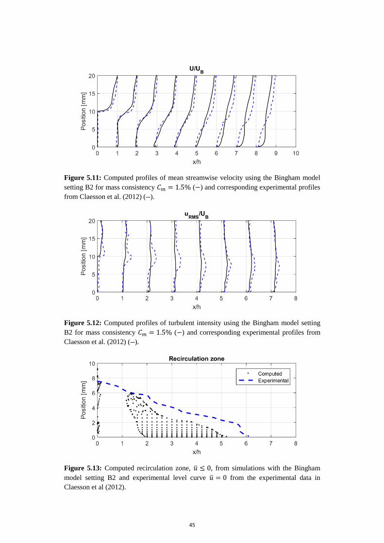
45
Figure 5.11: Computed profiles of mean streamwise velocity using the Bingham model
setting B2 for mass consistency ( ) and corresponding experimental profiles
from Claesson et al. (2012) (--).
Figure 5.12: Computed profiles of turbulent intensity using the Bingham model setting
B2 for mass consistency ( ) and corresponding experimental profiles from
Claesson et al. (2012) (--).
Figure 5.13: Computed recirculation zone, , from simulations with the Bingham
model setting B2 and experimental level curve from the experimental data in
Claesson et al (2012).

46
Bingham model with setting B3
Computed profiles of mean streamwise velocity for setting B3 can be seen together with
corresponding experimental profiles in Figure 5.14. Computed profiles of turbulent
intensity can be seen with corresponding experimental profiles in Figure 5.15. The
computed recirculation zone can be seen together with the experimental level
curve in Figure 5.16.
Figure 5.14: Computed profiles of mean streamwise velocity using the Bingham model
setting B3 for mass consistency ( ) and corresponding experimental profiles
from Claesson et al. (2012) (--).
Figure 5.15: Computed profiles of turbulent intensity using the Bingham model setting
B3 for mass consistency ( ) and corresponding experimental profiles from
Claesson et al. (2012) (--).

47
Figure 5.16: Computed recirculation zone, , from simulations with the Bingham
model setting B3 and experimental level curve from the experimental data in
Claesson et al (2012).
Comparison of Bingham setting B1,B2 and B3
By comparing the profiles of mean streamwise velocity and turbulent intensity resulting
from the simulations with the Bingham model setting B1, B2 and B3 it can be observed
that the general flow pattern is the same for all three settings. This is expected since the
same model is used with different parameter settings. In Figure 5.17 the computed RMS
errors from experimental profiles of mean streamwise velocity are plotted for the three
settings along the channel. All three settings produced the largest error in the downstream
part of the channel after the flow reattachment. In Figure 5.18 the computed RMS errors
of turbulent intensity can be seen for the three settings. A weak trend along the channel
may be identified for the turbulent intensity error with a local maximum around
and a local minimum around . However, all three settings fail to capture the
mixing layer seen in the experimental data, which is a major source of error.
Comparing the recirculation zones computed with the three model settings it can be seen
that the experimental recirculation zone is clearly better resembled by setting B3 than
with the other two settings. Looking at the computed errors it can also be observed that
the setting B3 produced the smallest or next to smallest errors among the three settings
along the channel. Given the results it may inferred that setting B3 is the best parameter
setting in the first step of the validation study.

48
Figure 5.17: Standard error from experimental profiles of mean streamwise velocity at
streamwise points downstream of the step from simulations with Bingham model setting
B1, B2 and B3.
Figure 5.18: Standard error from experimental profiles of turbulent intensity at
streamwise points downstream of the step from simulations with Bingham model setting
B1, B2 and B3.
Bingham model with setting B4
Computed profiles of mean streamwise velocity for setting B4 can be seen together with
corresponding experimental profiles in Figure 5.19. Computed profiles of turbulent
intensity can be seen with corresponding experimental profiles in Figure 5.20. The
computed recirculation can be seen together with experimental level curve in
Figure 5.21. The zone resembles experimental data to some extent with respect to shape.
Size and position of the zone is poorly resembled.

49
Figure 5.19: Computed profiles of mean streamwise velocity using the Bingham model
setting B4 for mass consistency ( ) and corresponding experimental profiles
from Claesson et al. (2012) (--).
Figure 5.20: Computed profiles of turbulent intensity using the Bingham model setting
B4 for mass consistency ( ) and corresponding experimental profiles from
Claesson et al. (2012) (--).
Figure 5.21: Computed recirculation zone, , from simulations with the Bingham
model setting B4 and experimental level curve from the experimental data in
Claesson et al (2012).

50
Bingham model with setting B5
Computed profiles of mean streamwise velocity for setting B5 can be seen together with
corresponding experimental profiles in Figure 5.22. Computed profiles of turbulent
intensity can be seen with corresponding experimental profiles in Figure 5.23. The
computed recirculation zone can be seen together with the experimental level
curve in Figure 5.24.
Figure 5.22: Computed profiles of mean streamwise velocity using the Bingham model
setting B5 for mass consistency ( ) and corresponding experimental profiles
from Claesson et al. (2012) (--).
Figure 5.23: Computed profiles of turbulent intensity using the Bingham model setting
B5 for mass consistency ( ) and corresponding experimental profiles from
Claesson et al. (2012) (--).

51
Figure 5.24: Computed recirculation zone, , from simulations with the Bingham
model setting B5 and experimental level curve from the experimental data in
Claesson et al (2012).
Comparison of Bingham setting B3, B4 and B5
Computed RMS errors from the experimental profiles of mean streamwise velocity can
be seen for the three settings in Figure 5.25 for setting B3, B4 and B5. RMS errors from
experimental profiles of turbulent intensity can be seen in Figure 5.26. Similar general
trends as for the settings in the first step of the Bingham model validation study, i.e.
setting B1, B2 and B3, can also be seen for setting B4 and B5. The mean velocity errors
increase with the downstream distance from the step and the turbulent intensity error has
a local maximum around and a local minimum around . However, all
three settings fail to capture mixing layer seen in the experimental data, which again is a
major source of error.
By comparing the computed recirculation zones for the three settings it can be observed
that both setting B4 and B5 yielded zones that resembled the experimental data
significantly worse than setting B3. Setting B3 also yielded the smallest or next to
smallest errors among the three in the major part of the channel downstream of the step,
both with respect to mean streamwise velocity and turbulent intensity. Given these results
it may be inferred that setting B3 is the best parameter setting for the Bingham model of
the ones studied.

52
Figure 5.25: Standard error from experimental profiles of mean streamwise velocity at
streamwise points downstream of the step from simulations with Bingham model setting
B3, B4 and B5.
Figure 5.26: Standard error from experimental profiles of turbulent intensity at
streamwise points downstream of the step from simulations with Bingham model setting
B3, B4 and B5.
5.1.4 Simulations with the ODF model
Results obtained from all simulations performed with the ODF model are presented in
this section. The results from each step of the validation study are first presented
individually and then compared to all simulations in the same step.
ODF model setting R1
Computed profiles of mean streamwise velocity for setting R1 can be seen together with
corresponding experimental profiles in Figure 5.27. Computed profiles of turbulent
intensity can be seen with corresponding experimental profiles in Figure 5.28. The
computed recirculation zone can be seen together with the experimental level
curve in Figure 5.29.
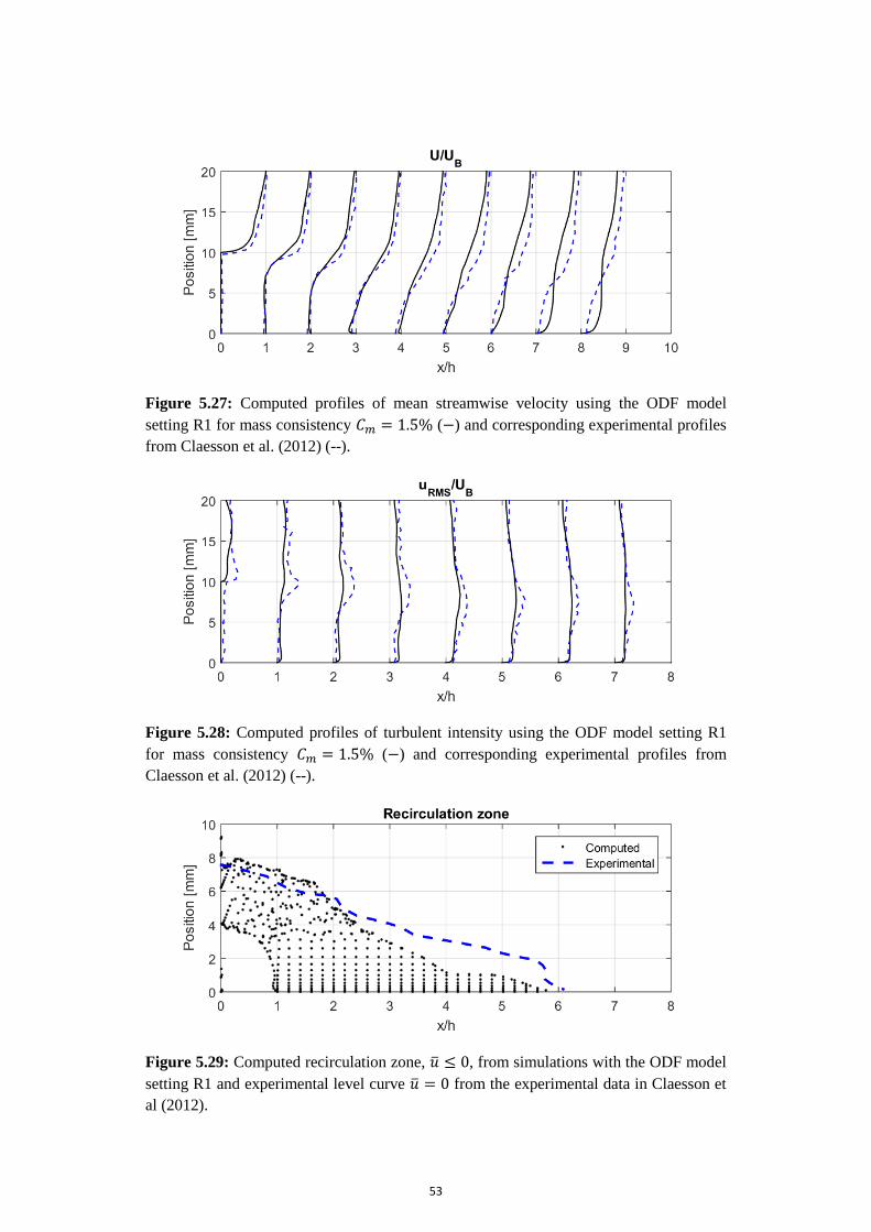
53
Figure 5.27: Computed profiles of mean streamwise velocity using the ODF model
setting R1 for mass consistency ( ) and corresponding experimental profiles
from Claesson et al. (2012) (--).
Figure 5.28: Computed profiles of turbulent intensity using the ODF model setting R1
for mass consistency ( ) and corresponding experimental profiles from
Claesson et al. (2012) (--).
Figure 5.29: Computed recirculation zone, , from simulations with the ODF model
setting R1 and experimental level curve from the experimental data in Claesson et
al (2012).

54
ODF model setting R2
Computed profiles of mean streamwise velocity for setting R2 can be seen together with
corresponding experimental profiles in Figure 5.30. Computed profiles of turbulent
intensity can be seen with corresponding experimental profiles in Figure 5.31. The
computed recirculation zone can be seen together with the experimental level
curve in Figure 5.32.
Figure 5.30: Computed profiles of mean streamwise velocity using the ODF model
setting R2 for mass consistency ( ) and corresponding experimental profiles
from Claesson et al. (2012) (--).
Figure 5.31: Computed profiles of turbulent intensity using the ODF model setting R2
for mass consistency ( ) and corresponding experimental profiles from
Claesson et al. (2012) (--).

55
Figure 5.32: Computed recirculation zone, , from simulations with the ODF model
setting R2 and experimental level curve from the experimental data in Claesson et
al (2012).
ODF model setting R3
Computed profiles of mean streamwise velocity for setting R3 can be seen together with
corresponding experimental profiles in Figure 5.33. Computed profiles of turbulent
intensity can be seen with corresponding experimental profiles in Figure 5.34. The
computed recirculation zone can be seen together with the experimental level
curve in Figure 5.35.
Figure 5.33: Computed profiles of mean streamwise velocity using the ODF model
setting R3 for mass consistency ( ) and corresponding experimental profiles
from Claesson et al. (2012) (--).

56
Figure 5.34: Computed profiles of turbulent intensity using the ODF model setting R3
for mass consistency ( ) and corresponding experimental profiles from
Claesson et al. (2012) (--).
Figure 5.35: Computed recirculation zone, , from simulations with the ODF model
setting R3 and experimental level curve from the experimental data in Claesson et
al (2012).
Comparison of ODF model setting R1, R2 and R3
In Figure 5.36 computed RMS errors from the experimental profiles of mean streamwise
velocity are plotted for settings R1, R2 and R3. In Figure 5.36 the computed RMS errors
from experimental profiles of mean streamwise velocity can be seen for the three settings.
In the same way as for the simulations with the Bingham model a general trend can be
seen for the mean velocity errors as they increase with downstream distance from the
step. A similar trend as for the Bingham model simulations can also be seen for the
turbulent intensity errors with local maxima slightly downstream of the step and local
minima further downstream.
By comparing the computed recirculation zones for setting R1, R2 and R3 it can be seen
that neither of the settings gave as good resemblance as the best Bingham model setting,
B3. The different settings do however capture different features of the recirculation zone.
The given results indicate that the different choice of values of homogenous ODF
standard deviation may capture different parts of the flow pattern correctly. They also
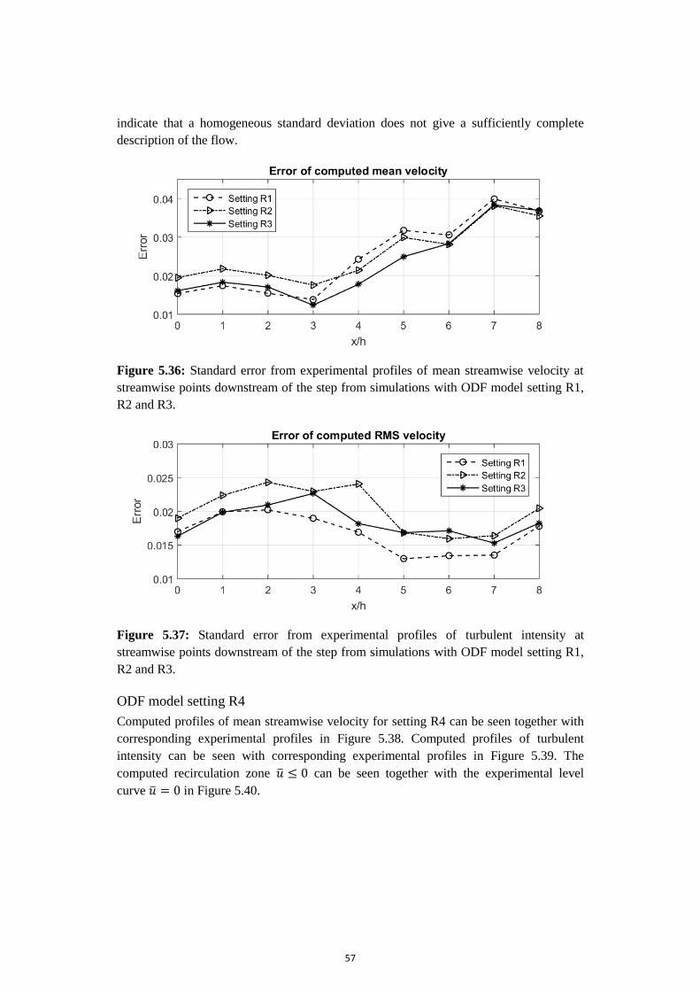
57
indicate that a homogeneous standard deviation does not give a sufficiently complete
description of the flow.
Figure 5.36: Standard error from experimental profiles of mean streamwise velocity at
streamwise points downstream of the step from simulations with ODF model setting R1,
R2 and R3.
Figure 5.37: Standard error from experimental profiles of turbulent intensity at
streamwise points downstream of the step from simulations with ODF model setting R1,
R2 and R3.
ODF model setting R4
Computed profiles of mean streamwise velocity for setting R4 can be seen together with
corresponding experimental profiles in Figure 5.38. Computed profiles of turbulent
intensity can be seen with corresponding experimental profiles in Figure 5.39. The
computed recirculation zone can be seen together with the experimental level
curve in Figure 5.40.

58
Figure 5.38: Computed profiles of mean streamwise velocity using the ODF model
setting R4 for mass consistency ( ) and corresponding experimental profiles
from Claesson et al. (2012) (--).
Figure 5.39: Computed profiles of turbulent intensity using the ODF model setting R4
for mass consistency ( ) and corresponding experimental profiles from
Claesson et al. (2012) (--).
Figure 5.40: Computed recirculation zone, , from simulations with the ODF model
setting R4 and experimental level curve from the experimental data in Claesson et
al (2012).

59
ODF model setting R5
Computed profiles of mean streamwise velocity for setting R5 can be seen together with
corresponding experimental profiles in Figure 5.41. Computed profiles of turbulent
intensity can be seen with corresponding experimental profiles in Figure 5.42. The
computed recirculation zone can be seen together with the experimental level
curve in Figure 5.43.
Figure 5.41: Computed profiles of mean streamwise velocity using the ODF model
setting R5 for mass consistency ( ) and corresponding experimental profiles
from Claesson et al. (2012) (--).
Figure 5.42: Computed profiles of turbulent intensity using the ODF model setting R5
for mass consistency ( ) and corresponding experimental profiles from
Claesson et al. (2012) (--).

60
Figure 5.43: Computed recirculation zone, , from simulations with the ODF model
setting R5 and experimental level curve from the experimental data in Claesson et
al (2012).
ODF model setting R6
Computed profiles of mean streamwise velocity for setting R6 can be seen together with
corresponding experimental profiles in Figure 5.44. Computed profiles of turbulent
intensity can be seen with corresponding experimental profiles in Figure 5.45. The
computed recirculation zone can be seen together with the experimental level
curve in Figure 5.46.
Figure 5.44: Computed profiles of mean streamwise velocity using the ODF model
setting R6 for mass consistency ( ) and corresponding experimental profiles
from Claesson et al. (2012) (--).

61
Figure 5.45: Computed profiles of turbulent intensity using the ODF model setting R6
for mass consistency ( ) and corresponding experimental profiles from
Claesson et al. (2012) (--).
Figure 5.46: Computed recirculation zone, , from simulations with the ODF model
setting R6 and experimental level curve from the experimental data in Claesson et
al (2012).
Comparison of ODF model setting R4, R5 and R6
In Figure 5.47 the computed RMS errors from experimental profiles of mean streamwise
velocity are plotted for setting R4, R5 and R6. In Figure 5.48 the computed RMS errors
from experimental profiles of turbulent intensity can be seen for the three settings. The
same general trends are seen as for all previous simulations with the Bingham model and
the ODF model.
Comparing the recirculation zones for the three settings it can be observed that while
setting R5 clearly gives the worst prediction of the three, setting R4 and R6 both predict
the recirculation zone to some extent. Setting R4 gives a good prediction on the length of
the zone but the shape is not correct. Setting R6 slightly underestimates the length of the
zone but the shape is well predicted. Setting R6 has the smallest or next to smallest error
with respect to mean velocity along the channel while the error with respect to turbulent
intensity actually is the largest of the three settings for the middle section of the channel.
Setting R4, the other hand has the smallest or next to smallest error with respect to

62
turbulent intensity along the channel while the mean velocity error is the largest among
the three for the middle section. Given the results both setting R4 and R6 could be seen as
the best parameter setting among the three. However, given that the turbulent intensity
contains large errors due to that the mixing layer was not captured by simulations, the
result that setting R6 performed well with respect to mean velocity and in resembling the
recirculation zone may be used as motivation to for setting R6 being the best setting out
of the three. It was therefore the one chosen for further validation.
Figure 5.47: Standard error from experimental profiles of mean streamwise velocity at
streamwise points downstream of the step from simulations with ODF model setting R4,
R5 and R6.
Figure 5.48: Standard error from experimental profiles of turbulent intensity at
streamwise points downstream of the step from simulations with ODF model setting R4,
R5 and R6.
ODF model setting R7
Computed profiles of mean streamwise velocity for setting R6 can be seen together with
corresponding experimental profiles in Figure 5.49. Computed profiles of turbulent
intensity can be seen with corresponding experimental profiles in Figure 5.50. The
computed recirculation zone can be seen together with the experimental level
curve in in Figure 5.51.

63
Figure 5.49: Computed profiles of mean streamwise velocity using the ODF model
setting R7 for mass consistency ( ) and corresponding experimental profiles
from Claesson et al. (2012) (--).
Figure 5.50: Computed profiles of turbulent intensity using the ODF model setting R7
for mass consistency ( ) and corresponding experimental profiles from
Claesson et al. (2012) (--).
Figure 5.51: Computed recirculation zone, , from simulations with the ODF model
setting R7 and experimental level curve from the experimental data in Claesson et
al (2012).

64
ODF model setting R8
Computed profiles of mean streamwise velocity for setting R6 can be seen together with
corresponding experimental profiles in Figure 5.52. Computed profiles of turbulent
intensity can be seen with corresponding experimental profiles in Figure 5.53. The
computed recirculation zone can be seen together with the experimental level
curve in Figure 5.54.
Figure 5.52: Computed profiles of mean streamwise velocity using the ODF model
setting R8 for mass consistency ( ) and corresponding experimental profiles
from Claesson et al. (2012) (--).
Figure 5.53: Computed profiles of turbulent intensity using the ODF model setting R8
for mass consistency ( ) and corresponding experimental profiles from
Claesson et al. (2012) (--).

65
Figure 5.54: Computed recirculation zone, , from simulations with the ODF model
setting R8 and experimental level curve from the experimental data in Claesson et
al (2012).
Comparison of ODF model setting R6, R7 and R8
In Figure 5.55 the computed RMS errors of mean streamwise velocity from
corresponding experimental profiles can be seen for setting R6, R7 and R8. In Figure
5.56 the computed root mean square errors of turbulent intensity can be seen for the tree
settings. The same general trends can be seen as for all presented simulations with the
fibre models. Setting R6 has the smallest or next to smallest error among the three
settings both with respect to mean streamwise velocity and turbulent intensity.
Comparing the three recirculation zones it can be observed that both setting R7 and R8
gave worse resemblance of the experimental data than setting R6. Given results indicate
the among the three settings compared setting R6 is the best performing parameter
setting.
Figure 5.55: Standard error from experimental profiles of mean streamwise velocity at
streamwise points downstream of the step from simulations with ODF model setting R6,
R7 and R8.

66
Figure 5.56: Standard error from experimental profiles of turbulent intensity at
streamwise points downstream of the step from simulations with ODF model setting R6,
R7 and R8.
5.1.5 Comparison between the respective models
Computed RMS errors from experimental profiles of mean streamwise velocity can be
seen in Figure 5.57 for the best performing Bingham model setting, setting B3, for the
best performing ODF model setting, setting R6, and computed in the same way from
simulations of pure water flow. Corresponding RMS square errors with respect to
turbulent intensity can be seen in Figure 5.58. It can be seen that for the upstream half of
the channel downstream of the step the simulations with pure water does actually produce
smaller errors than the fibre models. The result that pure water simulations may be able to
resemble suspension flow in that area is somewhat expected since it is a turbulent area
where the suspension is expected to be fluidised and exhibit Newtonian-like rheology.
Further downstream, as turbulence decays, fibre effects increase in significance for the
flow pattern and it can be seen in both Figure 5.57 and in Figure 5.58 that the fibre
models both result in smaller errors. The computed recirculation zones for the
three cases are shown for comparison in Figure 5.59. The experimental recirculation zone
curve from experiments with fibre mass consistency are included with
all three recirculation zones. It can be observed that both the Bingham model and the
ODF model outperform the pure water simulations in resembling the experimental
recirculation zone the fibre suspension flow.
The fibre models showed better agreement with experimental profiles of mean velocity
and turbulent intensity, respectively, in the downstream part of the channel downstream
of the step. The recirculation zones produced by the simulations with the fibre models are
both significantly better than the one obtained in the simulation of pure water. The results
indicate that the fibre models take into account fibre effects on the suspension flow that
are not captured by simulations of pure water. The performances of the best parameter
settings for the Bingham model and the ODF model, respectively, are close to similar
both with respect to computed errors and recirculation zones. Comparing the RMS errors
of the models it can be observed that the Bingham model has the larger error in the
upstream half of the channel and the lower error in the downstream part out of the two
models. The recirculation zone is slightly better resembled by the Bingham model,

67
mainly because the length is slightly better resembled. Given the results the Bingham
model is slightly more accurate than the ODF model, at least with the parameter settings
tested at current stage and with the given experimental data.
Figure 5.57: Standard error from experimental profiles of mean streamwise velocity at
streamwise points downstream of the step for the best performing settings of the Bingham
model and the ODF model and for pure water.
Figure 5.58: Standard error from experimental profiles of turbulent intensity at
streamwise points downstream of the step for the best performing settings of the Bingham
model and the ODF model and for pure water.

68
Figure 5.59: Computed recirculation zone using pure water (left), Bingham model setting
B3 (middle) and ODF model setting R6 (right) plotted together with the recirculation
curve obtained in the experiments by Claesson et al (2012) with fibre mass consistency
.
5.2 Comparison with experiments by Xu & Aidun (2005)
Computed profiles of mean streamwise velocity and turbulent intensity can be seen
plotted with corresponding experimental data from Xu & Aidun (2005) in Figure 5.60 for
fibre mass concentration and , in Figure 5.61 for and
, in Figure 5.62 for and and in Figure 5.63 for and
. A general trend observed is that both models resemble the experimental
velocity profiles better for higher Reynolds number than for lower and for lower fibre
concentration than for higher. The result is expected since both a high Reynolds number
and a low fibre concentration, respectively, decreases the effects of fibres in such a way
that the suspension will exhibit Newtonian rheology. At lower Reynolds number and,
especially, at the higher concentration fibre effects which are difficult to model correctly
become more important for the flow. In addition, Xu & Aidun (2005) also concluded that
increased flow rate decreases the influence of fibre effects.
With exception for the case of the lower Reynolds number and the higher concentration
the predicted turbulent intensity is systematically overestimated by both fibre models.
The results may indicate that the fibre models do not dampen the turbulence sufficiently
to resemble the experimental flow correctly. In the case of the lower Reynolds number
and the higher concentration, however, the Bingham model instead underestimates the
turbulent intensity, indicating the turbulence in that flow is instead to much dampened.
The overall results show that the performance of the studied fibre models depend strongly
on the flow regime and concentration. The models showed success in resembling the
experimental profiles of mean velocity and turbulent intensity in the more turbulent
flows, which they are intended for.

69
Figure 5.60: Profiles of velocity (left) and turbulent intensity (right) at and
. Computed using the Bingham model ( ), the ODF model (-- ) and read
from Xu & Aidun (2005)(o).
Figure 5.61: Profiles of velocity (left) and turbulent intensity (right) at and
. Computed using the Bingham model ( ), the ODF model (-- ) and read
from Xu & Aidun (2005) (o).

70
Figure 5.62: Profiles of velocity (left) and turbulent intensity (right) at and
. Computed using the Bingham model ( ), the ODF model (-- ) and read
from Xu & Aidun (2005) (o).
Figure 5.63: Profiles of velocity (left) and turbulent intensity (right) at and
. Computed using the Bingham model ( ), the ODF model (-- ) and read
from Xu & Aidun (2005) (o).
5.3 Disc refiner application
Results from the simulation of the disc refiner, described in Section 4.4, are presented in
this section. Computed data was plotted over the cross section of the refiner groove at
four different positions downstream of the inlet, namely at -coordinates , ,
and , respectively. A model showing the cross sections can be seen in
Figure 5.64. The top wall is moving in the direction from right to left in all plots, as seen
from the flow inlet. A clarifying sketch can be seen in Figure 5.65.

71
Figure 5.64: 3-D model of disc refiner groove geometry showing the cross sections used
for visualising computed data.
Figure 5.65: Direction of movement of the top wall in the disc refiner model, as seen
from the inlet.
For the four positions in the groove direction, the velocity magnitude can be seen in
Figure 5.66 plotted over the cross section. It can be observed that at , i.e. fairly
close to the inlet, the velocity is practically uniform over the cross section, with exception
for boundary layers near channel walls and the moving top wall. Increasing with distance
from the inlet the uniformity in the velocity is disturbed to a greater extent. The top wall
is moving with velocity , which is on the same order of magnitude as the
streamwise flow with velocity . A certain disturbance in the resulting flow is
therefore to expect. The moving top wall should induce some swirling pattern in the flow.
The intensity of the swirling motion should also increase with distance from the inlet, as
the inlet is not swirling.
Figure 5.66: Velocity magnitude plotted in the groove cross section at four
different streamwise coordinates .
Vectors of velocity projected in the cross section can be seen in Figure 5.67 for channel-
part of the cross section, i.e. without the part section in the gap between bars and the
moving wall. The gap area was left out since it only had very large velocities in the

72
direction of the top wall movement. It can be observed from the vectors that the flow is
indeed swirling in upper part of the groove. The intensity of the swirling motion is also,
as expected, increasing with distance from the inlet. In the lower part of the groove the
swirling motion is practically non-existent and it can be seen from the velocity magnitude
in Figure 5.66 together with the small magnitude of the projected vectors in Figure 5.67
that the flow there is mainly in the groove direction. Similar results with swirling flow in
the upper part of the groove were also found in physical and numerical experiments in
Prahl Wittberg et. al (2012) for a similar flow model and geometry.
Figure 5.67: Velocity vectors projected in the plane perpendicular to the flow
direction plotted in the disc refiner groove.
Turbulent intensity in the flow was computed as
√
(5.2)
where is bulk velocity in the flow and turbulent kinetic energy. The bulk velocity
was defined as the free stream velocity at the inlet in the simulation, . In
Figure 5.68 the turbulent intensity is plotted over the cross section of the groove at the
same four positions as previous plots. It can be observed that a lot of turbulence occurs
close to the moving top wall, especially where the movement forces fluid into to the small
gap and onto the bar in the upper left corner. Results near and in the thin gaps should,
however, be interpreted carefully because of the poor mesh resolution in the area.
Turbulent intensity near all walls increases with increased distance from the inlet which is
likely due to increased disturbance from the moving wall on motion and flow
development.

73
Figure 5.68: Turbulent intensity plotted in the groove cross section at four different
streamwise coordinates . Bulk velocity taken as maximum inlet velocity .
The pressure field can be seen plotted over the groove cross section at the four positions
in Figure 5.69. Different scales on the colour bars are used for the plots since no common
scale showed variations over the cross section clearly. It can be observed that the general
pattern over the cross section, although decreasing in magnitude from inlet to outlet, is
roughly the same for the four positions. They all show a high pressure zone in the upper
left corner of the groove, where the moving top wall forces fluid into the narrow gap and
onto the channel wall. Again these results should be interpreted carefully due to the low
mesh resolution in the area.
Figure 5.69: Pressure plotted in the groove cross section at four different
streamwise coordinates .
The effective viscosity computed from the Bingham model is plotted over the cross
section at the four positions in Figure 5.70. The results are consistent with the rest of the

74
presented results, given that the effective viscosity decreases with shear rate. At the inlet
the velocity field is close to uniform except for in the boundary layers so that the shear
rate is large close to walls but not away from them. The effective viscosity is thus large in
the centre but low near walls. The viscosity is lower in the upper half of the channel
which most likely is due to increased shear rate from the induced swirling motion. As the
distance from the inlet increases the swirl increases in the top part of the channel and
therefore also the shear rate, lowering the effective viscosity. At all walls the turbulent
intensity increases further away from the wall, which results in increased boundary layer
thickness and higher shear rates further from the wall compared to near the inlet. The
zone of high viscosity in the centre of the channel therefore decreases in size as the
distance from the inlet increases.
Figure 5.70: Effective viscosity plotted in the groove cross section at four
different streamwise coordinates .

75
6
Discussion
Important parts and aspects of the project are discussed in this section. First a general
discussion on relevant error sources is given. The fibre models are then discussed with
respect to performance, specific features and possible further development. The two fibre
models are also discussed in comparison to one another. A short coverage on the disc
refiner simulation is then made. Finally an outlook on future work is presented.
6.1 Error sources
There is always a trade-off between accuracy and computational cost in CFD-simulations
and in numerical modelling in general. A coarse numerical grid may give low
computational costs but yield inaccurate results. High resolution, on the other hand, gives
accurate results but to high if not unaffordable computational costs. In addition, transient
simulations with high spatial resolution also demand high temporal resolution CFL
condition to be fulfilled, enhancing solution stability. A sufficient number of
iterations time step must also be executed at each time step to obtain convergence, but a
too large number of iterations will increase the computational cost.
Modelling is often a major source of error in CFD-simulations. Turbulence modelling is
commonly used, which significantly reduces the mesh resolution required compared to
resolving all turbulent fluctuations in a flow. On the other hand certain modelling errors
are also introduced. How large the modelling errors are varies between models and
different turbulence models are suitable for different flows. In simulations performed
within this thesis work fibre modelling should also be considered a major source of
errors. Both fibre models tested used macroscopic approaches in contrary to resolving
micro-scale mechanisms. In addition, the complex rheology of fibre suspensions varies
with concentration and flow regime and it may be difficult to capture all flow features
within such simplified models. Certain modelling errors are therefore expected. It may
also be remarked that since only two experimental flow cases were used to validate the
models the risk of over-fitting must be considered. That would be the case if parameters
are fitted very well to the data used for tuning parameters, but may not be representative
for flows in general. To further validate the models and the parameter settings more
rigorously additional experiments for a variety of representative flow situations would be
preferable.

76
Regarding the validation procedure one should always expect certain errors when
comparing results from numerical simulations to experimentally obtained data, as was
made in this work. Numerical data has its own error sources, as discussed above, and
experimental data itself contains measurement errors. In addition, it can be difficult to
correctly model the experimental flow case correctly with respect to, for instance,
geometry. The numerical mesh may be differing slightly from the experimental geometry
which can cause major errors. An example of this was seen in the process of creating a
mesh for the backwards facing step, described in Section 4.2.1, where the flow geometry
upstream of the step showed to have a large impact the flow downstream of the step.
For the ODF model a miscalculation in the derivation of a relation between , and
, which was then used to compute , led to that computations were executed with a
fibre aspect ratio half as large as originally intended. The error was discovered after all
simulations were completed. The wrong values used for is clearly a possible source of
error. It should, though, be remarked that the error generated by systematically using
instead of , which resulted from miscalculation, may have been cancelled out by, for
instance, the choice of slope in the relation for computing the ODF standard deviation
which was tuned to experimental data. A correct value of may result in another slope
being required to resemble the experimental data correctly.
A possible concrete example of a modelling error was the results that all simulations
failed to capture the mixing layer in the backwards facing step flow, a feature that could
be seen in the experimental data. Even in the case of pure water, which has lower average
viscosity than a fibre suspension and should thus exhibit more turbulence, simulations
failed to capture the mixing layer. The profiles of turbulent intensity for pure water can be
seen in Figure 6.1. The source of the error could, for instance, be either the flow geometry
or the turbulence modelling.
Figure 6.1: Computed profiles of turbulent intensity from simulations of pure water in
the backwards facing step ( ) and experimental profiles fibre suspension with mass
concentration from Claesson et al. (2012) (--).
77
6.2 Fibre models
Results obtained from simulations with both of the studied fibre models succeeded to a
large degree to reproduce experimental data both in the flow over the backwards facing
step and in the rectangular channel. In both flow cases the resemblance of experimental
data was better in the more turbulent flow areas and flow cases, respectively, than where
turbulence was less significant. The lower the turbulence levels in a flow are, and as
turbulence decays, the more the fibres affect the suspension rheology. The systematic
errors in such parts of the flows serve to illustrate the difficulties in finding a model that
correctly takes fibre effects into account for all regimes of a flow. As it may be expected,
an accurate macroscopic model that is valid for flows governed by complex micro-scale
physical phenomena is difficult to construct. However, with the parameters identified as
the best for the respective models both models resembled experimental data better than
simulations of pure water in the backwards facing step case. In addition the models were
further validated in the rectangular channel case. Those simulations showed that the fibre
models both yielded results that resembled experimental data well, with exception for
slightly overestimation of turbulent intensity, for low concentration and high flow rate.
Again cases of turbulent flows where the fibre models give good results. Individual
features of the respective models are discussed below.
6.2.1 Bingham model
By modelling fibre suspension flow with the Bingham model a highly simplified
description of the rheology is obtained, based on empirical observations and relations. For
instance, the parameters and , which are used to compute the yield stress , are not
general but varies from suspension to suspension. Modelling a fibre suspension as a non-
Newtonian fluid using a Bingham model have been done by others prior to this work
where laminar flow was assumed (Fock et al., 2010), (Ford et al., 2006), (Prahl Wittberg
et al., 2012). In this work, however, the Bingham model also used for simulation of
turbulent suspension flow. To argue that the Bingham model may be valid for turbulent
flow it can be shown that it exhibits certain features which are expected from
experimental observations. Fibre suspensions become fluidised in sufficiently turbulent
flows, as described in Section 3.2, meaning that the suspension rheology approaches that
of a Newtonian fluid. It can be seen from Equation (4.2) that this is the case with the
Bingham model since at large shear rates , which occur in turbulent flows, the effective
viscosity is
(6.1)
What constant viscosity value should then be assigned to the consistency index ? In the
study performed within this work focus was pointed at the parameters , and while
consistency index was set to the viscosity of water. The same was made in Fock et al.
(2010) and Ford et al. (2006). However, a study on the parameter would be desired to
fully evaluate the model. Varying the parameters and , used to computed the yield
stress, and showed to have significant impact on the results which could be the case
also for . It should be stressed that the parameter optimisation performed with

78
simulations on the backwards facing step was done in separate steps. In reality the
existence of a correlation between the parameters, including , is likely. A more rigorous
study of the model should therefore include all possible combinations of the model
parameters. However, in such a study the number of simulations increases rapidly with
the number of values for each parameter.
Since the model effectively acts through a modification of the suspension viscosity the
implementation in Fluent was straightforward and of low complexity. A single UDF was
created to compute the viscosity from the shear rate according to Equation (4.2). The
simple nature of the implementation also only resulted in a slightly increased
computational cost, compared to simulations of pure water flow. Some instabilities were
found, though, causing the need for an increased number of iterations per time step and
smaller under-relaxation factors. A stable solution computed with constant viscosity
before activating the Bingham model was also crucial to obtain stability. The exact source
of the instabilities is not known for certain, but they may arise from large gradients in
effective viscosity in some parts of the flow.
6.2.2 ODF model
Although being a lot more complex than the Bingham model, the ODF model does also
provide a simplified description of fibre suspension rheology. The coupling from the
orientation distribution of fibres to the fluid momentum equations rely on assumptions
such as fibres being rigid and in a certain concentration regime. Anisotropic effects of
fibre orientation are accounted for and influence the rheology while possible additional
anisotropic effects from fibres bending and twisting are neglected. The developed model
for the fibre distribution is empirical as it is based on results from numerical and
experimental results on the ODF in turbulent fibre suspension flows. Micro-scale
mechanisms determining movement and interaction of fibres, and thus the evolution of
the ODF, are being modelled and not resolved. Now, is the level of detail sufficient to
successfully describe a fibre suspension and can the modelling justified? First of all,
further evaluation of the model is needed to answer the questions fully. However,
computed results showed resemblance with experimental data to a certain extent. It
should also be remarked that while many levels of anisotropy can be incorporated in a
fibre model, at some point one needs to stop at a level that is possible to implement and
computationally affordable. In this work both computational resources and time were
limiting factors and the model was therefore only subjected to a limited study.
Since the model involves computation of the many components of the fibre orientation
tensors, where a lot of work was put into constructing the a priori expressions, the
implementation itself of the model was rather time-consuming and complex. The model
increased the number of computations performed per iteration and therefore also
increased the computation cost slightly. However, the a priori construction of the explicit
expressions for the orientation tensor components significantly decreased the number of
operations needed compared to numerically solve the integrals (4.17) (4.18) in each
iteration. The model showed good stability and converged easily without the need to
increase under-relaxation factors or the number of iterations per time step, compared to
simulations of pure water in the same geometries.
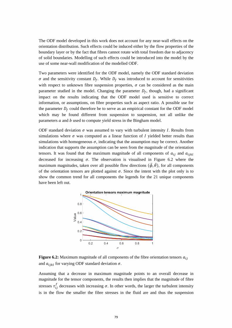
79
The ODF model developed in this work does not account for any near-wall effects on the
orientation distribution. Such effects could be induced either by the flow properties of the
boundary layer or by the fact that fibres cannot rotate with total freedom due to adjacency
of solid boundaries. Modelling of such effects could be introduced into the model by the
use of some near-wall modification of the modelled ODF.
Two parameters were identified for the ODF model, namely the ODF standard deviation
and the sensitivity constant . While was introduced to account for sensitivities
with respect to unknown fibre suspension properties, can be considered as the main
parameter studied in the model. Changing the parameter , though, had a significant
impact on the results indicating that the ODF model used is sensitive to correct
information, or assumptions, on fibre properties such as aspect ratio. A possible use for
the parameter could therefore be to serve as an empirical constant for the ODF model
which may be found different from suspension to suspension, not all unlike the
parameters and used to compute yield stress in the Bingham model.
ODF standard deviation was assumed to vary with turbulent intensity . Results from
simulations where was computed as a linear function of yielded better results than
simulations with homogeneous , indicating that the assumption may be correct. Another
indication that supports the assumption can be seen from the magnitude of the orientation
tensors. It was found that the maximum magnitude of all components of and
decreased for increasing . The observation is visualised in Figure 6.2 where the
maximum magnitudes, taken over all possible flow directions ( ), for all components
of the orientation tensors are plotted against . Since the intent with the plot only is to
show the common trend for all components the legends for the 21 unique components
have been left out.
Figure 6.2: Maximum magnitude of all components of the fibre orientation tensors
and for varying ODF standard deviation .
Assuming that a decrease in maximum magnitude points to an overall decrease in
magnitude for the tensor components, the results then implies that the magnitude of fibre
stresses
decreases with increasing . In other words, the larger the turbulent intensity
is in the flow the smaller the fibre stresses in the fluid are and thus the suspension

80
behaves more like a Newtonian fluid. The behaviour is expected for a fibre suspensions
as it should become fluidised in turbulent flow, as described in Section 3.2. It should be
remarked that computing the ODF standard deviation from turbulent intensity in the
way that was done in this work introduces some arbitrariness in how is defined. The
computation of demands the definition of a bulk velocity which may be far from
obvious in some flow cases. The consequence is that the model is not be well-defined for
an arbitrary flow case.
6.2.3 Comparison of fibre models
Both the Bingham model and the ODF model yielded results that resembled the
experimental data well in large parts of the flow. For both models it was also observed
that varying model parameters had clear impact on the computed results. Which one of
the Bingham model and the ODF model is then the best? To answer the question the
purpose of the modelling should be considered. The scope of this work was to find a fibre
model suitable for engineering applications with sufficient accuracy and with limited
computational cost. The ODF model opens up for a detailed description of the fibres
suspension due to its complexity and description of individual components of the
additional stresses arising from fibres in the suspension. It should be stressed, though, that
the ODF model proposed is a new model and has been studied to a very limited extent
within this work. The Bingham model, on the other hand, contains fewer uncertainties
and relies on fewer parameters that also can be found literature. In addition it has been
used to model fibre suspension flow prior to this work with examples to be found in
literature. Further, it also has slightly lower computational cost than the ODF model and
is easier to implement. With further investigation of the ODF model it may open up for
the possibility of using it as an alternative to the Bingham model for applications with
turbulent fibre suspension flows. However, for the sake of this project the Bingham
model was considered more suitable.
6.3 Disc refiner application The simulation performed with the disc refiner model was made to further validate the
use of the chosen fibre model in an application relevant for the pulp and paper industry.
Results from the simulation model showed a flow pattern that was expected and that
could be found for flow cases studied experimentally and numerically in Prahl Wittberg
et al. (2012). In their study different types of wood fibres at different consistencies
yielded slightly different results, though. Results from the simulation in this thesis work
did to a large extent yield results that could be expected prior to computations. However,
it should be stressed that since the gap clearance in the refiner model has the size on the
order of a few fibre diameters it is questionable if a fibre model where the suspension is
seen as a continuum, as the Bingham model, can really be justified. The results should
therefore at most be seen as coarse guidelines to the flow pattern in a disc refiner groove
rather than as a detailed description.
6.4 Future work The fibre models covered in this thesis work were only subjected to a small study due to
limitations in time and computational resources. To gain further knowledge on either of

81
the fibre models additional and more thorough studies need to be conducted. Additional
physical and numerical experimental studies are also crucial a process of further
developing the models. Physical experiments can give knowledge on fibre suspension
flow structures that are needed to develop the models to more sophisticated levels of
detail. Numerical experiments are needed to further validate the models with
experimental data, but also to determine numerical issues and advantages for the
respective models. Approaches for further development of the two models studies in this
thesis work are proposed below.
6.4.1 Bingham model
Current form of the Bingham model provides a simple description of fibre suspension
rheology implemented by modifying the suspension viscosity. The method results an
isotropic modification of viscous stresses, as all stresses are multiplied by the same factor
as
( ) (6.2)
A conceivable concept to further develop the rheology model could be to extend the
detail by introducing some anisotropic modification where the viscosity is modified
individually for each stress component . The viscous stresses could be computed on the
form
( ) ( ) (6.3)
where the viscosity then no longer is isotropic and its components depend on the
strain rate components in some way. A model on this form would introduce a higher
extent of freedom for the model and might therefore give better description of fibre
suspension rheology. However, thorough experimental and mathematical studies would
be needed to correctly construct such a model.
6.4.2 ODF model
First of all, since the ODF model at this stage is new and many of uncertainties exist,
simulations on a variety of flows should be performed and compared with experiments
where information on all model parameters are known. By conducting such a rigorous
study two main questions could come closer to being answered. Those questions are how
do the different parameters affect the rheology described by the model, and what fibre
types and concentration regimes are they valid for? A more detailed investigation on the
structures of the fibre stresses
could also serve as valid input for further development
of the model.
A more sophisticated method to compute the ODF standard deviation is needed. As
discussed in Section 6.2.2 computing from the turbulent intensity introduces some
arbitrariness since a reference velocity is needed to compute . In the Fokker-Planck
equation the rotational diffusivity of the ODF can be related to the strain rate in the
flow (Zhang, 2014). The idea that velocity gradients in the fluid will affect and induce
rotational motion of fibres and increase the variance of the ODF is also somewhat

82
intuitive. In addition, the strain rate is used to model the effect of unresolved turbulent
fluctuations in both RANS models and LES models. A use of the strain rate tensor to
connect ODF standard deviation with turbulence is therefore conceivable. The idea also
opens up for possible further development of the ODF model to incorporate a higher level
of detail. holds anisotropic information on the flow which could be used for a model
where the ODF standard deviation needs not to be equal in all directions. The ODF could
instead be modelled with a more general bivariate normal distribution, where the
correlation between the angles and not necessarily need to be zero. It should
remarked, though, that the method of fitting one-dimensional Fourier series expression
for the - and -parts of the fibre orientation tensors would in that case fall apart due to
the non-zero correlation of and . A suitable two-dimensional regression model would
instead be appropriate.

83
7
Conclusion
Approaches for modelling of turbulent fibre suspension flow were studied and two
models of different type were successfully implemented numerically. Both models
effectively act as single-phase flow models through modification or addition of viscous
stresses in the Navier-Stokes equation. A simpler model was denoted the Bingham model,
where the suspension is modelled as a non-Newtonian fluid by computing the effective
viscosity as a function of shear rate. A more complex model was denoted the ODF model,
where the suspension rheology was modelled through an additional stress tensor
computed from the orientation distribution of suspended fibres. A model for the
orientation distribution function (ODF) was developed using normal distributions for the
angular coordinates describing fibre rotation and their variance was connected to
turbulence. Explicit expressions to compute the fibre stresses as functions of the flow
field were constructed from the model using Fourier series.
For both models simulation results were compared to experimental data for the purpose
of validation. The parameter settings yielding the results with best resemblance of
experimental data for the respective models were then identified. Both models performed
well along with reasonable computational cost and stability. The Bingham model had a
simple implementation and resembled experimental data slightly better than the ODF
model. In addition, the ODF model is in need of further studies at the current stage. The
Bingham model was therefore identified as the best model and was also used to simulate
the flow in a disc refiner model and successfully resembled general flow patterns from
numerical and physical experiments in literature. In summary the aim of the work was
fulfilled and a suitable fibre model was delivered.


85
References
Andersson, S.R., Ringnér, J. & Rasmuson, A., 1999. The network strength of non-
flocculated fibre suspensions. Nordic Pulp and Paper Research Journal, 14(1), pp.61-70.
Andric, J. et al., 2013. A study of a flexible fiber model and its behavior in DNS of
turbulent channel flow. Acta Mechanica, 224(10), pp.2359-74.
ANSYS Inc. (a), 2013. ANSYS Fluent Theory Guide. Canonsburg, PA, USA: ANSYS
Inc.
ANSYS Inc. (b), 2013. ANSYS Fluent User's Guide. Canonsburg, PA, USA: ANSYS Inc.
Bennington, C.P.J. & Kerekes, R.J., 1996. Power requirements for pulp suspension
fluidization. TAPPI Journal, 79(2), pp.253-58.
BETA CAE Systems S.A., 2014. ANSA version 15.0.x User's Guide. Epanomi, Greece:
BETA CAE Systems S.A.
Claesson, J., Wikström, T. & Rasmuson, A., 2012. Flow of concentrated fiber
suspensions over a backward facing step studied using LDA. Nordic Pulp and Paper
Research Journal, 27(3), pp.653-61.
Crowe, C.T. & Michaelides, E.E., 2006. Multiphase Flow Handbook. Boca Raton: CRC
Press.
Davidson, L., 2014. Fluid Mechanics, Turbulent Flow and Turbulence. Lecture notes.
Gothenburg: Chalmers University of Technology Department of Applied Mechanics.
Davidson, L., 2015. An Introduction to Turbulence Models. Lecture notes. Göteborg:
Chalmers University of Technology Department of Thermo and Fluid Dynamics.
Derakhshandeh, B., Hatzikiriakos, S.G. & Bennington, C.P.J., 2010. The Apparent Yield
Stress of Pulp Fiber Suspensions. Journal of Rheology, 54(5), pp.1137-54.
Derakhshandeh, B., Kerekes, R.J., Hatzikiriakos, S.G. & Bennington, C.P.J., 2011.
Rheology of pulp fibre suspensions: A critical review. Chemical Engineering Science, 66,
pp.3460-70.
European Commission, 2014. Progress Towards Achieving the Kyoto and 2020
Objectives. Progress report. Brussels: European Comission.
Fock, H., Claesson, J. & Wikström, T., 2011. Near Wall Effects in the Plug Flow of Pulp
Suspensions. The Canadian Journal of Chemical Engineering, 89, pp.1207-16.

86
Fock, H., Rasmuson, A. & Wikström, T., 2010. CFD modeling of non-newtonian fluid
mixing accounting for transient changes in local solids concentration - application to an
agitated pulp stock chest. Nordic Pulp and Paper Research Journal, 25(1), pp.56-64.
Ford, C., Ein-Mozaffari, F., Bennington, C.P.J. & Taghipour, F., 2006. Simulation of
Mixing Dynamics in Agitated Pulp Stock Chests using CFD. AlChE Journal, 52(10),
pp.3562-69.
Frenander, K. et al., 2015. Flow Induced Venturi Cavitation to Improve Energy
Efficiency in Pulp Production [unpublished]., 2015.
Illikainen, M., Härkönen, E., Ullmar, M. & Niinimäki, J., 2007. Power consumption
distribution in a TMP refiner: comparison of the first and second stages. TAPPI Journal,
6(9), pp.18-23.
IPCC, 2014. Climate Change 2014. [Online] Available at:
http://www.ipcc.ch/pdf/assessment-
report/ar5/syr/SYR_AR5_LONGERREPORT_Corr2.pdf [Accessed 23 January 2015].
Irgens, F., 2014. Rheology and Non-Newtonian Fluids. Springer. (eBook).
Johansson, Ö. & Landström, L.-O., 2010. Slutrapport: Hur kan resonansfenomen
utnyttjas för att minska energiförbrukningen vid framställning av papper. Technical
report. ÅForsk.
Kerekes, R.J., 2006. Rheology of fibre suspensions in papermaking: An overview of
recent research. Nordic Pulp and Paper Research Journal, 21(5), pp.598-612.
Krochak, P.J., Olson, J.A. & Martinez, M., 2009. Fiber suspension flow in a tapered
channel: The effect of flow/fiber coupling. International Journal of Multiphase Flow,
35(7), pp.676-88.
Lindström, S.B. & Uesaka, T., 2008. Particle-level simulation of forming of the fiber
network in papermaking. International Journal of Engineering Science, 46(9), pp.858-76.
Lin, J., Liang, X. & Zhang, S., 2011. Fibre orientation distribution in turbulent fibre
suspensions flowing through an axisymmetric contraction. The Canadian Journal of
Chemical Engineering, 89(6), pp.1416-25.
Lin, J.Z., Liang, X.Y. & Zhang, S.L., 2012. Numerical simulation of fiber orientation
distribution in round turbulent jet of fiber suspension. Chemical Engineering Research
and Design, 90, pp.766-75.
Lin, J.-Z., Sun, K. & Lin, J., 2005. Distribution of Orientations in Fibre Suspension
Flowing in a Turbulent Boundary Layer. Chinese Physics Letters, 22(12).
Lundberg, A. et al., 2014. An automatic method for optimizing venturi shape in cavitation
flows [unpublished]., 2014. (Abstract accepted in July 2014).
87
Lundberg, A. et al., 2015. Automated Aerodynamic Vehicle Shape Optimization Using
Neural Networks and Evolutionary Optimization. SAE International journal of passenger
cars. Mechanical systems, 8(1).
Lundberg, A. et al., 2015. Flow Induced Cavitation - Phase 2. Technical Report. ÅF-
Industry AB.
Moosaie, A. & Manhart, M., 2013. Direct Monte Carlo simulation of turbulent drag
reduction by rigid fibers in a channel flow. Acta Mechanica, 224(10), pp.2385-413.
Mörtstedt, S.-E. & Hellsten, G., 2010. Data och Diagram, Energi- och kemitekniska
tabeller. 7th ed. Stockholm: Liber AB.
Nordling, C. & Österman, J., 2006. Physics Handbook for Science and Engineering. 84th
ed. Lund, Sweden: Studentlitterature AB.
Olson, J.A., Frigaard, I., Chan, C. & Hämäläinen, J.P., 2004. Modeling a turbulent fibre
suspension flowing in a planar contraction: The one-dimensional headbox. International
Journal of Multiphase Flow, 30(1), pp.51-66.
Prahl Wittberg, L. et al., 2012. Flow conditions in the grooves of a Low-Consistency
refiner. Nordic Pulp and Paper Research Journal, 27(2), pp.173-83.
Rajabi Nasab, N., Olson, J.A., Heymer, J. & Martinez, M.D., 2014. Understandnig of No-
load Power in Low Consistency Refiners. The Canadian Journal of Chemical
Engineering, 92(3), pp.524-35.
Rice, J.A., 2007. Mathematical Statistics and Data Analysis. 3rd ed. Belmont, California:
Thomson Brooks/Cole.
Shaqfeh, E.S.G. & Fredrickson, G.H., 1990. The hydrodynamic stress in a suspension of
rods. Physics of Fluids, 2(1), pp.7-24.
Swedish Energy Agency, 2014. En samlad bild över energiläget i Sverige. [Online]
Available at: http://www.energimyndigheten.se/Press/Nyheter/En-samlad-bild-over-
energilaget-i-Sverige/ [Accessed 23 January 2015].
Tu, J., Yeoh, G.-H. & Liu, C., 2013. Computational Fluid Dynamics A Practical
Approach. 2nd ed. Waltham MA, USA: Elsevier.
Xu, H. & Aidun, C.K., 2005. Characteristics of fiber suspension flow in a rectangular
channel. International Journal of Multiphase Flow, 31, pp.318-36.
Yang, W., Shen, S. & Ku, X., 2013. A new model of turbulent fibre suspension and its
application in the pipe flow. The Canadian Journal of Chemical Engineering, 91(5),
pp.992-99.
Zhang, F., 2014. Instability in Settling Fibres: A Numerical study. Doctoral thesis in
Engineering Mechanics. Stockholm, Sweden: Royal Institute of Technology KTH
Department of Mechanics.