Embed Size (px)
Citation preview

Second Edition, Version 2.24-2-2
http://www.freefem.org/ff++
F. Hecht, O. PironneauA. Le Hyaric, K. Ohtsuka
Laboratoire Jacques-Louis Lions, Universite Pierre et Marie Curie, Paris


FreeFem++Second Edition, Version 2.24-2-2
http://www.freefem.org/ff++
Frederic Hecht1,4mailto:[email protected]
http://www.ann.jussieu.fr/˜hecht
Olivier Pironneau1,3
mailto:[email protected]://www.ann.jussieu.fr/pironneau
Antoine Le Hyaric1,2
mailto:[email protected]://www.ann.jussieu.fr/˜lehyaric/
Kohji Ohtsuka5
mailto:[email protected]://http://www.comfos.org/
1. Laboratoire Jacques-Louis Lions, 175 rue du Chevaleret , 75013 Paris, France
Universite Pierre et Marie Curie, 4 Place Jussieu, 75252 PARIS cedex 05, France.
2. CNRS, UMR 7598, Laboratoire Jacques-Louis Lions, 175 rue du Chevaleret , 75013 Paris,France.
3. Institut de France, Academie des sciences, 23, quai de Conti, 75006 Paris, France.
4. INRIA, Projet Gamma, Domaine de Voluceau, Rocquencourt, B.P. 105, 78153 Le ChesnayCedex, France.
5. Hiroshima Kokusai Gakuin University, Hiroshima, Japan.
Acknowledgments We are very grateful to l’Ecole Polytechnique (Palaiseau, France) for printing the sec-ond edition of this manual (http://www.polytechnique.fr ), and to l’Agence Nationale de laRecherche (Paris, France) for funding of the extension of FreeFem++ to a parallel tridimensional version(http://www.agence-nationale-recherche.fr).

iv

Contents
1 Introduction 11.1 Installation . . . . . . . . . . . . . . . . . . . . . . . . . . . . . . . . . . . . . . 2
1.1.1 Installation from sources . . . . . . . . . . . . . . . . . . . . . . . . . . . 21.1.2 Windows binaries install . . . . . . . . . . . . . . . . . . . . . . . . . . . 41.1.3 MacOS X binaries install . . . . . . . . . . . . . . . . . . . . . . . . . . . 5
1.2 How to use FreeFem++ . . . . . . . . . . . . . . . . . . . . . . . . . . . . . . 51.3 Environment variables, and the init file . . . . . . . . . . . . . . . . . . . . . . . . 81.4 History . . . . . . . . . . . . . . . . . . . . . . . . . . . . . . . . . . . . . . . . 9
2 Getting Started 112.0.1 FEM by FreeFem++ : how does it work? . . . . . . . . . . . . . . . . . 122.0.2 Some Features of FreeFem++ . . . . . . . . . . . . . . . . . . . . . . . 16
2.1 The Development Cycle: Edit–Run/Visualize–Revise . . . . . . . . . . . . . . . . 16
3 Learning by Examples 193.1 Membranes . . . . . . . . . . . . . . . . . . . . . . . . . . . . . . . . . . . . . . 193.2 Heat Exchanger . . . . . . . . . . . . . . . . . . . . . . . . . . . . . . . . . . . . 243.3 Acoustics . . . . . . . . . . . . . . . . . . . . . . . . . . . . . . . . . . . . . . . 263.4 Thermal Conduction . . . . . . . . . . . . . . . . . . . . . . . . . . . . . . . . . 28
3.4.1 Axisymmetry: 3D Rod with circular section . . . . . . . . . . . . . . . . . 293.4.2 A Nonlinear Problem : Radiation . . . . . . . . . . . . . . . . . . . . . . 30
3.5 Irrotational Fan Blade Flow and Thermal effects . . . . . . . . . . . . . . . . . . . 303.5.1 Heat Convection around the airfoil . . . . . . . . . . . . . . . . . . . . . . 32
3.6 Pure Convection : The Rotating Hill . . . . . . . . . . . . . . . . . . . . . . . . . 333.7 A Projection Algorithm for the Navier-Stokes equations . . . . . . . . . . . . . . 373.8 The System of elasticity . . . . . . . . . . . . . . . . . . . . . . . . . . . . . . . . 393.9 The System of Stokes for Fluids . . . . . . . . . . . . . . . . . . . . . . . . . . . 413.10 A Large Fluid Problem . . . . . . . . . . . . . . . . . . . . . . . . . . . . . . . . 423.11 An Example with Complex Numbers . . . . . . . . . . . . . . . . . . . . . . . . . 453.12 Optimal Control . . . . . . . . . . . . . . . . . . . . . . . . . . . . . . . . . . . . 473.13 A Flow with Shocks . . . . . . . . . . . . . . . . . . . . . . . . . . . . . . . . . . 493.14 Classification of the equations . . . . . . . . . . . . . . . . . . . . . . . . . . . . 51
4 Syntax 554.1 Data Types . . . . . . . . . . . . . . . . . . . . . . . . . . . . . . . . . . . . . . 554.2 List of major types . . . . . . . . . . . . . . . . . . . . . . . . . . . . . . . . . . 564.3 Global Variables . . . . . . . . . . . . . . . . . . . . . . . . . . . . . . . . . . . . 57
i

ii CONTENTS
4.4 System Commands . . . . . . . . . . . . . . . . . . . . . . . . . . . . . . . . . . 584.5 Arithmetic . . . . . . . . . . . . . . . . . . . . . . . . . . . . . . . . . . . . . . . 584.6 One Variable Functions . . . . . . . . . . . . . . . . . . . . . . . . . . . . . . . . 614.7 Functions of Two Variables . . . . . . . . . . . . . . . . . . . . . . . . . . . . . . 63
4.7.1 Formula . . . . . . . . . . . . . . . . . . . . . . . . . . . . . . . . . . . . 634.7.2 FE-function . . . . . . . . . . . . . . . . . . . . . . . . . . . . . . . . . . 63
4.8 Arrays . . . . . . . . . . . . . . . . . . . . . . . . . . . . . . . . . . . . . . . . . 644.8.1 Arrays with two integer indices versus matrix . . . . . . . . . . . . . . . . 684.8.2 Matrix construction and setting . . . . . . . . . . . . . . . . . . . . . . . 694.8.3 Matrix Operations . . . . . . . . . . . . . . . . . . . . . . . . . . . . . . 704.8.4 Other arrays . . . . . . . . . . . . . . . . . . . . . . . . . . . . . . . . . . 73
4.9 Loops . . . . . . . . . . . . . . . . . . . . . . . . . . . . . . . . . . . . . . . . . 744.10 Input/Output . . . . . . . . . . . . . . . . . . . . . . . . . . . . . . . . . . . . . . 754.11 Exception handling . . . . . . . . . . . . . . . . . . . . . . . . . . . . . . . . . . 76
5 Mesh Generation 795.1 Commands for Mesh Generation . . . . . . . . . . . . . . . . . . . . . . . . . . . 79
5.1.1 Square . . . . . . . . . . . . . . . . . . . . . . . . . . . . . . . . . . . . 795.1.2 Border . . . . . . . . . . . . . . . . . . . . . . . . . . . . . . . . . . . . 805.1.3 Data Structure and Read/Write Statements for a Mesh . . . . . . . . . . . 815.1.4 Mesh Connectivity . . . . . . . . . . . . . . . . . . . . . . . . . . . . . . 845.1.5 The keyword ”triangulate” . . . . . . . . . . . . . . . . . . . . . . . . . . 85
5.2 Boundary FEM Spaces Built as Empty Meshes . . . . . . . . . . . . . . . . . . . 865.3 Remeshing . . . . . . . . . . . . . . . . . . . . . . . . . . . . . . . . . . . . . . 87
5.3.1 Movemesh . . . . . . . . . . . . . . . . . . . . . . . . . . . . . . . . . . 875.4 Regular Triangulation: hTriangle . . . . . . . . . . . . . . . . . . . . . . . . . 905.5 Adaptmesh . . . . . . . . . . . . . . . . . . . . . . . . . . . . . . . . . . . . . . 905.6 Trunc . . . . . . . . . . . . . . . . . . . . . . . . . . . . . . . . . . . . . . . . . 945.7 Splitmesh . . . . . . . . . . . . . . . . . . . . . . . . . . . . . . . . . . . . . . . 955.8 Meshing Examples . . . . . . . . . . . . . . . . . . . . . . . . . . . . . . . . . . 96
6 Finite Elements 1036.1 Lagrange finite element . . . . . . . . . . . . . . . . . . . . . . . . . . . . . . . . 105
6.1.1 P0-element . . . . . . . . . . . . . . . . . . . . . . . . . . . . . . . . . . 1056.1.2 P1-element . . . . . . . . . . . . . . . . . . . . . . . . . . . . . . . . . . 1056.1.3 P2-element . . . . . . . . . . . . . . . . . . . . . . . . . . . . . . . . . . 106
6.2 P1 Nonconforming Element . . . . . . . . . . . . . . . . . . . . . . . . . . . . . 1076.3 Other FE-space . . . . . . . . . . . . . . . . . . . . . . . . . . . . . . . . . . . . 1086.4 Vector valued FE-function . . . . . . . . . . . . . . . . . . . . . . . . . . . . . . 109
6.4.1 Raviart-Thomas element . . . . . . . . . . . . . . . . . . . . . . . . . . . 1096.5 A Fast Finite Element Interpolator . . . . . . . . . . . . . . . . . . . . . . . . . . 1116.6 Keywords: Problem and Solve . . . . . . . . . . . . . . . . . . . . . . . . . . . . 113
6.6.1 Weak form and Boundary Condition . . . . . . . . . . . . . . . . . . . . . 1146.7 Parameters affecting solve and problem . . . . . . . . . . . . . . . . . . . . . 1156.8 Problem definition . . . . . . . . . . . . . . . . . . . . . . . . . . . . . . . . . . 1166.9 Numerical Integration . . . . . . . . . . . . . . . . . . . . . . . . . . . . . . . . . 1176.10 Variational Form, Sparse Matrix, PDE Data Vector . . . . . . . . . . . . . . . . . 119

CONTENTS iii
6.11 Interpolation matrix . . . . . . . . . . . . . . . . . . . . . . . . . . . . . . . . . . 1246.12 Finite elements connectivity . . . . . . . . . . . . . . . . . . . . . . . . . . . . . 125
7 Visualization 1277.1 Plot . . . . . . . . . . . . . . . . . . . . . . . . . . . . . . . . . . . . . . . . . . 1277.2 link with gnuplot . . . . . . . . . . . . . . . . . . . . . . . . . . . . . . . . . . . 1317.3 link with medit . . . . . . . . . . . . . . . . . . . . . . . . . . . . . . . . . . . . 131
8 Algorithms 1338.1 conjugate Gradient/GMRES . . . . . . . . . . . . . . . . . . . . . . . . . . . . . 1338.2 Optimization . . . . . . . . . . . . . . . . . . . . . . . . . . . . . . . . . . . . . 136
9 Mathematical Models 1379.1 Static Problems . . . . . . . . . . . . . . . . . . . . . . . . . . . . . . . . . . . . 137
9.1.1 Soap Film . . . . . . . . . . . . . . . . . . . . . . . . . . . . . . . . . . . 1379.1.2 Electrostatics . . . . . . . . . . . . . . . . . . . . . . . . . . . . . . . . . 1399.1.3 Aerodynamics . . . . . . . . . . . . . . . . . . . . . . . . . . . . . . . . 1419.1.4 Error estimation . . . . . . . . . . . . . . . . . . . . . . . . . . . . . . . 1429.1.5 Periodic . . . . . . . . . . . . . . . . . . . . . . . . . . . . . . . . . . . 1449.1.6 Poisson with mixed boundary condition . . . . . . . . . . . . . . . . . . . 1479.1.7 Poisson with mixte finite element . . . . . . . . . . . . . . . . . . . . . . 1489.1.8 Metric Adaptation and residual error indicator . . . . . . . . . . . . . . . . 1509.1.9 Adaptation using residual error indicator . . . . . . . . . . . . . . . . . . 151
9.2 Elasticity . . . . . . . . . . . . . . . . . . . . . . . . . . . . . . . . . . . . . . . 1539.2.1 Fracture Mechanics . . . . . . . . . . . . . . . . . . . . . . . . . . . . . . 156
9.3 Nonlinear Static Problems . . . . . . . . . . . . . . . . . . . . . . . . . . . . . . 1609.3.1 Newton-Raphson algorithm . . . . . . . . . . . . . . . . . . . . . . . . . 160
9.4 Eigenvalue Problems . . . . . . . . . . . . . . . . . . . . . . . . . . . . . . . . . 1629.5 Evolution Problems . . . . . . . . . . . . . . . . . . . . . . . . . . . . . . . . . . 166
9.5.1 Mathematical Theory on Time Difference Approximations. . . . . . . . . . 1679.5.2 Convection . . . . . . . . . . . . . . . . . . . . . . . . . . . . . . . . . . 1699.5.3 2D Black-Scholes equation for an European Put option . . . . . . . . . . . 172
9.6 Navier-Stokes Equation . . . . . . . . . . . . . . . . . . . . . . . . . . . . . . . . 1739.6.1 Stokes and Navier-Stokes . . . . . . . . . . . . . . . . . . . . . . . . . . 1739.6.2 Uzawa Conjugate Gradient . . . . . . . . . . . . . . . . . . . . . . . . . . 1789.6.3 NSUzawaCahouetChabart.edp . . . . . . . . . . . . . . . . . . . . . . . . 179
9.7 Variational inequality . . . . . . . . . . . . . . . . . . . . . . . . . . . . . . . . . 1809.8 Domain decomposition . . . . . . . . . . . . . . . . . . . . . . . . . . . . . . . . 183
9.8.1 Schwarz Overlap Scheme . . . . . . . . . . . . . . . . . . . . . . . . . . 1839.8.2 Schwarz non Overlap Scheme . . . . . . . . . . . . . . . . . . . . . . . . 1859.8.3 Schwarz-gc.edp . . . . . . . . . . . . . . . . . . . . . . . . . . . . . . . . 187
9.9 Fluid/Structures Coupled Problem . . . . . . . . . . . . . . . . . . . . . . . . . . 1899.10 Transmission Problem . . . . . . . . . . . . . . . . . . . . . . . . . . . . . . . . 1929.11 Free Boundary Problem . . . . . . . . . . . . . . . . . . . . . . . . . . . . . . . . 1959.12 nolinear-elas.edp . . . . . . . . . . . . . . . . . . . . . . . . . . . . . . . . . . . 1979.13 Compressible Neo-Hookean Materials: Computational Solutions . . . . . . . . . . 201
9.13.1 Notation . . . . . . . . . . . . . . . . . . . . . . . . . . . . . . . . . . . 201

iv CONTENTS
9.13.2 A Neo-Hookean Compressible Material . . . . . . . . . . . . . . . . . . . 2029.13.3 An Approach to Implementation in FreeFem++ . . . . . . . . . . . . . . 203
10 Parallel version experimental 20510.1 Schwarz in parallel . . . . . . . . . . . . . . . . . . . . . . . . . . . . . . . . . . 205
11 Graphical User Interface 207
12 Mesh Files 20912.1 File mesh data structure . . . . . . . . . . . . . . . . . . . . . . . . . . . . . . . . 20912.2 bb File type for Store Solutions . . . . . . . . . . . . . . . . . . . . . . . . . . . . 21012.3 BB File Type for Store Solutions . . . . . . . . . . . . . . . . . . . . . . . . . . . 21012.4 Metric File . . . . . . . . . . . . . . . . . . . . . . . . . . . . . . . . . . . . . . 21112.5 List of AM FMT, AMDBA Meshes . . . . . . . . . . . . . . . . . . . . . . . . . 211
13 Add new finite element 21513.1 Some notation . . . . . . . . . . . . . . . . . . . . . . . . . . . . . . . . . . . . . 21513.2 Which class of add . . . . . . . . . . . . . . . . . . . . . . . . . . . . . . . . . . 216
A Table of Notations 221A.1 Generalities . . . . . . . . . . . . . . . . . . . . . . . . . . . . . . . . . . . . . . 221A.2 Sets, Mappings, Matrices, Vectors . . . . . . . . . . . . . . . . . . . . . . . . . . 221A.3 Numbers . . . . . . . . . . . . . . . . . . . . . . . . . . . . . . . . . . . . . . . . 222A.4 Differential Calculus . . . . . . . . . . . . . . . . . . . . . . . . . . . . . . . . . 222A.5 Meshes . . . . . . . . . . . . . . . . . . . . . . . . . . . . . . . . . . . . . . . . 223A.6 Finite Element Spaces . . . . . . . . . . . . . . . . . . . . . . . . . . . . . . . . . 223
B Grammar 225B.1 The bison grammar . . . . . . . . . . . . . . . . . . . . . . . . . . . . . . . . . . 225B.2 The Types of the languages, and cast . . . . . . . . . . . . . . . . . . . . . . . . . 229B.3 All the operators . . . . . . . . . . . . . . . . . . . . . . . . . . . . . . . . . . . 229
C Dynamical link 235C.1 A first example myfunction.cpp . . . . . . . . . . . . . . . . . . . . . . . . . . . 235C.2 Example Discrete Fast Fourier Transform . . . . . . . . . . . . . . . . . . . . . . 238C.3 Load Module for Dervieux’ P0-P1 Finite Volume Method . . . . . . . . . . . . . . 240C.4 Add a new finite element . . . . . . . . . . . . . . . . . . . . . . . . . . . . . . . 243C.5 Add a new sparse solver . . . . . . . . . . . . . . . . . . . . . . . . . . . . . . . 246
D Keywords 257

Preface
Fruit of a long maturing process, freefem, in its last avatar, FreeFem++, is a high level integrateddevelopment environment (IDE) for numerically solving partial differential equations (PDE). It isthe ideal tool for teaching the finite element method but it is also perfect for research to quicklytest new ideas or multi-physics and complex applications.
FreeFem++ has an advanced automatic mesh generator, capable of a posteriori mesh adaptation;it has a general purpose elliptic solver interfaced with fast algorithms such as the multi-frontalmethod UMFPACK, SuperLU . Hyperbolic and parabolic problems are solved by iterative algo-rithms prescribed by the user with the high level language of FreeFem++. It has several triangu-lar finite elements, including discontinuous elements. Finally everything is there in FreeFem++to prepare research quality reports: color display online with zooming and other features andpostscript printouts.
This book is ideal for students at Master level, for researchers at any level, and for engineers, andalso in financial mathematics.
v

vi CONTENTS

Chapter 1
Introduction
A partial differential equation is a relation between a function of several variables and its (partial)derivatives. Many problems in physics, engineering, mathematics and even banking are modeledby one or several partial differential equations.
FreeFem++ is a software to solve these equations numerically. As its name says, it is a freesoftware (see copyright for full detail) based on the Finite Element Method; it is not a package, itis an integrated product with its own high level programming language. This software runs on allUNIX OS (with g++ 2.95.2 or later, and X11R6) , on Window95, 98, 2000, NT, XP, and MacOSX.
Moreover FreeFem++ is highly adaptive. Many phenomena involve several coupled system, forexample: fluid-structure interactions, Lorenz forces for aluminium casting and ocean-atmosphereproblems are three such systems. These require different finite element approximations degrees,possibly on different meshes. Some algorithms like Schwarz’ domain decomposition methodalso require data interpolation on multiple meshes within one program. FreeFem++ can han-dle these difficulties, i.e. arbitrary finite element spaces on arbitrary unstructured and adaptedbi-dimensional meshes.
The characteristics of FreeFem++ are:
• Problem description (real or complex valued) by their variational formulations, with accessto the internal vectors and matrices if needed.
• Multi-variables, multi-equations, bi-dimensional (or 3D axisymmetric) , static or time de-pendent, linear or nonlinear coupled systems; however the user is required to describe theiterative procedures which reduce the problem to a set of linear problems.
• Easy geometric input by analytic description of boundaries by pieces; however this softwareis not a CAD system; for instance when two boundaries intersect, the user must specify theintersection points.
• Automatic mesh generator, based on the Delaunay-Voronoi algorithm. Inner point density isproportional to the density of points on the boundary [7].
1

2 CHAPTER 1. INTRODUCTION
• Metric-based anisotropic mesh adaptation. The metric can be computed automatically fromthe Hessian of any FreeFem++ function [8].
• High level user friendly typed input language with an algebra of analytic and finite elementfunctions.
• Multiple finite element meshes within one application with automatic interpolation of dataon different meshes and possible storage of the interpolation matrices.
• A large variety of triangular finite elements : linear and quadratic Lagrangian elements, dis-continuous P1 and Raviart-Thomas elements, elements of a non-scalar type, mini-element,. . .(but no quadrangles).
• Tools to define discontinuous Galerkin formulations via finite elements P0, P1dc, P2dcand keywords: jump, mean, intalledges.
• A large variety of linear direct and iterative solvers (LU, Cholesky, Crout, CG, GMRES,UMFPACK) and eigenvalue and eigenvector solvers.
• Near optimal execution speed (compared with compiled C++ implementations programmeddirectly).
• Online graphics, generation of ,.txt,.eps,.gnu, mesh files for further manipula-tions of input and output data.
• Many examples and tutorials: elliptic, parabolic and hyperbolic problems, Navier-Stokesflows, elasticity, Fluid structure interactions, Schwarz’s domain decomposition method, eigen-value problem, residual error indicator, ...
• An experimental parallel version using mpi
1.1 InstallationFirst open the following web page
http://www.freefem.org/ff++/
And choose your platform: Linux, Windows, MacOS X, or go to the end of the page to get the fulllist of downloads.Remark: Binaries are available for Microsoft Windows and Apple Mac OS X and Linux.
1.1.1 Installation from sourcesOnly for those who need to recompile FreeFem++ or install it from the source code:To compile the documentation and the application under MS-Windows we have used the LATEX andthe cygwin environment from
http://www.cygwin.com

1.1. INSTALLATION 3
and under MacOS X we have used the apple Developer Tools Xcode, LATEX from http://www.ctan.org/system/mac/texmac.FreeFem++ must be compiled and installed from the source archive. This archive is availablefrom:
http://www.freefem.org/ff++/index.htm
To extract files from the compressed archive freefem++-(VERSION).tar.gz to a directorycalled
freefem++-(VERSION)
enter the following commands in a shell window :
tar zxvf freefem++-(VERSION).tar.gzcd freefem++-(VERSION)
To compile and install FreeFem++ , just follow the INSTALL and README files. The followingprograms are produced, depending on the system you are running (Linux, Windows, MacOS) :After installation, The list of application ( depending of the system and the compiling option ) canbe :
1. FreeFem++, standard version, with a graphical interface based on X11, Win32
2. FreeFem++-nw, postscript plot output only (batch version, no graphics windows)
3. FreeFem++-mpi, parallel version, postscript output only
4. FreeFem++-glx, graphics using OpenGL and X11
5. FreeFem++-cs, integrated development environment (please see chapter Graphical UserInterface 11 for more details).
6. /Applications/FreeFem++.app, Drag and Drop CoCoa MacOs Application
7. FreeFem++-CoCoa, MacOS Shell script for MacOS OpenGL version (MacOS 10.2 orbetter) (note: it uses /Applications/FreeFem++.app)
8. bamg , the bamg mesh generator
9. cvmsh2 , a mesh file convertor
10. drawbdmesh , a mesh file viewer
Remark, in most cases you can set the level of output (verbosity) to value nn by adding the param-eters -v nn on the command line.As an installation test, under unix: go into the directory examples++-tutorial and runFreeFem++ on the example script LaplaceP1.edp with the command :
FreeFem++ LaplaceP1.edp
If you are using nedit as your text editor, do one time nedit -import edp.nedit to havecoloring syntax for your .edp files.

4 CHAPTER 1. INTRODUCTION
1.1.2 Windows binaries installFirst download the windows installation file, then execute the download file to install FreeFem++.After that you have three new icons on your desktop:
• FreeFem++ (VERSION).exe the classical FreeFem++ application.
• FreeFem++ (VERSION) GUI.exe the GUI FreeFem++ application, see section 11for more information.
• FreeFem++ (VERSION) Examples a link to the FreeFem++ directory examples.
where (VERSION) is the version of the files (for example 2.3-0-P4).By default, the installed files are in
C:\Programs Files\FreeFem++
In this directory, you have all the .dll files and and other applications: FreeFem++-nw.exethe FreeFem++ application without graphic windows.
Remark: If you specify the path to C:\Program Files\FreeFem++ by adding this directoryto the environment variables PATH, you can use all the programs in the window Command-lineshell. (Use System in Control Panel, On the Advanced tab, click Environment Variables, then addthe correct string).The syntax of tools on the command-line are
• FreeFem++.exe [-vnn] [-b] [-s] [-n] [-h] [-f] [ filepath ] where the
-b no color (black and white plot)
-n no edit
-s not wait at end of execution
-vnn set the level of verbosity to nn before execution of the script.
if no file path then you get a dialog box to choose the edp file.
• FreeFem++-nw.exe [-v nn] [[-f] filepath]
where the part in [] is optional.
Link with other text editor
Crimson Editor at http://www.crimsoneditor.com/ and adapt it as follows:
• Go to the Tools/Preferences/File association menu and add the .edp exten-sion set
• In the same panel in Tools/User Tools, add a FreeFem++ item (1st line) with thepath to freefem++.exe on the second line and $(FilePath) and $(FileDir)on third and fourth lines. Tick the 8.3 box.
• for color syntax, extract file from crimson-freefem.zip and put files in the corre-sponding sub-folder of Crimson folder (C:\Program Files\Crimson Editor).

1.2. HOW TO USE FREEFEM++ 5
winedt for Windows : this is the best but it could be tricky to set up. Download it from
http://www.winedt.com
this is a multipurpose text editor with advanced features such as syntax coloring; a macro isavailable on www.freefem.org to localize winedt to FreeFem++ without disturbingthe winedt functional mode for LateX, TeX, C, etc. However winedt is not free after the trialperiod.
TeXnicCenter for Windows: this is the easiest and will be the best once we find a volunteer toprogram the color syntax. Download it from
http://www.texniccenter.org/
It is also an editor for TeX/LaTeX. It has a ”‘tool”’ menu which can be configured to launchFreeFem++ programs as in:
• Select the Tools/Customize item which will bring up a dialog box.
• Select the Tools tab and create a new item: call it freefem.
• in the 3 lines below,
1. search for FreeFem++.exe2. select Main file with further option then Full path and click also on the 8.3 box
3. select main file full directory path with 8.3
nedit on the Mac OS, Cygwin/Xfree and linux, to import the color syntax do
nedit -import edp.nedit
1.1.3 MacOS X binaries installDownload the MacOS X binary version file, extract all the files with a double click on the icon ofthe file, go the the directory and put the FreeFem+.app application in the /Applicationsdirectory. If you want a terminal access to FreeFem++ just copy the file FreeFem++-CoCoain a directory of your $PATH shell environment variable.If you want to automatically launch the FreeFem++.app, double click on a .edp file icon.Under the finder pick a .edp in directory examples++-tutorial for example, select menuFile -> Get Info an change Open with: (choose FreeFem++.app) and click on buttonchange All....
1.2 How to use FreeFem++Under Windows with Graphic Interfaces The executable freefem++.exe opens a dialogbox for choosing the input file, then it executes the input file content and produces graphics andoutput files.
You can create and modify FreeFem++ programs with your favorite text editor.

6 CHAPTER 1. INTRODUCTION
Figure 1.1: The 3 panels of the integrated environment built with the Crimson Editor withFreeFem++ in action. The Tools menu has an item to launch FreeFem++ by a Ctrl+1 com-mand.

1.2. HOW TO USE FREEFEM++ 7
An integrated environment (FreeFem++ GUI), written by A. Le Hyaric, is also included withthe distribution. the application name is FreeFem++-cs; note however that the graphics displayis much slower in this mode. There are other ways to have an integrated environment. TeX usersusually have an editor installed; if it is winedt or TeXnicCenter then these can be programmedto handle the edit-run-correct cycle of FreeFem++ with color syntax and automatic launch offreefem. If you don’t have one of these installed the easiest is to download the freeware CrimsonEditor.
Figure 1.2: The 3 panels of the integrated environment freefem++-cs: to the top left one hasthe program (which can be edited?), on the top right the graphic output window, and the bottompane displays text messages.
Under MacOS X with Graphic Interfaces For testing or running an .edp file, just drag anddrop the file icon on the MacOS application FreeFem++.app icon. You can also use the menu:File→ Open after launching the application.One of the best ways on MacOS is to use the text editor mi.app
http://www.mimikaki.net/en/
and to use the edp mode stored in mode-mi-edp.zip. After downloading and installing themi editor, unzip mode-mi-edp.zip and put the created folder in the folder opened with the

8 CHAPTER 1. INTRODUCTION
mi.app menu Option->Open Mode Folder menu and set mi as the default applicationfor all the .edp files.
Figure 1.3: Screen of edp with mi text editor
Under terminal First choose the type of application from FreeFem++, FreeFem++-nw,. . . depending on your pleasure, system, etc. . . . Next you enter, for example
FreeFem++ your-edp-file-path
1.3 Environment variables, and the init fileFreeFem++ reads a user’s init file named freefem++.pref to initialize global variables:verbosity, includepath, loadpath.Remark: the variable verbosity changes the level of internal printing (0, nothing (except mis-take), 1 few, 10 lots, etc. ...), the default value is 2. The include files are searched from theincludepath list and the load files are searched from loadpath list.The syntax of the file is:
verbosity= 5loadpath += "/Library/FreeFem++/lib"loadpath += "/Users/hecht/Library/FreeFem++/lib"includepath += "/Library/FreeFem++/edp"includepath += "/Users/hecht/Library/FreeFem++/edp"
1.4. HISTORY 9
# commentload += "funcTemplate"load += "myfunction"
The possible paths for this file are
• under unix and MacOs
/etc/freefem++.pref$(HOME)/.freefem++.preffreefem++.pref
• under windows
freefem++.pref
We can also use shell environment variable to change verbosity and the search rule.
export FF_VERBOSITY=50export FF_INCLUDEPATH="dir;;dir2"export FF_LOADPATH="dir;;dir3""
Remark: the separator between directories must be ”;” and not ”:” because ”:” is used underWindows.
1.4 HistoryThe project has evolved from MacFem, PCfem, written in Pascal. The first C version lead tofreefem 3.4; it offered mesh adaptativity on a single mesh only.
A thorough rewriting in C++ led to freefem+ (freefem+ 1.2.10was its last release), whichincluded interpolation over multiple meshes (functions defined on one mesh can be used on anyother mesh); this software is no longer maintained but still in use because it handles a problemdescription using the strong form of the PDEs. Implementing the interpolation from one unstruc-tured mesh to another was not easy because it had to be fast and non-diffusive; for each point, onehad to find the containing triangle. This is one of the basic problems of computational geometry(see Preparata & Shamos[17] for example). Doing it in a minimum number of operations was thechallenge. Our implementation is O(n log n) and based on a quadtree. This version also grew outof hand because of the evolution of the template syntax in C++.
We have been working for a few years now on FreeFem++ , entirely re-written again in C++with a thorough usage of template and generic programming for coupled systems of unknownsize at compile time. Like all versions of freefem it has a high level user friendly input languagewhich is not too far from the mathematical writing of the problems.
The freefem language allows for a quick specification of any partial differential system of equa-tions. The language syntax of FreeFem++ is the result of a new design which makes use of the

10 CHAPTER 1. INTRODUCTION
STL [25], templates and bison for its implementation; more detail can be found in [11]. The out-come is a versatile software in which any new finite element can be included in a few hours; but arecompilation is then necessary. Therefore the library of finite elements available in FreeFem++will grow with the version number and with the number of users who program more new ele-ments. So far we have discontinuous P0 elements,linear P1 and quadratic P2 Lagrangian elements,discontinuous P1 and Raviart-Thomas elements and a few others like bubble elements.

Chapter 2
Getting Started
To illustrate with an example, let us explain how FreeFem++ solves the Poisson’s equation: fora given function f (x, y), find a function u(x, y) satisfying
− ∆u(x, y) = f (x, y) for all (x, y) ∈ Ω, (2.1)u(x, y) = 0 for all (x, y) on ∂Ω, . (2.2)
Here ∂Ω is the boundary of the bounded open set Ω ⊂ R2 and ∆u = ∂2u∂x2 + ∂2u
∂y2 .The following is a FreeFem++ program which computes u when f (x, y) = xy and Ω is the unitdisk. The boundary C = ∂Ω is
C = (x, y)| x = cos(t), y = sin(t), 0 ≤ t ≤ 2π
Note that in FreeFem++ the domain Ω is assumed to described by its boundary that is on the leftside of its boundary oriented by the parameter. As illustrated in Fig. 2.2, we can see the isovalueof u by using plot (see line 13 below).
Figure 2.1: mesh Th by build(C(50)) Figure 2.2: isovalue by plot(u)
Example 2.1
// defining the bourndary1: border C(t=0,2*pi)x=cos(t); y=sin(t);
11

12 CHAPTER 2. GETTING STARTED
// the triangulated domain Th is on the left side of its boundary2: mesh Th = buildmesh (C(50));
// the finite element space defined over Th is called here Vh3; fespace Vh(Th,P1);4: Vh u,v; // defines u and v as piecewise-P1 continuous functions5: func f= x*y; // definition of a called f function6: real cpu=clock(); // get the clock is second7: solve Poisson(u,v,solver=LU) = // defines the PDE8: int2d(Th)(dx(u)*dx(v) + dy(u)*dy(v)) // bilinear part9: - int2d(Th)( f*v) // right hand side10: + on(C,u=0) ; // Dirichlet boundary condition11: plot(u);12: cout << " CPU time = " << clock()-cpu << endl;
Note that the qualifier solver=LU is not required and by default a multi-frontal LU would havebeen used. Note also that the lines containing clock are equally not required. Finally notehow close to the mathematics FreeFem++ input language is. 8 and 9 corresponds to themathematical variational equation∫
Th
(∂u∂x
∂v∂x
+∂u∂y∂v∂y
)dxdy =
∫Th
f vdxdy
for all v which are in the finite element space Vh and zero on the boundary C.
Exercise : Change P1 into P2 and run the program.
2.0.1 FEM by FreeFem++ : how does it work?This first example shows how FreeFem++ executes with no effort all the usual steps required bythe finite element method (FEM). Let us go through them one by one.
1st line: the boundary Γ is described analytically by a parametric equation for x and for y. WhenΓ =
∑Jj=0 Γ j then each curve Γ j, must be specified and crossings of Γ j are not allowed except at
end points .The keyword “label” can be added to define a group of boundaries for later use (boundary con-ditions for instance). Hence the circle could also have been described as two half circle with thesame label:
border Gamma1(t=0,pi) x=cos(t); y=sin(t); label=Cborder Gamma2(t=pi,2*pi)x=cos(t); y=sin(t); label=C
Boundaries can be referred to either by name ( Gamma1 for example) or by label ( C here) or evenby its internal number here 1 for the first half circle and 2 for the second (more examples are inSection 5.8).
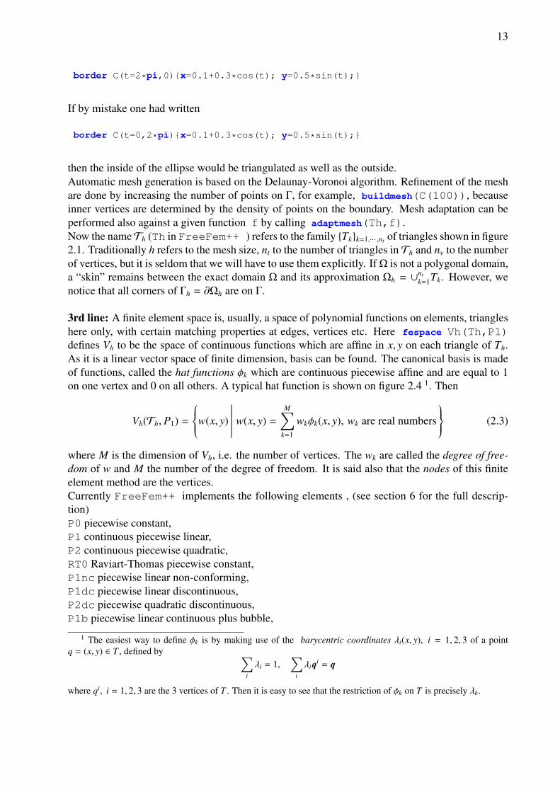
2nd line: the triangulation Th of Ω is automatically generated by buildmesh(C(50)) using 50points on C as in Fig. 2.1.The domain is assumed to be on the left side of the boundary which is implicitly oriented by theparametrization. So an elliptic hole can be added by
13
border C(t=2*pi,0)x=0.1+0.3*cos(t); y=0.5*sin(t);
If by mistake one had written
border C(t=0,2*pi)x=0.1+0.3*cos(t); y=0.5*sin(t);
then the inside of the ellipse would be triangulated as well as the outside.Automatic mesh generation is based on the Delaunay-Voronoi algorithm. Refinement of the meshare done by increasing the number of points on Γ, for example, buildmesh(C(100)), becauseinner vertices are determined by the density of points on the boundary. Mesh adaptation can beperformed also against a given function f by calling adaptmesh(Th,f).Now the nameTh (Th in FreeFem++ ) refers to the family Tkk=1,··· ,nt of triangles shown in figure2.1. Traditionally h refers to the mesh size, nt to the number of triangles in Th and nv to the numberof vertices, but it is seldom that we will have to use them explicitly. If Ω is not a polygonal domain,a “skin” remains between the exact domain Ω and its approximation Ωh = ∪
ntk=1Tk. However, we
notice that all corners of Γh = ∂Ωh are on Γ.
3rd line: A finite element space is, usually, a space of polynomial functions on elements, triangleshere only, with certain matching properties at edges, vertices etc. Here fespace Vh(Th,P1)defines Vh to be the space of continuous functions which are affine in x, y on each triangle of Th.As it is a linear vector space of finite dimension, basis can be found. The canonical basis is madeof functions, called the hat functions φk which are continuous piecewise affine and are equal to 1on one vertex and 0 on all others. A typical hat function is shown on figure 2.4 1. Then
Vh(Th, P1) =
w(x, y)
∣∣∣∣∣∣∣ w(x, y) =
M∑k=1
wkφk(x, y), wk are real numbers
(2.3)
where M is the dimension of Vh, i.e. the number of vertices. The wk are called the degree of free-dom of w and M the number of the degree of freedom. It is said also that the nodes of this finiteelement method are the vertices.Currently FreeFem++ implements the following elements , (see section 6 for the full descrip-tion)P0 piecewise constant,P1 continuous piecewise linear,P2 continuous piecewise quadratic,RT0 Raviart-Thomas piecewise constant,P1nc piecewise linear non-conforming,P1dc piecewise linear discontinuous,P2dc piecewise quadratic discontinuous,P1b piecewise linear continuous plus bubble,
1 The easiest way to define φk is by making use of the barycentric coordinates λi(x, y), i = 1, 2, 3 of a pointq = (x, y) ∈ T , defined by ∑
i
λi = 1,∑
i
λiqi = q
where qi, i = 1, 2, 3 are the 3 vertices of T . Then it is easy to see that the restriction of φk on T is precisely λk.

14 CHAPTER 2. GETTING STARTED
15
8
74
3
2
6
6 21
7
53
4
Figure 2.3: mesh Th
2
34 7
8
5
34
8
7
Figure 2.4: Graph of φ1 (left hand side) and φ6
P2b piecewise quadratic continuous plus bubble....To get the full list do in a unix terminal, in directory examples++-tutorial do
FreeFem++ dumptable.edp
grep TypeOfFE lestables
The user can add other elements fairly easily if required.
Step3: Setting the problem4th line: Vh u,v declares that u and v are approximated as above, namely
u(x, y) ' uh(x, y) =
M−1∑k=0
ukφk(x, y) (2.4)
5th line: the right hand side f is defined analytically using the keyword func.7th–9th lines: defines the bilinear form of equation (2.1) and its Dirichlet boundary conditions(2.2).This variational formulation is derived by multiplying (2.1) by v(x, y) and integrating the resultover Ω:
−
∫Ω
v∆u dxdy =
∫Ω
v f dxdy
Then, by Green’s formula, the problem is converted into finding u such that
a(u, v) − `( f , v) = 0 ∀v satisfying v = 0 on ∂Ω. (2.5)
with a(u, v) =
∫Ω
∇u · ∇v dxdy, `( f , v) =
∫Ω
f v dxdy (2.6)
In FreeFem++ the problem Poisson can be declared only (see below) for future use or declaredand solved at the same time in which case
Vh u,v; solve Poisson(u,v) =

15
and (2.5) is written with dx(u) = ∂u/∂x, dy(u) = ∂u/∂y and∫Ω
∇u · ∇v dxdy −→ int2d(Th)( dx(u)*dx(v) + dy(u)*dy(v) )∫Ω
f v dxdy −→ int2d(Th)( f*v ) (notice here, u is unused)
In FreeFem++ there is no need to distinguish the bilinear form a from the linear form `, as longas the terms are inside different integrals, FreeFem++ find out which one is the bilinear form bychecking where both terms u and v are present.
The other way is to defined the problem and after we solve it, write :
Vh u,v; problem Poisson(u,v) =...
Poisson; // the problem now is solve here
Step4: Solution and visualization
6th line: The current time in second is stored into the real-valued variable cpu.7th line The problem is solved11th line: The visualization is done as illustrated in Fig. 2.2 (see Section 7.1 for zoom, postscriptand other commands).12th line: The computing time (not counting graphics) is written on the console Notice the C++-like syntax; the user needs not study C++ for using FreeFem++ , but it helps to guess what isallowed in the language.
Access to matrices and vectorsInternally FreeFem++ will solve a linear system of the type
M−1∑j=0
Ai ju j − Fi = 0, i = 0, · · · ,M − 1; Fi =
∫Ω
fφi dxdy (2.7)
which is found by using (2.4) and replacing v by φi in (2.5). And the Dirichlet conditions areimplemented by penalty namely by setting Aii = 1030 and Fi = 1030 ∗ 0 if i is a boundary degreeof freedom. Note, that the number 1030 is called tgv (tres grande valeur ) and it is generallypossible to change this value , see the index item solve!tgv=.
The matrix A = (Ai j) is called stiffness matrix .If the user wants to access A directly he can do so by using (see section 6.10 page 120 for details)
varf a(u,v) = int2d(Th)( dx(u)*dx(v) + dy(u)*dy(v))+ on(C,u=0) ;
matrix A=a(Vh,Vh); // stiffness matrix,
The vector F in (2.7) can also be constructed manually
varf l(unused,v) = int2d(Th)(f*v)+on(C,u=0);Vh F; F[] = l(0,V); // F[] is the vector associated to the function F

16 CHAPTER 2. GETTING STARTED
The problem can then be solved at the level of algebra by
u[]=Aˆ-1*F[]; // u[] is the vector associated to the function u
Note 2.1 Here u and F are finite element function, and u[] and F[] give the array of valueassociated ( u[]≡ (ui)i=0,...,M−1 and F[]≡ (Fi)i=0,...,M−1). So we have
u(x, y) =
M−1∑i=0
u[][i]φi(x, y), F(x, y) =
M−1∑i=0
F[][i]φi(x, y)
where φi, i = 0..., ,M − 1 are the basis functions of Vh like in equation (2.3), and M = Vh.ndof isthe number of degree of freedom (i.e. the dimension of the space Vh).
The linear system (2.7) is solved by UMFPACK unless another option is mentioned specifically asin
Vh u,v; problem Poisson(u,v,solver=CG) = int2d(...
meaning that Poisson is declared only here and when it is called (by simply writing Poisson; )then (2.7) will be solved by the Conjugate Gradient method.
2.0.2 Some Features of FreeFem++The language of FreeFem++ is typed, polymorphic and reentrant with macro generation (see9.12). Every variable must be typed and declared in a statement each statement separated fromthe next by a semicolon ”;”. The syntax is that of C++ by default augmented with something thatis more akin to TEX. For the specialist, one key guideline is that FreeFem++ rarely generatesan internal finite element array; this was adopted for speed and consequently FreeFem++ couldbe hard to beat in terms of execution speed, except for the time lost in the interpretation of thelanguage (which can be reduced by a systematic usage of varf and matrices instead of problem.
2.1 The Development Cycle: Edit–Run/Visualize–ReviseAn integrated environment is provided with FreeFem++ written by A. Le Hyaric; Many exam-ples and tutorials are also given along with this documentation and it is best to study them and learnby example. Explanations for some of these examples are given in this book in the next chapter. Ifyou are a FEM beginner, you also may want to read a book on variational formulations.The development cycle will have the following steps:
Modeling: From strong forms of PDE to weak forms, one must know the variational formulationto use FreeFem++ ; one should also have an eye on the reusability of the variationalformulation so as to keep the same internal matrices; a typical example is the time dependentheat equation with an implicit time scheme: the internal matrix can be factorized only onceand FreeFem++ can be taught to do so.
Programming: Write the code in FreeFem++ language using a text editor such as the oneprovided in the integrated environment.
2.1. THE DEVELOPMENT CYCLE: EDIT–RUN/VISUALIZE–REVISE 17
Run: Run the code (e.g. written in file mycode.edp). If not from the integrated environment it canbe done at the console level by
% FreeFem++ mycode.edp
Note, the name of the command FreeFem++ may depend on your installation.
Visualization: Use the keyword plot to display functions while FreeFem++ is running. Usethe plot-parameter wait=1 to stop the program to have time to see the plot. Use the plot-parameter ps="toto.eps" to generate a postscript file to archive the results.
Debugging: A global variable ”debug” (for example) can help as in wait=true to wait=false.
bool debug = true;border a(t=0,2*pi) x=cos(t); y=sin(t);label=1;border b(t=0,2*pi) x=0.8+0.3*cos(t); y=0.3*sin(t);label=2;plot(a(50)+b(-30),wait=debug); // plot the borders to see the intersection
// (so change (0.8 in 0.3 in b) then needs a mouse clickmesh Th = buildmesh(a(50)+b(-30));plot(Th,wait=debug); // plot Th then needs a mouse clickfespace Vh(Th,P2);Vh f = sin(pi*x)*cos(pi*y);plot(f,wait=debug); // plot the function fVh g = sin(pi*x + cos(pi*y));plot(g,wait=debug); // plot the function g
Changing debug to false will make the plots flow continuously; drinking coffee and watchingthe flow of graph on the screen can then become a pleasant experience.
Error messages are displayed in the console window. They are not always very explicitbecause of the template structure of the C++ code, sorry! Nevertheless they are displayed atthe right place. For example, if you forget parenthesis as in
bool debug = true;mesh Th = square(10,10;plot(Th);
then you will get the following message from FreeFem++,
2 : mesh Th = square(10,10;Error line number 2, in file bb.edp, before token ;
parse errorcurrent line = 2
Compile error : parse errorline number :2, ;
error Compile error : parse errorline number :2, ;
code = 1
If you use the same symbol twice as in
real aaa =1;real aaa;

18 CHAPTER 2. GETTING STARTED
then you will get the message
2 : real aaa; The identifier aaa existthe existing type is <Pd>the new type is <Pd>
If you find that the program isn’t doing what you want you may also use cout to display intext format on the console window the value of variables.
The following example works:
...;fespace Vh...; Vh u;...cout<<u;...matrix A=a(Vh,Vh);...cout<<A;
Another trick is to comment in and out by using the“ //” as in C++. For example
real aaa =1;// real aaa;
Chapter 3
Learning by Examples
This chapter is for those, like us, who don’t like manuals. A number of simple examples cover agood deal of the capacity of FreeFem++ and are self-explanatory. For the modelling part thischapter continues at Chapter 9 where some PDEes of physics, engineering and finance are studiedin greater depth.
3.1 MembranesSummary Here we shall learn how to solve a Dirichlet and/or mixed Dirichlet Neumann prob-lem for the Laplace operator with application to the equilibrium of a membrane under load. Weshall also check the accuracy of the method and interface with other graphics packages.
An elastic membrane Ω is attached to a planar rigid support Γ, and a force f (x)dx is exerted oneach surface element dx = dx1dx2. The vertical membrane displacement, ϕ(x), is obtained bysolving Laplace’s equation:
−∆ϕ = f in Ω.
As the membrane is fixed to its planar support, one has:
ϕ|Γ = 0.
If the support wasn’t planar but at an elevation z(x1, x2) then the boundary conditions would be ofnon-homogeneous Dirichlet type.
ϕ|Γ = z.
If a part Γ2 of the membrane border Γ is not fixed to the support but is left hanging, then due to themembrane’s rigidity the angle with the normal vector n is zero; thus the boundary conditions are
ϕ|Γ1 = z,∂ϕ
∂n|Γ2 = 0
where Γ1 = Γ − Γ2; recall that ∂ϕ
∂n = ∇ϕ · n. Let us recall also that the Laplace operator ∆ is definedby:
∆ϕ =∂2ϕ
∂x21
+∂2ϕ
∂x22
.
19
20 CHAPTER 3. LEARNING BY EXAMPLES
With such ”mixed boundary conditions” the problem has a unique solution (see (1987), Dautray-Lions (1988), Strang (1986) and Raviart-Thomas (1983)); the easiest proof is to notice that ϕ isthe state of least energy, i.e.
E(φ) = minϕ−z∈V
E(v), with E(v) =
∫Ω
(12|∇v|2 − f v)
and where V is the subspace of the Sobolev space H1(Ω) of functions which have zero trace on Γ1.Recall that (x ∈ Rd, d = 2 here)
H1(Ω) = u ∈ L2(Ω) : ∇u ∈ (L2(Ω))d
Calculus of variation shows that the minimum must satisfy, what is known as the weak form of thePDE or its variational formulation (also known here as the theorem of virtual work)∫
Ω
∇ϕ · ∇w =
∫Ω
f w ∀w ∈ V
Next an integration by parts (Green’s formula) will show that this is equivalent to the PDE whensecond derivatives exist.
WARNING Unlike freefem+ which had both weak and strong forms, FreeFem++ imple-ments only weak formulations. It is not possible to go further in using this software if you don’tknow the weak form (i.e. variational formulation) of your problem: either you read a book, orask help from a colleague or drop the matter. Now if you want to solve a system of PDE likeA(u, v) = 0, B(u, v) = 0 don’t close this manual, because in weak form it is∫
Ω
(A(u, v)w1 + B(u, v)w2) = 0 ∀w1,w2...
Example Let an ellipse have the length of the semimajor axis a = 2, and unitary the semiminoraxis Let the surface force be f = 1. Programming this case with FreeFem++ gives:
Example 3.1 (membrane.edp) // file membrane.edpreal theta=4.*pi/3.;real a=2.,b=1.; // the length of the semimajor axis and semiminor axisfunc z=x;
border Gamma1(t=0,theta) x = a * cos(t); y = b*sin(t); border Gamma2(t=theta,2*pi) x = a * cos(t); y = b*sin(t); mesh Th=buildmesh(Gamma1(100)+Gamma2(50));
fespace Vh(Th,P2); // P2 conforming triangular FEMVh phi,w, f=1;
solve Laplace(phi,w)=int2d(Th)(dx(phi)*dx(w) + dy(phi)*dy(w))- int2d(Th)(f*w) + on(Gamma1,phi=z);
plot(phi,wait=true, ps="membrane.eps"); // Plot phiplot(Th,wait=true, ps="membraneTh.eps"); // Plot Th
savemesh(Th,"Th.msh");

3.1. MEMBRANES 21
-2
-1.5
-1
-0.5
0
0.5
1
1.5
2
-2-1.5
-1-0.5
0 0.5
1 1.5
2
-1-0.8
-0.6-0.4
-0.2 0
0.2 0.4
0.6 0.8
1
-2-1.5
-1-0.5
0 0.5
1 1.5
2
"phi.txt"
Figure 3.1: Mesh and level lines of the membrane deformation. Below: the same in 3D drawn bygnuplot from a file generated by FreeFem++ .

22 CHAPTER 3. LEARNING BY EXAMPLES
A triangulation is built by the keyword buildmesh. This keyword calls a triangulation subrou-tine based on the Delaunay test, which first triangulates with only the boundary points, then addsinternal points by subdividing the edges. How fine the triangulation becomes is controlled by thesize of the closest boundary edges.
The PDE is then discretized using the triangular second order finite element method on the triangu-lation; as was briefly indicated in the previous chapter, a linear system is derived from the discreteformulation whose size is the number of vertices plus the number of mid-edges in the triangula-tion. The system is solved by a multi-frontal Gauss LU factorization implemented in the packageUMFPACK. The keyword plot will display both Th and ϕ (remove Th if ϕ only is desired) andthe qualifier fill=true replaces the default option (colored level lines) by a full color display.Results are on figure 3.1.
plot(phi,wait=true,fill=true); // Plot phi with full color display
Next we would like to check the results!One simple way is to adjust the parameters so as to know the solutions. For instance on the unitcircle a=1 , ϕe = sin(x2 + y2 − 1) solves the problem when
z = 0, f = −4(cos(x2 + y2 − 1) − (x2 + y2) sin(x2 + y2 − 1))
except that on Γ2 ∂nϕ = 2 instead of zero. So we will consider a non-homogeneous Neumanncondition and solve ∫
Ω
(∇ϕ · ∇w =
∫Ω
f w +
∫Γ2
2w ∀w ∈ V
We will do that with two triangulations, compute the L2 error:
ε =
∫Ω
|ϕ − ϕe|2
and print the error in both cases as well as the log of their ratio an indication of the rate of conver-gence.
Example 3.2 (membranerror.edp) // file membranerror.edpverbosity =0; // to remove all default outputreal theta=4.*pi/3.;real a=1.,b=1.; // the length of the semimajor axis and semiminor axisborder Gamma1(t=0,theta) x = a * cos(t); y = b*sin(t); border Gamma2(t=theta,2*pi) x = a * cos(t); y = b*sin(t);
func f=-4*(cos(xˆ2+yˆ2-1) -(xˆ2+yˆ2)*sin(xˆ2+yˆ2-1));func phiexact=sin(xˆ2+yˆ2-1);
real[int] L2error(2); // an array two valuesfor(int n=0;n<2;n++)
mesh Th=buildmesh(Gamma1(20*(n+1))+Gamma2(10*(n+1)));fespace Vh(Th,P1);Vh phi,w;
solve laplace(phi,w)=int2d(Th)(dx(phi)*dx(w) + dy(phi)*dy(w))- int2d(Th)(f*w) - int1d(Th,Gamma2)(2*w)+ on(Gamma1,phi=0);

3.1. MEMBRANES 23
plot(Th,phi,wait=true,ps="membrane.eps"); // Plot Th and phi
L2error[n]= sqrt(int2d(Th)((phi-phiexact)ˆ2));
for(int n=0;n<2;n++)cout << " L2error " << n << " = "<< L2error[n] <<endl;
cout <<" convergence rate = "<< log(L2error[0]/L2error[1])/log(2.) <<endl;
the output is
L2error 0 = 0.00699498L2error 1 = 0.00182818convergence rate = 1.93591
times: compile 0.02s, execution 6.94s
We find a rate of 1.93591, which is not close enough to the 3 predicted by the theory. The Geometryis always a polygon so we lose one order due to the geometry approximation in O(h2)
Now if you are not satisfied with the .eps plot generated by FreeFem++ and you want to useother graphic facilities, then you must store the solution in a file very much like in C++. It will beuseless if you don’t save the triangulation as well, consequently you must do
ofstream ff("phi.txt");ff << phi[];
savemesh(Th,"Th.msh");
For the triangulation the name is important: it is the extension that determines the format.Still that may not take you where you want. Here is an interface with gnuplot to produce the rightpart of figure 3.2.
// to build a gnuplot data file ofstream ff("graph.txt");
for (int i=0;i<Th.nt;i++) for (int j=0; j <3; j++)
ff<<Th[i][j].x << " "<< Th[i][j].y<< " "<<phi[][Vh(i,j)]<<endl;ff<<Th[i][0].x << " "<< Th[i][0].y<< " "<<phi[][Vh(i,0)]<<"\n\n\n"
We use the finite element numbering, where Wh(i,j) is the global index of jTh degrees offreedom of triangle number i.Then open gnuplot and do
set palette rgbformulae 30,31,32splot "graph.txt" w l pal
This works with P2 and P1, but not with P1nc because the 3 first degrees of freedom of P2 orP2 are on vertices and not with P1nc.

24 CHAPTER 3. LEARNING BY EXAMPLES
3.2 Heat ExchangerSummary Here we shall learn more about geometry input and triangulation files, as well asread and write operations.
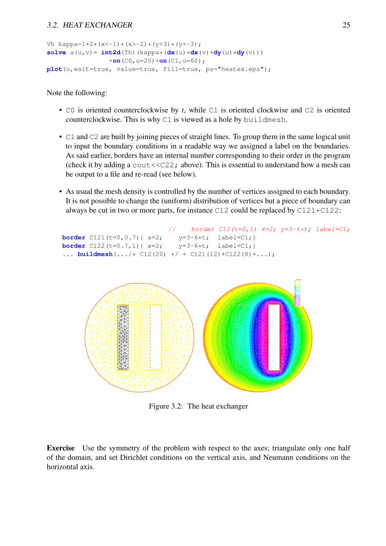
The problem Let Ci1,2, be 2 thermal conductors within an enclosure C0. The first one is heldat a constant temperature u1 the other one has a given thermal conductivity κ2 5 times larger thanthe one of C0. We assume that the border of enclosure C0 is held at temperature 20C and that wehave waited long enough for thermal equilibrium.In order to know u(x) at any point x of the domain Ω, we must solve
∇ · (κ∇u) = 0 in Ω, u|Γ = g
where Ω is the interior of C0 minus the conductors C1 and Γ is the boundary of Ω, that is C0 ∪ C1
Here g is any function of x equal to ui on Ci. The second equation is a reduced form for:
u = ui on Ci, i = 0, 1.
The variational formulation for this problem is in the subspace H10(Ω) ⊂ H1(Ω) of functions which
have zero traces on Γ.
u − g ∈ H10(Ω) :
∫Ω
∇u∇v = 0 ∀v ∈ H10(Ω)
Let us assume that C0 is a circle of radius 5 centered at the origin, Ci are rectangles, C1 being atthe constant temperature u1 = 60C.
Example 3.3 (heatex.edp) // file heatex.edpint C1=99, C2=98; // could be anything such that , 0 and C1 , C2border C0(t=0,2*pi)x=5*cos(t); y=5*sin(t);
border C11(t=0,1) x=1+t; y=3; label=C1;border C12(t=0,1) x=2; y=3-6*t; label=C1;border C13(t=0,1) x=2-t; y=-3; label=C1;border C14(t=0,1) x=1; y=-3+6*t; label=C1;
border C21(t=0,1) x=-2+t; y=3; label=C2;border C22(t=0,1) x=-1; y=3-6*t; label=C2;border C23(t=0,1) x=-1-t; y=-3; label=C2;border C24(t=0,1) x=-2; y=-3+6*t; label=C2;
plot( C0(50) // to see the border of the domain+ C11(5)+C12(20)+C13(5)+C14(20)+ C21(-5)+C22(-20)+C23(-5)+C24(-20),wait=true, ps="heatexb.eps");
mesh Th=buildmesh( C0(50)+ C11(5)+C12(20)+C13(5)+C14(20)+ C21(-5)+C22(-20)+C23(-5)+C24(-20));
plot(Th,wait=1);
fespace Vh(Th,P1); Vh u,v;
3.2. HEAT EXCHANGER 25
Vh kappa=1+2*(x<-1)*(x>-2)*(y<3)*(y>-3);solve a(u,v)= int2d(Th)(kappa*(dx(u)*dx(v)+dy(u)*dy(v)))
+on(C0,u=20)+on(C1,u=60);plot(u,wait=true, value=true, fill=true, ps="heatex.eps");
Note the following:
• C0 is oriented counterclockwise by t, while C1 is oriented clockwise and C2 is orientedcounterclockwise. This is why C1 is viewed as a hole by buildmesh.
• C1 and C2 are built by joining pieces of straight lines. To group them in the same logical unitto input the boundary conditions in a readable way we assigned a label on the boundaries.As said earlier, borders have an internal number corresponding to their order in the program(check it by adding a cout<<C22; above). This is essential to understand how a mesh canbe output to a file and re-read (see below).
• As usual the mesh density is controlled by the number of vertices assigned to each boundary.It is not possible to change the (uniform) distribution of vertices but a piece of boundary canalways be cut in two or more parts, for instance C12 could be replaced by C121+C122:
// border C12(t=0,1) x=2; y=3-6*t; label=C1;border C121(t=0,0.7) x=2; y=3-6*t; label=C1;border C122(t=0.7,1) x=2; y=3-6*t; label=C1;... buildmesh(.../* C12(20) */ + C121(12)+C122(8)+...);
IsoValue15.789522.105326.315830.526334.736838.947443.157947.368451.578955.78956064.210568.421172.631676.842181.052685.263289.473793.6842104.211
Figure 3.2: The heat exchanger
Exercise Use the symmetry of the problem with respect to the axes; triangulate only one halfof the domain, and set Dirichlet conditions on the vertical axis, and Neumann conditions on thehorizontal axis.

26 CHAPTER 3. LEARNING BY EXAMPLES
Writing and reading triangulation files Suppose that at the end of the previous program weadded the line
savemesh(Th,"condensor.msh");
and then later on we write a similar program but we wish to read the mesh from that file. Then thisis how the condenser should be computed:
mesh Sh=readmesh("condensor.msh");fespace Wh(Sh,P1); Wh us,vs;solve b(us,vs)= int2d(Sh)(dx(us)*dx(vs)+dy(us)*dy(vs))
+on(1,us=0)+on(99,us=1)+on(98,us=-1);plot(us);
Note that the names of the boundaries are lost but either their internal number (in the case of C0)or their label number (for C1 and C2) are kept.
3.3 AcousticsSummary Here we go to grip with ill posed problems and eigenvalue problemsPressure variations in air at rest are governed by the wave equation:
∂2u∂t2 − c2∆u = 0.
When the solution wave is monochromatic (and that depend on the boundary and initial condi-tions), u is of the form u(x, t) = Re(v(x)eikt) where v is a solution of Helmholtz’s equation:
k2v + c2∆v = 0 in Ω,∂v∂n|Γ = g. (3.1)
where g is the source. Note the “+” sign in front of the Laplace operator and that k > 0 is real. Thissign may make the problem ill posed for some values of c
k , a phenomenon called “resonance”.At resonance there are non-zero solutions even when g = 0. So the following program may or maynot work:
Example 3.4 (sound.edp) // file sound.edpreal kc2=1;func g=y*(1-y);
border a0(t=0,1) x= 5; y= 1+2*t ;border a1(t=0,1) x=5-2*t; y= 3 ;border a2(t=0,1) x= 3-2*t; y=3-2*t ;border a3(t=0,1) x= 1-t; y= 1 ;border a4(t=0,1) x= 0; y= 1-t ;border a5(t=0,1) x= t; y= 0 ;border a6(t=0,1) x= 1+4*t; y= t ;
mesh Th=buildmesh( a0(20) + a1(20) + a2(20)+ a3(20) + a4(20) + a5(20) + a6(20));
fespace Vh(Th,P1);

3.3. ACOUSTICS 27
Vh u,v;
solve sound(u,v)=int2d(Th)(u*v * kc2 - dx(u)*dx(v) - dy(u)*dy(v))- int1d(Th,a4)(g*v);
plot(u, wait=1, ps="sound.eps");
Results are on Figure 3.3. But when kc2 is an eigenvalue of the problem, then the solution is notunique: if ue . 0 is an eigen state, then for any given solution u + ue is another a solution. To findall the ue one can do the following
real sigma = 20; // value of the shift// OP = A - sigma B ; // the shifted matrix
varf op(u1,u2)= int2d(Th)( dx(u1)*dx(u2) + dy(u1)*dy(u2) - sigma* u1*u2 );varf b([u1],[u2]) = int2d(Th)( u1*u2 ) ; // no Boundary condition see note9.1
matrix OP= op(Vh,Vh,solver=Crout,factorize=1);matrix B= b(Vh,Vh,solver=CG,eps=1e-20);
int nev=2; // number of requested eigenvalues near sigma
real[int] ev(nev); // to store the nev eigenvalueVh[int] eV(nev); // to store the nev eigenvector
int k=EigenValue(OP,B,sym=true,sigma=sigma,value=ev,vector=eV,tol=1e-10,maxit=0,ncv=0);
cout<<ev(0)<<" 2 eigen values "<<ev(1)<<endl;v=eV[0];plot(v,wait=1,ps="eigen.eps");
Figure 3.3: Left:Amplitude of an acoustic signal coming from the left vertical wall. Right: firsteigen state (λ = (k/c)2 = 19.4256) close to 20 of eigenvalue problem :−∆ϕ = λϕ and ∂ϕ
∂n = 0 on Γ

28 CHAPTER 3. LEARNING BY EXAMPLES
3.4 Thermal ConductionSummary Here we shall learn how to deal with a time dependent parabolic problem. We shallalso show how to treat an axisymmetric problem and show also how to deal with a nonlinearproblem.
How air cools a plate We seek the temperature distribution in a plate (0, Lx) × (0, Ly) × (0, Lz)of rectangular cross section Ω = (0, 6) × (0, 1); the plate is surrounded by air at temperature ue
and initially at temperature u = u0 + xLu1. In the plane perpendicular to the plate at z = Lz/2, the
temperature varies little with the coordinate z; as a first approximation the problem is 2D.
We must solve the temperature equation in Ω in a time interval (0,T).
∂tu − ∇ · (κ∇u) = 0 in Ω × (0,T ),u(x, y, 0) = u0 + xu1
κ∂u∂n
+ α(u − ue) = 0 on Γ × (0,T ). (3.2)
Here the diffusion κ will take two values, one below the middle horizontal line and ten times lessabove, so as to simulate a thermostat. The term α(u − ue) accounts for the loss of temperature byconvection in air. Mathematically this boundary condition is of Fourier (or Robin, or mixed) type.
The variational formulation is in L2(0,T ; H1(Ω)); in loose terms and after applying an implicitEuler finite difference approximation in time; we shall seek un(x, y) satisfying for all w ∈ H1(Ω):∫
Ω
(un − un−1
δtw + κ∇un∇w) +
∫Γ
α(un − uue)w = 0
func u0 =10+90*x/6;func k = 1.8*(y<0.5)+0.2;real ue = 25, alpha=0.25, T=5, dt=0.1 ;
mesh Th=square(30,5,[6*x,y]);fespace Vh(Th,P1);Vh u=u0,v,uold;
problem thermic(u,v)= int2d(Th)(u*v/dt + k*(dx(u) * dx(v) + dy(u) * dy(v)))+ int1d(Th,1,3)(alpha*u*v)- int1d(Th,1,3)(alpha*ue*v)- int2d(Th)(uold*v/dt) + on(2,4,u=u0);
ofstream ff("thermic.dat");for(real t=0;t<T;t+=dt)
uold=u; // uold ≡ un−1 = un ≡uthermic; // here solve the thermic problemff<<u(3,0.5)<<endl;plot(u);
Notice that we must separate by hand the bilinear part from the linear one.
3.4. THERMAL CONDUCTION 29
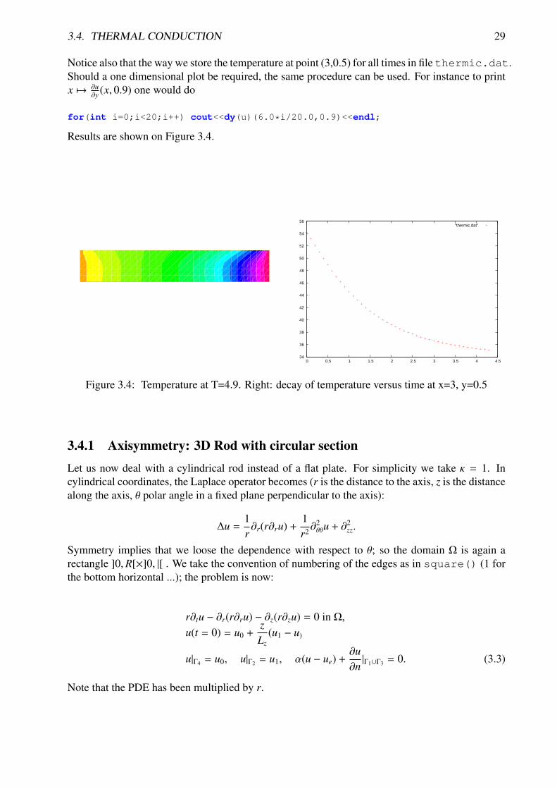
Notice also that the way we store the temperature at point (3,0.5) for all times in file thermic.dat.Should a one dimensional plot be required, the same procedure can be used. For instance to printx 7→ ∂u
∂y (x, 0.9) one would do
for(int i=0;i<20;i++) cout<<dy(u)(6.0*i/20.0,0.9)<<endl;
Results are shown on Figure 3.4.
34
36
38
40
42
44
46
48
50
52
54
56
0 0.5 1 1.5 2 2.5 3 3.5 4 4.5
"thermic.dat"
Figure 3.4: Temperature at T=4.9. Right: decay of temperature versus time at x=3, y=0.5
3.4.1 Axisymmetry: 3D Rod with circular sectionLet us now deal with a cylindrical rod instead of a flat plate. For simplicity we take κ = 1. Incylindrical coordinates, the Laplace operator becomes (r is the distance to the axis, z is the distancealong the axis, θ polar angle in a fixed plane perpendicular to the axis):
∆u =1r∂r(r∂ru) +
1r2∂
2θθu + ∂2
zz.
Symmetry implies that we loose the dependence with respect to θ; so the domain Ω is again arectangle ]0,R[×]0, |[ . We take the convention of numbering of the edges as in square() (1 forthe bottom horizontal ...); the problem is now:
r∂tu − ∂r(r∂ru) − ∂z(r∂zu) = 0 in Ω,
u(t = 0) = u0 +zLz
(u1 − u)
u|Γ4 = u0, u|Γ2 = u1, α(u − ue) +∂u∂n|Γ1∪Γ3 = 0. (3.3)
Note that the PDE has been multiplied by r.

30 CHAPTER 3. LEARNING BY EXAMPLES
After discretization in time with an implicit scheme, with time steps dt, in the FreeFem++syntax r becomes x and z becomes y and the problem is:
problem thermaxi(u,v)=int2d(Th)((u*v/dt + dx(u)*dx(v) + dy(u)*dy(v))*x)+ int1d(Th,3)(alpha*x*u*v) - int1d(Th,3)(alpha*x*ue*v)- int2d(Th)(uold*v*x/dt) + on(2,4,u=u0);
Notice that the bilinear form degenerates at x = 0. Still one can prove existence and uniquenessfor u and because of this degeneracy no boundary conditions need to be imposed on Γ1.
3.4.2 A Nonlinear Problem : RadiationHeat loss through radiation is a loss proportional to the absolute temperature to the fourth power(Stefan’s Law). This adds to the loss by convection and gives the following boundary condition:
κ∂u∂n
+ α(u − ue) + c[(u + 273)4 − (ue + 273)4] = 0
The problem is nonlinear, and must be solved iteratively. If m denotes the iteration index, a semi-linearization of the radiation condition gives
∂um+1
∂n+ α(um+1 − ue) + c(um+1 − ue)(um + ue + 546)((um + 273)2 + (ue + 273)2) = 0,
because we have the identity a4 − b4 = (a− b)(a + b)(a2 + b2). The iterative process will work withv = u − ue.
...fespace Vh(Th,P1); // finite element spacereal rad=1e-8, uek=ue+273; // def of the physical constantsVh vold,w,v=u0-ue,b;problem thermradia(v,w)
= int2d(Th)(v*w/dt + k*(dx(v) * dx(w) + dy(v) * dy(w)))+ int1d(Th,1,3)(b*v*w)- int2d(Th)(vold*w/dt) + on(2,4,v=u0-ue);
for(real t=0;t<T;t+=dt)vold=v;for(int m=0;m<5;m++)
b= alpha + rad * (v + 2*uek) * ((v+uek)ˆ2 + uekˆ2);thermradia;
vold=v+ue; plot(vold);
3.5 Irrotational Fan Blade Flow and Thermal effectsSummary Here we will learn how to deal with a multi-physics system of PDEs on a Complexgeometry, with multiple meshes within one problem. We also learn how to manipulate the regionindicator and see how smooth is the projection operator from one mesh to another.

3.5. IRROTATIONAL FAN BLADE FLOW AND THERMAL EFFECTS 31
Incompressible flow Without viscosity and vorticity incompressible flows have a velocity givenby:
u =
∂ψ
∂x2
−∂ψ
∂x1
, where ψ is solution of ∆ψ = 0
This equation expresses both incompressibility (∇ · u = 0) and absence of vortex (∇ × u = 0).As the fluid slips along the walls, normal velocity is zero, which means that ψ satisfies:
ψ constant on the walls.
One can also prescribe the normal velocity at an artificial boundary, and this translates into nonconstant Dirichlet data for ψ.
Airfoil Let us consider a wing profile S in a uniform flow. Infinity will be represented by a largecircle C where the flow is assumed to be of uniform velocity; one way to model this problem is towrite
∆ψ = 0 in Ω, ψ|S = 0, ψ|C = u∞y, (3.4)
where ∂Ω = C ∪ S
The NACA0012 Airfoil An equation for the upper surface of a NACA0012 (this is a classicalwing profile in aerodynamics) is:
y = 0.17735√
x − 0.075597x − 0.212836x2 + 0.17363x3 − 0.06254x4.
Example 3.5 (potential.edp) // file potential.edp
real S=99;border C(t=0,2*pi) x=5*cos(t); y=5*sin(t);border Splus(t=0,1) x = t; y = 0.17735*sqrt(t)-0.075597*t
- 0.212836*(tˆ2)+0.17363*(tˆ3)-0.06254*(tˆ4); label=S;border Sminus(t=1,0) x =t; y= -(0.17735*sqrt(t)-0.075597*t
-0.212836*(tˆ2)+0.17363*(tˆ3)-0.06254*(tˆ4)); label=S;mesh Th= buildmesh(C(50)+Splus(70)+Sminus(70));fespace Vh(Th,P2); Vh psi,w;
solve potential(psi,w)=int2d(Th)(dx(psi)*dx(w)+dy(psi)*dy(w))+on(C,psi = y) + on(S,psi=0);
plot(psi,wait=1);
A zoom of the streamlines are shown on Figure 3.5.
32 CHAPTER 3. LEARNING BY EXAMPLES
IsoValue-10.9395-3.121592.090377.3023312.514317.726222.938228.150233.362138.574143.786148.99854.2159.421964.633969.845975.057880.269885.481798.5116
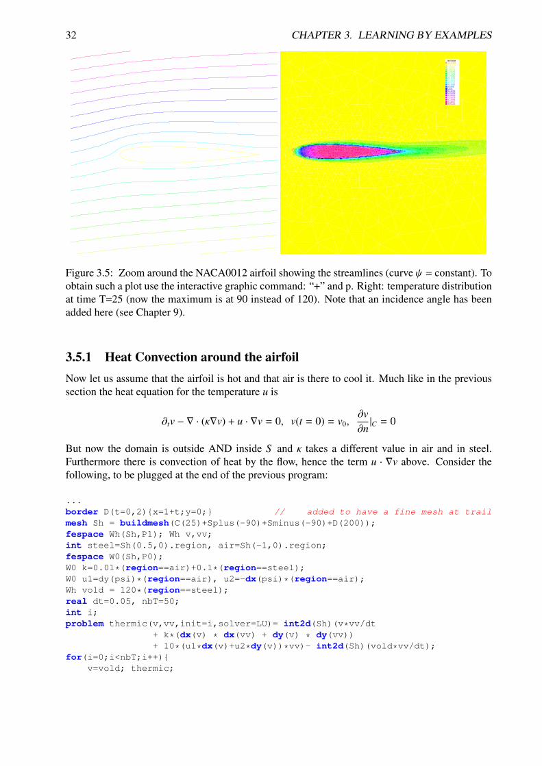
Figure 3.5: Zoom around the NACA0012 airfoil showing the streamlines (curve ψ = constant). Toobtain such a plot use the interactive graphic command: “+” and p. Right: temperature distributionat time T=25 (now the maximum is at 90 instead of 120). Note that an incidence angle has beenadded here (see Chapter 9).
3.5.1 Heat Convection around the airfoilNow let us assume that the airfoil is hot and that air is there to cool it. Much like in the previoussection the heat equation for the temperature u is
∂tv − ∇ · (κ∇v) + u · ∇v = 0, v(t = 0) = v0,∂v∂n|C = 0
But now the domain is outside AND inside S and κ takes a different value in air and in steel.Furthermore there is convection of heat by the flow, hence the term u · ∇v above. Consider thefollowing, to be plugged at the end of the previous program:
...border D(t=0,2)x=1+t;y=0; // added to have a fine mesh at trailmesh Sh = buildmesh(C(25)+Splus(-90)+Sminus(-90)+D(200));fespace Wh(Sh,P1); Wh v,vv;int steel=Sh(0.5,0).region, air=Sh(-1,0).region;fespace W0(Sh,P0);W0 k=0.01*(region==air)+0.1*(region==steel);W0 u1=dy(psi)*(region==air), u2=-dx(psi)*(region==air);Wh vold = 120*(region==steel);real dt=0.05, nbT=50;int i;problem thermic(v,vv,init=i,solver=LU)= int2d(Sh)(v*vv/dt
+ k*(dx(v) * dx(vv) + dy(v) * dy(vv))+ 10*(u1*dx(v)+u2*dy(v))*vv)- int2d(Sh)(vold*vv/dt);
for(i=0;i<nbT;i++)v=vold; thermic;

3.6. PURE CONVECTION : THE ROTATING HILL 33
plot(v);
Notice here
• how steel and air are identified by the mesh parameter region which is defined when buildmeshis called and takes an integer value corresponding to each connected component of Ω;
• how the convection terms are added without upwinding. Upwinding is necessary when thePecley number |u|L/κ is large (here is a typical length scale), The factor 10 in front of theconvection terms is a quick way of multiplying the velocity by 10 (else it is too slow to seesomething).
• The solver is Gauss’ LU factorization and when init, 0 the LU decomposition is reusedso it is much faster after the first iteration.
3.6 Pure Convection : The Rotating Hill
Summary Here we will present two methods for upwinding for the simplest convection prob-lem. We will learn about Characteristics-Galerkin and Discontinuous-Galerkin Finite ElementMethods.Let Ω be the unit disk centered at 0; consider the rotation vector field
u = [u1, u2], u1 = y, u2 = −x.
Pure convection by u is
∂tc + u.∇c = 0 in Ω × (0,T ) c(t = 0) = c0 in Ω.
The exact solution c(xt, t) at time t en point xt is given by
c(xt, t) = c0(x, 0)
where xt is the particle path in the flow starting at point x at time 0. So xt are solutions of
xt = u(xt), , xt=0 = x, where xt =d(t 7→ xt)
dt
The ODE are reversible and we want the solution at point x at time t ( not at point xt) the initialpoint is x−t, and we have
c(x, t) = c0(x−t, 0)
The game consists in solving the equation until T = 2π, that is for a full revolution and to comparethe final solution with the initial one; they should be equal.

34 CHAPTER 3. LEARNING BY EXAMPLES
Solution by a Characteristics-Galerkin Method In FreeFem++ there is an operator calledconvect([u1,u2],dt,c) which compute cX with X is the convect field defined by X(x) =
xdt and where xτ is particule path in the steady state velocity field u = [u1, u2] starting at point xat time τ = 0, so xτ is solution of the following ODE:
xτ = u(xτ), xτ=0 = x.
When u is piecewise constant; this is possible because xτ is then a polygonal curve which canbe computed exactly and the solution exists always when u is divergence free; convect returnsc(xd f ) = C X.
Example 3.6 (convects.edp) // file convects.edp
border C(t=0, 2*pi) x=cos(t); y=sin(t); ;mesh Th = buildmesh(C(100));fespace Uh(Th,P1);Uh cold, c = exp(-10*((x-0.3)ˆ2 +(y-0.3)ˆ2));
real dt = 0.17,t=0;Uh u1 = y, u2 = -x;for (int m=0; m<2*pi/dt ; m++)
t += dt; cold=c;c=convect([u1,u2],-dt,cold);plot(c,cmm=" t="+t + ", min=" + c[].min + ", max=" + c[].max);
The method is very powerful but has two limitations: a/ it is not conservative, b/ it may diverge inrare cases when |u| is too small due to quadrature error.
Solution by Discontinuous-Galerkin FEM Discontinuous Galerkin methods take advantage ofthe discontinuities of c at the edges to build upwinding. There are may formulations possible. Weshall implement here the so-called dual-PDC
1 formulation (see Ern[10]):∫Ω
(cn+1 − cn
δt+ u · ∇c)w +
∫E(α|n · u| −
12
n · u)[c]w =
∫E−
Γ
|n · u|cw ∀w
where E is the set of inner edges and E−Γ
is the set of boundary edges where u · n < 0 (in our casethere is no such edges). Finally [c] is the jump of c across an edge with the convention that c+
refers to the value on the right of the oriented edge.
Example 3.7 (convects end.edp) // file convects.edp...fespace Vh(Th,P1dc);
Vh w, ccold, v1 = y, v2 = -x, cc = exp(-10*((x-0.3)ˆ2 +(y-0.3)ˆ2));real u, al=0.5; dt = 0.05;
macro n(N.x*v1+N.y*v2) // problem Adual(cc,w) =int2d(Th)((cc/dt+(v1*dx(cc)+v2*dy(cc)))*w)

3.6. PURE CONVECTION : THE ROTATING HILL 35
+ intalledges(Th)((1-nTonEdge)*w*(al*abs(n)-n/2)*jump(cc))// - int1d(Th,C)((n<0)*abs(n)*cc*w) // unused because cc=0 on ∂Ω−
- int2d(Th)(ccold*w/dt);
for ( t=0; t< 2*pi ; t+=dt)
ccold=cc; Adual;plot(cc,fill=1,cmm="t="+t + ", min=" + cc[].min + ", max=" + cc[].max);
;real [int] viso=[-0.2,-0.1,0,0.1,0.2,0.3,0.4,0.5,0.6,0.7,0.8,0.9,1,1.1];plot(c,wait=1,fill=1,ps="convectCG.eps",viso=viso);plot(c,wait=1,fill=1,ps="convectDG.eps",viso=viso);
Notice the new keywords, intalledges to integrate on all edges, nTonEdge which is one if thetriangle has a boundary edge and zero otherwise, jump to implement [c]. Results of both methodsare shown on Figure 3.6 with identical levels for the level line; this is done with the plot-modifierviso.Notice also the macro where the parameter u is not used (but the syntax needs one) and which endswith a //; it simply replaces the name n by (N.x*v1+N.y*v2). As easily guessed N.x,N.y isthe normal to the edge.
IsoValue-0.100.50.10.50.20.250.30.350.40.450.50.550.60.650.70.750.80.91
IsoValue-0.100.50.10.50.20.250.30.350.40.450.50.550.60.650.70.750.80.91
Figure 3.6: The rotated hill after one revolution, left with Characteristics-Galerkin, on the rightwith Discontinuous P1 Galerkin FEM.
Now if you think that DG is too slow try this
// the same DG very much fastervarf aadual(cc,w) = int2d(Th)((cc/dt+(v1*dx(cc)+v2*dy(cc)))*w)
+ intalledges(Th)((1-nTonEdge)*w*(al*abs(n)-n/2)*jump(cc));varf bbdual(ccold,w) = - int2d(Th)(ccold*w/dt);matrix AA= aadual(Vh,Vh);

36 CHAPTER 3. LEARNING BY EXAMPLES
matrix BB = bbdual(Vh,Vh);set (AA,init=t,solver=sparsesolver);Vh rhs=0;for ( t=0; t< 2*pi ; t+=dt)
ccold=cc;rhs[] = BB* ccold[];cc[] = AAˆ-1*rhs[];plot(cc,fill=0,cmm="t="+t + ", min=" + cc[].min + ", max=" + cc[].max);
;
Notice the new keyword set to specify a solver in this framework; the modifier init is used to telthe solver that the matrix has not changed (init=true), and the name parameter are the same that inproblem definition (see. 6.7) .
Finite Volume Methods can also be handled with FreeFem++ but it requires programming.For instance the P0 − P0 Finite Volume Method of Dervieux et al associates to each P0 function c1
a P0 function c0 with constant value around each vertex qi equal to c1(qi) on the cell σi made byall the medians of all triangles having qi as vertex. Then upwinding is done by taking left or rightvalues at the median: ∫
σi
1δt
(c1n+1− c1n) +
∫∂σi
u · nc− = 0 ∀i
It can be programmed as
load "mat_dervieux"; // external module in C++ must be loadedborder a(t=0, 2*pi) x = cos(t); y = sin(t); mesh th = buildmesh(a(100));fespace Vh(th,P1);
Vh vh,vold,u1 = y, u2 = -x;Vh v = exp(-10*((x-0.3)ˆ2 +(y-0.3)ˆ2)), vWall=0, rhs =0;
real dt = 0.025;// qf1pTlump means mass lumping is used
problem FVM(v,vh) = int2d(th,qft=qf1pTlump)(v*vh/dt)- int2d(th,qft=qf1pTlump)(vold*vh/dt)
+ int1d(th,a)(((u1*N.x+u2*N.y)<0)*(u1*N.x+u2*N.y)*vWall*vh)+ rhs[] ;
matrix A;MatUpWind0(A,th,vold,[u1,u2]);
for ( int t=0; t< 2*pi ; t+=dt)vold=v;rhs[] = A * vold[] ; FVM;plot(v,wait=0);
;
the mass lumping parameter forces a quadrature formula with Gauss points at the vertices so asto make the mass matrix diagonal; the linear system solved by a conjugate gradient method forinstance will then converge in one or two iterations.The right hand side rhs is computed by an external C++ function MatUpWind0(...) which isprogrammed as

3.7. A PROJECTION ALGORITHM FOR THE NAVIER-STOKES EQUATIONS 37
// computes matrix a on a triangle for the Dervieux FVMint fvmP1P0(double q[3][2], // the 3 vertices of a triangle T
double u[2], // convection velocity on Tdouble c[3], // the P1 function on Tdouble a[3][3], // output matrixdouble where[3] ) // where>0 means we’re on the boundary
for(int i=0;i<3;i++) for(int j=0;j<3;j++) a[i][j]=0;
for(int i=0;i<3;i++)int ip = (i+1)%3, ipp =(ip+1)%3;double unL =-((q[ip][1]+q[i][1]-2*q[ipp][1])*u[0]
-(q[ip][0]+q[i][0]-2*q[ipp][0])*u[1])/6;if(unL>0) a[i][i] += unL; a[ip][i]-=unL;
else a[i][ip] += unL; a[ip][ip]-=unL;if(where[i]&&where[ip]) // this is a boundary edge
unL=((q[ip][1]-q[i][1])*u[0] -(q[ip][0]-q[i][0])*u[1])/2;if(unL>0) a[i][i]+=unL; a[ip][ip]+=unL;
return 1;
It must be inserted into a larger .cpp file, shown in Appendix A, which is the load module linkedto FreeFem++ .
3.7 A Projection Algorithm for the Navier-Stokes equationsSummary Fluid flows require good algorithms and good triangultions. We show here an exam-ple of a complex algorithm and or first example of mesh adaptation.
An incompressible viscous fluid satisfies:
∂tu + u · ∇u + ∇p − ν∆u = 0, ∇ · u = 0 in Ω×]0,T [,
u|t=0 = u0, u|Γ = uΓ.
A possible algorithm, proposed by Chorin, is1δt
[um+1 − umoXm] + ∇pm − ν∆um = 0, u|Γ = uΓ,
−∆pm+1 = −∇ · umoXm, ∂n pm+1 = 0,
where uoX(x) = u(x − u(x)δt) since ∂tu + u · ∇u is approximated by the method of characteristics,as in the previous section.
An improvement over Chorin’s algorithm, given by Rannacher, is to compute a correction, q, tothe pressure (the overline denotes the mean over Ω)
−∆q = ∇ · u − ∇ · u
and defineum+1 = u + ∇qδt, pm+1 = pm − q − pm − q
where u is the (um+1, vm+1) of Chorin’s algorithm.

38 CHAPTER 3. LEARNING BY EXAMPLES
The backward facing step The geometry is that of a channel with a backward facing step so thatthe inflow section is smaller than the outflow section. This geometry produces a fluid recirculationzone that must be captured correctly.This can only be done if the triangulation is sufficiently fine, or well adapted to the flow.
Example 3.8 (NSprojection.edp) // file NSprojection.edp
border a0(t=1,0) x=0; y=t; label=1;border a1(t=0,1) x=2*t; y=0; label=2;border a2(t=0,1) x=2; y=-t/2; label=2;border a3(t=0,1) x=2+18*tˆ1.2; y=-0.5; label=2;border a4(t=0,1) x=20; y=-0.5+1.5*t; label=3;border a5(t=1,0) x=20*t; y=1; label=4;int n=1;mesh Th= buildmesh(a0(3*n)+a1(20*n)+a2(10*n)+a3(150*n)+a4(5*n)+a5(100*n));plot(Th);fespace Vh(Th,P1);real nu = 0.0025, dt = 0.2; // Reynolds=400Vh w,u = 4*y*(1-y)*(y>0)*(x<2), v =0, p = 0, q=0;real area= int2d(Th)(1.);
for(int n=0;n<100;n++)Vh uold = u, vold = v, pold=p;Vh f=convect([u,v],-dt,uold), g=convect([u,v],-dt,vold);
solve pb4u(u,w,init=n,solver=LU)=int2d(Th)(u*w/dt +nu*(dx(u)*dx(w)+dy(u)*dy(w)))-int2d(Th)((f/dt-dx(p))*w)+ on(1,u = 4*y*(1-y)) + on(2,4,u = 0)+ on(3,u=f);
plot(u);
solve pb4v(v,w,init=n,solver=LU)= int2d(Th)(v*w/dt +nu*(dx(v)*dx(w)+dy(v)*dy(w)))-int2d(Th)((g/dt-dy(p))*w)+on(1,2,3,4,v = 0);
real meandiv = int2d(Th)(dx(u)+dy(v))/area;
solve pb4p(q,w,init=n,solver=LU)= int2d(Th)(dx(q)*dx(w)+dy(q)*dy(w))- int2d(Th)((dx(u)+ dy(v)-meandiv)*w/dt)+ on(3,q=0);
real meanpq = int2d(Th)(pold - q)/area;if(n==50)
Th = adaptmesh(Th,u,v,q); plot(Th, wait=true);p = pold-q-meanpq;u = u + dx(q)*dt;v = v + dy(q)*dt;
We show in figure 3.7 the numerical results obtained for a Reynolds number of 400 where meshadaptation is done after 50 iterations on the first mesh.

3.8. THE SYSTEM OF ELASTICITY 39
Figure 3.7: Rannacher’s projection algorithm: result on an adapted mesh (top) showing the pres-sure (middle) and the horizontal velocity u at Reynolds 400.
3.8 The System of elasticityElasticity Solid objects deform under the action of applied forces: a point in the solid, originallyat (x, y, z) will come to (X,Y,Z) after some time; the vector u = (u1, u2, u3) = (X − x,Y − y,Z − z)is called the displacement. When the displacement is small and the solid is elastic, Hooke’s lawgives a relationship between the stress tensor σ(u) = (σi j(u)) and the strain tensor ε(u) = εi j(u)
σi j(u) = λδi j∇.u + 2µεi j(u),
where the Kronecker symbol δi j = 1 if i = j, 0 otherwise, with
εi j(u) =12
(∂ui
∂x j+∂u j
∂xi),
and where λ, µ are two constants that describe the mechanical properties of the solid, and arethemselves related to the better known constants E, Young’s modulus, and ν, Poisson’s ratio:
µ =E
2(1 + ν), λ =
Eν(1 + ν)(1 − 2ν)
.
Lame’s system Let us consider a beam with axis Oz and with perpendicular section Ω. Thecomponents along x and y of the strain u(x) in a section Ω subject to forces f perpendicular to theaxis are governed by
−µ∆u − (µ + λ)∇(∇.u) = f in Ω,
where λ, µ are the Lame coefficients introduced above.Remark, we do not used this equation because the associated variationnal form does not give theright boundary condition, we simply use
−div(σ) = f inΩ
where the corresponding variationnal form is:∫Ω
σ(u) : ε(v) dx −∫
Ω
v f dx = 0;

40 CHAPTER 3. LEARNING BY EXAMPLES
where : denote the tensor scalar product, i.e. a : b =∑
i, j ai jbi j.So the variationnal form can be written as :∫
Ω
λ∇.u∇.v + 2µε(u) : ε(v) dx −∫
Ω
v f dx = 0;
Example Consider elastic plate with the undeformed rectangle shape [0, 20]× [−1, 1]. The bodyforce is the gravity force f and the boundary force g is zero on lower, upper and right sides. Theleft vertical sides of the beam is fixed. The boundary conditions are
σ.n = g = 0 on Γ1,Γ4,Γ3,
u = 0 on Γ2
Here u = (u, v) has two components.
The above two equations are strongly coupled by their mixed derivatives, and thus any iterative so-lution on each of the components is risky. One should rather use FreeFem++ ’s system approachand write:
Example 3.9 (lame.edp) // file lame.edp
mesh Th=square(10,10,[20*x,2*y-1]);fespace Vh(Th,P2);
Vh u,v,uu,vv;
real sqrt2=sqrt(2.);
macro epsilon(u1,u2) [dx(u1),dy(u2),(dy(u1)+dx(u2))/sqrt2] // EOM
// the sqrt2 is because we want: epsilon(u1,u2)’* epsilon(v1,v2) == ε(u) : ε(v)macro div(u,v) ( dx(u)+dy(v) ) // EOM
real E = 21e5, nu = 0.28, mu= E/(2*(1+nu));
real lambda = E*nu/((1+nu)*(1-2*nu)), f = -1; //
solve lame([u,v],[uu,vv])= int2d(Th)(
lambda*div(u,v)*div(uu,vv)+2.*mu*( epsilon(u,v)’*epsilon(uu,vv) ) )
- int2d(Th)(f*vv)
+ on(4,u=0,v=0);
real coef=100;
plot([u,v],wait=1,ps="lamevect.eps",coef=coef);
mesh th1 = movemesh(Th, [x+u*coef, y+v*coef]);
plot(th1,wait=1,ps="lamedeform.eps");real dxmin = u[].min;
real dymin = v[].min;
cout << " - dep. max x = "<< dxmin<< " y=" << dymin << endl;
cout << " dep. (20,0) = " << u(20,0) << " " << v(20,0) << endl;

3.9. THE SYSTEM OF STOKES FOR FLUIDS 41
The numerical results are shown on figure 3.8 and the output is:
-- square mesh : nb vertices =121 , nb triangles = 200 , nb boundary edges 40-- Solve : min -0.00174137 max 0.00174105
min -0.0263154 max 1.47016e-29- dep. max x = -0.00174137 y=-0.0263154
dep. (20,0) = -1.8096e-07 -0.0263154times: compile 0.010219s, execution 1.5827s
Figure 3.8: Solution of Lame’s equations for elasticity for a 2D beam deflected by its own weightand clamped by its left vertical side; result are shown with a amplification factor equal to 100.Remark: the size of the arrow is automatically bound, but the color gives the real length
3.9 The System of Stokes for FluidsIn the case of a flow invariant with respect to the third coordinate (two-dimensional flow), flows atlow Reynolds number (for instance micro-organisms) satisfy,
−∆u + ∇p = 0∇ · u = 0
where u = (u1, u2) is the fluid velocity and p its pressure.The driven cavity is a standard test. It is a box full of liquid with its lid moving horizontally atspeed one. The pressure and the velocity must be discretized in compatible fintie element spacesfor the LBB conditions to be satisfied:
supp∈Ph
(u,∇p)|p|
≥ β|u| ∀u ∈ Uh

42 CHAPTER 3. LEARNING BY EXAMPLES
// file stokes.edpint n=3;mesh Th=square(10*n,10*n);fespace Uh(Th,P1b); Uh u,v,uu,vv;fespace Ph(Th,P1); Ph p,pp;
solve stokes([u,v,p],[uu,vv,pp]) =int2d(Th)(dx(u)*dx(uu)+dy(u)*dy(uu) + dx(v)*dx(vv)+ dy(v)*dy(vv)
+ dx(p)*uu + dy(p)*vv + pp*(dx(u)+dy(v)))+ on(1,2,4,u=0,v=0) + on(3,u=1,v=0);
plot([u,v],p,wait=1);
Figure 3.9: Solution of Stokes’ equations for the driven cavity problem, showing the velocity fieldand the pressure level lines.
Results are shown on figure 3.9
3.10 A Large Fluid ProblemA friend of one of us in Auroville-India was building a ramp to access an air conditioned room.As I was visiting the construction site he told me that he expected to cool air escaping by the doorto the room to slide down the ramp and refrigerate the feet of the coming visitors. I told him ”noway” and decided to check numerically. The results are on the front page of this book.The fluid velocity and pressure are solution of the Navier-Stokes equations with varying densityfunction of the temperature.The geometry is trapezoidal with prescribed inflow made of cool air at the bottom and warm airabove and so are the initial conditions; there is free outflow, slip velocity at the top (artificial)boundary and no-slip at the bottom. However the Navier-Stokes cum temperature equations havea RANS k − ε model and a Boussinesq approximation for the buoyancy. This comes to
∂tθ + u∇θ − ∇ · (κmT∇θ) = 0

3.10. A LARGE FLUID PROBLEM 43
∂tu + u∇u − ∇ · (µT∇u) + ∇p + e(θ − θ0)e2, ∇ · u = 0
µT = cµk2
ε, κT = κµT
∂tk + u∇k + ε − ∇ · (µT∇k) =µT
2|∇u + ∇uT |2
∂tε + u∇ε + c2ε2
k−
cεcµ∇ · (µT∇ε) =
c1
2k|∇u + ∇uT |2 = 0 (3.5)
We use a time discretization which preserves positivity and uses the method of characteristics(Xm(x) ≈ x − um(x)δt)
1δt
(θm+1 − θm Xm) − ∇ · (κmT∇θ
m+1) = 01δt
(um+1 − um Xm) − ∇ · (µmT∇um+1) + ∇pm+1 + e(θm+1 − θ0)e2, ∇ · um+1 = 0
1δt
(km+1 − km Xm) + km+1 εm
km − ∇ · (µmT∇km+1) =
µmT
2|∇um + ∇umT
|2
1δt
(εm+1 − εm Xm) + c2εm+1 ε
m
km −cεcµ∇(µm
T∇εm+1) =
c1
2km|∇um + ∇umT
|2
µm+1T = cµ
km+12
εm+1 , κm+1T = κµm+1
T (3.6)
In variational form and with appropriated boundary conditions the problem is:
real L=6;border aa(t=0,1)x=t; y=0 ;border bb(t=0,14)x=1+t; y= - 0.1*t ;border cc(t=-1.4,L)x=15; y=t ;border dd(t=15,0)x= t ; y = L;border ee(t=L,0.5) x=0; y=t ;border ff(t=0.5,0) x=0; y=t ;int n=8;mesh Th=buildmesh(aa(n)+bb(9*n) + cc(4*n) + dd(10*n)+ee(6*n) + ff(n));real s0=clock();
fespace Vh2(Th,P1b); // velocity spacefespace Vh(Th,P1); // pressure spacefespace V0h(Th,P0); // for gradientsVh2 u2,v2,up1=0,up2=0;Vh2 u1,v1;Vh u1x=0,u1y,u2x,u2y, vv;
real reylnods=500;// cout << " Enter the reynolds number :"; cin >> reylnods;
assert(reylnods>1 && reylnods < 100000);up1=0;up2=0;func g=(x)*(1-x)*4; // inflowVh p=0,q, temp1,temp=35, k=0.001,k1,ep=0.0001,ep1;V0h muT=1,prodk,prode, kappa=0.25e-4, stress;real alpha=0, eee=9.81/303, c1m = 1.3/0.09 ;real nu=1, numu=nu/sqrt( 0.09), nuep=pow(nu,1.5)/4.1;int i=0,iter=0;real dt=0;

44 CHAPTER 3. LEARNING BY EXAMPLES
problem TEMPER(temp,q) = // temperature equationint2d(Th)(
alpha*temp*q + kappa * ( dx(temp)*dx(q) + dy(temp)*dy(q) ))// + int1d(Th,aa,bb)(temp*q* 0.1)
+ int2d(Th) ( -alpha*convect([up1,up2],-dt,temp1)*q )+ on(ff,temp=25)
+ on(aa,bb,temp=35) ;
problem kine(k,q)= // get the kinetic turbulent energyint2d(Th)(
(ep1/k1+alpha)*k*q + muT * ( dx(k)*dx(q) + dy(k)*dy(q) ))// + int1d(Th,aa,bb)(temp*q*0.1)
+ int2d(Th) ( prodk*q-alpha*convect([up1,up2],-dt,k1)*q )+ on(ff,k=0.0001) + on(aa,bb,k=numu*stress) ;
problem viscturb(ep,q)= // get the rate of turbulent viscous energyint2d(Th)(
(1.92*ep1/k1+alpha)*ep*q + c1m*muT * ( dx(ep)*dx(q) + dy(ep)*dy(q)))
// + int1d(Th,aa,bb)(temp*q*0.1)+ int2d(Th) ( prode*q-alpha*convect([up1,up2],-dt,ep1)*q )+ on(ff,ep= 0.0001) + on(aa,bb,ep=nuep*pow(stress,1.5)) ;
solve NS ([u1,u2,p],[v1,v2,q]) = // Navier-Stokes k-epsilon and Boussinesqint2d(Th)(
alpha*( u1*v1 + u2*v2)+ muT * (dx(u1)*dx(v1)+dy(u1)*dy(v1)+dx(u2)*dx(v2)+dy(u2)*dy(v2))
// ( 2*dx(u1)*dx(v1) + 2*dy(u2)*dy(v2)+(dy(u1)+dx(u2))*(dy(v1)+dx(v2)))+ p*q*(0.000001)- p*dx(v1) - p*dy(v2)- dx(u1)*q - dy(u2)*q
)+ int1d(Th,aa,bb,dd)(u1*v1* 0.1)+ int2d(Th) (eee*(temp-35)*v1 -alpha*convect([up1,up2],-dt,up1)*v1
-alpha*convect([up1,up2],-dt,up2)*v2 )+ on(ff,u1=3,u2=0)
+ on(ee,u1=0,u2=0)+ on(aa,dd,u2=0)+ on(bb,u2= -up1*N.x/N.y)+ on(cc,u2=0) ;
plot(coef=0.2,cmm=" [u1,u2] et p ",p,[u1,u2],ps="StokesP2P1.eps",value=1,wait=1);
real[int] xx(21),yy(21),pp(21);for (int i=0;i<21;i++)
yy[i]=i/20.;xx[i]=u1(0.5,i/20.);pp[i]=p(i/20.,0.999);
cout << " " << yy << endl;
// plot([xx,yy],wait=1,cmm="u1 x=0.5 cup");// plot([yy,pp],wait=1,cmm="pressure y=0.999 cup");
dt = 0.05;

3.11. AN EXAMPLE WITH COMPLEX NUMBERS 45
int nbiter = 3;real coefdt = 0.25ˆ(1./nbiter);real coefcut = 0.25ˆ(1./nbiter) , cut=0.01;real tol=0.5,coeftol = 0.5ˆ(1./nbiter);nu=1./reylnods;
for (iter=1;iter<=nbiter;iter++)cout << " dt = " << dt << " ------------------------ " << endl;alpha=1/dt;for (i=0;i<=500;i++)
up1=u1;up2=u2;temp1=max(temp,25);temp1=min(temp1,35);k1=k; ep1=ep;muT=0.09*k*k/ep;NS; plot([u1,u2],wait=1); // Solves Navier-Stokes
prode =0.126*k*(pow(2*dx(u1),2)+pow(2*dy(u2),2)+2*pow(dx(u2)+dy(u1),2))/2;prodk= prode*k/ep*0.09/0.126;kappa=muT/0.41;stress=abs(dy(u1));kine; plot(k,wait=1);viscturb; plot(ep,wait=1);TEMPER; // solves temperature equationif ( !(i % 5))
plot(temp,value=1,fill=true,ps="temp_"+iter+"_"+i+".ps");plot(coef=0.2,cmm=" [u1,u2] et p ",p,[u1,u2],ps="plotNS_"+iter+"_"+i+".ps");
cout << "CPU " << clock()-s0 << "s " << endl;
if (iter>= nbiter) break;Th=adaptmesh(Th,[dx(u1),dy(u1),dx(u1),dy(u2)],splitpbedge=1,
abserror=0,cutoff=cut,err=tol, inquire=0,ratio=1.5,hmin=1./1000);plot(Th,ps="ThNS.eps");dt = dt*coefdt;tol = tol *coeftol;cut = cut *coefcut;
cout << "CPU " <<clock()-s0 << "s " << endl;
3.11 An Example with Complex NumbersIn a microwave oven heat comes from molecular excitation by an electromagnetic field. For aplane monochromatic wave, amplitude is given by Helmholtz’s equation:
βv + ∆v = 0.
We consider a rectangular oven where the wave is emitted by part of the upper wall. So theboundary of the domain is made up of a part Γ1 where v = 0 and of another part Γ2 = [c, d] wherefor instance v = sin(π y−c
c−d ).

46 CHAPTER 3. LEARNING BY EXAMPLES
Within an object to be cooked, denoted by B, the heat source is proportional to v2. At equilibrium,one has
−∆θ = v2IB, θΓ = 0
where IB is 1 in the object and 0 elsewhere.
Figure 3.10: A microwave oven: real (left) and imaginary (middle) parts of wave and temperature(right).
Results are shown on figure 3.10In the program below β = 1/(1 − I/2) in the air and 2/(1 − I/2) in the object (i =
√−1):
Example 3.10 (muwave.edp) // file muwave.edpreal a=20, b=20, c=15, d=8, e=2, l=12, f=2, g=2;border a0(t=0,1) x=a*t; y=0;label=1;border a1(t=1,2) x=a; y= b*(t-1);label=1;border a2(t=2,3) x=a*(3-t);y=b;label=1;border a3(t=3,4)x=0;y=b-(b-c)*(t-3);label=1;border a4(t=4,5)x=0;y=c-(c-d)*(t-4);label=2;border a5(t=5,6) x=0; y= d*(6-t);label=1;
border b0(t=0,1) x=a-f+e*(t-1);y=g; label=3;border b1(t=1,4) x=a-f; y=g+l*(t-1)/3; label=3;border b2(t=4,5) x=a-f-e*(t-4); y=l+g; label=3;border b3(t=5,8) x=a-e-f; y= l+g-l*(t-5)/3; label=3;int n=2;mesh Th = buildmesh(a0(10*n)+a1(10*n)+a2(10*n)+a3(10*n)
+a4(10*n)+a5(10*n)+b0(5*n)+b1(10*n)+b2(5*n)+b3(10*n));plot(Th,wait=1);fespace Vh(Th,P1);real meat = Th(a-f-e/2,g+l/2).region, air= Th(0.01,0.01).region;Vh R=(region-air)/(meat-air);
Vh<complex> v,w;solve muwave(v,w) = int2d(Th)(v*w*(1+R)
-(dx(v)*dx(w)+dy(v)*dy(w))*(1-0.5i))+ on(1,v=0) + on(2, v=sin(pi*(y-c)/(c-d)));
Vh vr=real(v), vi=imag(v);

3.12. OPTIMAL CONTROL 47
plot(vr,wait=1,ps="rmuonde.ps", fill=true);plot(vi,wait=1,ps="imuonde.ps", fill=true);
fespace Uh(Th,P1); Uh u,uu, ff=1e5*(vrˆ2 + viˆ2)*R;
solve temperature(u,uu)= int2d(Th)(dx(u)* dx(uu)+ dy(u)* dy(uu))- int2d(Th)(ff*uu) + on(1,2,u=0);
plot(u,wait=1,ps="tempmuonde.ps", fill=true);
3.12 Optimal ControlThanks to the function BFGS it is possible to solve complex nonlinear optimization problem withinFreeFem++. For example consider the following inverse problem
minb,c,d∈R
J =
∫E(u − ud)2 : − ∇(κ(b, c, d) · ∇u) = 0, u|Γ = uΓ
where the desired state ud, the boundary data uΓ and the observation set E ⊂ Ω are all given.Furthermore let us assume that
κ(x) = 1 + bIB(x) + cIC(x) + dID(x) ∀x ∈ Ω
where B,C,D are separated subsets of Ω.
To solve this problem by the quasi-Newton BFGS method we need the derivatives of J with respectto b, c, d. We self explanatory notations, if δb, δc, δd are variations of b, c, d we have
δJ ≈ 2∫
E(u − ud)δu, − ∇(κ · ∇δu) ≈ ∇(δκ · ∇u) δu|Γ = 0
Obviously J′b is equal to δJ when δb = 1, δc = 0, δd = 0, and so on for J′c and J′d.
All this is implemented in the following program
// file optimcontrol.edpborder aa(t=0, 2*pi) x = 5*cos(t); y = 5*sin(t); ;border bb(t=0, 2*pi) x = cos(t); y = sin(t); ;border cc(t=0, 2*pi) x = -3+cos(t); y = sin(t); ;border dd(t=0, 2*pi) x = cos(t); y = -3+sin(t); ;mesh th = buildmesh(aa(70)+bb(35)+cc(35)+dd(35));fespace Vh(th,P1);Vh Ib=((xˆ2+yˆ2)<1.0001),
Ic=(((x+3)ˆ2+ yˆ2)<1.0001),Id=((xˆ2+(y+3)ˆ2)<1.0001),Ie=(((x-1)ˆ2+ yˆ2)<=4),ud,u,uh,du;
real[int] z(3);problem A(u,uh) =int2d(th)((1+z[0]*Ib+z[1]*Ic+z[2]*Id)*(dx(u)*dx(uh)
+dy(u)*dy(uh))) + on(aa,u=xˆ3-yˆ3);z[0]=2; z[1]=3; z[2]=4;A; ud=u;

48 CHAPTER 3. LEARNING BY EXAMPLES
ofstream f("J.txt");func real J(real[int] & Z)
for (int i=0;i<z.n;i++)z[i]=Z[i];A; real s= int2d(th)(Ie*(u-ud)ˆ2);f<<s<<" "; return s;
real[int] dz(3), dJdz(3);
problem B(du,uh)=int2d(th)((1+z[0]*Ib+z[1]*Ic+z[2]*Id)*(dx(du)*dx(uh)+dy(du)*dy(uh)))+int2d(th)((dz[0]*Ib+dz[1]*Ic+dz[2]*Id)*(dx(u)*dx(uh)+dy(u)*dy(uh)))+on(aa,du=0);
func real[int] DJ(real[int] &Z)
for(int i=0;i<z.n;i++) for(int j=0;j<dz.n;j++) dz[j]=0;dz[i]=1; B;dJdz[i]= 2*int2d(th)(Ie*(u-ud)*du);
return dJdz;
real[int] Z(3);for(int j=0;j<z.n;j++) Z[j]=1;BFGS(J,DJ,Z,eps=1.e-6,nbiter=15,nbiterline=20);cout << "BFGS: J(z) = " << J(Z) << endl;for(int j=0;j<z.n;j++) cout<<z[j]<<endl;plot(ud,value=1,ps="u.eps");
In this example the sets B,C,D, E are circles of boundaries bb, cc, dd, ee are the domain Ω is thecircle of boundary aa. The desired state ud is the solution of the PDE for b = 2, c = 3, d = 4. Theunknowns are packed into array z. Notice that it is necessary to recopy Z into z because one is alocal variable while the other one is global. The program found b = 2.00125, c = 3.00109, d =
4.00551. Figure 3.11 shows u at convergence and the successive function evaluations of J. Note
IsoValue-118.75-106.25-93.75-81.25-68.75-56.25-43.75-31.25-18.75-6.256.2518.7531.2543.7556.2568.7581.2593.75106.25118.75
0
5
10
15
20
25
30
35
40
45
0 5 10 15 20 25 30 35
"J.txt"
Figure 3.11: On the left the level lines of u. On the right the successive evaluations of J by BFGS(5 values above 500 have been removed for readability)

3.13. A FLOW WITH SHOCKS 49
that an adjoint state could have been used. Define p by
−∇ · (κ∇p) = 2IE(u − ud), p|Γ = 0
Consequently
δJ = −
∫Ω
(∇ · (κ∇p))δu
=
∫Ω
(κ∇p · ∇δu) = −
∫Ω
(δκ∇p · ∇u) (3.7)
Then the derivatives are found by setting δb = 1, δc = δd = 0 and so on:
J′b = −
∫B∇p · ∇u, J′c = −
∫C∇p · ∇u, J′d = −
∫D∇p · ∇u
Remark As BFGS stores an M × M matrix where M is the number of unknowns, it is dan-gerously expensive to use this method when the unknown x is a Finite Element Function. Oneshould use another optimizer such as the NonLinear Conjugate Gradient NLCG (also a key wordof FreeFem++). See the file algo.edp in the examples folder.
3.13 A Flow with ShocksCompressible Euler equations should be discretized with Finite Volumes or FEM with flux up-winding scheme but these are not implemented in FreeFem++ . Nevertheless acceptable resultscan be obtained with the method of characteristiscs provided that the mean values f = 1
2 ( f + + f −)are used at shocks in the scheme.
∂tρ + u∇ρ + ρ∇ · u = 0
ρ(∂tu +ρuρ∇u + ∇p = 0
∂t p + u∇p + (γ − 1)p∇ · u = 0 (3.8)
One possibility is to couple u, p and then update ρ, i.e.
1(γ − 1)δt pm (pm+1 − pm Xm) + ∇ · um+1 = 0
ρm
δt(um+1 − um Xm) + ∇pm+1 = 0
ρm+1 = ρm Xm +ρm
(γ − 1)pm (pm+1 − pm Xm) (3.9)
A numerical result is given on Figure 3.12 and the FreeFem++ script is
verbosity=1;int anew=1;real x0=0.5,y0=0, rr=0.2;border ccc(t=0,2)x=2-t;y=1;;border ddd(t=0,1)x=0;y=1-t;;border aaa1(t=0,x0-rr)x=t;y=0;;

50 CHAPTER 3. LEARNING BY EXAMPLES
IsoValue0.07141860.2126340.353850.4950660.6362820.7774980.9187141.059931.201151.342361.483581.624791.766011.907222.048442.189662.330872.472092.61332.75452
Figure 3.12: Pressure for a Euler flow around a disk at Mach 2 computed by (3.9)
border cercle(t=pi,0) x=x0+rr*cos(t);y=y0+rr*sin(t);border aaa2(t=x0+rr,2)x=t;y=0;;border bbb(t=0,1)x=2;y=t;;
int m=5; mesh Th;if(anew) Th = buildmesh (ccc(5*m) +ddd(3*m) + aaa1(2*m) + cercle(5*m)
+ aaa2(5*m) + bbb(2*m) );else Th = readmesh("Th_circle.mesh"); plot(Th,wait=0);
real dt=0.01, u0=2, err0=0.00625, pena=2;fespace Wh(Th,P1);fespace Vh(Th,P1);Wh u,v,u1,v1,uh,vh;Vh r,rh,r1;macro dn(u) (N.x*dx(u)+N.y*dy(u) ) // def the normal derivative
if(anew) u1= u0; v1= 0; r1 = 1;else
ifstream g("u.txt");g>>u1[];ifstream gg("v.txt");gg>>v1[];ifstream ggg("r.txt");ggg>>r1[];plot(u1,ps="eta.eps", value=1,wait=1);err0=err0/10; dt = dt/10;
problem eul(u,v,r,uh,vh,rh)= int2d(Th)( (u*uh+v*vh+r*rh)/dt
+ ((dx(r)*uh+ dy(r)*vh) - (dx(rh)*u + dy(rh)*v))

3.14. CLASSIFICATION OF THE EQUATIONS 51
)
+ int2d(Th)(-(rh*convect([u1,v1],-dt,r1) + uh*convect([u1,v1],-dt,u1)
+ vh*convect([u1,v1],-dt,v1))/dt)
+int1d(Th,6)(rh*u) // +int1d(Th,1)(rh*v)
+ on(2,r=0) + on(2,u=u0) + on(2,v=0);
int j=80;
for(int k=0;k<3;k++)
if(k==20) err0=err0/10; dt = dt/10; j=5;
for(int i=0;i<j;i++)
eul; u1=u; v1=v; r1=abs(r);
cout<<"k="<<k<<" E="<<int2d(Th)(uˆ2+vˆ2+r)<<endl;
plot(r,wait=0,value=1);
Th = adaptmesh (Th,r, nbvx=40000,err=err0,
abserror=1,nbjacoby=2, omega=1.8,ratio=1.8, nbsmooth=3,
splitpbedge=1, maxsubdiv=5,rescaling=1) ;
plot(Th,wait=0);
u=u;v=v;r=r;
savemesh(Th,"Th_circle.mesh");
ofstream f("u.txt");f<<u[];
ofstream ff("v.txt");ff<<v[];
ofstream fff("r.txt");fff<<r[];
r1 = sqrt(u*u+v*v);
plot(r1,ps="mach.eps", value=1);
r1=r;
3.14 Classification of the equations
Summary It is usually not easy to determine the type of a system. Yet the approximations andalgorithms suited to the problem depend on its type:
• Finite Elements compatible (LBB conditions) for elliptic systems
• Finite difference on the parabolic variable and a time loop on each elliptic subsystem ofparabolic systems; better stability diagrams when the schemes are implicit in time.
• Upwinding, Petrov-Galerkin, Characteristics-Galerkin, Discontinuous-Galerkin, Finite Vol-umes for hyperbolic systems plus, possibly, a time loop.
When the system changes type, then expect difficulties (like shock discontinuities)!

52 CHAPTER 3. LEARNING BY EXAMPLES
Elliptic, parabolic and hyperbolic equations A partial differential equation (PDE) is a relationbetween a function of several variables and its derivatives.
F(ϕ(x),∂ϕ
∂x1(x), · · · ,
∂ϕ
∂xd(x),
∂2ϕ
∂x21
(x), · · · ,∂mϕ
∂xmd
(x)) = 0 ∀x ∈ Ω ⊂ Rd.
The range of x over which the equation is taken, here Ω, is called the domain of the PDE. Thehighest derivation index, here m, is called the order. If F and ϕ are vector valued functions, thenthe PDE is actually a system of PDEs.Unless indicated otherwise, here by convention one PDE corresponds to one scalar valued F andϕ. If F is linear with respect to its arguments, then the PDE is said to be linear.The general form of a second order, linear scalar PDE is ∂2ϕ
∂xi∂x jand A : B means
∑di, j=1 ai jbi j.
αϕ + a · ∇ϕ + B : ∇(∇ϕ) = f in Ω ⊂ Rd,
where f (x), α(x) ∈ R, a(x) ∈ Rd, B(x) ∈ Rd×d are the PDE coefficients. If the coefficients areindependent of x, the PDE is said to have constant coefficients.To a PDE we associate a quadratic form, by replacing ϕ by 1, ∂ϕ/∂xi by zi and ∂2ϕ/∂xi∂x j by ziz j,where z is a vector in Rd :
α + a · z + zT Bz = f .
If it is the equation of an ellipse (ellipsoid if d ≥ 2), the PDE is said to be elliptic; if it is theequation of a parabola or a hyperbola, the PDE is said to be parabolic or hyperbolic. If A ≡ 0, thedegree is no longer 2 but 1, and for reasons that will appear more clearly later, the PDE is still saidto be hyperbolic.
These concepts can be generalized to systems, by studying whether or not the polynomial systemP(z) associated with the PDE system has branches at infinity (ellipsoids have no branches at infin-ity, paraboloids have one, and hyperboloids have several).If the PDE is not linear, it is said to be non linear. Those are said to be locally elliptic, parabolic,or hyperbolic according to the type of the linearized equation.For example, for the non linear equation
∂2ϕ
∂t2 −∂ϕ
∂x∂2ϕ
∂x2 = 1,
we have d = 2, x1 = t, x2 = x and its linearized form is:
∂2u∂t2 −
∂u∂x∂2ϕ
∂x2 −∂ϕ
∂x∂2u∂x2 = 0,
which for the unknown u is locally elliptic if ∂ϕ
∂x < 0 and locally hyperbolic if ∂ϕ
∂x > 0.
Examples Laplace’s equation is elliptic:
∆ϕ ≡∂2ϕ
∂x21
+∂2ϕ
∂x22
+ · · · +∂2ϕ
∂x2d
= f , ∀x ∈ Ω ⊂ Rd.
The heat equation is parabolic in Q = Ω×]0,T [⊂ Rd+1 :
∂ϕ
∂t− µ∆ϕ = f ∀x ∈ Ω ⊂ Rd, ∀t ∈]0,T [.

3.14. CLASSIFICATION OF THE EQUATIONS 53
If µ > 0, the wave equation is hyperbolic:
∂2ϕ
∂t2 − µ∆ϕ = f in Q.
The convection diffusion equation is parabolic if µ , 0 and hyperbolic otherwise:
∂ϕ
∂t+ a∇ϕ − µ∆ϕ = f .
The biharmonic equation is elliptic:
∆(∆ϕ) = f in Ω.
Boundary conditions A relation between a function and its derivatives is not sufficient to definethe function. Additional information on the boundary Γ = ∂Ω of Ω, or on part of Γ is necessary.Such information is called a boundary condition. For example,
ϕ(x) given, ∀x ∈ Γ,
is called a Dirichlet boundary condition. The Neumann condition is
∂ϕ
∂n(x) given on Γ (or n · B∇ϕ, given on Γ for a general second order PDE)
where n is the normal at x ∈ Γ directed towards the exterior of Ω (by definition ∂ϕ
∂n = ∇ϕ · n).Another classical condition, called a Robin (or Fourier) condition is written as:
ϕ(x) + β(x)∂ϕ
∂n(x) given on Γ.
Finding a set of boundary conditions that defines a unique ϕ is a difficult art.In general, an elliptic equation is well posed (i.e. ϕ is unique) with one Dirichlet, Neumann orRobin conditions on the whole boundary.Thus, Laplace’s equations is well posed with a Dirichlet or Neumann condition but also with
ϕ given on Γ1,∂ϕ
∂ngiven on Γ2, Γ1 ∪ Γ2 = Γ, Γ1 ∩ Γ2 = ∅.
Parabolic and hyperbolic equations rarely require boundary conditions on all of Γ×]0,T [. Forinstance, the heat equation is well posed with
ϕ given at t = 0 and Dirichlet or Neumann or mixed conditions on ∂Ω.
Here t is time so the first condition is called an initial condition. The whole set of conditions arealso called Cauchy conditions.The wave equation is well posed with
ϕ and∂ϕ
∂tgiven at t = 0 and Dirichlet or Neumann or mixed conditions on ∂Ω.

54 CHAPTER 3. LEARNING BY EXAMPLES

Chapter 4
Syntax
4.1 Data Types
In essence FreeFem++ is a compiler: its language is typed, polymorphic, with exception andreentrant. Every variable must be declared of a certain type, in a declarative statement; eachstatement are separated from the next by a semicolon ‘;’. The language allows the manipulationof basic types integers (int), reals (real), strings (string), arrays (example: real[int]),bidimensional (2D) finite element meshes (mesh), 2D finite element spaces (fespace) , analyt-ical functions (func), arrays of finite element functions (func[basic type]), linear and bilinearoperators, sparse matrices, vectors , etc. For instance
int i,n=20; // i, n are integer.
real[int] xx(n),yy(n); // two array of size n
for (i=0;i<=20;i++) // which can be used in statements such as
xx[i]= cos(i*pi/10); yy[i]= sin(i*pi/10);
The life of a variable is the current block . . ., except the fespace variable, and the variableslocal to a block are destroyed at the end of the block as follows.
Example 4.1
real r= 0.01;
mesh Th=square(10,10); // unit square mesh
fespace Vh(Th,P1); // P1 lagrange finite element space
Vh u = x+ exp(y);
func f = z * x + r * log(y);
plot(u,wait=true); // new block
real r = 2; // not the same r
fespace Vh(Th,P1); // error because Vh is a global name
// end of block
// here r back to 0.01
The type declarations are compulsory in FreeFem++ because it is easy to make bugs in a lan-guage with many types. The variable name is just an alphanumeric string, the underscore char-acter “ ” is not allowed, because it will be used as an operator in the future.
55

56 CHAPTER 4. SYNTAX
4.2 List of major typesbool is used for logical expression and flow-control. The result of a comparison is a boolean type
as in
bool fool=(1<2);
which makes fool to be true. Similar examples can be built with ==, <=, >=, <, >, ! =.
int declares an integer.
string declare the variable to store a text enclosed within double quotes, such as:
"This is a string in double quotes."
real declares the variable to store a number such as “12.345”.
complex Complex numbers, such as 1 + 2i, FreeFem++ understand that i =√−1.
complex a = 1i, b = 2 + 3i;cout << "a + b = " << a + b << endl;cout << "a - b = " << a + b << endl;cout << "a * b = " << a * b << endl;cout << "a / b = " << a / b << endl;
Here’s the output;
a + b = (2,4)a - b = (-2,-2)a * b = (-3,2)a / b = (0.230769,0.153846)
ofstream to declare an output file .
ifstream to declare an input file .
real[int ] declares a variable that stores multiple real numbers with integer index.
real[int] a(5);a[0] = 1; a[1] = 2; a[2] = 3.3333333; a[3] = 4; a[4] = 5;cout << "a = " << a << endl;
This produces the output;
a = 5 :1 2 3.33333 4 5
real[string ] declares a variable that store multiple real numbers with string index.
string[string ] declares a variable that store multiple strings with string index.
4.3. GLOBAL VARIABLES 57
func defines a function without argument, if independent variables are x, y. For example
func f=cos(x)+sin(y) ;
Remark that the function’s type is given by the expression’s type. Raising functions to anumerical power is done, for instance, by xˆ1, yˆ0.23.
mesh creates the triangulation, see Section 5.
fespace defines a new type of finite element space, see Section Section 6.
problem declares the weak form of a partial differential problem without solving it.
solve declares a problem and solves it.
varf defines a full variational form.
matrix defines a sparse matrix.
4.3 Global VariablesThe names x,y,z,label,region,P,N,nu_triangle are reserved words used to link thelanguage to the finite element tools:
x is the x coordinate of the current point (real value)
y is the y coordinate of the current point (real value)
z is the z coordinate of the current point (real value) , but is reserved for future use.
label contains the label number of a boundary if the current point is on a boundary, 0 otherwise(int value).
region returns the region number of the current point (x,y) (int value).
P gives the current point (R2 value. ). By P.x, P.y, we can get the x, y components of P . AlsoP.z is reserved.
N gives the outward unit normal vector at the current point if it is on a curve define by border(R3 value). N.x and N.y are x and y components of the normal vector. N.z is reserved. .
lenEdge gives the length of the current edge
lenEdge = |qi − q j| if the current edge is [qi, q j]
hTriangle gives the size of the current triangle
nuTriangle gives the index of the current triangle (int value).
nuEdge gives the index of the current edge in the triangle (int value).

58 CHAPTER 4. SYNTAX
nTonEdge gives the number of adjacent triangle of the current edge (integer ).
area give the area of the current triangle (real value).
cout is the standard output device (default is console). On MS-Windows, the standard output isonly to console, in this time. ostream
cin is the standard input device (default is keyboard). (istreamvalue).
endl give the end of line in the input/output devices.
true means “true” in bool value.
false means “false” in bool value.
pi is the realvalue approximation value of π.
4.4 System Commands
Here is how to show all the types, and all the operator and functions of a FreeFem++ program:
dumptable(cout);
To execute a system command in the string (not implemented on Carbon MacOS)
exec("shell command");
On MS-Windows, we need the full path. For example, if there is the command “ls.exe” in thesubdirectory “c:\cygwin\bin\”, then we must write
exec("c:\\cygwin\\bin\\ls.exe");
Another useful system command is assert() to make sure something is true.
assert(version>=1.40);
4.5 Arithmetic
On integers, +, −, ∗ express the usual arithmetic summation (plus), subtraction (minus) and mul-tiplication (times), respectively,The operators / and % yield the quotient and the remainder fromthe division of the first expression by the second. If the second number of / or % is zero the be-havior is undefined. The maximum or minimum of two integers a, b are obtained by max(a,b)of min(a,b). The power ab of two integers a, b is calculated by writing aˆb. The classical C++”arithmetical if” expression a ? b : c is equal to the value of expression b if the valueof expression a is true otherwise is equal to value of expression c.

4.5. ARITHMETIC 59
Example 4.2 Calculations with the integers
int a = 12, b = 5;cout <<"plus, minus of "<<a<<" and "<<b<<" are "<<a+b<<", "<<a-b<<endl;cout <<"multiplication, quotient of them are "<<a*b<<", "<<a/b<<endl;cout <<"remainder from division of "<<a<<" by "<<b<<" is "<<a%b<<endl;cout <<"the minus of "<<a<<" is "<< -a << endl;cout <<a<<" plus -"<<b<<" need bracket:"<<a<<"+(-"<<b<<")="<<a+(-b)<<endl;cout <<"max and min of "<<a<<" and "<<b<<" is "<<max(a,b)<<","<<min(a,b)<< endl;cout <<b<<"th power of "<<a<<" is "<<aˆb<< endl;cout << " min == (a < b ? a : b ) is " << (a < b ? a : b) << endl;
b=0;cout <<a<<"/0"<<" is "<< a/b << endl;cout <<a<<"%0"<<" is "<< a%b << endl;
produce the following result:
plus, minus of 12 and 5 are 17, 7multiplication, quotient of them are 60, 2remainder from division of 12 by 5 is 2the minus of 12 is -1212 plus -5 need bracket :12+(-5)=7max and min of 12 and 5 is 12,55th power of 12 is 248832min == (a < b ? a : b) is 512/0 : long long longFatal error : ExecError Div by 0 at exec line 9Exec error : exit
By the relation integer ⊂ real, the operators “+, −, ∗, /, %” and “ max, min, ˆ” are also ap-plicable on real-typed variables. However, % calculates the remainder of the integer parts of tworeal numbers.The following are examples similar to Example 4.2
real a=sqrt(2.), b = pi;cout <<"plus, minus of "<<a<<" and "<<pi<<" are "<< a+b <<", "<< a-b << endl;cout <<"multiplication, quotient of them are "<<a*b<<", "<<a/b<< endl;cout <<"remainder from division of "<<a<<" by "<<b<<" is "<< a%b << endl;cout <<"the minus of "<<a<<" is "<< -a << endl;cout <<a<<" plus -"<<b<<" need bracket :"<<a<<"+(-"<<b<<")="<<a + (-b) << endl;
It gives the following output:
plus, minus of 1.41421 and 3.14159 are 4.55581, -1.72738multiplication, quotient of them are 4.44288, 0.450158remainder from division of 1.41421 by 3.14159 is 1the minus of 1.41421 is -1.414211.41421 plus -3.14159 need bracket :1.41421+(-3.14159)=-1.72738
By the relationbool ⊂ int ⊂ real ⊂ complex,

60 CHAPTER 4. SYNTAX
the operators “+, −, ∗, /” and “ ˆ” are also applicable on complex-typed variables, but “%, max,min” fall into misuse. Complex numbers such as 5+9i, i=
√−1, can be a little tricky. For real
variables a=2.45, b=5.33, we must write the complex numbers a + i b and a + i√
2.0 as
complex z1 = a+b*1i, z2=a+sqrt(2.0)*1i;
The imaginary and real parts of complex number z is obtained by imag and real. The conjugateof a + bi (a, b are real) is defined by a− bi, which is denoted by conj(a+b*1i) in FreeFem++.The complex number z = a + ib is considered as the pair (a, b) of real numbers a, b. We can attachto it the point (a, b) in the Cartesian plane where the x-axis is for the real part and the y-axis forthe imaginary part. The same point (a, b) has a representation with polar coordinate (r, φ), So zhis also z = r(cos φ + i sin φ), r =
√a2 + b2 and φ = tan−1(b/a); r is called the modulus and φ the
argument of z. In the following example, we shall show them using FreeFem++ programming,and de Moivre’s formula zn = rn(cos nφ + i sin nφ).
Example 4.3
real a=2.45, b=5.33;complex z1=a+b*1i, z2 = a+sqrt(2.)*1i;func string pc(complex z) // printout complex to (real)+i(imaginary)
string r = "("+real(z);if (imag(z)>=0) r = r+"+";return r+imag(z)+"i)";
// printout complex to |z|*(cos(arg(z))+i*sin(arg(z)))
func string toPolar(complex z)
return abs(z)+"*(cos("+arg(z)+")+i*sin("+arg(z)+"))";cout <<"Standard output of the complex "<<pc(z1)<<" is the pair "
<<z1<<endl;cout <<"Plus, minus of "<<pc(z1)<<" and "<<pc(z2)<<" are "<< pc(z1+z2)
<<", "<< pc(z1-z2) << endl;cout <<"Multiplication, quotient of them are "<<pc(z1*z2)<<", "
<<pc(z1/z2)<< endl;cout <<"Real/imaginary part of "<<pc(z1)<<" is "<<real(z1)<<", "
<<imag(z1)<<endl;cout <<"Absolute of "<<pc(z1)<<" is "<<abs(z1)<<endl;cout <<pc(z2)<<" = "<<toPolar(z2)<<endl;cout <<" and polar("<<abs(z2)<<","<<arg(z2)<<") = "
<< pc(polar(abs(z2),arg(z2)))<<endl;cout <<"de Moivre’s formula: "<<pc(z2)<<"ˆ3 = "<<toPolar(z2ˆ3)<<endl;cout <<"conjugate of "<<pc(z2)<<" is "<<pc(conj(z2))<<endl;cout <<pc(z1)<<"ˆ"<<pc(z2)<<" is "<< pc(z1ˆz2) << endl;
Here’s the output from Example 4.3
Standard output of the complex (2.45+5.33i) is the pair (2.45,5.33)Plus, minus of (2.45+5.33i) and (2.45+1.41421i) are (4.9+6.74421i), (0+3.91579i)Multiplication, quotient of them are (-1.53526+16.5233i), (1.692+1.19883i)Real/imaginary part of (2.45+5.33i) is 2.45, 5.33Absolute of (2.45+5.33i) is 5.86612

4.6. ONE VARIABLE FUNCTIONS 61
(2.45+1.41421i) = 2.82887*(cos(0.523509)+i*sin(0.523509))and polar(2.82887,0.523509) = (2.45+1.41421i)
de Moivre’s formula: (2.45+1.41421i)ˆ3= 22.638*(cos(1.57053)+i*sin(1.57053))
conjugate of (2.45+1.41421i) is (2.45-1.41421i)(2.45+5.33i)ˆ(2.45+1.41421i) is (8.37072-12.7078i)
4.6 One Variable FunctionsFundamental functions are built into FreeFem++ .
The power function xˆ y = pow(x,y)= xy; the exponent function exp(x) (= ex);the logarithmic function log(x)(= ln x) or log10(x) (= log10 x); the trigonometricfunctions sin(x), cos(x), tan(x) depending on angles measured by radian; the in-verse of sin x, cos x, tan x called circular function or also call inverse trigonometric functionasin(x)(=arcsin x), acos(x)(=arccos x), atan(x)(=arctan x); the atan2(x,y) func-tion computes the principal value of the arc tangent of y/x, using the signs of both argumentsto determine the quadrant of the return value;
the hyperbolic function,
sinh x =(ex − e−x) /2, cosh x =
(ex + e−x) /2.
and tanh x = sinh x/ cosh x written by sinh(x), cosh(x), tanh(x), asinh(x),acosh(x) and atanh(x).
sinh−1 x = ln[x +√
x2 + 1], cosh−1 x = ln
[x +√
x2 − 1].
The real function to round to integer are floor(x) round to largest integral value not greaterthan x, ceil(x) round to smallest integral value not less than x, rint(x) functions returnthe integral value nearest to x (according to the prevailing rounding mode) in floating-pointformat).
Elementary Functions is the class of functions consisting of the functions in this section(polynomials, exponential, logarithmic, trigonometric, circular) and the functions obtainedfrom those listed by the four arithmetic operations
f (x) + g(x), f (x) − g(x), f (x)g(x), f (x)/g(x)
and by superposition f (g(x)), in which four arithmetic operarions and superpositions arepermitted finitely many times. In FreeFem++ , we can create all elementary functions.The derivative of an elementary function is also elementary. However, the indefinite integralof an elementary function cannot always be expressed in terms of elementary functions.
Example 4.4 The following s an example where an elementary function is used to build theborder of a domain. Cardioid
real b = 1.;real a = b;

62 CHAPTER 4. SYNTAX
func real phix(real t)
return (a+b)*cos(t)-b*cos(t*(a+b)/b);func real phiy(real t)
return (a+b)*sin(t)-b*sin(t*(a+b)/b);border C(t=0,2*pi) x=phix(t); y=phiy(t); mesh Th = buildmesh(C(50));
Taking the principal value, we can define log z for z , 0 by
ln z = ln |z| + i arg z.
Using FreeFem++ , we calculated exp(1+4i), sin(pi+1i), cos(pi/2-1i) andlog(1+2i), we then have
−1.77679 − 2.0572i, 1.8896710−16 − 1.1752i,9.4483310−17 + 1.1752i, 0.804719 + 1.10715i.
Random Functions from Mersenne Twister (see page http://www.math.sci.hiroshima-u.ac.jp/˜m-mat/MT/emt.html for full detail). It is A very fast random number gener-ator Of period 2219937 − 1, and the functions are:
• randint32() generates unsigned 32-bit integers.
• randint31() generates unsigned 31-bit integers.
• randreal1() generates uniform real in [0, 1] (32-bit resolution).
• randreal2() generates uniform real in [0, 1) (32-bit resolution).
• randreal3() generates uniform real in (0, 1) (32-bit resolution).
• randres53() generates uniform real in [0, 1) with 53-bit resolution.
• randinit(seed ) initializes the state vector by using one 32-bit integer ”seed”,which may be zero.
Library Functions form the mathematical library (version 2.17).
• the functions j0(x), j1(x), jn(n,x), y0(x), y1(x), yn(n,x) are theBessel functions of first and second kind.The functions j0(x) and j1(x) compute the Bessel function of the first kind of theorder 0 and the order 1, respectively; the function jn(n, x) computes the Besselfunction of the first kind of the integer order n.The functions y0(x) and y1(x) compute the linearly independent Bessel functionof the second kind of the order 0 and the order 1, respectively, for the positive integervalue x (expressed as a real); the function yn(n, x) computes the Bessel function ofthe second kind for the integer order n for the positive integer value x (expressed as areal).

4.7. FUNCTIONS OF TWO VARIABLES 63
• the function tgamma(x) calculates the Γ function of x. lgamma(x) calculates thenatural logorithm of the absolute value of the Γ function of x.
• The erf(x) function calculates the error function, where erf(x) = 2√
(pi)
∫ x
0exp(−t2)dt.
The erfc(x) = function calculates the complementary error function of x, i.e. erfc(x) =
1 − erf(x).
4.7 Functions of Two Variables
4.7.1 FormulaThe general form of real functions with two independent variables x, y is usually written as z =
f (x, y). In FreeFem++ , x and y are reserved word in Section 4.3. When two independentvariables are x and y, we can define a function without argument, for example
func f=cos(x)+sin(y) ;
Remark that the function’s type is given by the expression’s type. The power of functions aregiven in FreeFem++ such as xˆ1, yˆ0.23. In func, we can write an elementary functionas follows
func f = sin(x)*cos(y);func g = (xˆ2+3*yˆ2)*exp(1-xˆ2-yˆ2);func h = max(-0.5,0.1*log(fˆ2+gˆ2));
Complex valued function create functions with 2 variables x, y as follows,
mesh Th=square(20,20,[-pi+2*pi*x,-pi+2*pi*y]); // ] − π, π[2
fespace Vh(Th,P2);func z=x+y*1i; // z = x + iyfunc f=imag(sqrt(z)); // f = =
√z
func g=abs( sin(z/10)*exp(zˆ2/10) ); // g = | sin z/10 exp z2/10|Vh fh = f; plot(fh); // contour lines of fVh gh = g; plot(gh); // contour lines of g
We call also by two variable elementary function functions obtained from elementary functionsf (x) or g(y) by the four arithmetic operations and by superposition in finite times.
4.7.2 FE-functionArithmetic built-in functions are able to construct a new function by the four arithmetic operationsand superposition of them (see elementary functions), which are called formulas to distinguishfrom FE-functions. We can add new formulas easily, if we want. Here, FE-function is an elementof finite element space (real or complex) (see Section Section 6). Or to put it another way: formulasare the mathematical expressions combining its numerical analogs, but it is independent of meshes(triangulations).Also, in FreeFem++, we can give an arbitrary symbol to FE-function combining numerical cal-culation by FEM. The interpolation of a formula-function f in a FE-space is done as in

64 CHAPTER 4. SYNTAX
func f=xˆ2*(1+y)ˆ3+yˆ2;mesh Th = square(20,20,[-2+2*x,-2+2*y]); // square ] − 2, 2[2
fespace Vh(Th,P1);Vh fh=f; // fh is the projection of f to Vh (real value)func zf=(xˆ2*(1+y)ˆ3+yˆ2)*exp(x+1i*y);Vh<complex> zh = zf; // zh is the projection of zf
// to complex value Vh space
The construction of fh (= fh) is explained in Section 6.
Note 4.1 The command plot is valid only for real FE-functions.
Complex valued functions create functions with 2 variables x, y as follows,
mesh Th=square(20,20,[-pi+2*pi*x,-pi+2*pi*y]); // ] − π, π[2
fespace Vh(Th,P2);func z=x+y*1i; // z = x + iyfunc f=imag(sqrt(z)); // f = =
√z
func g=abs( sin(z/10)*exp(zˆ2/10) ); // g = | sin z/10 exp z2/10|Vh fh = f; plot(fh); // Fig. 4.1 isovalue of fVh gh = g; plot(gh); // Fig. 4.2 isovalue of g
Figure 4.1: =√
z has branch Figure 4.2: | sin(z/10) exp(z2/10)|
4.8 ArraysAn array stores multiple objects, and there are 2 kinds of arrays: The first is the vector that isarrays with integer indices and arrays with string indices.In the first case, the size of this array must be know at the execution time, and the implementationis done with the KN<> class so all the vector operator of KN<> are implemented. The sample
real [int] tab(10), tab1(10); // 2 array of 10 realreal [int] tab2; // bug array with no sizetab = 1.03; // set all the array to 1.03tab[1]=2.15;cout << tab[1] << " " << tab[9] << " size of tab = "
<< tab.n << " min: " << tab.min << " max:" << tab.max
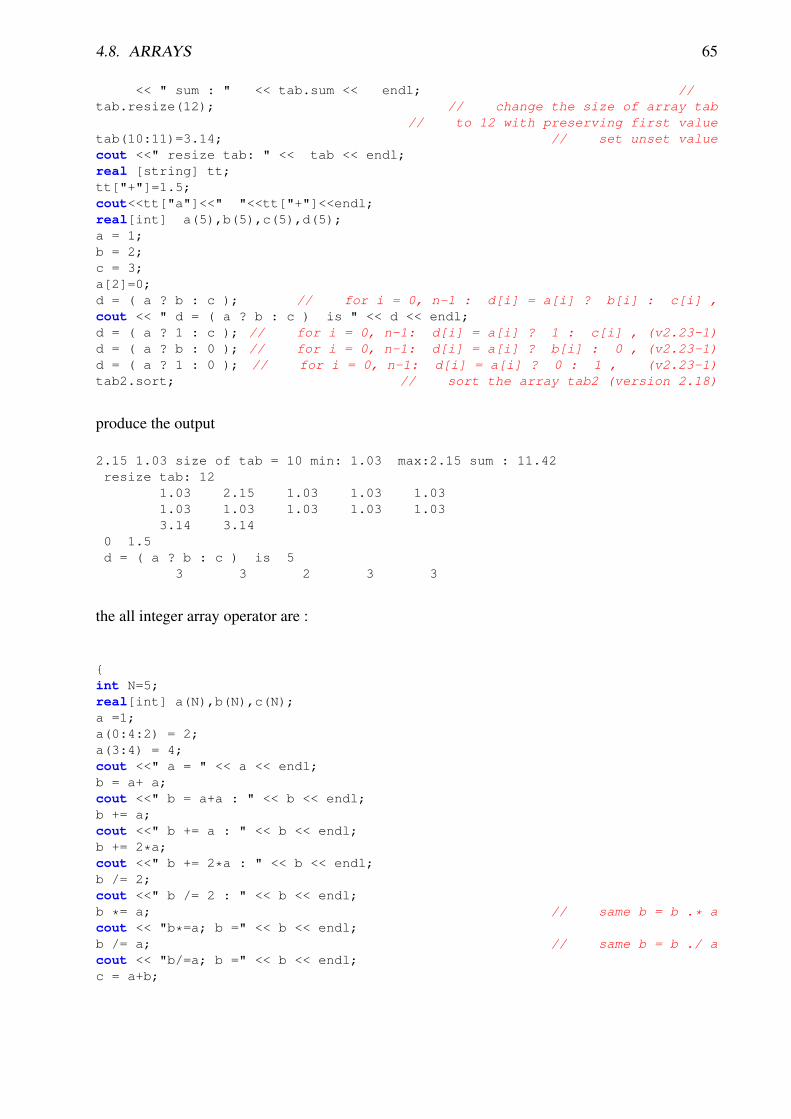
4.8. ARRAYS 65
<< " sum : " << tab.sum << endl; //tab.resize(12); // change the size of array tab
// to 12 with preserving first valuetab(10:11)=3.14; // set unset valuecout <<" resize tab: " << tab << endl;real [string] tt;tt["+"]=1.5;cout<<tt["a"]<<" "<<tt["+"]<<endl;real[int] a(5),b(5),c(5),d(5);a = 1;b = 2;c = 3;a[2]=0;d = ( a ? b : c ); // for i = 0, n-1 : d[i] = a[i] ? b[i] : c[i] ,cout << " d = ( a ? b : c ) is " << d << endl;d = ( a ? 1 : c ); // for i = 0, n-1: d[i] = a[i] ? 1 : c[i] , (v2.23-1)d = ( a ? b : 0 ); // for i = 0, n-1: d[i] = a[i] ? b[i] : 0 , (v2.23-1)d = ( a ? 1 : 0 ); // for i = 0, n-1: d[i] = a[i] ? 0 : 1 , (v2.23-1)tab2.sort; // sort the array tab2 (version 2.18)
produce the output
2.15 1.03 size of tab = 10 min: 1.03 max:2.15 sum : 11.42resize tab: 12
1.03 2.15 1.03 1.03 1.031.03 1.03 1.03 1.03 1.033.14 3.14
0 1.5d = ( a ? b : c ) is 5
3 3 2 3 3
the all integer array operator are :
int N=5;real[int] a(N),b(N),c(N);a =1;a(0:4:2) = 2;a(3:4) = 4;cout <<" a = " << a << endl;b = a+ a;cout <<" b = a+a : " << b << endl;b += a;cout <<" b += a : " << b << endl;b += 2*a;cout <<" b += 2*a : " << b << endl;b /= 2;cout <<" b /= 2 : " << b << endl;b *= a; // same b = b .* acout << "b*=a; b =" << b << endl;b /= a; // same b = b ./ acout << "b/=a; b =" << b << endl;c = a+b;
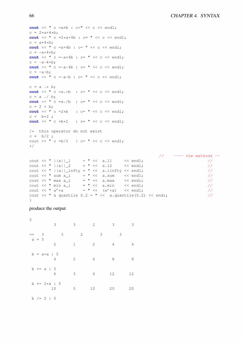
66 CHAPTER 4. SYNTAX
cout << " c =a+b : c=" << c << endl;c = 2*a+4*b;cout << " c =2*a+4b : c= " << c << endl;c = a+4*b;cout << " c =a+4b : c= " << c << endl;c = -a+4*b;cout << " c =-a+4b : c= " << c << endl;c = -a-4*b;cout << " c =-a-4b : c= " << c << endl;c = -a-b;cout << " c =-a-b : c= " << c << endl;
c = a .* b;cout << " c =a.*b : c= " << c << endl;c = a ./ b;cout << " c =a./b : c= " << c << endl;c = 2 * b;cout << " c =2*b : c= " << c << endl;c = b*2 ;cout << " c =b*2 : c= " << c << endl;
/* this operator do not existc = b/2 ;cout << " c =b/2 : c= " << c << endl;
*/
// ---- the methods --cout << " ||a||_1 = " << a.l1 << endl; //cout << " ||a||_2 = " << a.l2 << endl; //cout << " ||a||_infty = " << a.linfty << endl; //cout << " sum a_i = " << a.sum << endl; //cout << " max a_i = " << a.max << endl; //cout << " min a_i = " << a.min << endl; //cout << " a’*a = " << (a’*a) << endl; //cout << " a quantile 0.2 = " << a.quantile(0.2) << endl; //
produce the output
53 3 2 3 3
== 3 3 2 3 3a = 5
2 1 2 4 4
b = a+a : 54 2 4 8 8
b += a : 56 3 6 12 12
b += 2*a : 510 5 10 20 20
b /= 2 : 5

4.8. ARRAYS 67
5 2.5 5 10 10
b*=a; b =510 2.5 10 40 40
b/=a; b =55 2.5 5 10 10
c =a+b : c=57 3.5 7 14 14
c =2*a+4b : c= 524 12 24 48 48
c =a+4b : c= 522 11 22 44 44
c =-a+4b : c= 518 9 18 36 36
c =-a-4b : c= 5-22 -11 -22 -44 -44
c =-a-b : c= 5-7 -3.5 -7 -14 -14
c =a.*b : c= 510 2.5 10 40 40
c =a./b : c= 50.4 0.4 0.4 0.4 0.4
c =2*b : c= 510 5 10 20 20
c =b*2 : c= 510 5 10 20 20
||a||_1 = 13||a||_2 = 6.403124237||a||_infty = 4sum a_i = 13max a_i = 4min a_i = 1a’*a = 41a quantile 0.2 = 2
Note 4.2 Quantiles are points taken at regular intervals from the cumulative distribution functionof a random variable. Here the random is the array value.This statisticial function a.quantile(q) and commute v of an array a of size n for a givennumber q ∈]0, 1[ such than
#i/a[i] < v ∼ q ∗ n
which is equivalent to v = a[q ∗ n] when the array a is sorted.

68 CHAPTER 4. SYNTAX
Example of array with renumbering (version 2.3 or better) . The renumbering is always given byan integer array, and if a value in the array is negative, the mining is not image, so we do not setthe value.
int[int] I=[2,3,4,-1,0]; // the integer mapping to set the renumberingb=c=-3;b= a(I); // for( i=0;i<b.n;i++) if(I[i] >=0) b[i]=a[I[i]];c(I)= a; // for( i=0;i<I.n;i++) if(I[i] >=0) C(I[i])=a[i];cout << " b = a(I) : " << b << "\n c(I) = a " << c << endl;
The output is
b = a(I) : 52 4 4 -3 2
c(I) = a 54 -3 2 1 2
4.8.1 Arrays with two integer indices versus matrixSome example transform full matrices in sparse matrices.
int N=3,M=4;
real[int,int] A(N,M);real[int] b(N),c(M);b=[1,2,3];c=[4,5,6,7];
complex[int,int] C(N,M);complex[int] cb=[1,2,3],cc=[10i,20i,30i,40i];
b=[1,2,3];
int [int] I=[2,0,1];int [int] J=[2,0,1,3];
A=1; // set the all matrixA(2,:) = 4; // the full line 2A(:,1) = 5; // the full column 1A(0:N-1,2) = 2; // set the column 2A(1,0:2) = 3; // set the line 1 from 0 to 2
cout << " A = " << A << endl;// outer product
C = cb*cc’;C += 3*cb*cc’;C -= 5i*cb*cc’;cout << " C = " << C << endl;
// the way to transform a array to a sparse matrixmatrix B;B = A;

4.8. ARRAYS 69
B=A(I,J); // B(i,j)= A(I(i),J(j))B=A(Iˆ-1,Jˆ-1); // B(I(i),J(j))= A(i,j)
A = 2.*b*c’; // outer productcout << " A = " << A << endl;B = b*c’; // outer product B(i,j) = b(i)*c(j)B = b*c’; // outer product B(i,j) = b(i)*c(j)B = (2*b*c’)(I,J); // outer product B(i,j) = b(I(i))*c(J(j))B = (3.*b*c’)(Iˆ-1,Jˆ-1); // outer product B(I(i),J(j)) = b(i)*c(j)cout << "B = (3.*b*c’)(Iˆ-1,Jˆ-1) = " << B << endl;
the output is
b = a(I) : 52 4 4 -3 2
c(I) = a 54 -3 2 1 2
A = 3 41 5 2 13 3 3 14 5 2 4
C = 3 4(-50,-40) (-100,-80) (-150,-120) (-200,-160)(-100,-80) (-200,-160) (-300,-240) (-400,-320)(-150,-120) (-300,-240) (-450,-360) (-600,-480)
A = 3 48 10 12 1416 20 24 2824 30 36 42
4.8.2 Matrix construction and setting• To change the solver associated to a matrix do
set(M,solver=sparsesolver);
The default solver is GMRES.
• from a variationnal form: (see section 6.10 page 120 for details)
varf vDD(u,v) = int2d(Thm)(u*v*1e-10);matrix DD=vDD(Lh,Lh);
• To set from a constant matrix
matrix A =[[ 0, 1, 0, 10],[ 0, 0, 2, 0],[ 0, 0, 0, 3],

70 CHAPTER 4. SYNTAX
[ 4,0 , 0, 0]];
• To set from a block matrix
matrix M=[[ Asd[0] ,0 ,0 ,0 ,Csd[0] ],[ 0 ,Asd[1] ,0 ,0 ,Csd[1] ],[ 0 ,0 ,Asd[2] ,0 ,Csd[2] ],[ 0 ,0 ,0 ,Asd[3] ,Csd[3] ],[ Csd[0]’,Csd[1]’,Csd[2]’,Csd[3]’,DD ]
];
// to now to pack the right hand sidereal[int] bb =[rhssd[0][], rhssd[1][],rhssd[2][],rhssd[3][],rhsl[] ];set(M,solver=sparsesolver);xx = Mˆ-1 * bb;[usd[0][],usd[1][],usd[2][],usd[3][],lh[]] = xx; // to dispatch
// the solution on each part.
where here Asd and Csd are array of matrix (from example mortar-DN-4.edp ofexamples++-tuturial).
• To set or get all the indices and coef of the sparse matrix A, let I,J,C respectively twoint[int] array and a real[int] array. The three array defined the matrix as follow
A =∑
k
C[k]MI[k],J[k] where Mab = (δiaδ jb)i j
and you have: Mab is a basic matrix with the only non zero term mab = 1.
You can write [I,J,C]=A ; to get all the term of the matrix A (the arrays are automat-icaly resize), and A=[I,J,C] ; to change all the term matrix. remark the size of thematrix is with n= I.max and m=J.max. Remark you forget I,J when the build adiagonal matrix, and n,m of the matrix.
4.8.3 Matrix OperationsThe multiplicative operators *, /, and % group left to right.
• ’ is unary right transposition of array, matrix in real case or Hermitian conjugation incomplex case.
• .* is the term to term multiply operator.
• ./ is the term to term divide operator.
there are some compound operator:
• ˆ-1 is for solving the linear system (example: b = Aˆ-1 x)

4.8. ARRAYS 71
• ’ * is the compound of transposition and matrix product, so it is the dot product (examplereal DotProduct=a’*b) , in complex case you get the Hermitian product, so mathe-matically we have a’*b= aT b .
• a*b’ is the outer product (example matrix B=a’*b )
Example 4.5
mesh Th = square(2,1);fespace Vh(Th,P1);Vh f,g;f = x*y;g = sin(pi*x);Vh<complex> ff,gg; // a complex valued finite element functionff= x*(y+1i);gg = exp(pi*x*1i);varf mat(u,v) =
int2d(Th)(1*dx(u)*dx(v)+2*dx(u)*dy(v)+3*dy(u)*dx(v)+4*dy(u)*dy(v))+ on(1,2,3,4,u=1);
varf mati(u,v) =int2d(Th)(1*dx(u)*dx(v)+2i*dx(u)*dy(v)+3*dy(u)*dx(v)+4*dy(u)*dy(v))+ on(1,2,3,4,u=1);
matrix A = mat(Vh,Vh); matrix<complex> AA = mati(Vh,Vh); // a complexsparse matrix
Vh m0; m0[] = A*f[];Vh m01; m01[] = A’*f[];Vh m1; m1[] = f[].*g[];Vh m2; m2[] = f[]./g[];cout << "f = " << f[] << endl;cout << "g = " << g[] << endl;cout << "A = " << A << endl;cout << "m0 = " << m0[] << endl;cout << "m01 = " << m01[] << endl;cout << "m1 = "<< m1[] << endl;cout << "m2 = "<< m2[] << endl;cout << "dot Product = "<< f[]’*g[] << endl;cout << "hermitien Product = "<< ff[]’*gg[] << endl;cout << "outer Product = "<< (A=ff[]*gg[]’) << endl;cout << "hermitien outer Product = "<< (AA=ff[]*gg[]’) << endl;real[int] diagofA(A.n);
diagofA = A.diag; // get the diagonal of the matrixA.diag = diagofA ; // set the diagonal of the matrix
// version 2.17 or better ---int[int] I(1),J(1); real[int] C(1);[I,J,C]=A; // get of the sparse term of the matrix A (the array areresized)cout << " I= " << I << endl;cout << " J= " << J << endl;cout << " C= " << C << endl;A=[I,J,C]; // set a new matrixmatrix D=[diagofA] ; // set a diagonal matrix D from the array diagofA.cout << " D = " << D << endl;
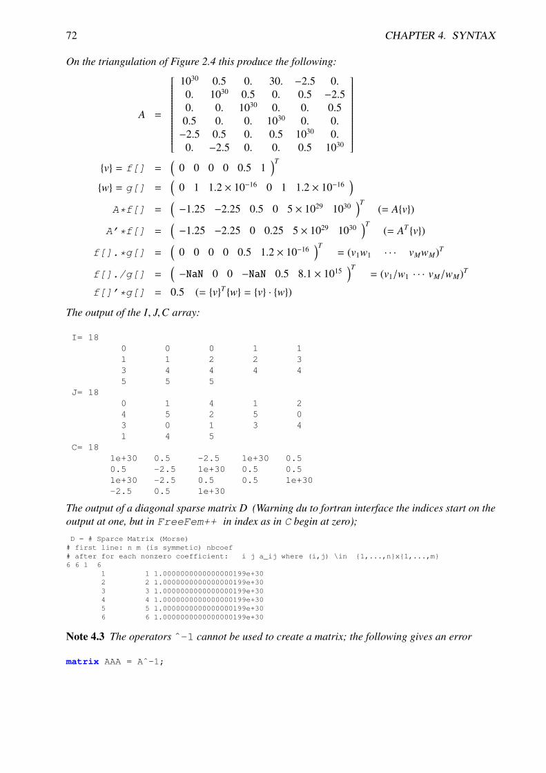
72 CHAPTER 4. SYNTAX
On the triangulation of Figure 2.4 this produce the following:
A =
1030 0.5 0. 30. −2.5 0.0. 1030 0.5 0. 0.5 −2.50. 0. 1030 0. 0. 0.5
0.5 0. 0. 1030 0. 0.−2.5 0.5 0. 0.5 1030 0.
0. −2.5 0. 0. 0.5 1030
v = f[] =
(0 0 0 0 0.5 1
)T
w = g[] =(
0 1 1.2 × 10⁻¹⁶ 0 1 1.2 × 10⁻¹⁶)
A*f[] =(−1.25 −2.25 0.5 0 5 × 1029 1030
)T(= Av)
A’*f[] =(−1.25 −2.25 0 0.25 5 × 1029 1030
)T(= AT v)
f[].*g[] =(
0 0 0 0 0.5 1.2 × 10⁻¹⁶)T
= (v1w1 · · · vMwM)T
f[]./g[] =(−NaN 0 0 −NaN 0.5 8.1 × 10¹⁵
)T= (v1/w1 · · · vM/wM)T
f[]’*g[] = 0.5 (= vT w = v · w)
The output of the I, J,C array:
I= 180 0 0 1 11 1 2 2 33 4 4 4 45 5 5
J= 180 1 4 1 24 5 2 5 03 0 1 3 41 4 5
C= 181e+30 0.5 -2.5 1e+30 0.50.5 -2.5 1e+30 0.5 0.51e+30 -2.5 0.5 0.5 1e+30-2.5 0.5 1e+30
The output of a diagonal sparse matrix D (Warning du to fortran interface the indices start on theoutput at one, but in FreeFem++ in index as in C begin at zero);D = # Sparce Matrix (Morse)# first line: n m (is symmetic) nbcoef# after for each nonzero coefficient: i j a_ij where (i,j) \in 1,...,nx1,...,m6 6 1 6
1 1 1.0000000000000000199e+302 2 1.0000000000000000199e+303 3 1.0000000000000000199e+304 4 1.0000000000000000199e+305 5 1.0000000000000000199e+306 6 1.0000000000000000199e+30
Note 4.3 The operators ˆ-1 cannot be used to create a matrix; the following gives an error
matrix AAA = Aˆ-1;

4.8. ARRAYS 73
4.8.4 Other arraysIt is also possible to make an array of FE functions, with the same syntax, and we can treat themas vector valued function if we need them.
Example 4.6 In the following example, Poisson’s equation is solved for 3 different given functionsf = 1, sin(πx) cos(πy), |x − 1||y − 1|, whose solutions are stored in an array of FE function.
mesh Th=square(20,20,[2*x,2*y]);fespace Vh(Th,P1);Vh u, v, f;problem Poisson(u,v) =
int2d(Th)( dx(u)*dx(v) + dy(u)*dy(v))+ int2d(Th)( -f*v ) + on(1,2,3,4,u=0) ;
Vh[int] uu(3); // an array of FE functionf=1; // problem1Poisson; uu[0] = u;f=sin(pi*x)*cos(pi*y); // problem2Poisson; uu[1] = u;f=abs(x-1)*abs(y-1); // problem3Poisson; uu[2] = u;for (int i=0; i<3; i++) // plots all solutions
plot(uu[i], wait=true);
For the second case, it is just a map of the STL1[25] so no operations on vector are allowed, exceptthe selection of an item .The transpose or Hermitian conjugation operator is ’ like Matlab or Scilab, so the way to computethe dot product of two array a,b is real ab= a’*b.
int i;real [int] tab(10), tab1(10); // 2 array of 10 real
real [int] tab2; // Error: array with no sizetab = 1; // set all the array to 1tab[1]=2;cout << tab[1] << " " << tab[9] << " size of tab = "
<< tab.n << " " << tab.min << " " << tab.max << " " << endl;tab1=tab; tab=tab+tab1; tab=2*tab+tab1*5; tab1=2*tab-tab1*5;tab+=tab; cout << " dot product " << tab’*tab << endl; // ttab tabcout << tab << endl; cout << tab[1] << " "<< tab[9] << endl; real[string] map; // a dynamic arrayfor (i=0;i<10;i=i+1)
tab[i] = i*i;cout << i << " " << tab[i] << "\n";
;
map["1"]=2.0;map[2]=3.0; // 2 is automatically cast to the string "2"
cout << " map[\"1\"] = " << map["1"] << "; "<< endl;cout << " map[2] = " << map[2] << "; "<< endl;
1Standard template Library, now part of standard C++

74 CHAPTER 4. SYNTAX
4.9 Loops
The for and while loops are implemented with break and continue keywords.In for-loop, there are three parameters; the INITIALIZATION of a control variable, the CONDI-TION to continue, the CHANGE of the control variable. While CONDITION is true, for-loopcontinue.
for (INITIALIZATION; CONDITION; CHANGE)
BLOCK of calculations
Below, the sum from 1 to 10 is calculated by (the result is in sum),
int sum=0;
for (int i=1; i<=10; i++)
sum += i;
The while-loop
while (CONDITION)
BLOCK of calculations or change of control variables
is executed repeatedly until CONDITION become false. The sum from 1 to 10 is also written bywhile as follows,
int i=1, sum=0;
while (i<=10)
sum += i; i++;
We can exit from a loop in midstream by break. The continue statement will pass the part fromcontinue to the end of the loop.
Example 4.7
for (int i=0;i<10;i=i+1)
cout << i << "\n";
real eps=1;
while (eps>1e-5)
eps = eps/2;
if( i++ <100) break;
cout << eps << endl;
for (int j=0; j<20; j++)
if (j<10) continue;
cout << "j = " << j << endl;

4.10. INPUT/OUTPUT 75
4.10 Input/OutputThe syntax of input/output statements is similar to C++ syntax. It uses cout, cin, endl, <<,>>.To write to (resp. read from) a file, declare a new variable ofstream ofile("filename");or ofstream ofile("filename",append); (resp. ifstream ifile("filename");) and use ofile (resp. ifile) as cout (resp. cin).The word append in ofstream ofile("filename",append); means openning a file inappend mode.
Note 4.4 The file is closed at the exit of the enclosing block,
Example 4.8
int i;cout << " std-out" << endl;cout << " enter i= ? ";cin >> i ;
ofstream f("toto.txt");f << i << "coucou’\n";
; // close the file f because the variable f is delete
ifstream f("toto.txt");f >> i;
ofstream f("toto.txt",append);// to append to the existing file "toto.txt"
f << i << "coucou’\n";; // close the file f because the variable f is delete
cout << i << endl;
We add function to format the output.
• int nold=f.precision(n) Sets the number of digits printed to the right of the deci-mal point. This applies to all subsequent floating point numbers written to that output stream.However, this won’t make floating-point ”integers” print with a decimal point. It’s necessaryto use fixed for that effect.
• f.scientific Formats floating-point numbers in scientific notation ( d.dddEdd )
• f.fixed Used fixed point notation ( d.ddd ) for floating-point numbers. Opposite of sci-entific.
• f.showbase Converts insertions to an external form that can be read according to the C++lexical conventions for integral constants. By default, showbase is not set.
• f.noshowbase unset showbase flags
• f.showpos inserts a plus sign (+) into a decimal conversion of a positive integral value.

76 CHAPTER 4. SYNTAX
• f.noshowpos unset showpos flags
• f.default reset all the previous flags (fmtflags) to the default expect precision.
Where f is output stream descriptor, for example cout.Remark, all this method exept the first return the stream f, so you can write
cout.scientific.showpos << 3 << endl;
4.11 Exception handlingIn the version 2.3 of FreeFem++, we add exception handing like in C++. But to day we onlycatch all the C++ exception, and in the C++ all the errors like ExecError, assert, exit,... are exception so you can have some surprise with the memory management.The exception handle all ExecError:
Example 4.9 A simple example first to catch a division by zero:
real a;try a=1./0.;
catch (...) // today only all exceptions are permitted
cout << " Catch an ExecError " << endl;a =0;
The output is
1/0 : d d dcurrent line = 3
Exec error : Div by 0-- number :1
Try:: catch (...) exceptionCatch an ExecError
Add a more realistic example:
Example 4.10 A case with none invertible matrix:
int nn=5 ;mesh Th=square(nn,nn);verbosity=5;fespace Vh(Th,P1); // P1 FE spaceVh uh,vh; // unkown and test function.func f=1; // right hand side functionfunc g=0; // boundary condition functionreal cpu=clock();problem laplace(uh,vh,solver=Cholesky,tolpivot=1e-6) = //definion of the problem

4.11. EXCEPTION HANDLING 77
int2d(Th)( dx(uh)*dx(vh) + dy(uh)*dy(vh) ) // bilinear form+ int2d(Th)( -f*vh ) // linear form
;
try cout << " Try Cholesky \n";laplace; // solve the problem plot(uh); // to see the resultcout << "-- lap Cholesky " << nn << "x" << nn << " : " << -cpu+clock()
<< " s, max =" << uh[].max << endl;catch(...) // catch all
cout << " Catch cholesky PB " << endl;
The output is
-- square mesh : nb vertices =36 , nb triangles = 50 ...Nb of edges on Mortars = 0Nb of edges on Boundary = 20, neb = 20Nb Mortars 0
number of real boundary edges 20Number of Edges = 85Number of Boundary Edges = 20 neb = 20Number of Mortars Edges = 0Nb Of Mortars with Paper Def = 0 Nb Of Mortars = 0 ...
Nb Of Nodes = 36Nb of DF = 36Try Cholesky
-- Change of Mesh 0 0x312e9e8Problem(): initmat 1 VF (discontinuous Galerkin) = 0-- SizeOfSkyline =210-- size of Matrix 196 Bytes skyline =1-- discontinous Galerkin =0 size of Mat =196 Bytes-- int in Optimized = 1, ...
all-- boundary int Optimized = 1, all
ERREUR choleskypivot (35)= -1.23124e-13 < 1e-06current line = 28
Exec error : FATAL ERREUR dans ../femlib/MatriceCreuse_tpl.hppcholesky line:
-- number :545catch an erreur in solve => set sol = 0 !!!!!!!Try:: catch (...) exceptionCatch cholesky PB

78 CHAPTER 4. SYNTAX

Chapter 5
Mesh Generation
5.1 Commands for Mesh Generationborder, buildmesh are explained.All the examples in this section come from the files mesh.edp and tablefunction.edp.
5.1.1 SquareFor easy and simple testing, there is the command “square”. The following
mesh Th = square(4,5);
generate a 4 × 5 grid in the unit squre [0, 1]2 whose labels are shown in Fig. 5.1. If you want to
l a b e l= 4
l a b e l = 1
l a b e l = 3
l a b e l= 2
Figure 5.1: Boundary labels of the mesh by square(10,10)
construct a n × m grid in the rectangle [x0, x1] × [y0, y1], you can write
real x0=1.2,x1=1.8;real y0=0,y1=1;int n=5,m=20;mesh Th=square(n,m,[x0+(x1-x0)*x,y0+(y1-y0)*y]);
Note 5.1 Adding the parameter flags=1, will produce a Union Jack flag type of mesh.
79

80 CHAPTER 5. MESH GENERATION
mesh Th=square(n,m,[x0+(x1-x0)*x,y0+(y1-y0)*y],flags=1);
5.1.2 BorderA domain is defined as being on the left (resp right) of its parameterized boundary
Γ j = (x, y)∣∣∣ x = ϕx(t), y = ϕy(t), a j ≤ t ≤ b j
We can easily check the orientation by drawing the curve t 7→ (ϕx(t), ϕy(t)), t0 ≤ t ≤ t1. If it is asin Fig. 5.2, then the domain lie on the shaded area, otherwise it lies on the opposite sideThe boundaries Γ j can only intersect at their end points.
G j
t = t 0
t = t 1( x = j x ( t ) , y = j y ( t ) )
( d j x ( t ) / d t , d j y ( t ) / d t )( x = t , y = t ) ( x = t , y = - t )t = t 0
t = t 1
t = t 1
t = t 0
Figure 5.2: Orientation of the boundary defined by (φx(t), φy(t))
The general expression to define a triangulation with buildmesh is
mesh Mesh_Name = buildmesh(Γ1(m1) + · · · + ΓJ(m j) OptionalParameter
);
where m j are positive or negative numbers to indicate how may point should be put on Γ j, Γ =
∪Jj=1ΓJ, an the optional parameter (separed with comma) can be
nbvx=<int value> , to set the maximal number of vertices in the mesh.
fixeborder=<bool value> , to say if the mesh generator can change the boundary meshor not (by default the boundary mesh can change and in case of periodic boundary problem(see. 6), it can be dangerous .
We can change the orientation of boundaries by changing the sign of m j. The following exampleshows how to change the orientation. The example generates the unit disk with a small circularhole, and assign “1” to the unit disk (“2” to the circle inside). The boundary label must be non-zero,but it can also be omitted.
1: border a(t=0,2*pi) x=cos(t); y=sin(t);label=1;2: border b(t=0,2*pi) x=0.3+0.3*cos(t); y=0.3*sin(t);label=2;3: plot(a(50)+b(+30)) ; // to see a plot of the border mesh4: mesh Thwithouthole= buildmesh(a(50)+b(+30));5: mesh Thwithhole = buildmesh(a(50)+b(-30));6: plot(Thwithouthole,wait=1,ps="Thwithouthole.eps"); // figure 5.37: plot(Thwithhole,wait=1,ps="Thwithhole.eps"); // figure 5.4

5.1. COMMANDS FOR MESH GENERATION 81
Figure 5.3: mesh without hole Figure 5.4: mesh with hole
Note 5.2 You must notice that the orientation is changed by “b(-30)” in 5th line. In 7th line,ps="fileName" is used to generate a postscript file identification that is shown on screen.
Note 5.3 The border is evaluated only at the time plot or buildmesh is called so the globalvariable are defined at this time and the following code can not work:
real r=1; border a(t=0,2*pi) x=r*cos(t); y=r*sin(t);label=1;r=0.3 ; border b(t=0,2*pi) x=r*cos(t); y=r*sin(t);label=1;mesh Thwithhole = buildmesh(a(50)+b(-30)); // bug (a trap) because
// the two circle have the same radius = 0.3
5.1.3 Data Structure and Read/Write Statements for a MeshUsers who want to use a triangulation made elsewhere should see the file structure of the filegenerated below:
border C(t=0,2*pi) x=cos(t); y=sin(t); mesh Th = buildmesh(C(10));savemesh("mesh_sample.msh");
the mesh is shown on Fig. 5.5.
The informations about Th are save in the file “mesh sample.msh”. whose structure is shown onTable 5.1.There nv denotes the number of vertices, nt number of triangles and ns the number of edges onboundary.For each vertex qi, i = 1, · · · , nv, we denote by (qi
x, qiy) the x-coordinate and y-coordinate.
Each triangle Tk, k = 1, · · · , 10 has three vertices qk1 , qk2 , qk3 that are oriented counterclockwise.The boundary consists of 10 lines Li, i = 1, · · · , 10 whose end points are qi1 , qi2 .

82 CHAPTER 5. MESH GENERATION
1 2
1 13
1 3
5
4
53
8
9
7
1 1
8
1 2
1 4 1 3
1 0
69
2
1 3
1
4
1 0
1 5
1 46
7
1 2
Figure 5.5: mesh by buildmesh(C(10))
In the left figure, we have the following.
nv = 14, nt = 16, ns = 10
q1 = (−0.309016994375, 0.951056516295)...
......
q14 = (−0.309016994375, −0.951056516295)
The vertices of T1 are q9, q12, q10....
......
The vertices of T16 are q9, q10, q6.
The edge of 1st side L1 are q6, q5....
......
The edge of 10th side L10 are q10, q6.
Contents of file Explanation14 16 10 nv nt ne
-0.309016994375 0.951056516295 1 q1x q1
y boundary label=10.309016994375 0.951056516295 1 q2
x q2y boundary label=1
· · · · · ·...
-0.309016994375 -0.951056516295 1 q14x q14
y boundary label=19 12 10 0 11 12 13 region label=05 9 6 0 21 22 23 region label=0· · ·
9 10 6 0 161 162 163 region label=06 5 1 11 12 boundary label=15 2 1 21 22 boundary label=1· · ·
10 6 1 101 102 boundary label=1
Table 5.1: The structure of “mesh sample.msh”

5.1. COMMANDS FOR MESH GENERATION 83
There are many mesh file formats available for communication with other tools such as emc2,modulef.. (see Section 12), The extension of a file gives the chosen type. More details can befound in the article by F. Hecht ”bamg : a bidimentional anisotropic mesh generator” availablefrom the FreeFem web site.
A mesh file can be read back into FreeFem++ but the names of the borders are lost. So theseborders have to be referenced by the number which corresponds to their order of appearance in theprogram, unless this number is forced by the keyword ”label”. Here are some examples:
border floor(t=0,1) x=t; y=0; label=1;; // the unit squareborder right(t=0,1) x=1; y=t; label=5;;border ceiling(t=1,0) x=t; y=1; label=5;;border left(t=1,0) x=0; y=t; label=5;;int n=10;mesh th= buildmesh(floor(n)+right(n)+ceiling(n)+left(n));savemesh(th,"toto.am_fmt"); // "formatted Marrocco" formatsavemesh(th,"toto.Th"); // "bamg"-type meshsavemesh(th,"toto.msh"); // freefem formatsavemesh(th,"toto.nopo"); // modulef format see [9]mesh th2 = readmesh("toto.msh"); // read the mesh
Example 5.1 (Readmesh.edp) border floor(t=0,1) x=t; y=0; label=1;; // theunit squareborder right(t=0,1) x=1; y=t; label=5;;border ceiling(t=1,0) x=t; y=1; label=5;;border left(t=1,0) x=0; y=t; label=5;;int n=10;mesh th= buildmesh(floor(n)+right(n)+ceiling(n)+left(n));savemesh(th,"toto.am_fmt"); // format "formated Marrocco"savemesh(th,"toto.Th"); // format database db mesh "bamg"savemesh(th,"toto.msh"); // format freefemsavemesh(th,"toto.nopo"); // modulef format see [9]mesh th2 = readmesh("toto.msh");fespace femp1(th,P1);femp1 f = sin(x)*cos(y),g; // save solutionofstream file("f.txt");file << f[] << endl; // close the file (end block) // readifstream file("f.txt");file >> g[] ; // close reading file (end block)fespace Vh2(th2,P1);Vh2 u,v;plot(g);// find u such that// u + ∆u = g in Ω ,// u = 0 on Γ1 and ∂u
∂n = g on Γ2solve pb(u,v) =

84 CHAPTER 5. MESH GENERATION
int2d(th)( u*v - dx(u)*dx(v)-dy(u)*dy(v) )+ int2d(th)(-g*v)+ int1d(th,5)( g*v) // ∂u
∂n = g on Γ2+ on(1,u=0) ;
plot (th2,u);
5.1.4 Mesh ConnectivityThe following example explains methods to obtain mesh information.
// get mesh information (version 1.37)mesh Th=square(2,2);
// get data of the meshint nbtriangles=Th.nt;cout << " nb of Triangles = " << nbtriangles << endl;for (int i=0;i<nbtriangles;i++)
for (int j=0; j <3; j++)cout << i << " " << j << " Th[i][j] = "
<< Th[i][j] << " x = "<< Th[i][j].x << " , y= "<< Th[i][j].y<< ", label=" << Th[i][j].label << endl;
// Th(i) return the vextex i of Th// Th[k] return the triangle k of Th
fespace femp1(Th,P1);femp1 Thx=x,Thy=y; // hack of get vertex coordinates
// get vertices information :int nbvertices=Th.nv;cout << " nb of vertices = " << nbvertices << endl;for (int i=0;i<nbvertices;i++)
cout << "Th(" <<i << ") : " // << endl;<< Th(i).x << " " << Th(i).y << " " << Th(i).label // v 2.19<< " old method: " << Thx[][i] << " " << Thy[][i] << endl;
// method to find information of point (0.55,0.6)
int it00 = Th(0.55,0.6).nuTriangle; // then triangle numberint nr00 = Th(0.55,0.6).region; //
// info of a trianglereal area00 = Th[it00].area; // new in version 2.19real nrr00 = Th[it00].region; // new in version 2.19real nll00 = Th[it00].label; // same as region in this case.
// Hack to get a triangle contening point x,y// or region number (old method)// -------------------------------------------------------
fespace femp0(Th,P0);femp0 nuT; // a P0 function to get triangle numbering
for (int i=0;i<Th.nt;i++)nuT[][i]=i;
femp0 nuReg=region; // a P0 function to get the region number// inquire

5.1. COMMANDS FOR MESH GENERATION 85
int it0=nuT(0.55,0.6); // number of triangle Th’s contening (0.55,0,6);int nr0=nuReg(0.55,0.6); // number of region of Th’s contening (0.55,0,6);
// dump// -------------------------------------------------------
cout << " point (0.55,0,6) :triangle number " << it00 << " " << it00<< ", region = " << nr0 << " == " << nr00 << ", area K " << area00 << endl;
the output is:
-- square mesh : nb vertices =9 , nb triangles = 8 , nb boundary edges 8Nb of Vertices 9 , Nb of Triangles 8Nb of edge on user boundary 8 , Nb of edges on true boundary 8
number of real boundary edges 8nb of Triangles = 8
0 0 Th[i][j] = 0 x = 0 , y= 0, label=40 1 Th[i][j] = 1 x = 0.5 , y= 0, label=10 2 Th[i][j] = 4 x = 0.5 , y= 0.5, label=0...6 0 Th[i][j] = 4 x = 0.5 , y= 0.5, label=06 1 Th[i][j] = 5 x = 1 , y= 0.5, label=26 2 Th[i][j] = 8 x = 1 , y= 1, label=37 0 Th[i][j] = 4 x = 0.5 , y= 0.5, label=07 1 Th[i][j] = 8 x = 1 , y= 1, label=37 2 Th[i][j] = 7 x = 0.5 , y= 1, label=3Nb Of Nodes = 9Nb of DF = 9-- vector function’s bound 0 1-- vector function’s bound 0 1nb of vertices = 9
Th(0) : 0 0 4 old method: 0 0Th(1) : 0.5 0 1 old method: 0.5 0...Th(7) : 0.5 1 3 old method: 0.5 1Th(8) : 1 1 3 old method: 1 1Nb Of Nodes = 8Nb of DF = 8
5.1.5 The keyword ”triangulate”FreeFem++ is able to build a triangulation from a set of points. This triangulation is a Delaunaymesh of the convex hull of the set of points. It can be useful to build a mesh form a table function.The coordinates of the points and the value of the table function are defined separately with rowsof the form: x y f(x,y) in a file such as:
0.51387 0.175741 0.6362370.308652 0.534534 0.7467650.947628 0.171736 0.8998230.702231 0.226431 0.8008190.494773 0.12472 0.580623
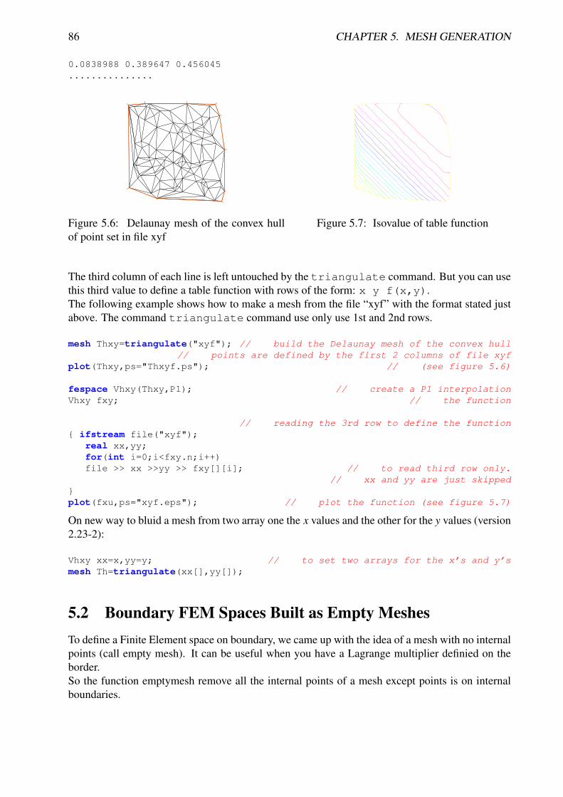
86 CHAPTER 5. MESH GENERATION
0.0838988 0.389647 0.456045...............
Figure 5.6: Delaunay mesh of the convex hullof point set in file xyf
Figure 5.7: Isovalue of table function
The third column of each line is left untouched by the triangulate command. But you can usethis third value to define a table function with rows of the form: x y f(x,y).The following example shows how to make a mesh from the file “xyf” with the format stated justabove. The command triangulate command use only use 1st and 2nd rows.
mesh Thxy=triangulate("xyf"); // build the Delaunay mesh of the convex hull// points are defined by the first 2 columns of file xyf
plot(Thxy,ps="Thxyf.ps"); // (see figure 5.6)
fespace Vhxy(Thxy,P1); // create a P1 interpolationVhxy fxy; // the function
// reading the 3rd row to define the function ifstream file("xyf");
real xx,yy;for(int i=0;i<fxy.n;i++)file >> xx >>yy >> fxy[][i]; // to read third row only.
// xx and yy are just skippedplot(fxu,ps="xyf.eps"); // plot the function (see figure 5.7)
On new way to bluid a mesh from two array one the x values and the other for the y values (version2.23-2):
Vhxy xx=x,yy=y; // to set two arrays for the x’s and y’smesh Th=triangulate(xx[],yy[]);
5.2 Boundary FEM Spaces Built as Empty MeshesTo define a Finite Element space on boundary, we came up with the idea of a mesh with no internalpoints (call empty mesh). It can be useful when you have a Lagrange multiplier definied on theborder.So the function emptymesh remove all the internal points of a mesh except points is on internalboundaries.

5.3. REMESHING 87
// new stuff 2004 emptymesh (version 1.40)// -- useful to build Multiplicator space
// build a mesh without internal point// with the same boundary
// -----assert(version>=1.40);border a(t=0,2*pi) x=cos(t); y=sin(t);label=1;mesh Th=buildmesh(a(20));Th=emptymesh(Th);
plot(Th,wait=1,ps="emptymesh-1.eps"); // see figure 5.8
It is also possible to build an empty mesh of a pseudo subregion with emptymesh(Th,ssd)with the set of edges of the mesh Th; a edge e is in this set if with the two adjacent trianglese = t1 ∩ t2 and ssd[T1] , ssd[T2] where ssd refers to the pseudo region numbering of triangles,when they are stored in an int[int] array of size the number of triangles.
// new stuff 2004 emptymesh (version 1.40)// -- useful to build Multiplicator space// build a mesh without internal point// of peusdo sub domain// -----assert(version>=1.40);mesh Th=square(10,10);int[int] ssd(Th.nt);for(int i=0;i<ssd.n;i++) // build the pseudo region numbering int iq=i/2; // because 2 triangle per quad
int ix=iq%10; //int iy=iq/10; //
ssd[i]= 1 + (ix>=5) + (iy>=5)*2;
Th=emptymesh(Th,ssd); // build emtpy with// all edge e = T1 ∩ T2 and ssd[T1] , ssd[T2]
plot(Th,wait=1,ps="emptymesh-2.eps"); // see figure 5.9savemesh(Th,"emptymesh-2.msh");
5.3 Remeshing
5.3.1 MovemeshMeshes can be translated, rotated and deformed by movemesh; this is useful for elasticity towatch the deformation due to the displacement Φ(x, y) = (Φ1(x, y),Φ2(x, y)) of shape. It is alsouseful to handle free boundary problems or optimal shape problems.If Ω is triangulated as Th(Ω), and Φ is a displacement vector then Φ(Th) is obtained by
mesh Th=movemesh(Th,[Φ1,Φ2]);
Sometimes the moved mesh is invalid because some triangle becomes reversed (with a negativearea). This is why we should check the minimum triangle area in the transformed mesh withcheckmovemesh before any real transformation.

88 CHAPTER 5. MESH GENERATION
Figure 5.8: The empty mesh with boundaryFigure 5.9: An empty mesh defined from apseudo region numbering of triangle
Example 5.2 Φ1(x, y) = x + k ∗ sin(y ∗ π)/10), Φ2(x, y) = y + k ∗ cos(yπ)/10) for a big numberk > 1.
verbosity=4;border a(t=0,1)x=t;y=0;label=1;;border b(t=0,0.5)x=1;y=t;label=1;;border c(t=0,0.5)x=1-t;y=0.5;label=1;;border d(t=0.5,1)x=0.5;y=t;label=1;;border e(t=0.5,1)x=1-t;y=1;label=1;;border f(t=0,1)x=0;y=1-t;label=1;;func uu= sin(y*pi)/10;func vv= cos(x*pi)/10;
mesh Th = buildmesh ( a(6) + b(4) + c(4) +d(4) + e(4) + f(6));plot(Th,wait=1,fill=1,ps="Lshape.eps"); // see figure 5.10real coef=1;real minT0= checkmovemesh(Th,[x,y]); // the min triangle areawhile(1) // find a correct move mesh
real minT=checkmovemesh(Th,[x+coef*uu,y+coef*vv]);// the min triangle areaif (minT > minT0/5) break ; // if big enoughcoef=/1.5;
Th=movemesh(Th,[x+coef*uu,y+coef*vv]);plot(Th,wait=1,fill=1,ps="movemesh.eps"); // see figure 5.11
Note 5.4 Consider a function u defined on a mesh Th. A statement like Th=movemesh(Th...)does not change u and so the old mesh still exists. It will be destroyed when no function use it. Astatement like u = u redefines u on the new mesh Th with interpolation and therefore destroys theold Th if u was the only function using it.

5.3. REMESHING 89
Figure 5.10: L-shape Figure 5.11: moved L-shape
Example 5.3 (movemesh.edp) Now, we given an example of moving mesh with a lagrangianfunction u defined on the moving mesh.
// simple movemesh example
mesh Th=square(10,10);
fespace Vh(Th,P1);
real t=0;
// ---
// the problem is how to build data without interpolation
// so the data u is moving with the mesh as you can see in the plot
// ---
Vh u=y;
for (int i=0;i<4;i++)
t=i*0.1;
Vh f= x*t;
real minarea=checkmovemesh(Th,[x,y+f]);
if (minarea >0 ) // movemesh will be ok
Th=movemesh(Th,[x,y+f]);
cout << " Min area " << minarea << endl;
real[int] tmp(u[].n);
tmp=u[]; // save the value
u=0; // to change the FEspace and mesh associated with u
u[]=tmp; // set the value of u without any mesh update
plot(Th,u,wait=1);;
// In this program, since u is only defined on the last mesh, all the
// previous meshes are deleted from memory.
// --------

90 CHAPTER 5. MESH GENERATION
5.4 Regular Triangulation: hTriangleFor a set S , we define the diameter of S by
diam(S ) = sup|x − y|; x, y ∈ S
The sequence Thh↓0 of Ω is called regular if they satisfy the following:
1.limh↓0
maxdiam(Tk)| Tk ∈ Th = 0
2. There is a number σ > 0 independent of h such that
ρ(Tk)diam(Tk)
≥ σ for all Tk ∈ Th
where ρ(Tk) are the diameter of the inscribed circle of Tk.
We put h(Th) = maxdiam(Tk)| Tk ∈ Th, which is obtained by
mesh Th = ......;fespace Ph(Th,P0);Ph h = hTriangle;cout << "size of mesh = " << h[].max << endl;
5.5 AdaptmeshThe function
f (x, y) = 10.0x3 + y3 + tan−1[ε/(sin(5.0y) − 2.0x)] ε = 0.0001
sharply varies in value. However, the initial mesh given by the command in Section 5.1 cannotreflect its sharp variations.
Example 5.4
real eps = 0.0001;real h=1;real hmin=0.05;func f = 10.0*xˆ3+yˆ3+h*atan2(eps,sin(5.0*y)-2.0*x);
mesh Th=square(5,5,[-1+2*x,-1+2*y]);fespace Vh(Th,P1);Vh fh=f;plot(fh);for (int i=0;i<2;i++)
Th=adaptmesh(Th,fh);fh=f; // old mesh is deletedplot(Th,fh,wait=1);

5.5. ADAPTMESH 91
I n i t i a l m e s h
F i r s t a d a p t a t i o n
S e c o n d a d a p t a t i o n
Figure 5.12: 3D graphs for the initial mesh and 1st and 2nd mesh adaptation
FreeFem++ uses a variable metric/Delaunay automatic meshing algorithm. The command
mesh ATh = adaptmesh(Th, f);
create the new mesh ATh by the Hessian
D2 f = (∂2 f /∂x2, ∂2 f /∂x∂y, ∂2 f /∂y2)
of a function (formula or FE-function). Mesh adaptation is a very powerful tool when the solutionof a problem vary locally and sharply.Here we solve the problem (2.1)-(2.2), when f = 1 and Ω is a L-shape domain.
Example 5.5 (Adapt.edp) The solution has the singularity r3/2, r = |x − γ| at the point γ of theintersection of two lines bc and bd (see Fig. 5.13).
border ba(t=0,1.0)x=t; y=0; label=1;;border bb(t=0,0.5)x=1; y=t; label=1;;border bc(t=0,0.5)x=1-t; y=0.5;label=1;;border bd(t=0.5,1)x=0.5; y=t; label=1;;border be(t=0.5,1)x=1-t; y=1; label=1;;border bf(t=0.0,1)x=0; y=1-t;label=1;;mesh Th = buildmesh ( ba(6)+bb(4)+bc(4)+bd(4)+be(4)+bf(6) );fespace Vh(Th,P1); // set FE spaceVh u,v; // set unknown and test functionfunc f = 1;real error=0.1; // level of error

92 CHAPTER 5. MESH GENERATION
b a
b b
b cb d
b e
b f
Figure 5.13: L-shape domain and its boundaryname
Figure 5.14: Final solution after 4-times adap-tation
problem Poisson(u,v,solver=CG,eps=1.0e-6) =int2d(Th)( dx(u)*dx(v) + dy(u)*dy(v))
- int2d(Th) ( f*v )+ on(1,u=0) ;
for (int i=0;i< 4;i++)
Poisson;Th=adaptmesh(Th,u,err=error);error = error/2;
;plot(u);
To speed up the adaptation we change by hand a default parameter err of adaptmesh, whichspecifies the required precision, so as to make the new mesh finer. The problem is coercive andsymmetric, so the linear system can be solved with the conjugate gradient method (parametersolver=CG with the stopping criteria on the residual, here eps=1.0e-6). By adaptmesh,we get good slope of the final solution near the point of intersection of bc and bd as in Fig. 5.14.This method is described in detail in [8]. It has a number of default parameters which can bemodified :
hmin= Minimum edge size. (val is a real. Its default is related to the size of the domain to bemeshed and the precision of the mesh generator).
hmax= Maximum edge size. (val is a real. It defaults to the diameter of the domain to bemeshed)
err= P1 interpolation error level (0.01 is the default).
errg= Relative geometrical error. By default this error is 0.01, and in any case it must be lowerthan 1/
√2. Meshes created with this option may have some edges smaller than the -hmin
due to geometrical constraints.
nbvx= Maximum number of vertices generated by the mesh generator (9000 is the default).
nbsmooth= number of iterations of the smoothing procedure (5 is the default).

5.5. ADAPTMESH 93
nbjacoby= number of iterations in a smoothing procedure during the metric construction, 0means no smoothing (6 is the default).
ratio= ratio for a prescribed smoothing on the metric. If the value is 0 or less than 1.1 nosmoothing is done on the metric (1.8 is the default).
If ratio > 1.1, the speed of mesh size variations is bounded by log(ratio). Note: Asratio gets closer to 1, the number of generated vertices increases. This may be useful tocontrol the thickness of refined regions near shocks or boundary layers .
omega= relaxation parameter for the smoothing procedure (1.0 is the default).
iso= If true, forces the metric to be isotropic (false is the default).
abserror= If false, the metric is evaluated using the criterium of equi-repartion of relative error(false is the default). In this case the metric is defined by
M =
(1
err coef2
|H|
max(CutOff, |η|)
)p
(5.1)
otherwise, the metric is evaluated using the criterium of equi-distribution of errors. In thiscase the metric is defined by
M =
(1
err coef2
|H|
sup(η) − inf(η)
)p
. (5.2)
cutoff= lower limit for the relative error evaluation (1.0e-6 is the default).
verbosity= informational messages level (can be chosen between 0 and∞). Also changes thevalue of the global variable verbosity (obsolete).
inquire= To inquire graphically about the mesh (false is the default).
splitpbedge= If true, splits all internal edges in half with two boundary vertices (true is thedefault).
maxsubdiv= Changes the metric such that the maximum subdivision of a background edge isbound by val (always limited by 10, and 10 is also the default).
rescaling= if true, the function with respect to which the mesh is adapted is rescaled to bebetween 0 and 1 (true is the default).
keepbackvertices= if true, tries to keep as many vertices from the original mesh as possible(true is the default).
isMetric= if true, the metric is defined explicitly (false is the default). If the 3 functionsm11,m12,m22 are given, they directly define a symmetric matrix field whose Hessian is com-puted to define a metric. If only one function is given, then it represents the isotropic meshsize at every point.
94 CHAPTER 5. MESH GENERATION
For example, if the partial derivatives fxx (= ∂2 f /∂x2), fxy (= ∂2 f /∂x∂y), fyy (= ∂2 f /∂y2)are given, we can set
Th=adaptmesh(Th,fxx,fxy,fyy,IsMetric=1,nbvx=10000,hmin=hmin);
power= exponent power of the Hessian used to compute the metric (1 is the default).
thetamax= minimum corner angle in degrees (default is 0).
splitin2= boolean value. If true, splits all triangles of the final mesh into 4 sub-triangles.
metric= an array of 3 real arrays to set or get metric data information. The size of these threearrays must be the number of vertices. So if m11,m12,m22 are three P1 finite elementsrelated to the mesh to adapt, you can write: metric=[m11[],m12[],m22[]] (see fileconvect-apt.edp for a full example)
nomeshgeneration= If true, no adapted mesh is generated (useful to compute only a metric).
periodic= As writing periodic=[[4,y],[2,y],[1,x],[3,x]]; it builds an adaptedperiodic mesh. The sample build a biperiodic mesh of a square. (see periodic finite elementspaces 6, and see sphere.edp for a full example)
Example 5.6 uniformmesh.edpWe can use the command adaptmesh to build uniform mesh with a contant mesh size.So to buid a mesh with a constant mesh size equal to 1
30 do
mesh Th=square(2,2); // to have initial mesh
plot(Th,wait=1,ps="square-0.eps");
Th= adaptmesh(Th,1./30.,IsMetric=1,nbvx=10000); //
plot(Th,wait=1,ps="square-1.eps");
Th= adaptmesh(Th,1./30.,IsMetric=1,nbvx=10000); // more the one time du to
Th= adaptmesh(Th,1./30.,IsMetric=1,nbvx=10000); // adaptation boundmaxsubdiv=
plot(Th,wait=1,ps="square-2.eps");
5.6 Trunc
Two operators have been introduce to remove triangles from a mesh or to divide them. Operatortrunc has two parameters
label= sets the label number of new boundary item (one by default)
split= sets the level n of triangle splitting. each triangle is splitted in n × n ( one by default).
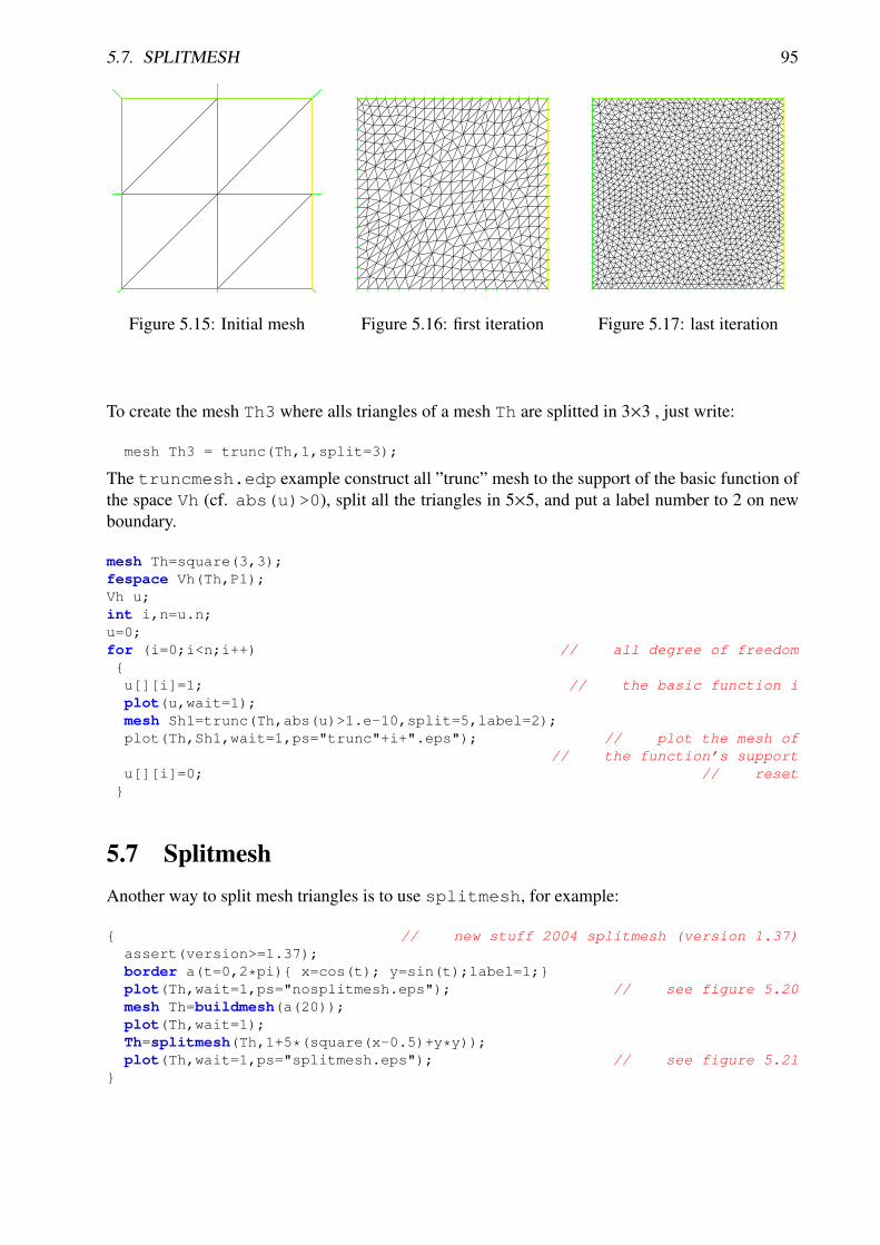
5.7. SPLITMESH 95
Figure 5.15: Initial mesh Figure 5.16: first iteration Figure 5.17: last iteration
To create the mesh Th3 where alls triangles of a mesh Th are splitted in 3×3 , just write:
mesh Th3 = trunc(Th,1,split=3);
The truncmesh.edp example construct all ”trunc” mesh to the support of the basic function ofthe space Vh (cf. abs(u)>0), split all the triangles in 5×5, and put a label number to 2 on newboundary.
mesh Th=square(3,3);fespace Vh(Th,P1);Vh u;int i,n=u.n;u=0;for (i=0;i<n;i++) // all degree of freedomu[][i]=1; // the basic function iplot(u,wait=1);mesh Sh1=trunc(Th,abs(u)>1.e-10,split=5,label=2);plot(Th,Sh1,wait=1,ps="trunc"+i+".eps"); // plot the mesh of
// the function’s supportu[][i]=0; // reset
5.7 SplitmeshAnother way to split mesh triangles is to use splitmesh, for example:
// new stuff 2004 splitmesh (version 1.37)assert(version>=1.37);border a(t=0,2*pi) x=cos(t); y=sin(t);label=1;plot(Th,wait=1,ps="nosplitmesh.eps"); // see figure 5.20mesh Th=buildmesh(a(20));plot(Th,wait=1);Th=splitmesh(Th,1+5*(square(x-0.5)+y*y));plot(Th,wait=1,ps="splitmesh.eps"); // see figure 5.21

96 CHAPTER 5. MESH GENERATION
Figure 5.18: mesh of support the function P1number 0, splitted in 5×5
Figure 5.19: mesh of support the function P1number 6, splitted in 5×5
5.8 Meshing ExamplesExample 5.7 (Two rectangles touching by a side)
border a(t=0,1)x=t;y=0;;border b(t=0,1)x=1;y=t;;border c(t=1,0)x=t ;y=1;;border d(t=1,0)x = 0; y=t;;border c1(t=0,1)x=t ;y=1;;border e(t=0,0.2)x=1;y=1+t;;border f(t=1,0)x=t ;y=1.2;;border g(t=0.2,0)x=0;y=1+t;;int n=1;mesh th = buildmesh(a(10*n)+b(10*n)+c(10*n)+d(10*n));mesh TH = buildmesh ( c1(10*n) + e(5*n) + f(10*n) + g(5*n) );plot(th,TH,ps="TouchSide.esp"); // Fig. 5.22
Example 5.8 (NACA0012 Airfoil)
border upper(t=0,1) x = t;y = 0.17735*sqrt(t)-0.075597*t
- 0.212836*(tˆ2)+0.17363*(tˆ3)-0.06254*(tˆ4); border lower(t=1,0) x = t;
y= -(0.17735*sqrt(t)-0.075597*t-0.212836*(tˆ2)+0.17363*(tˆ3)-0.06254*(tˆ4));
border c(t=0,2*pi) x=0.8*cos(t)+0.5; y=0.8*sin(t); mesh Th = buildmesh(c(30)+upper(35)+lower(35));plot(Th,ps="NACA0012.eps",bw=1); // Fig. 5.23

5.8. MESHING EXAMPLES 97
Figure 5.20: initial mesh Figure 5.21: all left mesh tri-angle is split conformaly inint(1+5*(square(x-0.5)+y*y)2triangles.
Example 5.9 (Cardioid)
real b = 1, a = b;border C(t=0,2*pi) x=(a+b)*cos(t)-b*cos((a+b)*t/b);
y=(a+b)*sin(t)-b*sin((a+b)*t/b); mesh Th = buildmesh(C(50));plot(Th,ps="Cardioid.eps",bw=1); // Fig. 5.24
Example 5.10 (Cassini Egg)
border C(t=0,2*pi) x=(2*cos(2*t)+3)*cos(t);y=(2*cos(2*t)+3)*sin(t);
mesh Th = buildmesh(C(50));
a b cd
h
e
fg
( 0 , - 1 0 )
( 0 , 0 )( 0 , 2 )
( 1 0 , - 1 0 )
T H
t h
Figure 5.22: Two rectangles touching by a side Figure 5.23: NACA0012 Airfoil
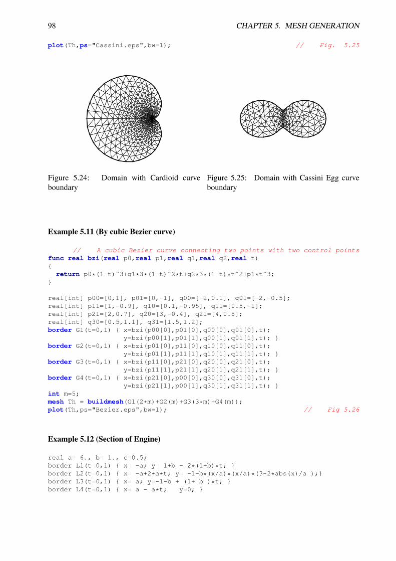
98 CHAPTER 5. MESH GENERATION
plot(Th,ps="Cassini.eps",bw=1); // Fig. 5.25
Figure 5.24: Domain with Cardioid curveboundary
Figure 5.25: Domain with Cassini Egg curveboundary
Example 5.11 (By cubic Bezier curve)
// A cubic Bezier curve connecting two points with two control pointsfunc real bzi(real p0,real p1,real q1,real q2,real t)
return p0*(1-t)ˆ3+q1*3*(1-t)ˆ2*t+q2*3*(1-t)*tˆ2+p1*tˆ3;
real[int] p00=[0,1], p01=[0,-1], q00=[-2,0.1], q01=[-2,-0.5];real[int] p11=[1,-0.9], q10=[0.1,-0.95], q11=[0.5,-1];real[int] p21=[2,0.7], q20=[3,-0.4], q21=[4,0.5];real[int] q30=[0.5,1.1], q31=[1.5,1.2];border G1(t=0,1) x=bzi(p00[0],p01[0],q00[0],q01[0],t);
y=bzi(p00[1],p01[1],q00[1],q01[1],t); border G2(t=0,1) x=bzi(p01[0],p11[0],q10[0],q11[0],t);
y=bzi(p01[1],p11[1],q10[1],q11[1],t); border G3(t=0,1) x=bzi(p11[0],p21[0],q20[0],q21[0],t);
y=bzi(p11[1],p21[1],q20[1],q21[1],t); border G4(t=0,1) x=bzi(p21[0],p00[0],q30[0],q31[0],t);
y=bzi(p21[1],p00[1],q30[1],q31[1],t); int m=5;mesh Th = buildmesh(G1(2*m)+G2(m)+G3(3*m)+G4(m));plot(Th,ps="Bezier.eps",bw=1); // Fig 5.26
Example 5.12 (Section of Engine)
real a= 6., b= 1., c=0.5;border L1(t=0,1) x= -a; y= 1+b - 2*(1+b)*t; border L2(t=0,1) x= -a+2*a*t; y= -1-b*(x/a)*(x/a)*(3-2*abs(x)/a );border L3(t=0,1) x= a; y=-1-b + (1+ b )*t; border L4(t=0,1) x= a - a*t; y=0;

5.8. MESHING EXAMPLES 99
border L5(t=0,pi) x= -c*sin(t)/2; y=c/2-c*cos(t)/2; border L6(t=0,1) x= a*t; y=c; border L7(t=0,1) x= a; y=c + (1+ b-c )*t; border L8(t=0,1) x= a-2*a*t; y= 1+b*(x/a)*(x/a)*(3-2*abs(x)/a); mesh Th = buildmesh(L1(8)+L2(26)+L3(8)+L4(20)+L5(8)+L6(30)+L7(8)+L8(30));plot(Th,ps="Engine.eps",bw=1); // Fig. 5.27
G 1
G 2
G 3
G 4
Figure 5.26: Boundary drawed by Bezier curves
L 1
L 1L 2
L 3L 6
L 7
L 4L 5
Figure 5.27: Section of Engine
Example 5.13 (Domain with U-shape channel)
real d = 0.1; // width of U-shapeborder L1(t=0,1-d) x=-1; y=-d-t; border L2(t=0,1-d) x=-1; y=1-t; border B(t=0,2) x=-1+t; y=-1; border C1(t=0,1) x=t-1; y=d; border C2(t=0,2*d) x=0; y=d-t; border C3(t=0,1) x=-t; y=-d; border R(t=0,2) x=1; y=-1+t; border T(t=0,2) x=1-t; y=1; int n = 5;mesh Th = buildmesh (L1(n/2)+L2(n/2)+B(n)+C1(n)+C2(3)+C3(n)+R(n)+T(n));plot(Th,ps="U-shape.eps",bw=1); // Fig 5.28
Example 5.14 (Domain with V-shape cut)
real dAg = 0.01; // angle of V-shapeborder C(t=dAg,2*pi-dAg) x=cos(t); y=sin(t); ;real[int] pa(2), pb(2), pc(2);pa[0] = cos(dAg); pa[1] = sin(dAg);pb[0] = cos(2*pi-dAg); pb[1] = sin(2*pi-dAg);pc[0] = 0; pc[1] = 0;border seg1(t=0,1) x=(1-t)*pb[0]+t*pc[0]; y=(1-t)*pb[1]+t*pc[1]; ;border seg2(t=0,1) x=(1-t)*pc[0]+t*pa[0]; y=(1-t)*pc[1]+t*pa[1]; ;mesh Th = buildmesh(seg1(20)+C(40)+seg2(20));plot(Th,ps="V-shape.eps",bw=1); // Fig. 5.29

100 CHAPTER 5. MESH GENERATION
L 1C 1
L 2
C 2C 3
B
R
T( - c a , c b )
( c a , c b )
( t i p , d )( t i p , - d )
Figure 5.28: Domain with U-shape channelchanged by d
Cs e g 1s e g 2
Figure 5.29: Domain with V-shape cut changedby dAg
Example 5.15 (Smiling face)
real d=0.1;int m=5;real a=1.5, b=2, c=0.7, e=0.01;border F(t=0,2*pi) x=a*cos(t); y=b*sin(t); border E1(t=0,2*pi) x=0.2*cos(t)-0.5; y=0.2*sin(t)+0.5; border E2(t=0,2*pi) x=0.2*cos(t)+0.5; y=0.2*sin(t)+0.5; func real st(real t)
return sin(pi*t)-pi/2;border C1(t=-0.5,0.5) x=(1-d)*c*cos(st(t)); y=(1-d)*c*sin(st(t)); border C2(t=0,1)x=((1-d)+d*t)*c*cos(st(0.5));y=((1-d)+d*t)*c*sin(st(0.5));border C3(t=0.5,-0.5) x=c*cos(st(t)); y=c*sin(st(t)); border C4(t=0,1) x=(1-d*t)*c*cos(st(-0.5)); y=(1-d*t)*c*sin(st(-0.5));
border C0(t=0,2*pi) x=0.1*cos(t); y=0.1*sin(t); mesh Th=buildmesh(F(10*m)+C1(2*m)+C2(3)+C3(2*m)+C4(3)
+C0(m)+E1(-2*m)+E2(-2*m));plot(Th,ps="SmileFace.eps",bw=1); // see Fig. 5.30
Example 5.16 (3point bending)
// Square for Three-Point Bend Specimens fixed on Fix1, Fix2// It will be loaded on Load.
real a=1, b=5, c=0.1;int n=5, m=b*n;border Left(t=0,2*a) x=-b; y=a-t; border Bot1(t=0,b/2-c) x=-b+t; y=-a; border Fix1(t=0,2*c) x=-b/2-c+t; y=-a; border Bot2(t=0,b-2*c) x=-b/2+c+t; y=-a; border Fix2(t=0,2*c) x=b/2-c+t; y=-a; border Bot3(t=0,b/2-c) x=b/2+c+t; y=-a; border Right(t=0,2*a) x=b; y=-a+t;

5.8. MESHING EXAMPLES 101
border Top1(t=0,b-c) x=b-t; y=a; border Load(t=0,2*c) x=c-t; y=a; border Top2(t=0,b-c) x=-c-t; y=a; mesh Th = buildmesh(Left(n)+Bot1(m/4)+Fix1(5)+Bot2(m/2)+Fix2(5)+Bot3(m/4)
+Right(n)+Top1(m/2)+Load(10)+Top2(m/2));plot(Th,ps="ThreePoint.eps",bw=1); // Fig. 5.31
FE 1 E 2
C 1E 1 C 2C 4
Figure 5.30: Smiling face (Mouth is change-able)
L e f t R i g h tB o t 1 B o t 2 B o t 3
T o p 1T o p 2 L o a d
F i x 1 F i x 2
( - b , a )
( b , - a )
Figure 5.31: Domain for three-point bendingtest

102 CHAPTER 5. MESH GENERATION

Chapter 6
Finite Elements
As stated in Section 2. FEM approximates all functions w as
w(x, y) ' w0φ0(x, y) + w1φ1(x, y) + · · · + wM−1φM−1(x, y)
with finite element basis functions φk(x, y) and numbers wk (k = 0, · · · ,M − 1). The functionsφk(x, y) is constructed from the triangle Tik , so φk(x, y) is a shape function. The finite elementspace
Vh = w | w0φ0 + w1φ1 + · · · + wM−1φM−1, wi ∈ R
is easily created by
fespace IDspace(IDmesh,<IDFE>) ;
or with ` pairs of periodic boundary condition
fespace IDspace(IDmesh,<IDFE>,periodic=[[la 1,sa 1],[lb 1,sb 1],
...[la k,sa k],[lb k,sb `]]);
where IDspace is the name of the space (e.g. Vh), IDmesh is the name of the associatedmesh and <IDFE> is a identifier of finite element type. In a pair of periodic boundary condition,if [la i,sa i],[lb i,sb i] is a pair of int, the 2 labels la i and lb i define the 2 piece ofboundary to be in equivalence; If [la i,sa i],[lb i,sb i] is a pair of real, then sa i andsb i give two common abscissa on the two boundary curve, and two points are identified as one ifthe two abscissa are equal.Remark, the mesh of the two identified border must be the same, so to be sure, used the parameterfixeborder=true in buildmesh command (see 5.1.2) like in example periodic2bis.edp(see ??).
As of today, the known types of finite element are:
P0 piecewise constante discontinuous finite element
P0h =v ∈ L2(Ω)
∣∣∣ for all K ∈ Th there is αK ∈ R : v|K = αK
(6.1)
P1 piecewise linear continuous finite element
P1h =v ∈ H1(Ω)
∣∣∣ ∀K ∈ Th v|K ∈ P1
(6.2)
103

104 CHAPTER 6. FINITE ELEMENTS
P1dc piecewise linear discontinuous finite element
P1dch =v ∈ L2(Ω)
∣∣∣ ∀K ∈ Th v|K ∈ P1
(6.3)
P1b piecewise linear continuous finite element plus bubble
P1bh =v ∈ H1(Ω)
∣∣∣ ∀K ∈ Th v|K ∈ P1 ⊕ SpanλK0 λ
K1 λ
K2
(6.4)
where λKi , i = 0, 1, 2 are the 3 area coordinate functions of the triangle K
P2 piecewise P2 continuous finite element,
P2h =v ∈ H1(Ω)
∣∣∣ ∀K ∈ Th v|K ∈ P2
(6.5)
where P2 is the set of polynomials of R2 of degrees ≤ 2.
P2b piecewise P2 continuous finite element plus bubble,
P2h =v ∈ H1(Ω)
∣∣∣ ∀K ∈ Th v|K ∈ P2 ⊕ SpanλK0 λ
K1 λ
K2
(6.6)
P2dc piecewise P2 discontinuous finite element,
P2dch =v ∈ L2(Ω)
∣∣∣ ∀K ∈ Th v|K ∈ P2
(6.7)
RT0 Raviart-Thomas finite element
RT0h =v ∈ H(div)
∣∣∣ ∀K ∈ Th v|K(x, y) =∣∣∣ αKβK + γK
∣∣∣ xy
(6.8)
where by writing div w = ∂w1/∂x + ∂w2/∂y, w = (w1,w2),
H(div) =w ∈ L2(Ω)2
∣∣∣div w ∈ L2(Ω)
and αK , βK , γK are real numbers.
P1nc piecewise linear element continuous at the middle of edge only.
If we get the finite element spaces
Xh = v ∈ H1(]0, 1[2)| ∀K ∈ Th v|K ∈ P1
Xph = v ∈ Xh| v(∣∣∣ 0. ) = v(
∣∣∣ 1. ), v(| .0 ) = v(| .1 )
Mh = v ∈ H1(]0, 1[2)| ∀K ∈ Th v|K ∈ P2
Rh = v ∈ H1(]0, 1[2)2| ∀K ∈ Th v|K(x, y) =∣∣∣ αKβK + γK
∣∣∣ xy
when Th is a mesh 10 × 10 of the unit square ]0, 1[2, we only write in FreeFem++ as follows:
mesh Th=square(10,10);fespace Xh(Th,P1); // scalar FEfespace Xph(Th,P1,
periodic=[[2,y],[4,y],[1,x],[3,x]]); // bi-periodic FE

6.1. LAGRANGE FINITE ELEMENT 105
fespace Mh(Th,P2); // scalar FEfespace Rh(Th,RT0); // vectorial FE
where Xh,Mh,Rh expresses finite element spaces (called FE spaces ) Xh, Mh, Rh, respectively. Ifwe want use FE-functions uh, vh ∈ Xh and ph, qh ∈ Mh and Uh,Vh ∈ Rh , we write in FreeFem++
Xh uh,vh;Xph uph,vph;Mh ph,qh;Rh [Uxh,Uyh],[Vxh,Vyh];Xh[int] Uh(10); // array of 10 function in XhRh[int] [Wxh,Wyh](10); // array of 10 functions in Rh.
The functions Uh,Vh have two components so we have
Uh =∣∣∣ Uxh
Uyh and Vh =∣∣∣ V xh
Vyh
6.1 Lagrange finite element
6.1.1 P0-elementFor each triangle Tk, the basis function φk in Vh(Th,P0) is given by
φk(x, y) = 1 if (x, y) ∈ Tk, φk(x, y) = 0 if (x, y) < Tk
If we write
Vh(Th,P0); Vh fh= f (x.y);
then for vertices qki , i = 1, 2, 3 in Fig. 6.1(a), fh is built as
fh = fh(x, y) =
nt∑k=1
f (qk1) + f (qk2) + f (qk3)3
φk
See Fig. 6.3 for the projection of f (x, y) = sin(πx) cos(πy) on Vh(Th,P0) when the mesh Th isa 4 × 4-grid of [−1, 1]2 as in Fig. 6.2.
6.1.2 P1-elementFor each vertex qi, the basis function φi in Vh(Th,P1) is given by
φi(x, y) = aki + bk
i x + cki y for (x, y) ∈ Tk,
φi(qi) = 1, φi(q j) = 0 if i , j
The basis function φk1(x, y) with the vertex qk1 in Fig. 6.1(a) at point p = (x, y) in triangle Tk simplycoincide with the barycentric coordinates λk
1 (area coordinates) :
φk1(x, y) = λk1(x, y) =
area of triangle(p, qk2 , qk3)area of triangle(qk1 , qk2 , qk3)

106 CHAPTER 6. FINITE ELEMENTS
1kq
2kq 3kq
kTp
1kq
2kq 3kq
4kq 5kq6kq
kT
( a ) ( b )
Figure 6.1: P1 and P2 degrees of freedom on triangle Tk
If we write
Vh(Th,P1); Vh fh=g(x.y);
then
fh = fh(x, y) =
nv∑i=1
f (qi)φi(x, y)
See Fig. 6.4 for the projection of f (x, y) = sin(πx) cos(πy) into Vh(Th,P1).
Figure 6.2: Test mesh Th for projection Figure 6.3: projection to Vh(Th,P0)
6.1.3 P2-elementFor each vertex or midpoint qi. the basis function φi in Vh(Th,P2) is given by
φi(x, y) = aki + bk
i x + cki y + dk
i x2 + eki xy + f f
j y2 for (x, y) ∈ Tk,
φi(qi) = 1, φi(q j) = 0 if i , j
The basis function φk1(x, y) with the vertex qk1 in Fig. 6.1(b) is defined by the barycentric coordi-nates:
φk1(x, y) = λk1(x, y)(2λk
1(x, y) − 1)

6.2. P1 NONCONFORMING ELEMENT 107
and for the midpoint qk2
φk2(x, y) = 4λk1(x, y)λk
4(x, y)
If we write
Vh(Th,P2); Vh fh= f (x.y);
then
fh = fh(x, y) =
M∑i=1
f (qi)φi(x, y) (summation over all vetex or midpoint)
See Fig. 6.5 for the projection of f (x, y) = sin(πx) cos(πy) into Vh(Th,P2).
Figure 6.4: projection to Vh(Th,P1) Figure 6.5: projection to Vh(Th,P2)
6.2 P1 Nonconforming ElementRefer to [22] for details; briefly, we now consider non-continuous approximations so we shall losethe property
wh ∈ Vh ⊂ H1(Ω)
If we write
Vh(Th,P1nc); Vh fh= f (x.y);
then
fh = fh(x, y) =
nv∑i=1
f (mi)φi(x, y) (summation over all midpoint)
Here the basis function φi associated with the midpoint mi = (qki + qki+1)/2 where qki is the i-thpoint in Tk, and we assume that j + 1 = 0 if j = 3:
φi(x, y) = aki + bk
i x + cki y for (x, y) ∈ Tk,
φi(mi) = 1, φi(m j) = 0 if i , j

108 CHAPTER 6. FINITE ELEMENTS
Strictly speaking ∂φi/∂x, ∂φi/∂y contain Dirac distribution ρδ∂Tk . The numerical calculations willautomatically ignore them. In [22], there is a proof of the estimation nv∑
k=1
∫Tk
|∇w − ∇wh|2dxdy
1/2
= O(h)
The basis functions φk have the following properties.
1. For the bilinear form a defined in (2.6) satisfy
a(φi, φi) > 0, a(φi, φ j) ≤ 0 if i , jnv∑
k=1
a(φi, φk) ≥ 0
2. f ≥ 0⇒ uh ≥ 0
3. If i , j, the basis function φi and φ j are L2-orthogonal:∫Ω
φiφ j dxdy = 0 if i , j
which is false for P1-element.
See Fig. 6.6 for the projection of f (x, y) = sin(πx) cos(πy) into Vh(Th,P1nc). See Fig. 6.6 forthe projection of f (x, y) = sin(πx) cos(πy) into Vh(Th,P1nc).
Figure 6.6: projection to Vh(Th,P1nc) Figure 6.7: projection to Vh(Th,P1b)
6.3 Other FE-spaceFor each triangle Tk ∈ Th, let λk1(x, y), λk2(x, y), λk3(x, y) be the area cordinate of the triangle (seeFig. 6.1), and put
βk(x, y) = 27λk1(x, y)λk2(x, y)λk3(x, y) (6.9)
called bubble function on Tk. The bubble function has the feature:
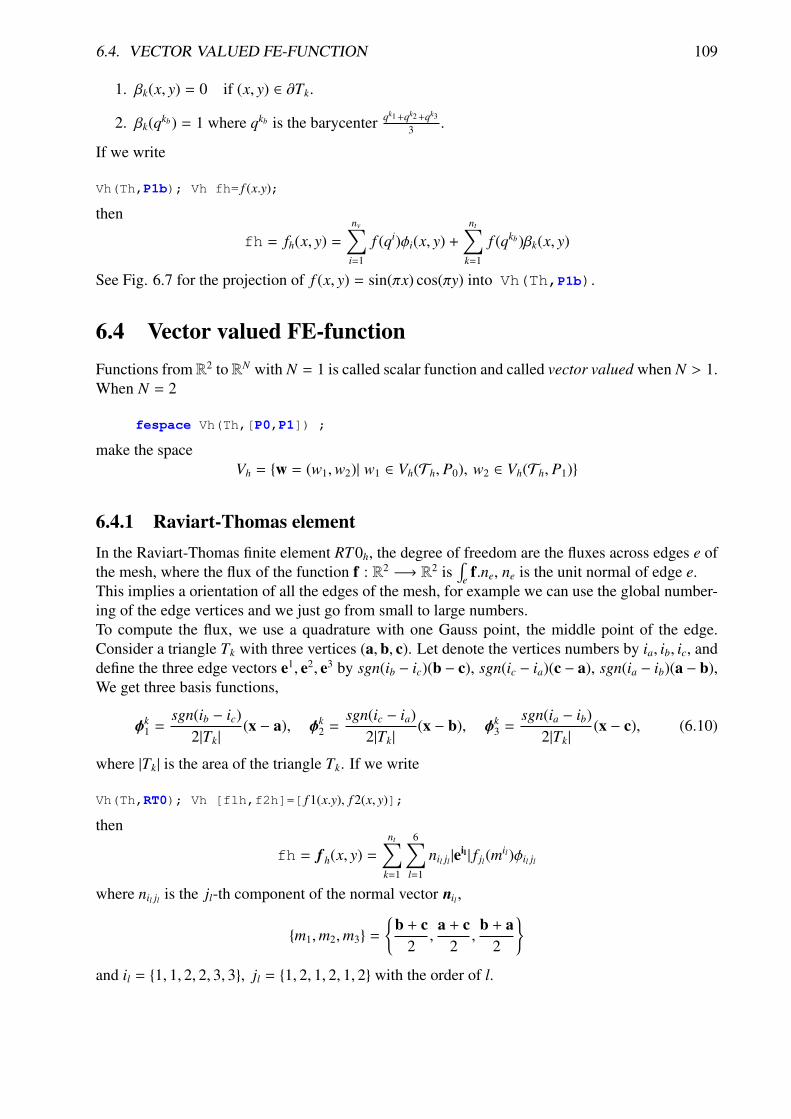
6.4. VECTOR VALUED FE-FUNCTION 109
1. βk(x, y) = 0 if (x, y) ∈ ∂Tk.
2. βk(qkb) = 1 where qkb is the barycenter qk1 +qk2 +qk3
3 .
If we write
Vh(Th,P1b); Vh fh= f (x.y);
then
fh = fh(x, y) =
nv∑i=1
f (qi)φi(x, y) +
nt∑k=1
f (qkb)βk(x, y)
See Fig. 6.7 for the projection of f (x, y) = sin(πx) cos(πy) into Vh(Th,P1b).
6.4 Vector valued FE-functionFunctions from R2 to RN with N = 1 is called scalar function and called vector valued when N > 1.When N = 2
fespace Vh(Th,[P0,P1]) ;
make the spaceVh = w = (w1,w2)| w1 ∈ Vh(Th, P0), w2 ∈ Vh(Th, P1)
6.4.1 Raviart-Thomas elementIn the Raviart-Thomas finite element RT0h, the degree of freedom are the fluxes across edges e ofthe mesh, where the flux of the function f : R2 −→ R2 is
∫e
f.ne, ne is the unit normal of edge e.This implies a orientation of all the edges of the mesh, for example we can use the global number-ing of the edge vertices and we just go from small to large numbers.To compute the flux, we use a quadrature with one Gauss point, the middle point of the edge.Consider a triangle Tk with three vertices (a,b, c). Let denote the vertices numbers by ia, ib, ic, anddefine the three edge vectors e1, e2, e3 by sgn(ib − ic)(b − c), sgn(ic − ia)(c − a), sgn(ia − ib)(a − b),We get three basis functions,
φk1 =
sgn(ib − ic)2|Tk|
(x − a), φk2 =
sgn(ic − ia)2|Tk|
(x − b), φk3 =
sgn(ia − ib)2|Tk|
(x − c), (6.10)
where |Tk| is the area of the triangle Tk. If we write
Vh(Th,RT0); Vh [f1h,f2h]=[ f 1(x.y), f 2(x, y)];
then
fh = f h(x, y) =
nt∑k=1
6∑l=1
nil jl |eil | f jl(m
il)φil jl
where nil jl is the jl-th component of the normal vector nil ,
m1,m2,m3 =
b + c
2,
a + c2
,b + a
2
and il = 1, 1, 2, 2, 3, 3, jl = 1, 2, 1, 2, 1, 2 with the order of l.

110 CHAPTER 6. FINITE ELEMENTS
ab
c
T
n 3
n 2
n 1
Figure 6.8: normal vectors of each edge
Example 6.1 mesh Th=square(2,2);fespace Xh(Th,P1);fespace Vh(Th,RT0);Xh uh,vh;Vh [Uxh,Uyh];[Uxh,Uyh] = [sin(x),cos(y)]; // ok vectorial FE functionvh= xˆ2+yˆ2; // vhTh = square(5,5); // change the mesh
// Xh is unchangeuh = xˆ2+yˆ2; // compute on the new XhUxh = x; // error: impossible to set only 1 component
// of a vector FE function.vh = Uxh; // ok
// and now uh use the 5x5 mesh// but the fespace of vh is alway the 2x2 mesh
plot(uh,ps="onoldmesh.eps"); // figure 6.9uh = uh; // do a interpolation of vh (old) of 5x5 mesh
// to get the new vh on 10x10 mesh.plot(uh,ps="onnewmesh.eps"); // figure 6.10vh([x-1/2,y])= xˆ2 + yˆ2; // interpolate vh = ((x − 1/2)2 + y2)
Figure 6.9: vh Iso on mesh 2 × 2 Figure 6.10: vh Iso on mesh 5 × 5

6.5. A FAST FINITE ELEMENT INTERPOLATOR 111
To get the value at a point x = 1, y = 2 of the FE function uh, or [Uxh,Uyh],one writes
real value;value = uh(2,4); // get value= uh(2,4)value = Uxh(2,4); // get value= Uxh(2,4)
// ------ or ------x=1;y=2;value = uh; // get value= uh(1,2)value = Uxh; // get value= Uxh(1,2)value = Uyh; // get value= Uyh(1,2).
To get the value of the array associated to the FE function uh, one writes
real value = uh[][0] ; // get the value of degree of freedom 0real maxdf = uh[].max; // maximum value of degree of freedomint size = uh.n; // the number of degree of freedomreal[int] array(uh.n)= uh[]; // copy the array of the function uh
Note 6.1 For a none scalar finite element function [Uxh,Uyh] the two array Uxh[] and Uyh[]are the same array, because the degree of freedom can touch more than one component.
6.5 A Fast Finite Element Interpolator
In practice one may discretize the variational equations by the Finite Element method. Then therewill be one mesh for Ω1 and another one for Ω2. The computation of integrals of products offunctions defined on different meshes is difficult. Quadrature formulae and interpolations fromone mesh to another at quadrature points are needed. We present below the interpolation operatorwhich we have used and which is new, to the best of our knowledge. Let T 0
h = ∪kT 0k ,T
1h = ∪kT 1
k
be two triangulations of a domain Ω. Let
V(T ih) = C0(Ωi
h) : f |T ik∈ P0, i = 0, 1
be the spaces of continuous piecewise affine functions on each triangulation.Let f ∈ V(T 0
h ). The problem is to find g ∈ V(T 1h ) such that
g(q) = f (q) ∀q vertex of T 1h
Although this is a seemingly simple problem, it is difficult to find an efficient algorithm in practice.We propose an algorithm which is of complexity N1 log N0, where N i is the number of vertices ofT
ih, and which is very fast for most practical 2D applications.
AlgorithmThe method has 5 steps. First a quadtree is built containing all the vertices of mesh T 0
h such thatin each terminal cell there are at least one, and at most 4, vertices of T 0
h .For each q1, vertex of T 1
h do:

112 CHAPTER 6. FINITE ELEMENTS
Step 1 Find the terminal cell of the quadtree containing q1.
Step 2 Find the the nearest vertex q0j to q1 in that cell.
Step 3 Choose one triangle T 0k ∈ T
0h which has q0
j for vertex.
Step 4 Compute the barycentric coordinates λ j j=1,2,3 of q1 in T 0k .
• − if all barycentric coordinates are positive, go to Step 5
• − else if one barycentric coordinate λi is negative replace T 0k by the adjacent triangle
opposite q0i and go to Step 4.
• − else two barycentric coordinates are negative so take one of the two randomly andreplace T 0
k by the adjacent triangle as above.
Step 5 Calculate g(q1) on T 0k by linear interpolation of f :
g(q1) =∑
j=1,2,3
λ j f (q0j)
End
Figure 6.11: To interpolate a function at q0 the knowledge of the triangle which contains q0 isneeded. The algorithm may start at q1 ∈ T 0
k and stall on the boundary (thick line) because the lineq0q1 is not inside Ω. But if the holes are triangulated too (doted line) then the problem does notarise.
Two problems need to be solved:
• What if q1 is not in Ω0h ? Then Step 5 will stop with a boundary triangle. So we add a step
which test the distance of q1 with the two adjacent boundary edges and select the nearest,and so on till the distance grows.
• What if Ω0h is not convex and the marching process of Step 4 locks on a boundary? By
construction Delaunay-Voronoı mesh generators always triangulate the convex hull of thevertices of the domain. So we make sure that this information is not lost when T 0
h ,T1h are
constructed and we keep the triangles which are outside the domain in a special list. Hencein step 5 we can use that list to step over holes if needed.

6.6. KEYWORDS: PROBLEM AND SOLVE 113
Note 6.2 Step 3 requires an array of pointers such that each vertex points to one triangle of thetriangulation.
Note 6.3 The operator = is the interpolation operator of FreeFem++ , The continuous finitefunctions are extended by continuity to the outside of the domain. Try the following example
mesh Ths= square(10,10);mesh Thg= square(30,30,[x*3-1,y*3-1]);plot(Ths,Thg,ps="overlapTh.eps",wait=1);
fespace Ch(Ths,P2); fespace Dh(Ths,P2dc);fespace Fh(Thg,P2dc);Ch us= (x-0.5)*(y-0.5);Dh vs= (x-0.5)*(y-0.5);Fh ug=us,vg=vs;plot(us,ug,wait=1,ps="us-ug.eps"); // see figure 6.12plot(vs,vg,wait=1,ps="vs-vg.eps"); // see figure 6.13
Figure 6.12: Extension of a continuous FE-function
Figure 6.13: Extention of discontinuous FE-function
6.6 Keywords: Problem and SolveFor FreeFem++ a problem must be given in variational form, so we need a bilinear form a(u, v), a linear form `( f , v), and possibly a boundary condition form must be added.
problem P(u,v) =a(u,v) - `(f,v)+ (boundary condition);
Note 6.4 When you want to formulate the problem and to solve it in the same time, you can usethe keywork solve.

114 CHAPTER 6. FINITE ELEMENTS
6.6.1 Weak form and Boundary ConditionTo present the principles of Variational Formulations or also called weak forms fr the PDEs, let ustake a model problem : a Poisson equation with Dirichlet and Robin Boundary condition .The problem is: Find u a real function defined on domain Ω of R2 such that
−∇.(ν∇u) = f , in Ω, au + ν∂u∂n
= b on Γr, u = g on Γd (6.11)
where
• ∇.(ν∇u) = ∂x(ν∂xu) + ∂y(ν∂yu) with ∂xu = ∂u∂x and ∂yu = ∂u
∂y
• the border Γ = ∂Ω is split in Γd and Γn such that Γd ∪ Γn = ∅ and Γd ∩ Γn = ∂Ω,
• ν is a given positive function, such that ∃ν0 ∈ R, 0 < ν0 ≤ ν.
• a a given non negative function,
• b a given function.
Note 6.5 This problem, we can be a classical Neumann boundary condition if a is 0, and if Γd isempty. In this case the function is defined just by derivative, so this defined too a constant (if u isa solution then u + 1 is also a solution).
Let v a regular test function null on Γd , by integration par part we get
−
∫Ω
∇.(ν∇u) v dω =
∫Ω
ν∇v.∇u dω =
∫Ω
f v dω −∫
Γ
vν∂u∂n
dγ, (6.12)
where ∇v.∇u = ∂u∂x
∂v∂x + ∂u
∂y∂v∂y , and where n is the unitary outside normal of ∂Ω.
Now we note that ν∂u∂n = −au + g on Γr and v = 0 on Γd and ∂Ω = Γd ∪ Γn thus
−
∫∂Ω
vν∂u∂n
=
∫Γr
auv −∫
Γr
bv
The problem become:Find u ∈ Vg = v ∈ H1(Ω)/v = g on Γd such that∫
Ω
ν∇v.∇u dω +
∫Γr
auv dγ =
∫Ω
f v dω +
∫Γr
bv dγ, ∀v ∈ V0 (6.13)
where V0 = v ∈ H1(Ω)/v = 0 on Γd
The problem (6.13) is generally well posed if we do not have only Neumann boundary condition (ie. Γd = ∅ and a = 0).
Note 6.6 If we have only Neumann boundary condition, then solution is not unique and linearalgebra tells us that the right hand side must be orthogonal to the kernel of the operator. Here theproblem is defined to a constant, and since 1 ∈ V0 one way of writing the compatibility conditionis:
∫Ω
f dω +∫
Γb dγ and a way to fix the constant is to solve for u ∈ H1(Ω) such that:∫
Ω
εuv dω + ν∇v.∇u dω =
∫Ω
f v dω +
∫Γr
bv dγ, ∀v ∈ H1(Ω) (6.14)

6.7. PARAMETERS AFFECTING SOLVE AND PROBLEM 115
where ε is a small parameter ( ∼ 10−10 ).Remark that if the solution is of order 1
εthen the compatibility condition is unsatisfied, otherwise
we get the solution such that∫
Ωu = 0.
In FreeFem++, the problem (6.13) become
problem Pw(u,v) =int2d(Th)( nu* ( dx(u)*dx(u) + dy(u)*dy(u))) //
∫Ων∇v.∇u dω
+ int1d(Th,gn)( a * u*v ) //∫
Γrauv dγ
- int2d(Th)(f*v) //∫
Ωf v dω
- int1d(Th,gn)( b * v ) //∫
Γrbv dγ
+ on(gd)(u= g) ; // u = g on Γd
where Th is a mesh of the domain Ω, and gd and gn are respectively the boundary label ofboundary Γd and Γn.
6.7 Parameters affecting solve and problemThe parameters are FE functions real or complex, the number n of parameters is even (n = 2 ∗ k),the k first function parameters are unknown, and the k last are test functions.
Note 6.7 If the functions are a part of vectoriel FE then you must give all the functions of thevectorial FE in the same order (see laplaceMixte problem for example).
Note 6.8 Don’t mix complex and real parameters FE function.
Bug: 1 The mixing of fespace with different periodic boundary condition is not implemented.So all the finite element spaces used for test or unknown functions in a problem, must have thesame type of periodic boundary condition or no periodic boundary condition. No clean messageis given and the result is impredictible, Sorry.
The parameters are:
solver= LU, CG, Crout,Cholesky,GMRES,sparsesolver, UMFPACK ...
The default solver is sparsesolver ( it is equal to UMFPACK if not other sparce solver isdefined) or is set to LU if no direct sparse solver is available. The storage mode of the matrixof the underlying linear system depends on the type of solver chosen; for LU the matrixis sky-line non symmetric, for Crout the matrix is sky-line symmetric, for Cholesky thematrix is sky-line symmetric positive definite, for CG the matrix is sparse symmetric positive,and for GMRES, sparsesolver or UMFPACK the matrix is just sparse.
eps= a real expression. ε sets the stopping test for the iterative methods like CG. Note that if ε isnegative then the stopping test is:
||Ax − b|| < |ε|
if it is positive then the stopping test is
||Ax − b|| <|ε|
||Ax0 − b||

116 CHAPTER 6. FINITE ELEMENTS
init= boolean expression, if it is false or 0 the matrix is reconstructed. Note that if the meshchanges the matrix is reconstructed too.
precon= name of a function (for example P) to set the precondioner. The prototype for thefunction P must be
func real[int] P(real[int] & xx) ;
tgv= Huge value (1030) used to implement Dirichlet boundary conditions.
tolpivot= set the tolerence of the pivot in UMFPACK (10−1) and, LU, Crout, Cholesky factorisa-tion (10−20).
tolpivotsym= set the tolerence of the pivot sym in UMFPACK
strategy= set the integer UMFPACK strategy (0 by default).
6.8 Problem definitionBelow v is the unknown function and w is the test function.After the ”=” sign, one may find sums of:
• identifier(s); this is the name given earlier to the variational form(s) (type varf ) for possiblereuse.
Remark, that the name in the ”varf” of the unknow of test function is forgotten, we just usedthe order in argument list to recall name as in a C++ function, see note 6.12,
• the terms of the bilinear form itself: if K is a given function,
-) int2d(Th)( K*v*w) =∑T∈Th
∫T
K v w
-) int2d(Th,1)( K*v*w) =∑
T∈Th,T⊂Ω1
∫T
K v w
-) int1d(Th,2,5)( K*v*w) =∑T∈Th
∫(∂T∪Γ)∩(Γ2∪Γ5)
K v w
-) intalledges(Th)( K*v*w) =∑T∈Th
∫∂T
K v w
-) intalledges(Th,1)( K*v*w) =∑
T∈Th,T⊂Ω1
∫∂T
K v w
-) they contribute to the sparse matrix of type matrixwhich, whether declared explicitlyor not is contructed by FreeFem++ .
• the right handside of the PDE, volumic terms of the linear form: for given functions K, f :
-) int1d(Th)( K*w) =∑T∈Th
∫T
K w

6.9. NUMERICAL INTEGRATION 117
-) int1d(Th,2,5)( K*w) =∑T∈Th
∫(∂T∪Γ)∩(Γ2∪Γ5)
K w
-) intalledges(Th)( f*w) =∑T∈Th
∫∂T
f w
-) a vector of type real[int]
• The boundary condition terms :
– An ”on” form (for Dirichlet ) : on(1, u = g )
The meaning is for all node i the this associated boundary, the diagonal term of thematrix aii = tgv with the terrible geant value tgv (=1030 by default) and the righthand side b[i] = ”g[i]” × tgv, where the ”g[i]” is the boundary node value given by theinterpolation of g.
– a linear form on Γ (for Neumann ) -int1d(Th))( f*w) or -int1d(Th,3))(f*w)
– a bilinear form on Γ or Γ2 (for Robin ) int1d(Th))( K*v*w) or int1d(Th,2))(K*v*w).
Note 6.9 • If needed, the different kind of terms in the sum can appear more than once.
• the integral mesh and the mesh associated to test function or unknown function can be dif-ferent in the case of linear form.
• N.x and N.y are the normal’s components.
Important: it is not possible to write in the same integral the linear part and the bilinear part suchas in int1d(Th)( K*v*w - f*w) .
6.9 Numerical IntegrationLet D be a N-dimensional bounded domain. For an arbitrary polynomials f of degree r, if we canfind particular points ξ j, j = 1, · · · , J in D and constants ω j such that∫
Df (x) =
L∑`=1
c` f (ξ`) (6.15)
then we have the error estimation (see Crouzeix-Mignot (1984)), and then there exists a constantC > 0 such that, ∣∣∣∣∣∣∣
∫D
f (x) −L∑`=1
ω` f (ξ`)
∣∣∣∣∣∣∣ ≤ C|D|hr+1 (6.16)
for any function r + 1 times continuously differentiable f in D, where h is the diameter of D and|D| its measure (a point in the segment [qiq j] is given as
(x, y)| x = (1 − t)qix + tq j
x, y = (1 − t)qiy + tq j
y, 0 ≤ t ≤ 1).

118 CHAPTER 6. FINITE ELEMENTS
For a domain Ωh =∑nt
k=1 Tk, Th = Tk, we can calculate the integral over Γh = ∂Ωh by∫Γh
f (x)ds = int1d(Th)(f)
= int1d(Th,qfe=*)(f)
= int1d(Th,qforder=*)(f)
where * stands for the name of the quadrature formula or the precision (order) of the Gauss for-mula. where |qiq j| is the length of segment qiq j. For a part Γ1 of Γh with the label “1”, we can
L (qfe=) qforder= point in [qiq j](= t) ω` exact on Pk, k =
1 qf1pE 2 1/2 |qiq j| 12 qf2pE 3 (1 ±
√1/3)/2 |qiq j|/2 3
3 qf3pE 6 (1 ±√
3/5)/2 (5/18)|qiq j| 51/2 (8/18)|qiq j|
4 qf4pE 8 (1 ±√
525+70√
3035 )/2. 18−
√30
72 |qiq j| 7
(1 ±√
525−70√
3035 )/2. 18+
√30
72 |qiq j|
5 qf5pE 10 (1 ±√
245+14√
7021 )/2 322−13
√70
1800 |qiq j| 91/2 64
225 |qiq j|
(1 ±√
245−14√
7021 )/2 322+13
√70
1800 |qiq j|
2 qf1pElump 2 −1 |qiq j|/2 1+1 |qiq j|/2
calculate the integral over Γ1 by∫Γ1
f (x, y)ds = int1d(Th,1)(f)
= int1d(Th,1,qfe=qf2pE)(f)
The integral over Γ1, Γ3 are given by∫Γ1∪Γ3
f (x, y)ds = int1d(Th,1,3)(f)
For each triangule Tk = [qk1qk2qk3] , the point P(x, y) in Tk is expressed by the area coordinate asP(ξ, η):
|Tk| =
∣∣∣∣∣∣∣∣∣1 qk1
x qk1y
1 qk2x qk2
y
1 qk3x qk3
y
∣∣∣∣∣∣∣∣∣ D1 =
∣∣∣∣∣∣∣∣∣1 x y1 qk2
x qk2y
1 qk3x qk3
y
∣∣∣∣∣∣∣∣∣ D2 =
∣∣∣∣∣∣∣∣∣1 qk1
x qk1y
1 x y1 qk3
x qk3y
∣∣∣∣∣∣∣∣∣ D3 =
∣∣∣∣∣∣∣∣∣1 qk1
x qk1y
1 qk2x qk2
y
1 x y
∣∣∣∣∣∣∣∣∣ξ = D1/|Tk| η = D2/|Tk| then 1 − ξ − η = D3/|Tk|
For a domain Ωh =∑nt
k=1 Tk, Th = Tk, we can calculate the integral over Ωh by∫Ωh
f (x, y) = int2d(Th)(f)
= int2d(Th,qft=*)(f)
= int2d(Th,qforder=*)(f)
where * stands for the name of quadrature formula or the order of the Gauss formula.

6.10. VARIATIONAL FORM, SPARSE MATRIX, PDE DATA VECTOR 119
L qft= qforder= point in Tk ω` degree of exact
1 qf1pT 2(
13 ,
13
)|Tk| 1
3 qf2pT 3(
12 ,
12
)|Tk|/3 2(
12 , 0
)|Tk|/3(
0, 12
)|Tk|/3
7 qf5pT 6(
13 ,
13
)0.225|Tk| 5(
6−√
1521 , 6−
√15
21
)(155−
√15)|Tk |
1200(6−√
1521 , 9+2
√15
21
)(155−
√15)|Tk |
1200(9+2√
1521 , 6−
√15
21
)(155−
√15)|Tk |
1200(6+√
1521 , 6+
√15
21
)(155+
√15)|Tk |
1200(6+√
1521 , 9−2
√15
21
)(155+
√15)|Tk |
1200(9−2√
1521 , 6+
√15
21
)(155+
√15)|Tk |
1200
3 qf1pTlump (0, 0) |Tk|/3 1(1, 0) |Tk|/3(0, 1) |Tk|/3
9 qf2pT4P1(
14 ,
34
)|Tk|/12 1(
34 ,
14
)|Tk|/12(
0, 14
)|Tk|/12(
0, 34
)|Tk|/12(
14 , 0
)|Tk|/12(
34 , 0
)|Tk|/12(
14 ,
14
)|Tk|/6(
14 ,
12
)|Tk|/6(
12 ,
14
)|Tk|/6
15 qf7pT 8 see [35] for detail 721 qf9pT 10 see [35] for detail 9
Note 6.10 By default, we use the formula which is exact for polynomes of degrees 5 on trianglesor edges (in bold in two tables).
6.10 Variational Form, Sparse Matrix, PDE Data VectorFirst, it is possible to define variational forms, and use this forms to build matrix and vector tomake very fast script (4 times faster here).For example solve the Thermal Conduction problem of section 3.4.The variational formulation is in L2(0,T ; H1(Ω)); we shall seek un satisfying
∀w ∈ V0;∫
Ω
un − un−1
δtw + κ∇un∇w) +
∫Γ
α(un − uue)w = 0
where V0 = w ∈ H1(Ω)/w|Γ24 = 0.

120 CHAPTER 6. FINITE ELEMENTS
So the to code the method with the matrices A = (Ai j), M = (Mi j), and the vectors un, bn, b′, b”, bcl
( notation if w is a vector then wi is a component of the vector).
un = A−1bn, b′ = b0 + Mun−1, b” = ν∞ bcl, bni =
b”i if i ∈ Γ24
b′i else if < Γ24(6.17)
Where with ν∞ = tgv = 1030 :
Ai j =
ν∞ if i ∈ Γ24, and j = i∫
Ω
w jwi/dt + k(∇w j.∇wi) +
∫Γ13
αw jwi else if i < Γ24, or j , i (6.18)
Mi j =
ν∞ if i ∈ Γ24, and j = i∫
Ω
w jwi/dt else if i < Γ24, or j , i (6.19)
b0,i =
∫Γ13
αuuewi (6.20)
bcl = u0 the initial data (6.21)
// file thermal-fast.edp in examples++-tutorial
func fu0 =10+90*x/6;func k = 1.8*(y<0.5)+0.2;real ue = 25. , alpha=0.25, T=5, dt=0.1 ;
mesh Th=square(30,5,[6*x,y]);fespace Vh(Th,P1);
Vh u0=fu0,u=u0;
Create three variational formulation, and build the matrices A,M.
varf vthermic (u,v)= int2d(Th)(u*v/dt + k*(dx(u) * dx(v) + dy(u) * dy(v)))+ int1d(Th,1,3)(alpha*u*v)+ on(2,4,u=1);
varf vthermic0(u,v) = int1d(Th,1,3)(alpha*ue*v);
varf vMass (u,v)= int2d(Th)( u*v/dt) + on(2,4,u=1);
real tgv = 1e30;matrix A= vthermic(Vh,Vh,tgv=tgv,solver=CG);matrix M= vMass(Vh,Vh);
Now, to build the right hand size we need 4 vectors.
real[int] b0 = vthermic0(0,Vh); // constant part of the RHSreal[int] bcn = vthermic(0,Vh); // tgv on Dirichlet boundary node ( !=0 )
// we have for the node i : i ∈ Γ24 ⇔ bcn[i] , 0real[int] bcl=tgv*u0[]; // the Dirichlet boundary condition part

6.10. VARIATIONAL FORM, SPARSE MATRIX, PDE DATA VECTOR 121
Note 6.11 The boundary condition is implemented by penalization and vector bcn contains thecontribution of the boundary condition u=1 , so to change the boundary condition, we have just tomultiply the vector bc[] by the current value f of the new boundary condition term by term withthe operator .*. Section 9.6.2 Examples++-tutorial/StokesUzawa.edp gives a realexample of using all this features.
And the new version of the algorithm:
ofstream ff("thermic.dat");for(real t=0;t<T;t+=dt)
real[int] b = b0 ; // for the RHSb += M*u[]; // add the the time dependant part
// lock boundary part:b = bcn ? bcl : b ; // do ∀i: b[i] = bcn[i] ? bcl[i] : b[i] ;u[] = Aˆ-1*b;ff << t <<" "<<u(3,0.5)<<endl;plot(u);
for(int i=0;i<20;i++)
cout<<dy(u)(6.0*i/20.0,0.9)<<endl;plot(u,fill=true,wait=1,ps="thermic.eps");
Note 6.12 The functions appearing in the variational form are formal; they must be declared butnot necessarily defined, the only important think in the order in the parameter list, like in
varf vb1([u1,u2],q) = int2d(Th)( (dy(u1)+dy(u2)) *q) + int2d(Th)(1*q);varf vb2([v1,v2],p) = int2d(Th)( (dy(v1)+dy(v2)) *p) + int2d(Th)(1*p);
To build matrix A from the bilinear part the the variational form a of type varf do simply
A = a(Vh,Wh [, ...] );// where Vh is "unkown fespace" with a correct number of component
// where Wh is "test fespace" with a correct number of component
The possible named parameter " [, ... ] " of the construction are
solver= LU, CG, Crout, Cholesky, GMRES, sparsesolver, UMFPACK ...
The default solver is GMRES. The storage mode of the matrix of the underlying linear sys-tem depends on the type of solver chosen; for LU the matrix is sky-line non symmetric,for Crout the matrix is sky-line symmetric, for Cholesky the matrix is sky-line sym-metric positive definite, for CG the matrix is sparse symmetric positive, and for GMRES,sparsesolver or UMFPACK the matrix is just sparse.
factorize = if true then do the matrix factorization for LU, Cholesky or Crout, the defaultvalue is f alse.
eps= a real expression. ε sets the stopping test for the iterative methods like CG. Note that if ε isnegative then the stopping test is:
||Ax − b|| < |ε|
if it is positive then the stopping test is
||Ax − b|| <|ε|
||Ax0 − b||
122 CHAPTER 6. FINITE ELEMENTS
precon= name of a function (for example P) to set the precondioner. The prototype for thefunction P must be
func real[int] P(real[int] & xx) ;
tgv= Huge value (1030) used to implement Dirichlet boundary conditions.
tolpivot= set the tolerence of the pivot in UMFPACK (10−1) and, LU, Crout, Cholesky factorisa-tion (10−20).
tolpivotsym= set the tolerence of the pivot sym in UMFPACK
strategy= set the integer UMFPACK strategy (0 by default).
Note 6.13 The line of the matrix corresponding to the space Wh and the column of the matrixcorresponding to the space Vh.
To build the dual vector b (of type real[int]) from the linear part of the variational form a do simply
real b(Vh.ndof);b = a(0,Vh);
A first example to compute the area of each triangle K of mesh Th, just do:
fespace Nh(Th,P0); // the space function contant / triangleNh areaK;varf varea(unused,chiK) = int2d(Th)(chiK);etaK[]= varea(0,Ph);
Effectively, the basic functions of space Nh, are the characteristic function of the element of Th,and the numbering is the numeration of the element, so by construction:
etaK[i] =
∫1|Ki =
∫Ki
1;
Now, we can use this to compute error indicator like in examples AdaptResidualErrorIndi-cator.edp in directory examples++-tutorial.First to compute a continuous approximation to the function h ”density mesh size” of the mesh Th.
fespace Vh(Th,P1);Vh h ;real[int] count(Th.nv); varf vmeshsizen(u,v)=intalledges(Th,qfnbpE=1)(v);varf vedgecount(u,v)=intalledges(Th,qfnbpE=1)(v/lenEdge);
// computation of the mesh size// -----------------------------
count=vedgecount(0,Vh); // number of edge / vertexh[]=vmeshsizen(0,Vh); // sum length edge / vertexh[]=h[]./count; // mean lenght edge / vertex
To compute error indicator for Poisson equation :
ηK =
∫K
h2K |( f + ∆uh)|2 +
∫∂K
he|[∂uh
∂n]|2

6.10. VARIATIONAL FORM, SPARSE MATRIX, PDE DATA VECTOR 123
where hK is size of the longest edge ( hTriangle), he is the size of the current edge ( lenEdge),n the normal.
fespace Nh(Th,P0); // the space function contant / triangleNh etak;varf vetaK(unused,chiK) =
intalledges(Th)(chiK*lenEdge*square(jump(N.x*dx(u)+N.y*dy(u))))+int2d(Th)(chiK*square(hTriangle*(f+dxx(u)+dyy(u))) );
etak[]= vetaK(0,Ph);
We add automatic expression optimization by default, if this optimization creates problems, it canbe removed with the keyword optimize as in the following example :
varf a(u1,u2)= int2d(Th,optimize=false)( dx(u1)*dx(u2) + dy(u1)*dy(u2) )+ on(1,2,4,u1=0) + on(3,u1=1) ;
Remark, it is all possible to build interpolation matrix, like in the following example:
mesh TH = square(3,4);mesh th = square(2,3);mesh Th = square(4,4);
fespace VH(TH,P1);fespace Vh(th,P1);fespace Wh(Th,P1);
matrix B= interpolate(VH,Vh); // build interpolation matrixVh->VH matrix BB= interpolate(Wh,Vh); // build interpolation
matrix Vh->Wh
and after some operations on sparse matrices are available for example
int N=10;real [int,int] A(N,N); // a full matrixreal [int] a(N),b(N);A =0;for (int i=0;i<N;i++)
A(i,i)=1+i;if(i+1 < N) A(i,i+1)=-i;a[i]=i;
b=A*b;cout << "xxxx\n";matrix sparseA=A;cout << sparseA << endl;sparseA = 2*sparseA+sparseA’;sparseA = 4*sparseA+sparseA*5; //matrix sparseB=sparseA+sparseA+sparseA; ;cout << "sparseB = " << sparseB(0,0) << endl;

124 CHAPTER 6. FINITE ELEMENTS
6.11 Interpolation matrixThis becomes possible to store the matrix of a linear interpolation operator from a finite elementspace Vh to Wh with interpolate function. Note that the continuous finite functions are ex-tended by continuity to the outside of the domain.The named parameter of function interpolate are:
inside= set true to create zero-extension.
t= set true to get the transposed matrix
op= set an integer written below
0 the default value and interpolate of the function
1 interpolate the ∂x
2 interpolate the ∂y
. .
Example 6.2 (mat interpol.edp)
mesh Th=square(4,4);mesh Th4=square(2,2,[x*0.5,y*0.5]);plot(Th,Th4,ps="ThTh4.eps",wait=1);fespace Vh(Th,P1); fespace Vh4(Th4,P1);fespace Wh(Th,P0); fespace Wh4(Th4,P0);
matrix IV= interpolate(Vh,Vh4); // here the function is// exended by continuity
cout << " IV Vh<-Vh4 " << IV << endl;Vh v, vv; Vh4 v4=x*y;v=v4; vv[]= IV*v4[];
// here v == vv =>real[int] diff= vv[] - v[];cout << " || v - vv || = " << diff.linfty << endl;assert( diff.linfty<= 1e-6);
matrix IV0= interpolate(Vh,Vh4,inside=1); // here the fonction is// exended by zero
cout << " IV Vh<-Vh4 (inside=1) " << IV0 << endl;
matrix IVt0= interpolate(Vh,Vh4,inside=1,t=1);cout << " IV Vh<-Vh4ˆt (inside=1) " << IVt0 << endl;
matrix IV4t0= interpolate(Vh4,Vh);cout << " IV Vh4<-Vhˆt " << IV4t0 << endl;
matrix IW4= interpolate(Wh4,Wh);cout << " IV Wh4<-Wh " << IW4 << endl;
matrix IW4V= interpolate(Wh4,Vh);cout << " IV Wh4<-Vh " << IW4 << endl;

6.12. FINITE ELEMENTS CONNECTIVITY 125
6.12 Finite elements connectivityHere, we show how get the informations of a finite element space Wh(Tn, ∗), where “*” denotesP1, P2, P1nc, etc.
• Wh.nt gives the number of element of Wh
• Wh.ndof gives the number of degree of freedom or unknown
• Wh.ndofK gives the number of degree of freedom on one element
• Wh(k,i) gives the number of ith degree of freedom of element k.
See the following for an example:
Example 6.3 (FE.edp) mesh Th=square(5,5);fespace Wh(Th,P2);cout << " nb of degree of freedom : " << Wh.ndof << endl;cout << " nb of degree of freedom / ELEMENT : " << Wh.ndofK << endl;int k= 2; // element 2int kdf= Wh.ndofK ;cout << " df of element " << k << ":" ;for (int i=0;i<kdf;i++)
cout << Wh(k,i) << " ";cout << endl;
and the output is:
Nb Of Nodes = 121Nb of DF = 121FESpace:Gibbs: old skyline = 5841 new skyline = 1377nb of degree of freedom : 121nb of degree of freedom / ELEMENT : 6df of element 2:78 95 83 87 79 92

126 CHAPTER 6. FINITE ELEMENTS

Chapter 7
Visualization
Results created by FEM are huge data, so it is very important to render them visible. There are twoways of visualization in FreeFem++ : One, the default view, supports the drawing of meshes,isovalues of real FE-functions and of vector fields, all by the command plot (see Section 7.1below). For later use, FreeFem++ can store these plots as postscript files.Another method is to use the external tools, for example, gnuplot (see Section 7.2), medit (seeSection 7.3) using the command system to launch them and/or to save the data in text files.
7.1 PlotWith the command plot, meshes, isovalues of scalar functions and vector fields can be displayed.The parameters of the plot command can be , meshes, real FE functions , arrays of 2 real FEfunctions, arrays of two arrays of double, to plot respectively a mesh, a function, a vector field, ora curve defined by the two arrays of double.
Note 7.1 The length of a arrow is always bound to be in [5‰, 5%] of the screen size, to seesomething not a porcupine.
The parameters are
wait= boolean expression to wait or not (by default no wait). If true we wait for a keyboard upevent or mouse event, they respond to an event by the following characters
+ to zoom in around the mouse cursor,
- to zoom out around the mouse cursor,
= to restore de initial graphics state,
c to decrease the vector arrow coef,
C to increase the vector arrow coef,
r to refresh the graphic window,
f to toggle the filling between isovalues,
b to toggle the black and white,
g to toggle to grey or color ,
v to toggle the plotting of value,
127
128 CHAPTER 7. VISUALIZATION
p to save to a postscript file,
? to show all actives keyboard char,
to redraw, otherwise we continue.
ps= string expression to save the plot on postscript file
coef= the vector arrow coef between arrow unit and domain unit.
fill= to fill between isovalues.
cmm= string expression to write in the graphic window
value= to plot the value of isoline and the value of vector arrow.
aspectratio= boolean to be sure that the aspect ratio of plot is preserved or not.
bb= array of 2 array ( like [[0.1,0.2],[0.5,0.6]]), to set the bounding box and specifya partial view where the box defined by the two corner points [0.1,0.2] and [0.5,0.6].
nbiso= (int) sets the number of isovalues (20 by default)
nbarrow= (int) sets the number of colors of arrow values (20 by default)
viso= sets the array value of isovalues (an array real[int])
varrow= sets the array value of color arrows (an array real[int])
bw= (bool) sets or not the plot in black and white color.
grey= (bool) sets or not the plot in grey color.
hsv= (array of float) to defined color of 3*n value in HSV color model declare with for example
real[int] colors = [h1,s1,v1,... , hn,vn,vn];
where hi,si,vi is the ith color to defined the color table.
boundary= (bool) to plot or not the boundary of the domain (true by default).
For example:
real[int] xx(10),yy(10);mesh Th=square(5,5);fespace Vh(Th,P1);Vh uh=x*x+y*y,vh=-yˆ2+xˆ2;int i;
// compute a cutfor (i=0;i<10;i++)
x=i/10.; y=i/10.;xx[i]=i;yy[i]=uh; // value of uh at point (i/10. , i/10.)

7.1. PLOT 129
plot(Th,uh,[uh,vh],value=true,ps="three.eps",wait=true); // figure 7.1
// zoom on box defined by the two corner points [0.1,0.2] and [0.5,0.6]plot(uh,[uh,vh],bb=[[0.1,0.2],[0.5,0.6]],
wait=true,grey=1,fill=1,value=1,ps="threeg.eps"); // figure 7.2plot([xx,yy],ps="likegnu.eps",wait=true); // figure 7.3
IsoValue0.050.150.250.350.450.550.650.750.850.951.051.151.251.351.451.551.651.751.851.95
Vec Value00.10.20.30.40.50.60.70.80.911.11.21.31.41.51.61.71.81.9
Figure 7.1: mesh, isovalue, and vector
IsoValue-0.1052630.05263160.1578950.2631580.3684210.4736840.5789470.6842110.7894740.89473711.105261.210531.315791.421051.526321.631581.736841.842112.10526
Vec Value00.10.20.30.40.50.60.70.80.911.11.21.31.41.51.61.71.81.9
Figure 7.2: enlargement in grey of isovalue, andvector
Figure 7.3: Plots a cut of uh. Note that a refinement of the same can be obtained in combinationwith gnuplot
To change the color table and to choose the value of iso line you can do :
// from: http://en.wikipedia.org/wiki/HSV_color_space// The HSV (Hue, Saturation, Value) model,// defines a color space in terms of three constituent components://// HSV color space as a color wheel 7.4
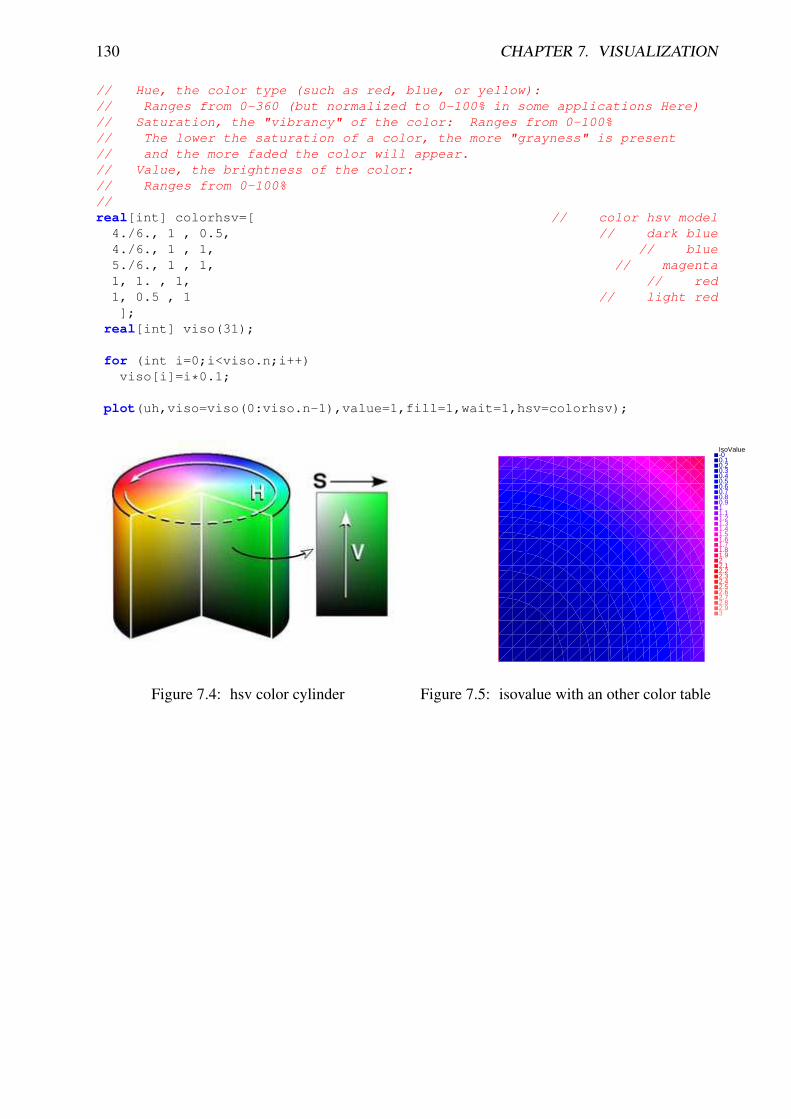
130 CHAPTER 7. VISUALIZATION
// Hue, the color type (such as red, blue, or yellow):// Ranges from 0-360 (but normalized to 0-100% in some applications Here)// Saturation, the "vibrancy" of the color: Ranges from 0-100%// The lower the saturation of a color, the more "grayness" is present// and the more faded the color will appear.// Value, the brightness of the color:// Ranges from 0-100%//real[int] colorhsv=[ // color hsv model
4./6., 1 , 0.5, // dark blue4./6., 1 , 1, // blue5./6., 1 , 1, // magenta1, 1. , 1, // red1, 0.5 , 1 // light red];
real[int] viso(31);
for (int i=0;i<viso.n;i++)viso[i]=i*0.1;
plot(uh,viso=viso(0:viso.n-1),value=1,fill=1,wait=1,hsv=colorhsv);
Figure 7.4: hsv color cylinder
IsoValue-00.10.20.30.40.50.60.70.80.911.11.21.31.41.51.61.71.81.922.12.22.32.42.52.62.72.82.93
Figure 7.5: isovalue with an other color table

7.2. LINK WITH GNUPLOT 131
7.2 link with gnuplotExample 3.2 shows how to generate a gnu-plot from a FreeFem++ file. Let us present here an-other technique which has the advantage of being online, i.e. one doesn’t need to quit FreeFem++to generate a gnu-plot. But this work only if gnuplot1 is installed , and only on unix computer.Add to the previous example:
// file for gnuplot
ofstream gnu("plot.gp");for (int i=0;i<=n;i++)
gnu << xx[i] << " " << yy[i] << endl;
// the file plot.gp is close because the variable gnu is delete
// to call gnuplot command and wait 5 second (thanks to unix command)// and make postscript plot
exec("echo ’plot \"plot.gp\" w l \pause 5 \set term postscript \set output \"gnuplot.eps\" \replot \quit’ | gnuplot");
0
0.5
1
1.5
2
0 5 10 15 20
"plot.gp"
Figure 7.6: Plots a cut of uh with gnuplot
7.3 link with meditFirst you must install medit 2, a freeware display package by Pascal Frey using OpenGL. Then youmay run the follwoing example.
mesh Th=square(10,10,[2*x-1,2*y-1]);fespace Vh(Th,P1);Vh u=2-x*x-y*y;
savemesh(Th,"mm",[x,y,u*.5]); // save mm.points and mm.faces file// for medit
// build a mm.bb file
1http://www.gnuplot.info/2http://www-rocq.inria.fr/gamma/medit/medit.html

132 CHAPTER 7. VISUALIZATION
Figure 7.7: medit plot
ofstream file("mm.bb");file << "2 1 1 "<< u[].n << " 2 \n";for (int j=0;j<u[].n ; j++)
file << u[][j] << endl;
// call medit commandexec("medit mm");
// clean files on unix OSexec("rm mm.bb mm.faces mm.points");

Chapter 8
Algorithms
The complete example is in algo.edp file.
8.1 conjugate Gradient/GMRESSuppose we want to solve the Euler problem: find x ∈ Rn such that
∇J(x) =
(∂J∂xi
(x))
= 0 (8.1)
where J is a functional (to minimize for example) from Rn to R.If the function is convex we can use the conjugate gradient to solve the problem, and we just needthe function (named dJ for example) which compute ∇J, so the two parameters are the name ofthe function with prototype func real[int] dJ(real[int] & xx) which compute ∇J, avector x of type real[int] to initialize the process and get the result.Given an initial value x(0), a maximum number imax of iterations, and an error tolerance 0 < ε < 1:Put x = x(0) and write
NLCG(∇J, x, precon= M, nbiter= imax, eps= ε);
will give the solution of x of ∇J(x) = 0. We can omit parameters precon, nbiter, eps.Here M is the preconditioner whose default is the identity matrix. The stopping test is
‖∇J(x)‖P ≤ ε‖∇J(x(0))‖P
Writing the minus value in eps=, i.e.,
NLCG(∇J, x, precon= M, nbiter= imax, eps= −ε);
we can use the stopping test‖∇J(x)‖2P ≤ ε
The parameters of these three functions are:
nbiter= set the number of iteration (by default 100)
precon= set the preconditioner function (P for example) by default it is the identity, remark theprototype is func real[int] P(real[int] &x).
133
134 CHAPTER 8. ALGORITHMS
eps= set the value of the stop test ε (= 10−6 by default) if positive then relative test ||∇J(x)||P ≤ε||∇J(x0)||P, otherwise the absolute test is ||∇J(x)||2P ≤ |ε|.
veps= set and return the value of the stop test, if positive then relative test ||∇J(x)||P ≤ ε||∇J(x0)||P,otherwise the absolute test is ||∇J(x)||2P ≤ |ε|. The return value is minus the real stop test (re-mark: it is useful in loop).
Example 8.1 (algo.edp) For a given function b, let us find the minimizer u of the functional
J(u) =12
∫Ω
f (|∇u|2) −∫
Ω
ub
f (x) = ax + x − ln(1 + x), f ′(x) = a +x
1 + x, f ′′(x) =
1(1 + x)2
under the boundary condition u = 0 on ∂Ω.
mesh Th=square(10,10); // mesh definition of Ω
fespace Vh(Th,P1); // finite element spacefespace Ph(Th,P0); // make optimization
/* A small hack to construct a function
Cl =
1 on interior degree of freedom0 on boundary degree of freedom
*/// Hack to construct an array :// 1 on interior nodes and 0 on boundary nodes
varf vCl(u,v) = on(1,2,3,4,u=1);Vh Cl;Cl[]= vCl(0,Vh,tgv=1); // 0 and tgvreal tgv=Cl[].max; //Cl[] = -Cl[]; Cl[] += tgv; Cl[] /=tgv;
// the definition of f , f ′, f ′′ and b
real a=0.001;
func real f(real u) return u*a+u-log(1+u); func real df(real u) return a+u/(1+u);func real ddf(real u) return 1/((1+u)*(1+u));Vh b=1; // to defined b
// the routine to compute the functional Jfunc real J(real[int] & x)
Vh u;u[]=x;real r=int2d(Th)(0.5*f( dx(u)*dx(u) + dy(u)*dy(u) ) - b*u) ;cout << "J(x) =" << r << " " << x.min << " " << x.max << endl;return r;
// The function to compute DJ, where u is the current solution.
Vh u=0; // the current value of the solution

8.1. CONJUGATE GRADIENT/GMRES 135
Vh alpha; // of store f ′(|∇u|2)int iter=0;alpha=df( dx(u)*dx(u) + dy(u)*dy(u) ); // optimization
func real[int] dJ(real[int] & x)
int verb=verbosity; verbosity=0;Vh u;u[]=x;alpha=df( dx(u)*dx(u) + dy(u)*dy(u) ); // optimizationvarf au(uh,vh) = int2d(Th)( alpha*( dx(u)*dx(vh) + dy(u)*dy(vh) ) - b*vh);x= au(0,Vh);x = x.* Cl[]; // the grad in 0 on boundaryverbosity=verb;return x; // warning no return of local array
/* We want to construct also a preconditioner C with solving the problem: find uh ∈ V0h such that
∀vh ∈ V0h,
∫Ω
α∇uh.∇vh =
∫Ω
bvh
where α = f ′(|∇u|2). */
varf alap(uh,vh,solver=Cholesky,init=iter)=int2d(Th)( alpha *( dx(uh)*dx(vh) + dy(uh)*dy(vh) )) + on(1,2,3,4,uh=0);
varf amass(uh,vh,solver=Cholesky,init=iter)=int2d(Th)( uh*vh) + on(1,2,3,4,uh=0);
matrix Amass = alap(Vh,Vh,solver=CG); //
matrix Alap= alap(Vh,Vh,solver=Cholesky,factorize=1); //
// the preconditionner functionfunc real[int] C(real[int] & x)
real[int] u(x.n);u=Amass*x;x = Alapˆ-1*u;x = x .* Cl[];return x; // no return of local array variable
/* To solve the problem, we make 10 iteration of the conjugate gradient, recompute the precondi-tioner and restart the conjugate gradient: */
verbosity=5;int conv=0;real eps=1e-6;for(int i=0;i<20;i++)
conv=NLCG(dJ,u[],nbiter=10,precon=C,veps=eps); //if (conv) break; // if converge break loop
alpha=df( dx(u)*dx(u) + dy(u)*dy(u) ); // recompute alpha optimizationAlap = alap(Vh,Vh,solver=Cholesky,factorize=1);

136 CHAPTER 8. ALGORITHMS
cout << " restart with new preconditionner " << conv << " eps =" << eps <<endl;
plot (u,wait=1,cmm="solution with NLCG");
For a given symmetric positive matrix A, consider the quadratic form
J(x) =12
xT Ax − bT x
then J(x) is minimized by the solution x of Ax = b. In this case, we can use the functionLinearCG
LinearCG(A, x, precon= M, nbiter= imax, eps= ±ε);
If A is not symmetric, we can use GMRES(Generalized Minimum Residual) algorithm by
LinearGMRES(A, x, precon= M, nbiter= imax, eps= ±ε);
Also, we can use the non-linear version of GMRES algorithm (the functional J is just convex)
LinearGMRES(∇J, x, precon= M, nbiter= imax, eps= ±ε);
For detail of these algorithms, refer to [13][Chapter IV, 1.3].
8.2 OptimizationTwo algorithms of COOOL a package [26] are interfaced with the Newton Raphson method (callNewton) and the BFGS method. Be careful of these algorithms, because their implementationuse full matrices.Example of utilization
func real J(real[int] & x)
real s=0;for (int i=0;i<x.n;i++)
s +=(i+1)*x[i]*x[i]*0.5 - b[i]*x[i];cout << "J ="<< s << " x =" << x[0] << " " << x[1] << "...\n" ;
return s;
b=1; x=2; // set right hand side and initial gestBFGS(J,dJ,x,eps=1.e-6,nbiter=20,nbiterline=20);cout << "BFGS: J(x) = " << J(x) << " err=" << error(x,b) << endl;
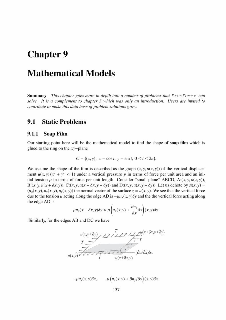
Chapter 9
Mathematical Models
Summary This chapter goes more in depth into a number of problems that FreeFem++ cansolve. It is a complement to chapter 3 which was only an introduction. Users are invited tocontribute to make this data base of problem solutions grow.
9.1 Static Problems
9.1.1 Soap FilmOur starting point here will be the mathematical model to find the shape of soap film which isglued to the ring on the xy−plane
C = (x, y); x = cos t, y = sin t, 0 ≤ t ≤ 2π.
We assume the shape of the film is described as the graph (x, y, u(x, y)) of the vertical displace-ment u(x, y) (x2 + y2 < 1) under a vertical pressure p in terms of force per unit area and an ini-tial tension µ in terms of force per unit length. Consider “small plane” ABCD, A:(x, y, u(x, y)),B:(x, y, u(x + δx, y)), C:(x, y, u(x + δx, y + δy)) and D:(x, y, u(x, y + δy)). Let us denote by n(x, y) =
(nx(x, y), ny(x, y), nz(x, y)) the normal vector of the surface z = u(x, y). We see that the vertical forcedue to the tension µ acting along the edge AD is −µnx(x, y)δy and the the vertical force acting alongthe edge AD is
µnx(x + δx, y)δy ' µ(nx(x, y) +
∂nx
∂xδx
)(x, y)δy.
Similarly, for the edges AB and DC we have
u ( x , y )
u ( x , y + d y )
u ( x + d x , y )
u ( x + d x , y + d y )
( ¶ u / ¶ x ) d x
TTT
T
−µny(x, y)δx, µ(ny(x, y) + ∂ny/∂y
)(x, y)δx.
137

138 CHAPTER 9. MATHEMATICAL MODELS
The force in the vertical direction on the surface ABCD due to the tension µ is given by
µ (∂nx/∂x) δxδy + T(∂ny/∂y
)δyδx.
Assuming small displacements, we have
νx = (∂u/∂x)/√
1 + (∂u/∂x)2 + (∂u/∂y)2 ' ∂u/∂x,
νy = (∂u/∂y)/√
1 + (∂u/∂x)2 + (∂u/∂y)2 ' ∂u/∂y.
Letting δx → dx, δy → dy, we have the equilibrium of the vertical displacement of soap film onABCD by p
µdxdy∂2u/∂x2 + µdxdy∂2u/∂y2 + pdxdy = 0.
Using the Laplace operator ∆ = ∂2/∂x2 + ∂2/∂y2, we can find the virtual displacement write thefollowing
−∆u = f in Ω (9.1)
where f = p/µ, Ω = (x, y); x2 + y2 < 1. Poisson’s equation (2.1) appear also in electrostaticstaking the form of f = ρ/ε where ρ is the charge density, ε the dielectric constant and u is namedas electrostatic potential. The soap film is glued to the ring ∂Ω = C, then we have the boundarycondition
u = 0 on ∂Ω (9.2)
If the force is gravity, for simplify, we assume that f = −1.
Example 9.1 (a tutorial.edp)
1 : border a(t=0,2*pi) x = cos(t); y = sin(t);label=1;;2 :3 : mesh disk = buildmesh(a(50));4 : plot(disk);5 : fespace femp1(disk,P1);6 : femp1 u,v;7 : func f = -1;8 : problem laplace(u,v) =9 : int2d(disk)( dx(u)*dx(v) + dy(u)*dy(v) ) // bilinear form
10 : - int2d(disk)( f*v ) // linear form11 : + on(1,u=0) ; // boundary condition12 : func ue = (xˆ2+yˆ2-1)/4; // ue: exact solution13 : laplace;14 : femp1 err = u - ue;15 :16 : plot (u,ps="aTutorial.eps",value=true,wait=true);17 : plot(err,value=true,wait=true);18 :19 : cout << "error L2=" << sqrt(int2d(disk)( errˆ2) )<< endl;20 : cout << "error H10=" << sqrt( int2d(disk)((dx(u)-x/2)ˆ2)21 : + int2d(disk)((dy(u)-y/2)ˆ2))<< endl;22 :23 : disk = adaptmesh(disk,u,err=0.01);24 : plot(disk,wait=1);25 :26 : laplace;27 :

9.1. STATIC PROBLEMS 139
28 : plot (u,value=true,wait=true);29 : err = u - ue; // become FE-function on adapted mesh30 : plot(err,value=true,wait=true);31 : cout << "error L2=" << sqrt(int2d(disk)( errˆ2) )<< endl;32 : cout << "error H10=" << sqrt(int2d(disk)((dx(u)-x/2)ˆ2)33 : + int2d(disk)((dy(u)-y/2)ˆ2))<< endl;
IsoValue-0.243997-0.231485-0.218972-0.206459-0.193947-0.181434-0.168921-0.156409-0.143896-0.131383-0.11887-0.106358-0.0938451-0.0813324-0.0688198-0.0563071-0.0437944-0.0312817-0.018769-0.00625634
Figure 9.1: isovalue of u
Figure 9.2: a side view of u
In 19th line, the L2-error estimation between the exact solution ue,
‖uh − ue‖0,Ω =
(∫Ω
|uh − ue|2 dxdy
)1/2
and from 20th line to 21th line, the H1-error seminorm estimation
|uh − ue|1,Ω =
(∫Ω
|∇uh − ∇ue|2 dxdy
)1/2
are done on the initial mesh. The results are ‖uh − ue‖0,Ω = 0.000384045, |uh − ue|1,Ω = 0.0375506.After the adaptation, we hava ‖uh − ue‖0,Ω = 0.000109043, |uh − ue|1,Ω = 0.0188411. So thenumerical solution is improved by adaptation of mesh.
9.1.2 ElectrostaticsWe assume that there is no current and a time independent charge distribution. Then the electricfield E satisfy
divE = ρ/ε, curlE = 0 (9.3)
where ρ is the charge density and ε is called the permittivity of free space. From the secondequation in (9.3), we can introduce the electrostatic potential such that E = −∇φ. Then we havePoisson equation −∆φ = f , f = −ρ/ε. We now obtain the equipotential line which is the levelcurve of φ, when there are no charges except conductors Ci1,··· ,K . Let us assume K conductorsC1, · · · ,CK within an enclosure C0. Each one is held at an electrostatic potential ϕi. We assume

140 CHAPTER 9. MATHEMATICAL MODELS
that the enclosure C0 is held at potential 0. In order to know ϕ(x) at any point x of the domain Ω,we must solve
−∆ϕ = 0 in Ω, (9.4)
where Ω is the interior of C0 minus the conductors Ci, and Γ is the boundary of Ω, that is∑N
i=0 Ci.Here g is any function of x equal to ϕi on Ci and to 0 on C0. The boundary equation is a reducedform for:
ϕ = ϕi on Ci, i = 1...N, ϕ = 0 on C0. (9.5)
Example 9.2 First we give the geometrical informations; C0 = (x, y); x2 + y2 = 52, C1 =
(x, y) : 10.32 (x − 2)2 + 1
32 y2 = 1, C2 = (x, y) : 10.32 (x + 2)2 + 1
32 y2 = 1. Let Ω be the disk enclosedby C0 with the elliptical holes enclosed by C1 and C2. Note that C0 is described counterclockwise,whereas the elliptical holes are described clockwise, because the boundary must be oriented sothat the computational domain is to its left.
// a circle with center at (0 ,0) and radius 5border C0(t=0,2*pi) x = 5 * cos(t); y = 5 * sin(t); border C1(t=0,2*pi) x = 2+0.3 * cos(t); y = 3*sin(t); border C2(t=0,2*pi) x = -2+0.3 * cos(t); y = 3*sin(t);
mesh Th = buildmesh(C0(60)+C1(-50)+C2(-50));plot(Th,ps="electroMesh"); // figure 9.3fespace Vh(Th,P1); // P1 FE-spaceVh uh,vh; // unknown and test function.problem Electro(uh,vh) = // definition of the problem
int2d(Th)( dx(uh)*dx(vh) + dy(uh)*dy(vh) ) // bilinear+ on(C0,uh=0) // boundary condition on C0+ on(C1,uh=1) // +1 volt on C1+ on(C2,uh=-1) ; // -1 volt on C2
Electro; // solve the problem, see figure 9.4 for the solutionplot(uh,ps="electro.eps",wait=true); // figure 9.4
Figure 9.3: Disk with two elliptical holes Figure 9.4: Equipotential lines, where C1 is lo-cated in right hand side

9.1. STATIC PROBLEMS 141
9.1.3 AerodynamicsLet us consider a wing profile S in a uniform flow. Infinity will be represented by a large circleΓ∞. As previously, we must solve
∆ϕ = 0 in Ω, ϕ|S = c, ϕ|Γ∞ = u∞1x − u∞2x (9.6)
where Ω is the area occupied by the fluid, u∞ is the air speed at infinity, c is a constant to be deter-mined so that ∂nϕ is continuous at the trailing edge P of S (so-called Kutta-Joukowski condition).Lift is proportional to c. To find c we use a superposition method. As all equations in (9.6) arelinear, the solution ϕc is a linear function of c
ϕc = ϕ0 + cϕ1, (9.7)
where ϕ0 is a solution of (9.6) with c = 0 and ϕ1 is a solution with c = 1 and zero speed at infinity.With these two fields computed, we shall determine c by requiring the continuity of ∂ϕ/∂n at thetrailing edge. An equation for the upper surface of a NACA0012 (this is a classical wing profile inaerodynamics; the rear of the wing is called the trailing edge) is:
y = 0.17735√
x − 0.075597x − 0.212836x2 + 0.17363x3 − 0.06254x4. (9.8)
Taking an incidence angle α such that tanα = 0.1, we must solve
−∆ϕ = 0 in Ω, ϕ|Γ1 = y − 0.1x, ϕ|Γ2 = c, (9.9)
where Γ2 is the wing profile and Γ1 is an approximation of infinity. One finds c by solving:
− ∆ϕ0 = 0 in Ω, ϕ0|Γ1 = y − 0.1x, ϕ0|Γ2 = 0, (9.10)−∆ϕ1 = 0 in Ω, ϕ1|Γ1 = 0, ϕ1|Γ2 = 1. (9.11)
The solution ϕ = ϕ0+cϕ1 allows us to find c by writing that ∂nϕ has no jump at the trailing edge P =
(1, 0). We have ∂nϕ − (ϕ(P+) − ϕ(P))/δ where P+ is the point just above P in the direction normalto the profile at a distance δ. Thus the jump of ∂nϕ is (ϕ0|P+ + c(ϕ1|P+ − 1)) + (ϕ0|P− + c(ϕ1|P− − 1))divided by δ because the normal changes sign between the lower and upper surfaces. Thus
c = −ϕ0|P+ + ϕ0|P−
(ϕ1|P+ + ϕ1|P− − 2), (9.12)
which can be programmed as:
c = −ϕ0(0.99, 0.01) + ϕ0(0.99,−0.01)
(ϕ1(0.99, 0.01) + ϕ1(0.99,−0.01) − 2). (9.13)
Example 9.3 // Computation of the potential flow around a NACA0012 airfoil.// The method of decomposition is used to apply the Joukowski condition
// The solution is seeked in the form psi0 + beta psi1 and beta is// adjusted so that the pressure is continuous at the trailing edge
border a(t=0,2*pi) x=5*cos(t); y=5*sin(t); ; // approximates infinity

142 CHAPTER 9. MATHEMATICAL MODELS
border upper(t=0,1) x = t;y = 0.17735*sqrt(t)-0.075597*t
- 0.212836*(tˆ2)+0.17363*(tˆ3)-0.06254*(tˆ4); border lower(t=1,0) x = t;
y= -(0.17735*sqrt(t)-0.075597*t-0.212836*(tˆ2)+0.17363*(tˆ3)-0.06254*(tˆ4));
border c(t=0,2*pi) x=0.8*cos(t)+0.5; y=0.8*sin(t);
wait = true;mesh Zoom = buildmesh(c(30)+upper(35)+lower(35));mesh Th = buildmesh(a(30)+upper(35)+lower(35));fespace Vh(Th,P2); // P1 FE spaceVh psi0,psi1,vh; // unknown and test function.fespace ZVh(Zoom,P2);
solve Joukowski0(psi0,vh) = // definition of the problemint2d(Th)( dx(psi0)*dx(vh) + dy(psi0)*dy(vh) ) // bilinear form
+ on(a,psi0=y-0.1*x) // boundary condition form+ on(upper,lower,psi0=0);
plot(psi0);
solve Joukowski1(psi1,vh) = // definition of the problemint2d(Th)( dx(psi1)*dx(vh) + dy(psi1)*dy(vh) ) // bilinear form
+ on(a,psi1=0) // boundary condition form+ on(upper,lower,psi1=1);
plot(psi1);
// continuity of pressure at trailing edgereal beta = psi0(0.99,0.01)+psi0(0.99,-0.01);beta = -beta / (psi1(0.99,0.01)+ psi1(0.99,-0.01)-2);
Vh psi = beta*psi1+psi0;plot(psi);ZVh Zpsi=psi;plot(Zpsi,bw=true);ZVh cp = -dx(psi)ˆ2 - dy(psi)ˆ2;plot(cp);ZVh Zcp=cp;plot(Zcp,nbiso=40);
9.1.4 Error estimationThere are famous estimation between the numerical result uh and the exact solution u of the prob-lem 2.1 and 2.2: If triangulations Thh↓0 is regular (see Section 5.4), then we have the estimates
|∇u − ∇uh|0,Ω ≤ C1h (9.14)‖u − uh‖0,Ω ≤ C2h2 (9.15)
with constants C1, C2 independent of h, if u is in H2(Ω). It is known that u ∈ H2(Ω) if Ω is convex.

9.1. STATIC PROBLEMS 143
Figure 9.5: isovalue of cp = −(∂xψ)2 − (∂yψ)2 Figure 9.6: Zooming of cp
In this section we check (9.14) and (9.15). We will pick up numericall error if we use the numericalderivative, so we will use the following for (9.14).∫
Ω
|∇u − ∇uh|2 dxdy =
∫Ω
∇u · ∇(u − 2uh) dxdy +
∫Ω
∇uh · ∇uh dxdy
=
∫Ω
f (u − 2uh) dxdy +
∫Ω
f uh dxdy
The constants C1, C2 are depend on Th and f , so we will find them by FreeFem++ . In general,we cannot get the solution u as a elementary functions (see Section 4.7) even if spetical functionsare added. Instead of the exact solution, here we use the approximate solution u0 in Vh(Th, P2), h ∼0.
Example 9.4
1 : mesh Th0 = square(100,100);2 : fespace V0h(Th0,P2);3 : V0h u0,v0;4 : func f = x*y; // sin(pi*x)*cos(pi*y);5 :6 : solve Poisson0(u0,v0) =7 : int2d(Th0)( dx(u0)*dx(v0) + dy(u0)*dy(v0) ) // bilinear form8 : - int2d(Th0)( f*v0 ) // linear form9 : + on(1,2,3,4,u0=0) ; // boundary condition
10 :11 : plot(u0);12 :13 : real[int] errL2(10), errH1(10);14 :15 : for (int i=1; i<=10; i++) 16 : mesh Th = square(5+i*3,5+i*3);17 : fespace Vh(Th,P1);18 : fespace Ph(Th,P0);19 : Ph h = hTriangle; // get the size of all triangles20 : Vh u,v;21 : solve Poisson(u,v) =

144 CHAPTER 9. MATHEMATICAL MODELS
22 : int2d(Th)( dx(u)*dx(v) + dy(u)*dy(v) ) // bilinear form23 : - int2d(Th)( f*v ) // linear form24 : + on(1,2,3,4,u=0) ; // boundary condition25 : V0h uu = u;26 : errL2[i-1] = sqrt( int2d(Th0)((uu - u0)ˆ2) )/h[].maxˆ2;27 : errH1[i-1] = sqrt( int2d(Th0)( f*(u0-2*uu+uu) ) )/h[].max;28 : 29 : cout << "C1 = " << errL2.max <<"("<<errL2.min<<")"<< endl;30 : cout << "C2 = " << errH1.max <<"("<<errH1.min<<")"<< endl;
We can guess that C1 = 0.0179253(0.0173266) and C2 = 0.0729566(0.0707543), where the num-bers inside the parentheses are minimum in calculation.
9.1.5 PeriodicWe now solve the Poisson equation
−∆u = sin(x + π/4.) ∗ cos(y + π/4.)
on the square ]0, 2π[2 under bi-periodic boundary condition u(0, y) = u(2π, y) for all y and u(x, 0) =
u(x, 2π) for all x. These boundary conditions are achieved from the definition of the periodic finiteelement space.
Example 9.5 (periodic.edp)
mesh Th=square(10,10,[2*x*pi,2*y*pi]);// defined the fespacewith periodic condition
// label : 2 and 4 are left and right side with y the curve abscissa// 1 and 2 are bottom and upper side with x the curve abscissa
fespace Vh(Th,P2,periodic=[[2,y],[4,y],[1,x],[3,x]]);Vh uh,vh; // unknown and test function.func f=sin(x+pi/4.)*cos(y+pi/4.); // right hand side function
problem laplace(uh,vh) = // definion of the problemint2d(Th)( dx(uh)*dx(vh) + dy(uh)*dy(vh) ) // bilinear form
+ int2d(Th)( -f*vh ) // linear form;
laplace; // solve the problem plot(uh); // to see the resultplot(uh,ps="period.eps",value=true);
The periodic condition does not necessarily require parallel to the axis. Example 9.6 give suchexample.
Example 9.6 (periodic4.edp)
real r=0.25;// a diamond with a hole
border a(t=0,1)x=-t+1; y=t;label=1;;border b(t=0,1) x=-t; y=1-t;label=2;;border c(t=0,1) x=t-1; y=-t;label=3;;border d(t=0,1) x=t; y=-1+t;label=4;;

9.1. STATIC PROBLEMS 145
IsoValue-0.441699-0.391928-0.342157-0.292387-0.242616-0.192845-0.143075-0.0933038-0.04353310.006237610.05600830.1057790.155550.205320.2550910.3048620.3546330.4044030.4541740.503945
Figure 9.7: The isovalue of solution u with periodic boundary condition
border e(t=0,2*pi) x=r*cos(t); y=-r*sin(t);label=0;;int n = 10;mesh Th= buildmesh(a(n)+b(n)+c(n)+d(n)+e(n));plot(Th,wait=1);real r2=1.732;func abs=sqrt(xˆ2+yˆ2);// warning for periodic condition:// side a and c// on side a (label 1) x ∈ [0, 1] or x − y ∈ [−1, 1]// on side c (label 3) x ∈ [−1, 0] or x − y ∈ [−1, 1]
// so the common abscissa can be respectively x and x + 1// or you can can try curviline abscissa x − y and x − y
// 1 first way// fespace Vh(Th,P2,periodic=[[2,1+x],[4,x],[1,x],[3,1+x]]);// 2 second wayfespace Vh(Th,P2,periodic=[[2,x+y],[4,x+y],[1,x-y],[3,x-y]]);
Vh uh,vh;
func f=(y+x+1)*(y+x-1)*(y-x+1)*(y-x-1);real intf = int2d(Th)(f);real mTh = int2d(Th)(1);real k = intf/mTh;problem laplace(uh,vh) =
int2d(Th)( dx(uh)*dx(vh) + dy(uh)*dy(vh) ) + int2d(Th)( (k-f)*vh ) ;laplace;plot(uh,wait=1,ps="perio4.eps");
A other example with no equal border, just to see if the code works.
Example 9.7 (periodic4bis.edp)
// irregular boundary condition.// to build border AB
macro LINEBORDER(A,B,lab) border A#B(t=0,1)real t1=1.-t;x=A#x*t1+B#x*t;y=A#y*t1+B#y*t;label=lab; // EOM

146 CHAPTER 9. MATHEMATICAL MODELS
Figure 9.8: The isovalue of solution u for ∆u = ((y + x)2 + 1)((y − x)2 + 1) − k, in Ω and ∂nu = 0on hole,and with two periodic boundary condition on external border
// compute ||AB|| a=(ax,ay) et B =(bx,by)macro dist(ax,ay,bx,by) sqrt(square((ax)-(bx))+ square((ay)-(by))) // EOMmacro Grad(u) [dx(u),dy(u)] // EOM
real Ax=0.9,Ay=1; real Bx=2,By=1;real Cx=2.5,Cy=2.5; real Dx=1,Dy=2;real gx = (Ax+Bx+Cx+Dx)/4.; real gy = (Ay+By+Cy+Dy)/4.;
LINEBORDER(A,B,1)LINEBORDER(B,C,2)LINEBORDER(C,D,3)LINEBORDER(D,A,4)
int n=10;
real l1=dist(Ax,Ay,Bx,By);real l2=dist(Bx,By,Cx,Cy);real l3=dist(Cx,Cy,Dx,Dy);real l4=dist(Dx,Dy,Ax,Ay);func s1=dist(Ax,Ay,x,y)/l1; // absisse on AB = ||AX||/||AB||func s2=dist(Bx,By,x,y)/l2; // absisse on BC = ||BX||/||BC||func s3=dist(Cx,Cy,x,y)/l3; // absisse on CD = ||CX||/||CD||func s4=dist(Dx,Dy,x,y)/l4; // absisse on DA = ||DX||/||DA||
mesh Th=buildmesh(AB(n)+BC(n)+CD(n)+DA(n),fixeborder=1); //
verbosity=6; // to see the abscisse value pour the periodic condition.fespace Vh(Th,P1,periodic=[[1,s1],[3,s3],[2,s2],[4,s4]]);verbosity=1;Vh u,v;real cc=0;cc= int2d(Th)((x-gx)*(y-gy)-cc)/Th.area;cout << " compatibility =" << int2d(Th)((x-gx)*(y-gy)-cc) <<endl;

9.1. STATIC PROBLEMS 147
solve Poission(u,v)=int2d(Th)(Grad(u)’*Grad(v)+ 1e-10*u*v)-int2d(Th)(10*v*((x-gx)*(y-gy)-cc));
plot(u,wait=1,value=1);
9.1.6 Poisson with mixed boundary conditionHere we consider the Poisson equation with mixed boundary value problems: For given functionsf and g, find u such that
− ∆u = f in Ω
u = g on ΓD, ∂u/∂n = 0 on ΓN (9.16)
where ΓD is a part of the boundary Γ and ΓN = Γ\ΓD. The solution u has the singularity at the pointsγ1, γ2 = ΓD ∩ ΓN . When Ω = (x, y); −1 < x < 1, 0 < y < 1, ΓN = (x, y); −1 ≤ x < 0, y = 0,ΓD = ∂Ω \ ΓN , the singularity will appear at γ1 = (0, 0), γ2(−1, 0), and u has the expression
u = KiuS + uR, uR ∈ H2(near γi), i = 1, 2
with a constants Ki. Here uS = r1/2j sin(θ j/2) by the local polar coordinate (r j, θ j at γ j such that
(r1, θ1) = (r, θ). Instead of poler coordinate system (r, θ), we use that r = sqrt( x2+y2 ) andθ = atan2(y,x) in FreeFem++ .
Example 9.8 Assume that f = −2 × 30(x2 + y2) and g = ue = 10(x2 + y2)1/4 sin([tan−1(y/x)]/2
)+
30(x2y2), where ueS is the exact solution.
1 : border N(t=0,1) x=-1+t; y=0; label=1; ;2 : border D1(t=0,1) x=t; y=0; label=2;;3 : border D2(t=0,1) x=1; y=t; label=2; ;4 : border D3(t=0,2) x=1-t; y=1; label=2;;5 : border D4(t=0,1) x=-1; y=1-t; label=2; ;6 :7 : mesh T0h = buildmesh(N(10)+D1(10)+D2(10)+D3(20)+D4(10));8 : plot(T0h,wait=true);9 : fespace V0h(T0h,P1);
10 : V0h u0, v0;11 :12 : func f=-2*30*(xˆ2+yˆ2); // given function13 : // the singular term of the solution is K*us (K: constant)14 : func us = sin(atan2(y,x)/2)*sqrt( sqrt(xˆ2+yˆ2) );15 : real K=10.;16 : func ue = K*us + 30*(xˆ2*yˆ2);17 :18 : solve Poisson0(u0,v0) =19 : int2d(T0h)( dx(u0)*dx(v0) + dy(u0)*dy(v0) ) // bilinear form20 : - int2d(T0h)( f*v0 ) // linear form21 : + on(2,u0=ue) ; // boundary condition22 :23 : // adaptation by the singular term24 : mesh Th = adaptmesh(T0h,us);25 : for (int i=0;i< 5;i++)26 :

148 CHAPTER 9. MATHEMATICAL MODELS
27 : mesh Th=adaptmesh(Th,us);28 : ;29 :30 : fespace Vh(Th, P1);31 : Vh u, v;32 : solve Poisson(u,v) =33 : int2d(Th)( dx(u)*dx(v) + dy(u)*dy(v) ) // bilinear form34 : - int2d(Th)( f*v ) // linear form35 : + on(2,u=ue) ; // boundary condition36 :37 : /* plot the solution */38 : plot(Th,ps="adaptDNmix.ps");39 : plot(u,wait=true);40 :41 : Vh uue = ue;42 : real H1e = sqrt( int2d(Th)( dx(uue)ˆ2 + dy(uue)ˆ2 + uueˆ2 ) );43 :44 : /* calculate the H1 Sobolev norm */45 : Vh err0 = u0 - ue;46 : Vh err = u - ue;47 : Vh H1err0 = int2d(Th)( dx(err0)ˆ2+dy(err0)ˆ2+err0ˆ2 );48 : Vh H1err = int2d(Th)( dx(err)ˆ2+dy(err)ˆ2+errˆ2 );49 : cout <<"Relative error in first mesh "<< int2d(Th)(H1err0)/H1e<<endl;50 : cout <<"Relative error in adaptive mesh "<< int2d(Th)(H1err)/H1e<<endl;
From 24th line to 28th, adaptation of meshes are done using the base of singular term. In 42thline, H1e=‖ue‖1,Ω is calculated. In last 2 lines, the relative errors are calculated, that is,
‖u0h − ue‖1,Ω/H1e = 0.120421‖ua
h − ue‖1,Ω/H1e = 0.0150581
where u0h is the numerical solution in T0h and ua
h is u in this program.
9.1.7 Poisson with mixte finite elementHere we consider the Poisson equation with mixed boundary value problems: For given functionsf , gd, gn, find p such that
− ∆p = 1 in Ω
p = gd on ΓD, ∂p/∂n = gn on ΓN (9.17)
where ΓD is a part of the boundary Γ and ΓN = Γ \ ΓD.The mixte formulation is: find p and u such that
∇p + u = 0 in Ω
∇.u = f in Ω
p = gd on ΓD, ∂u.n = gn.n on ΓN (9.18)
where gn is a vector such that gn.n = gn.

9.1. STATIC PROBLEMS 149
The variationnal formulation is,
∀v ∈ V0,∫
Ωp∇.v + vv =
∫Γd
gdv.n
∀q ∈ P∫
Ωq∇.u =
∫Ω
q f
∂u.n = gn.n on ΓN (9.19)
where the functionnal space are:
P = L2(Ω), V = H(div) = v ∈ L2(Ω)2,∇.v ∈ L2(Ω)
andV0 = v ∈ V; v.n = 0 on ΓN.
To write, the FreeFem++ example, we have just to choose the finites elements spaces. here Vspace is discretize with Raviart-Thomas finite element RT0 and P is discretize by constant finiteelement P0.
Example 9.9 (LaplaceRT.edp)
mesh Th=square(10,10);
fespace Vh(Th,RT0);
fespace Ph(Th,P0);
func gd = 1.;
func g1n = 1.;
func g2n = 1.;
Vh [u1,u2],[v1,v2];
Ph p,q;
problem laplaceMixte([u1,u2,p],[v1,v2,q],
solver=GMRES,eps=1.0e-10,
tgv=1e30,dimKrylov=150)
=
int2d(Th)( p*q*1e-15 // this term is here to be sur
// that all sub matrix are inversible (LU requirement)
+ u1*v1 + u2*v2 + p*(dx(v1)+dy(v2)) + (dx(u1)+dy(u2))*q )
+ int2d(Th) ( q)
- int1d(Th,1,2,3)( gd*(v1*N.x +v2*N.y)) // on ΓD
+ on(4,u1=g1n,u2=g2n); // on ΓN
laplaceMixte;
plot([u1,u2],coef=0.1,wait=1,ps="lapRTuv.eps",value=true);
plot(p,fill=1,wait=1,ps="laRTp.eps",value=true);

150 CHAPTER 9. MATHEMATICAL MODELS
9.1.8 Metric Adaptation and residual error indicatorWe do metric mesh adaption and compute the classical residual error indicator ηT on the elementT for the Poisson problem.
Example 9.10 (adaptindicatorP2.edp) First, we solve the same problem as in a previous ex-ample.
1 : border ba(t=0,1.0)x=t; y=0; label=1;; // see Fig,5.132 : border bb(t=0,0.5)x=1; y=t; label=2;;3 : border bc(t=0,0.5)x=1-t; y=0.5;label=3;;4 : border bd(t=0.5,1)x=0.5; y=t; label=4;;5 : border be(t=0.5,1)x=1-t; y=1; label=5;;6 : border bf(t=0.0,1)x=0; y=1-t;label=6;;7 : mesh Th = buildmesh (ba(6) + bb(4) + bc(4) +bd(4) + be(4) + bf(6));8 : savemesh(Th,"th.msh");9 : fespace Vh(Th,P2);
10 : fespace Nh(Th,P0);11 : Vh u,v;12 : Nh rho;13 : real[int] viso(21);14 : for (int i=0;i<viso.n;i++)15 : viso[i]=10.ˆ(+(i-16.)/2.);16 : real error=0.01;17 : func f=(x-y);18 : problem Probem1(u,v,solver=CG,eps=1.0e-6) =19 : int2d(Th,qforder=5)( u*v*1.0e-10+ dx(u)*dx(v) + dy(u)*dy(v))20 : + int2d(Th,qforder=5)( -f*v);21 : /*************
Now, the local error indicator ηT is:
ηT =
h2T || f + ∆uh||
2L2(T ) +
∑e∈EK
he || [∂uh
∂nk] ||2L2(e)
12
where hT is the longest’s edge of T , ET is the set of T edge not on Γ = ∂Ω, nT is the outside unitnormal to K, he is the length of edge e, [g] is the jump of the function g across edge (left valueminus right value).Of coarse, we can use a variational form to compute η2
T , with test function constant function ineach triangle.
29 : *************/30 :31 : varf indicator2(uu,chiK) =32 : intalledges(Th)(chiK*lenEdge*square(jump(N.x*dx(u)+N.y*dy(u))))33 : +int2d(Th)(chiK*square(hTriangle*(f+dxx(u)+dyy(u))) );34 : for (int i=0;i< 4;i++)35 : 36 : Probem1;37 : cout << u[].min << " " << u[].max << endl;38 : plot(u,wait=1);39 : cout << " indicator2 " << endl;40 :41 : rho[] = indicator2(0,Nh);

9.1. STATIC PROBLEMS 151
42 : rho=sqrt(rho);
43 : cout << "rho = min " << rho[].min << " max=" << rho[].max << endl;44 : plot(rho,fill=1,wait=1,cmm="indicator density ",ps="rhoP2.eps",
value=1,viso=viso,nbiso=viso.n);
45 : plot(Th,wait=1,cmm="Mesh ",ps="ThrhoP2.eps");
46 : Th=adaptmesh(Th,[dx(u),dy(u)],err=error,anisomax=1);47 : plot(Th,wait=1);48 : u=u;
49 : rho=rho;
50 : error = error/2;
51 : ;
If the method is correct, we expect to look the graphics by an almost constant function η on yourcomputer as in Fig. 9.9.
IsoValue1e-083.16228e-081e-073.16228e-071e-063.16228e-061e-053.16228e-050.00010.0003162280.0010.003162280.010.03162280.10.31622813.162281031.6228100
indicator density Mesh
Figure 9.9: Density of the error indicator with isotropic P2 metric
9.1.9 Adaptation using residual error indicator
In the previous example we compute the error indicator, now we use it, to adapt the mesh.The new mesh size is given by the following formulae:
hn+1(x) =hn(x)
fn(ηK(x))
where ηn(x) is the level of error at point x given by the local error indicator, hn is the previous “meshsize” field, and fn is a user function define by fn = min(3,max(1/3, ηn/η
∗n)) where η∗n = mean(ηn)c,
and c is an user coefficient generally close to one.

152 CHAPTER 9. MATHEMATICAL MODELS
Example 9.11 (AdaptResidualErrorIndicator.edp)First a macro MeshSizecomputation to get a P1 mesh size as the average of edge lenght.
// macro the get the current mesh size// parameter// in: Th the mesh// Vh P1 fespace on Th// out :// h: the Vh finite element finite set to the current mesh sizemacro MeshSizecomputation(Th,Vh,h) /* Th mesh Vh P1 finite element spaceh the P1 mesh size value */
real[int] count(Th.nv);/* mesh size (lenEdge = integral(e) 1 ds) */varf vmeshsizen(u,v)=intalledges(Th,qfnbpE=1)(v);/* number of edge / par vertex */varf vedgecount(u,v)=intalledges(Th,qfnbpE=1)(v/lenEdge);
/*computation of the mesh size----------------------------- */
count=vedgecount(0,Vh);h[]=0.;h[]=vmeshsizen(0,Vh);cout << " count min = "<< count.min << " " << count.max << endl;h[]=h[]./count;
cout << " -- bound meshsize = " <<h[].min << " " << h[].max << endl; // end of macro MeshSizecomputation
A second macro to remesh according to the new mesh size.
// macro to remesh according the de residual indicator// in:// Th the mesh// Ph P0 fespace on Th// Vh P1 fespace on Th// vindicator the varf of to evaluate the indicator to 2
// coef on etameam ..// ------
macro ReMeshIndicator(Th,Ph,Vh,vindicator,coef)Vh h=0;/*evalutate the mesh size */MeshSizecomputation(Th,Vh,h);Ph etak;etak[]=vindicator(0,Ph);etak[]=sqrt(etak[]);real etastar= coef*(etak[].sum/etak[].n);cout << " etastar = " << etastar << " sum=" << etak[].sum << " " << endl;
/* here etaK is discontinouswe use the P1 L2 projection with mass lumping . */
Vh fn,sigma;varf veta(unused,v)=int2d(Th)(etak*v);varf vun(unused,v)=int2d(Th)(1*v);

9.2. ELASTICITY 153
fn[] = veta(0,Vh);sigma[]= vun(0,Vh);fn[]= fn[]./ sigma[];fn = max(min(fn/etastar,3.),0.3333) ;
/* new mesh size */h = h / fn ;/* plot(h,wait=1); *//* build the new mesh */Th=adaptmesh(Th,IsMetric=1,h,splitpbedge=1,nbvx=10000);
We skip the mesh construction, see the previous example,
// FE space definition ---fespace Vh(Th,P1); // for the mesh size and solutionfespace Ph(Th,P0); // for the error indicator
real hinit=0.2; // initial mesh sizeVh h=hinit; // the FE function for the mesh size
// to build a mesh with a given mesh size : meshsizeTh=adaptmesh(Th,h,IsMetric=1,splitpbedge=1,nbvx=10000);plot(Th,wait=1,ps="RRI-Th-init.eps");Vh u,v;
func f=(x-y);
problem Poisson(u,v) =int2d(Th,qforder=5)( u*v*1.0e-10+ dx(u)*dx(v) + dy(u)*dy(v))
- int2d(Th,qforder=5)( f*v);
varf indicator2(unused,chiK) =intalledges(Th)(chiK*lenEdge*square(jump(N.x*dx(u)+N.y*dy(u))))
+int2d(Th)(chiK*square(hTriangle*(f+dxx(u)+dyy(u))) );
for (int i=0;i< 10;i++)u=u;Poisson;plot(Th,u,wait=1);real cc=0.8;if(i>5) cc=1;ReMeshIndicator(Th,Ph,Vh,indicator2,cc);plot(Th,wait=1);
9.2 ElasticityConsider an elastic plate with undeformed shape Ω×] − h, h[ in R3, Ω ⊂ R2. By the deforma-tion of the plate, we assume that a point P(x1, x2, x3) moves to P(ξ1, ξ2, ξ3). The vector u =
(u1, u2, u3) = (ξ1 − x1, ξ2 − x2, ξ3 − x3) is called displacement vector. By the deformation, the

154 CHAPTER 9. MATHEMATICAL MODELS
IsoValue5.89664e-050.0001118870.0001471670.0001824470.0002177270.0002530080.0002882880.0003235680.0003588480.0003941290.0004294090.0004646890.0004999690.0005352490.000570530.000605810.000641090.000676370.0007116510.000799851
IsoValue-123.488-123.476-123.464-123.452-123.44-123.428-123.416-123.404-123.392-123.38-123.368-123.356-123.344-123.332-123.32-123.308-123.296-123.284-123.272-123.26
Figure 9.10: the error indicator with isotropic P1 , the mesh and isovalue of the solution
line segment x, x + τ∆x moves approximately to x + u(x), x + τ∆x + u(x + τ∆x) for small τ, wherex = (x1, x2, x3), ∆x = (∆x1,∆x2,∆x3). We now calculate the ratio between two segments
η(τ) = τ−1|∆x|−1 (|u(x + τ∆x) − u(x) + τ∆x| − τ|∆x|)
then we have (see e.g. [15, p.32])
limτ→0
η(τ) = (1 + 2ei jνiν j)1/2 − 1, 2ei j =∂uk
∂xi
∂uk
∂x j+
(∂ui
∂x j+∂u j
∂xi
)where νi = ∆xi|∆x|−1. If the deformation is small, then we may consider that
(∂uk/∂xi)(∂uk/∂xi) ≈ 0
and the following is called small strain tensor
εi j(u) =12
(∂ui
∂x j+∂u j
∂xi
)The tensor ei j is called finite strain tensor.Consider the small plane ∆Π(x) centered at x with the unit normal direction n = (n1, n2, n3), thenthe surface on ∆Π(x) at x is
(σ1 j(x)n j, σ2 j(x)n j, σ3 j(x)n j)
where σi j(x) is called stress tensor at x. Hooke’s law is the assumption of a linear relation betweenσi j and εi j such as
σi j(x) = ci jkl(x)εi j(x)
with the symmetry ci jkl = c jikl, ci jkl = ci jlk, ci jkl = ckli j.

9.2. ELASTICITY 155
If Hooke’s tensor ci jkl(x) do not depend on the choice of coordinate system, the material is calledisotropic at x. If ci jkl is constant, the material is called homogeneous. In homogeneous isotropiccase, there is Lame constants λ, µ (see e.g. [15, p.43]) satisfying
σi j = λδi jdivu + 2µεi j (9.20)
where δi j is Kronecker’s delta. We assume that the elastic plate is fixed on ΓD×]−h, h[, ΓD ⊂ ∂Ω. Ifthe body force f = ( f1, f2, f3) is given in Ω×]−h, h[ and surface force g is given in ΓN×]−h, h[,ΓN =
∂Ω \ ΓD, then the equation of equilibrium is given as follows:
− ∂ jσi j = fi in Ω×] − h, h[, i = 1, 2, 3 (9.21)σi jn j = gi on ΓN×] − h, h[, ui = 0 on ΓD×] − h, h[, i = 1, 2, 3 (9.22)
We now explain the plain elasticity.
Plain strain: On the end of plate, the contact condition u3 = 0, g3 = is satisfied. In this case, wecan suppose that f3 = g3 = u3 = 0 and u(x1, x2, x3) = u(x1, x2) for all −h < x3 < h.
Plain stress: The cylinder is assumed to be very thin and subjected to no load on the ends x3 = ±h,that is,
σ3i = 0, x3 = ±h, i 1, 2, 3
The assumption leads that σ3i = 0 in Ω×] − h, h[ and u(x1, x2, x3) = u(x1, x2) for all −h <x3 < h.
Generalized plain stress: The cylinder is subjected to no load on the ends x3 = ±h. Introducingthe mean values with respect to thickness,
ui(x1, x2) =1
2h
∫ h
−hu(x1, x2, x3)dx3
and we derive u3 ≡ 0. Similarly we define the mean values f , g of the body force andsurface force as well as the mean values εi j and σi j of the components of stress and strain,respectively.
In what follows we omit the overlines of u, f , g, εi j and εi j. Then we obtain similar equation ofequilibrium given in (9.21) replacing Ω×]−h, h[ with Ω and changing i = 1, 2. In the case of planestress, σi j = λ∗δi jdivu + 2µεi j, λ
∗ = (2λµ)/(λ + µ).The equations of elasticity are naturally written in variational form for the displacement vectoru(x) ∈ V as ∫
Ω
[2µεi j(u)εi j(v) + λεii(u)ε j j(v)] =
∫Ω
f · v +
∫Γ
g · v,∀v ∈ V
where V is the linear closed subspace of H1(Ω)2.
Example 9.12 (Beam.edp) Consider elastic plate with the undeformed rectangle shape [0, 10] ×[0, 2]. The body force is the gravity force f and the boundary force g is zero on lower and upperside. On the two vertical sides of the beam are fixed.
// a weighting beam sitting on a

156 CHAPTER 9. MATHEMATICAL MODELS
int bottombeam = 2;border a(t=2,0) x=0; y=t ;label=1;; // left beamborder b(t=0,10) x=t; y=0 ;label=bottombeam;; // bottom of beamborder c(t=0,2) x=10; y=t ;label=1;; // rigth beamborder d(t=0,10) x=10-t; y=2; label=3;; // top beamreal E = 21.5;real sigma = 0.29;real mu = E/(2*(1+sigma));real lambda = E*sigma/((1+sigma)*(1-2*sigma));real gravity = -0.05;mesh th = buildmesh( b(20)+c(5)+d(20)+a(5));fespace Vh(th,[P1,P1]);Vh [uu,vv], [w,s];cout << "lambda,mu,gravity ="<<lambda<< " " << mu << " " << gravity << endl;
// deformation of a beam under its own weightreal sqrt2=sqrt(2.); // see lame.edp example 3.9macro epsilon(u1,u2) [dx(u1),dy(u2),(dy(u1)+dx(u2))/sqrt2] // EOMmacro div(u,v) ( dx(u)+dy(v) ) // EOM
solve bb([uu,vv],[w,s])=int2d(th)(
lambda*div(w,s)*div(uu,vv)+2.*mu*( epsilon(w,s)’*epsilon(uu,vv) )
)+ int2d(th) (-gravity*s)+ on(1,uu=0,vv=0);
plot([uu,vv],wait=1);plot([uu,vv],wait=1,bb=[[-0.5,2.5],[2.5,-0.5]]);mesh th1 = movemesh(th, [x+uu, y+vv]);plot(th1,wait=1);
9.2.1 Fracture MechanicsConsider the plate with the crack whose undeformed shape is a curve Σ with the two edges γ1, γ2.We assume the stress tensor σi j is the state of plate stress regarding (x, y) ∈ ΩΣ = Ω \ Σ. Here Ω
stands for the undeformed shape of elastic plate without crack. If the part ΓN of the boundary ∂Ω isfixed and a load L = ( f , g) ∈ L2(Ω)2 × L2(ΓN)2 is given, then the displacement u is the minimizerof the potential energy functional
E(v;L,ΩΣ) =
∫ΩΣ
w(x, v) − f · v −∫
ΓN
g · v
over the functional space V(ΩΣ),
V(ΩΣ) =v ∈ H1(ΩΣ)2; v = 0 on ΓD = ∂Ω \ ΓN
,
where w(x, v) = σi j(v)εi j(v)/2,
σi j(v) = Ci jkl(x)εkl(v), εi j(v) = (∂vi/∂x j + ∂v j/∂xi)/2, (Ci jkl : Hooke’s tensor).

9.2. ELASTICITY 157
If the elasticity is homogeneous isotropic, then the displacement u(x) is decomposed in an openneighborhood Uk of γk as in (see e.g. [16])
u(x) =
2∑l=1
Kl(γk)r1/2k S C
kl(θk) + uk,R(x) for x ∈ ΩΣ ∩ Uk, k = 1, 2 (9.23)
with uk,R ∈ H2(ΩΣ ∩ Uk)2, where Uk, k = 1, 2 are open neighborhoods of γk such that ∂L1 ∩ U1 =
γ1, ∂Lm ∩ U2 = γ2, and
S Ck1(θk) =
14µ
1(2π)1/2
[[2κ − 1] cos(θk/2) − cos(3θk/2)−[2κ + 1] sin(θk/2) + sin(3θk/2)
], (9.24)
S Ck2(θk) =
14µ
1(2π)1/2
[−[2κ − 1] sin(θk/2) + 3 sin(3θk/2)−[2κ + 1] cos(θk/2) + cos(3θk/2)
].
where µ is the shear modulus of elasticity, κ = 3 − 4ν (ν is the Poisson’s ratio) for plane strain andκ = 3−ν
1+νfor plane stress.
The coefficients K1(γi) and K2(γi), which are important parameters in fracture mechanics, arecalled stress intensity factors of the opening mode (mode I) and the sliding mode (mode II), re-spectively.For simplicity, we consider the following simple crack
Ω = (x, y) : −1 < x < 1,−1 < y < 1, Σ = (x, y) : −1 ≤ x ≤ 0, y = 0
with only one crack tip γ = (0, 0). Unfortunately, FreeFem++ cannot treat crack, so we usethe modification of the domain with U-shape channel (see Fig. 5.28) with d = 0.0001. Theundeformed crack Σ is approximated by
Σd = (x, y) : −1 ≤ x ≤ −10 ∗ d,−d ≤ y ≤ d∪(x, y) : −10 ∗ d ≤ x ≤ 0,−d + 0.1 ∗ x ≤ y ≤ d − 0.1 ∗ x
and ΓD = R in Fig. 5.28. In this example, we use three technique:
• Fast Finite Element Interpolator from the mesh Th to Zoom for the scale-up of near γ.
• After obtaining the displacement vector u = (u, v), we shall watch the deformation of thecrack near γ as follows,
mesh Plate = movemesh(Zoom,[x+u,y+v]);plot(Plate);
• Important technique is adaptive mesh, because the large singularity occur at γ as shown in(9.23).
First example create mode I deformation by the opposed surface force on B and T in the verticaldirection of Σ, and the displacement is fixed on R.In a laboratory, fracture engineer use photoelasticity to make stress field visible, which shows theprincipal stress difference
σ1 − σ2 =
√(σ11 − σ22)2 + 4σ2
12 (9.25)
where σ1 and σ2 are the principal stresses. In opening mode, the photoelasticity make symmetricpattern concentrated at γ.

158 CHAPTER 9. MATHEMATICAL MODELS
Example 9.13 (Crack Opening, K2(γ) = 0) CrackOpen.edpreal d = 0.0001;int n = 5;real cb=1, ca=1, tip=0.0;border L1(t=0,ca-d) x=-cb; y=-d-t; border L2(t=0,ca-d) x=-cb; y=ca-t; border B(t=0,2) x=cb*(t-1); y=-ca; border C1(t=0,1) x=-ca*(1-t)+(tip-10*d)*t; y=d; border C21(t=0,1) x=(tip-10*d)*(1-t)+tip*t; y=d*(1-t); border C22(t=0,1) x=(tip-10*d)*t+tip*(1-t); y=-d*t; border C3(t=0,1) x=(tip-10*d)*(1-t)-ca*t; y=-d; border C4(t=0,2*d) x=-ca; y=-d+t; border R(t=0,2) x=cb; y=cb*(t-1); border T(t=0,2) x=cb*(1-t); y=ca; mesh Th = buildmesh (L1(n/2)+L2(n/2)+B(n)
+C1(n)+C21(3)+C22(3)+C3(n)+R(n)+T(n));cb=0.1; ca=0.1;plot(Th,wait=1);mesh Zoom = buildmesh (L1(n/2)+L2(n/2)+B(n)+C1(n)
+C21(3)+C22(3)+C3(n)+R(n)+T(n));plot(Zoom,wait=1);real E = 21.5;real sigma = 0.29;real mu = E/(2*(1+sigma));real lambda = E*sigma/((1+sigma)*(1-2*sigma));fespace Vh(Th,[P2,P2]);fespace zVh(Zoom,P2);Vh [u,v], [w,s];solve Problem([u,v],[w,s]) =
int2d(Th)(2*mu*(dx(u)*dx(w)+ ((dx(v)+dy(u))*(dx(s)+dy(w)))/4 )+ lambda*(dx(u)+dy(v))*(dx(w)+dy(s))/2)
-int1d(Th,T)(0.1*(4-x)*s)+int1d(Th,B)(0.1*(4-x)*s)+on(R,u=0)+on(R,v=0); // fixed
;
zVh Sx, Sy, Sxy, N;for (int i=1; i<=5; i++)
mesh Plate = movemesh(Zoom,[x+u,y+v]); // deformation near γSx = lambda*(dx(u)+dy(v)) + 2*mu*dx(u);Sy = lambda*(dx(u)+dy(v)) + 2*mu*dy(v);Sxy = mu*(dy(u) + dx(v));N = 0.1*1*sqrt((Sx-Sy)ˆ2+4*Sxyˆ2); // principal stress differenceif (i==1)
plot(Plate,ps="1stCOD.eps",bw=1); // Fig. 9.11plot(N,ps="1stPhoto.eps",bw=1); // Fig. 9.11
else if (i==5) plot(Plate,ps="LastCOD.eps",bw=1); // Fig. 9.12plot(N,ps="LastPhoto.eps",bw=1); // Fig. 9.12break;
Th=adaptmesh(Th,[u,v]);Problem;
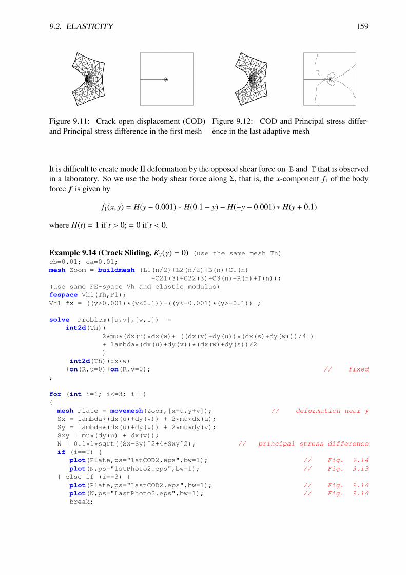
9.2. ELASTICITY 159
Figure 9.11: Crack open displacement (COD)and Principal stress difference in the first mesh
Figure 9.12: COD and Principal stress differ-ence in the last adaptive mesh
It is difficult to create mode II deformation by the opposed shear force on B and T that is observedin a laboratory. So we use the body shear force along Σ, that is, the x-component f1 of the bodyforce f is given by
f1(x, y) = H(y − 0.001) ∗ H(0.1 − y) − H(−y − 0.001) ∗ H(y + 0.1)
where H(t) = 1 if t > 0; = 0 if t < 0.
Example 9.14 (Crack Sliding, K2(γ) = 0) (use the same mesh Th)cb=0.01; ca=0.01;mesh Zoom = buildmesh (L1(n/2)+L2(n/2)+B(n)+C1(n)
+C21(3)+C22(3)+C3(n)+R(n)+T(n));(use same FE-space Vh and elastic modulus)fespace Vh1(Th,P1);Vh1 fx = ((y>0.001)*(y<0.1))-((y<-0.001)*(y>-0.1)) ;
solve Problem([u,v],[w,s]) =int2d(Th)(
2*mu*(dx(u)*dx(w)+ ((dx(v)+dy(u))*(dx(s)+dy(w)))/4 )+ lambda*(dx(u)+dy(v))*(dx(w)+dy(s))/2)
-int2d(Th)(fx*w)+on(R,u=0)+on(R,v=0); // fixed
;
for (int i=1; i<=3; i++)
mesh Plate = movemesh(Zoom,[x+u,y+v]); // deformation near γSx = lambda*(dx(u)+dy(v)) + 2*mu*dx(u);Sy = lambda*(dx(u)+dy(v)) + 2*mu*dy(v);Sxy = mu*(dy(u) + dx(v));N = 0.1*1*sqrt((Sx-Sy)ˆ2+4*Sxyˆ2); // principal stress differenceif (i==1)
plot(Plate,ps="1stCOD2.eps",bw=1); // Fig. 9.14plot(N,ps="1stPhoto2.eps",bw=1); // Fig. 9.13
else if (i==3) plot(Plate,ps="LastCOD2.eps",bw=1); // Fig. 9.14plot(N,ps="LastPhoto2.eps",bw=1); // Fig. 9.14break;

160 CHAPTER 9. MATHEMATICAL MODELS
Th=adaptmesh(Th,[u,v]);Problem;
Figure 9.13: (COD) and Principal stress differ-ence in the first mesh
Figure 9.14: COD and Principal stress differ-ence in the last adaptive mesh
9.3 Nonlinear Static ProblemsWe propose how to solve the following non-linear academic problem of minimization of a func-tional
J(u) =
∫Ω
12
f (|∇u|2) − u ∗ b
where u is function of H10(Ω) and f defined by
f (x) = a ∗ x + x − ln(1 + x), f ′(x) = a +x
1 + x, f ′′(x) =
1(1 + x)2
9.3.1 Newton-Raphson algorithmNow, we solve the Euler problem ∇J(u) = 0 with Newton-Raphson algorithm, that is,
un+1 = un − (∇2J(un))−1 ∗ ∇J(un)
First we introduice the two variational form vdJ and vhJ to compute respectively ∇J and ∇2J
// method of Newton-Raphson to solve dJ(u)=0;//
un+1 = un − (∂dJ∂ui
)−1 ∗ dJ(un)
// ---------------------------------------------Ph dalpha ; // to store 2 f ′′(|∇u|2) optimisation

9.3. NONLINEAR STATIC PROBLEMS 161
// the variational form of evaluate dJ = ∇J// --------------------------------------// dJ = f’()*( dx(u)*dx(vh) + dy(u)*dy(vh)varf vdJ(uh,vh) = int2d(Th)( alpha*( dx(u)*dx(vh) + dy(u)*dy(vh) ) - b*vh)+ on(1,2,3,4, uh=0);
// the variational form of evaluate ddJ = ∇2J// hJ(uh,vh) = f’()*( dx(uh)*dx(vh) + dy(uh)*dy(vh)
// + 2*f’’()( dx(u)*dx(uh) + dy(u)*dy(uh) ) * (dx(u)*dx(vh) +dy(u)*dy(vh))
varf vhJ(uh,vh) = int2d(Th)( alpha*( dx(uh)*dx(vh) + dy(uh)*dy(vh) )+ dalpha*( dx(u)*dx(vh) + dy(u)*dy(vh) )*( dx(u)*dx(uh) + dy(u)*dy(uh) ) )+ on(1,2,3,4, uh=0);
// the Newton algorithmVh v,w;u=0;for (int i=0;i<100;i++)alpha = df( dx(u)*dx(u) + dy(u)*dy(u) ) ; // optimizationdalpha = 2*ddf( dx(u)*dx(u) + dy(u)*dy(u) ) ; // optimizationv[]= vdJ(0,Vh); // v = ∇J(u)real res= v[]’*v[]; // the dot productcout << i << " residuˆ2 = " << res << endl;if( res< 1e-12) break;matrix H= vhJ(Vh,Vh,factorize=1,solver=LU); //w[]=Hˆ-1*v[];u[] -= w[];plot (u,wait=1,cmm="solution with Newton-Raphson");
Remark: This example is in Newton.edp file of examples++-tutorial directory.

162 CHAPTER 9. MATHEMATICAL MODELS
9.4 Eigenvalue ProblemsThis section depend on your FreeFem++ compilation process (see README arpack), of thistools. This tools is available in FreeFem++ if the word “eigenvalue” appear in line “Load:”, like:
-- FreeFem++ v1.28 (date Thu Dec 26 10:56:34 CET 2002)file : LapEigenValue.edpLoad: lg_fem lg_mesh eigenvalue
This tools is based on the arpack++ 1 the object-oriented version of ARPACK eigenvalue pack-age [1].The function EigenValue compute the generalized eigenvalue of Au = λBu where sigma =σ is theshift of the method. The matrix OP is defined with A − σB. The return value is the number ofconverged eigenvalue (can be greater than the number of eigen value nev=)
int k=EigenValue(OP,B,nev= , sigma= );
where the matrix OP = A − σB with a solver and boundary condition, and the matrix B.
Note 9.1 Boundary condition and Eigenvalue ProblemsThe lock (Dirichlet ) boundary condition is make with exact penalization so we put 1e30=tgv onthe diagonal term of the lock degree of freedom (see equation (6.17)). So take Dirichlet boundarycondition just on A and not on B. because we solve w = OP−1 ∗ B ∗ v.If you put lock (Dirichlet ) boundary condition on B matrix (with key work on) you get smallspurious modes (10−30), du to boundary condition, but if you forget the lock boundary condition onB matrix (no key work ”on”) you get huge spurious (1030) modes associated to boundary conditon.We compute only small mode, so we get the good one in this case.
sym= the problem is symmetric (all the eigen value are real)
nev= the number desired eigenvalues (nev) close to the shift.
value= the array to store the real part of the eigenvalues
ivalue= the array to store the imag. part of the eigenvalues
vector= the FE function array to store the eigenvectors
rawvector= an array of type real[int,int] to store eigenvectors by column. (up toversion 2-17).
For real nonsymmetric problems, complex eigenvectors are given as two consecutive vectors,so if eigenvalue k and k+1 are complex conjugate eigenvalues, the kth vector will contain thereal part and the k + 1th vector the imaginary part of the corresponding complex conjugateeigenvectors.
tol= the relative accuracy to which eigenvalues are to be determined;
sigma= the shift value;1http://www.caam.rice.edu/software/ARPACK/
9.4. EIGENVALUE PROBLEMS 163
maxit= the maximum number of iterations allowed;
ncv= the number of Arnoldi vectors generated at each iteration of ARPACK.
Example 9.15 (lapEignenValue.edp) In the first example, we compute the eigenvalue and theeigenvector of the Dirichlet problem on square Ω =]0, π[2.The problem is find: λ, and ∇uλ in R×H1
0(Ω)∫Ω
∇uλ∇v = λ
∫Ω
uv ∀v ∈ H10(Ω)
The exact eigenvalues are λn,m = (n2 + m2), (n,m) ∈ N∗2 with the associated eigenvectors areum,n = sin(nx) ∗ sin(my).We use the generalized inverse shift mode of the arpack++ library, to find 20 eigenvalue andeigenvector close to the shift value σ = 20.
// Computation of the eigen value and eigen vector of the// Dirichlet problem on square ]0, π[2
// ----------------------------------------// we use the inverse shift mode// the shift is given with the real sigma// -------------------------------------// find λ and uλ ∈ H1
0(Ω) such that:
//
∫Ω
∇uλ∇v = λ
∫Ω
uλv,∀v ∈ H10(Ω)
verbosity=10;mesh Th=square(20,20,[pi*x,pi*y]);fespace Vh(Th,P2);Vh u1,u2;
real sigma = 20; // value of the shift
// OP = A - sigma B ; // the shifted matrixvarf op(u1,u2)= int2d(Th)( dx(u1)*dx(u2) + dy(u1)*dy(u2) - sigma* u1*u2 )
+ on(1,2,3,4,u1=0) ; // Boundary condition
varf b([u1],[u2]) = int2d(Th)( u1*u2 ); // no Boundary condition see note9.1matrix OP= op(Vh,Vh,solver=Crout,factorize=1); // crout solver because thematrix in not positivematrix B= b(Vh,Vh,solver=CG,eps=1e-20);
// important remark:// the boundary condition is make with exact penalization:
// we put 1e30=tgv on the diagonal term of the lock degree of freedom.// So take Dirichlet boundary condition just on a variational form
// and not on b variational form.// because we solve w = OP−1 ∗ B ∗ v
int nev=20; // number of computed eigen value close to sigma
real[int] ev(nev); // to store the nev eigenvalueVh[int] eV(nev); // to store the nev eigenvector

164 CHAPTER 9. MATHEMATICAL MODELS
int k=EigenValue(OP,B,sym=true,sigma=sigma,value=ev,vector=eV,tol=1e-10,maxit=0,ncv=0);
// tol= the tolerance// maxit= the maximum iteration see arpack doc.// ncv see arpack doc. http://www.caam.rice.edu/software/ARPACK/// the return value is number of converged eigen value.
for (int i=0;i<k;i++)
u1=eV[i];real gg = int2d(Th)(dx(u1)*dx(u1) + dy(u1)*dy(u1));real mm= int2d(Th)(u1*u1) ;cout << " ---- " << i<< " " << ev[i]<< " err= "
<<int2d(Th)(dx(u1)*dx(u1) + dy(u1)*dy(u1) - (ev[i])*u1*u1) << " --- "<<endl;plot(eV[i],cmm="Eigen Vector "+i+" valeur =" + ev[i] ,wait=1,value=1);
The output of this example is:
Nb of edges on Mortars = 0Nb of edges on Boundary = 80, neb = 80
Nb Of Nodes = 1681Nb of DF = 1681
Real symmetric eigenvalue problem: A*x - B*x*lambda
Thanks to ARPACK++ class ARrcSymGenEigReal symmetric eigenvalue problem: A*x - B*x*lambdaShift and invert mode sigma=20
Dimension of the system : 1681Number of ’requested’ eigenvalues : 20Number of ’converged’ eigenvalues : 20Number of Arnoldi vectors generated: 41Number of iterations taken : 2
Eigenvalues:lambda[1]: 5.0002lambda[2]: 8.00074lambda[3]: 10.0011lambda[4]: 10.0011lambda[5]: 13.002lambda[6]: 13.0039lambda[7]: 17.0046lambda[8]: 17.0048lambda[9]: 18.0083lambda[10]: 20.0096lambda[11]: 20.0096lambda[12]: 25.014lambda[13]: 25.0283lambda[14]: 26.0159

9.4. EIGENVALUE PROBLEMS 165
lambda[15]: 26.0159lambda[16]: 29.0258lambda[17]: 29.0273lambda[18]: 32.0449lambda[19]: 34.049lambda[20]: 34.0492
---- 0 5.0002 err= -0.000225891 ------- 1 8.00074 err= -0.000787446 ------- 2 10.0011 err= -0.00134596 ------- 3 10.0011 err= -0.00134619 ------- 4 13.002 err= -0.00227747 ------- 5 13.0039 err= -0.004179 ------- 6 17.0046 err= -0.00623649 ------- 7 17.0048 err= -0.00639952 ------- 8 18.0083 err= -0.00862954 ------- 9 20.0096 err= -0.0110483 ------- 10 20.0096 err= -0.0110696 ------- 11 25.014 err= -0.0154412 ------- 12 25.0283 err= -0.0291014 ------- 13 26.0159 err= -0.0218532 ------- 14 26.0159 err= -0.0218544 ------- 15 29.0258 err= -0.0311961 ------- 16 29.0273 err= -0.0326472 ------- 17 32.0449 err= -0.0457328 ------- 18 34.049 err= -0.0530978 ------- 19 34.0492 err= -0.0536275 ---
IsoValue-0.809569-0.724351-0.639134-0.553916-0.468698-0.38348-0.298262-0.213045-0.127827-0.04260890.04260890.1278270.2130450.2982620.383480.4686980.5539160.6391340.7243510.809569
Eigen Vector 11 valeur =25.014
Figure 9.15: Isovalue of 11th eigenvector u4,3 −
u3,4
IsoValue-0.807681-0.722662-0.637643-0.552624-0.467605-0.382586-0.297567-0.212548-0.127529-0.04250950.04250950.1275290.2125480.2975670.3825860.4676050.5526240.6376430.7226620.807681
Eigen Vector 12 valeur =25.0283
Figure 9.16: Isovalue of 12th eigenvector u4,3 +
u3,4
166 CHAPTER 9. MATHEMATICAL MODELS
9.5 Evolution ProblemsFreeFem++ also solve evolution problems such as the heat problem
∂u∂t− µ∆u = f in Ω×]0,T [, (9.26)
u(x, 0) = u0(x) in Ω; (∂u/∂n) (x, t) = 0 on ∂Ω×]0,T [.
with a positive viscosity coefficient µ and homogeneous Neumann boundary conditions. We solve(9.26) by FEM in space and finite differences in time. We use the definition of the partial derivativeof the solution in the time derivative,
∂u∂t
(x, y, t) = limτ→0
u(x, y, t) − u(x, y, t − τ)τ
which indicate that um(x, y) = u(x, y,mτ) imply
∂u∂t
(x, y,mτ) 'um(x, y) − um−1(x, y)
τ
The time discretization of heat equation (9.27) is as follows:
um+1 − um
τ− µ∆um+1 = f m+1 in Ω (9.27)
u0(x) = u0(x) in Ω; ∂um+1/∂n(x) = 0 on ∂Ω, for all m = 0, · · · , [T/τ],
which is so-called backward Euler method for (9.27). Multiplying the test function v both sides ofthe formula just above, we have∫
Ω
um+1v − τ∆um+1v =
∫Ω
um + τ f m+1v .
By the divergence theorem, we have∫Ω
um+1v + τ∇um+1 · ∇v −∫∂Ω
τ(∂um+1/∂n
)v =
∫Ω
umv + τ f m+1v.
By the boundary condition ∂um+1/∂n = 0, it follows that∫Ω
um+1v + τ∇um+1 · ∇v −∫
Ω
umv + τ f m+1v = 0. (9.28)
Using the identity just above, we can calculate the finite element approximation umh of um in a
step-by-step manner with respect to t.
Example 9.16 We now solve the following example with the exact solution u(x, y, t) = tx4.
∂u∂t− µ∆u = x4 − µ12tx2 in Ω×]0, 3[, Ω =]0, 1[2
u(x, y, 0) = 0 on Ω, u|∂Ω = t ∗ x4

9.5. EVOLUTION PROBLEMS 167
// heat equation ∂tu = −µ∆u = x4 − µ12tx2
mesh Th=square(16,16);fespace Vh(Th,P1);
Vh u,v,uu,f,g;real dt = 0.1, mu = 0.01;problem dHeat(u,v) =
int2d(Th)( u*v + dt*mu*(dx(u)*dx(v) + dy(u)*dy(v)))+ int2d(Th) (- uu*v - dt*f*v )+ on(1,2,3,4,u=g);
real t = 0; // start from t=0uu = 0; // u(x,y,0)=0for (int m=0;m<=3/dt;m++)
t=t+dt;f = xˆ4-mu*t*12*xˆ2;g = t*xˆ4;dHeat;plot(u,wait=true);uu = u;cout <<"t="<<t<<"Lˆ2-Error="<<sqrt( int2d(Th)((u-t*xˆ4)ˆ2) ) << endl;
In the last statement, the L2-error(∫
Ω
∣∣∣u − tx4∣∣∣2)1/2
is calculated at t = mτ, τ = 0.1. At t = 0.1, theerror is 0.000213269. The errors increase with m and 0.00628589 at t = 3.The iteration of the backward Euler (9.28) is made by for loop (see Section 4.9).
Note 9.2 The stiffness matrix in loop is used over and over again. FreeFem++ support reusesof stiffness matrix.
9.5.1 Mathematical Theory on Time Difference Approximations.In this section, we show the advantage of implicit schemes. Let V,H be separable Hilbert spaceand V is dense in H. Let a be a continuous bilinear form over V ×V with coercivity and symmetry.Then
√a(v, v) become equivalent to the norm ‖v‖ of V .
Problem Ev( f ,Ω): For a given f ∈ L2(0,T ; V ′), u0 ∈ H
ddt
(u(t), v) + a(u(t), v) = ( f (t), v) ∀v ∈ V, , a.e. t ∈ [0,T ] (9.29)
u(0) = u0
where V ′ is the dual space of V . Then, there is an unique solution u ∈ L∞(0,T ; H) ∩ L2(0,T ; V).Let us denote the time step by τ > 0, NT = [T/τ]. For the discretization, we put un = u(nτ) andconsider the time difference for each θ ∈ [0, 1]
1τ
(un+1
h − unh, φi
)+ a
(un+θ
h , φi
)= 〈 f n+θ, φi〉 (9.30)
i = 1, · · · ,m, n = 0, · · · ,NT
un+θh = θun+1
h + (1 − θ)unh, f n+θ = θ f n+1 + (1 − θ) f n

168 CHAPTER 9. MATHEMATICAL MODELS
Formula (9.30) is the forward Euler scheme if θ = 0, Crank-Nicolson scheme if θ = 1/2, thebackward Euler scheme if θ = 1.Unknown vectors un = (u1
h, · · · , uMh )T in
unh(x) = un
1φ1(x) + · · · + unmφm(x), un
1, · · · , unm ∈ R
are obtained from solving the matrix
(M + θτA)un+1 = M − (1 − θ)τAun + τθ f n+1 + (1 − θ) f n
(9.31)
M = (mi j), mi j = (φ j, φi), A = (ai j), ai j = a(φ j, φi)
Refer [21, pp.70–75] for solvability of (9.31). The stability of (9.31) is in [21, Theorem 2.13]:
Let Thh↓0 be regular triangulations (see Section 5.4). Then there is a numberc0 > 0 independent of h such that,
|unh|
2 ≤
1δ
|u0
h|2 + τ
∑n−1k=0 ‖ f
k+θ‖2V′h
θ ∈ [0, 1/2)
|u0h|
2 + τ∑n−1
k=0 ‖ fk+θ‖2V′h
θ ∈ [1/2, 1](9.32)
if the following are satisfied:
1. When θ ∈ [0, 1/2), then we can take a time step τ in such a way that
τ <2(1 − δ)
(1 − 2θ)c20
h2 (9.33)
for arbitrary δ ∈ (0, 1).
2. When 1/2 ≤ θ ≤ 1, we can take τ arbitrary.
Example 9.17
mesh Th=square(12,12);fespace Vh(Th,P1);fespace Ph(Th,P0);
Ph h = hTriangle; // mesh sizes for each trianglereal tau = 0.1, theta=0.;func real f(real t)
return xˆ2*(x-1)ˆ2 + t*(-2 + 12*x - 11*xˆ2 - 2*xˆ3 + xˆ4);ofstream out("err02.csv"); // file to store calculationsout << "mesh size = "<<h[].max<<", time step = "<<tau<<endl;for (int n=0;n<5/tau;n++) \\
out<<n*tau<<",";out << endl;Vh u,v,oldU;Vh f1, f0;problem aTau(u,v) =int2d(Th)( u*v + theta*tau*(dx(u)*dx(v) + dy(u)*dy(v) + u*v))- int2d(Th)(oldU*v - (1-theta)*tau*(dx(oldU)*dx(v)+dy(oldU)*dy(v)+oldU*v))- int2d(Th)(tau*( theta*f1+(1-theta)*f0 )*v );

9.5. EVOLUTION PROBLEMS 169
while (theta <= 1.0) real t = 0, T=3; // from t=0 to ToldU = 0; // u(x,y,0)=0out <<theta<<",";for (int n=0;n<T/tau;n++)
t = t+tau;f0 = f(n*tau); f1 = f((n+1)*tau);aTau;oldU = u;plot(u);Vh uex = t*xˆ2*(1-x)ˆ2; // exact sol.= tx2(1 − x)2
Vh err = u - uex; // err =FE-sol - exactout<< abs(err[].max)/abs(uex[].max) <<","; // ‖err‖L∞(Ω)/‖uex‖L∞(Ω)
out << endl;theta = theta + 0.1;
q
Figure 9.17: maxx∈Ω |unh(θ) − uex(nτ)|/maxx∈Ω |uex(nτ)| at n = 0, 1, · · · , 29
We can see in Fig. 9.17 that unh(θ) become unstable at θ = 0.4, and figures are omitted in the case
θ < 0.4.
9.5.2 ConvectionThe hyperbolic equation
∂tu + α · ∇u = f ; for a vector-valued function α, ∂t =∂
∂t, (9.34)
appear frequently in scientific problems, for example, Navier-Stokes equation, Convection-Diffusionequation, etc.In the case of 1-dimensional space, we can easily find the general solution (x, t) 7→ u(x, t) =
u0(x − αt) of the following equation, if α is constant,
∂tu + α∂xu = 0, u(x, 0) = u0(x), (9.35)
170 CHAPTER 9. MATHEMATICAL MODELS
because ∂tu+α∂xu = −αu0+au0 = 0, where u0 = du0(x)/dx. Even if α is not constant construction,the principle is similar. One begins the ordinary differential equation (with convention which α isprolonged by zero apart from (0, L) × (0,T )):
X(τ) = +α(X(τ), τ), τ ∈ (0, t) X(t) = x
In this equation τ is the variable and x, t is parameters, and we denote the solution by Xx,t(τ). Thenit is noticed that (x, t)→ v(X(τ), τ) in τ = t satisfy the equation
∂tv + α∂xv = ∂tXv + a∂xXv = 0
and by the definition ∂tX = X = +α and ∂xX = ∂xx in τ = t, because if τ = t we have X(τ) = x.The general solution of (9.35) is thus the value of the boundary condition in Xx,t(0), it is has to sayu(x, t) = u0(Xx,t(0)) if Xx,t(0) is on the x axis, u(x, t) = u0(Xx,t(0)) if Xx,t(0) is on the axis of t.In higher dimension Ω ⊂ Rd, d = 2, 3, the equation of the convection is written
∂tu + α · ∇u = 0 in Ω × (0,T )
where a(x, t) ∈ Rd. FreeFem++ implements the Characteristic-Galerkin method for convectionoperators. Recall that the equation (9.34) can be discretized as
DuDt
= f i.e.dudt
(X(t), t) = f (X(t), t) wheredXdt
(t) = α(X(t), t)
where D is the total derivative operator. So a good scheme is one step of backward convection bythe method of Characteristics-Galerkin
1τ
(um+1(x) − um(Xm(x))
)= f m(x) (9.36)
where Xm(x) is an approximation of the solution at t = mτ of the ordinary differential equation
dXdt
(t) = αm(X(t)), X((m + 1)τ) = x.
where αm(x) = (α1(x,mτ), α2(x,mτ)). Because, by Taylor’s expansion, we have
um(X(mτ)) = um(X((m + 1)τ)) − τd∑
i=1
∂um
∂xi(X((m + 1)τ))
∂Xi
∂t((m + 1)τ) + o(τ)
= um(x) − ταm(x) · ∇um(x) + o(τ) (9.37)
where Xi(t) are the i-th component of X(t), um(x) = u(x,mτ) and we used the chain rule andx = X((m + 1)τ). From (9.37), it follows that
um(Xm(x)) = um(x) − ταm(x) · ∇um(x) + o(τ). (9.38)
Also we apply Taylor’s expansion for t 7→ um(x − αm(x)t), 0 ≤ t ≤ τ, then
um(x − ατ) = um(x) − ταm(x) · ∇um(x) + o(τ).
Puttingconvect (α,−τ, um) ≈ um (x − αmτ) ,

9.5. EVOLUTION PROBLEMS 171
we can get the approximation
um (Xm(x)) ≈ convect([am
1 , am2 ],−τ, um)
by Xm ≈ x 7→ x − τ[am1 (x), am
2 (x)]).
A classical convection problem is that of the “rotating bell” (quoted from [13][p.16]). Let Ω bethe unit disk centered at 0, with its center rotating with speed α1 = y, α2 = −x We consider theproblem (9.34) with f = 0 and the initial condition u(x, 0) = u0(x), that is, from (9.36)
um+1(x) = um(Xm(x)) ≈ convect(α,−τ, um).
The exact solution is u(x, t) = u(X(t)) where X equals x rotated around the origin by an angleθ = −t (rotate in clockwise). So, if u0 in a 3D perspective looks like a bell, then u will have exactlythe same shape, but rotated by the same amount. The program consists in solving the equationuntil T = 2π, that is for a full revolution and to compare the final solution with the initial one; theyshould be equal.
Example 9.18 (convect.edp) border C(t=0, 2*pi) x=cos(t); y=sin(t); ; //the unit circlemesh Th = buildmesh(C(70)); // triangulates the diskfespace Vh(Th,P1);Vh u0 = exp(-10*((x-0.3)ˆ2 +(y-0.3)ˆ2)); // give u0
real dt = 0.17,t=0; // time stepVh a1 = -y, a2 = x; // rotation velocityVh u; // um+1
for (int m=0; m<2*pi/dt ; m++) t += dt;u=convect([a1,a2],-dt,u0); // um+1 = um(Xm(x))u0=u; // m++plot(u,cmm=" t="+t + ", min=" + u[].min + ", max=" + u[].max,wait=0);
;
Note 9.3 The scheme convect is unconditionally stable, then the bell become lower and lower(the maximum of u37 is 0.406 as shown in Fig. 9.19).
convection: t=0, min=1.55289e-09, max=0.983612
Figure 9.18: u0 = e−10((x−0.3)2+(y−0.3)2)
convection: t=6.29, min=1.55289e-09, max=0.40659m=37
Figure 9.19: The bell at t = 6.29

172 CHAPTER 9. MATHEMATICAL MODELS
9.5.3 2D Black-Scholes equation for an European Put optionIn mathematical finance, an option on two assets is modeled by a Black-Scholes equations in twospace variables, (see for example Wilmott et al[36] or Achdou et al [3]).
∂tu +(σ1x)2
2∂2u∂x2 +
(σ2y)2
2∂2u∂y2 (9.39)
+ ρxy∂2u∂x∂y
+ rS 1∂u∂x
+ rS 2∂u∂y− rP = 0
which is to be integrated in (0,T ) × R+ × R+ subject to, in the case of a put
u (x, y,T ) = (K −max (x, y))+ . (9.40)
Boundary conditions for this problem may not be so easy to device. As in the one dimensionalcase the PDE contains boundary conditions on the axis x1 = 0 and on the axis x2 = 0, namelytwo one dimensional Black-Scholes equations driven respectively by the data u (0,+∞,T ) andu (+∞, 0,T ). These will be automatically accounted for because they are embedded in the PDE.So if we do nothing in the variational form (i.e. if we take a Neumann boundary condition at thesetwo axis in the strong form) there will be no disturbance to these. At infinity in one of the variable,as in 1D, it makes sense to impose u = 0. We take
σ1 = 0.3, σ2 = 0.3, ρ = 0.3, r = 0.05, K = 40, T = 0.5 (9.41)
An implicit Euler scheme is used and a mesh adaptation is done every 10 time steps. To havean unconditionally stable scheme, the first order terms are treated by the Characteristic Galerkinmethod, which, roughly, approximates
∂u∂t
+ a1∂u∂x
+ a2∂u∂y≈
1τ
(un+1 (x) − un (x − ατ)
)(9.42)
Example 9.19 [BlackSchol.edp]
// file BlackScholes2D.edpint m=30,L=80,LL=80, j=100;real sigx=0.3, sigy=0.3, rho=0.3, r=0.05, K=40, dt=0.01;mesh th=square(m,m,[L*x,LL*y]);fespace Vh(th,P1);
Vh u=max(K-max(x,y),0.);Vh xveloc, yveloc, v,uold;
for (int n=0; n*dt <= 1.0; n++)
if(j>20) th = adaptmesh(th,u,verbosity=1,abserror=1,nbjacoby=2,err=0.001, nbvx=5000, omega=1.8, ratio=1.8, nbsmooth=3,splitpbedge=1, maxsubdiv=5,rescaling=1) ;
j=0;xveloc = -x*r+x*sigxˆ2+x*rho*sigx*sigy/2;yveloc = -y*r+y*sigyˆ2+y*rho*sigx*sigy/2;u=u;
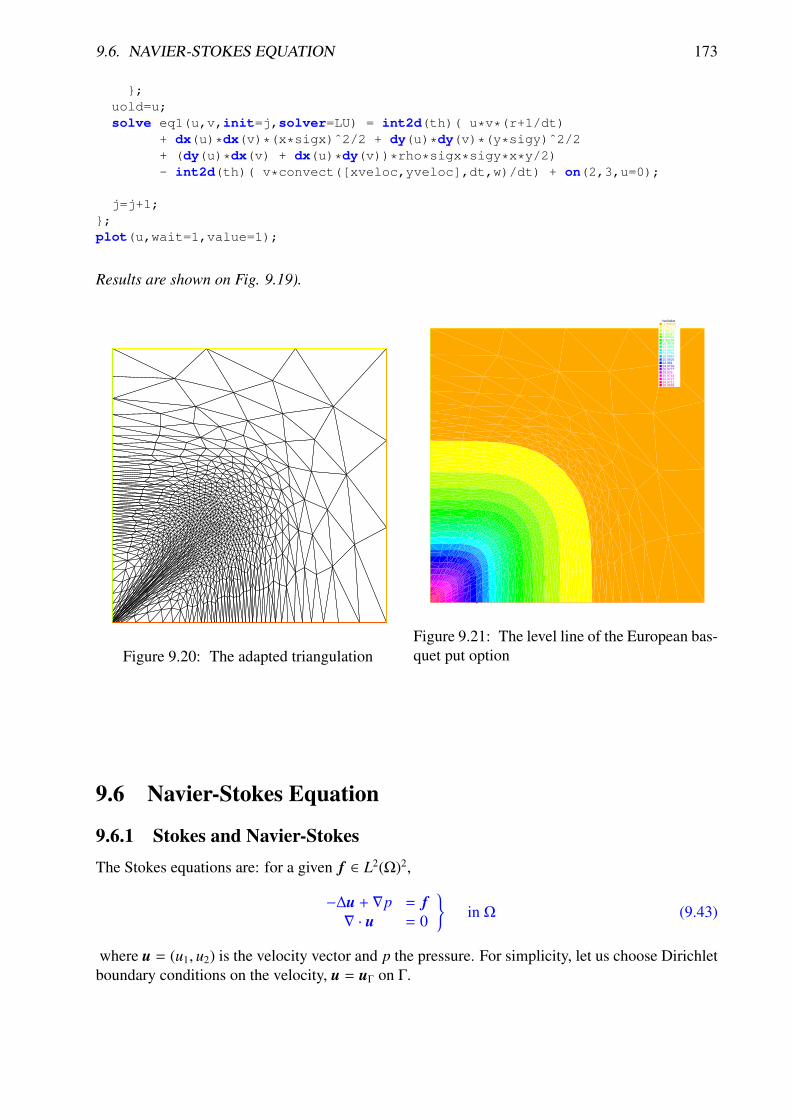
9.6. NAVIER-STOKES EQUATION 173
;uold=u;solve eq1(u,v,init=j,solver=LU) = int2d(th)( u*v*(r+1/dt)
+ dx(u)*dx(v)*(x*sigx)ˆ2/2 + dy(u)*dy(v)*(y*sigy)ˆ2/2+ (dy(u)*dx(v) + dx(u)*dy(v))*rho*sigx*sigy*x*y/2)- int2d(th)( v*convect([xveloc,yveloc],dt,w)/dt) + on(2,3,u=0);
j=j+1;;plot(u,wait=1,value=1);
Results are shown on Fig. 9.19).
Figure 9.20: The adapted triangulation
IsoValue-1.998350.9991732.997524.995876.994218.9925610.990912.989314.987616.985918.984320.982622.98124.979326.977728.97630.974432.972734.971139.9669
Figure 9.21: The level line of the European bas-quet put option
9.6 Navier-Stokes Equation
9.6.1 Stokes and Navier-StokesThe Stokes equations are: for a given f ∈ L2(Ω)2,
−∆u + ∇p = f∇ · u = 0
in Ω (9.43)
where u = (u1, u2) is the velocity vector and p the pressure. For simplicity, let us choose Dirichletboundary conditions on the velocity, u = uΓ on Γ.

174 CHAPTER 9. MATHEMATICAL MODELS
In Temam [Theorem 2.2], there ia a weak form of (9.43): Find v = (v1, v2) ∈ V(Ω)
V(Ω) = w ∈ H10(Ω)2| divw = 0
which satisfy2∑
i=1
∫Ω
∇ui · ∇vi =
∫Ω
f · w for all v ∈ V
Here it is used the existence p ∈ H1(Ω) such that u = ∇p, if∫Ω
u · v = 0 for all v ∈ V
Another weak form is derived as follows: We put
V = H10(Ω)2; W =
q ∈ L2(Ω)
∣∣∣∣∣ ∫Ω
q = 0
By multiplying the first equation in (9.43) with v ∈ V and the second with q ∈ W, subsequentintegration over Ω, and an application of Green’s formula, we have∫
Ω
∇u · ∇v −∫
Ω
divv p =
∫Ω
f · v∫Ω
divu q = 0
This yields the weak form of (9.43): Find (u, p) ∈ V ×W such that
a(u, v) + b(v, p) = ( f , v) (9.44)b(u, q) = 0 (9.45)
for all (v, q) ∈ V ×W, where
a(u, v) =
∫Ω
∇u · ∇v =
2∑i=1
∫Ω
∇ui · ∇vi (9.46)
b(u, q) = −
∫Ω
divu q (9.47)
Now, we consider finite element spaces Vh ⊂ V and Wh ⊂ W, and we assume the following basisfunctions
Vh = Vh × Vh, Vh = vh| vh = v1φ1 + · · · + vMVφMV ,
Wh = qh| qh = q1ϕ1 + · · · + qMWϕMW
The discrete weak form is: Find (uh, ph) ∈ Vh ×Wh such that
a(uh, vh) + b(vh, p) = ( f , vh), ∀vh ∈ Vh
b(uh, qh) = 0, ∀qh ∈ Wh(9.48)

9.6. NAVIER-STOKES EQUATION 175
Note 9.4 Assume that:
1. There is a constant αh > 0 such that
a(vh, vh) ≥ α‖vh‖21,Ω for all vh ∈ Zh
whereZh = vh ∈ Vh| b(wh, qh) = 0 for all qh ∈ Wh
2. There is a constant βh > 0 such that
supvh∈Vh
b(vh, qh)‖vh‖1,Ω
≥ βh‖qh‖0,Ω for all qh ∈ Wh
Then we have an unique solution (uh, ph) of (9.48) satisfying
‖u − uh‖1,Ω + ‖p − ph‖0,Ω ≤ C(
infvh∈Vh
‖u − vh‖1,Ω + infqh∈Wh
‖p − qh‖0,Ω
)with a constant C > 0 (see e.g. [19, Theorem 10.4]).
Let us denote that
A = (Ai j), Ai j =
∫Ω
∇φ j · ∇φi i, j = 1, · · · ,MV (9.49)
B = (Bxi j, Byi j), Bxi j = −
∫Ω
∂φ j/∂xϕi Byi j = −
∫Ω
∂φ j/∂yϕi
i = 1, · · · ,MW ; j = 1, · · · ,MV
then (9.48) is written by (A B∗
B 0
) (Uh
ph
)=
(Fh
0
)(9.50)
where
A =
(A 00 A
)B∗ =
BxT
ByT
Uh =
u1,h
u2,h
Fh =
∫
Ωf1φi
∫
Ωf2φi
Penalty method: This method consists of replacing (9.48) by a more regular problem: Find(vεh, pεh) ∈ Vh × Wh satisfying
a(uεh, vh) + b(vh, pεh) = ( f , vh), ∀vh ∈ Vh
b(uεh, qh) − ε(pεh, qh) = 0, ∀qh ∈ Wh(9.51)
where Wh ⊂ L2(Ω). Formally, we have
divuεh = εpεh
and the corresponding algebraic problem(A B∗
B −εI
) (Uε
hpεh
)=
(Fh
0
)
176 CHAPTER 9. MATHEMATICAL MODELS
Note 9.5 We can eliminate pεh = (1/ε)BUεh to obtain
(A + (1/ε)B∗B)Uεh = Fε
h (9.52)
Since the matrix A + (1/ε)B∗B is symmetric, positive-definite, and sparse, (9.52) can be solved byknown technique. There is a constant C > 0 independent of ε such that
‖uh − uεh‖1,Ω + ‖ph − pεh‖0,Ω ≤ Cε
(see e.g. [19, 17.2])
Example 9.20 (Cavity.edp) The driven cavity flow problem is solved first at zero Reynolds num-ber (Stokes flow) and then at Reynolds 100. The velocity pressure formulation is used first and thenthe calculation is repeated with the stream function vorticity formulation.We solve the driven cavity problem by the penalty method (9.51) where uΓ · n = 0 and uΓ · s = 1on the top boundary and zero elsewhere ( n is the unit normal to Γ, and s the unit tangent to Γ).The mesh is constructed by
mesh Th=square(8,8);
We use a classical Taylor-Hood element technic to solve the problem:
The velocity is approximated with the P2 FE ( Xh space), and the the pressure is approximated withthe P1 FE ( Mh space),
whereXh =
v ∈ H1(]0, 1[2)
∣∣∣ ∀K ∈ Th v|K ∈ P2
and
Mh =v ∈ H1(]0, 1[2)
∣∣∣ ∀K ∈ Th v|K ∈ P1
The FE spaces and functions are constructed by
fespace Xh(Th,P2); // definition of the velocity component spacefespace Mh(Th,P1); // definition of the pressure spaceXh u2,v2;Xh u1,v1;Mh p,q;
The Stokes operator is implemented as a system-solve for the velocity (u1, u2) and the pressure p.The test function for the velocity is (v1, v2) and q for the pressure, so the variational form (9.48)in freefem language is:
solve Stokes (u1,u2,p,v1,v2,q,solver=Crout) =int2d(Th)( ( dx(u1)*dx(v1) + dy(u1)*dy(v1)
+ dx(u2)*dx(v2) + dy(u2)*dy(v2) )- p*q*(0.000001)- p*dx(v1) - p*dy(v2)- dx(u1)*q - dy(u2)*q)
+ on(3,u1=1,u2=0)

9.6. NAVIER-STOKES EQUATION 177
+ on(1,2,4,u1=0,u2=0); // see Section 5.1.1 for labels 1,2,3,4
Each unknown has its own boundary conditions.
If the streamlines are required, they can be computed by finding ψ such that rotψ = u or better,
−∆ψ = ∇ × u
Xh psi,phi;
solve streamlines(psi,phi) =int2d(Th)( dx(psi)*dx(phi) + dy(psi)*dy(phi))
+ int2d(Th)( -phi*(dy(u1)-dx(u2)))+ on(1,2,3,4,psi=0);
Now the Navier-Stokes equations are solved
∂u∂t
+ u · ∇u − ν∆u + ∇p = 0, ∇ · u = 0
with the same boundary conditions and with initial conditions u = 0.This is implemented by using the convection operator convect for the term ∂u
∂t + u · ∇u, giving adiscretization in time
1τ(un+1 − un Xn) − ν∆un+1 + ∇pn+1 = 0,
∇ · un+1 = 0 (9.53)
The term un Xn(x) ≈ un(x − un(x)τ) will be computed by the operator “convect” , so we obtain
int i=0;real nu=1./100.;real dt=0.1;real alpha=1/dt;
Xh up1,up2;
problem NS (u1,u2,p,v1,v2,q,solver=Crout,init=i) =int2d(Th)(
alpha*( u1*v1 + u2*v2)+ nu * ( dx(u1)*dx(v1) + dy(u1)*dy(v1)+ dx(u2)*dx(v2) + dy(u2)*dy(v2) )- p*q*(0.000001)- p*dx(v1) - p*dy(v2)- dx(u1)*q - dy(u2)*q
)+ int2d(Th) ( -alpha*
convect([up1,up2],-dt,up1)*v1 -alpha*convect([up1,up2],-dt,up2)*v2 )+ on(3,u1=1,u2=0)+ on(1,2,4,u1=0,u2=0)
;

178 CHAPTER 9. MATHEMATICAL MODELS
for (i=0;i<=10;i++)
up1=u1;up2=u2;NS;if ( !(i % 10)) // plot every 10 iterationplot(coef=0.2,cmm=" [u1,u2] and p ",p,[u1,u2]);
;
Notice that the stiffness matrices are reused (keyword init=i)
9.6.2 Uzawa Conjugate GradientWe solve Stokes problem without penalty. The classical iterative method of Uzawa is described bythe algorithm (see e.g.[19, 17.3], [28, 13] or [29, 13] ):
Initialize: Let p0h be an arbitrary chosen element of L2(Ω).
Calculate uh: Once pnh is known, vn
h is the solution of
unh = A−1( f h − B∗pn
h)
Advance ph: Let pn+1h be defined by
pn+1h = pn
h + ρnBunh
There is a constant α > 0 such that α ≤ ρn ≤ 2 for each n, then unh converges to the solution uh,
and then Bvnh → 0 as n→ ∞ from the Advance ph. This method in general converges quite slowly.
First we define mesh, and the Taylor-Hood approximation. So Xh is the velocity space, and Mh isthe pressure space.
Example 9.21 (StokesUzawa.edp)
mesh Th=square(10,10);fespace Xh(Th,P2),Mh(Th,P1);Xh u1,u2,v1,v2;Mh p,q,ppp; // ppp is a working pressure
varf bx(u1,q) = int2d(Th)( -(dx(u1)*q));varf by(u1,q) = int2d(Th)( -(dy(u1)*q));varf a(u1,u2)= int2d(Th)( dx(u1)*dx(u2) + dy(u1)*dy(u2) )
+ on(3,u1=1) + on(1,2,4,u1=0) ;// remark: put the on(3,u1=1) before on(1,2,4,u1=0)
// because we want zero on intersection %
matrix A= a(Xh,Xh,solver=CG);matrix Bx= bx(Xh,Mh); // B = (Bx By)matrix By= by(Xh,Mh);
Xh bc1; bc1[] = a(0,Xh); // boundary condition contribution on u1Xh bc2; bc2 = O ; // no boundary condition contribution on u2Xh b;

9.6. NAVIER-STOKES EQUATION 179
pnh → BA−1(−B∗pn
h) = −divuh is realized as the function divup.
func real[int] divup(real[int] & pp)
// compute u1(pp)b[] = Bx’*pp; b[] *=-1; b[] += bc1[] ; u1[] = Aˆ-1*b[];
// compute u2(pp)b[] = By’*pp; b[] *=-1; b[] += bc2[] ; u2[] = Aˆ-1*b[];// un = A−1(BxT pn ByT pn)T
ppp[] = Bx*u1[]; // ppp = Bxu1
ppp[] += By*u2[]; // +Byu2
return ppp[] ;;
Call now the conjugate gradient algorithm:
p=0;q=0; // p0h = 0
LinearCG(divup,p[],eps=1.e-6,nbiter=50); // pn+1h = pn
h + Bunh
// if n > 50 or |pn+1h − pn
h| ≤ 10−6, then the loop end.divup(p[]); // compute the final solution
plot([u1,u2],p,wait=1,value=true,coef=0.1);
9.6.3 NSUzawaCahouetChabart.edpIn this example we solve the Navier-Stokes equation, in the driven-cavity, with the Uzawa algo-rithm preconditioned by the Cahouet-Chabart method (see [30] for all the details).The idea of the preconditioner is that in a periodic domain, all differential operators commute andthe Uzawa algorithm comes to solving the linear operator ∇.((αId+ν∆)−1∇, where Id is the identityoperator. So the preconditioer suggested is α∆−1 + νId.
To implement this, we reuse the previous example, by including a file. Then we define the timestep ∆t, viscosity, and new variational form and matrix.
Example 9.22 (NSUzawaCahouetChabart.edp)
include "StokesUzawa.edp" // include the Stokes partreal dt=0.05, alpha=1/dt; // ∆t
cout << " alpha = " << alpha;real xnu=1./400; // viscosity ν = Reynolds number−1
// the new variational form with mass termvarf at(u1,u2)= int2d(Th)( xnu*dx(u1)*dx(u2)
+ xnu*dy(u1)*dy(u2) + u1*u2*alpha )+ on(1,2,4,u1=0) + on(3,u1=1) ;
A = at(Xh,Xh,solver=CG); // change the matrix
// set the 2 convect variational formvarf vfconv1(uu,vv) = int2d(Th,qforder=5) (convect([u1,u2],-dt,u1)*vv*alpha);varf vfconv2(v2,v1) = int2d(Th,qforder=5) (convect([u1,u2],-dt,u2)*v1*alpha);

180 CHAPTER 9. MATHEMATICAL MODELS
int idt; // index of time setreal temps=0; // current time
Mh pprec,prhs;varf vfMass(p,q) = int2d(Th)(p*q);matrix MassMh=vfMass(Mh,Mh,solver=CG);
varf vfLap(p,q) = int2d(Th)(dx(pprec)*dx(q)+dy(pprec)*dy(q) + pprec*q*1e-10);matrix LapMh= vfLap(Mh,Mh,solver=Cholesky);
The function to define the preconditioner
func real[int] CahouetChabart(real[int] & xx) // xx =
∫(divu)wi
// αLapMh−1 + νMassMh−1
pprec[]= LapMhˆ-1* xx;prhs[] = MassMhˆ-1*xx;pprec[] = alpha*pprec[]+xnu* prhs[];return pprec[];
;
The loop in time. Warning with the stop test of the conjugate gradient, because we start fromthe previous solution and the end the previous solution is close to the final solution, don’t take arelative stop test to the first residual, take an absolute stop test ( negative here)
for (idt = 1; idt < 50; idt++)
temps += dt;cout << " --------- temps " << temps << " \n ";b1[] = vfconv1(0,Xh);b2[] = vfconv2(0,Xh);cout << " min b1 b2 " << b1[].min << " " << b2[].min << endl;cout << " max b1 b2 " << b1[].max << " " << b2[].max << endl;
// call Conjugate Gradient with preconditioner ’// warning eps < 0 => absolue stop test
LinearCG(divup,p[],eps=-1.e-6,nbiter=50,precon=CahouetChabart);divup(p[]); // computed the velocity
plot([u1,u2],p,wait=!(idt%10),value= 1,coef=0.1);
9.7 Variational inequalityWe present, a classical examples of variational inequality.Let us denote C = u ∈ H1
0(Ω), u ≤ gThe problem is :
u = arg minu∈C
J(u) =12
∫Ω
∇u.∇u −∫
Ω
f u
where f and g are given function.

9.7. VARIATIONAL INEQUALITY 181
IsoValue-0.0791073-0.0611287-0.0431501-0.0251715-0.007192850.01078580.02876440.0467430.06472170.08270030.1006790.1186580.1366360.1546150.1725930.1905720.2085510.2265290.2445080.262487
Vec Value00.050.10.150.20.250.30.350.40.450.50.550.60.650.70.750.80.850.90.95
[u1,u2],p || u^n+1 - u^n ]]_L2 =0.00149613
Figure 9.22: Solution of the cavity driven problem at Reynolds number 400 with the Cahouet-Chabart algorithm.
The solution is a projection on the convex C of f ? for the scalar product ((v,w)) =∫
Ω∇v.∇w of
H10(Ω) where f ? is solution of (( f ?, v)) =
∫Ω
f v,∀v ∈ H10(Ω). The projection on a convex satisfy
clearly ∀v ∈ C, ((u − v, u − f )) ≤ 0, and after expanding, we get the classical inequality
∀v ∈ C,∫
Ω
∇(u − v)∇u ≤∫
Ω
(u − v) f .
We can also rewrite the problem as a saddle point problemFind λ, u such that:
maxλ∈L2(Ω),λ≥0
minu∈H1
0 (Ω)L(u, λ) =
12
∫Ω
∇u.∇u −∫
Ω
f u +
∫Ω
λ(u − g)+
where ((u − g)+ = max(0, u − g)This saddle point problem is equivalent to find u, λ such that:
∫Ω
∇u.∇v + λv+ dω =
∫Ω
f u, ∀v ∈ H10(Ω)∫
Ω
µ(u − g)+ = 0, ∀µ ∈ L2(Ω), µ ≥ 0, λ ≥ 0,(9.54)
A algorithm to solve the previous problem is:
1. k=0, and choose, λ0 belong H−1(Ω)
2. loop on k = 0, .....
(a) set Ik = x ∈ Ω/λk + c ∗ (uk+1 − g) ≤ 0
(b) Vg,k+1 = v ∈ H10(Ω)/v = g on Ik,

182 CHAPTER 9. MATHEMATICAL MODELS
(c) V0,k+1 = v ∈ H10(Ω)/v = 0 on Ik,
(d) Find uk+1 ∈ Vg,k+1 and λk+1 ∈ H−1(Ω) such that∫
Ω
∇uk+1.∇vk+1 dω =
∫Ω
f vk+1, ∀vk+1 ∈ V0,k+1
< λk+1, v >=
∫Ω
∇uk+1.∇v − f v dω
where <, > is the duality bracket between H10(Ω) and H−1(Ω), and c is a penalty constant
(large enough).
You can find all the mathematic about this algorithm in [32].Now how to do that in FreeFem++The full example is:
Example 9.23 (VI.edp)
mesh Th=square(20,20);real eps=1e-5;fespace Vh(Th,P1); // P1 FE spaceint n = Vh.ndof; // number of Degree of freedomVh uh,uhp; // solution and previous oneVh Ik; // to def the set where the containt is reached.real[int] rhs(n); // to store the right and side of the equationreal c=1000; // the penalty parameter of the algoritmfunc f=1; // right hand side functionfunc fd=0; // Dirichlet boundary condition functionVh g=0.05; // the discret function g
real[int] Aii(n),Aiin(n); // to store the diagonal of the matrix 2 version
real tgv = 1e30; // a huge value for exact penalization// of boundary condition
// the variatonal form of the problem:varf a(uh,vh) = // definition of the problem
int2d(Th)( dx(uh)*dx(vh) + dy(uh)*dy(vh) ) // bilinear form- int2d(Th)( f*vh ) // linear form+ on(1,2,3,4,uh=fd) ; // boundary condition form
// two version of the matrix of the problemmatrix A=a(Vh,Vh,tgv=tgv,solver=CG); // one changingmatrix AA=a(Vh,Vh,solver:GC); // one for computing residual
// the mass Matrix construction:varf vM(uh,vh) = int2d(Th)(uh*vh);matrix M=vM(Vh,Vh); // to do a fast computing of L2 norm : sqrt(u’*(w=M*u))
Aii=A.diag; // get the diagonal of the matrix (appear in version 1.46-1)
rhs = a(0,Vh,tgv=tgv);Ik =0;uhp=-tgv; // previous value is
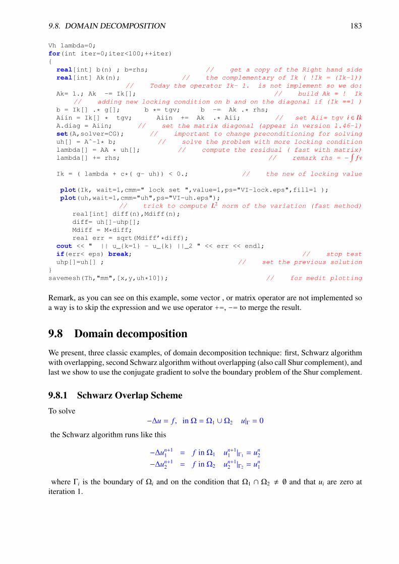
9.8. DOMAIN DECOMPOSITION 183
Vh lambda=0;for(int iter=0;iter<100;++iter)
real[int] b(n) ; b=rhs; // get a copy of the Right hand sidereal[int] Ak(n); // the complementary of Ik ( !Ik = (Ik-1))
// Today the operator Ik- 1. is not implement so we do:Ak= 1.; Ak -= Ik[]; // build Ak = ! Ik
// adding new locking condition on b and on the diagonal if (Ik ==1 )b = Ik[] .* g[]; b *= tgv; b -= Ak .* rhs;Aiin = Ik[] * tgv; Aiin += Ak .* Aii; // set Aii= tgv i ∈ IkA.diag = Aiin; // set the matrix diagonal (appear in version 1.46-1)set(A,solver=CG); // important to change preconditioning for solvinguh[] = Aˆ-1* b; // solve the problem with more locking conditionlambda[] = AA * uh[]; // compute the residual ( fast with matrix)lambda[] += rhs; // remark rhs = −
∫f v
Ik = ( lambda + c*( g- uh)) < 0.; // the new of locking value
plot(Ik, wait=1,cmm=" lock set ",value=1,ps="VI-lock.eps",fill=1 );plot(uh,wait=1,cmm="uh",ps="VI-uh.eps");
// trick to compute L2 norm of the variation (fast method)real[int] diff(n),Mdiff(n);diff= uh[]-uhp[];Mdiff = M*diff;real err = sqrt(Mdiff’*diff);
cout << " || u_k=1 - u_k ||_2 " << err << endl;if(err< eps) break; // stop testuhp[]=uh[] ; // set the previous solution
savemesh(Th,"mm",[x,y,uh*10]); // for medit plotting
Remark, as you can see on this example, some vector , or matrix operator are not implemented soa way is to skip the expression and we use operator +=, -= to merge the result.
9.8 Domain decompositionWe present, three classic examples, of domain decomposition technique: first, Schwarz algorithmwith overlapping, second Schwarz algorithm without overlapping (also call Shur complement), andlast we show to use the conjugate gradient to solve the boundary problem of the Shur complement.
9.8.1 Schwarz Overlap SchemeTo solve
−∆u = f , in Ω = Ω1 ∪Ω2 u|Γ = 0
the Schwarz algorithm runs like this
−∆un+11 = f in Ω1 un+1
1 |Γ1 = un2
−∆un+12 = f in Ω2 un+1
2 |Γ2 = un1
where Γi is the boundary of Ωi and on the condition that Ω1 ∩ Ω2 , ∅ and that ui are zero atiteration 1.

184 CHAPTER 9. MATHEMATICAL MODELS
Here we take Ω1 to be a quadrangle, Ω2 a disk and we apply the algorithm starting from zero.
Figure 9.23: The 2 overlapping mesh TH and th
Example 9.24 (Schwarz-overlap.edp)
int inside = 2; // inside boundaryint outside = 1; // outside boundaryborder a(t=1,2)x=t;y=0;label=outside;;border b(t=0,1)x=2;y=t;label=outside;;border c(t=2,0)x=t ;y=1;label=outside;;border d(t=1,0)x = 1-t; y = t;label=inside;;border e(t=0, pi/2) x= cos(t); y = sin(t);label=inside;;border e1(t=pi/2, 2*pi) x= cos(t); y = sin(t);label=outside;;int n=4;mesh th = buildmesh( a(5*n) + b(5*n) + c(10*n) + d(5*n));mesh TH = buildmesh( e(5*n) + e1(25*n) );plot(th,TH,wait=1); // to see the 2 meshes
The space and problem definition is :
fespace vh(th,P1);fespace VH(TH,P1);vh u=0,v; VH U,V;int i=0;
problem PB(U,V,init=i,solver=Cholesky) =int2d(TH)( dx(U)*dx(V)+dy(U)*dy(V) )
+ int2d(TH)( -V) + on(inside,U = u) + on(outside,U= 0 ) ;problem pb(u,v,init=i,solver=Cholesky) =
int2d(th)( dx(u)*dx(v)+dy(u)*dy(v) )+ int2d(th)( -v) + on(inside ,u = U) + on(outside,u = 0 ) ;
The calculation loop:
for ( i=0 ;i< 10; i++)
PB;
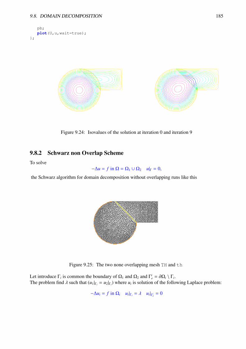
9.8. DOMAIN DECOMPOSITION 185
pb;plot(U,u,wait=true);
;
Figure 9.24: Isovalues of the solution at iteration 0 and iteration 9
9.8.2 Schwarz non Overlap SchemeTo solve
−∆u = f in Ω = Ω1 ∪Ω2 u|Γ = 0,
the Schwarz algorithm for domain decomposition without overlapping runs like this
Figure 9.25: The two none overlapping mesh TH and th
Let introduce Γi is common the boundary of Ω1 and Ω2 and Γie = ∂Ωi \ Γi.
The problem find λ such that (u1|Γi = u2|Γi) where ui is solution of the following Laplace problem:
−∆ui = f in Ωi ui|Γi = λ ui|Γie
= 0

186 CHAPTER 9. MATHEMATICAL MODELS
To solve this problem we just make a loop with upgradingλ with
λ = λ±(u1 − u2)
2
where the sign + or − of ± is choose to have convergence.
Example 9.25 (Schwarz-no-overlap.edp)
// schwarz1 without overlapping
int inside = 2;
int outside = 1;
border a(t=1,2)x=t;y=0;label=outside;;
border b(t=0,1)x=2;y=t;label=outside;;
border c(t=2,0)x=t ;y=1;label=outside;;
border d(t=1,0)x = 1-t; y = t;label=inside;;
border e(t=0, 1) x= 1-t; y = t;label=inside;;
border e1(t=pi/2, 2*pi) x= cos(t); y = sin(t);label=outside;;
int n=4;
mesh th = buildmesh( a(5*n) + b(5*n) + c(10*n) + d(5*n));
mesh TH = buildmesh ( e(5*n) + e1(25*n) );
plot(th,TH,wait=1,ps="schwarz-no-u.eps");fespace vh(th,P1);
fespace VH(TH,P1);
vh u=0,v; VH U,V;
vh lambda=0;
int i=0;
problem PB(U,V,init=i,solver=Cholesky) =
int2d(TH)( dx(U)*dx(V)+dy(U)*dy(V) )
+ int2d(TH)( -V)
+ int1d(TH,inside)(-lambda*V) + on(outside,U= 0 ) ;
problem pb(u,v,init=i,solver=Cholesky) =
int2d(th)( dx(u)*dx(v)+dy(u)*dy(v) )
+ int2d(th)( -v)
+ int1d(th,inside)(+lambda*v) + on(outside,u = 0 ) ;
for ( i=0 ;i< 10; i++)
PB;
pb;
lambda = lambda - (u-U)/2;
plot(U,u,wait=true);;
plot(U,u,ps="schwarz-no-u.eps");

9.8. DOMAIN DECOMPOSITION 187
Figure 9.26: Isovalues of the solution at iteration 0 and iteration 9 without overlapping
9.8.3 Schwarz-gc.edpTo solve
−∆u = f in Ω = Ω1 ∪Ω2 u|Γ = 0,
the Schwarz algorithm for domain decomposition without overlapping runs like thisLet introduce Γi is common the boundary of Ω1 and Ω2 and Γi
e = ∂Ωi \ Γi.The problem find λ such that (u1|Γi = u2|Γi) where ui is solution of the following Laplace problem:
−∆ui = f in Ωi ui|Γi = λ ui|Γie
= 0
The version of this example for Shur componant. The border problem is solve with conjugategradient.First, we construct the two domain
Example 9.26 (Schwarz-gc.edp)
// Schwarz without overlapping (Shur complenement Neumann -> Dirichet)real cpu=clock();int inside = 2;int outside = 1;
border Gamma1(t=1,2)x=t;y=0;label=outside;;border Gamma2(t=0,1)x=2;y=t;label=outside;;border Gamma3(t=2,0)x=t ;y=1;label=outside;;
border GammaInside(t=1,0)x = 1-t; y = t;label=inside;;
border GammaArc(t=pi/2, 2*pi) x= cos(t); y = sin(t);label=outside;;int n=4;
// build the mesh of Ω1 and Ω2mesh Th1 = buildmesh( Gamma1(5*n) + Gamma2(5*n) + GammaInside(5*n) + Gamma3(5*n));mesh Th2 = buildmesh ( GammaInside(-5*n) + GammaArc(25*n) );plot(Th1,Th2);
// defined the 2 FE spacefespace Vh1(Th1,P1), Vh2(Th2,P1);

188 CHAPTER 9. MATHEMATICAL MODELS
Note 9.6 It is impossible to define a function just on a part of boundary, so the lambda functionmust be defined on the all domain Ω1 such as
Vh1 lambda=0; // take λ ∈ Vh1
The two Poisson problem:
Vh1 u1,v1; Vh2 u2,v2;int i=0; // for factorization optimizationproblem Pb2(u2,v2,init=i,solver=Cholesky) =
int2d(Th2)( dx(u2)*dx(v2)+dy(u2)*dy(v2) )+ int2d(Th2)( -v2)+ int1d(Th2,inside)(-lambda*v2) + on(outside,u2= 0 ) ;
problem Pb1(u1,v1,init=i,solver=Cholesky) =int2d(Th1)( dx(u1)*dx(v1)+dy(u1)*dy(v1) )
+ int2d(Th1)( -v1)+ int1d(Th1,inside)(+lambda*v1) + on(outside,u1 = 0 ) ;
or, we define a border matrix , because the lambda function is none zero inside the domain Ω1:
varf b(u2,v2,solver=CG) =int1d(Th1,inside)(u2*v2);matrix B= b(Vh1,Vh1,solver=CG);
The boundary problem function,
λ −→
∫Γi
(u1 − u2)v1
func real[int] BoundaryProblem(real[int] &l)
lambda[]=l; // make FE function form lPb1; Pb2;i++; // no refactorization i !=0v1=-(u1-u2);lambda[]=B*v1[];return lambda[] ;
;
Note 9.7 The difference between the two notations v1 and v1[] is: v1 is the finite elementfunction and v1[] is the vector in the canonical basis of the finite element function v1 .
Vh1 p=0,q=0;// solve the problem with Conjugate Gradient
LinearCG(BoundaryProblem,p[],eps=1.e-6,nbiter=100);// compute the final solution, because CG works with increment
BoundaryProblem(p[]); // solve again to have right u1,u2
cout << " -- CPU time schwarz-gc:" << clock()-cpu << endl;plot(u1,u2); // plot
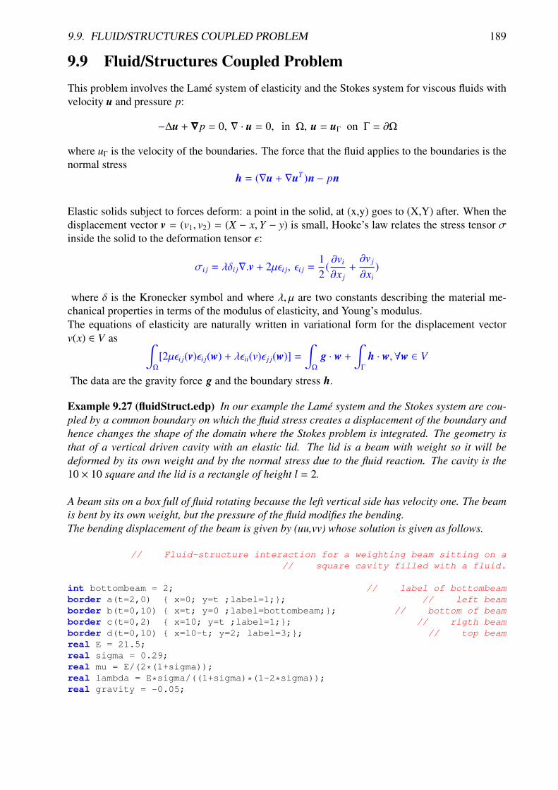
9.9. FLUID/STRUCTURES COUPLED PROBLEM 189
9.9 Fluid/Structures Coupled ProblemThis problem involves the Lame system of elasticity and the Stokes system for viscous fluids withvelocity u and pressure p:
−∆u + ∇p = 0, ∇ · u = 0, in Ω, u = uΓ on Γ = ∂Ω
where uΓ is the velocity of the boundaries. The force that the fluid applies to the boundaries is thenormal stress
h = (∇u + ∇uT )n− pn
Elastic solids subject to forces deform: a point in the solid, at (x,y) goes to (X,Y) after. When thedisplacement vector v = (v1, v2) = (X − x,Y − y) is small, Hooke’s law relates the stress tensor σinside the solid to the deformation tensor ε:
σi j = λδi j∇.v + 2µεi j, εi j =12
(∂vi
∂x j+∂v j
∂xi)
where δ is the Kronecker symbol and where λ, µ are two constants describing the material me-chanical properties in terms of the modulus of elasticity, and Young’s modulus.The equations of elasticity are naturally written in variational form for the displacement vectorv(x) ∈ V as ∫
Ω
[2µεi j(v)εi j(w) + λεii(v)ε j j(w)] =
∫Ω
g · w +
∫Γ
h · w,∀w ∈ V
The data are the gravity force g and the boundary stress h.
Example 9.27 (fluidStruct.edp) In our example the Lame system and the Stokes system are cou-pled by a common boundary on which the fluid stress creates a displacement of the boundary andhence changes the shape of the domain where the Stokes problem is integrated. The geometry isthat of a vertical driven cavity with an elastic lid. The lid is a beam with weight so it will bedeformed by its own weight and by the normal stress due to the fluid reaction. The cavity is the10 × 10 square and the lid is a rectangle of height l = 2.
A beam sits on a box full of fluid rotating because the left vertical side has velocity one. The beamis bent by its own weight, but the pressure of the fluid modifies the bending.The bending displacement of the beam is given by (uu,vv) whose solution is given as follows.
// Fluid-structure interaction for a weighting beam sitting on a// square cavity filled with a fluid.
int bottombeam = 2; // label of bottombeamborder a(t=2,0) x=0; y=t ;label=1;; // left beamborder b(t=0,10) x=t; y=0 ;label=bottombeam;; // bottom of beamborder c(t=0,2) x=10; y=t ;label=1;; // rigth beamborder d(t=0,10) x=10-t; y=2; label=3;; // top beamreal E = 21.5;real sigma = 0.29;real mu = E/(2*(1+sigma));real lambda = E*sigma/((1+sigma)*(1-2*sigma));real gravity = -0.05;

190 CHAPTER 9. MATHEMATICAL MODELS
mesh th = buildmesh( b(20)+c(5)+d(20)+a(5));fespace Vh(th,P1);Vh uu,w,vv,s,fluidforce=0;cout << "lambda,mu,gravity ="<<lambda<< " " << mu << " " << gravity << endl;
// deformation of a beam under its own weightsolve bb([uu,vv],[w,s]) =
int2d(th)(lambda*div(w,s)*div(uu,vv)+2.*mu*( epsilon(w,s)’*epsilon(uu,vv) )
)+ int2d(th) (-gravity*s)+ on(1,uu=0,vv=0)+ fluidforce[];;
plot([uu,vv],wait=1);mesh th1 = movemesh(th, [x+uu, y+vv]);plot(th1,wait=1);
Then Stokes equation for fluids ast low speed are solved in the box below the beam, but the beamhas deformed the box (see border h):
// Stokes on square b,e,f,g driven cavite on left side gborder e(t=0,10) x=t; y=-10; label= 1; ; // bottomborder f(t=0,10) x=10; y=-10+t ; label= 1; ; // rightborder g(t=0,10) x=0; y=-t ;label= 2;; // leftborder h(t=0,10) x=t; y=vv(t,0)*( t>=0.001 )*(t <= 9.999);
label=3;; // top of cavity deformed
mesh sh = buildmesh(h(-20)+f(10)+e(10)+g(10));plot(sh,wait=1);
We use the Uzawa conjugate gradient to solve the Stokes problem like in example Section 9.6.2
fespace Xh(sh,P2),Mh(sh,P1);Xh u1,u2,v1,v2;Mh p,q,ppp;
varf bx(u1,q) = int2d(sh)( -(dx(u1)*q));
varf by(u1,q) = int2d(sh)( -(dy(u1)*q));
varf Lap(u1,u2)= int2d(sh)( dx(u1)*dx(u2) + dy(u1)*dy(u2) )+ on(2,u1=1) + on(1,3,u1=0) ;
Xh bc1; bc1[] = Lap(0,Xh);Xh brhs;
matrix A= Lap(Xh,Xh,solver=CG);matrix Bx= bx(Xh,Mh);matrix By= by(Xh,Mh);Xh bcx=0,bcy=1;
func real[int] divup(real[int] & pp)

9.9. FLUID/STRUCTURES COUPLED PROBLEM 191
int verb=verbosity;verbosity=0;brhs[] = Bx’*pp; brhs[] += bc1[] .*bcx[];u1[] = Aˆ-1*brhs[];brhs[] = By’*pp; brhs[] += bc1[] .*bcy[];u2[] = Aˆ-1*brhs[];ppp[] = Bx*u1[];ppp[] += By*u2[];verbosity=verb;return ppp[] ;
;
do a loop on the two problem
for(step=0;step<2;++step)
p=0;q=0;u1=0;v1=0;
LinearCG(divup,p[],eps=1.e-3,nbiter=50);divup(p[]);
Now the beam will feel the stress constraint from the fluid:
Vh sigma11,sigma22,sigma12;Vh uu1=uu,vv1=vv;
sigma11([x+uu,y+vv]) = (2*dx(u1)-p);sigma22([x+uu,y+vv]) = (2*dy(u2)-p);sigma12([x+uu,y+vv]) = (dx(u1)+dy(u2));
which comes as a boundary condition to the PDE of the beam:
varf fluidf([uu,vv],[w,s]) fluidforce =solve bbst([uu,vv],[w,s],init=i) =
int2d(th)(lambda*div(w,s)*div(uu,vv)+2.*mu*( epsilon(w,s)’*epsilon(uu,vv) )
)+ int2d(th) (-gravity*s)+ int1d(th,bottombeam)( -coef*( sigma11*N.x*w + sigma22*N.y*s
+ sigma12*(N.y*w+N.x*s) ) )+ on(1,uu=0,vv=0);plot([uu,vv],wait=1);real err = sqrt(int2d(th)( (uu-uu1)ˆ2 + (vv-vv1)ˆ2 ));cout << " Erreur L2 = " << err << "----------\n";
Notice that the matrix generated by bbst is reused (see init=i). Finally we deform the beam
th1 = movemesh(th, [x+0.2*uu, y+0.2*vv]);plot(th1,wait=1); // end of loop

192 CHAPTER 9. MATHEMATICAL MODELS
IsoValue-2.62541-2.26528-1.90515-1.54503-1.1849-0.824776-0.46465-0.1045240.2556030.6157290.9758551.335981.696112.056232.416362.776493.136613.496743.856864.21699
Vec Value00.04998610.09997220.1499580.1999440.2499310.2999170.3499030.3998890.4498750.4998610.5498470.5998330.6498190.6998060.7497920.7997780.8497640.899750.949736
[u1,u2],p
Figure 9.27: Fluid velocity and pressure (left) and displacement vector (center) of the structureand displaced geometry (right) in the fluid-structure interaction of a soft side and a driven cavity
9.10 Transmission ProblemConsider an elastic plate whose displacement change vertically, which is made up of three platesof different materials, welded on each other. Let Ωi, i = 1, 2, 3 be the domain occupied by i-th material with tension µi (see Section 9.1.1). The computational domain Ω is the interior ofΩ1 ∪Ω2 ∪Ω3. The vertical displacement u(x, y) is obtained from
− µi∆u = f in Ωi (9.55)µi∂nu|Γi = −µ j∂nu|Γ j on Ωi ∩Ω j if 1 ≤ i < j ≤ 3 (9.56)
where ∂nu|Γi denotes the value of the normal derivative ∂nu on the boundary Γi of the domain Ωi.By introducing the characteristic function χi of Ωi, that is,
χi(x) = 1 if x ∈ Ωi; χi(x) = 0 if x < Ωi (9.57)
we can easily rewrite (9.55) and (9.56) to the weak form. Here we assume that u = 0 on Γ = ∂Ω.problem Transmission: For a given function f , find u such that
a(u, v) = `( f , v) for all v ∈ H10(Ω) (9.58)
a(u, v) =
∫Ω
µ∇u · ∇v, `( f , v) =
∫Ω
f v
where µ = µ1χ1 + µ2χ2 + µ3χ3. Here we notice that µ become the discontinuous function.With dissipation, and at the thermal equilibrium, the temperature equation is:This example explains the definition and manipulation of region, i.e. subdomains of the wholedomain.Consider this L-shaped domain with 3 diagonals as internal boundaries, defining 4 subdomains:
// example using region keyword

9.10. TRANSMISSION PROBLEM 193
// construct a mesh with 4 regions (sub-domains)border a(t=0,1)x=t;y=0;;border b(t=0,0.5)x=1;y=t;;border c(t=0,0.5)x=1-t;y=0.5;;border d(t=0.5,1)x=0.5;y=t;;border e(t=0.5,1)x=1-t;y=1;;border f(t=0,1)x=0;y=1-t;;
// internal boundaryborder i1(t=0,0.5)x=t;y=1-t;;border i2(t=0,0.5)x=t;y=t;;border i3(t=0,0.5)x=1-t;y=t;;
mesh th = buildmesh (a(6) + b(4) + c(4) +d(4) + e(4) +f(6)+i1(6)+i2(6)+i3(6));
fespace Ph(th,P0); // constant discontinuous functions / elementfespace Vh(th,P1); // P1 continuous functions / element
Ph reg=region; // defined the P0 function associated to region numberplot(reg,fill=1,wait=1,value=1);
IsoValue-0.3157890.1578950.4736840.7894741.105261.421051.736842.052632.368422.6842133.315793.631583.947374.263164.578954.894745.210535.526326.31579
Figure 9.28: the function reg
IsoValue11111111111111111111
Figure 9.29: the function nu
region is a keyword of FreeFem++ which is in fact a variable depending of the current position(is not a function today, use Ph reg=region; to set a function). This variable value returnedis the number of the subdomain of the current position. This number is defined by ”buildmesh”which scans while building the mesh all its connected component. So to get the number of a regioncontaining a particular point one does:
int nupper=reg(0.4,0.9); // get the region number of point (0.4,0.9)int nlower=reg(0.9,0.1); // get the region number of point (0.4,0.1)cout << " nlower " << nlower << ", nupper = " << nupper<< endl;

194 CHAPTER 9. MATHEMATICAL MODELS
// defined the characteristics functions of upper and lower regionPh nu=1+5*(region==nlower) + 10*(region==nupper);plot(nu,fill=1,wait=1);
This is particularly useful to define discontinuous functions such as might occur when one part ofthe domain is copper and the other one is iron, for example.We this in mind we proceed to solve a Laplace equation with discontinuous coefficients (ν is 1, 6and 11 below).
Ph nu=1+5*(region==nlower) + 10*(region==nupper);plot(nu,fill=1,wait=1);problem lap(u,v) = int2d(th)( nu*( dx(u)*dx(v)*dy(u)*dy(v) ))
+ int2d(-1*v) + on(a,b,c,d,e,f,u=0);plot(u);
IsoValue0.0009002590.002700780.00450130.006301810.008102330.009902850.01170340.01350390.01530440.01710490.01890540.0207060.02250650.0243070.02610750.0279080.02970860.03150910.03330960.0351101
Figure 9.30: the isovalue of the solution u

9.11. FREE BOUNDARY PROBLEM 195
9.11 Free Boundary ProblemThe domain Ω is defined with:
real L=10; // longueur du domainereal h=2.1; // hauteur du bord gauchereal h1=0.35; // hauteur du bord droite
// maillage d’un tapezeborder a(t=0,L)x=t;y=0;; // bottom: Γa
border b(t=0,h1)x=L;y=t;; // right: Γb
border f(t=L,0)x=t;y=t*(h1-h)/L+h;; // free surface: Γ f
border d(t=h,0)x=0;y=t;; // left: Γd
int n=4;mesh Th=buildmesh (a(10*n)+b(6*n)+f(8*n)+d(3*n));plot(Th,ps="dTh.eps");
Figure 9.31: The mesh of the domain Ω
The free boundary problem is:Find u and Ω such that:
−∆u = 0 in Ω
u = y on Γb∂u∂n
= 0 on Γd ∪ Γa
∂u∂n
=qK
nx and u = y on Γ f
We use a fixed point method; Ω0 = Ω
in two step, fist we solve the classical following problem:−∆u = 0 in Ωn
u = y on Γnb
∂u∂n
= 0 on Γnd ∪ Γn
a
u = y on Γnf
The variational formulation is:find u on V = H1(Ωn), such than u = y on Γn
b and Γnf∫
Ωn∇u∇u′ = 0, ∀u′ ∈ V with u′ = 0 on Γn
b ∪ Γnf

196 CHAPTER 9. MATHEMATICAL MODELS
and secondly to construct a domain deformation F (x, y) = [x, y − v(x, y)]where v is solution of the following problem:
−∆v = 0 in Ωn
v = 0 on Γna
∂v∂n
= 0 on Γnb ∪ Γn
d
∂v∂n
=∂u∂n−
qK
nx on Γnf
The variational formulation is:find v on V , such than v = 0 on Γn
a∫Ωn∇v∇v′ =
∫Γn
f
(∂u∂n−
qK
nx)v′, ∀v′ ∈ V with v′ = 0 on Γna
Finally the new domain Ωn+1 = F (Ωn)
Example 9.28 (freeboundary.edp) The FreeFem++ :implementation is:
real q=0.02; // flux entrantreal K=0.5; // permeabilite
fespace Vh(Th,P1);int j=0;
Vh u,v,uu,vv;
problem Pu(u,uu,solver=CG) = int2d(Th)( dx(u)*dx(uu)+dy(u)*dy(uu))+ on(b,f,u=y) ;
problem Pv(v,vv,solver=CG) = int2d(Th)( dx(v)*dx(vv)+dy(v)*dy(vv))+ on (a, v=0) + int1d(Th,f)(vv*((q/K)*N.y- (dx(u)*N.x+dy(u)*N.y)));
real errv=1;real erradap=0.001;verbosity=1;while(errv>1e-6)
j++;Pu;Pv;plot(Th,u,v ,wait=0);errv=int1d(Th,f)(v*v);real coef=1;
//real mintcc = checkmovemesh(Th,[x,y])/5.;real mint = checkmovemesh(Th,[x,y-v*coef]);
if (mint<mintcc || j%10==0) // mesh to bad => remeshingTh=adaptmesh(Th,u,err=erradap ) ;mintcc = checkmovemesh(Th,[x,y])/5.;

9.12. NOLINEAR-ELAS.EDP 197
while (1)
real mint = checkmovemesh(Th,[x,y-v*coef]);
if (mint>mintcc) break;
cout << " min |T] " << mint << endl;coef /= 1.5;
Th=movemesh(Th,[x,y-coef*v]); // calcul de la deformationcout << "\n\n"<<j <<"------------ errv = " << errv << "\n\n";
plot(Th,ps="d_Thf.eps");plot(u,wait=1,ps="d_u.eps");
Figure 9.32: The final solution on the new domain Ω72
Figure 9.33: The adapted mesh of the domain Ω72
9.12 nolinear-elas.edpThe nonlinear elasticity problem is find the displacement (u1, u2) minimizing J
min J(u1, u2) =
∫Ω
f (F2) −∫
Γp
Pa u2
where F2(u1, u2) = A(E[u1, u2], E[u1, u2]) and A(X,Y) is bilinear sym. positive form with respecttwo matrix X,Y . where f is a given C2 function, and E[u1, u2] = (Ei j)i=1,2, j=1,2 is the Green-SaintVenant deformation tensor defined with:
Ei j = 0.5(∂iu j + ∂ jui) +∑
k
∂iuk×∂ juk

198 CHAPTER 9. MATHEMATICAL MODELS
denote u = (u1, u2), v = (v1, v2), w = (w1,w2).So, the differential of J is
DJ(u)(v) =
∫DF2(u)(v) f ′(F2(u))) −
∫Γp
Pav2
where DF2(u)(v) = 2 A( DE[u](v) , E[u] ) and DE is the first differential of E.The second order differential is
D2J(u)((v), (w)) =
∫DF2(u)(v) DF2(u)(w) f ′′(F2(u)))
+
∫D2F2(u)(v,w) f ′(F2(u)))
where
D2F2(u)(v,w) = 2 A( D2E[u](v,w) , E[u] ) + 2 A( DE[u](v) ,DE[u](w) ).
and D2E is the second differential of E.
So all notation can be define with macro like:
macro EL(u,v) [dx(u),(dx(v)+dy(u)),dy(v)] // is [ε11, 2ε12, ε22]
macro ENL(u,v) [(dx(u)*dx(u)+dx(v)*dx(v))*0.5,(dx(u)*dy(u)+dx(v)*dy(v)) ,(dy(u)*dy(u)+dy(v)*dy(v))*0.5 ] // EOM ENL
macro dENL(u,v,uu,vv) [(dx(u)*dx(uu)+dx(v)*dx(vv)),(dx(u)*dy(uu)+dx(v)*dy(vv)+dx(uu)*dy(u)+dx(vv)*dy(v)),(dy(u)*dy(uu)+dy(v)*dy(vv)) ] //
macro E(u,v) (EL(u,v)+ENL(u,v)) // is [E11, 2E12, E22]macro dE(u,v,uu,vv) (EL(uu,vv)+dENL(u,v,uu,vv)) //macro ddE(u,v,uu,vv,uuu,vvv) dENL(uuu,vvv,uu,vv) //macro F2(u,v) (E(u,v)’*A*E(u,v)) //macro dF2(u,v,uu,vv) (E(u,v)’*A*dE(u,v,uu,vv)*2. ) //macro ddF2(u,v,uu,vv,uuu,vvv) (
(dE(u,v,uu,vv)’*A*dE(u,v,uuu,vvv))*2.+ (E(u,v)’*A*ddE(u,v,uu,vv,uuu,vvv))*2. ) // EOM
The Newton Method ischoose n = 0,and uO, vO the initial displacement
• loop:
• find (du, dv) : solution of
D2J(un, vn)((w, s), (du, dv)) = DJ(un, vn)(w, s), ∀w, s
• un = un − du, vn = vn − dv

9.12. NOLINEAR-ELAS.EDP 199
• until (du, dv) small is enough
The way to implement this algorithm in FreeFem++ is use a macro tool to implement A and F2,f , f ′, f ′′.A macro is like is ccp preprocessor of C++ , but this begin by macro and the end of the macrodefinition is the begin of the comment //. In this case the macro is very useful because the type ofparameter can be change. And it is easy to make automatic differentiation.
Figure 9.34: The deformed domain
// non linear elasticity model
// for hyper elasticity problem// -----------------------------
macro f(u) (u) // end of macromacro df(u) (1) // end of macromacro ddf(u) (0) // end of macro
// -- du caouchouc --- CF cours de Herve Le Dret.// -------------------------------
real mu = 0.012e5; // kg/cm2
real lambda = 0.4e5; // kg/cm2
//// σ = 2µE + λtr(E)Id// A(u, v) = σ(u) : E(v)//// ( a b )// ( b c )//// tr*Id : (a,b,c) -> (a+c,0,a+c)// so the associed matrix is:// ( 1 0 1 )// ( 0 0 0 )// ( 1 0 1 )
// ------------------vreal a11= 2*mu + lambda ;real a22= mu ; // because [0, 2 ∗ t12, 0]′A[0, 2 ∗ s12, 0] =
// = 2 ∗ mu ∗ (t12 ∗ s12 + t21 ∗ s21) = 4 ∗ mu ∗ t12 ∗ s12real a33= 2*mu + lambda ;real a12= 0 ;real a13= lambda ;real a23= 0 ;
// symetric part
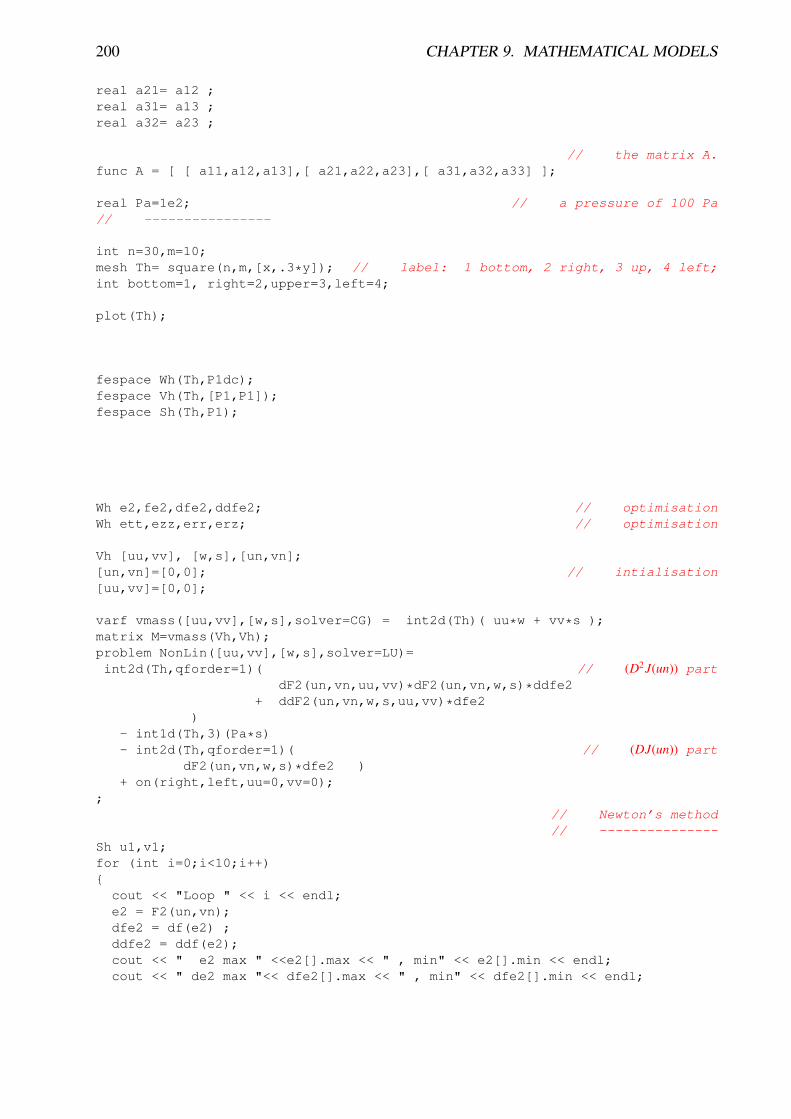
200 CHAPTER 9. MATHEMATICAL MODELS
real a21= a12 ;real a31= a13 ;real a32= a23 ;
// the matrix A.func A = [ [ a11,a12,a13],[ a21,a22,a23],[ a31,a32,a33] ];
real Pa=1e2; // a pressure of 100 Pa// ----------------
int n=30,m=10;mesh Th= square(n,m,[x,.3*y]); // label: 1 bottom, 2 right, 3 up, 4 left;int bottom=1, right=2,upper=3,left=4;
plot(Th);
fespace Wh(Th,P1dc);fespace Vh(Th,[P1,P1]);fespace Sh(Th,P1);
Wh e2,fe2,dfe2,ddfe2; // optimisationWh ett,ezz,err,erz; // optimisation
Vh [uu,vv], [w,s],[un,vn];[un,vn]=[0,0]; // intialisation[uu,vv]=[0,0];
varf vmass([uu,vv],[w,s],solver=CG) = int2d(Th)( uu*w + vv*s );matrix M=vmass(Vh,Vh);problem NonLin([uu,vv],[w,s],solver=LU)=int2d(Th,qforder=1)( // (D2J(un)) part
dF2(un,vn,uu,vv)*dF2(un,vn,w,s)*ddfe2+ ddF2(un,vn,w,s,uu,vv)*dfe2
)- int1d(Th,3)(Pa*s)- int2d(Th,qforder=1)( // (DJ(un)) part
dF2(un,vn,w,s)*dfe2 )+ on(right,left,uu=0,vv=0);
;// Newton’s method// ---------------
Sh u1,v1;for (int i=0;i<10;i++)
cout << "Loop " << i << endl;e2 = F2(un,vn);dfe2 = df(e2) ;ddfe2 = ddf(e2);cout << " e2 max " <<e2[].max << " , min" << e2[].min << endl;cout << " de2 max "<< dfe2[].max << " , min" << dfe2[].min << endl;

9.13. COMPRESSIBLE NEO-HOOKEAN MATERIALS: COMPUTATIONAL SOLUTIONS201
cout << "dde2 max "<< ddfe2[].max << " , min" << ddfe2[].min << endl;NonLin; // compute [uu, vv] = (D2J(un))−1(DJ(un))
w[] = M*uu[];real res = sqrt(w[]’ * uu[]); // norme L2o f [uu, vv]u1 = uu;v1 = vv;cout << " Lˆ2 residual = " << res << endl;cout << " u1 min =" <<u1[].min << ", u1 max= " << u1[].max << endl;cout << " v1 min =" <<v1[].min << ", v2 max= " << v1[].max << endl;plot([uu,vv],wait=1,cmm=" uu, vv " );un[] -= uu[];plot([un,vn],wait=1,cmm=" deplacement " );if (res<1e-5) break;
plot([un,vn],wait=1);mesh th1 = movemesh(Th, [x+un, y+vn]);plot(th1,wait=1); // see figure 9.34
9.13 Compressible Neo-Hookean Materials: Computational So-lutions
Author : Alex Sadovsky [email protected]
9.13.1 NotationIn what follows, the symbols u,F,B,C, σ denote, respectively, the displacement field, the defor-mation gradient, the left Cauchy-Green strain tensor B = FFT , the right Cauchy-Green straintensor C = FT F, and the Cauchy stress tensor. We also introduce the symbols I1 := tr C andJ := det F. Use will be made of the identity
∂J∂C
= JC−1 (9.59)
The symbol I denotes the identity tensor. The symbol Ω0 denotes the reference configuration of thebody to be deformed. The unit volume in the reference (resp., deformed) configuration is denoteddV (resp., dV0); these two are related by
dV = JdV0,
which allows an integral over Ω involving the Cauchy stress T to be rewritten as an integral of theKirchhoff stress κ = JT over Ω0.
Recommended ReferencesFor an exposition of nonlinear elasticity and of the underlying linear- and tensor algebra, see [33].For an advanced mathematical analysis of the Finite Element Method, see [34]. An explanationof the Finite Element formulation of a nonlinear elastostatic boundary value problem, see http://www.engin.brown.edu/courses/en222/Notes/FEMfinitestrain/FEMfinitestrain.
htm.

202 CHAPTER 9. MATHEMATICAL MODELS
9.13.2 A Neo-Hookean Compressible MaterialConstitutive Theory and Tangent Stress Measures The strain energy density function is givenby
W =µ
2(I1 − tr I − 2 ln J) (9.60)
(see [31], formula (12)).The corresponding 2nd Piola-Kirchoff stress tensor is given by
Sn :=∂W∂E
(Fn) = µ(I − C−1) (9.61)
The Kirchhoff stress, then, isκ = FSFT = µ(B − I) (9.62)
The tangent Kirchhoff stress tensor at Fn acting on δFn+1 is, consequently,∂κ
∂F(Fn)δFn+1 = µ
[Fn(δFn+1)T + δFn+1(Fn)T
](9.63)
The Weak Form of the BVP in the Absence of Body (External) Forces The Ω0 we are con-sidering is an elliptical annulus, whose boundary consists of two concentric ellipses (each allowedto be a circle as a special case), with the major axes parallel. Let P denote the dead stress load(traction) on a portion ∂Ωt
0 (= the inner ellipse) of the boundary ∂Ω0. On the rest of the boundary,we prescribe zero displacement.The weak formulation of the boundary value problem is
0 =∫
Ω0κ[F] :
(∇ ⊗ w)(F)−1
−
∫∂Ωt
0P · N0
For brevity, in the rest of this section we assume P = 0. The provided FreeFem++ code, however,does not rely on this assumption and allows for a general value and direction of P.Given a Newton approximation un of the displacement field u satisfying the BVP, we seek thecorrection δun+1 to obtain a better approximation
un+1 = un + δun+1
by solving the weak formulation
0 =∫
Ω0κ[Fn + δFn+1] :
(∇ ⊗ w)(Fn + δFn+1)−1
−
∫∂Ω0
P · N0
=∫
Ω0
κ[Fn] + ∂κ
∂F [Fn]δFn+1
:
(∇ ⊗ w)(Fn + δFn+1)−1
=
∫Ω0
κ[Fn] + ∂κ
∂F [Fn]δFn+1
:
(∇ ⊗ w)(F−1
n + F−2n δFn+1)
=
∫Ω0κ[Fn] :
(∇ ⊗ w)F−1
n
−
∫Ω0κ[Fn] :
(∇ ⊗ w)(F−2
n δFn+1)
+∫
Ω0
∂κ∂F [Fn]δFn+1
:
(∇ ⊗ w)F−1
n
for all test functions w,
(9.64)where we have taken
δFn+1 = ∇ ⊗ δun+1
Note: Contrary to standard notational use, the symbol δ here bears no variational context. By δwe mean simply an increment in the sense of Newton’s Method. The role of a variational virtualdisplacement here is played by w.

9.13. COMPRESSIBLE NEO-HOOKEAN MATERIALS: COMPUTATIONAL SOLUTIONS203
9.13.3 An Approach to Implementation in FreeFem++The associated file is examples++-tutorial/nl-elast-neo-Hookean.edp.Introducing the code-like notation, where a string in <>’s is to be read as one symbol, the individualcomponents of the tensor
< TanK >:=∂κ
∂F[Fn]δFn+1 (9.65)
will be implemented as the macros < TanK11 >, < TanK12 >, . . ..The individual components of the tensor quantities
D1 := Fn(δFn+1)T + δFn+1(Fn)T ,
D2 := F−Tn δFn+1,
D3 := (∇ ⊗ w)F−2n δFn+1,
andD4 := (∇ ⊗ w)F−1
n ,
will be implemented as the macros
< d1Aux11 >, < d1Aux12 >, . . . , < d1Aux22 >,< d2Aux11 >, < d2Aux12 >, . . . , < d2Aux22 >< d3Aux11 >, < d3Aux12 >, . . . , < d3Aux22 >< d4Aux11 >, < d4Aux12 >, . . . , < d4Aux22 >
, (9.66)
respectively.In the above notation, the tangent Kirchhoff stress term becomes
∂κ
∂F(Fn) δFn+1 = µ D1 (9.67)
while the weak BVP formulation acquires the form
0 =∫
Ω0κ[Fn] : D4
−∫
Ω0κ[Fn] : D3
+∫
Ω0
∂κ∂F [Fn]δFn+1
: D4
for all test functions w (9.68)

204 CHAPTER 9. MATHEMATICAL MODELS

Chapter 10
Parallel version experimental
A first attempt of parallelization of FreeFem++ is made here with mpi. We add 4 words in thelanguage:
mpisize The total number of processes
mpirank the number of my current process in 0, ...,mpisize − 1.
processor a function to set the possessor to send or receive data
broadcast a function to broadcast from a processor to all other a data
processor(10) << a ; // send to the process 10 the data a;processor(10) >> a ; // receive from the process 10 the data a;
10.1 Schwarz in parallelThis example is just the rewritting of example schwarz-overlap in section 9.8.1.
[examples++-mpi] Hecht%lamboot
LAM 6.5.9/MPI 2 C++/ROMIO - Indiana University
[examples++-mpi] hecht% mpirun -np 2 FreeFem++-mpi schwarz-c.edp
// a new coding version c, methode de schwarz in parallele// with 2 proc.// -------------------------------// F.Hecht december 2003// ----------------------------------// to test the broadcast instruction// and array of mesh// add add the stop test// ---------------------------------
if ( mpisize != 2 )
205
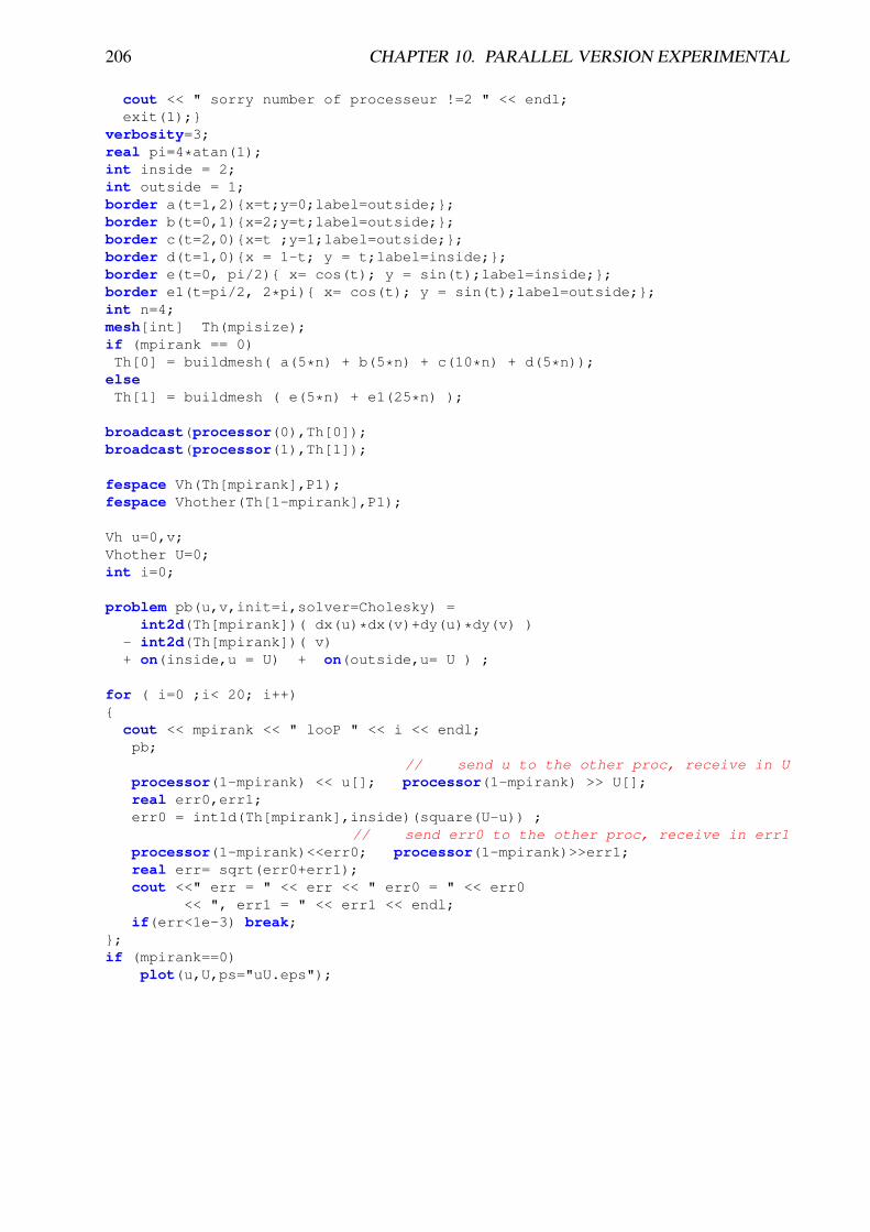
206 CHAPTER 10. PARALLEL VERSION EXPERIMENTAL
cout << " sorry number of processeur !=2 " << endl;exit(1);
verbosity=3;real pi=4*atan(1);int inside = 2;int outside = 1;border a(t=1,2)x=t;y=0;label=outside;;border b(t=0,1)x=2;y=t;label=outside;;border c(t=2,0)x=t ;y=1;label=outside;;border d(t=1,0)x = 1-t; y = t;label=inside;;border e(t=0, pi/2) x= cos(t); y = sin(t);label=inside;;border e1(t=pi/2, 2*pi) x= cos(t); y = sin(t);label=outside;;int n=4;mesh[int] Th(mpisize);if (mpirank == 0)Th[0] = buildmesh( a(5*n) + b(5*n) + c(10*n) + d(5*n));
elseTh[1] = buildmesh ( e(5*n) + e1(25*n) );
broadcast(processor(0),Th[0]);broadcast(processor(1),Th[1]);
fespace Vh(Th[mpirank],P1);fespace Vhother(Th[1-mpirank],P1);
Vh u=0,v;Vhother U=0;int i=0;
problem pb(u,v,init=i,solver=Cholesky) =int2d(Th[mpirank])( dx(u)*dx(v)+dy(u)*dy(v) )
- int2d(Th[mpirank])( v)+ on(inside,u = U) + on(outside,u= U ) ;
for ( i=0 ;i< 20; i++)
cout << mpirank << " looP " << i << endl;pb;
// send u to the other proc, receive in Uprocessor(1-mpirank) << u[]; processor(1-mpirank) >> U[];real err0,err1;err0 = int1d(Th[mpirank],inside)(square(U-u)) ;
// send err0 to the other proc, receive in err1processor(1-mpirank)<<err0; processor(1-mpirank)>>err1;real err= sqrt(err0+err1);cout <<" err = " << err << " err0 = " << err0
<< ", err1 = " << err1 << endl;if(err<1e-3) break;
;if (mpirank==0)
plot(u,U,ps="uU.eps");
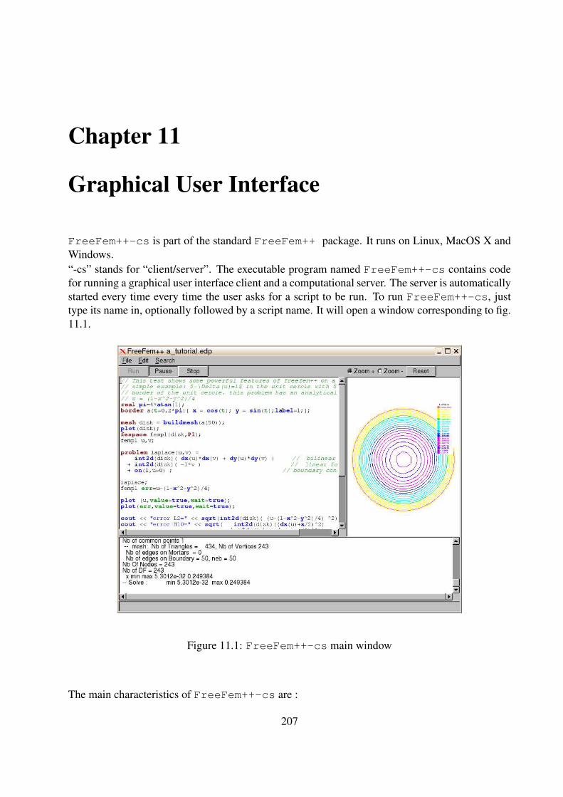
Chapter 11
Graphical User Interface
FreeFem++-cs is part of the standard FreeFem++ package. It runs on Linux, MacOS X andWindows.“-cs” stands for “client/server”. The executable program named FreeFem++-cs contains codefor running a graphical user interface client and a computational server. The server is automaticallystarted every time every time the user asks for a script to be run. To run FreeFem++-cs, justtype its name in, optionally followed by a script name. It will open a window corresponding to fig.11.1.
Figure 11.1: FreeFem++-cs main window
The main characteristics of FreeFem++-cs are :
207

208 CHAPTER 11. GRAPHICAL USER INTERFACE
• A main window composed of three panels : editor with syntax highlighting (right), FreeFem++messages (bottom) and graphics (left).
• Panel sizes can be changed by dragging their borders with the mouse. Any of the threepanels can be made to fill the whole window.
• The edited script can be run at any time by clicking on the “Run” button.
• Dragging a FreeFem++ script file icon from a file manager into the editor window makesFreeFem++-cs edit that script.
• Graphics can be examined (e.g. zoomed) while FreeFem++ is running.
• A running FreeFem++ computation can be paused or stopped at any time.
All commands should be self-explanatory. Here are just a few useful hints :
• There is no need to save a FreeFem++ script to run it. It is run exactly as displayed in theeditor window, and the corresponding file is not touched.
• The current directory is updated every time a script is loaded or saved. All include direc-tives are therefore relative to the directory where the main script is located.
• Specifying wait=1 in a plot command is exactly equivalent to clicking on the “Pause”button when the plot is displayed.
• In zoom mode, if your mouse has more than one button, a middle-click resets any zoomingcoefficient, and a right-click zooms in the opposite way of the left-click.

Chapter 12
Mesh Files
12.1 File mesh data structureThe mesh data structure, output of a mesh generation algorithm, refers to the geometric data struc-ture and in some case to another mesh data structure.In this case, the fields are
• MeshVersionFormatted 0
• Dimension (I) dim
• Vertices (I) NbOfVertices( ((R) x j
i , j=1,dim ) , (I) Re fφvi , i=1 , NbOfVertices )
• Edges (I) NbOfEdges(@@Vertex1
i ,@@Vertex2i , (I) Re fφe
i , i=1 , NbOfEdges )• Triangles (I) NbOfTriangles
( (@@Vertex ji , j=1,3 ) , (I) Re fφt
i , i=1 , NbOfTriangles )• Quadrilaterals (I) NbOfQuadrilaterals
( (@@Vertex ji , j=1,4 ) , (I) Re fφt
i , i=1 , NbOfQuadrilaterals )• Geometry(C*) FileNameOfGeometricSupport
– VertexOnGeometricVertex(I) NbOfVertexOnGeometricVertex(@@Vertexi ,@@Vertexgeo
i , i=1,NbOfVertexOnGeometricVertex )– EdgeOnGeometricEdge(I) NbOfEdgeOnGeometricEdge(@@Edgei ,@@Edgegeo
i , i=1,NbOfEdgeOnGeometricEdge )
• CrackedEdges (I) NbOfCrackedEdges(@@Edge1
i ,@@Edge2i , i=1 , NbOfCrackedEdges )
209

210 CHAPTER 12. MESH FILES
When the current mesh refers to a previous mesh, we have in addition
• MeshSupportOfVertices(C*) FileNameOfMeshSupport
– VertexOnSupportVertex(I) NbOfVertexOnSupportVertex(@@Vertexi ,@@Vertexsupp
i , i=1,NbOfVertexOnSupportVertex )– VertexOnSupportEdge(I) NbOfVertexOnSupportEdge(@@Vertexi ,@@Edgesupp
i , (R) usuppi , i=1,NbOfVertexOnSupportEdge )
– VertexOnSupportTriangle(I) NbOfVertexOnSupportTriangle(@@Vertexi ,@@Triasupp
i , (R) usuppi , (R) vsupp
i ,i=1 , NbOfVertexOnSupportTriangle )
– VertexOnSupportQuadrilaterals(I) NbOfVertexOnSupportQuadrilaterals(@@Vertexi ,@@Quadsupp
i , (R) usuppi , (R) vsupp
i ,i=1 , NbOfVertexOnSupportQuadrilaterals )
12.2 bb File type for Store SolutionsThe file is formatted such that:2 nbsol nbv 2((Ui j, ∀i ∈ 1, ..., nbsol
), ∀ j ∈ 1, ..., nbv
)where
• nbsol is a integer equal to the number of solutions.
• nbv is a integer equal to the number of vertex .
• Ui j is a real equal the value of the i solution at vertex j on the associated mesh background ifread file, generated if write file.
12.3 BB File Type for Store SolutionsThe file is formatted such that:2 n typesol1 ... typesoln nbv 2(((Uk
i j, ∀i ∈ 1, ..., typesolk), ∀k ∈ 1, ...n
)∀ j ∈ 1, ..., nbv
)where
• n is a integer equal to the number of solutions
• typesolk, type of the solution number k, is

12.4. METRIC FILE 211
– typesolk = 1 the solution k is scalar (1 value per vertex)
– typesolk = 2 the solution k is vectorial (2 values per unknown)
– typesolk = 3 the solution k is a 2×2 symmetric matrix (3 values per vertex)
– typesolk = 4 the solution k is a 2×2 matrix (4 values per vertex)
• nbv is a integer equal to the number of vertices
• Uki j is a real equal to the value of the component i of the solution k at vertex j on the associated
mesh background if read file, generated if write file.
12.4 Metric FileA metric file can be of two types, isotropic or anisotropic.the isotropic file is such thatnbv 1hi ∀i ∈ 1, ..., nbvwhere
• nbv is a integer equal to the number of vertices.
• hi is the wanted mesh size near the vertex i on background mesh, the metric isMi = h−2i Id,
where Id is the identity matrix.
The metric anisotropenbv 3a11i,a21i,a22i ∀i ∈ 1, ..., nbvwhere
• nbv is a integer equal to the number of vertices,
• a11i, a12i, a22i is metric Mi =(
a11i a12ia12i a22i
)which define the wanted mesh size in a vicinity
of the vertex i such that h in direction u ∈ R2 is equal to |u|/√
u · Mi u , where · is the dotproduct in R2, and | · | is the classical norm.
12.5 List of AM FMT, AMDBA MeshesThe mesh is only composed of triangles and can be defined with the help of the following twointegers and four arrays:
nbt is the number of triangles.
nbv is the number of vertices.
nu(1:3,1:nbt) is an integer array giving the three vertex numbers
counterclockwise for each triangle.
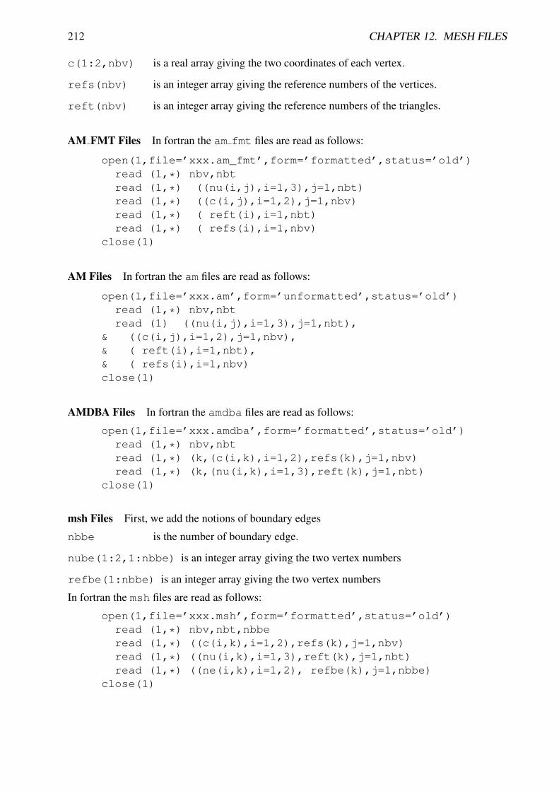
212 CHAPTER 12. MESH FILES
c(1:2,nbv) is a real array giving the two coordinates of each vertex.
refs(nbv) is an integer array giving the reference numbers of the vertices.
reft(nbv) is an integer array giving the reference numbers of the triangles.
AM FMT Files In fortran the am fmt files are read as follows:
open(1,file=’xxx.am_fmt’,form=’formatted’,status=’old’)read (1,*) nbv,nbtread (1,*) ((nu(i,j),i=1,3),j=1,nbt)read (1,*) ((c(i,j),i=1,2),j=1,nbv)read (1,*) ( reft(i),i=1,nbt)read (1,*) ( refs(i),i=1,nbv)
close(1)
AM Files In fortran the am files are read as follows:
open(1,file=’xxx.am’,form=’unformatted’,status=’old’)read (1,*) nbv,nbtread (1) ((nu(i,j),i=1,3),j=1,nbt),
& ((c(i,j),i=1,2),j=1,nbv),& ( reft(i),i=1,nbt),& ( refs(i),i=1,nbv)close(1)
AMDBA Files In fortran the amdba files are read as follows:
open(1,file=’xxx.amdba’,form=’formatted’,status=’old’)read (1,*) nbv,nbtread (1,*) (k,(c(i,k),i=1,2),refs(k),j=1,nbv)read (1,*) (k,(nu(i,k),i=1,3),reft(k),j=1,nbt)
close(1)
msh Files First, we add the notions of boundary edges
nbbe is the number of boundary edge.
nube(1:2,1:nbbe) is an integer array giving the two vertex numbers
refbe(1:nbbe) is an integer array giving the two vertex numbers
In fortran the msh files are read as follows:
open(1,file=’xxx.msh’,form=’formatted’,status=’old’)read (1,*) nbv,nbt,nbberead (1,*) ((c(i,k),i=1,2),refs(k),j=1,nbv)read (1,*) ((nu(i,k),i=1,3),reft(k),j=1,nbt)read (1,*) ((ne(i,k),i=1,2), refbe(k),j=1,nbbe)
close(1)

12.5. LIST OF AM FMT, AMDBA MESHES 213
ftq Files In fortran the ftq files are read as follows:
open(1,file=’xxx.ftq’,form=’formatted’,status=’old’)read (1,*) nbv,nbe,nbt,nbqread (1,*) (k(j),(nu(i,j),i=1,k(j)),reft(j),j=1,nbe)read (1,*) ((c(i,k),i=1,2),refs(k),j=1,nbv)close(1)
where if k(j) = 3 then the element j is a triangle and if k = 4 the the element j is a quadrilat-eral.

214 CHAPTER 12. MESH FILES

Chapter 13
Add new finite element
13.1 Some notationFor a function f taking value in RN , N = 1, 2, · · · , we define the finite element approximation Πh f of f .Let us denote the number of the degrees of freedom of the finite element by NbDoF. Then the i-th base ωK
i(i = 0, · · · ,NbDoF − 1) of the finite element space has the j-th component ωK
i j for j = 0, · · · ,N − 1.The operator Πh is called the interpolator of the finite element. We have the identity ωK
i = ΠhωKi .
Formally, the interpolator Πh is constructed by the following formula:
Πh f =
kPi−1∑k=0
αk f jk (Ppk )ωKik (13.1)
where Pp is a set of npPi points,In the formula (13.1), the list pk, jk, ik depend just on the type of finite element (not on the element), butthe coefficient αk can be depending on the element.
Example 1: classical scalar Lagrange finite element, first we have kPi = npPi = NbOfNode and
• Pp is the point of the nodal points
• the αk = 1, because we take the value of the function at the point Pk
• pk = k , jk = k because we have one node per function.
• jk = 0 because N = 1
Example 2: The Raviart-Thomas finite element:
RT0h = v ∈ H(div)/∀K ∈ Th v|K(x, y) =∣∣∣ αKβK + γK
∣∣∣ xy (13.2)
The degree of freedom are the flux throw an edge e of the mesh, where the flux of the function f : R2 −→ R2
is∫
e f.ne, ne is the unit normal of edge e (this implies a orientation of all the edges of the mesh, for examplewe can use the global numbering of the edge vertices and we just go to small to large number).To compute this flux, we use an quadrature formula with one point, the middle point of the edge. Consider atriangle T with three vertices (a,b, c). Let denote the vertices numbers by ia, ib, ic, and define the three edgevectors e0, e1, e2 by sgn(ib − ic)(b − c), sgn(ic − ia)(c − a), sgn(ia − ib)(a − b),The three basis functions are:
ωK0 =
sgn(ib − ic)2|T |
(x − a), ωK1 =
sgn(ic − ia)2|T |
(x − b), ωK2 =
sgn(ia − ib)2|T |
(x − c), (13.3)
where |T | is the area of the triangle T .So we have N = 2, kPi = 6; npPi = 3; and:
215

216 CHAPTER 13. ADD NEW FINITE ELEMENT
• Pp =
b+c2 , a+c
2 , b+a2
• α0 = −e0
2, α1 = e01, α2 = −e1
2, α3 = e11, α4 = −e2
2, α5 = e21 (effectively, the vector (−em
2 , em1 ) is
orthogonal to the edge em = (em1 , e
m2 ) with a length equal to the side of the edge or equal to
∫em 1).
• ik = 0, 0, 1, 1, 2, 2,
• pk = 0, 0, 1, 1, 2, 2 , jk = 0, 1, 0, 1, 0, 1, 0, 1.
13.2 Which class of addAdd file FE ADD.cpp in directory src/femlib for example first to initialize :
#include "error.hpp"#include "rgraph.hpp"using namespace std;#include "RNM.hpp"#include "fem.hpp"#include "FESpace.hpp"#include "AddNewFE.h"
namespace Fem2D
Second, you are just a class which derive for public TypeOfFE like:
class TypeOfFE_RTortho : public TypeOfFE public:static int Data[]; // some numbersTypeOfFE_RTortho():
TypeOfFE( 0+3+0, // nb degree of freedom on element2, // dimension N of vectorial FE (1 if scalar FE)Data, // the array data1, // nb of subdivision for plotting1, // nb of sub finite element (generaly 1)6, // number kPi of coef to build the interpolator (13.1)3, // number npPi of integration point to build interpolator0 // an array to store the coef αk to build interpolator
// here this array is no constant so we have// to rebuilt for each element.
)
const R2 Pt[] = R2(0.5,0.5), R2(0.0,0.5), R2(0.5,0.0) ;// the set of Point in K
for (int p=0,kk=0;p<3;p++) P_Pi_h[p]=Pt[p];for (int j=0;j<2;j++)
pij_alpha[kk++]= IPJ(p,p,j); // definition of ik, pk, jk in (13.1)
void FB(const bool * watdd, const Mesh & Th,const Triangle & K,const R2 &PHat, RNMK_ & val) const;
void Pi_h_alpha(const baseFElement & K,KN_<double> & v) const ;
;
where the array data is form with the concatenation of five array of size NbDoF and one array of size N.

13.2. WHICH CLASS OF ADD 217
This array is:
int TypeOfFE_RTortho::Data[]=
// for each df 0,1,3 :3,4,5,// the support of the node of the df0,0,0,// the number of the df on the node0,1,2,// the node of the df0,0,0,// the df come from which FE (generally 0)0,1,2,// which are de df on sub FE0,0 ; // for each component j = 0,N − 1 it give the sub FE associated
where the support is a number 0, 1, 2 for vertex support, 3, 4, 5 for edge support, and finaly 6 for elementsupport.The function to defined the function ωK
i , this function return the value of all the basics function or thisderivatives in array val, computed at point PHat on the reference triangle corresponding to point R2P=K(Phat); on the current triangle K.The index i, j, k of the array val(i, j, k) corresponding to:
i is basic function number on finite element i ∈ [0,NoF[
j is the value of component j ∈ [0,N[
k is the type of computed value f (P), dx( f )(P), dy( f )(P), ... i ∈ [0, last operatortype[. Remark foroptimization, this value is computed only if whatd[k] is true, and the numbering is defined with
enum operatortype op_id=0,op_dx=1,op_dy=2,op_dxx=3,op_dyy=4,op_dyx=5,op_dxy=5,op_dz=6,op_dzz=7,op_dzx=8,op_dxz=8,op_dzy=9,op_dyz=9;
const int last_operatortype=10;
The shape function :
void TypeOfFE_RTortho::FB(const bool *whatd,const Mesh & Th,const Triangle & K,const R2 & PHat,RNMK_ & val) const
//R2 P(K(PHat));R2 A(K[0]), B(K[1]),C(K[2]);R l0=1-P.x-P.y,l1=P.x,l2=P.y;assert(val.N() >=3);assert(val.M()==2 );val=0;R a=1./(2*K.area);R a0= K.EdgeOrientation(0) * a ;R a1= K.EdgeOrientation(1) * a ;R a2= K.EdgeOrientation(2) * a ;
// ------------if (whatd[op_id]) // value of the function

218 CHAPTER 13. ADD NEW FINITE ELEMENT
assert(val.K()>op_id);RN_ f0(val(’.’,0,0)); // value first componentRN_ f1(val(’.’,1,0)); // value second componentf1[0] = (P.x-A.x)*a0;f0[0] = -(P.y-A.y)*a0;
f1[1] = (P.x-B.x)*a1;f0[1] = -(P.y-B.y)*a1;
f1[2] = (P.x-C.x)*a2;f0[2] = -(P.y-C.y)*a2;
// ----------------
if (whatd[op_dx]) // value of the dx of functionassert(val.K()>op_dx);val(0,1,op_dx) = a0;val(1,1,op_dx) = a1;val(2,1,op_dx) = a2;
if (whatd[op_dy])assert(val.K()>op_dy);val(0,0,op_dy) = -a0;val(1,0,op_dy) = -a1;val(2,0,op_dy) = -a2;
for (int i= op_dy; i< last_operatortype ; i++)if (whatd[op_dx])
assert(op_dy);
The function to defined the coefficient αk:
void TypeOfFE_RT::Pi_h_alpha(const baseFElement & K,KN_<double> & v) const
const Triangle & T(K.T);
for (int i=0,k=0;i<3;i++)
R2 E(T.Edge(i));R signe = T.EdgeOrientation(i) ;v[k++]= signe*E.y;v[k++]=-signe*E.x;
Now , we just need to add a new key work in FreeFem++, Two way, with static or dynamic link so at theend of the file, we add :
With dynamic link is very simple (see section C of appendix), just add before the end of FEM2d namespaceadd:

13.2. WHICH CLASS OF ADD 219
static TypeOfFE_RTortho The_TypeOfFE_RTortho; //static AddNewFE("RT0Ortho", The_TypeOfFE_RTortho); // FEM2d namespace
Try with ”./load.link” command in examples++-load/ and see BernardiRaugel.cpp or Morley.cppnew finite element examples.
Otherwise with static link (for expert only), add
// let the 2 globals variablesstatic TypeOfFE_RTortho The_TypeOfFE_RTortho; //
// ----- the name in freefem ----static ListOfTFE typefemRTOrtho("RT0Ortho", & The_TypeOfFE_RTortho); //
// link with FreeFem++ do not work with static library .a// FH so add a extern name to call in init static FE// (see end of FESpace.cpp)void init_FE_ADD() ;// --- end -- // FEM2d namespace
To inforce in loading of this new finite element, we have to add the two new lines close to the end of filessrc/femlib/FESpace.cpp like:
// correct Problem of static library link with new make filevoid init_static_FE() // list of other FE file.o
extern void init_FE_P2h() ;init_FE_P2h() ;extern void init_FE_ADD() ; // new line 1init_FE_ADD(); // new line 2
and now you have to change the makefile.First, create a file FE ADD.cpp contening all this code, like in file src/femlib/Element P2h.cpp,after modifier the Makefile.am by adding the name of your file to the variable EXTRA DIST like:
# Makefile using Automake + Autoconf# ----------------------------------# $Id: addfe.tex,v 1.6 2005-12-27 16:32:24 hecht Exp $
# This is not compiled as a separate library because its# interconnections with other libraries have not been solved.
EXTRA_DIST=BamgFreeFem.cpp BamgFreeFem.hpp CGNL.hpp CheckPtr.cpp \ConjuguedGradrientNL.cpp DOperator.hpp Drawing.cpp Element_P2h.cpp \Element_P3.cpp Element_RT.cpp fem3.hpp fem.cpp fem.hpp FESpace.cpp \FESpace.hpp FESpace-v0.cpp FQuadTree.cpp FQuadTree.hpp gibbs.cpp \glutdraw.cpp gmres.hpp MatriceCreuse.hpp MatriceCreuse_tpl.hpp \MeshPoint.hpp mortar.cpp mshptg.cpp QuadratureFormular.cpp \QuadratureFormular.hpp RefCounter.hpp RNM.hpp RNM_opc.hpp RNM_op.hpp \RNM_tpl.hpp FE_ADD.cpp

220 CHAPTER 13. ADD NEW FINITE ELEMENT
and do in the freefem++ root directory
autoreconf./reconfiguremake
For codewarrior compilation add the file in the project an remove the flag in panal PPC linker FreeFEm++Setting Dead-strip Static Initializition Code Flag.

Appendix A
Table of Notations
Here mathematical expressions and corresponding FreeFem++ commands are noted.
A.1 Generalitiesδi j Kronecker delta (0 if i , j, 1 if i = j for integers i, j)
∀ for all
∃ there exist
i.e. that is
PDE partial differential equation (with boundary conditions)
∅ the empty set
N the set of integers (a ∈ N⇔ int a); “int” means long integer inside FreeFem++
R the set of real numbers (a ∈ R⇔ real a) ;double inside FreeFem++
C the set of complex numbers (a ∈ C⇔ complex a); complex¡double¿
Rd d-dimensional Euclidean space
A.2 Sets, Mappings, Matrices, VectorsLet E, F, G be three sets and A subset of E.
x ∈ E| P the subset of E consisting of the elements possessing the property P
E ∪ F the set of elements belonging to E or F
E ∩ F the set of elements belonging to E and F
E \ A the set x ∈ E| x < A
E + F E ∪ F with E ∩ F = ∅
221

222 APPENDIX A. TABLE OF NOTATIONS
E × F the cartesian product of E and F
En the n-th power of E (E2 = E × E, En = E × En−1)
f : E → F the mapping form E into F, i.e., E 3 x 7→ f (x) ∈ F
IE or I the identity mapping in E,i.e., I(x) = x ∀x ∈ E
f g for f : F → G and g : E → F, E 3 x 7→ ( f g)(x) = f (g(x)) ∈ G (see Section 4.6)
f |A the restriction of f : E → F to the subset A of E
ak column vector with components ak
(ak) row vector with components ak
(ak)T denotes the transpose of a matrix (ak), and is ak
ai j matrix with components ai j, and (ai j)T = (a ji)
A.3 Numbers
For two real numbers a, b
[a, b] is the interval x ∈ R| a ≤ x ≤ b
]a, b] is the interval x ∈ R| a < x ≤ b
[a, b[ is the interval x ∈ R| a ≤ x < b
]a, b[ is the interval x ∈ R| a < x < b
A.4 Differential Calculus
∂ f /∂x the partial derivative of f : Rd → R with respect to x ( dx(f))
∇ f the gradient of f : Ω→ R,i.e., ∇ f = (∂ f /∂x, ∂ f /∂y)
div f or ∇. f the divergence of f : Ω→ Rd, i.e., div f = ∂ f1/∂x + ∂ f2/∂y
∆ f the Laplacian of f : Ω→ R, i.e., ∆ f = ∂2 f /∂x2 + ∂2 f /∂y2

A.5. MESHES 223
A.5 MeshesΩ usually denotes a domain on which PDE is defined
Γ denotes the boundary of Ω,i.e., Γ = ∂Ω (keyword border, see Section 5.1.2)
Th the triangulation of Ω, i.e., the set of triangles Tk, where h stands for mesh size (keyword mesh,buildmesh, see Section 5)
nt the number of triangles in Th (get by Th.nt, see “mesh.edp”)
Ωh denotes the approximated domain Ωh = ∪ntk=1Tk of Ω. If Ω is polygonal domain, then it will be
Ω = Ωh
Γh the boundary of Ωh
nv the number of vertices in Th (get by Th.nv)
[qiq j ] the segment connecting qi and q j
qk1 , qk2 , qk3 the vertices of a triangle Tk with anti-clock direction (get the coordinate of qk j by(Th[k-1][j-1].x, Th[k-1][j-1].y))
IΩ the set i ∈ N| qi < Γh
A.6 Finite Element Spaces
L2(Ω) the set
w(x, y)∣∣∣∣∣ ∫
Ω
|w(x, y)|2dxdy < ∞
norm: ‖w‖0,Ω =
(∫Ω
|w(x, y)|2dxdy)1/2
scalar product: (v,w) =
∫Ω
vw
H1(Ω) the set
w ∈ L2(Ω)∣∣∣∣∣ ∫
Ω
(|∂w/∂x|2 + |∂w/∂y|2
)dxdy < ∞
norm: ‖w‖1,Ω =(‖w‖20,Ω + ‖∇u‖20.Ω
)1/2
Hm(Ω) the set
w ∈ L2(Ω)
∣∣∣∣∣∣∫
Ω
∂|α|w∂xα1∂yα2
∈ L2(Ω) ∀α = (α1, α2) ∈ N2, |α| = α1 + α2
scalar product: (v,w)1,Ω =∑|α|≤m
∫Ω
DαvDαw

224 APPENDIX A. TABLE OF NOTATIONS
H10(Ω) the set
w ∈ H1(Ω) | u = 0 on Γ
L2(Ω)2 denotes L2(Ω) × L2(Ω), and also H1(Ω)2 = H1(Ω) × H1(Ω)
Vh denotes the finite element space created by “ fespace Vh(Th,*)” in FreeFem++ (see Section6 for “*”)
Πh f the projection of the function f into Vh (“ func f=xˆ2*yˆ3; Vh v = f;” means v =Πh f)
v for FE-function v in Vh means the column vector (v1, · · · , vM)T if v = v1φ1 + · · ·+ vMφM, whichis shown by “ fespace Vh(Th,P2); Vh v; cout << v[] << endl;”

Appendix B
Grammar
B.1 The bison grammar
start: input ENDOFFILE;
input: instructions ;
instructions: instruction| instructions instruction ;
list_of_id_args:| id| id ’=’ no_comma_expr| FESPACE id| type_of_dcl id| type_of_dcl ’&’ id| ’[’ list_of_id_args ’]’| list_of_id_args ’,’ id| list_of_id_args ’,’ ’[’ list_of_id_args ’]’| list_of_id_args ’,’ id ’=’ no_comma_expr| list_of_id_args ’,’ FESPACE id| list_of_id_args ’,’ type_of_dcl id| list_of_id_args ’,’ type_of_dcl ’&’ id ;
list_of_id1: id| list_of_id1 ’,’ id ;
id: ID | FESPACE ;
list_of_dcls: ID| ID ’=’ no_comma_expr| ID ’(’ parameters_list ’)’| list_of_dcls ’,’ list_of_dcls ;
parameters_list:no_set_expr
| FESPACE ID| ID ’=’ no_set_expr
225

226 APPENDIX B. GRAMMAR
| parameters_list ’,’ no_set_expr| parameters_list ’,’ id ’=’ no_set_expr ;
type_of_dcl: TYPE| TYPE ’[’ TYPE ’]’ ;
ID_space:ID
| ID ’[’ no_set_expr ’]’| ID ’=’ no_set_expr| ’[’ list_of_id1 ’]’| ’[’ list_of_id1 ’]’ ’[’ no_set_expr ’]’| ’[’ list_of_id1 ’]’ ’=’ no_set_expr ;
ID_array_space:ID ’(’ no_set_expr ’)’
| ’[’ list_of_id1 ’]’ ’(’ no_set_expr ’)’ ;
fespace: FESPACE ;
spaceIDa : ID_array_space| spaceIDa ’,’ ID_array_space ;
spaceIDb : ID_space| spaceIDb ’,’ ID_space ;
spaceIDs : fespace spaceIDb| fespace ’[’ TYPE ’]’ spaceIDa ;
fespace_def: ID ’(’ parameters_list ’)’ ;
fespace_def_list: fespace_def| fespace_def_list ’,’ fespace_def ;
declaration: type_of_dcl list_of_dcls ’;’| ’fespace’ fespace_def_list ’;’| spaceIDs ’;’| FUNCTION ID ’=’ Expr ’;’| FUNCTION type_of_dcl ID ’(’ list_of_id_args ’)’ ’’ instructions’’| FUNCTION ID ’(’ list_of_id_args ’)’ ’=’ no_comma_expr ’;’ ;
begin: ’’ ;end: ’’ ;
for_loop: ’for’ ;while_loop: ’while’ ;
instruction: ’;’| ’include’ STRING| ’load’ STRING| Expr ’;’| declaration| for_loop ’(’ Expr ’;’ Expr ’;’ Expr ’)’ instruction| while_loop ’(’ Expr ’)’ instruction| ’if’ ’(’ Expr ’)’ instruction
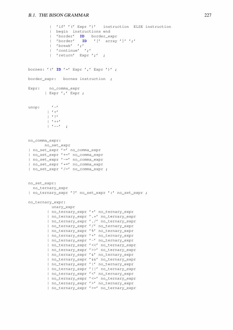
B.1. THE BISON GRAMMAR 227
| ’if’ ’(’ Expr ’)’ instruction ELSE instruction| begin instructions end| ’border’ ID border_expr| ’border’ ID ’[’ array ’]’ ’;’| ’break’ ’;’| ’continue’ ’;’| ’return’ Expr ’;’ ;
bornes: ’(’ ID ’=’ Expr ’,’ Expr ’)’ ;
border_expr: bornes instruction ;
Expr: no_comma_expr| Expr ’,’ Expr ;
unop: ’-’| ’+’| ’!’| ’++’| ’--’ ;
no_comma_expr:no_set_expr
| no_set_expr ’=’ no_comma_expr| no_set_expr ’+=’ no_comma_expr| no_set_expr ’-=’ no_comma_expr| no_set_expr ’*=’ no_comma_expr| no_set_expr ’/=’ no_comma_expr ;
no_set_expr:no_ternary_expr
| no_ternary_expr ’?’ no_set_expr ’:’ no_set_expr ;
no_ternary_expr:unary_expr
| no_ternary_expr ’*’ no_ternary_expr| no_ternary_expr ’.*’ no_ternary_expr| no_ternary_expr ’./’ no_ternary_expr| no_ternary_expr ’/’ no_ternary_expr| no_ternary_expr ’%’ no_ternary_expr| no_ternary_expr ’+’ no_ternary_expr| no_ternary_expr ’-’ no_ternary_expr| no_ternary_expr ’<<’ no_ternary_expr| no_ternary_expr ’>>’ no_ternary_expr| no_ternary_expr ’&’ no_ternary_expr| no_ternary_expr ’&&’ no_ternary_expr| no_ternary_expr ’|’ no_ternary_expr| no_ternary_expr ’||’ no_ternary_expr| no_ternary_expr ’<’ no_ternary_expr| no_ternary_expr ’<=’ no_ternary_expr| no_ternary_expr ’>’ no_ternary_expr| no_ternary_expr ’>=’ no_ternary_expr
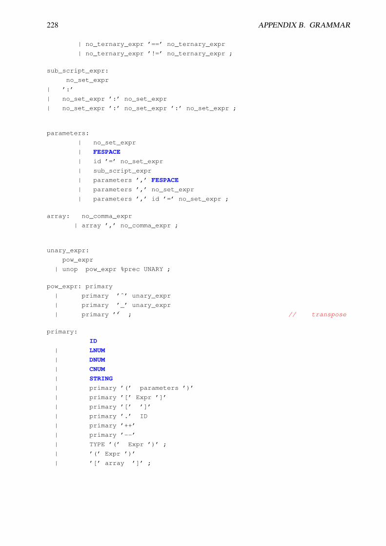
228 APPENDIX B. GRAMMAR
| no_ternary_expr ’==’ no_ternary_expr
| no_ternary_expr ’!=’ no_ternary_expr ;
sub_script_expr:
no_set_expr
| ’:’
| no_set_expr ’:’ no_set_expr
| no_set_expr ’:’ no_set_expr ’:’ no_set_expr ;
parameters:
| no_set_expr
| FESPACE
| id ’=’ no_set_expr
| sub_script_expr
| parameters ’,’ FESPACE
| parameters ’,’ no_set_expr
| parameters ’,’ id ’=’ no_set_expr ;
array: no_comma_expr
| array ’,’ no_comma_expr ;
unary_expr:
pow_expr
| unop pow_expr %prec UNARY ;
pow_expr: primary
| primary ’ˆ’ unary_expr
| primary ’_’ unary_expr
| primary ’’ ; // transpose
primary:
ID
| LNUM
| DNUM
| CNUM
| STRING
| primary ’(’ parameters ’)’
| primary ’[’ Expr ’]’
| primary ’[’ ’]’
| primary ’.’ ID
| primary ’++’
| primary ’--’
| TYPE ’(’ Expr ’)’ ;
| ’(’ Expr ’)’
| ’[’ array ’]’ ;

B.2. THE TYPES OF THE LANGUAGES, AND CAST 229
B.2 The Types of the languages, and cast
B.3 All the operators
- CG, type :<TypeSolveMat>- Cholesky, type :<TypeSolveMat>- Crout, type :<TypeSolveMat>- GMRES, type :<TypeSolveMat>- LU, type :<TypeSolveMat>- LinearCG, type :<Polymorphic> operator() :( <long> : <Polymorphic>, <KN<double> *>, <KN<double> *> )
- N, type :<Fem2D::R3>- NoUseOfWait, type :<bool *>- P, type :<Fem2D::R3>- P0, type :<Fem2D::TypeOfFE>- P1, type :<Fem2D::TypeOfFE>- P1nc, type :<Fem2D::TypeOfFE>- P2, type :<Fem2D::TypeOfFE>- RT0, type :<Fem2D::TypeOfFE>- RTmodif, type :<Fem2D::TypeOfFE>- abs, type :<Polymorphic> operator() :( <double> : <double> )
- acos, type :<Polymorphic> operator() :( <double> : <double> )
- acosh, type :<Polymorphic> operator() :( <double> : <double> )
- adaptmesh, type :<Polymorphic> operator() :( <Fem2D::Mesh> : <Fem2D::Mesh>... )
- append, type :<std::ios_base::openmode>- asin, type :<Polymorphic> operator() :( <double> : <double> )
- asinh, type :<Polymorphic> operator() :( <double> : <double> )
- atan, type :<Polymorphic> operator() :( <double> : <double> )( <double> : <double>, <double> )
- atan2, type :<Polymorphic> operator() :( <double> : <double>, <double> )
- atanh, type :<Polymorphic> operator() :( <double> : <double> )

230 APPENDIX B. GRAMMAR
- buildmesh, type :<Polymorphic> operator() :( <Fem2D::Mesh> : <E_BorderN> )
- buildmeshborder, type :<Polymorphic> operator() :( <Fem2D::Mesh> : <E_BorderN> )
- cin, type :<istream>- clock, type :<Polymorphic>( <double> : )
- conj, type :<Polymorphic> operator() :( <complex> : <complex> )
- convect, type :<Polymorphic> operator() :( <double> : <E_Array>, <double>, <double> )
- cos, type :<Polymorphic> operator() :( <double> : <double> )( <complex> : <complex> )
- cosh, type :<Polymorphic> operator() :( <double> : <double> )( <complex> : <complex> )
- cout, type :<ostream>- dumptable, type :<Polymorphic> operator() :( <ostream> : <ostream> )
- dx, type :<Polymorphic> operator() :( <LinearComb<MDroit, C_F0>> : <LinearComb<MDroit, C_F0>> )( <double> : <std::pair<FEbase<double> *, int>> )( <LinearComb<MGauche, C_F0>> : <LinearComb<MGauche, C_F0>> )
- dy, type :<Polymorphic> operator() :( <LinearComb<MDroit, C_F0>> : <LinearComb<MDroit, C_F0>> )( <double> : <std::pair<FEbase<double> *, int>> )( <LinearComb<MGauche, C_F0>> : <LinearComb<MGauche, C_F0>> )
- endl, type :<char>- exec, type :<Polymorphic> operator() :( <long> : <string> )
- exit, type :<Polymorphic> operator() :( <long> : <long> )
- exp, type :<Polymorphic> operator() :( <double> : <double> )( <complex> : <complex> )

B.3. ALL THE OPERATORS 231
- false, type :<bool>- imag, type :<Polymorphic> operator() :( <double> : <complex> )
- int1d, type :<Polymorphic> operator() :( <CDomainOfIntegration> : <Fem2D::Mesh>... )
- int2d, type :<Polymorphic> operator() :( <CDomainOfIntegration> : <Fem2D::Mesh>... )
- intalledges, type :<Polymorphic>operator( :( <CDomainOfIntegration> : <Fem2D::Mesh>... )
- jump, type :<Polymorphic>operator( :( <LinearComb<MDroit, C_F0>> : <LinearComb<MDroit, C_F0>> )( <double> : <double> )( <complex > : <complex > )( <LinearComb<MGauche, C_F0>> : <LinearComb<MGauche, C_F0>> )
- label, type :<long *>- log, type :<Polymorphic> operator() :( <double> : <double> )( <complex> : <complex> )
- log10, type :<Polymorphic> operator() :( <double> : <double> )
- max, type :<Polymorphic> operator() :( <double> : <double>, <double> )( <long> : <long>, <long> )
- mean, type :<Polymorphic>operator( :( <double> : <double> )( <complex> : <complex> )
- min, type :<Polymorphic> operator() :( <double> : <double>, <double> )( <long> : <long>, <long> )
- movemesh, type :<Polymorphic> operator() :( <Fem2D::Mesh> : <Fem2D::Mesh>, <E_Array>... )
- norm, type :<Polymorphic>operator( :( <double> : <std::complex<double>> )
- nuTriangle, type :<long>

232 APPENDIX B. GRAMMAR
- nuEdge, type :<long>- on, type :<Polymorphic> operator() :( <BC_set<double>> : <long>... )
- otherside, type :<Polymorphic>operator( :( <LinearComb<MDroit, C_F0>> : <LinearComb<MDroit, C_F0>> )( <LinearComb<MGauche, C_F0>> : <LinearComb<MGauche, C_F0>> )
- pi, type :<double>- plot, type :<Polymorphic> operator() :( <long> : ... )
- pow, type :<Polymorphic> operator() :( <double> : <double>, <double> )( <complex> : <complex>, <complex> )
- qf1pE, type :<Fem2D::QuadratureFormular1d>- qf1pT, type :<Fem2D::QuadratureFormular>- qf1pTlump, type :<Fem2D::QuadratureFormular>- qf2pE, type :<Fem2D::QuadratureFormular1d>- qf2pT, type :<Fem2D::QuadratureFormular>- qf2pT4P1, type :<Fem2D::QuadratureFormular>- qf3pE, type :<Fem2D::QuadratureFormular1d>- qf5pT, type :<Fem2D::QuadratureFormular>
- readmesh, type :<Polymorphic> operator() :( <Fem2D::Mesh> : <string> )
- real, type :<Polymorphic> operator() :( <double> : <complex> )
- region, type :<long *>- savemesh, type :<Polymorphic> operator() :( <Fem2D::Mesh> : <Fem2D::Mesh>, <string>... )
- sin, type :<Polymorphic> operator() :( <double> : <double> )( <complex> : <complex> )
- sinh, type :<Polymorphic> operator() :( <double> : <double> )( <complex> : <complex> )
- sqrt, type :<Polymorphic> operator() :( <double> : <double> )( <complex> : <complex> )
- square, type :<Polymorphic> operator() :( <Fem2D::Mesh> : <long>, <long> )

B.3. ALL THE OPERATORS 233
( <Fem2D::Mesh> : <long>, <long>, <E_Array> )
- tan, type :<Polymorphic> operator() :( <double> : <double> )
- true, type :<bool>- trunc, type :<Polymorphic> operator() :( <Fem2D::Mesh> : <Fem2D::Mesh>, <bool> )
- verbosity, type :<long *>- wait, type :<bool *>- x, type :<double *>- y, type :<double *>- z, type :<double *>

234 APPENDIX B. GRAMMAR

Appendix C
Dynamical link
Now, it’s possible to add built-in functionnalites in FreeFem++ under the three environnentsLinux, Windows and MacOS X 10.3 or newer. It is agood idea to, first try the example load.edpin directory example++-load.But unfortunately, you need to install a c++ compiler (generally g++/gcc compiler) to compileyour function.
Windows Install the cygwin environnent or the mingw
MacOs Install the developer tools xcode on the apple DVD
Linux/Unix Install the correct compiler (gcc for instance)
Now, assume , you are in a shell window (a cygwin window under Windows) in the directoryexample++-load. Remark that in the sub directory include they are all the FreeFem++include file to make the link with FreeFem++.
Note C.1 If you try to load dynamically a file with command load "xxx"
• Under unix (Linux or MacOs), the file xxx.so to be loaded must be either first in the searchdirectory of routine dlopen (see the environment variable $LD_LIBRARY_PATH or in thecurrent directory, and the suffix ".so" or the prefix "./" is automaticaly added.
• Under Windows, the file xxx.dll to be loaded must be in the loadLibary search direc-tory which includes the directory of the application,
The compilation of your module: the script ./load.link compiles and makes the link withFreeFem++, but be careful, the script has no way to known if you try to compile for a pureWindows environment or for a cygwin environment so to build the load module under cygwin youmust add the -cygwin parameter.
C.1 A first example myfunction.cppThe following defines a new function call myfunction with no parameter, but using the x, ycurrent value.
#include <iostream>
235

236 APPENDIX C. DYNAMICAL LINK
#include <cfloat>using namespace std;#include "error.hpp"#include "AFunction.hpp"#include "rgraph.hpp"#include "RNM.hpp"#include "fem.hpp"#include "FESpace.hpp"#include "MeshPoint.hpp"
using namespace Fem2D;double myfunction(Stack stack)
// to get FreeFem++ dataMeshPoint &mp= *MeshPointStack(stack); // the struct to get x,y, normal ,
valuedouble x= mp.P.x; // get the current x valuedouble y= mp.P.y; // get the current y value
// cout << "x = " << x << " y=" << y << endl;return sin(x)*cos(y);
Now the Problem is to build the link with FreeFem++, to do that we need two classes, one to callthe function myfunctionAll FreeFem++ evaluable expression must be a struct/class C++ which derive from E F0. Bydefault this expression does not depend of the mesh position, but if they derive from E F0mps theexpression depends of the mesh position, and for more details see [11].
// A class build the link with FreeFem++// generaly this class are already in AFunction.hpp
// but unfortunatly, I have no simple function with no parameter// in FreeFem++ depending of the mesh,
template<class R>class OneOperator0s : public OneOperator
// the class to defined a evaluated a new function// It must devive from E F0 if it is mesh independent
// or from E F0mps if it is mesh dependentclass E_F0_F :public E_F0mps public:
typedef R (*func)(Stack stack) ;func f; // the pointeur to the fnction myfunctionE_F0_F(func ff) : f(ff)
// the operator evaluation in FreeFem++AnyType operator()(Stack stack) const return SetAny<R>( f(stack)) ;
;
typedef R (*func)(Stack ) ;func f;
public:// the function which build the FreeFem++ byte code
E_F0 * code(const basicAC_F0 & ) const return new E_F0_F(f);// the constructor to say ff is a function without parameter
// and returning a ROneOperator0s(func ff): OneOperator(map_type[typeid(R).name()]),f(ff)
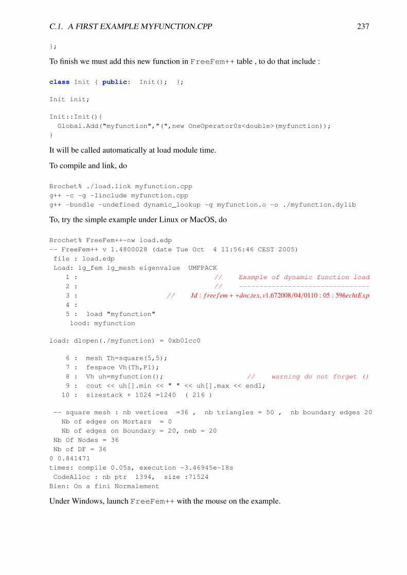
C.1. A FIRST EXAMPLE MYFUNCTION.CPP 237
;
To finish we must add this new function in FreeFem++ table , to do that include :
class Init public: Init(); ;
Init init;
Init::Init()
Global.Add("myfunction","(",new OneOperator0s<double>(myfunction));
It will be called automatically at load module time.
To compile and link, do
Brochet% ./load.link myfunction.cpp
g++ -c -g -Iinclude myfunction.cpp
g++ -bundle -undefined dynamic_lookup -g myfunction.o -o ./myfunction.dylib
To, try the simple example under Linux or MacOS, do
Brochet% FreeFem++-nw load.edp
-- FreeFem++ v 1.4800028 (date Tue Oct 4 11:56:46 CEST 2005)
file : load.edp
Load: lg_fem lg_mesh eigenvalue UMFPACK
1 : // Example of dynamic function load
2 : // --------------------------------
3 : // Id : f ree f em + +doc.tex, v1.672008/04/0110 : 05 : 59hechtExp4 :
5 : load "myfunction"
lood: myfunction
load: dlopen(./myfunction) = 0xb01cc0
6 : mesh Th=square(5,5);
7 : fespace Vh(Th,P1);
8 : Vh uh=myfunction(); // warning do not forget ()
9 : cout << uh[].min << " " << uh[].max << endl;
10 : sizestack + 1024 =1240 ( 216 )
-- square mesh : nb vertices =36 , nb triangles = 50 , nb boundary edges 20
Nb of edges on Mortars = 0
Nb of edges on Boundary = 20, neb = 20
Nb Of Nodes = 36
Nb of DF = 36
0 0.841471
times: compile 0.05s, execution -3.46945e-18s
CodeAlloc : nb ptr 1394, size :71524
Bien: On a fini Normalement
Under Windows, launch FreeFem++ with the mouse on the example.

238 APPENDIX C. DYNAMICAL LINK
C.2 Example Discrete Fast Fourier TransformThis will add FFT to FreeFem++,taken from http://www.fftw.org/. To download andinstall under download/include just go in download/fftw and trymake.
The 1D dfft (fast discret fourier transform) for a simple array f of size n is defined by the followingformula
dfft( f , ε)k =
n−1∑j=0
fieε2πik j/n
The 2D DFT for an array of size N = n × m is
dfft( f ,m, ε)k+nl =
m−1∑j′=0
n−1∑j=0
fi+n jeε2πi(k j/n+l j′/m)
Remark: the value n is given by size( f )/m, and the numbering is row-major order.So the classical discrete DFT is f = dfft( f ,−1)/
√n and the reverse dFT f = dfft( f , 1)/
√n
Remark: the 2D Laplace operator is
f (x, y) = 1/√
Nm−1∑j′=0
n−1∑j=0
fi+n jeε2πi(x j+y j′)
and we havefk+nl = f (k/n, l/m)
So∆ fkl = −((2π)2((k)2 + (l)2)) fkl
where k = k if k ≤ n/2 else k = k − n and l = l if l ≤ m/2 else l = l − m.And to get a real function we need all symetric modes around to zero, so n and m must be odd.To compile and make a new library
% ./load.link dfft.cpp ../download/install/lib/libfftw3.a -I../download/install/includeexport MACOSX_DEPLOYMENT_TARGET=10.3g++ -c -Iinclude -I../download/install/include dfft.cppg++ -bundle -undefined dynamic_lookup dfft.o -o ./dfft.dylib ../download/install/lib/libfftw3.a
To test ,
-- FreeFem++ v 1.4800028 (date Mon Oct 10 16:53:28 EEST 2005)file : dfft.edpLoad: lg_fem cadna lg_mesh eigenvalue UMFPACK
1 : // Example of dynamic function load2 : // --------------------------------3 : // Id : f ree f em + +doc.tex, v1.672008/04/0110 : 05 : 59hechtExp4 : // Discret Fast Fourier Transform5 : // -------------------------------6 : load "dfft" lood: init dfft
load: dlopen(dfft.dylib) = 0x2b0c700
7 :8 : int nx=32,ny=16,N=nx*ny;

C.2. EXAMPLE DISCRETE FAST FOURIER TRANSFORM 239
9 : // warning the fourier space is not exactly the unite square// due to periodic condition
10 : mesh Th=square(nx-1,ny-1,[(nx-1)*x/nx,(ny-1)*y/ny]);11 : // warring the numbering is of the vertices (x,y) is12 : // given by i = x/nx + nx ∗ y/ny13 :14 : fespace Vh(Th,P1);15 :16 : func f1 = cos(2*x*2*pi)*cos(3*y*2*pi);17 : Vh<complex> u=f1,v;18 : Vh w=f1;19 :20 :21 : Vh ur,ui;22 : // in dfft the matrix n,m is in row-major order ann array n,m is23 : // store j + m* i ( the transpose of the square numbering )24 : v[]=dfft(u[],ny,-1);25 : u[]=dfft(v[],ny,+1);26 : u[] /= complex(N);27 : v = f1-u;28 : cout << " diff = "<< v[].max << " " << v[].min << endl;29 : assert( norm(v[].max) < 1e-10 && norm(v[].min) < 1e-10) ;30 : // ------- a more hard example ----31 : // Lapacien en FFT32 : // −∆u = f with biperiodic condition33 : func f = cos(3*2*pi*x)*cos(2*2*pi*y); //34 : func ue = +(1./(square(2*pi)*13.))*cos(3*2*pi*x)*cos(2*2*pi*y); //
35 : Vh<complex> ff = f;36 : Vh<complex> fhat;37 : fhat[] = dfft(ff[],ny,-1);38 :39 : Vh<complex> wij;40 : // warning in fact we take mode between -nx/2, nx/2 and -ny/2,ny/241 : // thank to the operator ?:42 : wij = square(2.*pi)*(square(( x<0.5?x*nx:(x-1)*nx))
+ square((y<0.5?y*ny:(y-1)*ny)));43 : wij[][0] = 1e-5; // to remove div / 044 : fhat[] = fhat[]./ wij[]; //45 : u[]=dfft(fhat[],ny,1);46 : u[] /= complex(N);47 : ur = real(u); // the solution48 : w = real(ue); // the exact solution49 : plot(w,ur,value=1 ,cmm=" ue ", wait=1);50 : w[] -= ur[]; // array sub51 : real err= abs(w[].max)+abs(w[].min) ;52 : cout << " err = " << err << endl;53 : assert( err < 1e-6);54 : sizestack + 1024 =3544 ( 2520 )
----------CheckPtr:-----init execution ------ NbUndelPtr 2815 Alloc: 111320 NbPtr6368
-- square mesh : nb vertices =512 , nb triangles = 930 , nb boundary edges 92Nb of edges on Mortars = 0Nb of edges on Boundary = 92, neb = 92
Nb Of Nodes = 512

240 APPENDIX C. DYNAMICAL LINK
Nb of DF = 5120x2d383d8 -1 16 512 n: 16 m:32dfft 0x402bc08 = 0x4028208 n = 16 32 sign = -1--- --- ---0x2d3ae08 1 16 512 n: 16 m:32dfft 0x4028208 = 0x402bc08 n = 16 32 sign = 1--- --- --- diff = (8.88178e-16,3.5651e-16) (-6.66134e-16,-3.38216e-16)
0x2d3cfb8 -1 16 512 n: 16 m:32dfft 0x402de08 = 0x402bc08 n = 16 32 sign = -1--- --- ---0x2d37ff8 1 16 512 n: 16 m:32dfft 0x4028208 = 0x402de08 n = 16 32 sign = 1--- --- --- err = 3.6104e-12
times: compile 0.13s, execution 2.05s----------CheckPtr:-----end execution -- ------ NbUndelPtr 2815 Alloc: 111320NbPtr 26950CodeAlloc : nb ptr 1693, size :76084
Bien: On a fini NormalementCheckPtr:Nb of undelete pointer is 2748 last 114CheckPtr:Max Memory used 228.531 kbytes Memory undelete 105020
C.3 Load Module for Dervieux’ P0-P1 Finite Volume Methodthe associed edp file is examples++-load/convect dervieux.edp
// Implementation of P1-P0 FVM-FEM// ---------------------------------------------------------------------
// Id : f ree f em + +doc.tex, v1.672008/04/0110 : 05 : 59hechtExp// compile and link with ./load.link mat dervieux.cpp (i.e. the file name
without .cpp)#include <iostream>#include <cfloat>#include <cmath>using namespace std;#include "error.hpp"#include "AFunction.hpp"#include "rgraph.hpp"#include "RNM.hpp"
// remove problem of include#undef HAVE_LIBUMFPACK#undef HAVE_CADNA#include "MatriceCreuse_tpl.hpp"#include "MeshPoint.hpp"#include "lgfem.hpp"#include "lgsolver.hpp"#include "problem.hpp"
class MatrixUpWind0 : public E_F0mps public:typedef Matrice_Creuse<R> * Result;Expression emat,expTh,expc,expu1,expu2;MatrixUpWind0(const basicAC_F0 & args)
args.SetNameParam();emat =args[0]; // the matrix expression

C.3. LOAD MODULE FOR DERVIEUX’ P0-P1 FINITE VOLUME METHOD 241
expTh= to<pmesh>(args[1]); // a the expression to get the meshexpc = CastTo<double>(args[2]); // the expression to get c (must be a
double)// a array expression [ a, b]
const E_Array * a= dynamic_cast<const E_Array*>((Expression) args[3]);if (a->size() != 2) CompileError("syntax: MatrixUpWind0(Th,rhi,[u1,u2])");int err =0;expu1= CastTo<double>((*a)[0]); // fist exp of the array (must be a
double)expu2= CastTo<double>((*a)[1]); // second exp of the array (must be a
double)
˜MatrixUpWind0()
static ArrayOfaType typeargs() return ArrayOfaType(atype<Matrice_Creuse<R>*>(),
atype<pmesh>(),atype<double>(),atype<E_Array>());static E_F0 * f(const basicAC_F0 & args) return new MatrixUpWind0(args);AnyType operator()(Stack s) const ;
;
int fvmP1P0(double q[3][2], double u[2],double c[3], double a[3][3], double where[3]) // computes matrix a on a triangle for theDervieux FVM
for(int i=0;i<3;i++) for(int j=0;j<3;j++) a[i][j]=0;
for(int i=0;i<3;i++)int ip = (i+1)%3, ipp =(ip+1)%3;double unL =-((q[ip][1]+q[i][1]-2*q[ipp][1])*u[0]
-(q[ip][0]+q[i][0]-2*q[ipp][0])*u[1])/6;if(unL>0) a[i][i] += unL; a[ip][i]-=unL;
else a[i][ip] += unL; a[ip][ip]-=unL;if(where[i]&&where[ip]) // this is a boundary edge
unL=((q[ip][1]-q[i][1])*u[0] -(q[ip][0]-q[i][0])*u[1])/2;if(unL>0) a[i][i]+=unL; a[ip][ip]+=unL;
return 1;
// the evaluation routineAnyType MatrixUpWind0::operator()(Stack stack) const
Matrice_Creuse<R> * sparse_mat =GetAny<Matrice_Creuse<R>* >((*emat)(stack));MatriceMorse<R> * amorse =0;MeshPoint *mp(MeshPointStack(stack)) , mps=*mp;Mesh * pTh = GetAny<pmesh>((*expTh)(stack));ffassert(pTh);Mesh & Th (*pTh);

242 APPENDIX C. DYNAMICAL LINK
map< pair<int,int>, R> Aij;KN<double> cc(Th.nv);double infini=DBL_MAX;cc=infini;for (int it=0;it<Th.nt;it++)
for (int iv=0;iv<3;iv++)
int i=Th(it,iv);if ( cc[i]==infini) // if nuset the set
mp->setP(&Th,it,iv);cc[i]=GetAny<double>((*expc)(stack));
for (int k=0;k<Th.nt;k++)
const Triangle & K(Th[k]);const Vertex & A(K[0]), &B(K[1]),&C(K[2]);R2 Pt(1./3.,1./3.);R u[2];MeshPointStack(stack)->set(Th,K(Pt),Pt,K,K.lab);u[0] = GetAny< R>( (*expu1)(stack) ) ;u[1] = GetAny< R>( (*expu2)(stack) ) ;
int ii[3] = Th(A), Th(B),Th(C);double q[3][2]= A.x,A.y ,B.x,B.y,C.x,C.y ; // coordinates
of 3 vertices (input)double c[3]=cc[ii[0]],cc[ii[1]],cc[ii[2]];double a[3][3], where[3]=A.lab,B.lab,C.lab;if (fvmP1P0(q,u,c,a,where) )
for (int i=0;i<3;i++)for (int j=0;j<3;j++)
if (fabs(a[i][j]) >= 1e-30) Aij[make_pair(ii[i],ii[j])]+=a[i][j];
amorse= new MatriceMorse<R>(Th.nv,Th.nv,Aij,false);sparse_mat->pUh=0;sparse_mat->pVh=0;sparse_mat->A.master(amorse);sparse_mat->typemat=(amorse->n == amorse->m) ? TypeSolveMat(TypeSolveMat::GMRES)
: TypeSolveMat(TypeSolveMat::NONESQUARE); // none square matrice (morse)
*mp=mps;
if(verbosity>3) cout << " End Build MatrixUpWind : " << endl;
return sparse_mat;
class Init public:Init();
;

C.4. ADD A NEW FINITE ELEMENT 243
Init init;Init::Init()
cout << " lood: init Mat Chacon " << endl;Global.Add("MatUpWind0","(", new OneOperatorCode<MatrixUpWind0 >( ));
C.4 Add a new finite elementFirst read the section 13 of the appendix, we add two new finite elements examples in the directoryexamples++-load.
Bernardi Raugel The Bernardi-Raugel finite element is make to solve Navier Stokes equationin u, p formulation, and the velocity space Pbr
K is minimal to prove the inf-sup condition withpiecewise contante pressure by triangle.the finite element space Vh is
Vh = u ∈ H1(Ω)2; ∀K ∈ Th, u|K ∈ PbrK
wherePbr
K = spanλKi eki=1,2,3,k=1,2 ∪ λ
Ki λ
Ki+1nK
i+2i=1,2,3
with notation 4 = 1, 5 = 2 and where λKi are the barycentric coordonnate of the triangle K, (ek)k=1,2
the canonical basis of R2 and nKk the outer normal of triangle K opposite to vertex k.
// The P2BR finite element : the Bernadi Raugel Finite Element// F. Hecht, decembre 2005// -------------// See Bernardi, C., Raugel, G.: Analysis of some finite elements for the
Stokes problem. Math. Comp. 44, 71-79 (1985).// It is a 2d coupled FE// the Polynomial space is P12 + 3 normals bubbles edges function (P2)
// the degre of freedom is 6 values at of the 2 componantes at the 3vertices// and the 3 flux on the 3 edges// So 9 degrees of freedom and N= 2.
// ----------------------- related files:// to check and validate : testFE.edp// to get a real example : NSP2BRP0.edp// ------------------------------------------------------------
// -----------------------#include "error.hpp"#include "AFunction.hpp"#include "rgraph.hpp"using namespace std;#include "RNM.hpp"#include "fem.hpp"#include "FESpace.hpp"#include "AddNewFE.h"

244 APPENDIX C. DYNAMICAL LINK
namespace Fem2D
class TypeOfFE_P2BRLagrange : public TypeOfFE public:static int Data[];
TypeOfFE_P2BRLagrange(): TypeOfFE(6+3+0,2,Data,4,1,6+3*(2+2), // nb coef to build interpolation9, // np point to build interpolation0)
.... // to long see the source
void FB(const bool * whatd, const Mesh & Th,const Triangle & K,const R2 &P,
RNMK_ & val) const;void TypeOfFE_P2BRLagrange::Pi_h_alpha(const baseFElement & K,KN_<double> &
v) const; ;
// on what nu df on node node of dfint TypeOfFE_P2BRLagrange::Data[]=
0,0, 1,1, 2,2, 3,4,5,0,1, 0,1, 0,1, 0,0,0,0,0, 1,1, 2,2, 3,4,5,0,0, 0,0, 0,0, 0,0,0,0,1, 2,3, 4,5, 6,7,8,0,0
;
void TypeOfFE_P2BRLagrange::Pi_h_alpha(const baseFElement & K,KN_<double> & v) const
const Triangle & T(K.T);int k=0;
// coef pour les 3 sommets fois le 2 composantesfor (int i=0;i<6;i++)
v[k++]=1;// integration sur les aretes
for (int i=0;i<3;i++)
R2 N(T.Edge(i).perp());N *= T.EdgeOrientation(i)*0.5 ;
v[k++]= N.x;v[k++]= N.y;v[k++]= N.x;v[k++]= N.y;
void TypeOfFE_P2BRLagrange::FB(const bool * whatd,const Mesh & ,const Triangle& K,const R2 & P,RNMK_ & val) const
.... // to long see the source

C.4. ADD A NEW FINITE ELEMENT 245
// ---- cooking to add the finite elemet to freefem table --------// a static variable to def the finite element
static TypeOfFE_P2BRLagrange P2LagrangeP2BR;// now adding FE in FreeFEm++ table
static AddNewFE P2BR("P2BR",&P2LagrangeP2BR);// --- end cooking
// end FEM2d namespace
A way to check the finite element
load "BernadiRaugel"// a macro the compute numerical derivative
macro DD(f,hx,hy) ( (f(x1+hx,y1+hy)-f(x1-hx,y1-hy))/(2*(hx+hy))) //mesh Th=square(1,1,[10*(x+y/3),10*(y-x/3)]);
real x1=0.7,y1=0.9, h=1e-7;int it1=Th(x1,y1).nuTriangle;
fespace Vh(Th,P2BR);
Vh [a1,a2],[b1,b2],[c1,c2];
for (int i=0;i<Vh.ndofK;++i)cout << i << " " << Vh(0,i) << endl;for (int i=0;i<Vh.ndofK;++i)
a1[]=0;int j=Vh(it1,i);a1[][j]=1; // a bascis functionsplot([a1,a2], wait=1);
[b1,b2]=[a1,a2]; // do the interpolation
c1[] = a1[] - b1[];
cout << " ---------" << i << " " << c1[].max << " " << c1[].min << endl;cout << " a = " << a1[] <<endl;cout << " b = " << b1[] <<endl;assert(c1[].max < 1e-9 && c1[].min > -1e-9); // check if the
interpolation is correct
// check the derivative and numerical derivative
cout << " dx(a1)(x1,y1) = " << dx(a1)(x1,y1) << " == " << DD(a1,h,0) << endl;assert( abs(dx(a1)(x1,y1)-DD(a1,h,0) ) < 1e-5);assert( abs(dx(a2)(x1,y1)-DD(a2,h,0) ) < 1e-5);assert( abs(dy(a1)(x1,y1)-DD(a1,0,h) ) < 1e-5);assert( abs(dy(a2)(x1,y1)-DD(a2,0,h) ) < 1e-5);

246 APPENDIX C. DYNAMICAL LINK
A real example using this finite element, just a small modification of the NSP2P1.edp examples,just the begenning is change to
load "BernadiRaugel"
real s0=clock();mesh Th=square(10,10);fespace Vh2(Th,P2BR);fespace Vh(Th,P0);Vh2 [u1,u2],[up1,up2];Vh2 [v1,v2];
And the plot instruction is also change because the pressure is constant, and we cannot plot isoval-ues.
Morley See the example.
C.5 Add a new sparse solverI will show the sketch of the code, see the full code from SuperLU.cpp or NewSolve.cpp.First the include files:
#include <iostream>using namespace std;
#include "rgraph.hpp"#include "error.hpp"#include "AFunction.hpp"
// #include "lex.hpp"#include "MatriceCreuse_tpl.hpp"#include "slu_ddefs.h"#include "slu_zdefs.h"
A small template driver to unified the double and Complex version.
template <class R> struct SuperLUDriver
;
template <> struct SuperLUDriver<double>
.... double version;
template <> struct SuperLUDriver<Complex>.... Complex version;

C.5. ADD A NEW SPARSE SOLVER 247
To get Matrix value, we have just to remark that the Morse Matrice the storage, is the SLU NRformat is the compressed row storage, this is the transpose of the compressed column storage.So if AA is a MatriceMorse you have with SuperLU notatiopn.
n=AA.n;m=AA.m;nnz=AA.nbcoef;a=AA.a;asub=AA.cl;xa=AA.lg;options.Trans = TRANS;
Dtype_t R_SLU = SuperLUDriver<R>::R_SLU_T();Create_CompCol_Matrix(&A, m, n, nnz, a, asub, xa, SLU_NC, R_SLU, SLU_GE);
To get vector infomation, to solver the linear solver x = A−1b
void Solver(const MatriceMorse<R> &AA,KN_<R> &x,const KN_<R> &b) const....
Create_Dense_Matrix(&B, m, 1, b, m, SLU_DN, R_SLU, SLU_GE);Create_Dense_Matrix(&X, m, 1, x, m, SLU_DN, R_SLU, SLU_GE);
....
The two BuildSolverSuperLU function, to change the default sparse solver variableDefSparseSolver<double>::solver
MatriceMorse<double>::VirtualSolver *BuildSolverSuperLU(const MatriceMorse<double> *A,int strategy,double tgv, doubleeps,
double tol_pivot,double tol_pivot_sym,int NbSpace,int itmax ,const void * precon, ?void * stack)
if(verbosity>9)
cout << " BuildSolverSuperLU<double>" << endl;return new SolveSuperLU<double>(*A,strategy,tgv,eps,tol_pivot,tol_pivot_sym);
MatriceMorse<Complex>::VirtualSolver *BuildSolverSuperLU(const MatriceMorse<Complex> *A,int strategy,double tgv, doubleeps,
double tol_pivot,double tol_pivot_sym,int NbSpace,int itmax ,const void * precon, void * stack)
if(verbosity>9)cout << " BuildSolverSuperLU<Complex>" << endl;return new SolveSuperLU<Complex>(*A,strategy,tgv,eps,tol_pivot,tol_pivot_sym);
The link to FreeFem++
class Init public:Init();
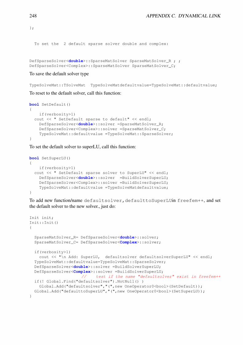
248 APPENDIX C. DYNAMICAL LINK
;
To set the 2 default sparse solver double and complex:
DefSparseSolver<double>::SparseMatSolver SparseMatSolver_R ; ;DefSparseSolver<Complex>::SparseMatSolver SparseMatSolver_C;
To save the default solver type
TypeSolveMat::TSolveMat TypeSolveMatdefaultvalue=TypeSolveMat::defaultvalue;
To reset to the default solver, call this function:
bool SetDefault()
if(verbosity>1)cout << " SetDefault sparse to default" << endl;
DefSparseSolver<double>::solver =SparseMatSolver_R;DefSparseSolver<Complex>::solver =SparseMatSolver_C;TypeSolveMat::defaultvalue =TypeSolveMat::SparseSolver;
To set the default solver to superLU, call this function:
bool SetSuperLU()
if(verbosity>1)cout << " SetDefault sparse solver to SuperLU" << endl;
DefSparseSolver<double>::solver =BuildSolverSuperLU;DefSparseSolver<Complex>::solver =BuildSolverSuperLU;TypeSolveMat::defaultvalue =TypeSolveMatdefaultvalue;
To add new function/name defaultsolver,defaulttoSuperLUin freefem++, and setthe default solver to the new solver., just do:
Init init;Init::Init()
SparseMatSolver_R= DefSparseSolver<double>::solver;SparseMatSolver_C= DefSparseSolver<Complex>::solver;
if(verbosity>1)cout << "\n Add: SuperLU, defaultsolver defaultsolverSuperLU" << endl;
TypeSolveMat::defaultvalue=TypeSolveMat::SparseSolver;DefSparseSolver<double>::solver =BuildSolverSuperLU;DefSparseSolver<Complex>::solver =BuildSolverSuperLU;
// test if the name "defaultsolver" exist in freefem++if(! Global.Find("defaultsolver").NotNull() )
Global.Add("defaultsolver","(",new OneOperator0<bool>(SetDefault));Global.Add("defaulttoSuperLU","(",new OneOperator0<bool>(SetSuperLU));

C.5. ADD A NEW SPARSE SOLVER 249
To compile superlu.cpp, just do:
1. download the SuperLu 3.0 package and do
curl http://crd.lbl.gov/˜xiaoye/SuperLU/superlu_3.0.tar.gz -o superlu_3.0.tar.gztar xvfz superlu_3.0.tar.gzgo SuperLU_3.0 directory$EDITOR make.incmake
2. In directoy include do to have a correct version of SuperLu header due to mistake in caseof inclusion of double and Complex version in the same file.
tar xvfz ../SuperLU_3.0-include-ff.tar.gz
I will give a correct one to compile with freefm++.
To compile the freefem++ load file of SuperLu with freefem do: some find like :
./load.link SuperLU.cpp -L$HOME/work/LinearSolver/SuperLU_3.0/ -lsuperlu_3.0
And to test the simple example:
A example:
load "SuperLU"verbosity=2;for(int i=0;i<3;++i)// if i == 0 then SuperLu solver// i == 1 then GMRES solver// i == 2 then Default solver
matrix A =
[[ 0, 1, 0, 10],[ 0, 0, 2, 0],[ 0, 0, 0, 3],[ 4,0 , 0, 0]];
real[int] xx = [ 4,1,2,3], x(4), b(4);b = A*xx;cout << b << " " << xx << endl;set(A,solver=sparsesolver);x = Aˆ-1*b;cout << x << endl;
matrix<complex> A =
[[ 0, 1i, 0, 10],[ 0 , 0, 2i, 0],[ 0, 0, 0, 3i],[ 4i,0 , 0, 0]];
complex[int] xx = [ 4i,1i,2i,3i], x(4), b(4);

250 APPENDIX C. DYNAMICAL LINK
b = A*xx;cout << b << " " << xx << endl;set(A,solver=sparsesolver);x = Aˆ-1*b;cout << x << endl;
if(i==0)defaulttoGMRES();if(i==1)defaultsolver();
To Test do for exemple:
FreeFem++ SuperLu.edp

FreeFem++ LGPL License
This is The FreeFem++ software. Programs in it were maintained by
• Frederic hecht <[email protected]>
• Olivier Pironneau <[email protected]>
• Antoine Le Hyaric <[email protected]>
All its programs except files the comming from ARPACK++ software (files in directory ARPACK/a-pack++/include ) COOOL sofware (files in directory src/Algo) and the file mt19937ar.cppwhich may be redistributed under the terms of the GNU LESSER GENERAL PUBLIC LICENSEVersion 2.1, February 1999GNU LESSER GENERAL PUBLIC LICENSE TERMS AND CONDITIONS FOR COPYING,DISTRIBUTION AND MODIFICATION0. This License Agreement applies to any software library or other program which contains anotice placed by the copyright holder or other authorized party saying it may be distributed underthe terms of this Lesser General Public License (also called ”this License”). Each licensee isaddressed as ”you”.A ”library” means a collection of software functions and/or data prepared so as to be convenientlylinked with application programs (which use some of those functions and data) to form executables.The ”Library”, below, refers to any such software library or work which has been distributed underthese terms. A ”work based on the Library” means either the Library or any derivative work undercopyright law: that is to say, a work containing the Library or a portion of it, either verbatim or withmodifications and/or translated straightforwardly into another language. (Hereinafter, translationis included without limitation in the term ”modification”.)”Source code” for a work means the preferred form of the work for making modifications to it.For a library, complete source code means all the source code for all modules it contains, plus anyassociated interface definition files, plus the scripts used to control compilation and installation ofthe library.Activities other than copying, distribution and modification are not covered by this License; theyare outside its scope. The act of running a program using the Library is not restricted, and outputfrom such a program is covered only if its contents constitute a work based on the Library (inde-pendent of the use of the Library in a tool for writing it). Whether that is true depends on what theLibrary does and what the program that uses the Library does.1. You may copy and distribute verbatim copies of the Library’s complete source code as youreceive it, in any medium, provided that you conspicuously and appropriately publish on eachcopy an appropriate copyright notice and disclaimer of warranty; keep intact all the notices thatrefer to this License and to the absence of any warranty; and distribute a copy of this License alongwith the Library.
251

252 APPENDIX C. DYNAMICAL LINK
You may charge a fee for the physical act of transferring a copy, and you may at your option offerwarranty protection in exchange for a fee.2. You may modify your copy or copies of the Library or any portion of it, thus forming a workbased on the Library, and copy and distribute such modifications or work under the terms of Section1 above, provided that you also meet all of these conditions:a) The modified work must itself be a software library.b) You must cause the files modified to carry prominent notices stating that you changed the filesand the date of any change.c) You must cause the whole of the work to be licensed at no charge to all third parties under theterms of this License.d) If a facility in the modified Library refers to a function or a table of data to be supplied by anapplication program that uses the facility, other than as an argument passed when the facility isinvoked, then you must make a good faith effort to ensure that, in the event an application does notsupply such function or table, the facility still operates, and performs whatever part of its purposeremains meaningful.(For example, a function in a library to compute square roots has a purpose that is entirely well-defined independent of the application. Therefore, Subsection 2d requires that any application-supplied function or table used by this function must be optional: if the application does not supplyit, the square root function must still compute square roots.)These requirements apply to the modified work as a whole. If identifiable sections of that work arenot derived from the Library, and can be reasonably considered independent and separate worksin themselves, then this License, and its terms, do not apply to those sections when you distributethem as separate works. But when you distribute the same sections as part of a whole which isa work based on the Library, the distribution of the whole must be on the terms of this License,whose permissions for other licensees extend to the entire whole, and thus to each and every partregardless of who wrote it.Thus, it is not the intent of this section to claim rights or contest your rights to work written entirelyby you; rather, the intent is to exercise the right to control the distribution of derivative or collectiveworks based on the Library.In addition, mere aggregation of another work not based on the Library with the Library (or witha work based on the Library) on a volume of a storage or distribution medium does not bring theother work under the scope of this License.3. You may opt to apply the terms of the ordinary GNU General Public License instead of thisLicense to a given copy of the Library. To do this, you must alter all the notices that refer to thisLicense, so that they refer to the ordinary GNU General Public License, version 2, instead of tothis License. (If a newer version than version 2 of the ordinary GNU General Public License hasappeared, then you can specify that version instead if you wish.) Do not make any other change inthese notices.Once this change is made in a given copy, it is irreversible for that copy, so the ordinary GNUGeneral Public License applies to all subsequent copies and derivative works made from that copy.This option is useful when you wish to copy part of the code of the Library into a program that isnot a library.4. You may copy and distribute the Library (or a portion or derivative of it, under Section 2) inobject code or executable form under the terms of Sections 1 and 2 above provided that you accom-pany it with the complete corresponding machine-readable source code, which must be distributedunder the terms of Sections 1 and 2 above on a medium customarily used for software interchange.
C.5. ADD A NEW SPARSE SOLVER 253
If distribution of object code is made by offering access to copy from a designated place, thenoffering equivalent access to copy the source code from the same place satisfies the requirementto distribute the source code, even though third parties are not compelled to copy the source alongwith the object code.5. A program that contains no derivative of any portion of the Library, but is designed to work withthe Library by being compiled or linked with it, is called a ”work that uses the Library”. Such awork, in isolation, is not a derivative work of the Library, and therefore falls outside the scope ofthis License.However, linking a ”work that uses the Library” with the Library creates an executable that is aderivative of the Library (because it contains portions of the Library), rather than a ”work thatuses the library”. The executable is therefore covered by this License. Section 6 states terms fordistribution of such executables.When a ”work that uses the Library” uses material from a header file that is part of the Library, theobject code for the work may be a derivative work of the Library even though the source code isnot. Whether this is true is especially significant if the work can be linked without the Library, orif the work is itself a library. The threshold for this to be true is not precisely defined by law.If such an object file uses only numerical parameters, data structure layouts and accessors, andsmall macros and small inline functions (ten lines or less in length), then the use of the object fileis unrestricted, regardless of whether it is legally a derivative work. (Executables containing thisobject code plus portions of the Library will still fall under Section 6.)Otherwise, if the work is a derivative of the Library, you may distribute the object code for thework under the terms of Section 6. Any executables containing that work also fall under Section6, whether or not they are linked directly with the Library itself.6. As an exception to the Sections above, you may also combine or link a ”work that uses theLibrary” with the Library to produce a work containing portions of the Library, and distribute thatwork under terms of your choice, provided that the terms permit modification of the work for thecustomer’s own use and reverse engineering for debugging such modifications.You must give prominent notice with each copy of the work that the Library is used in it and thatthe Library and its use are covered by this License. You must supply a copy of this License. If thework during execution displays copyright notices, you must include the copyright notice for theLibrary among them, as well as a reference directing the user to the copy of this License. Also,you must do one of these things:a) Accompany the work with the complete corresponding machine-readable source code for theLibrary including whatever changes were used in the work (which must be distributed under Sec-tions 1 and 2 above); and, if the work is an executable linked with the Library, with the completemachine-readable ”work that uses the Library”, as object code and/or source code, so that the usercan modify the Library and then relink to produce a modified executable containing the modifiedLibrary. (It is understood that the user who changes the contents of definitions files in the Librarywill not necessarily be able to recompile the application to use the modified definitions.)b) Use a suitable shared library mechanism for linking with the Library. A suitable mechanism isone that (1) uses at run time a copy of the library already present on the user’s computer system,rather than copying library functions into the executable, and (2) will operate properly with amodified version of the library, if the user installs one, as long as the modified version is interface-compatible with the version that the work was made with.c) Accompany the work with a written offer, valid for at least three years, to give the same user thematerials specified in Subsection 6a, above, for a charge no more than the cost of performing thisdistribution.

254 APPENDIX C. DYNAMICAL LINK
d) If distribution of the work is made by offering access to copy from a designated place, offerequivalent access to copy the above specified materials from the same place.e) Verify that the user has already received a copy of these materials or that you have already sentthis user a copy.For an executable, the required form of the ”work that uses the Library” must include any data andutility programs needed for reproducing the executable from it. However, as a special exception,the materials to be distributed need not include anything that is normally distributed (in eithersource or binary form) with the major components (compiler, kernel, and so on) of the operatingsystem on which the executable runs, unless that component itself accompanies the executable.It may happen that this requirement contradicts the license restrictions of other proprietary librariesthat do not normally accompany the operating system. Such a contradiction means you cannot useboth them and the Library together in an executable that you distribute.7. You may place library facilities that are a work based on the Library side-by-side in a singlelibrary together with other library facilities not covered by this License, and distribute such acombined library, provided that the separate distribution of the work based on the Library and ofthe other library facilities is otherwise permitted, and provided that you do these two things:a) Accompany the combined library with a copy of the same work based on the Library, uncom-bined with any other library facilities. This must be distributed under the terms of the Sectionsabove.b) Give prominent notice with the combined library of the fact that part of it is a work based on theLibrary, and explaining where to find the accompanying uncombined form of the same work.8. You may not copy, modify, sublicense, link with, or distribute the Library except as expresslyprovided under this License. Any attempt otherwise to copy, modify, sublicense, link with, ordistribute the Library is void, and will automatically terminate your rights under this License.However, parties who have received copies, or rights, from you under this License will not havetheir licenses terminated so long as such parties remain in full compliance.9. You are not required to accept this License, since you have not signed it. However, nothing elsegrants you permission to modify or distribute the Library or its derivative works. These actions areprohibited by law if you do not accept this License. Therefore, by modifying or distributing theLibrary (or any work based on the Library), you indicate your acceptance of this License to do so,and all its terms and conditions for copying, distributing or modifying the Library or works basedon it.10. Each time you redistribute the Library (or any work based on the Library), the recipientautomatically receives a license from the original licensor to copy, distribute, link with or modifythe Library subject to these terms and conditions. You may not impose any further restrictionson the recipients’ exercise of the rights granted herein. You are not responsible for enforcingcompliance by third parties with this License.11. If, as a consequence of a court judgment or allegation of patent infringement or for any otherreason (not limited to patent issues), conditions are imposed on you (whether by court order, agree-ment or otherwise) that contradict the conditions of this License, they do not excuse you from theconditions of this License. If you cannot distribute so as to satisfy simultaneously your obliga-tions under this License and any other pertinent obligations, then as a consequence you may notdistribute the Library at all. For example, if a patent license would not permit royalty-free redis-tribution of the Library by all those who receive copies directly or indirectly through you, then theonly way you could satisfy both it and this License would be to refrain entirely from distributionof the Library.

C.5. ADD A NEW SPARSE SOLVER 255
If any portion of this section is held invalid or unenforceable under any particular circumstance,the balance of the section is intended to apply, and the section as a whole is intended to apply inother circumstances.It is not the purpose of this section to induce you to infringe any patents or other property rightclaims or to contest validity of any such claims; this section has the sole purpose of protecting theintegrity of the free software distribution system which is implemented by public license practices.Many people have made generous contributions to the wide range of software distributed throughthat system in reliance on consistent application of that system; it is up to the author/donor todecide if he or she is willing to distribute software through any other system and a licensee cannotimpose that choice.This section is intended to make thoroughly clear what is believed to be a consequence of the restof this License.12. If the distribution and/or use of the Library is restricted in certain countries either by patentsor by copyrighted interfaces, the original copyright holder who places the Library under this Li-cense may add an explicit geographical distribution limitation excluding those countries, so thatdistribution is permitted only in or among countries not thus excluded. In such case, this Licenseincorporates the limitation as if written in the body of this License.13. The Free Software Foundation may publish revised and/or new versions of the Lesser GeneralPublic License from time to time. Such new versions will be similar in spirit to the present version,but may differ in detail to address new problems or concerns.Each version is given a distinguishing version number. If the Library specifies a version numberof this License which applies to it and ”any later version”, you have the option of following theterms and conditions either of that version or of any later version published by the Free SoftwareFoundation. If the Library does not specify a license version number, you may choose any versionever published by the Free Software Foundation.14. If you wish to incorporate parts of the Library into other free programs whose distributionconditions are incompatible with these, write to the author to ask for permission. For softwarewhich is copyrighted by the Free Software Foundation, write to the Free Software Foundation; wesometimes make exceptions for this. Our decision will be guided by the two goals of preservingthe free status of all derivatives of our free software and of promoting the sharing and reuse ofsoftware generally.NO WARRANTY15. BECAUSE THE LIBRARY IS LICENSED FREE OF CHARGE, THERE IS NO WAR-RANTY FOR THE LIBRARY, TO THE EXTENT PERMITTED BY APPLICABLE LAW. EX-CEPT WHEN OTHERWISE STATED IN WRITING THE COPYRIGHT HOLDERS AND/OROTHER PARTIES PROVIDE THE LIBRARY ”AS IS” WITHOUT WARRANTY OF ANY KIND,EITHER EXPRESSED OR IMPLIED, INCLUDING, BUT NOT LIMITED TO, THE IMPLIEDWARRANTIES OF MERCHANTABILITY AND FITNESS FOR A PARTICULAR PURPOSE.THE ENTIRE RISK AS TO THE QUALITY AND PERFORMANCE OF THE LIBRARY ISWITH YOU. SHOULD THE LIBRARY PROVE DEFECTIVE, YOU ASSUME THE COST OFALL NECESSARY SERVICING, REPAIR OR CORRECTION.16. IN NO EVENT UNLESS REQUIRED BY APPLICABLE LAW OR AGREED TO IN WRIT-ING WILL ANY COPYRIGHT HOLDER, OR ANY OTHER PARTY WHO MAY MODIFYAND/OR REDISTRIBUTE THE LIBRARY AS PERMITTED ABOVE, BE LIABLE TO YOUFOR DAMAGES, INCLUDING ANY GENERAL, SPECIAL, INCIDENTAL OR CONSEQUEN-TIAL DAMAGES ARISING OUT OF THE USE OR INABILITY TO USE THE LIBRARY (IN-CLUDING BUT NOT LIMITED TO LOSS OF DATA OR DATA BEING RENDERED INAC-

256 APPENDIX C. DYNAMICAL LINK
CURATE OR LOSSES SUSTAINED BY YOU OR THIRD PARTIES OR A FAILURE OF THELIBRARY TO OPERATE WITH ANY OTHER SOFTWARE), EVEN IF SUCH HOLDER OROTHER PARTY HAS BEEN ADVISED OF THE POSSIBILITY OF SUCH DAMAGES.END OF TERMS AND CONDITIONS
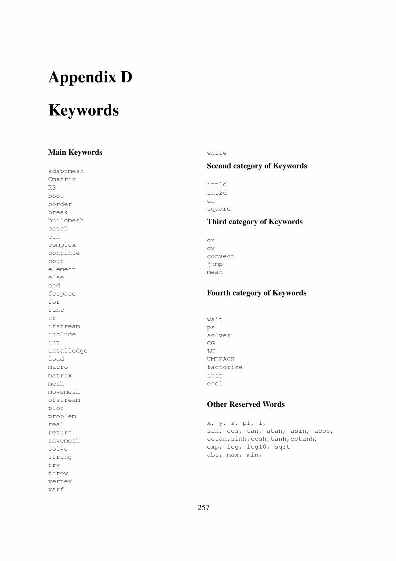
Appendix D
Keywords
Main Keywords
adaptmeshCmatrixR3boolborderbreakbuildmeshcatchcincomplexcontinuecoutelementelseendfespaceforfuncififstreamincludeintintalledgeloadmacromatrixmeshmovemeshofstreamplotproblemrealreturnsavemeshsolvestringtrythrowvertexvarf
while
Second category of Keywords
int1dint2donsquare
Third category of Keywords
dxdyconvectjumpmean
Fourth category of Keywords
waitpssolverCGLUUMFPACKfactorizeinitendl
Other Reserved Words
x, y, z, pi, i,sin, cos, tan, atan, asin, acos,cotan,sinh,cosh,tanh,cotanh,exp, log, log10, sqrtabs, max, min,
257

258 APPENDIX D. KEYWORDS

Bibliography
[1] R. B. LEHOUCQ, D. C. SORENSEN, AND C. YANG ARPACK Users’ Guide: Solution ofLarge-Scale Eigenvalue Problems with Implicitly Restarted Arnoldi Methods SIAM, ISBN0-89871-407-9 // http://www.caam.rice.edu/software/ARPACK/
[2] BABBUSKA, I: Error bounds for finite element method, Numer. Math. 16, 322-333.
[3] Y. ACHDOU AND O. PIRONNEAU: Computational Methods for Option Pricing. SIAM mono-graph (2005).
[4] D. BERNARDI, F.HECHT, K. OHTSUKA, O. PIRONNEAU: freefem+ documentation, on theweb at ftp://www.freefem.org/freefemplus.
[5] D. BERNARDI, F.HECHT, O. PIRONNEAU, C. PRUD’HOMME: freefem documentation, onthe web at http://www. freefem.fr/freefem
[6] DAVIS, T. A: Algorithm 8xx: UMFPACK V4.1, an unsymmetric-pattern multifrontalmethod TOMS, 2003 (under submission) http://www.cise.ufl.edu/research/sparse/umfpack
[7] GEORGE, P.L: Automatic triangulation, Wiley 1996.
[8] HECHT, F: The mesh adapting software: bamg. INRIA report 1998.
[9] Library Modulef , INRIA, http://www.inria-rocq/modulef
[10] A. ERN AND J.-L. GUERMOND, Discontinuous Galerkin methods for Friedrichs’ symmetricsystems and Second-order PDEs, SIAM J. Numer. Anal., (2005). See also: Theory and Prac-tice of Finite Elements, vol. 159 of Applied Mathematical Sciences, Springer-Verlag, NewYork, NY, 2004.
[11] F. HECHT. C++ Tools to construct our user-level language. Vol 36, N°, 2002 pp 809-836,Model. math et Anal Numer.
[12] J.L. LIONS, O. PIRONNEAU: Parallel Algorithms for boundary value problems, Note CRAS.Dec 1998. Also : Superpositions for composite domains (to appear)
[13] B. LUCQUIN, O. PIRONNEAU: Introduction to Scientific Computing Wiley 1998.
[14] I. DANAILA, F. HECHT, AND O. PIRONNEAU. Simulation numerique en C++. Dunod,Paris, 2003.
[15] J. NECAS AND L/ HLAVACEK, Mathematical theory of elastic and elasto-plastic bodies: Anintroduction, Elsevier, 1981.
259

260 BIBLIOGRAPHY
[16] K. OHTSUKA, O. PIRONNEAU AND F. HECHT: Theoretical and Numerical analysis of en-ergy release rate in 2D fracture, INFORMATION 3 (2000), 303–315.
[17] F. PREPARATA, M. SHAMOS Computational Geometry Springer series in Computer sci-ences, 1984.
[18] R. RANNACHER: On Chorin’s projection method for the incompressible Navier-Stokes equa-tions, in ”Navier-Stokes Equations: Theory and Numerical Methods” (R. Rautmann, et al.,eds.), Proc. Oberwolfach Conf., August 19-23, 1991, Springer, 1992
[19] ROBERTS, J.E. AND THOMAS J.-M: Mixed and Hybrid Methods, Handbook of NumericalAnaysis, Vol.II, North-Holland, 1993
[20] J.L. STEGER: The Chimera method of flow simulation, Workshop on applied CFD, Univ ofTennessee Space Institute, August 1991.
[21] TABATA, M: Numerical solutions of partial differential equations II (in Japanese), IwanamiApplied Math., 1994
[22] THOMASSET, F: Implementation of finite element methods of Navier-Stokes Equations,Springer-Verlag, 1981
[23] N. WIRTH: Algorthims + Data Structures = Programs, Prentice Hall, 1976
[24] Bison documentation
[25] Bjarne Stroustrup: The C++ , programming language, Third edition, Addison-Wesley 1997.
[26] COOOL: a package of tools for writing optimization code and solving optimization problems,http://coool.mines.edu
[27] B. RIVIERE, M. WHEELER, V. GIRAULT, A priori error estimates for finite element methodsbased on discontinuous approximation spaces for elliptic problems. SIAM J. Numer. Anal.39 (2001), no. 3, 902–931 (electronic).
[28] R. GLOWINSKI AND O.PIRONNEAU, Numerical methods for the Stokes problem,Chapter 13 of Energy Methods in Finite Element Analysis, R.Glowinski, E.Y. Rodin, O.C.Zienkiewicz eds., J.Wiley & Sons, Chichester, UK, 1979, pp. 243-264.
[29] R. GLOWINSKI, Numerical Methods for Nonlinear Variational Problems, Springer-Verlag,New York, NY, 1984.
[30] R. GLOWINSKI, Finite Element Methods for Incompressible Viscous Flow. In Handbookof Numerical Analysis, Vol. IX, P.G. Ciarlet and J.L. Lions, eds., North-Holland, Amsterdam,2003, pp.3-1176.
[31] Horgan, C; Saccomandi, G; “Constitutive Models for Compressible Nonlinearly Elastic Ma-terials with Limiting Chain Extensibility,” Journal of Elasticity, Volume 77, Number 2,November 2004, pp. 123-138(16).
[32] KAZUFUMI ITO, AND KARL KUNISCH, Semi smooth newton methods for variational in-equalities of the first kind , M2AN, vol 37, N, 2003, pp 41-62.

BIBLIOGRAPHY 261
[33] Ogden, RW; Non-Linear Elastic Deformations, Dover, 1984.
[34] Raviart, P; Thomas J; Introduction a l’analyse numerique des equations aux derivees par-tielles, Masson, 1983.
[35] M. A. TAYLOR, B. A. WINGATE , L. P. BOS, Several new quadrature formulas for poly-nomial integration in the triangle , Report-no: SAND2005-0034J, http://xyz.lanl.gov/format/math.NA/0501496
[36] Wilmott, Paul and Howison, Sam and Dewynne, Jeff : A student introduction to mathematicalfinance, Cambridge University Press (1995).

Index
<<, 75matrix, 72
>>, 75.*, 70.*, 121./, 70=, 113?:, 58[], 15, 111, 188, 55
’, 70
time dependent, 28
accuracy, 19acos, 61acosh, 61adaptmesh, 90, 92
abserror=, 93cutoff=, 93err=, 92errg=, 92hmax=, 92hmin=, 92inquire=, 93isMetric=, 93iso=, 93keepbackvertices=, 93maxsubdiv=, 93metric=, 94nbjacoby=, 93nbsmooth=, 92nbvx=, 92nomeshgeneration=, 94omega=, 93periodic=, 94powerin=, 94ratio=, 93rescaling=, 93splitin2, 94
splitpbedge=, 93uniform, 94verbosity= , 93
alphanumeric, 55append, 75area, 58area coordinate, 118argument, 60array, 56, 64, 73, 119
.l1, 66
.l2, 66
.linfty, 66
.max, 66
.min, 66
.sum, 66?:, 65= + - * / .* ./ += -= /= *= , 65column, 68dot product, 66FE function, 73fespace, 105line, 68max, 65mesh, 205min, 65, 73quantile, 66renumbering, 68resize, 65sort, 65sum, 65varf, 122
asin, 61asinh, 61assert(), 58atan, 61atanh, 61axisymmetric, 28
backward Euler method, 166bamg, 83
262

INDEX 263
barycentric coordinates, 13bessel, 62BFGS, 136block matrix, 70bool, 56border, 80boundary condition, 121break, 74broadcast, 205bubble, 108buildmesh
fixeborder, 80fixeborder=1, 146nbvx=, 80
catch, 76Cauchy, 53ceil, 61CG, 115Characteristics-Galerkin, 33checkmovemesh, 87Cholesky, 115, 135cin, 58, 75column, 68compatibility condition, 114compiler, 55Complex, 56complex, 45, 60, 71Complex geometry,, 30concatenation, 92connectivity, 125continue, 74convect, 34, 177, 179cos, 61cosh, 61cout, 58, 75Crout, 115
de Moivre’s formula, 60default, 75degree of freedom, 13DFFT, 238diag, 71, 182diagonal matrix, 71Dirichlet, 19, 25, 53, 114discontinuous functions, 194Discontinuous-Galerkin, 33
displacement vector, 153divide
term to term, 70domain decomposition, 185, 187dot product, 71, 73dumptable, 58
EigenValue, 163ivalue=, 162maxit=, 163ncv=, 163nev=, 162rawvector=, 162sigma=, 162sym=, 162tol=, 162value=, 162vector=, 162
eigenvalue problems, 26elements, 13emptymesh, 86endl, 75erf, 62erfc, 62exception, 76exec, 58, 131exp, 61expression optimization, 123external C++ function, 36
factorize=, 135false, 56, 58FE function
[], 111complex, 45, 64, 71n, 111value, 111
FE space, 105FE-function, 63, 105FEspace
(int ,int ), 125ndof, 125nt, 125
fespace, 103P0, 103P1, 103P1b, 104
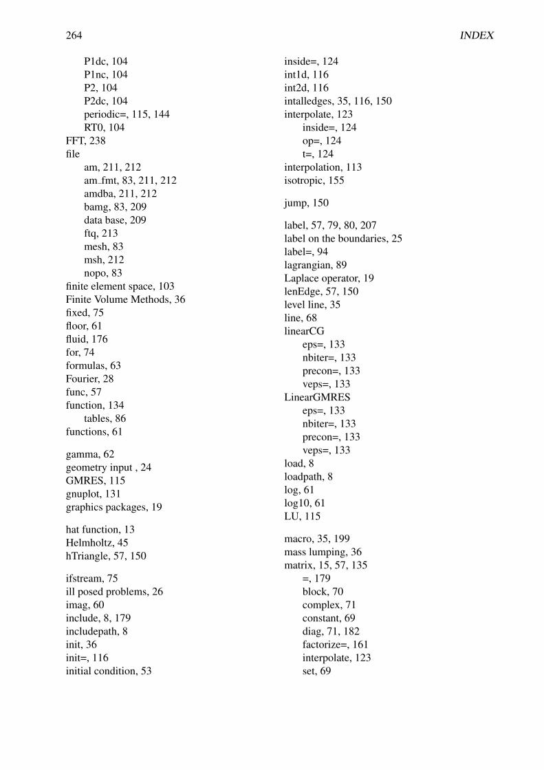
264 INDEX
P1dc, 104P1nc, 104P2, 104P2dc, 104periodic=, 115, 144RT0, 104
FFT, 238file
am, 211, 212am fmt, 83, 211, 212amdba, 211, 212bamg, 83, 209data base, 209ftq, 213mesh, 83msh, 212nopo, 83
finite element space, 103Finite Volume Methods, 36fixed, 75floor, 61fluid, 176for, 74formulas, 63Fourier, 28func, 57function, 134
tables, 86functions, 61
gamma, 62geometry input , 24GMRES, 115gnuplot, 131graphics packages, 19
hat function, 13Helmholtz, 45hTriangle, 57, 150
ifstream, 75ill posed problems, 26imag, 60include, 8, 179includepath, 8init, 36init=, 116initial condition, 53
inside=, 124int1d, 116int2d, 116intalledges, 35, 116, 150interpolate, 123
inside=, 124op=, 124t=, 124
interpolation, 113isotropic, 155
jump, 150
label, 57, 79, 80, 207label on the boundaries, 25label=, 94lagrangian, 89Laplace operator, 19lenEdge, 57, 150level line, 35line, 68linearCG
eps=, 133nbiter=, 133precon=, 133veps=, 133
LinearGMRESeps=, 133nbiter=, 133precon=, 133veps=, 133
load, 8loadpath, 8log, 61log10, 61LU, 115
macro, 35, 199mass lumping, 36matrix, 15, 57, 135
=, 179block, 70complex, 71constant, 69diag, 71, 182factorize=, 161interpolate, 123set, 69
INDEX 265
solver=, 179stiffness matrix, 15varf, 69, 121
eps=, 121precon=, 122solver=, 121solver=factorize, 121tgv=, 122tolpivot =, 122
max, 65maximum, 58medit, 131membrane, 19mesh, 57
(), 84[], 843point bending, 100beam, 96Bezier curve, 98Cardioid, 97Cassini Egg, 97connectivity, 84NACA0012, 96regular, 90Section of Engine, 98Smiling face, 100U-shape channel, 99uniform, 94V-shape cut, 99
mesh adaptation, 37min, 65, 73minimum, 58mixed, 28mixed Dirichlet Neumann, 19modulus, 60movemesh, 87mpirank, 205mpisize, 205multi-physics system, 30multiple meshes, 30
N, 57, 117n, 111Navier-Stokes, 177, 179ndof, 125ndofK, 125Neumann, 53, 117
Newton, 136, 160NLCG, 135
eps=, 133nbiter=, 133veps=, 133
nodes, 13non-homogeneous Dirichlet, 19nonlinear, 30nonlinear problem, 28normal, 35, 117noshowbase, 75noshowpos, 75nt, 125nTonEdge, 35, 58nuEdge, 57number of degree of freedom, 125number of element, 125nuTriangle, 57
ofstream, 75append, 75
on, 117intersection, 178
optimize=, 123outer product, 68, 71
P, 57P0, 103P1, 103P1b, 104P1dc, 104P1nc, 104P2, 104P2dc, 104parabolic, 28periodic, 103, 115, 144pi, 58plot
aspectratio =, 128nbiso =, 128bb=, 128border, 80boundary =, 128bw=, 128cmm=, 128coef=, 128cut, 128
266 INDEX
grey=, 128hsv=, 128mesh, 80nbarraw=, 128ps=, 128value=, 128varrow=, 128viso=, 128
pointregion, 84triange, 84
pow, 61precision, 75precon=, 116, 122, 180problem, 36, 57, 113
eps=, 115init=, 116precon=, 116solver=, 115strategy =, 116, 122tgv=, 116tolpivot =, 116tolpivotsym =, 116, 122
processor, 205product
Hermitian dot, 71dot, 71, 73outer, 71term to term, 70
qforder=, 179quadrature: qf5pT, 119quadrature:default, 119quadrature:qf1pE, 118quadrature:qf1pElump, 118quadrature:qf1pT, 119quadrature:qf1pTlump, 119quadrature:qf2pE, 118quadrature:qf2pT, 119quadrature:qf2pT4P1, 119quadrature:qf3pE, 118quadrature:qf7pT, 119quadrature:qfe=, 119quadrature:qforder=, 119quadrature:qft=, 119quantile, 67
radiation, 30rand, 62randinit, 62randint31, 62randint32, 62random, 62read files, 83readmesh, 81real, 56, 60region, 57, 84, 193region indicator, 30renumbering, 68resize, 65Reusable matrices, 178rint, 61Robin, 28, 114, 117RT0, 104
savemesh, 81schwarz, 205scientific, 75sec:Plot, 127set, 36
matrix, 69showbase, 75showpos, 75shurr, 185, 187sin, 61singularity, 91sinh, 61solve, 57, 113
eps=, 115init=, 116linear system, 70precon=, 116solver=, 115strategy=, 116, 122tgv=, 15, 116tolpivot=, 116tolpivotsym=, 116, 122
solver=, 135CG, 92, 115Cholesky, 115Crout, 115GMRES, 115LU, 115sparsesolver, 115
INDEX 267
UMFPACK, 115sparsesolver, 115split=, 94square, 150
flags=, 79Stokes, 176stokes, 173stop test, 115
absolue, 180strain tensor, 154streamlines, 177stress tensor, 154string, 56subdomains, 192sum, 65
tan, 61Taylor-Hood, 178transpose, 70, 73, 228triangle
[], 84area, 84label, 84region, 84
triangulate, 85triangulation files, as well as read and write, 24true, 56, 58trunc, 94
label=, 94split=, 94
try, 76tutorial
LaplaceRT.edp, 149adapt.edp, 91adaptindicatorP2.edp, 150AdaptResidualErrorIndicator.edp, 152aTutorial.edp, 138beam.edp, 155BlackSchol.edp, 172convect.edp, 171fluidStruct.edp, 189freeboundary.edp, 196movemesh.edp, 89NSUzawaCahouetChabart.edp, 179periodic.edp, 144periodic4.edp, 144periodic4bis.edp, 145
readmesh.edp, 83Schwarz-gc.edp, 187Schwarz-no-overlap.edp, 186Schwarz-overlap.edp, 184StokesUzawa.edp, 178
tutotialVI.edp, 182
type of finite element, 103
UMFPACK, 115upwinding, 33
varf, 15, 57, 116, 119, 179array, 121matrix, 121optimize=, 123
variable, 55variational formulation, 20veps=, 135verbosity, 3, 8vertex
label, 84x, 84y, 84
viso, 35
weak form, 20while, 74write files, 83
x, 57
y, 57
z, 57

268 INDEX


Book Description
Fruit of a long maturing process freefem, in its last avatar, FreeFem++, is a highlevel integrated development environment (IDE) for partial differential equations(PDE). It is the ideal tool for teaching the finite element method but it is also perfectfor research to quickly test new ideas or multi-physics and complex applications.
FreeFem++ has an advanced automatic mesh generator, capable of a posteri-ori mesh adaptation; it has a general purpose elliptic solver interfaced with fastalgorithms such as the multi-frontal method UMFPACK. Hyperbolic and parabolicproblems are solved by iterative algorithms prescribed by the user with the highlevel language of FreeFem++. It has several triangular finite elements, includingdiscontinuous elements. Finally everything is there in FreeFem++ to prepare re-search quality reports: color display online with zooming and other features andpostscript printouts.
This book is ideal for students at Master level, for researchers at any level and forengineers also in financial mathematics.
Editorial Reviews
”. . . Impossible to put the book down, suspense right up to the last page. . . ”A. TANH, Siam Chronicle.
”. . . The chapter on discontinuous fems is so hilarious . . . .”B. GALERKINE, .
About the AuthorsFrederic Hecht is a professor of numerical analysis at the university ofParis VI and does his research at the Laboratoire Jacques-Louis Lions(LJLL). He is also a member of the project gamma at INRIA. He is theauthor of several advanced software tools for automatic triangula-tions including the public domain EMC2.
Olivier Pironneau is a professor of numerical analysis at the univer-sity of Paris VI and at LJLL. His scientific contributions are in numeri-cal methods for fluids. He is a member of the Institut Universitaire deFrance and of the French Academy of Sciences
Koji Ohtsuka is a professor at the Hiroshima Kokusai Gakuin Univer-sity, Japan and chairman of the World Scientific and Engineeringacademy and Society, Japan chapter. His research is in fracture dy-namics, modelling and computing.
Antoine Le Hyaric is a research engineer from the ”Centre Nationalde la Recherche Scientifique” (CNRS) at LJLL . He is an expert in soft-ware engineering for scientific applications. He has applied his skillsmainly to electromagnetics simulation, parallel computing and three-dimensional visualization.