Fertility Theories: Can They Explain the

Negative Fertility-Income Relationship?∗

Larry E. Jones

University of Minnesota, Federal Reserve Bank of Minneapolis, and NBER

Alice Schoonbroodt

University of Southampton

Michele Tertilt

Stanford University, NBER and CEPR

June 2008

Abstract

In this chapter we revisit the relationship between income and fertility.

There is overwhelming empirical evidence that fertility is negatively related

to income in most countries at most times. Several theories have been pro-

posed in the literature to explain this somewhat puzzling fact. The most

common one is based on the opportunity cost of time being higher for in-

dividuals with higher earnings. Alternatively, people might differ in their

desire to procreate and accordingly some people invest more in children and

less in market-specific human capital and thus have lower earnings. We re-

visit these and other possible explanations. We find that these theories are

not as robust as is commonly believed. That is, several special assumptions

are needed to generate the negative relationship. Not all assumptions are

equally plausible. Such findings will be useful to distinguish alternative the-

ories. We conclude that further research along these lines is needed.

∗We thank Todd Schoellman, John Knowles, and the participants at the NBER pre-conferencein Boston, the Stanford Junior Faculty Bag Lunch, and the Economics and Demography con-ference in Napa California for helpful suggestions. We thank Amalia Miller in particular fora thoughtful discussion. Financial support by the NSF (grants SES-0519324 and SES-0452473)and the Stanford Institute for Economic Policy Research (SIEPR) is greatly appreciated. WilliamG. Woolston provided excellent research assistance. Part of this research was completed whileMichele Tertilt was a National Fellow at the Hoover Institution at Stanford.

1

Contents

1 Introduction 3

2 Data on Fertility and Income 6

3 Basic Framework and Results 11

3.1 The Basic Model . . . . . . . . . . . . . . . . . . . . . . . . . . . . . . 12

3.2 The Price of Time Theory . . . . . . . . . . . . . . . . . . . . . . . . . 15

4 Endogenous Wage Differences 18

4.1 Exogenous Fertility and Endogenous Wages . . . . . . . . . . . . . 19

4.2 Endogenous Fertility and Endogenous Wages . . . . . . . . . . . . . 20

4.3 An Aside on Wages vs. Income . . . . . . . . . . . . . . . . . . . . . 23

4.4 Empirical Evidence and Related Work . . . . . . . . . . . . . . . . . 23

4.5 Outlook . . . . . . . . . . . . . . . . . . . . . . . . . . . . . . . . . . . 26

5 Quantity-Quality Theory 26

5.1 A Simple Example . . . . . . . . . . . . . . . . . . . . . . . . . . . . 28

5.2 The Quality Production Function. . . . . . . . . . . . . . . . . . . . . 30

6 Married Couples and the Female Time Allocation Hypothesis 34

6.1 Empirical Findings . . . . . . . . . . . . . . . . . . . . . . . . . . . . 35

6.2 Theory . . . . . . . . . . . . . . . . . . . . . . . . . . . . . . . . . . . 37

7 Nannies 46

7.1 An Example with Ability Heterogeneity . . . . . . . . . . . . . . . . 46

7.2 A Working Example with Preference Heterogeneity . . . . . . . . . 48

8 Time Series Implications 52

9 Conclusion 57

A Appendix 61

A.1 Adding Parental Altruism . . . . . . . . . . . . . . . . . . . . . . . . 61

A.2 A Dynamic Version of the Endogenous Wage Example . . . . . . . 65

A.3 Summary of Findings for Couples’ Models . . . . . . . . . . . . . . 66

2

1 Introduction

Empirical studies find a clear negative relationship between income, or wages,

and fertility. This finding has been confirmed across time and for different coun-

tries. For example, Jones and Tertilt (2008) document a negative cross-sectional

relationship between income and fertility in the United States and find that the re-

lationship has been surprisingly stable over time. In particular, the paper shows

a negative relationship for 30 birth cohorts between 1830 and 1960, with the in-

come elasticity of fertility remaining roughly constant at about -0.30.1

Why do richer people have fewer children, and what explains the relatively

time-invariant nature of the relationship? The negative correlation is particularly

puzzling if one thinks about children as a consumption good, unless one believes

that children are an inferior good. An early discussion of this fact appears in the

seminal article on fertility choice by Becker (1960). Indeed, this puzzling corre-

lation was a main impetus behind Becker’s early work.2 The ensuing literature

can be roughly divided into two strands. One attacks the question from a theo-

retical point of view and finds that, properly interpreted or with the appropriate

additions in choice variables, economic theory says that fertility should be neg-

atively related to income. The basic idea is that the price of children is largely

time, and because of this, children are more expensive for parents with higher

wages. Another argument is that higher-wage people have a higher demand for

child quality, making quantity more costly, and hence those parents want fewer

children. The other strand of literature attacks the question from an empirical

point of view, arguing that the negative relationship is mainly a statistical fluke—

due to a missing variables problem. This literature focuses on identifying those

crucial missing variables, such as female earnings potential. Once those miss-

1We discuss the empirical evidence in more detail in Section 2.2Quoting from Becker (1960), (p. 217): “Having set out the formal analysis and framework

suggested by economic theory, we now investigate its usefulness in the study of fertility patterns.It suggests that a rise in income would increase both the quality and quantity of children desired;the increase in quality being large and the increase in quantity small. The difficulties in sepa-rating expenditures on children from general family expenditures notwithstanding, it is evidentthat wealthier families and countries spend much more per child than do poorer families andcountries. The implication with respect to quantity is not so readily confirmed by the raw data.Indeed, most data tend to show a negative relationship between income and fertility.” See alsothe discussion in Hotz, Klerman, and Willis (1993).

3

ing variables are controlled for, fertility and income—so the argument goes—are

actually positively related.3

In this paper, we revisit these theories of the cross-sectional relationship be-

tween income and fertility. They are largely based on ability or wage hetero-

geneity. We also formalize a new theory, based on heterogeneity in the taste

for children, in which wages are also endogenous. For each of the theories, we

catalogue whether they basically never work (i.e., never produce the negative

income-fertility relation), whether they work only with specific additional as-

sumptions, or whether they are relatively robust to changes in assumptions. We

also often compare the results to the conditional correlations found in the statis-

tical strand of the literature. For those theories that work sometimes, we try to be

as explicit as possible about what kinds of conditions are needed (e.g., curvature

and/or functional form restrictions) to generate a negative relationship between

income and fertility. We also show what goes wrong by giving examples about

how they fail. Finally, of the theories that work and appear robust, we ask for

more. Can the theory also match the time series properties of fertility? If so,

what exactly does it take? If not, why not? Finally, we want to know whether

such a theory is consistent with a recursive formulation of dynastic altruism.

Our main findings can be summarized as follows:

1. (Almost) all theories depend on the assumption that raising children takes

time and that this time must be incurred by the parents.

2. Theories based on exogenous wage heterogeneity crucially depend on the

assumption of a high elasticity of substitution between consumption and

children.

3. Adding a quality choice by itself does not generate a negative fertility-

income relationship. The quantity-quality trade-off works only in conjunc-

tion with assumptions similar to those needed in (2).

4. Theories based on heterogeneity in tastes for children are able to generate a

negative fertility-income relationship without requiring a high elasticity of

substitution between consumption and children.

3See Hotz, Klerman, and Willis (1993) for a survey. An early literature review on fertilitychoice is Bagozzi and Van Loo (1978).

4

5. Theories that explicitly distinguish between fathers and mothers are very

similar to one-parent theories. However, to get fertility to be decreasing in

men’s income, one needs to assume that there is positive assortative match-

ing of spouses.

6. Several of the theories that match the cross-sectional patterns of fertility

also match, at least loosely, some of the broad time series trends in fertil-

ity. Theories based on wage heterogeneity produce this relationship more

naturally.

7. Extending the models that are successful at matching the cross-sectional

properties of fertility choice to fully dynamic models based on parental al-

truism is very challenging. Basic theories with wage heterogeneity do not

appear to be robust to this extension. Theories based on heterogeneity in

tastes are more promising, but leave many open questions.

Our findings may be relevant in several different contexts. First, there has

been a recent increase in research relating the demographic transition and eco-

nomic development among macroeconomists.4 Similarly, several recent contri-

butions try to understand why fertility is higher in poor countries than in rich

ones.5 Further, there is a recent literature that uses dynamic macro-style models

to analyze the interplay between fertility, labor force participation, marriage, and

inequality6—including studies of gender wage gap7 and the baby boom follow-

ing World War II.8 Often dynamic macro-style models are used to analyze the im-

pacts of various policy changes—for example, parental leave policies, the impact

4See, for example, Becker, Murphy, and Tamura (1990), Galor and Weil (1996), Galor andWeil (1999), Galor and Weil (2000), Greenwood and Seshadri (2002), Hansen and Prescott (2002),Boldrin and Jones (2002), Doepke (2004, 2005), Greenwood, Seshadri, and Vandenbroucke (2005),Moav (2005), Tertilt (2005), Jones and Schoonbroodt (2007b), Murtin (2007) and Bar and Leukhina(2007). See Galor (2005a) and Galor (2005b) for an extensive analysis and a critical survey oftheories of the demographic transition.

5See Manuelli and Seshadri (2007).6See Alvarez (1999), Caucutt, Guner, and Knowles (2002), and Falcao and Soares (2007).7See Erosa, Fuster, and Restuccia (2005b).8See Greenwood, Seshadri, and Vandenbroucke (2005), Doepke, Hazan, and Maoz (2007),

and Jones and Schoonbroodt (2007a).

5

of tax reform, welfare reform, social security.9 Typically, they use an “off-the-

shelf” fertility model as one of their building blocks, and need to make a careful

decision about which one to use. What may help guide this choice is an informed

understanding of the implications of the models for the fertility-income relation-

ship in the cross section. Because of this, it is natural to use successful models of

the cross sectional properties of fertility as a way to inform that choice.

This is easier said than done, however. Economists have been developing and

testing theories of fertility ever since Gary Becker’s seminal paper, but still there

is no full consensus on the motivations behind fertility choices. Here, we provide

a systematic comparison of the properties of various fertility theories. We hope

that this catalogue may be a useful step towards finding a consensus.

This paper is organized as follows. In the next section, we summarize the

empirical evidence on the fertility-income relationship. Section 3 describes a ba-

sic model with wage heterogeneity. Section 4 develops a new theory based on

preference heterogeneity in the desire to have children which generates endoge-

nous wage heterogeneity. Section 5 adds quality to the basic model. In Section 6

we depart from the simplest framework and analyze more realistic theories with

two parents. We investigate whether theories are robust to allowing parents to

hire nannies in Section 7. Section 8 pushes several of the working theories to

also address the secular decline in fertility, while Section 9 concludes. The Ap-

pendix analyzes the extent to which our results apply to a dynastic formulation

of fertility.

2 Data on Fertility and Income

A robust fact about fertility is that it is decreasing in income. This fact has been

documented from a time-series point of view, across countries, and across indi-

viduals. Quoting from Becker (1960) (p. 217): “Indeed, most data tend to show

a negative relationship between income and fertility. This is true of the Census

data for 1910, 1940 and 1950, where income is represented by father’s occupation,

9Recent contributions include Aiyagari, Greenwood, and Guner (2000), Erosa, Fuster, andRestuccia (2005a), Fernandez, Guner, and Knowles (2005), Greenwood, Guner, and Knowles(2003), Sylvester (2007), and Zhao (2008).

6

mother’s education or monthly rental; the data from the Indianapolis survey,

the data for nineteenth century Providence families, and several other studies as

well.”10

Figure 1: Fertility by Occupational Income in 2000 DollarsFigure 3: CEB vs. Occupational Income in 2000 Dollars

1.5

2.0

2.5

3.0

3.5

4.0

4.5

5.0

5.5

6.0

6.5

0 20,000 40,000 60,000 80,000

Occupational Income in 2000 Dollars

Ch

ild

ren

ever

Bo

rn

1828 1838

1848 1858

1868 1878

1888 1898

1908 1918

1928 1938

1948 1958

Birth Cohort

Source: Jones and Tertilt (2008)

In a recent study, Jones and Tertilt (2008) use U. S. Census Data on lifetime

fertility and occupations to document this negative cross-sectional relationship

in the United States.11 They find a robust negative cross-sectional relationship

between husband’s income12 and fertility for all cohorts for which data is avail-

10The studies Becker is referring to are U.S. Census (1945), U.S. Census (1955), Whelpton andKiser (1951), and Jaffe (1940).

11Income is based on the median annual income for a given occupation in 1950 and adjustedfor TFP growth. A measure of income based on occupation is a better measure of lifetime incomethan income in any particular year. See Ruggles, Sobek, Alexander, Fitch, Goeken, Hall, King,and Ronnander (2004) for a description of how occupational income scores (OIS) are constructedas well as its robustness as a proxy for income. See Jones and Tertilt (2008) for a description ofhow the OIS was converted into 2000 dollars.

12The focus on husband’s income allows a consistent analysis over time. In particular, it allowsthe analysis of periods for which data on wife’s income is practically nonexistent.

7

able, that is for women born between 1826 and 1960.13 Not only are the correla-

tions always negative, but also they are surprisingly similar in magnitude over

time. Figure 1, reproduced from their paper, shows this very clearly. While the

relationship is not perfect, it seems that most of the fertility decline over time can

be “explained” by rising incomes alone, at least in a statistical sense.

To give a sense of the magnitudes, Table 1 reproduces some of the most rel-

evant numbers from Jones and Tertilt (2008). For a selected number of birth co-

horts, the table displays average husband’s income and average fertility.14 To

quantify the fertility-income relationship, two different empirical measures were

constructed: the income elasticity of fertility, and the fertility gap between the top

and bottom 50 percent of the income distribution. The income elasticity roughly

hovers around minus one-third, meaning that for a family with an income that is

10% higher than another family, the number of children is about 3% lower. This

is a large difference. For example, for women born during the 19th century, those

in the bottom half of the income distribution had easily one child more on aver-

age than those in the top half. Today, the difference is is much smaller in absolute

numbers, with a fertility gap of roughly a quarter of a child. But since fertility

is significantly lower for all women, the income elasticity has declined only very

mildly over time, to about -0.20 for the most recent cohorts.

Note that the income measure used in Figure 1 and Table 1 is based on occu-

pations, and can also be viewed as a proxy for wages. Therefore, the findings can

be interpreted as showing a negative fertility-wage relationship.

Many other studies have documented this kind of relationship, typically for

a specific geographic area at a particular point in time. For example, Borg (1989)

finds a negative relationship using panel data from South Korea in 1976, and

13Fertility is measured as children ever born (CEB) to the current wife. Of course, this measurecould differ from male completed fertility if men had children with different women. Unfortu-nately not much data on male completed fertility are available. We are aware of two exceptions.First, the 2002 National Survey of Family Growth asked men and women independently abouttheir fertility. Preston and Sten (2008) use this data to construct a measure of the elasticity ofmale fertility to male education and also find a negative coefficient. Given that divorce was rarefor most of the period under consideration, we believe that the wife’s fertility is a good proxy.Second, Shiue (2008) compiled Chinese data from 1300 to 1850. She finds a weak positive rela-tionship between male fertility and social status, but since richer men also had more women onaverage, fertility per wife is actually decreasing.

14The definitions of fertility and income in the table are identical to those used in Figure 1.

8

Birth Cohort Income top/bottom Fertility Annual income Number ofelasticity fertility gap in 2000 Dollar observations

1826-1830 -0.33 0.95 5.59 4,154 4521836-1840 -0.20 0.74 5.49 5,064 1,9601846-1850 -0.32 1.26 5.36 6,173 4,5201856-1860 -0.35 1.24 4.90 7,525 7,2411866-1870 -0.34 1.27 4.50 9,173 7,3471876-1880 -0.42 1.06 3.25 11,182 3,2031886-1890 -0.45 1.05 3.15 13,631 6,6441896-1900 -0.50 0.93 2.82 16,616 8,4621906-1910 -0.42 0.57 2.30 20,255 11,8121916-1920 -0.25 0.34 2.59 24,690 46,9081926-1930 -0.17 0.27 3.11 30,097 97,1431936-1940 -0.19 0.31 3.01 36,688 44,4281946-1950 -0.20 0.26 2.22 44,723 62,2101956-1960 -0.22 0.23 1.80 54,517 71,517

Source: Jones and Tertilt (2008)

Table 1: Fertility-Income Relationship for 14 U.S. Cross Sections

Docquier (2004) documents a similar relationship for the U.S. using data from

the PSID in 1994. Westoff (1954) finds a negative relationship between fertility

and occupational status for the years 1900-1952 using U.S. Census data.

Part of the literature argues that a negative income-fertility relationship is pri-

marily a statistical fluke—i.e., that it is due to a problem of missing variables. The

idea is that once enough variables are controlled for, one would actually find a

positive income-fertility relation. Indeed, this was Becker’s original view on the

topic. He went into great detail focusing on knowledge of the proper use of con-

traceptives as the important missing variable.15 Similarly, many authors have

argued that a distinction between male and female income is crucial and that the

relationship between male income and fertility is indeed (weakly) positive once

one correctly controls for female income.16 Authors of studies that find a positive

15He showed that, in his sample, in those households that were actively engaged in familyplanning, fertility and income were positively related while the opposite was true for familiesnot engaged in family planning. Other early papers along this line are cited by Becker in hisoriginal piece. They include Edin and Hutchinson (1935) and Banks (1955).

16Empirical studies distinguishing explicitly between husbands and wives include Cho (1968),Fleischer and Rhodes (1979), Freedman and Thorton (1982), Schultz (1986), Heckman and Walker(1990), Merrigan and Pierre (1998), Blau and van der Klaauw (2007), and Jones and Tertilt (2008).

9

relationship after controlling for women’s wages, often interpret such finding as

having resolved the “puzzle.” This is, however, not necessarily the case. The

reason is that even though the finding reconciles the conditional correlations in

the data with the simplest model of fertility, the question remains of what kind

of theories would explain the unconditional negative correlation of men’s wages

and fertility. At the very least it requires some assumptions about matching.17

In this paper we take a somewhat different approach: rather than controlling for

important factors (such as wives’ wages) in the data, we try to add such impor-

tant factors into the model and then ask whether the augmented model delivers

the same qualitative facts as the data does.

It is sometimes argued that early on in the development process, a positive

relationship between income and fertility existed.18 Most of the studies that doc-

ument such a positive relationship are set in agrarian economies, and often in-

come is proxied by farm size. Examples include Simon (1977, chapter 16), who

documents a positive relationship between farm size in hectares and the average

numbers of children born for rural areas in Poland in 1948, and Clark and Hamil-

ton (2006), who document a positive relationship between occupational status

and the number of surviving children in England in the late 16th and early 17th

century (see also Clark (2005) and Clark (2007)). Weir (1995) finds a weakly pos-

itive relationship between economic status and fertility in 18th century France,

while Wrigley (1961) and Haines (1976) document higher fertility in the coal min-

ing areas of France and Prussia than in surrounding agricultural areas during the

end of the 19th century. Also, Lee (1987) documents a similar finding using data

from the U.S. and Canada.19 This body of work suggests that the fundamental

forces determining the demand for children might be different in areas where

agriculture is the primary economic activity.

Of course, there is no reason why the fertility-income relationship should not

The findings are mixed.17We discuss this in detail in Section 6.18A more recent version of such a positive relationship is that U.S. fertility is higher than most

other countries in the OECD even though U.S. income is higher. This does not hold for a largerset of countries, however. See Ahn and Mira (2002) and Manuelli and Seshadri (2007) for a dis-cussion of related points. Bongaarts (2003) finds a slight U-shaped fertility-education relationshipin Portugal and Greece using three education levels of women. The other eight countries concurwith previous findings of a strictly negative relationship.

19See also the papers cited in Lee (1987).

10

change over time or vary in different cross sections. It may be that in some sub-

groups of the population, fertility increases in income once all other relevant cor-

relates are controlled for, while in other subgroups the primary change across

the income distribution is in the price of a child and, because of this, that fertil-

ity is lower at higher income levels. And in fact, it is plausible that fertility and

wealth were indeed positively related in early agrarian economies, but that this

relationship was reversed after industrialization.20

To sum up, the fact that people with higher lifetime earnings have fewer chil-

dren seems very robust, at least during the last century and a half in the United

States. Other countries and other episodes display a similar relationship. In-

spired by these facts, this paper analyzes which theories of fertility are consistent

with this relationship.

3 Basic Framework and Results

In this section we introduce notation and explore some basic models of fertility

choice. The basic examples that we discuss here focus on the roles played by the

nature of the cost of children, the sources of family income and the formulation

of preferences. We find that the simplest versions of these ideas do not generate

a negative relationship between fertility and income. Special assumptions on the

nature of costs of children, the utility function, the sources of income and/or

the child quality production function are needed. This it not to say that these

theories are wrong. Rather, by making explicit the assumptions behind the ideas

we hope to facilitate the testing of the theories and, ultimately, to improve our

understanding of fertility decision-making.

To keep the analysis tractable, we focus on a static, monoparental set-up. This

approach allows for closed form solutions and lets us focus on the basic mechan-

ics behind the results. Obviously, there are many dynamic elements in real world

fertility-decision making, for example, choices about the timing of births, etc. We

20For example, Skirbekk (2008) (using a large data set including various world regions overtime) finds that as fertility declines, there is a general shift from a positive to a negative or neutralstatus-fertility relation. Those with high income/wealth or high occupation/social class switchfrom having relatively many to fewer or the same number of children as others. Education,however, depresses fertility for as long as this relation is observed (early 20th century).

11

see our basic examples as a way to gain insights into modeling ingredients of

more complex dynamic models. Clearly, many important features are left out

in the simplest example we start with. Some of these features are particularly

important and we come back to those in later sections of this paper. One such

element is that any child necessarily has a father and a mother. In fact, many

authors have emphasized that it may be female time rather than male time that is

important to generate the negative relationship between fertility and income. We

get back to this in Section 6. In later sections of the paper we extend the model to

include more dynamic elements including limited forms of human capital/child

quality (Sections 4 and 5) and parental altruism (Appendix A).

Two more caveats are in order. First, throughout the paper we analyze only

rational theories of fertility.21 Behavioral concerns might be relevant, especially

for teenage child-bearing, but are not considered here. Second, we focus on theo-

ries in which children provide direct utility benefits, i.e. children are a consump-

tion good. Note that children are sometimes also viewed as an investment, pro-

viding old-age security.22 While the investment motive may have important im-

plications for the fertility-income relationship, this analysis is beyond the scope

of this paper and is left for future research.

3.1 The Basic Model

The general static model of fertility choice that we consider is as follows. Peo-

ple maximize utility subject to a budget constraint, a time constraint, and a child

quality production function. People (potentially) derive utility from four differ-

ent goods: consumption, c, number of children, n, the average quality of children,

q, and leisure, ℓ. Producing children takes b0 units of goods and b1 units of time

(per child). We let lw denote the time spent working and normalize the total time

endowment to one. The wage per unit of time is denoted by w. In addition to

21We also abstract from costs and technologies to prevent births or to inseminate artificially.Several authors have given these issues more thought, and we refer the reader to them (see forexample (Hotz and Miller 1988), Goldin and Katz (2002), Bailey (2006) and Greenwood and Guner(2005)).

22Examples include Ehrlich and Lui (1991), Boldrin and Jones (2002) and Boldrin, De Nardi,and Jones (2005). Zhao (2008) uses the Boldrin-Jones framework to jointly address the fertilitydecline and the narrowing of fertility differentials by income in response to changes in socialsecurity.

12

labor income, we also allow for non-labor income, y. Finally, child quality is

a function of educational child inputs, s (we abstract from direct parental time

inputs into child quality). Thus, the choice problem is as follows:

maxc,n,q,e,lw

U(c, n, q, ℓ) (1)

s. t. lw + b1n + ℓ ≤ 1

c + (b0 + s)n ≤ y + wlw

q = f(s)

In order to highlight the crucial ingredients to generate a negative income (or

wage) to fertility relationship, we distinguish between various combinations of

utility specifications, concept of wealth/income/earnings used, costs of children

and quality production functions. We now briefly discuss each of these compo-

nents.

Utility: We focus on separable utilities. That is:

U(c, n, q, ℓ) = uc(c) + un(n) + uq(q) + uℓ(ℓ)

We consider the CES utility case, ux(x) = αxx1−σx−1

1−σxfor values of σx > 0. We

will often distinguish three cases: (i) σx > 1 (high curvature, low elasticity of

substitution), (ii) σx < 1 (low curvature, high elasticity of substitution) and (iii)

σx = 1 corresponding to log utility.23

Income/Wealth: We use the following (standard) language: w is the wage, W =

w + y is total wealth, and I = wlw is earned income (often also called labor earn-

ings). In most of our examples, there are only two uses of time (working and

child-rearing), in which case earned income is equal to w(1 − b1n). An interest-

ing special case is the case where all income is labor income, y = 0 and W = w.

In several examples, we focus on the fertility-earnings (rather than wage) rela-

tionship. In these examples, there is no wage heterogeneity. However, the logic

underlying those examples can easily be generalized to (endogenous) wage het-

23This utility function has the added advantage that, in some cases, it can be interpreted as theproblem in Bellman’s equation for a Barro-Becker style dynasty with parental altruism. There,the term un(n) is the value function for continuations. This interpretation is only valid for certainchoices of the αn’s however. See Appendix A for details.

13

erogeneity. We do so in Section 4. In this context, the wage will be equal to human

capital, H , and human capital is a function of schooling inputs. For simplicity,

we will omit H and say that the wage w is a function of schooling inputs.

Costs of Children: We allow for both goods and time costs, denoted by b0 and

b1, respectively. To get starker results, we sometimes shut down one of the two

types of costs. It turns out that a time cost appears to be essential to almost all

the theories and examples we present here. To see this, note that with separable

utility, no time cost (b1 = 0) and no quality in utility (αq = 0), n is a normal

good, and hence, it follows that n is increasing in both y and w.24 Thus, we will

typically require that b1 > 0. While it seems fairly obvious that it takes time

to raise a child, it is less clear whether the time spent must be the parent’s time

rather than a nanny or a day-care center. We analyze the implications of allowing

for nannies in Section 7.25

Quality Production Function: One important feature for the quantity-quality

trade-off to generate the desired relationship is the specification of the quality

production function, f(·). We experiment with various specifications. Note that

making special assumptions on f(·) is technically equivalent to making special

assumptions on uq(·). That is, let vq(·) = uq(f(·)) and make assumptions about

this function. The interpretation, however, can be quite different. With homoth-

etic preferences to start with, unless f(s) is of the form f(s) = sκ, this introduces

non-homotheticity into the overall problem (1). We will analyze quality produc-

tion functions in some detail in Section 5.

Leisure: For some of the examples in Sections 6 and 7, we need leisure as an

alternative use of time in order to reproduce the negative fertility-income rela-

tionship. For most examples, this is not necessary, and hence we will typically

assume that αℓ = 0.

24When αq > 0, the constraint becomes non-linear which complicates matters. In certain cases,the problem can be written in aggregate quality Q = nq. In this case if b1 = 0, both n and Q arenormal goods and hence increasing in both y and w.

25We restrict attention to linear child costs. Analyzing the robustness of our results to otherchild cost specifications would be of interest. There seems to be little consensus in the empiricalliterature on the shape of the child cost function, however. Empirical papers that estimate thecosts of children and economies of scale in the household include Hotz and Miller (1988), Bernal(2004), Lazear and Michael (1980), and Espenshade (1984). Taking maternal health and maternalmortality risk into account, one might also want to argue that a convex cost function is the mostreasonable formulation (e.g. Tertilt (2005)).

14

3.2 The Price of Time Theory

To highlight the necessary ingredients, we start by discussing a simple example

that does not generate the desired negative relationship between fertility and

income. We then show what special assumptions are needed to obtain the desired

result.

Starting from the general formulation (1), we assume log utility (ux(x) =

αx log(x)), no utility from child quality (αq = 0) or leisure (αℓ = 0) and no non-

labor income (y = 0). Then the problem reduces to

maxc,n

αc log(c) + αn log(n) (2)

s. t. c + b0n ≤ w(1 − b1n)

The solution for fertility is:

n∗ =αnw

(αc + αn)(b0 + wb1)

As is apparent from this example, as long as the goods cost of children is pos-

itive (b0 > 0) higher-wage households (higher w) will have strictly more children

in this set-up. This is the opposite prediction from what we observe in the data.

Setting the goods cost to zero with just a time cost results in fertility choice be-

ing independent of w – still, not a negative relationship. Adding leisure or child

quality (say, with q = f(e) = e) will not reverse this result (see Section 5).

To give the price of time theory a chance, it seems fairly obvious that a devia-

tion from log utility is needed, i.e. a specification where income and substitution

effects do not cancel out. We thus turn now to general CES utility functions. Also,

since a time cost is essential here and a goods cost does not really add anything,

we set b0 = 0 and assume b1 > 0, but reintroduce non-labor income, y ≥ 0. Thus,

our next example takes the form

maxc,n

αcc1−σ − 1

1 − σ+ αn

n1−σ − 1

1 − σ(3)

s. t. c ≤ y + w(1 − b1n)

It is easy to solve for a closed form solution of this specification. Optimal fertility

15

is given by:

n∗ =yw

+ 1(

αcb1αn

)1/σ

w1−σ

σ + b1

Elasticity of substitution. In problem (3) wage heterogeneity leads indeed to a

negative wage-fertility relationship if the right amount of curvature is assumed

in the utility function. To see this, assume first that y = 0. If the only way in

which individuals differ is in their wages, we can see that when σ ≥ 1, fertility is

either independent of or increasing in w. However, when σ < 1, it follows that

n∗(w) is decreasing.

The intuition here is simple: when the only cost of children is time, and that

time must be the parents’ own time, higher wage families face a higher price

of children. This induces the usual wealth and substitution effects familiar from

demand theory. Certainly it implies that compensated demand for children is de-

creasing. This is not sufficient, however, to automatically imply that the demand

for children is decreasing in income, since those families that face higher prices

also have more wealth. Thus, it depends on which of the two forces is stronger. If

the elasticity of substitution between children and consumption is high enough

(low σ), the substitution effect dominates and n∗(w) is decreasing, as in the data.

Moreover, it can be seen that this relationship is approximately isoelastic when

y is small and w is large relative to b1. In this example, the income elasticity of

demand for children is σ−1σ

.

In sum, this theory works, but not without extra restrictions on preferences.

An additional requirement could be that the formulation be consistent with dy-

namic maximization in a setting with parental altruism a la Barro and Becker

(1989) (i.e., parents care about number and utility of children multiplicatively).

In Appendix A.1 we discuss the relationship between this static problem and a

reinterpretation of it as the Bellman equation of a dynamic problem. The diffi-

culty with the dynamic reinterpretation of the current example is that αn is no

longer a parameter but represents children’s average level of utility. It there-

fore becomes a function of the wage. It turns out that once this is taking into

account properly, fertility is independent of the wage independently of σ. More-

over, Jones and Schoonbroodt (2007b) show that in this kind of models, σ > 1

is needed to generate the decreases in fertility observed over the past 200 years

16

in response to increased productivity growth and decreased mortality. Hence, it

seems that this dynamic interpretation of the static model presented here is at an

impasse to get both the cross-sectional and trend features of fertility at the same

time. In Appendix A.1, we show that with preference heterogeneity, both the

cross section as well as the trend observations can be generated.

Non-Labor Income. An alternative specification that also works is to assume log

utility but positive non-labor income. Assume σ → 1 and y > 0, then the solution

to (3) becomes

n∗ =αn( y

w+ 1)

(αc + αn)b1

Note that for y > 0, fertility is indeed decreasing in the wage.26 Note that the

slope of the relationship depends on the size of the non-labor income. That is, for

small amounts of non-labor income fertility is decreasing in the wage only very

mildly, and in the limit, when non-labor income is zero, fertility does not depend

on the wage at all.

Note, however, that the only income that would really qualify as non-labor

income here are gifts, lottery income, bequests and the like.27 Since most fami-

lies have no or very little such non-labor income, it is questionable whether this

should be the main mechanism by which fertility and income are connected. Yet,

variations of this formulation are used a lot in the literature. For example, the re-

finement that it is female time that determines the opportunity cost falls into this

category. In particular, sometimes y is interpreted as the husband’s income and

w as the wife’s wage. Then fertility is decreasing in the latter. We will turn our

attention to two-parent fertility models in Section 6.

Non-homothetic preferences. Another way to generate the desired relationship

is to move away from homothetic utility.28 Assume for example that σc = 0. Then

26Adding non-labor income effectively changes the curvature of the utility function, and hencethe technical reason that makes this example succeed is similar to the σ < 1 case above. Theinterpretation, of course, is very different.

27Any interest income from assets that are accumulated labor earnings would be proportionalto labor income, and hence would not generate the result outlined here.

28See for example Greenwood, Guner, and Knowles (2003).

17

the problem to solve is

maxc,n

αcc + αnn1−σ − 1

1 − σ(4)

s.t. c ≤ (1 − b1n)w

And the solution is:

n∗ =

[

αn

αcb1

]1/σ

w−1/σ

which is clearly decreasing in w for any value of σ.29 We are not emphasizing

non-homothetic utilities any further, because one broader aim of the proposed

research agenda here is to develop a theory that encompasses cross-sectional,

trend, and cyclical features of fertility choice. Embedding this example into a

fully dynamic growth model has the unfortunate property that income shares to

consumption tend to one. Because of this these models would be of limited use.

4 Endogenous Wage Differences

In the previous section we focused on theories of the cross-sectional relationship

between fertility and wages in which the fundamental difference was exogenous

variation in ability (wages). In this section, we explore an alternative view with

an alternative causation. Suppose that the basic source of heterogeneity is in

tastes for children versus material goods—some people want large families and

others want to travel the world, go to fancy restaurants and drive a sports car.

This basic difference in taste for either “life-style” affects the investment in hu-

man capital and hence wages. That is, parents who want large families will allo-

cate less time to developing market-based skills in anticipation of having many

children, and will therefore have lower wages and lower earned income.

Rather than assuming people differ in their taste for children, one could sim-

ply assume that people differ exogenously in fertility and choose human capital

investments accordingly. This kind of model also gets the basic relationship right,

29This specification (with σ → 1) is used in Fernandez, Guner, and Knowles (2005), Erosa,Fuster, and Restuccia (2005a) and Erosa, Fuster, and Restuccia (2005b). Note that the incomeelasticity of demand for children here is −1/σ which is close to the data for σ = 3.0.

18

and is useful for understanding the basic mechanism. We start with this simple

version, even though the interpretation of exogenous fertility is not straightfor-

ward. We then move to a more general case that has a more plausible interpre-

tation: deterministic heterogeneity in the taste for children versus consumption

goods. Here schooling is chosen in anticipation of fertility decisions.

Finally, as long as raising children takes time, a simpler mechanism can be

considered. Again assuming taste heterogeneity, parents who choose large fam-

ilies will have less time available to work and hence will have lower earned in-

come, even if wages are exogenous. This simplification will be helpful in subse-

quent sections. Note that whenever the simple mechanism works and one can

generate a negative fertility-income relationship, it is straightforward to also gen-

erate a negative fertility-wage relationship by adding endogenous human capital

investments to the model.

4.1 Exogenous Fertility and Endogenous Wages

The simplest version illustrating the mechanism we want to focus on is one

where fertility is exogenously different across people. Let ni be the number of

children that are attached to adult i. Each child requires b1 units of parental time.

The parent solves one lifetime maximization problem by choosing how much

time (net of child-rearing time) to allocate to schooling vs. earning wages. Even

though we write this as a one-period problem, the decisions are best interpreted

in a sequential fashion: time is first spent on schooling, ls, which determines fu-

ture human capital als. Normalizing the wage per unit of human capital to one,

als is also the wage, so that total lifetime income simply becomes wlw = alslw.

The problem then is:

maxc,lw,ls

αcc1−σ

1 − σ+ αn

n1−σi

1 − σ(5)

s. t. ls + lw ≤ 1 − b1ni

w = als

c ≤ wlw

19

The solution is

lis = liw =1 − b1ni

2

It follows immediately that the wage is decreasing in fertility.

wi = alis =a

2(1 − b1ni)

Note that the derived negative relationship is quite robust, i.e. it does not depend

on specific functional forms or parameter restrictions. The only crucial assump-

tion is that it takes time to raise children.

One interpretation of this example is that people are ex-ante identical, but are

exposed to stochastic fertility shocks (e.g., birth control failures). Then, ex-post,

people will have different fertility realizations, which leads them to optimally

invest different amounts into human capital. However, for such shocks to be the

main driving force behind the negative fertility-income relationship, it would

need to be the case that most people know their fertility realizations before they

make their human capital accumulation decisions. While this seems implausible

for schooling decisions, it is more plausible for human capital that is accumulated

on the job through experience. Exogenous fertility shocks may also be important

for some margins, such as drop-out decisions for girls that become pregnant in

high school.

4.2 Endogenous Fertility and Endogenous Wages

Next, we extend the basic intuition given above to allow for both the choice of

fertility and the endogenous determination of wages. Assume now that parents

differ in their preferences for children, i.e. some people value children more than

others. To do this, we add a fertility choice to problem (5) and allow for prefer-

ence heterogeneity. We also generalize the model along two other dimensions,

which will turn out to be useful later on. First, following Ben-Porath (1976) and

Heckman (1976) we allow for decreasing returns in the human capital accumula-

tion process: w = alνss , νs ∈ (0, 1]. Second, we allow for decreasing returns when

working. That is, an individual working lw units (hours/weeks/years) will earn

a total income of wlνww , νw ∈ (0, 1]. While this formulation is non-standard (i.e.

20

most of the literature assumes that income is linear in hours worked), we find it

quite plausible since many jobs pay a premium for full time work. Note also that

setting νw = 1 gives the standard model in which income is the product of an

hourly wage and hours worked. The modified problem then is

maxc,n,lw,ls

αcc1−σ

1 − σ+ αn

n1−σ

1 − σ(6)

s. t. ls + lw ≤ 1 − b1n

w = alνss

c ≤ wlνw

w

The first order conditions are:

ls : αc(alνs

s lνw

w )−σaνslνs−1s lνw

w = αn

(

1 − ls − lwb1

)−σ1

b1

lw : αc(alνss lνw

w )−σaνwlνss lνw−1

w = αn

(

1 − ls − lwb1

)−σ1

b1

It follows immediately that ls = νs

νwlw. Using this, the optimal amount of work

solves the following equation

αca1−σνs

(

νs

νw

)νs−1−νsσ

l−(νs+νw)σ+νs+νw−1w = αn

(

1

b1

)1−σ (

1 −νs + νw

νwlw

)−σ

It is easy to derive closed form solutions for two special cases: (i) constant

returns to scale (νw +νs = 1) and a general σ and (ii) general production function,

but assuming log utility σ = 1.30 The solution for case (ii) is

l∗w =αcνw

αn + (νs + νw)αc

l∗s =αcνs

αn + (νs + νw)αc

n∗ =1

b1

(

αn

αn + (νs + νw)αc

)

30We analyze case (i) with dynastic altruism in Appendix A.2.

21

Note that the wage rate is

w∗ = a(l∗s)νs

which increases monotonically in time spent at school. Taking derivatives with

respect to the child preference parameters, αn, gives

∂n∗

∂αn

=(νs + νw)αc

b1[αn + (νs + νw)αc]2> 0

∂l∗s∂αn

=−αcνs

[αn + (νs + νw)αc]2< 0 .

So, clearly, people who have a higher preference for children will have both, more

children and a lower wage.

As can be seen from these expressions, fertility is independent of the raw

learning ability, a. That is, without differences in preferences, parents will all

have the same fertility.31

There are a couple of special cases where the implicit relationship between

fertility and wages can be solved for explicitly.

In addition to σ = 1, now assume that νw = νs = 1: human capital is linear

in years of schooling, and total income is simply the wage multiplied time spent

working. For this case, we can substitute out all preference parameters to derive

an equilibrium relationship between wage and fertility that will hold across all

consumers (i.e. independent of their individual αn and αc):

n∗ =1

b1(1 −

2

aw∗).

In this case, it follows that fertility is linearly decreasing in wages.

A second case that admits a straightforward closed form solution is when

νs = νw. Then, the relationship can be written as:

n∗ =1

b1

(

1 − 2

(

w∗

a

)1

νs

)

.

In this case the relationship between the wage and fertility is non-linear with its

31Of course, if in addition one assumes that σ < 1, then fertility decreases in a for the samereasons as in Section 3.2.

22

curvature determined by the parameter νs.

In sum, this direction of causation generates the negative income-fertility and

wage-fertility relationships under fairly general assumptions. In Appendix A.2,

we add parental altruism to this model. Similar results go through.

4.3 An Aside on Wages vs. Income

Here we have focused on the cross-sectional relationship between wages and

fertility when the basic heterogeneity is differences, across people, in preferences

for children vis-a-vis consumption goods. To do this we needed a model in which

wages themselves are endogenous. An alternative, weaker, version of a similar

property can be derived without explicitly including human capital formation

in the model. This involves the relationship between fertility and income. For

simplicity, assume that all households have the same w. Recall the solution to

Problem (3),

n∗ =yw

+ 1(

αcb1αn

)1/σ

w1−σ

σ + b1

and consider two families that differ only in their values of αn and/or αc. As

we can see, the family with the higher αn will have more children for any value

of σ and y. It also follows that this family will have lower earned income, I =

[1 − b1n∗(αn, αc)]w, simply because it will spend more time raising children and

less time working. Thus, preference heterogeneity of this type will also generate

a negative correlation between fertility and earned income, without further as-

sumptions on elasticities, or the formation of human capital, as long as children

take parental time.

4.4 Empirical Evidence and Related Work

Empirical papers have confirmed the mechanism emerging from Section 4.1 in

the data, though most research (with the exception of Angrist and Evans (1998))

focuses on its importance for female wages, or income, and has little to say about

the relationship between male income and fertility as shown in Figure 1.32 Sim-

32Nor do they say much about most of the time period we are discussing in which few womenwere earning market wages. In addition, good data for IV estimation, on twins for example, has

23

ilarly, the structural microeconomics literature, as well as some authors in the

macroeconomics literature, also primarily focuses on female wages. These pa-

pers address the mechanism emerging from Section 4.2, though not in isolation.

We review these results below.

4.4.1 Empirical Evidence

There is a large statistical literature that tries to assess the effect of (exogenous)

fertility variation on labor supply, experience accumulation, wages and/or earned

income (see Browning (1992) for an early review). Mincer and Polachek (1974)

find that work interruptions for childbearing have lead to large human capi-

tal depreciations. Mincer and Ofek (1982) find that longer interruptions cause

larger human capital losses. While there is a large and rapid increase in wages

upon reentry, full earnings potential is not regained after interruption and reen-

try. These findings suggests that children have a lasting effect on income through

forgone experience, which is a specific type of human capital accumulation.33

These papers view the number of children as exogenous. More recent research

has focused on identifying valid instruments for fertility, such as miscarriages

and unwanted pregnancies. For example, Miller (2007) finds that an exogenous

delay in childbirth leads to a substantial increase in earnings, wage rates, and

hours worked. She finds evidence for both, fixed wage penalties and lower re-

turns to experience for mothers. Since delay in fertility is typically associated

with lower completed fertility, this result suggests that the number of children

may have a strong effect on human capital accumulation of various types.

While all the papers mentioned so far focus on female earnings and leave

father’s and family income aside, Angrist and Evans (1998) use IV estimation to

look at both parents’ labor supply and labor income as well as family income.

They look at families with two children and use the gender composition of the

existing children as an instrument for the desire to have a third child. The authors

only become available recently.33Mincer and Polachek (1974) go on to answer the question: “Do family size and number of

children currently present affect the accumulation of earning power beyond the effect on workexperience? The answer is largely negative: when numbers of children and some measures oftheir age are added to work histories in the [regression] equations, the children variables arenegative but usually not significant statistically.”

24

find that families with a stronger desire for a third child work less and earn less.

This is true for wives alone, husbands alone and family income.34 Unfortunately,

nothing is said about hourly wages. Note that income is measured before the

family actually has the third child. The fact that income is already lower prior

to childbirth is in line with the theory above: people who want to have more

children (i.e. higher αn) anticipate working less in the future, and thus have a

weaker incentive to accumulate human capital through experience.

4.4.2 Related Theory

As for the mechanism in Section 4.2 with endogenous fertility, the structural mi-

croeconomics literature on joint fertility and female labor supply choices also

uses preference heterogeneity to generate a distribution of fertility and wages

as observed in the data. Again, the focus is on female labor supply, experience,

schooling and wages or earnings, while our mechanism is meant to address men

(see Figure 1) as well as women (see Section 6 for details). Furthermore, per-

manent taste is typically not the only source of heterogeneity in these papers.

Fixed and stochastic ability heterogeneity, as well as preference shocks over the

life-cycle, are additional necessary ingredients to fit the data. Francesconi (2002)

estimates such a combined model with part-time and full-time employment. In a

similar framework, Del Boca and Sauer (2006) analyze the effects of institutions

on fertility, timing and labor supply decisions. Finally, Keane and Wolpin (2006)

add schooling and marriage decisions to estimate the effects of welfare programs

on fertility and female labor supply.35 All these papers use some version of the

mechanism described here, though not in isolation. Our aim is to contrast pure

taste and pure ability heterogeneity. In reality, of course, both may be relevant.

Finally, this mechanism is also sometimes used in the macroeconomics liter-

34Their instrument is based on the following observation. Families with two children of thesame sex are more likely to have a third child because sex mix is presumably preferred. Sincegender of children is exogenous, the willingness to bear a third child—in the hope for the oppositesex—is also largely exogenous.

35This literature is based on a combination of two basic models: Eckstein and Wolpin (1989)who analyze female labor force participation and experience accumulation with exogenous fer-tility heterogeneity, and Hotz and Miller (1988) who analyze contraceptive effort with taste het-erogeneity thereby endogenizing fertility but abstracting from labor supply and human capitalaccumulation of any kind.

25

ature. For example, Erosa, Fuster, and Restuccia (2005a) have stochastic fertility

opportunities and stochastic values of children, together with learning-by-doing

on the job, so that higher fertility translates into lower wages.36 Again, male in-

vestment decisions are assumed not to be affected by fertility preferences and

realizations. A similar mechanism is also at work in Erosa, Fuster, and Restuccia

(2005b) and Knowles (2007).37

4.5 Outlook

While the empirical evidence seems to support the idea that heterogeneity in

tastes for children is to some extent responsible for the observed negative fertility-

income relationship, this mechanism has received far less attention in the theoret-

ical literature. Rather, most research starts with the assumption that exogenous

differences in income (or ability) cause fertility to vary systematically across the

income distribution. We therefore address the preference channel in all subse-

quent sections. Recall from Section 4.3 that a simpler version of the mechanism

can be used to derive a negative fertility-income relationship. For tractability, we

use this shortcut when we analyze preference heterogeneity in Sections 5 and 6.

However, in all cases, the model can easily be extended to human capital accu-

mulation and wages. We reintroduce endogenous wages in Section 7 where we

present an example in which parental time is not essential and Appendix A.2

where we build the dynastic analog of Problem (6).

5 Quantity-Quality Theory

In this section, we revisit the idea that the demand for child quality naturally

leads richer parents to want more quality and thus less quantity, what is often

called the quantity-quality hypothesis.38 This idea turns out not to be a very

36Although, this is not the only channel through which fertility and income are related in theirmodel.

37Attanasio, Low, and Sanchez-Marcos (forthcoming) analyze a similar model to Eckstein andWolpin (1989) with exogenous fertility and endogenous experience to account for the increase infemale labor force participation across cohorts.

38Rosenzweig and Wolpin (1980) use exogenous variation in fertility (twins) to confirm the hy-pothesis that exogenous increases in fertility decrease child quality and suggest that a decrease in

26

robust theory of the negative fertility-income hypothesis.

In his seminal work, Becker (1960) argued that there is a trade-off between

quantity and quality of children. Originally, however, Becker did not propose

the quantity-quality trade-off as an explanation for why fertility and income

were negatively correlated. Indeed, in the 1960 paper Becker argues, by anal-

ogy with other durable goods, that economic theory suggests that fertility and

income should be positively related, but perhaps only weakly so, while quality

of children and income should be strongly positively correlated. The intuition for

Becker’s argument is simple. While richer parents do spend more on their chil-

dren (better schools, better clothes, higher bequests, etc.), richer people spend

more on everything. They have higher quality houses and cars as well, yet no

one would argue that we should expect rich people to have fewer houses than

poor people. As a first cut, the same logic should apply to children: richer people

would want more quality, but probably not less quantity, the same way they also

would not want better but fewer cars.

So what makes children different? Hotz, Klerman, and Willis (1993), review-

ing Becker’s arguments, seem to emphasize that what might be the case is that

not children per se are normal goods, but that expenditures on children are: ”If

children are normal goods in the sense that total expenditures on children are

an increasing function of income, then the sum of the income elasticities of the

number and quality of children must be positive [...], but it is still possible that

the income elasticity of demand for the number of children is negative [...] if the

income elasticity of quality is large enough.” This is not our reading of the paper.

Our reading is that, by analogy, quantity should be slightly increasing in income

and quality should be greatly increasing in income. Becker’s argument is then

that the observation of a negative relationship is a missing variables problem,

namely knowledge about contraceptives. Becker and Lewis (1973) and Becker

and Tomes (1976) were important follow-ups on Becker (1960). Becker and Lewis

(1973) argue that, once income is measured correctly, the true fertility-income

family size brought about, say, by exogenous improvements in birth control technology, wouldincrease schooling levels (in India). Many authors have found similar results in other data sets.In a recent paper, Angrist, Lavy, and Schlosser (2005) criticize these findings. Their IV strategiesgenerate little evidence for a quantity-quality trade-off in the sense of a causal link between sib-ship size and outcome variables describing the human capital, earnings, or social status of first-and second-born children.

27

elasticity is positive, even if the observed one is negative. Becker and Tomes

(1976) argue that the quality production function has an endowment component

which generates a negative correlation between fertility and income.

Below, we derive conditions under which simple examples including child

quality can generate this negative correlation without making children inferior

goods. We start with the simplest specification of the example in Section 3 with

log utility and a linear quality production function. In this example, it becomes

apparent that even with quality choice and ability heterogeneity, we need a pos-

itive time cost and zero goods costs for fertility to be non-increasing in income.

Next, we derive the requirements on the quality production function for fertil-

ity to be strictly decreasing in wages—under both, wage and taste heterogeneity.

One example that generates the desired relation is an affine production function

with a positive constant, as in Becker and Tomes (1976) together with the as-

sumption that children take time while child quality requires purchased inputs

as in Moav (2005). Various interpretations of this specification can be used to ac-

commodate the cross section of fertility with respect to income and the trend in

fertility over time. Finally, under preference heterogeneity, none of these require-

ments on the quality production function are needed.

5.1 A Simple Example

First, we show by example that including a quality choice in and of itself does not

necessarily lead to a negative relationship between fertility and income. That is,

including quality does not necessarily lead richer people to want fewer children.

They might want more quality and accordingly, a smaller increase in number of

children—as argued in Becker (1960)—but the relationship between fertility and

income is still positive.

Suppose U(c, n, q) = αc log c + αn log n + αq log q, αq > 0, q = f(s) = s and

28

y = 0. Then the problem from Section 3 is:

maxc,n,q,s,lw

αc log c + αn log n + αq log q

s. t. lw + b1n ≤ 1

c + (b0 + s)n ≤ wlw

q ≤ s

This is a version of the problem considered in Becker and Lewis (1973), while

Becker (1960) assumed b0 = b1 = 0. The constraint set in this problem is not

convex because of the term ns. We therefore rewrite the problem in terms of total

quality, Q = qn.39 We also know that the constraints hold with equality. Using

this, the problem becomes:

maxc,n,Q

αc log c + (αn − αq) log n + αq log Q

s. t. c + b0n + Q ≤ w(1 − b1n)

This is now a standard problem under the assumption that αn > αq. The solution

is given by:

n∗ =αn − αq

(αc + αn)(b0 + b1w)w

q∗ =αq(b0 + b1w)

αn − αq

c∗ =αc

αc + αnw

Similar to what we found in the example in Section 3.2, as long as the goods

cost is positive (b0 > 0), fertility is strictly increasing in the wage, w.40 On the

39Rosenzweig and Wolpin (1980) write a model with b1 = 0 but a children-independent priceof quality. If this price is strictly positive, our formulation cannot be used.

40Whether earned income, I = (1 − b1n)w, increases or decreases depends on the size of theincrease in n in response to an increase in w. In the present example, we have:

dI

dw= (1 − b1n) − b1w

dn

dw=

(αc + αq)(b0 + b1w)2 + (αn − αq)b2

0

(αc + αn)(b0 + b1w)2> 0

Thus, in this case, income and fertility are positively related.

29

other hand, if b0 = 0, fertility is independent of w, while earned income is I =

w(1 − b1n∗). Again, this does not give a negative relationship between income

and fertility since there is no heterogeneity in fertility choice. Instead, we get an

extreme version of Becker’s original argument. That is, if there is only a time cost

of children, b0 = 0, then we have high income elasticity of quality per child (q

is strictly increasing in w and hence I) and low income elasticity of number of

children (n is independent of w or I).41

There are at least two ways in which this “negative result” can be overturned.

First, keeping wage heterogeneity, the quality production function can be gen-

eralized. Second, one can consider preference heterogeneity instead of ability

heterogeneity in this simple example. We consider these two avenues in turn

below.42,43

5.2 The Quality Production Function.

The next example is based on the analysis in Moav (2005) who argued that pro-

ducing children takes time, while educating each child requires goods costs. This

assumption makes quality relatively cheaper for higher wage people and one

might expect a quantity-quality trade-off to result. However, the comparative

advantage alone, does not imply that higher wage people have fewer children,

as we have seen above. The properties of the human capital production function

41It is useful to note that the time intensity in the cost of children matters (the relative size of b0

and b1) for the size of these effects. Also, similarly to the cost of time theory, one could vary theelasticity of substitution in the utility function. We leave this part to the reader.

42We have also explored a third channel—non-separable preferences—to a limited degree (cf.Jones and Schoonbroodt (2007b)). For example, assume q = s and solve:

max{c,n,q} αc log c + log[

[(αn − αq)nρ + αq(nq)ρ]

1ρ

]

s.t. c + (b0 + b1w)n + nq ≤ w

In this case, if ρ ∈ (0, 1) then n and Q = nq are substitutes in utility and fertility is decreasing in wwhile the opposite is true if ρ < 0. In the text, we are implicitly assuming the case, where ρ → 0.The substitutes case works because number of children is time intensive and hence more costlyto high wage parents while the price of quality is the same across people.

43Another way of generating a negative income-fertility relationship through a quantity-quality trade-off is to assume that the educational choice is indivisible: the choice is betweenskilled and unskilled children. This mechanism was used in Doepke (2004). In this case, lowability people would choose (some) unskilled children and have more of them than high abilitypeople who have skilled children. Among the latter group, however, fertility will be increasingin ability again.

30

are also a crucial ingredient, as noted in Moav (2005).

We make the same assumptions as above, except that we let q = f(s) be un-

specified for now. The maximization problem is given by:

maxc,n,q,s

αc log c + αn log n + αq log q (7)

s. t. c + b0n + sn ≤ w(1 − b1n)

q = f(s)

The first order conditions give

sf ′(s)

f(s)=

αn

αq

(

sw

b0w

+ b1 + sw

)

(8)

n∗ =

(

αn

αc + αn

)

1b0w

+ b1 + s∗

w

(9)

Let the elasticity on the left-hand side of equation (8) be η(s) ≡ sf ′(s)f(s)

.44

Ability Heterogeneity

Suppose, that households differ in their abilities, w. In the case where b0 = 0, we

can see from equation (9) that for n∗ to be a decreasing function in w, s∗

wneeds to

be increasing in w. But the right-hand side of (8) is increasing in this ratio. Thus

the left-hand side has to be increasing as well. Hence, we need that η′(s) > 0,

which is purely a property of f(s). An example of a human capital production

function that satisfies this property was first introduced by Becker and Tomes

(1976):45

f(s) = d0 + d1s, d0 > 0, d1 > 0

44Note that unless f(s) = sλ for some λ > 0, this formulation is very similar to the non-homothetic preference example given in Section 3 since we can rewrite the utility function asαc log c + αn log n + αq log f(s).

45De la Croix and Doepke (2003, 2004) use a more complex production function that allowsquality to depend on parental human capital, but overall has similar properties: f(s, w) = d1(d0+s)γwτ , where γ, τ ∈ (0, 1) are parameters. Examples of production functions that do not satisfy

the condition include f(s) = sa and f(s) = as which lead to a constant s∗

w, and f(s) = log(s) and

f(s) = exp(as) which lead to decreasing s∗

w.

31

In this case, the solution is:

s∗ =

αq

αnb1w − d0

d1

(1 − αq

αn)

which is well-defined as long as αq < αn and d0 is small enough, i.e. d0 <

d1αq

αnb1w.46 Solving for n∗ gives

n∗ =

αn−αq

αc+αn

b1 −d0

wd1

From this it is clear that ∂n∗

∂w< 0.

Finally, notice that this example still requires a time cost. In fact, in the case

with b0 > 0, the solution is given by:

s∗ =

αq

αn(b0 + b1w) − d0

d1

(1 − αq

αn)

which is well-defined as long as

αq < αn andαq

αn(b0 + b1w) >

d0

d1(10)

Solving for n∗ gives

n∗ =

αn−αq

αc+αn

b1 + b0w− d0

wd1

Hence, fertility is decreasing in w if and only if

d0

d1> b0 (11)

In the case where b1 = 0, conditions (10) and (11) are mutually exclusive.

Interpretation and further predictions of the model. Becker and Tomes (1976) in-

terpret d0 as an endowment of child quality, or “innate ability”. In this interpreta-

tion, one might want to take intergenerational persistence in ability into account.

If the child’s quality endowment and parent’s ability, w, are positively correlated

in the sense that E(d0) = w, then fertility is, again, independent of w while qual-

46Otherwise s = 0 is the solution.

32

ity is still increasing in w. An alternative would be that in those families in which

parents have higher market wages, the marginal value of education is higher—

d1 is perfectly positively correlated with w. For example, assume that d1 = κw.

Then even if innate ability, d0, is perfectly correlated with w, fertility is still de-

creasing while education is increasing in w. This educational investment does

not require time per se. Instead, for a given amount of goods, the high ability

parent produces more quality.

An alternative interpretation of d0 is publicly provided schooling. Since this

has increased over time, we see that the predicted response is that fertility will

increase, at least holding w fixed. In contrast, holding d0 fixed, an increase in

income over time would cause fertility to decrease. Hence, under this interpreta-

tion the example suggests that the increase in income was more important than

the increase in publicly provided schooling.47

Preference Heterogeneity

Next, assume that w is the same for all households but suppose that people differ

in their preference for the consumption good, αc. In all the examples above, the

more people like the consumption good, the fewer children they will have and,

as long as b1 > 0, the more income they will earn. However, the quality choice, q,

is independent of αc and hence income, I .

If, on the other hand, we consider heterogeneity in the preference for children,

αn, we see that the more people like children, n (relative to both consumption, c,

and quality, q), the more they will have, the less income they will earn and the less

quality investments they make per child. Thus, in this case, fertility and income

are still negatively related, while quality per child will be positively related with

income.

Note that this does not depend on any particular assumption about goods

costs or the quality production function. As usual, however, a positive time cost

is required so that earned income, I , is decreasing in number of children, n, which

generates the negative correlation.48

47See the conclusion for suggestive simulations of such changes over time.48Pushing the idea of preference heterogeneity one step further, Galor and Moav (2002) argue

that the forces of natural selection selected individual preferences that are culturally or geneticallypre-disposed towards investment in child quality, bringing about a demographic transition.

33

6 Married Couples and the Female Time Allocation

Hypothesis

A refinement of the price of time theory of fertility is to view the decision making

unit as a married couple and to explicitly distinguish between the time of the wife

and the husband. In this version, since it is typically the case that most childcare

responsibility rests with the woman, it is the time of the wife that is critical to the

fertility decision.49 In its simplest form, the idea is that the price of children is

higher for high productivity couples, even if only the husband is working.50

The aim of this section is threefold. First, we test how robust the results de-

rived in previous sections are to introducing women explicitly. In particular,

we ask whether the same restrictions on parameters are necessary to generate a

negative fertility-relationship when the division of labor within couples is taken

into account. Second, we move to more general formulations that model home

production explicitly, examining the restrictions needed on the home production

technology under log utility (in the spirit of Willis (1973)). Third, we show that

specific patterns of assortative mating are needed to match the data. A richer

model also necessitates a more nuanced look at the data. The findings in the

empirical literature can be summarized as the following three findings:

(1) The correlation between fertility and wife’s wage (or productivity). Evi-

dence suggests that this correlation is strongly negative whether controlling

for the husband’s wage or not.

(2) The conditional correlation between fertility and husband’s wage, holding

49A related idea was first formalized in Willis (1973) who studied the time allocation problemfor a couple in which the time of both the husband and wife are used in raising children whileconsumption is produced using the time of the wife and market purchased goods.

50In the words of Hotz, Klerman, and Willis (1993): “A second major reason for a negative rela-tionship between income and fertility, in addition to quality-quantity interaction, is the hypothe-sis that higher income is associated with a higher cost of female time, either because of increasedfemale wage rates or because higher household income raises the value of female time in non-market activities. Given the assumption that childrearing is a relatively time intensive activity,especially for mothers, the opportunity cost of children tends to increase relative to other sourcesof satisfaction not related to children, leading to a substitution effect against children. As notedearlier, the cost of time hypothesis was first advanced by Mincer (1963) and, following Becker’s(1965) development of the household production model, the relationship between fertility andfemale labor supply has become a standard feature of of models of household behavior.”

34

the wife’s wage constant. Evidence here is very mixed (e.g., Blau and van

der Klaauw (2007) find it is strongly positive, Jones and Tertilt (2008) find it

is negative and Schultz (1986) finds that it depends on the exact subgroup

of the population one considers; see below).

(3) The unconditional correlation between fertility and husband’s wage. Evi-

dence suggests that this correlation is strongly negative in the data.

We show that simple examples imply that fertility should be decreasing in the

productivity or wage of the wife (1) and (weakly) increasing in the wage of the

husband (2). Because of this theoretical result, much of the empirical literature

has taken the stand that the negative estimated correlation between income of

the husband and fertility (3) is contaminated by a missing variables problem—

the productivity of the wife. Since productivities or wages within couples are

typically positively correlated, a downward bias (perhaps enough to change the

sign) is induced on the true effect of husband’s income on fertility. One might

think that this effect is large enough, in theory, that any restrictions on the form

of preferences, etc., are no longer necessary. This is not what we find in the ex-

amples below. Rather, we find that specific assumptions on elasticity, the home

production function and assortative mating (either in terms of productivities or

preferences) are still required to generate facts (1) and (3).51 We summarize those

combinations of assumptions that successfully generate facts (1) and (3) in Table 3

in Appendix A.3.

6.1 Empirical Findings

Testing predictions (1) and (2) in the data is complicated because of the difficulty

in obtaining direct measures of the value of the wife’s time. Until recently many

wives did not work and even now, those that do are a ‘selected’ sample. Hence,

other proxies must be used, such as inferred productivities based on a Mincer

regression or education. The evidence on (1) and (3) are quite robust while evi-

dence on (2) is mixed. Below is a summary of the findings of three recent studies.

51Given the mixed evidence on (2), we do not focus too much on the model prediction for (2).

35

Schultz (1986) estimates a reduced-form fertility equation based on his house-

hold demand framework:52

ni = β0 + β1 ln wfi + β2wmi + βyi + ǫi

where n is the number of children, wf and wm are female and male wages re-

spectively, y is asset income, and ǫ is an error term. This equation is estimated

separately for different age and race groups. The data are from the 1967 Sur-

vey of Economic Opportunities, an augmented version of the Current Population

Survey. He finds that “in every age and race regression the wife’s wage is nega-

tively associated with fertility. The coefficient on the husband’s predicted wages

changes sign over the life cycle, adding to the number of children ever born for

younger wives [...] but contributing to lower fertility among older wives. [...]

For white wives over age 35 and for black wives aged 35-54, a higher predicted

husband’s wage is significantly associated with lower completed fertility. The

elasticities of fertility with respect to the wage rates of wives and husbands are

of similar magnitude for blacks and whites, although for blacks the level of fer-

tility is higher and wage levels are lower. [...] These estimates give credence to

the hypothesis that children are time-intensive. In all age and race regressions the

sum of the coefficients on the wife’s and husband’s wage rates is negative and in-

creases generally for older age groups. [...] The hypothesis that children are more

female than male time-intensive is also consistent with these estimates.”(Table 1,

pp. 93)

Using NLSY longitudinal data for women born between 1957 and 1964, Blau

and van der Klaauw (2007) find that “a one standard deviation increase in the

male wage rate is estimated to have some fairly large effects on white women,

but none of the underlying coefficient estimates are significantly different from

zero. Several of the black and Hispanic interactions are statistically significant,

however, and the simulated effects are in some cases quite large. A higher male

wage rate increases the number of children ever born to black women by 0.169.

52Schultz (1986, p. 91) also says: “Empirical studies of fertility that have sought to estimate thedistinctive effects of the wage opportunities for men and women generally find β1 to be negative,while β2 tends to be negative in high-income urban populations and frequently positive in low-income agricultural populations Schultz (1981)”.

36

For Hispanic women, a higher male wage rate also increases fertility. Concern-

ing female wage rates, a higher female wage rate generally has effects that are of

the opposite sign from those of the male wage rate. As with the male wage rate,

the effects are not significantly different from zero for whites, but for blacks and

Hispanics a higher female wage rate has negative effects on fertility that are sig-

nificantly different from zero. Children ever born decline by about 0.1 for blacks

and Hispanics.”

Jones and Tertilt (2008) also experiment with this hypothesis. Since very few

women worked in the early cohorts, education is chosen as a measure of potential

income. They find that CEB is declining in both the education level of the wife

and the husband, and significantly so. Moreover, the coefficients on husband’s

and wife’s education are similar in size (the wife’s being slightly larger) and there

is no systematic time trend.

6.2 Theory

It is convenient to break this variant of the story into two separate parts, one in

which the woman does not work in the market and one in which she can and

does. Roughly, we can think of the first version as corresponding to a time in

history when very few married women participated in the formal labor market.

The second corresponds to more recent history. It is clear that the critical features

necessary to reproduce the observations must be different in the two cases. We

summarize all models that are consistent with the facts in Table 3 in Appendix

A.3.

6.2.1 Full Specialization in the Household

In this example, the husband works in the market, lm, earning wage, wm, or en-

joys leisure, ℓm while the wife works only in the home, lhf , so that her tradeoff

is between how much time to allocate to producing home goods versus raising

children, b1n, or enjoying leisure, ℓf . Her productivity in home production is de-

noted wf . This setup may be more relevant to the early period in the data when

(married) women’s labor force participation was roughly zero.

37

The gender-specific utility function is given by

Ug = αcg log(cg) + αng log(n) + αℓg log(ℓg) + αhg log(chg)

where g = f, m indicates gender, cg is market consumption, n is the number

of children, ℓ is leisure, and chg is the home good. Note that only the hus-

band’s leisure is needed for some of the results below. That is, αℓf could be zero,

while the husband needs an alternative use of time to generate any endogenous

wage/income heterogeneity for the husband. Given our previous results, we

assume that children cost only time, i.e., b0 = 0

We assume that there is unitary decision making in the household. The family

solves the problem:

max{cm,cf ,chm,chf ,n,ℓm,ℓf ,lm,lhf}

λfUf + λmUm (12)

s. t. cf + cm ≤ wmlm

lm + ℓm ≤ 1

chf + chm ≤ wf lhf

lhf + ℓf + b1n ≤ 1

Here ℓf and ℓm are leisure of the female and male respectively, wm is the wage

of the man, wf is the productivity of the woman in home production, chf and

chm are consumption of home goods by the woman and the man respectively.

Note that it is assumed that the wife spends b1 hours for each child being raised

(and the husband spends none). To keep it simple, assume perfect agreement

of couples: assume αxf = αxm = αx for x = c, h, n, ℓ. Further, without loss of

generality, assume λf + λm = 1 and αc + αn + αℓ + αh = 1.

This problem separates into two maximization problems, one concerning the

allocation of the man’s time and one concerning the allocation of the woman’s

time. The one for the man is straightforward and does not involve fertility. No-

tice however, that male earnings are increasing in αc since leisure becomes less

desirable relative to consumption. The problem for the woman’s time allocation

38

is:

max{chm,chf ,n,ℓf}

λfαℓ log(ℓf) + λfαh log(chf) + λmαh log(chm) + (λf + λm)αn log(n)

s. t. b1wfn + chf + chm + ℓf ≤ wf

The solution is:

n∗ =αn

λfαℓ + αh + αn

1

b1(13)

Ability Heterogeneity, Elasticity and the Home Production Function

Suppose households differ in their productivities, (wf , wm). We see that n∗ is in-

dependent of woman’s productivity in the home. If education is a good proxy

for female home productivity, then the evidence in Jones and Tertilt (2008) con-

tradicts this model implication. That is, this model is not consistent with Fact

(1).53 Fertility is also independent of wm, holding wf fixed. Finally, even if the

productivity of the husband and wife are positively correlated (or independent),

fertility is independent of both productivities. Thus, fact (3) is not predicted here,

either.54 Clearly, something is missing in the theory.

As can be seen from the above, since the couple’s problem splits into two

separate maximization problems, and the one for the wife’s time looks just like

those discussed in Section 3 above (additional goods permitting), the natural next

step is to analyze a more general version in which utility is given by:

Ug = αc

c1−σg

1 − σ+ αn

n1−σ

1 − σ+ αℓ

ℓ1−σg

1 − σ+ αh

c1−σhg

1 − σ

With σ < 1, it follows that n∗ will be decreasing in the productivity at home of

the wife, wf , fact (1). Holding the wife’s productivity fixed, fertility is still in-

dependent of the husband’s wage, “fact (2)”. Thus, if wf and wm are positively

53One should note though that Fact (1) is based on evidence from the 20th century, so a modelwhere fertility is constant across women, conditional on husband’s income, could still be a gooddescription of the 19th century.

54It can also be shown that if children have a nonmarket goods cost, b0 > 0, n∗ is increasing inwf . It follows that if wf is positively correlated with wm (which is what we might expect), n∗ andwm will also be positively correlated.

39

correlated, and σ < 1, the partial correlation between n∗ and wm is negative as

well, fact (3). This example is summarized in the first row of Table 3 in the Ap-

pendix.

A second variation that also reproduces the negative correlation in the cross

section can be obtained by making the home production technology slightly more

complex. Assume that utility is given by

Ug = αn log(n) + αh log(chg)

where the home good, chg, is produced using market goods, c, and time of the

wife, lhf with productivity wf , i.e., chf + chm = F (c, wf lhf). To simplify the analy-

sis, we now assume that leisure is not valued, αℓg = 0. Thus the problem is:

max{cm,cf ,chm,chf ,n,ℓm,ℓf ,lhf}

λfUf + λmUm

s. t. c ≤ wm

b1n + lhf ≤ 1

chf + chm ≤ F (c, wf lhf)

The first-order conditions can be reduced to one equation involving the amount

of time the wife spends making home goods, which directly relates to fertility:

(1 − lhf) =αn

αh

1

wf

F (wm, wf lhf)

F2(wm, wf lhf)

n∗ =1 − lhf

b1

That is, time spent in child-rearing (1 − lhf) is positively related to the relative

desirability of children to consumption, αn

αh, and negatively related to the produc-

tivity of the wife, wf , all else equal. Thus, so is fertility, n∗. When F is assumed

to be CES, F (c, wf lhf) = [δcρ + (1 − δ)(wf lhf)ρ]

1

ρ , this becomes:

n∗ =1 − lhf

b1

=αn

αh

(b1(1 − δ))−1

[

δ

[

wm

wf

]ρ

l1−ρhf + (1 − δ)lhf

]

(14)

We can see from the second equality that in the Cobb-Douglas case (ρ → 0),

40

(1 − lhf ) is independent of both wm and wf , but does depend on αn

αh. Thus, the

same must be true of n∗ (first equality).

We can also see that for any value of ρ, if wf and wm are proportional—

wf = φ wm, then lhf is independent of wm and wf and hence the same is true for

fertility. That is, under perfect assortative mating, fertility and the wage of the

husband and the productivity of the wife are independent.

When this correlation is imperfect and ρ 6= 0, the analysis is more complicated.

Let’s assume another extreme, that wm and wf are independent, in what follows.

When ρ > 0, market goods and female time are substitutes in the production of

consumption, an increase in wm holding wf fixed causes lhf to fall and hence n∗

rises in this case. That is, fertility is an increasing function of husband’s wage if

wm and wf are independent.

On the other hand, when ρ < 0, market goods and female time are com-

plements in the production of consumption, an increase in wm holding wf fixed

causes lhf to rise and hence n∗ falls in this case. That is, fertility is a decreasing

function of husband’s wage if time and goods are complements and wages of

husbands and wives are independent.

Thus, assuming enough complementarity between time and goods in pro-

duction, F , and enough independence between productivities of husbands and

wives, also gives a model that can reproduce the negative correlation between

husbands income and fertility, fact (3). From (14) it is also obvious that female

and male productivities enter in the opposite ways. Thus, if ρ < 0, it follows im-

mediately that a higher home female home productivity leads to lower optimal

fertility. Of course, home productivity is difficult to measure, and hence, it is not

obvious that this implication is counterfactual. Alternatively, assume wf = w, i.e.

women are homogenous in their home productivity (e.g. perhaps because more

schooling does not increase productivity in cooking, cleaning, etc.). Then, we still

generate fact (3), while the model has nothing to say about women. But again,

given that home productivity is difficult to assess empirically, this may well be in

line with the facts. This result is summarized as row 2 in Table 3.

In sum then, we see that fertility and wages/home productivities are uncor-

related without the same kinds of assumptions over utility function curvature

that we have identified in earlier sections. As a substitute, we can generate the

41

observed curvature, even with unitary elasticity in preferences, if we move away

from unitary elasticity in the home production technology. But this requires the

right correlation between husband’s wages and wife’s productivity in the home.

Preference Heterogeneity

Now assume there is heterogeneity in tastes rather than productivities, i.e. house-

holds differ in how much they like children, αn, consumption, αc, and/or the

home good, αh. Going back to Problem (12), the comparative statics of fertility

with respect to preference parameters can immediately be derived from equation

(13). Similarly, one can solve for labor earnings. Note that since the woman does

not work in the market in this version, total household earnings are equal to male

earnings and are given by:

Im = wm(1 − ℓ∗m) = wm

(

1 −αℓ

αc[λf

λm+ 1] + αℓ

)

.

The results are as follows:55

1. With heterogeneity in αc alone, while (male) earnings are increasing in αc,

fertility is the same for all households.

2. With heterogeneity in αn or αh alone, (male) earnings are the same for all

households while fertility is decreasing in αh and increasing in αn.

3. With simultaneous heterogeneity in αc and αh and a positive correlation of

these preferences within households, fertility will be negatively correlated

with husband’s earnings, fact (3). This finding hinges on the husband hav-

ing an alternative use of time to market work—leisure in this case. This

case is row 3 in Table 3.

In sum, only the third case (heterogeneity in tastes for all consumption goods,

and positive correlation of these tastes within couples) can generate the negative

income-fertility relationship observed for men. Similar results can be derived in

the examples with general elasticities or home production functions.

55Using a model along the lines of Section 4, these findings can be generalized to apply to malewages instead of labor earnings.

42

6.2.2 Partial Specialization

To capture better the realities of the 20th century, we now allow for more gen-

der symmetry. Women and men both work in the market and there is no home

production. We still assume that only women can raise children. Also, as before,

we add leisure, ℓg. Then, husbands have to allocate their time between work and

leisure, while women’s time is allocated between three activities: working, enjoy-

ing leisure, and child-rearing. This example might be more relevant for the more

recent experience, when women’s labor force participation has been relatively

large.

The gender-specific utility function is given by

Ug = αcg log(cg) + αng log(n) + αℓg log(ℓg)

and the couple solves the problem:

max{cm,cf ,n,ℓm,ℓf}

λfUf + λmUm

s. t. cf + cm ≤ wm(1 − ℓm) + wf(1 − ℓf − b1n)

where ℓf and ℓm are leisure of the female and male respectively and wf and wm

are the respective wages. Each child takes b1 units of female time. Without loss

of generality, assume that λf +λm = 1 and αc +αn +αℓ = 1. Define W = wf +wm

as total wealth.

Given the assumption of logarithmic utility, we obtain the standard result that

expenditure on each good is a constant fraction of wealth, given by preferences:

cf = λfαcW ;

cm = λmαcW ;

wfℓf = λfαℓW ;

wmℓm = λmαℓW ;

b1wfn = (λm + λf)αnW.

43

This immediately implies that:

n∗ =(λm + λf)αn

b1

[

1 +wm

wf

]

(15)

Comparing (15) to the full specialization analogue (13), one can see that the main

difference is that the male wage and the husband’s weight affect optimal fertility

in the partial specialization versions, but not when full specialization is assumed.

With partial specialization, the time allocation of husband and wife is more inter-

dependent since they can, to some extent, substitute tasks between them. This is

technologically infeasible in the full specialization model and hence, male wages

are irrelevant for fertility choices.

Ability Heterogeneity

Suppose households differ in their market wages, wf and wm. We see that fertil-

ity, n∗, is decreasing in the wife’s wage, wf , if the husband’s wage, wm, is held

constant. Further, fertility, n∗, is increasing in the husband’s wage, wm, if the

wife’s wage, wf , is held constant.

Thus, this model is consistent with fact (1) and in line with some authors’

findings on “fact (2)” (e.g., Blau and van der Klaauw (2007)). What remains to

be seen is conditions under which fact (3), i.e. the negative correlation between

male wages and fertility, can be accommodated as well. From equation (15), we

also see that:

E [n|wm] =(λm + λf)αn

b1

[

1 + wmE

[

1

wf|wm

]]

Thus, the partial correlation between fertility and husbands income depends on

E[

1wf

|wm

]

. That is, it depends on the correlation between husband’s and wife’s

market wages. Depending on the matching pattern, we can distinguish three

cases:

1. Perfectly (positively) correlated wages within couples:

(a) If wf = φwm, then E[

1wf

|wm

]

= 1φwm

and so n∗ is independent of wm.

(b) Similarly, if wf = φwνm, then wmE

[

1wf

|wm

]

is increasing (decreasing)

in wm if ν < 1 (ν > 1 ). That is, n∗ is increasing in wm for ν < 1 and

44

decreasing in wm for ν > 1. Note that ν > 1 means that a 1% increase

in the husband’s wage is associated with a more than 1% increase in

the productivity of his wife.

(c) More generally, assuming matching can be characterized by a deter-

ministic function wf(wm), then n∗ is decreasing in wm if and only ifw′

f(wm)

wf /wm> 1. In words, the elasticity of female wages with respect to

male wages must be larger than one. This seems unlikely. This case is

summarized in row 4 in Table 3.

2. Independent wages within couples:

Then E[

1wf

|wm

]

= E[ 1wf

] and so n∗ is increasing as a function of wm.

3. Negatively correlated wages within couples:

Suppose that wf = D − νwm (where D > 0 so that wf > 0). In this case

wmE[

1wf

|wm

]

= wm

D−νwm= 1

D/wm−ν. Again this is increasing in wm.

Thus, this version of the theory is consistent with the fact (1) that the regres-

sion coefficient on wife’s wage is positive, and with the “debated fact (2)” that

the regression coefficient on husband’s income is positive (as in Blau and van der

Klaauw (2007)). But this version is not consistent with a negative partial corre-

lation between husband’s income and fertility (unless the correlation is positive

with ν > 1, which seems unlikely). Thus, simply considering couples does not

remove the need for special assumptions about the curvature on utility as in the

simpler examples above.

Preference Heterogeneity

From equation (15), we can also see the relationship between income and fertility

when the basic source of heterogeneity is in preferences. Thus, for example, if

couples differ in their values of αc and assuming, both αℓ and αn are lower so

that αc + αℓ + αn = 1 for all households, those with higher desire for consump-

tion choose lower leisure (both ℓf and ℓm), and also lower fertility, n∗. Because

of this, those couples with higher αc will have both higher incomes, since they

work more, and lower fertility (row 5, Table 3). Note that we have assumed that

couples are matched perfectly in terms of their preferences.

45

7 Nannies

So far, the assumption that children take time has been an essential ingredient for

deriving a negative wage-fertility relationship. It is easy to see that with goods

costs only, none of the examples above works. That is, with b0 > 0 and b1 =

0, the negative wage-fertility relationship gets reversed in any of the (working)

examples of Sections 3, 4, 5, and 6.

While it is fairly obvious that children are time-intensive, it is less clear that

it is specifically the parent’s time that is needed. In fact, outsourcing child care

is quite common, and has been throughout history. Examples include nannies,

au pairs, relatives, wet nurses, and even orphanages.56 In short, these kind of

arrangements mean that even though children take time to raise, this time, in

principle, can be hired. Hence, it is not clear why the price of children should be

higher for high wage people.

In this section we first show how, when buying nanny-time is an option,

higher wage parents will choose to have more children in simple models. We

then ask what assumptions would restore the negative wage-fertility relation-

ship, even when hiring nannies is possible. We give one example where a specific

type of preference heterogeneity gives the desired result.

7.1 An Example with Ability Heterogeneity

To see that the assumption of parental time is a critical one, consider the following

simple example:

maxc,n,γ

αcu(c) + αnu(n)

s.t. c + wn(1 − γ)b1n ≤ w(1 − γb1n)

where b1n is the total time requirement for raising n children, as before, but the

time cost of children can now be split into parental time, γb1n, or nanny time,

56In the 19th century, many poor children were sent to orphanages, even when the parents werestill alive, but too poor to feed the children. In 1853, Charles Loring Brace founded the Children’sAid Society, which rescued more than 150,000 abandoned, abused and orphaned children fromthe streets of New York City and took them by train to start new lives with families on farmsacross the country between 1853 and 1929.

46

(1− γ)b1n, where γ ∈ [0, 1]. We denote the cost of a nanny by wn per unit of time.

The optimal use of nannies in this example depends on the relative market

wage of nannies vs. parents. As long as w < wn, it is never optimal to hire a

nanny (γ∗ = 1), and hence, this case is analog to our previous analysis of exam-

ples in which children require parental time. On the other hand, when w > wn,

parents prefer to hire a nanny, so that γ∗ = 0. This case is equivalent to examples

where children are a goods cost only, and there we have seen that dn∗/dw ≥ 0. So

while in this example dn∗/dw < 0 is possible, it occurs only in the region where

nannies are irrelevant.

Thus, if some people have market wages that are lower than wages of nannies

and others have higher wages, this model implies a v-shaped wage-fertility rela-

tionship. That is, fertility is downward sloping in wages for people with wages

below the nanny wage and upward sloping thereafter. Recall from Figure 1 how-

ever, that the data do not display such a v-shaped relationship.57

Going one step further, one may ask: what determines the nannies’ wage?

Notice that in this model, everyone is equally productive at child-care. One unit

of time produces (1/b) children. Since this is the case, everyone with a market

ability, w, below the nannies’ wage would be better off becoming a nanny and

raising (1/b) children since leisure is not valued. Everyone with ability above

the nannies’ wage would hire a nanny. The nannies’ wage is then determined

through demand and supply and wn should be the lowest wage observed in the

data. That is, we would observe an increasing relationship between wages and

fertility throughout the income ladder.

One might rephrase the question as follows: why is fertility decreasing in

wages even for those people whose (after-tax) wages are higher than the hourly

cost of day-care or nannies?

There are, of course, several plausible answers to this question, such as the

moral hazard problem involved in child care. Even though, in principle, nannies

can be hired, if there is some effort involved in raising a high quality child, then

57Some authors have argued that at the very top of the income distribution, the fertility-incomerelation might be positive. Due to top coding and small samples at the top of the income distri-butions, these estimates are often statistically insignificant. Also, if this theory were applied tosuch a v-shape, it would mean that nannies are so expensive (either due to high wages or hightax wedges) that only the top income group finds it worthwhile hiring nannies. This seems to beat odds with the evidence as well.

47

the incentives for a nanny might be different from those of a parent. If monitoring

is costly, parents might optimally choose to do the child-rearing themselves. In

this case, the opportunity cost of a child again is increasing in income. Alterna-

tively, perhaps parents enjoy spending time with their children over and above the

pure utility effect of having children. If people derive pleasure from, say, spend-

ing the weekend with their children, then nannies are a poor substitute for own

child-rearing. To the best of our knowledge, these ideas have not been formalized

seriously, yet.58 Also, not everyone is equally productive in raising children, in

particular, if nannies are also teachers. While we believe these are interesting and

potentially promising channels, they are well beyond the scope of this paper, and

are left for future research. In the next subsection, we pursue yet another possi-

bility, based on preference heterogeneity and endogenous wages along the lines

of Section 4.

7.2 A Working Example with Preference Heterogeneity

The idea is that people differ in how much they like “material goods” goods vis-

a-vis non-material goods such as children and leisure. That is, some people like

a “market-consumption life-style” while others like a “family-leisure life-style”.

Because of these different preferences, the former invest more in human capital

and therefore have a higher wage, while the latter know they will enjoy leisure,

which makes human capital investments less profitable. These are also the peo-

ple who like large families. As we will see in the next example, one can recover

the negative wage-fertility relationship in this set-up even allowing for nannies.

However, the result rests on a particular form of preference heterogeneity across

households. Therefore, rather than seeing this example as a definite answer to

the question raised at the beginning of this section, we view it as a starting point

for discussion and further research.

The starting point here is the example of Section 4, where parents make school-

ing choices for themselves, which in turn determine their wage. To keep it simple,

assume νs = νw = 1. We add one additional good to the utility function: leisure,

58Erosa, Fuster, and Restuccia (2005a) have an indirect way of modeling the idea that parentslike to spend time with children. That is, the value of staying at home can only be enjoyed if themother gave birth in the past but has not returned to work since.

48

ℓ. As above, each child requires a time input b1. Again, this can be a nanny’s time,

(1 − γ)b1n, or the parent’s time, γb1n, (where γ ∈ [0, 1]). In this choice, the parent

takes the nanny’s wage, wn, as given.

The choice problem is:

maxc,n,ℓ,ls,lw,γ

αc log(c) + αn log(n) + αℓ log(ℓ)

s.t. ls + lw + ℓ + γb1n ≤ 1

w = als

c + wn(1 − γ)b1n ≤ wlw

It is easy to see that l∗s = l∗w. That is, given the child-care choice, γ, and the leisure

choice, ℓ, this maximizes market income. In terms of the nanny choice, one can

show that an interior choice is never optimal. We therefore solve the problem for

γ = 1 and γ = 0 and show that, assuming people differ in preferences, fertility

and wages are negatively related for both, γ = 1 and γ = 0.59 Finally, we compare

utilities across the two choices and derive the condition on parameters for which

parents optimally hire a nanny.

Suppose, the parent cares for the child, γ = 1. Then the solution is given by:

l∗s =αc

αℓ + αn + 2αc

n∗ =αn

(αℓ + αn + 2αc)b1

ℓ∗ =αℓ

αℓ + αn + 2αc

This is very similar to the solution in Section 4, except that leisure is an additional

choice variable. All the results go through. In particular, if parents take care of

their children themselves, those who like the consumption good more, i.e. higher

αc relative to αn and αl, will invest more in human capital, ls, and hence have

higher wages, w = als. They will also choose fewer children and less leisure.

In the case where parents choose to outsource child-care, γ = 0, the solution

59Formally, when γ = 0, the problem reduces to a pure goods cost example with b0 ≡ wnb1.

49

is given by:

l∗s =αc + αn

αℓ + 2(αn + αc)

n∗ =αn(αc + αn)

[αℓ + 2(αc + αn)]2a

wnb1

ℓ∗ =αℓ

αℓ + 2(αc + αn)

Again, suppose that people differ in their preference for the consumption good

αc. Then, time in school, and hence wages, are strictly increasing in αc and fer-

tility is strictly decreasing in αc as long as leisure is not too important (the exact

condition is: 2(αc + αn) > αℓ). Hence, we obtain the negative fertility-wage rela-

tionship even if nannies are hired.

Finally, the condition for using a nanny is given by:

U∣∣γ=0

> U∣∣γ=1

iffa

wn>

[ ααcc (αℓ + 2(αn + αc))

(αℓ+2(αn+αc))

(αℓ + αn + 2αc)(αℓ+αn+2αc)(αn + αc)(αn+αc)

]1

αn

The higher one’s ability, a, relative to nanny wages, wn, the more likely it

is that the parent will hire a nanny. This is similar to the logic in the previous

example with the v-shaped (or increasing) fertility wage relationship. What is

different here is that, assuming households differ in αc, fertility and wages will

be negatively related even among those parents who do use nannies, i.e., those

who choose a goods cost rather than a time cost.

Figure 2 illustrates the model graphically. In this example, all households

have the same ability, a, but differ in their preferences, αc. The figure then plots

optimal choices as a function of αc both conditional on using a nanny or parent-

ing one’s own child. The solid line depicts the solution under the optimal nanny

choice. The figure shows clearly how fertility decreases and wages increase in

the desire to consume (αc). Once consumption becomes important enough, peo-

ple optimally will use a nanny. At this point, the wage jumps up discretely: the

decision to use a nanny frees up time, which will be used partly for schooling,

50

0 0.5 11

2

3

4

5

αc

kid

s

0 0.5 10

20

40

60

80

αc

wag

e

parenting

nannies

optimal

nanny wage

0 0.5 10

10

20

30

αc

con

sum

pti

on

0 0.5 10.1

0.2

0.3

0.4

0.5

αc

leis

ure

Figure 2: Example with Nanny Choice

which directly translates into the wage. At this point, consumption jumps up and

leisure jumps down. Fertility falls somewhat, but note that for high αc types, par-

ents who use nannies have higher fertility than they would have had if nannies

did not exist.

The mechanism behind this example is essentially the same as in Section 4.

People who put a higher weight on consumption goods will invest more in school-

ing, and hence have higher wages. At the same time, they care less about children

and hence have fewer. Note that having leisure in this example is crucial, because

once nannies become an option, parents allocate their time only between invest-

ing in (own) human capital and working. Given our functional forms, without

leisure (αℓ = 0), the optimal allocation would be l∗s = l∗w = 0.5. But then, wages

would no longer differ across people, since independent of the preference pa-

rameters, everyone would make the same schooling choice. Adding leisure al-

lows for an alternative use of time so that optimal schooling, and hence wages,

51

actually differ across people with different preferences.60 People who value con-

sumption goods more choose more schooling and less leisure, and therefore have

higher wages. These same people also have fewer children. This logic holds even

when child-care time can be outsourced to nannies, since it is ultimately the rela-

tive dislike of children that drives the low fertility of high wage people, and not

the high time cost of children. Because of this logic, heterogeneity in preferences,

rather than in exogenous ability, is essential for this result. Starting from exoge-

nous ability heterogeneity would lead to very different conclusions, as is obvious

from the solution above (and recalling w = al∗s): higher a people have both higher

wages and more children.

Of course, the mechanism in this example is probably not the only (or even

the main) reason for why higher wage people choose lower fertility, even when

nannies are an option. Our goal here is to raise an important question and pro-

pose a first attempt to answer it. One limitation of the present example is that

nanny quality is not a choice. When nanny quality is an input into child quality,

specific functional form assumptions are needed to preserve the desired result.

This relates back to the quantity-quality trade-off analyzed in Section 5.

8 Time Series Implications

Throughout most of this paper, we have focused on what kind of theories of

fertility can match the downward sloping fertility-wage relationship observed

in cross-sectional data. We have seen that special assumptions are needed, such

as a high elasticity of substitution between fertility and (parent’s) consumption.

One might want to ask more of such theories. For example, one might want to

know the conditions under which such models could also match the decline in

average fertility over the last century and a half. In other words, which of these

theories can also get the time series facts right, or, how must they be modified

to do so?61 Our static examples are too stylized to empirically test them in any

60This is similar to the preference heterogeneity examples in the couples section in which theleisure of the husband generated the desired correlation even if his time was not needed to raisechildren.

61One could also ask the opposite question: which of the existing theories of the demographictransition can generate the cross-sectional fertility facts? Such an analysis is beyond the scope of

52

serious fashion. Yet, from Section 2 there emerged several stylized facts and one

way to tackle this question is to see which of the theories can produce a picture

that looks qualitatively like Figure 1. The stylized facts that emerge from this

figure can be summarized as:

1. Fertility is very high at low wages (about 6).

2. Fertility is very low at high wages (about 2).

3. Fertility is decreasing (and convex) in wages for each cross section.

4. Fertility falls over time, as consecutive cross sections move to the right.

In terms of forcing variables, it is not obvious which exogenous changes over

time to consider. One obvious change over this time period are increases in wages

driven by TFP growth. Another potentially important change is the develop-

ment of education, both through technological change that made human capital

production more efficient and changes in government policies through the (free)

public provision of schooling. Sometimes it is argued that children have become

more costly over time, and so we look at this change as well. The interpretation

of this change, however, is not straightforward.

Below, we show four numerical examples, each based on a different theory

analyzed in the text. Each graph displays four cross-sectional relationships be-

tween income and fertility. Depending on the example, the difference between

people within a cross section (i.e., on one line) is either wages or preferences,

while the difference between different cross sections (i.e. between the four differ-

ent lines) is either wages, schooling technology, and/or child rearing costs.

The first two figures are based on two different examples from Section 3. Fig-

ure 3 is based on Problem (3) while Figure 4 is based on Problem (4), both variants

of the simplest “price of time theory.”62 In each case, the only difference across

people (both in the cross section and over time) is wages. Both examples match

the stylized facts described above fairly well. Thus, as long as one is willing to

this paper.62The main qualitative difference between the two examples is that the income elasticity is

constant in Figure 4, while it is increasing in absolute value in Figure 3. Recall also that theempirical elasticity appears to slightly decrease over this time horizon (as shown in Table 1).

53

0 1 2 3 4 5 6 7 8

x 104

1

2

3

4

5

6

7

Wage

Fer

tili

ty

low wages

medium wageshigh wages

highest wages

Figure 3: Time Series based on price of time example, σ < 1, increasing wages

0 1 2 3 4 5 6 7 8

x 104

1

2

3

4

5

6

Wage

Fer

tili

ty

low wage

medium wagehigh wage

highest wage

Figure 4: Time Series in example with non-homothetic utility, increasing wages

54

0 1 2 3 4 5 6 7 8

x 104

2

3

4

5

6

Wage

Fer

tili

ty

low wages

medium wages and d0 up

high wages + d0 even higher

highest wages + d1 up

Figure 5: Time Series based on Quantity-Quality example

assume a high elasticity of substitution between parent’s consumption and fer-

tility, the basic theory seems to work well—at least in this simple formulation.

Once one moves to a truly dynamic formulation, where parents have preferences

over their children’s utility, the same logic no longer holds, as we discuss in Ap-

pendix A.1. The intuition is simple: when wages go up, both parents’ and chil-

dren’s wages are affected. Thus, while the opportunity cost of having a child is

higher for richer parents, the benefit of having a child also increases (because the

wage of a child of a rich parent is also high). Thus, even though these results

seem like strong successes for the theory at first glance, there are other reason-

able, but more stringent, requirements for which their success is more limited.

Figure 5 considers the quantity-quality trade-off example from Problem (7)

with f(s) = d0 + d1s. Note that to distinguish this example from the first two

pictures, this assumes log-utility, and all curvature comes in through the child

quality production function only. In this example, fertility is essentially hyper-

bolic in wages, and hence the shape of the curve does not match Figure 1 very

well.63 However, this example lends itself to think about potential changes in

63One way of stating the qualitative difference between Figure 5 and the data is that the incomeelasticity of fertility in the example converges to zero very fast as wages increase, while in the

55

0 1 2 3 4 5 6 7 8

x 104

0

1

2

3

4

5

6

7

8

Wage

Fer

tili

ty

low TFP, low cost

medium TFP, medium costhigh TFP, high cost

highest TFP, highest cost

Figure 6: Time Series based on increasing TFP and increasing cost of children,cross section due to preference heterogeneity

the education sector. In addition to increasing wages, consecutive cross sections

in Figure 5 face different quality production functions. In particular, the sec-

ond cross section has a higher d0 which one could interpret as the introduction

of elementary public education. The third cross section has an even higher d0

which might represent a further expansion of the public education system. The

last cross section has a higher d1, which is a parameter that determines the re-

turns to parental education inputs. This could be interpreted as improvements

in education technology. Alternatively, without this last change in the child qual-

ity production function, the last cross section would simply be a continuation of

the third cross section, converging to 2.14 children (in this example) as wages go

to infinity. So while this picture matches Figure 1 qualitatively, more work on

the underlying changes in education technology (i.e., their historical analogues)

would be required before one could call this theory a success.

Finally, Figure 6 is based on the preference heterogeneity example from Sec-

tion 4. In this Figure the cross section and time series both slope downward,

but the mechanisms behind the two are different. The cross section is based on

preference heterogeneity. That is, people who like children invest less in market-

data, the elasticity is roughly constant.

56

specific human capital and therefore have lower wages, while those who put a

higher weight on consumption goods do the opposite and therefore have higher

wages. Over time, as in the examples above, we assume that average productiv-

ity, a, goes up. However, in this example, increases in productivity do not affect

fertility decisions. Hence, without more bells and whistles (e.g. changing the

curvature to the utility function), this example will not lead to falling fertility for

consecutive cross sections. Thus, we have added a second channel to the time se-

ries in the figure: increases in child costs—i.e. the units of time required per child

increase exogenously over time. This picture looks roughly like the data, but its

interpretation is not clear, i.e. what is the real world analogue of an increase in

child-rearing costs (measured in units of time)? 64

These simple examples are only meant to spur thinking about the possibili-

ties of the models examined in this paper. Much more work in carefully calibrat-

ing/estimating the relevant parameters and documenting the needed changes in

the forcing variables, is necessary before any final conclusions can be drawn. In

the end, we cannot offer a clear answer to our own question, but we hope that

the ideas here will stimulate further research leading to a better understanding

of fertility decision-making.

9 Conclusion

We have investigated the ability of fertility theories to match the cross-sectional

relationship between fertility and income. The main focus has been on compar-

ing two sets of theories, one in which ability heterogeneity causes fertility differ-

ences and another in which heterogeneity in the taste for children causes income

differences. Several interesting findings emerge and are summarized in Table 2.

In particular, we find that low incomes cause high fertility only if the elasticity of

substitution between consumption and the number of children is high. Empirical

research estimating this elasticity would be desirable.

Theories based on taste heterogeneity, on the other hand, do not require any

64One rationale for this change may be the progressive introduction of child labor laws. Thatis, while the time cost remained the same, the time that children contribute to the household’sincome decreases. Hence, this would be equivalent to a net increase in the time cost.

57

elasticity assumptions. The mechanism causing the negative income-fertility re-

lationship is a very different one, and does not depend on the relative sizes of in-

come and substitution effects. Thus, one may conclude that taste-based theories

are more robust. Another advance of taste-based theories is that the assumption

of parental time as a critical input into child production is not necessarily needed.

One may also require theories to generate simultaneously a negative income

and child quality relationship. While this follows immediately from ability-driven

stories, the result is somewhat harder to generate within the class of taste-driven

stories. Whether 2-parent versions of these theories can generate male wages

to be negatively correlated with fertility depends on the details of the models.

Generally speaking, with additional assumptions, both classes of theories can

do so. However, these both require specific assumptions about how spouses are

matched, or about how male and female inputs are combined in family produc-

tion. In particular, taste-based stories require assortative matching along prefer-

ence lines, while ability-driven stories require assortative matching (or comple-

mentarities in production) in abilities. Finally, one may ask whether the same

driving force that explains the cross-section can also generate the time trend.

This is a relatively easy task to accomplish for ability-based stories, because liter-

ally the same force that causes richer people to have fewer children in the cross-

section also operates as incomes go up for everyone, and thereby mechanically

causes a demographic transition. It seems clear that the same mechanism will not

be able to generate a demographic transition in taste-based theories, unless one

believes that tastes for children declined systematically over time.

In some ways, the analysis in this paper raises more questions than it answers.

It points to several directions for further research, both theoretical as well as em-

pirical. On the empirical side, estimates of the elasticity of substitution between

own consumption and children (and child quality vs. quantity) would be useful.

More generally, clever ways of empirically estimating the contribution of taste-

based vs. ability-based theories in explaining the negative fertility-income cor-

relation would be valuable. One such attempt is provided in Amialchuk (2006)

who uses PSID data and finds that in response to income shocks (specifically, job

displacements), couples do not change their lifetime fertility in a significant way.

Angrist and Evans (1998), on the other hand, estimate the impact of exogenous

58

Table 2: Comparison

Assumptions andRobustness

Ability Heterogeneity Taste Heterogeneity

Elasticity (c,n) Elasticity < 1 Elasticity irrelevant

Parental time Crucial Not necessary

Can also get childquality to increase inincome?

Yes, plus may help relaxelasticity assumption

Depends on details ofpreference heterogeneity

Can get fertility todecrease in maleincome, when womendo child-rearing?

Need positive assortativematching in ability orcomplementarities in homeproduction

Need matching alongpreference lines

Can model also matchtime series?

Yes No

variation in fertility (due to twins) on parents’ labor supply and find little effect.

To the extent that human capital is accumulated on the job, this finding can be

interpreted as showing a negligible causal effect from fertility shocks to income.

It does not, however, invalidate theories based on preference heterogeneity for

consumption goods vis-a-vis children. Clearly, further empirical research to test

the various theories needed.

In addition, a better empirical understanding of the spousal matching pro-

cess would be helpful. While assortative mating in education has long been doc-

umented in the data (for example Pencavel (1998)), assortative mating in pref-

erences has received less attention. Recent research estimating preferences for

marriage markets (e.g. Ariely, Hitsch, and Hortacscu (2006) and Lee (2008) ) may

prove useful for understanding better why higher income men have fewer chil-

dren even though, typically, their wives do most of the child-rearing. Is it because

high ability men tend to marry high ability women? Or is it because men with

a preference for consumption goods tend to marry women with similar prefer-

ences, leading them to spend most of their income on material goods and less on

59

children accordingly?

New research should also develop models of fertility that allow parents to

outsource childcare. All successful theories of fertility rely on the assumption

that it takes the parents’ time to raise children. Alternative child care options ex-

ist, yet, as soon as child care can be bought in the market, the time cost becomes

a goods cost for the parents. However, models with only goods cost cannot gen-

erate a negative income fertility relationship (with one very specific exception).

More theoretical research would be of interest here. For example, modeling ex-

plicitly that nannies require monitoring, which in itself may be time-intensive,

could be a promising avenue to pursue.

Finally, we found that expanding the successful models to full dynamic ver-

sions based on parental altruism is very challenging. Dynamic models are very

important for understanding the connection between cross-sectional fertility dif-

ferences and the demographic transition. More research in this area is needed.

60

A Appendix

A.1 Adding Parental Altruism

To this point, our focus has been on examining simple models of fertility choice

that give rise to the observed pattern in the cross section with respect to income.

As we have seen, there are several examples that are capable of this, though they

differ in their details. One property that is missing from all of the examples in the

main text, however, is altruism of parents towards their children. That is, parents

are made happy by things that increase the utility of their children. Altruism in-

troduces an additional dynamic aspect to the fertility choice automatically: when

choosing their own fertility levels, parents must forecast the utility levels of their

own children. Following this logic, the utility of the children will depend on the

utility levels of their own children – i.e., the grandchildren – and so forth. That

is, the utility of the current period decision maker depends on the entire future

evolution of the path of consumption and fertility, not just the levels chosen this

period.

Although this task sounds complex, models of fertility choice based on parental

altruism of this form have been worked out in detail in Becker and Barro (1988)

and Barro and Becker (1989). Here we develop a simple version of the Barro-

Becker model (B-B henceforth) and discuss its relationship with the examples

developed in the main text. We show that the simple example discussed in Sec-

tion 3 can be interpreted as the problem solved by the typical parent under a

setting with dynastic altruism, but that this requires some extra assumptions and

has some additional implications. In particular, the simple, static problem with

homothetic preferences can be interpreted as the problem from the Bellman’s

equation for the fully dynamic model where the term relating to fertility choice

corresponds to the value function for continuation payoffs. However, this inter-

pretation has the additional implication that the value function also depends on

the wage, and because of this, has the property that families with different base

wage rates all make the same fertility choices. Thus, although the high elasticity

homothetic example has the correct cross-sectional property in the static exam-

ple, this property does not extend to the fully dynamic version of the model.

In the simplest version of the B-B model, the time t parent solves:

61

maxct,ntu(ct) + βg(nt)Ut+1,

subject to: ct + θtnt ≤ wt,

where ct is current period consumption, nt is the fertility choice, and Ut+1 is

the utility level of the typical child. Assuming that g(n) = nη , u(c) = c1−σ/(1 −

σ), successively substituting and changing to aggregate variables for all of the

descendants of a given time 0 household, the equilibrium sequence of choices

can be represented as the solution to the following time 0 maximization problem:

max{Ct,Nt}

∑∞t=0 βtNη+σ−1

t C1−σt /(1 − σ)

Subject to:

Ct + θtNt+1 ≤ wtNt,

N0 given,

where Ct is aggregate consumption in period t, Nt is the number of adults in

period t, θt is the cost of producing a child and wt is the wage rate. Implicit in this

formulation is the assumption that each adult has the same level of consumptionCt

Nt= ct in any period.

For this problem to satisfy the typical monotonicity and concavity restrictions

some restrictions on σ and η must be satisfied. There are two sets of parameter

choices that satisfy these requirements. The first is the original assumption in

Becker and Barro (1988) and Barro and Becker (1989): 0 ≤ η + σ − 1 < 1, 0 <

1 − σ < 1 and 0 < η = η + σ − 1 + 1 − σ < 1. In this case U > 0 for all (N, C) ∈

R2+. The second possibility is one which allows for intertemporal elasticities of

substitution in line with the standard growth and business cycle literature: σ > 1,

η + σ − 1 ≤ 0. In this case, utility is negative and η < 0. When η = 1− σ (allowed

under both configurations), utility becomes a function of aggregate consumption

only.65

There are two types of situations under which this maximization problem

becomes a stationary dynamic program (where the state variable is N). Both

65This formulation for the dynasty utility flow gives rise to some very useful simplificationsthat we will exploit below. One disadvantage of it, however, is that it is not equivalent to loga-rithmic utility when σ = 1. However, when η = 1 − σ and σ → 1, the preferences, will convergeto those given by the utility function

∑

βt log(Ct). See Bar and Leukhina (2007) for an explicitderivation of Barro-Becker preferences with an IES equal to one.

62

cases require constant growth in wages – wt = γtww0. The first is when the cost

of children is in terms of goods, and this cost grows at the same rate as wages –

θt = aγtw. The second case is when the cost of having a child is in terms of time

only, θt = b1twt where b1t is the amount of time it takes to raise one surviving

child.

In either of these cases, the problem of the dynasty overall has a homogeneous

of degree one constraint set and an objective function that is homogeneous of

degree η. Because of this structure, it follows that the solution to the sequence

problem has several useful properties that we will exploit below.

Following the discussion in Section 3, it follows that only the time cost case is

capable of matching the facts from the cross section and hence, we will limit our

attention to this case.

Under the special case that η = 1 − σ, it follows that the value function for

this problem, V (N) is homogeneous of degree 1 − σ in N – V (N) = V (1)N1−σ .

Because of this fact, it follows that, after detrending, Bellman’s equation for this

problem can be written as:

V (N) = sup{C,N ′}

C1−σ/(1 − σ) + βV (1)N ′(1−σ)

s.t. C + θN ′ ≤ wN

where β = βγηw. V (1) can be found explicitly. It is given by:

V (1) =(w + θ(π − γN))1−σ

(1 − σ)(1 − βγηNγ1−σ)

It follows that the solution to the dynastic problem has a representation in

which each date t adult chooses his own consumption and fertility level so as

to solve:

max{c,n}

c1−σt /(1 − σ) + βV (1)n1−σ

t

s.t. ct + θtnt ≤ wt

Note that this problem is similar to the CES utility function problem laid out

in Section 3.2. However, there is one important difference. The coefficient on

63

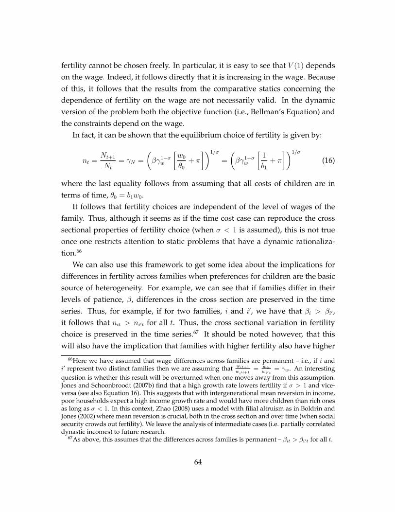
fertility cannot be chosen freely. In particular, it is easy to see that V (1) depends

on the wage. Indeed, it follows directly that it is increasing in the wage. Because

of this, it follows that the results from the comparative statics concerning the

dependence of fertility on the wage are not necessarily valid. In the dynamic

version of the problem both the objective function (i.e., Bellman’s Equation) and

the constraints depend on the wage.

In fact, it can be shown that the equilibrium choice of fertility is given by:

nt =Nt+1

Nt

= γN =

(

βγ1−σw

[

w0

θ0

+ π

])1/σ

=

(

βγ1−σw

[

1

b1

+ π

])1/σ

(16)

where the last equality follows from assuming that all costs of children are in

terms of time, θ0 = b1w0.

It follows that fertility choices are independent of the level of wages of the

family. Thus, although it seems as if the time cost case can reproduce the cross

sectional properties of fertility choice (when σ < 1 is assumed), this is not true

once one restricts attention to static problems that have a dynamic rationaliza-

tion.66

We can also use this framework to get some idea about the implications for

differences in fertility across families when preferences for children are the basic

source of heterogeneity. For example, we can see that if families differ in their

levels of patience, β, differences in the cross section are preserved in the time

series. Thus, for example, if for two families, i and i′, we have that βi > βi′ ,

it follows that nit > ni′t for all t. Thus, the cross sectional variation in fertility

choice is preserved in the time series.67 It should be noted however, that this

will also have the implication that families with higher fertility also have higher

66Here we have assumed that wage differences across families are permanent – i.e., if i andi′ represent two distinct families then we are assuming that wit+1

wi′t+1

= wit

wi′t= γw. An interesting

question is whether this result will be overturned when one moves away from this assumption.Jones and Schoonbroodt (2007b) find that a high growth rate lowers fertility if σ > 1 and vice-versa (see also Equation 16). This suggests that with intergenerational mean reversion in income,poor households expect a high income growth rate and would have more children than rich onesas long as σ < 1. In this context, Zhao (2008) uses a model with filial altruism as in Boldrin andJones (2002) where mean reversion is crucial, both in the cross section and over time (when socialsecurity crowds out fertility). We leave the analysis of intermediate cases (i.e. partially correlateddynastic incomes) to future research.

67As above, this assumes that the differences across families is permanent – βit > βi′t for all t.

64

savings rates. This probably does not hold in the cross section.

A.2 A Dynamic Version of the Endogenous Wage Example

Next, we develop a version of the endogenous wage model in Section 4 that is

consistent with parental altruism as in the B-B model.

Assume that the resource constraints are given by those of problem (6), but

assume that νs + νw = 1. (To simplify notation, write νs = ν and νw = 1 − ν.)

Using capital letters to denote aggregate quantities (i.e. defining Lt ≡ Ntlt etc.),

the planner’s problem can be rewritten as:

max

∞∑

t=0

βtNη+σ−1t C1−σ

t /(1 − σ) (17)

s.t. Lst + Lwt + Lnt ≤ Nt

Ct ≤ aLνstL

1−νwt

bNt+1 ≤ Lnt

As above, the constraint correspondence is homogeneous of degree 1 and the

utility function is homogeneous of degree η in initial condition N0. Assuming

that η = 1 − σ as above, the value function is of the form V (N) = V (1)N1−σ. It

follows that the Bellman Equation is:

V (N) = supC,N ′

C1−σ/(1 − σ) + βV (1)N ′(1−σ)

s.t. Ls + Lw + bN ′ ≤ N

C ≤ aLνsL

1−νw

So for the appropriate choice of αn and αc, the solution to problem (6) can be

interpreted as the solution to the dynamic problem (17) with N0 = 1 in some

cases. Here, normalizing αc = 1, it follows that αn = βV (1).

It is not clear in this framework exactly which comparative statics exercise

corresponds to the one in Section 4, where αn is increased. In principle, it could

correspond either to an increase in β, or to any increase that makes V (1) larger.

In what follows, we consider only the implications of increases, across dynasties,

65

of increases in β’s.

Using the first order conditions to the problem in sequence form and simpli-

fying, we obtain a characterization of the balanced growth path dynamics. The

system is determined by the division of time between schooling and working and

the intertemporal choice of family size involving fertility. It is given by:

Lwt

Lst= 1−ν

ν, and

nσt = γσ

N = β/b1.

That is, fertility is increasing in β. Because of this fact, it follows that bothLst

Ntand Lwt

Ntare decreasing in β, and hence, fertility and income (or wages) are

negatively related as desired.

Thus, for the endogenous wage example, an explicit dynastic form can be pro-

vided that is still consistent with the cross-sectional facts. There are still some is-

sues here, however. Foremost, when discount factors differ across agents, strong

forces for borrowing and lending are typically present. The analysis here ignores

these considerations. It is not certain that the results will be robust to this exten-

sion. 68

A.3 Summary of Findings for Couples’ Models

In Table 3 we summarize the sets of assumptions that are able to generate both a

negative correlation between husband’s as well as wife’s income and fertility.

68Another issue not considered here is variants of intergenerational persistence in preferences.

66

Table 3: Couples: Model Versions that Work

Specialization Exogenous Curvature Spousal (1) (2) (3)# in production heterogeneity in utility matching other ∂n

∂wf

∂n∂wm

∣

∣

wf

∂n∂wm

DATA < 0 mixed < 0

1 full§ ability σ < 1 corr(wf , wm) > 0 < 0 = 0 < 02 full§ ability σ = 1 wf = w ρ < 0♯ n/a∗∗ < 0 < 03 full§ taste any σ prefs matching leisure < 0∗ n/a♭ < 0∗

4 partial ability σ = 1 w′f(wm)wm

wf> 1 < 0 > 0 < 0

5 partial taste any σ prefs matching leisure < 0∗ n/a♭ < 0∗∗ The correlation here is for earnings not wages, but including schooling as in Section 4 will extend the results to wages.∗∗ All women have the same productivity in this example, hence the correlation ∂n/∂wf is not well-defined.§ In the full specialization version wf refers to female productivity at home and cannot be compared directly

to data on female wages.♯ Market goods and female time are complements in home production.♭ The conditional correlation will depend on the details of the matching process. With perfectly aligned preferences,

there is no residual variation in the husband’s wage/earnings, conditional on the wife’s wage/earnings.Hence the conditional correlation is not well-defined in the model analyzed in the paper.

References

AHN, N., AND P. MIRA (2002): “A Note on the Changing Relationship between

Fertility and Female Employment Rates in Developed Countries,” Journal of

Population Economics, 15 (4), 667–682.

AIYAGARI, S. R., J. GREENWOOD, AND N. GUNER (2000): “On the State of the

Union,” Journal of Political Economy, 108(2), 213–244.

ALVAREZ, F. E. (1999): “Social Mobility: The Barro-Becker Children Meet the

Laitner-Loury Dynasties,” Review of Economic Dynamics, 2(1), 65–103.

AMIALCHUK, A. (2006): “The Effect of Husband’s Earnings Shocks on the Timing

of Fertility,” University of Houston, unpublished manuscript.

ANGRIST, J., AND W. N. EVANS (1998): “Children and Their Parents’ Labor Sup-

ply: Evidence from Exogenous Variation in Family Size,” The American Eco-

nomic Review, 88(3), 450–477.

ANGRIST, J. D., V. LAVY, AND A. SCHLOSSER (2005): “New Evidence on the

Causal Link Between the Quantity and Quality of Children,” NBER Working

Papers 11835, National Bureau of Economic Research, Inc.

ARIELY, D., G. HITSCH, AND A. HORTACSCU (2006): “What Makes You Click?

An Empirical Analysis of Online Dating,” University of Chicago, unpublished

manuscript.

ATTANASIO, O., H. LOW, AND V. SANCHEZ-MARCOS (forthcoming): “Explain-

ing Changes in Female Labour Supply in a Life-cycle Model,” The American

Economic Review.

BAGOZZI, R. P., AND M. F. VAN LOO (1978): “Fertility as Consumption: Theories

from the Behavioral Sciences,” The Journal of Consumer Research, 4(4), 199–228.

BAILEY, M. J. (2006): “More power to the pill: The impact of contraceptive free-

dom on women’s lifecycle labor supply,” Quarterly Journal of Economics, 121(1),

289–320.

68

BANKS, W. H. (1955): “Differential Fertility in Madison Country, New York,

1965,” Milbank Memorial Fund Quarterly, 33, 161–186.

BAR, M., AND O. LEUKHINA (2007): “Demographic Transition and Industrial

Revolution: A Macroeconomic Investigation,” University of North Carolina,

unpublished manuscript.

BARRO, R., AND G. BECKER (1989): “Fertility Choice in a Model of Economic

Growth,” Econometrica, 57(2), 481–501.

BECKER, G., AND R. BARRO (1988): “A Reformulation of the Theory of Fertility,”

Quarterly Journal of Economics, 103(1), 1–25.

BECKER, G., K. MURPHY, AND R. TAMURA (1990): “Human Capital, Fertility,

and Economic Growth,” Journal of Political Economy, 98, 812–837.

BECKER, G. S. (1960): “An Economic Analysis of Fertility,” in Demographic and

Economic Change in Developed Countries, no. 11 in Universities – National Bu-

reau Conference Series. Princeton University Press.

(1965): “A Theory of the Allocation of Time,” The Economic Journal,

75(299), 493–517.

BECKER, G. S., AND H. G. LEWIS (1973): “On the Interaction between the Quan-

tity and Quality of Children,” The Journal of Political Economy, 81(2), S279–S288.

BECKER, G. S., AND N. TOMES (1976): “Child Endowments and the Quantity and

Quality of Children,” Journal of Political Economy, 84(4), S143–62.

BEN-PORATH, Y. (1976): “Fertility Response to Child Mortality: Micro Data from

Israel,” Journal of Political Economy, 84(4), S163–78.

BERNAL, R. (2004): “Employment and Child Care Decisions of Women and the

Well-Being of their Children,” IPR Working Paper Series WP-03-03.

BLAU, D., AND W. VAN DER KLAAUW (2007): “The Impact of Social and Eco-

nomic Policy on the Family Structure Experiences of Children in the United

States,” Department of Economics and Carolina Population Center, University

of North Carolina, unpublished manuscript.

69

BOLDRIN, M., M. DE NARDI, AND L. E. JONES (2005): “Fertility and Social Secu-

rity,” NBER Working Paper 11146, National Bureau of Economic Research.

BOLDRIN, M., AND L. E. JONES (2002): “Mortality, Fertility and Saving in a

Malthusian Economy,” Review of Economic Dynamics, 5, 775–814.

BONGAARTS, J. (2003): “Completing the Fertility Transition in the Developing

World: The Role of Educational Differences and Fertility Preferences,” Work-

ing Paper 177, Population Council Policy Research Division.

BORG, M. O. (1989): “The Income–Fertility Relationship: Effect of the Net Price

of a Child,” Demography, 26(2), 301–310.

BROWNING, M. (1992): “Children and Household Economic Behavior,” Journal

of Economic Literature, 30(3), 1434–1475.

CAUCUTT, E., N. GUNER, AND J. KNOWLES (2002): “Why do Women Wait?

Matching, Wage Inequality, and the Incentives for Fertility Delay,” Review of

Economic Dynamics, 5(4).

CHO, L.-J. (1968): “Income and Differentials in Current Fertility,” Demography,

5(1), 198–211.

CLARK, G. (2005): “Human Capital, Fertility, and the Industrial Revolution,”

Journal of the European Economic Association, 3(2-3), 505–515.

(2007): Farewell to Alms: A Brief Economic History of the World. Princeton

University Press.

CLARK, G., AND G. HAMILTON (2006): “Survival of the Richest: The Malthusian

Mechanism in Pre-Industrial England,” Journal of Economic History, 66(3), 707–

736.

DE LA CROIX, D., AND M. DOEPKE (2003): “Inequality and Growth: Why Differ-

ential Fertility Matters,” The American Economic Review, 93(4), 1091–1113.

DE LA CROIX, D., AND M. DOEPKE (2004): “Public versus private education

when differential fertility matters,” Journal of Development Economics, 73(2),

607–629.

70

DEL BOCA, D., AND R. M. SAUER (2006): “Life Cycle Employment and Fertility

Across Institutional Environments,” IZA Discussion Papers 2285, Institute for

the Study of Labor.

DOCQUIER, F. (2004): “Income Distribution, Non-Convexities and the Fertility-

Income Relationship,” Economica, 71 (282), 261–273.

DOEPKE, M. (2004): “Accounting for Fertility Decline During the Transition to

Growth,” Journal of Economic Growth, 9(3), 347–383.

DOEPKE, M. (2005): “Child mortality and fertility decline: Does the Barro-Becker

model fit the facts?,” Journal of Population Economics, 18(2), 337–366.

DOEPKE, M., M. HAZAN, AND Y. MAOZ (2007): “The Baby Boom and World War

II: A Macroeconomic Analysis,” NBER Working Paper 13707, National Bureau

of Economic Research.

ECKSTEIN, Z., AND K. I. WOLPIN (1989): “Dynamic Labour Force Participation

of Married Women and Endogenous Work Experience,” The Review of Economic

Studies, 56(3), 375–390.

EDIN, K. A., AND E. P. HUTCHINSON (1935): Studies of Differential Fertility. Lon-

don: P.S. King and Son.

EHRLICH, I., AND F. T. LUI (1991): “Intergenerational Trade, Longevity, and Eco-

nomic Growth,” Journal of Political Economy, 99(5), 1029–59.

EROSA, A., L. FUSTER, AND D. RESTUCCIA (2005a): “A General Equilibrium

Analysis of Parental Leave Policies,” Working Papers tecipa-197, University of

Toronto, Department of Economics.

(2005b): “A Quantitative Theory of the Gender Gap in Wages,” Working

Papers tecipa-199, University of Toronto, Department of Economics.

ESPENSHADE, T. J. (1984): Investing in Children: New Estimates of Parental Expen-

ditures. Washington,D.C.: Urban Institute Press.

71

FALCAO, B. L. S., AND R. R. SOARES (2007): “The Demographic Transition and

the Sexual Division of Labor,” NBER Working Paper 12838, National Bureau

of Economic Research.

FERNANDEZ, R., N. GUNER, AND J. KNOWLES (2005): “Love and Money: A

Theoretical and Empirical Analysis of Household Sorting and Inequality,” The

Quarterly Journal of Economics, 120(1), 273–344.

FLEISCHER, B. M., AND G. RHODES (1979): “Fertility, Women’s Wage Rates, and

Labor Supply,” The American Economic Review, 69(1), 14–24.

FRANCESCONI, M. (2002): “A Joint Dynamic Model of Fertility and Work of Mar-

ried Women,” Journal of Labor Economics, 20(2), 336–380.

FREEDMAN, D. S., AND A. THORTON (1982): “Income and Fertility: The Elusive

Relationship,” Demography, 19(1), 65–78.

GALOR, O. (2005a): “The Demographic Transition and the Emergence of Sus-

tained Economic Growth,” Journal of the European Economic Association, 3(2-3),

494–504.

(2005b): “From Stagnation to Growth: Unified Growth Theory,” in Hand-

book of Economic Growth, ed. by P. Aghion, and S. Durlauf, vol. 1, chap. 4, pp.

171–293. Elsevier.

GALOR, O., AND O. MOAV (2002): “Natural Selection And The Origin Of Eco-

nomic Growth,” The Quarterly Journal of Economics, 117(4), 1133–1191.

GALOR, O., AND D. N. WEIL (1996): “The Gender Gap, Fertility and Growth,”

The American Economic Review, 86(3), 374–387.

(1999): “From Malthusian Stagnation to Modern Growth,” The American

Economic Review, Papers and Proceedings, 89(2), 150–154.

(2000): “Population, Technology, and Growth: From Malthusian Stag-

nation to the Demographic Transition and Beyond,” The American Economic

Review, 90(4), 806–28.

72

GOLDIN, C., AND L. F. KATZ (2002): “The Power of the Pill: Oral Contracep-

tives and Women’s Career and Marriage Decisions,” Journal of Political Econ-

omy, 110(4), 730–770.

GREENWOOD, J., AND N. GUNER (2005): “Social Change,” Economie d’Avant

Garde Research Paper No. 9.

GREENWOOD, J., N. GUNER, AND J. A. KNOWLES (2003): “More on Marriage,

Fertility, and the Distribution of Income,” International Economic Review, 44(3),

827–862.

GREENWOOD, J., AND A. SESHADRI (2002): “The U.S. Demographic Transition,”

The American Economic Review, Papers and Proceedings, 92(2), 153–159.

GREENWOOD, J., A. SESHADRI, AND G. VANDENBROUCKE (2005): “The Baby

Boom and Baby Bust,” The American Economic Review, 95 (1), 183–207.

HAINES, M. R. (1976): “Population and Economic Change in Nineteenth Cen-

tury Eastern Europe: Prussian Upper Silesia, 1840-1913,” The Journal of Eco-

nomic History, 36(2), 334–358.

HANSEN, G. D., AND E. C. PRESCOTT (2002): “Malthus to Solow,” The American

Economic Review, 92(4), 1205–17.

HECKMAN, J. J. (1976): “A Life Cycle Model of Earnings, Learning, and Con-

sumption,” Journal of Political Economy, 84(4), S11–S44.

HECKMAN, J. J., AND J. R. WALKER (1990): “The Relationship between Wages

and the Timing and Spacing of Births: Evidence from Swedish Longitudinal

Data,” Econometrica, 58(6), 1411–1441.

HOTZ, J. V., AND R. A. MILLER (1988): “An Empirical Analysis of Life Cycle

Fertility and Female Labor Supply,” Econometrica, 56(1), 91–118.

HOTZ, V. J., J. A. KLERMAN, AND R. J. WILLIS (1993): “The Economics of Fer-

tility in Developed Countries,” in Handbook of Population and Family Economics,

ed. by M. Rosenzweig, and O. Stark, vol. 1, chap. 7, pp. 275–347. Elsevier.

73

JAFFE, A. J. (1940): “”Differential Fertility in the White Population in Early Amer-

ica,” Journal of Heredity, pp. 407–411.

JONES, L. E., AND A. SCHOONBROODT (2007a): “Baby Busts and Baby Booms:

The Fertility Response to Shocks in Dynastic Models,” Discussion papers in

economics and econometrics, 0706, University of Southampton.

(2007b): “Complements versus Substitutes and Trends in Fertility Choice

in Dynastic Models,” NBER Working Paper 13680, National Bureau of Eco-

nomic Research.

JONES, L. E., AND M. TERTILT (2008): “An Economic History of Fertility in the

U.S.: 1826-1960,” in Frontiers of Family Economics, ed. by P. Rupert, vol. 1. Emer-

ald Press, forthcoming.

KEANE, M. P., AND K. I. WOLPIN (2006): “The Role of Labor and Marriage Mar-

kets, Preference Heterogeneity and the Welfare System in the Life Cycle De-

cisions of Black, Hispanic and White Women,” PIER Working Paper Archive

06-004, Penn Institute for Economic Research, Department of Economics, Uni-

versity of Pennsylvania.

KNOWLES, J. (2007): “Why Are Married Men Working So Much? The Macroeco-

nomics of Bargaining between Spouses,” IZA Discussion Papers 2909, Institute

for the Study of Labor.

LAZEAR, E. P., AND R. T. MICHAEL (1980): “Family Size and the Distribution of

Real Per Capita Income,” The American Economic Review, 70(1), 91107.

LEE, R. (1987): “Population Dynamics of Humans and Other Animals,” Demog-

raphy, 24(4), 443–466, Presidential Address to the Population Association of

America.

LEE, S. (2008): “Preferences and Choice Constraints in Marital Sorting: Evidence

from Korea,” Stanford University, unpublished manuscript.

MANUELLI, R. E., AND A. SESHADRI (2007): “Explaining International Fertility

Differences,” University of Wisconsin, unpublished manuscript.

74

MERRIGAN, P., AND Y. S. PIERRE (1998): “An Econometric and Neoclassical

Analysis of the Timing and Spacing of Births in Canada from 1950-1990,” Jour-

nal of Population Economics, 11(1), 29–51.

MILLER, A. (2007): “The Effects of Motherhood Timing on Career Path,” Working

paper, University of Virginia.

MINCER, J. (1963): “Market Prices, Opportunity Costs, and Income Effects,” in

Measurement in Economics: Studies in Mathematical Economics in Honor of Yehuda

Grundeld, ed. by C. C. et al., pp. 67–82. Stanford University Press, CA.

MINCER, J., AND H. OFEK (1982): “Interrupted Work Careers: Depreciation and

Restoration of Human Capital,” The Journal of Human Resources, 17(1), 3–24.

MINCER, J., AND S. POLACHEK (1974): “Family Investments in Human Capital:

Earnings of Women,” The Journal of Political Economy, 82(2), S76–S108.

MOAV, O. (2005): “Cheap Children and the Persistence of Poverty,” Economic

Journal, 115(500), 88–110.

MURTIN, F. (2007): “American Economic Development or the Virtues of Educa-

tion,” Stanford Center for the Study of Poverty and Inequality, unpublished

manuscript.

PENCAVEL, J. (1998): “Assortative Mating by Schooling and the Work Behavior

of Wives and Husbands,” The American Economic Review, 88(2), 326–329.

PRESTON, S., AND C. STEN (2008): “The Future of American Fertility,” Discussion

paper, University of Pennsylvania, manuscript prepared for NBER Conference

on Demography and Economics, Napa, California, April 2008.

ROSENZWEIG, M. R., AND K. I. WOLPIN (1980): “Testing the Quantity-Quality

Fertility Model: The Use of Twins as a Natural Experiment,” Econometrica,

48(1), 227–40.

RUGGLES, S., M. SOBEK, T. ALEXANDER, C. A. FITCH, R. GOEKEN, P. K. HALL,

M. KING, AND C. RONNANDER (2004): “Integrated Public Use Microdata Se-

ries: Version 3.0,” Minneapolis: Minnesota Population Center.

75

SCHULTZ, T. (1981): Economics of Population. Addison Wesley Publishing Com-

pany, Reading.

SCHULTZ, T. P. (1986): “The Value and Allocation of Time in High-Income Coun-

tries: Implications for Fertility,” Population and Development Review, 12, 87–108.

SHIUE, C. H. (2008): “Human Capital and Fertility in Chinese Clans, 1300-1850,”

University of Colorado at Boulder, unpublished manuscript.

SIMON, J. L. (1977): The Economics of Population Growth. Princeton, New Jersey.

SKIRBEKK, V. (2008): “Fertility trends by social status,” Demographic Research,

18(5), 145–180.

SYLVESTER, M. S. (2007): “The Career and Family Choices of Women: A Dy-

namic Analysis of Labor Force Participation, Schooling, Marriage and Fertility

Decisions,” Review of Economic Dynamics, 10(3), 367–399.

TERTILT, M. (2005): “Polygyny, Fertility, and Savings,” Journal of Political Econ-

omy, 113 (6), 1341–1371.

U.S. CENSUS (1945): “Differential Fertility 1910 and 1940,” U.S. Bureau of the

Census, Census of Population, Government Printing Office, Washington.

(1955): “Fertility,” U.S. Bureau of the Census, Census of Population, Gov-

ernment Printing Office, Washington.

WEIR, D. R. (1995): “Family Income, Mortality, and Fertility on the Eve of the

Demographic Transition: A Case Study of Rosny-Sous-Bois,” The Journal of

Economic History, 55(1), 1–26.

WESTOFF, C. F. (1954): “Differential Fertility in the United States: 1900 to 1952,”

American Sociological Review, 19(5), 549–561.

WHELPTON, P., AND C. KISER (eds.) (1951): Social and Psychological Factors Af-

fecting Fertility. Milbank Memorial Fund.

WILLIS, R. J. (1973): “A New Approach to the Economic Theory of Fertility Be-

havior,” The Journal of Political Economy, 81(2), S14–S64.

76

WRIGLEY, E. A. (1961): Industrial Growth and Population Change. Cambridge Uni-

versity Press, Cambridge.

ZHAO, K. (2008): “Social Security, Differential Fertility, and the Dynamics

of the Earnings Distribution,” University of Western Ontario, unpublished

manuscript.

77