Embed Size (px)
Citation preview

Fertility Limits on Local Politicians in India∗
S Anukriti† Abhishek Chakravarty‡
October 2014
Abstract
We examine the demographic implications of fertility limits on local politicians. Several
Indian states disbar individuals who have more than two children from membership
to Village Councils, or Panchayats. Panchayats are the lowest unit of governance in
India with a large number of elected members who exercise considerable power at
the village level. We find that families are less likely to have more than two children
due to fertility limits on Panchayat members, but second births among politically
dominant upper-caste families (with historically stronger preference for sons) are more
likely to be male. Although these limits are intended to change constituents’ behavior
through a role-model effect, we show that the fertility decline instead reflects strong
local leadership aspirations among Indians. We identify incentives for political power
as a novel instrument of demographic change in democratic settings.
JEL Codes: J13, J16, H75, O11Keywords: India, Panchayat Elections, Fertility Limits, Sex Ratios, Political Aspirations
∗We thank Heather Banic and Priyanka Sarda for excellent research assistance. The paper benefittedfrom presentations at Indian School of Business, Indian Statistical Institute (Delhi), Shiv Nadar University,South Asia University, and University of Essex.†Department of Economics, Boston College. [email protected].‡Department of Economics, University of Essex. [email protected].
0
1 IntroductionDeveloping countries with large populations often employ policy tools to decrease fertility.
Recent measures include direct fertility limits on citizens (e.g., China’s One Child Policy),
conditional cash transfer programs (e.g., Haryana’s Devirupak scheme), and incentives to
promote contraceptive prevalence (e.g., sterilization incentives in India). This paper examines
a novel policy experiment that imposes fertility limits on political candidates running for
leadership positions in the local government. Specifically, we analyze the impact of state-
level legislations that disbar individuals with more than two children from contesting Village
Council (Panchayat) elections on fertility-related outcomes in India. To the best of our
knowledge, these two-child limits are the first instance of a democratic country instituting
a fertility ceiling for candidates aspiring to elected office. This paper is hence the first to
examine how households trade-off the chance to hold political office against having more
children. We also investigate the role of son preference in this trade-off by examining how
fertility and sex-selection responses to the policy differ by the number of sons households
already have when it is implemented.
Starting with Rajasthan in 1992, eleven Indian states have enacted fertility limits on
local elected representatives of village, block, and district-level Panchayats. While four states
revoked these laws after a few years of implementation, it remains in effect in seven states. In
all cases, the law included a one year post-announcement grace-period, births during which
were not counted towards the limit. Candidates who already had two or more children when
the law was enacted are disqualified if they have an additional child after the grace-period
cut-off date. Individuals who had fewer than two children when the law was enacted are
disqualified if they have a third or higher order birth after the grace-period. We utilize the
quasi-experimental geographical and temporal variation in the announcement of these laws
and the allowance of a grace-period to estimate the causal impact of these limits on fertility-
related outcomes through regression discontinuity (RD) graphs and differences-in-differences
1
(DD) methods. We combine complete retrospective birth histories from large-scale individual
surveys to construct a woman-year panel that spans the years from 1973 to 2006.
We find that the two-child limits on electoral candidates decrease fertility in the general
population but have unintended consequences for the sex ratio at birth when son preference
is strong. Overall, the likelihood that a woman has more than two children in any given year
decreases. However, this decline is not immediate: during the grace-period, there is a large
increase in the probability of a third birth, which is then followed by fertility decline. This
pattern is unlikely to be driven by a role-model effect, which would require a period of time
to pass after the law’s enactment for the constituents to observe and emulate their leaders’
fertility decisions. Instead, the fertility increase during the grace-period and the immediate
decline thereafter are more plausibly attributable to ambitious individuals attempting to
have a third birth before the grace-period window closes, while still remaining eligible for
future elections. Thus, households appear to be driven by their own leadership aspirations
rather than their leaders’ actions.
We also examine the effect on the likelihood of second births and their sex ratio for
women whose first child was born before the laws were announced. In addition to a DD
specification, we also estimate the effect on second births in a triple-DD framework by
utilizing the variation in the sex of the firstborn child. Prior literature shows that the sex
of first births in India is close to random in most states, despite availability of prenatal
sex-determination technology. We find that, due to the two-child limits, upper-caste women
with firstborn girls are less likely to have a second birth and are more likely to have a male
child if there is a second birth. The negative fertility effect on second births can be explained
by increased sex-selection as each abortion delays the next birth, at the minimum, by a year
(Bhalotra and Cochrane (2010)). These results indicate that, among those whose first child
was born before the treatment year, upper-caste households wishing to remain eligible for
Village Council leadership restrict their fertility to two children, but ensure that the second
child is male if the first is not. Thus, a preference for sons can cause policies that target
2
lower fertility to have unintended effects for sex ratios; thereby reiterating the need for more
careful policy design.
Our paper makes novel contributions to three distinct literatures: (i) on the effects of
leaders’ characteristics on followers’ behaviors, (ii) on the strength of political aspirations
in democratic countries, and (iii) on the determinants of fertility and sex ratios in high-
son preference countries. Apart from the large literature on peer-effects, the socio-economic
characteristics of individuals in positions of authority (e.g., teachers, mothers, television
characters, and religious leaders) have been shown to exert considerable influence on their
followers’ behaviors and outcomes (e.g., Fernandez et al. (2004), Bettinger and Long (2005),
Jensen and Oster (2009), Beaman et al. (2012), Chong et al. (2012), Olivetti et al. (2013),
and Bassi and Rasul (2014)). Indeed, the stated rationale behind the Indian two-child lim-
its is that restricting fertility of elected representatives can decrease fertility among their
constituents through a “role-model” effect.1
However, these limits also directly incentivize individuals who aspire to run for local
office in the future to have fewer children. Our results suggest that the incentive effect domi-
nates the role-model effect. Thus, we identify access to political power as a novel instrument
for demographic influence in democratic settings. Our results also imply that local leader-
ship ambitions in India are quite strong as individuals are willing to decrease fertility for
a chance to hold political office in the future. This finding also highlights the participatory
and inclusive nature of the Panchayati Raj system.
Recent work on the determinants of fertility in developing countries has highlighted the
causal relationship between fertility decline and rising sex ratios in societies like India where
sons are preferred (Ebenstein (2010), Anukriti (2014), Jayachandran (2014)). We augment
this literature by investigating a new source of fertility decline that has an unintended effect
on sex ratios similar to programs like the One Child Policy and Devirupak.
1http://www.nytimes.com/2003/11/07/world/states-in-india-take-new-steps-to-limit-births.html
3
In recent discussions, similar limits have been proposed for state legislative assembly
members as well as members of the national Parliament in India. To the extent that in-
dividuals might find it easier to aspire to becoming a local leader and the socio-economic
characteristics, especially fertility, of local politicians might be more salient due to greater
visibility, policies that affect officials at the grassroots level might be more effective than
limits on leaders situated in state or national capitals. Our results thus shed light on the
potential consequences of these measures for fertility and sex ratio outcomes.
The remainder of the paper is organized as follows. Section 2 discusses the fertility limits
in detail. Sections 3 and 4 describe our data and empirical strategy. Section 5 presents the
estimation results. Section 6 conducts some robustness checks and Section 7 concludes.
2 BackgroundIndia is the world’s second most populous country and houses a third of the world’s poorest
1.2 billion citizens (Olinto et al. (2013)). Consequently, fertility reduction continues to be
atop its policy agenda. Based on the recommendations of the Committee on Population
set up by the National Development Council (NDC) in 1992, several Indian states have
enacted legislations that disbar individuals with more than two children from contesting
local elections. The stated rationale behind these laws is that two-child norms for elected
representatives will decrease fertility among their constituents through a role-model effect.
However, these laws also incentivize individuals who intend to run for elections in the future
to plan smaller families.
India has a three-tiered decentralized system of local governance in rural areas, known as
the Panchayati Raj. It comprises village-level councils (Gram Panchayat), block-level coun-
cils (Panchayat Samiti), and district-level councils (Zila Parishad). Although the Panchayat
system has existed in several Indian states since the 1950s, it was granted constitutional sta-
tus in 1992 through the 73rd Amendment of the Indian Constitution (The Panchayati Raj
(PR) Act). Since then, regular Panchayat elections have taken place every five years in most
4
states. These elected local councils, particularly at the village level, are the building blocks of
the Indian democratic system and exercise considerable power in their constituencies. They
receive substantial funds from the national and the state governments,2 and are authorized to
implement developmental schemes.3 Additionally, Panchayats can collect taxes, license fees,
and fines, and receive seignorage from the auction of local mineral and forestry resources,
giving elected members discretion over a large share of local public funds.
The PR Act requires that at least one-third of all member and chief positions are reserved
for women. Similarly, positions are reserved for Scheduled Castes (SC) and Scheduled Tribes
(ST) in proportion to their share in the village, block, or district population. Reservations
for these groups are implemented in a stratified manner—among positions or seats reserved
for SC, ST, and “general” castes, one-third are randomly chosen for women.
In most states, the fertility limits have been enacted for elections to rural Panchayats;
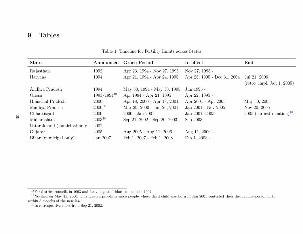
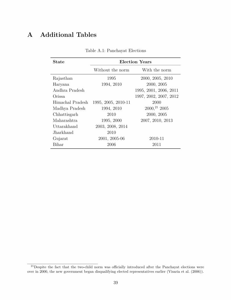
however, a few states have also imposed these norms on urban municipalities. Table 1 presents
the timeline for the enactment and implementation of the two-child laws across Indian states4
and Table A.1 shows the local election years for which they were effective. The relevant
clauses from each state’s PR Acts are presented in Section B.
Rajasthan was the first state to introduce such a law in 19925 and provided for a one
year grace-period—any births during the grace-period were not counted towards the limit.
A candidate who had two or more children at the start of the cut-off and had an additional
child after the grace-period cut-off date was disqualified. However, no elections were held
under this amended law. The two-child norm was then included in Rajasthan’s 1994 PR Act
which stipulated that anyone who had a third or higher-order birth after April 1994 would be
2For example, in Tamil Nadu, all Panchayats receive a minimum of approximately USD 4,900 in annualstate grants as of 2009-10. About 35% of these Panchayats receive funds in the range of approximately USD16,330-40,800. These are significant budgets considering that India’s annual per capital GNI was USD 1,570in 2013 (Source: The World Bank).
3Panchayats are also often authorized to identify local beneficiaries of major central and state developmentschemes such as the National Rural Employment Guarantee Scheme.
4This information is largely based on Buch (2005) and Buch (2006).5Rajasthan’s law predates the NDC recommendations.
5
ineligible to contest elections. Due to popular pressure, a grace-period was provided whereby
births during April 23, 1994 - November 27, 1995 were not counted towards the fertility cut-
off. Effectively, this translated into a nearly three-year grace-period (from the announcement
in 1992 till November 1995). As a result, the law came into effect after Rajasthan’s first
post-73rd Amendment Panchayat election (that took place in 1995). A similar law was also
passed for municipal elections in urban areas.
In Haryana, the law was announced through the PR Act in 1994 with a one-year grace
period (until April 24, 1995). However, the first Panchayat elections had already taken place
in 1994 and since members of the local councils are elected for a period of five years, no one
was disqualified during 1995-2000. The Haryana government revoked this law in July 2006
and the repeal came into effect retroactively from January 1, 2005.
Andhra Pradesh (AP) introduced the fertility limit in its 1994 PR Act and also provided
a one-year grace period. Orissa announced the law first for its district councils in November
1993 and then for the village and block councils in April 1994.6 Himachal Pradesh (HP),
Madhya Pradesh (MP), and Chhattisgarh7 introduced their laws in 2000 and, like Haryana,
repealed them in 2005. Maharashtra adopted the norm in 2003 with retrospective effect from
September 21, 2002. Lastly, Bihar and Uttarakhand have adopted the law for municipal
elections, but not for Panchayat elections.
At the time of filing the nomination papers, the candidates do not have to explicitly
declare their number of children. However, they do have to sign a declaration that includes:
“...to the best of my knowledge and belief, I am qualified and not also disqualified for being
chosen to fill the seat.” The Returning Officer (nominated by the Election Commission) is
responsible for scrutinizing the information submitted by the nominees and any objections
raised by the rival candidates, general public, or the media. Table 2 shows the number of
6Additionally, in Orissa, an individual who cannot read and write Oriya or who has more than one livingspouse is also disqualified. The illiteracy criterion is not applicable to the village council elections.
7Chhattisgarh inherited the law when it was carved out of MP in 2000. Since 2004, candidates below 30years of age in Chhattisgarh are also required to be literate.
6

Panchayat members that have been disqualified under these laws in Haryana, Rajasthan,
MP, and AP during 2000-04.8
Although their formulation is quite similar across states, the two-child laws are ambiguous
in some cases. For example, the laws in Haryana and MP explicitly mention two living
children, whereas in AP, Orissa, and Rajasthan the clauses do not distinguish between births
and living children. In Rajasthan, twins are considered as one birth and a still-birth is not
counted as a birth, while in MP the District Collector has discretion over disqualification
in these events. However, children given up for adoption are counted towards the two-child
limit for disqualification in all states. In most states, for a disqualification, a complaint has
to be filed with the appropriate adjudicating authority, except in Orissa (for village councils)
and MP where the competent authority can initiate action on its own.
These fertility limits are believed to be in conflict with the National Population Policy
(2000) that is critical of “any form of coercion” to achieve population stabilization. Newspa-
per reports suggest that, in some instances, wives have been abandoned by their husbands,
female fetuses have been selectively aborted, and children have been given up for adoption to
avoid disqualification. Consequently, implementing states have faced criticism from women’s
rights advocates and civil society organizations, as well as the central government and the
Union Ministry of Panchayati Raj.9 Due to the resulting pressure, these laws have been re-
voked in four states. Thus, eleven Indian states have imposed a fertility limit on their local
politicians for at least a few years and they remain in effect in seven major states.
These laws affect a large number of people. Typically, a Village Panchayat has 5-15
elected members. According to the 2011 Census of India, AP had 12,810 Village Panchayats,
which implies that 64,050 to 192,150 people are directly affected by these limits in one state
alone. This figure grows to a minimum of 281,130 Panchayat members once we consider the
8Reliable data for the remaining states and years is not readily available and is being collected by theauthors.
9http://policydialogue.org/files/events/Aiyar_Key_Role_of_Panchayati_Raj_in_India.pdf
7

other states where the norm is currently active, and multiplies rapidly if we also consider
aspiring individuals who wish to run for future elections. The number of individuals affected
grows further if we also include the block and district tiers of the Panchayat system, and the
states where the norm was active in the past.
3 DataWe utilize repeated cross-sectional data from three rounds of the National Family Health
Survey (NFHS-1, 2, 3) and one round of the District-Level Household Survey (DLHS-2)
of India.10 Each survey-round is representative at the state-level and includes a complete
retrospective birth history for every woman interviewed, containing information on the month
and the year of child’s birth, birth order, and mother’s age at birth. We combine these birth
histories to construct an unbalanced woman-year panel;11 a woman enters the panel in her
year of first marriage and exits in her year of survey.
For consistency across rounds, we limit the sample to currently-married women in the
15-44 age-group at the time of survey.12 We also drop women (i) who were married more
than 20 years prior to the survey to avoid issues related to imperfect recall, (ii) whose
husband’s age was below 15 or above 80 in the year of survey, and (iii) who have given birth
to more than ten children, to prevent any composition-bias since these women are likely to
be fundamentally different from rest of the sample. Lastly, we exclude mothers who have had
twins since multiple births in our context are largely unplanned and do not reflect parents’
fertility preferences.13 However, our results are not driven by any of these selection criteria.
10The years of survey are 1992-93, 1998-99, and 2005-06 for the NFHS and 2002-04 for the DLHS.11The DLHS and the NFHS are similar in terms of the selection of respondents, the conduct of interviews,
and the questionnaires used. Sample sizes, however, are much larger for the DLHS since it is also represen-tative at the district-level. As shown in Section 6, our results do not change if only one of these datasets isused.
12Survey questionnaires were administered to 13-49-year old ever-married women in NFHS-1, 15-49-yearold ever-married women in NFHS-2,3, and 15-44-year old currently-married women in DLHS-2.
13Additionally, we drop women who were visiting the household when the survey took place, and wereinterviewed as a result, since there is no information on their actual state of residence.
8
Our final sample comprises 511,542 women and 1,261,711 births from 18 major states14
and covers the time period 1973-2006. As discussed earlier, the fertility limits were an-
nounced, enacted, and became effective (during an election) over several years. Moreover, a
one-year grace-period was provided in all instances. To err on the side of caution, we define
treatment based on the year of announcement, i.e., the earliest and the most conservative
year when the law might have had an effect. Since the most recent year in our sample is
2006, we cannot credibly examine the effect of revocations that took place in 2005. However,
we have a large number of post-announcement years, ranging from 4 to 13 years, to estimate
the relatively long-term effect of the fertility limits.
Table 3 displays the years we use for defining the pre- and post-treatment period for
each affected state. Table 4 presents the sample means and standard deviations for the key
variables used in our analyses, separately for never-treated and treated states. We further
split the treated sample into pre- and post-treatment observations. About two-thirds of
women in our sample live in a rural area. A majority of them are Hindus, with a larger
share (90%) among treated relative to never-treated households (79%). In terms of caste-
composition, upper-castes and other backward classes (OBC) comprise about 40% and 35%
of the sample, while the rest belong to Scheduled Castes (SC) and Scheduled Tribes (ST).
Educational attainment is low for women, with more than half the sample being uneducated;
in comparison, 29% of the husbands are uneducated. In terms of our outcome variables,
women in the post-treatment group are less likely to give birth and are more likely to have
two children relative to women in the never-treated and pre-treatment sub-samples.
The sample means for the three groups in Table 3 are similar along most, if not all,
socio-economic dimensions. Nevertheless, to ensure that our estimates are not confounded
by any underlying differences between these samples, we control for religion, caste, standard
14The states of Uttarakhand, Jharkhand, and Chhattisgarh were, respectively, carved out from UttarPradesh (UP), Bihar, and MP in 2000. Since our data does not include districts-identifiers for all rounds, wesubsume these three new states into their parent states for our analyses.
9
of living, husband’s and wife’s years of schooling, and residence in an urban area in our
regressions. To take into account state-specific factors, we include state fixed effects and also
control for state-specific linear time trends. In addition, we conduct several robustness checks
to establish that our estimates are measuring the causal effect of fertility limits.
4 Empirical StrategyThe goal of our empirical strategy is to estimate the causal effect of fertility limits on local
politicians in a state on fertility-related outcomes among residents in the same state. To do so,
we utilize the quasi-experimental geographical and temporal variation in the announcement
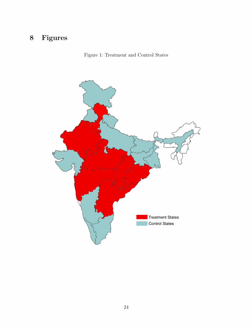
of these laws across Indian states. Although eleven states have enacted such a law thus far,
due to data limitations we can estimate its impact for only eight states: Rajasthan, Haryana,
AP, Orissa, HP, MP, Chhattisgarh, and Maharashtra. The law came into effect in Bihar and
Gujarat after 2006, so in our sample these states are not treated. Although Uttarakhand
announced its law for urban municipal elections in 2002, our analyses exclude it from the
group of treatment states because Uttarakhand was a part of Uttar Pradesh until 2000 and
we cannot distinguish between the two in the pre-2000 sample.15 Our results, however, are
robust to the exclusion of Uttar Pradesh. In addition to Bihar, Gujarat, and Uttarakhand,
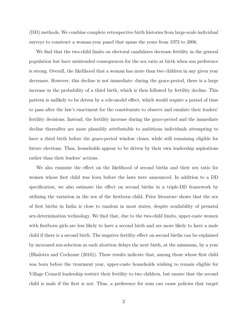
our control group comprises nine other states. Figure 1 depicts the treatment and control
states in a map.
If the two-child limits are effective, we expect to observe changes in the probability of third
births for couples who already have two children when the law is announced. To examine if
this is the case, we estimate the following DD-type regression specification for a woman i of
age a in state s and year t:
Yisat = α + β1Treatst +X′
iδ + γs + θt + ψa + νs ∗ t+ εisat (1)
15Note that Uttar Pradesh has never enacted a two-child limit for its local politicians.
10

where Treatst is equal to one for women residing in the treated states if t > the year
of announcement, and zero otherwise; γs, θt, and ψa are fixed effects for state, year, and
woman’s age. We also control for state-specific linear time trends (νs ∗ t) and the following
covariates (Xi): five categories each for a woman’s and her husband’s years of schooling,
indicators for the religion (five categories), caste (four categories), and the standard of living
(three categories) of the household, residence in an urban area, and indicators for the year
of interview. We restrict the sample to women whose first two children are born before the
treatment is announced in their state. The key coefficient of interest is β1, which measures
the effect of two-child limits on our outcomes variable which is an indicator for a third birth.
It is likely that the two-child laws also affect second parity births for couples who have
one child at announcement. For example, if son preference is strong, women who have one
daughter when the law is announced may be more likely to practice sex-selection at second
parity due to the two-child limit, which might delay their second birth. In addition to a
DD specification similar to (1) for second births, we also estimate a triple DD specification
by interacting Treatst with an indicator (Girli) for whether the first child (born before
treatment) is a girl:
Yisat = α + β2Treatst ∗Girli + φTreatst + ωGirli
+X′
iδ + γs + θt + ψa + νs ∗ t+ τs ∗Girli + εisat
(2)
The outcome variables are indicators for a second birth and, conditional on birth, the
likelihood that the child is male. The coefficient φ estimates the effect of the two-child laws
on couples whose firstborn is a boy while β2 estimates the differential effect on couples
whose firstborn is a girl. Prior literature on India has shown that, despite the availability of
prenatal sex-determination technology, sex of the first birth is plausibly random (Bhalotra
and Cochrane (2010)) and most instances of sex-selection occur for higher-order births.
However, Anukriti (2014) finds that this is not true for first births in Haryana after 2002 when
firstborn children are more likely to be male due to the Devirupak scheme. Therefore, we
11
drop post-2002 observations for Haryana from our sample while estimating (2). In addition,
we restrict the sample to women whose first child is born before the year of treatment.
The inclusion of state and year fixed effects in our specifications controls for any time-
invariant state-level variables and state-invariant overall time trends that might affect fertility
outcomes. Moreover, state-specific time trends account for differential linear trends in fertility
patterns across states over the time period of analysis. We cluster standard errors at the state
level when both treated and never-treated states are included in the sample. In specifications
where the sample is restricted to only the treated states, we cluster at the state-year level
to avoid econometric issues pertaining to a small number of clusters.
Our underlying identifying assumption is that the state-year variation in the timing of
law announcement is uncorrelated with other time-varying determinants of the outcomes of
interest. In addition to controlling for state-specific linear trends in our regressions, in the
next section we show that there are no significant differences in pre-treatment trends for our
treatment and control groups. This supports our identifying assumption that the treatment
and comparison women would have had similar trends in fertility rates in the absence of the
two-child limits. Moreover, in Section 6 we show that the timing of announcement is uncor-
related with other socio-economic characteristics that vary by state and time. Lastly, during
the time period we examine, there were no other state-specific programs in the treatment
states that promoted smaller families and whose timing coincided with the fertility limits.
5 Results
5.1 Event-Study Graphs
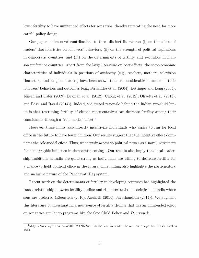
We first present graphical evidence for the effect of the fertility limits. In Figures 2 and 3 we
focus only on treated states and use an event-study framework to depict the evolution of the
likelihood that a woman has more than two, three, or four living children in a given year. The
plotted coefficients show the differential trends in the likelihood of having more than two,
three, or four living children for women in treatment and control groups, after controlling for
12
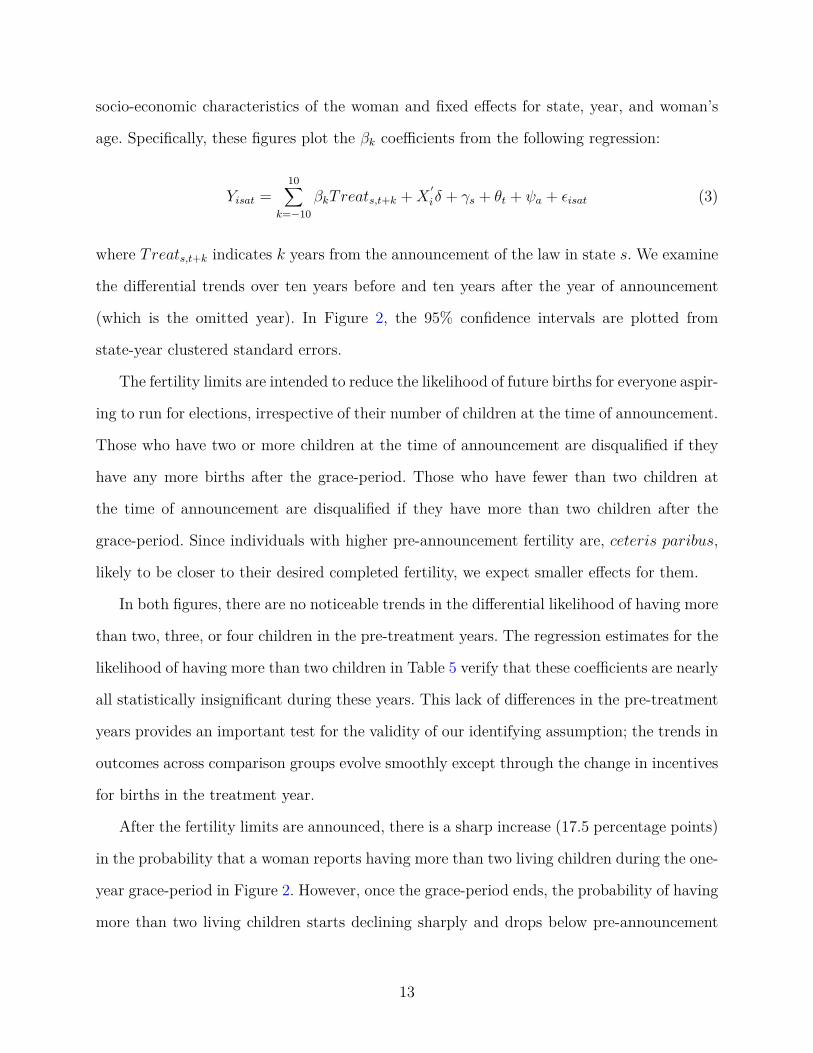
socio-economic characteristics of the woman and fixed effects for state, year, and woman’s
age. Specifically, these figures plot the βk coefficients from the following regression:
Yisat =10∑
k=−10βkTreats,t+k +X
′
iδ + γs + θt + ψa + εisat (3)
where Treats,t+k indicates k years from the announcement of the law in state s. We examine
the differential trends over ten years before and ten years after the year of announcement
(which is the omitted year). In Figure 2, the 95% confidence intervals are plotted from
state-year clustered standard errors.
The fertility limits are intended to reduce the likelihood of future births for everyone aspir-
ing to run for elections, irrespective of their number of children at the time of announcement.
Those who have two or more children at the time of announcement are disqualified if they
have any more births after the grace-period. Those who have fewer than two children at
the time of announcement are disqualified if they have more than two children after the
grace-period. Since individuals with higher pre-announcement fertility are, ceteris paribus,
likely to be closer to their desired completed fertility, we expect smaller effects for them.
In both figures, there are no noticeable trends in the differential likelihood of having more
than two, three, or four children in the pre-treatment years. The regression estimates for the
likelihood of having more than two children in Table 5 verify that these coefficients are nearly
all statistically insignificant during these years. This lack of differences in the pre-treatment
years provides an important test for the validity of our identifying assumption; the trends in
outcomes across comparison groups evolve smoothly except through the change in incentives
for births in the treatment year.
After the fertility limits are announced, there is a sharp increase (17.5 percentage points)
in the probability that a woman reports having more than two living children during the one-
year grace-period in Figure 2. However, once the grace-period ends, the probability of having
more than two living children starts declining sharply and drops below pre-announcement
13
levels within three years after the grace-period, and further declines in the following years.
Since the effective grace-period for Rajasthan was nearly three years long, it is not surprising
that it takes about that many years for the likelihood of more than two children to return to
its pre-announcement levels. The fertility drop is significant in every post-treatment year up
to ten years after the law is announced, with a maximum decrease of about 14 percentage
points in the sixth year.
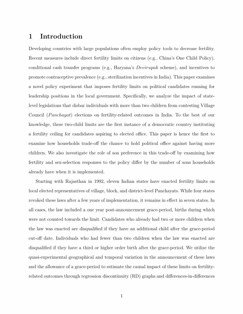
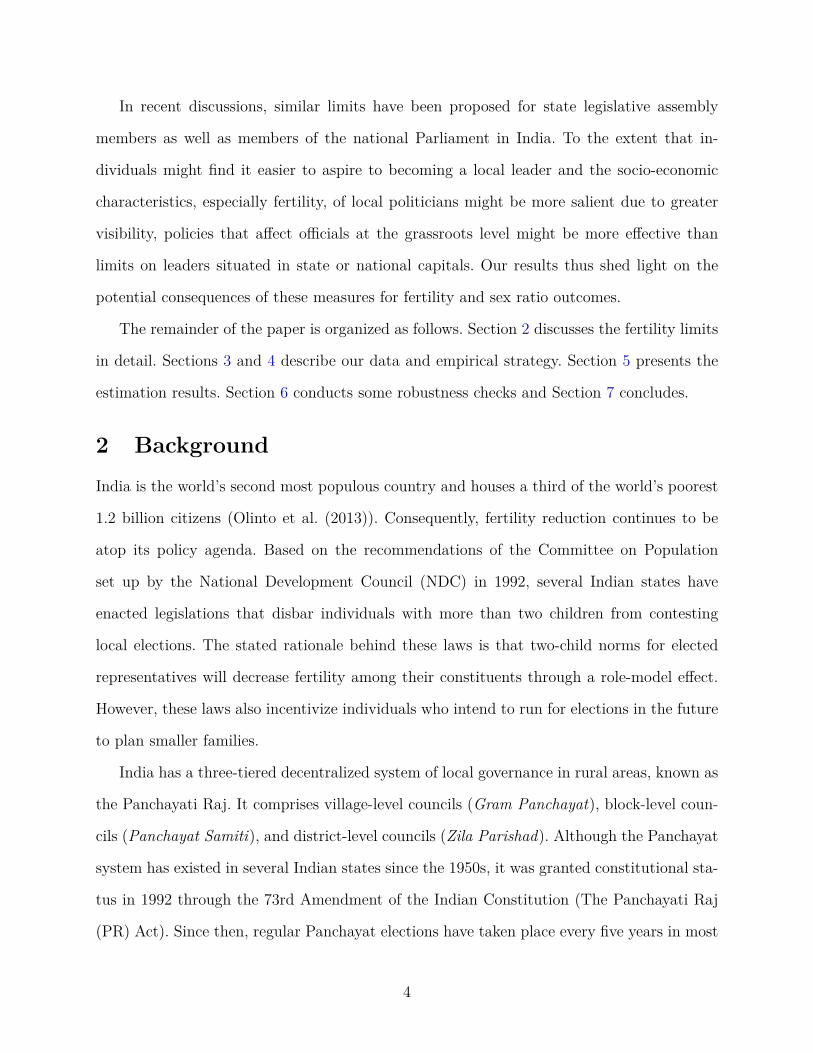
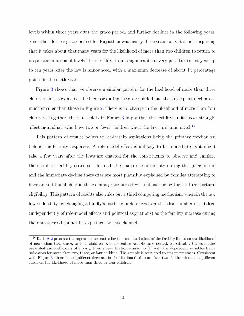
Figure 3 shows that we observe a similar pattern for the likelihood of more than three
children, but as expected, the increase during the grace-period and the subsequent decline are
much smaller than those in Figure 2. There is no change in the likelihood of more than four
children. Together, the three plots in Figure 3 imply that the fertility limits most strongly
affect individuals who have two or fewer children when the laws are announced.16
This pattern of results points to leadership aspirations being the primary mechanism
behind the fertility responses. A role-model effect is unlikely to be immediate as it might
take a few years after the laws are enacted for the constituents to observe and emulate
their leaders’ fertility outcomes. Instead, the sharp rise in fertility during the grace-period
and the immediate decline thereafter are most plausibly explained by families attempting to
have an additional child in the exempt grace-period without sacrificing their future electoral
eligibility. This pattern of results also rules out a third competing mechanism wherein the law
lowers fertility by changing a family’s intrinsic preferences over the ideal number of children
(independently of role-model effects and political aspirations) as the fertility increase during
the grace-period cannot be explained by this channel.
16Table A.2 presents the regression estimates for the combined effect of the fertility limits on the likelihoodof more than two, three, or four children over the entire sample time period. Specifically, the estimatespresented are coefficients of Treatst from a specification similar to (1) with the dependent variables beingindicators for more than two, three, or four children. The sample is restricted to treatment states. Consistentwith Figure 3, there is a significant decrease in the likelihood of more than two children but no significanteffect on the likelihood of more than three or four children.
14
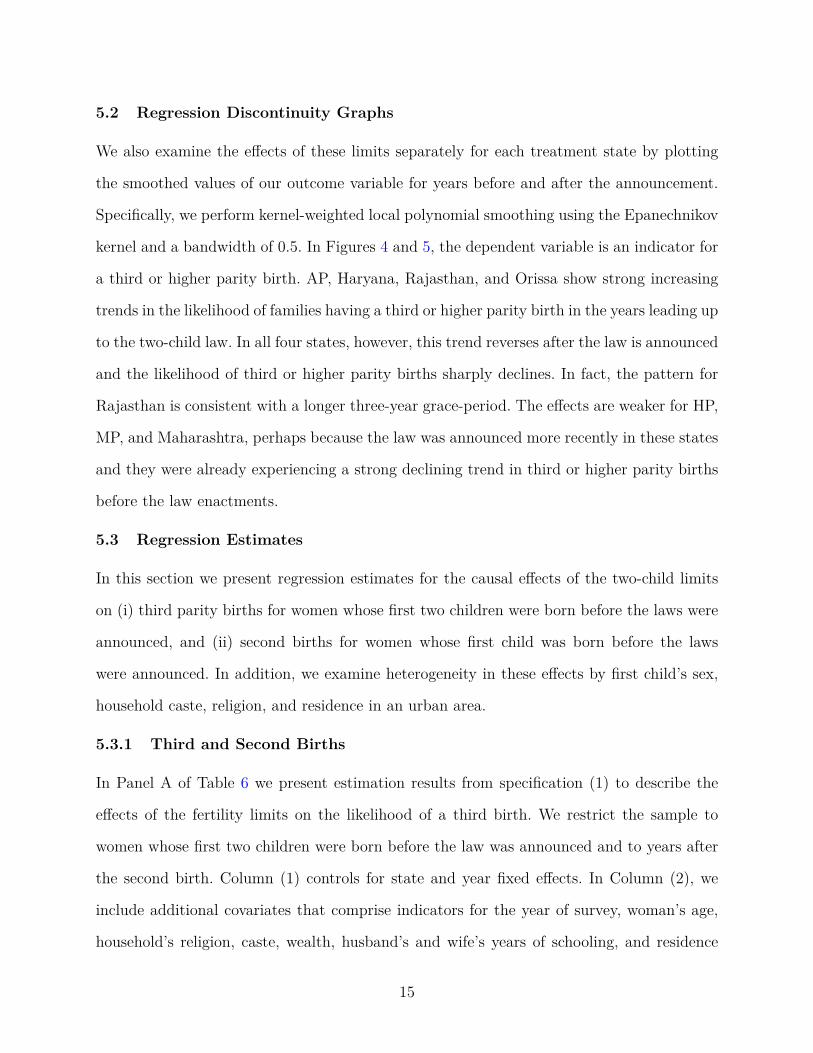
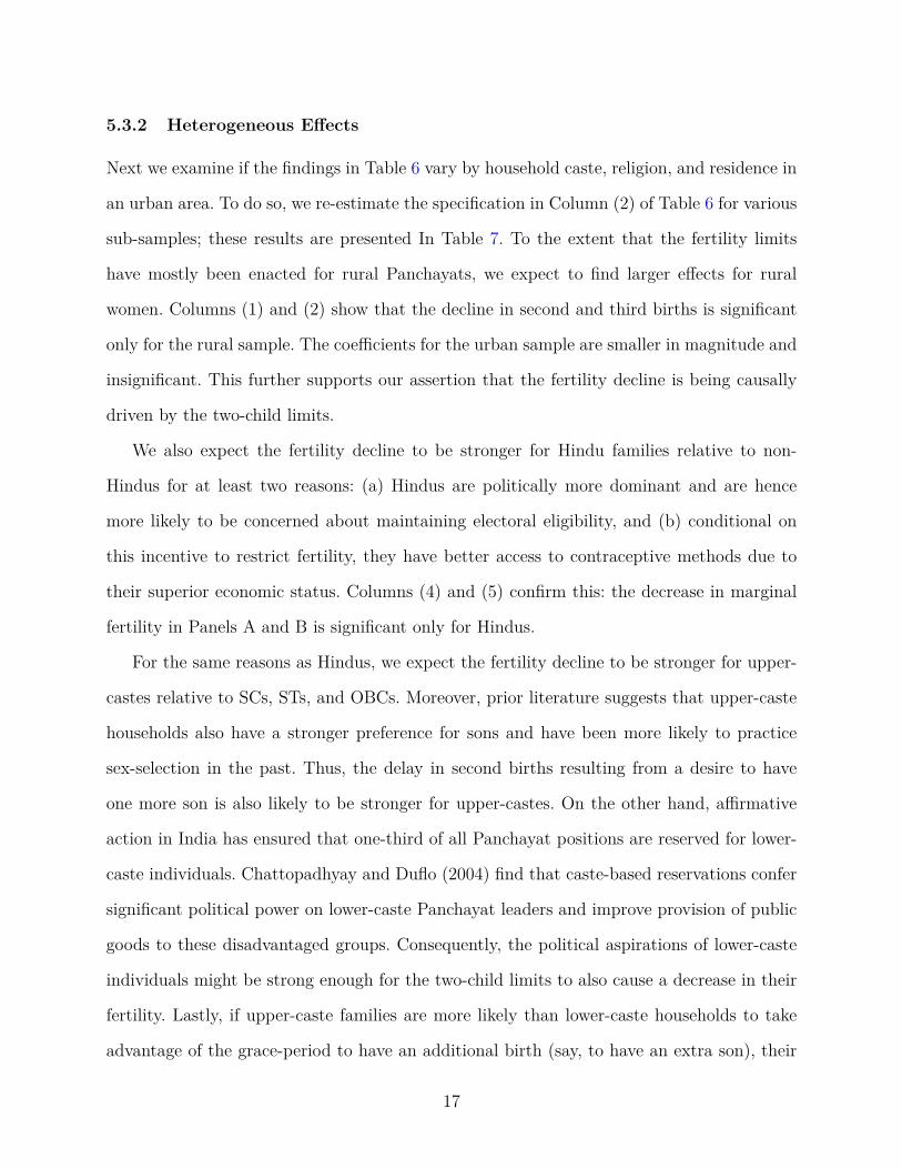
5.2 Regression Discontinuity Graphs
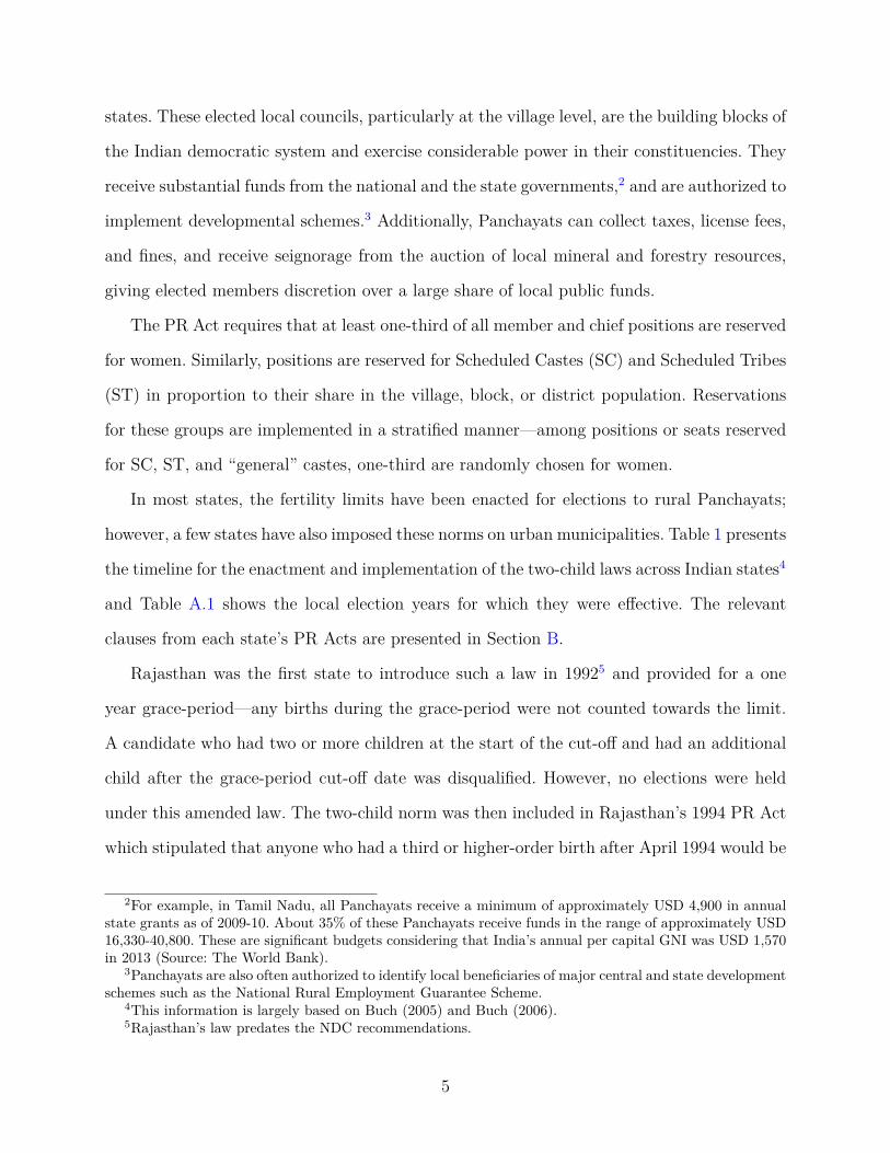
We also examine the effects of these limits separately for each treatment state by plotting
the smoothed values of our outcome variable for years before and after the announcement.
Specifically, we perform kernel-weighted local polynomial smoothing using the Epanechnikov
kernel and a bandwidth of 0.5. In Figures 4 and 5, the dependent variable is an indicator for
a third or higher parity birth. AP, Haryana, Rajasthan, and Orissa show strong increasing
trends in the likelihood of families having a third or higher parity birth in the years leading up
to the two-child law. In all four states, however, this trend reverses after the law is announced
and the likelihood of third or higher parity births sharply declines. In fact, the pattern for
Rajasthan is consistent with a longer three-year grace-period. The effects are weaker for HP,
MP, and Maharashtra, perhaps because the law was announced more recently in these states
and they were already experiencing a strong declining trend in third or higher parity births
before the law enactments.
5.3 Regression Estimates
In this section we present regression estimates for the causal effects of the two-child limits
on (i) third parity births for women whose first two children were born before the laws were
announced, and (ii) second births for women whose first child was born before the laws
were announced. In addition, we examine heterogeneity in these effects by first child’s sex,
household caste, religion, and residence in an urban area.
5.3.1 Third and Second Births
In Panel A of Table 6 we present estimation results from specification (1) to describe the
effects of the fertility limits on the likelihood of a third birth. We restrict the sample to
women whose first two children were born before the law was announced and to years after
the second birth. Column (1) controls for state and year fixed effects. In Column (2), we
include additional covariates that comprise indicators for the year of survey, woman’s age,
household’s religion, caste, wealth, husband’s and wife’s years of schooling, and residence
15

in an urban area, and state-specific linear time trends. The specifications in Columns (3)
and (4) restrict the sample to the treated states but are otherwise similar to Column (2).
The standard errors are clustered by state except in Column (4) where we cluster at the
state-year level to avoid inference issues due to the small number of clusters as the sample
is restricted to just the treated states.
The coefficient for Treatst is negative and significant in all four columns implying that
the two-child limits decreased higher-order fertility for couples who had already borne two
children by the time the law was announced in their state. The coefficient in Column (2)
translates into a 0.5 percentage point or a 6.25 percent decrease in the likelihood of a third
birth from the baseline probability of 8 percent.
In Panel B of Table 6, the dependent variable is an indicator for a second birth. We
restrict the sample to women whose first child was born before the law was announced and
to years after the first birth. To remain eligible for future elections, these women (couples)
can have only one additional birth. Moreover, the grace-period is not relevant for these
women. Consequently, if son preference is sufficiently strong, they may be more likely to
practice sex-selection at second parity, which will mechanically delay their second birth (in
addition to a reduction in completed fertility caused by the limits). Second births may also
be postponed for reasons other than sex-selection, e.g., to improve the survival probability
of the last birth.
In all four columns of Panel B, the coefficient is negative and significant implying that
the two child limits did in fact decrease the likelihood of a second birth in a given year for
women who had already borne their first child before the law was announced in their state.
The coefficient in Column (2) translates into a 0.6 percentage point or a 6.7 percent decrease
in the likelihood of a second birth from the baseline probability of 9 percent. To confirm that
this decrease in the likelihood of second birth is indeed driven by greater sex-selection, we
examine heterogeneity in this effect by the sex of the first child in the following sub-section.
16
5.3.2 Heterogeneous Effects
Next we examine if the findings in Table 6 vary by household caste, religion, and residence in
an urban area. To do so, we re-estimate the specification in Column (2) of Table 6 for various
sub-samples; these results are presented In Table 7. To the extent that the fertility limits
have mostly been enacted for rural Panchayats, we expect to find larger effects for rural
women. Columns (1) and (2) show that the decline in second and third births is significant
only for the rural sample. The coefficients for the urban sample are smaller in magnitude and
insignificant. This further supports our assertion that the fertility decline is being causally
driven by the two-child limits.
We also expect the fertility decline to be stronger for Hindu families relative to non-
Hindus for at least two reasons: (a) Hindus are politically more dominant and are hence
more likely to be concerned about maintaining electoral eligibility, and (b) conditional on
this incentive to restrict fertility, they have better access to contraceptive methods due to
their superior economic status. Columns (4) and (5) confirm this: the decrease in marginal
fertility in Panels A and B is significant only for Hindus.
For the same reasons as Hindus, we expect the fertility decline to be stronger for upper-
castes relative to SCs, STs, and OBCs. Moreover, prior literature suggests that upper-caste
households also have a stronger preference for sons and have been more likely to practice
sex-selection in the past. Thus, the delay in second births resulting from a desire to have
one more son is also likely to be stronger for upper-castes. On the other hand, affirmative
action in India has ensured that one-third of all Panchayat positions are reserved for lower-
caste individuals. Chattopadhyay and Duflo (2004) find that caste-based reservations confer
significant political power on lower-caste Panchayat leaders and improve provision of public
goods to these disadvantaged groups. Consequently, the political aspirations of lower-caste
individuals might be strong enough for the two-child limits to also cause a decrease in their
fertility. Lastly, if upper-caste families are more likely than lower-caste households to take
advantage of the grace-period to have an additional birth (say, to have an extra son), their
17

overall fertility decline might be lower as a result. The coefficients in Columns (5) and (6)
capture the net effect of these channels.
In Panel A, the decrease in third births is larger in magnitude and more significant for
lower-castes. We do not find any significant difference in the grace-period response by caste,17
suggesting that the decrease in third births for lower-castes is being driven by their political
aspirations. For second births in Panel B, the coefficients are negative and significant for
both groups, but the magnitude is slightly larger for upper-castes, consistent with their
higher propensity to sex-select. To further confirm the sex-selection mechanism, next we
explicitly examine if the effect on the sex ratio of second births also varies by the sex of the
first child and household caste.
In Table 8, we present results for the effects on the probability and sex of the second
birth by sex of the first child. We restrict the sample to women whose first child was born
before the law was announced and to years after the first birth. In Columns (2), (3), (5), and
(6), the sample is restricted to treated states. Columns (1)-(3) show that, before the law is
announced, a firstborn girl, relative to a firstborn boy, increases the probability of a second
birth by 0.2 percentage points, reflecting parents’ desire for at least one son. However, once
the law is announced, there is a decrease in the likelihood of a second birth, with a larger
decrease for those with a firstborn girl. The interaction term in the first row is negative,
significant, and of a similar magnitude in Columns (1)-(3).
In Columns (4)-(6) of Table 8, we examine the effect of the two-child limits on the
likelihood that the second child is male. Before the law is announced, a firstborn girl, relative
to a boy, increases the probability of a second birth being male by 1 percentage point,
reflecting the greater propensity for sex-selection at second parity by parents whose first
child is a girl. While the coefficients in the first two rows of Columns (4)-(6) are positive,
there is no significant effect of the fertility limits on sex-selection in the overall sample.
17These results are available upon request.
18
Table 9 further splits these results by household caste to understand the mechanisms
underlying the caste results we find in Columns (5)-(6) in Panel B of Table 7. Before the
laws are announced, both upper- and lower-caste groups are more likely to have a second
child and it is more likely to be a boy if the first child is a girl. Like Table 8, for lower-castes
the effects do not vary by the sex of the first child (Column (2)). Upper-caste results in
Column (1) of Panel B show that the fertility limits do not affect the sex ratio of second
birth if the first child is a boy. However, if the firstborn is a girl, there is a significantly larger
(3 percentage points) increase in the sex ratio of second birth. The fertility decline in Panel
A is also significantly larger for upper-caste families with a firstborn girl suggesting that
the decrease in second parity births we observed earlier reflects a delay induced by greater
sex-selection. If their first child is a girl, upper-caste families increase sex-selection at second
parity to ensure that they have at least one son whilst not sacrificing future eligibility for
political office.
6 RobustnessIn this section we perform a few robustness checks to ensure that our previous results truly
capture the causal effect of fertility limits on politicians. First, we conduct a placebo test by
reassigning the intervention or treatment to a year before the actual law was announced. If
our results are capturing the causal effect of the fertility limits, we should not find significant
effects in these placebo regressions. In Table 10, each column uses a different year as a
placebo treatment year. For example, in Column (1), we assume that the fertility limits
were announced in all treatment states in 1980. Since these laws are fictitious, a significant
“effect” at the 5% level may be found roughly 5% of the time. There is no cell where we find
a significant effect on the likelihood of a third birth in the same direction as our main results
in Panel A of Table 6. These findings lend support to our DD estimation strategy and make
a causal interpretation more credible.
Column (1) of Table 11 shows that our results also remain robust when only NFHS data
19
is used, thereby addressing concerns about the bias introduced by any unobserved differences
in data collection, or small variations in the sampling methodology for NFHS and DLHS.
One potential mechanism through which these laws can affect fertility outcomes is through
adjustments in the age at marriage. Forward-looking individuals (or their parents) wishing
to maintain eligibility for local elections in the future may take into account the lower com-
pleted fertility requirements (i.e., a maximum of two children) and delay marriage, which
could explain the decrease in likelihood of births we observe in Section 5. To test if this is
the case, we estimate specification (1) with age at first marriage as the dependent variable.
The results are presented in Column (2) of Table 11 and show that there is no impact of the
two-child limits on the age at first marriage.
Although we control for a number of socio-economic variables in our regressions, to further
support our identification strategy, we show that the timing of announcement of these laws
across states is uncorrelated with changes in these characteristics that vary across states
and over time. Specifically, in Table 12 we present the coefficients from regressions that
use various maternal, paternal, and household characteristics as dependent variables in the
estimation of equation (1) with state and year fixed effects, and state-specific time trends, but
without any other controls. Out of 20 coefficients, the only marginally significant coefficient
is a negative effect on the likelihood of the mother being Hindu.
7 ConclusionThis paper examines whether demographic restrictions on locally elected representatives
affect fertility and sex ratio outcomes in their constituency. To do so, we utilize quasi-
experimental variation in the enactment of two-child eligibility requirements for individuals
running for office in India. Our results show that fertility limits on Panchayat officials lower
fertility among the general populace, but also lead to an unintended increase in the already
male-biased sex ratio in certain socio-economic groups. Thus, we highlight a new channel of
demographic influence, namely local politicians.
20
While the stated rationale for these fertility limits is that local leaders serve as role-models
and adoption of a small family norm by Panchayat members will motivate their constituents
to follow suit. Our results, however, suggest that the incentive effect for individuals aspiring
to run for office in the future is the dominant explanation for the observed fertility decline.
Although we have alluded to caste-based reservations as being a potential reason for
heterogeneity in some of our findings, we have not directly exploited the random selection of
villages for reservation due to lack of Panchayat-level information in NFHS and DLHS. In
ongoing work, we seek to exploit variation in the gender- and caste-based reservation status
of village councils as an exogenous shock to the “attainability” of these leadership positions.
Moreover, we plan to use data from the Rural Economic and Demographic Survey (REDS)
to examine heterogeneity in the effects of these laws by the presence of a family member
who has contested or been elected to a local council in the past.
Lastly, to the extent that women and lower-caste households might have relatively less
control over their fertility decisions, these laws may have unintended consequences for the po-
litical representation of socio-economically disadvantaged groups who have relatively higher
fertility. Therefore, in future work, we also plan to examine the interactions between these
fertility limits and caste- and gender-based affirmative action in terms of their effects on the
characteristics of elected candidates.
�
21
ReferencesAnukriti, S. (2014): “The Fertility-Sex Ratio Trade-off: Unintended Consequences of Fi-
nancial Incentives,” IZA Discussion Paper No. 8044.
Bassi, V. and I. Rasul (2014): “Persuasion: A Case Study of Papal Influence on Fertility
Preferences and Behavior,” .
Beaman, L., E. Duflo, R. Pande, and P. Topalova (2012): “Female Leadership
Raises Aspirations and Educational Attainment for Girls: A Policy Experiment in India,”
Science, 335, 581–586.
Bettinger, E. P. and B. T. Long (2005): “Do Faculty Serve as Role Models? The
Impact of Instructor Gender on Female Students Do Faculty Serve as Role Models? The
Impact of Instructor Gender on Female Students,” American Economic Review, 95, 152–7.
Bhalotra, S. and T. Cochrane (2010): “Where Have All the Young Girls Gone? Iden-
tification of Sex Selection in India,” IZA Discussion Paper No. 5381.
Buch, N. (2005): “Law of Two-Child Norm in Panchayats: Implications, Consequences and
Experiences,” Economic and Political Weekly, XL.
——— (2006): The Law of Two Child Norm in Panchayats, Concept Publishing Company.
Chattopadhyay, R. and E. Duflo (2004): “The Impact of Reservation in the Panchay-
ati Raj: Evidence from a Nationwide Randomized Experiment,” Economic and Political
Weekly, 39, 979–986.
Chong, A., S. Duryea, and E. La Ferrara (2012): “Soap Operas and Fertility: Evi-
dence from Brazil,” American Economic Journal: Applied Economics, 4, 1–31.
Ebenstein, A. (2010): “The “Missing" Girls of China and the Unintended Consequences of
the One Child Policy,” Journal of Human Resources, 45, 87–115.
22
Fernandez, R., A. Fogli, and C. Olivetti (2004): “Mothers and Sons: Preference
Formation and Female Labor Force Dynamics,” Quarterly Journal of Economics, 119,
1249–99.
Jayachandran, S. (2014): “Fertility Decline and Missing Women,” NBER Working Paper
20272.
Jensen, R. and E. Oster (2009): “The Power of TV: Cable Television and Women’s
Status in India,” Quarterly Journal of Economics, 124, 1057–94.
Olinto, P., K. Beegle, C. Sobrado, and H. Uematsu (2013): “The State of the Poor:
Where are the Poor, Where is Extreme Poverty Harder to End, and What is the Current
Profile of the World’s Poor?” Economic Premise.
Olivetti, C., E. Patacchini, and Y. Zenou (2013): “Mothers, Friends and Gender
Identity,” NBER Working Paper 19610.
Visaria, L., A. Acharya, and F. Raj (2006): “Two-Child Norm: Victimising the Vul-
nerable?” Economic and Political Weekly, XLI.
23
8 Figures
Figure 1: Treatment and Control States
24

Figure 2: Likelihood of more than two living children, by year
NOTES: This figure plots the βk coefficients and their 95% confidence intervals (dashed lines) from estimatingthe following equation for a woman i in state s of age a in year t:Yisat =
∑10k=−10 βkTreats,t+k + X
′
iδ + γs + θt + ψa + εisat, where Treats,t+k indicates k years from theannouncement of the law in state s. Standard errors are clustered by state-year. The first vertical line (atk = 0) indicates the year of announcement. The second vertical line indicates the end of the one-year graceperiod. The sample is restricted to women in treatment states. Other covariates comprise indicators for theyear of survey, woman’s age, household’s religion (Hindu, Muslim, Sikh, Christian), caste (SC, ST, OBC),wealth (low and high SLI), husband’s and wife’s years of schooling (5 categories each), and residence in anurban area.
25
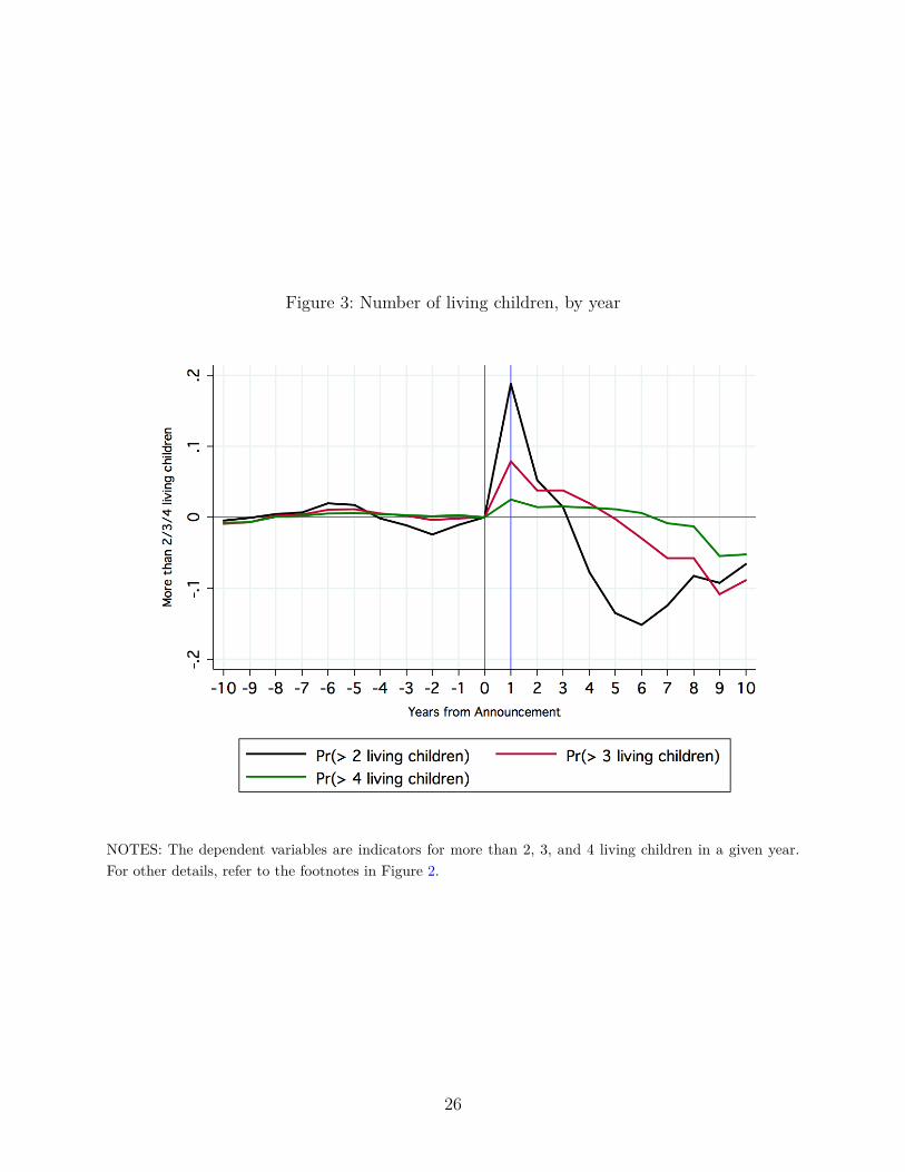
Figure 3: Number of living children, by year
NOTES: The dependent variables are indicators for more than 2, 3, and 4 living children in a given year.For other details, refer to the footnotes in Figure 2.
26

Figure 4: Likelihood of third or higher order births, by state
NOTES: This figure plots the smoothed values of the outcome variable (an indicator for third or higherorder birth) for years before and after the announcement of the law using kernel-weighted local polynomialsmoothing with an Epanechnikov kernel and a bandwidth of 0.5. The dashed lines indicate the 95% confidenceintervals. The vertical line indicates the year of announcement.
27
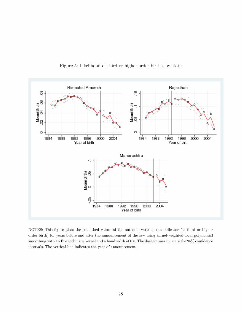
Figure 5: Likelihood of third or higher order births, by state
NOTES: This figure plots the smoothed values of the outcome variable (an indicator for third or higherorder birth) for years before and after the announcement of the law using kernel-weighted local polynomialsmoothing with an Epanechnikov kernel and a bandwidth of 0.5. The dashed lines indicate the 95% confidenceintervals. The vertical line indicates the year of announcement.
28
9 Tables
Table 1: Timeline for Fertility Limits across States
State Announced Grace Period In effect End
Rajasthan 1992 Apr 23, 1994 - Nov 27, 1995 Nov 27, 1995 -Haryana 1994 Apr 21, 1994 - Apr 24, 1995 Apr 25, 1995 - Dec 31, 2004 Jul 21, 2006
(retro. impl. Jan 1, 2005)Andhra Pradesh 1994 May 30, 1994 - May 30, 1995 Jun 1995 -Orissa 1993/199418 Apr 1994 - Apr 21, 1995 Apr 22, 1995 -Himachal Pradesh 2000 Apr 18, 2000 - Apr 18, 2001 Apr 2001 - Apr 2005 May 30, 2005Madhya Pradesh 200019 Mar 29, 2000 - Jan 26, 2001 Jan 2001 - Nov 2005 Nov 20, 2005Chhattisgarh 2000 2000 - Jan 2001 Jan 2001- 2005 2005 (earliest mention)18
Maharashtra 200320 Sep 21, 2002 - Sep 20, 2003 Sep 2003 -Uttarakhand (municipal only) 2002Gujarat 2005 Aug 2005 - Aug 11, 2006 Aug 11, 2006 -Bihar (municipal only) Jan 2007 Feb 1, 2007 - Feb 1, 2008 Feb 1, 2008 -
18For district councils in 1993 and for village and block councils in 1994.19Notified on May 31, 2000. This created problems since people whose third child was born in Jan 2001 contested their disqualification for birth
within 8 months of the new law.20In retrospective effect from Sep 21, 2002.
29
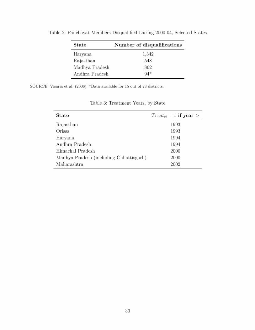
Table 2: Panchayat Members Disqualified During 2000-04, Selected States
State Number of disqualifications
Haryana 1,342Rajasthan 548Madhya Pradesh 862Andhra Pradesh 94*
SOURCE: Visaria et al. (2006). *Data available for 15 out of 23 districts.
Table 3: Treatment Years, by State
State Treatst = 1 if year >
Rajasthan 1993Orissa 1993Haryana 1994Andhra Pradesh 1994Himachal Pradesh 2000Madhya Pradesh (including Chhattisgarh) 2000Maharashtra 2002
30
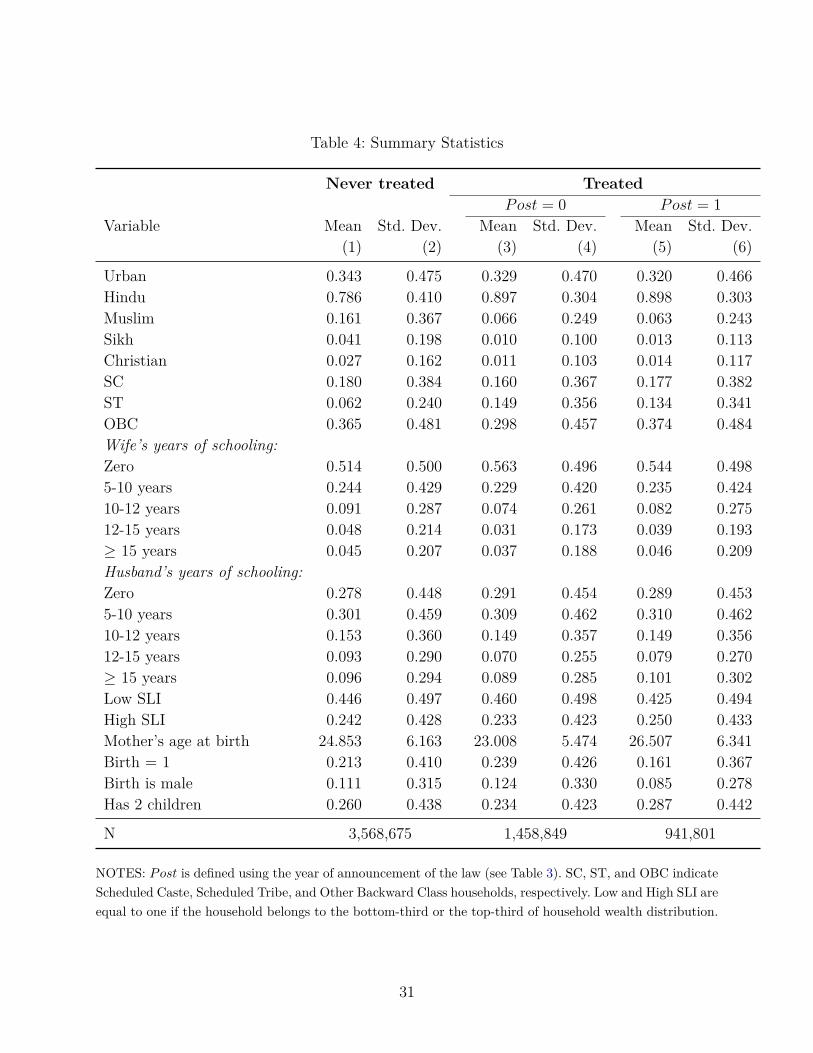
Table 4: Summary Statistics
Never treated TreatedPost = 0 Post = 1
Variable Mean Std. Dev. Mean Std. Dev. Mean Std. Dev.(1) (2) (3) (4) (5) (6)
Urban 0.343 0.475 0.329 0.470 0.320 0.466Hindu 0.786 0.410 0.897 0.304 0.898 0.303Muslim 0.161 0.367 0.066 0.249 0.063 0.243Sikh 0.041 0.198 0.010 0.100 0.013 0.113Christian 0.027 0.162 0.011 0.103 0.014 0.117SC 0.180 0.384 0.160 0.367 0.177 0.382ST 0.062 0.240 0.149 0.356 0.134 0.341OBC 0.365 0.481 0.298 0.457 0.374 0.484Wife’s years of schooling:Zero 0.514 0.500 0.563 0.496 0.544 0.4985-10 years 0.244 0.429 0.229 0.420 0.235 0.42410-12 years 0.091 0.287 0.074 0.261 0.082 0.27512-15 years 0.048 0.214 0.031 0.173 0.039 0.193≥ 15 years 0.045 0.207 0.037 0.188 0.046 0.209Husband’s years of schooling:Zero 0.278 0.448 0.291 0.454 0.289 0.4535-10 years 0.301 0.459 0.309 0.462 0.310 0.46210-12 years 0.153 0.360 0.149 0.357 0.149 0.35612-15 years 0.093 0.290 0.070 0.255 0.079 0.270≥ 15 years 0.096 0.294 0.089 0.285 0.101 0.302Low SLI 0.446 0.497 0.460 0.498 0.425 0.494High SLI 0.242 0.428 0.233 0.423 0.250 0.433Mother’s age at birth 24.853 6.163 23.008 5.474 26.507 6.341Birth = 1 0.213 0.410 0.239 0.426 0.161 0.367Birth is male 0.111 0.315 0.124 0.330 0.085 0.278Has 2 children 0.260 0.438 0.234 0.423 0.287 0.442
N 3,568,675 1,458,849 941,801
NOTES: Post is defined using the year of announcement of the law (see Table 3). SC, ST, and OBC indicateScheduled Caste, Scheduled Tribe, and Other Backward Class households, respectively. Low and High SLI areequal to one if the household belongs to the bottom-third or the top-third of household wealth distribution.
31
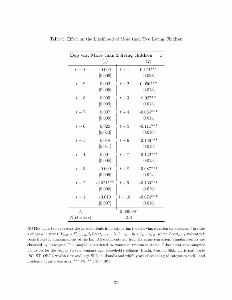
Table 5: Effect on the Likelihood of More than Two Living Children
Dep var: More than 2 living children = 1(1) (2)
t− 10 -0.006 t+ 1 0.174***[0.006] [0.038]
t− 9 0.002 t+ 2 0.056***[0.006] [0.013]
t− 8 0.005 t+ 3 0.027**[0.009] [0.013]
t− 7 0.007 t+ 4 -0.054***[0.009] [0.014]
t− 6 0.020 t+ 5 -0.111***[0.013] [0.016]
t− 5 0.018 t+ 6 -0.136***[0.011] [0.019]
t− 4 0.001 t+ 7 -0.122***[0.008] [0.023]
t− 3 -0.009 t+ 8 -0.087***[0.006] [0.024]
t− 2 -0.021*** t+ 9 -0.103***[0.006] [0.020]
t− 1 -0.010 t+ 10 -0.074***[0.007] [0.016]
N 2,390,087N(clusters) 214
NOTES: This table presents the βk coefficients from estimating the following equation for a woman i in states of age a in year t: Yisat =
∑10k=−10 βkTreats,t+k +X
′
iδ + γs + θt + ψa + εisat, where Treats,t+k indicates kyears from the announcement of the law. All coefficients are from the same regression. Standard errors areclustered by state-year. The sample is restricted to women in treatment states. Other covariates compriseindicators for the year of survey, woman’s age, household’s religion (Hindu, Muslim, Sikh, Christian), caste(SC, ST, OBC), wealth (low and high SLI), husband’s and wife’s years of schooling (5 categories each), andresidence in an urban area. *** 1%, ** 5%, * 10%
32
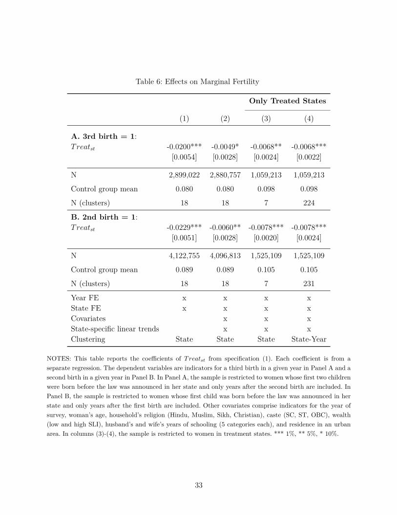
Table 6: Effects on Marginal Fertility
Only Treated States
(1) (2) (3) (4)
A. 3rd birth = 1:Treatst -0.0200*** -0.0049* -0.0068** -0.0068***
[0.0054] [0.0028] [0.0024] [0.0022]
N 2,899,022 2,880,757 1,059,213 1,059,213
Control group mean 0.080 0.080 0.098 0.098
N (clusters) 18 18 7 224
B. 2nd birth = 1:Treatst -0.0229*** -0.0060** -0.0078*** -0.0078***
[0.0051] [0.0028] [0.0020] [0.0024]
N 4,122,755 4,096,813 1,525,109 1,525,109
Control group mean 0.089 0.089 0.105 0.105
N (clusters) 18 18 7 231
Year FE x x x xState FE x x x xCovariates x x xState-specific linear trends x x xClustering State State State State-Year
NOTES: This table reports the coefficients of Treatst from specification (1). Each coefficient is from aseparate regression. The dependent variables are indicators for a third birth in a given year in Panel A and asecond birth in a given year in Panel B. In Panel A, the sample is restricted to women whose first two childrenwere born before the law was announced in her state and only years after the second birth are included. InPanel B, the sample is restricted to women whose first child was born before the law was announced in herstate and only years after the first birth are included. Other covariates comprise indicators for the year ofsurvey, woman’s age, household’s religion (Hindu, Muslim, Sikh, Christian), caste (SC, ST, OBC), wealth(low and high SLI), husband’s and wife’s years of schooling (5 categories each), and residence in an urbanarea. In columns (3)-(4), the sample is restricted to women in treatment states. *** 1%, ** 5%, * 10%.
33
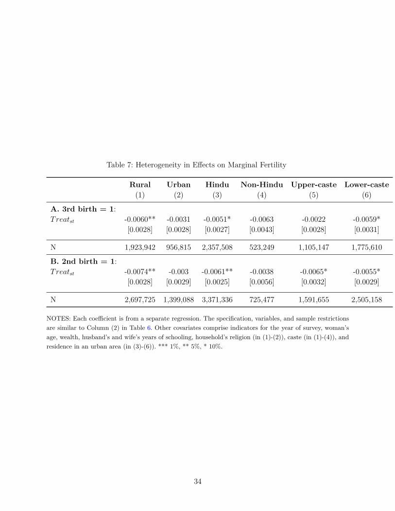
Table 7: Heterogeneity in Effects on Marginal Fertility
Rural Urban Hindu Non-Hindu Upper-caste Lower-caste(1) (2) (3) (4) (5) (6)
A. 3rd birth = 1:Treatst -0.0060** -0.0031 -0.0051* -0.0063 -0.0022 -0.0059*
[0.0028] [0.0028] [0.0027] [0.0043] [0.0028] [0.0031]
N 1,923,942 956,815 2,357,508 523,249 1,105,147 1,775,610
B. 2nd birth = 1:Treatst -0.0074** -0.003 -0.0061** -0.0038 -0.0065* -0.0055*
[0.0028] [0.0029] [0.0025] [0.0056] [0.0032] [0.0029]
N 2,697,725 1,399,088 3,371,336 725,477 1,591,655 2,505,158
NOTES: Each coefficient is from a separate regression. The specification, variables, and sample restrictionsare similar to Column (2) in Table 6. Other covariates comprise indicators for the year of survey, woman’sage, wealth, husband’s and wife’s years of schooling, household’s religion (in (1)-(2)), caste (in (1)-(4)), andresidence in an urban area (in (3)-(6)). *** 1%, ** 5%, * 10%.
34
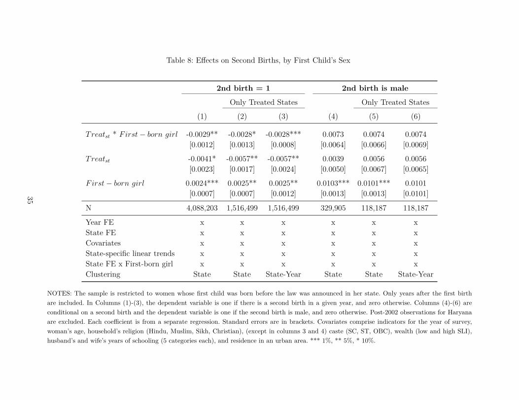
Table 8: Effects on Second Births, by First Child’s Sex
2nd birth = 1 2nd birth is male
Only Treated States Only Treated States
(1) (2) (3) (4) (5) (6)
Treatst * First− born girl -0.0029** -0.0028* -0.0028*** 0.0073 0.0074 0.0074[0.0012] [0.0013] [0.0008] [0.0064] [0.0066] [0.0069]
Treatst -0.0041* -0.0057** -0.0057** 0.0039 0.0056 0.0056[0.0023] [0.0017] [0.0024] [0.0050] [0.0067] [0.0065]
First− born girl 0.0024*** 0.0025** 0.0025** 0.0103*** 0.0101*** 0.0101[0.0007] [0.0007] [0.0012] [0.0013] [0.0013] [0.0101]
N 4,088,203 1,516,499 1,516,499 329,905 118,187 118,187
Year FE x x x x x xState FE x x x x x xCovariates x x x x x xState-specific linear trends x x x x x xState FE x First-born girl x x x x x xClustering State State State-Year State State State-Year
NOTES: The sample is restricted to women whose first child was born before the law was announced in her state. Only years after the first birthare included. In Columns (1)-(3), the dependent variable is one if there is a second birth in a given year, and zero otherwise. Columns (4)-(6) areconditional on a second birth and the dependent variable is one if the second birth is male, and zero otherwise. Post-2002 observations for Haryanaare excluded. Each coefficient is from a separate regression. Standard errors are in brackets. Covariates comprise indicators for the year of survey,woman’s age, household’s religion (Hindu, Muslim, Sikh, Christian), (except in columns 3 and 4) caste (SC, ST, OBC), wealth (low and high SLI),husband’s and wife’s years of schooling (5 categories each), and residence in an urban area. *** 1%, ** 5%, * 10%.
35
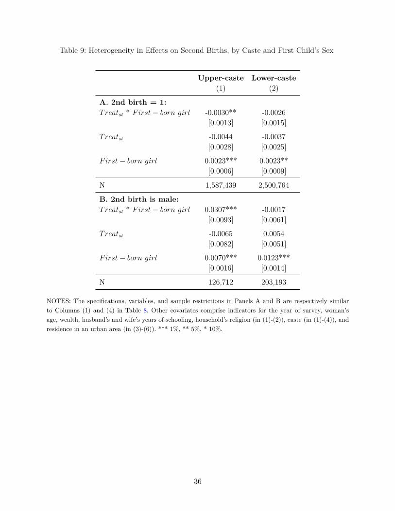
Table 9: Heterogeneity in Effects on Second Births, by Caste and First Child’s Sex
Upper-caste Lower-caste(1) (2)
A. 2nd birth = 1:Treatst * First− born girl -0.0030** -0.0026
[0.0013] [0.0015]
Treatst -0.0044 -0.0037[0.0028] [0.0025]
First− born girl 0.0023*** 0.0023**[0.0006] [0.0009]
N 1,587,439 2,500,764
B. 2nd birth is male:Treatst * First− born girl 0.0307*** -0.0017
[0.0093] [0.0061]
Treatst -0.0065 0.0054[0.0082] [0.0051]
First− born girl 0.0070*** 0.0123***[0.0016] [0.0014]
N 126,712 203,193
NOTES: The specifications, variables, and sample restrictions in Panels A and B are respectively similarto Columns (1) and (4) in Table 8. Other covariates comprise indicators for the year of survey, woman’sage, wealth, husband’s and wife’s years of schooling, household’s religion (in (1)-(2)), caste (in (1)-(4)), andresidence in an urban area (in (3)-(6)). *** 1%, ** 5%, * 10%.
36
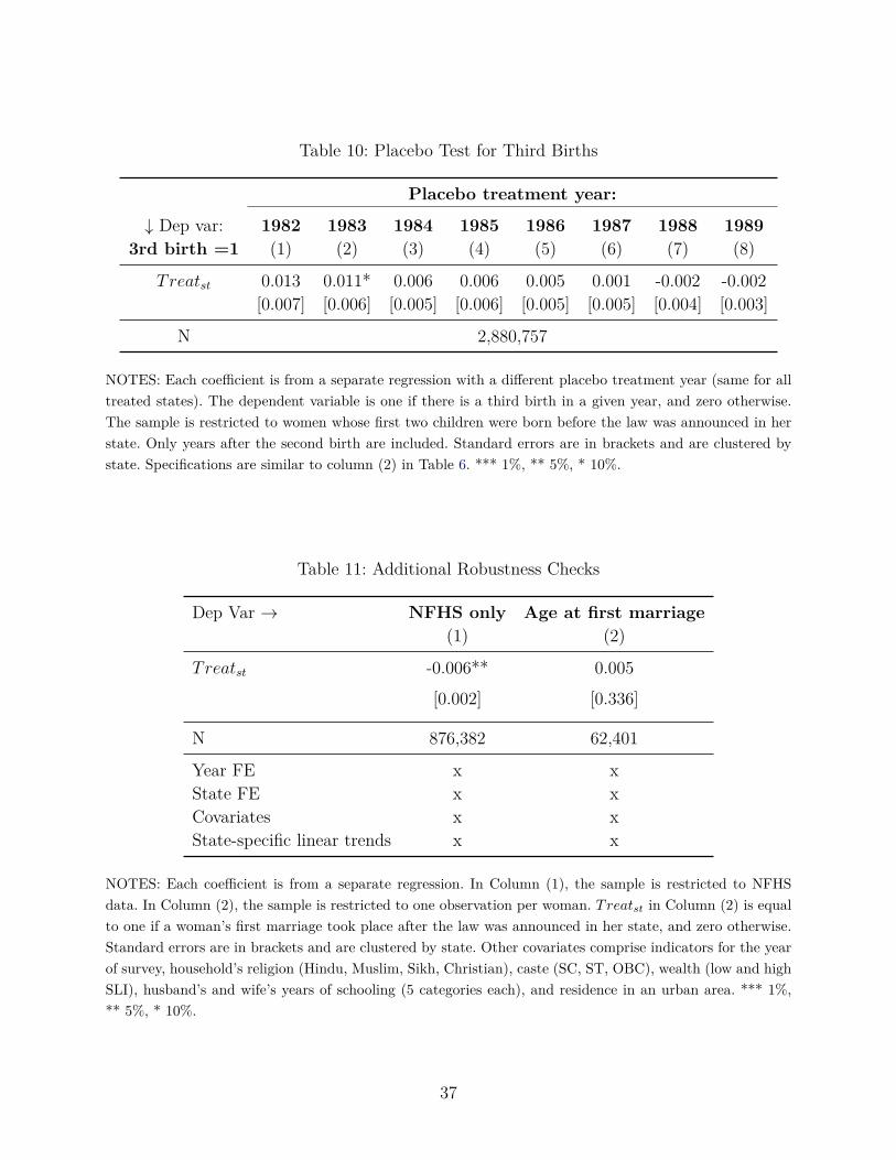
Table 10: Placebo Test for Third Births
Placebo treatment year:
↓ Dep var: 1982 1983 1984 1985 1986 1987 1988 19893rd birth =1 (1) (2) (3) (4) (5) (6) (7) (8)
Treatst 0.013 0.011* 0.006 0.006 0.005 0.001 -0.002 -0.002[0.007] [0.006] [0.005] [0.006] [0.005] [0.005] [0.004] [0.003]
N 2,880,757
NOTES: Each coefficient is from a separate regression with a different placebo treatment year (same for alltreated states). The dependent variable is one if there is a third birth in a given year, and zero otherwise.The sample is restricted to women whose first two children were born before the law was announced in herstate. Only years after the second birth are included. Standard errors are in brackets and are clustered bystate. Specifications are similar to column (2) in Table 6. *** 1%, ** 5%, * 10%.
Table 11: Additional Robustness Checks
Dep Var → NFHS only Age at first marriage(1) (2)
Treatst -0.006** 0.005
[0.002] [0.336]
N 876,382 62,401
Year FE x xState FE x xCovariates x xState-specific linear trends x x
NOTES: Each coefficient is from a separate regression. In Column (1), the sample is restricted to NFHSdata. In Column (2), the sample is restricted to one observation per woman. Treatst in Column (2) is equalto one if a woman’s first marriage took place after the law was announced in her state, and zero otherwise.Standard errors are in brackets and are clustered by state. Other covariates comprise indicators for the yearof survey, household’s religion (Hindu, Muslim, Sikh, Christian), caste (SC, ST, OBC), wealth (low and highSLI), husband’s and wife’s years of schooling (5 categories each), and residence in an urban area. *** 1%,** 5%, * 10%.
37
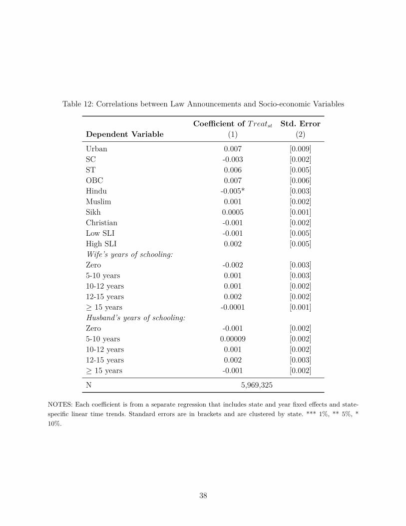
Table 12: Correlations between Law Announcements and Socio-economic Variables
Coefficient of Treatst Std. ErrorDependent Variable (1) (2)
Urban 0.007 [0.009]SC -0.003 [0.002]ST 0.006 [0.005]OBC 0.007 [0.006]Hindu -0.005* [0.003]Muslim 0.001 [0.002]Sikh 0.0005 [0.001]Christian -0.001 [0.002]Low SLI -0.001 [0.005]High SLI 0.002 [0.005]Wife’s years of schooling:Zero -0.002 [0.003]5-10 years 0.001 [0.003]10-12 years 0.001 [0.002]12-15 years 0.002 [0.002]≥ 15 years -0.0001 [0.001]Husband’s years of schooling:Zero -0.001 [0.002]5-10 years 0.00009 [0.002]10-12 years 0.001 [0.002]12-15 years 0.002 [0.003]≥ 15 years -0.001 [0.002]
N 5,969,325
NOTES: Each coefficient is from a separate regression that includes state and year fixed effects and state-specific linear time trends. Standard errors are in brackets and are clustered by state. *** 1%, ** 5%, *10%.
38
A Additional Tables
Table A.1: Panchayat Elections
State Election Years
Without the norm With the norm
Rajasthan 1995 2000, 2005, 2010Haryana 1994, 2010 2000, 2005Andhra Pradesh 1995, 2001, 2006, 2011Orissa 1997, 2002, 2007, 2012Himachal Pradesh 1995, 2005, 2010-11 2000Madhya Pradesh 1994, 2010 2000,21 2005Chhattisgarh 2010 2000, 2005Maharashtra 1995, 2000 2007, 2010, 2013Uttarakhand 2003, 2008, 2014Jharkhand 2010Gujarat 2001, 2005-06 2010-11Bihar 2006 2011
21Despite the fact that the two-child norm was officially introduced after the Panchayat elections wereover in 2000, the new government began disqualifying elected representatives earlier (Visaria et al. (2006)).
39

Table A.2: Effects on Marginal Fertility in Treatment States
Dep Var: > 2 living children > 3 living children > 4 living children(1) (2) (3)
Treatst -0.003* -0.002 -0.0004[0.002] [0.002] [0.001]
N 2,390,087 2,390,087 2,390,087
Year FE x x xState FE x x xCovariates x x xState-specific linear trends x x xClustering State-Year State-Year State-YearN (clusters) 238 238 238
NOTES: This table reports the coefficients of Treatst from specification (1). Each coefficient is from aseparate regression. Other covariates comprise indicators for the year of survey, woman’s age, household’sreligion (Hindu, Muslim, Sikh, Christian), caste (SC, ST, OBC), wealth (low and high SLI), husband’s andwife’s years of schooling (5 categories each), and residence in an urban area. The sample is restricted towomen in treatment states. *** 1%, ** 5%, * 10%.
40

B State-wise Regulations1. Rajasthan:19
According to the the Rajasthan Panchayati Raj Act, 1994, “...Every person registered as a
voter in the list of voters of a Panchayati Raj Institution shall be qualified for election as
a Panch or, as the case may be, a member of such Panchayati Raj Institution unless such
person-...(l) has more than two children.”...“The birth during the period from the date of
commencement of the Act (23rd April, 1994), hereinafter in this proviso referred to as the
date of such commencement, to 27th November, 1995, of an additional child shall not be
taken into consideration for the purpose of the disqualification mentioned in Clause (l) and
a person having more than two children (excluding the child, if any, born during the period
from the date of such commencement to 27th November, 1995) shall not be disqualified
under that clause for so long as the number of children he had on the date of commencement
of this Act does not increase.”
2. Haryana:
According to the 1994 Act20, “...No person shall be a Sarpanch or a Panch or a Gram
Panchayat or a member of a Panchayat Samiti or Zila Parishad or continue as such who– (q)
has more than two living children: Provided that a person having more than two children
on or upto the expiry or one year of the commencement of this Act, shall not be deemed to
be disqualified.”
Prior to revocation:21 “Person shall be disqualified for being elected to a Gram Panchayat,
Panchayat Samiti or Zila Parishad if:
...(xvii) has more than two living children; provided that this disqualification of more than
two living children shall not apply for the persons who had more than two living children
19Source: http://www.rajpanchayat.gov.in/common/toplinks/act/act.pdf20Source: http://www.panchayat.gov.in/documents/10198/350801/The%20Haryana%20Panchayati%
20%20Raj%20Act%201994.pdf21Source: http://secharyana.gov.in/html/faq1.htm
41
before 21st April, 1995 unless he had additional child after the said date.”
The Haryana government amended Section 175(q) of the Haryana Panchayati Raj Act,
1994, retrospectively with effect from January 1, 2005 to omit the section (q).22
3. Andhra Pradesh:23
According to Section 19 (3) of the Andhra Pradesh Panchayati Raj Act, 1994,“...A person
having more than two children shall be disqualified for election or for continuing as member:
Provided that the birth within one year from the date of commencement of the Andhra
Pradesh Panchayat Raj Act, 1994 hereinafter in this clause referred to as the date of such
commencement, of an additional child shall not be taken into consideration for the purposes
of this clause;
Provided further that a person having more than two children (excluding the child if any
born within one year from the date of such commencement) shall not be disqualified under
this clause for so long as the number of children he had on the date of such commencement
does not increase;
Provided also that the Government may direct that the disqualification in this section
shall not apply in respect of a person for reasons to be recorded in writing.”24
4. Orissa:25
A person shall be disqualified for being elected to a PR institution if he “...has more than one
spouse living or has more than two children. The last named disqualification shall not apply
if the person had had more than two children before 21.04.1995 unless he begot an additional
child after the said date. Rule 25 of O.G.P. Act gives full description of the disqualifications.”
5. Madhya Pradesh:26
“...condition to disqualify an office bearer of the Panchayat for holding the post: (1) that he
22Source: http://hindu.com/2006/07/22/stories/2006072207150500.htm23Source: http://www.ielrc.org/content/e9412.pdf24Further explanation at: http://www.apsec.gov.in/RLBS_GPs/CLARIFICATIONS%202013/877%20-%
20Qualification.pdf.25Source: http://secorissa.org/download/FAQ2.pdf26Source: http://www.indiankanoon.org/doc/1285129/
42

must have more than two living children, and (2) out of whom one is born on or after the
26th day of January, 2001...”
The Population Policy of Madhya Pradesh states that “persons having more than two
children after January 26, 2001 would not be eligible for contesting elections for panchayats,
local bodies, mandis or cooperatives in the state. In case they get elected, and in the mean-
time they have the third child, they would be disqualified for that post.”
6. Chhattisgarh:27
“Section 36: Disqualification for being office bearer of Panchayat:- 36(1) No person shall be
eligible to be an office bearer of Panchayat who:...(m) has more than two living children one
of whom is born on or after the 26th day of January, 2001.”
7. Maharashtra:
“...(j-1) No person shall be a member of a Panchayat or continue as such, who has more than
two children:
Provided that, a person having two children on the date of commencement of the Bombay
Village Panchayats and the Maharashtra Zila Parishads and Panchayat Samitis (Amend-
ment) Act 1995 (hereinafter in this clause referred to as “the date of such commencement”)
shall not be disqualified under this clause so long as the number of children he had on the
date of such commencement does not increase;
Provided further that, a child or more than one child born in a single delivery within the
period of one year from the date of such commencement shall not be taken into consideration
for the purpose of disqualification mentioned in this clause.
... For the purposes of clause (j-1):
Where the couple has only one child on or after that date of such commencement, any
number of children born out of a single subsequent delivery shall be deemed to be one entity.
“Child” does not include an adopted child or children....”
27Source: http://www.the-laws.com/Encyclopedia/Browse/ShowCase.aspx?CaseId=023002211000
43