Fermi-Liquid Theory of a Quantum Dot · Fermi-Flüssigkeits-Theorie eines Quanten Punktes Sören Arlt Bachelorarbeit an der Fakultät für Physik der Ludwig–Maximilians–Universität

Fermi-Liquid Theory of a Quantum Dot

Sören Arlt

München 2016

Fermi-Flüssigkeits-Theorie eines QuantenPunktes

Sören Arlt

Bachelorarbeitan der Fakultät für Physik

der Ludwig–Maximilians–UniversitätMünchen

vorgelegt vonSören Arlt

aus Großenhain

München, den 4. Juli 2016

Gutachter: Professor Jan von DelftTag der mündlichen Prüfung: 6. Juli 2016

Contents

Contents v

1 Introduction 1

2 SIAM and Fermi-liquid Theory 32.1 SIAM . . . . . . . . . . . . . . . . . . . . . . . . . . . . . . . . . . . . . . . . . . . . 32.2 Scattering and Fermi-liquid Theory . . . . . . . . . . . . . . . . . . . . . . . . . . . 4

2.2.1 Scattering . . . . . . . . . . . . . . . . . . . . . . . . . . . . . . . . . . . . . 4Lead electrons . . . . . . . . . . . . . . . . . . . . . . . . . . . . . . . . . . . 4S-matrix . . . . . . . . . . . . . . . . . . . . . . . . . . . . . . . . . . . . . . 6

2.2.2 Fermi-liquid Theory . . . . . . . . . . . . . . . . . . . . . . . . . . . . . . . 7

3 Application to the Quantum Dot 113.1 The Quantum Dot . . . . . . . . . . . . . . . . . . . . . . . . . . . . . . . . . . . . . 113.2 SIAM Fermi-liquid parameters for the Quantum Dot . . . . . . . . . . . . . . . . 13

3.2.1 Phases in the Quantum Dot . . . . . . . . . . . . . . . . . . . . . . . . . . . 133.2.2 (A) Effective level position . . . . . . . . . . . . . . . . . . . . . . . . . . . . 163.2.3 (B) Chemical potential . . . . . . . . . . . . . . . . . . . . . . . . . . . . . . 22

Reduction to central region . . . . . . . . . . . . . . . . . . . . . . . . . . . 24Using the full form of the Friedel sum rule . . . . . . . . . . . . . . . . . . 26

3.2.4 Comparing both approaches . . . . . . . . . . . . . . . . . . . . . . . . . . 28

4 Conclusion 31

vi Contents

Chapter 1

Introduction

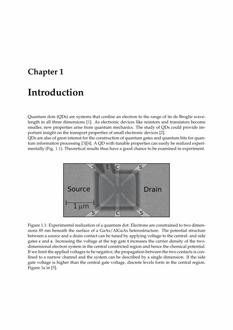
Quantum dots (QDs) are systems that confine an electron to the range of its de Broglie wave-length in all three dimensions [1]. As electronic devices like resistors and transistors becomesmaller, new properties arise from quantum mechanics. The study of QDs could provide im-portant insight on the transport properties of small electronic devices [2].QDs are also of great interest for the construction of quantum gates and quantum bits for quan-tum information processing [3][4]. A QD with tunable properties can easily be realized experi-mentally (Fig. 1.1). Theoretical results thus have a good chance to be examined in experiment.

s sct

s sc1 µm

Source Drain

Figure 1.1: Experimental realization of a quantum dot: Electrons are constrained to two dimen-sions 85 nm beneath the surface of a GaAs/AlGaAs heterostructure. The potential structurebetween a source and a drain contact can be tuned by applying voltage to the central- and sidegates c and s. Increasing the voltage at the top gate t increases the carrier density of the two-dimensional electron system in the central constricted region and hence the chemical potential.If we limit the applied voltages to be negative, the propagation between the two contacts is con-fined to a narrow channel and the system can be described by a single dimension. If the sidegate voltage is higher than the central gate voltage, discrete levels form in the central region.Figure 1a in [5].

2 1. Introduction

In this thesis, we want to examine the properties of a QD in one dimension. We will see thatthe levels in a QD can effectively be modelled by the Single Impurity Anderson Model (SIAM),which was introduced by Anderson in 1961 to describe localized magnetic states in metals [6].The SIAM consists of a single level with interaction and couples to leads on both sides. Despiteits simple construction, the SIAM is highly nontrivial and offers a lot of interesting behavior.The Kondo model, which explains an anomalous resistivity minimum in dilute magnetic alloys,can be acquired as a limit of the SIAM, where a single magnetic state forms.Nozières formulated a Fermi-liquid theory of the Kondo model, describing its low-temperaturebehavior in terms of weakly interaction quasiparticles [7]. This approach was generalized tothe SIAM in Ref. [8].We will explore how this Fermi-liquid theory can be applied to the QD. We calculate scatteringphases and susceptibilities numerically using a program by Lukas Weidinger based on thefunctional renormalization group (fRG). The fRG program produces data for zero temperatureand at equilibrium. Once we find the FL parameters of the QD, we can compute transportcoefficients and are able to describe conduction behavior at low magnetic fields, temperaturesand bias voltages.We follow two approaches. For approach (A), we appoint an effective SIAM level positionto QDs of varying gate voltage. We improved on a previous calculation of the Fermi-liquidparameters by Phillip Rosenberger [9]. Since the QD is significantly more complicated thanthe SIAM, this model will not be perfectly accurate. We will see where and how the SIAMdescription fails.We can also attempt to describe the QD in terms of Fermi-liquid theory without assigning aneffective level by varying the chemical potential. We will show advantages and disadvantagesof this approach and compare both results.Showing that approaches (A) and (B) yield equivalent results for the transport coefficients, wegain important understanding for systems that cannot be assigned an effective level position.

Chapter 2

SIAM and Fermi-liquid Theory

2.1 SIAM

The Single Impurity Anderson Model (SIAM) describes a level of energy εd occupied by parti-cles with spin up or down, with number operators nd,↑ and nd,↓. The Hamiltonian is

Hd =∑σ

εdnd,σ + Und,↑nd,↓, (2.1)

summing over spins σ. The number operators can be expressed by creation- and annihilationoperators in the impurity: nd,σ = c†d,σcd,σ. The impurity couples to leads on both sides (L/R).The kinetic energy εkσ of particles with momentum k in the leads is

HL/R =∑k,σ

εkσnL/R,kσ. (2.2)

Again, the number operators are a combination of creation- and annihilation operators: nL/R,kσ =

c†L/R,kσcL/R,kσ The hopping from each one of the leads to the impurity and vice versa is ex-pressed by additional terms of the Hamiltonian.

Hhop =∑k,σ

τ(c†L,kσcd,σ + c†R,kσcd,σ + h.c.). (2.3)

τ is the hopping energy. The full Hamiltonian is the sum of these terms

HSIAM = HL +HR +Hhop +Hd. (2.4)

In the next section we want to show an approach to find the low-energy conductance behaviorof the SIAM by generalization of Nozières Fermi-liquid Theory.

4 2. SIAM and Fermi-liquid Theory

2.2 Scattering and Fermi-liquid Theory

Properties such as the conductance behavior as a function of magnetic field, temperature andbias voltage at low energies can be extracted from considering an effective Fermi-liquid the-ory [8], i.e. weakly interacting quasiparticles representing the behavior of the system. In thissection we want to introduce the required scattering theory along with the essential Landauer-Büttiker formula and the Friedel sum rule.

2.2.1 Scattering

Lead electrons

We want to describe the conductance of the electrons in a metal with impurities. We do this bydescribing their scattering off an impurity. The electron states before and after scattering canbe described by eigenstates of the free Hamiltonian HL/R [10].The behavior in the leads is modelled by tight binding chains. Position is described by dis-crete sites and hopping between nearest neighbors is possible. In many solid state physicsapplications these sites correspond to single atoms. Here, the lattice is artificial. The spacingbetween the lattice sites is much larger than the spacing of the underlying crystal. We can writethe Hamiltonian of each one of the (half-infinite) leads in second quantization with a hoppingenergy τ between nearest neighbors i and j:

Hhop =

∞∑〈i,j〉

∑σ

τ(c†j,σci,σ + c†i,σcj,σ). (2.5)

The eigenstates of this Hamiltonian are found to be

|ψk,σ〉 =

√2C

π

∞∑j=1

sin(kj) |j, σ〉 , (2.6)

for k ∈(0, πC

), where C is the lattice spacing [11]. By considering the eigenvalues

Hhop |ψk,σ〉 = ω(k) |ψk,σ〉 , (2.7)

we find the dispersion relation to be

ω(k) = 2τ cos k. (2.8)

For the scattering at the impurity we will need the local density of states of the lead electronsat the contact point, i.e. the end point of the half infinite chain. This is given by components ofthe retarded Green’s function Gσ,R [11]:

ρσc (ω) = − 1

πIm(Gσ,R11 ). (2.9)

The retarded Green’s function of a system with Hamiltonian H and frequency ω is

GR =1

ω −H + i0+. (2.10)

2.2 Scattering and Fermi-liquid Theory 5

To calculate the G11 component of the Green’s function we follow the calculation of [12]. An-other site is added at the end of the tight-binding chain. The hopping between the aditionalsite and the next is considered a perturbation V . g is the unperturbed Green’s function.

G =

G11 G12 G13 · · ·G21 G22 G23 · · ·G31 G32 G33 · · ·

......

.... . .

, (2.11a)

g =

g11 0 0 · · ·0 G11 G12 · · ·0 G21 G22 · · ·...

......

. . .

, (2.11b)

V =

0 τ 0 · · ·τ 0 0 · · ·0 0 0 · · ·...

......

. . .

. (2.11c)

We write the Dyson equation

G = g + gV G, (2.12)

yielding the system of equations

G11 =g11 + (gV G)11 = g11 + g11V12G21, (2.13)G21 =g21 + (gV G)21 = g21 + g22V21G11. (2.14)

We obtain a quadratic equation in G11 by insertion:

G11 = g11 + g11τ2G2

11. (2.15)

g11 = [ω −H0]−1. With H0 = 0, we can write g11 = 1ω . Solving for G11:

G11 =ω

2τ2± 1

2τ2

√ω2 − 4τ2. (2.16)

We thus get our final expression for the density of states at the contact site,

ρσc (ω) =1

2πτ2

√4τ2 − ω2. (2.17)

Requiring the density to be a non-negative real number, the sign in Eq. (2.16) is fixed to +. Itfollows from Eq. (2.16) that ρσ(|ω| > 2τ) = 0, resulting in a total band width of 4τ .


S-matrix

The asymptotic states can be expressed in a basis of left lead eigenstates 〈ψL| and right leadeigenstates 〈ψR| by complex numbers. The S-matrix describes the evolution of an asymptoticstate in the infinite past to asymptotic states in the infinite future.(

CD

)= lim

t→∞,t′→−∞

(〈ψL| U(t, t′) |ψL〉〈ψL| U(t, t′) |ψR〉〈ψR| U(t, t′) |ψL〉〈ψR| U(t, t′) |ψR〉

)(AB

)=

(SLL SLRSRL SRR

)(AB

)(2.18)

We are interested in the phases the components of a complex vector pick up in the scatteringprocess. The information about the impurity is brought into the S-matrix via the Green’s func-tion of the impurity Gσ,R. Considering impurities with multiple sites, such as the QD, we areinterested in the S-matrix from their leftmost to their rightmost site l and r. As seen in [10] wecan write the S-matrix as

Sσ = 1− 2πiτ2ρσc (ω = µ)

(Gσ,Rl,l Gσ,Rl,rGσ,Rr,l Gσ,Rr,r

). (2.19)

This utilizes the local density of states at the contact points ρσ0 , which we found earlier. TheS-matrix is unitary (S† = S−1). It is also symmetric (S = S>), if the impurity is symmetric (in

particular Gσ,Rl,r = Gσ,Rr,l ). We can diagonalize the S-matrix using W = 1√2

(1 11 −1

):

W †SσW =

(eiδσ,s 0

0 eiδσ,a

)= eiδref

(ei2δσ,1 0

0 ei2δσ,2

). (2.20)

δref is a constant reference phase which will later be fixed at the same value for both spins. Wedefine two more quantities:

δσ,+ = δσ,1 + δσ,2 =1

2(δσ,s + δσ,a − 2δref ), (2.21a)

δσ,− = δσ,1 − δσ,2 =1

2(δσ,s − δσ,a). (2.21b)

The Landauer-Büttiker formula describes the relation between conductance g and the phaseshift δσ,−. At zero temperature:

g = G/GQ =1

2

∑σ

|SσLR|2 =1

2

∑σ

sin2(δσ−). (2.22)

g is normalized by GQ = 2e2/h making it dimensionless. Another essential relation in the latercalculation is the Friedel sum rule. The number of spin σ electrons bound by the impurity isgiven in [13] by[

1

2πi

(Tr logSfull − Tr logSband

)−(nfull − nband

)]mod Z = 0, (2.23)


where the index full denotes the system with non-zero potential and interaction and bandstands for the system without potential. Since interaction reduces to an effective potential instatic fRG, we can also take band to be noninteracting. S is the S-matrix and n is the total num-ber of particles in the system. If the band values remain constant, we can simplify this relationto

nσ mod Z =δσ,+π. (2.24)

2.2.2 Fermi-liquid Theory

The Fermi-liquid theory we introduce in this subsection describes low energy transport prop-erties of a SIAM in terms of a set of Fermi-liquid parameters. Extracting these parameters outof transport properties at low magnetic fields for zero temperature and zero bias voltage willempower us to immediately describe transport at low temperature and low bias voltage.To introduce the Fermi-liquid parameters, relate them to susceptibilities of the systems, and usethem to express transport coefficients of the SIAM, we consider one electron scattering prop-erties of the SIAM. The shift δσ,− between the symmetric phase and the antisymmetric phasecan be expanded in terms of kinetic energy ε of the incoming particles and the deviation of thedistribution function δnσ,ε0 = nσ − n0

ε0 around an unphysical reference energy ε0 with distri-bution function n0

ε0 = θ(ε0 − ε) at zero temperature. We will exploit the arbitrariness of ε0 tofind relations between the expansion coefficients α1, φ1, α2 and φ2, which we call Fermi-liquidparameters.

δσ,−(ε, nσ, nσ) =δ0,εd−ε0 + α1,εd−ε0(ε− ε0)− φ1,εd−ε0

∫ ∞−∞

dε′δnσ,ε0(ε′) + α2,εd−ε0(ε− ε0)2

− 1

2φ2,εd−ε0

∫ ∞−∞

dε′(ε+ ε′ − 2ε0)δnσ,ε0(ε′)− ...

σ is the spin opposite to σ. Since ε0 is unphysical and arbitrarily chosen, we know that ∂ε0δ(ε, nσ′) =0. Performing this differentiation and comparing constant terms and coefficients of each ∝(ε− ε0),

∫ε′ δnσ,ε0 and their higher powers yields the following set of useful equations

−dδ0

dεd− α1 + φ1 = 0, (2.25a)

−dα1

dεd− 2α2 + φ2/2 = 0, (2.25b)

dφ1

dεd+ φ2 = 0. (2.25c)

For zero temperature and low magnetic field B, δσ,− can be expressed by B and the Fermi-liquid parameters: [8]

δσ,−(µσ, n0µσ′

) = δ0 +σ

2(α1 + φ1)B +

1

4(α2 + φ2/4)B2. (2.26)


We can write the charge of the impurity as nd = nd↑ + nd↓ and the magnetization as md =nd,↑ − nd,↓. Antisymmetric modes do not interact with a single site impurity. Correspondingly,their phase shift is zero, δσ,a = 0. Via Eq. (2.24) and Eq. (2.21) this leads us to

nσ =δσ,+π

=δσ,−π. (2.27)

The charge and spin susceptibilities atB = 0 can then be expressed entirely by the Fermi-liquidparameters:

χc = −∂nd∂εd|B=0 = − 2

π

∂δ0

∂εd=

2

π(α1 − φ1), χs =

∂md

∂B|B=0 =

1

2π(α1 + φ1). (2.28)

We obtain two more equations by differentiating the susceptibilities with respect to εd (χ′α =∂χα∂εd

). Using Eq. (2.25) and Eq. (2.28) we get:

α1 =π(χs + χc/4), (2.29a)

α2 =π(−3

4χ′s − χ′c/16), (2.29b)

φ1 =π(χs − χc/4), (2.29c)φ2 =π(−χ′s + χ′c/4). (2.29d)

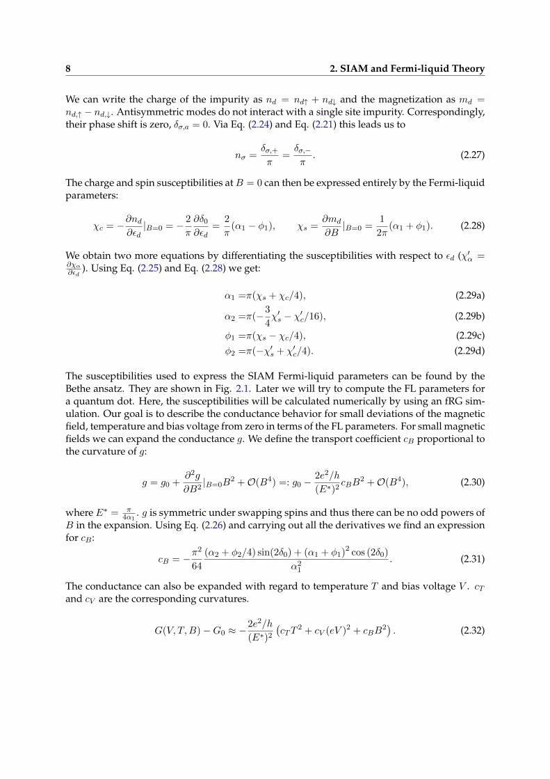
The susceptibilities used to express the SIAM Fermi-liquid parameters can be found by theBethe ansatz. They are shown in Fig. 2.1. Later we will try to compute the FL parameters fora quantum dot. Here, the susceptibilities will be calculated numerically by using an fRG sim-ulation. Our goal is to describe the conductance behavior for small deviations of the magneticfield, temperature and bias voltage from zero in terms of the FL parameters. For small magneticfields we can expand the conductance g. We define the transport coefficient cB proportional tothe curvature of g:

g = g0 +∂2g

∂B2|B=0B

2 +O(B4) =: g0 −2e2/h

(E∗)2cBB

2 +O(B4), (2.30)

where E∗ = π4α1

. g is symmetric under swapping spins and thus there can be no odd powers ofB in the expansion. Using Eq. (2.26) and carrying out all the derivatives we find an expressionfor cB :

cB = −π2

64

(α2 + φ2/4) sin(2δ0) + (α1 + φ1)2 cos (2δ0)

α21

. (2.31)

The conductance can also be expanded with regard to temperature T and bias voltage V . cTand cV are the corresponding curvatures.

G(V, T,B)−G0 ≈ −2e2/h

(E∗)2

(cTT

2 + cV (eV )2 + cBB2). (2.32)


0

1

2

3

−6 −4 −2 0 2 4 6

−1

0

1

Figure 2.1: Fermi-liquid parameters of the SIAM. Figure 1 in Ref. [8]

Similar results to cB are obtained in for cT and cV :

cT =π4

16

(φ12 − α2

3

)sin (2δ0)−

(α22

3 +2φ213

)cos (2δ0)

α21

, (2.33)

cV =π2

64

(3φ24 − α2) sin 2δ0 − (α2

1 + 5φ21) cos 2δ0

α21

, (2.34)

their derivation will not be repeated here. It can be found in [8].


Chapter 3

Application to the Quantum Dot

3.1 The Quantum Dot

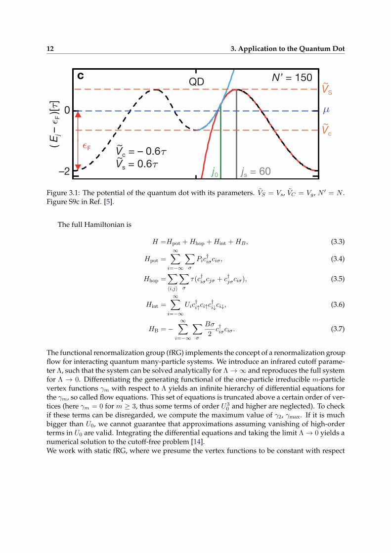
We model the quantum dot (QD) by a special form of potential barrier. In our case, it is ofsymmetric shape with two maxima on the sides. Their height is varied by the side gate voltageVs and their spatial position determines the width of the potential well in between. The well isparabolic in the center and its depth is described by the gate voltage Vg. The fRG simulation ofthe system uses the discretized potential shown in Fig. 3.1

Pj =

Vg + 2τ + µ+ Ω2

xi2

4τ sgn(Vs − Vg), for 0 ≤ |j| ≤ j0,(Vs + 2τ + µ)[2( |j|−Njs−N )2 − ( |j|−Njs−N )4], for j0 ≤ |j| ≤ N,0, for |j| > N.

(3.1)

2N + 1 is the total number of sites and 2js + 1 is the distance between the two side gates. Theparameters Ωx and js are chosen such that the potential is continuously differentiable. 4τ is theband width. Additional terms of the Hamiltonian are on-site interactions of the electrons anda kinetic hopping term. The interaction is limited to the central region.

Uj =

U0 exp

[− (j/N)6

1−(j/N)2

], for 0 ≤ |j| ≤ N,

0, for |j| > N.(3.2)

12 3. Application to the Quantum Dot

QD

QPC

0

–2

0

0

( Ej –

εF )[τ

]( E

j – ε

F )[τ

]U

j [τ]

Vc = – 0.6τVs = 0.6τ

~~

Vc = 0.3τVs = – 0.3τ

~~

Vc~

VS~

Vc~

VS~

εF

εF

e

d

c

µ

µ

j0

j0 js = 60

js

N’ = 150

N’ = 150

U = 0.5τ

j150–150

–2

0.5

Figure 3.1: The potential of the quantum dot with its parameters. VS = Vs, VC = Vg, N ′ = N .Figure S9c in Ref. [5].

The full Hamiltonian is

H =Hpot +Hhop +Hint +HB, (3.3)

Hpot =

∞∑i=−∞

∑σ

Pic†iσciσ, (3.4)

Hhop =∑〈i,j〉

∑σ

τ(c†iσcjσ + c†jσciσ), (3.5)

Hint =∞∑

i=−∞Uic†i↑ci↑c

†i↓ci↓, (3.6)

HB =−∞∑

i=−∞

∑σ

Bσ

2c†iσciσ. (3.7)

The functional renormalization group (fRG) implements the concept of a renormalization groupflow for interacting quantum many-particle systems. We introduce an infrared cutoff parame-ter Λ, such that the system can be solved analytically for Λ→∞ and reproduces the full systemfor Λ → 0. Differentiating the generating functional of the one-particle irreducible m-particlevertex functions γm with respect to Λ yields an infinite hierarchy of differential equations forthe γm, so called flow equations. This set of equations is truncated above a certain order of ver-tices (here γm = 0 for m ≥ 3, thus some terms of order U3

0 and higher are neglected). To checkif these terms can be disregarded, we compute the maximum value of γ2, γmax. If it is muchbigger than U0, we cannot guarantee that approximations assuming vanishing of high-orderterms in U0 are valid. Integrating the differential equations and taking the limit Λ→ 0 yields anumerical solution to the cutoff-free problem [14].We work with static fRG, where we presume the vertex functions to be constant with respect

3.2 SIAM Fermi-liquid parameters for the Quantum Dot 13

to frequency. As a result of the static fRG flow, we obtain a static self energy Σ and a static2-particle vertex γ2. We can extract single-particle properties from the effective Hamiltonian

Heff = Hpot +Hhop +HB + Σ. (3.8)

Σ may contain long range hopping terms.The feedback length L is a quantity in fRG that determines how the different channels of thetwo-particle vertex γ2 couple. For all following computations we set N = 30, j0 = 10, U0 = 1and L = 20.

3.2 SIAM Fermi-liquid parameters for the Quantum Dot

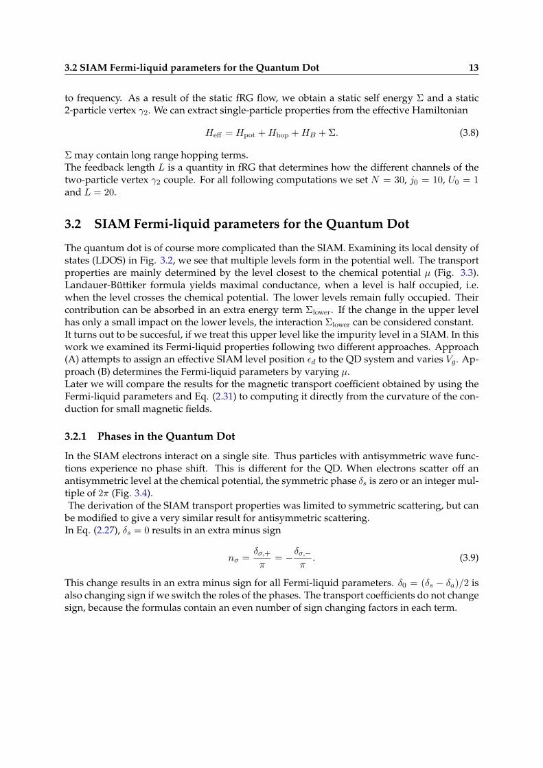
The quantum dot is of course more complicated than the SIAM. Examining its local density ofstates (LDOS) in Fig. 3.2, we see that multiple levels form in the potential well. The transportproperties are mainly determined by the level closest to the chemical potential µ (Fig. 3.3).Landauer-Büttiker formula yields maximal conductance, when a level is half occupied, i.e.when the level crosses the chemical potential. The lower levels remain fully occupied. Theircontribution can be absorbed in an extra energy term Σlower. If the change in the upper levelhas only a small impact on the lower levels, the interaction Σlower can be considered constant.It turns out to be succesful, if we treat this upper level like the impurity level in a SIAM. In thiswork we examined its Fermi-liquid properties following two different approaches. Approach(A) attempts to assign an effective SIAM level position εd to the QD system and varies Vg. Ap-proach (B) determines the Fermi-liquid parameters by varying µ.Later we will compare the results for the magnetic transport coefficient obtained by using theFermi-liquid parameters and Eq. (2.31) to computing it directly from the curvature of the con-duction for small magnetic fields.

3.2.1 Phases in the Quantum Dot

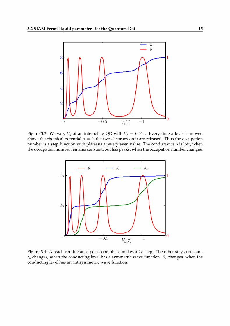
In the SIAM electrons interact on a single site. Thus particles with antisymmetric wave func-tions experience no phase shift. This is different for the QD. When electrons scatter off anantisymmetric level at the chemical potential, the symmetric phase δs is zero or an integer mul-tiple of 2π (Fig. 3.4).The derivation of the SIAM transport properties was limited to symmetric scattering, but can

be modified to give a very similar result for antisymmetric scattering.In Eq. (2.27), δs = 0 results in an extra minus sign

nσ =δσ,+π

= −δσ,−π. (3.9)

This change results in an extra minus sign for all Fermi-liquid parameters. δ0 = (δs − δa)/2 isalso changing sign if we switch the roles of the phases. The transport coefficients do not changesign, because the formulas contain an even number of sign changing factors in each term.


0

1

2

3

ρ[1/τ

]

−20 0 20Position

−0.5

0

ω[τ]

Figure 3.2: The LDOS of an interacting QD with Vg = −1τ , Vs = 0.01τ and µ = 0τ is plottedhere for varying energies ω relative to the middle of the band. We can see localized levels inthe central region (sites -10 to 10, white dotted line). Each level below the chemical potentialis occupied by one spin-up and one spin-down electron. Lower lying levels can have a highlifetime leading to a very small linewidth. These levels can be missed if the stepwidth in ω istoo big. We artificially reduce the lifetime by adding a small imaginary part iδ to the frequencyin the Green’s function. Thus the levels appear broader. Here δ = 1/100.


−1−0.50

2

4

6

8

Vg[τ ]0

1

ng

Figure 3.3: We vary Vg of an interacting QD with Vs = 0.01τ . Every time a level is movedabove the chemical potential µ = 0, the two electrons on it are released. Thus the occupationnumber is a step function with plateaus at every even value. The conductance g is low, whenthe occupation number remains constant, but has peaks, when the occupation number changes.

−1−0.50

2π

4π

Vg[τ ]0

1

g δs δa

Figure 3.4: At each conductance peak, one phase makes a 2π step. The other stays constant.δs changes, when the conducting level has a symmetric wave function. δa changes, when theconducting level has an antisymmetric wave function.


3.2.2 (A) Effective level position

We want to apply the previous Fermi-liquid calculations to the quantum dot. However, it is notsufficient to determine the level position in the LDOS for the fully interacting system, because italready factors in the interaction on the upper level. This interaction would be twice accountedfor if we were to use this level position in the SIAM Hamiltonian where there is an extra termfor the interaction on the conducting level. We find an effective level position by considering achemical potential µ sufficiently below the upper level such that all lower levels are occupied(see Fig. 3.5). Only they contribute to the self energy Σµ of the system with chemical potential µ.We now construct an effective Hamilonian without shifted level position due to the interactionin the upper level

Heff = Hpot +Hhop + Σµ. (3.10)

When we look at the LDOS resulting from Heff we can read off the effective level position εd.In a previous examination of the QD, Ref. [9] determined εd by computing the local densityof particles in the lower levels for µ and acquiring Heff by adding a resulting Hartree shift tothe upper level. The method used here includes the Hartree shift, but also takes interactions ofhigher order involving the lower levels into account. To compute the Fermi-liquid parametersover a range of εd, we vary Vg and find εd(Vg). As seen in Fig. 3.6, εd is a linear function of Vg.When we need to differentiate an arbitrary quantity A by εd in Eq. (2.29) we simply use the

chain rule∂A

∂εd=∂A

∂Vg

(∂εd∂Vg

)−1

, (3.11)

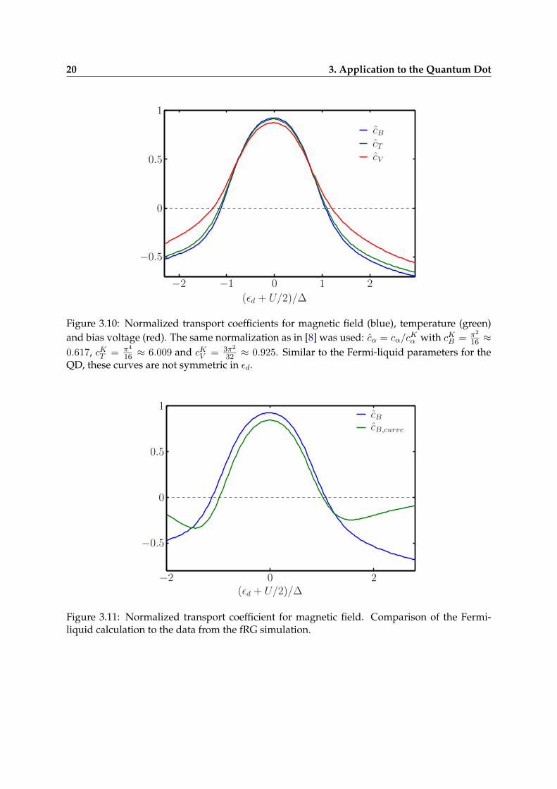
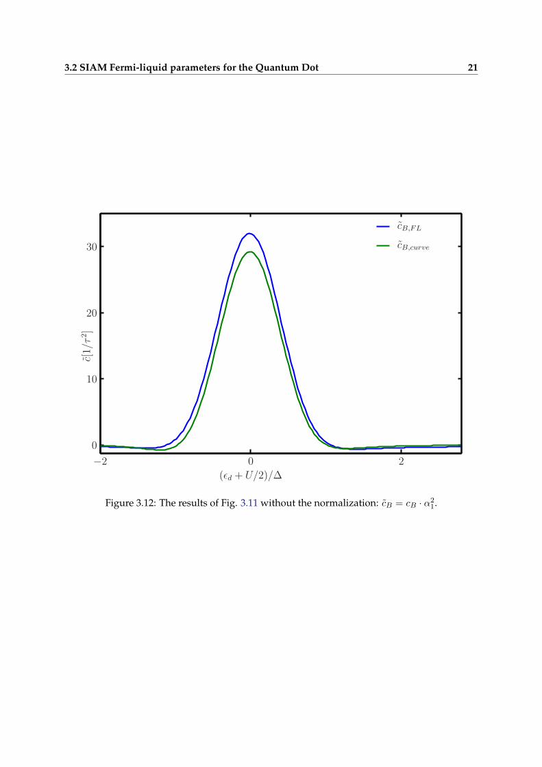
which effectively is a multiplication by a constant here. The susceptibilities are calculated fromthe densities given by the fRG program at varying Vg and small B. The occupation of the up-per level and the scattering phases are shown in Fig. 3.8. We see, how the occupation numberdecreases by two, when the level rises above the chemical potential. δs remains constant, whileδa goes from 2π to 0. It is essential for the comparison to the SIAM that one phase can be con-sidered constant at the conductance peak, so that Eq. (2.27) is satisfied. We can now calculatethe Fermi-liquid parameters and subsequently the transport coefficients. The resulting Fermi-liquid parameters obtained by this approach can be seen in Fig. 3.9. Compared to the valuesfor the SIAM in Fig. 2.1 the QD demonstrates a slight asymmetry. This is expected, because theQD is not a perfectly symmetric system like the SIAM. The fraction U/∆ describes the strengthof the interaction. When well is made more shallow, the tunneling rate and thus the hybridiza-tion ∆ increases significantly (Fig. 3.7), leading to an effective decrease in interaction strength.This feature is completely absent for a SIAM in the wide band limit. The transport coefficientsthat were computed by Eq. (2.31) and Eq. (2.33) are shown in Fig. 3.2.2. We can compare the cBfrom our FL calculation to the curvature of the conductance we determine directly from the fRGdata. This is a good test of the validity of our model. Figure 3.11 shows good agreement in thecentral region, but large deviation on the sides of the plot, corresponding to the mixed-valenceregime, where the determination of the effective level position described above presumablybecomes unreliable. We can argue that the differences on the sides are exaggerated by a factorof 1

α21, where α1 → 0. We can see in Eq. (2.30), that the curvature of g is proportional to cBα2

1.Figure 3.12 shows agreement between the FL and fRG results for cB .


−20 0 20

Position

−0.3

0

0.3

ω[τ]

0

1

2

3

ρ[1/τ

]

−20 0 20

Position

Figure 3.5: LDOS of an interacting QD with Vg = −1.1τ and different chemical potentialsindicated by the red solid line. For this and all of the following figures in (A) we set Vs = 0.01τ .The energy ω is measured relative to the middle of the band. On the left side (for chemicalpotential µ = 0τ ), the level is occupied and its position is higher than that of the right side,where the upper level is unoccupied (chemical potential µ = −0.05τ ). The difference lies in theinteraction of the electrons in the upper level. The position of the upper level (dashed orangeline) for the chemical potential µ is what we determine to be the effective level position.


−1.1−1−0.9

−0.04

−0.02

0

Vg[τ ]

ǫ d[τ]

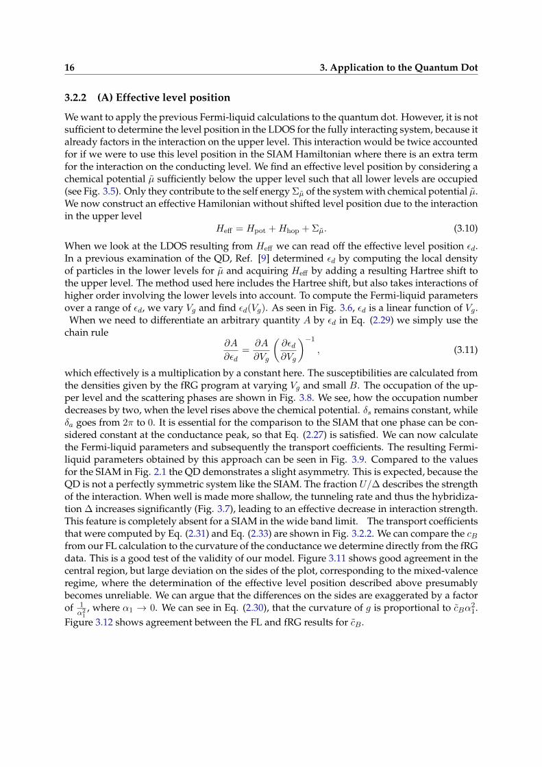
Figure 3.6: εd is determined for a range of Vg. εd is linear with a slope of approximately 0.25.

−1.1−1−0.9

0.015

0.02

0.025

∆[τ]

Vg[τ ]

Figure 3.7: The hybridization ∆ was determined by fitting a Lorentzian function to the upperlevel at chemical potential µ. ∆ = Γ/2, where Γ is the linewidth of the Lorentzian. In thefollowing, we set the ∆ to its value at the conductance peak, ∆(Vg = 0.98) = 0.0181.


0

1

2

0

1

0

1

−2 −1 0 1 2 3(ǫd + U/2)/∆

gnlevel

δ+/πn

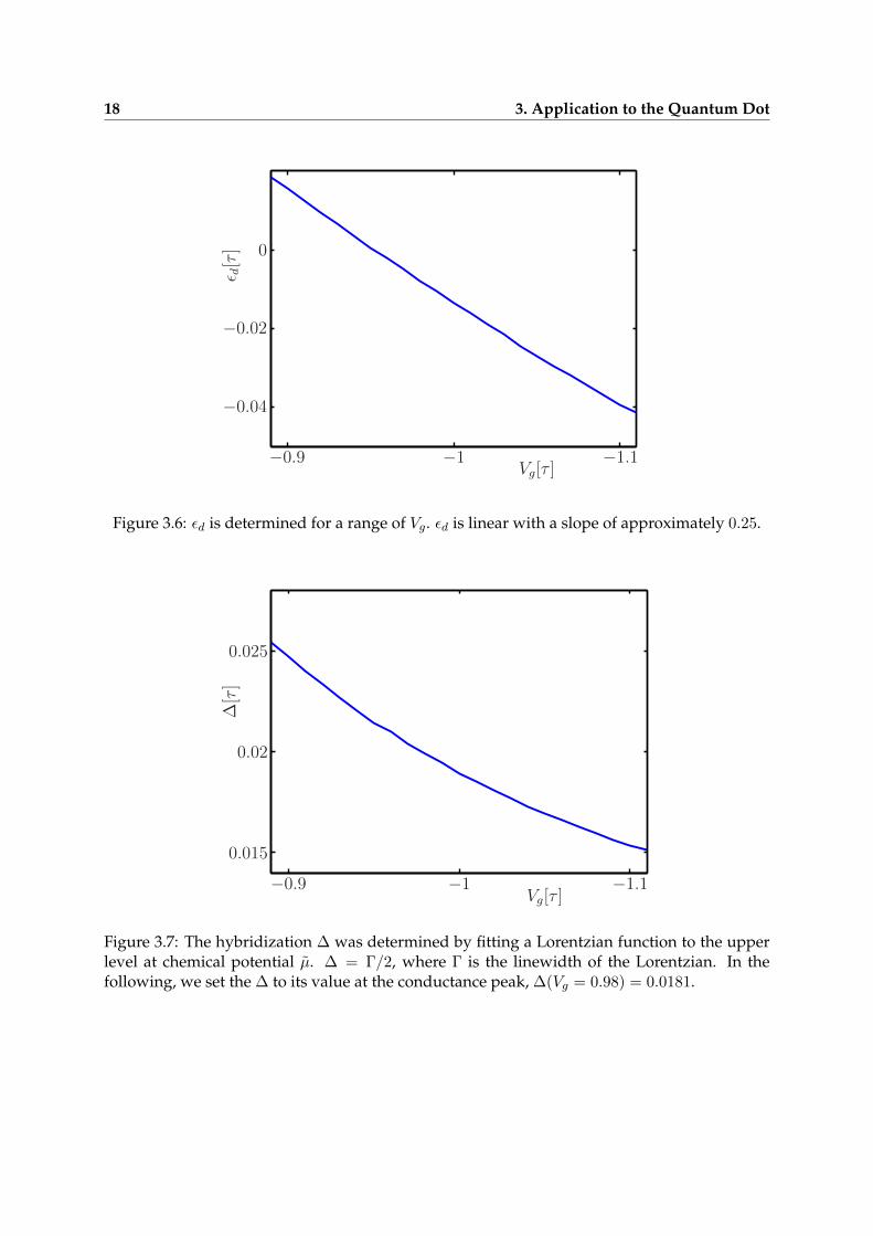
Figure 3.8: We show the total number n = n↑ + n↓ of electrons in the system and the phases δaand δs close to the resonance, where the conductance g has a peak. We plot n = (nσ)Z and δ+/πto demonstrate the validity of the Friedel sum rule.

π

π/2

0

0

1

0

−5

5

0

−5

−1 0 1 3(ǫd + U/2)/∆

gδ0

∆α1

∆φ1

∆2α2

∆2φ2

Figure 3.9: Fermi-liquid parameters determined for effective level positions. In the SIAM, atthe particle-hole symmetric point, εd = U/2 is fulfilled, when µ = 0. Also, α2 = φ2 = 0. Weseek out the point, where α2 = φ2 = 0 and apply the symmetry condition to find U = 1.9∆ forthe QD used here. Here, we considered a bound state with antisymmetric wave function. Asdiscussed in 3.2.1, all quantities except conductance switch sign. To preserve comparability tothe SIAM, we flip the y-axes of these quantities.


−2 −1 0 1 2

(ǫd + U/2)/∆

−0.5

0

0.5

1

cBcTcV

Figure 3.10: Normalized transport coefficients for magnetic field (blue), temperature (green)and bias voltage (red). The same normalization as in [8] was used: cα = cα/c

Kα with cKB = π2

16 ≈0.617, cKT = π4

16 ≈ 6.009 and cKV = 3π2

32 ≈ 0.925. Similar to the Fermi-liquid parameters for theQD, these curves are not symmetric in εd.

−2 0 2(ǫd + U/2)/∆

−0.5

0

0.5

1cBcB,curve

Figure 3.11: Normalized transport coefficient for magnetic field. Comparison of the Fermi-liquid calculation to the data from the fRG simulation.


−2 0 2

(ǫd + U/2)/∆

c[1/τ2]

0

10

20

30

cB,FL

cB,curve

Figure 3.12: The results of Fig. 3.11 without the normalization: cB = cB · α21.


3.2.3 (B) Chemical potential

We consider the wide band limit, where every energy can be considered far away from thebands bottom and top and change in distances relative to band limits are disregarded as small.No physical quantity in the SIAM can depend just on the absolute value of εd or µ because theenergy can have an arbitrary offset. They should only depend on the difference εd − µ. It isthe same for the QD as long as we do not change the shape of the potential. This enables us torewrite the differentiation of any physical quantity A as

∂A

∂εd= −∂A

∂µ. (3.12)

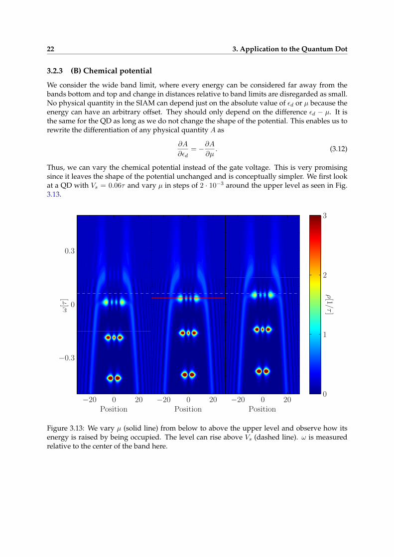
Thus, we can vary the chemical potential instead of the gate voltage. This is very promisingsince it leaves the shape of the potential unchanged and is conceptually simpler. We first lookat a QD with Vs = 0.06τ and vary µ in steps of 2 · 10−3 around the upper level as seen in Fig.3.13.

−20 0 20Position

−0.3

0

0.3

ω[τ]

−20 0 20Position

0

1

2

3

ρ[1/τ

]

−20 0 20Position

Figure 3.13: We vary µ (solid line) from below to above the upper level and observe how itsenergy is raised by being occupied. The level can rise above Vs (dashed line). ω is measuredrelative to the center of the band here.


−0.08−0.0406

8

µ[τ ]1

10

100

nγmax

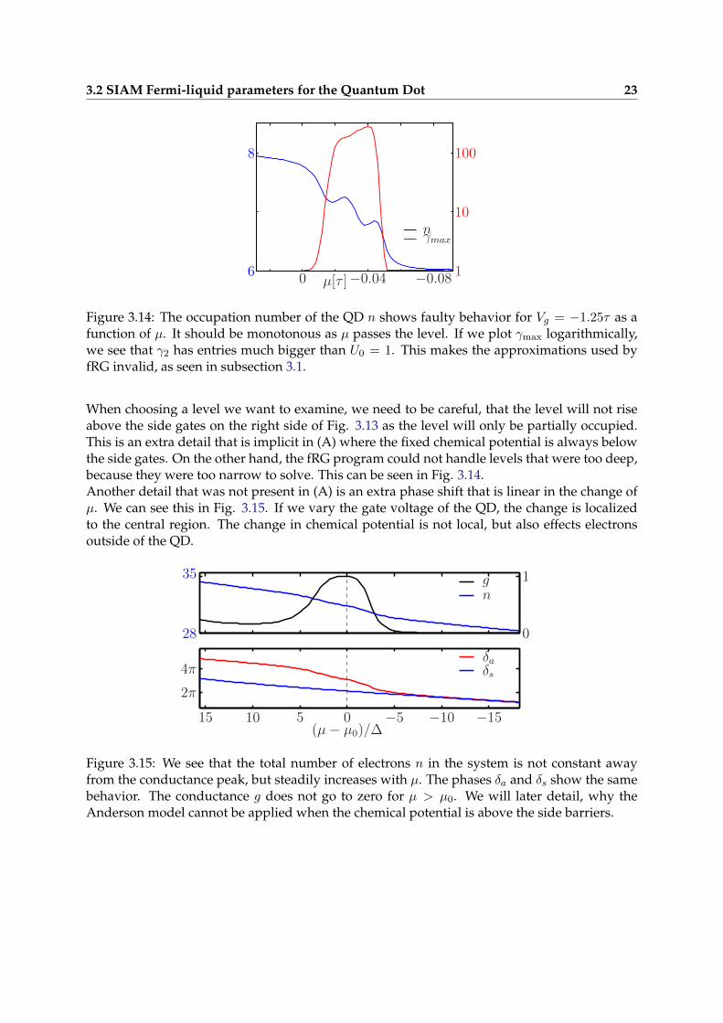
Figure 3.14: The occupation number of the QD n shows faulty behavior for Vg = −1.25τ as afunction of µ. It should be monotonous as µ passes the level. If we plot γmax logarithmically,we see that γ2 has entries much bigger than U0 = 1. This makes the approximations used byfRG invalid, as seen in subsection 3.1.

When choosing a level we want to examine, we need to be careful, that the level will not riseabove the side gates on the right side of Fig. 3.13 as the level will only be partially occupied.This is an extra detail that is implicit in (A) where the fixed chemical potential is always belowthe side gates. On the other hand, the fRG program could not handle levels that were too deep,because they were too narrow to solve. This can be seen in Fig. 3.14.Another detail that was not present in (A) is an extra phase shift that is linear in the change ofµ. We can see this in Fig. 3.15. If we vary the gate voltage of the QD, the change is localizedto the central region. The change in chemical potential is not local, but also effects electronsoutside of the QD.

28

35

0

1

2π

4π

(µ− µ0)/∆−15−10−5051015

gn

δaδs

Figure 3.15: We see that the total number of electrons n in the system is not constant awayfrom the conductance peak, but steadily increases with µ. The phases δa and δs show the samebehavior. The conductance g does not go to zero for µ > µ0. We will later detail, why theAnderson model cannot be applied when the chemical potential is above the side barriers.


00.05 µ[τ ]0

0.5

1gfullgsections

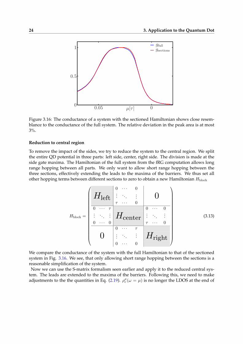
Figure 3.16: The conductance of a system with the sectioned Hamiltonian shows close resem-blance to the conductance of the full system. The relative deviation in the peak area is at most3%.

Reduction to central region

To remove the impact of the sides, we try to reduce the system to the central region. We splitthe entire QD potential in three parts: left side, center, right side. The division is made at theside gate maxima. The Hamiltonian of the full system from the fRG computation allows longrange hopping between all parts. We only want to allow short range hopping between thethree sections, effectively extending the leads to the maxima of the barriers. We thus set allother hopping terms between different sections to zero to obtain a new Hamiltonian Hblock

Hblock =

0 · · · 0

Hleft... . . .

... 0τ · · · 0

0 · · · τ 0 · · · 0... . . .

... Hcenter... . . .

...0 · · · 0 τ · · · 0

0 · · · τ

0 .... . .

... Hright0 · · · 0

(3.13)

We compare the conductance of the system with the full Hamiltonian to that of the sectionedsystem in Fig. 3.16. We see, that only allowing short range hopping between the sections is areasonable simplification of the system.Now we can use the S-matrix formalism seen earlier and apply it to the reduced central sys-

tem. The leads are extended to the maxima of the barriers. Following this, we need to makeadjustments to the the quantities in Eq. (2.19). ρσc (ω = µ) is no longer the LDOS at the end of


0

π

2π

(µ− µ0)/∆−15−10−5051015

δaδs

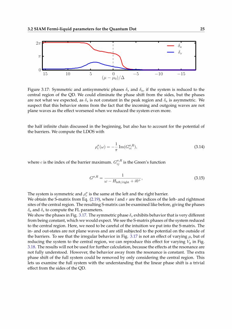
Figure 3.17: Symmetric and antisymmetric phases δs and δa, if the system is reduced to thecentral region of the QD. We could eliminate the phase shift from the sides, but the phasesare not what we expected, as δs is not constant in the peak region and δa is asymmetric. Wesuspect that this behavior stems from the fact that the incoming and outgoing waves are notplane waves as the effect worsened when we reduced the system even more.

the half infinite chain discussed in the beginning, but also has to account for the potential ofthe barriers. We compute the LDOS with

ρσc (ω) = − 1

πIm(Gσ,Rcc ), (3.14)

where c is the index of the barrier maximum. Gσ,Rij is the Green’s function

Gσ,R =1

ω −Hleft/right + i0+, (3.15)

The system is symmetric and ρσc is the same at the left and the right barrier.We obtain the S-matrix from Eq. (2.19), where l and r are the indices of the left- and rightmostsites of the central region. The resulting S-matrix can be examined like before, giving the phasesδa and δs to compute the FL parameters.We show the phases in Fig. 3.17. The symmetric phase δs exhibits behavior that is very differentfrom being constant, which we would expect. We see the S-matrix phases of the system reducedto the central region. Here, we need to be careful of the intuition we put into the S-matrix. Thein- and out-states are not plane waves and are still subjected to the potential on the outside ofthe barriers. To see that the irregular behavior in Fig. 3.17 is not an effect of varying µ, but ofreducing the system to the central region, we can reproduce this effect for varying Vg in Fig.3.18. The results will not be used for further calculation, because the effects at the resonance arenot fully understood. However, the behavior away from the resonance is constant. The extraphase shift of the full system could be removed by only considering the central region. Thislets us examine the full system with the understanding that the linear phase shift is a trivialeffect from the sides of the QD.


0

2π

−2 −1 0 1 2 3(ǫd + U/2)/∆

δaδs

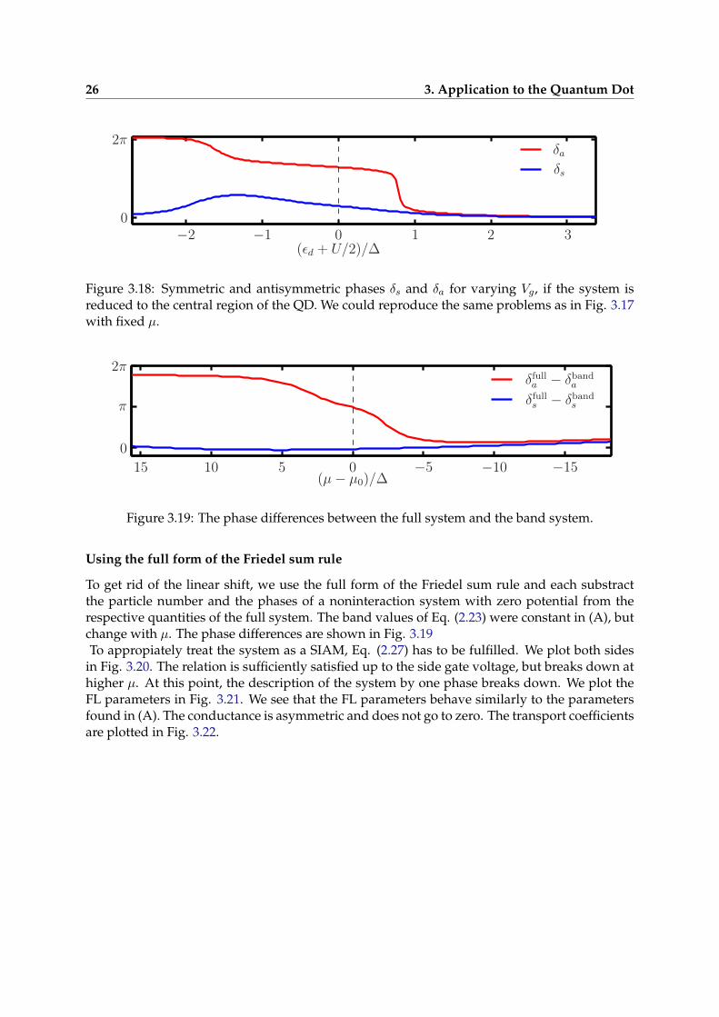
Figure 3.18: Symmetric and antisymmetric phases δs and δa for varying Vg, if the system isreduced to the central region of the QD. We could reproduce the same problems as in Fig. 3.17with fixed µ.

0

π

2π

(µ− µ0)/∆−15−10−5051015

δfulla − δbanda

δfulls − δbands

Figure 3.19: The phase differences between the full system and the band system.

Using the full form of the Friedel sum rule

To get rid of the linear shift, we use the full form of the Friedel sum rule and each substractthe particle number and the phases of a noninteraction system with zero potential from therespective quantities of the full system. The band values of Eq. (2.23) were constant in (A), butchange with µ. The phase differences are shown in Fig. 3.19To appropiately treat the system as a SIAM, Eq. (2.27) has to be fulfilled. We plot both sides

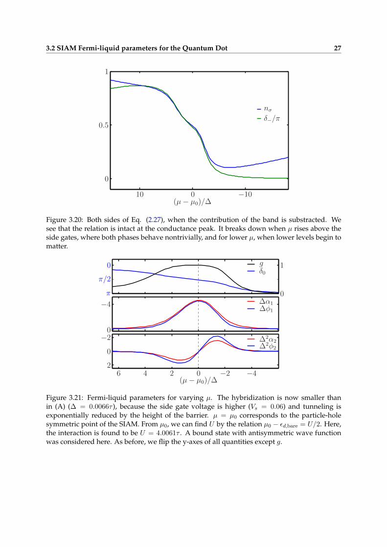
in Fig. 3.20. The relation is sufficiently satisfied up to the side gate voltage, but breaks down athigher µ. At this point, the description of the system by one phase breaks down. We plot theFL parameters in Fig. 3.21. We see that the FL parameters behave similarly to the parametersfound in (A). The conductance is asymmetric and does not go to zero. The transport coefficientsare plotted in Fig. 3.22.


−10010(µ− µ0)/∆

0

0.5

1

nσ

δ−/π

Figure 3.20: Both sides of Eq. (2.27), when the contribution of the band is substracted. Wesee that the relation is intact at the conductance peak. It breaks down when µ rises above theside gates, where both phases behave nontrivially, and for lower µ, when lower levels begin tomatter.

0

π/2

π 0

1

−4

0−2

0

2−4−20246

(µ− µ0)/∆

gδ0

∆α1∆φ1

∆2α2∆2φ2

Figure 3.21: Fermi-liquid parameters for varying µ. The hybridization is now smaller thanin (A) (∆ = 0.0066τ ), because the side gate voltage is higher (Vs = 0.06) and tunneling isexponentially reduced by the height of the barrier. µ = µ0 corresponds to the particle-holesymmetric point of the SIAM. From µ0, we can find U by the relation µ0 − εd,bare = U/2. Here,the interaction is found to be U = 4.0061τ . A bound state with antisymmetric wave functionwas considered here. As before, we flip the y-axes of all quantities except g.


04(µ− µ0)/∆

−0.3

0

0.5

1

cB

cT

cV

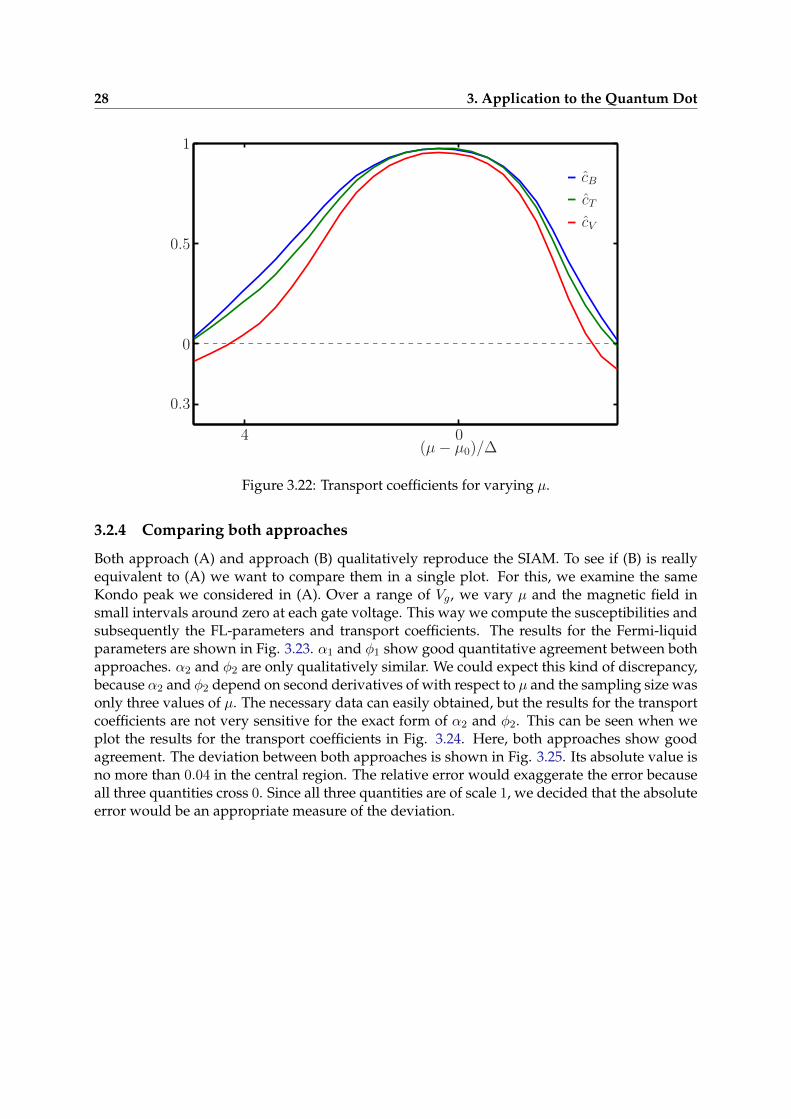
Figure 3.22: Transport coefficients for varying µ.

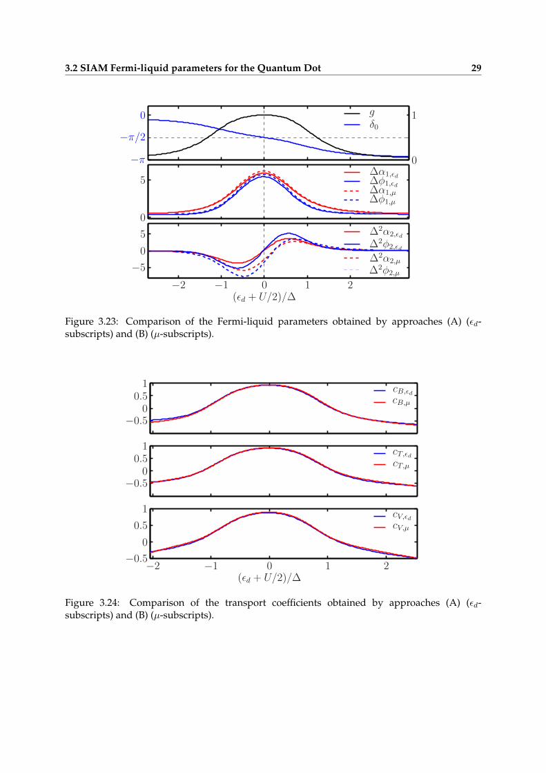
3.2.4 Comparing both approaches

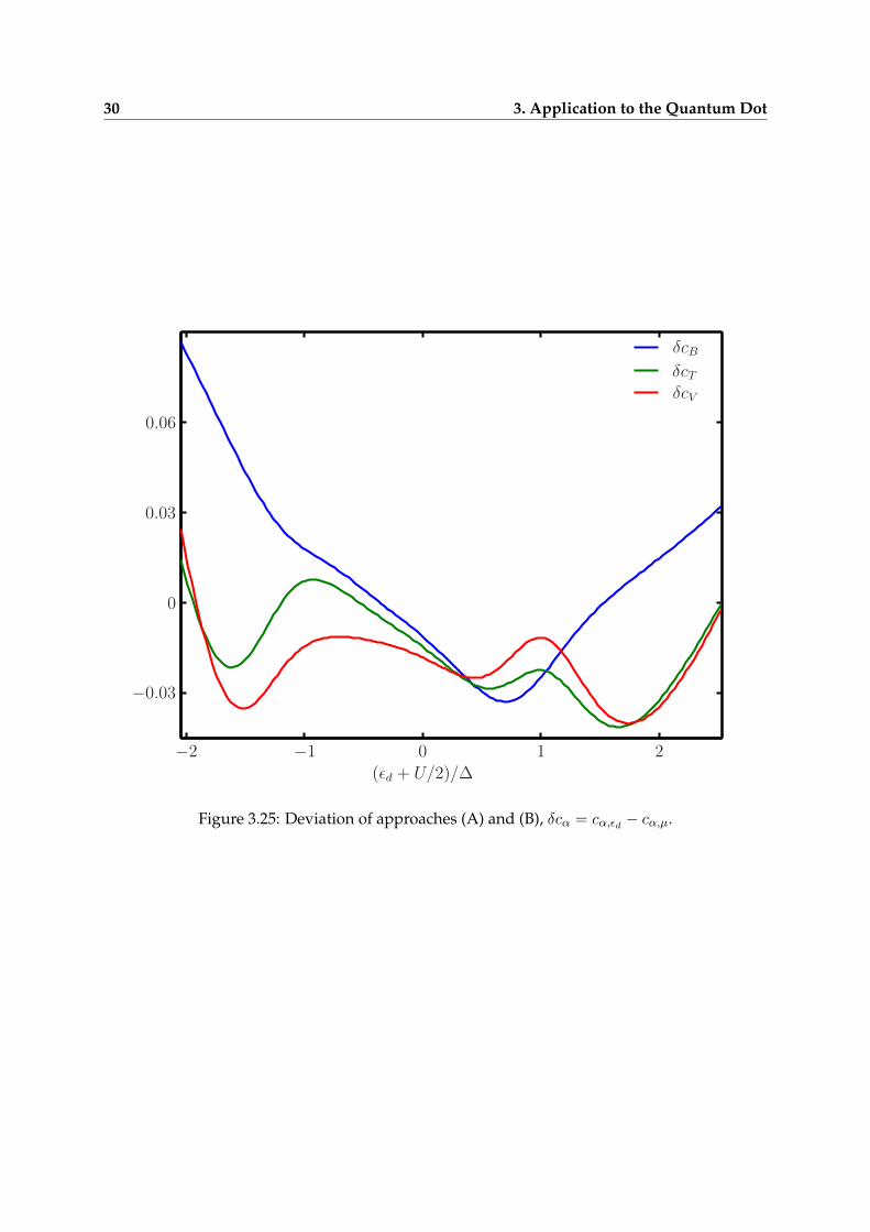
Both approach (A) and approach (B) qualitatively reproduce the SIAM. To see if (B) is reallyequivalent to (A) we want to compare them in a single plot. For this, we examine the sameKondo peak we considered in (A). Over a range of Vg, we vary µ and the magnetic field insmall intervals around zero at each gate voltage. This way we compute the susceptibilities andsubsequently the FL-parameters and transport coefficients. The results for the Fermi-liquidparameters are shown in Fig. 3.23. α1 and φ1 show good quantitative agreement between bothapproaches. α2 and φ2 are only qualitatively similar. We could expect this kind of discrepancy,because α2 and φ2 depend on second derivatives of with respect to µ and the sampling size wasonly three values of µ. The necessary data can easily obtained, but the results for the transportcoefficients are not very sensitive for the exact form of α2 and φ2. This can be seen when weplot the results for the transport coefficients in Fig. 3.24. Here, both approaches show goodagreement. The deviation between both approaches is shown in Fig. 3.25. Its absolute value isno more than 0.04 in the central region. The relative error would exaggerate the error becauseall three quantities cross 0. Since all three quantities are of scale 1, we decided that the absoluteerror would be an appropriate measure of the deviation.


−π

−π/2

0

0

1

0

5

−5

0

5

−2 −1 0 1 2(ǫd + U/2)/∆

gδ0

∆α1,ǫd∆φ1,ǫd∆α1,µ∆φ1,µ

∆2α2,ǫd

∆2φ2,ǫd

∆2α2,µ

∆2φ2,µ

Figure 3.23: Comparison of the Fermi-liquid parameters obtained by approaches (A) (εd-subscripts) and (B) (µ-subscripts).

−0.50

0.51

−0.50

0.51

−0.5

0

0.5

1

−2 −1 0 1 2(ǫd + U/2)/∆

cB,ǫdcB,µ

cT,ǫdcT,µ

cV,ǫdcV,µ

Figure 3.24: Comparison of the transport coefficients obtained by approaches (A) (εd-subscripts) and (B) (µ-subscripts).


−0.03

0

0.03

0.06

−2 −1 0 1 2(ǫd + U/2)/∆

δcBδcTδcV

Figure 3.25: Deviation of approaches (A) and (B), δcα = cα,εd − cα,µ.

Chapter 4

Conclusion

In this thesis, we applied the Fermi-liquid description of a SIAM to a Quantum Dot poten-tial to compute transport properties at low energies via relations taken from [8]. We exploredtwo approaches, (A) finding an effective level position for a given potential and (B) varyingthe chemical potential of the system. For (A), we expanded on Philipp Rosenbergers Bachelorthesis, finding a more elaborate way to determine the effective level postition. We computedthe Fermi-liquid parameters and transport coefficients for small magnetic fields, temperatureand bias voltage. The magnetic transport coefficients were successfully compared to the re-spective transport coefficient taken directly from fRG data. One problem we encountered, wasthat the hybridization of the level is not constant when we vary the gate voltage. Introducingan effective level position that is not physically realized is also very artificial. It is favourableto describe the system independent of this. With approach (B), we could escape some of theproblems faced in approach (A). We could compute FL parameters and transport coefficientsfor a varying chemical potential. We compared the results to those of approach (A) and sawthat describing the QD by varying the chemical potential is valid, if we are careful of certainthings: (1) The upper level position is pinned to the chemical potential, when µ passes the highconductance range. This means that the level can rise above the side gate voltage resulting in anonly partially occupied level. If we set the QD too deep in an effort to keep the level below theside gate voltage, the fRG results can become inaccurate. We expect, that this problem could becircumvented in a modified potential. If the side barriers are very narrow, tunneling becomesgreater and the fRG could yield valid results. (2) Changing the chemical potential results in aglobal phase shift. We need to utilize the full form of the Friedel sum rule. (3) When µ is big,both phases of the S-matrix become important and the single phase description taken from theSIAM breaks down. Applying the Fermi-liquid description to the QD without assigning aneffective level position is a useful advancement. In systems like the Quantum Point Contact(QPC) no bound states exist and we will need to use this description once a FL-theory existsfor the QPC.

32 4. Conclusion

Bibliography

[1] L. Jacak, P. Hawrylak, and A. Wojs. Quantum Dots. NanoScience and Technology. SpringerBerlin Heidelberg, 2013.

[2] L.L. Sohn, L.P. Kouwenhoven, and G. Schön. Mesoscopic Electron Transport. Nato ScienceSeries E:. Springer Netherlands, 1997.

[3] Knill E., Laflamme R., and Milburn G. J. A scheme for efficient quantum computationwith linear optics. Nature, 409(6816):46–52, jan 2001. 10.1038/35051009.

[4] Guido Burkard, Daniel Loss, and David P. DiVincenzo. Coupled quantum dots as quan-tum gates. Phys. Rev. B, 59:2070–2078, Jan 1999.

[5] Bauer Florian, Heyder Jan, Schubert Enrico, Borowsky David, Taubert Daniela, BruognoloBenedikt, Schuh Dieter, Wegscheider Werner, von Delft Jan, and Ludwig Stefan. Micro-scopic origin of the /‘0.7-anomaly/’ in quantum point contacts. Nature, 501(7465):73–78,sep 2013.

[6] P. W. Anderson. Localized Magnetic States in Metals. Phys. Rev., 124:41–53, Oct 1961.

[7] P. Nozières. A “fermi-liquid” description of the Kondo problem at low temperatures.Journal of Low Temperature Physics, 17(1):31–42, 1974.

[8] Christophe Mora, Catalin Pa scu Moca, Jan von Delft, and Gergely Zaránd. Fermi-liquidtheory for the single-impurity Anderson model. Phys. Rev. B, 92:075120, Aug 2015.

[9] Philipp Rosenberger. Application of a Fermi-liquid theory for the SIAM on an fRG-approach for the description of quantum dots. Master’s thesis, LMU Munich, 2015.

[10] J.R. Taylor. Scattering Theory: The Quantum Theory of Nonrelativistic Collisions. Dover Bookson Engineering. Dover Publications, 2012.

[11] Severin Georg Jakobs. Functional renormalization group studies of quantum transport throughmesoscopic systems. PhD thesis, RWTH Aachen University, 2009.

[12] Matias Zilly. Electronic conduction in linear quantum systems. PhD thesis, University Duis-burg, Duisburg, Essen, 2010. Duisburg, Essen, Univ., Diss., 2010.

34 BIBLIOGRAPHY

[13] J. S. Langer and V. Ambegaokar. Friedel Sum Rule for a System of Interacting Electrons.Phys. Rev., 121:1090–1092, Feb 1961.

[14] C. Karrasch. Transport Through Correlated Quantum Dots – A Functional Renormaliza-tion Group Approach. eprint arXiv:cond-mat/0612329, December 2006.

Acknowledgements

This thesis was written by one author, but relied on important contributions from many people.I want to thank my family for their support in every way. I am very lucky and grateful to havethem.This thesis was made possible by Professor von Delft, who offered me to work on this topic.Writing a thesis is challenging, but thanks to the exceptional conditions he provided it was agreat learning opportunity and a very good experience.My advisors and office companions Dennis Schimmel and Lukas Weidinger are to be thanked.From start to finish I could always count on them to offer answers, ideas and encouragement.Without them my thesis would have been impossible and my code a lot buggier.

Eidesstattliche Erklärung zur Bachelorarbeit

Hiermit erkläre ich, die vorliegende Arbeit selbständig verfasst zu haben und keine anderenals die in der Arbeit angegebenen Quellen und Hilfsmittel benutzt zu haben.

Unterschrift: München, 4. Juli 2016.

Documents

Fermi-Liquid Theory of a Quantum Dot · Fermi-Flüssigkeits-Theorie eines Quanten Punktes Sören Arlt Bachelorarbeit an der Fakultät für Physik der Ludwig–Maximilians–Universität