Embed Size (px)
Citation preview

Draft version January 20, 2020Typeset using LATEX twocolumn style in AASTeX62
Fermi Large Area Telescope Fourth Source Catalog
S. Abdollahi,1 F. Acero,2 M. Ackermann,3 M. Ajello,4 W. B. Atwood,5 M. Axelsson,6, 7 L. Baldini,8 J. Ballet,2
G. Barbiellini,9, 10 D. Bastieri,11, 12 J. Becerra Gonzalez,13, 14, 15 R. Bellazzini,16 A. Berretta,17 E. Bissaldi,18, 19
R. D. Blandford,20 E. D. Bloom,20 R. Bonino,21, 22 E. Bottacini,23, 20 T. J. Brandt,14 J. Bregeon,24 P. Bruel,25
R. Buehler,3 T. H. Burnett,26 S. Buson,27 R. A. Cameron,20 R. Caputo,14 P. A. Caraveo,28 J. M. Casandjian,2
D. Castro,29, 14 E. Cavazzuti,30 E. Charles,20 S. Chaty,2 S. Chen,11, 23 C. C. Cheung,31 G. Chiaro,28 S. Ciprini,32, 33
J. Cohen-Tanugi,24 L. R. Cominsky,34 J. Coronado-Blazquez,35, 36 D. Costantin,37 A. Cuoco,38, 21 S. Cutini,39
F. D’Ammando,40 M. DeKlotz,41 P. de la Torre Luque,18 F. de Palma,21 A. Desai,4 S. W. Digel,20 N. Di Lalla,8
M. Di Mauro,14 L. Di Venere,18, 19 A. Domınguez,42 D. Dumora,43 F. Fana Dirirsa,44 S. J. Fegan,25
E. C. Ferrara,14 A. Franckowiak,3 Y. Fukazawa,1 S. Funk,45 P. Fusco,18, 19 F. Gargano,19 D. Gasparrini,32, 33
N. Giglietto,18, 19 P. Giommi,33 F. Giordano,18, 19 M. Giroletti,40 T. Glanzman,20 D. Green,46 I. A. Grenier,2
S. Griffin,14 M.-H. Grondin,43 J. E. Grove,31 S. Guiriec,47, 14 A. K. Harding,14 K. Hayashi,48 E. Hays,14
J.W. Hewitt,49 D. Horan,25 G. Johannesson,50, 51 T. J. Johnson,52 T. Kamae,53 M. Kerr,31 D. Kocevski,14
M. Kovac’evic’,39 M. Kuss,16 D. Landriu,2 S. Larsson,7, 54, 55 L. Latronico,21 M. Lemoine-Goumard,43 J. Li,3
I. Liodakis,20 F. Longo,9, 10 F. Loparco,18, 19 B. Lott,43 M. N. Lovellette,31 P. Lubrano,39 G. M. Madejski,20
S. Maldera,21 D. Malyshev,45 A. Manfreda,8 E. J. Marchesini,22 L. Marcotulli,4 G. Martı-Devesa,56
P. Martin,57 F. Massaro,22, 21, 58 M. N. Mazziotta,19 J. E. McEnery,14, 15 I.Mereu,17, 39 M. Meyer,20, 20, 20
P. F. Michelson,20 N. Mirabal,14, 59 T. Mizuno,60 M. E. Monzani,20 A. Morselli,32 I. V. Moskalenko,20
M. Negro,21, 22 E. Nuss,24 R. Ojha,14 N. Omodei,20 M. Orienti,40 E. Orlando,20, 61 J. F. Ormes,62 M. Palatiello,9, 10
V. S. Paliya,3 D. Paneque,46 Z. Pei,12 H. Pena-Herazo,22, 21, 58, 63 J. S. Perkins,14 M. Persic,9, 64 M. Pesce-Rollins,16
V. Petrosian,20 L. Petrov,14 F. Piron,24 H., Poon,1 T. A. Porter,20 G. Principe,40 S. Raino,18, 19 R. Rando,11, 12
M. Razzano,16, 65 S. Razzaque,44 A. Reimer,56, 20 O. Reimer,56 Q. Remy,24 T. Reposeur,43 R. W. Romani,20
P. M. Saz Parkinson,5, 66, 67 F. K. Schinzel,68, 69 D. Serini,18 C. Sgro,16 E. J. Siskind,70 D. A. Smith,43 G. Spandre,16
P. Spinelli,18, 19 A. W. Strong,71 D. J. Suson,72 H. Tajima,73, 20 M. N. Takahashi,46 D. Tak,74, 14 J. B. Thayer,20
D. J. Thompson,14 L. Tibaldo,57 D. F. Torres,75, 76 E. Torresi,77 J. Valverde,25 B. Van Klaveren,20
P. van Zyl,78, 79, 80 K. Wood,81 M. Yassine,9, 10 and G. Zaharijas61, 82
1Department of Physical Sciences, Hiroshima University, Higashi-Hiroshima, Hiroshima 739-8526, Japan2AIM, CEA, CNRS, Universite Paris-Saclay, Universite Paris Diderot, Sorbonne Paris Cite, F-91191 Gif-sur-Yvette, France
3Deutsches Elektronen Synchrotron DESY, D-15738 Zeuthen, Germany4Department of Physics and Astronomy, Clemson University, Kinard Lab of Physics, Clemson, SC 29634-0978, USA
5Santa Cruz Institute for Particle Physics, Department of Physics and Department of Astronomy and Astrophysics, University ofCalifornia at Santa Cruz, Santa Cruz, CA 95064, USA
6Department of Physics, Stockholm University, AlbaNova, SE-106 91 Stockholm, Sweden7Department of Physics, KTH Royal Institute of Technology, AlbaNova, SE-106 91 Stockholm, Sweden
8Universita di Pisa and Istituto Nazionale di Fisica Nucleare, Sezione di Pisa I-56127 Pisa, Italy9Istituto Nazionale di Fisica Nucleare, Sezione di Trieste, I-34127 Trieste, Italy
10Dipartimento di Fisica, Universita di Trieste, I-34127 Trieste, Italy11Istituto Nazionale di Fisica Nucleare, Sezione di Padova, I-35131 Padova, Italy
12Dipartimento di Fisica e Astronomia “G. Galilei”, Universita di Padova, I-35131 Padova, Italy13Instituto de Astrofısica de Canarias, Observatorio del Teide, C/Via Lactea, s/n, E38205, La Laguna, Tenerife, Spain
14NASA Goddard Space Flight Center, Greenbelt, MD 20771, USA15Department of Astronomy, University of Maryland, College Park, MD 20742, USA
16Istituto Nazionale di Fisica Nucleare, Sezione di Pisa, I-56127 Pisa, Italy17Dipartimento di Fisica, Universita degli Studi di Perugia, I-06123 Perugia, Italy
18Dipartimento di Fisica “M. Merlin” dell’Universita e del Politecnico di Bari, I-70126 Bari, Italy19Istituto Nazionale di Fisica Nucleare, Sezione di Bari, I-70126 Bari, Italy
20W. W. Hansen Experimental Physics Laboratory, Kavli Institute for Particle Astrophysics and Cosmology, Department of Physics andSLAC National Accelerator Laboratory, Stanford University, Stanford, CA 94305, USA
arX
iv:1
902.
1004
5v5
[as
tro-
ph.H
E]
17
Jan
2020

2 Fermi-LAT collaboration
21Istituto Nazionale di Fisica Nucleare, Sezione di Torino, I-10125 Torino, Italy22Dipartimento di Fisica, Universita degli Studi di Torino, I-10125 Torino, Italy
23Department of Physics and Astronomy, University of Padova, Vicolo Osservatorio 3, I-35122 Padova, Italy24Laboratoire Univers et Particules de Montpellier, Universite Montpellier, CNRS/IN2P3, F-34095 Montpellier, France
25Laboratoire Leprince-Ringuet, Ecole polytechnique, CNRS/IN2P3, F-91128 Palaiseau, France26Department of Physics, University of Washington, Seattle, WA 98195-1560, USA
27Institut fur Theoretische Physik and Astrophysik, Universitat Wurzburg, D-97074 Wurzburg, Germany28INAF-Istituto di Astrofisica Spaziale e Fisica Cosmica Milano, via E. Bassini 15, I-20133 Milano, Italy
29Harvard-Smithsonian Center for Astrophysics, Cambridge, MA 02138, USA30Italian Space Agency, Via del Politecnico snc, 00133 Roma, Italy
31Space Science Division, Naval Research Laboratory, Washington, DC 20375-5352, USA32Istituto Nazionale di Fisica Nucleare, Sezione di Roma “Tor Vergata”, I-00133 Roma, Italy
33Space Science Data Center - Agenzia Spaziale Italiana, Via del Politecnico, snc, I-00133, Roma, Italy34Department of Physics and Astronomy, Sonoma State University, Rohnert Park, CA 94928-3609, USA
35Instituto de Fısica Teorica UAM/CSIC, Universidad Autonoma de Madrid, 28049, Madrid, Spain36Departamento de Fısica Teorica, Universidad Autonoma de Madrid, 28049 Madrid, Spain37University of Padua, Department of Statistical Science, Via 8 Febbraio, 2, 35122 Padova
38RWTH Aachen University, Institute for Theoretical Particle Physics and Cosmology, (TTK),, D-52056 Aachen, Germany39Istituto Nazionale di Fisica Nucleare, Sezione di Perugia, I-06123 Perugia, Italy
40INAF Istituto di Radioastronomia, I-40129 Bologna, Italy41Stellar Solutions Inc., 250 Cambridge Avenue, Suite 204, Palo Alto, CA 94306, USA
42Grupo de Altas Energıas, Universidad Complutense de Madrid, E-28040 Madrid, Spain43Centre d’Etudes Nucleaires de Bordeaux Gradignan, IN2P3/CNRS, Universite Bordeaux 1, BP120, F-33175 Gradignan Cedex, France
44Department of Physics, University of Johannesburg, PO Box 524, Auckland Park 2006, South Africa45Friedrich-Alexander Universitat Erlangen-Nurnberg, Erlangen Centre for Astroparticle Physics, Erwin-Rommel-Str. 1, 91058 Erlangen,
Germany46Max-Planck-Institut fur Physik, D-80805 Munchen, Germany
47The George Washington University, Department of Physics, 725 21st St, NW, Washington, DC 20052, USA48Department of Physics and Astrophysics, Nagoya University, Chikusa-ku Nagoya 464-8602, Japan49University of North Florida, Department of Physics, 1 UNF Drive, Jacksonville, FL 32224 , USA
50Science Institute, University of Iceland, IS-107 Reykjavik, Iceland51Nordita, Royal Institute of Technology and Stockholm University, Roslagstullsbacken 23, SE-106 91 Stockholm, Sweden
52College of Science, George Mason University, Fairfax, VA 22030, resident at Naval Research Laboratory, Washington, DC 20375, USA53Department of Physics, Graduate School of Science, University of Tokyo, 7-3-1 Hongo, Bunkyo-ku, Tokyo 113-0033, Japan
54The Oskar Klein Centre for Cosmoparticle Physics, AlbaNova, SE-106 91 Stockholm, Sweden55School of Education, Health and Social Studies, Natural Science, Dalarna University, SE-791 88 Falun, Sweden
56Institut fur Astro- und Teilchenphysik, Leopold-Franzens-Universitat Innsbruck, A-6020 Innsbruck, Austria57IRAP, Universite de Toulouse, CNRS, UPS, CNES, F-31028 Toulouse, France
58Istituto Nazionale di Astrofisica-Osservatorio Astrofisico di Torino, via Osservatorio 20, I-10025 Pino Torinese, Italy59Department of Physics and Center for Space Sciences and Technology, University of Maryland Baltimore County, Baltimore, MD
21250, USA60Hiroshima Astrophysical Science Center, Hiroshima University, Higashi-Hiroshima, Hiroshima 739-8526, Japan
61Istituto Nazionale di Fisica Nucleare, Sezione di Trieste, and Universita di Trieste, I-34127 Trieste, Italy62Department of Physics and Astronomy, University of Denver, Denver, CO 80208, USA
63Instituto Nacional de Astrofısica, Optica y Electronica, Tonantzintla, Puebla 72840, Mexico64Osservatorio Astronomico di Trieste, Istituto Nazionale di Astrofisica, I-34143 Trieste, Italy
65Funded by contract FIRB-2012-RBFR12PM1F from the Italian Ministry of Education, University and Research (MIUR)66Department of Physics, The University of Hong Kong, Pokfulam Road, Hong Kong, China
67Laboratory for Space Research, The University of Hong Kong, Hong Kong, China68National Radio Astronomy Observatory, 1003 Lopezville Road, Socorro, NM 87801, USA
69University of New Mexico, MSC07 4220, Albuquerque, NM 87131, USA70NYCB Real-Time Computing Inc., Lattingtown, NY 11560-1025, USA
71Max-Planck Institut fur extraterrestrische Physik, D-85748 Garching, Germany72Purdue University Northwest, Hammond, IN 46323, USA
73Solar-Terrestrial Environment Laboratory, Nagoya University, Nagoya 464-8601, Japan74Department of Physics, University of Maryland, College Park, MD 20742, USA
75Institute of Space Sciences (CSICIEEC), Campus UAB, Carrer de Magrans s/n, E-08193 Barcelona, Spain

Fermi-LAT Fourth Catalog 3
76Institucio Catalana de Recerca i Estudis Avancats (ICREA), E-08010 Barcelona, Spain77INAF-Istituto di Astrofisica Spaziale e Fisica Cosmica Bologna, via P. Gobetti 101, I-40129 Bologna, Italy
78Hartebeesthoek Radio Astronomy Observatory, PO Box 443, Krugersdorp 1740, South Africa79School of Physics, University of the Witwatersrand, Private Bag 3, WITS-2050, Johannesburg, South Africa
80Square Kilometre Array South Africa, Pinelands, 7405, South Africa81Praxis Inc., Alexandria, VA 22303, resident at Naval Research Laboratory, Washington, DC 20375, USA
82Center for Astrophysics and Cosmology, University of Nova Gorica, Nova Gorica, Slovenia
ABSTRACT
We present the fourth Fermi Large Area Telescope catalog (4FGL) of γ-ray sources. Based on the
first eight years of science data from the Fermi Gamma-ray Space Telescope mission in the energy
range from 50 MeV to 1 TeV, it is the deepest yet in this energy range. Relative to the 3FGL catalog,
the 4FGL catalog has twice as much exposure as well as a number of analysis improvements, including
an updated model for the Galactic diffuse γ-ray emission, and two sets of light curves (1-year and 2-
month intervals). The 4FGL catalog includes 5064 sources above 4σ significance, for which we provide
localization and spectral properties. Seventy-five sources are modeled explicitly as spatially extended,
and overall 358 sources are considered as identified based on angular extent, periodicity or correlated
variability observed at other wavelengths. For 1336 sources we have not found plausible counterparts
at other wavelengths. More than 3130 of the identified or associated sources are active galaxies of the
blazar class, and 239 are pulsars.
Keywords: Gamma rays: general — surveys — catalogs
1. INTRODUCTION
The Fermi Gamma-ray Space Telescope was launched
in June 2008, and the Large Area Telescope (LAT) on-
board has been continually surveying the sky in the GeV
energy range since then. Integrating the data over many
years, the Fermi -LAT collaboration produced several
generations of high-energy γ-ray source catalogs (Table
1). The previous all-purpose catalog (3FGL, Acero et al.
2015) contained 3033 sources, mostly active galactic nu-
clei (AGN) and pulsars, but also a variety of other types
of extragalactic and Galactic sources.
This paper presents the fourth catalog of sources, ab-
breviated as 4FGL (for Fermi Gamma-ray LAT) de-tected in the first eight years of the mission. As in
previous catalogs, sources are included based on the sta-
tistical significance of their detection considered over the
entire time period of the analysis. For this reason the
4FGL catalog does not contain transient γ-ray sources
which are detectable only over a short duration, includ-
ing Gamma-ray Bursts (GRBs, Ajello et al. 2019), solar
flares (Ackermann et al. 2014a), and most novae (Ack-
ermann et al. 2014b).
The 4FGL catalog benefits from a number of improve-
ments with respect to the 3FGL, besides the twice longer
exposure:
1. We used Pass 8 data1 (§ 2.2). The principal dif-
ference relative to the P7REP data used for 3FGL
is improved angular resolution above 3 GeV and
about 20% larger acceptance at all energies, reach-
ing 2.5 m2 sr between 2 and 300 GeV. The accep-
tance is defined here as the integral of the effective
area over the field of view. It is the most relevant
quantity for a survey mission such as Fermi -LAT.
2. We developed a new model of the underlying dif-
fuse Galactic emission (§ 2.4).
3. We introduced weights in the maximum likelihood
analysis (§ 3.2) to mitigate the effect of system-
atic errors due to our imperfect knowledge of the
Galactic diffuse emission.
4. We accounted for the effect of energy dispersion
(reconstructed event energy not equal to the true
energy of the incoming γ ray). This is a small
correction (§ 4.2.2) and was neglected in previ-
ous Fermi -LAT catalogs because the energy res-
olution (measured as the 68% containment half
width) is better than 15% over most of the LAT
energy range and the γ-ray spectra have no sharp
features.
1 See http://fermi.gsfc.nasa.gov/ssc/data/analysis/documentation/Pass8 usage.html.

4 Fermi-LAT collaboration
Table 1. Previous Fermi-LAT catalogs
Acronym IRFs/Diffuse model Energy range/Duration Sources Analysis/Reference
1FGL P6 V3 DIFFUSE 0.1 – 100 GeV 1451 (P) Unbinned, F/B
gll iem v02 11 months Abdo et al. (2010a)
2FGL P7SOURCE V6 0.1 – 100 GeV 1873 (P) Binned, F/B
gal 2yearp7v6 v0 2 years Nolan et al. (2012)
3FGL P7REP SOURCE V15 0.1 – 300 GeV 3033 (P) Binned, F/B
gll iem v06 4 years Acero et al. (2015)
FGES P8R2 SOURCE V6 10 GeV – 2 TeV 46 (E) Binned, PSF, |b| < 7◦
gll iem v06 6 years Ackermann et al. (2017b)
3FHL P8R2 SOURCE V6 10 GeV – 2 TeV 1556 (P) Unbinned, PSF
gll iem v06 7 years Ajello et al. (2017)
FHES P8R2 SOURCE V6 1 GeV – 1 TeV 24 (E) Binned, PSF, |b| > 5◦
gll iem v06 7.5 years Ackermann et al. (2018)
4FGL P8R3 SOURCE V2 0.05 GeV – 1 TeV 5064 (P) Binned, PSF
gll iem v07 (§ 2.4.1) 8 years this work
Note—In the Analysis column, F/B stands for Front/Back, and PSF for PSF event typesa. In theSources column, we write (P) when the catalog’s objective is to look for point-like sources, (E) whenit looks for extended sources.aSee https://fermi.gsfc.nasa.gov/ssc/data/analysis/LAT essentials.html.
5. We tested all sources with three spectral models
(power law, log normal and power law with subex-
ponential cutoff, § 3.3).
6. We explicitly modeled 75 sources as extended
emission regions (§ 3.4), up from 25 in 3FGL.
7. We built light curves and tested variability using
two different time bins (one year and two months,
§ 3.6).
8. To study the associations of LAT sources with
counterparts at other wavelengths, we updated
several of the counterpart catalogs, and corre-
spondingly recalibrated the association procedure.
A preliminary version of this catalog (FL8Y2) was built
from the same data and the same software, but using
the previous interstellar emission model (gll iem v06)
as background, starting at 100 MeV and switching to
curved spectra at TScurv > 16 (see § 3.3 for definition).
We use it as a starting point for source detection and
localization, and to estimate the impact of changing the
underlying diffuse model. The result of a dedicated ef-
fort for studying the AGN population in the 4FGL cat-
alog is published in the accompanying fourth LAT AGN
catalog (4LAC, Fermi-LAT collaboration 2019) paper.
2 See https://fermi.gsfc.nasa.gov/ssc/data/access/lat/fl8y/.
Section 2 describes the LAT, the data, and the mod-
els for the diffuse backgrounds, celestial and otherwise.
Section 3 describes the construction of the catalog, with
emphasis on what has changed since the analysis for
the 3FGL catalog. Section 4 describes the catalog it-
self, Section 5 explains the association and identification
procedure, and Section 6 details the association results.
We conclude in Section 7. We provide appendices with
technical details of the analysis and of the format of the
electronic version of the catalog.
2. INSTRUMENT & BACKGROUND
2.1. The Large Area Telescope
The LAT detects γ rays in the energy range from
20 MeV to more than 1 TeV, measuring their arrival
times, energies, and directions. The field of view of
the LAT is ∼ 2.7 sr at 1 GeV and above. The per-
photon angular resolution (point-spread function, PSF,
68% containment radius) is ∼ 5◦ at 100 MeV, improv-
ing to 0.◦8 at 1 GeV (averaged over the acceptance of the
LAT), varying with energy approximately as E−0.8 and
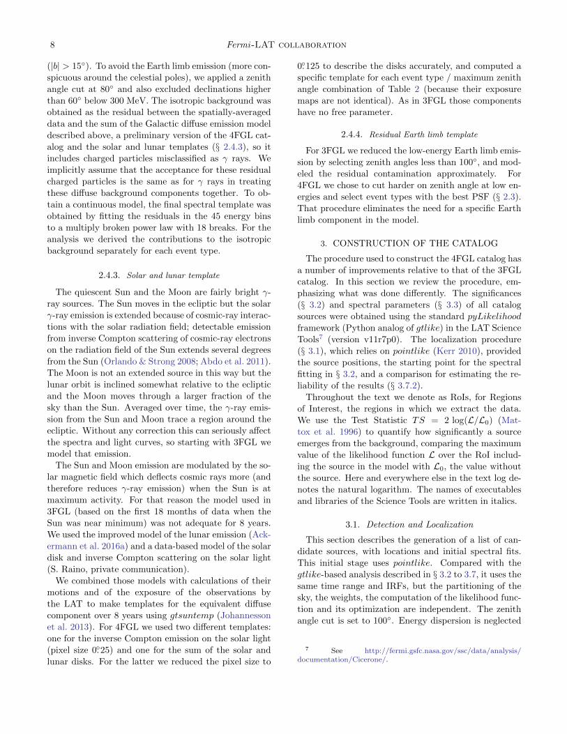
asymptoting at ∼ 0.◦1 above 20 GeV (Figure 1). The
tracking section of the LAT has 36 layers of silicon strip
detectors interleaved with 16 layers of tungsten foil (12
thin layers, 0.03 radiation length, at the top or Front
of the instrument, followed by 4 thick layers, 0.18 radi-
ation lengths, in the Back section). The silicon strips
track charged particles, and the tungsten foils facilitate

Fermi-LAT Fourth Catalog 5
conversion of γ rays to positron-electron pairs. Beneath
the tracker is a calorimeter composed of an 8-layer array
of CsI crystals (∼8.5 total radiation lengths) to deter-
mine the γ-ray energy. More information about the LAT
is provided in Atwood et al. (2009), and the in-flight cal-
ibration of the LAT is described in Abdo et al. (2009a),
Ackermann et al. (2012a) and Ackermann et al. (2012b).
Figure 1. Containment angle (68%) of the Fermi-LAT PSFas a function of energy, averaged over off-axis angle. Theblack line is the average over all data, whereas the coloredlines illustrate the difference between the four categories ofevents ranked by PSF quality from worst (PSF0) to best(PSF3).
The LAT is also an efficient detector of the intense
background of charged particles from cosmic rays and
trapped radiation at the orbit of the Fermi satellite.
A segmented charged-particle anticoincidence detec-
tor (plastic scintillators read out by photomultiplier
tubes) around the tracker is used to reject charged-
particle background events. Accounting for γ rays
lost in filtering charged particles from the data, the
effective collecting area at normal incidence (for the
P8R3 SOURCE V2 event selection used here; see be-
low)3 exceeds 0.3 m2 at 0.1 GeV, 0.8 m2 at 1 GeV, and
remains nearly constant at ∼ 0.9 m2 from 2 to 500 GeV.
The live time is nearly 76%, limited primarily by inter-
ruptions of data taking when Fermi is passing through
the South Atlantic Anomaly (SAA, ∼15%) and readout
dead-time fraction (∼9%).
2.2. The LAT Data
The data for the 4FGL catalog were taken during the
period 2008 August 4 (15:43 UTC) to 2016 August 2
(05:44 UTC) covering eight years. During most of this
3 See http://www.slac.stanford.edu/exp/glast/groups/canda/lat Performance.htm.
time, Fermi was operated in sky-scanning survey mode
(viewing direction rocking north and south of the zenith
on alternate orbits). As in 3FGL, intervals around solar
flares and bright GRBs were excised. Overall, about
two days were excised due to solar flares, and 39 ks due
to 30 GRBs. The precise time intervals corresponding
to selected events are recorded in the GTI extension of
the FITS file (Appendix A). The maximum exposure
(4.5 × 1011 cm2 s at 1 GeV) is reached at the North
celestial pole. The minimum exposure (2.7× 1011 cm2 s
at 1 GeV) is reached at the celestial equator.
The current version of the LAT data is Pass 8 P8R3
(Atwood et al. 2013; Bruel et al. 2018). It offers 20%
more acceptance than P7REP (Bregeon et al. 2013) and
a narrower PSF at high energies. Both aspects are
very useful for source detection and localization (Ajello
et al. 2017). We used the Source class event selec-
tion, with the Instrument Response Functions (IRFs)
P8R3 SOURCE V2. Pass 8 introduced a new partition
of the events, called PSF event types, based on the qual-
ity of the angular reconstruction (Figure 1), with ap-
proximately equal effective area in each event type at all
energies. The angular resolution is critical to distinguish
point sources from the background, so we split the data
into those four categories to avoid diluting high-quality
events (PSF3) with poorly localized ones (PSF0). We
split the data further into 6 energy intervals (also used
for the spectral energy distributions in § 3.5) because
the extraction regions must extend further at low en-
ergy (broad PSF) than at high energy, but the pixel
size can be larger. After applying the zenith angle se-
lection (§ 2.3), we were left with the 15 components
described in Table 2. The log-likelihood is computed for
each component separately, then they are summed for
the SummedLikelihood maximization (§ 3.2).
The lower bound of the energy range was set to
50 MeV, down from 100 MeV in 3FGL, to constrain
the spectra better at low energy. It does not help de-
tecting or localizing sources because of the very broad
PSF below 100 MeV. The upper bound was raised
from 300 GeV in 3FGL to 1 TeV. This is because as
the source-to-background ratio decreases, the sensitiv-
ity curve (Figure 18 of Abdo et al. 2010a, 1FGL) shifts
to higher energies. The 3FHL catalog (Ajello et al. 2017)
went up to 2 TeV, but only 566 events exceed 1 TeV over
8 years (to be compared to 714,000 above 10 GeV).
2.3. Zenith angle selection
The zenith angle cut was set such that the contribu-
tion of the Earth limb at that zenith angle was less than
10% of the total (Galactic + isotropic) background. In-
tegrated over all zenith angles, the residual Earth limb

6 Fermi-LAT collaboration
Table 2. 4FGL Summed Likelihood components
Energy interval NBins ZMax Ring width Pixel size (deg)
(GeV) (deg) (deg) PSF0 PSF1 PSF2 PSF3 All
0.05 – 0.1 3 80 7 · · · · · · · · · 0.6 · · ·0.1 – 0.3 5 90 7 · · · · · · 0.6 0.6 · · ·0.3 – 1 6 100 5 · · · 0.4 0.3 0.2 · · ·1 – 3 5 105 4 0.4 0.15 0.1 0.1 · · ·3 – 10 6 105 3 0.25 0.1 0.05 0.04 · · ·10 – 1000 10 105 2 · · · · · · · · · · · · 0.04
Note—We used 15 components (all in binned mode) in the 4FGL Summed Likelihoodapproach (§ 3.2). Components in a given energy interval share the same number ofenergy bins, the same zenith angle selection and the same RoI size, but have differentpixel sizes in order to adapt to the PSF width (Figure 1). Each filled entry under Pixelsize corresponds to one component of the summed log-likelihood. NBins is the numberof energy bins in the interval, ZMax is the zenith angle cut, Ring width refers to thedifference between the RoI core and the extraction region, as explained in item 5 of§ 3.2.
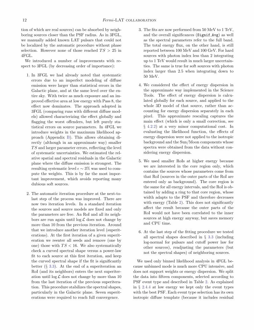
Figure 2. Exposure as a function of declination and energy,averaged over right ascension, summed over all relevant eventtypes as indicated in the figure legend.
contamination is less than 1%. We kept PSF3 event
types with zenith angles less than 80◦ between 50 and
100 MeV, PSF2 and PSF3 event types with zenith an-
gles less than 90◦ between 100 and 300 MeV, and PSF1,
PSF2 and PSF3 event types with zenith angles less than
100◦ between 300 MeV and 1 GeV. Above 1 GeV we kept
all events with zenith angles less than 105◦ (Table 2).
The resulting integrated exposure over 8 years is
shown in Figure 2. The dependence on declination is
due to the combination of the inclination of the orbit
(25.◦6), the rocking angle, the zenith angle selection and
the off-axis effective area. The north-south asymmetry
is due to the SAA, over which no scientific data is taken.
Because of the regular precession of the orbit every 53
days, the dependence on right ascension is small when
averaged over long periods of time. The main depen-
dence on energy is due to the increase of the effective
area up to 1 GeV, and the addition of new event types
at 100 MeV, 300 MeV and 1 GeV. The off-axis effec-
tive area depends somewhat on energy and event type.
This, together with the different zenith angle selections,
introduces a slight dependence of the shape of the curve
on energy.
Selecting on zenith angle applies a kind of time se-
lection (which depends on direction in the sky). This
means that the effective time selection at low energy is
not exactly the same as at high energy. The periods of
time during which a source is at zenith angle < 105◦
but (for example) > 90◦ last typically a few minutes ev-
ery orbit. This is shorter than the main variability time
scales of astrophysical sources in 4FGL, and therefore
not a concern. There remains however the modulation
due to the precession of the spacecraft orbit on longer
time scales over which blazars can vary. This is not
a problem for a catalog (it can at most appear as a
spectral effect, and should average out when consider-
ing statistical properties) but it should be kept in mind
when extracting spectral parameters of individual vari-
able sources. We used the same zenith angle cut for all
event types in a given energy interval, to reduce system-
atics due to that time selection.
Because the data are limited by systematics at low
energies everywhere in the sky (Appendix B) rejecting
half of the events below 300 MeV and 75% of them below

Fermi-LAT Fourth Catalog 7
100 MeV does not impact the sensitivity (if we had kept
these events, the weights would have been lower).
2.4. Model for the Diffuse Gamma-Ray Background
2.4.1. Diffuse emission of the Milky Way
We extensively updated the model of the Galactic dif-
fuse emission for the 4FGL analysis, using the same
P8R3 data selections (PSF types, energy ranges, and
zenith angle limits). The development of the model is
described in more detail (including illustrations of the
templates and residuals) online4. Here we summarize
the primary differences from the model developed for
the 3FGL catalog (Acero et al. 2016a). In both cases,
the model is based on linear combinations of templates
representing components of the Galactic diffuse emis-
sion. For 4FGL we updated all of the templates, and
added a new one as described below.
We have adopted the new, all-sky high-resolution,
21-cm spectral line HI4PI survey (HI4PI Collaboration
et al. 2016) as our tracer of H i, and extensively refined
the procedure for partitioning the H i and H2 (traced
by the 2.6-mm CO line) into separate ranges of Galac-
tocentric distance (‘rings’), by decomposing the spec-
tra into individual line profiles, so the broad velocity
dispersion of massive interstellar clouds does not effec-
tively distribute their emission very broadly along the
line of sight. We also updated the rotation curve, and
adopted a new procedure for interpolating the rings
across the Galactic center and anticenter, now incor-
porating a general model for the surface density dis-
tribution of the interstellar medium to inform the in-
terpolation, and defining separate rings for the Central
Molecular Zone (within ∼150 pc of the Galactic center
and between 150 pc and 600 pc of the center). With
this approach, the Galaxy is divided into ten concentric
rings.
The template for the inverse Compton emission is still
based on a model interstellar radiation field and cosmic-
ray electron distribution (calculated in GALPROP v56,
described in Porter et al. 2017)5 but now we formally
subdivide the model into rings (with the same Galac-
tocentric radius ranges as for the gas templates), which
are fit separately in the analysis, to allow some spatial
freedom relative to the static all-sky inverse-Compton
model.
We have also updated the template of the ‘dark gas’
component (Grenier et al. 2005), representing interstel-
4 https://fermi.gsfc.nasa.gov/ssc/data/analysis/software/aux/4fgl/Galactic Diffuse Emission Model for the 4FGL CatalogAnalysis.pdf
5 http://galprop.stanford.edu
lar gas that is not traced by the H i and CO line surveys,
by comparison with the Planck dust optical depth map6.
The dark gas is inferred as the residual component after
the best-fitting linear combination of total N(H i) and
WCO (the integrated intensity of the CO line) is sub-
tracted, i.e., as the component not correlated with the
atomic and molecular gas spectral line tracers, in a pro-
cedure similar to that used in Acero et al. (2016a). In
particular, as before we retained the negative residuals
as a ‘column density correction map’.
New to the 4FGL model, we incorporated a tem-
plate representing the contribution of unresolved Galac-
tic sources. This was derived from the model spatial
distribution and luminosity function developed based on
the distribution of Galactic sources in Acero et al. (2015)
and an analytical evaluation of the flux limit for source
detection as a function of direction on the sky.
As for the 3FGL model, we iteratively determined and
re-fit a model component that represents non-template
diffuse γ-ray emission, primarily Loop I and the Fermi
bubbles. To avoid overfitting the residuals, and possi-
bly suppressing faint Galactic sources, we spectrally and
spatially smoothed the residual template.
The model fitting was performed using Gardian (Ack-
ermann et al. 2012d), as a summed log-likelihood analy-
sis. This procedure involves transforming the ring maps
described above into spatial-spectral templates evalu-
ated in GALPROP. We used model SLZ6R30T 150C2
from Ackermann et al. (2012d). The model is a linear
combination of these templates, with free scaling func-
tions of various forms for the individual templates. For
components with the largest contributions, a piecewise
continuous function, linear in the logarithm of energy,
with nine degrees of freedom was used. Other compo-
nents had a similar scaling function with five degrees
of freedom, or power-law scaling, or overall scale fac-
tors, chosen to give the model adequate freedom while
reducing the overall number of free parameters. The
model also required a template for the point and small-
extended sources in the sky. We iterated the fitting using
preliminary versions of the 4FGL catalog. This template
was also given spectral degrees of freedom. Other diffuse
templates, described below and not related to Galactic
emission, were included in the model fitting.
2.4.2. Isotropic background
The isotropic diffuse background was derived over 45
energy bins covering the energy range 30 MeV to 1 TeV,
from the eight-year data set excluding the Galactic plane
6 COM CompMap Dust-GNILC-Model-Opacity 2048 R2.01.fits,Planck Collaboration et al. (2016)
8 Fermi-LAT collaboration
(|b| > 15◦). To avoid the Earth limb emission (more con-
spicuous around the celestial poles), we applied a zenith
angle cut at 80◦ and also excluded declinations higher
than 60◦ below 300 MeV. The isotropic background was
obtained as the residual between the spatially-averaged
data and the sum of the Galactic diffuse emission model
described above, a preliminary version of the 4FGL cat-
alog and the solar and lunar templates (§ 2.4.3), so it
includes charged particles misclassified as γ rays. We
implicitly assume that the acceptance for these residual
charged particles is the same as for γ rays in treating
these diffuse background components together. To ob-
tain a continuous model, the final spectral template was
obtained by fitting the residuals in the 45 energy bins
to a multiply broken power law with 18 breaks. For the
analysis we derived the contributions to the isotropic
background separately for each event type.
2.4.3. Solar and lunar template
The quiescent Sun and the Moon are fairly bright γ-
ray sources. The Sun moves in the ecliptic but the solar
γ-ray emission is extended because of cosmic-ray interac-
tions with the solar radiation field; detectable emission
from inverse Compton scattering of cosmic-ray electrons
on the radiation field of the Sun extends several degrees
from the Sun (Orlando & Strong 2008; Abdo et al. 2011).
The Moon is not an extended source in this way but the
lunar orbit is inclined somewhat relative to the ecliptic
and the Moon moves through a larger fraction of the
sky than the Sun. Averaged over time, the γ-ray emis-
sion from the Sun and Moon trace a region around the
ecliptic. Without any correction this can seriously affect
the spectra and light curves, so starting with 3FGL we
model that emission.
The Sun and Moon emission are modulated by the so-
lar magnetic field which deflects cosmic rays more (and
therefore reduces γ-ray emission) when the Sun is at
maximum activity. For that reason the model used in
3FGL (based on the first 18 months of data when the
Sun was near minimum) was not adequate for 8 years.
We used the improved model of the lunar emission (Ack-
ermann et al. 2016a) and a data-based model of the solar
disk and inverse Compton scattering on the solar light
(S. Raino, private communication).
We combined those models with calculations of their
motions and of the exposure of the observations by
the LAT to make templates for the equivalent diffuse
component over 8 years using gtsuntemp (Johannesson
et al. 2013). For 4FGL we used two different templates:
one for the inverse Compton emission on the solar light
(pixel size 0.◦25) and one for the sum of the solar and
lunar disks. For the latter we reduced the pixel size to
0.◦125 to describe the disks accurately, and computed a
specific template for each event type / maximum zenith
angle combination of Table 2 (because their exposure
maps are not identical). As in 3FGL those components
have no free parameter.
2.4.4. Residual Earth limb template
For 3FGL we reduced the low-energy Earth limb emis-
sion by selecting zenith angles less than 100◦, and mod-
eled the residual contamination approximately. For
4FGL we chose to cut harder on zenith angle at low en-
ergies and select event types with the best PSF (§ 2.3).
That procedure eliminates the need for a specific Earth
limb component in the model.
3. CONSTRUCTION OF THE CATALOG
The procedure used to construct the 4FGL catalog has
a number of improvements relative to that of the 3FGL
catalog. In this section we review the procedure, em-
phasizing what was done differently. The significances
(§ 3.2) and spectral parameters (§ 3.3) of all catalog
sources were obtained using the standard pyLikelihood
framework (Python analog of gtlike) in the LAT Science
Tools7 (version v11r7p0). The localization procedure
(§ 3.1), which relies on pointlike (Kerr 2010), provided
the source positions, the starting point for the spectral
fitting in § 3.2, and a comparison for estimating the re-
liability of the results (§ 3.7.2).
Throughout the text we denote as RoIs, for Regions
of Interest, the regions in which we extract the data.
We use the Test Statistic TS = 2 log(L/L0) (Mat-
tox et al. 1996) to quantify how significantly a source
emerges from the background, comparing the maximum
value of the likelihood function L over the RoI includ-
ing the source in the model with L0, the value without
the source. Here and everywhere else in the text log de-
notes the natural logarithm. The names of executables
and libraries of the Science Tools are written in italics.
3.1. Detection and Localization
This section describes the generation of a list of can-
didate sources, with locations and initial spectral fits.
This initial stage uses pointlike. Compared with the
gtlike-based analysis described in § 3.2 to 3.7, it uses the
same time range and IRFs, but the partitioning of the
sky, the weights, the computation of the likelihood func-
tion and its optimization are independent. The zenith
angle cut is set to 100◦. Energy dispersion is neglected
7 See http://fermi.gsfc.nasa.gov/ssc/data/analysis/documentation/Cicerone/.

Fermi-LAT Fourth Catalog 9
for the sources (we show in § 4.2.2 that it is a small ef-
fect). Events below 100 MeV are not useful for source
detection and localization, and are ignored at this stage.
3.1.1. Detection settings
The process started with an initial set of sources, from
the 8-year FL8Y analysis, including the 75 spatially ex-
tended sources listed in § 3.4, and the three-component
representation of the Crab (§ 3.3). The same spectral
models were considered for each source as in § 3.3, but
the favored model (power law, curved, or pulsar-like)
was not necessarily the same. The point-source loca-
tions were also re-optimized.
The generation of a candidate list of additional
sources, with locations and initial spectral fits, is sub-
stantially the same as for 3FGL. The sky was partitioned
using HEALPix8 (Gorski et al. 2005) with Nside = 12,
resulting in 1728 tiles of ∼24 deg2 area. (Note: refer-
ences to Nside in the following refer to HEALPix.) The
RoIs included events in cones of 5◦ radius about the
center of the tiles. The data were binned according to
energy, 16 energy bands from 100 MeV to 1 TeV (up
from 14 bands to 316 GeV in 3FGL), Front or Back
event types, and angular position using HEALPix, but
with Nside varying from 64 to 4096 according to the
PSF. Only Front events were used for the two bands
below 316 MeV, to avoid the poor PSF and contribution
of the Earth limb. Thus the log-likelihood calculation,
for each RoI, is a sum over the contributions of 30 energy
and event type bands.
All point sources within the RoI and those nearby,
such that the contribution to the RoI was at least 1%
(out to 11◦ for the lowest energy band), were included.
Only the spectral model parameters for sources within
the central tile were allowed to vary to optimize the like-
lihood. To account for correlations with fixed nearby
sources, and a factor of three overlap for the data (each
photon contributes to ∼ 3 RoIs), the following iteration
process was followed. All 1728 RoIs were optimized in-
dependently. Then the process was repeated, until con-
vergence, for all RoIs for which the log-likelihood had
changed by more than 10. Their nearest neighbors (pre-
sumably affected by the modified sources) were iterated
as well.
Another difference from 3FGL was that the diffuse
contributions were adjusted globally. We fixed the
isotropic diffuse source to be actually constant over the
sky, but globally refit its spectrum up to 10 GeV, since
point-source fits are insensitive to diffuse energies above
this. The Galactic diffuse emission component also was
8 http://healpix.sourceforge.net.
treated quite differently. Starting with a version of the
Galactic diffuse model (§ 2.4.1) without its non-template
diffuse γ-ray emission, we derived an alternative ad-
justment by optimizing the Galactic diffuse normaliza-
tion for each RoI and the eight bands below 10 GeV.
These values were turned into an 8-layer map which
was smoothed, then applied to the PSF-convolved dif-
fuse model predictions for each band. Then the correc-
tions were remeasured. This process converged after two
iterations, such that no further corrections were needed.
The advantage of the procedure, compared to fitting the
diffuse spectral parameters in each RoI (§ 3.2), is that
the effective predictions do not vary abruptly from an
RoI to its neighbors, and are unique for each point. Also
it does not constrain the spectral adjustment to be a
power law.
After a set of iterations had converged, the localization
procedure was applied, and source positions updated for
a new set of iterations. At this stage, new sources were
occasionally added using the residual TS procedure de-
scribed in § 3.1.2. The detection and localization process
resulted in 7841 candidate point sources with TS > 10,
of which 3179 were new. The fit validation and likeli-
hood weighting were done as in 3FGL, except that, due
to the improved representation of the Galactic diffuse,
the effect of the weighting factor was less severe.
The pointlike unweighting scheme is slightly different
from that described in the 3FGL paper (§ 3.1.2). A mea-
sure of the sensitivity to the Galactic diffuse component
is the average count density for the RoI divided by the
peak value of the PSF, Ndiff , which represents a measure
of the diffuse background under the point source. For
the RoI at the Galactic center, and the lowest energy
band, this is 4.15 × 10⁴ counts. We unweight the like-
lihood for all energy bands by effectively limiting this
implied precision to 2%, corresponding to 2500 counts.
As before, we divide the log-likelihood contribution from
this energy band by max(1, Ndiff/2500). For the afore-
mentioned case, this value is 16.6. A consequence is
to increase the spectral fit uncertainty for the lowest
energy bins for every source in the RoI. The value for
this unweighting factor was determined by examining
the distribution of the deviations between fluxes fitted
in individual energy bins and the global spectral fit (sim-
ilar to what is done in § 3.5). The 2% precision was set
such that the RMS for the distribution of positive de-
viations in the most sensitive lowest energy band was
near the statistical expectation. (Negative deviations
are distorted by the positivity constraint, resulting in
an asymmetry of the distribution.)
An important validation criterion is the all-sky counts
residual map. Since the source overlaps and diffuse

10 Fermi-LAT collaboration
uncertainties are most severe at the lowest energy, we
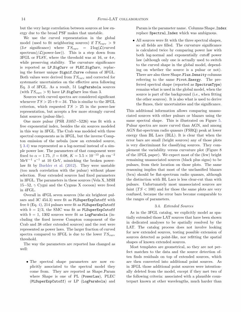
present, in Figure 3, the distribution of normalized resid-
uals per pixel, binned with Nside = 64, in the 100 – 177
MeV Front energy band. There are 49,920 such pix-
els, with data counts varying from 92 to 1.7× 10⁴. For
|b| > 10◦, the agreement with the expected Gaussian
distribution is very good, while it is clear that there are
issues along the plane. These are of two types. First,
around very strong sources, such as Vela, the discrepan-
cies are perhaps a result of inadequacies of the simple
spectral models used, but the (small) effect of energy
dispersion and the limited accuracy of the IRFs may
contribute. Regions along the Galactic ridge are also
evident, a result of the difficulty modeling the emission
precisely, the reason we unweight contributions to the
likelihood.
Figure 3. Photon count residuals with respect to themodel per Nside = 64 bin, for energies 100 – 177 MeV,normalized by the Poisson uncertainty, that is, (Ndata −Nmodel)/
√Nmodel. Histograms are shown for the values at
high latitude (|b| > 10◦) and low latitude (|b| < 10◦) (cappedat ±5σ). Dashed lines are the Gaussian expectations for thesame number of sources. The legend shows the mean andstandard deviation for the two subsets.
3.1.2. Detection of additional sources
As in 3FGL, the same implementation of the likeli-
hood used for optimizing source parameters was used to
test for the presence of additional point sources. This
is inherently iterative, in that the likelihood is valid
to the extent that the model used to calculate it is a
fair representation of the data. Thus, the detection of
the faintest sources depends on accurate modeling of all
nearby brighter sources and the diffuse contributions.
The FL8Y source list from which this started repre-
sented several such additions from the 4-year 3FGL. As
Table 3. Spectral shapes for source search
α β E0 (GeV) Template Generated Accepted
1.7 0.0 50.00 Hard 471 101
2.2 0.0 1.00 Intermediate 889 177
2.7 0.0 0.25 Soft 476 84
2.0 0.5 2.00 Peaked 686 151
2.0 0.3 1.00 Pulsar-like 476 84
Note—The spectral parameters α, β and E0 refer to the Log-Parabola spectral shape (Eq. 2). The last two columns showthe number, for each shape, that were successfully added to thepointlike model, and the number accepted for the final 4FGLlist.
before, an iteration starts with choosing a HEALPix
Nside = 512 grid, 3.1 M points with average separa-
tion 0.15 degrees. But now, instead of testing a single
power-law spectrum, we try five spectral shapes; three
are power laws with different indices, two with signifi-
cant curvature. Table 3 lists the spectral shapes used
for the templates. They are shown in Figure 4.
Figure 4. Spectral shape templates used in source finding.
For each trial position, and each of the five templates,
the normalizations were optimized, and the resulting TS
associated with the pixel. Then, as before, but inde-
pendently for each template, a cluster analysis selected
groups of pixels with TS > 16, as compared to TS > 10
for 3FGL. Each cluster defined a seed, with a position
determined by weighting the TS values. Finally, the
five sets of potential seeds were compared and, for those
within 1◦, the seed with the largest TS was selected for
inclusion.

Fermi-LAT Fourth Catalog 11
Each candidate was added to its respective RoI, then
fully optimized, including localization, during a full like-
lihood optimization including all RoIs. The combined
results of two iterations of this procedure, starting from
a pointlike model including only sources imported from
the FL8Y source list, are summarized in Table 3, which
shows the number for each template that was success-
fully added to the pointlike model, and the number fi-
nally included in 4FGL. The reduction is mostly due to
the TS > 25 requirement in 4FGL, as applied to the
gtlike calculation (§ 3.2), which uses different data and
smaller weights. The selection is even stricter (TS > 34,
§ 3.3) for sources with curved spectra. Several can-
didates at high significance were not accepted because
they were too close to even brighter sources, or inside
extended sources, and thus unlikely to be independent
point sources.
3.1.3. Localization
The position of each source was determined by max-
imizing the likelihood with respect to its position only.
That is, all other parameters are kept fixed. The pos-
sibility that a shifted position would affect the spectral
models or positions of nearby sources is accounted for
by iteration. In the ideal limit of large statistics the log-
likelihood is a quadratic form in any pair of orthogonal
angular variables, assuming small angular offsets. We
define LTS, for Localization Test Statistic, to be twice
the log of the likelihood ratio of any position with re-
spect to the maximum; the LTS evaluated for a grid of
positions is called an LTS map. We fit the distribution of
LTS to a quadratic form to determine the uncertainty
ellipse (position, major and minor axes, and orienta-
tion). The fitting procedure starts with a prediction of
the LTS distribution from the current elliptical parame-
ters. From this, it evaluates the LTS for eight positions
in a circle of a radius corresponding to twice the geo-
metric mean of the two Gaussian sigmas. We define a
measure, the localization quality (LQ), of how well the
actual LTS distribution matches this expectation as the
sum of squares of differences at those eight positions.
The fitting procedure determines a new set of elliptical
parameters from the eight values. In the ideal case, this
is a linear problem and one iteration is sufficient from
any starting point. To account for finite statistics or
distortions due to inadequacies of the model, we iter-
ate until changes are small. The procedure effectively
minimizes LQ.
We flagged apparently significant sources that do not
have good localization fits (LQ > 8) with Flag 9 (§ 3.7.3)
and for them estimated the position and uncertainty by
performing a moment analysis of an LTS map instead of
fitting a quadratic form. Some sources that did not have
a well-defined peak in the likelihood were discarded by
hand, on the consideration that they were most likely
related to residual diffuse emission. Another possibil-
ity is that two adjacent sources produce a dumbbell-like
shape; for a few of these cases we added a new source
by hand.
As in 3FGL, we checked the sources spatially associ-
ated with 984 AGN counterparts, comparing their loca-
tions with the well-measured positions of the counter-
parts. Better statistics allowed examination of the dis-
tributions of the differences separately for bright, dim,
and moderate-brightness sources. From this we estimate
the absolute precision ∆abs (at the 95% confidence level)
more accurately at ∼ 0.◦0068, up from ∼ 0.◦005 in 3FGL.
The systematic factor frel was 1.06, slightly up from 1.05
in 3FGL. Eq. 1 shows how the statistical errors ∆stat are
transformed into total errors ∆tot:
∆2tot = (frel ∆stat)
2 + ∆2abs (1)
which is applied to both ellipse axes.
3.2. Significance and Thresholding
The framework for this stage of the analysis is inher-
ited from the 3FGL catalog. It splits the sky into RoIs,
varying typically half a dozen sources near the center of
the RoI at the same time. Each source is entered into the
fit with the spectral shape and parameters obtained by
pointlike (§ 3.1), the brightest sources first. Soft sources
from pointlike within 0.◦2 of bright ones were intention-
ally deleted. They appear because the simple spectral
models we use are not sufficient to account for the spec-
tra of bright sources, but including them would bias the
spectral parameters. There are 1748 RoIs for 4FGL,
listed in the ROIs extension of the catalog (Appendix
A). The global best fit is reached iteratively, injecting
the spectra of sources in the outer parts of the RoI from
the previous step or iteration. In this approach, the dif-
fuse emission model (§ 2.4) is taken from the global tem-
plates (including the spectrum, unlike what is done with
pointlike in § 3.1) but it is modulated in each RoI by
three parameters: normalization (at 1 GeV) and small
corrective slope of the Galactic component, and normal-
ization of the isotropic component.
Among the more than 8,000 seeds coming from the
localization stage, we keep only sources with TS > 25,
corresponding to a significance of just over 4σ evaluated
from the χ2 distribution with 4 degrees of freedom (po-
sition and spectral parameters of a power-law source,
Mattox et al. 1996). The model for the current RoI
is readjusted after removing each seed below threshold.
The low-energy flux of the seeds below threshold (a frac-
12 Fermi-LAT collaboration
tion of which are real sources) can be absorbed by neigh-
boring sources closer than the PSF radius. As in 3FGL,
we manually added known LAT pulsars that could not
be localized by the automatic procedure without phase
selection. However none of those reached TS > 25 in
4FGL.
We introduced a number of improvements with re-
spect to 3FGL (by decreasing order of importance):
1. In 3FGL we had already noted that systematic
errors due to an imperfect modeling of diffuse
emission were larger than statistical errors in the
Galactic plane, and at the same level over the en-
tire sky. With twice as much exposure and an im-
proved effective area at low energy with Pass 8, the
effect now dominates. The approach adopted in
3FGL (comparing runs with different diffuse mod-
els) allowed characterizing the effect globally and
flagging the worst offenders, but left purely sta-
tistical errors on source parameters. In 4FGL we
introduce weights in the maximum likelihood ap-
proach (Appendix B). This allows obtaining di-
rectly (although in an approximate way) smaller
TS and larger parameter errors, reflecting the level
of systematic uncertainties. We estimated the rel-
ative spatial and spectral residuals in the Galactic
plane where the diffuse emission is strongest. The
resulting systematic level ε ∼ 3% was used to com-
pute the weights. This is by far the most impor-
tant improvement, which avoids reporting many
dubious soft sources.
2. The automatic iteration procedure at the next-to-
last step of the process was improved. There are
now two iteration levels. In a standard iteration
the sources and source models are fixed and only
the parameters are free. An RoI and all its neigh-
bors are run again until logL does not change by
more than 10 from the previous iteration. Around
that we introduce another iteration level (superit-
erations). At the first iteration of a given superit-
eration we reenter all seeds and remove (one by
one) those with TS < 16. We also systematically
check a curved spectral shape versus a power-law
fit to each source at this first iteration, and keep
the curved spectral shape if the fit is significantly
better (§ 3.3). At the end of a superiteration an
RoI (and its neighbors) enters the next superiter-
ation until logL does not change by more than 10
from the last iteration of the previous superitera-
tion. This procedure stabilizes the spectral shapes,
particularly in the Galactic plane. Seven superit-
erations were required to reach full convergence.
3. The fits are now performed from 50 MeV to 1 TeV,
and the overall significances (Signif Avg) as well
as the spectral parameters refer to the full band.
The total energy flux, on the other hand, is still
reported between 100 MeV and 100 GeV. For hard
sources with photon index less than 2 integrating
up to 1 TeV would result in much larger uncertain-
ties. The same is true for soft sources with photon
index larger than 2.5 when integrating down to
50 MeV.
4. We considered the effect of energy dispersion in
the approximate way implemented in the Science
Tools. The effect of energy dispersion is calcu-
lated globally for each source, and applied to the
whole 3D model of that source, rather than ac-
counting for energy dispersion separately in each
pixel. This approximate rescaling captures the
main effect (which is only a small correction, see
§ 4.2.2) at a very minor computational cost. In
evaluating the likelihood function, the effects of
energy dispersion were not applied to the isotropic
background and the Sun/Moon components whose
spectra were obtained from the data without con-
sidering energy dispersion.
5. We used smaller RoIs at higher energy because
we are interested in the core region only, which
contains the sources whose parameters come from
that RoI (sources in the outer parts of the RoI are
entered only as background). The core region is
the same for all energy intervals, and the RoI is ob-
tained by adding a ring to that core region, whose
width adapts to the PSF and therefore decreases
with energy (Table 2). This does not significantly
affect the result because the outer parts of the
RoI would not have been correlated to the inner
sources at high energy anyway, but saves memory
and CPU time.
6. At the last step of the fitting procedure we tested
all spectral shapes described in § 3.3 (including
log-normal for pulsars and cutoff power law for
other sources), readjusting the parameters (but
not the spectral shapes) of neighboring sources.
We used only binned likelihood analysis in 4FGL be-
cause unbinned mode is much more CPU intensive, and
does not support weights or energy dispersion. We split
the data into fifteen components, selected according to
PSF event type and described in Table 2. As explained
in § 2.4.4 at low energy we kept only the event types
with the best PSF. Each event type selection has its own
isotropic diffuse template (because it includes residual

Fermi-LAT Fourth Catalog 13
charged-particle background, which depends on event
type). A single component is used above 10 GeV to
save memory and CPU time: at high energy the back-
ground under the PSF is small, so keeping the event
types separate does not markedly improve significance;
it would help for localization, but this is done separately
(§ 3.1.3).
A known inconsistency in acceptance exists between
Pass 8 PSF event types. It is easy to see on bright
sources or the entire RoI spectrum and peaks at the
level of 10% between PSF0 (positive residuals, under-
estimated effective area) and PSF3 (negative residuals,
overestimated effective area) at a few GeV. In that range
all event types were considered so the effect on source
spectra average out. Below 1 GeV the PSF0 event type
was discarded but the discrepancy is lower at low energy.
We checked by comparing with preliminary corrected
IRFs that the energy fluxes indeed tend to be underes-
timated, but by only 3%. The bias on power-law index
is less than 0.01.
3.3. Spectral Shapes
The spectral representation of sources largely follows
what was done in 3FGL, considering three spectral mod-
els (power law, power law with subexponential cutoff,
and log-normal). We changed two important aspects of
how we parametrize the cutoff power law:
• The cutoff energy was replaced by an exponential
factor (a in Eq. 4) which is allowed to be positive.
This makes the simple power law a special case of
the cutoff power law and allows fitting that model
to all sources, even those with negligible curvature.
• We set the exponential index (b in Eq. 4) to 2/3
(instead of 1) for all pulsars that are too faint for it
to be left free. This recognizes the fact that b < 1
(subexponential) in all six bright pulsars that have
b free in 4FGL. Three have b ∼ 0.55 and three have
b ∼ 0.75. We chose 2/3 as a simple intermediate
value.
For all three spectral representations in 4FGL, the
normalization (flux density K) is defined at a reference
energy E0 chosen such that the error on K is minimal.
E0 appears as Pivot Energy in the FITS table version
of the catalog (Appendix A). The 4FGL spectral forms
are thus:
• a log-normal representation (LogParabola under
SpectrumType in the FITS table) for all signifi-
cantly curved spectra except pulsars, 3C 454.3 and
the Small Magellanic Cloud (SMC):
dN
dE= K
(E
E0
)−α−β log(E/E0)
. (2)
The parameters K, α (spectral slope at E0)
and the curvature β appear as LP Flux Density,
LP Index and LP beta in the FITS table, respec-
tively. No significantly negative β (spectrum
curved upwards) was found. The maximum al-
lowed β was set to 1 as in 3FGL. Those parameters
were used for fitting because they allow minimizing
the correlation between K and the other parame-
ters, but a more natural representation would use
the peak energy Epeak at which the spectrum is
maximum (in νFν representation)
Epeak = E0 exp
(2− α2β
). (3)
• a subexponentially cutoff power law for all signif-
icantly curved pulsars (PLSuperExpCutoff under
SpectrumType in the FITS table):
dN
dE= K
(E
E0
)−Γ
exp(a (Eb0 − Eb)
)(4)
where E0 and E in the exponential are expressed
in MeV. The parametersK, Γ (low-energy spectral
slope), a (exponential factor in MeV−b) and b (ex-
ponential index) appear as PLEC Flux Density,
PLEC Index, PLEC Expfactor and PLEC Exp Index
in the FITS table, respectively. Note that
in the Science Tools that spectral shape is
called PLSuperExpCutoff2 and no Eb0 term ap-
pears in the exponential, so the error on K
(Unc PLEC Flux Density in the FITS table) was
obtained from the covariance matrix. The mini-
mum Γ was set to 0 (in 3FGL it was set to 0.5, but
a smaller b results in a smaller Γ). No significantly
negative a (spectrum curved upwards) was found.
• a simple power-law form (Eq. 4 without the ex-
ponential term) for all sources not significantly
curved. For those parameters K and Γ appear as
PL Flux Density and PL Index in the FITS table.
The power law is a mathematical model that is rarely
sustained by astrophysical sources over as broad a band
as 50 MeV to 1 TeV. All bright sources in 4FGL are actu-
ally significantly curved downwards. Another drawback
of the power-law model is that it tends to exceed the
data at both ends of the spectrum, where constraints
are weak. It is not a worry at high energy, but at low
energy (broad PSF) the collection of faint sources mod-
eled as power laws generates an effectively diffuse excess
in the model, which will make the curved sources more
curved than they should be. Using a LogParabola spec-
tral shape for all sources would be physically reasonable,
14 Fermi-LAT collaboration
but the very large correlation between sources at low en-
ergy due to the broad PSF makes that unstable.
We use the curved representation in the global
model (used to fit neighboring sources) if TScurv > 9
(3σ significance) where TScurv = 2 log(L(curved
spectrum)/L(power-law)). This is a step down from
3FGL or FL8Y, where the threshold was at 16, or 4σ,
while preserving stability. The curvature significance
is reported as LP SigCurv or PLEC SigCurv, replac-
ing the former unique Signif Curve column of 3FGL.
Both values were derived from TScurv and corrected for
systematic uncertainties on the effective area following
Eq. 3 of 3FGL. As a result, 51 LogParabola sources
(with TScurv > 9) have LP SigCurv less than 3.
Sources with curved spectra are considered significant
whenever TS > 25+9 = 34. This is similar to the 3FGL
criterion, which requested TS > 25 in the power-law
representation, but accepts a few more strongly curved
faint sources (pulsar-like).
One more pulsar (PSR J1057−5226) was fit with a
free exponential index, besides the six sources modeled
in this way in 3FGL. The Crab was modeled with three
spectral components as in 3FGL, but the inverse Comp-
ton emission of the nebula (now an extended source,
§ 3.4) was represented as a log-normal instead of a sim-
ple power law. The parameters of that component were
fixed to α = 1.75, β = 0.08, K = 5.5 × 10⁻¹³ ph cm−2
MeV−1 s−1 at 10 GeV, mimicking the broken power-
law fit by Buehler et al. (2012). They were unstable
(too much correlation with the pulsar) without phase
selection. Four extended sources had fixed parameters
in 3FGL. The parameters in these sources (Vela X, MSH
15−52, γ Cygni and the Cygnus X cocoon) were freed
in 4FGL.
Overall in 4FGL seven sources (the six brightest pul-
sars and 3C 454.3) were fit as PLSuperExpCutoff with
free b (Eq. 4), 214 pulsars were fit as PLSuperExpCutoff
with b = 2/3, the SMC was fit as PLSuperExpCutoff
with b = 1, 1302 sources were fit as LogParabola (in-
cluding the fixed inverse Compton component of the
Crab and 38 other extended sources) and the rest were
represented as power laws. The larger fraction of curved
spectra compared to 3FGL is due to the lower TScurv
threshold.
The way the parameters are reported has changed as
well:
• The spectral shape parameters are now ex-
plicitly associated to the spectral model they
come from. They are reported as Shape Param
where Shape is one of PL (PowerLaw), PLEC
(PLSuperExpCutoff) or LP (LogParabola) and
Param is the parameter name. Columns Shape Index
replace Spectral Index which was ambiguous.
• All sources were fit with the three spectral shapes,
so all fields are filled. The curvature significance
is calculated twice by comparing power law with
both log-normal and exponentially cutoff power
law (although only one is actually used to switch
to the curved shape in the global model, depend-
ing on whether the source is a pulsar or not).
There are also three Shape Flux Density columns
referring to the same Pivot Energy. The pre-
ferred spectral shape (reported as SpectrumType)
remains what is used in the global model, when the
source is part of the background (i.e., when fitting
the other sources). It is also what is used to derive
the fluxes, their uncertainties and the significance.
This additional information allows comparing unasso-
ciated sources with either pulsars or blazars using the
same spectral shape. This is illustrated on Figure 5.
Pulsar spectra are more curved than AGN, and among
AGN flat-spectrum radio quasars (FSRQ) peak at lower
energy than BL Lacs (BLL). It is clear that when the
error bars are small (bright sources) any of those plots
is very discriminant for classifying sources. They com-
plement the variability versus curvature plot (Figure 8
of the 1FGL paper). We expect most of the (few) bright
remaining unassociated sources (black plus signs) to be
pulsars, from their location on those plots. The same
reasoning implies that most of the unclassified blazars
(bcu) should be flat-spectrum radio quasars, although
the distinction with BL Lacs is less clear-cut than with
pulsars. Unfortunately most unassociated sources are
faint (TS < 100) and for those the same plots are very
confused, because the error bars become comparable to
the ranges of parameters.
3.4. Extended Sources
As in the 3FGL catalog, we explicitly model as spa-
tially extended those LAT sources that have been shown
in dedicated analyses to be spatially resolved by the
LAT. The catalog process does not involve looking
for new extended sources, testing possible extension of
sources detected as point-like, nor refitting the spatial
shapes of known extended sources.
Most templates are geometrical, so they are not per-
fect matches to the data and the source detection of-
ten finds residuals on top of extended sources, which
are then converted into additional point sources. As
in 3FGL those additional point sources were intention-
ally deleted from the model, except if they met two of
the following criteria: associated with a plausible coun-
terpart known at other wavelengths, much harder than

Fermi-LAT Fourth Catalog 15
Figure 5. Spectral parameters of all bright sources (TS > 1000). The different source classes (§ 6) are depicted by differentsymbols and colors. Left: log-normal shape parameters Epeak (Eq. 3) and β. Right: subexponentially cutoff power-law shapeparameters Γ and a (Eq. 4).
the extended source (Pivot Energy larger by a factor e
or more), or very significant (TS > 100). Contrary to
3FGL, that procedure was applied inside the Cygnus X
cocoon as well.
The latest compilation of extended Fermi -LAT
sources prior to this work consists of the 55 extended
sources entered in the 3FHL catalog of sources above
10 GeV (Ajello et al. 2017). This includes the result of
the systematic search for new extended sources in the
Galactic plane (|b| < 7◦) above 10 GeV (FGES, Acker-
mann et al. 2017b). Two of those were not propagated
to 4FGL:
• FGES J1800.5−2343 was replaced by the W 28
template from 3FGL, and the nearby excesses
(Hanabata et al. 2014) were left to be modeled
as point sources.
• FGES J0537.6+2751 was replaced by the radio
template of S 147 used in 3FGL, which fits bet-
ter than the disk used in the FGES paper (S 147
is a soft source, so it was barely detected above
10 GeV).
The supernova remnant (SNR) MSH 15-56 was re-
placed by two morphologically distinct components, fol-
lowing Devin et al. (2018): one for the SNR (SNR mask
in the paper), the other one for the pulsar wind neb-
ula (PWN) inside it (radio template). We added back
the W 30 SNR on top of FGES J1804.7−2144 (coinci-
dent with HESS J1804−216). The two overlap but the
best localization clearly moves with energy from W 30
to HESS J1804−216.
Eighteen sources were added, resulting in 75 extended
sources in 4FGL:
• The Rosette nebula and Monoceros SNR (too soft
to be detected above 10 GeV) were characterized
by Katagiri et al. (2016b). We used the same tem-
plates.
• The systematic search for extended sources outside
the Galactic plane above 1 GeV (FHES, Acker-
mann et al. 2018) found sixteen reliable extended
sources. Three of them were already known as
extended sources. Two were extensions of the
Cen A lobes, which appear larger in γ rays than
the WMAP template that we use following Abdo
et al. (2010b). We did not consider them, waiting
for a new morphological analysis of the full lobes.
We ignored two others: M 31 (extension only
marginally significant, both in FHES and Acker-
mann et al. 2017a) and CTA 1 (SNR G119.5+10.2)
around PSR J0007+7303 (not significant withoutphase gating). We introduced the nine remain-
ing FHES sources, including the inverse Comp-
ton component of the Crab nebula and the ρ Oph
star-forming region (= FHES J1626.9−2431). One
of them (FHES J1741.6−3917) was reported by
Araya (2018a) as well, with similar extension.
• Four HESS sources were found to be extended
sources in the Fermi -LAT range as well: HESS
J1534−571 (Araya 2017), HESS J1808−204 (Ye-
ung et al. 2016), HESS J1809−193 and HESS
J1813−178 (Araya 2018b).
• Three extended sources were discovered in the
search for GeV emission from magnetars (Li et al.
2017a). They contain SNRs (Kes 73, Kes 79 and
G42.8+0.6) but are much bigger than the radio

16 Fermi-LAT collaboration
SNRs. One of them (around Kes 73) was also
noted by Yeung et al. (2017).
Table 4 lists the source name, origin, spatial tem-
plate and the reference for the dedicated analysis. These
sources are tabulated with the point sources, with the
only distinction being that no position uncertainties are
reported and their names end in e (see Appendix A).
Unidentified point sources inside extended ones are in-
dicated as “xxx field” in the ASSOC2 column of the cat-
alog.
Table 4. Extended Sources Modeled in the 4FGL Analysis
4FGL Name Extended Source Origin Spatial Form Extent [deg] Reference
J0058.0−7245e SMC Galaxy Updated Map 1.5 Caputo et al. (2016)
J0221.4+6241e HB 3 New Disk 0.8 Katagiri et al. (2016a)
J0222.4+6156e W 3 New Map 0.6 Katagiri et al. (2016a)
J0322.6−3712e Fornax A 3FHL Map 0.35 Ackermann et al. (2016c)
J0427.2+5533e SNR G150.3+4.5 3FHL Disk 1.515 Ackermann et al. (2017b)
J0500.3+4639e HB 9 New Map 1.0 Araya (2014)
J0500.9−6945e LMC FarWest 3FHL Mapa 0.9 Ackermann et al. (2016d)
J0519.9−6845e LMC Galaxy New Mapa 3.0 Ackermann et al. (2016d)
J0530.0−6900e LMC 30DorWest 3FHL Mapa 0.9 Ackermann et al. (2016d)
J0531.8−6639e LMC North 3FHL Mapa 0.6 Ackermann et al. (2016d)
J0534.5+2201e Crab nebula IC New Gaussian 0.03 Ackermann et al. (2018)
J0540.3+2756e S 147 3FGL Disk 1.5 Katsuta et al. (2012)
J0617.2+2234e IC 443 2FGL Gaussian 0.27 Abdo et al. (2010c)
J0634.2+0436e Rosette New Map (1.5, 0.875) Katagiri et al. (2016b)
J0639.4+0655e Monoceros New Gaussian 3.47 Katagiri et al. (2016b)
J0822.1−4253e Puppis A 3FHL Disk 0.443 Ackermann et al. (2017b)
J0833.1−4511e Vela X 2FGL Disk 0.91 Abdo et al. (2010d)
J0851.9−4620e Vela Junior 3FHL Disk 0.978 Ackermann et al. (2017b)
J1023.3−5747e Westerlund 2 3FHL Disk 0.278 Ackermann et al. (2017b)
J1036.3−5833e FGES J1036.3−5833 3FHL Disk 2.465 Ackermann et al. (2017b)
J1109.4−6115e FGES J1109.4−6115 3FHL Disk 1.267 Ackermann et al. (2017b)
J1208.5−5243e SNR G296.5+10.0 3FHL Disk 0.76 Acero et al. (2016b)
J1213.3−6240e FGES J1213.3−6240 3FHL Disk 0.332 Ackermann et al. (2017b)
J1303.0−6312e HESS J1303−631 3FGL Gaussian 0.24 Aharonian et al. (2005)
J1324.0−4330e Centaurus A (lobes) 2FGL Map (2.5, 1.0) Abdo et al. (2010b)
J1355.1−6420e HESS J1356−645 3FHL Disk 0.405 Ackermann et al. (2017b)
J1409.1−6121e FGES J1409.1−6121 3FHL Disk 0.733 Ackermann et al. (2017b)
J1420.3−6046e HESS J1420−607 3FHL Disk 0.123 Ackermann et al. (2017b)
J1443.0−6227e RCW 86 3FHL Map 0.3 Ajello et al. (2016)
J1501.0−6310e FHES J1501.0−6310 New Gaussian 1.29 Ackermann et al. (2018)
J1507.9−6228e HESS J1507−622 3FHL Disk 0.362 Ackermann et al. (2017b)
J1514.2−5909e MSH 15−52 3FHL Disk 0.243 Ackermann et al. (2017b)
J1533.9−5712e HESS J1534−571 New Disk 0.4 Araya (2017)
J1552.4−5612e MSH 15−56 PWN New Map 0.08 Devin et al. (2018)
J1552.9−5607e MSH 15−56 SNR New Map 0.3 Devin et al. (2018)
J1553.8−5325e FGES J1553.8−5325 3FHL Disk 0.523 Ackermann et al. (2017b)
J1615.3−5146e HESS J1614−518 3FGL Disk 0.42 Lande et al. (2012)
J1616.2−5054e HESS J1616−508 3FGL Disk 0.32 Lande et al. (2012)
J1626.9−2431e FHES J1626.9−2431 New Gaussian 0.29 Ackermann et al. (2018)
J1631.6−4756e FGES J1631.6−4756 3FHL Disk 0.256 Ackermann et al. (2017b)
J1633.0−4746e FGES J1633.0−4746 3FHL Disk 0.61 Ackermann et al. (2017b)
J1636.3−4731e SNR G337.0−0.1 3FHL Disk 0.139 Ackermann et al. (2017b)
J1642.1−5428e FHES J1642.1−5428 New Disk 0.696 Ackermann et al. (2018)
J1652.2−4633e FGES J1652.2−4633 3FHL Disk 0.718 Ackermann et al. (2017b)
J1655.5−4737e FGES J1655.5−4737 3FHL Disk 0.334 Ackermann et al. (2017b)
Table 4 continued

Fermi-LAT Fourth Catalog 17
Table 4 (continued)
4FGL Name Extended Source Origin Spatial Form Extent [deg] Reference
J1713.5−3945e RX J1713.7−3946 3FHL Map 0.56 H. E. S. S. Collaboration et al. (2018a)
J1723.5−0501e FHES J1723.5−0501 New Gaussian 0.73 Ackermann et al. (2018)
J1741.6−3917e FHES J1741.6−3917 New Disk 1.65 Ackermann et al. (2018)
J1745.8−3028e FGES J1745.8−3028 3FHL Disk 0.528 Ackermann et al. (2017b)
J1801.3−2326e W 28 2FGL Disk 0.39 Abdo et al. (2010e)
J1804.7−2144e HESS J1804−216 3FHL Disk 0.378 Ackermann et al. (2017b)
J1805.6−2136e W 30 2FGL Disk 0.37 Ajello et al. (2012)
J1808.2−2028e HESS J1808−204 New Disk 0.65 Yeung et al. (2016)
J1810.3−1925e HESS J1809−193 New Disk 0.5 Araya (2018b)
J1813.1−1737e HESS J1813−178 New Disk 0.6 Araya (2018b)
J1824.5−1351e HESS J1825−137 2FGL Gaussian 0.75 Grondin et al. (2011)
J1834.1−0706e SNR G24.7+0.6 3FHL Disk 0.214 Ackermann et al. (2017b)
J1834.5−0846e W 41 3FHL Gaussian 0.23 Abramowski et al. (2015)
J1836.5−0651e FGES J1836.5−0651 3FHL Disk 0.535 Ackermann et al. (2017b)
J1838.9−0704e FGES J1838.9−0704 3FHL Disk 0.523 Ackermann et al. (2017b)
J1840.8−0453e Kes 73 New Disk 0.32 Li et al. (2017a)
J1840.9−0532e HESS J1841−055 3FGL 2D Gaussian (0.62, 0.38) Aharonian et al. (2008)
J1852.4+0037e Kes 79 New Disk 0.63 Li et al. (2017a)
J1855.9+0121e W 44 2FGL 2D Ring (0.30, 0.19) Abdo et al. (2010f)
J1857.7+0246e HESS J1857+026 3FHL Disk 0.613 Ackermann et al. (2017b)
J1908.6+0915e SNR G42.8+0.6 New Disk 0.6 Li et al. (2017a)
J1923.2+1408e W 51C 2FGL 2D Disk (0.375, 0.26) Abdo et al. (2009b)
J2021.0+4031e γ Cygni 3FGL Disk 0.63 Lande et al. (2012)
J2028.6+4110e Cygnus X cocoon 3FGL Gaussian 3.0 Ackermann et al. (2011a)
J2045.2+5026e HB 21 3FGL Disk 1.19 Pivato et al. (2013)
J2051.0+3040e Cygnus Loop 2FGL Ring 1.65 Katagiri et al. (2011)
J2129.9+5833e FHES J2129.9+5833 New Gaussian 1.09 Ackermann et al. (2018)
J2208.4+6443e FHES J2208.4+6443 New Gaussian 0.93 Ackermann et al. (2018)
J2301.9+5855e CTB 109 3FHL Disk 0.249 Ackermann et al. (2017b)
J2304.0+5406e FHES J2304.0+5406 New Gaussian 1.58 Ackermann et al. (2018)
aEmissivity model.
Note— List of all sources that have been modeled as spatially extended. The Origin column gives the name of the Fermi-LATcatalog in which that spatial template was introduced. The Extent column indicates the radius for Disk (flat disk) sources, the68% containment radius for Gaussian sources, the outer radius for Ring (flat annulus) sources, and an approximate radius forMap (external template) sources. The 2D shapes are elliptical; each pair of parameters (a, b) represents the semi-major (a) andsemi-minor (b) axes.
3.5. Flux Determination
Thanks to the improved statistics, the source photon
fluxes in 4FGL are reported in seven energy bands (1: 50
to 100 MeV; 2: 100 to 300 MeV; 3: 300 MeV to 1 GeV;
4: 1 to 3 GeV; 5: 3 to 10 GeV; 6: 10 to 30 GeV; 7: 30
to 300 GeV) extending both below and above the range
(100 MeV to 100 GeV) covered in 3FGL. Up to 10 GeV,
the data files were exactly the same as in the global fit
(Table 2). To get the best sensitivity in band 6 (10 to
30 GeV), we split the data into 4 components per event
type, using pixel size 0.◦04 for PSF3, 0.◦05 for PSF2, 0.◦1
for PSF1 and 0.◦2 for PSF0. Above 30 GeV (band 7)
we used unbinned likelihood, which is as precise while
using much smaller files. It does not allow correcting
for energy dispersion, but this is not an important issue
in that band. The fluxes were obtained by freezing the
power-law index to that obtained in the fit over the full
range and adjusting the normalization in each spectral
band. For the curved spectra (§ 3.3) the photon index
in a band was set to the local spectral slope at the loga-
rithmic mid-point of the band√EnEn+1, restricted to
be in the interval [0,5].
In each band, the analysis was conducted in the same
way as for the 3FGL catalog. To adapt more easily to
new band definitions, the results (photon fluxes and un-
certainties, νFν differential fluxes, and significances) are
reported in a set of four vector columns (Appendix A:
Flux Band, Unc Flux Band, nuFnu Band, Sqrt TS Band)
instead of a set of four columns per band as in previous
FGL catalogs.
The spectral fit quality is computed in a more precise
way than in 3FGL from twice the sum of log-likelihood

18 Fermi-LAT collaboration
Figure 6. Spectral energy distributions of four sources flagged with bad spectral fit quality (Flag 10 in Table 5). On all plotsthe dashed line is the best fit from the analysis over the full energy range, and the gray shaded area shows the uncertaintyobtained from the covariance matrix on the spectral parameters. Downward triangles indicate upper limits at 95% confidencelevel. The vertical scale is not the same in all plots. Top left, the Cen A radio galaxy (4FGL J1325.5−4300) fit by a power lawwith Γ = 2.65: it is a good representation up to 10 GeV, but the last two points deviate from the power-law fit. Top right,the Large Magellanic Cloud (4FGL J0519.9−6845e): the fitted LogParabola spectrum appears to drop too fast at high energy.Bottom left, the unassociated source 4FGL J0336.0+7502: the low-energy points deviate from the LogParabola fit. Bottomright, the Cygnus X cocoon (4FGL J2028.6+4110e): the deviation from the LogParabola fit at the first two points is probablyspurious, due to source confusion.
differences, as we did for the variability index (Sect. 3.6
of the 2FGL paper). The contribution from each band
S2i also accounts for systematic uncertainties on effective
area via
S2i =
2σ2i
σ2i + (f rel
i F fiti )2
log[Li(F best
i )/Li(F fiti )]
(5)
where i runs over all bands, F fiti is the flux predicted by
the global model, F besti is the flux fitted to band i alone,
σi is the statistical error (upper error if F besti ≤ F fit
i ,
lower error if F besti > F fit
i ) and the spectral fit quality
is simply∑i S
2i . The systematic uncertainties9 f rel
i are
set to 0.15 in the first band, 0.1 in the second and the
last bands, and 0.05 in bands 3 to 6. The uncertainty
is larger in the first band because only PSF3 events are
used.
Too large values of spectral fit quality are flagged
(Flag 10 in Table 5). Since there are 7 bands and (for
most sources, which are fit with the power-law model)
9 See https://fermi.gsfc.nasa.gov/ssc/data/analysis/LAT caveats.html.

Fermi-LAT Fourth Catalog 19
2 free parameters, the flag is set when∑i S
2i > 20.5
(probability 10−3 for a χ2 distribution with 5 degrees of
freedom). Only 6 sources trigger this. We also set the
same flag whenever any individual band is off by more
than 3σ (S2i > 9). This occurs in 26 sources. Among the
27 sources flagged with Flag 10 (examples in Figure 6),
the Vela and Geminga pulsars are very bright sources for
which our spectral representation is not good enough. A
few show signs of a real second component in the spec-
trum, such as Cen A (H. E. S. S. Collaboration et al.
2018b). Several would be better fit by a different spec-
tral model: the Large Magellanic Cloud (LMC) prob-
ably decreases at high energy as a power law like our
own Galaxy, and 4FGL J0336.0+7502 is better fit by
a PLSuperExpCutoff model. The latter is an unassoci-
ated source at 15◦ latitude, which has a strongly curved
spectrum and is not variable: it is a good candidate
for a millisecond pulsar. Other sources show deviations
at low energy and are in confused regions or close to a
brighter neighbor, such as the Cygnus X cocoon. This
extended source contains many point sources inside it
and the PSF below 300 MeV is too broad to provide a
reliable separation.
The fluxes in the 50 to 100 MeV band are very hard
to estimate because of the enormous confusion. The
average distance between sources (1.◦7) is about equal
to the half width at half maximum of PSF3 events in
that band, so it is nearly always possible to set a source
to 0 and compensate by a suitable combination of flux
adjustments in its neighbors. This is why only 34 sources
have TS > 25 in that band (all are bright sources with
global TS > 700). This is far fewer than the 198 low-
energy (30 - 100 MeV) Fermi -LAT sources reported by
Principe et al. (2018, 1FLE). The reason is that in 4FGL
we consider that even faint sources in the catalog can
have strong low-energy emission, so the total source flux
is distributed over 5000 sources, whereas 1FLE focused
on finding individual peaks.
At the other extreme, 618 sources have TS > 25 in
the 30 to 300 GeV band, which is entirely limited by
photon counting (TS > 25 in that band corresponds to
about 5 events). Only 13 of those are not associated
to a 3FHL or FHES source. The brightest of them (at
TS = 54 in that band) is a hard source associated with
1RXS J224123.5+294244, mostly significant in the last
year, after the 3FHL time range.
As in past FGL catalogs, the photon fluxes between
1 and 100 GeV as well as the energy fluxes between
100 MeV and 100 GeV were derived from the full-band
analysis assuming the best spectral shape, and their
uncertainties come from the covariance matrix. Even
though the full analysis is carried out down to 50 MeV
Figure 7. Light curve of Vela X (4FGL J0833.1−4511e) inthe 0.1 to 100 GeV band. It is an extended source that shouldnot be variable. Indeed the yearly fluxes are compatible witha constant (the average flux is 2.9× 10⁻⁷ ph cm−2 s−1), butnot with the flux extracted over the full eight years (dashedline, too low). That inconsistency is due to differences in thedata analysis settings between the global fit and the fits peryear (the weights in particular). Vela X is very close to thevery bright Vela pulsar, so it is strongly attenuated by theweights. For most sources the average flux is much closer tothe global flux.
and up to 1 TeV in 4FGL, we have not changed the en-
ergy range over which we quote fluxes so that they can
be easily compared with fluxes in past catalogs. The
photon fluxes above 100 GeV are negligible except in the
very hardest power-law sources, and the energy fluxes
below 100 MeV and above 100 GeV are not precisely
measured (even for soft and hard sources, respectively).
3.6. Variability
3.6.1. One-year intervals
We started by computing light curves over 1-year in-
tervals. This is much faster and more stable than fitting
smaller time intervals, and provides a good variability
assessment already. We used binned likelihood and the
same data as in the main run up to 10 GeV (Table 2),
but to save disk space and CPU time we merged event
types together. Above 10 GeV we used unbinned like-
lihood (more efficient when there are few events). We
ignored events above 100 GeV (unimportant for vari-
ability).
As in 3FGL the fluxes in each interval were obtained
by freezing the spectral parameters to those obtained in
the fit over the full range and adjusting the normaliza-
tion. As in previous FGL catalogs, the fluxes in each

20 Fermi-LAT collaboration
Figure 8. Distribution of the variability index (Eq. 6) overone-year intervals. The dotted line at left is the χ2 distri-bution for 7 degrees of freedom, expected for a set of non-variable sources. The dotted line at right is a power-law de-creasing as TS−0.6
var . The vertical dashed line is the thresholdabove which we consider that a source is likely variable.
interval are reported as photon fluxes between 0.1 and
100 GeV.
The weights appropriate for one year were computed
using the procedure explained in Appendix B, enter-
ing the same data cube divided by 8 (we use the same
weights in each year), and ignoring the last steps specific
to splitting event types. The weights are of course much
larger than those for 8 years, but remain a significant
correction (the weights are less than 0.2 in the Galactic
Ridge up to 300 MeV). We used the same Sun/Moon
model for each year. This amounts to neglecting the
modulation of their intrinsic flux along the 11-year solar
cycle.
Because of the different weights between the full anal-
ysis and that in 1-year intervals, the average flux from
the light curve Fav can differ somewhat from the flux in
the total analysis Fglob (low energies are less attenuated
in the analysis over 1-year intervals). This is illustrated
in Figure 7. In 4FGL we compute the variability index
TSvar (reported as Variability Index in the FITS file)
as
TSvar = 2∑i
log
[Li(Fi)Li(Fglob)
]−max
(χ2(Fglob)− χ2(Fav), 0
)(6)
χ2(F ) =∑i
(Fi − F )2
σ2i
(7)
where Fi are the individual flux values, Li(F ) the like-
lihood in interval i assuming flux F and σi the errors
on Fi (upper error if Fi ≤ F , lower error if Fi > F ).
The first term in Eq. 6 is the same as Eq. 4 of 2FGL.
The second term corrects (in the Gaussian limit) for the
difference between Fglob and Fav (since the average flux
is known only at the very end, it could not be entered
when computing Li(F )). We subtract the second term
only when it is positive (it is not necessarily positive
because the best χ2 is reached at the average weighted
by σ−2i , not the straight average). On the other hand,
we did not correct the variability index for the relative
systematic error, which is already accounted for in the
weighting procedure.
The distribution of observed TSvar is shown in Fig-
ure 8. It looks like a composite of a power-law distribu-
tion and a χ2(7) distribution with Nint − 1 = 7 degrees
of freedom, where Nint is the number of intervals. The
left branch corresponds both to constant sources (such
as most pulsars) and sources too faint to have measur-
able variability. There are many blazars among them,
which are most likely just as variable as brighter blazars.
This contribution of real variability to TSvar is the rea-
son why the histogram is a little offset to the right of the
χ2(7) distribution (that offset is absent in the Galactic
plane, and stronger off the plane).
Variability is considered probable when TSvar >
18.48, corresponding to 99% confidence in a χ2(7) dis-
tribution. We find 1327 variable sources with that
criterion. After the χ2-based correction of Eq. 6, Vela
X remains below that threshold. One extended source
still exceeds the variability threshold. This is HESS
J1420−607 (Figure 9), confused with its parent pulsar
PSR J1420−6048. A similar flux transfer occured in the
third year between the Crab pulsar and the Crab Neb-
ula. This can be understood because the synchrotron
emission of the nebula becomes much harder during
flares, while our pipeline assumes the soft power-law fit
over the full interval applies throughout. None of those
variabilities are real.
Besides the Crab and the known variable pulsars PSR
J1227−4853 (Johnson et al. 2015) and PSR J2021+4026
(Allafort et al. 2013), three other pulsars are above the
variability threshold. Two are just above it and can be
chance occurrences (there are more than 200 pulsars, so
we expect two above the 1% threshold). The last one is
PSR J2043+2740 (Figure 10), which looks like a case of
real variability (secular flux decrease by a factor of 3).
In 4FGL we report the fractional variability of the
sources in the FITS file as Frac Variability. It is de-
fined for each source from the excess variance on top of
the statistical and systematic fluctuations:
V ar=1
Nint − 1
∑i
(Fi − Fav)2 (8)
δF =
√max
(V ar −
∑i σ
2i
Nint, 0
)(9)

Fermi-LAT Fourth Catalog 21
Figure 9. Light curves of the pulsar wind nebula HESS J1420−607 (4FGL J1420.3−6046e) at TSvar = 23.4 over one-yearintervals and its parent pulsar PSR J1420−6048 (4FGL J1420.0−6048). The apparent variability of HESS J1420−607 is due tothe low point in the 6th year (the downward triangle is an upper limit at 95% confidence level), which corresponds to a highpoint in the light curve of PSR J1420−6048. This is clearly a case of incorrect flux transfer due to the strong spatial confusion(the nebula is only 0.◦12 in radius), despite the spectral difference between the two sources. The perturbation of the pulsar(brighter than the nebula) is not enough to exceed the variability threshold.
Figure 10. Light curve of the pulsar PSR J2043+2740(4FGL J2043.7+2741), at TSvar = 33 over one-year intervals.The flux of this pulsar appears to be decreasing secularly.
σFF
= max
(1√
2(Nint − 1)
ViFav δF
, 10
)(10)
where the fractional variability itself is simply δF/Fav.
This is similar to Eq. 3 of 1FGL, except we omit the
systematic error term because it is now incorporated in
the σ2i via the weights. The error σF /F is estimated
from the expected scatter on the sample variance V ar,
which is the dominant source of uncertainty. We cap
it at 10 to avoid reporting meaningless high uncertain-
Figure 11. Fractional variability of all sources plotted asa function of variability index, over one-year intervals. Thevertical dashed line (below which the points have no errorbar) is the variability threshold. The horizontal dashed lineis the maximum fractional variability that can be reached(√Nint − 1). The dotted lines show how the variability index
depends on δF/F at TS = 100 and at TS = 10, 000. At agiven TS threshold, the lower right part of the diagram is notaccessible. The error bars are omitted below the variabilitythreshold for clarity.
ties. Figure 11 can be compared to Figure 8 of Abdo
et al. (2009c), which was based on 1-week intervals (and
contained many fewer sources, of course). The fractional
variability is similar in the two figures, going up to 1, re-
flecting the absence of a preferred variability time scale

22 Fermi-LAT collaboration
in blazars. The criterion we use is not sensitive to rela-
tive variations smaller than 50% at TS = 100, so only
bright sources can populate the lower part of the plot.
There is no indication that fainter sources are less vari-
able than brighter ones, but we simply cannot measure
their variability.
3.6.2. Two-month intervals
To characterize variability, it is of course useful to have
information on shorter time scales than one year. Rather
than use monthly bins as in 3FGL (which would have
resulted in many upper limits), we have chosen to keep
the same number of intervals and build light curves over
48 two-month bins. Because the analysis is not lim-
ited by systematics at low energy over two months, we
tried to optimize the data selection differently. We used
binned likelihood up to 3 GeV and the same zenith angle
cuts as in Table 2, but included PSF2 events between 50
and 100 MeV (not only PSF3), and added PSF1 events
between 100 and 300 MeV to our standard PSF2+3 se-
lection. This improves the average source significance
over one bin, and the Earth limb contamination remains
minor. Similarly to the one-year analyses, to save disk
space and CPU time we merged event types together
in the binned data sets. We used unbinned likelihood
above 3 GeV and again ignored events above 100 GeV
(unimportant for variability).
The weights appropriate for two months were com-
puted using the same procedure (Appendix B), entering
the total data cube divided by 48 (same weights in each
interval). The weights are of course larger than those
for one year, but remain a significant correction in the
Galactic plane. Up to 100 MeV the weights range from
0.2 in the Galactic Ridge to 0.85 at high latitude. At
300 MeV they increase to 0.55 in the Galactic Ridge and
0.99 at high latitude. We used a different Sun/Moon
model for each interval (the Sun averages out only over
one year), but again assuming constant flux.
Variability is considered probable when TSvar >
72.44, corresponding to 99% confidence in a χ2 dis-
tribution with Nint − 1 = 47 degrees of freedom. We
find 1173 variable sources with that criterion, 1057 of
which were also considered variable with one-year inter-
vals. Among the 116 sources considered variable only
with 2-month light curves, 37 (1% of 3738) would be
expected by chance, so more than two thirds must be
really variable. Similarly, 270 sources are considered
variable only with one-year intervals (39 expected by
chance).
Two extended sources exceed the two-month variabil-
ity threshold. They are the Monoceros SNR and the Cen
A lobes. Both are very extended (several degrees). It is
Figure 12. Comparison of the reduced variability index(divided by Nint − 1) from two-month intervals with thatfor one-year intervals. This illustrates that, for the majorityof sources (AGN characterized by red noise) using longerintervals detects variability better. The dotted line is thediagonal (expected for white noise). The dashed lines showthe two variability thresholds.
likely that their variability is due to a flaring background
source that was missed by the global source detection
over eight years. Indeed the peak in the light curve of
the Monoceros SNR is in June - July 2012, at the time
of Nova V959 Mon 2012 (Ackermann et al. 2014b). An-
other unexpected variable source is the Geminga pulsar.
We think that its variability is not real but due to the
direct pointings triggered toward the Crab when it was
flaring (Geminga is 15◦ away), combined with details of
the effective area or PSF dependence on off-axis angle,
that normally average out in scanning mode.
Because the source fluxes are not allowed to be nega-
tive, the distribution of fluxes for a given source is trun-
cated at 0. For faint sources, this results in a slight
overestimate of the average flux (of no consequence) but
also an underestimate of the sample variance (Eq. 8). As
a result, the fractional variability (Eq. 9) is underesti-
mated for faint sources and is often zero for weakly vari-
able sources (below threshold). This even happens for
two sources considered variable (just above threshold).
More sources are found to be variable using one-year
intervals than using two-month intervals. The reason is
illustrated in Figure 12, which shows the variability in-
dices divided by Nint − 1 (so that they become directly
comparable). If the sources behaved like white noise (as
the statistical errors) then the correlation would be ex-
pected to follow the diagonal. But blazars behave as

Fermi-LAT Fourth Catalog 23
Figure 13. Light curves over two-month intervals of two blazars showing fast variability. Downward triangles indicate upperlimits at 95% confidence level. Left: unclassified blazar PMN J0427−3900 (4FGL J0427.3−3900) at TSvar = 202. This is thehighest TSvar among sources considered non-variable over one-year intervals (TSvar = 17.8). Its variability is very fast (morelike white noise than red noise) and averages out over one-year intervals. Right: flat-spectrum radio quasar RX J0011.5+0058(4FGL J0011.4+0057) at TSvar = 278, showing a single flare in the last 2-month bin. This source was detected as variable withone-year intervals (TSvar = 79).
red noise (more variability on longer time scales) so the
correlation is shifted to the right and it is more advan-
tageous to use longer intervals to detect variability with
that criterion, because statistical errors decrease more
than intrinsic variability.
Extending this relation to even shorter intervals, the
2FAV catalog of Fermi -LAT flaring sources (Abdollahi
et al. 2017), which used 1-week intervals, found 518 sig-
nificantly varying sources. The methodology was com-
pletely different (it didn’t start from a catalog over many
years) and the duration a little shorter (7.4 years) but
the same trend remains to find fewer variable sources on
shorter intervals. Not all sources are dominated by red
noise however, and a fraction are above the diagonal in
Figure 12. An example is provided in Figure 13 (left).
In all cases, the variability is of course much better char-
acterized with smaller intervals. An extreme example is
provided in Figure 13 (right).
3.7. Limitations and Systematic Uncertainties
3.7.1. Diffuse emission model
The model of diffuse emission is the main source of
uncertainties for faint sources. Contrary to the effective
area, it does not affect all sources equally: its effects
are smaller outside the Galactic plane where the diffuse
emission is fainter and varying on larger angular scales.
It is also less of a concern at high energy (> 3 GeV)
where the core of the PSF is narrow enough that the
sources dominate the background under the PSF. But
it is a serious concern inside the Galactic plane at low
energy (< 1 GeV) and particularly inside the Galactic
ridge (|l| < 60◦) where the diffuse emission is strongest
and very structured, following the molecular cloud dis-
tribution. It is not easy to assess precisely how large the
uncertainties are, because they relate to uncertainties in
the distributions of interstellar gas, the interstellar radi-
ation field, and cosmic rays, which depend in detail on
position on the sky.
We estimate, from the residuals over the entire Galac-
tic plane, that the systematics are at the 3% level. This
is already an achievement, but the statistical Poisson
errors corresponding to the diffuse emission integrated
over the PSF (as described in Appendix B) are much
smaller than this. Integrating energies up to twice the
current one in the Galactic ridge, the statistical preci-
sion is 0.2, 0.4, 1, 2, 5% above 100, 200, 500 MeV, 1,
2 GeV respectively.
The weights are able to mitigate the systematic ef-
fects globally, but cannot correct the model locally. In
particular, underestimating the mass of an interstellar
cloud will always tend to create spurious sources on top
of it, and overestimating diffuse emission at a particu-
lar place tends to make the sources on top of it harder
than they should be (because the model creates neg-
ative residuals there, and those are felt mostly at low
energy). For an approximate local assessment, we have
compared the 4FGL catalog with a version of the FL8Y
source list (which used the 3FGL Galactic diffuse model

24 Fermi-LAT collaboration
gll iem v06) obtained with the same setup as 4FGL
(see § 4.2.2). Flags 1, 2 and 3 in Table 5 reflect that.
As we did for the 2FGL and 3FGL catalogs, we have
checked which unidentified, non-variable sources with
detection TS < 150 can be biased by large uncertainties
in the modeling of the underlying Galactic interstellar
emission. As described in more detail in the 2FGL pa-
per, we have flagged sources that are potentially con-
fused with complex small-scale structures in the inter-
stellar emission. Their positions, fluxes, and spectral
characteristics may not be reliable because of the un-
certain contributions of the different gas components in
their direction. Most flagged sources have TS < 100,
but a large TS value does not guarantee their reliability
since a deficit in the bright interstellar background is
necessarily compensated by one bright, statistically sig-
nificant, point source (or several of them). Most of the
flagged sources have power-law indices above 2.2, but
nine of them are harder. This is possible if the interstel-
lar deficit is at sub-degree angular scales. The diffuse
model can adapt spectrally up to the energy at which
the PSF is at the same angular scale as the interstellar
deficit, leaving only a high-energy excess. Those sources
are assigned Flag 6 in the catalog (Table 5). We also ap-
pend c to the source names (except the extended ones).
Most (64, ∼70%) of those suspect sources have no asso-
ciation with a counterpart at other wavelengths, 10 have
class UNK and 7 have class SPP (§ 5).
3.7.2. Analysis method
As in 3FGL, we use the pointlike-based method de-
scribed in § 3.1 to estimate systematic errors due to the
way the main gtlike-based method (§ 3.2) is set up in
detail. Many aspects differ between the two methods:
the code, the weights implementation, the RoIs, and the
diffuse model adjustments. The pointlike-based method
does not remove faint sources (with TS < 25) from the
model. Even the data differ, since the pointlike-based
method uses Front and Back event types whereas the
gtlike-based method uses PSF event types with a differ-
ent zenith angle cut. Both methods reject a fraction of
the events below 1 GeV, but not the same one.
Because of all those differences, we expect that com-
paring the results of the two methods source by source
can provide an estimate of the sensitivity of the source
list to details of the analysis. In particular we use it
to flag sources whose spectral characterization differs
strongly with the two methods (Flags 1 and 3 in Ta-
ble 5).
3.7.3. Analysis Flags
As in 3FGL we identified a number of conditions that
should be considered cautionary regarding the reality of
a source or the magnitude of the systematic uncertain-
ties of its measured properties. They are described in
Table 5, together with the number of sources flagged for
each reason. Flags 1, 2 and 3 alert to a different re-
sult with pointlike or the previous diffuse model. Flag
4 indicates a low source-to-background ratio. Flag 5
alerts to confusion, Flag 6 to a possible contamination
by diffuse emission, Flag 9 to a bad localization, Flag 10
to a bad spectral representation and Flag 12 to a very
highly curved spectrum. We have changed slightly the
definition of Flag 5 on the conservative side. For any
source, we define its best band k0 as before (i.e., the
highest-energy band in which it has TS > 25, or the
band with highest TS if none reaches 25). Defining TS0
as the TS of the source in that band, we now consider
that a neighbor is brighter whenever it has TS > TS0 in
band k0 or in any higher-energy band. This catches soft
sources close to a harder neighbor only somewhat more
significant. The localization check with gtfindsrc (Flag
7 in 3FGL) was not done because unbinned likelihood
is very slow and does not support energy dispersion nor
weights. The Sun check (Flag 11 in 3FGL) is no longer
necessary since we now have a good model of the solar
emission.
In total 1163 sources are flagged in 4FGL (about 23%,
similar to 3FGL). Only 15% of the sources with power-
law index Γ < 2.5 are flagged, but 47% of the soft sources
with Γ ≥ 2.5. This attests to the exacerbated sensitiv-
ity of soft sources to the underlying background emis-
sion and nearby sources. For the same reason, and also
because of more confusion, 52% of sources close to the
Galactic plane (latitude less than 10◦) are flagged while
only 12% outside that region are. Only 15% of associ-
ated sources are flagged but 45% of the non-associated
ones are flagged. This is in part because the associ-
ated sources tend to be brighter, therefore more robust,
and also because many flagged sources are close to the
Galactic plane where the association rate is low.
4. THE 4FGL CATALOG
4.1. Catalog Description
The catalog is available online10, together with as-
sociated products. It contains 5064 sources11. The
source designation is 4FGL JHHMM.m+DDMM where the 4
indicates that this is the fourth LAT catalog, FGL rep-
resents Fermi Gamma-ray LAT. Sources confused with
interstellar cloud complexes are singled out by a c ap-
10 See https://fermi.gsfc.nasa.gov/ssc/data/access/lat/8yr catalog/.
11 The file has 5065 entries because the Crab PWN is repre-sented by two components (§ 3.3).

Fermi-LAT Fourth Catalog 25
Figure 14. Full sky map (top) and blow-up of the Galactic plane split into three longitude bands (bottom) showing sourcesby source class (see § 6, no distinction is made between associations and identifications). All AGN classes are plotted with thesame blue symbol for simplicity. Other associations to a well-defined class are plotted in red. Unassociated sources and sourcesassociated to counterparts of unknown nature are plotted in black.

26 Fermi-LAT collaboration
Table 5. Definitions of the Analysis Flags
Flaga Nsources Meaning
1 215 Source with TS > 35 which went to TS < 25 when changing the diffuse model
(§ 3.7.1) or the analysis method (§ 3.7.2). Sources with TS ≤ 35 are not flagged
with this bit because normal statistical fluctuations can push them to TS < 25.
2 215 Moved beyond its 95% error ellipse when changing the diffuse model.
3 343 Flux (> 1 GeV) or energy flux (> 100 MeV) changed by more than 3σ when
changing the diffuse model or the analysis method. Requires also that the flux
change by more than 35% (to not flag strong sources).
4 212 Source-to-background ratio less than 10% in highest band in which TS > 25.
Background is integrated over πr268 or 1 square degree, whichever is smaller.
5 399 Closer than θrefb from a brighter neighbor.
6 92 On top of an interstellar gas clump or small-scale defect in the model of
diffuse emission; equivalent to the c designator in the source name (§ 3.7.1).
7 · · · Not used.
8 · · · Not used.
9 136 Localization Quality > 8 in pointlike (§ 3.1) or long axis of 95% ellipse > 0.◦25.
10 27∑
i S2i > 20.5 or S2
i > 9 in any band (Eq. 5).
11 · · · Not used.
12 102 Highly curved spectrum; LP beta fixed to 1 or PLEC Index fixed to 0 (see § 3.3).
a In the FITS version (see Appendix A) the values are encoded as individual bits in a single column,
with Flag n having value 2(n−1).
b θref is defined in the highest band in which source TS > 25, or the band with highest TS if all are< 25. θref is set to 3.◦77 below 100 MeV, 1.◦68 between 100 and 300 MeV (FWHM), 1.◦03 between300 MeV and 1 GeV, 0.◦76 between 1 and 3 GeV (in-between FWHM and 2 r68), 0.◦49 between 3 and10 GeV and 0.◦25 above 10 GeV (2 r68).

Fermi-LAT Fourth Catalog 27
pended to their names, where the c indicates that cau-
tion should be used in interpreting or analyzing these
sources. The 75 sources that were modeled as extended
for 4FGL (§ 3.4) are singled out by an e appended to
their names. The catalog columns are described in Ap-
pendix A. Figure 14 illustrates the distribution of the
4FGL sources over the sky, separately for AGN (blue)
and other (red) classes.
4.2. Comparison with 3FGL and earlier
4.2.1. General comparison
Figure 15. Distributions of the energy flux for the high-latitude sources (|b| > 10◦) in the 1FGL (1043 sources, blue),2FGL (1319 sources, red), 3FGL (2193 sources, green) and4FGL (3646 sources, black) catalogs, illustrating the approx-imate detection threshold.
Figure 15 shows the energy flux distribution in 1FGL,
2FGL, 3FGL and 4FGL outside the Galactic plane.
Comparing the current flux threshold with those pub-
lished in previous LAT Catalog papers we see that in
4FGL the threshold is down to ' 2 × 10⁻¹² erg cm−2
s−1. This is about a factor of two better than 3FGL.
In the background-limited regime (up to a few GeV)
doubling the exposure time would lead only to a factor√2. The remaining factor is due to the increased accep-
tance, the better PSF, and splitting the data into the
PSF event types (§ 2.2). The weights (Appendix B) do
not limit the general detection at high latitudes. Above
10−11 erg cm−2 s−1 the 2FGL and 3FGL distributions
are entirely compatible with 4FGL. The 1FGL distri-
bution shows a distinct bump between 1 and 2× 10⁻¹¹
erg cm−2 s−1. That accumulation of fluxes was clearly
incorrect. We attribute it primarily to overestimating
significances and fluxes due to the unbinned likelihood
bias in the 1FGL analysis, and also to the less accurate
Figure 16. Energy flux and power-law index of all sourcesoutside the Galactic plane (|b| > 10◦). The solid line showsthe expected detection threshold for a power-law spectrum.It is consistent with the fluxes of detected power-law sources(diamonds). The four sources furthest below the line are allcurved (+ signs). Indeed the detection threshold (in terms ofenergy flux from 0.1 to 100 GeV) is lower for curved sources.
procedure then used to extract source flux (see discus-
sion in the 2FGL paper).
The threshold at low flux is less sharp in 4FGL than it
was in 2FGL or 3FGL. This reflects a larger dependence
of the detection threshold on the power-law index (Fig-
ure 16). The expected detection threshold is computed
from Eq. A1 of Abdo et al. (2010a). The systematic lim-
itation ε (entered in the weighted log-likelihood as de-
scribed in Appendix B) is accounted for approximately
by limiting the integral over angles to θmax(E) such that
g(θmax, E) = ε, since g(θmax, E) in that equation is ex-
actly the source to background ratio. The detection
threshold for soft sources decreases only slowly with ex-
posure due to that. On the other hand, the detection
threshold improves nearly inversely proportional to ex-
posure for hard sources because energies above 10 GeV
are still photon-limited (not background-limited).
The power-law index Γ is a way to compare all sources
over all catalog generations, ignoring the complexities
of the curved models. Figure 17 shows the four distri-
butions of the power-law indices of the sources at high
Galactic latitude are very similar. Their averages and
widths are Γ1FGL = 2.22 ± 0.33, Γ2FGL = 2.17 ± 0.30,
Γ3FGL = 2.22± 0.31 and Γ4FGL = 2.23± 0.30.
Small differences in the power-law index distributions
could be related to slightly different systematic uncer-
tainties in the effective area between the IRFs used re-
spectively for 4FGL, 3FGL, 2FGL, and 1FGL (Table 1).
There is actually no reason why the distribution should
remain the same, since the detection threshold depends

28 Fermi-LAT collaboration
Figure 17. Distributions of the power-law index for thehigh-latitude sources in the 1FGL (blue), 2FGL (red), 3FGL(green) and 4FGL (black) catalogs. The sources are the sameas in Fig 15.
on the index and the log N-log S of flat-spectrum ra-
dio quasars, which are soft Fermi -LAT sources, differs
from that of BL Lacs, whose spectra are hard in the
LAT band (Ackermann et al. 2015, Fig. 7). The appar-
ent constancy may largely be the result of competing
effects.
Figure 18. Distributions of the 95% confidence error radiifor high-latitude sources with significance < 10σ in 1FGL(713 sources, blue), 2FGL (843 sources, red), 3FGL (1387sources, green) and 4FGL (2090 sources, black), illustratingthe improvement of localizations for sources of equivalentdetection significances.
We have compared the distribution of error radii (de-
fined as the geometric mean of the semi-major and semi-
minor axes of the 95% confidence error ellipse) of the
1FGL, 2FGL, 3FGL and 4FGL sources at high Galac-
tic latitude. Overall the source localization improves
with time as more photons are added to previously de-
tected sources. We concentrate instead on what happens
specifically for faint sources. Figure 18 shows the dis-
tribution of 95% confidence error radii for those sources
with 25 < TS < 100 in any of the catalogs. The im-
provement at a given TS level is partly due to the event-
level analysis (from Pass 6 to 7 and 8, see Table 1) and
partly to the fact that, at a given significance level and
for a given spectrum, fainter sources over longer expo-
sures are detected with more photons. This improve-
ment is key to preserving a high rate of source associa-
tions (§ 6) even though the source density increases.
4.2.2. Step-by-step from 3FGL to 4FGL
To understand the improvements of the 4FGL analysis
with respect to 3FGL, we have considered the effects of
changing the analysis and the data set without changing
the time range (i.e., leaving it as four years). To that
end we started with the same seeds as the 3FGL cata-
log, changed each element in sequence (in the order of
the list below) and compared each intermediate result
with the previous one. The effect of introducing energy
dispersion was described in § 3.2.
• We first switched from P7REP to Pass 8 (P8R3),
eliminating the Earth limb by cutting zenith an-
gles > 90◦ at 100 to 300 MeV and > 97.5◦ at
300 MeV to 1 GeV for Front, > 80◦ at 100 to
300 MeV and > 95◦ at 300 MeV to 1 GeV for
Back. The resulting TS increased by 27%, in
keeping with the effective area increase (the num-
ber of sources at TS > 25 did not rise, for lack
of seeds). Energy flux decreased by 7% in faint
sources. In the Galactic plane, source spectra
tended to soften, with power-law indices increasing
by 0.04 on average. Both effects appear to be dueto the diffuse emission modeling, because they are
absent in the bright sources. The isotropic spec-
trum was recomputed, and even though the Galac-
tic diffuse model was the same, its effects differed
because the effective area increase with Pass 8 is
stronger at low energy. Those offsets are accom-
panied by a large scatter: only 72% of P7REP γ
rays are still in P8R3, and even for those the re-
constructed direction differs.
• Accounting for energy dispersion increased energy
flux on average by 2.4%. The effect was larger for
soft sources (3% at Γ > 2.1). The average power-
law index did not change, but hard sources got a
little softer and soft sources a little harder (with
shifts no larger than 0.02), reducing the width of
the power-law index distribution. Spectra became

Fermi-LAT Fourth Catalog 29
more curved as expected (energy dispersion can
only broaden the spectra): the curvature β in-
creased by 0.014 on average. None of these trends
depends on Galactic latitude. The logLikelihood
improved, but only by a few tens.
• Switching from Front/Back to PSF event types
increased TS by 10% (140 more sources). This
was the intended effect (not diluting good events
with bad ones should increase significance). No
systematic effect was noted on energy flux. Soft
sources got somewhat softer with PSF event types
(power-law indices larger than 2.7 increased by 0.1
on average), but the bias averaged over all sources
was only +0.01. The number of curved sources de-
creased by 50 and the curvature β by 0.025 (this is
the same effect: low energies moved up, so spectra
got closer to a power law).
• Applying the weights results in a general decrease
of TS and increase of errors, as expected. How-
ever, because source detection is dominated by en-
ergies above 1 GeV even without weights, the ef-
fect is modest (the number of sources decreased
by only 40). The difference is of course largest for
soft sources and in the Galactic plane, where the
background is larger and the weights are smaller.
There are a few other side effects. The number
of curved sources decreased by 30. This is because
the lever arm is less as the contributions from low-
energy γ rays are unweighted. The pivot energy
tended to increase for the same reason, and this
resulted in a softening of the power-law index of
curved sources (not exceeding 0.1). Overall in the
Galactic ridge the power-law index increased by
0.025.
We evaluated the other two changes on eight years of
data:
• Changing the energy range to start at 50 MeV
did not improve TS, as expected (the PSF is
too broad below 100 MeV to contribute to sig-
nificance). The energy flux (defined in the same
100 MeV to 100 GeV band) tended to decrease in
the Galactic plane (by as much as −10% in the
Galactic ridge) and the power-law index tended to
become harder (by as much as −0.05 in the Galac-
tic ridge). This is because the low-energy infor-
mation tends to stabilize artificially soft sources.
Neither effect was noticeable outside the Galactic
plane. The other consequence was to increase the
number of significantly curved sources by 80, be-
cause the broader energy range made it easier to
detect curvature (this was true everywhere in the
sky).
• Changing the Galactic diffuse emission model from
gll iem v06 used in 3FGL to that used here
(§ 2.4), without changing the analysis or the data,
had a noticeable effect. The flags in § 3.7.3 are
based on the comparison to a version of the FL8Y
source list (using gll iem v06) extending the en-
ergy range to start at 50 MeV, and using the same
extended sources and TScurv threshold as 4FGL.
The source significance is lower in 4FGL by 0.1 σ
on average and the number of sources decreased by
10%. The energy flux is lower in 4FGL by 2%, the
power-law index is smaller (harder) by 0.02 and
there are more curved sources than in FL8Y. This
is all because the intensity of the new diffuse model
is somewhat higher below 100 MeV. Because this
is a background-related effect, it affects primarily
the faint sources. The strong overprediction west
of Carina in gll iem v06 is gone but overall the
residuals are at a similar level.
In conclusion, to first order the resulting net changesare not very large, consistent with the general compar-
ison between 4FGL and 3FGL in § 4.2.1. Systematic
effects are collectively visible but within calibration er-
rors, and within statistical errors of individual sources.
5. AUTOMATED SOURCE ASSOCIATIONS
Table 6. Catalogs Used for the Automatic Source Association Methods
Name Objectsa Ref.
High E/d2 pulsars 313 Manchester et al. (2005)b
Other normal pulsars 2248 Manchester et al. (2005)b
Millisecond pulsars 240 Manchester et al. (2005)b
Pulsar wind nebulae 69 Collaboration internal
Table 6 continued

30 Fermi-LAT collaboration
Table 6 (continued)
Name Objectsa Ref.
High-mass X-ray binaries 137 Garcia et al. (2019)
Low-mass X-ray binaries 187 Liu et al. (2007)
Point-like SNR 158 Green (2014)c
Extended SNRf 295 Green (2014)c
Globular clusters 160 Harris (1996)
Dwarf galaxiesf 100 McConnachie (2012)
Nearby galaxies 276 Schmidt et al. (1993)
IRAS bright galaxies 82 Sanders et al. (2003)
BZCAT (Blazars) 3561 Massaro et al. (2009)
BL Lac 1371 Veron-Cetty & Veron (2010)
AGN 10066 Veron-Cetty & Veron (2010)
QSO 129,853 Veron-Cetty & Veron (2010)
Seyfert galaxies 27651 Veron-Cetty & Veron (2010)
Narrow-line Seyfert galaxies 18 Berton et al. (2015)
Narrow-line Seyfert galaxies 556 Rakshit et al. (2017)
FRICAT (Radio galaxies) 233 Capetti et al. (2017a)
FRIICAT (Radio galaxies) 123 Capetti et al. (2017b)
Giant Radio Source 349 Kuzmicz et al. (2018)
2WHSP 1691 Chang et al. (2017)
WISE blazar catalog 12319 D’Abrusco et al. (2014)
Radio Fundamental Catalog (2019a) 15740 http://astrogeo.org/rfc
CGRaBS 1625 Healey et al. (2008)
CRATES 11499 Healey et al. (2007)
ATCA 20 GHz southern sky survey 5890 Murphy et al. (2010)
105-month Swift/BAT catalog 1632 Oh et al. (2018)
4th IBIS catalog 939 Bird et al. (2016)
2nd AGILE cataloge 175 Bulgarelli et al. (2019)
3rd EGRET cataloge 271 Hartman et al. (1999)
EGR cataloge 189 Casandjian & Grenier (2008)
0FGL liste 205 Abdo et al. (2009c, 0FGL)
1FGL cataloge 1451 Abdo et al. (2010a, 1FGL)
2FGL cataloge 1873 Nolan et al. (2012, 2FGL)
3FGL cataloge 3033 Acero et al. (2015, 3FGL)
1FHL cataloge 514 Ackermann et al. (2013, 1FHL)
2FHL cataloge 360 Ackermann et al. (2016b, 1FHL)
3FHL cataloge 1556 Ajello et al. (2017, 1FHL)
TeV point-like source cataloge,f 108 http://tevcat.uchicago.edu/
TeV extended source catalogg 72 http://tevcat.uchicago.edu/
LAT pulsars 234 Collaboration internald
LAT identified 145 Collaboration internal
aNumber of objects in the catalog.
b version 1.56, http://www.atnf.csiro.au/research/pulsar/psrcat
c Green D. A., 2017, ‘A Catalogue of Galactic Supernova Remnants (2017 June version)’,Cavendish Laboratory, Cambridge, United Kingdom (available at http://www.mrao.cam.ac.uk/surveys/snrs/)
d https://confluence.slac.stanford.edu/display/GLAMCOG/Public+List+of+LAT-Detected+Gamma-Ray+Pulsars
e For these catalogs, the association is performed according to Eq. 11.
fVersion of 2018 November 30.
g For these catalogs of extended sources, the association is performed by requiring that theseparation from the 4FGL sources is less than the quadratic sum of the 95% confidenceerror radii.
We use two complementary methods in the association
task. The Bayesian method is based only on spatial co-

Fermi-LAT Fourth Catalog 31
incidence between the gamma-ray sources and their po-
tential counterparts. This method does not require any
additional information (like an available log N-log S) for
the considered catalogs. It is of general use and appli-
cable to many counterpart catalogs. However it is inap-
proppriate when considering large surveys (e.g., in the
radio or X-ray bands) because of their high source den-
sities. The Likelihood Ratio method on the other hand
can be applied to these surveys, owing to the use of their
log N-log S. This method allows us to retrieve some as-
sociations with relatively bright counterparts that were
missed with the Bayesian method. The mitigation of
the effect of large effective counterpart densities is not
perfect. The resulting association probabilities are typ-
ically lower than for the Bayesian method.
The Bayesian source association method (Abdo et al.
2010a) for the Fermi-LAT, implemented with the gtsrcid
tool12, was developed following the prescription devised
by Mattox et al. (1997) for EGRET. It relies on the
fact that the angular distance between a LAT source
and a candidate counterpart is driven by i) the posi-
tion uncertainty in the case of a real association and ii)
the counterpart density in the case of a false (random)
association. In addition to the angular-distance prob-
ability density functions for real and false associations,
the posterior probability depends on a prior. This prior
is calibrated via Monte Carlo simulations so that the
number of false associations, Nfalse is equal to the sum
of the association-probability complements. For a given
counterpart catalog, the so-obtained prior is found to
be close to Nassoc/Ntot, where Nassoc is the number of
associations from this catalog and Ntot is the number of
catalog sources. The sum of the association probabilities
over all pairs (γ-ray source, potential counterpart) gives
the total number of real associations for a particular cat-
alog, allowing the number of subthreshold associations
to be estimated. The total numbers of associations are
reported in § 6 for the various classes, where the over-
lap between associations from different catalogs is taken
into account. A uniform threshold of P ≥ 0.8 is applied
to the posterior probability for the association to be re-
tained. The reliability of the Bayesian associations is
assessed by verifying that the distribution of the angu-
lar offset between γ-ray source and counterpart matches
well the expected one in the case of a true association,
i.e., a Rayleigh function with its width parameter given
by the sources’ positional uncertainties.
The counterpart catalogs (Table 6) include known
γ-ray-emitting source classes: Active Galactic Nuclei
12 https://fermi.gsfc.nasa.gov/ssc/data/analysis/scitools/overview.html
(AGNs, Ackermann et al. 2015), galaxies (Abdo et al.
2010g), pulsars (Abdo et al. 2013), pulsar-wind nebulae
(PWNe, Ackermann et al. 2011c), supernova remnants
(SNRs, Acero et al. 2016b), globular clusters (GLCs,
Abdo et al. 2010h), low- and high-mass X-ray bina-
ries (Abdo et al. 2010i, 2009d) or surveys of candidate
blazars at other frequencies (radio, IR, X-rays). The re-
ported source classes are derived in the same way as in
3FGL. For non-AGN sources, this classification is based
on the nature of the association catalogs. For AGNs,
the subclasses as flat-spectrum radio quasars (FSRQs),
BL Lac-type objects (BLLs), blazar candidates of un-
certain type (BCUs), radio galaxies (RDGs), narrow-
line Seyfert 1 (NLSY1s), steep spectrum radio quasars
(SSRQs), Seyfert galaxies (SEYs) or simply AGNs (if
no other particular subclass can be assigned), have been
selected according to the counterpart properties at other
wavelengths. Please note that we did not use the blazar
classes from the Simbad database13 since some of them
correspond to predictions based on the WISE-strip ap-
proach (D’Abrusco et al. 2014) and not to assessment
with the measured strengths of the emission lines.
In complement to the Bayesian method, the Likelihood-
Ratio (LR) method (Ackermann et al. 2011b, 2015),
following de Ruiter et al. (1977) provides supplemen-
tary associations with blazar candidates based on large
radio and X-ray surveys: NVSS (Condon et al. 1998),
SUMSS (Mauch et al. 2003), ROSAT (Voges et al. 1999,
2000) and AT20G (Murphy et al. 2010). This method
is similar in essence to the Bayesian method but the
false association rate is derived from the density of ob-
jects brighter than the considered candidate, assessed
from the survey log N-log S distribution. While the
LR method is able to handle large surveys, its frac-
tion of false associations is notably larger than for the
Bayesian method (typically 10% vs. 2% ). The overlap
between the results of the Bayesian and LR methods
is about 75% for blazars. Because the surveys include
a large number of Galactic sources at low Galactic lat-
itudes, the class of |b| < 10◦ sources associated solely
via the LR-method has been set to UNK (standing for
unknown) as opposed to the BCU class used by default
for sources at higher latitudes.
Firm identifications are based on periodic variability
for LAT-detected pulsars or X-ray binaries, correlated
variability at other wavelengths for AGNs or spatial
morphology related to that found in another band for
extended sources.
13 http://simbad.u-strasbg.fr/simbad/

32 Fermi-LAT collaboration
The association and classification procedures greatly
benefited from data of recent intensive follow-up
programs, motivated by the study of the unidenti-
fied/unassociated γ-ray sources. This study was rec-
ognized as one of the major scientific goals of the Fermi
mission. Many groups carried out follow-up observa-
tions and/or applied statistical procedures to investigate
and discern the nature of the unassociated sources from
their gamma-ray properties (see, e.g., Ackermann et al.
2012c; Hassan et al. 2013; Doert & Errando 2014). In
particular, follow-up campaigns were carried out at dif-
ferent wavelengths with both ground-based and space
telescopes above GHz frequencies (see, e.g., Kovalev
2009; Petrov et al. 2011, 2013; Hovatta et al. 2012,
2014; Schinzel et al. 2015, 2017) and below (see, e.g.,
Massaro et al. 2013; Nori et al. 2014; Giroletti et al.
2016), or using sub-millimeter (see, e.g., Giommi et al.
2012; Lopez-Caniego et al. 2013) and infrared obser-
vations (see, e.g., Massaro et al. 2011, 2012b,a; Arsioli
et al. 2015; Massaro & D’Abrusco 2016; D’Abrusco
et al. 2014) up to the X-rays with Swift (e.g., Mirabal
& Halpern 2009; Paggi et al. 2013; Takeuchi et al. 2013;
Stroh & Falcone 2013; Acero et al. 2013; Landi et al.
2015; Paiano et al. 2017b) as well as with Chandra and
Suzaku (e.g., Maeda et al. 2011; Cheung et al. 2012;
Kataoka et al. 2012; Takahashi et al. 2012; Takeuchi
et al. 2013). Over the years, these observations allowed
additions to the lists of potential counterparts, which
were then used with the methods previously described.
In addition, to assess the real nature and classify all
newly associated sources, it has been crucial to perform
additional spectroscopic optical observations, which for
extragalactic objects were also able to provide estimates
of their cosmological distances (see, e.g., Shaw et al.
2013b,a; Paggi et al. 2014; Massaro et al. 2015b; Ricci
et al. 2015; Massaro et al. 2015a; Landoni et al. 2015b,a;
Chiaro et al. 2016; Alvarez Crespo et al. 2016a,b; Lan-
doni et al. 2018; Paiano et al. 2017a,c,d; Pena-Herazo
et al. 2017; Marchesi et al. 2018; Marchesini et al. 2019).
These campaigns are continuously updated including
searches in the optical databases of the major surveys
(see, e.g., Cowperthwaite et al. 2013; Massaro et al.
2014; Maselli et al. 2015; Alvarez Crespo et al. 2016c;
Massaro et al. 2016; de Menezes et al. 2019).
The false-association rate is difficult to estimate for
the new associations resulting from these follow-up ob-
servations, preventing them from being treated on the
same footing as those obtained as described above.
The most-recent Radio Fundamental Catalog14 (RFC)
14 Available at http://astrogeo.org/rfc
includes many new entries that came from dedicated
follow-up observations. Applying the Bayesian method
to the whole catalog and retaining associations with
P ≥0.8, the association probability attached to the re-
cent additions (181 sources) are reported as NULL to
distinguish them from the others.
6. ASSOCIATION SUMMARY
Figure 19. Upper panel: Distributions in Galactic latitudeb of 4FGL sources (black histogram) and associated sources(red histogram). Lower panel: Association fraction as a func-tion of Galactic latitude.
The association summary is given in Table 7. Out
of 5064 LAT sources in 4FGL, 1336 are unassociated
(26.4%). Some 92 others are classified as UNKs, and
78 as SPPs (sources of unknown nature but overlapping
with known SNRs or PWNe and thus candidates to these
classes), representing 3.3% in total. Some 3463 sources
are associated with the Bayesian method (1069 associa-
tions from this method only, overall Nfalse=36.6), 2604
sources with the LR method (210 associations from this
method only, Nfalse= 22.2 for the latter). The overall
association fraction, 70%, is similar to that obtained in
previous LAT catalogs. The association fraction is lower
for fainter sources (essentially all TS > 500 sources are
associated), in particular due to their larger error re-
gions. This fraction also decreases as sources lie closer

Fermi-LAT Fourth Catalog 33
Table 7. LAT 4FGL Source Classes
Description Identified Associated
Designator Number Designator Number
Pulsar, identified by pulsations PSR 232 · · · · · ·Pulsar, no pulsations seen in LAT yet · · · · · · psr 7
Pulsar wind nebula PWN 11 pwn 6
Supernova remnant SNR 24 snr 16
Supernova remnant / Pulsar wind nebula SPP 0 spp 78
Globular cluster GLC 0 glc 30
Star-forming region SFR 3 sfr 0
High-mass binary HMB 5 hmb 3
Low-mass binary LMB 1 lmb 1
Binary BIN 1 bin 0
Nova NOV 1 nov 0
BL Lac type of blazar BLL 22 bll 1109
FSRQ type of blazar FSRQ 43 fsrq 651
Radio galaxy RDG 6 rdg 36
Non-blazar active galaxy AGN 1 agn 10
Steep spectrum radio quasar SSRQ 0 ssrq 2
Compact Steep Spectrum radio source CSS 0 css 5
Blazar candidate of uncertain type BCU 2 bcu 1310
Narrow-line Seyfert 1 NLSY1 4 nlsy1 5
Seyfert galaxy SEY 0 sey 1
Starburst galaxy SBG 0 sbg 7
Normal galaxy (or part) GAL 2 gal 1
Unknown UNK 0 unk 92
Total · · · 358 · · · 3370
Unassociated · · · · · · · · · 1336
Note—The designation ‘spp’ indicates potential association with SNR or PWN. Des-ignations shown in capital letters are firm identifications; lower case letters indicateassociations.
to the Galactic plane as illustrated in Figure 19. It de-
creases from about 85% at high Galactic latitudes to '40% close to the Galactic plane. The reason for such an
effect is twofold. We are not able to associate many of
the Galactic sources with high confidence. In addition,
the association of background extragalactic sources is
impeded by the larger flux limits of some extragalactic-
counterpart catalogs due to absorption effects for the
X-ray band through the Galactic plane. The properties
of the unassociated sources are discussed below.
Sources reported as new below were not in previous
FGL catalogs, although their detections may have been
reported in other works (e.g., Zhang et al. 2016; Arsioli
& Polenta 2018) or in specialized LAT catalogs. Table
8 lists the 12 3FGL sources that have different coun-
terparts in 4FGL. Pulsations have been detected for 5
sources previously classified as SPPs. As discussed be-
low, the association of 4FGL J0647.7−4418 with RX
J0648.0−4418 instead of SUMSS J064744−441946 re-
mains uncertain.
6.1. Extragalactic sources
6.1.1. Active Galactic Nuclei
The largest source population in 4FGL is that of
AGNs, with 3137 blazars, 42 radio galaxies and 28 other
AGNs. The blazar sample comprises 694 FSRQs, 1131
BLLs and 1312 BCUs. The detailed properties of the
4FGL AGNs, including redshifts and fitted synchrotron-
peak positions, will be the subject of the 4LAC com-
panion catalog. We note here that the separation in
γ-ray spectral hardness between FSRQs and BL Lacs
already reported in previous LAC AGN catalogs is con-
firmed: 93% of FSRQs and 81% of BL Lacs have power-
law photon indices greater and lower than 2.2 respec-
tively. Among the 70 non-blazar AGNs, 35 were present
in 3FGL. Note that the location of the γ-ray source as-
sociated with Cen B is not coincident with that of the
radio-galaxy core but points to the southern radio jet.
Twenty-three radio galaxies, listed in Table 9, are new.
Four 3FGL sources have changed classes to radio galax-
ies: three former BCU (IC 1531, TXS 0149+710, PKS
1304−215) and one former BLL (B3 1009+427). The
28 other AGNs include five compact steep spectrum ra-
dio sources (CSS, three are new: 3C 138, 3C 216, 3C
309.1), two steep spectrum radio quasars (SSRQ, new is
3C 212), 9 narrow-line Seyferts 1 (NLSY1), one Seyfert

34 Fermi-LAT collaboration
Table 8. 3FGL sources with different counterparts in 4FGL
3FGL name 3FGL counterpart 3FGL class 4FGL name 4FGL counterpart 4FGL class
J0500.3+5237 · · · spp J0500.2+5237 GB6 J0500+5238 bcu
J0618.0+7819 1REX J061757+7816.1 fsrq J0618.1+7819 NGC 2146 sbg
J0647.1−4415 SUMSS J064648−441929 bcu J0647.7−4418 RX J0648.0−4418 hmb
J0941.6+2727 MG2 J094148+2728 fsrq J0941.9+2724 GB6 J0941+2721 bll
J1048.6+2338 NVSS J104900+233821 bll J1048.6+2340 PSR J1048+2339 PSR
J1111.9−6038 · · · spp J1111.8−6039 PSR J1111−6039 PSR
J1132.8+1015 4C +10.33 fsrq J1130.8+1016 2MASS J11303636+1018245 bcu
J1741.1−3053 MSH 17−39 snr J1741.4−3046 NVSS J174122−304712 unk
J1811.3−1927c · · · spp J1811.5−1925 PSR J1811−1925 psr
J1817.2−1739 · · · spp J1817.1−1742 PSR J1817−1742 PSR
J2022.2+3840 · · · spp J2022.3+3840 PSR J2022+3842 PSR
J2224.6−1122 PKS 2221−116 bll J2225.5−1114 PKS 2223−114 bll
Table 9. New radio galaxies in4FGL
4FGL name 4FGL counterpart
J0038.7−0204 3C 17
J0057.7+3023 NGC 315
J0237.7+0206 PKS 0235+017
J0312.9+4119 B3 0309+411B
J0433.0+0522 3C 120
J0708.9+4839 NGC 2329
J0931.9+6737 NGC 2892
J1116.6+2915 B2 1113+29
J1149.0+5924 NGC 3894
J1236.9−7232 PKS 1234−723
J1306.3+1113 TXS 1303+114
J1449.5+2746 B2 1447+27
J1516.5+0015 PKS 1514+00
J1518.6+0614 TXS 1516+064
J1521.1+0421 PKS B1518+045
J1724.2−6501 NGC 6328
J1843.4−4835 PKS 1839−48
J2156.0−6942 PKS 2153−69
J2227.9−3031 PKS 2225−308
J2302.8−1841 PKS 2300−18
J2326.9−0201 PKS 2324−02
J2329.7−2118 PKS 2327−215
J2341.8−2917 PKS 2338−295
galaxy (the Circinus galaxy, SEY) and 11 AGNs of other
types (AGN). Three NLSY1 are new: IERS B1303+515,
B3 1441+476, TXS 2116−077.
6.1.2. Other galaxies
No other nearby galaxies, besides the SMC, LMC, and
M 31, are detected. Seven starburst galaxies in the IRAS
catalog (Sanders et al. 2003) are associated with 4FGL
sources. Two sources, Arp 220 (Peng et al. 2016; Griffin
et al. 2016; Yoast-Hull et al. 2017) and NGC 2146 (Tang
et al. 2014), have been reported as LAT detections since
the 3FGL release. Yoast-Hull et al. (2017) found an ex-
cess of γ rays over the expected starburst contribution
in Arp 220, similar to the case of the Circinus galaxy
(Hayashida et al. 2013). NGC 2146 being close (0.◦1)
to the FSRQ 1REX J061757+7816.1, the association is
ambiguous. We favor the NGC 2146 association as no
evidence for variability is found and the 4FGL photon
index (2.17±0.17) is somewhat low for a FSRQ. Another
source, NGC 3424, was not present in 3FGL. The IRAS
source UGC 11041, which could have been classified as
sbg shows significant variability in the LAT band, so the
γ-ray emission most likely arises from an AGN (there is
a flat-spectrum radio source, MG2 J175448+3442 at a
distance of 2.4′) and it is classified as such. In addition
to these seven associations, the Bayesian method pre-
dicts that three more 4FGL sources should be starburst
galaxies (corresponding to the subthreshold associations
mentioned in § 5). Some 4FGL sources are positionally
consistent with known galaxy clusters, but these clusters
host radio galaxies which are the most likely emitters.
No dwarf galaxies have been detected.
6.2. Galactic sources
The Galactic sources include:
• 239 pulsars (PSR). The public list of LAT-detected
pulsars is regularly updated15. Some 232 pulsars
in this list are included in 4FGL (68 would have
been missed by the association pipeline using the
ATNF catalog), while 6 are absent because they
did not pass the TS > 25 criterion. These pulsars
represent by far the largest population of identi-
fied sources in 4FGL. Another 7 pulsars from the
ATNF database are associated with 4FGL sources
with high-confidence via the Bayesian method that
15 See https://confluence.slac.stanford.edu/display/GLAMCOG/Public+List+of+LAT-Detected+Gamma-Ray+Pulsars
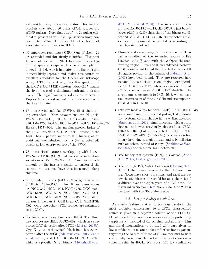
Fermi-LAT Fourth Catalog 35
we consider γ-ray pulsar candidates. This method
predicts that about 30 other 4FGL sources are
ATNF pulsars. Note that out of the 24 pulsar can-
didates presented in 3FGL, pulsations have now
been detected for 19 of them. The other 5 are not
associated with pulsars in 4FGL.
• 40 supernova remnants (SNR). Out of them, 24
are extended and thus firmly identified. The other
16 are not resolved. SNR G150.3+4.5 has a log-
normal spectral shape with a very hard photon
index Γ of 1.6, which indicates that the emission
is most likely leptonic and makes this source an
excellent candidate for the Cherenkov Telescope
Array (CTA). In contrast, the softer spectrum of
the LMC SNR N 132D (photon index=2.07) makes
the hypothesis of a dominant hadronic emission
likely. The significant spectral curvature seen in
Puppis A is consistent with its non-detection in
the TeV domain.
• 17 pulsar wind nebulae (PWN), 15 of them be-
ing extended. New associations are N 157B,
PWN G63.7+1.1, HESS J1356−645, FGES
J1631.6−4756, FGES J1836.5−0651, FGES J1838.9−0704,
HESS J1857+026. The median photon index of
the 4FGL PWNe is 2.31. N 157B, located in the
LMC, has a photon index of 2.0, hinting at an
additional contribution from a (yet-undetected)
pulsar at low energy on top of the PWN.
• 78 unassociated sources overlapping with known
PWNe or SNRs (SPP). Estimation of missed as-
sociations of SNR, PWN and SPP sources is made
difficult by the intrinsic spatial extension of the
sources; no attempts have thus been made along
this line.
• 30 globular clusters (GLC). Missing relative to
3FGL is 2MS−GC01. The 16 new associations
are NGC 362, NGC 1904, NGC 5286, NGC 5904,
NGC 6139, NGC 6218, NGC 6304, NGC 6341,
NGC 6397, NGC 6402, NGC 6838, NGC 7078,
Terzan 1, Terzan 2, GLIMPSE C01, GLIMPSE
C02. Only two other 4FGL sources are estimated
to be GLCs.
• Six high-mass X-ray binaries (HMB). The three
new sources are HESS J0632+057, which has a re-
ported LAT detection after 3FGL (Li et al. 2017b),
Cyg X-1, an archetypical black-hole binary re-
ported after the 3FGL (Zdziarski et al. 2017; Zanin
et al. 2016), and RX J0648.0−4418/HD 49798,
which is a peculiar X-ray binary (Mereghetti et al.
2011; Popov et al. 2018). The association proba-
bility of RX J0648.0−4418/HD 49798 is just barely
larger (0.85 vs 0.80) than that of the blazar candi-
date SUMSS J064744−441946. Three other 4FGL
sources are estimated to be HMBs according to
the Bayesian method.
• Three star-forming regions; new since 3FHL is
the association of the extended source FHES
J1626.9−2431 (§ 3.4) with the ρ Ophiuchi star-
forming region. Positional coincidences between
4FGL sources and two of the brightest extended H
II regions present in the catalog of Paladini et al.
(2003) have been found. They are reported here
as candidate associations: one region corresponds
to NGC 6618 in M17, whose extension of 6′ at
2.7 GHz encompasses 4FGL J1820.4−1609; the
second one corresponds to NGC 4603, which has a
similar extension of 6′ at 2.7 GHz and encompasses
4FGL J1115.1−6118.
• Two low-mass X-ray binaries (LMB). PSR J1023+0038
is a known binary millisecond pulsar/LMB transi-
tion system, with a change in γ-ray flux detected
(Stappers et al. 2014) simultaneously with a state
change, and was previously detected as 2FGL
J1023.6+0040 (but not detected in 3FGL). The
LMB 2S 0921−630 (V395 Car) is a well-studied
binary involving a neutron star and a K0 III star
with an orbital period of 9 days (Shahbaz & Wat-
son 2007) and is a new LAT detection.
• One binary star system (BIN), η Carinae (Abdo
et al. 2010i; Reitberger et al. 2015).
• One nova (NOV), V5668 Sagittarii (Cheung et al.
2016). Other novae detected by the LAT are miss-
ing. Novae have short durations, and most are be-
low the significance threshold because their signal
is diluted over the eight years of 4FGL data. As
discussed in Section 3.6.2, Nova V959 Mon 2012 is
confused with the SNR Monoceros.
6.3. Low-probability associations
As a new feature relative to previous catalogs, the
most probable counterpart to a 4FGL unassociated
source is given in a separate column of the FITS ta-
ble, along with the corresponding association probability
(applying a threshold of 0.1 on that probability). This
additional information, to be used with care given its
low confidence, is meant to foster further investigations
regarding the nature of these 4FGL sources and to help
clarify why detections claimed in other works are some-
times missing in 4FGL. We report 124 low-confidence

36 Fermi-LAT collaboration
(0.1< P <0.8) associations with the Bayesian method.
Note that the relative distances between γ-ray and coun-
terpart sources remain quite small (53 are within r95 and
all within 1.85 r95). This quite small number of low-
association sources illustrates how quickly the Bayesian
association probability drops with increasing relative
distance in the case of 4FGL. Except for rare excep-
tions, the other 1199 4FGL sources (having not even
low-confidence associations) will not get associated with
any of the tested sources (i.e., belonging to the catalogs
listed in Table 6) in a future LAT catalog. We also re-
port 42 matches (classified as UNK) with sources from
the Planck surveys (with 0.1< P ≤ 1) to guide future
investigations.
6.4. Unassociated sources
Figure 20. Distributions in Galactic latitude b of 4FGLlow-latitude, unassociated sources (black histogram), com-pared to those of LAT-detected pulsars (young pulsars: bluehistogram, millisecond pulsars (MSP): red histogram).
Out of the 1336 sources unassociated in 4FGL, 368
already present in 3FGL had no associations there. An-
other 27 sources previously associated in 3FGL have now
lost their associations because of a shift in their locations
relative to 3FGL.
About half of the unassociated sources are located less
than 10◦ away from the Galactic plane. Their wide lat-
itude extension is hard to reconcile with those of known
classes of Galactic γ-ray sources. For instance, Fig-
ure 20 compares this latitude distribution with that of
LAT pulsars. In addition to nearby millisecond pulsars,
which have a quasi isotropic distribution, the LAT de-
tects only young isolated pulsars (age <106 y) which are
by nature clustered close to the plane. Older pulsars,
which have had time to drift further off the plane, show
a wider Galactic-latitude distribution, more compati-
ble with the observed distribution of the unassociated
sources, but these pulsars have crossed the ‘γ-ray death
line’ (see Abdo et al. 2013) and are hence undetectable.
Figure 21. Green symbols: Power-law photon index versusGalactic latitude, b, for the unassociated 4FGL sources. Redbars: average photon index for different bins in b. Dashedblue line: average photon index of 4FGL BCU blazars.
Attempts to spatially cross correlate the unassociated
population with other potential classes, e.g., LMBs (Liu
et al. 2007), O stars16, and Be stars17 have been unsuc-
cessful. The observed clustering of these unassociated
sources in high-density ‘hot spots’ may be a clue that
they actually correspond to yet-to-be identified, rela-
tively nearby extended sources. The Galactic latitude
distribution near the plane is clearly non-Gaussian as
visible in Figure 20, which may indicate the presence of
several components.
The spectral properties of these sources can also pro-
vide insight into their nature, as illustrated in Figure
21 which shows the latitude distribution of their spec-
tral indices. The change in spectral hardness with sky
location demonstrates the composite nature of the unas-
sociated population. The high-latitude sources have anaverage photon index compatible with that of blazars of
unknown type (Γ=2.24), a hint that these sources could
be predominantly blazars. Unassociated sources lying
closer to the Galactic plane have softer spectra, closer
to that expected for young pulsars (Γ=2.42). Another
interesting possibility is that some of these unassociated
sources actually correspond to WIMP dark matter anni-
hilating in Galactic subhalos (Ackermann et al. 2012e;
Coronado-Blazquez et al. 2019). Indeed, ΛCDM cos-
mology predicts the existence of thousands of subhalos
below ∼ 107M�, i.e., not massive enough to retain gas
or stars at all. As a result, they are not expected to
16 Galactic O-star catalog (GOSC) https://gosc.cab.inta-csic.es/
17 Be Star Spectra (BeSS) http://basebe.obspm.fr/basebe/

Fermi-LAT Fourth Catalog 37
emit at other wavelengths and therefore they would not
possess astrophysical counterparts. Annihilation of par-
ticle dark matter may yield a pulsar-like spectrum (Baltz
et al. 2007).
6.5. Sources missing from previous Fermi catalogs
The correspondence of 4FGL sources with previous
Fermi -LAT catalogs (reported in the ASSOC FGL and
ASSOC FHL columns) was based, as in 3FGL, on error-
circle overlap at the 95% confidence level, amounting
to
∆ ≤ dx,a =√θ2x,a + θ2
x,4FGL (11)
where ∆ is the angular distance between a 4FGL source
and a source in catalog a, and the θx are derived from
the Conf 95 SemiMajor columns in the two catalogs at
the x% confidence level (assuming a 2-D normal dis-
tribution). We also considered that a previous LAT
source corresponds to a 4FGL source whenever they
have the same association (the associations can have
offsets greater than θ95, depending on the density of
sources in the catalogs of counterparts at other wave-
lengths).
We checked all sources that did not have an obvious
counterpart in 4FGL inside d95, nor a common associa-
tion. The procedure is described in detail in § 4.2.3 of
the 3FGL paper. The result is provided in one FITS
file per catalog18, reporting the same information as
Table 11 of the 3FGL paper: counterparts up to 1◦,
whether they are inside d99.9 ( = 1.52 d95) or not, and
specific conditions (flagged, c source, close to an ex-
tended source, split into several sources). The number
of missed sources and their nature are provided in Ta-
ble 6.5.
We have looked at the most-recent catalogs, 3FGL and
3FHL, in more detail. Because the first four years are
in common, we expect the 3FGL and 4FGL positions
to be correlated. That correlation is however less than
one might think because the data have changed (from
Pass 7 to Pass 8, § 2.2). We found that the distribution
of ∆/d95,3FGL (when it is less than 1) is narrower by a
factor 0.83 than the Rayleigh distribution. This means
that, by cutting at d95,3FGL, we expect only 1.3% misses
by chance (about 40 sources). With 3FHL the correla-
tion is larger because it used Pass 8 already, the overlap
is 7 years, and for the hard sources present in 3FHL the
lower-energy photons do not contribute markedly to the
localization. The distribution of ∆/d95,3FHL is narrowed
by a factor 0.62, and the number of chance misses by cut-
18 The files are available at https://www-glast.stanford.edu/pub data/1626/.
ting at d95,3FHL should be only 0.04% (about 1 source).
The correlation is similarly large with 2FHL (6 years of
Pass 8 data). That correlation effect is less for earlier
catalogs, so for them the fraction of true counterparts
that are found outside the combined 95% error circle is
closer to 5%. Most of those true sources are expected to
have a 4FGL counterpart at the 99.9% level in the FITS
files.
Out of 3033 3FGL sources, 469 are missing in 4FGL
for various reasons, including the change of diffuse emis-
sion model, point sources being absorbed into new ex-
tended ones, or variability effects. Most of these missing
sources had low significance in 3FGL. Only 72 sources
were associated. The majority are blazars (35 BCUs,
17 FSRQs, one BLL, and one SSRQ) plus one AGN.
While BLLs are 36% more numerous relative to FSRQs
in 3FGL, only one has gone away in 4FGL, an effect
possibly related to the larger variability of FSRQs rel-
ative to BLLs observed in the LAT energy band (Ack-
ermann et al. 2015). Other missing sources include 11
SPPs, 3 PSRs, one SNR, and one PWN. The nova V407
Cyg is now missing as it no longer fulfills the average-
significance criterion.
Two LAT pulsars are considered lost. PSR J1513−5908
(= 3FGL J1513.9−5908) inside the PWN MSH 15−52
is a pulsar peaking at MeV energies (Kuiper et al.
1999), very soft in the LAT band (Pellizzoni et al. 2009;
Abdo et al. 2010j), which has gone below threshold af-
ter applying the weights. PSR J1112−6103 (= 3FGL
J1111.9−6058) was split into two 4FGL sources. One is
still associated to the pulsar, but it is not the one closest
to the 3FGL position. The third missing pulsar associa-
tion was between 3FGL J1632.4−4820 and the non-LAT
PSR J1632−4818, in a confused region now covered by
the extended source 4FGL J1633.0−4746e. Among the
five most significant lost 3FGL sources (> 20σ), the
brightest one (3FGL J1714.5−3832 = CTB 37A) was
split into two 4FGL sources, the brighter of which is
associated instead to the newly discovered pulsar PSR
J1714−3830 (Saz Parkinson et al. 2018) inside the CTB
37A SNR, and hence was not recognized as a com-
mon association. Two others (3FGL J1906.6+0720 and
3FGL J0536.4−3347) were also split, and now both
members of each pair are associated. This is definitely
an improvement. The last two (3FGL J1745.3−2903c
and 3FGL J1747.0−2828) were within 0.◦6 of the Galac-
tic center, a region of the sky where changing the diffuse
model had a strong impact. They have no 4FGL coun-
terpart at all.
Concerning sources missing from 3FHL, established
with Pass 8 data as 4FGL, they amount to 33, with
17 unassociated, 9 blazars (4 BLLs and 5 BCUs), one

38 Fermi-LAT collaboration
Table 10. Statistics of previous Fermi sources missing in 4FGL
0FGL 1FGL 2FGL 3FGL 1FHL 2FHL 3FHL
All 16 283 311 469 23 34 33
With flags (a) · · · 117 229 262 · · · · · · · · ·Name-FGL c (b) · · · 83 97 52 · · · · · · · · ·Split into several 4FGL sources (c) 13 58 68 65 3 3 5
Within 1◦ of a 4FGL e (d) 11 45 65 93 4 6 5
AGN 1 8 17 55 1 2 10
PSR 0 1 2 3 0 0 0
spp 4 7 19 11 2 0 0
Other class-type 0 1 2 3 0 1 3
Unassociated 11 266 271 397 20 31 20
Present in 0FGL · · · 6 2 6 1 1 0
Present in 1FGL 8 · · · 56 35 4 3 3
Present in 2FGL 4 74 · · · 78 4 6 1
Present in 3FGL 7 52 91 · · · 6 4 4
Present in 1FHL 0 12 7 2 · · · 8 2
Present in 2FHL 1 3 0 2 5 · · · 1
Present in 3FHL 0 8 4 4 2 4 · · ·Not in any other Fermi-LAT catalog 4 186 188 369 12 21 27
aThose are flagged as F in the FITS files.
b c indicates that based on the region of the sky the source is considered to be potentially confusedwith Galactic diffuse emission.
c Those are flagged as S in the FITS files.
d e indicates a source that was modeled as spatially extended. Those are flagged as E in the FITSfiles.
AGN, one SNR, four UNKs and the transient HMB PSR
B1259−63 (diluted over 8 years). All these sources had
a TS close to the TS = 25 significance threshold.
6.6. TeV sources
Table 11. Associations of 4FGL with Extended TeV Sources
TeVCat Namea 4FGL Name
Boomerang J2229.0+6114
CTA 1 J0007.0+7303
CTB 37A J1714.4−3830
CTB 37B J1714.1−3811
Crab J0534.5+2201e
G318.2+00.1 J1453.4−5858
Geminga J0633.9+1746
HESS J1018−589B J1016.3−5857
HESS J1026−582 J1028.5−5819
HESS J1303−631 J1303.0−6312e
HESS J1356−645 J1355.2−6420e
HESS J1420−607 J1420.3−6046e
HESS J1427−608 J1427.8−6051
HESS J1458−608 J1456.7−6050, J1459.5−6053
HESS J1507−622 J1507.9−6228e
HESS J1534−571 J1533.9−5712e
HESS J1614−518 J1615.3−5146e
HESS J1616−508 J1616.2−5054e
Table 11 continued
Table 11 (continued)
TeVCat Namea 4FGL Name
HESS J1632−478 J1633.0−4746e
HESS J1640−465 J1640.6−4632
HESS J1702−420 J1705.7−4124
HESS J1718−385 J1718.2−3825
HESS J1729−345 J1730.1−3422
HESS J1745−303 J1745.8−3028e
HESS J1800−240A J1801.8−2358
HESS J1800−240B J1800.2−2403, J1800.7−2355, J1800.9−2407
HESS J1804−216 J1804.7−2144e
HESS J1808−204 J1808.2−2028e
HESS J1809−193 J1810.3−1925e
HESS J1813−126 J1813.4−1246
HESS J1813−178 J1813.1−1737e
HESS J1825−137 J1824.5−1351e
HESS J1826−130 J1826.1−1256
HESS J1834−087 J1834.5−0846e
HESS J1841−055 J1840.9−0532e
HESS J1848−018 J1847.2−0141, J1848.6−0202, J1848.7−0129
HESS J1857+026 J1857.7+0246e
HESS J1858+020 J1858.3+0209
HESS J1912+101 J1911.7+1014, J1912.7+0957, J1913.3+1019
IC 443 J0617.2+2234e
Kookaburra (Rabbit) J1417.7−6057, J1418.7−6057
Kookaburra PWN J1420.0−6048
Table 11 continued

Fermi-LAT Fourth Catalog 39
Table 11 (continued)
TeVCat Namea 4FGL Name
MGRO J1908+06 J1906.2+0631, J1907.9+0602
MGRO J2031+41 J2028.6+4110e
MSH 15−52 J1514.2−5909e
RCW 86 J1443.0−6227e
RX J0852.0−4622 J0851.9−4620e
RX J1713.7−3946 J1713.5−3945e
SNR G292.2−00.5 J1119.1−6127
TeV J1626−490 J1628.2−4848
Terzan 5 J1748.0−2446
VER J2019+407 J2021.0+4031e
Vela X J0833.1−4511e
W 28 J1801.3−2326e
W 51 J1923.2+1408e
Westerlund 1 J1645.8−4533, J1648.4−4611, J1649.2−4513,
J1650.3−4600, J1652.2−4516
Westerlund 2 J1023.3−5747e
aFrom http://tevcat.uchicago.edu.
The synergy between the LAT and the Cherenkov tele-
scopes operating in the TeV energy domain has proven
extremely fruitful, in particular by bringing out promis-
ing TeV candidates in the LAT catalogs. This approach,
further motivated by the upcoming deployment of the
Cherenkov Telescope Array, has justified the release
of LAT source catalogs above 10 GeV, like the 3FHL
(Ajello et al. 2017) based on 7 years of data. The asso-
ciations of 4FGL sources with extended sources listed in
TeVCat19 are presented in Table 11. Relative to 3FHL, 9
new extended TeV sources are associated with 4FGL ex-
tended sources (TeV sources: HESS J1534−571, HESS
J1808−204, HESS J1809−193, see § 3.4), or (some-
times multiple) 4FGL point sources (TeV sources: HESS
J1718−385, HESS J1729−345, HESS J1848−018, HESS
J1858+020, MGRO J1908+06, HESS J1912+101). AllTeV blazars have 4FGL counterparts. The median value
of Γ for 4FGL point sources associated with TeV point
sources is 1.95, indicating hard spectra as expected. In
associations with extended TeV sources, the median Γ
changes from 2.09 to 2.38 depending on whether the
4FGL sources are extended or not. This fairly large dif-
ference favors the interpretation that most associations
between extended TeV sources and non-extended 4FGL
sources are accidental.
6.7. Counterpart positions
Whenever a high-confidence association with a point-
like counterpart is obtained, we provide the most accu-
rate counterpart position available and its uncertainty.
19 http://tevcat.uchicago.edu/
In particular, 2775 4FGL AGNs have Very Long Base-
line Interferometry (VLBI) counterparts. VLBI, i.e., ra-
dio interferometry with baseline lengths of >1000 km,
is sensitive to radio emission from compact regions of
AGNs that are smaller than 20 milliarcsecond (mas),
which corresponds to parsec scales. Such observations
allow the determination of positions of the AGN jet base
with mas level accuracy. We used the RFC catalog based
on the dedicated on-going observing program (Schinzel
et al. 2015, 2017) with the Very Long Baseline Array
(Napier et al. 1994), as well as VLBI data under other
programs. The association between γ-ray source and
VLBI counterpart was evaluated along a similar, but
distinct, scheme as that presented in § 5. This scheme
(see Petrov et al. 2013, for more details) is based on
the strong connection between the γ-ray emission and
radio emission at parsec scales and on the sky density of
bright compact radio sources being relatively low. The
chance to find a bright background, unrelated compact
radio source within the LAT positional error ellipse is
low enough to establish association. The likelihood ratio
(with a somewhat different definition from that imple-
mented in the LR-method) was required to be greater
than 8 to claim an association, with an estimated false
association fraction of 1%.
For AGNs without VLBI counterparts, the position
uncertainties were set to typical values of 20′′ for sources
associated from the RASS survey and 10′′ otherwise.
For identified pulsars, the position uncertainties come
from the rotation ephemeris used to find γ-ray pulsa-
tions, many of which were obtained from radio obser-
vations (Smith et al. 2019). If the ephemeris does not
include the uncertainties and for pulsar candidates, we
use the ATNF psrcat values. If neither of those exist,
we use the 0.1◦ uncertainties from the list maintained
by the WVU Astrophysics group20. Ephemeris position
uncertainties are often underestimated, so we arbitrarily
apply a minimum uncertainty of 1 mas. For GLC from
Harris (1996)21, the position uncertainties were assigned
a typical value of 2′′.
7. CONCLUSIONS
The fourth Fermi LAT source catalog is the deepest-
yet in the GeV energy range. The increased sensitivity
relative to the 3FGL catalog is due to both the longer
time interval (8 years versus 4 years) and the use of
Pass 8 data, which provides more acceptance over the
entire energy range and a narrower PSF at high energy.
20 http://astro.phys.wvu.edu/GalacticMSPs/GalacticMSPs.txt
21 https://heasarc.gsfc.nasa.gov/w3browse/all/globclust.html

40 Fermi-LAT collaboration
The 4FGL catalog also benefits from higher-level im-
provements in the analysis, including an improved model
for Galactic diffuse emission, a weighted log-likelihood
method to mitigate the systematic effects due to that
diffuse emission model, and systematic testing of three
spectral representations, useful to classify unassociated
sources.
The 4FGL catalog includes 5064 sources. The sources
are detected (TS > 25) based on their average fluxes
in the 8-year data set; 1327 of the sources are found
to be significantly variable on one-year timescales, and
1173 on two-month timescales. We mark 92 (1.8%) of
the sources as potentially related to imperfections in the
model for Galactic diffuse emission; the character c is
appended to their names (except those already marked
as e for extended). An additional 1071 (21.1%) are
flagged in the catalog for less serious concerns, e.g., for
the spectral model having a poor fit or for being close to
a brighter source. Of the 5064 sources in the catalog, 358
(7.1%) are considered identified, based on pulsations,
correlated variability, or correlated angular sizes with
observations at other wavelengths. We find likely lower-
energy counterparts for 3370 other sources (66.5%). The
remaining 1336 sources (26.4%) are unassociated.
The identified and associated sources in the 4FGL
catalog include many Galactic and extragalactic source
classes. The largest Galactic source class continues to be
pulsars, with 232 known γ-ray pulsars and 7 associations
to non-LAT pulsars. Other Galactic source classes have
continued to grow; 30 globular clusters, 40 supernova
remnants and 17 pulsar wind nebulae are now associated
with LAT sources. Blazars remain the largest class of
extragalactic sources, with more than 1800 identified or
associated with BL Lac or FSRQ active galaxies. Non-
blazar classes of active galaxies are also found, including
9 narrow-line Seyfert galaxies, 5 compact steep spectrum
radio sources and 42 radio galaxies. The populations of
active galaxies in 4FGL are considered in more detail in
the companion 4LAC catalog.
The Fermi LAT Collaboration acknowledges gener-
ous ongoing support from a number of agencies and
institutes that have supported both the development
and the operation of the LAT as well as scientific data
analysis. These include the National Aeronautics and
Space Administration and the Department of Energy in
the United States, the Commissariat a l’Energie Atom-
ique and the Centre National de la Recherche Scien-
tifique / Institut National de Physique Nucleaire et de
Physique des Particules in France, the Agenzia Spaziale
Italiana and the Istituto Nazionale di Fisica Nucleare in
Italy, the Ministry of Education, Culture, Sports, Sci-
ence and Technology (MEXT), High Energy Accelerator
Research Organization (KEK) and Japan Aerospace Ex-
ploration Agency (JAXA) in Japan, and the K. A. Wal-
lenberg Foundation, the Swedish Research Council and
the Swedish National Space Board in Sweden.
Additional support for science analysis during the
operations phase is gratefully acknowledged from the
Istituto Nazionale di Astrofisica in Italy and the Cen-
tre National d’Etudes Spatiales in France. This work
performed in part under DOE Contract DE-AC02-
76SF00515.
This work made extensive use of the ATNF pulsar
catalog22 (Manchester et al. 2005). This research has
made use of the NASA/IPAC Extragalactic Database
(NED) which is operated by the Jet Propulsion Labora-
tory, California Institute of Technology, under contract
with the National Aeronautics and Space Administra-
tion, and of archival data, software and online services
provided by the ASI Science Data Center (ASDC) op-
erated by the Italian Space Agency. We used the Mani-
toba SNR catalog (Ferrand & Safi-Harb 2012) to check
recently published extended sources.
Software: Gardian (Ackermann et al. 2012d), GAL-
PROP23 (Porter et al. 2017), HEALPix24 (Gorski et al.
2005), Aladin25, TOPCAT26 (Taylor 2005), APLpy, an
open-source plotting package for Python27 (Robitaille &
Bressert 2012), XSPEC28
Facility: Fermi -LAT
REFERENCES
22 http://www.atnf.csiro.au/research/pulsar/psrcat23 http://galprop.stanford.edu24 http://healpix.jpl.nasa.gov/25 http://aladin.u-strasbg.fr/26 http://www.star.bristol.ac.uk/∼mbt/topcat/27 http://aplpy.github.com
Abdo, A. A., Ackermann, M., Ajello, M., et al. 2009a,
Astroparticle Physics, 32, 193,
doi: 10.1016/j.astropartphys.2009.08.002
28 https://heasarc.gsfc.nasa.gov/xanadu/xspec/

Fermi-LAT Fourth Catalog 41
—. 2009b, ApJL, 706, L1,
doi: 10.1088/0004-637X/706/1/L1
—. 2009c, ApJS, 183, 46, doi: 10.1088/0067-0049/183/1/46
—. 2009d, ApJL, 701, L123,
doi: 10.1088/0004-637X/701/2/L123
—. 2010a, ApJS, 188, 405,
doi: 10.1088/0067-0049/188/2/405
—. 2010b, Science, 328, 725, doi: 10.1126/science.1184656
—. 2010c, ApJ, 712, 459,
doi: 10.1088/0004-637X/712/1/459
—. 2010d, ApJ, 713, 146,
doi: 10.1088/0004-637X/713/1/146
—. 2010e, ApJ, 718, 348,
doi: 10.1088/0004-637X/718/1/348
—. 2010f, Science, 327, 1103, doi: 10.1126/science.1182787
—. 2010g, ApJL, 709, L152,
doi: 10.1088/2041-8205/709/2/L152
—. 2010h, A&A, 524, A75,
doi: 10.1051/0004-6361/201014458
—. 2010i, ApJ, 723, 649,
doi: 10.1088/0004-637X/723/1/649
—. 2010j, ApJ, 714, 927,
doi: 10.1088/0004-637X/714/1/927
—. 2011, ApJ, 734, 116, doi: 10.1088/0004-637X/734/2/116
Abdo, A. A., Ajello, M., Allafort, A., et al. 2013, ApJS,
208, 17, doi: 10.1088/0067-0049/208/2/17
Abdollahi, S., Ackermann, M., Ajello, M., et al. 2017, ApJ,
846, 34, doi: 10.3847/1538-4357/aa8092
Abramowski, A., Aharonian, F., Ait Benkhali, F., et al.
2015, A&A, 574, A27, doi: 10.1051/0004-6361/201322694
Acero, F., Ackermann, M., Ajello, M., et al. 2015, ApJS,
218, 23, doi: 10.1088/0067-0049/218/2/23
—. 2016a, ApJS, 223, 26, doi: 10.3847/0067-0049/223/2/26
—. 2016b, ApJS, 224, 8, doi: 10.3847/0067-0049/224/1/8
Acero, F., Donato, D., Ojha, R., et al. 2013, ApJ, 779, 133,
doi: 10.1088/0004-637X/779/2/133
Ackermann, M., Ajello, M., Albert, A., et al. 2012a, ApJS,
203, 4, doi: 10.1088/0067-0049/203/1/4
—. 2014a, ApJ, 787, 15, doi: 10.1088/0004-637X/787/1/15
—. 2014b, Science, 345, 554, doi: 10.1126/science.1253947
—. 2016a, PhRvD, 93, 082001,
doi: 10.1103/PhysRevD.93.082001
—. 2017a, ApJ, 836, 208, doi: 10.3847/1538-4357/aa5c3d
Ackermann, M., Ajello, M., Allafort, A., et al. 2011a,
Science, 334, 1103
—. 2011b, ApJ, 743, 171,
doi: 10.1088/0004-637X/743/2/171
—. 2012b, Astroparticle Physics, 35, 346,
doi: 10.1016/j.astropartphys.2011.10.007
—. 2012c, ApJ, 753, 83, doi: 10.1088/0004-637X/753/1/83
—. 2013, ApJS, 209, 34, doi: 10.1088/0067-0049/209/2/34
Ackermann, M., Ajello, M., Atwood, W. B., et al. 2012d,
ApJ, 750, 3, doi: 10.1088/0004-637X/750/1/3
—. 2012e, ApJ, 761, 91, doi: 10.1088/0004-637X/761/2/91
—. 2015, ApJ, 810, 14, doi: 10.1088/0004-637X/810/1/14
—. 2016b, ApJS, 222, 5, doi: 10.3847/0067-0049/222/1/5
Ackermann, M., Ajello, M., Baldini, L., et al. 2011c, ApJ,
726, 35, doi: 10.1088/0004-637X/726/1/35
—. 2016c, ApJ, 826, 1, doi: 10.3847/0004-637X/826/1/1
—. 2017b, ApJ, 843, 139, doi: 10.3847/1538-4357/aa775a
—. 2018, ApJS, 237, 32, doi: 10.3847/1538-4365/aacdf7
Ackermann, M., Albert, A., Atwood, W. B., et al. 2016d,
A&A, 586, A71, doi: 10.1051/0004-6361/201526920
Aharonian, F., Akhperjanian, A. G., Aye, K.-M., et al.
2005, A&A, 439, 1013, doi: 10.1051/0004-6361:20053195
Aharonian, F., Akhperjanian, A. G., Barres de Almeida,
U., et al. 2008, A&A, 477, 353,
doi: 10.1051/0004-6361:20078516
Ajello, M., Allafort, A., Baldini, L., et al. 2012, ApJ, 744,
80, doi: 10.1088/0004-637X/744/1/80
Ajello, M., Arimoto, M., Axelsson, M., et al. 2019, ApJ,
878, 52, doi: 10.3847/1538-4357/ab1d4e
Ajello, M., Atwood, W. B., Baldini, L., et al. 2017, ApJS,
232, 18, doi: 10.3847/1538-4365/aa8221
Ajello, M., Baldini, L., Barbiellini, G., et al. 2016, ApJ,
819, 98, doi: 10.3847/0004-637X/819/2/98
Allafort, A., Baldini, L., Ballet, J., et al. 2013, ApJL, 777,
L2, doi: 10.1088/2041-8205/777/1/L2
Alvarez Crespo, N., Masetti, N., Ricci, F., et al. 2016a, AJ,
151, 32, doi: 10.3847/0004-6256/151/2/32
Alvarez Crespo, N., Massaro, F., Milisavljevic, D., et al.
2016b, AJ, 151, 95, doi: 10.3847/0004-6256/151/4/95
Alvarez Crespo, N., Massaro, F., D’Abrusco, R., et al.
2016c, Ap&SS, 361, 316, doi: 10.1007/s10509-016-2902-1
Araya, M. 2014, MNRAS, 444, 860,
doi: 10.1093/mnras/stu1484
Araya, M. 2017, ApJ, 843, 12,
doi: 10.3847/1538-4357/aa7261
Araya, M. 2018a, MNRAS, 474, 102,
doi: 10.1093/mnras/stx2779
—. 2018b, ApJ, 859, 69, doi: 10.3847/1538-4357/aabd7e
Arsioli, B., Fraga, B., Giommi, P., Padovani, P., & Marrese,
P. M. 2015, A&A, 579, A34,
doi: 10.1051/0004-6361/201424148
Arsioli, B., & Polenta, G. 2018, A&A, 616, A20,
doi: 10.1051/0004-6361/201832786
Atwood, W. B., Abdo, A. A., Ackermann, M., et al. 2009,
ApJ, 697, 1071, doi: 10.1088/0004-637X/697/2/1071

42 Fermi-LAT collaboration
Atwood, W. B., Albert, A., Baldini, L., et al. 2013, Fermi
Symposium proceedings - eConf C121028.
https://arxiv.org/abs/1303.3514
Ballet, J., et al. 2015, in ICRC, Vol. 34, ICRC 2015, ed.
A. S. Borisov et al., 848
Baltz, E. A., Taylor, J. E., & Wai, L. L. 2007, ApJ, 659,
L125, doi: 10.1086/517882
Berton, M., Foschini, L., Ciroi, S., et al. 2015, A&A, 578,
A28, doi: 10.1051/0004-6361/201525691
Bird, A. J., Bazzano, A., Malizia, A., et al. 2016, ApJS,
223, 15, doi: 10.3847/0067-0049/223/1/15
Bregeon, J., Charles, E., & Wood, M. 2013, Fermi
Symposium proceedings - eConf C121028.
https://arxiv.org/abs/1304.5456
Bruel, P., Burnett, T. H., Digel, S. W., et al. 2018, 8th
Fermi Symposium. https://arxiv.org/abs/1810.11394
Buehler, R., Scargle, J. D., Blandford, R. D., et al. 2012,
ApJ, 749, 26, doi: 10.1088/0004-637X/749/1/26
Bulgarelli, A., Fioretti, V., Parmiggiani, N., et al. 2019,
A&A, 627, A13, doi: 10.1051/0004-6361/201834143
Capetti, A., Massaro, F., & Baldi, R. D. 2017a, A&A, 598,
A49, doi: 10.1051/0004-6361/201629287
—. 2017b, A&A, 601, A81,
doi: 10.1051/0004-6361/201630247
Caputo, R., Buckley, M. R., Martin, P., et al. 2016,
PhRvD, 93, 062004, doi: 10.1103/PhysRevD.93.062004
Casandjian, J.-M., & Grenier, I. A. 2008, A&A, 489, 849,
doi: 10.1051/0004-6361:200809685
Chang, Y.-L., Arsioli, B., Giommi, P., & Padovani, P. 2017,
A&A, 598, A17, doi: 10.1051/0004-6361/201629487
Cheung, C. C., Donato, D., Gehrels, N., Sokolovsky, K. V.,
& Giroletti, M. 2012, ApJ, 756, 33,
doi: 10.1088/0004-637X/756/1/33
Cheung, C. C., Jean, P., Shore, S. N., et al. 2016, ApJ, 826,
142, doi: 10.3847/0004-637X/826/2/142
Chiaro, G., Salvetti, D., La Mura, G., et al. 2016, MNRAS,
462, 3180, doi: 10.1093/mnras/stw1830
Condon, J. J., Cotton, W. D., Greisen, E. W., et al. 1998,
AJ, 115, 1693, doi: 10.1086/300337
Coronado-Blazquez, J., Sanchez-Conde, M. A., Domınguez,
A., et al. 2019, Journal of Cosmology and Astroparticle
Physics, 2019, 020, doi: 10.1088/1475-7516/2019/07/020
Cowperthwaite, P. S., Massaro, F., D’Abrusco, R., et al.
2013, AJ, 146, 110, doi: 10.1088/0004-6256/146/5/110
D’Abrusco, R., Massaro, F., Paggi, A., et al. 2014, ApJS,
215, 14, doi: 10.1088/0067-0049/215/1/14
de Menezes, R., Pena-Herazo, H. A., Marchesini, E. J.,
et al. 2019, A&A, 630, A55,
doi: 10.1051/0004-6361/201936195
de Ruiter, H. R., Willis, A. G., & Arp, H. C. 1977, A&AS,
28, 211
Devin, J., Acero, F., Ballet, J., & Schmid, J. 2018, A&A,
617, A5, doi: 10.1051/0004-6361/201833008
Doert, M., & Errando, M. 2014, ApJ, 782, 41,
doi: 10.1088/0004-637X/782/1/41
Fermi-LAT collaboration. 2019, arXiv:1905.10771.
https://arxiv.org/abs/1905.10771
Ferrand, G., & Safi-Harb, S. 2012, Advances in Space
Research, 49, 1313, doi: 10.1016/j.asr.2012.02.004
Garcia, F., Chaty, S., & Fortin, F. 2019, to be submitted to
A&A
Giommi, P., Polenta, G., Lahteenmaki, A., et al. 2012,
A&A, 541, A160, doi: 10.1051/0004-6361/201117825
Giroletti, M., Massaro, F., D’Abrusco, R., et al. 2016,
A&A, 588, A141, doi: 10.1051/0004-6361/201527817
Gorski, K. M., Hivon, E., Banday, A. J., et al. 2005, ApJ,
622, 759, doi: 10.1086/427976
Green, D. A. 2014, Bulletin of the Astronomical Society of
India, 42, 47. https://arxiv.org/abs/1409.0637
Grenier, I. A., Casandjian, J.-M., & Terrier, R. 2005,
Science, 307, 1292, doi: 10.1126/science.1106924
Griffin, R. D., Dai, X., & Thompson, T. A. 2016, ApJL,
823, L17, doi: 10.3847/2041-8205/823/1/L17
Grondin, M.-H., Funk, S., Lemoine-Goumard, M., et al.
2011, ApJ, 738, 42, doi: 10.1088/0004-637X/738/1/42
H. E. S. S. Collaboration, Abdalla, H., Abramowski, A.,
et al. 2018a, A&A, 612, A6,
doi: 10.1051/0004-6361/201629790
—. 2018b, A&A, 619, A71,
doi: 10.1051/0004-6361/201832640
Hanabata, Y., Katagiri, H., Hewitt, J. W., et al. 2014, ApJ,
786, 145, doi: 10.1088/0004-637X/786/2/145
Harris, W. E. 1996, AJ, 112, 1487, doi: 10.1086/118116
Hartman, R. C., Bertsch, D. L., Bloom, S. D., et al. 1999,
ApJS, 123, 79, doi: 10.1086/313231
Hassan, T., Mirabal, N., Contreras, J. L., & Oya, I. 2013,
MNRAS, 428, 220, doi: 10.1093/mnras/sts022
Hayashida, M., Stawarz, L., Cheung, C. C., et al. 2013,
ApJ, 779, 131, doi: 10.1088/0004-637X/779/2/131
Healey, S. E., Romani, R. W., Cotter, G., et al. 2008,
ApJS, 175, 97, doi: 10.1086/523302
Healey, S. E., Romani, R. W., Taylor, G. B., et al. 2007,
ApJS, 171, 61, doi: 10.1086/513742
HI4PI Collaboration, Ben Bekhti, N., Floer, L., et al. 2016,
A&A, 594, A116, doi: 10.1051/0004-6361/201629178
Hovatta, T., Lister, M. L., Aller, M. F., et al. 2012, AJ,
144, 105, doi: 10.1088/0004-6256/144/4/105
Hovatta, T., Aller, M. F., Aller, H. D., et al. 2014, AJ, 147,
143, doi: 10.1088/0004-6256/147/6/143
Fermi-LAT Fourth Catalog 43
Hu, F., & Zidek, J. V. 2002, Canad. J. Statist., 30, 347
Johannesson, G., Orlando, E., & the Fermi-LAT
collaboration. 2013, ICRC proceedings.
https://arxiv.org/abs/1307.0197
Johnson, T. J., Ray, P. S., Roy, J., et al. 2015, ApJ, 806,
91, doi: 10.1088/0004-637X/806/1/91
Katagiri, H., Tibaldo, L., Ballet, J., et al. 2011, ApJ, 741,
44, doi: 10.1088/0004-637X/741/1/44
Katagiri, H., Yoshida, K., Ballet, J., et al. 2016a, ApJ, 818,
114, doi: 10.3847/0004-637X/818/2/114
Katagiri, H., Sugiyama, S., Ackermann, M., et al. 2016b,
ApJ, 831, 106, doi: 10.3847/0004-637X/831/1/106
Kataoka, J., Yatsu, Y., Kawai, N., et al. 2012, ApJ, 757,
176, doi: 10.1088/0004-637X/757/2/176
Katsuta, J., Uchiyama, Y., Tanaka, T., et al. 2012, ApJ,
752, 135, doi: 10.1088/0004-637X/752/2/135
Kerr, M. 2010, PhD thesis, University of Washington,
ArXiv:1101:6072. https://arxiv.org/abs/1101:6072
Kovalev, Y. Y. 2009, ApJ, 707, L56,
doi: 10.1088/0004-637X/707/1/L56
Kuiper, L., Hermsen, W., Krijger, J. M., et al. 1999, A&A,
351, 119. https://arxiv.org/abs/astro-ph/9903474
Kuzmicz, A., Jamrozy, M., Bronarska, K., Janda-Boczar,
K., & Saikia, D. J. 2018, ApJS, 238, 9,
doi: 10.3847/1538-4365/aad9ff
Lande, J., Ackermann, M., Allafort, A., et al. 2012, ApJ,
756, 5, doi: 10.1088/0004-637X/756/1/5
Landi, R., Bassani, L., Stephen, J. B., et al. 2015, A&A,
581, A57, doi: 10.1051/0004-6361/201526221
Landoni, M., Falomo, R., Treves, A., Scarpa, R., & Reverte
Paya, D. 2015a, AJ, 150, 181,
doi: 10.1088/0004-6256/150/6/181
Landoni, M., Paiano, S., Falomo, R., Scarpa, R., & Treves,
A. 2018, ApJ, 861, 130, doi: 10.3847/1538-4357/aac77c
Landoni, M., Massaro, F., Paggi, A., et al. 2015b, AJ, 149,
163, doi: 10.1088/0004-6256/149/5/163
Li, J., Rea, N., Torres, D. F., & de Ona-Wilhelmi, E. 2017a,
ApJ, 835, 30, doi: 10.3847/1538-4357/835/1/30
Li, J., Torres, D. F., Cheng, K. S., et al. 2017b, ApJ, 846,
169, doi: 10.3847/1538-4357/aa7ff7
Liu, Q. Z., van Paradijs, J., & van den Heuvel, E. P. J.
2007, VizieR Online Data Catalog, 346, 90807
Lopez-Caniego, M., Gonzalez-Nuevo, J., Massardi, M., et al.
2013, MNRAS, 430, 1566, doi: 10.1093/mnras/sts680
Maeda, K., Kataoka, J., Nakamori, T., et al. 2011, ApJ,
729, 103, doi: 10.1088/0004-637X/729/2/103
Manchester, R. N., Hobbs, G. B., Teoh, A., & Hobbs, M.
2005, AJ, 129, 1993, doi: 10.1086/428488
Marchesi, S., Kaur, A., & Ajello, M. 2018, AJ, 156, 212,
doi: 10.3847/1538-3881/aae201
Marchesini, E. J., Pena-Herazo, H. A., Alvarez Crespo, N.,
et al. 2019, Ap&SS, 364, 5,
doi: 10.1007/s10509-018-3490-z
Maselli, A., Massaro, F., D’Abrusco, R., et al. 2015,
Ap&SS, 357, 141, doi: 10.1007/s10509-015-2372-x
Massaro, E., Giommi, P., Leto, C., et al. 2009, A&A, 495,
691, doi: 10.1051/0004-6361:200810161
Massaro, F., & D’Abrusco, R. 2016, ApJ, 827, 67,
doi: 10.3847/0004-637X/827/1/67
Massaro, F., D’Abrusco, R., Ajello, M., Grindlay, J. E., &
Smith, H. A. 2011, ApJ, 740, L48,
doi: 10.1088/2041-8205/740/2/L48
Massaro, F., D’Abrusco, R., Giroletti, M., et al. 2013,
ApJS, 207, 4, doi: 10.1088/0067-0049/207/1/4
Massaro, F., D’Abrusco, R., Tosti, G., et al. 2012a, ApJ,
750, 138, doi: 10.1088/0004-637X/750/2/138
—. 2012b, ApJ, 752, 61, doi: 10.1088/0004-637X/752/1/61
Massaro, F., Landoni, M., D’Abrusco, R., et al. 2015a,
A&A, 575, A124, doi: 10.1051/0004-6361/201425119
Massaro, F., Masetti, N., D’Abrusco, R., Paggi, A., & Funk,
S. 2014, AJ, 148, 66, doi: 10.1088/0004-6256/148/4/66
Massaro, F., D’Abrusco, R., Landoni, M., et al. 2015b,
ApJS, 217, 2, doi: 10.1088/0067-0049/217/1/2
Massaro, F., Alvarez Crespo, N., D’Abrusco, R., et al. 2016,
Ap&SS, 361, 337, doi: 10.1007/s10509-016-2926-6
Mattox, J. R., Bertsch, D. L., Chiang, J., et al. 1996, ApJ,
461, 396, doi: 10.1086/177068
Mattox, J. R., Wagner, S. J., Malkan, M., et al. 1997, ApJ,
476, 692, doi: 10.1086/303639
Mauch, T., Murphy, T., Buttery, H. J., et al. 2003,
MNRAS, 342, 1117,
doi: 10.1046/j.1365-8711.2003.06605.x
McConnachie, A. W. 2012, AJ, 144, 4,
doi: 10.1088/0004-6256/144/1/4
Mereghetti, S., Palombara, N. L., Tiengo, A., et al. 2011,
ApJ, 737, 51, doi: 10.1088/0004-637x/737/2/51
Mirabal, N., & Halpern, J. P. 2009, ApJ, 701, L129,
doi: 10.1088/0004-637X/701/2/L129
Murphy, T., Sadler, E. M., Ekers, R. D., et al. 2010,
MNRAS, 402, 2403,
doi: 10.1111/j.1365-2966.2009.15961.x
Napier, P. J., Bagri, D. S., Clark, B. G., et al. 1994, IEEE
Proceedings, 82, 658
Nolan, P. L., Abdo, A. A., Ackermann, M., et al. 2012,
ApJS, 199, 31, doi: 10.1088/0067-0049/199/2/31
Nori, M., Giroletti, M., Massaro, F., et al. 2014, ApJS, 212,
3, doi: 10.1088/0067-0049/212/1/3
Oh, K., Koss, M., Markwardt, C. B., et al. 2018, ApJS,
235, 4, doi: 10.3847/1538-4365/aaa7fd

44 Fermi-LAT collaboration
Orlando, E., & Strong, A. W. 2008, Astronomy and
Astrophysics, 480, 847, doi: 10.1051/0004-6361:20078817
Paggi, A., Massaro, F., D’Abrusco, R., et al. 2013, ApJS,
209, 9, doi: 10.1088/0067-0049/209/1/9
Paggi, A., Milisavljevic, D., Masetti, N., et al. 2014, AJ,
147, 112, doi: 10.1088/0004-6256/147/5/112
Paiano, S., Falomo, R., Franceschini, A., Treves, A., &
Scarpa, R. 2017a, ApJ, 851, 135,
doi: 10.3847/1538-4357/aa9af4
Paiano, S., Franceschini, A., & Stamerra, A. 2017b,
MNRAS, 468, 4902, doi: 10.1093/mnras/stx749
Paiano, S., Landoni, M., Falomo, R., Treves, A., & Scarpa,
R. 2017c, ApJ, 844, 120, doi: 10.3847/1538-4357/aa7aac
Paiano, S., Landoni, M., Falomo, R., et al. 2017d, ApJ, 837,
144, doi: 10.3847/1538-4357/837/2/144
Paladini, R., Burigana, C., Davies, R. D., et al. 2003, A&A,
397, 213, doi: 10.1051/0004-6361:20021466
Pena-Herazo, H. A., Marchesini, E. J., Alvarez Crespo, N.,
et al. 2017, Ap&SS, 362, 228,
doi: 10.1007/s10509-017-3208-7
Pellizzoni, A., Pilia, M., Possenti, A., et al. 2009, ApJL,
695, L115, doi: 10.1088/0004-637X/695/1/L115
Peng, F.-K., Wang, X.-Y., Liu, R.-Y., Tang, Q.-W., &
Wang, J.-F. 2016, ApJL, 821, L20,
doi: 10.3847/2041-8205/821/2/L20
Petrov, L., Mahony, E. K., Edwards, P. G., et al. 2013,
MNRAS, 432, 1294, doi: 10.1093/mnras/stt550
Petrov, L., Phillips, C., Bertarini, A., Murphy, T., &
Sadler, E. M. 2011, MNRAS, 414, 2528,
doi: 10.1111/j.1365-2966.2011.18570.x
Pivato, G., Hewitt, J. W., Tibaldo, L., et al. 2013, ApJ,
779, 179, doi: 10.1088/0004-637X/779/2/179
Planck Collaboration, Aghanim, N., Ashdown, M., et al.
2016, A&A, 596, A109,
doi: 10.1051/0004-6361/201629022
Popov, S. B., Mereghetti, S., Blinnikov, S. I., Kuranov,
A. G., & Yungelson, L. R. 2018, MNRAS, 474, 2750,
doi: 10.1093/mnras/stx2910
Porter, T. A., Johannesson, G., & Moskalenko, I. V. 2017,
ApJ, 846, 67, doi: 10.3847/1538-4357/aa844d
Principe, G., Malyshev, D., Ballet, J., & Funk, S. 2018,
A&A, 618, A22, doi: 10.1051/0004-6361/201833116
Rakshit, S., Stalin, C. S., Chand, H., & Zhang, X.-G. 2017,
ApJS, 229, 39, doi: 10.3847/1538-4365/aa6971
Reitberger, K., Reimer, A., Reimer, O., & Takahashi, H.
2015, A&A, 577, A100,
doi: 10.1051/0004-6361/201525726
Ricci, F., Massaro, F., Landoni, M., et al. 2015, AJ, 149,
160, doi: 10.1088/0004-6256/149/5/160
Robitaille, T., & Bressert, E. 2012, APLpy: Astronomical
Plotting Library in Python, Astrophysics Source Code
Library. http://ascl.net/1208.017
Sanders, D. B., Mazzarella, J. M., Kim, D.-C., Surace,
J. A., & Soifer, B. T. 2003, AJ, 126, 1607,
doi: 10.1086/376841
Saz Parkinson, P., Limyansky, B., Clark, C., Marelli, M., &
Abdollahi, S. 2018, Discovery of two energetic
gamma-ray pulsars powering supernova remnants MSH
11-62 and CTB 37A
Schinzel, F. K., Petrov, L., Taylor, G. B., & Edwards, P. G.
2017, ApJ, 838, 139, doi: 10.3847/1538-4357/aa6439
Schinzel, F. K., Petrov, L., Taylor, G. B., et al. 2015, ApJS,
217, 4, doi: 10.1088/0067-0049/217/1/4
Schmidt, K., Priebe, A., & Boller, T. 1993, Astronomische
Nachrichten, 314, 371
Shahbaz, T., & Watson, C. A. 2007, A&A, 474, 969,
doi: 10.1051/0004-6361:20078251
Shaw, M. S., Filippenko, A. V., Romani, R. W., Cenko,
S. B., & Li, W. 2013a, AJ, 146, 127,
doi: 10.1088/0004-6256/146/5/127
Shaw, M. S., Romani, R. W., Cotter, G., et al. 2013b, ApJ,
764, 135, doi: 10.1088/0004-637X/764/2/135
Smith, D. A., Bruel, P., Cognard, I., et al. 2019, ApJ, 871,
78, doi: 10.3847/1538-4357/aaf57d
Stappers, B. W., Archibald, A. M., Hessels, J. W. T., et al.
2014, ApJ, 790, 39, doi: 10.1088/0004-637X/790/1/39
Stroh, M. C., & Falcone, A. D. 2013, ApJS, 207, 28,
doi: 10.1088/0067-0049/207/2/28
Takahashi, Y., Kataoka, J., Nakamori, T., et al. 2012, ApJ,
747, 64, doi: 10.1088/0004-637X/747/1/64
Takeuchi, Y., Kataoka, J., Maeda, K., et al. 2013, ApJS,
208, 25, doi: 10.1088/0067-0049/208/2/25
Tang, Q.-W., Wang, X.-Y., & Tam, P.-H. T. 2014, ApJ,
794, 26, doi: 10.1088/0004-637X/794/1/26
Taylor, M. B. 2005, in Astronomical Society of the Pacific
Conference Series, Vol. 347, Astronomical Data Analysis
Software and Systems XIV, ed. P. Shopbell, M. Britton,
& R. Ebert, 29
Veron-Cetty, M.-P., & Veron, P. 2010, A&A, 518, A10,
doi: 10.1051/0004-6361/201014188
Voges, W., Aschenbach, B., Boller, T., et al. 1999, A&A,
349, 389
—. 2000, VizieR Online Data Catalog, 9029
Yeung, P. K. H., Kong, A. K. H., Tam, P. H. T., et al.
2017, ApJ, 837, 69, doi: 10.3847/1538-4357/aa5df1
—. 2016, ApJ, 827, 41, doi: 10.3847/0004-637X/827/1/41
Yoast-Hull, T. M., Gallagher, John S., I., Aalto, S., &
Varenius, E. 2017, MNRAS, 469, L89,
doi: 10.1093/mnrasl/slx054

Fermi-LAT Fourth Catalog 45
Zanin, R., Fernandez-Barral, A., de Ona Wilhelmi, E., et al.
2016, A&A, 596, A55, doi: 10.1051/0004-6361/201628917
Zdziarski, A. A., Malyshev, D., Chernyakova, M., & Pooley,
G. G. 2017, MNRAS, 471, 3657,
doi: 10.1093/mnras/stx1846
Zhang, P. F., Xin, Y. L., Fu, L., et al. 2016, MNRAS, 459,
99, doi: 10.1093/mnras/stw567
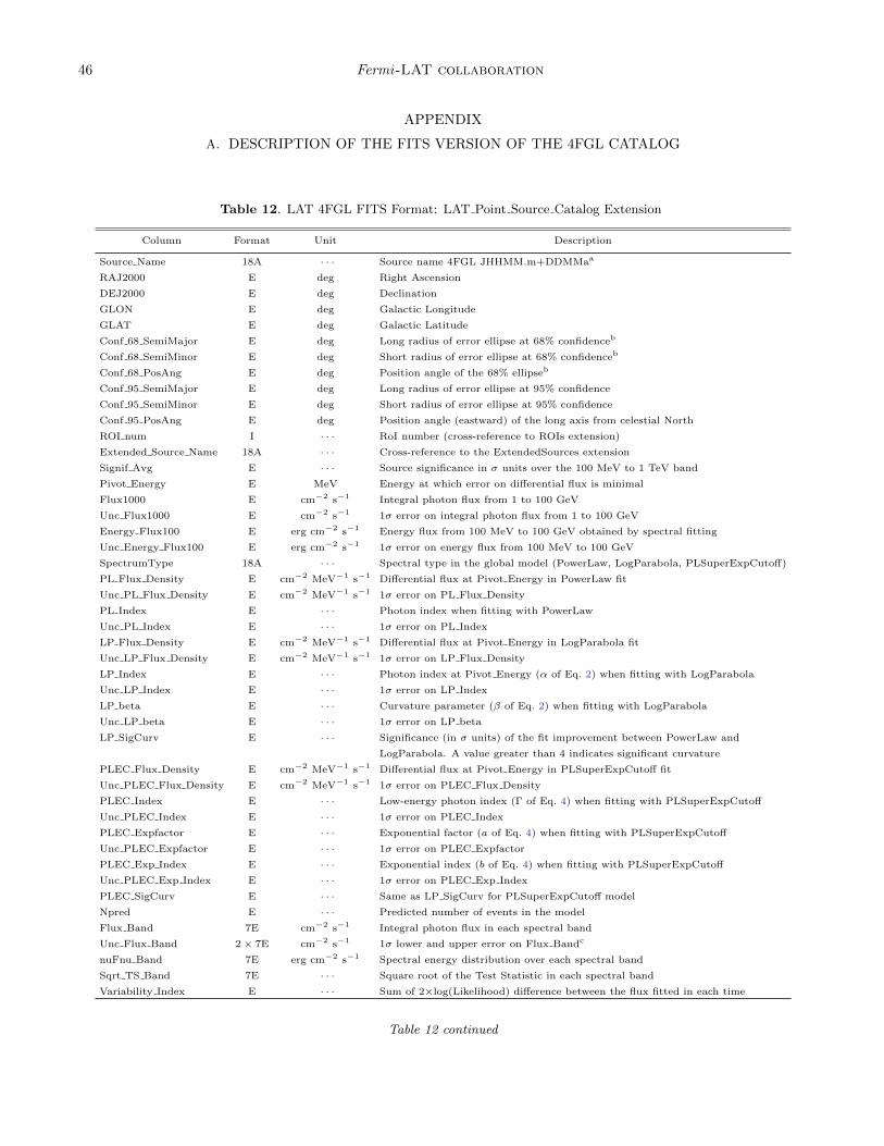
46 Fermi-LAT collaboration
APPENDIX
A. DESCRIPTION OF THE FITS VERSION OF THE 4FGL CATALOG
Table 12. LAT 4FGL FITS Format: LAT Point Source Catalog Extension
Column Format Unit Description
Source Name 18A · · · Source name 4FGL JHHMM.m+DDMMaa
RAJ2000 E deg Right Ascension
DEJ2000 E deg Declination
GLON E deg Galactic Longitude
GLAT E deg Galactic Latitude
Conf 68 SemiMajor E deg Long radius of error ellipse at 68% confidenceb
Conf 68 SemiMinor E deg Short radius of error ellipse at 68% confidenceb
Conf 68 PosAng E deg Position angle of the 68% ellipseb
Conf 95 SemiMajor E deg Long radius of error ellipse at 95% confidence
Conf 95 SemiMinor E deg Short radius of error ellipse at 95% confidence
Conf 95 PosAng E deg Position angle (eastward) of the long axis from celestial North
ROI num I · · · RoI number (cross-reference to ROIs extension)
Extended Source Name 18A · · · Cross-reference to the ExtendedSources extension
Signif Avg E · · · Source significance in σ units over the 100 MeV to 1 TeV band
Pivot Energy E MeV Energy at which error on differential flux is minimal
Flux1000 E cm−2 s−1 Integral photon flux from 1 to 100 GeV
Unc Flux1000 E cm−2 s−1 1σ error on integral photon flux from 1 to 100 GeV
Energy Flux100 E erg cm−2 s−1 Energy flux from 100 MeV to 100 GeV obtained by spectral fitting
Unc Energy Flux100 E erg cm−2 s−1 1σ error on energy flux from 100 MeV to 100 GeV
SpectrumType 18A · · · Spectral type in the global model (PowerLaw, LogParabola, PLSuperExpCutoff)
PL Flux Density E cm−2 MeV−1 s−1 Differential flux at Pivot Energy in PowerLaw fit
Unc PL Flux Density E cm−2 MeV−1 s−1 1σ error on PL Flux Density
PL Index E · · · Photon index when fitting with PowerLaw
Unc PL Index E · · · 1σ error on PL Index
LP Flux Density E cm−2 MeV−1 s−1 Differential flux at Pivot Energy in LogParabola fit
Unc LP Flux Density E cm−2 MeV−1 s−1 1σ error on LP Flux Density
LP Index E · · · Photon index at Pivot Energy (α of Eq. 2) when fitting with LogParabola
Unc LP Index E · · · 1σ error on LP Index
LP beta E · · · Curvature parameter (β of Eq. 2) when fitting with LogParabola
Unc LP beta E · · · 1σ error on LP beta
LP SigCurv E · · · Significance (in σ units) of the fit improvement between PowerLaw and
LogParabola. A value greater than 4 indicates significant curvature
PLEC Flux Density E cm−2 MeV−1 s−1 Differential flux at Pivot Energy in PLSuperExpCutoff fit
Unc PLEC Flux Density E cm−2 MeV−1 s−1 1σ error on PLEC Flux Density
PLEC Index E · · · Low-energy photon index (Γ of Eq. 4) when fitting with PLSuperExpCutoff
Unc PLEC Index E · · · 1σ error on PLEC Index
PLEC Expfactor E · · · Exponential factor (a of Eq. 4) when fitting with PLSuperExpCutoff
Unc PLEC Expfactor E · · · 1σ error on PLEC Expfactor
PLEC Exp Index E · · · Exponential index (b of Eq. 4) when fitting with PLSuperExpCutoff
Unc PLEC Exp Index E · · · 1σ error on PLEC Exp Index
PLEC SigCurv E · · · Same as LP SigCurv for PLSuperExpCutoff model
Npred E · · · Predicted number of events in the model
Flux Band 7E cm−2 s−1 Integral photon flux in each spectral band
Unc Flux Band 2× 7E cm−2 s−1 1σ lower and upper error on Flux Bandc
nuFnu Band 7E erg cm−2 s−1 Spectral energy distribution over each spectral band
Sqrt TS Band 7E · · · Square root of the Test Statistic in each spectral band
Variability Index E · · · Sum of 2×log(Likelihood) difference between the flux fitted in each time
Table 12 continued

Fermi-LAT Fourth Catalog 47
Table 12 (continued)
Column Format Unit Description
interval and the average flux over the full catalog interval; a value greater
than 18.48 over 12 intervals indicates <1% chance of being a steady source
Frac Variability E · · · Fractional variability computed from the fluxes in each year
Unc Frac Variability E · · · 1σ error on fractional variability
Signif Peak E · · · Source significance in peak interval in σ units
Flux Peak E cm−2 s−1 Peak integral photon flux from 100 MeV to 100 GeV
Unc Flux Peak E cm−2 s−1 1σ error on peak integral photon flux
Time Peak D s (MET) Time of center of interval in which peak flux was measured
Peak Interval E s Length of interval in which peak flux was measured
Flux History 12E cm−2 s−1 Integral photon flux from 100 MeV to 100 GeV in each year (best fit from
likelihood analysis with spectral shape fixed to that obtained over full interval)
Unc Flux History 2× 12E cm−2 s−1 1σ lower and upper error on integral photon flux in each yearc
Sqrt TS History 12E · · · Square root of the Test Statistic in each year
Variability2 Index E · · · Variability Index over two-month intervals; a value greater than 72.44
over 48 intervals indicates <1% chance of being a steady source
Frac2 Variability E · · · Fractional variability computed from the fluxes every two months
Unc Frac2 Variability E · · · 1σ error on Frac2 Variability
Signif2 Peak E · · · Source significance in peak interval in σ units
Flux2 Peak E cm−2 s−1 Peak integral photon flux from 100 MeV to 100 GeV
Unc Flux2 Peak E cm−2 s−1 1σ error on peak integral photon flux
Time2 Peak D s (MET) Time of center of interval in which peak flux was measured
Peak2 Interval E s Length of interval in which peak flux was measured
Flux2 History 48E cm−2 s−1 Integral photon flux from 100 MeV to 100 GeV in each two-month interval
Unc Flux2 History 2× 48E cm−2 s−1 1σ lower and upper error on Flux2 Historyc
Sqrt TS2 History 48E · · · Square root of the Test Statistic in each two-month interval
ASSOC FGL 18A · · · Most recent correspondence to previous FGL source catalogs, if any
ASSOC FHL 18A · · · Most recent correspondence to previous FHL source catalogs, if any
ASSOC GAM1 18A · · · Name of likely corresponding 2AGL source, if any
ASSOC GAM2 18A · · · Name of likely corresponding 3EG source, if any
ASSOC GAM3 18A · · · Name of likely corresponding EGR source, if any
TEVCAT FLAG A · · · P if positional association with non-extended source in TeVCat
E if associated with an extended source in TeVCat, N if no TeV association
ASSOC TEV 24A · · · Name of likely corresponding TeV source from TeVCat, if any
CLASS1 5A · · · Class designation for associated source; see Table 7
CLASS2 5A · · · Class designation for low-confidence association
ASSOC1 28A · · · Name of identified or likely associated source
ASSOC2 26A · · · Name of low-confidence association or of enclosing extended source
ASSOC PROB BAY E · · · Probability of association according to the Bayesian methodd
ASSOC PROB LR E · · · Probability of association according to the Likelihood Ratio methode
RA Counterpart D deg Right Ascension of the counterpart ASSOC1
DEC Counterpart D deg Declination of the counterpart ASSOC1
Unc Counterpart E deg 95% precision of the counterpart localizationf
Flags I · · · Source flags (binary coding as in Table 5)g
Table 12 continued

48 Fermi-LAT collaboration
Table 12 (continued)
Column Format Unit Description
aThe coordinates are rounded, following the IAU convention. The letter at the end can be c (coincident with interstellar clump), e (extendedsource), i (for Crab nebula inverse Compton) or s (for Crab nebula synchrotron).
b from the 95% ellipse, assuming a Gaussian distribution.
c Separate 1σ errors are computed from the likelihood profile toward lower and larger fluxes. The lower error is set equal to NULL and the uppererror is derived from a Bayesian upper limit if the 1σ interval contains 0 (TS < 1).
dNaN in this column when ASSOC1 is defined means that the probability could not be computed, either because the source is extended or becausethe counterpart is the result of dedicated follow-up.
e Probabilities < 0.8 are formally set to 0.
f For extended counterparts, this reports their extension radius.
gEach condition is indicated by one bit among the 16 bits forming Flags. The bit is raised (set to 1) in the dubious case, so that sources withoutany warning sign have Flags = 0.
The FITS format version of the second release of the
4FGL catalog has eight binary table extensions. The ex-
tension LAT Point Source Catalog Extension has all
of the information about the sources. Its format is de-
scribed in Table 12. The table has 5065 rows for 5064
sources because the Crab nebula is described by two en-
tries (the synchrotron component and the inverse Comp-
ton component) but counted as only one source. The
Crab pulsar is another entry and counted as a separate
source.
The extension GTI is a standard Good-Time Interval
listing the precise time intervals (start and stop in Mis-
sion Elapsed Time, MET) included in the data analy-
sis. The number of intervals is fairly large because on
most orbits (∼95 min) Fermi passes through the SAA,
and science data taking is stopped during these times.
In addition, data taking is briefly interrupted on each
non-SAA-crossing orbit, as Fermi crosses the ascend-
ing node. Filtering of time intervals with large rocking
angles, gamma-ray bursts, solar flares, data gaps, or op-
eration in non-standard configurations introduces some
more entries. The GTI is provided for reference and is
useful, e.g., for reconstructing the precise data set that
was used for the analysis.
The extension ExtendedSources (format unchanged
since 2FGL) contains information about the 75 spatially
extended sources that are modeled in the 4FGL source
list (§ 3.4), including locations and shapes. The ex-
tended sources are indicated by an e appended to their
names in the main table.
The extension ROIs contains information about the
1748 RoIs over which the analysis ran. In particular
it reports the best-fit diffuse parameters. Its format is
very close to that in 3FGL, with one exception. The
RADIUS column is replaced by CoreRadius which reports
the radius of the RoI core (in which the sources which
belong to the RoI are located). The RoI radius (half-
width in binned mode) depends on the component, and
is given by the core radius plus RingWidth, where the
latter is given in the Components extension.
The extension Components is new to 4FGL. It reports
the settings of each individual component (15 in all)
whose sum forms the entire data set for the Summed-
Likelihood approach, as described in Table 2. Its format
is given by Table 13.
The extension EnergyBounds is new to 4FGL. It con-
tains the definitions of the bands in which the fluxes
reported in the xx Band columns of the main extension
were computed, and the settings of the analysis. Its for-
mat is the same as that of the Components extension,
plus one more column (SysRel) reporting the system-
atic uncertainty on effective area used to flag the sources
with Flag 10 (Table 5). When several components were
used in one band, several lines appear with the same
LowerEnergy and UpperEnergy.
The extension Hist Start (format unchanged since
1FGL) contains the definitions of the time intervals
used to build the light curves. The new extension
Hist2 Start (same format) describes the time intervals
used to build the second series of light curves.
B. WEIGHTED LOG-LIKELIHOOD
In 3FGL we introduced a first attempt at accounting
for systematic errors in the maximum likelihood process
itself, at the source detection level. It was not used
in the source characterization, however, for lack of a
suitable framework. The standard way to account for
systematic errors (for example in XSPEC29) is to define
them as a fraction ε of the signal and add them to the
statistical errors in quadrature, in a χ2 formalism. This
29 https://heasarc.gsfc.nasa.gov/xanadu/xspec/

Fermi-LAT Fourth Catalog 49
Table 13. LAT 4FGL FITS Format: Components Extension
Column Format Unit Description
LowerEnergy E MeV Lower bound of component’s energy interval
UpperEnergy E MeV Upper bound of component’s energy interval
ENumBins I · · · Number of bins inside energy interval
EvType I · · · Event type selection for this component
ZenithCut E deg Maximum zenith angle for this component
RingWidth E deg Difference between RoI radius and core radius
PixelSize E deg Pixel size for this component (of exposure map in unbinned mode)
BinnedMode I · · · 0=Unbinned, 1=Binned
Weighted I · · · 1 if weights were applied to this component
Figure 22. Data-based log-likelihood weights as a functionof latitude across the Galactic Center, at 100 MeV, 300 MeV,1 GeV and 3 GeV, assuming all events are used throughout,and the same zenith cut at 105◦. The dips at some lati-tudes are point sources, which are included in the data-basedweights. Those weights were not used in 4FGL (which usesseparate event types), they are shown here only for illustra-tion.
can be adapted to the maximum likelihood framework
by introducing weights wi < 1 (Hu & Zidek 2002) as
logL =∑i
wi(ni logMi −Mi) (B1)
where Mi and ni are the model and observed counts in
each bin, and the sum runs over all bins in space and
energy. The source significance can then be quantified in
the same way, via the Test Statistic TS = 2 log(L/L0)
in which L and L0 are the (weighted) log-likelihood with
and without the source of interest, respectively.
Since the statistical variance in Poisson statistics is
the signal itself, a first guess for the weights could be
wi =Mi
Mi + (εMi)2=
1
1 + ε2Mi(B2)
However, that formulation has a serious flaw, which is
that it is not stable to rebinning. If one splits the bins in
Figure 23. Contribution to TS as a function of energy fora power-law source with Γ = 2.5 at high latitude, with andwithout weights. This assumes all events are used through-out (and with the same zenith cut at 105◦), as in Figure 22.
half, then Mi is split in half while ε stays the same (it is
defined externally). In the limit of very small bins, obvi-
ously the weights will all tend to 1 and the logL formula
will tend to the unweighted one, even though nothing
has changed in the underlying data or the model.
The solution we propose, originally presented in Ballet
et al. (2015), is to define a suitable integral over energy
(E) and space (r) N(r, E) which does not depend on
binning. Mi in the weight formula is then replaced by
N(ri, Ei) taken at the event’s coordinates. For the in-
tegral over space, since the catalog mostly deals with
point sources, the logical solution is to integrate the
background under the PSF, i.e., to convolve the model
with the PSF P (r, E), normalized to 1 at the peak (this
is equivalent, for a flat diffuse emission, to multiplying
by the PSF solid angle). Note that the model already
contains the PSF, so this amounts to applying a double
convolution to the sky model.
For the energy integral the choice is less obvious. The
source spectrum is not a narrow line, so convolving with
the energy dispersion (similar to what is done for space)

50 Fermi-LAT collaboration
is not justified. An integral over the full energy range
would give the same weight to all energies, which is
clearly not what we want (there is no reason to down-
play the few high-energy events). The option we adopt
here is to start the integration at the current energy.
wi=1
1 + ε2N(ri, Ei)(B3)
N(ri, Ei) =
∫ Emax
Ei
S(ri, E) dE (B4)
S(r, E) =dM
dE(r, E) ∗ P (r, E) (B5)
where dM/dE is the differential model. As energy in-
creases, the spectra (in counts) decrease and the LAT
PSF gets narrower so the convolution makes S even
steeper than dM/dE. As a result, the integral giving
N is nearly always dominated by the lowest energies, so
the exact upper bound Emax is not critical. The only
spectral region where it is important is the very low-
est energies (< 100 MeV) where the effective area rises
steeply. In order not to penalize the lowest energies too
much, we set Emax = 2Ei in Eq. B4.
There are two possibilities to define dM/dE. Since
the main origin of the systematic error is the diffuse
emission, we can restrict dM/dE to the diffuse emission
model only (we call the result model-based weights). On
the other hand there are also systematic uncertainties on
sources due to PSF calibration and our imperfect spec-
tral representation, so another option is to enter the full
model (or the data themselves) into dM/dE (we call
the result data-based weights). That second choice lim-
its spurious sources next to bright sources. There is of
course no reason why the level of systematics ε should be
the same for the diffuse emission model and the sources,
but in practice it is a reasonable approximation.
Another important point, for the procedure to be sta-
ble, is that the weights should not change with the model
parameters. So dM/dE must be defined beforehand (for
example from a previous fit). In this work we use data-
based weights computed from the data themselves, with
a common ε. The data are not as smooth as the model,
but this is not a problem in the regime of large counts
where weights play a role.
We assume here that ε is a true constant (it depends
neither on space nor on energy). For a given ε the
weights are close to 1 at high energy and decrease toward
low energy. At a given energy the weights are smallest
where the data is largest (in the Galactic ridge). We
illustrate that behavior in Figure 22, merging all event
types together (not what we do in 4FGL), for 8 years and
ε = 3%. The width of the trough in the Galactic Ridge
gets narrower at high energy, as the PSF improves. At
Figure 24. Data-based weights at 1 GeV for ZMax = 105◦
as a function of latitude (for the interesting [−30◦, 30◦] re-gion) across the Galactic Center, for different PSF eventtypes, computed according to Eq. B9. These weights wereactually used in 4FGL. The average (over event types) weightis larger than the weight using all events together at the same1 GeV energy (blue dashed line in Figure 22). This is be-cause keeping event types separate is more favorable thanmerging them and losing the event type information.
100 MeV the weights are everywhere less than 12%.
They reach 50% at high latitude at 250 MeV, and 90%
at 500 MeV. This justifies our choice of discarding 75%
of the events below 100 MeV and 50% below 300 MeV
(Table 2). The entire sky is limited by systematic effects
below 300 MeV. On average in the Galactic ridge (a lit-
tle better than the very center shown in Figure 22), the
weights are 0.5% at 100 MeV, 1.5% at 250 MeV, 5% at
500 MeV, 20% at 1 GeV, 60% at 2 GeV and reach 90%
at 4.5 GeV.
Another way to illustrate the effect of the weights is
Figure 23 (similar to Figure 18 of the 1FGL paper).It shows the contribution to TS of all energies, for a
rather soft source at high latitude (the background and
exposure are averaged over all latitudes larger than 10◦),
with and without weights. Energies below 300 MeV con-
tribute very little when the weights are applied. This re-
mains true with the actual data selection used in 4FGL.
A specific difficulty remains because at a given en-
ergy we split the data into several components, each
corresponding to a particular event type (with a differ-
ent PSF). Since the systematics act in the same way
on all components, the weights must be computed glob-
ally (i.e., weights must be lower when using PSF2 and
PSF3 events than when using PSF3 alone). On the
other hand, the resulting uncertainties with two com-
ponents should be smaller than those with a single com-
ponent (adding a second one adds information). In this
work, we started by computing weights wk individually

Fermi-LAT Fourth Catalog 51
for each component k (the dependence on E and r is left
implicit). Then we assumed that the final weights are
simply proportional to the original ones, with a factor
α < 1 (α depends on E and r as well). A reasonable
solution is then
Nmin = minkNk (B6)
Ktot =∑k
(Nmin
Nk
)2
(B7)
α=1 + ε2Nmin
1 + ε2NminKtot(B8)
wk =α
1 + ε2Nk(B9)
Ktot and α are 1 if one component dominates over the
others, and Ktot is the number of components if they
are all similar. The effect of this procedure is depicted
in Figure 24 at 1 GeV, the lowest energy at which we
use all event types. It illustrates quantitatively how the
PSF0 events are unweighted at low latitudes, compared
to better event types.

![arXiv:1508.04449v1 [astro-ph.HE] 18 Aug 2015 · 2015. 8. 20. · catalog of Fermi-LAT sources, 3FGL, Acero et al. 2015). Typically, Fermi-LAT catalog studies are based on source detection](https://img.dokumen.tips/doc/110x75/61293b44ec3bb05f1415c777/arxiv150804449v1-astro-phhe-18-aug-2015-2015-8-20-catalog-of-fermi-lat.jpg)


![Fermi Puzzle - viXravixra.org/pdf/1704.0194v1.pdf · Fermi Puzzle In physics, the Fermi-Pasta-Ulam ... [Enrico] Fermi had thought probably ... second law of thermodynamics that we](https://img.dokumen.tips/doc/110x75/5b146ac67f8b9a437c8cec3e/fermi-puzzle-fermi-puzzle-in-physics-the-fermi-pasta-ulam-enrico-fermi.jpg)