ferent in the two cases, and the latter agreed well withthe observations. The deepening rate accelerated dur-ing the initial rise in wind stress, but decreasedabruptly as 8V was reduced during the second half ofthe inertial period, even though u2 continued to in-crease. They thus found no evidence of deepening dri-ven by wind stress alone on this time scale, althoughturbulence generated near the surface must still havecontributed to keeping the surface layer stirred.

A particularly clear-cut series of observations on con-vective deepening was reported by Farmer (1975). Hehas also given an excellent account of the related lab-oratory and atmospheric observations and models inthe convective situation. The convection in the caseconsidered by Farmer was driven by the density in-crease produced by surface heating of water, which wasbelow the temperature of maximum density in an ice-covered lake. Thus there were no horizontal motions,and no contribution from a wind stress at the surface.From successive temperature profiles he deduced therate of deepening, and showed that this was on average17% greater than that corresponding to "nonpenetra-tive" mixing into a linear density gradient. Thus asmall, but not negligible, fraction of the convectiveenergy was used for entrainment. [The numerical val-ues of the energy ratio derived in this and earlier stud-ies will not be discussed here; but note that the rele-vance of the usual definition has been called intoquestion by Manins and Turner (1978).]

In certain well-documented cases, models developedfrom that of Kraus and Turner (1967) (using a para-meterization in terms of the surface wind stress andthe surface buoyancy flux) have given a good predictionof the time-dependent behavior of deep surface mixedlayers. Denman and Miyake (1973), for example, wereable to simulate the behavior of the upper mixed layerat ocean weather station P over a 2-week period. Theyused observed values of the wind speed and radiation,and a fixed ratio between the surface energy input andthat needed for mixing at the interface.

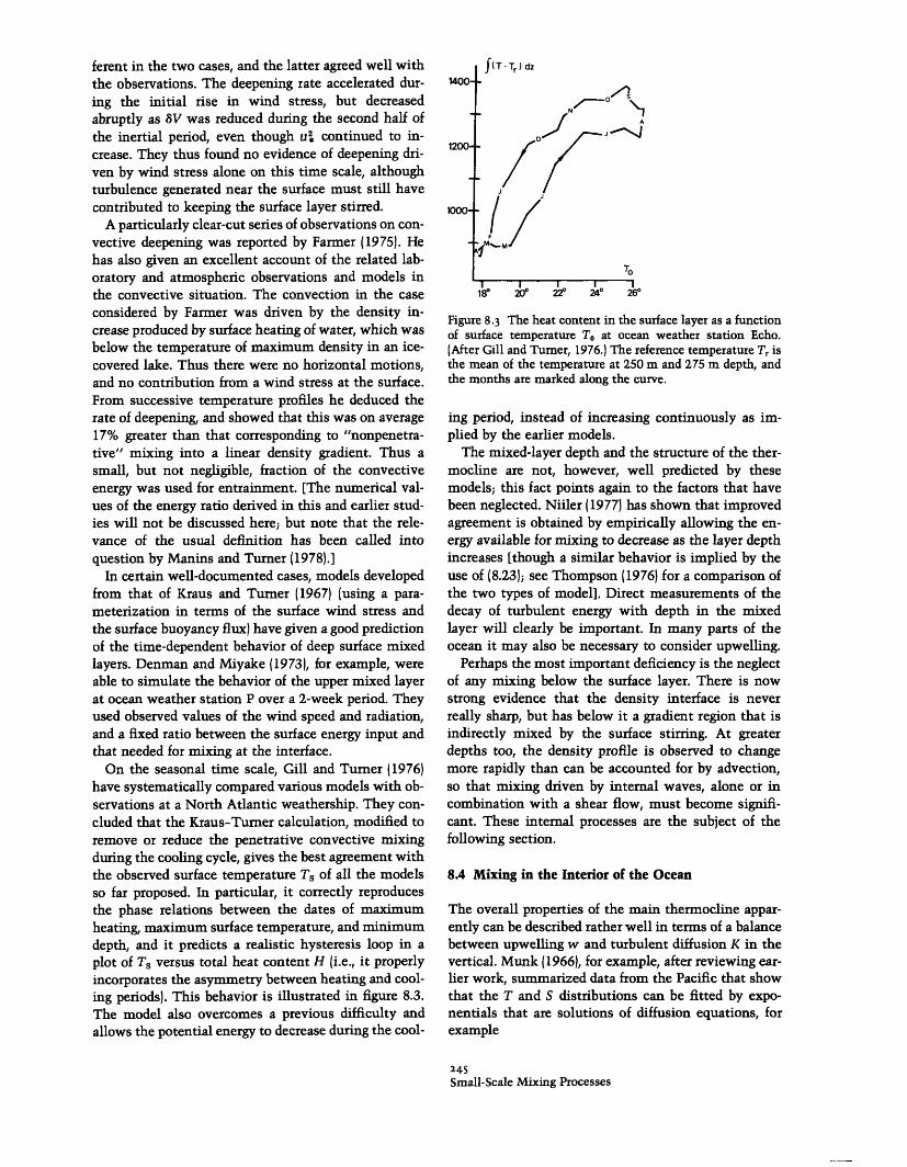
On the seasonal time scale, Gill and Turner (1976)have systematically compared various models with ob-servations at a North Atlantic weathership. They con-cluded that the Kraus-Turner calculation, modified toremove or reduce the penetrative convective mixingduring the cooling cycle, gives the best agreement withthe observed surface temperature Ts of all the modelsso far proposed. In particular, it correctly reproducesthe phase relations between the dates of maximumheating, maximum surface temperature, and minimumdepth, and it predicts a realistic hysteresis loop in aplot of Ts versus total heat content H (i.e., it properlyincorporates the asymmetry between heating and cool-ing periods). This behavior is illustrated in figure 8.3.The model also overcomes a previous difficulty andallows the potential energy to decrease during the cool-

J t I - dz

1

I I I I I180 200 220 240 260

Figure 8.3 The heat content in the surface layer as a functionof surface temperature T at ocean weather station Echo.(After Gill and Turner, 1976.) The reference temperature T, isthe mean of the temperature at 250 m and 275 m depth, andthe months are marked along the curve.

ing period, instead of increasing continuously as im-plied by the earlier models.

The mixed-layer depth and the structure of the ther-mocline are not, however, well predicted by thesemodels; this fact points again to the factors that havebeen neglected. Niiler (1977) has shown that improvedagreement is obtained by empirically allowing the en-ergy available for mixing to decrease as the layer depthincreases [though a similar behavior is implied by theuse of (8.23); see Thompson (1976) for a comparison ofthe two types of model]. Direct measurements of thedecay of turbulent energy with depth in the mixedlayer will clearly be important. In many parts of theocean it may also be necessary to consider upwelling.

Perhaps the most important deficiency is the neglectof any mixing below the surface layer. There is nowstrong evidence that the density interface is neverreally sharp, but has below it a gradient region that isindirectly mixed by the surface stirring. At greaterdepths too, the density profile is observed to changemore rapidly than can be accounted for by advection,so that mixing driven by internal waves, alone or incombination with a shear flow, must become signifi-cant. These internal processes are the subject of thefollowing section.

8.4 Mixing in the Interior of the Ocean

The overall properties of the main thermocline appar-ently can be described rather well in terms of a balancebetween upwelling w and turbulent diffusion K in thevertical. Munk (1966), for example, after reviewing ear-lier work, summarized data from the Pacific that showthat the T and S distributions can be fitted by expo-nentials that are solutions of diffusion equations, forexample

245Small-Scale Mixing Processes

1400-

1200-

1000-

[. -T i

, -"'

d2T dTKz - z = 0,

with the scaleheight K/w 1 km. By using distribu-tions of a decaying tracer '4C, he also evaluated a scaletime K/w2, and the resulting upwelling velocity w 1.2 cm day-' and eddy diffusivity K 1.3 cm2 s-1 havebeen judged "reasonable" by modelers of the large-scaleocean circulation (chapter 15). Munk found the up-welling velocity consistent with the quantity of bot-tom water produced in the Antarctic, but he was notable to deduce K using any well-documented physicalmodel. The most likely candidate seemed to be themixing produced by breakdown of internal waves, butother possibilities are double-diffusive processes, andquasi-horizontal advection following vertical mixing inlimited regions (such as near boundaries or acrossfronts).

Some progress has been made in each of these areasin the past 10 years, and they will be reviewed in turn.First, however, we shall discuss a set of interrelatedideas about the energetics of the process that are vitalto the understanding of all types of mixing in a strati-fied fluid.

8.4.1 Mechanical Mixing Processes

(a) Energy Constraints on Mixing The overall Richard-son number Rio [defined by equation (8.8)] based on thevelocity and density differences over the whole depthof the ocean, is typically very large, implying that theassociated flow is dynamically very stable. But a secondimportant fact is that the profiles of density and otherproperties) are now known to be very nonuniform, withnearly homogeneous layers separated by interfaceswhere the gradients are much larger. Is it possible thata discontinuous structure of this kind (figure 8.4) isless stable, allowing turbulence to exist when it couldnot do so in the smooth average conditions?

Part of the answer was given by Stewart (1969),whose argument was developed by Turner (1973a,chapter 10). It can be shown that nonuniform profiles(different for velocity and density) can be chosen suchthat any value of the gradient Richardson number isattained everywhere in the interior, whatever the valueof Ri,--essentially because

(AU/Az )2 (u/oaz)2 (8.25)

Thus a redistribution of properties can always reducethe gradient Ri to a value at which turbulence can bemaintained.

But a crucial question remains: how is this redistri-bution actually produced? Consider the energy changesassociated with a transition from linear gradients ofvelocity and density u = az, p = -z + po say, to awell-mixed layer of depth H (see figure 8.4). The change

(a)

VELOCITY DENSITY

Figure 8.4 Discontinuous profiles produced by mixing, frominitially linear density and velocity distributions. In (a) thefinal profiles, different for density and velocity, correspond toa constant gradient Richardson number everywhere, and (b)is the simpler model of homogeneous layers and thin inter-faces used to derive (8.26).

in kinetic energy is (1/24)a2H3 and in potential energy(l/12)gf3H3 ; the two are equal when

Rio = gf3/a2 = 1/2. (8.26)

This argument implies that for all Rio>> 1 there is notenough kinetic energy in the local mean motion toproduce the observed, nonuniform profiles, even whendissipation is neglected entirely. In the absence ofsources of convective energy due to double-diffusiveprocesses (see section 8.4.2), the general conclusion isinescapable: extra energy must be propagated into theregion from the boundaries in the form of inertial orinternal gravity waves if mixing is to be sustained.

The role of internal waves and their relation to thenonuniform density structure may be approached inanother way, using the argument set out by Turner(1973a, p. 137), and extensions of it. Consider a deepregion of stable fluid, having linear profiles of bothdensity and velocity through it. Suppose there is aconstant stress (momentum flux) To0 = pU2* and buoy-ancy flux B through this region, sustained by small-scale turbulent motions. Mixing occurs only with fluidimmediately above and below any level, so that onlythe internal lengthscale L defined by (8.9) will be rel-evant, not the overall depth or the distance from theboundaries. It follows on dimensional grounds that

du -B u,= i .T = , L'

g dp B2 U2N1 = -g =k2- =kL

p dz u4 2L2

(8.27)

(8.28)

where k, and k 2 are constants (which have not beendetermined experimentally). This is thus an equilib-rium, self-regulated state, in which there is a uniquerelation between the gradients and the fluxes. The flux

246J. S. Turner

(8.24)

II_

Richardson number (8.7) has a fixed value Rf = k1,and so does the gradient Richardson number

Ri = k2k k2= Rie, (8.29)

which has been called the equilibrium Richardsonnumber.

Only in rather special cases can this equilibriumstate be maintained--one good example is the edge ofa turbulent gravity current, which is treated in section8.5.2. When density and velocity differences are im-posed over a given depth, the only equilibrium state isRio = Rie. If Ri0 < Rie, the shear will dominate, andmixing will soon be influenced directly by the bound-aries. If Rio > Rie, as it is in the case of most interesthere, then the stratification will dominate, though wehave already seen how a nonuniform stratification al-lows the local Ri to be much smaller than Ri0, so thatturbulence can persist.

In this nonuniform state, however, (8.27) shows thatthe transport of momentum by turbulent processes ismuch less efficient in the interfaces where du/dz islarger, and it is impossible to have constant purelyturbulent fluxes of both buoyancy and momentumthrough the whole depth. But the existence of inttrfa-cial waves provides a complementary mechanism totransport momentum across the steep gradient regionswithout a corresponding increase in the buoyancy flux.

There have been other suggestions about the mech-anism of formation of layers from a linear gradient thatcan be related to the above ideas. Posmentier (1977),extending an idea formulated by Phillips (1972), sug-gested that if the vertical turbulent flux of buoyancydecreases as the vertical density gradient increases, anyperturbation causing an increase in the gradient willbe amplified. This occurs because the local decrease influx leads to an accumulation of mass, which increasesthe density gradient further. This behavior is in con-trast to the more familiar case, described by an eddydiffusivity, where an increase in gradient increases theflux, thus tending to smooth out any irregularity.

Linden (1979) has recently reviewed a wide range oflaboratory experiments on "mechanical" mixing acrossa density interface, including those that use a shearflow, or stirring with oscillating grids [cf. sections8.3.2(a) and 8.3.2(c)], and has suggested how they canbe unified in terms of an energy argument. Briefly, hehas shown that as the overall Richardson number Ri0increases from zero, the flux Richardson number Rf atfirst increases, reaches a maximum, and then falls asRio becomes even larger (see figure 8.5). This form canmost readily be understood in terms of the grid-stirringresults already described in section 8.3.2(c). The rate ofincrease in potential energy is gApueD2 , where ue isthe entrainment velocity, and the rate of supply ofkinetic energy is Jpu3 D. Thus by definition

Rf = g p = Rio.11 i.u2 l (8.30)

Using the power-law fit to the experiments udeu Rio-we find

Rf - Ri - n. (8.31)

In fact, the experimental results with salinity differ-ences, described in section 8.3.2(c) imply that Rf is anincreasing function of Rio at low Rio and a decreasingfunction at high Rio (when n = ). The point wheren = 1 corresponds to the simple overall energy argu-ment, with a constant fraction of the energy supplybeing used for mixing.

Relating this now to the earlier argument, the max-imum on figure 8.5 (which is schematic, but has thesame form for the grid-stirred and shear-driven exper-iments) corresponds to the "equilibrium" conditions,where the gradients and fluxes are in balance [equa-tions (8.27) and (8.28)]. If there is a self-balancing mech-anism operating in which the rate of energy supply isitself regulated by the mixing it produces [cf. section8.5.2(a)], then this is the state attained. If there is anexcess of mechanical energy and a weak gradient (tothe left of the maximum), mixing acts throughout thedepth to reduce the gradient and spread out the inter-face. When the density gradient is the dominant factor(to the right of the maximum), turbulence is suppressedin an interface but can remain unaffected elsewhere,so that it acts to sharpen incipient interfaces. The re-lation to Phillips's and Posmentier's stability argumentbecomes clear once we note that, for a fixed rate ofkinetic energy supply, Rf is proportional to the buoy-ancy flux and Rio to the density gradient.

(b) Instability of Waves in a Smoothly StratifiedFluid Next, we consider the mechanisms of instabilityin a stratified fluid that can lead to local mixing, andthus produce or accentuate nonuniformities of the gra-dient. All of these involve waves propagating in fromthe boundaries, with or without a large-scale back-ground shear set up by horizontal pressure gradients.When interfaces are already present, these will be the

Rf

RI.Rio

Figure 8.5 Schematic relation between the flux Richardsonnumber Rf and the overall Richardson number Ri0 for exper-iments on mixing across a density interface. (After Linden,1979.) The maximum of the curve corresponds to the "equi-librium" condition.

247Small-Scale Mixing Processes

first regions to become unstable [see section 8.4.1(c)],but it is logical first to describe how such a structurecan be set up.

It is only recently that precisely what is meant bythe "breaking" of internal waves has been properlyinvestigated (see chapter 9). Some mechanisms areclearly related to localized sources of wave energy ata nearby boundary. Lee waves can be generated by theflow over bottom topography, and when the amplitudebecomes large, overturning and the production of "ro-tors" is possible. When the mean horizontal velocityu varies in the vertical, the "critical-layer" mechanismalso leads to the growth of the waves and the localabsorption of energy near the level where u equals thehorizontal phase velocity of the waves (Bretherton1966c). Small-scale "jets" attributable to this mecha-nism have been reported in the ocean.

Nearly always, however, the source of wave energyat a point in the interior of the ocean is not clearlyidentifiable, and the motion is the result of the super-position of many waves. Energy can then be concen-trated in limited regions through two types of inter-action. Strong interactions between an arbitrary pair ofwaves of large amplitude can feed energy rapidly intosmall-scale forced waves that overturn locally. Reso-nant interactions are more selective, and require twowaves to be such that the sum or difference of theirwavenumbers is related to the sum or difference oftheir frequencies by the same dispersion relation as theindividual waves. These are discussed in detail by Phil-lips (1977a).

Various laboratory experiments have played an im-portant part in illuminating these processes; these (andmany other experiments relevant to the subject of thischapter) have been reviewed by Maxworthy and Bro-wand (1975), and by Sherman et al. (1978). McEwan(1971) generated a single low-mode standing wave, andshowed that for sufficiently large amplitudes, the orig-inal waveform became modulated with two highermodes that formed a resonant triplet with the forcedwave. These grew by extracting energy from the orig-inal mode until the superposition of the several mo-tions produced visible local disturbances of the smoothgradient, and eventually turbulent patches that wereattributed to a shear-breakdown in regions of enhanceddensity gradient. Orlanski (1972) carried out a similarexperiment, but concluded that local overturning wasresponsible for the production of turbulence. McEwan(1973) used two traveling internal waves of differentfrequency, interacting in a limited volume of an ex-perimental tank, to examine the local conditions justbefore breakdown, but he was unable to say definitelywhether the primary mechanism for the production ofturbulence was shear breakdown or overturning.

During the experiments reported in 1971, McEwanfound that patches of turbulence could also be formed

under conditions such that no resonant interaction waspredicted [see also Turner (1973a, plate 24)]. More re-cently, this case has been studied in detail by McEwanand Robinson (1975), who explained it in terms of a"parametric" instability, which is, in fact, another res-onant mechanism that had not previously been consid-ered. This one is less selective, and gives rise to waveswithin a large range of much shorter wavelengths thanthe forcing wave, as follows. The original long waveproduces a modulation of the effective component ofgravity acting on shorter waves propagating throughthe same volume of fluid. When the forcing frequencyis nearly twice the frequency of the growing disturb-ance, energy is fed into this disturbance through amechanism analogous to that which causes the side-ways oscillations of a pendulum to grow when thesupport is oscillated vertically. The major predictionsof the theory, which include an estimate of the ampli-tude of the forcing wave required for the disturbancesto overcome internal viscous dissipation and grow,were accurately verified in a most elegant laboratoryexperiment.

The application of this mechanism to the ocean hasnot yet been thoroughly tested, though McEwan andRobinson have extended Garrett and Munk's (1972a)ideas (based on their universal internal wave spectrum)to compute a mean-square slope of the isopycnals,which they deduce is large enough to excite the para-metric instability. Much more work on this process isindicated; it certainly seems capable in principle oftransferring energy directly from a broad range of large-scale internal waves to much smaller scales and thuscreating patches of mixing in an otherwise smoothlystratified ocean.

(c) Mixing Due to Interfacial Shears Once sharp tran-sition regions exist, across which both density and ve-locity vary markedly, it is easier to understand howlocal instabilities arise. The now extensive literaturein this field has been well reviewed by Maxworthy andBrowand (1975), and it will be treated only briefly here.

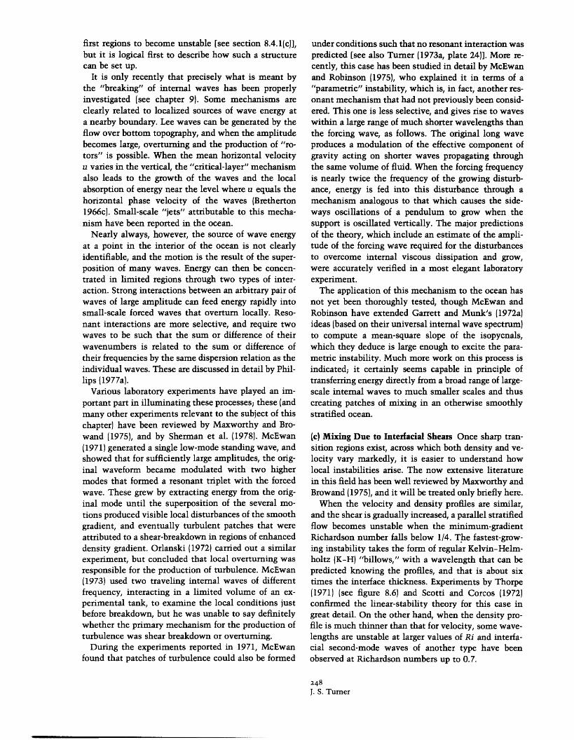
When the velocity and density profiles are similar,and the shear is gradually increased, a parallel stratifiedflow becomes unstable when the minimum-gradientRichardson number falls below 1/4. The fastest-grow-ing instability takes the form of regular Kelvin-Helm-holtz (K-H) "billows," with a wavelength that can bepredicted knowing the profiles, and that is about sixtimes the interface thickness. Experiments by Thorpe(1971) (see figure 8.6) and Scotti and Corcos (1972)confirmed the linear-stability theory for this case ingreat detail. On the other hand, when the density pro-file is much thinner than that for velocity, some wave-lengths are unstable at larger values of Ri and interfa-cial second-mode waves of another type have beenobserved at Richardson numbers up to 0.7.

248J. S. Turner

this observation period, and it is likely to be equallyimportant in the ocean under comparable conditions.

The maximum thickening of the interface, due tomixing following the K-H instability, is limited byenergy considerations closely related to those set outin section 8.4.1(a). If an initial discontinuity is trans-formed by this process into linear gradients of velocityand density over the same interfacial depth 8, thenequating the changes in kinetic and potential energiesgives

6max = 2poU2/g Ap. (8.32)

Figure 8.6 The breakdown of an interface in a shear flow toproduce an array of Kelvin- Helmholtz billows. (Thorpe, 1971.)

The growth beyond the stage of initial instability hasalso been studied experimentally [see Thorpe (1973a) fora good review]. When the: shear is increased, and thenkept constant, the array of billows becomes unstableto a subharmonic disturbance, which leads to a two-dimensional rolling-up and merging of alternate vor-tices, a process that continues until limited by an en-ergy constraint (as discussed below). Small-scale tur-bulence is produced by the concentration of vorticityinto discrete lumps along the interface, and by gravi-tational instability within the overturned regions. Thesystem of vortices stops growing, and then collapses,with much horizontal interleaving of mixed regionsand a rapid dampening of the turbulence. This leavesbehind a smoothly varying, nearly linear mean gradientof density, with thin higher gradient regions superim-posed on it. Woods and Wiley (1972) suggested, how-ever, on the basis of measurements in the ocean, thatthis overturning process should produce a well-mixedlayer bounded by sharp interfaces. The implied "split-ting" of interfaces to form new regions of high gradientdoes not seem to be borne out by the subsequent de-tailed laboratory experiments.

Thorpe (1978a) has reported observations of the mix-ing across the interface bounding a near-surface layerin a lake under stable conditions. Detailed measure-ments of temperature profiles as a function of time atone station contain all the features, including over-turning and small scale mixing, described for the lab-oratory experiments. Thorpe concluded that the K-Hinstability was the dominant mechanism for mixing in

The process is not perfectly efficient, however, andenergy dissipation leads to much smaller limiting val-ues. The numerical factor varies with the initial Rich-ardson number of the interface, but Sherman et al.(1978) suggest using 6 = 0.3poU2/g Ap as a typical value.

There are two important implications of this result.First, the instability is self-limiting. Unless the shearis increased, no further instability can occur, becausethe Richardson number in the thickened state is abovethat needed for instability. Second, the amount of ver-tical mixing that K-H instabilities alone can accountfor is small. Some other mechanism is needed to pro-duce the turbulence in the well-mixed layers, which isessential both to transport heat and salt across themand produce the thinning of the interfaces requiredbefore further shear instabilities will be possible.

The shear needed to reduce Ri and so lead to insta-bility at an interface can often be produced by internalwaves. When a long internal wave propagates throughthe ocean, vorticity is concentrated at density inter-faces. The sharper the interface, the more unstable itwill be (i.e., the smaller the wave amplitude at whichbillows will form at the crests and troughs). Thorpe(1978b) has recently studied the interaction betweenfinite-amplitude waves and an interfacial shear flow inthe laboratory, and has shown that the slope at whichbreaking occurs can be significantly reduced. Directvisual observations of billows in the ocean generated inthis way were made by Woods (1968a), using skin-div-ing techniques and dye tracers. Those observations hada great influence on subsequent work, by concentratingattention on the need to understand individual mixingevents and processes in some detail, rather than alwaysthinking in statistical terms. They also clearly dem-onstrated the relevance of simple experiments in theocean and in the laboratory.

Recent, more sophisticated work has confirmed theimportance of fine structure as a means for producingmixing in an internal wave field. Eriksen (1978) hasdescribed measurements made with an array of mooredinstruments, which he interprets in terms of large-scalewaves "breaking." (This paper also contains a goodsummary of the relevant wave theory, and referencesto related work.) He has shown that the appearance of

249Small-Scale Mixing Processes

local temperature inversions (overturning) is associatedwith high shears, and that these are dominated by thefine-structure contribution. Moreover, there is a cutoffin the measured values of Ri at Ri = 1/4, indicatingthat regions with lower values of Ri are continuouslybecoming unstable, and implying some kind of satu-ration of the wave spectrum (see figure 9.28). Breakingis equally likely at any internal-wave frequency. Thesedeductions were made using differences over 7 m, andit seems probable that the actual mixing events wereunresolved at a smaller scale.

(d) Microstructure in Turbulent Patches The break-down of internal waves by the mechanisms describedabove leaves behind a turbulent patch of fluid thattends to be thin, but very elongated in the horizontal.Such "blini" or pancakes of turbulence are distributedvery intermittently in space and time, and are sur-rounded by fluid in which the level of fluctuations isvery low. Measurements using towed instruments haveshown that sometimes the turbulence is "active," i.e.,there are both velocity and temperature-salinity fluc-tuations, but there can also be "fossil turbulence," orT-S microstructure remaining after the velocity fluc-tuations have decayed. This specialized field can onlybe mentioned briefly here, though it is importantenough to deserve a full-scale review [see Phillips(1977a, chapter 6)]. It has developed somewhat inde-pendently, along lines established from the statisticalmeasurements of turbulence properties in laboratorywind tunnels and in the atmosphere, and groups in theU.S.S.R. have been particularly active [see Monin, Ka-menkovich, and Kort (1974, chapter 3); Grant, Stewart,and Moilliet (1962); Gargett (1976)]. Recently, othergroups have become involved, and more measurementswill be summarized in section 8.4.3. In this section wejust refer to two results relating to the smallest scalesof motion, where the turbulence is isotropic and de-caying.

For active three-dimensional turbulence to persist,it is found that the Ozmidov length scale (8.10) mustbe larger than about 60 times the Kolmogoroff dissi-pation scale (v3

/E)14 ; for typical conditions this implies

Lo 1 m. When this is so, the form of the velocity,temperature and salinity-fluctuation spectra can bepredicted from the local similarity theory (Batchelor,1959), using a scaling that does not depend on thebuoyancy frequency. When an actively turbulent patchis damped by stratification, however, the form of thefossil (T or S) turbulence is clearly affected by N, anda different scaling is appropriate. The cutoff lengthscale in the latter case is larger, and in principle thetwo can be distinguished. The important point madehere, and reinforced below, is that fluctuation meas-urements can only be properly interpreted with a full

knowledge of various other parameters, relating tolarge as well as small scales.

Osborn and Cox (1972) introduced a method (whichis now widely used) for estimating the vertical flux ofheat from measurements of temperature fluctuationsT' in the dissipation range. They suggested that thereis a balance between the production of small-scale var-iance by turbulent velocities acting in a mean vertical-temperature gradient OT/Oz and the destruction of var-iance by molecular processes acting on sharpenedmicroscale gradients. An effective vertical eddy diffu-sivity Kz can be defined by

Kz = K(OT'/z) 2(OT/Oz)-2 = KC, (8.33)

where the overbar denotes an average taken over thewhole record, and C has been called the Cox number.There is an uncertainty of a factor between 1 and 3because of the unknown degree of isotropy, but thereare also some more fundamental constraints on the useof this idea [e.g., see Gargett (1978)]. Particularly whenthere are horizontal intrusions, with associated T andS anomalies that can produce correlations betweenmicroscale temperature and salinity fluctuations (seesection 8.4.3), it is not appropriate to think in terms ofa gradient diffusion process based on temperaturealone. Stern (1975a, chapter 11) has derived more gen-eral thermodynamic relations involving both T and Svariances, but these have not yet been properly testedby detailed measurements.

8.4.2 Convective Mixing

(a) Double-Diffusive Instabilities The most dramaticchange in the whole field of oceanic mixing has comeabout through the recognition that molecular processescan have significant effects, even on scales of motionlarger than those over which molecular diffusion canact directly. It is not sufficient just to know the netdensity distribution: the separate contributions of Sand T are also important, and when these have oppos-ing effects on the density, the transports of the twoproperties are quite different, and certainly cannot bedescribed in terms of a single eddy diffusivity. Fortyyears ago this was unsuspected; twenty years ago a firstconsequence of unequal transports was recognized butregarded as "an oceanographical curiosity" (Stommel,Arons, and Blanchard, 1956), while in recent years theexamples and literature documenting coupled molec-ular effects has multiplied rapidly.

When temperature and salinity both increase or bothdecrease with depth, one of the properties is "unstably"distributed, in the hydrostatic sense. The basic factabout double-diffusive convection is that the differencein molecular diffusivities allows potential energy to bereleased from the component that is heavy at the top,even though the mean density distribution is hydro-

25oJ. S. Turner

I�___�_______ _

statically stable. Stommel (1962a) was one of the firstto recognize that this convective source of energy im-plies that the potential energy is decreased, and thedensity difference between two vertically separated re-gions is increased following mixing-just the oppositeto the changes occurring during mechanical mixing(see figure 8.7).

The interaction between theory and laboratory ex-periments on the one hand, and ocean observations onthe other, has played a particularly important role inthis field. The early work has been reviewed by Turner(1973a, chapter 8; 1974) and Stern (1975a, chapter 11),and more recent developments by Sherman et al.(1978). It is nevertheless worth repeating a descriptionof two basic experiments that illustrate the differentmechanisms of instability in the cases where the tem-perature and salinity distributions, respectively, pro-vide the potential energy to drive the motion.

When a linear stable salinity gradient is heated frombelow (Turner and Stommel, 1964; Turner, 1968) thebottom boundary layer breaks down to form a con-vecting layer of depth d that grows in time as d t2.

The experiments show that there is no discontinuityof density at the top of this layer, i.e., the temperatureand salinity steps are compensating. When the thermalboundary layer ahead of the convecting region reachesa critical Rayleigh number Rae, it too becomes unsta-ble. The first layer stops growing when d reaches

d, = (vRaI/4K,) 114B3 14N-2, (8.34)

and a second convecting layer is formed. Here dc is thecritical depth, B = -gaF 1IpC the imposed buoyancyflux corresponding to a heat flux FH (a being the coef-ficient of expansion and C the specific heat), and Nsthe initial buoyancy frequency of the salinity distri-bution. Huppert and Linden (1979) recently have ex-tended this work to describe the formation of multiplelayers as heating is continued. Linden (1976) used theanalog system of salt-sugar solutions to study the casewhere there is a destabilizing salt (T) gradient partiallycompensating the stabilizing sugar (S) gradient in theinterior. He found that as the density gradients becomenearly equal, the properties of the layers depend mostlyon the internal properties of the gradient region, withthe boundary flux just acting as a trigger. [This analoghas been much used for laboratory work, since it elim-inates unwanted heat losses, and more experimentsusing this device will be discussed later. Salt is herethe analog of heat, or temperature T, since it has ahigher diffusivity than sugar (S).]

This first group of experiments illustrates well animportant general consequence of opposing distribu-tions of S and T: smooth gradients of properties areoften unstable, and can break up to form a series ofconvecting layers, separated by sharper interfaces. Inthe case described, where the hotter, saltier water is

INITIAL STATE

PT PS NET DENSITY

FINAL STATE

PT PS NET DENSITY

(8.7A)

It

M

.oD:

I-

.4SAL INITY '/.o)

(8.7B)

Figure 8.7 The changes in the separate concentrations and inthe net densities produced by double-diffusion in a two-layersystem: (A) schematic diagram of the initial and final prop-erties, with a flux ratio fFs/aFT = 0.2; (B) the water propertiesin the Greenland Sea on a -S correlation diagram. (AfterCarmack and Aagaard, 1973.) A = Atlantic water. S = Polarwater, BW = Bottom water. The double-diffusive flux altersA in direction A' and S in direction S'.

25ISmall-Scale Mixing Processes

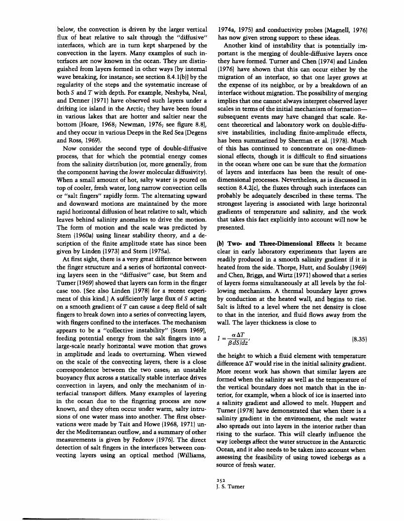
below, the convection is driven by the larger verticalflux of heat relative to salt through the "diffusive"interfaces, which are in turn kept sharpened by theconvection in the layers. Many examples of such in-terfaces are now known in the ocean. They are distin-guished from layers formed in other ways [by internalwave breaking, for instance; see section 8.4.1(b)] by theregularity of the steps and the systematic increase ofboth S and T with depth. For example, Neshyba, Neal,and Denner (1971) have observed such layers under adrifting ice island in the Arctic; they have been foundin various lakes that are hotter and saltier near thebottom (Hoare, 1968; Newman, 1976; see figure 8.8),and they occur in various Deeps in the Red Sea (Degensand Ross, 1969).

Now consider the second type of double-diffusiveprocess, that for which the potential energy comesfrom the salinity distribution (or, more generally, fromthe component having the lower molecular diffusivity).When a small amount of hot, salty water is poured ontop of cooler, fresh water, long narrow convection cellsor "salt fingers" rapidly form. The alternating upwardand downward motions are maintained by the morerapid horizontal diffusion of heat relative to salt, whichleaves behind salinity anomalies to drive the motion.The form of motion and the scale was predicted byStem (1960a) using linear stability theory, and a de-scription of the finite amplitude state has since beengiven by Linden (1973) and Stem (1975a).

At first sight, there is a very great difference betweenthe finger structure and a series of horizontal convect-ing layers seen in the "diffusive" case, but Stem andTurner (1969) showed that layers can form in the fingercase too. [See also Linden (1978) for a recent experi-ment of this kind.] A sufficiently large flux of S actingon a smooth gradient of T can cause a deep field of saltfingers to break down into a series of convecting layers,with fingers confined to the interfaces. The mechanismappears to be a "collective instability" (Stem 1969),feeding potential energy from the salt fingers into alarge-scale nearly horizontal wave motion that growsin amplitude and leads to overturning. When viewedon the scale of the convecting layers, there is a closecorrespondence between the two cases; an unstablebuoyancy flux across a statically stable interface drivesconvection in layers, and only the mechanism of in-terfacial transport differs. Many examples of layeringin the ocean due to the fingering process are nowknown, and they often occur under warm, salty intru-sions of one water mass into another. The first obser-vations were made by Tait and Howe (1968, 1971) un-der the Mediterranean outflow, and a summary of othermeasurements is given by Fedorov (1976). The directdetection of salt fingers in the interfaces between con-vecting layers using an optical method (Williams,

1974a, 1975) and conductivity probes (Magnell, 1976)has now given strong support to these ideas.

Another kind of instability that is potentially im-portant is the merging of double-diffusive layers oncethey have formed. Turner and Chen (1974) and Linden(1976) have shown that this can occur either by themigration of an interface, so that one layer grows atthe expense of its neighbor, or by a breakdown of aninterface without migration. The possibility of mergingimplies that one cannot always interpret observed layerscales in terms of the initial mechanism of formation-subsequent events may have changed that scale. Re-cent theoretical and laboratory work on double-diffu-sive instabilities, including finite-amplitude effects,has been summarized by Sherman et al. (1978). Muchof this has continued to concentrate on one-dimen-sional effects, though it is difficult to find situationsin the ocean where one can be sure that the formationof layers and interfaces has been the result of one-dimensional processes. Nevertheless, as is discussed insection 8.4.2(c), the fluxes through such interfaces canprobably be adequately described in these terms. Thestrongest layering is associated with large horizontalgradients of temperature and salinity, and the workthat takes this fact explicitly into account will now bepresented.

(b) Two- and Three-Dimensional Effects It becameclear in early laboratory experiments that layers arereadily produced in a smooth salinity gradient if it isheated from the side. Thorpe, Hutt, and Soulsby (1969)and Chen, Briggs, and Wirtz (1971) showed that a seriesof layers forms simultaneously at all levels by the fol-lowing mechanism. A thermal boundary layer growsby conduction at the heated wall, and begins to rise.Salt is lifted to a level where the net density is closeto that in the interior, and fluid flows away from thewall. The layer thickness is close to

a ATp1 dS/dz' 18.35)

the height to which a fluid element with temperaturedifference AT would rise in the initial salinity gradient.More recent work has shown that similar layers areformed when the salinity as well as the temperature ofthe vertical boundary does not match that in the in-terior, for example, when a block of ice is inserted intoa salinity gradient and allowed to melt. Huppert andTurner (1978) have demonstrated that when there is asalinity gradient in the environment, the melt wateralso spreads out into layers in the interior rather thanrising to the surface. This will clearly influence theway icebergs affect the water structure in the AntarcticOcean, and it also needs to be taken into account whenassessing the feasibility of using towed icebergs as asource of fresh water.

252J. S. Turner

Various two-dimensional processes were explored byTurner and Chen (1974) using a tank stratified withopposing vertical gradients of sugar and salt. When aninclined boundary is inserted into a stable "diffusive"system [i.e., one having a maximum salt (T) concen-tration at the top, and a maximum of sugar (S) at thebottom], a series of layers forms by a closely relatedmechanism to that of side-wall heating. Both dependon there being a mismatch between conditions at theboundary and in the interior, and again a series ofextending "noses" forms, and extends out into the in-terior. With countergradients in the "finger" sense, dis-turbances can propagate much more rapidly across thetank in the form of a wave motion, which leads tonearly simultaneous overturning and convection by amechanism reminiscent of Stem's (1969) collectiveinstability.

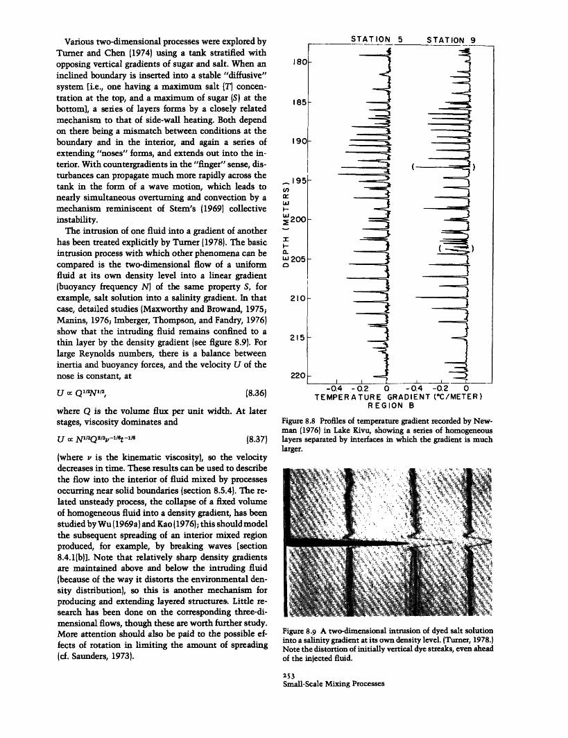
The intrusion of one fluid into a gradient of anotherhas been treated explicitly by Turner (1978). The basicintrusion process with which other phenomena can becompared is the two-dimensional flow of a uniformfluid at its own density level into a linear gradient(buoyancy frequency N) of the same property S, forexample, salt solution into a salinity gradient. In thatcase, detailed studies (Maxworthy and Browand, 1975;Manins, 1976; Imberger, Thompson, and Fandry, 1976)show that the intruding fluid remains confined to athin layer by the density gradient (see figure 8.9). Forlarge Reynolds numbers, there is a balance betweeninertia and buoyancy forces, and the velocity U of thenose is constant, at

U C Ql/2NI/2 (8.36)

where Q is the volume flux per unit width. At laterstages, viscosity dominates and

U o: N 1 13Q2/ 3v-l/_6 t- 1l (8.37)

(where v is the kinematic viscosity), so the velocitydecreases in time. These results can be used to describethe flow into the interior of fluid mixed by processesoccurring near solid boundaries (section 8.5.4). The re-lated unsteady process, the collapse of a fixed volumeof homogeneous fluid into a density gradient, has beenstudied byWu (1969a) and Kao (1976); this should modelthe subsequent spreading of an interior mixed regionproduced, for example, by breaking waves [section8.4.1(b)]. Note that relatively sharp density gradientsare maintained above and below the intruding fluid(because of the way it distorts the environmental den-sity distribution), so this is another mechanism forproducing and extending layered structures. Little re-search has been done on the corresponding three-di-mensional flows, though these are worth further study.More attention should also be paid to the possible ef-fects of rotation in limiting the amount of spreading(cf. Saunders, 1973).

STATION 5

-0.4 -0.2 0 -0.4 -0.2 0TEMPERATURE GRADIENT ("C/METER)

REGION B

Figure 8.8 Profiles of temperature gradient recorded by New-man (1976) in Lake Kivu, showing a series of homogeneouslayers separated by interfaces in which the gradient is muchlarger.

Figure 8.9 A two-dimensional intrusion of dyed salt solutioninto a salinity gradient at its own density level. (Turner, 1978.)Note the distortion of initially vertical dye streaks, even aheadof the injected fluid.

253Small-Scale Mixing Processes

__- -

STATION 9

When the source fluid has different T-S propertiesfrom its surroundings, but still the density appropriateto its depth, the behavior is very different. (The labo-ratory experiments were carried out using a source ofsugar in a salinity gradient, but they will be describedin terms of the oceanic analog of warm, salty waterreleased into temperature-stratified fresher water.) Asshown in figure 8.10, there is a strong vertical convec-tion near the source; this is limited by the stratifica-tion, and "noses" begin to spread out at several levelsabove and below the source. Further layers appear, andthe volume of fluid affected by mixing with the inputis many times the original volume. Each individualnose as it spreads is warmer and saltier than its sur-roundings, so "diffusive" interfaces form above andfingers below, and there a local decrease of T or aninversion through each layer. Note too the slight up-ward tilt of each layer as it extends. This implies thatthe net buoyancy flux [see section 8.4.2(c)] through thefinger interface is greater than that through the diffu-sive interface, so that the layer becomes lighter andmoves across isopycnals. These conclusions have beensupported by experiments using a source of salt in agradient of sugar in which the sense of the interfaces,and the tilt, are just the inverse of those just described.Strong systematic shears are also associated with thelayers, and the sense of these motions has been ex-plained in terms of the horizontal density anomaliesset up by the net buoyancy flux.

Another geometry of direct relevance to the ocean isa discontinuity of T-S properties in the horizontal overa narrow frontal surface. In the present context, weconsider only "fronts" across which the net densitydifference is small, and neglect rotational effects. [Thelarger-scale (baroclinic) instabilities that could lead to

enhanced horizontal mixing in other circumstanceswill not be discussed here.] To model this case, Rud-dick and Turner (1979) have set up identical verticaldensity distributions on two sides of a barrier, usingsugar (S) in one-half of a tank and salt (T) in the other.When the barrier is withdrawn, a series of regular,interleaving layers develops (figure 8.11) whose depthand speed of advance are both proportional to the hor-izontal property differences, and therefore increasewith depth. The scale is of the form (8.35), where a ATis now the horizontal anomaly across the front (thougha rather different energy argument has been used toderive this result).

A general conclusion to be drawn from all the ex-periments just described is that the formation andpropagation of interleaving double-diffusive layers is aself-driven process, sustained by local density anom-alies due to the quasi-vertical transports across theinterfaces. Thus, however layers have formed, whetherthrough strictly one-dimensional processes or by inter-leaving, it is important to understand the mechanismand magnitude of the fluxes of S and T through them.

(c) Double-Diffusive Fluxes through InterfacesQuantitative laboratory measurements have beenmade of the S and T fluxes across an interface betweena hot, salty layer below a cold, fresh layer. They can beinterpreted using an extension of well-known resultsfor pure thermal convection at high Rayleigh numberRa. Explicitly, Turner (1965), Crapper (1975), and Mar-morino and Caldwell (1976) have shown that the heatflux aFH in density units) is well described by Nu Ra, where Nu is the Nusselt number. This may beexpressed in the form

aFH = AI(a AT)413, (8.38)

where A, has the dimensions of a velocity. For a spec-ified pair of diffusing substances, Al is a function onlyof the ratio R, of contributions of S and T to the densitydifference

R, = AS/aAT, (8.39)

where p is the factor relating salinity to density. WhenR, < 2, A > A - O.l(gK2/v)113, the corresponding con-stant for solid boundaries, and for R > 2, A fallsprogressively below A as R, increases and more energyis used to transport salt across the interface. As dis-cussed further by Turner (1973a), the empirical form

A,1 A = 3.8(PAS/ AT) -2

Figure 8.Io The flow produced by releasing sugar solutioninto a salinity gradient at its own density level. (Turner, 1978.)The gradient and the flow rate are exactly the same as forfigure 8.9, but because of the double-diffusive effects, there isnow strong convection and mixing near the source, followedby intrusion at several levels.

(Huppert, 1971) gives a good fit to the observations.The salt flux also depends systematically on R, and

has the same dependence on AT as does the heat flux.Thus the ratio of salt to heat fluxes should be a func-tion of Ro alone:

254J. S. Turner

(8.40)

Figure 8.i I A system of interleaving layers produced by re- lution (right), which have identical linear vertical density dis-moving a barrier separating sugar solution (left) and salt so- tributions. (Ruddick and Turner, 1979.)

R, = Fs/aFH, = f,(f AS /a AT). (8.41)

The first two papers cited above suggest that RF fallsrapidly from unity at R, = 1 to 0.15 at R, = 2, and thenstays constant at RF = 0.15 0.02 for 2 < R < 7. (Itmust always be less than 1 for energetic reasons, andthis implies that the density difference between thetwo layers will always be increasing in time.) The morerecent paper of Marmorino and Caldwell (1976) sug-gests that the flux ratio can be as high as 0.4 withmuch smaller heat fluxes, and also gives different val-ues of the normalized heat flux, for reasons that are asyet unresolved. The discrepancy merits further study,since Huppert and Turner (1972) applied the earlierlaboratory values to explain the temperature structureof a salt-stratified Antarctic lake, with an accuracy thatseemed to make an error of a factor of two unlikely.

Linden and Shirtcliffe (1978) have extended the"thermal-burst" model of Howard (1964a) to calculatefluxes and flux ratios in the two-component case.Transports through the center of the interface are bypure molecular diffusion, while the outer edge becomesintermittently unstable when the Rayleigh numberbased on its thickness reaches a critical value. [Thisprocess had previously been discussed by Veronis(1968a) in a more qualitative way.] The constancy of RFover a certain range can be predicted by assuming thatboundary layers of T and S grow by diffusion to thick-nesses proportional to K

2 and KS12, and then break away

together, down to the level where a AT = g AS. Thefluxes will then be in the ratio T1/2 = (KSI/KT)1

12, a resultin reasonable agreement with experiments using bothsalt-heat and sugar-salt systems. The agreement withthe individual flux measurements is much less im-pressive.

For finger interfaces, the condition for fingers to formin the first place has been examined by Huppert andManins (1973). They showed that when a hot, salty

layer is placed on a cold, fresh layer (or the equivalentin the analogous system), fingers can form in the in-terface, as it thickens by diffusion, provided

3 AS/a AT > 73/2 (8.42)

Since r 10-2 for heat-salt fingers, only very smalldestabilizing salinity differences are needed for themto form, and this suggests that salt fingers will be ubiq-uitous phenomena in the ocean.

Fluxes have also been measured across finger inter-faces, and relations like (8.38) and (8.41) are again foundto hold. Both the salt flux and the flux ratio are sys-tematic functions of the density ratio, now more con-veniently defined in the inverse sense as R =aAT/3AS. In particular, Turner (1967) found aF/,lfFs =0.56 for heat-salt fingers over the range 2 < R < 10.This result seems to be confirmed by recent work dueto Schmitt (1979) and by the author (unpublished),though a much lower value of the flux ratio obtainedby Linden (1973) remains unexplained. No experimentshave convincingly achieved values of R very close to1, where an increase in flux ratio might be expected,but this range could be of great importance for theocean.

The experiments of Linden (1974) are also of interest.He applied a shear across a finger interface and showedthat a steady shear has little effect on the fluxes,though it changes the (nearly square) fingers into two-dimensional sheets aligned down shear. Thus fluxes ofS and T will be expected to persist in spite of the shearsset up by interleaving motions across a front (figure8.11). Unsteady shears, on the other hand (i.e., me-chanical stirring on both sides of the interface) canrapidly disrupt the interface and decrease the salt flux.

Stern (1975a, 1976) has extended his collective-instability model (in two different ways) to describethe breakdown of fingers at the edge of an interface. Hesupposes that instability sets in when the salt flux

255Small-Scale Mixing Processes

becomes too large for the existing temperature gra-dient, a condition that can be expressed in terms of aReynolds number of the finger motions, and that isachieved first near the edges. This is consistent witha steady state through the interface in which the fluxis

PF, FS C(gKT)1/3f(A3S)4 /3, (8.43)

where C is a function of R* only when r = K/KT is

small. When R* < 2, various laboratory experimentsagree in giving C = 0.1, and this form is in betteraccord with experiments than previous expressions,which involved Ks explicitly. Griffiths (1979) has re-cently proposed a model based on the intermittentgrowth and instability (in the Rayleigh-number sense)of the edge of an interface, the model previously appliedonly to diffusive interfaces. He has been able to predicta flux ratio of about 0.6, and also various properties ofthe fingers in the interface, including the relation be-tween the width h and length L of the fingers (h c L4approximately) that was observed by Shirtcliffe andTurner (1970) for sugar-salt fingers.

(d) Multiple Transports through Diffusive Interfaces Itis clear from all the results described in the previoussection that the "transport coefficients," defined as thevertical fluxes divided by the corresponding mean gra-dients, are inevitably different for heat and salt whenthe transports are due to double-diffusive processes act-ing across interfaces. For a diffusive interface, for ex-ample,

Ks Fs TR~T 1/2. {8.44)

KH AS FH 8.44)

The effective "eddy diffusivity" of the driving (unstablydistributed) component will always be larger than thedriven (see figure 8.7): KH > KS in the diffusive case,and Ks > KH when there are salt fingers. Both T and Sare transported down their respective gradients, at dif-ferent rates, but the inappropriateness of the eddy dif-fusivity approach becomes obvious when one considersthe net density flux. This is transported against thegradient, since the potential energy is decreasing andthe density difference tending to increase. Moreover,the largest individual transports occur when the den-sity gradient is weakest, i.e., when Rp - 1.

When there are several different stabilizing salts ina hot, salty layer below a cold, fresh layer, the relativetransports of each across the diffusive interface can,however, be usefully described in terms of the ratio oftransport coefficients Ki. Turner, Shirtcliffe, andBrewer (1970) suggested that the individual Ki can de-pend on the molecular diffusivities, and Griffiths (1979)has recently examined this more carefully, both theo-retically and experimentally. He has predicted, using

a further extension of Linden and Shirtcliffe's (1978)"intermittent instability" model, that K1/K2 should beproportional to T1/

2 = (K1/K2)1 1 2 at low total solute-heat

density ratios RI, and to r at higher Rt , where a steadydiffusive core dominates. The results are insensitive tothe relative contributions of each component to thetotal density difference.

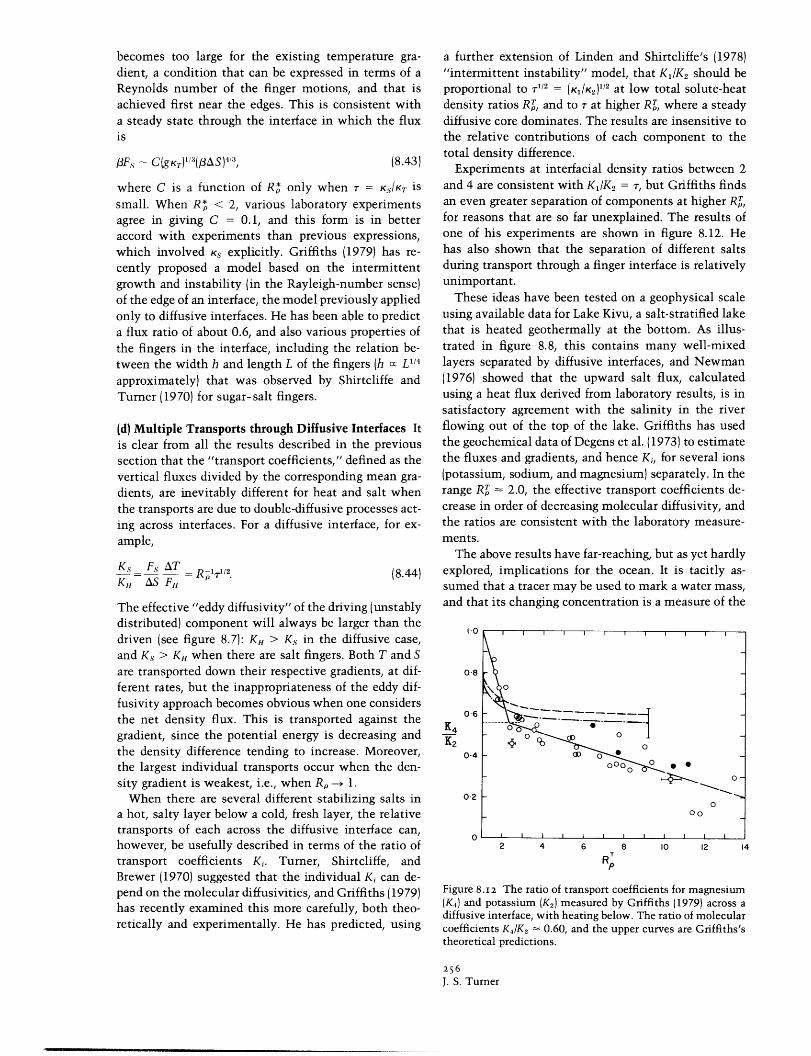
Experiments at interfacial density ratios between 2and 4 are consistent with K1/K2 = r, but Griffiths findsan even greater separation of components at higher RI',for reasons that are so far unexplained. The results ofone of his experiments are shown in figure 8.12. Hehas also shown that the separation of different saltsduring transport through a finger interface is relativelyunimportant.

These ideas have been tested on a geophysical scaleusing available data for Lake Kivu, a salt-stratified lakethat is heated geothermally at the bottom. As illus-trated in figure 8.8, this contains many well-mixedlayers separated by diffusive interfaces, and Newman(1976) showed that the upward salt flux, calculatedusing a heat flux derived from laboratory results, is insatisfactory agreement with the salinity in the riverflowing out of the top of the lake. Griffiths has usedthe geochemical data of Degens et al. (1973) to estimatethe fluxes and gradients, and hence Ki, for several ions(potassium, sodium, and magnesium) separately. In therange RT - 2.0, the effective transport coefficients de-crease in order of decreasing molecular diffusivity, andthe ratios are consistent with the laboratory measure-ments.

The above results have far-reaching, but as yet hardlyexplored, implications for the ocean. It is tacitly as-sumed that a tracer may be used to mark a water mass,and that its changing concentration is a measure of the

K4K2

1.0

0-8

0-6

0'4

02

02 4 6 8 10 12 14

RT

P

Figure 8. I2 The ratio of transport coefficients for magnesium(K4) and potassium (K2) measured by Griffiths (1979) across adiffusive interface, with heating below. The ratio of molecularcoefficients K4/IK2 0.60, and the upper curves are Griffiths'stheoretical predictions.

256J. S. Turner

--- ----- _ _

"mixing rate" for the water mass as a whole. But ifdiffusive interfaces are important, the transport of atracer having a different molecular diffusivity is notnecessarily a good indicator of the transport of a majorcomponent, much less of heat. In the absence of defi-nite knowledge of the mixing mechanisms operatingbetween the source and the sampling point, a single"eddy diffusivity" must be used with great caution.

(e) Cabbeling and Related Instabilities Another kind of

convective instability that can lead to internal mixingdepends on the nonlinear-density behavior of sea water.Particularly at low temperatures, the mixing of twoparcels of water with the same density but different T-S properties produces a mixture with a greater densitythan that of the constituents. This will sink, generatingadditional mixing, and the whole process is called cab-beling (various other spellings appear in the literature).Even when S and T are not quite compensating, so thatthe density decreases upward, a finite amplitude ver-tical displacement, followed by mixing, can lead to theeffect described.

This possibility was first recognized at the turn ofthe century. Fofonoff (1956) showed that the formationof Antarctic bottom water is probably influenced bythis process, and Foster (1972) has given a good accountof the history, as well as a stability analysis for thecase of superimposed water masses. He has applied hisresults to the Weddell Sea, in which the surface isgenerally colder and fresher than the underlying deepwater. When the salinity at the surface increases dueto sea-ice formation in the winter, mixtures of surfaceand deep water may become denser than the deepwater, and thus sink through it and contribute to bot-tom-water formation.

Foster and Carmak (1976b) have since applied relatedideas to the explanation of layers at mid-depth in thecenter of the Weddell Sea. They note that where the Tand S gradients are weak and nearly compensating,deep well-mixed layers are formed, and they attributethis to cabbeling. But the sense of the two opposinggradients is just that required for double-diffusive in-stabilities to produce layers, separated by "diffusive"interfaces. At shallower depths, the gradients are largerand the layers thinner; no cabbeling instability appearsto be possible, and layer formation due solely to double-diffusive effects is postulated. A closer study of theconditions separating these regimes would be instruc-tive.

Gill (1973) has shown that when parcels of water aregiven finite vertical displacements, instabilities canarise due to the different compressibility of sea waterat different temperatures and pressures. The compress-ibility of cold water is generally greater than that ofwarm, so in the situation discussed above, a cold parcel

displaced downward could in principle become heavierthan its new surroundings. The displacements re-quired, however, are rather large, and though the effectmay be significant for bottom-water formation (seeKillworth, 1977), no evidence has been found that itcan influence the formation of layers in the interior, ormixing on a smaller scale.

8.4.3 Observations of Fine Structure andMicrostructureThere are now many observations in the deeper oceanin which the influence of the processes described insections 8.4.1 and 8.4.2 can be identified. Most of thesehave been made using vertical profiles from lowered orfreely falling instruments, with a few significant con-tributions from towed sensors [see section 8.4.1(d)].Temperature and salinity fluctuations are the mostcommonly measured quantities, though small-scalevelocity shear measurements are just becoming avail-able (Simpson, 1975; Osborn, 1978).

A useful summary of the observations up to about1974 has been given by Fedorov (1976) (with extra ref-erences in the English translation to mid-1977). Heemphasizes the fine structure, or nonuniformities, ofvertical gradient associated with a "layer-and-inter-face" structure, which needs to be known before mi-crostructure measurements in the water column canbe understood properly. The strongest layering is foundnear boundaries between water masses of different or-igin, and it is most prominent when there is a largehorizontal contrast in T-S but a small net density dif-ference. Interleaving motions, with associated temper-ature inversions, readily develop in these circum-stances, and the double-diffusive processes describedin section 8.4.2(b) become especially relevant.

Only two recent examples will be cited here: profilesacross the Antarctic polar front (Gordon, Georgi, andTaylor, 1977) reveal inversions that decrease instrength with increasing distance away from the front.Joyce, Zenk, and Toole (1978) have made a more de-tailed analysis of observations in this area, and haveconcluded that double-diffusive processes are signifi-cant. Coastal fronts between colder, fresh water on acontinental shelf and warmer, salty water offshore alsoexhibit strong interleaving (Voorhis, Webb and Millard1976). More observations and laboratory experimentsrelated to such intrusions have been reviewed and com-pared by Turner (1978). It must be emphasized thatdouble-diffusive processes can be important even inregions where the mean S increases and T decreaseswith depth, and both distributions are stabilizing [e.g.,off the coast of California (Gregg, 1975)]. Horizontalinterleaving organizes the gradients so that double-dif-fusive convection can act: it is a self-driven process,sustained by local density anomalies set up by thequasi-vertical fluxes. In this way double-diffusion

257Small-Scale Mixing Processes

serves both to produce the layering and to dissipate theenergy within it. Observations also show (Howe andTait, 1972; Gargett, 1976) that the density gradientabove a warm intrusion is typically much larger thanthat below, in accord with the laboratory observationof sharp diffusive interfaces above and more diffusefinger interfaces below such an intrusion.

More detailed measurements of microstructure inrelation to the fine structure also show the importanceof intrusions, though the interpretation of the detailedmechanism involved is sometimes ambiguous. Wehave already discussed [section 8.4.1(c)] the observa-tions of Eriksen (1978), who related wave-breakingevents to the fine structure, so there are certainly someoccasions on which shear-generated turbulence is im-portant. Gregg (1975) concluded from T and S micro-structure profiles measured in the Pacific that the re-gions of most intense activity are the upper and lowerboundaries of intrusions produced by interleaving, andsuggested alternative explanations in terms of shear-generated turbulence and double-diffusive phenomena.The undersides of temperature-inversion layers werefound to have the highest level of activity, which wecan now attribute to salt fingers. Williams (1976) alsofound, using thermal sensors mounted on a mid-waterfloat, that the regions of most intense mixing areclosely associated with intrusive features, and he wasable to distinguish occasions when one or other mech-anism was dominant.

Gargett (1976) has shown that higher levels of small-scale temperature fluctuations are invariably found inareas where the vertical profiles of T and/or S havefine-structure inversions. The highest percentage of thesampled water volume was found to be turbulent whenthe local T and S gradients are in the finger sense. Sowe come back to the point made by Gargett (1978), andmentioned in section 8.4.1(d); double-diffusive proc-esses, associated with intrusions, are very often im-portant in producing fine structure and microstructure.Thus deductions made on the basis of temperaturefluctuations alone, which, moreover, imply that thetransport is entirely vertical, are not likely to be valid.

We turn now to examples of the large-scale effectsof vertical double-diffusive transports across theboundaries of intrusions. Lambert and Sturges (1977)have shown that the decrease in salinity in and belowthe core of a warm saline intrusion can be explained interms of the downward flux of salt in fingers. Theyobserved a series of stable layers separated by fingerinterfaces, through which the flux (calculated usinglaboratory results) was sufficient to account for theobserved rate of decrease of S with distance. Voorhis etal. (1976) used neutrally buoyant floats to record thechange in T and S in the same water mass over a periodof days. They found evidence of rapid vertical fluxes of

heat and salt between layers, at different rates consist-ent with aFH/l3Fs 0.5, approximately the laboratoryvalue for salt fingers.

Schmitt and Evans (1978) have shown that salt fin-gers grow rapidly enough to survive even in an activeinternal wave field. They have calculated salt fluxesfor measured profiles of S and T, using laboratory dataand assuming that fingers are intermittently active onthe high gradient regions. The calculated flux of salt iscomparable to the surface input of salt due to evapo-ration, i.e., they deduce that fingers can account for allthe vertical flux in the ocean. Carmack and Aagaard(1973) have given an example of the large-scale impor-tance of vertical transports in the "diffusive" sense.From the changes in S and T in the deep water of theGreenland Sea, they suggest that bottom water is notformed at the sea surface, but by a subsurface modifi-cation across an interface between a colder, freshersurface layer of Polar water and a warm salty lowerlayer of Atlantic water (see figure 8.7B). Their deducedratio of Ks/KTr 0.3, showing that heat is definitelytransported faster than salt, supports this view.

Thus, far from being an amusing curiosity, double-diffusive convection is playing a significant, and insome regions dominant, role in the vertical mixing ofheat and salt in the world's oceans. Its overall impor-tance relative to other processes such as wave breakingand boundary mixing (reviewed in the following sec-tion) has not yet been assessed adequately.

8.5 Mixing near the Bottom of the Ocean

Compared to that in the atmospheric boundary layer,or even the surface layers of the ocean, work on theocean-bottom layer has been very sparse. The earlyresearch, summarized by Bowden (1962), concentratedon shallow seas, but the measurements of heat fluxesthrough the deep ocean bottom made it desirable toknow more about the flows in those regions (Wimbushand Munk, 1970). More sophisticated instruments havenow been developed to allow more detailed measure-ments, but as the proceedings of a recent conferenceon the subject show (Nihoul, 1977), there is as yet noclear consensus in this field.

8.5.1 Mixing Induced by Mean CurrentsMost measurements of the depth of the benthic bound-ary layer have been referred to the "Ekman depth"

he = 0.4u./f, (8.45)

which is the scale appropriate to an unstratified, tur-bulent flow in a rotating system. A logarithmic layer,described by (8.2), is contained within the lowest partof this, where the stress can be regarded as constantand rotation is unimportant. The Ekman theory also

258J. S. Turner

predicts a veering of the current with height above theboundary.

But the data suggest (in various ways) that this maynot be a directly relevant scale, because of the stablestratification of the water column. For example, figure8.13 shows profiles of 0 and S measured by Armi andMillard (1976) on an abyssal plain. The well-mixedlayer, bounded by a sharper interface, strongly suggeststhat this structure has been formed by stirring up thebottom part of the gradient region above (cf. figure8.1a). This stirring is therefore an "external" mixingprocess, driven by turbulent energy put in at the bound-ary. The buoyancy flux associated with the heat fluxthrough the bottom has a negligible effect, except whenthe speed of the current is very low. The layer depthh in this case is about six times he, and the mean depthon different days was correlated with the mean currentvelocity U. Armi and Millard showed that

F = U/(g Ph) /2

a Froude number, was approximately constant at -1.7.This led to the hypothesis that the layer depth is con-trolled by the instability of large-scale waves travelingalong the interface. No direct evidence of such a wave-breaking process has been reported, though the tem-poral variation of layer depth in these and other meas-urements [see, e.g., Greenewalt and Gordon (1978)] in-dicate that waves of large amplitude are often present.Note that this Froude-number criterion is closely re-lated to the "constant-overall-Richardson-number" hy-pothesis used in surface mixed-layer models [sections8.3.2(a) and 8.3.3].

A different picture has been developed by Weatherlyand van Leer (1977), on the basis of their measurementsof temperature and current profiles on a continentalshelf. Their boundary-layer thicknesses (defined fromcurrent profiles) were substantially smaller than (8.45),and they attributed this to the effect of stable stratifi-cation. They did, however, observe large changes ofcurrent direction in a sense consistent with Ekmanveering, particularly when the stratification was large,and they have described their results in terms of astably stratified turbulent Ekman layer. Relatively fewof their profiles had well-mixed layers at the bottom,and even those suggested an advective origin, ratherthan local turbulent mixing. When the bottom wassloping, and the flow was along the isobaths, the ob-servations contain a systematic increase or decrease oftemperature in time, which is consistent with down-welling or upwelling along the slope produced by theEkman transport.

It seems likely that the difference between theseobservations and those of Armi and Millard (1976) liesin the much weaker stratification in the deep ocean,

5400

5500 -a*0

.

2!-Fl

tL

5600

Salinity (/oo)341 344 341s5 346 341? 348 3489 348 34 91

i i . , . i , . i

Pot. Temp. (C)

Figure 8.I3 Salinity (S) and potential temperature (0) profilesmeasured by Armi and Millard (1976) in the middle of theHatteras Abyssal Plain. The dashed line indicates that thestructure could have formed by mixing up a stratified regionabove the bottom.

and the consequently larger values of F there. But be-fore this can be regarded as certain, more measure-ments at other sites will be needed. Theoreticiansshould also look more carefully at the properties ofmixed layers shallower and deeper than the Ekmandepth, and systematically compare the bottom-layerresults with surface mixed layers.

In shallow seas, mixing driven by turbulence pro-duced at the bottom can extend to the surface. Thistendency is counteracted by the input of heat at thesurface, which produces a stabilizing temperature gra-dient. Qualitatively, one can see that the larger thecurrent and the shallower the depth, the more likelyis the water to be uniformly mixed for a given surfaceflux [cf. section 8.3.2(d)].

Simpson and Hunter (1974) showed, in fact, thatthere are marked frontal structures in the Irish Sea,separating well-mixed from stratified regions. The lo-cation of these fronts is determined by the parameterh/u3, where h is the water depth and u the amplitudeof the tidal stream. The choice of this form can bejustified using an energy argument, related to that usedto obtain (8.21). The relevant dimensionless parametermust include the buoyancy flux B, and is Bh/u3. Thusthe only extra assumption is that B varies little overthe region of interest. Simpson and his coworkers havenow extended this model to include the effects of windstress as well as tidal currents, and find that this hasa significant, though less important, influence.

259Small-Scale Mixing Processes

152 .54 .56 .58, i , i~~~~~~

- .

62 64 66 68

8.5.2 Buoyancy-Driven Bottom Flows

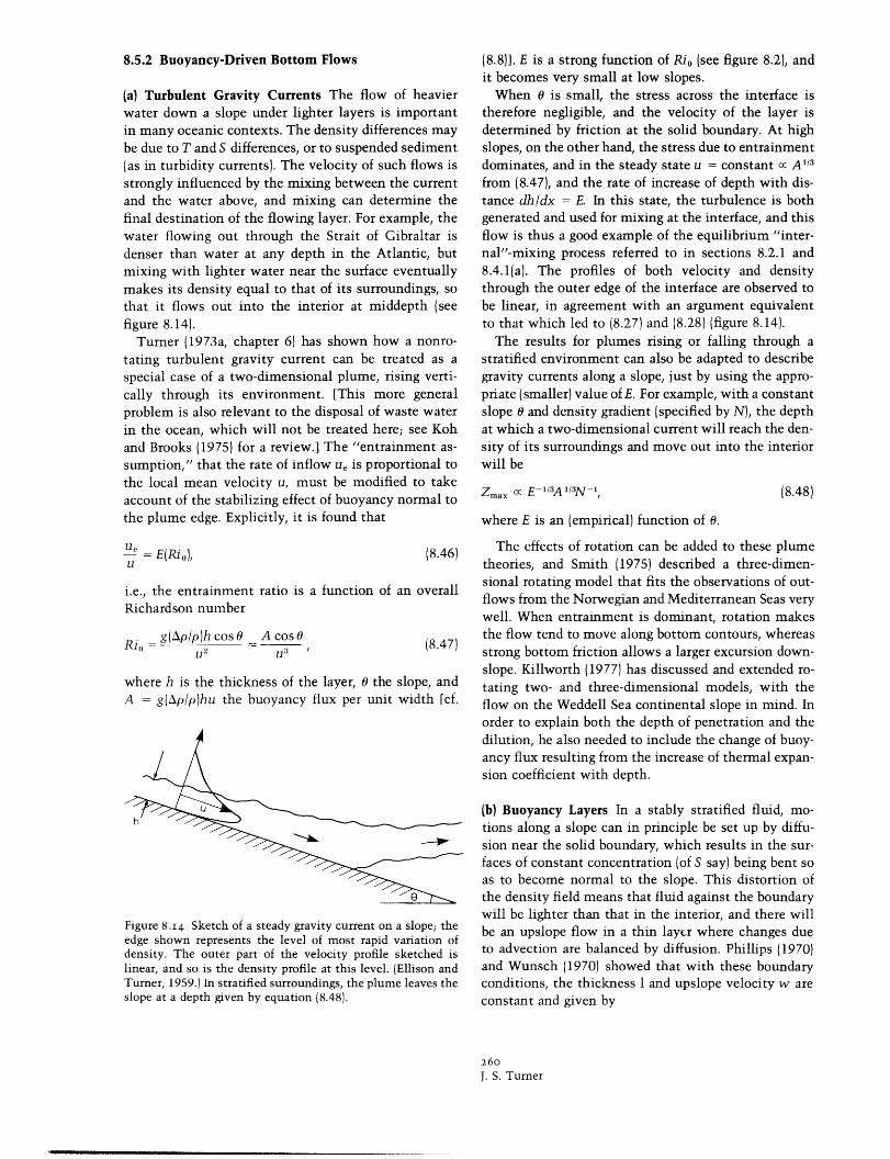
(a) Turbulent Gravity Currents The flow of heavierwater down a slope under lighter layers is importantin many oceanic contexts. The density differences maybe due to T and S differences, or to suspended sediment(as in turbidity currents). The velocity of such flows isstrongly influenced by the mixing between the currentand the water above, and mixing can determine thefinal destination of the flowing layer. For example, thewater flowing out through the Strait of Gibraltar isdenser than water at any depth in the Atlantic, butmixing with lighter water near the surface eventuallymakes its density equal to that of its surroundings, sothat it flows out into the interior at middepth (seefigure 8.14).

Turner (1973a, chapter 6) has shown how a nonro-tating turbulent gravity current can be treated as aspecial case of a two-dimensional plume, rising verti-cally through its environment. [This more generalproblem is also relevant to the disposal of waste waterin the ocean, which will not be treated here; see Kohand Brooks (1975) for a review.] The "entrainment as-sumption," that the rate of inflow ue is proportional tothe local mean velocity u, must be modified to takeaccount of the stabilizing effect of buoyancy normal tothe plume edge. Explicitly, it is found that

u = E(Rio), (8.46)

i.e., the entrainment ratio is a function of an overallRichardson number

g(Ap/p)h cos 0 A cos 0 8.47)Ri,,- U

3

where h is the thickness of the layer, 0 the slope, andA = g(Ap/p)hu the buoyancy flux per unit width [cf.

h

Figure 8.14 Sketch of a steady gravity current on a slope; theedge shown represents the level of most rapid variation ofdensity. The outer part of the velocity profile sketched islinear, and so is the density profile at this level. (Ellison andTurner, 1959.) In stratified surroundings, the plume leaves theslope at a depth given by equation (8.48).

(8.8)]. E is a strong function of Ri, (see figure 8.2), andit becomes very small at low slopes.

When 0 is small, the stress across the interface istherefore negligible, and the velocity of the layer isdetermined by friction at the solid boundary. At highslopes, on the other hand, the stress due to entrainmentdominates, and in the steady state u = constant cc A1'3

from (8.47), and the rate of increase of depth with dis-tance dhldx = E. In this state, the turbulence is bothgenerated and used for mixing at the interface, and thisflow is thus a good example of the equilibrium "inter-nal"-mixing process referred to in sections 8.2.1 and8.4.1(a). The profiles of both velocity and densitythrough the outer edge of the interface are observed tobe linear, in agreement with an argument equivalentto that which led to (8.27) and (8.28) (figure 8.14).

The results for plumes rising or falling through astratified environment can also be adapted to describegravity currents along a slope, just by using the appro-priate (smaller) value of E. For example, with a constantslope 0 and density gradient (specified by N), the depthat which a two-dimensional current will reach the den-sity of its surroundings and move out into the interiorwill be

(8.48)Zmax . C E-13A1/3N - 1,

where E is an (empirical) function of 0.

The effects of rotation can be added to these plumetheories, and Smith (1975) described a three-dimen-sional rotating model that fits the observations of out-flows from the Norwegian and Mediterranean Seas verywell. When entrainment is dominant, rotation makesthe flow tend to move along bottom contours, whereasstrong bottom friction allows a larger excursion down-slope. Killworth (1977) has discussed and extended ro-tating two- and three-dimensional models, with theflow on the Weddell Sea continental slope in mind. Inorder to explain both the depth of penetration and thedilution, he also needed to include the change of buoy-ancy flux resulting from the increase of thermal expan-sion coefficient with depth.

(b) Buoyancy Layers In a stably stratified fluid, mo-tions along a slope can in principle be set up by diffu-sion near the solid boundary, which results in the sur-faces of constant concentration (of S say) being bent soas to become normal to the slope. This distortion ofthe density field means that fluid against the boundarywill be lighter than that in the interior, and there willbe an upslope flow in a thin layer where changes dueto advection are balanced by diffusion. Phillips (1970)and Wunsch (1970) showed that with these boundaryconditions, the thickness 1 and upslope velocity w areconstant and given by

260J. S. Turner

_ 1�1_ _I_ __ __

1 - (vK)1"4N-12, W - (VK )114N11 2.

Under laboratory conditions these are very small,but Wunsch (1970) proposed that (8.49) could be ex-tended to oceanic slopes by using "eddy" values for vand K rather than molecular coefficients. With v, K -

104 cm 2 s-', 1 - 20 m, w - 5 cms -1, and more intensemixing will drive a stronger upslope current. There areseveral difficulties with this interpretation. It is im-plied that the larger mixing coefficients must be drivenby some external mixing process, which is most likelyto be associated with currents against the slope. Thisbeing so, it seems more appropriate to regard these"mechanical" processes as the cause, not the effect, ofthe near-slope motions and to investigate directly theireffects on mixing. Second, the presence of two strati-fying components, in the interior; with compensatingeffects on the density, changes the behavior markedly.As discussed in section 8.4.2(b) [see also Turner (1974)],counterflows along the slope are then produced, withmuch larger velocities than in the single-componentcase. These cannot remain steady, however, and thenet result is the formation of a series of layers, extend-ing out into the interior (cf. figure 8.10). When condi-tions near the slope are quiet, this mechanism couldproduce enhanced mixing and fine structure, but againit is likely to be overwhelmed by the mixing producedby currents.

8.5.3 Mixing Due to Internal WavesInternal waves impinging on a sloping boundary canprovide enough energy to cause significant mixing. Theconditions under which this occurs in a continuouslystratified fluid have been convincingly illustrated inthe laboratory experiments of Cacchione and Wunsch(1974).

When waves of lowest mode propagate into a wedge-shaped region bounded by a solid sloping boundary anda free surface (or interface), three types of behavior arepossible. These depend on the relative magnitudes ofthe slope f3 of the boundary and the wave-characteristicslope a = sin-l(w/N), which is the direction of the groupvelocity, and of the particle motions [see figure 8.15and Wunsch (1969)]. If P > a, then energy can be re-flected back into the interior. If P < a, which occursonly at sufficiently high frequencies for a given Pand stratification N, the horizontal component of thegroup velocity after reflexion is still directed towardthe slope. Energy thus cannot escape backward, and isfed into the corner region. For example, when thedeeper layers are stratified, and there is a well-mixedlayer above, the amplitude will build up in the ther-mocline and strong local mixing can occur there. When1, = a, the particle motions become parallel to theslope, and this strong shearing motion becomes un-stable to form a series of periodic vortices. Overturning

(b)

Figure 8.I 5 Propagation of waves into a wedge of angle 1. Theangle a that rays make with the horizontal stays constant, sothat when 1 > a [case (a)] energy can be reflected, and when(8 < a [case (b)] energy is trapped in the corner. The criticalcase 1 = a produces strong shearing motions against the slope.

associated with these produces mixed fluid that prop-agates into the interior as regularly spaced layers allalong the slope.

Though there is a suggestion in these and other ex-periments that the layer spacing is related to the am-plitude of the excursion along the slope, they do notprovide a definite length scale that can be used forpredictions in the ocean. Nor do there yet seem to beany oceanic measurements that are detailed enough todistinguish the structure resulting from this mecha-nism from other possibilities.

Waves formed on density interfaces can also producemixing when they approach a sloping boundary. Forexample, in a fjord that has a well-mixed surface layerand a strong pycnocline at sill depth, Stigebrandt (1976)showed that interfacial waves generated at the sill canpropagate toward the landward end, where they breakon the sloping shore. Using field data and a laboratoryexperiment, he described the vertical mixing in thelower layer in terms of this wave-breaking process,followed by the flow of mixed fluid into the interior.Similar observations have been reported by Perkin andLewis (1978), who concluded that this mechanismprobably dominates the transport between the surfaceand bottom layers of fiords for most of the year.

8.5.4 The Effect of Bottom Mixing on the InteriorThere is no doubt that mixing near the bottom is muchstronger than it is in the interior of the ocean. Hogg,Katz, and Sanford (1978), continuing a series of meas-urements near Bermuda initiated by Wunsch (1972a),recently have documented a close relation between thedistribution of temperature fine structure and strongcurrents associated with large eddies near the island.They are cautious about identifying the precise mech-anism of interaction (from among those describedabove, and others not discussed here), but the genera-tion of the structure at the island slope and its decaywith distance away from Bermuda is very clear.

Armi (1978) has used the contrast between verticaltemperature profiles near topographic features and inthe interior of an ocean basin to support one of themechanisms for vertical mixing discussed by Munk

26ISmall-Scale Mixing Processes

(8.49)

(1966): that the largest cross-isopycnal mixing occursin boundary-mixed layers, and that these are then ad-vected into the interior and so influence the structurethere as well. The single well-mixed bottom layer dis-cussed in section 8.5.1 and shown in figure 8.13 ischaracteristic of a smooth bottom on an abyssal plain,but over rougher topography a number of steps is oftenobserved, suggesting bottom mixing at several depths,followed by spreading out along isopycnals that inter-sect the slope. The horizontal variability of such lay-ering indicates that the process is patchy and inter-mittent.

The layer structure decays and the profiles becomesmoother as the water moves out into the interior. Thevarious mechanisms that could play a part at this stagehave been discussed in section 8.4. Some layers ofwater with distinctive T-S properties are identifiable,however, over large distances. Armi (1978) has shownthat Norwegian Sea water can be followed as a 20-m-thick layer for over 3000 km into the North Atlantic,and cites this as evidence both for large-scale advectionand slow vertical mixing. Carmack and Killworth(1978) have identified a layer with anomalously low Tand S characteristics that interleaves along a surface ofconstant potential density with Antarctic bottomwater near the Ross Sea. They also suggest that thesinking of water in the form of plumes along the con-tinental margin, followed by an outflow at mid-depth,is possible nearly everywhere round Antarctica, al-though water masses that are so clearly distinguishablefrom their surroundings are rather rare.

In summary, the available evidence supports theview that the bottom of the ocean, particularly thesloping bottom around coasts or topographic features,plays an essential role in the internal-mixing process.Near the topography, the dominant mixing mecha-nisms are probably mechanical, driven by large-scalecurrents, though gravity currents can sometimes beimportant. The main way in which the resulting mixedlayers are carried into the interior of the ocean mustbe by large-scale advection, associated with processesthat are nearly independent of the layers themselves.The extra spreading and interleaving due to local hor-izontal density anomalies [described by equations(8.36) or (8.37)] occur on a longer time scale, thoughthese processes will also affect the final profiles in theinterior. Direct vertical mixing driven by internalwaves is probably active too, and bottom topographyenters here in another way as a mechanism for gener-ating the internal wave field.

The only other regions where the deduced mixingrates are comparable with those at solid boundaries areboundaries between different water masses. The evi-dence presented in section 8.4.3, for example, shows

that frontal surfaces with large horizontal T and Sanomalies but a small net density difference are par-ticularly active. The primary process envisaged in thatcase is double-diffusive transport in the vertical, pro-ducing local density anomalies that drive quasi-hori-zontal interleaving. Double-diffusive convection canalso be significant when water masses with very dif-ferent T-S properties lie one on top of the other.

We conclude on a cautionary note. Though therehave been rapid advances in the observation and un-derstanding of many individual physical processes, par-ticularly in the past 10 years, these have not yet beenput together to give a satisfactory, unified picture ofmixing in the ocean. We must now seek ways to dis-tinguish between the effects of the diverse vertical andhorizontal processes that have been reviewed, and toassess their relative importance in controlling the ver-tical distributions of temperature and salinity in theocean as a whole.

262J. S. Turner