SLAC–PUB–15421

April 2013

Femtosecond x-ray free electron laser pulse duration

measurement from spectral correlation function

A.A. Lutman1, Y. Ding1, Y. Feng1, Z. Huang1,

M. Messerschmidt1, J. Wu1, J. Krzywinski1

1 SLAC National Accelerator Laboratory, Menlo Park, CA 94025, USA

Abstract

We present a novel method for measuring the duration of femtosecond x-ray

pulses from self-amplified spontaneous emission free electron lasers by perform-

ing statistical analysis in the spectral domain. Analytical expressions of the

spectral correlation function were derived in the linear regime to extract both

the pulse duration and the spectrometer resolution. Numerical simulations con-

firmed that the method can be also used in the nonlinear regime. The method

was demonstrated experimentally at the Linac Coherent Light Source by mea-

suring pulse durations down to 13 fs FWHM.

Phys. Rev. ST Accel. Beams 15, 030705 (2012)

Work supported by Department of Energy contract DE-AC02-76SF00515.

2

INTRODUCTION

The Linac Coherent Light Source (LCLS) at SLAC National Accelerator Laboratory is

the world’s first hard x-ray Free-Electron Laser (FEL) source that began lasing in 2009 [1]

and is now in user operation, supporting a wide range of scientific research including physics,

structural biology, energy, chemistry, and material science. An FEL x-ray source, such as

the LCLS, is based on the so-called Self-Amplified Spontaneous Emission (SASE) process.

It exhibits three unique properties: ultra-fast pulse duration ranging from a few to hundreds

of femtoseconds, ultra-high peak brightness that is many orders of magnitude greater than

the brightest storage-ring based synchrotron sources, and nearly full spatial coherence in

the transverse directions. Although having these unprecedented characteristics, SASE FEL

sources are, however, considered to be chaotic in nature, giving rise to statistical fluctuations

in the beam properties on a pulse-by-pulse basis. In particular, the temporal profile of the

LCLS FEL x-ray pulse consists of a large number of coherent spikes of varying magnitudes.

However, the development of an appropriate diagnostic tool for “seeing” the exact temporal

details, including such simple measurement as the pulse duration, has proven to be very chal-

lenging and elusive. This is largely due to the vanishingly small cross-sections in nonlinear

processes at x-ray wavelengths that make temporal correlation techniques, commonly used

in optical regime, exceedingly difficult. The lack of progress in this regard has hindered the

LCLS users from knowing the exact pulse duration for resolving atomic/molecular motions

and for calculating the exact fluence in studying x-ray nonlinear light-matter interactions.

SASE FEL radiation originates from the initial random distribution of the electrons

within a bunch, and its statistical properties are related to the ones of the shot noise. After

a start up phase, FEL enters in the exponential linear regime, where the output power grows

exponentially with the undulator length and is proportional to the shot noise power of the

electron bunch current. At some undulator length, FEL power does not grow exponentially

anymore and reaches saturation. To extract more power from the electrons, post saturation

taper can be applied [2]. After saturation, the relationship between the input shot noise

power and the output radiation power is nonlinear.

Statistical fluctuation of the incoherent radiation intensity has been used to get informa-

tion about the electron bunch length [3, 4], as demonstrated by earlier experiments using

spontaneous radiation sources [5–8]. However, a SASE FEL differs from a spontaneous

3

source in two aspects. First, although the amplification process in a linear regime does not

change the statistical properties of the radiation, it can modify the x-ray pulse duration

compared to the electron bunch length due to the exponential gain and slippage effects.

Recent studies of the statistical fluctuation and the x-ray pulse duration in the exponential

gain regime can be found in Refs. [9, 10]. Secondly, a SASE FEL typically operates in the

saturation regime for the purposes of intensity stability and a higher power extraction. Here

the FEL process is very nonlinear, and it is not obvious whether statistical fluctuations may

be useful to retrieve the radiation pulse duration.

In this paper, we present a novel method for measuring the x-ray pulse duration through

the analysis of the statistical properties of the SASE FEL spectra. First, we show theoret-

ically how this method can be applied in the exponential growth regime. Then, through

numerical simulations, we show why this method still applies in the FEL saturation regime.

Finally, we apply this technique to experimental data taken at the LCLS. The measurements

were performed at various machine settings where the x-ray pulse durations were determined

in the range from 10 fs to 200 fs.

THEORY

The SASE FEL behaves as a narrow band amplifier, which selectively amplifies a wide-

band random input signal. The fluctuations result from the shot noise of the electron beam

current

I(t) = (−e)N∑k=1

δ(t− tk), (1)

at the undulator entrance, where the arrival times tk are random variables with the probabil-

ity density f(t). In our theoretical approach we will use an one dimensional model assuming

that a single transverse mode is established through gain guiding [2]. The spectrum of the

FEL electric field E(t) is calculated as E(ω) =∫ +∞−∞ E(t)eiωtdt. The first and second order

4

spectral correlation functions are introduced as [11]

g1(ω, δω) =

⟨E(ω − δω/2)E∗(ω + δω/2)

⟩√⟨∣∣∣E(ω − δω/2)

∣∣∣2⟩⟨∣∣∣E(ω + δω/2)∣∣∣2⟩ , (2)

g2(ω, δω) =

⟨∣∣∣E(ω − δω/2)∣∣∣2 ∣∣∣E(ω + δω/2)

∣∣∣2⟩⟨∣∣∣E(ω − δω/2)∣∣∣2⟩⟨∣∣∣E(ω + δω/2)

∣∣∣2⟩ . (3)

We express a single-shot spectrum taken by the spectrometer as

S(ω) =

∫ +∞

−∞

e− (ω′−ω)2

2σ2m

√2πσm

|E(ω′)|2dω′, (4)

where we assume that the spectrometer resolution function has a Gaussian shape with σm

rms width. We define the weighted spectral second order correlation function as

G2(δω) =

∫ +∞

−∞W (ω)

[〈S(ω − δω/2)S(ω + δω/2)〉〈S(ω − δω/2)〉 〈S(ω + δω/2)〉

− 1

]dω, (5)

where the weight function W is described as

W (ω) =

∫ +∞−∞ 〈S(ω + b/2)〉 〈S(ω − b/2)〉 db∫ +∞−∞ 〈S(ω + b/2)〉 〈S(ω − b/2)〉 dbdω

(6)

We introduce a simple model for the exponential growth regime that allows us to obtain

an analytical formula for Eq. (5). The process of amplification, within a one-dimensional

model, can be described by a Green function h(t, τ), and the electric field can be calculated

as the convolution

E(t) =

∫h(t, τ)I(τ)dτ. (7)

For electron beams with constant parameters, the SASE FEL Green function has the

form [11, 12]

hti(t− τ) = A0(z)eik0ze−iω0(t−τ)− (t−τ−z/vg)2

4σ2ht

(1+ i√

3

), (8)

where A0(z) ∝ ezlg contains the exponential growth factor, with lg representing the field gain

length. The time dependent growth process, originating from an electron beam with a non

flat current profile, can be described assuming that the gain length is a function of t [13].

The gain mechanism also depends on other quantities, such as transverse emittance, energy

spread and undulator taper. To model this, we introduce a time-dependent gain function

5

htd, which is a slow-varying function on the scale of the FEL radiation coherence length.

Thus we express the time dependent SASE FEL impulse response function as:

h(t, τ) = hti(t− τ)htd(τ). (9)

In Appendix we show that, within the proposed model,

g2(ω, δω) = 1 + |g1(ω, δω)|2 (10)

and we derive the analytical formula (37) for the weighted spectral correlation function (5).

When the average spike width is much narrower than the FEL bandwidth σa = 1√3σht

(37)

simplifies to:

G2(δω) =

∫ +∞

−∞

e−(ξ−δωξ0)2

2σ2 |X(ξ)|2√2πσ|X(0)|2

dξ, (11)

where X(ω) is the Fourier transform of the average profile

X(t) =⟨|E(t)|2

⟩(12)

and

σ =√

2 σaσm√σ2a+σ2

m

, ξ0 = σ2a

σ2a+σ2

m. (13)

Equation (11) can be particularized for different X(t) shapes. For a Gaussian profile with

rms duration σt, we have

G2(δω) =e− δω2ξ20σ

2t

1+2σ2σ2t√

1 + 2σ2σ2t

, (14)

and for a flat top profile with full length duration T ,

G2(δω) = 2

∫ 1

0

e−ζ2σ2T 2/2(1− ζ) cos (δωξ0Tζ)dζ. (15)

The measurement procedure of the pulse duration is described below. First, a large set

of spectra is recorded. By fitting the average spectrum we obtain σ2a + σ2

m. Thus only the

spectrometer resolution σm and the pulse duration are unknown. By fitting the experimental

G2 function with the analytical model one can finally derive both the pulse duration and the

spectrometer resolution. For typical measurement conditions σa >>σm, σ ≈√

2σm, ξ0 ≈ 1

and the measurement is insensitive to errors on σa.

6

Now we would like to compare Eqs. (14) and (15) under the condition that σa >>σm, one

can conveniently rewrite the G2 function expressions using the variables Ω = δωσm

, Tg = σtσm

and Tf = Tσm. In particular, with this notation,

1

G2(0)=√

1 + 4T 2g (16)

gives a measure of the average number of x-ray spectral spikes (coherent modes) within the

spectrometer resolution. The number of modes can be approximated by 2Tg, when Tg is

large. Mathematical details of the comparison can be found in Appendix . One can also

note that when Tf >> 1, the method cannot distinguish between Gaussian and flat top

pulses having the same r.m.s. duration. This is because when T =√

12σt the number of

modes and the shapes of the G2 function are the same (see Fig. 10 and Eq. (45) and (46)

). In this sense the method gives an rms pulse duration measure for compact x-ray pulse

shapes, regardless of the shape. For the case Tf << 1, achievable by using a finer resolution

spectrometer, the method is able to distinguish between the two shapes. In this case G2

is proportional to the square of the modulus of the Fourier transform of the X-ray pulse

envelope. Figure 1 represents both described cases for a fixed pulse duration Tf = Tg√

12

and for different spectrometer resolutions.

0 0.5 1 1.5

x 10−4

0

0.2

0.4

0.6

0.8

1

δ ω / ω0

G2(δ

ω/ ω

0)

F.T. Tf = 0.1

Gauss Tf = 0.1

F.T. Tf = 1

Gauss Tf = 1

(a)When Tf << 1, Gaussian and flat top

profiles having the same rms duration yield

different G2 functions.

0 0.2 0.4 0.6 0.8 1

x 10−3

0

0.02

0.04

0.06

0.08

0.1

0.12

δ ω / ω0

G2(δ

ω/ ω

0)

F.T. Tf = 15

Gauss Tf = 15

F.T. Tf = 30

Gauss Tf = 30

(b)When Tf >> 1, Gaussian and flat top

profiles having the same rms duration cannot

be distinguished.

FIG. 1. Comparison between G2 functions derived for the flat top model and the Gaussian average

x-ray profiles.

The measurement method described above is based on the exponential growth model

7

introduced in Eqs. (7-9). Since, within that model, the FEL behaves as a linear amplifier,

the properties of the random Gaussian process of the input signal are retained [14]. Moreover,

the expression for the steady-state Green function allows us to derive the analytical relation

between the average profile X(t) and the weighted spectral correlation function G2.

However, in the saturation regime, Eq. (10) does not hold true in general and we do

not have any analytical model such as Eq. (8) to work out an expression for G2. The

statistical properties in this regime have been studied by numerical simulations in [15], and

a simplified analytical model is described in [12]. The most interesting conclusion that can

be drawn from these studies is that the quasi-Gaussian statistics is retained for narrow band

instantaneous power fluctuations, and that Eq. (10) holds true even at saturation.

Based on the above conclusion we derived an approximate expression for the G2 function

without reference to any of the analytical models. The details of the derivation are presented

in Appendix . By assuming that the spectrometer has Gaussian resolution function with

rms width σm we obtain

G2(δω) =

∫ ∞−∞

e−∆2

4σ2m |X(δω + ∆)|2

2√πσm|X(0)|2

d∆. (17)

The derivation of expression (17) involves several approximations. We assumed that Eq.

(10) is valid also in the saturation regime. This result was found in [15] and was also

confirmed by our simulations. We considered the case when the average spike width is

much narrower than the FEL bandwidth, and the spectrometer resolution width is much

narrower than the FEL bandwidth as well. Further, we assume that the approximation (56)

is valid. An important result found in [15] is that the spectral correlation functions do not

change considerably between the exponential growth and saturation regime. This means

that g1(ω, δω) has a width in δω of the order of 1/T where T is the duration of the profile.

First, the approximation (56) requires an assumption that the phase of g1(ω+b/2, δω)g∗1(ω−

b/2, δω) is nearly zero for δω being inside the described region, and for b being inside the

FEL bandwidth. Secondly, it requires that the amplitude of g1(ω, δω) changes slowly in the

ω variable. This allows us to use the approximation (56) which is crucial for deriving Eq.

(17).

As expected, when σm << σa Eq. (11) gives Eq. (17).

8

NUMERICAL SIMULATIONS

We ran a series of numerical simulations using a 1D FEL code in order to check if the

proposed method is also applicable at saturation and in deep saturation. A flat top electron

beam with an energy of 5.9 GeV, a peak current of 3 kA, and a 1 mm mrad normalized

transverse emittance was used. The undulator has a period of 3 cm and a strength parameter

of 3.5, yielding a radiation wavelength of 0.8 nm (photon energy 1.55 keV) and saturation

occurring close to 40 m. Two different electron bunch lengths, 30 µm and 3 µm, were used

during the simulations. Figure 2 shows the X-ray pulse power as a function of the undulator

distance for each case. Simulation parameters were chosen to be close to the experimental

conditions used in section .

0 10 20 30 40 50 60 70 80 90

102

104

106

108

1010

Undulator distance [m]

Ave

rage

pow

er [

W]

FIG. 2. X-ray pulse average power vs undulator distance. Simulation with the 30 µm electron

bunch (solid line), simulation with the 3 µm electron bunch (dashed line).

Figure 3 shows that the simulated pulse duration measurements, based on Eq. (17),

relate well to the pulse durations obtained directly from the 1D code. The simulations were

performed for both the 30 µm and the 3 µm electron bunch using 2000 independent shots.

In the short bunch case, the slippage and the edge effects played a more important role as

compared to the longer bunch, showing that the method works well for ultra-short bunches.

Two different relative spectrometer resolutions, σm/ω0, 10−4 and 2×10−4, were used to show

that prior knowledge of the spectrometer resolution is not needed. The relative resolutions

have been retrieved as (1.00± 0.01)×10−4 and (2.01± 0.05)×10−4 for the long bunch case,

and as (1.00± 0.02)× 10−4 and (1.96± 0.10)× 10−4 for the short bunch case.

9

20 30 40 50 60 7060

70

80

90

100

110

120

130

140

150

160

Undulator Distance [m]

Pul

se d

urat

ion

full

leng

th fl

at to

p [fs

]

pulse duration from time domain

simulated measurement, σm

/ω0=1 × 10−4

simulated measurement, σm

/ω0=2 × 10−4

(a)Electron bunch is flat top, 30 µm long.

20 30 40 50 60 70 80 906

7

8

9

10

11

12

13

14

15

16

Undulator Distance [m]

Pul

se d

urat

ion

full

leng

th fl

at to

p [fs

]

pulse duration from time domain

simulated measurement, σm

/ω0=1 × 10−4

simulated measurement, σm

/ω0=2 × 10−4

(b)Electron bunch is flat top, 3 µm long.

FIG. 3. Simulated measurement of x-rays pulse duration vs undulator distance. (Diamonds)

relative spectrometer resolution σm/ω0 = 10−4, (squares) relative spectrometer resolution σm/ω0 =

2× 10−4.

Simulations starting with a flat top electron bunch show that the method can measure

the average pulse duration both in the linear and non-linear regime. The pulse duration,

however, stays almost constant for different undulator distances. We have also ran simula-

tions with non-flat electron current profiles to prove that the method can actually measure

the pulse duration also when the average profile duration changes during the FEL process.

We used Gaussian electron bunches with the following parameters: an energy of 5.9 GeV, a

peak current of 3 kA, and a 1 mm mrad normalized transverse emittance. 500 independent

shots were simulated for each electron bunch starting condition. Two rms electron bunch

lengths were used: 18 µm and 6 µm. The relative spectrometer resolution of 8 × 10−5 was

used in the simulated measurements. The results of the simulated measurements were com-

pared with the rms pulse duration derived directly from the 1D code. Figure 4 shows the

comparison for the long bunch case. Figure 4(a) represents the normalized average pulse

profiles for different undulator distances. During the exponential growth regime, the selec-

tive growth mechanism described by means of the htd function favors the growth where the

density current is higher. This effectively results in a shortening of the x-ray average pro-

file. Figure 4(b) shows the relation between the retrieved pulse duration and the calculated

average profile rms duration. We find that the results are in very good agreement both in

the exponential growth and in the non-linear regime. The solid line in Fig. 4(b) is a quick

10

estimate of the pulse duration obtained by considering the field gain length lg as a function

of the current density and neglecting the slippage effects. We can write this formula in a

closed form when approximating the gain up to the second order in time:

σt(z) = σt(0)

√3lg0

2(3lg0 + z), (18)

where lg0 is the field gain length for the maximum bunch current. Equation (18) predicts

a shortening of the pulse duration during the exponential growth. The retrieved relative

spectrometer resolution for this case is 7.90 × 10−5 ± 0.09 × 10−5. The simulation starting

from the 6 µm electron bunch yields shorter pulse durations, which are similar to the shortest

measured pulse durations presented in the experimental section. Figure 5(a) shows the

normalized average pulse profiles for different undulator distances, and Fig. 5(b) shows

the comparison between the retrieved pulse duration and the calculated average profile rms

duration. Again we find good agreement between the retrieved pulse duration and the actual

rms duration of the average profile. The retrieved relative spectrometer resolution for the

short bunch case is 7.90× 10−5 ± 0.11× 10−5.

−80 −60 −40 −20 0 20 40 60 800

1

2

3

4

5

6

7

8x 10

−4

time [fs]

Nor

mal

ized

ave

rage

pro

file

z = 10 mz = 20 mz = 30 mz = 40 mz = 60 mz = 80 m

(a)Normalized average x-ray profile. A low pass

filter has been used to remove the residual spiky

structure from the 500 shots average.

0 20 40 60 80 10020

25

30

35

40

45

50

55

Undulator distance [z]

Puls

e du

ratio

n [f

s]

Simulated Measurement rms durationAverage pulse profile rms duration

(b)Pulse duration vs undulator distance.

Calculated average profile rms duration

(diamonds), simulated measurement rms

duration (stars).

FIG. 4. Results for the Gaussian electron bunch profile with 18 µm rms length.

As expected, our simulations confirm that Eq. (10) holds true in the exponential growth

regime. At saturation, the second order correlation function can be empirically approximated

11

−30 −20 −10 0 10 20 300

0.5

1

1.5

2

2.5x 10

−3

time [fs]

Nor

mal

ized

ave

rage

pro

file

z = 10 mz = 20 mz = 30 mz = 40 mz = 60 mz = 80 m

(a)Normalized average x-ray profile. A low pass

filter has been used to remove the residual spiky

structure from the 500 shots average.

0 20 40 60 806

8

10

12

14

16

Undulator distance [z]

Puls

e du

ratio

n [f

s]

Simulated Measurement rms durationAverage pulse profile rms duration

(b)Pulse duration vs undulator distance.

Calculated average profile rms duration

(diamonds), simulated measurement rms

duration (stars).

FIG. 5. Results for the Gaussian electron bunch profile with 6 µm rms length.

as g2(ω, δω) ≈ A + B|g1(ω, δω)|2, when δω is not too large. This has been confirmed for

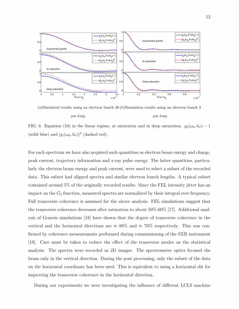
simulations using different electron bunch current profiles and lengths. Figure 6 shows the

comparison between g2(ω0, δω)− 1 and |g1(ω0, δω)|2 in the non-linear regime. In saturation,

we found A close to 0.88 for the short bunch simulation, and close to 0.99 for the long

bunch simulation, while B equals to 1.03 and 1.01, respectively. This can eventually lead to

negative values in Eq. (5), suggesting that it is necessary to fit Eq. (17) with a free offset

parameter. This behavior, predicted by the simulations, is confirmed by the experimental

data. In the long bunch simulation Eq. (47) holds better, since the slippage and the edge

effects play a less important role. Similar results were found in [15] where the authors explain

that, within the accuracy of their simulations, the spectral first and second order correlation

functions do not change from the exponential growth regime to the non-linear regime.

EXPERIMENTAL RESULTS

The experimental demonstration of the method described above was performed at the

LCLS operating at 1.5 keV photon energy. The spectra were recorded by the LCLS soft x-

rays spectrometer [16]. For each machine setting around 40 000 spectra have been recorded.

12

0

0.5

1

Exponential growth

g2(ω

0,δ ω/ω

0)−1

|g1(ω

0,δ ω/ω

0)|2

0

0.5

1

At saturation

g2(ω

0,δ ω/ω

0)−1

|g1(ω

0,δ ω/ω

0)|2

0 0.5 1 1.5 2 2.5 3 3.5

x 10−4

0

0.5

1

Deep saturation

δ ω / ω0

g2(ω

0,δ ω/ω

0)−1

|g1(ω

0,δ ω/ω

0)|2

(a)Simulated results using an electron bunch 30

µm long.

0

0.5

1

Exponential growth

g2(ω

0,δ ω/ω

0)−1

|g1(ω

0,δ ω/ω

0)|2

0

0.5

1

At saturation

g2(ω

0,δ ω/ω

0)−1

|g1(ω

0,δ ω/ω

0)|2

0 0.2 0.4 0.6 0.8 1

x 10−4

0

0.5

1

Deep saturation

δ ω / ω0

g2(ω

0,δ ω/ω

0)−1

|g1(ω

0,δ ω/ω

0)|2

(b)Simulation results using an electron bunch 3

µm long.

FIG. 6. Equation (10) in the linear regime, at saturation and in deep saturation. g2(ω0, δω) − 1

(solid blue) and |g1(ω0, δω)|2 (dashed red).

For each spectrum we have also acquired such quantities as electron beam energy and charge,

peak current, trajectory information and x-ray pulse energy. The latter quantities, particu-

larly the electron beam energy and peak current, were used to select a subset of the recorded

data. This subset had aligned spectra and similar electron bunch lengths. A typical subset

contained around 5% of the originally recorded results. Since the FEL intensity jitter has an

impact on the G2 function, measured spectra are normalized by their integral over frequency.

Full transverse coherence is assumed for the above analysis. FEL simulations suggest that

the transverse coherence decreases after saturation to about 50%-60% [17]. Additional anal-

ysis of Genesis simulations [18] have shown that the degree of transverse coherence in the

vertical and the horizontal directions are ≈ 80% and ≈ 70% respectively. This was con-

firmed by coherence measurements performed during commissioning of the SXR instrument

[19]. Care must be taken to reduce the effect of the transverse modes on the statistical

analysis. The spectra were recorded as 2D images. The spectrometer optics focused the

beam only in the vertical direction. During the post processing, only the subset of the data

on the horizontal coordinate has been used. This is equivalent to using a horizontal slit for

improving the transverse coherence in the horizontal direction.

During our experiments we were investigating the influence of different LCLS machine

13

conditions on the statistical properties of measured spectra. We varied the undulator length

and the electron bunch peak current. We also applied the slotted foil technique to change

the effective electron bunch length that was able to lase [13].

In the first experiment we measured the pulse duration for different undulator lengths.

The peak current was set to 3 kA, which yields an 83 fs electrons bunch length for a flat

top shape. Pulse duration measurements are presented in Fig. 7 showing that x-ray pulses

were shorter than electron bunches and that, with our post saturation taper configuration,

the pulse duration increases when the deep saturation is reached. The measured relative

spectrometer resolution was similar for the different analyzed data sets, and was equal to

σm/ω0 = (1.02± 0.04)×10−4. The designed spectrometer resolution at 1.5 keV is 0.85×10−4

[16]. Measurements performed at LCLS pointed out that the SXR instrument resolution at

that photon energy should be closer to 1.4×10−4 [21]. The discrepancy could be attributed to

the fact that this resolution was derived from an averaged spectra, and it could be influenced

by such uncertainties as vibrations and photon beam jitters. The resolution derived by our

method is based on the intensity interferometry principle. Therefore, it is much less sensitive

to such instabilities. A non-Gaussian shape of the resolution function of the spectrometer

could also contribute to the differences in the resolution derived from the two methods.

In the second experiment pulse durations were measured for different peak currents at a

fixed electron bunch charge. For these data sets, undulator taper has been applied in order

to maximize the output power with 28 undulator segments present. Experimental results

have been collected for the peak current from 1.5 kA to 3 kA. Figure 8 shows the measured

x-ray pulse duration compared to the electron bunch length in the hypothesis of a flat

top electron bunch distribution. Higher peak current electron bunches yield clearly shorter

average FEL pulses. Finally, we measured shorter x-rays pulse durations by controlling the

electron bunch length using the slotted foil technique [13]. The shortest pulse duration was

measured for the slotted foil configuration corresponding to an estimated unspoiled electron

bunch length of 10 fs FWHM [20]. With this setting, the measured average x-ray pulse

duration was 13 fs FWHM. Figure 9(a) shows a typical measured spectrum for different foil

settings. It is evident from this figure that the shortest pulses yield spectra with higher

fluctuations (Fig. 9(a)) and larger values of G2(0) (Fig. 9(b)). This figure also shows that

the analytical model can fit the experimental data well.

14

50 60 70 80 9030

40

50

60

70

80

90

100

Undulator Distance [m]

Puls

e du

ratio

n fu

ll le

ngth

fla

t top

[fs

]

FIG. 7. Measured x-ray pulse duration vs undulator distance (diamonds). Pulse duration expressed

as full length flat top. Electron bunch length within the flat top model (dashed).

TABLE I. Electron bunch length controlled using the slotted foil and measured x-ray pulse duration

as FWHM Gaussian. Electron bunch length is calculated with the formula presented in [20]. σm/ω0

is the relative spectrometer resolution measured for each dataset.

Estimated unspoiled electron Measured x-ray pulse Measured relative spectrometer

bunch length FWHM [fs] duration FWHM [fs] resolution σm/ω0

10 13 0.87× 10−4

18 24 0.92× 10−4

28 39 0.87× 10−4

56 50 0.85× 10−4

CONCLUSION

We have developed an effective approach for measuring the average length of ultrafast

x-ray pulses from SASE based FEL sources by using the statistical characteristics not in

the time, but in the spectral domain. This technique was shown to be experimentally ap-

plicable not only in the exponential growth region, but also in the nonlinear region of the

SASE amplification process as confirmed by analyzing simulated data sets. We observed

15

1.5 2 2.5 3

80

100

120

140

160

180

200

Peak Current [kA]

Puls

e du

ratio

n fu

ll le

ngth

fla

t top

[fs

]

Electrons (Flat top model)Measured pulse duration

FIG. 8. (Diamonds) Measured x-rays pulse duration vs different peak currents, duration expressed

as flat top full length. (Solid) Electrons bunch length for a 250 pC flat top profile as function of

the peak current.

−5 −2.5 0 2.5 5Dispersion from central energy [eV]

Am

plitu

de [a

rbitr

ary

units

]

50 fs FWHM

39 fs FWHM

24 fs FWHM

13 fs FWHM

(a)Typical measured spectra. Shorter x-ray

pulses present spectra with larger amplitude

fluctuations.

0 2 4 6 8 10 12

x 10−4

−0.1

0

0.1

0.2

0.3

0.4

0.5

δ ω/ω0

G2(δ

ω /ω

0)

13 fs experimental data13 fs model fit24 fs experimental data24 fs model fit39 fs experimental data39 fs model fit50 fs experimental data50 fs model fit

(b)Experimental G2 function for different pulse

durations (FWHM Gaussian) and fitting with the

theoretical model.

FIG. 9. Pulse duration measurement controlling the bunch length using the slotted foil.

that the extracted x-ray pulse duration varied consistently with the manipulated electron

bunch length. The hypothesized evolution of the pulse duration as a function of the undula-

16

tor distance was also observed for the first time, lending further credence to our analysis. In

addition, this method can be used to measure the resolution function of a spectrometer as a

cross check to other direct experimental techniques, such as using an absorption line. We be-

lieve that our method can be extended to other SASE-based FELs at arbitrary wavelengths.

This approach can be also considered for the analysis of any chaotic process where the output

signal originates from a nonlinear, narrow-band amplification of a Gaussian process.

We wish to thank P. Emma, W. Schlotter, J.J. Turner for assistance in the soft x-

ray spectrometer experiments, H. Durr, W. Fawley, P. Heimann and J. Stohr for useful

comments and discussions. This work was supported by Department of Energy Contract

No. DE-AC02-76SF00515.

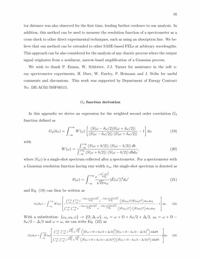
G2 function derivation

In this appendix we derive an expression for the weighted second order correlation G2

function defined as

G2(δω) =

∫ +∞

−∞W (ω)

[〈S(ω − δω/2)S(ω + δω/2)〉〈S(ω − δω/2)〉 〈S(ω + δω/2)〉

− 1

]dω (19)

with

W (ω) =

∫ +∞−∞ 〈S(ω + b/2)〉 〈S(ω − b/2)〉 db∫ +∞−∞ 〈S(ω + b/2)〉 〈S(ω − b/2)〉 dbdω

, (20)

where S(ω) is a single-shot spectrum collected after a spectrometer. For a spectrometer with

a Gaussian resolution function having rms width σm, the single-shot spectrum is denoted as

S(ω) =

∫ +∞

−∞

e− (ω′−ω)2

2s2m

√2πsm

|E(ω′)|2dω′ (21)

and Eq. (19) can then be written as

G2(δω) =

∫ +∞

−∞W (ω)

∫+∞−∞

∫+∞−∞ e

− (ωa−ω−δω/2)2

2σ2m e

− (ωb−ω+δω/2)2

2σ2m

⟨|E(ωa)|2|E(ωb)|2

⟩dωadωb∫+∞

−∞∫+∞−∞ e

− (ωa−ω−δω/2)2

2σ2m e

− (ωb−ω+δω/2)2

2σ2m

⟨|E(ωa)|2

⟩⟨|E(ωb)|2

⟩dωadωb

− 1

dω. (22)

With a substitution: ωa, ωb, ω → Ω,∆, ω, ωa = ω + Ω + δω/2 + ∆/2, ωb = ω + Ω −δω/2−∆/2 and ω = ω, we can write Eq. (22) as

G2(δω) =

∫ +∞

−∞W (ω)

∫+∞−∞

∫+∞−∞ e

−∆2

4σ2m e

−Ω2

σ2m

⟨∣∣∣E(ω + Ω + δω/2 + ∆/2)∣∣∣2∣∣∣E(ω + Ω− δω/2−∆/2)

∣∣∣2⟩ d∆dΩ

∫+∞−∞

∫+∞−∞ e

−∆2

4σ2m e

−Ω2

σ2m

⟨|E(ω + Ω + δω/2 + ∆/2)|2

⟩⟨|E(ω + Ω− δω/2−∆/2)|2

⟩d∆dΩ

−1

dω. (23)

17

Let us derive a particular expression for the G2 for the exponential growth regime by using

the model based on Eq. (8,9). The Fourier transform of the electric field is evaluated as

E(ω) =

∫ +∞

−∞(−e)

N∑k=1

hti(t− tk)htd(tk)eiωtdt = (−e)Hti(ω)N∑k=1

eiωtkhtd(tk), (24)

where Hti(ω) =∫ +∞−∞ hti(t)e

iωt.First we show the validity of Eq. (10) by following an approach similar to the one describedin [11]. We calculate the first order spectral correlation as

⟨E(ω + δω/2)E∗(ω − δω/2)

⟩= e2Hti(ω + δω/2)H∗ti(ω − δω/2)

⟨N∑k=1

N∑j=1

htd(tk)h∗td(tj)ei(ω+δω/2)tke−i(ω−δω/2)tj

⟩

= e2Hti(ω + δω/2)H∗ti(ω − δω/2)

⟨ N∑k=1

|htd(tk)|2eiδωtk⟩

+

⟨N∑k=1

N∑j=1,j 6=k

htd(tk)h∗td(tj)ei(ω+δω/2)tke−i(ω−δω/2)tj

⟩(25)

By using the hypothesis that the arrival times are independent, and that they are describedby the density probability function f(t), Eq. (25) yields:

⟨E(ω + δω/2)E∗(ω − δω/2)

⟩= e2Hti(ω + δω/2)H∗ti(ω − δω/2)N

∫ +∞

−∞|htd(tk)|2eiδωtkf(tk)dtk

+e2Hti(ω + δω/2)H∗ti(ω − δω/2)N(N − 1)

∫ +∞

−∞htd(tk)f(tk)ei(ω+δω/2)tkdtk

∫ +∞

−∞h∗td(tj)f(tj)e

−i(ω−δω/2)tjdtj (26)

Second term on right hand side is negligible with respect to the first one. It can be shown

by using the same arguments presented in [15], while discussing the spectral correlation of

the first order.⟨E(ω + δω/2)E∗(ω − δω/2)

⟩≈ e2NHti(ω + δω/2)H∗ti(ω − δω/2)

∫ +∞

−∞|htd(t)|2f(t)eiδωtdt

(27)

We now calculate the spectral correlation of the second order⟨|E(ω + δω/2)|2|E(ω − δω/2)|2

⟩= e4|Hti(ω + δω/2)|2|Hti(ω − δω/2)|2 ×⟨

N∑k=1

N∑j=1

N∑l=1

N∑m=1

htd(tk)h∗td(tj)htd(tl)h

∗td(tm)ei(ω+δω/2)tke−i(ω+δω/2)tjei(ω−δω/2)tle−i(ω−δω/2)tm

⟩(28)

As clarified in [15], the most contributing terms are (k = j) ∧ (l = m) ∧ (k 6= l), (k =m) ∧ (j = l) ∧ (k 6= j). Since the arrival times are independent, we have:

⟨|E(ω + δω/2)|2|E(ω − δω/2)|2

⟩e4|Hti(ω + δω/2)|2|Hti(ω − δω/2)|2

≈N∑k=1

N∑l=1,l 6=k

⟨|htd(tk)|2

⟩ ⟨|htd(tl)|2

⟩+

N∑k=1

N∑j=1,j 6=k

⟨|htd(tk)|2eiδωtk

⟩⟨|htd(tj)|2e−iδωtj

⟩(29)

yielding

⟨|E(ω + δω/2)|2|E(ω − δω/2)|2

⟩e4N(N − 1)|Hti(ω + δω/2)|2|Hti(ω − δω/2)|2

=

(∫ +∞

−∞|htd(t)|2f(t)dt

)2

+

∣∣∣∣∫ +∞

−∞|htd(t)|2f(t)eiδωtdt

∣∣∣∣2 . (30)

Equation (30) togheter with (27) proves Eq. (10).

18

We now consider the average profile X(t) = 〈|E(t)|2〉 and its Fourier transform

X(δω) =

∫ ∞−∞

⟨|E(t)2|

⟩e−iδωt =

1

2π

∫ +∞

−∞

⟨E(ωa − δω/2)E∗(ωa + δω/2)

⟩dωa. (31)

The squared modulus of X can be written as

|X(δω)|2 =1

4π2

∫ +∞

−∞

∫ +∞

−∞

⟨E(ωa − δω/2)E∗(ωa + δω/2)

⟩⟨E∗(ωb − δω/2)E(ωb + δω/2)

⟩dωadωb

(32)By doing the substitution ωa, ωb → ω, b, so that ωa = ω + b/2 and ωb = ω − b/2 oneobtains:

|X(δω)|2 =1

4π2

∫ +∞

−∞dω

∫ +∞

−∞

⟨E(ω + b/2− δω/2)E∗(ω + b/2 + δω/2)

⟩⟨E∗(ω − b/2− δω/2)E(ω − b/2 + δω/2)

⟩db. (33)

From Eq. (33) by using Eq.(27) and Eq. (24), neglecting e4N2 terms and with σa = 1√3σht

we have

4π2|X(δω)|2 =

∫ +∞

−∞

2√πe− δω

2+3(ω−ω0)2

3σ2a

3σ2a

dω

∣∣∣∣∫ +∞

−∞|htd(t)|2f(t)eiδωtdt

∣∣∣∣2 =2πe− δω

2

3σ2a

3σ2a

∣∣∣∣∫ +∞

−∞|htd(t)|2f(t)eiδωtdt

∣∣∣∣2 (34)

Equation (20) is evaluated as

W (ω) =e− (ω−ω0)2

σ2a+σ2

m

√π√σ2a + σ2

m

, (35)

and from Eq.(23) by using Eq. (30)

G2(δω) =

∫ +∞

−∞W (ω)dω

∫ +∞

−∞e−

(∆σ2a+(∆+δω)σ2

m)2

4σ2aσ

2m(σ2

a+σ2m)

√σ2a + σ2

m

∣∣∣∫ +∞−∞ |htd(t)|

2f(t)ei(∆+δω)tdt∣∣∣2

2√πσaσm

∣∣∣∫ +∞−∞ |htd(t)|2f(t)

∣∣∣2 d∆

(36)

We can substitute Eq. (34, 35) into (36) and integrate over ω obtaining,

G2(δω) =

∫ +∞

−∞e−

(∆σ2a+(∆+δω)σ2

m)2

4σ2aσ

2m(σ2

a+σ2m)

√σ2a + σ2

me(∆+δω)2

3σ2a |X(∆ + δω)|2

2√πσaσm|X(0)|2

d∆ (37)

By choosing a particular shape of the average profile, one can find an analytical expression

for the G2 function. In the case of a Gaussian profile, with rms length σt, Eq. (37), under

the condition σt >1

2√

3σagives

e− δω2σ2

a(3σ2aσ

2t−1)

(σ2a+σ2

m)(3σ2a(1+4σ2

mσ2t )−σ2

m)√3σ2a(1+4σ2

mσ2t )−σ2

m

3(σ2a+σ2

m)

(38)

19

Eq. (38) can be simplified when σt >>1√3σa

, where σt is the rms duration of the average

profile, yielding

G2(δω) =

∫ +∞

−∞

e−(ξ−δωξ0)2

2σ2 |X(ξ)|2√2πσ|X(0)|2

dξ, (39)

where σ =√

2 σaσm√σ2a+σ2

m

and ξ0 = σ2a

σ2a+σ2

m.

Comparison between Gaussian and flat top model

We can rewrite explicitly Eqs.(14) and (15) by using the variables

Ω =δω

σm, Tg = σtσm, Tf = Tσm, (40)

and we obtain:

Gg2(Ω) =

e−

Ω2T2g√

1+4T2g√

1 + 4T 2g

, (41)

Gft2 (Ω) =e

−Ω2

4√π

2Tf

(erf

(Tf −

iΩ

2

)+ c.c.

)+e−T

2f cosTfΩ

T 2f

−e−

Ω2

4 Ω√π

4T 2f

(i erf

(Tf −

iΩ

2

)− c.c.

)−

2− iΩ√πe−

Ω2

4 erf(iΩ2

)

2T 2f

.

(42)

Now, we look for the relation between Tf and Tg giving the same number of modes 1G2(0)

within the two different models. Such value of Tg is found as a function of Tf

Tg =1

2

√√√√√ e2T 2f T 4

f − 1(1 + eT

2f (√πTf erf(Tf )− 1)

)2 (43)

The behavior ofTf

Tg(Tf )is represented in Fig. 10, together with the values at the extremes of

the domain

limTf→0

TfTg(Tf )

=√

12 limTf→∞

TfTg(Tf )

= 2√π. (44)

It turns out that Tf =√

12Tg is a very good approximation for the condition to have the

same number of modes in pulses described by above profiles for any value of Tf .

When the number of modes is large, the asymptotic expressions for the G2 functions can be

written as

Gg2(Ω) =

e−Ω2

4

2Tg+

(Ω2 − 2)e−Ω2

4

32T 3g

+ o

(1

T 4g

), (45)

Gft2 (Ω) =

√πe−

Ω2

4

Tf+−2 +

√π erfi

(Ω2

)Ωe−

Ω2

4

2T 2f

+ o

(1

T 4g

). (46)

20

It shows that, for both models, the main contributing terms have Gaussian shapes with the

same rms, which depend only on the spectrometer resolution σm.

0 10 20 30 40 50 60 70 80 90 1003.2

3.25

3.3

3.35

3.4

3.45

3.5

3.55

3.6

Tf

Tf/T

g

FIG. 10.TfTg

as function of Tf giving the same value for Gg2(0) = Gft2 (0) (bold solid),√

12 (dashed),

2√π (dotted).

TfTg

=√

12 is a good approximation to have the same value G2(0) for both the flat

top and the Gaussian models.

G2 derivation without using the linear amplifier model

As it was shown by our simulations, and in [15] even in the non-linear regime, Eq. (10)

is nearly valid. We write it in the form⟨|E(ωa)|2|E(ωb)|2

⟩≈⟨E(ωa)E

∗(ωb)⟩⟨

E∗(ωa)E(ωb)⟩

+⟨|E(ωa)|2

⟩⟨|E(ωb)|2

⟩. (47)

This allows us to write Eq. (23) as

G2(δω) =

∫ +∞

−∞W (ω)

∫+∞−∞

∫+∞−∞ e

−∆2

4σ2m e

−Ω2

σ2m

∣∣∣⟨E(ω + Ω + δω/2 + ∆/2)E∗(ω + Ω− δω/2−∆/2)⟩∣∣∣2 d∆dΩ

∫+∞−∞

∫+∞−∞ e

−∆2

4σ2m e

−Ω2

σ2m

⟨|E(ω + Ω + δω/2 + ∆/2)|2

⟩⟨|E(ω + Ω− δω/2−∆/2)|2

⟩d∆dΩ

dω. (48)

If the spectrometer resolution function is much narrower than the FEL bandwidth, then we

use the following approximation:∫ +∞

−∞e− x2

2σ2m

⟨|E(ω + x)|2

⟩dx ≈

∫ +∞

−∞e− x2

2σ2m

⟨|E(ω)|2

⟩dΩ. (49)

By using this Eq.(49) and Eq. (33), we can rewrite expressions (48,20) as

G2(δω) =

∫ +∞

−∞W (ω)

∫+∞−∞

∫+∞−∞ e

−∆2

4σ2m e

−Ω2

σ2m

∣∣∣⟨E(ω + Ω + δω/2 + ∆/2)E∗(ω + Ω− δω/2−∆/2)⟩∣∣∣2 d∆dΩ

2πσ2m

⟨|E(ω + δω/2)|2

⟩⟨|E(ω − δω/2)|2

⟩ dω (50)

21

W (ω) =

∫+∞−∞

⟨|E(ω − b/2)|2

⟩ ⟨|E(ω + b/2)|2

⟩4π2|X(0)|2

(51)

We introduce g1 formalism as in Eq. (2) and rewrite Eq. (50) and (33) as

G2(δω) =

∫ ∞−∞

∫ ∞−∞

∫ +∞

−∞

∫ +∞

−∞dωdbd∆dΩe

−∆2

4σ2m e

−Ω2

σ2m |g1(ω + Ω, δω + ∆)|2 ×⟨

|E∗(ω + Ω−∆/2− δω/2)|2⟩⟨|E∗(ω + Ω + ∆/2 + δω/2)|2

⟩2πσ2

m

⟨|E(ω + δω/2)|2

⟩⟨|E(ω − δω/2)|2

⟩ ⟨|E(ω − b/2)|2

⟩ ⟨|E(ω + b/2)|2

⟩4π2|X(0)|2

(52)

|X(δω)|2 =1

4π2

∫ +∞

−∞dω

∫ +∞

−∞g1(ω + b/2, δω)g∗1(ω − b/2, δω)×√⟨

|E(ω − b/2− δω/2)|2⟩⟨|E(ω − b/2 + δω/2)|2

⟩⟨|E(ω + b/2− δω/2)|2

⟩⟨|E(ω + b/2 + δω/2)|2

⟩db (53)

Equations (52) can be simplified by using the approximation (49) on ∆ and Ω

G2(δω) =

∫ ∞−∞

∫ ∞−∞

∫ ∞−∞

∫ ∞−∞

e−∆2

4σ2m e

−Ω2

σ2m |g1(ω + Ω, δω + ∆)|2

⟨|E(ω − b/2)|2

⟩ ⟨|E(ω + b/2)|2

⟩2πσ2

m4π2|X(0)|2dωdbd∆dΩ (54)

and in a similar way, Eq. (53) can be simplified when the average spectral spike width is

much narrower than the FEL bandwidth as

|X(δω)|2 =1

4π2

∫ +∞

−∞dω

∫ +∞

−∞g1(ω+b/2, δω)g∗1(ω−b/2, δω)

⟨|E(ω − b/2)|2

⟩⟨|E(ω + b/2)|2

⟩db

(55)

Further we approximate∫ +∞

−∞dω

∫ +∞

−∞g1(ω + b/2, δω)g∗1(ω − b/2, δω)

⟨|E(ω − b/2)|2

⟩⟨|E(ω + b/2)|2

⟩db ≈∫ +∞

−∞dω

∫ +∞

−∞|g1(ω, δω)|2

⟨|E(ω − b/2)|2

⟩⟨|E(ω + b/2)|2

⟩db(56)

The expression is exact for δω = 0 but it is approximated, in general, for other values of δω.

Referring to the exponential growth model, from Eq. (27) we have

g1(ω + b/2, δω)g∗1(ω − b/2, δω) = e−i 1

2σ2a

b√3δω

∣∣∣∫ +∞−∞ |htd(t)|

2f(t)eiδωtdt∣∣∣2∣∣∣∫ +∞

−∞ |htd(t)|2f(t)dt∣∣∣2 (57)

Eq. (57) is not a function of ω, and its width in the variable δω is of the order of 1/T ,

where T is the characteristic length of the profile. From Eq. (56), if b is larger than the

FEL bandwidth, then⟨|E(ω − b/2)|2

⟩⟨|E(ω + b/2)|2

⟩becomes close to zero. Inside this

bounded region for b and δω the phase of exponential factor in Eq. (57) is approximately zero

when 1/T << σa, showing that, within these assumptions, Eq. (56) is valid. An important

result found in [15] is that the spectral correlation functions do not change considerably

22

between the exponential growth and the saturation regime. This means that g1(ω, δω) has

a width in δω of the order of 1/T also in the saturation regime. First, the approximation

(56) requires an assumption that the phase of g1(ω − b/2, δω)g∗1(ω − b/2, δω) is nearly zero

for δω being inside the described region, and for b inside the FEL bandwidth. Secondly

it requires that the amplitude of g1(ω, δω) changes slowly in the ω variable. By using the

approximation (56) we obtain:

G2(δω) =

∫ ∞−∞

∫ ∞−∞

∫ ∞−∞

e−∆2

4σ2m |g1(ω, δω + ∆)|2 〈|E(ω − b/2)|2〉 〈|E(ω + b/2)|2〉

2√πσm4π2|X(0)|2

dωdbd∆

(58)

|X(δω)|2 =1

4π2

∫ +∞

−∞dω

∫ +∞

−∞|g1(ω, δω)|2

⟨|E(ω − b/2)|2

⟩⟨|E(ω + b/2)|2

⟩db (59)

By substituting (59) into (58) we finally obtain:

G2(δω) =

∫ ∞−∞

e−∆2

4σ2m |X(δω + ∆)|2

2√πσm|X(0)|2

d∆. (60)

For σa >> σm Eq. (39) gives, as expected, Eq. (60).

[1] P. Emma et al., Nature Photonics 4, 641 (2010).

[2] Z. Huang and K.-J. Kim, Phys. Rev. ST Accel. Beams 10, 034801 (2007).

[3] M. Zolotorev and G. Stupakov, in Proc. of PAC1997 (Vancouver, Canada, 1997), 2180.

[4] J. Krzywinski et al., Nucl. Instrum. Methods A 401, 429 (1997).

[5] P. Catravas et al., Phys. Rev. Lett. 82, 5261 (1999).

[6] V. Sajaev, in Proc. of EPAC2000 (EPS, Geneva, 2000), p. 1806.

[7] F. Sannibale et al., Phys. Rev. ST Accel. Beams 12, 032801 (2009).

[8] M. Yabashi et al., Phys. Rev. Lett. 88, 244801 (2002).

[9] W. Ackermann et al., Nature Photonics 1, 336 (2007).

[10] J. Wu et al., in Proc. of FEL2010 (Malmo, 2010), p. 147.

[11] E.L. Saldin, E.A. Schneidmiller, and M.V. Yurkov, The Physics of Free Electron Lasers,

(Springer, Berlin, 2000).

[12] S. Krinsky, Phys. Rev. E 69, 066503 (2004).

[13] P. Emma, K. Bane, M. Cornacchia, Z. Huang, H. Schlarb, G. Stupakov and D. Walz, Phys.

Rev. Lett., 92, 07801 (2004)

23

[14] J.W. Goodman, Statistical Optics, (John Wiley & Sons, Inc., 1985).

[15] E.L. Saldin, E.A. Schneidmiller, and M.V. Yurkov, Optics Commun. 148, 383, (1998).

[16] P. Heimann et al., Rev. Sci. Instrum, 82, 093104 (2011).

[17] Y. Ding et al., in Proc. of FEL2010 (Malmo, 2010), p. 151.

[18] S. Reiche, Nucl. Instrum. Meth A 429, 243 (1999).

[19] I. Vartaniants et al., accepted for publication in Phys. Rev. Lett.

[20] P. Emma, Z. Huang, M. Borland, in Proc. of FEL2004 (Trieste, 2004), p. 333.

[21] P. Heimann, Private communication.