Embed Size (px)
Citation preview
HAL Id: tel-00922203https://tel.archives-ouvertes.fr/tel-00922203
Submitted on 24 Dec 2013
HAL is a multi-disciplinary open accessarchive for the deposit and dissemination of sci-entific research documents, whether they are pub-lished or not. The documents may come fromteaching and research institutions in France orabroad, or from public or private research centers.
L’archive ouverte pluridisciplinaire HAL, estdestinée au dépôt et à la diffusion de documentsscientifiques de niveau recherche, publiés ou non,émanant des établissements d’enseignement et derecherche français ou étrangers, des laboratoirespublics ou privés.
Femtosecond time-resolved spectroscopy in polyatomicsystems investigated by velocity-map imaging and
high-order harmonic generationDavid Staedter
To cite this version:David Staedter. Femtosecond time-resolved spectroscopy in polyatomic systems investigatedby velocity-map imaging and high-order harmonic generation. Atomic and Molecular Clusters[physics.atm-clus]. Université Paul Sabatier - Toulouse III, 2013. English. tel-00922203
THESEEn vue de l’obtention du
DOCTORAT DE L’UNIVERSITE DE TOULOUSE
Delivre par l’Universite Toulouse III – Paul Sabatier
Discipline ou specialite: Physique
Femtosecond time-resolved spectroscopy in polyatomic
systems investigated by velocity-map imaging and
high-order harmonic generation
Presente et soutenue par
David STADTER
20. September 2013
JURY
Mme Valerie BLANCHET Chargee de recherche, CNRS LCAR, Toulouse Directrice de These
M. Timo FLEIG Professeur, LCPQ, Universite Paul Sabatier Toulouse President de Jury
M. Laurent NAHON Chercheur, Synchrotron SOLEIL Examinateur
M. Andrew ORR-EWING Professeur, School of Chemistry University of Bristol Rapporteur
M. Lionel POISSON Charge de recherche, CNRS IRAMIS, Paris Rapporteur
Ecole doctorale: Sciences de la Matiere (SDM)
Unite de recherche: Laboratoire Collisions Agregats Reactivite (LCAR IRSAMC UMR5589)
Directrice de These: Valerie BLANCHET


Ph.D. Thesis
Femtosecond time-resolved spectroscopy in polyatomic
systems investigated by velocity-map imaging and
high-order harmonic generation
presented by:
David STADTER
A thesis submitted to the
Graduate School (Sciences de la Matiere (SDM)) of the
Universite Toulouse III – Paul Sabatier
in partial fulfillment of the requirements for the degree of
Doctor of Philosophy (Ph.D.) of the Univeriste de Toulouse
Toulouse, 20. September 2013
JURY
Mme Valerie BLANCHET Chargee de recherche, CNRS LCAR, Toulouse Supervisor
M. Timo FLEIG Professor, LCPQ, Universite Paul Sabatier Toulouse President of the Jury
M. Laurent NAHON Chercheur CEA, Synchrotron SOLEIL Examiner
M. Andrew ORR-EWING Professor, School of Chemistry University of Bristol Reviewer
M. Lionel POISSON Charge de recherche, CNRS IRAMIS, Paris Reviewer
Graduate School: Sciences de la Matiere (SDM)
Research laboratory: Laboratoire Collisions Agregats Reactivite (LCAR IRSAMC UMR5589)
Supervisor: Valerie BLANCHET

c© 2013 by David STADTER
Femtosecond time-resolved spectroscopy in polyatomic systems investigated by velocity-
map imaging and high-order harmonic generation
Ph.D. thesis, 20. September 2013
Supervisor: Valerie BLANCHET
Reviewers: Andrew ORR-EWING and Lionel POISSON
Examiners: Timo FLEIG and Laurent NAHON
Universite Toulouse III – Paul Sabatier
Sciences de la Matiere (SDM)
Laboratoire Collisions Agregats Reactivite (LCAR IRSAMC UMR5589)
118 Rue de Narbonne – 31062 Toulouse – France


Imaging and CONtrol In Chemistry
Marie Curie Initial Training Network (ITN)
under the Seventh Framework Program of the European Union
LCAR - LCPQ - LPCNO - LPT


To my mother


Darkness cannot drive out darkness;
only light can do that.
– Martin Luther King, Jr.

Acknowledgments
My Ph.D. has been an incredible and wonderful, if often overwhelming, experience – a true
marathon event from an academic, professional and personal perspective. It is not easy to
pinpoint whether this has been due to engaging with the topic itself, dividing time between
two universities and groups, working in a foreign country, staying in the lab until dawn, over-
coming experimental setbacks or just staying on track..., to only mention a few. Regardless of
the reasons, it is always the people around you who make the difference. One of the joys of
completion, whatever the challenge – in this case my Ph.D. – is reflecting back on the journey,
and remembering all the colleagues, friends and family who have helped and supported me
along this long but fulfilling road. Without them I would not have been able to complete it and
I am grateful to them for making the past three years exceptional and unforgettable.
First and foremost, this Ph.D. thesis would not have been possible without the continuous
encouragement of my principal supervisor, Dr. Valerie Blanchet – not to mention her advice,
patience, motivation, enthusiasm and unsurpassed knowledge. For all of this I would like
to express my sincere gratitude. From the beginning, she apparently effortlessly managed to
divide her time between two different labs in two different cities, closely supervising two Ph.D.
students in Toulouse and helping out a third one in Bordeaux. Through all of this, without any
complaint, she stayed late in the lab, always had time to talk, to share a joke, or help me with
the French administration. I have appreciated her steady influence throughout my Ph.D. career,
giving me orientation and support with promptness, forbearance and care, particularly during
some of the more difficult periods of my time in her lab. Especially towards the end, during the
writing of this manuscript, when she had already left the lab in Toulouse to move permanently
to Bordeaux, she managed to come and see me regularly in Toulouse, as well as hosting me for
my visits to Bordeaux. A particular thank-you goes to both her and her husband, Prof. David
Dean, for their continued hospitality. I reflect fondly on the times we spent at their place in
Bordeaux, discussing science and life, while drinking beer and making BBQ. I could not have
imagined having a better advisor and mentor for my Ph.D. research.
I would like to thank all the members of my dissertation committee: Prof. Andrew Orr-Ewing,
Dr. Lionel Poisson, Dr. Laurent Nahon, and Prof. Timo Fleig. I am especially grateful to Prof.
Andrew Orr-Ewing and Dr. Lionel Poisson for agreeing to be the reviewers of my thesis, and
for reading through my manuscript before, after and even during their summer holidays; to

Dr. Laurent Nahon for being an examiner and guest on my defense panel; and to Prof. Timo
Fleig for kindly acting as the president of the jury, even though particularly as a theoretician
it is no easy task to read an experimental thesis. I very much appreciate all the thoughtful
and detailed comments, as well as the encouraging and constructive feedback, which the jury
members have provided me with.
I want to thank as well the organizers of the ICONIC network for a wonderful experience. As
a Ph.D. fellow within this network I was privileged to have the opportunity to learn first-hand
about imaging techniques. In addition, the various training schools and network meetings all
over Europe broadened my knowledge of the field and made networking easy. I recognize that
the research carried out for this thesis would not have been possible without the financial as-
sistance of grants from the Marie Curie ICONIC initial training network (ITN-ICONICPITN-
GA-2009-238671) and from the ANR HARMODYN.
A particularly big thank-you goes to Dr. Yann Mairesse, who was not officially my co-
supervisor in Bordeaux, but who definitely took me under his wing while I was there, and
always made me feel at home even though I was only a guest there. I am indebted to him for
his valuable advice in scientific discussions. Furthermore, Yann made a significant contribu-
tion to the experimental knowhow that I acquired over the course of my Ph.D. studies. I will
always be very envious of his magic touch, with which he could make an experiment work in
minutes, where I spent hours trying.
Special thanks go to Nico, who when I started my Ph.D. was in his last year of his own Ph.D.
with Valerie. I owe him big time, not only because I learned from him what VMI is, how things
work in the lab, and how to handle my boss, but also because he and his partner Amelie really
helped me feel home away from home, especially outside of the lab. I have great memories of
the soirees at his place with raclette, wine and other typical French food. Merci beaucoup for
being so kind and patient with me and my poor French.
I am very grateful for the assistance given by the permanent staff of the Laboratoire Colli-
sion Agregats et Reactivite at IRSAMC. I would particularly like to thank Elsa Baynard and
Stephane Faure, for their technical support during the experiments. As a one woman show
Elsa managed the femtosecond laser system so that it was ready for me to use. I learned a
great deal from her about femtosecond laser systems and all their little aches and pains. With-
out Stephane I guess I would still be in the lab trying to take data. I am grateful for his help
making the connection between computer and experiment run flawlessly, and for teaching me
about efficient data acquisition. I appreciate his expertise and kindness, and thank him for
always finding time for me in his busy schedule. Special thanks go to the secretary staff:
Marie-France Rolland, who retired shortly after my arrival; Sylvie Boukhari; and Christine
Soucasse, for taking on the burden of administrative work, and for being always kind and
patient with me and my elementary French. I also received generous support from Laurent
Polizzi, Gerard Trenec, William Volondat, Michel Gianesin and Daniel Castex, the engineer-
ing and technical staff, whom I thank for their expertise and professionalism. I apologize for
all my last minute requests when something broke or had to be replaced in the lab - it always
happens just before the end of the day. They did a wonderful job in designing, constructing
xii Acknowledgments
and adapting the experimental setup which underwent a huge change and modernization dur-
ing my Ph.D. time, which would have not been possible without their unwavering dedication.
I would also like to thank Roland Lagarrigue and Emmanuelle Kierbel, our IT staff, for their
technical computer support. Furthermore, I would like to express my gratitude to Dr. Beat-
rice Chatel, Prof. Jacques Vigue, Dr. Jean-Marc L’Hermite, Prof. Chirstoph Meier, Dr. Benoit
Chalopin, Dr. Alexandre Gauguet, Dr. Sebastien Zamith, Dr. Julien Boulon, Dr. Jean-Philippe
Champeaux, Dr. Peter Klupfel and all other members of the LCAR for being friendly to me at
all times. I also want to thank all of my fellow Ph.D. students at LCAR, both former and cur-
rent, especially Arun, Jonathan, Gabriel, Charlotte, Marina and my office colleague Mina. A
special thank-you goes to Ayhan my next-door office and lab colleague, who started his Ph.D.
with Beatrice just one year before me. I owe my deepest gratitude to him for being not only
a fellow Ph.D. student, but a perfect friend. He and his wife Neda were always kind to me, at
times even feeding me, when I stayed another late night in the lab. I will always remember the
wonderful and great evenings we spent together, talking about all aspects of life while having
BBQ or typical iranian food.
Then there is the group in Bordeaux, my second home. Here besides Yann, whom I have
already mentioned, I want to thank Prof. Eric Mevel and Prof. Eric Constant the group leaders
of the Harmodyn group at the Centre Laser Intense et Application (CELIA) at the Universite
Bordeaux 1, and Dr. Baptiste Fabre for their kindness, help and support. I also want to thank
Celine Oum, the secretary at CELIA, for her generous support and help with the administration
while I was in Bordeaux. I would also like to thank the other members at CELIA, especially Dr.
Dominique Descamps, for managing the laser system, and also being present in the lab, giving
advise at anytime; Dr. Patrick Martin, for giving me a space in his office and Dr. Fabrice
Catoire. Special thanks goes to Amelie, Charles and Hartmut, fellow Ph.D. students, with
whom I worked closely. Charles and I worked on building the fs-VUV experiment, combining
HHG and VMI and I do not know how many days and nights we spent together in the lab trying
to get the experiment to work, but it was always fun working together. Hartmut, who I already
knew from my undergraduate studies in Konstanz, is actually the reason I did my Ph.D. in
France, and I am very grateful for his friendship. Having been doing his Ph.D. already for one
year in Bordeaux in the Harmodyn group, he told me, in his words: “There is an open position
in Toulouse, the guys are cool, so look at it” (Of course, he said this in German), and thats
how I got there. A particular thank-you goes to him and his partner Felicite for being good
friends, and for their hospitality, since they often gave me a place to stay while I was doing
experiments in Bordeaux. I also want to thank Hartmut’s flatmates who always welcomed
me in their home. A final (Bordeaux) thank-you goes to the other Ph.D. students at CELIA,
including Ondrei Hort, for their humor and for the nice atmosphere in the lab.
In general there are always more people involved besides your group members and I have
been very privileged to get to know and to collaborate with many other great people during the
course of my Ph.D. I owe a very important debt to Dr. Petros Samartzis. Sama (as he intro-
duces himself), brought the ClN3 project to Toulouse. During his three-month visit with us in
Toulouse he introduced me to the world of real practical chemistry. His immense knowledge,
and humor made working in the lab a blast. I was also lucky to meet him again in Heraklion,
xiii
on the Greek island Crete, while I was visiting his own lab. Thank you for the fun and the
encouraging discussions during my visit at the Institute of Electronic Structure and Laser at
the Foundation for Research and Technology (Forth) lab. Here, I also want to thank Andreas
and Pavle, fellow Ph.D. students in the ICONIC network, who were working with Sama, who
not only assisted me in the lab and let me ‘play’ with their setup, but also made the visit
to Crete outside of the lab a fun experience, with weekend trips and amazing Greek food –
εuχαριστω . Many thanks also go to Dr. Catarina Vozzi and Prof. Salvatore Stagira, who I
was fortunate to work with during a research visit at the Terawatt Laser Laboratory in Milan at
the Dipartimento di Fisica at the Politecnico di Milano. A thank-you also goes to Matteo, who
at this time was a Ph.D. student with Catarina – mille grazie. I have greatly benefited from
working with Andras Bodi and Patrick Hemberger, the beamline scientists at the Swiss Light
Source at the Paul Scherrer Institut, where Valerie and I spent one week with them using their
iPEPICO setup. Unfortunately we dismantled the whole experiment during this time loosing
valuable beamtime, but I learned a huge amount about the inside of this experiment and, nev-
ertheless, we were able to produce some interesting results on TTF. For further collaboration
on the TTF study, I want to thank Prof. Paul Mayer from the Chemistry Department at the
University of Ottawa. For his collaboration on the azulene project, a thank-you goes also to
Prof. Piotr Piecuch from the Department of Chemistry at the Michigan State University, who
is one of the few people on this earth who can actually calculate doubly excited states.
I am also greatly indebted to many of my former teachers and I especially want to thank Klaus
Stegele, for encouraging me to study Physics, and Prof. Jure Demsar, my Masters’ thesis
supervisor, who encouraged me to proceed to a Ph.D. even though I turned him down on his
Ph.D. position offer.
I have dedicated this thesis to my mom who is a very special and important person in my life.
If it wasn’t for her strength in letting me go I would not have been able to come as far as I have.
Whether it was leaving home to go to study in a different city, my travels to Australia, or now
my more recent move to the South of France for this Ph.D., she has always encouraged me to
chase my goals, even if this meant being geographically separated. Though, undoubtedly if I
had remained in Freiburg all this time we would have driven each other crazy anyway. But I
can always count on her wholehearted support and no words can describe my appreciation and
love for her.
I have made many friends along the way, and they have helped me, one way or another, in my
struggle to complete my Ph.D.. I would like to thank all of them, especially Chris; Dennis;
Tom; Wolle; Susan; Yen: Koli; Sebastian and Kathrin; Uli and Regina; and my French flat-
mates, Fanny and Julien, for their help, support and understanding. Last but not least, I want to
thank Sara who since she stepped into my life two plus years ago, completely changed it. Her
intelligence, sometimes hurting honesty but constructive feedback, funny humor, strange taste,
liveliness and beauty have enriched my life in countless ways. Without her encouragement,
support and editing assistance, I would not have been able to finished this journey.
xiv Acknowledgments
Abstract
Femtosecond time-resolved spectroscopy in polyatomic
systems investigated by velocity-map imaging and
high-order harmonic generation
presented by
David STADTER
Revealing the underlying ultrafast dynamics in molecular reaction spectroscopy de-
mands state-of-the-art imaging techniques to follow a molecular process step by step.
Femtosecond time-resolved velocity-map imaging is used to study the photodissoci-
ation dynamics of chlorine azide (ClN3). Here especially the co-fragments chlorine
and N3 are studied on the femtosecond timescale in two excitation energy regions
around 4.67 eV and 6.12 eV, leading to the formation of a linear N3 fragment and
a cyclic N3 fragment, respectively. This work is the first femtosecond spectroscopy
study revealing the formation of cyclic N3. Tetrathiafulvalene (TTF, C6H4S4) elec-
tronic relaxation is studied, while scanning the electronic excitation around 4 eV, by
time resolved mass and photoelectron spectroscopy. As only few is known about the
ion continuum about TTF the imaging photoelectron photoion coincidence (iPEPICO)
technique is used in order to disentangle the complex ionic dissociation.
The second part of the thesis is based on the generation and application of XUV light
pulses by high-order harmonic generation with an intense femtosecond laser pulse
in a molecular target. Two types of phase sensitive attosecond spectroscopy experi-
ments were conducted to study the vibrational dynamics of SF6: one using strong field
transient grating spectroscopy, where high-order harmonic generation takes place in
a grating of excitation, and the second experiment using high-order harmonic inter-
ferometry using two intense XUV probe pulses. The temporal dependencies in phase
and amplitude reveal the vibrational dynamics in SF6 and demonstrate that high-order
harmonic generation is sensitive to the internal excitations. Last but not least, the use
of high-order harmonics as a XUV photon source for the velocity-map imaging spec-
trometer is investigated. Using time-resolved photoelectron imaging, the relaxation
dynamics initiated with 15.5 eV in argon and 9.3 eV in acetylene are revealed.


Contents
List of Figures xxiv
List of Tables xxv
List of Abbreviations xxviii
Introduction 1
1 From femtosecond to attosecond imaging 7
1.1 Introduction . . . . . . . . . . . . . . . . . . . . . . . . . . . . . . . . . . 8
1.1.1 Imaging in molecular dynamics . . . . . . . . . . . . . . . . . . . . 8
1.1.2 Photoinduced Dynamics and the pump-probe technique . . . . . . . . 9
1.2 Velocity-map imaging . . . . . . . . . . . . . . . . . . . . . . . . . . . . . 11
1.2.1 Introduction . . . . . . . . . . . . . . . . . . . . . . . . . . . . . . . 11
1.2.2 Newton spheres and the VMI experiment . . . . . . . . . . . . . . . 13
1.2.3 Back conversion of 2D projected images to Newton spheres . . . . . 16
1.2.4 Energy and Angular Distributions . . . . . . . . . . . . . . . . . . . 17
1.2.5 VMI calibration . . . . . . . . . . . . . . . . . . . . . . . . . . . . . 20
1.2.6 The VMI vacuum system . . . . . . . . . . . . . . . . . . . . . . . . 21
1.3 High-order harmonic generation . . . . . . . . . . . . . . . . . . . . . . . 23
1.3.1 The three step model: a quasi classical description of HHG . . . . . . 23
1.3.2 The quantum model of HHG . . . . . . . . . . . . . . . . . . . . . . 33
1.3.3 Macroscopic high harmonic generation, phase matching and photon flux 34
1.3.4 HHG as extreme nonlinear optical spectroscopy . . . . . . . . . . . . 40
References . . . . . . . . . . . . . . . . . . . . . . . . . . . . . . . . . . . . . . 42
2 Photodissociation of chlorine azide (ClN3) 49
2.1 Introduction . . . . . . . . . . . . . . . . . . . . . . . . . . . . . . . . . . 50
2.1.1 The route to a unique all nitrogen ring - cyclic N3 . . . . . . . . . . . 50
2.1.2 The Structure of ClN3 and N3 . . . . . . . . . . . . . . . . . . . . . 55
2.2 Experimental . . . . . . . . . . . . . . . . . . . . . . . . . . . . . . . . . . 57
2.2.1 The excitation scheme for ClN3 at 268 and 201 nm . . . . . . . . . . 57
2.2.2 Femtosecond-UV-VMI setup . . . . . . . . . . . . . . . . . . . . . . 58
2.2.3 Alignment procedure . . . . . . . . . . . . . . . . . . . . . . . . . . 60
2.2.4 ClN3 Production . . . . . . . . . . . . . . . . . . . . . . . . . . . . 62
2.2.5 Image analysis in the case of ClN3 . . . . . . . . . . . . . . . . . . . 63
2.3 Time-resolved transients of ClN3 fragments . . . . . . . . . . . . . . . . . 66
2.4 N3 - Cl translational energy and angular distributions . . . . . . . . . . . 72
2.4.1 The rising of N3 linear and cyclic . . . . . . . . . . . . . . . . . . . 74
2.4.2 Time-dependence of the N3 photofragment angular distribution . . . 78
2.4.3 Energy and angular distribution of the Cl fragment . . . . . . . . . . 82
2.5 Chlorine abnormality at 268 nm . . . . . . . . . . . . . . . . . . . . . . . 85
2.6 The other fragments N, N2, NCl . . . . . . . . . . . . . . . . . . . . . . . 89
2.7 Conclusion . . . . . . . . . . . . . . . . . . . . . . . . . . . . . . . . . . . 91
References . . . . . . . . . . . . . . . . . . . . . . . . . . . . . . . . . . . . . . 91
3 Relaxation and dissociation dynamics in tetrathiafulvalene (TTF) 95
3.1 Introduction . . . . . . . . . . . . . . . . . . . . . . . . . . . . . . . . . . 96
3.1.1 Tetrathiafulvalen, an organic conductor . . . . . . . . . . . . . . . . 96
3.1.2 Absorption spectrum and photo-electron spectrum of TTF . . . . . . 97
3.2 Time-resolved electron relaxation dynamics in TTF . . . . . . . . . . . . 99
3.2.1 The fs-UV-VIS-VMI setup . . . . . . . . . . . . . . . . . . . . . . . 99
3.2.2 A probe centered at 266 nm . . . . . . . . . . . . . . . . . . . . . . 101
3.2.3 A probe centered at 398 nm . . . . . . . . . . . . . . . . . . . . . . 104
3.2.4 A probe centered at 800 nm . . . . . . . . . . . . . . . . . . . . . . 104
3.2.5 Photoelectron spectrum of TTF with an intense 800 nm . . . . . . . . 108
3.3 The iPEPICO breakdown diagrams and the dissociation model . . . . . . 109
3.3.1 iPEPICO setup . . . . . . . . . . . . . . . . . . . . . . . . . . . . . 109
3.3.2 Computational procedures . . . . . . . . . . . . . . . . . . . . . . . 109
3.3.3 Results and Discussion . . . . . . . . . . . . . . . . . . . . . . . . . 110
3.4 Conclusion . . . . . . . . . . . . . . . . . . . . . . . . . . . . . . . . . . . 114
References . . . . . . . . . . . . . . . . . . . . . . . . . . . . . . . . . . . . . . 115
4 Quantum beats in sulfur hexafluoride (SF6) 121
4.1 Introduction . . . . . . . . . . . . . . . . . . . . . . . . . . . . . . . . . . 122
4.1.1 SF6, a man-made molecule . . . . . . . . . . . . . . . . . . . . . . . 122
4.1.2 HHG spectroscopy on SF6 . . . . . . . . . . . . . . . . . . . . . . . 122
4.1.3 Tunnel-ionization and molecular orbitals of SF6 . . . . . . . . . . . . 126
4.1.4 The vibrational spectrum of SF6 . . . . . . . . . . . . . . . . . . . . 131
4.2 Strong field transient grating spectroscopy . . . . . . . . . . . . . . . . . 134
4.2.1 Experimental . . . . . . . . . . . . . . . . . . . . . . . . . . . . . . 134
4.2.2 Results from the transient grating setup . . . . . . . . . . . . . . . . 138
4.3 Two HHG source interferometry . . . . . . . . . . . . . . . . . . . . . . . 143
4.3.1 Experimental . . . . . . . . . . . . . . . . . . . . . . . . . . . . . . 143
4.3.2 Results from the two HHG source setup . . . . . . . . . . . . . . . . 146
4.4 Conclusion . . . . . . . . . . . . . . . . . . . . . . . . . . . . . . . . . . . 151
References . . . . . . . . . . . . . . . . . . . . . . . . . . . . . . . . . . . . . . 152
5 fs-VUV-VMI – HHG as a probe in the VMI 157
5.1 Introduction: the need for direct ionization . . . . . . . . . . . . . . . . . 158
5.2 The fs-VUV spectrometer . . . . . . . . . . . . . . . . . . . . . . . . . . . 158
5.2.1 Spectral selection . . . . . . . . . . . . . . . . . . . . . . . . . . . . 160
5.2.2 VUV focusing . . . . . . . . . . . . . . . . . . . . . . . . . . . . . 162
xviii Contents
5.2.3 VUV flux optimization . . . . . . . . . . . . . . . . . . . . . . . . . 163
5.3 fs-VUV VMI characterization . . . . . . . . . . . . . . . . . . . . . . . . 167
5.3.1 Photoelectron detection of argon using a VUV spectrum . . . . . . . 167
5.3.2 Argon ionization with only one harmonic: spectral selection . . . . . 169
5.3.3 VUV plus 400 nm: The lifetime of a Rydberg state in argon . . . . . 169
5.3.4 Conclusion . . . . . . . . . . . . . . . . . . . . . . . . . . . . . . . 177
5.4 Photodissociation of acetylene, C2H2, using 9.3 eV . . . . . . . . . . . . . 177
5.4.1 Motivation . . . . . . . . . . . . . . . . . . . . . . . . . . . . . . . 177
5.4.2 Acetylene’s electronic configuration, structure and Rydberg states . . 178
5.4.3 The spectroscopy of acetylene . . . . . . . . . . . . . . . . . . . . . 181
5.4.4 Experimental excitation scheme and experimental realization . . . . . 183
5.4.5 Time-resolved photoelectron spectrum of acetylene . . . . . . . . . . 185
5.4.6 Conclusion . . . . . . . . . . . . . . . . . . . . . . . . . . . . . . . 188
References . . . . . . . . . . . . . . . . . . . . . . . . . . . . . . . . . . . . . . 190
Conclusion and Perspectives 193
Appendices: 200
A Femtosecond laser pulses 201
A.1 The femtosecond laser chain . . . . . . . . . . . . . . . . . . . . . . . . . 201
A.2 General characteristics of femtosecond laser pulses . . . . . . . . . . . . 205
A.3 Nonlinear optical effects - frequency mixing . . . . . . . . . . . . . . . . . 207
B Reconstructing velocity-map images 213
C Angular distribution and the Legendre polynomials 217
D The Lewenstein model of high-order harmonic generation 219
E Molecular symmetry: point group character and product tables 225
Extended French summary 229
List of Publications 241
Contents xix


List of Figures
1 Electromagnetic spectrum and molecular timescales . . . . . . . . . . . . . . 2
1.1 Evolution of techniques for time-resolved observation of microscopic processes 9
1.2 Two color pump-probe experiment principle . . . . . . . . . . . . . . . . . . 10
1.3 Velocity-map Principle . . . . . . . . . . . . . . . . . . . . . . . . . . . . . 12
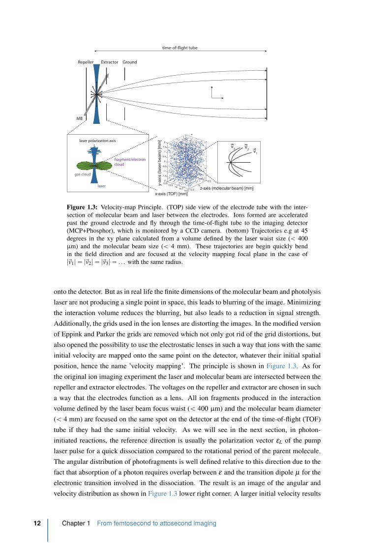
1.4 Schematic energy potential surface for translational spectroscopy . . . . . . . 13
1.5 Schematic pump-probe VMI setup . . . . . . . . . . . . . . . . . . . . . . . 15
1.6 Nested Newton spheres from photofragments A and B . . . . . . . . . . . . 16
1.7 Experimental steps in photofragment imaging . . . . . . . . . . . . . . . . . 17
1.8 Photofragment spectroscopy – angular distribution . . . . . . . . . . . . . . 19
1.9 Photoelectron spectra of NO at various ionization wavelength . . . . . . . . . 20
1.10 Schematic drawing of the experimental vacuum setup . . . . . . . . . . . . . 22
1.11 High harmonic spectrum . . . . . . . . . . . . . . . . . . . . . . . . . . . . 24
1.12 The three step model of HHG . . . . . . . . . . . . . . . . . . . . . . . . . . 25
1.13 Regimes of strong-field ionization. . . . . . . . . . . . . . . . . . . . . . . . 26
1.14 Regimes of strong-field ionization 2. . . . . . . . . . . . . . . . . . . . . . . 27
1.15 Calculated electron trajectories after ionization of argon . . . . . . . . . . . . 29
1.16 Predicted and observed HHG phase-matching cutoffs. . . . . . . . . . . . . . 31
1.17 Temporal and spectral structure of HHG emission . . . . . . . . . . . . . . . 32
1.18 High harmonic phase matching conditions . . . . . . . . . . . . . . . . . . . 36
1.19 HHG saturation due to reabsorption . . . . . . . . . . . . . . . . . . . . . . 38
1.20 The HHG far-field spatial profile . . . . . . . . . . . . . . . . . . . . . . . . 39
1.21 Schematic high harmonic spectroscopy setup . . . . . . . . . . . . . . . . . 41
2.1 The UV absorption spectrum of ClN3. . . . . . . . . . . . . . . . . . . . . . 51
2.2 Velocity-map imaging evidence for cyclic-N3 formation. . . . . . . . . . . . 52
2.3 Energy threshold of slow Cl production . . . . . . . . . . . . . . . . . . . . 53
2.4 Energy-level diagram for the Cl-N-N-N system. . . . . . . . . . . . . . . . . 54
2.5 Molecular plane of ClN3 . . . . . . . . . . . . . . . . . . . . . . . . . . . . 55
2.6 ClN3 and N3 molecular structure . . . . . . . . . . . . . . . . . . . . . . . . 56
2.7 ClN3 excitation schemes at 268 and 201 nm. . . . . . . . . . . . . . . . . . . 57
2.8 Schematic fs-UV-VMI setup. . . . . . . . . . . . . . . . . . . . . . . . . . . 58
2.9 Laser spectra . . . . . . . . . . . . . . . . . . . . . . . . . . . . . . . . . . 60
2.10 VMI alignment . . . . . . . . . . . . . . . . . . . . . . . . . . . . . . . . . 61
2.11 Schematic reactor setup for the ClN3-production. . . . . . . . . . . . . . . . 63
2.12 ClN3 image analyis . . . . . . . . . . . . . . . . . . . . . . . . . . . . . . . 64

2.13 Schematic drawing of the new implemented acquisition statistic . . . . . . . 65
2.14 Time-of-flight mass spectrum of ClN3. . . . . . . . . . . . . . . . . . . . . . 67
2.15 Integrated ion signals of all ClN3 fragments in parallel. . . . . . . . . . . . . 68
2.16 Fit parameters for the integrated ion signals of all ClN3 fragments in parallel . 70
2.17 Integrated ion signals of all ClN3 fragments in perpendicular. . . . . . . . . . 71
2.18 Fit parameters for the integrated ion signals of all ClN3 fragments in perpen-
dicular . . . . . . . . . . . . . . . . . . . . . . . . . . . . . . . . . . . . . . 72
2.19 Translational energy release (TER) the co-fragments Cl and N3 at 1 ps. . . . . 73
2.20 Translational energy release TER of the fragment N3 at 268 and 201 nm as
function of the pump-probe delay . . . . . . . . . . . . . . . . . . . . . . . . 75
2.21 Time dependences of the N3 fragments at 268 and 201 nm . . . . . . . . . . 76
2.22 Time dependences of the lower energetic components . . . . . . . . . . . . . 77
2.23 Angular distribution anlysis . . . . . . . . . . . . . . . . . . . . . . . . . . . 79
2.24 Anisotropy parameter β2 as function of the time delay at 268 and 201 nm . . 80
2.25 Translational energy release TER of the fragment Cl at 268 and 201 nm as
function of the pump-probe delay . . . . . . . . . . . . . . . . . . . . . . . . 83
2.26 Time dependences of the Cl fragments at 268 and 201 nm . . . . . . . . . . . 84
2.27 Translational energy release TER and angular distribution of the fragment Cl
at 201 nm . . . . . . . . . . . . . . . . . . . . . . . . . . . . . . . . . . . . 85
2.28 Abnormality of the chlorine fragment at 268 nm with an perpendicular 803
nm probe pulse . . . . . . . . . . . . . . . . . . . . . . . . . . . . . . . . . 86
2.29 Pump pulse configuration in the case of an perpendicular 803 nm probe pulse
in respect to the molecular plane of ClN3 selected by the first 268 nm pump
pulse. . . . . . . . . . . . . . . . . . . . . . . . . . . . . . . . . . . . . . . 87
2.30 Schematic potential energy surface diagram for the 21A1 and 21A2 states . . . 88
2.31 Secondary dissociation pathways of ClN3 . . . . . . . . . . . . . . . . . . . 89
2.32 Abel inverted VMI images and kinetic energy distributions (KER) of N, N2
and NCl . . . . . . . . . . . . . . . . . . . . . . . . . . . . . . . . . . . . . 90
3.1 Structure of TTF and TTF` . . . . . . . . . . . . . . . . . . . . . . . . . . . 97
3.2 Absorption and photo-electron spectrum of TTF . . . . . . . . . . . . . . . . 98
3.3 Schematic fs-UV-VIS VMI setup . . . . . . . . . . . . . . . . . . . . . . . . 99
3.4 Different experimental pump-probe excitation schemes for TTF . . . . . . . 100
3.5 Femtosecond time-resolved transients of TTF` as function of the pump pulse
wavelength with a probe pulse centered at 266 nm. . . . . . . . . . . . . . . 102
3.6 Photoelectron kinetic energy distribution of TTF` at 317 + 267 nm . . . . . . 103
3.7 Femtosecond time-resolved transient TTF` at 317 + 398 nm . . . . . . . . . 104
3.8 Photoelectron kinetic energy distribution of TTF` at 318 + 398 nm as a func-
tion of the pump-probe delay . . . . . . . . . . . . . . . . . . . . . . . . . . 105
3.9 Mass spectra of TTF at 318 + 800 nm . . . . . . . . . . . . . . . . . . . . . 106
3.10 Time-resolved transients of different cations of TTF at 317 + 800 nm . . . . . 107
3.11 Photoelectron image of TTF recorded with an intense 808 nm fs pulse . . . . 108
3.12 Breakdown diagram for the dissociation of ionized TTF . . . . . . . . . . . . 111
3.13 Simplified model for the dissociation of ionized TTF based on observations of
the breakdown diagram. . . . . . . . . . . . . . . . . . . . . . . . . . . . . . 112
3.14 Threshold photoionization TOF distributions for the m/z = 159 peak as a func-
tion of photon energy . . . . . . . . . . . . . . . . . . . . . . . . . . . . . . 113
3.15 Modified breakdown diagram of TTF . . . . . . . . . . . . . . . . . . . . . 114
xxii List of Figures
4.1 Sulfur hexafluoride structure . . . . . . . . . . . . . . . . . . . . . . . . . . 123
4.2 Summary of high-order harmonic spectroscopy experiments done on SF6 . . 124
4.3 HeII photoelectron spectrum of SF6 . . . . . . . . . . . . . . . . . . . . . . 126
4.4 Graphical illustration of the calculated tunnel ionization probability . . . . . 128
4.5 Simple theoretical study of HHG emission from SF6 . . . . . . . . . . . . . 129
4.6 The absolute photoioniation cross section and photoionization quantum effi-
ciency of SF6 . . . . . . . . . . . . . . . . . . . . . . . . . . . . . . . . . . 130
4.7 Schematic diagram of the two-well potential of SF6 . . . . . . . . . . . . . . 131
4.8 Normal modes of the vibration of SF6 . . . . . . . . . . . . . . . . . . . . . 133
4.9 Principle of strong field transient grating spectroscopy . . . . . . . . . . . . 135
4.10 Schematic diagram of the TGS setup . . . . . . . . . . . . . . . . . . . . . . 136
4.11 Transient grating image analysis . . . . . . . . . . . . . . . . . . . . . . . . 137
4.12 Integrated signal of the first order diffraction of the TG as function of pump-
probe time delay . . . . . . . . . . . . . . . . . . . . . . . . . . . . . . . . 139
4.13 Amplitude, area, and bandwidth of the vibrational modes in SF6 . . . . . . . 140
4.14 Phase of the temporal FFT of the time resolved oscillations in the TG setup . 141
4.15 Principle of the two XUV source setup . . . . . . . . . . . . . . . . . . . . . 143
4.16 Schematic setup of the two HHG sources interferometry setup . . . . . . . . 144
4.17 Two HHG source alignment . . . . . . . . . . . . . . . . . . . . . . . . . . 145
4.18 Two HHG source image analysis . . . . . . . . . . . . . . . . . . . . . . . . 146
4.19 Spatial Fourier-transform (amplitude (SA) and phase (SP)) of the HHG fringe
pattern as a function of pump-probe delay . . . . . . . . . . . . . . . . . . . 147
4.20 Amplitude of the tFFT of the spatial amplitude and phase . . . . . . . . . . . 148
4.21 Amplitude, area, and bandwidth of the vibrational modes in SF6 observed in
the two HHG source setup . . . . . . . . . . . . . . . . . . . . . . . . . . . 149
4.22 Phase of SA and SP as function of the harmonic order from the two HHG
source setup . . . . . . . . . . . . . . . . . . . . . . . . . . . . . . . . . . . 150
5.1 Schematic diagram of the fs-VUV HHG spectrometer . . . . . . . . . . . . . 159
5.2 The different configurations of the HHG selection chamber . . . . . . . . . . 161
5.3 Harmonic spectra generated with an 800 nm driving laser in krypton, argon
and Acetylen. . . . . . . . . . . . . . . . . . . . . . . . . . . . . . . . . . . 164
5.4 Internal quantum efficiency of the photodiode VUV-100 from OSI Optoelec-
tronics . . . . . . . . . . . . . . . . . . . . . . . . . . . . . . . . . . . . . . 165
5.5 Photoelectron spectrum of argon obtained with a harmonic spectrum produced
in krypton . . . . . . . . . . . . . . . . . . . . . . . . . . . . . . . . . . . . 168
5.6 Scheme of the electron spectra generated with the RABBITT-technique . . . 170
5.7 Photoelectron spectrum in argon obtained by a VUV spectrum generated with
400 nm and and an extra 400 nm beam . . . . . . . . . . . . . . . . . . . . . 172
5.8 Integrated photoelectron signal of SB6, SB8 and H7 in argon as function of
the pump-probe delay . . . . . . . . . . . . . . . . . . . . . . . . . . . . . . 173
5.9 Photoelectron spectrum backgrounds of argon . . . . . . . . . . . . . . . . . 174
5.10 Vibrational modes of C2H2 in its three geometries . . . . . . . . . . . . . . . 179
5.11 Fluorescence excitation (a) and absorption (b) spectra of acetylene in the 150
- 100 nm region . . . . . . . . . . . . . . . . . . . . . . . . . . . . . . . . . 181
5.12 H atom fragment spectra from VUV photolysis of C2H2 . . . . . . . . . . . . 182
5.13 C2H2 excitation scheme . . . . . . . . . . . . . . . . . . . . . . . . . . . . . 183
5.14 Time-of-flight mass spectrum of C2H2 . . . . . . . . . . . . . . . . . . . . . 184
List of Figures xxiii
5.15 Photoelectron spectrum of acetylene obtained with the harmonic spectrum
generated at 400 nm in argon plus an extra 400 nm beam . . . . . . . . . . . 186
5.16 Integrated photoelectron signal of SB4, H5 and H7 in C2H2 . . . . . . . . . . 187
5.17 Spectrum of harmonic 3 (purple) overlapped with the absorption cross-section
of acetylene . . . . . . . . . . . . . . . . . . . . . . . . . . . . . . . . . . . 188
A.1 Setup of the femtosecond laser chain in Toulouse and Bordeaux . . . . . . . 202
A.2 Typical cavity setup of a KLM Ti:sapphire laser . . . . . . . . . . . . . . . . 203
A.3 Principle setup of a chirped pulse amplification (CPA) system . . . . . . . . . 204
A.4 Principle setup of an amplification system . . . . . . . . . . . . . . . . . . . 205
B.1 Velocity-map images, experimental data vs scientific important information. . 214
C.1 Angular distribution of a Newton sphere on the VMI detector with higher or-
ders of the Legendre polynomials . . . . . . . . . . . . . . . . . . . . . . . . 217
D.1 Calculated dipole phase . . . . . . . . . . . . . . . . . . . . . . . . . . . . . 222
xxiv List of Figures

List of Tables
1.1 Calibration factor for various repeller (extractor) set voltages determined on
the photoelectron spectra of NO with the typical resolution obtained from Fig-
ure 1.9 as ∆E at E. . . . . . . . . . . . . . . . . . . . . . . . . . . . . . . . 21
1.2 Calculation of the saturation energy (barrier suppression) for different rare gases 28
2.1 Ionization energies (Ip) for all fragments of ClN3 . . . . . . . . . . . . . . . 55
2.2 Utilized BBO crystals for the generation of third (268 nm) and fourth (201
nm) harmonic . . . . . . . . . . . . . . . . . . . . . . . . . . . . . . . . . . 59
2.3 Vibrational modes of ClN3 . . . . . . . . . . . . . . . . . . . . . . . . . . . 63
2.4 Anisotropy parameter β2 for linear and cyclic N3 . . . . . . . . . . . . . . . 81
2.5 Comparison of the extracted experimental values between the two co-fragments
N3 and Cl . . . . . . . . . . . . . . . . . . . . . . . . . . . . . . . . . . . . 85
3.1 Summary of the assignments of the excited states of TTF at 303 and 317 nm . 98
3.2 The maximum kinetic energies possibly for the photoelectron kinetic energy . 101
3.3 Summary of the different decay times measured on the parent molecule and
the fragments of TTF . . . . . . . . . . . . . . . . . . . . . . . . . . . . . . 107
4.1 Calculated tunnel ionization of the molecular orbitals of SF6 . . . . . . . . . 128
4.2 Summary of the photoelectron band assignments in SF6 . . . . . . . . . . . . 132
4.3 Harmonic yield in the undiffracted (m “ 0) and diffracted (m “ ˘1) signal and
harmonic modulation depth . . . . . . . . . . . . . . . . . . . . . . . . . . . 139
4.4 Harmonic modulation depths for SA and SP. . . . . . . . . . . . . . . . . . . 147
5.1 Estimation of the number of VUV photon per pulse in the HHG generation
zone and in the interaction region in the VMI. . . . . . . . . . . . . . . . . . 166
A.1 Characteristics of the femtosecond laser chain in Toulouse and Bordeaux . . . 203
E.1 Cs point group character and product table. . . . . . . . . . . . . . . . . . . . 225
E.2 C2v point group character and product table . . . . . . . . . . . . . . . . . . 225
E.3 C2h point group character and product table . . . . . . . . . . . . . . . . . . 225
E.4 D3h point group character and product table . . . . . . . . . . . . . . . . . . 226
E.5 D8h point group character and product table . . . . . . . . . . . . . . . . . . 226
E.6 Oh point group character and product table . . . . . . . . . . . . . . . . . . . 227

List of Abbreviations
as attosecond, 10´18 seconds
ATAS absorption transient attosecond
spectroscopy
ATI above threshold ionization
BBO Beta-Barium Borate, β -
BaB2O4
BSI barrier-suppressed ionization
CCD charged coupled devide
CEP carrier envelope phase
CI conical intersection
CMB crossed molecular beams
CPL chirped pulse amplification
CRATI channel resolved above thresh-
old ionization
cw continuous wave
ENLOS extreme nonlinear optical spec-
troscopy
EUV extreme ultra-violet
FEL free-electron laser
fs femtosecond, (10´15sec)
FTL Fourier-transform limited
FWHM full width at half maximum
GDD group delay dispersion
HEF high energy form
HHG high-order harmonic generation
HOMO highest occupied molecular or-
bital
HX harmonix X, i.e. H5 = harmonic
5
Ip ionization potential (IP) or ion-
ization energy (IE)
iPEPICO imaging photo- electron pho-
toion coincidence spectroscopy
IR infrared
KER kinetic energy release
KLM Kerr-lens mode locking
LUMO lowest unoccupied molecular
orbital
MB molecular beam
MCP micro channel plate
MI multiphoton ionization
MSX intersystem crossing
NOPA nonlinear optical parametric
amplification
ns nanosecond, 10´12 seconds
ps picosecond, 10´12 sec.
REMPI resonance enhanced multipho-
ton ionization
SAE single active electron approxi-
mation
SB side band
SFA strong field approximation
TDSE time-dependent Schrodinger
equation
TER translational energy release
TI tunnel ionization
Ti:Sa Titanium-Sapphire
TKER total kinetic energy release
TOF time-of-flight
TOF-MS Wiley-McLaren time-of-flight
mass spectrometer
TS transition state
VMI velocity-map imaging
VUV vacuum ultra-violet
XUV = EUV


Introduction
The gaps between the fields of physics, chemistry, and biology are bridged by the motion
of molecules in complex structures, atoms in molecules, and electrons within atoms and
molecules [1]. Diverse tools appeared in the last decades which have enabled the direct prob-
ing of time-averaged, static structure of matter, such as electron and neutron diffraction, X-ray
absorption and diffraction, NMR spectroscopy and electron microscopy [2]. Using these tech-
niques it is possible to determine three-dimensional structures with atomic scale resolution.
However, to form a complete understanding of chemical reactions, phase transitions, or bi-
ological functions, the actual events have to be resolved in real-time. These changes follow
different timescales and proceed through different transition states and intermediates. These
dynamics and structural changes are naturally linked through the laws of quantum mechan-
ics [1]. For example, the solution of the Schrodinger equation for a particle’s wave function
yields an oscillatory motion with the oscillation period Tosc “ 2πph∆Eq where ∆E is the en-
ergy difference between two eigenstates. The larger the energy separation between the two
eigenstates, the faster is the particle’s motion in the superposition state. The energy spacing
and the change from one state to another is closely connected with the absorption and emission
of photons. The energy spacing of vibrational energy levels is on the order of tenth to several
hundred milli-electron volts for instance, which implies that molecular vibrations occur on a
timescale of tens to hundreds of femtoseconds (fs = 10´15 sec, 0.000 000 000 000 001 seconds
or one quadrillionth, or one millionth of one billionth, of a second). This defines the character-
istic timescale for the motion of atoms in a molecule, including those resulting in irreversible
structural changes during chemical reactions like isomerization.
The invention of short pulsed laser systems provided the possibility of detecting these pro-
cesses in real time. Spectroscopy, mass spectrometry, and diffraction techniques play the
modern day role of ‘ultrahigh-speed photography’ in the investigation of molecular processes
to capture the involved steps. One of the earliest examples of high-speed photography exper-
iments was the ‘horse in motion’ in 1878 by Eadweard Muybridge. Using a row of cameras
with tripwires, he was bale to capture the motion of a galloping horse. In a sense this is consid-
ered the birth of photographic studies of motion and motion-picture projection. Since nuclear
motion within molecules occurs on a femtosecond timescale, femtosecond lasers have the ap-
propriate ‘shutter speed’ to capture the evolution of important nuclear rearrangements such as
LASER LIGHT UPCONVERTED LIGHT (HHG)
100 keV10 keV1 keV10 eV 100 eV1 eV100 meV
0.1 Å1 Å1 nm100 nm 10 nm1 μm10 μm
MID-IRNEAR-IR
NEAR-UVVACUUM-UV
EXTREME-UV
SOFT X-RAYSHARD X-RAYS
E [eV]
λ
GAMMA-RAYSMICROWAVES
700 nm 400 nm500 nm600 nm750 nm
VISIBLE REGION
RADAR
100 μm1mm 0.01 Å
1 MeV10 meV1 meV
RADIO COSMIC-RAYS
Electronic motion on atomic / molecular scalesAtomic motion on
molecular scales
106103110-3
zepto10-21
atto10-18
femto10-15
pico10-12
T [sec]
T [attosec]110100100010000
Motion of individual electrons in
inner shellouter shells / valence bandconduction band
102510231021Density of free electrons [cm-3]
Collective motion of free electrons in
fusion mattersolid matter / biomoleculesionized matter
Nucleonic motion
within the nuclei
1 keV2 eV 2 keV4 eV 6 eV 200 eV
VUV VUV
EUV
X-RAYS
NEAR_IR
MID_IR
phase matching
up to >11th order
phase matching
up to >101st order
phase matching
up to > 5001st order
λ = 0.3 μm
λ = 0.8 μm
λ = 3.9 μm
hig
h-o
rder
harm
onic
genera
tion
ele
ctr
om
agentic s
pectr
um
energ
y a
nd tim
escale
connection
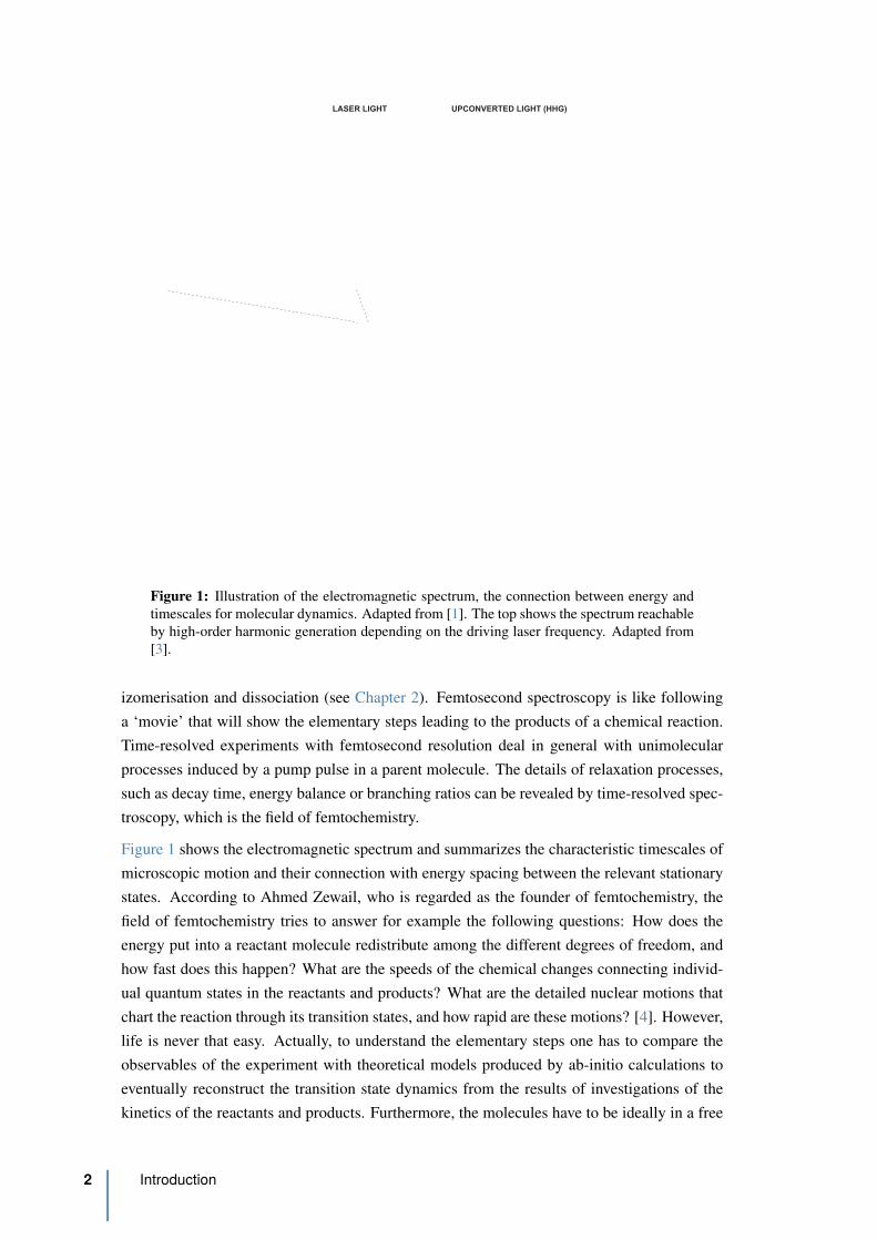
Figure 1: Illustration of the electromagnetic spectrum, the connection between energy and
timescales for molecular dynamics. Adapted from [1]. The top shows the spectrum reachable
by high-order harmonic generation depending on the driving laser frequency. Adapted from
[3].
izomerisation and dissociation (see Chapter 2). Femtosecond spectroscopy is like following
a ‘movie’ that will show the elementary steps leading to the products of a chemical reaction.
Time-resolved experiments with femtosecond resolution deal in general with unimolecular
processes induced by a pump pulse in a parent molecule. The details of relaxation processes,
such as decay time, energy balance or branching ratios can be revealed by time-resolved spec-
troscopy, which is the field of femtochemistry.
Figure 1 shows the electromagnetic spectrum and summarizes the characteristic timescales of
microscopic motion and their connection with energy spacing between the relevant stationary
states. According to Ahmed Zewail, who is regarded as the founder of femtochemistry, the
field of femtochemistry tries to answer for example the following questions: How does the
energy put into a reactant molecule redistribute among the different degrees of freedom, and
how fast does this happen? What are the speeds of the chemical changes connecting individ-
ual quantum states in the reactants and products? What are the detailed nuclear motions that
chart the reaction through its transition states, and how rapid are these motions? [4]. However,
life is never that easy. Actually, to understand the elementary steps one has to compare the
observables of the experiment with theoretical models produced by ab-initio calculations to
eventually reconstruct the transition state dynamics from the results of investigations of the
kinetics of the reactants and products. Furthermore, the molecules have to be ideally in a free
2 Introduction

environment, for instance produced in gas phase. Now the main puzzling question is how to
detect such drastic nuclear changes and what will be the observables in gas phase. On even
shorter timescales than the motion of atoms and molecules is the motion of electrons. The
characteristic timescales for the motion of one or several electrons and for the collective mo-
tion of an electronic ensemble are shown in Figure 1. Atomic distances are on the order of a
few Angtrom and therefore one obtains oscillation periods of valence electron wave packets
in bound atomic or molecular systems on the order of a few to hundreds of attoseconds (as
= 10´18 sec.) [1]. As femtochemisty is the science of the motion of atoms and molecules,
attosecond physics is the science of the motion of electrons. To produce light pulses in the
attosecond regime one has to go to photon energies with 100 eV up to keV, meaning to the
ultraviolet and vacuum ultraviolet region in the electromagnetic spectrum. This is where high-
order harmonic generation comes into the picture as a tool to upconvert the near-IR femtosec-
ond laser light into the VUV or even up to the soft X-ray region.
In this manuscript, two pump-probe techniques with two different observables are developed;
one based on the traditional femtochemistry and one based on high-order harmonic generation.
Generally, pump-probe experiments using two femtosecond laser pulses, the relative delay
between them will be the main controllable of the experiment. The pump pulse switches on
dynamics by fulfilling a resonance. This first laser light-molecule interaction determines time
‘zero’ with the precision of the pump pulse duration by generating a wave packet that will start
to oscillate and/or relax over time. The resonances presented in this manuscript are mostly
electronic resonances (excitation in the UV range, see Chapter 2, Chapter 3 and Chapter 5)
and vibrational resonances (Raman excitation in the IR, see Chapter 4). The probe pulse is the
second light-molecule interaction that will produce the observable. The most important issue
in such pump-probe experiments is to detect the wave packet created by the pump whatever
the potential surfaces on which it evolves. One of most widely used probe steps in gas-phase
studies is ionization, since ions can be readily detected. Two kinds of ionization are used
in this manuscript. The first type is the traditional ionization with observables such as the
angular and energy distributions of the products of ionization (electrons, parent ions, ionized
fragments). The energy and angular distributions of photoelectrons and photofragments are
recorded through an imaging technique collecting charged particals, in particular velocity-
map imaging (VMI). Ionization potentials (Ip) for the parent molecules are in general larger
than 7 eV and even higher for the fragments. These high energies have been reached up to
now by multiphoton ionization (see Chapter 2) with the unavoidable complication related to
resonances and weak efficiencies. This has motivated the development of a universal ionization
technique, namely a fs-VUV pulse which will be addressed in Chapter 5. The second type of
ionization uses tunnel ionization with its main observable being the XUV emission produced
by the recombination of the electron emitted by the cationic core. This process is called
high-order harmonic generation which can be described in three steps (the three step model):
tunnel ionization, acceleration of the the electron in the continuum dressed by the intense laser
field and then recombination with XUV emission. This new pump-probe femtochemistry is
based on XUV photon detection and is attractive due to its phase sensitivity compared to VMI
detection. A key ingredient in this all-optical technique has been the tunnel ionization by a
3
strong laser field with the prevailing approximation that only one electron – the less bound one
to the cation (HOMO = highest occupied molecular orbital) – is emitted by tunnel ionization.
Furthermore, any dynamics in the cation or effects by the strong laser field on the cationic
core during the high-order harmonic generation process are generally disregarded, and will be
addressed in Chapter 4.
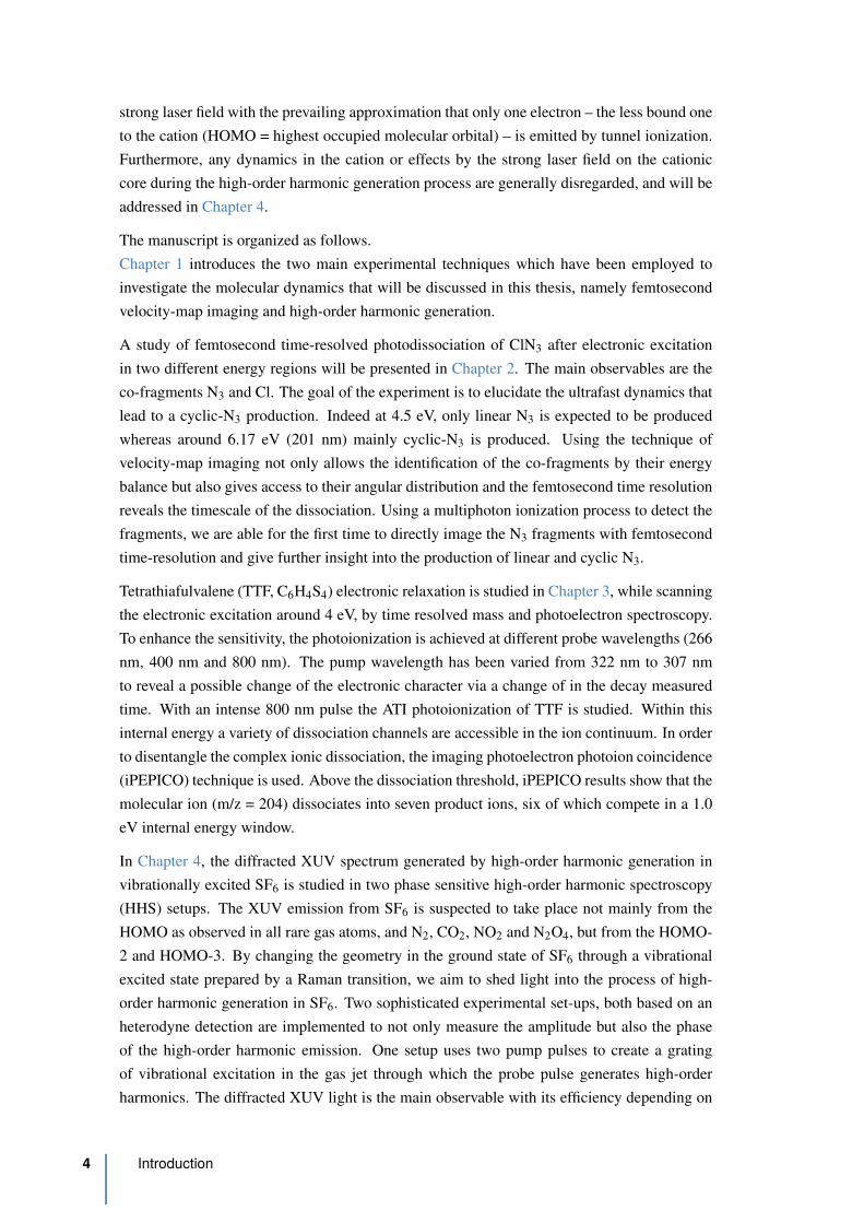
The manuscript is organized as follows.
Chapter 1 introduces the two main experimental techniques which have been employed to
investigate the molecular dynamics that will be discussed in this thesis, namely femtosecond
velocity-map imaging and high-order harmonic generation.
A study of femtosecond time-resolved photodissociation of ClN3 after electronic excitation
in two different energy regions will be presented in Chapter 2. The main observables are the
co-fragments N3 and Cl. The goal of the experiment is to elucidate the ultrafast dynamics that
lead to a cyclic-N3 production. Indeed at 4.5 eV, only linear N3 is expected to be produced
whereas around 6.17 eV (201 nm) mainly cyclic-N3 is produced. Using the technique of
velocity-map imaging not only allows the identification of the co-fragments by their energy
balance but also gives access to their angular distribution and the femtosecond time resolution
reveals the timescale of the dissociation. Using a multiphoton ionization process to detect the
fragments, we are able for the first time to directly image the N3 fragments with femtosecond
time-resolution and give further insight into the production of linear and cyclic N3.
Tetrathiafulvalene (TTF, C6H4S4) electronic relaxation is studied in Chapter 3, while scanning
the electronic excitation around 4 eV, by time resolved mass and photoelectron spectroscopy.
To enhance the sensitivity, the photoionization is achieved at different probe wavelengths (266
nm, 400 nm and 800 nm). The pump wavelength has been varied from 322 nm to 307 nm
to reveal a possible change of the electronic character via a change of in the decay measured
time. With an intense 800 nm pulse the ATI photoionization of TTF is studied. Within this
internal energy a variety of dissociation channels are accessible in the ion continuum. In order
to disentangle the complex ionic dissociation, the imaging photoelectron photoion coincidence
(iPEPICO) technique is used. Above the dissociation threshold, iPEPICO results show that the
molecular ion (m/z = 204) dissociates into seven product ions, six of which compete in a 1.0
eV internal energy window.
In Chapter 4, the diffracted XUV spectrum generated by high-order harmonic generation in
vibrationally excited SF6 is studied in two phase sensitive high-order harmonic spectroscopy
(HHS) setups. The XUV emission from SF6 is suspected to take place not mainly from the
HOMO as observed in all rare gas atoms, and N2, CO2, NO2 and N2O4, but from the HOMO-
2 and HOMO-3. By changing the geometry in the ground state of SF6 through a vibrational
excited state prepared by a Raman transition, we aim to shed light into the process of high-
order harmonic generation in SF6. Two sophisticated experimental set-ups, both based on an
heterodyne detection are implemented to not only measure the amplitude but also the phase
of the high-order harmonic emission. One setup uses two pump pulses to create a grating
of vibrational excitation in the gas jet through which the probe pulse generates high-order
harmonics. The diffracted XUV light is the main observable with its efficiency depending on
4 Introduction
the geometry of SF6. The second experiment uses two spatially separated probe pulses, both
generating a XUV beam which interfere spatially in far field. The interferences in amplitude
and phase carry information about the vibrational excitations induced by the a pump pulse
overlapped with only one of the two probes.
Chapter 5 makes a link between Chapter 2 / Chapter 3 and Chapter 4, since here the high-order
harmonic emission is used as a secondary source lying in the XUV range to realize a universal
detection scheme. For this a new XUV spectrometer was built and coupled to a velocity-map
imaging spectrometer. After a description and characterization of the new setup the first time-
resolved ionization made on Argon and C2H2 are presented. Here the observables are sideband
photoelectrons that are produced by two quantum paths involving different resonances.
The thesis concludes with a summary about the presented work and a discussion about future
implications and perspectives.
References
[1] Krausz, F. Attosecond physics. Rev. Mod. Phys. 81:1 163–234 (2009) (cited p. 1–3).
[2] Zewail, AH. The new age of structural dynamics. Acta Cryst. 66:2 135–136 (2010)
(cited p. 1).
[3] Popmintchev, T, Chen, MC, Popmintchev, D, Arpin, P, Brown, S, Alisauskas, S, An-
driukaitis, G, Balciunas, T, Mucke, OD, Pugzlys, A, Baltuska, A, Shim, B, Schrauth,
SE, Gaeta, A, Hernandez-Garcia, C, Plaja, L, Becker, A, Jaron-Becker, A, Murnane,
MM, and Kapteyn, HC. Bright Coherent Ultrahigh Harmonics in the keV X-ray Regime
from Mid-Infrared Femtosecond Lasers. Science 336:6086 1287–1291 (2012) (cited
p. 2).
[4] Zewail, AH. Femtochemistry: Atomic-scale dynamics of the chemical bond. J. Phys.
Chem. A 104:24 5660–5694 (2000) (cited p. 2).
References 5


1
From femtosecond to attosecond imaging
Contents
1.1 Introduction . . . . . . . . . . . . . . . . . . . . . . . . . . . . . . . . . . . 8
1.1.1 Imaging in molecular dynamics . . . . . . . . . . . . . . . . . . . . 8
1.1.2 Photoinduced Dynamics and the pump-probe technique . . . . . . . . 9
1.2 Velocity-map imaging . . . . . . . . . . . . . . . . . . . . . . . . . . . . . . 11
1.2.1 Introduction . . . . . . . . . . . . . . . . . . . . . . . . . . . . . . . 11
1.2.2 Newton spheres and the VMI experiment . . . . . . . . . . . . . . . 13
1.2.3 Back conversion of 2D projected images to Newton spheres . . . . . 16
1.2.4 Energy and Angular Distributions . . . . . . . . . . . . . . . . . . . 17
1.2.5 VMI calibration . . . . . . . . . . . . . . . . . . . . . . . . . . . . . 20
1.2.6 The VMI vacuum system . . . . . . . . . . . . . . . . . . . . . . . . 21
1.3 High-order harmonic generation . . . . . . . . . . . . . . . . . . . . . . . 23
1.3.1 The three step model: a quasi classical description of HHG . . . . . . 23
1.3.2 The quantum model of HHG . . . . . . . . . . . . . . . . . . . . . . 33
1.3.3 Macroscopic high harmonic generation, phase matching and photon flux 34
1.3.4 HHG as extreme nonlinear optical spectroscopy . . . . . . . . . . . . 40
References . . . . . . . . . . . . . . . . . . . . . . . . . . . . . . . . . . . . . . . 42
Abstract
The chapter gives an introduction to the two main experimental setups used in this thesis
to investigate molecular dynamics, namely femtosecond velocity-map imaging and high-order
harmonic generation. After introducing the general concept of imaging in molecular dynamics
and the pump-probe technique in Section 1.1, Section 1.2 illustrates the fundamental concepts
of velocity-map imaging. In Section 1.3 the concept of high-order harmonic generation is
described.
Keywords: molecular dynamics, femtosecond, attosecond, photoinduced dynamics, pump-probe tech-
nique, velocity-map imaging, Newton spheres, Abel transformation, kinetic energy release, angular
distribution, high-order harmonic generation, three-step model, phase matching, extreme nonlinear op-
tical spectroscopy, fs-XUV spectroscopy

1.1 Introduction
1.1.1 Imaging in molecular dynamics
The technique of ion and electron imaging has become a versatile tool in the study of molecu-
lar dynamic processes [1] where most of these processes are simple two-body events that end
with the particles departing from each other with a fixed amount of kinetic and internal energy
and a fixed direction. The product angular (direction) and velocity (energy) distributions pro-
vide insight into some of the most basic chemical phenomena: the breaking and forming of
chemical bonds and is essential for a fundamental understanding of chemical reactivity. One
can distinguish two experimental directions in imaging molecular dynamics, crossed molecu-
lar beam (CMB) and photoinduced experiments:
1. Crossed molecular beam experiments (CMB) are studying bimolecular reactions [2]
or molecular scattering [3] as presented by the following reactions:
• bimolecular reactions: A + BC Ñ ABC˚ Ñ AB + C
• inelastic scattering: AB(v,J) + C Ñ ABC˚ Ñ AB(v1,J1) + C
where ABC˚ is a collision complex. CMB experiments, invented by Taylor and Daz
1955 [4, 5], were the first experiments used to measure the product angular and velocity
distributions. The basic principle underlying these experiments is very simple. Two
molecular beams containing the reactants are crossed, usually at right angles, reaction
occurs at the point of intersection, and products scattered at a particular angle are de-
tected by a mass spectrometer equipped with an electron-impact ion source. The flight
time from the crossing region to the detector yields the product velocity, and by step-
ping the detector through the possible scattering angles, the entire product velocity-angle
distribution may be obtained. The success of the research area of CMB reactions led to
the 1986 Nobel Prize in Chemistry to three of the leaders in this field, Dudley R Her-
schbach [6], Yuan T Lee [5, 7] and John C Polanyi [8, 9] for their incisive experimental
and interpretative work on the dynamics of elementary gas-phase reactions. However in
bimolecular reactions, the inherent distribution of the impact parameter leads to a dis-
tribution, in the picosecond domain, of the time (t=0) at which the reaction starts. To be
able to have access to dynamics on faster timescales this technique is not suitable.
2. Photoinduced molecular dynamic experiments are using light for photoionization
and photodissociation. After absorption of one or more photons a hypothetical bound
molecule AB can undergo the following reactions:
• photodissociation: AB + nhω Ñ AB˚ Ñ A + B
• photoionization: AB + nhω Ñ AB˚ Ñ AB` + e´
• dissociative ionization: AB + nhω Ñ AB˚ Ñ A` + B + e´
where AB˚ is photo-excited complex.
8 Chapter 1 From femtosecond to attosecond imaging
10-18
10-15
atto
1900 1950 2000
femto
pico
nano
micro
Year
1850
10-12
10-9
Pump-probe
spectroscopy
(Toepler)
Observation of
intermediates of
chemical reactions
(Norrish, Porter)
Real-time observation
of the breakage of a
chemical bond
(Zewail)
Real-time observation
of electronic motion
deep inside atoms
Optical synchronization
of pump and probe pulse
(Abraham and Lemoine)
Vibrational
period of H2
Str
uctu
ral d
yn
am
ics
Ele
ctr
on
ic d
yn
am
icsfa
ste
st
eve
nts
me
asu
red
[se
c]
10-6
Femtochemistry
Spark photography
Atosecond physics
pulsed lasers
HHG0.000 000 000 000 001 sec
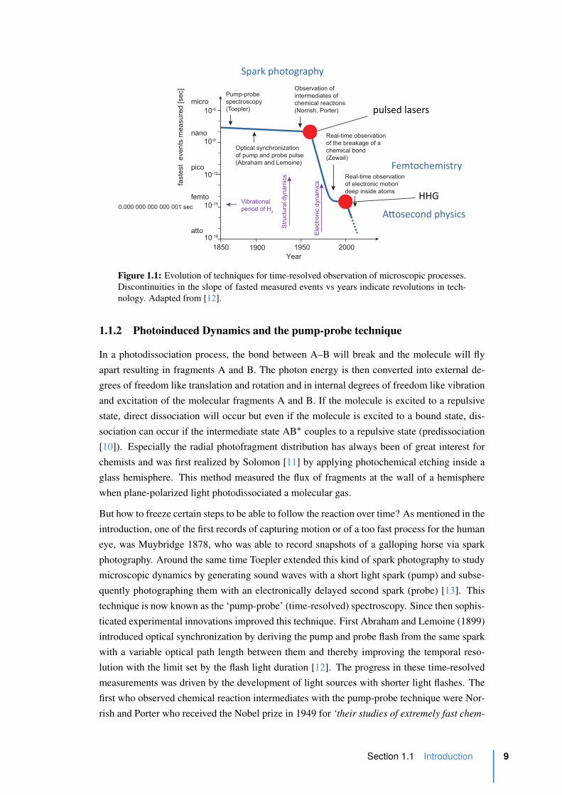
Figure 1.1: Evolution of techniques for time-resolved observation of microscopic processes.
Discontinuities in the slope of fasted measured events vs years indicate revolutions in tech-
nology. Adapted from [12].
1.1.2 Photoinduced Dynamics and the pump-probe technique
In a photodissociation process, the bond between A–B will break and the molecule will fly
apart resulting in fragments A and B. The photon energy is then converted into external de-
grees of freedom like translation and rotation and in internal degrees of freedom like vibration
and excitation of the molecular fragments A and B. If the molecule is excited to a repulsive
state, direct dissociation will occur but even if the molecule is excited to a bound state, dis-
sociation can occur if the intermediate state AB˚ couples to a repulsive state (predissociation
[10]). Especially the radial photofragment distribution has always been of great interest for
chemists and was first realized by Solomon [11] by applying photochemical etching inside a
glass hemisphere. This method measured the flux of fragments at the wall of a hemisphere
when plane-polarized light photodissociated a molecular gas.
But how to freeze certain steps to be able to follow the reaction over time? As mentioned in the
introduction, one of the first records of capturing motion or of a too fast process for the human
eye, was Muybridge 1878, who was able to record snapshots of a galloping horse via spark
photography. Around the same time Toepler extended this kind of spark photography to study
microscopic dynamics by generating sound waves with a short light spark (pump) and subse-
quently photographing them with an electronically delayed second spark (probe) [13]. This
technique is now known as the ‘pump-probe’ (time-resolved) spectroscopy. Since then sophis-
ticated experimental innovations improved this technique. First Abraham and Lemoine (1899)
introduced optical synchronization by deriving the pump and probe flash from the same spark
with a variable optical path length between them and thereby improving the temporal reso-
lution with the limit set by the flash light duration [12]. The progress in these time-resolved
measurements was driven by the development of light sources with shorter light flashes. The
first who observed chemical reaction intermediates with the pump-probe technique were Nor-
rish and Porter who received the Nobel prize in 1949 for ‘their studies of extremely fast chem-
Section 1.1 Introduction 9
pump probe
Δt =
excited state
population
2Δx
c
pump beam
probe beam
pathlength
adjustmentΔx
lens
target
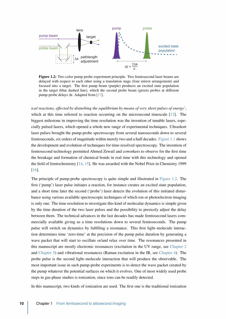
Figure 1.2: Two color pump-probe experiment principle. Two femtosecond laser beams are
delayed with respect to each other using a translation stage (four mirror arrangement) and
focused into a target. The first pump beam (purple) produces an excited state population
in the target (blue dashed line), which the second probe beam (green) probes at different
pump-probe delays ∆t. Adapted from [17].
ical reactions, effected by disturbing the equilibrium by means of very short pulses of energy’,
which at this time referred to reaction occurring on the microsecond timescale [12]. The
biggest milestone in improving the time resolution was the invention of tunable lasers, espe-
cially pulsed lasers, which opened a whole new range of experimental techniques. Ultrashort
laser pulses brought the pump-probe spectroscopy from several nanoseconds down to several
femtoseconds, six orders of magnitude within merely two and a half decades. Figure 1.1 shows
the development and evolution of techniques for time-resolved spectroscopy. The invention of
femtosecond technology permitted Ahmed Zewail and coworkers to observe for the first time
the breakage and formation of chemical bonds in real time with this technology and opened
the field of femtochemistry [14, 15]. He was awarded with the Nobel Prize in Chemistry 1999
[16].
The principle of pump-probe spectroscopy is quite simple and illustrated in Figure 1.2. The
first (‘pump’) laser pulse initiates a reaction, for instance creates an excited state population,
and a short time later the second (‘probe’) laser detects the evolution of this initiated distur-
bance using various available spectroscopic techniques of which ion or photoelectron imaging
is only one. The time resolution to investigate this kind of molecular dynamics is simple given
by the time duration of the two laser pulses and the possibility to presicely adjust the delay
between them. The technical advances in the last decades has made femtosecond lasers com-
mercially available giving us a time resolutions down to several femtoseconds. The pump
pulse will switch on dynamics by fulfilling a resonance. This first light–molecule interac-
tion determines time ‘zero-time’ at the precision of the pump pulse duration by generating a
wave packet that will start to oscillate or/and relax over time. The resonances presented in
this manuscript are mostly electronic resonances (excitation in the UV range, see Chapter 2
and Chapter 5) and vibrational resonances (Raman excitation in the IR, see Chapter 4). The
probe pulse is the second light–molecule interaction that will produce the observable. The
most important issue in such pump-probe experiments is to detect the wave packet created by
the pump whatever the potential surfaces on which it evolves. One of most widely used probe
steps in gas-phase studies is ionization, since ions can be readily detected.
In this manuscript, two kinds of ionization are used. The first one is the traditional ionization
10 Chapter 1 From femtosecond to attosecond imaging
with observables such as the angular and energy distributions of the products of ionization
(electrons, parent ions, ionized fragments). The energy and angular distributions of photoelec-
trons and photofragments are recorded through an imaging technique, in particular velocity-
map imaging (VMI) which will be described in the following section in more detail. This
method has enabled a number of remarkable advances over the past few years due to its simple
implementation for all polarities and to the 4π-steradian detection volume that compensates
the weak probability of pump-probe interactions. The second type of ionization uses tunnel
ionization with its main observable the XUV emission produced by the recombination of the
electron emitted by the cationic core. This is called high-order harmonic generation which can
be described in three steps (the three step model), with tunnel ionization, acceleration of the
the electron in the continuum dressed by the intense laser field and then recombination with
XUV emission and will be discussed in Section 1.3. In this second kind of probe step, the con-
dition on the laser is that it needs to be very short (ă30 fs) and very intense („1014W/cm2).
This new pump-probe femtochemistry is based on XUV photon detection and is attractive via
its phase sensitivity compared to VMI detection.
1.2 Velocity-map imaging
1.2.1 Introduction
The next step forward twenty years after the invention of ion imaging by Solomon [11] was
made by Chandler and Houston [18], introducing a technique in which the three-dimensional
spatial distribution of a photofragment, measured at a certain time after photodissociation,
is projected onto a two-dimensional surface (detector). This technique combined the use of
position sensitive ion detection with a Charge-Coupled Device (CCD), a camera, to provide
a more sensitive detection technique. The principle idea was to intersect a molecular beam
by a photolysis and a probe laser beam at a position between two electrostatic plates called
repeller and extractor. The photolysis laser (pump beam) ruptures the molecular bond, while
the probe laser ionizes the photofragment. The potential between the electrodes was such, that
the ion cloud was accelerated along the time-of-flight axis and compressed perpendicular to
it at the same time through a Wiley-McLaren Time-of-Flight Mass Spectrometer (TOF-MS)
[19] on to the detector so that all ions arrive at the position sensitive detector simultaneously
as a ‘pancake’. The detector consists of a pair of microchannel plates (MCP) coupled to a
phosphor screen. An ion hitting the MCP’s gives rise to a burst of electrons at the back face
(gain „106), which produces a flash of light when it strikes the phosphor screen. This can be
captures as an image by a CCD camera for processing and analysis in a PC.
This technique of ion imaging has been improved and modified by Eppink and Parker in 1997
[20] through the use of an electrostatic lens. This is now known as velocity-map imaging
(VMI), which constitutes a state-of-the-art spectroscopy method. The key improvement to the
imaging technique involves the ion optics used to direct ions towards the imaging detector.
In the original experiments, the repeller and extractor plates consisted of a pair of grids that
provided a uniform extraction field, ensuring a direct spatial mapping of photofragment ions
Section 1.2 Velocity-map imaging 11
gas cloud
laser
laser polarization axis
fragment/electroncloud
Repeller Extractor Ground
MB
time-of-ight tube
v2 v
1
v3
13.813.9
1414.1
14.2 -0.2
0
0.2-2
-1.5
-1
-0.5
0
0.5
1
1.5
2
z-axis (molecular beam) [mm]x-axis (TOF) [mm]
y-ax
is (l
aser
bea
m) [
mm
]
x
y
z
y
z
y
x
CCD
MCP Phosphore
|v2|
v2 v
1>
=|v1|
y
z
v2 v
1>
|v2|=|v
1|
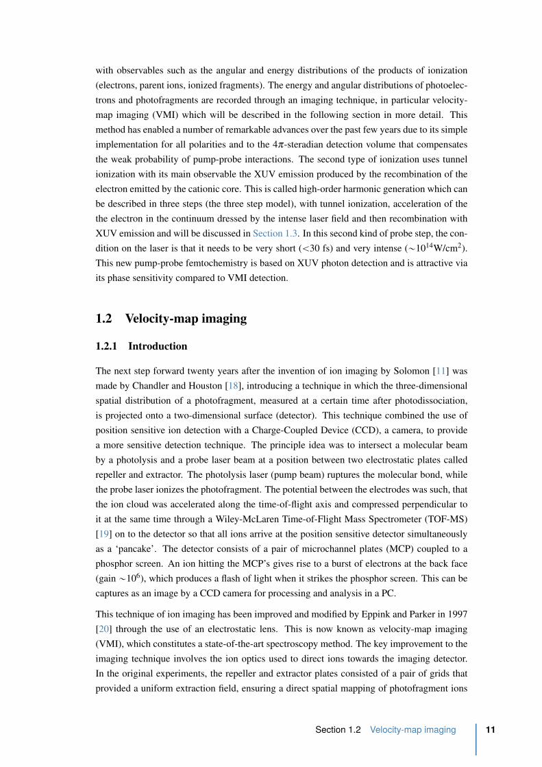
Figure 1.3: Velocity-map Principle. (TOP) side view of the electrode tube with the inter-
section of molecular beam and laser between the electrodes. Ions formed are accelerated
past the ground electrode and fly through the time-of-flight tube to the imaging detector
(MCP+Phosphor), which is monitored by a CCD camera. (bottom) Trajectories e.g at 45
degrees in the xy plane calculated from a volume defined by the laser waist size (ă 400
µm) and the molecular beam size (ă 4 mm). These trajectories are begin quickly bend
in the field direction and are focused at the velocity mapping focal plane in the case of
|~v1| “ |~v2| “ |~v3| “ . . . with the same radius.
onto the detector. But as in real life the finite dimensions of the molecular beam and photolysis
laser are not producing a single point in space, this leads to blurring of the image. Minimizing
the interaction volume reduces the blurring, but also leads to a reduction in signal strength.
Additionally, the grids used in the ion lenses are distorting the images. In the modified version
of Eppink and Parker the grids are removed which not only got rid of the grid distortions, but
also opened the possibility to use the electrostatic lenses in such a way that ions with the same
initial velocity are mapped onto the same point on the detector, whatever their initial spatial
position, hence the name ’velocity mapping’. The principle is shown in Figure 1.3. As for
the original ion imaging experiment the laser and molecular beam are intersected between the
repeller and extractor electrodes. The voltages on the repeller and extractor are chosen in such
a way that the electrodes function as a lens. All ion fragments produced in the interaction
volume defined by the laser beam focus waist (ă 400 µm) and the molecular beam diameter
(ă 4 mm) are focused on the same spot on the detector at the end of the time-of-flight (TOF)
tube if they had the same initial velocity. As we will see in the next section, in photon-
initiated reactions, the reference direction is usually the polarization vector εL of the pump
laser pulse for a quick dissociation compared to the rotational period of the parent molecule.
The angular distribution of photofragments is well defined relative to this direction due to the
fact that absorption of a photon requires overlap between ε and the transition dipole µ for the
electronic transition involved in the dissociation. The result is an image of the angular and
velocity distribution as shown in Figure 1.3 lower right corner. A larger initial velocity results
12 Chapter 1 From femtosecond to attosecond imaging
TERmax
A + BD
0
Internuclear distance, RA-B
Po
ten
tia
l E
ne
rgy
Repulsive
hv
μ(R)
AB
AB*
Figure 1.4: Schematic energy potential surface for translational spectroscopy. The trans-
lational energy release TER for a photolysis reaction AB ` hν Ñ A ` B is determined by
measuring the velocity of product A or B. Absorption strength is governed by the projec-
tion of the AB wave-function combined with the transition dipole moment function µpRq (an
arbitrary µpRq is shown) onto the repulsive excited state. Adapted from [17].
in a distribution further away from the center whereas the angular distributions comes from all
ions with the same initial velocity but different initial velocity directions.
1.2.2 Newton spheres and the VMI experiment
As mentioned before for photodissociation in general a ’pump-probe’ configuration is used. In
this case the photodissociation is initiated by the first ’pump’ laser and the photolysis reaction
can be written as
AB ` hω Ñ AB˚ Ñ Apv,Jq ` Bpv,Jq (1.1)
where hω is the photon energy used to dissociate and v and J are vibrational and rotational
quantum numbers of the molecular fragments. When a molecule AB, where A-B may be
polyatomic, absorbs a photon and undergoes fragmentation, both energy and momentum must
be conserved. A certain amount of energy is required to dissociate the bond, the so called
bond energy D0 as illustrated in the schematic potential energy surface plot in Figure 1.4.
Normally the photon energy will be higher than D0 and the remaining energy after dissociation
is released into translational and internal energy of the products as
hω ´ D0 “ Ei,A ` Ei,B ` T ER (1.2)
where Ei are the internal energies of the fragments A and B and T ER is the translational energy
release or total kinetic energy release (TKER) relative to the center of mass. Assuming A and
B are produced in the ground state with no internal energies gives us an upper limit for the
kinetic energy by:
T ERmax “ hω ´ D0. (1.3)
Section 1.2 Velocity-map imaging 13
The translational energy release in the center of mass frame is given by:
T ER “ 1
2µ 1v12
rel “ 1
2mAv2
A ` 1
2mBv2
B (1.4)
where mA, mB, vA and vB are the mass and velocity of the fragments A and B, respectively. µ 1
is the reduced mass and v1rel the relative velocity in the center of mass frame for the molecule
AB. Conservation of momentum given by
mA~vA ` mB~vB “ 0 (1.5)
results in the kinetic energy partitioning where the kinetic energy release (KER) of each frag-
ment is given by
KERA “ mB
mABT ER and KERB “ mA
mABT ER. (1.6)
In order to detect the fragments a second laser is used for ionization, the so called ’probe’
laser. The interaction of this probe laser for instance with fragment A can be written in the
same manner as
A ` hω Ñ A` ` e´ ` T ER (1.7)
The photoionization process with m´e ! mA and Eq. (1.6) results in a photoelectron receiving
essentially all the translational energy T ER, leaving the ion A` in the state defined by the
first ’pump’ laser process. Each photodissociation or photoionization event yields two partner
fragments flying with equal momentum in opposite directions in the centre-of-mass frame due
to the conservation of momentum. For a given photon energy and given product quantum states
(internal energies) the photofragment speeds (kinetic energy) are well defined. Repeating the
same event for many times, the fragments build up a spherical distributions in velocity space.
These are the so-called Newton (velocity) spheres for the process. The size of the Newton
sphere tells us about the balance of internal and translational energy in the reaction and the
surface pattern of the Newton sphere tells us about the electronic transitions involved in the
dissociation.
Figure 1.5 shows the schematic pump-probe VMI setup. The pump and probe laser pulses are
intersected with the molecular beam between the repeller and extractor. The newton spheres
of the ions are then velocity mapped on to a 2D position sensitive detector which consists of
a microchannel plate (MCP), a phosphor and a charged coupled device (CCD) camera. As
this sphere is pushed towards the detector it is magnified and squeezed and ends up as a 2D
projection of this 3D sphere on the detector. A single photodissociation event where mass A
ă mass B creates the Newton spheres shown in Figure 1.6. Over time, the photodissociation
will produce two nested spheres with a radii ratio of
RA
RB“
c
mA
mB(1.8)
The radius is directly proportional to the initial velocity in the yz-direction except for a mag-
14 Chapter 1 From femtosecond to attosecond imaging

CCD
Phosphore
MCP
TOF
Δt
R
E
G
Molecular Beam
Newton Sphere E
0
1
0
1
E
Abel Transformation
3D Slice
Integration
over angle
Radial distribution
E
pump pulse
probe pulse
polar plot
θ [degrees]
radiu
s [pix
el]
0 360
Integration
over Radius
Angular Distribution
180
θ [degrees]
Inte
nsity
2D Projection
y
x
z
μ-Metal
KER [eV]
Figure 1.5: Schematic pump-probe VMI setup. The left part shows the electrode system
with repeller (R), extrator (E) and ground (G) to accelerate the photo-products towards the
detector which consists of a microchannel plate (MCP) a phosphor and a charged-coupled-
device CCD to image the phosphor and to send a digitized picture to the PC. Two laser
pulses with a variable delay between them are intersected in the molecular beam between the
repeller end extractor electrodes. The time-of-flight (TOF) which is shielded by a µ-metal,
is in the µsec range and gives enough time to separate the fragments in mass and to stretch
the Newton spheres in the yz-plane. Consequently the 3D distribution of the photo products
in projected on to a 2D image on the detector, shown on the left. An Abel transformations
allows the reconstruction of the 3D distribution and by integrating this reconstructed image
over the angle and the radius one obtains the radial or energy distribution (KER) and the
angular distributions, respectively.
nification factor caused by the electric field component in the yz-direction and can be written
as
R “ Mvyzt (1.9)
where t is the time-of-flight and M a magnification factor [20]. The time-of-flight t is given by
the velocity in x direction (TOF-axis) and the length L of the TOF, which is in our case 42 cm.
vx is the velocity of the charged particle gained in the electric field given by vx “a
2V qm
where q is the charge and V the potential in which the charged particle is accelerated, which
is given by the potential difference of the repeller and extrator voltages (Vrep - Vex). If the
electric field component in the yz-direction is neglected and the acceleration region is small
compared to the total length L of the spectrometer (here 42 cm / 4 cm), the time-of-flight can
be written as
t « L
vx“ L
c
m
2qV(1.10)
From this one can get the relationship between the radius R and the initial kinetic energy KER
of the fragments, which is given by:
R “ ML
d
KER
qV“ α
?KER (1.11)
Section 1.2 Velocity-map imaging 15
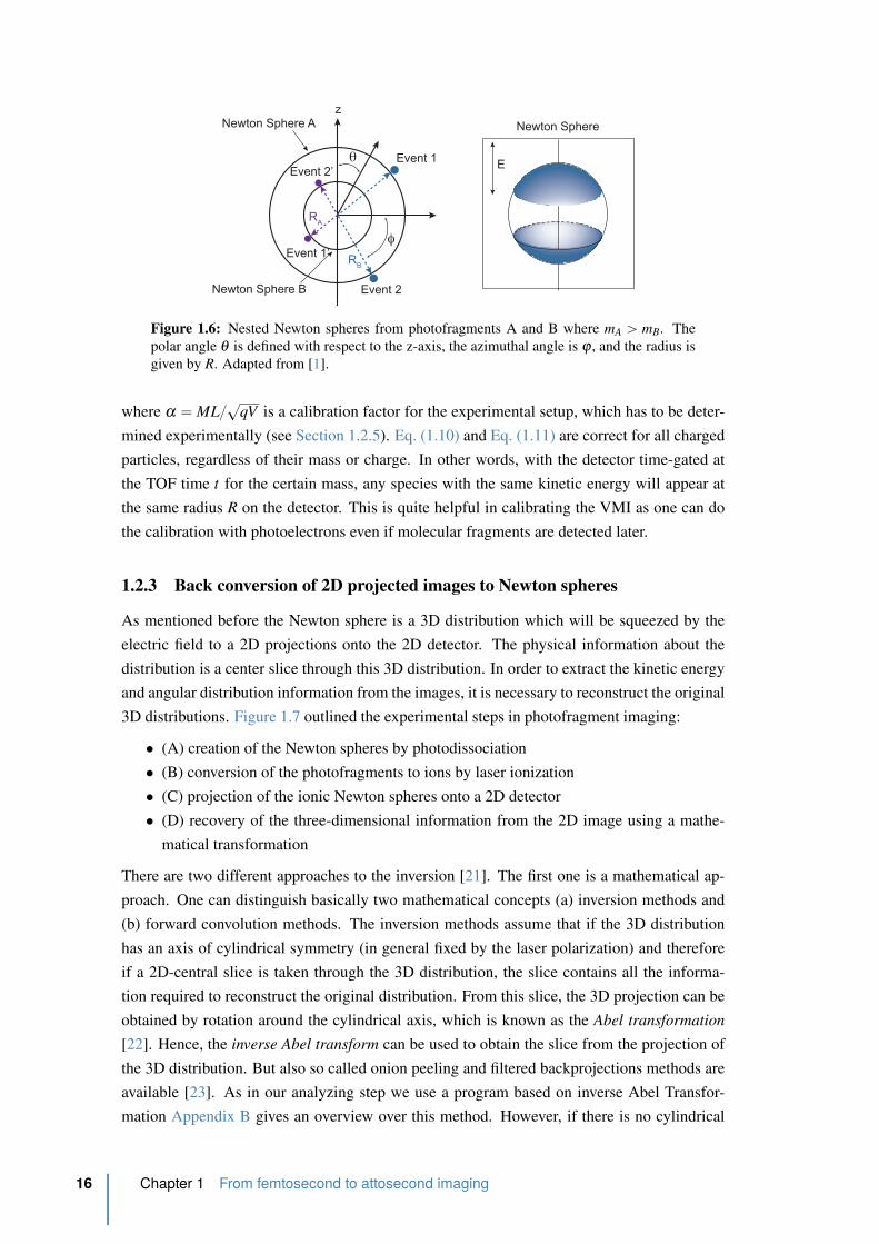
z
φ
θ Event 1
Event 2
RB
RA
Event 2’
Event 1’
Newton Sphere
E
Newton Sphere A
Newton Sphere B
Figure 1.6: Nested Newton spheres from photofragments A and B where mA ą mB. The
polar angle θ is defined with respect to the z-axis, the azimuthal angle is ϕ , and the radius is
given by R. Adapted from [1].
where α “ ML?qV is a calibration factor for the experimental setup, which has to be deter-
mined experimentally (see Section 1.2.5). Eq. (1.10) and Eq. (1.11) are correct for all charged
particles, regardless of their mass or charge. In other words, with the detector time-gated at
the TOF time t for the certain mass, any species with the same kinetic energy will appear at
the same radius R on the detector. This is quite helpful in calibrating the VMI as one can do
the calibration with photoelectrons even if molecular fragments are detected later.
1.2.3 Back conversion of 2D projected images to Newton spheres
As mentioned before the Newton sphere is a 3D distribution which will be squeezed by the
electric field to a 2D projections onto the 2D detector. The physical information about the
distribution is a center slice through this 3D distribution. In order to extract the kinetic energy
and angular distribution information from the images, it is necessary to reconstruct the original
3D distributions. Figure 1.7 outlined the experimental steps in photofragment imaging:
• (A) creation of the Newton spheres by photodissociation
• (B) conversion of the photofragments to ions by laser ionization
• (C) projection of the ionic Newton spheres onto a 2D detector
• (D) recovery of the three-dimensional information from the 2D image using a mathe-
matical transformation
There are two different approaches to the inversion [21]. The first one is a mathematical ap-
proach. One can distinguish basically two mathematical concepts (a) inversion methods and
(b) forward convolution methods. The inversion methods assume that if the 3D distribution
has an axis of cylindrical symmetry (in general fixed by the laser polarization) and therefore
if a 2D-central slice is taken through the 3D distribution, the slice contains all the informa-
tion required to reconstruct the original distribution. From this slice, the 3D projection can be
obtained by rotation around the cylindrical axis, which is known as the Abel transformation
[22]. Hence, the inverse Abel transform can be used to obtain the slice from the projection of
the 3D distribution. But also so called onion peeling and filtered backprojections methods are
available [23]. As in our analyzing step we use a program based on inverse Abel Transfor-
mation Appendix B gives an overview over this method. However, if there is no cylindrical
16 Chapter 1 From femtosecond to attosecond imaging
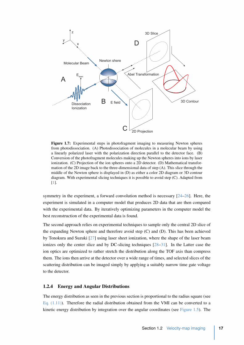
A
B
C
D
Dissociation
Ionization
E field
2D Projection
3D Slice
3D Contour
Molecular Beam
Elaser
x
z
y
Newton shere
Abel Transformation
Figure 1.7: Experimental steps in photofragment imaging to measuring Newton spheres
from photodissociation. (A) Photodissociation of molecules in a molecular beam by using
a linearly polarized laser with the polarization direction parallel to the detector face. (B)
Conversion of the photofragment molecules making up the Newton spheres into ions by laser
ionization. (C) Projection of the ion spheres onto a 2D detector. (D) Mathematical transfor-
mation of the 2D image back to the three-dimensional data of step (A). This slice through the
middle of the Newton sphere is displayed in (D) as either a color 2D diagram or 3D contour
diagram. With experimental slicing techniques it is possible to avoid step (C). Adapted from
[1].
symmetry in the experiment, a forward convolution method is necessary [24–26]. Here, the
experiment is simulated in a computer model that produces 2D data that are then compared
with the experimental data. By iteratively optimizing parameters in the computer model the
best reconstruction of the experimental data is found.
The second approach relies on experimental techniques to sample only the central 2D slice of
the expanding Newton sphere and therefore avoid step (C) and (D). This has been achieved
by Tonokura and Suzuki [27] using laser sheet ionization, where the shape of the laser beam
ionizes only the center slice and by DC-slicing techniques [28–31]. In the Latter case the
ion optics are optimized to rather stretch the distribution along the TOF axis than compress
them. The ions then arrive at the detector over a wide range of times, and selected slices of the
scattering distribution can be imaged simply by applying a suitably narrow time gate voltage
to the detector.
1.2.4 Energy and Angular Distributions
The energy distribution as seen in the previous section is proportional to the radius square (see
Eq. (1.11)). Therefore the radial distribution obtained from the VMI can be converted to a
kinetic energy distribution by integration over the angular coordinates (see Figure 1.5). The
Section 1.2 Velocity-map imaging 17

kinetic energy is related to the mass and the speed of the fragment. Following the conserva-
tion of momentum from Eq. (1.5) and the energy partitioning from Eq. (1.6) we can predict the
kinetic energy of its co-fragment and even determine if two observed fragments are coming
from the same dissociation channel, meaning they are co-fragments. The maximum transla-
tional energy is given by
T ERmax “ hω ´ D0 (1.12)
where hν is the photon energy used for the dissociation and D0 the bond energy needed to
break the molecule. By conservation of energy, any energy that is not released into product
translational degrees of freedom is released in the form of internal degrees of freedom like
vibrational and rotational excitation of the co-fragments. This results in a broadening of the
energy distribution to lower energy than the upper limit given by Eq. (1.12). Random gas-
phase collisions create Newton spheres with homogeneous (isotropic) surface patterns. An
anisotropic surface pattern is the result of a selected directionality in the process. A direction-
ality can be introduced in several ways: by crossing a molecular beam at a specified angle with
another molecular beam, by selecting special reactant molecular angular momenta, molecular
axis alignment and/or orientation or by using a linearly polarized laser beam. In latter case,
which is the case in photoselection the directionality is due to the polarization vector of the
incident photon beam we use for photodissociation.
For photodissociation, the directionality of the ejected A and B fragments yields information
on the direction of the transition dipole with respect to the bond-breaking axis and thus the
nature of the excited electronic state. Herschbach and Zare first pointed out that the vector
correlation between the parent’s transition dipole moment, ~µ , and the recoil velocity of the
product, ~v, can lead to an anisotropic distribution of photofragments [32]. Looking at an
ensemble of molecules with a transition dipole moment µ randomly oriented in the laboratory
frame the probability of absorbing one photon is given by the product of the transition dipole
moment ~µ and the polarization vector ~εp of the electric field via:
P “ |~µ~εp|2 (1.13)
Is the electric field linear polarized, it will preferable excite molecules with their transition
dipole moment ~µ parallel to ~εp. This relationship establishes the relationship between the
molecular frame and the laboratory axes. In the following, only the axial recoil of a diatomic
molecule as illustrated in Figure 1.8 (recoil velocity of the fragments is along the direction of
molecular axis which is in this case the bond axis) is considered. In this case for each product
velocity the angular distribution is given by [33]:
Ipθq “ 1
4π
ż 2π
0
|~µ~εp|2 dΦ
“ pµεpq2
4πˆ r1 ` 2P2pcos χqP2pcosθqs
(1.14)
where P2pxq is the second Legendre polynomial P2pxq “ 12p3x2 ´ 1q. χ is the angle between
the the transition dipole moment and the recoil velocity and θ the angle between the elec-
18 Chapter 1 From femtosecond to attosecond imaging
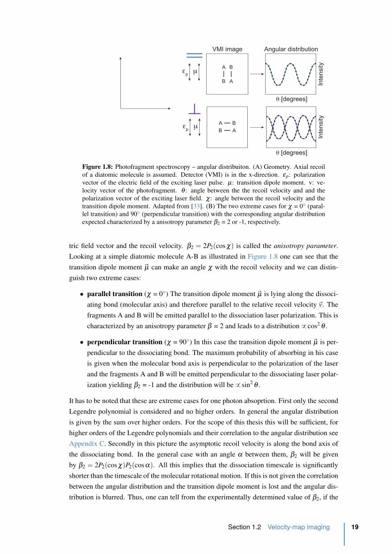
A B
AB
A B
AB
Angular distribution
θ [degrees]
Inte
nsity
θ [degrees]
Inte
nsity
VMI image
εp
μ
εp
μ
x (TOF)
y (MB)
z (Laser)
μv
Φ
θε
p
χχ = 0
χ = 90
y
z
β2 = 2
β2 = −1
(A) (B)
Figure 1.8: Photofragment spectroscopy – angular distribuiton. (A) Geometry. Axial recoil
of a diatomic molecule is assumed. Detector (VMI) is in the x-direction. εp: polarization
vector of the electric field of the exciting laser pulse. µ: transition dipole moment. v: ve-
locity vector of the photofragment. θ : angle between the the recoil velocity and and the
polarization vector of the exciting laser field. χ: angle between the recoil velocity and the
transition dipole moment. Adapted from [33]. (B) The two extreme cases for χ = 0˝ (paral-
lel transition) and 90˝ (perpendicular transition) with the corresponding angular distribution
expected characterized by a anisotropy parameter β2 = 2 or -1, respectively.
tric field vector and the recoil velocity. β2 “ 2P2pcos χq is called the anisotropy parameter.
Looking at a simple diatomic molecule A-B as illustrated in Figure 1.8 one can see that the
transition dipole moment ~µ can make an angle χ with the recoil velocity and we can distin-
guish two extreme cases:
• parallel transition (χ = 0˝) The transition dipole moment ~µ is lying along the dissoci-
ating bond (molecular axis) and therefore parallel to the relative recoil velocity ~v. The
fragments A and B will be emitted parallel to the dissociation laser polarization. This is
characterized by an anisotropy parameter β = 2 and leads to a distribution 9cos2 θ .
• perpendicular transition (χ = 90˝) In this case the transition dipole moment ~µ is per-
pendicular to the dissociating bond. The maximum probability of absorbing in his case
is given when the molecular bond axis is perpendicular to the polarization of the laser
and the fragments A and B will be emitted perpendicular to the dissociating laser polar-
ization yielding β2 = -1 and the distribution will be 9sin2 θ .
It has to be noted that these are extreme cases for one photon absoprtion. First only the second
Legendre polynomial is considered and no higher orders. In general the angular distribution
is given by the sum over higher orders. For the scope of this thesis this will be sufficient, for
higher orders of the Legendre polynomials and their correlation to the angular distribution see
Appendix C. Secondly in this picture the asymptotic recoil velocity is along the bond axis of
the dissociating bond. In the general case with an angle α between them, β2 will be given
by β2 “ 2P2pcos χqP2pcosαq. All this implies that the dissociation timescale is significantly
shorter than the timescale of the molecular rotational motion. If this is not given the correlation
between the angular distribution and the transition dipole moment is lost and the angular dis-
tribution is blurred. Thus, one can tell from the experimentally determined value of β2, if the
Section 1.2 Velocity-map imaging 19

0 0.5 1 1.5 2 2.5 3
x 104
0
0.5
1
1.5
2
2.5
3
pixel2
ener
gy [e
V]
V0
V1
V2
NO
404 + 809 nm 202 + 809 nm
0809 nm1*202 + 3*809 nm2*404 + 3*809 nm2*404 + 4*809 nm2*202 nm
V0
V1
V2
809 nm 404 nm 202 nm
photo-e-
404 + 809
slope = 9.44 x 10⁻⁵
Figure 1.9: Photo-electron spectra of NO at various ionization wavelength to determine the
calibration factor of the VMI setup for a repeller and extractor voltage of 2 kV and 1.42 kV,
respectively.
dissociation is direct, meaning the molecule has little time to rotate before the dissociation act,
and if the relevant excited state is associated with a parallel or perpendicular transition. Doing
the experiment on the femtosecond timescale, instead of pico or nanosecond scales means that
we are naturally on a timescale shorter then the rotational period of the parent molecule and
this degree of freedom is frozen for most of the time delay.
1.2.5 VMI calibration
Eq. (1.11) from Section 1.2
R “ ML
d
KER
qV“ α
?KER Ñ Ekin “ α R2
gave us the relationship between the radius where the fragments are observed on the detector
and their kinetic energy. The proportionality factor α depends on the experimental setup and
the alignment of the laser beams relative to the molecular beam and the repeller and extractor
plate for a fixed repeller voltage and has to be determined through a calibration. In general,
in femtolaser facilities where narrow bandwidth laser are not available, this is done detecting
photoelectrons of a system for which the spectroscopy is well known. In our case we used
NO or Xenon which posseses the advantage of having very close electronic states which are
well known. Figure 1.9 shows the Abel-inverted photo-electron images of NO obtained for
different ionization wavelengths. The graph shows the extracted spectrum at 404 + 809 nm
at ∆t = 0 between these two lasers pulses (center image). Plotted is the intensity versus pixel
square (blue line). NO` is detected in its ground electronic state (X1Σ
`) by ionizing NO from
20 Chapter 1 From femtosecond to attosecond imaging
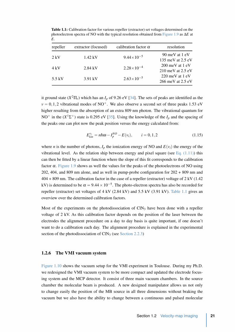
Table 1.1: Calibration factor for various repeller (extractor) set voltages determined on the
photoelectron spectra of NO with the typical resolution obtained from Figure 1.9 as ∆E at
E.
repeller extractor (focused) calibration factor α resolution
2 kV 1.42 kV 9.44ˆ10´5 90 meV at 1 eV
135 meV at 2.5 eV
4 kV 2.84 kV 2.28ˆ10´4 200 meV at 1 eV
210 meV at 2.5 eV
5.5 kV 3.91 kV 2.63ˆ10´5 220 meV at 1 eV
266 meV at 2.5 eV
it ground state (X2Πr) which has an Ip of 9.26 eV [34]. The sets of peaks are identified as the
v “ 0,1,2 vibrational modes of NO`. We also observe a second set of three peaks 1.53 eV
higher resulting from the absorption of an extra 809 nm photon. The vibrational quantum for
NO` in the (X1Σ
`) state is 0.295 eV [35]. Using the knowledge of the Ip and the spacing of
the peaks one can plot now the peak position versus the energy calculated from:
Evi
kin “ nhω ´ INOp ´ Epviq, i “ 0,1,2 (1.15)
where n is the number of photons, Ip the ionization energy of NO and Epviq the energy of the
vibrational level. As the relation ship between energy and pixel square (see Eq. (1.11)) this
can then be fitted by a linear function where the slope of this fit corresponds to the calibration
factor α . Figure 1.9 shows as well the values for the peaks of the photoelectrons of NO using
202, 404, and 809 nm alone, and as well in pump-probe configuration for 202 + 809 nm and
404 + 809 nm. The calibration factor in the case of a repeller (extractor) voltage of 2 kV (1.42
kV) is determined to be α “ 9.44 ˆ 10´5. The photo-electron spectra has also be recorded for
repeller (extractor) set voltages of 4 kV (2.84 kV) and 5.5 kV (3.91 kV). Table 1.1 gives an
overview over the determined calibration factors.
Most of the experiments on the photodissociation of ClN3 have been done with a repeller
voltage of 2 kV. As this calibration factor depends on the position of the laser between the
electrodes the alignment procedure on a day to day basis is quite important, if one doesn’t
want to do a calibration each day. The alignment procedure is explained in the experimental
section of the photodissociation of ClN3 (see Section 2.2.3)
1.2.6 The VMI vacuum system
Figure 1.10 shows the vacuum setup for the VMI experiment in Toulouse. During my Ph.D.
we redesigned the VMI vacuum system to be more compact and updated the electrode focus-
ing system and the MCP detector. It consist of three main vacuum chambers. In the source
chamber the molecular beam is produced. A new designed manipulator allows us not only
to change easily the position of the MB source in all three dimensions without braking the
vacuum but we also have the ability to change between a continuous and pulsed molecular
Section 1.2 Velocity-map imaging 21

detection chambersource chamber
electrodes
manipulator
interaction chamber
pulsed MB
cw MB
MCP
Figure 1.10: Schematic drawing of the experimental vacuum setup for the VMI spectrometer
in Toulouse.
beam source. We are able to mount an Even-Lavie pulsed valve1 [36] and a piezo pulsed valve
designed by Maurice Janssen [37, 38]. The molecular beam is then send into the interaction
chamber through a skimmer, where it is send in between the repeller and extractor plates and
intersected by the two laser pulses. The skimmer is mounted on a rotation plate which allows
us to mount up to three different skimmers and which can be controlled from outside to change
the skimmer without braking the vacuum. On top of the interaction chamber is the detection
chamber, consisting of a time-of-flight tube shielded by a µ-metal (green part in Figure 1.10)
and finishing with the detector. The detector is a MCP and phosphor screen combination from
Photek (VID275). It consist of two MCP plates with a diameter of 75 mm mounted in a z-
configuration on a CF-flange and a P43 phosphor. On top of the MCP a digital CCD camera
C8484-05G form Hamamatsu is mounted. The camera is equipped with a high-resolution
sensor featuring an effective pixel count of 1344x1023 pixels and a frame rate of about 10
Hz.
The vacuum chambers are pumped by four turbo pumps backed up by two primary pumps.
A magnetic turbo pump with a capacity of 3200l/s is used to pump the source chamber. The
interaction chamber is pumped by two turbo molecular pumps, one mounted in the direction of
the molecular beam with a capacity of 300l/s and one mounted underneath the TOF with 500
l/s. A fourth small turbo pump is mounted just below the detector with 300 l/s. In the source
chamber typically a pressure of 10´7mbar is reached and in the detection chamber 10´8 mbar.
If the gas jet is switched on we typically measure a few 10´4 mbar in the source chamber
1 Evan-Lavie valve website
22 Chapter 1 From femtosecond to attosecond imaging
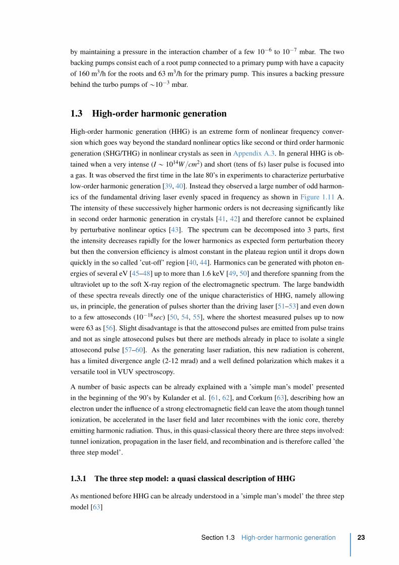
by maintaining a pressure in the interaction chamber of a few 10´6 to 10´7 mbar. The two
backing pumps consist each of a root pump connected to a primary pump with have a capacity
of 160 m3/h for the roots and 63 m3/h for the primary pump. This insures a backing pressure
behind the turbo pumps of „10´3 mbar.
1.3 High-order harmonic generation
High-order harmonic generation (HHG) is an extreme form of nonlinear frequency conver-
sion which goes way beyond the standard nonlinear optics like second or third order harmonic
generation (SHG/THG) in nonlinear crystals as seen in Appendix A.3. In general HHG is ob-
tained when a very intense (I „ 1014Wcm2) and short (tens of fs) laser pulse is focused into
a gas. It was observed the first time in the late 80’s in experiments to characterize perturbative
low-order harmonic generation [39, 40]. Instead they observed a large number of odd harmon-
ics of the fundamental driving laser evenly spaced in frequency as shown in Figure 1.11 A.
The intensity of these successively higher harmonic orders is not decreasing significantly like
in second order harmonic generation in crystals [41, 42] and therefore cannot be explained
by perturbative nonlinear optics [43]. The spectrum can be decomposed into 3 parts, first
the intensity decreases rapidly for the lower harmonics as expected form perturbation theory
but then the conversion efficiency is almost constant in the plateau region until it drops down
quickly in the so called ’cut-off’ region [40, 44]. Harmonics can be generated with photon en-
ergies of several eV [45–48] up to more than 1.6 keV [49, 50] and therefore spanning from the
ultraviolet up to the soft X-ray region of the electromagnetic spectrum. The large bandwidth
of these spectra reveals directly one of the unique characteristics of HHG, namely allowing
us, in principle, the generation of pulses shorter than the driving laser [51–53] and even down
to a few attoseconds (10´18sec) [50, 54, 55], where the shortest measured pulses up to now
were 63 as [56]. Slight disadvantage is that the attosecond pulses are emitted from pulse trains
and not as single attosecond pulses but there are methods already in place to isolate a single
attosecond pulse [57–60]. As the generating laser radiation, this new radiation is coherent,
has a limited divergence angle (2-12 mrad) and a well defined polarization which makes it a
versatile tool in VUV spectroscopy.
A number of basic aspects can be already explained with a ’simple man’s model’ presented
in the beginning of the 90’s by Kulander et al. [61, 62], and Corkum [63], describing how an
electron under the influence of a strong electromagnetic field can leave the atom though tunnel
ionization, be accelerated in the laser field and later recombines with the ionic core, thereby
emitting harmonic radiation. Thus, in this quasi-classical theory there are three steps involved:
tunnel ionization, propagation in the laser field, and recombination and is therefore called ’the
three step model’.
1.3.1 The three step model: a quasi classical description of HHG
As mentioned before HHG can be already understood in a ’simple man’s model’ the three step
model [63]
Section 1.3 High-order harmonic generation 23

Multiphoton
pertubative regime
Plateau
Cutoff
2ω0
Energy
Inte
nsity
Energy
H15 H17 H19 H21 H23 H25
short trajectories
long trajectories
Space
2ω0
(A) (B)
Figure 1.11: High harmonic spectrum. (A) schematic spectrum of a typical high harmonic
radiation showing 3 part, rapid decrease of the intensity for the first harmonics in the mul-
tiphoton pertubative regime, followed by an plateau where the emission efficiency is almost
constant until the signal drops suddenly in the cut off region. (B) Harmonic spectrum pro-
duced in argon at a fundamental laser wavelength of 800 nm. Visible here is the spacial
structure of HHG as two different ring structures referred to as short and long trajectories.
1. Tunnel Ionization
The strong focused electric field is bending the Coulomb potential and the outer valence
electron can tunnel from the ground state of the atom or molecule through the potential
barrier.
2. Acceleration in the laser field
The electron is accelerated and driven back to the parent ion as the electric field reverses,
in less time than half of the optical period.
3. Recombination
The electron recombines radiatively with its parent ion onto the ground state. This
continuum-bound transition converts the kinetic energy of the electron into an extreme
ultraviolet (EUV) photon.
which are graphically shown in Figure 1.12. In the following each step will be introduced.
1. Tunnel Ionization
There are basically 3 types of ionization due to an intense laser if the photon energy is lower
than the ionization energy (Ip) of the atom or molecule: multiphoton ionization (MI), tun-
nel ionization (TI) and barrier-suppressed ionization (BSI) depending on the laser intensity
as shown in Figure 1.13. The first one is regarded as non-perturbative where the Coulomb
potential is not deformed. Ionization occurs by absorbing n photons to reach the IP. This tech-
nique is used in femtochemistry as we will see later. HHG in contrary is a regime where the
ionization doesn’t happen through multiphoton absorption but through tunnel ionization. This
happens when the oscillating electric field of the laser given by |~ELptq| “ E0 cospωLtq, becomes
comparable to the intra-atomic field strength („ 108 V/cm). This leads to deformation of the
coulomb potential and can lower the barrier so much that tunneling becomes possible. The
24 Chapter 1 From femtosecond to attosecond imaging
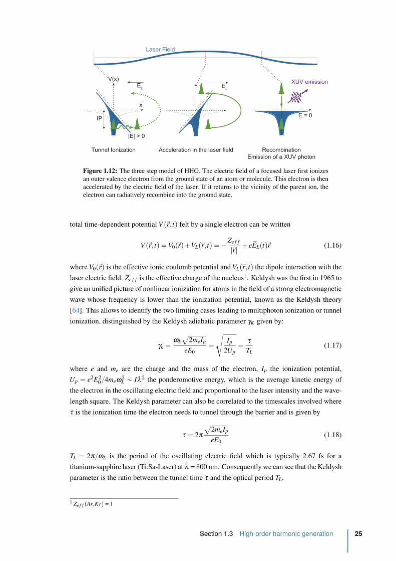
Tunnel Ionization Acceleration in the laser field Recombination
Emission of a XUV photon
IPE = 0
V(x)
x
|E| > 0
Laser Field
XUV emissionE
L EL
Figure 1.12: The three step model of HHG. The electric field of a focused laser first ionizes
an outer valence electron from the ground state of an atom or molecule. This electron is then
accelerated by the electric field of the laser. If it returns to the vicinity of the parent ion, the
electron can radiatively recombine into the ground state.
total time-dependent potential V p~r, tq felt by a single electron can be written
V p~r, tq “ V0p~rq `VLp~r, tq “ ´Ze f f
|~r| ` e~ELptq~r (1.16)
where V0p~rq is the effective ionic coulomb potential and VLp~r, tq the dipole interaction with the
laser electric field. Ze f f is the effective charge of the nucleus1. Keldysh was the first in 1965 to
give an unified picture of nonlinear ionization for atoms in the field of a strong electromagnetic
wave whose frequency is lower than the ionization potential, known as the Keldysh theory
[64]. This allows to identify the two limiting cases leading to multiphoton ionization or tunnel
ionization, distinguished by the Keldysh adiabatic parameter γK given by:
γk “ωL
a
2meIp
eE0“
d
Ip
2Up“ τ
TL(1.17)
where e and me are the charge and the mass of the electron, Ip the ionization potential,
Up “ e2E20 4meω2
L „ Iλ 2 the ponderomotive energy, which is the average kinetic energy of
the electron in the oscillating electric field and proportional to the laser intensity and the wave-
length square. The Keldysh parameter can also be correlated to the timescales involved where
τ is the ionization time the electron needs to tunnel through the barrier and is given by
τ “ 2π
a
2meIp
eE0(1.18)
TL “ 2πωL is the period of the oscillating electric field which is typically 2.67 fs for a
titanium-sapphire laser (Ti:Sa-Laser) at λ = 800 nm. Consequently we can see that the Keldysh
parameter is the ratio between the tunnel time τ and the optical period TL.
1 Ze f f pAr,Krq = 1
Section 1.3 High-order harmonic generation 25
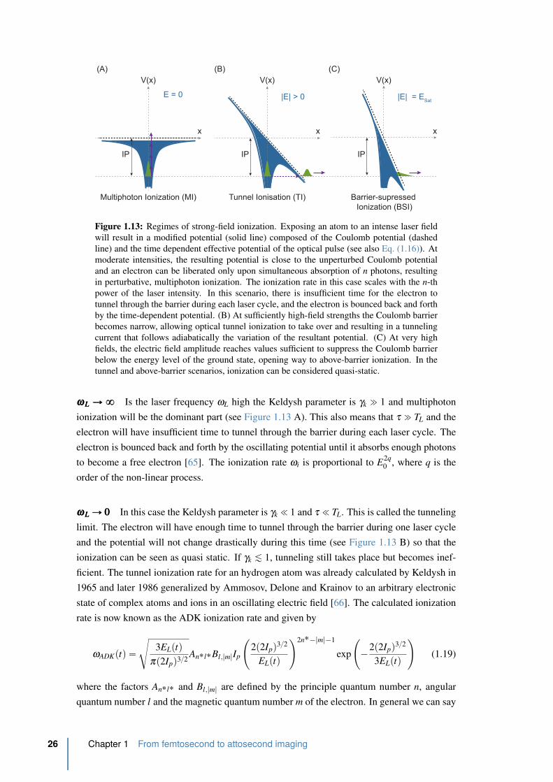
IP
V(x)
x
E = 0
IP
V(x)
x
|E| > 0
IP
V(x)
x
|E| = ESat
(A) (B) (C)
Multiphoton Ionization (MI) Tunnel Ionisation (TI) Barrier-supressed
Ionization (BSI)
Figure 1.13: Regimes of strong-field ionization. Exposing an atom to an intense laser field
will result in a modified potential (solid line) composed of the Coulomb potential (dashed
line) and the time dependent effective potential of the optical pulse (see also Eq. (1.16)). At
moderate intensities, the resulting potential is close to the unperturbed Coulomb potential
and an electron can be liberated only upon simultaneous absorption of n photons, resulting
in perturbative, multiphoton ionization. The ionization rate in this case scales with the n-th
power of the laser intensity. In this scenario, there is insufficient time for the electron to
tunnel through the barrier during each laser cycle, and the electron is bounced back and forth
by the time-dependent potential. (B) At sufficiently high-field strengths the Coulomb barrier
becomes narrow, allowing optical tunnel ionization to take over and resulting in a tunneling
current that follows adiabatically the variation of the resultant potential. (C) At very high
fields, the electric field amplitude reaches values sufficient to suppress the Coulomb barrier
below the energy level of the ground state, opening way to above-barrier ionization. In the
tunnel and above-barrier scenarios, ionization can be considered quasi-static.
ωωωLLL ÑÑÑ 888 Is the laser frequency ωL high the Keldysh parameter is γk " 1 and multiphoton
ionization will be the dominant part (see Figure 1.13 A). This also means that τ " TL and the
electron will have insufficient time to tunnel through the barrier during each laser cycle. The
electron is bounced back and forth by the oscillating potential until it absorbs enough photons
to become a free electron [65]. The ionization rate ωi is proportional to E2q0 , where q is the
order of the non-linear process.
ωωωLLL ÑÑÑ 000 In this case the Keldysh parameter is γk ! 1 and τ ! TL. This is called the tunneling
limit. The electron will have enough time to tunnel through the barrier during one laser cycle
and the potential will not change drastically during this time (see Figure 1.13 B) so that the
ionization can be seen as quasi static. If γk À 1, tunneling still takes place but becomes inef-
ficient. The tunnel ionization rate for an hydrogen atom was already calculated by Keldysh in
1965 and later 1986 generalized by Ammosov, Delone and Krainov to an arbitrary electronic
state of complex atoms and ions in an oscillating electric field [66]. The calculated ionization
rate is now known as the ADK ionization rate and given by
ωADKptq “d
3ELptqπp2Ipq32
An˚l˚Bl,|m|Ip
˜
2p2Ipq32
ELptq
¸2n˚´|m|´1
exp
˜
´2p2Ipq32
3ELptq
¸
(1.19)
where the factors An˚l˚ and Bl,|m| are defined by the principle quantum number n, angular
quantum number l and the magnetic quantum number m of the electron. In general we can say
26 Chapter 1 From femtosecond to attosecond imaging

inte
nsity [
W/c
m2]
photon energy [eV]
800 nm 400 nm
relativistic
field
ionisation
tunnel
ionization
MPI perturbative
MPI non-perturbative
γΚ = 1
1 10 1001x1010
1x10¹²
1x10¹⁴
1x10¹⁶
1x10¹⁸
1x10²⁰
Figure 1.14: Different photoionisation regimes as a function of the laser intensity and photon
energy. For the rather low laser intensities ionization proceeds either by a multiphoton per-
turbative process for the lowest intensities or a multiphoton non-perturbative process [67]. If
the laser frequency is quite low but the laser intensity is moderately strong, ionization occurs
via tunneling [68]. Field ionisation happens at even higher laser intensity when the poten-
tial barrier is completely suppressed by the laser field. At extremely hight laser intensities
relativistic effects play an important role [69]. The vertical dotted blue and purple lines indi-
cate the photon energies related to the laser wavelength of 800 nm and 400 nm, respectively,
which are used in this manuscript. The dashed black line shows the case of γk = 1 for argon.
Adapted from [70].
that the tunnel ionization depends exponentially on the electric field strength and the ionization
potential:
ωADKptq9 I0.25p exp
˜
´5.65pIpq32
3ELptq
¸
(1.20)
One also sees that the Keldysh parameter depends on both the strength of the electric field
EL and the frequency of the laser ωL, which is graphically shown in Figure 1.14. At the
intensity of 1014 W/cm2 and at 800 nm, the Keldysh parameter is around 1 for example in
the case of argon. Thus we are in the intermediate region between tunnel and multiphoton
ionization. When the electric field becomes much stronger than the regime of tunnel ionization
the coulomb potential can be bent so much that the barrier becomes significantly lower than
the Ip, and the electron is then ripped off the parent ion as shown in Figure 1.13 C. This is
called barrier-supressed ionization (BSI) [68]. In between these two regimes we will have an
electric field intensity for which we saturate the tunnel ionization. The total probability of
ionization pI can be calculated by integrating the ionization rate over the pulse duration of the
electric field:
pI “ 1 ´ exp
ˆ
´ż 8
´8ωADKptqdt
˙
(1.21)
The tunnel ionization will increase exponentially with increasing the laser intensity until the
probability reaches one. This is defined as the saturation intensity Isat which depends on the
laser duration and the spacial profile. If one assumes that the potential V p~r, tq from Eq. (1.16) is
mainly one dimensional along the z-polarization of the laser V p~r, tq “ V pzq “ ´Ze f f |z|´eEz,
at the threshold the derivative of the potential has to be zero, V 1pz0q “ 0 which leads to z0 “a
Ze f f peELq and the saturation potential itself is given by Vsat “ ´Ip. With this we can
Section 1.3 High-order harmonic generation 27

estimate the saturation energy and intensity as function of the ionization potential to:
Esat “I2p
4Ze f f(1.22a)
Isat “I4p
16Z2e f f
(1.22b)
Isat rWcm2s “4.02 ˆ 109I4p
Z2e f f
reV s (1.22c)
Note that the electric field needed to lower the potential barrier has a quadratic dependence
on the ionization potential. For a given laser intensity, the ionization regime may be totally
different depending on the gas used. Table 1.2 shows the intensities needed to suppress the
barrier in rare gases, calculated from equation Eq. (1.22b).
Table 1.2: Calculation of the saturation energy (barrier suppression) for different
rare gases.
gaz He Ne Ar Kr Xe
Ip [eV] 24.59 21.56 15.76 14.00 12.13
Isat [1014 W/cm2] 14.62 8.65 2.47 1.54 0.87
While in atoms it is clear that it is the least bound electron which participates in the tunnel
ionization process, in molecules one of the challenges is to determine which molecular orbital
participates and how it depends on the geometry of the molecule. This issue will be discussed
in Chapter 4 about the HHG spectroscopy of SF6.
2. Acceleration in the laser field
This is the part of the semiclassical theory which is treated classically. In the context of
the strong field approximation (SFA) the coulomb potential of the atom is neglected and the
electron is regarded as a free electron whose motion is governed only by the external laser
field given by |~ELptq| “ E0 cospωLtq. The differential equation for the motion of the electron
can then be written as:
xptq “ ´eE0
mecospωLtq “ ´eE0
mecospϕq (1.23)
where ϕ “ ω0t. We consider an electron which is ab initio bound to an atom and appears in the
continuum at time zero ti with an initial velocity of approximately v0 “ xptiq “ 0. Furthermore,
by neglecting the distance between the electron and the nucleus and puting xptiq “ 0, the
velocity vptq and the position xptq of the free electron, born at an arbitrary phase φ of the
oscillating electric field, can be calculated to be:
vptq “ż t
0
´ e
meELpt 1qdt 1 “ ´ eE0
meωLrsinpωLt ` φq ´ sinpφqs (1.24a)
xptq “ż t
0
vpt 1qdt 1 “ eE0
meω2L
rcospωLt ` φq ´ cospφq ` sinpφqts (1.24b)
28 Chapter 1 From femtosecond to attosecond imaging
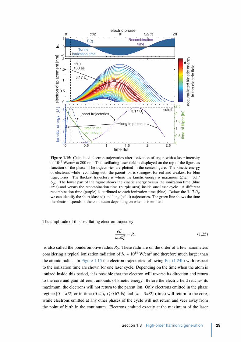
0
0.5
1
1.5
2
accum
ula
ted k
inetic e
nerg
y
in the e
lectr
ic fie
ld
−1
0
1
E0
Recombination
time
Tunnel
Ionization time
E(t)
0 π/2 π 3/2 π 2πelectric phase
0 0.5 1 1.5 2 2.50
1
2
3
time [fs]
kine
tic e
nerg
y [U
p]
0
0.5
1
1.5
2
2.5
time
of fl
ight
[fs]3.17 U
p
time in the
continuum
short trajectories
long trajectories
π/10130 as
3.17 Up
cutoff
elec
tron
dis
plac
emen
t [nm
]
Figure 1.15: Calculated electron trajectories after ionization of argon with a laser intensity
of 1014 W/cm2 at 800 nm. The oscillating laser field is displayed on the top of the figure as
function of the phase. The trajectories are plotted in the center figure. The kinetic energy
of electrons while recolliding with the parent ion is strongest for red and weakest for blue
trajectories. The thickest trajectory is where the kinetic energy is maximum (Ekin = 3.17
Up). The lower part of the figure shows the kinetic energy versus the ionization time (blue
area) and versus the recombination time (purple area) inside one laser cycle. A different
recombination time (purple) is attributed to each ionization time (blue). Below the 3.17 Up
we can identify the short (dashed) and long (solid) trajectories. The green line shows the time
the electron spends in the continuum depending on when it is emitted.
The amplitude of this oscillating electron trajectory
eE0
meω2L
“ R0 (1.25)
is also called the ponderomotive radius R0. These radii are on the order of a few nanometers
considering a typical ionization radiation of IL „ 1014 W/cm2 and therefore much larger than
the atomic radius. In Figure 1.15 the electron trajectories following Eq. (1.24b) with respect
to the ionization time are shown for one laser cycle. Depending on the time when the atom is
ionized inside this period, it is possible that the electron will reverse its direction and return
to the core and gain different amounts of kinetic energy. Before the electric field reaches its
maximum, the electrons will not return to the parent ion. Only electrons emitted in the phase
regime [0 – π/2] or in time (0 ď ti ď 0.67 fs) and [π – 3π/2] (time) will return to the core,
while electrons emitted at any other phases of the cycle will not return and veer away from
the point of birth in the continuum. Electrons emitted exactly at the maximum of the laser
Section 1.3 High-order harmonic generation 29

intensity will have no kinetic energy when they return, whereas the electron emitted at « π10
(ti “ 130 as) will gain the maximum kinetic energy which is given by 3.17 Up, where Up is
the ponderomotive energy. Its trajectory refers to the cut-off trajectory. In Figure 1.15 lower
part the kinetic energy the electron is gaining during the time in the laser field is plotted versus
the ionization (blue area) and recombination time (purple) area. If the return kinetic energy
of the electron is below 3.17 Up, two different electron trajectories (solid and dashed lines)
can be associated with this kinetic energy having different time of flight values. These two
trajectories are refeered to as long (solid) and short (dashed) trajectories:
• short trajectories identifies electrons emitted after π/10, they don’t travel far away from
the ionic core and the propagation time in the continuum is short and increases with
harmonic order.
• long trajectories in contrary identifies electrons emitted before π/10 near the maximum
of the laser field, they can travel up to 2 nm away form the ionic core and the time of
propagation in the continuum is rather long and decreases with harmonic order.
The earlier an electron is emitted during a laser cycle, the longer it will remain in the contin-
uum and will acquire a phase shift with respect to the electron-hole left behind in the ionic
core. This phase shift is proportional to the average time delay between ionization and recom-
bination and the ionization potential:
∆ϕq « ´αq ∆IL (1.26)
As the time-of-flight is larger for long compared to short trajectories so will be the phase
difference when electron and ion recombine. This will effect each harmonic order and can
be used to identify spatially different ionization channels [71, 72]. For instance in argon
αshort “ 12 ˆ 10´14 rad.cm2/W and αlong “ 25 ˆ 10´14 rad.cm2/W with an laser intensity of
1.5 10´14 W/cm2 [73].
3. Recombination
In the case the electron returns to the parent ion one can observe several processes. The
electron can be scattered inelastically by the ion core, transferring part of its energy to another
electron. Thus, a second electron may be ejected from the ionic ground state to the continuum.
This process is called non-sequential double ionisation (NSDI) [74–77]. Alternatively, the
electron can be elastically scattered by the ion core. In this case, it can acquire drift energies
up to 10 Up. Such effect is referred to as high order above threshold ionisation (HATI) [78–
80]. And finally, the electron can recombine with the ion emitting its energy in form of a
high energy photon which we know as high harmonic generation (HHG). In the latter case
the excess energy gained by the electron in the external oscillating field is carried away by
emitting a high energy photon. This energy can be expressed as:
hω “ Ekin ` Ip (1.27)
30 Chapter 1 From femtosecond to attosecond imaging
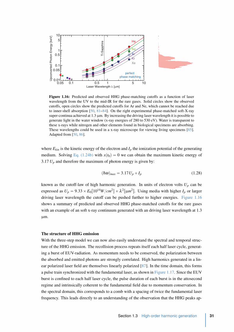
1
5
1 5 100.05 0.1 0.5Laser Wavelength λ [μm]
Upc
onve
rted
Pho
ton
Ene
rgy
[keV
]
perfect phase matching
Ti:S
apph
ire
0.5
10
0.10.05
0.01
He
Ne
ArKrXe
Ar
0 0.5 1
0.1
0.2
0.3
0.4
0.5
0.6
Ne
Ar
HHG intensity [normalized]
HHG spectrum @ λ = 1.3 μm
Water window
Water window
He
Figure 1.16: Predicted and observed HHG phase-matching cutoffs as a function of laser
wavelength from the UV to the mid-IR for the rare gases. Solid circles show the observed
cutoffs, open circles show the predicted cutoffs for Ar and Ne, which cannot be reached due
to inner-shell absorption [50, 81–84]. On the right experimental phase-matched soft-X-ray
super-continua achieved at 1.3 µm. By increasing the driving laser wavelength it is possible to
generate light in the water window (x-ray energies of 280 to 530 eV). Water is transparent to
these x-rays while nitrogen and other elements found in biological specimens are absorbing.
These wavelengths could be used in a x-ray microscope for viewing living specimens [85].
Adapted from [50, 86].
where Ekin is the kinetic energy of the electron and Ip the ionization potential of the generating
medium. Solving Eq. (1.24b) with xpt0q “ 0 we can obtain the maximum kinetic energy of
3.17 Up and therefore the maximum of photon energy is given by:
phωqmax “ 3.17Up ` Ip (1.28)
known as the cutoff-law of high harmonic generation. In units of electron volts Up can be
expressed as Up “ 9.33 ˆ E0r1014Wcm2s ˆ λ 2rµm2s. Using media with higher Ip or larger
driving laser wavelength the cutoff can be pushed further to higher energies. Figure 1.16
shows a summary of predicted and observed HHG phase-matched cutoffs for the rare gases
with an example of an soft x-ray continuum generated with an driving laser wavelength at 1.3
µm.
The structure of HHG emission
With the three-step model we can now also easily understand the spectral and temporal struc-
ture of the HHG emission. The recollision process repeats itself each half laser cycle, generat-
ing a burst of EUV-radiation. As momentum needs to be conserved, the polarization between
the absorbed and emitted photons are strongly correlated. High harmonics generated in a lin-
ear polarized laser field are themselves linearly polarized [87]. In the time domain, this forms
a pulse train synchronized with the fundamental laser, as shown in Figure 1.17. Since the EUV
burst is confined to each half laser cycle, the pulse duration of each burst is in the attosecond
regime and intrinsically coherent to the fundamental field due to momentum conservation. In
the spectral domain, this corresponds to a comb with a spacing of twice the fundamental laser
frequency. This leads directly to an understanding of the observation that the HHG peaks ap-
Section 1.3 High-order harmonic generation 31
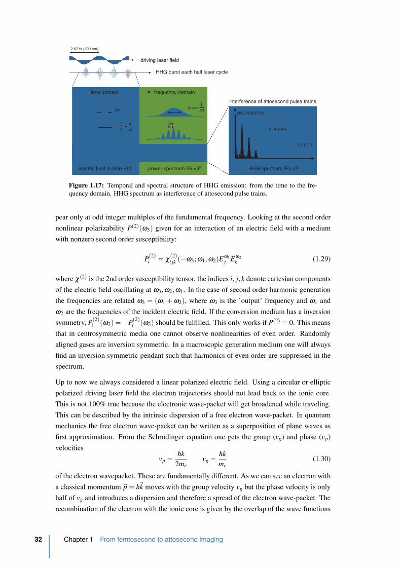
electric field in time E(t) power spectrum |E(ω)|2 HHG spectrum |E(ω)|2
time domain frequency demain
Δτ
πω
Τ2
=2ω
Δω ≈ 1Δτ
interference of attosecond pulse trains
PLATEAU
MULTIPHOTON
CUTOFF
driving laser field
HHG burst each half laser cycle
2.67 fs (800 nm)
Figure 1.17: Temporal and spectral structure of HHG emission: from the time to the fre-
quency domain. HHG spectrum as interference of attosecond pulse trains.
pear only at odd integer multiples of the fundamental frequency. Looking at the second order
nonlinear polarizability Pp2qpω3q given for an interaction of an electric field with a medium
with nonzero second order susceptibility:
Pp2qi “ χ
p2qi jk p´ω3;ω1,ω2qE
ω1j E
ω2
k (1.29)
where χp2q is the 2nd order susceptibility tensor, the indices i, j,k denote cartesian components
of the electric field oscillating at ω3,ω2,ω1. In the case of second order harmonic generation
the frequencies are related ω3 “ pω1 ` ω2q, where ω3 is the ’output’ frequency and ω1 and
ω2 are the frequencies of the incident electric field. If the conversion medium has a inversion
symmetry, Pp2qi pω3q “ ´P
p2qi pω3q should be fulfilled. This only works if Pp2q ” 0. This means
that in centrosymmetric media one cannot observe nonlinearities of even order. Randomly
aligned gases are inversion symmetric. In a macroscopic generation medium one will always
find an inversion symmetric pendant such that harmonics of even order are suppressed in the
spectrum.
Up to now we always considered a linear polarized electric field. Using a circular or elliptic
polarized driving laser field the electron trajectories should not lead back to the ionic core.
This is not 100% true because the electronic wave-packet will get broadened while traveling.
This can be described by the intrinsic dispersion of a free electron wave-packet. In quantum
mechanics the free electron wave-packet can be written as a superposition of plane waves as
first approximation. From the Schrodinger equation one gets the group (vg) and phase (vp)
velocities
vp “ hk
2mevg “ hk
me(1.30)
of the electron wavepacket. These are fundamentally different. As we can see an electron with
a classical momentum ~p “ h~k moves with the group velocity vg but the phase velocity is only
half of vg and introduces a dispersion and therefore a spread of the electron wave-packet. The
recombination of the electron with the ionic core is given by the overlap of the wave functions
32 Chapter 1 From femtosecond to attosecond imaging
and therefore if the ellipticity of the driving laser is small (εL ă 15%) there can still be an
overlap. But the HHG emission yield is decreasing rapidly with increasing ellipticity of the
driving laser. This effect is not so drastic in molecules [88] and clusters [89] because of the
extension of the molecular orbital (see Section 1.3.4)
1.3.2 The quantum model of HHG
The three step model explains all basic concept of HHG and agrees often with the experimen-
tal observations. It allows us even to determine phase information and can distinguish between
electrons emitted at different times during the laser cycle. But looking for example at the tun-
nel ionization time we find a huge discrepancy between the predictions and the experimental
results [90], for instance in the case of elliptical polarized driving laser field. In the quantum
mechanical picture the returning free electron is regarded as a wave function and not as a parti-
cle and this wave function has to overlap with the initial wave function in order to recombine.
Due to the quantum-mechanical nature of the electron, which suffers from dispersion when
not bound to a potential the rescattering electron wave-function spreads spatially which leads
to smaller overlap with the parent ion than classically expected.
To deal with the strong field response of atoms and molecules in general and HHG in particular
in a quantum mechanical picture, one has to solve the time-dependent Schrodinger equation
(TDSE):
ihδ
δ tψp~r, tq “ Hψp~r, tq (1.31)
where ψ is the wave function of the quantum system and H is the Hamiltonian operator, which
characterizes the total energy of any given wave function. The Hamiltonian is given by:
H “ ´ h2
2m∇
2 `V p~r, tq (1.32)
where in this case the time-dependent potential V p~r, tq is given by the sum of the atomic
coulomb potential and the dipole interaction with the electric field as seen in the three step
model. Although the TDSE can be solved numerically for the simplest case of an hydrogen
atom, it requires considerable computational time. To solve this equation for multielectron
systems is almost impossible. Thus one has to consider approximations to derive an analytical
solution. In the case of atoms in strong laser fields this has been done the first time in 1994
by Lewenstein and coworkers and is known as the strong field approximation (SFA) [91]
which uses the single active electron approximation (SAE) developed by Keldysh in 1965
[64]. This quantum mechanical treatment of HHG is now known as the Lewenstein model
of high harmonic generation. It allows to analyze the experimental results qualitative and
quantitative and justifies the hypothesizes done in the three step model. As it it not necessary
to understand the basic concept of HHG, it is not treated here but a summary can be found in
the Appendix D of this manuscript.
Section 1.3 High-order harmonic generation 33
1.3.3 Macroscopic high harmonic generation, phase matching and photon flux
More important than the quantum mechanical description of HHG is the macroscopic re-
sponse. So far only one atom in a strong electric field has been considered with its microscopic
response to an external strong electric field. Under experimental conditions high harmonics
are generated typically in a gas which has a density (1017-1018cm´3) and the driving laser
has a focal length which is larger than zero (Rayleigh length) defining an interaction volume
with a certain number of atoms. On one hand a certain density or volume is needed because
like in second harmonic generation in crystals phase matching within a certain coherence
length has to be sustained in order to improve the efficiency of the generation and to mea-
sure a macroscopic response. On the other hand, if the generation volume is longer than its
absorption length, the emitted photons can be reabsorbed by the medium itself reducing the
efficiency again. The typical low flux and the low efficiency of HHG („ 10´7) is the most
important technical bottleneck for attosecond science and HHG as a new XUV light source as
an emerging field. Therefore to further enhance the conversion efficiency and photon flux the
understanding of these macroscopic phenomena is important.
Phase matching conditions for HHG
The phase matching for constructive interference as schematically shown Figure 1.18 A is
characterized by the phase mismatch ∆k between the wave vectors k of the driving laser and
of the qth harmonic order given by
∆k “ kpqωLq ´ qkpωLq “ π
Lc(1.33)
where ωL is the fundamental laser frequency and Lc is the coherence length over which the
accumulated phase slip between the fundamental and the generated light is π . In an ideal
situation ∆k should be zero or at least very small for an efficient conversion. Or in other words,
the different emitters should radiate in phase at any given point in the generation volume. The
wave vector k is governed by four physical dispersion effects: atom, plasma, geometrical and
atomic dipole phase dispersions which add to the gaussian beam vector kvacpωq in vacuum and
can be written as a sum of these:
kpωq “ kvacpωq ` katomspωq ` kplasmapωq ` kgeompωq ` kADphasepωq (1.34)
where kvac “ 2πc is the wave vector in vacuum. In vacuum phase matching is always achieved
(∆kvac = 0) and the phase mismatch can be written as:
∆k “ ∆katoms ` ∆kplasma ` ∆kgeom ` ∆kADphase (1.35)
• neutral atom dispersion: The neutral gas used for HHG has typically a frequency
dependent index of refraction which can be written as npλ ,ρq “ 1 ` δndpλ qρ , where
δndpλ q is the dispersion per unit of atomic density. For a partially ionized medium
one gets npλ ,ρ, Iq “ 1 ` δndpλ qρ p1 ´ ηpIqq. The nonlinear component of the index is
found negligible for experimental pressures and intensities and can be omitted and thus
34 Chapter 1 From femtosecond to attosecond imaging
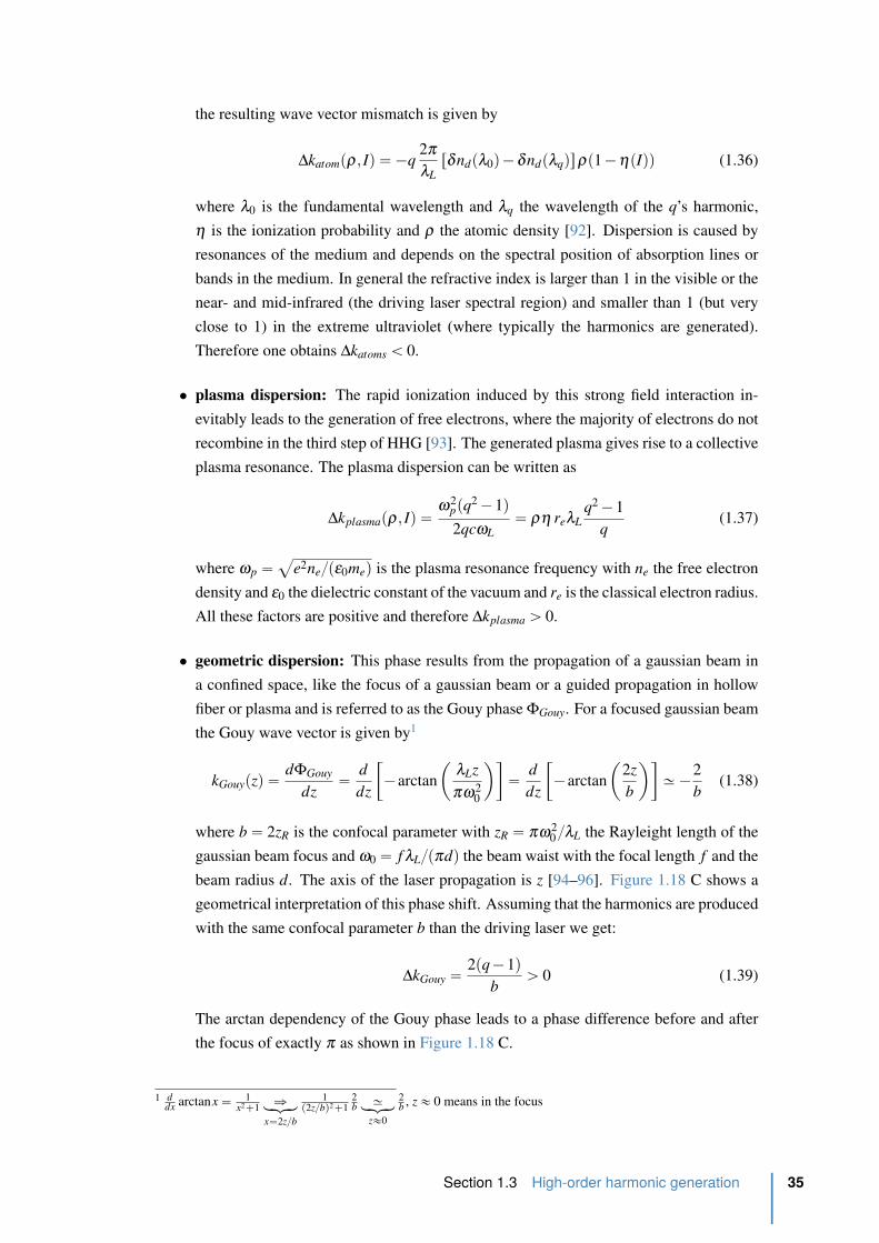
the resulting wave vector mismatch is given by
∆katompρ, Iq “ ´q2π
λLrδndpλ0q ´ δndpλqqsρp1 ´ ηpIqq (1.36)
where λ0 is the fundamental wavelength and λq the wavelength of the q’s harmonic,
η is the ionization probability and ρ the atomic density [92]. Dispersion is caused by
resonances of the medium and depends on the spectral position of absorption lines or
bands in the medium. In general the refractive index is larger than 1 in the visible or the
near- and mid-infrared (the driving laser spectral region) and smaller than 1 (but very
close to 1) in the extreme ultraviolet (where typically the harmonics are generated).
Therefore one obtains ∆katoms ă 0.
• plasma dispersion: The rapid ionization induced by this strong field interaction in-
evitably leads to the generation of free electrons, where the majority of electrons do not
recombine in the third step of HHG [93]. The generated plasma gives rise to a collective
plasma resonance. The plasma dispersion can be written as
∆kplasmapρ, Iq “ω2
ppq2 ´ 1q2qcωL
“ ρη reλLq2 ´ 1
q(1.37)
where ωp “a
e2nepε0meq is the plasma resonance frequency with ne the free electron
density and ε0 the dielectric constant of the vacuum and re is the classical electron radius.
All these factors are positive and therefore ∆kplasma ą 0.
• geometric dispersion: This phase results from the propagation of a gaussian beam in
a confined space, like the focus of a gaussian beam or a guided propagation in hollow
fiber or plasma and is referred to as the Gouy phase ΦGouy. For a focused gaussian beam
the Gouy wave vector is given by1
kGouypzq “ dΦGouy
dz“ d
dz
„
´arctan
ˆ
λLz
πω20
˙
“ d
dz
„
´arctan
ˆ
2z
b
˙
» ´2
b(1.38)
where b “ 2zR is the confocal parameter with zR “ πω20 λL the Rayleight length of the
gaussian beam focus and ω0 “ f λLpπdq the beam waist with the focal length f and the
beam radius d. The axis of the laser propagation is z [94–96]. Figure 1.18 C shows a
geometrical interpretation of this phase shift. Assuming that the harmonics are produced
with the same confocal parameter b than the driving laser we get:
∆kGouy “ 2pq ´ 1qb
ą 0 (1.39)
The arctan dependency of the Gouy phase leads to a phase difference before and after
the focus of exactly π as shown in Figure 1.18 C.
1 ddx arctanx “ 1
x2`1ñ
loomoon
x“2zb
1p2zbq2`1
2b »
loomoon
z«0
2b , z « 0 means in the focus
Section 1.3 High-order harmonic generation 35

Laser field
constructive addition
of X-ray elds
z/zR
ΔΦ/π(A)
(C)
(B)
(D)
qk1
kX-ray
Katomic
(a)
(b)
(c)
Figure 1.18: High harmonic phase matching conditions. (A) Illustration of phase matching
for constructive addition of the X-ray fields. (B) Phase matching conditions for different
points of the focal region: (a) On axis at focus before focus, (b) on axis after the focus, (c)
off-axis before the focus. Adapted form [86, 100]. (C) Wave vector k1 of the fundamental
laser beam going through a focus including the effect of the Gouy phase shift. (D) The
effective dipole phase wave vector Katomic in the focal region. Adapted from [100].
• atomic dipole dispersion: The origin of this phase is the trajectory acquired by the
electron leading to the emission of the qth harmonic in the continuum. It is proportional
to the laser intensity
∆kADphase “ α∇ILpr,zq (1.40)
The laser intensity can vary spatially in both the longitudinal and radial directions.
Therefore, the atom dipole phase also varies axially as well as radially. This leads to
a reduced harmonic emission as well as strong spatial distortion [97–99]
The relative importance of these terms depends on the geometry of the generation of HHG.
With tight focusing and long pulses, the efficiency of HHG is limited by the geometrical phase
shift [100] and/or by defocusing due to the large density of free electrons [101]. Loose focus-
ing reduces the effect of the Gouy shift and ultrashort pulses minimize the ionization effect and
increase the atomic response as required to optimize HHG [47, 85, 102, 103] Guiding the fun-
damental beam in hollow-core fibers has been shown to have extraordinary spatial coherence
properties [104] as it acts as a spatial filter. This can be used to further reduce the defocusing
and to optimize the phase matching and has been studied extensively [105–109].
In our case, a Gaussian laser beam is focused into a thin gas jet (for HHG used as a probe
process) or a gas cell (for HHG used as a secondary VUV light source). Therefore the intensity
dependent atomic dipole phase and the Gouy phase are the dominant terms. Neglecting the
other terms we can already make some qualitative conclusions [100]. The phase matching
36 Chapter 1 From femtosecond to attosecond imaging
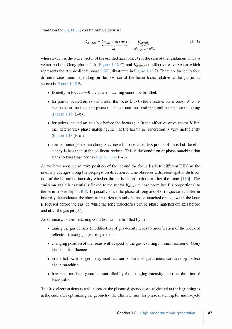
condition for Eq. (1.33) can be summarized as:
kX´ray “ kGouy ` qkpωLqlooooooomooooooon
qk1
` Katomicloomoon
„∆kADphase“α∇IL
(1.41)
where kX´ray is the wave vector of the emitted harmonic, k1 is the sum of the fundamental wave
vector and the Gouy phase shift (Figure 1.18 C) and Katomic an effective wave vector which
represents the atomic dipole phase [100], illustrated in Figure 1.18 D. There are basically four
different conditions depending on the position of the beam focus relative to the gas jet as
shown in Figure 1.18 B:
• Directly in focus z “ 0 the phase matching cannot be fulfilled.
• for points located on axis and after the focus (z ą 0) the effective wave vector K com-
pensates for the focusing phase mismatch and thus realizing collinear phase matching
(Figure 1.18 (B-b)).
• for points located on axis but before the focus (z ă 0) the effective wave vector K fur-
ther deteriorates phase matching, so that the harmonic generation is very inefficiently
(Figure 1.18 (B-a))
• non-collinear phase matching is achieved, if one considers points off axis but the effi-
ciency is less than in the collinear regime. This is the condition of phase matching that
leads to long trajectories (Figure 1.18 (B-c)).
As we have seen the relative position of the jet and the focus leads to different HHG as the
intensity changes along the propagation direction z. One observes a different spatial distribu-
tion of the harmonic intensity whether the jet is placed before or after the focus [110]. The
emission angle is essentially linked to the vector Katomic whose norm itself is proportional to
the term α (see Eq. (1.40)). Especially since the phase of long and short trajectories differ in
intensity dependence, the short trajectories can only be phase-matched on axis when the laser
is focused before the gas jet, while the long trajectories can be phase matched off axis before
and after the gas jet [97].
As summary, phase-matching condition can be fulfilled by i.e:
• tuning the gas density (modification of gas density leads to modification of the index of
reflection), using gas jets or gas cells.
• changing position of the focus with respect to the gas resulting in minimization of Gouy
phase-shift influence
• in the hollow-fiber geometry modification of the fiber parameters can develop perfect
phase-matching
• free electron density can be controlled by the changing intensity and time duration of
laser pulse
The free electron density and therefore the plasma dispersion we neglected at the beginning is
at the end, after optimizing the geometry, the ultimate limit for phase matching for multi-cycle
Section 1.3 High-order harmonic generation 37
no absorption
LC >> Labs
LC = 10 Labs
LC = 5 Labs
LC = Labs
0 2 4 6 8 10 12 14
medium length [in units of Labs
]
0.0
0.2
0.4
0.6
0.8
1.0
1.2
hig
h-h
arm
onic
yie
ld
(B)
-40 -30 -20 -10 0 10 20 30 40
time [fs]
macroscopic response
Atomic response
LC = π/Δk
0
1
2
3
LC [
cm
]
(A)
Figure 1.19: (A) Photon yield of the atomic response (dotted dashed line) for a 40 fs laser
pulse with a peak intensity of 1014 W/cm2 using a 4 cm long, 200 µm core diameter capillary
filled with 8 mbar of Xe. Phase matching reduces the HHG to a much shorter time interval
leading to a macroscopic response (purple solid line) (adapted from [92]. Note that both
the atomic and macroscopic responses are shifted slightly to negative delays as at ∆t = 0
ionization starts to dominate. (B) Number of on-axis emitted photos at different coherence
length and absorption length ratios. Adapted from [111].
lasers. With ionization, the plasma mismatch provides an additional positive contribution
that tends to overbalance the neutral gas dispersion effect when starting from the optimum
pressure. But when a higher neutral gas pressure is used, transient phase matching is achieved
through time dependent ionization at the time the plasma exactly compensates the initial wave
vector mismatch. Calculations show that the time dependent harmonic field at the output of the
medium is strongly peaked at the time for which phase matching is reached (see Figure 1.19
A). It is of crucial importance that phase matched harmonic generation could be achieved
in presence of ionization allowing the use of high intensities required to increase the atomic
response. Another important consequence is the shortening of the harmonic pulse duration
due to the transient phase matching. This can be seen on Figure 1.19 where the macroscopic
response is much shorter than the single atom response [92].
Reabsorption of the generated light
The generated EUV-light is typically in the range of 10-100 eV for a standard Ti:saphhire laser
at 800 nm. The same reason that makes this wavelength region so interesting for molecular
dynamics also produces a drawback in the efficiency: the valence electrons of many materials
are bound with energies of „ 10 eV and above. Therefore a strong absorption efficiency
characterizes this energy region, but so does as well the generating gas. In the absence of
reabsorption the high harmonic flux would grow quadratically with the pressure length product
ρopt Lmed where ρopt is the optimal pressure and Lmed the length of the generating medium
(see Figure 1.19 B). The critical length at which reabsorption plays a role is given by the
absorption length Labs “ 1pσρq, where σ is the single photon ionization cross section and
ρ the gas density. This length corresponds to the distance at which the harmonic intensity is
attenuated by a factor 1e. With absorption the HHG flux will saturate. The saturation level
depends on the coherence length, and becomes very low if the coherence length becomes equal
to the absorption length [92, 111]. The optimizing conditions for HHG can be summarized as:
38 Chapter 1 From femtosecond to attosecond imaging

I(z)
long trajectories
short trajectories
z
long trajectories
short trajectories
z
Near-field (generation zone) Far-field (detector zone)
Iqj (z)ϕ
qj (z)
Figure 1.20: The HHG far field spatial profile is obtained by a Fourier transform of the near
field profile at generation. The stronger the phase (9α iqILpr,z, tq) the stronger the divergence
of the emitted harmonics. Adapted from [114].
Lmed ą3Labs (1.42a)
Lc ą5Labs (1.42b)
which is also shown in Figure 1.19 B.
Short and long trajectories in the far-field
Looking at the high harmonic spectrum in Figure 1.11 B we actually see that we are able
to spatially separate the two different trajectories on the detector. These structure can be
explained beginning with the linear intensity dependence of the atomic dipole phase as seen
in Eq. (1.40) [112]:
ϕq “ ´α iqIptq (1.43)
with i for short or long trajectory. Suppose that the driving laser pulse shows an gaussian
temporal profile ILptq “ I0e´t2τ2. At a point in the generation volume, we can write the
amplitude of the harmonic emission q as:
Eq “ Aqptqeipωqt´ϕqptqq “ Aqptqeipωqt`αq Iptqq “ AqptqeiΦptq (1.44)
From this equation, we can go back to the expression of instantaneous harmonic frequency Ω
[113]:
Ωptq “ dΦptqdt
“ ωq ` α iq
dIptqdt
“ ωq ´ α iq
2tI0e´t2τ2
τ2(1.45)
As α iq ą 0 this equation says that the XUV emission in the leading edge is blue-shifted and
the XUV emission at the trailing edge is red-shifted. We know that αshortq « 1 - 5 ˆ 10´14
cm2/W for short trajectories and α longq « 20 - 25 ˆ 10´14 cm2/W for long trajectories and
therefore α longq ą αshort
q [112], which means that this frequency chirp is stronger for the long
and weaker for short trajectories. This leads to a XUV pulse duration per harmonic of around
15 fs for a 30 fs fundamental pulse. The α iq dependency produces as well a spatial dependence
illustrated in Figure 1.20. The short trajectory signal remains closer on axis whereas the long
Section 1.3 High-order harmonic generation 39
trajectory signal is very divergent.
1.3.4 HHG as extreme nonlinear optical spectroscopy
The three major properties of HHG which are: a coherent light source in the XUV, a self-
probing mechanism and the generation of attosecond pulses, makes HHG as versatile tool in
spectroscopy. These properties can basically be used in two ways to study molecular dynam-
ics. The most straightforward is to consider it as a source of femtosecond pulses in the VUV
which can be used to photoionize excited molecules as fragments with a direct one photon ion-
ization, the fs-VUV Spectroscopy. Alternatively, high-harmonic generation process itself can
be used as a probe of the structure of the emitting medium, the Extreme Non-Linear Optical
Spectroscopy (ENLOS). In this manuscript, I will present results using both applications (see
Chapter 4 and Chapter 5).
HHG form molecules: ENLOS
Non-Linear Optical Spectroscopy is commonly used to study ultrafast dynamics in matter. In
general, one or several pump pulses first excite a sample then a delayed probe pulse interacts
with this sample, resulting in the emission of light through a low (second or third) order non-
linear process. The emitted light carries structural information on the sample which is used to
retrieve dynamical information. The principle of ENLOS is similar but the nonlinear process
that is used is HHG. HHG from molecules can be understood by the same three-step model
as in atomic gases. However, the orbital structure of molecules and thus the description of the
mechanism of HHG in this case is significantly different. The fact that the electron leaves and
comes back to the same atom or molecule (recombination step) can be seen as a self-probing
technique. Due to the wave-particle dualism of matter, this electron can be seen as a matter
wave with a de Broglie wavelength λB “ hp, where h is the Planck constant and p the mo-
mentum of the particle. Harmonic 311 from a fundamental wavelength of 800 nm for instance
would correspond to a de Broglie wavelength of 2 A and therefore be able to probe the struc-
ture of atomic and molecular orbitals2. HHG can be seen as a spectroscopic tool to extract
structural and dynamical information about the generating medium encoded in the HHG radi-
ation. A schematic diagram of a ENLOS setup as used in Bordeaux is shown in Figure 1.21
A.
The most interesting feature of HHG in molecules is that the efficiency of particular harmonic
orders depend drastically on the polarization ellipticity of the driving laser and its orientation
with the respect to the molecular axis. The fact that HHG efficiency depends on the orientation
of the molecule [115], suggests that the HHG process is strongly affected by the shape of the
molecular orbitals and the polarization of the laser especially the laser ellipticity [116]. HHG
from molecules was already reported in 1995 on N2 [117]. But it was in 2004 when Itatani et al.
1 at 800 nm (1.55 eV) and argon with an Ip = 15.76 eV this corresponds for instance to a kinetic energy of the of
the electron Ekin = 32.24 eV. With λB “ hp “ h?2meEkin this corresponds to 2.13 A
2 for instance the van der Waals radius of argon is 1.88 A
40 Chapter 1 From femtosecond to attosecond imaging

Target JET
generating
800 nm pulse
Far-field
harmonic spectrum
GAS JET
pump pulse
XUV
grating
generating
800 nm pulse
Generating JET
pump pulse
Extreme Non-Linear Optical Spectroscopy (ENLOS)
fs-VUV spectroscopy
fs-VUV
probe pulse
(A)
(B)
Δt
Δt
XUV
spectrometer
photo-electron spectrum
VMIspectral selection
and focusing
Figure 1.21: Schematic high harmonic spectroscopy setup. (A) Experimental setup for spec-
troscopically resolving a high harmonic spectrum in the ENLOS configuration. (B) fs-VUV
spectroscopy setup using HHG as a source of XUV light for pump-probe experiments in the
velocity-map imaging spectromter.
was able to make a connection between the orientation of the molecule and spectral intensities
of the harmonics that the full power of HHG in molecules was revealed [118]. By performing
inverse calculation Itatani and co-workers were able to obtain a tomographic reconstruction of
the most-outer orbital of the N2 molecule. This was the first time to image molecular orbitals
with a potential to resolve changes in the structure on a femto or even attosecond timescale.
The outer most valence orbitals are responsible for the chemical properties and therefore are
the most interesting ones in terms of understanding chemical bond formation. This was a big
step to making the ’molecular movie’, showing the time-resolved process of the creation of a
chemical bond.
It has been successfully used to topographically image molecular orbitals and electronic wave
packets [72, 118–120] and combined with pump-probe techniques it can resolve molecu-
lar dynamics on an attosecond timescale [121]. The molecular structural information is not
only encoded in the spectrum of the emitted light but also in its polarization state and espe-
cially the phase of the high harmonic emission. More versatile techniques has been proposed
like polarization-resolved pump-probe spectroscopy [122, 123], transient grating spectroscopy
[124] and high harmonic interferometry [119]. The latter two are used in this thesis and will
be explained later on (see Chapter 4).
HHG as a XUV light source: fs-VUV spectroscopy
Apart from using HHG as a structural tool due to its fascinating characteristics, HHG it is
also a new source of radiation giving easily access to the the electromagnetic spectrum from
ultraviolet region (NUV/EUV) down to the soft X-ray regime which is normally only accessi-
Section 1.3 High-order harmonic generation 41
ble through synchrotrons and free-electron lasers (FEL). It can be used to construct Table-top
tunable EUV sources. The extreme ultraviolet (EUV/XUV) region, sometimes also called the
vacuum ultraviolet (VUV) region is from special interest. In conventional spectroscopy the
ionization of atoms and molecules is usually done by a multiphoton absorption process due
to the lack of laser light with energies in the region of the ionization energy („ 10 eV). This
EUV-region with wavelength of 200 nm down to 10 nm, thus photon energies of 6 eV up to
100 eV is therefore suitable for the implementation of direct (one photon) ionization processes,
namely an ’universal’ ionization tool (Figure 1.21 B).
References
[1] Whitaker, BJ. Imaging in Molecular Dynamics: Technology and Applications. Cam-
bridge: Cambridge Univ. Press, 2003 (cited p. 8, 16, 17).
[2] Houston, PL. Snapshots of Chemistry: Product Imaging of Molecular Reactions. Ac-
counts of Chemical Research 28:11 453–460 (1995) (cited p. 8).
[3] Houston, PL. New Laser-Based and Imaging Methods for Studying the Dynamics of
Molecular Collisions. J. Phys. Chem. 100:31 12757–12770 (1996) (cited p. 8).
[4] TAYLOR, EH and DATZ, S. Study of Chemical Reaction Mechanisms with Molecular
Beams - the Reaction of K with Hbr. J. Chem. Phys. 23:9 1711–1718 (1955) (cited
p. 8).
[5] Lee, YT. Molecular beam studies of elementary chemical processes. Science 236:4803
793–798 (1987) (cited p. 8).
[6] Herschbach, DR. Molecular Dynamics of Elementary Chemical Reactions(Nobel Lec-
ture). Angew. Chem. Int. Ed. Engl. 26:12 1221–1243 (1987) (cited p. 8).
[7] Lee, YT. Molecular Beam Studies of Elementary Chemical Processes(Nobel Lecture).
Angew. Chem. Int. Ed. Engl. 26:10 939–951 (1987) (cited p. 8).
[8] Polanyi, JC. Some concepts in reaction dynamics. Science 236:4802 680–690 (1987)
(cited p. 8).
[9] Polanyi, JC. Some Concepts in Reaction Dynamics(Nobel Lecture). Angew. Chem. Int.
Ed. Engl. 26:10 952–971 (1987) (cited p. 8).
[10] Thire, N, Cireasa, R, Staedter, D, Blanchet, V, and Pratt, ST. Time-resolved predis-
sociation of the vibrationless level of the B state of CH3I. Phys. Chem. Chem. Phys.
13:41 18485–18496 (2011) (cited p. 9).
[11] Solomon, J. Photodissociation as studied by Photolysis Mapping. J. Chem. Phys. 47:
889 (1967) (cited p. 9, 11).
[12] Krausz, F. Attosecond physics. Rev. Mod. Phys. 81:1 163–234 (2009) (cited p. 9, 10).
[13] Krehl, P and Engemann, S. August Toepler - The first who visualized shock waves.
Shock Waves 5:1-2 1–18 (1995) (cited p. 9).
[14] Zewail, AH and Guo, H. Femtosecond real-time probing of reactions. XIV. Rydberg
states of methyl iodide. Can. J. Chem. 72:3 947–957 (1994) (cited p. 10).
[15] Zewail, AH. Femtochemistry: Recent Progress in Studies of Dynamics and Control of
Reactions and Their Transition States. J. Phys. Chem. 100:31 12701–12724 (1996)
(cited p. 10).
[16] Zewail, AH. Femtochemistry: Atomic-Scale Dynamics of the Chemical Bond Using
Ultrafast Lasers (Nobel Lecture). Angew. Chem. Int. Ed. Engl. 104:15 2586–2631
(2000) (cited p. 10).
[17] Brouard, M and Vallance, C. Tutorials in molecular reaction dynamics. Royal Society
of Chemistry Cambridge, UK, 2010 (cited p. 10, 13).
42 Chapter 1 From femtosecond to attosecond imaging

[18] Chandler, DW and Houston, PL. Two-dimensional imaging of state-selected photodis-
sociation products detected by multiphoton ionization. J. Chem. Phys. 87: 1445 (1987)
(cited p. 11).
[19] Wiley, WC and McLaren, H. Time-of-Flight Mass Spectrometer with Improved Reso-
lution. Rev. Sci. Instr. 26: 1150 (1955) (cited p. 11).
[20] Eppink, AT and Parker, DH. Velocity map imaging of ions and electrons using electro-
static lenses: Application in photoelectron and photofragment ion imaging of molecu-
lar oxygen. Rev. Sci. Instr. 68:9 3477–3484 (1997) (cited p. 11, 15).
[21] Garcia, GA, Nahon, L, and Powis, I. Two-dimensional charged particle image inver-
sion using a polar basis function expansion. Rev. Sci. Instr. 75:11 4989 (2004) (cited
p. 16).
[22] Heck, AJR and Chandler, DW. Imaging Techniques for the Study of Chemical Reaction
Dynamics. Ann. Rev. Phys. Chem. 46:1 335–372 (1995) (cited p. 16).
[23] Dasch, CJ. One-dimensional tomography: a comparison of Abel, onion-peeling, and
filtered backprojection methods. Appl. Opt. 31:8 1146–1152 (1992) (cited p. 16).
[24] Bontuyan, LS, Suits, AG, Houston, PL, and Whitaker, BJ. State-resolved differential
cross sections for crossed-beam argon-nitric oxide inelastic scattering by direct ion
imaging. J. Phys. Chem. 97:24 6342–6350 (1993) (cited p. 17).
[25] Lorenz, KT, Westley, MS, and Chandler, DW. Rotational state-to-state differential
cross sections for the HCl–Ar collision system using velocity-mapped ion imaging.
Phys. Chem. Chem. Phys. 2:4 481–494 (2000) (cited p. 17).
[26] Westley, MS, Lorenz, KT, Chandler, DW, and Houston, PL. Differential cross sections
for rotationally inelastic scattering of NO from He and D2. J. Chem. Phys. 114:6 2669
(2001) (cited p. 17).
[27] Tonokura, K and Suzuki, T. Slicing photofragment spatial distribution by laser sheet
ionization. Chem. Phys. Lett. 224:1 1–6 (1994) (cited p. 17).
[28] Gebhardt, CR, Rakitzis, TP, Samartzis, PC, Ladopoulos, V, and Kitsopoulos, TN.
Slice imaging: A new approach to ion imaging and velocity mapping. Rev. Sci. In-
str. 72:10 3848 (2001) (cited p. 17).
[29] Townsend, D, Minitti, MP, and Suits, AG. Direct current slice imaging. Rev. Sci. Instr.
74:4 2530 (2003) (cited p. 17).
[30] Lin, JJ, Zhou, J, Shiu, W, and Liu, K. Application of time-sliced ion velocity imaging
to crossed molecular beam experiments. Rev. Sci. Instr. 74:4 2495–2500 (2003) (cited
p. 17).
[31] Ryazanov, M and Reisler, H. Improved sliced velocity map imaging apparatus opti-
mized for H photofragments. J. Chem. Phys. 138:14 pages (2013) (cited p. 17).
[32] Zare, RN and Herschbach, DR. Doppler line shape of atomic fluorescence excited by
molecular photodissociation. Proc. of the IEEE 51:1 173–182 (1963) (cited p. 18).
[33] Sato, H. Photodissociation of simple molecules in the gas phase. Chem. Rev. 101:9
2687–2726 (2001) (cited p. 18, 19).
[34] Reiser, G, Habenicht, W, Muller-Dethlefs, K, and Schlag, EW. The ionization energy
of nitric oxide. Chem. Phys. Lett. 152:2-3 119–123 (1988) (cited p. 21).
[35] Turner, DW. Franck-Condon Factors in Ionization: Experimental Measurement Using
Molecular Photoelectron Spectroscopy. J. Chem. Phys. 45:2 471 (1966) (cited p. 21).
[36] Even, U, Jortner, J, Noy, D, Lavie, N, and Cossart-Magos, C. Cooling of large molecules
below 1 K and He clusters formation. J. Chem. Phys. 112:18 8068–8071 (2000) (cited
p. 22).
[37] Irimia, D, Kortekaas, R, and Janssen, MHM. In situ characterization of a cold and
short pulsed molecular beam by femtosecond ion imaging. Phys. Chem. Chem. Phys.
11:20 3958 (2009) (cited p. 22).
References 43
[38] Irimia, D, Dobrikov, D, Kortekaas, R, Voet, H, Ende, DA van den, Groen, WA, and
Janssen, MHM. A short pulse (7 microsec FWHM) and high repetition rate (dc-5kHz)
cantilever piezovalve for pulsed atomic and molecular beams. Rev. Sci. Instr. 80:11
113303–113303 (2009) (cited p. 22).
[39] McPherson, A, Gibson, G, Jara, H, Johann, U, Luk, TS, MCINTYRE, IA, Boyer, K,
and Rhodes, CK. Studies of Multiphoton Production of Vacuum Ultraviolet-Radiation
in the Rare-Gases. J. Opt. Soc. Am. B 4: 595–601 (1987) (cited p. 23).
[40] Ferray, M, L’Huillier, A, Li, XF, ’e, LAL, Mainfray, G, and Manus, C. Multiple-
harmonic conversion of 1064 nm radiation in rare gases. J. Phys. B 21:3 L31–L35
(1988) (cited p. 23).
[41] Franken, PA, Hill, AE, Peters, CW, and Weinreich, G. Generation of Optical Harmon-
ics. Phys. Rev. Lett. 7:4 118–119 (1961) (cited p. 23).
[42] Franken, P and Ward, J. Optical Harmonics and Nonlinear Phenomena. Rev. Mod.
Phys. 35:1 23–39 (1963) (cited p. 23).
[43] Armstrong, J, Bloembergen, N, Ducuing, J, and Pershan, P. Interactions between Light
Waves in a Nonlinear Dielectric. Phys. Rev. 127:6 1918–1939 (1962) (cited p. 23).
[44] Li, X, L’Huillier, A, Ferray, M, Lompre, L, and Mainfray, G. Multiple-harmonic gen-
eration in rare gases at high laser intensity. Phys. Rev. A 39:11 5751–5761 (1989)
(cited p. 23).
[45] L’Huillier, A and Balcou, P. High-order harmonic generation in rare gases with a 1-ps
1053-nm laser. Phys. Rev. Lett. 70:6 774–777 (1993) (cited p. 23).
[46] Macklin, JJ, Kmetec, JD, and Gordon III, CL. High-order harmonic generation using
intense femtosecond pulses. Phys. Rev. Lett. 70:6 766–769 (1993) (cited p. 23).
[47] Chang, Z, Rundquist, A, Wang, H, Murnane, M, and Kapteyn, H. Generation of Co-
herent Soft X Rays at 2.7 nm Using High Harmonics. Phys. Rev. Lett. 79:16 2967–
2970 (1997) (cited p. 23, 36).
[48] Vozzi, C, Calegari, F, Frassetto, F, Poletto, L, Sansone, G, VILLORESI, P, NISOLI,
M, De Silvestri, S, and Stagira, S. Coherent continuum generation above 100 eV driven
by an ir parametric source in a two-color scheme. Phys. Rev. A 79:3 033842 (2009)
(cited p. 23).
[49] Seres, J, Seres, E, Verhoef, AJ, Tempea, G, Streli, C, Wobrauschek, P, Yakovlev, V,
Scrinzi, A, Spielmann, C, and Krausz, F. Laser technology: Source of coherent kilo-
electronvolt X-rays. Nature 433:7026 596–596 (2005) (cited p. 23).
[50] Popmintchev, T, Chen, MC, Popmintchev, D, Arpin, P, Brown, S, Alisauskas, S, An-
driukaitis, G, Balciunas, T, Mucke, OD, Pugzlys, A, Baltuska, A, Shim, B, Schrauth,
SE, Gaeta, A, Hernandez-Garcia, C, Plaja, L, Becker, A, Jaron-Becker, A, Murnane,
MM, and Kapteyn, HC. Bright Coherent Ultrahigh Harmonics in the keV X-ray Regime
from Mid-Infrared Femtosecond Lasers. Science 336:6086 1287–1291 (2012) (cited
p. 23, 31).
[51] Sekikawa, T, Ohno, T, Yamazaki, T, Nabekawa, Y, and Watanabe, S. Pulse Compres-
sion of a High-Order Harmonic by Compensating the Atomic Dipole Phase. Phys.
Rev. Lett. 83:13 2564–2567 (1999) (cited p. 23).
[52] Toma, ES, Muller, HG, Paul, PM, Breger, P, Cheret, M, Agostini, P, Le Blanc, C,
Mullot, G, and Cheriaux, G. Ponderomotive streaking of the ionization potential as a
method for measuring pulse durations in the XUV domain with fs resolution. Phys.
Rev. A 62:6 061801 (2000) (cited p. 23).
[53] Drescher, M. X-ray Pulses Approaching the Attosecond Frontier. Science 291:5510
1923–1927 (2001) (cited p. 23).
[54] Papadogiannis, N, Witzel, B, Kalpouzos, C, and Charalambidis, D. Observation of
Attosecond Light Localization in Higher Order Harmonic Generation. Phys. Rev. Lett.
83:21 4289–4292 (1999) (cited p. 23).
44 Chapter 1 From femtosecond to attosecond imaging
[55] Paul, PM, Toma, ES, Breger, P, Mullot, G, Balcou, P, Muller, HG, and Agostini, P.
Observation of a Train of Attosecond Pulses from High Harmonic Generation. Science
292:5522 1689–1692 (2001) (cited p. 23).
[56] Ko, DH, Kim, KT, Park, J, Lee, J, and Nam, CH. Attosecond chirp compensation over
brandband hight-order harmonics to generate near transform-linited 63 as pulses.
New Jour. Phys. 12:6 063008 (2010) (cited p. 23).
[57] Goulielmakis, E, Schultze, M, Hofstetter, M, Yakovlev, VS, Gagnon, J, Uiberacker, M,
Aquila, AL, Gullikson, EM, Attwood, DT, Kienberger, R, Krausz, F, and Kleineberg,
U. Single-Cycle Nonlinear Optics. Science 320:5883 1614–1617 (2008) (cited p. 23).
[58] Feng, X, Gilbertson, S, Mashiko, H, Wang, H, Khan, SD, Chini, M, Wu, Y, Zhao, K,
and Chang, Z. Generation of Isolated Attosecond Pulses with 20 to 28 Femtosecond
Lasers. Phys. Rev. Lett. 103:18 183901 (2009) (cited p. 23).
[59] Ferrari, F, Calegari, F, Lucchini, M, Vozzi, C, Stagira, S, Sansone, G, and NISOLI,
M. High-energy isolated attosecond pulses generated by above-saturation few-cycle
fields. Nature Photonics 4:12 875–879 (2010) (cited p. 23).
[60] Vincenti, H and Quere, F. Attosecond Lighthouses: How To Use Spatiotemporally
Coupled Light Fields To Generate Isolated Attosecond Pulses. Phys. Rev. Lett. 108:11
113904 (2012) (cited p. 23).
[61] Krause, J, Schafer, K, and Kulander, K. High-order harmonic generation from atoms
and ions in the high intensity regime. Phys. Rev. Lett. 68:24 3535–3538 (1992) (cited
p. 23).
[62] Kulander, KC, Schafer, KJ, and Krause, JL. Dynamics of Short-Pulse Excitation, Ion-
ization and Harmonic Conversion. Super-Intense Laser-Atom Physics 316:Chapter 10
pages (1993) (cited p. 23).
[63] Corkum, PB. Plasma Perspective on Strong-Field Multiphoton Ionization. Phys. Rev.
Lett. 71:13 1994–1997 (1993) (cited p. 23).
[64] Keldysh, LV. Ionization in the field of a strong electromagnetic wave. Sov. Phys. JETP
20:5 1307–1314 (1965) (cited p. 25, 33).
[65] Ivanov, MY, Spanner, M, and Smirnova, O. Anatomy of strong field ionization. J. Mod.
Opt. 52:2-3 165–184 (2005) (cited p. 26).
[66] Ammosov, MV, Delone, NB, and Krainov, VP. Tunnel ionization of complex atoms
and atomic ions in electromagnetic field. Sov. Phys. JETP 64: 1191 (1986) (cited
p. 26).
[67] Mainfray, G and Manus, G. Multiphoton ionization of atoms. Rep. Prog. Phys. 54:10
1333–1372 (1999) (cited p. 27).
[68] Augst, S, Strickland, D, Meyerhofer, D, Chin, S, and Eberly, J. Tunneling ionization
of noble gases in a high-intensity laser field. Phys. Rev. Lett. 63:20 2212–2215 (1989)
(cited p. 27).
[69] Joachain, CJ and Kylstra, NJ. Relativistic effects in laser-atom interactions. Laser
Phys. 11:2 212–215 (2001) (cited p. 27).
[70] Shchatsinin, I. Free clusters and free molecules in strong, shaped laser fields. PhD
thesis. Freie Universitat Berlin, 2009 (cited p. 27).
[71] Kanai, T, Takahashi, EJ, Nabekawa, Y, and Midorikawa, K. Destructive Interference
during High Harmonic Generation in Mixed Gases. Phys. Rev. Lett. 98:15 153904
(2007) (cited p. 30).
[72] Smirnova, O, Patchkovskii, S, Mairesse, Y, Dudovich, N, and Ivanov, MY. Strong-field
control and spectroscopy of attosecond electron-hole dynamics in molecules. Proc.
Natl. Acad. Sci. 106:39 16556–16561 (2009) (cited p. 30, 41).
[73] Gaarde, M and Schafer, K. Quantum path distributions for high-order harmonics in
rare gas atoms. Phys. Rev. A 65:3 031406 (2002) (cited p. 30).
References 45

[74] Fittinghoff, D, Bolton, P, Chang, B, and Kulander, K. Observation of nonsequential
double ionization of helium with optical tunneling. Phys. Rev. Lett. 69:18 2642–2645
(1992) (cited p. 30).
[75] Walker, B, Sheehy, B, DiMauro, LF, Agostini, P, Schafer, KJ, and Kulander, KC.
Precision measurement of strong field double ionization of helium. Phys. Rev. Lett.
73:9 1227–1230 (1994) (cited p. 30).
[76] Weber, T, Giessen, H, Weckenbrock, M, Urbasch, G, Staudte, A, Spielberger, L, Jagutzki,
O, Mergel, V, Vollmer, M, and Dorner, R. Correlated electron emission in multiphoton
double ionization. Nature 405:6787 658–661 (2000) (cited p. 30).
[77] Weber, T, Weckenbrock, M, Staudte, A, Spielberger, L, Jagutzki, O, Mergel, V, Afaneh,
F, Urbasch, G, Vollmer, M, and Giessen, H. Recoil-ion momentum distributions for
single and double ionization of helium in strong laser fields. Phys. Rev. Lett. 84:3
443–446 (2000) (cited p. 30).
[78] Agostini, P, Fabre, F, Mainfray, G, Petite, G, and Rahman, NK. Free-Free Transitions
Following Six-Photon Ionization of Xenon Atoms. Phys. Rev. Lett. 42:17 1127–1130
(1979) (cited p. 30).
[79] Paulus, G, Nicklich, W, Xu, H, Lambropoulos, P, and Walther, H. Plateau in above
threshold ionization spectra. Phys. Rev. Lett. 72:18 2851–2854 (1994) (cited p. 30).
[80] Milosevic, DB, Paulus, GG, and Becker, W. High-order above-threshold ionization
with few-cycle pulse: a meter of the absolute phase. Opt. Express 11:12 1418–1429
(2003) (cited p. 30).
[81] Popmintchev, T, Chen, MC, Cohen, O, Grisham, ME, Rocca, JJ, Murnane, MM, and
Kapteyn, HC. Extended phase matching of high harmonics driven by mid-infrared
light. Opt. Lett. 33:18 2128–2130 (2008) (cited p. 31).
[82] Popmintchev, T, Chen, MC, Bahabad, A, Gerrity, M, Sidorenko, P, Cohen, O, Chris-
tov, IP, Murnanea, MM, and Kapteyn, HC. Phase matching of high harmonic genera-
tion in the soft and hard X-ray regions of the spectrum. Proc. Natl. Acad. Sci. 106:26
10516–10521 (2009) (cited p. 31).
[83] Takahashi, EJ, Kanai, T, Ishikawa, KL, Nabekawa, Y, and Midorikawa, K. Coherent
Water Window X Ray by Phase-Matched High-Order Harmonic Generation in Neutral
Media. Phys. Rev. Lett. 101:25 253901 (2008) (cited p. 31).
[84] Chen, MC, Arpin, P, Popmintchev, T, Gerrity, M, Zhang, B, Seaberg, M, Popmintchev,
D, Murnane, MM, and Kapteyn, HC. Bright, Coherent, Ultrafast Soft X-Ray Harmon-
ics Spanning the Water Window from a Tabletop Light Source. Phys. Rev. Lett. 105:17
173901 (2010) (cited p. 31).
[85] Spielmann, C, Burnett, N, Sartania, S, Koppitsch, R, Schnurer, M, Kan, C, Lenzner, M,
Wobrauschek, P, and Krausz, F. Generation of Coherent X-rays in the Water Window
Using 5-Femtosecond Laser Pulses. Science 278:5338 661–664 (1997) (cited p. 31,
36).
[86] Popmintchev, T, Chen, MC, Arpin, P, Murnane, MM, and Kapteyn, HC. The attosec-
ond nonlinear optics of bright coherent X-ray generation. Nature Photonics 4:12 822–
832 (2010) (cited p. 31, 36).
[87] Antoine, P, Carre, B, L’Huillier, A, and Lewenstein, M. Polarization of high-order
harmonics. Phys. Rev. A 55:2 1314 (1997) (cited p. 31).
[88] Wong, MCH, Brichta, JP, and Bhardwaj, VR. Signatures of symmetry and electronic
structure in high-order harmonic generation in polyatomic molecules. Phys. Rev. A
81:6 061402 (2010) (cited p. 33).
[89] Ruf, H, Handschin, C, Cireasa, R, Thire, N, Ferre, A, Petit, S, Descamps, D, Mevel, E,
Constant, E, Blanchet, V, Fabre, B, and Mairesse, Y. Inhomogeneous High Harmonic
Generation in Krypton Clusters. Phys. Rev. Lett. 110:8 083902 (2013) (cited p. 33).
46 Chapter 1 From femtosecond to attosecond imaging

[90] Shafir, D, Soifer, H, Bruner, BD, Dagan, M, Mairesse, Y, Patchkovskii, S, Ivanov, MY,
Smirnova, O, and Dudovich, N. Resolving the time when an electron exits a tunnelling
barrier. Nature 485:7398 343–346 (2012) (cited p. 33).
[91] Lewenstein, M, Balcou, P, Ivanov, MY, L’Huillier, A, and Corkum, PB. Theory of
High-Harmonic Generation by Low-Frequency Laser Fields. Phys. Rev. A 49:3 2117–
2132 (1994) (cited p. 33).
[92] Mevel, E, Constant, ’, Garzella, D, Breger, P, Dorrer, C, Le Blanc, C, Salin, F, and
Agostini, P. Optimizing high order harmonic generation in absorbing gases. AIP Con-
ference Proceedings 525:1 373–384 (2000) (cited p. 35, 38).
[93] Brabec, T and Krausz, F. Intense few-cycle laser fields: Frontiers of nonlinear optics.
Rev. Mod. Phys. 72:2 545–591 (2000) (cited p. 35).
[94] Pfeifer, T, Spielmann, C, and Gerber, G. Femtosecond x-ray science. Rep. Prog. Phys.
69:2 443–505 (2006) (cited p. 35).
[95] Rubinowicz, A. On the Anomalous Propagation of Phase in the Focus. Phys. Rev.
54:11 931–936 (1938) (cited p. 35).
[96] Paschotta, R. Beam quality deterioration of lasers caused by intracavity beam distor-
tions. Opt. Express 14:13 6069–6074 (2006) (cited p. 35).
[97] Salieres, P, L’Huillier, A, and Lewenstein, M. Coherence Control of High-Order Har-
monics. Phys. Rev. Lett. 74:19 3776–3779 (1995) (cited p. 36, 37).
[98] Peatross, J, Fedorov, MV, and Kulander, KC. Intensity-dependent phase-matching ef-
fects in harmonic generation. J. Opt. Soc. Am. B 12:5 863–870 (1995) (cited p. 36).
[99] Peatross, J and Meyerhofer, D. Intensity-dependent atomic-phase effects in high-order
harmonic generation. Phys. Rev. A 52:5 3976–3987 (1995) (cited p. 36).
[100] Balcou, P, Sali eres, P, L’Huillier, A, and Lewenstein, M. Generalized phase-matching
conditions for high harmonics: The role of field-gradient forces. Phys. Rev. A 55:4
3204–3210 (1997) (cited p. 36, 37).
[101] Altucci, C, Starczewski, T, Mevel, E, Wahlstrom, CG, Carre, B, and L’Huillier, A.
Influence of atomic density in high-order harmonic generation. J. Opt. Soc. Am. B
13:1 148–156 (1996) (cited p. 36).
[102] Schafer, K and Kulander, K. High harmonic generation from ultrafast pump lasers.
Phys. Rev. Lett. 78:4 638–641 (1997) (cited p. 36).
[103] Kan, C, Burnett, N, Capjack, C, and Rankin, R. Coherent XUV Generation from Gases
Ionized by Several Cycle Optical Pulses. Phys. Rev. Lett. 79:16 2971–2974 (1997)
(cited p. 36).
[104] Bartels, RA, Paul, A, Green, H, Kapteyn, HC, Murnane, MM, Backus, S, Christov,
IP, Liu, YW, Attwood, D, and Jacobsen, C. Generation of spatially coherent light at
extreme ultraviolet wavelengths. Science 297:5580 376–378 (2002) (cited p. 36).
[105] NISOLI, M, De Silvestri, S, and Svelto, O. Generation of high energy 10 fs pulses by
a new pulse compression technique. Appl. Phys. Lett. 68:20 2793–2795 (1996) (cited
p. 36).
[106] Rundquist, A. Phase-Matched Generation of Coherent Soft X-rays. Science 280:5368
1412–1415 (1998) (cited p. 36).
[107] Durfee, CG, Rundquist, AR, Backus, S, Herne, C, Murnane, MM, and Kapteyn, HC.
Phase matching of high-order harmonics in hollow waveguides. Phys. Rev. Lett. 83:
2187–2190 () (cited p. 36).
[108] Schnuerrer, M, Cheng, Z, Sartania, S, Hentschel, M, Tempea, G, Brabec, T, and Krausz,
F. Guiding and high-harmonic generation of sub-10-fs pulses in hollow-core fibers at
1015 W/cm2. Appl. Phys. B 67:2 263–266 (1998) (cited p. 36).
[109] Durfee III, CG, Rundquist, A, Kapteyn, HC, and Murnane, MM. Guided wave meth-
ods and apparatus for nonlinear frequency generation. Patent 6151155: (2000) (cited
p. 36).
References 47
[110] Lewenstein, M, Salieres, P, and L’Huillier, A. Phase of the atomic polarization in
high-order harmonic generation. Phys. Rev. A 52:6 4747–4754 (1995) (cited p. 37).
[111] Constant, E, Garzella, D, Breger, P, M ’evel, E, Dorrer, C, Le Blanc, C, Salin, F, and
Agostini, P. Optimizing High Harmonic Generation in Absorbing Gases: Model and
Experiment. Phys. Rev. Lett. 82:8 1668–1671 (1999) (cited p. 38).
[112] Varju, K, Mairesse, Y, ’e, BC, Gaarde, MB, Johnsson, P, Kazamias, S, Lopez-Martens,
R, Mauritsson, J, Schafer, KJ, Balcou, P, L’Huillier, A, and eres, PS. Frequency chirp
of harmonic and attosecond pulses. J. Mod. Opt. 52:2-3 379–394 (2005) (cited p. 39).
[113] Gaarde, MB, Salin, F, Constant, E, Balcou, P, Schafer, KJ, Kulander, KC, and L’Huillier,
A. Spatiotemporal separation of high harmonic radiation into two quantum path com-
ponents. Phys. Rev. A 59:2 1367–1373 (1999) (cited p. 39).
[114] Higuet, J. Etudes structurelles et dynamiques de systemes atomiques ou moleculaires
par generation d’harmoniques d’ordre eleve. PhD thesis. Universite de Bordeaux,
2010 (cited p. 39).
[115] Kanai, T, Minemoto, S, and Sakai, H. Ellipticity Dependence of High-Order Harmonic
Generation from Aligned Molecules. Phys. Rev. Lett. 98:5 053002 (2007) (cited p. 40).
[116] Cireasa, R, Bhardwaj, R, Blanchet, V, Boguslavsky, A, Descamps, D, Fabre, B, Legare,
F, Mairesse, Y, Patchkovskii, S, Pons, B, Ruf, H, Schmidt, B, Surarez, J, Thire, N, and
Wong, M. High-harmonic generation sensitive to chirality. in preparation for Nature
Physics (2013) (cited p. 40).
[117] Sakai, H and Miyazaki, K. High-Order Harmonic-Generation in Nitrogen Molecules
with Subpicosecond Visible Dye-Laser Pulses. Appl. Phys. B 61:5 493–498 (1995)
(cited p. 40).
[118] Itatani, J, Levesque, J, Zeidler, D, Niikura, H, Pepin, H, Kieffer, JC, Corkum, PB, and
Villeneuve, DM. Tomographic imaging of molecular orbitals. Nature 432:7019 867–
871 (2004) (cited p. 41).
[119] Smirnova, O, Mairesse, Y, Patchkovskii, S, Dudovich, N, Villeneuve, D, Corkum, P,
and Ivanov, MY. High harmonic interferometry of multi-electron dynamics in molecules.
Nature 460:7258 972–977 (2009) (cited p. 41).
[120] Haessler, S, Caillat, J, Boutu, W, Giovanetti-Teixeira, C, Ruchon, T, Auguste, T, Di-
veki, Z, Breger, P, Maquet, A, ’e, BC, ieb, RT, and eres, PS. Attosecond imaging of
molecular electronic wavepackets. Nature Phys. 6: 200–206 (2010) (cited p. 41).
[121] Baker, S. Probing Proton Dynamics in Molecules on an Attosecond Time Scale. Sci-
ence 312:5772 424–427 (2006) (cited p. 41).
[122] Levesque, J, Mairesse, Y, Dudovich, N, Pepin, H, Kieffer, JC, Corkum, P, and Vil-
leneuve, D. Polarization State of High-Order Harmonic Emission from Aligned Molecules.
Phys. Rev. Lett. 99:24 243001 (2007) (cited p. 41).
[123] Mairesse, Y, Haessler, S, Fabre, B, Higuet, J, Boutu, W, Breger, P, Constant, E,
Descamps, D, Mevel, E, and Petit, S. Polarization-resolved pump–probe spectroscopy
with high harmonics. New Jour. Phys. 10:2 025028 (2008) (cited p. 41).
[124] Mairesse, Y, Zeidler, D, Dudovich, N, Spanner, M, Levesque, J, Villeneuve, DM,
Corkum, and B, P. High-Order Harmonic Transient Grating Spectroscopy in a Molec-
ular Jet. Phys. Rev. Lett. 100:14 143903 (2008) (cited p. 41).
48 Chapter 1 From femtosecond to attosecond imaging
2
Photodissociation of chlorine azide (ClN3)
Contents
2.1 Introduction . . . . . . . . . . . . . . . . . . . . . . . . . . . . . . . . . . . 50
2.1.1 The route to a unique all nitrogen ring - cyclic N3 . . . . . . . . . . . 50
2.1.2 The Structure of ClN3 and N3 . . . . . . . . . . . . . . . . . . . . . 55
2.2 Experimental . . . . . . . . . . . . . . . . . . . . . . . . . . . . . . . . . . 57
2.2.1 The excitation scheme for ClN3 at 268 and 201 nm . . . . . . . . . . 57
2.2.2 Femtosecond-UV-VMI setup . . . . . . . . . . . . . . . . . . . . . . 58
2.2.3 Alignment procedure . . . . . . . . . . . . . . . . . . . . . . . . . . 60
2.2.4 ClN3 Production . . . . . . . . . . . . . . . . . . . . . . . . . . . . 62
2.2.5 Image analysis in the case of ClN3 . . . . . . . . . . . . . . . . . . . 63
2.3 Time-resolved transients of ClN3 fragments . . . . . . . . . . . . . . . . . 66
2.4 N3 - Cl translational energy and angular distributions . . . . . . . . . . . 72
2.4.1 The rising of N3 linear and cyclic . . . . . . . . . . . . . . . . . . . 74
2.4.2 Time-dependence of the N3 photofragment angular distribution . . . . 78
2.4.3 Energy and angular distribution of the Cl fragment . . . . . . . . . . 82
2.5 Chlorine abnormality at 268 nm . . . . . . . . . . . . . . . . . . . . . . . . 85
2.6 The other fragments N, N2, NCl . . . . . . . . . . . . . . . . . . . . . . . . 89
2.7 Conclusion . . . . . . . . . . . . . . . . . . . . . . . . . . . . . . . . . . . . 91
References . . . . . . . . . . . . . . . . . . . . . . . . . . . . . . . . . . . . . . . 91
Abstract
This chapter reports the first time-resolved study of photochemistry of ClN3 by femtosecond
velocity-map imaging (fs-VMI). Goal of the experiment is to elucidate the ultrafast dynamics
that lead to a cyclic-N3 production. The photodissociation of ClN3 is studied at two different
energies, namely around 4.63 eV (268 nm) where only linear N3 is produced and around 6.17
eV (201 nm) where mainly cyclic-N3 is produced. After an introduction to molecule ClN3
and its spectroscopy and previous experiments in Section 2.1.1, the experimental setup with
the alignment procedure and typical image analysis is explained in Section 2.2. Section 2.3
shows the experimental results from the time-of-flight data followed by the femtosecond time-
resolved translational energy and angular distributions analysis of Cl and N3 in Section 2.4.
Section 2.5 discusses a phenomena observed on the chlorine fragments and Section 2.6 gives
a short summary of the other fragments from the photodissociation of ClN3 before the chapter
is closed by a summary and conclusion in Section 2.7.
Keywords: velocity-map imaging, photodissociation, chlorine azide, linear N3, cyclic N3
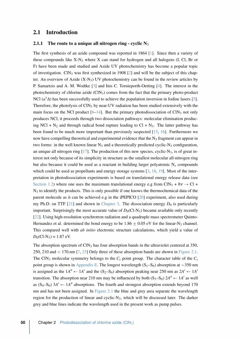
2.1 Introduction
2.1.1 The route to a unique all nitrogen ring - cyclic N3
The first synthesis of an azide compound was reported in 1864 [1]. Since then a variety of
these compounds like X-N3 where X can stand for hydrogen and all halogens (I, Cl, Br or
F) have been made and studied and Azide UV photochemistry has become a popular topic
of investigation. ClN3 was first synthesized in 1908 [2] and will be the subject of this chap-
ter. An overview of Azide (X-N3) UV photochemistry can be found in the review articles by
P. Samartzis and A. M. Wodtke [3] and Inis C. Tornieporth-Oetting [4]. The interest in the
photochemistry of chlorine azide (ClN3) comes from the fact that the primary photo-product
NCl (a1∆) has been successfully used to achieve the population inversion in Iodine lasers [5].
Therefore, the photolysis of ClN3 by near-UV radiation has been studied extensively with the
main focus on the NCl product [6–14]. But the primary photodissociation of ClN3 not only
produces NCl, it proceeds through two dissociation pathways: molecular elimination produc-
ing NCl + N2 and through radical bond rupture leading to Cl + N3. The latter pathway has
been found to be much more important than previously suspected [15, 16]. Furthermore we
now have compelling theoretical and experimental evidence that the N3 fragment can appear in
two forms: in the well known linear N3 and a theoretically predicted cyclic-N3 configuration,
an unique all nitrogen ring [17]. The production of this new species, cyclic-N3, is of great in-
terest not only because of its simplicity in structure as the smallest molecular all-nitrogen ring
but also because it could be used as a reactant in building larger polyatomic Nx compounds
which could be used as propellants and energy storage systems [3, 18, 19]. Most of the inter-
pretation in photodissociation experiments is based on translational energy release data (see
Section 1.2) where one uses the maximum translational energy e.g from ClN3 + hν Ñ Cl +
N3 to identify the products. This is only possible if one knows the thermochemical data of the
parent molecule as it can be achieved e.g in the iPEPICO [20] experiment, also used during
my Ph.D. on TTF [21] and shown in Chapter 3. The dissociation energy D0 is particularly
important. Surprisingly the most accurate value of D0(Cl-N3) became available only recently
[22]. Using high-resolution synchrotron radiation and a quadruple mass spectrometer Quinto-
Hernandez et al. determined the bond energy to be 1.86 ˘ 0.05 eV for the linear-N3 channel.
This compared well with ab initio electronic structure calculations, which yield a value of
D0(Cl-N3) = 1.87 eV.
The absorption spectrum of ClN3 has four absorption bands in the ultraviolet centered at 350,
250, 210 and ă 170.nm [7, 23] Only three of these absorption bands are shown in Figure 2.1.
The ClN3 molecular symmetry belongs to the Cs point group. The character table of the Cs
point group is shown in Appendix E. The longest wavelength (S1–S0) absorption at „350 nm
is assigned as the 1A2 Ð 1A1 and the (S2–S0) absorption peaking near 250 nm as 2A1 Ð 1A1
transition. The absorption near 210 nm may be influenced by both (S3–S0) 2A2 Ð 1A1 as well
as (S4–S0) 3A1 Ð 1A2 absorptions. The fourth and strongest absorption extends beyond 170
nm and has not been assigned. In Figure 2.1 the blue and grey area separate the wavelength
region for the production of linear and cyclic-N3, which will be discussed later. The darker
grey and blue lines indicate the wavelength used in the present work as pump pulses.
50 Chapter 2 Photodissociation of chlorine azide (ClN3)
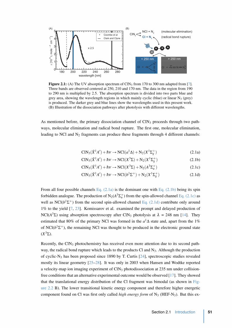
ClN3
NCl + N2
Cl + N3
> 250 nm< 250 nm
Cl + N N NCl +
N
N
N
(B)(A)
(molecular elimination)
(radical bond rupture)
Cl
N N N
180 200 220 240 260 2800
1
2
3
4
5
wavelength [nm]
ε [1
03 L
mol
e−1
cm
−1]
Coombe et al
Clark and Clyne
x 2.5
201268
Figure 2.1: (A) The UV absorption spectrum of ClN3 from 170 to 300 nm adapted from [7].
Three bands are observed centered at 250, 210 and 170 nm. The data in the region from 190
to 290 nm is multiplied by 2.5. The absorption spectrum is divided into two parts blue and
grey area, showing the wavelength regions in which mainly cyclic (blue) or linear N3 (grey)
is produced. The darker grey and blue lines show the wavelengths used in this present work.
(B) Illustration of the dissociation pathways after photolysis with different wavelengths.
As mentioned before, the primary dissociation channel of ClN3 proceeds through two path-
ways, molecular elimination and radical bond rupture. The first one, molecular elimination,
leading to NCl and N2 fragments can produce these fragments through 4 different channels:
ClN3pX1A1q ` hν Ñ NClpa1∆q ` N2pX1
Σ`g q (2.1a)
ClN3pX1A1q ` hν Ñ NClpX3Σq ` N2pX1
Σ`g q (2.1b)
ClN3pX1A1q ` hν Ñ NClpX3Σq ` N2pA3
Σ`u q (2.1c)
ClN3pX1A1q ` hν Ñ NClpb1Σ
`q ` N2pX1Σ
`g q (2.1d)
From all four possible channels Eq. (2.1a) is the dominant one with Eq. (2.1b) being its spin
forbidden analogue. The production of N2(A3Σ
`u ) from the spin-allowed channel Eq. (2.1c) as
well as NCl(b1Σ
`) from the second spin-allowed channel Eq. (2.1d) contribute only around
1% to the yield [7, 23]. Komissarov et al. examined the prompt and delayed production of
NCl(A3Σ) using absorption spectroscopy after ClN3 photolysis at λ = 248 nm [14]. They
estimated that 80% of the primary NCl was formed in the a1∆ state and, apart from the 1%
of NCl(b1Σ
`), the remaining NCl was thought to be produced in the electronic ground state
(X3Σ).
Recently, the ClN3 photochemistry has received even more attention due to its second path-
way, the radical bond rupture which leads to the products Cl and N3. Although the production
of cyclic-N3 has been proposed since 1890 by T. Curtis [24], spectroscopic studies revealed
mostly its linear geometry [25–28]. It was only in 2003 when Hansen and Wodtke reported
a velocity-map ion imaging experiment of ClN3 photodissociation at 235 nm under collision-
free conditions that an alternative experimental outcome would be observed [17]. They showed
that the translational energy distribution of the Cl fragment was bimodal (as shown in Fig-
ure 2.2 B). The lower transitional kinetic energy component and therefore higher energetic
component found on Cl was first only called high energy form of N3 (HEF-N3). But this ex-
Section 2.1 Introduction 51
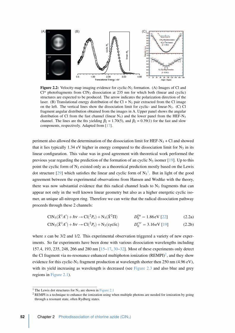
(A) (B) (C)
Figure 2.2: Velocity-map imaging evidence for cyclic-N3 formation. (A) Images of Cl and
Cl* photofragments from ClN3 dissociation at 235 nm for which both (linear and cyclic)
structures are expected to be produced. The arrow indicates the polarization direction of the
laser. (B) Translational energy distribution of the Cl + N3 pair extracted from the Cl image
on the left. The vertical lines show the dissociation limit for cyclic- and linear-N3. (C) Cl
fragment angular distribution obtained from the images in A. Upper panel shows the angular
distribution of Cl from the fast channel (linear N3) and the lower panel from the HEF-N3
channel. The lines are the fits yielding β2 = 1.70(5), and β2 = 0.39(1) for the fast and slow
components, respectively. Adapted from [17].
periment also allowed the determination of the dissociation limit for HEF-N3 + Cl and showed
that it lies typically 1.34 eV higher in energy compared to the dissociation limit for N3 in its
linear configuration. This value was in good agreement with theoretical work performed the
previous year regarding the prediction of the formation of an cyclic N3 isomer [19]. Up to this
point the cyclic form of N3 existed only as a theoretical prediction mostly based on the Lewis
dot structure [29] which satisfies the linear and cyclic form of N31. But in light of the good
agreement between the experimental observations from Hansen and Wodtke with the theory,
there was now substantial evidence that this radical channel leads to N3 fragments that can
appear not only in the well known linear geometry but also as a higher energetic cyclic iso-
mer, an unique all-nitrogen ring. Therefore we can write that the radical dissociation pathway
proceeds through these 2 channels:
ClN3pX1A1q ` hν Ñ Clp2Pxq ` N3pX2Πq Dlin
0 “ 1.86eV [22] (2.2a)
ClN3pX1A1q ` hν Ñ Clp2Pxq ` N3pcyclicq Dcyc0 “ 3.16eV [19] (2.2b)
where x can be 3/2 and 1/2. This experimental observation triggered a variety of new exper-
iments. So far experiments have been done with various dissociation wavelengths including
157.4, 193, 235, 248, 266 and 280 nm [15–17, 30–32]. Most of these experiments only detect
the Cl fragment via ns-resonance enhanced multiphoton ionization (REMPI)2, and they show
evidence for this cyclic-N3 fragment production at wavelength shorter then 250 nm (4.96 eV),
with its yield increasing as wavelength is decreased (see Figure 2.3 and also blue and grey
regions in Figure 2.1).
1 The Lewis dot structures for N3 are shown in Figure 2.12 REMPI is a technique to enhance the ionization using when multiple photons are needed for ionization by going
through a resonant state, often Rydberg states.
52 Chapter 2 Photodissociation of chlorine azide (ClN3)
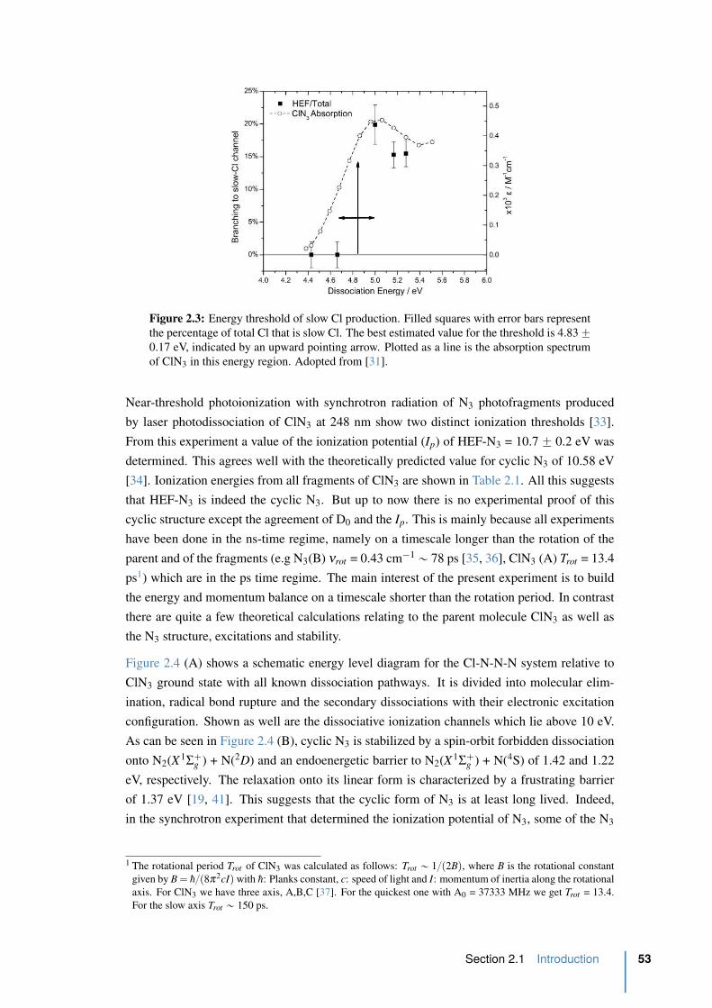
Figure 2.3: Energy threshold of slow Cl production. Filled squares with error bars represent
the percentage of total Cl that is slow Cl. The best estimated value for the threshold is 4.83 ˘0.17 eV, indicated by an upward pointing arrow. Plotted as a line is the absorption spectrum
of ClN3 in this energy region. Adopted from [31].
Near-threshold photoionization with synchrotron radiation of N3 photofragments produced
by laser photodissociation of ClN3 at 248 nm show two distinct ionization thresholds [33].
From this experiment a value of the ionization potential (Ip) of HEF-N3 = 10.7 ˘ 0.2 eV was
determined. This agrees well with the theoretically predicted value for cyclic N3 of 10.58 eV
[34]. Ionization energies from all fragments of ClN3 are shown in Table 2.1. All this suggests
that HEF-N3 is indeed the cyclic N3. But up to now there is no experimental proof of this
cyclic structure except the agreement of D0 and the Ip. This is mainly because all experiments
have been done in the ns-time regime, namely on a timescale longer than the rotation of the
parent and of the fragments (e.g N3(B) νrot = 0.43 cm´1 „ 78 ps [35, 36], ClN3 (A) Trot = 13.4
ps1) which are in the ps time regime. The main interest of the present experiment is to build
the energy and momentum balance on a timescale shorter than the rotation period. In contrast
there are quite a few theoretical calculations relating to the parent molecule ClN3 as well as
the N3 structure, excitations and stability.
Figure 2.4 (A) shows a schematic energy level diagram for the Cl-N-N-N system relative to
ClN3 ground state with all known dissociation pathways. It is divided into molecular elim-
ination, radical bond rupture and the secondary dissociations with their electronic excitation
configuration. Shown as well are the dissociative ionization channels which lie above 10 eV.
As can be seen in Figure 2.4 (B), cyclic N3 is stabilized by a spin-orbit forbidden dissociation
onto N2(X1Σ
`g ) + N(2D) and an endoenergetic barrier to N2(X1
Σ`g ) + N(4S) of 1.42 and 1.22
eV, respectively. The relaxation onto its linear form is characterized by a frustrating barrier
of 1.37 eV [19, 41]. This suggests that the cyclic form of N3 is at least long lived. Indeed,
in the synchrotron experiment that determined the ionization potential of N3, some of the N3
1 The rotational period Trot of ClN3 was calculated as follows: Trot „ 1p2Bq, where B is the rotational constant
given by B “ hp8π2cIq with h: Planks constant, c: speed of light and I: momentum of inertia along the rotational
axis. For ClN3 we have three axis, A,B,C [37]. For the quickest one with A0 = 37333 MHz we get Trot = 13.4.
For the slow axis Trot „ 150 ps.
Section 2.1 Introduction 53
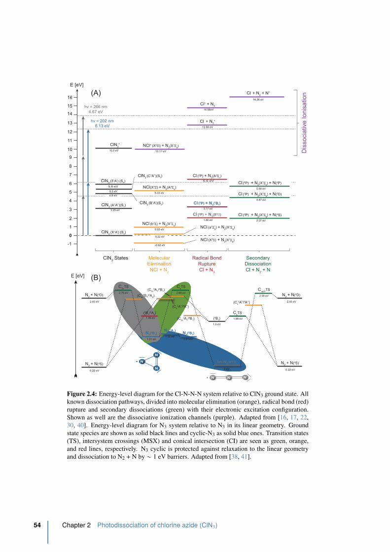
ClN3
(X1A’) (S0)
0
1
2
3
4
5
6
7
8
9
10
11
12
13
14
15
ClN3
(A1A’’)(S1)
3.25 eV
ClN3 (B1A’)(S
2)
4.9 eV
ClN3
(31A’) (S4)
5.8 eV
ClN3 States Molecular
Elimination
NCl + N2
Radical Bond
Rupture
Cl + N3
Secondary
Dissociation
Cl + N2 + N
Dis
socia
tive Ionis
ation
E [eV]
NCl (X2Σ) + N
2(X1Σ
g)
-1
NCl (a1Σ
g) + N
2(X1Σ
g)
NCl (b1Σ) + N
2(X1Σ
g)
0.93 eV
0.22 eV
NCl(X3Σ) + N2(A3Σ
g)
5.33 eV
Cl (2P) + N
3(X2Π)
1.86 eV
Cl (2P) + N
3(2B
1)
3.17 eV
Cl (2P) + N
3(A2Σ
u)
Cl (2P) + N
2(X1Σ
g) + N(4S)
2.07 eV
Cl (2P) + N
2(X1Σ
g) + N(2D)
4.47 eV
Cl (2P) + N
2(X1Σ
g) + N(2P)
5.68 eV
hv = 202 nm
6.13 eV
hv = 266 nm
4.67 eV
ClN3+
10.2 eV
NCl+ (X2Π) + N
2(X1Σ
g)
10.17 eV
Cl + N
3+
12.88 eV
Cl+ + N3
14.98eV
Cl + N
2 + N+
16.36 eV
6.6 eV
16
-0.92 eV
5.2 eV
ClN3 (C1A’’)(S
3)
E [eV]
N2 + N(4S)
0.22 eV
lin-N3(X2Π)
0 eV
N2 + N(4S)
0.22 eV
N2 + N(2D)
2.45 eV
N2 + N(2D)
2.45 eV
N3(2B
1)
N3(2A
2)
N3(2B
1)
C2v
TS
2.75 eV
1.31 eV1.32 eV
1.31 eV
CsTS
2.69 eVC∞V
TS
2.58 eV
1.99 eV1.96 eV
1.9 eV
(2B1/2A
2) C
sTS
(4B1)
(C2v
2B1/4A
2)
(Cs2A’’/4A’’)
(C2v
2A1/4B
1)
(C2v
2A1/4B
1)
(Cs2A’’/4A’’)
N
N
N
N N N
(A)
(B)
Figure 2.4: Energy-level diagram for the Cl-N-N-N system relative to ClN3 ground state. All
known dissociation pathways, divided into molecular elimination (orange), radical bond (red)
rupture and secondary dissociations (green) with their electronic excitation configuration.
Shown as well are the dissociative ionization channels (purple). Adapted from [16, 17, 22,
30, 40]. Energy-level diagram for N3 system relative to N3 in its linear geometry. Ground
state species are shown as solid black lines and cyclic-N3 as solid blue ones. Transition states
(TS), intersystem crossings (MSX) and conical intersection (CI) are seen as green, orange,
and red lines, respectively. N3 cyclic is protected against relaxation to the linear geometry
and dissociation to N2 + N by „ 1 eV barriers. Adapted from [38, 41].
54 Chapter 2 Photodissociation of chlorine azide (ClN3)
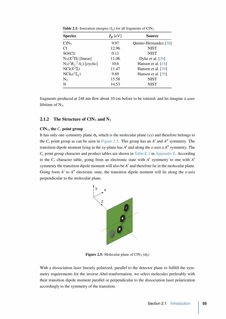
Table 2.1: Ionization energies (Ip) for all fragments of ClN3
Species IIIppp [eV] Source
ClN3 9.97 Quinto-Hernandez [38]
Cl 12.96 NIST
SO(Cl) 0.11 NIST
N3(X2Π) [linear] 11.06 Dyke et al. [26]
N3(2B1,2 A2) [cyclic] 10.6 Hansen et al. [16]
NCl(X2Σ) 11.47 Hansen et al. [39]
NCl(a1Σg) 9.69 Hansen et al. [39]
N2 15.58 NIST
N 14.53 NIST
fragments produced at 248 nm flew about 10 cm before to be ionized, and let imagine a µsec
lifetime of N3.
2.1.2 The Structure of ClN3 and N3
ClN3, the Cs point group
It has only one symmetry plane σh which is the molecular plane (xy) and therefore belongs to
the Cs point group as can be seen in Figure 2.5. This group has an A1 and A2 symmetry. The
transition dipole moment lying in the xy-plane has A1 and along the z-axis a A2 symmetry. The
Cs point group character and product tables are shown in Table E.1 in Appendix E. According
to the Cs character table, going from an electronic state with A1 symmetry to one with A1
symmetry the transition dipole moment will also be A1 and therefore lie in the molecular plane.
Going form A1 to A2 electronic state, the transition dipole moment will lie along the z-axis
perpendicular to the molecular plane.
z
y x
Figure 2.5: Molecular plane of ClN3 (σh)
With a dissociation laser linearly polarized, parallel to the detector plane to fullfill the sym-
metry requirements for the inverse Abel-tranformation, we select molecules preferably with
their transition dipole moment parallel or perpendicular to the dissociation laser polarization
accordingly to the symmetry of the transition.
Section 2.1 Introduction 55
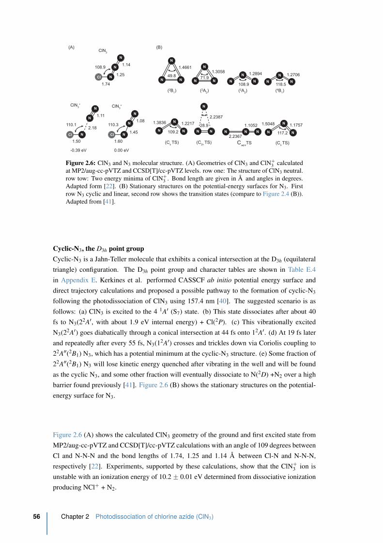
(A) (B)
Cl N
N
N
1.74
1.25
1.14108.9
ClN3
Cl N
N
N
1.50
2.18
1.11
110.1
ClN3
+
Cl N
N
N
1.60
1.45
1.08110.3
ClN3
+
-0.39 eV 0.00 eV
N N N
N
N N
N
N N
N
N N
N
N N
N
N N N N
N
N
N N
1.4661
49.81.3058 1.2894 1.2706
1.3836 1.2217
2.2387
2.2367
1.1052 1.5048 1.1757
71.9
108.9 118.5
109.2
28.9
117.2
(2B1) (2A
2) (2A
2) (4B
1)
(Cs TS) (C
2v TS) C∞v
TS (Cs TS)
Figure 2.6: ClN3 and N3 molecular structure. (A) Geometries of ClN3 and ClN`3 calculated
at MP2/aug-cc-pVTZ and CCSD[T]/cc-pVTZ levels. row one: The structure of ClN3 neutral.
row tow: Two energy minima of ClN`3 . Bond length are given in A and angles in degrees.
Adapted form [22]. (B) Stationary structures on the potential-energy surfaces for N3. First
row N3 cyclic and linear, second row shows the transition states (compare to Figure 2.4 (B)).
Adapted from [41].
Cyclic-N3, the D3h point group
Cyclic-N3 is a Jahn-Teller molecule that exhibits a conical intersection at the D3h (equilateral
triangle) configuration. The D3h point group and character tables are shown in Table E.4
in Appendix E. Kerkines et al. performed CASSCF ab initio potential energy surface and
direct trajectory calculations and proposed a possible pathway to the formation of cyclic-N3
following the photodissociation of ClN3 using 157.4 nm [40]. The suggested scenario is as
follows: (a) ClN3 is excited to the 4 1A1 (S7) state. (b) This state dissociates after about 40
fs to N3(22A1, with about 1.9 eV internal energy) + Cl(2P). (c) This vibrationally excited
N3(22A1) goes diabatically through a conical intersection at 44 fs onto 12A1. (d) At 19 fs later
and repeatedly after every 55 fs, N3(12A1) crosses and trickles down via Coriolis coupling to
22A2(2B1) N3, which has a potential minimum at the cyclic-N3 structure. (e) Some fraction of
22A2(2B1) N3 will lose kinetic energy quenched after vibrating in the well and will be found
as the cyclic N3, and some other fraction will eventually dissociate to N(2D) +N2 over a high
barrier found previously [41]. Figure 2.6 (B) shows the stationary structures on the potential-
energy surface for N3.
Figure 2.6 (A) shows the calculated ClN3 geometry of the ground and first excited state from
MP2/aug-cc-pVTZ and CCSD[T]/cc-pVTZ calculations with an angle of 109 degrees between
Cl and N-N-N and the bond lengths of 1.74, 1.25 and 1.14 A between Cl-N and N-N-N,
respectively [22]. Experiments, supported by these calculations, show that the ClN`3 ion is
unstable with an ionization energy of 10.2 ˘ 0.01 eV determined from dissociative ionization
producing NCl` + N2.
56 Chapter 2 Photodissociation of chlorine azide (ClN3)

(X1A’) (S0)
0
1
2
3
4
5
6
7
8
9
10
11
(A1A’’)(S1)
3.25 eV
(B1A’)(S2)4.9 eV
(C1A’’) (S3)
5.8 eV
E [eV]
20
1 n
m -
6.1
7 e
V
26
8 n
m -
4.6
3 e
V
ClN3+
10.2 eV
(31A’) (S4)
5.2 eV
Cl
N3
Cl N3
Cl (2P) + N
3(X2Π)
1.86 eV
Cl (2P) + N
3(2B
1)
3.17 eV
8 photons for N3
9 photons for Cl
805
nm
dissociative
ionization
12
13
14
15
Cl + N
3+
12.88 eV
Cl+ + N3
14.98eV
IP N
3lin
= 1
1.0
3 e
V
IP C
l =
12.9
7 e
V
multiphoton
ionization
dissociation
A‘ (xy) - β2 = 2
A“ (z) - β2 = -1
εp
εp
VMI image
NCl+ (X2Π) + N
2(X1Σ
g)
10.17 eV
Figure 2.7: ClN3 excitation scheme at 268 and 201 nm with only the dissociative ionization
channels of Cl` and N`3 . Shown are the electronic states of ClN3 with their symmetry and
the expected angular distribution for the possible electronic transitions.
2.2 Experimental
2.2.1 The excitation scheme for ClN3 at 268 and 201 nm
Figure 2.7 shows the energy levels of ClN3 which is a reduced version of Figure 2.4 focusing
on the electronic states reachable by a one photon transition with 268 nm and 201 nm. We
can see that in the two energy regions we can reach with these photon energies, there are
three excited states of ClN3. In the 250 nm absorption band there is the S2 state with an A1
symmetry and in the 210 nm absorption band there is the S3 and S4 state with an A2 and
A1 symmetry, respectively. The ground state of ClN3 has an A1 symmetry and therefore the
two A1 states should be reach from the ground state by an electronic transition of A1. This
means that the linear polarized pump laser will excite preferably ClN3 molecules with the
molecular plane (xy) containing the laser field. Consequently the dissociation will lead to an
angular distribution characterized by β2 “ 2. This will be the case for the S2 and S4 electronic
states if the dissociation is fast compared to the rotation or out of plane bending modes of the
molecule. The A2 transition to the S3 electronic state leads to a selection of the molecular
plane perpendicular to the laser polarization and to an angular distribution characterized by
β2 “ ´1.
The ionization potentials of N3 cyclic/linear and Cl are 10.6/11.03 eV and 12.97 eV, respec-
tively. Using an 803 nm pulse for ionizing we are using 8-9 photons to reach the ionization
thresholds of the fragments. This extreme multiphoton ionization needs high laser intensities
in the range of ą 1012 W/cm2. High laser intensities also allows us to do dissociative ioniza-
tion. This means we have enough intensity to ionize and dissociate at the same time. As we
will see later the signal coming from this dissociative ionization is rather strong and can be
Section 2.2 Experimental 57
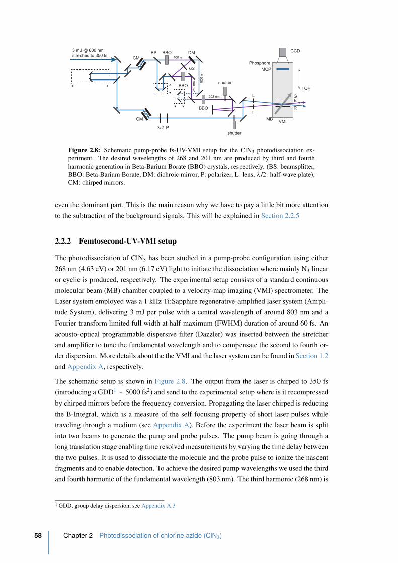
BS BBO400 nm
800 n
m
DM
BBO
269 n
m
BBO
λ/2
202 nm
VMI
L
L
λ/2 P
CCD
Phosphore
MCP
TOF
R
EG
MB
CM
CM
3 mJ @ 800 nm
streched to 350 fs
shutter
shutter
Figure 2.8: Schematic pump-probe fs-UV-VMI setup for the ClN3 photodissociation ex-
periment. The desired wavelengths of 268 and 201 nm are produced by third and fourth
harmonic generation in Beta-Barium Borate (BBO) crystals, respectively. (BS: beamsplitter,
BBO: Beta-Barium Borate, DM: dichroic mirror, P: polarizer, L: lens, λ /2: half-wave plate),
CM: chirped mirrors.
even the dominant part. This is the main reason why we have to pay a little bit more attention
to the subtraction of the background signals. This will be explained in Section 2.2.5
2.2.2 Femtosecond-UV-VMI setup
The photodissociation of ClN3 has been studied in a pump-probe configuration using either
268 nm (4.63 eV) or 201 nm (6.17 eV) light to initiate the dissociation where mainly N3 linear
or cyclic is produced, respectively. The experimental setup consists of a standard continuous
molecular beam (MB) chamber coupled to a velocity-map imaging (VMI) spectrometer. The
Laser system employed was a 1 kHz Ti:Sapphire regenerative-amplified laser system (Ampli-
tude System), delivering 3 mJ per pulse with a central wavelength of around 803 nm and a
Fourier-transform limited full width at half-maximum (FWHM) duration of around 60 fs. An
acousto-optical programmable dispersive filter (Dazzler) was inserted between the stretcher
and amplifier to tune the fundamental wavelength and to compensate the second to fourth or-
der dispersion. More details about the the VMI and the laser system can be found in Section 1.2
and Appendix A, respectively.
The schematic setup is shown in Figure 2.8. The output from the laser is chirped to 350 fs
(introducing a GDD1 „ 5000 fs2) and send to the experimental setup where is it recompressed
by chirped mirrors before the frequency conversion. Propagating the laser chirped is reducing
the B-Integral, which is a measure of the self focusing property of short laser pulses while
traveling through a medium (see Appendix A). Before the experiment the laser beam is split
into two beams to generate the pump and probe pulses. The pump beam is going through a
long translation stage enabling time resolved measurements by varying the time delay between
the two pulses. It is used to dissociate the molecule and the probe pulse to ionize the nascent
fragments and to enable detection. To achieve the desired pump wavelengths we used the third
and fourth harmonic of the fundamental wavelength (803 nm). The third harmonic (268 nm) is
1 GDD, group delay dispersion, see Appendix A.3
58 Chapter 2 Photodissociation of chlorine azide (ClN3)

produced by mixing the fundamental wavelength (803 nm) with the second harmonic (402 nm)
in a Beta-Barium Borate (BBO) crystal. In the case of the fourth harmonic (201 nm) the third
harmonic is again mixed with the fundamental wavelength in a BBO crystal. For 268 nm we
achieve typically around 60 µJ/p with a FWHM bandwidth of 1.54 nm. These values depend
largely on the crystal in use. The thicker the crystal the greater is the power but the bandwidth
gets smaller and therefore the duration longer (see Appendix A). We tried to get the shortest
pulses as possible by reducing the thickness but not loosing too much of the energy. Table 2.2
gives an overview of the crystals used and the achieved power conversions along with their
bandwidths and expected theoretical pulse durations (Fourier-transform limited FTL).
The typical pump pulse energies were „20 µJ and „9µJ for the 268 and 201 nm, respec-
tively. All results presented here have been detected by a multiphoton ionization process due
to the fact that a probe pulse centered at 803 nm was used and all ionization energies of the
detected fragments lie in the 10 eV region. Typically „200 µJ was required for the ionization
to effectively get the Ip from the fragments (Ip ą 10 eV). The spectral bandwidths of the used
pulses were measured to be 1.54 nm for the 268 nm, 0.85 nm for the 201 nm and 15.5 nm for
the 803 nm. This corresponds to Fourier-transform limited bandwidths of 97 fs, 100 fs and
86 fs, respectively, and thus leading to a theoretical cross-correlation time between the pump
and probe pulse of 92 fs (268 + 803 nm) and 93 fs (201 + 803 nm). The experimental values
for the cross-correlation time measured in argon of 110 fs and 145 fs shown in Figure 2.9 is
somewhat longer than the theoretical value due to high power effects, especially due to the
viewport and the fact that no compression line is used after the last frequency conversion step
to compress the UV beams. Indeed such a compression, e.g a prism compressor, would reduce
the cross-correlation time but easily reduce the intensity output by a factor of two and intro-
duce more spatial chirp. The beams were focused into the molecular beam by using 250 and
200 mm focal length lenses for the pump and probe beam, respectively. The dimensions of the
laser spots were determined using a UV-CCD camera and the resulting pulse intensities were
calculated to be „5 ˆ 1012 W/cm2 for the 268 nm and „1 ˆ 1013 W/cm2 for 803 nm radiation.
The pump beam polarization was set parallel to the detector plane to provide the cylindrical
symmetry required for the image reconstruction (see Section 1.2.3). The polarization of the
probe beam was first also set to parallel and was later changed to perpendicular as comparison,
Table 2.2: Utilized BBO crystals for the generation of third (268 nm) and fourth (201 nm) harmonic
with their characteristics and achieved conversion values. The beam is typically 7 mm is diameter.
λ [nm] BBO type dim [mm] P [µJ] ∆λ [nm] ∆T (FTL) [fs]
403:type1, θ = 35˝, φ = 90˝
P/P @ 500-700 nm8x8x0.2 „250 8.44(15) „40
268:type1, θ = 44.3˝, φ = 90˝
P/P @ 400-803/266 nm12x12x0.2 „60 1.542(3) „97
201:type1, θ = 64˝, φ = 90˝
P/P @ 266-803/201 nm10x10x0.1 „12 0.841(8) „100
803: „300 15.55(7) „86
Section 2.2 Experimental 59
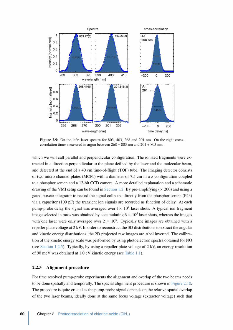
266 268 270
268.416(1)
1.542(3)
200 201 202
201.315(3)
0.841(8)
783 803 823
803.47(3)
15.55(7)
393 403 413
403.27(2)
8.44(15)
wavelength [nm]
time delay [fs]
−200 0 200
Ar
268 nm
110 fs
−200 0 200
Ar
201 nm
145 fs
wavelength [nm]
0
0.2
0.4
0.6
0.8
1
Inte
nsity
[nor
mal
ized
]
0
0.2
0.4
0.6
0.8
1
Inte
nsity
[nor
mal
ized
]
Spectra cross-correlation
Figure 2.9: On the left: laser spectra for 803, 403, 268 and 201 nm. On the right cross-
correlation times measured in argon between 268 + 803 nm and 201 + 803 nm.
which we will call parallel and perpendicular configuration. The ionized fragments were ex-
tracted in a direction perpendicular to the plane defined by the laser and the molecular beam,
and detected at the end of a 40 cm time-of-flight (TOF) tube. The imaging detector consists
of two micro-channel plates (MCPs) with a diameter of 7.5 cm in a z-configuration coupled
to a phosphor screen and a 12-bit CCD camera. A more detailed explanation and a schematic
drawing of the VMI setup can be found in Section 1.2. By pre-amplifying (ˆ 200) and using a
gated boxcar integrator to record the signal collected directly from the phosphor screen (P43)
via a capacitor (100 pF) the transient ion signals are recorded as function of delay. At each
pump-probe delay the signal was averaged over 1ˆ 104 laser shots. A typical ion fragment
image selected in mass was obtained by accumulating 6 ˆ 105 laser shots, whereas the images
with one laser were only averaged over 2 ˆ 105. Typically the images are obtained with a
repeller plate voltage at 2 kV. In order to reconstruct the 3D distributions to extract the angular
and kinetic energy distributions, the 2D projected raw images are Abel inverted. The calibra-
tion of the kinetic energy scale was performed by using photoelectron spectra obtained for NO
(see Section 1.2.5). Typically, by using a repeller plate voltage of 2 kV, an energy resolution
of 90 meV was obtained at 1.0 eV kinetic energy (see Table 1.1).
2.2.3 Alignment procedure
For time resolved pump-probe experiments the alignment and overlap of the two beams needs
to be done spatially and temporally. The spacial alignment procedure is shown in Figure 2.10.
The procedure is quite crucial as the pump-probe signal depends on the relative spatial overlap
of the two laser beams, ideally done at the same focus voltage (extractor voltage) such that
60 Chapter 2 Photodissociation of chlorine azide (ClN3)
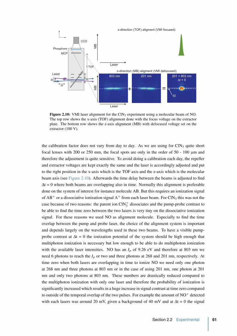
803 nm 201 nm 201 + 803 nm
Δt = 0
α
Laser
MB
Laser
MB
+ =Δt
Laser
VMI
CCD
Phosphore
MCP
TOF
R
E
G
MB
α
z-direction (MB) aligment (VMI defocused)
x-direction (TOF) aligment (VMI focused)
y - Laser
x - TOF
z - MB
TOF [μsec]
803 nm201 nm
Δt = 0
overlap
laser at right
TOF-axis position
(focused)
laser slighly off
(out of focus)
Figure 2.10: VMI laser alignment for the ClN3 experiment using a molecular beam of NO.
The top row shows the x-axis (TOF) alignment done with the focus voltage on the extractor
plate. The bottom row shows the z-axis alignment (MB) with defocused voltage set on the
extractor (100 V).
the calibration factor does not vary from day to day. As we are using for ClN3 quite short
focal lenses with 200 or 250 mm, the focal spots are only in the order of 50 - 100 µm and
therefore the adjustment is quite sensitive. To avoid doing a calibration each day, the repeller
and extractor voltages are kept exactly the same and the laser is accordingly adjusted and put
to the right position in the x-axis which is the TOF axis and the z-axis which is the molecular
beam axis (see Figure 2.10). Afterwards the time delay between the beams is adjusted to find
∆t = 0 where both beams are overlapping also in time. Normally this alignment is preferable
done on the system of interest for instance molecule AB. But this requires an ionization signal
of AB` or a dissociative ionization signal A` from each laser beam. For ClN3 this was not the
case because of two reasons: the parent ion ClN`3 dissociates and the pump-probe contrast to
be able to find the time zero between the two lasers is very tiny on the dissociative ionization
signal. For these reasons we used NO as alignment molecule. Especially to find the time
overlap between the pump and probe laser, the choice of the alignment system is important
and depends largely on the wavelengths used in these two beams. To have a visible pump-
probe contrast at ∆t = 0 the ionization potential of the system should be high enough that
multiphoton ionization is necessary but low enough to be able to do multiphoton ionization
with the available laser intensities. NO has an Ip of 9.26 eV and therefore at 803 nm we
need 6 photons to reach the Ip or two and three photons at 268 and 201 nm, respectively. At
time zero when both lasers are overlapping in time to ionize NO we need only one photon
at 268 nm and three photons at 803 nm or in the case of using 201 nm, one photon at 201
nm and only two photons at 803 nm. These numbers are drastically reduced compared to
the multiphoton ionization with only one laser and therefore the probability of ionization is
significantly increased which results in a huge increase in signal contrast at time zero compared
to outside of the temporal overlap of the two pulses. For example the amount of NO` detected
with each lasers was around 20 mV, given a background of 40 mV and at ∆t = 0 the signal
Section 2.2 Experimental 61
increased over 200 mV.
In the first step the two laser beams are adjusted in vertical and horizontal position before
and after the entrance in the VMI by pinholes to ensure that the beams are going perfectly
horizontal through voltage plates. Then the x-axis (TOF-axis, in our setup the vertical axis)
is aligned by putting the extractor voltage to the value for which the calibration factor was
determined. The laser beam is adjusted to be in focus on the camera which results in a signal
spot on the detector as shown in Figure 2.10 on the right in the first row. If the beam is not
exactly at the same vertical position the image will be out of focus for this particular set of
voltages and the signal on the camera gets more diffuse (second image). In this case the focus
voltage would be different and therefore also the calibration factor. The same is done with
the second laser so that on the TOF monitored on the oscilloscope the two signals from each
laser are overlapping (grey peak in Figure 2.10 first row on the right). To align the z-axis
overlap, the MB direction and in our setup the horizontal axis, the VMI is defocused. In this
case we are sensitive to the MB diameter and direction. As we can see in Figure 2.10 on the
bottom row we now have a horizontal line on the detector where we are able to overlap both
beams in the MB direction. We can even see that the line is slightly tilted with respect to the
horizontal axis which is the laser direction. This corresponds to the small angle α between
the two laser beams. After the alignment of both the TOF- and MB-axis the delay between
the two beams is scanned to find the time zero. When both beams are overlapping in time we
observe the increase in contrast on the CCD and on the oscilloscope as shown in Figure 2.10
on the outermost right plot. At this point fine adjustments on the MB- and TOF-axis can be
done to increase the contrast further and to optimize the spatial overlap on the pump-probe
signal directly. All adjustments are done with micrometer screws with the two last mirrors or
with the lenses which are mounted in xyz translation stages. In the case where the VMI is
defocused and we observe the horizontal line we can also adjust the lens position in the laser
direction (y-axis) so that we observe a relatively homogeneous horizontal line, meaning that
the laser waist is perfectly in the center of the VMI y-axis.
2.2.4 ClN3 Production
ClN3 is produced on site in a two-step reaction during the measurement. Typically ă 5% of
Cl2 in an Ar/He (20/80%) mixture is lead through moist sodium azide (NaN3 with water) in a
reactor. The reactor setup is shown schematic in Figure 2.11.
Initially NaN3 and water react to form HN3 + NaOH. In the second step HN3 reacts with Cl2
to produce ClN3 and HCl.
NaN3 ` H2O Ñ HN3 ` NaOH
HN3 ` Cl2 Ñ ClN3 ` HCl
A standard drying agent (Drierite, anhydous CaSO4) is used to remove water from the ClN3/Ar/He
mixture at the exit of the reactor. Helium is the preferred carrier gas to obtain very cold molec-
ular beams with almost no internal energies. But because Helium is hard to ionize, especially
62 Chapter 2 Photodissociation of chlorine azide (ClN3)
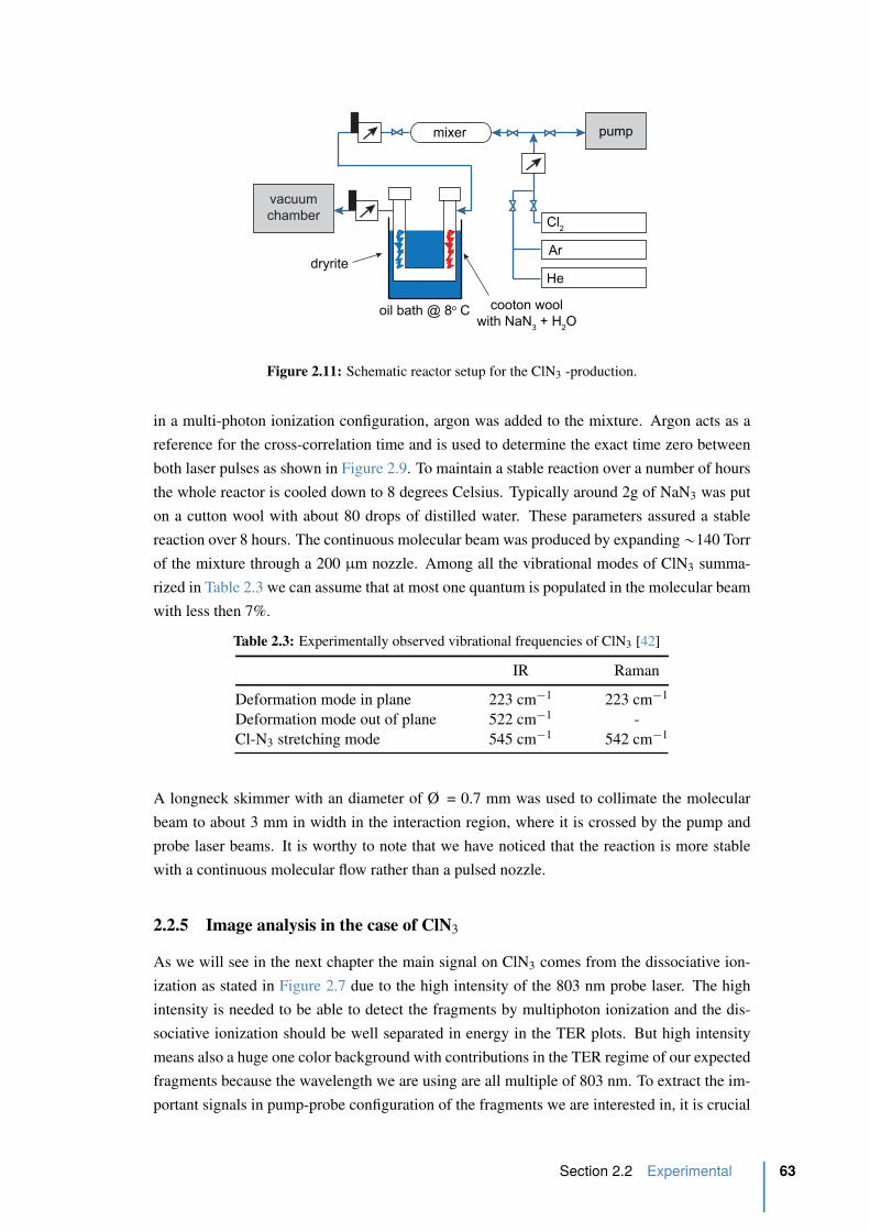
mixer pump
Cl2
Ardryrite
oil bath @ 8o C cooton wool
with NaN3 + H
2O
vacuum
chamber
He
Figure 2.11: Schematic reactor setup for the ClN3 -production.
in a multi-photon ionization configuration, argon was added to the mixture. Argon acts as a
reference for the cross-correlation time and is used to determine the exact time zero between
both laser pulses as shown in Figure 2.9. To maintain a stable reaction over a number of hours
the whole reactor is cooled down to 8 degrees Celsius. Typically around 2g of NaN3 was put
on a cutton wool with about 80 drops of distilled water. These parameters assured a stable
reaction over 8 hours. The continuous molecular beam was produced by expanding „140 Torr
of the mixture through a 200 µm nozzle. Among all the vibrational modes of ClN3 summa-
rized in Table 2.3 we can assume that at most one quantum is populated in the molecular beam
with less then 7%.
Table 2.3: Experimentally observed vibrational frequencies of ClN3 [42]
IR Raman
Deformation mode in plane 223 cm´1 223 cm´1
Deformation mode out of plane 522 cm´1 -
Cl-N3 stretching mode 545 cm´1 542 cm´1
A longneck skimmer with an diameter of Ø = 0.7 mm was used to collimate the molecular
beam to about 3 mm in width in the interaction region, where it is crossed by the pump and
probe laser beams. It is worthy to note that we have noticed that the reaction is more stable
with a continuous molecular flow rather than a pulsed nozzle.
2.2.5 Image analysis in the case of ClN3
As we will see in the next chapter the main signal on ClN3 comes from the dissociative ion-
ization as stated in Figure 2.7 due to the high intensity of the 803 nm probe laser. The high
intensity is needed to be able to detect the fragments by multiphoton ionization and the dis-
sociative ionization should be well separated in energy in the TER plots. But high intensity
means also a huge one color background with contributions in the TER regime of our expected
fragments because the wavelength we are using are all multiple of 803 nm. To extract the im-
portant signals in pump-probe configuration of the fragments we are interested in, it is crucial
Section 2.2 Experimental 63
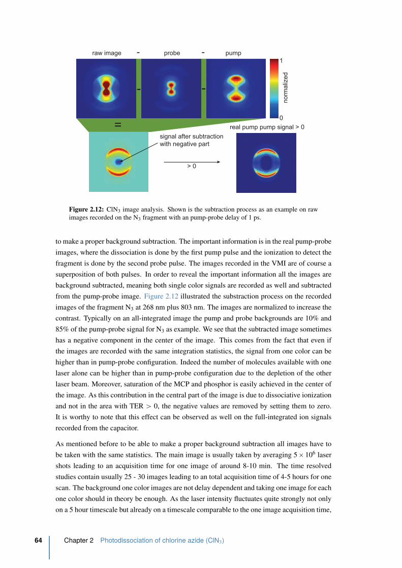
raw image probe pump- -
real pump pump signal > 0
- -
0
1
signal after subtraction
with negative part
no
rma
lize
d
=
> 0
Figure 2.12: ClN3 image analysis. Shown is the subtraction process as an example on raw
images recorded on the N3 fragment with an pump-probe delay of 1 ps.
to make a proper background subtraction. The important information is in the real pump-probe
images, where the dissociation is done by the first pump pulse and the ionization to detect the
fragment is done by the second probe pulse. The images recorded in the VMI are of course a
superposition of both pulses. In order to reveal the important information all the images are
background subtracted, meaning both single color signals are recorded as well and subtracted
from the pump-probe image. Figure 2.12 illustrated the substraction process on the recorded
images of the fragment N3 at 268 nm plus 803 nm. The images are normalized to increase the
contrast. Typically on an all-integrated image the pump and probe backgrounds are 10% and
85% of the pump-probe signal for N3 as example. We see that the subtracted image sometimes
has a negative component in the center of the image. This comes from the fact that even if
the images are recorded with the same integration statistics, the signal from one color can be
higher than in pump-probe configuration. Indeed the number of molecules available with one
laser alone can be higher than in pump-probe configuration due to the depletion of the other
laser beam. Moreover, saturation of the MCP and phosphor is easily achieved in the center of
the image. As this contribution in the central part of the image is due to dissociative ionization
and not in the area with TER ą 0, the negative values are removed by setting them to zero.
It is worthy to note that this effect can be observed as well on the full-integrated ion signals
recorded from the capacitor.
As mentioned before to be able to make a proper background subtraction all images have to
be taken with the same statistics. The main image is usually taken by averaging 5 ˆ 106 laser
shots leading to an acquisition time for one image of around 8-10 min. The time resolved
studies contain usually 25 - 30 images leading to an total acquisition time of 4-5 hours for one
scan. The background one color images are not delay dependent and taking one image for each
one color should in theory be enough. As the laser intensity fluctuates quite strongly not only
on a 5 hour timescale but already on a timescale comparable to the one image acquisition time,
64 Chapter 2 Photodissociation of chlorine azide (ClN3)
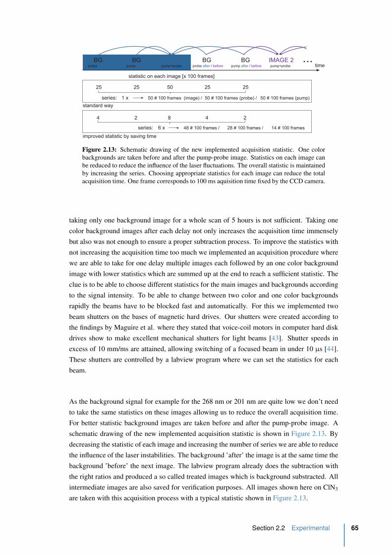
BG BG BG BGIMAGE 1time
25 25 25 2550
pump beforeprobe before pump+probe pump after / before
IMAGE 2pump+probe
...probe after / before
50 # 100 frames (image) /1 x 50 # 100 frames (probe) / 50 # 100 frames (pump)
4 2 4 28
48 # 100 frames /6 x 28 # 100 frames / 14 # 100 frames
standard way
improved statistic by saving time
series:
statistic on each image [x 100 frames]
series:
Figure 2.13: Schematic drawing of the new implemented acquisition statistic. One color
backgrounds are taken before and after the pump-probe image. Statistics on each image can
be reduced to reduce the influence of the laser fluctuations. The overall statistic is maintained
by increasing the series. Choosing appropriate statistics for each image can reduce the total
acquisition time. One frame corresponds to 100 ms aquisition time fixed by the CCD camera.
taking only one background image for a whole scan of 5 hours is not sufficient. Taking one
color background images after each delay not only increases the acquisition time immensely
but also was not enough to ensure a proper subtraction process. To improve the statistics with
not increasing the acquisition time too much we implemented an acquisition procedure where
we are able to take for one delay multiple images each followed by an one color background
image with lower statistics which are summed up at the end to reach a sufficient statistic. The
clue is to be able to choose different statistics for the main images and backgrounds according
to the signal intensity. To be able to change between two color and one color backgrounds
rapidly the beams have to be blocked fast and automatically. For this we implemented two
beam shutters on the bases of magnetic hard drives. Our shutters were created according to
the findings by Maguire et al. where they stated that voice-coil motors in computer hard disk
drives show to make excellent mechanical shutters for light beams [43]. Shutter speeds in
excess of 10 mm/ms are attained, allowing switching of a focused beam in under 10 µs [44].
These shutters are controlled by a labview program where we can set the statistics for each
beam.
As the background signal for example for the 268 nm or 201 nm are quite low we don’t need
to take the same statistics on these images allowing us to reduce the overall acquisition time.
For better statistic background images are taken before and after the pump-probe image. A
schematic drawing of the new implemented acquisition statistic is shown in Figure 2.13. By
decreasing the statistic of each image and increasing the number of series we are able to reduce
the influence of the laser instabilities. The background ’after’ the image is at the same time the
background ’before’ the next image. The labview program already does the subtraction with
the right ratios and produced a so called treated images which is background substracted. All
intermediate images are also saved for verification purposes. All images shown here on ClN3
are taken with this acquisition process with a typical statistic shown in Figure 2.13.
Section 2.2 Experimental 65
2.3 Time-resolved transients of ClN3 fragments
Because ClN3 is produced in a reaction on site during the experiment as seen in the previous
section it is important to check that one is not polluting the molecular beam with the interme-
diate products of this reaction. Both the UV and the 803 nm pulses are ideal sources to detect
pollution due to the multiphoton processes easily achieved in the femtosecond time regime
[45].
By pre-amplifying the signal extracted directly from the phosphor one is able the record the
time-of-flight (TOF) mass spectrum of the species in the molecular beam using the VMI as
a sophisticated mass spectrometer. In Figure 2.14 the time-of-flight (TOF) mass spectrum of
ClN3 is shown at both investigated wavelengths. Looking at the TOF spectrum it is evident
that there is no measurable pollution of the intermediate products like HN3, NaOH, HCl or
Cl2. Cl2 from the seeding mixture is starting to appear when the mixture of NaN3 and water
on the cotton wool is depleted indicated that the reaction is coming to an end. Furthermore
we observe that no parent ion ClN`3 is detected which would be expected at m/z = 77 amu.
This indicates that the parent ion is not stable and dissociated directly to the NCl`pX3Σq +
N2pX1Σ
`g q. Indeed, N. Hansen et al. measured the NCl and N2 fragments from ClN3 pho-
todissociation at 118 nm and 202 nm and they showed that ClN`3 is produced by 1 (118 nm)
or 2 (202 nm) photon excitation probably in the first excited cation state [39]. They argument
from the TER of NCl` is that the parent ion is short-lived requiring less than 0.28 eV to dis-
sociate to NCl + N2. They also showed quantum chemical calculations which suggest that
the barrier to dissociation for this cation may be no greater than 0.09 eV. Electronic structure
calculations on ClN`3 confirm that due to the large change in geometry compared to the parent
neutral ClN3 ionization leads to vibrational excited ClN`3 with more than enough energy to
dissociate [22].
Even though we are not able the measure the decay of the parent ion ClN`3 , a first guess of
the typical time constants in our system can be done by recording this TOF mass spectrum
for each fragment as a function of the delay between the dissociating (pump) and ionizing
(probe) laser. The discrimination of the fragments is given by the flight time. All ions with the
same mass and same TOF time are collected without energetic or angular discrimination by
boxcar integrators. Our setup had six channels allowing us to record at the same time all five
fragments plus argon as a reference. The signal out from the boxcar is an hardware average
over 100 ms which means 100 laser shots. This signal is sent to the computer where one delay
is typically integrated over 10-20 values in the computer. In addition 5 to 10 scans are acquired
and averaged. Figure 2.15 shows the femtosecond time-resolved transients of each fragment
coming from the dissociation of ClN3 at 268 (top) and 201 nm (bottom). The argon reference
is used to determine the exact time ’zero’ and the time resolution between the two laser pulses,
by fitting the argon transient with a gaussian function y “ y0 ` Ae´12˚ppt´t0qwq2. The time
’zero’ is given by the position t0 and the time resolution, called the cross-correlation time Tcc
given by the FWHM (“ 2?
2ln2w) of the gaussian fit. The transients of the fragments are
then corrected according to this fit, shifting ’zero’ to the one determined on argon. Intensities
of 18 µJ and 9 µJ per pulse for the 268 and 201 nm dissociation laser pulse, respectively
66 Chapter 2 Photodissociation of chlorine azide (ClN3)
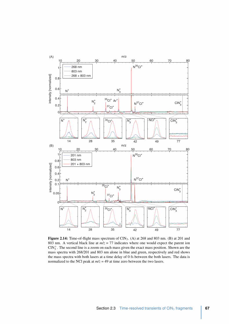
0.6
0.8
1
14 35 42 49 77
0
0.2
0.4
inte
nsity
[nor
mal
ized
]
268 nm803 nm268 + 803 nm
28
N+
N35Cl+
ClN3+
35Cl+N2+
N3+ ClN
3+NCl+
37Cl+
35Cl+N2+
N+
Ar+
N3+
N37Cl+
10 20 30 40 50 60 70 80m/z
0.2
0.4
0.6
0.8
1
14 35 42 49 77
10 20 30 40 50 60 70 80
0
0.05
0.1
m/z
inte
nsity
[nor
mal
ized
]
201 nm803 nm201 + 803 nm
28
N+
N35Cl+
N2+ 35Cl+ ClN
3+
ClN3+
N3+ NCl+
N37Cl+N+
N2+
35Cl+
37Cl+
N3+
(A)
(B)
Figure 2.14: Time-of-flight mass spectrum of ClN3. (A) at 268 and 803 nm. (B) at 201 and
803 nm. A vertical black line at m/z = 77 indicates where one would expect the parent ion
ClN`3 . The second line is a zoom on each mass given the exact mass position. Shown are the
mass spectra with 268/201 and 803 nm alone in blue and green, respectively and red shows
the mass spectra with both lasers at a time delay of 0 fs between the both lasers. The data is
normalized to the NCl peak at m/z = 49 at time zero between the two lasers.
Section 2.3 Time-resolved transients of ClN3 fragments 67
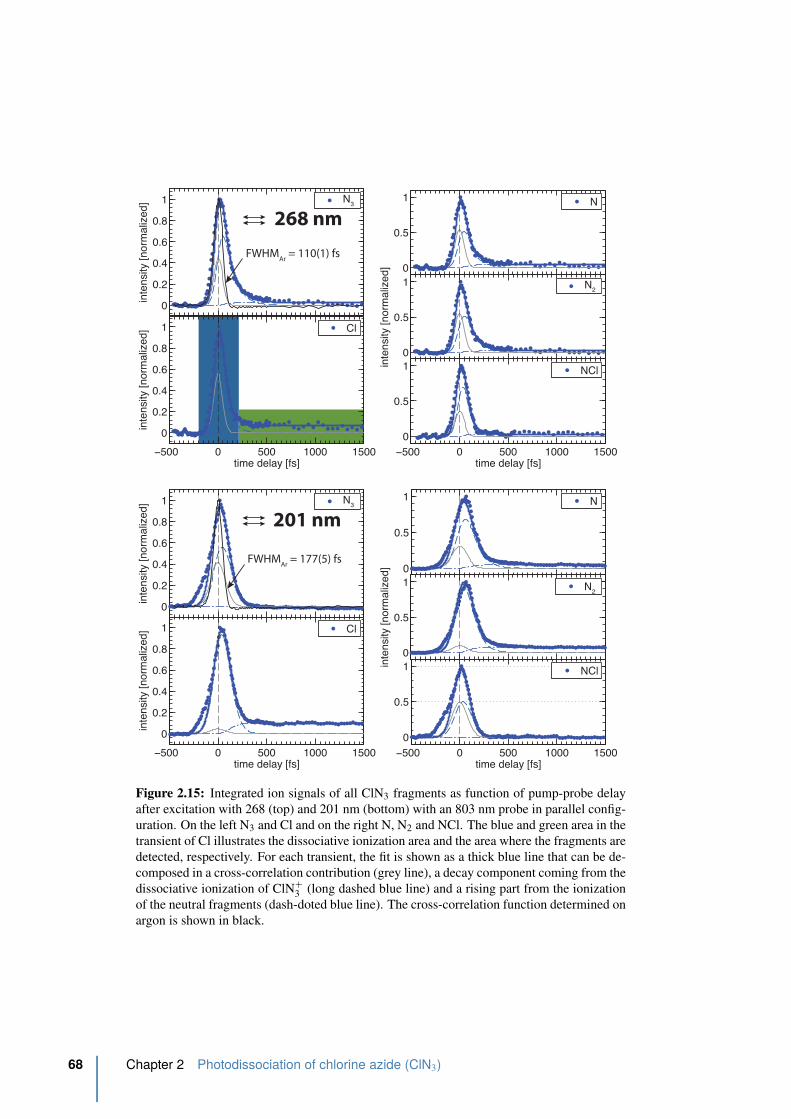
−500 0 500 1000 15000
0.20.40.60.8
1
inte
nsity
[nor
mal
ized
]
time delay [fs]
N3
−500 0 500 1000 1500time delay [fs]
−500 0 500 1000 1500
−500 0 500 1000 15000
0.5
1
inte
nsity
[nor
mal
ized
]
time delay [fs]
N
−500 0 500 1000 15000
0.20.40.60.8
1
inte
nsity
[nor
mal
ized
]
time delay [fs]
Cl
−500 0 500 1000 15000
0.5
1
inte
nsity
[nor
mal
ized
]time delay [fs]
N2
−500 0 500 1000 15000
0.5
1
inte
nsity
time delay [fs]
NCl
−500 0 500 1000 15000
0.5
1
time delay [fs]
N
−500 0 500 1000 15000
0.20.40.60.8
1
inte
nsity
[nor
mal
ized
]
time delay [fs]
N3
−500 0 500 1000 1500−500 0 500 1000 1500
−500 0 500 1000 15000
0.20.40.60.8
1
inte
nsity
[nor
mal
ized
]
time delay [fs]
Cl
−500 0 500 1000 15000
0.5
1
inte
nsity
[nor
mal
ized
]
time delay [fs]
N2
−500 0 500 1000 15000
0.5
1
time delay [fs]
NCl
268 nm
201 nm
FWHMAr
= 110(1) fs
FWHMAr
= 177(5) fs
Figure 2.15: Integrated ion signals of all ClN3 fragments as function of pump-probe delay
after excitation with 268 (top) and 201 nm (bottom) with an 803 nm probe in parallel config-
uration. On the left N3 and Cl and on the right N, N2 and NCl. The blue and green area in the
transient of Cl illustrates the dissociative ionization area and the area where the fragments are
detected, respectively. For each transient, the fit is shown as a thick blue line that can be de-
composed in a cross-correlation contribution (grey line), a decay component coming from the
dissociative ionization of ClN`3 (long dashed blue line) and a rising part from the ionization
of the neutral fragments (dash-doted blue line). The cross-correlation function determined on
argon is shown in black.
68 Chapter 2 Photodissociation of chlorine azide (ClN3)
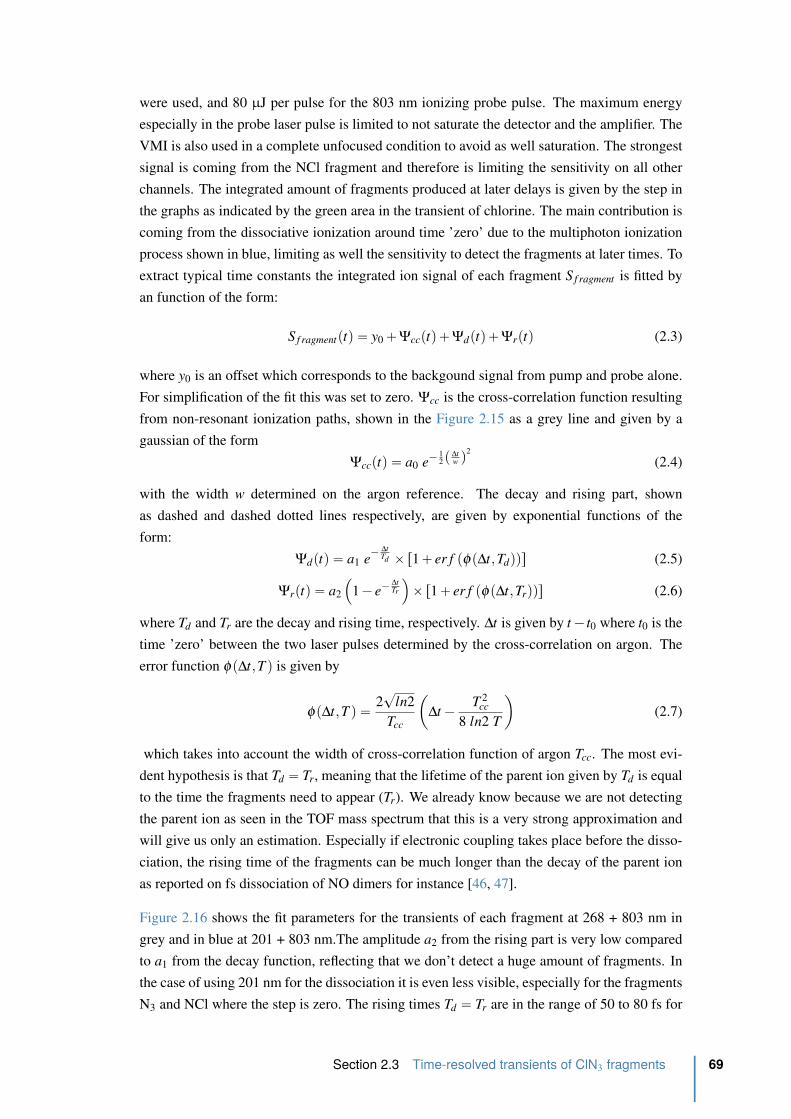
were used, and 80 µJ per pulse for the 803 nm ionizing probe pulse. The maximum energy
especially in the probe laser pulse is limited to not saturate the detector and the amplifier. The
VMI is also used in a complete unfocused condition to avoid as well saturation. The strongest
signal is coming from the NCl fragment and therefore is limiting the sensitivity on all other
channels. The integrated amount of fragments produced at later delays is given by the step in
the graphs as indicated by the green area in the transient of chlorine. The main contribution is
coming from the dissociative ionization around time ’zero’ due to the multiphoton ionization
process shown in blue, limiting as well the sensitivity to detect the fragments at later times. To
extract typical time constants the integrated ion signal of each fragment S f ragment is fitted by
an function of the form:
S f ragmentptq “ y0 ` Ψccptq ` Ψdptq ` Ψrptq (2.3)
where y0 is an offset which corresponds to the backgound signal from pump and probe alone.
For simplification of the fit this was set to zero. Ψcc is the cross-correlation function resulting
from non-resonant ionization paths, shown in the Figure 2.15 as a grey line and given by a
gaussian of the form
Ψccptq “ a0 e´ 12 p ∆t
w q2
(2.4)
with the width w determined on the argon reference. The decay and rising part, shown
as dashed and dashed dotted lines respectively, are given by exponential functions of the
form:
Ψdptq “ a1 e´ ∆t
Td ˆ r1 ` er f pφp∆t,Tdqqs (2.5)
Ψrptq “ a2
´
1 ´ e´ ∆tTr
¯
ˆ r1 ` er f pφp∆t,Trqqs (2.6)
where Td and Tr are the decay and rising time, respectively. ∆t is given by t ´ t0 where t0 is the
time ’zero’ between the two laser pulses determined by the cross-correlation on argon. The
error function φp∆t,T q is given by
φp∆t,T q “ 2?
ln2
Tcc
ˆ
∆t ´ T 2cc
8 ln2 T
˙
(2.7)
which takes into account the width of cross-correlation function of argon Tcc. The most evi-
dent hypothesis is that Td “ Tr, meaning that the lifetime of the parent ion given by Td is equal
to the time the fragments need to appear (Tr). We already know because we are not detecting
the parent ion as seen in the TOF mass spectrum that this is a very strong approximation and
will give us only an estimation. Especially if electronic coupling takes place before the disso-
ciation, the rising time of the fragments can be much longer than the decay of the parent ion
as reported on fs dissociation of NO dimers for instance [46, 47].
Figure 2.16 shows the fit parameters for the transients of each fragment at 268 + 803 nm in
grey and in blue at 201 + 803 nm.The amplitude a2 from the rising part is very low compared
to a1 from the decay function, reflecting that we don’t detect a huge amount of fragments. In
the case of using 201 nm for the dissociation it is even less visible, especially for the fragments
N3 and NCl where the step is zero. The rising times Td “ Tr are in the range of 50 to 80 fs for
Section 2.3 Time-resolved transients of ClN3 fragments 69
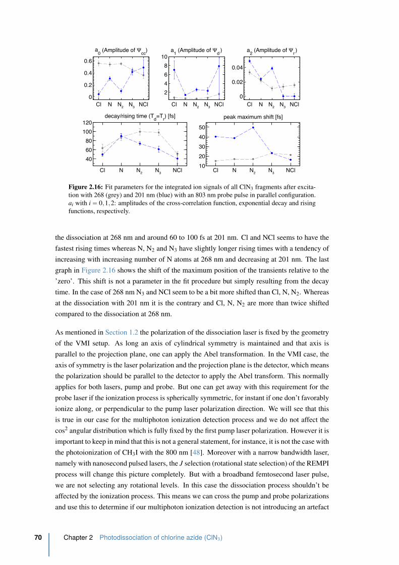
Cl N N2 N3 NCl0
0.2
0.4
0.6
a0 (Amplitude of Ψ
cc)
Cl N N2 N3 NCl
2
4
6
8
10a
1 (Amplitude of Ψ
d)
Cl N N2 N3 NCl0
0.02
0.04
a2 (Amplitude of Ψ
r)
Cl N N2 N3 NCl
40
60
80
100
120decay/rising time (T
d=T
r) [fs]
Cl N N2 N3 NCl10
20
30
40
50
peak maximum shift [fs]
Figure 2.16: Fit parameters for the integrated ion signals of all ClN3 fragments after excita-
tion with 268 (grey) and 201 nm (blue) with an 803 nm probe pulse in parallel configuration.
ai with i “ 0,1,2: amplitudes of the cross-correlation function, exponential decay and rising
functions, respectively.
the dissociation at 268 nm and around 60 to 100 fs at 201 nm. Cl and NCl seems to have the
fastest rising times whereas N, N2 and N3 have slightly longer rising times with a tendency of
increasing with increasing number of N atoms at 268 nm and decreasing at 201 nm. The last
graph in Figure 2.16 shows the shift of the maximum position of the transients relative to the
’zero’. This shift is not a parameter in the fit procedure but simply resulting from the decay
time. In the case of 268 nm N3 and NCl seem to be a bit more shifted than Cl, N, N2. Whereas
at the dissociation with 201 nm it is the contrary and Cl, N, N2 are more than twice shifted
compared to the dissociation at 268 nm.
As mentioned in Section 1.2 the polarization of the dissociation laser is fixed by the geometry
of the VMI setup. As long an axis of cylindrical symmetry is maintained and that axis is
parallel to the projection plane, one can apply the Abel transformation. In the VMI case, the
axis of symmetry is the laser polarization and the projection plane is the detector, which means
the polarization should be parallel to the detector to apply the Abel transform. This normally
applies for both lasers, pump and probe. But one can get away with this requirement for the
probe laser if the ionization process is spherically symmetric, for instant if one don’t favorably
ionize along, or perpendicular to the pump laser polarization direction. We will see that this
is true in our case for the multiphoton ionization detection process and we do not affect the
cos2 angular distribution which is fully fixed by the first pump laser polarization. However it is
important to keep in mind that this is not a general statement, for instance, it is not the case with
the photoionization of CH3I with the 800 nm [48]. Moreover with a narrow bandwidth laser,
namely with nanosecond pulsed lasers, the J selection (rotational state selection) of the REMPI
process will change this picture completely. But with a broadband femtosecond laser pulse,
we are not selecting any rotational levels. In this case the dissociation process shouldn’t be
affected by the ionization process. This means we can cross the pump and probe polarizations
and use this to determine if our multiphoton ionization detection is not introducing an artefact
70 Chapter 2 Photodissociation of chlorine azide (ClN3)
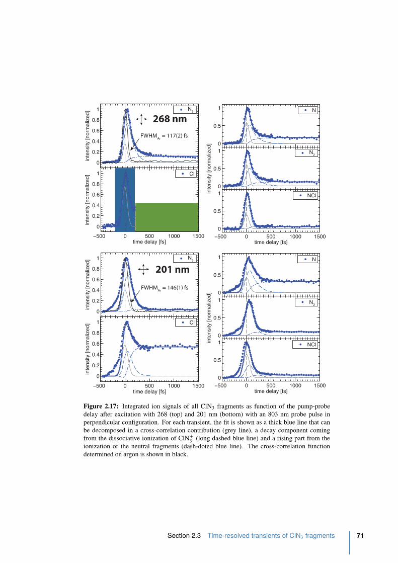
−500 0 500 1000 15000
0.5
1
inte
nsity
[nor
mal
ized
]
time delay [fs]
N
−500 0 500 1000 15000
0.20.40.60.8
1
inte
nsity
[nor
mal
ized
]
time delay [fs]
N3
−500 0 500 1000 1500−500 0 500 1000 1500
−500 0 500 1000 15000
0.20.40.60.8
1
inte
nsity
[nor
mal
ized
]
time delay [fs]
Cl
−500 0 500 1000 15000
0.5
1
inte
nsity
[nor
mal
ized
]
time delay [fs]
N2
−500 0 500 1000 15000
0.5
1
time delay [fs]
NCl
−500 0 500 1000 15000
0.5
1
inte
nsity
[nor
mal
ized
]
time delay [fs]
N
−500 0 500 1000 15000
0.20.40.60.8
1
inte
nsity
[nor
mal
ized
]
time delay [fs]
N3
−500 0 500 1000 15000
0.20.40.60.8
1
inte
nsity
[nor
mal
ized
]
time delay [fs]
Cl
−500 0 500 1000 15000
0.5
1
inte
nsity
[nor
mal
ized
]
time delay [fs]
N2
−500 0 500 1000 15000
0.5
1
time delay [fs]
NCl
268 nm
201 nm
FWHMAr
= 117(2) fs
FWHMAr
= 146(1) fs
Figure 2.17: Integrated ion signals of all ClN3 fragments as function of the pump-probe
delay after excitation with 268 (top) and 201 nm (bottom) with an 803 nm probe pulse in
perpendicular configuration. For each transient, the fit is shown as a thick blue line that can
be decomposed in a cross-correlation contribution (grey line), a decay component coming
from the dissociative ionization of ClN`3 (long dashed blue line) and a rising part from the
ionization of the neutral fragments (dash-doted blue line). The cross-correlation function
determined on argon is shown in black.
Section 2.3 Time-resolved transients of ClN3 fragments 71

Cl N N2 N3 NCl0
0.2
0.4
0.6
0.8
a0 (Amplitude of Ψ
cc)
Cl N N2 N3 NCl
1
2
3
Cl N N2 N3 NCl0
0.1
0.2
Cl N N2 N3 NCl
50
100
150
decay/rising time (Td=T
r) [fs]
Cl N N2 N3 NCl10
20
30
40
50
peak maximum shift [fs]
a1 (Amplitude of Ψ
d) a
2 (Amplitude of Ψ
r)
Figure 2.18: Fit parameters for the integrated ion signals of all ClN3 fragments after ex-
citation with 268 (grey) and 201 nm (blue) with an 803 nm probe pulse in perpendicular
configuration. ai with i “ 0,1,2: amplitudes of the cross-correlation function, exponential
decay and rising functions, respectively.
due to its high intensity. High laser intensities can introduce some alignment which would
affect the outcome of the dissociation process like we have observed in the study of the CH3I
predissociation [48]. Figure 2.17 shows the femtosecond time-resolved transients of each
fragment coming from the dissociation of ClN3 at 268 (top) and 201 nm (bottom) with an 803
nm probe in perpendicular configuration. The transients are analyzed as described above. The
difference to the parallel configuration is clearly observed on the transient of Cl. The ratio
between the dissociative ionization (blue area) and the detection of the fragments (green area)
is almost a factor five better, at least for Cl, N and N2. For the fragments N3 and NCl the step
is again much smaller but also more visible. The time constants observed in perpendicular
configuration are slightly larger but still around 80 - 100 fs. suggesting that the intense 803
nm probe pulse is not affecting the measurement drastically. Nevertheless, the dissociative
ionization process with a perpendicular 803 nm probe pulse seems to be less efficient.
Instead of detecting the time-of-flight we will now use the VMI in its pulsed mode. This
will allow us to increase the sensitivity for the detection of the fragments produced in small
amounts, like N3.
2.4 N3 - Cl translational energy and angular distributions
In order to determine if we are able to detect the fragments coming from the right dissociation
channel namely the radical bond rupture producing N3 and Cl one can check the translational
energy release TER of these fragments far away from the dissociation. Figure 2.19 on the right
shows reconstructed velocity-map image slices of the three-dimensional velocity distribution
of the fragments N3 and Cl with a pump-probe delay of 1 ps obtained by using the inverse-
Abel transformation. The single laser background images have been subtracted and the images
are analyzed as discussed in Section 2.2.5. The first row shows the images recorded with a
72 Chapter 2 Photodissociation of chlorine azide (ClN3)
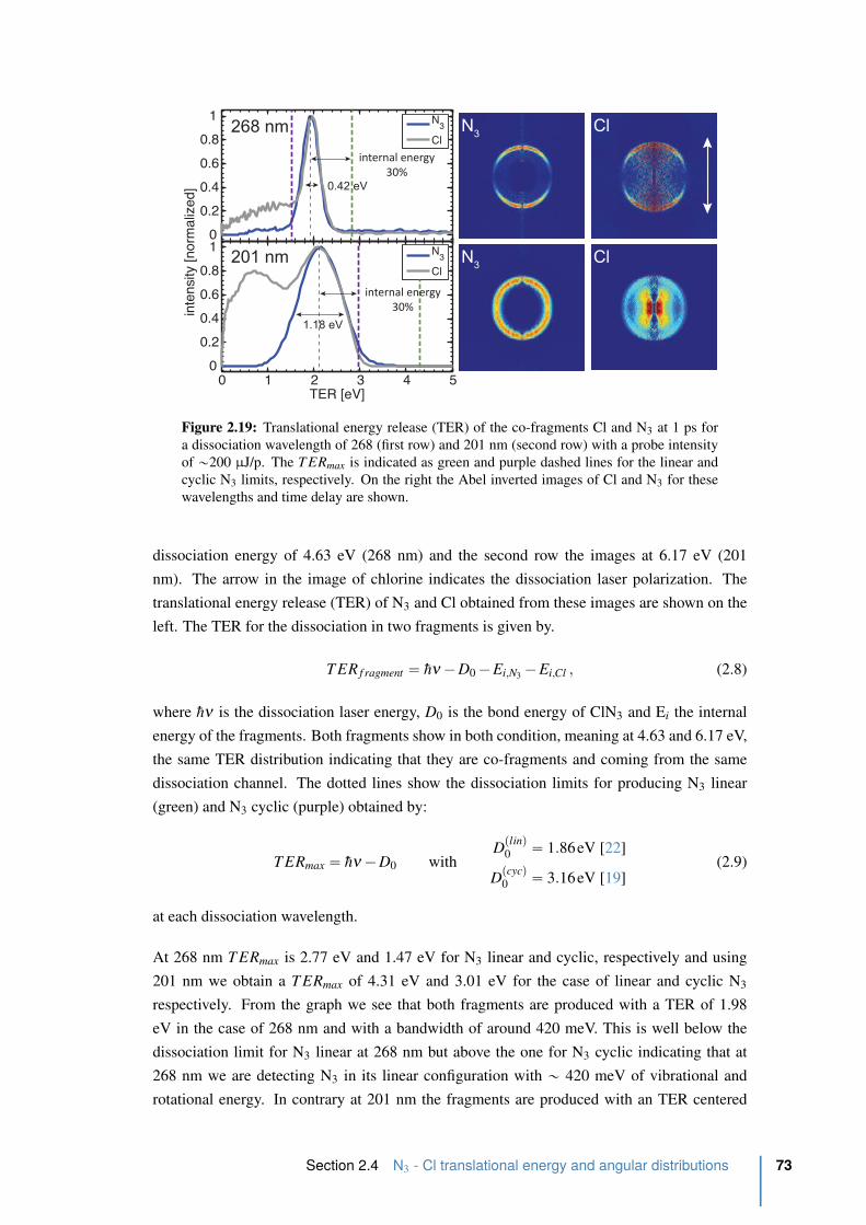
0
0.2
0.4
0.6
0.8
1
N3
Cl
0 1 2 3 4 50
0.2
0.4
0.6
0.8
1
TER [eV]
N3
Cl
268 nm
201 nm
inte
nsity [norm
aliz
ed]
N3 Cl
N3 Cl
1.18 eV
0.42 eV
internal energy
30%
internal energy
30%
Figure 2.19: Translational energy release (TER) of the co-fragments Cl and N3 at 1 ps for
a dissociation wavelength of 268 (first row) and 201 nm (second row) with a probe intensity
of „200 µJ/p. The T ERmax is indicated as green and purple dashed lines for the linear and
cyclic N3 limits, respectively. On the right the Abel inverted images of Cl and N3 for these
wavelengths and time delay are shown.
dissociation energy of 4.63 eV (268 nm) and the second row the images at 6.17 eV (201
nm). The arrow in the image of chlorine indicates the dissociation laser polarization. The
translational energy release (TER) of N3 and Cl obtained from these images are shown on the
left. The TER for the dissociation in two fragments is given by.
T ER f ragment “ hν ´ D0 ´ Ei,N3´ Ei,Cl , (2.8)
where hν is the dissociation laser energy, D0 is the bond energy of ClN3 and Ei the internal
energy of the fragments. Both fragments show in both condition, meaning at 4.63 and 6.17 eV,
the same TER distribution indicating that they are co-fragments and coming from the same
dissociation channel. The dotted lines show the dissociation limits for producing N3 linear
(green) and N3 cyclic (purple) obtained by:
T ERmax “ hν ´ D0 withD
plinq0 “ 1.86eV [22]
Dpcycq0 “ 3.16eV [19]
(2.9)
at each dissociation wavelength.
At 268 nm T ERmax is 2.77 eV and 1.47 eV for N3 linear and cyclic, respectively and using
201 nm we obtain a T ERmax of 4.31 eV and 3.01 eV for the case of linear and cyclic N3
respectively. From the graph we see that both fragments are produced with a TER of 1.98
eV in the case of 268 nm and with a bandwidth of around 420 meV. This is well below the
dissociation limit for N3 linear at 268 nm but above the one for N3 cyclic indicating that at
268 nm we are detecting N3 in its linear configuration with „ 420 meV of vibrational and
rotational energy. In contrary at 201 nm the fragments are produced with an TER centered
Section 2.4 N3 - Cl translational energy and angular distributions 73

at 2.1 eV with a much larger bandwidth of 1.18 eV. Furthermore, the detected TER at 201
nm is more than 1 eV lower than the dissociation limit for N3 linear indicated by the green
dotted line and more in agreement with the dissociation limit of N3 cyclic (purple line). Based
on the energy threshold this is the first indication that N3 at 201 nm is maybe produced in its
cyclic form with a huge distribution („1.18 eV) of vibrational and rotational energy. Next we
will discuss the time dependency of these components and as well the time dependency of the
angular distributions seen in the Abel inverted images on the right of Figure 2.19.
2.4.1 The rising of N3 linear and cyclic
Figure 2.20 shows the translational energy release TER of the fragment N3 at 268 and 201
nm as function of the delay between the dissociation and ionizing laser for both, parallel
and perpendicular configuration. Shown are the TER just outside the cross-correlation time
(indicated by the shaded area around zero) at 150 fs and far away at 1 ps. Around zero up to
500 fs images were taken each 50 fs and sometimes even each 25 fs, whereas at longer delays
the step was increased to 200 fs. As this makes the time-resolved data not equidistant, to plot
the intensity maps the data was interpolated at longer delays where the step was not 50 fs and
should be regarded for representation purposes only.
To determine the rising time of N3 and therefore the dissociation time of ClN3 at both dissoci-
ation wavelengths the area under the peak corresponding to this contribution (see blue area in
Figure 2.20) was extracted. As one can see in the cuts shown in Figure 2.20 on the right at 150
fs, there are lower energetic components shown in green and purple. In order to get a more
accurate rising time of the neutral fragments Cl and N3, these components have to be taken
into account. For this analysis the TER distribution is fit by
T ER “3
ÿ
i“1
ai e´ 1
2
´
x´x0iwi
¯2
(2.10)
which is a sum of three gaussians where i “ 1,2,3 corresponds to the three contributions we
can identify in the TER distribution at short delays (purple, green, blue). The area under the
third gaussian (blue) that corresponds to the ionization of the neutral N3 fragment is shown
in Figure 2.21 as function of the time delay. To extract the dissociation time, this transient is
fitted by the same function introduced in Eq. (2.6) which was an exponential rising function
corrected by an error function to take the cross-correlation into account. It is important to
remind, that each study in the pulsed mode of the VMI is started by a quick ion scan over the
TOF to record precisely the time zero between the two laser pulses and the cross-correlation
time on argon.
The shaded blue area in the graph represents the FWHM of this cross-correlation function
determined on Ar. The extracted dissociation time at 268 nm is 262 ˘ 38 fs and 252 ˘ 30 fs for
parallel and perpendicular configuration, respectively. This refers again to the polarization of
the 803 nm ionization laser polarization relative to the pump polarization. It is quite important
to check that these values are the same to rule out any alignment of the fragments due to the
intense probe pulse itself as mentioned before. The dissociation time at 201 nm is 178 ˘ 22 fs
74 Chapter 2 Photodissociation of chlorine azide (ClN3)

time delay [fs]
TE
R [
eV
]
0 500 1000 1500
0
2
4
6
0 0.02 0.04 0.06
0
2
4
6
TE
R [e
V]
intensity [arb. units]
time delay [fs]
TE
R [
eV
]
0 500 1000 1500
0
2
4
6
N3 @ 268 nm
0 0.02 0.04 0.06
0
2
4
6
TE
R [e
V]
0 0.02 0.04 0.06intensity [arb. units]
Δt = 1 ps
Δt
= 1
50
fs
Δt = 1 psΔt = 150fs
Δt
= 1
ps
Δt
= 1
50
fs
Δt
= 1
ps
time delay [fs]
TE
R [
eV
]
0 500 1000 1500
0
2
4
6
Δt
=1
50
fs
Δt
= 1
ps
0 0.02 0.04
0
2
4
6
TE
R [e
V]
intensity [arb. units]
Δt = 1 ps
time delay [fs]
TE
R [
eV
]
0 500 1000 1500
0
2
4
6
N3 @ 201 nm
0 0.02 0.04 0.06
Δt = 150fs
0 0.02 0.04
Δt = 150fs
0 0.02 0.04 0 0.02 0.04
0
2
4
6T
ER
[eV
]
intensity [arb. units]
Δt
=1
50
fs
Δt
= 1
ps
Δt = 1 psΔt = 150fs
FW
HM
Ar =
11
0(1
) fs
FW
HM
Ar =
11
7(2
) fs
FW
HM
Ar =
11
2(2
) fs
FW
HM
Ar =
14
6(1
) fs
D0
lin
D0
cyc
Figure 2.20: Translational energy release TER of the fragment N3 at 268 and 201 nm as
function of the delay between the dissociation and ionizing laser for both, parallel and per-
pendicular configuration.
Section 2.4 N3 - Cl translational energy and angular distributions 75

0
0.2
0.4
0.6
0.8
1
parallelperpendicular
N3 @ 268 nm
Tr = 262 ± 38 fs
Tr = 252 ± 30 fs
N N N
0 500 1000 1500 2000 2500
0
0.2
0.4
0.6
0.8
1
time delay [fs]
parallelperpendicularN
3 @ 201 nm
Tr = 178 ± 22 fs
Tr = 173 ± 14 fs
N
N
N
N3
peak
are
a [n
orm
aliz
ed]
0.42
0.44
0.46
FWHM [eV]
1.95
1.97
1.99
2.01
x0
[eV]
11.21.41.61.8
FWHM [eV]
0-400
-400
500 1000 1500 2000 2500
0 1000 2000 30002
2.1
2.2
time delay [fs]
x0
[eV]
0 1000 2000 3000
Figure 2.21: Time dependences of the N3 fragments at 268 and 201 nm recorded two con-
figurations, where the 803 nm probe polarization is either parallel or perpendicular to the
pump polarization and detector plane. On the right: FWHM and peak position from the fit as
function of the pump-probe delay.
and 173 ˘ 14 fs for parallel and perpendicular configuration, respectively, and therefore about
80 fs faster than in the case of dissociation with 268 nm. At both dissociation wavelengths the
difference between parallel and perpendicular configuration is insignificant. It safe to say that
the intense 803 nm probe pulse doesn’t introduce any artifact. On the right side of Figure 2.21
the FWHM and the position of the maximum x0 of the main contribution is shown. In the
case of 268 nm the FWHM outside the cross-correlation is not changing a lot and an average
of 0.437 ˘ 0.012 eV and 0.438 ˘ 0.012 eV for parallel and perpendicular configuration,
respectively, can be obtained.
The position of the maximum of this main contribution seem to increase slightly with time but
only by 1,7%, which is nevertheless slightly larger than the standard deviation of the average
of the maximum given by 1.972 ˘ 0.014 eV. For cyclic N3 at 201 nm the FWHM decreases
during the dissociation time from 1.8 to 1 eV. Taking all values after the dissociation („ 180
fs), from 200 fs till 2.5 ps we get an average FWHM of 1.12 ˘ 0.13 eV and 1.16 ˘ 0.15 eV in
parallel and perpendicular configuration, respectively. The position of the maximum is given
by 2.17 ˘ 0.05 eV in parallel and 2.03 ˘ 0.03 eV in perpendicular. However, it is important to
note that in this energy region a ∆E„0.02 eV corresponds to „1 pixel shift in the radius of the
image. As we don’t have a pixel energy resolution the change of the position of the main peak
observed here of „0.05 eV is negligible and in the resolution limit of our detection.
The lower energetic components
The fit parameters for the lower energetic components which were subtracted from the main
peak around 2 eV are shown in Figure 2.22. The area under this gaussian fit is normalized to
76 Chapter 2 Photodissociation of chlorine azide (ClN3)

0
0.1
0.2
0.4
0.5
0.6
0 500 1000
0.2
0.4
0.6
0.2
0.4
1
1.5
0 1000 2000 30000.8
1
1.2
FWHM [eV]
x0
[eV]
Area [normalized]
component 1 component 2
parallelperpendicular
N3 @ 268 nm
N3 @ 201 nm
0
0.2
0.4
00.5
11.5
0 500 1000 1500 2000
0.4
0.8
1.2
time delay [fs]
component 1
FWHM [eV]
x0
[eV]
Area [normalized]
time delay [fs]
304 ± 67 fs
272 ± 25 fs
Figure 2.22: Time dependence of the lower energetic components. At 268 nm there are two
components marked as purple and green and at 201 nm only one (green). Shown are the area
under the curve, normalized to the area under the main peak, the FWHM and the position of
this contribution.
the area of the main contribution. The first lower energetic component at 268 nm (purple, see
Figure 2.20) has a TER of around 0.55 eV and is only around 10% of the main contribution
around time zero. It disappears basically after the dissociation time indicated as dashed lines.
The FWHM of the cross-correlation on Ar is again shown as the shaded blue area. The second
component (green) around 1.2 eV doesn’t go to zero but it only accounts 20% of the main
contribution. The peak width (shown is the FWHM) and the peak position seem not to vary
a lot with the time delay. At 201 nm we can observe only one lower energetic component
(green) around 0.8 eV. Its contribution drops to zero during the dissociation time.
Energy analysis summary
The dissociation timescale observed on the neutral N3 fragment is the same whatever the
polarization configuration of the 803 nm probe pulse. We observe a faster dissociation time
at 201 nm. Both dissociation times are more than twice longer than the time observed on
Section 2.4 N3 - Cl translational energy and angular distributions 77
the full integrated signal (Figure 2.16, Figure 2.18). This lets us conclude that in the case of
detecting the TOF as function of time a detection threshold exists that limits the detection of
all the masses produced. Indeed the maximal value on the MCP is fixed by the gain of the
preamplifier and the largest signal (NCl`). On the contrary for the pulsed mode, the choice
of MCP voltage is mass dependent and in general was fixed to the maximum allowed namely
1500V. The extra components on the TER at lower energies are most likely due to dissociative
ionization as they disappear on a similar timescale as the dissociation time. The long decay
reveals that the dissociation is not a direct dissociation as suggested before [17]. Indeed, a
direct dissociation would occur roughly on half of the Cl-N3 stretching period which is only
30 fs (νstretch = 545 cm´1 = 61 fs). The fact that the relaxation dynamics can be followed
whatever the electronic state encountered, means that dissociative ionization is not sensitive
to the electronic character, but simply depending on the amount of excited parent molecules.
Maybe an ionization experiment, recording the fragments and the photo-electrons at the same
time could reveal properly the electronic states encountered.
2.4.2 Time-dependence of the N3 photofragment angular distribution
More important than the time-dependency of the intensity of the fragment is the angular distri-
bution. As we have seen in Section 1.2 the dissociation is sensitive to the relative alignments
of the laser polarization and the molecular dipole moment. In general a linear polarized laser
will preferentially excite molecules with their dipole moments parallel to its polarization. By
looking at the angular distribution we can distinguish if the dissociation goes via an excited
state with a parallel or perpendicular transition. Figure 2.23 (A) shows the Abel-inverted im-
age of the N3 fragment at the dissociation with 268 nm at a time delay of 1 ps outside of the
dissociation time. The angular distribution is analyzed by first converting the radial image into
a radius versus angle plot (Figure 2.23 (B)) by transforming it into polar-coordinates. After
that the area of interest is selected corresponding to the FWHM of the peak in the energy dis-
tribution. The corresponding pixels are then averaged and plotted as seen in Figure 2.23 (C).
The intensity variation as function of angle is afterwards fitted by:
Ipθq “ 1 ` β2P2pcosθq, P2pxq “ 1
2p3x2 ´ 1q (2.11)
where β2 is the anisotropy parameter and P2pxq the second Legendre polynomial. The anisotropy
parameter β2 can take values between -1 and 2 where the two extreme values corresponding
to a perpendicular or parallel transition, respectively, as seen in Section 1.2.4.
Figure 2.24 shows the extracted β2 parameter at a dissociation with 268 and 201 nm each
using a parallel (blue) and perpendicular (grey) 803 nm probe pulse. One can identify three
areas. The blue area in the graph represents again the FWHM of our cross-correlation time
determined on Ar. Outside this cross-correlation time we can identify 2 areas, in which the β2
parameter is changing with increasing time delay and one in which β2 stays almost constant.
The vertical dashed line represents the dissociation time determined in the previous section.
In the case of linear N3 at 268 nm one can extract a β2 parameter of β2 = 1.61 ˘ 0.07 and β K2
= 1.67 ˘ 0.05 for a parallel and perpendicular 803 nm probe pulse, respectively by averaging
78 Chapter 2 Photodissociation of chlorine azide (ClN3)

Δt = 1000 fs
Rθ
rad
ius
angle
0 45 90 135 1800
5
10
x 107
θ [degrees]
inten
sity [
arb.
unit
s]
N3
polar plot
Fit (β2 = 1.61 ± 0.02)
ΔR = FWHMN3
integration over ΔR
(A) (B)
(C)
0 360
Figure 2.23: Angular distribution anlysis. Shown is the Abel inverted image of N3 following
dissociation at 268 nm at 1 ps. The image is converted into polar coordinates and the intensity
of the relevant pixels are then fit by the anisotropy function from Eq. (2.11).
the data points after the dashed line. This compares quite well with the β2 „ 1.71 ˘ 0.1
at 266 nm found previously on the chlorine fragment in the nanosecond time regime [31].
Shortly after the initiation of the dissociation we observe a higher β2, changing rapidly during
the dissociation time from 2 to 1.7. An exponential fit (β2ptq “ y0 `A expr´tτs) gives a time
constant of this changing β2 parameter at 268 nm of τ268 = 170 ˘ 45 fs and is therefore slightly
faster than the dissociation time („260 fs). The fact that it is starting at a β2 = 2 suggests that
this dissociation is initiated by a parallel transition B1A1 Ð X1A1 from the ground state to the
second excited state of ClN3 which is also in agreement with the results in the ns- regime on
chlorine.
If the fact that we don’t measure a β2 = 2 but „1.64 is coming from the rotation of the parent
molecule, we can write the anisotropy parameter like[49]:
β2 « 2P2pcos χq 1 ` ω2τ2
1 ` 4ω2τ2(2.12)
where ω “ pπkT 2lq12 is the angular velocity of the parent molecule, l the moment of inertia,
and χ the angle between the internuclear axis and the direction of the transition dipole for
the final state. Note that this equation assumes that the rotational period of the electronically
excited ClN3 is comparable to the dissociation time τ , thus taking into account the change of
the orientation of the dissociation axis with respect to the direction of the polarization of the
photolysis laser due to the rotation of the parent. With a measured dissociation time of „ 257
fs and rotational periods for the parent molecule of „13 ps for the fast axis and „150 ps for the
two slow axis, this is a tough assumption. Nevertheless, within this assumtion we can extract
Section 2.4 N3 - Cl translational energy and angular distributions 79
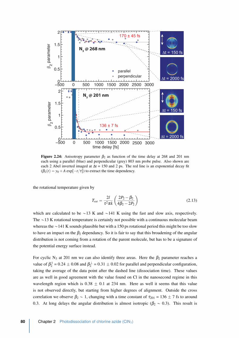
parallelperpendicular
A B
AB
θ [degrees]
μ
β2 = 2
β2 = −1
Δt = 2000 fs
Δt = 150 fs
−500 0 500 1000 1500 20000
0.5
1
1.5
2
time delay [fs]
β 2 par
amet
er
N3 @ 201 nm
Δt = 150 fs
Δt = 2000 fs
136 ± 7 fs
−500 0 500 1000 1500 2000 2500 30000
0.5
1
1.5
2
β 2 par
amet
er
N3 @ 268 nm
170 ± 45 fs
2500 3000
Figure 2.24: Anisotropy parameter β2 as function of the time delay at 268 and 201 nm
each using a parallel (blue) and perpendicular (grey) 803 nm probe pulse. Also shown are
each 2 Abel inverted imaged at ∆t = 150 and 2 ps. The red line is an exponential decay fit
(β2ptq “ y0 ` A expr´tτs) to extract the time dependency.
the rotational temperature given by
Trot “ 2l
τ2πk
ˆ
2P2 ´ β2
4β2 ´ 2P2
˙
(2.13)
which are calculated to be „13 K and „141 K using the fast and slow axis, respectively.
The „13 K rotational temperature is certainly not possible with a continuous molecular beam
whereas the „141 K sounds plausible but with a 150 ps rotational period this might be too slow
to have an impact on the β2 dependancy. So it is fair to say that this broadening of the angular
distribution is not coming from a rotation of the parent molecule, but has to be a signature of
the potential energy surface instead.
For cyclic N3 at 201 nm we can also identify three areas. Here the β2 parameter reaches a
value of β2 = 0.24 ˘ 0.08 and β K2 = 0.31 ˘ 0.02 for parallel and perpendicular configuration,
taking the average of the data point after the dashed line (dissociation time). These values
are as well in good agreement with the value found on Cl in the nanosecond regime in this
wavelength region which is 0.38 ˘ 0.1 at 234 nm. Here as well it seems that this value
is not observed directly, but starting from higher degrees of alignment. Outside the cross
correlation we observe β2 „ 1, changing with a time constant of τ201 = 136 ˘ 7 fs to around
0.3. At long delays the angular distribution is almost isotropic (β2 „ 0.3). This result is
80 Chapter 2 Photodissociation of chlorine azide (ClN3)
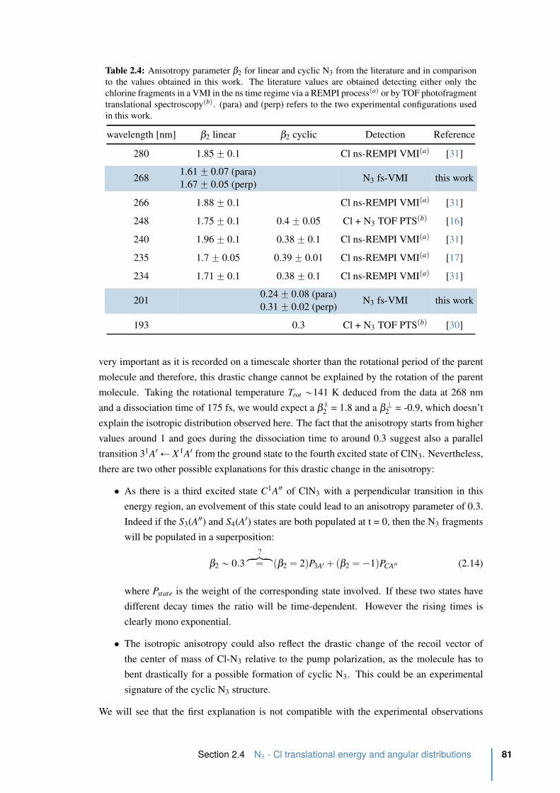
Table 2.4: Anisotropy parameter β2 for linear and cyclic N3 from the literature and in comparison
to the values obtained in this work. The literature values are obtained detecting either only the
chlorine fragments in a VMI in the ns time regime via a REMPI processpaq or by TOF photofragment
translational spectroscopypbq. (para) and (perp) refers to the two experimental configurations used
in this work.
wavelength [nm] β2 linear β2 cyclic Detection Reference
280 1.85 ˘ 0.1 Cl ns-REMPI VMIpaq [31]
2681.61 ˘ 0.07 (para)
1.67 ˘ 0.05 (perp)N3 fs-VMI this work
266 1.88 ˘ 0.1 Cl ns-REMPI VMIpaq [31]
248 1.75 ˘ 0.1 0.4 ˘ 0.05 Cl + N3 TOF PTSpbq [16]
240 1.96 ˘ 0.1 0.38 ˘ 0.1 Cl ns-REMPI VMIpaq [31]
235 1.7 ˘ 0.05 0.39 ˘ 0.01 Cl ns-REMPI VMIpaq [17]
234 1.71 ˘ 0.1 0.38 ˘ 0.1 Cl ns-REMPI VMIpaq [31]
2010.24 ˘ 0.08 (para)
0.31 ˘ 0.02 (perp)N3 fs-VMI this work
193 0.3 Cl + N3 TOF PTSpbq [30]
very important as it is recorded on a timescale shorter than the rotational period of the parent
molecule and therefore, this drastic change cannot be explained by the rotation of the parent
molecule. Taking the rotational temperature Trot „141 K deduced from the data at 268 nm
and a dissociation time of 175 fs, we would expect a β2 = 1.8 and a β K2 = -0.9, which doesn’t
explain the isotropic distribution observed here. The fact that the anisotropy starts from higher
values around 1 and goes during the dissociation time to around 0.3 suggest also a parallel
transition 31A1 Ð X1A1 from the ground state to the fourth excited state of ClN3. Nevertheless,
there are two other possible explanations for this drastic change in the anisotropy:
• As there is a third excited state C1A2 of ClN3 with a perpendicular transition in this
energy region, an evolvement of this state could lead to an anisotropy parameter of 0.3.
Indeed if the S3(A2) and S4(A1) states are both populated at t = 0, then the N3 fragments
will be populated in a superposition:
β2 „ 0.3
?hkkikkj
“ pβ2 “ 2qP3A1 ` pβ2 “ ´1qPCA2 (2.14)
where Pstate is the weight of the corresponding state involved. If these two states have
different decay times the ratio will be time-dependent. However the rising times is
clearly mono exponential.
• The isotropic anisotropy could also reflect the drastic change of the recoil vector of
the center of mass of Cl-N3 relative to the pump polarization, as the molecule has to
bent drastically for a possible formation of cyclic N3. This could be an experimental
signature of the cyclic N3 structure.
We will see that the first explanation is not compatible with the experimental observations
Section 2.4 N3 - Cl translational energy and angular distributions 81
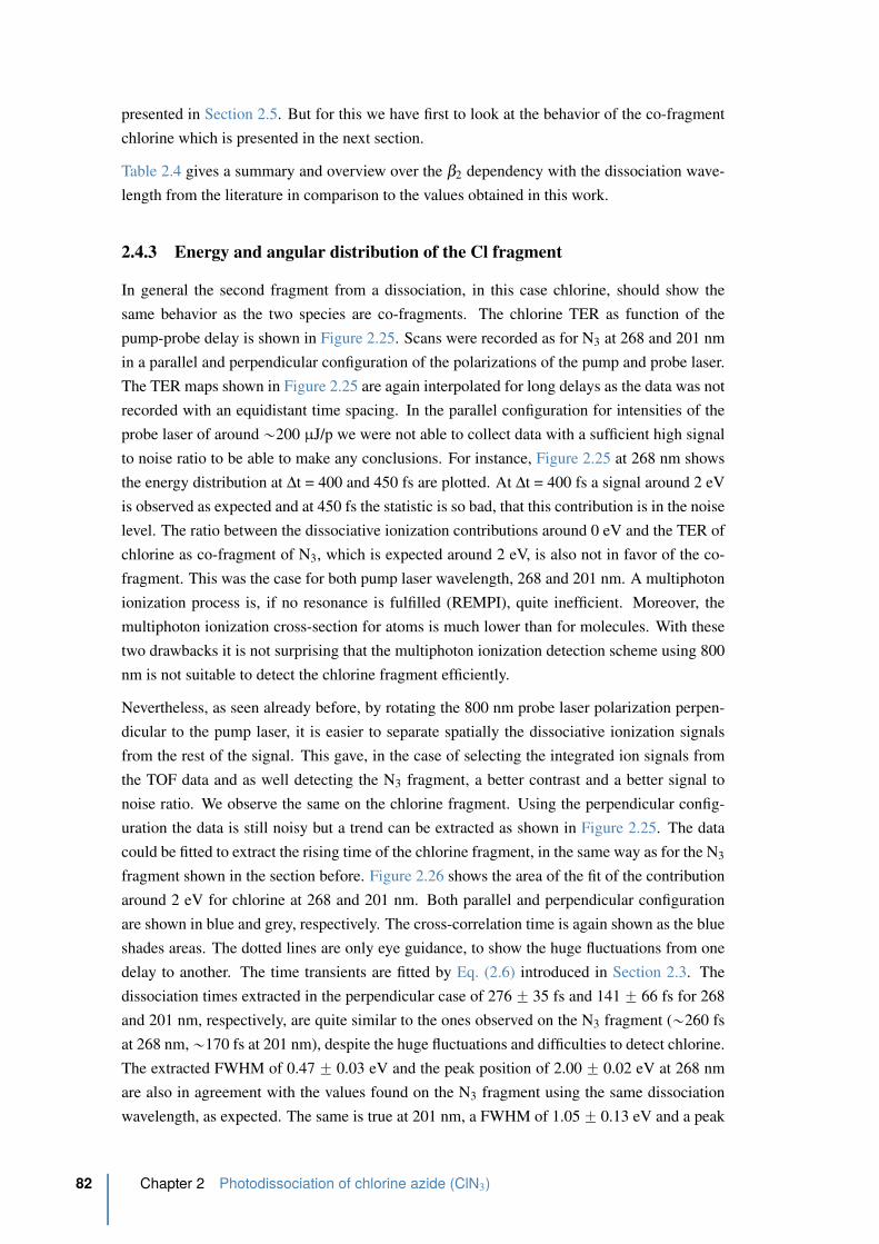
presented in Section 2.5. But for this we have first to look at the behavior of the co-fragment
chlorine which is presented in the next section.
Table 2.4 gives a summary and overview over the β2 dependency with the dissociation wave-
length from the literature in comparison to the values obtained in this work.
2.4.3 Energy and angular distribution of the Cl fragment
In general the second fragment from a dissociation, in this case chlorine, should show the
same behavior as the two species are co-fragments. The chlorine TER as function of the
pump-probe delay is shown in Figure 2.25. Scans were recorded as for N3 at 268 and 201 nm
in a parallel and perpendicular configuration of the polarizations of the pump and probe laser.
The TER maps shown in Figure 2.25 are again interpolated for long delays as the data was not
recorded with an equidistant time spacing. In the parallel configuration for intensities of the
probe laser of around „200 µJ/p we were not able to collect data with a sufficient high signal
to noise ratio to be able to make any conclusions. For instance, Figure 2.25 at 268 nm shows
the energy distribution at ∆t = 400 and 450 fs are plotted. At ∆t = 400 fs a signal around 2 eV
is observed as expected and at 450 fs the statistic is so bad, that this contribution is in the noise
level. The ratio between the dissociative ionization contributions around 0 eV and the TER of
chlorine as co-fragment of N3, which is expected around 2 eV, is also not in favor of the co-
fragment. This was the case for both pump laser wavelength, 268 and 201 nm. A multiphoton
ionization process is, if no resonance is fulfilled (REMPI), quite inefficient. Moreover, the
multiphoton ionization cross-section for atoms is much lower than for molecules. With these
two drawbacks it is not surprising that the multiphoton ionization detection scheme using 800
nm is not suitable to detect the chlorine fragment efficiently.
Nevertheless, as seen already before, by rotating the 800 nm probe laser polarization perpen-
dicular to the pump laser, it is easier to separate spatially the dissociative ionization signals
from the rest of the signal. This gave, in the case of selecting the integrated ion signals from
the TOF data and as well detecting the N3 fragment, a better contrast and a better signal to
noise ratio. We observe the same on the chlorine fragment. Using the perpendicular config-
uration the data is still noisy but a trend can be extracted as shown in Figure 2.25. The data
could be fitted to extract the rising time of the chlorine fragment, in the same way as for the N3
fragment shown in the section before. Figure 2.26 shows the area of the fit of the contribution
around 2 eV for chlorine at 268 and 201 nm. Both parallel and perpendicular configuration
are shown in blue and grey, respectively. The cross-correlation time is again shown as the blue
shades areas. The dotted lines are only eye guidance, to show the huge fluctuations from one
delay to another. The time transients are fitted by Eq. (2.6) introduced in Section 2.3. The
dissociation times extracted in the perpendicular case of 276 ˘ 35 fs and 141 ˘ 66 fs for 268
and 201 nm, respectively, are quite similar to the ones observed on the N3 fragment („260 fs
at 268 nm, „170 fs at 201 nm), despite the huge fluctuations and difficulties to detect chlorine.
The extracted FWHM of 0.47 ˘ 0.03 eV and the peak position of 2.00 ˘ 0.02 eV at 268 nm
are also in agreement with the values found on the N3 fragment using the same dissociation
wavelength, as expected. The same is true at 201 nm, a FWHM of 1.05 ˘ 0.13 eV and a peak
82 Chapter 2 Photodissociation of chlorine azide (ClN3)

time delay [fs]
TE
R [eV
]
0 500 1000 1500
0
2
4
6
0 0.01 0.02 0.03
0
2
4
6
TE
R [e
V]
intensity [arb. units]
Δt = 1.2 ps
0 0.01 0.02 0.03
Δt = 450fsΔt = 400fs
Cl @ 268 nm
Δt
= 4
50
fs
Δt
= 4
00
fs
Δt
= 1
.2 p
s
FW
HM
Ar =
11
2(2
) fs
time delay [fs]
TE
R [eV
]
0 500 1000 1500
0
2
4
6
Δt
= 3
00
fs
Δt
= 1
.2 p
s
FW
HM
Ar =
111
(3)
fs
0 0.02 0.04
0
2
4
6
TE
R [e
V]
0 0.02 0.04intensity [arb. units]
Δt = 1 psΔt = 150fs
time delay [fs]
TE
R [eV
]
0 500 1000 1500
0
2
4
6
Cl @ 201 nm
Δt
= 1
50
fs
Δt
= 4
00
fs
Δt
= 1
ps
FW
HM
Ar =
11
2(2
) fs
0 0.005 0.01
0
2
4
6T
ER
[eV
]0 0.005 0.01
intensity [arb. units]
Δt = 400fsΔt = 150fs
Δt = 1.5 psΔt = 1 ps
time delay [fs]
TE
R [eV
]
0 500 1000 1500
0
2
4
6
Δt
=1
50
fs
Δt
= 1
.2 p
s
FW
HM
Ar =
14
8(3
) fs
0 0.005 0.01intensity [arb. units]
Δt = 1.2 psΔt = 200fs
0 0.005 0.01
0
2
4
6
TE
R [e
V]
D0
cyc
D0
lin
Figure 2.25: Translational energy release TER of the fragment Cl at 268 and 201 nm as
function of the delay between the dissociation and ionizing laser for both, parallel and per-
pendicular configuration. Typical probe intensity is „200 µJ/p.
Section 2.4 N3 - Cl translational energy and angular distributions 83
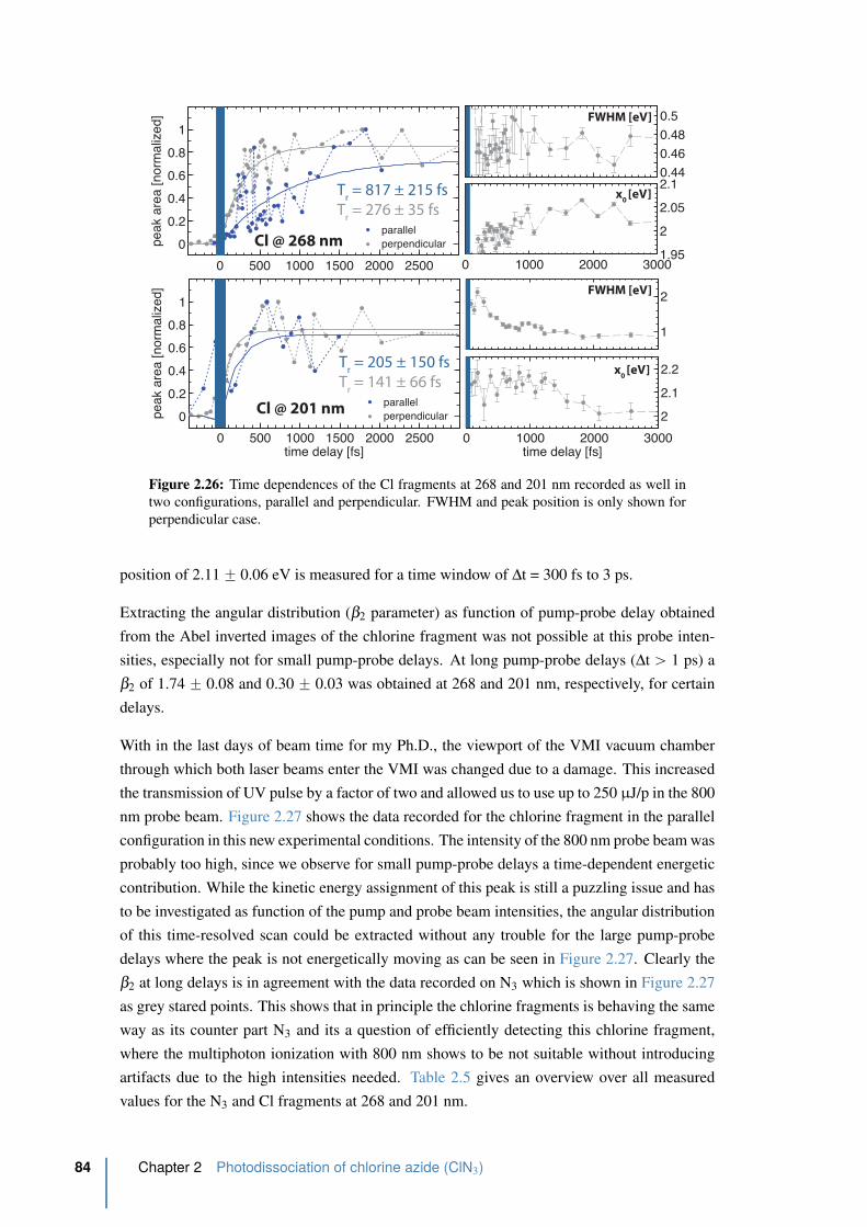
0 500 1000 1500 2000 2500
0
0.2
0.4
0.6
0.8
1
time delay [fs]
peak
are
a [n
orm
aliz
ed]
0 500 1000 1500 2000 2500
0
0.2
0.4
0.6
0.8
1
peak
are
a [n
orm
aliz
ed]
parallelperpendicularCl @ 201 nm
Tr = 205 ± 150 fs
Tr = 141 ± 66 fs
parallelperpendicularCl @ 268 nm
Tr = 817 ± 215 fs
Tr = 276 ± 35 fs
0.440.46
0.48
0.5
FWHM [eV]
0 1000 2000 30001.95
2
2.05
2.1
x
0 [eV]
1
2
FWHM [eV]
0 1000 2000 3000
2
2.1
2.2
time delay [fs]
x
0 [eV]
Figure 2.26: Time dependences of the Cl fragments at 268 and 201 nm recorded as well in
two configurations, parallel and perpendicular. FWHM and peak position is only shown for
perpendicular case.
position of 2.11 ˘ 0.06 eV is measured for a time window of ∆t = 300 fs to 3 ps.
Extracting the angular distribution (β2 parameter) as function of pump-probe delay obtained
from the Abel inverted images of the chlorine fragment was not possible at this probe inten-
sities, especially not for small pump-probe delays. At long pump-probe delays (∆t ą 1 ps) a
β2 of 1.74 ˘ 0.08 and 0.30 ˘ 0.03 was obtained at 268 and 201 nm, respectively, for certain
delays.
With in the last days of beam time for my Ph.D., the viewport of the VMI vacuum chamber
through which both laser beams enter the VMI was changed due to a damage. This increased
the transmission of UV pulse by a factor of two and allowed us to use up to 250 µJ/p in the 800
nm probe beam. Figure 2.27 shows the data recorded for the chlorine fragment in the parallel
configuration in this new experimental conditions. The intensity of the 800 nm probe beam was
probably too high, since we observe for small pump-probe delays a time-dependent energetic
contribution. While the kinetic energy assignment of this peak is still a puzzling issue and has
to be investigated as function of the pump and probe beam intensities, the angular distribution
of this time-resolved scan could be extracted without any trouble for the large pump-probe
delays where the peak is not energetically moving as can be seen in Figure 2.27. Clearly the
β2 at long delays is in agreement with the data recorded on N3 which is shown in Figure 2.27
as grey stared points. This shows that in principle the chlorine fragments is behaving the same
way as its counter part N3 and its a question of efficiently detecting this chlorine fragment,
where the multiphoton ionization with 800 nm shows to be not suitable without introducing
artifacts due to the high intensities needed. Table 2.5 gives an overview over all measured
values for the N3 and Cl fragments at 268 and 201 nm.
84 Chapter 2 Photodissociation of chlorine azide (ClN3)

−500 0 500 1000 1500 2000 2500 3000
0.5
1
1.5
2
time delay [fs]
β 2 par
amet
er
β2 Cl @ 201 nm
β2 N3 @ 201 nm
time delay [fs]T
ER
[eV
]0 500 1000 1500
0
2
4
6
Cl @ 201 nm
Figure 2.27: (A) Translational energy release TER of the fragment Cl at 201 nm as function
of the delay between the dissociation and ionizing laser for parallel configuration with the
new viewport and a probe intensity of „250 µJ/p. (B) Anisotropy parameter β2 as function
of the time delay 201 nm. Also shown in grey is the β2 parameter of N3 at 201 nm.
However, in the case of the photodissociation of ClN3 at 268 nm in the perpendicular con-
figuration we observed a second contribution in the translational energy release distribution
of chlorine at higher energy as can be seen in Figure 2.25 second row (purple fit). This new
component will be discussed in the following section.
Table 2.5: Comparison of the extracted experimental values between the two co-fragments N3 and
Cl. The values for N3 are an average over the parallel and perpendicular configuration, whereas the
values for Cl are only from the perpendicular configuration.
dissociation
time [fs]FWHM [eV]
peak position
x0 [eV]β2
268 nmN3 257 ˘ 34 0.437 ˘ 0.012 1.972 ˘ 0.014 1.64 ˘ 0.06
Cl 276 ˘ 35 0.47 ˘ 0.03 2.00 ˘ 0.02 1.74 ˘ 0.08
201 nmN3 175 ˘ 18 1.14 ˘ 0.14 2.10 ˘ 0.04 0.27 ˘ 0.05
Cl 141 ˘ 66 1.05 ˘ 0.13 2.11 ˘ 0.06 0.30 ˘ 0.03
2.5 Chlorine abnormality at 268 nm
As mentioned before by turning the polarization of the 803 nm ionization probe pulse from
parallel to perpendicular to the pump pulse polarization, we found out that not only the de-
tection of chlorine is easier but we were producing at a dissociation wavelength of 268 nm
Section 2.5 Chlorine abnormality at 268 nm 85
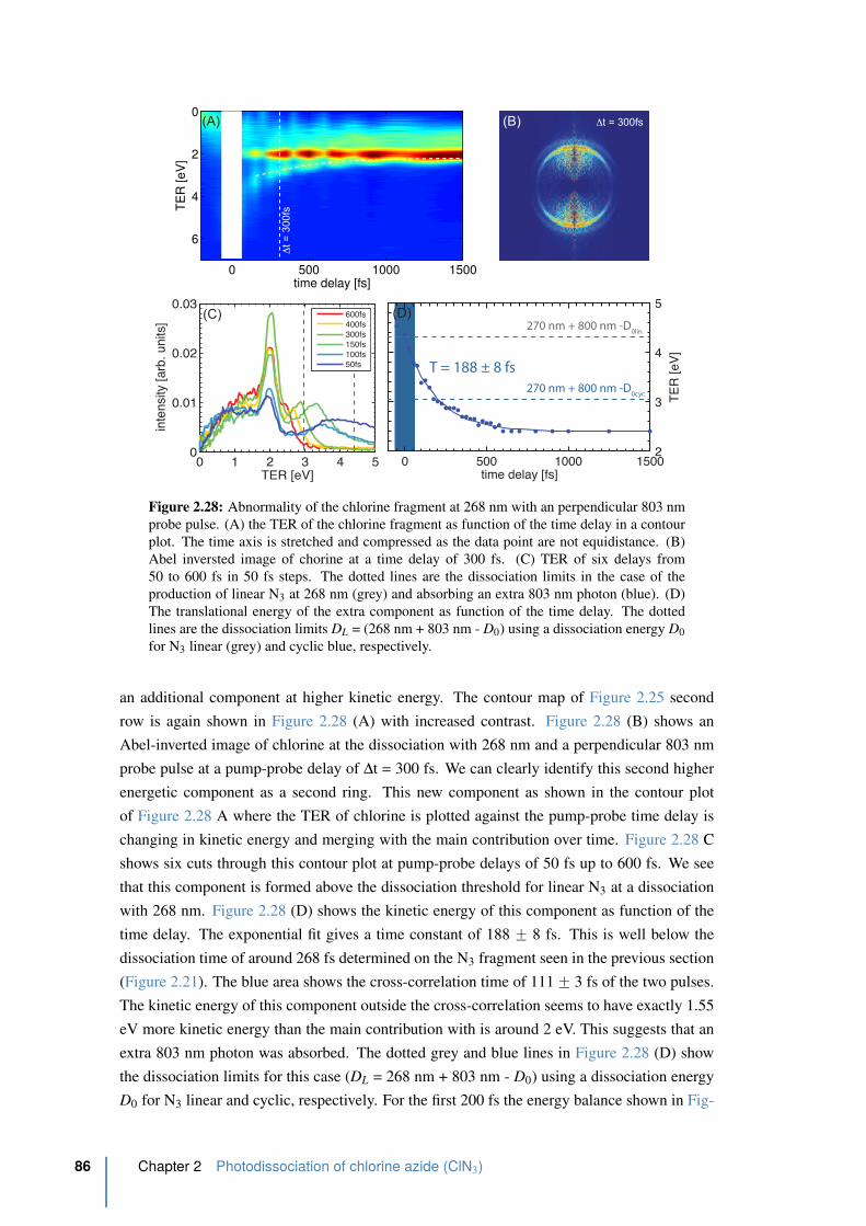
0 500 1000 15002
3
4
5
time delay [fs]
TE
R [e
V]
T = 188 ± 8 fs
270 nm + 800 nm -D0lin
270 nm + 800 nm -D0cyc
Δt = 300fs
0 1 2 3 4 50
0.01
0.02
0.03
TER [eV]
inte
nsity
[arb
. uni
ts]
600fs400fs300fs150fs100fs50fs
(C) (D)
(B)
time delay [fs]
TE
R [eV
]
0 500 1000 1500
0
2
4
6
Δt =
300fs
(A)
FW
HM
Ar =
112(2
) fs
Figure 2.28: Abnormality of the chlorine fragment at 268 nm with an perpendicular 803 nm
probe pulse. (A) the TER of the chlorine fragment as function of the time delay in a contour
plot. The time axis is stretched and compressed as the data point are not equidistance. (B)
Abel inversted image of chorine at a time delay of 300 fs. (C) TER of six delays from
50 to 600 fs in 50 fs steps. The dotted lines are the dissociation limits in the case of the
production of linear N3 at 268 nm (grey) and absorbing an extra 803 nm photon (blue). (D)
The translational energy of the extra component as function of the time delay. The dotted
lines are the dissociation limits DL = (268 nm + 803 nm - D0) using a dissociation energy D0
for N3 linear (grey) and cyclic blue, respectively.
an additional component at higher kinetic energy. The contour map of Figure 2.25 second
row is again shown in Figure 2.28 (A) with increased contrast. Figure 2.28 (B) shows an
Abel-inverted image of chlorine at the dissociation with 268 nm and a perpendicular 803 nm
probe pulse at a pump-probe delay of ∆t = 300 fs. We can clearly identify this second higher
energetic component as a second ring. This new component as shown in the contour plot
of Figure 2.28 A where the TER of chlorine is plotted against the pump-probe time delay is
changing in kinetic energy and merging with the main contribution over time. Figure 2.28 C
shows six cuts through this contour plot at pump-probe delays of 50 fs up to 600 fs. We see
that this component is formed above the dissociation threshold for linear N3 at a dissociation
with 268 nm. Figure 2.28 (D) shows the kinetic energy of this component as function of the
time delay. The exponential fit gives a time constant of 188 ˘ 8 fs. This is well below the
dissociation time of around 268 fs determined on the N3 fragment seen in the previous section
(Figure 2.21). The blue area shows the cross-correlation time of 111 ˘ 3 fs of the two pulses.
The kinetic energy of this component outside the cross-correlation seems to have exactly 1.55
eV more kinetic energy than the main contribution with is around 2 eV. This suggests that an
extra 803 nm photon was absorbed. The dotted grey and blue lines in Figure 2.28 (D) show
the dissociation limits for this case (DL = 268 nm + 803 nm - D0) using a dissociation energy
D0 for N3 linear and cyclic, respectively. For the first 200 fs the energy balance shown in Fig-
86 Chapter 2 Photodissociation of chlorine azide (ClN3)

(X1A’) (S0)
0
1
2
3
4
5
6
(A1A’’)(S1)
3.25 eV
(B1A’)(S2)4.9 eV
(C1A’’) (S3)
5.8 eV
26
8 n
m -
4.6
7 e
V
(31A’) (S4)
5.2 eV
z
y x
pump pulse
probe pulse
Δt
(A) (B)
A‘‘(z)
A‘(z)
Figure 2.29: (A) pump pulse configuration in the case of an perpendicular 803 nm probe
pulse in respect to the molecular plane of ClN3 selected by the first 268 nm pump pulse. (B)
electronic excitation states of ClN3 reachable with 268 + 803 nm.
ure 2.28 (D) seems in agreement with the production of linear N3 even though with 268 + 803
nm the excitation energy in total is the same as in the case of 201 nm excitation. Figure 2.29
B shows again the excitation levels of ClN3. One can recognize the two states accessible in
this energy region, the S3 state with an A2 transition symmetry and the S4 state with an A1
transition symmetry. However, the electronic transition rules allow us to claim that the S3 state
is the main state populated since the polarizations of the 268 and 803 nm beam are crossed.
The 268 nm transition to the S2pA1q state at ∆t = 0 selects molecular planes containing the
pump polarization. This means that in the perpendicular configuration, the probe polariza-
tion will be mostly perpendicular to the molecular plane (see Figure 2.29 A). Consequently
in the 268 + 803 nm excitation scheme, the second transition from S2(A1) state can be only a
perpendicular transition, namely only the S3(A2) state can be populated. Since the molecular
plane is selected by the first transition S2pA1q Ð S0pA1q, dissociation taking place from S3 will
still have a anisotropy of β2 ą 0, even taking into account the perpendicular character of the
S3pA2q Ð S2pA1q transition.
The fact that we can see the contribution from this S3(A2) state can let us conclude that the
dissociation time of this electronic state has to be much faster than the duration of the probe
laser. Indeed, if the dissociation from S3 would be longer than 60 fs we wouldn’t be able to
absorb all the extra 803 nm photons to ionize the produced N3 fragment at the same time (9
more photons are needed for ionization). Note that in a parallel configuration of the pump
and probe laser beams at 268 + 201 nm, we should access the S4(A1) state like in the 201 nm
excitation scheme. On the data recorded in parallel configuration, there is however no obvious
contribution observed. This is in agreement with the long lifetime (178 ˘ 22 fs) recorded for
the S4 state, populated at 201 nm (see Figure 2.21).
To explain the changing in kinetic energy of this component over time we have to look at the
contributing energy balance. The translational energy release of this component as function of
time can be written as follows:
T ERptq “ S3 pRN´Clptqq ` EN´ClpRN´Clptqq ´ Dlin0 (2.15)
where S3 pRN´Clptqq is the potential energy surface of the C1A2 state as function of the in-
Section 2.5 Chlorine abnormality at 268 nm 87
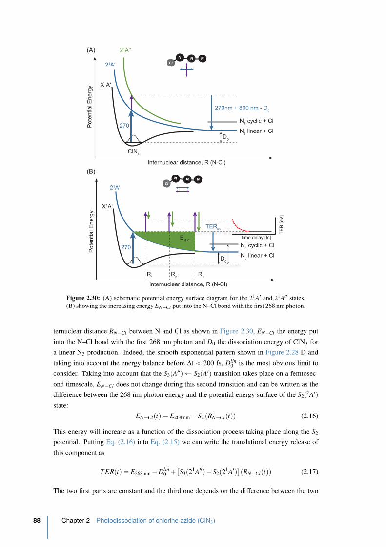
N3 linear + Cl
D0
Internuclear distance, R (N-Cl)
Pote
ntial E
nerg
y
21A‘
270
ClN3
X1A‘
21A‘‘
Cl
N N N
270nm + 800 nm - D0
N3 cyclic + Cl
TERlin
D0
Internuclear distance, R (N-Cl)
Pote
ntial E
nerg
y
21A‘
270
R1
X1A‘
Cl
N N N
R2
R∞
EN-Cl
N3 linear + Cl
N3 cyclic + Cl
(A)
(B)
time delay [fs]
TE
R [e
V]
Figure 2.30: (A) schematic potential energy surface diagram for the 21A1 and 21A2 states.
(B) showing the increasing energy EN´Cl put into the N–Cl bond with the first 268 nm photon.
ternuclear distance RN´Cl between N and Cl as shown in Figure 2.30, EN´Cl the energy put
into the N–Cl bond with the first 268 nm photon and D0 the dissociation energy of ClN3 for
a linear N3 production. Indeed, the smooth exponential pattern shown in Figure 2.28 D and
taking into account the energy balance before ∆t ă 200 fs, Dlin0 is the most obvious limit to
consider. Taking into account that the S3pA2q Ð S2pA1q transition takes place on a femtosec-
ond timescale, EN´Cl does not change during this second transition and can be written as the
difference between the 268 nm photon energy and the potential energy surface of the S2(2A1qstate:
EN´Clptq “ E268 nm ´ S2 pRN´Clptqq (2.16)
This energy will increase as a function of the dissociation process taking place along the S2
potential. Putting Eq. (2.16) into Eq. (2.15) we can write the translational energy release of
this component as
T ERptq “ E268 nm ´ Dlin0 ` rS3p21A2q ´ S2p21A1qspRN´Clptqq (2.17)
The two first parts are constant and the third one depends on the difference between the two
88 Chapter 2 Photodissociation of chlorine azide (ClN3)
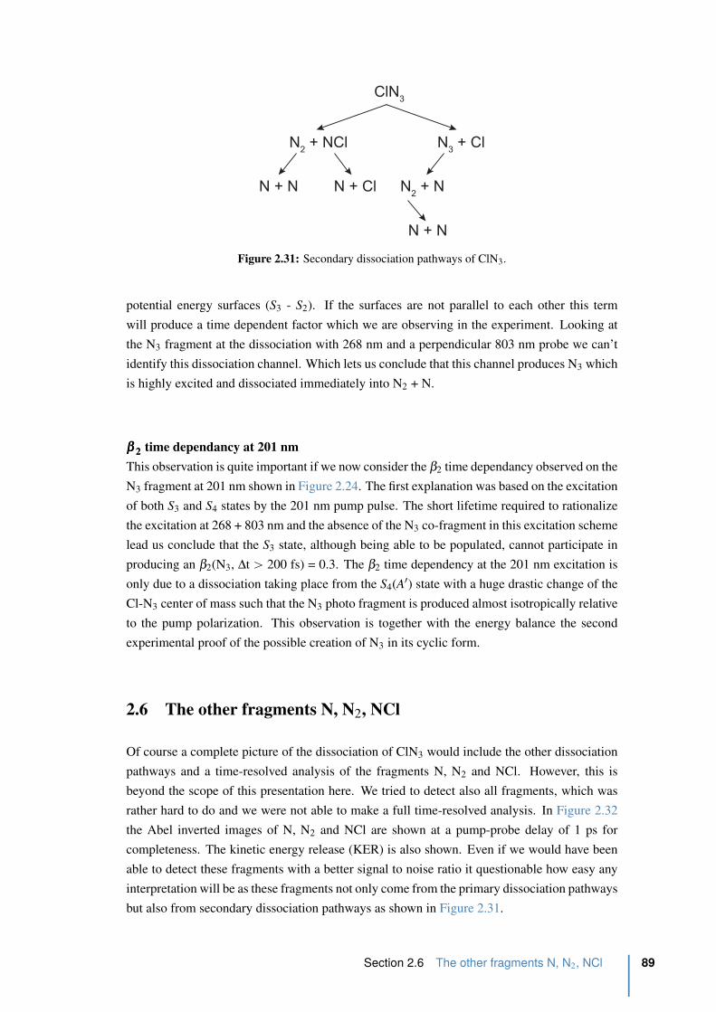
ClN3
N2 + NCl N
3 + Cl
N + N N + Cl N2 + N
N + N
Figure 2.31: Secondary dissociation pathways of ClN3.
potential energy surfaces (S3 - S2). If the surfaces are not parallel to each other this term
will produce a time dependent factor which we are observing in the experiment. Looking at
the N3 fragment at the dissociation with 268 nm and a perpendicular 803 nm probe we can’t
identify this dissociation channel. Which lets us conclude that this channel produces N3 which
is highly excited and dissociated immediately into N2 + N.
βββ 222 time dependancy at 201 nm
This observation is quite important if we now consider the β2 time dependancy observed on the
N3 fragment at 201 nm shown in Figure 2.24. The first explanation was based on the excitation
of both S3 and S4 states by the 201 nm pump pulse. The short lifetime required to rationalize
the excitation at 268 + 803 nm and the absence of the N3 co-fragment in this excitation scheme
lead us conclude that the S3 state, although being able to be populated, cannot participate in
producing an β2(N3, ∆t ą 200 fs) = 0.3. The β2 time dependency at the 201 nm excitation is
only due to a dissociation taking place from the S4(A1) state with a huge drastic change of the
Cl-N3 center of mass such that the N3 photo fragment is produced almost isotropically relative
to the pump polarization. This observation is together with the energy balance the second
experimental proof of the possible creation of N3 in its cyclic form.
2.6 The other fragments N, N2, NCl
Of course a complete picture of the dissociation of ClN3 would include the other dissociation
pathways and a time-resolved analysis of the fragments N, N2 and NCl. However, this is
beyond the scope of this presentation here. We tried to detect also all fragments, which was
rather hard to do and we were not able to make a full time-resolved analysis. In Figure 2.32
the Abel inverted images of N, N2 and NCl are shown at a pump-probe delay of 1 ps for
completeness. The kinetic energy release (KER) is also shown. Even if we would have been
able to detect these fragments with a better signal to noise ratio it questionable how easy any
interpretation will be as these fragments not only come from the primary dissociation pathways
but also from secondary dissociation pathways as shown in Figure 2.31.
Section 2.6 The other fragments N, N2, NCl 89
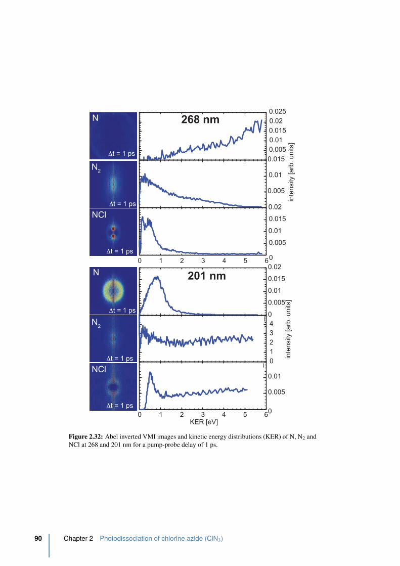
N
N2
NCl
0 1 2 3 4 5 6KER [eV]
inte
nsity [arb
. units]
0
0.005
0.01
0.015
0.02
0
1
2
3
4
0
0.005
0.01
Δt = 1 ps
Δt = 1 ps
Δt = 1 ps
201 nm
0.005
0.01
0.015
0.02
0.025
0.005
0.01
0.015
inte
nsity [arb
. units]
0 1 2 3 4 5 60
0.005
0.01
0.015
0.02
Δt = 1 ps
Δt = 1 ps
Δt = 1 ps
268 nmN
N2
NCl
Figure 2.32: Abel inverted VMI images and kinetic energy distributions (KER) of N, N2 and
NCl at 268 and 201 nm for a pump-probe delay of 1 ps.
90 Chapter 2 Photodissociation of chlorine azide (ClN3)
2.7 Conclusion
The femtosecond time-resolved photodissociation study of ClN3 was able to detect for the first
time the fragments N3 directly using a velocity-map imaging spectrometer. This enabled us
to measure not only the dissociation time but also a time-resolved angular distribution in two
major energy regions, using a dissociation energy of 4.67 eV (268 nm), where linear N3 is pro-
duced and 6.13 (201 nm), where cyclic N3 is produced. The dissociation time was determined
to be 262 ˘ 38 fs and 178 ˘ 22 fs for linear and cyclic N3, respectively. Both dissociation
times are more than twice longer as the time observed on the full integrated signal detecting
the TOF directly. From this we can conclude that in the case of detecting the integrated signal
as function of the pump-probe delay, the measurement is filtered in intensity and we are not
able to detect the small amount of fragments that are produced. The smooth decay reveals
that the dissociation is not a direct dissociation as suggested before [17]. A direct dissociation
would occur roughly on half of the Cl-N3 stretching period which is only 30 fs (νstretch = 545
cm´1 = 61 fs). The fact that the relaxation dynamics can be followed whatever the electronic
state encountered, means that dissociative ionization is not sensitive to the electronic character,
but simply depending on the amount of excited parent molecules. Maybe an ionization exper-
iment, recording the fragments and the photo-electrons in coincidence could reveal properly
the electronic states encountered.
The angular distribution measured from the N3 velocity-map image revealed at long delays a
β2 parameter of 1.64 ˘ 0.06 and 0.27 ˘ 0.05 for linear and cyclic N3, respectively. These
values are in agreement with previous measurements done in the ns-time regime detecting
only the Cl fragment via a REMPI transition. In addition, the time-resolved data shows in
addition that these value are not reached immediately. It takes 170 ˘ 45 fs and 136 ˘ 7 fs for
the linear and cyclic N3 fragment, respectively, to reach the long delay limits. Unfortunately,
the multiphoton ionization detection was not suitable to detect the chlorine fragment with a
good signal-to-noise ratio at short pump-probe delays and no in depth time-resolved analysis
has been possible so far. However, at long pump-probe delays the β2 parameter obtained
from the chlorine images is in good agreement with the values obtained from the N3 images.
Using a probe pulse with a polarization perpendicular to the dissociation laser delivered a
better signal-to-noise ratio and allowed a dissociation time to be determined from the chlorine
images, which is comparable, within the error bars, to the dissociation time obtained from the
N3 fragment.
Instead of a multiphoton ionization detection process, it would be ideal to employ a XUV
photoionization detection, especially for detecting the chlorine fragment. The next experiment
to confirm the formation of cyclic N3 would be to generate a VUV pulse, such that only N3
cyclic would be photoionized (VUV tuned to the ionization potential of N3 cyclic) and to
realize a Coulomb explosion with a 10 fs IR laser pulse to detect in coincidence the relative
positions of the N fragments, along the lines of the study performed by Hasegawa et al. on
CS2 for instance [50].
Section 2.7 Conclusion 91
References
[1] Griess, P. Proc. R. Soc. 13: 375–384 (1864) (cited p. 50).
[2] Raschig, F. Chem. Ber. 41: 4194 (1908) (cited p. 50).
[3] Samartzis, PC and Wodtke, AM. Casting a new light on azide photochemistry: pho-
tolytic production of cyclic-N3. Phys. Chem. Chem. Phys. 9:24 3054 (2007) (cited
p. 50).
[4] Tornieporth-oetting, I and Klapotke, T. Recent Developments in the Chemistry of Bi-
nary Nitrogen-Halogen Species. Comments on Inorg. Chem. 15:3 137–169 (1994)
(cited p. 50).
[5] Ray, AJ and Coombe, RD. An I* laser pumped by NCl(a1∆). J. Phys. Chem. 99:20
7849–7852 (1995) (cited p. 50).
[6] Pritt, AT. Decay kinetics of NCl(b1Σ
`,v1). J. Chem. Phys. 75:12 5720–5727 (1981)
(cited p. 50).
[7] Coombe, RD. Photodissociation of ClN3 at 193 and 249 nm. J. Chem. Phys. 75:5
2177–2190 (1981) (cited p. 50, 51).
[8] Coombe, RD and Van Benthem, MH. Radiative rates of singlet–triplet transitions in
nitrogen halide diatomics. J. Chem. Phys. 81:7 2984 (1984) (cited p. 50).
[9] Benard, DJ, Chowdhury, MA, Winker, BK, Seder, TA, and Michels, HH. Production
of NCl(a) by thermal decomposition of chlorine azide. J. Phys. Chem. 94:19 7507–
7514 (1990) (cited p. 50).
[10] Ray, AJ and Coombe, RD. Collisional Quenching of NCl(a1∆,v “ 0) and the Chain
Decomposition of ClN3. J. Phys. Chem. 98:36 8940–8945 (1994) (cited p. 50).
[11] Henshaw, TL, Herrera, SD, Haggquist, GW, and Schlie, L. Kinetics of NCl(a1∆) via
photodissociation of ClN3. J. Phys. Chem. A 101:22 4048–4056 (1997) (cited p. 50).
[12] Jensen, RH, Mann, A, and Coombe, RD. Energy Transfer from N2(v) to ClN3 and
a Kinetic Model for the Chain Decomposition of Chlorine Azide. J. Phys. Chem. A
104:28 6573–6579 (2000) (cited p. 50).
[13] Komissarov, AV, Manke II, GC, Davis, SJ, and Heaven, MC. Kinetic spectroscopy of
NCl. Proc. SPIE 3931 138: pages (2000) (cited p. 50).
[14] Komissarov, AV, Manke, GC, Davis, SJ, and Heaven, MC. Rate constants for quench-
ing and self-annihilation of NCl(a1∆). J. Phys. Chem. A 106:36 8427–8434 (2002)
(cited p. 50, 51).
[15] Wodtke, AM, Hansen, N, Robinson, JC, Sveum, NE, Goncher, SJ, and Neumark, DM.
The Cl to NCl branching ratio in 248-nm photolysis of chlorine azide. Chem. Phys.
Lett. 391:4-6 334–337 (2004) (cited p. 50, 52).
[16] Hansen, N, Wodtke, AM, Goncher, SJ, Robinson, JC, Sveum, NE, and Neumark, DM.
Photofragment translation spectroscopy of ClN3 at 248 nm: Determination of the pri-
mary and secondary dissociation pathways. J. Chem. Phys. 123:10 104305 (2005)
(cited p. 50, 52, 54, 55, 81).
[17] Hansen, N and Wodtke, AM. Velocity Map Ion Imaging of Chlorine Azide Photolysis:
Evidence for Photolytic Production of Cyclic-N`3 . J. Phys. Chem. A 107:49 10608–
10614 (2003) (cited p. 50–52, 54, 78, 81, 91).
[18] Friedmann, A, Soliva, AM, Nizkorodov, SA, Bieske, EJ, and Maier, JP. A 3Πu Ð
X3Σ
´g Electronic Spectrum of N`
3 . J. Phys. Chem. 98:36 8896–8902 (1994) (cited
p. 50).
[19] Bittererova, M, Ostmark, H, and Brinck, T. A theoretical study of the azide (N3) dou-
blet states. A new route to tetraazatetrahedrane (N4): N+N3 Ñ N4. J. Chem. Phys.
116:22 9740–9748 (2002) (cited p. 50, 52, 53, 73).
92 Chapter 2 Photodissociation of chlorine azide (ClN3)
[20] Bodi, A, Johnson, M, Gerber, T, Gengeliczki, Z, Sztaray, B, and Baer, T. Imaging
photoelectron photoion coincidence spectroscopy with velocity focusing electron op-
tics. Rev. Sci. Instr. 80:3 (2009) (cited p. 50).
[21] Mayer, PM, Staedter, D, Blanchet, V, Hemberger, P, and Bodi, A. Comparing Fem-
tosecond Multiphoton Dissociative Ionization of Tetrathiafulvene with Imaging Pho-
toelectron Photoion Coincidence Spectroscopy. J. Phys. Chem. A 117:13 2753–2759
(2013) (cited p. 50).
[22] Quinto-Hernandez, A, Lee, YY, Huang, TP, Pan, WC, Lin, JJM, Bobadova-Parvanova,
P, Morokuma, K, Samartzis, PC, and Wodtke, AM. Dissociative photoionization of
ClN3 using high-resolution synchrotron radiation: The N-Cl bond energy in ClN3. Int.
J. Mass Spec. 265:2-3 261–266 (2007) (cited p. 50, 52, 54, 56, 66, 73).
[23] Coombe, RD, St, D, Henshaw, TL, and May, DJ. Generation and quenching of N2
(A3σ `u) in the photodissociation of CIN3. Chem. Phys. Lett. 120:4-5 433–436 (1985)
(cited p. 50, 51).
[24] Curtius, T. Ueber Stickstoffwasserstoffsaure (Azoimid) N3H. Chem. Ber. 23:2 3023–
3033 (1890) (cited p. 51).
[25] Douglas, AE and Jones, WJ. The 2 700 Angstrom bands of the N3 molecule. Can. J.
Phys. 43:12 2216–2221 (1965) (cited p. 51).
[26] Dyke, JM, Jonathan, NBH, Lewis, AE, and Morris, A. Vacuum ultraviolet photoelec-
tron spectroscopy of transient species. Mol. Phys. 47:5 1231–1240 (1982) (cited p. 51,
55).
[27] Beaman, RA, Nelson, T, Richards, DS, and Setser, DW. Observation of azido radical
by laser-induced fluorescence. J. Phys. Chem. 91:24 6090–6092 (1987) (cited p. 51).
[28] Tian, R, Facelli, JC, and Michl, J. Vibrational and electronic spectra of matrix-isolated
nitrogen trimer radical and azide. J. Phys. Chem. 92:14 4073–4079 (1988) (cited
p. 51).
[29] Lewis, GN. The Atom and the Molecule. J. Am. Chem. Soc. 38:4 762–785 (1916)
(cited p. 52).
[30] Goncher, SJ, Sveum, NE, Moore, DT, Bartlett, ND, and Neumark, DM. Photodissoci-
ation dynamics of ClN3 at 193 nm. J. Chem. Phys. 125:22 224304 (2006) (cited p. 52,
54, 81).
[31] Samartzis, PC, Hansen, N, and Wodtke, AM. Imaging CIN3 photodissociation from
234 to 280 nm. Phys. Chem. Chem. Phys. 8:25 2958 (2006) (cited p. 52, 53, 79, 81).
[32] Samartzis, PC, Lin, JJM, Ching, TT, Chaudhuri, C, Lee, SH, and Wodtke, AM. The
simplest all-nitrogen ring: Photolytically filling the cyclic-N3 well. J. Chem. Phys.
126:4 041101 (2007) (cited p. 52).
[33] Samartzis, PC, Lin, J, Ching, TT, Chaudhuri, C, Lee, YT, Lee, SH, and Wodtke, AM.
Two photoionization thresholds of N3 produced by ClN3 photodissociation at 248 nm:
Further evidence for cyclic N3. J. Chem. Phys. 123:5 051101 (2005) (cited p. 53).
[34] Tarroni, R and Tosi, P. Cyclic and bent electronic states of the N`3 ion. Chem. Phys.
Lett. 389:4-6 274–278 (2004) (cited p. 53).
[35] Pahnke, R, Ashworth, SH, and Brown, JM. Detection of the N3 free radical by laser
magnetic resonance at 6.08 µm. Chem. Phys. Lett. (1988) (cited p. 53).
[36] Chambaud, G and Rosmus, P. Rovibronic spectrum of the N3 radical in the X2Πg state.
J. Chem. Phys. 96:1 77 (1992) (cited p. 53).
[37] Cook, RL. Microwave Spectrum and Structure of Chlorine Azide. J. Chem. Phys. 53:6
2525–2528 (1970) (cited p. 53).
[38] Quinto-Hernandez, A. Spectroscopic Studies of Azide compounds: Thermochemistry,
Chemical Kinetics and Photodissociation Dynamics. PhD thesis. University of Cali-
fornia, 2012 (cited p. 54, 55).
References 93
[39] Hansen, N, Wodtke, AM, Komissarov, AV, Morokuma, K, and Heaven, MC. Ion dis-
sociation dynamics of the chlorine azide cation (ClN`3 ) investigated by velocity map
imaging. J. Chem. Phys. 118:23 10485–10493 (2003) (cited p. 55, 66).
[40] Kerkines, ISK, Wang, Z, Zhang, P, and Morokuma, K. Photodissociation of ClN3 at
157 nm: Theory suggests a pathway leading to cyclic N3. J. Chem. Phys. 129:17 pages
(2008) (cited p. 54, 56).
[41] Zhang, P, Morokuma, K, and Wodtke, AM. High-level ab initio studies of unimolec-
ular dissociation of the ground-state N3 radical. J. Chem. Phys. 122: 014106 (2005)
(cited p. 53, 54, 56).
[42] Schulz, A, Tornieporth-Oetting, IC, and Klapoetke, TM. Experimental and Theoreti-
cal Vibrational Studies of Covalent X-N3 Azides (X=H, F, Cl, Br, I) - Application of
the Density-Functional Theory and Comparison with Ab-Initio Results. Inorg. Chem.
34:17 4343–4346 (1995) (cited p. 63).
[43] Maguire, LP, Szilagyi, S, and Scholten, RE. High performance laser shutter using a
hard disk drive voice-coil actuator. Rev. Sci. Instr. 75:9 3077 (2004) (cited p. 65).
[44] Scholten, RE. Enhanced laser shutter using a hard disk drive rotary voice-coil actua-
tor. Rev. Sci. Instr. 78:2 026101 (2007) (cited p. 65).
[45] Peng, J, Puskas, N, Corkum, PB, Rayner, DM, and Loboda, AV. High-Pressure Gas
Phase Femtosecond Laser Ionization Mass Spectrometry. Anal. Chem. 84:13 5633–
5640 (2012) (cited p. 66).
[46] Blanchet, V and Stolow, A. Nonadiabatic dynamics in polyatomic systems studied by
femtosecond time-resolved photoelectron spectroscopy. J. Chem. Phys. 108:11 4371–
4374 (1998) (cited p. 69).
[47] Gessner, O. Femtosecond Multidimensional Imaging of a Molecular Dissociation. Sci-
ence 311:5758 219–222 (2006) (cited p. 69).
[48] Thire, N, Cireasa, R, Staedter, D, Blanchet, V, and Pratt, ST. Time-resolved predis-
sociation of the vibrationless level of the B state of CH3I. Phys. Chem. Chem. Phys.
13:41 18485–18496 (2011) (cited p. 70, 72).
[49] Gougousi, T, Samartzis, PC, and Kitsopoulos, TN. Photodissociation study of CH3Br
in the first continuum. J. Chem. Phys. 108:14 5742–5746 (1998) (cited p. 79).
[50] Hasegawa, H, Hishikawa, A, and Yamanouchi, K. Coincidence imaging of Coulomb
explosion of CS2 in intense laser fields. Chem. Phys. Lett. 349:1-2 57–63 (2001) (cited
p. 91).
94 Chapter 2 Photodissociation of chlorine azide (ClN3)
3
Relaxation and dissociation dynamics in
tetrathiafulvalene (TTF)
Contents
3.1 Introduction . . . . . . . . . . . . . . . . . . . . . . . . . . . . . . . . . . . 96
3.1.1 Tetrathiafulvalen, an organic conductor . . . . . . . . . . . . . . . . 96
3.1.2 Absorption spectrum and photo-electron spectrum of TTF . . . . . . 97
3.2 Time-resolved electron relaxation dynamics in TTF . . . . . . . . . . . . . 99
3.2.1 The fs-UV-VIS-VMI setup . . . . . . . . . . . . . . . . . . . . . . . 99
3.2.2 A probe centered at 266 nm . . . . . . . . . . . . . . . . . . . . . . 101
3.2.3 A probe centered at 398 nm . . . . . . . . . . . . . . . . . . . . . . 104
3.2.4 A probe centered at 800 nm . . . . . . . . . . . . . . . . . . . . . . 104
3.2.5 Photoelectron spectrum of TTF with an intense 800 nm . . . . . . . . 108
3.3 The iPEPICO breakdown diagrams and the dissociation model . . . . . . 109
3.3.1 iPEPICO setup . . . . . . . . . . . . . . . . . . . . . . . . . . . . . 109
3.3.2 Computational procedures . . . . . . . . . . . . . . . . . . . . . . . 109
3.3.3 Results and Discussion . . . . . . . . . . . . . . . . . . . . . . . . . 110
3.4 Conclusion . . . . . . . . . . . . . . . . . . . . . . . . . . . . . . . . . . . . 114
References . . . . . . . . . . . . . . . . . . . . . . . . . . . . . . . . . . . . . . . 115
Abstract
Tetrathiafulvalene (TTF, C6H4S4) electronic relaxation is studied, while scanning the elec-
tronic excitation around 4 eV, by time resolved mass spectrometry and photoelectron spec-
troscopy. To enhance the sensitivity, the photoionization is achieved at different probe wave-
lengths (266 nm, 400 nm and 800 nm). With an intense 800 nm pulse the above threshold
ionization (ATI) of TTF is studied. Within the internal energy achieved a variety of dissocia-
tion channels of the ion are accessible. In order to disentangle the complex ionic dissociation,
we utilized the imaging photoelectron photoion coincidence (iPEPICO) technique. Above the
dissociation threshold, iPEPICO results show that the molecular ion (m/z = 204) dissociates
into seven product ions, six of which compete in a 1.0 eV internal energy window. The chap-
ter starts with an introduction to TTF and its spectroscopy in Section 3.1. Section 3.2 covers
the femtosecond electronic relaxation dynamics at various pump and probe wavelength. Sec-
tion 3.3 presents the VUV dissociation results from the iPEPICO experiment.
Keywords: tetrathiafulvalene, electronic relaxation, iPEPICO, appearance energies, RRKM
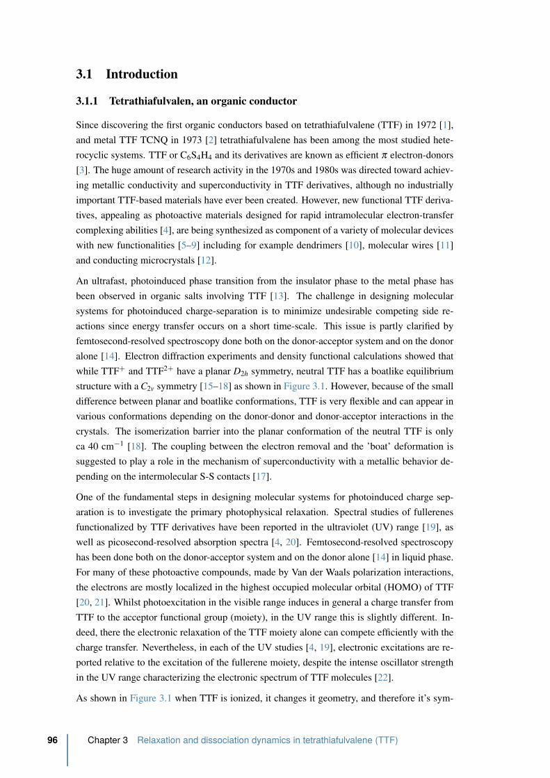
3.1 Introduction
3.1.1 Tetrathiafulvalen, an organic conductor
Since discovering the first organic conductors based on tetrathiafulvalene (TTF) in 1972 [1],
and metal TTF TCNQ in 1973 [2] tetrathiafulvalene has been among the most studied hete-
rocyclic systems. TTF or C6S4H4 and its derivatives are known as efficient π electron-donors
[3]. The huge amount of research activity in the 1970s and 1980s was directed toward achiev-
ing metallic conductivity and superconductivity in TTF derivatives, although no industrially
important TTF-based materials have ever been created. However, new functional TTF deriva-
tives, appealing as photoactive materials designed for rapid intramolecular electron-transfer
complexing abilities [4], are being synthesized as component of a variety of molecular devices
with new functionalities [5–9] including for example dendrimers [10], molecular wires [11]
and conducting microcrystals [12].
An ultrafast, photoinduced phase transition from the insulator phase to the metal phase has
been observed in organic salts involving TTF [13]. The challenge in designing molecular
systems for photoinduced charge-separation is to minimize undesirable competing side re-
actions since energy transfer occurs on a short time-scale. This issue is partly clarified by
femtosecond-resolved spectroscopy done both on the donor-acceptor system and on the donor
alone [14]. Electron diffraction experiments and density functional calculations showed that
while TTF` and TTF2` have a planar D2h symmetry, neutral TTF has a boatlike equilibrium
structure with a C2v symmetry [15–18] as shown in Figure 3.1. However, because of the small
difference between planar and boatlike conformations, TTF is very flexible and can appear in
various conformations depending on the donor-donor and donor-acceptor interactions in the
crystals. The isomerization barrier into the planar conformation of the neutral TTF is only
ca 40 cm´1 [18]. The coupling between the electron removal and the ’boat’ deformation is
suggested to play a role in the mechanism of superconductivity with a metallic behavior de-
pending on the intermolecular S-S contacts [17].
One of the fundamental steps in designing molecular systems for photoinduced charge sep-
aration is to investigate the primary photophysical relaxation. Spectral studies of fullerenes
functionalized by TTF derivatives have been reported in the ultraviolet (UV) range [19], as
well as picosecond-resolved absorption spectra [4, 20]. Femtosecond-resolved spectroscopy
has been done both on the donor-acceptor system and on the donor alone [14] in liquid phase.
For many of these photoactive compounds, made by Van der Waals polarization interactions,
the electrons are mostly localized in the highest occupied molecular orbital (HOMO) of TTF
[20, 21]. Whilst photoexcitation in the visible range induces in general a charge transfer from
TTF to the acceptor functional group (moiety), in the UV range this is slightly different. In-
deed, there the electronic relaxation of the TTF moiety alone can compete efficiently with the
charge transfer. Nevertheless, in each of the UV studies [4, 19], electronic excitations are re-
ported relative to the excitation of the fullerene moiety, despite the intense oscillator strength
in the UV range characterizing the electronic spectrum of TTF molecules [22].
As shown in Figure 3.1 when TTF is ionized, it changes it geometry, and therefore it’s sym-
96 Chapter 3 Relaxation and dissociation dynamics in tetrathiafulvalene (TTF)
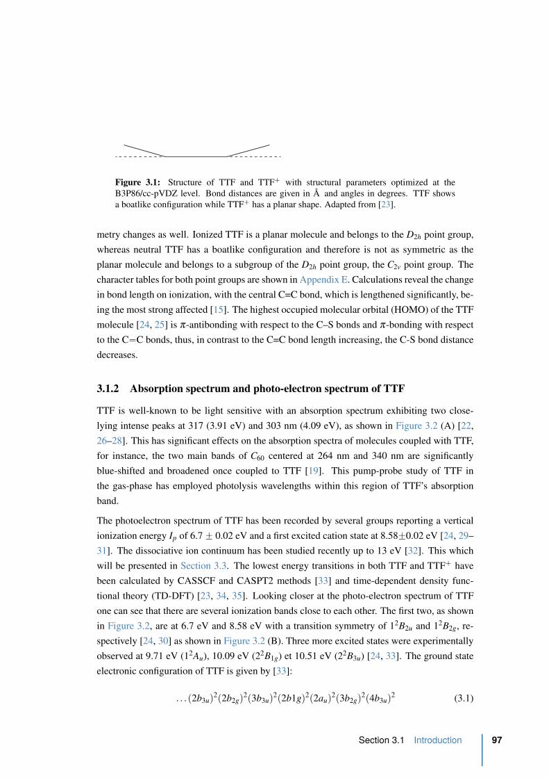
117.8
124.8114.0
94.4
1.353
1.776
1.090
1.339
1.756
117.1
125.2114.7
95.5
1.399
1.739
1.091
1.348
1.733
TTF TTF+
S
S S
SH
H
H
H
S
S S
SH
H
H
H
Figure 3.1: Structure of TTF and TTF` with structural parameters optimized at the
B3P86/cc-pVDZ level. Bond distances are given in A and angles in degrees. TTF shows
a boatlike configuration while TTF` has a planar shape. Adapted from [23].
metry changes as well. Ionized TTF is a planar molecule and belongs to the D2h point group,
whereas neutral TTF has a boatlike configuration and therefore is not as symmetric as the
planar molecule and belongs to a subgroup of the D2h point group, the C2v point group. The
character tables for both point groups are shown in Appendix E. Calculations reveal the change
in bond length on ionization, with the central C=C bond, which is lengthened significantly, be-
ing the most strong affected [15]. The highest occupied molecular orbital (HOMO) of the TTF
molecule [24, 25] is π-antibonding with respect to the C–S bonds and π-bonding with respect
to the C“C bonds, thus, in contrast to the C=C bond length increasing, the C-S bond distance
decreases.
3.1.2 Absorption spectrum and photo-electron spectrum of TTF
TTF is well-known to be light sensitive with an absorption spectrum exhibiting two close-
lying intense peaks at 317 (3.91 eV) and 303 nm (4.09 eV), as shown in Figure 3.2 (A) [22,
26–28]. This has significant effects on the absorption spectra of molecules coupled with TTF,
for instance, the two main bands of C60 centered at 264 nm and 340 nm are significantly
blue-shifted and broadened once coupled to TTF [19]. This pump-probe study of TTF in
the gas-phase has employed photolysis wavelengths within this region of TTF’s absorption
band.
The photoelectron spectrum of TTF has been recorded by several groups reporting a vertical
ionization energy Ip of 6.7 ˘ 0.02 eV and a first excited cation state at 8.58˘0.02 eV [24, 29–
31]. The dissociative ion continuum has been studied recently up to 13 eV [32]. This which
will be presented in Section 3.3. The lowest energy transitions in both TTF and TTF` have
been calculated by CASSCF and CASPT2 methods [33] and time-dependent density func-
tional theory (TD-DFT) [23, 34, 35]. Looking closer at the photo-electron spectrum of TTF
one can see that there are several ionization bands close to each other. The first two, as shown
in Figure 3.2, are at 6.7 eV and 8.58 eV with a transition symmetry of 12B2u and 12B2g, re-
spectively [24, 30] as shown in Figure 3.2 (B). Three more excited states were experimentally
observed at 9.71 eV (12Au), 10.09 eV (22B1g) et 10.51 eV (22B3u) [24, 33]. The ground state
electronic configuration of TTF is given by [33]:
. . .p2b3uq2p2b2gq2p3b3uq2p2b1gq2p2auq2p3b2gq2p4b3uq2 (3.1)
Section 3.1 Introduction 97
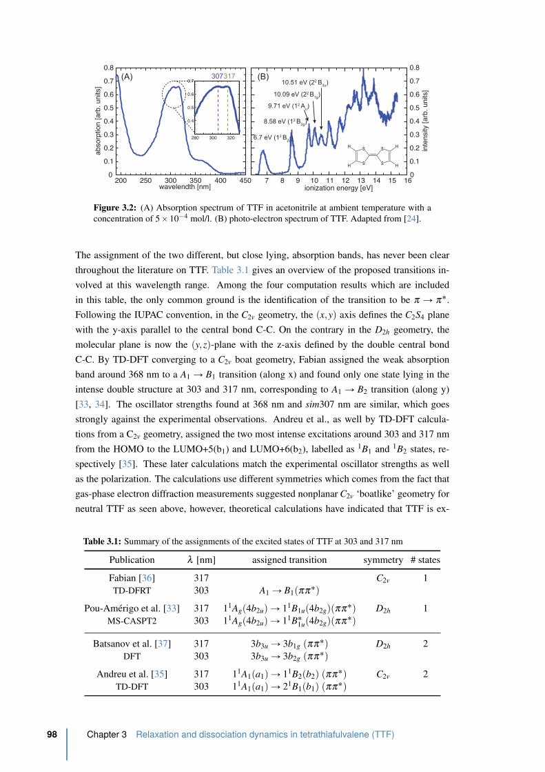
7 8 9 10 11 12 13 14 15 160
0.1
0.2
0.3
0.4
0.5
0.6
0.7
0.8
ionization energy [eV]
inte
nsity
[arb
. uni
ts]
6.7 eV (12 B2u
)
8.58 eV (12 B2g
)
9.71 eV (12 Au)
10.09 eV (22 B1g
)
10.51 eV (22 B3u
)
S
S S
SH
H
H
H
(A) (B)
200 250 300 350 400 4500
0.1
0.2
0.3
0.4
0.5
0.6
0.7
0.8
wavelendth [nm]
abso
rptio
n [a
rb. u
nits
]
280 300 320
0.4
0.5
0.6
0.7307317
Figure 3.2: (A) Absorption spectrum of TTF in acetonitrile at ambient temperature with a
concentration of 5 ˆ 10´4 mol/l. (B) photo-electron spectrum of TTF. Adapted from [24].
The assignment of the two different, but close lying, absorption bands, has never been clear
throughout the literature on TTF. Table 3.1 gives an overview of the proposed transitions in-
volved at this wavelength range. Among the four computation results which are included
in this table, the only common ground is the identification of the transition to be π Ñ π˚.
Following the IUPAC convention, in the C2v geometry, the px,yq axis defines the C2S4 plane
with the y-axis parallel to the central bond C-C. On the contrary in the D2h geometry, the
molecular plane is now the py,zq-plane with the z-axis defined by the double central bond
C-C. By TD-DFT converging to a C2v boat geometry, Fabian assigned the weak absorption
band around 368 nm to a A1 Ñ B1 transition (along x) and found only one state lying in the
intense double structure at 303 and 317 nm, corresponding to A1 Ñ B2 transition (along y)
[33, 34]. The oscillator strengths found at 368 nm and sim307 nm are similar, which goes
strongly against the experimental observations. Andreu et al., as well by TD-DFT calcula-
tions from a C2v geometry, assigned the two most intense excitations around 303 and 317 nm
from the HOMO to the LUMO+5(b1) and LUMO+6(b2), labelled as 1B1 and 1B2 states, re-
spectively [35]. These later calculations match the experimental oscillator strengths as well
as the polarization. The calculations use different symmetries which comes from the fact that
gas-phase electron diffraction measurements suggested nonplanar C2v ‘boatlike’ geometry for
neutral TTF as seen above, however, theoretical calculations have indicated that TTF is ex-
Table 3.1: Summary of the assignments of the excited states of TTF at 303 and 317 nm
Publication λ [nm] assigned transition symmetry # states
Fabian [36] 317 C2v 1
TD-DFRT 303 A1 Ñ B1pππ˚qPou-Amerigo et al. [33] 317 11Agp4b2uq Ñ 11B1up4b2gqpππ˚q D2h 1
MS-CASPT2 303 11Agp4b2uq Ñ 11B˚1up4b2gqpππ˚q
Batsanov et al. [37] 317 3b3u Ñ 3b1g pππ˚q D2h 2
DFT 303 3b3u Ñ 3b2g pππ˚qAndreu et al. [35] 317 11A1pa1q Ñ 11B2pb2q pππ˚q C2v 2
TD-DFT 303 11A1pa1q Ñ 21B1pb1q pππ˚q
98 Chapter 3 Relaxation and dissociation dynamics in tetrathiafulvalene (TTF)
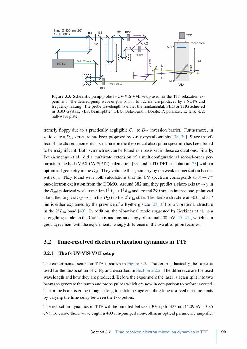
BS BS BS BBO400 nm
BBO
λ/2
L
L
λ/2
NOPA500 - 570 nm
BBO
307 - 322 nm
26
5 n
m
VMI
CCD
Phosphore
MCP
TOF
R
EG
MB
3 mJ @ 800 nm (20)
1 kHz, 80 fs
Figure 3.3: Schematic pump-probe fs-UV-VIS VMI setup used for the TTF relaxation ex-
periment. The desired pump wavelengths of 303 to 322 nm are produced by a NOPA and
frequency mixing. The probe wavelength is either the fundamental, SHG or THG achieved
in BBO crystals. (BS: beamsplitter, BBO: Beta-Barium Borate, P: polarizer, L: lens, λ /2:
half-wave plate).
tremely floppy due to a practically negligible C2v to D2h inversion barrier. Furthermore, in
solid state a D2h structure has been proposed by x-ray crystallography [38, 39]. Since the ef-
fect of the chosen geometrical structure on the theoretical absorption spectrum has been found
to be insignificant. Both symmetries can be found as a basis set in these calculations. Finally,
Pou-Armengo et al. did a multistate extension of a multiconfigurational second-order per-
turbation method (MAS-CAPSPT2) calculation [33] and a TD-DFT calculation [23] with an
optimized geometry in the D2h. They validate this geometry by the weak isomerization barrier
with C2v. They found with both calculations that the UV spectrum corresponds to π Ñ π˚
one-electron excitation from the HOMO. Around 382 nm, they predict a short-axis (x Ñ y in
the D2h) polarized weak transition 11Ag Ñ 11B2u and around 290 nm, an intense one, polarized
along the long axis (y Ñ z in the D2h) to the 21B1u state. The double structure at 303 and 317
nm is either explained by the presence of a Rydberg state [23, 33] or a vibrational structure
in the 21B1u band [40]. In addition, the vibrational mode suggested by Kerkines et al. is a
strengthing mode on the C“C axis and has an energy of around 200 mV [15, 41], which is in
good agreement with the experimental energy difference of the two absorption features.
3.2 Time-resolved electron relaxation dynamics in TTF
3.2.1 The fs-UV-VIS-VMI setup
The experimental setup for TTF is shown in Figure 3.3. The setup is basically the same as
used for the dissociation of ClN3 and described in Section 2.2.2. The difference are the used
wavelength and how they are produced. Before the experiment the laser is again split into two
beams to generate the pump and probe pulses which are now in comparison to before inverted.
The probe beam is going though a long translation stage enabling time resolved measurements
by varying the time delay between the two pulses.
The relaxation dynamics of TTF will be initiated between 303 up to 322 nm (4.09 eV - 3.85
eV). To create these wavelength a 400 nm-pumped non-collinear optical parametric amplifier
Section 3.2 Time-resolved electron relaxation dynamics in TTF 99

0
1
2
3
4
5
6
7
8
9
10
11
6.7 eV
E [eV]
11B1
805 nm
317 nm
403 nm
269 nm
11B2
21B1
D0(b
1u)-1
D1(b
2g)-1
11B2u
21B1u
C2v
D2h
TTF
TTF+
8.58 eV
303 nm
dissociative continuum
Figure 3.4: Different experimental pump-probe excitation schemes used for TTF. Electrons
states of neutral TTF are shown in black and electronic states of the ion are displayed in grey.
(NOPA), with three-steps of amplification provides a 30 µJ/p pulse, tunable between between
500 and 700 nm, is used. A fused-silica pair of prisms in double path is used to for compres-
sion. The duration is measured to « 80 fs by autocorrelation via a 50 µm BBO crystal. The
UV pump pulse is produced by a subsequent sum frequency mixing (FM) or second harmonic
(SHG), allowing a tuneability of the pump pulse from 370 to 300 nm. This is achieved through
a 200 µm BBO crystal by focusing gently a 50 µJ part of the fundamental beam with about
15-18 µJ/p visible pulse, resulting in around 5-7 µJ/p UV pulse. The typical pulse bandwidth
in the UV range is of 150 cm´1 (»2 nm), that would correspond to FWHM „70 fs. How-
ever no prism compression is used to pre-compensate the chirp introduced by the different
optics crossed by the UV pump pulse (mostly the vacuum chamber viewport and the BBO
crystal). The probe pulse is either the fundamental pulse, its second harmonic (SHG- 40 µJ/p)
or third harmonic (THG- 6 µJ/pulse). The Fourier-limited durations expected for these pump
and probe pulses from their bandwidths are of 65 fs. The pump and the probe are focused on
the molecular beam by 250 mm and 500 mm focal lengths, respectively, and combined with
an angle of 7 ˝ between them.
The TTF molecules (Aldrich, 97% without further purification) are sublimed continuously at
380K with 200 Torr of Argon and then expanded through a 250 µm nozzle at 450 K to avoid
cork formation. In most of the experiments presented here the polarizations are parallel to
each other and parallel to the detector. For each pump-probe delay, an average over 210k laser
pulses is done over 5 scans.
In the present experiment, the wavelength of the pump is varied from 322 nm to 307 nm as
mentioned before. The idea is to reveal the possible change of the electronic character via a
change in the measured decay time. As expected from the electron donor propriety of this
compound, the two first vertical ionizations from the ground electronic state lie quite low at
6.7˘0.02 eV and 8.58˘0.02 eV [24]. They are as ssen before, assigned mainly to the departure
of an electron from the highest occupied molecular orbital b1upπq (HOMO) and the second
highest occupied molecular orbital b3gpπq, respectively. The excitation scheme is summarized
100 Chapter 3 Relaxation and dissociation dynamics in tetrathiafulvalene (TTF)
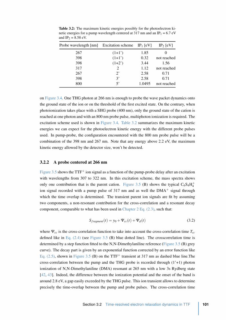
Table 3.2: The maximum kinetic energies possibly for the photoelectron ki-
netic energies for a pump wavelength centered at 317 nm and an IP1 = 6.7 eV
and IP2 = 8.58 eV.
Probe wavelength [nm] Excitation scheme IP1 [eV] IP2 [eV]
267 (1+1’) 1.85 0
398 (1+1’) 0.32 not reached
398 (1+2’) 3.44 1.56
317 2 1.12 not reached
267 2’ 2.58 0.71
398 3’ 2.58 0.71
800 5’ 1.0495 not reached
on Figure 3.4. One THG photon at 266 nm is enough to probe the wave packet dynamics onto
the ground state of the ion or on the threshold of the first excited state. On the contrary, when
photoionization takes place with a SHG probe (400 nm), only the ground state of the cation is
reached at one photon and with an 800 nm probe pulse, multiphoton ionization is required. The
excitation scheme used is shown in Figure 3.4. Table 3.2 summarizes the maximum kinetic
energies we can expect for the photoelectron kinetic energy with the different probe pulses
used. In pump-probe, the configuration encountered with the 800 nm probe pulse will be a
combination of the 398 nm and 267 nm. Note that any energy above 2.2 eV, the maximum
kinetic energy allowed by the detector size, won’t be detected.
3.2.2 A probe centered at 266 nm
Figure 3.5 shows the TTF` ion signal as a function of the pump-probe delay after an excitation
with wavelengths from 307 to 322 nm. In this excitation scheme, the mass spectra shows
only one contribution that is the parent cation. Figure 3.5 (B) shows the typical C6S4H`4
ion signal recorded with a pump pulse of 317 nm and as well the DMA` signal through
which the time overlap is determined. The transient parent ion signals are fit by assuming
two components, a non-resonant contribution for the cross-correlation and a resonant decay
component, comparable to what has been used in Chapter 2 Eq. (2.3), such that:
S f ragmentptq “ y0 ` Ψccptq ` Ψdptq (3.2)
where Ψcc is the cross-correlation function to take into account the cross-correlation time Tcc
defined like in Eq. (2.4) (see Figure 3.5 (B) blue dotted line). The crosscorrelation time is
determined by a step function fitted to the N,N-Dimethylaniline reference (Figure 3.5 (B) grey
curve). The decay part is given by an exponential function corrected by an error function like
Eq. (2.5), shown in Figure 3.5 (B) on the TTF` transient at 317 nm as dashed blue line.The
cross-correlation between the pump and the THG probe is recorded through (1’+1) photon
ionization of N,N-Dimethylaniline (DMA) resonant at 265 nm with a low 3s Rydberg state
[42, 43]. Indeed, the difference between the ionization potential and the onset of the band is
around 2.8 eV, a gap easily exceeded by the THG pulse. This ion transient allows to determine
precisely the time-overlap between the pump and probe pulses. The cross-correlation time
Section 3.2 Time-resolved electron relaxation dynamics in TTF 101
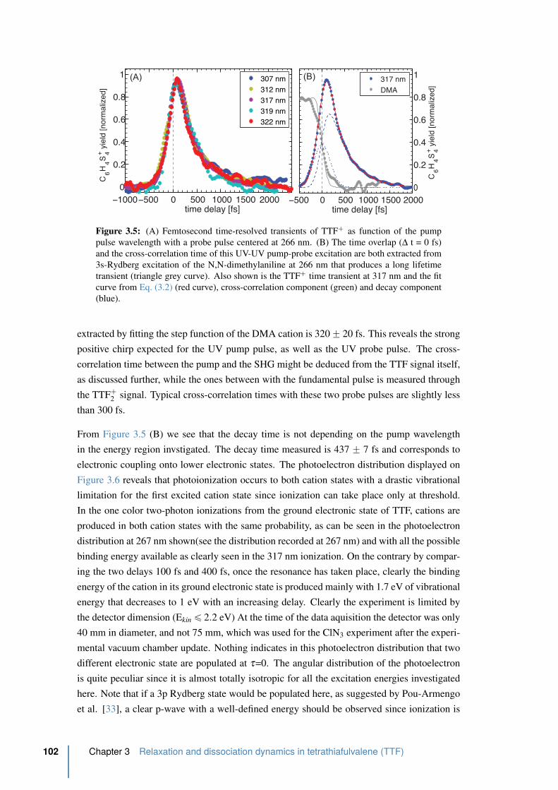
−1000−500 0 500 1000 1500 20000
0.2
0.4
0.6
0.8
1
time delay [fs]
C6H
4S4+ y
ield
[nor
mal
ized
]
307 nm312 nm317 nm319 nm322 nm
−500 0 500 1000 1500 20000
0.2
0.4
0.6
0.8
1
time delay [fs]
C6H
4S4+ y
ield
[nor
mal
ized
]
317 nmDMA
(A) (B)
Figure 3.5: (A) Femtosecond time-resolved transients of TTF` as function of the pump
pulse wavelength with a probe pulse centered at 266 nm. (B) The time overlap (∆ t = 0 fs)
and the cross-correlation time of this UV-UV pump-probe excitation are both extracted from
3s-Rydberg excitation of the N,N-dimethylaniline at 266 nm that produces a long lifetime
transient (triangle grey curve). Also shown is the TTF` time transient at 317 nm and the fit
curve from Eq. (3.2) (red curve), cross-correlation component (green) and decay component
(blue).
extracted by fitting the step function of the DMA cation is 320 ˘ 20 fs. This reveals the strong
positive chirp expected for the UV pump pulse, as well as the UV probe pulse. The cross-
correlation time between the pump and the SHG might be deduced from the TTF signal itself,
as discussed further, while the ones between with the fundamental pulse is measured through
the TTF`2 signal. Typical cross-correlation times with these two probe pulses are slightly less
than 300 fs.
From Figure 3.5 (B) we see that the decay time is not depending on the pump wavelength
in the energy region invstigated. The decay time measured is 437 ˘ 7 fs and corresponds to
electronic coupling onto lower electronic states. The photoelectron distribution displayed on
Figure 3.6 reveals that photoionization occurs to both cation states with a drastic vibrational
limitation for the first excited cation state since ionization can take place only at threshold.
In the one color two-photon ionizations from the ground electronic state of TTF, cations are
produced in both cation states with the same probability, as can be seen in the photoelectron
distribution at 267 nm shown(see the distribution recorded at 267 nm) and with all the possible
binding energy available as clearly seen in the 317 nm ionization. On the contrary by compar-
ing the two delays 100 fs and 400 fs, once the resonance has taken place, clearly the binding
energy of the cation in its ground electronic state is produced mainly with 1.7 eV of vibrational
energy that decreases to 1 eV with an increasing delay. Clearly the experiment is limited by
the detector dimension (Ekin ď 2.2 eV) At the time of the data aquisition the detector was only
40 mm in diameter, and not 75 mm, which was used for the ClN3 experiment after the experi-
mental vacuum chamber update. Nothing indicates in this photoelectron distribution that two
different electronic state are populated at τ=0. The angular distribution of the photoelectron
is quite peculiar since it is almost totally isotropic for all the excitation energies investigated
here. Note that if a 3p Rydberg state would be populated here, as suggested by Pou-Armengo
et al. [33], a clear p-wave with a well-defined energy should be observed since ionization is
102 Chapter 3 Relaxation and dissociation dynamics in tetrathiafulvalene (TTF)

Δt = 100 fs
31
7 n
m +
26
7 n
m -
IP
1 =
1.8
5 e
V
Δt = 400 fs
317 nm
267 nm
0
2
4
6
8
photo
ele
ctr
on y
ield
[arb
. units]
317 + 267 nm Δ t = 100 fs
317 + 267 nm Δ t = 400 fs
0 0.5 1 1.50
2
4
6
8
KER [eV]
photo
ele
ctr
on y
ield
[arb
. units]
317 nm
267 nm 3
17
nm
+ 2
67
nm
- IP
2 =
0 e
V
2 x
31
7 n
m -
IP
1
= 1
.12
eV
2 x
26
7 n
m -
IP
2
= 0
.7 e
V
Figure 3.6: Photoelectron kinetic energy distribution of TTF` at 317 + 267 nm as a function
of the pump-probe delay or (b) the pump and the probe alone. The images on right are the
Abel inverted VMI images, 105 laser shot acquisitions and background free. The reference
lines are respectively : 317 nm + 267 nm - IP1 (green), 317 nm + 267 nm - IP2 (red), 2ˆ317
nm - IP1 (blue) and 2ˆ267 nm - IP2 (black).
ruled by the conservation of the vibrational energy.
The invariance of the decay time as a function of the pump wavelength shown on the cation
transient (Figure 3.5), suggests that only one electronic state is defining the absorption band
around 4 eV. The long lifetime measured is quite unexpected taking into account the large
bandwidth characterizing this absorption band. Indeed, within the assumption of a homoge-
neous broadening due to electronic relaxation, the 437 fs lifetime would correspond to a band-
width of around 12 cm´1, namely hundred times narrower than the bandwidths observed on
Figure 3.2 (A). This indicates that at this excitation energy, the internal conversion rate depends
on the difference in entropy between the initial and the final electronic states [44]. When the
entropy in the prepared initial state increases at the same rate that the entropy in the final state,
the internal conversion rate reaches a converging limit and won’t vary anymore as function of
the excitation energy as observed over the „200 meV investigated in Figure 3.5 [44]. Indeed,
the entropy of the initial state has to be taken into account to reflect the dissipative character
of the intramolecular vibrational relaxation. This is confirmed by the photoelectron spectrum
that shows a vibrational energy distribution that converges to the flat photoelectron distribution
observed when photoionization takes place from the ground electronic state of TTF. Knowing
the adiabatic energies of the initial and final states and as well the density of states, the cou-
pling parameter between the initial and final states could be deduced for such configuration
[44]. The remaining question is what is the final electronic state involved. There are eight
singlet states including the only one optically allowed at 370 nm (11B2u) and the ground state
Section 3.2 Time-resolved electron relaxation dynamics in TTF 103
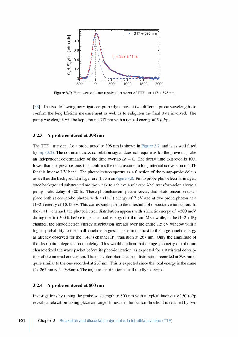
−500 0 500 1000 1500 20000
0.2
0.4
0.6
0.8
1
C6H
4S4+ yi
eld [a
rb. u
nits]
317 + 398 nm
Td = 367 ± 11 fs
Figure 3.7: Femtosecond time-resolved transient of TTF` at 317 + 398 nm.
[33]. The two following investigations probe dynamics at two different probe wavelengths to
confirm the long lifetime measurement as well as to enlighten the final state involved. The
pump wavelength will be kept around 317 nm with a typical energy of 5 µJ/p.
3.2.3 A probe centered at 398 nm
The TTF` transient for a probe tuned to 398 nm is shown in Figure 3.7, and is as well fitted
by Eq. (3.2). The dominant cross-correlation signal does not require as for the previous probe
an independent determination of the time overlap ∆t “ 0. The decay time extracted is 10%
lower than the previous one, that confirms the conclusion of a long internal conversion in TTF
for this intense UV band. The photoelectron spectra as a function of the pump-probe delays
as well as the background images are shown onFigure 3.8. Pump probe photoelectron images,
once background substracted are too weak to achieve a relevant Abel transformation above a
pump-probe delay of 300 fs. These photoelectron spectra reveal, that photoionization takes
place both at one probe photon with a (1+1’) energy of 7 eV and at two probe photon at a
(1+2’) energy of 10.13 eV. This corresponds just to the threshold of dissociative ionization. In
the (1+1’) channel, the photoelectron distribution appears with a kinetic energy of „200 meV
during the first 300 fs before to get a smooth energy distribution. Meanwhile, in the (1+2’)-IP2
channel, the photoelectron energy distribution spreads over the entire 1.5 eV window with a
higher probability to the small kinetic energies. This is in contrast to the large kinetic energy
as already observed for the (1+1’) channel IP1 transition at 267 nm. Only the amplitude of
the distribution depends on the delay. This would confirm that a huge geometry distribution
characterized the wave packet before its photoionization, as expected for a statistical descrip-
tion of the internal conversion. The one color photoelectron distribution recorded at 398 nm is
quite similar to the one recorded at 267 nm. This is expected since the total energy is the same
(2ˆ267 nm « 3ˆ398nm). The angular distribution is still totally isotropic.
3.2.4 A probe centered at 800 nm
Investigations by tuning the probe wavelength to 800 nm with a typical intensity of 50 µJ/p
reveals a relaxation taking place on longer timescale. Ionization threshold is reached by two
104 Chapter 3 Relaxation and dissociation dynamics in tetrathiafulvalene (TTF)
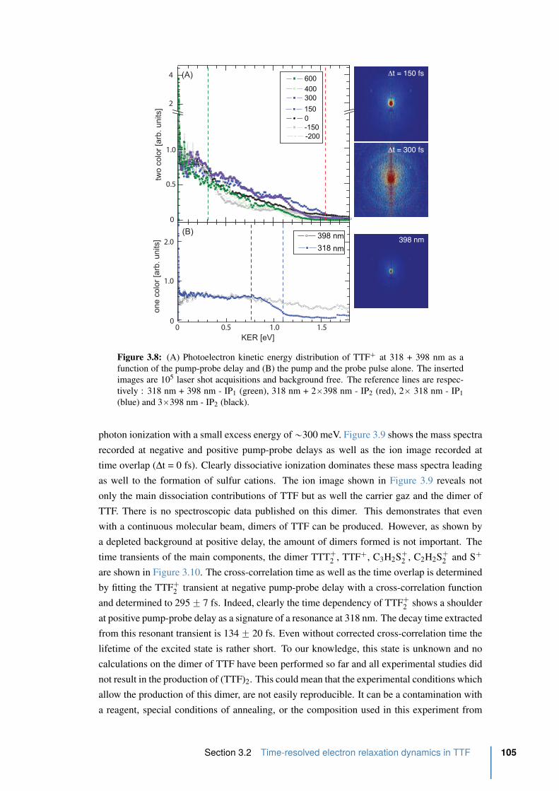
two
co
lor
[arb
. u
nits]
(A) Δt = 150 fs
Δt = 300 fs
398 nm
KER [eV]
on
e c
olo
r [a
rb.
un
its]
(B)
0 0.5 1.0 1.50
1.0
2.0
0
0.5
1.0
2
4
Figure 3.8: (A) Photoelectron kinetic energy distribution of TTF` at 318 + 398 nm as a
function of the pump-probe delay and (B) the pump and the probe pulse alone. The inserted
images are 105 laser shot acquisitions and background free. The reference lines are respec-
tively : 318 nm + 398 nm - IP1 (green), 318 nm + 2ˆ398 nm - IP2 (red), 2ˆ 318 nm - IP1
(blue) and 3ˆ398 nm - IP2 (black).
photon ionization with a small excess energy of „300 meV. Figure 3.9 shows the mass spectra
recorded at negative and positive pump-probe delays as well as the ion image recorded at
time overlap (∆t = 0 fs). Clearly dissociative ionization dominates these mass spectra leading
as well to the formation of sulfur cations. The ion image shown in Figure 3.9 reveals not
only the main dissociation contributions of TTF but as well the carrier gaz and the dimer of
TTF. There is no spectroscopic data published on this dimer. This demonstrates that even
with a continuous molecular beam, dimers of TTF can be produced. However, as shown by
a depleted background at positive delay, the amount of dimers formed is not important. The
time transients of the main components, the dimer TTT`2 , TTF`, C3H2S`
2 , C2H2S`2 and S`
are shown in Figure 3.10. The cross-correlation time as well as the time overlap is determined
by fitting the TTF`2 transient at negative pump-probe delay with a cross-correlation function
and determined to 295 ˘ 7 fs. Indeed, clearly the time dependency of TTF`2 shows a shoulder
at positive pump-probe delay as a signature of a resonance at 318 nm. The decay time extracted
from this resonant transient is 134 ˘ 20 fs. Even without corrected cross-correlation time the
lifetime of the excited state is rather short. To our knowledge, this state is unknown and no
calculations on the dimer of TTF have been performed so far and all experimental studies did
not result in the production of (TTF)2. This could mean that the experimental conditions which
allow the production of this dimer, are not easily reproducible. It can be a contamination with
a reagent, special conditions of annealing, or the composition used in this experiment from
Section 3.2 Time-resolved electron relaxation dynamics in TTF 105
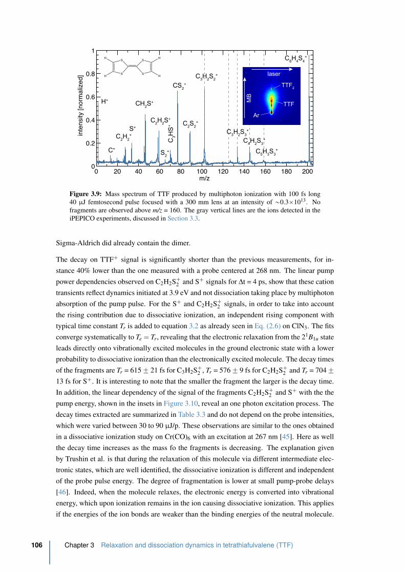
0 20 40 60 80 100 120 140 160 180 2000
0.2
0.4
0.6
0.8
1
m/z
inte
nsity
[nor
mal
ized
] C3H
2S
2+
C2S
2+
CS2
+
C2H
2S+
CH2S+
S+
C2H
2+
C6H
4S
4+
Ar
TTF
TTF2
laser
MB
C3H
S+
S2
+C+C
5H
3S
3+
C4H
2S
3+
C3H
2S
3+
S
S S
SH
H
H
H
H+
Figure 3.9: Mass spectrum of TTF produced by multiphoton ionization with 100 fs long
40 µJ femtosecond pulse focused with a 300 mm lens at an intensity of „0.3ˆ1013. No
fragments are observed above m/z = 160. The gray vertical lines are the ions detected in the
iPEPICO experiments, discussed in Section 3.3.
Sigma-Aldrich did already contain the dimer.
The decay on TTF` signal is significantly shorter than the previous measurements, for in-
stance 40% lower than the one measured with a probe centered at 268 nm. The linear pump
power dependencies observed on C2H2S`2 and S` signals for ∆t = 4 ps, show that these cation
transients reflect dynamics initiated at 3.9 eV and not dissociation taking place by multiphoton
absorption of the pump pulse. For the S` and C2H2S`2 signals, in order to take into account
the rising contribution due to dissociative ionization, an independent rising component with
typical time constant Tr is added to equation 3.2 as already seen in Eq. (2.6) on ClN3. The fits
converge systematically to Te “ Tr, revealing that the electronic relaxation from the 21B1u state
leads directly onto vibrationally excited molecules in the ground electronic state with a lower
probability to dissociative ionization than the electronically excited molecule. The decay times
of the fragments are Tr = 615 ˘ 21 fs for C3H2S`2 , Tr = 576 ˘ 9 fs for C2H2S`
2 and Tr = 704 ˘13 fs for S`. It is interesting to note that the smaller the fragment the larger is the decay time.
In addition, the linear dependency of the signal of the fragments C2H2S`2 and S` with the the
pump energy, shown in the insets in Figure 3.10, reveal an one photon excitation process. The
decay times extracted are summarized in Table 3.3 and do not depend on the probe intensities,
which were varied between 30 to 90 µJ/p. These observations are similar to the ones obtained
in a dissociative ionization study on Cr(CO)6 with an excitation at 267 nm [45]. Here as well
the decay time increases as the mass fo the fragments is decreasing. The explanation given
by Trushin et al. is that during the relaxation of this molecule via different intermediate elec-
tronic states, which are well identified, the dissociative ionization is different and independent
of the probe pulse energy. The degree of fragmentation is lower at small pump-probe delays
[46]. Indeed, when the molecule relaxes, the electronic energy is converted into vibrational
energy, which upon ionization remains in the ion causing dissociative ionization. This applies
if the energies of the ion bonds are weaker than the binding energies of the neutral molecule.
106 Chapter 3 Relaxation and dissociation dynamics in tetrathiafulvalene (TTF)
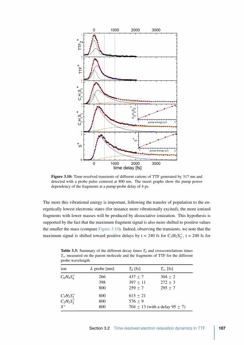
pump energy [μJ]
pump energy [μJ]
1
1 5
5
Figure 3.10: Time-resolved transients of different cations of TTF generated by 317 nm and
detected with a probe pulse centered at 800 nm. The insert graphs show the pump power
dependency of the fragments at a pump-probe delay of 4 ps.
The more this vibrational energy is important, following the transfer of population to the en-
ergetically lowest electronic states (for instance more vibrationally excited), the more ionized
fragments with lower masses will be produced by dissociative ionization. This hypothesis is
supported by the fact that the maximum fragment signal is also more shifted to positive values
the smaller the mass (compare Figure 3.10). Indeed, observing the transients, we note that the
maximum signal is shifted toward positive delays by t = 240 fs for C3H2S`2 , t = 240 fs for
Table 3.3: Summary of the different decay times Td and crosscorrelations times
Tcc measured on the parent molecule and the fragments of TTF for the different
probe wavelength
ion λ probe [nm] Td [fs] Tcc [fs]
C6H4S`4 266 437 ˘ 7 304 ˘ 2
398 397 ˘ 11 272 ˘ 3
800 259 ˘ 7 295 ˘ 7
C3H2S`2 800 615 ˘ 21
C2H2S`2 800 576 ˘ 9
S` 800 704 ˘ 13 (with a delay 95 ˘ 7)
Section 3.2 Time-resolved electron relaxation dynamics in TTF 107
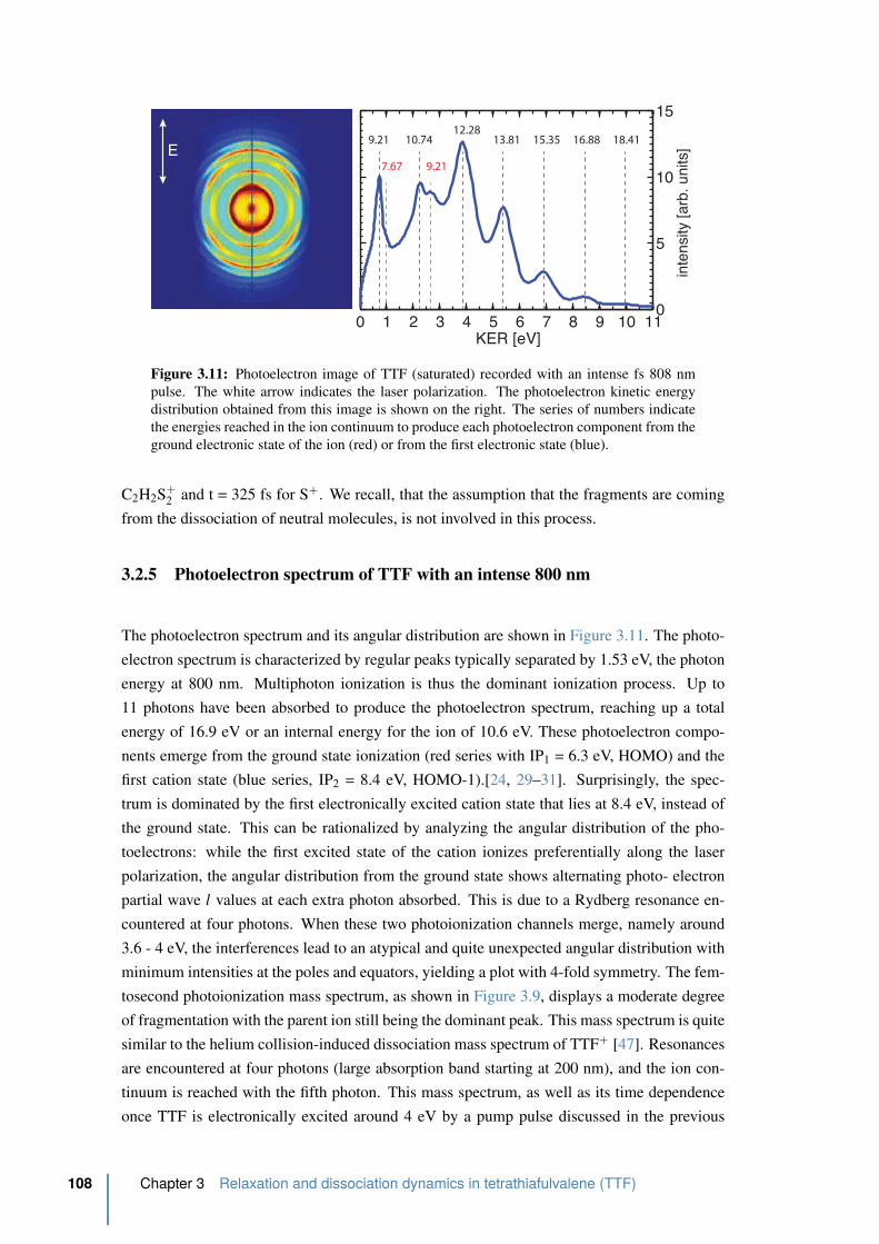
0 1 2 3 4 5 6 7 8 9 10 110
5
10
15
KER [eV]
inte
nsity
[arb
. uni
ts]
9.21 10.74
7.67 9.21
12.2813.81 15.35 16.88 18.41
E
Figure 3.11: Photoelectron image of TTF (saturated) recorded with an intense fs 808 nm
pulse. The white arrow indicates the laser polarization. The photoelectron kinetic energy
distribution obtained from this image is shown on the right. The series of numbers indicate
the energies reached in the ion continuum to produce each photoelectron component from the
ground electronic state of the ion (red) or from the first electronic state (blue).
C2H2S`2 and t = 325 fs for S`. We recall, that the assumption that the fragments are coming
from the dissociation of neutral molecules, is not involved in this process.
3.2.5 Photoelectron spectrum of TTF with an intense 800 nm
The photoelectron spectrum and its angular distribution are shown in Figure 3.11. The photo-
electron spectrum is characterized by regular peaks typically separated by 1.53 eV, the photon
energy at 800 nm. Multiphoton ionization is thus the dominant ionization process. Up to
11 photons have been absorbed to produce the photoelectron spectrum, reaching up a total
energy of 16.9 eV or an internal energy for the ion of 10.6 eV. These photoelectron compo-
nents emerge from the ground state ionization (red series with IP1 = 6.3 eV, HOMO) and the
first cation state (blue series, IP2 = 8.4 eV, HOMO-1).[24, 29–31]. Surprisingly, the spec-
trum is dominated by the first electronically excited cation state that lies at 8.4 eV, instead of
the ground state. This can be rationalized by analyzing the angular distribution of the pho-
toelectrons: while the first excited state of the cation ionizes preferentially along the laser
polarization, the angular distribution from the ground state shows alternating photo- electron
partial wave l values at each extra photon absorbed. This is due to a Rydberg resonance en-
countered at four photons. When these two photoionization channels merge, namely around
3.6 - 4 eV, the interferences lead to an atypical and quite unexpected angular distribution with
minimum intensities at the poles and equators, yielding a plot with 4-fold symmetry. The fem-
tosecond photoionization mass spectrum, as shown in Figure 3.9, displays a moderate degree
of fragmentation with the parent ion still being the dominant peak. This mass spectrum is quite
similar to the helium collision-induced dissociation mass spectrum of TTF` [47]. Resonances
are encountered at four photons (large absorption band starting at 200 nm), and the ion con-
tinuum is reached with the fifth photon. This mass spectrum, as well as its time dependence
once TTF is electronically excited around 4 eV by a pump pulse discussed in the previous
108 Chapter 3 Relaxation and dissociation dynamics in tetrathiafulvalene (TTF)
sections, has motivated the iPEPICO experiment which will be presented in Section 3.3. In-
deed fragments such as S`2 show that strong rearrangement processes are at play in the ion
continuum. The intensity of 1013 Wcm´2 corresponds to an electric field of about 1 V/A. At
this intensity, field ionization may compete with multiphoton ionization, i.e., n photons cou-
pled simultaneously into the molecule [48]. The pulse duration is too short, and the size of
the system too small, for thermal ionization to play a role [49]. The ionization regime can
be roughly estimated by calculating the Keldysh parameter γ as introduces in Section 1.3 (γ
is the ratio between the laser and the tunnel frequency, here around 2) and by experimentally
collecting the photoelectron spectrum [50]. Multiphoton ionization can produce photoelectron
spectra characterized by discrete peaks regularly spaced by the photon energy (here 1.53 eV)
attributed to above-threshold ionization, while field ionization produces a broad distribution
extending far beyond the average quivering energy of the electron in the laser field, namely
the ponderomotive energy, Up “ IP2γ2. In our case Up reaches a maximum of around 1.2
eV.
3.3 The iPEPICO breakdown diagrams and the dissociation model
3.3.1 iPEPICO setup
In order to disentangle the complex ionic dissociation of TTF, the imaging photoelectron pho-
toion coincidence (iPEPICO) technique is utilized to study the appearance energies of the TTF
fragments. The iPEPICO experiment was carried out on the VUV beamline at the Swiss Light
Source (Paul Scherrer Institute, Villigen, Switzerland). The apparatus and the measurement
details have been described in detail elsewhere [51–53], and only a short introduction is given
here. iPEPICO threshold ionization mass spectra were obtained by selecting ions detected in
coincidence with threshold electrons (initially zero kinetic energy), arriving in the centre of an
imaging multichannel plate (MCP) detector. ‘Hot’ electron contamination (the contribution to
the mass spectra of coincidence events resulting from non-threshold electrons that happen to
hit the same central spot on the MCP, was corrected by subtracting the mass spectrum obtained
for electrons arriving in a narrow ring around the central spot [54]. Data were acquired as a
function of photon energy from 10.0 eV to 12.6 eV, in steps of 0.2 eV. TTF was introduced via
a ‘probe’ fitting, heated up to 74˝C. Ions are accelerated first in 5 cm long region at the same
low field as is used in velocity-map imaging photoelectrons, namely 40 – 120 Vcm´1. If the
TTF ions dissociate in a 100 ns up to a few µs time window, i.e. during the flight time in the
first acceleration region, they will arrive at the detector at a time larger than the daughter ion
time-of-flight (TOF). The resulting asymmetric peak shapes are a measure of the dissociation
rate constant and can be used to extract experimental rates. The fractional parent and daughter
ion abundances are also evaluated based on the TOF distributions, and plotted as a function of
the photon energy in the breakdown diagram.
3.3.2 Computational procedures
Density functional theory calculations of molecular structure and vibrational frequencies were
performed by P. Mayer at the B3-LYP/6-31+G(d) level of theory using the Gaussian 03 suite
Section 3.3 The iPEPICO breakdown diagrams and the dissociation model 109

programs [55]. The harmonic vibrational frequencies and rotational constants of the neu-
tral TTF molecule were used to calculate the internal energy distribution of the molecule at
74˝ Celsius. The vibrational frequencies and rotational constants of the ion were used in the
calculation of the RRKM1 rate constant for each channel using the standard expression [56,
57]:
kpEq “ σNpE ´ E0qhρpEq (3.3)
where ρ(E) and NpE ´ E0q are the density and sum of states, respectively, at an ion internal
energy E and transition state energy E ´ E0 above the activation energy E0. Sums and densi-
ties were calculated according to the direct count algorithm of Beyer and Swinehart [58]. The
transition states of the reactions were approximated by using the frequencies of the parent ion,
removing the normal mode that best corresponds to the reaction coordinate, and scaling the
transitional modes to adjust the entropy of activation, which was calculated from the standard
statistical mechanics equation. Possible isomer fragment ion structures were calculated with
the G3B3 composite method [59], and their energies were compared with the experimental
onsets. With the exception of the parent ion breaking in half to yield the m/z = 102 fragment,
all dissociative photoionization reactions involve rearrangement or concerted bond-breaking
steps, which are typically associated with reverse barriers. Therefore, we were searching for
fragmentation pathways below the observed onset energies, and we propose product ion struc-
tures for five fragmentation channels. Direct dynamics calculations can be used to explore
the potential energy surface [60] and have confirmed several unimolecular and bimolecular
reaction pathways [61, 62]. Typical trajectory propagation times for comparable molecules
are at most 3-6 ps [63] meaning that simulating the dissociation of the long-lived metastable
TTF` ion close to threshold is intractable. In fact, only two of 20 B3LYP/6-31G(d) trajecto-
ries dissociated within 1.7 ps even at an internal energy of 12.25 eV: one by C2H2 loss and
one by C2H2S loss. This mirrors two of the actually observed fragmentation channels in the
low-energy regime. These calculations were done by A. Boedi. The breakdown diagrams were
fitted using the MinimalPepico program developed by Sztaray, Boedi and Baer [64]. The pro-
gram combines the RRKM dissociation rate curve, kpEq, with the internal energy distribution
and instrument functions to model and fit the breakdown diagram and the experimental TOF
distributions.
3.3.3 Results and Discussion
Figure 3.12 (A) contains the complete breakdown diagram for TTF ions over the photon energy
range of 10.0 - 12.6 eV. Upon closer examination of the m/z = 133, 100, and 84 peaks, it is
evident that these ions have relative intensities that are independent of the photon energy.
Thus, they were assumed to be artifacts from impurities in the sample and were removed from
Figure 3.12. Three significant observations from Figure 3.12 can be made:
(i) the m/z = 178, 171, 159, 146, 140, and 127 peaks all appear at approximately 10.0 eV.
1 RRKM stands for Rice–Ramsperger–Kassel–Marcus theory. This method enables the computation of simple
estimates of the unimolecular reaction rates from a few characteristics of the potential energy surface.
110 Chapter 3 Relaxation and dissociation dynamics in tetrathiafulvalene (TTF)
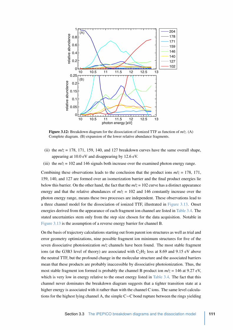
10 10.5 11 11.5 12 12.5 130
0.2
0.4
0.6
0.8
1
rela
tive
abun
danc
e
10 10.5 11 11.5 12 12.5 130
0.05
0.1
0.15
0.2
0.25
photon energy [eV]
rela
tive
abun
danc
e
204178171159146140127102
(A)
(B)
Figure 3.12: Breakdown diagram for the dissociation of ionized TTF as function of m/z. (A)
Complete diagram. (B) expansion of the lower relative abundance fragments.
(ii) the m/z = 178, 171, 159, 140, and 127 breakdown curves have the same overall shape,
appearing at 10.0 eV and disappearing by 12.6 eV.
(iii) the m/z = 102 and 146 signals both increase over the examined photon energy range.
Combining these observations leads to the conclusion that the product ions m/z = 178, 171,
159, 140, and 127 are formed over an isomerization barrier and the final product energies lie
below this barrier. On the other hand, the fact that the m/z = 102 curve has a distinct appearance
energy and that the relative abundances of m/z = 102 and 146 constantly increase over the
photon energy range, means these two processes are independent. These observations lead to
a three channel model for the dissociation of ionized TTF, illustrated in Figure 3.13. Onset
energies derived from the appearance of each fragment ion channel are listed in Table 3.4. The
stated uncertainties stem only from the step size chosen for the data acquisition. Notable in
Figure 3.13 is the assumption of a reverse energy barrier for channel B.
On the basis of trajectory calculations starting out from parent ion structures as well as trial and
error geometry optimizations, nine possible fragment ion minimum structures for five of the
seven dissociative photoionization m/z channels have been found. The most stable fragment
ions (at the G3B3 level of theory) are associated with C2H2 loss at 8.69 and 9.15 eV above
the neutral TTF, but the profound change in the molecular structure and the associated barriers
mean that these products are probably inaccessible by dissociative photoionization. Thus, the
most stable fragment ion formed is probably the channel B product ion m/z = 146 at 9.27 eV,
which is very low in energy relative to the onset energy listed in Table 3.4. The fact that this
channel never dominates the breakdown diagram suggests that a tighter transition state at a
higher energy is associated with it rather than with the channel C ions. The same level calcula-
tions for the highest lying channel A, the simple C“C bond rupture between the rings yielding
Section 3.3 The iPEPICO breakdown diagrams and the dissociation model 111
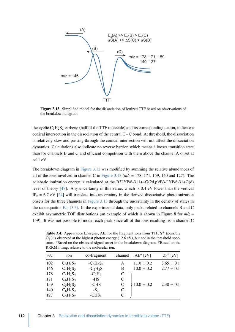
(A)
(B)(C)
TTF+
m/z = 146
m/z = 178, 171, 159,
140, 127
E0(A) >> E
0(B) > E
0(C)
ΔS(A) >> ΔS(C) > ΔS(B)
Figure 3.13: Simplified model for the dissociation of ionized TTF based on observations of
the breakdown diagram.
the cyclic C3H2S2 carbene (half of the TTF molecule) and its corresponding cation, indicate a
conical intersection in the dissociation of the central C“C bond. At threshold, the dissociation
is relatively slow and passing through the conical intersection will not affect the dissociation
dynamics. Calculations also indicate no reverse barrier, which means a looser transition state
than for channels B and C and efficient competition with them above the channel A onset at
«11 eV.
The breakdown diagram in Figure 3.12 was modified by summing the relative abundances of
all of the ions involved in channel C in Figure 3.13 (m/z = 178, 171, 159, 140 and 127). The
adiabatic ionization energy is calculated at the B3LYP/6-311++G(2d,p)/B3-LYP/6-31+G(d)
level of theory [47]. Any uncertainty in this value, which is 0.4 eV lower than the vertical
IPv = 6.7 eV [24] will translate into uncertainty in the derived dissociative photoionization
onsets for the three channels in Figure 3.13 through the uncertainty in the density of states in
the rate equation Eq. (3.3). In the experimental data, only peaks related to channels B and C
exhibit asymmetric TOF distributions (an example of which is shown in Figure 8 for m/z =
159). It was not possible to model each peak since all of the ions resulting from channel C
Table 3.4: Appearance Energies, AE, for the fragment ions from TTF. S` (possibly
O`2 ) is observed at the highest photon energy (12.6 eV), but not in the threshold spec-
trum. aBased on the observed signal onset in the breakdown diagram. bBased on the
RRKM fitting, relative to the molecular ion.
m/z ion co-fragment channel AEa [eV] E0b [eV]
102 C3H2S2 -C3H2S2 A 11.0 ˘ 0.2 3.65 ˘ 0.1
146 C4H2S3 -C2H2S B 10.0 ˘ 0.2 2.77 ˘ 0.1
178 C4H2S4 -C2H2 C,
/
/
/
/
.
/
/
/
/
-
10.0 ˘ 0.2 2.38 ˘ 0.1
171 C6H3S3 -HS C
159 C5H3S3 -CHS C
140 C6H4S2 -S2 C
127 C5H3S2 -CHS2 C
112 Chapter 3 Relaxation and dissociation dynamics in tetrathiafulvalene (TTF)
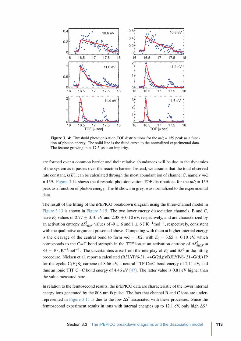
16 16.5 17 17.5 18
0
0.2
0.4
16 16.5 17 17.5 180
0.2
0.4
0.6
16 16.5 17 17.5 180
0.5
1
16 16.5 17 17.5 180
1
2
16 16.5 17 17.5 180
1
2
TOF [μ sec]16 16.5 17 17.5 180
1
2
3
TOF [μ sec]
10.6 eV 10.8 eV
11.0 eV 11.2 eV
11.4 eV 11.6 eV
Figure 3.14: Threshold photoionization TOF distributions for the m/z = 159 peak as a func-
tion of photon energy. The solid line is the fitted curve to the normalized experimental data.
The feature growing in at 17.5 µs is an impurity.
are formed over a common barrier and their relative abundances will be due to the dynamics
of the system as it passes over the reaction barrier. Instead, we assume that the total observed
rate constant, kpEq, can be calculated through the most abundant ion of channel C, namely m/z
= 159. Figure 3.14 shows the threshold photoionization TOF distributions for the m/z = 159
peak as a function of photon energy. The fit shown in grey, was normalized to the experimental
data.
The result of the fitting of the iPEPICO breakdown diagram using the three-channel model in
Figure 3.13 is shown in Figure 3.15. The two lower energy dissociation channels, B and C,
have E0 values of 2.77 ˘ 0.10 eV and 2.38 ˘ 0.10 eV, respectively, and are characterized by
an activation entropy ∆S;600K values of -9 ˘ 6 and 1 ˘ 6 J K´1mol´1, respectively, consistent
with the qualitative argument presented above. Competing with them at higher internal energy
is the cleavage of the central bond to form m/z = 102, with E0 = 3.65 ˘ 0.10 eV, which
corresponds to the C“C bond strength in the TTF ion at an activation entropy of ∆S;600K =
83 ˘ 10 JK´1mol´1. The uncertainties arise from the interplay of E0 and ∆S; in the fitting
procedure. Nielsen et al. report a calculated (B3LYP/6-311++G(2d,p)/B3LYP/6- 31+G(d)) IP
for the cyclic C3H2S2 carbene of 8.66 eV, a neutral TTF C“C bond energy of 2.11 eV, and
thus an ionic TTF C“C bond energy of 4.46 eV [47]. The latter value is 0.81 eV higher than
the value measured here.
In relation to the femtosecond results, the iPEPICO data are characteristic of the lower internal
energy ions generated by the 808 nm fs pulse. The fact that channel B and C ions are under-
represented in Figure 3.11 is due to the low ∆S; associated with these processes. Since the
femtosecond experiment results in ions with internal energies up to 12.1 eV, only high ∆S`
Section 3.3 The iPEPICO breakdown diagrams and the dissociation model 113
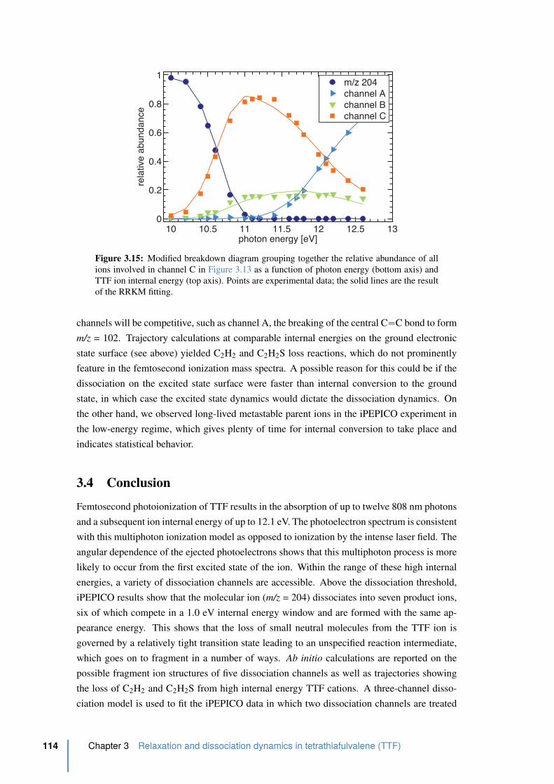
10 10.5 11 11.5 12 12.5 130
0.2
0.4
0.6
0.8
1
photon energy [eV]
rela
tive
abun
danc
e
m/z 204channel Achannel Bchannel C
Figure 3.15: Modified breakdown diagram grouping together the relative abundance of all
ions involved in channel C in Figure 3.13 as a function of photon energy (bottom axis) and
TTF ion internal energy (top axis). Points are experimental data; the solid lines are the result
of the RRKM fitting.
channels will be competitive, such as channel A, the breaking of the central C“C bond to form
m/z = 102. Trajectory calculations at comparable internal energies on the ground electronic
state surface (see above) yielded C2H2 and C2H2S loss reactions, which do not prominently
feature in the femtosecond ionization mass spectra. A possible reason for this could be if the
dissociation on the excited state surface were faster than internal conversion to the ground
state, in which case the excited state dynamics would dictate the dissociation dynamics. On
the other hand, we observed long-lived metastable parent ions in the iPEPICO experiment in
the low-energy regime, which gives plenty of time for internal conversion to take place and
indicates statistical behavior.
3.4 Conclusion
Femtosecond photoionization of TTF results in the absorption of up to twelve 808 nm photons
and a subsequent ion internal energy of up to 12.1 eV. The photoelectron spectrum is consistent
with this multiphoton ionization model as opposed to ionization by the intense laser field. The
angular dependence of the ejected photoelectrons shows that this multiphoton process is more
likely to occur from the first excited state of the ion. Within the range of these high internal
energies, a variety of dissociation channels are accessible. Above the dissociation threshold,
iPEPICO results show that the molecular ion (m/z = 204) dissociates into seven product ions,
six of which compete in a 1.0 eV internal energy window and are formed with the same ap-
pearance energy. This shows that the loss of small neutral molecules from the TTF ion is
governed by a relatively tight transition state leading to an unspecified reaction intermediate,
which goes on to fragment in a number of ways. Ab initio calculations are reported on the
possible fragment ion structures of five dissociation channels as well as trajectories showing
the loss of C2H2 and C2H2S from high internal energy TTF cations. A three-channel disso-
ciation model is used to fit the iPEPICO data in which two dissociation channels are treated
114 Chapter 3 Relaxation and dissociation dynamics in tetrathiafulvalene (TTF)
as simple dissociations (one with a reverse barrier), while the rest involve a shared barrier.
These channels cannot compete at higher internal energies with more entropically favorable
pathways. The S` fragment in the VUV photoionization seems to appear at 12.6 eV from a
secondary dissociation of S`2 . This confirms that in the pump-probe studies of the second UV
band of TTF a particular vibrational energy characterizes the S` production following disso-
ciative ionization of TTF. This would explain why the time profile of the S` fragment has a
95 fs shift on its decay function.
References
[1] Wudl, F, Wobschall, D, and Hufnagel, EJ. Electrical conductivity by the bis(1,3-dithiole)-
bis(1,3-dithiolium) system. J. Am. Chem. Soc. 94:2 670–672 (1972) (cited p. 96).
[2] Ferraris, J, Cowan, DO, and Walatka, V. Electron transfer in a new highly conducting
donor-acceptor complex - Journal of the American Chemical Society (ACS Publica-
tions). Angew. Chem. Int. Ed. Engl. 40:8 1372–1409 (2001) (cited p. 96).
[3] Segura, JL and Martin, N. New Concepts in Tetrathiafulvalene Chemistry. Angew.
Chem. Int. Ed. Engl. 40:8 1372–1409 (2001) (cited p. 96).
[4] Martin, C, Sanchez, L, Herranz, MA, and Guldi, DM. Evidence for two separate one-
electron transfer events in excited fulleropyrrolidine dyads containing tetrathiafulva-
lene (TTF). J. Phys. Chem. A 104:19 4648–4657 (2000) (cited p. 96).
[5] Becher, J, Jeppesen, JO, and Nielsen, K. Tetrathiafulvalenes: from heterocyclic chem-
istry to molecular devices. Synthetic Metals 133-134: 309–315 (2003) (cited p. 96).
[6] Sawano, F, Terasaki, I, Mori, H, Mori, T, Watanabe, M, Ikeda, N, Nogami, Y, and
Noda, Y. An organic thyristor. Nature 437:7058 522–524 (2005) (cited p. 96).
[7] Fang, CJ, Zhu, Z, Sun, W, Xu, CH, and Yan, CH. New TTF derivatives: several
molecular logic gates based on their switchable fluorescent emissions. New Journal
of Chemistry 31:4 580 (2007) (cited p. 96).
[8] Canevet, D, Salle, M, Zhang, G, and Zhang, D. Tetrathiafulvalene (TTF) derivatives:
key building-blocks for switchable processes. Chem. Comm. (2009) (cited p. 96).
[9] Jia, C, Zhang, J, Bai, J, Zhang, L, Wan, Z, and Yao, X. Synthesis, physical properties
and self-assembly of conjugated donor–acceptor system based on tetrathiafulvalene
and functionalized with binding sites. Dyes and Pigments 94:3 403–409 (2012) (cited
p. 96).
[10] Wang, C, Bryce, MR, Batsanov, AS, Goldenberg, LM, and Howard, JAK. Synthesis
and electrochemistry of new tetrathiafulvalene (TTF) dendrimers:X-ray crystal struc-
ture of a tetrafunctionalised TTF core unit. J. Mater. Chem. 7:7 1189–1197 (1997)
(cited p. 96).
[11] Sakai, M, Iizuka, M, Nakamura, M, and Kudo, K. Fabrication and Electrical Char-
acterization of Tetrathiafulvalene-tetracyanoquinodimethane Molecular Wires. Jpn. J.
Appl. Phys. 42:Part 1, No. 4B 2488–2491 (2003) (cited p. 96).
[12] Mas-Torrent, M and Hadley, P. Electrochemical Growth of Organic Conducting Mi-
crocrystals of Tetrathiafulvalene Bromide. Small 1:8-9 806–808 (2005) (cited p. 96).
[13] Chollet, M. Gigantic Photoresponse in 1/4-Filled-Band Organic Salt (EDO-TTF)2PF6.
Science 307:5706 86–89 (2005) (cited p. 96).
[14] Hal, PA van, Janssen, RAJ, Lanzani, G, Cerullo, G, Zavelani-Rossi, M, and De Sil-
vestri, S. Full temporal resolution of the two-step photoinduced energy-electron trans-
fer in a fullerene-oligothiophene-fullerene triad using sub-10 fs pump-probe spec-
troscopy. Chem. Phys. Lett. 345:1-2 33–38 (2001) (cited p. 96).
References 115
[15] Katan, C. First-Principles Study of the Structures and Vibrational Frequencies for
Tetrathiafulvalene TTF and TTF-d4 in Different Oxidation States. J. Phys. Chem. A
103:10 1407–1413 (1999) (cited p. 96, 97, 99).
[16] HARGITTAI, I, BRUNVOLL, J, KOLONITS, M, and KHODORKOVSKY, V. Tetrathi-
afulvalene - Gas-Phase Molecular-Structure From Electron-Diffraction. J. Mol. Struct.
317:3 273–277 (1994) (cited p. 96).
[17] Demiralp, E and Goddard, WA. Structures and Energetics Study of Tetrathiafulvalene-
Based Donors of Organic Superconductors. J. Phys. Chem. A 101:43 8128–8131
(1997) (cited p. 96).
[18] Viruela, R, Viruela, PM, Pou-Amerigo, R, and Orti, E. ScienceDirect.com - Synthetic
Metals - Flexibility of TTF. a theoretical study. Synthetic Metals 103:1-3 1991–1992
(1999) (cited p. 96).
[19] Graja, A, Olejniczak, I, and Bogucki, A. Spectral studies of the bis-linked tetrathiaful-
valenes to [60]fullerene. Journal of molecular structure (2002) (cited p. 96, 97).
[20] Kreher, D, Hudhomme, Pt, Gorgues, A, Luo, H, Araki, Y, and Ito, O. Photoinduced
electron transfer processes of a fused C60-TTF-C60 dumbbell triad. Phys. Chem.
Chem. Phys. 5:20 4583–4592 (2003) (cited p. 96).
[21] Allard, E, Cousseau, J, Ord na, J, Garin, J, Luo, H, Araki, Y, and Ito, O. Photoinduced
electron-transfer processes in C60-tetrathiafulvalene dyads containing a short or long
flexible spacer. Phys. Chem. Chem. Phys. 4:24 5944–5951 (2002) (cited p. 96).
[22] Coffen, DL, Chambers, JQ, Williams, DR, Garrett, PE, and Canfield, ND. Tetrathioethylenes.
J. Am. Chem. Soc. 93:9 2258–2268 (1971) (cited p. 96, 97).
[23] Pou-Amerigo, R, Viruela, PM, Viruela, R, Rubio, M, and Orti, E. Electronic spectra
of tetrathiafulvalene and its radical cation: analysis of the performance of the time-
dependent DFT approach. Chem. Phys. Lett. 352:5-6 491–498 (2002) (cited p. 97,
99).
[24] Lichtenberger, DL, Johnston, RL, Hinkelmann, K, Suzuki, T, and Wudl, F. Relative
electron donor strengths of tetrathiafulvene derivatives: effects of chemical substitu-
tions and the molecular environment from a combined photoelectron and electrochem-
ical study. J. Am. Chem. Soc. 112:9 3302–3307 (1990) (cited p. 97, 98, 100, 108,
112).
[25] Haddon, RC. Quantum chemical studies in the design of organic metals. II. The equi-
librium geometries and electronic structure of tetrathiofulvalene (ttf) andtetracyanoquin-
odimethane (tcnq) and their uni- and di-valent ions. Aust. J. Chem. 28:11 2333–2342
(1975) (cited p. 97).
[26] Wudl, F, Kruger, AA, Kaplan, ML, and Hutton, RS. Unsymmetrical dimethyltetrathi-
afulvalene. J. Org. Chem. 42:4 768–770 (1977) (cited p. 97).
[27] Engler, EM, Scott, BA, Etemad, S, Penney, T, and Patel, VV. Organic alloys: synthesis
and properties of solid solutions of tetraselenafulvalene-tetracyano-p-quinodimethane
(TSeF-TCNQ) and tetrathiafulvalene-tetracyano-p-quinodimethane (TTF-TCNQ). J.
Am. Chem. Soc. 99:18 5909–5916 (1977) (cited p. 97).
[28] Sandman, DJ, Holmes, TJ, and Warner, DE. ” One-pot” construction of the bithiopy-
ran ring system from an acyclic precursor. J. Org. Chem 44:5 880–882 (1979) (cited
p. 97).
[29] Gleiter, R, Schmidt, E, Cowan, DO, and Ferraris, JP. The electronic structure of tetrathio-
fulvalene. J. Electron Spec. and Relat. Phen. 2:2 207–210 (1973) (cited p. 97, 108).
[30] Berlinsky, AJ, Carolan, JF, and Weiler, L. Photoelectron Spectrum and Electronic
Structure of Tetrathiofulvalene (TTF). Can. J. Chem. 52:19 3373–3377 (1974) (cited
p. 97, 108).
116 Chapter 3 Relaxation and dissociation dynamics in tetrathiafulvalene (TTF)

[31] Sato, N, Saito, G, and Inokuchi, H. Ionization potentials and polarization energies
of tetraselenafulvalene (TSF) derivatives determined from ultraviolet photoelectron
spectroscopy. Chem. Phys. 76:1 79–88 (1983) (cited p. 97, 108).
[32] Mayer, PM, Staedter, D, Blanchet, V, Hemberger, P, and Bodi, A. Comparing Fem-
tosecond Multiphoton Dissociative Ionization of Tetrathiafulvene with Imaging Pho-
toelectron Photoion Coincidence Spectroscopy. J. Phys. Chem. A 117:13 2753–2759
(2013) (cited p. 97).
[33] Pou-Amerigo, R, Orti, E, Merchan, M, Rubio, M, and Viruela, PM. Electronic Tran-
sitions in Tetrathiafulvalene and Its Radical Cation: A Theoretical Contribution. J.
Phys. Chem. A 106:4 631–640 (2002) (cited p. 97–99, 102, 104).
[34] Fabian, J, Diaza, LA, Seifert, G, and Niehaus, T. Calculation of excitation energies
of organic chromophores: a critical evaluation. J. Mol. Struct. 594:1-2 41–53 (2002)
(cited p. 97, 98).
[35] Andreu, R, Garin, J, and Orduna, J. Electronic absorption spectra of closed and open-
shell tetrathiafulvalenes: the firste time-dependent density-functional study. Tetrahe-
dron 57:37 7883–7892 (2001) (cited p. 97, 98).
[36] Fabian, J. Electronic excitation of sulfur-organic compounds–performance of time-
dependent density functional theory. Theor Chem Acc 106:3 199–217 (2001) (cited
p. 98).
[37] Batsanov, AS, Bryce, MR, Heaton, JN, Moore, AJ, Skabara, PJ, Howard, JAK, Orti,
E, Viruela, PM, and Viruela, R. New functionalized tetrathiafulvalenes: X-ray crystal
structures and physico-chemical properties of TTF–C (O) NMe2 and TTF–C (O)–O–
C4H9: a joint experimental and theoretical study. J. Mater. Chem. 5:10 1689–1696
(1995) (cited p. 98).
[38] Yakushi, K, Nishimura, S, Sugano, T, Kuroda, H, and Ikemoto, I. The structure of
tetrathiafulvalenium perchlorate, TTF`.ClO´4 . Acta Cryst. 36:2 358–363 (1980) (cited
p. 99).
[39] Kistenmacher, TJ, Rossi, M, Chiang, CC, Van Duyne, RP, and Siedle, AR. Crystal and
molecular structure of an unusual salt formed from the radical cation of tetrathiaful-
valene (TTF) and the trichloromercurate anion (HgCl3), (TTF)(HgCl3). Inorg. Chem.
19:12 3604–3608 (1980) (cited p. 99).
[40] Kerkines, ISK, Petsalakis, ID, Theodorakopoulos, G, and Klopper, W. Low-lying ab-
sorption and emission spectra of pyrene, 1,6-dithiapyrene, and tetrathiafulvalene: A
comparison between ab initio and time-dependent density functional methods. J. Chem.
Phys. 131:22 pages (2009) (cited p. 99).
[41] Tugsuz, T. DFT Study on the Standard Electrode Potentials of Imidazole, Tetrathiaful-
valene, and Tetrathiafulvalene-Imidazole. J. Phys. Chem. 114:51 17092–17101 (2010)
(cited p. 99).
[42] Tsubomura, H and Sakata, T. A new electronic transition found for the aniline deriva-
tives. Chem. Phys. Lett. 21:3 511–512 (1973) (cited p. 101).
[43] Fuke, K and Nagakura, S. Rydberg transitions of aniline and N,N-diethylaniline. J.
Mol. Spec. 64:1 139–146 (1977) (cited p. 101).
[44] Blanchet, V, Raffael, K, Turri, G, and Chatel, B. Time-dependent photoionization of
azulene: Competition between ionization and relaxation in highly excited states —
Issue 16 - Journal of Chemical Physics. The Journal of chemical . . . (2008) (cited
p. 103).
[45] Trushin, SA, Fuss, W, Schmid, WE, and Kompa, KL. Femtosecond Dynamics and
Vibrational Coherence in Gas-Phase Ultraviolet Photodecomposition of Cr(CO) 6. J.
Phys. Chem. A 102:23 4129–4137 (1998) (cited p. 106).
References 117
[46] Fuss, W, Kosmidis, C, Schmid, WE, and Trushin, SA. The lifetime of the perpendic-
ular minimum of cis-stilbene observed by dissociative intense-laser field ionization.
Chem. Phys. Lett. 385: 423–430 (2004) (cited p. 106).
[47] Nielsen, SB, Nielsen, MB, and Jensen, HJA. The tetrathiafulvalene dication in the gas
phase: its formation and stability. Phys. Chem. Chem. Phys. 5:7 1376–1380 (2003)
(cited p. 108, 112, 113).
[48] DeWitt, MJ and Levis, RJ. Concerning the ionization of large polyatomic molecules
with intense ultrafast lasers. J. Chem. Phys. 110:23 11368 (1999) (cited p. 109).
[49] Kjellberg, M, Bulgakov, AV, and Goto, M. Femtosecond electron spectroscopy of
coronene, benzo[GHI]perylene, and anthracene — Browse - Journal of Chemical
Physics. The Journal of chemical . . . (2010) (cited p. 109).
[50] DeWitt, M and Levis, R. Observing the Transition from a Multiphoton-Dominated to a
Field-Mediated Ionization Process for Polyatomic Molecules in Intense Laser Fields.
Phys. Rev. Lett. 81:23 5101–5104 (1998) (cited p. 109).
[51] Bodi, A, Sztaray, B, Baer, T, Johnson, M, and Gerber, T. Data acquisition schemes for
continuous two-particle time-of-flight coincidence experiments. Rev. Sci. Instr. 78:8
084102 (2007) (cited p. 109).
[52] Bodi, A, Johnson, M, Gerber, T, Gengeliczki, Z, Sztaray, B, and Baer, T. Imaging
photoelectron photoion coincidence spectroscopy with velocity focusing electron op-
tics. Rev. Sci. Instr. 80:3 (2009) (cited p. 109).
[53] Johnson, M, Bodi, A, Schulz, L, and Gerber, T. Vacuum ultraviolet beamline at the
Swiss Light Source for chemical dynamics studies. Nuclear Instruments and Methods
in Physics Research Section A: Accelerators, Spectrometers, Detectors and Associated
Equipment 610:2 597–603 (2009) (cited p. 109).
[54] Sztaray, B and Baer, T. Suppression of hot electrons in threshold photoelectron pho-
toion coincidence spectroscopy using velocity focusing optics. Rev. Sci. Instr. 74:8
3763–3768 (2003) (cited p. 109).
[55] Frisch, MJ, Trucks, GW, Schlegel, HB, Scuseria, GE, Robb, MA, Cheeseman, JR,
Scalmani, G, Barone, V, Mennucci, B, Petersson, GA, Nakatsuji, H, Caricato, M,
Li, X, Hratchian, HP, Izmaylov, AF, Bloino, J, Zheng, G, Sonnenberg, JL, Hada, M,
Ehara, M, Toyota, K, Fukuda, R, Hasegawa, J, Ishida, M, Nakajima, T, Honda, Y, Ki-
tao, O, Nakai, H, Vreven, T, Montgomery, Jr, A, J, Peralta, JE, Ogliaro, F, Bearpark,
M, Heyd, JJ, Brothers, E, Kudin, KN, Staroverov, VN, Kobayashi, R, Normand, J,
Raghavachari, K, Rendell, A, Burant, JC, Iyengar, SS, Tomasi, J, Cossi, M, Rega, N,
Millam, JM, Klene, M, Knox, JE, Cross, JB, Bakken, V, Adamo, C, Jaramillo, J, Gom-
perts, R, Stratmann, RE, Yazyev, O, Austin, AJ, Cammi, R, Pomelli, C, Ochterski, JW,
Martin, RL, Morokuma, K, Zakrzewski, VG, Voth, GA, Salvador, P, Dannenberg, JJ,
Dapprich, S, Daniels, AD, Farkas, O, Foresman, JB, Ortiz, JV, Cioslowski, J, and Fox,
DJ. Gaussian 09, Revision A.1. Gaussian, Inc., Wallingford CT (2009) (cited p. 110).
[56] Baer, T and Hase, WL. Unimolecular reaction dynamics: Theory and experiments.
Oxford University Press: New York, 1996 (cited p. 110).
[57] Baer, T and Mayerfn, PM. Statistical Rice-Ramsperger-Kassel-Marcus quasiequilib-
rium theory calculations in mass spectrometry. J. Am. Soc. Mass. Spectrom. 8:2 103–
115 (1997) (cited p. 110).
[58] Beyer, T and Swinehart, DF. Algorithm 448: number of multiply-restricted partitions.
Communications of the ACM 16:6 379 (1973) (cited p. 110).
[59] Baboul, AG, Curtiss, LA, Redfern, PC, and Raghavachari, K. Gaussian-3 theory using
density functional geometries and zero-point energies. J. Chem. Phys. 110:16 7650–
7657 (1999) (cited p. 110).
[60] Schlegel, HB. Exploring potential energy surfaces for chemical reactions: An overview
of some practical methods. J. Comput. Chem. 24:12 1514–1527 (2003) (cited p. 110).
118 Chapter 3 Relaxation and dissociation dynamics in tetrathiafulvalene (TTF)

[61] Spezia, R, Salpin, JY, Gaigeot, MP, Hase, WL, and Song, K. Protonated Urea Collision-
Induced Dissociation. Comparison of Experiments and Chemical Dynamics Simula-
tions. J. Phys. Chem. A 113:50 13853–13862 (2009) (cited p. 110).
[62] Sekiguchi, O, Letzel, MC, Kuck, D, and Uggerud, E. The unimolecular dissociation
of protonated glyoxylic acid: Structure and dynamics of a step-by-step process. Int. J.
Mass Spec. 255: 177–184 (2006) (cited p. 110).
[63] Tian, SX and Yang, J. Ab initio photoionization dynamics of β -alanine. J. Chem. Phys.
126:14 141103 (2007) (cited p. 110).
[64] Sztaray, B, Bodi, A, and Baer, T. Modeling unimolecular reactions in photoelec-
tron photoion coincidence experiments. J. Mass Spec. 45:11 1233–1245 (2010) (cited
p. 110).
References 119

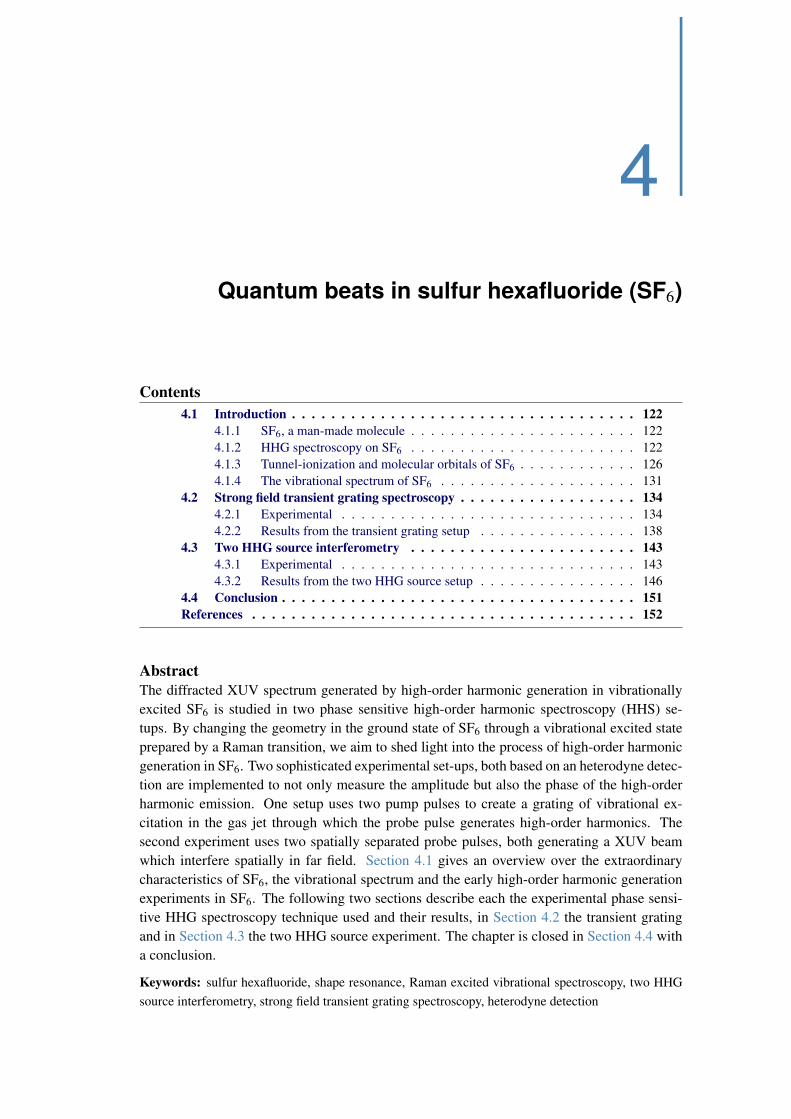
4
Quantum beats in sulfur hexafluoride (SF6)
Contents
4.1 Introduction . . . . . . . . . . . . . . . . . . . . . . . . . . . . . . . . . . . 122
4.1.1 SF6, a man-made molecule . . . . . . . . . . . . . . . . . . . . . . . 122
4.1.2 HHG spectroscopy on SF6 . . . . . . . . . . . . . . . . . . . . . . . 122
4.1.3 Tunnel-ionization and molecular orbitals of SF6 . . . . . . . . . . . . 126
4.1.4 The vibrational spectrum of SF6 . . . . . . . . . . . . . . . . . . . . 131
4.2 Strong field transient grating spectroscopy . . . . . . . . . . . . . . . . . . 134
4.2.1 Experimental . . . . . . . . . . . . . . . . . . . . . . . . . . . . . . 134
4.2.2 Results from the transient grating setup . . . . . . . . . . . . . . . . 138
4.3 Two HHG source interferometry . . . . . . . . . . . . . . . . . . . . . . . 143
4.3.1 Experimental . . . . . . . . . . . . . . . . . . . . . . . . . . . . . . 143
4.3.2 Results from the two HHG source setup . . . . . . . . . . . . . . . . 146
4.4 Conclusion . . . . . . . . . . . . . . . . . . . . . . . . . . . . . . . . . . . . 151
References . . . . . . . . . . . . . . . . . . . . . . . . . . . . . . . . . . . . . . . 152
Abstract
The diffracted XUV spectrum generated by high-order harmonic generation in vibrationally
excited SF6 is studied in two phase sensitive high-order harmonic spectroscopy (HHS) se-
tups. By changing the geometry in the ground state of SF6 through a vibrational excited state
prepared by a Raman transition, we aim to shed light into the process of high-order harmonic
generation in SF6. Two sophisticated experimental set-ups, both based on an heterodyne detec-
tion are implemented to not only measure the amplitude but also the phase of the high-order
harmonic emission. One setup uses two pump pulses to create a grating of vibrational ex-
citation in the gas jet through which the probe pulse generates high-order harmonics. The
second experiment uses two spatially separated probe pulses, both generating a XUV beam
which interfere spatially in far field. Section 4.1 gives an overview over the extraordinary
characteristics of SF6, the vibrational spectrum and the early high-order harmonic generation
experiments in SF6. The following two sections describe each the experimental phase sensi-
tive HHG spectroscopy technique used and their results, in Section 4.2 the transient grating
and in Section 4.3 the two HHG source experiment. The chapter is closed in Section 4.4 with
a conclusion.
Keywords: sulfur hexafluoride, shape resonance, Raman excited vibrational spectroscopy, two HHG
source interferometry, strong field transient grating spectroscopy, heterodyne detection

4.1 Introduction
4.1.1 SF6, a man-made molecule
Sulfur hexafluoride (SF6) is a species of growing importance in the field of chemistry. This
can be attributed to its ’fascinating characteristics’ which include it being gaseous even at
low temperature, chemically inert, non-flammable, non-toxic, non-corrosive. It shows a high
dielectric strength through fluorine’s high electronegativity, a high molar heat capacity, low
viscosity and good heat transfer capabilities [1–3]. Due to its excellent dielectric properties it
is heavily used for high voltage gas insulated systems where it is utilized above atmospheric
pressure to circumvent electrical discharge [4]. It is also used in semiconductor manufac-
turing, and other sophisticated applications as thermoacoustic insulator and inert solvent for
supercritical fluid chemical reactions [5, 6]. Furthermore, it is used in the medical field [7],
e.g as inert gas in ophthalmologic surgeries [8] or as contrast agent in ultrasonography [9].
Its concentration in the Earths atmosphere is increasing at a rate of about 7 % per year due to
industrial emissions and its extremely long lifetime in the atmosphere („3200 years), and be-
came a subject of interest in the field of atmospheric physics as a pollutant that can contribute
to the greenhouse effect (GHE) [10]. Even though per molecule it is one of the strongest
greenhouse gases known in its ambient mixing ratio of less than four parts per trillion (ppt,
10´12 moles per mole in dry air), it does not yet cause any significant climate change [11].
Nevertheless SF6 is one of six chemical compounds to control since 2005 within in the Kyoto
protocol [12]. Due to its relatively long lifetime it can be used as a trace gas in the evolvement
of the greenhouse effect and its concentration has been reduced by 30-40% (depending on the
country) between 1990 and 2004 [13].
The spectroscopy of this molecule, which is essential for quantitative measurements in the
atmosphere and an understanding of the role of SF6 in there, is still insufficiently known [14–
18]. The structure of SF6 was already determined by electron diffraction studies as early as
1933 [19] and showed a highly symmetrical molecule with the six fluorine atoms occupying
the corners of a regular octahedron with the sulfur atom at the center. Today SF6 is known
as a textbook example of a spherical-top molecule which belongs to the highly symmetric Oh
point group with three C4 axes, four C3 axes, six C2 axes, three σh planes, six σd planes and a
center of inversion i. Its structure is shown in Figure 4.1. The character and product tables for
the Oh point group are shown in Appendix E in Table E.6.
4.1.2 HHG spectroscopy on SF6
As seen in Section 1.3 high-order harmonic generation in molecules is an attractive tool in
spectroscopy. From the harmonic emission, photochemical processes induced by a pump pulse
can be revealed, with an analysis strongly based on molecular orbitals from and to which
the electron is emitted and recombined [20]. Moreover attosecond hole dynamics induced
by the probe laser field can eventually be extracted [21, 22]. All these aspects make high-
order harmonic spectroscopy (HHS) a very appealing technique to complement conventional
ultrafast spectroscopy.
122 Chapter 4 Quantum beats in sulfur hexafluoride (SF6)

S
F
F
F
FF
F
90o156.4 pm
(A) (B) (C)
F
F
F
F
F
F
S
Figure 4.1: The structure of sulfur hexafluoride SF6. A) B) octahedron structure C) surface
simulation of SF6. Surface view shows the electrostatic potential of the structure mapped
onto the solvent excluded surface, based on a probe of radius 1.4 A. Regions of negative
potential mainly localized on the flour atoms are shown in red, positive in blue.
As early as 1996 Lynga et al. observed that SF6 shows an anomaly in the HHG spectrum
[23]. They measured the intensity of HHG in molecular gases and draw a comparison of
the HHG spectra of Ar, N2 and SF6 which is shown in Figure 4.2 (A). N2 and Ar exhibit
a very similar behavior and show a typical HHG spectrum with perturbative regime (up to
H11), plateau (up to H17) and cutoff (up to H29). SF6 does not have the characteristic plateau
behavior. Instead, the intensity plot of the harmonics shows a clear minimum around the 17th
harmonic [23]. They postulated, that SF6 dissociates at low intensities, during the rising time
of the laser pulse, and that the minimum could come from harmonics produced from neutral
fragments of SF5 that is defined by an extra Ip of 9.6 eV. If two fragments, with different Ip
generate harmonics it could lead to two plateaus of different heights and widths. However SF`5
appears as soon as the ionization threshold of SF6 is reached [24]. This leads to a dissociation
threshold of SF5 neutral to around 5.8 eV. Moreover, the SF5 produced by dissociation will
have initially a square pyramidal geometry. But the equilibrium structure of SF5 is a trigonal
bipyramidal (D3h), which means extensive rearrangement must occur during the dissociation
process, leading to a dissociation time certainly longer than the short pulse duration observed
in HHG (ă 35 fs). Clearly in the excitation scheme proposed by Lynga et al., the differences in
the Ip between SF6 and SF5 and the strong nuclear rearrangement required can not explain the
spectrum they observed. However, this dissociative ionization of SF`6 as soon as the HOMO
electron is removed should have a strong effect on HHG and consequently dynamics of the
cation should take place in the HHG process.
Around 16 years after this discovery there is still no answer to this anomaly in the plateau of
SF6 around harmonic 17. As the technology and knowledge advances we are not restricted
anymore to just a measurement of the intensity of the HHG spectrum. The CELIA group un-
dertook a complex investigation of the HHG spectrum of SF6 in various experimental setups
which is summarized in Figure 4.2 B and will be discussed here shortly as it is the initiation of
the pump-probe investigations described in this chapter. This advanced optical characteriza-
tion of high-order harmonic emission from SF6 was done by measuring not only the high-order
harmonic spectrum, but also its dependence to the driving laser ellipticity, the direction of po-
larization of the harmonics from short and long trajectories, and the degree of ellipticity of the
Section 4.1 Introduction 123
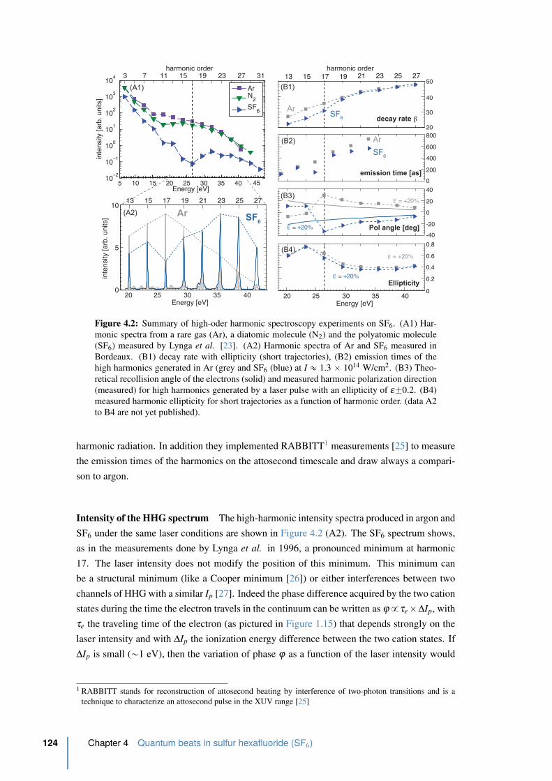
13 15 17 19 21 23 25 27
0
5
10
inte
nsity
[arb
. uni
ts]
13 15 17 19 21 23 25 27harmonic order
20
30
40
50
0
200
400
600
800
-40
-20
0
20
40
(A2)
(B1)
(B2)
(B3)
0
0.2
0.4
0.6
0.8(B4)
ε = +20%
ε = +20%
SF6
Ar
decay rate β
emission time [as]
Pol angle [deg]
Ellipticity
SF6
Ar
SF6
Ar
3 7 11 15 19 23 27 31
10−2
10−1
100
101
102
103
104
inte
nsity
[arb
. uni
ts]
ArN
2SF
6
(A1)
harmonic order
20 25 30 35 40 455 10 15Energy [eV]
20 25 30 35 40Energy [eV]
20 25 30 35 40Energy [eV]
ε = +20%
ε = +20%
Figure 4.2: Summary of high-oder harmonic spectroscopy experiments on SF6. (A1) Har-
monic spectra from a rare gas (Ar), a diatomic molecule (N2) and the polyatomic molecule
(SF6) measured by Lynga et al. [23]. (A2) Harmonic spectra of Ar and SF6 measured in
Bordeaux. (B1) decay rate with ellipticity (short trajectories), (B2) emission times of the
high harmonics generated in Ar (grey and SF6 (blue) at I « 1.3 ˆ 1014 W/cm2. (B3) Theo-
retical recollision angle of the electrons (solid) and measured harmonic polarization direction
(measured) for high harmonics generated by a laser pulse with an ellipticity of ε˘0.2. (B4)
measured harmonic ellipticity for short trajectories as a function of harmonic order. (data A2
to B4 are not yet published).
harmonic radiation. In addition they implemented RABBITT1 measurements [25] to measure
the emission times of the harmonics on the attosecond timescale and draw always a compari-
son to argon.
Intensity of the HHG spectrum The high-harmonic intensity spectra produced in argon and
SF6 under the same laser conditions are shown in Figure 4.2 (A2). The SF6 spectrum shows,
as in the measurements done by Lynga et al. in 1996, a pronounced minimum at harmonic
17. The laser intensity does not modify the position of this minimum. This minimum can
be a structural minimum (like a Cooper minimum [26]) or either interferences between two
channels of HHG with a similar Ip [27]. Indeed the phase difference acquired by the two cation
states during the time the electron travels in the continuum can be written as ϕ 9τe ˆ∆Ip, with
τe the traveling time of the electron (as pictured in Figure 1.15) that depends strongly on the
laser intensity and with ∆Ip the ionization energy difference between the two cation states. If
∆Ip is small („1 eV), then the variation of phase ϕ as a function of the laser intensity would
1 RABBITT stands for reconstruction of attosecond beating by interference of two-photon transitions and is a
technique to characterize an attosecond pulse in the XUV range [25]
124 Chapter 4 Quantum beats in sulfur hexafluoride (SF6)
not be drastic, leading to an invariance of the minima at H17 as a function of the laser intensity.
The comparison with argon is done as the Ip’s are quite close: 15.32 eV for SF6 and 15.76 eV
for argon. Consequently the cutoff energy, given by measured from these two systems should
be similar. By taking a cutoff energy around harmonic 27 on argon („ 42 eV) and by using
Eq. (1.28), the ponderomotive energy is 8.23 eV for a laser intensity of 1.38 ˆ 1014 W/cm2.
For SF6 this should lead to a cutoff energy of around 41.5 eV. Clearly on Figure 4.2 (A2),
the cut-off energy is larger than harmonic 27. By fixing a cutoff energy around harmonic 29
(45 eV), the effective Ip in SF6 would be around 19 eV. Already on this spectrum only, two
features are already intriguing: the minimum and the extension of the cut-off.
Ellipticity dependance of the HHG spectrum Using elliptical polarized light to generate
high-order harmonics, the efficiency of HHG normally drops drastically with increasing ellip-
ticity ε , where the largest efficiency for the harmonic emission is certainly reached for linear
polarisation (ε “ 0), except in chiral system [28] and aligned molecules [29]. This effect can
be less drastic in molecules compared to atoms because of the extension of the molecular or-
bital [30]. For small ellipticities the decaying harmonic intensity can be fitted by an gaussian
function, Iqpεq “ I0q e´βqε2
, where q is the harmonic order and βq the decay rate with ellipticity.
A lower β means a better acceptance to a lateral drift of the electron trajectory. This type of
measurement has been shown to be sensitive to molecular structure like demonstrated on dif-
ferent chloromethane molecules [30]. Figure 4.2 B1 shows the decay rate βq of the harmonic
signal as function of the harmonic order for Ar and SF6. For harmonic 19 to 27, above the
minimum in the harmonic spectrum, the decay with ellipticity are remarkably similar, whereas
below harmonic 17 the signal is less sensitive to ellipticity in SF6 than in Ar. This means that
the extension of the wavefunction is larger for the lowest harmonics, since the overlap between
the returning electron with a lateral kick and the initial wavefunction is larger. This observation
is coherent with a change in the polarization angle for harmonics smaller than H17 (Figure 4.2
(B3)). Also the emission time measured in a RABBITT setup shows a difference between
harmonic 15 and 17 (Figure 4.2 (B2)).
HHG polarimetry The harmonic polarimetry measurements were performed by recording
the harmonic spectrum as a function of the polarization direction of the 800 nm driving laser
beam. The resulting signal follows an oscillatory law (Malus’ law1) as a function of the wave-
plate orientation used to change the polarization direction. The phase and contrast of the
oscillations (extracted from a Fourier transformation) provide respectively the polarization
angle and the degree of ellipticity of the radiation, assuming a fully polarized state2 [34]. The
harmonic polarization angles as function of the harmonic order are shown in Figure 4.2 (B3).
If the ground state wavefunction is fully symmetric (s orbital), the polarization direction of
1 The classical Malus law predicts an attenuation of a polarized light beam through a linear polarizer which depends
on the relative angle θ , between the polarization direction of the incoming wave and the orientation of the
polarizer and is simply given by I “ I0 cos2 θ [31, 32].2 the polarization state of an electromagnetic wave is characterized by the so called Stokes parameters. The Stokes
vector spans the space of unpolarized, partially polarized, and fully polarized light [33].
Section 4.1 Introduction 125

14 16 18 20 22 24 26 28 300
5
10
15
20
Energy [eV]
coun
ts [x
1000
]
X2T1g
A2T1u
B2T2u
C2Eg D2T
2g
E2T1u
F2A1g
(He 1s)(Kr 4p
1/2)
SF6 PES
X A B C ArD
HOMO HOMO-1 HOMO-2 HOMO-3 HOMO-4
Figure 4.3: HeII (hω = 40.8 eV) photo-electron spectrum of SF6 reported in binding energy
between 15 and 30 eV. adapted from [38]. Calculated molecular orbitals of SF6 from the
HOMO to the HOMO-4.
the harmonics is expected to be equal to the recollision angle. Deviations from this situation
reflect the influence of the orbital structure and symmetry [35]. One can again observe a drastic
change in the harmonic polarization around H17. The ellipticity of the harmonic emission
for short trajectories, assuming the light is fully polarized, is shown in Figure 4.2 (B4). It
reaches almost 80% for harmonic 15 and drops to 40% above harmonic 17. This result is the
most puzzling one. Indeed, in argon with an incident laser ellipticity of ε˘0.2, the maximum
ellipticity observed is 2% [36]. The significant polarization jump between H15 and H17 does
not depend on the incident intensity.
Clearly these observations converge to a HHG process involving more than one molecular
orbital. In the next section I will summarize the peculiar features encountered in the ion
continuum of SF6.
4.1.3 Tunnel-ionization and molecular orbitals of SF6
To understand the the observations of HHG in SF6 and the results shown here one has to look
a bit closer to the special characteristics of SF6 due to its highly symmetric structure and see
which molecular orbitals are responsible for HHG in SF6. Due to its highly symmetric shape
and the encountered Jahn-Teller effect, the theoretical modeling of HHG in SF6 is a complex
task. The chemical bounds of SF6 are linked to the electrons of the sulfur in the 3M shell (four
in the 3p and two in the 3s). However as soon as valence excitation is activated, the 3d electrons
of the sulfur are involved. This is the case for the Ñ εt2g transition for the shape resonance
[37]. Each of the 6 F atoms is missing a p electron to fill the 2L-p shell. Consequently the
last occupied valence orbitals are closed in energies, making the photoelectron spectrum very
dense near the Ip [38]. For the cation states investigated here, the emitted electrons are all
from the 2p orbital of fluorine, only the atomic orbital of the sulfur changes. The d-orbitals
might induce high mobility for the Sulfur electrons. To go a little bit further, the Hartree-
Fock configuration for the ground electronic state of SF6 with (16 + 9 ˆ 6 = 70) electrons to
126 Chapter 4 Quantum beats in sulfur hexafluoride (SF6)
distribute is [39]:
p...q22loomoon
core
p4a1gq2p3t1uq6p2egq4p5a1gq2p4t1uq6p1t2gq6p3egq4rp1t2uqp5t1uqs6p1t1gq6looooooooooooooooooooooooooooooooooooooooooomooooooooooooooooooooooooooooooooooooooooooon
valence electrons
1A1g
p6a1gq0p6t1uq0p2t2gq0p4egq0looooooooooooooomooooooooooooooon
unoccupied
(4.1)
The four highest occupied molecular orbitals (HOMO) are lying within 3 eV. Figure 4.3 shows
the photo-electron spectrum of SF6 and the assignments of the features. In this molecule, there
is a direct assignment between the electron removal from the molecular orbitals and the cation
states. Underneath the calculated molecular orbitals for the ground state and the HOMO-1 to
HOMO-3 are shown.
To understand the origin of the drastic change in the harmonic emission around harmonic
17, the CELIA group and Serguei Patchovskii developed a simple harmonic emission model,
where the harmonic dipole moment is determined by the tunnel ionization probability, the
propagation of the electron in the continuum, and the recombination cross section. The dif-
ferent channels corresponding to ionization from different molecular orbitals are considered
as uncoupled. The harmonic intensity for each molecular channel j (= X, A, B, C, D) is given
by:
I j “ˇ
ˇ
ˇP
jT I d j
rec eiϕ jˇ
ˇ
ˇ
2(4.2)
where Pj
T I is the tunnel-ionization probability, djrec the recombination dipole moment which is
assumed to be equal to the photoionization cross-section in the VUV range and ϕ j 9∆Ijpτe is
a phase term accounting for the accumulated phase by the molecule between ionization and
recombination due to the propagation in the continuum. ∆Ijp is the difference between the
ionization potential of channel j and the X channel, and τe is the electron travel time in the
continuum, which increases with harmonic order from 0.6 fs to 1.7 fs for short trajectories
[40]. Because the cross-sections are very similar, this picture is still very complex. In gen-
eral, one would expect that the HOMO is the main contributing orbital due to the exponential
dependence of the tunnel ionization (see Eq. (1.20)). Figure 4.4 shows the tunnel ionization
probability calculated by Serguei Patchovskii summed over the different directions between
the molecular axis and the linear polarized electric field. A summary of the values is given in
Table 4.1. The tunneling probability from the HOMO is significantly reduced by the presence
of nodes in the orbital, such that deeper channels are favored. The resulting contributions for
the tunnel ionization probability shows only a significant contribution for channel B (HOMO-
2) and C (HOMO-3). Indeed the HOMO-2 is the first molecular orbital with a simple parity
(a single nodal plane ) and the HOMO-3 is the first contracted molecular orbital, not as dif-
fuse as the HOMO and the HOMO-1. By taking into account the contracted nature of the C
orbital along the S-F bonds as can be seen in Figure 4.4 for the first molecular orientation, we
can expect that the outgoing electron will have an extended wavefunction compared to the B
channel that is a more diffuse molecular orbital. This feature will explain why the β param-
eters are lower at low energy in Figure 4.2 (B1) where tunnel-ionization is assumed to take
place from the C channel. Clearly the B (HOMO-2) and C (HOMO-3) channels are largely
Section 4.1 Introduction 127
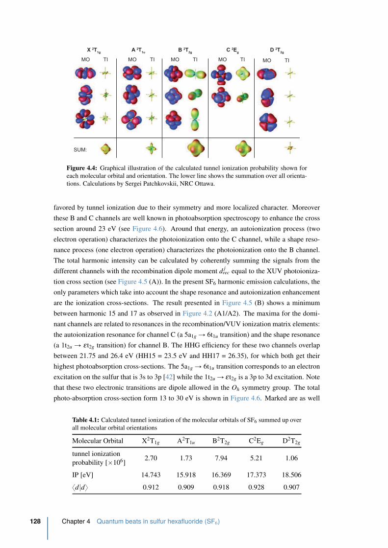
X 2T1g
A 2T1u
B 2T2g
C 2Eg
D 2T2g
MO TI MO TI MO TI MO TI MO TI
SUM:
Figure 4.4: Graphical illustration of the calculated tunnel ionization probability shown for
each molecular orbital and orientation. The lower line shows the summation over all orienta-
tions. Calculations by Sergei Patchkovskii, NRC Ottawa.
favored by tunnel ionization due to their symmetry and more localized character. Moreover
these B and C channels are well known in photoabsorption spectroscopy to enhance the cross
section around 23 eV (see Figure 4.6). Around that energy, an autoionization process (two
electron operation) characterizes the photoionization onto the C channel, while a shape reso-
nance process (one electron operation) characterizes the photoionization onto the B channel.
The total harmonic intensity can be calculated by coherently summing the signals from the
different channels with the recombination dipole moment djrec equal to the XUV photoioniza-
tion cross section (see Figure 4.5 (A)). In the present SF6 harmonic emission calculations, the
only parameters which take into account the shape resonance and autoionization enhancement
are the ionization cross-sections. The result presented in Figure 4.5 (B) shows a minimum
between harmonic 15 and 17 as observed in Figure 4.2 (A1/A2). The maxima for the domi-
nant channels are related to resonances in the recombination/VUV ionization matrix elements:
the autoionization resonance for channel C (a 5a1g Ñ 6t1u transition) and the shape resonance
(a 1t2u Ñ εt2g transition) for channel B. The HHG efficiency for these two channels overlap
between 21.75 and 26.4 eV (HH15 = 23.5 eV and HH17 = 26.35), for which both get their
highest photoabsorption cross-sections. The 5a1g Ñ 6t1u transition corresponds to an electron
excitation on the sulfur that is 3s to 3p [42] while the 1t2u Ñ εt2g is a 3p to 3d excitation. Note
that these two electronic transitions are dipole allowed in the Oh symmetry group. The total
photo-absorption cross-section form 13 to 30 eV is shown in Figure 4.6. Marked are as well
Table 4.1: Calculated tunnel ionization of the molecular orbitals of SF6 summed up over
all molecular orbital orientations
Molecular Orbital X2T1g A2T1u B2T2g C2Eg D2T2g
tunnel ionization
probability [ˆ106]2.70 1.73 7.94 5.21 1.06
IP [eV] 14.743 15.918 16.369 17.373 18.506
xd|dy 0.912 0.909 0.918 0.928 0.907
128 Chapter 4 Quantum beats in sulfur hexafluoride (SF6)
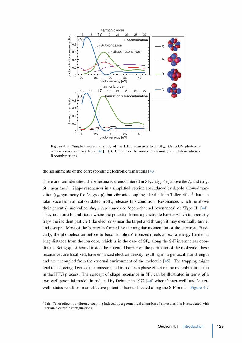
20 25 30 35 400
0.2
0.4
0.6
0.8
1
photon energy [eV]
phot
oioniz
ation
cros
s−se
ction
20 25 30 35 400
0.2
0.4
0.6
0.8
1
photon energy [eV]
harm
onic
em
issi
on
13 15 17 19 21 23 25 27
harmonic order
13 15 17 19 21 23 25 27harmonic order
X
A
B
C
Autoionization
Shape resonances
Recombination
Ionization x Recombination
(A)
(B)
Figure 4.5: Simple theoretical study of the HHG emission from SF6. (A) XUV photoion-
ization cross sections from [41]. (B) Calculated harmonic emission (Tunnel-Ionization x
Recombination).
the assignments of the corresponding electronic transitions [43].
There are four identified shape resonances encountered in SF6: 2t2g, 4eg above the Ip and 6a1g,
6t1u near the Ip. Shape resonances in a simplified version are induced by dipole allowed tran-
sition (t1u symmetry for Oh group), but vibronic coupling like the Jahn-Teller effect1 that can
take place from all cation states in SF6 releases this condition. Resonances which lie above
their parent Ip are called shape resonances or ‘open-channel resonances’ or ‘Type II’ [44].
They are quasi bound states where the potential forms a penetrable barrier which temporarily
traps the incident particle (like electrons) near the target and through it may eventually tunnel
and escape. Most of the barrier is formed by the angular momentum of the electron. Basi-
cally, the photoelectron before to become ‘photo’ (ionized) feels an extra energy barrier at
long distance from the ion core, which is in the case of SF6 along the S-F internuclear coor-
dinate. Being quasi bound inside the potential barrier on the perimeter of the molecule, these
resonances are localized, have enhanced electron density resulting in larger oscillator strength
and are uncoupled from the external environment of the molecule [45]. The trapping might
lead to a slowing down of the emission and introduce a phase effect on the recombination step
in the HHG process. The concept of shape resonance in SF6 can be illustrated in terms of a
two-well potential model, introduced by Dehmer in 1972 [46] where ’inner-well’ and ’outer-
well’ states result from an effective potential barrier located along the S-F bonds. Figure 4.7
1 Jahn-Teller effect is a vibronic coupling induced by a geometrical distortion of molecules that is associated with
certain electronic configurations.
Section 4.1 Introduction 129

1t 1
g 4p
5t 1
u 4s
3e
g 6t 1
u
1t 1
g 5p
5t 1
u 5s
1t 2
g 6t 1
u
4t 1
u 6a
1g
4t 1
u
4
s
4t 1
u 5s
B:
5t 1
u 2t 2
gC:
5a
1g 6t 1
u
5a
1g 4p
5a
1g 5p
5a
1g 6p
4t 1
u 2t 2
g
0
50
100
150
phot
o-ab
sorp
tion
cros
s se
ctio
n σ
[10−2
2 m2 ]
0
0.2
0.4
0.6
0.8
1
phot
oion
izat
ion
quan
tum
effi
cien
cy
a c
d
e
f
b
g
h
i
14 16 18 20 22 24 26 28 30Energy [eV]
9 11 13 15 17 19harmonic order
4t 1
u ns
Figure 4.6: The absolute photoioniation cross section σpi (blue) and the photoionization
quantum efficiency (green) of SF6 with assignments. The two vertical purple lines indicate
the energy of harmonic 15 (23.25 eV, 53.3 nm) and 17 (26.3 eV, 47.14 nm) using an 800 nm
driving laser pulse. Adapted from [43].
shows a schematic diagram of this two-well potential [24]. In the case of SF6, the fluorine
atom traps the d-electron from the sulfur that wants to leave the core, due to the strong elec-
tronegativity of the fluorine1 [42]. The inner well corresponds to valence orbitals. One can
see from Figure 4.7, that four electronic levels seem to be supported by the barrier, assigned
to the unoccupied molecular orbitals: 6a1g and 6t1u near the vacuum level/ionization threshold
and 2t2g and 4eg lying in the electron continuum but within the effective barrier. Calculations
by Stener et al. puts the 6a1g also above the Ip [42]. Any electronic transition to these states
will give an enhancement in the absorption cross section. This enhancement is called shape
resonances. The outer-well corresponds to Rydberg orbitals. Since the overlap between the
Rydberg orbitals and the initial electronic wavefunction is expected to be poor along the S-F
distance, Rydberg transitions are in general weaker when shaped resonances characterize the
molecular ionic potential. Due to the well defined position of the fluorine atoms, it is as well
expected to get a really anisotropic molecular field, which is encoded in the photoelectron
angular distribution (β “ 0) [47–49]. The shape resonance/auto-ionization feature observed
by Holland et al.[43] is 4 eV large and centered at 23.6 eV (see dark blue area in Figure 4.6).
Table 4.2 summarizes the assignments of the photo-electron bands by removal of one electron
of a molecular orbital. Also shown are the observed corresponding resonances in the absorp-
tion spectrum. This shape resonance appears as well very clearly on dissociative ionization
onto SF`5 + F [50]. Since the shape resonance of the B channel is a photoelectron which is
trapped for a few hundred attoseconds due to the electronegativity of the fluorine atoms, the
arising question is how this effect will change as a function of S-F internuclear distance. In-
deed, it is expected that the electronic barrier to the ionization might vary as a function of the
1 Electronegativity of fluorine is 3.98 and of sulfur only 2.58 in Pauling units
130 Chapter 4 Quantum beats in sulfur hexafluoride (SF6)

20
10
0
-10
-20
-30
-40
-50
3t1u
6t1u
2t2g
4t1u
2eg
4a1g
6a1g
1t1g
5a1g
3eg
1t2u
1t2g
5t1u
4eg
Satom
- Fatom
Oribital energ
y [eV
]
allowed transitions
valence
molecular
orbitals
vacuum level
outer-well
Rydberg orbitals
C
B
3s4s
1t2u
2t2g
5a1g
6t1u
, 3eg
5a1g
shape resonance (B channel)
autoionization (C channel)
Figure 4.7: Schematic diagram of the two-well potential of SF6 acting on the outgoing elec-
trons in the photoabsorption process. Dashed lines are vacant orbital levels and full lines
indicate occupied valence orbital levels. The arrows show the allowed transitions by the
electric dipole moment for the Oh symmetry group. Marked in red are the autoionization
resonance (C channel) and the shape resonance (B channel). Adapted from [24].
S-F distance [37]. The equilibrium S-F distance is known to be 1.556 A for the molecular
ground state [51]. By varying this distance, it is expected that the position, the intensity and
the line shape of the 2t2g-shape resonance will vary. Changing the intermolecular distance can
be achieved by vibrational excitation of the molecule. In the pump-probe experiments shown
here, the goal was to determine the phase variation of the high harmonic emission as a function
of the geometry of SF6. The geometry variation is a vibrational wave packet oscillating in the
ground electronic state and created at ∆t = 0 by a Raman pump pulse. Two HHG techniques
have been used in this thesis, one based on two non-colinear pump pulses (transient grating
setup) and the second one based on two spatially separated probe pulses. The two setups will
be described in the experimental section. But first we have to take a look at the vibrational
spectrum of SF6.
4.1.4 The vibrational spectrum of SF6
The vibrational spectrum can be investigated by two types of spectroscopy, Raman and Infra-
red (IR) spectroscopy. When light (a photon) interacts with a molecule, it can either be elasti-
cally or inelastically scattered. In the first case, the absorbed photon has the same wavelength
as the emitted one (Rayleigh scattering), but in the second case, the photon has lost or gained
an amount of energy related to the vibrational energy spacing in the molecule. This amount
corresponds to the wavelength of the so called Stokes and anti-Stokes lines which are equally
displaced from the Rayleigh lines in the Raman spectrum. Infra-red spectroscopy also mea-
sures the vibrational energies of molecules. The absorption of light in the infrared region of
the electromagnetic spectrum, gives a spectrum that corresponds to specific vibrational modes
Section 4.1 Introduction 131
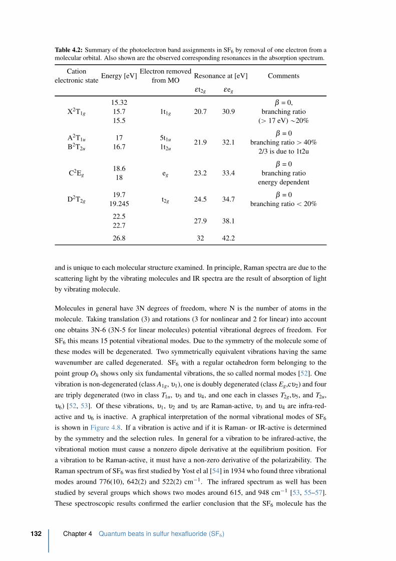
Table 4.2: Summary of the photoelectron band assignments in SF6 by removal of one electron from a
molecular orbital. Also shown are the observed corresponding resonances in the absorption spectrum.
Cation
electronic stateEnergy [eV]
Electron removed
from MOResonance at [eV] Comments
εt2g εeg
X2T1g
15.32
15.7
15.5
1t1g 20.7 30.9
β = 0,
branching ratio
(ą 17 eV) „20%
A2T1u
B2T2u
17
16.7
5t1u
1t2u21.9 32.1
β = 0
branching ratio ą 40%
2/3 is due to 1t2u
C2Eg18.6
18eg 23.2 33.4
β = 0
branching ratio
energy dependent
D2T2g19.7
19.245t2g 24.5 34.7
β = 0
branching ratio ă 20%
22.5
22.727.9 38.1
26.8 32 42.2
and is unique to each molecular structure examined. In principle, Raman spectra are due to the
scattering light by the vibrating molecules and IR spectra are the result of absorption of light
by vibrating molecule.
Molecules in general have 3N degrees of freedom, where N is the number of atoms in the
molecule. Taking translation (3) and rotations (3 for nonlinear and 2 for linear) into account
one obtains 3N-6 (3N-5 for linear molecules) potential vibrational degrees of freedom. For
SF6 this means 15 potential vibrational modes. Due to the symmetry of the molecule some of
these modes will be degenerated. Two symmetrically equivalent vibrations having the same
wavenumber are called degenerated. SF6 with a regular octahedron form belonging to the
point group Oh shows only six fundamental vibrations, the so called normal modes [52]. One
vibration is non-degenerated (class A1g, υ1), one is doubly degenerated (class Eg,cυ2) and four
are triply degenerated (two in class T1u, υ3 and υ4, and one each in classes T2g,υ5, and T2u,
υ6) [52, 53]. Of these vibrations, υ1, υ2 and υ5 are Raman-active, υ3 and υ4 are infra-red-
active and υ6 is inactive. A graphical interpretation of the normal vibrational modes of SF6
is shown in Figure 4.8. If a vibration is active and if it is Raman- or IR-active is determined
by the symmetry and the selection rules. In general for a vibration to be infrared-active, the
vibrational motion must cause a nonzero dipole derivative at the equilibrium position. For
a vibration to be Raman-active, it must have a non-zero derivative of the polarizability. The
Raman spectrum of SF6 was first studied by Yost el al [54] in 1934 who found three vibrational
modes around 776(10), 642(2) and 522(2) cm´1. The infrared spectrum as well has been
studied by several groups which shows two modes around 615, and 948 cm´1 [53, 55–57].
These spectroscopic results confirmed the earlier conclusion that the SF6 molecule has the
132 Chapter 4 Quantum beats in sulfur hexafluoride (SF6)

F
F
F
F
F
F
S
775 cm-1 (43 fs)
Raman-active
very strong
ν1
F
F
F
F
F
F
S
643 cm-1 (52 fs)
Raman-active
Double Degenerate
weak
ν2
F
F
F
F
F
F
S
948 cm-1 (25 fs)
Infrared-active
Triply Degenerate
very stong
ν3
F
F
F
F
F
F
S
615 cm-1 (54 fs)
Infrared-active
Triply Degenerate
very strong
ν4
F
F
F
F
F
F
S
525 cm-1 (63 fs)
Raman-active
Triply Degenerate
weak
ν5
F
F
F
F
F
F
S
351 cm-1 (94 fs)
Forbidden
Triply Degenerate
very weak
ν6
A1g
Eg
T1u
T1u
T2g
T2u
Figure 4.8: Normal modes of the vibration of SF6. The wavenumber, period, degeneracy,
and activity of each mode is shown. Of these 6 normal mode vibrations, υ1, υ2 and υ5 are
Raman-active, υ3 and υ4 are IR-active and υ6 is inactive. Adapted from [52, 58].
octahedral symmetry Oh given by electron diffraction measurements.
Femtosecond laser pulses have shown to be able to excite vibrational wave packets in molecules,
by Raman transitions [59–62]. One of the hot topics in HHG is to investigate the capacities
of high-order harmonic spectroscopy to reveal nuclear dynamics. Measurements using HHG
as time resolved signal in SF6 have shown that the HHG emission is sensitive to the excited
vibrational modes [58]. The high-order harmonic yield is observed to oscillate, at frequen-
cies corresponding to all of the Raman-active modes of SF6. These observations collectively
demonstrate that monitoring HHG from vibrationally excited molecules yields useful data on
intramolecular dynamics that can be directly interpreted independent of complex models or
tomographic deconvolution techniques. Since the shape resonance which seems to play an
important role in the minimum of the harmonic emission in SF6 is strongly linked to S–F dis-
tance, they have a tendency to be smeared out by nuclear motion. By vibrational exciting the
molecule we might therefore affect the shape resonance and the process of HHG in SF6. In
[58], a single pump and a single probe were used in a colinear geometry. This type of mea-
surement leads only to the access of amplitude information without the phase information. In
this work, the three Raman active modes that are 525 cm´1, 643 cm´1 and 775 cm´1 appear
with a branching ratio of 48%/9.6%/42%, respectively. These experimental results have been
tentatively reproduced by calculations giving 5.6%/7%/87% branching ratio for 525/643/775
cm´1 vibrational modes, respectively [63]. This calculation however does not reproduce the
Section 4.1 Introduction 133

experimental data. Moreover, they assume that tunnel ionization takes place only from the
ground cation state X and not from the B and C channels. However, these are the most devel-
oped calculations so far to reproduce this type of experiment, since they take into account the
Jahn-Teller effect in the ion continua, the possibility of an extra Raman transition induced by
the probe pulse and cross-terms of ionization and recombination between vibrational levels of
the cation state.
The goal here is to observe the vibrational dynamics as function of the harmonic order through
a phase sensitive pump-probe measurement. The phase resolved dynamical measurements
were performed in two different setups using a HHG interferometry setup (two probe pulses)
and a transient grating setup (two pump pulses) at CELIA at the University of Bordeaux. The
two setups will be described in the following sections. The Aurore laser system at CELIA1 was
used in both setups which delivers 7 mJ/p at a center wavelength of 800 nm and a repetition
rate of 1 kHz with a pulse duration of 28 fs. The typival characteristics of the Aurore laser can
be found in Appendix A.
4.2 Strong field transient grating spectroscopy
4.2.1 Experimental
The signal change after an excitation used in pump-probe experiments can be very weak lead-
ing to unfavorable S/N ratios. In case of electrical signals usually a Lock-In amplifier can be
used to improve the S/N ratio. This electric filtering method cannot be applied for optical sig-
nals recorded via a CCD camera at 20 Hz. Therefore we choose an experimental setup that uses
the well-known femtosecond degenerate four-wave mixing (DFWM) technique, also called
femtosecond transient grating spectroscopy [64] which comes from the context of conven-
tional perturbative nonlinear spectroscopy but was recently applied to nonperturbative nonlin-
ear optics where it was used in high harmonic generation experiments [65]. Transient grating
spectroscopy (TGS) is the method of choice for measuring femtosecond dynamics in solids,
liquids, or gases whenever background suppression is important.
Two beams are used to create a grating of molecular excitation and a third beam is used to
generate high-order harmonic radiation. The principle of a TGS setup is shown in Figure 4.9.
Two synchronized non-collinear pump beams are crossed with an angle θ between them in the
molecular beam to create an optical interference grating and thus the excitation of the sample
is spatially modulated: a grating of molecular excitation is created. The fringe spacing a of
the grating depends on the angle θ between the two pulses and is given by:
a “ λ
2sinpθ2q (4.3)
In the present experiments the fringe spacing is 18 µm. The third probe beam is focused
into the grating of excitation in the gas target to generate high-order harmonics. With a waist
1 CELIA, Centre Lasers Intenses et Applications, Universite Bordeaux 1
134 Chapter 4 Quantum beats in sulfur hexafluoride (SF6)

XUV far-field
harmonic spetrum
pump pulses
0 1r 1-r
Δϕ
excited
molecules
unexcited
molecules
populationsXUV near-field
emission
XUV far-field
pattern
m = 0
m = + 1
m = - 1
generating pulse
GAS JET
Δt
XUV
spectrometer
Figure 4.9: Principle of strong field transient grating spectroscopy. Two synchronized pump
pulses set up a transient grating of excitation in the molecular beam. A delayed 800-nm
pulse generates high-order harmonics from the grating. The periodic modulation of the high-
harmonic amplitude and phase in the near field (in the laser focus) results, in the far field (at
the detector), in an additional first-order diffraction (m = ˘ 1) signal.
size of 100 µm, the diffraction occurs through five fringes. At positions of low intensities,
molecules remain unexcited and at high intensities they are excited. As amplitude and phase
of the generated high harmonics are different for vibrational excited and unexcited molecules
in the near field, the grating leads to a diffraction pattern in the far field. The geometry is
chosen such that there is no light emitted in the diffraction direction if there is no grating
(phase matching conditions such that HHG for long trajectories is not satisfied). Thus, the
detected signal is zero when there is no excitation and the measurement is background free.
The lower part of Figure 4.9 illustrates the spatially modulated fraction of excited molecules
which has its maximum value r at constructive interference of the optical grating. The fraction
of excited molecules is expressed as rpzq “ rpcospkzq ` 1q, where k “ 2πa is defined by
the fringe spacing a, in case of a single photon excitation process [66]. Consequently, the
harmonic emission E across the transient grating at photon energy Ω in the near field is a
superposition of the emission from molecules in the ν “ 0 state (Eg) and in the vibrationally
excited state (Ee):
EpΩ,zq “EgpΩ,zq ` EepΩ,zq“p1 ´ rpzqqAgpΩqeiφg ` rpzqAepΩqeiφe
(4.4)
where A and φ are the amplitude and phase of the emission from the molecules in the ν “ 0
state (g = ground) and in a non-stationary vibrational state (e = excited) , called a vibrational
wave packet. The signal in the far-field is the Fourier transform of this with the spatial fre-
Section 4.2 Strong field transient grating spectroscopy 135
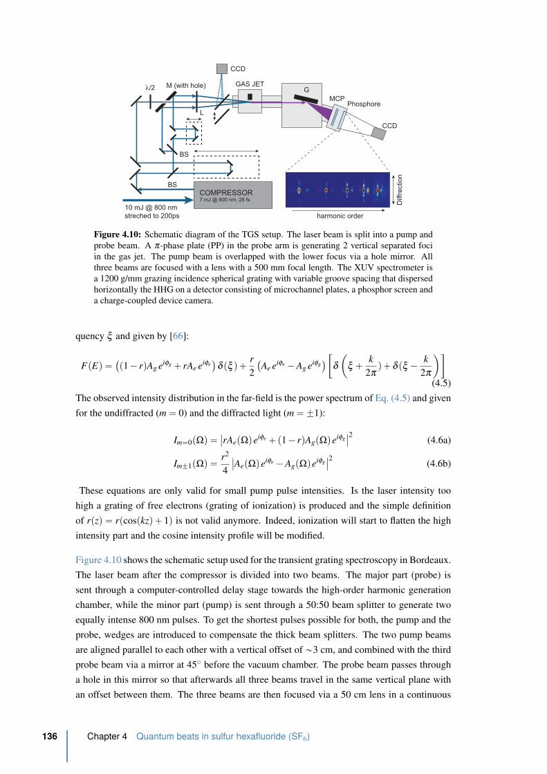
COMPRESSOR7 mJ @ 800 nm, 28 fs
L
GAS JET
10 mJ @ 800 nm
streched to 200ps
λ/2
BS
BS
M (with hole)
PhosphoreMCP
G
CCD
harmonic order
Diffr
ectio
n
CCD
Figure 4.10: Schematic diagram of the TGS setup. The laser beam is split into a pump and
probe beam. A π-phase plate (PP) in the probe arm is generating 2 vertical separated foci
in the gas jet. The pump beam is overlapped with the lower focus via a hole mirror. All
three beams are focused with a lens with a 500 mm focal length. The XUV spectrometer is
a 1200 g/mm grazing incidence spherical grating with variable groove spacing that dispersed
horizontally the HHG on a detector consisting of microchannel plates, a phosphor screen and
a charge-coupled device camera.
quency ξ and given by [66]:
FpEq “`
p1 ´ rqAg eiφg ` rAe eiφe˘
δ pξ q ` r
2
`
Ae eiφe ´ Ag eiφg˘
„
δ
ˆ
ξ ` k
2πq ` δ pξ ´ k
2π
˙
(4.5)
The observed intensity distribution in the far-field is the power spectrum of Eq. (4.5) and given
for the undiffracted (m “ 0) and the diffracted light (m “ ˘1):
Im“0pΩq “ˇ
ˇrAepΩqeiφe ` p1 ´ rqAgpΩqeiφgˇ
ˇ
2(4.6a)
Im˘1pΩq “ r2
4
ˇ
ˇAepΩqeiφe ´ AgpΩqeiφgˇ
ˇ
2(4.6b)
These equations are only valid for small pump pulse intensities. Is the laser intensity too
high a grating of free electrons (grating of ionization) is produced and the simple definition
of rpzq “ rpcospkzq ` 1q is not valid anymore. Indeed, ionization will start to flatten the high
intensity part and the cosine intensity profile will be modified.
Figure 4.10 shows the schematic setup used for the transient grating spectroscopy in Bordeaux.
The laser beam after the compressor is divided into two beams. The major part (probe) is
sent through a computer-controlled delay stage towards the high-order harmonic generation
chamber, while the minor part (pump) is sent through a 50:50 beam splitter to generate two
equally intense 800 nm pulses. To get the shortest pulses possible for both, the pump and the
probe, wedges are introduced to compensate the thick beam splitters. The two pump beams
are aligned parallel to each other with a vertical offset of „3 cm, and combined with the third
probe beam via a mirror at 45˝ before the vacuum chamber. The probe beam passes through
a hole in this mirror so that afterwards all three beams travel in the same vertical plane with
an offset between them. The three beams are then focused via a 50 cm lens in a continuous
136 Chapter 4 Quantum beats in sulfur hexafluoride (SF6)
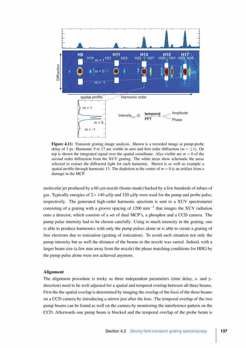
H9 H11 H13 H15 H17
m = 1
m = -1
m = 0
Harmonic order
Diffr
actio
n
m = 1
m = -1
m = 0
spatial profile
temporal
FFT
Amplitude
Phase Intensity
m±1 (t)
H19 H23 H27 H31 H35H21 H25 H29 H33
Figure 4.11: Transient grating image analysis. Shown is a recorded image at pump-probe
delay of 1 ps. Harmonic 9 to 17 are visible in zero and first order diffraction (m “ ˘1). On
top is shown the integrated signal over the spatial coordinate. Also visible are m “ 0 of the
second order diffraction from the XUV grating. The white areas show schematic the areas
selected to extract the diffracted light for each harmonic. Shown is as well as example a
spatial profile through harmonic 13. The depletion at the center of m “ 0 is an artifact from a
damage in the MCP.
molecular jet produced by a 60 µm nozzle (home-made) backed by a few hundreds of mbars of
gas. Typically energies of 2ˆ 140 µJ/p and 320 µJ/p were used for the pump and probe pulse,
respectively. The generated high-order harmonic spectrum is sent to a XUV spectrometer
consisting of a grating with a groove spacing of 1200 mm´1 that images the XUV radiation
onto a detector, which consists of a set of dual MCP’s, a phosphor and a CCD camera. The
pump pulse intensity had to be chosen carefully. Using to much intensity in the grating, one
is able to produce harmonics with only the pump pulses alone or is able to create a grating of
free electrons due to ionization (grating of ionization). To avoid such situation not only the
pump intensity but as well the distance of the beams to the nozzle was varied. Indeed, with a
larger beam size (a few mm away from the nozzle) the phase matching conditions for HHG by
the pump pulse alone were not achieved anymore.
Alignment
The alignment procedure is tricky as three independent parameters (time delay, z- and y-
direction) need to be well adjusted for a spatial and temporal overlap between all three beams.
First the the spatial overlap is determined by imaging the overlap of the focii of the three beams
on a CCD camera by introducing a mirror just after the lens. The temporal overlap of the two
pump beams can be found as well on the camera by monitoring the interference pattern on the
CCD. Afterwards one pump beam is blocked and the temporal overlap of the probe beam is
Section 4.2 Strong field transient grating spectroscopy 137
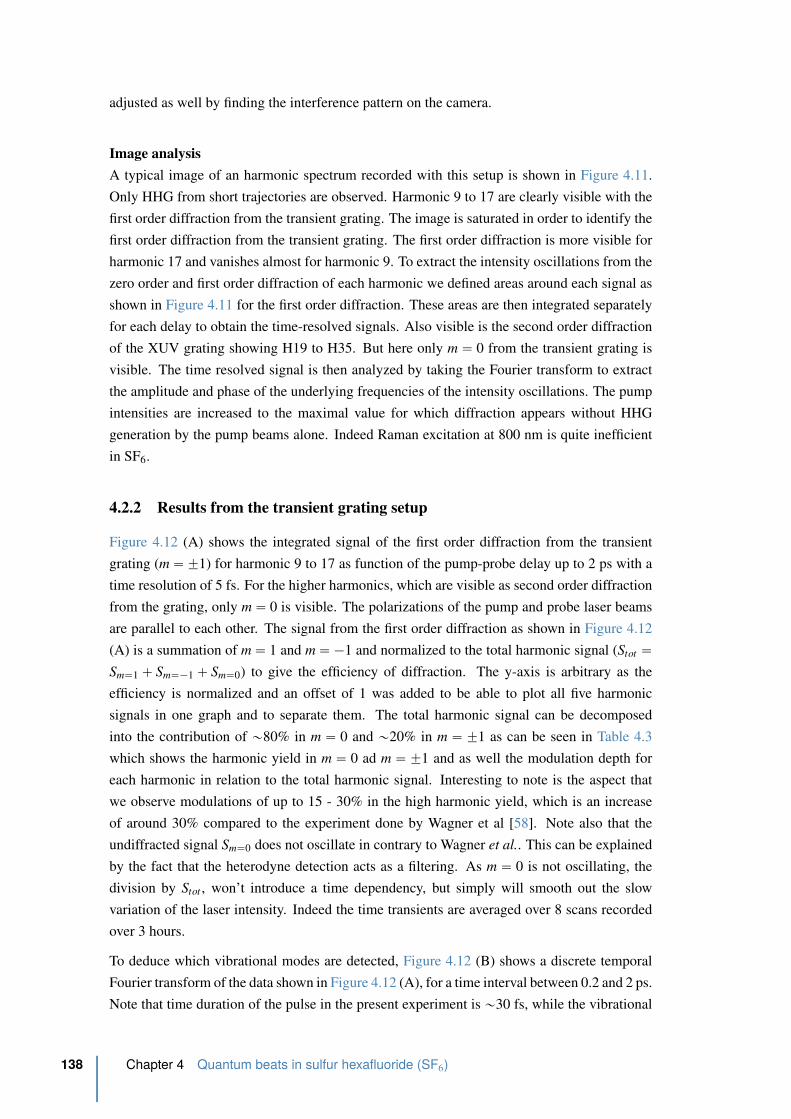
adjusted as well by finding the interference pattern on the camera.
Image analysis
A typical image of an harmonic spectrum recorded with this setup is shown in Figure 4.11.
Only HHG from short trajectories are observed. Harmonic 9 to 17 are clearly visible with the
first order diffraction from the transient grating. The image is saturated in order to identify the
first order diffraction from the transient grating. The first order diffraction is more visible for
harmonic 17 and vanishes almost for harmonic 9. To extract the intensity oscillations from the
zero order and first order diffraction of each harmonic we defined areas around each signal as
shown in Figure 4.11 for the first order diffraction. These areas are then integrated separately
for each delay to obtain the time-resolved signals. Also visible is the second order diffraction
of the XUV grating showing H19 to H35. But here only m “ 0 from the transient grating is
visible. The time resolved signal is then analyzed by taking the Fourier transform to extract
the amplitude and phase of the underlying frequencies of the intensity oscillations. The pump
intensities are increased to the maximal value for which diffraction appears without HHG
generation by the pump beams alone. Indeed Raman excitation at 800 nm is quite inefficient
in SF6.
4.2.2 Results from the transient grating setup
Figure 4.12 (A) shows the integrated signal of the first order diffraction from the transient
grating (m “ ˘1) for harmonic 9 to 17 as function of the pump-probe delay up to 2 ps with a
time resolution of 5 fs. For the higher harmonics, which are visible as second order diffraction
from the grating, only m “ 0 is visible. The polarizations of the pump and probe laser beams
are parallel to each other. The signal from the first order diffraction as shown in Figure 4.12
(A) is a summation of m “ 1 and m “ ´1 and normalized to the total harmonic signal (Stot “Sm“1 ` Sm“´1 ` Sm“0) to give the efficiency of diffraction. The y-axis is arbitrary as the
efficiency is normalized and an offset of 1 was added to be able to plot all five harmonic
signals in one graph and to separate them. The total harmonic signal can be decomposed
into the contribution of „80% in m “ 0 and „20% in m “ ˘1 as can be seen in Table 4.3
which shows the harmonic yield in m “ 0 ad m “ ˘1 and as well the modulation depth for
each harmonic in relation to the total harmonic signal. Interesting to note is the aspect that
we observe modulations of up to 15 - 30% in the high harmonic yield, which is an increase
of around 30% compared to the experiment done by Wagner et al [58]. Note also that the
undiffracted signal Sm“0 does not oscillate in contrary to Wagner et al.. This can be explained
by the fact that the heterodyne detection acts as a filtering. As m “ 0 is not oscillating, the
division by Stot , won’t introduce a time dependency, but simply will smooth out the slow
variation of the laser intensity. Indeed the time transients are averaged over 8 scans recorded
over 3 hours.
To deduce which vibrational modes are detected, Figure 4.12 (B) shows a discrete temporal
Fourier transform of the data shown in Figure 4.12 (A), for a time interval between 0.2 and 2 ps.
Note that time duration of the pulse in the present experiment is „30 fs, while the vibrational
138 Chapter 4 Quantum beats in sulfur hexafluoride (SF6)
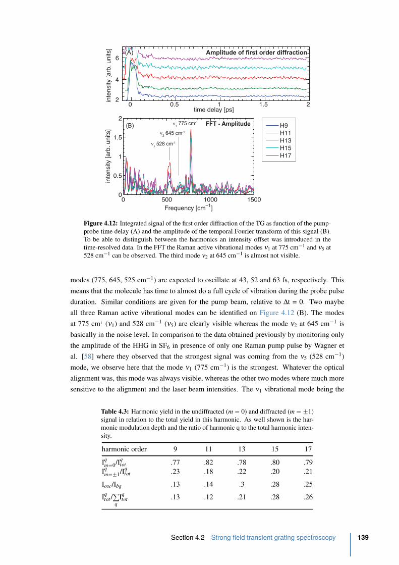
(B)
0 500 1000 15000
0.5
1
1.5
2
Frequency [cm−1]
inte
nsity
[arb
. uni
ts]
0 0.5 1 1.5 22
4
6
inte
nsity
[arb
. uni
ts]
time delay [ps]
Amplitude of first order diffraction
H9H11H13H15H17
FFT - Amplitude
ν5 528 cm-1
ν2 645 cm-1
ν1 775 cm-1
(A)
Figure 4.12: Integrated signal of the first order diffraction of the TG as function of the pump-
probe time delay (A) and the amplitude of the temporal Fourier transform of this signal (B).
To be able to distinguish between the harmonics an intensity offset was introduced in the
time-resolved data. In the FFT the Raman active vibrational modes ν1 at 775 cm´1 and ν5 at
528 cm´1 can be observed. The third mode ν2 at 645 cm´1 is almost not visible.
modes (775, 645, 525 cm´1) are expected to oscillate at 43, 52 and 63 fs, respectively. This
means that the molecule has time to almost do a full cycle of vibration during the probe pulse
duration. Similar conditions are given for the pump beam, relative to ∆t = 0. Two maybe
all three Raman active vibrational modes can be identified on Figure 4.12 (B). The modes
at 775 cm1 (ν1) and 528 cm´1 (ν5) are clearly visible whereas the mode ν2 at 645 cm´1 is
basically in the noise level. In comparison to the data obtained previously by monitoring only
the amplitude of the HHG in SF6 in presence of only one Raman pump pulse by Wagner et
al. [58] where they observed that the strongest signal was coming from the ν5 (528 cm´1)
mode, we observe here that the mode ν1 (775 cm´1) is the strongest. Whatever the optical
alignment was, this mode was always visible, whereas the other two modes where much more
sensitive to the alignment and the laser beam intensities. The ν1 vibrational mode being the
Table 4.3: Harmonic yield in the undiffracted (m “ 0) and diffracted (m “ ˘1)
signal in relation to the total yield in this harmonic. As well shown is the har-
monic modulation depth and the ratio of harmonic q to the total harmonic inten-
sity.
harmonic order 9 11 13 15 17
Iqm“0/I
qtot .77 .82 .78 .80 .79
Iqm“˘1/I
qtot .23 .18 .22 .20 .21
Iosc/Ibg .13 .14 .3 .28 .25
Iqtot /
ř
q
Iqtot .13 .12 .21 .28 .26
Section 4.2 Strong field transient grating spectroscopy 139
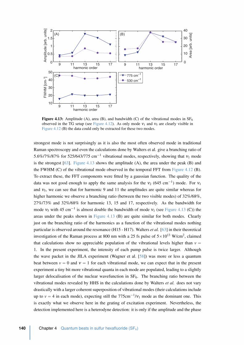
775 cm−1
530 cm−1
9 11 13 15 1710
20
30
40
50
harmonic order
(C)
FW
HM
[cm
_1]
9 11 13 15 17 0
10
20
30
40
harmonic order
(B)
Are
a [
arb
. u
nits]
9 11 13 15 170
0.5
1
1.5
2
harmonic order
(A)
Am
plit
ud
e [
arb
. u
nits]
Figure 4.13: Amplitude (A), area (B), and bandwidth (C) of the vibrational modes in SF6
observed in the TG setup (see Figure 4.12). As only mode ν1 and ν5 are clearly visible in
Figure 4.12 (B) the data could only be extracted for these two modes.
strongest mode is not surprisingly as it is also the most often observed mode in traditional
Raman spectroscopy and even the calculations done by Walters et al. give a branching ratio of
5.6%/7%/87% for 525/643/775 cm´1 vibrational modes, respectively, showing that ν1 mode
is the strongest [63]. Figure 4.13 shows the amplitude (A), the area under the peak (B) and
the FWHM (C) of the vibrational mode observed in the temporal FFT from Figure 4.12 (B).
To extract these, the FFT components were fitted by a gaussian function. The quality of the
data was not good enough to apply the same analysis for the ν2 (645 cm´1) mode. For ν1
and ν5, we can see that for harmonic 9 and 11 the amplitudes are quite similar whereas for
higher harmonic we observe a branching ratio (between the two visible modes) of 32%/68%,
27%/73% and 32%/68% for harmonic 13, 15 and 17, respectively. As the bandwidth for
mode ν5 with 45 cm´1 is almost double the bandwidth of mode ν1 (see Figure 4.13 (C)) the
areas under the peaks shown in Figure 4.13 (B) are quite similar for both modes. Clearly
just on the branching ratio of the harmonics as a function of the vibrational modes nothing
particular is observed around the resonance (H15 - H17). Walters et al. [63] in their theoretical
investigation of the Raman process at 800 nm with a 25 fs pulse of 5ˆ1013 W/cm2, claimed
that calculations show no appreciable population of the vibrational levels higher than v “1. In the present experiment, the intensity of each pump pulse is twice larger. Although
the wave packet in the JILA experiment (Wagner et al. [58]) was more or less a quantum
beat between v “ 0 and ν “ 1 for each vibrational mode, we can expect that in the present
experiment a tiny bit more vibrational quanta in each mode are populated, leading to a slightly
larger delocalisation of the nuclear wavefunction in SF6. The branching ratio between the
vibrational modes revealed by HHS in the calculations done by Walters et al. does not vary
drastically with a larger coherent superposition of vibrational modes (their calculations include
up to v “ 4 in each mode), expecting still the 775cm´1/ν1 mode as the dominant one. This
is exactly what we observe here in the grating of excitation experiment. Nevertheless, the
detection implemented here is a heterodyne detection: it is only if the amplitude and the phase
140 Chapter 4 Quantum beats in sulfur hexafluoride (SF6)
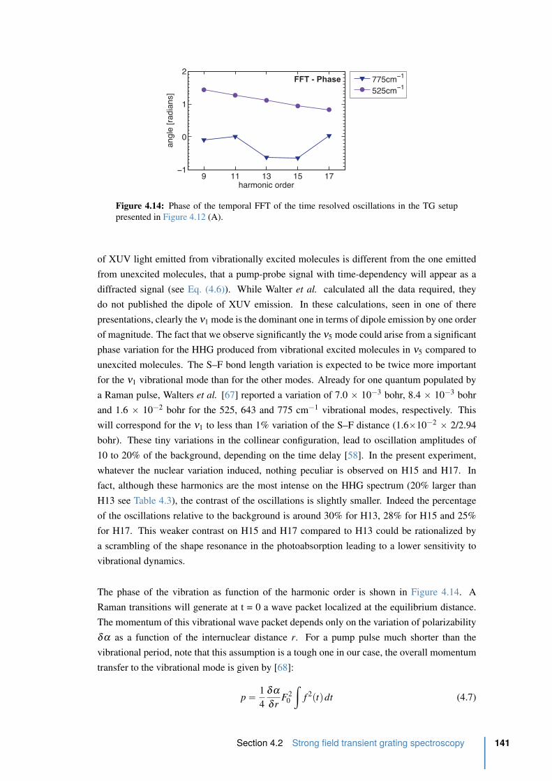
9 11 13 15 17−1
0
1
2
harmonic order
angl
e [r
adia
ns]
775cm−1
525cm−1FFT - Phase
Figure 4.14: Phase of the temporal FFT of the time resolved oscillations in the TG setup
presented in Figure 4.12 (A).
of XUV light emitted from vibrationally excited molecules is different from the one emitted
from unexcited molecules, that a pump-probe signal with time-dependency will appear as a
diffracted signal (see Eq. (4.6)). While Walter et al. calculated all the data required, they
do not published the dipole of XUV emission. In these calculations, seen in one of there
presentations, clearly the ν1 mode is the dominant one in terms of dipole emission by one order
of magnitude. The fact that we observe significantly the ν5 mode could arise from a significant
phase variation for the HHG produced from vibrational excited molecules in ν5 compared to
unexcited molecules. The S–F bond length variation is expected to be twice more important
for the ν1 vibrational mode than for the other modes. Already for one quantum populated by
a Raman pulse, Walters et al. [67] reported a variation of 7.0 ˆ 10´3 bohr, 8.4 ˆ 10´3 bohr
and 1.6 ˆ 10´2 bohr for the 525, 643 and 775 cm´1 vibrational modes, respectively. This
will correspond for the ν1 to less than 1% variation of the S–F distance (1.6ˆ10´2 ˆ 2/2.94
bohr). These tiny variations in the collinear configuration, lead to oscillation amplitudes of
10 to 20% of the background, depending on the time delay [58]. In the present experiment,
whatever the nuclear variation induced, nothing peculiar is observed on H15 and H17. In
fact, although these harmonics are the most intense on the HHG spectrum (20% larger than
H13 see Table 4.3), the contrast of the oscillations is slightly smaller. Indeed the percentage
of the oscillations relative to the background is around 30% for H13, 28% for H15 and 25%
for H17. This weaker contrast on H15 and H17 compared to H13 could be rationalized by
a scrambling of the shape resonance in the photoabsorption leading to a lower sensitivity to
vibrational dynamics.
The phase of the vibration as function of the harmonic order is shown in Figure 4.14. A
Raman transitions will generate at t = 0 a wave packet localized at the equilibrium distance.
The momentum of this vibrational wave packet depends only on the variation of polarizability
δα as a function of the internuclear distance r. For a pump pulse much shorter than the
vibrational period, note that this assumption is a tough one in our case, the overall momentum
transfer to the vibrational mode is given by [68]:
p “ 1
4
δα
δ rF2
0
ż
f 2ptqdt (4.7)
Section 4.2 Strong field transient grating spectroscopy 141
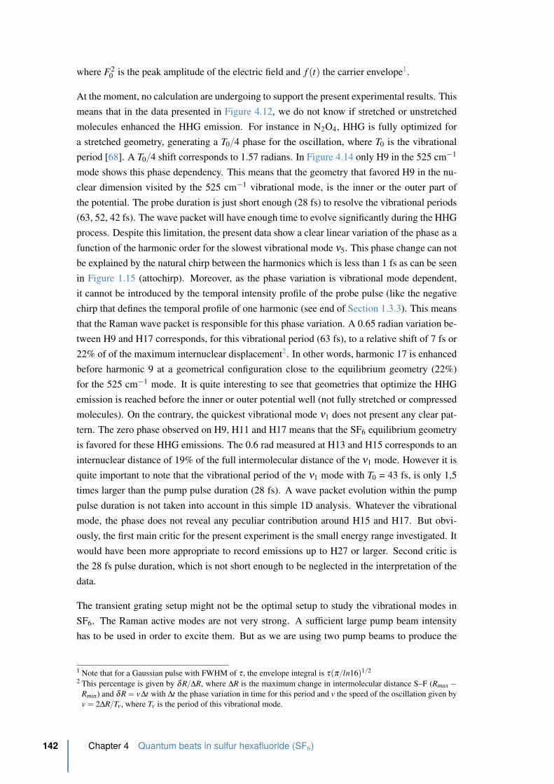
where F20 is the peak amplitude of the electric field and f ptq the carrier envelope1.
At the moment, no calculation are undergoing to support the present experimental results. This
means that in the data presented in Figure 4.12, we do not know if stretched or unstretched
molecules enhanced the HHG emission. For instance in N2O4, HHG is fully optimized for
a stretched geometry, generating a T04 phase for the oscillation, where T0 is the vibrational
period [68]. A T04 shift corresponds to 1.57 radians. In Figure 4.14 only H9 in the 525 cm´1
mode shows this phase dependency. This means that the geometry that favored H9 in the nu-
clear dimension visited by the 525 cm´1 vibrational mode, is the inner or the outer part of
the potential. The probe duration is just short enough (28 fs) to resolve the vibrational periods
(63, 52, 42 fs). The wave packet will have enough time to evolve significantly during the HHG
process. Despite this limitation, the present data show a clear linear variation of the phase as a
function of the harmonic order for the slowest vibrational mode ν5. This phase change can not
be explained by the natural chirp between the harmonics which is less than 1 fs as can be seen
in Figure 1.15 (attochirp). Moreover, as the phase variation is vibrational mode dependent,
it cannot be introduced by the temporal intensity profile of the probe pulse (like the negative
chirp that defines the temporal profile of one harmonic (see end of Section 1.3.3). This means
that the Raman wave packet is responsible for this phase variation. A 0.65 radian variation be-
tween H9 and H17 corresponds, for this vibrational period (63 fs), to a relative shift of 7 fs or
22% of of the maximum internuclear displacement2. In other words, harmonic 17 is enhanced
before harmonic 9 at a geometrical configuration close to the equilibrium geometry (22%)
for the 525 cm´1 mode. It is quite interesting to see that geometries that optimize the HHG
emission is reached before the inner or outer potential well (not fully stretched or compressed
molecules). On the contrary, the quickest vibrational mode ν1 does not present any clear pat-
tern. The zero phase observed on H9, H11 and H17 means that the SF6 equilibrium geometry
is favored for these HHG emissions. The 0.6 rad measured at H13 and H15 corresponds to an
internuclear distance of 19% of the full intermolecular distance of the ν1 mode. However it is
quite important to note that the vibrational period of the ν1 mode with T0 = 43 fs, is only 1,5
times larger than the pump pulse duration (28 fs). A wave packet evolution within the pump
pulse duration is not taken into account in this simple 1D analysis. Whatever the vibrational
mode, the phase does not reveal any peculiar contribution around H15 and H17. But obvi-
ously, the first main critic for the present experiment is the small energy range investigated. It
would have been more appropriate to record emissions up to H27 or larger. Second critic is
the 28 fs pulse duration, which is not short enough to be neglected in the interpretation of the
data.
The transient grating setup might not be the optimal setup to study the vibrational modes in
SF6. The Raman active modes are not very strong. A sufficient large pump beam intensity
has to be used in order to excite them. But as we are using two pump beams to produce the
1 Note that for a Gaussian pulse with FWHM of τ , the envelope integral is τpπln16q12
2 This percentage is given by δR∆R, where ∆R is the maximum change in intermolecular distance S–F (Rmax ´Rmin) and δR “ v∆t with ∆t the phase variation in time for this period and v the speed of the oscillation given by
v “ 2∆RTv, where Tv is the period of this vibrational mode.
142 Chapter 4 Quantum beats in sulfur hexafluoride (SF6)
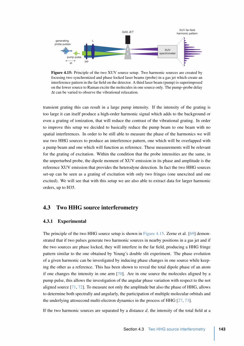
generating
probe pulses
pump pulse
Δt
XUV far-field
harmonic patternGAS JET
XUV
spectrometer
PP
L
Figure 4.15: Principle of the two XUV source setup. Two harmonic sources are created by
focusing two synchronized and phase locked laser beams (probe) in a gas jet which create an
interference pattern in the far field on the detector. A third laser beam (pump) is superimposed
on the lower source to Raman excite the molecules in one source only. The pump–probe delay
∆t can be varied to observe the vibrational relaxation.
transient grating this can result in a large pump intensity. If the intensity of the grating is
too large it can itself produce a high-order harmonic signal which adds to the background or
even a grating of ionization, that will reduce the contrast of the vibrational grating. In order
to improve this setup we decided to basically reduce the pump beam to one beam with no
spatial interferences. In order to be still able to measure the phase of the harmonics we will
use two HHG sources to produce an interference pattern, one which will be overlapped with
a pump beam and one which will function as reference. These measurements will be relevant
for the grating of excitation. Within the condition that the probe intensities are the same, in
the unperturbed probe, the dipole moment of XUV emission in its phase and amplitude is the
reference XUV emission that provides the heterodyne detection. In fact the two HHG sources
set-up can be seen as a grating of excitation with only two fringes (one unexcited and one
excited). We will see that with this setup we are also able to extract data for larger harmonic
orders, up to H35.
4.3 Two HHG source interferometry
4.3.1 Experimental
The principle of the two HHG source setup is shown in Figure 4.15. Zerne et al. [69] demon-
strated that if two pulses generate two harmonic sources in nearby positions in a gas jet and if
the two sources are phase locked, they will interfere in the far field, producing a HHG fringe
pattern similar to the one obtained by Young’s double slit experiment. The phase evolution
of a given harmonic can be investigated by inducing phase changes in one source while keep-
ing the other as a reference. This has been shown to reveal the total dipole phase of an atom
if one changes the intensity in one arm [70]. Are in one source the molecules aligned by a
pump pulse, this allows the investigation of the angular phase variation with respect to the not
aligned source [71, 72]. To measure not only the amplitude but also the phase of HHG, allows
to determine both spectrally and angularly, the participation of multiple molecular orbitals and
the underlying attosecond multi-electron dynamics in the process of HHG [27, 73].
If the two harmonic sources are separated by a distance d, the intensity of the total field at a
Section 4.3 Two HHG source interferometry 143

PP
λ/2
COMPRESSOR7 mJ @ 800 nm, 28 fs
L
GAS JET
10 mJ @ 800 nm
streched to 200ps
BS
BS
M (with hole)
PhosphoreMCP
G
CCD
harmonic order
Inte
rfe
ren
ce
CCD
Figure 4.16: Schematic setup of the two HHG sources interferometry setup. The laser beam
is split into a pump and probe beam. A π-phase plate (PP) in the probe arm is generating 2
vertical separated foci in the gas jet. The pump beam is overlapped with the lower focus via
a hole mirror.
point X in an observation plane at distance L can be expressed by [69]:
Iptq “ I1 ` I2ptq ` 2a
I1 I2ptq ˆ cos
„
2πdX
λqL` ϕ1 ´ ϕ2ptq
(4.8)
where I1 and I2ptq are the intensities of the two harmonic beams at the same point, λq the
wavelength of the harmonic order q and ϕ1, ϕ2 are the phases of the generated fields at the
observation point at time t. The pump pulse is superposed to I2, making I2 time-dependent in
amplitude and phase. In the simple case, with no intensity-dependent phase and no chirp, the
visibility or contrast of the fringes is given by:
V “ Imax ´ Imin
Imax ` Imin“ 2
a
I1I2
1 ` pI1I2q (4.9)
which is equal to 1 when both sources have the same intensity.
The setup is shown in Figure 4.16. The laser beam after the compressor is divided into two
parts. The generating arm passes through a long translation stage to be able to vary the delay
between the pump and probe laser pulse. A π-phase plate1 is introduced to generate 2 spots
at the focus in order to generate the two HHG sources. The π-phase plate is introducing a
phase shift of π between the upper and lower part of the 800 nm laser beam, so that in the
focus (far field) we observe two spots separated vertically due to the interference of the upper
and lower beam as shown in Figure 4.16, recorded with a CCD camera put into the focus
of the probe beam. High harmonics are generated by focusing the pulses with a f = 50 cm
lens in a continuous jet produced by a 250 µm nozzle backed by a few hundreds of mbars of
gas. Typically energies of 500 µJ/p and 300 µJ/p were used for the probe and pump pulse,
respectively. The emitted radiation is analyzed by an extreme ultraviolet spectrometer the
same way as with the previous experiment.
1 The π phase is only a variation of the thickness of a fused silica plate by λ2 = 400 nm
144 Chapter 4 Quantum beats in sulfur hexafluoride (SF6)

probes alone pump + probes
lower part blocked
upper part blocked
image center
(A)
(B)
(C) (D)
Figure 4.17: Two HHG source alignment. (A) and (B) shows the harmonic spectrum with
the upper and lower part, respectively, of the beam blocked. (C) and (D) the interference
pattern without and with the pump beam, respectively.
Alignment
To be sure that the pump beam is only overlapping with one of the two sources we observed the
fringes at a long positive time delay with the highest available intensity of the pump beam. In
theory if the pump beam is strong enough to ionize the molecules, the later arriving probe pulse
is not able to generate HHG anymore in this volume. This should kill the fringes observed on
the detector in the far field, leaving only the XUV light generated by the other HHG source
visible. Figure 4.17 (A) and (B) shows what happens if half of the beam is blocked. The
fringes are lost and the XUV beam in the far field is on the upper (A) or lower (B) part of
the MCP when the upper or lower part is blocked, respectively. This can be explained as by
blocking the upper or lower part of the beam, the beam is not going through the center of the
lens which results in a kick upwards or downwards. Figure 4.17 (C) and (D) shows the HHG
fringe pattern of the two sources without and with the pump pulse, repevely. We can clearly
see that with the pump beam the fringe pattern is reduced and moved downwards indicating
an overlap with the lower beam in the focus.
Image analysis
The HHG interference pattern was taken as a function of the pump-probe delay for a pump
intensity of 300-330 µJ/p. A typical recorded interferometric HHG spectrum recorded in SF6
at a pump-probe delay of 1 ps is shown in Figure 4.18. We are able to resolve harmonic 9 to
17 and as well visible is the second order of diffraction of the grating from harmonic 19 to
35. The data analysis is basically done in two steps. First the spatial Fourier transformation
(sFFT) of the interference pattern for each harmonic is taken as a function of pump-probe
delay. This first sFFT allows to extract an amplitude and phase of the spatial interferences for
each pump-probe delay which we will call spatial amplitude (SA) and spatial phase (SP). The
spatial phase of the interferogram gives us access to another observable. This spatial phase as
function of the pump-probe delay will also have the oscillations encoded but does not depend
on the laser intensities, which makes it less sensitive to any laser fluctuation. Afterwards in
the second step the temporal FFT (tFFT) is produced from this amplitude and this new phase
Section 4.3 Two HHG source interferometry 145
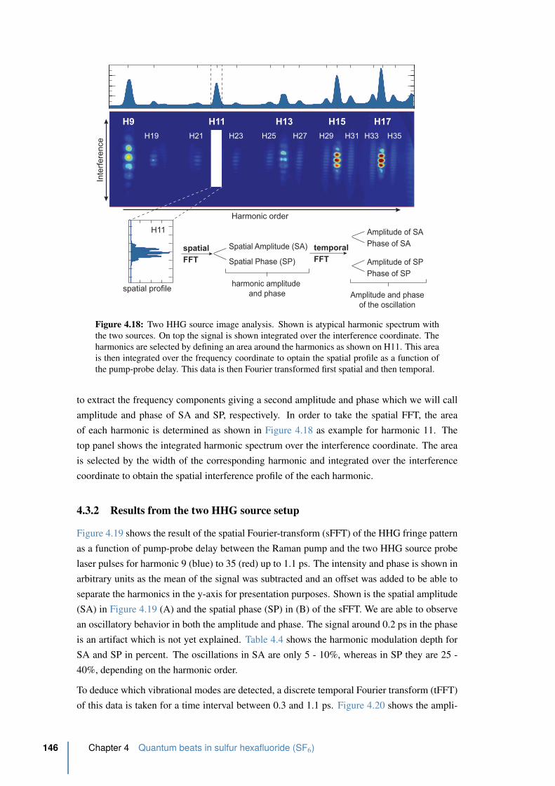
H9
H19
H11
H23
H13
H27
H15
H31
H17
H35H21 H25 H29 H33
Harmonic order
Inte
rfe
ren
ce
spatial profile
H11
spatial
FFT
Spatial Amplitude (SA)
Spatial Phase (SP)
temporal
FFT
Amplitude of SA
Amplitude of SP
Phase of SA
Phase of SP
harmonic amplitude
and phase Amplitude and phase
of the oscillation
Figure 4.18: Two HHG source image analysis. Shown is atypical harmonic spectrum with
the two sources. On top the signal is shown integrated over the interference coordinate. The
harmonics are selected by defining an area around the harmonics as shown on H11. This area
is then integrated over the frequency coordinate to optain the spatial profile as a function of
the pump-probe delay. This data is then Fourier transformed first spatial and then temporal.
to extract the frequency components giving a second amplitude and phase which we will call
amplitude and phase of SA and SP, respectively. In order to take the spatial FFT, the area
of each harmonic is determined as shown in Figure 4.18 as example for harmonic 11. The
top panel shows the integrated harmonic spectrum over the interference coordinate. The area
is selected by the width of the corresponding harmonic and integrated over the interference
coordinate to obtain the spatial interference profile of the each harmonic.
4.3.2 Results from the two HHG source setup
Figure 4.19 shows the result of the spatial Fourier-transform (sFFT) of the HHG fringe pattern
as a function of pump-probe delay between the Raman pump and the two HHG source probe
laser pulses for harmonic 9 (blue) to 35 (red) up to 1.1 ps. The intensity and phase is shown in
arbitrary units as the mean of the signal was subtracted and an offset was added to be able to
separate the harmonics in the y-axis for presentation purposes. Shown is the spatial amplitude
(SA) in Figure 4.19 (A) and the spatial phase (SP) in (B) of the sFFT. We are able to observe
an oscillatory behavior in both the amplitude and phase. The signal around 0.2 ps in the phase
is an artifact which is not yet explained. Table 4.4 shows the harmonic modulation depth for
SA and SP in percent. The oscillations in SA are only 5 - 10%, whereas in SP they are 25 -
40%, depending on the harmonic order.
To deduce which vibrational modes are detected, a discrete temporal Fourier transform (tFFT)
of this data is taken for a time interval between 0.3 and 1.1 ps. Figure 4.20 shows the ampli-
146 Chapter 4 Quantum beats in sulfur hexafluoride (SF6)
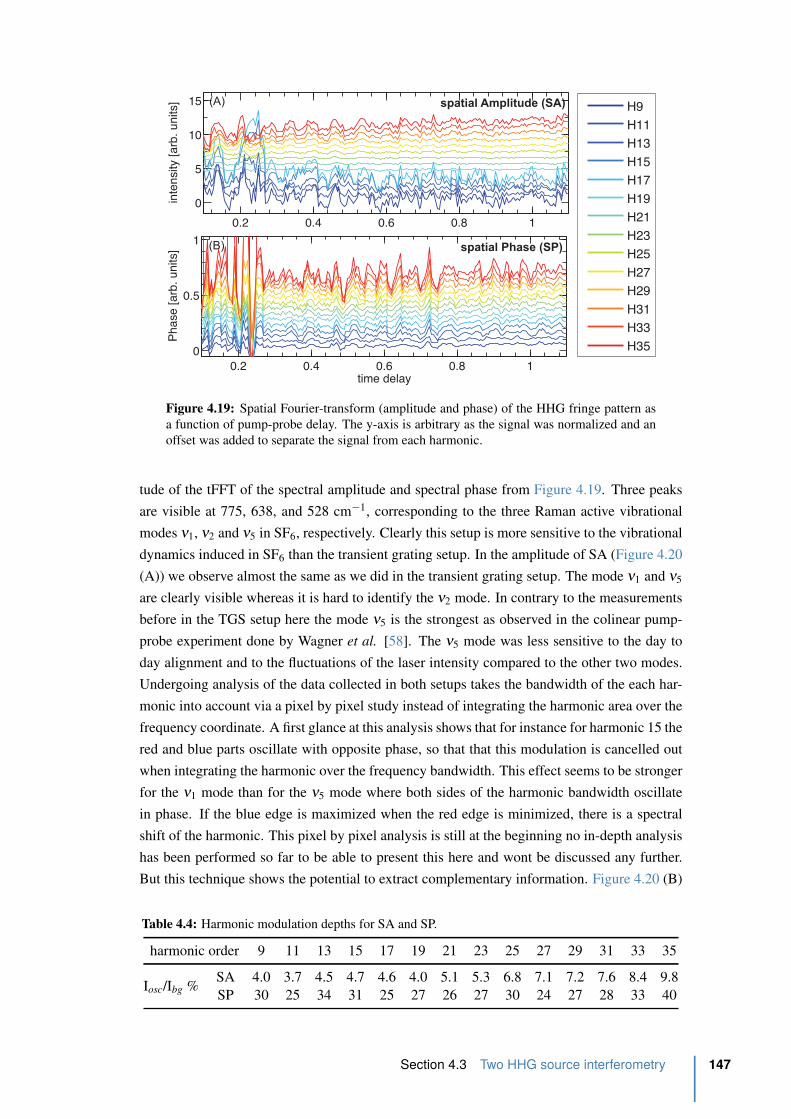
0.2 0.4 0.6 0.8 10
0.5
1
Pha
se [a
rb. u
nits
]
time delay
0.2 0.4 0.6 0.8 1
0
5
10
15
inte
nsity
[arb
. uni
ts] H9
H11H13H15H17H19H21H23H25H27H29H31H33H35
spatial Phase (SP)
spatial Amplitude (SA)(A)
(B)
Figure 4.19: Spatial Fourier-transform (amplitude and phase) of the HHG fringe pattern as
a function of pump-probe delay. The y-axis is arbitrary as the signal was normalized and an
offset was added to separate the signal from each harmonic.
tude of the tFFT of the spectral amplitude and spectral phase from Figure 4.19. Three peaks
are visible at 775, 638, and 528 cm´1, corresponding to the three Raman active vibrational
modes ν1, ν2 and ν5 in SF6, respectively. Clearly this setup is more sensitive to the vibrational
dynamics induced in SF6 than the transient grating setup. In the amplitude of SA (Figure 4.20
(A)) we observe almost the same as we did in the transient grating setup. The mode ν1 and ν5
are clearly visible whereas it is hard to identify the ν2 mode. In contrary to the measurements
before in the TGS setup here the mode ν5 is the strongest as observed in the colinear pump-
probe experiment done by Wagner et al. [58]. The ν5 mode was less sensitive to the day to
day alignment and to the fluctuations of the laser intensity compared to the other two modes.
Undergoing analysis of the data collected in both setups takes the bandwidth of the each har-
monic into account via a pixel by pixel study instead of integrating the harmonic area over the
frequency coordinate. A first glance at this analysis shows that for instance for harmonic 15 the
red and blue parts oscillate with opposite phase, so that that this modulation is cancelled out
when integrating the harmonic over the frequency bandwidth. This effect seems to be stronger
for the ν1 mode than for the ν5 mode where both sides of the harmonic bandwidth oscillate
in phase. If the blue edge is maximized when the red edge is minimized, there is a spectral
shift of the harmonic. This pixel by pixel analysis is still at the beginning no in-depth analysis
has been performed so far to be able to present this here and wont be discussed any further.
But this technique shows the potential to extract complementary information. Figure 4.20 (B)
Table 4.4: Harmonic modulation depths for SA and SP.
harmonic order 9 11 13 15 17 19 21 23 25 27 29 31 33 35
Iosc/Ibg %SA 4.0 3.7 4.5 4.7 4.6 4.0 5.1 5.3 6.8 7.1 7.2 7.6 8.4 9.8
SP 30 25 34 31 25 27 26 27 30 24 27 28 33 40
Section 4.3 Two HHG source interferometry 147

0 500 1000 15000
1
2
3
4
5x 10
−3
Frequency [cm−1]
inte
nsity
[arb
. uni
ts]
0 500 1000 15000
1
2
3
4
5x 10
−3
inte
nsity
[arb
. uni
ts]
H9H11H13H15H17H19H21H23H25H27H29H31H33H35
ν2 638 cm-1
ν1 775 cm-1
ν5 528 cm-1 Amplitude of SA
Amplitude of SP
(A)
(B)
Figure 4.20: Amplitude of the tFFT of the spatial amplitude and phase. All three Raman
active modes (528, 638 and 775 cm´1) are visible.
shows the amplitude of the tFFT of the spatial phase. Whereas in the amplitude of SA we al-
ways observed the ν5 mode and had difficulties to resolve the other two, in the amplitude of SP
it was easier to observe the ν1 mode. In general it was easier to observe the three vibrational
modes in the spatial phase than in the spatial amplitude. Indeed the spatial phase corresponds
to the determination where the maximum is in the interference pattern. Where the maximum
is located is not sensitive to the fluctuations of the laser intensity, in contrary to the amplitude
which is how many photons are produced. This is also reflected in the oscillation depth shown
in Table 4.4 where there is almost a factor 10 between spatial amplitude and spatial phase. This
makes the two source experiment due to the new observable of the spatial phase or harmonic
phase, more sensitive as we are not limited like in the transient grating setup to measure only
amplitudes.
It is evident that the branching ratios between the modes is changing with harmonic order. The
peaks are fitted by a gaussian function to deduce not only the amplitude but also the area under
the curve and the bandwidth at FWHM as function of the harmonic order as done before in
the grating of excitation experiment. This is shown in Figure 4.21 on the left for the amplitude
of SA and on the right for the amplitude of SP, where the amplitude was normalized to the
total signal. For points in the amplitude that are close to 1ˆ10´3 the area and the FWHM
has to be regarded as noise, as these amplitudes are in the noise level. As we are looking for
differences around harmonic 17, as observed in the static experiments (see Figure 4.2), H17 is
marked by a dotted line. In the spatial amplitude we observe that the amplitude of the ν5 (530
148 Chapter 4 Quantum beats in sulfur hexafluoride (SF6)

13 17 21 25 29 330
3
6
x 10−2
Fit Amplitude of SA
Am
plitu
de [n
orm
aliz
ed]
(A)
9
−2
Fit Amplitude of SP
9 13 17 21 25 29 330
1
2
3
4
5x 10
(D)
Am
plitu
de [n
orm
aliz
ed]
9 13 17 21 25 29 330
0.1
0.2
0.3
9 13 17 21 25 29 3340
50
60
70
80
harmonic order
9 13 17 21 25 29 330
0.05
0.1
0.15
0.2
9 13 17 21 25 29 3325
30
35
40
45
50
harmonic order
FW
HM
[cm
-1]
Are
a [a
rb. u
nits
] (B)
(F)
FW
HM
[cm
-1]
Are
a [a
rb. u
nits
]
528 cm
775 cm−1
638 cm−1−1
(C)
Figure 4.21: Amplitude, area, and bandwidth of the vibrational modes in SF6 observed in
the two HHG source setup (see Figure 4.20). (A)-(C) amplitude of SA, (D)-(F) amplitude of
SP. The horizontal lines in (A) and (D) indicate the noise level. Shown as well in (A) in grey
is the calculated HHG emission from Figure 4.5 (B) in comparision.
cm´1) mode (Figure 4.21 (A) purple) shows a minimum at harmonic 15/17 and is increasing
at higher harmonics. A minimum in the XUV spatial interferences, filtered at 525 cm´1 could
mean that the phase between the two XUV beams around H15/17 are quite similar for this
vibrational wave packet. This minimum cannot come from the overall harmonic emission
minimum as it is the difference in amplitude of excited and non-excited molecules. This
means that it is really an effect introduced by the vibrational wave packet, which corresponds
exactly to the switching between the two molecular orbitals claimed to be involved in the
HHG emission around this energy. This is the first experimental evidence that a particular
high-order harmonic process in affected by a vibrational excited molecule, in SF6 especially
around harmonic 17. Mode ν1 at 775 cm´1 is decreasing with harmonic order and the ν2
mode at 645 cm´1 is basically constant. We also see that mode ν2 is almost not visible and
shows a bad signal-to-noise ratio as the amplitude is only slightly higher than the noise level
which is around 1ˆ10´3, indicated by the horizontal dashed line. Mode ν1 is vanishing with
harmonic order. In contrary to the experiment with the transient grating the areas under the
curves show exactly the same behavior as the amplitudes of the frequencies. In the spatial
phase we can observe a switching in the amplitudes of ν1 and ν5 before an after H13/15. For
lower harmonics than H13 the ν5 mode is stronger than the ν1 mode and after H15 it is the
Section 4.3 Two HHG source interferometry 149

9 13 17 21 25 29 33−2
−1
0
1
2
harmonic order
Phase of SP
9 13 17 21 25 29 33−2
−1
0
1
2
harmonic order
Phase of SA
525 cm
775 cm−1−1
phas
e [r
adia
ns]
phas
e [r
adia
ns]
Figure 4.22: Phase of SA and SP as function of the harmonic order from the two HHG
source setup for the the active Raman modes 775 and 528 cm´1. Also shown in grey is the
calculated HHG emission from Figure 4.5 (B) in comparision.
reverse. This could as well correspond to the switching in of the two molecular orbitals, as
the two molecular orbitals have different structures and therefore will also react differently to
different vibrational modes. The ν2 mode vanishes almost totally after harmonic 17 and the
amplitudes are lower than the noise level indicated by the horizontal dashed line. The areas
show the same behavior. Nothing exceptional is going on around harmonic 17 in the FWHM
plot.
Figure 4.22 shows the phase of the temporal FFT for the two vibrational modes ν1 and ν5
which show a nonzero amplitude (see Figure 4.21) as function of the harmonic order. In the
phase of SA in contrary to the amplitude we observe a clear feature around harmonic 15 for the
ν1. This minimum for ν1 around H17 is also visible in the phase of SP. Harmonic 11 shows
a phase jump in the phase of SA in the ν1 mode. In the phase of SP we observe as well a
phase jump at harmonic 11. In the spatial amplitude, a phase jump around harmonic 15 for
the ν5 mode at 528 cm´1 is observed. Comparing these phase features with the absorption
cross-section plot in Figure 4.6, we can identify all phase features with absorption peaks. The
ones around H15/17 corresponds to the large absorption peak associated with the shape and
autoionization resonance introduced in the introduction of this chapter and which seem to play
a large role in the HHG emission of SF6 around the energy of 25 eV. The phase feature at
H11 as well corresponds to an absorption peak which is also associated with an autoionization
resonance but which was not included in the theoretical model as no calculation is done at
this low energy. Regarding the absolute values of the phase we observe that no harmonic is
produced with a phase shift of T04 which would correspond to 1.57 radians as expected for a
Raman transition where the vibrational wave packet is created at the equilibrium distance of
the S–F bond length. But this is not surprising and the absolute values have to be regarded
with caution. As mentioned before our Raman pump pulse has a FWHM duration of around
150 Chapter 4 Quantum beats in sulfur hexafluoride (SF6)
30 fs and the vibrational periods of the encountered modes are all in this range, form 43, 52
and 63 fs for the ν1, ν2 and ν5 mode, respectively. Nevertheless,for both vibrational modes (ν1
and ν5) in SA and SP the phase shift seems to be constant as function of harmonic order, only
showing a change around harmonic 15 and 17. As mentioned before, this is the energy region
where the autoionization resonance and the shape resonance play a role in the generation of
high-order harmonics in SF6 and maybe this change is a signature of these resonance.
4.4 Conclusion
Our goal was to observe, if the S–F distance in SF6 is varied, whether the harmonic spectrum
produced in SF6 around H15 - H17 changes drastically compared to the HHG spectrum pro-
duced in static SF6. To enhance the sensitivity, the experiments are done with interferometric
techniques, based on a heterodyne detection in which the reference signal is always SF6 in
v “ 0, namely at its equilibrium geometry. One setup uses two pump pulses to create a grat-
ing of vibrational excitation in the gas jet through which the probe pulse generates high-order
harmonics. The second experiment uses two spatially separated probe pulses, both generating
a XUV beam which interfere spatially in far field. Both setups showed that they are sensi-
tive to the vibrational excitations in the generating medium. All three Raman active modes of
SF6, ν1(775 cm´1), ν2(638 cm´1), ν5(528 cm´1), could be observed in the amplitude of the
harmonic emission and as well in the phase.
For the transient grating setup it was possible to investigate harmonic 9 to 17 whereas in the
two HHG source setup the harmonic spectrum from H9 up to H35 was analyzed. In both
setups the main modes populated by this Raman excitation are the ν1 and ν5 modes as via
traditional Raman spectroscopy. For the two HHG source setup the amplitude of the ν5 mode
shows a clear minimum around harmonic 17, whereas in the phase we observe a jump around
harmonic 15. Mode ν1 shows no clear pattern in the amplitude but in the phase we observe as
well a minimum around harmonic 17. These minima cannot come from the previous observed
minimum in the harmonic emission of SF6, as we are in a heterodyne detection. This let us
conclude that the features observed here are only introduced by the change of the S–F distance
introduced by the vibrational wave packets. In addition, it seems that the harmonic emission is
not optimized for fully stretched or compressed molecules as observed in similar experiments
on N2O4. A full interpretation of these experimental results requires the development of a
theoretical model to reproduce the amplitude and phase minima. Nevertheless, this is the first
phase-resolved study of HHG, which provides a first step in understanding the origin of the
modulation in the harmonic spectrum of SF6.
As mentioned earlier, the recorded data is currently been analyzed to take the bandwidth of
each harmonic into account, with a pixel by pixel analysis. A first glance at this showed that
the intensity of the red and blue parts in the bandwidth of one harmonic is oscillating with a
phase shift and sometimes even in opposite phase. Consequently, this modulation is cancelled
out when integrating the one harmonic over the frequency coordinate as has been done in this
analysis. Damages to the detector prevents an accurate pixel by pixel analysis. Ideally the
data should be acquired again once an undamaged MCP is sourced. Furthermore, it would
Section 4.4 Conclusion 151
be interesting to use shorter pulse durations for the probe and pump pulse, as our „30 fs
pulse duration is quite close to the vibrational periods. The Raman transitions as well could
probably be enhanced by using a different pump wavelength. As well the polarization of the
pump and probe laser in this experiment was fixed to a parallel configuration and should be
changed to a crossed polarization configuration to investigate the polarization dependency of
the incident laser beams. With an undamaged MCP both experiments, the transient grating
and two sources could be realized in one integrated setup to measure both at the same time,
under the same experimental conditions, namely an interference pattern from the two probe
sources on the diffracted signals from the transient grating.
References
[1] Gianturco, FA. Electronic Properties of Sulphur Hexafluoride. II. Molecular Orbital
Interpretation of Its X-Ray Absorption Spectra. J. Chem. Phys. 57:2 840–846 (1972)
(cited p. 122).
[2] Boggs, S. Sulfur hexafluoride: Introduction to the material and dielectric. IEEE Electr.
Insul. Mag. 5:5 18–21 (1989) (cited p. 122).
[3] EFCTC, EFTC. About Sulphur hexafluoride (SF6). http://www.fluorocarbons.org/chemical-
families/sf6 () (cited p. 122).
[4] Christophorou, LG, Olthoff, JK, and Van Brunt, RJ. Sulfur hexafluoride and the elec-
tric power industry. IEEE Electr. Insul. Mag. 13:5 20–24 (1997) (cited p. 122).
[5] Ihmels, EC and Gmehling, J. Densities of sulfur hexafluoride and dinitrogen monox-
ide over a wide temperature and pressure range in the sub-and supercritical states.
International Journal of Thermophysics 23:3 709–743 (2002) (cited p. 122).
[6] Olivet, A and Vega, LF. Optimized molecular force field for sulfur hexafluoride simu-
lations. J. Chem. Phys. 126:14 pages (2007) (cited p. 122).
[7] Maggon, KK. Medical uses of sulfur hexafluoride. Drugs of the Future 19: 1101 (1994)
(cited p. 122).
[8] RF, W and JT, T. Prediction of the kinetics of disappearance of sulfur hexafluoride
and perfluoropropane intraocular gas bubbles. Ophthalmology 95:5 609–613 (1988)
(cited p. 122).
[9] Schneider, M. SonoVue, a new ultrasound contrast agent. Eur. Radiol. 9:S3 S347–
S348 (1999) (cited p. 122).
[10] Khalil, M. Non-CO2 greenhouse gases in the atmosphere. Annual Review of Energy
and the Environment 24:1 645–661 (1999) (cited p. 122).
[11] Geller, LS, Elkins, JW, Lobert, JM, Clarke, AD, Hurst, DF, Butler, JH, and Myers,
RC. Tropospheric SF6: Observed latitudinal distribution and trends, derived emissions
and interhemispheric exchange time. Geophys. Res. Lett. 24:6 675–678 (1997) (cited
p. 122).
[12] Reilly, J, Mayer, M, and Harnisch, J. The Kyoto Protocol and non-CO2 greenhouse
gases and carbon sinks. Environmental Modeling & Assessment 7:4 217–229 (2002)
(cited p. 122).
[13] Maiss, M, Steele, LP, Francey, RJ, Fraser, PJ, Langenfelds, RL, Trivett, NBA, and
Levin, I. Sulfur hexafluoride - A powerful new atmospheric tracer. Atmos Environ
30:10-11 1621–1629 (1996) (cited p. 122).
[14] Boudon, V and Pierre, G. Rovibrational spectroscopy of sulfur hexafluoride: A review.
Recent Res. Devel. Mol. Spec. 1: 25–55 (2002) (cited p. 122).
152 Chapter 4 Quantum beats in sulfur hexafluoride (SF6)
[15] Boudon, V, Hepp, M, Herman, M, Pak, I, and Pierre, G. High-Resolution Jet-Cooled
Spectroscopy of SF6: The ν2 ` ν6 Combination Band of 32SF6 and the ν3 Band of the
Rare Isotopomers. J. Mol. Spec. 192:2 359–367 (1998) (cited p. 122).
[16] Bermejo, D, Martinez, RZ, Loubignac, E, Boudon, V, and Pierre, G. Simultaneous
Analysis of the ν2 Raman and ν2 + ν6 Infrared Spectra of the SF6 Molecule. J. Mol.
Spec. 201:1 164–171 (2000) (cited p. 122).
[17] Boudon, V, Pierre, G, and Burger, H. High-Resolution Spectroscopy and Analysis of
the ν4 Bending Region of SF6 near 615 cm´1. J. Mol. Spec. 205:2 304–311 (2001)
(cited p. 122).
[18] Boudon, V and Bermejo, D. First High-Resolution Raman Spectrum and Analysis
of the ν5 Bending Fundamental of SF6. J. Mol. Spec. 213:2 139–144 (2002) (cited
p. 122).
[19] L O Brockway, LP. The Determination of the Structures of the Hexafluorides of Sulfur,
Selenium and Tellurium by the Electron Diffraction Method. Proc. Natl. Acad. Sci.
19:1 68 (1933) (cited p. 122).
[20] Ruf, H, Handschin, C, Ferre, A, Thire, N, Bertrand, JB, Bonnet, L, Cireasa, R, Con-
stant, E, Corkum, PB, Descamps, D, Fabre, B, Larregaray, P, Mevel, E, Petit, S, Pons,
B, Staedter, D, Worner, HJ, Villeneuve, DM, Mairesse, Y, Halvick, P, and Blanchet, V.
High-harmonic transient grating spectroscopy of NO2 electronic relaxation. J. Chem.
Phys. 137: 224303 (2012) (cited p. 122).
[21] Smirnova, O, Patchkovskii, S, Mairesse, Y, Dudovich, N, and Ivanov, MY. Strong-field
control and spectroscopy of attosecond electron-hole dynamics in molecules. Proc.
Natl. Acad. Sci. 106:39 16556–16561 (2009) (cited p. 122).
[22] Haessler, S, Caillat, J, Boutu, W, Giovanetti-Teixeira, C, Ruchon, T, Auguste, T, Di-
veki, Z, Breger, P, Maquet, A, ’e, BC, ieb, RT, and eres, PS. Attosecond imaging of
molecular electronic wavepackets. Nature Phys. 6: 200–206 (2010) (cited p. 122).
[23] Lynga, C, L’Huillier, A, and Wahlstrom, CG. High-order harmonic generation in
molecular gases. J. Phys. B 29:14 3293–3302 (1996) (cited p. 123, 124).
[24] Sasanuma, M, Ishiguro, E, Masuko, H, Morioka, Y, and Nakamura, M. Absorption
structures of SF6 in the VUV region. Journal of Physics B: Atomic and Molecular
Physics 11:21 3655 (1978) (cited p. 123, 130, 131).
[25] Paul, PM, Toma, ES, Breger, P, Mullot, G, Balcou, P, Muller, HG, and Agostini, P.
Observation of a Train of Attosecond Pulses from High Harmonic Generation. Science
292:5522 1689–1692 (2001) (cited p. 124).
[26] Higuet, J, Ruf, H, Thire, N, Cireasa, R, Constant, E, Cormier, E, Descamps, D, Mevel,
E, Petit, S, Pons, B, Mairesse, Y, and Fabre, B. High-order harmonic spectroscopy of
the Cooper minimum in argon: Experimental and theoretical study. Phys. Rev. A 83:5
053401 (2011) (cited p. 124).
[27] Smirnova, O, Mairesse, Y, Patchkovskii, S, Dudovich, N, Villeneuve, D, Corkum, P,
and Ivanov, MY. High harmonic interferometry of multi-electron dynamics in molecules.
Nature 460:7258 972–977 (2009) (cited p. 124, 143).
[28] Cireasa, R, Bhardwaj, R, Blanchet, V, Boguslavsky, A, Descamps, D, Fabre, B, Legare,
F, Mairesse, Y, Patchkovskii, S, Pons, B, Ruf, H, Schmidt, B, Surarez, J, Thire, N, and
Wong, M. High-harmonic generation sensitive to chirality. in preparation for Nature
Physics (2013) (cited p. 125).
[29] Mairesse, Y, Dudovich, N, Levesque, J, Ivanov, MY, Corkum, PB, and Villeneuve,
DM. Electron wavepacket control with elliptically polarized laser light in high har-
monic generation from aligned molecules. New Jour. Phys. 10: 025015 (2008) (cited
p. 125).
References 153
[30] Wong, MCH, Brichta, JP, and Bhardwaj, VR. Signatures of symmetry and electronic
structure in high-order harmonic generation in polyatomic molecules. Phys. Rev. A
81:6 061402 (2010) (cited p. 125).
[31] Wodkiewicz, K. Classical and quantum Malus laws. Phys. Rev. A 51:4 2785 (1995)
(cited p. 125).
[32] Kahr, B and Claborn, K. The Lives of Malus and His Bicentennial Law. Chem. Phys.
Chem. 9:1 43–58 (2008) (cited p. 125).
[33] Collett, E. Field guide to polarization. Vol. FG05. SPIE PRESS BOOK, 2005 (cited
p. 125).
[34] Antoine, P, Carre, B, L’Huillier, A, and Lewenstein, M. Polarization of high-order
harmonics. Phys. Rev. A 55:2 1314 (1997) (cited p. 125).
[35] Shafir, D, Mairesse, Y, Villeneuve, DM, Corkum, PB, and Dudovich, N. Atomic wave-
functions probed through strong-field light-matter interaction. Nature Phys. 5:6 412–
416 (2009) (cited p. 126).
[36] Shafir, D, Fabre, B, Higuet, J, Soifer, H, Dagan, M, Descamps, D, Mevel, E, Petit, S,
Worner, HJ, Pons, B, Dudovich, N, and Mairesse, Y. Role of the Ionic Potential in
High Harmonic Generation. Phys. Rev. Lett. 108:20 203001 (2012) (cited p. 126).
[37] Pavlychev, AA, Brykalova, XO, Mistrov, DA, Flesch, R, and Ruhl, E. Position and
line shape of the 2t2g-shape resonance in S 2p-excited sulfur hexafluoride clusters. J.
Electron Spec. and Relat. Phen. 166-167: 45–52 (2008) (cited p. 126, 131).
[38] Holland, D, MacDonald, MA, Baltzer, P, Karlsson, L, Lundqvist, M, Wannberg, B,
and Niessen, W von. An experimental and theoretical study of the valence shell photo-
electron spectrum of sulphur hexafluoride. Chem. Phys. 192:3 333–353 (1995) (cited
p. 126).
[39] Christophorou, LG and Olthoff, JK. Electron interactions with SF6. J. Phys. B 29:3
267–330 (2000) (cited p. 127).
[40] Mairesse, Y. Generation et caracterisation d’impulsions attosecondes. PhD thesis.
Universite Paris X1 Orsay, 2005 (cited p. 127).
[41] Yang, L, Agren, H, Carravetta, V, Vahtras, O, Karlsson, L, Wannberg, B, Holland,
D, and MacDonald, MA. Energy-dependent valence photoelectron spectra of SF6. Ab
initio calculations and measurements. J. Electron Spec. and Relat. Phen. 94: 163–179
(1997) (cited p. 129).
[42] Stener, M, Toffoli, D, Fronzoni, G, and Decleva, P. Time dependent density functional
study of the photoionization dynamics of SF6. J. Chem. Phys. 124:11 114306 (2006)
(cited p. 128, 130).
[43] Holland, DMP, Shaw, DA, Hopkirk, A, MacDonald, MA, and McSweeney, SM. A
study of the absolute photoabsorption cross section and the photoionization quantum
efficiency of sulphur hexafluoride from the ionization threshold to 420 A. J. Phys. B
25:22 4823–4834 (1992) (cited p. 129, 130).
[44] Taylor, HS. Qualitative Aspects of Resonances in Electron-Atom and Electron-Molecule
Scattering, Excitation, and Reactions. J. Chem. Phys. 45:8 2872 (1966) (cited p. 129).
[45] Dehmer, JL, Parr, AC, and Southworth, SH. “Resonances in molecular photoioniza-
tion”. Handbook on synchrotron radiation. Ed. by Marr, GV. North Holland, 1987,
241–353 (cited p. 129).
[46] Dehmer, JL. Evidence of Effective Potential Barriers in the X-Ray Absorption Spectra
of Molecules. J. Chem. Phys. 56:9 4496 (1972) (cited p. 129).
[47] Dehmer, J, Parr, A, Wallace, S, and Dill, D. Photoelectron branching ratios and an-
gular distributions for the valence levels of SF6 in the range 16 ď hν ď 30 eV. Phys.
Rev. A 26:6 3283–3292 (1982) (cited p. 130).
154 Chapter 4 Quantum beats in sulfur hexafluoride (SF6)

[48] Holland, DMP, MacDonald, MA, Hayes, MA, Karlsson, L, Wannberg, B, and Baltzer,
P. A study of resonant behaviour in the photoelectron band of sulphur hexafluoride. J.
Phys. B 29:3 487–498 (1999) (cited p. 130).
[49] Ono, M and Mitsuke, K. Anisotropy of fragment ions from SF6 by photoexcitation
between 23 and 210 eV. Chem. Phys. Lett. 366:5-6 595–600 (2002) (cited p. 130).
[50] Peterka, DS, Ahmed, M, Ng, CY, and Suits, AG. Dissociative photoionization dynam-
ics of SF6 by ion imaging with synchrotron undulator radiation. Chem. Phys. Lett.
312:2-4 108–114 (1999) (cited p. 130).
[51] Boudon, V, Domenech, JL, Bermejo, D, and Willner, H. High-resolution Raman spec-
troscopy of the ν1 region and Raman-Raman double resonance spectroscopy of the
2ν1 ´ ν1 band of 32SF6 and 34SF6. Determination of the equilibrium bond length of
sulfur hexafluoride. J. Mol. Spec. 228:2 392–400 (2004) (cited p. 131).
[52] Herzberg, G. Molecular spectra and molecular structure. Vol.2: Infrared and Ra-
man spectra of polyatomic molecules. Vol. -1. Molecular spectra, molecular structure.
Vol.2: Infrared, and Raman spectra of polyatomic molecules, by G. Herzberg. New
York: Van Nostrand, Reinhold, 1945, 1945 (cited p. 132, 133).
[53] Gaunt, J. The Infra-Red Spectra and Molecular Structure of Some Group-6 Hexafluo-
rides. Trans. Faraday Soc. 49: 1122–1131 () (cited p. 132).
[54] Yost, DM, Steffens, CC, and Gross, ST. The Raman Spectra and Molecular Constants
of the Hexafluorides of Sulfur, Selenium and Tellurium. J. Chem. Phys. 2:6 311–316
(1934) (cited p. 132).
[55] Lagemann, RT and Jones, EA. The Infrared Spectrum of Sulfur Hexafluoride. J. Chem.
Phys. 19:5 534–536 (1951) (cited p. 132).
[56] Edelson, D and McAfee, KB. Note on the Infrared Spectrum of Sulfur Hexafluoride.
J. Chem. Phys. 19:10 1311 (1951) (cited p. 132).
[57] Lattre, A de. Infrared Spectrum of SF6 in the LiF Region. J. Chem. Phys. 20:3 520–522
(1952) (cited p. 132).
[58] Wagner, NL, Wuest, A, Christov, IP, Popmintchev, T, Zhou, X, Murnane, MM, and
Kapteyn, HC. Monitoring molecular dynamics using coherent electrons from high har-
monic generation. Proc. Natl. Acad. Sci. 103:36 13279–13285 (2006) (cited p. 133,
138–141, 147).
[59] Weiner, AM, Leaird, DE, Wiederrecht, GP, and Nelson, KA. Femtosecond pulse se-
quences used for optical manipulation of molecular motion. Science 247:4948 1317–
1319 (1990) (cited p. 133).
[60] Wittmann, M, Nazarkin, A, and Korn, G. fs-Pulse Synthesis Using Phase Modula-
tion by Impulsively Excited Molecular Vibrations. Phys. Rev. Lett. 84:24 5508–5511
(2000) (cited p. 133).
[61] Weinacht, TC, Bartels, R, Backus, S, Bucksbaum, PH, Pearson, B, Geremia, JM, Rab-
itz, H, Kapteyn, HC, and Murnane, MM. Coherent learning control of vibrational mo-
tion in room temperature molecular gases. Chem. Phys. Lett. 344:3 333–338 (2001)
(cited p. 133).
[62] Bartels, R, Weinacht, T, Leone, S, Kapteyn, H, and Murnane, M. Nonresonant Control
of Multimode Molecular Wave Packets at Room Temperature. Phys. Rev. Lett. 88:3
033001 (2002) (cited p. 133).
[63] Walters, ZB, Tonzani, S, and Greene, CH. Vibrational interference of Raman and high
harmonic generation pathways. Chem. Phys. 366:1-3 103–114 (2009) (cited p. 133,
140).
[64] Brown, EJ, Zhang, Q, and Dantus, M. Femtosecond transient-grating techniques: Pop-
ulation and coherence dynamics involving ground and excited states. J. Chem. Phys.
110: 5772 (1999) (cited p. 134).
References 155

[65] Mairesse, Y, Zeidler, D, Dudovich, N, Spanner, M, Levesque, J, Villeneuve, DM,
Corkum, and B, P. High-Order Harmonic Transient Grating Spectroscopy in a Molec-
ular Jet. Phys. Rev. Lett. 100:14 143903 (2008) (cited p. 134).
[66] Woerner, HJ, Bertrand, JB, Kartashov, DV, Corkum, PB, and Villeneuve, DM. Follow-
ing a chemical reaction using high-harmonic interferometry. Nature 466:7306 604–
607 (2010) (cited p. 135, 136).
[67] Walters, ZB, Tonzani, S, and Greene, CH. High harmonic generation in SF6: Raman-
excited vibrational quantum beats. J. Phys. B 40:18 F277–F283 (2007) (cited p. 141).
[68] Spanner, M, Mikosch, J, Boguslavskiy, AE, Murnane, MM, Stolow, A, and Patchkovskii,
S. Strong-field ionization and high-order-harmonic generation during polyatomic molec-
ular dynamics of N2O4. Phys. Rev. A 85:3 033426 (2012) (cited p. 141, 142).
[69] Zerne, R, Altucci, C, Bellini, M, Gaarde, M, Hansch, T, L’Huillier, A, Lynga, C, and
Wahlstrom, CG. Phase-Locked High-Order Harmonic Sources. Phys. Rev. Lett. 79:6
1006–1009 (1997) (cited p. 143, 144).
[70] Corsi, C, Pirri, A, Sali, E, Tortora, A, and Bellini, M. Direct Interferometric Measure-
ment of the Atomic Dipole Phase in High-Order Harmonic Generation. Phys. Rev.
Lett. 97:2 023901 (2006) (cited p. 143).
[71] Zhou, X, Lock, R, Li, W, Wagner, N, Murnane, MM, and Kapteyn, HC. Molecular
recollision interferometry in high harmonic generation. Phys. Rev. Lett. 100:7 73902
(2008) (cited p. 143).
[72] Lock, RM, Zhou, X, Li, W, Murnane, MM, and Kapteyn, HC. Measuring the inten-
sity and phase of high-order harmonic emission from aligned molecules. Chem. Phys.
366:1-3 22–32 (2009) (cited p. 143).
[73] Bertrand, JB, Worner, HJ, Salieres, P, Villeneuve, DM, and Corkum, PB. Linked at-
tosecond phase interferometry for molecular frame measurements. Nature Phys. 9:3
174–178 (2013) (cited p. 143).
156 Chapter 4 Quantum beats in sulfur hexafluoride (SF6)
5
fs-VUV-VMI – HHG as a probe in the VMI
Contents
5.1 Introduction: the need for direct ionization . . . . . . . . . . . . . . . . . 158
5.2 The fs-VUV spectrometer . . . . . . . . . . . . . . . . . . . . . . . . . . . 158
5.2.1 Spectral selection . . . . . . . . . . . . . . . . . . . . . . . . . . . . 160
5.2.2 VUV focusing . . . . . . . . . . . . . . . . . . . . . . . . . . . . . 162
5.2.3 VUV flux optimization . . . . . . . . . . . . . . . . . . . . . . . . . 163
5.3 fs-VUV VMI characterization . . . . . . . . . . . . . . . . . . . . . . . . . 167
5.3.1 Photoelectron detection of argon using a VUV spectrum . . . . . . . 167
5.3.2 Argon ionization with only one harmonic: spectral selection . . . . . 169
5.3.3 VUV plus 400 nm: The lifetime of a Rydberg state in argon . . . . . 169
5.3.4 Conclusion . . . . . . . . . . . . . . . . . . . . . . . . . . . . . . . 177
5.4 Photodissociation of acetylene, C2H2, using 9.3 eV . . . . . . . . . . . . . . 177
5.4.1 Motivation . . . . . . . . . . . . . . . . . . . . . . . . . . . . . . . 177
5.4.2 Acetylene’s electronic configuration, structure and Rydberg states . . 178
5.4.3 The spectroscopy of acetylene . . . . . . . . . . . . . . . . . . . . . 181
5.4.4 Experimental excitation scheme and experimental realization . . . . . 183
5.4.5 Time-resolved photoelectron spectrum of acetylene . . . . . . . . . . 185
5.4.6 Conclusion . . . . . . . . . . . . . . . . . . . . . . . . . . . . . . . 188
References . . . . . . . . . . . . . . . . . . . . . . . . . . . . . . . . . . . . . . . 190
Abstract
This chapter makes a link between Chapter 2 and Chapter 4, since here the high-order har-
monic emission is used as a secondary source lying in the VUV range to realize a universal
detection scheme. For this a new VUV spectrometer was built and coupled to a velocity-map
imaging spectrometer. The chapter is organized as follows, Section 5.1 gives an introduc-
tion to the need of direct ionization followed by the description of the new designed fs-VUV
spectrometer in Bordeaux in Section 5.2. The first characterization using the fs-XUV spec-
trometer as a VUV source in the VMI analyzing the photoelectron spectra of argon is shown
in Section 5.3. Section 5.4 describes the experimental results studying the photodissociation
of acetylene at 9.3 eV using the VUV photon source as probe pulse in the VMI.
Keywords: fs-VUV VMI, fs-VUV spectrometer, spectral selection, direct ionization, VUV flux, side
bands, acetylene
5.1 Introduction: the need for direct ionization
Apart from using HHG as an imaging tool for structural dynamics and electron dynamics on an
attosecond timescale, HHG is also a new source of radiation giving easily access to the electro-
magnetic spectrum in the ultraviolet region (NUV/EUV) down to the soft X-ray regime, which
is normally only accessible through synchrotrons and free-electron lasers (FEL). The use of
coherent radiation in the EUV region for experiments in molecular dynamics and femtochem-
istry is demanding as methods are often based on the ionization of the reaction products.
However, in many situations, the ionization potentials exceed 7 electron volts. To reach such
thresholds with conventional lasers necessarily involves multiphoton ionization and therefore
the use of high laser intensities as we have seen in Chapter 2. These high intensities can
cause disruptive effects related to the electric field (like the Stark effect), and thereby compli-
cating the measurement and interpretation. Often the presence of resonances is important in
the multiphoton regime, and used by techniques like REMPI. But resonances also introduce
complications and lead to difficulties in the interpretation of the results [1].
In molecules, the situation is even more complicated as the states may consist of absorption
bands rather than levels, like in atoms. Using photons with energies exceeding the ionization
threshold conducting one-photon transitions or a direct ionization, can not only circumvent
the problem of resonances, but also reduce the intensity of the laser light, and thus eliminate
the disruptive effects of the electric field. For instance, the dynamic Stark effect with an 1ω2
dependency is found significantly reduced with the use of EUV radiation.
HHG can be used to construct Table-top tunable EUV sources. This EUV-region with wave-
length of 200 nm down to 10 nm, thus photon energies of 6 eV up to 100 eV is therefore
suitable for the implementation of direct (one photon) ionization processes. Indeed, the phe-
nomenon is now sufficiently well known and mastered to be used routinely, with specific
requirements for experimental setups (stability, repetition rate, spectral and temporal charac-
terization of laser pulses [2]). The considerable advantage of high-order harmonic generation
is undoubtedly that it fits on an optical table and is relatively cheap to operate, compared to
other EUV sources as synchrotrons and free electron lasers which are large and expensive fa-
cilities with only short periods of availability. Moreover, the extremely short duration of the
pulse train is also an attractive factor for the HHG source, which are of course on the order
of a few femtoseconds depending on the driving laser duration. Indeed pulse duration pro-
vided by synchrotrons are more on the order of picoseconds. The new developed free electron
laser facilities provide pulse durations on the order of 20 fs but with a serious jitter on the
synchronization with another laser which is essential for pump-probe experiments.
5.2 The fs-VUV spectrometer
There are already different experimental schemes for HHG as a VUV light source using a
grating monochromator for spectral selection. For instance, the grating monochromator at
the Artemis facility uses four different gratings [3]. The overall monochromator transmission
varies between 21% and 28% and pulses with 1.6ˆ107 photons per pulse for harmonic 21
158 Chapter 5 fs-VUV-VMI – HHG as a probe in the VMI
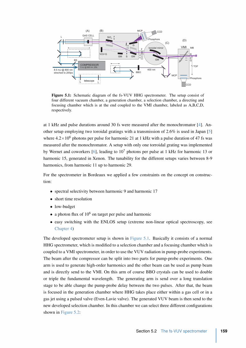
COMPRESSOR5 mJ @ 800 nm, 25fs
L
BS
BBO
GAS CELL
G
SiO2
VUV-GGM S GM
toroidal mirror
GM
L Ltelescope
CCD
Phosphore
MCP
8.5 mJ @ 800 nm
streched to 200ps
FVMI
CCD
PhosphoreMCP
TOF
R
EG
MB
400 nm
(A) (B)
(C)(D)
Figure 5.1: Schematic diagram of the fs-VUV HHG spectrometer. The setup consist of
four different vacuum chamber, a generation chamber, a selection chamber, a directing and
focusing chamber which is at the end coupled to the VMI chamber, labeled as A,B,C,D,
respectively.
at 1 kHz and pulse durations around 30 fs were measured after the monochromator [4]. An-
other setup employing two toroidal gratings with a transmission of 2.6% is used in Japan [5]
where 4.2ˆ106 photons per pulse for harmonic 21 at 1 kHz with a pulse duration of 47 fs was
measured after the monochromator. A setup with only one torroidal grating was implemented
by Wernet and coworkers [6], leading to 107 photons per pulse at 1 kHz for harmonic 13 or
harmonic 15, generated in Xenon. The tunability for the different setups varies between 8-9
harmonics, from harmonic 11 up to harmonic 29.
For the spectrometer in Bordeaux we applied a few constraints on the concept on construc-
tion:
• spectral selectivity between harmonic 9 and harmonic 17
• short time resolution
• low-budget
• a photon flux of 106 on target per pulse and harmonic
• easy switching with the ENLOS setup (extreme non-linear optical spectroscopy, see
Chapter 4)
The developed spectrometer setup is shown in Figure 5.1. Basically it consists of a normal
HHG spectrometer, which is modified to a selection chamber and a focusing chamber which is
coupled to a VMI spectrometer, in order to use the VUV radiation in pump-probe experiments.
The beam after the compressor can be split into two parts for pump-probe experiments. One
arm is used to generate high-order harmonics and the other beam can be used as pump beam
and is directly send to the VMI. On this arm of course BBO crystals can be used to double
or triple the fundamental wavelength. The generating arm is send over a long translation
stage to be able change the pump-probe delay between the two pulses. After that, the beam
is focused in the generation chamber where HHG takes place either within a gas cell or in a
gas jet using a pulsed valve (Even-Lavie valve). The generated VUV beam is then send to the
new developed selection chamber. In this chamber we can select three different configurations
shown in Figure 5.2:
Section 5.2 The fs-VUV spectrometer 159
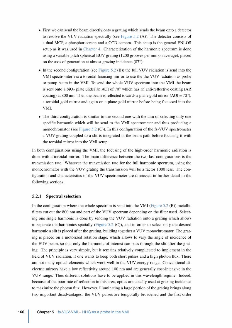
• First we can send the beam directly onto a grating which sends the beam onto a detector
to resolve the VUV radiation spectrally (see Figure 5.2 (A)). The detector consists of
a dual MCP, a phosphor screen and a CCD camera. This setup is the general ENLOS
setup as it was used in Chapter 4. Characterization of the harmonic spectrum is done
using a variable pitch spherical EUV grating (1200 grooves per mm on average), placed
on the axis of generation at almost grazing incidence (87˝).
• In the second configuration (see Figure 5.2 (B)) the full VUV radiation is send into the
VMI spectromter via a toroidal focusing mirror to use the the VUV radiation as probe
or pump beam in the VMI. To send the whole VUV spectrum into the VMI the beam
is sent onto a SiO2 plate under an AOI of 70˝ which has an anti-reflective coating (AR
coating) at 800 nm. Then the beam is reflected towards a plane gold mirror (AOI = 70˝),
a toroidal gold mirror and again on a plane gold mirror before being focussed into the
VMI.
• The third configuration is similar to the second one with the aim of selecting only one
specific harmonic which will be send to the VMI spectrometer and thus producing a
monochromator (see Figure 5.2 (C)). In this configuration of the fs-VUV spectrometer
a VUV-grating coupled to a slit is integrated in the beam path before focusing it with
the toroidal mirror into the VMI setup.
In both configurations using the VMI, the focusing of the high-order harmonic radiation is
done with a toroidal mirror. The main difference between the two last configurations is the
transmission rate. Whatever the transmission rate for the full harmonic spectrum, using the
monochromator with the VUV grating the transmission will be a factor 1000 less. The con-
figuration and characteristics of the VUV spectrometer are discussed in further detail in the
following sections.
5.2.1 Spectral selection
In the configuration where the whole spectrum is send into the VMI (Figure 5.2 (B)) metallic
filters cut out the 800 nm and part of the VUV spectrum depending on the filter used. Select-
ing one single harmonic is done by sending the VUV radiation onto a grating which allows
to separate the harmonics spatially (Figure 5.2 (C)), and in order to select only the desired
harmonic a slit is placed after the grating, building together a VUV monochromator. The grat-
ing is placed on a motorized rotation stage, which allows to vary the angle of incidence of
the EUV beam, so that only the harmonic of interest can pass through the slit after the grat-
ing. The principle is very simple, but it remains relatively complicated to implement in the
field of VUV radiation, if one wants to keep both short pulses and a high photon flux. There
are not many optical elements which work well in the VUV energy range. Conventional di-
electric mirrors have a low reflectivity around 100 nm and are generally cost-intensive in the
VUV range. Thus different solutions have to be applied in this wavelength regime. Indeed,
because of the poor rate of reflection in this area, optics are usually used at grazing incidence
to maximize the photon flux. However, illuminating a large portion of the grating brings along
two important disadvantages: the VUV pulses are temporally broadened and the first order
160 Chapter 5 fs-VUV-VMI – HHG as a probe in the VMI
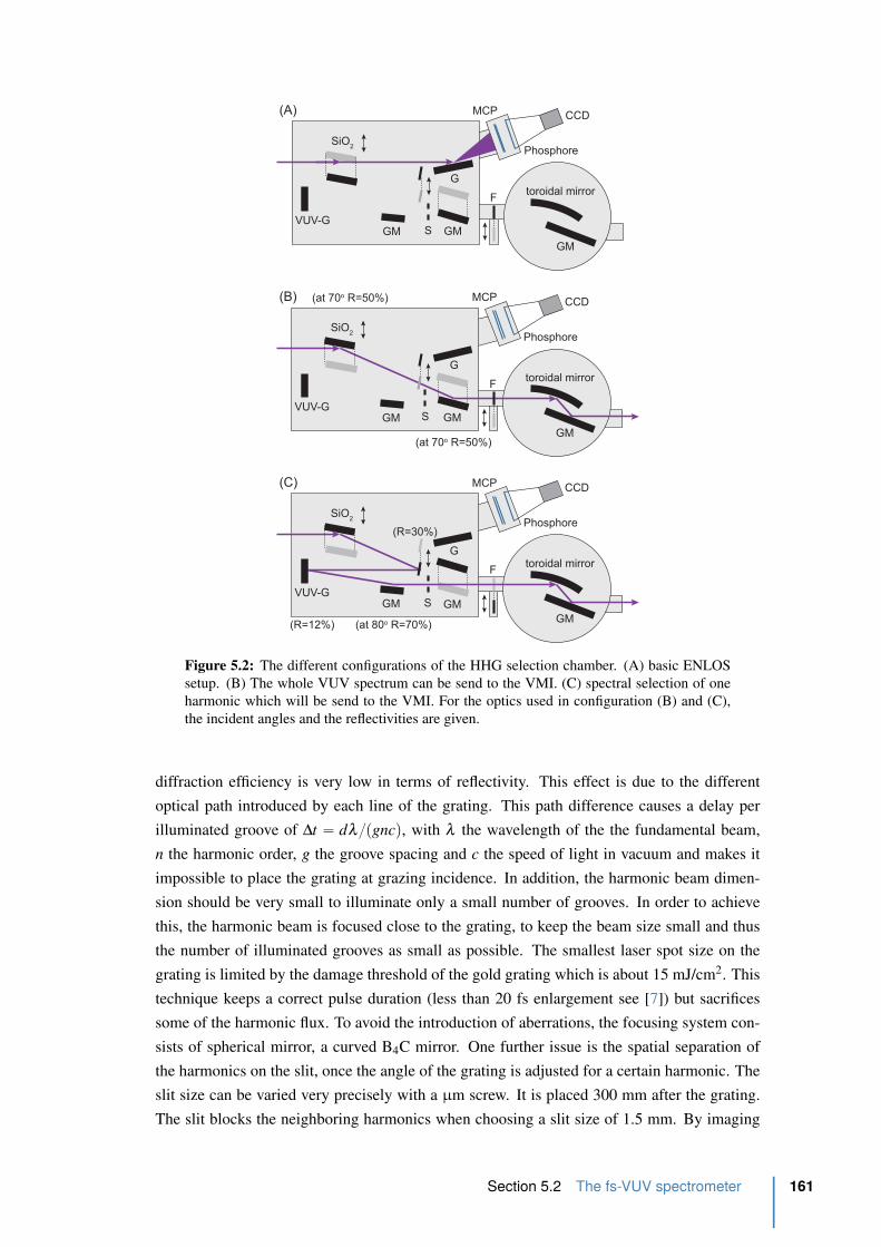
G
SiO2
VUV-GGM GM
toroidal mirror
GM
CCD
Phosphore
MCP
F
G
SiO2
VUV-GGM GM
toroidal mirror
GM
CCD
Phosphore
MCP
F
G
SiO2
VUV-GGM
toroidal mirror
GM
CCD
Phosphore
MCP
F
(A)
(B)
(C)
S
S
S GM
(at 70o R=50%)
(at 80o R=70%)
(at 70o R=50%)
(R=12%)
(R=30%)
Figure 5.2: The different configurations of the HHG selection chamber. (A) basic ENLOS
setup. (B) The whole VUV spectrum can be send to the VMI. (C) spectral selection of one
harmonic which will be send to the VMI. For the optics used in configuration (B) and (C),
the incident angles and the reflectivities are given.
diffraction efficiency is very low in terms of reflectivity. This effect is due to the different
optical path introduced by each line of the grating. This path difference causes a delay per
illuminated groove of ∆t “ dλpgncq, with λ the wavelength of the the fundamental beam,
n the harmonic order, g the groove spacing and c the speed of light in vacuum and makes it
impossible to place the grating at grazing incidence. In addition, the harmonic beam dimen-
sion should be very small to illuminate only a small number of grooves. In order to achieve
this, the harmonic beam is focused close to the grating, to keep the beam size small and thus
the number of illuminated grooves as small as possible. The smallest laser spot size on the
grating is limited by the damage threshold of the gold grating which is about 15 mJ/cm2. This
technique keeps a correct pulse duration (less than 20 fs enlargement see [7]) but sacrifices
some of the harmonic flux. To avoid the introduction of aberrations, the focusing system con-
sists of spherical mirror, a curved B4C mirror. One further issue is the spatial separation of
the harmonics on the slit, once the angle of the grating is adjusted for a certain harmonic. The
slit size can be varied very precisely with a µm screw. It is placed 300 mm after the grating.
The slit blocks the neighboring harmonics when choosing a slit size of 1.5 mm. By imaging
Section 5.2 The fs-VUV spectrometer 161
the harmonics on a pair of MCPs the spatial selection of the slit up to harmonic 19 has been
experimentally tested. As a matter of fact the spatial selection of the slit works even for sec-
ond order diffracted harmonics. This type of monochromator is used to select the different
harmonic spectrum with a resolution of about 0.5 nm in average (0.7 nm for harmonic 7 and
0.3 for harmonic 17) but with only a transmission rate between 0.5 and 1.5%, depending on the
harmonic order. The characteristics are not among the best in the field but on the other hand,
the cost of installation was very cheap (about 600 e for the monochromator grating against
10000-30000 e seen on the market or in other laboratories). A more detailed description of
the device exists in the PhD thesis of H. Ruf, who designed and characterized the device of
the monochromator during part of his thesis [7]. Unfortunately as we will see in Section 5.4
the monochromator has not been used to record pump-probe data in the VMI because of its
poor transmission. We have indeed developed another strategy based on HHG at 400 nm and
sideband detection to overcome the pour transmission of the monochromator.
5.2.2 VUV focusing
In order to maximize the laser illumination and to reduce the dimension of the interaction
area in the VMI the VUV radiation has to be focused into the interaction chamber. The only
focusing systems usable with EUV radiation are operated by optical reflection. Furthermore to
minimize losses of VUV photons the focusing mirror must be positioned at grazing incidence
as mentioned before. Such an procedure necessarily involves significant astigmatism at the
harmonic focus, and focusing the radiation is not optimal (see [8]). One way around this
problem is to use a toroidal mirror. In this case, astigmatism can be corrected by choosing
wisely the radius of curvature R of the surface on which the incidence is high (tangential
plane). The relationship between the focus position S1 and the radi of curvature for a toroidal
mirror is given by:
1
S` 1
S1s
“ 2cosα
Rs“ 1
fs(5.1a)
1
S` 1
S1t
“ 2
Rt cosα“ 1
ft(5.1b)
where α is the angle of incidence (to normal), S the object conjugate distance, S1 the image
conjugate distance and R the radius of curvature. The subscripts s and t are standing for the
sagittal and tangential plane, respectively. Rs is also called the cylinder curve and Rt the base
curve. The angle for which the object and image distance are equal is given by
cos2 α “ Rs
RtÑ fs “ ft (5.2)
The radii of curvature that characterizes the mirror are ultimately determined by the desired
focusing distance and the incident angle imposed which are given by the experimental setup.
In our situation, the choice of the focusing distance is not trivial. It should be relatively short
to allow the sharpest focus as possible, but should still leave enough room to insert the VMI
spectrometer with its dimensions. An experimental compromise was made, setting this dis-
162 Chapter 5 fs-VUV-VMI – HHG as a probe in the VMI
tance to 50 cm. With an incidence angle of 85˝, the radii of curvature of the toroidal mirror are
-11.474 m for the tangential radius and -8.7 cm for the sagittal radius. Toroidal mirrors have
the advantage of being able to remove the astigmatism introduced by large angles of incidence,
however, they are designed to operate at a particular angle of incidence. Unfortunately, if the
angle of incidence of the beam deviates only slightly from the theoretical value, one intro-
duces very fast a strong geometric aberration, distortion and astigmatism [8]. This sensitivity
of the beam incidence makes the alignment of a toroidal mirror rather delicate. For optimum
alignment of the mirror, it is mounted on a vertical micrometer translation stage for accurately
positioning the laser beam on the mirror. Further, this translation stage itself is mounted on a
rotation stage with seconds precision for fine tuning the angle of incidence according to the
tangential plane. Finally, to facilitate the alignment of the VUV radiation into the VMI spec-
trometer we use a plane gold mirror placed at grazing incidence just after the toroidal mirror.
The theoretical focus waist of the VUV beam was estimated to be around 60 µm [7]. One
major drawback in the present setup is that the alignment of the toroidal mirror cannot be done
under vacuum and that the spatial mode of the VUV light is not monitored. This is one of the
updates that the team in Bordeaux wants to implement on this setup in the future.
5.2.3 VUV flux optimization
The observation of probably any pump-probe measurement with lasers involving molecular
systems is a result of the interplay of different processes, involving the excitation of the sys-
tem by the pump beam, the photodissociation following the excitation, the generation of the
harmonic radiation if probed by an VUV radiation, ionization of the dissociation fragments via
the VUV radiation, and the detection of these fragments or electrons produced by the interac-
tion. Each of these steps can be connected to a yield, like the molecular excitation rate, the rate
of dissociation after excitation, the efficiency of the HHG process, the ionization rate and the
detection efficiency. The two main variables we can control is the HHG process using different
gases to maximize the VUV photon flux and the molecular density to maximize the interaction
by i.e. using a pulsed valve instead of a continous molecular beam like in Chapter 2.
For the new developed VUV spectrometer we therefore tried to optimize the VUV photon
flux and to evaluate the number of events we can expect in the VMI using the VUV pho-
ton source as an universal detection (probe beam) in the pump-probe experiments planned.
Figure 5.3 shows the harmonic spectra generated with a 800 nm driving laser pulse with an
intensity of 800 µJ/p in krypton, argon and acetylene. A 1 cm long gas cell was used with
an input and output hole generated by the laser itself to minimize the pressure in the source
chamber. The gas pressures were optimized for each gas separately to 9, 20 and 6.5 mbar for
krypton, argon and acetylene, respectively. At larger pressures the VUV radiation starts to
be reabsobed. We can already see that by using krypton instead of argon we can increase the
harmonic yield by a factor of two to three depending on the harmonic order. We also generated
harmonics in acetylene where it can be seen that between harmonic 11 and 15 the HHG yield
(purple line in Figure 5.3) lies somewhat between krypton and argon. Due to the relatively
low ionization energy of 11.4 eV compared to argon and krypton with Ip’s of 15.76 eV and
Section 5.2 The fs-VUV spectrometer 163

Energy [eV]
Inte
nsity
[arb
. uni
ts]
H11
H13
H15
H17
H19
150
0.5
1
1.5
2
2.5
3
3.5× 10⁶
20 25 30 35 40 45
H21
H23
H25
H27
KrArC2H2
Figure 5.3: Harmonic spectra generated with an 800 nm driving laser with a lens with 1 m
focal length in krypton, argon and acetylene at optimized pressures of 9, 20 and 6.5 mbar,
respectively. The gas cell is 1cm long with an input and output hole created by the laser itself.
Due to the diameter of the MCP (4 cm) only HHG ą H11 are detected. A laser intensity of
800 µJ/p was used.
14.0 eV, respectively, the cutoff is obtained relatively fast. Here we have demonstrated that
using acetylene gas for HHG, combined with a aluminium filter cutting energies higher than
harmonic 11, allows already to produce a VUV radiation consisting only of a few harmonics
by maintaining a reasonable high photon flux without using the monochromator and loosing a
factor 1000.
Measurement of the number of VUV photons in the VMI
To be able to estimate the number of pump-probe events, we measured the total VUV photon
flux with a VUV photodiode1. We used the calibration of the model to recover the number
of photons per harmonic which is shown in Figure 5.4. Two aluminium filters are used to cut
the 800 nm and a preamplifier with a factor of ˆ5 is employed to measure the signal of the
photodiode with an oscilloscope. The number of VUV photons NVUV is given by
NVUV “ Ne
η(5.3)
where Ne is the amount of electrons supplied by the photodiode and η the internal quantum
efficiency of the photodiode as shown in Figure 5.4. The amount of electrons Ne supplied by
the photodiode in a time interval ∆t is given by:
Ne “ U∆t
Tf Rqe(5.4)
1 VUV-100 photodiode from OSI Optoelectronics
164 Chapter 5 fs-VUV-VMI – HHG as a probe in the VMI
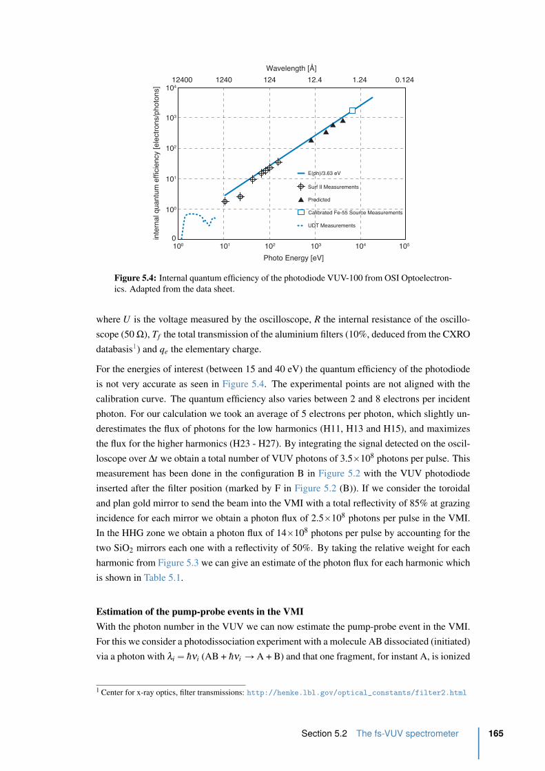
inte
rnal
qua
ntum
effi
cien
cy [e
lect
rons
/pho
tons
]
Photo Energy [eV]
101 102 103 104 105100
100
101
102
103
104
E(ph)/3.63 eV
Surf II Measurements
Predicted
Calibrated Fe-55 Source Measurements
UDT Measurements
0
12400 1240 124 12.4 1.24 0.124
Wavelength [Å]
Figure 5.4: Internal quantum efficiency of the photodiode VUV-100 from OSI Optoelectron-
ics. Adapted from the data sheet.
where U is the voltage measured by the oscilloscope, R the internal resistance of the oscillo-
scope (50 Ω), Tf the total transmission of the aluminium filters (10%, deduced from the CXRO
databasis1) and qe the elementary charge.
For the energies of interest (between 15 and 40 eV) the quantum efficiency of the photodiode
is not very accurate as seen in Figure 5.4. The experimental points are not aligned with the
calibration curve. The quantum efficiency also varies between 2 and 8 electrons per incident
photon. For our calculation we took an average of 5 electrons per photon, which slightly un-
derestimates the flux of photons for the low harmonics (H11, H13 and H15), and maximizes
the flux for the higher harmonics (H23 - H27). By integrating the signal detected on the oscil-
loscope over ∆t we obtain a total number of VUV photons of 3.5ˆ108 photons per pulse. This
measurement has been done in the configuration B in Figure 5.2 with the VUV photodiode
inserted after the filter position (marked by F in Figure 5.2 (B)). If we consider the toroidal
and plan gold mirror to send the beam into the VMI with a total reflectivity of 85% at grazing
incidence for each mirror we obtain a photon flux of 2.5ˆ108 photons per pulse in the VMI.
In the HHG zone we obtain a photon flux of 14ˆ108 photons per pulse by accounting for the
two SiO2 mirrors each one with a reflectivity of 50%. By taking the relative weight for each
harmonic from Figure 5.3 we can give an estimate of the photon flux for each harmonic which
is shown in Table 5.1.
Estimation of the pump-probe events in the VMI
With the photon number in the VUV we can now estimate the pump-probe event in the VMI.
For this we consider a photodissociation experiment with a molecule AB dissociated (initiated)
via a photon with λi “ hνi (AB + hνi Ñ A + B) and that one fragment, for instant A, is ionized
1 Center for x-ray optics, filter transmissions: http://henke.lbl.gov/optical_constants/filter2.html
Section 5.2 The fs-VUV spectrometer 165
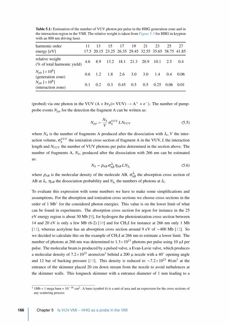
Table 5.1: Estimation of the number of VUV photon per pulse in the HHG generation zone and in
the interaction region in the VMI. The relative weight is taken from Figure 5.3 for HHG in krypton
with an 800 nm driving laser.
harmonic order 11 13 15 17 19 21 23 25 27
energy [eV] 17.5 20.15 23.25 26.35 29.45 32.55 35.65 38.75 41.85
relative weight
(% of total harmonic yield)4.6 8.9 13.2 18.1 21.3 20.9 10.1 2.5 0.4
Nph [ˆ108]
(generation zone)0.6 1.2 1.8 2.6 3.0 3.0 1.4 0.4 0.06
Nph [ˆ108]
(interaction zone)0.1 0.2 0.3 0.45 0.5 0.5 0.25 0.06 0.01
(probed) via one photon in the VUV (A + hνp(= VUV) Ñ A` + e´). The number of pump-
probe events Npp for the detection the fragment A can be written as:
Npp “ NA
VσVUV
A LNVUV (5.5)
where NA is the number of fragments A produced after the dissociation with λi, V the inter-
action volume, σVUVA the ionization cross section of fragment A in the VUV, L the interaction
length and NVUV the number of VUV photons per pulse determined in the section above. The
number of fragments A, NA, produced after the dissociation with 266 nm can be estimated
as:
NA “ ρAB σλi
AB ηAB LNλi(5.6)
where ρAB is the molecular density of the molecule AB, σλi
AB the absorption cross section of
AB at λi, ηAB the dissociation probability and Nλithe numbers of photons at λi.
To evaluate this expression with some numbers we have to make some simplifications and
assumptions. For the absorption and ionization cross sections we choose cross sections in the
order of 1 Mb1 for the considered photon energies. This value is on the lower limit of what
can be found in experiments. The absorption cross section for argon for instance in the 25
eV energy region is about 30 Mb [9], for hydrogen the photoionization cross section between
14 and 20 eV is only a few Mb (6-2) [10] and for CH3I for instance at 266 nm only 1 Mb
[11], whereas acetylene has an absorption cross section around 9 eV of „400 Mb [12]. So
we decided to calculate this on the example of CH3I at 266 nm to estimate a lower limit. The
number of photons at 266 nm was determined to 1.3ˆ1013 photons per pulse using 10 µJ per
pulse. The molecular beam is produced by a pulsed valve, a Evan-Lavie valve, which produces
a molecular density of 7.2ˆ1023 atoms/cm3 behind a 200 µ nozzle with a 40˝ opening angle
and 12 bar of backing pressure [13]. This density is reduced to „7.2ˆ1021 #/cm3 at the
entrance of the skimmer placed 20 cm down stream from the nozzle to avoid turbulences at
the skimmer walls. This longneck skimmer with a entrance diameter of 1 mm leading to a
1 1Mb = 1 mega barn = 10´18 cm2. A barn (symbol b) is a unit of area and an expression for the cross sections of
any scattering process
166 Chapter 5 fs-VUV-VMI – HHG as a probe in the VMI

transmission factor of 0.03 and a length of 4.5 cm [13] will leading to density of 2.6ˆ1019
#/cm3. The beam leaving the skimmer is still expanding radially by 0.1 steradian reducing
the beam density 8 cm away from the skimmer in the interaction region (fixed by the µ-metal
diamter) by a factor 6.4 to 4ˆ1018 #/cm3. Consequently, if we assume a 1% mixture of CH3I
in the molecular beam (to avoid cluster formation), we will achieve a molecular density of
„ ˆ1016 #/cm3. The interaction volume and the interaction length is determined by the waist
of the laser pulse and the diameter of the molecular beam. The interaction length is fixed
to 3 mm, which corresponds to the molecular beam diameter 8 cm after the skimmer. The
laser beam waist was determined to be 85 µm for the 266 nm using a lens with 50 cm focal
length. If we consider that all molecules in the interaction region in the molecular beam are
dissociated (ηAB = 1) we get a number of fragments NA of 4ˆ1010 per pulse which means
43000 pump-probe events per laser shot. Considering the detection efficiency of the MCP, the
phosphor and the CCD which we assume to be around 25% we detect around 10000 events
per laser shot. With a laser repetition rate of 1 kHz, the number of detected events should be
quite suitable to obtain usable images after integration over a couple of minutes. In conclusion
we can say that experiments using VUV light generated by HHG as a probe with femtosecond
time resolution is possible and feasible. But in fact as we will see in Section 5.4, we did not
observe any pump-probe signal with a VUV pulse as a probe beam.
5.3 fs-VUV VMI characterization
For testing the new VMI - VUV spectrometer combination we choose argon as target gas,
which has two main advantages for the experiment apart from that it is a well known system.
Firstly it has a relatively high absorption cross section of about 25 to 35 Mb between 15 and
30 eV. On the other hand, as argon is an atom we are not bothered by secondary processes
(like for instance dissociation), which gives us a larger molecular density in the interaction
volume. We undertook three different experiments to test the fs-VUV spectrometer. In the
first experiment we detected the photoelectron spectrum of argon using the full VUV spectrum
produced with a 800 nm driving laser (see Figure 5.3). For the second experiment we used
the VUV monochromator in the spectral selection configuration to select only one harmonic
(harmonic 11 and 13) to ionize argon. In the third experiment we recorded the photoelectron
spectrum of argon in pump-probe configuration using the VUV radiation generated at 400
nm plus an additional 400 nm pulse. In the following three sections the results of these test
experiments are presented.
5.3.1 Photoelectron detection of argon using a VUV spectrum
The HHG spectrum is produced by focusing „800 µmJ/p of the 800 nm driving laser, spatially
filtered by a diaphragm, with a 1 m focal length lens into a 1 cm long gas cell, filled with
krypton at 10 mbar. In addition an aluminium filter with a thickness of 150 nm is used which
cuts all photons with photon energies lower than 15 eV and therefor also the remaining 800
nm. The setup is actually shown in Figure 5.1 without using the second arm to produce the
Section 5.3 fs-VUV VMI characterization 167
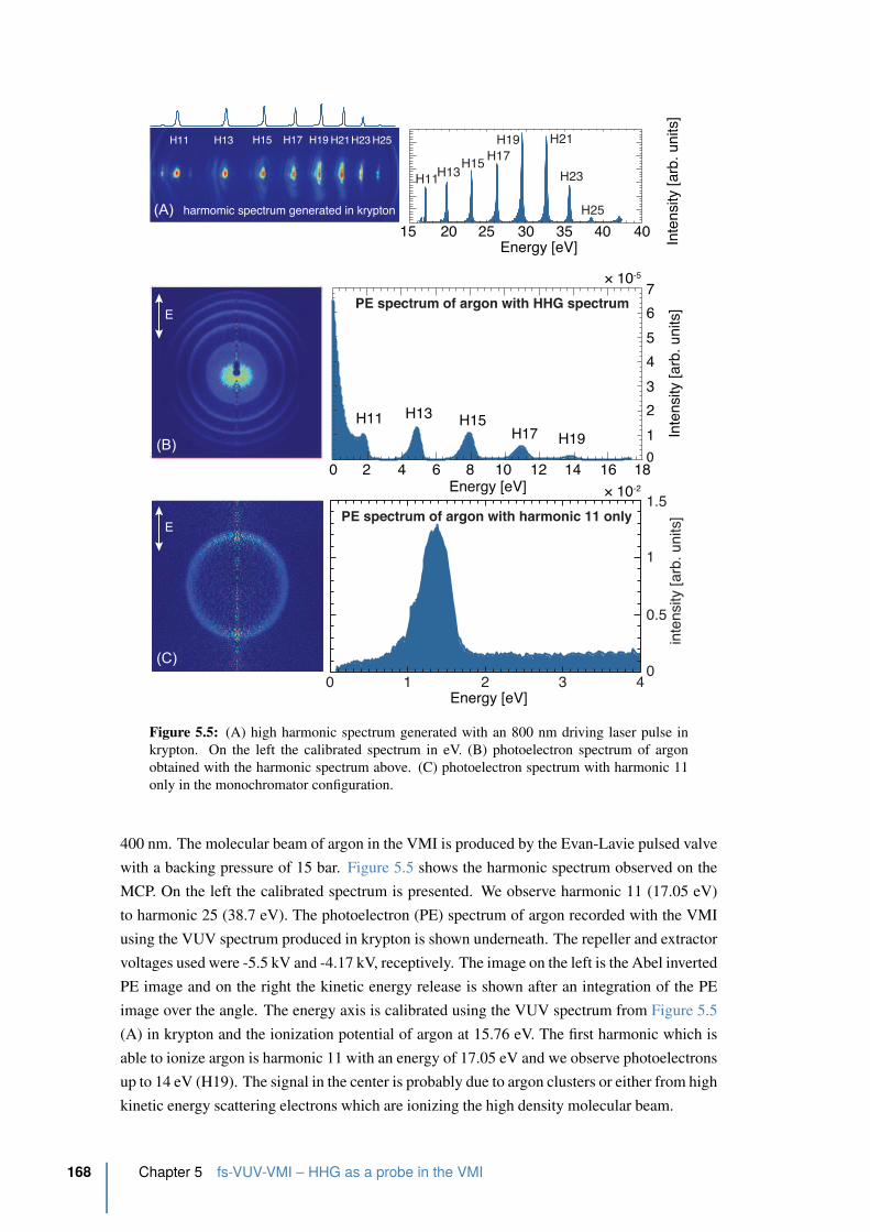
Energy [eV]
H11 H13 H15H17 H19
0 2 4 6 8 10 12 14 16 18
E
Energy [eV]15 20 25 30 35 40 40
H11 H13 H15 H17 H19 H21H23 H25
H11H13
H15H17
H19 H21
H23
H25
Inte
nsity [a
rb. u
nits]
harmomic spectrum generated in krypton
PE spectrum of argon with HHG spectrum
Inte
nsity [a
rb. u
nits]
0
1
2
3
4
5
6
7× 10⁻⁵
PE spectrum of argon with harmonic 11 only
× 10-2
E
(A)
(B)
(C)
0 1 2 3 40
0.5
1
1.5
inte
nsity [
arb
. u
nits]
Energy [eV]
Figure 5.5: (A) high harmonic spectrum generated with an 800 nm driving laser pulse in
krypton. On the left the calibrated spectrum in eV. (B) photoelectron spectrum of argon
obtained with the harmonic spectrum above. (C) photoelectron spectrum with harmonic 11
only in the monochromator configuration.
400 nm. The molecular beam of argon in the VMI is produced by the Evan-Lavie pulsed valve
with a backing pressure of 15 bar. Figure 5.5 shows the harmonic spectrum observed on the
MCP. On the left the calibrated spectrum is presented. We observe harmonic 11 (17.05 eV)
to harmonic 25 (38.7 eV). The photoelectron (PE) spectrum of argon recorded with the VMI
using the VUV spectrum produced in krypton is shown underneath. The repeller and extractor
voltages used were -5.5 kV and -4.17 kV, receptively. The image on the left is the Abel inverted
PE image and on the right the kinetic energy release is shown after an integration of the PE
image over the angle. The energy axis is calibrated using the VUV spectrum from Figure 5.5
(A) in krypton and the ionization potential of argon at 15.76 eV. The first harmonic which is
able to ionize argon is harmonic 11 with an energy of 17.05 eV and we observe photoelectrons
up to 14 eV (H19). The signal in the center is probably due to argon clusters or either from high
kinetic energy scattering electrons which are ionizing the high density molecular beam.
168 Chapter 5 fs-VUV-VMI – HHG as a probe in the VMI
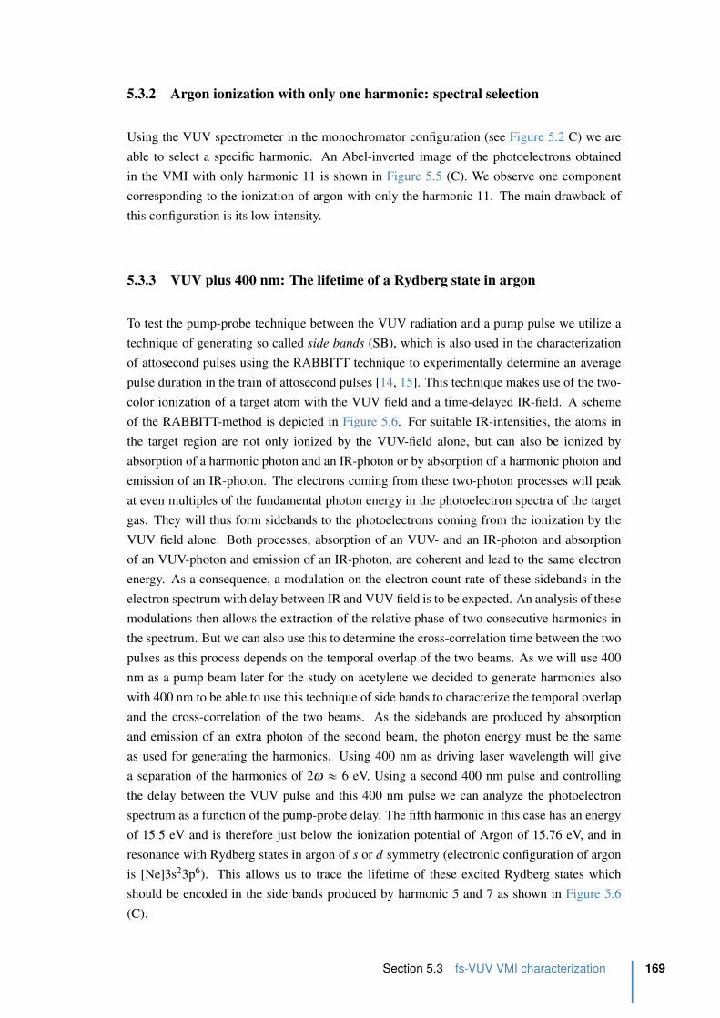
5.3.2 Argon ionization with only one harmonic: spectral selection
Using the VUV spectrometer in the monochromator configuration (see Figure 5.2 C) we are
able to select a specific harmonic. An Abel-inverted image of the photoelectrons obtained
in the VMI with only harmonic 11 is shown in Figure 5.5 (C). We observe one component
corresponding to the ionization of argon with only the harmonic 11. The main drawback of
this configuration is its low intensity.
5.3.3 VUV plus 400 nm: The lifetime of a Rydberg state in argon
To test the pump-probe technique between the VUV radiation and a pump pulse we utilize a
technique of generating so called side bands (SB), which is also used in the characterization
of attosecond pulses using the RABBITT technique to experimentally determine an average
pulse duration in the train of attosecond pulses [14, 15]. This technique makes use of the two-
color ionization of a target atom with the VUV field and a time-delayed IR-field. A scheme
of the RABBITT-method is depicted in Figure 5.6. For suitable IR-intensities, the atoms in
the target region are not only ionized by the VUV-field alone, but can also be ionized by
absorption of a harmonic photon and an IR-photon or by absorption of a harmonic photon and
emission of an IR-photon. The electrons coming from these two-photon processes will peak
at even multiples of the fundamental photon energy in the photoelectron spectra of the target
gas. They will thus form sidebands to the photoelectrons coming from the ionization by the
VUV field alone. Both processes, absorption of an VUV- and an IR-photon and absorption
of an VUV-photon and emission of an IR-photon, are coherent and lead to the same electron
energy. As a consequence, a modulation on the electron count rate of these sidebands in the
electron spectrum with delay between IR and VUV field is to be expected. An analysis of these
modulations then allows the extraction of the relative phase of two consecutive harmonics in
the spectrum. But we can also use this to determine the cross-correlation time between the two
pulses as this process depends on the temporal overlap of the two beams. As we will use 400
nm as a pump beam later for the study on acetylene we decided to generate harmonics also
with 400 nm to be able to use this technique of side bands to characterize the temporal overlap
and the cross-correlation of the two beams. As the sidebands are produced by absorption
and emission of an extra photon of the second beam, the photon energy must be the same
as used for generating the harmonics. Using 400 nm as driving laser wavelength will give
a separation of the harmonics of 2ω « 6 eV. Using a second 400 nm pulse and controlling
the delay between the VUV pulse and this 400 nm pulse we can analyze the photoelectron
spectrum as a function of the pump-probe delay. The fifth harmonic in this case has an energy
of 15.5 eV and is therefore just below the ionization potential of Argon of 15.76 eV, and in
resonance with Rydberg states in argon of s or d symmetry (electronic configuration of argon
is [Ne]3s23p6). This allows us to trace the lifetime of these excited Rydberg states which
should be encoded in the side bands produced by harmonic 5 and 7 as shown in Figure 5.6
(C).
Section 5.3 fs-VUV VMI characterization 169
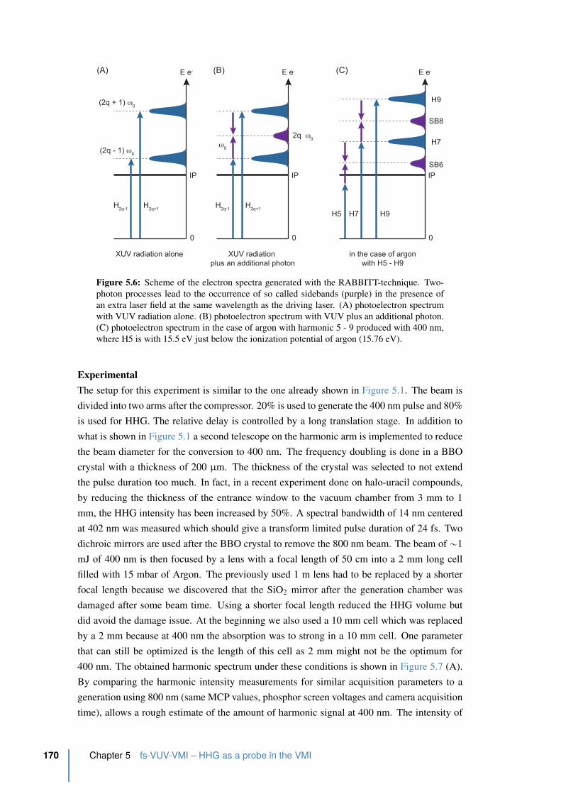
E e-
H2q+1
H2q-1
IP
(2q - 1) ω0
(2q + 1) ω0
E e-
H2q+1
H2q-1
2q ω0
ω0
0
IP
0
(A) (B)
XUV radiation alone XUV radiation
plus an additional photon
E e-
H7H5
IP
0
(C)
in the case of argon
with H5 - H9
H9
H7
H9
SB6
SB8
Figure 5.6: Scheme of the electron spectra generated with the RABBITT-technique. Two-
photon processes lead to the occurrence of so called sidebands (purple) in the presence of
an extra laser field at the same wavelength as the driving laser. (A) photoelectron spectrum
with VUV radiation alone. (B) photoelectron spectrum with VUV plus an additional photon.
(C) photoelectron spectrum in the case of argon with harmonic 5 - 9 produced with 400 nm,
where H5 is with 15.5 eV just below the ionization potential of argon (15.76 eV).
Experimental
The setup for this experiment is similar to the one already shown in Figure 5.1. The beam is
divided into two arms after the compressor. 20% is used to generate the 400 nm pulse and 80%
is used for HHG. The relative delay is controlled by a long translation stage. In addition to
what is shown in Figure 5.1 a second telescope on the harmonic arm is implemented to reduce
the beam diameter for the conversion to 400 nm. The frequency doubling is done in a BBO
crystal with a thickness of 200 µm. The thickness of the crystal was selected to not extend
the pulse duration too much. In fact, in a recent experiment done on halo-uracil compounds,
by reducing the thickness of the entrance window to the vacuum chamber from 3 mm to 1
mm, the HHG intensity has been increased by 50%. A spectral bandwidth of 14 nm centered
at 402 nm was measured which should give a transform limited pulse duration of 24 fs. Two
dichroic mirrors are used after the BBO crystal to remove the 800 nm beam. The beam of „1
mJ of 400 nm is then focused by a lens with a focal length of 50 cm into a 2 mm long cell
filled with 15 mbar of Argon. The previously used 1 m lens had to be replaced by a shorter
focal length because we discovered that the SiO2 mirror after the generation chamber was
damaged after some beam time. Using a shorter focal length reduced the HHG volume but
did avoid the damage issue. At the beginning we also used a 10 mm cell which was replaced
by a 2 mm because at 400 nm the absorption was to strong in a 10 mm cell. One parameter
that can still be optimized is the length of this cell as 2 mm might not be the optimum for
400 nm. The obtained harmonic spectrum under these conditions is shown in Figure 5.7 (A).
By comparing the harmonic intensity measurements for similar acquisition parameters to a
generation using 800 nm (same MCP values, phosphor screen voltages and camera acquisition
time), allows a rough estimate of the amount of harmonic signal at 400 nm. The intensity of
170 Chapter 5 fs-VUV-VMI – HHG as a probe in the VMI
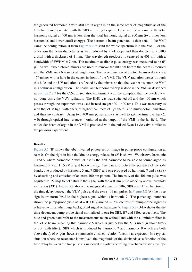
the generated harmonic 7 with 400 nm in argon is on the same order of magnitude as of the
13th harmonic generated with the 800 nm using krypton. However, the amount of the total
harmonic signal at 400 nm is less than the total harmonic signal at 800 nm (two times less
harmonics and lower cutoff energy). The harmonic beam generated is then send to the VMI
using the configuration B from Figure 5.2 to send the whole spectrum into the VMI. For the
other arm the beam diameter is as well reduced by a telescope and then doubled in a BBO
crystal with a thickness of 1 mm. The wavelength produced is centered at 401 nm with a
bandwidth of FWHM = 7 nm. The maximum available pulse energy was measured to be 65
µJ. As well two dichroic mirrors are used to remove the 800 nm before the beam is focused
into the VMI via a 60 cm focal length lens. The recombination of the two beam is done via a
45˝ mirror with a hole in the center in front of the VMI. The VUV radiation passes through
this hole and the UV radiation is reflected by the mirror, so that the two beams enter the VMI
in a collinear configuration. The spatial and temporal overlap is done in the VMI as described
in Section 2.2.3 for the ClN3 dissociation experiment with the exception that the overlap was
not done using the VUV radiation. The HHG gas was switched off and the 400 nm which
passes through the experiment was used instead (to get 400 + 400 nm). This was necessary as
with the VUV light with energies higher than most of Ip’s there is no multiphoton ionization
and thus no contrast. Using two 400 nm pulses allows as well to get the time overlap (∆t
= 0) through optical interferences monitored at the output of the VMI in the far field. The
molecular beam of argon in the VMI is produced with the pulsed Evan-Lavie valve similar to
the previous experiment.
Results
Figure 5.7 (B) shows the Abel inverted photoelectron image in pump-probe configuration at
∆t = 0. On the right in blue the kinetic energy release in eV is shown. We observe harmonic
7 and 9 where harmonic 7 with 21 eV is the first harmonic to be able to ionize argon as
harmonic 5 with 15.5 eV is just below the Ip. One can also notice the presence of the side
bands, one produced by harmonic 5 and 7 (SB6) and one produced by harmonic 7 and 9 (SB8)
by absorbing and emission of an extra 400 nm photon. The intensity of the 401 nm pulse was
adjusted to 15 µJ/p to not saturate the signal with the 401 nm pulse alone by above threshold
ionization (ATI). Figure 5.8 shows the integrated signal of SB6, SB8 and H7 as function of
the time delay between the VUV pulse and the extra 401 nm pulse. In Figure 5.8 (A) the three
signals are normalized to the highest signal which is harmonic 7. The percentage numbers
shows the pump-probe yield at ∆t = 0. Only around „15% contrast of pump-probe signal is
achieved with a rather huge background signal on harmonic 7. Figure 5.8 (B-D) shows the the
time-dependent pump-probe signal normalized to one for SB8, H7 and SB6, respectively. The
blue and green data refer to the measurements taken without and with the aluminium filter in
the VUV beam, meaning that harmonic 5 which is just below the Ip is used (without filter)
or cut (with filter). SB8 which is produced by harmonic 7 and harmonic 9 which are both
above the Ip of Argon shows a symmetric cross-correlation function as expected. In a typical
situation where no resonance is involved, the magnitude of the sidebands as a function of the
time delay between the two pulses is supposed to evolve according to a characteristic envelope
Section 5.3 fs-VUV VMI characterization 171
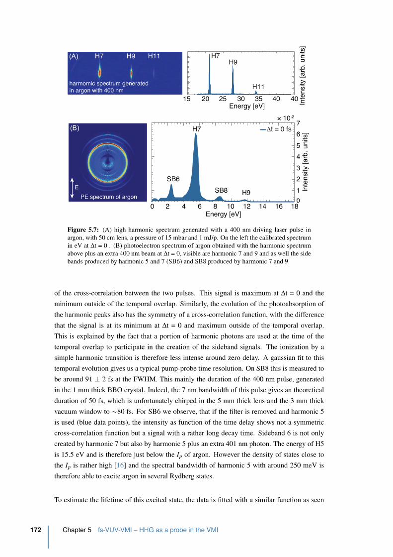
Energy [eV]
H7
SB6
SB8 H9
0 2 4 6 8 10 12 14 16 18
E
Energy [eV]15 20 25 30 35 40 40
H7 H9 H11
H11
H7H9
Inte
nsity [
arb
. u
nits]
harmomic spectrum generated
in argon with 400 nm
PE spectrum of argon
Inte
nsity [
arb
. u
nits]
0
1
2
3
4
5
6
7× 10⁻²
Δt = 0 fs
(A)
(B)
Figure 5.7: (A) high harmonic spectrum generated with a 400 nm driving laser pulse in
argon, with 50 cm lens, a pressure of 15 mbar and 1 mJ/p. On the left the calibrated spectrum
in eV at ∆t = 0 . (B) photoelectron spectrum of argon obtained with the harmonic spectrum
above plus an extra 400 nm beam at ∆t = 0, visible are harmonic 7 and 9 and as well the side
bands produced by harmonic 5 and 7 (SB6) and SB8 produced by harmonic 7 and 9.
of the cross-correlation between the two pulses. This signal is maximum at ∆t = 0 and the
minimum outside of the temporal overlap. Similarly, the evolution of the photoabsorption of
the harmonic peaks also has the symmetry of a cross-correlation function, with the difference
that the signal is at its minimum at ∆t = 0 and maximum outside of the temporal overlap.
This is explained by the fact that a portion of harmonic photons are used at the time of the
temporal overlap to participate in the creation of the sideband signals. The ionization by a
simple harmonic transition is therefore less intense around zero delay. A gaussian fit to this
temporal evolution gives us a typical pump-probe time resolution. On SB8 this is measured to
be around 91 ˘ 2 fs at the FWHM. This mainly the duration of the 400 nm pulse, generated
in the 1 mm thick BBO crystal. Indeed, the 7 nm bandwidth of this pulse gives an theoretical
duration of 50 fs, which is unfortunately chirped in the 5 mm thick lens and the 3 mm thick
vacuum window to „80 fs. For SB6 we observe, that if the filter is removed and harmonic 5
is used (blue data points), the intensity as function of the time delay shows not a symmetric
cross-correlation function but a signal with a rather long decay time. Sideband 6 is not only
created by harmonic 7 but also by harmonic 5 plus an extra 401 nm photon. The energy of H5
is 15.5 eV and is therefore just below the Ip of argon. However the density of states close to
the Ip is rather high [16] and the spectral bandwidth of harmonic 5 with around 250 meV is
therefore able to excite argon in several Rydberg states.
To estimate the lifetime of this excited state, the data is fitted with a similar function as seen
172 Chapter 5 fs-VUV-VMI – HHG as a probe in the VMI
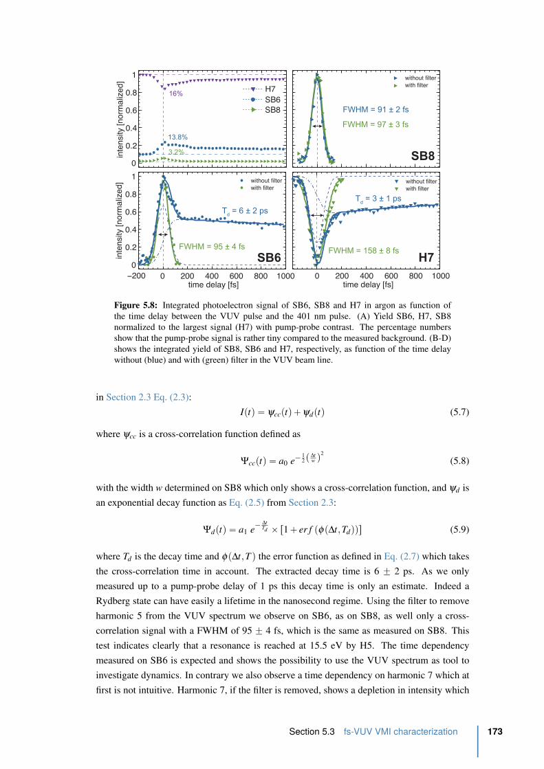
without filterwith filter
SB80.2
0.4
0.6
0.8
1
inte
nsity
[nor
mal
ized
]
16%
13.8%
3.2%
FWHM = 91 ± 2 fs
FWHM = 97 ± 3 fs
without filterwith filter
SB6FWHM = 95 ± 4 fs
Td = 6 ± 2 ps
0 200 400 600 800 1000time delay [fs]
0 200 400 600 800 1000time delay [fs]
without filterwith filter
FWHM = 158 ± 8 fs
Td = 3 ± 1 ps
H7
−2000
0.2
0.4
0.6
0.8
1
inte
nsity
[nor
mal
ized
]
0
H7SB6SB8
Figure 5.8: Integrated photoelectron signal of SB6, SB8 and H7 in argon as function of
the time delay between the VUV pulse and the 401 nm pulse. (A) Yield SB6, H7, SB8
normalized to the largest signal (H7) with pump-probe contrast. The percentage numbers
show that the pump-probe signal is rather tiny compared to the measured background. (B-D)
shows the integrated yield of SB8, SB6 and H7, respectively, as function of the time delay
without (blue) and with (green) filter in the VUV beam line.
in Section 2.3 Eq. (2.3):
Iptq “ ψccptq ` ψdptq (5.7)
where ψcc is a cross-correlation function defined as
Ψccptq “ a0 e´ 12 p ∆t
w q2
(5.8)
with the width w determined on SB8 which only shows a cross-correlation function, and ψd is
an exponential decay function as Eq. (2.5) from Section 2.3:
Ψdptq “ a1 e´ ∆t
Td ˆ r1 ` er f pφp∆t,Tdqqs (5.9)
where Td is the decay time and φp∆t,T q the error function as defined in Eq. (2.7) which takes
the cross-correlation time in account. The extracted decay time is 6 ˘ 2 ps. As we only
measured up to a pump-probe delay of 1 ps this decay time is only an estimate. Indeed a
Rydberg state can have easily a lifetime in the nanosecond regime. Using the filter to remove
harmonic 5 from the VUV spectrum we observe on SB6, as on SB8, as well only a cross-
correlation signal with a FWHM of 95 ˘ 4 fs, which is the same as measured on SB8. This
test indicates clearly that a resonance is reached at 15.5 eV by H5. The time dependency
measured on SB6 is expected and shows the possibility to use the VUV spectrum as tool to
investigate dynamics. In contrary we also observe a time dependency on harmonic 7 which at
first is not intuitive. Harmonic 7, if the filter is removed, shows a depletion in intensity which
Section 5.3 fs-VUV VMI characterization 173
0 2 4 6 8 10 12 140
0.02
0.04
0.06
0.08
0.1
Energy [eV]
inte
nsity
[arb
. uni
ts]
XUV + 401 @ −200 fs401 nm armXUV armresidual 400 nm (XUV arm)
SB6
H7
SB8 H9
Figure 5.9: Photoelectron spectrum backgrounds of argon, showing the signals with the 401
nm probe alone (blue), the VUV beam alone (purple), and the residual 400 nm from the HHG
arm (green) in comparison to the pump-probe signal at ∆t = -200 fs (grey).
recovers on a timescale of 3 ˘ 1 ps. The data is fitted with the same function (Eq. (5.7)) as
SB6. To explain this we will look first at the one laser background signal.
Figure 5.9 shows the photoelectron spectra of the one laser backgrounds, meaning for the 401
nm beam alone (blue curve), for the VUV beam alone (purple curve) and for the residual
400 nm from HHG driving pulse (green curve), when the gas is switched off, in comparison
to a pump-probe signal at negative delays (grey curve). We see directly that the residual
400 nm in the HHG arm is not producing any background signal. For the 401 nm probe
beam the main peak corresponds to SB6 with 6ˆ401 nm. The two extra components at lower
energies („0.2 eV and „0.8 eV) are explained by two Freeman resonances encountered at
two different intensities in the time and spatial profile of the 401 nm pulse. Basically because
resonances are encountered at 5 photons, only 200 meV below the IP, not only the direction
ionization is observed (SB6) but as well two resonances. However these resonances will be
fulfilled at different laser intensities (time or spatial profile) and shifted in energy as well as
in Ip. Important to notice here, is that the signal of SB6 at 401 nm is „40% larger than the
signal of SB6 in pump-probe at time overlap (compare to Figure 5.7 (B)). This decrease of the
SB6 pump-probe signal related to the SB6 signal from the 401 nm alone (ATI) indicates that
the ground state is depleted by the VUV and thus a background subtraction is not possible.
There is a background signal on SB6 with the VUV beam alone, which is coming from the
VUV beam plus one photon from the residual 400 nm. For harmonic 7 we do not observe a
background signal with the 401 nm alone coming from 7 photons which would be the second
ATI peak. Again the background signal from the VUV alone is larger than the pump-probe
signal at time zero and outside the cross-correlation. Here as well the background subtraction
will not work because the 401 nm alone is depleting the ground state of argon.
The time profile of H7 is really intriguing and for the moment we don’t have yet a clear
explanation. Its picoseconds rising time at positive delay seems to indicate that a pump-probe
path via the resonance reached at H5 is involved. Indeed, when the metallic filter is used and
H5 is blocked, the expected cross-correlation profile is retrieved on H7. The obvious pump-
174 Chapter 5 fs-VUV-VMI – HHG as a probe in the VMI

Table 5.2: Background signals for SB6 and H7 with one laser in comparison to the pump-probe signals
at ∆t = -200 fs and ∆t = 0 fs
SB6 H7
401 nm 2.5ˆ10´2 0
VUV 4.4ˆ10´3 8.3ˆ10´2
VUV + 401 nm
∆t = -200 fs4.8ˆ10´3 6.9ˆ10´2
VUV + 401 nm
∆t = 0 fs1.49ˆ10´2 5.9ˆ10´2
conclusions
S(401 nm)ąS(∆t=0)
Ñ depletion of the ground state
S(VUV)«S(∆t=-200)
Ñ no dynamics from 400 nm
S(VUV)ąS(∆t=-200)
Ñ depletion of the ground state
by ATI at 401 nm
probe path on H7 would be H5 + 2ˆ401 nm. However this quantum path will be present
as soon as the Rydberg states are populated, meaning during the VUV pulse duration. This
should result in a time behaviour for this path in the order of a few tenth of femtoseconds
and not in a picoseconds rising profile. Obviously, the picosecond rising time reveals that the
state(s) detected through the H7 transient is not the ‘zeroth order state’ populated by H5, but
some other electronic state populated by the relaxation from this ‘zeroth order state’. If this
is the case and since this contribution appears on the photoelectron signal of H7, the energy
En of this electronic state energy should satisfy the relation En ` p ˆ E401nm “ EH7, where p
is an integer. Taking into account the density required for such a coupling, we will assume
that the electronic coupling takes place without photon emission, namely at the energy of the
‘zeroth order state’. The fact, that we do not observe a double exponential dependency on
SB6 (only a long decay with a time constant of „6 ps is observed), means that a one photon
ionization is improbable and a two photons ionization onto the ground state of the cation will
be highly probable. A doubly excited state, which will be the obvious electronic configuration,
is however energetically not accessible since it starts at 273075 cm´1 (33.86 eV) with the 4s-
4p excitation [17].
Taking into account the electronic ground state of argon [Ne]3s23p6, the populated Rydberg
states must be of s or d symmetries. There are five allowed Rydberg series by electric dipole
transitions: three series that converge to the first IP – 2P32 at 127110 cm´1 : ns(3/2)1, nd(3/2)1,
nd(1/2)1 and two series that converge to the second IP – 2P12 at 128542 cm´1 : ns1(1/2)1,
nd1(3/2)1. Note that the VMI resolution combined with the large bandwidth of the H5 is not
enough to resolved the spin-orbit splitting of Ar`, that is only 177 meV. Yoshino et al. showed
that these two types of Rydberg series are coupled to each other with the main coupled pair
being the nd(1/2) and the nd1(3/2) [16]. Based on the spectroscopy done by Yoshino et al.,
the main Rydberg states that might be populated by our H5 at „125000 cm´1 („15.5 eV)
with a FWHM of „2000 cm´1 („250 meV) are shown in Table 5.3. Clearly the dominant
Rydberg character is expected to be nd(3/2). Two important questions remain: first, if the
nd(x) Rydberg states relaxes to the nd1 series, why are these ones not observed by a one-
Section 5.3 fs-VUV VMI characterization 175
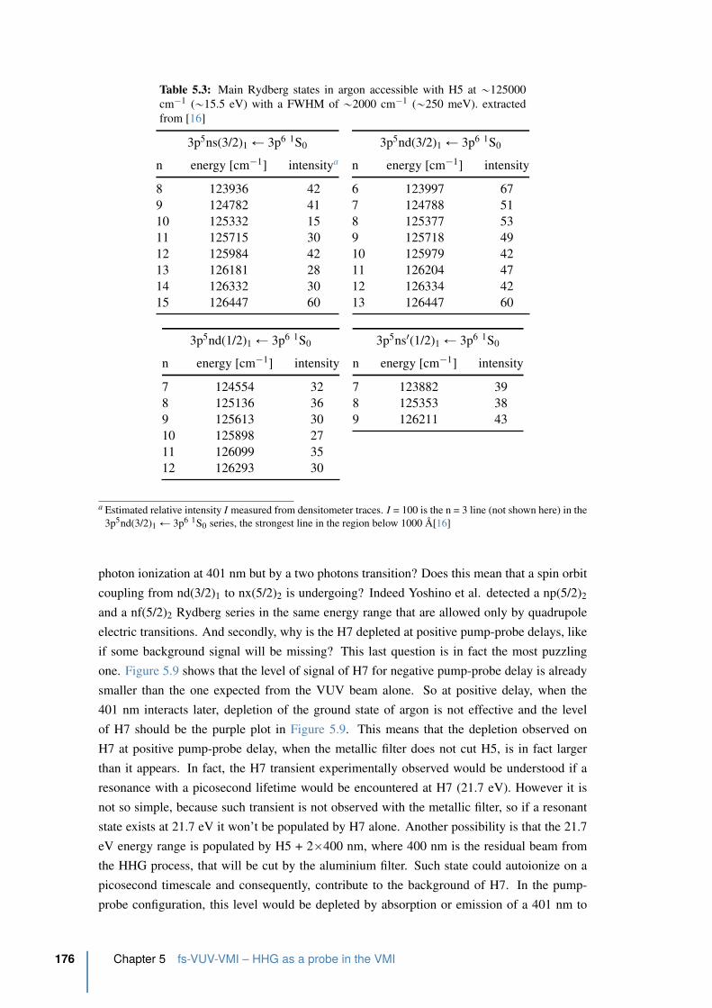
Table 5.3: Main Rydberg states in argon accessible with H5 at „125000
cm´1 („15.5 eV) with a FWHM of „2000 cm´1 („250 meV). extracted
from [16]
3p5ns(3/2)1 Ð 3p6 1S0
n energy [cm´1] intensitya
8 123936 42
9 124782 41
10 125332 15
11 125715 30
12 125984 42
13 126181 28
14 126332 30
15 126447 60
3p5nd(3/2)1 Ð 3p6 1S0
n energy [cm´1] intensity
6 123997 67
7 124788 51
8 125377 53
9 125718 49
10 125979 42
11 126204 47
12 126334 42
13 126447 60
3p5nd(1/2)1 Ð 3p6 1S0
n energy [cm´1] intensity
7 124554 32
8 125136 36
9 125613 30
10 125898 27
11 126099 35
12 126293 30
3p5ns1(1/2)1 Ð 3p6 1S0
n energy [cm´1] intensity
7 123882 39
8 125353 38
9 126211 43
a Estimated relative intensity I measured from densitometer traces. I = 100 is the n = 3 line (not shown here) in the
3p5nd(3/2)1 Ð 3p6 1S0 series, the strongest line in the region below 1000 A[16]
photon ionization at 401 nm but by a two photons transition? Does this mean that a spin orbit
coupling from nd(3/2)1 to nx(5/2)2 is undergoing? Indeed Yoshino et al. detected a np(5/2)2
and a nf(5/2)2 Rydberg series in the same energy range that are allowed only by quadrupole
electric transitions. And secondly, why is the H7 depleted at positive pump-probe delays, like
if some background signal will be missing? This last question is in fact the most puzzling
one. Figure 5.9 shows that the level of signal of H7 for negative pump-probe delay is already
smaller than the one expected from the VUV beam alone. So at positive delay, when the
401 nm interacts later, depletion of the ground state of argon is not effective and the level
of H7 should be the purple plot in Figure 5.9. This means that the depletion observed on
H7 at positive pump-probe delay, when the metallic filter does not cut H5, is in fact larger
than it appears. In fact, the H7 transient experimentally observed would be understood if a
resonance with a picosecond lifetime would be encountered at H7 (21.7 eV). However it is
not so simple, because such transient is not observed with the metallic filter, so if a resonant
state exists at 21.7 eV it won’t be populated by H7 alone. Another possibility is that the 21.7
eV energy range is populated by H5 + 2ˆ400 nm, where 400 nm is the residual beam from
the HHG process, that will be cut by the aluminium filter. Such state could autoionize on a
picosecond timescale and consequently, contribute to the background of H7. In the pump-
probe configuration, this level would be depleted by absorption or emission of a 401 nm to
176 Chapter 5 fs-VUV-VMI – HHG as a probe in the VMI
produce SB8 or SB6, leading to the depletion observed on H7, until this state autoionizes by
itself. The main problem is that there is no such state expected at that energy. However we
could imagine that at that energy a Kramers–Henneberger (KH) potential can be created with
a picoseconds lifetime. This hypothesis needs of course more experimental investigations, to
be confirmed. A KH atom is mostly a theoretical concept, since it has been put in evidence
experimentally only via one experiment [18]. A KH state is a stable state against ionization
due to an effective binding potential created by the presence of a strong electric field (here the
residual 400 nm) [19]. This is called a stabilization state. Definitively this first pump-probe
experiment on a simple system like argon, requires more experimental investigations which
was not expected.
5.3.4 Conclusion
The VUV pump 400 nm probe excitation of argon has shown that we were able to probe
the relaxation dynamics of a Rydberg state via photoelectron sideband detection. For this
we generated high-order harmonics using 400 nm, where the energy of the fifth harmonic is
approximately 250 meV below the ionization threshold of argon and in resonance with a series
of Rydberg states. These states are then probed by a one-photon transition with another 400
nm pulse, producing sideband 6. We observed as well, that the photoelectron peak connected
to harmonic 7, shows also a relaxation dynamic. However, the transient observed on H7, and
especially its depletion at positive delay, need further experimental investigation in order to be
understood.
Although the main interest of this experiment was not probing Rydberg states in argon, given
the extremely broad spectral bandwidth of our harmonic pulse compared to the energy levels
of the spectroscopic excitation in this region, this experience has allowed us to verify the
feasibility of such pump-probe experiments with the new fs-VUV-VMI spectrometer.
5.4 Photodissociation of acetylene, C2H2, using 9.3 eV
5.4.1 Motivation
After testing the new fs-VUV VMI spectrometer we looked for a molecular system with a
scientific interest that wont ask for too many experimental constraints in order to use this
technique. Acetylene seemed a good candidate because of the dissociation dynamics taking
place in the far ultraviolet around 9.3 eV, and as well as mentioned before, because acetylene
has numerous absorption bands, with a very large absorption cross-section („ 400 Mb around
9.3 eV) [12]. Furthermore, acetylene may be used in gaseous form at very high pressures (tens
of bars), which allows us to use a pulse molecular beam source (Even-Lavie valve) producing
a molecular beam with higher densities. Acetylene is also not corrosive and does not present
any particular health hazard.
The molecule acetylene (C2H2) was first synthesized in 1836 by Edmund Davy and the first ex-
perimental studies of the absorption spectroscopy of acetylene in ultraviolet date back as early
Section 5.4 Photodissociation of acetylene, C2H2, using 9.3 eV 177

as 1931 [20], followed by studies in the VUV range in 1935 [21]. The formation mechanism of
amino acids and polyols in the extraterrestrial atmosphere is an important question in biology,
planetary astrophysics, and cosmology. The existence of a variety of important species can be
traced to interstellar photochemistry taking place in interstellar molecular clouds [22, 23]. The
most abundant molecules in the interstellar medium include H2, CO, and acetylene. Ultravi-
olet photolysis of these simple molecules is a fundamental process in understanding the steps
leading to larger carbon-based systems, a challenge for interstellar chemistry. One of the main
dissociation products is the C2H radical which is in the models of interstellar chemistry one
of the precursor to the formation of carbon chains. A detailed understanding of photoinduced
reactions, including direct dissociation and predissociative mechanisms, is implicit to com-
pleting the photoreactive scenario behind the formation of larger molecules such as sugars and
amino acids. In despite its relatively simple structure (H–C”C–H), acetylene has an abundant
spectroscopy, especially in the UV and VUV region and shows numerous vibrational modes
and several types of geometries [24]. These different aspects have motivated the scientific
community and this molecule has been the subject of numerous studies. Here I can only give
a short introduction and summary to the spectroscopy of acetylene to show why we wanted to
study this molecule using the fs-VUV-VMI setup.
5.4.2 Acetylene’s electronic configuration, structure and Rydberg states
Acetylene is a linear molecule in its ground state (X1Σ
`g ) and belongs to the symmetry group
D8h (which has in addition to its linearity a center of inversion). The two central carbon atoms
are connected by a triple bond. When the molecule is in its ground state, the 14 electrons are
distributed as follows:
p1σgq2p1σuq2p2σgq2p2σuq2p3σgq2p1πuq4p1πgq0 (5.10)
The first two orbitals (1σ ) contain the core electrons of the molecule. The following two
orbitals (2σ ) form the C–H bond. The triple bond C”C is formed by the last two occupied
orbitals: 3σg and 1πu. When the molecule is excited, the valence electrons are promoted to
the first excited states of the molecule:
...p3σgq2p1πuq4 Ñ p3σgq2p1πuq3p1πgq1
Ñ p3σgq1p1πuq4p1πgq1
Ñ p3σgq2p1πuq2p1πgq2
The molecule then relaxes through different degrees freedom. During the relaxation, the
molecule may change its geometry, from a linear D8h geometry to planar geometries of the
type C2h (also called trans) or C2v (also called cis). Figure 5.10 shows the different vibra-
tional modes of the molecule in the three types of geometries. The vibrational transitions are
identified by the following notation: νn fni where ν represents the mode of vibration for a tran-
sition occurring from the initial state i to state final state f and ni and n f are the number of
quanta excited during the transition [24]. These notations are regularly used to specify the
178 Chapter 5 fs-VUV-VMI – HHG as a probe in the VMI
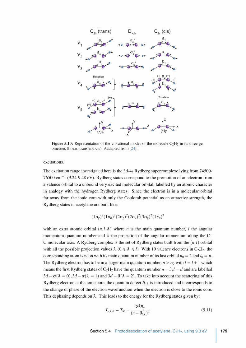
C2h
(trans)
ν1
ν2
ν3
ν4
C2v
(cis)D∞h
ν5
ag
ag
bu
ag
au
bu
a1
a1
b1
a2
b2
a1
σg
+
σg
+
σu
+
πg
πu
x
y
(*)z
(+)
(+)
(+)
(+)
x
yz
z
x(*)y
(-) (-)
(-)
(-)Rotation
Rotation
Figure 5.10: Representation of the vibrational modes of the molecule C2H2 in its three ge-
ometries (linear, trans and cis). Aadapted from [24].
excitations.
The excitation range investigated here is the 3d-4s Rydberg supercomplexe lying from 74500-
76500 cm´1 (9.24-9.48 eV). Rydberg states correspond to the promotion of an electron from
a valence orbital to a unbound very excited molecular orbital, labelled by an atomic character
in analogy with the hydrogen Rydberg states. Since the electron is in a molecular orbital
far away from the ionic core with only the Coulomb potential as an attractive strength, the
Rydberg states in acetylene are built like:
p1σgq2p1σuq2p2σgq2p2σuq2p3σgq2p1πuq3
with an extra atomic orbital pn, l,λ q where n is the main quantum number, l the angular
momentum quantum number and λ the projection of the angular momentum along the C–
C molecular axis. A Rydberg complex is the set of Rydberg states built from the pn, lq orbital
with all the possible projection values λ (0 ď λ ď l). With 10 valence electrons in C2H2, the
corresponding atom is neon with its main quantum number of its last orbital n0 “ 2 and l0 “ p.
The Rydberg electron has to be in a larger main quantum number, n ą n0 with l “ l ` 1 which
means the first Rydberg states of C2H2 have the quantum number n “ 3, l “ d and are labelled
3d ´ σpλ “ 0q,3d ´ πpλ “ 1q and 3d ´ δ pλ “ 2q. To take into account the scattering of this
Rydberg electron at the ionic core, the quantum defect δl,λ is introduced and it corresponds to
the change of phase of the electron wavefunction when the electron is close to the ionic core.
This dephasing depends on λ . This leads to the energy for the Rydberg states given by:
Tn,l,λ “ T8 ´ Z2Ry
pn ´ δl,λ q2(5.11)
Section 5.4 Photodissociation of acetylene, C2H2, using 9.3 eV 179
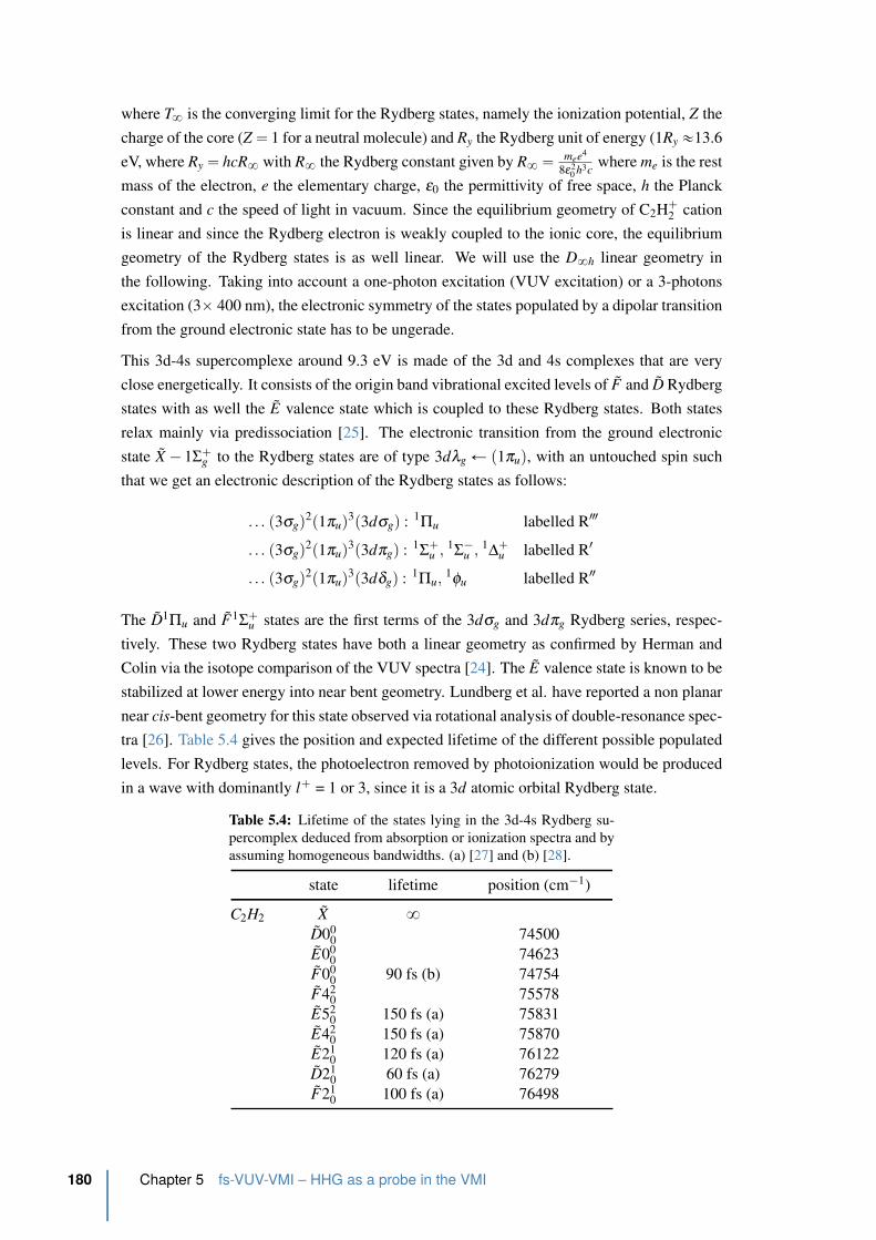
where T8 is the converging limit for the Rydberg states, namely the ionization potential, Z the
charge of the core (Z “ 1 for a neutral molecule) and Ry the Rydberg unit of energy (1Ry «13.6
eV, where Ry “ hcR8 with R8 the Rydberg constant given by R8 “ mee4
8ε20 h3c
where me is the rest
mass of the electron, e the elementary charge, ε0 the permittivity of free space, h the Planck
constant and c the speed of light in vacuum. Since the equilibrium geometry of C2H`2 cation
is linear and since the Rydberg electron is weakly coupled to the ionic core, the equilibrium
geometry of the Rydberg states is as well linear. We will use the D8h linear geometry in
the following. Taking into account a one-photon excitation (VUV excitation) or a 3-photons
excitation (3ˆ 400 nm), the electronic symmetry of the states populated by a dipolar transition
from the ground electronic state has to be ungerade.
This 3d-4s supercomplexe around 9.3 eV is made of the 3d and 4s complexes that are very
close energetically. It consists of the origin band vibrational excited levels of F and D Rydberg
states with as well the E valence state which is coupled to these Rydberg states. Both states
relax mainly via predissociation [25]. The electronic transition from the ground electronic
state X ´ 1Σ`g to the Rydberg states are of type 3dλg Ð p1πuq, with an untouched spin such
that we get an electronic description of the Rydberg states as follows:
. . . p3σgq2p1πuq3p3dσgq : 1Πu labelled R3
. . . p3σgq2p1πuq3p3dπgq : 1Σ
`u ,
1Σ
´u ,
1∆
`u labelled R1
. . . p3σgq2p1πuq3p3dδgq : 1Πu,
1φu labelled R2
The D1Πu and F1
Σ`u states are the first terms of the 3dσg and 3dπg Rydberg series, respec-
tively. These two Rydberg states have both a linear geometry as confirmed by Herman and
Colin via the isotope comparison of the VUV spectra [24]. The E valence state is known to be
stabilized at lower energy into near bent geometry. Lundberg et al. have reported a non planar
near cis-bent geometry for this state observed via rotational analysis of double-resonance spec-
tra [26]. Table 5.4 gives the position and expected lifetime of the different possible populated
levels. For Rydberg states, the photoelectron removed by photoionization would be produced
in a wave with dominantly l` = 1 or 3, since it is a 3d atomic orbital Rydberg state.
Table 5.4: Lifetime of the states lying in the 3d-4s Rydberg su-
percomplex deduced from absorption or ionization spectra and by
assuming homogeneous bandwidths. (a) [27] and (b) [28].
state lifetime position (cm´1)
C2H2 X 8D00
0 74500
E000 74623
F000 90 fs (b) 74754
F420 75578
E520 150 fs (a) 75831
E420 150 fs (a) 75870
E210 120 fs (a) 76122
D210 60 fs (a) 76279
F210 100 fs (a) 76498
180 Chapter 5 fs-VUV-VMI – HHG as a probe in the VMI
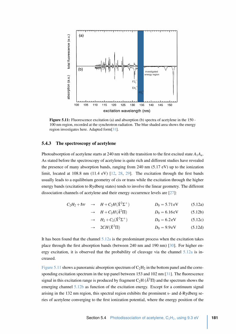
investigated
energy region
F00
0
F20
1
E40
3
Figure 5.11: Fluorescence excitation (a) and absorption (b) spectra of acetylene in the 150 -
100 nm region, recorded at the synchrotron radiation. The blue shaded area shows the energy
region investigates here. Adapted form[31].
5.4.3 The spectroscopy of acetylene
Photoabsorption of acetylene starts at 240 nm with the transition to the first excited state A1Au.
As stated before the spectroscopy of acetylene is quite rich and different studies have revealed
the presence of many absorption bands, ranging from 240 nm (5.17 eV) up to the ionization
limit, located at 108.8 nm (11.4 eV) [12, 28, 29]. The excitation through the first bands
usually leads to a equilibrium geometry of cis or trans while the excitation through the higher
energy bands (excitation to Rydberg states) tends to involve the linear geometry. The different
dissociation channels of acetylene and their energy occurrence levels are [27]:
C2H2 ` hν Ñ H `C2HpX2Σ
`q D0 “ 5.71eV (5.12a)
Ñ H `C2HpA2Πq D0 “ 6.16eV (5.12b)
Ñ H2 `C2pX2Σ
`q D0 “ 6.2eV (5.12c)
Ñ 2CHpX2Πq D0 “ 9.9eV (5.12d)
It has been found that the channel 5.12a is the predominant process when the excitation takes
place through the first absorption bands (between 240 nm and 190 nm) [30]. For higher en-
ergy excitation, it is observed that the probability of cleavage via the channel 5.12a is in-
creased.
Figure 5.11 shows a panoramic absorption spectrum of C2H2 in the bottom panel and the corre-
sponding excitation spectrum in the top panel between 153 and 102 nm [31]. The fluorescence
signal in this excitation range is produced by fragment C2H (A2Π) and the spectrum shows the
emerging channel 5.12b as function of the excitation energy. Except for a continuum signal
arising in the 132 nm region, this spectral region exhibits the prominent s- and d-Rydberg se-
ries of acetylene converging to the first ionization potential, where the energy position of the
Section 5.4 Photodissociation of acetylene, C2H2, using 9.3 eV 181
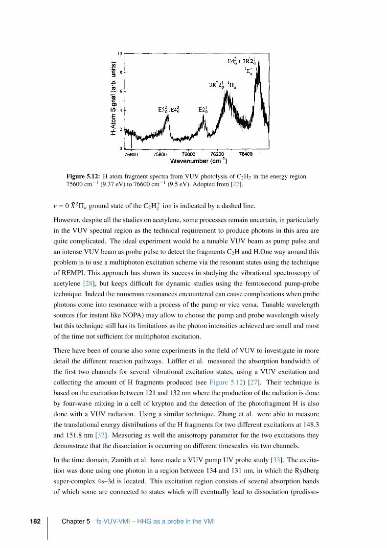
Figure 5.12: H atom fragment spectra from VUV photolysis of C2H2 in the energy region
75600 cm´1 (9.37 eV) to 76600 cm´1 (9.5 eV). Adopted from [27].
v “ 0 X2Πu ground state of the C2H`
2 ion is indicated by a dashed line.
However, despite all the studies on acetylene, some processes remain uncertain, in particularly
in the VUV spectral region as the technical requirement to produce photons in this area are
quite complicated. The ideal experiment would be a tunable VUV beam as pump pulse and
an intense VUV beam as probe pulse to detect the fragments C2H and H.One way around this
problem is to use a multiphoton excitation scheme via the resonant states using the technique
of REMPI. This approach has shown its success in studying the vibrational spectroscopy of
acetylene [28], but keeps difficult for dynamic studies using the femtosecond pump-probe
technique. Indeed the numerous resonances encountered can cause complications when probe
photons come into resonance with a process of the pump or vice versa. Tunable wavelength
sources (for instant like NOPA) may allow to choose the pump and probe wavelength wisely
but this technique still has its limitations as the photon intensities achieved are small and most
of the time not sufficient for multiphoton excitation.
There have been of course also some experiments in the field of VUV to investigate in more
detail the different reaction pathways. Loffler et al. measured the absorption bandwidth of
the first two channels for several vibrational excitation states, using a VUV excitation and
collecting the amount of H fragments produced (see Figure 5.12) [27]. Their technique is
based on the excitation between 121 and 132 nm where the production of the radiation is done
by four-wave mixing in a cell of krypton and the detection of the photofragment H is also
done with a VUV radiation. Using a similar technique, Zhang et al. were able to measure
the translational energy distributions of the H fragments for two different excitations at 148.3
and 151.8 nm [32]. Measuring as well the anisotropy parameter for the two excitations they
demonstrate that the dissociation is occurring on different timescales via two channels.
In the time domain, Zamith et al. have made a VUV pump UV probe study [33]. The excita-
tion was done using one photon in a region between 134 and 131 nm, in which the Rydberg
super-complex 4s–3d is located. This excitation region consists of several absorption bands
of which some are connected to states which will eventually lead to dissociation (predisso-
182 Chapter 5 fs-VUV-VMI – HHG as a probe in the VMI
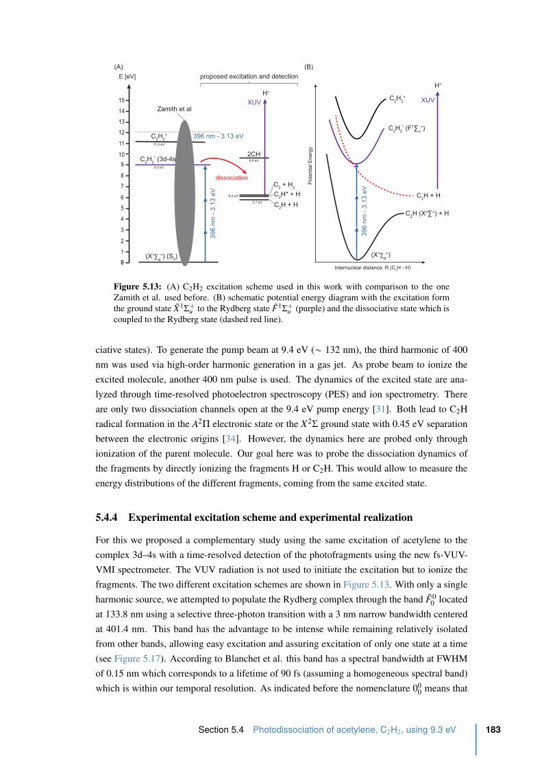
(X1∑g+) (S
0)
0
1
2
3
4
5
6
7
8
9
10
11
E [eV]
C2H
2* (3d-4s)9.3 eV
C2H
2+
11.4 eV
12
13
14
15
132 n
m -
9.4
eV
396 nm - 3.13 eV
2CH
C2 + H
2
C2H* + H
C2H + H
9.9 eV
5.7 eV
6.2 eV
396 n
m -
3.1
3 e
V
XUV
H+
dissociation
Zamith et al
proposed excitation and detection
Internuclear distance, R (C2H - H)
Po
ten
tia
l E
ne
rgy
C2H (X2∑+) + H
C2H
2* (F1∑
u+)
C2H
2+
C2H + H
396 n
m -
3.1
3 e
V
H+
(X1∑g+)
XUV
(A) (B)
Figure 5.13: (A) C2H2 excitation scheme used in this work with comparison to the one
Zamith et al. used before. (B) schematic potential energy diagram with the excitation form
the ground state X1Σ
`u to the Rydberg state F1
Σ`u (purple) and the dissociative state which is
coupled to the Rydberg state (dashed red line).
ciative states). To generate the pump beam at 9.4 eV („ 132 nm), the third harmonic of 400
nm was used via high-order harmonic generation in a gas jet. As probe beam to ionize the
excited molecule, another 400 nm pulse is used. The dynamics of the excited state are ana-
lyzed through time-resolved photoelectron spectroscopy (PES) and ion spectrometry. There
are only two dissociation channels open at the 9.4 eV pump energy [31]. Both lead to C2H
radical formation in the A2Π electronic state or the X2
Σ ground state with 0.45 eV separation
between the electronic origins [34]. However, the dynamics here are probed only through
ionization of the parent molecule. Our goal here was to probe the dissociation dynamics of
the fragments by directly ionizing the fragments H or C2H. This would allow to measure the
energy distributions of the different fragments, coming from the same excited state.
5.4.4 Experimental excitation scheme and experimental realization
For this we proposed a complementary study using the same excitation of acetylene to the
complex 3d–4s with a time-resolved detection of the photofragments using the new fs-VUV-
VMI spectrometer. The VUV radiation is not used to initiate the excitation but to ionize the
fragments. The two different excitation schemes are shown in Figure 5.13. With only a single
harmonic source, we attempted to populate the Rydberg complex through the band F00 located
at 133.8 nm using a selective three-photon transition with a 3 nm narrow bandwidth centered
at 401.4 nm. This band has the advantage to be intense while remaining relatively isolated
from other bands, allowing easy excitation and assuring excitation of only one state at a time
(see Figure 5.17). According to Blanchet et al. this band has a spectral bandwidth at FWHM
of 0.15 nm which corresponds to a lifetime of 90 fs (assuming a homogeneous spectral band)
which is within our temporal resolution. As indicated before the nomenclature 000 means that
Section 5.4 Photodissociation of acetylene, C2H2, using 9.3 eV 183
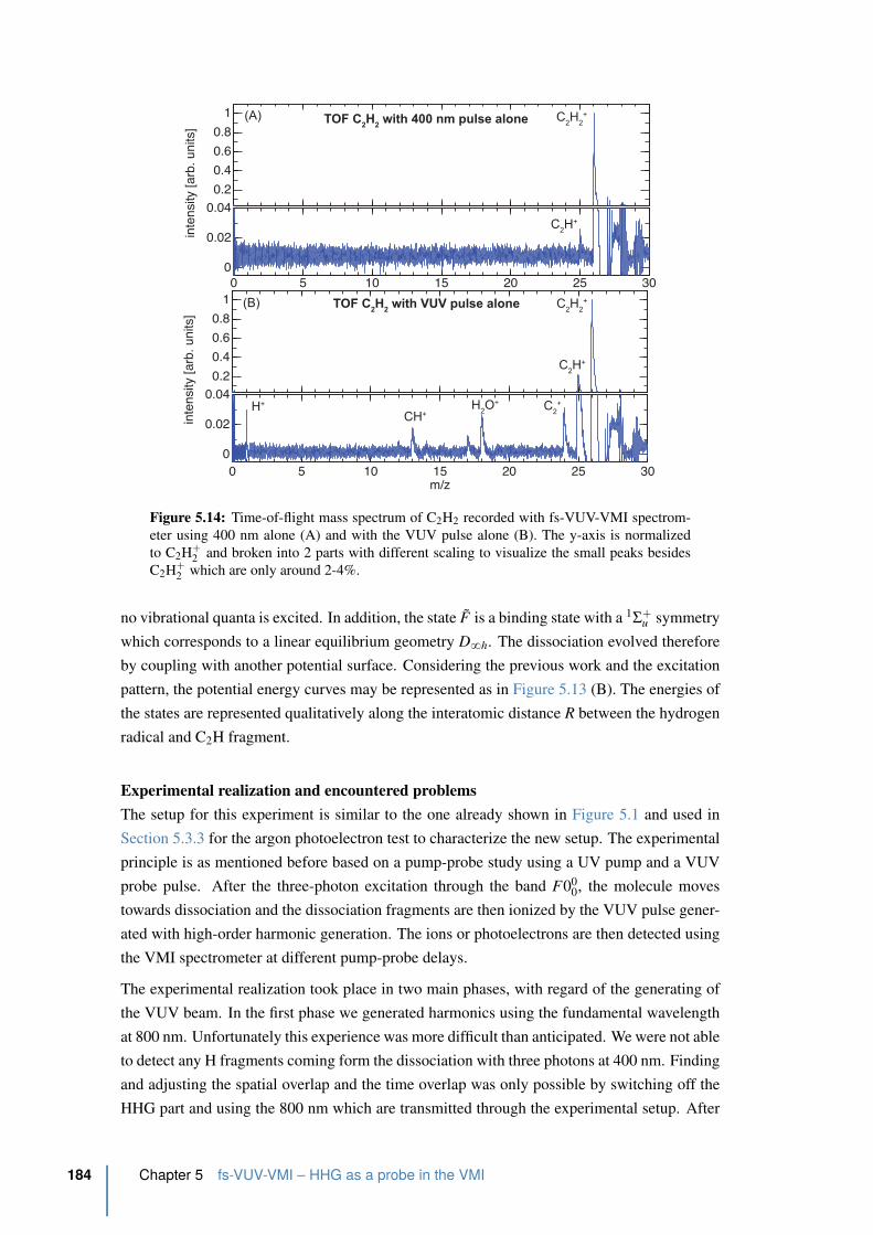
0 5 10 15 20 25 300
0.02
0.04
m/z
inte
nsity
[arb
. uni
ts]
0.2
0.4
0.6
0.8
1
H+
C2H
2+
C2H+
C2+H
2O+
CH+
TOF C2H
2 with VUV pulse alone
0 5 10 15 20 25 300
0.02
0.04
inte
nsity
[arb
. uni
ts]
0.2
0.4
0.6
0.8
1 C2H
2+
C2H+
TOF C2H
2 with 400 nm pulse alone
(B)
(A)
Figure 5.14: Time-of-flight mass spectrum of C2H2 recorded with fs-VUV-VMI spectrom-
eter using 400 nm alone (A) and with the VUV pulse alone (B). The y-axis is normalized
to C2H`2 and broken into 2 parts with different scaling to visualize the small peaks besides
C2H`2 which are only around 2-4%.
no vibrational quanta is excited. In addition, the state F is a binding state with a 1Σ
`u symmetry
which corresponds to a linear equilibrium geometry D8h. The dissociation evolved therefore
by coupling with another potential surface. Considering the previous work and the excitation
pattern, the potential energy curves may be represented as in Figure 5.13 (B). The energies of
the states are represented qualitatively along the interatomic distance R between the hydrogen
radical and C2H fragment.
Experimental realization and encountered problems
The setup for this experiment is similar to the one already shown in Figure 5.1 and used in
Section 5.3.3 for the argon photoelectron test to characterize the new setup. The experimental
principle is as mentioned before based on a pump-probe study using a UV pump and a VUV
probe pulse. After the three-photon excitation through the band F000, the molecule moves
towards dissociation and the dissociation fragments are then ionized by the VUV pulse gener-
ated with high-order harmonic generation. The ions or photoelectrons are then detected using
the VMI spectrometer at different pump-probe delays.
The experimental realization took place in two main phases, with regard of the generating of
the VUV beam. In the first phase we generated harmonics using the fundamental wavelength
at 800 nm. Unfortunately this experience was more difficult than anticipated. We were not able
to detect any H fragments coming form the dissociation with three photons at 400 nm. Finding
and adjusting the spatial overlap and the time overlap was only possible by switching off the
HHG part and using the 800 nm which are transmitted through the experimental setup. After
184 Chapter 5 fs-VUV-VMI – HHG as a probe in the VMI
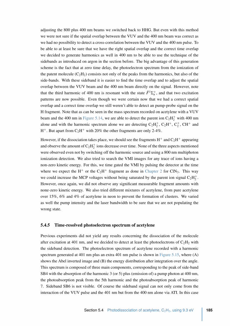
adjusting the 800 plus 400 nm beams we switched back to HHG. But even with this method
we were not sure if the spatial overlap between the VUV and the 400 nm beam was correct as
we had no possibility to detect a cross-correlation between the VUV and the 400 nm pulse. To
be able to at least be sure that we have the right spatial overlap and the correct time overlap
we decided to generate harmonics as well in 400 nm to be able to use the technique of the
sidebands as introduced on argon in the section before. The big advantage of this generation
scheme is the fact that at zero time delay, the photoelectron spectrum from the ionization of
the patent molecule (C2H2) consists not only of the peaks from the harmonics, but also of the
side-bands. With these sideband it is easier to find the time overlap and to adjust the spatial
overlap between the VUV beam and the 400 nm beam directly on the signal. However, note
that the third harmonic of 400 nm is resonant with the state F1Σ
`u , and that two excitation
patterns are now possible. Even though we were certain now that we had a correct spatial
overlap and a correct time overlap we still weren’t able to detect an pump-probe signal on the
H fragment. Note that as can be seen in the mass spectrum recorded on acetylene with a VUV
beam and the 400 nm in Figure 5.14, we are able to detect the parent ion C2H`2 with 400 nm
alone and with the harmonic spectrum alone we are detecting C2H`2 , C2H`, C`
2 , CH` and
H`. But apart from C2H` with 20% the other fragments are only 2-4%.
However, if the dissociation takes place, we should see the fragments H` and C2H` appearing
and observe the amount of C2H`2 ions decrease over time. None of the three aspects mentioned
were observed even not by switching off the harmonic source and using a 800 nm multiphoton
ionization detection. We also tried to search the VMI images for any trace of ions having a
non-zero kinetic energy. For this, we time gated the VMI by pulsing the detector at the time
where we expect the H` or the C2H` fragment as done in Chapter 2 for ClN3. This way
we could increase the MCP voltages without being saturated by the parent ion signal C2H`2 .
However, once again, we did not observe any significant measurable fragment amounts with
none-zero kinetic energy. We also tried different mixtures of acetylene, from pure acetylene
over 15%, 6% and 4% of acetylene in neon to prevent the formation of clusters. We varied
as well the pump intensity and the laser bandwidth to be sure that we are not populating the
wrong state.
5.4.5 Time-resolved photoelectron spectrum of acetylene
Previous experiments did not yield any results concerning the dissociation of the molecule
after excitation at 401 nm, and we decided to detect at least the photoelectrons of C2H2 with
the sideband detection. The photoelectron spectrum of acetylene recorded with a harmonic
spectrum generated at 401 nm plus an extra 401 nm pulse is shown in Figure 5.15, where (A)
shows the Abel inverted image and (B) the energy distribution after integration over the angle.
This spectrum is composed of three main components, corresponding to the peak of side-band
SB4 with the absorption of the harmonic 3 (or 5) plus (emission of) a pump photon at 400 nm,
the photoabsorption peak from the 5th harmonic and the photoabsorption peak of harmonic
7. Sideband SB6 is not visible. Of course the sideband signal can not only come from the
interaction of the VUV pulse and the 401 nm but from the 400 nm alone via ATI. In this case
Section 5.4 Photodissociation of acetylene, C2H2, using 9.3 eV 185
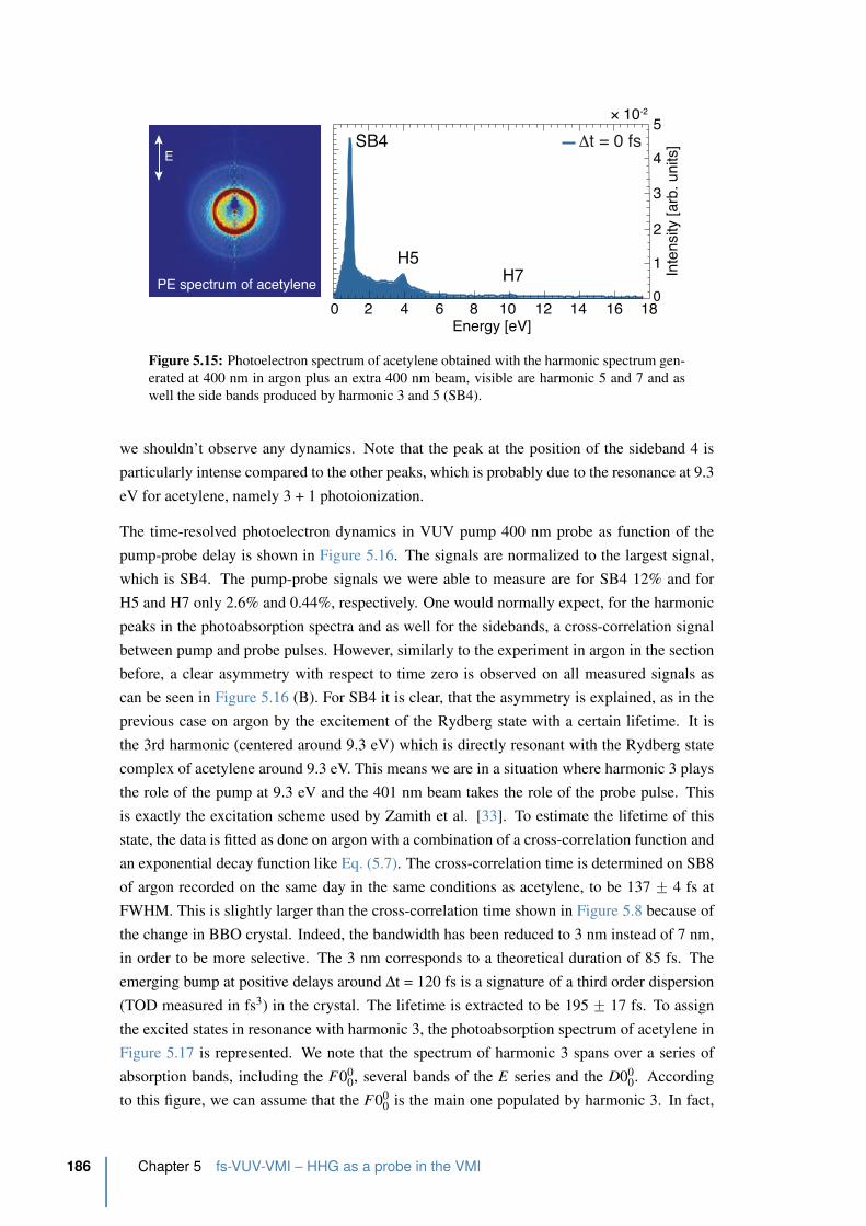
Energy [eV]
H5
SB4
H7
0 2 4 6 8 10 12 14 16 18
Inte
nsity [arb
. units]
0
1
2
3
4
5× 10⁻²
Δt = 0 fsE
PE spectrum of acetylene
Figure 5.15: Photoelectron spectrum of acetylene obtained with the harmonic spectrum gen-
erated at 400 nm in argon plus an extra 400 nm beam, visible are harmonic 5 and 7 and as
well the side bands produced by harmonic 3 and 5 (SB4).
we shouldn’t observe any dynamics. Note that the peak at the position of the sideband 4 is
particularly intense compared to the other peaks, which is probably due to the resonance at 9.3
eV for acetylene, namely 3 + 1 photoionization.
The time-resolved photoelectron dynamics in VUV pump 400 nm probe as function of the
pump-probe delay is shown in Figure 5.16. The signals are normalized to the largest signal,
which is SB4. The pump-probe signals we were able to measure are for SB4 12% and for
H5 and H7 only 2.6% and 0.44%, respectively. One would normally expect, for the harmonic
peaks in the photoabsorption spectra and as well for the sidebands, a cross-correlation signal
between pump and probe pulses. However, similarly to the experiment in argon in the section
before, a clear asymmetry with respect to time zero is observed on all measured signals as
can be seen in Figure 5.16 (B). For SB4 it is clear, that the asymmetry is explained, as in the
previous case on argon by the excitement of the Rydberg state with a certain lifetime. It is
the 3rd harmonic (centered around 9.3 eV) which is directly resonant with the Rydberg state
complex of acetylene around 9.3 eV. This means we are in a situation where harmonic 3 plays
the role of the pump at 9.3 eV and the 401 nm beam takes the role of the probe pulse. This
is exactly the excitation scheme used by Zamith et al. [33]. To estimate the lifetime of this
state, the data is fitted as done on argon with a combination of a cross-correlation function and
an exponential decay function like Eq. (5.7). The cross-correlation time is determined on SB8
of argon recorded on the same day in the same conditions as acetylene, to be 137 ˘ 4 fs at
FWHM. This is slightly larger than the cross-correlation time shown in Figure 5.8 because of
the change in BBO crystal. Indeed, the bandwidth has been reduced to 3 nm instead of 7 nm,
in order to be more selective. The 3 nm corresponds to a theoretical duration of 85 fs. The
emerging bump at positive delays around ∆t = 120 fs is a signature of a third order dispersion
(TOD measured in fs3) in the crystal. The lifetime is extracted to be 195 ˘ 17 fs. To assign
the excited states in resonance with harmonic 3, the photoabsorption spectrum of acetylene in
Figure 5.17 is represented. We note that the spectrum of harmonic 3 spans over a series of
absorption bands, including the F000, several bands of the E series and the D00
0. According
to this figure, we can assume that the F000 is the main one populated by harmonic 3. In fact,
186 Chapter 5 fs-VUV-VMI – HHG as a probe in the VMI
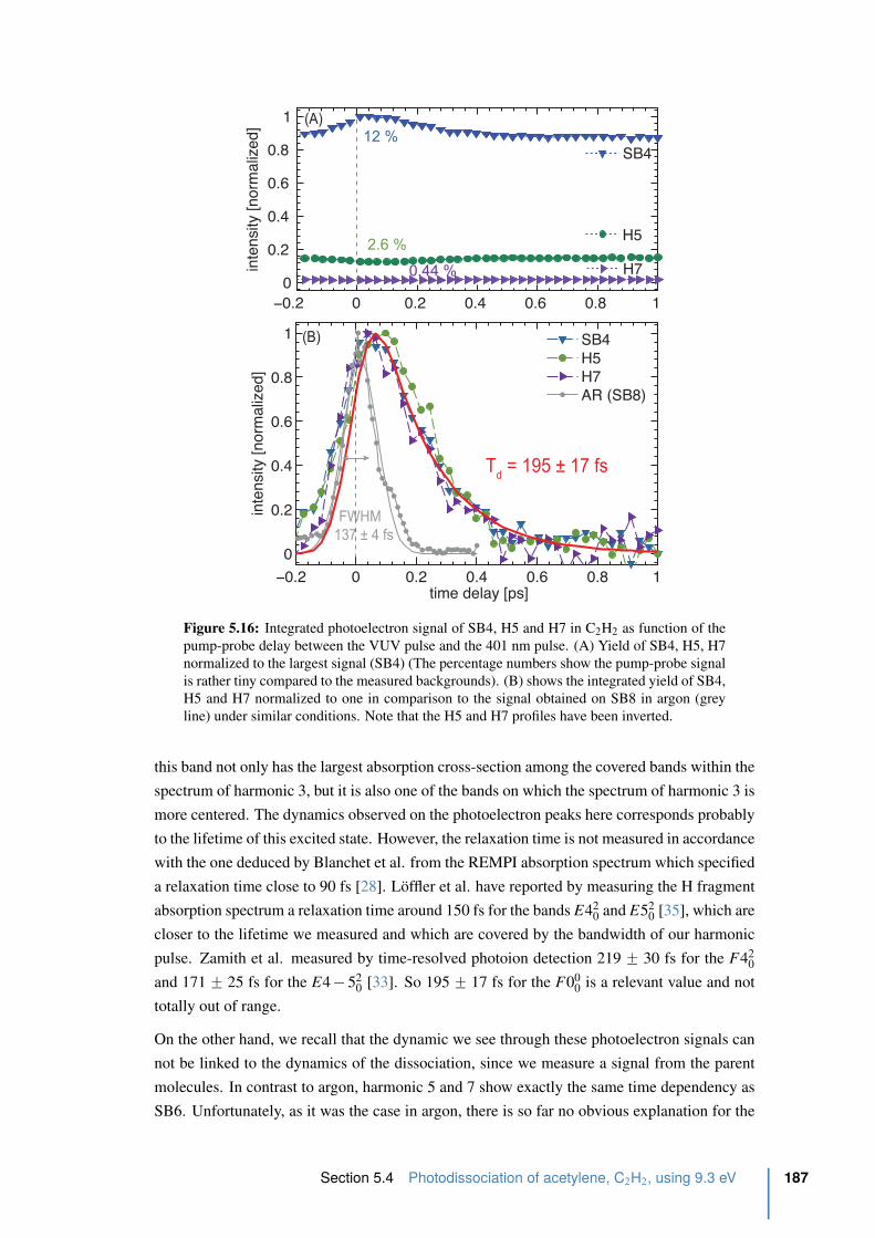
−0.2 0 0.2 0.4 0.6 0.8 10
0.2
0.4
0.6
0.8
1
inte
nsity
[nor
mal
ized
]
−0.2 0 0.2 0.4 0.6 0.8 1
0
0.2
0.4
0.6
0.8
1
time delay [ps]
inte
nsity
[nor
mal
ized
]
SB4H5H7AR (SB8)
12 %
2.6 %
0.44 %
SB4
H5
H7
FWHM
137 ± 4 fs
Td = 195 ± 17 fs
(A)
(B)
Figure 5.16: Integrated photoelectron signal of SB4, H5 and H7 in C2H2 as function of the
pump-probe delay between the VUV pulse and the 401 nm pulse. (A) Yield of SB4, H5, H7
normalized to the largest signal (SB4) (The percentage numbers show the pump-probe signal
is rather tiny compared to the measured backgrounds). (B) shows the integrated yield of SB4,
H5 and H7 normalized to one in comparison to the signal obtained on SB8 in argon (grey
line) under similar conditions. Note that the H5 and H7 profiles have been inverted.
this band not only has the largest absorption cross-section among the covered bands within the
spectrum of harmonic 3, but it is also one of the bands on which the spectrum of harmonic 3 is
more centered. The dynamics observed on the photoelectron peaks here corresponds probably
to the lifetime of this excited state. However, the relaxation time is not measured in accordance
with the one deduced by Blanchet et al. from the REMPI absorption spectrum which specified
a relaxation time close to 90 fs [28]. Loffler et al. have reported by measuring the H fragment
absorption spectrum a relaxation time around 150 fs for the bands E420 and E52
0 [35], which are
closer to the lifetime we measured and which are covered by the bandwidth of our harmonic
pulse. Zamith et al. measured by time-resolved photoion detection 219 ˘ 30 fs for the F420
and 171 ˘ 25 fs for the E4 ´ 520 [33]. So 195 ˘ 17 fs for the F00
0 is a relevant value and not
totally out of range.
On the other hand, we recall that the dynamic we see through these photoelectron signals can
not be linked to the dynamics of the dissociation, since we measure a signal from the parent
molecules. In contrast to argon, harmonic 5 and 7 show exactly the same time dependency as
SB6. Unfortunately, as it was the case in argon, there is so far no obvious explanation for the
Section 5.4 Photodissociation of acetylene, C2H2, using 9.3 eV 187
72000 73000 74000 75000 76000 77000 780000
0.2
0.4
0.6
0.8
1ab
sorp
tion
cros
s−se
ction
[nor
mali
zed]
Excitation energy [cm-1]
0
1
2
3
4
5x 10⁴
3+1
REM
PI si
gnal
[arb
. unit
s]
8.9 9 9.1 9.2 9.3 9.4 9.5 9.6 [eV]130132134136138 [nm]
3 x 401 nm
H3
D00
0
E00
0
F00
0
E40
1
F40
2
E40
2
E50
2
E20
1
D20
1
F20
1 + E4
0
3
Figure 5.17: Spectrum of harmonic 3 (purple) overlapped with the absorption cross-section
of acetylene (blue) obtained in the synchrotron in this energy region [12] and the 3+1 REMPI
signal (green) [28]. Also shown is the spectrum of the 401 nm (3 photons at 401 nm) in light
blue.
time dependency observed on the depletion of these harmonics. Similarly, if our interpretation
of the dynamics observed in argon is valid, the time-resolved dynamic observed on H5 and
H7 reflects the fact that the excited molecules relax to other electronic states with energies
En that again have to fullfill the energy conservation given by En ` p ˆ E401nm “ EH5/EH7.
However, this means that the contribution from molecules moving towards dissociation is
negligible. This consideration seems to be an argument for the fact that the excitement over
the band F000 does lead to very low dissociation probability, and the relaxation evolves through
vibrational excitation. This statement remains very suggestive and has to be considered with
precaution. It would be interesting to verify whether the observed relaxation is due to the
excitation via the band F000 by slightly moving the harmonic spectrum to lower energies, so
that it no longer includes the E state series. This might be achieved by playing very lightly on
the phase-matching angle of the doubling crystal, being careful not to lose too much doubling
efficiency in order to maintain enough intensity for the HHG. This way one could also see if
the transients observed on H5 and H7 depend on which states are involved in this broadband
exciatation.
5.4.6 Conclusion
We have attempted to study the photodissociation of acetylene at 9.3 eV using the new the fs-
VUV-VMI spectroscopy setup. Two different approaches were used. Initially, we employed a
three-photon pump transition centered at 401.3 nm and a probe step using the harmonic spec-
trum to ionize the dissociation fragments. However, no dissociation fragments were detected
188 Chapter 5 fs-VUV-VMI – HHG as a probe in the VMI
with this method. It is still unclear as to why the experiment did not work. On one hand, it is
possible that our harmonic photon flux is insufficient to probe the dissociation fragments with
low absorption cross-sections, as is the case for the hydrogen fragments, which are moreover,
the results from low efficiency processes (low dissociation efficiency). On the other hand, it
does not exclude that we do not control the pump excitation step precise enough. Although
we excite the molecule at an absorption band with a very high absorption cross-section (a
three-photon resonance), it is possible that we do not leave any population in the excited state
due to a single photon transition from this state to the ion continuum. The dissociation rate of
F000 might not be sufficient to study the photodissociation via this state. The employed type
of multiphoton excitation scheme is particularly problematic, especially when the resonant
transition involves a relatively large number of photons compared to the transition leading to
ionization. This illustrates the relevance of photon sources in the VUV range. Indeed, mak-
ing a one-photon transition from the ground state to the state of interest brings the focus on
the excitation without risking ionization of the molecule by a transition involving a second
photon. This aspect we tried to develop in the second experimental approach, by exciting the
molecule acetylene by a one-photon transition using the third harmonic generated at 400 nm.
A second pulse at 400 nm was used to probe the dissociation of the molecule. Once again, no
trace of ionized fragments was found. The analysis of the photoelectron spectra as a function
of the pump-probe delay revealed, nevertheless, the femtosecond dynamics of the relaxation
of the excited states brought into play. However, given the large spectral bandwidth of the 3rd
harmonic, it is difficult to assign the states involved. This large spectral bandwidth is the major
drawback of HHG as a source of VUV photons for atomic and molecular spectroscopy.
Recently, a novel scheme for HHG based on using two gas cells has been demonstrated [36].
This allows the production of fs-VUV pulses by HHG generation in the nJ/p regime. Such
high energy pulses could overcome the issue of low photon flux and could prove to be the key
to ion detection for the fs-VUV-VMI setup. The principle is based on using below-threshold
harmonics, generated in a ‘seeding cell’, to boost the HHG process in a ‘generation cell’,
placed further downstream in the focused laser beam. By modifying the fundamental driving
field, these low-order harmonics alter the ionization step of the nonlinear HHG process and it
has been shown that the HHG process is boosted by a factor of 7 in neon.
Furthermore, to increase the VUV photon flux in the monochromator configuration we could
replace the gold grating by a aluminium grating which would increase the monochromator
transmission by a factor of 10 from 1ˆ10´3 to 1ˆ10´2. In addition, replacing the B4C fo-
cussing mirror with an aluminium mirror would lead to monochromator transmission of about
3ˆ10´2. Howeber, using aluminium would mean we cut all harmonics above H10. A pricier
alternative would be to invest in a new diffraction grating. To increase the HHG efficiency pro-
duced with 400 nm the plan is also to generate 400 nm under vacuum with a metallic focusing
mirror to focus the 400 nm in a cell. This will result in a shorter transform-limited pulse at
400 nm and therefore increase the efficiency of the HHG process.
There are two key drawbacks on the present experimental setup, which should be implemented.
The first one, the real duration of the VUV pulse cannot be measured. Indeed, it is currently
Section 5.4 Photodissociation of acetylene, C2H2, using 9.3 eV 189
assumed that the duration of the VUV pulse is around half of the duration of the fundamental
pulse. This could mean for harmonics generated at 400 nm a VUV pulse with a duration of
around 20 fs. However, to be able to measure this duration, an even shorter pulse is required.
This could be achieved by first broadening an 800 nm pulse via a with neon filled capillary
and afterwards recompressing it with chirped mirrors. Unfortunately, such equipment was not
available and has not been implemented on the experimental apparatus. The second drawback
is that it is not possible to investigate the quality of the VUV spatial mode. We examined only
the 400 nm waist position, in order to place the center of the VMI directly at this position.
Later on the VMI position was optimized at the multiphoton signal at 400 nm. As mentioned
before, the impossibility to adjust the toroidal mirror under vacuum has to be overcome in
order to adjust the VUV spatial mode directly. For this particular optomechnics are required
to control the mirror positions from outside and to be able to adjust the VUV spatial mode
based for instance on detecting the waist of the VUV pulse by the luminescence emitted by a
crystal. With this, the pump-probe volume could be optimized, leading to a larger pump-probe
contrast compared to the unsatisfactory 10% observed here.
Recently the fs-VUV-VMI facility has been used to study fenchone to investigate the circular
dichroism of the photoelectons when the VUV light is produced in SF6. For this experiment
the source has been changed for a needle placed between the repeller and extractor plate.
Compared to the previous experiments using a pulsed molecular beam source place 12 cm
away from the VMI center, the signals were multiplied by 100. Pump-probe experiments with
such source developments are ongoing.
References
[1] HIPPLER, M and PFAB, J. Detection and Probing of Nitric-Oxide (No) by 2-Color
Laser Photoionization (Rempi) Spectroscopy on the a[-X Transition. Chem. Phys. Lett.
243:5-6 500–505 (1995) (cited p. 158).
[2] Mairesse, Y, Gobert, O, Breger, P, Merdji, H, Meynadier, P, Monchicourt, P, Perdrix,
M, eres, PS, and ’e, BC. High Harmonic XUV Spectral Phase Interferometry for Direct
Electric-Field Reconstruction. Phys. Rev. Lett. 94:17 173903 (2005) (cited p. 158).
[3] Frassetto, F, Bonora, S, VILLORESI, P, Poletto, L, Springate, E, Froud, CA, Turcu,
ICE, Langley, AJ, Wolff, DS, Collier, JL, Dhesi, SS, and Cavalleri, A. Design and
characterization of the XUV monochromator for ultrashort pulses at the ARTEMIS
facility. Optical Engineering + Applications 7077: pages (2008) (cited p. 158).
[4] Frassetto, F, Cacho, C, Froud, CA, Turcu, ICE, Villoresi, P, Bryan, WA, Springate,
E, and Poletto, L. Single-grating monochromator for extreme-ultraviolet ultrashort
pulses. Opt. Express 19:20 19169 (2011) (cited p. 159).
[5] Ito, M, Kataoka, Y, Okamoto, T, Yamashita, M, and Sekikawa, T. Spatiotemporal
characterization of single-order high harmonic pulses from time-compensated toroidal-
grating monochromator. Opt. Express 18:6 6071–6078 (2010) (cited p. 159).
[6] Wernet, P, Gaudin, Jm, Godehusen, K, Schwarzkopf, O, and Eberhardt, W. Fem-
tosecond time-resolved photoelectron spectroscopy with a vacuum-ultraviolet photon
source based on laser high-order harmonic generation. Rev. Sci. Instr. 82:6 pages
(2011) (cited p. 159).
[7] Ruf, H. Dynamique moleculaire par imagerie attoseconde. PhD thesis. Universite Bor-
deuax 1, 2012 (cited p. 161–163).
190 Chapter 5 fs-VUV-VMI – HHG as a probe in the VMI
[8] Bourassin-Bouchet, C, Mang, MM, Delmotte, F, Chavel, P, and Rossi, S de. How to
focus an attosecond pulse. Opt. Express 21:2 2506–2520 (2013) (cited p. 162, 163).
[9] Chan, WF, Cooper, G, Guo, X, Burton, GR, and Brion, CE. Absolute optical oscil-
lator strengths for the electronic excitation of atoms at high resolution. III. The pho-
toabsorption of argon, krypton, and xenon. Phys. Rev. A 46:1 149–171 (1992) (cited
p. 166).
[10] Palenius, H, Kohl, J, and Parkinson, W. Absolute measurement of the photoionization
cross section of atomic hydrogen with a shock tube for the extreme ultraviolet. Phys.
Rev. A 13:5 1805–1816 (1976) (cited p. 166).
[11] Jenkin, ME, Murrells, TP, Shalliker, SJ, and Hayman, GD. Kinetics and product study
of the self-reactions of allyl and allyl peroxy radicals at 296 K. J. Chem. Soc. Fara.
Trans. 89:3 433 (1993) (cited p. 166).
[12] Suto, M and LEE, LC. Quantitative photoexcitation and fluorescence studies of C2H2
in vacuum ultraviolet. J. Chem. Phys. 80:10 4824 (1984) (cited p. 166, 177, 181, 188).
[13] Luria, K, Christen, W, and Even, U. Generation and Propagation of Intense Super-
sonic Beams. J. Phys. Chem. A 115:25 7362–7367 (2011) (cited p. 166, 167).
[14] Paul, PM, Toma, ES, Breger, P, Mullot, G, Balcou, P, Muller, HG, and Agostini, P.
Observation of a Train of Attosecond Pulses from High Harmonic Generation. Science
292:5522 1689–1692 (2001) (cited p. 169).
[15] Varju, K, Johnsson, P, Lopez-Martens, R, Remetter, T, Gustafsson, E, Mauritsson, J,
Gaarde, MB, Schafer, KJ, Erny, C, and Sola, I. Experimental studies of attosecond
pulse trains. Laser Phys. 15:6 888–898 (2005) (cited p. 169).
[16] YOSHINO, K. Absorption Spectrum of the Argon Atom in the Vacuum-Ultraviolet
Region. J. Opt. Soc. Am. 60:9 1220 (1970) (cited p. 172, 175, 176).
[17] Baig, M, Ahmad, S, Connerade, J, Dussa, W, and Hormes, J. Overlapping sequence
of doubly excited series in the vuv spectrum of argon. Phys. Rev. A 45:11 7963–7968
(1992) (cited p. 175).
[18] Eichmann, U, Nubbemeyer, T, Rottke, H, and Sandner, W. Acceleration of neutral
atoms in strong short-pulse laser fields. Nature 461:7268 1261–1264 (2009) (cited
p. 177).
[19] Morales, F, Richter, M, Patchkovskii, S, and Smirnova, O. From the Cover: Imaging
the Kramers-Henneberger atom. Proceedings of the National Academy of Sciences
108:41 16906–16911 (2011) (cited p. 177).
[20] Kistiakowsky, G. On the Ultraviolet Absorption Spectrum of Acetylene. Phys. Rev.
37:3 276–278 (1931) (cited p. 178).
[21] Price, W. The Absorption Spectra of Acetylene, Ethylene and Ethane in the Far Ultra-
violet. Phys. Rev. 47:6 444–452 (1935) (cited p. 178).
[22] Bernstein, MP, Dworkin, JP, Sandford, SA, and Cooper, GW. Racemic amino acids
from the ultraviolet photolysis of interstellar ice analogues. Nature (2002) (cited p. 178).
[23] Caro, G, Meierhenrich, UJ, Schutte, WA, and Barbier, B. Amino acids from ultraviolet
irradiation of interstellar ice analogues. Nature (2002) (cited p. 178).
[24] Herman, M and Colin, R. The absorption spectra of C2H2, C2D2, and C2HD in the
region 1260 to 1370 A. J. Mol. Spec. 85:2 449–461 (1981) (cited p. 178–180).
[25] Kono, M, Hoshina, K, and Yamanouchi, K. Photofragment emission yield spectroscopy
of acetylene in the D1Πu, E1A, and F1
Σ`u states by vacuum ultraviolet and infrared
vacuum ultraviolet double-resonance laser excitations. J. Chem. Phys. 117:3 1040
(2002) (cited p. 180).
[26] Lundberg, JK, Jonas, DM, Rajaram, B, Chen, Y, and Field, RW. Rotationally resolved
ultraviolet–ultraviolet double resonance study of the nonplanar E state of acetylene.
J. Chem. Phys. 97:10 7180–7196 (1992) (cited p. 180).
References 191
[27] Loffler, P, Lacombe, D, Ross, A, Wrede, E, Schnieder, L, and Welge, KH. Photofrag-
ment action spectroscopy of the acetylene molecule in the vacuum ultraviolet. Chem.
Phys. Lett. 252:5-6 304–310 (1996) (cited p. 180–182).
[28] Blanchet, V, Boye, S, Zamith, S, Campos, A, Girard, B, Lievin, J, and Gauyacq, D.
(3+1)-resonantly enhanced multiphoton ionization-photoelectron spectroscopy of the
(3d-4s) supercomplex of acetylene: The geometry of the E state revisited through ex-
periment and theory. J. Chem. Phys. 119:7 3751 (2003) (cited p. 180–182, 187, 188).
[29] Van Craen, JC, Herman, M, Colin, R, and Watson, J. The A ´ X band system of acety-
lene: Analysis of medium-wavelength bands, and vibration-rotation constants for the
levels nν 13 (n = 4-6), ν 1
2 + nν 13 (n = 3-5), and ν 1
1 + nν 13 (n = 2,3). J. Mol. Spec. 111:1
185–197 (1985) (cited p. 181).
[30] Wodtke, AM and Lee, YT. Photodissociation of acetylene at 193.3 nm. J. Phys. Chem.
89:22 4744–4751 (1985) (cited p. 181).
[31] Campos, A, Boye, S, Brechignac, P, Douin, S, Fellows, C, Shafizadeh, N, and Gauy-
acq, D. Vacuum–ultraviolet photodissociation of C2H2 via Rydberg states: a study
of the fluorescent pathways. Chem. Phys. Lett. 314:1-2 91–100 (1999) (cited p. 181,
183).
[32] Zhang, Y, Yuan, K, Yu, S, Parker, DH, and Yang, X. Photodissociation dynamics of
acetylene via the C 1Πu electronic state. J. Chem. Phys. 133:1 014307 (2010) (cited
p. 182).
[33] Zamith, S, Blanchet, V, Girard, B, Andersson, J, Sorensen, SL, Hjelte, I, Bjorne-
holm, O, Gauyacq, D, Norin, J, Mauritsson, J, and L’Huillier, A. The predissociation
of highly excited states in acetylene by time-resolved photoelectron spectroscopy. J.
Chem. Phys. 119:7 3763–3773 (2003) (cited p. 182, 186, 187).
[34] Hsu, YC, Chen, FT, Chou, LC, and Shiu, YJ. 193.3 nm photodissociation of acetylene:
Nascent state distribution of CCH radical studied by laser-induced fluorescence. J.
Chem. Phys. 105:20 9153 (1996) (cited p. 183).
[35] Loffler, P, Wrede, E, Schnieder, L, Halpern, JB, Jackson, WM, and Welge, KH. Dis-
sociation dynamics of acetylene Rydberg states as a function of excited state lifetime.
J. Chem. Phys. 109:13 5231 (1998) (cited p. 187).
[36] Brizuela, F, Heyl, CM, Rudawski, P, Kroon, D, and Rading, L. Efficient high-order
harmonic generation boosted by below-threshold harmonics : Scientific Reports : Na-
ture Publishing Group. Scientific Reports (2013) (cited p. 189).
192 Chapter 5 fs-VUV-VMI – HHG as a probe in the VMI

Conclusion and Perspectives
The femtosecond time-resolved molecular spectroscopy studies treated in this manuscript in-
cluded the photodissociation of chlorine azide (ClN3) in two excitation regimes using fem-
tosecond velocity-map imaging (VMI), a phase resolved Raman pump high-order harmonic
generation (HHG) probe study of sulfur hexafluoride (SF6) and last but not least the develop-
ment of of a new femtosecond XUV-VMI spectrometer to use high-order harmonic generation
as a XUV photon source for pump-probe experiments.
The femtosecond time-resolved photodissociation study of ClN3 using a velocity-map imaging
spectrometer presented in Chapter 2, was able to detect for the first time the fragment N3
directly in two major energy regions, using a dissociation energy of 4.67 eV (268 nm), to
access the region where linear N3 is produced and of 6.13 eV (201 nm), where cyclic N3 is
produced. The dissociation time was determined to be 262 ˘ 38 fs and 178 ˘ 22 fs for linear
and cyclic N3, respectively. The energy distribution balance confirms that at 6 eV, N3 and
Cl are produced in agreement with the cyclic N3 energy threshold. The angular distribution
revealed at large pump-probe delays a β2 parameter of 1.64 ˘ 0.06 and 0.27 ˘ 0.05 for linear
and cyclic N3, respectively which are in agreement with previous measurements in the ns-time
regime, detecting only the Cl fragment via a REMPI transition. In addition, the time-resolved
data reveals that these values are not reached immediately. It takes 170 ˘ 45 fs and 136 ˘7 fs for the linear and cyclic N3 fragment, respectively, to reach the long delay limits. The
β2 „0.3 angular distribuiton obtained on a shorter timescale than the rotational period of the
parent ion, lead us conclude that N3 is indeed produced in its cyclic form and the isotropic
angular distribution is a signature of a drastic rearrangement during the dissociation process
with a huge change of the N3–Cl center of mass.
Chapter 3 presented the tetrathiafulvalene (TTF, C6H4S4) electronic relaxation study by time
resolved mass and photoelectron spectroscopy. The pump wavelength has been varied from
322 nm to 307 nm to reveal a possible change of the electronic character via a change of in
the decay measured time and we were able to show that the main absorption band of TTF is
the excitation of the system in a single electronic state and not two as predicted by theory.
Femtosecond photoionization of TTF at 800 nm results in the absorption of up to twelve
photons leading to ion internal energies up to 12.1 eV as deduced from the photoelectron
spectrum. Within this internal energy a variety of dissociation channels are accessible. In order
to disentangle the complex ionic dissociation, we utilized the imaging photoelectron photoion
coincidence (iPEPICO) technique. Above the dissociation threshold, iPEPICO results show
that the molecular ion (m/z = 204) dissociates into seven product ions, six of which compete in
a 1.0 eV internal energy window and are formed with the same appearance energy. Ab initio
calculations are reported on the possible fragment ion structures of five dissociation channels
as well as trajectories showing the loss of C2H2 and C2H2S from high internal energy TTF
cations. A three-channel dissociation model is used to fit the iPEPICO data in which two
dissociation channels are treated as simple dissociations (one with a reverse barrier), while the
rest involve a shared barrier. The two lower energy dissociation channels, m/z = 146 and the
channel leading to m/z = 178, 171, 159, 140, and 127, have E0 values of 2.77 ˘ 0.10 and
2.38 ˘ 0.10 eV, respectively, and are characterized by ∆S;600K values of -9 ˘ 6 and 1 ˘ 6
JK´1mol´1, respectively. Competing with them at higher internal energy is the cleavage of
the central bond to form the m/z = 102 fragment ion, with an E0 value of 3.65 ˘ 0.10 eV and
∆S;600K = 83 ˘ 10 JK´1mol´1.
In Chapter 4 the high-order harmonic generation in vibrational excited SF6 was investigated
with two phase sensitive interferometric techniques based on heterodyne detection (strong
field transient grating spectroscopy and two HHG source interferometry). The transient grat-
ing setup uses two pump pulses to create a grating of vibrational excitation in the gas jet
through which the probe pulse generates high-order harmonics. The second experiment uses
two spatially separated probe pulses, both generating an XUV beam, which interfere spatially
in far field. All three Raman active modes of SF6, ν1(775 cm´1), ν2(638 cm´1), ν5(528 cm´1),
could be observed in the amplitude and phase of the harmonic emission. The amplitude of the
ν5 mode shows a clear minimum around harmonic 17, whereas in the phase we observe a
jump around harmonic 15. Mode ν1 shows no clear pattern in the amplitude but in the phase
we observe a minimum around harmonic 17. These minima cannot result form the previously
observed minimum in the harmonic emission of SF6, due to the heterodyne detection used
here. From this we are able to conclude that the features observed here are only due to the
change of the S–F distance, introduced by the vibrational wave packet. In addition, it appears
that the harmonic emission is not optimized for fully stretched or compressed molecules as
it is the case in a similar experiments on N2O4. Moreover, we observe a frequency chirp on
each harmonic that is vibrational dependent. In order to fully interpret the results, a theoretical
model to reproduce the amplitude and phase minima has to be developed. Nevertheless, this
is the first phase-resolved study of HHG, which provides a first step in understanding the ori-
gin of the modulation in the harmonic spectrum of SF6. The recorded data is currently being
analyzed to take the bandwidth of each harmonic into account, with a pixel by pixel analysis.
A first glance at this showed that the intensity of the red and blue parts in the bandwidth of
one harmonic are oscillating with a phase shift and sometimes even in opposite phase. Con-
sequently, this modulation is cancelled out when integrating one harmonic over the frequency
coordinate as has been done in this analysis. Several additional experimental properties could
be modified to complete the picture, for instance employing a shorter pulse duration, as the
currently 30 fs duration is quite close to the vibrational periods observed. Changing the par-
allel polarization configuration between the pump and probe laser to a crossed configuration
194 Conclusion and Perspectives
could also bring further insights. The transient grating and two sources setup could be realized
in one integrated setup to measure both at the same time, under the same experimental con-
ditions, namely an interference pattern from the two probe sources on the diffracted signals
from the transient grating.
The last chapter (Chapter 5) described the development of the femtosecond XUV spectrome-
ter to use high-order harmonic generation as an XUV photon source for pump-probe studies
in the VMI. We tested the new VMI spectrometer by recording the photoelectron spectra of
argon with a HHG spectrum, with one single harmonic and in pump-probe configuration using
an additional laser pulse at the same frequency as the HHG driving laser frequency, to detect
sidebands. In particular, we were able to measure the lifetime of an initially excited Rydberg
state in argon, which showed the potential of this setup. After these preliminary test of the
experimental setup had been performed, the fs-XUV spectrometer was employed to study the
photodissociation of acetylene (C2H2) around 9.3 eV. In the first experimental attempt, we
tried to observe the dissociation into the co-fragments H and C2H, following an excitation of
9.3 eV (133.8 nm). The excitation was realized by a three-photon transition using 401.4 nm
and we used the XUV pulse to detect the dissociation fragments via a one photon ionization.
However, we observed no measurable amount of the desired dissociation fragments. In second
experimental attempt, the setup was modified to use a 400 nm pulse for the HHG process. This
way the molecule would be excited by the third harmonic and then probed by the additional
400 nm pulse creating sidebands in the photoelectron spectrum. By studying these photoelec-
tron spectra as a function of the delay between the two pulses, we are able to observe dynamics
of the relaxation of the excited state. However, these dynamics are not the result of the disso-
ciation, but rather reflect the relaxation of the excited parent molecule. In fact, the ionization
cross-section of hydrogen in the XUV region is significantly smaller than for acetylene around
9.3 eV, which means the detection process does not have a high enough efficiency. There are
already several concepts in place on how to increase the XUV photon flux or the density of the
molecular beam. On the other hand, it is not excluded that the dissociation of the acetylene
is not very efficient either for the absorption band we excite. In such a case, it is normal to
have observed no dissociation fragments. One should, apart from improving the the harmonic
flux, consider the study of other molecular systems, which might show a better dissociation
efficiency.
For the studies discussed in both Chapter 2 and Chapter 4, strong field interaction has been
used. However, only little is known on how to describe a molecular system dressed by a strong
electromagnetic field. Indeed, to properly treat a molecule in a strong field, electronic states up
to the cation states have to be calculated and then investigated under the influence of a strong
electric field. For femtochemistry purposes, these types of calculations have to be performed
not only at equilibrium geometries, but also for all the main geometries encountered. This is
an excellent challenge to theory as a proper quantum description of the dynamics demands
time-dependent computations of the field-distorted potential energy surfaces, including mul-
tiexcited states. We have seen in azulene [1] that these type of states can be accessed from
any geometry whatever the vibrational energy (more than 2 eV investigated) and relaxes ef-
ficiently to Rydberg states. These are pure electronic state dynamics and it will be relevant
195

to investigate how this description is maintained in a strong field approach. Another aspect is
the adiabaticity in the electron dynamics in conventional femtochemistry experiments. This
adiabaticity in HHG originates from the fact that, upon reaching the field strength required for
tunneling, the electron has sufficient time to tunnel and recombine before there is any further
increase in field strength. However, the notion of handling one electron at a time seems quite
a rough approximation. For instance in tetrathiafulvalene (TTF), we have seen that the ATI
photoelectron spectrum is mostly produced from the first excited state of the cation and not
from the ground state of the ion [2]. However, this is not the most obvious example. The
main one that I encountered during my Ph.D. is when HHG is produced on large polyatomic
systems such as SF6. We are still puzzled to understand for instance how the cation dynamics
during the short „500 attosecond travel time of the electron in the continuum can produced a
frequency chirp for each harmonic that is vibrational dependent.
These different experimental observations lead us to the conclusion that we need to investigate
experimentally what it actually means if a large polyatomic molecule is dressed by a strong
electromagnetic field. Most of the strong field experiments in the past, have been based on
detecting the amount of ionized fragments produced as a function of either the electric field or
the wavelength. [3–8]. But recently with the advances in coincidence detection with high effi-
ciency (COLTRIMS) [9], in the carrier envelope phase (CEP) control [10, 11] and the merging
of attosecond science with femtochemistry, one of the main question which arises is how im-
portant is the coherent interaction between different molecular orbitals [12–18]. Obviously,
although strong field effects have been studied for a long time, to understand sequential ion-
ization or the formation of new species [16, 19], there is a need to follow non-adiabaticity
dynamics of electrons at the level of the electric field oscillations [20]. Two totally differ-
ent techniques seem to emerge to investigate this issue, both based on a control of the CEP.
The first one is coincidence experiments coupled to Coulomb explosion [21] or dissociative
ionization. Coincidence set-ups allow the determination of the orientation of the molecular
system [22, 23], which is exactly what we would like to achieve to confirm the isomerization
of N3 following the dissociation of ClN3 at 6 eV ). In addition, in the case of tunnel ioniza-
tion, it allows the determination from which molecular orbital the electron is tunneling [13,
24], which is known as channel resolved above threshold ionization (CRATI). The channel
observed here is in fact the cation state from which the ATI electrons are emitted. ATI kinetic
energy spectra are recorded in covariance with the parent ion and the fragment ions. Once a
direct strong field ionization to an electronically excited ion state takes place, the correlated
ion fragments will exhibit an ATI comb shifted relative to the one related to the parent ion. In
contrast, if the excited ion states were populated subsequently by post-ionization excitation,
meaning that the continuum electron has departed before further excitation occurs, then the
fragments would have the same ATI spectrum as the parent ion because post-ionization excita-
tion can no longer influence the departed continuum electron. This CRATI measurement, that
is strongly dependent on a well-known spectroscopy of the dissociative ionization, directly
reveals the population of multiple electronic continua and the Stark shifts in the strong field
ionization of polyatomic molecules [20]. CRATI measurements on SF6 are ongoing in the
moment. The most recent update of this technology is the use intense laser pulses defined
196 Conclusion and Perspectives

by only a few optical cycles with CEP control [25]. This tremendous technological achieve-
ment allows, for instance, to disentangle bond softening, recollision excitation and sequential
ionization by simply varying the CEP and recording the anisotropy of the fragments and the
change in the kinetic energy distribution [26, 27]. The other technique is XUV absorption
spectroscopy using a laser pulse with only a few optical cycles. In the moment, this emerg-
ing technique is mostly used on atomic systems and known as absorption transient attosecond
spectroscopy (ATAS). ATAS combines an IR pulse and an attosecond XUV pulse, overlapping
in time. The signal is the delay-dependent absorption spectrum of the XUV light. The first
experiments were performed with attosecond pulse trains to reveal the interference of elec-
tron wave packets in atoms initiated by the individual pulses in the train [28, 29]. Recently,
these experiments have been extended to single attosecond XUV pulses, giving access to the
instantaneous response of the excited system both on femtosecond and attosecond timescales.
It has allowed, for instance, to determine if coherence exists when photoionization of an atom
takes place with a few optical cycle laser pulse [30]. To the best of our knowledge, no such
studies have been performed experimentally on molecular systems. However, experiments
employing sub-cycle field transients with CEP control, such as ATAS, open new prospects
to reveal as well the non-adiabatic electron dynamics of outer valence electrons in molecular
systems.
References
[1] Piecuch, P, Hansen, JA, Staedter, D, Faure, S, and Blanchet, V. Communication: Exis-
tence of the doubly excited state that mediates the photoionization of azulene. J. Chem.
Phys. 138:20 201102–4 (2013) (cited p. 195).
[2] Mayer, PM, Staedter, D, Blanchet, V, Hemberger, P, and Bodi, A. Comparing Fem-
tosecond Multiphoton Dissociative Ionization of Tetrathiafulvene with Imaging Pho-
toelectron Photoion Coincidence Spectroscopy. J. Phys. Chem. A 117:13 2753–2759
(2013) (cited p. 196).
[3] Corkum, PB, Ivanov, MY, and Wright, JS. Subfemtosecond processes in strong laser
fields. Ann. Rev. Phys. Chem. 48:1 387–406 (1997) (cited p. 196).
[4] DeWitt, MJ and Levis, RJ. Concerning the ionization of large polyatomic molecules
with intense ultrafast lasers. J. Chem. Phys. 110:23 11368 (1999) (cited p. 196).
[5] Hankin, S, Villeneuve, D, Corkum, P, and Rayner, D. Nonlinear Ionization of Organic
Molecules in High Intensity Laser Fields. Phys. Rev. Lett. 84:22 5082–5085 (2000)
(cited p. 196).
[6] Lezius, M, Blanchet, V, Ivanov, MY, and Stolow, A. Polyatomic molecules in strong
laser fields: Nonadiabatic multielectron dynamics. J. Chem. Phys. 117:4 1575–1588
(2002) (cited p. 196).
[7] Lezius, M, Blanchet, V, Rayner, DM, Villeneuve, DM, Stolow, A, and Ivanov, MY.
Nonadiabatic multielectron dynamics in strong field molecular ionization. Phys. Rev.
Lett. 86:1 51–54 (2001) (cited p. 196).
[8] Harada, H, Tanaka, M, Murakami, M, Shimizu, S, Yatsuhashi, T, Nakashima, N, Sak-
abe, S, Izawa, Y, Tojo, S, and Majima, T. Ionization and Fragmentation of Some Chlo-
rinated Compounds and Dibenzo- p-dioxin with an Intense Femtosecond Laser Pulse
at 800 nm. J. Phys. Chem. A 107:34 6580–6586 (2003) (cited p. 196).
References 197
[9] Ullrich, J, Moshammer, R, Dorn, A, D rner, R, Schmidt, LPH, and Schmidt-B cking,
H. Recoil-ion and electron momentum spectroscopy: reaction-microscopes. Rep. Prog.
Phys. 66:9 1463–1545 (2003) (cited p. 196).
[10] Feng, X, Gilbertson, S, Mashiko, H, Wang, H, Khan, SD, Chini, M, Wu, Y, Zhao, K,
and Chang, Z. Generation of Isolated Attosecond Pulses with 20 to 28 Femtosecond
Lasers. Phys. Rev. Lett. 103:18 183901 (2009) (cited p. 196).
[11] Kienberger, R, Goulielmakis, E, Uiberacker, M, Baltuska, A, Yakovlev, V, Bammer,
F, Scrinzi, A, Westerwalbesloh, T, Kleineberg, U, Heinzmann, U, Drescher, M, and
Krausz, F. Atomic transient recorder. Nature 427:6977 817–821 (2004) (cited p. 196).
[12] Akagi, H, Otobe, T, Staudte, A, Shiner, A, Turner, F, Dorner, R, Villeneuve, DM,
and Corkum, PB. Laser Tunnel Ionization from Multiple Orbitals in HCl. Science
325:5946 1364–1367 (2009) (cited p. 196).
[13] Boguslavskiy, AE, Mikosch, J, Gijsbertsen, A, Spanner, M, Patchkovskii, S, Gador,
N, Vrakking, MJJ, and Stolow, A. The Multielectron Ionization Dynamics Underlying
Attosecond Strong-Field Spectroscopies. Science 335:6074 1336–1340 (2012) (cited
p. 196).
[14] Kelkensberg, F, Lefebvre, C, Siu, W, Ghafur, O, Nguyen-Dang, T, Atabek, O, Keller,
A, Serov, V, Johnsson, P, Swoboda, M, Remetter, T, L’Huillier, A, Zherebtsov, S,
Sansone, G, Benedetti, E, Ferrari, F, NISOLI, M, Lepine, F, Kling, M, and Vrakking,
M. Molecular Dissociative Ionization and Wave-Packet Dynamics Studied Using Two-
Color XUV and IR Pump-Probe Spectroscopy. Phys. Rev. Lett. 103:12 123005 (2009)
(cited p. 196).
[15] Znakovskaya, I, Hoff, P von den, Zherebtsov, S, Wirth, A, Herrwerth, O, Vrakking,
M, Vivie-Riedle, R de, and Kling, M. Attosecond Control of Electron Dynamics in
Carbon Monoxide. Phys. Rev. Lett. 103:10 103002 (2009) (cited p. 196).
[16] Markevitch, A, Romanov, D, Smith, S, and Levis, R. Coulomb Explosion of Large
Polyatomic Molecules Assisted by Nonadiabatic Charge Localization. Phys. Rev. Lett.
92:6 063001 (2004) (cited p. 196).
[17] Patchkovskii, S, Zhao, Z, Brabec, T, and Villeneuve, D. High Harmonic Generation
and Molecular Orbital Tomography in Multielectron Systems: Beyond the Single Ac-
tive Electron Approximation. Phys. Rev. Lett. 97:12 123003 (2006) (cited p. 196).
[18] Smirnova, O, Mairesse, Y, Patchkovskii, S, Dudovich, N, Villeneuve, D, Corkum, P,
and Ivanov, MY. High harmonic interferometry of multi-electron dynamics in molecules.
Nature 460:7258 972–977 (2009) (cited p. 196).
[19] Furukawa, Y, Hoshina, K, Yamanouchi, K, and Nakano, H. Ejection of triatomic hy-
drogen molecular ion from methanol in intense laser fields. Chem. Phys. Lett. 414:1-3
117–121 (2005) (cited p. 196).
[20] Spanner, M, Mikosch, J, Gijsbertsen, A, Boguslavskiy, AE, and Stolow, A. Multielec-
tron effects and nonadiabatic electronic dynamics in above threshold ionization and
high-harmonic generation. New Jour. Phys. 13:9 093010 (2011) (cited p. 196).
[21] Eremina, E, Liu, X, Rottke, H, Sandner, W, Schatzel, M, Dreischuh, A, Paulus, G,
Walther, H, Moshammer, R, and Ullrich, J. Influence of Molecular Structure on Double
Ionization of N2 and O2 by High Intensity Ultrashort Laser Pulses. Phys. Rev. Lett.
92:17 173001 (2004) (cited p. 196).
[22] Itakura, R, Yamanouchi, K, Yasuike, T, and Someda, K. Formation of [C5H6(NH3)2]`
and [NH4(NH3)m]` (m=1–3) from size-selected aniline–ammonia cluster cations in
intense laser fields. Chem. Phys. Lett. 396:1-3 208–212 (2004) (cited p. 196).
[23] Legare, F, Lee, K, Litvinyuk, I, Dooley, P, Wesolowski, S, Bunker, P, Dombi, P,
Krausz, F, Bandrauk, A, Villeneuve, D, and Corkum, P. Laser Coulomb-explosion
imaging of small molecules. Phys. Rev. A 71:1 013415 (2005) (cited p. 196).
198 Conclusion and Perspectives
[24] Kotur, M, Weinacht, TC, Zhou, C, and Matsika, S. Strong-Field Molecular Ionization
from Multiple Orbitals. Physical Review X 1:2 021010 (2011) (cited p. 196).
[25] Kremer, M, Fischer, B, Feuerstein, B, Jesus, VLB de, Sharma, V, Hofrichter, C, Rudenko,
A, Thumm, U, Schroter, CD, Moshammer, R, and Ullrich, J. Electron Localization in
Molecular Fragmentation of H2 by Carrier-Envelope Phase Stabilized Laser Pulses.
Phys. Rev. Lett. 103:21 213003 (2009) (cited p. 197).
[26] Kling, MF, Siedschlag, C, Verhoef, AJ, Khan, JI, Schultze, M, Uphues, T, Ni, Y, Uib-
eracker, M, Drescher, M, Krausz, F, and Vrakking, MJJ. Control of Electron Localiza-
tion in Molecular Dissociation. Science 312:5771 246–248 (2006) (cited p. 197).
[27] Xie, X, Doblhoff-Dier, K, Roither, S, Schoffler, MS, Kartashov, D, Xu, H, Rathje, T,
Paulus, GG, Baltuska, A, Grafe, S, and Kitzler, M. Attosecond-Recollision-Controlled
Selective Fragmentation of Polyatomic Molecules. Phys. Rev. Lett. 109:24 243001
(2012) (cited p. 197).
[28] Loh, ZH, Khalil, M, Correa, R, Santra, R, Buth, C, and Leone, S. Quantum State-
Resolved Probing of Strong-Field-Ionized Xenon Atoms Using Femtosecond High-
Order Harmonic Transient Absorption Spectroscopy. Phys. Rev. Lett. 98:14 143601
(2007) (cited p. 197).
[29] Holler, M, Schapper, F, Gallmann, L, and Keller, U. Attosecond Electron Wave-Packet
Interference Observed by Transient Absorption. Phys. Rev. Lett. 106:12 123601 (2011)
(cited p. 197).
[30] Goulielmakis, E, Loh, ZH, Wirth, A, Santra, R, Rohringer, N, Yakovlev, VS, Zherebtsov,
S, Pfeifer, T, Azzeer, AM, Kling, MF, Leone, SR, and Krausz, F. Real-time observa-
tion of valence electron motion. Nature 466:7307 739–743 (2010) (cited p. 197).
References 199

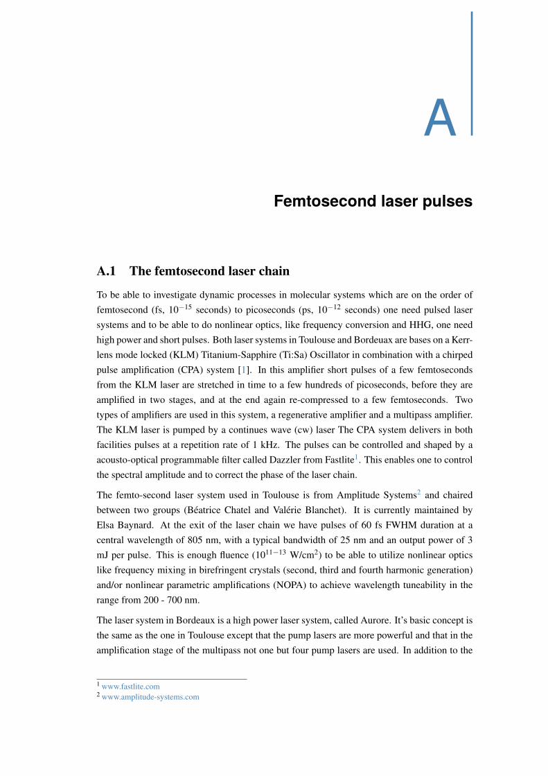
A
Femtosecond laser pulses
A.1 The femtosecond laser chain
To be able to investigate dynamic processes in molecular systems which are on the order of
femtosecond (fs, 10´15 seconds) to picoseconds (ps, 10´12 seconds) one need pulsed laser
systems and to be able to do nonlinear optics, like frequency conversion and HHG, one need
high power and short pulses. Both laser systems in Toulouse and Bordeuax are bases on a Kerr-
lens mode locked (KLM) Titanium-Sapphire (Ti:Sa) Oscillator in combination with a chirped
pulse amplification (CPA) system [1]. In this amplifier short pulses of a few femtoseconds
from the KLM laser are stretched in time to a few hundreds of picoseconds, before they are
amplified in two stages, and at the end again re-compressed to a few femtoseconds. Two
types of amplifiers are used in this system, a regenerative amplifier and a multipass amplifier.
The KLM laser is pumped by a continues wave (cw) laser The CPA system delivers in both
facilities pulses at a repetition rate of 1 kHz. The pulses can be controlled and shaped by a
acousto-optical programmable filter called Dazzler from Fastlite1. This enables one to control
the spectral amplitude and to correct the phase of the laser chain.
The femto-second laser system used in Toulouse is from Amplitude Systems2 and chaired
between two groups (Beatrice Chatel and Valerie Blanchet). It is currently maintained by
Elsa Baynard. At the exit of the laser chain we have pulses of 60 fs FWHM duration at a
central wavelength of 805 nm, with a typical bandwidth of 25 nm and an output power of 3
mJ per pulse. This is enough fluence (1011´13 W/cm2) to be able to utilize nonlinear optics
like frequency mixing in birefringent crystals (second, third and fourth harmonic generation)
and/or nonlinear parametric amplifications (NOPA) to achieve wavelength tuneability in the
range from 200 - 700 nm.
The laser system in Bordeaux is a high power laser system, called Aurore. It’s basic concept is
the same as the one in Toulouse except that the pump lasers are more powerful and that in the
amplification stage of the multipass not one but four pump lasers are used. In addition to the
1 www.fastlite.com2 www.amplitude-systems.com
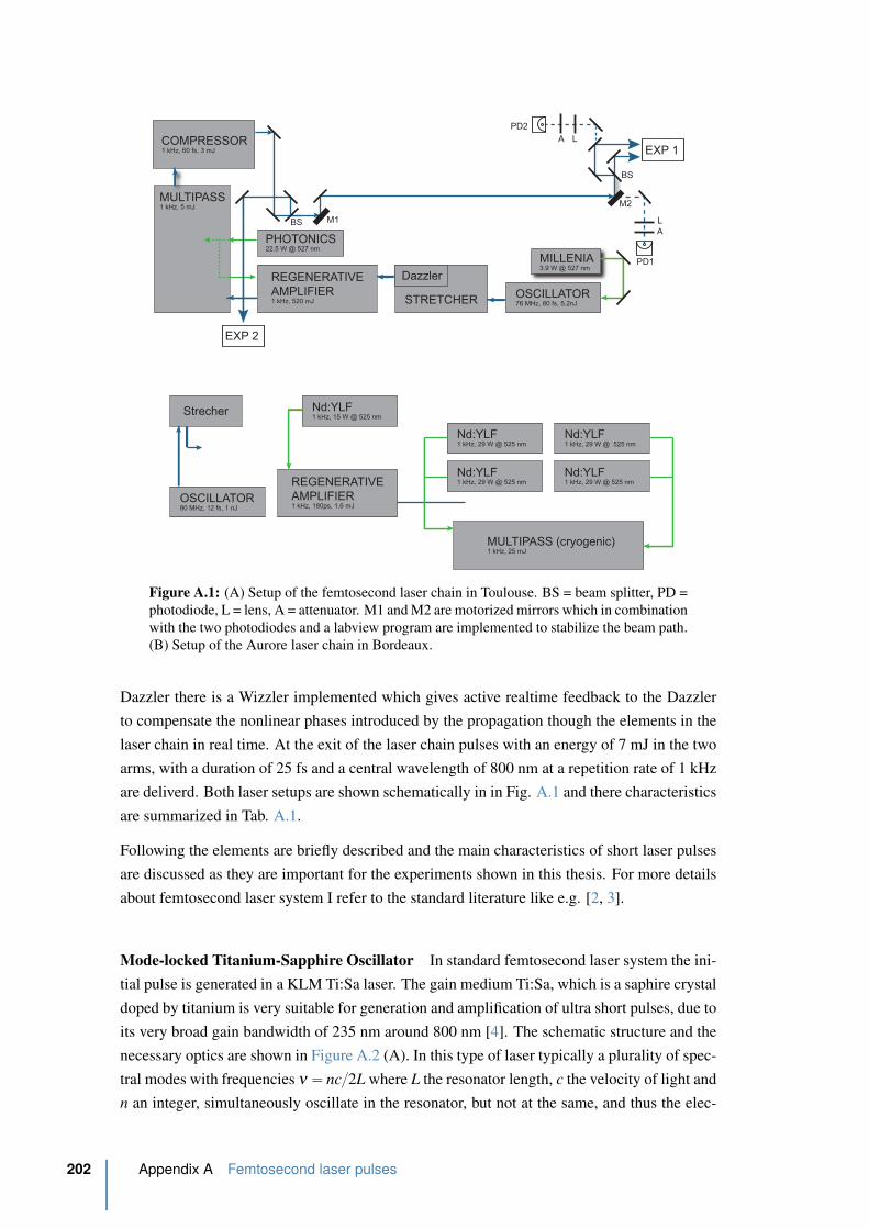
COMPRESSOR1 kHz, 60 fs, 3 mJ
REGENERATIVE
AMPLIFIER1 kHz, 520 mJ STRETCHER
OSCILLATOR76 MHz, 80 fs, 5.2nJ
MILLENIA3.9 W @ 527 nm
BS
BS
M1
M2
PD1
L
A
PD2
LA
MULTIPASS1 kHz, 5 mJ
PHOTONICS22.5 W @ 527 nm
EXP 2
EXP 1
Dazzler
Strecher
OSCILLATOR80 MHz, 12 fs, 1 nJ
REGENERATIVE
AMPLIFIER1 kHz, 180ps, 1.6 mJ
Nd:YLF1 kHz, 15 W @ 525 nm
MULTIPASS (cryogenic)1 kHz, 25 mJ
Nd:YLF1 kHz, 29 W @ 525 nm
Nd:YLF1 kHz, 29 W @ 525 nm
Nd:YLF1 kHz, 29 W @ 525 nm
Nd:YLF1 kHz, 29 W @ 525 nm
1 kHz 25 fs, 2 x 7 mJ
@ 800 nm (50)
(A)
(B)
Dazzler
Wizzler
Dazzler-Wizzler feedback loop
Figure A.1: (A) Setup of the femtosecond laser chain in Toulouse. BS = beam splitter, PD =
photodiode, L = lens, A = attenuator. M1 and M2 are motorized mirrors which in combination
with the two photodiodes and a labview program are implemented to stabilize the beam path.
(B) Setup of the Aurore laser chain in Bordeaux.
Dazzler there is a Wizzler implemented which gives active realtime feedback to the Dazzler
to compensate the nonlinear phases introduced by the propagation though the elements in the
laser chain in real time. At the exit of the laser chain pulses with an energy of 7 mJ in the two
arms, with a duration of 25 fs and a central wavelength of 800 nm at a repetition rate of 1 kHz
are deliverd. Both laser setups are shown schematically in in Fig. A.1 and there characteristics
are summarized in Tab. A.1.
Following the elements are briefly described and the main characteristics of short laser pulses
are discussed as they are important for the experiments shown in this thesis. For more details
about femtosecond laser system I refer to the standard literature like e.g. [2, 3].
Mode-locked Titanium-Sapphire Oscillator In standard femtosecond laser system the ini-
tial pulse is generated in a KLM Ti:Sa laser. The gain medium Ti:Sa, which is a saphire crystal
doped by titanium is very suitable for generation and amplification of ultra short pulses, due to
its very broad gain bandwidth of 235 nm around 800 nm [4]. The schematic structure and the
necessary optics are shown in Figure A.2 (A). In this type of laser typically a plurality of spec-
tral modes with frequencies ν “ nc2L where L the resonator length, c the velocity of light and
n an integer, simultaneously oscillate in the resonator, but not at the same, and thus the elec-
202 Appendix A Femtosecond laser pulses
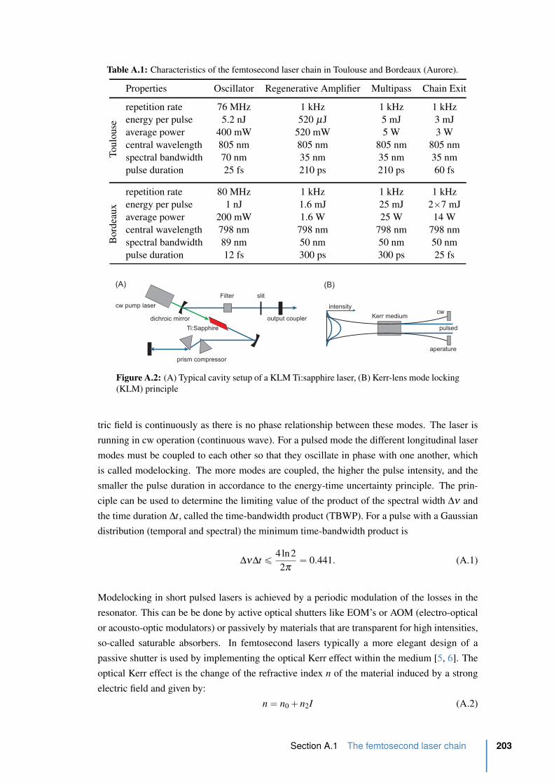
Table A.1: Characteristics of the femtosecond laser chain in Toulouse and Bordeaux (Aurore).
Properties Oscillator Regenerative Amplifier Multipass Chain Exit
Toulo
use
repetition rate 76 MHz 1 kHz 1 kHz 1 kHz
energy per pulse 5.2 nJ 520 µJ 5 mJ 3 mJ
average power 400 mW 520 mW 5 W 3 W
central wavelength 805 nm 805 nm 805 nm 805 nm
spectral bandwidth 70 nm 35 nm 35 nm 35 nm
pulse duration 25 fs 210 ps 210 ps 60 fs
Bord
eaux
repetition rate 80 MHz 1 kHz 1 kHz 1 kHz
energy per pulse 1 nJ 1.6 mJ 25 mJ 2ˆ7 mJ
average power 200 mW 1.6 W 25 W 14 W
central wavelength 798 nm 798 nm 798 nm 798 nm
spectral bandwidth 89 nm 50 nm 50 nm 50 nm
pulse duration 12 fs 300 ps 300 ps 25 fs
output coupler
Filter
dichroic mirror
prism compressor
cw pump laser
Ti:Sapphire
slit
Kerr mediumcw
pulsed
intensity
(A) (B)
aperature
Figure A.2: (A) Typical cavity setup of a KLM Ti:sapphire laser, (B) Kerr-lens mode locking
(KLM) principle
tric field is continuously as there is no phase relationship between these modes. The laser is
running in cw operation (continuous wave). For a pulsed mode the different longitudinal laser
modes must be coupled to each other so that they oscillate in phase with one another, which
is called modelocking. The more modes are coupled, the higher the pulse intensity, and the
smaller the pulse duration in accordance to the energy-time uncertainty principle. The prin-
ciple can be used to determine the limiting value of the product of the spectral width ∆ν and
the time duration ∆t, called the time-bandwidth product (TBWP). For a pulse with a Gaussian
distribution (temporal and spectral) the minimum time-bandwidth product is
∆ν∆t ď 4ln2
2π“ 0.441. (A.1)
Modelocking in short pulsed lasers is achieved by a periodic modulation of the losses in the
resonator. This can be be done by active optical shutters like EOM’s or AOM (electro-optical
or acousto-optic modulators) or passively by materials that are transparent for high intensities,
so-called saturable absorbers. In femtosecond lasers typically a more elegant design of a
passive shutter is used by implementing the optical Kerr effect within the medium [5, 6]. The
optical Kerr effect is the change of the refractive index n of the material induced by a strong
electric field and given by:
n “ n0 ` n2I (A.2)
Section A.1 The femtosecond laser chain 203

Amplifier
amplified pulse
streched pulse
short pulse
Strecher Compressor amplified short pulse
L1
L2
f 2f f
G1 G2
Δx Δx
image
planeobject
plane
RF
G1
G2
Lg
RF
γθ
(A) (B)
(C)
Figure A.3: (A) Principle setup of a chirped pulse amplification (CPA) system, (B) Strecher,
(C) Compressor setup.
with n0 the low intensity linear refractive index (n0 = 1.76 at 800 nm in Ti:sapphire), and
n2 is the non-linear refractive index which changed as function of the light intensity I (n2 =
3.1ˆ10´16cm2W´1) [7]. At high intensities lensing effects will occur because the refractive
index will be higher in the centre of the laser pulse, creating a gradient index lens in the
material due to the spacial shape of the pulse which has a Gaussian profile. In combination
with an additional slit in the beam path this allows to increase the losses of the CW beam.
For this purpose, the slit is placed at a position at which the mode-locked beam has a smaller
diameter than the CW beam. This Kerr-lens and the slit together form a saturable absorber
and is graphically shown in Figure A.2 (B). This type of mode locking is successfully used
for the generation of laser pulses with a duration down to 10 fs [6]. Each element in the beam
path causes a chirp of the pulse due to dispersion, as the refractive index of the materials is in
general wavelength dependent. When light travels through a dispersive medium like glass, the
red spectral component will travel faster than the blue spectral components, in this manner the
pulse will be stretched, as the spectral components arrive at different times at a detector after
passing through a medium. This separation of spectral components in time is called chirp. The
intensity-dependent self-focusing (Kerr effect) gives rise to a self-phase modulation. Because
of the intensity dependent refractive index this leads to a spectral broadening inside the laser
medium, and so actually to shorter pulses. Since the self-phase modulation in the Ti:sapphire
crystal is not as strong as the dispersion of the elements in the laser chain, an additional element
must be installed. In the KLM laser the material dispersion of one round trip in the laser is
compensated by a prism pair placed within the resonator cavity. The length of the resonator
dominates the repetition rate as: τrep “ 1T “ cp2Lq. A summary of the mechanisms in
compact ultrfast lasers is given for instance in the review article by Ursula Keller [8]
Chirped pulse amplification (CPA) In this amplifier short pulses of a few femtoseconds
from the KLM laser are stretched in time to a few hundreds of picoseconds, before they are
amplified in mostly two stages before being re-compressed to a few femtoseconds at the end as
illustrated in Figure A.3. Most high-power ultrafast laser systems use a high gain preamplifier
stage, placed just after the pulse stretcher, which is designed to increase the energy of the nJ
pulses from the laser oscillator to the 1-10 mJ level. The preamplifier is then followed by sev-
204 Appendix A Femtosecond laser pulses

cw pump laserTi:Sa
Pockels cell
λ/4
TFP
TFP
λ/2
input
output
(A) (B)
cw pump laser
Ti:Sa
input
output
Figure A.4: Principle setup of an amplification system. (A) regenerative amplifier, (B) mul-
tipass amplifier.
eral power amplifiers designed to efficiently extract the stored energy in the amplifier and to
increase the output pulse power even further. There are two basic preamplifier designs, regen-
erative [9, 10] and multipass [11] amplifiers. Both are illustrated in Figure A.4. Regenerative
amplifiers are very similar to a laser cavity or resonator. The low-energy chirped pulse is
injected into the cavity using a time-gated polarization device such as a Pockels cell and a
thin film polarizer. The pulse then makes a couple of roundtrips through a relatively low gain
medium, after that the high energy pulse is switched out by a second time-gated Pockels cell.
A low gain configuration is typically used in this amplifier cavity to prevent amplified spon-
taneous emission (ASE). With high gain, ASE can build up quite rapidly in this configuration
and deplete the gain before it can be extracted.
A multipass preamplifier configuration differs from the regenerative amplifier in that, as its
name suggests, the beam passes through the gain medium multiple times without the use
of a cavity. In a multipass amplifier, since the optical path is not a resonator, ASE can be
suppressed to a greater degree than with a regenerative amplifier. Thus, multipass amplifiers
typically have higher gain per pass, and fewer passes through the gain medium are needed.
As a result, there is less high-order phase accumulation in multipass systems, and shorter
pulses are easier to obtain upon recompression. Moreover, nonlinear phase accumulation due
to the B-integral is also less in multipass amplifiers. We will come back to the B-integral in a
moment. Multipass preamplifiers are not as efficient as regenerative amplifiers since the pump
signal overlap must change on successive passes through the gain medium in order to extract
the beam by separating it spatially.
A.2 General characteristics of femtosecond laser pulses
Light is described as an electromagnetic wave, a solution of the Maxwell equations, and can
be written as
Ep~r, tq “ E0eip~k~r´ωtq (A.3)
These solutions stand for the sinus waves traveling in vacuum at an angular frequency of ω
and a wavenumber of k, where ω and k have a relation of c “ f λ “ ωk. E0 is the amplitude
of the waves and~k~r ´ ωt stands for the phase of the sinus wave. An optical pulse is formed
through the coherent superposition of optical waves in a broadband frequency range. The
electric fields in the temporal domain are described by adding the optical waves through the
Section A.2 General characteristics of femtosecond laser pulses 205
whole spectral domain (Fourier transform), and the electric fields in the frequency domain are
described by the summation of the optical wave through the whole temporal domain (Inverse
Fourier transform):
Ep~r, tq “ż `8
´8Ep~r,ωqe´iωt dω (A.4a)
Ep~r,ωq “ 1
2π
ż `8
´8Ep~r, tqe´iωt dt (A.4b)
Since half-maximum quantities are experimentally easier to measure, the relationship between
the duration and spectral bandwidth of the laser pulse can be written as
∆ν∆t ď K (A.5)
where ∆ν is the frequency bandwidth measured at full-width at half- maximum (FWHM) with
ω “ 2πν and ∆t is the FWHM in time of the pulse. The number K will depends only on the
pulse shape. In order to generate a laser pulse within femtosecond time domain one needs
to use a broad spectral bandwidth. If the equality is reached one speaks about a Fourier-
transform-limited pulse or simply a transform limited pulse. The minimum time duration of
this transform limited pulse is given by
∆t “ Kλ 2
0
∆λc(A.6)
with ∆λ is the bandwidth in nm at FWHM and λ0 the central wavelength.
A transform-limited pulse is obtained under the constant phase. In vacuum the optical pulse
receives no modulation because the wave vector doesn’t depend on the frequency. In a disper-
sive device however the wave vector becomes a function of the frequency so the electric field
is rewritten as follows:
Ep~r,ωq “ Ep0,ωqei~kpωq~r “ Epωqeiφpωq (A.7)
where Ep0,ωq “ Epωq is the spectral amplitude of the incident beam and kpωq is the frequency-
dependent wave-vector. The spectral phase φpωq “ kpωqr becomes a function of the angular
frequency. The temporal electric field is then described as:
Ep~r, tq “ż `8
´8Epωqeiφpωqe´iωt dω (A.8)
If a transform limited pulse propagates through a dispersive medium, the spectral phase will be
chirped as discussed earlier due to the wavelength dependent refractive index. Mathematically,
if a spectral phase φpωq varies slowly with the frequency ω , it can be expanded into a Taylor
series around the carrier frequency ωo as follows:
φpωq “8ÿ
k“0
φ pkqpω0qk!
pω ´ ω0qk (A.9)
206 Appendix A Femtosecond laser pulses
with
φ kpω0q “ δ kφpωqδωk
∣
∣
∣
∣
ω“ω0
(A.10)
The first term φpω0q describes the absolute phase of the pulse in the time domain. The first
derivative φ 1 “ Tgpω0q is called the group delay (GD). The GD leads to a shift of the pulse
envelope in the time domain. The second derivative φ 2 “ D2pω0q is the group delay dispersion
(GDD) and φ 12 “ D3pω0q is the third-order dispersion (TOD) etc, respectively. Since these
higher order derivatives (GDD and higher) describe the frequency dependence of the GD they
are responsible for dispersive effects and changes in temporal structure of the pulse envelope.
By analogy, the temporal phase φptq can be expanded into the Taylor series around time zero
for small derivations:
φptq “8ÿ
k“0
φ pkqp0qk!
tk (A.11)
with
φ kp0q “ δ kφptqδ tk
∣
∣
∣
∣
t“0
(A.12)
The time derivative of the temporal phase defines the instantaneous frequency
ωptq “ ω0 ´ dφptqdt
(A.13)
The first term in the Taylor series φp0q is the absolute phase of the pulse. and gives the
temporal relation of the pulse envelope with respect to the underlying carrier oscillation. The
first derivative φ 1 which is linear with time, describes a shift of the carrier frequency ω0 and the
term with φ 2 corresponds to the linear motion of the instantaneous frequency and called linear
chirp. The next terms are the quadratic, cubic, etc chirp. For example, the phase introduced
by a material is given by φmat “ Lmatnpωqωc, where n is the refractive index of the material,
which can be decomposed as seen in Eq. (A.1) into a linear refractive index n0 and a laser
intensity dependent refractive index n2. The value of the nonlinear phase contribution due to
the nonlinear refractive index is given by [1]:
φnonlinear “ 2πn2
λ
ż
Ipt,zqdz (A.14)
The peak value of this expression is also known as the B-integral which gives a measure of
of the nonlinear phase shift at peak intensity. The nonlinear group delay is approximately
dφdω “ B∆ω , where ∆ω is the half-width of the spectrum. A B-integral of 1 rad over a
spectral half-width of 20 nm would add not only an additional delay variation of 17 fs but
also introduce severe distortions as the phase varies across the beam. Thus, it is important if
possible to maintain a value of the B-integral of less than 1.
A.3 Nonlinear optical effects - frequency mixing
In general for pump-probe experiments one would like to adjust the laser wavelength accord-
ingly to the system or excited states of interest. The possibility of up- or down-converting
Section A.3 Nonlinear optical effects - frequency mixing 207
the fundamental frequency of the laser (usually 800 nm form a Ti:sapphire laser) is the field
of nonlinear optics. First discovered by Franken who focused light from a ruby laser into a
quartz crystal and observed how a small amount of laser light was converted to the second
harmonic [12]. However, the full impact and realization of nonlinear optics came only with an
understanding of how a signal wave generated through a nonlinear optical polarization grows
as it propagates through a nonlinear medium [13]. The beautiful and elegant perturbation
treatment of nonlinear optics developed by Bloembergen and co-workers made it possible to
develop both birefringent-phase-matching and quasi-phase- matching (QPM) techniques for
efficiently converting laser light from one wavelength to another [14]. Optics is the study of
the interaction of electromagnetic radiation and matter. Electromagnetic radiation is described
by the Maxwell’s equations and for the case here the Gauss’s law given by:
∇~D “ 4πρ (A.15)
is the most important one. The electric displacement field D is related to the electric field E
through the polarization field P in a medium by:
~D “ ~E ` 4π~P (A.16)
In general the polarization field in the medium depends linearly on the incident electric field
~P “ ε0χp1q~E (A.17)
where ε0 is the permittivity of the free space χp1q “ n2 ´ 1 is the linear susceptibility of the
medium with n the (complex) refractive index of the sample. In reality the polarization field
is more complex and especially when dealing with higher field intensities such as in laser
beams, the induced polarization is often not a linear function anymore. For small variations,
the nonlinear polarization can be expanded in a Taylor series:
~P “ ε0
´
χp1q~E ` χp2q~E2 ` χp3q~E3 ` . . .¯
(A.18)
where χpnq is the nth order susceptibility. In general an nth order will lead to pn ` 1qth wave
mixing. As an example, if we consider only a second order nonlinearity (three-wave mixing),
then the polarization ~Pp2q, takes the form
~Pp2q “ ε0χp2q~E2ptq (A.19)
Considering an electric field ~Eptq, made up of two components at frequencies ω1 and ω2,
given by ~Eptq “ ~E1 e´iω1t ` ~E2 e´iω2t ` cc one can write the second-order polarization field
208 Appendix A Femtosecond laser pulses
with nonzero chip2q for instance as
~Pp2qptq “ ε0χp2q~E2ptq “ ε0χp2q“
E1 e´iω1t ` E2 e´iω2t ` cc‰2
“ ε0χp2q“
|E1|2 e´i2ω1t ` |E2|2 e´i2ω2t
` 2E1E2 e´ipω1`ω2qt
` 2E1E˚2 e´ipω1´ω2qt
`2p|E1| ` |E2|qe0‰
(A.20)
The resulting polarization field contains components oscillating at various frequencies (2ω1,
2ω2, ω1 `ω1, ω1 ´ω1 and 0). The first two terms oscillating at 2ω are called second harmonic
generation (SHG). The third and fourth term are known as sum frequency generation (SFG)
and difference frequency generation (DFG). The last term does not oscillate in time and is
known as optical rectification, a conversion of an oscillating electric field to a static DC field.
The third-order susceptibility not discussed here would give rise to nonlinear effects known
as the DC Kerr effect, the third harmonic generation and the optical Kerr effect. Of course
these phenomena are not all automatically observed. The above representation ignores the
position dependence of the electrical fields. Additional constrains apply, that both energy
and momentum of the photons involved must be conserved. Considering an electric field
E jp~x, tq “ eip~k j~xω jtq at position ~x with the wave vector |~k| “ npω jqω jc, where npω jq is the
frequency dependent refractive index and c the speed of light, the second order polarization
field at the angular frequency ω3 “ ω1 ` ω2 is given by:
~Pp2qp~x, tq9E21 E2
2 eirp~k1~k2q~x´ω3ts (A.21)
Energy conservation is given by hpω3q “ hω1 ` hω2. Constructive interference and a high
intensity conversion will only occur if also the momentum is conserved given by k3 “ k1 ` k2,
which is known as the phase-matching condition. If this relationship is not maintained during
the propagation in the medium, destructive interference will make the conversion process ex-
tremely inefficient. Thus for constructive interference the two waves have to be phase matched
which means they have to travel with the same phase velocity. This can be achieved for in-
stance for SHG, when the refractive index of the material is equal for the two frequencies
(npω3q “ npω1q). In general anisotropic crystals are used like β -barium borate (BBO), where
the refractive index varies with the propagation direction. As the velocity in the medium is
related to the refractive index by v “ cn anisotropic crystals are often said to have a fast and
slow axis of propagation. If the fundamental and the second harmonic wave are polarized
at right angles to each other it is generally straightforward to find an angle of propagation
through the crystal for which the refractive index and therefore the velocity for both beams are
equal. Parametric amplification (OPA) optical parametric generation (OPG) are variations of
difference frequency generation, where in general ω1 ‰ ω2 and where the lower frequency of
one of the two generating fields is much weaker (parametric amplification). This can be used
as a laser light source that emits light of variable wavelengths.
Section A.3 Nonlinear optical effects - frequency mixing 209
Conversion efficiency, phase-matching bandwidth and time duration of SHG
The efficiency of the second-harmonic generation ηSHG “ Ip2ωqIpωq is proportional to L2 Ipωq,
where Ipωq “ PA, with P the incident power and A the cross-sectional area of the interaction
volume. Therefore, the SHG efficiency can be written as [15]
ηSHG “ C2 L2
AP C2 “ 2ω2η2
0
d2
n3(A.22)
where C2 is a material constant depending on the second-order susceptibility χp2q “ 2d and the
refractive index n of the material. Apart from increasing P, to maximize the the efficiency, the
ratio L2A has to maximum. Therefore, the beam must be focused and the interaction length
L should be maximized. If the dimensions of the nonlinear crystal are not limiting factors, the
maximum value of L for a given area A is limited by the beam diffraction. A Gaussian beam,
focused to a beam width W0 maintains a beam cross-sectional area A “ πW 20 over a depth
of focus L “ 2z0 with z0 “ 2πW 20 λ the Rayleigh length, so that the ratio L2A “ 2Lλ “
4Aλ 2
For a finite interaction length L, a phase mismatch |∆k| ď 2πL is tolerated (equality would
give the coherence length). If exact phase matching is achieved at a set of nominal frequencies
of the mixed waves, then small frequency deviations from those values may be tolerated, as
long as the condition ω3 “ ω1 ` ω2 is satisfied. For SHG we have two waves with frequencies
omega1 “ ω and ω3 “ 2ω . The crystal is designed for exact phase matching at a nominal
fundamental frequency ω0, ∆kpω0q “ 0. For phase-matching conditions with a bandwidth
∆ω: |∆kpω0 ` ∆ωq “ 2πL|. For small ∆ω one can write this as ∆kpω0 ` ∆ωq “ pddωq∆ω
at ω0 and therefore
∆ω “ 2π
|∆k1|L or ∆ν “ 1
|∆k1|L (A.23)
As ∆kpωq “ k3p2ωq ´ 2k1pωq and dkipωqdω “ 1vi with vi the group velocity at of wave i,
the spectral width can be written as:
∆ν “ 1
2L
ˇ
ˇ
ˇ
ˇ
1
v3´ 1
v1
ˇ
ˇ
ˇ
ˇ
´1
(A.24)
One can see, the thiner the crystal, the larger the bandwidth and the shorter the pulse dura-
tion.
References
[1] Backus, S, Durfee, CG, Murnane, MM, and Kapteyn, HC. High power ultrafast lasers.
Rev. Sci. Instr. 69:3 1207–1223 (1998) (cited p. 201, 207).
[2] Svelto, O. Principles of Lasers. Springer. 2010 (cited p. 202).
[3] Trager, F. Springer handbook of lasers and optics. Springer, 2007 (cited p. 202).
[4] MOULTON, PF. Spectroscopic and Laser Characteristics of Ti-Al2O3. J. Opt. Soc.
Am. B 3:1 125–133 (1986) (cited p. 202).
[5] Brabec, T, Spielmann, C, Curley, PF, and Krausz, F. Optics InfoBase: Optics Letters -
Kerr lens mode locking. Optics letters (1992) (cited p. 203).
210 Appendix A Femtosecond laser pulses
[6] Christov, IP, Stoev, VD, Murnane, MM, and Kapteyn, HC. Optics InfoBase: Optics
Letters - Sub-10-fs operation of Kerr-lens mode-locked lasers. Optics letters (1996)
(cited p. 203, 204).
[7] Brouard, M and Vallance, C. Tutorials in molecular reaction dynamics. Royal Society
of Chemistry Cambridge, UK, 2010 (cited p. 204).
[8] Keller, U. Recent developments in compact ultrafast lasers. Nature (2003) (cited p. 204).
[9] Wynne, K, Reid, GD, and Hochstrasser, RM. Optics InfoBase: Optics Letters - Re-
generative amplification of 30-fs pulses in Ti:sapphire at 5 kHz. Optics letters (1994)
(cited p. 205).
[10] Barty, C, Korn, G, Raksi, F, and Rose-Petruck, C. Optics InfoBase: Optics Letters -
Regenerative pulse shaping and amplification of ultrabroadband optical pulses. Optics
. . . (1996) (cited p. 205).
[11] Backus, S, Peatross, J, Huang, CP, and Murnane, MM. Optics InfoBase: Optics Letters
- Ti:sapphire amplifier producing millijoule-level, 21-fs pulses at 1 kHz. Optics . . .
(1995) (cited p. 205).
[12] Franken, PA, Hill, AE, Peters, CW, and Weinreich, G. Generation of Optical Harmon-
ics. Phys. Rev. Lett. 7:4 118–119 (1961) (cited p. 208).
[13] Popmintchev, T, Chen, MC, Arpin, P, Murnane, MM, and Kapteyn, HC. The attosec-
ond nonlinear optics of bright coherent X-ray generation. Nature Photonics 4:12 822–
832 (2010) (cited p. 208).
[14] Armstrong, J, Bloembergen, N, Ducuing, J, and Pershan, P. Interactions between Light
Waves in a Nonlinear Dielectric. Phys. Rev. 127:6 1918–1939 (1962) (cited p. 208).
[15] “Nonlinear Optics”. Fundamentals of Photonics. Ed. by Saleh, B. Wiley, 2013 (cited
p. 210).
References 211


B
Reconstructing velocity-map images
Velocity-map images are 2D projections of the 3D velocity distribution as we have seen in
Section 1.2. The physical information is lying only in the central slice of this 3D distribution.
If one doesn’t use slicing techniques but has an axis of cylindrical symmetry the 2D projection
parallel to this axis contains enough information to reconstruct the full 3D distribution using a
mathematical inversion method. The reconstruction method will be summarized here shortly
and follows the description given in [1].
In the case of photodissociation experiments the polarization of the photolysis laser is usually
put parallel to the detector plane so that the photofragments are ejected with cylindrical sym-
metry around this axis parallel to the detector. Under these circumstances the mathematical
procedure known as inverse Abel transformation is able to recover the 3D distribution from its
projection [2].
The velocity distribution of the photofragment ions in cartesian coordinates centred on the
point of interaction can be written as ipx,y,zq, where z is the symmetry axis (in this case the
laser polarization vector), and y the direction of the extraction field. Than the distribution on
the detector can be written as:
Ipx,yq “ż `8
´8ipx,y,zqdy (B.1)
If we consider just one row of the image taken along the x axis at some value of z “ z0 we
have:
f pxq “ Ipx,z0q “ż `8
´8gpx,yqdy “ 2
ż `8
0
gpx,yqdy (B.2)
where gpx,yq “ ipx,y;z0q is a slice through the 3D distribution perpendicular to the symmetry
axis taken at z0. The function f pxq is illustrated in Figure B.1 B. To reconstruct the original
velocity distribution (illustrated in Figure B.1 C.) one has to recover gpx,yq from the measured
function f pxq. As the problem is cylindrical symmetric one can by a simple change of variables
with
x2 ` y2 “ r2 Ñ y “a
r2 ´ x2 ñ dy “ rdr?r2 ´ x2
(B.3)
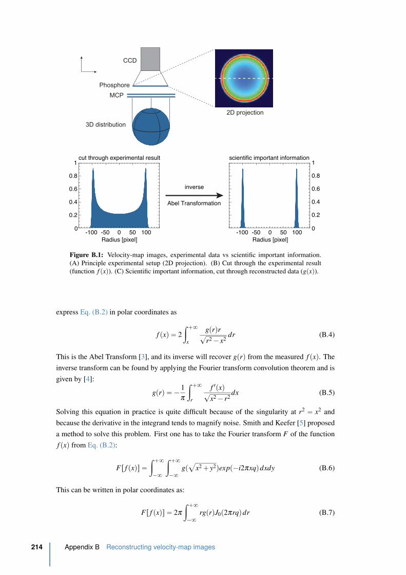
Radius [pixel]0 50
0
0.2
0.4
0.6
0.8
1
100-50-100Radius [pixel]
0 50 100-50-100
CCD
Phosphore
MCP
0
0.2
0.4
0.6
0.8
1
inverse
Abel Transformation
cut through experimental result scientific important information
3D distribution
2D projection
x
y
z
EA
B C
Figure B.1: Velocity-map images, experimental data vs scientific important information.
(A) Principle experimental setup (2D projection). (B) Cut through the experimental result
(function f pxq). (C) Scientific important information, cut through reconstructed data (gpxq).
express Eq. (B.2) in polar coordinates as
f pxq “ 2
ż `8
x
gprqr?r2 ´ x2
dr (B.4)
This is the Abel Transform [3], and its inverse will recover gprq from the measured f pxq. The
inverse transform can be found by applying the Fourier transform convolution theorem and is
given by [4]:
gprq “ ´ 1
π
ż `8
r
f 1pxq?x2 ´ r2
dx (B.5)
Solving this equation in practice is quite difficult because of the singularity at r2 “ x2 and
because the derivative in the integrand tends to magnify noise. Smith and Keefer [5] proposed
a method to solve this problem. First one has to take the Fourier transform F of the function
f pxq from Eq. (B.2):
Fr f pxqs “ż `8
´8
ż `8
´8gp
a
x2 ` y2qexpp´i2πxqqdxdy (B.6)
This can be written in polar coordinates as:
Fr f pxqs “ 2π
ż `8
´8rgprqJ0p2πrqqdr (B.7)
214 Appendix B Reconstructing velocity-map images
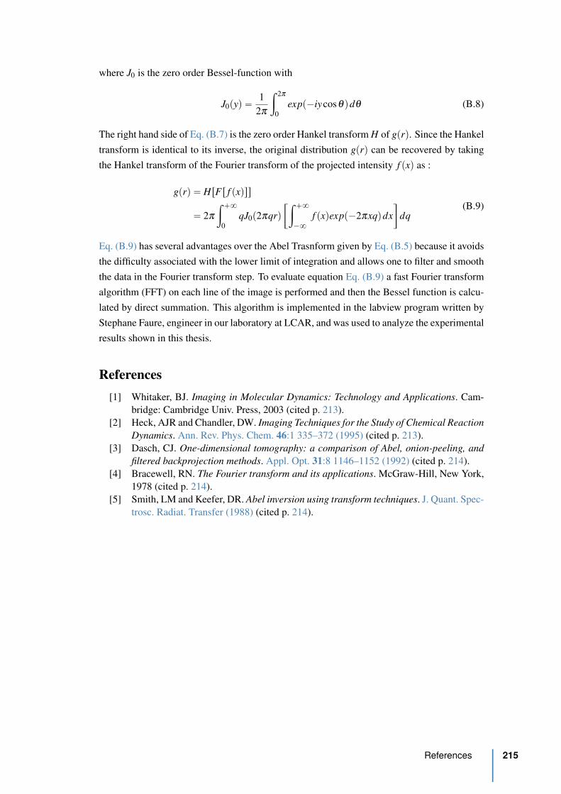
where J0 is the zero order Bessel-function with
J0pyq “ 1
2π
ż 2π
0
expp´iycosθqdθ (B.8)
The right hand side of Eq. (B.7) is the zero order Hankel transform H of gprq. Since the Hankel
transform is identical to its inverse, the original distribution gprq can be recovered by taking
the Hankel transform of the Fourier transform of the projected intensity f pxq as :
gprq “ HrFr f pxqss
“ 2π
ż `8
0
qJ0p2πqrq„
ż `8
´8f pxqexpp´2πxqqdx
dq(B.9)
Eq. (B.9) has several advantages over the Abel Trasnform given by Eq. (B.5) because it avoids
the difficulty associated with the lower limit of integration and allows one to filter and smooth
the data in the Fourier transform step. To evaluate equation Eq. (B.9) a fast Fourier transform
algorithm (FFT) on each line of the image is performed and then the Bessel function is calcu-
lated by direct summation. This algorithm is implemented in the labview program written by
Stephane Faure, engineer in our laboratory at LCAR, and was used to analyze the experimental
results shown in this thesis.
References
[1] Whitaker, BJ. Imaging in Molecular Dynamics: Technology and Applications. Cam-
bridge: Cambridge Univ. Press, 2003 (cited p. 213).
[2] Heck, AJR and Chandler, DW. Imaging Techniques for the Study of Chemical Reaction
Dynamics. Ann. Rev. Phys. Chem. 46:1 335–372 (1995) (cited p. 213).
[3] Dasch, CJ. One-dimensional tomography: a comparison of Abel, onion-peeling, and
filtered backprojection methods. Appl. Opt. 31:8 1146–1152 (1992) (cited p. 214).
[4] Bracewell, RN. The Fourier transform and its applications. McGraw-Hill, New York,
1978 (cited p. 214).
[5] Smith, LM and Keefer, DR. Abel inversion using transform techniques. J. Quant. Spec-
trosc. Radiat. Transfer (1988) (cited p. 214).
References 215

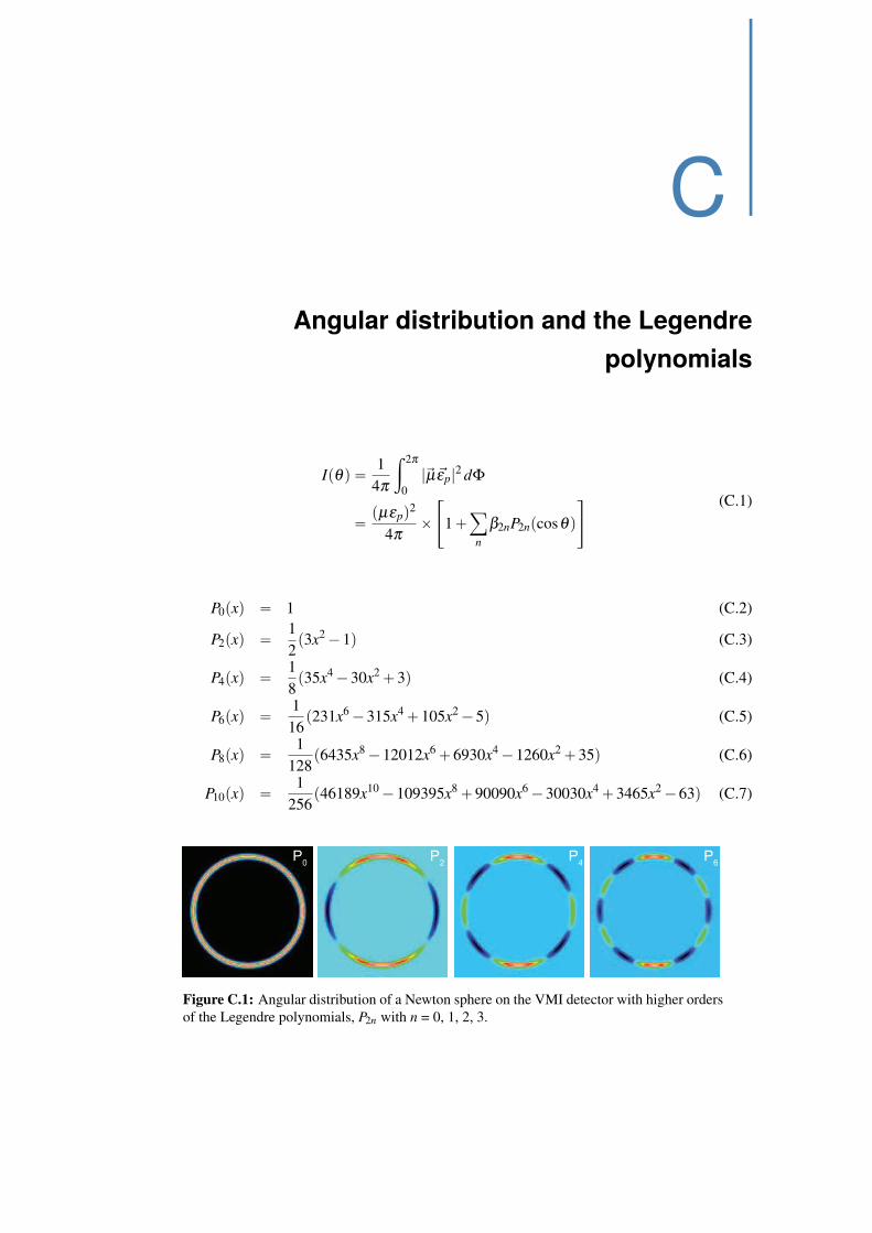
C
Angular distribution and the Legendre
polynomials
Ipθq “ 1
4π
ż 2π
0
|~µ~εp|2 dΦ
“ pµεpq2
4πˆ
«
1 `ÿ
n
β2nP2npcosθqff (C.1)
P0pxq “ 1 (C.2)
P2pxq “ 1
2p3x2 ´ 1q (C.3)
P4pxq “ 1
8p35x4 ´ 30x2 ` 3q (C.4)
P6pxq “ 1
16p231x6 ´ 315x4 ` 105x2 ´ 5q (C.5)
P8pxq “ 1
128p6435x8 ´ 12012x6 ` 6930x4 ´ 1260x2 ` 35q (C.6)
P10pxq “ 1
256p46189x10 ´ 109395x8 ` 90090x6 ´ 30030x4 ` 3465x2 ´ 63q (C.7)
P0
P2
P4
P6
Figure C.1: Angular distribution of a Newton sphere on the VMI detector with higher orders
of the Legendre polynomials, P2n with n = 0, 1, 2, 3.

D
The Lewenstein model of high-order harmonic
generation
To deal with the strong field response of atoms and molecules in general and HHG in particular
in a quantum mechanical picture one has to solve the time-dependent Schrodinger equation
(TDSE):
ihδ
δ tψp~r, tq “ Hψp~r, tq (D.1)
where ψ is the wave function of the quantum system and H is the Hamiltonian operator, which
characterizes the total energy of any given wave function. The Hamiltonian is given by:
H “ ´ h2
2m∇
2 `V p~r, tq (D.2)
where in this case the time-dependent potential V p~r, tq is the given by the sum of the atomic
coulomb potential and the dipole interaction with the electric field as seen in the three step
model. Although the TDSE can be solved numerically for the simplest case of an hydrogen
atom, it requires considerable computational time. And to solve this equation for multielectron
systems is almost impossible. Thus one has to consider approximations to derive an analytical
solution. In the case of atoms in strong laser fields this has been done the first time in 1994
by Lewenstein and coworkers and is known as the strong field approximation (SFA) [1] which
uses the single active electron approximation (SAE) developed by Keldysh in 1965 [2]. Within
the scope of the SFA, the follwing assumptions are necessary:
• In order to ensure the horizontal ionization channel (tunnel ionization) γ ! 1 is sufficient.
This assumes a low frequency of the laser field and a strong laser field. Only the ground
state of the atomic/molecular system is considered.
• The electron in the continuum is unaffected by the Coulomb potential and only the
interaction with the laser field is taken into account. The electron is assumed to be free
in the continuum Up " Ip.
• Depletion of the ground state is neglected I0 ! Isat .
These assumption are conflicting. On one side the field has to be strong but not too strong.
This defines a small intensity regime for HHG. The theory of high harmonic generation can
be divided into two parts: First, the single atom response is the dipole of a single atom in a
strong optical field. Second, propagation deals with the phase-matching and absorption in the
medium and effectively adds up the contributions for all of the atoms generating harmonics.
The goal of this model is to calculate the dipole responsible for the emission of high harmonics
for an arbitrary optical pulse. The nonlinear dipole is calculated as a function of time in the
fundamental field. This dipole is then twice differentiated to get the electric field of the emitted
harmonics. A Fourier transform then gives the high harmonic spectrum. The time-dependant
dipole moment can be written as:
~µptq “ xψp~r, tq| ´~r|ψp~r, tqy (D.3)
from which we can then extract the harmonic spectrum by Fourier transformation. The time-
dependent electron wavefunction (where only one electron is considered to be responsible for
harmonic generation ‘single-active electron approximation’ (SAE) can be written in terms of
the bound electron ground state of the atom and the continuum states |~vy where v stands for
the kinetic momentum as:
|ψp~r, tqy “ eiIpt
ˆ
aptq|0y `ż
bp~v, tq|~vyd3~v
˙
(D.4)
with time-dependent ground-state aptq, and continuum-state amplitudes, bp~v, tq. By doing so,
we do not take into account excited bound states of the electron. Since the continuum states
are defined to be solutions to the free electron Schrodinger equation Ekin|~vy “ ´12∇2|~vy, the
potential of the nucleus is neglected as soon as the electron is ionized. Using the definition
of the time-dependent electron wavefunction in equation Eq. (D.4), the time-dependent dipole
moment can be calculated to be:
~µptq “ i
ż t
0
dti
ż
d3~pE cospωtiq ˆ ~dp~vptiqqloomoon
paq
ˆexpp´iSp~p, t, tiqqloooooooomoooooooon
pbq
ˆ ~d˚p~vptiqqlooomooon
pcq
`c.c. (D.5)
where~vptq is given by the vector potential of the laser field ~Aptq and the canonical momentum
~p by~vptq “ ~p ´~Aptq. S is the so-called quasi-classical action and given by
Sp~p, t, tiq “ ´ż tr
ti
dt 1
˜
p~p `~Apt 1qq2
2` Ip
¸
(D.6)
The expression ~dp~vq in Eq. (D.5) stands for the transition probability from the bound elec-
tronic state |0y to a continuum state x~v| (describing ionization), where the complex conju-
gate describes the inverse process, i.e. recombination of the free electron to the ground state:
220 Appendix D The Lewenstein model of high-order harmonic generation
~dp~vq “x~v|~r|0y (D.7a)
~d˚p~vq “x0|~r|~vy (D.7b)
With this we can identify the different parts of the formula Eq. (D.5) as follows:
(a) ionization of the ground state at time ti,
(b) propagation in the continuum in the time interval tr ´ ti
(c) recombination to the ground state at time tr.
Thus, the classical three-step model discussed before is contained in the quantum- mechanical
description as well. By Fourier transforming the time-dependent dipole moment, the harmonic
spectra can be calculated:
~µpωqq “ż `8
´8dtr~µptrqeiωqtr “
ż `8
´8dtr
ż tr
0
dti
ż
d3~p~Bp~p, tr, tiqeiϕp~p,tr,tiq (D.8)
where ~B is the amplitude of the integrant in the integral from Eq. (D.5) and the dipole phase ϕ
defined as:
ϕp~p, tr, tiq “ ωqtr ´ Sp~p, tr, tiq (D.9)
Sattle-point approximation
Eq. (D.8) can be interpreted with the help of the Feynman path integrals [3]. To calculate ~µptqwe do not need to calculate the integral over all possible paths ~p. We only need to consider the
pathways ~p for which the action becomes stationary:
~∇pSp~p, tr, tiq “ 0 (D.10)
According to Hamilton’s principle the trajectory which is fulfilling this condition corresponds
exactly to the classical path and the relation can again be interpreted in terms of the classical
three-step model and the following statements have to be fulfilled (sattle point equations):
p~p ´~Aptiqq2
2` Ip “ 0 (D.11a)
ż tr
ti
dt~p `~Aptqq2 “ 0 (D.11b)
p~p ´~Aptrqq2
2` Ip “ ωq (D.11c)
Eq. (D.11a) states that the sum of the kinetic energy and the ionization potential is zero at
the time of ionization ti. This results in a negative kinetic energy of the electron which can
be justified by tunnel ionization when allowing complex values. Eq. (D.11b) shows that we
only need to account for those electron trajectories that return at time tr to the same point they
left at time ti, where they were ionized. In other words its trajectory is closed. Eq. (D.11b)
221
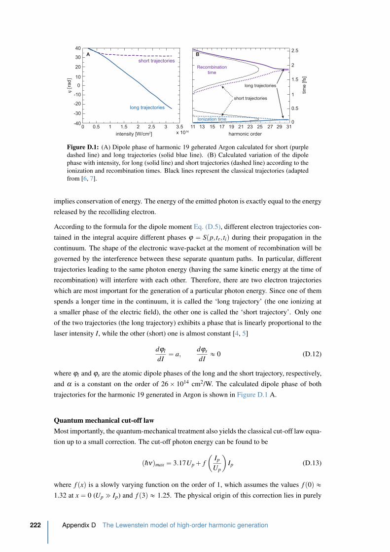
0
10
20
30
40
-40
-30
-20
-10
ϕ [
rad
]
1.510.50 2.52 3.53x 10¹⁴
intensity [W/cm2]
short trajectories
long trajectories
short trajectories
long trajectories
Recombination
time
Ionization time
harmonic order
17151311 2119 2523 27 31290
0.5
2.5
2
1.5
1
tim
e [fs
]
A B
Figure D.1: (A) Dipole phase of harmonic 19 geherated Argon calculated for short (purple
dashed line) and long trajectories (solid blue line). (B) Calculated variation of the dipole
phase with intensity, for long (solid line) and short trajectories (dashed line) according to the
ionization and recombination times. Black lines represent the classical trajectories (adapted
from [6, 7].
implies conservation of energy. The energy of the emitted photon is exactly equal to the energy
released by the recolliding electron.
According to the formula for the dipole moment Eq. (D.5), different electron trajectories con-
tained in the integral acquire different phases ϕ “ Spp, tr, tiq during their propagation in the
continuum. The shape of the electronic wave-packet at the moment of recombination will be
governed by the interference between these separate quantum paths. In particular, different
trajectories leading to the same photon energy (having the same kinetic energy at the time of
recombination) will interfere with each other. Therefore, there are two electron trajectories
which are most important for the generation of a particular photon energy. Since one of them
spends a longer time in the continuum, it is called the ‘long trajectory’ (the one ionizing at
a smaller phase of the electric field), the other one is called the ‘short trajectory’. Only one
of the two trajectories (the long trajectory) exhibits a phase that is linearly proportional to the
laser intensity I, while the other (short) one is almost constant [4, 5]
dϕl
dI“ a,
dϕs
dI« 0 (D.12)
where ϕl and ϕs are the atomic dipole phases of the long and the short trajectory, respectively,
and α is a constant on the order of 26 ˆ 1014 cm2/W. The calculated dipole phase of both
trajectories for the harmonic 19 generated in Argon is shown in Figure D.1 A.
Quantum mechanical cut-off law
Most importantly, the quantum-mechanical treatment also yields the classical cut-off law equa-
tion up to a small correction. The cut-off photon energy can be found to be
phνqmax “ 3.17Up ` f
ˆ
Ip
Up
˙
Ip (D.13)
where f pxq is a slowly varying function on the order of 1, which assumes the values f p0q «1.32 at x “ 0 (Up " Ip) and f p3q « 1.25. The physical origin of this correction lies in purely
222 Appendix D The Lewenstein model of high-order harmonic generation
quantum mechanical effects such as tunneling and the spreading of the electron wave-packet
in the continuum that have not been included in the purely classical treatment. These effects
enable the electron to collect more energy on its trajectory than the amount predicted by the
classical equations of motion.
References
[1] Lewenstein, M, Balcou, P, Ivanov, MY, L’Huillier, A, and Corkum, PB. Theory of
High-Harmonic Generation by Low-Frequency Laser Fields. Phys. Rev. A 49:3 2117–
2132 (1994) (cited p. 219).
[2] Keldysh, LV. Ionization in the field of a strong electromagnetic wave. Sov. Phys. JETP
20:5 1307–1314 (1965) (cited p. 219).
[3] Salieres, P, Carre, B, Le Deroff, L, Grasbon, F, Paulus, GG, Walther, H, Kopold, R,
Becker, W, Milosevic, DB, and Sanpera, A. Feynman’s path-integral approach for
intense-laser-atom interactions. Science 292:5518 902–905 (2001) (cited p. 221).
[4] Gaarde, MB, Salin, F, Constant, E, Balcou, P, Schafer, KJ, Kulander, KC, and L’Huillier,
A. Spatiotemporal separation of high harmonic radiation into two quantum path com-
ponents. Phys. Rev. A 59:2 1367–1373 (1999) (cited p. 222).
[5] Balcou, P, Dederichs, AS, Gaarde, MB, and L’Huillier, A. Quantum-path analysis and
phase-matching of high-order harmonic generation and high-order frequency mixing
processes in strong laser fields. J. Phys. B 32: 2973 (1999) (cited p. 222).
[6] Varju, K, Mairesse, Y, ’e, BC, Gaarde, MB, Johnsson, P, Kazamias, S, Lopez-Martens,
R, Mauritsson, J, Schafer, KJ, Balcou, P, L’Huillier, A, and eres, PS. Frequency chirp
of harmonic and attosecond pulses. J. Mod. Opt. 52:2-3 379–394 (2005) (cited p. 222).
[7] Mairesse, Y. Generation et caracterisation d’impulsions attosecondes. PhD thesis.
Universite Paris X1 Orsay, 2005 (cited p. 222).
References 223


E
Molecular symmetry: point group character and
product tables
Table E.1: Cs point group character and product table (e.g. ClN3).
E σhlinear
rotationsquadratic
A1 1 1 x, y, Rz x2, y2, z2, xy
A2 1 -1 z, Rx, Ry yz, xz
A1 A2
A1 A1 A2
A2 A2 A1
Table E.2: C2v point group character and product table (e.g. C2H2 cis).
E C2(z) σv(xz) σv(yz)linear
rotationsquadratic
A1 1 1 1 1 z x2, y2, z2
A2 1 1 -1 -1 Rz xy
B1 1 -1 1 -1 x, Ry xz
B2 1 -1 -1 1 y, Rx yz
A1 A2 B1 B2
A1 A1 A2 B1 B2
A2 A2 A1 B2 B1
B1 B1 B2 A1 A2
B2 B2 B1 A2 A1
Table E.3: C2h point group character and product table (e.g. C2H2 trans).
E C2(z) i σhlinear
rotationsquadratic
Ag 1 1 1 1 Rz x2, y2, z2, xy
Bg 1 -1 1 -1 Rx, Ry xz, yz
Au 1 1 -1 -1 z
Bu 1 -1 -1 1 x, y
Ag Bg Au Bu
Ag Ag Bg Au Bu
Bg Bg Ag Bu Au
Au Au Bu Ag Bg
Bu Bu Au Bg Ag
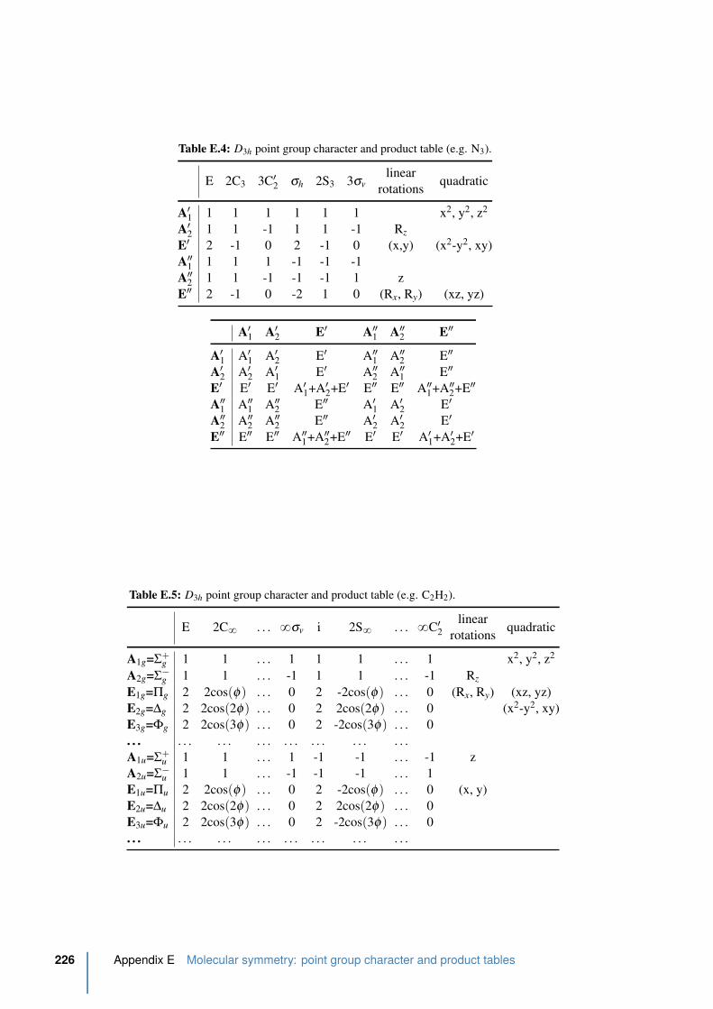
Table E.4: D3h point group character and product table (e.g. N3).
E 2C3 3C12 σh 2S3 3σv
linear
rotationsquadratic
A11 1 1 1 1 1 1 x2, y2, z2
A12 1 1 -1 1 1 -1 Rz
E1 2 -1 0 2 -1 0 (x,y) (x2-y2, xy)
A21 1 1 1 -1 -1 -1
A22 1 1 -1 -1 -1 1 z
E2 2 -1 0 -2 1 0 (Rx, Ry) (xz, yz)
A11 A1
2 E1 A21 A2
2 E2
A11 A1
1 A12 E1 A2
1 A22 E2
A12 A1
2 A11 E1 A2
2 A21 E2
E1 E1 E1 A11+A1
2+E1 E2 E2 A21+A2
2+E2
A21 A2
1 A22 E2 A1
1 A12 E1
A22 A2
2 A22 E2 A1
2 A12 E1
E2 E2 E2 A21+A2
2+E2 E1 E1 A11+A1
2+E1
Table E.5: D3h point group character and product table (e.g. C2H2).
E 2C8 . . . 8σv i 2S8 . . . 8C12
linear
rotationsquadratic
A1g=Σ`g 1 1 . . . 1 1 1 . . . 1 x2, y2, z2
A2g=Σ´g 1 1 . . . -1 1 1 . . . -1 Rz
E1g=Πg 2 2cospφq . . . 0 2 -2cospφq . . . 0 (Rx, Ry) (xz, yz)
E2g=∆g 2 2cosp2φq . . . 0 2 2cosp2φq . . . 0 (x2-y2, xy)
E3g=Φg 2 2cosp3φq . . . 0 2 -2cosp3φq . . . 0
. . . . . . . . . . . . . . . . . . . . . . . .
A1u=Σ`u 1 1 . . . 1 -1 -1 . . . -1 z
A2u=Σ´u 1 1 . . . -1 -1 -1 . . . 1
E1u=Πu 2 2cospφq . . . 0 2 -2cospφq . . . 0 (x, y)
E2u=∆u 2 2cosp2φq . . . 0 2 2cosp2φq . . . 0
E3u=Φu 2 2cosp3φq . . . 0 2 -2cosp3φq . . . 0
. . . . . . . . . . . . . . . . . . . . . . . .
226 Appendix E Molecular symmetry: point group character and product tables

Table E.6: Oh point group character and product table (e.g. SF6).
E 8C3 6C2 6C4 3C2 = (C4)2 i 6S4 8S6 3σh 6σdlinear
rotationsquadratic
A1g 1 1 1 1 1 1 1 1 1 1 x2+y2+z2
A2g 1 1 -1 -1 1 1 -1 1 1 -1
Eg 2 -1 0 0 2 2 0 -1 2 0 (2z2-x2-y2, x2-y2)
T1g 3 0 -1 1 -1 3 1 0 -1 -1 (Rx, Ry, Rz)
T2g 3 0 1 -1 -1 3 -1 0 -1 1 (xz, yz, xy)
A1u 1 1 1 1 1 -1 -1 -1 -1 -1
A2u 1 1 -1 -1 1 -1 1 -1 -1 1
Eu 2 -1 0 0 2 -2 0 1 -2 0
T1u 3 0 -1 1 -1 -3 -1 0 1 1 (x, y, z)
T2u 3 0 1 -1 -1 -3 1 0 1 -1
A1g A2g Eg T1g T2g A1u A2u Eu T1u T2u
A1g A1g A2g Eg T1g T2g A1u A2u Eu T1u T2u
A2g A2g A1g Eg T2g T1g A2u A1u Eu T2u T1u
Eg Eg Eg A1g+A2g+Eg T1g+T2g T1g+T2g Eu Eu A1u+A2u+Eu T1u+T2u T1u+T2u
T1g T1g T2g T1g+T2g A1g+Eg+T1g+T2g A2g+Eg+T1g+T2g T1u T2u T1u+T2u A1u+Eu+T1u+T2u A2u+Eu+T1u+T2u
T2g T2g T1g T1g+T2g A2g+Eg+T1g+T2g A1g+Eg+T1g+T2g T2u T1u T1u+T2u A2u+Eu+T1u+T2u A1u+Eu+T1u+T2u
A1u A1u A2u Eu T1u T2u A1g A2g Eg T1g T2g
A2u A2u A1u Eu T2u T1u A2g A1g Eg T2g T1g
Eu Eu Eu A1u+A2u+Eu T1u+T2u T1u+T2u Eg Eg A1g+A2g+Eg T1g+T2g T1g+T2g
T1u T1u T2u T1u+T2u A1u+Eu+T1u+T2u A2u+Eu+T1u+T2u T1g T2g T1g+T2g A1g+Eg+T1g+T2g A2g+Eg+T1g+T2g
T2u T2u T1u T1u+T2u A2u+Eu+T1u+T2u A1u+Eu+T1u+T2u T2g T1g T1g+T2g A2g+Eg+T1g+T2g A1g+Eg+T1g+T2g
227


Longue resume en francais
Reveler la dynamique ultrarapide sous-jacente a toute reaction chimique exige des techniques
d’imagerie capable de suivre un processus moleculaire etape par etape. Dans ces processus
elementaires, le mouvement des noyaux et des electrons de valence de l’edifice moleculaire
sont lies et l’importance de ces dynamiques est un point commun a la biologie, la chimie
et la physique [1]. Divers outils sont apparus dans les dernieres decennies qui ont permis
de sonder directement la moyenne temporelle de la structure moleculaire, comme la diffrac-
tion electronique ou de neutrons, l’absorption et diffraction des rayons X , la RMN et la mi-
croscopie electronique [2]. L’utilisation de ces techniques a permis de determiner les struc-
tures tridimensionnelles avec une resolution a l’echelle atomique. Cependant, pour former une
comprehension complete de fonctions biologiques, des reactions chimiques ou des transitions
de phase les processus elementaires doivent etre resolus en temps reel. Hors ces changements
s’etalent sur differentes echelles de temps et differents etats de transition et intermediaires. Ces
dynamiques et changements structurels sont naturellement lies par les lois de la mecanique
quantique [1].
L’invention des chaines laser pulsees ultracourtes a fourni l’outil pour detecter ces processus
en temps reel. Spectroscopie d’absorption et d’emission, spectrometrie de masse par pho-
toionization, et les techniques de diffraction jouent le role moderne des photographies ultra-
haute vitesse pour resoudre ces processus moleculaires elementaires. L’une des premieres
experiences de photographie prenant compte de la vitesse du processus est celle d’un cheval
en mouvement en 1878 par Eadweard Muybridge. Il a reussi a capturer le mouvement d’un
cheval galopant en mettant en place une rangee de cameras avec des cables de declenchement.
Ansi chaque camera prend une image capturant ainsi une fraction de seconde du mouvement.
Ce premier film est considere comme la naissance d’etudes photographiques du mouvement
et de la projection cinematographique. Puisque l’echelle de temps typique des mouvements
des noyaux dans une molecule est l’echelle femtoseconde, les impulsions laser femtosecon-
des sont les outils les plus pertinents pour saisir l’evolution des rearrangements nucleaires,
tels que l’isomerisation et la dissociation (voir Chapitre 2). La spectroscopie femtoseconde
est comme regarder un !film" ou chaque sequence revele l’etape elementaire conduisant in
fine aux produits de la reaction chimique. Resoudre dans le temps des dynamiques a l’echelle
femtoseconde necessite de declencher une dynamique sur cette echelle. Ceci n’est possible
que sur des evenements a declenchement non-statistiques comme des reactions unimolecu-
laires. Ainsi une impulsion laser pompe ultracourte induit une excitation dans la molecule
parent, definissant ainsi t “ 0. Les details du processus de relaxation, tel que le temps de
decroissance, le bilan energetique ou les rapports de branchement peuvent ainsi etre mesures
par la spectroscopie resolue en temps, ce qui definit le domaine de la femtochimie .
La femtochimie tente de repondre par exemple aux questions suivantes : Comment l’ energie
deposee dans le systeme est redistribuee dans les differents degres de liberte de la molecule, et
a quelle vitesse cela se produit-il? Quelles sont les vitesses des changements de liaisons entre
les etats quantiques des reactifs et ceux des produites? Quels sont les mouvements nucleaires
qui declenchent la reaction et definissent ainsi les etats de transition? Quels sont les echelles
de temps typiques de ces mouvement et quelle est la pertinence d’une description statistique
de la relaxation? [3]. Cependant, repondre a ces questions n’est pas aussi simple qu’il y
parait. En fait, pour comprendre ces etapes elementaires il faut tout d’abord comparer les
observables issues de l’experience avec celles produites par les modeles theoriques bases sur
des calculs ab initio. Seul cette confrontation experience-theorie permet eventuellement de
reconstruire la dynamique des etats de transition, soit la cinetique des reactifs aux produits.
Cette comparaison experience-theorie est d’autant plus facile que les molecules sont libres
d’un environnement. En effet, il est difficile de modeliser theoriquement environnement. Pro-
duire des molecules libres d’un environnement consiste principalement a les produire en phase
gazeuse dans un jet moleculaire, permettant ainsi d’avoir des molecules initialement dans une
distribution d’etats internes (comme la rotation et la vibration), les plus froides possible. Ainsi
l’impulsion pompe cree par absorption d’un ou plusieurs photons une excitation electronique,
vibrationnelle et/ou rotationnelle. C’est le temps t = 0 defini par la duree de l’impulsion
pompe. Maintenant, la question principale est comment detecter ces changements drastiques
nucleaires et quelles seront les observables en phase gazeuse. Dans cette these deux tech-
niques ont ete utilisees, l’une basee sur la photoionization classique tandis que la seconde est
basee sur des techniques tout optique. Differents systemes moleculaires ont ete etudies par
ces deux differentes techniques. Sur des echelles de temps encore plus courts que le mouve-
ment des atomes et des molecules est le mouvement des electrons. Les distances des orbites
stationnaires des electrons de valence sont de l’ordre de quelques Angtrom. Ainsi les periodes
d’oscillation des paquets d’ondes d’electrons dans les systemes atomiques ou moleculaires
lies sont de quelques centaines d’attosecondes (as = 1018 sec.) [1]. Si la femtochimie est la
science du mouvement des noyaux dans des edifices moleculaires, La physique attoseconde
est la science du mouvement des electrons. Produire des impulsions de lumiere dans le regime
attoseconde implique, du fait de la transformee de Fourier temps-frequence, de trouver une
gamme de longueur d’onde supportant plus que 50 eV. Le domaine privilege des impulsions
attosecondes est donc celui de l’ultraviolet du vide (VUV) avec des energies de photons allant
jusqu’a 100 eV voir meme jusqu’au keV. C’est la qu’intervient la generation d’harmoniques
d’ordre eleve comme un outil de conversion de photons du proche infrarouge issus d’une
chaine laser femtoseconde intense (1014 photons) vers quelques 108 photons dans le VUV
voir meme jusqu’a la region des rayons X mous.
230 Extended french summary
Chapitre 1: De la imagerie femtoseconde a l’attoseconde
Chapitre 1 est une introduction aux deux principales configurations experimentales utilisees
dans cette these pour sonder la dynamique moleculaire, a savoir l’imagerie de vecteurs vitesse
femtoseconde et la generation d’harmonique d’ordre eleve. Apres avoir introduit le concept
general de la dynamique moleculaire et la technique pompe-sonde dans la Section 1.1, Sec-
tion 1.2 illustre les concepts fondamentaux de l’imagerie des vecteurs vitesse. Dans la Sec-
tion 1.3 les concepts fondamentaux de la generation d’harmoniques d’ordre eleve sont intro-
duits.
Chapitre 2: Photodissociation de chlore azoture (ClN3)
Une experience resolue a l’echelle femtoseconde est realisee pour etudier la photodissociation
du ClN3 apres excitation electronique dans deux regions energetiquement differentes. Les
resultats obtenus sont l’objet du Chapitre 2. Les principales observables sont les co-fragments
N3 et Cl. Le but de l’experience est d’elucider la dynamique ultra-rapides qui conduit a la
production d’un fragment cyclique-N3. En effet a 4,5 eV (268 nm) d’excitation electronique,
le fragment N3 est produit dans une geometrie lineaire alors qu’autour de 6,17 eV (201 nm ),
N3 est suppose etre essentiellement produit sous forme cyclique. En fait la production d’un
fragment cyclique N3 est l’objet de controverse dans la litterature. La technique d’imagerie de
vecteur vitesse permet pas seulement l’identification des co-fragments, et un bilan energetique
de la dissociation mais aussi elle donne egalement acces a leur distribution angulaire. Ainsi
la resolution temporelle femtoseconde revele l’echelle de temps de la dissociation. Grace a
une ionisation multiphotonique des fragments, nous sommes en mesure pour la premiere fois
de detecter directement les fragments N3 produits sur des temps ultracourts tels que la dizaine
de femtoseconde. Detecter ce fragment est relativement important pour comprendre la differ-
ence entre les chemins menant a des fragments lineaires ou cycliques. Les etudes prealables
ont en effet toute ete realisees sur des echelles de temps nanoseconde en detectant principale-
ment le fragment de Cl dont la spectroscopie d’ionisation multiphotonique est bien etablie.
L’echelle de temps de la photodissociation de ClN3 a pu etre mesuree pour la premiere fois.
Un bilan d’energie resolu en temps du fragment Cl mais surtout du fragment N3 a pu etre
obtenu par le spectrometre d’imagerie des vecteurs vitesse. Ceci a permis non seulement de
confronter ce bilan d’energie resolu en temps a ceux obtenus en regime nanoseconde, mais
aussi de resoudre en temps les distributions angulaires d’emission des fragments dans les deux
regions d’excitation electronique soit a une energie de dissociation de 4,67 eV (268 nm ), ou
le fragment N3 est produit principalement lineairement et a 6.13 eV ( 201 nm ), ou N3 cy-
clique est produit. L’emploi d’une impulsion sonde avec une polarisation perpendiculaire au
laser de dissociation pompe permet d’obtenir un meilleur rapport signal sur bruit. Dans cette
configuration, peu commune en imagerie de vecteur vitesse, des polarisations des impulsions
pompe et sonde, les temps de dissociation mesures sur le co-fragment chlore sont comparables,
dans les barres d’erreurs, aux temps de dissociation mesures sur le fragment N3. Le temps de
dissociation a ete etablie a 262 ˘ 38 fs et 178 ˘ 22 fs pour ces deux domaines d’energie.
Ces temps de dissociation sont en fait les temps d’apparition des fragments par selection en
masse et energie (mais integre en angle). Ces temps de dissociation sont en fait deux fois plus
231
longs que les temps de decroissance mesures sur le spectre de masse (integre en energie et
angle) collecte directement en sortie du temps de vol (soit sur les galettes de microcanaux).
Notons que ce spectre de masse est constitue principalement des fragments d’ionisation disso-
ciative et revelent ainsi le temps de decroissance de l’etat electronique d’ordre zero prepare par
l’impulsion pompe. De ces differences sur le temps de dissociation et le temps de decroissance,
nous pouvons conclure que la dissociation n’est pas une dissociation directe comme suggere
auparavant [4] et qu’au moins un etat de transition est atteint avant d’acceder au continuum
de dissociation. Une dissociation directe se produirait a peu pres sur la moitie de la periode
de vibration de la liaison Cl–N3 qui n’est que de 30 fs (νstretch = 545 cm1 = 61 fs). Le fait
que la dynamique de dissociation n’est pas totalement revelee dans les signaux integres en
energie et angle revele que l’ionisation dissociative est sensible a la nature electronique ou la
structure nucleaire. Des experiences d’ionisation, enregistrant en coıncidence les fragments
et les photoelectrons associes pourraient reveler eventuellement les etats electroniques ren-
contres. La distribution angulaire du fragment N3 mesuree en fonction du temps revele a de
longs delais un parametre d’anistropie β2 de 1.64 ˘ 0.06 et 0.27 ˘ 0.05 pour les canaux de
dissociation menant a un N3 lineaire et ceux menant a un N3 cyclique. Ces valeurs sont en
accord avec les seules mesures publiee en regime ns mesurant uniquement la distribution an-
gulaire du fragment Cl. En effet l’ionisation multiphotonique resonante de N3 n’a pas encore
ete etudiee. Ainsi aucune valeur d’anistropie angulaire de ce fragment n’a ete publiee En
outre, la dependance temporelle de cette distribution angulaire montre que ces valeurs asymp-
totiques d’emission des fragments ne sont pas atteints immediatement . Il faut 170 ˘ 45 fs et
136 ˘ 7 fs pour le fragment N3 lineaire et cyclique pour atteindre les limites asymptotiques
d’emission anisotropique. Malheureusement, la detection d’ionisation multiphotonique non
resonante n’est pas adaptee pour detecter le fragment Cl avec un bon rapport signal sur bruit,
specialement aux delais courts ou peu de fragments sont produits. Cependant, a de longs re-
tards pompe-sonde le parametre β2 mesure a partir des images de Cl est en bon accord avec
les valeurs obtenues a partir des images N3.
Chapitre 3: Relaxation electronique et dissociation du tetrathiaful-
valene (TTF)
La relaxation electronique du tetrathiafulvalene (TTF, C6H4S4 ) est etudiee dans le Chapitre 3,
en variant l’excitation electronique initiee par l’impulsion pompe autour de 4 eV. Les observ-
ables sont un spectre de masse et la spectroscopie de photoelectrons, toutes deux resolus en
temps. Pour ameliorer la sensibilite , la photo-ionisation est realisee a differentes longueurs
d’onde de sonde (266 nm , 400 nm et 800 nm). La longueur d’onde de la pompe a ete variee de
322 nm a 307 nm pour reveler eventuellement sur les temps de decroissance, un changement
possible du caractere electronique ou vibrationnel. Avec une impulsion de 800 nm intense la
photo-ionisation au dessus du seuil (ATI) du TTF est etudiee. Le spectre de photoelectrons par
photoionisation femtoseconde de TTF revele une ionisation multiphotonique par absorption
de douze photons a 808 nm, soit une energie interne de l’ion de 12.1 eV. La dependance angu-
laire des photoelectrons ejectes montre que ce processus multiphotonique est plus susceptible
de survenir des le premier etat excite de l’ion. Dans l’intervalle de ces energies internes d’ion
232 Extended french summary
elevees, une variete de canaux de dissociation sont accessibles. A cette gamme d’energie une
variete de canaux de dissociation sont accessibles dans le continuum d’ions. Afin de demeler
cette dissociation ionique complexe, l’imagerie de photoelectrons en coıncidence avec les
photoion (iPEPICO) est utilisee. Au-dessus du seuil de dissociation, les resultats iPEPICO
montrent que l’ion moleculaire (m/z = 204) dissocie en sept ions produits, dont six sont en
concurrence dans une fenetre de l’energie 1,0 eV avec une meme energie de seuil de 10 eV.
Ceci montre que la dissociation de l’ion TTF est regi par un etat de transition relativement
serre menant a un produit de reaction intermediaire non specifie, qui par la suite dissocie via
plusieurs canaux de dissociation, menant ainsi a une multitude de fragment. Des calculs ab
initio sur les structures d’ions fragments possibles de dissociation via cinq canaux montre
tous la perte de C2H2 et C2H2S pour les cations TTF d’energie interne elevee. Un modele
de dissociation a trois canaux de dissociation est utilise pour ajuster les donnees iPEPICO.
Deux canaux de dissociation sont traites comme des dissociations simples (dont une avec un
renversement de barriere), tandis que le reste impliquent une barriere partagee. Ces canaux
ne peuvent pas rivaliser avec des energies internes superieures ou des voies plus entropiques
deviennent dominantes. Le fragment S en photoionization VUV semble apparaıtre a 12,6 eV
a partir d’une dissociation secondaire du fragment reorganise S2. Cela confirme que, dans les
etudes pompe-sonde femtoseconde de la deuxieme bande UV de TTF, une vibration d’energie
particuliere caracterise la production du fragment ionise S. Cela expliquerait le profil temporel
du fragment S presentant un decalage de 95 fs sur sa fonction de decroissance.
Chapitre 4: Quantum battements dans l’hexafluorure de soufre
(SF6)
Dans le Chapitre 4, le spectre XUV diffracte produit par generation d’harmoniques d’ordre
eleve sur des molecules SF6 vibrationnellement excitee est etudie par deux techniques toutes
deux sensibles a la phase des harmoniques. L’emission XUV de SF6 devrait prendre place prin-
cipalement depuis la HOMO (orbitale moleculaire occupee la plus haute en energie) comme
precedemment observe dans tous les atomes de gaz rares et les petits systemes moleculaires
tels que N2, CO2, NO2 et N2O4. Ceci resulte de la probabilite dune ionisation tunnel par
abaissement du potentiel coulombien qui depend exponentiellement de l’energie des orbitales
(ou encore du potentiel d’ionisation). En fait la tres haute symetrie de SF6, les resonances de
forme et l’autoionization qui caracterise son continuum de l’ion a basse energie font que les
harmoniques dans SF6 sont en fait produites a partir de l’emission d’un electron depuis les
HOMO-2 et HOMO-3. En variant de maniere coherente la geometrie de SF6 dans l’etat fon-
damental, nous visons a faire la lumiere sur le processus de generation d’harmoniques d’ordre
eleve dans SF6. Cette modification de la geometrie de SF6 est realisee en creant un paquet
d’ondes vibrationnelles prepare par une transition Raman. Deux montages experimentaux so-
phistiques, tous deux bases sur une detection heterodyne sont mis en oeuvre pour mesurer non
seulement l’amplitude mais egalement la phase de l’emission harmonique d’ordre eleve. Un
montage utilise deux impulsions de pompage pour creer un reseau de diffraction de l’excitation
vibrationnelle dans le jet de gaz. Ainsi l’impulsion sonde genere des harmoniques d’ordre
eleve sur ce reseau d’excitation. La lumiere diffractee XUV est l’observable principale avec
233
son efficacite de diffraction variant en fonction de la geometrie du SF6. La deuxieme experience
utilise quant a elle deux impulsions sonde separees spatialement en introduisant simplement
une lame de phase de pi dans le faisceau sonde intense. Ces deux impulsions generent chacune
un faisceau XUV, qui interferent tout deux en champ lointain, soit aux niveaux du detecteur.
L’impulsion pompe n’est superposee spatialement qu’avec une seule des impulsions sonde,
venant ainsi modifier le diagramme d’interference XUV a la fois en amplitude et en phase.
Les variations temporelles (soit pompe sonde) d’amplitude et de phase contiennent ainsi des
informations sur les excitations vibrationnelles induites par l’impulsion pompe. Les deux
configurations ont montre qu’elles sont toute deux sensibles aux excitations vibrationnelles
caracterisant le milieu de production. Les trois modes Raman actifs de SF6, ν1 (775 cm1),
ν2 (638 cm1), ν5 (528 cm1), ont pu etre observes dans l’amplitude de l’emission harmonique
mais aussi dans les variations en phase. Pour la configuration du reseau transitoire (deux
pompes et une sonde), les harmoniques produites s’etalent de la 9ieme a la 17ieme alors que
dans l’experience a deux sources, le spectre harmonique s’etale de H9 jusqu’a H35. Dans
les deux experiences, les principaux modes reveles sont les modes ν1 et ν5 similairement a la
spectroscopie Raman traditionnelle. Pour la configuration a deux sources XUV, l’amplitude
du mode ν5 montre un minimum clair autour de l’harmonique 17, tandis que dans la phase
un saut est observe autour de l’harmonique 15. Le mode ν5 montre aucune tendance claire
en amplitude mais sa phase presente un minimum autour de l’harmonique 17. Ces minima ne
peuvent pas venir des precedents minima observes dans l’emission harmonique de SF6 statique
a H15 et H17, minima statique qui concluent sur l’implication des HOMO-2 et HOMO-3. En
effet, nous sommes dans une detection heterodyne. Ceci nous laisse conclure que les car-
acteristiques observees ici ne sont introduites que par la modification de la distance S–F pro-
pre au le paquets d’ondes vibrationnelles. En outre, il semble que l’emission harmonique n’est
pas optimisee pour les molecules entierement etiree ou compressee comme observe dans des
experiences similaires sur N2O4. Une interpretation complete de ces resultats experimentaux
necessite le developpement d’un modele theorique pour reproduire l’amplitude et la phase.
Neanmoins, cette etude est la premiere resolue en phase, ce qui constitue une premiere etape
dans la comprehension de l’origine de la modulation dans le spectre harmonique de SF6.
Chapitre 5: fs-VUV-VMI – HHG comme impulsion couple a un
VMI
Le Chapitre 5 etablit un lien entre le Chapitre 2/Chapitre 3 et Chapitre 4, car ici l’emission har-
monique d’ordre eleve est utilise comme une source secondaire XUV permettant de realiser
un systeme de detection universelle. Pour cela, un nouveau spectrometre XUV a ete con-
struit et couple a un spectrometre d’imagerie de vecteur vitesse. Apres une description et
une caracterisation de la nouvelle configuration de l’ionisation pompe sonde est realisee sur
argon et C2H2. Ici, les observables sont les photoelectrons de bandes laterales produits par
deux chemins quantiques impliquant differentes resonances. Nous avons tente d’etudier la
photodissociation de l’acetylene a 9.3 eV en utilisant la nouvelle configuration fs-VUV-VMI.
Deux approches differentes ont ete utilisees. Au depart, nous avons utilise une transition
pompe a trois photons centre a 401.3 nm et une etape de la sonde VUV a partir du spectre
234 Extended french summary
harmonique pour ioniser les fragments de dissociation. Cependant, aucune dissociation des
fragments n’a ete detectee par cette methode. On ignore encore les raisons pour lesquelles
ce schema pompe-sonde d’excitation n’a pas fonctionne. D’une part, il est possible que notre
flux de photons harmonique soit insuffisante pour sonder les fragments de dissociation du
fait des sections efficaces d’absorption trop faibles, comme c’est le cas pour les fragments
d’hydrogene (qui d’ailleurs peuvent etre produits eux meme en faible quantite du fait d’une
faible efficacite dissociation). En revanche, il n’est pas exclut pas que nous ne controlons
pas suffisament l’excitation pompe assez precis. En effet, meme si on excite la molecule
a une bande d’absorption avec une section efficace tres forte (resonance a trois photons), il
est possible que nous ne laissons pas suffisamment de population dans l’etat excite en raison
d’une ionization a un photon trop efficace depuis l’etat excite. Le taux de dissociation de
l’etat F000 pourrait egalement ne pas etre suffisant pour etudier la photodissociation de cet etat.
Utiliser une excitation multiphotonique est particulierement problematique, surtout lorsque la
transition resonant implique un nombre relativement eleve de photons (ici 3) par rapport a la
transition menant a l’ionisation (ici 4). Ceci illustre la pertinence des sources de photons dans
le domaine VUV. En effet, effectuer une transition a un photon de l’etat fondamental a l’etat
excite apporte un interet sur l’excitation sans risquer d’ionisation la molecule par une transi-
tion impliquant un deuxieme photon. C’est cet aspect que nous avons essaye de developper
dans la deuxieme approche experimentale, en excitant la molecule d’acetylene par une transi-
tion a un photon utilisant la troisieme harmonique generee a 400 nm. Une seconde impulsion
a 400 nm a alors ete utilise pour sonder la dissociation de la molecule. Ce montage ne permet
pas cependant d’ioniser des fragments car trop peu de photons sont utilises pour la sonde afin
de garder un signal pompe-sonde sur le parent de bon contraste. L’analyse des spectres de
photoelectrons en fonction du delai pompe-sonde a revele une dynamique femtoseconde de la
relaxation des etats excites mis en jeu. Toutefois, compte tenu de la large bande spectrale de la
3eme harmonique, il est difficile d’attribuer les etats concernes. Cette grande largeur de bande
spectrale est l’inconvenient majeur de HHG comme une source de photons VUV pompe pour
la spectroscopie atomique et moleculaire.
Conclusion et perspectives
Ces differentes observations experimentales nous conduisent a la conclusion que nous devons
etudier experimentalement ce qu’est reellement une grosse molecule polyatomique habillee
par un fort champ electromagnetique. La plupart des experiences sur les champs forts dans
le passe, sont des detection de la quantite de fragments ionises produites en fonction soit du
champ electrique ou de la longueur d’onde [5–10]. Mais recemment, avec les progres de la
detection de coıncidence avec 4π steradian de collection (COLTRIMS) [11], du controle de la
phase de l’enveloppe porteuse (CEP) [12, 13] et la fusion de la science de l’attoseconde avec la
femtochimie, l’une des principale question qui se pose maintenant est quelle est l’importance
de l’interaction coherente entre differentes orbitales moleculaire [14–20]. Evidemment, bien
que les effets de champ fort ont ete etudies depuis longtemps, pour comprendre l’ionisation
sequentielle ou la formation de nouvelles especes [18, 21], il est necessaire de suivre la dy-
namique non-adiabatique d’electrons au niveau des oscillations du champ electrique [22].
235
Deux techniques totalement differentes semblent emerger pour investir cette question, toutes
deux necessitant un controle de la CEP. La premiere est une detection en coincidence couplee
a de l’explosion Coulomb [23]. Ce montage de coincidence permet la determination de
l’orientation du systeme moleculaire [24, 25], ce qui est exactement ce que nous souhaitons
realiser pour confirmer l’isomerisation de N3 suite a la dissociation des ClN3 a 6 eV. En
outre, dans le cas de l’ionisation tunnel, il permet de determiner a partir de quelle orbitale
moleculaire les electrons sont emis [15, 26], En effet en se basant sur l’ionisation dissociation
en VUV, les seuils d’apparition des fragment issus de l’ionisation dissociative sont connus
(experience I-PEPICO telle que realisee sur TTF au SLS-Villegen). Souvent ces seuils coin-
cident energetiquement avec des etats excites de l’ion. Ainsi collecter les spectres d’electrons
ATI en coincidence avec les fragments ionises permet de determiner a partir de quels etats
excites ils ont ete emis et donc de quelle orbitale. Ce type d’experience pour l’instant realisee
seulement au NRC (Albert Stolow, Steaci Institute, Ottawa) est appelee CRATI pour chan-
nel resolved above threshold ionisation. Il est important de noter que ce type d’experience
ne donne une information que sur l’orbitale moleculaire d’emission et non sur l’etape de re-
combinaison dans la generation d’harmonique. De plus la validite de la comparaison champ
forts/HHG ne tient qu’a une equivalence entre la spectroscopie VUV et la spectroscopie en
champ fort. Hors sur un systeme tel que SF6, la comparaison presente deja ses limites puisque
le fragment souffre est dominant en ionisation dissociative en champ fort au contraire de
l’ionisation VUV. Les ATI spectres d’energie cinetique de photoelectrons dans CRATI sont
enregistres donc en co-variance avec l’ion parent et les ions fragments. Cette mesure CRATI
qui est fortement depend de la spectroscopie VUV de l’ionisation dissociative, revele directe-
ment la population de multiple continua electronique et les deplacements par effet Stark de ces
etats [22]. Mesures CRATI sur SF6 sont en cours a Ottawa. Le developpement technologique
le plus important pour la physique des champs forts est des impulsions laser de quelques cy-
cles optiques avec un controle de la phase de la porteuse (CEP- carrier envelop phase) et ce
tir a tir [27]. Cette prouesse technologique enorme permet, par exemple, de decoupler les
deformations de potentiel, les excitations electroniques resonantes, et l’ionisation sequentielle
par recollision electronique en faisant simplement varier la CEP et collectant l’anisotropie des
fragments et le changement dans la distribution de l’energie cinetique [28, 29]. La seconde
technique de detection est totalement differente; c’est la spectroscopie absorption XUV. Cette
technique emergente est principalement utilise sur les systemes atomiques et connue sous le
nom d’absorption transitoire attosecond spectroscopie (ATAS). ATAS combine une impulsion
IR et une impulsion XUV attosecondes, qui se chevauchent dans le temps. Le signal est le
spectre d’absorption de l’impulsion attoseconde XUV en fonction du retard de cette impul-
sion par rapport a l’impulsion IR intense de quelques cycle (typiquement 10 a 20 fs). Les
premieres experiences ont ete effectuees avec des trains d’impulsions attosecondes revelant
ainsi l’interference de paquets d’ondes d’electrons dans les atomes initiees par les impulsions
individuelles dans le train [30, 31]. Recemment, ces experiences ont ete etendues a des im-
pulsions XUV attosecondes simples, donnant acces a la reponse instantanee du systeme excite
a la fois sur des echelles de temps femtoseconde et attoseconde. Cette experience a permis,
par exemple, de determiner si la coherence existe dans la photo-ionisation d’un atome et ce
236 Extended french summary

en fonction de la duree de l’impulsion IR en champ intense utilisee. [32]. Au meilleur de
notre connaissance, aucune etude n’a ete realisee experimentalement sur des systemes poly-
atomiques. Cependant, des experiences ATAS peuvent, ouvrir de nouvelles perspectives pour
reveler la dynamique electronique non adiabatique des electrons de valence peu lies dans les
systemes moleculaires.
References
[1] Krausz, F. Attosecond physics. Rev. Mod. Phys. 81:1 163–234 (2009) (cited p. 229,
230).
[2] Zewail, AH. The new age of structural dynamics. Acta Cryst. 66:2 135–136 (2010)
(cited p. 229).
[3] Zewail, AH. Femtochemistry: Atomic-scale dynamics of the chemical bond. J. Phys.
Chem. A 104:24 5660–5694 (2000) (cited p. 230).
[4] Hansen, N and Wodtke, AM. Velocity Map Ion Imaging of Chlorine Azide Photolysis:
Evidence for Photolytic Production of Cyclic-N`3 . J. Phys. Chem. A 107:49 10608–
10614 (2003) (cited p. 232).
[5] Corkum, PB, Ivanov, MY, and Wright, JS. Subfemtosecond processes in strong laser
fields. Ann. Rev. Phys. Chem. 48:1 387–406 (1997) (cited p. 235).
[6] DeWitt, MJ and Levis, RJ. Concerning the ionization of large polyatomic molecules
with intense ultrafast lasers. J. Chem. Phys. 110:23 11368 (1999) (cited p. 235).
[7] Hankin, S, Villeneuve, D, Corkum, P, and Rayner, D. Nonlinear Ionization of Organic
Molecules in High Intensity Laser Fields. Phys. Rev. Lett. 84:22 5082–5085 (2000)
(cited p. 235).
[8] Lezius, M, Blanchet, V, Ivanov, MY, and Stolow, A. Polyatomic molecules in strong
laser fields: Nonadiabatic multielectron dynamics. J. Chem. Phys. 117:4 1575–1588
(2002) (cited p. 235).
[9] Lezius, M, Blanchet, V, Rayner, DM, Villeneuve, DM, Stolow, A, and Ivanov, MY.
Nonadiabatic multielectron dynamics in strong field molecular ionization. Phys. Rev.
Lett. 86:1 51–54 (2001) (cited p. 235).
[10] Harada, H, Tanaka, M, Murakami, M, Shimizu, S, Yatsuhashi, T, Nakashima, N, Sak-
abe, S, Izawa, Y, Tojo, S, and Majima, T. Ionization and Fragmentation of Some Chlo-
rinated Compounds and Dibenzo- p-dioxin with an Intense Femtosecond Laser Pulse
at 800 nm. J. Phys. Chem. A 107:34 6580–6586 (2003) (cited p. 235).
[11] Ullrich, J, Moshammer, R, Dorn, A, D rner, R, Schmidt, LPH, and Schmidt-B cking,
H. Recoil-ion and electron momentum spectroscopy: reaction-microscopes. Rep. Prog.
Phys. 66:9 1463–1545 (2003) (cited p. 235).
[12] Feng, X, Gilbertson, S, Mashiko, H, Wang, H, Khan, SD, Chini, M, Wu, Y, Zhao, K,
and Chang, Z. Generation of Isolated Attosecond Pulses with 20 to 28 Femtosecond
Lasers. Phys. Rev. Lett. 103:18 183901 (2009) (cited p. 235).
[13] Kienberger, R, Goulielmakis, E, Uiberacker, M, Baltuska, A, Yakovlev, V, Bammer,
F, Scrinzi, A, Westerwalbesloh, T, Kleineberg, U, Heinzmann, U, Drescher, M, and
Krausz, F. Atomic transient recorder. Nature 427:6977 817–821 (2004) (cited p. 235).
[14] Akagi, H, Otobe, T, Staudte, A, Shiner, A, Turner, F, Dorner, R, Villeneuve, DM,
and Corkum, PB. Laser Tunnel Ionization from Multiple Orbitals in HCl. Science
325:5946 1364–1367 (2009) (cited p. 235).
[15] Boguslavskiy, AE, Mikosch, J, Gijsbertsen, A, Spanner, M, Patchkovskii, S, Gador,
N, Vrakking, MJJ, and Stolow, A. The Multielectron Ionization Dynamics Underlying
Attosecond Strong-Field Spectroscopies. Science 335:6074 1336–1340 (2012) (cited
p. 235, 236).
References 237

[16] Kelkensberg, F, Lefebvre, C, Siu, W, Ghafur, O, Nguyen-Dang, T, Atabek, O, Keller,
A, Serov, V, Johnsson, P, Swoboda, M, Remetter, T, L’Huillier, A, Zherebtsov, S,
Sansone, G, Benedetti, E, Ferrari, F, NISOLI, M, Lepine, F, Kling, M, and Vrakking,
M. Molecular Dissociative Ionization and Wave-Packet Dynamics Studied Using Two-
Color XUV and IR Pump-Probe Spectroscopy. Phys. Rev. Lett. 103:12 123005 (2009)
(cited p. 235).
[17] Znakovskaya, I, Hoff, P von den, Zherebtsov, S, Wirth, A, Herrwerth, O, Vrakking,
M, Vivie-Riedle, R de, and Kling, M. Attosecond Control of Electron Dynamics in
Carbon Monoxide. Phys. Rev. Lett. 103:10 103002 (2009) (cited p. 235).
[18] Markevitch, A, Romanov, D, Smith, S, and Levis, R. Coulomb Explosion of Large
Polyatomic Molecules Assisted by Nonadiabatic Charge Localization. Phys. Rev. Lett.
92:6 063001 (2004) (cited p. 235).
[19] Patchkovskii, S, Zhao, Z, Brabec, T, and Villeneuve, D. High Harmonic Generation
and Molecular Orbital Tomography in Multielectron Systems: Beyond the Single Ac-
tive Electron Approximation. Phys. Rev. Lett. 97:12 123003 (2006) (cited p. 235).
[20] Smirnova, O, Mairesse, Y, Patchkovskii, S, Dudovich, N, Villeneuve, D, Corkum, P,
and Ivanov, MY. High harmonic interferometry of multi-electron dynamics in molecules.
Nature 460:7258 972–977 (2009) (cited p. 235).
[21] Furukawa, Y, Hoshina, K, Yamanouchi, K, and Nakano, H. Ejection of triatomic hy-
drogen molecular ion from methanol in intense laser fields. Chem. Phys. Lett. 414:1-3
117–121 (2005) (cited p. 235).
[22] Spanner, M, Mikosch, J, Gijsbertsen, A, Boguslavskiy, AE, and Stolow, A. Multielec-
tron effects and nonadiabatic electronic dynamics in above threshold ionization and
high-harmonic generation. New Jour. Phys. 13:9 093010 (2011) (cited p. 235, 236).
[23] Eremina, E, Liu, X, Rottke, H, Sandner, W, Schatzel, M, Dreischuh, A, Paulus, G,
Walther, H, Moshammer, R, and Ullrich, J. Influence of Molecular Structure on Double
Ionization of N2 and O2 by High Intensity Ultrashort Laser Pulses. Phys. Rev. Lett.
92:17 173001 (2004) (cited p. 236).
[24] Itakura, R, Yamanouchi, K, Yasuike, T, and Someda, K. Formation of [C5H6(NH3)2]`
and [NH4(NH3)m]` (m=1–3) from size-selected aniline–ammonia cluster cations in
intense laser fields. Chem. Phys. Lett. 396:1-3 208–212 (2004) (cited p. 236).
[25] Legare, F, Lee, K, Litvinyuk, I, Dooley, P, Wesolowski, S, Bunker, P, Dombi, P,
Krausz, F, Bandrauk, A, Villeneuve, D, and Corkum, P. Laser Coulomb-explosion
imaging of small molecules. Phys. Rev. A 71:1 013415 (2005) (cited p. 236).
[26] Kotur, M, Weinacht, TC, Zhou, C, and Matsika, S. Strong-Field Molecular Ionization
from Multiple Orbitals. Physical Review X 1:2 021010 (2011) (cited p. 236).
[27] Kremer, M, Fischer, B, Feuerstein, B, Jesus, VLB de, Sharma, V, Hofrichter, C, Rudenko,
A, Thumm, U, Schroter, CD, Moshammer, R, and Ullrich, J. Electron Localization in
Molecular Fragmentation of H2 by Carrier-Envelope Phase Stabilized Laser Pulses.
Phys. Rev. Lett. 103:21 213003 (2009) (cited p. 236).
[28] Kling, MF, Siedschlag, C, Verhoef, AJ, Khan, JI, Schultze, M, Uphues, T, Ni, Y, Uib-
eracker, M, Drescher, M, Krausz, F, and Vrakking, MJJ. Control of Electron Localiza-
tion in Molecular Dissociation. Science 312:5771 246–248 (2006) (cited p. 236).
[29] Xie, X, Doblhoff-Dier, K, Roither, S, Schoffler, MS, Kartashov, D, Xu, H, Rathje, T,
Paulus, GG, Baltuska, A, Grafe, S, and Kitzler, M. Attosecond-Recollision-Controlled
Selective Fragmentation of Polyatomic Molecules. Phys. Rev. Lett. 109:24 243001
(2012) (cited p. 236).
[30] Loh, ZH, Khalil, M, Correa, R, Santra, R, Buth, C, and Leone, S. Quantum State-
Resolved Probing of Strong-Field-Ionized Xenon Atoms Using Femtosecond High-
Order Harmonic Transient Absorption Spectroscopy. Phys. Rev. Lett. 98:14 143601
(2007) (cited p. 236).
238 Extended french summary

[31] Holler, M, Schapper, F, Gallmann, L, and Keller, U. Attosecond Electron Wave-Packet
Interference Observed by Transient Absorption. Phys. Rev. Lett. 106:12 123601 (2011)
(cited p. 236).
[32] Goulielmakis, E, Loh, ZH, Wirth, A, Santra, R, Rohringer, N, Yakovlev, VS, Zherebtsov,
S, Pfeifer, T, Azzeer, AM, Kling, MF, Leone, SR, and Krausz, F. Real-time observa-
tion of valence electron motion. Nature 466:7307 739–743 (2010) (cited p. 237).
References 239


List of Publications
[1] Thire, N, Cireasa, R, Staedter, D, Blanchet, V, and Pratt, ST. Time-resolved predis-
sociation of the vibrationless level of the B state of CH3I. Phys. Chem. Chem. Phys.
13:41 18485–18496 (2011).
[2] Ruf, H, Handschin, C, Ferre, A, Thire, N, Bertrand, JB, Bonnet, L, Cireasa, R, Con-
stant, E, Corkum, PB, Descamps, D, Fabre, B, Larregaray, P, Mevel, E, Petit, S, Pons,
B, Staedter, D, Worner, HJ, Villeneuve, DM, Mairesse, Y, Halvick, P, and Blanchet, V.
High-harmonic transient grating spectroscopy of NO2 electronic relaxation. J. Chem.
Phys. 137: 224303 (2012).
[3] Mayer, PM, Staedter, D, Blanchet, V, Hemberger, P, and Bodi, A. Comparing Fem-
tosecond Multiphoton Dissociative Ionization of Tetrathiafulvene with Imaging Pho-
toelectron Photoion Coincidence Spectroscopy. J. Phys. Chem. A 117:13 2753–2759
(2013).
[4] Piecuch, P, Hansen, JA, Staedter, D, Faure, S, and Blanchet, V. Communication: Exis-
tence of the doubly excited state that mediates the photoionization of azulene. J. Chem.
Phys. 138:20 201102–4 (2013).
[5] Staedter, D, Thire, N, Baynard, E, Samartzis, PC, and Blanchet, V. 268 nm photodis-
sociation of ClN3: a femtosecond velocity-map imaging study. Phys. Chem. Chem.
Phys. 16:2 540–549 (2014).
Publications in preparation at the time of printing this manuscript:
[6] Staedter, D, Samartzis, PC, and Blanchet, V. Photodissociation dynamics in ClN3
probed by femtosecond time-resolved velocity-map imaging at 202 nm. in preparation
for Phys. Rev. Lett. (2013).
[7] Thire, N, Staedter, D, Polizzi, L, Marsden, C, and Blanchet, V. Time-resolved Elec-
tronic Relaxation Dynamics in Tetrathiafulvalene probed by velocity-map imaging. in
preparation for J. Chem. Phys. (2013).
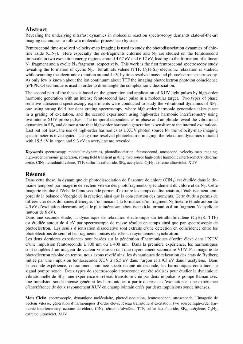
AbstractRevealing the underlying ultrafast dynamics in molecular reaction spectroscopy demands state-of-the-art
imaging techniques to follow a molecular process step by step.
Femtosecond time-resolved velocity-map imaging is used to study the photodissociation dynamics of chlo-
rine azide (ClN3). Here especially the co-fragments chlorine and N3 are studied on the femtosecond
timescale in two excitation energy regions around 4.67 eV and 6.12 eV, leading to the formation of a linear
N3 fragment and a cyclic N3 fragment, respectively. This work is the first femtosecond spectroscopy study
revealing the formation of cyclic N3. Tetrathiafulvalene (TTF, C6H4S4) electronic relaxation is studied,
while scanning the electronic excitation around 4 eV, by time resolved mass and photoelectron spectroscopy.
As only few is known about the ion continuum about TTF the imaging photoelectron photoion coincidence
(iPEPICO) technique is used in order to disentangle the complex ionic dissociation.
The second part of the thesis is based on the generation and application of XUV light pulses by high-order
harmonic generation with an intense femtosecond laser pulse in a molecular target. Two types of phase
sensitive attosecond spectroscopy experiments were conducted to study the vibrational dynamics of SF6:
one using strong field transient grating spectroscopy, where high-order harmonic generation takes place
in a grating of excitation, and the second experiment using high-order harmonic interferometry using
two intense XUV probe pulses. The temporal dependencies in phase and amplitude reveal the vibrational
dynamics in SF6 and demonstrate that high-order harmonic generation is sensitive to the internal excitations.
Last but not least, the use of high-order harmonics as a XUV photon source for the velocity-map imaging
spectrometer is investigated. Using time-resolved photoelectron imaging, the relaxation dynamics initiated
with 15.5 eV in argon and 9.3 eV in acetylene are revealed.
Keywords spectroscopy, molecular dynamics, photodissociation, femtosecond, attosecond, velocity-map imaging,
high-order harmonic generation, strong field transient grating, two source high-order harmonic interferometry, chlorine
azide, ClN3, tetrathiafulvalene, TTF, sulfur hexafluoride, SF6, acetylene, C2H2, extreme ultraviolet, XUV
ResumeDans cette these, la dynamique de photodissociation de l’azoture de chlore (ClN3) est etudiee dans le do-
maine temporel par imagerie de vecteur vitesse des photofragments, specialement du chlore et de N3. Cette
imagerie resolue a l’echelle femtoseconde permet d’extraire les temps de dissociation, l’etablissement tem-
porel de la balance d’energie de la reaction ainsi que la conservation des moments. Cette etude a permis de
differencier deux domaines d’energie: l’un menant a la formation d’un fragment N3 lineaire (etude autour de
4.5 eV d’excitation electronique) et le plus interessant aboutissant a la formation d’un fragment N3 cyclique
(autour de 6 eV).
Dans une seconde etude, la dynamique de relaxation electronique du tetrathiafulvalene (C6H4S4-TTF)
est etudiee autour de 4 eV par spectroscopie de masse resolue en temps ainsi que par spectroscopie de
photoelectron. Les seuils d’ionisation dissociative sont extraits d’une detection en coıncidence entre les
photoelectrons de seuil et les fragments ionises realisee sur rayonnement synchrotron.
Les deux dernieres experiences sont basees sur la generation d’harmoniques d’ordre eleve dans l’XUV
d’une impulsion femtoseconde a 800 nm ou a 400 nm. Dans la premiere experience, les harmoniques
sont couplees a un imageur de vecteur vitesse en tant que rayonnement secondaire VUV. Par imagerie de
photoelectron resolue en temps, nous avons revele ainsi les dynamiques de relaxation des etats de Rydberg
initiee par une impulsion femtoseconde XUV a 15.5 eV dans l’argon et a 9.3 eV dans l’acetylene. Dans
la seconde experience, couramment nommee spectroscopie attoseconde, les harmoniques constituent le
signal pompe sonde. Deux types de spectroscopie attoseconde ont ete realises pour etudier la dynamique
vibrationnelle de SF6: une experience en reseau transitoire cree par deux impulsions pompe Raman avec
une impulsion sonde intense generant les harmoniques a partir du reseau d’excitation et une experience
d’interference de deux rayonnement XUV en champ lointain crees par deux impulsions sonde intenses.
Mots Clefs: spectroscopie, dynamique moleculaire, photodissociation, femtoseconde, attoseconde, l’imagerie de
vecteur vitesse, generation d’harmoniques d’ordre eleve, reseau transitoire d’excitation, two source high-order har-
monic interferometry, azoture de chlore, ClN3, tetrathiafulvalene, TTF, sulfur hexafluoride, SF6, acetylene, C2H2,
extreme ultraviolet, XUV


![Methods and applications of femtosecond time-resolved ...faculty.chem.queensu.ca/.../jelectrspec.pdf · time resolved electronic spectroscopy [16,17] in upon removal of a single active](https://img.dokumen.tips/doc/110x75/5f7019d1cbce526ccf6a2d20/methods-and-applications-of-femtosecond-time-resolved-time-resolved-electronic.jpg)