Embed Size (px)
Citation preview
ICT-248891 STP FREEDOM
Femtocell-based network enhancement by interference management and coordination of information for seamless connectivity
D3.2
Interference Coordination Protocols in Femto-based Networks
Contractual Date of Delivery to the CEC: 31st July 2011
Actual Date of Delivery to the CEC: 28th November 2011
Author(s): A. Agustin, O. Muñoz, J. Vidal, M. Goldhamer, J. R. Fonollosa, A. Pastore (UPC), Stefania Sardellitti, Loreto Pescosolido, Paolo di Lorenzo, Sergio Barbarossa, Andrea Baiocchi (INFO), Enrico de Marinis, Giovanni Imponente, Fabrizio Pucci, Guido Rosi (DUN)
Participant(s): UPC, INFO, DUN
Workpackage: WP3
Est. person months: 28
Security: P
Dissemination Level: PU
Version: f
Total number of pages: 180
Abstract: This document looks into coordinated radio resource allocation algorithms in deployments of huge number of femto-access points (FAP) by exploiting the message exchange at control-plane level through the wired ISP backhaul link. The algorithms present in this document are based on decentralized cooperative strategies supported by Game Theory. Decentralized resource allocation algorithms based on price exchange have been derived under different criteria: guaranteeing a minimum rate with the minimum power, maximizing the weighted sum-rate of the system, maximizing the opportunistic throughput when there are different source of randomness like random link failures and noise quantization or when the activity of macro-users is not known by FAPs (coordinated channel sensing or modelling the activity). Additionally, a genetic-based resource allocation is investigated, providing centralized and decentralized algorithms, to which the Game Theory solutions are challenged. In all cases, the techniques derived require modifications of the current LTE-A standard which are identified. Finally, some of those algorithms have been evaluated in a realistic corporate scenario elucidating the advantages of coordinated resource allocation techniques proposed. Keyword list: Cooperative games, MIMO, Genetic optimization, Decentralized optimization, resource block optimization, multi-user communication, opportunistic throughput, backhaul limitation.

2
Document Revision History DATE ISSUE AUTHOR SUMMARY OF MAIN CHANGES 11-07-2011 a All partners Contributions are collected and the first draft is
elaborated 9-09-2011 b UPC 2nd draft version including the latest
contributions 15-11-2011 c UPC 3rd draft version with the evaluation of the
UPC’s algorithms in a sector-based scenario 23-11-2011 d All partners Final contributions. Updates on INFO
contribution, and comparison of two algorithms in a common scenario, UPC and DUNE
28-11-2011 e UPC New contributions from UPC related to a LTE Standard contribution and Patent Application
12-01-2012 f UPC Added reference to the two patent applications generated from the work described in section 11.2
ICT-248891 STP Document number: D3.2 Title of deliverable: Interference coordination protocols in femto-based networks
FREEDOM_3D2UPCf 3
Executive Summary
The theme addressed in this work is the development of distributed interference-aware resource allocation algorithms that coordinate different FAPs by exchanging parameters at control-plane level through the backhaul link. We are assuming a dense femtocell deployment and hence a high level of interference that negatively influences the system spectral efficiency. Under the assumption that femtocells are connected through a wired ISP backhaul link, the quality of that connection impacts the exchange of information messages at the control-plane level and needs to be taken into consideration.
We propose a set of algorithms that are able to address the resource allocation of the system in a decentralized way under the following criteria:
Power minimization. The objective is to allocate resources (power allocation) efficiently using the minimum power and guaranteeing a minimum rate per user (in section 5).
Weighted sum-rate (WSR) maximization. Assuming that the attained bitrate is weighted by a factor that accounts for the priority of each user in a scenario where there are multiples FUEs per FAP, the resource allocation (power allocation and carrier assignment per FAP) is optimized so that the weighted sum-rate is maximum, constrained to a maximum transmitted power and a maximum rate per FAP (given by the quality of the backhaul) (in section 6).
Those criteria are adopted following a decentralized operation principle, and their performance is compared to a centralized solution based on Genetic Algorithm (in section 8). This latter solution is attractive for its simplicity, modularity and suitable for both synchronous and asynchronous scenario.
A femto-cell system in which channel access is not coordinated with the Macro Users’ network is inherently subject to the performance of the new system functionalities that are introduced to implement the proposed algorithms. We follow the approach of using a statistical model for a particular aspect of the problem and build on this model to devise suitable algorithms (in section 7):
Coordinated channel sensing. FAPs/FUEs track the activity of the interference (i.e. MBS) and exchange the measures over nearby FAPs. Using that set of measures, each FAP is able to allocate the resources in a smart way when the detection and channel access parameters are jointly done. The spectrum sensing detection performance has a key role in the definition of the optimal access strategy. The performance metric to maximize is opportunistic throughput, a notion that redefines the concept of throughput taking into account the presence of the macro users’ communication, which the proposed system should preserve as much as possible.
Markovian interference model. The activity on each frequency subchannel is assumed to follow a general Markov model whose parameters are estimated on the basis of recorded observations of the interference over time.
Random failures and noise quantization. The exchanged control messages (prices) are quantized or possibly loss in a random way.
The main benefits showed by the proposed algorithms for coordinating the generated interference are:
Possibility of addressing a joint resource allocation in a decentralized way.
To partially overcome the inefficiency of Nash Equilibria present in similar algorithms that avoid using exchanging messages at the control plane (like those in [FREEDOM-D3.1]).
Messages only have to be exchanged amongst the interfering neighboring terminals, so that, algorithm are scalable with the number of FAPs.
A simpler LTE based pricing solution has been derived for MBS-FAPs interference coordination and the required standard enhancements have been identified (section 11.1).
Finally, an algorithm to maximize the rate or minimize the power under interference power constraints has been considered for two patent applications (section 11.2).

4

ICT-248891 STP Document number: D3.2 Title of deliverable: Interference coordination protocols in femto-based networks
FREEDOM_3D2UPCf 5
DISCLAIMER
The work associated with this report has been carried out in accordance with the highest technical standards and the FREEDOM partners have endeavoured to achieve the degree of accuracy and reliability appropriate to the work in question. However since the partners have no control over the use to which the information contained within the report is to be put by any other party, any other such party shall be deemed to have satisfied itself as to the suitability and reliability of the information in relation to any particular use, purpose or application.
Under no circumstances will any of the partners, their servants, employees or agents accept any liability whatsoever arising out of any error or inaccuracy contained in this report (or any further consolidation, summary, publication or dissemination of the information contained within this report) and/or the connected work and disclaim all liability for any loss, damage, expenses, claims or infringement of third party rights.

6
Table of Contents
1 INTRODUCTION ............................................................................................... 15
2 SCENARIOS ........................................................................................................ 18
2.1 BUSINESS SCENARIOS ............................................................................................... 18 2.2 TECHNICAL SCENARIOS ........................................................................................... 18
3 SYSTEM ASSUMPTIONS ................................................................................. 20
3.1 PHY ASSUMPTIONS ................................................................................................... 20 3.2 MAC SUPPORT .......................................................................................................... 20 3.3 NETWORK ARCHITECTURE ...................................................................................... 21
4 SIMULATION METHODOLOGY ................................................................... 22
5 DECENTRALIZED POWER MINIMIZATION ............................................ 24
5.1 SISO CASE AND PRICING MECHANISMS .................................................................. 24 5.1.1 Preliminaries ...................................................................................................... 24 5.1.2 Problem formulation ........................................................................................... 25 5.1.3 Numerical results ................................................................................................ 28
5.2 MIMO CASE .............................................................................................................. 29 5.2.1 Preliminaries ...................................................................................................... 29 5.2.2 Description ......................................................................................................... 29 5.2.3 Numerical results ................................................................................................ 33
5.3 CONCLUSIONS ........................................................................................................... 35
6 DECENTRALIZED WEIGHTED SUM RATE MAXIMIZATION ............. 36
6.1 SISO CASE: COMPLEX VS. SIMPLE TRANSMITTERS ................................................ 36 6.1.1 System model ...................................................................................................... 37 6.1.2 Decentralized Resource Allocation .................................................................... 39 6.1.3 Numerical results ................................................................................................ 47
6.2 MIMO CASE AND BACKHAUL RATE CONSTRAINTS ................................................ 50 6.2.1 Description ......................................................................................................... 50 6.2.2 Radio resource allocation at the k-th FAP ......................................................... 52
6.2.2.1 Rate and Power allocation given a certain RB assignment ............................. 52 6.2.2.2 Rate, Power and RB optimization ................................................................... 53
6.2.3 Generation of prices ........................................................................................... 54 6.2.4 Numerical results ................................................................................................ 54
6.3 CONCLUSIONS ........................................................................................................... 57
7 DECENTRALIZED COORDINATION STRATEGIES BASED ON STATISTICAL MODELLING ............................................................................................................. 58
7.1 PRELIMINARIES ........................................................................................................ 58 7.2 COORDINATED CHANNEL SENSING .......................................................................... 62
7.2.1 System and detection models .............................................................................. 62 7.2.2 Maximization of the aggregated opportunistic throughput ................................ 63 7.2.3 Opportunistic throughput maximization: A game theoretic approach ............... 67 7.2.4 Numerical results ................................................................................................ 71
7.3 DYNAMIC RESOURCE ALLOCATION UNDER MARKOVIAN INTERFERENCE MODEL75 7.3.1 Preliminaries ...................................................................................................... 75 7.3.2 Maximum expected rage game ........................................................................... 76
7.3.2.1 Numerical results ............................................................................................ 79
ICT-248891 STP Document number: D3.2 Title of deliverable: Interference coordination protocols in femto-based networks
FREEDOM_3D2UPCf 7
7.3.3 Min-power game subject to Markovian interference .......................................... 81 7.4 DISTRIBUTED STOCHASTIC PRICING FOR SUM-RATE MAXIMIZATION WITH RANDOM
GRAPH AND QUANTIZED COMMUNICATIONS .................................................................... 83 7.4.1 Preliminaries ...................................................................................................... 83 7.4.2 System model ...................................................................................................... 84 7.4.3 Distributed Stochastic Pricing Algorithm (DSPA) ............................................. 88 7.4.4 Numerical results ................................................................................................ 89
7.5 CONCLUSIONS ........................................................................................................... 90
8 CENTRALIZED DYNAMIC INTERFERENCE MANAGEMENT ............. 92
8.1 PRELIMINARIES ........................................................................................................ 92 8.2 CELL SYSTEM OPTIMIZATION BY GENETIC ALGORITHM ...................................... 94
8.2.1 Distributed or centralized implementation ......................................................... 94 8.2.2 Working of the GA implementation .................................................................... 95 8.2.3 GO implementation for a set of FAPs ................................................................. 96 8.2.4 GO formulation................................................................................................... 97
8.3 GO FOR FLAT FADING SCENARIO .......................................................................... 101 8.3.1 Fitness function................................................................................................. 101 8.3.2 Analysis of topologies for a single block .......................................................... 102
8.3.2.1 Flat fading channel ........................................................................................ 102 8.3.2.2 GO for frequency selective channel .............................................................. 106
8.4 GENETIC ALGORITHM AND SCALABILITY ............................................................ 108 8.4.1 Benefits of clustering ........................................................................................ 108 8.4.2 Clustering of FAPs ........................................................................................... 109
8.5 SYNCHRONIZATION ISSUES AND GO ..................................................................... 110 8.5.1 Asynchronous scenario ..................................................................................... 110 8.5.2 Design principles and constraints .................................................................... 113 8.5.3 GA tested on a fully asynchronous frame sequence ......................................... 113
8.5.3.1 Results of GA tested on fixed frame sequences ............................................ 113 8.5.3.2 Results of GA tested on randomly changing frame sequences ..................... 114 8.5.3.3 Conclusions on second tier synchronization and GA ................................... 116
8.6 CONCLUSIONS OF THE GO OPTIMIZATION ........................................................... 116
9 SIMULATION RESULTS ................................................................................ 117
9.1 RESOURCE ALLOCATION BASED ON WEIGHTED SUM-RATE (WSR) MAXIMIZATION 118 9.1.1 Small Corporate configuration ......................................................................... 119 9.1.2 Simulated Corporate configuration .................................................................. 122 9.1.3 Conclusions ...................................................................................................... 125
9.2 RESOURCE ALLOCATION BASED ON POWER MINIMIZATION ............................... 125 9.2.1 Results for a single scenario with a fixed number of FAPs .............................. 126 9.2.2 Results for several scenarios ............................................................................ 129 9.2.3 Results for varying FAP density ....................................................................... 133 9.2.4 Conclusions ...................................................................................................... 136
9.3 DYNAMIC RESOURCE ALLOCATION UNDER MARKOVIAN INTERFERENCE MODEL136 9.4 DECENTRALIZED VS. CENTRALIZED RESOURCE ALLOCATION ........................... 139 9.5 GO FOR REALISTIC FREQUENCY SELECTIVE CHANNEL - POWER CONSTRAINED141
9.5.1 Macro-network UL ........................................................................................... 141 9.5.2 Macro-network DL ........................................................................................... 142 9.5.3 Overall results .................................................................................................. 143
10 IMPLEMENTATION NOTES ...................................................................... 146
10.1 SCALABILITY ....................................................................................................... 146 10.2 APPLICABILITY ................................................................................................... 147
8
10.3 COMPLEXITY ....................................................................................................... 148
11 LTE-BASED RESOURCE ALLOCATION ................................................ 150
11.1 LTE-A ADAPTED PRICING MECHANISMS .......................................................... 150 11.1.1 A pricing based mechanism for MCS and bandwidth part selection. ............... 150
11.1.1.1 Fundamentals ............................................................................................ 151 11.1.1.2 Procedure for coordinated bandwidth part selection ................................. 154
11.1.1.2.1 Sensing and sharing the CQI degradation .............................................. 155 CQI detection in the serving cell ..................................................................................... 155 CQI degradation in the serving cell ................................................................................ 156
11.1.1.2.2 Decision making ..................................................................................... 157 11.1.2 Exponential Effective SINR Mapping (EESM) ................................................. 157 11.1.3 Simulation results ............................................................................................. 159 11.1.4 Conclusions and recommended actions ............................................................ 163
11.2 RATE MAX OR POWER MIN UNDER INTERFERENCE-POWER CONSTRAINTS .. 164 11.2.1 LTE signals and measurements ........................................................................ 164
11.3 RESOURCE BLOCK POWER ALLOCATION IN LTE FEMTOCELL NETWORKS ... 165
12 GENERAL CONCLUSIONS ........................................................................ 168
13 SUMMARY OF RESULTS TOWARDS OTHER ACTIVITIES .............. 170
13.1 TOWARDS WP4 ................................................................................................... 170 13.2 TOWARDS WP5 ................................................................................................... 170 13.3 TOWARDS WP6 ................................................................................................... 170
14 APPENDIX ...................................................................................................... 171
14.1 SIMULATION METHODOLOGY ............................................................................ 171 14.2 GEOMETRY OF THE SCENARIO ........................................................................... 172 14.3 PATHLOSS MODELS ............................................................................................. 173
14.3.1 ITU and 3GPP formulation .............................................................................. 173 14.3.2 Pathloss and clustering .................................................................................... 174
14.4 MORE RESULTS OF SECTION 8.3.2.1 ................................................................... 175 14.4.1 Frequency GO under power constraint ............................................................ 178 14.4.2 GO output for different FAP load FAP/FUE couples ...................................... 178

ICT-248891 STP Document number: D3.2 Title of deliverable: Interference coordination protocols in femto-based networks
FREEDOM_3D2UPCf 9
References & Standards [3GPP TS 36.213] 3GPP TS 36.213, “Physical layer procedures”
[3GPP-TR36.814] 3GPP TR 36.814, “Further advancements for E-UTRA physical layer aspects”
[Agustin11a] A. Agustin, J. Vidal, O. Muñoz-Medina, “Interference Pricing for Self-organisation in OFDMA Femtocell Networks”, European Workshop on Broadband Femtocell Networks – Future Network and Mobile Summit (FuNeMS), Warsaw, Poland, June 2011
[Agustin11b] A. Agustin, J. Vidal, O. Muñoz-Medina, J.R. Fonollosa, “DecentralizedWeighted Sum Rate Maximization in MIMO-OFDMA Femtocell Networks”, IEEE Proc. the Second Globecom 2011 Workshop on Femtocell Networks (GC'11 Workshop-FEMnet), Houston,USA,Dec.2011
[Ban03] S. Bandyopadhyay, E. J. Coyle, “An Energy Efficient Hierarchical Clustering Algorithm for Wireless Sensor Networks”, IEEE INFOCOM 2003, vol.3 pp. 1713-1723.
[Barbarossa10] S. Barbarossa, S. Sardellitti, A. Carfagna, P. Vecchiarelli, “Decentralized Interference Management in Femtocells: A Game-Theoretic Approach”, Proc. CrownCom 2010, Cannes, France, June 2010.
[Barbarossa11a] S. Barbarossa, A. Carfagna, S. Sardellitti, M. Omilipo, L. Pescosolido“Optimal Radio Access in Femtocell Networks Based on Markov Modeling of Interferers’ activity”, in Proc. IEEE ICASSP 2011
[Barbarossa11b] S. Barbarossa, S. Sardellitti, A. Carfagna, “Decentralized Resource Allocation in Femtocell Networks Based on Game Theory and Markov Modeling”, submitted for publication, available online at http://infocom.uniroma1.it/sergio/jsac-femtocells.pdf.
[Bertsekas95] D.P. Bertsekas, Nonlinear Programming. Athena Scientific, Belmont, Massachusetts, 1995.
[Bertsekas03] D.P. Bertsekas, Convex Analysis and Optimization. Athena Scientific, Belmont, Massachusetts, 2003.
[Boyd04] S. Boyd, L. Vandenberghe, Convex optimization, Cambridge University Press, 2004.
[Cendrillon05] R. Cendrillon, M. Moonen, “Iterative Spectrum balancing for digital subscriber lines, in Proc. IEEE Intl. Conf. on Communications (ICC), June 2005
[DiLorenzo11] P. Di Lorenzo, S. Barbarossa, M. Omilipo, “Distributed sum-rate maximization in femtocell networks with random graph and quantized communications”, submitted to IEEE Trans. on Signal Processing, 2011
[DOCOMO] TSG-RAN Working Group (Radio) meeting #52 R4-093244 Shenzen, 24-28 August 2009, NTT DOCOMO Downlink Interference Coordination Between eNodeB and Home eNodeB
[Facchinei03] F. Facchinei and J.-Pang, Finite-Dimensional Varational Inequalities and Complementarity Problems, New-York: Springer-Verlag, 2003.
[Facchinei2010] F. Facchinei, V. Piccialli and M. Sciandrone, “Decomposition algorithms for generalized potential games”, Computational Optim. and Appl., Springer-Verlag New York Inc., May 2010.

10
[FREEDOM-D21] ICT FP7-248891 STP FREEDOM project deliverable D2.1, “Scenario, requirements and first business model analysis”, June 2010. [Online]: http://www.ict-freedom.eu/index.php?option=com_spcom&Itemid=88
[FREEDOM-D31] ICT FP7-248891 STP FREEDOM project deliverable D3.1, “Interference identification in the femto-based networks”, July 2011. [Online]: http://www.ict-freedom.eu/index.php?option=com_spcom&Itemid=88
[FREEDOM-D42] ICT FP7-248891 STP FREEDOM project deliverable D4.2, “Design and evaluation of effective procedures for MAC layer”, Dec. 2011. [Online]: http://www.ict-freedom.eu/index.php?option=com_spcom&Itemid=88.
[FREEDOM-D52] ICT FP7-248891 STP FREEDOM project deliverable D5.2, “System Interference Management Evaluation”, Dec. 2011. [Online]: http://www.ict-freedom.eu/index.php?option=com_spcom&Itemid=88
[Huang06] J. Huang, R.A. Berry, M.L. Honig, “Distributed Interference Compensation for Wireless Networks”, IEEE J. on Selected Areas in Commun., Vol. 24, pp. 1074--1084, May 2006.
[Ho09] L.T.W. Ho, I.Ashraf, H.Claussen, “Evolving Femtocell Coverage Optimization Algorithms using Genetic Programming”, IEEE Personal, Indoor and Mobile Radio Communic. Conference, PIMRC 2009, , pp. 2132 – 2136, 2009.
[http://www.nt.tuwien.ac.at/ltesimulator]
Institute of Communications and Radio-Frequency Engineering, Vienna University of Technology, Austria
[ITU1238] ITU-R P.1238-6, “Propagation data and prediction methods for the planning of indoor radiocommunication systems and radio local area networks in the frequency range 900 MHz to 100 GHz”, 2009.
[Jorswieck08] E. A. Jorswieck, E. G. Larsson, and D. Danev, “Complete Characterization of the Pareto Boundary for the MISO Interference Channel”, IEEE Trans. on Signal Processing, vol. 56, no. 10, October 2008.
[Kum02] R. Kumar, P.P. Parida, M. Gupta, “Topological design of communication networks using multiobjective genetic optimization”, Evolutionary Computation, CEC '02 Proceedings, pp. 425-430, 2002.
[Lie98] K. Lieska, E. Laitinen, J. Latheenmaki, “Radio coverage optimization with genetic algorithms”, Ninth IEEE Intern. Symposium on Personal, Indoor and Mobile Radio Communications, PIMRC 1998, pp. 318-322, 1998.
[Meu00] H. Meunier, E.-G. Talbi, P. Reininger, “A multiobjective genetic algorithm for radio network optimization”, Proceedings of the 2000 Congress on Evolutionary Computation, pp. 317-324, 2000.
[MondererShapely96] D. Monderer, and L. S. Shapley, “Potential Games”, Games and Economics Behaviour, Vol. 14, pp. 124-143, 1996.
[Munoz11a] O. Munoz-Medina, A. Pascual, P. Baquero, J. Vidal , “Preemption and QoS Management Algorithms for Coordinated and Uncoordinated Base Stations”, SPAWC 2011, San Francisco, June 2011
[Munoz11b] O. Muñoz, J. Vidal, A. Agustín, A. Pascual-Iserte, S. Barbarossa, “Coordinated MIMO Precoding for Power Minimization in Femtocell Systems”, The Second GlobeCom 2011 Workshop on Femtocell Networks (GC'11 Workshop - FEMnet).Houston, USA, Dec. 2011

ICT-248891 STP Document number: D3.2 Title of deliverable: Interference coordination protocols in femto-based networks
FREEDOM_3D2UPCf 11
[Olfati-Saber07]
R. Olfati-Saber, J.A. Fax, R.M. Murray, “Consensus and Cooperation in Networked Multi-Agent Systems,” Proc. of the IEEE, Vol. 95, pp. 215–233, Jan. 2007.
[Pang08] J.S. Pang, G. Scutari, F. Facchinei, C. Wang, “Distributed Power Allocation With Rate Constraints in Gaussian Parallel Interference Channels”, IEEE Trans. on Inform. Theory., Vol. 54, no. 8, pp. 3471-3489, August 2008.
[Quan08] Z. Quan, S. Cui, H. V. Poor and A. H. Sayed, “Collaborative wideband sensing for cognitive radio,” IEEE Signal Process. Mag., Vol. 25, pp. 60--73, November 2008.
[Quan09] Z. Quan, S. Cui, H. V. Poor and A. H. Sayed, “Optimal multiband joint detection for spectrum sensing in cognitive radio networks,” IEEE Trans. on Signal Processing, Vol. 57, pp. 1128--1140, March 2009.
[R3-112701] R3-112701, “Way forward on Carrier based ICIC LTE”, AT&T, China Unicom, Mitsubishi Electric, NEC, Telefonica, TeliaSonera, Verizon Wireless, ZTE
[R3-112752] R3-112752, DAC-UPC, Proposal for DL interference coordination in Macro – SC HeNB scenario, 3GPP TSG-RAN WG3 #74, November 14-18, 2011, San Francisco, USA
[R3-112953] DAC-UPC, Telefonica, Text proposal for carrier-based ICIC TR on use cases for Macro - SC HeNB scenario, 3GPP TSG-RAN WG3 #74, November 14-18, 2011, San Francisco, USA
[R4-071617] R4-071617, “HNB and HNB-Macro Propagation Models”, Qualcomm Europe, 3GPP TSG-RAN Working Group 4 (Radio) meeting #44bis, October 2007.
[R4-080149] R4-080149, “Simulation assumptions for the block of flats scenario”, Ericsson, 3GPP TSG-RAN Working Group 4 (Radio) meeting #46, February 2008.
[Robbins51] H. Robbins, S. Monro, “A stochastic approximation method”, The Annals of Mathematical Statistics 22, 1951, no.3, pp. 400-407.
[Scutari08a] G. Scutari, D.P. Palomar and S. Barbarossa, “Cognitive MIMO Radio”,IEEE Signal Processing Mag., Vol. 25, pp. 46–59, Nov.2008.
[Scutari08b] G. Scutari, D. P. Palomar, S. Barbarossa, “Optimal Linear Precoding strategies for wideband noncooperative systems based on Game Theory – Part I: Nash Equilibria and – Part II: Algorithms”, IEEE Trans. on Signal Proc., vol.56, no.3 March 2008, pp. 1230-1267
[Seong06] K. Seong, M. Mohseni, J.M. Cioffi, “Optimal Resource allocation for Downlink Systems”, in Proc. IEEE Intl. Symposium on Information Theory (ISIT), Seattle, USA, July 2006
[Sesia09] S. Sesia, I. Toufik , M. Baker, LTE–The UMTS Long Term Evolution, John Wiley & Sons, 2009
[Shi08] C. Shi, R. Berry, and M. Honig, “Distributed Interference Pricing for OFDM Wireless Networks with Non-Separable Utilities”, Proc. of Conference on Information Sciences and Systems (CISS),Princeton University, NJ, USA, March 2008
[Shi09a] C. Shi, R. A. Berry, and M. L. Honig, “Monotonic Convergence of Distributed Interference Pricing in Wireless Networks,” IEEE Int. Symposium on Information Theory, ISIT 2009, Seoul, Korea, June 2009.

12
[Shi09b] C. Shi, et al., “Distributed Interference Pricing for the MIMO interference channel”, in Proc. IEEE Intl. Conf. on Comm., Dresden, Germany, June 2009.
[Son09] K. Son, B. C. Jung, S. Chong and D. K. Sung, “Opportunistic underlay transmission in multi-carrier cognitive radio systems,” Proc. IEEE WCNC 2009, Budapest, Hungary, April 2009.
[Schmidt09] D. A. Schmidt, C. Shi, R. A. Berry, M. L. Honig, W. Utschick, “Distributed Resource Allocation Schemes: Pricing algorithms for power control and beamformer design in interference networks”, IEEE Signal Processing Magazine, Sep. 2009.
[TSG-RAN 2009] TSG-RAN Working Group 4 (Radio) meeting #52 R4-093244 Shenzhen, 24-28 August 2009, NTT DOCOMO Downlink Interference Coordination Between eNodeB and Home eNodeB.
[Vishwanath04] S. Vishwanath, N.Jindal, A.Goldsmith, “On Duality of Gaussian Multiple-Access and Broadcast channels”, IEEE Tran. on Information Theory, vol. 50, no. 5, pp. 768-783, May 2004
[Yu07] W. Yu, “Multiuser Water-filling in the presence of Crosstalk”, in Proc. of Information Theory and Applications Workshop (ITAW), Jan-Feb 2007
[Yu06] W. Yu, R. Lui, “Dual methods for nonconvex spectrum optimization of multicarrier systems”, IEEE Trans. on Comm., vol.54, no.7, Jul. 2006
[Yu02] W. Yu, G. Ginis, and J.M. Cioffi, “Distributed Multiuser Power Control for Digital Subscriber Lines”, IEEE J. of Selected Areas in Commun., Vol. 20, pp. 1105-1115, June 2002.
[Zhang10] R. Zhang, S. Cui, “Cooperative Interference Management with MISO Beamforming”, IEEE Trans. on Signal Processing, vol. 58, no. 10, pp. 5450-5457, October 2010.
ICT-248891 STP Document number: D3.2 Title of deliverable: Interference coordination protocols in femto-based networks
FREEDOM_3D2UPCf 13
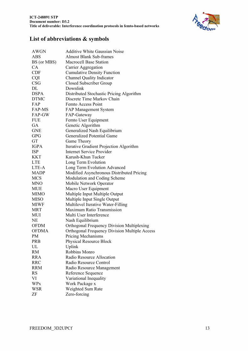
List of abbreviations & symbols AWGN Additive White Gaussian Noise ABS Almost Blank Sub-frames BS (or MBS) Macrocell Base Station CA Carrier Aggregation CDF Cumulative Density Function CQI Channel Quality Indicator CSG Closed Subscriber Group DL Downlink DSPA Distributed Stochastic Pricing Algorithm DTMC Discrete Time Markov Chain FAP Femto Access Point FAP-MS FAP Management System FAP-GW FAP-Gateway FUE Femto User Equipment GA Genetic Algorithm GNE Generalized Nash Equilibrium GPG Generalized Potential Game GT Game Theory IGPA Iterative Gradient Projection Algorithm ISP Internet Service Provider KKT Karush-Khun Tucker LTE Long Term Evolution LTE-A Long Term Evolution Advanced MADP Modified Asynchronous Distributed Pricing MCS Modulation and Coding Scheme MNO Mobile Network Operator MUE Macro User Equipment MIMO Multiple Input Multiple Output MISO Multiple Input Single Output MIWF Multilevel Iterative Water-Filling MRT Maximum Ratio Transmission MUI Multi User Interference NE Nash Equilibrium OFDM Orthogonal Frequency Division Multiplexing OFDMA Orthogonal Frequency Division Multiple Access PM Pricing Mechanisms PRB Physical Resource Block UL Uplink RM Robbins Monro RRA Radio Resource Allocation RRC Radio Resource Control RRM Radio Resource Management RS Reference Sequence VI Variational Inequality WPx Work Package x WSR Weighted Sum Rate ZF Zero-forcing

14
Description Femto Forum 3GPP/LTE-A 802.16/WiMAX FREEDOM
Base Station of the macrocell
Macro Node B (MNB)
Macro Node B (MNB)
Macro Advanced BS
(Macro ABS)
Macro BS (MBS or BS)
User attached to the macrocell
Macro User Equipment
(MUE)
Macro User Equipment
(MUE)
Advanced (AMS) Macro User Equipment
(MUE)
femtocell Femto Acces Point or Home Node B (HNB or FAP)
Home Node B
(HNB) H(e)NB includes HeNB and FAP
Femto ABS FAP
Access Station, can be either FAP or BS
AS
User attached to the femtocell
Femto UE or Home UE
(HUE or FUE)
Home User Equipment
(HUE)
AMS Femto UE
(FUE)
The network element that terminates
TR-069 with the femtocell to hankdel
the remote management of a large number of
femtocells
Auto-configuration Server (ACS)
Home NodeB Management
System (HMS)
femtocell
Management system
in Femto Network Service Provider (Femto – NSP)
Femtocell Management system FAP Management
System (FAP-MS)
The network element that
directly terminates the Iuh interface
with the femtocell and the existing IuCS and IuPS
interface with the core Networks
FAP Gateway (FAP-GW)
Home Node B gateway
(FAP-GW)
Femto Access Service Network
Gateway (Femto-ASN GW)
Femto gateway FAP gateway (FAP-GW)
Handovers femto-femto, BS-femto
handover (or handoff)
femto-macro: handout
macro-femto: hand-in
handover (or handoff)
Handover Hand-in: handover
from macro to femto Hand-out: handover from femto to macro
Table 1. Summary of terminology used in standard and within FREEDOM

ICT-248891 STP Document number: D3.2 Title of deliverable: Interference coordination protocols in femto-based networks
FREEDOM_3D2UPCf 15
1 INTRODUCTION This document explores the activities undergone in 3A2 regarding the use of the wired ISP backhaul link for interference management in a cellular scenario where MBS and FUE might coexist on the same bands. On a first phase, it will be assumed that the available bandwidth and delay constraints on the backhaul link are enough to support parameter exchange at control-plane level among different network nodes. As the backhaul quality may not be assumed perfect, an insight will also be done to evaluate the impact of quantizing the exchanged information and the effect of packet losses. Unlike the approach in [FREEDOM-D31], where no control information is assumed to be exchanged through the backhaul link, we can now coordinate the resource allocation in a distributed way, whereby each source takes decisions independently in an egoistic way for optimizing his resources (see for example [Pang08], [Scutari08b] for the SISO case or [Jorswiek08] for the MISO case). While the purely egoistic strategy for the sources has been proved to be inefficient from a global point of view (especially in high interference scenarios), we elaborate on the results presented in [Huang06], [Shi08] and [Shi09] to derive a decentralized resource allocation algorithm, where some parameters are exchanged among the sources in the neighbourhood. As a consequence, sources become more altruistic since the impact of their decisions is being considering beforehand. In this respect, section 5 is devoted to optimize the resource allocation (transmitted power, allocated resource blocks and MIMO precoders) that minimizes the transmitted power and guarantees a minimum rate per user. SISO and MIMO cases are addressed. Section 6 tackles the decentralized resource allocation that maximizes the WSR assuming a maximum backhaul link capacity. Simple transmitters (each source assigns one carrier to at most one destination) and complex transmitters (multiple destinations per carrier using dirty-paper coding) are analysed. In all cases, each source can serve multiple destinations under an OFDMA scheme. All those solutions scale with the number FAPs and hence are suitable for a massive deployment and the presence of a MBS is considered as an additional FAP whose transmitter power. The possibility of associating different priorities allows preserving QoS to the macro user equipments (MUE). This way, prices exchange gives a natural support to different QoS grades for different users. Section 7 investigates how the decentralized algorithms need to be adapted to combat different sources of randomness. In this respect, section 7.2 and 7.3 look into the case where macro BS (MBS) is serving MUEs in the same band employed by FAPs, but FUEs are not allowed to interfere the macro user communications. It is assumed here that MBS does not inform of the usage of resources to the FAPs. Therefore, FAPs must estimate somehow the activity of the MBS to avoid introducing interference. Two approximations are followed: section 7.2 assumes that neighboring FAPs can perform a coordinated channel sensing to improve the estimation of the MBS activity; section 7.3 models the MBSs activity by a Markov model and under such model the radio resource allocation at the FAPs is performed. In both cases, the obtained throughput is opportunistic, due to the presence of uncertainties. Finally, section 7.4 addresses the randomness due to the random link failure or to the dithered quantization of messages exchanged by FAPs. In general, the analysed decentralized algorithms do not provide globally optimal solutions, because the resource allocation over an interference network is not a convex problem. In order to evaluate the loss of performance (the so-called price of anarchy), section 8 looks into a centralized algorithm based on Genetic Optimization that tackles the whole problem. In such a case, it is assumed that there is a central node able to collect all the required information from the different nodes of the network. This approach will be considered as a benchmark of the previous decentralized solutions. The centralized approach is applicable straightforwardly for scenarios with a low/moderate number of nodes, although the computational load increases with the number of users. In a scenario with a high number of nodes, an efficient implementation of the algorithm requires a fragmentation of the network

16
in subsets, non-interfering each other or partially interfering, as happens for example in a cluster of FAPs placed in the same building. The central computing unit can optimize only the UL, only the DL, or both of the FAPs/FUEs network, based on MNO strategy. Information collected from the nodes of the network will be average SNRs of FAPs, FUEs, or both, respectively. Section 9 is devoted to evaluate the techniques and compare the decentralized and centralized algorithms in a common scenario. In section 10 we analyse the applicability, scalability and complexity of the investigated techniques in sections 5-8. On the other hand, section 11 presents algorithms adapted to the current LTE standard, like a pricing solution for MBS-FAPs interference coordination, an algorithm for maximizing the rate or minimize the power and a resource block power allocation. Finally, section 12 present the conclusions obtained in this work. A summary of achievements obtained in activity 3A2 follows:
Pricing-based algorithms allow performing a joint resource allocation in a decentralized way, while maintaining a given QoS.
We have proposed a decentralized algorithm that designs the resources in order to guarantee a minimum rate for all the users in the system, if the rate is feasible. In those cases where non-pricing algorithms also satisfy that minimum rate, the proposed algorithm defines a low complexity power reduction procedure.
If the objective is to maximize the weighted sum-rate of the system, we have observed that pricing-based algorithms are able to improve the outage rate of the users in the system by a factor of 2-3. In case where each source serves multiple users in an OFDMA fashion, then the spectral efficiency is also improved when the resource blocks (or carriers) assignment is jointly optimized with transmitted power and spatial precoders.
A centralised approach to resource allocation has been implemented by a Genetic Algorithm (GA), attractive for its simplicity, modularity and suitable for both synchronous and asynchronous scenarios. Its only inputs are the mean SNIRs from FAPs and FUEs and outputs the “optimal” (in the sense of the adopted metric) radio resources allocation. Its main drawbacks rely in the convergence time and in the distance from the optimal solutions. Many computational aids can help to overcome the latter, but the compliance between the convergence time and the requirements at system level cannot be insured a priori in all scenarios. The results of the simulations in an asynchronous scenario have shown to be consistent with the “physical meaning” implemented in the adopted fitness functions, on which a specific effort must be spent in order to obtain a meaningful target and functional slopes easing the GA convergence capabilities.
We have determined the optimal access strategy when relying on spectrum sensing to decide whether a channel is left unused by Macro User using the notion of opportunistic throughput.
We have derived a decentralized iterative water filling algorithm that incorporates a Markovian modelling of the resource block use by Macro users in an OFDMA-like time frequency frame structure. With respect to conventional IWFA algorithm, our proposed one exploits not only on the frequency domain, but also the time domain while allocating resources among FAPs. This creates a benefit in terms of the frequency with which the algorithm needs to be run to adapt to the macro users’ activity.
Assuming a decentralized resource allocation strategy based on the local exchange of interference prices, we have proposed a stochastic algorithm which takes into account the non-idealities of realistic communications, i.e. quantization noise and random link failures.

ICT-248891 STP Document number: D3.2 Title of deliverable: Interference coordination protocols in femto-based networks
FREEDOM_3D2UPCf 17
A version of the cooperative game algorithms with a higher degree of compliance with LTE has been obtained for MBS-FAPs interference coordination. The solution and the required standard enhancements have been presented in the 3GPP meeting held in San Francisco in November 2011 [R3-112752]. A contribution for the specifications of the DL MeNB-HeNB use case within RAN3, addressing DL interference MeNB-HeNB scenario and Operational requirements was generated and submitted to 3GPP as document [R3- 112953].
An algorithm for rate maximization or power minimization under interference power constraints is patent application pending.
18
2 SCENARIOS 2.1 Business scenarios
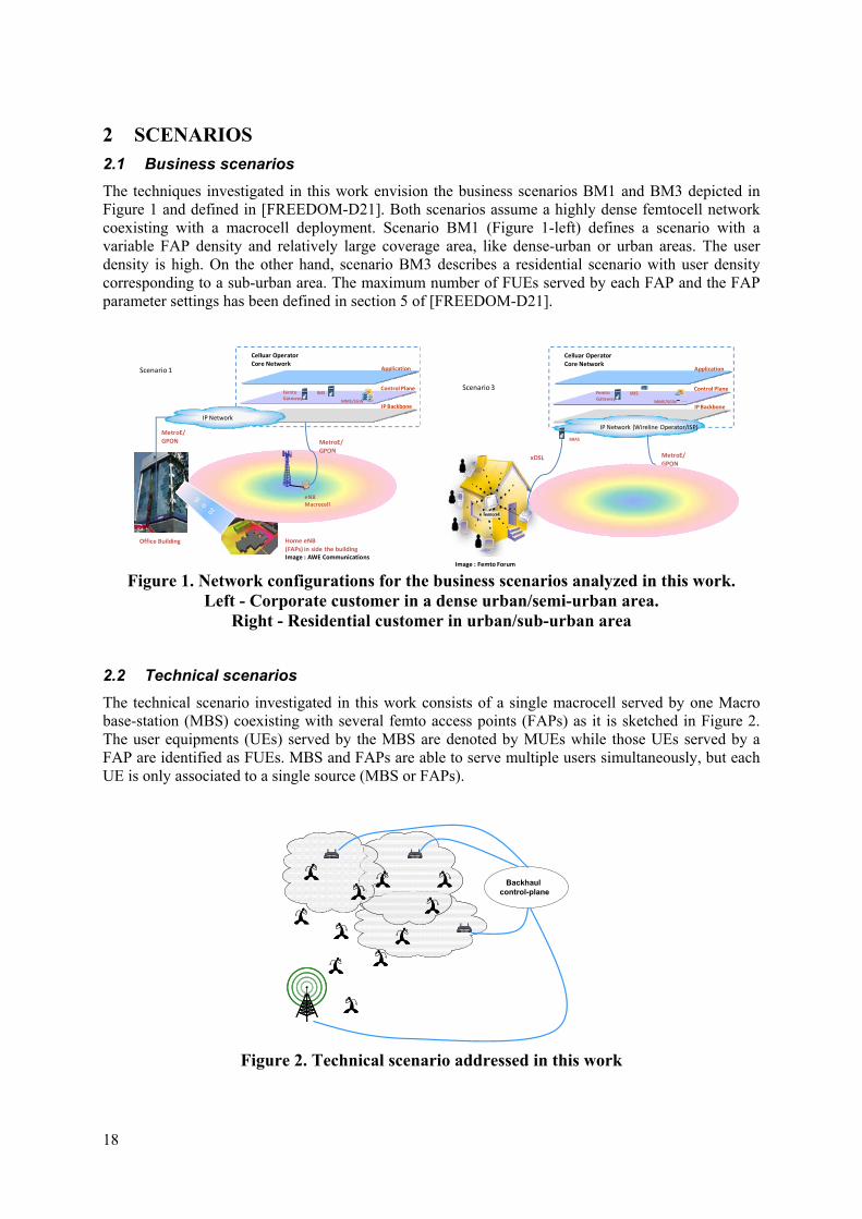
The techniques investigated in this work envision the business scenarios BM1 and BM3 depicted in Figure 1 and defined in [FREEDOM-D21]. Both scenarios assume a highly dense femtocell network coexisting with a macrocell deployment. Scenario BM1 (Figure 1-left) defines a scenario with a variable FAP density and relatively large coverage area, like dense-urban or urban areas. The user density is high. On the other hand, scenario BM3 describes a residential scenario with user density corresponding to a sub-urban area. The maximum number of FUEs served by each FAP and the FAP parameter settings has been defined in section 5 of [FREEDOM-D21].
Figure 1. Network configurations for the business scenarios analyzed in this work.
Left - Corporate customer in a dense urban/semi-urban area. Right - Residential customer in urban/sub-urban area
2.2 Technical scenarios
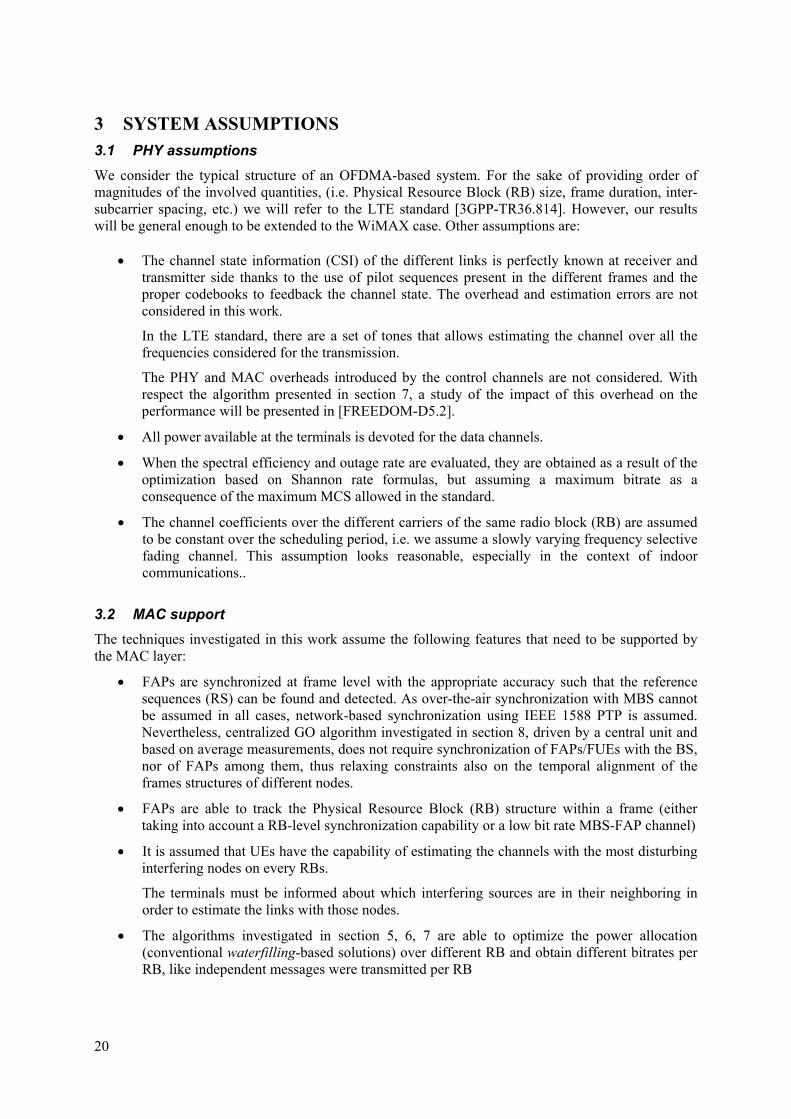
The technical scenario investigated in this work consists of a single macrocell served by one Macro base-station (MBS) coexisting with several femto access points (FAPs) as it is sketched in Figure 2. The user equipments (UEs) served by the MBS are denoted by MUEs while those UEs served by a FAP are identified as FUEs. MBS and FAPs are able to serve multiple users simultaneously, but each UE is only associated to a single source (MBS or FAPs).
Backhaul control-plane
Figure 2. Technical scenario addressed in this work
Celluar Operator Core Network
Application
Control Plane
IP Backbone
FemtoGateway
MME/SGW
IMS
IP Network (Wireline Operator/ISP)
eNBMacrocell
MetroE/GPON
BRAS
xDSL
Scenario 3
Image : Femto Forum
MetroE/GPON
eNBMacrocell
Home eNB(FAPs) in side the buildingImage : AWE Communications
Celluar Operator Core Network
Application
Control Plane
IP Backbone
FemtoGateway
MME/SGW
IMS
IP Network
MetroE/GPON
Scenario 1
Office Building

ICT-248891 STP Document number: D3.2 Title of deliverable: Interference coordination protocols in femto-based networks
FREEDOM_3D2UPCf 19
In contrast to the MBS which is placed by the mobile operator, FAPs will be installed by the end-users. That means that the positions become random and the generated interference has to be managed properly. In this work we exploit the fact that MBS and FAPs are connected through a backhaul link that allows the exchange of parameters at the control-plane level, in order to design the techniques to manage the interference. The techniques investigated are developed in a framework compliant with the LTE air-interface based on Orthogonal Frequency Division Multiple Access (OFDMA) with multi-antenna terminals. Those techniques can be applied to the uplink (UL) and downlink (DL). Three scenarios describe the type of coexistence between the macro cell and femto cells in terms of occupied bandwidth and generated interference:
1. MBS and FAPs operate in orthogonal (or non-overlapped) bands. The resources allocated to the MUEs and to the FUEs are orthogonal while the band employed by all FAPs is the same. In this case, MBS perform the resource allocation to its associated MUEs independently from the resource allocation performed by the FAPs to their associated FUEs.
2. MBS and FAPs operate in the same band with same role. In this case MBS and FAPs perform a joint resource allocation and they are mutually influenced by the decisions taken.
3. MBS and FAPs operate in the same band with different role. Here, FAPs design their resource allocation in a jointly way but taking into account their impact on MUEs in terms of achieved rate or generated interference. In contrast, MBS do not take into consideration the generated interference to the FUEs.
In must be emphasized that in all cases, FAPs must perform a joint resource allocation over the same band. In this regard, the second scenario is easily addressed by the same algorithm considered for the first scenario at the FAPs, but assuming the MBS as an additional entity with the appropriate channel models and power transmission levels. In this regard, the techniques investigated in sections 5.1, 5.2, 6.1, 6.2 and 8 apply to technical scenarios 1 and 2. On the other hand, the work presented in sections 7.2 and 7.3 consider the technical scenario 3. Finally, the technique introduced in section 7.4 accounts for technical scenarios 1 and 2 assuming a quantified (or missing) exchanged information. Notice that the techniques are analysed in a general framework, without imposing any constraint on neither the current standard (LTE or WiMAX) nor the UL/DL duplexing mode. However, section 10 is devoted to address how the new techniques fit in the current version of LTE and WiMAX standards and what changes would be required.
20
3 SYSTEM ASSUMPTIONS 3.1 PHY assumptions
We consider the typical structure of an OFDMA-based system. For the sake of providing order of magnitudes of the involved quantities, (i.e. Physical Resource Block (RB) size, frame duration, inter-subcarrier spacing, etc.) we will refer to the LTE standard [3GPP-TR36.814]. However, our results will be general enough to be extended to the WiMAX case. Other assumptions are:
The channel state information (CSI) of the different links is perfectly known at receiver and transmitter side thanks to the use of pilot sequences present in the different frames and the proper codebooks to feedback the channel state. The overhead and estimation errors are not considered in this work.
In the LTE standard, there are a set of tones that allows estimating the channel over all the frequencies considered for the transmission.
The PHY and MAC overheads introduced by the control channels are not considered. With respect the algorithm presented in section 7, a study of the impact of this overhead on the performance will be presented in [FREEDOM-D5.2].
All power available at the terminals is devoted for the data channels.
When the spectral efficiency and outage rate are evaluated, they are obtained as a result of the optimization based on Shannon rate formulas, but assuming a maximum bitrate as a consequence of the maximum MCS allowed in the standard.
The channel coefficients over the different carriers of the same radio block (RB) are assumed to be constant over the scheduling period, i.e. we assume a slowly varying frequency selective fading channel. This assumption looks reasonable, especially in the context of indoor communications..
3.2 MAC support
The techniques investigated in this work assume the following features that need to be supported by the MAC layer:
FAPs are synchronized at frame level with the appropriate accuracy such that the reference sequences (RS) can be found and detected. As over-the-air synchronization with MBS cannot be assumed in all cases, network-based synchronization using IEEE 1588 PTP is assumed. Nevertheless, centralized GO algorithm investigated in section 8, driven by a central unit and based on average measurements, does not require synchronization of FAPs/FUEs with the BS, nor of FAPs among them, thus relaxing constraints also on the temporal alignment of the frames structures of different nodes.
FAPs are able to track the Physical Resource Block (RB) structure within a frame (either taking into account a RB-level synchronization capability or a low bit rate MBS-FAP channel)
It is assumed that UEs have the capability of estimating the channels with the most disturbing interfering nodes on every RBs.
The terminals must be informed about which interfering sources are in their neighboring in order to estimate the links with those nodes.
The algorithms investigated in section 5, 6, 7 are able to optimize the power allocation (conventional waterfilling-based solutions) over different RB and obtain different bitrates per RB, like independent messages were transmitted per RB

ICT-248891 STP Document number: D3.2 Title of deliverable: Interference coordination protocols in femto-based networks
FREEDOM_3D2UPCf 21
In the current LTE standard it is assumed that the MCS have to be the same for the messages transmitted over the RBs, and additionally, the same power is allocated to the employed RB.
The resource allocation algorithm investigated in section 6 optimizes the RB assignment over
those users associated to the same source without imposing any constraint on how RBs are distributed. Moreover, the power constraint at the source is assumed in terms of sum-power constrain.
The LTE standard adopts localized FDMA which defines that the consecutive RBs are assigned to the same user and in a given subframe they are in multiples of 2, 3 and 5 for low complexity DFT implementation.
3.3 Network architecture
There is a protocol able to support the exchange of control-plane information between FAPs and FAPs-MBS. In [FREEDOM-D42] some modifications are proposed for accommodating the messages to/from FAPs.
So far, the existing X2 protocol in LTE standard only allows the communication between MBS as it was described in [FREEDOM-D21]
We assume that there is not a critical delay in the exchange of messages and there are not lost messages, except in section 7.4 we deal with the case that this situation might happen.
For the centralized resource optimization it is assumed that a network entity exists (the central processor unit or CPU) that collects all the required information from FAPs (and possibly from MBS) and performs the optimization.

22
4 SIMULATION METHODOLOGY The techniques investigated in this work have considered the models and parameters presented in Table 2
Description Key Parameters adopted
Traffic models
Since the objective of the present work is to investigate novel techniques to manage the generated interference in a coordinated way, it is assumed a full-buffer traffic model for a given set of users to be served that are defined a priori
Interference models
When FAPs do not know which RB are employed by the MBS when all are employing the same band, we model such activity by two-state homogeneous Discrete Time Markov Chain (DTMC). The activity on different RB is assumed to be statistically independent.
No inter-macrocell interference is considered in the simulations below, but this is not limiting the validity of the techniques developed
MAC overhead The final results should be scaled by factors 0.745 (SISO), 0.717 (MIMO 22) or 0.677 (MIMO 44)
FAP access modes The proposed techniques do not distinguish among different FAP access modes.
Backhaul quality model 5, 10, 20, 30, 40, Ideal () Mbits/s
Link adaptation and packet error modelling
The techniques analyzed in this work are evaluated in term of achievable rate (mutual information) and abstract metrics. Hence, no generation of encoded packets is required.
System performance indicators
Transmit Power
Spectral efficiency
Outage rate
Number of iterations for convergence
Table 2. System models and parameters adopted The terminal deployments that are commonly found in the business/residential scenarios have been defined in sec. 5.2.2 of [FREEDOM-D21]. Taking into account those deployments we have considered four reference scenarios to evaluate the proposed techniques which are depicted in Figure 3, Figure 4 and Figure 5. In this regard, reference scenario I, Figure 3, assumes one FAP area [FREEDOM-D21] consisting of two buildings separated by a street, where the MBS might be active. This scenario has been considered in sections 5.1, 7.3 and 8. Additionally, reference scenario II, depicted in Figure 4, has been considered for evaluating the algorithm investigated in section 7.2 and 7.4, from which we have performed repeated trials over random FAP topologies. Finally, reference scenario III and IV, sketched in Figure 5, are considered for evaluating the techniques in a more realistic scenario taking into account all parameters defined in [FREEDOM-D21]. Both reference scenarios describe the terminal deployment for one sector of a given cell for a residential and corporate scenario. Reference scenario III has been considered in sections 5.2 and 6.2, while reference scenario IV is tackled in section 9.

ICT-248891 STP Document number: D3.2 Title of deliverable: Interference coordination protocols in femto-based networks
FREEDOM_3D2UPCf 23
Figure 3. Reference scenario I. (Considered in sections 5.1, 7.3 and 8)
Figure 4. Reference scenario II. (Considered in sections 7.2 and 7.4)
Residential Corporate Figure 5. Left- Reference scenario III (Residential). Right- Reference scenario IV
(Corporate)
The common scenario assumes one 120º sector of a cell, featuring a MBS and a number of randomly deployed FAP, enough for the comparison pursued in this deliverable. The key-parameters have been extracted from [FREEDOM-D21].

24
5 DECENTRALIZED POWER MINIMIZATION One of the major goals in the design and deployment of femtocell networks is the reduction of the overall transmit power, with respect to the macro counterpart, while satisfying some prescribed QoS constraint. In massive femtocell deployments, it is of interest to devise decentralized strategies able to minimize the transmit power by ensuring a desired, application and user-dependent, information rate. A possible approach for distributed self-organizing operation is considering femtocells as selfish agents competing for the resources available in the common spectrum band. This approach comes, however, at the expenses of injecting undue interference to the whole system, lack of fairness and efficiency loss. For such a reason, we adopt an alternate method based on the exchanged of limited information among FAPs in the form of interference prices, that represent the interference cost at each receiver. This avoids performance degradation and yet gracefully scales under a massive deployment. We focus therefore on the minimization of the total transmitted power subject to minimum user rate constraints, assuming that the different FAPs may exchange information at the control plane (pricing). Section 5.1 considers the SISO case, while section 5.2 considers multiple antennas at both transmitter and receivers, providing a close-form for the transmit covariance matrices which depends on the pricing values exchanged. Finally, section 5.3 presents the conclusions for the decentralized power minimization approach.
5.1 SISO case and pricing mechanisms
5.1.1 Preliminaries
In the case of Gaussian parallel interference channels, a game theoretic approach to the minimum power problem has been proposed in [Pang08], formulating the problem as a pure competitive game for which the generalized Nash Equilibrium (NE) point can be found through totally decentralized algorithms. A NE, however, just because of its purely competitive nature, could be Pareto inefficient. It is then of interest to check if there are strategies to modify the minimum power game in order to make its equilibrium point more efficient and improve as much as possible its performance. To reach this goal, in this section we introduce the min-power game with pricing mechanisms where the players are the FAPs which compete against each-other by choosing the optimal power allocation subject to a rate constraint for each FAP. The introduction of pricing mechanisms implies a modification of the formulation of each FAP’s strategy by incorporating a cost quantifying the “damage” that each FAP’s action can induce on the other players (FAPs) strategies. In this way we incentivize each FAP to achieve more socially efficient NE points by requiring a local exchange of a few data among FAPs through the backhaul wired link. As a by-product of the proposed procedure, the aggregated interference generated towards to the other FAPs and MBSs (or MUEs) is consequently reduced. In this case, it is assumed that the receivers have access, through a spectrum sensing operation, to the current channel occupation state of the macro users. The features of the presented technique are those described in the following, and summarized in Table 3
Technique Objective function
Constraints Price Exchange Spectrum sensing
Minimum power optimization with rate constraint and exact interference
knowledge
Transmit power
Per user information
rate
Deterministic: prices are correctly
exchanged between FAPs
Each user needs to sense the whole set of subchannels for
each realization of the channel use, i.e. for each
slot.
Table 3. Minimum power algorithm features

ICT-248891 STP Document number: D3.2 Title of deliverable: Interference coordination protocols in femto-based networks
FREEDOM_3D2UPCf 25
5.1.2 Problem formulation As first step we formulate the min-power game. We then modify it by introducing pricing mechanism.
Denoting by Rq0 the rate required by FAP q, 1[ ,..., ]q q T
Nq p pp the power vector of q-th FAP, with qkp
the power allocated by the q-th FAP on the k-th subchannel, the set of feasible strategies of player q is
0( ) : ( , ) ,0 ( ), 1, ,N q maxq q q q q q q k qR R p p k k N p p p p (1)
The utility of each player is the transmit power, i.e. 1
( )N
qq q k
k
u p
p . Hence, the min-power game is
, ( ) , ( ) q q q q q qu p p , (2)
with the set of players (FAPs). Each player chooses the strategy that solves the following constrained problem
2 0s.t.
min ( )( )
( ) ;0 ( ), 1, , .q
q q
q maxq q k q
uP
R R p p k k N p
p
p (3)
Each user, given the others’ strategies optimizes on its own power, in order to find the minimum power allocation vector that assures a rate value at least equal to 0
qR . It is worth to point out that the feasible set of every player now depends on the strategies chosen by the other players. In other words, while the max-rate game has coupled utility functions and uncoupled constraints, the min-power game has uncoupled utilities and coupled constraints. This is clear because, in the max-rate game, the (power) constraint of FAP q does not depend on the constraints of the other FAPs while, in this case, increasing or decreasing power of q-th FAP translates into in an increasing, or decreasing, of other FAPs’ information rate, which is the constraint of the optimization problem. This makes the problem of finding an NE for the min-power game harder to solve. In this case, the possible equilibrium points of the game are called Generalized NE (GNE), to point out the coupled nature of the constraints. Anyway the GNE's of game may be Pareto-inefficient, because of its purely competitive nature. Hence, it is worth asking whether it is possible to modify game in order to improve its performance. This case is different from the max rate game because, even if unknowingly, every player of game is already pursuing a social utility goal. In fact, game is a generalized exact potential game [MondererShapely96]. We recall that a game with utility function ( , )q q qu p p is an exact potential game if there exists a function ( , )q qU p p , called the potential, such that for all q ( , ) ( , ) ( , ) ( , ), ) ( , q q q q q q q q q q q q q qu u U U x p y p x p y p x y p (4)
It is easy to check that the potential of game is simply the sum of all the powers: 1 1
( )Q N
qk
q k
U p
p .
More specifically, since the constraints of are coupled, is a generalized potential game (GPG) [Facchinei2010]. Hence, since in this case each player is already pursuing a social goal (minimization of the total radiated power), we may wonder whether it is still possible to improve the performance of

26
game by incorporating some pricing mechanism, similarly to what done for max-rate game in [Shi08]. To this end, we reformulate game , as follows
1
0s.t.
min ( )( )
( ) ,
0 ( ), 1, , ,
Q
q q
q
q q
q maxk q
uP
R R q
p p k k N q
pp
p
(5)
with 1[ ,..., ]T T T
Qp p p the power allocation vector of all Q FAPs and ( )q qu p defined as above. In
principle, the solution of this problem requires the existence of a central station that has all the necessary information. Nevertheless, a limited exchange of information among nearby FAPs is sufficient to implement a decentralized solution of (P), which requires only local coordination among nearby FAPs. For the optimization problem (P) to be meaningful, it is necessary to check first that the feasible set is nonempty. In [Barbarossa11b] we give sufficient conditions guaranteeing that the feasible set of (P) is nonempty and compact so that the problem admits at least a solution point. It can be proved that any local optimum of (P) is a regular point (a feasible point is said to be regular if the equality constraints gradients and the active inequality gradients are linearly independent [Bertsekas95]) then it must satisfy the Karush-Kuhn Tucker (KKT) necessary conditions [Bertsekas95]. In particular, the Lagrangian associated to problem (5) is
0
1 1 1 1 1 1 1
( , , , ) ( ( ) ) ( ( ))Q Q Q QN N N
q q q q q maxk q q q k k k k q
q k q q k q k
p R R p p p k
p p
(6)
and the KKT conditions are ( a b means that the vectors a and b are orthogonal):
0
( , , , )1 0
0 0
0 ( ) 0
0 ( ) 0
q q qrq r k kq q q
k k kr q
q qk k
q max qk q k
q q q
R R
p p p
p
p k p
R R
p
p
(7)
with
2 2 2
2 2 2 2 2
| | | | | |; ( ),
| | (
)( | | )
qq rr qr rq k k k kr
qq q qq q q r r rr rk qk k k k k rk k rk k k k
R H H H pRr
p I H p p I I H p
(8)
where
2| |kxyH is the channel transfer coefficient over the k-th subchannel between the x-th
transmitter and the y-th receiver;
2| |j
j ij ik k k
i
I H p
is the interference that the j-th FAP receives from all its neighbours j on
the k-th subchannel; ( )X is a logical function equal to one, if X is true, or zero, otherwise;
Proceeding as in [Huang06] it is useful to introduce the price coefficient for user r on the k-th subchannel:

ICT-248891 STP Document number: D3.2 Title of deliverable: Interference coordination protocols in femto-based networks
FREEDOM_3D2UPCf 27
( )
:r rk r
k
R
I
p, (9)
which is proportional to the marginal decrease of user r rate because of an increase of the q-th transmit
power, as ( ) r
r krkq q
k k
IR
p p
p
. If the prices are assumed to be constant with respect to qkp , solving
problem (5) with respect to qp is equivalent to solving the following local problem (in general, the
assumption of rk to be constant with respect to q
kp is only an approximation. Nevertheless, the resulting algorithm provides significant performance improvement with respect to the purely competitive game).
2
12
0
min (1 | | )( )
s.t. ( ) ,0 ( ), 1, ,
Nr qr q
r k k k
k r
q maxq q k q
H pP
R R p p k k N
p
p
, (10)
where the local Lagrangian coefficient q must satisfy the equality 0( ( ) ) 0q q qR R p , with
0( )q qR Rp . This problem can be solved locally, by FAP q, provided that all its neighbours send the
coefficients rr k . The local solution, given the powers used by all other FAPs, is
( )2
2
01 | |
maxqp kq
q k qkqk q qq
k k
Ip
b H
(11)
where [ ]b
ax denotes the projection of x into the interval [a, b], in our case [0, ( )]maxqp k , and
2| |q
q r qrk r k k
r
b H
(parameter that takes into account the pricing coefficients). From (11) we see
that the multiplier q associated to the rate constraint, must be strictly greater than zero, otherwise the
powers qkp will all be equal to zero and this would contradict the inequality 0( )q qR Rp . Hence, 0( )q qR Rp and, as a consequence, q can be found as the coefficient that guarantees 0( )q qR Rp .
Some power coefficients qkp can be null. Let us denote by q the set of subcarriers where user q
allocates a non-null power ( )q maxk qp p k and by q
the set of subcarriers where user q allocates a
power ( )q maxk qp p k . After a few algebraic manipulations, we can express q in closed form as
2 20
2 2
| | | |1log log 1 ( )
| | ( )(1 )
qq qqmaxk k
q qq q qq qk qkk k k kq k qq
H HR p k
I b I
q e
(12)
In summary, the proposed decentralized, min-power allocation strategy for the FAPs is described by the algorithm inTable 4:
28
Algorithm: Minimum power optimization with pricing mechanisms
S.0: Choose any feasible power allocation 0p =( 01p ,..., 0
Qp ) and set n=0;
S.1: If qp (n) satisfies a suitable termination criterion then STOP,
otherwise;
S.2: Set n=n+1 and for q=1,…,Q compute qkp (n) from (11), using (12);
S.3: Compute q and qk and broadcast q
q k to the neighbors with index
i q ;
S.4: Set p (n)=( 1p (n),…, Qp (n)) and go to S.1.
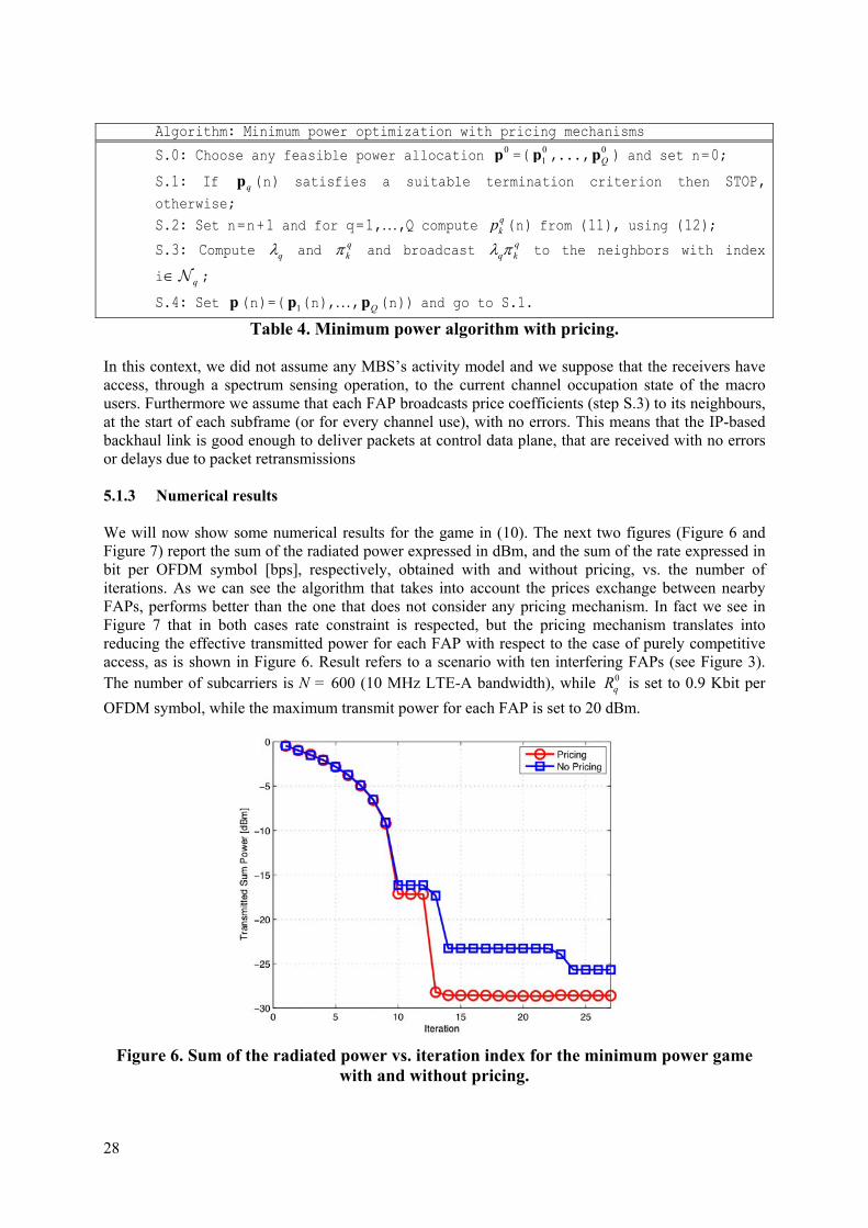
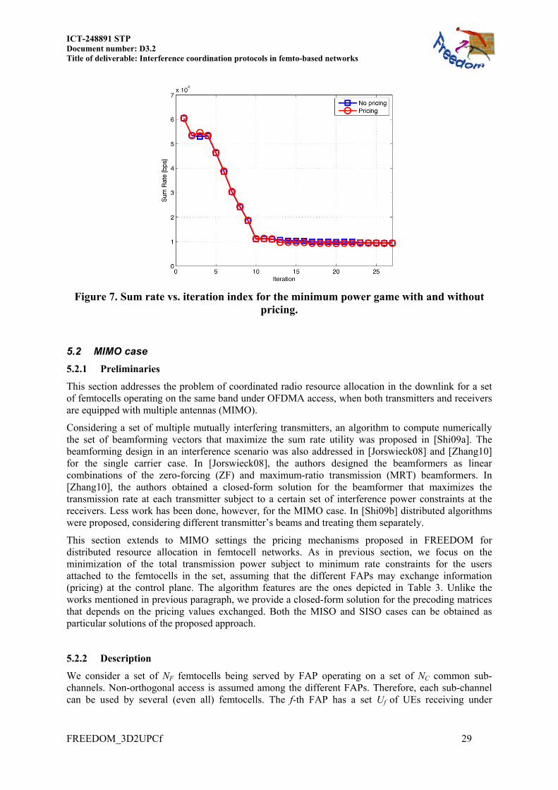
Table 4. Minimum power algorithm with pricing. In this context, we did not assume any MBS’s activity model and we suppose that the receivers have access, through a spectrum sensing operation, to the current channel occupation state of the macro users. Furthermore we assume that each FAP broadcasts price coefficients (step S.3) to its neighbours, at the start of each subframe (or for every channel use), with no errors. This means that the IP-based backhaul link is good enough to deliver packets at control data plane, that are received with no errors or delays due to packet retransmissions 5.1.3 Numerical results We will now show some numerical results for the game in (10). The next two figures (Figure 6 and Figure 7) report the sum of the radiated power expressed in dBm, and the sum of the rate expressed in bit per OFDM symbol [bps], respectively, obtained with and without pricing, vs. the number of iterations. As we can see the algorithm that takes into account the prices exchange between nearby FAPs, performs better than the one that does not consider any pricing mechanism. In fact we see in Figure 7 that in both cases rate constraint is respected, but the pricing mechanism translates into reducing the effective transmitted power for each FAP with respect to the case of purely competitive access, as is shown in Figure 6. Result refers to a scenario with ten interfering FAPs (see Figure 3). The number of subcarriers is N = 600 (10 MHz LTE-A bandwidth), while 0
qR is set to 0.9 Kbit per
OFDM symbol, while the maximum transmit power for each FAP is set to 20 dBm.
Figure 6. Sum of the radiated power vs. iteration index for the minimum power game
with and without pricing.
ICT-248891 STP Document number: D3.2 Title of deliverable: Interference coordination protocols in femto-based networks
FREEDOM_3D2UPCf 29
Figure 7. Sum rate vs. iteration index for the minimum power game with and without
pricing.
5.2 MIMO case
5.2.1 Preliminaries
This section addresses the problem of coordinated radio resource allocation in the downlink for a set of femtocells operating on the same band under OFDMA access, when both transmitters and receivers are equipped with multiple antennas (MIMO).
Considering a set of multiple mutually interfering transmitters, an algorithm to compute numerically the set of beamforming vectors that maximize the sum rate utility was proposed in [Shi09a]. The beamforming design in an interference scenario was also addressed in [Jorswieck08] and [Zhang10] for the single carrier case. In [Jorswieck08], the authors designed the beamformers as linear combinations of the zero-forcing (ZF) and maximum-ratio transmission (MRT) beamformers. In [Zhang10], the authors obtained a closed-form solution for the beamformer that maximizes the transmission rate at each transmitter subject to a certain set of interference power constraints at the receivers. Less work has been done, however, for the MIMO case. In [Shi09b] distributed algorithms were proposed, considering different transmitter’s beams and treating them separately.
This section extends to MIMO settings the pricing mechanisms proposed in FREEDOM for distributed resource allocation in femtocell networks. As in previous section, we focus on the minimization of the total transmission power subject to minimum rate constraints for the users attached to the femtocells in the set, assuming that the different FAPs may exchange information (pricing) at the control plane. The algorithm features are the ones depicted in Table 3. Unlike the works mentioned in previous paragraph, we provide a closed-form solution for the precoding matrices that depends on the pricing values exchanged. Both the MISO and SISO cases can be obtained as particular solutions of the proposed approach.
5.2.2 Description
We consider a set of NF femtocells being served by FAP operating on a set of NC common sub-channels. Non-orthogonal access is assumed among the different FAPs. Therefore, each sub-channel can be used by several (even all) femtocells. The f-th FAP has a set Uf of UEs receiving under

30
OFDMA access in the downlink. We use Cu to represent the set of sub-channels allocated to the u-th user and u(f,c) to denote the user attached to the f-th FAP receiving signal at the c-th sub-channel.
We assume that the FAP and the UE are provided with M and N antennas respectively (to simplify the notation we assume M to be equal for all the FAPs and N to be equal for all the UEs, although the generalization is simple). The problem consists on designing the optimum transmit covariance matrix for the f-th FAP at the c-th sub-channel,
cfS under the goal of minimizing the total transmission power,
and provided that every user achieves a given target rate. To further simplify notation let us define the following noise and interference matrix at the c-th sub-channel for the user u(f,c):
' ' ''
NFc c c c Hf N ff f ff
f f
R I H S H (13)
where NI is the N×N identity matrix and 'cffH stands for the N×M MIMO channel matrix, including
the path-loss and the random channel amplitude. The superindex corresponds to the sub-channel, the first subindex denotes the FAP serving the receiving user u(f,c) and the second subindex corresponds to the FAP that is producing interference over the intended user. Therefore, '
cffH represents the channel
between the u(f,c) UE and the neighbour FAP f’. Without loss of generality, we consider that the channels are normalized by the noise power at each receiver.
Under the minimum power consumption criterion, the problem to solve is the following:
1 1
minCF
cf
NNcf
f c
trace
SS (14)
1
2s.t. log , for , 1,..., ,c c H c cM f ff f ff u f F
c Cu
R u U f N
I S H R H
(15)
0, for 1,..., and 1,..., .c
f C Fc N f N S
(16)
where 0 stands for positive semidefinite.
This is a non-convex problem and, therefore, it may have multiple local optima. We focus on finding a local optimum. Furthermore, for the sake of scalability, we also focus on finding a local optimum in a distributed way. To that end, we proceed as in [Huang06] and [Shi08]: we take into account that any local optimum must fulfil the Karush-Kuhn-Tucker (KKT) conditions [Boyd04] of the global problem and we separate the KKT conditions in subsets of equations, one for each femtocell. This way, we obtain a set of NF distributed problems.
The solution of each problem, however, depends on other femtocells variables, which results in a highly complex coupled problem for which a closed-form solution has not been found. In order to derive a solution to the previous problem, we consider that, at a given time, the allocation of resources of a single FAP is optimized while considering that powers and precoders for the rest of FAP are fixed. Using this approach, the precoding matrix for the f-th femtocell at the c-th sub-channel is given by the solution of the following convex problem [Munoz11b], that can be solved separately for each transmitter (either centralized or decentralized):
' ' '',1 '
minNC
c H c c cM f f f f f fu f c
f c f f
trace
S
I H Π H S
(17)
1
2s.t. log , for c c H c cM f ff f ff u f
c Cu
R u U
I S H R H
(18)

ICT-248891 STP Document number: D3.2 Title of deliverable: Interference coordination protocols in femto-based networks
FREEDOM_3D2UPCf 31
0, for 1,..., .cf i NS (19)
Notice that the objective function in (17) is different from the objective function in the original problem in eq. (14). Instead of minimizing the trace of the transmit covariance matrix, c
fS , the goal now is to minimize the trace of the product between the so called pricing matrix, defined as follows:
' ' '','
c c H c cf M f f f f fu f c
f f
B I H Π H
(20)
and the transmit covariance matrix, cfS .
The pricing matrix defined in eq. (20) is a full rank matrix with probability one. In the MISO case the rank of this matrix is one, and in the SISO case is a scalar value. The role of the pricing matrix is to reflect the compensation to pay for the interference generated to the users connected to other FAPs. It measures the degradation on other FAPs performance due to the interference generated by the f-th FAP. It is computed, for each sub-channel, from three factors:
The Lagrange multiplier, ',u f c , associated to rate constraint of the user allocated by the neighbor FAP 'f at the c-th sub-channel. It is greater as the rate constraint is tighter, meaning that a small change in the constraint will affect greatly to the optimal value of the cost function.
The cross channel ' .c
f fH
The sensitivity to the noise and interference, in the c-th sub-channel, for the user allocated by the neighbor FAP 'f at this sub-channel. In the general MIMO case, this sensitivity is given by matrix
'cfΠ computed as
11 1 1 1
2 2log log ,
T
c c c c H c c c c c cf N ff f ff f f N f f f fc
f
e
Π I H S H R R I X R X R
R
(21)
which for the SISO and MISO cases boils down to a scalar value, '
cf , which ranges between
0 and 1.
The global procedure for computing the pricing matrix at each transmitter is as follows:
Step 1. Each UE detects the global identifier (GI) and channel state information (CSI) of surrounding FAPs and sends reports to the FAP that this UE is connected to. The UE also reports his interference sensitivity.
Step 2. The FAP that the UE is connected to, signals a DL-pricing message to potentially interfering FAPs. This message consists of the GI of the sending FAP and the identifier of the potentially interfering FAP and a field/s indicating the price for each RB.
Step 3. The FAP receiving a DL pricing message or messages from neighbor FAPs computes a global price per sub-channel according to eq. (20), and solves problem (17)-(19). Intuitively, for the SISO case, if the global price is high, the FAP will avoid allocating large power in this sub-channel. In the MISO (and MIMO) case, the FAP will avoid the sub-channels and directions with a greater price.
Based on the pricing information sent by the neighbors FAPs, and its own users measurements (channel and noise plus interference correlation matrix), each transmitter computes and equivalent channel per sub-channel that depends on the pricing matrix, c
fB , the user channel, cffH , and the
measured noise and interference, cfR . By the eigenvalue decomposition theorem, this equivalent
channel can be decomposed as follows:

32
1/2 1 1/2,c c H c c c c c c H
f ff f ff f f f f
B H R H B U Λ U
(22)
where cfU is a unitary matrix, containing the eigenvectors of the equivalent channel, and c
fΛ is a diagonal matrix containing the corresponding eigenvalues, ,c m
f , for 1, ,m M . The optimal transmission strategy, when fixing the interference sensitivity matrices and the precoders for the rest of the transmitters, is given by the following transmit covariance matrix [Munoz11b]:
1/2 1/2,c c c c c H c
f f f f f f
S B U S U B (23)
where cfS is a diagonal matrix, whose entries depend on the eigenvalues of the equivalent channel,
,c mf , and the Lagrange multiplier, ,u f c , which is adjusted to satisfy the user rate constraint defined
in (18):
,
, ,
1.c m
f u f c c mf
s
(24)
By setting the pricing matrix equal to the identity matrix, the solution obtained boils down to the waterfilling solution [Pang08]. Intuitively, if the users connected to other FAPs are far away or the interference is not affecting them (low cross channel eigenvalues or low interference sensitivity), the pricing matrix in (20) tends to be the identity matrix, and the solution given by eq. (22)-(24) tends to be the waterfilling solution.
The solution given by eq. (22)-(24) can be particularized for the SISO and MISO case. In the MISO case, the interference observed by the UE allocated at the c-th sub-channel by the f-th FAP is a scalar value given by
' ''
,FN
c c c c Hf ff f ff
f f
I
h S h
(25)
with 'cffh the 1×M channel vector. The equivalent channel in (22) has only one eigenvalue different
from 0. Therefore, the optimal transmit covariance matrix is a rank one matrix which is given by
,c c c Hf f fS w w (26)
with
1
2 1/21/2
1.
c c Hcf fffc c
f fc c Hc c Hf fff ff
I
B hw
B hB h
(27)
Different from the work in [Jorswieck08], where the authors designed the beamformers as linear combinations of ZF and MRT beamformers, here the solution is obtained from MRT beamformer multiplied by a prewhitening matrix which steers nulls in the directions of the potentially interfered neighbors. The deep of the nulls, however, depend on the impact of the transmission on the neighbors’ performance, measured through the pricing matrix.
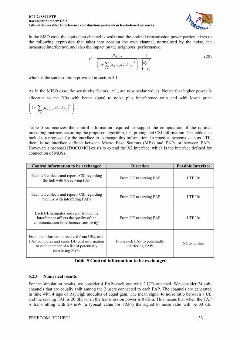
ICT-248891 STP Document number: D3.2 Title of deliverable: Interference coordination protocols in femto-based networks
FREEDOM_3D2UPCf 33
In the SISO case, the equivalent channel is scalar and the optimal transmission power particularizes to the following expression that takes into account the own channel, normalized by the noise, the measured interference, and also the impact on the neighbors’ performance.
,
22
' '','
1
11
u f ccf
cc c fff f fu f c
cf ff
phh
I
(28)
which is the same solution provided in section 5.1.
As in the MISO case, the sensitivity factors, 'cf , are now scalar values. Notice that higher power is
allocated to the RBs with better signal to noise plus interference ratio and with lower price
2
' '','
1 c cf f fu f c
f f
h
.
Table 5 summarizes the control information required to support the computation of the optimal precoding matrices according the proposed algorithm, i.e., pricing and CSI information. The table also includes a proposal for the interface to exchange this information. In practical systems such as LTE, there is no interface defined between Macro Base Stations (MBs) and FAPs or between FAPs. However, a proposal [DOCOMO] exists to extend the X2 interface, which is the interface defined for connection of MBSs.
Control information to be exchanged Direction Possible Interface
Each UE collects and reports CSI regarding
the link with the serving FAP
From UE to serving FAP LTE Uu
Each UE collects and reports CSI regarding
the link with interfering FAPs
From UE to serving FAP LTE Uu
Each UE estimates and reports how the interference affects the quality of the
communication (interference sensitivity)
From UE to serving FAP LTE Uu
From the information received from UEs, each FAP computes and sends DL-cost information
to each member of a list of potentially interfering FAPs
From each FAP to potentially interfering FAPs
X2 extension
Table 5 Control information to be exchanged
5.2.3 Numerical results
For the simulation results, we consider 4 FAPs each one with 2 UEs attached. We consider 24 sub-channels that are equally split among the 2 users connected to each FAP. The channels are generated in time with 4 taps of Rayleigh modulus of equal gain. The mean signal to noise ratio between a UE and the serving FAP is 20 dB, when the transmission power is 0 dBm. This means that when the FAP is transmitting with 20 mW (a typical value for FAPs) the signal to noise ratio will be 33 dB.
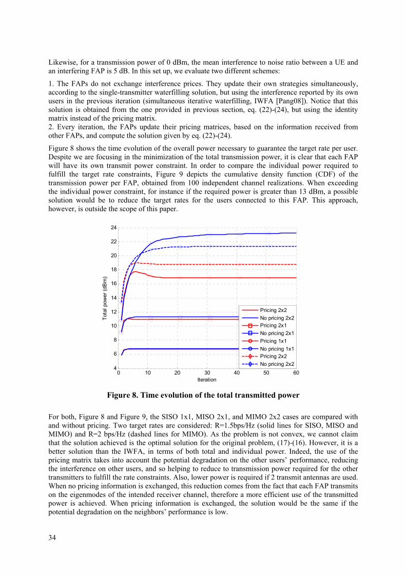
34
Likewise, for a transmission power of 0 dBm, the mean interference to noise ratio between a UE and an interfering FAP is 5 dB. In this set up, we evaluate two different schemes:
1. The FAPs do not exchange interference prices. They update their own strategies simultaneously, according to the single-transmitter waterfilling solution, but using the interference reported by its own users in the previous iteration (simultaneous iterative waterfilling, IWFA [Pang08]). Notice that this solution is obtained from the one provided in previous section, eq. (22)-(24), but using the identity matrix instead of the pricing matrix. 2. Every iteration, the FAPs update their pricing matrices, based on the information received from other FAPs, and compute the solution given by eq. (22)-(24).
Figure 8 shows the time evolution of the overall power necessary to guarantee the target rate per user. Despite we are focusing in the minimization of the total transmission power, it is clear that each FAP will have its own transmit power constraint. In order to compare the individual power required to fulfill the target rate constraints, Figure 9 depicts the cumulative density function (CDF) of the transmission power per FAP, obtained from 100 independent channel realizations. When exceeding the individual power constraint, for instance if the required power is greater than 13 dBm, a possible solution would be to reduce the target rates for the users connected to this FAP. This approach, however, is outside the scope of this paper.
0 10 20 30 40 50 604
6
8
10
12
14
16
18
20
22
24
Iteration
Tot
al p
ower
(dB
m)
Pricing 2x2
No pricing 2x2Pricing 2x1
No pricing 2x1
Pricing 1x1
No pricing 1x1Pricing 2x2
No pricing 2x2
Figure 8. Time evolution of the total transmitted power
For both, Figure 8 and Figure 9, the SISO 1x1, MISO 2x1, and MIMO 2x2 cases are compared with and without pricing. Two target rates are considered: R=1.5bps/Hz (solid lines for SISO, MISO and MIMO) and R=2 bps/Hz (dashed lines for MIMO). As the problem is not convex, we cannot claim that the solution achieved is the optimal solution for the original problem, (17)-(16). However, it is a better solution than the IWFA, in terms of both total and individual power. Indeed, the use of the pricing matrix takes into account the potential degradation on the other users’ performance, reducing the interference on other users, and so helping to reduce to transmission power required for the other transmitters to fulfill the rate constraints. Also, lower power is required if 2 transmit antennas are used. When no pricing information is exchanged, this reduction comes from the fact that each FAP transmits on the eigenmodes of the intended receiver channel, therefore a more efficient use of the transmitted power is achieved. When pricing information is exchanged, the solution would be the same if the potential degradation on the neighbors’ performance is low.

ICT-248891 STP Document number: D3.2 Title of deliverable: Interference coordination protocols in femto-based networks
FREEDOM_3D2UPCf 35
On the contrary, if the potential degradation is high, the precoders will minimize the transmission power in the direction of those neighbors which have strongest constraints. Nevertheless, the improvement due to the exchange of pricing information is greater in the SISO case, as in this situation the spatial dimension cannot be used to minimize the interference. For the MIMO case, when the target rate is 1.5 bps/Hz, the advantage using pricing seems to be marginal. However, if the user requirements increases (target rate equal to 2 bps/Hz, dashed lines) the transmitter needs to increase the power. In such a case, it is clear that the exchange of pricing information helps to reduce the degradation on other users, and consequently the required individual power of other transmitters, resulting in a global reduction of the overall transmitted power within the set of FAPs.
0 2 4 6 8 10 12 14 16 18 200
0.1
0.2
0.3
0.4
0.5
0.6
0.7
0.8
0.9
1
Femtocell Power (dBm)
Per
cent
age
Pricing 2x2
No pricing 2x2Pricing 2x1
No pricing 2x1
Pricing 1x1
No pricing 1x1Pricing 2x2
No pricing 2x2
Figure 9. CDF of the transmission power per transmitter.
5.3 Conclusions
In section 5 we have proposed alternative game-theoretic techniques that exploit the backhaul link among femto-access points to set up local coordination games which provide performance improvement with respect to purely competitive games. More specifically, we have proposed the minimum power game with pricing by showing the advantage of using pricing mechanism to reduce the radiated power still maintaining the same service quality (desired information rate). For MIMO systems, a closed-form solution for the transmit covariance matrix has been obtained, assuming that the different transmitters may exchange information at the control plane. MISO and SISO cases can be obtained as particular cases of the general MIMO solution. When the impact of the interference caused to the users connected to other FAPs is low, the performance for the proposed strategy approaches the performance of the waterfilling solution for the minimum power problem [Pang08]. However, the reduction in power increases when the requirements of the transmitters in terms of user target rates increases.
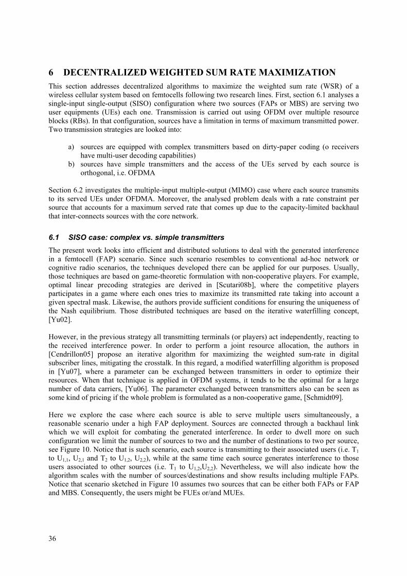
36
6 DECENTRALIZED WEIGHTED SUM RATE MAXIMIZATION This section addresses decentralized algorithms to maximize the weighted sum rate (WSR) of a wireless cellular system based on femtocells following two research lines. First, section 6.1 analyses a single-input single-output (SISO) configuration where two sources (FAPs or MBS) are serving two user equipments (UEs) each one. Transmission is carried out using OFDM over multiple resource blocks (RBs). In that configuration, sources have a limitation in terms of maximum transmitted power. Two transmission strategies are looked into:
a) sources are equipped with complex transmitters based on dirty-paper coding (o receivers have multi-user decoding capabilities)
b) sources have simple transmitters and the access of the UEs served by each source is orthogonal, i.e. OFDMA
Section 6.2 investigates the multiple-input multiple-output (MIMO) case where each source transmits to its served UEs under OFDMA. Moreover, the analysed problem deals with a rate constraint per source that accounts for a maximum served rate that comes up due to the capacity-limited backhaul that inter-connects sources with the core network.
6.1 SISO case: complex vs. simple transmitters
The present work looks into efficient and distributed solutions to deal with the generated interference in a femtocell (FAP) scenario. Since such scenario resembles to conventional ad-hoc network or cognitive radio scenarios, the techniques developed there can be applied for our purposes. Usually, those techniques are based on game-theoretic formulation with non-cooperative players. For example, optimal linear precoding strategies are derived in [Scutari08b], where the competitive players participates in a game where each ones tries to maximize its transmitted rate taking into account a given spectral mask. Likewise, the authors provide sufficient conditions for ensuring the uniqueness of the Nash equilibrium. Those distributed techniques are based on the iterative waterfilling concept, [Yu02]. However, in the previous strategy all transmitting terminals (or players) act independently, reacting to the received interference power. In order to perform a joint resource allocation, the authors in [Cendrillon05] propose an iterative algorithm for maximizing the weighted sum-rate in digital subscriber lines, mitigating the crosstalk. In this regard, a modified waterfilling algorithm is proposed in [Yu07], where a parameter can be exchanged between transmitters in order to optimize their resources. When that technique is applied in OFDM systems, it tends to be the optimal for a large number of data carriers, [Yu06]. The parameter exchanged between transmitters also can be seen as some kind of pricing if the whole problem is formulated as a non-cooperative game, [Schmidt09]. Here we explore the case where each source is able to serve multiple users simultaneously, a reasonable scenario under a high FAP deployment. Sources are connected through a backhaul link which we will exploit for combating the generated interference. In order to dwell more on such configuration we limit the number of sources to two and the number of destinations to two per source, see Figure 10. Notice that is such scenario, each source is transmitting to their associated users (i.e. T1 to U1,1, U2,1 and T2 to U1,2, U2,2), while at the same time each source generates interference to those users associated to other sources (i.e. T1 to U1,2,U2,2). Nevertheless, we will also indicate how the algorithm scales with the number of sources/destinations and show results including multiple FAPs. Notice that scenario sketched in Figure 10 assumes two sources that can be either both FAPs or FAP and MBS. Consequently, the users might be FUEs or/and MUEs.
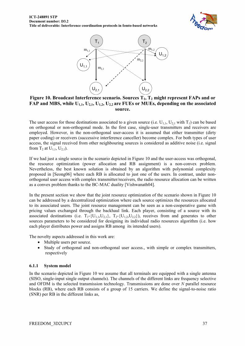
ICT-248891 STP Document number: D3.2 Title of deliverable: Interference coordination protocols in femto-based networks
FREEDOM_3D2UPCf 37
T1 T2
U2,1 U2,2
m2,2
m1,1
U1,1
U1,2
m2,1
m1,2
Figure 10. Broadcast Interference scenario. Sources T1, T2 might represent FAPs and or FAP and MBS, while U1,1, U2,1, U1,2, U2,2 are FUEs or MUEs, depending on the associated
source.
The user access for those destinations associated to a given source (i.e. U1,1, U2,1 with T1) can be based on orthogonal or non-orthogonal mode. In the first case, single-user transmitters and receivers are employed. However, in the non-orthogonal user-access it is assumed that either transmitter (dirty paper coding) or receivers (successive interference canceller) become complex. For both types of user access, the signal received from other neighbouring sources is considered as additive noise (i.e. signal from T2 at U1,1, U2,1). If we had just a single source in the scenario depicted in Figure 10 and the user-access was orthogonal, the resource optimization (power allocation and RB assignment) is a non-convex problem. Nevertheless, the best known solution is obtained by an algorithm with polynomial complexity proposed in [Seong06] where each RB is allocated to just one of the users. In contrast, under non-orthogonal user access with complex transmitter/receivers, the radio resource allocation can be written as a convex problem thanks to the BC-MAC duality [Vishwanath04]. In the present section we show that the joint resource optimization of the scenario shown in Figure 10 can be addressed by a decentralized optimization where each source optimizes the resources allocated to its associated users. The joint resource management can be seen as a non-cooperative game with pricing values exchanged through the backhaul link. Each player, consisting of a source with its associated destinations (i.e. T1-U1,1,U2,1, T2-U1,2,U2,2), receives from and generates to other sources parameters to be considered for designing its individual radio resources algorithm (i.e. how each player distributes power and assigns RB among its intended users). The novelty aspects addressed in this work are:
Multiple users per source. Study of orthogonal and non-orthogonal user access., with simple or complex transmitters,
respectively
6.1.1 System model
In the scenario depicted in Figure 10 we assume that all terminals are equipped with a single antenna (SISO, single-input single output channels). The channels of the different links are frequency selective and OFDM is the selected transmission technology. Transmissions are done over N parallel resource blocks (RB), where each RB consists of a group of 15 carriers. We define the signal-to-noise ratio (SNR) per RB in the different links as,

38
2
, ,0
2
, , , ,0
link to from the j-th source to its i-th user
interfering link from the t-th source to the i-th user of the j-th source
l li j i j
l li j t i j t
Ph
N
Ph
N
(29)
where l defines the selected RB, i,j indicates that SNR is that of the link from the j-th source to its i-th destination,
,l
i jh is the channel coefficient of the link at the l-th RB, P denotes the maximum transmitted power and N0 stands for the AWGN (Additive White Gaussian Noise) power. The interfering links are denoted with sub-indexes i,j,t , describing the link from the t-th source to the i-th destination attached to the j-th source. In such a case the channel coefficient is represented by
, ,l
i j th . It should be remarked that the instantaneous SNR per RB is dependent on the fraction of allocated power. Hence, equation (29) denotes the maximum SNR for a given RB in case all power was allocated to that RB. All sources share the same bandwidth, that is, all destinations are interfered by the active sources in their neighbourhood. Likewise, since each source is serving multiple users, the destinations might observe an additional kind of interference coming from its associated source, due to the messages intended to the other destinations and served by the same source. Notice that such interference depends on the employed user access mode. For example, under the orthogonal user access only one user is active per RB and that interference does not come up. We define the set of RB allocated to the different destinations under orthogonal user access as,
, ,| active orthogonal user accessu k u kS i U (30)
The bitrate attained by the u,k-th user (u-th user attached to the k-th source) will be denoted by,
, ,
2
, , ,
, 2 , 2
,0 ,
1 1log 1 log 1
11u k u k
i i iu k u k u ki
u k u k iii S i S u ku k
h PR
N N IN I
where ,i
u k denotes the fraction of power allocated to u,k-th user at the ith RB and ,i
u kI stands for the received interference normalized by the noise power. The generated interference at the UE can be defined by,
1,2 1,2 1,2 1,2
1,1 1,2 2,2 1,1,2 2.1 1,2 2,2 2,1,2
2,2 2,2 2,2 2,2
1,1 1,1
1,2 1,1 2,1 1,2,1 2,2 1,1 2,1 2,2
2,1 2,1
0 0,
0 0
0,
0
i i
i i i i i i i i
i i
i
i i i i i i i
i
if i S if i SI I
if i S if i S
if i SI I
if i S
1,1 1,1
,1
2,1 2,1
0
0
i
i
i
if i S
if i S
(31)
On the other hand, when there is a non-orthogonal user access we assume that sources operate under superposition coding as a transmission strategy to its associated users (i.e. T1-U1,1,U2,1 in Figure 10). Since there is a SISO channel configuration, the channel is degraded and the associated destinations can be classified as strong or weak over different RB. The strong user is able to decode its message and the one intended to the other destination. Consequently, receivers must have successive interference canceller (SIC) capability. Notice that we are assuming that independent messages are transmitted over each RB by the same transmitter. In contrast, the weak user only is able to decode its intended message assuming the other message as additive noise. Such classification of the users per RB is summarized by the following ensembles,
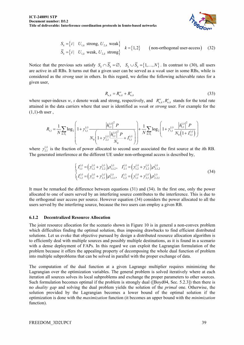
ICT-248891 STP Document number: D3.2 Title of deliverable: Interference coordination protocols in femto-based networks
FREEDOM_3D2UPCf 39
1, 2,
1, 2,
| strong, weak1,2 non-orthogonal user-access
| weak, strong
k k k
k k k
S i U Uk
S i U U
(32)
Notice that the previous sets satisfy , 1, ,k k k kS S S S N . In contrast to (30), all users are active in all RBs. It turns out that a given user can be served as a weak user in some RBs, while is considered as the strong user in others. In this regard, we define the following achievable rates for a given user,
, , ,w s
u k u k u kR R R (33)
where super-indexes w, s denote weak and strong, respectively, and , ,,w su k u kR R stands for the total rate
attained in the data carriers where that user is identified as weak or strong user. For example for the (1,1)-th user ,
1 1
2 2
1,1 1,1
1,1 2 1,1 2 1,120 1,11,1
0 2,1 1,10
1 1log 1 log 1
11
i i
i i
iii S i Si i
h P h PR
N N N Ih PN I
N
where 2,1i is the fraction of power allocated to second user associated the first source at the ith RB.
The generated interference at the different UE under non-orthogonal access is described by,
1,1 1,2 2,2 1,1,2 2.1 1,2 2,2 2,1,2
1,2 1,1 2,1 1,2,1 2,2 1,1 2,1 2,2,1
,
,
i i i i i i i i
i i i i i i i i
I I
I I
(34)
It must be remarked the difference between equations (31) and (34). In the first one, only the power allocated to one of users served by an interfering source contributes to the interference. This is due to the orthogonal user access per source. However equation (34) considers the power allocated to all the users served by the interfering source, because the two users can employ a given RB.
6.1.2 Decentralized Resource Allocation
The joint resource allocation for the scenario shown in Figure 10 is in general a non-convex problem which difficulties finding the optimal solution, thus imposing drawbacks to find efficient distributed solutions. Let us evoke that objective pursued by design a distributed resource allocation algorithm is to efficiently deal with multiple sources and possibly multiple destinations, as it is found in a scenario with a dense deployment of FAPs. In this regard we can exploit the Lagrangian formulation of the problem because it offers the appealing property of decomposing the whole dual function of problem into multiple subproblems that can be solved in parallel with the proper exchange of data. The computation of the dual function at a given Lagrange multiplier requires minimizing the Lagrangian over the optimization variables. The general problem is solved iteratively where at each iteration all sources solves its local subproblems and exchange the proper parameters to other sources. Such formulation becomes optimal if the problem is strongly dual ([Boyd04, Sec. 5.2.3]) then there is no duality gap and solving the dual problem yields the solution of the primal one. Otherwise, the solution provided by the Lagrangian becomes a lower bound of the optimal solution if the optimization is done with the maximization function (it becomes an upper bound with the minimization function).

40
We will be able to provide a decentralized solution to our resource allocation problem under the assumption that the received interference at each iteration by the users is constant and do not depend on the transmitted power of the other sources. The obtained distributed RRM could be seen as a non-cooperative game where each player (sources with its associated destinations) maximizes its own payoff function which takes into account pricing values. The pricing value has information about the changes of the generated interference by a given source over the non-associated destinations of its neighbourhood, [Schmidt09]. In the ensuing sections, A and B, we present how the joint resource allocation problem for the scenario introduced in Figure 10 is tackled in a decentralized way when the user-access is orthogonal with simple transmitters or non-orthogonal with complex transmitters. A. Orthogonal user-access with simple transmitters
The joint radio resource allocation is obtained as the solution of the following optimization problem,
, , ,
2 2Orth
0 , ,, , 1 11,2 , 1,2
, ,, , , 2
,
2
,1 1
,
minimize
1: log 1 0, 1,2 , 1,2
1
: 1 0,
0
u k u k u k
k
u k u kR S u k
k u
i iu k u k
u k u k u k ii S u k
Ni
k k u ki u
u k
P R
f R k uN I
h
R
γ
(35)
where Ru,k, denotes the rate allocated to the messages intended to u,k-th destination, ,u kγ stands for the vector of allocated powers, ,u kS defines the set of carriers assigned to that user, (30). Lagrange multiplier u,k, is tied to the rate constraint (function fu,k,), while Lagrange multiplier k is associated to the power constraint per source (function hk). The observed interference by each user is defined in (31).
The Lagrange function of problem Orth0P in (35) is given by,
, 1 2 , , ,
2 2 2 2
, , , , 1 1 2 2, , , , ,1 1 1 1
u k u k u k u ku k u k u k u kR S
u k u k
L R f h h
γ (36)
Any local optimum with respect the power allocation variable ij should satisfy
, 1 2 , , ,
2 2
, , , ,, , , , ,1, 1, , ,
0u k u k u k u k
u k u k p t p t ki i iR St t k pu k u k u k
L f f
γ (37)
with

ICT-248891 STP Document number: D3.2 Title of deliverable: Interference coordination protocols in femto-based networks
FREEDOM_3D2UPCf 41
2
,
0, 2
, ,
, ,0
2
, ,
, ,0, , , 2
,, , , , ,
,0
1
11
iu k
u ki iu k u ki i
u k u k
i ip t p t
ii u k t
p t p t p ti i i ii ip tu k p t u k p t p ti
p t
h P
Nf
h PI
N
h P
Nf f I
II h PI
N
(38)
We define
2
,
,0
, 2,,
, ,0
, , , , , ,
1
11
ip ti
p ti
p t iip tp ti i
p t p t
i i ip t k p t p t p t k
h P
N
Ih PI
N
(39)
Assuming that
, ,ip t k are fixed and a given power profiles [Shi08] the KKT conditions of problem
Orth0P are the same as those if each transmitter carries out the following optimization problem
, , ,
2 2 2Orth
, , , , ,, , 1 1 1, 11,2
, ,, , , 2
,
2
,1 1
,
minimize
1: log 1 0, 1,2
1
: 1 0,
0
u k u k u k
k
Ni i
k u k u k p t k u kR S u i t t k p
u
i iu k u k
u k u k u k ii S u k
Ni
k k u ki u
u k
P R
f R uN I
h
R
γ
(40)
Therefore, Orth0P is solved in a decentralized way by applying the iterative procedure described in
Table 6.
, , , ,Orth
, ,
0. Initialize , 0, =0 , , 1,2
1. Every source solves problem P using eq.(40), 1, 2
2. The -th source generates using eq.(39), 1, 2 , , 1, 23. Pr
iip k p k p t k
kip t k
R I p k t
k
t p k t
Ω
Ω
,
ice exchange through the backhaul link
4. Update transmit precoders with the solution of step 1
5. The -th source collects all prices generated by neigboring sources 1,2
6. Every source
ip k
k k
,collects the noise plus interference,
7. Go to 1
ip kI
Table 6. Decentralized algorithm to solve problem Orth0P (35).

42
Although we have reduced the complexity of problem Orth0P thanks to the decentralized solution, the
problem to be solved at each transmitter OrthkP is still non-convex due to the RB assignment. In this
regard, we will consider the algorithm proposed in [Seong06] that provides the best known solution with a polynomial complexity.
Let us introduce the Lagrangian of problem OrthkP as
, , , ,
2 2
, , , , ,, , ,1 1 1
u k k u k u k u k
Ni i
u k u k k u k u k u k k kR Su i u
G R w f h
γ
(41)
where ,i
u kw collects all the parameters generated by the neighboring sources and intended to the k-th
source,
2 2
, ,1, 1
i ik p t k
t t k p
w
(42)
One of the conditions to by satisfied with respect the variable Ru,k is,
, , , ,, , , ,, , ,
,
0u k k u k u k u k
u k u k u k u kR Su k
GR
γ (43)
Hence, the Lagrangian given in (41) turns out into,
, ,
,
2 2, , ,
, , 2 ,, ,1 1 1 1,
log 11k u k u k
u k
i iN Ni i iu k u k u k
p t u k k u k kiSi u i S i uu k
G wN I
γ
(44)
Moreover, an additional condition to be satisfied by the power allocation is given by,
, ,
,
, ,
, ,, ,,
,
10
ln 21
1
k u k u k
iu k
ii u k u k
t ki i iSu k u ku k
iu k
IG w
N
I
γ (45)
Where we can get a semiclosed-form expression for the power allocation,
, ,
,
,
11
ln 2
ii u k u k
u k i iu kk k
I
N w
(46)
Since each RB only is assigned to one user, we follow the same approach used in [Seong06] and we perform such allocation in order to minimize the Lagrangian
,
,
2 2 2, , ,
, 2 ,,1 1 1 1 1,
1
log 11k u k
u k
i iN Ni i iu k u k k u k
t u k k k u k k kiSu i u i S i uu k
N
k kii
G wN I
G
(47)
It turns out that the minimization is obtained by searching over all the served users by a given source at each carrier, and select that one that mimimizes kiG ,
2, , ,
, 2 ,
1 ,
log 11
i ii i iu k u k k u k
k t u k k k u k ki iu u k
G wN I
(48)
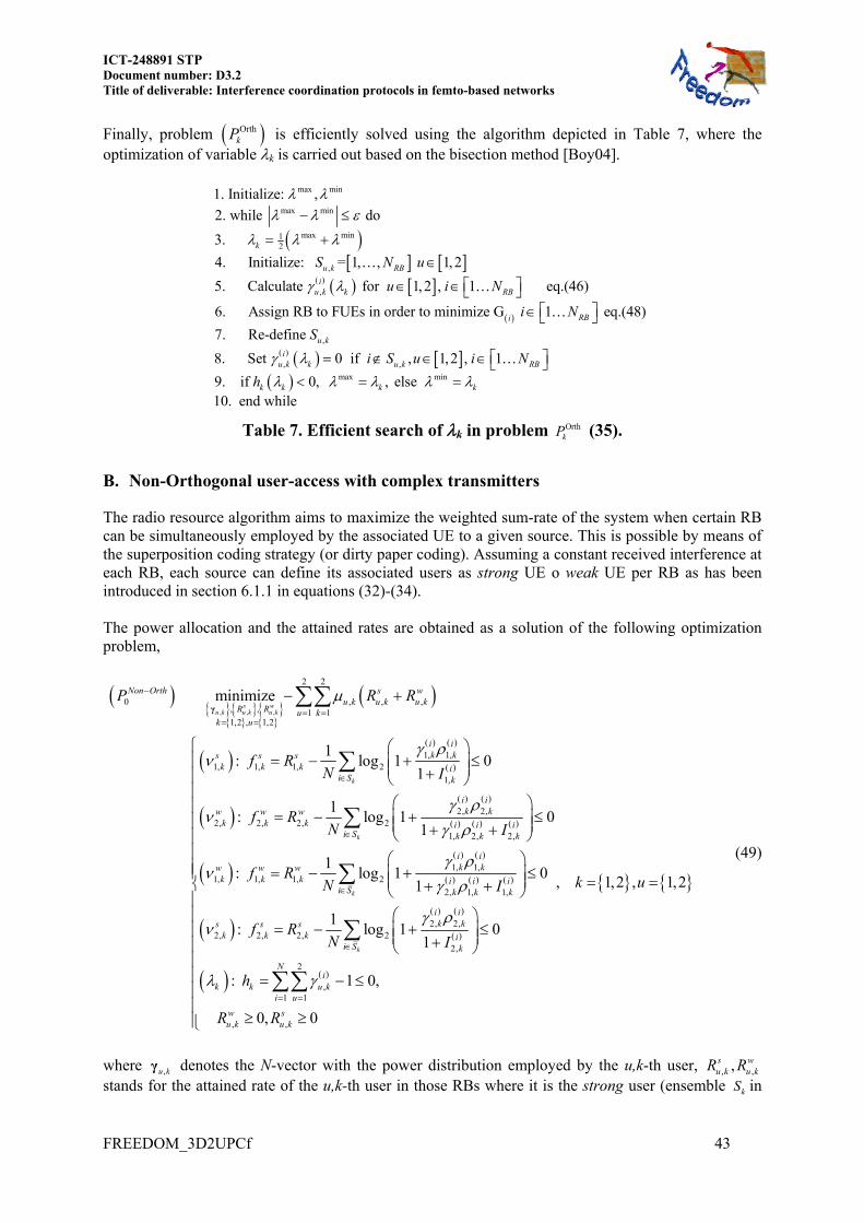
ICT-248891 STP Document number: D3.2 Title of deliverable: Interference coordination protocols in femto-based networks
FREEDOM_3D2UPCf 43
Finally, problem OrthkP is efficiently solved using the algorithm depicted in Table 7, where the
optimization of variable k is carried out based on the bisection method [Boy04].
max min
max min
max min12
,
,
1. Initialize: ,
2. while do
3.
4. Initialize: = 1, , 1, 2
5. Calculate for 1, 2 , 1 eq.(46)
6. Assign RB to FUE
k
u k RB
iu k k RB
S N u
u i N
,
, ,
max min
s in order to minimize G 1 eq.(48)
7. Re-define
8. Set 0 if , 1,2 , 1
9. if 0, , else 10. end while
RBi
u k
iu k k u k RB
k k k k
i N
S
i S u i N
h
Table 7. Efficient search of k in problem OrthkP (35).
B. Non-Orthogonal user-access with complex transmitters
The radio resource algorithm aims to maximize the weighted sum-rate of the system when certain RB can be simultaneously employed by the associated UE to a given source. This is possible by means of the superposition coding strategy (or dirty paper coding). Assuming a constant received interference at each RB, each source can define its associated users as strong UE o weak UE per RB as has been introduced in section 6.1.1 in equations (32)-(34). The power allocation and the attained rates are obtained as a solution of the following optimization problem,
, , ,
2 2
0 , , ,, , 1 11,2 , 1,2
1, 1,1, 1, 1, 2
1,
2, 2,2, 2, 2, 2
1, 2, 2,
1
minimize
1: log 1 0
1
1: log 1 0
1
s wu k u k u k
k
k
Non Orth s wu k u k u k
R R u kk u
i ik ks s s
k k k ii S k
i ik kw w w
k k k i i ii S k k k
P R R
f RN I
f RN I
γ
1, 1,
, 1, 1, 2
2, 1, 1,
2, 2,2, 2, 2, 2
2,
2
,1 1
, ,
1: log 1 0
, 1,2 , 1,21
1: log 1 0
1
: 1 0,
0, 0
k
k
i ik kw w w
k k k i i ii S k k k
i ik ks s s
k k k ii S k
Ni
k k u ki u
w su k u k
f Rk uN I
f RN I
h
R R
(49)
where ,u kγ denotes the N-vector with the power distribution employed by the u,k-th user, , ,,s w
u k u kR R stands for the attained rate of the u,k-th user in those RBs where it is the strong user (ensemble kS in
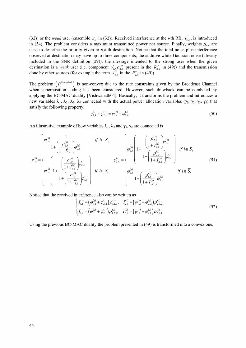
44
(32)) or the weak user (ensemble kS in (32)). Received interference at the i-th RB, ,i
u kI , is introduced in (34). The problem considers a maximum transmitted power per source. Finally, weights u,k are used to describe the priority given to u,k-th destination. Notice that the total noise plus interference observed at destination may have up to three components, the additive white Gaussian noise (already included in the SNR definition (29)), the message intended to the strong user when the given destination is a weak user (i.e. component
1, 2,i ik k present in the 2,
wkR in (49)) and the transmission
done by other sources (for example the term 2,ikI in the 2,
wkR in (49))
The problem 0
Non OrthP is non-convex due to the rate constraints given by the Broadcast Channel when superposition coding has been considered. However, such drawback can be combated by applying the BC-MAC duality [Vishwanath04]. Basically, it transforms the problem and introduces a new variables 1, 2, 3, 4 connected with the actual power allocation variables (1, 2, 3, 4) that satisfy the following property,
1, 2, 1, 2,
i i i ik k k k (50)
An illustrative example of how variables 1, 2 and 1, 2 are connected is
2,1,1,
2,2,
2,2,
2,2,
2,1, 2,1, 2,
2,
1,
1,
1,1,
1,
1
11 111
1
11
11
iik ik ki ki
k i kikik ik
ki ii ik kk ki
kiki
k kik i
kik
if i SI
I
I
Iif i S
I
2,
1,1,
1,
1
11
k
ik
ik ki
k iki
k
if i S
if i S
I
(51)
Notice that the received interference also can be written as
1,1 1,2 2,2 1,1,2 2.1 1,2 2,2 2,1,2
1,2 1,1 2,1 1,2,1 2,2 1,1 2,1 2,2,1
,
,
i i i i i i i i
i i i i i i i i
I I
I I
(52)
Using the previous BC-MAC duality the problem presented in (49) is transformed into a convex one,

ICT-248891 STP Document number: D3.2 Title of deliverable: Interference coordination protocols in femto-based networks
FREEDOM_3D2UPCf 45
, , ,
2 2
0 , , ,, , 1 11,2 , 1,2
1, 1, 2, 2,1, 1, 1, 2, 2
1, 2,
2, 2,2, 2, 2, 2
2,
minimize
1: log 1 0
1 1
1: log 1
1
s wu k u k u k
k
Non Orth s wu k u k u k
R R u kk u
i i i ik k k ks s s w
k k k k i ii S k k
i ik kw w w
k k k ik
P R R
f R RN I I
f RN I
1, 1,1, 1, 1, 2
1,
1, 1, 2, 2,2, 2, 1, 2, 2
1, 2,
2
,1 1
, ,
0
1: log 1 0
1
1: log 1 0
1 1
: 1 0,
0,
k
k
k
i S
i ik kw w w
k k k ii S k
i i i ik k k ks s w s
k k k k i ii S k k
Ni
k k u ki u
w su k u k
f RN I
f R RN I I
h
R R
, 1,2 , 1,2
0
k u
(53)
The Lagrangian is given by,
, 1 2 , , ,
2 2 2 2 2 2 2
, , , , , , ,, , , , ,1 1 1 1 1 1 1
s wu k u k u k u k
s w s s s wu k u k u k u k u k u k u k k kR R
u k u k u k k
L R R f f h
(54)
Any local optimum with respect the power allocation ,i
u k should satisfy the following equation
, 1 2 , , ,, , , , ,,
2 2 2
, , , , , , , ,
1 1, 1, , , ,
0
s wu k u k u k u k
i R Ru k
s s w w s s w wz k z k u k u k p t p t p t p t ki i i i
z t t k pu k u k u k u k
L
f f f f
(55)
where derivatives of the functions associated to other sources different the k-th one are addressed as,
, , 1, , 2,
, 1, , 2, ,
, 1,
1, ,
,
,, 2,
2, ,
1
2
i is s sp t p t t p t ti i i i i
u k t u k t u k
iwp t ti i
k u kwp ti
iwu kp t ti i
k u k
f f I f II I
f I if pI
f
f I if pI
Following similar steps as in (39) we define,

46
1, 1, 2, 2,1, , 2, ,2 2
1, 2,
1, , 2, ,1, 1, 2, 2,
1, 2,
1 1 1, ln
ln 2 11 1
0 otherwise
i i i it t t ti i
t k t ki it t
ts i w ii i i it k t kt t t t
i it t
I Iif i S
NN
I I
2, 2,2, ,2
2,
2, 2,
2,
1, 1,1, ,2
1,
1, , 1, 1,
1,
1
21
1
0 otherwise
11
ln 21
1
0
i it t i
t kit
ti it t
it
i it t i
t kit
tw i i it k t t
it
Iif i S
I
Iif i S
N
I
1, 1, 2, 2,1, , 2, ,2 2
2, , 1, 2,
1, 1, 2, 2,
1, 2,
0 otherwise
, 1 1
ln 2 11 1 otherwise
i i i it t t ti i
t k t ks i i it k t t
i i i it t t t
i it t
I Ii
NI I
tf i S
Likewise, the interference values received at the k-th source and generated at the t-th source are defined by,
1, 1, , 2, 2, ,
,
1, 1, , 2, 2, ,
,
,
, , 1,2
s i w is wt t k t t k ti
k tw i s iw s
t t k t t k t
i ik k t
t t k
if i Sk t k t
if i S
w
(56)
Finally, the problem Non-Orth
0P introduced in (49) is addressed in a decentralized and iterative way using the algorithm depicted in Table 8 where each source optimizes the resources allocation by minimizing the following problem at each step,
, , ,
2 2
, , , 1, 2,, , 1 1 1
, 1,2
1, 1, 2, 2,1, 1, 1, 2, 2
1, 2,
2, 2, 2,
minimize
1: log 1 0
1 1
1: l
s wu k u k u k
k
Ni i iNon Orth s w
k u k u k u k k k kR R u k i
u
i i i ik k k ks s s w
k k k k i ii S k k
w w wk k k
P R R w
f R RN I I
f RN
2, 2,2
2,
1, 1,1, 1, 1, 2
1,
1, 1, 2, 2,2, 2, 1, 2, 2
1, 2,
2
,1
og 1 01
1: log 1 0
1
1: log 1 0
1 1
:
k
k
k
i ik k
ii S k
i ik kw w w
k k k ii S k
i i i ik k k ks s w s
k k k k i ii S k k
ik k u k
u
I
f RN I
f R RN I I
h
1
, ,
, 1,2
1 0,
0, 0
N
i
w su k u k
u
R R
(57)

ICT-248891 STP Document number: D3.2 Title of deliverable: Interference coordination protocols in femto-based networks
FREEDOM_3D2UPCf 47
It has to be remarked that the previous solution is found assuming that the interference received at each step remains constant. Moreover, the actual power allocation is obtained by using equation (51) once we have obtained variables ,u k ,
, , ,Non-Orth
k,t
0. Initialize , , 0, =0 , , 1, 2
1. Every source solves problem P , 1, 2
2. The -th source generates using eq.(56), , 1, 23. Price exchange
is w ip k p k p k k
ki
R R I w p k t
k
t k t
, ,
through the backhaul link
4. Update transmit precoders using and eq. (51)
5. The -th source collects all prices generated by neigboring sources eq.(56)
6. Every source collects
i ip k p k
ikk w
, the noise plus interference, 7. Go to 1
ip kI
Table 8. Decentralized algorithm to solve problem Non-Orth0P (35).
6.1.3 Numerical results
We have considered the scenario depicted in Figure 10 with the following average SNR at the different channels,
11 3212 22 31 41
21 42
14 12, , Interf
12 10
dB dBdB
dB dB
where the interference received by each terminal becomes the same (variable Interf) and we will tune it in order to analyse the performance of the investigated techniques. The channel is frequency selective and presents a Rayleigh distributed with 6 symbol length and equal average power taps. All terminals are equipped with single antennas and the transmission is carried out along 16 orthogonal carriers or resource blocks (RB). We will study the sum-rate served by T2 (U1,2, U2,2), i.e. R1,2+R2,2, as a function of the sum-rate served by T1 (U1,1, U2,1), i.e. R1,1+R2,1, for four distributed resource allocation algorithms depending on the type of coordination and the user-access. They are based on a competitive user approach (Iterative Waterfilling, ITW) or in a coordinated approach (ITW + pricing). Likewise, we also take into account if we have an orthogonal user access with simple transmitters (Orth UA), see section A, or in contrast, there is a non-orthogonal user access with complex transmitters (Non-Orth UA), see section B. We have considered different values of the priorities assigned to the uses, but limited to be,
2,1 1,1 1,1
1,22,2 1,2
2 1, , 0,1
3
Figure 11 depicts the achievable rate region of the four transmissions schemes when the received interference at each terminal is equal to Interf=0, 5, 10, 15 dB, which accounts for a very low, low, medium and high interference scenarios. We can observe that in all cases, the ITW and ITW+pricing approaches tend to have a similar performance when priorities 1,1 1,2 1 2 , and when only one source is active. For other values of user’s priorities, the pricing method allows improving the achieved rates. Such gain increases as the generated interference is higher.
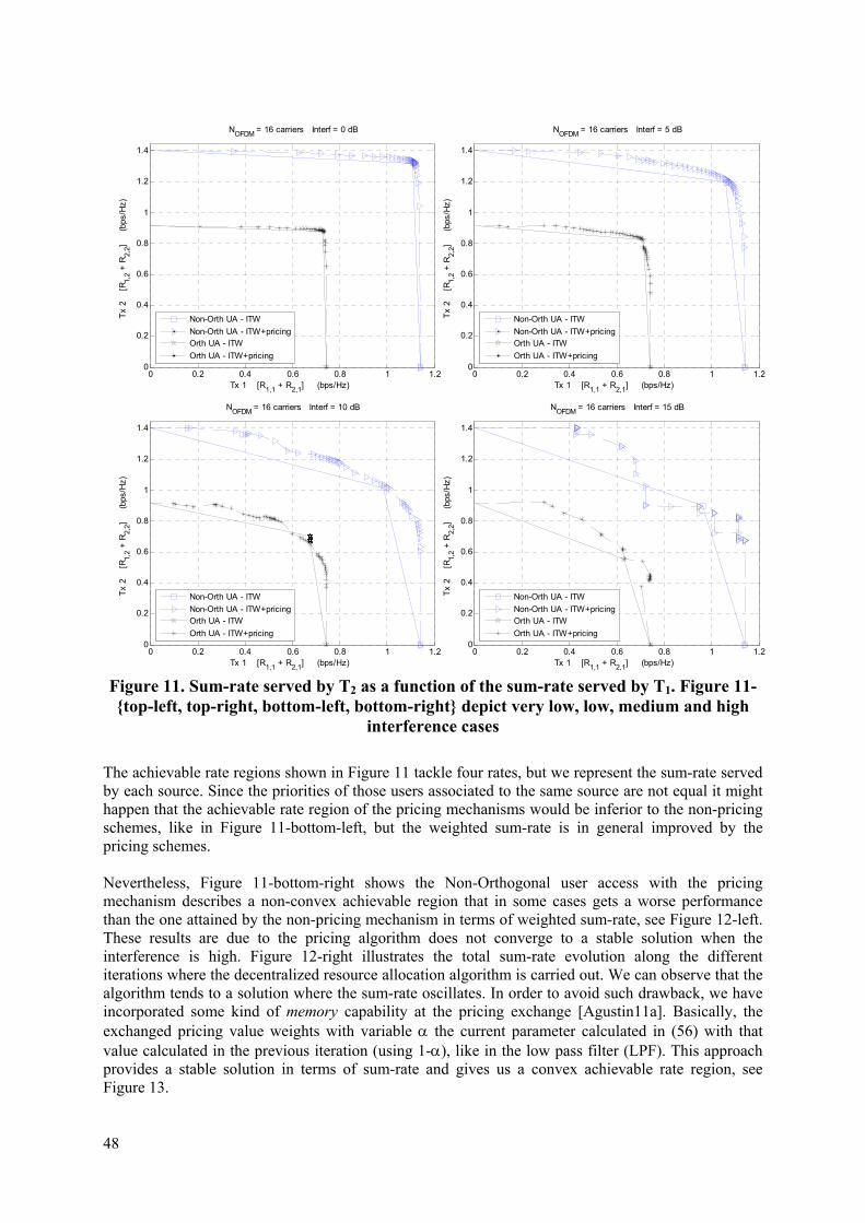
48
Figure 11. Sum-rate served by T2 as a function of the sum-rate served by T1. Figure 11-top-left, top-right, bottom-left, bottom-right depict very low, low, medium and high
interference cases
The achievable rate regions shown in Figure 11 tackle four rates, but we represent the sum-rate served by each source. Since the priorities of those users associated to the same source are not equal it might happen that the achievable rate region of the pricing mechanisms would be inferior to the non-pricing schemes, like in Figure 11-bottom-left, but the weighted sum-rate is in general improved by the pricing schemes. Nevertheless, Figure 11-bottom-right shows the Non-Orthogonal user access with the pricing mechanism describes a non-convex achievable region that in some cases gets a worse performance than the one attained by the non-pricing mechanism in terms of weighted sum-rate, see Figure 12-left. These results are due to the pricing algorithm does not converge to a stable solution when the interference is high. Figure 12-right illustrates the total sum-rate evolution along the different iterations where the decentralized resource allocation algorithm is carried out. We can observe that the algorithm tends to a solution where the sum-rate oscillates. In order to avoid such drawback, we have incorporated some kind of memory capability at the pricing exchange [Agustin11a]. Basically, the exchanged pricing value weights with variable the current parameter calculated in (56) with that value calculated in the previous iteration (using 1-), like in the low pass filter (LPF). This approach provides a stable solution in terms of sum-rate and gives us a convex achievable rate region, see Figure 13.
0 0.2 0.4 0.6 0.8 1 1.20
0.2
0.4
0.6
0.8
1
1.2
1.4
Tx 1 [R1,1 + R2,1] (bps/Hz)
Tx
2
[R
1,2 +
R2,
2]
(b
ps/H
z)
NOFDM = 16 carriers Interf = 0 dB
Non-Orth UA - ITW
Non-Orth UA - ITW+pricingOrth UA - ITW
Orth UA - ITW+pricing
0 0.2 0.4 0.6 0.8 1 1.20
0.2
0.4
0.6
0.8
1
1.2
1.4
Tx 1 [R1,1 + R2,1] (bps/Hz)
Tx
2
[R
1,2 +
R2,
2]
(b
ps/H
z)
NOFDM = 16 carriers Interf = 5 dB
Non-Orth UA - ITW
Non-Orth UA - ITW+pricingOrth UA - ITW
Orth UA - ITW+pricing
0 0.2 0.4 0.6 0.8 1 1.20
0.2
0.4
0.6
0.8
1
1.2
1.4
Tx 1 [R1,1 + R2,1] (bps/Hz)
Tx
2
[R
1,2 +
R2,
2]
(b
ps/H
z)
NOFDM = 16 carriers Interf = 10 dB
Non-Orth UA - ITW
Non-Orth UA - ITW+pricingOrth UA - ITW
Orth UA - ITW+pricing
0 0.2 0.4 0.6 0.8 1 1.20
0.2
0.4
0.6
0.8
1
1.2
1.4
Tx 1 [R1,1 + R2,1] (bps/Hz)
Tx
2
[R
1,2 +
R2,
2]
(b
ps/H
z)
NOFDM = 16 carriers Interf = 15 dB
Non-Orth UA - ITW
Non-Orth UA - ITW+pricingOrth UA - ITW
Orth UA - ITW+pricing

ICT-248891 STP Document number: D3.2 Title of deliverable: Interference coordination protocols in femto-based networks
FREEDOM_3D2UPCf 49
Figure 12. Left) Weighted sum rate (WSR) served by Tx2 as a function of the WSR
served by Tx1 in the high interference scenario, Right) Sum-rate evolution for the Non-Orthogonal user-access when 1,1=0.41, 1,2=0.59, 2,1=21,1, 2,2=31,2. Introduction of a
LPF with =0.7 for the pricing
0 0.2 0.4 0.6 0.8 1 1.20
0.2
0.4
0.6
0.8
1
1.2
1.4
Tx 1 [R1,1
+ R2,1
] (bps/Hz)
Tx
2
[R
1,2 +
R2,
2]
(b
ps/H
z)
NOFDM
= 16 carriers Interf = 15 dB
Non-Orth UA - ITWNon-Orth UA - ITW+pricing
Non-Orth UA - ITW+pricing LPF =0.7
Figure 13. Sum-rate served by T2 as a function of the sum-rate served by T1 in the high
interference scenario. Introduction of a LPF with =0.7 for the pricing
0 5 10 15 20 25 301.4
1.5
1.6
1.7
1.8
1.9
2
NOFDM = 16 carriers Interf = 15 dB
iterations
Sum
-Rat
e [
R1,
1+R
1,2+
R1,
2+R
2,2]
(b
ps/H
z)
Non-Orth UA - ITW+pricing
Non-Orth UA - ITW+pricing LPF =0.7
0 0.2 0.4 0.6 0.8 1 1.20
0.2
0.4
0.6
0.8
1
1.2
1.4
1.6
1.8
Weighted Sum Rate Tx1 [mu
1,1*R
1,1 + mu
2,1*R
2,1]
Wei
ghte
d S
um R
ate
Tx 2
[mu 1,
2*R1,
2 + m
u 2,2*R
2,2]
NOFDM
= 16 carriers Interf = 15 dB
Non-Orth UA - ITW
Non-Orth UA - ITW+pricingOrth UA - ITW
Orth UA - ITW+pricing
1,1 = 0.41
1,2 = 0.59
50
6.2 MIMO case and backhaul rate constraints
In this section we look into a decentralized technique for downlink interference management in overlaid MIMO femtocell-macrocell deployments operating in the same band under OFDMA access. The carrier allocation and MIMO precoders are optimized by considering the weighted sum rate as target function. Being the overall problem non-convex, we propose to solve it in a decentralized way where each femto access point (FAP) optimizes a convex problem based on interference levels reported by the user equipments (UE) and interference prices exchanged with other FAPs and with the macro base station (MBS), exploiting the wired backhaul connection. The problem includes a rate restriction that accounts for the limited bitrate provided by the Internet Service Provider (ISP) wired backhaul. Numerical results compare strategies based on pricing exchange and on pure competition in dense FAP deployments Present work looks into decentralized solutions for the resource allocation in downlink transmissions based on interference price exchange. Such coordination is carried out through the IP-based backhaul link present in femtocell networks. The key innovative aspects analyzed are
- Backhaul rate constraint. As the air interface might provide much larger spectral efficiency than current ISP connection, resource allocation has to consider a total rate constraint that accordingly limits the transmitted power and the number of resource blocks (RB) used.
- Resource block assignment. Each source terminal (be it macro base station, MBS, or FAP) is serving multiple users simultaneously under OFDMA. Assuming low complexity receivers, a given RB is assigned to just one UE associated to that source terminal. The optimal solution requires an exhaustive search over all RBs. However, we borrow results from [Seong06] where an efficient polynomial complexity search is presented.
- Multi-antenna configuration. We derive the transmit precoder structure and interference prices to be generated for the MIMO case. In contrast to [Shi09b], we do not consider the different transmitter beams separately.
- Preserving Quality of Service. By maximizing the weighted sum-rate of the system, we can assign different priorities to users. If the MBS becomes an additional player it may hold higher priority than FUEs to preserve quality for the macro user equipments (MUE). We will see that user priorities affect the interference prices.
6.2.1 Description
We consider an OFDMA-based wireless deployment of one macro base station (MBS) and NFAP femto access points (FAPs), all connected through an IP-based backhaul link. The k-th FAP serves up to
kFUEN FUEs simultaneously. We impose that a physical resource block (RB) is assigned to just one of
the FUEs associated to the same FAP. All terminals are equipped with multiple antennas. The bitrate of the u-th FUE associated to the k-th FAP, denoted by (u,k)-th FUE in the following, is given by the Shannon capacity of the wireless MIMO link assuming the received interference as additive white Gaussian nose (AWGN) noise,
,
,
, ,
1, 1
2 , , , ,
12, , , , , , ,1, 1
log det
u k
u k
RB
Ak
EF P FU
Uu k u kS Si U
u k i i i i HS u k u k u k u kN
Ni i i i i Hu k k u k u k t p t u k tt t k p
N
R R i
R i
I R H S H
R S I H S H
(58)
where NRB denotes the total number of RBs, Uu,k defines the set of RBs assigned to the (u,k)-th user,
,i
u kH is the MIMO channel matrix at the i-th RB between the k-th FAP and the u-th FUE, ,i
u kS stands for the transmit covariance matrix employed by the (u,k)-th FUE at the i-th RB, while i
kS denotes the transit covariance matrix used by the interfering FAPs (all except the k-th one) at the i-th RB, and finally
,i
u kR is the noise plus interference covariance matrix measured by the (u,k)-th FUE at the i-th

ICT-248891 STP Document number: D3.2 Title of deliverable: Interference coordination protocols in femto-based networks
FREEDOM_3D2UPCf 51
RB. Notice that (58) considers the interference received from the remaining FAPs with , ,i
u k tH the MIMO channel between the (u,k)-th FUE and the t-th interfering FAP. However, the maximum transmitted rate per FAP (sum of bitrates of its associated FUEs) depends also on available quality of the backhaul link. Such limitation influences on the resource allocation and the service given.
The resources to be optimized at the k-th FAP
1, ,
1,1, , ,,
,1,
, ,
, , , , ,
, ,
kFUE
RBkFUE
kFUE
k k kNN
k u kk u k u kN k
N kk k
r r
UU U
r
Σ Σ Σ Σ S S
(59)
where kr , kΣ and Uk define the bitrate vector, the transmit covariance matrices and the set of RB assigned to the FUEs associated to the k-th FAP, respectively. If the j-th RB is not assigned to the (u,k)-th FUE then
,j
u k S 0 .
The resource allocation is obtained as the solution of the following optimization problem where the weighted sum-rate (WSR) of the system is maximized,
1 2 1
1 2 1
1
0 , ,1 1, , ,, ,
1
P : min
subject to , 1
kFAP FUE
NFAP
NFAP
N N
u k u kk u
k FAP
r
C k N
r r rΣ Σ Σ
(60)
where ,u k is the priority of the (u,k)-th FUE, ru,k denotes the optimized bitrate and Ck is the set of constraints to be satisfied by the k-th FAP which are given by
,
,
,, , , , ,
,1
,1
, , ,
, ,
: , , 0
: tr 0
: 0,
tr 0,
, 1, ,
kFUE u k
u k
kFUE
u k i iu k u k u k S u k k u k
N U i kk k u k MAXu i U
N kkk k u k Bu
i iu k u k u k
ku k p k FUE
f r R U
h P
Cg r R
if i U
U U u p N
S S
S
S S 0
(61)
where kBR stands for the maximum rate that can be served by the k-th FAP due to the current quality of
the backhaul link, kMAXP denotes the maximum transmitted power, ,u kU defines the set of RBs
assigned to the (u,k)-th FUE and finally, ,u k , k , k stand for the Lagrange multipliers associated to the Shannon capacity constraint at the (u,k)-th FUE (function fu,k), sum-power (function hk) and sum-rate (function gk) constraints at the k-th FAP. Notice that the precoding matrix of a given user is set to zero on those RBs assigned to other FUEs. Let us define the price generated by the FUEs associated to the t-th FAP and intended to k-th FAP by
,i
k tΩ and the total price received by the k-th FAP by ikW in the i-th RB,
1
, , , , ,, ,1 1,
1 1
, , , , , ,
, ,
tFUE FAPN
i ii H i i ip t k p t p t k kk t k t
p t t k
i i i i i i H i ip t p t t p t p t p t
N
t
p
p
t t
Ω H Π H W Ω
Π R S H S H R S
(62)
Following [Shi09] and assuming given fixed interference prices and power profiles, the global
problem P0 is decomposed into NFAP subproblems, [Agustin11a],[Agustin11b] where each FAP has to solve,

52
,
, , ,,
, , ,, ,
1
P : minimize tr
subject to
ku kFUE
u k u k u ku k
UNi i
k u k u k k u kr U
u i U
k
r
C
Σ
W S (63)
It is important to remark the information to be exchanged also depends on Lagrange multiplier ,p t , associated to the Shannon rate constraint for the (p,t)-th FUE.. The final values of
, ,,t
ip tp Π are
obtained in the following sections.
Finally, problem P0 can be addressed in a decentralized way following the iterative algorithm depicted in Table 9.
2, ,
k 1
,
0. Initialize , 1. Every FAP solves problem P using eq.(79), 1, ,
2. Every FAP generates the eq.(80), 1, ,3. Pricing exchange th
i ip k p kk
FAPi k
FUEp k
k N
p N
W 0 R I
Ω
,
,
rough the backhaul link
4. Update transmit precoders with the solution of step 1
5. Every FAP collects all prices into ,
6. Every FAP collects the noise plus interference,
m
ip k
ik
ip k
S
W
R
easured at the UE eq.(55), 1, , 7. Go to 1
kFUEp N
Table 9. Decentralized WSR maximization of P0
6.2.2 Radio resource allocation at the k-th FAP
Problem Pk in (63) is a convex problem when the bitrate and precoding matrices are the optimized variables. However, when RB assignment is an additional variable, then problem Pk becomes non-convex.
6.2.2.1 Rate and Power allocation given a certain RB assignment
The optimal transmit covariance when there is a RB pre-assignment over the served FUEs such as
, , ,u k p kU U u p can be obtained as a solution of,
,
, ,,
, , ,,
1
P : minimize tr
subject to
ku kFUE
u k u ku k
UNi i
k u k u k k u kr
u i U
k
r
C
Σ
W S (64)
Proposition 1. The transmit covariance matrix used by the (u,k)-th user at the i-th RB (iUu,k) is defined by,
, , , ,
1,, ,, ,
, ,
,ln 2
i i i i Hu k k k u k u k k k u k
u k ki iu k k k u k km m m m
RBN
S Z Θ Z
Θ Λ (65)
where k and k are the Lagrange multipliers associated the max sum-power and max sum-rate constraints,
,i
u kΘ stands for a diagonal matrix that contains the power allocation over the different modes (up to
,i
u k ), [a]+ is an operator used for max(a,0) and remaining matrices are defined by,
ICT-248891 STP Document number: D3.2 Title of deliverable: Interference coordination protocols in femto-based networks
FREEDOM_3D2UPCf 53
1 12 2
12
, , ,
, , ,
, , , ,
, , ,
, , ,
eigenvec , eigenvec
,
eigenval , rank
eigenval
i i i i H ik k u k u k u k
i i i i iu k u k u k k k k
i i i iu k k k k u k u k u k k
i i i i H ik k u k u k u ki i H i
u k u k u k
B W V H H
H R H B D I
Z B D I V
D W H H
Λ H H
(66)
The bitrate ru,k is obtained by applying the Shannon capacity, (58), with the optimal transmit covariance matrix depicted in (65). Proof. See [Agustin 11b] The optimal values for the Lagrange multipliers k and k in Proposition 1 can be efficiently obtained using the algorithm presented in Table 10. It is based on the bisection method [Boyd04] and the subgradient concept [Yu06]. Functions hk and gk in (64) are the subgradients employed to update k k, respectively.
max min
max min
max min12
max min
max min
max min12
1. Initialize: ,
2. while do
3.
4. Initialize: max , 0
5. while do
6.
7. Calcuate power a
k
u
k
llocation ( , ) using eq.(82)
8. Get bitrates eq.(76)
9. Obtain subgradients , , , eq.(81)
10. ifk k k k k kh g
max min
max min
, 0, , else
11. end while
12. if , 0, , else
13. end while
k k k k k
k k k k k
g
h
Table 10. Efficient Search of k, k in problem Pk
6.2.2.2 Rate, Power and RB optimization
Problem Pk in (63) becomes non-convex when the RB assignment has to be optimized. Similarly for the SISO-OFDMA case, an efficient method with polynomial complexity is proposed in [Seong06] to maximize the WSR. It is based on the Lagrange dual function where each tone is taken by at most one user. We apply the same principle to our problem. where the Lagrangian at the k-th FAP is defined by,
, , ,,, ,, , , ,, , 1 1
k kFUE FUE
u k uu k k kk k u
N N
u k u kr U u u k u k k ku k krG f h g
Σ (67)
where fu,k, hk, and gk depend on Uu,k and are given in (61). In those RB where the (u,k)-th FUE is active the transmit covariance matrix satisfy Proposition 1. Hence, (67) becomes,
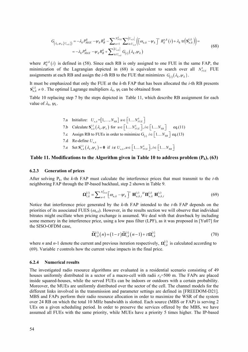
54
,
, ,
,
,
,,
, ,, 1tr
,
kFU
k k
E u k
u k u k
u k
u k
N Uk k u k iMAX B u k k k u kSU u ik k
k k k
U
Uk kMAX B i kiU
P R R i
P R G
G
S (68)
where ,u kSR i is defined in (58). Since each RB is only assigned to one FUE in the same FAP, the
minimization of the Lagrangian depicted in (68) is equivalent to search over all kFUEN FUE
assignments at each RB and assign the i-th RB to the FUE that minimizes ,i k kG .
It must be emphasized that only the FUE at the k-th FAP that has been allocated the i-th RB presents
, 0iu k S . The optimal Lagrange multipliers k, k can be obtained from
Table 10 replacing step 7 by the steps depicted in Table 11, which describe RB assignment for each value of k, k..
,
,
7.a Initialize: = 1, , 1
7.b Calculate , for 1 , 1 eq.(11)
7.c Assign RB to FUEs in order to minimize G 1 eq.(13)
7.d Re-def
ku k RB FUE
i ku k k k FUE RB
RBi
U N u N
u N i N
i N
S
,
, ,
ine
7.e Set , if , 1 , 1u k
i ku k k k u k FUE RB
U
i U u N i N S 0
Table 11. Modifications to the Algorithm given in Table 10 to address problem (Pk), (63)
6.2.3 Generation of prices
After solving Pk, the k-th FAP must calculate the interference prices that must transmit to the t-th neighboring FAP through the IP-based backhaul, step 2 shown in Table 9.
, , , , , , ,1
FUk
Ei i H i it k u k k u k t u k u k tu
N
Ω H Π H (69)
Notice that interference price generated by the k-th FAP intended to the t-th FAP depends on the priorities of its associated FUES (u,k). However, in the results section we will observe that individual bitrates might oscillate when pricing exchange is assumed. We deal with that drawback by including some memory in the interference price, using a low pass filter (LPF), as it was proposed in [Yu07] for the SISO-OFDM case,
, , ,1 1i i i
t k t k t kn n Ω Ω Ω (70)
where n and n-1 denote the current and previous iteration respectively, ,i
t kΩ is calculated according to (69). Variable controls how the current value impacts in the final price.
6.2.4 Numerical results
The investigated radio resource algorithms are evaluated in a residential scenario consisting of 49 houses uniformly distributed in a sector of a macro-cell with radii ro=500 m. The FAPs are placed inside squared-houses, while the served FUEs can be indoors or outdoors with a certain probability. Moreover, the MUEs are uniformly distributed over the sector of the cell. The channel models for the different links involved in the transmission and parameter settings are defined in [FREEDOM-D21]. MBS and FAPs perform their radio resource allocation in order to maximize the WSR of the system over 24 RB on which the total 10 MHz bandwidth is slotted. Each source (MBS or FAP) is serving 2 UEs on a given scheduling period. In order to preserve the services offered by the MBS, we have assumed all FUEs with the same priority, while MUEs have a priority 5 times higher. The IP-based
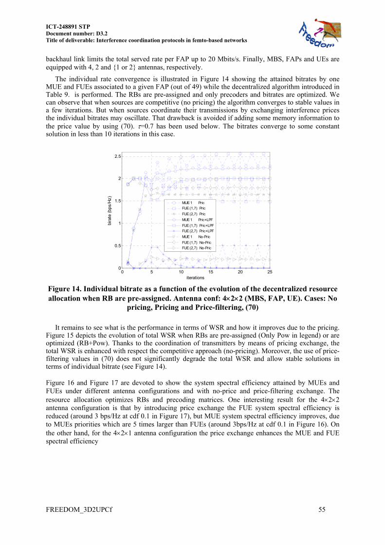
ICT-248891 STP Document number: D3.2 Title of deliverable: Interference coordination protocols in femto-based networks
FREEDOM_3D2UPCf 55
backhaul link limits the total served rate per FAP up to 20 Mbits/s. Finally, MBS, FAPs and UEs are equipped with 4, 2 and 1 or 2 antennas, respectively.
The individual rate convergence is illustrated in Figure 14 showing the attained bitrates by one MUE and FUEs associated to a given FAP (out of 49) while the decentralized algorithm introduced in Table 9. is performed. The RBs are pre-assigned and only precoders and bitrates are optimized. We can observe that when sources are competitive (no pricing) the algorithm converges to stable values in a few iterations. But when sources coordinate their transmissions by exchanging interference prices the individual bitrates may oscillate. That drawback is avoided if adding some memory information to the price value by using (70). =0.7 has been used below. The bitrates converge to some constant solution in less than 10 iterations in this case.
0 5 10 15 20 250
0.5
1
1.5
2
2.5
iterations
bira
te (
bps/
Hz)
MUE 1 Pric
FUE (1,7) Pric
FUE (2,7) Pric
MUE 1 Pric+LPF
FUE (1,7) Pric+LPF
FUE (2,7) Pric+LPF
MUE 1 No-Pric
FUE (1,7) No-Pric
FUE (2,7) No-Pric
Figure 14. Individual bitrate as a function of the evolution of the decentralized resource allocation when RB are pre-assigned. Antenna conf: 422 (MBS, FAP, UE). Cases: No
pricing, Pricing and Price-filtering, (70)
It remains to see what is the performance in terms of WSR and how it improves due to the pricing.
Figure 15 depicts the evolution of total WSR when RBs are pre-assigned (Only Pow in legend) or are optimized (RB+Pow). Thanks to the coordination of transmitters by means of pricing exchange, the total WSR is enhanced with respect the competitive approach (no-pricing). Moreover, the use of price-filtering values in (70) does not significantly degrade the total WSR and allow stable solutions in terms of individual bitrate (see Figure 14). Figure 16 and Figure 17 are devoted to show the system spectral efficiency attained by MUEs and FUEs under different antenna configurations and with no-price and price-filtering exchange. The resource allocation optimizes RBs and precoding matrices. One interesting result for the 422 antenna configuration is that by introducing price exchange the FUE system spectral efficiency is reduced (around 3 bps/Hz at cdf 0.1 in Figure 17), but MUE system spectral efficiency improves, due to MUEs priorities which are 5 times larger than FUEs (around 3bps/Hz at cdf 0.1 in Figure 16). On the other hand, for the 421 antenna configuration the price exchange enhances the MUE and FUE spectral efficiency

56
0 5 10 15 20 25
130
135
140
145
150
155
iterations
Tot
al W
eigh
ted
Sum
Rat
e (W
SR
)
Only Pow No Pric
Only Pow Pric
Only Pow Pric+LPF
RB+Pow No Pric
RB+Pow Pric
RB+Pow Pric+LPF
Optimization Pow
Optimization RB and Pow
Figure 15. Evolution of the total WSR when decentralized resource allocation is carried out: RBs are pre-assigned or RBs are also optimized. Antenna conf: 422 (MBS, FAP,
UE). Cases: No pricing, Pricing and Price-filtering, (70)
0 2 4 6 8 10 120
0.1
0.2
0.3
0.4
0.5
0.6
0.7
0.8
0.9
1
Macro-User System Spectral efficiency (bps/Hz)
Cum
ulat
ive
Den
sity
Fun
ctio
n (c
df)
RB+Pow No Pric
RB+Pow Pric+LPF4x2x2
4x2x1
Figure 16. Macro-User system spectral efficiency when no-pricing or price-filtering exchange is assumed. Antenna conf: 422,1

ICT-248891 STP Document number: D3.2 Title of deliverable: Interference coordination protocols in femto-based networks
FREEDOM_3D2UPCf 57
84 86 88 90 92 94 96 980
0.1
0.2
0.3
0.4
0.5
0.6
0.7
0.8
0.9
1
Femto-User System Spectral efficiency (bps/Hz)
Cum
ulat
ive
Den
sity
Fun
ctio
n (c
df)
RB+Pow No Pric
RB+Pow Pric+LPF
4x2x2
4x2x1
Figure 17. Femto-User system spectral efficiency when no-pricing or price-filtering exchange is assumed. Antenna conf: 422,1
6.3 Conclusions
We have investigated a radio resource allocation algorithm suitable for downlink transmissions in femtocell networks which is scalable with the number of active FAPs. It is based on the exchange of interference prices through wired backhaul link connecting FAPs and MBS. The procedure adjusts the transmitted power and served rate as a function of current backhaul link bitrate. When maximizing the WSR criterion, the priorities of all users are taken into account because they are present in the exchanged prices, in contrast to competitive strategies. Moreover, incorporating some memory term to the exchanged price is useful to reduce the individual bitrate oscillations when the iterative decentralized resource allocation is performed without degrading significantly the total WSR We have analysed the SISO and MIMO cases when each FAP is serving multiple users under OFDMA criterion. In this regard, the investigated algorithm shows that the best results are obtained when resource blocks (RB) are optimized along with the transmit precoders.

58
7 DECENTRALIZED COORDINATION STRATEGIES BASED ON STATISTICAL MODELLING
In this section, we propose a set of decentralized resource allocation algorithms allowing a set of nearby FAPs to automatically adapt to the channel conditions and the macro users’ activity, seen as interference. The objective of the allocation strategies can be either the sum-rate maximization, under a power constraint, or the power minimization under a per-user rate constraint. The common characteristic in the proposed strategies, is that they are based on a statistical model of a particular aspect of the system. Specifically focus on the following properties and/or assumptions:
1. FAPs, thanks to backhaul link availability, can perform coordinated channel sensing, the sensing performance are by simple parameters, and such parameters are incorporate in the optimization of the channel access.
2. The MBS’s activity, on each sub-channel, is modelled as a set of Discrete Time Markov Chain. Assuming error-free communication among the FAPs through the backhaul link, game-theory based decentralized algorithms are proposed that incorporate the parameters of such a model.
3. Assuming a given, deterministic, MBS’s activity, and FAPs still operating in a coordinated
manner, we propose a strategy that takes into account statistical models for the quantization error inherent to the inter-FAP signalling messages and the probability of packet losses in such communications, and incorporate them in the design of a suitable resource allocation strategy.
These algorithms have been devised following an approach where a set of femtocells self-organizes, exchanging data at the control plane with the neighboring FAPs only, in order to find out the most appropriate resource allocation strategy and improve the performance that the system would have in the case of a purely competitive approach. In the practical situation of a femtocell deployment, this approach reflects the situation in which 1) the resource allocation mechanism is decentralized; and 2): there is exchange of signalling traffic among the neighboring cells. From a qualitative point of view, in terms of assumptions, what differentiates the contribution of this section from the rest of the deliverable is the presence, for each algorithm, of a “source of randomness” to which the algorithm is tailored. In the first case randomness is explicitly taken into account when we consider the false alarm probabilities, or equivalently detection probabilities, that come out from channel sensing procedures. In the second one, it is related to the fact that the MBS’s activity is described as a DTMC then it assumes a statistical description. While, in the last case, we explicitly take into account the fact that prices are quantized at the transmitter side (thus we have a quantization noise), and then received with a given probability p, because of the possibility of link failures between neighboring FAPs, at control data plane. 7.1 Preliminaries
Unlike macro networks, femtocells are typically installed by subscribers and they are deployed and maintained without global planning, with no special consideration about traffic demands or interference with other cells, either femto or macro cells. Hence, a potential massive deployment of FAPs might induce an intolerable interference from femto to macro users, as well as from femto to femto users, as in Figure 18, where the black lines represent the IP-based backhaul link (where neighboring FAPs can exchange signalling traffic at the control plane), while the red lines and blue lines represent the interference and data link, respectively.
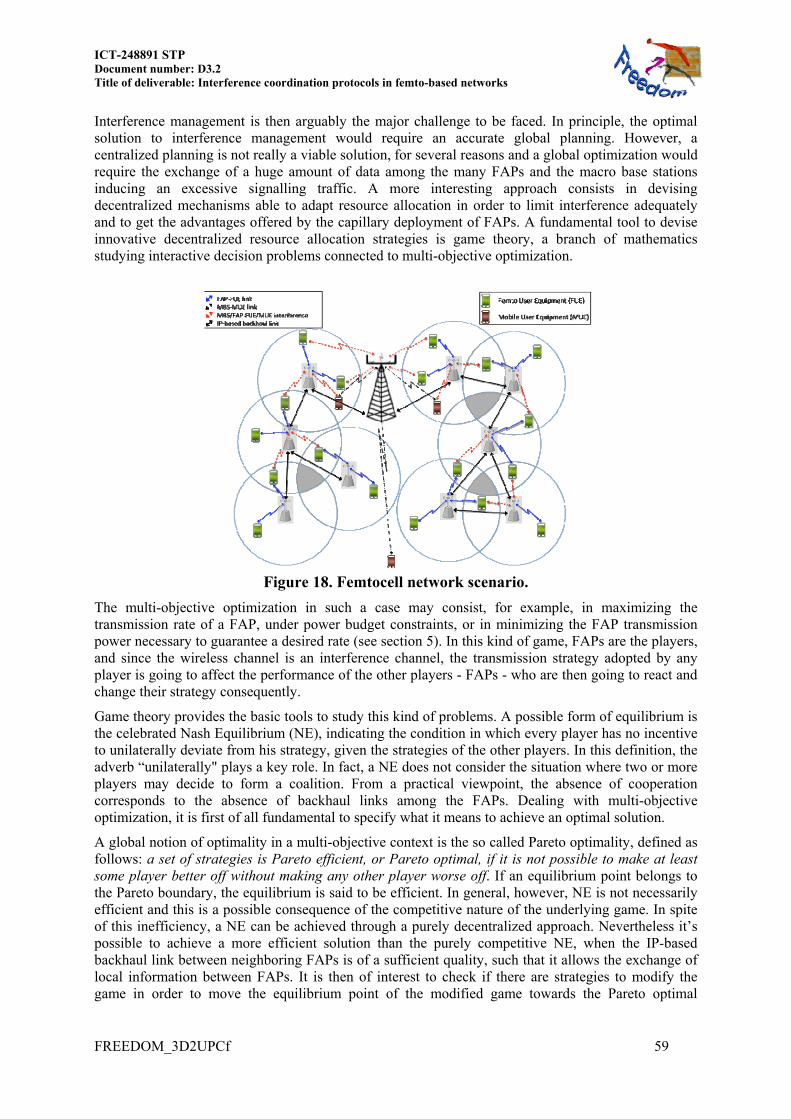
ICT-248891 STP Document number: D3.2 Title of deliverable: Interference coordination protocols in femto-based networks
FREEDOM_3D2UPCf 59
Interference management is then arguably the major challenge to be faced. In principle, the optimal solution to interference management would require an accurate global planning. However, a centralized planning is not really a viable solution, for several reasons and a global optimization would require the exchange of a huge amount of data among the many FAPs and the macro base stations inducing an excessive signalling traffic. A more interesting approach consists in devising decentralized mechanisms able to adapt resource allocation in order to limit interference adequately and to get the advantages offered by the capillary deployment of FAPs. A fundamental tool to devise innovative decentralized resource allocation strategies is game theory, a branch of mathematics studying interactive decision problems connected to multi-objective optimization.
Figure 18. Femtocell network scenario.
The multi-objective optimization in such a case may consist, for example, in maximizing the transmission rate of a FAP, under power budget constraints, or in minimizing the FAP transmission power necessary to guarantee a desired rate (see section 5). In this kind of game, FAPs are the players, and since the wireless channel is an interference channel, the transmission strategy adopted by any player is going to affect the performance of the other players - FAPs - who are then going to react and change their strategy consequently.
Game theory provides the basic tools to study this kind of problems. A possible form of equilibrium is the celebrated Nash Equilibrium (NE), indicating the condition in which every player has no incentive to unilaterally deviate from his strategy, given the strategies of the other players. In this definition, the adverb “unilaterally" plays a key role. In fact, a NE does not consider the situation where two or more players may decide to form a coalition. From a practical viewpoint, the absence of cooperation corresponds to the absence of backhaul links among the FAPs. Dealing with multi-objective optimization, it is first of all fundamental to specify what it means to achieve an optimal solution.
A global notion of optimality in a multi-objective context is the so called Pareto optimality, defined as follows: a set of strategies is Pareto efficient, or Pareto optimal, if it is not possible to make at least some player better off without making any other player worse off. If an equilibrium point belongs to the Pareto boundary, the equilibrium is said to be efficient. In general, however, NE is not necessarily efficient and this is a possible consequence of the competitive nature of the underlying game. In spite of this inefficiency, a NE can be achieved through a purely decentralized approach. Nevertheless it’s possible to achieve a more efficient solution than the purely competitive NE, when the IP-based backhaul link between neighboring FAPs is of a sufficient quality, such that it allows the exchange of local information between FAPs. It is then of interest to check if there are strategies to modify the game in order to move the equilibrium point of the modified game towards the Pareto optimal
60
boundary. One of the mechanisms to be used to achieve such a goal is pricing, which requires some exchange of information (prices) among players (FAPs) at control plane level. From a practical point of view, each price reflects the marginal cost of increasing interference to the other users on a particular subchannel. This possible local coordination among FAPs is made possible in femtocell networks through the, IP-based, backhaul link, which creates an underlying wired network connecting FAPs and MBSs [Barbarossa10].
In this section, we categorize our techniques considering the following issues (the same description is given for the minimum power game in Section 5.1):
1. Objective function: the description of any allocation strategy must clearly identify the objective function, which is being optimized. The objective function is then a natural performance indicator for the considered technique.
2. Constraints: typically, the optimization problem that the proposed technique attempts to solve in a distributed fashion is characterized by one or more constraints on some system parameters or indicators.
3. Price Exchange: the way in which prices are exchanged. It could be deterministic (backhaul link is good enough to allow price exchange with no errors), or stochastic (backhaul link allows price exchange with a given probability). This last case is taken into account in Section 7.4.
4. Spectrum Sensing: in this deliverable we assume that the FAPs are able to implement spectrum
sensing, with a certain periodicity, over the system bandwidth. Furthermore, as exchange of local information among FAPs is possible, they could perform coordinated spectrum sensing.
The presented techniques are decentralized strategies based on the achievement of an equilibrium that, thanks to this local coordination, will be surely more efficient than the purely competitive NE. Our work assumes as the operating situation one in which the backhaul network is good enough to allow the exchange of signalling traffic between neighboring FAPs or FAPs and MBSs. As usual, the FAPs operate as competitors over common radio resources, but when they decide for a given strategy, they take into account those price coefficients exchanged at the control plane level, performing a sort of coordination. Just an introductory example to better understand the effect of pricing mechanisms, Figure 19 shows the sum rate in bit per OFDM symbol [bps] of 20 active FAPs deployed over a given area vs. the interference coverage radius of each FAP1. Sum-rate values are those taken at convergence, when a simultaneous distributed gradient projection algorithm with pricing (red lines) and without pricing (blue lines), is run. As expected, with the increasing of interference coverage radius, we have a considerable loss in term of sum rate (interference is higher), but pricing mechanisms allow us to improve equilibrium efficiency.
1 The considered example was obtained considering a simple Gaussian channel, in which case the interference power of a transmitter versus a given receiver, can be interchanged with the notion of coverage radius, i.e. the distance above within which two transceivers are defined to interfere with each other. Following the so called “protocol model,” interference is then modeled assuming that only nodes within interference distance from each other give a significant contribution to each other’s interference terms.

ICT-248891 STP Document number: D3.2 Title of deliverable: Interference coordination protocols in femto-based networks
FREEDOM_3D2UPCf 61
Figure 19. Pricing vs. No Pricing.
The features of the proposed techniques are described in the following, and summarized in Table 12.
Technique Objective function
Constraints Price
Exchange Spectrum sensing
Joint optimization of FAP’s throughput
and detection parameters
Opportunistic throughput
Interference constraint
towards the MUEs
No price exchange, IP-
based backhaul link is exploited
to perform coordinated
channel sensing
Each user needs to sense the whole set of subchannels for each realization of the channel use, i.e. for each slot. FAPs aggregate their observations to identify unused subbands
Max rate optimization with
power constraint and statistical interference
knowledge.
Per user rate Average power
Deterministic: prices are correctly
exchanged between FAPs
Periodical channel sensing with a period larger than the channels allocation time unit of the macro system.
Minimum power optimization with rate constraint and exact interference
knowledge
Transmit power
Per user information
rate
Deterministic: prices are correctly
exchanged between FAPs
Each user needs to sense the whole set of subchannels for each realization of the channel use, i.e. for each slot.
Table 12. Decentralized resource allocation strategies classification In Section 7.2 we propose a distributed mechanism where FAPs perform a coordinated channel sensing, and focus on how to incorporate the performance and parameter setting of the spectrum sensing phase in the resource allocation algorithm design, so as to optimize the overall network efficiency. Each FAP optimizes its own opportunistic throughput by choosing detection thresholds, sensing time and allocation power vector jointly, under a constraint on the interference to MUEs and a constraint on the total transmit power. In Section 7.3, following the current trend in 3G systems and their evolution like WiMax and LTE, we consider the problem of allocating power optimally in the joint time-frequency domain, exploiting the use of a statistical model for the interference activity in the time-frequency plane. We propose an optimal power allocation strategy based on modelling the interferer’s activity, in particular, as a two-

62
state Markov chain and show how to maximize the expected value of the femto-users’ rate, averaged over the interference statistical model, when some pricing mechanisms are taken into account. In this case we assume that FAPs perform a spectrum sensing periodically at the start of allocation time interval, in order to acquire knowledge of the current channel occupation state of the macro users. Finally in Section 7.4 we address the problem of rate maximization when price coefficients are quantized, and then received with a given probability p. It’s important to remark that algorithms in Section 7.2 and 7.3 follow a game theoretic approach, while algorithm in Section 7.4 is a decentralized gradient projection algorithm aimed to maximize the network sum-rate function this algorithm does not follow any game theoretic approach.. 7.2 Coordinated channel sensing
In a scenario where FAPs coexist with one or more MBSs, without the latter sending real-time resource allocation information to the FAPs, coordinated channel sensing by a group of nearby FAPs may be a useful tool to enhance their capability to track the activity of the MBS, and hence be able to allocate resources in a smart way. It can be showed that, within this framework, to maximize what we define the opportunistic throughput of the FAPs, which quantifies their ability to send information on a given portion of the spectrum, the choice of the detection and channel access parameters should be done in a joint manner.
Therefore, we consider the joint optimization of sensing time, detection thresholds and power allocation across multichannel links, in order to maximize the aggregated opportunistic throughput, given a probabilistic constraint on the interference generated towards the macro users. The problem will be first studied in the single FAP case and then extended to the multi FAP scenario by following a game theoretic set-up, where each FAP competes against others to maximize its own opportunistic throughput by choosing, jointly, the detection parameters, and the vector of power allocation over a multichannel link.
It is important to remark that, in this particular case, coordination among FAPs is taken into account in the detection phase. All the algorithms follow a purely competitive approach, with the only exception of algorithm shown in Table 15, where a particular step of the algorithm is performed running an average consensus, which provides a local exchange of information between neighboring FAPs 7.2.1 System and detection models
Let us consider a femtocell system where a group of nearby FAPs (e.g. co-located in a building or in the same area, such as a corporate compound) utilize a wideband channel composed by N nonoverlapping subbands. Each FAP senses the available spectrum with the aim of identifying subbands unused by the MBS, to be used for transmission. To do this, the FAPs aggregate their sensing result and decide, for each subband, on the basis of such an aggregated data set, between the two hypotheses 1,k and 0,k , denoting, respectively, the presence and absence of MBS’s signal. Let
CQ be the number of coordinating FAPs and SK the number of observations taken by each FAP on each subband. We assume that the FAPs acquire their signal samples in the same interval. At the end of the sensing interval, through a suitable signalling protocol and using the backhaul link, each FAP disseminates its results to the remaining FAPs. After that, each FAP is able to take a decision on the usage of each subband by the MBSs on the basis of the whole data set. We denote with ,q kx m the m-th observation taken by the q-th FAP on the k-th subband with 1,...,k N , 1,..., Cq Q , 1,..., Sm K and introduce the corresponding vector of observations , ,, 1 ,...,q
T
q k q k Sk x x K x . The whole data set used for the final decision on the k-th subband is represented by the vector 1, ,,...,k
TT Tk M k x x x ,
which has S CK Q elements. For the k-th subband, under the two hypotheses of being unused or used by the MBS, we have

ICT-248891 STP Document number: D3.2 Title of deliverable: Interference coordination protocols in femto-based networks
FREEDOM_3D2UPCf 63
0, , ,
1, , , ,
( ) ( )
( ) ( ) ( )
:
1, , , : k q k q k
k q k q k q k
x m w m
x m I m w m k N
(71)
for 1, , Sm K and 1, , Cq Q , where , ( )q kI m and , ( )q kw m denote, respectively, the m-th sample of the aggregated2 signal from the MBSs and noise, over the k-th subband. Under the assumption that noise and aggregated interference samples, over each subband, are zero mean, statistically independent, Gaussian random variables, the optimal detector, over each subband, is the energy detector [Quan08]:
1,
0,1
2( ) | ( , , ) | , 1k
k
C SQ K
k k k
i
kD i k N
x x
, (72)
where k is the threshold associated to the k-th subband. If the received samples are not Gaussian, the energy detector is no longer optimal, but it is still the most popular detector. For sK sufficiently large, invoking the central limit theorem, ( )k kD x can be well approximated by a Gaussian probability density function (pdf) [Quan08]. In particular, 0, 0,( ) ~ ( , )k k k kD x under 0,k and
1, 1,( ) ~ ( , )k k k kD x under 1,k with
2
0,2 2
1,
( )[ ( )]
( ( ) ( ))k C S n
k kk C S n I
Q K kE D
Q K k k
x (73)
where 2 ( )n k and 2 ( )I k denote the variance of noise and aggregated MBSs, respectively, over the k-th subchannel. Furthermore, we have
2 40,
2 2 2 21,
2 ( )Var[ ( )]
2 ( )( ( ) 2 ( ))k C S n
k kk C S n n I
Q K kD
Q K k k k
x . (74)
As sensing performance metrics per subchannel, we use the probability of successfully identifying the unused band (or spectral holes), i.e.
0, 0,Prob( | )k k k , and the probability of transmitting over bands occupied by the MBS-MUE links, i.e.
0, 1,Prob( | )k k k , where k is the final decision of the hypotheses test. According to these assumptions, the false alarm and detection probabilities depend on the detection thresholds and the number of observation as:
0,
0,
( )( )
,( )
k k C Sfa k
kSC
C S
Q KQ Q
Q KP K
(75)
and
1,
1,
(( ,
)
( )) k k C S
d k C Sk C S
Q KP Q K Q
Q K
. (76)
where ( )Q x denotes the Q-function. 7.2.2 Maximization of the aggregated opportunistic throughput
Since the detection process inevitably affects the power allocation of the FAP over the sensed spectrum, we provide now a novel formulation of the optimal access strategy, considering jointly the detection parameters (thresholds and sensing time) and the power allocation over all the available
2 In this context, i.e. for the purpose of deciding whether a given subband is used or not by any MBS, the interference signal is the sum of the signal coming from different MBSs.

64
subbands. We assume that the FAP knows the channel towards the intended receiver. This information can be made available either by a feedback link from receiver to transmitter, or just exploiting channel reciprocity when transmitter and receiver transmit over the same band (Time Division Duplexing).
The goal of the optimization is the maximization of the so called aggregated opportunistic throughput, defined in [Quan09] as the aggregate rate effectively transmitted by the FAP over the unoccupied bands, under the constraint that the power generated towards MBSs be confined within prescribed limits. We provide now a mathematical formulation of this problem. As channel model we consider frequency selective channels with uncorrelated scattering. Furthermore we assume that the spatial distribution of the macro user receiver follows an homogeneous Poisson point process with known spatial density (number of MUEs/m2). The rate of the k-th subband for each FAP is:
rk log
21
pk
| H (k ) |2
k2
, (77)
where kp is the power transmitted over the k-th subchannel, H(k) denotes the secondary channel (complex) transfer function over the k-th subband, and
k2
n2 (k )
I2 (k ) represents the total
disturbance, i.e. noise plus interference generated by MBS. Since the k-th subcarrier is used by the FAP only when no MBS is detected over that subcarrier, the probability of using that carrier is
, where k represents the detection threshold over subcarrier k. Hence, denoting by 1[ , , ]Np p p the power vector, the aggregated opportunistic throughput for a given interference profile 2
k can be written as
(78)
where we denote with T the total frame duration, ST the sensing time, and thus sT T T denotes the portion of the frame duration available for the data transmission while TN represents the total number of observations in the frame. We adopt as detection rule the Neyman-Pearson criterion, so that the false alarm probability is fixed and the threshold is chosen in order to maximize the detection probability. In particular, we assume the same false alarm rate over all the subchannels, i.e., we set
( , )fa k C s faP Q K p . Since, in general, the disturbance level over the available subcarriers is not constant, we allow the detection thresholds to vary over the subchannels, under the constraint that the false alarm rate over all the channels is the same.
Introducing the variable 2
2
| ( ) |k
k
H ka
, the aggregate opportunistic throughput can be written as
2 0,
1
( , , ) 1 1 log 1 Prob( )N
sfa s fa k k k
Tk
KR p K p p a
N
p . (79)
The major constraint in a femtocell deployment scenario is to either avoid the interference towards macro-users or to keep it under a tolerable level. Interference over, let us say, the k-th subchannel is generated only when the FAP erroneously misses the presence of a MBS over that channel. Hence, in order to limit the femto-to-mobile interference we can consider the interference power generated by the FAP , i.e.
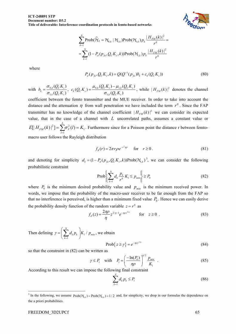
ICT-248891 STP Document number: D3.2 Title of deliverable: Interference coordination protocols in femto-based networks
FREEDOM_3D2UPCf 65
2
0, 1, 1,
1
2
1,
1
| ( ) |Prob( | )Prob( )
(1 ( , , ))Pro| ( )
b(|
)
NFM
k k k k k
k
NFM
d fa C s k k
k
H k
H k
pr
P p Q K k pr
where 1( , , ) ( ( ) ( ))d fa C s fa k k C sP p Q K k Q Q p b c Q K (80)
with 0,
1,
( )
( )k C s
kk C s
Q Kb
Q K
, 0, 1,
1,
( ) ( )( )
( )k C s k C s
k C sk C s
Q K Q Kc Q K
Q K
, while 2| ( ) |FMH k denotes the channel
coefficient between the femto transmitter and the MUE receiver. In order to take into account the
distance and the attenuation from wall penetration we have included the term r . Since the FAP
transmitter has no knowledge of the channel coefficient 2| ( ) |FMH k we can consider its expected
value, that in the case of a channel with L uncorrelated paths, assumes a constant value or
2 21
1
( )[| ( ) | ]L
FMl
F KH lE k
. Furthermore since for a Poisson point the distance r between femto-
macro user follows the Rayleigh distribution
2
( ) 2 for 0rRf r r e r . (81)
and denoting for simplicity 1,(1 ( , , ))Prob( )k d fa C s kd P p Q K k 3, we can consider the following
probabilistic constraint
1 0
1
ProbN
kk min
k
pd p P
rK
(82)
where 0P is the minimum desired probability value and minp is the minimum received power. In
words, we impose that the probability of the macro-user receiver to be far enough from the FAP so that no interference is perceived, is higher than a minimum fixed value 0P . Hence we can easily derive
the probability density function of the random variable z r as
2/2/ 1( )
2for 0z
Zf z z e z
. (83)
Then defining 1
1
/N
k k min
k
d p K p
, we obtain
2/
Prob z e (84)
so that the constraint in (82) can be written as
/2
01 1
1
ln( )with min
K
P pP P
. (85)
According to this result we can impose the following final constraint
1
1
N
k k
k
d p P
(86)
3 In the following, we assume
1, 0,Prob( Pr) )ob( 1 / 2k k and, for simplicity, we drop in our formulas the dependence on
the a priori probabilities.

66
We are now able to formulate the constrained optimization problem. Denoting by tP the transmit power budget of the single FAP, the goal of this last one is the following:
* * *2
1
1
1
1
( , , ) argmax 1 1 log 1
subject to (1 ( , , ))
,
0 1 / 2, 1 1
Ns
fa s fa k kTk
N
d fa C s k
k
N
k t
k
fa s T
Kp K p p a
N
P p Q K k p P
p P
p K N
p
p 0
. (87)
Note that the first constraint is meaningful if we assume 2/
1( / )0
t minKP pP e . Unfortunately, this
problem is not convex because the feasible set (the interference constraint) is not convex. Nevertheless, it is interesting to note that fixed fap and sK the resulting optimization problem is convex and a closed-form solution can be found. Furthermore we will show next that the problem can be reduced into the exhaustive search for the maximum of a two variables function, without loss of generality. In particular, it is easy to check that, if the false alarm probability value fap and the number of observations sK are given, the previous problem simplifies into the search of the power allocation vector *( , )fa sp Kp p solving the following optimization problem:
*2
1
1
1
1
( , ) argmax 1 1 log 1
subject to ( , )
Ns
fa s fa k kTk
N
k fa C s k
k
N
k t
k
Kp K p p a
N
d p Q K p P
p P
p
p 0
, (88)
with 1( , ) 1 ( ( ) ( ) ( )))k fa C s fa k C s k C sd p Q K Q Q p b Q K c Q K . This problem is strictly convex and the Slater's constraints qualifications hold true, so it has a unique solution, which can be found exploring the KKT optimality conditions. The solution can be found in closed form as a function of the Lagrange multipliers u and v, associated to the first and second constraint, and is equal to:
* 1( ) ( )k k
k
p wa
y y . (89)
where [ , ]fa sp Ky , [ ] max(0, )a a , ( )
( )( ( ))k
k
gw
v ud
y
yy
and ( ) (1 ) 1 / ln(2)sfa
T
Kg p
N
y .The
Lagrange multipliers , 0u v have to be chosen in order to satisfy the following complementary constraints
1
1 1
1
1 1
( ( ) ) 0, ( ) 0,
( ) , .
N N
k k k t
k k
N N
k k k t
k k
u d p P v p P
d p P p P
y
y
(90)

ICT-248891 STP Document number: D3.2 Title of deliverable: Interference coordination protocols in femto-based networks
FREEDOM_3D2UPCf 67
Several algorithms can be used to solve the nonlinear system (90). A practical algorithm can be found, e.g. in [Son09]. Once the multipliers u and v are found, (89) provides a closed form solution for the optimal power vector, which we denote as * ( , )fa sp Kp , to remark its dependence on fap and sK . As a consequence, the original optimization problem boils down to searching for the fap and sK values that maximizes *( ( , ), , )fa s fa sR p K p Kp . The solution of this problem can be obtained numerically, as shown in the following table.
Algorithm I: Single user optimization problem
S.0: Set the vectors fap =[0:1/2] and '
SK =[1:NT-1]
S.1: Set Rmax=0
S.2: for n=1:length( fap )
fa fap p (n)
for k=1:length( 'SK )
's SK K (k);
find *p ( fap , sK ) by solving the convex problem in (88);
if R( *p ( fap , sK ), fap , sK ) Rmax;
Rmax=R(*p ( fap , sK ), fap , sK );
*fap = fap ;
*sK = sK ;
end end
end
Table 13. Single User Optimization Algorithm. 7.2.3 Opportunistic throughput maximization: A game theoretic approach
In a femtocell deployment scenario, FAPs are expected to operate in an uncoordinated manner, so that they are competing over the same set of radio resources and there is no central authority assigning them the channel resources. A game theoretic formulation of the access from secondary users, under constraints imposed by the macro-users, is then well appropriate in this context, to find out decentralized solutions, as proposed in [Scutari08a]. However, in [Scutari08a] the payoff of each player did not take into account the decision process and the sensing time. But the detection process is inevitably going to affect the overall network efficiency on one side, as well as the level of undue interference towards macro-users, on the other side. For this reason, we provide in this section a novel formulation of the game, where the payoff function of each player is the opportunistic throughput, which takes into account the detection thresholds and the sensing time. Furthermore, we add a probabilistic constraint on the average interference towards the MBSs that is explicitly written as a function of the detection thresholds and the sensing time. The problem can be formulated as follows. The transmission rate over the k-th channel for the q-th FAP is
2
22 2
1,
( ) | ( ) |log 1
| ( ) | )(
q qqqk M
k rq r
r r q
p k H kr
H k p k
(91)

68
where ( )qp k is the power allocated by the q-th FAP user over the k-th subchannel, ( )rqH k denotes the FAP channel transfer function between source r and destination q over the k-th subband, and
2 2 2( ) ( )k n Ik k represents the total disturbance, i.e. noise plus interference generated by macro-users (for simplicity and without loss of generality we have assumed that 2
, ( )q n k is independent of q and equal to 2 ( )n k ). Hence, denoting by [ (1), , ( )]q q qp p N p the q-th user power vector and assuming 1 [ , , ]M p p p , and with q
CQ the number of FAPs that coordinate with the q-th one in the sensing phase (remark that value q
CQ takes into account the q-th FAP too), the opportunistic throughput is
1 0, 0, 0,
1
2
0, 2 2 21
ˆ( ; ( , ), , ( , )) Prob( | )Prob(
( ) | ( ) |1 ( , ) 1 Prob( log 1
| (
)
)) | ( )
Nq q q q q q qs
q fa C s fa N C s k k k k k
k
N qq qqq q q s
fa k C s kTk k rq r
r q
T TR p Q K p Q K H r
T
p k H kKp Q K
N H k p k
p
(92)
with 1, ,q Q . The competition among FAPs can then be cast as a non-cooperative strategic game whose structure is , , q q q qR (93)
where 1,2, , Q is the set of the players (the FAPs), q represents the set of admissible
strategies for the q-th user given by
1, 1
1 1
, [0,1/ 2],1 1: ( ) , (1 ( , , ) ))Prob ( ) ( N N
N q q q q q q qq q fa s T q t d fa C s k q
k k
p K N p k P P p Q K k p k P
p (94)
where qtP is the transmit power budget, while
/2
01
1
ln( )qq minP p
PK
depends on the lower bound
0qP which we impose on the probability that the macro-user receiver perceives no interference by the
FAP transmitter. Finally, qR is the opportunistic throughput, given in (79). In the game , each
player aims to solve the following optimization problem
,
maximize ( , , , ):
subject to ( , , )
qq fa
q qq q q fa s
p
q qq fa s q
R p K
p K
q
pp p
p
(95)
where . Unfortunately, the existence of a Nash equilibrium for the game appears quite difficult to prove because the admissible strategies space is nonconvex (observe that the second constraint in (94) compromises the convexity of the admissible set). Nevertheless, it can be noted that given q
fap and qsK the feasible set q is convex. This allows us to propose two alternative strategies,
one aiming at optimizing the power allocation, qfap and q
sK , for every FAP, the other forcing the same qfap and q
sK for all users and maximizing the sum throughput. Multilevel Iterative Water-Filling (MIWF)
The non-convexity of the feasible set (94) in the joint domain , , q qq fa sp Kp makes the search for a
solution non trivial. However, as in the single user problem we assume that qfap and q
sK are somehow
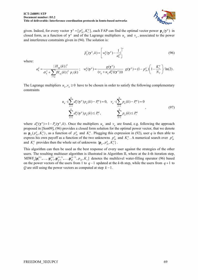
ICT-248891 STP Document number: D3.2 Title of deliverable: Interference coordination protocols in femto-based networks
FREEDOM_3D2UPCf 69
given. Indeed, for every vector [ , ]q q qfa sp Ky , each FAP can find the optimal vector power ( )q
qp y in closed form, as a function of qy and of the Lagrange multipliers qu and qv , associated to the power and interference constraints given in (94). The solution is:
* 1( , ) ( )q q q
q k qk
p k wa
y y (96)
where: 2
2 2
| ( ) |
| ( ) | ( )
qqqk
k rq r
r q
H ka
H k p k
; ( )
( )( (( )))
qq qk q q
q q k
gw
v u d
y
yy
( ) (1 ) 1 / ln(2)q
q q sfa
T
Kg p
N
y .
The Lagrange multipliers , 0q qu v have to be chosen in order to satisfy the following complementary constraints
1
1 1
1
1 1
( ( ) ( ) ) 0, ( ( ) ) 0
( ) ( ) , ( )
N Nq q q q
q k q q q t
k k
N Nq q q qk q q t
k k
u d p k P v p k P
d p k P p k P
y
y
, (97)
where ( ) 1 ( , )q q qk dd P k y y . Once the multipliers qu and qv are found, e.g. following the approach
proposed in [Son09], (96) provides a closed form solution for the optimal power vector, that we denote as ( , )q q
q fa sp Kp , as a function of qfap and q
sK . Plugging this expression in (92), user q is then able to express his own payoff as a function of the two unknowns q
fap and qsK . A numerical search over q
fap and q
sK provides then the whole set of unknowns , , q qq fa sp Kp .
This algorithm can then be used as the best response of every user against the strategies of the other users. The resulting multiuser algorithm is illustrated in Algorithm II, where at the k-th iteration step,
( ) ( ) ( 1) ( 1)1 1 1MIWF [ , , , , , , , ]k k k k
q q q faQ sp K p p p p denotes the multilevel water-filling operator (96) based
on the power vectors of the users from 1 to 1q updated at the k-th step, while the users from 1q to Q are still using the power vectors as computed at step 1k .

70
Algorithm II: Multilevel Iterative Water-Filling (MIWF)
S.0: Set the vectors fap =[0:1/2], '
SK =[1:NT-1] and fix CQ
S.1: Set k=0, and initialize with any (0) p 0
S.2: while k num_iter k=k+1 for q=1:Q
Max=0;
for n=1:length( fap )
fa fap p (n);
for m=1:length( 'SK )
's SK K (m);
qopp =MIWFq[
( )1
kp ,..., ( )1
kqp , ( 1)
1k
qp ,..., ( 1)
Qkp , fap , sK ];
if Rq(qopp , qp , fap , sK ) Max
Max=Rq(qopp , qp , fap , sK );
( )kqp = q
opp ;
end; end;
end end
end
Table 14. Multilevel Iterative Water-Filling Algorithm. Sum-throughput decentralized maximization
The game theoretic approach illustrated in the previous section shows interesting numerical results but it is hard to substantiate in mathematical terms. To overcome this difficulty, in this section we propose an alternative approach that requires some exchange of information between nearby nodes, that is possible, thanks to backhaul link availability. The approach is sub-optimal in the sense that the false alarm rate and the number of observations used in the sensing phase are forced to be the same for all the FAPs, but the common values are still the object of the optimization. Proceeding as in Algorithm II, the search over the optimal q
fap and qsK are carried out numerically. For each value of the vector
[ , ]fa sp Ky , every FAP runs a two-step algorithm composed of two phases:
1. Compute the Nash equilibrium of the game for the given y using the same steps as in Algorithm II;
2. Run an average consensus algorithm [Olfati-Saber07] to evaluate the throughput averaged over all the FAPs.
The second step requires the interaction between nearby nodes. It is known that if the FAP’s network is connected, under mild assumptions on the consensus algorithm, every FAP is able to get the average throughput, for any given values of fap and sK . Repeating the previous two-steps procedure, for every y value, each FAP ends up with a curve of the average throughput as a function of fap and sK . This curve allows every FAP to choose the (common) fap and sK values that maximize the average throughput. In [Scutari08b], the authors provided sufficient conditions guaranteeing the uniqueness of the Nash equilibrium p of the game , for fixed fap and sK , as well as the global convergence of

ICT-248891 STP Document number: D3.2 Title of deliverable: Interference coordination protocols in femto-based networks
FREEDOM_3D2UPCf 71
totally asynchronous algorithms based on the MIWF mapping. Under these conditions Algorithm III, described in the next table, is thus guaranteed to converge.
Algorithm III: Sum-throughput decentralized maximization
S.0: Set the vectors fap =[0:1/2], '
SK =[1:NT-1] and fix CQ
S.1: for n=1:length( fap )
fa fap p (n);
for m=1:length( 'SK )
's SK K (m);
Set ' qs SK K (m), q=1,…,Q;
Compute the Nash equilibrium *p ( qfap , q
sK ) of the game keeping
fixed qfap = fap (n) and q
sK = 'SK (m);
sum_rate(n,m)1
Q
r
Rr(*p ( fap (n), '
SK (m)) fap (n), 'SK (m)), (average
consensus); end
end
Table 15. Sum-throughput decentralized maximization algorithm. 7.2.4 Numerical results
In this section we show some numerical results proving the effectiveness of the proposed approaches.
A. Single FAP scenario
The first important property to verify is the behaviour of the objective function * ,( ( ))fa SR Kpp , obtained using the optimal power allocation * ,( )fa Sp Kp , for any given false alarm value fap and number of observations sK . As an example, in Figure 20, we plot the opportunistic throughput
* ,( ( ))fa SR Kpp as a function of fap and SK . It can be seen that there exists a couple of values * *( , )fa sp K that maximize the opportunistic throughput. Simulation results are related to a single FAP
scenario with 10tP , 1 0.1P , 1 , 1minp and assuming that the number of coordinating FAPs during the sensing phase is 5cQ . In Figure 21 we report ** ,( ( ))fa SKR pp vs. fap for different values of the minimum probability 0P , or equivalently for several values of the parameter 1P . The behaviors reported in Figure 21 show that, for every 0P , there exists a value *
fap of the false alarm probability that maximizes the aggregate rate. The value *
fap increases, as the minimum value 0P imposed to the probability to have no interference is higher, or the same as 1P increases. In particular, the interference constraint is inactive when 1 tP P ; in such a case, the optimal solution to (88) reduces to the classical waterfilling and * 0fap .

72
Figure 20. Optimal sum rate versus the false alarm probability fap and the number of
observations sK for N=10.
Figure 21. ** ,( ( ))fa SKR pp vs. fap .
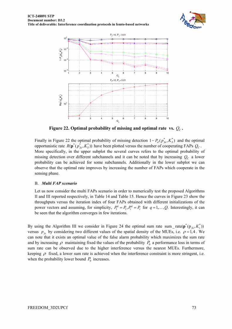
ICT-248891 STP Document number: D3.2 Title of deliverable: Interference coordination protocols in femto-based networks
FREEDOM_3D2UPCf 73
Figure 22. Optimal probability of missing and optimal rate vs. CQ .
Finally in Figure 22 the optimal probability of missing detection * * )1 ( ,d fa SpP K and the optimal opportunistic rate * **( ( )),fa SR Kpp have been plotted versus the number of cooperating FAPs CQ . More specifically, in the upper subplot the several curves refers to the optimal probability of missing detection over different subchannels and it can be noted that by increasing CQ a lower probability can be achieved for some subchannels. Additionally in the lower subplot we can observe that the optimal rate improves by increasing the number of FAPs which cooperate in the sensing phase. B. Multi FAP scenario
Let us now consider the multi FAPs scenario in order to numerically test the proposed Algorithms II and III reported respectively, in Table 14 and Table 15. Hence the curves in Figure 23 show the throughputs versus the iteration index of four FAPs obtained with different initializations of the power vectors and assuming, for simplicity, 11 ,q q
t tP P P P for .,1,q Q Interestingly, it can be seen that the algorithm converges in few iterations.
By using the Algorithm III we consider in Figure 24 the optimal sum rate * *sum _ rate( (p , ))fa sKp versus fap by considering two different values of the spatial density of the MUEs, i.e. 1,4 . We can note that it exists an optimal value of the false alarm probability which maximizes the sum rate and by increasing maintaining fixed the values of the probability 0P a performance loss in terms of sum rate can be observed due to the higher interference versus the nearest MUEs. Furthermore, keeping fixed, a lower sum rate is achieved when the interference constraint is more stringent, i.e. when the probability lower bound 0P increases.

74
Figure 23. Optimal opportunistic throughput vs. iterations.
Figure 24. Optimal sum rate versus the false alarm probability
Finally in Figure 25 in order to quantify the dependence on the number of FAPs which cooperate in the sensing phase, we plot the optimal sum rate versus CQ . It can be observed that by increasing CQ the optimal sum rate obtained by running the Algorithm III improves since more accurate sensing results can be achieved.

ICT-248891 STP Document number: D3.2 Title of deliverable: Interference coordination protocols in femto-based networks
FREEDOM_3D2UPCf 75
Figure 25. Optimal sum rate versus the number of cooperating FAPs.
7.3 Dynamic resource allocation under Markovian interference model 7.3.1 Preliminaries
In this section we incorporate pricing mechanism to the maximum rate and min power games proposed in Section 7.6.3 of [FREEDOM-D31], assuming that the IP-based backhaul link allows a limited local exchange of data among the FAPs. Let us first recall the idea behind the optimization problem in Section 7.6.3 of [FREEDOM-D31]. Femtocells must be fully compliant with cellular standards. Given the current evolution of 3G systems (see, e.g. WiMax and LTE), it is of interest to look at power allocation techniques in a time-frequency frame. In typical distributed resource allocation algorithms based on game theory, the channel status in terms of channel gain and interference (possibly over multiple subchannels) are assumed to be constant over a given period of time, along which the resources are allocated according to the particular algorithm used. It is a fact, however, that while the constant channel assumption is perfectly reasonable given the low indoor mobility, the interference from macro-users may well vary during an allocation time interval of a group of FAPs. Tracking the interference variations at the level of time-slots would in fact be too cumbersome for the FAPs, as they would spend most of the time sensing the channel and running an iterative algorithm. In other words, the correct power allocation across time and frequency would require a non-causal knowledge of the interference, which of course is not available. To circumvent this inconvenient, we propose a time-frequency resource allocation based on a Markov modelling of the interference activity on each frequency subchannel. In the following, we generalize the max-rate and min-power games to the case of Markovian interference activity. From a system point of view, we have a MBS transmitting over the considered system bandwidth composed of N subchannels, a resource allocation instance takes place every frame composed of M time slots, i.e. on a time-frequency grid of NM resources. For simplicity, the activity on each subchannel is modelled as a two state DTMC with transition probabilities defined as k (idle to idle transition probability) and k (busy to busy transition probability), which correspond to steady states probabilities

76
1 0
0 1 1 0
0 1
0 1 1 0
( 1): probability to be in the idle state
( 2)
( 1): probability to be in the busy state
( 2)
kk
k k kk k
kk
k k kk k
p
p p
p
p p
We remark that the transition probabilities between the different states depend on the application layer traffic statistic, but are not uniquely determined by it. Particularly, the one considered here are the traffic statistics of sub-channel occupation at the physical layer, therefore, they also depend on the implementation of the whole protocol stack, including multi user and multi radio-bearer scheduling and i.e. physical resource block assignment to different radio bearers within one frame. The set of resources is used by a set of FAPs, each one connected, for simplicity, to a single FUE. The FAPs perform spectrum sensing at the start of each frame to acquire knowledge on the channel occupation status from the MBS. Notice, however, that this knowledge will be limited to the first time-slot of the frame. This is the major difference with respect to the preceding section, in which the temporal rate at which the channel occupation status changes is not addressed as a problem. Since the interference level along the frame is unknown, we propose to modify maximum rate and minimum power games [Scutari08b] by substituting the utility function with the expected value of the rate ( , )q q qR p p conditioned to the observation performed on the first time slot. 7.3.2 Maximum expected rage game
Considering an arbitrary time slot indexed with the letter m, we indicate with ( '),, 0 m
m k mkS and ( '),, 1 m
m k mkS the probabilities that channel k is idle or busy, at time m, conditioned on the observed state in an arbitrary preceding step m´ < m. Without loss of generality, we now set m´ = 0 and use the notation ,k m and ,k m to indicate the conditional occupancy states, dropping the index m´ even from the expected rate definition. The expected rate is then
, , , ,
1 1
( , ) log 1 ( , ) log 1 ( , )M N
q q q qq q q k m k m n k m k m I
m k
R p a k m p a k m
p p (98)
where ,qk mp is the power over the k-th subchannel at the m-th time slot for the q-th FAP, while
2 2
2 2 2 2 2, , , ,
| | | |( , ) , ( , ) ,
( ) | | ( ) | | ( , )q
q q
qq qqq qk kn Ir rq r rq
n q k m k n q k m k Ir r
H Ha k m a k m
k p H k p H k m
(99)
with 2, ( )n q k that denotes the noise variance on the k-th subchannel, 2 ( , )qI
k m denotes the received
interference power from the MBS at time m on the subchannel k - resource block (k,m) - and 2
, | |q
r rqk m k
r
p H
the interference that the q-th FAP receives from its neighbors (with q the set of
these neighbors). Finally we indicate with 2| |kxyH the channel transfer coefficient, over subchannel k,
between the x-th transmitter and the y-th receiver (we do not have the channel depending on time slot m because we assumed it to be time unvarying for the frame duration). Knowing the transition probabilities through preliminary estimation, the occupancy probabilities and at any time m are related to the occupancy probabilities of the preceding step by the following recursion rule:
, 1 ,
, 1 ,
1
1k m k mk k
k m k mk k
, (100)

ICT-248891 STP Document number: D3.2 Title of deliverable: Interference coordination protocols in femto-based networks
FREEDOM_3D2UPCf 77
with 10, ,m M , 1, ,k N , where k and k denote the idle-to-idle and busy-to-busy transition probabilities, respectively; in case of error free spectrum sensing we have ,0 0k and
,0 1k , if channel k is sensed busy at time 0, or ,0 1k and ,0 0k , if channel k is idle at time 0. In (98), we distinguish between the interference from the macro-users, which is assumed as given, and the interference from other FAPs, which are modeled as competitive players. In the maximum expected rate game, , each player must solve the following local problem:
(101)
where the feasible set of user q is:
(102)
Since the objective function in (101) is strictly concave in q qp , for any given qp , and the feasible set is compact and convex, game admits a non-empty solution set for any set of channels and transmit power constraints of the users. In [Barbarossa11b] we reformulated this game as a Variational Inequality (VI) [Facchinei03] and we applied the Iterative Gradient Projection Algorithm (IGPA) to solve it, deriving sufficient conditions for its convergence. Anyway we can’t say anything about equilibrium efficiency and, due to the purely competitive approach of this kind of games, in general, it could be really inefficient. The problem is then how to modify the game in order to reduce as much as possible the performance loss related to a NE or, in other words, how to move the NE's of the modified game towards the Pareto optimal boundary. We will now show to introduce a pricing mechanism to this game, and then to improve overall performance (equilibrium). First of all, we have to introduce the price coefficient for the r-th FAP, for a given resource block (k,m), ,
rk m , that’s
defined as:
,,
( ):
( )r rk m r
k m r
R
I
p
p, (103)
with 2, , ,( ) : | |
r
r i irk m r k m k m
i
I p H
p
, the interference received by r-th FAP on the resource block (k,m)
from its neighboring FAPs, and ( )rR p defined as in (98). From (103) we see that price coefficients are introduced in order to incorporate a cost quantifying the damage that each player's action can induce on the other players utilities. In other words, pricing is a way to incorporate, in each player's strategy, some kind of care about a socially meaningful performance parameter, rather than being purely selfish. Now, the modified game, incorporating pricing mechanisms, is:
2
, ,
1 1
max ( ,
s.t
) | |
.
M Nq r qr
q q q k m k m k
m k r
q q
R p H
p
p
p p
(104)
with defined as in (102). The proposed strategy channel allocation strategy for the FAPs is made
up of the following steps:

78
a. Each FAP observes the set of channels during slot 0 (i.e. at the beginning of a frame) b. Based on this observation that we assume, for simplicity, to be error free, the each FAP is
able to compute the occupancy probabilities for all the slots. c. Each FAP evaluates the price coefficients in (103) and broadcast them to its neighbors. d. The (time-frequency) NM-dimensional power allocation vector is optimized in order to
maximize the objective function in (104). The best response of each FAP leads to power coefficients ,
qk mp that, within the interval [0, ( ))max
qp k , must satisfy the following equation
aq (k ,m )(pk ,mq )2 bq (k ,m )p
k ,m c q (k ,m ) 0 (105)
where, denoting with q the Lagrange multiplier, we have set
(106)
We can verify that, 0q , we have bq (k ,m )2 4 aq (k ,m ) c q (k ,m ) 0, and the only solution is
pk ,mb
b q (k ,m ) b q (k ,m )2 4 aq (k ,m ) c q (k ,m )
2 aq (k ,m ) (107)
More specifically, we get
(108)
and the optimal power allocation vector is pk ,mq* [ p
k ,mb ]
0
pqmax (k )
where the multiplier q is chosen in
order to satisfy the power constraint m1
M
k 1
N
[ pk ,mb ]
0
pqmax (k ) P
q. The previous solution assumes, for each
player, that the powers used by the other players are given. In practice, the game evolves with each FAP reacting to the choices of the other FAPs. It is then fundamental to prove the convergence of this iterative mechanism. In the following, we present a version of the so called Modified Asynchronous Distributed Pricing algorithm (MADP) proposed in [Shi08] adapted to our formulation. To find the user's best response, it is useful to rewrite (104) introducing a unique index h so that the entries of the power vector qp are for 1, ,q
hp h NM . Then, defining the quantities

ICT-248891 STP Document number: D3.2 Title of deliverable: Interference coordination protocols in femto-based networks
FREEDOM_3D2UPCf 79
2 2
2 22 2 2, ,
: , : ,( ) ( ) ( )
q q
q
q q
q qq q qqh h h h
h hr rq r rq
n q h h n q h h I
r r
p H p HSNIR SNIR
h p H h p H h
(109)
we can derive the q-th user best response as
*
2
21,..., ,
q
qq qhh h
r qr qh h q h
r
cp p h MN
H
(110)
where 1 1
q q
q q
q qq h h h hh
h h
SNIR SNIRc
SNIR SNIR
and q and q
h are the Lagrange multipliers. Given this setting,
the modified MADP algorithm is illustrated in Table 16.
Algorithm: Modified Asynchronous Distributed Pricing
S.0: Each user q chooses an initial power profile in the set q and set
n=0;
S.1: Each user computes its interference prices qh (n), h=1,..,MN and sends
them to the other users; S.2: At each time n, one user q is randomly selected to maximize its utility
function qR and update its power profile given the other user's power
profiles qp and price vectors rh (n) according to
qhp (n+1)= q
hp (n)+ q (n)*[ *qhp - q
hp (n)] for h=1,..,MN, where *qhp is given by
(110); S.3: Set n=n+1, go to step S.1 and repeat until convergence is reached.
Table 16. MADP Algorithm. Following similar arguments as [Shi08], we proved in [Barbarossa11b] that there exists a small enough step size values ( )q n for which the MADP algorithm converges monotonically to a fixed point.
7.3.2.1 Numerical results
The following example shows the effects of pricing on the maximum expected rate game. In Figure 26 and Figure 27 we report the sum rate of ten FAPs, in the case where the macro user activity is modeled as a two-state first order DTMC, vs. the number of time slots. In particular, Figure 26 refers to the purely competitive maximum expected rate game of [Barbarossa11a], while Figure 27 refers to the modified game including pricing for a scenario composed by 10 active FAPs. The results are obtained with idle-to-idle transition probabilities 0.5k and busy-to-busy transition probabilities
0.5k . The number of subcarriers is set to 600, which is the LTE-A 10 MHz bandwidth system. MBS’s activity is supposed to be the same for groups of 12 subchannels. Maximum FAPs’ transmit power is set to 20 dBm. Rates are expressed in bit per OFDM symbol [bps].

80
The three different curves in each figure indicate the sum rate obtained by assuming perfect (non-causal) knowledge of the macro-user activity, no knowledge at all (future activity is the same of the present one), or statistical knowledge, i.e. knowledge of the Markov parameters. Surely Markov parameters are known thanks to a preliminary estimation; this means that there will be an initial time in which each FAP estimates both the transition probabilities k and k , see [FREEDOM-D31 – Appendix A].
Figure 26. Sum rate of ten FAPs vs. number of time slots for the maximum expected rate
game without pricing.
Figure 27. Sum rate of ten FAPs vs. number of time slots for the maximum expected rate
game with pricing.
Both figures show that the statistical knowledge (estimation) of the interference activity parameters (Markov transition rates) yields a performance advantage over the case with no information and brings the performance close to the ideal case of perfect non-causal knowledge of the interference activity. Moreover, if we compare Figure 26 and Figure 27 it is evident the gain achieved with the introduction
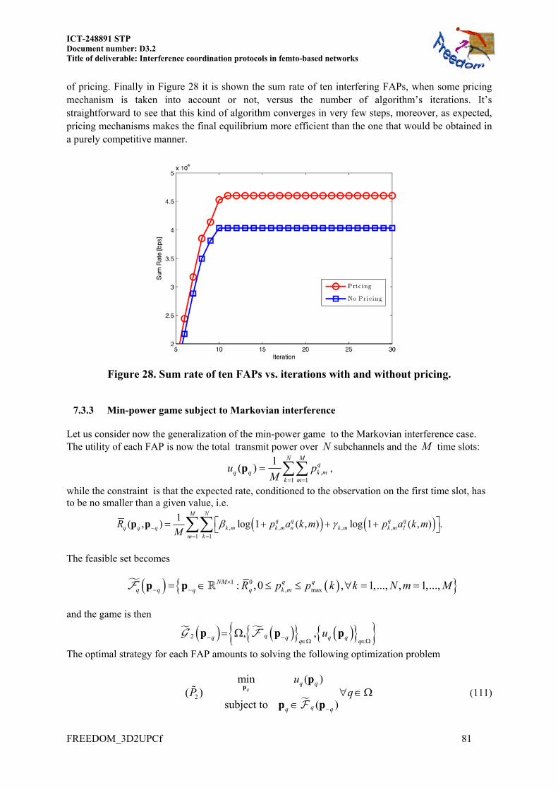
ICT-248891 STP Document number: D3.2 Title of deliverable: Interference coordination protocols in femto-based networks
FREEDOM_3D2UPCf 81
of pricing. Finally in Figure 28 it is shown the sum rate of ten interfering FAPs, when some pricing mechanism is taken into account or not, versus the number of algorithm’s iterations. It’s straightforward to see that this kind of algorithm converges in very few steps, moreover, as expected, pricing mechanisms makes the final equilibrium more efficient than the one that would be obtained in a purely competitive manner.
Figure 28. Sum rate of ten FAPs vs. iterations with and without pricing.
7.3.3 Min-power game subject to Markovian interference Let us consider now the generalization of the min-power game to the Markovian interference case. The utility of each FAP is now the total transmit power over N subchannels and the M time slots:
,1 1
1( )
N Mq
q q k mk mM
u p
p ,
while the constraint is that the expected rate, conditioned to the observation on the first time slot, has to be no smaller than a given value, i.e.
, , , ,
1 1
1( , ) log 1 ( , ) log 1 ( , ) .
M Nq q q q
q q q k m k m n k m k m I
m k
R p a k m p a k mM
p p
The feasible set becomes
1 0, max: ,0 , 1,..., , 1,...,NM q q
q q q q k mR p p k k N m M p p
and the game is then
2 , ,qq q q qq q
u p p p
The optimal strategy for each FAP amounts to solving the following optimization problem
2
min ( )( )
subject to ( )
qq q
qq q
uP q
pp
p p
(111)

82
where the set q qp given the power vector qp of the other FAPs, is a convex set. The
minimization problem 2P for each player q, given the strategies of the others, is then a convex
optimization problem, since the objective function is a linear (then convex) function of qp The best
response of each FAP can be written in closed form *
q qp = g p , where
max2
,
, , 4 , ,, 1,..., , 1,..., ,
2 ,
qp kq q q q
q qk m
b k m b k m a k m c k mk N m M
a k m
g p
with
, ,
( , ) , ,
( , ) , , , ,
( ,
) 1 , ,
q q qn I
q q q q qn I q n I
q q qq n k m I k m
a k m a k m a k m
b k m a k m a k m a k m a k m
c k m a k m a k m
,
where the Lagrange multiplier q must satisfy the rate constraint 0( , )q q q qR R p p Since game 2 is
a Generalized Potential Game, the existence of a NE of the potential game can be proved directly by
the existence of a maximum of the potential function 1
Q
q qqu
p = p on the feasible set of the
game. In order to solve the game 2 we have considered an iterative and distributed approach where at each step each FAP calculates its own best response in closed form given the strategies of all the
other active FAPs as *
q qp = g p .
Similarly to what done for the max-rate game proposed in the previous section, we can now improve the efficiency of the Nash equilibrium towards the Pareto optimal boundary by incorporating some
pricing mechanisms. To this end we can reformulate 2 as
2
,13
,1
min ( ) | |(
subject to ( )
M Nqr q
q q r k m k k mm k
q q
rr
q
u H pP q
p
p
p p
(112)
where r is the Lagrangian multiplier associated to the rate constraint and the pricing coefficients are
defined as in (103), i.e. ,,
( ):
( )r rk m r
k m r
R
I
p
p with 2
, , ,( ) : | |r
r i irk m r k m k m
i
I p H
p
, the interference
received by r-th FAP on the resource block (k,m) from its neighboring FAPs. We can see that price coefficients are introduced in order to quantify the damage that each FAP's action can induce on the other FAPs utilities by including, in each player's payoff function, some kind of care about a socially meaningful performance parameter. Then the proposed power allocation strategy for the FAPs can be resumed as follows:
a. Each FAP observes the set of channels during slot 0 and based on this observation is able to compute the occupancy probabilities for all the slots.
ICT-248891 STP Document number: D3.2 Title of deliverable: Interference coordination protocols in femto-based networks
FREEDOM_3D2UPCf 83
b. Each FAP evaluates the price coefficients ,qk m and the Lagrangian multiplier q and
broadcast them to its neighbors.
c. The (time-frequency) NM-dimensional power allocation vector is optimized by solving
problem 3P .
The best response of each FAP leads to the optimal powers ,qk mp which must satisfy the following
equation 2
1 , 2 , 3( , )( ) ( , ) ( , ) 0q q q qk m k mc k m p c k m p c k m (113)
where, denoting with q the Lagrange multiplier, we have set
2
3
21 ,
2,
2, , ,
( , ) (1 | | ) ( , ) ( , );
( , ) (1 | | )( ( , ) ( , )) ( , ) ( , );
( , ) 1 | | ( , ) ( , )
q
q
q
q qr q qr k m k n I
q qr q q q qr k m k n I q n
rr
rr
r
I
q qr q qr r k m k q n k m I k m
c k m H a k m a k m
c k m H a k m a k m a k m a k m
c k m H a k m a k m
(114)
We can verify that, 0q , we have 22 1 3( , ) 4 ( , ) ( , ) 0q q qc k m c k m c k m , and the only solution is
2
1
3,
12
2 ( , ) ( , ) 4 ( , ) ( , )
2 ( , )c
q q q q
k m q
c k m c k m c k m c k mp
c k m
(115)
More specifically, we get , ,max0, q
kc
m k mp p (116)
and the optimal power allocation vector is pk ,mq* [ p
k ,mb ]
0
pqmax (k )
where the multiplier q is chosen in
order to satisfy the rate constraint * 0( )q qR Rp .
7.4 Distributed Stochastic Pricing for Sum-Rate Maximization with Random Graph
and Quantized Communications 7.4.1 Preliminaries
We now consider a pricing mechanism aimed at maximizing the sum-rate of a femtocell network in a distributed manner, thanks to a limited exchange of information among neighbor femto access points (FAPs), in the particular case in which the exchange of information among FAPs is quantized and happens through a network graph (typically a sparse graph), whose links fail randomly across iterations. The backhaul link among the FAPs is an IP-based internet connection, which delivers packets in the network using a best-effort protocol. Hence, control packets sent through the backhaul might experience large delays, because of retransmissions of packets corrupted by errors. This random delay and the associated delay jitter could jeopardize the potential benefits of coordination. It is then of interest to examine a protocol that simply discards packets that are received with a delay exceeding a given threshold.

84
We analyze the effect of this protocol by modelling the graph describing the interaction among FAPs as a random graph, where each link is on with a probability equal to the probability that the packet is correctly delivered within the given maximum delay. Furthermore, we take into account the quantization of the information exchanged among the FAPs. These sources of randomness introduce stochastic noise in the pricing mechanism that needs to be handled to insure convergence of the distributed algorithm. Using results from stochastic approximation theory, we propose a distributed projection based Robbins-Monro (RM) [Robbins51] scheme that converges almost surely (a.s.) on a final allocation equilibrium dependent on the mean graph of the network, even in the presence of such imperfect communication scenario.
Numerical results show how the system performance is affected by link failures, in fact, reducing the probability to establish a communication link among FAPs, the system performance decreases due to the lower coordination to mitigate interference. Nevertheless, supposing to know the probability with which each link fails, we show how to counteract the effect of random links through a proper weighting of the price coefficients coming from the neighbors. The main assumption is that, even under busy backhaul conditions, FAPs are able to exchange data on the backhaul link, with a given probability.
Furthermore, in practice, given the limited transmit power and the attenuation resulting from indoor propagation, only nearby FAPs interfere with each other. Then, in this distributed pricing mechanism, each FAP needs to exchange interference prices only with few neighbors, thus remarkably reducing the signaling in the network. 7.4.2 System model
We consider an OFDMA (according to LTE-A) wireless system with Q distinct pairs of transmitters and receivers, sharing the same physical resources, e.g., time and bandwidth. No multiplexing strategy is imposed a priori so that, in principle, each FAP interferes with each other. In practice, interference is limited only between nearby FAPs. Then, to study the interference mechanism, it is useful to introduce what we call the interference graph ( , )I I IG V E , defined as the graph whose vertices are FAPs and where there is an edge between two vertices only if the relative FAPs interfere with each other.
Typically, the interference graph is a sparse graph (i.e., with a number of links much smaller than the maximum number of possible links). We denote by i
q the set of interfering neighbors of user q. We also introduce the notation 1col Q
q qp p , where 1( , , )q qq Np p p denotes the power vector of FAP q,
whose element qmp is the power transmitted by node q over the m-th subcarrier. Under the previous
assumptions, resorting to Shannon capacity expression, the rate of FAP q is given by
2
2 21
| |( ) log 1 ,
| |iq
N qq qm m
q rq rm qm m m
r
H pR
H p
p
(117)
where ymxH is the channel transfer function of the x-th subchannel between the y-th transmitter and the
q-th receiver, and 2qm is the variance (power) received on the m-th subchannel including receiver
noise and power coming from the macro users, while 2| |iq
rq rm m
r
H p
is the interference received from
the q-th FAP from its interfering neighbors ( iq ) on the m-th subchannel.
We are interested in a cooperative approach where FAPs pursue a common social objective. In particular, the optimization problem we would like to solve is the maximization of the sum rate of the Q FAPs under power constraints, i.e.,
ICT-248891 STP Document number: D3.2 Title of deliverable: Interference coordination protocols in femto-based networks
FREEDOM_3D2UPCf 85
1
max ( )
s.t.
Q
q
q
R
pp
p
, (118)
where 1
Q
q
q
and 1
: , 0 ( ), 1, , N
N q q maxq q m q m q
m
p P p p m m N
p , with qP and
( )maxqp m denoting, respectively, the power budget of user q and the mask constraint that limits the
maximum transmit power over each channel. In general, the objective function in (118) is not concave in the power allocation p and, as a consequence, the problem may have multiple local optima. A local solution can be found in a centralized manner using standard optimization algorithms. However, we focus on distributed solutions where it is allowed a local coordination among FAPs through a limited exchange of data. In this work, we take into account the presence of an imperfect communication scenario, considering the following assumptions on the stochastic processes affecting the algorithm. 1. Random link failure model:
The exchange of data is described by a communication graph Gc (Vc,Ec), i.e., the graph whose vertices are FAPs and where there is an edge between two vertices only if the relative FAPs exchange data with each other. An example of communication graph for 20 FAPs is shown in Figure 29, where the blue dots represent the FAPs, and the red line the IP-based backhaul link. We denote by A aqr the adjacency matrix of graph Gc , whose nonnegative qra entries are either one or zero,
depending on whether there is a link between nodes q and r. In our intended application, each FAP needs to exchange data only with neighbor FAPs in order to manage the Multi User Interference (MUI) generated by the active links. In an ideal communication scenario, the set of neighbors of FAP q in the communication graph coincides with the set of interfering FAPs in the interference graph.
Nevertheless, in a realistic communication scenario, some packets may be lost at random times. Typically, erroneous packets have to be resent and this induces a further complexity to handle packet retransmission, besides increased risks of congestion. It is then of interest to examine what happens if the erroneous packets are simply dropped, without requiring retransmissions. Random packet drops may be analyzed by modeling the network as a time-varying, or switched, network, where the presence of an edge (link) depends on the packet error rate. The communication network at time k is modeled as an undirected graph, Gc[k] (Vc,Ec[k]) and the graph adjacency matrices as a sequence
of independent identically distributed (i.i.d.) matrices A[k]. We model the graph adjacency matrices as
(119)
where is a zero-mean sequence of independent identically distributed matrices, and [ [ ]]kA A denotes the adjacency matrix of the expected graph.

86
Figure 29. Example of communication graph.
2. Dithered quantization:
We assume that each inter-node communication channel uses a uniform quantizer, whose input-output relation may be modelled by the quantizing function, ( ) :q with quantization step 0 . Conditioned on the input, the quantization error is deterministic, influencing the convergence of the algorithm. Now, adding to the input [ ]y k a dither sequence 0 [ ]kd k of i.i.d. uniformly distributed random variables on [ / 2, / 2) independent of the input sequence, the resultant error sequence
0 [ ]ke k becomes [ ] ( [ ] [ ]) ( [ ] [ ]).e k q y k d k y k d k (120) The sequence 0 [ ]ke k is now an i.i.d. sequence of uniformly distributed random variables on [ / 2, / 2) , which is independent of the input sequence. In the following, we will study the effect of the random communication graph and of the price quantization on the gradient of the sum-rate.
Introducing the notation 1
( ) ( )Q
q
q
R R
p p , that’s the sum of the rates of all the Q FAPs that are
randomly placed in a given area A, the partial derivative of the sum-rate ( )R p with respect to qmp can
be written as
( ) ( )( )
.iq
q rq q qm m mr
R RR
p p p
p pp
(121)
Following the same steps as in [Huang06], [Shi08], it is useful to introduce the price coefficients as:
( )
( ) ,r rm r
m
R
I
pp (122)
with 2|ri
srm
s
r rm mI H p
the interference received from the r-th receiver on the m-th subchannel.
The price ( )r
m p is always nonnegative and is proportional to the marginal decrease of user r's rate because of an increase of the q-th node's transmit power, as:
ICT-248891 STP Document number: D3.2 Title of deliverable: Interference coordination protocols in femto-based networks
FREEDOM_3D2UPCf 87
2( ) ( )( ) ( ) | | .
r rr r qrm mr rm m mq r q q
m m m m
I IR RH
p I p p
p p
p p (123)
Then, substituting expression (124) in (122), we get
2
1
( )( )| | ( ).
Qq qr r
qr m mq qm m r
RRa H
p p
pp
p (124)
To evaluate expression (124), FAP q needs to know the price vectors 1( ) col r r N N
m m π p , iqr , which are transmitted by the neighbors through the backhaul link. The communication
graph is then present in (124) through the coefficients qra of the adjacency matrix A. Collecting all the contributions in (124), the gradient of the sum-rate with respect to p can be written in compact vector form as ( ) ( ) ( )HR p p p πA pr (125)
where 1
( ) col ( )q
QQN
R
pr p p , 1( ) [ ( ), , ( )] QNQ π pπ p pπ is the vector collecting the
interference prices of the entire network and QN QNH A is a multidimensional adjacency matrix
weighted by the cross channels between FAPs. Expression (125) shows the dependence of the sum-rate gradient with respect to the network graph in the case of an ideal communication scenario. Considering the presence of failures and dithered quantization noise, expression (124) evaluated at time k, takes the form
2
1
( [ ])( [ ])[ ] | | ( ( [ ]) [ ] [ ]),
Qq qr r qr qr
qr m m m mq qm m r
R kR ka k H k k k
p p
ppp 1, ,m N , 1, ,q Q , (126)
where [ ]qrm k and [ ]qr
m k are contributions of dithered quantization noise that the q-th FAP receives from the r-th FAP on the m-th subchannel, at time k. To rewrite (126) in compact form, we introduce the random vectors 1[ ] col [ ]Q QN
q qk k and 1[ ] col [ ]Q QNq qk k , which are
aggregated contribution of dithered quantization noise. Then, the sum-rate gradient with respect to the power allocation [ ]kp , in the presence of random link failures and dithered quantization, can be written in compact form as ( [ ]) ( [ ]) [ ] ( [ ]) [ ] [ ].HR k k k k k k p p p A pr π (127)
Now, expanding the multidimensional weighted adjacency matrix [ ]H kA as in (119), we can write expression (127) as the sum of a deterministic function ( [ ]) QNk F p plus a random function
( [ ]) QNk p , where
( [ ]) ( [ ]) [ ] ( [ ]),Hk k k k A pπF rp p (128)
( [ ]) [ ] ( [ ]) [ ] [ ].Hk k k k k p π pA (129) The problem in (118) can then be converted in the search, inside the feasible set , for the zeros of a deterministic function ( )F p whose value, measurable at each time instant k, is corrupted by an additive random disturbance ( [ ])k p .

88
7.4.3 Distributed Stochastic Pricing Algorithm (DSPA)
To find a solution of the problem (118) affected by random disturbances, it is useful to introduce stochastic approximation algorithm. In the remainder of this section we introduce a stochastic approximation scheme for solving the problem in (118) in a distributed manner. In particular, we consider a projection-based Robbins-Monro (RM) stochastic approximation procedure, taking in consideration a simultaneous update of the users' power profiles and providing supporting convergence results. The problem is amenable for distributed solutions because the optimization set
1
Q
q
q
is given by the Cartesian product of sets q , allowing the parallel computation of the
algorithm. Let us now focus on a distributed stochastic simultaneous solution. We call it Distributed Stochastic Pricing Algorithm (DSPA) which is summarized as follows:
Algorithm: Distributed Stochastic Pricing
S.0: Each FAP q chooses an initial power profile qp [0] satisfying the
power constraint;
S.1: Using (122), each FAP computes the interference price vector qπ ,
given the current power profiles, and transmits this to the neighbor FAPs; S.2: At each time k, every FAP, given the neighbors' power profiles and price vectors, simultaneously updates its power profile according to
qp [k+1]=[ qp [k]+ [k]q
p R(p [k])]q= qT (p [k]), (130)
with q=1,...,Q and k 0, where [ ]q denotes the projection over the
feasible set q , [k] is an iteration-dependent step size and
qp R(p [k]) N is the q-th vector element of (127);
S.3: Go to step 2 and repeat until a convergence criterion is satisfied.
Table 17. DSPA. We consider two assumptions on the stochastic procedure in (130).
1. Persistence: The step size sequence [ ]k satisfies:
2
0 0
[ ] 0, [ ] , [ ]k k
k k k
(131)
Condition (131) ensures that the step-size decays to zero, but not too fast. It is standard in stochastic adaptive signal processing and control;
2. Independence: The stochastic sequences 0 [ ]kk A , 0 0 an [ ] [ ]d k kk k are mutually
independent.

ICT-248891 STP Document number: D3.2 Title of deliverable: Interference coordination protocols in femto-based networks
FREEDOM_3D2UPCf 89
Next, we provide the convergence result for the distributed stochastic algorithm in (130). Let [ ]kp the sequence generated by the distributed stochastic pricing algorithm in (130), with step-size satisfying the conditions in (131). Then, the sum rate sequence 0 ( [ ])kR k p converges a.s. to a finite
value *R , i.e.
*Prob lim ( [ ]) 1,k
R k R
p (132)
where Prob[ ] denotes the probability of the event . Furthermore, let *p be an accumulation point
of the sequence [ ]kp , as k , the optimal solution *p is a fixed point of the mapping
1( ) col ( )Qq qT p T p , such that * *( )p T p . The proof can be found in [DiLorenzo11].
7.4.4 Numerical results
In this section we provide some numerical results to validate the theoretical findings and to assess the performance of the proposed algorithm. We assume the presence of 20 FAPs randomly placed over an area A, interfering (and communicating) according to the topology graph depicted in Figure 29. Because of the randomness introduced by the control channel, a link between two neighbors has a certain probability cp to be established correctly. The values to be exchanged are also affected by dithered quantization noise, supposing the presence of a 6 bit mapping. We consider a number of subchannels N = 12 and Rayleigh frequency selective fading channels, with channel order 4CL . FAP maximum transmit power is 20 dBm and rates are expressed in bit per OFDM symbol [bps]. In Figure 30 we show a numerical example of sum-rate behavior as a function of the iteration index, considering different values of probability cp .
Figure 30. Sum rate vs. iteration index, for different probabilities of link failures.
The ideal case corresponds to 1cp and it is shown as a benchmark. We also report the case 0cp , corresponding to the behavior of the classical iterative water filling algorithm (IWFA) without pricing. In particular, considering two intermediate values 0.6cp and 0.3cp , we compare the ideal behaviors obtained having a mean graph dependent on these probability values and the average behaviors, averaged over 500 independent realizations, given by the algorithm in (130) in the presence

90
of random links and quantization noise. As we can notice, the stochastic algorithm converges to the same equilibrium of the correspondent ideal case evaluated for the expected graph. The effect of the diminishing step size in (131) is to reduce the convergence speed of the algorithm with respect to the correspondent ideal case.
As expected, link failures determine a performance degradation due to the lower coordination among FAPs to mitigate interference. However, from theoretical results, validated in the previous numerical example, we know that the final convergence value of the stochastic algorithm depends on the expected graph of the network. Hence, assuming that each FAP knows, through preliminary estimation, the probability cp to establish a communication over each link, it is possible to counteract the effect of the graph randomness by weighting the price coefficients coming from each link with the inverse of the probability cp . In this way, we are "normalizing" the mean network graph in order to be coincident with the ideal graph in the case of absence of failures.
Considering the same settings of the previous simulation, in Figure 31 we show the behavior of the sum-rate as a function of the iteration index. In particular, we report the ideal case correspondent to
1cp , as a benchmark, compared to the average behaviors, averaged over 500 independent realizations, given by the compensated stochastic algorithm in (130) in the presence of quantization noise and for different probabilities to establish a communication link. As we can notice, thanks to the compensation, the final equilibrium value of the stochastic algorithm coincides with the ideal case for every value of probability cp . However, reducing the probability to establish a communication link, the network requires more time to reach the final equilibrium state.
Figure 31. Sum rate vs. iteration index, for different probabilities of link failures.
7.5 Conclusions In this section we have considered different aspects of the resource allocation problem among a single or a set of FAPs operating in the same band as a Macro Base Station in a multi-carrier system setup. First, we addressed the problem of maximizing the opportunistic throughput while maintaining a prescribed maximum interference level towards the macro users: we studied an algorithm based on collaborative spectrum sensing and showed that the system gets a real benefit from a joint

ICT-248891 STP Document number: D3.2 Title of deliverable: Interference coordination protocols in femto-based networks
FREEDOM_3D2UPCf 91
optimization of the false alarm rate and the power allocation over the set of potentially available subbands. This approach only requires the knowledge of the channel from the FAP to its intended receiver. The proposed solution is shown to be a multi-level water-filling when we add to the classical transmit power constraint the constraint on the maximum allowed harmful interference to the MBSs. In particular, we showed that the FAP tends to allocate more powers over the subbands where not only the channel is stronger but also the probability of a correct decision is higher. We have shown how the rate gain with respect to the case where fap is not optimized becomes more and more evident as the FAP is forced to limit its maximum interference level towards MBSs. For this particular problem we have considered a single FAP, so that the only constraint is the interference towards MBSs. Furthermore, we have considered decentralized resource allocation strategies based on sensing at the local level to determine channel status and interference: we have proposed alternative game-theoretic techniques that exploit the backhaul link among FAPs to set up local coordination games which provide performance improvement with respect to purely competitive games. The most important contribution with respect to algorithms already present in the literature is the inclusion, in the optimization strategy, of a Markovian model of the interference activity while using alternative pricing mechanism to allocate power in the joint time-frequency plane. Since conventional algorithms require knowledge of the actual channel and interference status, they require to perform spectrum sensing and to run the algorithm with the same frequency with which the channel occupation of the Macro users varies. In contrast, our approach allows to reduce such frequency, thus leaving more resources available for data transmission. The use of pricing appears as an interesting solution in femtocell networks where the exchange of information among nearby FAPs can occur through the backhaul wired link. The exchange of information entails the transmission of only a few data, the so called prices coefficients, so that no significant rate loss due to signalling occurs. Finally, we have studied a decentralized (gradient projection) stochastic pricing algorithm aimed to allocate power in OFDMA based femtocell networks where the communications among FAPs are affected by random link failures and quantization noise. We have proposed a projection-based RM stochastic approximation scheme that converges almost surely to a final allocation dependent on the mean graph of the network. Numerical results show how the network performance is affected by link failures. Assuming to know the failure probability over each link, we have shown how to counteract the effect of random links, thus making the allocation algorithm robust to channel imperfections, whose effect is only to slow down the convergence process.

92
8 CENTRALIZED DYNAMIC INTERFERENCE MANAGEMENT A mobile network operator can implement a policy for the allocation of the transmission parameters, chosen at central level by adopting a dedicated unit/processor linked to the RRM. The transmission power and frequency band of each unit can be assigned by adopting a strategy targeting (for instance) at minimising interference and maximising system capacity. To this purpose, here we investigate the search of sub-optimal transmission parameters in a dense deployment of FAPs, based on Genetic Optimization Algorithm (GO). Since the optimization method is influenced by some parameters characterizing the deployment (e.g., number and position of buildings, number of floors), the algorithm has been tested in a variety of cases, in order to assess its performances and gain when compared to other methods of resources assignment, in terms of capacity improvement and convergence time. The technical scenario presented in Figure 2 considers a deployment of several FAPs in a series of buildings, with varying number of floors (e.g., 3 to 6) for which was implemented a model of pathloss influenced by the internal structure of the buildings.
8.1 Preliminaries
The resources allocation for a generic deployment of FAPs requires specifying a set of parameters that can be measured and fed back from the single FAP to the RRM in order to tune the single allocations after a centralized optimization process.
The system can be constituted of a high number of FAPs (from several tens to hundreds) whose relative position is assumed unknown.
The proposed approach for the system optimization is based on the Global Optimization theory and Distributed Optimization techniques with major focus on Statistic Evolutionary approaches (based on Genetic Optimization and Multivariate Constrained Optimization), which are search methods well suited for finding suboptimal solutions of complex constrained problems with unknown objective function.
Before the development of the present activity, Genetic programming has been used in [Ho09] as a method to optimize the parameters maximizing coverage and minimizing pilot power signalling, for a slowly running algorithm (algorithm collecting data for 30 minutes of transmissions) and in other works to address planning of MBS [Kum02], [Meu00],[Lie98].
To our knowledge, Genetic Optimization (GO) has not been implemented so far to assign frequency and/or transmission power to manage/reduce interference among transmitters in a network of femtocells. In this activity we introduce the GO algorithm applied to a deployment of femtocells and address system performance, describing how it can be implemented by a Mobile Network Operator (MNO) in centralized manner. Currently deployed networks are managed from a central unit, limiting uncontrolled use of resources and possibly balancing traffic load depending on the type of data (e.g., voice vs. P2P).
Clusters of users can be figured out on the basis of their interference relation even in a homogenous deployment of transmitters (especially in an urban scenario, where buildings naturally break homogeneity) guaranteeing scalability for deployments over more than a single building. Clustering methods are not the purpose of this WP and will be addressed in [FREEDOM-D52]), considering for example [Ban03] for possible approaches.
Genetic Optimization has shown to be well suited for a wide class of multivariate problems, generally providing (sub)-optimal results for the minimization of a generic performance metric (objective

ICT-248891 STP Document number: D3.2 Title of deliverable: Interference coordination protocols in femto-based networks
FREEDOM_3D2UPCf 93
function), to be designed to represent the global property of the system (e.g. overall capacity and system fairness).
The adopted search method maximizes a performance metric (objective function) representing a global property of the system which, for our analysis, is expressed in terms of the single-user capacities and takes into account a principle of fairness
Simulations have been initially performed for limited (few units) sets of FAPs interfering in UL and then have been extended to a more populated scenario (e.g., some tens of FAPs). Scalability issues can be addressed by identifying clusters of FAPs and FUEs and adapting the optimization algorithms accordingly to the notion of clustering. In this study, the concept of clusters naturally emerges by the physical characteristics of transmission in a realistic environment and is mathematically reflected in the form of the pathloss matrix. Although forming groups from a large set of transmitter requires a certain level of abstraction, we outlined how such concept can be defined in some realistic deployment. That wok will be analyzed in [FREEDOM-D52].
The optimization algorithm collects the SNR (or the estimated capacity) sensed by each FUE or FAP (DL or UL, respectively) and outputs the power and RRA of each FAP or FUE that maximize the performance metrics (e.g. aggregate sum rate).
Figure 32. Scheme of the backhaul link activity for centralized RRM.
The analysis does not assume any interaction between FAPs and MBS. As depicted in Figure 32, the FAPs communicate to the RRM the sensed SNR through the backhaul link and the centralized algorithm feeds back the radio allocations (band and power, or power only) to the FAPs. Each FAP acts independently, excluding any direct FAP-FAP communication through the backhaul link. The algorithm developed so far considers the SISO scheme.
The optimization paradigm has been faced both on the design and on the simulation side. Starting by a geometric parameterization of a set of nearby buildings with several FAPs deployed inside, different propagation loss models have been implemented (i.e., no propagation loss, flat fading channel or frequency selective fading) to test the performances of the genetic algorithm (GA), by mimicking the internal structure of the buildings and its effect on a realistic scenario. The scenario and propagation properties are synthesized in the single parameter (the sensed SINR averaged over time, e.g. at least one frame duration) that each node, FAP and/or FUE, sends back to the central processor. The simulations were run for varying sets of genetic parameters (migration rate, generations, population size, iterations), finding the acceptable range of variability ensuring the sub-optimum results.
The system scalability has been investigated extending the algorithm architecture to take into account clustering/aggregation criteria to reduce the variables space, addressing some methods to outline how sub-sets of transmitters can be analyzed together reducing the computation load (as described in Section 10). The simulations have been employed both to confirm the theoretical results and to give indications about the tradeoff to be implemented.
94
8.2 Cell system optimization by Genetic Algorithm
8.2.1 Distributed or centralized implementation
Although presented as a centralized approach, the GO method can be implemented either in a centralized or a distributed manner by reproducing the optimization performed at the central processor unit (RRM in Figure 32) on each terminal. Such distributed solution is not suitable for scenarios for large number of users. For example, given a neighborhood of N nodes, the decentralized solutions presented in sections 5, 6 and 7 derive algorithms where each node needs (N-1) messages from its neighboring nodes. In contrast, the centralized implementation considered in this section requires of N
or 2N messages (2N if the GA optimizes both UL and DL, N if only one traffic direction). In this view, N is the number of nodes undergoing optimization that can be the overall number of users in the network or, in the cluster case, the number Nk of nodes in a single cluster K. In the clustered scenario, interference among users in nearby clusters can be tamed or not, depending on optimization strategy. Also in that case, for moderate number of interfering users such algorithm can be taken into account. Centralized GO method also becomes an interesting solution when interfering nodes could be easily connected to certain a central controller, for instance those FAPs in the same building GW. Centralized and distributed GO methods have pros and cons, depending on the business model of the MNO. When an operator deploys a large number of FAPs, interference among transmitters is strongly dumped after few hundred meters, therefore the optimization of the whole system of FAPs with a unique step would be a meaningless effort. The centralized case, coherently with the current commercial methodologies for traffic management, can be of interest for a MNO willing to maintain a centralized control of resources allocation and can provide subsets of users (namely grouped in clusters) for GO, for example on the basis of those linked to the same femto-gateway of an operator with a license in a certain area. In this case, all users have to send periodically their SNR to a central processor, giving rise to a maximum backhaul information overhead requirement per single link which can be estimated to be roughly around 3.2 Kbit/s: that is the worst case, with highest signaling rate, given by a feedback coded in 16 bits from the FAP to the RRM every frame (5ms duration). In case of longer frame duration (e.g., 10ms) and implementation policies, such information overhead can be much less demanding. The optimization process is performed over a time scale according to the channel coherence time. The central unit performs one GO iteration and distributes optimized values to transmitters which use them until next SNR collection. The scheme is the following:
o Step 1. Every node sends its SNR to the central unit; o Step 2. Central unit performs one step of GO (output is a population of p individuals I).
Every individual corresponds to a possible set of transmission parameters distributed to the nodes;
o Step 3. Every user adopts for a fixed number of frames the transmission parameters corresponding to all individuals I;
o Step 4. All SNRs sensed in correspondence of all realizations are fed back to the central processor;
o Step 5. Central unit generates a new population of p individuals J and distributes them.
In this implementation it is supposed that the central unit, nor the nodes, has no knowledge of channels among different nodes, thus it is necessary to realize all transmission with the parameters specified by the number of individuals of GO to collect their score. On the other side, if the system has implemented, by other resources, a method to be aware of channels and attenuation of signals among different nodes, this knowledge can be exploited to directly generate the new population at the core processor, thus speeding up the optimization. This could be gained, for example, by dedicating periodic and coordinated sensing of pilot tones among nodes, but is not relevant to the purposes of the present study. Indeed, such case would prevent the test of all individuals, in favour of a direct computation of all SNRs. The time necessary to get the final output is:

ICT-248891 STP Document number: D3.2 Title of deliverable: Interference coordination protocols in femto-based networks
FREEDOM_3D2UPCf 95
o T = 2*T(frame) x NGenerations x NIndividuals [effective realization of transmissions] o T = computing time [prior knowledge of channels, depends on processor time only]
The resulting effectiveness of the GO convergence time must be benchmarked against the requirements at application level, e.g. against the most delay-sensitive applications. The users receive the assigned parameters, during the following transmission events perform again a SNR measurement and feed back again such values which are used as an input for the next iteration of the GO in the centralized implementation. What here is called a step or iteration of GO corresponds to a “generation”, in GO language (see section 8.2.3). The sequence of computations proceeds until a stop criterion is fulfilled or can continue adapting to varying environment conditions due to channel variability or mobility. In the distributed implementation, the GO must run on each transmitter. Similarly to the centralized case, each user has to collect the SNR of the nearby interfering units involved in the optimization, adopt such set of values as input for the GO computation and extract from the output the parameters values to use for the following transmissions. Each node has to collect N-1 SNRs from nearby nodes. How this information is encoded by the GO is explained in section 8.2.3. In the method is implicit how the computation should involve only transmitters in range. All processors get the same output (encoding resulting transmission parameters also for the other transmitters) provided that the seed adopted for (pseudo)-random generators is the same, which can be gained by the same initialization. The distributed option for a massive FAP density prescribes that GO is implemented on each set of first neighbors, thus leading to the emerging idea of clustering intrinsic to the selection of users whose mutual interference requires mitigation. In both implementations the role of signaling (UL only) could in principle raise routing issues at local level for exchange of information (discussed in section 8.2.3).), in terms of overhead on the backhaul link and of maximum tolerable delay, thus in absence of optimized routing methods (to date not yet implemented) the required constraints on maximum delay for UL and DL could be a drawback. Finally, as for other distributed approaches, GO could have a difficult implementation in case of many users interfering with two (or more) disjoint groups. The algorithm presented here has the same performances in terms of resources assignments in both cases (centralized or distributed). System scalability has been investigated by identifying clusters of FAPs (or FUEs) and by extending the algorithm architecture to account for clustering/aggregation criteria to reduce the variables space, by addressing methods to outline how to analyze sub-sets of transmitters, instead of the whole network in a bunch, for reducing the computation load. Such issues regard topics out of scope of the GO algorithm procedure presented here.
8.2.2 Working of the GA implementation
Given the such design for the optimisation procedure, the GA is a sub-optimal implementation, very simple, scalable and modular, with basically no computational burden (each cycle is just a re-assignment of variables). The employed terminology relies on the concept of:
individual: one individual is the vector of the radio resources; for instance, assuming M FAP-FUE couples and optimization is towards frequency assignments, one individual could be a 2xM-elements vector with the starting frequency and bandwidth of each FAP-FUE couple;
population: it is an ensemble of P individuals; for example, a population is a “guess” of P possible vectors of frequency assignments;
96
generations: number representing how many times a population undergoes a selection, mating and reproduction process; for example, it is a measure of how many times the algorithm has to evaluate an ensemble of frequency allocations, measure a score (given by the optimisation metric) and, based on this score, operate a selection and mating to produce a new population.
From an implementation point of view, the complete procedure is described below for the generic kth generation:
1. The population computed at generation k-1 is sent to the FAPs; this means that each FAP-FUE couple is told to employ in the next P (population size) frames, P different frequency allocations; this process will indeed take P frames to be completed.
2. At the end of each of the P frames, each FAP and each FUE collects its mean SNR in the frame and sends it to the central processing unit; the delivery of these 2NP values of the SNR will take (approximately) the time needed by P frames to be completed;
3. So, after P frames from the k-1 generation, 2N new SNR values for each one of the P individuals are available as input to the GA: the GA task now is to rank the score of the metric (solely depending on the input SNRs) against the P individuals and perform the GA operations of selection, mating, reproduction and mutation.
4. The output of the GA at the kth generation is thus a new population and the process is repeated from step 1, until a stop criterion is met.
This scheme can be summarized as: The input of the GA is: 2NP mean SNR values (N mean SNR values from each FAP, N mean
SNR values from each FUE, repeated P times to complete the whole P-dimensional population). The number N depends on the relevant scenario, whereas P is a GA processing parameter;
The output of the GA at each generation is a population of P individuals (i.e. frequency/power allocations); when a stop criterion is met, the “best” individual of the latest generation is taken as “best” solution and the other P-1 individuals are disregarded;
the initial guess of the P frequency allocations (population) should be as random as possible to better explore the solution space, unless some side or a-priori knowledge is available to restrict the search of the solution in a narrower space;
the higher is the number of employed individuals P, the better the solution space is explored, but more time is needed to complete the cycle belonging to each individual;
none insures that an (sub-)optimal solution is actually approached; when the GA internal parameters (e.g. mating function, mutation probability) and the metric to be optimised are not properly designed, the GA solution might be locked into a local (and unsatisfactory) minima;
the GA convergence process is time consuming: assuming, for instance, a frame duration of T=1 ms, a population P=50 individuals and a convergence time of G=50 generations, the time needed to output a (sub-)optimal frequency allocation is TGP = 2.5 s. By increasing the population size P, the more diversity is given and the less generations are needed to attain a satisfactory solution, but the best balance between the two is not known a priori.
8.2.3 GO implementation for a set of FAPs
GO is based on the reduction of the problem to a population of individuals, each representing a realization of the system status. Individuals, selected on the basis of a fitness evaluation, reproduce by
ICT-248891 STP Document number: D3.2 Title of deliverable: Interference coordination protocols in femto-based networks
FREEDOM_3D2UPCf 97
crossover and mutation and finally terminate. Each step is characterized by a corresponding parameter (e.g., crossover order or mutation rate) whose values can be assigned or randomly chosen in an appropriate range at every step. The problem of network optimization can be treated by GO by encoding the set of transmission parameters in terms of an individual, which is defined as a vector containing the set of parameters characterizing the system in the current status: for example, N channel assignments and N transmission powers. In our case, fitness is evaluated by measuring system capacity and the score is given by the average capacity per user. Thus, the population is constituted by a fixed number of individuals and each of them represents a trial for parameter assignment to every user before getting to the next generation of individuals, iterating the algorithm until termination is reached. In the case of centralized implementation, incoming signaling towards the central unit (computing the optimization of the parameters) is given by the set of all SNRs sensed by users. Such an input is processed to get the transmission parameters to be used in the next frame and then broadcasted to the users involved by system optimization. In the distributed case, each unit undergoing optimization must receive as incoming signaling the sensed SNRs, where noise and interference are provided by the ensemble of users in range (i.e. first neighbors). The output of the computation contains the values of the transmission parameters for all users, thus each unit has to decode its own parameters and use them, giving no outgoing signaling traffic. Indeed, a unique initialization (including the seeds of the random sequences generators) allows each user to obtain the same overall GO output and therefore unique assignment of transmission parameters. In fact each user computes a step of GO (the reproduction of a set of individuals) obtaining an output population of individuals, each encoding a set of possible transmitting parameters to get values of the fitness function. For GO evaluation, we will describe centralized processing, keeping in mind that the distributed one can be implemented with the same performances. It is assumed that each FUE or FAP (DL or UL, respectively) can deliver to the RRM the sensed SNR through the backhaul link, then the optimization feeds back to each entity the relevant radio allocations (band and power, or power only) that maximize the adopted performance metrics (e.g. aggregate sum rate). The system can be constituted of a high number of FAPs (from several tens to hundreds) whose relative locations are assumed unknown. Nearby buildings, each with several FAPs within, are simulated by a geometric parameterization, implementing different propagation loss models (i.e., several realizations of flat fading channel) and mimicking building internal structure for a realistic scenario. Convergence time of the algorithm depends on population size and number of generations needed to converge. Complexity of computations is very low due to the type of operations involved. Pseudo-random parameters of GO are migration rate, generations, population size, and iterations, whose values don’t affect complexity but only convergence effectiveness and time. GO for the considered scenarios involve a maximum 100 transmitters (N) which is a reasonable number for simultaneous interferers. A high rate of changes within the search space ensures better GO performances and this parameter is given by the population size. GO performs satisfactorily for population size Psize at least N and number of generations G at least 2xN. System time is given by the overall number of realizations needed to evaluate the Genetic algorithm, given by Psize x G. As a benchmark, GO has been tested in scenarios where the optimal solution is known, giving solutions close to theoretical results.
8.2.4 GO formulation
Let , 1,...,j j n
be a set of parameters n
where is the space of variation for the
single parameters values and be ( )f
a function of such parameters. The genetic algorithm is a search
98
method to find in the search space n where is defined as f, a set of values
in the feasible region such that the fitness function ˆ( )f
is maximum. The search space is defined as a
n-dimensional rectangle in n defined by the lower and upper bounds
( ) ( ), 1il i u i i n (133)
and the feasible region is defined by the set of additional constraints ( 0m )
( ) 0, for 1,..., , and ( ) 0 for 1,...,j jg j q h j q m . (134)
Applied to a deployment of N FAPs, the objective of the problem is to find the transmission parameters for all transmitters (optimization of UL, DL or both) maximizing the overall capacity of the system
,
1
maxk k
N
tot kk
B Pc c
(135)
where the capacity of the single transmitter for a flat fading channel is
2log 1kkk k P
W
Bc (136)
is measured in bits/s/Hz and is expressed in terms of the ratio between the dedicated band Bk to the total bandwidth W and of the signal to noise plus interference ratio k, given by
0
; j k
k kkk
k j kj j k jj B B
P L
B N P L B B B
(137)
where Lkk is the link loss (including channel gain) of the k-th FAP/FUE couple, Ljk is the signal
attenuation of j-th interferer, Pk the transmitted signal power, N0 the noise power spectral level, Pj the interfering powers ( 1,..., ;j N j k ). The sum in (137) accounts for the interference arising from the overlap of the bands assigned to the k-th and j-th transmitters.
For a frequency selective channel the algorithm can be implemented splitting the GA parameters search over each coherence band fb of the channel (f=1,..,F), evaluating kf k fc c b , so that the overall capacity is given by
,
1 1
maxk k
N
fB
F
tk
Pot k
f
c c b
(138)
In this case, capacity for user q reads as
2
221
( ) ( )log 1
( ) ( ) ( )
Fq qq
qf
nq n nqn q
P f H fc
f P f H f
(138)
In the case of UL, the signal is the transmission of the current k-th FUE and the interference is given by all other j-th ( j k ) FUEs. For the DL, one suffices to exchange the role of FUEs with that of FAPs.
The system analysis to maximize capacity has been designed to address different schemes that can be applied either to DL or to UL, the only difference being the nature of the local transmitters and interferers (FAPs or FUEs).
ICT-248891 STP Document number: D3.2 Title of deliverable: Interference coordination protocols in femto-based networks
FREEDOM_3D2UPCf 99
The metrics adopted as fitness function for measuring the goodness of the optimization algorithm are evaluable by the cell sum-rate and the geometric mean in terms of the obtained capacity
11
N
kk
I c
(139)
1/
21
NN
kk
I c
(140)
The expression 1I in (139) is directly based on the aggregate capacity of the system while the functional 2I in (140) has been implemented to evaluate a fairness criterion on the single transmitters capacities.
In general, on the basis of the above introduced capacity per user, it is possible to design some ancillary fitness functions, whose solely inputs are the 2N mean SNR values and the output is a single-valued scalar, representing the “score”. The fitness functions selected for this test are: 'max_sum_rate_overall', i.e. the average sum-rate, descending directly from 1I ,
2
01
1
2
N
kk
f cN
(140)
aims to maximise the aggregated theoretical capacity both on the FAPs and FUEs (employing the mean SNR of both). This metric cannot insure any fairness of the system, as a there are infinite frequency allocations with the same aggregated theoretical capacity with unfair sharing of capacity.
'max_sum_rate_UL'
1 0 FAPsf f (140)
the same as above, but employing only the SNR available at the FAPs;
'max_sum_rate_DL'
2 0 FUEsf f (140)
the same as above, but employing only the SNR available at the FUEs;
'max_rate_fairness'
3 0 ( )f f c (140)
a weighted metric trying to maximise the sum rate, but adding a penalty factor decreasing with the fairness of the solution;
'max_service'
2 224
1:
k kc s
k N
f e
(140)
it does not try to assign all the available resources to the entities, but exploits the fact that each entity has a specific requirement (in terms of Mbps) depending on the running application and thus tries to allocate only the bandwidth needed to meet the requirement of

100
each unit, decreasing the score when the given capacity is both above or below the requested capacity.
where sk is the mean capacity request and , are simulation parameters. Their values are summarized
in Table 18.
Parameters Selected values Ptx [16, 15, 17] dBm for the case of 3 couples s
k [1, 3, 4] Mb/s for the case of 3 couples
[1, 1.3]
2 / 2
Table 18. Values of parameters adopted for the computations.
The following approaches have been adopted for the GA optimization:
1. GO for power and frequency (see Figure 33, activity 1). Firstly the GA is applied to find (sub-)optimal power and band allocations for all the transmitting FAPs (or FUEs). The core investigation has been performed assuming that all nodes transmit UL or DL following the same scheme for the frame structure. The algorithm has been verified to converge also in the generic case, when all nodes have different clock drifts and frames have all different structures, even changing from frame to frame. The band allocation is determined by the starting value and relative width of the current band allocated. The constraints over frequency and the power of transmission are summarized as
min max min max
max
, ,
0
k k k k k
k
C C C C C
P P
(141)
where Ck is an adimensional label indicating the number of contiguous frequency channels (each channel width being selectable from 1.4 MHz to 20 MHz according to 3GPP; Ck
min=1, Ck
max=32) giving rise to the kth-users band, max 20P dB is the maximum overall power. Frequency allocations and transmission power per channel are treated as independent variables and the approach is equivalent for UL or DL phase. The number of variables in the GO is given by 3xN, i.e., one for lower frequency value of user band, one for its bandwidth and one for power. The algorithm simultaneously optimizes frequency allocations and the relevant transmission power so that power is distributed among different chunks as an output of the GA run. Power and frequency are simultaneously treated as independent variables.
2. GO for power only (see Figure 33, activity 2). This assumes that the frequency allocations of each transmitting unit has been already performed, the GA is implemented to determine the solely (sub-)optimal transmission power, for FAPs co-existing (and thus interfering) on the same sub-band. This method is based on the clustering of units, considered at two levels of operation: the first is by separation of FAPs on the basis of the sub-band assigned for transmission, the other on a clustering based on the effect of the pathloss driving the mutual interference.
The constraint for system optimization is
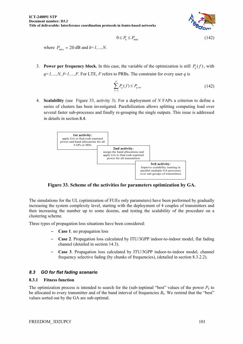
ICT-248891 STP Document number: D3.2 Title of deliverable: Interference coordination protocols in femto-based networks
FREEDOM_3D2UPCf 101
max0 kP P (142)
where max 20P dB and k=1,…,N.
3. Power per frequency block. In this case, the variable of the optimization is still ( )qP f , with
q=1,…,N, f=1,…,F. For LTE, F refers to PRBs. The constraint for every user q is
1
( )F
q q totf
P f P
(142)
4. Scalability (see Figure 33, activity 3). For a deployment of N FAPs a criterion to define a series of clusters has been investigated. Parallelization allows splitting computing load over several faster sub-processes and finally re-grouping the single outputs. This issue is addressed in details in section 8.4.
1st activity: apply GA to find (sub-)optimal
power and band allocations for all FAPs or MSs
2nd activity: assign the band allocations and apply GA to find (sub-)optimal
power for all transmitters
3rd activity: Improve scalability running in parallel multiple GA processes over sub-groups of transmitters
Figure 33. Scheme of the activities for parameters optimization by GA.
The simulations for the UL (optimization of FUEs only parameters) have been performed by gradually increasing the system complexity level, starting with the deployment of 4 couples of transmitters and then increasing the number up to some dozens, and testing the scalability of the procedure on a clustering scheme.
Three types of propagation loss situations have been considered:
– Case 1. no propagation loss
– Case 2. Propagation loss calculated by ITU/3GPP indoor-to-indoor model, flat fading channel (detailed in section 14.3).
– Case 3. Propagation loss calculated by ITU/3GPP indoor-to-indoor model, channel frequency selective fading (by chunks of frequencies), (detailed in section 8.3.2.2).
8.3 GO for flat fading scenario
8.3.1 Fitness function
The optimization process is intended to search for the (sub-)optimal “best” values of the power Pk to be allocated to every transmitter and of the band interval of frequencies Bk. We remind that the “best” values sorted out by the GA are sub-optimal.

102
When considering the genetic search for best transmission values, the simulation does not need synchronization among FAPs since this would require other resources to be provided and is not part of the present analysis. If by other means one could obtain synchronization among FAPs, and therefore among FUEs and the entire network, such properties could be taken into account and included in a modification of the present scheme.
The algorithm is designed to search for the frequency value at the beginning of the current band allocated, its relative width and the power of transmission, under the constraints in (141). The metrics measuring the goodness of the optimization algorithm expressed by the fitness functions defined in (139) and (140), the first based on maximizing the overall capacity of the system, the latter the second inspired by a more fair allocation of resources at system level.
8.3.2 Analysis of topologies for a single block
The performance of the genetic algorithm optimization has been tested in several cases of pathloss matrix structures, providing an output coherent with the value theoretically expected for the considered deployments.
In the present simulations we assume frame duration of 5 ms and that each FAP feeds back a single SNR data on the backhaul link per frame.
The parameters search by means of the GA has been implemented in two schemes:
1. Frequency and power search. The algorithm provides either the frequency allocation (starting value and bandwidth), or the power of transmission for the single FUESs to the corresponding FAPs. This analysis has been performed for flat fading and for selective fading propagation scenarios.
2. Power search only. We consider the case that the system has exploited other resources/strategies to assign the frequency channels to the various equipments (eventually also a preliminary run of a separate GA devoted to it), thus the GA searches for (sub)-optimal values of the transmission power in order to maximize capacity and minimize interference. The strategy can depend on the topology of the network and on the requirements of the analysis.
8.3.2.1 Flat fading channel
We present the results obtained for four FAPs in the same building, to assess the properties of the optimization procedure. As a test case, the simulations refer to a flat fading channel, thus one pathloss matrix suffices to provide a snapshot of the transmission capabilities of the system.
Let us first analyze the simple case of four FAPs equally interfering each other with a pathloss matrix constituted of zeros only, as expressed in dB by
0 0 0 0
0 0 0 0
0 0 0 0
0 0 0 0
lossL
(143)
The output of the genetic parameters search is depicted in Figure 34. The upper panel shows the evolution of the fitness function up to convergence, which stopped when the cumulative change in the fitness function is less than a fixed parameter (in our simulations equal to 1e-10), without computing the predetermined number of generations (350 in this scheme) and without a significant dependence on the population size (here fixed at 100 elements). The algorithm quickly converges providing the values to adopt for the transmission of the FUEs registered to the FAPs as shown in the bottom panel. The twelve variables subject to optimization are the starting frequency chunk (1st to 4th), the

ICT-248891 STP Document number: D3.2 Title of deliverable: Interference coordination protocols in femto-based networks
FREEDOM_3D2UPCf 103
bandwidth associated to each unit (5th to 8th) and the power allocated to each transmitter (9th to 12th). Thus, the value of the 1st variable represents the initial frequency value whose associated width is given by the value of the 5th variable and the power given by the 9th variable, and so on.
Figure 34. GA output for a set of 4 FUEs equally interfering each other. The variables in the bottom panel represent: 1-4 initial values of the frequency bands, 5-8 corresponding
bandwidth, 9-12 power allocations.
Every FUE has been assigned the same power (see the last four bars in the bottom plot), the capacity has been distributed as (50, 68, 35, 56) bits/s/Hz over the four FUEs. The resulting frequency and power allocations can be better viewed in the representation of Figure 35: the four FUEs can be assigned orthogonal frequency bands, thus minimizing the interference in UL, for an overall average capacity of 52.25 bits/s/Hz for the system, in this idealized test case.
Figure 35. GA output for 4 FUEs in terms of frequency and power allocations.

104
Let us consider an interference scenario in which one FUE (for example FUE number 1 in (144)) is mildly interfering with the other three which, on the other side, have a much higher level of mutual interference, as expressed by a pathloss matrix as
30 400 400 400
400 30 30 30
400 30 30 30
400 30 30 30
loss dL B
(144)
Such deployment refers to a case similar to the one depicted in Figure 36, leaving unmodified the assumption of one FUE per FAP.
Figure 36. Possible deployment corresponding to an interference scenario such as for a pathloss matrix of the type in Eq. (144).
In this case one gets a genetic algorithm output as detailed in Figure 37. The convergence is indeed fast, in terms of number of generations needed to find (sub-)optimal values for the twelve parameters. Once again, the four transmitters are assigned the maximum power of transmission, with a more imbalanced capacity as (142, 23, 136, 5) bits/s/Hz per transmitter, but a higher capacity (76.65 bits/s/Hz) for the overall system. This numbers are related to the chosen scenario: the pathloss expression and the little number of transmitters are simply adopted to validate the methodology. The band sharing is orthogonal among the three FUEs in a bunch (black, blue and green line in right panel of Figure 37) while the remaining FUE can use the whole spectrum (red line, in the same Figure).
Figure 37. GA output for 4 FUEs deployed as in Figure 36 and interference scenario
such as for a pathloss matrix of the type in Eq. (144).

ICT-248891 STP Document number: D3.2 Title of deliverable: Interference coordination protocols in femto-based networks
FREEDOM_3D2UPCf 105
Let us now consider the generic case of a realistic pathloss given for example by the matrix
56 78 93 93
55 45 84 85
95 84 58 83
87 84 66 61
loss dL B
(145)
which results in an optimization with capacity (9, 28, 14, 23) bits/s/Hz but with a spectrum assignment on orthogonal frequencies (overall capacity equal to 77 bits/s/Hz).
Figure 38. GA output for 4 FUEs deployed with an interference scenario such as for a pathloss matrix of the type in Eq. (145).
The same pathloss matrix (145) can give rise to a GA parameters search as displayed in Figure 39 three FUEs have been assigned orthogonal frequency chunks while the remaining one is fully interfering with one of them but with a definitely low power which, would indicate no transmission opportunity. The capacities are (0.06, 22.21, 54.04, 30.39) bits/s/Hz, respectively and the overall one 27 bits/s/Hz. The score of the fitness function is in both cases almost the same, with a value below -7, irrespective of fairness.
Figure 39. GA output for 4 FUEs deployed with an interference scenario corresponding to a pathloss matrix of the type in Eq. (145).
More examples can be found in section 14.4.

106
In the following sections we will analyze an approach to parallelization of the genetic algorithm parameters search for a large number of FAPs by developing the concept of clusterization on the basis, for example, of the analysis of effective pathloss matrix as discussed in Section 14.3.2.
8.3.2.2 GO for frequency selective channel
Let us consider the FAPs deployment in an environment of propagation with a frequency selective channel: the whole bandwidth is separated in a set of frequency chunks, whose number depends on the scenario of propagation, and the system is described by a pathloss matrix for every chunk.
As an example, let us address the case of a frequency selective channel divided in five chunks, each constituted by 16 subcarriers, every subcarrier 10 kHz wide.
Let us consider two realizations.
In the first, a set of pathloss matrices is given as in Table 19. In the first band of frequencies (chunk number 1) every FUE can communicate with its own FAP without interfering with others, while interference increases for the other frequency chunks.
0 60 120 120 60 0 60 60 120 60 0 120 120 60 120 0
0 60 60 60 60 0 120 120 60 120 0 120 60 120 120 0
0 0 60 60 60 0 60 60 60 0 0 60 60 0 60 0
0 30 30 30 30 0 120 120 30 80 0 80 30 120 120 0
0 120 120 120 120 0 120 120 120 120 0 120 120 120 120 0
Chunk 1 Chunk 2 Chunk 3
Chunk 5 Chunk 4
Table 19. Propagation loss matrices, in dB, for the separate frequency chunks. Rows follow FUE’s index, columns FAP’s index.
Figure 40. Overall output of the GA for the set of pathlosses described in Table 19.
The corresponding output of the GA optimization is shown in Figure 40. The result can be read in terms of frequency chunks allocations: the algorithm assigns maximum power to FAP/FUE when

ICT-248891 STP Document number: D3.2 Title of deliverable: Interference coordination protocols in femto-based networks
FREEDOM_3D2UPCf 107
interference from other transmitters is negligible and tends to reduce frequency allocations when it increases.
In the second realization pathlosses are the outcome of a scenario in which every FAP interferes with all other transmitters. Thus the pathlosses for the various chunks summarized in Table 20, give rise to a more variegate framework. In this example, we assumed that the first two frequency chunks have the same pathloss structure, while the other three frequency chunks are characterized by a certain propagation environment. Values in bold are relevant for the interpretation of the output detailed in Figure 41.
38 15 9 20 2 58 77 95 8 68 57 102 29 89 97 53
38 75 69 20 71 58 77 35 69 68 57 42 20 29 37 53
38 135 69 80 131 58 137 155 69 128 57 102 80 149 97 53
38 75 129 80 71 58 137 95 129 128 57 162 80 89 157 53
Chunks 1 and 2 Chunk 3
Chunk 4 Chunk 5
Table 20. Propagation loss matrices in dB for the separate frequency chunks. Rows follow FUE’s index, columns FAP’s index.
In chunk number 1, the first FUE has not been assigned a transmission opportunity as the pathloss with its own FAP is sensibly higher than with other FAPs in the environment. In the third chunk, the first three FUEs are privileged with respect to the fourth while in the fourth chunk we note how the second FUE has the best link with its own FAP. The same can be said for the FUE number 3 in chunk number 5.
As expected, the solution provided by the algorithm depends on the relative values of the pathloss matrix entries. Considering the increase of the unknown variables space by a factor equal to the number of chunks in the propagation emulation, convergence time of the GA is not affected by adopting several parallel GA processes.
Figure 41. Overall output of the GA for the set of pathlosses described in Table 20.
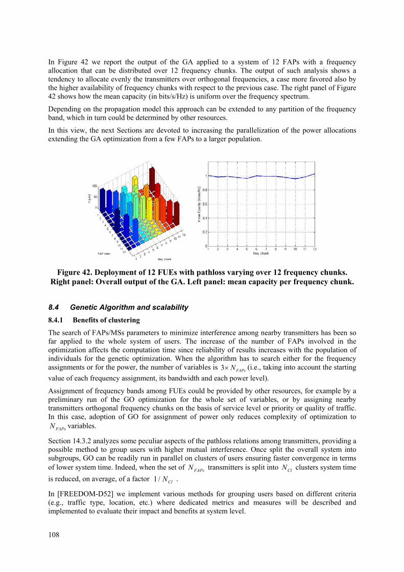
108
In Figure 42 we report the output of the GA applied to a system of 12 FAPs with a frequency allocation that can be distributed over 12 frequency chunks. The output of such analysis shows a tendency to allocate evenly the transmitters over orthogonal frequencies, a case more favored also by the higher availability of frequency chunks with respect to the previous case. The right panel of Figure 42 shows how the mean capacity (in bits/s/Hz) is uniform over the frequency spectrum.
Depending on the propagation model this approach can be extended to any partition of the frequency band, which in turn could be determined by other resources.
In this view, the next Sections are devoted to increasing the parallelization of the power allocations extending the GA optimization from a few FAPs to a larger population.
Figure 42. Deployment of 12 FUEs with pathloss varying over 12 frequency chunks. Right panel: Overall output of the GA. Left panel: mean capacity per frequency chunk.
8.4 Genetic Algorithm and scalability
8.4.1 Benefits of clustering
The search of FAPs/MSs parameters to minimize interference among nearby transmitters has been so far applied to the whole system of users. The increase of the number of FAPs involved in the optimization affects the computation time since reliability of results increases with the population of individuals for the genetic optimization. When the algorithm has to search either for the frequency assignments or for the power, the number of variables is 3 FAPsN (i.e., taking into account the starting
value of each frequency assignment, its bandwidth and each power level).
Assignment of frequency bands among FUEs could be provided by other resources, for example by a preliminary run of the GO optimization for the whole set of variables, or by assigning nearby transmitters orthogonal frequency chunks on the basis of service level or priority or quality of traffic. In this case, adoption of GO for assignment of power only reduces complexity of optimization to
FAPsN variables.
Section 14.3.2 analyzes some peculiar aspects of the pathloss relations among transmitters, providing a possible method to group users with higher mutual interference. Once split the overall system into subgroups, GO can be readily run in parallel on clusters of users ensuring faster convergence in terms of lower system time. Indeed, when the set of FAPsN transmitters is split into ClN clusters system time
is reduced, on average, of a factor 1 / ClN .
In [FREEDOM-D52] we implement various methods for grouping users based on different criteria (e.g., traffic type, location, etc.) where dedicated metrics and measures will be described and implemented to evaluate their impact and benefits at system level.
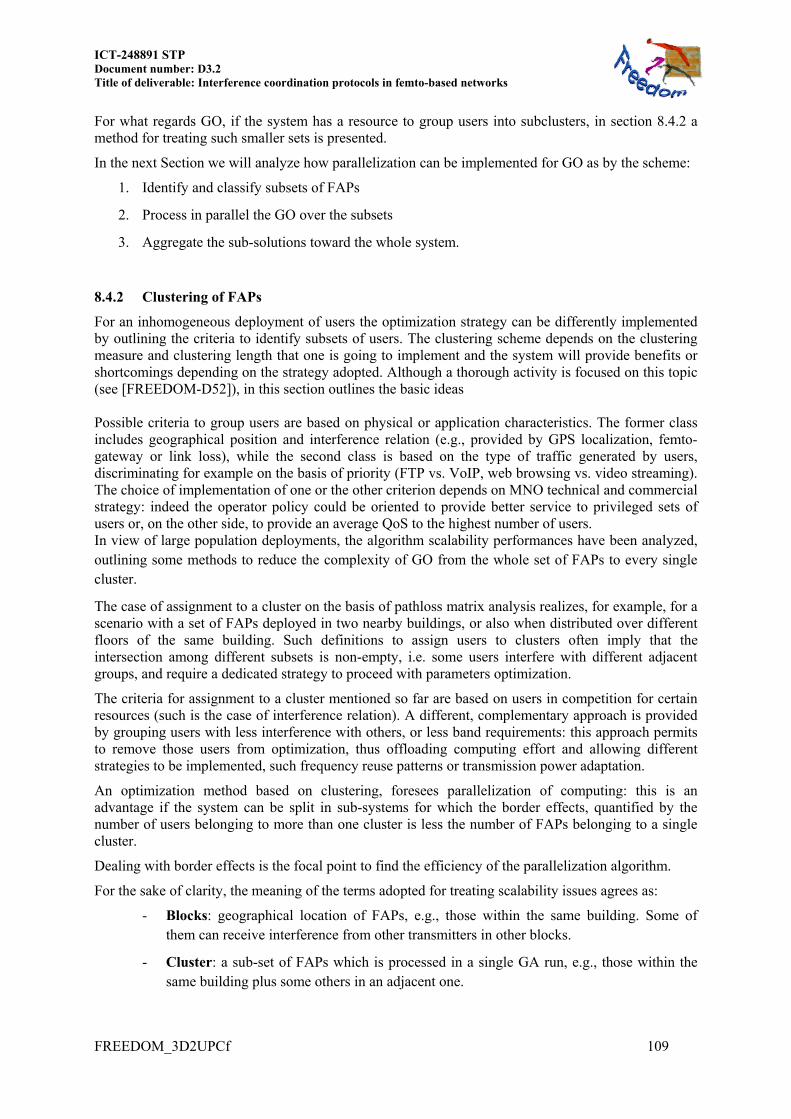
ICT-248891 STP Document number: D3.2 Title of deliverable: Interference coordination protocols in femto-based networks
FREEDOM_3D2UPCf 109
For what regards GO, if the system has a resource to group users into subclusters, in section 8.4.2 a method for treating such smaller sets is presented.
In the next Section we will analyze how parallelization can be implemented for GO as by the scheme:
1. Identify and classify subsets of FAPs
2. Process in parallel the GO over the subsets
3. Aggregate the sub-solutions toward the whole system.
8.4.2 Clustering of FAPs
For an inhomogeneous deployment of users the optimization strategy can be differently implemented by outlining the criteria to identify subsets of users. The clustering scheme depends on the clustering measure and clustering length that one is going to implement and the system will provide benefits or shortcomings depending on the strategy adopted. Although a thorough activity is focused on this topic (see [FREEDOM-D52]), in this section outlines the basic ideas Possible criteria to group users are based on physical or application characteristics. The former class includes geographical position and interference relation (e.g., provided by GPS localization, femto-gateway or link loss), while the second class is based on the type of traffic generated by users, discriminating for example on the basis of priority (FTP vs. VoIP, web browsing vs. video streaming). The choice of implementation of one or the other criterion depends on MNO technical and commercial strategy: indeed the operator policy could be oriented to provide better service to privileged sets of users or, on the other side, to provide an average QoS to the highest number of users. In view of large population deployments, the algorithm scalability performances have been analyzed, outlining some methods to reduce the complexity of GO from the whole set of FAPs to every single cluster.
The case of assignment to a cluster on the basis of pathloss matrix analysis realizes, for example, for a scenario with a set of FAPs deployed in two nearby buildings, or also when distributed over different floors of the same building. Such definitions to assign users to clusters often imply that the intersection among different subsets is non-empty, i.e. some users interfere with different adjacent groups, and require a dedicated strategy to proceed with parameters optimization.
The criteria for assignment to a cluster mentioned so far are based on users in competition for certain resources (such is the case of interference relation). A different, complementary approach is provided by grouping users with less interference with others, or less band requirements: this approach permits to remove those users from optimization, thus offloading computing effort and allowing different strategies to be implemented, such frequency reuse patterns or transmission power adaptation.
An optimization method based on clustering, foresees parallelization of computing: this is an advantage if the system can be split in sub-systems for which the border effects, quantified by the number of users belonging to more than one cluster is less the number of FAPs belonging to a single cluster.
Dealing with border effects is the focal point to find the efficiency of the parallelization algorithm.
For the sake of clarity, the meaning of the terms adopted for treating scalability issues agrees as:
- Blocks: geographical location of FAPs, e.g., those within the same building. Some of them can receive interference from other transmitters in other blocks.
- Cluster: a sub-set of FAPs which is processed in a single GA run, e.g., those within the same building plus some others in an adjacent one.

110
- Sub-set: any sub-group within the set of N FAPs.
The best-case for parallelization results when the whole set of FAPs can be split in N independent sub-sets, i.e. with empty intersection: in this event, the complexity of the optimization depends on hardware capability to deal with N independent computations. Complexity grows when an increasing number of FAPs belonging to a certain sub-set overlaps (e.g., interferes) with some FAPs of another sub-set. The system has to implement a strategy to deal with the parameters provided by two (or more, depending on the interference scheme among FAPs belonging to different sub-sets) independent GA optimizations.
When the output of an optimization runs over different clusters provides two possible parameters values for FAPs lying within the intersection, the system can swap or average the obtained values before running the next step of system optimization (for GO, typically a dozen times), adopting the results as initial values for the next run.
8.5 Synchronization issues and GO
8.5.1 Asynchronous scenario
The reference scenario is made up of an asynchronous ensemble FAP-FUE couples (assuming, one FUE and one FAP). This assumption should be better viewed as the lack of assumption on synchronism among an ensemble of objects driven by timers. Their natural state is to be asynchronous, unless specific resources and assumptions are introduced to insure a certain (sufficient) degree of synchronism among them. For instance, each FAP belonging to an ensemble of FAPs could be synchronised with the external BS, thus insuring a certain degree of synchronism among the ensemble. This implicitly introduces the assumption of a BS-FAP link not too weak (to let the FAP sense and synchronise) and not too strong (otherwise the FAP presence would be pointless). A similar consideration holds for a FAP-FAP synchronisation. In general, LTE identifies seven possible UL/DL structures for a frame, as summarized in Table 21 and, in principle, every FAP can adopt one different from others, due to its own requirements (e.g., UL/DL traffic ratio, etc.).
Table 21. UL/DL frame structures for LTE: -1 corresponds to DL, 1 to UL, 0 to
temporal slots.
case 0 subframe_structure = [-1 0 1 1 1 -1 0 1 1 1] ; case 1 subframe_structure = [-1 0 1 1 -1 -1 0 1 1 -1] ; case 2 subframe_structure = [-1 0 1 -1 -1 -1 0 1 -1 -1] ; case 3 subframe_structure = [-1 0 1 1 1 -1 -1 -1 -1 -1] ; case 4 subframe_structure = [-1 0 1 1 -1 -1 -1 -1 -1 -1] ; case 5 subframe_structure = [-1 0 1 -1 -1 -1 -1 -1 -1 -1] ; case 6 subframe_structure = [-1 0 1 1 1 -1 0 1 1 -1] ;
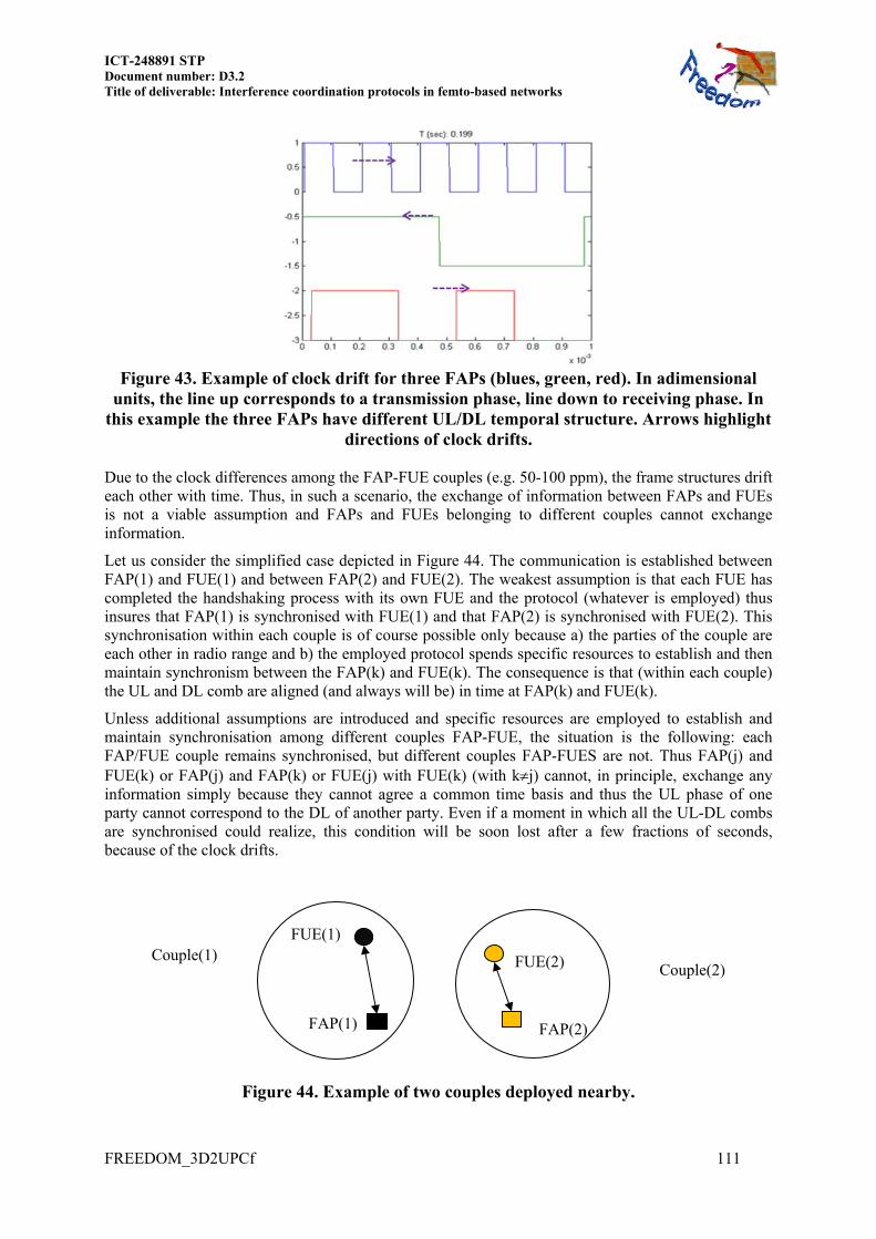
ICT-248891 STP Document number: D3.2 Title of deliverable: Interference coordination protocols in femto-based networks
FREEDOM_3D2UPCf 111
Figure 43. Example of clock drift for three FAPs (blues, green, red). In adimensional
units, the line up corresponds to a transmission phase, line down to receiving phase. In this example the three FAPs have different UL/DL temporal structure. Arrows highlight
directions of clock drifts. Due to the clock differences among the FAP-FUE couples (e.g. 50-100 ppm), the frame structures drift each other with time. Thus, in such a scenario, the exchange of information between FAPs and FUEs is not a viable assumption and FAPs and FUEs belonging to different couples cannot exchange information.
Let us consider the simplified case depicted in Figure 44. The communication is established between FAP(1) and FUE(1) and between FAP(2) and FUE(2). The weakest assumption is that each FUE has completed the handshaking process with its own FUE and the protocol (whatever is employed) thus insures that FAP(1) is synchronised with FUE(1) and that FAP(2) is synchronised with FUE(2). This synchronisation within each couple is of course possible only because a) the parties of the couple are each other in radio range and b) the employed protocol spends specific resources to establish and then maintain synchronism between the FAP(k) and FUE(k). The consequence is that (within each couple) the UL and DL comb are aligned (and always will be) in time at FAP(k) and FUE(k).
Unless additional assumptions are introduced and specific resources are employed to establish and maintain synchronisation among different couples FAP-FUE, the situation is the following: each FAP/FUE couple remains synchronised, but different couples FAP-FUES are not. Thus FAP(j) and FUE(k) or FAP(j) and FAP(k) or FUE(j) with FUE(k) (with kj) cannot, in principle, exchange any information simply because they cannot agree a common time basis and thus the UL phase of one party cannot correspond to the DL of another party. Even if a moment in which all the UL-DL combs are synchronised could realize, this condition will be soon lost after a few fractions of seconds, because of the clock drifts.
Figure 44. Example of two couples deployed nearby.
FAP(1)
FUE(1)
FAP(2)
FUE(2) Couple(1) Couple(2)

112
An example of how the frame structures drift each other has been purposely analyzed for the scenario with 3 FAP-FUE couples with different frame UL-DL combs and overall frame duration of 10 ms. Once given the timing differences of the quartzes, Figure 45 reports an example of the time variation of the mean (mean in each frame) theoretical capacity (solely depending on SNR) of the 3 FAPs, along with a detail showing the “fine structure” of the mean theoretical capacity. The leftmost plot shows the continuous drift among the UL-DL frame structures. Upper, intermediate and bottom lines correspond to the three FAPs. The observed time variation is solely due to the frame drifting, because of the relevant overlap between the UL and DL phases (unknown to each entity, as well as to a “hypothetic” central unit).
Figure 45. Capacity evolution for three couples FUEs/FAPs.
It is assumed that
Each unit in the scenario has at least the capability of estimating its own mean SNR experienced in a frame;
At the end of each frame, this estimated SNR can be delivered to the central processing unit, linked to each FAP via the backhaul link;
Each FAP may (or may not) know also the mean SNR (mean in a frame) of its FUE.
Summarising, in the case each FAP knows both its own mean SNR and the mean SNR of its FUE, once in a frame (at the end of) these 2 values can be delivered to the central processing unit. In such a case it can be implemented a procedure capable to jointly “optimise” the appropriate metric accounting for both UL and DL. In the case (maybe way too restrictive but worth to be considered for completeness) each FAP doesn’t know the mean SNR of its FUE, optimization of a suitable metric is only relevant to the UL. This is what could be referred as “optimisation of the UL”: as the metric includes only (mean) information coming from the UL, none can insure that the “optimal” resources allocations found in this case could not jeopardise the DL performance.
ICT-248891 STP Document number: D3.2 Title of deliverable: Interference coordination protocols in femto-based networks
FREEDOM_3D2UPCf 113
8.5.2 Design principles and constraints
Given the above, the design is the following:
The FAP-FUE couples in the scenario are not synchronised, so the design cannot rely on the exchange of information among them;
Each FAP and each FUE knows its own mean SNR experienced in a frame;
Once in a frame, the value of the mean SNR of each FAP and each FUE can be delivered (from the FAP ADSL link) to a central processing unit;
The central processing unit collects ONLY the SNR of FAPs and FUEs and knows who is who, but (of course) has no knowledge of who is interfering with who;
In the asynchronous scenario the contributions to SINR cannot be separated, because each FAP or FUE cannot know who is interfering with it. For N FAP-FUE couples, there are 2N entities in the scenario and thus the mean SNIR estimated by each unit is collected (including the interfering contributions, unknown to the unit, due to the other units). The assumption that each FAP can measure/estimate its own mean SNIR once in a frame and the same can do each FUE is extremely relaxed. These 2N numbers (i.e. some history) are sent and processed by the central unit, providing as output a resource allocation (e.g. frequency assignments) optimising the metric.
8.5.3 GA tested on a fully asynchronous frame sequence
In order to evaluate the effect on GA optimization method of lack of synchronization as detailed above, in this Section we present the results of running the GO for frequency only, keeping fixed the average transmission power. It has to be considered, as a simulation example, the case limited to the management of 3 FAP-FUE couples, but the simulation principle applies to an arbitrary number of FAP-FUE couples. Taking into account the continuous frame drift among the FAP-FUE couples, the simulator computes the mean SNR of each entity at each frame, implementing the asynchronous GA optimisation process giving as outputs the “best” frequency allocation.
8.5.3.1 Results of GA tested on fixed frame sequences
In this subsection, we present the results of GO for f3 and f4 metrics under the assumption the the system is asynchronous, every coupe FAP/FUE adopts a different frame structure and clocks have different time drifts un-compensated by synchronization methods. By adopting the 'max_service' fitness function and assuming that the requests of FAP1, 2 and 3 are 1, 3 and 4 Mbps, respectively, the output of the GA allocation is the one reported in Figure 46. It is clear that in both cases the output of the GA process actually approaches is compliant with the design of the fitness function.

114
Figure 46. Capacity output for GO implementing the ‘max_service’ metric. Implementation of the 'max_rate_fairness' fitness function, gives an output of the GA allocation whose effect on SNR (and therefore capacity) in time is reported in Figure 47.
Figure 47. Capacity output for GO implementing the ‘max_rate_fairness’ metric.
8.5.3.2 Results of GA tested on randomly changing frame sequences
This subsection reports for f0, f1, f2, f3 and f4 metrics influence on the SNR temporal evolution, testing the GA output in a peculiarly structured case. Although in principle unlikely, it has been tested the a scenario in which at every frame the sequence of UL and DL for the next frame is randomly changed for every couple. Convergence of the GA is verified and the optimization of results lead to a uniform of SNR in time, a pattern allowed by the intrinsic orthogonalization of frequency allocations.

ICT-248891 STP Document number: D3.2 Title of deliverable: Interference coordination protocols in femto-based networks
FREEDOM_3D2UPCf 115
Figure 48. Randomly changing frame schemes: GA capacity results for max sum rate and right max service metrics, left and right plots, respectively.
Figure 49. Randomly changing frame schemes: left UL, right DL.
Figure 50. Randomly changing frame schemes: maximum rate with fairness, left =1, right =1.3.
116
8.5.3.3 Conclusions on second tier synchronization and GA
When the synchronism assumption among all the FAPs and FUEs is removed, it is still possible to design a sub optimal resources allocation procedure, based on the mean SNR measured (in a frame) by each entity in the scenario and made available at a central processing unit. The GA approach has a working principle suitable for such a kind of problem. Although it is not the unique possible algorithmic approach, it is attractive for its simplicity and modularity. End-to-end, it inputs the mean SNRs from FAPs and FUEs (as many times as established by the choice operated on the “population” size) and outputs the “optimal” (in the sense of the adopted metric) radio resources allocation. Its main drawbacks rely in the convergence time and in the distance from the optimal solutions. Many computational aids can help to overcome the latter, but the compliance between the convergence time and the requirements at system level cannot be insured a priori in all scenarios. The results of the simulations in an asynchronous scenario have shown to be consistent with the “physical meaning” implemented in the adopted fitness functions, on which a specific effort must be spent in order to obtain a meaningful target and functional slopes easing the GA convergence capabilities.
8.6 Conclusions of the GO optimization
The search for transmission parameters minimizing interference in a system of FUEs and maximizing the overall system capacity has been performed by a genetic algorithm method implemented in the network at a centralized level. The same optimization can also be implemented as a distributed algorithm as introduced in Section 8.2.1, providing the same performances.
On the basis of the SNR fed back at a regular basis, not relevant for the present part of the analysis, the RRM can determine the frequency allocation and/or the power of transmission for the UL of every FUE in order to maximize the system capacity.
The method has been tested starting from some study-cases with already known best-solutions for various types of metrics investigating different constraints, finally extending the analysis to deployments with more than 100 FAPs/FUEs. For larger numbers it is reasonable that not all FUEs interfere with every other radio source, but this relation can be limited on the basis of distance and of obstacles in between. When this property is expressed in terms of a set of system features, such for example the pathloss matrix, it has been proposed a method to scale the system, splitting the whole set of users into sub-sets, reducing the computing complexity and obtaining faster results.

ICT-248891 STP Document number: D3.2 Title of deliverable: Interference coordination protocols in femto-based networks
FREEDOM_3D2UPCf 117
9 SIMULATION RESULTS The techniques investigated in this deliverable have been evaluated in two corporate-based scenarios: Small Corporate configuration which consists of one MBS and one FAP area (uniformly
distributed over the sector). The small Corporate scenario is depicted Figure 51 where one FAP area is deployed in a macrocell sector of radii equal to 500m. The FAP area contains two twin buildings separated by one street. We define by FAPload as the probability that an office/apartment has a FAP and it is active, i.e. FAPload=1 means that all offices have an active FAP (there are 60 FAPs in average). Each FAP is serving up to two FUEs. The system operates over a bandwidth of 5 MHz and we consider several limiting values for the backhaul connection (5Mbps, 10Mbps, 20Mbps, Mbps). See further details of this scenario in Table 22.
Figure 51. Small Corporate scenario
Parameters Values
Number of floors per building Uniform r.v. [1,..6] Number of offices per floor 25 Antenna configuration 4 (MBS) , 2 (FAP), 2 (MUE) Number of FAPs 12, 24, 36, 48, 60 in average Position of the FAP Indoor. Number of FUEs per FAP 1 or 2 Position of FUEs Indoor or Outdoor Prob. of an outdoor FUE 1
0.8n
n
for a FAP in the n-th floor
Number of MUEs 1 or 2
Table 22. Parameters considered for the scenario depicted in Figure 51
Simulated Corporate configuration which consists of one MBS and 10 FAP areas. In contrast to the previous scenario where all channel parameters (pathloss, shadowing, ...) were obtained from [FREEDOM-D21], this configuration have obtained those channel parameters by means of simulating all the buildings and terminal deployment using a VOLCANO-based simulator from SIRADEL. In this scenario we will assume that each office/apartment have a probability equal to 0.16 to have a FAP. The number of inhabitants/km2 is set to 740 for a given wireless mobile operator. Details on the FAP area configuration are introduced in Table 23. All FAPs are placed indoors and they are serving two FUEs. The served FUEs might be indoor or outdoor. In this
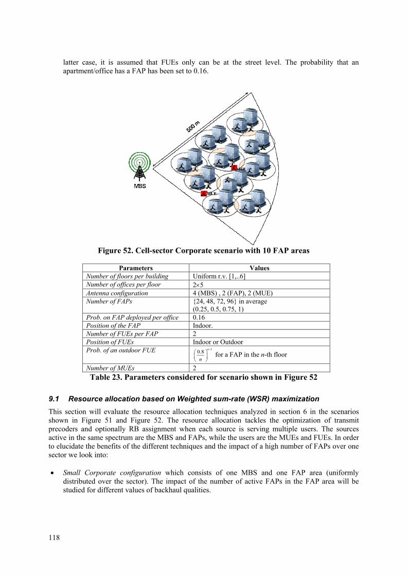
118
latter case, it is assumed that FUEs only can be at the street level. The probability that an apartment/office has a FAP has been set to 0.16.
Figure 52. Cell-sector Corporate scenario with 10 FAP areas
Parameters Values
Number of floors per building Uniform r.v. [1,..6] Number of offices per floor 25 Antenna configuration 4 (MBS) , 2 (FAP), 2 (MUE) Number of FAPs 24, 48, 72, 96 in average
(0.25, 0.5, 0.75, 1) Prob. on FAP deployed per office 0.16 Position of the FAP Indoor. Number of FUEs per FAP 2 Position of FUEs Indoor or Outdoor Prob. of an outdoor FUE 1
0.8n
n
for a FAP in the n-th floor
Number of MUEs 2
Table 23. Parameters considered for scenario shown in Figure 52
9.1 Resource allocation based on Weighted sum-rate (WSR) maximization
This section will evaluate the resource allocation techniques analyzed in section 6 in the scenarios shown in Figure 51 and Figure 52. The resource allocation tackles the optimization of transmit precoders and optionally RB assignment when each source is serving multiple users. The sources active in the same spectrum are the MBS and FAPs, while the users are the MUEs and FUEs. In order to elucidate the benefits of the different techniques and the impact of a high number of FAPs over one sector we look into: Small Corporate configuration which consists of one MBS and one FAP area (uniformly
distributed over the sector). The impact of the number of active FAPs in the FAP area will be studied for different values of backhaul qualities.

ICT-248891 STP Document number: D3.2 Title of deliverable: Interference coordination protocols in femto-based networks
FREEDOM_3D2UPCf 119
Parameters Values Priority of users Inversely proportional to the served rate
(proportional fair criterion) FUEs: 1/rFUE MUEs: 5/rMUE
Number of RB 25 (5MHz) Optimization variables Transmit precoders and RB assignment Maximum Backhaul rate at FAP 5, 10, 20, Mbps Resource allocation techniques Pricing vs. non-pricing Resource allocation criterion Maximization of the weighted sum rate
Table 24. Parameters considered when the evaluation is done over the Small Corporate configuration
Simulated Corporate configuration which consists of one MBS and 10 FAP areas. In contrast to
the previous scenario where all channel parameters (pathloss, shadowing, ...) were obtained from [FREEDOM-D21], this configuration have obtained those channel parameters by means of simulating all the buildings and terminal deployment using a VOLCANO-based simulator from SIRADEL. In this scenario we will assume that each office/apartment have a probability equal to 0.16 to have a FAP.
Parameters Values Priority of users FUEs: equal to 1
MUEs: equal to 5 Number of RB 100 (20MHz) Optimization variables a) Transmit precoders and RB assignment
b) Transmit precoders Maximum Backhaul rate 10, 20, 40, 80, Mbps Resource allocation techniques Pricing vs. non-pricing Resource allocation criterion Maximization of the weighted sum rate
Table 25. Parameters considered when the evaluation is done over the Simulated Corporate configuration
9.1.1 Small Corporate configuration
We would like to emphasize that the resource allocation algorithm tackles the optimization at the FAP and MBS, since both type of sources are sharing the same spectrum. In the scenario shown in Figure 51, MUEs are uniformly deployed over the sector, so in general will not be interfered by FAPs. However, MBS plays a dominant interferer for all FUEs. Therefore, the possible performance degradation at MUEs will be a consequence of decreasing the transmitted power used by the MBS. Figure 53 depicts the spectral efficiency attained by FUEs and MUEs for different configurations of active FAPs (denoted by variable FAPload) and maximum backhaul rate when pricing and non-pricing techniques are considered. Under maximum backhaul rates B=5,10 Mbps, the spectral efficiency of pricing and non-pricing techniques are almost the same for all FAPload configurations. When the B=20 Mbps the pricing technique improves the performance attained by the non-pricing one when FAPload= 1 (60 FAPs in average) with 10 bps/Hz. Furthermore, in case of B= Mbps, the gains become 6, 17, 29, 39, 51 bps/Hz when there are 12, 24, 36, 48, 60 FAPs in average, i.e. figures of merit 6%, 10%, 12%, 12%, 14% over the performance of non-pricing techniques. On the other hand, the spectral efficiency of MUEs, shown in Figure 53-right, illustrate that pricing techniques impose a worse performance compared with the non-pricing ones for B=5,10, 20 Mbps. Under the ideal backhaul configuration, the performance is the other way round. Notice, that in all cases FUEs improve their performance thanks to the pricing exchange, although in some cases the gain is very small. For example, B=20 Mbps and FAPload=0.8, FUEs can get 191 bps/Hz considering

120
the pricing technique, while they obtain 185 bps/Hz when non-pricing technique is envisioned. This gain comes at the cost of reducing the MUEs spectral efficiency from 7.98 bps/Hz to 7.14 bps/Hz
Figure 53. Spectral efficiency attained by Left) FUEs and Right) MUEs for a max
Backhaul rate B=5, 10, 20, Mbps with a FAPload l=0.2,04,0.6,0.8,1 (12, 24, 36, 48, 60) FAPs in average for pricing (P) and non-pricing (nP) techniques.
Figure 54. 10%-Outage Rate attained by Left) FUEs and Right) MUEs for max
Backhaul rate B=5, 10, 20, Mbps with a FAPload l=0.2,04,0.6,0.8,1 (12, 24, 36, 48, 60) FAPs in average for pricing (P) and non-pricing (nP) techniques
Figure 54 shows the performance of pricing and non-pricing techniques in terms of 10%-Outage Rate, i.e. the minimum achieved rate by the 90% of the users (FUEs and MUEs). Similar to the spectral efficiency results, the benefits of pricing techniques come up when the backhaul quality is not limiting the wireless communications, for example when B=20 Mbps and FAPload=1 or when B= Mbps and FAPload= 0.2, .., 1. FUEs get significant gains around 200-300% in this latter case. With respect the 10%-Outage Rate attained by MUEs, see Figure 54-right, using the pricing technique we can get bitrate different from zero in those cases where B=20, Mbps. This performance confirms that the pricing techniques are able to take into account the QoS (in terms of user priorities) of the different neighboring users. Under the configuration where all FAPs are active (and B= Mbps) it seems reasonable that in order to maximize the sum-rate of the system, the MBS should (the dominant interferer from the FUEs’ point of view) shut down because there are many FUEs.
1 2 3 46.5
7
7.5
8
8.5
bps
/Hz
Spectral Efficiency attained by MUEs
l= 0.2 nP
l= 0.4 nP
l= 0.6 nP
l= 0.8 nP
l= 1 nP
l= 0.2 P
l= 0.4 P
l= 0.6 P
l= 0.8 P
l= 1 P
B=5 Mbps B=10 Mbps B=20 Mbps
nopricing
B= Mbps
pricing
pricingnopricing
pricingnopricing
pricingnopricing
1 2 3 40
50
100
150
200
250
300
350
400
450
bps
/Hz
Spectral Efficiency attained by FUEs
l= 0.2 nP
l= 0.4 nP
l= 0.6 nP
l= 0.8 nP
l= 1 nP
l= 0.2 P
l= 0.4 P
l= 0.6 P
l= 0.8 P
l= 1 P
B=5 Mbpsnopricing pricing
pricingnopricing
B=10 Mbps
pricingnopricing
B=20 Mbps
nopricing
pricingB= Mbps
1 2 3 40
0.2
0.4
0.6
0.8
1
1.2
1.4
1.6
1.8
2
bps
/Hz
FUE 10%-Outage Rate
l= 0.2 nP
l= 0.4 nP
l= 0.6 nP
l= 0.8 nP
l= 1 nP
l= 0.2 P
l= 0.4 P
l= 0.6 P
l= 0.8 P
l= 1 P
B= Mbps
B=20 Mbps
B=10 Mbps
B=5 Mbps
nopricing
pricing
nopricing
pricing
nopricing pricing
nopricing pricing
1 2 3 40
0.2
0.4
0.6
0.8
1
1.2
1.4
1.6
1.8
2
bps
/Hz
MUE 10%-Outage Rate
l= 0.2 nP
l= 0.4 nP
l= 0.6 nP
l= 0.8 nP
l= 1 nP
l= 0.2 P
l= 0.4 P
l= 0.6 P
l= 0.8 P
l= 1 P
nopricing
B=5 Mbps
pricing
B=10 Mbps
B=20 Mbps
nopricing
B= Mbps
pricingnopricing
nopricing pricing
pricing
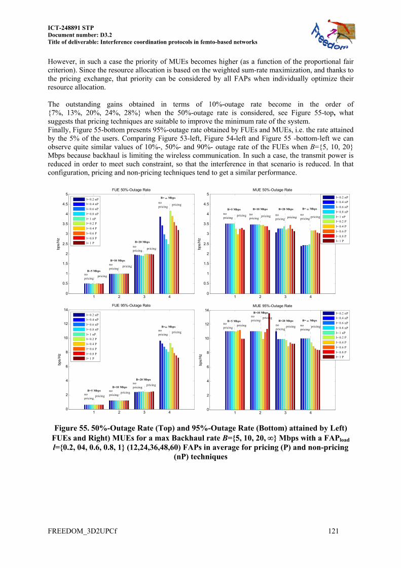
ICT-248891 STP Document number: D3.2 Title of deliverable: Interference coordination protocols in femto-based networks
FREEDOM_3D2UPCf 121
However, in such a case the priority of MUEs becomes higher (as a function of the proportional fair criterion). Since the resource allocation is based on the weighted sum-rate maximization, and thanks to the pricing exchange, that priority can be considered by all FAPs when individually optimize their resource allocation. The outstanding gains obtained in terms of 10%-outage rate become in the order of 7%, 13%, 20%, 24%, 28% when the 50%-outage rate is considered, see Figure 55-top, what suggests that pricing techniques are suitable to improve the minimum rate of the system. Finally, Figure 55-bottom presents 95%-outage rate obtained by FUEs and MUEs, i.e. the rate attained by the 5% of the users. Comparing Figure 53-left, Figure 54-left and Figure 55 -bottom-left we can observe quite similar values of 10%-, 50%- and 90%- outage rate of the FUEs when B=5, 10, 20 Mbps because backhaul is limiting the wireless communication. In such a case, the transmit power is reduced in order to meet such constraint, so that the interference in that scenario is reduced. In that configuration, pricing and non-pricing techniques tend to get a similar performance.
Figure 55. 50%-Outage Rate (Top) and 95%-Outage Rate (Bottom) attained by Left)
FUEs and Right) MUEs for a max Backhaul rate B=5, 10, 20, Mbps with a FAPload l=0.2, 04, 0.6, 0.8, 1 (12,24,36,48,60) FAPs in average for pricing (P) and non-pricing
(nP) techniques
1 2 3 40
0.5
1
1.5
2
2.5
3
3.5
4
4.5
5
bps
/Hz
FUE 50%-Outage Rate
l= 0.2 nP
l= 0.4 nP
l= 0.6 nP
l= 0.8 nP
l= 1 nP
l= 0.2 P
l= 0.4 P
l= 0.6 P
l= 0.8 P
l= 1 P
B= Mbps
B=20 Mbps
B=10 Mbps
B=5 Mbps
nopricing
pricing
pricingnopricing
pricingnopricing
pricingnopricing
1 2 3 40
0.5
1
1.5
2
2.5
3
3.5
4
4.5
5 b
ps/H
z
MUE 50%-Outage Rate
l= 0.2 nP
l= 0.4 nP
l= 0.6 nP
l= 0.8 nP
l= 1 nP
l= 0.2 P
l= 0.4 P
l= 0.6 P
l= 0.8 P
l= 1 P
nopricingpricing
nopricing
pricingnopricing
pricingnopricing
B=5 Mbps B=10 Mbps B=20 Mbps B= Mbps
pricing
1 2 3 40
2
4
6
8
10
12
14
bps
/Hz
FUE 95%-Outage Rate
l= 0.2 nP
l= 0.4 nP
l= 0.6 nP
l= 0.8 nP
l= 1 nP
l= 0.2 P
l= 0.4 P
l= 0.6 P
l= 0.8 P
l= 1 P
nopricing
pricing
B= Mbps
nopricing
pricing
B=20 Mbps
nopricing
B=10 MbpsB=5 Mbps
nopricing
pricingpricing
1 2 3 40
2
4
6
8
10
12
14
bps
/Hz
MUE 95%-Outage Rate
l= 0.2 nP
l= 0.4 nP
l= 0.6 nP
l= 0.8 nP
l= 1 nP
l= 0.2 P
l= 0.4 P
l= 0.6 P
l= 0.8 P
l= 1 P
nopricing
pricingB=5 Mbps
B=10 Mbpsnopricing
pricingB=20 Mbps
pricingnopricing
B= Mbps
nopricing
pricing
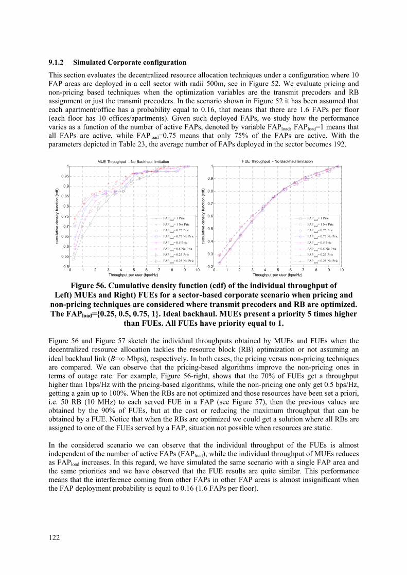
122
9.1.2 Simulated Corporate configuration
This section evaluates the decentralized resource allocation techniques under a configuration where 10 FAP areas are deployed in a cell sector with radii 500m, see in Figure 52. We evaluate pricing and non-pricing based techniques when the optimization variables are the transmit precoders and RB assignment or just the transmit precoders. In the scenario shown in Figure 52 it has been assumed that each apartment/office has a probability equal to 0.16, that means that there are 1.6 FAPs per floor (each floor has 10 offices/apartments). Given such deployed FAPs, we study how the performance varies as a function of the number of active FAPs, denoted by variable FAPload, FAPload=1 means that all FAPs are active, while FAPload=0.75 means that only 75% of the FAPs are active. With the parameters depicted in Table 23, the average number of FAPs deployed in the sector becomes 192.
Figure 56. Cumulative density function (cdf) of the individual throughput of
Left) MUEs and Right) FUEs for a sector-based corporate scenario when pricing and non-pricing techniques are considered where transmit precoders and RB are optimized. The FAPload=0.25, 0.5, 0.75, 1. Ideal backhaul. MUEs present a priority 5 times higher
than FUEs. All FUEs have priority equal to 1. Figure 56 and Figure 57 sketch the individual throughputs obtained by MUEs and FUEs when the decentralized resource allocation tackles the resource block (RB) optimization or not assuming an ideal backhaul link (B= Mbps), respectively. In both cases, the pricing versus non-pricing techniques are compared. We can observe that the pricing-based algorithms improve the non-pricing ones in terms of outage rate. For example, Figure 56-right, shows that the 70% of FUEs get a throughput higher than 1bps/Hz with the pricing-based algorithms, while the non-pricing one only get 0.5 bps/Hz, getting a gain up to 100%. When the RBs are not optimized and those resources have been set a priori, i.e. 50 RB (10 MHz) to each served FUE in a FAP (see Figure 57), then the previous values are obtained by the 90% of FUEs, but at the cost or reducing the maximum throughput that can be obtained by a FUE. Notice that when the RBs are optimized we could get a solution where all RBs are assigned to one of the FUEs served by a FAP, situation not possible when resources are static. In the considered scenario we can observe that the individual throughput of the FUEs is almost independent of the number of active FAPs (FAPload), while the individual throughput of MUEs reduces as FAPload increases. In this regard, we have simulated the same scenario with a single FAP area and the same priorities and we have observed that the FUE results are quite similar. This performance means that the interference coming from other FAPs in other FAP areas is almost insignificant when the FAP deployment probability is equal to 0.16 (1.6 FAPs per floor).
0 1 2 3 4 5 6 7 8 9 100.2
0.3
0.4
0.5
0.6
0.7
0.8
0.9
1
Throughput per user (bps/Hz)
cum
ulat
ive
dens
ity f
unct
ion
(cdf
)
FUE Throughput - No Backhaul limitation
FAPload
= 1 Pric
FAPload
= 1 No Pric
FAPload
= 0.75 Pric
FAPload
= 0.75 No Pric
FAPload
= 0.5 Pric
FAPload
= 0.5 No Pric
FAPload
= 0.25 Pric
FAPload
= 0.25 No Pric
0 1 2 3 4 5 6 7 8 9 100.5
0.55
0.6
0.65
0.7
0.75
0.8
0.85
0.9
0.95
1
Throughput per user (bps/Hz)
cum
ulat
ive
dens
ity f
unct
ion
(cdf
)
MUE Throughput - No Backhaul limitation
FAPload
= 1 Pric
FAPload
= 1 No Pric
FAPload
= 0.75 Pric
FAPload
= 0.75 No Pric
FAPload
= 0.5 Pric
FAPload
= 0.5 No Pric
FAPload
= 0.25 Pric
FAPload
= 0.25 No Pric
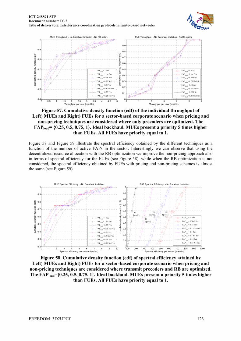
ICT-248891 STP Document number: D3.2 Title of deliverable: Interference coordination protocols in femto-based networks
FREEDOM_3D2UPCf 123
Figure 57. Cumulative density function (cdf) of the individual throughput of
Left) MUEs and Right) FUEs for a sector-based corporate scenario when pricing and non-pricing techniques are considered where only precoders are optimized. The
FAPload= 0.25, 0.5, 0.75, 1. Ideal backhaul. MUEs present a priority 5 times higher than FUEs. All FUEs have priority equal to 1.
Figure 58 and Figure 59 illustrate the spectral efficiency obtained by the different techniques as a function of the number of active FAPs in the sector. Interestingly we can observe that using the decentralized resource allocation with the RB optimization we improve the non-pricing approach also in terms of spectral efficiency for the FUEs (see Figure 58), while when the RB optimization is not considered, the spectral efficiency obtained by FUEs with pricing and non-pricing schemes is almost the same (see Figure 59).
Figure 58. Cumulative density function (cdf) of spectral efficiency attained by
Left) MUEs and Right) FUEs for a sector-based corporate scenario when pricing and non-pricing techniques are considered where transmit precoders and RB are optimized. The FAPload=0.25, 0.5, 0.75, 1. Ideal backhaul. MUEs present a priority 5 times higher
than FUEs. All FUEs have priority equal to 1.
0 0.5 1 1.5 2 2.5 3 3.5 4 4.5 50.4
0.5
0.6
0.7
0.8
0.9
1
Throughput per user (bps/Hz)
cum
ulat
ive
dens
ity f
unct
ion
(cdf
)MUE Throughput - No Backhaul limitation - No RB optim.
FAPload
= 1 Pric
FAPload
= 1 No Pric
FAPload
= 0.75 Pric
FAPload
= 0.75 No Pric
FAPload
= 0.5 Pric
FAPload
= 0.5 No Pric
FAPload
= 0.25 Pric
FAPload
= 0.25 No Pric
0 1 2 3 4 5 60
0.1
0.2
0.3
0.4
0.5
0.6
0.7
0.8
0.9
1
Throughput per user (bps/Hz)
cum
ulat
ive
dens
ity f
unct
ion
(cdf
)
FUE Throughput - No Backhaul limitation - No RB optim.
FAPload
= 1 Pric
FAPload
= 1 No Pric
FAPload
= 0.75 Pric
FAPload
= 0.75 No Pric
FAPload
= 0.5 Pric
FAPload
= 0.5 No Pric
FAPload
= 0.25 Pric
FAPload
= 0.25 No Pric
0 1 2 3 4 5 6 7 8 9 100.2
0.3
0.4
0.5
0.6
0.7
0.8
0.9
1
Spectral efficiency per sector (bps/Hz)
cum
ulat
ive
dens
ity f
unct
ion
(cdf
)
MUE Spectral Efficiency - No Backhaul limitation
FAPload
= 1 Pric
FAPload
= 1 No Pric
FAPload
= 0.75 Pric
FAPload
= 0.75 No Pric
FAPload
= 0.5 Pric
FAPload
= 0.5 No Pric
FAPload
= 0.25 Pric
FAPload
= 0.25 No Pric
100 200 300 400 500 600 700 800 900 10000
0.1
0.2
0.3
0.4
0.5
0.6
0.7
0.8
0.9
1
Spectral efficiency per sector (bps/Hz)
cum
ulat
ive
dens
ity f
unct
ion
(cdf
)
FUE Spectral Efficiency - No Backhaul limitation
FAPload
= 1 Pric
FAPload
= 1 No Pric
FAPload
= 0.75 Pric
FAPload
= 0.75 No Pric
FAPload
= 0.5 Pric
FAPload
= 0.5 No Pric
FAPload
= 0.25 Pric
FAPload
= 0.25 No Pric
10bps/Hz
14bps/Hz
28bps/Hz
38bps/Hz

124
Figure 59. Cumulative density function (cdf) of spectral efficiency attained by
Left) MUEs and Right) FUEs for a sector-based corporate scenario when pricing and non-pricing techniques are considered where only transmit precoders are optimized.
The FAPload= 0.25, 0.5, 0.75, 1. Ideal backhaul. MUEs present a priority 5 times higher than FUEs. All FUEs have priority equal to 1.
Finally, Figure 60 depicts how the spectral efficiency attained by FUEs and MUEs evolves as a function of different qualities on the backhaul link and number of active FAPs. The pricing technique becomes useful from the point of view of FUEs when there is an ideal backhaul. Notice that in this simulated scenario all FUEs have the same priority. On the other hand, pricing enhances the non-pricing performance attained by MUEs in all cases. It has to be remarked that as we increase the quality of the backhaul, the FUEs improve their spectral efficiency. Therefore, its impact of the overall weighted sum rate (considering FUEs and MUEs) also increases. Since the MBS is a dominant interferer for all FUEs, the MBS has to reduce its transmitted power and the spectral efficiency attained by MUEs decrease.
Figure 60. Average Spectral Efficiency attained by Left) FUEs and Right) MUEs when B=10, 20, 40, 80, Mbps and FAPload=0.75, 1. Pricing and non-pricing techniques
with transmit precoders and RB assignment optimization are considered. MUEs present a priority 5 times higher than FUEs. All FUEs have priority equal to 1
1 2 3 4 51.5
2
2.5
3
3.5
4
bps
/Hz
Spectral Efficiency attained by MUEs
l= 0.75 nP
l= 1 nP
l= 0.75 P
l= 1 P
B= 10 Mbps
pricing
B= Mbps
B= 40 Mbps
B= 20 Mbps
pricingnopricingpricing pricing
nopricing
pricing
B= 80 Mbps
nopricing
nopricing
nopricing
1 2 3 4 50
100
200
300
400
500
600
700
bps
/Hz
Spectral Efficiency attained by FUEs
l= 0.75 nP
l= 1 nP
l= 0.75 P
l= 1 P
B= Mbps
pricingnopricing
B= 80 Mbps
pricingnopricing
pricingnopricing
B= 40 Mbps
pricingnopricing
B= 20 Mbps
pricingnopricing
B= 10 Mbps
0 1 2 3 4 5 6 7 8 9 100.2
0.3
0.4
0.5
0.6
0.7
0.8
0.9
1
Spectral efficiency per sector (bps/Hz)
cum
ulat
ive
dens
ity f
unct
ion
(cdf
)MUE Spectral Efficiency - No Backhaul limitation - No RB optim.
FAPload
= 1 Pric
FAPload
= 1 No Pric
FAPload
= 0.75 Pric
FAPload
= 0.75 No Pric
FAPload
= 0.5 Pric
FAPload
= 0.5 No Pric
FAPload
= 0.25 Pric
FAPload
= 0.25 No Pric
100 200 300 400 500 600 700 800 900 10000
0.1
0.2
0.3
0.4
0.5
0.6
0.7
0.8
0.9
1
Spectral efficiency per sector (bps/Hz)
cum
ulat
ive
dens
ity f
unct
ion
(cdf
)
FUE Spectral Efficiency - No Backhaul limitation - No RB optim.
FAPload
= 1 Pric
FAPload
= 1 No Pric
FAPload
= 0.75 Pric
FAPload
= 0.75 No Pric
FAPload
= 0.5 Pric
FAPload
= 0.5 No Pric
FAPload
= 0.25 Pric
FAPload
= 0.25 No Pric

ICT-248891 STP Document number: D3.2 Title of deliverable: Interference coordination protocols in femto-based networks
FREEDOM_3D2UPCf 125
9.1.3 Conclusions
Pricing techniques are suitable for interference-limited scenarios. The backhaul link influences
on the maximum power transmitted, and the generated interference.
Pricing techniques are able to improve gains in the order of 5-15% in terms of spectral efficiency
Pricing allows controlling the quality of service, improving the minimum rate (10%-outage rate) by a factor of 2-3 times, i.e. gains of 200 -300% over the non-pricing techniques
The interference generated by other FAP areas to FUEs is almost insignificant because the FAPs are placed indoors and they are not transmitting at full power in all cases because their FUEs are nearby. .
We have observed that the resource allocation techniques that optimize transmit precoders and RB assignment are able to get gains in terms of spectral efficiency and outage rate when pricing exchange is considered. However, when only transmit precoders are optimized, the obtained gains are in terms of outage rate.
9.2 Resource allocation based on power minimization
This section will present simulation results for the proposed approach in the FREEDOM corporate scenario shown in Figure 51. Specific aspects of the simulations results included in this section are:
- MBS transmissions are considered in the FREEDOM small corporate scenario. While the MBS sends cost information to neighbor FAPs to prevent them to transmit at certain directions/carriers, the MBS ignores any pricing information from the FAPs.
- In the FREEDOM small corporate scenario, FAP and MBS nominal powers are respectively 20 dBm and 46 dBm. This power can never be surpassed, even in the initial iterations of the minimum power proposed algorithm. If at some iteration, a serving station (FAP or MBS) requires transmitting a higher power than this to fulfil the target rate, it will not be allowed. In this situation, we have use the QoS readjustment algorithm proposed in [Munoz11a] to reduce the target rate at this iteration in order to keep the power in the margin (19.5,20] dBm and (45.5,46] dBm for the FAPs and MBS respectively4. If the serving stations do not need to exceed the maximum power for the served UEs to achieve the target rate, the total transmission power will be minimized.
All the results presented in this section have been obtained for two target rates, 2 bps/Hz and 4 bps/Hz (the same target rate is considered for all FUEs and MUEs), and for the following cases regarding FAP antennas and UE antennas: 22 (MIMO), 21 (MISO), and 11 (SISO). The MBS is considered always with 4 antennas.
4 A narrower power margin can be considered for the QoS readjustment at the expense of a higher computational load for the calculation of the afforded rates.

126
9.2.1 Results for a single scenario with a fixed number of FAPs
The first set of results corresponds to a single realization of the scenario depicted in Figure 51. A FAP area with 32 active FAPs has been deployed within a sector of the MBS. In the same sector, the MBS is serving 2 MUEs. Each FAP has 1 FUE connected to. Figure 61 and Figure 62 depict the average rate received by FUEs and MUEs and transmitted power of FAPs and MBS, respectively. For the 2 bps/Hz, all the schemes allow the FUEs to achieve the target rate with the serving FAP transmitting well below the maximum transmission power. In such a case, it is clear the advantage of using pricing in terms of the average FAP power (equivalently total transmission power) for all the antenna schemes: MIMO (22), MISO (21), and SISO (21).
Figure 61. (Top) Average rate per FUE for a UE target rate of 2 bps/Hz (top-left) and 4 bps/Hz (top-right). (Bottom) Average rate for the two MUEs, considering a UE target
rate of 2 bps/Hz (bottom-left) and 4 bps/Hz (bottom-right). MUEs randomly deployed in the sector.
When increasing the target rate up to 4 bps/Hz, the SISO scheme fails to provide the target rate with and without pricing (see in Figure 61-top-right). However, the achieved rate in the SISO case is higher when pricing is used, achieving the same value than the MISO (21) scheme without pricing. There is no power saving in the SISO case because of the pricing, due to the fact that, for the SISO scheme and target rate of 4 bps/Hz, a lot of FAPs are in the limited power zone, and the limitation is the same for both pricing and no pricing cases, see Figure 62-top-right. As for the MISO (21) case, while this scheme fails to provide the target rate without pricing, it can provide the target rate when pricing is used. Furthermore, the use of pricing allows reducing the transmission power significantly. For the MIMO (22) case, there is no difference regarding the achieved rate with and without pricing, as in
0 5 10 15 20 25 300
0.5
1
1.5
2
2.5
Iteration
Ave
rage
FU
E r
ate(
bps/
Hz)
Average FUE rate, # FAPs=32, UE Target Rate=2 bps/Hz
Pricing 2x2No pricing 2x2
Pricing 2x1
No pricing 2x1
Pricing 1x1No pricing 1x1
0 5 10 15 20 25 300
0.5
1
1.5
2
2.5
3
3.5
4
4.5
Iteration
Ave
rage
FU
E r
ate(
bps/
Hz)
Average FUE rate, # FAPs=32, UE Target Rate=4 bps/Hz
Pricing 2x2No pricing 2x2
Pricing 2x1
No pricing 2x1
Pricing 1x1No pricing 1x1
0 5 10 15 20 25 300
0.5
1
1.5
2
2.5
Iteration
Ave
rage
MU
E r
ate(
bps/
Hz)
Average MUE rate, # FAPs=32, UE Target Rate=2 bps/Hz
Pricing 2x2No pricing 2x2
Pricing 2x1
No pricing 2x1
Pricing 1x1No pricing 1x1
0 5 10 15 20 25 300
0.5
1
1.5
2
2.5
3
3.5
4
4.5
Iteration
Ave
rage
MU
E r
ate(
bps/
Hz)
Average MUE rate, # FAPs=32, UE Target Rate=4 bps/Hz
Pricing 2x2No pricing 2x2
Pricing 2x1
No pricing 2x1
Pricing 1x1No pricing 1x1

ICT-248891 STP Document number: D3.2 Title of deliverable: Interference coordination protocols in femto-based networks
FREEDOM_3D2UPCf 127
any case the target rate is achieved, but there is also a significant saving in the transmission power if pricing is used (see Figure 62-top-right). The MBS always transmits with 4 antennas. The two MUEs are in this particular realization far from the FAP area and close to the MBS. Furthermore the MBS does not take into account the impact of its own transmissions on FUEs. This explains why there is no difference between pricing and no pricing for the MUEs performance and the MBS power, see Figure 61-bottom and Figure 62-bottom, respectively. Notice that the results are independent of the number of antennas in the FAPs, therefore the performance for the MISO (22) and SISO (11) case are equal, as the only change is on the number of FAP antennas.
Figure 62. (Top) Average power per FAP (#FAPs=32) for a UE target rate of 2 bps/Hz
(top-left) and 4 bps/Hz (top-right). (Bottom) MBS power for a UE target rate of 2 bps/Hz (bottom-left) and 4 bps/Hz (bottom-right). MUEs randomly deployed in the
sector. Instead of deploying the MUEs close to the MBS and far from the FAP area, for the next set of results the MUEs have been placed randomly within the FAP area. Therefore, the conditions for the MUEs become worse and the MBS must increase the power to fulfill the rate constraint, interfering more the FUEs. On the other hand, when pricing is considered, the FAPs should allocate their resources to avoid degrading MUEs performance, which may result in some degradation for the FUEs performance, as the MBS does not act in the same way. In such a situation, the next figures depict the average rate at the FUEs and MUEs (2), and average transmitted power by FAPs and MBS in Figure 63 and Figure 64, respectively.
0 5 10 15 20 25 30-12
-11
-10
-9
-8
-7
-6
-5
-4
Iteration
Ave
rage
pow
er p
er F
AP
(dB
m)
Average FAP power, # FAPs=32, UE Target Rate=2 bps/Hz
Pricing 2x2No pricing 2x2
Pricing 2x1
No pricing 2x1
Pricing 1x1No pricing 1x1
0 5 10 15 20 25 30-10
-5
0
5
10
15
20
Iteration
Ave
rage
pow
er p
er F
AP
(dB
m)
Average FAP power, # FAPs=32, UE Target Rate=4 bps/Hz
Pricing 2x2No pricing 2x2
Pricing 2x1
No pricing 2x1
Pricing 1x1No pricing 1x1
0 5 10 15 20 25 3011
12
13
14
15
16
17
18
Iteration
Ave
rage
MB
S p
ower
(dB
m)
MBS power,# FAPs=32, UE Target Rate=2 bps/Hz
Pricing 2x2No pricing 2x2
Pricing 2x1
No pricing 2x1
Pricing 1x1No pricing 1x1
0 5 10 15 20 25 3017
18
19
20
21
22
23
24
25
Iteration
Ave
rage
MB
S p
ower
(dB
m)
MBS power,# FAPs=32, UE Target Rate=4 bps/Hz
Pricing 2x2No pricing 2x2
Pricing 2x1
No pricing 2x1
Pricing 1x1No pricing 1x1

128
Figure 63. (Top) Average rate per FUE for a UE target rate of 2 bps/Hz (top-left) and 4 bps/Hz (top-right). (Bottom) Average rate for the two MUEs, considering a UE target
rate of 2 bps/Hz (bottom-left) and 4 bps/Hz (bottom-right). MUEs in the FAP area. For the FAPs and FUEs similar conclusions than from Figure 61 and Figure 62 can be extracted. The system is now more constrained for the reasons explained above. It is worthy of comment that the difference between pricing and no pricing in term of transmission power decreases when the station is transmitting with very high power (observe the SISO case in Figure 64-top-right), as the maximum value of the transmission power is limited. The major benefits from pricing in terms of power occur when the system is not too constrained (that is, when the power does not need to be close to the maximum value), but the required power is not too low (as if the required power is too low, it is likely because the experienced interference is too low, so pricing is not necessary). Now the interference from FAPs to the MUEs is significant. Therefore, the MBS is forced to transmit at its maximum power (see Figure 64-bottom). Even doing so, the target rate cannot be achieved by the MUEs placed within the FAP area (see Figure 63-bottom). Nevertheless, the use of pricing allows the MUEs to achieve a higher rate, as the pricing will make the FAPs to transmit less power and also to allocate their resources to reduce the degradation on the MUEs performance.
0 5 10 15 20 25 300
0.5
1
1.5
2
2.5
Iteration
Ave
rage
FU
E r
ate(
bps/
Hz)
Average FUE rate, # FAPs=33, UE Target Rate=2 bps/Hz
Pricing 2x2No pricing 2x2
Pricing 2x1
No pricing 2x1
Pricing 1x1No pricing 1x1
0 5 10 15 20 25 300
0.5
1
1.5
2
2.5
3
3.5
4
4.5
Iteration
Ave
rage
FU
E r
ate(
bps/
Hz)
Average FUE rate, # FAPs=33, UE Target Rate=4 bps/Hz
Pricing 2x2No pricing 2x2
Pricing 2x1
No pricing 2x1
Pricing 1x1No pricing 1x1
0 5 10 15 20 25 300
0.2
0.4
0.6
0.8
1
1.2
1.4
Iteration
Ave
rage
MU
E r
ate(
bps/
Hz)
Average MUE rate, # FAPs=33, UE Target Rate=2 bps/Hz
Pricing 2x2No pricing 2x2
Pricing 2x1
No pricing 2x1
Pricing 1x1No pricing 1x1
0 5 10 15 20 25 300
0.2
0.4
0.6
0.8
1
1.2
1.4
Iteration
Ave
rage
MU
E r
ate(
bps/
Hz)
Average MUE rate, # FAPs=33, UE Target Rate=4 bps/Hz
Pricing 2x2No pricing 2x2
Pricing 2x1
No pricing 2x1
Pricing 1x1No pricing 1x1

ICT-248891 STP Document number: D3.2 Title of deliverable: Interference coordination protocols in femto-based networks
FREEDOM_3D2UPCf 129
Figure 64. (Top) Average power per FAP (#FAPs=32) for a UE target rate of 2 bps/Hz
(top-left) and 4 bps/Hz (top-right). (Bottom) MBS power for a UE target rate of 2 bps/Hz (bottom-left) and 4 bps/Hz (bottom-right). MUEs in the FAP area.
9.2.2 Results for several scenarios
In the following we are going to show the CDF of the FUEs/MUEs rate in Figure 65 and CDF of the transmitted power by FAPs/MBS in Figure 66. To that end 50 independent scenarios are generated. In each of them, the FAP area is placed randomly within the sector. The average number of active FAPs is 30, despite it is a random variable, and each FAP is serving 1 FUE. The MBS is serving 2 MUEs randomly placed within the sector. Observing the CDF of the FUE rates in Figure 65-top-left, we see that for a target rate of 2 bps/Hz, all the FUEs achieve the target rate if pricing is used. However, if pricing is not used, 5% of the users in the MISO (2x1) case and 15% of the users in the SISO (1x1) case will not achieve the target rate. The percentage increases when increasing the target rate (see Figure 65-top-right), up to 25% and near 40% for MISO and SISO without pricing. In such a case, the use of pricing allows to increase the number of satisfied users a 10%, 20% and 10% for the SISO, MISO and MIMO case respectively. Also from the CDF of the FAP power in Figure 66-top, power savings can be observed when pricing is used. Taking for instance, a target rate of 4 bps/Hz, for MIMO and MISO case, we observe a reduction between 5% and 15% respectively of the number of FAPs transmitting at the maximum power if pricing is used. Finally, for the MBS, as the probability for the MUEs to be close to the FAP area is low, there is no difference between pricing and no pricing (see Figure 65-bottom and Figure 66-bottom).
0 5 10 15 20 25 30-10
-5
0
5
10
15
Iteration
Ave
rage
pow
er p
er F
AP
(dB
m)
Average FAP power, # FAPs=33, UE Target Rate=2 bps/Hz
Pricing 2x2No pricing 2x2
Pricing 2x1
No pricing 2x1
Pricing 1x1No pricing 1x1
0 5 10 15 20 25 30-5
0
5
10
15
20
Iteration
Ave
rage
pow
er p
er F
AP
(dB
m)
Average FAP power, # FAPs=33, UE Target Rate=4 bps/Hz
Pricing 2x2No pricing 2x2
Pricing 2x1
No pricing 2x1
Pricing 1x1No pricing 1x1
0 5 10 15 20 25 3040
41
42
43
44
45
46
47
48
49
50
Iteration
Ave
rage
MB
S p
ower
(dB
m)
MBS power,# FAPs=33, UE Target Rate=2 bps/Hz
Pricing 2x2No pricing 2x2
Pricing 2x1
No pricing 2x1
Pricing 1x1No pricing 1x1
0 5 10 15 20 25 3040
41
42
43
44
45
46
47
48
49
50
Iteration
Ave
rage
MB
S p
ower
(dB
m)
MBS power,# FAPs=33, UE Target Rate=4 bps/Hz
Pricing 2x2No pricing 2x2
Pricing 2x1
No pricing 2x1
Pricing 1x1No pricing 1x1
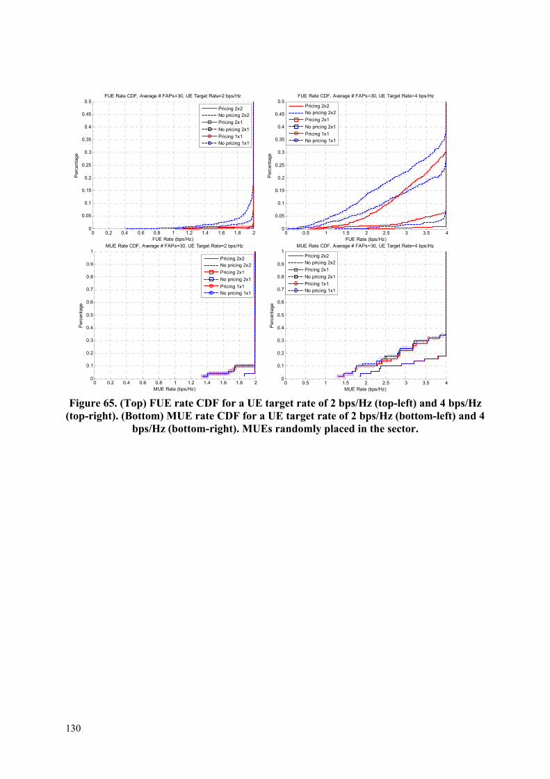
130
Figure 65. (Top) FUE rate CDF for a UE target rate of 2 bps/Hz (top-left) and 4 bps/Hz
(top-right). (Bottom) MUE rate CDF for a UE target rate of 2 bps/Hz (bottom-left) and 4 bps/Hz (bottom-right). MUEs randomly placed in the sector.
0 0.2 0.4 0.6 0.8 1 1.2 1.4 1.6 1.8 20
0.05
0.1
0.15
0.2
0.25
0.3
0.35
0.4
0.45
0.5
FUE Rate (bps/Hz)
Per
cent
age
FUE Rate CDF, Average # FAPs=30, UE Target Rate=2 bps/Hz
Pricing 2x2No pricing 2x2
Pricing 2x1
No pricing 2x1
Pricing 1x1No pricing 1x1
0 0.5 1 1.5 2 2.5 3 3.5 40
0.05
0.1
0.15
0.2
0.25
0.3
0.35
0.4
0.45
0.5
FUE Rate (bps/Hz)
Per
cent
age
FUE Rate CDF, Average # FAPs=30, UE Target Rate=4 bps/Hz
Pricing 2x2No pricing 2x2
Pricing 2x1
No pricing 2x1
Pricing 1x1No pricing 1x1
0 0.2 0.4 0.6 0.8 1 1.2 1.4 1.6 1.8 20
0.1
0.2
0.3
0.4
0.5
0.6
0.7
0.8
0.9
1
MUE Rate (bps/Hz)
Per
cent
age
MUE Rate CDF, Average # FAPs=30, UE Target Rate=2 bps/Hz
Pricing 2x2No pricing 2x2
Pricing 2x1
No pricing 2x1
Pricing 1x1No pricing 1x1
0 0.5 1 1.5 2 2.5 3 3.5 40
0.1
0.2
0.3
0.4
0.5
0.6
0.7
0.8
0.9
1
MUE Rate (bps/Hz)
Per
cent
age
MUE Rate CDF, Average # FAPs=30, UE Target Rate=4 bps/Hz
Pricing 2x2No pricing 2x2
Pricing 2x1
No pricing 2x1
Pricing 1x1No pricing 1x1
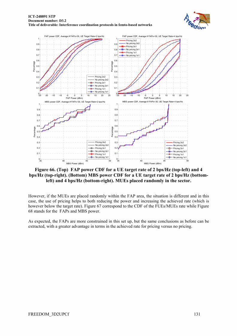
ICT-248891 STP Document number: D3.2 Title of deliverable: Interference coordination protocols in femto-based networks
FREEDOM_3D2UPCf 131
Figure 66. (Top) FAP power CDF for a UE target rate of 2 bps/Hz (top-left) and 4
bps/Hz (top-right). (Bottom) MBS power CDF for a UE target rate of 2 bps/Hz (bottom-left) and 4 bps/Hz (bottom-right). MUEs placed randomly in the sector.
However, if the MUEs are placed randomly within the FAP area, the situation is different and in this case, the use of pricing helps to both reducing the power and increasing the achieved rate (which is however below the target rate). Figure 67 correspond to the CDF of the FUEs/MUEs rate while Figure 68 stands for the FAPs and MBS power. As expected, the FAPs are more constrained in this set up, but the same conclusions as before can be extracted, with a greater advantage in terms in the achieved rate for pricing versus no pricing.
-25 -20 -15 -10 -5 0 5 10 15 20 250
0.1
0.2
0.3
0.4
0.5
0.6
0.7
0.8
0.9
1
FAP Power (dBm)
Per
cent
age
FAP power CDF, Average # FAPs=30, UE Target Rate=2 bps/Hz
Pricing 2x2No pricing 2x2
Pricing 2x1
No pricing 2x1
Pricing 1x1No pricing 1x1
-25 -20 -15 -10 -5 0 5 10 15 20 250
0.1
0.2
0.3
0.4
0.5
0.6
0.7
0.8
0.9
1
FAP Power (dBm)
Per
cent
age
FAP power CDF, Average # FAPs=30, UE Target Rate=4 bps/Hz
Pricing 2x2No pricing 2x2
Pricing 2x1
No pricing 2x1
Pricing 1x1No pricing 1x1
35 40 45 500
0.1
0.2
0.3
0.4
0.5
0.6
0.7
0.8
0.9
1
MBS Power (dBm)
Per
cent
age
MBS power CDF, Average # FAPs=30, UE Target Rate=2 bps/Hz
Pricing 2x2No pricing 2x2
Pricing 2x1
No pricing 2x1
Pricing 1x1No pricing 1x1
35 40 45 500
0.1
0.2
0.3
0.4
0.5
0.6
0.7
0.8
0.9
1
MBS Power (dBm)
Per
cent
age
MBS power CDF, Average # FAPs=30, UE Target Rate=4 bps/Hz
Pricing 2x2No pricing 2x2
Pricing 2x1
No pricing 2x1
Pricing 1x1No pricing 1x1

132
Figure 67. (Top) FUE rate CDF for a UE target rate of 2 bps/Hz (top-left) and 4 bps/Hz (top-right). (Bottom) MUE rate CDF for a UE target rate of 2 bps/Hz (bottom-left) and 4
bps/Hz (bottom-right). MUEs in the FAP area.
Figure 68. (Top) FAP power CDF for a UE target rate of 2 bps/Hz (top-left) and 4
bps/Hz (top-right). (Bottom) MBS power CDF for a UE target rate of 2 bps/Hz (bottom-left) and 4 bps/Hz (bottom-right). MUEs in the FAP area.
0 0.2 0.4 0.6 0.8 1 1.2 1.4 1.6 1.8 20
0.1
0.2
0.3
0.4
0.5
0.6
0.7
0.8
0.9
1
MUE Rate (bps/Hz)
Per
cent
age
MUE Rate CDF, Average # FAPs=30, UE Target Rate=2 bps/Hz
Pricing 2x2No pricing 2x2
Pricing 2x1
No pricing 2x1
Pricing 1x1No pricing 1x1
0 0.2 0.4 0.6 0.8 1 1.2 1.4 1.6 1.8 20
0.05
0.1
0.15
0.2
0.25
0.3
0.35
0.4
0.45
0.5
FUE Rate (bps/Hz)
Per
cent
age
FUE Rate CDF, Average # FAPs=30, UE Target Rate=2 bps/Hz
Pricing 2x2No pricing 2x2
Pricing 2x1
No pricing 2x1
Pricing 1x1No pricing 1x1
0 0.5 1 1.5 2 2.5 3 3.5 40
0.05
0.1
0.15
0.2
0.25
0.3
0.35
0.4
0.45
0.5
FUE Rate (bps/Hz)
Per
cent
age
FUE Rate CDF, Average # FAPs=30, UE Target Rate=4 bps/Hz
Pricing 2x2No pricing 2x2
Pricing 2x1
No pricing 2x1
Pricing 1x1No pricing 1x1
0 0.5 1 1.5 2 2.5 3 3.5 40
0.1
0.2
0.3
0.4
0.5
0.6
0.7
0.8
0.9
1
MUE Rate (bps/Hz)
Per
cent
age
MUE Rate CDF, Average # FAPs=30, UE Target Rate=4 bps/Hz
Pricing 2x2No pricing 2x2
Pricing 2x1
No pricing 2x1
Pricing 1x1No pricing 1x1
-25 -20 -15 -10 -5 0 5 10 15 20 250
0.1
0.2
0.3
0.4
0.5
0.6
0.7
0.8
0.9
1
FAP Power (dBm)
Per
cent
age
FAP power CDF, Average # FAPs=30, UE Target Rate=2 bps/Hz
Pricing 2x2No pricing 2x2
Pricing 2x1
No pricing 2x1
Pricing 1x1No pricing 1x1
-25 -20 -15 -10 -5 0 5 10 15 20 250
0.1
0.2
0.3
0.4
0.5
0.6
0.7
0.8
0.9
1
FAP Power (dBm)
Per
cent
age
FAP power CDF, Average # FAPs=30, UE Target Rate=4 bps/Hz
Pricing 2x2No pricing 2x2
Pricing 2x1
No pricing 2x1
Pricing 1x1No pricing 1x1
35 40 45 500
0.1
0.2
0.3
0.4
0.5
0.6
0.7
0.8
0.9
1
MBS Power (dBm)
Per
cent
age
MBS power CDF, Average # FAPs=30, UE Target Rate=2 bps/Hz
Pricing 2x2No pricing 2x2
Pricing 2x1
No pricing 2x1
Pricing 1x1No pricing 1x1
35 40 45 500
0.1
0.2
0.3
0.4
0.5
0.6
0.7
0.8
0.9
1
MBS Power (dBm)
Per
cent
age
MBS power CDF, Average # FAPs=30, UE Target Rate=4 bps/Hz
Pricing 2x2No pricing 2x2
Pricing 2x1
No pricing 2x1
Pricing 1x1No pricing 1x1

ICT-248891 STP Document number: D3.2 Title of deliverable: Interference coordination protocols in femto-based networks
FREEDOM_3D2UPCf 133
9.2.3 Results for varying FAP density
To conclude this section, Figure 69 shows the percentage of FUEs and MUEs not achieving the target rate, while Figure 70 shows the percentage of FAPs transmitting in the limited power zone, both figures as a function of the average number of active FAPs. Finally, Figure 71 depicts the 50%-tile of the MBS transmission power versus the average number of active FAPs, including the case of no active FAPs. Each curve is presented for a target rate of 2 bps/Hz and 4 bps/Hz. The MUEs are randomly placed within the sector. As the average number of active FAPs increases, the percentage of FAPs operating in the limited power zone and the percentage of FUEs not achieving the target rate increases. However, the use of pricing allows for the same percentage for a higher number of active FAPs. When the MUEs are randomly placed within the sector, the performance is not affected by the FAPs density.
Figure 69. (Top) Percentage of FUEs not achieving the target rate vs. average # active
FAPs for a UE target rate of 2 bps/Hz (top-left) and 4 bps/Hz (top-right). (Bottom) Percentage of MUEs not achieving the target rate vs. average # active FAPs for a UE target rate of 2 bps/Hz (bottom-left) and 4 bps/Hz (bottom-right). MUEs randomly
placed in the sector.
0 5 10 15 20 25 300
0.05
0.1
0.15
0.2
0.25
0.3
0.35
0.4
0.45
0.5
Per
cent
age
Average # of FAPs
% of FUEs not achieving the target rate, UE Target Rate=2 bps/Hz
Pricing 2x2No pricing 2x2
Pricing 2x1
No pricing 2x1
Pricing 1x1No pricing 1x1
0 5 10 15 20 25 300
0.05
0.1
0.15
0.2
0.25
0.3
0.35
0.4
0.45
0.5
Per
cent
age
Average # of FAPs
% of FUEs not achieving the target rate, UE Target Rate=4 bps/Hz
Pricing 2x2No pricing 2x2
Pricing 2x1
No pricing 2x1
Pricing 1x1No pricing 1x1
0 5 10 15 20 25 300
0.05
0.1
0.15
0.2
0.25
0.3
0.35
0.4
0.45
0.5
Per
cent
age
Average # of FAPs
% of MUEs not achieving the target rate, UE Target Rate=2 bps/Hz
Pricing 2x2No pricing 2x2
Pricing 2x1
No pricing 2x1
Pricing 1x1No pricing 1x1
0 5 10 15 20 25 300
0.05
0.1
0.15
0.2
0.25
0.3
0.35
0.4
0.45
0.5
Per
cent
age
Average # of FAPs
% of MUEs not achieving the target rate, UE Target Rate=4 bps/Hz
Pricing 2x2No pricing 2x2
Pricing 2x1
No pricing 2x1
Pricing 1x1No pricing 1x1

134
Figure 70. Percentage of FAPs transmitting in the limited power zone vs. average #
active FAPs for a UE target rate of 2 bps/Hz (left) and 4 bps/Hz (right). MUEs randomly placed in the sector.
Figure 71. 50%-tile MBS transmission power vs. average # active FAPs for a UE target
rate of 2 bps/Hz (left) and 4 bps/Hz (right). MUEs randomly placed in the sector. Finally, for the case of the MUEs placed randomly within the FAP area, Figure 72 shows the percentage of FUEs/MUEs not achieving the target rate as a function of the average number of active FAPs. Similarly, Figure 73 shows the percentage of FAPs transmitting in the limited power zone and Figure 74 depicts the 50%-tile of the MBS transmission power versus the average number of active FAPs, including the case of no active FAPs. Each curve is presented for a target rate of 2 bps/Hz and 4 bps/Hz. We can observe that when the MUEs are randomly placed within the sector, their performance is clearly degraded. For 4 bps/Hz, the MBS needs to transmit almost always at its maximum power (see Figure 74), whatever the FAPs density, pricing or not. The pricing however, allows reducing the percentage of MUEs not achieving the target rate due to the combined effect of:
o The pricing will make the FAPs to transmit less power o The pricing will make the FAPs to allocate their resources to reduce the degradation
on the MUEs performance.
0 5 10 15 20 25 300
0.05
0.1
0.15
0.2
0.25
0.3
0.35
0.4
0.45
0.5P
erce
ntag
e
Average # of FAPs
% FAPs transmitting in the limited power zone, UE Target Rate=2 bps/Hz
Pricing 2x2No pricing 2x2
Pricing 2x1
No pricing 2x1
Pricing 1x1No pricing 1x1
0 5 10 15 20 25 300
0.05
0.1
0.15
0.2
0.25
0.3
0.35
0.4
0.45
0.5
Per
cent
age
Average # of FAPs
% FAPs transmitting in the limited power zone, UE Target Rate=4 bps/Hz
Pricing 2x2No pricing 2x2
Pricing 2x1
No pricing 2x1
Pricing 1x1No pricing 1x1
0 5 10 15 20 25 3020
25
30
35
40
45
50
MB
S P
ower
(dB
m)
Average # of FAPs
50%-tile MBS power, UE Target Rate=2 bps/Hz
Pricing 2x2No pricing 2x2
Pricing 2x1
No pricing 2x1
Pricing 1x1No pricing 1x1
0 5 10 15 20 25 3020
25
30
35
40
45
50
MB
S P
ower
(dB
m)
Average # of FAPs
50%-tile MBS power, UE Target Rate=4 bps/Hz
Pricing 2x2No pricing 2x2
Pricing 2x1
No pricing 2x1
Pricing 1x1No pricing 1x1

ICT-248891 STP Document number: D3.2 Title of deliverable: Interference coordination protocols in femto-based networks
FREEDOM_3D2UPCf 135
Figure 72. (Top) Percentage of FUEs not achieving the target rate vs. average # active
FAPs for a UE target rate of 2 bps/Hz (top-left) and 4 bps/Hz (top-right). (Bottom) Percentage of MUEs not achieving the target rate vs. average # active FAPs for a UE target rate of 2 bps/Hz (bottom-left) and 4 bps/Hz (bottom-right). MUEs in the FAP
area.
Figure 73. Percentage of FAPs transmitting in the limited power zone vs. average #
active FAPs for a UE target rate of 2 bps/Hz (left) and 4 bps/Hz (right). MUEs in the FAP area.
0 5 10 15 20 25 300
0.05
0.1
0.15
0.2
0.25
0.3
0.35
0.4
0.45
0.5
Per
cent
age
Average # of FAPs
% FAPs transmitting in the limited power zone, UE Target Rate=2 bps/Hz
Pricing 2x2No pricing 2x2
Pricing 2x1
No pricing 2x1
Pricing 1x1No pricing 1x1
0 5 10 15 20 25 300
0.05
0.1
0.15
0.2
0.25
0.3
0.35
0.4
0.45
0.5
Per
cent
age
Average # of FAPs
% FAPs transmitting in the limited power zone, UE Target Rate=4 bps/Hz
Pricing 2x2No pricing 2x2
Pricing 2x1
No pricing 2x1
Pricing 1x1No pricing 1x1
0 5 10 15 20 25 300
0.05
0.1
0.15
0.2
0.25
0.3
0.35
0.4
0.45
0.5
Per
cent
age
Average # of FAPs
% of FUEs not achieving the target rate, UE Target Rate=2 bps/Hz
Pricing 2x2No pricing 2x2
Pricing 2x1
No pricing 2x1
Pricing 1x1No pricing 1x1
0 5 10 15 20 25 300
0.05
0.1
0.15
0.2
0.25
0.3
0.35
0.4
0.45
0.5
Per
cent
age
Average # of FAPs
% of FUEs not achieving the target rate, UE Target Rate=4 bps/Hz
Pricing 2x2No pricing 2x2
Pricing 2x1
No pricing 2x1
Pricing 1x1No pricing 1x1
0 5 10 15 20 25 30
0.4
0.5
0.6
0.7
0.8
0.9
1
Per
cent
age
Average # of FAPs
% of MUEs not achieving the target rate, UE Target Rate=2 bps/Hz
Pricing 2x2No pricing 2x2
Pricing 2x1
No pricing 2x1
Pricing 1x1No pricing 1x1
0 5 10 15 20 25 300
0.1
0.2
0.3
0.4
0.5
0.6
0.7
0.8
0.9
1
Per
cent
age
Average # of FAPs
% of MUEs not achieving the target rate, UE Target Rate=4 bps/Hz
Pricing 2x2No pricing 2x2
Pricing 2x1
No pricing 2x1
Pricing 1x1No pricing 1x1

136
Figure 74. 50%-tile MBS transmission power vs. average # active FAPs for a UE target
rate of 2 bps/Hz (left) and 4 bps/Hz (right). MUEs in the FAP area.
9.2.4 Conclusions
The benefit due to pricing increases, either in terms of total FAP power or percentage of users achieving the target rate, when the system is more constrained. The system is more constrained due to worse interference conditions occurring either because the FAP density increases or because the target rate increases as this makes the FAPs to increase the transmission power, increasing therefore the interference. When the MUEs are placed close to a FAP area, the use of pricing allows the MUEs to achieve a higher rate compared to the case of no pricing. This is because the pricing mechanism allows the FAPs to transmit less power with the consequent reduction in the interference caused, and also because the cost values sent by the MBS makes the FAPs to allocate their resources to reduce the degradation on the MUEs performance.
9.3 Dynamic resource allocation under Markovian interference model
In this section we report some simulation results for the max-rate and min-power game with Markovian activity of the MBS analysed in section 7.3. The scenario is similar to the small corporate configuration introduced in Figure 51 and Table 22, with 2 buildings separated by a street. More specifically, we have considered 25 resource blocks each one composed of 12 subcarriers for a total number of available subcarriers equal to 300N (20 MHz bandwidth). In Figure 75 and Figure 76 we have plotted the sum rate per FAP and per OFDM symbol versus the number of time slots M assuming, respectively, a number of active FAPs equal to 12 and 8. The MBS activity is the same over all the subchannels and we have considered both the cases of pricing (dashed line), and no pricing (continuous line) algorithms by setting the overall transmit power per FAP equal to 1. The three curves in each figure indicate the sum rate per FAP and per OFDM symbol by assuming perfect (non-causal) knowledge of the macro-user activity, no knowledge at all or statistical knowledge of the macro activity which is modelled as a Markov chain of the first order with idle-to-idle transition probabilities
k 0.1 and busy-to-busy transition probabilities
0.1k .
0 5 10 15 20 25 3030
32
34
36
38
40
42
44
46
48
50M
BS
Pow
er (
dBm
)
Average # of FAPs
50%-tile MBS power, UE Target Rate=2 bps/Hz
Pricing 2x2No pricing 2x2
Pricing 2x1
No pricing 2x1
Pricing 1x1No pricing 1x1
0 5 10 15 20 25 3030
32
34
36
38
40
42
44
46
48
50
MB
S P
ower
(dB
m)
Average # of FAPs
50%-tile MBS power, UE Target Rate=4 bps/Hz
Pricing 2x2No pricing 2x2
Pricing 2x1
No pricing 2x1
Pricing 1x1No pricing 1x1
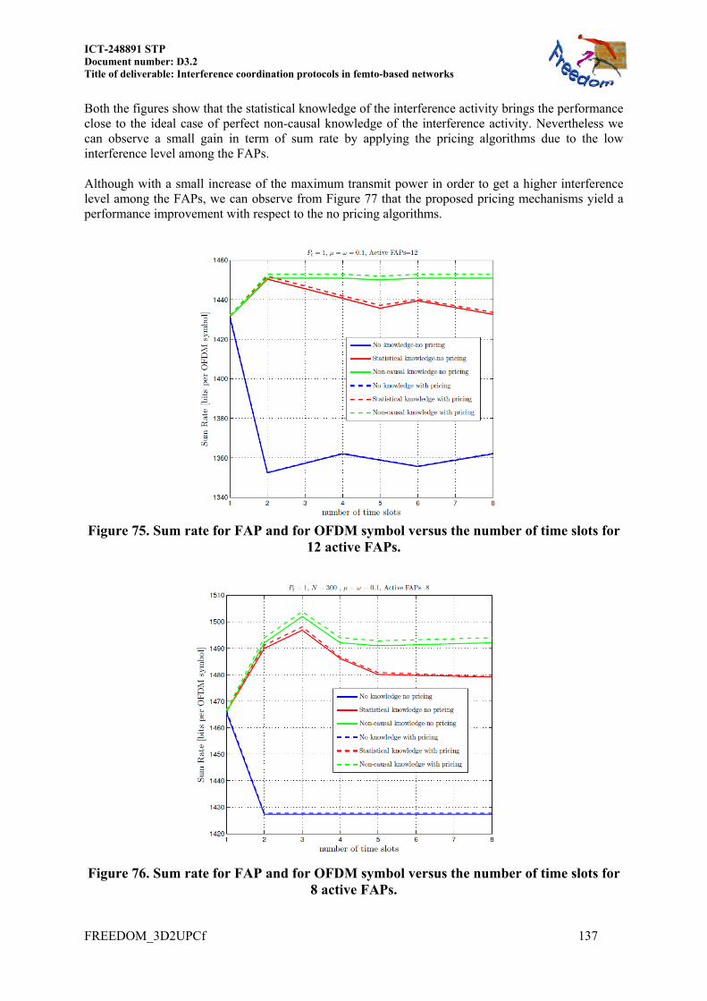
ICT-248891 STP Document number: D3.2 Title of deliverable: Interference coordination protocols in femto-based networks
FREEDOM_3D2UPCf 137
Both the figures show that the statistical knowledge of the interference activity brings the performance close to the ideal case of perfect non-causal knowledge of the interference activity. Nevertheless we can observe a small gain in term of sum rate by applying the pricing algorithms due to the low interference level among the FAPs. Although with a small increase of the maximum transmit power in order to get a higher interference level among the FAPs, we can observe from Figure 77 that the proposed pricing mechanisms yield a performance improvement with respect to the no pricing algorithms.
Figure 75. Sum rate for FAP and for OFDM symbol versus the number of time slots for
12 active FAPs.
Figure 76. Sum rate for FAP and for OFDM symbol versus the number of time slots for
8 active FAPs.

138
Figure 77. Sum rate for FAP and for OFDM symbol versus the number of time slots for
8 active FAPs and .
Finally in Figure 78 and Figure 79 we have considered the simulation results for the min power game with Markovian interference considering both the cases of pricing (dashed line), and no pricing (continuous line) algorithms. In order to have a fair comparison between the transmitted powers we have forced the same value of R
0 for the three cases of perfect (non-causal) knowledge of the macro-
user activity, no knowledge at all or statistical knowledge of the macro activity . The parameters used in the simulations are 0 750R bits per OFDM symbol, with transition probabilities
k 0.1,
0.1k while the MBS activity is the same for groups of 12 consecutive subcarriers. From Figure 78 and Figure 79, respectively, for 8 and 12 active FAPs, we can note the performance improvement of the proposed statistical approach with respect to the one that considers the future exactly equal to the present. Furthermore we can observe that the pricing mechanisms allow a performance gain with respect to the no pricing algorithms by reducing the radiated power still maintaining the same service quality.

ICT-248891 STP Document number: D3.2 Title of deliverable: Interference coordination protocols in femto-based networks
FREEDOM_3D2UPCf 139
Figure 78. Average transmitted power vs. number of time slots for 8 active FAPs.
Figure 79. Average transmitted power vs. number of time slots for 12 active FAPs.
9.4 Decentralized vs. Centralized resource allocation
We evaluated the performance of the proposed algorithms for resource allocation under a common scenario deployment with a Macro Base-Station. One terminal deployment has been selected where there are up to 20 FAPs, each serving a single user, see Figure 51 and Table 22. The considered decentralised algorithms is the iterative water-filling algorithm based on statistical inference of the probability of RB occupation by the MBS, that we call Statistical Inference Driven

140
Iterative Water Filling Algorithm presented in Subsection 7.3.2 (SIDIWFA for brevity). The centralised approach is the Genetic Algorithm described in Section 8. In order to fully compare the results, both approaches share and implement the same assumptions:
macro and femto networks fully share the same bandwidth; the system is synchronous, allowing the separation of the DL and UL phases of the MBS and
FAPs. These assumptions entail that, when the MBS is in DL phase, also the FAPs are performing their DL; thus the interference suffered by each FUE comes from the BS and the other FAPs. On the other hand, when the macro-network is in the UL phase, also the FUEs are performing their UL; thus the interference suffered by each FAP comes from the other FUEs and from all the MUEs. It is worth remarking that:
these assumptions do not emphasise the advantages of the decentralized algorithm incorporating the statistical characterization of the MBS band usage;
the following evaluations do not take into account the overhead due to the implementation of all the control plane-related procedures required by the algorithms;
Considering the above, [FREEDOM-D52] will provide additional comparisons, taking into account the above points, along with the dynamic behaviour of the MBS.
Figure 80. Comparison between centralized and decentralized resource allocation.
Figure 80 shows the results obtained with the two algorithms, the genetic centralized algorithm (GA) and the Statistical Inference Driven Iterative Water Filling Algorithm (SIDIWFA). The chosen performance metric is the per-FAP average (achievable) rate, measured in bits per OFDM symbol interval. We would like to emphasize that the decentralized approach is able to get similar results that the centralized approach. In fact, there is a better performance for the scenario considered in Figure 80. We also remark that the above results were achieved assuming a static behavior of the MBS, i.e., for each frequency block, the MBS is either always active, or always idle. Particularly, we have considered a completely silent MBS, a MBS whose traffic saturates the whole bandwidth, and a case in which about a half of the frequency resource blocks are used while the other half is idle. We expect that the inclusion of the dynamic nature of the Macro users’ traffic will show the advantages of including such time-dynamicity in the problem formulation at the basis of the algorithm derivation.
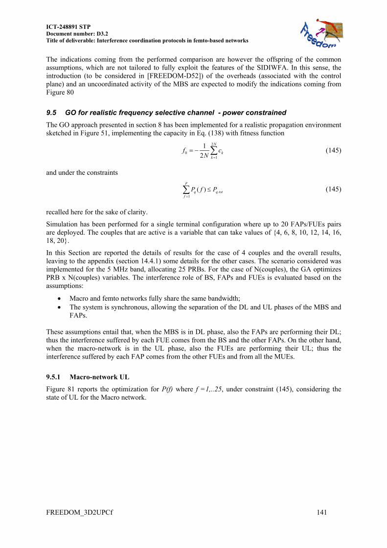
ICT-248891 STP Document number: D3.2 Title of deliverable: Interference coordination protocols in femto-based networks
FREEDOM_3D2UPCf 141
The indications coming from the performed comparison are however the offspring of the common assumptions, which are not tailored to fully exploit the features of the SIDIWFA. In this sense, the introduction (to be considered in [FREEDOM-D52]) of the overheads (associated with the control plane) and an uncoordinated activity of the MBS are expected to modify the indications coming from Figure 80
9.5 GO for realistic frequency selective channel - power constrained
The GO approach presented in section 8 has been implemented for a realistic propagation environment sketched in Figure 51, implementing the capacity in Eq. (138) with fitness function
2
01
1
2
N
kk
f cN
(145)
and under the constraints
1
( )F
q q totf
P f P
(145)
recalled here for the sake of clarity.
Simulation has been performed for a single terminal configuration where up to 20 FAPs/FUEs pairs are deployed. The couples that are active is a variable that can take values of 4, 6, 8, 10, 12, 14, 16, 18, 20.
In this Section are reported the details of results for the case of 4 couples and the overall results, leaving to the appendix (section 14.4.1) some details for the other cases. The scenario considered was implemented for the 5 MHz band, allocating 25 PRBs. For the case of N(couples), the GA optimizes PRB x N(couples) variables. The interference role of BS, FAPs and FUEs is evaluated based on the assumptions:
Macro and femto networks fully share the same bandwidth; The system is synchronous, allowing the separation of the DL and UL phases of the MBS and
FAPs. These assumptions entail that, when the MBS is in DL phase, also the FAPs are performing their DL; thus the interference suffered by each FUE comes from the BS and the other FAPs. On the other hand, when the macro-network is in the UL phase, also the FUEs are performing their UL; thus the interference suffered by each FAP comes from the other FUEs and from all the MUEs.
9.5.1 Macro-network UL
Figure 81 reports the optimization for P(f) where f =1,..25, under constraint (145), considering the state of UL for the Macro network.
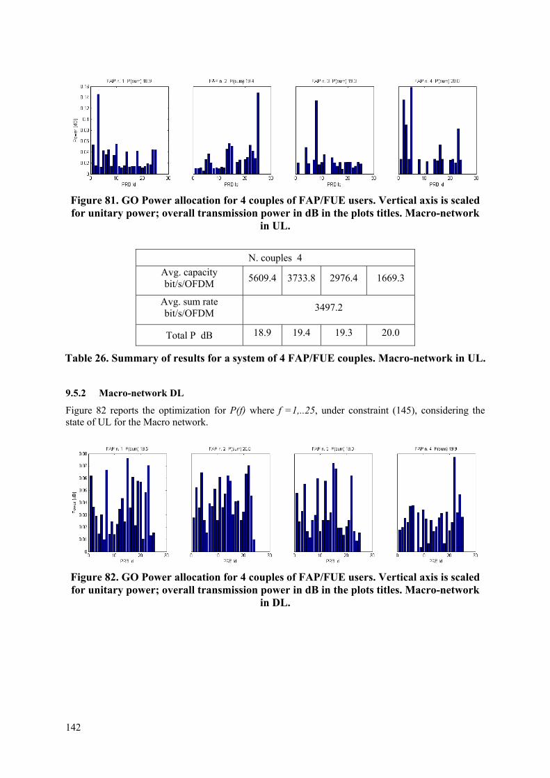
142
Figure 81. GO Power allocation for 4 couples of FAP/FUE users. Vertical axis is scaled for unitary power; overall transmission power in dB in the plots titles. Macro-network
in UL.
N. couples 4
Avg. capacity bit/s/OFDM
5609.4 3733.8 2976.4 1669.3
Avg. sum rate bit/s/OFDM
3497.2
Total P dB 18.9 19.4 19.3 20.0
Table 26. Summary of results for a system of 4 FAP/FUE couples. Macro-network in UL.
9.5.2 Macro-network DL
Figure 82 reports the optimization for P(f) where f =1,..25, under constraint (145), considering the state of UL for the Macro network.
Figure 82. GO Power allocation for 4 couples of FAP/FUE users. Vertical axis is scaled for unitary power; overall transmission power in dB in the plots titles. Macro-network
in DL.
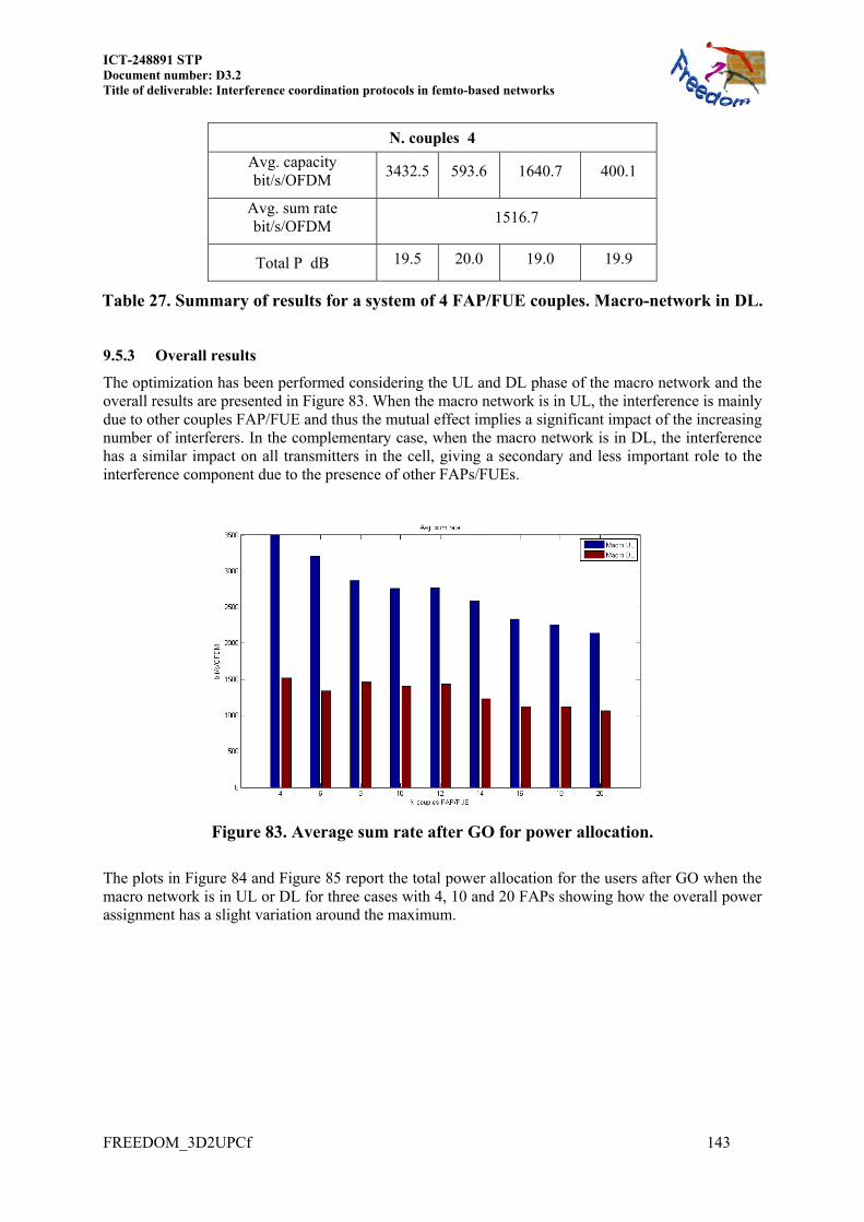
ICT-248891 STP Document number: D3.2 Title of deliverable: Interference coordination protocols in femto-based networks
FREEDOM_3D2UPCf 143
N. couples 4
Avg. capacity bit/s/OFDM
3432.5 593.6 1640.7 400.1
Avg. sum rate bit/s/OFDM
1516.7
Total P dB 19.5 20.0 19.0 19.9
Table 27. Summary of results for a system of 4 FAP/FUE couples. Macro-network in DL.
9.5.3 Overall results
The optimization has been performed considering the UL and DL phase of the macro network and the overall results are presented in Figure 83. When the macro network is in UL, the interference is mainly due to other couples FAP/FUE and thus the mutual effect implies a significant impact of the increasing number of interferers. In the complementary case, when the macro network is in DL, the interference has a similar impact on all transmitters in the cell, giving a secondary and less important role to the interference component due to the presence of other FAPs/FUEs.
Figure 83. Average sum rate after GO for power allocation.
The plots in Figure 84 and Figure 85 report the total power allocation for the users after GO when the macro network is in UL or DL for three cases with 4, 10 and 20 FAPs showing how the overall power assignment has a slight variation around the maximum.

144
Figure 84. Average power allocation after GO during BS UL or DL. Left panel, 4 couples; right panel, 10 couples.
Figure 85. Average transmission power after GO in the case of 20 couples. Comparison
of power allocation during BS UL or DL.
The plots reported in Figure 86 and Figure 87 report for two scenarios of interest corresponding to 10 and 20 couples, sketching the capacity of the single users, measured in bit/s/OFDM, showing how the interference of the macro BS strongly affects the performances of each transmitter.

ICT-248891 STP Document number: D3.2 Title of deliverable: Interference coordination protocols in femto-based networks
FREEDOM_3D2UPCf 145
Figure 86. Capacity per user after GO in the case of 10 couples FAP/FUE. Comparison
during BS UL or DL.
Figure 87. Capacity per user after GO in the case of 20 couples FAP/FUE. Comparison
during BS UL or DL.

146
10 IMPLEMENTATION NOTES
10.1 Scalability
The investigated resource allocation algorithms in this work are easily scalable as the number of the number of terminals increases. Algorithms proposed in sections 5, 6 and 7 are based on the message exchange at control-plane level at a local level, i.e. among neighboring FAPs and terminals. This imposes that the overhead due to the control-plane signalling does not scale with the total number of nodes. Rather, the impact of such overhead is determined by the nodes’ density and the interference range (given by the propagating conditions). A study of the control traffic in the backhaul during the exchange of prices is done in D4.2, where it is shown its relatively modest impact. The algorithms tend to reach a stable solution in less than 15-20 iterations, irrespective of the number of terminals in the system Although the genetic optimization-based algorithm analysed in section 8 is centralized, it can also deal with scalability in a corporate scenario, where each building might have a central processor unit, where all the resources of the FAPs deployed in that building are optimized. Since FAPs are placed indoors and transmit with low power, in general the interference from one building to another is not so significant. The algorithm needs of the SNIRs of all transmitters to be sent to the central processor unit and provides a sub-optimal solution for the resource allocation. One of the main drawbacks is the convergence time that needs of the order of hundreds of subframes.

ICT-248891 STP Document number: D3.2 Title of deliverable: Interference coordination protocols in femto-based networks
10.2 Applicability
Table 28. Applicability of the proposed techniques
Technical contribution Main enhancements required in the current LTE specifications to support FREEDOM solutions
PHY layer MAC layer
Identification of the interference by
coordinated channel sensing
Availability of spectrum sensing procedures at the nodes over the whole bandwidth.
The algorithm is applicable, in a general sense to any MAC which schedules femto users in a given way but foresees the sensing of the presence of a Macro user signal. With respect to LTE, the MAC protocol is inherently different due to the fact that power allocation across subcarriers, or block of subcarriers, is a determined by the sensing performance.
Decentralized resource allocation in DL based on
pricing
and
Decentralized resource allocation based on game
theory
Availability of (complex) channel knowledge of active users of own and neighboring FAPs.
Possibility of applying waterfilling-based power-allocation per RB.
Knowledge of the neighboring terminals in order to estimate the links (information about the pilot sequences to be scanned).
Define messages (information elements) to support the pricing exchange through the X2 interface over the players involved in the resource allocation.
A message can employ different MCS over the different RB.
Centralized dynamic interference management
No specific modification at PHY layer.
The feasibility of a centralised interference management requires specific resources at network level and application level (e.g. the presence of a dedicated entity performing the computation, the allocation of dedicated resources of the backhaul messaging for the exchange of relevant information).
No specific modification at MAC layer.
The feasibility of a centralised interference management requires specific resources at network level and application level (e.g. the presence of a dedicated entity performing the computation, the allocation of dedicated resources of the backhaul messaging for the exchange of relevant information).

148
10.3 Complexity
Table 29. Complexity of the proposed techniques
Technical contribution
Complexity of the optimisation procedures
Complexity at the MBS
Complexity at the FAP Complexity at the UE Complexity at network
management level
Identification of the interference by
coordinated channel sensing
A set of cooperating FAP’s performs cooperative sensing to characterize the status of the network in terms of active users
For each sensing interval, the procedure requires each FAP to disseminate its sensing outcome to its neighbors
None, the MBS is not involved
Each FAP must run a local sensing algorithm and a global one to fuse the sensing outcomes from its neighbors.
FUE’s not involved The exchange of sensing information exploits the backbone link
Decentralized resource allocation
in DL based on pricing
(bitrate, power allocation and
carrier assignment)
Pricing values are generated per resource block and distributed among interfering FAPs
Impact of CSI quantization
The channel coefficients to the serving FAP and to the interfering FAP have to be measured at the FUE
In the decentralized approach, the MBS can be seen as an additional FAP
If there are multiple FUEs per FAP and OFDMA is assumed, the complexity of allocating the best resource block is proportional to the number of carriers times the number of users, and it is done at each FAP
Under the non-orthogonal user-access per FAP the transmitters can be complex (based on dirty paper coding, DPC) or simple (using superposition coding, SC)
When the user-access per FAP is orthogonal, then simple receivers can be used at the UE (FUE or MUE)
When the user-access in non-orthogonal and transmitters are DPC-based devices, then simple receivers can be considered. However, if SC transmitters are used, then successive decoding receivers are required. In this latter case, the UE must be informed about the proper decoding order.
The procedure to exchange the pricing values among FAPs is not standardized. Some modification of the X2 interface is needed.
Meeting the conditions for convergence of game-theory based methods might require the presence of new network elements. This is under study at this time.

ICT-248891 STP Document number: D3.2 Title of deliverable: Interference coordination protocols in femto-based networks
FREEDOM_3D2UPCf 149
Decentralized resource allocation
based on game theory
Channel estimates (or equivalent information) and pricing values per subcarrier are calculated by each FAP and communicated to the other interfering FAPs.
None: the MBS’s are not involved in the procedure
Channel estimation is required at the FAPs: channel estimation is required even for the interfering channels.
Initially, a simple FAP-FUE link is considered; CSI is required at the FUE’s if the algorithm is used for the uplink
A suitable protocol to exchange the pricing values among FAPs must be devised for the backbone network.
Centralized dynamic
interference management
Transmitters undergoing optimization need to regularly evaluate their SNR and/or CSI and feed it back to the centralized processor.
At application level, the system should provide a dedicated IP two-ways channel.
Can be implemented either as a centralized or as a distributed algorithm.
n/a The backhaul transmission should allow establishing a dedicated channel for signalling.
The communication link should allow establishing a dedicated channel for signalling, at least at application level.
The optimization is based on a computation performed at Network level
In the case of distributed implementation, signalling is required in DL only.

ICT-248891 STP Document number: D3.2 Title of deliverable: Interference coordination protocols in femto-based networks
FREEDOM_3D2UPCf 150
11 LTE-BASED RESOURCE ALLOCATION In contrast to previous sections, here we present different techniques that consider the constraints imposed by the current LTE-A standard.
11.1 LTE-A adapted pricing mechanisms
Two alternative forms of pricing mechanisms have been proposed to deal with the mutual interference among neighboring FAPs. One is focused on the maximization of the weighted sum-rate, while the other is focused on the minimization of the total transmission power while guaranteeing a minimum bit rate per user [Munoz11b]. Both mechanisms require the exchange of pricing information among neighboring FAPs through the backhaul, including interference sensitivity, Lagrange multipliers and cross channels. Also, each user needs to report to the serving FAP the signal to noise plus interference ratio (SNIR) measured at each resource block (or minimum resource allocation unit). With this information, the proposed mechanisms optimize the power allocation per carrier, according to one of the above mentioned criteria. Despite the promising results, applying the proposed algorithms to LTE-A is not straightforward. Last version of LTE has some specific features that need to be taken into account:
• In LTE, there is no DL power control • In LTE, there is no direct report of the Signal-to-Interference plus Noise Ratio (SNIR). Instead
the maximum modulation and coding scheme (MCS) for a common group of resource blocks (RB) is reported.
• In LTE, all the RBs allocated to one user at each sub-frame use the same MCS Customizing the proposed pricing algorithms to LTE may therefore require changes at both LTE and the algorithms themselves:
Some modifications in LTE are necessary in order to support the proposed algorithms. Indeed, MCS sensitivity to interference (to obtain pricing) is an intrinsic feature of the proposed algorithms, so new procedures are unavoidable, as well as new messages to exchange a quantized version of this information between FUE-FAP, FAP-FAP and FAP-MBS.
At the same time, some simplifications can be done in the proposed algorithms to make them fit better within LTE, such as on/off transmission per RB, use of MCS instead of SNIR, etc.
In this section we will present a simpler and better LTE-adapted solution than those presented in sections 5, 6 and 7 , and the unavoidable modifications for LTE to support this simpler scheme will be described. The contents of this section have been presented in the last November meeting of 3GPP [R3-112752].
11.1.1 A pricing based mechanism for MCS and bandwidth part selection.
The goal of this section is to provide a coordinated mechanism to maximize the sum of the MCSs (and equivalently the sum of transmission rates) employed by a set of nearby FAPs. While the MBS may perform carrier aggregation (CA), the FAPs operate as a single carrier system, with different channel bandwidths. The proposed mechanism can be employed to select the DL operational frequency for wideband channels (e.g. 5MHz) and the bandwidth part for broadband channels (i.e. 10MHz, 15MHz or 20MHz). Also, given the operational frequency/bandwidth part, the same mechanism can be employed to select the sub-bands if the DL traffic is scheduled in a portion of the channel bandwidth or a portion of the previously selected bandwidth part. To describe the procedure, we will focus in the first case, i.e. selection of the operational frequency/ bandwidth part.

ICT-248891 STP Document number: D3.2 Title of deliverable: Interference coordination protocols in femto-based networks
FREEDOM_3D2UPCf 151
Figure 88 illustrates possible bandwidth partitions within the frequency channel, i.e. bandwidth part. Note that the width of a bandwidth part is approx. 5MHz, when the total channel BW is 20MHz. For a 20MHz channel width, a bandwidth part has the same number of resource blocks as a 5MHz carrier.
CA-MBS
f1 f2 f3
FAP
FAP
frequency
5MHz f4
FAP
Figure 88. Example of bandwidth partitions
11.1.1.1 Fundamentals
Let us consider the following notation: NF: Total number of serving stations (FAPs and, maybe, also the MBS).
S : Set of available bandwidth parts in the system
fS : Set of available bandwidth parts for the f-th serving station.
suMCS : Modulation and coding scheme reported by user u in the bandwidth part s
sfb : Binary variable which equals 1 if the f-th FAP transmits in the s-th bandwidth part, and 0
otherwise. Notice that 0,sfb if fs S S .
fP and gP : Transmission power per resource block (RB) for the f-th and the g-th serving
station respectively
,,
s ru gh and ,
,s ru gh : Cross- channel amplitudes between the user u and the f-th and g-th serving
station, respectively, on the r-th RB in the s-th bandwidth part. ,s r
ui : Interference measured by the user u at the the r-th resource block in the s-th bandwidth
part.
sui : Vector containing the interference measured the user u for the N RBs in the s-th bandwidth
part, i.e, , 1 ,[ , , ]s s r s r N T
u u ui i i
Uf : Set of users connected to the f-th serving station. To simplify notation, we consider initially that each serving station is serving a single user, and we will use u(f) to denote the user connected to the f-th serving station, i.e., Uf= u(f), | Uf|=1. The signal to noise plus interference ratio measured at the r-th RB in the s-th bandwidth part by the user connected to the f-th serving station is given by:
2,
,,
2, ,
,1F
s rfu f fs r
u f Ns r s rg gu f g
g f
h PSNIR
b h P
(146)

ICT-248891 STP Document number: D3.2 Title of deliverable: Interference coordination protocols in femto-based networks
152
While the channel could remain constant within each RB, it is unlikely that it remains constant on all the RBs in the considered band. When all the subcarriers of a specific user are modulated using the same modulation MCS a function that maps the set of SINRs to a single value of MCS for a given Block Error Rate (BLER) is required. For the s-th bandwidth part, the user u computes a MCS value based on the SNIR measures for the N RBs that compose this bandwidth part:
, 1 ,,...,s s r s r Nu u uMCS function SNIR SNIR
The maxrate problem to solve by the f-th serving station is the following:
max
sf
s sf u f
b s S
b MCS
(147)
s.t. 0,1 for , sf fb s S
(148)
0 for , sf fb s S
(149)
1.s
fs S
b
(150)
Let us consider now the total rate achieved within a set of NF neighbour serving stations. In such a case, problem (147)-(150) becomes:
1, , 1
maxF
sf
f NF
Ns sf u f
b f s S
b MCS
(151)
s.t. 0,1 for , 1, , ,sf f Fb s S f N
(152)
0 for , 1, , ,sf f Fb s S f N
(153)
1, for 1, , .s
f Fs S
b f N
(154)
The interference measured at the the r-th resource block in the s-th sub-band by the user connected to the f-th serving station, u(f), is
2, ,
,1
F
g f
Ns r s s r
g gu f u f gg
i b P h
(155)
Due to the cross-interference, the modulation and coding scheme reported at each bandwidth part by the user connected to the f-th serving station will change if the other serving stations are transmitting
or not in this bandwidth part. Let us use the following linear approximation for the su fMCS which
depends on sg g f
b
:
,,0
10
2, ,
,01 1
0
sf
su f
F
su f
g f
sNfs s s r
u f u f u fs rr u f
NNs s r s s s r
g g gu f u f u f gr g
MCSMCS MCS i
i
MCS b b P h
ii
i
(156)

ICT-248891 STP Document number: D3.2 Title of deliverable: Interference coordination protocols in femto-based networks
FREEDOM_3D2UPCf 153
where su fi is the vector containing the interference measured for the N RBs in the s-th bandwidth
part, 0su fi and 0s
gb denotes the previous value for su fi and s
gb respectively, and ,s r
u f is the
interference sensitivity factor defined as follows:
,,
0su f
su fs r
u f s ru f
MCS
i
i
(157)
Using the linear approximation in (156), the cost function in (151) can be rewritten as follows:
1, ,
2, ,( ) ( ) ( ),0
1 1 1
max 0F F
ss fff NF
g f
N NNs s s r s s s rf u f u f g g g u f g
b f s S r g
b MCS b b P h
i
(158)
Notice that the terms for the f-th serving station depend on the other station variables, which results in a highly complex coupled problem. In order to derive a solution, we consider a set of distributed problems in which, at a given time, each serving station variables, i.e. s
fb are optimized while the variables for the rest of the transmitters are fixed. Under this assumption, the terms in the cost function (158) that depend on the f-th transmitter are:
2, ,
,1 1
2, ,
,1 1
F
j f
F
j f
N Ns s s s r s s rf j f fu f u j u j f
s S j s S r
N Ns s s s r s rf j fu f u j u j f
s S j r
b MCS b b P h
b MCS b P h
(159)
Assuming that other serving stations’ variables are given, the problem can be decomposed in sub-problems, where each FAP optimizes its own variables, and the problem to be solved by the f-th serving station is therefore:
2, ,
,1 1 1
maxF F
sf
g f
N N Ns s s s r s rf g fu f u g u g f
b f s S g r
b MCS b P h
(160)
s.t. 0,1 for , sf fb s S
(161)
0 for , 1, , ,sf f Fb s S f N
(162)
1.s
fs S
b
(163)
When comparing problem (160)-(163) with problem (147)-(150), we observe that the solution now
is to select the bandwidth part, not with the highest reported MCS, but with the highest difference between the reported MCS and the pricing term
2, ,
,1 1
F
g f
N Ns s s r s rf g fu g u g f
g r
price b P h
(164)
This pricing term measures the degradation on other stations MCS due to the interference generated by the f-th serving station. It is computed as the sum over all neighbor serving stations of the cost that the transmission of the f-th serving stations has in terms of the supported MCS in the s-th bandwidth part:

ICT-248891 STP Document number: D3.2 Title of deliverable: Interference coordination protocols in femto-based networks
154
2, ,
, ,1
costN
s s r s rg f fu g u g f
r
P h
(165)
This cost is equal to the sum, over the N resource blocks in the s-th sub-band, of the product of three terms:
1. The term ,s r
u g , which measures the sensitivity, of the MCS reported for the s-th sub-band due
to the interference in the r-th RB (see eq. (157)). 2. The transmission power of the f-th serving station. 3. The cross channel gain in the r-th RB of the s-th sub-band between the f-th serving station and
the user connected to the neighbour serving station g.
Notice that the impact on the price term defined (164) of the cost for the g-th serving station due to the
transmission by the f-th serving station in the s-th bandwidth part, ,cost sg f , is cero if s
gb =0, i.e. if the
g-th serving station does not use of the s-th bandwidth part. In the proposed approach, each serving station updates its resource allocation strategy assuming that other FAPs’ variables are given. In practice, several approaches are possible, i.e., the serving stations may perform synchronously or asynchronously (either at random time instances or sequentially). In order to speed up convergence, we will consider that the serving stations update the resource allocation simultaneously at each frame. When the serving stations update the resource allocation strategy simultaneously a problem that may happen is that they go back and forward on the same RBs. To avoid this undesired effect we propose to use some memory to update the pricing values. Therefore, for the n-th frame, the pricing values are computed as follows:
2, ,
,1 1
1 1 ,F
g f
N Ns s s s r s rf f g fu g u g f
g r
price n price n b P h
(166)
with a parameter between 0 a 1.
11.1.1.2 Procedure for coordinated bandwidth part selection
Based on the above, our interference coordination approach involves the following steps:
1. A potential interference victim UE identifies the interference created by each one of the surrounding cells operating in the considered frequency band;
2. Based on this information, the UE determines which the strongest interferes are; 3. UE determines the influence of scheduling each strong interfering serving station DL
transmission in one or more parts of the frequency channel. This influence, measured as MCS degradation, is the “cost”5 defined in eq. (165);
4. For each relevant subframe and full channel or bandwidth part, the “cost” information associated to each interfering serving station is sent by UE over the Uu interface to its serving station;
5. The high-level “costs” are shared, over the X2 interface, between the FAPs and MBS in the area;
5 The degradation of UE data rate due to the degradation of its MCS caused by a specific FAP DL transmission in a specific frequency channel or frequency channel part and subframe is named “cost”.

ICT-248891 STP Document number: D3.2 Title of deliverable: Interference coordination protocols in femto-based networks
FREEDOM_3D2UPCf 155
6. Each FAP determines the “price” of its activity on the MCSs of other FAPs and on the MBS providing the coverage layer (see eq. (164);
7. Each FAP determines the frequency resource to be used such to better solve the trade-off between maximizing performance and minimizing the interference to other FAPs and to the MBS. The MBS has a “privileged” status, while the FAPs will have to change their operating frequency channel or the bandwidth part for a specific DL transmission.
The full channel (wideband) reports are applied for wideband channels (e.g. 5MHz), while the channel part reporting is applied for broadband channels (i.e. 10MHz, 15MHz or 20MHz). The serving station (FAP or MBS) may alter the cost, if for example there are free resources in other subframes and may decide to transmit or not the resulting cost to other stations. If the decision is positive, the costs are distributed by the serving station over the X2 interface to the other stations in the area. Based on the costs received from others serving stations (FAPs or MBS), each interfering FAP which is looking for scheduling DL traffic on a given part of the frequency channel will be able to calculate the interference “price” of re-using the specific part of the frequency channel for the affected UEs which are receiving DL traffic in that frequency channel part. Based on this information the interfering FAP will take steps for changing the operational frequency or the bandwidth part or the operational frequency channel such to create minimum interference to the population of other operational UEs.
11.1.1.2.1 Sensing and sharing the CQI degradation
In fact the UE is not reporting the MCS, but the channel quality indicator (CQI), which for the SISO case is identical to MCS. We will first look at the CQI detection, based on existing 3GPP specs, and after that at the evaluation of CQI degradation due to the other stations DL interference.
CQI detection in the serving cell
We start from a point in which the system is operational and the serving station (FAP or MBS) transmits to UE on the frequency bandwidth part or the frequency channel chosen by the serving station. The UE has the capability of reporting to the serving station the CQI information, as detailed in clause 7.2 of TS 36.213 0, for the serving cell. It is defined that: “Based on an unrestricted observation interval in time and frequency, the UE shall derive for each CQI value reported in uplink subframe n the highest CQI index between 1 and 15 in Table 7.2.3-1 which satisfies the following condition, or CQI index 0 if CQI index 1 does not satisfy the condition: A single PDSCH transport block with a combination of modulation scheme and transport block size corresponding to the CQI index, and occupying a group of downlink physical resource blocks termed the CSI reference resource, could be received with a transport block error probability not exceeding 0.1. “
Periodic and aperiodic CQI reporting is possible for LTE system. The CQI is computed for a set a resource blocks. Wideband (the CQI is computed for the whole bandwidth) and UE-selected sub-band feedback are possible. For instance, for periodic CQI reporting, the UE-selected sub-band is as follows. The total number of sub-bands N is divided into bandwidth parts. Considering a system bandwidth between 64 and 110 RBs, the sub-band size is 8 RBs grouped into 4 bandwidth parts (smaller sub-band sizes are considered for smaller system bandwidths). One CQI value is computed and reported for a single selected sub-band from each bandwidth part, along with the corresponding sub-band index [Sesia2009].

ICT-248891 STP Document number: D3.2 Title of deliverable: Interference coordination protocols in femto-based networks
156
CQI degradation in the serving cell
Let us suppose that UE is able to use the reference signals (RS) sent by other cells for assessing the interference caused by the DL transmissions of these cells. Let us also suppose that there is a suitable mapping of these RSs, such to associate a RS with a specific cell
IDN . In such a case, the potential interference victim UE connected to the g-th FAP, ( )u g , can evaluate the impact of the interference caused by the DL transmission of the cell f on its achievable CQI in the bandwidth part s. Given the interference impact on CQI degradation, UE ( )u g can establish the “cost”,
which depends on the interference sensitivity and the interference power received in the RBs on the bandwidth part k (see eq. (165)). We assume that the can be reported over Uu interface to the serving station (FAP or MBS). The serving station may decide to transmit the cost information over X2 interface to other stations in the area. If the sensitivity to the interferer power is low, for example due to a high SINR at UE ( )u g , there
will be no need for further communicating this information to other stations. The MBS may report much higher adjusted costs as compared with FAPs. In this way, the UEs served by MBSs will be better protected to the interference from FAPs. We have identified a number of issues with the existing standards, which impede on the application of the proposed solution. These issues are listed below:
Issue 1: For determining the interference power from a single transmission, it is necessary to define changes to the standards for extending the protected measurements to bandwidth parts.
Issue 2: X2 should support the transmission of information covering the resource allocated for the protected measurement.
Issue 3: The Uu interface should support the transmission of the interference cost.
Issue 4: The existing standards do not support the measurement of the degradation caused by the activity of another station and the calculation of the “interference sensitivity”.
Each report of cost related to a specific UE, serving station and interference source station, will be shared between the stations in the neighborhood, using the X2 interface. To limit the traffic, the bandwidth part should be chosen such to reflect the frequency resources needed for UE scheduling. The generated traffic should be relatively low, due to the fact that only the “potential victim” UEs and stations will generate it.
Issue 5: It is necessary to define the information elements for distributing the “interference cost” over X2 interface.
Issue 6: the existing splitting of the channel width in bandwidth parts (TS36.213 Table 7.2.2-2) is suitable for 20MHz channels only; for 10MHz and 15MHz channel the channel part is not equal with the 5MHz channel width.
Issue 7: In case that there is no synchronization between FAP and MBS and also between FAPs, the ICIC as defined in Release 8 and the eICIC based on synchronized ABS frames is not useful. FFR was designed for cases in which all the frequency channels have the same bandwidth. It is needed to define an additional eICIC mechanism, possibly using the bandwidth parts as main resource elements.
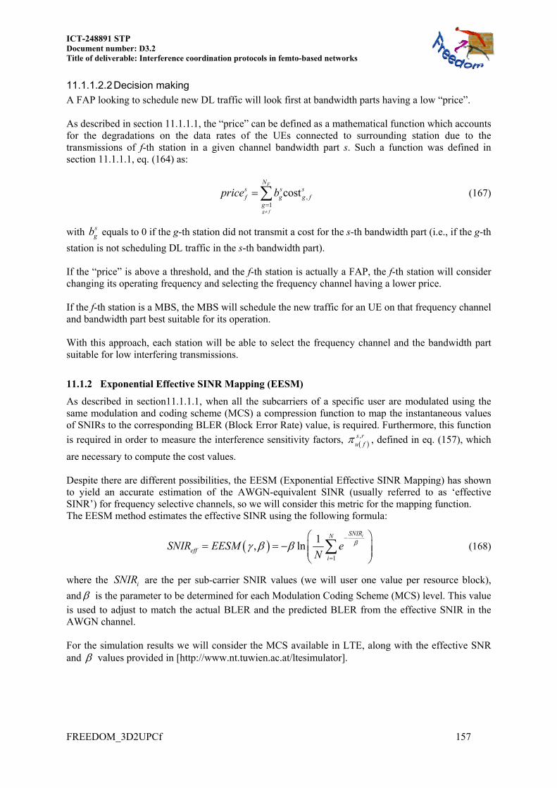
ICT-248891 STP Document number: D3.2 Title of deliverable: Interference coordination protocols in femto-based networks
FREEDOM_3D2UPCf 157
11.1.1.2.2 Decision making
A FAP looking to schedule new DL traffic will look first at bandwidth parts having a low “price”. As described in section 11.1.1.1, the “price” can be defined as a mathematical function which accounts for the degradations on the data rates of the UEs connected to surrounding station due to the transmissions of f-th station in a given channel bandwidth part s. Such a function was defined in section 11.1.1.1, eq. (164) as:
,1
costF
g f
Ns s sf g g f
g
price b
(167)
with sgb equals to 0 if the g-th station did not transmit a cost for the s-th bandwidth part (i.e., if the g-th
station is not scheduling DL traffic in the s-th bandwidth part). If the “price” is above a threshold, and the f-th station is actually a FAP, the f-th station will consider changing its operating frequency and selecting the frequency channel having a lower price. If the f-th station is a MBS, the MBS will schedule the new traffic for an UE on that frequency channel and bandwidth part best suitable for its operation. With this approach, each station will be able to select the frequency channel and the bandwidth part suitable for low interfering transmissions.
11.1.2 Exponential Effective SINR Mapping (EESM)
As described in section11.1.1.1, when all the subcarriers of a specific user are modulated using the same modulation and coding scheme (MCS) a compression function to map the instantaneous values of SNIRs to the corresponding BLER (Block Error Rate) value, is required. Furthermore, this function
is required in order to measure the interference sensitivity factors, ,s r
u f , defined in eq. (157), which
are necessary to compute the cost values. Despite there are different possibilities, the EESM (Exponential Effective SINR Mapping) has shown to yield an accurate estimation of the AWGN-equivalent SINR (usually referred to as ‘effective SINR’) for frequency selective channels, so we will consider this metric for the mapping function. The EESM method estimates the effective SINR using the following formula:
1
1, ln
iSNIRN
effi
SNIR EESM eN
(168)
where the iSNIR are the per sub-carrier SNIR values (we will user one value per resource block),
and is the parameter to be determined for each Modulation Coding Scheme (MCS) level. This value is used to adjust to match the actual BLER and the predicted BLER from the effective SNIR in the AWGN channel. For the simulation results we will consider the MCS available in LTE, along with the effective SNR and values provided in [http://www.nt.tuwien.ac.at/ltesimulator].

ICT-248891 STP Document number: D3.2 Title of deliverable: Interference coordination protocols in femto-based networks
158
MCS Effective SNIR (dB) value0.1523 -6.934 1 0.2344 -5.147 1.44 0.3770 -3.18 1.4 0.6016 -1.254 1.48 0.8770 0.761 1.5 1.1758 2.70 1.62 1.4766 4.697 3.10 1.9141 6.528 4.32 2.4063 8.576 5.37 2.7305 10.37 7.71 3.3223 12.3 15.5 3.9023 14.18 19.6 4.5234 15.89 24.7 5.1152 17.82 27.6 5.5547 19.83 28
Table 30 MCS and required effective SNIR
This table has been obtained through extensive simulations using the LTE codes. The effective SNR for each MCS value is the required effective SNR to achieve a BLER less than 10% when using this MCS value. As show in Figure 89, the relationship between the MCS and the required effective SNR (red points) can be approximated by the following empirical SNIR-to CQI mapping function (solid blue line):
1.2213 ln 1eff effMCS SNR SNR
(169)
-10 -5 0 5 10 15 200
1
2
3
4
5
6
Effective SNIR (dB)
Sup
port
ed M
CS
CQI mapping
BLER=10% points from the BLER curves
SINR-to-CQI mapping function
Figure 89. CQI mapping.
The approach is as follows: from the SINR values measured at a given bandwidth part, each user computes the effective SNIR for every possible value (each value is associated to one MCS). The so computed effective SNIR is compared with the effective SNR required for the MCS corresponding to the value. The highest MCS such that the computed effective SNIR is equal or greater than the required effective SNIR is selected.

ICT-248891 STP Document number: D3.2 Title of deliverable: Interference coordination protocols in femto-based networks
FREEDOM_3D2UPCf 159
Once the user u has selected the MCS for the bandwidth part s, the sensibility to the interference in this sub-band will be computed using the empirical SNIR-to CQI mapping function in (169):
,
,
2,
,2, ,
1
1.2213 1
1 1
s ru
s ru
s rSNIRsu f us r u
u ss r SNIR s rNu eff uu
r
h PMCSe
i SNR ie
(170)
11.1.3 Simulation results
This section provides performance results of our LTE-A adapted pricing approach. We have simplified the simulation by limiting the simulations to a single 20MHz frequency channel, covering a 20MHz allocation band, using four bandwidth parts. In this case a bandwidth part is similar with a 5MHz channel. The CQI and the cost are estimated per bandwidth part. In addition, we have applied the pricing policy, based on a deployment as shown in Figure 90. In this deployment there is one FAP area (FAP dual-strip zone) within the coverage area of the MBS. Specific parameters are:
- Channel bandwidth: 20MHz with four bandwidth parts corresponding each to 25RBs, same as in 5MHz;
- Number of UEs per FAP: 1, SISO mode;
- Number of UEs served by MBS and placed in the FAP area: 2 (the MBS will allocate these 2 UEs in two separate bandwidth parts, each one of 5 MHz);
- The dual-strip deployment was considered over a number of floors varying between 1 and 6;
- One serving station considers itself interfered if the average SNR received from an interfering FAP is greater than the SNR of the serving station minus 15 dB.
Figure 90. Deployment scenario
Figure 91, Figure 92 and Figure 93 correspond to the simulation results for FAPs and FUEs. In Figure 91, the operating frequency channel has 5MHz. The average FAP throughput depends on the number of active FAPs in the simulated area. In Figure 91 right, the average number of active FAPs in the area is 6. The total FAPs throughput gain is aprox. 2Mb/s.
UE
FAPsMBS
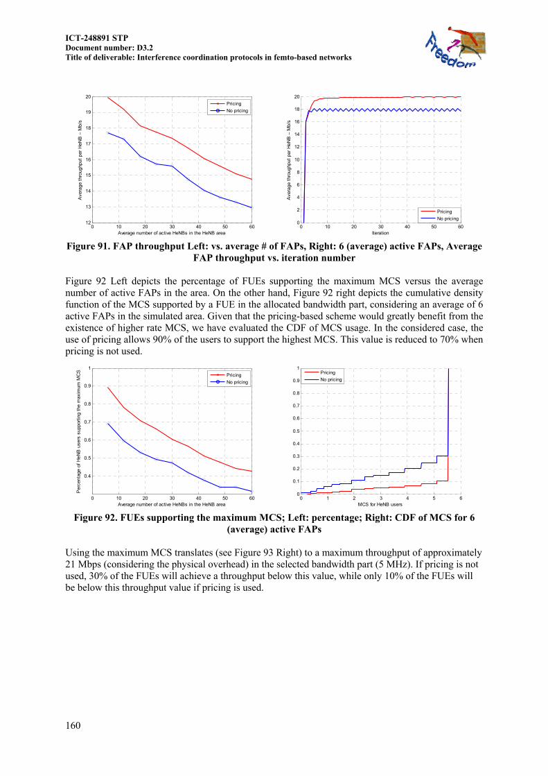
ICT-248891 STP Document number: D3.2 Title of deliverable: Interference coordination protocols in femto-based networks
160
0 10 20 30 40 50 6012
13
14
15
16
17
18
19
20
Ave
rage
thr
ough
put
per
HeN
B –
Mb/
s
Average number of active HeNBs in the HeNB area
Pricing
No pricing
0 10 20 30 40 50 60
0
2
4
6
8
10
12
14
16
18
20
Iteration
Ave
rage
thr
ough
put
per
HeN
B –
Mb/
s
Pricing
No pricing
Figure 91. FAP throughput Left: vs. average # of FAPs, Right: 6 (average) active FAPs, Average
FAP throughput vs. iteration number
Figure 92 Left depicts the percentage of FUEs supporting the maximum MCS versus the average number of active FAPs in the area. On the other hand, Figure 92 right depicts the cumulative density function of the MCS supported by a FUE in the allocated bandwidth part, considering an average of 6 active FAPs in the simulated area. Given that the pricing-based scheme would greatly benefit from the existence of higher rate MCS, we have evaluated the CDF of MCS usage. In the considered case, the use of pricing allows 90% of the users to support the highest MCS. This value is reduced to 70% when pricing is not used.
0 10 20 30 40 50 60
0.4
0.5
0.6
0.7
0.8
0.9
1
Per
cent
age
of H
eNB
use
rs s
uppo
rtin
g th
e m
axim
um M
CS
Average number of active HeNBs in the HeNB area
Pricing
No pricing
0 1 2 3 4 5 6
0
0.1
0.2
0.3
0.4
0.5
0.6
0.7
0.8
0.9
1
MCS for HeNB users
Pricing
No pricing
Figure 92. FUEs supporting the maximum MCS; Left: percentage; Right: CDF of MCS for 6
(average) active FAPs
Using the maximum MCS translates (see Figure 93 Right) to a maximum throughput of approximately 21 Mbps (considering the physical overhead) in the selected bandwidth part (5 MHz). If pricing is not used, 30% of the FUEs will achieve a throughput below this value, while only 10% of the FUEs will be below this throughput value if pricing is used.
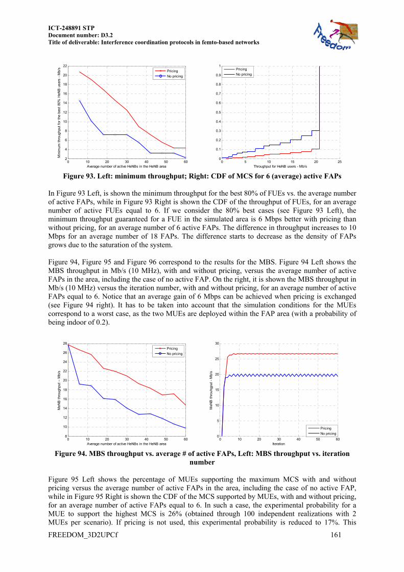
ICT-248891 STP Document number: D3.2 Title of deliverable: Interference coordination protocols in femto-based networks
FREEDOM_3D2UPCf 161
0 10 20 30 40 50 602
4
6
8
10
12
14
16
18
20
22
Min
imum
thr
ough
put
for
the
best
80%
HeN
B u
sers
- M
b/s
Average number of active HeNBs in the HeNB area
Pricing
No pricing
0 5 10 15 20 25
0
0.1
0.2
0.3
0.4
0.5
0.6
0.7
0.8
0.9
1
Throughput for HeNB users - Mb/s
Pricing
No pricing
Figure 93. Left: minimum throughput; Right: CDF of MCS for 6 (average) active FAPs
In Figure 93 Left, is shown the minimum throughput for the best 80% of FUEs vs. the average number of active FAPs, while in Figure 93 Right is shown the CDF of the throughput of FUEs, for an average number of active FUEs equal to 6. If we consider the 80% best cases (see Figure 93 Left), the minimum throughput guaranteed for a FUE in the simulated area is 6 Mbps better with pricing than without pricing, for an average number of 6 active FAPs. The difference in throughput increases to 10 Mbps for an average number of 18 FAPs. The difference starts to decrease as the density of FAPs grows due to the saturation of the system. Figure 94, Figure 95 and Figure 96 correspond to the results for the MBS. Figure 94 Left shows the MBS throughput in Mb/s (10 MHz), with and without pricing, versus the average number of active FAPs in the area, including the case of no active FAP. On the right, it is shown the MBS throughput in Mb/s (10 MHz) versus the iteration number, with and without pricing, for an average number of active FAPs equal to 6. Notice that an average gain of 6 Mbps can be achieved when pricing is exchanged (see Figure 94 right). It has to be taken into account that the simulation conditions for the MUEs correspond to a worst case, as the two MUEs are deployed within the FAP area (with a probability of being indoor of 0.2).
0 10 20 30 40 50 608
10
12
14
16
18
20
22
24
26
28
MeN
B t
hrou
ghpu
t –
Mb/
s
Average number of active HeNBs in the HeNB area
Pricing
No pricing
0 10 20 30 40 50 600
5
10
15
20
25
30
Iteration
MeN
B t
hrou
hgpu
t -
Mb/
s
Pricing
No pricing
Figure 94. MBS throughput vs. average # of active FAPs, Left: MBS throughput vs. iteration
number Figure 95 Left shows the percentage of MUEs supporting the maximum MCS with and without pricing versus the average number of active FAPs in the area, including the case of no active FAP, while in Figure 95 Right is shown the CDF of the MCS supported by MUEs, with and without pricing, for an average number of active FAPs equal to 6. In such a case, the experimental probability for a MUE to support the highest MCS is 26% (obtained through 100 independent realizations with 2 MUEs per scenario). If pricing is not used, this experimental probability is reduced to 17%. This
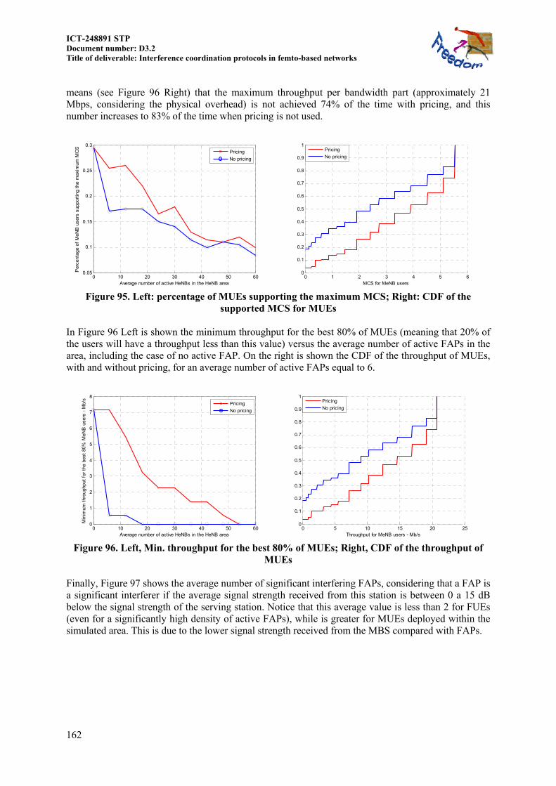
ICT-248891 STP Document number: D3.2 Title of deliverable: Interference coordination protocols in femto-based networks
162
means (see Figure 96 Right) that the maximum throughput per bandwidth part (approximately 21 Mbps, considering the physical overhead) is not achieved 74% of the time with pricing, and this number increases to 83% of the time when pricing is not used.
0 10 20 30 40 50 600.05
0.1
0.15
0.2
0.25
0.3
Per
cent
age
of M
eNB
use
rs s
uppo
rtin
g th
e m
axim
um M
CS
Average number of active HeNBs in the HeNB area
Pricing
No pricing
0 1 2 3 4 5 6
0
0.1
0.2
0.3
0.4
0.5
0.6
0.7
0.8
0.9
1
MCS for MeNB users
Pricing
No pricing
Figure 95. Left: percentage of MUEs supporting the maximum MCS; Right: CDF of the
supported MCS for MUEs
In Figure 96 Left is shown the minimum throughput for the best 80% of MUEs (meaning that 20% of the users will have a throughput less than this value) versus the average number of active FAPs in the area, including the case of no active FAP. On the right is shown the CDF of the throughput of MUEs, with and without pricing, for an average number of active FAPs equal to 6.
0 10 20 30 40 50 600
1
2
3
4
5
6
7
8
Min
imum
thr
ough
put
for
the
best
80%
MeN
B u
sers
- M
b/s
Average number of active HeNBs in the HeNB area
Pricing
No pricing
0 5 10 15 20 250
0.1
0.2
0.3
0.4
0.5
0.6
0.7
0.8
0.9
1
Throughput for MeNB users - Mb/s
Pricing
No pricing
Figure 96. Left, Min. throughput for the best 80% of MUEs; Right, CDF of the throughput of
MUEs
Finally, Figure 97 shows the average number of significant interfering FAPs, considering that a FAP is a significant interferer if the average signal strength received from this station is between 0 a 15 dB below the signal strength of the serving station. Notice that this average value is less than 2 for FUEs (even for a significantly high density of active FAPs), while is greater for MUEs deployed within the simulated area. This is due to the lower signal strength received from the MBS compared with FAPs.

ICT-248891 STP Document number: D3.2 Title of deliverable: Interference coordination protocols in femto-based networks
FREEDOM_3D2UPCf 163
0 10 20 30 40 50 600
2
4
6
8
10
12
14
16
18
20
Ave
rage
num
ber
of s
igni
fican
t in
terf
erin
g H
eNB
s (S
NR
>S
NR
o-15
dB)
Average number of active HeNBs in the HeNB area
per MUE
per FUE
Figure 97. Average number of dominant interferer FAPs detected per FUE and MUE.
For an average number of 6 active FAPs (see Figure 98 left), the probability for a FUE to detect more than 3 interfering FAPs is less than 4%. In the worst case, a FUE will detect up to 6 interfering FAPs. This user must report 6 cost values per bandwidth part, which means, assuming 6 bits for quantization of each cost value every frame, i.e., every 10ms, a rough value of 2.4 kbps. Notice, however, that detecting 6 interfering FAPs is a low likely case.
1 1.5 2 2.5 3 3.5 4 4.5 5 5.5 60.8
0.82
0.84
0.86
0.88
0.9
0.92
0.94
0.96
0.98
1
Per
cent
age
Number of detected interfering HeNBs for HeNB users (SNR>SNRo-15dB) 0 2 4 6 8 10 12 14
0.4
0.5
0.6
0.7
0.8
0.9
1
Per
cent
age
Number of detected interfering HeNBs for MeNB users (SNR>SNRo-15dB) Figure 98. CDF of the number of dominant interferer FAPs detected per FUE (left) and per
MUE (right). In the case of the MUEs deployed within the simulated area (see Figure 98 right), the number of detected interferers increases a little, with 6 interferers for 90% of the cases, and a worst case value of 14 interferers.
11.1.4 Conclusions and recommended actions
Our simulations demonstrate significantly higher performance as compared with the reference case (no pricing), justifying the investments in standard enhancements. We summarize below the missing elements in standards:
Issue 1: For determining the interference power from a single transmission, it is necessary to define changes to the standards for extending the protected measurements to bandwidth parts. Issue 2: X2 should support the transmission of information covering resource allocated for the protected measurement within the frequency channel. Issue 3: The Uu interface should support the transmission of the interference cost.

ICT-248891 STP Document number: D3.2 Title of deliverable: Interference coordination protocols in femto-based networks
164
Issue 4: The existing standards do not support the measurement of the degradation caused by the activity of another eNB and the calculation of the “interference sensitivity”. Issue 5: It is necessary to define the information elements for distributing the “interference cost” over X2 interface. Issue 6: the existing splitting of the channel width in bandwidth parts (TS36.213 Table 7.2.2-2) is suitable for 20MHz channels only; for 10MHz and 15MHz channel the channel part is not equal with the 5MHz channel width. Issue 7: In case that there is no synchronization between FAP and MBS and also between FAPs, the ICIC as defined in Release 8 and the eICIC based on ABS subframes are not useful. FFR was designed for cases in which all the frequency channels have the same bandwidth. eICIC requires inter-cell synchronization. It is needed to define an additional eICIC mechanism, possibly using the bandwidth parts as main resource elements.
11.2 Rate Max or Power Min under Interference-power constraints
In [Zhang 2010] the authors consider the downlink transmission of a cellular system in which base stations, each equipped with multiple antennas, cooperatively design their respective transmit beamforming vectors to optimize the overall system performance. Serving mobile stations are assumed to be equipped with a single antenna and only one of them can be active at any given time within each cell. The corresponding channel model is then that of the multiple-input single-output Gaussian interference-channel (MISO-IC). A method is proposed to characterize different rate-tuples on the Pareto boundary of the achievable rate region for the MISO-IC. It is shown that the Pareto-boundary rate-tuple of the MISO-IC can be achieved in a decentralized manner when each of the base stations attains its own channel capacity subject to a certain set of interference-power constraints at the mobile stations of the other cells. A decentralized algorithm for implementing the cooperative downlink beamforming method is proposed. The technique proposed in [Zhang 2010] has been extended to a femtocell based multi-cellular scenario with SISO, MISO or MIMO multi-carrier transmission in under the assumption that only one user is served using the same time-frequency resource. The proposed technique allows a simple pair-wise optimization scheme between cooperating femtocells each of which can either maximize its rate or minimize its total transmission power. The present work has been considered for two patent applications:
US 13/311,904 at USPTO (United States Patent and Trademark Office, USA) P201131913 at OEPM (Oficina Española de Patentes y Marcas, Spain)
11.2.1 LTE signals and measurements
LTE signals and measurements
Reference Signals (RS), both cell specific (including multiple antenna up to four) and UE-specific allowing beamforming.
Channel Quality Indicator (CQI) Feedback which can be: o Aperiodic CQI Reporting. Wideband and possibly eNodeB-configured sub-band
depending on the PDSCH transmission mode or UE-selected sub-band. o Periodic CQI Reporting. Wideband and UE-selected sub-band.
Cell Search signals:

ICT-248891 STP Document number: D3.2 Title of deliverable: Interference coordination protocols in femto-based networks
FREEDOM_3D2UPCf 165
o Primary Synchronization Signal (PSS) and Secondary Synchronization Signal (SSS) o Physical Broadcast Channel (PBCH) decoding in the initial synchronization but not
necessary for new cell identification
LTE Measurements which include:
o LTE Reference Signal Received Power (RSRP): RSRP is defined for a specific cell as the linear average over the power contributions (in Watts) of the Resource Elements (REs) which carry cell-specific RS within the considered measurement frequency bandwidth.
o LTE Carrier Received Signal Strength Indicator (RSSI): total received wideband power observed by the UE from all sources, including co-channel serving and nonserving cells, adjacent channel interference and thermal noise within the measurement bandwidth. LTE carrier RSSI is not reported as a measurement in its own right, but is used as an input to the LTE RSRQ measurement.
o LTE Reference Signal Received Quality (RSRQ): This measurement is intended to provide a cell-specific signal quality metric. Similarly to RSRP, this metric is used mainly to rank different LTE candidate cells according to their signal quality. This measurement is used as an input for handover and cell reselection decisions, for example in scenarios for which RSRP measurements do not provide sufficient information to perform reliable mobility decisions. The RSRQ is defined as the ratio N · RSRP/(LTE carrier RSSI), where N is the number of Resource Blocks (RBs) of the LTE carrier RSSI measurement bandwidth. The measurements in the numerator and denominator are made over the same set of resource blocks. While RSRP is an indicator of the wanted signal strength, RSRQ additionally takes the interference level into account due to the inclusion of RSSI. RSRQ therefore enables the combined effect of signal strength and interference to be reported in an efficient way
11.3 Resource block power allocation in LTE femtocell networks
The downlink of LTE is based on Orthogonal Frequency Division Multiple Access (OFDMA) and the smallest radio resource unit that the scheduler can assign to a user is a Resource Block (RB). Each RB has a time slot duration of 1ms, corresponding to 12 OFDM symbols and a constraint in LTE downlink is that each RB must use the same modulation and coding scheme. Let us suppose that a given FAP wishes to allocate bN resource blocks each one composed of N subcarriers with the goal
of maximizing the overall transmission rate with the constraint of ensuring the same modulation over each RB. Then this optimization problem can be formulated as
2 , ,1 1
,1 1
1, 1, , ,
1max log 1
1subject to]
1, , , 1, , ,
[
b
b
N N
k l k ll kb
N N
k l tl kb
l l k l k l b
p aNN
p PN N
p a p a k N l N
p
P0
p 0
where ,k lp represents the power allocated over the k-th subchannel of the l-th resource block;

ICT-248891 STP Document number: D3.2 Title of deliverable: Interference coordination protocols in femto-based networks
166
p is the power vector with entries ,k lp for k=1,…,N, l=1,…, bN ; 2
, 2
| ( , ) |
( , )FF
k ln
H k la
k l with
( , )FFH k l the discrete frequency response over the k-th subband of the l-th RB and 2 ( , )n k l denotes
the noise variance. Note that the third constraint in [P0] ensures that over each resource block the same modulation scheme is adopted since
1, 1, , , 2 1, 1, 2 , ,log 1 log 1 1, , , 1, , ,l l k l k l l l k l k l bp a p a p a p a k N l N
so that the number of unknown powers for each block can be reduced to one. More specifically, we choose as unknown power in the l-th block the power 1,lp corresponding to the
best channel conditions, i.e. to 1, 1, , ,maxl i N i la a in order to guarantee an efficient power
allocation on each RB.
Furthermore the constraint ,1 1
1 bN N
k l tl kb
p PN N
can be rewritten as
1, 1, 1, 1,, 1,
1 1 1 2, ,
( )b bN NN
l l l lk l l t b
l k l l N l
p a p ap p P
aN
aN
or
1, 1,1
bN
l l t bl
p w NPN
with 1, 1,2
11
N
l lk kl
w aa
.
Then the optimization problem in [P0] can be reformulated as
2 1, 1,1
1, 1,1
1,
1max log 1
1subject to
0 1, ,
b
b
N
l llb
N
l l tlb
l b
p aN
p w PNN
p l N
p
(171)
Note that this last problem is a convex optimization problem whose solution can be written found by using the KKT conditions as
1,21, , 1,
1, 1, ,
log ( ) 11, , ,, , 1,l
l k l ll l k l
b
ae Np p p k N l N
w a a
(172)
where is the Lagrangian multiplier which can be found as solution of the constraint (171). We can note that the solution in (172) is a multilevel water-filling with water levels
21,
1,
log ( )l
l
e N
w
.
As numerical examples we report in Figure 99 the optimal powers (172) allocated over each subchannel of the resource blocks, while from Figure 100 we can note that the same rate has been
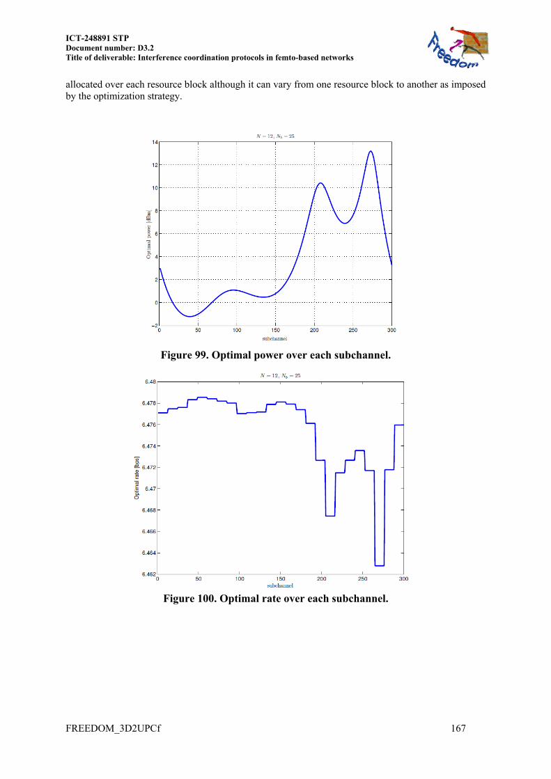
ICT-248891 STP Document number: D3.2 Title of deliverable: Interference coordination protocols in femto-based networks
FREEDOM_3D2UPCf 167
allocated over each resource block although it can vary from one resource block to another as imposed by the optimization strategy.
Figure 99. Optimal power over each subchannel.
Figure 100. Optimal rate over each subchannel.

ICT-248891 STP Document number: D3.2 Title of deliverable: Interference coordination protocols in femto-based networks
168
12 GENERAL CONCLUSIONS Activity 3A2 has focused on the investigation of decentralized approaches for designing the radio resource allocation when several femto access points (FAPs) and possibly the macro BS (MBS) coexist on the same band. We have elucidated that the system performance is improved when sources are able to exchange messages at control-plane level through the backhaul link that connects all the sources. Those messages, named pricing in this work, basically account for the sensitivity of the cost (or objective) function considered at each source as a function of the received interference. They also convey information about the priority of the served users and how the different constraints are met (target rate, max sum-rate, ...). Such information allows optimizing all radio resources jointly but in a decentralized way, by means of considering the individual constraints of other sources. This mode of operation is not possible when all sources optimize their resources in a competitive way (studied in activity 3A1). In this regard, when we want to guarantee a minimum rate in the system, the radio resource allocation becomes a solution of the problem analysed in section 5, where the power is minimized with the objective of obtain a minimum target rate (in SISO, MISO and MIMO configurations).
With the proposed approach the total radiated power is reduced and the minimum target rate is satisfied, which is not always possible when pricing messages are not exchanged.
On the other hand, section 6 provides radio resource algorithms to maximize the weighted sum rate (WSR) of the system, comparing simple vs. complex transmitters (based on superposition coding), analysing the impact of a maximum rate served by the FAP due to the backhaul link quality. Since FAPs are serving multiple users, we also investigate the best way of assigning the resource blocks (RB) over those users served by the same FAP.
When sources update its power simultaneously, the decentralized algorithm might lead to a solution where the bitrate of the users oscillates. By means of incorporating some memory term, that effect is reduced without degrading significantly the total WSR of the system.
When RB assignment has to be optimized over the served users by the same FAP (when users are served in an orthogonal ways), we have analysed a polynomial algorithm
Since the objective is to maximize the WSR, the decentralized algorithm gets solutions where some nodes should switch off their transmitters, or decrease the total transmitted power. This situation is not possible when pricing messages are not exchanged.
Results presented in section 9.1 have elucidated the benefits of the pricing exchange, able to improve the minimum rate of the system (10%-Outage rate) by a factor of 2-3 (200-300% gain) while the spectral efficiency gets a 15% gain, compared with algorithms without using the pricing exchange.
The gains in terms of spectral efficiency are obtained when transmit precoders and RB assignment are optimized, otherwise only gains in terms of minimum rate are attained.
In case the backhaul link limits the communication, the performance of pricing and non-pricing techniques tends to coincide because the generated price is zero. In a nutshell, since the power is not limiting the communication, if you receive additional interference, you have power resources to combat the interference, so it is not required to exchange any price to the interfering terminal in order to control the generated interference.
Section 7 has investigated decentralized resource allocation algorithms when there is a source of randomness.
In a scenario where FAPs employ the same band as the MBS, but they have to estimate the presence of a MBS in a given RB (with a false alarm probability) in order to not interfering the macro user, the solution to maximize the opportunistic throughput becomes an algorithm
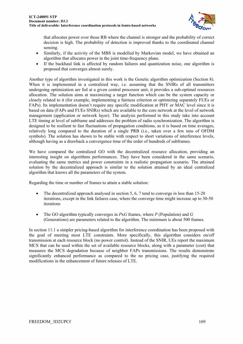
ICT-248891 STP Document number: D3.2 Title of deliverable: Interference coordination protocols in femto-based networks
FREEDOM_3D2UPCf 169
that allocates power over those RB where the channel is stronger and the probability of correct decision is high. The probability of detection is improved thanks to the coordinated channel sensing.
Similarly, if the activity of the MBS is modelled by Markovian model, we have obtained an algorithm that allocates power in the joint time-frequency plane.
If the backhaul link is affected by random failures and quantization noise, one algorithm is proposed that converges almost surely.
Another type of algorithm investigated in this work is the Genetic algorithm optimization (Section 8). When it is implemented in a centralized way, i.e. assuming that the SNIRs of all transmitters undergoing optimization are fed at a given central processor unit, it provides a sub-optimal resources allocation. The solution aims at maximizing a target function which can be the system capacity or closely related to it (for example, implementing a fairness criterion or optimizing separately FUEs or FAPs). Its implementation doesn’t require any specific modification at PHY or MAC level since it is based on data (FAPs and FUEs SNIRs) which are available to the core network at the level of network management (application or network layer). The analysis performed in this study take into account LTE timing at level of subframe and addresses the problem of radio synchronization. The algorithm is designed to be resilient to fast fluctuations of propagation conditions, as it is based on time averages, relatively long compared to the duration of a single PRB (i.e., taken over a few tens of OFDM symbols). The solution has shown to be stable with respect to short variations of interference levels, although having as a drawback a convergence time of the order of hundreds of subframes. We have compared the centralized GO with the decentralized resource allocation, providing an interesting insight on algorithms performances. They have been considered in the same scenario, evaluating the same metrics and power constraints in a realistic propagation scenario. The attained solution by the decentralized approach is similar to the solution attained by an ideal centralized algorithm that knows all the parameters of the system. Regarding the time or number of frames to attain a stable solution:
The decentralized approach analysed in section 5, 6, 7 tend to converge in less than 15-20 iterations, except in the link failures case, where the converge time might increase up to 30-50 iterations
The GO algorithm typically converges in PxG frames, where P (Population) and G (Generations) are parameters related to the algorithm. The minimum is about 500 frames.
In section 11.1 a simpler pricing-based algorithm for interference coordination has been proposed with the goal of meeting most LTE constraints. More specifically, this algorithm considers on/off transmission at each resource block (no power control). Instead of the SNIR, UEs report the maximum MCS that can be used within the set of available resource blocks, along with a parameter (cost) that measures the MCS degradation because of neighbor FAPs transmissions. The results demonstrate significantly enhanced performance as compared to the no pricing case, justifying the required modifications in the enhancement of future releases of LTE.
ICT-248891 STP Document number: D3.2 Title of deliverable: Interference coordination protocols in femto-based networks
170
13 SUMMARY OF RESULTS TOWARDS OTHER ACTIVITIES
13.1 Towards WP4
The investigated techniques in sections 5.2 and 6 at the physical layer have been inputs for the activities carried out in WP4 (4A2, MAC control procedures for femtocell and performance evaluation). Proper control plane procedures have been specified in order to accommodate the investigated algorithms into the standards.
13.2 Towards WP5
The investigated techniques have been considered for evaluation at system level in WP5.
13.3 Towards WP6
Possible useful information for WP6 (6A1 Hardware feasibility study and prototyping) is Table 29, describing the complexity of the different techniques. The objective of provide this input is to know the difficulties when devised WP3 techniques have to be implemented.

ICT-248891 STP Document number: D3.2 Title of deliverable: Interference coordination protocols in femto-based networks
FREEDOM_3D2UPCf 171
14 APPENDIX
14.1 Simulation methodology
The simulation of the interfering FAPs is based on defining the set of parameters describing the propagation environment and their reciprocal effect for the displacement of several FAPs, from few to tens of.
The characterization of the simulation scheme is represented in Figure 101. First the simulator sets the scenario and the relevant propagation parameters (Figure 102). Depending on the number of FAPs and on the capabilities implemented at RRM level, the transmitters can be either grouped in sub-sets or processed as a whole.
Different runs of the GA can provide somewhat different values of the parameters under search. The difference is intrinsic in the GA and the simulations included this intrinsic variability implementing a method for iterating every optimization using the current GA output as initial values for the next run.
Figure 101. Block scheme for the system simulation implementing GA optimization.
The scenario generation phase includes the definition of the transmission parameters related to the Standard of communication under study (i.e., LTE or WiMAX) which are summarized in the pathloss table representing the mutual interference among the FAPs finally deployed. According to Figure 102, the environment system generator is made of four blocks:
1. Setting the PHY characteristics of the Standard (carrier, number of subcarriers, channelization scheme, MCS, power of transmission;
2. Generating the geometry of the environment, in terms of FAPs density distribution, building shape, number of floors, number and type of internal/external walls, position within the apartments;
3. Definition of the channel model adopted, according to ITU or 3GPP;
4. Computation of the pathloss matrix, representing the pathloss for every FUE with respect to the corresponding FAP and to every other FAP/FUE in the system.
The scenario generation is summarized by the pathloss matrix which is the input for the GA optimization. Clustering and scalability based on the parallelization of sub-sets of FAPs is based on the analysis of the pathloss matrix and its structure. Some explicit examples are introduced in section 14.3.2.

ICT-248891 STP Document number: D3.2 Title of deliverable: Interference coordination protocols in femto-based networks
172
Figure 102. Scheme for the scenario generation expressed in terms of pathloss.
14.2 Geometry of the scenario
The study analyzes the downlink or uplink co-existence within a dense deployment of FAPs in blocks of flats (or offices) in a typical urban scenario (see [FREEDOM-D21]). A single block of flats consists of a square building made of three floors divided as a regular square grid of 25 apartments on each floor, separated by 3m. Each apartment is modeled as a square of 10m side. Another set of parameters describe the details of the environment, as summarized in Table 31.
Parameter used Description Value
min_separ Minimum separation FAP/FUE 1 m
Nfloor Number of floors in the building 3
Gr Size of the apartments grid 5
Lapt Apartment side 10 m
d_w Minimum separation between walls in the same apartment 3 m
prob_mw Probability of presence of a main wall between two transmitters 0.1
p_fap Probability of FAP presence in an apartment, i.e. FAP density 0.33-1
Table 31. Typical values for the parameters used for the scenario geometry and the deployment of FAPs.
On the basis of such parameters one can generate a deployment of FAPs in a block, summarized by a table of FAPs distances from FUEs. The effective parameters to model the propagation loss includes the presence of main walls and floors which, depending on the relative distances between FUEs and FAPs, are summarized in terms of an effective number of floors separating the devices.
The deployment of FAPs inside a building has been simulated for two different values of probability (33% and 100%) of presence of FAPs in an apartment. The effective positions of each FAP in the apartments are calculated by selecting a random position within a realistic parameters range (e.g., distance from floor, distance from ceiling) and calculating the equivalent floors of separation in terms of the real number of floors and taking account of the number of walls in between. The flats can allocate one FUE, one FAP, both transmitters or none (see [R4-080149]).
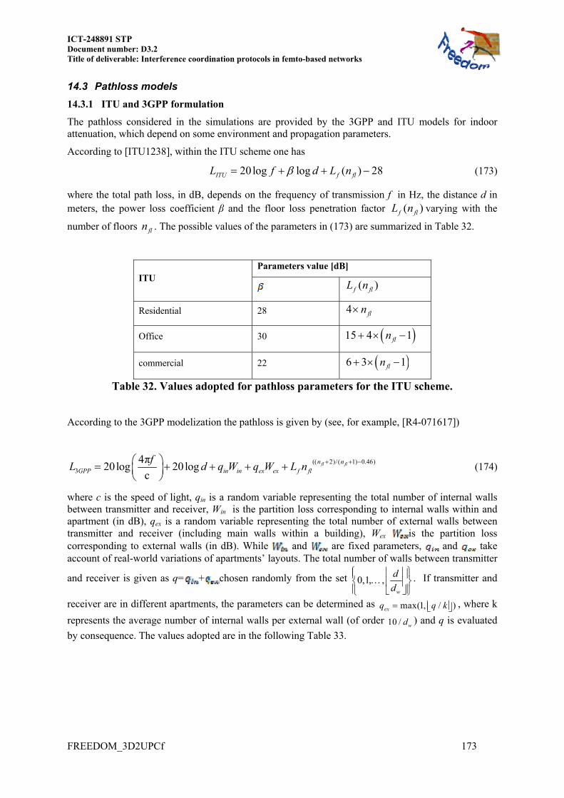
ICT-248891 STP Document number: D3.2 Title of deliverable: Interference coordination protocols in femto-based networks
FREEDOM_3D2UPCf 173
14.3 Pathloss models
14.3.1 ITU and 3GPP formulation
The pathloss considered in the simulations are provided by the 3GPP and ITU models for indoor attenuation, which depend on some environment and propagation parameters.
According to [ITU1238], within the ITU scheme one has
20 log log ( ) 28ITU f flL f d L n (173)
where the total path loss, in dB, depends on the frequency of transmission f in Hz, the distance d in meters, the power loss coefficient β and the floor loss penetration factor ( )f flL n varying with the
number of floors fln . The possible values of the parameters in (173) are summarized in Table 32.
ITU Parameters value [dB]
( )f flL n
Residential 28 4 fln
Office 30 15 14 fln
commercial 22 6 13 fln
Table 32. Values adopted for pathloss parameters for the ITU scheme.
According to the 3GPP modelization the pathloss is given by (see, for example, [R4-071617])
(( 2)/( 1) 0.46)
3
4π20log 20log
cfl fln n
GPP in in ex ex f fl
fL d q W q W L n
(174)
where c is the speed of light, qin is a random variable representing the total number of internal walls between transmitter and receiver, Win is the partition loss corresponding to internal walls within and apartment (in dB), qex is a random variable representing the total number of external walls between transmitter and receiver (including main walls within a building), Wex is the partition loss corresponding to external walls (in dB). While and are fixed parameters, and take account of real-world variations of apartments’ layouts. The total number of walls between transmitter
and receiver is given as q= + chosen randomly from the set 0,1, ,w
d
d
. If transmitter and
receiver are in different apartments, the parameters can be determined as max(1, / )exq q k , where k
represents the average number of internal walls per external wall (of order 10 / wd ) and q is evaluated
by consequence. The values adopted are in the following Table 33.

ICT-248891 STP Document number: D3.2 Title of deliverable: Interference coordination protocols in femto-based networks
174
Parameter Value
5 dB
5 dB
18.3 dB
k 5
f
Table 33. Values adopted for pathloss parameters in the 3GPP scheme.
After the scenario set up, the algorithm provides the set or values regarding linear distances, number of internal and external walls, number of floors between every FUE and every FAP, whose possible realization in summarized in Table 34.
MSs
5 13 6 15 16 11 1 18 8 5 10 16 1 16 19 12 8 12 5 11 11 6 14 6 7
Relative distances MSs/FAPs (m)
1 1 2 4 5 3 0 4 2 1 2 3 0 3 1 1 2 4 1 3 2 2 3 1 1
Number of internal walls
0 0 0 0 1 0 0 0 0 1 0 0 0 0 1 0 0 0 1 1 2 1 1 1 0
Number of equivalent floors in between
FAPs
Table 34. Values obtained for one simulation of the scenario geometry. Rows follow FUEs index, columns follow FAPs index.
For example, with the above values for the scenario definition, one gets the set of relative pathlosses in dB as
58 66 64 82 106
74 32 83 66 75
69 78 41 78 87
65 67 80 76 92
103 83 95 77 61
lossL
(175)
14.3.2 Pathloss and clustering
By increasing the number of FAPs, the simulation has analyzed the structure of the pathloss matrix taking into account the apartments deployment described above. The interference among FAPs is characterized by their relative distance and by the physical environment (walls, floors) surrounding the transmitters. As shown in Figure 103 a structure as clusters of interference appears as an effect of the effective distances: 3, 4, 5 or 6 clusters identify the groups of couples FAPs-FUEs which have a larger mutual influence. The typical maximum is along the diagonal (mostly blue squares, lowest pathloss) which characterizes the FUEs linked to their own FAP.

ICT-248891 STP Document number: D3.2 Title of deliverable: Interference coordination protocols in femto-based networks
FREEDOM_3D2UPCf 175
Figure 103. Pathloss representation in dB. Left: 27 FAPs, 3 floors building; Right: 64 FAPs, 4 floors building.
As supported by physical and geometrical considerations, FAPs scattered apart tend not to influence each other, therefore when considering a large number of FAPs one can set a criterion to determine if the problem is scalable or not. If from the pathloss matrix one can define a set of emerging clusters, the GO optimization method can be split in several sub-problems which can be run in parallel, saving computing time and decreasing the convergence time of the algorithm.
We will devote section 8.4 to the scalability of the GO based on the parallelization over several GO processes with a reduced number of variables.
14.4 More results of section 8.3.2.1
The optimization algorithm applies similarly in the case of a flat fading channel for an increasing number of FAPs/FUEs. The analysis for the case of twelve FAPs is shown for a pathloss matrix as visualized in Figure 104
Figure 104. Random deployment of 12 FUEs, pathloss matrix false color representation, values are in dB.
The genetic optimization with the fitness function evolution is shown in Figure 105 where the graph in the bottom represents the assignment of frequency (first 12 bars provide starting frequency value,

ICT-248891 STP Document number: D3.2 Title of deliverable: Interference coordination protocols in femto-based networks
176
second 12 bars provide bandwidth) and power (last 12 bars). Final allocation is visualized inFigure 106: the three parameters assigned to the k-th FAP are given by the value of the k-th bar in each of the three sets of 12.
Figure 105. GO output for 12 FUEs deployed with an interference scenario corresponding to a pathloss matrix as in Figure 104.
Figure 106. GO output for 12 FUEs, power/bandwidth allocation, for a pathloss matrix as in Figure 104.
Those FAPs that can be considered independent of each other, in terms of pathloss, are assigned the same frequencies without risk of interference.
The algorithm can deal with an increasing number of FAPs/FUEs, although reducing the speed of computation. Considering a sparse density with value 0.33, i.e. corresponding to a 33% probability of a FAP (and corresponding FUE) presence in a single apartment, the algorithm has been tested also for scenarios with an increasing number of FAPs/FUEs. The results for 32 FAPs deployed in a single building are shown in Figure 107 and Figure 108, while for 48 FAPs are reported in Figure 109 and Figure 110.
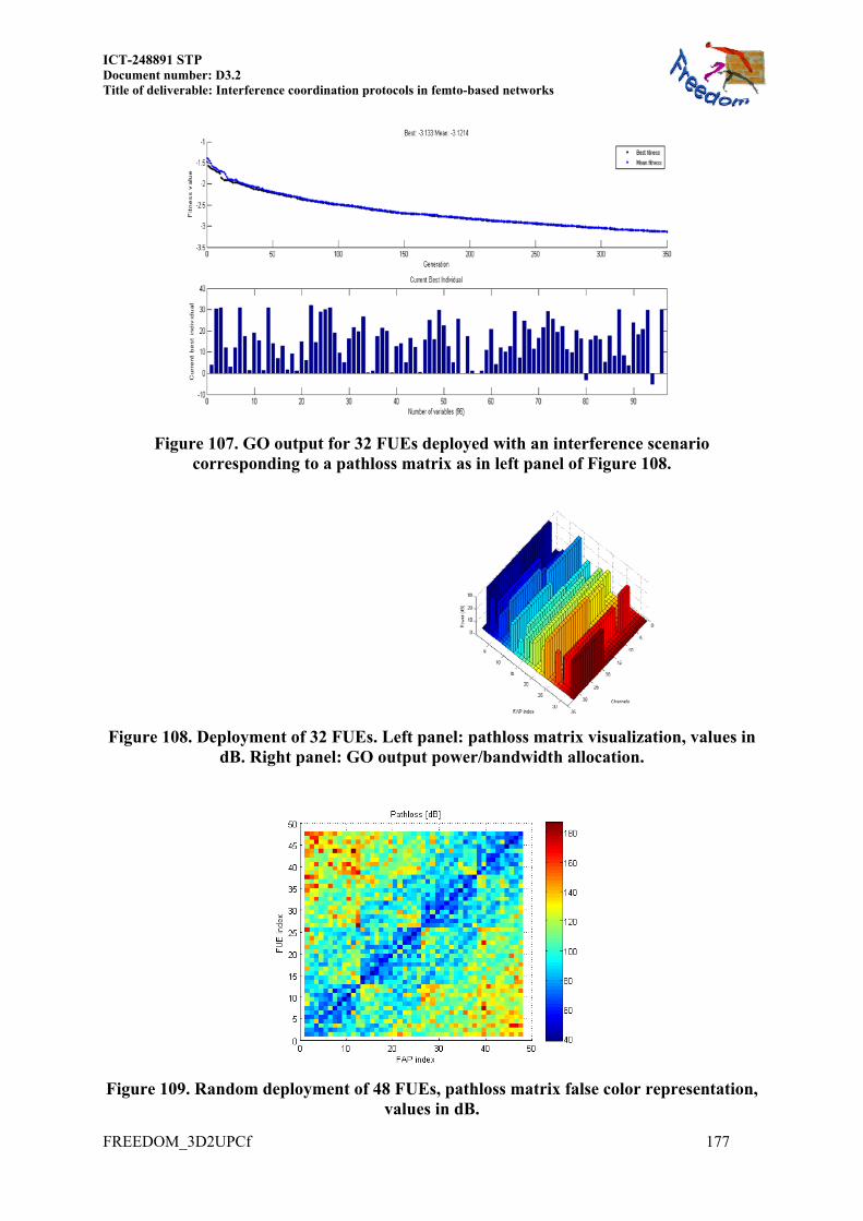
ICT-248891 STP Document number: D3.2 Title of deliverable: Interference coordination protocols in femto-based networks
FREEDOM_3D2UPCf 177
Figure 107. GO output for 32 FUEs deployed with an interference scenario corresponding to a pathloss matrix as in left panel of Figure 108.
Figure 108. Deployment of 32 FUEs. Left panel: pathloss matrix visualization, values in dB. Right panel: GO output power/bandwidth allocation.
Figure 109. Random deployment of 48 FUEs, pathloss matrix false color representation, values in dB.
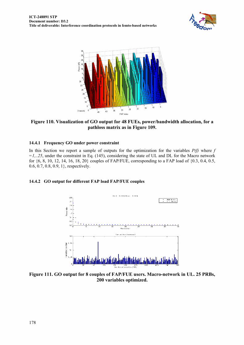
ICT-248891 STP Document number: D3.2 Title of deliverable: Interference coordination protocols in femto-based networks
178
Figure 110. Visualization of GO output for 48 FUEs, power/bandwidth allocation, for a pathloss matrix as in Figure 109.
14.4.1 Frequency GO under power constraint
In this Section we report a sample of outputs for the optimization for the variables P(f) where f =1,..25, under the constraint in Eq. (145), considering the state of UL and DL for the Macro network for 6, 8, 10, 12, 14, 16, 18, 20 couples of FAP/FUE, corresponding to a FAP load of 0.3, 0.4, 0.5, 0.6, 0.7, 0.8, 0.9, 1, respectively.
14.4.2 GO output for different FAP load FAP/FUE couples
Figure 111. GO output for 8 couples of FAP/FUE users. Macro-network in UL. 25 PRBs, 200 variables optimized.
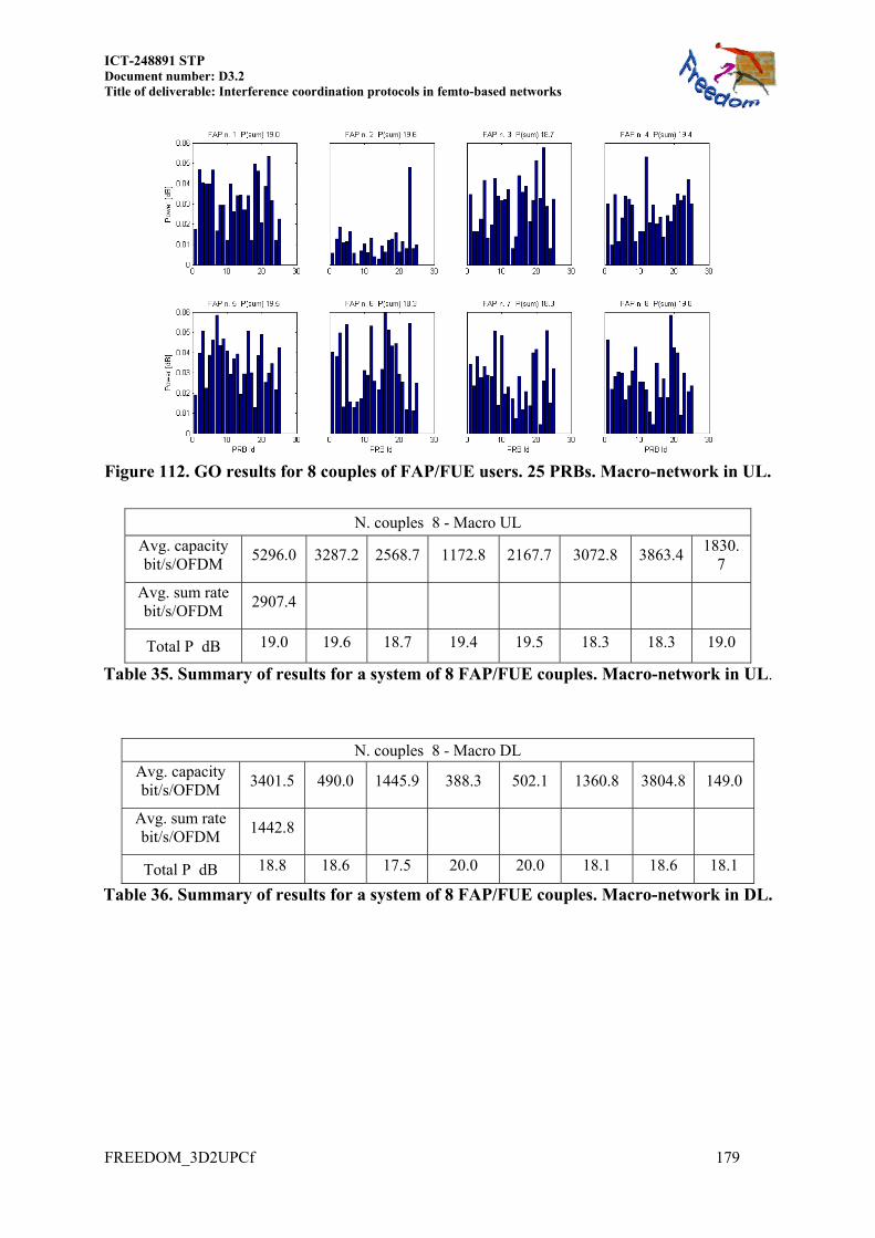
ICT-248891 STP Document number: D3.2 Title of deliverable: Interference coordination protocols in femto-based networks
FREEDOM_3D2UPCf 179
Figure 112. GO results for 8 couples of FAP/FUE users. 25 PRBs. Macro-network in UL.
N. couples 8 - Macro UL
Avg. capacity bit/s/OFDM
5296.0 3287.2 2568.7 1172.8 2167.7 3072.8 3863.4 1830.
7
Avg. sum rate bit/s/OFDM
2907.4
Total P dB 19.0 19.6 18.7 19.4 19.5 18.3 18.3 19.0
Table 35. Summary of results for a system of 8 FAP/FUE couples. Macro-network in UL.
N. couples 8 - Macro DL
Avg. capacity bit/s/OFDM
3401.5 490.0 1445.9 388.3 502.1 1360.8 3804.8 149.0
Avg. sum rate bit/s/OFDM
1442.8
Total P dB 18.8 18.6 17.5 20.0 20.0 18.1 18.6 18.1
Table 36. Summary of results for a system of 8 FAP/FUE couples. Macro-network in DL.
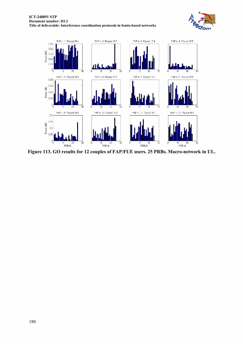
ICT-248891 STP Document number: D3.2 Title of deliverable: Interference coordination protocols in femto-based networks
180
Figure 113. GO results for 12 couples of FAP/FUE users. 25 PRBs. Macro-network in UL.