Embed Size (px)
Citation preview

Introduction to density functional theory
Feliciano Giustino
Department of Materials, University of Oxford
Department of Materials Science and Engineering, Cornell University
NSF/DOE Quantum Science Summer SchoolCornell University, June 10-22, 2018Feliciano Giustino, QS3 School, Cornell, June 2018

Organization of the DFT sessions
Betul Pamuk Guru Khalsa FG
F Giustino
02/88
Part 0/7
Feliciano Giustino, QS3 School, Cornell, June 2018

Organization of the DFT sessions
Monday 10 June
11:00–11:45 Theory Lecture 1 45m FG
11:55–12:40 Theory Lecture 2 45m FG
14:00–16:00 Hands-on Session 1 2h Betul Pamuk, Guru Khalsa, FG
Tuesday 11 June
14:00–17:30 Hands-on Session 2 3h30m Betul Pamuk, Guru Khalsa, FG
F Giustino
03/88
Part 0/7
Feliciano Giustino, QS3 School, Cornell, June 2018

Handouts and Tutorial Sheets
Handouts Tutorial Sheets
F Giustino
04/88
Part 0/7
Feliciano Giustino, QS3 School, Cornell, June 2018

Textbooks
MSc and 1st year PhD level
F Giustino
05/88
Part 0/7
Feliciano Giustino, QS3 School, Cornell, June 2018

Textbooks
MSc and 1st year PhD level
Advanced PhD level
F Giustino
05/88
Part 0/7
Feliciano Giustino, QS3 School, Cornell, June 2018

Textbooks
MSc and 1st year PhD level
Advanced PhD level Theoretical foundations
F Giustino
05/88
Part 0/7
Feliciano Giustino, QS3 School, Cornell, June 2018

Outline
Part 1 Ab initio materials modelling
Part 2 Many-body problem
Part 3 Density-functional theory
Part 4 Planewaves and pseudopotentials
Part 5 Equilibrium structures
Part 6 Band structures
Part 7 DFT beyond the LDA
F Giustino
06/88
Part 0/7
Feliciano Giustino, QS3 School, Cornell, June 2018

Part 1
Ab initio materials modelling
F Giustino
07/88
Part 1/7
Feliciano Giustino, QS3 School, Cornell, June 2018

Impact of DFT
Interview by R. Van Norden
Nature 514, 550 (2014)
F Giustino
08/88
Part 1/7
Feliciano Giustino, QS3 School, Cornell, June 2018

Impact of DFT
Interview by R. Van Norden
Nature 514, 550 (2014)
F Giustino
08/88
Part 1/7
Feliciano Giustino, QS3 School, Cornell, June 2018

Impact of DFT
HK 1964 Hohenberg, Kohn, Phys. Rev. 136, B864 (1964)
KS 1965 Kohn, Sham, Phys. Rev. 140, A1133 (1965)
CA 1980 Ceperley, Alder, Phys. Rev. Lett. 45, 566 (1980)
PZ 1981 Perdew, Zunger, Phys. Rev. B 23, 5048 (1981)
PBE 1996 Perdew, Burke, Ernzerhof, Phys. Rev. Lett. 77, 3865 (1996)
F Giustino
09/88
Part 1/7
Feliciano Giustino, QS3 School, Cornell, June 2018

Impact of DFT
The B3LYP papers ranked #7 and #8 in 2014 are now at ∼75k cites
F Giustino
10/88
Part 1/7
Feliciano Giustino, QS3 School, Cornell, June 2018

Examples of calculations based on DFT
Predictive calculations of optical properties
Zacharias, Patrick, and FG, Phys. Rev. Lett. 115, 177401 (2015)
F Giustino
11/88
Part 1/7
Feliciano Giustino, QS3 School, Cornell, June 2018

Examples of calculations based on DFT
Predictive calculations of transport properties
Image from Thathachary et al,
Nano Lett. 14, 626 (2014)
Silicon
Ponce, Margine, and FG, Phys. Rev. B(R) 97, 121201 (2018)
F Giustino
12/88
Part 1/7
Feliciano Giustino, QS3 School, Cornell, June 2018

Examples of calculations based on DFT
Materials characterization via vibrational spectroscopy
MAPbI3
Perez-Osorio, Milot, Filip, Patel, Herz, Johnston, and FG, J. Phys. Chem. C 119, 25703 (2015)
F Giustino
13/88
Part 1/7
Feliciano Giustino, QS3 School, Cornell, June 2018

Examples of calculations based on DFT
Computational materials discovery1 1.0079
HHydrogen
3 6.941
LiLithium
11 22.990
NaSodium
19 39.098
KPotassium
37 85.468
RbRubidium
55 132.91
CsCaesium
87 223
FrFrancium
4 9.0122
BeBeryllium
12 24.305
MgMagnesium
20 40.078
CaCalcium
38 87.62
SrStrontium
56 137.33
BaBarium
88 226
RaRadium
21 44.956
ScScandium
39 88.906
YYttrium
57 138.91
LaLanthanum
89 227
AcActinium
22 47.867
TiTitanium
40 91.224
ZrZirconium
72 178.49
HfHalfnium
23 50.942
VVanadium
41 92.906
NbNiobium
73 180.95
TaTantalum
24 51.996
CrChromium
42 95.94
MoMolybdenum
74 183.84
WTungsten
25 54.938
MnManganese
43 96
TcTechnetium
75 186.21
ReRhenium
26 55.845
FeIron
44 101.07
RuRuthenium
76 190.23
OsOsmium
27 58.933
CoCobalt
45 102.91
RhRhodium
77 192.22
IrIridium
28 58.693
NiNickel
46 106.42
PdPalladium
78 195.08
PtPlatinum
29 63.546
CuCopper
47 107.87
AgSilver
79 196.97
AuGold
30 65.39
ZnZinc
48 112.41
CdCadmium
80 200.59
HgMercury
31 69.723
GaGallium
13 26.982
AlAluminium
5 10.811
BBoron
49 114.82
InIndium
81 204.38
TlThallium
6 12.011
CCarbon
14 28.086
SiSilicon
32 72.64
GeGermanium
50 118.71
SnTin
82 207.2
PbLead
7 14.007
NNitrogen
15 30.974
PPhosphorus
33 74.922
AsArsenic
51 121.76
SbAntimony
83 208.98
BiBismuth
8 15.999
OOxygen
16 32.065
SSulphur
34 78.96
SeSelenium
52 127.6
TeTellurium
84 209
PoPolonium
9 18.998
FFlourine
17 35.453
ClChlorine
35 79.904
BrBromine
53 126.9
IIodine
85 210
AtAstatine
10 20.180
NeNeon
2 4.0025
HeHelium
18 39.948
ArArgon
36 83.8
KrKrypton
54 131.29
XeXenon
86 222
RnRadon
57 138.91
LaLanthanum
58 140.12
CeCerium
59 140.91
PrPraseodymium
60 144.24
NdNeodymium
61 145
PmPromethium
62 150.36
SmSamarium
63 151.96
EuEuropium
64 157.25
GdGadolinium
65 158.93
TbTerbium
66 162.50
DyDysprosium
67 164.93
HoHolmium
68 167.26
ErErbium
69 168.93
TmThulium
70 173.04
YbYtterbium
71 174.97
LuLutetium
89 227
AcActinium
90 232.04
ThThorium
91 231.04
PaProtactinium
92 238.03
UUranium
Volonakis, Filip, Haghighirad, Sakai, Wenger, Snaith, and FG, J. Phys. Chem. Lett. 7, 1254 (2016)
F Giustino
14/88
Part 1/7
Feliciano Giustino, QS3 School, Cornell, June 2018
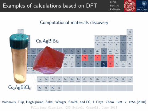
Examples of calculations based on DFT
Computational materials discovery1 1.0079
HHydrogen
3 6.941
LiLithium
11 22.990
NaSodium
19 39.098
KPotassium
37 85.468
RbRubidium
55 132.91
CsCaesium
87 223
FrFrancium
4 9.0122
BeBeryllium
12 24.305
MgMagnesium
20 40.078
CaCalcium
38 87.62
SrStrontium
56 137.33
BaBarium
88 226
RaRadium
21 44.956
ScScandium
39 88.906
YYttrium
57 138.91
LaLanthanum
89 227
AcActinium
22 47.867
TiTitanium
40 91.224
ZrZirconium
72 178.49
HfHalfnium
23 50.942
VVanadium
41 92.906
NbNiobium
73 180.95
TaTantalum
24 51.996
CrChromium
42 95.94
MoMolybdenum
74 183.84
WTungsten
25 54.938
MnManganese
43 96
TcTechnetium
75 186.21
ReRhenium
26 55.845
FeIron
44 101.07
RuRuthenium
76 190.23
OsOsmium
27 58.933
CoCobalt
45 102.91
RhRhodium
77 192.22
IrIridium
28 58.693
NiNickel
46 106.42
PdPalladium
78 195.08
PtPlatinum
29 63.546
CuCopper
47 107.87
AgSilver
79 196.97
AuGold
30 65.39
ZnZinc
48 112.41
CdCadmium
80 200.59
HgMercury
31 69.723
GaGallium
13 26.982
AlAluminium
5 10.811
BBoron
49 114.82
InIndium
81 204.38
TlThallium
6 12.011
CCarbon
14 28.086
SiSilicon
32 72.64
GeGermanium
50 118.71
SnTin
82 207.2
PbLead
7 14.007
NNitrogen
15 30.974
PPhosphorus
33 74.922
AsArsenic
51 121.76
SbAntimony
83 208.98
BiBismuth
8 15.999
OOxygen
16 32.065
SSulphur
34 78.96
SeSelenium
52 127.6
TeTellurium
84 209
PoPolonium
9 18.998
FFlourine
17 35.453
ClChlorine
35 79.904
BrBromine
53 126.9
IIodine
85 210
AtAstatine
10 20.180
NeNeon
2 4.0025
HeHelium
18 39.948
ArArgon
36 83.8
KrKrypton
54 131.29
XeXenon
86 222
RnRadon
57 138.91
LaLanthanum
58 140.12
CeCerium
59 140.91
PrPraseodymium
60 144.24
NdNeodymium
61 145
PmPromethium
62 150.36
SmSamarium
63 151.96
EuEuropium
64 157.25
GdGadolinium
65 158.93
TbTerbium
66 162.50
DyDysprosium
67 164.93
HoHolmium
68 167.26
ErErbium
69 168.93
TmThulium
70 173.04
YbYtterbium
71 174.97
LuLutetium
89 227
AcActinium
90 232.04
ThThorium
91 231.04
PaProtactinium
92 238.03
UUranium
Cs2AgBiCl6
Cs2AgBiBr6
Volonakis, Filip, Haghighirad, Sakai, Wenger, Snaith, and FG, J. Phys. Chem. Lett. 7, 1254 (2016)
F Giustino
14/88
Part 1/7
Feliciano Giustino, QS3 School, Cornell, June 2018

Examples of calculations based on DFT
Predictive calculations of the superconducting critical temperature
NbS2
Heil, Ponce, Lambert, Schlipf, Margine, and FG, Phys. Rev. Lett., 119, 087003 (2017)
F Giustino
15/88
Part 1/7
Feliciano Giustino, QS3 School, Cornell, June 2018

Examples of calculations based on DFT
Many-body effects in ARPES
Moser et al,
PRL 110, 196403 (2013)
TiO2 anatase
Verdi, Caruso, and FG, Nat. Commun. 8, 15769 (2017)
F Giustino
16/88
Part 1/7
Feliciano Giustino, QS3 School, Cornell, June 2018

Why is DFT so popular?
• TransferabilityWe can use the same codes/methods for very different materials
• SimplicityThe Kohn-Sham equations are conceptually very similar to theSchrodinger equation for a single electron in an external potential
• ReliabilityOften we can predict materials properties with high accuracy,sometimes even before experiments
• Software sharingThe development of DFT has become a global enterprise, e.g. opensource and collaborative software development
• Robust platformOften the shortcomings of DFT can be cured by using moresophisticated approaches, which still use DFT as their starting point
F Giustino
17/88
Part 1/7
Feliciano Giustino, QS3 School, Cornell, June 2018

Question 1
How many papers using DFT will be published
worldwide during the QS3 school?
A Ten
B At least four hundred
C Ten thousand
D More than a million
E I have no idea
F Giustino
18/88
Part 1/7
Feliciano Giustino, QS3 School, Cornell, June 2018

Part 2
Many-body problem
F Giustino
19/88
Part 2/7
Feliciano Giustino, QS3 School, Cornell, June 2018

Many-body Schrodinger equation
Materials = Electrons + Nuclei
• Schrodinger equation for the H atom(nucleus at r = 0)
− ~2
2me∇2ψ(r)− e2
4πε0
1
|r|ψ(r) = Etotψ(r)
• wavefunctions of H(from Wikipedia)
F Giustino
20/88
Part 2/7
Feliciano Giustino, QS3 School, Cornell, June 2018

Many-body Schrodinger equation
Materials = Electrons + Nuclei
• Schrodinger equation for the H atom(nucleus at r = 0)
− ~2
2me∇2ψ(r)− e2
4πε0
1
|r|ψ(r) = Etotψ(r)
• wavefunctions of H(from Wikipedia)
F Giustino
20/88
Part 2/7
Feliciano Giustino, QS3 School, Cornell, June 2018

Many-body Schrodinger equation
Materials = Electrons + Nuclei
1s 2px 3dz2
• Schrodinger equation for the H atom(nucleus at r = 0)
− ~2
2me∇2ψ(r)− e2
4πε0
1
|r|ψ(r) = Etotψ(r)
• wavefunctions of H(from Wikipedia)
F Giustino
20/88
Part 2/7
Feliciano Giustino, QS3 School, Cornell, June 2018
Many-body Schrodinger equation
• Many-body wavefunction (keep it simple: only 3 electrons)
ψ(r)→ Ψ = Ψ(r1, r2, r3)
• Probability of finding electron #1 at the point r
prob(r1 =r) =
∫|Ψ(r, r2, r3)|2 dr2dr3
• Electron density at the point r
n(r) = prob(r1 =r) + prob(r2 =r) + prob(r3 =r)
• Electrons are indistinguishable
n(r) = 3
∫|Ψ(r, r2, r3)|2 dr2dr3
F Giustino
21/88
Part 2/7
Feliciano Giustino, QS3 School, Cornell, June 2018
Many-body Schrodinger equation
( kinetic energy + potential energy ) Ψ = EtotΨ
• kinetic energy, electrons and nuclei
−N∑i=1
~2
2me∇2i −
M∑I=1
~2
2MI∇2I
• potential energy, electron-electron repulsion
1
2
∑i6=j
e2
4πε0
1
|ri − rj |
• potential energy, nucleus-nucleus repulsion
1
2
∑I 6=J
e2
4πε0
ZIZJ|RI −RJ |
• potential energy, electron-nucleus attraction
−∑i,I
e2
4πε0
ZI|ri −RI |
F Giustino
22/88
Part 2/7
Feliciano Giustino, QS3 School, Cornell, June 2018

Many-body Schrodinger equation
−∑i
~2
2me∇2i −
∑I
~2
2MI∇2I +
1
2
∑i6=j
e2
4πε0
1
|ri − rj |
+1
2
∑I 6=J
e2
4πε0
ZIZJ|RI −RJ |
−∑i,I
e2
4πε0
ZI|ri −RI |
Ψ = EtotΨ
−∑i
1
2∇2i −
∑I
1
2MI∇2I +
1
2
∑i6=j
1
|ri − rj |
+1
2
∑I 6=J
ZIZJ|RI −RJ |
−∑i,I
ZI|ri −RI |
Ψ = EtotΨ
F Giustino
23/88
Part 2/7
Feliciano Giustino, QS3 School, Cornell, June 2018

Many-body Schrodinger equation
−∑i
~2
2me∇2i −
∑I
~2
2MI∇2I +
1
2
∑i6=j
e2
4πε0
1
|ri − rj |
+1
2
∑I 6=J
e2
4πε0
ZIZJ|RI −RJ |
−∑i,I
e2
4πε0
ZI|ri −RI |
Ψ = EtotΨ
−∑i
1
2∇2i −
∑I
1
2MI∇2I +
1
2
∑i6=j
1
|ri − rj |
+1
2
∑I 6=J
ZIZJ|RI −RJ |
−∑i,I
ZI|ri −RI |
Ψ = EtotΨ
Hartree atomic units
• masses in units of me (electron mass)
• lengths in units of a0 (Bohr radius)
• energies in units of e2/4πε0a0 (Hartree)
F Giustino
23/88
Part 2/7
Feliciano Giustino, QS3 School, Cornell, June 2018

Many-body Schrodinger equation
MBSE
F Giustino
24/88
Part 2/7
Feliciano Giustino, QS3 School, Cornell, June 2018

Many-body Schrodinger equation
MBSE MBSE in Hartree units
F Giustino
24/88
Part 2/7
Feliciano Giustino, QS3 School, Cornell, June 2018

Exponential wall
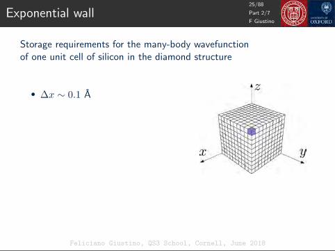
Storage requirements for the many-body wavefunctionof one unit cell of silicon in the diamond structure
• ∆x ∼ 0.1 A
• a = 5.43 A
• Np = (a3/4)/(∆x)3 ∼ 40, 000
• 8 valence electrons per unit cell
• Ψ = 40, 0008 complex numbers
F Giustino
25/88
Part 2/7
Feliciano Giustino, QS3 School, Cornell, June 2018
Exponential wall
Storage requirements for the many-body wavefunctionof one unit cell of silicon in the diamond structure
• ∆x ∼ 0.1 A
• a = 5.43 A
• Np = (a3/4)/(∆x)3 ∼ 40, 000
• 8 valence electrons per unit cell
• Ψ = 40, 0008 complex numbers
F Giustino
25/88
Part 2/7
Feliciano Giustino, QS3 School, Cornell, June 2018

Exponential wall
Storage requirements for the many-body wavefunctionof one unit cell of silicon in the diamond structure
• ∆x ∼ 0.1 A
• a = 5.43 A
• Np = (a3/4)/(∆x)3 ∼ 40, 000
• 8 valence electrons per unit cell
• Ψ = 40, 0008 complex numbers
1026 Terabytes
F Giustino
25/88
Part 2/7
Feliciano Giustino, QS3 School, Cornell, June 2018

Clamped nuclei approximation
Set nuclear masses MI =∞:−∑i
1
2∇2
i −∑I
1
2MI∇2
I +1
2
∑i6=j
1
|ri − rj |
+1
2
∑I 6=J
ZIZJ
|RI −RJ |−∑i,I
ZI
|ri −RI |
Ψ = EtotΨ
F Giustino
26/88
Part 2/7
Feliciano Giustino, QS3 School, Cornell, June 2018

Clamped nuclei approximation
Set nuclear masses MI =∞:−∑i
1
2∇2
i −
∑I
1
2MI∇2
I +1
2
∑i6=j
1
|ri − rj |
+1
2
∑I 6=J
ZIZJ
|RI −RJ |−∑i,I
ZI
|ri −RI |
Ψ = EtotΨ
F Giustino
26/88
Part 2/7
Feliciano Giustino, QS3 School, Cornell, June 2018

Clamped nuclei approximation
Set nuclear masses MI =∞:−∑i
1
2∇2
i −
∑I
1
2MI∇2
I +1
2
∑i6=j
1
|ri − rj |
+1
2
∑I 6=J
ZIZJ
|RI −RJ |−∑i,I
ZI
|ri −RI |
Ψ = EtotΨ
−∑i
∇2i
2+∑i
Vn(ri) +1
2
∑i6=j
1
|ri − rj |
Ψ = EΨ
Electronic structure theory in a nutshell
F Giustino
26/88
Part 2/7
Feliciano Giustino, QS3 School, Cornell, June 2018

Independent electrons approximation
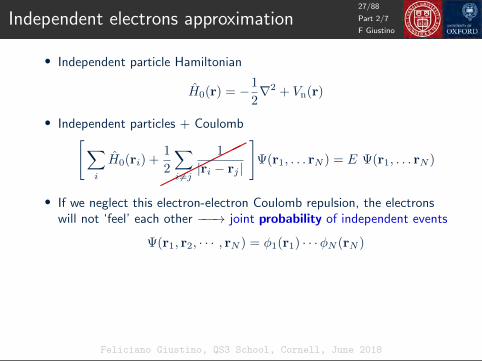
• Independent particle Hamiltonian
H0(r) = −1
2∇2 + Vn(r)
• Independent particles + Coulomb[∑i
H0(ri) +1
2
∑i6=j
1
|ri − rj |
]Ψ(r1, . . . rN ) = E Ψ(r1, . . . rN )
• If we neglect this electron-electron Coulomb repulsion, the electronswill not ‘feel’ each other −−−→ joint probability of independent events
Ψ(r1, r2, · · · , rN ) = φ1(r1) · · ·φN (rN )
H0(r)φi(r) = εiφi(r)
E = ε1 + · · ·+ εN
F Giustino
27/88
Part 2/7
Feliciano Giustino, QS3 School, Cornell, June 2018

Independent electrons approximation
• Independent particle Hamiltonian
H0(r) = −1
2∇2 + Vn(r)
• Independent particles + Coulomb[∑i
H0(ri) +1
2
∑i6=j
1
|ri − rj |
]Ψ(r1, . . . rN ) = E Ψ(r1, . . . rN )
• If we neglect this electron-electron Coulomb repulsion, the electronswill not ‘feel’ each other −−−→ joint probability of independent events
Ψ(r1, r2, · · · , rN ) = φ1(r1) · · ·φN (rN )
H0(r)φi(r) = εiφi(r)
E = ε1 + · · ·+ εN
F Giustino
27/88
Part 2/7
Feliciano Giustino, QS3 School, Cornell, June 2018
Independent electrons approximation
• Independent particle Hamiltonian
H0(r) = −1
2∇2 + Vn(r)
• Independent particles + Coulomb[∑i
H0(ri) +
1
2
∑i6=j
1
|ri − rj |
]Ψ(r1, . . . rN ) = E Ψ(r1, . . . rN )
• If we neglect this electron-electron Coulomb repulsion, the electronswill not ‘feel’ each other −−−→ joint probability of independent events
Ψ(r1, r2, · · · , rN ) = φ1(r1) · · ·φN (rN )
H0(r)φi(r) = εiφi(r)
E = ε1 + · · ·+ εN
F Giustino
27/88
Part 2/7
Feliciano Giustino, QS3 School, Cornell, June 2018

Exclusion principle
• Let us calculate the electron density for 2 electrons in theindependent-electron approximation
n(r) = 2
∫|Ψ(r, r2)|2 dr2
= 2
∫|φ1(r)|2|φ2(r2)|2 dr2 = 2 |φ1(r)|2
• Admissible wavefunctions must be antisymmetric w.r.t. exchange ofspace and spin variables −−−→ Slater determinant (spin-unpolarized)
Ψ(r1, r2) =1√2
[φ1(r1)φ2(r2)− φ1(r2)φ2(r1)]
• Let us try the density again
n(r) = 2
∫|Ψ(r, r2)|2 dr2 =
F Giustino
28/88
Part 2/7
Feliciano Giustino, QS3 School, Cornell, June 2018

Exclusion principle
• Let us calculate the electron density for 2 electrons in theindependent-electron approximation
n(r) = 2
∫|Ψ(r, r2)|2 dr2 = 2
∫|φ1(r)|2|φ2(r2)|2 dr2
= 2 |φ1(r)|2
• Admissible wavefunctions must be antisymmetric w.r.t. exchange ofspace and spin variables −−−→ Slater determinant (spin-unpolarized)
Ψ(r1, r2) =1√2
[φ1(r1)φ2(r2)− φ1(r2)φ2(r1)]
• Let us try the density again
n(r) = 2
∫|Ψ(r, r2)|2 dr2 =
F Giustino
28/88
Part 2/7
Feliciano Giustino, QS3 School, Cornell, June 2018

Exclusion principle
• Let us calculate the electron density for 2 electrons in theindependent-electron approximation
n(r) = 2
∫|Ψ(r, r2)|2 dr2 = 2
∫|φ1(r)|2|φ2(r2)|2 dr2 = 2 |φ1(r)|2
• Admissible wavefunctions must be antisymmetric w.r.t. exchange ofspace and spin variables −−−→ Slater determinant (spin-unpolarized)
Ψ(r1, r2) =1√2
[φ1(r1)φ2(r2)− φ1(r2)φ2(r1)]
• Let us try the density again
n(r) = 2
∫|Ψ(r, r2)|2 dr2 =
F Giustino
28/88
Part 2/7
Feliciano Giustino, QS3 School, Cornell, June 2018

Exclusion principle
• Let us calculate the electron density for 2 electrons in theindependent-electron approximation
n(r) = 2
∫|Ψ(r, r2)|2 dr2 = 2
∫|φ1(r)|2|φ2(r2)|2 dr2 = 2 |φ1(r)|2
• Admissible wavefunctions must be antisymmetric w.r.t. exchange ofspace and spin variables −−−→ Slater determinant (spin-unpolarized)
Ψ(r1, r2) =1√2
[φ1(r1)φ2(r2)− φ1(r2)φ2(r1)]
• Let us try the density again
n(r) = 2
∫|Ψ(r, r2)|2 dr2
=
F Giustino
28/88
Part 2/7
Feliciano Giustino, QS3 School, Cornell, June 2018

Exclusion principle
• Let us calculate the electron density for 2 electrons in theindependent-electron approximation
n(r) = 2
∫|Ψ(r, r2)|2 dr2 = 2
∫|φ1(r)|2|φ2(r2)|2 dr2 = 2 |φ1(r)|2
• Admissible wavefunctions must be antisymmetric w.r.t. exchange ofspace and spin variables −−−→ Slater determinant (spin-unpolarized)
Ψ(r1, r2) =1√2
[φ1(r1)φ2(r2)− φ1(r2)φ2(r1)]
• Let us try the density again
n(r) = 2
∫|Ψ(r, r2)|2 dr2 = |φ1(r)|2 + |φ2(r)|2
F Giustino
28/88
Part 2/7
Feliciano Giustino, QS3 School, Cornell, June 2018

Mean-field approximation
• The electron density can be used to determine the electrostatic fieldgenerated by the electrons
[−1
2∇2 + Vn(r)
]φi(r) = εiφi(r)
n(r) =∑i
|φi(r)|2
VH(r) =
∫dr′
n(r′)
|r− r′|[−1
2∇2 + Vn(r)+VH(r)
]φnewi (r) = εnewi φnewi (r)
• This is Hartree’s self-consistent field approximation (1928)
, No need for the many-body wavefunction
/ Requires iterative solution
F Giustino
29/88
Part 2/7
Feliciano Giustino, QS3 School, Cornell, June 2018

Mean-field approximation
• The electron density can be used to determine the electrostatic fieldgenerated by the electrons[
−1
2∇2 + Vn(r)
]φi(r) = εiφi(r)
n(r) =∑i
|φi(r)|2
VH(r) =
∫dr′
n(r′)
|r− r′|
[−1
2∇2 + Vn(r)+VH(r)
]φnewi (r) = εnewi φnewi (r)
• This is Hartree’s self-consistent field approximation (1928)
, No need for the many-body wavefunction
/ Requires iterative solution
F Giustino
29/88
Part 2/7
Feliciano Giustino, QS3 School, Cornell, June 2018

Mean-field approximation
• The electron density can be used to determine the electrostatic fieldgenerated by the electrons[
−1
2∇2 + Vn(r)
]φi(r) = εiφi(r)
n(r) =∑i
|φi(r)|2
VH(r) =
∫dr′
n(r′)
|r− r′|[−1
2∇2 + Vn(r)+VH(r)
]φnewi (r) = εnewi φnewi (r)
• This is Hartree’s self-consistent field approximation (1928)
, No need for the many-body wavefunction
/ Requires iterative solution
F Giustino
29/88
Part 2/7
Feliciano Giustino, QS3 School, Cornell, June 2018

Mean-field approximation
• The electron density can be used to determine the electrostatic fieldgenerated by the electrons[
−1
2∇2 + Vn(r)
]φi(r) = εiφi(r)
n(r) =∑i
|φi(r)|2
VH(r) =
∫dr′
n(r′)
|r− r′|[−1
2∇2 + Vn(r)+VH(r)
]φnewi (r) = εnewi φnewi (r)
• This is Hartree’s self-consistent field approximation (1928)
, No need for the many-body wavefunction
/ Requires iterative solution
F Giustino
29/88
Part 2/7
Feliciano Giustino, QS3 School, Cornell, June 2018

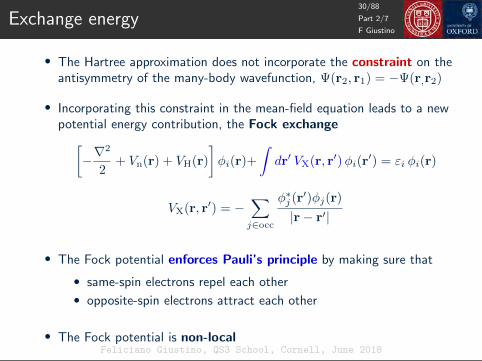
Exchange energy
• The Hartree approximation does not incorporate the constraint on theantisymmetry of the many-body wavefunction, Ψ(r2, r1) = −Ψ(r,r2)
• Incorporating this constraint in the mean-field equation leads to a newpotential energy contribution, the Fock exchange[−∇
2
2+ Vn(r) + VH(r)
]φi(r)+
∫dr′ VX(r, r′)φi(r
′) = εi φi(r)
VX(r, r′) = −∑j∈occ
φ∗j (r′)φj(r)
|r− r′|
• The Fock potential enforces Pauli’s principle by making sure that
• same-spin electrons repel each other
• opposite-spin electrons attract each other
• The Fock potential is non-local
F Giustino
30/88
Part 2/7
Feliciano Giustino, QS3 School, Cornell, June 2018

Correlation energy
• So far we assumed that electrons are independent, that is uncorrelated
prob(r1, r2) = prob(r1)× prob(r2)
• This is not true since electrons do repel each other, therefore the ‘true’wavefunction cannot be expressed as a Slater determinant
Ψtrue(r1, r2) 6= 1√2
[φ1(r1)φ2(r2)− φ1(r2)φ2(r1)]
• Since the Slater determinant is really useful for practical calculations,we keep it and we describe correlations by adding a fictitious potential[
−1
2∇2 + Vn + VH + VX + Vc
]φi = εi φi
F Giustino
31/88
Part 2/7
Feliciano Giustino, QS3 School, Cornell, June 2018

Correlation energy
• So far we assumed that electrons are independent, that is uncorrelated
prob(r1, r2) = prob(r1)× prob(r2)
• This is not true since electrons do repel each other, therefore the ‘true’wavefunction cannot be expressed as a Slater determinant
Ψtrue(r1, r2) 6= 1√2
[φ1(r1)φ2(r2)− φ1(r2)φ2(r1)]
• Since the Slater determinant is really useful for practical calculations,we keep it and we describe correlations by adding a fictitious potential[
−1
2∇2 + Vn + VH + VX + Vc
]φi = εi φi
correlationpotential
F Giustino
31/88
Part 2/7
Feliciano Giustino, QS3 School, Cornell, June 2018

Kohn-Sham equations
[−12∇2 + Vn + VH + Vxc
]φi = εi φi
Exchange and Correlation potential
F Giustino
32/88
Part 2/7
Feliciano Giustino, QS3 School, Cornell, June 2018

Question 2
We want to study the many-body wavefunction of a unit cell of Sr2RuO4.We discretize the volume using 100,000 mesh points.
How many terabytes would we need
to store this wavefunction?
A Less than 1 TB
B 10 TB
C 10784 TB
D Infinity
E How much is a terabyte?
F Giustino
33/88
Part 2/7
Feliciano Giustino, QS3 School, Cornell, June 2018

Part 3
Density-functional theory
F Giustino
34/88
Part 3/7
Feliciano Giustino, QS3 School, Cornell, June 2018

Functionals
Density Functional Theory = theory about the energy of electrons
being a functional of their density
F Giustino
35/88
Part 3/7
Feliciano Giustino, QS3 School, Cornell, June 2018

Functionals
Density Functional Theory = theory about the energy of electrons
being a functional of their density
function
number number
functional
function number
F Giustino
35/88
Part 3/7
Feliciano Giustino, QS3 School, Cornell, June 2018

Functionals
Density Functional Theory = theory about the energy of electrons
being a functional of their density
function
number number
functional
function number
g(x) = 3x2 g(x) = 3x2
g(2) = 12 F [g] =∫ 2
0dx g(x) = 8
x x
F Giustino
35/88
Part 3/7
Feliciano Giustino, QS3 School, Cornell, June 2018

Functionals
The total energy is a functional of the wavefunction
H Ψ = EΨ
−→ E =
∫dr1 . . . drN Ψ∗ H Ψ
So for a generic quantum state we have
Ψ(r1, . . . , rN ) −−→ E E = E[Ψ(r1, . . . , rN )]
In 1964 Hohenberg and Kohn noted that, for the lowest-energy state,the total energy is a functional of the density
n(r) −−−→ E E = E[n(r)]
F Giustino
36/88
Part 3/7
Feliciano Giustino, QS3 School, Cornell, June 2018

Functionals
The total energy is a functional of the wavefunction
H Ψ = EΨ −→ E =
∫dr1 . . . drN Ψ∗ H Ψ
So for a generic quantum state we have
Ψ(r1, . . . , rN ) −−→ E E = E[Ψ(r1, . . . , rN )]
In 1964 Hohenberg and Kohn noted that, for the lowest-energy state,the total energy is a functional of the density
n(r) −−−→ E E = E[n(r)]
F Giustino
36/88
Part 3/7
Feliciano Giustino, QS3 School, Cornell, June 2018

Hohenberg-Kohn theorem
n(r)
F Giustino
37/88
Part 3/7
Feliciano Giustino, QS3 School, Cornell, June 2018

Hohenberg-Kohn theorem
n(r)
Vn(r)
Potential uniquelydetermined by density
(suppl. slides)
F Giustino
37/88
Part 3/7
Feliciano Giustino, QS3 School, Cornell, June 2018

Hohenberg-Kohn theorem
n(r)
Vn(r)
Potential uniquelydetermined by density
(suppl. slides)
Ψ(r1, · · · , rN )
F Giustino
37/88
Part 3/7
Feliciano Giustino, QS3 School, Cornell, June 2018

Hohenberg-Kohn theorem
n(r)
Vn(r)
Potential uniquelydetermined by density
(suppl. slides)
Ψ(r1, · · · , rN )
E
F Giustino
37/88
Part 3/7
Feliciano Giustino, QS3 School, Cornell, June 2018

Hohenberg-Kohn theorem
n(r)
Vn(r)
Potential uniquelydetermined by density
(suppl. slides)
Ψ(r1, · · · , rN )
E
HK theorem
In the ground-state the electrondensity n0(r) uniquely determinesthe total energy E0
F Giustino
37/88
Part 3/7
Feliciano Giustino, QS3 School, Cornell, June 2018

Hohenberg-Kohn theorem
n(r)
Vn(r)
Potential uniquelydetermined by density
(suppl. slides)
Ψ(r1, · · · , rN )
E
HK theorem
In the ground-state the electrondensity n0(r) uniquely determinesthe total energy E0
HK variational principle
Any n(r) 6= n0(r) yields E > E0.
F Giustino
37/88
Part 3/7
Feliciano Giustino, QS3 School, Cornell, June 2018

The energy functional
The HK theorem states that, in the ground state, the total energy of manyelectrons is a functional of their density, E = E[n(r)].
What is this functional?
The energy functional is unknown
The scream by E. Munch (1910)
F Giustino
38/88
Part 3/7
Feliciano Giustino, QS3 School, Cornell, June 2018

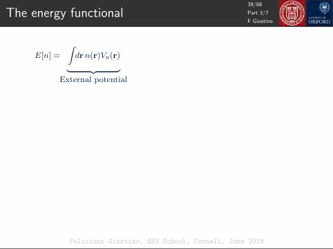
The energy functional
E[n] =
∫drn(r)Vn(r)︸ ︷︷ ︸
External potential
+1
2
∫dr dr′
n(r)n(r′)
|r− r′|︸ ︷︷ ︸Hartree energy
+ Everything Else
Kohn and Sham (1965) proposed to
(1) Express the electron density as if we had a system of independent electrons
n(r) =∑i∈occ
|φi(r)|2
(2) Take out the kinetic energy of these electrons from the “everything else”
Everything Else = −∑i
∫drφ∗i (r)
∇2
2φi(r) + Unknown Terms
F Giustino
39/88
Part 3/7
Feliciano Giustino, QS3 School, Cornell, June 2018

Kohn-Sham equations
Total energy
E[n] =
∫drn(r)Vn(r)+
1
2
∫drdr′
n(r)n(r′)
|r− r′|−∑i
∫drφ∗i (r)
∇2
2φi(r)+Exc[n]
We find the lowest energy state by looking for stationary points of E[n]δE
δn= 0
〈φi|φj〉 = δij
This leads to the Kohn-Sham equations
[−1
2∇2 + Vn(r) + VH(r) + Vxc(r)
]φi(r) = εiφi(r)
F Giustino
40/88
Part 3/7
Feliciano Giustino, QS3 School, Cornell, June 2018

Kohn-Sham equations
Total energy
E[n] =
∫drn(r)Vn(r)+
1
2
∫drdr′
n(r)n(r′)
|r− r′|−∑i
∫drφ∗i (r)
∇2
2φi(r)+Exc[n]
We find the lowest energy state by looking for stationary points of E[n]δE
δn= 0
〈φi|φj〉 = δij
This leads to the Kohn-Sham equations
[−1
2∇2 + Vn(r) + VH(r) + Vxc(r)
]φi(r) = εiφi(r)
Vxc =δExcδn
Exchange and Correlation Potential
F Giustino
40/88
Part 3/7
Feliciano Giustino, QS3 School, Cornell, June 2018

Local Density Approximation (LDA)
We consider the homogeneous electron gas (uniform gas of electrons in apositive compensating background)
n(r) = constant
EHEGx = −3
4
( 3
π
) 13
n43V
F Giustino
41/88
Part 3/7
Feliciano Giustino, QS3 School, Cornell, June 2018

Local Density Approximation (LDA)
We consider the homogeneous electron gas (uniform gas of electrons in apositive compensating background)
n(r) = constant
EHEGx = −3
4
( 3
π
) 13
n43V
ELDAx =
∫V
EHEGx [n(r)]
Vdr
= −3
4
( 3
π
) 13
∫V
n43 (r)dr
V LDAx =
δELDAx
δn= −
( 3
π
) 13
n13 (r)
F Giustino
41/88
Part 3/7
Feliciano Giustino, QS3 School, Cornell, June 2018

Local Density Approximation (LDA)
We consider the homogeneous electron gas (uniform gas of electrons in apositive compensating background)
n(r) = constant
EHEGx = −3
4
( 3
π
) 13
n43V
ELDAx =
∫V
EHEGx [n(r)]
Vdr = −3
4
( 3
π
) 13
∫V
n43 (r)dr
V LDAx =
δELDAx
δn= −
( 3
π
) 13
n13 (r)
F Giustino
41/88
Part 3/7
Feliciano Giustino, QS3 School, Cornell, June 2018

Self-consistent field calculations (SCF)F Giustino
42/88
Part 3/7
Feliciano Giustino, QS3 School, Cornell, June 2018

Question 3
How many terabytes would we need in DFT
to study wavefunctions in a unit cell of Sr2RuO4 ?
A 10 TB
B 10784 TB
C 1 MB
D 250 MB
E I need coffee
F Giustino
43/88
Part 3/7
Feliciano Giustino, QS3 School, Cornell, June 2018

Part 4
Planewaves and pseudopotentials
F Giustino
44/88
Part 4/7
Feliciano Giustino, QS3 School, Cornell, June 2018

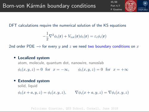
Born-von Karman boundary conditions
DFT calculations require the numerical solution of the KS equations
−1
2∇2φi(r) + Vtot(r)φi(r) = εiφi(r)
2nd order PDE −→ for every y and z we need two boundary conditions on x
• Localized systematom, molecule, quantum dot, nanowire, nanoslab
φi(x, y, z) = 0 for x = −∞, φi(x, y, z) = 0 for x = +∞
• Extended systemsolid, liquid
φi(x+ a, y, z) = φi(x, y, z), ∇φi(x+ a, y, z) = ∇φi(x, y, z)
F Giustino
45/88
Part 4/7
Feliciano Giustino, QS3 School, Cornell, June 2018

Born-von Karman boundary conditions
DFT calculations require the numerical solution of the KS equations
−1
2∇2φi(r) + Vtot(r)φi(r) = εiφi(r)
2nd order PDE −→ for every y and z we need two boundary conditions on x
• Localized systematom, molecule, quantum dot, nanowire, nanoslab
φi(x, y, z) = 0 for x = −∞, φi(x, y, z) = 0 for x = +∞
• Extended systemsolid, liquid
φi(x+ a, y, z) = φi(x, y, z), ∇φi(x+ a, y, z) = ∇φi(x, y, z)
Periodic (BvK) boundary conditions
F Giustino
45/88
Part 4/7
Feliciano Giustino, QS3 School, Cornell, June 2018
Born-von Karman boundary conditions
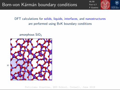
DFT calculations for solids, liquids, interfaces, and nanostructures
are performed using BvK boundary conditions
amorphous SiO2
H2O molecule
a
a
F Giustino
46/88
Part 4/7
Feliciano Giustino, QS3 School, Cornell, June 2018

Born-von Karman boundary conditions
DFT calculations for solids, liquids, interfaces, and nanostructures
are performed using BvK boundary conditions
amorphous SiO2 H2O molecule
a
a
a
a
a
F Giustino
46/88
Part 4/7
Feliciano Giustino, QS3 School, Cornell, June 2018

Planewaves
A convenient way of handling the KS wavefunctions is by expanding them
in a basis of planewaves −−→ standard Fourier transform
F Giustino
47/88
Part 4/7
Feliciano Giustino, QS3 School, Cornell, June 2018

Planewaves
A convenient way of handling the KS wavefunctions is by expanding them
in a basis of planewaves −−→ standard Fourier transform
1D case φ(x) =+∞∑
n=−∞cn ei2πnx/a
F Giustino
47/88
Part 4/7
Feliciano Giustino, QS3 School, Cornell, June 2018

Planewaves
A convenient way of handling the KS wavefunctions is by expanding them
in a basis of planewaves −−→ standard Fourier transform
x in units of a
Re ei2πx/a
Im ei2πx/a
1D case φ(x) =+∞∑
n=−∞cn ei2πnx/a
F Giustino
47/88
Part 4/7
Feliciano Giustino, QS3 School, Cornell, June 2018

Planewaves
A convenient way of handling the KS wavefunctions is by expanding them
in a basis of planewaves −−→ standard Fourier transform
x in units of a
Re ei2πx/a
Im ei2πx/a
1D case φ(x) =+∞∑
n=−∞cn ei2πnx/a
BvK conditions built in
φ(x+ a) = φ(x)
∇φ(x+ a) = ∇φ(x)
F Giustino
47/88
Part 4/7
Feliciano Giustino, QS3 School, Cornell, June 2018

Planewaves
In 2D and 3D we replace 2π/a by the primitive vectors of the reciprocal lattice
b1 = 2πa2 × a3
a1 · a2 × a3
Reciprocal lattice vectors
G = m1b1 +m2b2 +m3b3, with m1,m2,m3 integers
Example: graphene
direct lattice reciprocal lattice
F Giustino
48/88
Part 4/7
Feliciano Giustino, QS3 School, Cornell, June 2018

Planewaves
In 2D and 3D we replace 2π/a by the primitive vectors of the reciprocal lattice
b1 = 2πa2 × a3
a1 · a2 × a3
Reciprocal lattice vectors
G = m1b1 +m2b2 +m3b3, with m1,m2,m3 integers
Example: graphene
direct lattice reciprocal lattice
Planewave in 2D or 3D
exp(iG ·r)
F Giustino
48/88
Part 4/7
Feliciano Giustino, QS3 School, Cornell, June 2018

Planewaves
Kohn-Sham wavefunction in a basis of planewaves
φi(r) =∑
Gci(G) exp(iG · r)
By replacing in the KS equations we obtain
|G|2
2ci(G) +
∑G′Vtot(G−G′)ci(G′) = εi ci(G)
How many planewave G-vectors should we include in the expansion?
|G| = 2π/a
|G| = 2 · 2π/a
|G| = 3 · 2π/a
Ecut =~2|Gmax|2
2me
planewaves kinetic energy cutoff
F Giustino
49/88
Part 4/7
Feliciano Giustino, QS3 School, Cornell, June 2018

Pseudopotentials
Atomic wavefunctions of silicon (DFT/LDA)
Energy (eV)
F Giustino
50/88
Part 4/7
Feliciano Giustino, QS3 School, Cornell, June 2018

Pseudopotentials
Atomic wavefunctions of silicon (DFT/LDA)
Energy (eV)Only valence electrons
important for bonding
F Giustino
50/88
Part 4/7
Feliciano Giustino, QS3 School, Cornell, June 2018

Pseudopotentials
Atomic wavefunctions of silicon (DFT/LDA)
ψnl(r) =unl(r)
rYlm
(rr
)
F Giustino
51/88
Part 4/7
Feliciano Giustino, QS3 School, Cornell, June 2018

Pseudopotentials
Pseudization: make wavefunctions smooth by removing the nodes
F Giustino
52/88
Part 4/7
Feliciano Giustino, QS3 School, Cornell, June 2018

Pseudopotentials
Reverse-engineer the pseudo-potential potential which yields the
pseudo-wavefunction as solution of the atomic Schrodinger equation
−1
2
d2
dr2uPS
3s + V PS3s uPS
3s = E3s uPS3s −−−−→ V PS
3s = E3s +1
2uPS3s
d2uPS3s
dr2
F Giustino
53/88
Part 4/7
Feliciano Giustino, QS3 School, Cornell, June 2018

Brillouin zone sampling
In crystalline solids we label electronic states by their Bloch wavevector k
Bloch theorem φik(r) = eik·ruik(r) with uik(r + R) = uik(r)
F Giustino
54/88
Part 4/7
Feliciano Giustino, QS3 School, Cornell, June 2018

Brillouin zone sampling
In crystalline solids we label electronic states by their Bloch wavevector k
Bloch theorem φik(r) = eik·ruik(r) with uik(r + R) = uik(r)
n(r) =∑i∈occ
|φi(r)|2 −→∑i∈occ
∫BZ
dk
ΩBZ|uik(r)|2 ' 1
Nk
∑k∈BZ
∑i∈occ
|uik(r)|2
Brillouin zone of fcc crystal (e.g. Si, Cu)
DFT codes use a uniform discretization of this
volume and reduce the number of k-vectorsusing the crystal symmetry operations
F Giustino
54/88
Part 4/7
Feliciano Giustino, QS3 School, Cornell, June 2018

Question 4
What is a pseudopotential ?
A An effective atomic potential describing nucleus & core electrons
B A potential describing the pseudo spin
C A false potential
D The potential in the Kohn-Sham equations of DFT
E This question is too easy
F Giustino
55/88
Part 4/7
Feliciano Giustino, QS3 School, Cornell, June 2018

Part 5
Equilibrium structures
F Giustino
56/88
Part 5/7
Feliciano Giustino, QS3 School, Cornell, June 2018

Equilibrium structures
In order to find the equilibrium structures of materials
1) We determine the potential energy surface of the ions
2) We look for the minima of this surface −−→ zero net forces on the ions
Ionic coordinate
Po
ten
tial
ener
gy
F Giustino
57/88
Part 5/7
Feliciano Giustino, QS3 School, Cornell, June 2018

Born-Oppenheimer approximation
Clamped nuclei approximation
Back to the complete many-body Schrodinger equation for electrons & nuclei−∑i
∇2i
2−∑I
∇2I
2MI−∑i,I
ZI
|ri −RI |+
1
2
∑i6=j
1
|ri − rj |+
1
2
∑I 6=J
ZIZJ
|RI −RJ |
Ψ = EtotΨ
Here Ψ = Ψ(r1, . . . , rN ,R1, . . . ,RM )
F Giustino
58/88
Part 5/7
Feliciano Giustino, QS3 School, Cornell, June 2018

Born-Oppenheimer approximation
Clamped nuclei approximation
Back to the complete many-body Schrodinger equation for electrons & nuclei−∑i
∇2i
2−∑I
∇2I
2MI−∑i,I
ZI
|ri −RI |+
1
2
∑i6=j
1
|ri − rj |+
1
2
∑I 6=J
ZIZJ
|RI −RJ |
Ψ = EtotΨ
Here Ψ = Ψ(r1, . . . , rN ,R1, . . . ,RM )
Example: the wavefunction of an electron
vs. the wavefunction of the Pb nucleus
F Giustino
58/88
Part 5/7
Feliciano Giustino, QS3 School, Cornell, June 2018

Born-Oppenheimer approximation
Born and Oppenheimer (1927) proposed the following approximation
• Factorize the electron-nuclear wavefunction
Ψ(r1, . . . , rN ,R1, . . . ,RM ) ' ΨR(r1, . . . , rN )χ(R1, . . . ,RM )
• Find the electronic part as the ground state of Schrodinger equation with thenuclei clamped at R1, . . . ,RM−∑
i
∇2i
2+
∑i
Vn(ri;R) +1
2
∑i6=j
1
|ri − rj |
ΨR = E(R1, . . . ,RM ) ΨR
• Replace the result in the complete MBSE of the previous slide−∑I
∇2I
2MI+
1
2
∑I 6=J
ZIZJ|RI −RJ |
+ E(R1, . . . ,RM )
χ = Etot χ
Schrodinger equation for nuclei
F Giustino
59/88
Part 5/7
Feliciano Giustino, QS3 School, Cornell, June 2018

Potential energy surface
−∑I
∇2I
2MI︸ ︷︷ ︸Kinetic Energy
χ+
1
2
∑I 6=J
ZIZJ|RI −RJ |
+ E(R1, . . . ,RM )
︸ ︷︷ ︸
Potential Energy
χ = Etot χ
Potential energy surface
U(R1, . . . ,RM ) =1
2
∑I 6=J
ZIZJ|RI −RJ |
+E(R1, . . . ,RM )
F Giustino
60/88
Part 5/7
Feliciano Giustino, QS3 School, Cornell, June 2018

Potential energy surface
−∑I
∇2I
2MI︸ ︷︷ ︸Kinetic Energy
χ+
1
2
∑I 6=J
ZIZJ|RI −RJ |
+ E(R1, . . . ,RM )
︸ ︷︷ ︸
Potential Energy
χ = Etot χ
Potential energy surface
U(R1, . . . ,RM ) =1
2
∑I 6=J
ZIZJ|RI −RJ |
+E(R1, . . . ,RM )
Coulomb repulsionbetween positive nuclei
Glue resulting from thenegative charge of the electrons
F Giustino
60/88
Part 5/7
Feliciano Giustino, QS3 School, Cornell, June 2018

Potential energy surface
H-H distance d (A)
En
erg
y(e
V)
En
erg
y(e
V)
Coulomb repulsion
Electronic glue
Potential energy‘surface’
H+2 molecular ion
F Giustino
61/88
Part 5/7
Feliciano Giustino, QS3 School, Cornell, June 2018

Classical nuclei
−∑I
∇2I
2MI+ U(R1, . . . ,RM )
F Giustino
62/88
Part 5/7
Feliciano Giustino, QS3 School, Cornell, June 2018

Classical nuclei
−∑I
∇2I
2MI+ U(R1, . . . ,RM )
MId2RI
dt2= FI = − ∂U
∂RI
Newton’s equation for nuclei
F Giustino
62/88
Part 5/7
Feliciano Giustino, QS3 School, Cornell, June 2018

Structural optimization
Initial guess for ionic positionsR1, . . . ,RM
Calculate electron density n(r)and total energy EDFT
Calculate forces on ionsFI = −∂U/∂RI
Update ionic positions(eg using damped Verlet)
New positions=
Old positions
F Giustino
63/88
Part 5/7
Feliciano Giustino, QS3 School, Cornell, June 2018

Examples
Simplest case of structural optimization: N2 diatomic molecule
DFT/LDA Experiment Rel. Error
bond length (A) 1.102 1.098 0.4%
binding energy (eV) 11.46 9.76 17%
Note Nitrogen is [1s2]2s2p3, therefore it has a spin S = 3/2 after the Hund’s first rule. As the above calculations
are spin-unpolarized, the energy at infinity is higher than twice the energy of one N atom.
F Giustino
64/88
Part 5/7
Feliciano Giustino, QS3 School, Cornell, June 2018

Examples
Structural optimization of bulk crystals: Silicon
DFT/LDA Experiment Rel. Error
lattice parameter (A) 5.40 5.43 0.6%
cohesive energy (eV) 5.30 4.62 15%
F Giustino
65/88
Part 5/7
Feliciano Giustino, QS3 School, Cornell, June 2018
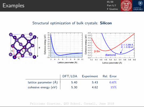
Examples
Structural optimization of bulk crystals: Silicon
DFT/LDA Experiment Rel. Error
lattice parameter (A) 5.40 5.43 0.6%
cohesive energy (eV) 5.30 4.62 15%
F Giustino
65/88
Part 5/7
Feliciano Giustino, QS3 School, Cornell, June 2018

Question 5
In which of the following systems the
Born-Oppenheimer approximation breaks down?
A Organic-inorganic lead halide perovskites
B Sulfur hydride high-temperature superconductors
C Diamond
D Graphene
E What is the Born-Oppenheimer approximation?
F Giustino
66/88
Part 5/7
Feliciano Giustino, QS3 School, Cornell, June 2018

Part 6
Band structures
F Giustino
67/88
Part 6/7
Feliciano Giustino, QS3 School, Cornell, June 2018

Band structures
Example: graphene direct lattice reciprocal lattice
φik(r) = eik·ruik(r) with uik(r) periodic
−1
2∇2φik(r)+Vtot(r)φik(r) = εik φik(r)
k-dependent
KS eigenvalue
F Giustino
68/88
Part 6/7
Feliciano Giustino, QS3 School, Cornell, June 2018

Band structures
Example: simplified tight-binding model of graphene
F Giustino
69/88
Part 6/7
Feliciano Giustino, QS3 School, Cornell, June 2018

Band structures
Example: DFT/LDA band structures of common semiconductors
F Giustino
70/88
Part 6/7
Feliciano Giustino, QS3 School, Cornell, June 2018

Fermi surfaces
Example: DFT/LDA band structure and Density of States of copper
F Giustino
71/88
Part 6/7
Feliciano Giustino, QS3 School, Cornell, June 2018

Fermi surfaces
Example: DFT/LDA Fermi surface and wavefunctions of copper
F Giustino
72/88
Part 6/7
Feliciano Giustino, QS3 School, Cornell, June 2018

Kohn-Sham wavefunctions
Example: Elpasolite Cs2InAgCl6
Volonakis et al, J. Phys. Chem. Lett., 8, 772 (2017)
F Giustino
73/88
Part 6/7
Feliciano Giustino, QS3 School, Cornell, June 2018

Meaning of band structures
• Are band structures real?
F Giustino
74/88
Part 6/7
Feliciano Giustino, QS3 School, Cornell, June 2018

Meaning of band structures
• Are band structures real?
ARPES spectrum of diamond and DFT/LDA bands
Experiment byProf. T. YokoyaOkayama University
F Giustino
74/88
Part 6/7
Feliciano Giustino, QS3 School, Cornell, June 2018

Meaning of band structures
The DFT total energy can be rewritten as
E[n] =∑i
dk
ΩBZfik εik︸ ︷︷ ︸
band structure term
−[EH +
∫drVxc(r)n(r)− Exc
]︸ ︷︷ ︸
double counting term
fik electron occupation
F Giustino
75/88
Part 6/7
Feliciano Giustino, QS3 School, Cornell, June 2018

Meaning of band structures
The DFT total energy can be rewritten as
E[n] =∑i
dk
ΩBZfik εik︸ ︷︷ ︸
band structure term
−[EH +
∫drVxc(r)n(r)− Exc
]︸ ︷︷ ︸
double counting term
fik electron occupation
• If the double-counting term could beneglected, the eigenvalues would givethe change of total energy upon addingor removing one electron
• The KS levels can be thought of asvery rough approximations to additionor removal energies
F Giustino
75/88
Part 6/7
Feliciano Giustino, QS3 School, Cornell, June 2018
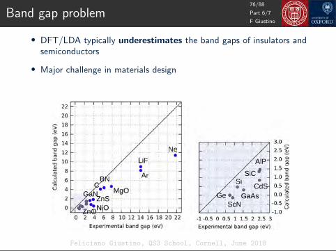
Band gap problem
• DFT/LDA typically underestimates the band gaps of insulators andsemiconductors
• Major challenge in materials design
F Giustino
76/88
Part 6/7
Feliciano Giustino, QS3 School, Cornell, June 2018

Question 6
Which of the following statements is true ?
A DFT band structures are generally good for sp semiconductors
B DFT predicts accurate band gaps in semiconductors and insulators
C DFT performs poorly for metals
D The DFT band gap problem has to do with pseudopotentials
E The Kohn-Sham eigenvalues correspond to electron addition orremoval energies
F Giustino
77/88
Part 6/7
Feliciano Giustino, QS3 School, Cornell, June 2018

Part 7
DFT beyond the LDA
F Giustino
78/88
Part 7/7
Feliciano Giustino, QS3 School, Cornell, June 2018

PBE exchange and correlation
• Within the LDA the XC energy is approximated using the local density
ELDAxc =
∫drn(r) εHEG
xc [n(r)]
• Generalized gradient approximations (GGA) like PBE incorporate also
information about the density gradient
EGGAxc =
∫dr f [n(r),∇n(r)]
Perdew, Burke & Ernzerhof, Phys. Rev. Lett. 77, 3865 (1996)
F Giustino
79/88
Part 7/7
Feliciano Giustino, QS3 School, Cornell, June 2018

PBE exchange and correlation
Perdew, Burke & Ernzerhof, Phys. Rev. Lett. 77, 3865 (1996)
Atomization energies
From Table 1 of Perdew, Burke, Ernzerhof, PRL 1996
Exp
erim
ent
(eV
)A
bs.
dev
iati
on
(eV
)
|EPBE − Eexp|
|ELDA − Eexp|
F Giustino
80/88
Part 7/7
Feliciano Giustino, QS3 School, Cornell, June 2018

Hubbard-corrected DFT
Anisimov, Zaanen & Andersen, Phys. Rev. B 44, 943 (1991)
• 3d transition metal and 4f rare earth
• LDA and PBE underestimate on-site Coulomb energy
• DFT+U adds Hubbard-like correction to remedy this deficiency
• Important for strongly-correlated materials
F Giustino
81/88
Part 7/7
Feliciano Giustino, QS3 School, Cornell, June 2018

Hubbard-corrected DFT
Anisimov, Zaanen & Andersen, Phys. Rev. B 44, 943 (1991)
Figure from: Cococcioni & De Gironcoli, PRB 2005
PBE PBE+UFeO (AF-II phase)
F Giustino
82/88
Part 7/7
Feliciano Giustino, QS3 School, Cornell, June 2018

Hubbard-corrected DFT
Anisimov, Zaanen & Andersen, Phys. Rev. B 44, 943 (1991)
Figure from: Cococcioni & De Gironcoli, PRB 2005
PBE PBE+UFeO (AF-II phase)
• Computationally efficient
• Hubbard U often used as an adjustable parameter
• Results can be very sensitive to U
F Giustino
82/88
Part 7/7
Feliciano Giustino, QS3 School, Cornell, June 2018

Hybrid functionals
PBE0 Perdew, Burke & Ernzerhof, J. Chem. Phys. 105 (1996)
HSE Heyd, Scuseria & Ernzerhof, J. Chem. Phys. 118, 8207 (2003)
F Giustino
83/88
Part 7/7
Feliciano Giustino, QS3 School, Cornell, June 2018

Hybrid functionals
PBE0 Perdew, Burke & Ernzerhof, J. Chem. Phys. 105 (1996)
HSE Heyd, Scuseria & Ernzerhof, J. Chem. Phys. 118, 8207 (2003)
• Improve upon semilocal GGA by including fully non-local Fock exchange
EHFx = −
∑j∈occ
∫dr1dr2
φ∗i (r1)φ∗j (r2)φi(r2)φj(r1)
|r1 − r2|
• PBE0 prescription
EPBE0xc =
3
4EPBEx +
1
4EFx + EPBE
c
• Requires the evaluation of the non-local Fock exchange potential (expensive)
VX(r, r′) = −∑j∈occ
φj(r)φ∗j (r′)
|r− r′|
F Giustino
83/88
Part 7/7
Feliciano Giustino, QS3 School, Cornell, June 2018
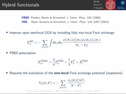
Hybrid functionals
PBE0 Perdew, Burke & Ernzerhof, J. Chem. Phys. 105 (1996)
HSE Heyd, Scuseria & Ernzerhof, J. Chem. Phys. 118, 8207 (2003)
• Improve upon semilocal GGA by including fully non-local Fock exchange
EHFx = −
∑j∈occ
∫dr1dr2
φ∗i (r1)φ∗j (r2)φi(r2)φj(r1)
|r1 − r2|
• PBE0 prescription
EPBE0xc =
3
4EPBEx +
1
4EFx + EPBE
c
• Requires the evaluation of the non-local Fock exchange potential (expensive)
VX(r, r′) = −∑j∈occ
φj(r)φ∗j (r′)
|r− r′|
F Giustino
83/88
Part 7/7
Feliciano Giustino, QS3 School, Cornell, June 2018

Hybrid functionals
PBE0 Perdew, Burke & Ernzerhof, J. Chem. Phys. 105 (1996)
HSE Heyd, Scuseria & Ernzerhof, J. Chem. Phys. 118, 8207 (2003)
• HSE prescription: separate short-range and long-range coulomb interactions
EHSExc =
[3
4EPBE,srx +
1
4EF,srx
]+ EPBE,lr
x + EPBEc
• The separation is carried our by breaking the Coulomb potential in two parts
F Giustino
84/88
Part 7/7
Feliciano Giustino, QS3 School, Cornell, June 2018

Hybrid functionals
PBE0 Perdew, Burke & Ernzerhof, J. Chem. Phys. 105 (1996)
HSE Heyd, Scuseria & Ernzerhof, J. Chem. Phys. 118, 8207 (2003)
• HSE prescription: separate short-range and long-range coulomb interactions
EHSExc =
[3
4EPBE,srx +
1
4EF,srx
]+ EPBE,lr
x + EPBEc
• The separation is carried our by breaking the Coulomb potential in two parts
1
r=
erfc(κr)
r+
erf(κr)
r
F Giustino
84/88
Part 7/7
Feliciano Giustino, QS3 School, Cornell, June 2018

Hybrid functionals
PBE0 Perdew, Burke & Ernzerhof, J. Chem. Phys. 105 (1996)
HSE Heyd, Scuseria & Ernzerhof, J. Chem. Phys. 118, 8207 (2003)
• Band gaps
Typically PBE underestimates band gaps while Hartree-Fock overestimates.Mixing PBE and HF yields values closer to experiments.
• Exchange fraction
Widespread practice of using the mixing fraction as an adjustable empiricalparameter. Loss of predictive power.
• Correlation
The correlation energy is still described at the PBE level.Misses van der Waals effects and dynamical renormalization effects.
F Giustino
85/88
Part 7/7
Feliciano Giustino, QS3 School, Cornell, June 2018
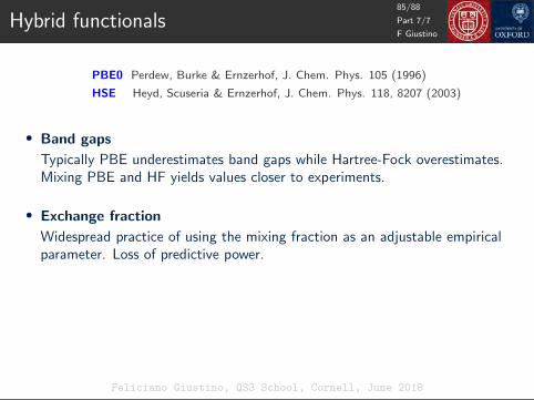
Hybrid functionals
PBE0 Perdew, Burke & Ernzerhof, J. Chem. Phys. 105 (1996)
HSE Heyd, Scuseria & Ernzerhof, J. Chem. Phys. 118, 8207 (2003)
• Band gaps
Typically PBE underestimates band gaps while Hartree-Fock overestimates.Mixing PBE and HF yields values closer to experiments.
• Exchange fraction
Widespread practice of using the mixing fraction as an adjustable empiricalparameter. Loss of predictive power.
• Correlation
The correlation energy is still described at the PBE level.Misses van der Waals effects and dynamical renormalization effects.
F Giustino
85/88
Part 7/7
Feliciano Giustino, QS3 School, Cornell, June 2018

Many-body perturbation theory
GW method Hedin & Lundqvist, Solid State Physics 23, 1 (1969)
Hybertsen & Louie, Phys Rev B 34, 5390 (1986)
KS −1
2∇2φi(r) + [Vn(r) + VH(r)]φi(r) + Vxc(r) φi(r) = εiφi(r)
F Giustino
86/88
Part 7/7
Feliciano Giustino, QS3 School, Cornell, June 2018
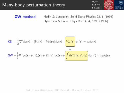
Many-body perturbation theory
GW method Hedin & Lundqvist, Solid State Physics 23, 1 (1969)
Hybertsen & Louie, Phys Rev B 34, 5390 (1986)
KS −1
2∇2φi(r) + [Vn(r) + VH(r)]φi(r) + Vxc(r) φi(r) = εiφi(r)
GW −1
2∇2φi(r) + [Vn(r) + VH(r)]φi(r) +
∫dr′Σ(r, r′, εi) φi(r
′) = εiφi(r)
Σ = GW
Electron Green’s function
Screened Coulomb interaction
F Giustino
86/88
Part 7/7
Feliciano Giustino, QS3 School, Cornell, June 2018

Many-body perturbation theory
GW method Hedin & Lundqvist, Solid State Physics 23, 1 (1969)
Hybertsen & Louie, Phys Rev B 34, 5390 (1986)
• DFT/LDA• GW
F Giustino
87/88
Part 7/7
Feliciano Giustino, QS3 School, Cornell, June 2018

Ready to start DFT calculations?
NSF/DOE Quantum Science Summer SchoolCornell University, June 10-22, 2018Feliciano Giustino, QS3 School, Cornell, June 2018

Proof of the Hohenberg-Kohn theorem
In order to prove the HK theorem we rewrite the energy more compactly
E =
∫drn(r)Vn(r) + 〈Ψ|U |Ψ〉, U = −
∑i
∇2i
2+
1
2
∑i6=j
1
|ri − rj |
Now we want to show the following
Theorem
In the ground-state, the electron density n(r) uniquely determines theexternal potential Vn(r)
−∑i
∇2i
2+∑i
Vn(ri) +1
2
∑i6=j
1
|ri − rj |
Ψ = EΨ
F Giustino
01/09
Part 7/7
Feliciano Giustino, QS3 School, Cornell, June 2018

Proof of the Hohenberg-Kohn theorem
• Assume there are two potentials V1 and V2 for the same density[For clarity we temporarily suppress the subscript ‘n’ in Vn]
• By solving the MBSE for each potential we find the lowest-energystates E1, Ψ1 and E2, Ψ2, respectively
• Since Ψ1 is the ground state of V1 we have∫nV1 + 〈Ψ1|U |Ψ1〉 = E1
• Since Ψ1 is not the ground state of V2 we have∫nV2 + 〈Ψ1|U |Ψ1〉 > E2
• The difference gives ∫n(V1 − V2) > E1 − E2
• By repeating the same argument starting from Ψ2 we have∫n(V2 − V1) > E2 − E1
• The sum of the last two equations yields the contradiction 0 > 0
F Giustino
02/09
Part 7/7
Feliciano Giustino, QS3 School, Cornell, June 2018
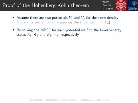
Proof of the Hohenberg-Kohn theorem
• Assume there are two potentials V1 and V2 for the same density[For clarity we temporarily suppress the subscript ‘n’ in Vn]
• By solving the MBSE for each potential we find the lowest-energystates E1, Ψ1 and E2, Ψ2, respectively
• Since Ψ1 is the ground state of V1 we have∫nV1 + 〈Ψ1|U |Ψ1〉 = E1
• Since Ψ1 is not the ground state of V2 we have∫nV2 + 〈Ψ1|U |Ψ1〉 > E2
• The difference gives ∫n(V1 − V2) > E1 − E2
• By repeating the same argument starting from Ψ2 we have∫n(V2 − V1) > E2 − E1
• The sum of the last two equations yields the contradiction 0 > 0
F Giustino
02/09
Part 7/7
Feliciano Giustino, QS3 School, Cornell, June 2018

Example: Ground state of He
Kinetic energy + electron-nucleus interaction −3.89 Ha −105.8 eV
Hartree energy +2.05 Ha +55.8 eV
Exchange energy −1.02 Ha −27.8 eV
Correlation energy −0.04 Ha −1.1 eV
Total energy −2.90 Ha −78.9 eV
F Giustino
03/09
Part 7/7
Feliciano Giustino, QS3 School, Cornell, June 2018


![12 24.305 Fe Mg...Cu 63.546 2, 1 [Ar] 3d104s 1 Copper 2836 1357.6 8.96 Plastocianina Azurina Nitrogenase Aldeído Oxidoreductase 26 Fe 55.847 2, 3 [Ar] 3d64s 2 Iron 3135 1809 7.86](https://img.dokumen.tips/doc/110x75/5ea8e39adfaaed251b0c5d8a/12-24305-fe-mg-cu-63546-2-1-ar-3d104s-1-copper-2836-13576-896-plastocianina.jpg)
![finarchemicals.comfinarchemicals.com/pdf/periodic_table.pdf · 1660 3287 4.55 29 63.546 1083 B 8.298 10.811 2079 2550 2.47 88 pm 14 12.011 3367 4827 C 2.27 77 pm 11.260 [He]2s2 2p2](https://img.dokumen.tips/doc/110x75/5acb4f387f8b9a73128b7fd6/3287-455-29-63546-1083-b-8298-10811-2079-2550-247-88-pm-14-12011-3367-4827.jpg)