Feedback Channel In Linear NoiselessDynamic Systems Controlled Over The

Packet Erasure Network

Alireza Farhadi ∗

December 27, 2014

Abstract

This paper is concerned with tracking state trajectory at remote controller, stabil-ity and performance of linear time-invariant noiseless dynamic systems with multipleobservations over the packet erasure network subject to random packet dropout andtransmission delay that does not necessarily use feedback channel full time. Three casesare considered in this paper: i) without feedback channel, ii) with feedback channel in-termittently, and iii) with full time availability of feedback channel. For all three cases,coding strategies that result in reliable tracking of state trajectory at remote controllerwith asymptotically zero mean absolute estimation error are presented. Asymptoticmean absolute stability of the controlled system equipped with each of these codingstrategies is shown; and trade-offs between duty cycle for feedback channel use, trans-mission delay and performance, which is defined in terms of the settling time, arestudied.

Index-Terms: Networked control system, stability and performance, feedback channel.

1 Introduction

1.1 Motivations and Background

Supervisory control systems have been widely used as they enable high level planning, moni-

toring, and intervention in case of emergency. On the other hand, most of today’s embedded

systems are wireless enabled due to the vast availability of cheap wireless modems. Therefore,

there is an increasing interest in supervisory control systems over wireless communication

networks.

Fig. 1 illustrates such a supervisory control system, which will be studied in this paper.

∗A. Farhadi is an Assistant Professor in the Department of Electrical Engineering at Sharif University ofTechnology, Tehran, Iran. E-mail: afarhadi@sharif.edu.

High level controller

Autonomous agent 1

Local controller 1

Autonomous agent 2

Local controller 2

Autonomous agent n

Local controller n

1y

u

2y n

y

Base station

u

u

1α

2α n

αβ β

β

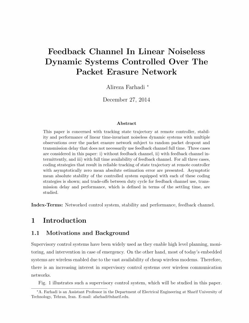
Figure 1: A supervisory control system over the packet erasure network.

This system can represent a fleet of autonomous underwater vehicles (agents) supervised

by an autonomous surface vessel (base station); or a fleet of unmanned aerial vehicles su-

pervised by a remote base station. In the control system of Fig. 1, each agent provides

measurements for high level controller (supervisory controller) and executes high level com-

mands produced by high level controller. Transmission of information between each agent

and high level controller is wireless and, in general, subject to communication imperfections,

such as long transmission delay and noise. In the system of Fig. 1, it is assumed that

each agent is equipped with limited power supply and hence is limited to transmit with low

power. Therefore, the communication from each agent to high level controller is subject to

quantization and noise, which results in distortion and packet dropout with random erasure

probability αi. That is, the communication from agents to high level controller is via the

packet erasure network. However; as the base station can broadcast with high power, the

communication of control signal from high level controller to each agent can be assumed

perfect. Therefore, from the point of view of high level controller, the system shown in Fig.

1 can be viewed as a control system with multiple observations when the transmission of

observation vector is subject to imperfections.

Thus, the system of Fig. 1 represents a networked control system. Some results address-

ing the basic problems in stability and estimation of networked control systems can be found

in [1]-[17]. [10] addressed the problem of asymptotic mean square estimation of a bounded

random variable over the binary erasure channel without feedback channel 1. In [11] the

authors addressed the problem of state estimation of distributed uncontrolled nonlinear Lip-

schitz systems subject to bounded process and measurement noises over the packet erasure

network. The objective in [11] is bounded mean absolute tracking of state trajectory at a

remote fusion center when noiseless feedback channel is available full time.[12] addressed

the problem of asymptotic stability and tracking of linear noiseless dynamic systems over

the digital noiseless channel (and hence when noiseless feedback channel is available full

time); and [13] addressed the stability problem of nonlinear noiseless systems over the dig-

ital noiseless channel. [14] addressed the problem of asymptotic almost sure stability and

tracking of the state trajectory at remote controller of linear noiseless dynamic systems

over the packet erasure channel when noiseless feedback channel is available full time; and

[15],[16],[17] addressed the problem of mean square stability and tracking of linear Gaussian

dynamic systems over Additive White Gaussian Noise (AWGN) channel when noiseless feed-

back channel is available full time. Similar to the control system of Fig. 1, [12], [13], [14],

[15], [16], [17] assumed that the communication of control signal from remote controller to

system is perfect.

The above literature review reveals that many results in the literature have been devel-

oped under the assumption of full time availability of noiseless feedback channel. Specifically,

to the best of our knowledge, there is not any result for stability and tracking with intermit-

tent noiseless feedback channel over the packet erasure channel, which is an important class

of digital communication channels as it is an abstract model for the commonly used infor-

mation technologies, such as the Internet, WiFi and mobile communication. Nevertheless,

the availability of noiseless feedback channel may not be possible full time. The full time

availability of noiseless feedback channel requires that feedback channel signal is transmit-

ted with high power full time. This results in significant power consumption at the receiver

(where the remote controller is located) if the control signal is also transmitted with high

power from receiver full time (see Fig. 1). Hence, as transmission of two high power signals

full time will result in a short life time for the transmitter of the receiver, this paper aims

to relax the full time availability assumption of noiseless feedback channel and address the

stability and tracking problem of linear noiseless dynamic systems over the packet erasure

network, as shown in Fig. 1, with intermittent noiseless feedback channel.

1An Acknowledgment from receiver to transmitter that represents the channel output.

1.2 Paper Contributions

As clear from the above discussion, in the control system of Fig. 1 it is more desirable to use

noiseless feedback channel that is available intermittently to avoid exhausting the receiver

power supply. Hence, to overcome the deficiency of the available results in the literature, as

described above, this paper is concerned with tracking state trajectory at remote controller

(high level controller), stability and performance of the supervisory control system of Fig. 1

described by linear time-invariant noiseless subsystems and the packet erasure network when

noiseless feedback channel is not necessarily available full time. To model such a feedback

channel, in the system of Fig. 1, feedback channel is represented by switches with known

duty cycle β ∈ [0, 1], where β is a rational number. β = 0 corresponds to the case of

non-availability of feedback channel while β = 1 corresponds to its full time availability. In

the system of Fig. 1 performance is described by the settling time. This paper overcomes

the deficiency of the available results in the literature by presenting coding strategies and

controller that guarantee asymptotic mean absolute tracking of state trajectory at remote

controller and stability for the following three cases: i) without feedback channel (i.e., β = 0),

ii) with feedback channel intermittently (i.e.,β ∈ (0, 1)), and iii) with full time availability

of feedback channel (β = 1). Asymptotic mean absolute stability of the system of Fig. 1

equipped with each of these coding strategies is shown. Trade-offs between duty cycle for

feedback channel use, transmission delay and performance are also studied in this paper.

1.3 Paper Organization

The paper is organized as follows. Section 2 describes the supervisory control system of

Fig. 1 in more detail. Section 3 presents coding strategies that compensate the effects of

distortion and random packet dropout and provides reliable tracking. This is followed by

the stability and performance analysis in Section 4. In Section 5, the paper is concluded by

summarizing the main contributions of the paper.

2 Problem Formulation

In this paper, the following conventions are used. z(t) denotes the value of the signal z at

time t ≥ 0. z[m], where m is a non-negative integer, denotes the value of the signal z at

sampling instant m. “ = ” denotes “by definition equals”, N+ = {0, 1, 2, ...} and A′

denotes

the transpose of a vector/matrix A. λl(M) denotes the lth eigenvalue of the square matrix

M , the block diagonal matrix is denoted by diag(·), and σmax(B) denotes the largest singular

value of matrix B. log(·) denotes the logarithm of base 2, bac denotes the floor of scalar a

One step ahead estimator

Communication

network

Deterministic

switch (feedback

channel)

Controller Predictor

Decoders

Encoders

Plant

i

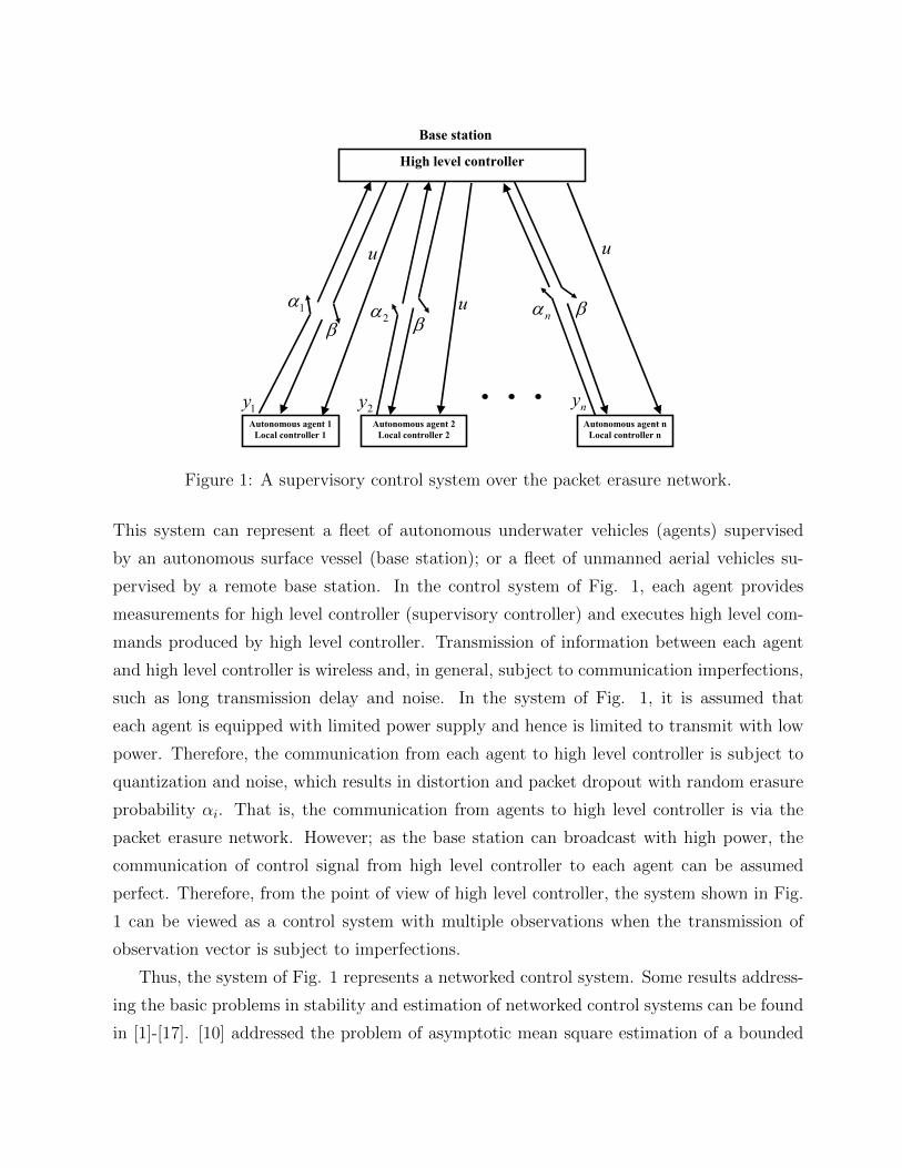
Figure 2: An unstable dynamic system over the packet erasure network.

and E[·] denotes the expected value. Euclidean norm is denoted by || · ||, the absolute value

by | · |, the set of real numbers by < and the standard uniform distribution is denoted by

U(0, 1).∏kj=1 aj denotes the ordered product, i.e.,

∏kj=1 aj = ak.ak−1.....a1, and 1 stands for

the indicator function.

2.1 Description of the System

This paper is concerned with tracking state trajectory, stability and performance of the su-

pervisory control system of Fig. 1 described by Linear Time-Invariant (LTI) subsystems over

the packet erasure network, as shown in more detail in Fig. 2. In the block diagram of Fig. 2,

we denote by yi the value of the ith sampled data (the measurement vector of the ith subsys-

tem) at time instant k, when the control action is updated. To avoid collision of transmitted

sampled data at controller, sampled data: y1, y2, ..., yn, which are all sampled at time instant

k, are transmitted sequentially, like a Time Division Multiple Access (TDMA) scheme, in

which, the time period between transmission of two successive samples is a positive scalar Tm.

The time period Tm is referred as sequential transmission period. The time period between

two successive time instants k and k+1 is Tβ(> Tm). The control action is updated with the

time period Tβ; and measurements are provided from subsystems with the same time period

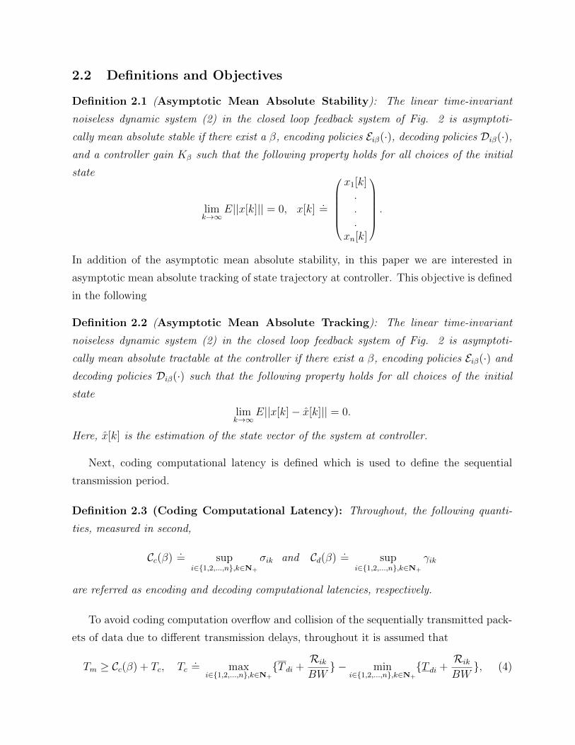
(see Fig. 3). During each time period that the control action is updated, feedback channel

can be used. That is, an acknowledgment bit is sent from receiver of controller to transmitter

Time

dataExchanged

mT

βT

βkT mTkT +β βTk )1( +

][1 kδ ][2 kδ ][knδ

]1[ +ku

The control action is updated at the

controller at each time step. Then,

controller broadcasts the updated

control vector and feedback channel

information to all subsystems

Figure 3: A TDMA scheme for exchanging information between the plant and controller.

of each subsystem to indicate whether a transmission from a subsystem has been successful

or not. This feedback channel is shown in Fig. 2 by a switch with known on/off duty cycle β.

The building blocks of Fig. 2 are described now.

Plant: Plant consists of the following linear time-invariant noiseless subsystems:{xi(t) = Aixi(t) +Biu(t),yi(t) = Cixi(t), i = {1, 2, ..., n}, (1)

where Ai ∈ <ni×ni , Bi ∈ <ni×m, Ci ∈ <li×ni , xi ∈ <ni , u ∈ <m, yi ∈ <li , and k ∈ N+. The

initial states xi(0), i ∈ {1, 2, ..., n}, are Random Variables (RVs) with bounded supports.

That is, for each i, there exists a closed bounded set Γi ⊂ <ni such that xi(0) ∈ Γi.

In the problem considered in this paper the control update action is of the hold type. That

is, at each time instant k, u(kT ) is applied and held until the next time instant. Also, at

each time instant k, yis are sampled. Therefore, the plant has the following discrete-time

equivalent representation.{xi[k + 1] = Adi(β)xi[k] +Bdi(β)u[k],

yi[k] = Cixi[k], xi[0]=xi(0), i = {1, 2, ..., n}, (2)

where Adi(β) = eAiTβ , Bdi(β) = (∫ Tβ

0 eAiτdτ)Bi. Throughout, it is assumed that there exists

a matrix Kβ such that the matrix Ad(β) +Bd(β)Kβ is stable, where

Ad(β) = diag(Ad1(β), ..., Adn(β)), Bd = diag(Bd1(β), ..., Bdn(β)).

Communication network: The communication channel from each subsystem to controller

is the packet erasure channel. It is a digital channel consisting of modulator, noisy media,

and de-modulator, which transmits a packet of binary data (subject to transmission delay)

in each channel use. Let δi(kTβ) denote the channel input, which is a packet of binary data

that includes information bits as well as overhead bits added by channel encoder for error

detection and correction. Let, also δi(kTβ + dik) denote the corresponding channel output,

where dik is the unknown time varying transmission delay. Also, let e denote the erasure

symbol. Then,

δi(kTβ + dik) = C(δi(kTβ)) =

{δi(kTβ) with probability 1− αi

e with probability αi

That is, this channel erases a transmitted packet with probability αi whenever channel

decoder detects flipped bits (due to transmission noise) that cannot be corrected by the

implemented error correction technique.

Note that the binary erasure channel is a special case of the packet erasure channel that

transmits one information bit in each channel use.

Throughout, it is assumed that the erasure probability αi is known a priori. Also,

the upper and lower bounds on unknown time varying transmission delay are known (i.e.,

T di ≤ dik ≤ T di, where T di and T di are known). Moreover, the input of modulator is binary;

while the output of de-modulator is ternary with three states: “0”, “1”, and “Idle” such that

when the channel is not in use, de-modulator outputs the “Idle” state.

Deterministic switch: During each time period that the control action is updated, a

feedback channel can be used from receiver of controller to transmitter of each subsystem.

That is, a noiseless acknowledgment bit from controller to each subsystem that indicates

whether a transmission from a subsystem has been successful or not. This is modeled by a

switch with a known switching policy to all transmitters and receivers, in which duty cycle

for turning on this switch (i.e., using feedback channel) is β = qp, q ∈ N+, p ∈ {1, 2, 3, ...},

q ≤ p. β = 0 corresponds to the case of non-availability of feedback channel and for the case

of β 6= 0, in each p updates of the control action, in the first q updates feedback channels

are used. It is assumed that in the first time step (i.e., within the time period between the

time instants k = 0 and k = 1) feedback channel is used.

In the closed loop feedback system of Fig. 2, encoders and decoders are used to com-

pensate the effects of random packet dropout. As the effect of channel encoder and channel

decoder in improving the transmission quality over a noisy media is present in the channel

model, without loss of generality, in what follows we only focus on source encoding and

source decoding operations.

Having that, encoders and decoders are described as follows.

Encoders: There is an encoder for each subsystem, which is a causal operator denoted

by Eiβ(·), i = {1, 2, ..., n}. For each subsystem i, let the random variable σik denote the

computational latency associated with the ith encoding operation during time instants k

and k + 1. Within this time period, each encoder Eiβ(·) maps the corresponding subsystem

output: yi(kTβ + (i− 1)Tm) to the channel input: δi(kTβ + (i− 1)Tm +σik), which is a string

of binaries with length Rik. In performing the above operation, the information about the

status of the previous transmission (its success or fail) is used in the encoding operation if

the deterministic switch was on at the previous time step. The encoders can also use the

sequence of control inputs up to time instant k in performing the above task.

Decoders: Decoders are also causal operators, which are denoted by Diβ(·), i = {1, 2, ..., n}.They map the channel outputs δi(kTβ + (i− 1)Tm + σik + Rik

BW+ dik) to the state estimates

xi(kTβ + (i − 1)Tm + σik + RikBW

+ dik + γik), i = 1, 2, ..., n, where BW is the bit rate of the

communication link, the random variable γik is the computational latency due to decoding

operation and xi(kTβ+(i−1)Tm+σik+ RikBW

+dik+γik), which is abbreviated by xi[k|k] for the

simplicity of presentation, is the estimation of xi[k]. In performing the decoding operation

for time instant k, the decoders can use the sequence of control inputs up to time instant k−1.

Controller: Control update action is of the hold type. That is, whenever the control

action is updated, the control value is applied on the plant and held until the next control

value is updated. In this paper controller has the following representation:

u[0] = 0, u[k + 1] = Kβx[k + 1], (3)

where

x[k + 1] =

x1[k + 1]

.

.

.xn[k + 1]

= Ad(β)

x1[k|k]

.

.

.xn[k|k]

+Bd(β)u[k]

represents the operation of the predictor block of the one step ahead estimator block of Fig.

2. In (3), x[k+1] is the output of the one step ahead estimator block, xi[k|k] are the outputs

of the decoders, and the controller gain Kβ ∈ <m×(n1+...+nn) is defined such that asymptotic

mean absolute stability, as defined in the following, is achieved.

2.2 Definitions and Objectives

Definition 2.1 (Asymptotic Mean Absolute Stability): The linear time-invariant

noiseless dynamic system (2) in the closed loop feedback system of Fig. 2 is asymptoti-

cally mean absolute stable if there exist a β, encoding policies Eiβ(·), decoding policies Diβ(·),

and a controller gain Kβ such that the following property holds for all choices of the initial

state

limk→∞

E||x[k]|| = 0, x[k] =

x1[k]...

xn[k]

.

In addition of the asymptotic mean absolute stability, in this paper we are interested in

asymptotic mean absolute tracking of state trajectory at controller. This objective is defined

in the following

Definition 2.2 (Asymptotic Mean Absolute Tracking): The linear time-invariant

noiseless dynamic system (2) in the closed loop feedback system of Fig. 2 is asymptoti-

cally mean absolute tractable at the controller if there exist a β, encoding policies Eiβ(·) and

decoding policies Diβ(·) such that the following property holds for all choices of the initial

state

limk→∞

E||x[k]− x[k]|| = 0.

Here, x[k] is the estimation of the state vector of the system at controller.

Next, coding computational latency is defined which is used to define the sequential

transmission period.

Definition 2.3 (Coding Computational Latency): Throughout, the following quanti-

ties, measured in second,

Cc(β) = supi∈{1,2,...,n},k∈N+

σik and Cd(β) = supi∈{1,2,...,n},k∈N+

γik

are referred as encoding and decoding computational latencies, respectively.

To avoid coding computation overflow and collision of the sequentially transmitted pack-

ets of data due to different transmission delays, throughout it is assumed that

Tm ≥ Cc(β) + Tc, Tc = maxi∈{1,2,...,n},k∈N+

{T di +Rik

BW} − min

i∈{1,2,...,n},k∈N+

{T di +Rik

BW}, (4)

Tm + mini∈{1,2,...,n},k∈N+

{T di +Rik

BW} ≥ Cd(β). (5)

Conditions (4) and (5) give enough time to encoders and decoders, respectively, to perform

their actions without encountering computation overflow.

To also give enough time to the controller to update its action, the controller sampling

period Tβ is chosen as follows (Ru is the length of binary representation of control signal).

Tβ= nTm + max{Tmax1, Cd(β)}+Ru + n

BW+ Tmax2,

Tmax1 = maxi∈{1,2,...,n},k∈N+

{T di +Rik

BW}, Tmax2= max

i∈{1,2,...,n}{T di}. (6)

Next, we define the settling time, which indicates the performance of the closed loop

system of Fig. 2.

Definition 2.4 (The Settling Time): Throughout, the smallest time T εs (β), under which

for a given ε > 0 the following inequality holds for all choices of the initial states, is referred

as the settling time.

E||x(t)|| ≤ ε, ∀t ≥ T εs (β), x(t) =

x1(t)...

xn(t)

.

The main objective of this paper is to address the problem of asymptotic mean absolute

stability and tracking of the control system of Fig. 2 when feedback channel is not necessar-

ily used full time. Other objective is to study trade-offs between performance, transmission

delay and duty cycle for feedback channel use. To address these questions, in the next

sections we present three types of coding strategies: i) strategy with no feedback channel,

ii) strategy with intermittent feedback channel, and iii) strategy with full time availability

of feedback channel. These strategies result in asymptotic mean absolute tracking. Sub-

sequently, asymptotic mean absolute stability of the system of Fig. 2 equipped with each

of these strategies is shown. Then, we discuss trade-offs between duty cycle for feedback

channel use, transmission delay and performance.

3 Coding Design

For large erasure probabilities αi, i ∈ {1, 2, ..., n}, the stability of the system of Fig. 2

may not be possible without compensating the effects of data dropout. Therefore, in this

section we propose coding strategies, which compensate the effects of communication error

and provide asymptotic mean absolute tracking of state trajectory at controller. We present

such coding strategies for three cases: i) β = 0 (non-availability of feedback channel), ii)

β = qp, q, p ∈ {1, 2, 3, ...}, q < p (feedback channel intermittently), and iii) β = 1 (full time

availability of feedback channel).

Note that following the assumption made on the controller sampling period and as the

control action is updated based on one step ahead prediction (see Fig. 2), the design of coding

strategies can be done independent of the computational latencies, transmission delays, and

delays induced by TDMA scheme and limited communication bit rate, i.e., without loss of

generality, in this section it is assumed that σik = γik = dik = 0.

3.1 Coding Strategy - β = 0

For β = 0 (i.e., non-availability of feedback channel), a coding strategy is presented, which is

based on the coding strategy of [10]. The coding strategy of [10] estimates initial states of the

system (2) using an anytime coding strategy that does not use feedback channel. The details

of this coding strategy are given in the Appendix. From ([10], Theorem 6.1) it follows that

using this strategy, the initial state of the system (2) are estimated in mean square sense,

in which the estimation error decreases, as time increases. That is, for each i ∈ {1, 2, ..., n},the following inequality holds.

E||xi[0]− xi[0|k]||2 ≤ c2i k2−2∆(Ri,ni,αi)k,

where xi[0|k] is the estimation of the initial state xi[0] at the end of the decoder of Fig. 2 at

time instant k, ci > 0 is a constant depending only on αi and Ri (which is related to the infor-

mation transmission rate as follows: Rik = bRi.(k+1)c), and ∆(Ri, ni, αi) = min{Rini, 1

2min0≤ηi≤1

H(ηi||1−αi) + [ηi−Ri]+}, where H(x||y) = x log xy

+ (1− x) log 1−x1−y and [x]+ = max{0, x}.

After estimating the initial state of the system (2) over the packet erasure channels using

the coding strategy of [10], the output of the one step ahead estimator block of Fig. 2 is

updated as follows.

x[k + 1] = Ad(β)x[k|k] +Bd(β)u[k],

where

x[k|k] =Akd(β)x[0|k] +k−1∑j=0

(Ad(β))k−1−jBd(β)u[j], (x[0|k] =

x1[0|k]...

xn[0|k]

). (7)

In the following proposition, it is shown that under some conditions, asymptotic mean square

tracking of the state trajectory of the system (2) over the packet erasure channels is possible

using the coding strategy of [10]. That is,

E||x[k]− x[k|k]||2 → 0, as k →∞.

Proposition 3.1 Suppose that ∆(Ri, ni, αi) > 2 log σmax(Adi(β)) for each i ∈ {1, 2, ..., n},where σmax(Adi(β)) is the largest singular value of the matrix Adi(β). Then, if we use the

coding strategy of [10] to estimate the initial state of the system (2) at the end of the decoders,

we have asymptotic mean square tracking over the packet erasure channels with erasure prob-

abilities αi, i ∈ {1, 2, ..., n}.

Proof: Using the coding strategy of [10] the following inequality holds.

E||x[k]− x[k|k]||2 =n∑i=1

E||(Aid(β))k(xi[0]− xi[0|k])||2

≤n∑i=1

(σmax(Adi(β))2kc2i k2−∆(Ri,ni,αi)k

=n∑i=1

c2i

k

2(∆(Ri,ni,αi)−2 log σmax(Adi(β))k.

(8)

Now, by applying the rule of Hopital - Bernoulli for limits, we have:

limk→∞

k

2(∆(Ri,ni,αi)−2 log σmax(Adi(β)))k= lim

k→∞

1

γi ln 2.2γik= 0,

where γi = ∆(Ri, ni, αi)−2 log σmax(Adi(β)). That is, under the assumption of ∆(Ri, ni, αi) >

2 log σmax(Adi(β)) for each i ∈ {1, 2, ..., n}, the right hand side of (8); and hence, E||x[k] −x[k|k]||2 converge to zero, as k →∞. This completes the proof.

We have the following remarks and corollary following the above result.

Remark 3.2 i) From the hierarchy of moment convergence [18], it follows that asymptotic

mean square tracking implies asymptotic mean absolute tracking. That is, E||x[k]−x[k|k]|| →0, as k →∞.ii) From the Holder inequality [18], it follows that an upper bound on E||x[k] − x[k|k]|| is

given by

E||x[k]− x[k|k]|| ≤√E||x[k]− x[k|k]||2 ≤

√√√√ n∑i=1

c2i

k

2(∆(Ri,ni,αi)−2 log σmax(Adi(β)))k. (9)

Remark 3.3 i) Among the available coding strategies that do not use feedback channel and

provide reliable tracking of the state trajectory of dynamic systems via estimating the initial

state, the coding strategy of [10] has the fastest decoding error decay rate (it has an exponential

decay rate). However, the decay rate of this strategy is not as fast as the strategies that use

feedback channel. Consequently, for unstable system matrix Ad(β), the coding strategy (7)

may not guarantee reliable tracking.

ii) From [10] it follows that for each i the number of required binary operations for generating

each source codeword follows from a binomial distribution with parameter Rik and 12. On

the other hand, reconstructing the initial state at the receiver requires at least O(k2) and at

most O(k3) binary operations for each time instant k. Therefore, the coding strategy (7) is

computationally expensive.

Corollary 3.4 Let e[k] = x[k]− x[k] be the estimation error and x[k] the output of the one

step ahead estimator block of Fig. 2, which is updated as follows:

x[k + 1] = Ad(β)x[k|k] +Bd(β)u[k].

Then,

e[k] = x[k]− x[k]

= Ad(β)(x[k − 1]− x[k − 1|k − 1])

⇒

||e[k]|| = σmax(Ad(β))||x[k − 1]− x[k − 1|k − 1]||.

Consequently, from Remark 3.2, it follows that

E||e[k]|| ≤ σmax(Ad(β))

√√√√ n∑i=1

c2i

k − 1

2(∆(Ri,ni,αi)−2 log σmax(Adi(β)))(k−1), (10)

and therefore E||e[k]|| converges to zero as k →∞ if the following condition holds:

∆(Ri, ni, αi) > 2 log σmax(Adi(β)), i = {1, 2, ..., n}.

3.2 Coding Strategy - β = qp, where p, q ∈ {1, 2, 3, ...}, q < p

In this section, for β = qp, p, q ∈ {1, 2, 3, ...}, q ≤ p, we develop a differential coding strategy

that uses feedback channel intermittently. That is, in each p updates of the control action,

in the first q updates, feedback channels are used in all encoders Eiβ(·), i = 1, 2, ..., n. For

the simplicity of presentation, without loss of generality, in what follows it is assumed that

the matrices Ci, i ∈ {1, 2, ..., n} in (2) are identity matrices (if a matrix Ci is not an identity

matrix but C ′iCi is invertible, then yi = (C ′iCi)−1C ′iyi = xi is treated as the observation

signal). It is also assumed that for each i, the encoder Eiβ(·) and the corresponding decoder

Diβ(·) are aware of each other policies.

In addition of the above assumptions, for the simplicity of presenting the encoding and

decoding operations, in what follows, without loss of generality, it is assumed that subsystems

are scalar. Having these assumptions, at time instant k ∈ N+, the ith encoder Eiβ(·) first

computes the error xi[k]− xei [k], where xei [k] is the encoder estimate from the corresponding

decoder output, as defined as follows.

For k = 0,

xei [k] = 0,

and for k 6= 0, if the feedback channel is used during the time period between time instants

k−1 and k, then as the ith encoder is aware of the policy of the ith decoder, by the knowledge

of the feedback acknowledgment it can determine xi[k−1|k−1]; and subsequently, it updates

its estimation from the decoder output as follows:

xei [k] = Adi(β)xi[k − 1|k − 1] +Bdi(β)u[k − 1].

Otherwise,

xei [k] = Adi(β)xei [k − 1] +Bdi(β)u[k − 1].

Next, the encoder Eiβ(·) partitions the interval [−Li[k], Li[k]], where xi[k]− xei [k] lies in (i.e.,

|xi[k] − xei [k]| ≤ Li[k]) into 2Ri equal size bins. Note that the ith encoder and decoder can

determine the upper bound Li[k] using feedback channel (if available) and the knowledge

of each other policies. Subsequently, the center of each bin is chosen as the index of the

bin, which is represented by z ∈ {0, 1, ..., 2Ri − 1}, where z = 0 corresponds to the center

of the first bin: [−Li[k],−(1 − 21−Ri)Li[k]), which is li0[k] = −(1 − 2−Ri)Li[k], z = 1

corresponds to the center of the second bin: [−(1− 21−Ri)Li[k],−(1− 22−Ri)Li[k]), which is

li1[k] = −(1− 3.2−Ri)Li[k], and so on and so forth.

Having that, upon observing xi[k], the ith encoder represents the index of the bin, where

xi[k]− xei [k] is located into Ri information bits and transmits the corresponding packet. The

output of the ith decoder Diβ(·), i.e., xi[k|k], is then updated as follows:

xi[k|k] =

{liz[k] + xei [k] if erasure does not occurxei [k] if erasure occurs

(11)

In (11), liz[k] is the center of the z + 1 bin, which contains xi[k] − xei [k]. Note that xei [0] =

0 and as the encoder Eiβ(·) and the decoder Diβ(·) are aware of each other policies, the

decoder can determine xei [k]. For the vector case, the ith encoder encodes the hth element

(h = {1, 2, ..., ni}) of the vector xi[k]− xei [k] into Rih information bits and transmits a packet

with length Ri =∑nih=1Rih containing information about vector xi[k]− xei [k] over the packet

erasure channel.

Now, we have the following proposition, which is used to show asymptotic mean absolute

tracking of the system (2) over the packet erasure channels using the above coding strategy.

Proposition 3.5 Consider the encoding-decoding pairs (Eiβ(·),Diβ(·)), as described above.

For a given duty cycle β = qp, where p, q ∈ {1, 2, 3, ...} q ≤ p, using these pairs, asymptotic

mean square tracking of the form limk→∞E||x[k] − x[k|k]||2 = 0 over the packet erasure

channels with erasure probabilities αi, i ∈ {1, 2, ..., n}, is achieved if for each i there exist

information rates Rih, h = {1, 2, ..., ni}, such that the following inequalities hold

|λh(Adi(β))|p+q((1− αi)1

22Rih+ αi)

q < 1, ∀i, h (12)

where λh(Adi(β)) denote the hth eigenvalue of the matrix Adi(β).

Proof: For the simplicity of presentation in what follows it is assumed that subsystems

are scalar. The extension of the results to the general vector case is straightforward and

follows by implementing a similarity transformation that turns matrix Adi(β) to the real

Jordan form.

Having that, as the initial state is bounded, the following inequality holds

|xi[0]| ≤ Li[0],

where for each i, Li[0] is known a priori.

At time instant k = 0, upon observing xi[0], the ith encoder Eiβ(·) partitions the interval

[−Li[0], Li[0]] and it determines the bin, where xi[0] − xei [0] (xei [0] = 0) is located and

represents the corresponding index byRi bits and transmits the corresponding packet. Then,

the output of the ith decoder is updated by (11) (recall that xei [0] = 0). Consequently, for

time instant k = 0, the decoding error is bounded above by

|xi[0]− xi[0|0]| ≤ Vi[0],

where

Vi[0] =

{Li[0]

2Riif erasure does not occur

Li[0] if erasure occurs

At time instant k = 1, using feedback acknowledgment, the encoder can determine Vi[0] and

xi[0|0]. Subsequently, it computes xei [1] = Adi(β)xi[0|0]+Bdi(β)u[0], and Li[1] = |Adi(β)|Vi[0]

(note that during the time period between the time instants k = 0 and k = 1, feedback

channel is used). Then, it partitions the interval [−Li[1], Li[1]] into 2Ri bins, as described

above. Upon observing xi[1], the encoder computes xi[1] − xei [1] and determines the bin,

where xi[1] − xei [1] is located. Then, it represents the index of this bin by Ri bits and

transmits the corresponding packet. Subsequently, the decoder output is updated by (11).

Hence, for this case the decoding error is bounded above by

|xi[1]− xi[1|1]| ≤ Vi[1],

where

Vi[1] =

{Li[1]

2Riif erasure does not occur

Li[1] if erasure occurs

Consequently, by following the above procedure, the following relationships hold:

At time instant k ∈ {1, 2, ..., q}, Li[k] = |Adi(β)|Vi[k − 1] and

|xi[k]− xi[k|k]| ≤ Vi[k],

where

Vi[k] =

{Li[k]

2Riif erasure does not occur

Li[k] if erasure occurs

At time instant k ∈ {q + 1, ..., p}, Li[k] = |(Adi(β))k−q+1|Vi[q − 1] and

|xi[k]− xi[k|k]| ≤ Vi[k],

where

Vi[k] =

{Li[k]

2Riif erasure does not occur

Li[k] if erasure occurs

And, in general, at time instant k:

|xi[k]− xi[k|k]| ≤ Vi[k],

where

• for k = pj, j ∈ {0, 1, 2, 3, ...}, we have

k = 0

Vi[0] = Fi[0]Li[0];

otherwise

Vi[pj] = Fi[pj]|(|Ap−q+1di (β)|Vi[p(j − 1) + q − 1]),

where the sequence Fi[t], t ∈ N+, is i.i.d. with the following common distribution

Fi[t] =

{1

2RiPr(Fi[t] = 1

2Ri) = 1− αi

1 Pr(Fi[t] = 1) = αi

• for k ∈ {pj + 1, ..., pj + q}, we have

Vi[k] = Fi[k]|Adi(β)|Vi[k − 1],

and

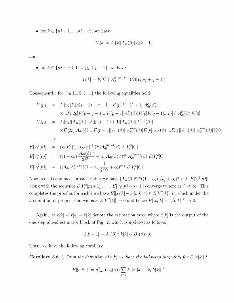
• for k ∈ {pj + q + 1, ..., pj + p− 1}, we have

Vi[k] = Fi[k]|(|Ak−pj−q+1di (β)|Vi[pj + q − 1]).

Consequently, for j ∈ {1, 2, 3, ...} the following equalities hold:

Vi[pj] = Fi[pj]Fi[p(j − 1) + q − 1]...Fi[p(j − 1) + 1]|Apdi(β)|

×...Fi[2p]Fi[p+ q − 1]...Fi[p+ 1]|Apdi(β)|Fi[p]Fi[q − 1]...Fi[1]|Apdi(β)|Vi[0]

Vi[pj] = Fi[pj]|Adi(β)|...Fi[p(j − 1) + 1]|Adi(β)||Ap−qdi (β)|

×Fi[2p]|Adi(β)|...Fi[p+ 1]|Adi(β)||Ap−qdi (β)|Fi[p]|Adi(β)|...Fi[1]|Adi(β)||Ap−qdi (β)|Vi[0]

⇒

E[V 2i [pj]] = (E[F 2

i [1]|Adi(β)|2])qj|Aj(p−q)di (β)|E[V 2i [0]]

E[V 2i [pj]] = ((1− αi)

|Adi(β)|2

22Ri+ αi|Adi(β)|2)qj|Aj(p−q)di (β)|E[V 2

i [0]]

E[V 2i [pj]] = (|Adi(β)|p+q((1− αi)

1

22Ri+ αi)

q)j|E[V 2i [0]].

Now, as it is assumed for each i that we have |Adi(β)|p+q((1− αi) 122Ri

+ αi)q < 1, E[V 2

i [pj]]

along with the sequence E[V 2i [pj+1]], ... , E[V 2

i [pj+p−1]] converge to zero as j →∞. This

completes the proof as for each i we have E[|xi[k]− xi[k|k]|2] ≤ E[V 2i [k]], in which under the

assumption of proposition, we have E[V 2i [k]]→ 0 and hence E[|xi[k]− xi[k|k]|2]→ 0.

Again, let e[k] = x[k]− x[k] denote the estimation error where x[k] is the output of the

one step ahead estimator block of Fig. 2, which is updated as follows:

x[k + 1] = Ad(β)x[k|k] +Bd(β)u[k].

Then, we have the following corollary.

Corollary 3.6 i) From the definition of e[k] we have the following inequality for E||e[k]||2

E||e[k]||2 = σ2max(Ad(β))

n∑i=1

E||xi[k]− xi[k|k]||2.

Hence, from the above proposition it follows that if the condition (12) holds, then E||e[k]||2

converges to zero, independent of the control action and the state variables, with an exponen-

tial rate. Hence, as mean square convergence implies mean absolute convergence [18], under

the assumption of Proposition 3.5, E||e(k)|| → 0, as k →∞.

ii) The above coding strategy has a semi recursive structure; and hence, it has very low coding

computational complexity.

3.3 Coding Strategy - β = 1

For p = q = 1, i.e., β = 1, the coding strategy 3.2 is reduced to the coding strategy that

uses feedback channel full time and result in asymptotic mean absolute tracking of the state

trajectory. For this case, the mean absolute estimation error converges to zero, as time

increases if the following inequality holds for all i ∈ {1, 2, ..., n} and h ∈ {1, 2, ..., ni}

(1− αi)|λh(Adi(β))|2

22Rih+ αi|λh(Adi(β))|2 < 1.

4 Stability and Performance Results

In this section, it is shown that for a given β, under some conditions, asymptotic mean

absolute stability is achieved if the corresponding coding strategy of Section 3 is combined

with the controller (3). This result is shown in the following theorem.

Theorem 4.1 Consider the closed loop feedback system of Fig. 2, which is described by

either the coding strategy 3.1 (i.e., β = 0), coding strategy 3.2 with β ∈ (0, 1), or the coding

strategy 3.3 (i.e., β = 1) and the controller (3), where the controller gain Kβ is chosen

such that the matrix Ad(β) + Bd(β)Kβ is a stable matrix. Suppose that the coding strategy

results in asymptotic mean absolute tracking of state trajectory at controller and computation

overflow does not occur (i.e., the conditions (4) and (5) are satisfied). Then, the system is

asymptotically mean absolute stable.

Proof: Consider the feedback system of Fig. 2 equipped with one of the above coding

strategies. Recall that the state estimate to be used in the stabilizing controller is given by

x[k + 1] = Ad(β)x[k|k] +Bd(β)u[k],

where the vector x[k|k] =

x1[k|k]

.

.

.xn[k|k]

is given either by (7) or (11) depending on the duty

cycle for feedback channel that is used. Recall also that e[k] = x[k]− x[k] is the estimation

error.

Now, for the corresponding closed loop feedback system, the following equalities hold

x[k + 1] = Ad(β)x[k] +Bd(β)u[k],

u[0] = 0, u[k + 1] = Kβx[k + 1], x[k + 1] = Ad(β)x[k|k] +Bd(β)u[k], k ∈ N+.

Subsequently, for k ≥ 1, we have:

x[1] = Ad(β)x[0], x[k + 1] = (Ad(β) +Bd(β)Kβ)x[k]−Bd(β)Kβe[k].

Therefore, for k ≥ 2, the following equality holds

x[k] = (Ad(β) +Bd(β)Kβ)k−1Ad(β)x[0]−k−1∑j=1

(Ad(β) +Bd(β)Kβ)k−1−jBd(β)Kβe[j].

Consequently, for k ≥ 2, the following inequality holds

E||x[k]|| ≤ (σmax(Ad(β) +Bd(β)Kβ))k−1σmax(Ad(β))E||x[0]||

+k−1∑j=1

(σmax(Ad(β) +Bd(β)Kβ))k−1−jσmax(Bd(β)Kβ)E||e[j]||. (13)

Now, as the matrix Ad(β) + Bd(β)Kβ is stable and, as shown in Section 3.1, E||e[j]|| con-

verges to zero, the first and the second terms of the right hand side of (13) vanish as time

increases. That is, limk→∞E||x[k]|| = 0.

As pointed out in Remark 3.3, among the available coding strategies that do not use

feedback channel and provide reliable tracking for dynamic systems via estimating the ini-

tial state, the coding strategy presented in Section 3.1 for the case of β = 0 has the fastest

decoding error decay rate. Moreover, the coding strategies, as proposed for the other cases,

i.e., β = 1 and β = qp

(p, q ∈ {1, 2, 3, ...}, q < p) have a fast decoding error decay rate as they

have exponential decay rates. In addition, as shown in this section, for each β there may

exist many controller gains Kβ that guarantee asymptotic mean absolute stability. Now, the

question is which gain results in the best performance? To address this question, we define

the parameter T ε(β), which is the smallest time instant under which for the given ε > 0, we

have E||x[k]|| ≤ ε, ∀k ≥ T ε(β).

As will be shown in the following, for a given β, in order to have the best performance

using the proposed stabilizing technique, the stabilizing controller (3) with gain Kβ that

results in the smallest possible σmax(Ad(β) +Bd(β)Kβ) must be used.

Theorem 4.2 Consider the closed loop feedback system of Fig. 2, in which for each β it

is described by the corresponding pairs of encoders-decoders (Eiβ(·),Diβ(·)) of Section 3, and

the controller (3). Then, an upper bound, T εup(β) on T ε(β) is the smallest integer T εup(β) that

satisfies the following inequality for all k ≥ T εup(β).

(σmax(Ad(β) +Bd(β)Kβ)

)k−1σmax(Ad(β))L[0]

+k−1∑j=1

(σmax(Ad(β) +Bd(β)Kβ)

)k−1−jσmax(Bd(β)Kβ)E||e(j)|| ≤ ε, (14)

where e[j] = x[j]− x[j] is the estimation error associated with the one step ahead estimator

block of Fig. 2 and L[0] =√∑n

i=1(Li[0])2, in which the non-negative scalars Li[0], i ∈{1, 2, ..., n}, are known upper bounds on the initial state (i.e., ||xi[0]|| ≤ Li[0]).

Proof: Recall that x[k + 1] = Ad(β)x[k] + Bd(β)u[k]. Therefore, the following equality

holds

x[k + 1] = (Ad(β) +Bd(β)Kβ)x[k]−Bd(β)Kβe[k], k ≥ 1.

Consequently, for k ≥ 1 the following relationships hold

x[k] =(Ad(β) +Bd(β)Kβ

)k−1Ad(β)x[0]−

k−1∑j=1

(Ad(β) +Bd(β)Kβ

)k−1−jBd(β)Kβe[j]

||x[k]|| ≤(σmax(Ad(β) +Bd(β)Kβ)

)k−1σmax(Ad(β))||x[0]||

+k−1∑j=1

(σmax(Ad(β) +Bd(β)Kβ)

)k−j−1σmax(Bd(β)Kβ)||e[j]||.

Now, from the inequality (14) it follows that E||x[k]|| ≤ ε, ∀k ≥ T εup(β). That is, an upper

bound on T ε(β) is T εup(β) that satisfies (14).

Remark 4.3 i) When subsystems are scalar, for the case of β 6= 0, from Corollary 3.6, i, it

follows that ||e[j]|| ≤ σmax(Ad(β))√∑n

i=1 Vi[j] (where an expression for Vi[j] was given in the

proof of Proposition 3.5). Hence, E||e[j]|| in (14) can be replaced by σmax(Ad(β))√∑n

i=1 Vi[j].

That is, for β = 1 and β = qp

(p, q ∈ {1, 2, 3, ...}, q < p), the upper bound T εup(β) is the

smallest integer that satisfies the following inequality for all k ≥ T εup(β)

(σmax(Ad(β) +Bd(β)Kβ)

)k−1σmax(Ad(β))L[0]

+k−1∑j=1

(σmax(Ad(β) +Bd(β)Kβ)

)k−j−1σmax(Bd(β)Kβ)σmax(Ad(β))

√√√√ n∑i=1

Vi[j] ≤ ε.(15)

ii) For the case of β = 0 from the inequality (10) it follows that the condition (14) can be

replaced by (σmax(Ad(β) +Bd(β)Kβ)

)k−1σmax(Ad(β))L[0]

+k−1∑j=1

(σmax(Ad(β) +Bd(β)Kβ)

)k−j−1σmax(Bd(β)Kβ)

×σmax(Ad(β))

√√√√ n∑i=1

c2i

j − 1

2(∆(Ri,ni,αi)−2 log σmax(Adi(β)))(j−1)≤ ε. (16)

iii) Note that the settling time T εs (β) can be approximated as follows: T εs (β) ≈ TβTε(β).

Hence, a scaled version of T εup(β) (i.e., TβTεup(β)) represents an upper bound on the settling

time.

Following the above remarks, for a given β by choosing the controller gain Kβ that results

in the smallest possible σmax(Ad(β)+Bd(β)Kβ), and using the corresponding coding strategy,

as given in Section 3, we can have the smallest possible upper bound T εup(β), as given by

(15) for the cases of β = 1 and β = qp

(p, q ∈ {1, 2, 3, ...}, q < p) and (16) for the case of

β = 0, using the proposed coding strategies and controller.

Following the above results, we have the following corollary, which summarizes the trade-

offs between duty cycle for feedback channel use, transmission delay and performance.

Corollary 4.4 i) As discussed in Remark 3.3 for β = 0, e[j] decays to zero very slowly such

that for σmax(Ad(β)) with unstable Ad(β), the coding strategy of Section 3.1 may not even

guarantee reliable tracking of state trajectory at controller. For this case (i.e., β = 0), the

sampling period Tβ is large due to high coding computational complexity. This results in a

large σmax(Ad(β)) for an unstable Ad(β). Therefore, from (16), it follows that if this coding

strategy guarantees reliable tracking, then the upper bound on the settling time can be very

large for a given ε.

ii) For β = 1 and β = qp

(p, q ∈ {1, 2, 3, ...}, q < p),∑ni=1 Vi[j] will decay to zero quickly. Also,

due to relatively low coding computational complexity of the corresponding coding strategy,

the sampling period Tβ is relatively small. This results in a relatively small σmax(Ad(β)) for

an unstable Ad(β). Therefore, from (15) it follows that the upper bound on the settling time

for β = 1 or β = qp

(p, q ∈ {1, 2, 3, ...}, q < p) is relatively smaller than that of the case of

β = 0.

For the purpose of illustration in the following we consider the closed loop feedback

system of Fig. 2 described by the following two subsystems.{x1(t) = 3x1(t) + 3u(t),y1(t) = x1(t), x1(0) ∼ U(0, 1),

β = 0 T εs (β) =∞β = 1/4 T εs (β) = 10.17 sec.β = 1/3 T εs (β) = 9.28 sec.β = 1/2 T εs (β) = 6.62 sec.β = 2/3 T εs (β) = 6.52 sec.β = 1 T εs (β) = 6.52 sec.

Table 1: Trade-off between β ∈ {0, 14, 1

3, 1

2, 2

3, 1} and the settling time.

{x2(t) = 3.6x2(t)− 3u(t),y2(t) = x2(t), x2(0) ∼ U(0, 1),

(17)

Here, it is assumed that ε = 0.02, α1 = 0.1, α2 = 0.1, and Kβ = [a1 a2], −10 ≤ a1, a2 ≤ 10.

It is also assumed that the transmission delay is Tdi = 0.04 second, i ∈ {1, 2}. Moreover, it is

assumed that the communication bit rate is large enough such that there is no transmission

delay due to the terms RikBW

and Ru+nBW

. For the stability and tracking of the dynamic system

(17) we apply the developed coding strategies and controller with different duty cycle for

feedback channel use β. For β = 0, we use the coding strategy of Section 3.1 with R1 = R2 =

1. For this case it is observed that Cd(β) = 0.03s and Cc(β) = 0.02s. Therefore, following

the conditions (4) and (5), we set Tm = 0.02s; and hence, Tβ = 0.12s. However, for this

time period it is observed that the coding strategy is not able to provide reliable tracking;

and therefore, we are not able to stabilize the controlled system using the proposed coding

strategy and controller. This result is expected from Corollary 3.4 as for ni = 1, αi = 0.1,

Ri = 1, we have ∆(Ri, ni, αi) = 0; and hence, the condition ∆(Ri, ni, αi) > 2 log σmax(Adi(β))

does not hold. In fact, for this system the maximum value of ∆(Ri, ni, αi) is achieved for

Ri = 0.28. For Ri = 0.28, we have ∆(Ri, ni, αi) = 0.28. Nevertheless, considering only

transmission delay, the smallest value for σmax(Adi(β)) is equivalent to e3.6×0.08 = 1.3312,

which indicates that the condition ∆(Ri, ni, αi) > 2 log σmax(Adi(β)) does not also hold for

other Ris.

For β > 0, we use the coding strategy of Section 3.2 with information ratesR1 = R2 = 6 bits.

For the cases of β ∈ {14, 1

3, 1

2, 2

3, 1} it is observed that the coding computational complexity

is negligible (it is of the order of 10−4s); and hence, we chose Tβ = 0.08 second. For

these cases, Kβ that results in the smallest σmax(Ad(β) +Bd(β)Kβ) is calculated as follows:

Kβ = ( 6.9 9.4 ).

In Table 1, we summarized trade-off between β ∈ {0, 14, 1

3, 1

2, 2

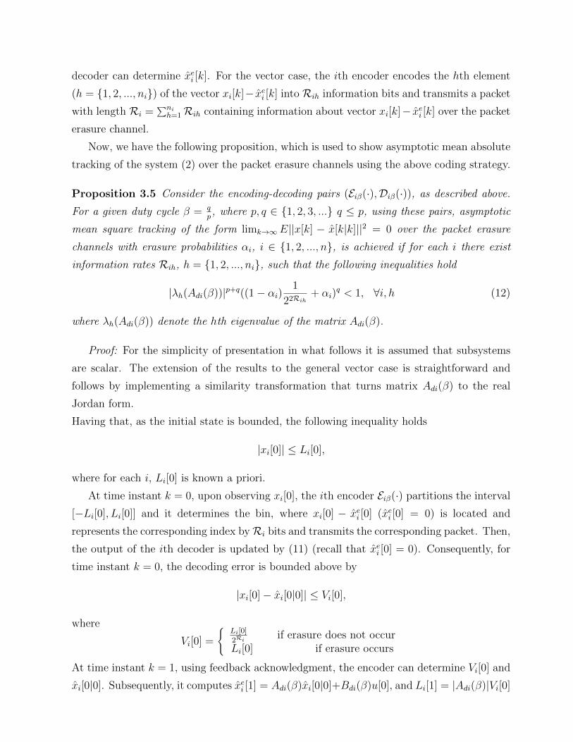
3, 1} and the settling time. In

Fig. 4, we also illustrated this trade-off. From Fig. 4 it is clear that for the condition

simulated, almost noting is lost in terms of performance if β ∈ [12, 1].

0.2 0.3 0.4 0.5 0.6 0.7 0.8 0.9 10

2

4

6

8

10

12

The Settling Time (Second)

ββββ

Figure 4: Trade-off between β and the settling time.

5 Conclusion

Many results in the literature (e.g., [11],[12],[13],[14],[15],[16],[17]) have been developed un-

der the assumption of full time availability of noiseless feedback channel. Specifically, there

is not any result for stability and tracking with intermittent noiseless feedback channel over

the packet erasure channel, which is an important class of digital communication channels

as it is an abstract model for the commonly used information technologies, such as the

Internet, WiFi and mobile communication. However, the availability of noiseless feedback

channel may not be possible full time. The full time availability of noiseless feedback channel

requires that feedback channel signal is transmitted with high power full time. This results

in significant power consumption at the base station of the control system of Fig. 1 as the

control signal in this system is also transmitted with high power full time. Hence, as trans-

mission of two high power signals full time will result in a short life time for the transmitter

of the high level controller, in this paper we relaxed the full time availability assumption of

noiseless feedback channel and addressed the problem of tracking state trajectory at remote

controller, stability and performance of linear time-invariant noiseless dynamic systems with

multiple observations over the packet erasure network subject to transmission delay that

does not necessarily use feedback channel full time. Three cases were considered in this

paper: i) without feedback channel, ii) with feedback channel intermittently, and iii) with

full time availability of feedback channel. For all three cases, coding strategies that result

in asymptotic mean absolute tracking were presented. Asymptotic mean absolute stabil-

ity of the controlled system equipped with each of these coding strategies was also shown.

Moreover, trade-offs between duty cycle for feedback channel use, transmission delay and

performance were studied.

Dynamic systems can be viewed as continuous alphabet sources with memory. Conse-

quently, many works in the literature (e.g.,[1],[15],[16],[17]) are concerned with the question

of stability and tracking over AWGN channel which itself is naturally a continuous alphabet

channel. In [15],[16] and [17] the authors addressed the problem of mean square stability and

tracking of linear unstable Gaussian systems (i.e., systems with terms that are not known

for design) under the assumption of full time availability of noiseless feedback channel. For

future, it is interesting to relax the assumption of full time availability of noiseless feed-

back channel and address the stability and tracking of linear Gaussian systems over AWGN

channel when feedback channel is available intermittently. Another research direction is

to address the stability and tracking problem of nonlinear Lipschitz systems with input

affine structure when feedback channel is available intermittently. As shown in [11], due to

the globally Lipschitz property of such systems, the developed techniques for stability and

tracking of linear systems can be easily extended to this class of nonlinear systems. Hence,

another research direction is to extend the developed techniques in this paper to nonlin-

ear noiseless Lipschitz systems with input affine structure over the packet erasure network

with intermittent noiseless feedback channel. Other research direction is to extend the de-

veloped techniques in this paper to nonlinear noiseless smooth systems via linearizing the

nonlinear system around the working points. These problems are left for future investigation.

Acknowledgment: The author would like to thank Professor Carlos Canudas de Wit for

many helpful discussion.

6 Appendix

In this section, we recall the coding strategy of [10] that is used to reconstruct a bounded

initial state, reliably, over the binary erasure channel.

Without loss of generality and for the simplicity of presentation, consider the following

unknown initial state

x[0] =

x1[0]...

xm[0]

with xh[0] ∈ [0, 1], h ∈ {1, 2, ...,m}. For a system with xh[0] /∈ [0, 1], we use the following

transformation: r[0] = Φ(x[0]−E), where the matrix Φ is invertible and Φ and E are chosen

such that rh[0] ∈ [0, 1].

xh[0] ∈ [0, 1] has the following binary representation:

xh[0] =∞∑j=1

whj2−j, whj ∈ {0, 1}.

At time instant k, for each h, the codeword/packet δh[k] with length Rk = bR.(k + 1)c,0 < R ≤ 1 are produced from the following linear operation:

δh[0]δh[1]

...δh[k]

...

= M⊕

wh1

wh2...

whlh...

,

M =

1 0 0 0 0 . . . 0 0 00 1 0 0 0 . . . 0 0 0...1 . . . 1 0 0 . . . 0 0 0...

,

where 0s and 1s on the lower triangular side of the matrix M are generated randomly; but

transmitter and receiver know the components of this matrix a priori. In the above equation,

the operator⊕

acts as follows:

δh[0] = wh1, δh[1] = (0 wh2), ..., δh[k] = (wh1...whlh), ... .

Then, for each h, the corresponding packet δh[k] is transmitted bit by bit via the binary

erasure channel at time instant k. At time instant k, the decoder can use all the received

packets up to time k, i.e., δh[0], δh[1], ..., δh[k] to reconstruct xh[0|k], which is the estimate

of the hth component of the initial state x[0] at time instant k. To achieve this goal, the

decoder ignores the packets containing filliped bits that cannot be recovered and produces

xh[0|k] using only the packets that received successfully. To understand how the decoding

operation works, let us assume that for the hth component, just the received codeword δh[1]

contains erased bits. Then, the decoder ignores δh[1] and uses the following linear system of

equations to reconstruct xh[0|k].zh[0]zh[2]

...zh[k]

= M

wh1

wh2...

whlh

,

where zh[k] is the decimal representation of the binary string δh[k], and M is the matrix M

without the second row (which corresponds to δh[1]) with 12p

corresponding to each 1 located

at the pth column of the matrix M . For illustration, for M given above,

M =

12

0 0 0 0 . . . 0 0 0...12

. . . 12p

0 0 . . . 0 0 0...

.

Consequently, using the above equation, the decoder estimates wh1, wh2, ..., whlh as follows:

wh1

wh2...

whlh

= (M′M)−1M

′

zh[0]zh[2]

...zh[k]

.

Subsequently, it outputs: xh[0|k] =∑lhj=1 whj2

−j.

References

[1] Elia, N.: ‘When Bode meets Shannon: control-oriented feedback communication

schemes’, IEEE Trans. Automat. Contr., 2004, 49(9), pp. 1477-1488.

[2] Elia, N. and Eisenbeis, J. N.: ‘Limitations of linear control over packet drop networks’,

IEEE Trans. Automat. Contr., 2011, 56(4), pp. 826-841.

[3] Martins, N. C., Dahleh, A., and Elia N.: ‘Feedback stabilization of uncertain systems in

the presence of a direct link’, IEEE Trans. Automat. Contr., 2006, 51(3), pp. 438-447.

[4] Minero, P., Franceschetti, M., Dey, S., and Nair, N.: ‘Data rate theorem for stabilization

over time-varying feedback channels’, IEEE Trans. Automat. Contr., 2009, 54(2), pp.

243-255.

[5] Minero, P., Coviello, L., and Franceschetti, M.:‘Stabilization over Markov feedback

channels: the general case’, IEEE Trans. Automat. Contr., 2013, 58(2), pp. 349-362.

[6] Nair, G. N. and Evans, R. J.: ‘Stabilizability of stochastic linear systems with finite

feedback data rates’, SIAM J. Control Optimization, 2004, 43(3), pp. 413-436.

[7] Canudas de Wit, C., Gomez-Estern, F., and Rodrigues Rubio, F.: ‘Delta-modulation

coding redesign for feedback-controlled systems’, IEEE Transactions on Industrial Elec-

tronics, 2009, 56(7), pp. 2684-2696.

[8] Brinon Arranz, L., Seuret, A., and Canudas de Wit, C.: ‘Translation control of a

fleet circular formation of AUVs under finite communication range’, Proc. 48th IEEE

Conference on Decision and Control, 2009, pp. 8345-8350.

[9] Brinon Arranz, L., Seuret, A., and Canudas de Wit, C.: ‘Collaborative estimation of

gradient direction by a formation of AUVs under communication constraints’, Proceed-

ings of the 50th IEEE Conference on Decision and Control, 2011, pp. 5583-5588.

[10] Como, G., Fagnani, F., and Zampeiri, S.: ‘Anytime reliable transmission of real - valued

information through digital noisy channels’, SIAM J. Control Optim.,2010, 48, pp. 3903-

3924.

[11] Farhadi, A., and Ahmed, N. U.: ‘Tracking nonlinear noisy dynamic systems over noisy

communication channels’, IEEE Transactions on Communications, 2011, 59(4), pp. 955-

961.

[12] Tatikonda, S., and Mitter, S.: ‘Control under communication constraints’, IEEE Trans.

Automat. Contr., 2004, 49(7), pp. 1056-1068.

[13] Nair, G. N., Evans, R. J., Mareels, I. M. Y., and Moran, W.: ‘Topological feedback

entropy and nonlinear stabilization’, IEEE Trans. Automat. Contr., 2004, 49(9), pp.

1585-1597.

[14] Tatikonda, S., and Mitter, S.:‘Control over noisy channels’,IEEE Trans. Automat.

Contr., 2004, 49(7), pp. 1196-1201.

[15] Charalambous, C. D., Farhadi, A., Denic, S. Z.: ‘Control of continuous-time linear

Gaussian systems over additive Gaussian wireless fading channels: a separation princi-

ple’, IEEE Trans. Automat. Contr., 2008, 53(4), pp. 1013-1019.

[16] Charalambous, C. D., and Farhadi, A.: ‘LQG optimality and separation principle for

general discrete time partially observed stochastic systems over finite capacity commu-

nication channels’, Automatica, 2008, 44(12),pp. 3181-3188.

[17] Tatikonda, S., Sahai, A., Mitter, S.:‘Stochastic linear control over a communication

channel’, IEEE Trans. Automat. Contr., 2004, 49(9), pp. 1549-1561.

[18] Billingsley, P.: ‘Probability and measure’ (John Wiley and Sons, 1995).