Embed Size (px)
Citation preview

Dark Matter and Higgs Physics at the LHC
Federica Giacchino
November 21, 2012

2

Contents
Introduzione 5
1 Astrophysical Evidences of Dark Matter 7
1.1 Astrophysical Evidences of Dark Matter . . . . . . . . . . . . 71.1.1 Local Dark Matter . . . . . . . . . . . . . . . . . . . . 71.1.2 Anomalies in rotation curves of galaxies . . . . . . . . 81.1.3 Cluster Dark Matter . . . . . . . . . . . . . . . . . . . 101.1.4 Gravitational lensing . . . . . . . . . . . . . . . . . . . 111.1.5 Bullet Cluster . . . . . . . . . . . . . . . . . . . . . . . 131.1.6 Compared of three matter abundance . . . . . . . . . . 141.1.7 Cosmic Microwave Background (CMB) . . . . . . . . . 17
1.2 General Features of Dark Matter . . . . . . . . . . . . . . . . 18
2 Production Mechanism of Dark Matter Particles 21
2.1 Freeze-out mechanism . . . . . . . . . . . . . . . . . . . . . . 222.1.1 Review of the Boltzmann equation with coannihilations 34
2.2 Freeze-in mechanism . . . . . . . . . . . . . . . . . . . . . . . 442.2.1 General mechanism of Freeze-in . . . . . . . . . . . . . 47
3 Higgs Portal 55
3.1 Higgs Portal in The Scalar Singlet Model . . . . . . . . . . . . 563.1.1 The Model . . . . . . . . . . . . . . . . . . . . . . . . . 563.1.2 Higgs portal in freeze-out scenario . . . . . . . . . . . . 603.1.3 Higgs portal in freeze-in scenario . . . . . . . . . . . . 65
3.2 Three model indipendent . . . . . . . . . . . . . . . . . . . . . 72
4 Z’ portal 81
4.1 Reheating Temperature . . . . . . . . . . . . . . . . . . . . . . 814.2 Heavy Z’ Boson . . . . . . . . . . . . . . . . . . . . . . . . . . 844.3 About the dependence of Ωh2 on reheting temperature . . . . 89
3

4 CONTENTS
Conclusioni 95
Bibliografia 96
Introduction
The fondamental interactions are described by Standard Model in particlesphysics. In this model, matter and interactions are coupling like rappresen-tation of gauge groups SU(3) × SU(2) × U(1), which is based in invarianceprinciple of local symmetries. This construction allows to explain (almost)all actual experimental data of particles physics. However, today the Stan-dard Model doesn’t answer to others importants interogatives: What is thenature and interaction forme of Dark Matter in the Universe, responsiblefor rotation curve of galaxies (weakly interaction massive particles, WIMP)?What is Boson Higgs mass and the nature of its interactions with visible anddark matter? A fifth strenght (the existence of a Z ) is still not excludedwhat would be its cosmological role within Extended Standard Model? Mywork aims to answer most of these questions, or to create a starting pointfor a new ways of thinking.
Indeed, for the first time in the history of particle physics, the sensitiv-ity of direct detention experiments (XENON1T,XMASS), indirect detection(FERMI, PAMELA, HESS, AMS2) and accelerators (CMS and ATLAS atLHC) will cover nearly 90% of the parameter space of any extension of theStandard Model, supersymmetric or non-supersymmetric. The WIMP hy-pothesis will therefore be tested at a level of precision never achieved so farduring the next 3 years. Now, the word “complementary” should no longerbe considered as a future projection, but as a present reality. In fact an hintof the Higgs boson have been unveiled in July 2012 by the CMS and ATLASexperiments at CERN. The discovery of a Higgs boson with SM coupling ornon-SM coupling can have huge consequences on direct detection rates orrelic abundance through the measurement of the Higgs coupling to the DarkSector. Indeed, any production rates at LHC are directly linked to limits onDark Matter annihilation or scattering processes. If one observe one signalon any of the accelerator or Dark Matter-dedicated experiment, the signatureto look for in the other detection modes would be determined.
5

6 CONTENTS

Chapter 1
Astrophysical Evidences of
Dark Matter
In the XX century studies in astrophysical scenario evidenced the existance ofa new form of matter that have inspired interest in modern physics scenario.We call that as “Dark Matter” (DM), the exotic name but with a clearmeaning: a component of matter that doesn’t emit luminous radiation.
Beginning from study presented by Zwicky (1933) who analyzed the mo-tion of the galaxies in the cluster Coma, subsequently other observationshave indicated the presence of dark matter from the kinematics of viriallysystems and rotating spiral galaxies, the effects of gravitational lensing ofbackground objects, various evidences among which the recent observationsof the Bullet cluster, untill recent observations from the PAMELA satellite.Furthermore, the dark matter appears to have an important role in the for-mation of the structures, in the evolution of galaxies and also has effects onnon-uniformity observed cosmological microwave of background radiation.What we will do in this chapter is to introduce the most important evidence(Section 1.1), explaining where the dark matter may intervene to resolve theoddities observed and to list the general features of dark matter particles(Section 1.2).
1.1 Astrophysical Evidences of Dark Matter
1.1.1 Local Dark Matter
The dynamical density of matter in the Solar vicinity can be estimated usingvertical oscillations of stars around the galactic plane. The orbital motionsof stars around the galactic center play a much smaller role in determining
7
8 CHAPTER 1. ASTROPHYSICAL EVIDENCES OF DARK MATTER
the local density. Oort (1932) indicated, in his analysis, as members of a“star atmosphere”, a statistical ensemble in which the density of stars andtheir velocity dispersion defines a “temperature” from which one obtains thegravitational potential. The result contradicted grossly the expectations: thepotential provided by the known stars was not sufficient to keep the starsbound to the Galactic disk because the density of visible stellar populationsby a factor of up to 2, and so the Galaxy should rapidly be losing stars [1].Since the Galaxy appeared to be stable there had to be some missing matternear the Galactic plane, Oort thought, exerting gravitational attraction. Thislimit is often called the Oort limit.
This used to be counted as the first indication for the possible presenceof dark matter in our Galaxy: the amount of invisible matter in the Solarvicinity should be approximately equal to the amount of visible matter.
1.1.2 Anomalies in rotation curves of galaxies
Radio radiation from interstellar gas, in particular that of neutral hydrogen,is not strongly absorbed or scattered by interstellar dust [2]. It can there-fore be used to map and to study the motion of neutral hydrogen cloudsconcentrated in spiral arms. Hence it can be determined angular velocity ofgas for various distance from the galactic centre and corresponding rotationcurve v = v(r), the circular velocity as a function of galactic radius. Themost convincing and direct evidence for dark matter on galactic scales comesreally from the observations of the rotation curves of galaxies.
Rotation curves are usually obtained by combining observations of the21cm line with optical surface photometry: if the angle θ between the velocityof the star and the line of sight, the velocity components are vr = v cos θ andvt = v sin θ. The tangential velocity vt results in the proper motion, whichcan be measured by taking plates at intervals of several years or decades. Theradial velocity vr can be measured from Doppler shift of the stellar spectrum,in which the spectral lines are often displaced towards the blue or red. Theblueshift means that the star is approching, while the redshift indicates thatit is receding. From 1940 (Oort) numerous observations in spiral galaxiesshowed, in outer regions of galaxies, an anomaly in rotation velocity thatcan be translet in an high M/L, mass-luminosity ratio.
Observed rotation curves usually exhibit that the part central of galaxyrotates like a rigid body, i.e. v ∝ r and successively the velocity reanching amaximum value. At this point we expected that decrease outwards, as thethird Kepler law suggests us, instead there is a characteristic flat behavioruntill edges of galaxy where is emitted not much light.
Considering a general spiral galaxy, we take for simplicity that matter

1.1. ASTROPHYSICAL EVIDENCES OF DARK MATTER 9
distribution of galaxy is spherical symmetry. In Newtonian dynamics thecircular velocity is expected to be
v =GM(r)/r (1.1)
Figure 1.1: Rotation curve of NGC 6503. The dotted, dashed and dash-dottedlines are the contributions of gas, disk and dark matter, respectively. [3].
where, as usual, M(r) = 4πρ(r)r2dr, and ρ(r) is the mass density
profile, and should be falling ∝√r beyond the optical disc. The fact that
v(r) is approximately constant implies the existence of an halo withM(r) ∝ rand ρ ∝ 1/r2 therefore the most of the mass is concentrated in the outer partof the galaxy. This implies that the most of mass of galaxy is situed in outergalactic part [3].
The distribution mass obtained from rotation curve and that determinedindirectly from light distribution considering all of luminous component ofgalaxy introduce a discrepance in mass that is expressed with “Paradox ofmissing mass”. In fact, for example, by photometry the estimed mass in ourGalaxy untill RS = 8Mpc (distance between the bulk and Solar Stystem)

10 CHAPTER 1. ASTROPHYSICAL EVIDENCES OF DARK MATTER
is M = 9 × 10¹⁰M⊙, while for outer edge of galaxy, where the luminositydecreases exponentially, the component of luminous is negligible. This valueof mass is able to demonstrate the rotational velocities until RS, but is notgood to solve the anomaly in the rotational curve.
This discrepancy can be explain of the presence of invisible mass halo,that is called dark matter, around our Galaxy.
Based on gravitational influence to luminous mass, this dark componentof matter would be spherically distributed in a halo extended untill 230 kpcfrom galactic center and having a density profile
ρ(r) =ρ0
(r/a)(1 + r/a)2(1.2)
This profile tell us that the galaxy behaves like 1/r at the center, r << aand like 1/r3 in the edges, r >> a. With this calculation the mass of haloof dark matter must be 5.4× 10¹¹M⊙ within 50 kpc and 2.5× 10¹²M⊙ untill230 kpc [4].
1.1.3 Cluster Dark Matter
A different mass discrepancy was found by Zwicky (1933) [1]. He measuredredshifts of galaxies in the “Coma cluster” and found that the velocities ofindividual galaxies with respect to the cluster mean velocity are much largerthan those expected from the estimated total mass of the cluster, calculatedfrom masses of individual galaxies.
Stars move in galaxies and galaxies in clusters along their orbits, those arevirially bound systems: the orbital velocities are balanced by the total gravityof the system, similar to the orbital velocities of planets moving around theSun in its gravitational field. In the simplest dynamical framework one treatsclusters of galaxies as statistically steady, spherical, self-gravitating systemsof N objects of average mass m and average orbital velocity v. The totalkinetic energy E of such a system is then
E =1
2Nmv2 (1.3)
If the average separation is r, the potential energy of N(N−1)/2 pairingsis
U =1
2N(N1)
Gm2
r(1.4)
The virial theorem states that for such a system
E = −U/2 (1.5)

1.1. ASTROPHYSICAL EVIDENCES OF DARK MATTER 11
The total dynamic mass M can then be estimated from v, and r from thecluster volume
M = Nm =2rv2
G(1.6)
Zwicky was the first to use the virial theorem to infer the existence ofunseen matter. He found that the orbital velocities are almost a factor of tenlarger than expected from the summed mass of all galaxies belonging to theclusters, and this implies that the average mass of galaxies within the clusterhas a value about 400 times greater than expected from their luminosity:the gravity of the visible galaxies in the cluster would be far too small forsuch fast orbits, so something entra was required. This is known as “missingmass problem” and he proposed that the most of the missing matter wasdark, non-visible form of matter which would provide enough of the massand gravity to hold the cluster together.
Exist another method to determinate the mass of cluster: the temperatureof the hot intracluster gas, like the galaxy motion, traces the cluster mass.X-ray emission by hot gas inside the clusters by bremsstrahlung process.Observations show that the gas is in hydrodinamics equilibrium (dFgrav =dFpress =
dPdr = −GMrρ
r2 with Mr inner total mass to r radius) and it movesin the gravitational field of cluster in orbits with velocities dependent tomass of cluster. Through spectroscopic analysis of hot gas we can obtaindensity and temperature of gas in function of galactic distance r. With theseparameters we can get mass distribution of cluster. For example gas massof Coma cluster is Mgas = 1.05 × 10¹⁴M⊙ that is larger than visible massM = 1.5×10¹³M⊙ but not sufficiently to explain the value obtained to virialtheorem that is MX = 3.3× 10¹⁵M⊙. [4].
An empirical formula often used in simulations of the density distributionof dark matter halos in clusters is
ρDM(r) =ρ0
(r/rs)α(1 + r/rs)3−α(1.7)
ρ0 is a normalization constant and 0 ≤ α ≤ 3/2 [1].
1.1.4 Gravitational lensing
We know by General Relativity that gravitational field curves the time-spaceand the particles or photons travel in geodetic trajectory. A consequence isthe gravitational lensing: a photon in a gravitational field moves as if it pos-sessed mass, and light rays therefore bend around gravitating masses. Thuscelestial bodies can serve as gravitational lenses probing the gravitationalfield, whether baryonic or dark without distinction.

12 CHAPTER 1. ASTROPHYSICAL EVIDENCES OF DARK MATTER
We consider that a trajectory of light ray in a gravitational filed at sphericsymmetry is represented as
d2
dϕ2(1
r) +
1
r= 3G
M
r2(1.8)
The solution of thi equation can be though as a perturbation of specialrelativity (without gravitational field)
1
r=
1
r0cosϕ+
GM
r20(1 + sin2 ϕ) (1.9)
To determinate the deflession angle δ = 2α we put a r → ∞. If ϕ =±(π2 + α) and we use the little angle approximation the eq. (1.9) becomes
− 1
r0α + 2
GM
r20= 0 (1.10)
and then the deflession angle is
δ = 2α = 4GM
r0(1.11)
The deflession provided for a light ray that enters in gravitational field ofSun is δ 1.75.
Since photons are neither emitted nor absorbed in the process of grav-itational light deflection, the surface brightness of lensed sources remainsunchanged. Changing the size of the cross-section of a light bundle onlychanges the flux observed from a source and magnifies it at fixed surface-brightness level. There are three cleasses of gravitational lensing [1][5]:
• Strong lensing, the photons move along geodesics in a strong gravi-tational potential which distorts space as well as time, causing largerdeflection angles and requiring the full theory of GR. The images in theobserver plane can then become quite complicated because there maybe more than one null geodesic connecting source and observer. Stronglensing is a tool for testing the distribution of mass in the lens ratherthan purely a tool for testing GR. The masses of clusters of galaxiesdetermined using this method confirm the results obtained by the virialtheorem and the X-ray data.
• Weak Lensing, refers to deflection through a small angle when the lightray can be treated as a straight line, and the deflection as if it occurreddiscontinuously at the point of closest approach (the thin-lens approx-imation in optics). One then only invokes SEP which accounts for the

1.1. ASTROPHYSICAL EVIDENCES OF DARK MATTER 13
distortion of clock rates. This kind of lensing allows to determine thedistribution of dark matter in clusters as well as in superclusters: thelensing mass estimate is almost twice as high as that determined fromX-ray data.
• Microlensing, if the mass of the lensing object is very small, one willmerely observe a magnification of the brightness of the lensed object.Microlensing of distant quasars by compact lensing objects (stars, plan-ets) has also been observed and used for estimating the mass distribu-tion of the lens-quasar systems. A fraction of the invisible baryonicmatter can lie in small compact object. To find the fraction of theseobject in the cosmic balance of matter, special studies have been ini-tiated, based on the microlensing effect. This process is used to findMassive Compact Halo Object (MACHOs), small baryonic objects asplanets, dead stars or brown dwarfs, which emit so little radiation thatthey are invisible most of time. A MACHOs may be detected whenit passes in fron of a star and the MACHOs gravity bends the light,causing the star to appear brighter. Some authors claimed that up to20% of dark matter in our Galaxy can be in low-mass stars.
1.1.5 Bullet Cluster
Figure 1.2: Bullet Cluster photo in X-ray, exposition time about 140 hoursand megaparsec scale [6].

14 CHAPTER 1. ASTROPHYSICAL EVIDENCES OF DARK MATTER
In Fig.(1.2) the image shows the galaxy cluster 1E 0657-56, also known asthe “bullet cluster”. This phenomenon was observed in 2004 by Chandra X-ray Observatory detected an effect never see before. This cluster was formedafter the collision of two large clusters of galaxies, the most energetic eventknown in the universe since the Big Bang[6].
Hot gas detected by Chandra in X-rays is seen as two pink clumps inthe image and contains most of the ”normal,” or baryonic, matter in the twoclusters. The bullet-shaped clump on the right is the hot gas from one cluster,which passed through the hot gas from the other larger cluster during thecollision. An optical image from Magellan and the Hubble Space Telescopeshows the galaxies in orange and white. The blue areas in this image showwhere astronomers find most of the mass in the clusters. The concentration ofmass is determined using the effect of so-called gravitational lensing, wherelight from the distant objects is distorted by intervening matter. Most ofthe matter in the clusters (blue) is clearly separate from the normal matter(pink), giving direct evidence that nearly all of the matter in the clusters isdark.
We know that when two clusters collide the star is gravitationally slowedbut not altered significantly since the stars do not interact with each other.The hot gas in each cluster was slowed down by a force like air resistance.In contrast, the dark matter was not slowed by the impact because it doesnot directly interact with the gas itself or if not through gravity. Therefore,during the collision the lumps of dark matter from the two clusters movedahead of the hot gas, producing the separation of dark matter and normalsees the image. If hot gas was the most massive component in the clusters,as proposed by alternative theories of gravity, this effect would not be seen.Instead, this result shows that dark matter is required.
1.1.6 Compared of three matter abundance
We can estimate the contribution Ωg from the mass concentrated in galaxiesto be [7]
Ωg =ρ0gρ0c
0.03 (1.12)
We can also estimate the contribution from baryonic material by com-paring the observed abundances of light elements (deuterium, 3He, 4He and7Li) with the predictions of primordial nucleosynthesis computations, thatgive us
Ωb ∼ 0.02h−2 (1.13)
We shall see later that a reasonable estimate for the total amount of mass

1.1. ASTROPHYSICAL EVIDENCES OF DARK MATTER 15
contributing to the gravitational dynamics of large-scale objects is around
Ωdyn 0.2− 0.4 (1.14)
The discrepancy between the three values of Ω given by eqns (1.12),(1.13) and (1.14) is attributed to the presence of non-luminous matter,thedark matter, which may play an important role in structure formation.
The first value we can found considering mean luminosity per unit volumeproduced by galaxies Lg and mean value of M/L (the mass-to-light ratio).These give us the galaxy density
ρ0g = Lg < M/L > (3.3×10⁸hL⊙Mpc−3)(30hM⊙/L⊙) 6×10⁻³¹h2gcm−3.(1.15)
From this we can obtain the value in eq. (1.12).The second value we have to analyze the Big Bang Nucleosynthesis. Ac-
cording to the Big Bang model, the Universe began in an extremely hotand dense state [5]. For the first second it was so hot that atomic nucleicould not form, space was filled with a hot soup of protons, neutrons, elec-trons, photons and other short, lived particles. Occasionally a proton anda neutron collided and sticked together to form a nucleus of deuterium (aheavy isotope of hydrogen), but at such high temperatures they were brokenimmediately by high-energy photons. When the Universe cooled off, thesehigh-energy photons became rare enough that it became possible for deu-terium to survive, deuterium bottleneck. These deuterium nuclei could keepsticking to more protons and neutrons, forming nuclei of 3He, 4He, lithium,and beryllium. This process of element-formation is called “nucleosynthesis”.The denser proton and neutron “gas” is at this time, the more of these lightelements will be formed. As the Universe expands, however, the density ofprotons and neutrons decreases and the process slows down. Neutrons areunstable (with a lifetime of about 15 minutes) unless they are bound up in-side a nucleus. After a few minutes, therefore, the free neutrons will be goneand nucleosynthesis will stop. There is only a small window of time in whichnucleosynthesis can take place, and the relationship between the expansionrate of the Universe (related to the total matter density) and the density ofprotons and neutrons (the baryonic matter density) determines how muchof each of these light elements are formed in the early Universe. The Fig.(1.3) shows the computed abundance of deuterium D, 3He, 3He+D and 7Li(compared with H hydrogen). The abundances are all shown as a function ofη, the baryon-to-photon ratio which is related to Ωb by Ωb 0.004h−2η/10−10
[7]. The estimates of the primordial values of the relative abundances of theseelements appear to be in accordo with nucleosynthesis predictions, but only

16 CHAPTER 1. ASTROPHYSICAL EVIDENCES OF DARK MATTER
Figure 1.3: Light-element abundance determined by numerical calculationsas functions of the matter density η. The arrow mark the possible deuteriumabundance [7].
if the density parameter in baryonic material is
Ω0bh2 0.02 (1.16)
Now we can analyze the mass-to-light ratio of galaxies. A study con-duct to Bahcall [8] showed the M/LB (LB blue band luminosity) of galax-ies (typical radius R 0.01 − 0.1Mpc) increases to increase the scale un-till R 0.2h−1Mpc. The M/LB remains approximatively constant forgroups or clusters of galaxies at higher scale about 0.2h−1Mpc at valueof M/LB 200 − 300hM⊙L−1⊙ (where h = H0/100kms−1Mpc−1 is theHubble constant). When integrated over the entire observed luminosity den-sity of the Universe, this mass-to-light ratio yields a mass density ρm 0.4 × 10⁻²⁹h2gcm−3 cor a mass density ratio Ωmat = ρm/ρcrit 0.2 ± 0.1.Since M/LB >> M⊙/L⊙ must exist matter not luminous like stars, that isdark matter. Besides the most dark matter is given to DM halos of galaxiesand clusters do not contain a substantial quantity of additional dark mat-

1.1. ASTROPHYSICAL EVIDENCES OF DARK MATTER 17
ter, since R > 1.5h−1Mpc (typical galaxy radius) the mass-to-light ratio ofsuperclusters of galaxies confirm that do not exist a additional quantity ofdark matt at higher scale, R = 6h−1Mpc.
1.1.7 Cosmic Microwave Background (CMB)
We discuss in this section how such information can be extracted from theanalysis of the Cosmic Microwave Background (CMB), radiation originatingfrom the propagation of photons in the early Universe once they decoupledfrom matter, recombiantion era [3]. In 1964 this radiation was detected andthis discovery was a powerful confirmation of the Big Bang theory. Aftermany decades of experimental effort, the CMB is known to be isotropic buthaving minimum temperature fluctuations called anisotropy with amplitudeof order 10−3−10−5 and it follows with extraordinary precision the sprectrumof a black body corresponding to a temperature T = 2.726K.
The variations of temperature of CMB can be expressed as sum of spher-ical harmonic Ylm
δT
T(θ,φ) =
∞
l=2
l
m=−l
almYlm(θ,φ) (1.17)
alm gives us the variance Cl =< |alm|2 >= 12l+1
lm=−l |alm|2. If the tem-
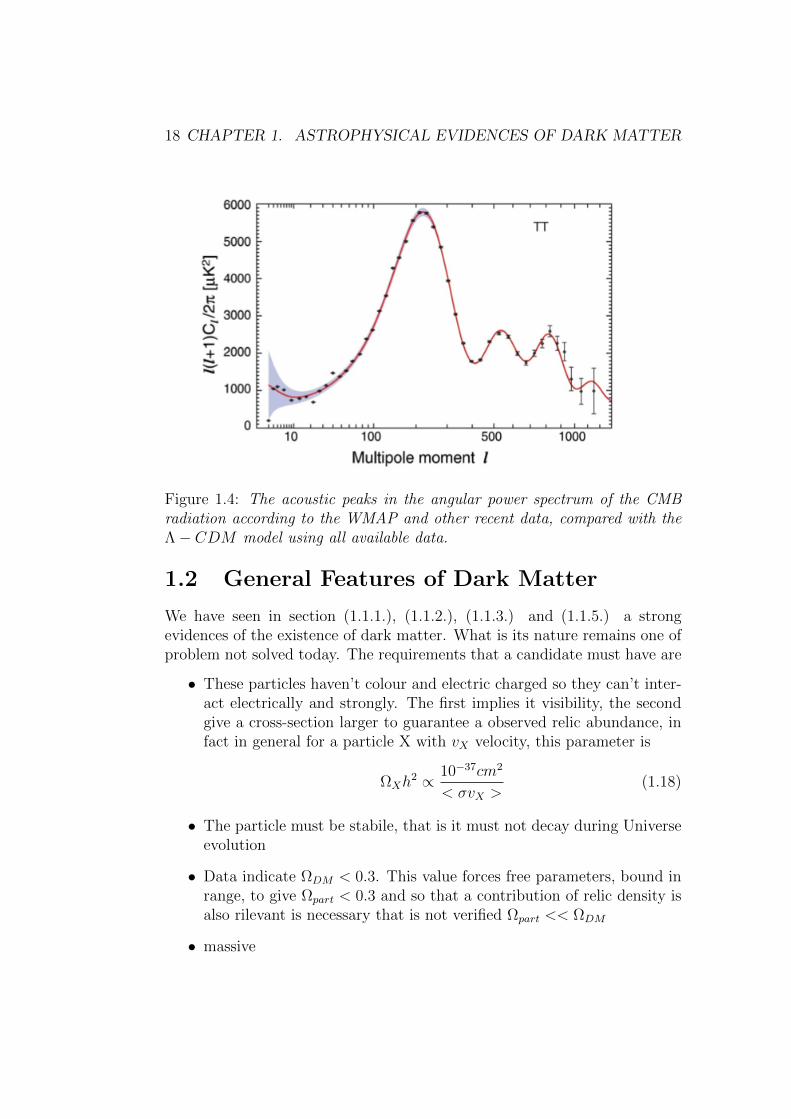
perature fluctuations are assumed to be Gaussian, as appears to be the case,all of the information contained in CMB maps can be compressed into thepower spectrum, essentially giving the behavior of l(l+1)Cl/2π as a functionof l. WMAP (Wilkinson Microwave Anisotropy Probe) data could map uni-versal fluctuations after remove dipole anisotropy (l = 1) and galactic andextragalactic contaminations. To extract information from CMB we mustconsider a cosmological model with fixed number parameters. The spectrumprofile is represented in Fig.(1.4). This graphics was be fitted by a model thatconsider a Universe with a cosmological constant Λ and a cold dark compo-nent of matter (Λ−CDM). The position of the first peak determines Ωmh2.Combining the 5-year WMAP measurements of the temperature power spec-trum (TT) with determinations of the Hubble constant h, the WMAP teamfinds the total mass density parameter Ωm 0.26. The ratio of amplitudes ofthe second-to-first Doppler peaks determines the baryonic density parameterΩb 0.04; the dark matter component is then ΩDM 0.22 [1].
18 CHAPTER 1. ASTROPHYSICAL EVIDENCES OF DARK MATTER
Figure 1.4: The acoustic peaks in the angular power spectrum of the CMBradiation according to the WMAP and other recent data, compared with theΛ− CDM model using all available data.
1.2 General Features of Dark Matter
We have seen in section (1.1.1.), (1.1.2.), (1.1.3.) and (1.1.5.) a strongevidences of the existence of dark matter. What is its nature remains one ofproblem not solved today. The requirements that a candidate must have are
• These particles haven’t colour and electric charged so they can’t inter-act electrically and strongly. The first implies it visibility, the secondgive a cross-section larger to guarantee a observed relic abundance, infact in general for a particle X with vX velocity, this parameter is
ΩXh2 ∝ 10−37cm2
< σvX >(1.18)
• The particle must be stabile, that is it must not decay during Universeevolution
• Data indicate ΩDM < 0.3. This value forces free parameters, bound inrange, to give Ωpart < 0.3 and so that a contribution of relic density isalso rilevant is necessary that is not verified Ωpart << ΩDM
• massive

1.2. GENERAL FEATURES OF DARK MATTER 19
• non relativistic
We know by Nucleosynthesis and CMB that the most of DM is non-baryonic, but a little quantity of that is baryonic. Candidates are the MAs-sive Compact Halo Object (MACHO), that is the little fraction of DM ofbaryonic nature which determinates the lensing effect and whose upper con-straints of abundance was assigned by BBN and CMB fluctuations, Ωb ≤ 0.05. An example is given by stars with ligher mass, M ≤ 0.05M⊙, as browndwarf, that have mass so small that the temperature of their nucleus is notsufficient to be able to allow to burn the hydrogen in helium.. This impliesthat are object that emitt a little quantity of radiation, since their sourceof luminosity is not more than the thermal energy that had in their birth.They are cosmologically cold and very difficult to observe
The baryonic candidates enter in Weakly Interacting Massive Particles(WIMP) class and can be classiefied in according to whether the dark matterparticles originated via decoupling from a thermal bath (thermal relics) orwere created in some non-thermal process (non-thermal relics).
In turn, thermal relics can be categorized further as to whether they wererelativistic or non-relativistic at the moment of decoupling. The relics whichwere relativistic at this time constitute hot dark matter, while those whichwere non-relativistic constitute cold dark matter.
Being not baryonic we have to find the candidate in extension of StandardModel. The most famous candidates belong to Supersymmetry Theories, asneutralino, gravitino e sneutrino, or a particle of SM, the neutrino, but ithave a relic abundance obtained to CMB anisotropy equal to Ωνh2 < 0.0067,not sufficient to be the dominant component of dark matter. Then we havea non thermal candidate, the axions, and finally Kaluza-Klein state.
Today there are many different esperiments to search of a signal of darkmatter particle. We can detect WIMP particles though differnet method:
• Indirect detection: we observe the annihilation products of WIMP asγ ray, neutrinos, antriprotons, positrons and anti-deuterons.
• Direct deterction: though elastic scattering of WIMP on target in ter-restrial detector of which we measure the recoil energy.
• Collider: in this apparatus particles collide and we analyze the productsas DM particles.
In next chapters studying the mechanism of production during Universeevolution we will talk about of candidates and their important properties asmass and coupling. Exist another category, called FIMP, that we will be

20 CHAPTER 1. ASTROPHYSICAL EVIDENCES OF DARK MATTER
produced with a feeble coupling with SM particles and not in equilibriumwith plasma background.

Chapter 2
Production Mechanism of Dark
Matter Particles
As we have seen in previous chapter it requires the presence of a non barionicmatter to explain many discrepancies between theoric prediction and exper-imental evidencies in astrophysics. Moreover it is satisfactory a Universedominated by dark matter for the study of evolution of perturbations.
This component of material is called dark because it not sends radi-ation and therefore we have evidences of them only for his gravitationalforce. Dynamical considerations suggest that the value of Ω0m (matter den-sity parameter) at the present epoch is around Ωdyn 0.28 and may wellbe higher. Given that modern observations of the light-element abundancesrequire Ωbh2 0.02 to be compatible with cosmological nucleosynthesis cal-culations, so dark matter must be in the form of non-baryonic particles [7].
One of the problems in these models is that we do not know enoughabout high-energy particle physics to know for sure which kinds of particlescan make up the dark matter, nor even what mass many of the predictedparticles might be expected to have or their productions mechanism. Ourapproach must therefore be to keep an open mind about the particle physics,but to place constraints where appropriate using astrophysical considerations.
In general we are sure that they are produced in the early stages of theBig Bang, so we call such particles cosmic relics. We distinguish at the outsetbetween two types of cosmic relics: thermal and non-thermal. Thermal relicsare held in thermal equilibrium with the other components of the Universeuntil they decouple; one can subdivide this class into hot and cold relics. Theformer are relativistic when they decouple, and the latter are non-relativistic.Non-thermal relics are not produced in thermal equilibrium with the rest ofthe Universe.
In this chapter we are going to describe the mechanisms able to form
21

22CHAPTER 2. PRODUCTIONMECHANISMOF DARKMATTER PARTICLES
dark matter particles in the early Universe. WIMP (Weakly InteractingMassive Particle) dark matter is a generic framework that can naturallyexplain the observed dark matter density. Its basic idea is that a stablemassive particle (M ∼ 100− 1000GeV ) with weak-strength interactions willtypically have, via freeze-out in the early Universe, a relic density not farfrom the observed dark matter density. Most of the experimental effort indark matter detection is focused on this kind of candidates. We analyze thegeneral characteristics of freeze-out (section 2.1) and we will consider thecoannihilation processes which change the cross section and so influence therelic abundance (subsection 2.1.1.).
It must be stressed, however, that currently there are no indications thatdark matter is actually composed of WIMPs. It is important therefore toconsider viable alternatives to this paradigm. One interesting alternative isFIMP (Feebly Interacting Massive Particle) dark matter. In this case theinteractions of the dark matter particles are so suppressed that they areunable to reach thermal equilibrium in the early Universe. They are slowlyproduced as the Universe cools down but are never abundant enough to anni-hilate among themselves. To reproduce the observed value of the dark matterdensity, the coupling between the dark matter and the thermal plasma shouldbe of order 10−11 − 10−12. As a result of such feeble interactions, FIMPs arenot expected to produce significant signals at direct or indirect detection ex-periments. It is, nonetheless, a framework as simple and predictive as theWIMP one. The mechanism that produces this kind of candidates is calledfreeze-in and we will describe it, we will compare it with the above mech-anism (section 2.2)and we will examine in detail the calculation of the DMabundance in three cases to freeze-in process: decay or invese decays of bathparticles to the FIMP and 2 → 2 scattering (section 2.2.1.)
2.1 Freeze-out mechanism
Many theories of Dark Matter (DM) genesis are based upon the mechanismof “thermal freeze out”, which provides that DM initial thermal density isvery large and then dilutes away until the annihilation to lighter speciesbecomes slower than the expansion rate of the universe and the comovingnumber density of DM particles becomes fixed. This process give us a relicabundance in according to dates.
It is important to realize that the determination of the DM relic densitydepends on the history of the Universe before Big Bang Nucleosynthesis(BBN), an epoch from which we have no data but many traces, namely theabundance of light elements D, 4He and 7Li. A general class of candidates

2.1. FREEZE-OUT MECHANISM 23
for non-baryonic cold dark matter are “weakly interacting massive particles”(WIMPs). The interest in WIMPs as dark matter candidates stems fromthe fact that WIMPs in chemical equilibrium in the early universe naturallyhave the right abundance to be cold dark matter and relic abundance is setby conventional freeze-out. If discovered, they would for the first time giveinformation on the pre-BBN phase of the Universe.
In the standard cosmological scenario, the computation of the relic densityrelies on the assumptions about the pre-BBN epoch that
• the entropy of matter and radiation was conserved because the Universeis in thermal equilibrium;
• DM particles were produced thermally, i.e. via interactions with theparticles in the plasma;
• they decoupled while the Universe expansion was dominated by radia-tion;
• they were in kinetic and chemical equilibrium before they decoupled.
During the radiation epoch (T >> mχ) dark matter particles and ra-diation/matter universe are coupling hence two reactions: annihilation andproduction of DM pairs are in equilibrium
χχ ↔ e−e+, µ−µ+, qq,W−W+, ZZ,HH, ...
and so they had common rate, given by
Γann =< σannv > neq (2.1)
where σann is the total annihilation cross section (all annihilation chan-nels), v is the relative velocity of annihilating particles, neq is the numberdensity in chemical equilibrium and the angle brackets denote an averageover the thermal distribution. The thermal equilibrium happens because therate of annihilations Γ must exceed the rate of change of T or rather
τi 1/Γ < τH 1/H (2.2)
where H is the Hubble constant1. This means that interactions occur ona timescale τi much less than expansion timescale τH , resulting in a coupling
1The Hubble constant H points out the velocity of universe expansion, H =
aa =
8π3M2
Pρ (MP = 1.22×10
19GeV is the Planck mass inserted in equation because G 1/M
2P
and a is scale factor of the universe).

24CHAPTER 2. PRODUCTIONMECHANISMOF DARKMATTER PARTICLES
between matter (barionc and non-barionic) and radiation. This guaranteesthat the radiative component and the matter component have the same tem-perature T. At those temperatures both radiation and T ∝ a−1.
In thermal equilibrium, the number density of WIMP particles (χ) is
neqχ = gχ
fχ(p)
d3p
(2π)3= gχ
d3p
(2π)31
e(Eχ−µ)/T ± 1(2.3)
= gχ
4πp2dp
(2π)31
e√
p2+m2χ−µ/T ± 1
, (d3p = 4πp2dp) (2.4)
with E2 = p2 + m2 and where gχ is the number of internal degree offreedom of the particle χ and f(p) phase space distribution function. Fora species in kinetic equilibrium the phase space distribution is given by thefamiliar Fermi-Dirac (“+” sign) or Bose-Einstein distribution (“-” sign)
f(p) = [exp((E − µ)/T ± 1]−1 (2.5)
where µ is the chemical potential of the species. In this scenario theprimordial plasma is at the same time in thermal and chemical equilibrium.
• The plasma is in thermal equilibrium under collisional effect of thetype: e+ γ → e+ γ.
• The chemical equilibrium is realized through reactions like:3γ ↔ e+e− ↔ 2γ
from the last reaction, ine can immediately deduce that the chemicalpotential of photon is null (3µγ = 2µγ) and that the chemical potential ofpositron and electrons are opposite (µe− = −µe+). Moreover, from the verytiny ratio of the baryon to photon ratio of today (nB/nγ 7 × 10⁻¹⁰),onecan deduce that µe− = µe+ . The two preceding hypothesis imply that µe− =µe+ = 0 and one can describe the primordial plasma as a group of bosonicand fermionic population at temperature T with null chemical potential.
Said that in the relativistic limit (T >> mχ) and for negligible chemicalpotential (T >> µ) we have
neqχ gχ
4πp2dp
(2π)31
epχ/T ± 1,
= gχ
4πx2T 3dx
(2π)31
ex ± 1, (x = p/T ) (2.6)
Using the relation ∞
0
dx(xn
ex − δ) = Γ(n+ 1)ζ(n+ 1)y(δ) (2.7)

2.1. FREEZE-OUT MECHANISM 25
with y(δ) = 1 if δ = 1 and 1 − 12n if δ = −1. Γ is the Euler function
(Γ(z + 1) = zΓ(z)) and ζ(s) is the zeta function defined by ζ(s) =∞
n=11ns
[ζ(0) = −1/2; ζ(1) = ∞; ζ(2) = π2/6; ζ(3) 1.2; ζ(4) = π4/90; ..].Integrating eq. (2.6) gives
neqχ ≈
3/41
gχ
ζ(3)T 3
π2(2.8)
The two different distribution produces different factors: 34 for fermions
and 1 for bosons [7] [9]. Therefore during this epoch, excluding numberfactors, thermal number density of DM particles was very high because neq
χ ∝T 3.
The same calculations we can use to definite the energy density for χrelativistic particle
ρχ(T ) = gχ
Eχ(p)fχ(p)
d3p
(2π)3= gχ
E(p)
d3p
(2π)31
e(Eχ−µχ)/T ± 1(2.9)
= gχ
4πp2dp
(2π)3
p2 +m2
χ
e√
p2+m2χ−µχ/T ± 1
, (d3p = 4πp2dp)
gχ
4πp3dp
(2π)31
epχ/T ± 1, (µχ = 0) and (T >> mχ)
= gχ
4πx3T 4dx
(2π)31
ex ± 1, (x = p/T )
≈
7/81
gχ
π2
30T 4 (2.10)
where 7/8 for fermions an 1 for bosons.As the universe expanded the temperature of the plasma began to de-
crease as T /T −H untill became T < mχ which implies that the particlesare non-relativistic species. While annihilation and production reactions re-mained in equilibrium, decreasing of temperature implies that in f(p) dis-tribution in the eq.(2.3) the Boltzamnn factor dominate the denominatorso bosonic and fermionic distribution are identical. Developing eq. (2.4)in expansion of p2/m2
χ and using∞0 x2e−ax2
= 14
πa3 , we obtain that the
abundance of the dark matter particles would decay as
neqχ gχ(
mχT
2π)3/2e−mχ/T (2.11)
since only particle-antiparticle collisions with kinetic energy in the tailof the Boltzmann distribution had enough energy to produce WIMP pairs.

26CHAPTER 2. PRODUCTIONMECHANISMOF DARKMATTER PARTICLES
The number of DM particles would tends to zero but at the same times thedensity per comoving volume of non relativistic particles in equilibrium inthe early Universe decreaced too and with it the production and annihila-tion rates,which are proportional to n. When the latter became smaller thanthe Hubble expansion rate, that is Γann < H, production of WIMPs ceased(chemical decoupling) and the number of WIMPs in a comoving volume re-mained approximately constant with the temperature (or in the other words,their number density decreased inversely with volume) [10]. To obtain thedecoupling temperature Tf of particles we must equal mean time betweencollisions τi(Tf ) = 1/(< σannv > n) and the characteristic time for the ex-pansion of the Universe τH(Tf ) = 1/H = a/a. This moment of chemicaldecoupling or equilibrium is called freeze-out.
The same approximation gives us the energy density for non-relativisticparticles
ρχ gχmχ(mχT
2π)3/2e−mχ/T (2.12)
The time evolution of the number density n in the freeze-out process isdescribed quantitativity by Boltzamnn equation2 [7]:
a−3 d
dt(na3) = − < σannv > n2 + ψ (2.13)
On the right-hand side, the first term accounts for dilution from expan-sion, in fact if we develop the derivate
a−3(dn
dta3 + n3a2
da
dt) = n+ 3
a
an =
dn
dt+ 3Hn (2.14)
the n2 term arises from processes χχ → ff that destroy χ particles,and the ψ term denotes the rate of the reverse process ff → χχ, whichcreates χ particles. If the creaction and annihilation process are non-zero,but equal to each other, i.e. if the system is in equilibrium, as our case,ψ = n2
eq < σannv >. Thus, eq.(2.13) can be written in the form
dn
dt= −3Hn− < σannv > (n2 − n2
eq) (2.15)
After freeze-out, when creaction and annihilation of particles is ceased,Boltzmann equation generalizes Friedmann’s second equation [11]
ρ+ 3(ρ+ P )a
a= 0 (2.16)
2In many of the current theories, WIMPs are their own antiparticles. For this kind of
WIMPs (e.g. neutralinos and Majorana neutrinos), the WIMP density is necessarily equal
to the antiWIMP density. In the following we restrict our discussion to this case.

2.1. FREEZE-OUT MECHANISM 27
in dust approximation P = 0
ρ+ 3ρa
a= 0 ⇒ a−3 d
dt(ρa3) = 0 ⇒ a−3 d
dt(na3) = 0 (2.17)
and here we can see that WIMPs number density decreased inversely withvolume, as mentioned before.
This equation can be written used two other variables
Y =n
sand x =
mχ
T(2.18)
where s is the entropy density. The expansion of the universe has noeffect on Y , because s scales inversely with the volume of the universe whenentropy is conserved. Using this relation, it follows that n+ 3Hn = sY andeq.(2.15) reads
sdY
dt= − < σannv > s2((
n
s)2 − (
neq
s)2) = − < σannv > s2(Y 2 − Y 2
eq) (2.19)
where Yeq =neq
s . Introducing other variable x, we can re-write the Boltz-mann equation in
dY
dx
dx
dt=
dY
dx(− T
Tx) =
dY
dx(−(−aa−2)
a−1x) =
dY
dx(a
a)x
=dY
dxHx = − < σannv > s(Y 2 − Y 2
eq) (2.20)
⇒ dY
dx= −< σannv > s
Hx(Y 2 − Y 2
eq) (2.21)
In this form, see Fig 2.1 [10], it is clear that before freeze-out, x << 1,when the annihilation rate is large compared with the expansion rate,theinteraction rate of WIMPs is strong enough to keep them in thermal andchemical equilibrium with the plasma, Y ≈ Yeq. Since the WIMPs are rel-ativistic at that time, their equilibrium abundance is given by eq. (2.11),so
Y ≈ Yeq ∝neq
T 3≈
geffT 3
π2
T 3=
geffπ2
∼ 1 (2.22)
where geff = gχ (bosons) and geff = 3/gχ4 (fermions) 3.To freeze-out, x ∼ 1, Yeq decreases exponentially as e−x. Eventually, the
WIMPs become so rare due to this suppression that they no longer can findeach other fast enough to maintain the equilibrium abundance. Yeq is no
3we have using in the denominator T
3because, as we see after in eq.(1.16) , s ∝ T
3

28CHAPTER 2. PRODUCTIONMECHANISMOF DARKMATTER PARTICLES
Figure 2.1: Typical evolution of the WIMP number density in the early uni-verse during the epoch of WIMP chemical decoupling (freeze-out) [10].
longer a good approximation to Y and after the freeze-out Y is much largerthan Yeq, as particles are not able to annihilate fast enough to mantain equi-librium. Then, when x >> 1, Y approaches a constant. This constant isdetermined by the annihilation cross section < σannv >: smaller annihilationcross sections lead to larger relic densities (”The weakest wins”). This canbe understood from the fact that WIMPs with stronger interactions remainin chemical equilibrium for a longer time, and hence decouple when the uni-verse is colder, wherefore their density is further suppressed by a smallerBoltzmann factor [10].
At the freeze-out the dark matter particle density scales4 as ρχ ∝ a−3.
4Using the equation for adiabatic expansion of universe d(ρa
3) = −pda
3and the equa-
tion of state for fluid p = wρ where the parameter w is 1/3 for radiation an 0 for mat-
ter/dust we obtain that ρm ∝ a−3
for matter/dust and ρr ∝ a−4
for radiation.

2.1. FREEZE-OUT MECHANISM 29
This means that its energy density today is equal to
ρχ(a0)a30 = ρχ(a1)a
31 ⇒ ρχ(a0) = ρχ(a1)(
a1a0
)3 = mχnχ(a1)(a1a0
)3
ρχ0 = mχY∞T 31 (
a1a0
)3 = mχY∞T 30 (
a1T1
a0T0)3 (2.23)
where a1 corresponds to the time when Y has reached its asymptoticvalue of Y∞ when x = ∞. We may expect that the ratio in the parenthesisis unity because we have used T ∝ a−1. Every time a particle decouple fromthe thermal bath, this decoupling happens at constant entropy S = sa3. Itmeans that this particle “gives” its entropy before leaving to the relativisticparticles still present in the bath. This information is in fact encoded inthe degree of freedom geff : after the decouplin of a spacies i the effectivedegree of freedom in the bath descrease. The entropy being constant impliesthat the decoupling of a spacie increase the temperature of the bath andthe relation between T and a is not valid. After this heating of the bath,the temperature of the plasma follows the a−1 law, the particles decoupledfollows the a−1 law too if they are relativistic and the a−2 law if they arenon-relativistic. Now we show this process quantitatively which leads thatratio [(a1T1)/(a0T0)]3 is different by 1 :
s =ρ+ P
T=
4
3
ρ
T=
4
3
g∗π2
30T4
T=
2π2
45g∗sT
3 (2.24)
where we are in radiation-dominated and so the pressure is P = 13ρ. To
obtain the expression for ρ we have to make this consideration: the totalenergy density of all species in equilibrium can be expressed in terms of thephoton temeprature T as
ρ = T 4
i=all species
(Ti
T)4
gi2π2
∞
xi
(u2 − x2i )
1/2u2du
exp(u− yi)± 1(2.25)
where xi = mi/T and yi = µi/T , and we have taken into account thepossibility that the species i may have a thermal distribution, but with adifferent temperature than that of the photons.
Since the energy density of a non-relativistic species is exponentiallysmaller than that of a relativistic species, it is very convenient and goodapproximation to include only the relativistic species in the sums for ρ. Inthis case the above expression greatly semplify in:
ρ =π2
30g∗T
4 (2.26)

30CHAPTER 2. PRODUCTIONMECHANISMOF DARKMATTER PARTICLES
where g∗ counts the total number of effectively massless degree of freedom(all of spacies with mi << T ), and
g∗ =
i=bosons
gib(Ti
T)4 +
7
8
i=fermions
gif (Ti
T)4 (2.27)
where gib indicates degree of freedom of bosons and gif indicates degreeof freedom of fermions. Note that g∗ is a function of T (see Fig. 2.2) sincethe sum runs over only those species with mass T >> mi. In the expression(2.24) then we have written g∗s that is defined
g∗s(T ) =
i=boson
gib(Ti
T)3 +
7
8
i=fermion
gif (Ti
T)3 (2.28)
For most of the history of the universe all particle species had a commontemperature, and g∗s can be replaced by g∗
Figure 2.2: Effective degree of freedom of the primordial plasma as functionof the temperature.

2.1. FREEZE-OUT MECHANISM 31
Considering that the entropy is conserved s1a31 = s0a30 and using thedefinition found in eq. (2.24)
4π2
90g∗(a1)T
31 a
31 =
4π2
90g∗(a0)T
30 a
30 ⇒ (
a1T1
a0T0)3 =
g∗(a0)
g∗(a1)(2.29)
Figure 2.3: Evolution of the temperature of different species (relativis-tic/massless and nonrelativistic/massive) after their decoupling from thethermal bath. It can be for instance the dark matter decoupling followedby the neutrino decoupling.
During decoupling process the universe doesn’t have the time to evoluatehence the volume is constant and so looking the eq. (2.29) to maintains alsothe entropy constant it need to have g∗(a)T 3=costant. If we indicate with thesymbols (-) and (+) appropriate quantities before and after T of decouplingand being that g∗(−)
> g∗(+)
T(+) =g∗(+)
g∗(−)
T(−) > T(−) (2.30)
we have showed that the decoupling generates the increasing of temper-ature, Fig. (2.3).
In our case:
• g∗(a0) = 3.36: at T 0.1MeV , after annihilation of electrons andpositrons ρ = π2
30 [T4γ
i=γ giγ + T 4
ν78
i=ν giν = π2
30T4γ [2 + (Tν
Tγ)4 786] =
π2
30 [2 + ( 411)
4/3 214 ] =
π2
30T4γ 3.36 ⇒ g∗(a0) = 3.36. [12]

32CHAPTER 2. PRODUCTIONMECHANISMOF DARKMATTER PARTICLES
• g∗(a1) = 106.75: when Y → Y∞ the costituent of particles are quarksgq = 6× 3× 2 = 36 (6 quarks less massive, 3 colors and 2 spin states),antiquarks gq = 36, leptons gl = 6 × 2 = 12 (6 leptons and 2 spinstates), gl = 12, mssive vector bosons gb = 3 × 3 (3 boson and 3 ),photons gγ = 2, gluons gg = 8 × 2 = 16 (8 colors and 2 spin states)and Higgs boson gH = 1 (because it is a scalar). This yields g∗ =2 + 16 + 9 + 1 + 7
8 × (36 + 36 + 12 + 12) = 106.75. [13]
Said that the ratio [(a1T1)/(a0T0)]3 = 3.36/106.75 1/30.The number density of the dark matter particles today is then
ρχ0 mχY∞T 30
30(2.31)
The density parameter today due to the dark matter particles is
Ωχ0 =ρχ0
ρc0 mχY∞
T 30
30ρc0 2.755× 10⁸Y∞mχ/GeV, (2.32)
where ρc = 3H2/8πG is the critical density. In obtaining the numericalvalue in eq. (2.32) we used the present value for critical density and T0 =2.726K for the present background radiation temperature [10].
The fraction of critical density due to dark matter today, Ωχ0 , depends im-plicitly on the mass of the χ particle and the asyntotic solution of eq. (2.21).Now we must find these parameters to know which is the good candidate tofreeze-out process, comparing the density parameter which is obtained withΩχ0 obtained from the observations and the predictions of the BBN, thatΩχ0 0.1131± 0.0034 [10] (observed by WMAP).
Assuming5
∆ = Y − Yeq, (2.33)
∆ = −Y eq − f(x)∆(2Yeq +∆), (2.34)
it leads to our final version of eq.(2.21) [3]. The f(x) function is definitedby
f(x) = −< σv > s
Hx= −
< σv > 2π2
45 g∗T3
H(x = 1)x−2x
m3χ
m3χ
= −< σv > m3
χx2 2π2
45 g∗4π3g∗(x=1)
45 MPm2χx
4
= −
πg∗45
mχMP
x2< σv > (2.35)
5prime denotes d/dx

2.1. FREEZE-OUT MECHANISM 33
This result we have obtained using definition of Hubble constant (generaland for x = 1), substituing ρ in terms of the effective degree of freedom
H =
8πρ
3M2P
=
4π3
45M2P
g∗T 4 =
4π3
45g∗
m2χ
MPx−2 (2.36)
H(x = 1) =
4π3
45g∗(x = 1)
m2χ
MP(2.37)
H = H(x = 1)x−2 (2.38)
Introducing xf ≡ m/Tf , where Tf is the freeze-out temperature of therelic particle, we notice tha eq.(2.34) can be solved in two extreme regions:
• At early time x << xf
∆ = 0 ⇒ ∆ = −Y eq
2f(x)Yeq(2.39)
• At late time x >> xf
∆ Y >> Yeq → Y eq = Yeq 0 ⇒ ∆ = −f(x)∆2 (2.40)
Integrating the last equation between xf and ∞ and using ∆∞ << ∆f ,we can derive the value of ∆∞ and arrive at the solution Y∞
Y∞ =
45
πg∗
xf
MPmχ < σv >(2.41)
Now we can put eq.(3.38) in eq. (3.29) to have
Ωχ0 =1.07× 10⁹GeV −1
MP
xf√g∗ < σv >
(2.42)
We know that freeze-out takes place when neq < σv >∼ H [14],
gχ(mχT
2π)3/2e−mχ/T < σv >∼ (
4π3
45M2P
g∗)1/2T 2 (2.43)
xf =mχ
Tf∼ ln
45
2
gχ2π3√g∗
mχ < σv > x1/2f
MP(2.44)
In standard scenario, considering dark matter particles non-relativistic(x ≥ 3), at freeze-out the thermally averaged annihilation cross section <

34CHAPTER 2. PRODUCTIONMECHANISMOF DARKMATTER PARTICLES
σv > has sometimes been approximated with the value of σv at s =< s >,the thermally averaged center-of-mass squared energy, and the expansion< s >= 4m2 + 6mT has been taken. Such an approximation is good onlywhen σv is almost linear in s, i.e. unfortunately almost never. A betterapproximation for non-relativistic gases is to expand < σv > in powers ofx−1 = T/m. A common way of doing this it to write s = 4m2+m2v2, expandσv in powers of v2 and take the thermal average to obtain [15]
< σv > = < a+ bv2 + cv4 + ... > (2.45)
= a+3
2bx−1 +
15
8cx−2 + ... (2.46)
When v → 0 then < σv >→ constant, and so in standard scenario wherewe consider WIMPs particles:
• σann ∼ σweak ⇒< σv >= a 10−36 cm2
• the relative freeze-out velocity vf ∼ 0.3c ⇒ 12mχv2f = 3
2Tf ⇒ xf =mχ
Tf∼ 30
• the WIMPs mass is mχ ≥ 100MeV ⇒ Tf ≈ mχ/30 ≥ 4MeV
we would have approximately the right order of magnitude of the DMdensity observed by WMAP [10].
2.1.1 Review of the Boltzmann equation with coanni-
hilations
The relic abundance Ωχh2 depends by mχ. If the particle has mχ < 1MeVfreeze out while relativistic. It can be stille relativistic today, or it wasmassive enough to have become non-relativistic after freeze-out. For particleshavier than ∼ 1MeV freeze-out while non-relativistic. Its relic density isdetermined by its annihilation cross section and so the cross section dependto mχ too.
For non-relativistic gases, we have doing the approximation that < σv >can expand in in powers of v2 if σv varies slowly withv,
σv = a+ bv2 +O(v4) → < σv > a+3
2bx−1 + ... (2.47)
Most species are not completely non-relativistic at decoupling: when x is oforder 20 − 25 (a typical value at freeze-out for weakly interacting particles)the mean rms velocity of particles is of order c/4, and relativistic corrections

2.1. FREEZE-OUT MECHANISM 35
of order 5−10% are expected. Moreover the expansion of the cross section σin power of the relative velocity becomes inappropriate either when the crosssection is poorly approximated by its expansions, as near the formation ofa resonance, or when its expansion diverges, as at the opening of a newannihilation channel [15], since it would lead to unphysical negative crosssections because σ varies rapidly with v [10]. Fully relativistic formulas forany cross section, with or without resonances, thersholds of new annihilationchannel and coannihilation want more sophisticated procedures (describedin the following) [16].
The resonance occurs when the annihilation takes place near a pole inthe cross section. This happens, for example, in Z0-exchange annihilationwhen the mass of the relic particle is near mZ/2. This involves in incorrectlyhandled the thermal averages and the integration of the Boltzamnn equation.When it occurs the annihilation into particles which are more massive thanthe relic particle, also it’s kinematically forbidden, the heavier particles areonly 5 − 15% more massive, these channels can dominate the annihilationcross section and determine the relic abundance. We call this the new channelannihilation. Examples include annihilation into bb, tt, W+W− or Higgsboson, when the annihilating particle is lighter than the final-state particle.
Finally there is the case where the relic particle is the lightest of a setof similar particles, its relic abundance is determined not only by its annihi-lation cross section, but also by annihilation of the heavier particles, whichwill later decay into the lightest. We call this the case of coannihilation. Asan example, considerer a supersymmetric theory in which the scalar quarksor scalar electrons are only slightly more massive than the lightest supersym-metric particle (LSP), usually taken to be a neutralino.
Coannihilations are an essential ingredient in the calculation of the WIMPrelic density. They are processes that deplete the number of WIMPs througha chain of reactions, and occur when another particle is close in mass to thedark matter WIMP χ1. If the mass difference δm = m−m1 is large compara-ted to the temperature Tf , when χ1 annihilations freeze-out, then the extraparticles play no significant role. However, if δm Tf , the extra particlesare thermally accessible. In the coannihilation case, this implies that theextra particles will be nearly as abundant as the relic species. Given that Tf
is of order m1/25 for the cases of interest annihilations involving the extraparticles can play a significant role in the determining the relic abundance.Reactions that occurs consist in scattering of the WIMP off a particle inthe thermal ”soup” can convert the WIMP into the slightly heavier particle,since the energy barrier that would otherwise prevent it (i.e. the mass dif-ference) is easily overcome. The particle participating in the coannihilationmay then decay and/or react with other particles and eventually effect the

36CHAPTER 2. PRODUCTIONMECHANISMOF DARKMATTER PARTICLES
disappearance of WIMPs. So in this scenario the standard calculation ofrelic density fails.
Consider the evolution in the early Universe of a class of particles χi (i =1, ..., N), which differ from standard-model particles by a multiplicativelyconserved quantum number. Examples include the supersymmetric particlesunder R parity and the pseudo-Higgs particles under their symmetry. Weassume masses mi and gi internal degrees of freedom and that m1 ≤ m2 ≤... ≤ mN−1 ≤ mN . Reactions of the following types change the χi numberdensities and determine their abundances in the early Universe are:
χiχj ↔ XX (2.48)
χiX ↔ χjX (2.49)
χj ↔ χiXX (2.50)
where X, X denote any standard-model particles. A choice of χi, χj andX will determine X .6 In the example of supersymmetry, χ1 would be theLSP and χj (j > 1) would be the squarks, etc. In this case, for particles i,abundances ni are determined by a set of N Boltzamann equations:
dni
dt= −3Hni −
N
j=1
< σijvij > (ninj − neqineqj)
−
j =i
[< σXijvij > (ninX − neqineqX )− < σ
Xijvij > (njnX − neqjneqX )]
−
j =i
[Γij(ni − neqi)− Γji(nj − neqj)]
(2.51)
vij is the “relative velocity defined” by
vij =
(pi · pj)2 −m2
im2j
EiEj(2.52)
(pi and Ei being the four-momentum and energy of particle i). neqi , weknow from eq.(2.3), is number density of particle χi in thermal equilibrium:
neqi =gi
(2π)3
d3pifi (2.53)
6reactions such as χiχk ↔ χkX and χiX ↔ XX are forbidden by the assumed sym-
metry.

2.1. FREEZE-OUT MECHANISM 37
and fi is equilibrium distribution function, that in the Maxwell-Boltzamnnapproximation, this function is fi = e−Ei/T .
In the eq.(2.51), the first term on the right-hand side is the dilution dueto the expansion of the Universe, described by Hubble parameter H. Thesecond term describes χiχj annihilations, with a annihilation cross sectionσij =
X σ(χiχj → X) expressed in eq.(2.48). The third term describes
χi → χj conversions by scattering off the cosmic thermal background, withcross section σ
Xij =
Y σ(χiX → χjY ) shown in eq.(2.49). The last termaccounts for χi decay, with inclusive decay rates Γij =
X Γ(χi → χjX)
expressed in eq.(2.50).For the thermal average < σijvij > we derive a general formula in the
relativistic contest which involves a single integration and does not requireexpansion:
< σijvij >=
d3pid3pjfifjσijvij
d3pid3pjfifj(2.54)
The decay rate of supersymmetric particles χi, other than the lightestwhich is stable is much faster than the age of the universe. Since we haveassumed R-parity conservation, all of these particles decay into the lightestone. So the relevant quantity is the total density of χi,
n =N
i=1
ni ⇒ dn
dt= −3Hn−
N
i,j=1
< σijvij > (ninj − neqineqj) (2.55)
and the third and fourth terms in eq. (2.51) are cancelled in the sum.Next, we note that there is a huge quantitative difference in the rates
of reactions in eq. (2.48) as compared to that of type in eq. (2.49) at thetemperatures relevant for freeze-out. The rate of first reaction is
Γij = ninjσij ∼ T 3m3/2i m3/2
j σije[−(mi+mj)/T ] (2.56)
while for the second reaction
ΓiX = ninXσ
ij ∼ T 9/2m3/2
i σije
(−mi/T ) (2.57)
So the latter rates are larger by a factor of roughly
ΓiX/Γij = nX/nj ∼ (T/mj)
3/2e(mj/T ) ∼ 109 (2.58)
This value follows from the fact that for a particle species to be a dark-matter candidate the freeze-out temperature will be roughly Tf ∼ m1/25,and we have assumed that cross section σij and σ
ij are not radically different.Reactions of type in eq. (2.50) may take place even faster than χiX → χjX ,

38CHAPTER 2. PRODUCTIONMECHANISMOF DARKMATTER PARTICLES
depending upon details of the kinematics. Since it is reactions of first typewhich determine the freeze-out, this allows us to approximate accurately ni
n neqineq
, i.e., the ratio of χi density to total χ density maintains its equilibriumvalue before, during, and after freeze-out.
We then get
dn
dt= −3Hn− < σeffv > (n2 − n2
eq) (2.59)
where< σeffv >=
ij
< σijvij >neqi
neq
neqj
neq(2.60)
We can reformulated the thermal average into the more convenient ex-pression [17].
We can write the equation < σeffv >= An2eq: the denominator is definied
neq =
i
neqi =
i
gi(2π)3
d3pie
−Ei/T =T
2π2
i
gim2iK2(
mi
T) (2.61)
where K2 is modified Bessl function of the second kind of order 2.The numerator is total annihilation rate per unit volume at temperature
T,
A =
ij
< σijvij > neqineqj =
ij
gigj(2π)6
d3pid
3pjfifjσijvij (2.62)
We can to cast it in a covariant form,
A =
ij
Wij
gifid3pi(2π)32Ei
gjfjd3pj(2π)32Ej
(2.63)
Wij is the unpolarized annihilation rate per unit volume correspondingto the covariant normalization of 2E colliding particles per unit volume. Wij
is a dimensionless Lorentz invariant, related to the unpolarized cross sectionthrough
Wij = 4pij√sσij = 4σij
(pi · pj)2 −m2
im2j = 4EiEjσijvij (2.64)
where pij is the momentum of particle χi or χj in the center-of-mass frameof the pair χiχj:
pij =[s− (mi +mj)2]1/2[s− (mi −mj)2]1/2
2√s
(2.65)

2.1. FREEZE-OUT MECHANISM 39
We can reduce the integral in the covariant expression for A, eq.(2.63),from 6 dimensions to 1. Using Boltzamnn statistics for fi
A =
ij
gigjWije
−Ei/T e−Ej/Td3pi
(2π)32Ei
d3pj(2π)32Ej
(2.66)
where pi and pj are the three momenta and Ei and Ej are the energies ofthe colliding particles. Following the procedure in [15], we can then rewritethe momentum volume element as
d3pid3pj = 4πpiEidEi4πpjEjdEj
1
2dcosθ (2.67)
where θ is the angle between pi and pj. Then we change integrationvariables from Ei, Ej, θ → E+, E−, s, given by
E+ = Ei + Ej
E− = Ei − Ej
s = m2i +m2
j + 2EiEj − 2|pi||pj|cosθso
dpi d3pj = 2π2EiEjdE+dE−ds (2.68)
For integration region, first Ei ≥ mi, Ej ≥ mj, |cosθ| ≤ 1, it becomes
E+ ≥√s
E− ≤
1− (mi+mj)2
s
E2
+ − s
s ≥ (mi +mj)2
Wije
−Ei/T e−Ej/Td3pi
(2π)32Ei
d3pj(2π)32Ej
=
Wije
−E+/T 1
(2π)4dE+dE−ds
8=
1
(2π)4
∞
(mi+mj)2
Wij√s
pij2ds
∞
√s
e−E+/T
E2+ − sdE+ =
T
32π4
∞
(mi+mj)2dspijWijK1(
√s
T)(2.69)
where K1 is the modified Bessel function of the second kind of order 1.Rewriting eq.(2.66) we have
A =T
32π4
ij
∞
(mi+mj)2dsgigjpijWijK1(
√s
T) (2.70)
We can take the sum inside the integral and define an effective annihila-tion rate Weff
Weff =
ij
pijpeff
gigjg21
Wij =
i
[s− (mi −mj)2][s− (mi +mj)2]
s(s− 4m21)
gigjg21
Wij.
(2.71)

40CHAPTER 2. PRODUCTIONMECHANISMOF DARKMATTER PARTICLES
with peff = p11 = 12
s− 4m2
1. The sums extend over all the N coanni-hilating particles, including the χ, and m1 = mχ, g1 = gχ.
In the terms of the cross sections, this is equivalent to the definition
σeff =
ij
p2ijp211
gigjg21
σij (2.72)
Then the eq. (2.70) we can write it as
A =g2i T
32π4
∞
4m2i
dspeffWeffK1(
√s
T) (2.73)
Using peff instead of s as integration variable, eq.(2.73) becomes
A =g2i T
4π4
∞
0
dpeffp2effWeffK1(
√s
T) (2.74)
since from peff , we have ds = 8peffdpeff and s = 4p2eff + 4m2χ.
Having expressions of A and neq, the average of the effective cross sectionresults
< σeffv >=
∞0 dpeffp2effWeffK1(
√s
T )
m4χT [
Ni=1
gigχ
m2i
m2χK2(
miT )]2
(2.75)
This expression is very similar to the case without coannihilations, thedifferences being the denominator and the replacement of the annihilationrate with the effective annihilation rate.
< σannv >=
∞0 dpp2Wχχ(s)K1(
√s/T )
m4χT [K2(mχ/T )]2
(2.76)
where Wχχ(s) is the χχ annihilation rate per unit volume and unit timeand s = 4(m2
χ + p2) is the center-of-mass energy squared.Resuming the assumptions underlying eq.(2.75) are [10]:
• all coannihilating particles decay into the lightest one, which is stable,and their decay rate is much faster than the expansion rate of theuniverse, so the final WIMP abundance is simply described by the sumof the density of all coannihilating particles;
• the scattering cross sections of coannihilating particles off the thermalbackground are of the same order of magnitude as their annihilationcross sections, since the relativistic background particle density is muchlarger than each of the non-relativistic coannihilating particle densities,the scattering rate is much faster and the momentum distributions ofthe coannihilating particles remain in thermal equilibrium;

2.1. FREEZE-OUT MECHANISM 41
• all coannihilating particle are semirelativistic, so the Fermi-Dirac andBose-Einstein thermal distributions can be replaced by Maxwell-Boltzmanndistribution fi = e−Ei/T .
The key feature is the definition of an effective annihilation rate indepen-dent of temperature, with peff as integration variable. This gives a remark-able calculational advantage, as Weff can be tabulated in advance, beforetaking the thermal average and solving the density evolution equation.
To illustrate the coannihilation effects we rewrite eq.(2.75) in the form[18]:
< σeffv >=
∞
0
dpeffWeff (peff )
4E2eff
κ(peff , T ) (2.77)
dove Eeff =
p2eff +m2χ is the energy per particle in the center of mass
for χ1χ1 annihilation. The term we factor out, Weff/4E2eff , can be thought of
as an effective σv term (compare with eq. (2.64)). The term κ we introducedin eq.(2.77) contains the Boltzamann factor and the phase-space integrandterm and can be regarded as a weight function, at the temperature, thatselects which range of peff is important in the thermal average. As thephase-space integrand term dominates at small peff and makes κ go to 0 inthe peff → 0 limit, κ shows a peak at an intermediate peff and then rapidlydecreases due to the Boltzmann suppression; the position and height of thepeak depends on the temperature considered and on the particles involved:at high T the peak shift to right, at low T it shift to left.
The examples we display have the lightest neutralino as the LSP andare in the mSUGRA framework (masses, widths and couplings of MSSMparticles) where the accuracy of the sparticle masses for a given set of inputparameters is less than 1%.
In Fig. 2.4a we consider a case in which the neutralino with mass ofabout 400GeV , is nearly mass degenerate with the lightest stau, the lightestselectron, the lightest smuon and the lightest stop are relatively close in massas well.The solid curve shows Weff/4E2
eff , and one can nicely see coannihi-lations appearing as thresholds at
√s equal to the sum of the masses of the
coannihilating particles. As usually happens when considering coannihila-tion effects with neutralinos as the LSP, the χ0
1 − χ01 contribution to Weff is
small compared with the one provided by the coannihilating particles. Thiscan be noticed looking the function κ (dashed curve, in units of GeV −1, andwith relative scale shown on the right-hand side of the figure). The fac-tor κ is plotted at the freeze out temperature, in this case Tf = mχ/24.3.On the top of the panel, the tick mark labelled 0 indicates the position ofthe momentum pmax
eff corresponding to the maximum of κ, while the other

42CHAPTER 2. PRODUCTIONMECHANISMOF DARKMATTER PARTICLES
Figure 2.4: The effective annihilation cross section a) with coannihilationsand b) without coannihilations for a model A. The solid line shows the ef-fective annihilation cross section Weff/4E2
eff as a function of momentumpeff , while the dashed line shows the thermal weight factor κ(peff , T ). Thethermally-averaged annihilation cross section is the integral over peff of theproduct of the two. Note that when including coannihilations, not only newthresholds appear, but the freeze-out temperature is also changing, meaningthat we sample a different region of the annihilation cross section. For thismodel, the relic density with coannihilations is Ωcoann
χ h2 = 0.135 and thatwithout is Ωno coann
χ h2 = 1.43 [18].

2.1. FREEZE-OUT MECHANISM 43
tick marks indicate the momenta p(n)max at which κ is 10−n of its maximumvalue, κ(p(n)eff )/κ(p
maxeff ) = 10−n. The tick marks provide a visual guide to
the interval in peff which is relevant in the thermal averaging. The integralof the product of Weff/4E2
eff and κ gives < σeffv > thermally averagedat the freeze out temperature (shown in the figure as a horizontal dottedline with the value < σeffv > 9 × 10⁻²⁶cm3s−1). This is the quantitywhich is sufficient to get a rough indication of the neutralino relic abundanceΩχh2 1027cm3s−1/ < σeffv >.
In Fig. 2.4b we consider the same model but ignore coannihilation ef-fects. One can see that Weff/4E2
eff is now, on average, much smaller, andtherefore one can expect tha relic abundance to be higher: Ωχh2 = 0.135including coannihilation (top panel) and Ωχh2 = 1.43 when coannihilationare neglected (bottom panel). Note, however, that the change in Ωχh2 issmaller than what one would naively expect from comparing the solid curvesin the two panels. This is due to the fact that there is a significant changein the freeze out temperature as well, from Tf = mχ/24.3 to Tf = mχ/21.7.The weight function κ for this new temperature is shown in the figure, andcomparing it to the one in the left panel, one clearly sees the change in nor-malization (partially due to the change in the number of degrees of freedominvolved in the two cases, see the denominator in eq. (2.75)) and in width(the shift in the scale shown on the top of the figure, while the displayedrange in peff has been kept fixed). The net result is that < σeffv > at thefreeze out temperature is lowered by just about an order of magnitude, andthen the increase in the relic abundance is of the same order.
When considering neutralino dark matter, Weff increases sharply whencoannihilating particles are included. The reason is that the coannihilatingparticles typically have non zero electric or colour charges, while the neu-tralino interacts only weakly. In fact the crosse sections σij is not all beidentical. Definited A = αs
αEWthe ratio of strong-interaction coupling and
electroweak coupling [16]
σjj = Aσ1j (2.78)
σjj = A2σ11 (2.79)
where we recorde that χ1 = LSP and χj(j > 1) is coannihilating particles.This yields many contribution in Weff (see eq. (2.64)), that produces “scale”function in Fig. 2.4a.

44CHAPTER 2. PRODUCTIONMECHANISMOF DARKMATTER PARTICLES
2.2 Freeze-in mechanism
Weakly Interacting Massive Particles (WIMPs) constitute the most studiedclass of dark matter candidates. They appear in several extensions of theStandard Model and have the virtue of acquiring, via thermal freeze out inthe early Universe, the right relic density to explain the dark matter. Itscandidates are included in Supersymmetric Model (neutralino), or UniversalExtra-dimensional models (Kaluza-Klein), or singlet or doublet scalar exten-sions of the Standard Model. At present, in spite of its popularity, the WIMPframework for dark matter has to be regarded as an interesting hypothesis tobe tested in current and future experiments. An important feature of WIMPsis that, thanks to their interaction strength and mass, they can be probed indifferent ways. They can be produced and observed at colliders such as theLHC, or be detected as they scatter of nuclei in direct detection experiments(XENON100), or in indirect detection experiments through their annihila-tion products, mainly gamma rays, antimatter, and neutrinos (PAMELA,AMS02). Most of the dark matter experiments running today, in fact, weredesigned to detect WIMP dark matter. As it is clear from this discussion,the WIMP framework is indeed a simple, predictive, and verifiable scenariofor dark matter [19].
Moreover, viable and well-motivated alternatives to the WIMP frame-work do exist. Now we introduce a new calculabre mechanism if dak matterproduction, “freeze-in mechanism”. This model involving a Feebly Interact-ing Massive Particle (FIMP), dark matter particles is never attains thermalequilibrium in the early Universe because interacting so feebly with the ther-mal bath and so it decouples from the plasma. The dark matter particle isslowly produced through annihilation into DM particles AA → DM DM ,or decay process A → DM B of thermal plasma particles A and, in con-trast to WIMPs, are never abundant enough to annihilate among themselves[20]. Freeze-in provides the only possible alternative thermal productionmechanism that is dominated by IR processes, and so can, in principle, becompletely tested and confirmed at colliders without knowledge of UV inter-actions and the complete thermal history of the early universe.
If dark matter particles are pair produced and annihilation process isimpossible, starting from eq. (2.13) we must exclude the first right-handterm. We can account the second term because light producing particleare assumed to be in complete equilibrium to the cosmic plasma and soψ = n2
eq < σannv > is still valid. The Boltzamann equation is
dn
dt= −3Hn+ < σannv > n2
eq (2.80)

2.2. FREEZE-IN MECHANISM 45
which becomes, expressed in Y = n/s, as
dY
dt= < σv > sY 2
eq (2.81)
dY
dT
dT
dt=
dY
dT
T
TT =< σv > sY 2
eq (2.82)
dY
dT=
< σv > s
HTY 2eq =
< σv > 2π2
45 g∗T3
4π3
45 g∗m2
DMMP
x−2TY 2eq (2.83)
dY
dT=
πg∗45
< σv > MPY2eq(T ) (2.84)
where in eq.(2.81) we have used the expression for entropy density ineq.(2.24) and constant Hubble in eq.(2.36) and x = mDM/T . Using eq.(2.84)we allow to represent the generic behavior of Y (T ) in a large class of models.Since the right-hand side is greater or equal to zero, the abundance eitherincreases or remains constant but never decreases, in agreement with theexpectation that dark matter annihilations, which would reduce the abun-dance, play no role in this regime. Here we give the general mechanism offreeze-in. At high temperatures, Yeq is constant and since all particles arerelativistic, we typically have that < σv >∝ 1/T 2. In that region then,Y (T ) ∼ 1/T . The dominant production occurs as T drops below the massof the lightest bath particle coupling to DM particle. This production ceaseswhen T ≤ mDM , the particles in the thermal plasma no longer have enoughenergy to produce dark matter particles in their scatterings, < σv >→ 0,so the right-hand side goes to zero and Y (T ) freeze in a constant value.Thus, the dark matter abundance (Y (T >> mDM) ∼ 0) initially increasesas the Universe cools down but at a certain point it reaches the freeze intemperature, below which the abundance no longer changes.
Integrating eq.(2.84) from Tin >> mDM to Tfin << mDM leads to thecurrent abundance of dark matetr, Y (T0). From it, the dark matter relicdensity can be calculated in the usual way followed in the paragrafh 2.1 [19]:
Ωh2 = 2.742× 10⁸mDM
GeVY (T0) (2.85)
In these processes, that are assumed to be out of thermal equilibrium,freeze-in when the temperature T drops below the mass of the source particleA or DM particle, i.e. when the production rate gets Boltzmann suppressed.Though being out-of-equilibrium, this mechanism is actually also thermal inthe sense that the source particle A is assumed to be in thermal equilibrium,

46CHAPTER 2. PRODUCTIONMECHANISMOF DARKMATTER PARTICLES
so that, here too, the number of particles produced depends only on themasses and couplings involved in the DM creation process [20]. Thereforeunknowing the interaction between bath particles and dark matter particleswe must create a model for the nature of DM particles and which allows usto determine the value Y (T0).
Figure 2.5: Log-Log plot of the evolution of the relic yields for conventionalfreeze-out (solid coloured) and freeze-in via a Yukawa interaction (dashedcoloured) as a function of x = mDM/T . The black solid line indicates theyield assuming equilibrium is maintained, while the arrows indicate the effectof increasing coupling strength for the two processes [21].
So freeze-in mechanism is opposite to freeze-out: particles generated withfreeze-out mechanism are coupled with thermal bath and are in thermalequilibrium each other because production and annihilation processes are inequilibrium, while freeze-in mechanism generates particles decoupled withplasma and not abundant enough to annihilate and so only processes to pro-duce them exist. Then as the temperature drops below the mass of relevantparticle, the DM is heading away from thermal equilibrium for freeze-outor towards thermal equilibrium for freeze-in. For that reason it cannot beassumed, as is the case for WIMPs, that the dark matter particle was inequilibrium, Y (T ) = Yeq(T ), for T ∼ mDM . Moreover freeze-out beginswith thermal number density of DM particles proportional to T 3, reducingstrongly when T << mχ, on the contrary freeze-in has a negligible initial DMabundance, but increasing the interaction strenght increase the productionfrom the thermal bath.

2.2. FREEZE-IN MECHANISM 47
These trends are illustrated in Fig. 2.5, which shows the evolution withtemperature of the dark matter abundance according to, respectively, con-ventional freeze-out, and the freeze-in mechanism we study here.
2.2.1 General mechanism of Freeze-in
It is easy to convince oneself that in all models where the interactions of thedark matter particle are determined by a free parameter λ, the dark matterconstraint can be satisfied not only in the usual WIMP regime but also formuch smaller couplings in the FIMP regime. The simplest realization ofthese frameworks is that of the Singlet Scalar Model, that we analize in thenext chapther, in freeze-in case. The basic mechanism of freeze-in is simpleto describe, it provides at temperatures well above the weak scale we assumethat there is a FIMP, X, that is only very weakly coupled to the thermal bathvia some renormalisable interaction. The interaction may involve more thanone particle from the thermal bath and the mass of the heaviest particle is m[21]. The dimensionless coupling strenght is λ. At very high temperatures weassume a negligible initial X abundance. As the universe evolves X particlesare produced from collision or decay of bath particles and the cross section ofinteraction is proportional to λ2/T 2. During a Hubble time at era T >> mX ,X abundance is
dY
dT∝ < σv > s
HT=
λ2/T 2T 3
T 2/MPT⇒ Y (T ) ∼ λ2MP
T(2.86)
Considering the coupling of feeble interaction (renormalisable), the abun-dance of DM at freeze-in YFI when T ∼ mX becomes
YFI(T0) λ2MP
mX(2.87)
To reproduce the observed value of the dark matter density, in eq.(2.85)the masses are in the GeV to TeV range and the coupling between the darkmatter and the thermal plasma should be of order 10−11− 10−12. As a resultof such feeble interactions, FIMPs are not expected to produce significantsignals at direct or indirect detection experiments. Thus, if within the nextdecade such experiments do not provide evidence of dark matter, the WIMPparadigm will have to be abandoned and FIMP dark matter may become themost suitable scenario to account for the absence of such signals. Conversely,if such evidence is found, FIMPs can be ruled out as the right explanationfor dark matter. Notice that, in any case, regarding dark matter the FIMPframework is as simple and predictive as the WIMP one. They both assumethe Standard Cosmological Model and their only difference is the typical
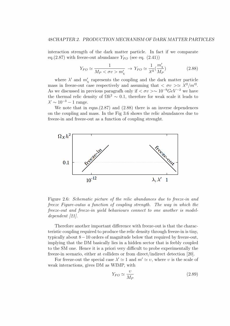
48CHAPTER 2. PRODUCTIONMECHANISMOF DARKMATTER PARTICLES
interaction strength of the dark matter particle. In fact if we comparateeq.(2.87) with freeze-out abundance YFO (see eq. (2.41))
YFO 1
MP < σv > mχ
→ YFO 1
λ2 (m
χ
MP) (2.88)
where λ and mχ rapresents the coupling and the dark matter particle
mass in freeze-out case respectively and assuming that < σv > λ2/m2.As we discussed in previous paragrafh only if < σv >∼ 10−9GeV −2 we havethe thermal relic density of Ωh2 ∼ 0.1, therefore for weak scale it leads toλ ∼ 10−3 − 1 range.
We note that in eqns.(2.87) and (2.88) there is an inverse dependenceson the coupling and mass. In the Fig 3.6 shows the relic abundances due tofreeze-in and freeze-out as a function of coupling strenght.
Figure 2.6: Schematic picture of the relic abundances due to freeze-in andfreeze Figure-outas a function of coupling strength. The way in which thefreeze-out and freeze-in yield behaviours connect to one another is model-dependent [21].
Therefore another important difference with freeze-out is that the charac-teristic coupling required to produce the relic density through freeze-in is tiny,typically about 8−10 orders of magnitude below that required by freeze-out,implying that the DM basically lies in a hidden sector that is feebly coupledto the SM one. Hence it is a priori very difficult to probe experimentally thefreeze-in scenario, either at colliders or from direct/indirect detection [20].
For freeze-out the special case λ 1 and m υ, where υ is the scale ofweak interactions, gives DM as WIMP, with
YFO υ
MP(2.89)

2.2. FREEZE-IN MECHANISM 49
In practice the cross section may involve more than one mass scale in theTeV domain, so that there are orders of magnitude spread in the abundanceexpected from WIMP dark matter. The prediction of a TeV mass particlewith coupling strenght of order unity offers the hope of collider verificationof the production mechanism.
For the freeze-in, if the particle masses are again at the weak scale, it isshowed the same dependence of the relic abundance if λ is linear in the weakscale, λ = υ/MP
YFI υ
MP(2.90)
As in the WIMP case, this parametric behaviour is significantly modifiedby numerical factors; nevertheless, it suggests seeking theories where smallcouplings arise at linear order in the weak scale.
Whether produced by freeze-out or freeze-in, stable DM is the lightest par-ticle transforming non-trivially under some unbroken symmetry. For conven-tional freeze-out, this lightest particle is automatically the WIMP, whereasfor freeze-in two particles are of interest: the FIMP and the lightest particlein the thermal bath that carries the symmetry, the LOSP. If the LOSP islighter, then LOSP DM is produced by FIMP decay. If FIMPs are lighter,then collider signals involve the production of LOSPs followed by decays toFIMPs. In either case, the freeze-in mechanism always introduces particlesof very long lifetime.
In conclusion thermal relic abundances conventionally arise by decouplingof a species that was previously in thermal equilibrium, whether with orwithout a chemical potential. Freeze-in provides the nly possible alternativethermal production mechanism that is dominated by IR processes.
Now we examine in detail the calculation of the DM abundance in threecases to freeze-in process: decay or invese decays of bath particles to theFIMP and 2 → 2 scattering [21].
We now turn to the calculation of the frozen-in dark matter density. Thefreeze-in process is dominated by decays or inverse decays of bath particlesto the FIMP depending on whether or not the FIMP is the lightest particlecarrying the conserved quantum number that stabilises the DM.
First case: decay of thermal bath particle
Now we consider a coupling λ between FIMPs dark matter particles, X,and two thermal bath, B1 and B2 expressed as λXB1B2. At very hightemperature T there is a set of bath particles that are in thermal equilibriumand some other long-lived particle X, having interactions with the bath thatare so feeble that X is thermally decoupled from the plasma. We make

50CHAPTER 2. PRODUCTIONMECHANISMOF DARKMATTER PARTICLES
assumption that the earlier history of the universe makes the abundance ofX negligibly small. If mB1 > mB2 + X the dominat freeze-in process is viadecays of heavier bath particle
B1 → B2 +X (2.91)
but X are never abundant enough to annihilate with each other. DuringT >> mB1 era, the X density is
Y1→2(T ) ∝MPmB1ΓB1
T 3(2.92)
We can be more precise by solving the Boltzmann equation for nX , thenumber density of X particles is this case
nX + 3HnX =
dΠXdΠB1dΠB2(2π)
4δ4(pX + pB1 − pB2)
×[|M |2B1→B2+XfB1(1± fB2)(1± fX)− |M |2B2+X→B1fB2fX(1± fB1)] (2.93)
where dΠi = d3pi/(2π)32Ei are phase space elements, fi is phase spacedensity of particle i and |M |2i are the matrix element summed over final andinitial spin of the participating particles without averanging over the initialspin degree of freedom. We assume that initial X abundance is negligibleso that fX = 0. Using definition of partial decay width7 ΓB1 of B1 → B2Xand considering that T << E alors f = 1/(e(E)/T ± 1) e−(E)/T << 1 ⇒1± fi 1. The Boltzmann equation becomes
nX + 3HnX 2gB1
ΠB1ΓB1mB1fB1 = gB1
d3pB1
(2π)3fB1ΓB1
γB1
(2.94)
The bath particles are assumed to be in thermal equilibrium and so ap-proximating f = 1/(eEB1/T ± 1) e−EB1/T and convering the integral overmomentum space into an integral over energy we have
nX + 3HnX gB1
d3pB1
(2π)3fB1ΓB1
γB1
= gB1
∞
mB1
mB1ΓB1
2π2(E2
B1−m2
B1)1/2e−EB1/TdEB1
=gB1m
2B1ΓB1
2π2TK1(mB1/T ) (2.95)
7The differential rate for the decay A → B + C into momentum elements d
3pB
and d3pC of the final state particle is dΓ(A → B + C) =
12EA
(2π)4δ4(pB + pC −
pA)|M |2 d3pB
(2π)32EB
d3pC
(2π)32EC

2.2. FREEZE-IN MECHANISM 51
where K1 is the first modified Bessel Function of the 2nd kind. Rewritingin terms of the yield, Y = n/s and using T −HT , applicable when thevariation of total plasma statistical degrees of freedom with temperaturedg/dT 0 approximately vanishes, we have
YX Tmax
Tmin
gB1m2B1ΓB1
2π2
K1(mB1/T )
sHdT (2.96)
If we substitute the expression of entropy (eq. (2.24)) and Hubble con-stant (eq. (2.37)) and use x = m/T we can rewrite above equation as
YX 45
1.66π4
gB1MPΓB1
m2B1g∗√g∗
xmax
xmin
K1x3(x)dx (2.97)
Doing the x integral with xmax = ∞ and xmin = 0 we finally arrive at theresult
Y1→2 135gB1
8π31.66g∗√g∗
MPΓB1
m2B1
(2.98)
Thus the abundance dependence by the three quantities mX , mB1 andΓB1 and has the form
ΩXh2 1.09× 1027gB1
g∗√g∗
mXΓB1
m2B1
(2.99)
This is the density of X produced by a single bath particle species. In fullFIMP models it is quite likely that a number of bath particles could have
similar interactions with the FIMP particle. Assuming ΓB1 =λ2mB1
8π to havethe observational value of abundance Ωobs
X h2 = 0.106 occurs for a coupling ofsize
λ 1.5× 10⁻¹²(mB1
mX)1/2(
g∗(T mB1)
102)3/4 (2.100)
if the FIMP couples with comparable strength to many (gbath) bath parti-cles of comparable mass, this value is reduced to λ 1.5×10⁻¹³(102/gbath)1/2.
Second case: Inverse decay
The alternative possibility is that the particle that freezes-in is unstableand decays to dark matter. Here we study the simplest possibility that theinteraction responsible for freeze-in also yields the decay. If FIMP X has acoupling to two bath particles, λXB1B2, then, for mX > mB1 + mB2 , thedominant freeze-in process is via inverse decays of X:
B1B2 → X (2.101)

52CHAPTER 2. PRODUCTIONMECHANISMOF DARKMATTER PARTICLES
At T >> mX , the X density is
Y2→1(T ) ∝MPmXΓX
T 3(2.102)
Assuming once again that the initial abundance of X particles is zero andtherefore setting fX = 0 the Boltzmann equation for this process can bewritten as
nX + 3HnX
dΠXdΠB1dΠB2(2π)4δ4(pX − pB1 − pB2)|M |2B1+B2→XfB1fB2
(2.103)Assuming CP invariance we may set |M |2B1+B2→X = |M |2X→B1+B2
andby invoking the principle of detailed balance we can rewrite the Boltzmannequation as
nX + 3HnX
dΠXdΠB1dΠB2(2π)4δ4(pX − pB1 − pB2)|M |2X→B1+B2
f eqX
(2.104)where f eq
X is the X equilibrium phase space distribution approximatedagain by f eq
X e−EX/T . If we perfom the same calculations of the first caseit yields
Y2→1 135gB1
8π31.66g∗√g∗
MPΓX
m2X
(2.105)
We assume that B1 bath particle is DM and its abundance is given fromdecay of X, so
ΩB1h2 1.09× 1027
g∗√g∗
mB1ΓX
m2X
(2.106)
Taking ΓX = λ2mX/8π, the required dark matter density occurs for acoupling of size
λ 1.5× 10⁻¹²(mX
mB1
)1/2(g∗(T mX)
102)3/4 (2.107)
Although eq. (2.106) is very similar in form to eq. (2.99), as was to beexpected, the physics is quite different.
Third case: Freeze-in by 2 → 2 scattering
At last we present the calculation of the FIMP relic abundance in the casewhere the FIMP, X, is a scalar and interacts with three scalar bath particlesB1, B2 and B3 via the operator
L = λXB1B2B3 (2.108)

2.2. FREEZE-IN MECHANISM 53
Considering this interaction we can calculate the resultinf FIMP yieldusing the Boltzmann equation
nX+3HnX 3
dΠXdΠB1dΠB2dΠB3(2π)
4δ4(pB1+pB2−pX−pB3)|M |2B1+B2→B3XfB1fB2
(2.109)where the factor of 3 accounts for the fact that we can have B1B2 → B3X,
B1B3 → B2X and B2B3 → B1X contributing to the FIMP yield all with thesame rate. We assume that the masses of B1, B2 and B3 are negligible com-pared to the FIMP particle mass. We can rewrite the Boltzmann equationas a one dimensional integral: we consider the unpolarized annihilation rateper unit volume WB1B2 corresponding to the covarinat normalization of 2Ecolliding particles per unit volume, averaging over initial B1 and B2 statesand summing over final B3 and X states, the contribute to it of a general2-body final state is
W 2−bodyB1B2
=1
gB1gB2SB3X
internal d.o.f.
|M |2(2π)4δ4(pB1+pB2−pB3−pX)
d3pB3
(2π)32EB3
d3pX(2π)32EX
(2.110)
nX + 3HnX 3
dΠB1dΠB2gB1gB2WB1+B2→B3XfB1fB2 (2.111)
We have still used this formula in section (2.1.1.), hence we found that
nX + 3HnX 3T
32π4
∞
m2X
gB1gB2WB1+B2→B3XpB1B2K1(
√s
T) (2.112)
where s is the center of mass energy of the interaction at a temperature
T and pij =[s−(mi+mj)2]1/2[s−(mi−mj)2]1/2
2√s . If we write
W 2−bodyB1B2
=pB3X
16π2gB1gB2SB3X√s
internal d.o.f.
|M |2dΩ (2.113)
the Boltzmann equation for our case of 2 → 2 process becomes
nX+3HnX 3T
512π6
∞
m2X
dsdΩ|M |2B1+B2→B3XpB1B2pB3XK1(
√s
T)1√s
(2.114)
we negliglete the bath mass respect to mX , consider |M |2 = λ2 andintegrate in angle solid Ω
nX + 3HnX 3Tλ2
512π5
∞
m2X
ds(s−m2X)K1(
√s
T)1√s
(2.115)

54CHAPTER 2. PRODUCTIONMECHANISMOF DARKMATTER PARTICLES
Doing this s integral, we have for Y expression
dYX
dT −3λ2T 2mX
SH
K1(mX/T )
128π5=
3λ2K1(mX/T )
1.66T 3g∗√g∗
45MPmX
256π7(2.116)
Changing variables from T to x and again doing the integral x under theapproximation that xmax = ∞ and xmin = 0 we finally arrive at the result
YX 135λ2MP
256π7g∗√g∗(1.66)mX
∞
0
xK1(x)dx =135λ2MP
512π6g∗√g∗(1.66)mX
(2.117)The relic density of X FIMP is then given by
ΩXh2 2mXYX
3.6× 10−9GeV=
1.01× 1024
g∗√g∗
λ2 (2.118)
To generate the required relic abundance we need
λ 10−11(g∗(mX)
102)3/4 (2.119)
larger than the corrsponding value for the three body interactions.These formulas are importants in the next chapter when we talk about
the Scalar Singlet Model and the interactions that generate DM particles.

Chapter 3
Higgs Portal
We have just described thermal kind of mechanism of production for DMparticles. We have just maken an hypothesis about the nature of dark matterwith Singlet Scalar Model, where DM is a scalar singlet of SM gauge and oddof new symmetry Z2 that maintains stable and it is contained in a hiddensector. With hidden sector it is defined a sector that is not coupled bymediator boson of SM to visible sector. Now we need to portal that we allowto know which are interactions between visible sector and hidden sector toform DM particles and through it derive relic density compatible with thatobserved.
Figure 3.1: The Higgs portal.
The first possibility for mixing between states at the renormalizable levelis kinetic mixing among the gauge bosons of U(1)Y and a U(1)hid, an extraU(1) gauge field, and it can be probed by direct experiment. So this can be aimportant probe to show any scenario where DM is created by hidden sectorrather by SM visible sector. The second possibility is Higgs portal thatenables us to realize coupling between two sectors by Higgs fields: a DMhidden sector could be generated from the SM sector through this portal. Todefine coupling is important because the relic density depend solely on theDM particle mass, on the portal and on the DM hidden sector interaction.
In thi chapter we describe the importance of Higgs-portal that permitsus to generate the interactions that produce dark matter. We analize the
55

56 CHAPTER 3. HIGGS PORTAL
special case of Scalar Singlet Model (section 4.1.1). We will study the freeze-out scenario and we will find viable space parameters to have relic abundance(section 4.1.2.) and in freeze-in scenario too (section 4.1.3). Successively weadopt a model independent approach and study generic scenarios for thecosmological relic density and direct detection rate in the context of theHiggs-portal DM scalar, vector or Majorana fermion. We first discuss theavailable constraints on the thermal DM from WMAP and current directdetection experiments, and show that the fermionic DM case is excludedwhile in the scalar and vector cases, one needs DM particles that are heavierthan about 60GeV . We then derive the direct DM detection rates to beprobed by the Xe100, upgrade and Xe1T experiments.
3.1 Higgs Portal in The Scalar Singlet Model
3.1.1 The Model
The singlet scalar model is a simple extension of Standard Model that allowto verify the existence of dark matter. This framework identifies DM witha real singlet scalar S which does not trasform under the Standard Modelgauge group and odd under a new unbroken Z2 (S → −S) symmetry thatguarantees its stability. Requiring that interactions be renormalizable impliesthat S can interact with the SM fields only through its coupling to the Higgs-doublet filed H. It follows that the general form of the scalar lagrangian is
L = LSM +1
2∂µS∂
µS − m20
2S2 − λSS
4 − λS2H†H (3.1)
where 12∂µS∂
µS is kinetic part and LSM is SM Lagrangian (it containsleptons and quaks kinetic energy and their interactions with gauge boson +kinetic terms and self-interactions of gauge bosons). H is a higgs doublet.Within this framework the properties of the field S are described by threeparameters. Two of these are internal to the S sector, λS and m0, char-acterizing the S mass and the strenght of its self-interaction. The later isunconstrained and largely irrelevant to the phenomenology of the model, sowe set λS ≤ 1 to guarantee a perturbative treatment. The third parameter λcontrolles the coupling between the singlet and all SM fileds that we noticeto be (eq. (3.1)) only through the higgs boson.
The constraints that the potential must satisfy to guarantee the couplingbetween higgs boson and singlet and stability of this later require that thevacuum produced acceptable symmetry-breaking pattern [22].

3.1. HIGGS PORTAL IN THE SCALAR SINGLET MODEL 57
Figure 3.2: The coupling between singlet scalar S and higgs boson h in singletscalar model. The interaction is controlled by λ coupling.
H ≡ (H†, h+υ√2) is a dobluet Higgs and in the unitary gauge,
√2H† = (h, 0)
with h is the real boson, the scalar potential takes the form:
V =m2
0
2S2 +
λ
2S2h2 +
λS
4S4 +
λh
4(h2 − υ2
EW )2 (3.2)
where λh is the higgs quartic coupling and υEW = 246GeV are valueexpectation vacuum, they are the usual parameters of the Standard ModelHiggs potential.
The existence of a vacuum is due by below constraints of potential thatprovides that the quartic couplings satisfy the following three conditions:
λS, λh ≥ 0 and (3.3)
λSλh ≥ λ2 for negativeλ (3.4)
Althrough the potential produces a desiderable symmetry breaking pat-tern we must study the minima of this. The first local minimum providesthe configuration < h > = 0 for spontaneously break the electroweak gaugegroup and < S >= 0 for not break the symmetry S → −S. The first requestis obvious in order to have acceptable particle masses, while the second isnecessary in order to ensure the longevity of S in a natural way (S particlesmust survive the age of the universe in order to play their proposed presentrole as dark matter).
This configuration is valid if and only if
υ2EW > 0 (3.5)
m20 + λυ2
EW > 0 (3.6)

58 CHAPTER 3. HIGGS PORTAL
The second local minimum, with h = 0 and S2 = −m20
λ can also co-existwith the desired minimum if λ > 0 and λ2 < λhλS. This minimum is presentso long as m2
0 < 0 and −λm20 > λSλhυ2
EW .In such case, to ensure that the former is the potential’s global minimum
we must require that0 < −m2
0 < υ2EW
λhλS (3.7)
Throughout the rest of this paper, the above conditions are assumed tohold, so that the model is in a phase having potentially acceptable phe-nomenology. It is therefore convenient to shift h by its vacuum value, h →h+ υEW , so that h represents the physical Higgs having mass m2
h = λhυ2EW .
The S-dependent part of the scalar potential then takes its final form
V = (m2
0 + λυ2EW
2)S2 +
λ
2S2h2 +
λS
4S4 + λυEWS2h (3.8)
and the S mass is seen to be
mS =m2
0 + λυ2EW (3.9)
In the following we takes mS and λ as the free parameters of singletscalar model. In addition, the higgs mass mh, a SM parameter, also affectsthe phenomenology of the model, the choice of its value is very important.
The only renormalizable interaction of such scalars with the SM occursvia the Higgs sector which thus serves as a portal to the hidden sector.
Figure 3.3: The Feynman graph relevant to S-particle annihilation via Higgsexchange. Various annihilation channels are open or forbidden, dependingon the value of 2mS .
In the early Universe, singlets are pair-produced as the particles in thethermal plasma scatter off each other. The dominant production processes

3.1. HIGGS PORTAL IN THE SCALAR SINGLET MODEL 59
are s-channel higgs boson mediated diagrams originating in a variety of initialstates: ff , W+W−, Z0Z0 , and hh . Likewise, they can be produced fromthe initial state hh either directly or through singlet exchange and also thescalar scatters elastically off nuclei through a t-channel Higgs
Therefore there are two processes which can produce a density of Sscalars: 2 → 2 annihilation processes and decay of a thermal equilibriumdensity of Higgs scalars to SS†. The cross section of this processes whichcreate the Si from the SM sector are estimated by using the centre-of-massannihilation cross section calculated for S scalars with typical energy ET T .
i
Γ(h → S2i ) =
i
λ2v2
8πEh
1−4m2
Si
m2h
(3.10)
i
σ(W+W− → S2i ) =
i
λ2
72π
s−m2
Si
s−m2W
s2 − 4m2W s+ 12m4
W
s(s−m2h)
2(3.11)
i
σ(ZZ → S2i ) =
i
λ2
72π
s−m2
Si
s−m2Z
s2 − 4m2Zs+ 12m4
Z
s(s−m2h)
2(3.12)
i
σ(ff → S2i ) =
i
λ2
16π
m2f
(s− 4mSi)(s− 4m2
f )
s(s−m2h)
2(3.13)
i
σ(hh → S2i ) =
i
λ2
8π
1
s
s−m2
Si
s−m2h
(1 +3m2
h
s−m2h
)2 (3.14)
where i = 1, .., n denotes the number of degree of freedom of scalr field.The main differences between the kinetic mixing and Higgs portal cases comefrom the fact that in the later case the mediator is quite massive, mh 125GeV . The consequences are two: (a) DM can be also created by thedecay of the mediator and (b) the various production channels are suppressedat small temperatures, either Boltzamann suppressed if the Higgs boson isreal in the process, or by the mass of the Higgs boson at the fourth powe ifthe Higgs boson is virtual.
For mS > mh/2 the DM is exclusively produced by scattering processesand for mS < mh/2 on top of the energy transferred through the variousscatterin processes there is also a contribution from the Higgs boson decay,which turns out to dominate.
Using the annihilation cross section expressed in the above formulas, onecan numerically calculate the thermally averaged annihilation cross section< σannv > and integrating the Boltzmann equation, one can numerically have

60 CHAPTER 3. HIGGS PORTAL
the actually abundance Y0. Then we obtain the DM relic density ΩSh2 ∝Y0mS/GeV and knowing its value by observations one can calculate the DM-Higgs coupling λ for the given mS and mh. This meaning analyze the viablespace parameter. For two scenario, freeze-out and freeze-in, we will find thisregions [23].
The main advantage of the singlet model with respect to other models ofdark matter is its simplicity and its predictivity, which allows one to makeconcrete hypotesis about dark matter observables. In fact, by imposing therelic density constraint, ΩS = ΩDM , that is identifity the dark matter particlelike a scalar particle S, one can eliminate λ and compute the expected ratesfor direct and indirect detection experiments as a function of the singlet massmS for a few rapresentative values of Higgs boson mh, the only standardmodel field that couples to it via quartic coupling λS†SH†H [19].
3.1.2 Higgs portal in freeze-out scenario
We sharpen the cosmological constraints on the model by demanding thepresent abundance of S particles to be close to today’s preferred value ofΩSh2. This imposes a strong relationship between the parameters λ and mS,which we now derive [22].
Assuming that interactions are strong enough, in the early Universe allparticle species will be in thermal equilibrium when T > mS. Hidden sectorwill stay in equilibrium through the Higgs portal. This is ensured so longas the coupling λ is not too small. Just how small λ must be is determinedby the following argument. As the universe cools down and dilutes hiddenparticles will not be able to find each other and energy transfer betweenthe sector becomes negligible. This is the freeze-out. After the freeze outhidden sector cools separately and since the particle is stable, dilutes by thechange of the volume of the universe. Being that the thermalization rateand the expansion rate vary differently with time, since they differ in theirtemperature dependence, Γ = λ2T for T >> mh and Γ = λ2T 5m−4
h forT << mh and H = T 2/MP , these temperature dependences imply that theratio R = Γ/H is maximized in electroweak epoch instead when T ∼ mh ∼mW , taking the maximum value R ∼ λ2MP/mh. S particles are thereforeguaranteed to remain thermalized down to this epoch if this maximum ratiois required to be of order one or larger, implying
λ
mW
MP∼ 10−8 (3.15)
Once thermalization is reached the S abundance is determined by the Sparticle mass mS and its annihilation cross section σv. This cross section

3.1. HIGGS PORTAL IN THE SCALAR SINGLET MODEL 61
depends very strongly on the Higgs mass mh, and on which annihilationchannels are kinematically open.
In the early Universe, dominant interaction that keeps two sectors atthe same temperature would be by the s-channel annihilation of two hiddenscalars into a virtual Higgs and through that into Standard Model pairs.Freeze-out temperatures are typically an order of magnitude smaller thanthe mass of the decoupled particle, Tf 0.05mS. In our case mass of thehidden scalar is around the electroweak scale, so it is safe to assume thatduring the freeze-out Higgs is a massive single degree of freedom scalar andboth particles are non-relativistic. Non-relativistic cross section of two scalarsinto Standard Model particles through an intermediary Higgs (Fig. 3.3) isgiven by:
σv =8λ2υ2
EW
(4m2S −m2
h)2 +m2
hΓ2h
Fx where Fx := limmh→2mS
(Γh
mh
) (3.16)
where Γh is the total Higgs decay rate and Γh is the decay rate for avirtual Higgs whose mass is mh = 2mS.
Of particular interest are the large- and small-mS limits. In small-mS
limit the particles annihilate mainly into the bb final state, with subdominantcontributions from other light fermions. The eq. (3.16) for mS << mW ,mh
implies the asymptotic behaviour
σv ∝ λ2m2S
m4h
(3.17)
For large mS the dominant contributions to the annihilation cross sectioncome fromW+W−, Z0Z0 and hh final states. We find the large-mS behaviourof the annihilation cross section to be
σv λ2
4πm2S
(3.18)
Fig. (3.4) displays the annihilation branching fractions as a function ofthe singlet mass for mh = 125GeV . The sharp contrast between the lightsinglet region and the heavy one is clearly observed.
These asymptotic forms are useful in what follows for understanding whatthe cosmological abundance constraint implies for the coupling λ in the limitwhere mS is very large or very small. In fact these expressions may be used,with standard results for the Standard Model Higgs decay widths, to predicthow the primordial S-particle abundance depends on the parameters mS andλ because in relic abundance, that we know by eq. (2.42)
ΩSh2 =
1.07× 10⁹
GeV
xf√g∗MP < σv >
(3.19)

62 CHAPTER 3. HIGGS PORTAL
Figure 3.4: Annichilation branching fractions as a function of the dark mattermass for the singlet model. The Higgs mass was set to 125GeV while thevalue of λ was obtained by imposing the dark matter constraint [24].
appears the cross section, (xf ≡ xf (mS, < σv >)). Knowing the valueΩSh2, required by observation, we have that for light singlet a large value ofλ( 0.1), and are consequently constrained by direct detection experiments,while for heavy singlet the required value of λ is typically smaller (∼ 0.01)and present direct detection constrains are ineffective.
Being a scalar field, the singlet annihilation rate today is not suppressedwith respect to that of the early Universe (s-wave annihilation). Moreover,throughout most of the viable parameter space < σv > is constant and equalto the weak typical annihilation rate, < σv >∼ 2.3× 10⁻²⁶cm3s−1. The onlytwo place where < σv > is smaller are at the W threshold and at the higgsresonance mh ∼ 2mS (section 2.1.1.). In fact the main effect of the higgsmass is to determine the position where this resonance lies. In our analysiswe set mh to 125GeV and considering only the remaining dependence on thesinglet mass that is taken below 600GeV .
For any given pair (mh,mS), there exits a unique value λ such that thedark matter constraint, ΩSh2 = 0.11, is fulfilled. Imposing the dark matterconstraint, the variable λ can be effectively eliminated for given values ofmh and mS, reducing the viable parameter space to two dimensional volume.In Fig. (3.5) plots the relationship between λ and mS which is predicted inthis way by the requirement that ΩSh2 ∼ 0.11. For most values of mS this

3.1. HIGGS PORTAL IN THE SCALAR SINGLET MODEL 63
Figure 3.5: The viable parameter space of the scalar singlet model.Along the lines the dark matter constrained is satisfied. We use mh =120, 150, 180, 200GeV as reference values for the higgs mass. The grey areasurrounding the line corresponding to mh = 120GeV shows the region com-patible with the observed dark matter density at 2σ [25].
curve is well described by the above simple formulae, which give sufficientaccuracy in most parts of the parameter space defined by varying mS, λ andmh. Important exceptions to this statement apply in kinematically specialregions, such as the Higgs threshold (2mS mh) and two-particle thresholdsin the final states (2mS 2mb or 2mS 2mW , and so on), where a moresophisticated treatment is required. Away from the higgs resonance, thetypical value of λ is O(10−1 − 10−2).
For mS sufficiently large or small, the asymptotic expressions (3.17) and(3.18) show that the abundance constraint forces λ to become large, eventu-ally becoming too large to believe perturbative expressions like eq. (3.16).In particular, if annihilation should occur before the electroweak transition,then the asymptotic relation between λ and mS becomes:
λ ∼ mS
10TeV(3.20)
so demanding the perturbative regime (λ 1) gives the upper boundmS 10TeV .
Now we set the Fig. (3.6) which show us the relic density as a functionof scalar mass mS for λ = 0.1 and different values of the higgs mass. Notice

64 CHAPTER 3. HIGGS PORTAL
that the scalar singlet model can explain tha dark matter naturally, thatis without any fine-tuning in the parameters. Indeed, for λ = 0.1 and mS
around the electroweak scale, the predicted relic density lies in the correctrange to be compatible with the observations. The most noticeable featurefrom this figure is the drastic suppression of the relic density that takes placeat the higgs resonance. In fact, around 2mS ∼ mh the relic density is ordersof magnitude smaller than anywhere else. The effect of the W± threshold isalso seen to be important. Above it, mS > mW , the W+W− annihilationchannel is open and consequently the relic density tends to be smaller thanbelow it.
Figure 3.6: The dark matter density as a function of mS for λ = 0.1 anddifferent values of the higgs mass [25].
There are several important points concerning the abundance conditionwhich bear emphasis:
• For all mS < few TeV (and away from poles and particle thresholds)the abundance constraint requires λ ∼ O(0.1 − 1). In this sense thismodel of dark matter is natural, in that obtaining the right primordialabundance does not require any fine tuning or special choice of theparameters.
• The coupling has to be significantly suppressed near the Higgs pole.This is because the Higgs resonance is rather narrow, and this narrow-

3.1. HIGGS PORTAL IN THE SCALAR SINGLET MODEL 65
ness considerably enhances the S annihilation rate, especially if 2mS isslightly smaller than mh.
• Different decay channels dominate the total annihilation cross sectionfor different ranges of mS. However, the range of values of most ex-perimental interest lies between the b and W thresholds, for which itis the bb final state that is most important.
• Since the abundance constraint is concerned with the strength of theinteractions between S scalars and ordinary matter, it is largely in-dependent of the strength of the S self-coupling, S. This leaves λS
completely free to be adjusted. Unfortunately, although the S parti-cles therefore can be very strongly interacting, this in itself does notmake them useful to solve the recently-perceived problems with galaxyformation. This is because the solution of these problems requires in-teraction cross sections which are of order 10−24 cm2, and cross sectionsthis large require mS 1GeV in addition to large λS. Unfortunatelymasses this small require fine tuning in this model, due to the relationm2
S = m20 + λυ2
EW . Since, as we saw earlier, the abundance constraintrequires λ to be of order one or larger for small mS , we require a part-per-million cancellation between λυ2 and m2
0 in order to obtain smallvalues for m2
S.
3.1.3 Higgs portal in freeze-in scenario
The interactions of the dark matter particle are determined by free parameterλ, in range 10−3 < λ < 1 lies WIMP model, but for much smaller couplingswe are in the FIMP regime.
Let us now analyze [19] how the relic density changes as we go fromλ = λWIMP to λ = λFIMP , and so we found an alternative solution to thedark matter constraint in the singlet model that we considere now.
We will compute the evolution of the dark matter abundance and thepredicted relic density as a function of the parameters of the singlet model:λ, mS and mh and we will find the new viable region corresponding to theFIMP solution to the dark matter constraint.
The evolution of the dark matter abundance as a function of the tem-perature is shown in Fig 3.7 for different singlet masses between 1GeV and1TeV . In it, λ and mh were fixed respectively to 10−11 and 120GeV .
The general behavior of Y is clear: it increases as the Universe coolsdown until a certain point where it freezes-in, remaining constant afterwards.As illustrated, the freeze-in point depends on the dark matter mass. It is

66 CHAPTER 3. HIGGS PORTAL
Figure 3.7: The dark matter abundance, Y , as a function of the temperaturefor different values of mS. In this figure mh was set to 120 GeV and λ to10−11 [19].
also clear that the rate at which Y increases depends on both mS and thetemperature T . At high temperature the singlet behaves as a relativisticparticle so Y is pretty much independent of mS , as observed in the figure forT > 1TeV . For mS = 100GeV and mS = 1TeV the dark matter abundancefreezes-in at T mS, for mS = 10GeV and mS = 1GeV the effect of thehiggs resonance (mS ∼ mh/2), which increases < σv > significantly, becomesimportant. So the main effect of the higgs mass is to determine the positionwhere this resonance lies.
The reason for which the abundance does not keep increasing until T mS for mS = 1GeV is that, as stated before, the production of singlet darkmatter is dominated by the W+W− final state, which ceases to be abundantin the thermal plasma well before T 1GeV . For the same reason, theabundances are exactly the same for mS = 1GeV and mS = 10GeV .
Let us now see how these results are modified when we vary λ and mh.The Fig 3.8 shows the dark matter abundance as a function of the tempera-ture for four different values of mS (1, 10, 100, 1000GeV , one in each panel)and three values of λ: 10−10 (upper, dashed-dotted line), 10−11 (middle, solidline) and 10−12 (lower, dashed line), while mh is fixed to 120GeV value.
The new feature observed in this figure is that the dark matter abundanceis, as expected, exactly proportional to λ2. This is a distinctive feature of the
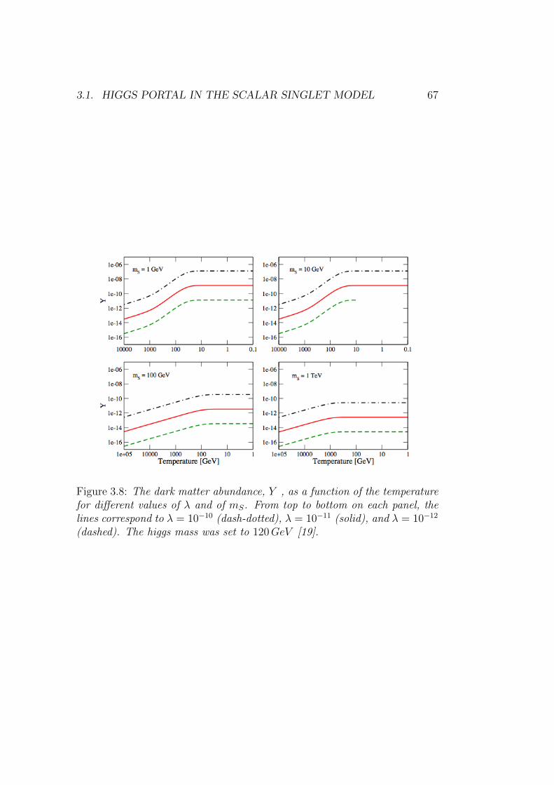
3.1. HIGGS PORTAL IN THE SCALAR SINGLET MODEL 67
Figure 3.8: The dark matter abundance, Y , as a function of the temperaturefor different values of λ and of mS. From top to bottom on each panel, thelines correspond to λ = 10−10 (dash-dotted), λ = 10−11 (solid), and λ = 10−12
(dashed). The higgs mass was set to 120GeV [19].

68 CHAPTER 3. HIGGS PORTAL
FIMP regime: the dark matter yield increases with the interaction strengthbetween the dark matter particle and the thermal plasma.
Figure 3.9: The dark matter abundance, Y , as a function of the temperaturefor different values of mh and of mS. From top to bottom in each panel, thelines correspond to mh = 120GeV (dash-dotted), mh = 150GeV (solid), andmh = 180GeV (dashed). In this figure λ was chosen to be 10−11 [19].
The dependence of the dark matter abundance with the higgs mass isillustrated in Fig 3.9. It displays Y as a function of the temperature for fourdifferent values of mS (1, 10, 100, 1000GeV , one in each panel) and threevalues of the higgs mass: 120GeV (upper, dashed-dotted line), 150GeV(middle, solid line) and 180GeV (lower, dashed line), while the coupling λis fixed to 10−11 value.
We see that for heavy singlets, which freeze-in at T >> mh, the abun-dance does not depend on the higgs mass at all. For lighter particles,mS = 1, 10GeV , the effect of different higgs masses become manifest atlow temperatures T ≤ 100GeV . The smaller the higgs mass, the larger thefreeze-in temperature and the final dark matter abundance, as observed inthe figure. In any case, since the higgs mass cannot vary over a wide range,the corresponding dark matter abundance does not change much either withmh. Its total effect amounts to a variation of less than one order of magnitudein Y .

3.1. HIGGS PORTAL IN THE SCALAR SINGLET MODEL 69
In the FIMP regime, as the previous figures illustrate, the dark matterparticles are slowly produced as the Universe cools down until the freeze intemperature is reached. In the singlet model, the freeze in temperature isgiven by the singlet mass for mS ≥ 100GeV and by T ∼ 30 − 50GeV forlighter singlets. Close to the higgs resonance the production accelerates butthe abundance remains small (Y << 1) throughout the entire history of theUniverse. In the FIMP regime, the dark matter particles never reach thermalequilibrium or annihilate among themselves.
Now we turn our attention to the relic density, the quantity that is actu-ally constrained by observational data. Ωh2|t0 ∝ mS and to the asymptoticvalue of Y (t0), see eq. (2.87) and, as we will show, it manifests the drasticsuppression of the relic density that takes place at the higgs resonance. Fig3.10 displays the predicted relic density as a function of the singlet mass formh = 120GeV and different values of the coupling λ. From top to bottomthe lines correspond to λ = 3 × 10⁻¹¹ (dashed line), λ = 10−11 (solid line),and λ = 3× 10⁻¹² (dashed-dotted line) and orizontal band represents the re-gion compatible with the WMAP determination of the dark matter density.
Figure 3.10: The relic density of dark matter, Ωh2, as a function of mS fordifferent values of λ. The higgs mass, mh, was fixed to 120GeV in this figure.The WMAP compatible region is also shown as a horizontal band [19].
As view on figure the relic density is proportional to λ2 and for λ =3×10⁻¹¹ (the dashed line) the relic density is, independently of mS, too high

70 CHAPTER 3. HIGGS PORTAL
to be compatible with the WMAP range. The other two values of λ, 10−11
and 10−12, are consistent with the data.It is clearly observed in the figure that the relic density has a sizable jump
at the higgs resonance, mS 60GeV , or more generally at mS mh/2. IfmS is slightly below the resonance the relic density is significantly larger thanif it is slightly above the resonance and there is a contribution given by Higgsdecay that dominate. Moreover, while above the resonance the relic densityis essentially independent of the singlet mass, it becomes proportional to mS
below the higgs resonance and DM is produced by scattering processes inpair. That is exactly the region where we have found the abundance, Y , tobe independent of mS.
Figure 3.11: The relic density of dark matter, Ωh2, as a function of mS fordifferent values of mh. In this figure the coupling λ was set to 10−11. TheWMAP compatible region is also shown as a horizontal band [19].
The variation of the relic density with the singlet mass and fixed couplingis shown in Fig 3.11. We can see that the region where the behavior of therelic density changes is indeed determined by the higgs resonance condition:mS mh/2. For high masses, mS > mh, the relic density is independent ofmh, for lower masses, mS < mh/2, the relic density turns out to be abouta factor 3 larger for mh = 120GeV than for mh = 180GeV . Hence, inthat region, the value of the mass that is compatible with the relic densitymight change by the same factor as mh varies. Usually we are interestedin obtaining the viable parameter space of the model, the regions where thepredicted relic density is consistent with the observed dark matter density.

3.1. HIGGS PORTAL IN THE SCALAR SINGLET MODEL 71
Figure 3.12: The viable parameter space of the singlet model in the FIMPregime. Inside the bands the dark matter constraint is satisfied for the givenvalue of the higgs mass [19].
Fig 3.12 shows, in the plane (mS,λ), the viable region of the singlet modelfor the FIMP. Each band shows the region compatible with the dark matterconstraint (at 2σ) for a given higgs mass. Notice that for heavy dark matter,mS > 100GeV , λ should be about 1.2 × 10¹¹ independently of the singletmass or the higgs mass. For 0.1GeV ≤ mS ≤ 50GeV the coupling requireddecreases from about 1.2× 10¹¹ to about 1012, reaching this minimum valuefor mS ∼ 40GeV and mh = 120GeV . Around the higgs resonance, the valueof λ that satisfies the dark matter constraint varies by about one order ofmagnitude in a narrow range of mS.
Notice if mS ≤ 100GeV for any given value of λ there usually exists twosolutions for mS.
This last figure clearly demonstrates our main result, that in the singletmodel the dark matter constraint can also be satisfied in a previously un-explored region of the parameter space. In this new viable region we haveunveiled, the interactions between the singlet and the Standard Model fieldsare very suppressed and the singlet behaves as a Feebly Interacting Mas-sive Particle (FIMP) rather than as a WIMP. We would like to emphasizethat this FIMP regime of the singlet model is as natural and predictive asthe WIMP regime. There is no need to include new particles, to introducenon-thermal production mechanisms, or to modify the cosmological modelin order to satisfy the dark matter constraint. From the dark matter pointof view, therefore, both regimes should be treated on equal footing.

72 CHAPTER 3. HIGGS PORTAL
A generic property of the new viable region we have found is the absence ofany direct or indirect detection signature of dark matter, a direct consequenceof the feeble interactions of the dark matter particles. This could become aadvantage if in the next years dark matter is not detected: such an eventwould force us to abandon the WIMP paradigm and to replace it with FIMPdark matter, which looks particularly attractive due to its simplicity andpredictivity.
Recently, it was found that the latest constraints on dark matter directdetection by the XENON100 experiment exclude a significant fraction of theparameter space of the singlet model. In particular, mS < 80GeV seems tobe strongly disfavored. We would like to stress, however, that such a boundapplies only to the WIMP regime of the singlet model and that no comparablebound exists in the FIMP regime. In it, the region mS < 80GeV , as well asthe entire GeV to TeV mass range, is perfectly compatible with the couplingλ dark matter constraint and with the absence of a dark matter signal indirect and indirect dark matter experiments.
3.2 Three model indipendent
In July 2012 at LHC it shows a hint of a signal of a particle with a massaround 125 GeV, this is Boson Higgs. The most pronounced signal is observedin the γγ final state, while the results from other available search channelsare in a reasonable agreement with the Higgs boson interpretation within theStandard Model. It is plausible that data from the ingoing 8 TeV run of theLHC will firmly establish the existence of a Higgs boson. If we split Higgsboson data into three categories according to the final states and computethe average for each one of them [26]:
observed rate
SM rate=
2.0± 0.5 photons0.5± 0.3 vectors : W and Z1.3± 0.5 fermions : b and τ
This shows the main anomalous features in current measurement. γγchannels exhibit some excess and there is a deficit in the vector channels. Ifwe analyze the most important contributions h → γγ and h ↔ gg branchingratio ratio it is show
BR(h ↔ gg)
BR(h → gg)SM 0.3
BR(h → γγ)
BR(h → γγ)SM 4 (3.21)
that is a significant deviation from the SM prediction.

3.2. THREE MODEL INDIPENDENT 73
On the one hand this anomalies may be statistical fluctuations, on theother hand, they may signal new physics beyond the SM: the Higgs particlemay have other decay channels that are not predicted by the SM calledextra invisible Higgs boson decay channel. Determining or constraining non-standard Higgs boson decays will provide a vital input to model building inthe context of physics beyond the SM. We know by Higgs portal that theHiggs boson could be coupled to the particle that constitutes all or part of thedark matter in the universe. Therefore the Higgs boson is the key mediator inthe process of dark matter annihilation and scattering, providing an intimatelink between Higgs hunting in collider experiments and the direct search fordark matter particles in their elastic scattering on nucleons. In fact, thepresent LHC Higgs search results, combined with the constraints on the directdetection cross section from the XENON experiment, severely constrain theHiggs couplings to dark matter particles and have strong consequences oninvisible Higgs decay modes for scalar, fermionic or vectorial dark mattercandidates.
We consider generic Higgs-portal scenarios [27] that follows the modelindependent approach: we consider the three possibilities that dark matterconsists of real scalars S, vectors V or Majorana fermions χ which interactwith the SM fields only through the Higgs-portal. The stability of the DMparticle is ensured by a Z2 parity. The relevant terms in the Lagrangians are
∆LS = −1
2m2
SS2 − 1
4λSS
4 − 1
4λhSSH
†HS2 (3.22)
∆LV =1
2m2
V VµVµ +
1
4λV (VµV
µ)2 +1
4λhV VH
†HVµVµ (3.23)
∆Lf = −1
2mf χχ− 1
4
λhff
ΛH†Hχχ (3.24)
Although in the fermionic case above the Higgs-DM coupling is not renor-malizable, we still include it for completeness. The selfinteraction terms S4
in the scalar case and the (VµV µ)2 term in the vector case are not essential forour discussion and we will ignore them. For electroweak symmetry breakingthe physical masses of the DM particles will be given by
M2S = m2
S +1
2λhSSυ
2 (3.25)
M2V = m2
V +1
2λhV V υ
2 (3.26)
Mf = mf +1
2
λhff
Λυ2 (3.27)

74 CHAPTER 3. HIGGS PORTAL
The relic abundance of the DM particles is obtained through the schannelannihilation via the exchange of the Higgs boson. For instance, the annihi-lation cross section into light fermions of mass mferm is given by
< σSfermv >=
λ2hSSm
2ferm
16π
1
(4m2S −m2
h)2
(3.28)
< σVfermv >=
λ2hV Vm
2ferm
48π
1
(4m2V −m2
h)2
(3.29)
< σffermv >=
λ2hffm
2ferm
32π
m2f
Λ2
1
(4m2S −m2
h)2
(3.30)
The connection between λhSS and mS derived from the abundance con-straint in the previous sections are very predictive. The sensibility of darkmatter detectors to S particles is controlled by their elastic scattering crosssection with visible matter, and with nuclei in particular. The cross sec-tions enters in one of two ways: a) it is the directly relevant quantity forexperiments designed to measure the recoil signal of dark matter collisionswithin detectors; b) it controls the abundance of dark matter particles whichbecome trapped at the terrestrial or solar core, and whose presence is de-tected indirectly through the flux of energetic neutrinos which is producedby subsequent S-particle annihilation.
Now we describe the elastic cross section in direct detection experimentsto study the properties of the dark matter particles in scalar, vector andfermion cases. The DM interacts elastically with nuclei through t-channelHiggs boson exchange. The resulting nuclear recoil is then interpreted interms of the DM mass and DM-nucleon cross section. In the limit non-relativistic the spin-independent DM-nucleon interaction can be expressedas
σSIX−N =
4M2(N)
π(Zfp + (A− Z)fn)
2 (3.31)
where M(N) = mXmN/(mX +mN) and mN is the target nucleus mass.Z and A − Z are the numbers of protons and neutrons in the nucleus. fp,nis the coupling between DM and protons or neutrons.
fp,n =
q=u,d,s
f (p,n)L aq
mp,n
mq+
2
27f (p,n)H
q=c,b,t
aqmp,n
mq(3.32)
aq is the DM-quark coupling by Higgs exchange and is
aq =λHXXmq
mXm2h
(3.33)

3.2. THREE MODEL INDIPENDENT 75
If we consider this results for X = S, V, f we have for DM-nucleus elasticspin-independent cross section
σSIS−N =
λ2hSS
16πm4h
m4Nf
2N
(mS +mN)2(3.34)
σSIV−N =
λ2hV V
16πm4h
m4Nf
2N
(mV +mN)2(3.35)
σSIf−N =
λ2hff
4πΛ2m4h
m4Nm
2ff
2N
(mf +mN)2(3.36)
where mN is the nucleon mass and fN parameterizes the Higgs-nucleoncoupling. If fL is the contribution of the light quarks and fH is for heavyquarks fN =
fL+3× 2
27fH . There exist different estimations of this factorin what follows we will use the lattice result fN = 0.326.
Figure 3.13: Bounds on the spin-independent direct detection cross sectionσSIχN in Higgs portal models derived for mh = 125GeV and the invisible branc-
ing fraction of 40% (colored lines) The curve take into account the full mχ
dependence, without using the approximation in eqns. (4.40-4.42). For com-parison, we plot the current and future direct bound from XENON experiment(black lines). [27].
We displays predictions fo the spin-indipendent DM-nucleon cross sectionσSI : in Fig. (3.13) the upper band corresponds on the fermion Hggs-portalDM and is excluded by XENON100. On the other hand, scalar and vectorDM are both allowed fo a wide range of masses. Apart from a very small

76 CHAPTER 3. HIGGS PORTAL
region around mh/2, this parameter space will be probed by XENON100-upgrade and XENON1T. The typical value for the scalar σSI is a few times10−9pb, whereas σSI for vectors is larger by a factor of 3 which accounts forthe number of degree of freedom.
Figure 3.14: The spin-independent proton-singlet cross section as a functionof mS for different values of the higgs mass. The thin lines show the presentconstraint from XENON10 and CDMS. The dotted line corresponds to theexpected sensitivity of SuperCDMS. Along the lines ΩSh2 = 0.11. [25].
In particular in Fig. (3.14) we show the spin-indipenent proton-singletcross section as a function of mS for different values of the higgs mass.
We see that since the higgs-singlets coupling is small close to the higgsresonance, the cross section is higly suppressed in that region. A heavy sin-glet, mS 150GeV , has an interaction cross section around 10−9pb. Becausethe singlet interacts with nucleons via t-channel higgs exchange, the crosssection typically decreases with the Higgs mass as observed in the figure. Forreference, current constraint from XENON100 and CDMS are also displayed.They rule out singlet masses below 50GeV indipendently of the higgs mass.Finally, notice from the figure that future experiments, such as SuperCDMS,will probe a significant region of the viable parameter space.
We next turn to the implications of the model for Higgs searches at collid-ers. The partial Higgs decay width into dark matter Γ(H → χχ), calculated

3.2. THREE MODEL INDIPENDENT 77
at tree level, for DM particle light enough mS < mh/2, are
Γinvh→SS =
λ2hSSυ
2βS
64πmh(3.37)
Γinvh→V V =
λ2hV V υ
2βV
256πm4V
(1− 4m2
V
m2h
+ 12m4
V
m4h
) (3.38)
Γinvh→ff =
λ2hffυ
2βf
32πΛ2(3.39)
where βχ =
1− 4m2χ/m
2h.
The first aim of our study is to derive constraints on the various DMparticles from the WMAP satellite and from the current direct detectionexperiment XENON100 nd to make predictions for future upgrades of thelatter experiment, assuming that the Higgs boson has a mass mh = 125GeVand is approximately SM-like such that its invisible decay branching ratio
BRinvX =
Γ(H → XX)
ΓSMH + Γ(H → XX)
=σSIX−N
ΓSMH σSI
X−N/Γ(H → XX) + σSIX−N
(3.40)
is smaller than 10%, (ΓSMH is the total decay width into all particles in the
SM).In Fig. (3.15), we delineate the viable parameter space for the Higgs-
portal scalar DM particle. The area between the two solid (red) curves sat-isfies the WMAP constraint, with the dip corresponding to resonant DM an-nihilation mediated by the Higgs exchange. The dash-dotted (brown) curvearound the Higgs pole region represents BRinv = 10% such that the area tothe left of this line is excluded by our constraint BRinv < 10%. The prospectsfor the upgrade of XENON100 (with a projected sensitivity correspondingto 60, 000 kg − d, 5− 30 keV and 45% efficiency) and XENON1T are shownby the dotted lines. We find that light dark matter, mDM < 60GeV , violatesthe bound on the invisible Higgs decay branching ratio and thus is excluded.On the other hand, heavier dark matter, particularly for mDM > 80GeV ,is allowed by both BRinv and XENON100. We note that almost the entireavaible parameter space will be probed by the XENON100 upgrade. Theexception is a small resonant region around 62GeV , where the Higgs-DMcoupling is extremely small.
In the case of vector Higgs-portal DM, the results is shown in Fig. (3.16)and are quite similar to the scalar case. WMAP require the Higgs-DM cou-pling to be almost twice as larga as that in the scalar case. This is becauseonly opposite polarization states can annihilate through the Higgs channel,

78 CHAPTER 3. HIGGS PORTAL
Figure 3.15: Scalar Higgs-portal parameter space allowed by WMAP (betweenthe solid red curves), XENON and BRinv = 10% for mh = 125GeV . Shownalso are te prospects for XENON upgrades [27].
Figure 3.16: Same as Fig. (3.15) for a vector DM particles. [implication].

3.2. THREE MODEL INDIPENDENT 79
which reduces the annihilation cross section by a factor of 3. The result-ing direct detection rates are therefore somewhat higher in the vector case.note that for DM masses below mh/2, only small value λhV V < O(10−2) areallowed if BRinv < 10%.
Figure 3.17: Same as in Fig. (3.15) for fermion DM;λhff/Λ is in GeV −1
[27].
Similarly, the fermion Higgs-portal results are shown in Fig. (3.17).We find no parameter regions satisfying the constraints, most notably theXENON100 bound, and this scenario is thus ruled out for λhff/Λ > 103 .

80 CHAPTER 3. HIGGS PORTAL

Chapter 4
Z’ portal
The relic density depends on the chatacteristics of the Universe immediatelybefore BBN, i.e. at temperature T > 4MeV . The standard scenario assumesthat radiation domination began before the main epoch of production of therelics and that the entropy matter and radiation has been conserved duringand after this epoch. Any modification of these assumptions would lead todifferent relic density values. This is the case of inflation epoch that producesa scalar field ψ that oscillates around its true minimum decayng in a dominantcomponent od Universe just before BBN. This field may be an inflaton. Thedecay of the inflaton finally reheat the Universe to reheating temperatureTRH that is estimated to be around 1015GeV = TGUT . In this chapter wetry to show from qualitative arguments the dependence od dark matter relicdensity on the reheating temperature. We use to describe the interactionbetween hidden sector and visible sector the Z’-portal, the new heavy bosonmediator of extension of Standard Model SU(3)× SU(2)× U(1)× U (1).
4.1 Reheating Temperature
The inflation epoch is suggested by any problems in Big Bang StandardTheory as flatness and horizon problem. To explain this phase of history ofUniverse exists the next generation of inflationary models shared the char-acteristics of a model called the new inflationary universe [7]. The idea atthe foundation of most models of inflation is that there was an epoch in theearly stages of the evolution of the Universe in which the energy density ofthe vacuum state of a scalar field ρv V (φ) is the dominant contribution tothe energy density. In this phase the expansion factor a grows in an acceler-ated fashion which is nearly exponential if V const. This, in turn, meansthat a small causally connected region with an original dimension of order
81

82 CHAPTER 4. Z’ PORTAL
H1 can grow to such a size that it exceeds the size of our present observableUniverse, which has a dimension of order H1
0 .In models of this type the candidate to drive inflation is a scalar field φ,
that involves symmetry breaking during a phase transition. The name givento such a fiel is inflaton. We seet that the energy-momuntum tensor for ascalar field can be written in a form which mimics an ideal fluid where theenergy density is
ρ =1
2φ2 + V (φ) (4.1)
and pressure
p =1
2φ2 − V (φ) (4.2)
The inflation starts when the potential, that has an absolute minimum atφ = 0 called “falsum” vacuum at T >> TG, evolves toward a “true” vacuum,a minimum at T << TG for φ = φ0. In this transition the system throughsthe potential barrier ∆V = V (0, TG) − V (φ0, 0) via thermal fluctuation orquantum tunneling effects. The dynamics of this process depends on theshape of the potential: if V (φ) is constant during the transition one talks ofthe φ field rolling down the potential towards the minimum at φ0. We canwrite the equation that describes the evolution of scalar field, that is calledKaluza-Klein equation
φ+ 3a
aφ+
∂V (φ)
∂φ= 0 (4.3)
The term −∂V/∂φ rappresents the force that force the φ to transition,while the second term 3aa is a sorce of friction. Wa said that during thetransition we hypotize V constant and this property ensures a very slowevolution of φ → φ0 usually called the slow rolling phase because in thisinterval the kinetic therm is negligible compared with the potential and φ 0. To have inflation we must assume that at some time the Universe containssome rapidly expanding regions in thermal equilibrium at a temperatureT > TG. This regions is trapped in the false vacuum phase and the systemis described by Friedmann equation
(a
a)2 8
3πGρφ (4.4)
if we substitute expression (4.1) in eq. (4.4) and we take in accountof slow-rolling approximation φ2 << V , we have that the factor scale varyexponentially
a ∝ e√
8πGV/3t (4.5)

4.1. REHEATING TEMPERATURE 83
τ = (3/8πGV )1/2 is of order 10−34 s if we put V 1013GeV .After the slow-rolling phase the field φ fall rapdly into true vacuum φ0 and
the inflaton undergoes oscillations. The energy density of the field φ decreasesi the same way as the energy density of non relativistic particles of mass m:ρφ ∼ a−3. Therefore the inflaton oscillations can be interpreted as a collectionof scalar particles, indipendent from each other, oscillating coherently at thesame frequency m. Neverthless these oscillations are damped because theinflaton begin to decay in particles and the convert of the energy raises thetemperature to some value TRH ≤ TG. This phenomenon is called reheatingand TRH is reheating temperature. The region thus acquires virtually allthe energy and entropy that originally resided in the quantum vacuum byparticle creation.Once the temperature has reached TRH , the evolution of theUnivers again takes the character of the usual radiative Friedmann models.
Figure 4.1: Evolution of φ inside a “patch” of the Universe. In the beginningwe have the slow-rolling phase between ti and tf , followed by the rapid fallinto the minimum at φ0, representing the true vacuum, and subsequent rapidoscillations which are eventually smeared out by particle creation leading toreheating of the Universe. [coles].
(Mukhanov) To describe reheating process we consider an inflation fieldφ of mass m coupled to a scalar field χ and a spinor field ψ. Their simplestinteractions are described by Lagrangian
∆Lint = −gφχ2 − hφψ†ψ (4.6)
The decay rate of the inflation field into χχ and ψ†ψ pairs, determinedby the coupling constants g and h respectively, can easily be calculed and
84 CHAPTER 4. Z’ PORTAL
are
Γχ = Γ(φ → χχ) =g2
8πm, Γψ = Γ(φ → ψψ) =
h2m
8π(4.7)
The quantum corrections do not modify the interactions only if g < mand h < m1/2. Therefore for m << MP (MP Planck mass), the highest decayrate into χ particles, Γχ ∝ m−1 is much larger than the highest possible ratefor the decay into fermions Γψ ∝ m.
We can write the time evolution of number density of inflaton
d
dt(a3nφ) = −a3nφΓχ (4.8)
This is nothing that else than Boltzamann equation, showing that thecomoving number density of φ particles exponentially decreases with thedecay rate Γχ
Therefore the oscillations of the inflaton convert the inflaton energy intoother scalar particles. These particles further decay in relativistic particlesor radiation and after this phase the Universe is the radiation dominatedand matter and radiation are in thermal equilibrium. Then we can find thereheating temperature imponing this relation: Γ > H.
H2 =8π
3M2P
ρφ(aRH) (4.9)
where at T = TRH ρφ is radiation energy density
ρrad = g∗(TRH)π2
30T 4RH (4.10)
So we obtain that
Γ2 >8π3
90M2P
g∗(TRH)T4RH (4.11)
TRH < (90
8π3g∗(TRH))1/4(ΓMP )
1/2 = 0.3(200
g∗(TRH))1/4
ΓMP (4.12)
It is remarquable that TRH does only depend on the particle theory pa-rameters and not on the initial value of φ. If we consider g ∼ m and soΓχ ∼ m ∼ 10−6MP , the reheating temperature is TRH ≤ 1016GeV .
4.2 Heavy Z’ Boson
We have examine that many astrophysical observations support the existenceof cold dark matter and many experiments are focused to detect dark matter

4.2. HEAVY Z’ BOSON 85
particles coming to Earth or more generally products of dark matter reactionsin outer space. We have seen that based on framework of production exist twocandidate: WIMP that interacts with a weakly strenght with mass aroud afew GeV/c2 or FIMP that have a fleeble coupling with SM particles with massmore higher than previous case. In both cases particle physics models thatinclude a light dark matter particle with the properties just discussed mustbe extensions of Standard Model. In addition of the minimal supersymmetricextension (MSSM) there exists models where the interaction of dark matterparticle with quarks is mediated by exchange of a Higgs boson (Higgs-portal)or models with extra abelian gauge bosons Z . In these models, the couplingbetween the dark matter and ordinary matter could be achieved throughkinetic mixing of the Z with the SM photon and Z boson, through exchangeof extra fermions, or through the exchange of the Z boson itself. In thissection we examine the latest case.
The Z gauge boson is a new boson mediator associated at U(1) gaugesymmetries which are one of the best motivated extensions of the standardmodel (SM). Considering the gauge group G = SU(N) with N − 1 diagonalgenerators, it can be broken by the vacuum expectation value of a real adjointHiggs representation φ. SU(N) is broken to a subgroup associated with thosegenerators which commute with vev of φ, < φ >. In a special cases some ofthese may be embedded in unbroken SU(K) subgroups that contains alwaysal least U(1)N−1. Soon after the proposal of the electroweak model therewere many suggestions for extended gauge theories, some of which involvedadditional U(1) factors. An especially compelling motivation came fromthe development of Grand Unified Theories (GUT) larger than the originalSU(5), such as based on SO(10). These had rank larger than 4 and couldbreak to SU(3) × SU(2) × U(1)Y × U(1)n where n ≥ 1. Some theories(string and GUT) induced Z’ would have a mass at an observable scale, insupersymmetric theories it provides TeV scale extensions to the SM and othermotivation for a new Z’ bosons that connects hidden sector and SM sector.
In our case, SU(2) × U(1)Y × U(1), the neutral current interactions ofthe fermions are described by the Lagrangian
−LNC = eJµemAµ +
2
α=1
gαJµαZ
0αµ (4.13)
where g1, Z01µ and Jµ
1 are respectively the gauge coupling, boson andcurrent of the Standard Model. Similarly, g2 and Z0
2µ are the gauge couplings

86 CHAPTER 4. Z’ PORTAL
and bosons for the additional U(1)’. The currents in eq. (4.13) is
Jµ2 =
i
fiγµ[2(i)PL + 2R(i)PR]fi
=1
2
i
fiγµ[g2V (i)− g2A(i)γ
5]fi (4.14)
The chiral couplings 2L,R(i) generate the corresponding vector and axialcouplings g2V,A(i) = 2L(i)± 2R(i).
Considering now the spontaneous breaking of SU(2) gauge symmetrywhere it is introduced φi individual doublet of complex scalar field. TheLagrangian is
L = (Dµφ)†(Dµφ)− µ2
0φφ† − λ(φ†φ)2 (4.15)
where the first terms is written
Dµφi = (∂µ + ieqiAµ + i2
α=1
gαQαiZ0αµ)φi (4.16)
and qi and Qαi are respectively the electric and U(1)α charges of φi. Weassume that electrally neutral scalar field φi acquire VEVs, so Aµ (photonfield) remains massless, while the Z0
αβ fields develop a mass term LmassZ =
12M
2αβZ
0αµZ
0µβ where M2
αβ = 2gαgβ
i QαiQβi| < φ > |2. M211 = M2
Z0 wouldbe the Z mass in the SM limit
M2Z0 =
1
2ρ0g2i
i
| < φ > |2 = 1
4ρ0g21υ
2 =M2
W
ρ0cos2θW(4.17)
υ2 ∼ (√2GF )−1 ∼ (246GeV )2 and ρ0 =
i(t
2i−t23i+ti)|<φ>|2i 2t
23i|<φ>|2 → 1 is a pa-
rameter that generalizes Higgs structure and acquires the value 1 if Higgsis doublet or singlet (ti labels the SU(2) rapresentation and t31 the thirdcomponent of weak isospin).
The mass matrix is
M2 =
M2
Z0∆2
∆2 M2Z
In our example many U(1) models involve an SU(2) singlet S with chargesQS,u,d and two Higgs doublets φu and φd, that given for element of massmatrix:
M2Z0
=1
4g21(|υu|2 + |υd|2) (4.18)
∆2 =1
2g1g2(Qu|υu|2 −Qd|υd|2) (4.19)
M2Z = g22(Q
2u|υu|2 +Q2
d|υd|2 +Q2S|s|2) (4.20)

4.2. HEAVY Z’ BOSON 87
υu,d =√2 < φ0
u,d >, s =√2 < S > and υ2 = |υu|2 + |υd|2.
The eigenvalues of a general mas matrix are
M21,2 =
1
2[M2
Z0 +M2Z ]∓
(M2
Z0 −M2Z)2 + 4∆4 (4.21)
An important limit is MZ >> (MZ0 , |∆|) that occurs because an SU(2)singlet field has a large VEV and contributes only to M
Z . One then has
M21 ∼ M2
Z0 −∆4
M2Z
<< M22 , M2
2 ∼ M2Z (4.22)
Now we analyze the coupling between DM particles and Z boson consid-ering two cases: scalar DM and DIrac fermion DM.
In the first case the scalar particles and SM particles coupling with thenew Z boson. We consider a scalar DM particle X charged under the newU(1) gauge group. We add the following lagrangian to the standard model,
L = DµX†DµX −m2
XX†X − λX
4(X†X)2
+Dµφ†Dµφ−m2
φφ†φ− λφ
4(φ†φ)2
−λHX
2X†XH†H − λXφ
2φ†φX†X
−λHφ
2φ†φH†H − 1
4Z
µνZµν (4.23)
where now covariant derivatives, for simplicity, we write it asDµ = DSMµ −
iQgZ µ where g is the U(1) gauge coupling constant and Q is the U(1)
charge of the field on which Dµ acts. We will use α = g2/4π. We assumethat U(1) gauge bosons couples tothe SM fermions vectorially.
In the above Lagrangian, H is the SM Higgs boson, and φ is the U(1)
Higgs boson. In order to realize < φ > = 0 and < H > = 0, at least m2φ and
m2H must be negative. The λHφ stabilizes the vacuum. For the stability of the
DM particle X on cosmological timescales, the field X should not acquirea non zero vev < X >, because a non zero < X > induces the trilinearcoupling which allows for decay processes. One can impose that stabilityof the X particle at the renormalizable level be means of the conditionsQ
X = ±2Qφ, 3Q
φ and assume that m2
X > 0 is satisfied and that higher-orderunsafe couplings are small enough to guarantee a life time for X particlescomparable or greater than the age of the Universe.
The annihilation cross section for XX → ff through Z exchange is
σXX→ff =8πQ2
XQ2fα2ββ(2E2 +m2
f ))
(4E2 −m2Z)2 +m2
ZΓ2Z(4.24)

88 CHAPTER 4. Z’ PORTAL
Here Qf is the U(1) charge of SM particle, E is the X or f certer-of-mass
energy and β =1−m2
X/E2 and β =
1−m2
f/E2 are center-of -mass
velocities of each X and f in center of mass frame.The decay width of the Z boson is given by
ΓZ =α
mZ
f
Q2f (m
2Z + 2m2
f )
1−4m2
f
m2Z
+α
12mZQ2
XQ2X(m
2Z − 4m2
X)
1− 2m2X
m2Z
(4.25)
In addition, for mX > mZ , the annihilation into Z pairs is allowed with
an extra cross section.Now we discuss the case of dark matter ψX , a Dirac fermion, charged Q
X
under U(1). The SM is augmented by the following lagrangian terms.
Lfermion = ψX(iγ
µ∂µ + gQXγ
µZ µ −mX)ψX
+Dµφ†Dµφ−m2
φφ†φ− λφ
4(φ†φ)2
−λHφ
2φ†φH†H − 1
4Z
µνZµν (4.26)
A global symmetry ψX → eiθψX can be enforced after the U(1) symme-try breaking, so that ψX is guaranteed to be stable. However higher-ordernon-renormalizable terms could generally break the global symmetry but weassume that the cut-off scale Λ is large enough that the X particles arecosmologically stable.
The annihilation cross section for XX → ff through Z exchange is
σXX→ff =4πQ2
XQ2f α
2
E2
β
β
(2E2 +m2f )(2E
2 +m2X)
(4E2 −m2Z)2 +m2
ZΓ2Z
(4.27)
We assume, as scalar case, Higgs exchange contributions are suppressed.The Z width ΓZ is the same of eq. (4.25) with the m2
Z − 4m2X in the X
contribution replaced by m2Z + 2m2
X . Also here for mX > mZ there is an
extra contribution from annihilations into pairs of Z boson with cross sectionσXX→ZZ
The coupling between the U(1) gauge boson and SM fermions we assumeto be vectorially. For a nucleus N of mass number A, electric charge Z andmass mN , one has the effective lagrangian term
QNZ
µNγµN (4.28)

4.3. ABOUT THE DEPENDENCE OF ΩH2 ONREHETING TEMPERATURE89
where QN = ZQ
p + (A − Z)Qn is the U(1) charge of the nucleus and
Qn = Q
u+2Qd and Q
p = 2Qu+Q
d are the U(1) charges of the neutron andproton, respectively. For our choice of Q
f = 1/3, we have QN = A.
The non-relativistic limit of the spin-independent cross section for directdetection then follows as
σXN =16πα2
m4Z
Q2XQ
2N(
mXmN
mX +mN)2 (4.29)
The value ofmZ/g is contrainted from the valuemX and σXp determinedin direct dark matter detection experiments. For example LEP-II bound isapproximately mZ/g ≥ 6TeV/c2.
4.3 About the dependence of Ωh2on reheting
temperature
Now knowing that is reheating temperature TRH and a new extension of SMwith a new particle Z we can talk about the dependence of DM relic densityon the reheating temperature.
We reume what happen when its decoupling because it is important un-derstand the role of mediator of interactions. We know that if a particle Ainteracting in the bath its interaction rate per particle is Γ = n < σv >,(n the density of the target particle and < σv > the average cross sectiontimes the relative velocity) or ∆t = 1/Γ represents the mean time betweentwo collisions. During this time ∆t the Universe has expanded by a factor∆a such as ∆a/a = H∆t = H/Γ. In another word, when H Γ, the size ofthe Universe has doubled and the density n of the target has been dividedby 8, as the interaction rate Γ ∝ n. In another word, the time (temperature)of the Universe when H Γ is the epoch where the particles decouple fromthe bath and their interaction rates with the plasma decrease exponentially.We illustrate it in Fig. (1.2). As we have done previously, the exact wayto treat the decoupling problem is to solve the Boltzmann equation and theapproximation H Γ to obtain the decoupling time of particles is usuallyquite accurate.
We know that relic density is given by Y0, Ωh2 ∝ Y0mDM . Y0 is theactualy value of abundance Y = n/s obtained integrating Boltzman equationfrom T = Tmax (where happens the decoupling) and T = T0 (the actuallytemperature). In abundance expression appears the average thermal of crosssection that is
< σv >=1
n2eq
T
64π4
smax
s
σ(s)√sK1(
√s/T )ds (4.30)

90 CHAPTER 4. Z’ PORTAL
Figure 4.2: Illustrative example of the decoupling epoch when the number ofinteraction is divided by 2 during a time ∆t due to the dilution of the target.The volume necessary to have 2 collision (Rbefore) is now just sufficient togive one collision (Rafter).
with nieq = gi2π2TmDMK2(mDM/T ) and σ(s) = σgi
1− 4m2
DMs where σ
indicates the annihilation cross-section for generals processes. Inserting thisresult in relic abundance we have the general expression
Ωh2 ∝ smax
s
σ(s)√sK1(
√s
T)ds (4.31)
Therefore Ωh2 depends to cross section calculated in a energy scale s. Ex-actly the choice of energy scale of our process induces the kind of interactionmediator.
We have to know the cross section of interaction. If DM is populatedthrough a 2 → 2 process of the type SM SM → DM DM through an s-channel exchange of a mediator of mass MM we can write the cross sectionof interaction on the available energy s as
σ ∼ 1
s|M|2 ∼ 1
s
s2
(s−M2M)2
(4.32)
where, for simplicity, we have neglected the masses of the initial and finalparticles, but this argument is indipendent of that.
Now we will give two specific example to understand how the nature of theinteraction can change drastically the temperature of decoupling of species.We will consider first a) interactions mediated by a massless gauge boson(like the photon or Higgs boson, that in this case it has a mass lighter thanTRH) and b) interactions mediated by a massive gauge boson (Z or Z ).
a) The exhange of a massless gauge field between two particles S and Sca be parameterized in a case of bosonic particles by a lagrangian of the formL = (DµS)(DµS)† + (DνS)(DνS)† with Dµ = ∂µ − igpµAµ. The lagrangianthen includes the terms of interactions igpµAµSS†+ igpνAνSS†, Aµ begining

4.3. ABOUT THE DEPENDENCE OF ΩH2 ONREHETING TEMPERATURE91
the massless vectorial field and g its coupling tothe particles in the bath. Oncan then compute the amplitude of the interaction
−iM = −igpµ(−iηµν
q2)− igpν = −ig2
pµηµν pνq2
(4.33)
where −iηµν/q2 is the photon propagator and −igpµ is the vertex factorsof interaction. Now
M = g2p · pq2
g2EE(1− cos θ)
E2(4.34)
where we considering E p and θ the diffused angle between S and S.Then
|M|2 g4(EE)2(1− cosθ)2/E4 (4.35)
Considering that the particles are relativistic in the plasma and usingthat < E >= ρ/n, in mS,S << T the energies E, E T . This involves thatσ g4/T 2.
The mediator mass is negligible with respect to avaiable energy (M2M <<
s). In this case the eq. (4.32) goes like
σ 1
s(4.36)
and we see that the cross section decrease with the avaiable energy.Γ =< σv > n g4/T 2T 3 = g4T and H = T 2/MP ⇒ Γ H; g4T
T 2/MP ⇒ T g4MP 1015GeV and so this implies that the process ofthermal equilibrium starts after reheating process, and so at very hight en-ergies (T TRH). If we substitute s = TRH and we use this approximationin eq. (1.31), it will has a negligible influence on the final DM relic den-sity. So the higher we go in TRH , the less the relic denisty cares about itsbeginning. The conclusion here is that Ωh2 is indipendent on the choiceof TRH . At T ≤ 1015GeV the forces mediated by massless or Higgs Boson(mh = 125GeV << TRH) will always be sufficient to maintain charged rela-tivistic particles in equilibrium in the bath: the decoupling will appears onlywhen the temperature will reach mS, where the density will be exponen-tially suppressed by the Boltzmann factor. In this case the interaction rateis exponantially fallen and expansion rate is much larger.
Another interesting case is that for which the amplitude of a process isconstant with respect to s. In this case we again have that σ 1/s and, asbefore, the solution of the Boltzmann equation gives a Ωh2 indipendent ofthis integration boundaries.

92 CHAPTER 4. Z’ PORTAL
b) When the interaction between two particles is mediated by a massivepropagator, we have
M = g2pµηµνpν
(q2 −M2M)
(4.37)
If the mediator is very massive q << MM and we have for amplitude
M g2EE(1− cosθ)
M2M
(4.38)
Using the same approximation of the previous case E E T we canwritten |M|2 g4 T 4
M4M.
The mediator mass is much heavier than the avaiable energy (M2M >> s).
For this case the eq. (4.32) goes like
σ ∼ s
M4M
(4.39)
and we see that the cross section increase with avaiable energy. Assum-ing that the DM production starts at the reheating temperature TRH , thatis reasonable that avaiable energy can not be greater than T 2
RH . Thus, whatthis dependence is saying, is that if DM production starts very early in time(i.e. TRH very high), the cross-section will be very large in the beginning,until reaching the point for which s ∼ 4m2
DM , where σ starts to be muchmore suppressed, after which eventually the DM get frozen-in (by Boltza-mann suppression). If this case, in order to keep the relic density undercontrol Ωh2 0.1, the mediator has to be very heavy, in order to suppressthe efficiency of the process at very high temperatures. On the contrary,for low reheating temperaturs, the process will occur in a shorter period oftime, and thus in order to increase the efficiency, we need to have a not soheavy mediator. The conclusion is that there is a direct correlation betweenthe reheating temperature and the mediator mass, for the process trying toexplain the correct relic density.
In fact if we consider the annihilation rate Γ =< σv > n g4 T 2
M4MT 3 =
g4 T 5
M4M
and expansion rate H T 2
MPwe have
Γ
H 1 ⇒ g4T 5MP
M4MT 2
1 ⇒ T (MM
g)4/5M−1/5
P . (4.40)
This is the relation that links the decoupling temperature and massivemediator MM . If we take as propagator the heavy Z’ boson depending to itsmass we have the T. For a mass ugual to 1016GeV we have the decoupling at

4.3. ABOUT THE DEPENDENCE OF ΩH2 ONREHETING TEMPERATURE93
T = TRH and in this case in the integral for relic abundance Ωh2 (eq. (4.31))we have the dependence to TRH because smax = TRH .
The evolution of H(T ) and Γ(T ) in different cases is represented in Fig.(4.3). For a representation in logaritmic scale we have
logH −2log1/T − 19; (4.41)
logΓγ −log1/T − 4; (4.42)
logΓMZ −5log1/T − 4logMZ − 4; (4.43)

94 CHAPTER 4. Z’ PORTAL
Figure 4.3: Evolution of H(T ), Γγ(T ) and ΓMZ (T ) for different masses ofZ and relativistic species. The black dots show the temperature when thedecoupling occurs (Γ/H 1).

Conclusioni
95

96 CHAPTER 4. Z’ PORTAL

Bibliography
[1] M. Roos. Dark Matter: The evidence from astronomy, astrophysics andcosmology, University of Helsinki, arXiv:1001.0316v2, 2010.
[2] H. Karttunen et al. Fundamental Astronomy”, Springer, 2007
[3] G. Bertone, D. Hooper and J. Silk Particle Dark Matter: Evidence, Can-didates and Costraints, arxiv.org/pdf/hep–ph/0404175.
[4] B. Carrol and D. Ostlie. An introduction of modern astrophysics, Pearson,2007.
[5] J. Einasto. Dark matter, Tartu Observatory, arXiv:0901.0632v1, 2009.
[6] http : //chandra.harvard.edu/press/06releases/press082106.html.
[7] P. Coles and F. Lucchin. Cosmology, The Origin and Evolution of CosmicStructure, Wiley, Second Edition.
[8] N.A. Bahcall. Cosmology with Clusters of Galaxies, Princeton University,arXiv:astro-ph/9901076v1, 1999
[9] E.W.Kolbs and M.S.Turner. The Early Universe, Addison-Wesley Pub-lishing Company, 1990.
[10] G.Gelmini and P.Gondolo. DM production mechanisms,arXiv:1009.3690, 2010.
[11] B. Terzic Lecture 17: Recombiantion and Dark Matter Production,PHYS652-Astrophysics, 2008.
[12] B.Terzic Lecture 15: Big Bang Nucleosynthesis (BBN) continuedPHYS652-Astrophysics, 2008.
[13] B.Terzic Lecture 18: Dark Matter Particles Production, PHYS652-Astrophysics, 2008.
97

98 BIBLIOGRAPHY
[14] Neutralino Dark Matter, Weizmann Institute of science
[15] P. Gondolo and G. Gelmini. Cosmic abundances of stable particles: Im-proved analysis, Nucl. Phys., B360:145179, 1991.
[16] K. Griest and D. Seckel. Three exceptions in the calculation of relicabundances, Phys. Rev., D43:31913203, 1991
[17] J. Edsjo and P. Gondolo. Neutralino Relic Density including Coannihi-lations, arXiv:hep-ph/9704361v2,1997
[18] J. Edsjo et al. Accurate relic densities with neutralino, chargino andsfermion coannihilations in mSUGRA, arXiv:hep-ph/0301106v2, 2003
[19] C. Yaguna. The Singlet Scalar as FIMP dark matter, arXiv:1105.1654v1[hep-ph], 2011
[20] X.Chu, T.Hambye and M.Tytgat. The Four Basic Ways of CreatingDark Matter Through a Portal, arXiv:1112.0493v1 [hep-ph], 2011
[21] L. Hall, K. Jedamzik, J.March-Russel and S. West. Freeze-in Productionof FIMP Dark Matter, arXiv:0911.1120v2 [hep-ph], 2009
[22] C.P. Burgess, M.Posplov and T. ter Veldhuis. The Minimal Model ofNon baryonic Dark Matter: A singlet scalar, arXiv:hep-ph/0011335v3,2001
[23] W. Guo and Y. Wu. The real singlet scalar dark matter model, arXiv:1006.2518v3, 2010.
[24] A. Goudelis, Y. Mambrini and C. Yaguna Antimatter signals of singletscalar dark matter, arXiv:0909.2799v2 [hep-ph], 2009
[25] C. Yaguna. Gamma rays from the annihilation of singlet scalar darkmatter, arXiv:0810.4267v4 [hep-ph], 2009
[26] P. Giardino, K. Kannike, M. Raidal and A. Strumia. Recon-structing Higgs boson properties from the LHC and Tevatron data,arXiv:1203.4254v1, 2012
[27] A. Djouadi, O. Lebedev, Y. Mambrini and J. Quevillon. Implications ofLHC searches for Higgs-portal dark matter, arXiv:1112.3299v3 [hep-ph],2012