Embed Size (px)
Citation preview

1
Final Report
Prepared for
Federal Highway Administration Office of Safety
Prepared by
The University of North Carolina Highway Safety Research Center
September 2013
2
TECHNICAL DOCUMENTATION PAGE
1. Report No.
FHWA-SA-14-004
2. Government Accession No. 3. Recipient's Catalog No.
4. Title and Subtitle
Safety Performance Function Decision Guide: SPF Calibration vs SPF Development
5. Report Date
September 2013
6. Performing Organization Code
7.Author(s)
Raghavan Srinivasan, Daniel Carter, and Karin Bauer
8. Performing Organization Report No.
9. Performing Organization Name and Address
Highway Safety Research Center University of North Carolina 730 Martin Luther King Jr Blvd Chapel Hill, NC 27599-3430
10. Work Unit No.
11. Contract or Grant No.
TPF-5(255)
12. Sponsoring Agency Name and Address
Federal Highway Administration Office of Safety
1200 New Jersey Ave., SE
Washington, DC 20590
13. Type of Report and Period
14. Sponsoring Agency Code
FHWA
15. Supplementary Notes
The contract manager for this report was Ms. Esther Strawder. A special note to all the States participating in the technical
advisory group and the HSM Implementation Pooled Fund Study: your time and contributions were extremely valuable to
the project team as we developed the Safety Performance Function Guides.
16. Abstract
This guidebook is intended to provide guidance on whether an agency should calibrate the safety performance functions
(SPFs) from the Highway Safety Manual (HSM) (AASHTO, 2010) or develop jurisdiction-specific SPFs. The guidebook
discusses the factors that need to be considered while making the decision. It is intended to be of use to practitioners at
state and local agencies and to researchers.
17. Key Words:
Safety Performance Functions, Highway Safety
Manual, Calibration, calibration function, Pooled
Fund Study TPF-5(255)
18. Distribution Statement
No restrictions.
19. Security Classif. (of this report)
Unclassified
20. Security Classif. (of this page)
Unclassified
21. No. of Pages
31
22. Price
Form DOT F 1700.7 (8-72) Reproduction of completed pages authorized
3
Notice This document is disseminated under the sponsorship of the U.S. Department of Transportation in the interest of information exchange. The U.S. Government assumes no liability for the use of the information contained in this document. The U.S. Government does not endorse products or manufacturers. Trademarks or manufacturers’ names appear in this report only because they are considered essential to the objective of the document.
Quality Assurance Statement The Federal Highway Administration (FHWA) provides high-quality information to serve
Government, industry, and the public in a manner that promotes public understanding. Standards
and policies are used to ensure and maximize the quality, objectivity, utility, and integrity of its
information. FHWA periodically reviews quality issues and adjusts its programs and processes to
ensure continuous quality improvement.

4
Contents
Acknowledgements ................................................................................................................................. 5
Executive Summary ................................................................................................................................. 6
1. Background and Context ...................................................................................................................... 7
Organization of this Document ............................................................................................................ 7
2. What Are SPFs? ................................................................................................................................... 8
3. How Are SPFs Used? ............................................................................................................................ 9
Network Screening Level: Identifying Locations with Promise .............................................................. 9
Project Level: Determining the Expected Safety Impacts of Design Changes......................................... 9
Evaluating the Effect of Engineering Treatments .................................................................................. 9
4. Options for Obtaining SPFs for a Jurisdiction ...................................................................................... 11
Calibrating SPFs ................................................................................................................................. 11
Developing SPFs ................................................................................................................................ 14
5. Decision Process: How an Agency Obtains SPFs ................................................................................. 17
Step-by-Step Process ......................................................................................................................... 17
Staff Time Required for Calibration and Development ....................................................................... 20
References ............................................................................................................................................ 22
Appendix A: Roadway and Intersection Types for which SPFs are provided in the HSM (1st Edition) and
Safety Analyst........................................................................................................................................ 24
Appendix B. Developing an Intersection Inventory ................................................................................. 26
Appendix C. Recent SPF Development Efforts from States ..................................................................... 28

5
Acknowledgements
This study was funded through the HSM Implementation Pooled Fund Study TPF-5(255). The authors
thank the pooled fund states for providing the necessary funding that made this effort possible. Esther
Strawder from FHWA was the COTM. The authors thank Esther Strawder for her support, patience, and
guidance throughout this effort. Ray Krammes, Stuart Thompson, Clayton Chen, and David Engstrom
from FHWA reviewed draft versions of this document and provided valuable comments. In addition, the
following individuals from the States reviewed earlier versions of the document and provided comments
and suggestions:
Idaho: Brent Jennings
Missouri: John Miller and Ashley Reinkemeyer
Wisconsin: John Corbin and Rebecca Szymkowski
North Carolina: Brian Mayhew
Illinois: Priscilla Tobias
Washington: Tim Carlile and John Milton
Ohio: Derek Troyer and Don Fisher
Kansas: Howard Lubliner
Pennsylvania: Gary Modi and Chris Speese
California: Craig Copelan
Oklahoma: David Glabas and Matt Warren
West Virginia: Donna Hardy
Oregon: Kevin Haas
Mississippi: Daniel Helms
Louisiana: Dan Magri
Nevada: Mike Colety and Ken Mammen
6
Executive Summary
This guidebook is intended to provide guidance on whether an agency should calibrate the safety
performance functions (SPFs) from the Highway Safety Manual (HSM) or develop jurisdiction-specific
SPFs. The guidebook discusses the factors that need to be considered while making the decision. It is
intended to be of use to practitioners at state and local agencies and to researchers.
The guidebook starts with a brief overview of other documents being developed by FHWA and NCHRP to
facilitate the implementation of the HSM. This is followed by a brief discussion of “What are SPFs”
(Section 2). This is then followed by a brief discussion on how SPFs are used for different applications,
i.e., network screening, project level analysis, and determining the safety effect of improvements
(Section 3).
Section 4 is a discussion of the options for obtaining SPFs for a jurisdiction. The two options: (1)
calibration of existing SPFs, and (2) development of jurisdiction specific SPFs, are discussed along with a
brief overview of the steps involved in the calibration and development of jurisdiction specific SPFs.
Section 5 discusses the step by step process that an agency could use to obtain SPFs. The following
steps are discussed:
Step 1. Determine intended use of SPF
Step 2. Determine facility type
Step 3. Identify existing SPF
Step 4. Consider sample size necessary for calibrating SPF
Step 5. Consider roadway data necessary for calibrating SPF
Step 6. Calibrate existing SPF Step 7. Assess quality of calibration factor
Step 8. Consider statistical expertise necessary for developing SPF
Step 9. Consider sample size necessary for developing SPF
Step 10. Determine crash type to be addressed by SPF
Step 11. Develop SPF
Section 5 also discusses the staff required for calibration and development of jurisdiction-specific SPFs.
The staff time estimates are based on the judgment of the project team.
This report also includes three appendices. Appendix A provides the list of intersection and roadway
types for which SPFs are available in the first edition of the HSM and Safety Analyst. Appendix B is a
discussion of the major considerations in building an intersection inventory. Appendix C is a brief
description of recent jurisdiction-specific SPF development efforts from different States.
7
1. Background and Context
This guidebook is intended to provide guidance on whether an agency should calibrate the safety
performance functions (SPFs) from the Highway Safety Manual (HSM) (AASHTO, 2010) or develop
jurisdiction-specific SPFs. The guidebook discusses the factors that need to be considered while making
the decision. It is intended to be of use to practitioners at state and local agencies and to researchers.
This document is part of a series of documents currently being developed by the Federal Highway
Administration (FHWA) and the National Cooperative Highway Research Program (NCHRP) to facilitate
the implementation of the HSM by the States. Following is the list of the other documents being
prepared as part of the series:
NCHRP Project 20-7 (Task 332): This effort, led by Dr. Geni Bahar of NAVIGATS will develop a
User’s Guide to Develop Highway Safety Manual Safety Performance Function Calibration
Factors (hereafter referred to as the SPF Calibration Guide). This document will provide
guidelines to assist an agency in developing statistically sound calibration factors. This
document will also provide guidance for assessing the quality of a calibration factor after it is
developed.
Safety Performance Function Development Guide: Developing Jurisdiction Specific SPFs
(hereafter referred to as the SPF Development Guide). If a jurisdiction decides that developing
jurisdiction-specific SPFs will fit their needs, this document will provide knowledge of what data,
expertise, tools, and other resources are required to develop jurisdiction-specific SPFs. This
effort is currently being funded by FHWA.
SPF Needs Assessment: This project, led by Volpe did a needs and alternatives assessment to
determine the set of potential resources that would best satisfy the future needs of the states
using SPFs. Part of this project involved conducting interviews with selected States to better
understand their needs and requirements regarding SPFs. Further information about this effort
can be obtained from http://safety.fhwa.dot.gov/rsdp/.
Organization of this Document
The next section of this document gives a brief discussion of “What are SPFs” (Section 2). This is then
followed by a brief discussion on how SPFs are used for different applications, i.e., network screening,
project level analysis, and determining the safety effect of improvements (Section 3). Section 4 is a
discussion of the options for obtaining SPFs for a jurisdiction. Section 5 discusses the step by step
process that an agency could use to obtain SPFs. This is a followed by a list of references. The
document concludes with three Appendices.

8
2. What Are SPFs?
SPFs are crash prediction models. They are essentially mathematical equations that relate the number
of crashes of different types to site characteristics. These models always include traffic volume (AADT)
but may also include site characteristics such as lane width, shoulder width, radius/degree of horizontal
curves, presence of turn lanes (at intersections), and traffic control (at intersections). One example is
the following SPF from Safety Analyst for predicting the total number of crashes on rural multilane
divided roads:
66.005.5)( AADTeLP
Where:
P is the total number of crashes in 1 year on a segment of length L.
The primary purpose of this SPF from Safety Analyst1 is to assist an agency in their network screening
process, i.e., to identify sites that may benefit from a safety treatment. This is a relatively simple SPF
where the predicted number of crashes per mile is a function of just AADT. On the other hand, Bauer
and Harwood (2012) provide a more complex prediction model for fatal and injury crashes on rural two
lane roads:
𝑁𝐹𝐼 = exp 𝑏0 + 𝑏1 ln 𝐴𝐴𝐷𝑇 + 𝑏2𝐺 + 𝑏3 ln 2 ×5730
𝑅 × 𝐼𝐻𝐶 + 𝑏4
1
𝑅
1
𝐿𝐶 × 𝐼𝐻𝐶
Where:
NFI = fatal-and-injury crashes/mi/yr AADT = veh/day G = absolute value of percent grade; 0 percent for level tangents; ≥ 1 percent
otherwise R = curve radius (ft); missing for tangents IHC = horizontal curve indicator: 1 for horizontal curves; 0 otherwise LC = horizontal curve length (mi); not applicable for tangents ln = natural logarithm function b0,…,b4 = regression coefficients
This prediction model was estimated using data from Washington. This model was estimated to
examine the safety aspects of horizontal and vertical curvature.
1 Safety Analyst is a set of software tools that can be used by state and local agencies for highway safety
management. It is available for licensing as an AASHTOWare product (see www.safetyanalyst.org for further details).

9
3. How Are SPFs Used?
The HSM outlines at least three different ways in which SPFs can be used by jurisdictions to make better
safety decisions. One application is to use SPFs as part of network screening to identify sections that
may have the best potential for improvements (i.e., Part B of the HSM). The second application is to use
SPFs to determine the safety impacts of design changes at the project level (i.e., Part C of the HSM). The
third application is the use of SPFs as part of a before-after study to evaluate the safety effects of
engineering treatments. Following is a brief discussion of these applications.
Network Screening Level: Identifying Locations with Promise
SPFs may be used to identify locations with promise, which are locations that may benefit the most from
a safety treatment. This application is also referred to as network screening. Here, SPFs can be used to
estimate the predicted number of crashes for a particular facility type with a particular traffic volume.
This predicted number can then be compared to the observed number of crashes at a particular site to
predict the expected number of crashes at that site. This result is used to determine if that site should
be categorized as a “site with promise”. Methods for using SPFs in network screening are discussed in
Part B of the HSM. SPFs that could be used for network screening are available in Safety Analyst, a set of
software tools that can be used by state and local agencies for safety management. Appendix A of this
document provides the default list of roadway, intersection, and ramp types for which SPFs are provided
in Safety Analyst.
Project Level: Determining the Expected Safety Impacts of Design
Changes
When SPFs are used in project-level decision making, they are used for estimating the average expected
crash frequency for existing conditions, alternatives to existing conditions, or proposed new roadways.
Part C of the HSM provides methods for estimating the average expected crash frequency of a site or
project. These methods involve the use of SPFs for predicting the crash frequency for a “base” condition
and crash modification factors (CMFs) to adjust the predictions for situations that differ from that base
condition. The SPFs for these base conditions along with the CMFs are available in Part C of the HSM.
The list of roadway and intersection types for which SPFs are available in Part C of the HSM is provided
in Appendix A of this document.
Evaluating the Effect of Engineering Treatments
Researchers commonly conduct safety evaluation studies to determine the effect on crashes (e.g., CMF)
from implementing some safety countermeasure. Most safety researchers agree that before-after
studies provide more reliable estimates of the safety effect of engineering treatments than do cross-
sectional comparisons of locations with and without a particular treatment. Since many engineering
treatments are implemented at locations that may have a higher than normal crash count, before-after
studies need to account for potential bias due to regression to the mean. One way to address this bias is
10
to make use of the empirical Bayes (EB) procedure developed by Hauer (1997). SPFs are an integral part
of the EB procedure. This guide does not discuss the application of SPFs as part of before-after
evaluations. Further discussion of this application can be found in Hauer (1997) and Gross et al. (2010).
For some situations where before-after evaluations are not feasible, the coefficients of the variables
from SPFs can be used to estimate the CMF associated with a particular treatment. However, there are
a number of issues associated with this approach for developing CMFs. This guide does not discuss the
use of SPFs for this application. A detailed discussion of the issues associated with such applications of
SPFs is provided Hauer (2010, 2013), Elvik (2011), and Carter et al. (2012).

11
4. Options for Obtaining SPFs for a Jurisdiction
An agency has two choices for obtaining SPFs to use in the above applications – calibrating existing SPFs
or developing jurisdiction-specific SPFs (hereafter referred to as “calibrating SPFs” and “developing
SPFs”, respectively). These options are described in the following sections.
Calibrating SPFs
One option for obtaining SPFs is to take existing SPFs that were developed in other geographic areas and
calibrate them for the local jurisdiction. If an agency wants to make use of existing SPFs from sources
such as the HSM or Safety Analyst, they need to be calibrated for the conditions in the jurisdiction.
Calibration is necessary because “the general level of crash frequencies may vary substantially from one
jurisdiction to another for a variety of reasons including crash reporting thresholds and crash reporting
system procedures” (HSM, page C-18). This section provides an overview of calibration. Further
discussion of the issues and steps will be available from the SPF Calibration Guide that is being
developed under NCHRP Project 20-07 (Task 332).
Sources of Existing SPFs
Existing SPFs may be obtained from sources such as Part C of the Highway Safety Manual (for project
level analysis) or Safety Analyst (for network screening). Regarding the SPFs in Part C of the HSM,
Chapter 10 includes SPFs that were estimated for rural two-lane, two-way roads developed using state
data from Minnesota, Washington, Michigan, and California. Chapter 11 includes SPFs that were
estimated for rural multilane highways using data from Texas, California, Minnesota, New York, and
Washington. Chapter 12 includes SPFs for roadway segments in urban and suburban arterials that were
estimated using data from Minnesota, Michigan, and Washington; the SPFs for intersections in urban
and suburban arterials were estimated using data from Minnesota, North Carolina, Florida, and Toronto
(Ontario). It should be noted that before these SPFs were included in the HSM, the roadway segment
SPFs were calibrated using data from Washington and the intersection SPFs were calibrated using data
from California (Srinivasan et al., 2008).
Safety Analyst includes SPFs for roadway segments, intersections, and ramps. SPFs for roadway
segments were estimated using data from Ohio, North Carolina, Minnesota, California, and Washington.
SPFs for intersections were estimated using data from Minnesota, and SPFs for ramps were estimated
using data from Washington. Calibration of these SPFs is automatically done within the software.
Although the Safety Analyst program and technical support are only available through purchase from
AASHTO, the default SPFs used in Safety Analyst are documented in Appendix E of Harwood et al.,
(2010).
The SPFs in Part C of the HSM and in Safety Analyst are negative binomial (NB) regression models
estimated using a procedure called generalized linear models (GLM).

12
Calibration Process
As discussed earlier, SPFs are essentially mathematical equations that relate the number of crashes of
different types to site characteristics. Mathematically speaking, an SPF can be represented in the
following manner:
....)4,3,2,1,( XXXXAADTfNp
Where Np is the predicted number of crashes during a particular time as a function of traffic volume
(AADT), and other site characteristics, X1, X2, X3, X4, and so on (f is a mathematical function that relates
the predicted number of crashes with AADT and other site characteristics). The relevant site
characteristics (X1, X2, X3, X4 and so on) may also be different depending on the type of road and
whether it is a roadway segment, intersection, or ramp. For example, in the case of intersections, AADT
may be replaced by major road AADT and minor road AADT.
In the context of calibration, it is important to understand the distinction between the SPFs in Safety
Analyst that are intended for network screening and the SPFs from Part C of the HSM that are intended
for project level analysis.
SPFs for network screening. The SPFs for roadway segments and ramps in Safety Analyst predict
the number of crashes per mile per year and include AADT as the only independent variable.
Similarly, the SPFs for intersections in Safety Analyst predict the number of crashes per
intersection per year and include major and minor road AADT as the only independent variables.
However, the SPFs in Safety Analyst were not estimated for any particular base condition. These
SPFs are intended to provide the average number of crashes for a particular traffic volume level
for a particular type of facility (the list of facility types covered in Safety Analyst is provided in
Appendix A of this document).
SPFs for project level analysis. As mentioned earlier, the prediction methods in Part C of the
HSM involve the use of SPFs for predicting the crash frequency for a “base” condition and crash
modification factors (CMFs) to adjust the predictions for situations that are different from a
base condition. For roadway segments, the prediction methods provide estimates for the
number of crashes per mile per year, and for intersections, the prediction methods for base
conditions provide estimates for the number of crashes per intersection per year. Typically, the
SPFs for base conditions include AADT (for roadway segments) as the independent variable, and
major and minor road AADTs as independent variables for intersections. CMFs are then used to
adjust this prediction for situations other than the base condition.
Below is a brief listing of the steps involved in calibrating network screening SPFs from Safety Analyst
and project level SPFs from Part C of the HSM.
Steps in Calibrating Network Screening SPFs
The steps involved in calibrating network screening SPFs are similar to those when calibrating project-
level SPFs since the ultimate aim is to determine the ratio of the total number of observed crashes to
13
the total number of predicted crashes. However, there are differences in the details of these steps since
both the SPFs and the data requirements are different. Following is an outline of the steps:
Step 1 – Identify facility types and appropriate SPFs. As discussed earlier, the SPFs in Safety Analyst are a logical starting point since SPFs are available for a large number of facility types and have already been used in the software. However, there is no reason why a jurisdiction could not make use of similar SPFs that were developed by other researchers, particularly if they had been estimated using data from the same jurisdiction from an earlier time period. In this context, it is important to note that Safety Analyst allows users to import custom SPFs and calibration is automatically done within the software before further analyses are conducted. Hence, the discussion of these steps are intended for those users who may want to use Safety Analyst type SPFs for network screening without actually using the software package.
Step 2 – Select sites for calibration. Unlike project level analysis where individual sites or group of sites are examined one at a time, network screening makes use of data from the entire network (for a particular facility type). Hence, the sample for calibration needs to cover the network that needs to be screened. Again, depending on the variation in terrain, climate, topography, crash reporting practices, driver population, animal population, and other factors across the jurisdiction, multiple calibration factors may be necessary if the jurisdiction feels that screening should be done separately for different groups based on these factors. Safety Analyst allows the user to create regional site sub-types that can be calibrated with regional data.
Step 3 – Obtain data for each facility type. Apart from crash counts, data for calibrating network screening SPFs could simply include AADT and segment length (for roadway segments and ramps) and major and minor road AADTs for intersections.
Step 4 – Apply the SPFs to predict total crash frequency for each site during the calibration period. The SPFs from Safety Analyst could be used to predict the number of crashes at each site.
Step 5 – Compute calibration factors for use in Part B predictive model. The calibration factor for a facility type is then defined as the ratio of the total number of observed crashes in the calibration sample to the total number of predicted crashes from Step 4. By estimating a calibration factor, the implicit assumption is that the relationship between observed crashes and predicted crashes is a straight line. Hauer (2013) suggests that the analyst should check whether this relationship is indeed a straight line by estimating the following model:
Observed crashes = C (predicted crashes)d
Where, the parameters C (calibration factor) and d can be estimated using regression modeling (e.g., poisson or negative binomial regression). If the relationship between observed crashes and predicted crashes is a straight line, then d will be close to 1.0. Another approach is to estimate C as a function of variables such as AADT, terrain, segment length, etc (this results in a calibration function rather than a calibration factor). This approach is discussed in the SPF Calibration Guide.
Steps in Calibrating Project Level SPFs Based on the discussion in the HSM, following are steps that can be used to calibrate the HSM SPFs:
Step 1 – Identify facility types for which the applicable Part C predictive model is to be calibrated. As discussed earlier, Part C of the HSM provides predictive methods for three types of facility types: rural two-lane, two-way roads, rural multilane roads, and urban and suburban arterials. For each facility type, models are provided separately for roadway segments and intersections.

14
Step 2 – Select sites for calibration of the predictive model for each facility type. The HSM indicates that sites should be selected without regard to the number of crashes. This can be accomplished by selecting sites at random from the pool of available sites. In most states, it may not be appropriate to develop a single calibration factor for a particular facility type across the entire state. Depending on the variation in terrain, climate, topography, crash reporting practices, driver population, animal population, and other factors across the state, multiple calibration factors may be necessary based on somewhat homogeneous subsets of sites of that particular facility type. In addition to considering these factors, Persaud et al., (2002) has argued that different calibration factors may also be necessary for different levels of traffic volume within a particular facility type. With regard to sample sizes needed for calibration, the HSM indicates that 30-50 sites that experience at least 100 crashes per year should be a desirable minimum sample size. This guideline in the HSM was introduced based on engineering judgment and has been challenged by a few researchers (e.g., Banihashemi, 2012). Further details about the sample sizes needed for calibration is available in the upcoming SPF Calibration Guide.
Step 3 – Obtain data for each facility type applicable to a specific calibration period. Data are needed on crash frequency and site characteristics. The list of site characteristics is available from Appendix C of the HSM. The characteristics which the HSM considered to be high impact are called required and other characteristics which the HSM considered as being not that sensitive to crash propensity are called desirable for which default values are provided in the HSM.
Step 4 – Apply the applicable Part C predictive model to predict total crash frequency for each site during the calibration period as a whole. The predictive method and the SPFs from Chapters 10, 11, and 12, are used to compute the predicted number of crashes for each site in the calibration sample.
Step 5 – Compute calibration factors for use in Part C predictive model. The calibration factor for a facility type is then defined as the ratio of the total number of observed crashes in the calibration sample to the total number of predicted crashes from Step 4 (as discussed earlier, a calibration function could be estimated instead of a calibration factor). If the calibrated models are used to estimate the expected number of crashes based on the EB procedure, then the overdispersion parameter of the negative binomial SPF needs to be included in this calculation. For this calculation, both the HSM procedures and Safety Analyst make use of the overdispersion parameter that was estimated from the data used to estimate the original SPFs in Safety Analyst and the HSM. Some researchers have suggested that the overdispersion parameters should be recalibrated based on the data from the calibration sample (e.g., CDOT, 2009).
It is important to note that in applying these steps, the implicit assumption is that the CMFs in Part C of
the HSM (for adjusting the predictions to situations other than the base conditions) are universal, i.e.,
they are applicable for all the States and are not functions of specific site characteristics. Persaud et al.,
(2012) and Sacci et al., (2012) have challenged this assumption based on their work when calibrating the
HSM prediction models using data from Ontario and Italy, respectively.
Developing SPFs
As discussed earlier, instead of calibrating existing SPFs, an agency may choose to develop their own
SPFs in order to improve the accuracy of the predictions. The HSM indicates that jurisdiction-specific

15
SPFs “are likely to enhance the reliability of the Part C predictive method” (HSM, page A-9). The
advantages of jurisdiction-specific SPFs are also discussed in previous studies (e.g., Lu et al., 2012; Sacci
et al., 2012). Jurisdiction-specific SPFs also provide the opportunity to examine alternative functional
forms (depending on the data) rather than using the default forms in the HSM and Safety Analyst.
Further discussion is provided in the SPF Development Guide that is being developed through funding
from FHWA.
In order to develop SPFs, it is necessary, at the minimum, to have an analyst with statistical expertise for
estimating simple negative binomial regression models using generalized linear modeling techniques.
The analyst also needs experience with the statistical tools discussed earlier. Such experience is
available in many Universities and research institutes across the country. Hence, at least a few states
have estimated jurisdiction-specific SPFs for network screening, especially for roadway segments (e.g.,
Srinivasan and Carter, 2011; Tegge et al., 2010).
With respect to project level SPFs, Appendix A to Part C of the HSM outlines two possible approaches for
developing SPFs. Following is a quote from page A-10 of the HSM:
“Two types of data sets may be used for SPF development. First, SPFs may be developed using
only data that represent the base conditions, which are defined for each SPF in Chapter 10, 11,
and 12. Second, it also acceptable to develop models using data for a broader set of conditions
than the base condition. In this approach, all variables that are part of the applicable base-
condition definition, but have non-base-condition values, should be included in the initial model.
Then, the initial model should be made applicable to the base conditions by substituting values
that correspond to those base conditions into the model”.
With either approach, detailed information is necessary about the site characteristics in addition to
traffic volume so that it can be determined whether the characteristics of the site correspond to the
base condition or not. As discussed earlier, at a minimum, data are needed for the site characteristics
that are considered required by the HSM for calibrating the Part C prediction (project level) models.
Unlike calibration, developing SPFs requires such data to be available or compiled for a relatively large
sample of sites (see Table 12 for sample size estimates). Very few states have such a database. States
that do not have a sufficiently detailed database may begin with calibrating SPFs from existing sources
but might find it cost prohibitive to develop SPFs.
Steps in Developing SPFs Below is an overview of steps that are needed in developing SPFs.
Step 1 - Identify Facility Type. The first step is to identify the type of facility for which SPFs will be developed. Depending on whether the SPF is being estimated for project-level analysis or network screening, the jurisdiction can decide which facility types they are most interested in.
Step 2 - Compile Necessary Data. Depending on whether the SPFs will be used for project level analysis or network screening, the data needs are quite different.
2 Table 1 is available in Section 5 of this document.

16
o For network screening SPFs, for each facility type, the number of crashes for each unit (intersection, segment, or ramp), and the traffic volume (AADT) associated with that unit are required. For intersections, it is recommended that AADT for both major and minor roads be available3. If SPFs are to be estimated for a particular crash type or severity, the number of crashes by severity and type will be necessary for each unit.
o For SPFs that will be used for project-level analysis, data on other site characteristics (apart from AADT) will be necessary. A good starting point is the list of variables that are considered required by the HSM for calibrating the Part C prediction models. This list for the different facility types is available in the Appendix to Part C of the HSM.
o At this stage, the sample size that is required for developing jurisdiction specific SPFs needs to be determined. This sample needs to be substantially higher than the minimum sample size suggested by the HSM for calibration (see Table 1).
o A decision needs to be made on how routes will be divided into segments for the analysis. A common approach is to use homogenous segments with respect to site characteristics and traffic volume. This often results in short segments. However, others have suggested using longer, though non-homogenous, sections to account for spatial correlation (Martinelli et al., 2009).
Step 3 - Determine Functional Form. The SPFs in Part C of the HSM and in Safety Analyst are negative binomial regression models with a log-linear relationship between crash frequency and site characteristics. However, that may not be most appropriate form (Hauer, 2004; Kononov et al., 2011). Different types of exploratory analysis need to be conducted to determine the appropriate functional form of the relationship between crash counts and independent variables, and the possible need for including interaction terms between independent variables. Examples include using plots to illustrate the functional form of the relationship between crash counts and different independent variables and a discussion of methods such as classification and regression trees (CART) to identify which independent variables and interactions are relevant in the model. This step is easier to accomplish for network screening SPFs where fewer variables (usually just AADT) are involved.
Step 4 - Develop the SPF. A number of statistical tools (statistical software) are available to develop SPFs. Common ones include SAS, STATA, and GENSTAT (all commercially available software packages). However, other software tools including R, an open source programming language, and Microsoft Excel, can be used as well. It is, however, important to consider in the modeling effort that crashes typically follow a negative binomial distribution, not a normal distribution.
Step 5 - Conduct Model Diagnostics. There are different steps involved in conducting effective diagnostics to determine if the estimated SPF is reasonable. These include checking the sign of the parameters’ coefficients, examining residuals via residual plots and cumulative residual plots (i.e., CURE plots), and identifying potential outliers using Cook’s D or other tools, and examining goodness-of-fit measures.
Step 6 - Re-estimate the SPF. Based on the results of Step 5, the SPF may have to be re-estimated using a different statistical model or functional form. The SPF may also need to be re-estimated after removing outliers that were identified in the diagnostics step.
3 There has been some discussion in the highway safety research community on whether SPFs for network
screening will be significantly improved by including other explanatory variables in addition to traffic volume and segment length – Srinivasan et al., (2011) provides some discussion on this topic.

17
5. Decision Process: How an Agency Obtains SPFs
An agency will have to undergo a process for determining the appropriate course to take when deciding
on the final SPFs to use. This may involve only calibrating existing SPFs or going further to develop their
own SPFs. Several factors can affect this process, including intended use of the SPF, intended facility
type, available sample size, quality of existing roadway data, and available analytical expertise. The
process is outlined below.
Step-by-Step Process
This process outlines the steps that an agency needs to take in order to obtain the final SPF to be used in
its jurisdiction. This process begins with SPF calibration and then moves to SPF development if the
calibration is deemed too low quality.
Step 1. Determine intended use of SPF.
As discussed in Section 3 of this guidebook, the two main uses of SPFs in this context are network
screening level and project level. Network screening level SPFs are used to identify sites that may have
the best potential for improvements. Project level SPFs are used to determine the safety impacts of
design changes at the project level. The agency must determine the intended use of the SPF. For more
description of these uses, see Section 3.
Step 2. Determine facility type.
The agency must determine which facility type will be addressed by the SPF. Facility types include
roadway segments, intersections, and ramps. The type of facility to be addressed by the SPF will affect
the type of data to be collected and will direct the identification of existing SPFs. Additionally, it is
conceivable that an agency may decide to develop jurisdiction-specific SPFs for certain facility types, but
calibrate existing SPFs (i.e., from the HSM, Safety Analyst, or other sources) for other facility types.
Developing SPFs for project-level analysis will require assembling a database with sufficient number of
sites with detailed information on site characteristics. Depending on the variables available in the
State’s roadway inventory files, the process of assembling a database may be easier for some facility
types than for others.
Step 3. Identify existing SPF.
The agency must identify an existing SPF according to the intended use and facility type. As described in
Section 4, existing SPFs for network screening may be obtained from Safety Analyst. Existing SPFs for
project level analysis may be obtained from Part C of the Highway Safety Manual. Appendix A lists the
types of facilities for which SPFs are available in these resources (e.g., rural two-lane roads, etc.).
Step 4. Consider sample size necessary for calibrating SPF.
The agency must consider what sample size is required to calibrate the SPF. For project level SPFs (as
determined in Step 1), the HSM specifies that 30 to 50 sites with at least 100 crashes per year would be
a reasonable sample for calibrating the HSM SPFs (the upcoming SPF Calibration Guide provides
guidance on the number of sites and crashes needed to estimate the calibration factor to a given

18
accuracy). For facility types that are fairly common (e.g., rural two-lane roads), identifying the site
needed for calibration would be a fairly easy task. For facility types that may be less common (e.g., rural
four-lane undivided), this could be more challenging and time consuming. In some cases, the number of
sites or miles of a particular facility type may be so small that developing a calibration factor for that
facility type would be of low priority, and the agency should consider whether it is worth the cost of
undergoing the calibration process for that facility type.
For urban facilities, this target crash number of 100 crashes (based on the HSM) would likely be met
with a small number of sites (given the higher traffic and crash frequencies at urban sites). For rural
facilities, it is likely that the agency would need to identify a larger group of sites in order to meet the
required minimum number of crashes per year to establish a good statistical base for calibration.
It should be noted that this group of sites for calibration should NOT be selected on the basis of crash
counts. That is, the agency should not hand pick a group of high crash sites simply to meet the minimum
crash frequency requirement. Doing so would strongly bias the calibration process. Rather, the selection
should be random from the population of the appropriate facility type (i.e., random selection of X
number of sites from the entire list of rural four-leg signalized intersections throughout the agency). A
procedure for randomly selecting sites for calibration is discussed in the upcoming SPF Calibration
Guide.
With respect to network screening SPFs, these SPFs will be used on a broad scale basis across the whole
network. Thus, all sites of the particular facility type (as determined in Step 2) over the entire network
should be used for the calibration effort.
Step 5. Consider roadway data necessary for calibrating SPF. The requirements for roadway data depends on the intended use of the SPF (product of Step 1) and the
intended facility type (product of Step 2). In general, calibrating project level SPFs requires more
detailed data than calibrating network screening level SPFs. For project level SPFs, an agency could
calibrate an SPF from the HSM. Calibrating the HSM SPFs requires detailed roadway data for calculating
the various crash modification factors (CMFs) that are part of the HSM predictive process. The list of site
characteristics is available from the Appendix to Part C of the HSM. The characteristics which the HSM
considered to be high impact are called required and other characteristics which the HSM considered as
being not as sensitive to crash propensity are called desirable (default values for desirable characteristics
are provided in the HSM).
For calibrating network screening level SPFs, the data requirements would be less stringent, including
only AADT and segment length (for roadway segments and ramps) and major and minor road AADT for
intersections. The data requirements are less detailed, since the intended use of network screening level
SPFs is on the broad scale across the whole network in order to select sites with promise for safety
improvements. Traffic volume data for roadway segments is available in most states. On the other
hand, many states do not have an inventory of intersections and ramps. Some have an inventory of
intersections on their state maintained roads but may not have minor road AADT, especially if the minor
roads are not state maintained. If this is the case, then the time required for site identification and data

19
collection will increase. Appendix B discusses the major considerations in building an intersection
inventory and some discussion of the cost involved.
The agency must evaluate the roadway data requirements and compare to its own roadway inventory. If
the level of detail available in the agency’s existing roadway inventory is high, then the work required to
assemble the data necessary for calibration will be minimal. However, if the existing roadway inventory
has only very basic data, then a more significant effort will be required to assemble the necessary data.
Table 1 provides an estimate of the hours required for data collection.
Step 6. Calibrate existing SPF. Once the previous steps have been executed, and the agency has determined the intended use of the
SPF, identified the facility type to be addressed, identified an SPF from the HSM or Safety Analyst, and
considered the requirements for sample size and roadway data, the agency can undertake the
calibration process. Calibration can be done by staff with limited to no statistical experience and can be
implemented using spreadsheet software such as Microsoft Excel. See section 4 for step-by-step
description of the calibration process. The result of this process is a calibration factor that is used to
adjust the crash predictions of the SPF to be accurate to the agency’s jurisdiction. As discussed earlier,
separate calibration factors may be needed for each specific terrain type, region, climate, or AADT
category. Further guidance for estimating the calibration factor along with its standard deviation is
available in the upcoming SPF Calibration Guide.
Step 7. Assess quality of calibration factor/function. Once the calibration factor has been developed, the agency must assess the quality of the calibration
process. There are many ways to do this. One is the value of the calibration factor itself. If the total SPF
crash predictions match exactly to the agency’s total number of observed crashes, then the process
would produce a calibration factor of 1.0. If the SPF under predicts an agency’s crashes, the calibration
factor would be greater than 1.0. If the SPF over predicts, the calibration factor would be less than 1.0. If
the calibration factor is very different from 1.0 (i.e., much less or much greater), this would indicate that
the agency’s crash experience is much different from the data that were used to estimate the original
SPFs.
Another way to assess the quality of calibration process is to use goodness of fit (GOF) tests such as
cumulative residual (CURE) plots. CURE plots and other GOF tests are discussed in Hauer (2013) and the
SPF Development guide. Further guidance on assessing the quality of the calibration is provided in the
upcoming SPF Calibration Guide.
For project level SPFs, if the calibration factor is of good quality, then it can be used along with the HSM
predictive methodology to conduct project level analysis. For network screening SPFs, if the quality of
the calibration factor is considered good, then it can be used for network screening. If the calibration
factor is not of good quality, then the agency should follow Steps 8-10 below to develop SPFs using the
procedure discussed in the upcoming SPF Development Guide.

20
Step 8. Consider statistical expertise necessary for developing SPF. Calibrating existing SPFs and developing new SPFs require different skill levels. As mentioned in Step 6,
calibration requires little to no statistical experience. However, developing SPFs requires personnel with
a background in statistical modeling. Agencies without such in-house expertise might consider hiring a
consultant (e.g., university consultants).
Step 9. Consider sample size necessary for developing SPF. As compared to calibrating SPFs, developing SPFs would typically require a larger sample. The amount
of sample required depends on the intended use (product of Step 1). For project level SPFs, the agency
should identify 100-200 intersections (for intersections models) or 100-200 miles (for segment models)
with at least 300 crashes per year for the whole group.
With respect to network screening SPFs, these SPFs will be used on a broad scale basis across the whole
network. Thus, all sites of the particular facility type (as determined in Step 2) over the entire network
should be used for the calibration effort. However, if the agency cannot assemble a group of at least
100-200 intersections or 100-200 miles with at least 300 crashes per year for the total group, then the
reliability of SPF development may be questionable.
Step 10. Determine crash type to be addressed by SPF. When conducting SPF calibration, only total crash counts are typically used to calculate the calibration
factor. However, when developing SPFs, there may be separate models to address each crash type. That
is, one SPF could be developed to predict total crashes and a separate SPF could be developed to predict
run-off-road crashes. The agency must determine which crash type will be addressed by the SPF.
Multiple crash types may require multiple SPFs to be developed. Further discussion of this topic will be
available in the SPF Development Guide.
Step 11. Develop SPF.
Once Steps 8-10 have been executed, the agency can undertake the development of the SPF. Section 4
provides a description of the basic steps involved in developing the SPF. Further detailed guidance on
developing an SPF will be provided in the SPF Development Guide.
Staff Time Required for Calibration and Development
Many agencies will want to have an idea of the cost of the effort to calibrate and/or develop SPFs. Table
1 provides the estimated ranges of staff time required for each endeavor. The staff time required to
collect and prepare the data can range greatly depending on the following factors:
Whether one or many SPFs are being addressed. If many SPFs are being calibrated or developed
in the same project, then the data collection is more efficient per SPF, since the data collector
can obtain data on many types of sites during the same effort. For instance, a data collector who
is collecting data on rural two-lane road segments can also gather information on rural two-lane
road intersections with minimal additional effort.
Available data in existing roadway inventory. If most of the required data elements are
contained in the agency’s existing inventory, the data collection time will be minimal. However,

21
the fewer the data elements available in the inventory, the greater is the time needed to
assemble the required data. Methods for collecting the data may involving aerial photos, online
imagery, construction plans, and/or field visits.
Table 1. Level of Effort Estimates for SPF Calibration and Development
Intended Use Process Sample needed
Staff hours needed - data collection and preparation (per SPF)
Staff hrs needed - statistical analyst (per SPF)
Project level Calibrate SPF
30-50 sites; at least 100 crashes per year for total groupa. At least 3 years of data are recommended.
150 to 350 n/ad
Project level Develop SPF
100-200 intersections or 100-200 miles; at least 300 crashes per year for total groupc. At least 3 years of data are recommended.
450 to 1050 16 to 40
Network screening
Calibrate SPF
Must use entire network to be screened. No minimum sample specified. At least 3 years of data are recommended.
24 to 40b n/ad
Network screening
Develop SPF
Must use entire network to be screened. Minimum sample would be 100-200 intersections or 100-200 miles; at least 300 crashes per year for total groupc. At least 3 years of data are recommended.
24 to 40b 8 to 24
Notes: aThis is based on the guidance from the HSM. The SPF Calibration Guide will provide further guidance on this issue.
bIn estimating the staff hours for data collection and preparation for network screening, it was assumed that all the necessary data are available in the jurisdiction’s inventory file. All state DOTs have some form of basic roadway segment inventory due to the requirements of the Highway Performance Monitoring System (HPMS). However, the situation is different for intersections. Very few states have an inventory of intersections along their public roads. Appendix B discusses the major considerations in building an intersection inventory and some discussion of the cost involved. cThe sample size estimates are based on the judgment of the project team. Methods for estimating the sample size for poisson type regression models are available (e.g., Shieh, 2001), but the project team did not feel that such methods were directly applicable for this situation. dNo statistical analytical experience is required for calibration.

22
References AASHTO (2010), Highway Safety Manual, AASHTO, Washington, D.C.
Banihashemi, M. (2012), Highway Safety Manual Calibration Dataset Sensitivity Analysis, Presented at the 91st Annual Meeting of the Transportation Research Board, Washington, D.C.
Bauer, K. and Harwood, D. (2012), Safety Effects of Horizontal Curve and Grade Combinations, Submitted to Federal Highway Administration.
Carter, D., R. Srinivasan, F. Gross, and F. Council (2012), Recommended Protocols for Developing Crash Modification Factors, Prepared as part of NCHRP Project 20-07 (Task 314), Washington, D.C. Available at http://www.cmfclearinghouse.org/resources_develop.cfm. Accessed January 2013.
CDOT (2009), Safety Performance Functions for Intersections, Report CDOT-2009-10, Developed for Colorado Department of Transportation, Developed by Persaud and Lyon, Inc. and Felsburg Holt & Ullevig, December 2009.
Dixon, K., C. Monsere, F. Xie, and K. Gladhill (2012), Calibrating the Future Highway Safety Manual Predictive Methods for Oregon State Highways, Final Report SPR 684, OTREC-RR-12-02, Oregon State University and Portland State University, Oregon.
Elvik, R. (2011), Assessing Causality in Multivariate Accident Models, Accident Analysis and Prevention, Vol. 43, pp. 253-264.
Gross, F., B. Persaud, and C. Lyon (2010), A Guide for Developing Quality Crash Modification Factors, Report FHWA-SA-10-032, Federal Highway Administration, Washington, D.C. Available at http://www.cmfclearinghouse.org/resources_develop.cfm. Accessed January 2013.
Harwood, D.W., D. J. Torbic, K. R. Richard, and M. M. Meyer (2010), SafetyAnalyst: Software Tools for Safety Management of Specific Highway Sites, Federal Highway Administration, Report Number FHWA-HRT-10-063, Available at http://www.safetyanalyst.org/docs.htm. Accessed January 2013.
Hauer, E. (1997), Observational Before After Studies in Road Safety, Elsevier Science, New York.
Hauer, E. (2004), Statistical Road Safety Modeling, Transportation Research Record 1897, pp. 81-87.
Hauer, E. (2010), Cause, Effect, and Regression in Road Safety: A Case Study, Accident Analysis and Prevention, Vol. 42, pp. 1128-1135.
Hauer, E. (2013), Safety Performance Functions: A Workshop, Baton Rouge, Louisiana, July 16-18, 2013.
Kononov, J., C. Lyon, B.K. Allery (2011), Relationship of Flow, Speed, and Density of Urban Freeways to Functional Form of a Safety Performance Function, Transportation Research Record 2236, pp. 11-19.
Lu, J., A. Gan, K. Haleem, P. Alluri, and K. Liu (2012), Comparing Locally-Calibrated and Safety-Analyst Default Safety Performance Functions for Florida’s Urban Freeways, Presented at the 91st Annual Meeting of the Transportation Research Board, Washington, D.C.
Martinelli, F., F. la Torre, and P. Vadi (2009), Calibration of the Highway Safety Manual’s Accident Prediction Model for Italian Secondary Road Network, Transportation Research Record 2103, pp. 1-9.

23
Persaud, B., D. Lord, and J. Palmisano (2002), Calibration and Transferability of Accident Prediction Models for Urban Intersections, Transportation Research Record 1784, pp. 57-64.
Persaud, B., Y. Chen, J. Sabbaghi, and C. Lyon (2012), Adoption of the Highway Safety Manual Methodologies for Safety Performance Assessment of Ontario Highway Segments, Proceedings of the 22nd Canadian Multidisciplinary Road Safety Conference, Alberta, June 2012.
Sacci, E., B. Persaud, and M. Bassani (2012), Assessing International Transferability of the Highway Safety Manual Crash Prediction Algorithm and its Components, Presented at the 91st Annual Meeting of the Transportation Research Board, Washington, D.C.
Shieh, G. (2001), Sample Size Calculations for Logistic and Poisson Regression Models, Biometrika, Vol. 88(2), pp. 1193-1199.
Srinivasan, R., Council, F., and Harkey, D. (2008), Calibration Factors for HSM Part C Predictive Models, Submitted to FHWA and HSM Task Force, October 2008.
Srinivasan, R. and D. Carter (2011), Development of Safety Performance Functions for North Carolina, Report FHWA/NC/2010-09, Submitted to NCDOT, December 2011.
Srinivasan, R., Lyon, C., Persaud, B., Martell, C., and Baek, J. (2011), Methods for Identifying High Collision Concentration Locations (HCCL) for Potential Safety Improvements – Phase II: Evaluation of Alternative Methods for Identifying HCCL, Submitted to California Department of Transportation (CFS Number 2078A DRI), January 2011.
Tegge, R.A., J. Jang-Hyeon, Y. Ouyang (2010), Development and Application of Safety Performance Functions for Illinois, Research Report ICT-10-066, Illinois Center for Transportation, Civil Engineering Studies, March 2010.
Vogt, A. and Bared, J.G. (1998), Accident Models for Two-lane Rural Roads: Segments and Intersections, Federal Highway Administration, Report # FHWA-RD-98-133.

24
Appendix A: Roadway and Intersection Types for which SPFs
are provided in the HSM (1st Edition) and Safety Analyst
Facility Types Included in Part C of the HSM (1st Edition)
For roadway sections, Part C of the HSM provides SPFs for the following 8 types:
Rural two lane roads
Rural four-lane divided
Rural four-lane undivided roads
Two lane urban and suburban arterials,
Three lane (with center TWLTL) urban and suburban arterials,
Four lane divided urban and suburban arterials,
Four lane undivided urban and suburban arterials,
Five lane (with center TWLTL) urban and suburban arterials.
For intersections, SPFs are available for the following 9 types:
Three-leg minor road stop controlled intersections on rural two lane roads
Four-leg minor road stop controlled intersections on rural two lane roads
Four-leg signalized intersections on rural two lane roads
Three-leg intersections on rural four lane roads Four-leg minor road stop controlled intersections on rural four lane roads
Three-leg minor road stop controlled intersections on urban and suburban arterials
Four-leg minor road stop controlled intersections on urban and suburban arterials
Three-leg signalized intersections on urban and suburban arterials
Four-leg signalized intersections on urban and suburban arterials
Facility Types in Safety Analyst
For roadway segments, SPFs are available for the following 17 types:
Rural two-lane roads
Rural multilane undivided roads
Rural multilane divided roads
Rural freeways – 4 lanes
Rural freeways – 6+ lanes
Rural freeway segments within an interchange area – 4 lanes
Rural freeway segments within an interchange area – 6+ lanes
Urban two-lane arterial segments
Urban multilane undivided arterial segments
Urban multilane divided arterial segments
25
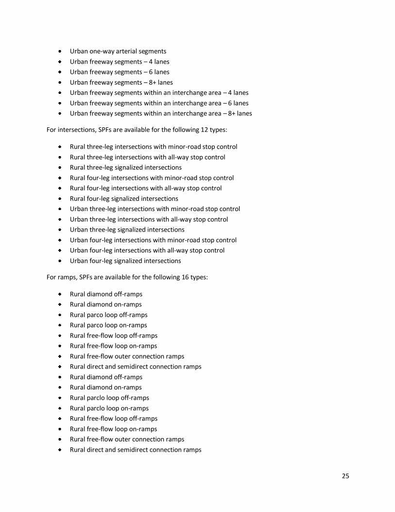
Urban one-way arterial segments
Urban freeway segments – 4 lanes
Urban freeway segments – 6 lanes
Urban freeway segments – 8+ lanes
Urban freeway segments within an interchange area – 4 lanes
Urban freeway segments within an interchange area – 6 lanes
Urban freeway segments within an interchange area – 8+ lanes
For intersections, SPFs are available for the following 12 types:
Rural three-leg intersections with minor-road stop control
Rural three-leg intersections with all-way stop control
Rural three-leg signalized intersections
Rural four-leg intersections with minor-road stop control
Rural four-leg intersections with all-way stop control
Rural four-leg signalized intersections
Urban three-leg intersections with minor-road stop control
Urban three-leg intersections with all-way stop control
Urban three-leg signalized intersections
Urban four-leg intersections with minor-road stop control
Urban four-leg intersections with all-way stop control
Urban four-leg signalized intersections
For ramps, SPFs are available for the following 16 types:
Rural diamond off-ramps
Rural diamond on-ramps
Rural parco loop off-ramps
Rural parco loop on-ramps
Rural free-flow loop off-ramps
Rural free-flow loop on-ramps
Rural free-flow outer connection ramps
Rural direct and semidirect connection ramps
Rural diamond off-ramps
Rural diamond on-ramps
Rural parclo loop off-ramps
Rural parclo loop on-ramps
Rural free-flow loop off-ramps
Rural free-flow loop on-ramps
Rural free-flow outer connection ramps
Rural direct and semidirect connection ramps
26
Appendix B. Developing an Intersection Inventory
Developing network screening SPFs requires an existing inventory for the facility of interest. For
roadway segments, this is not typically an issue. All state DOTs have some form of basic roadway
segment inventory, due to the requirements of the Highway Performance Monitoring System (HPMS).
However, the situation is different for intersections. Very few states have an inventory of intersections
along their public roads. States who are considering the use of network screening SPFs may be
interested in exploring the creation of an intersection inventory, particularly the staff time and cost that
would be necessary to develop such an inventory. Below are listed several of the major considerations in
building an intersection inventory and some discussion of the cost involved.
Location of Intersections Determining the location of each intersection is the most critical element for any intersection inventory.
Two of the most common ways of referencing an intersection location are a Linear Referencing System
(LRS) or Geographic Information System (GIS). Typically, an agency would use the same location system
that is used for their roadway segment inventory. Locating and assigning a unique ID to each
intersection is a substantial task. Ohio DOT developed a semi-automatic in-house process to create the
initial intersection inventory file (i.e., locations and unique identifiers). They report that it took
approximately 3 person months to develop the semi-automated process, but that the process was
designed to be used on an annual basis and takes 2-3 hours to run each time. Other agencies who keep
their roadway inventory in GIS have used built-in GIS tools to automatically create points where
roadway lines intersect. They then manually identified which points were intersections and assigned an
appropriate ID number. The amount of time required for this manual identification is unknown to the
authors.
Traffic Volume
Another crucial piece of an intersection inventory is traffic volumes on both the major and minor roads
of the intersection. This information can often be gleaned from the roadway segments adjacent to the
intersection. This is usually not an issue for the major road (especially, if the major road is state
maintained), but it can be a problem for obtaining volumes on the minor roads. The state roadway
inventory may not contain volume data on the minor road of the intersection, especially if it is not a
state-owned road.
Ohio DOT reports that they use a hierarchical approach in assigning traffic volume to the intersection
file. First, they use the volume information from the adjacent roadway sections. If that is not available
for one or more intersection legs, they obtain any volume information that can be supplied from
Metropolitan Planning Organization (MPO) data. If that is not available, they assign a traffic volume
value using default values for functional class by county.
Geometry and Traffic Control
The other major piece of information is the geometry and traffic control of the intersection. This is
necessary for categorizing intersections (SPFs are developed according to intersection type). Ohio DOT

27
obtained this information by manual effort, using interns to collect the data. They estimate
approximately 3000 hours were necessary to collect this information (along with other intersection-level
characteristics that were of interest). This was performed for a total of 47,000 intersections that lay on
Ohio state-maintained roads, for an average cost of $1.30 per intersection (assuming intern pay is
$20/hr).
The FHWA Office of Safety recently released a report containing estimated costs for collecting basic
inventory variables, known as the Model Inventory Roadway Elements (MIRE) Fundamental Data
Elements (Fiedler et al., 2013). They estimate that the cost of collecting basic geometry and traffic
control would be approximately $1.00 per intersection.
References
Fiedler, Rebecca, Kim Eccles, Nancy Lefler, Ana Fill, and Elsa Chan. MIRE Fundamental Data Elements
Cost-Benefit Estimation. Final Report, Contract DTFH61-11-C-00050, March 2013.

28
Appendix C. Recent SPF Development Efforts from States
Following is a brief description of recent jurisdiction specific SPF development efforts (rather than the
calibration of existing SPFs) from States. These were compiled based on a review of the published
literature. The focus was on SPF development for the purpose of network screening or project level
analysis. In addition to the states listed here, there are states that are in the process of developing SPFs
(examples include Alabama, Louisiana, and Washington).
Colorado
Persaud and Lyon, Inc. and Felsburg Holt and Ullevig, Safety Performance Functions for Intersections,
Report CDOT-2009-10, Developed for Colorado Department of Transportation, Denver, Colorado,
December 2009.
This study developed SPFs for 10 intersection categories:
Urban 4-Lane Divided Signalized 4-Leg
Urban 6-Lane Divided Signalized 4-Leg
Urban 4-Lane Divided Signalized 3-Leg
Urban 2-Lane Undivided Unsignalized 4-Leg
Urban 4-Lane Divided Unsignalized 4-Leg Urban 2-Lane Undivided Unsignalized 3-Leg
Urban 4-Lane Divided Unsignalized 3-Leg
Urban 4-Lane Undivided Unsignalized 4-Leg
Urban 2-Lane Divided Unsignalized 3-Leg
Urban 4-Lane Undivided Unsignalized 3-Leg
At least 5 years of data were available for each intersection that was used in the analysis. SPFs were
estimated for total and injury and fatal crashes. CURE plots and other goodness of fit measures were
used to assess the validity of the SPFs. Since the SPFs just used major and minor road AADT data, they
could be used for network screening.
Florida
Lu, J., A. Gan, K. Haleem, P. Alluri, and K. Liu, Comparing Locally-Calibrated and Safety Analyst Default
Safety Performance Functions for Florida’s Urban Freeways, Presented at the 91st Annual Meeting of the
Transportation Research Board, January 2012.
SPFs were estimated for network screening consistent with the format in Safety Analyst. SPFs were
estimated for total and fatal and injury crashes for the following road types:
4 lane urban freeways outside influence of interchanges 4 lane urban freeways within the influence of interchanges
6 lane urban freeways outside influence of interchanges
6 lane urban freeways within the influence of interchanges
29
8+ lane urban freeways outside influence of interchanges
8+ lane urban freeways within the influence of interchanges
Illinois
Tegge, R.A., J. Jang-Hyeon, and Y. Ouyang (2010), Development and Application of Safety Performance
Functions for Illinois, Research Report ICT-10-066, Illinois Center for Transportation, Civil Engineering
Studies, March 2010.
SPFs were estimated for roadway segments and intersections on state-maintained roads. SPFs were
estimated for fatal, type A injury, type B injury, and fatal and injury combined. The main focus was to
estimate the SPFs for network screening that could be used within Safety Analyst. For roadway
segments, SPFs were estimated for the following roadway types:
Rural Two-Lane Highway
Rural Multilane Undivided Highway
Rural Multilane Divided Highway
Rural Freeway, 4 Lanes
Rural Freeway, 6+ Lanes
Urban Two-Lane Highway
Urban One-Way Arterial
Urban Multilane Undivided Highway
Urban Multilane Divided Highway
Urban Freeway, 4 Lanes
Urban Freeway, 6 Lanes
Urban Freeway, 8+ Lanes
For intersections, SPFs were estimated for the following types: Rural Minor Leg Stop Control
Rural All-Way Stop Control
Rural Signalized Intersection
Rural Undetermined
Urban Minor Leg Stop Control
Urban All-Way Stop Control
Urban Signalized Intersection
Urban Undetermined
In addition to the SPFs for network screening, an SPF was estimate for KAB injury crashes for roadway
segments. This SPF included information about access control, shoulder width and type, lane width,
median type and other segment characteristics. This SPF is a possible starting point for project level
analysis.
North Carolina
Srinivasan, R. and D. Carter, Development of Safety Performance functions for North Carolina, Report
FHWA/NC/2010-09, Submitted to North Carolina Department of Transportation, December 2011.

30
All SPFs predicted the number of crashes per mile as a function of AADT consistent with the functional
form in Safety Analyst. North Carolina specific SPFs were estimated for the following crash types:
Total crashes
Injury and fatal crashes (K, A, B, C)
Injury and fatal crashes (K, A, B)
Property damage only (PDO) crashes Lane departure crashes
Single vehicle crashes (including animal crashes)
Multi vehicle crashes
Wet crashes
Night crashes – This included crashes with Ambient Light = (4) Dark – lighted roadway, or (5) Dark – roadway not lighted, or (6) Dark – unknown lighting
SPFs were estimated for the following roadway types:
Rural Two Lane Roads
Rural Freeways - 4 lanes - outside the influence of interchanges
Rural Freeways – 6+ lanes - outside the influence of interchanges
Rural Freeways - 4 lanes - within the influence of interchanges
Rural Freeways – 6+ lanes - within the influence of interchanges
Rural Multilane Divided Roads
Rural Multilane Undivided Roads
Urban Two Lane Roads
Urban Freeway - 4 lanes - outside the influence of interchanges
Urban Freeway - 6 lanes - outside the influence of interchanges Urban Freeway - 8+ lanes - outside the influence of interchanges
Urban Freeway - 4 lanes - within the influence of interchanges
Urban Freeway - 6 lanes - within the influence of interchanges
Urban Freeway - 8+ lanes - within the influence of interchanges
Urban Multilane Divided Roads
Urban Multilane Undivided Roads
In addition to these SPFs for network screening, SPFs were estimated for rural two lane roads that
included terrain, shoulder width, shoulder type, in addition to AADT. These SPFs are possible starting
points for project level analysis.
Utah
Brimley, B.K., M. Saito, and G.G. Schultz, Calibration of Highway Safety Manual Safety Performance
Function: Development of Models for Rural Two-Lane Two-Way Highways, Transportation Research
Record 2279, pp. 82-89.
SPFs for total crashes were estimated for rural two lane roads. The independent variables considered
included AADT, information about whether passing was permitted, whether shoulder rumble strips were
present, percent multiple-unit trucks, and speed limit. Different models were examined and a model

31
was selected based on the Bayesian Information Criterion (BIC). The recommended model could be
used for network screening and could be a starting point for project level analysis.
Virginia
Garber, N.J. and G. Rivera, Safety Performance Functions for Intersections on Highways Maintained by
the Virginia Department of Transportation, FHWA/VTRC 11-CR1, Virginia Department of Transportation,
October 2010.
SPFs were estimated primarily for use in Safety Analyst for network screening. SPFs were estimated for
the following intersection types:
Urban 4 leg signalized
Urban 4 leg minor road stop controlled
Urban 3 leg signalized Urban 3 leg minor road stop controlled
Rural 4 leg signalized
Rural 4 leg minor road stop controlled
Rural 3 leg signalized
Rural 3 leg minor road stop controlled
SPFs were estimated total and fatal and injury crashes. Separate SPFs were also estimated for different
regions in Virginia.