ARTICLE

Feasible future global scenarios for human lifeevaluationsChristopher Barrington-Leigh1 & Eric Galbraith 2,3,4

Subjective well-being surveys show large and consistent variation among countries, much of

which can be predicted from a small number of social and economic proxy variables. But the

degree to which these life evaluations might feasibly change over coming decades, at the

global scale, has not previously been estimated. Here, we use observed historical trends in

the proxy variables to constrain feasible future projections of self-reported life evaluations to

the year 2050. We find that projected effects of macroeconomic variables tend to lead to

modest improvements of global average life evaluations. In contrast, scenarios based on non-

material variables project future global average life evaluations covering a much wider range,

lying anywhere from the top 15% to the bottom 25% of present-day countries. These results

highlight the critical role of non-material factors such as social supports, freedoms, and

fairness in determining the future of human well-being.

https://doi.org/10.1038/s41467-018-08002-2 OPEN

1 Institute for Health and Social Policy; and School of Environment, McGill University, Montreal H3A1A3 QC, Canada. 2 ICREA, Pg. Lluís Companys 23, 08010Barcelona, Spain. 3 Institut de Ciència i Tecnologia Ambientals (ICTA) and Department of Mathematics, Universitat Autonoma de Barcelona, 08193Barcelona, Spain. 4 Department of Earth and Planetary Sciences, McGill University, Montreal, QC, Canada. Correspondence and requests for materials shouldbe addressed to C.B.-L. (email: Chris.Barrington-Leigh@McGill.ca)

NATURE COMMUNICATIONS | (2019) 10:161 | https://doi.org/10.1038/s41467-018-08002-2 | www.nature.com/naturecommunications 1

1234

5678

90():,;

Complex policy decisions, ranging from international cli-mate change negotiations to investments in education orinfrastructure, often rely on projections of readily quan-

tified material outcomes such as per capita income to assess theimpacts on human welfare, for example, refs. 1,2. An alternativeapproach, developed over the past few decades, aims to applymore direct measures of human experience that integrate manydimensions of life according to those living it. These well-beingmeasures have the disadvantage of being subjective, andcan therefore be difficult to interpret. Nevertheless, they havebeen shown to be consistent with external evaluations at theindividual level, are reproducible over time within populations,and are increasingly embraced by decision makers as a leadingobjective3–7. They also show consistent predictive relationshipswith other societal variables.

Here, we focus on one measure of subjective well-being (SWB)with particularly consistent predictive relationships: the cognitiveevaluation of life. Annual, near-global national samples of self-reported life evaluations, from Gallup’s World Poll, have recentlybecome available through the World Happiness Report. While thePoll’s extensive questionnaire is not designed expressly for explainingdifferences in life quality, it does contain several questions whichaddress dimensions of life known to be important to life evaluation.Prior work in a range of contexts has shown that, among these,income differences have significant explanatory power in accountingfor variation in life evaluations, while less tangible aspects of humanexperience can account for as much or more of the variation8; seeSupplementary Note 1. Following Helliwell et al.8, we account for aportion of international differences in life evaluation using four proxyvariables derived from the Gallup World Poll, which we will refer toas reflecting non-material factors (corruption9, freedom, giving10,and social support), and two proxy variables reflecting materialfactors (per capita gross domestic product (GDP) and life expec-tancy). When these measures are included in a simple linear modelof cross-country differences, they explain roughly three-quarters ofthe variation among annual national averages of life evaluations, andparameters are estimated with high statistical precision, as shown byprior work8; see Supplementary Note 2 for details.

Static inter-country comparisons such as these have been thefocus of much attention, but they do not address how the lifeevaluations of humans might change in the future, an importantconsideration for motivating and evaluating policy decisions.Although there is no mechanistic understanding on which toreliably predict these future changes directly, the time-span cov-ered by the Gallup World Poll (2005–2016) is now sufficient touse as an empirical constraint on the feasible rates at which proxyvariables might change, and reveals that strong trends haveoccurred in some countries (Supplementary Figure 1). The por-tion of life evaluations that can be predicted from the proxyvariables would be expected to change accordingly, providing ameans by which to estimate the range within which the futuretrajectories of life evaluations are most likely to fall.

Here, we use the historical survey data to develop a dynamicstatistical model and evaluate feasible rates of change, and con-struct simple scenarios for human life evaluations in 2050, withinthe time frame commonly considered in forward-looking policiesinformed by climate model projections11–16. We find that sig-nificant changes in global average life evaluations are feasible, andcould be either positive or negative. In addition, we find thesefuture outcomes to have a markedly larger dependence on non-material proxy variables as compared with material ones.

ResultsProxy model of life evaluations. Our statistical models predict aportion of the observed changes in life evaluations from the proxy

variables using both static (across countries, XS) and dynamic(within countries comparing two periods, 2P) models (Fig. 1, seeSupplementary Note 2 for details). As compared with the staticXS model of differences across countries (Fig. 1a), the dynamic 2Pmodel of within-country changes shows a relatively greateremphasis on freedom to make decisions, availability of socialsupport, and perception of corruption. The coefficients in Fig. 1a,b are normalized to standard deviations, meaning that a 1 s.d.change in income predicts a 0.19 s.d. change of life evaluations,holding other factors constant, while a 1 s.d. change in socialsupport predicts a 0.29 s.d. change in life evaluation. In ourprojections, below, we use the dynamic model (2P) to predictchanges in life evaluation over several decades, though as dis-cussed later, our main findings would be even more pronouncedwere the XS model coefficients to be used. We emphasize that theprojections that emerge are not predictions of the future, butillustrate the range of the most feasible futures that might occur,depending on human actions.

Projected range of global mean changes. The range of feasibleoutcomes spanned by the three sets of scenarios is shown inFig. 2. Two sets of scenarios relate to changes in material con-ditions. For the first of these sets (Organization for Economic Co-operation and Development (OECD) projections), both theoptimistic (strong-growth) and pessimistic (weak-growth) pro-jections show improvements of global average experienced lifeevaluation compared with the 2016 value of 5.24 out of 10. Theoptimistic case of the second material-factors pair (MaterialTrends) is characterized by steady growth at the 90th percentile ofrecently observed trends (4%/year for income and 0.55 years/yearfor healthy life expectancy), and this scenario’s outcome agreesvery closely with the optimistic OECD estimate. However, not allcountries have actually experienced positive real economicgrowth. As a result, the corresponding pessimistic MaterialTrends scenario, using 10th percentile observed trends, admitsthe possibility of a small decline of global average life evaluations,to 5.1, by 2050.

The range of feasible outcomes encompassed by these materialscenario sets is dwarfed by the range of outcomes in the non-material scenario set. In the top 10% of recent observed trends,freedom and social support grew at 2%/year and 0.6%/year,respectively, while corruption decreased at 1.3%/year. At theserates, our Non-material Trends scenario projects a radical globalmean improvement of life evaluation to 6.9, which—forcomparison—is close to the levels actually reported by Belgiumand Costa Rica in 2016, when they had the 18th and 14th highestlife evaluations17. Conversely, if the least favorable 10th percentileof observed non-material trends were to prevail in all countries,our projections suggest that the drop in life evaluations by 2050would take the global average to 3.4, below the level of Egypt andIndia in 2016, when they ranked 118th and 120th out of 157countries.

Figure 2 also shows our projections based on 30th and 70thpercentile recent trends. These provide very similar qualitativeconclusions as our primary analysis, in that the Non-materialTrend scenarios encompass more extreme positive and negativepossibilities than the material trends. Notably, the 30th to 70thpercentile Material Trend projections span a similar range of lifeevaluations as that of the OECD-derived projections, although thetrend-based projections are approximately 0.3 points lower thanthe OECD projections.

Geography of projected changes. We map the distribution ofprojected changes in life evaluation in our material OECD andNon-material Trend scenarios, according to population density

ARTICLE NATURE COMMUNICATIONS | https://doi.org/10.1038/s41467-018-08002-2

2 NATURE COMMUNICATIONS | (2019) 10:161 | https://doi.org/10.1038/s41467-018-08002-2 | www.nature.com/naturecommunications

projections for 2050, in Fig. 3 (the corresponding Material Trendscenarios, which are uniform across countries, are shown inSupplementary Figures 2–5). For the non-material scenarios, weshow only the most optimistic (90th percentile) and pessimistic(10th percentile) projections. The OECD’s material scenarios aredriven by national changes in per capita income, since in our 2Pmodel life expectancy has no significant effect on life evaluations.In general, the OECD projections show some degree ofimprovement in all countries, even under pessimistic assump-tions. Differences among countries reflect the details of theOECD’s macroeconomic projections and reflect an expectation ofeconomic convergence, that is, higher economic growth rates incountries with lower initial income.

Compared to the OECD projections, the non-materialprojection maps show a much wider range of possible changes,as did the global averages. In the optimistic non-material future,improvements of more than 1.5 on the 11-point life evaluationscale are widespread, including in densely populated regions ofIndia, China, eastern Europe, and sub-Saharan Africa. The scopefor improvement in non-material factors is smaller in westernEurope and North America, given that these countries are alreadycloser to the maximum values. Nonetheless, the improvements inpredicted life evaluation that would appear to be feasible due tonon-material changes by 2050 exceed those of even the mostoptimistic material changes in all countries.

The pessimistic projections show an even starker differencebetween material and non-material futures. Whereas the

−0.6 −0.4 −0.2 0.0 0.2 0.4 0.6 0.8 1.0

Predicted Δ life evaluation

−1.5

−1.0

−0.5

0.0

0.5

1.0

1.5

Δ Li

fe e

valu

atio

n

Central and Eastern EuropeMiddle East and North AfricaLatin America and Caribbean

Commonwealth of Independent StatesNorth America and ANZ

Western EuropeSub-Saharan Africa

South AsiaEast Asia

Southeast Asia

c

Lifeexpectancy

Corruption |Freedom

Giving Socialsupport

−0.2

0.0

0.2

0.4

b

Lifeexpectancy

Corruption |Freedom

Giving Socialsupport

−0.2

0.0

0.2

0.4

Log( GDPcapita)Log( GDP

capita)

Cross-section modelof life evaluation

a

2P s

tand

ardi

zed

coef

ficie

nts

XS

sta

ndar

dize

d co

effic

ient

s

Two-period change modelof life evaluation

Fig. 1 Predictions of life evaluations from proxy variables. a Six predictor variables are used simultaneously to predict life evaluations in static cross-sectionbetween countries (XS). All corresponding country-year observations are used, after removing global year-to-year changes. Effect sizes are shown, with90% confidence intervals, normalized to standard deviations, in order to compare the estimated coefficients across predictor variables. The strongestpredictor is the income variable, but all predictors have significant strength, and their confidence intervals largely overlap. b As in a but for the dynamic,two-period model (2P) which explains changes over time within countries. In the 2P model, confidence intervals are looser, and the income coefficientexcludes zero with only ~90% confidence intervals. However, models for annual changes (see Supplementary Information) show similar patterns and havetighter confidence intervals. c The relationship between observed and predicted changes in life evaluation using the 2P model. The changes are thedifferences in national average life evaluations between 2005–2007 and 2014–2016. Symbol size corresponds to the population size of each country

3.5 4.0 4.5 5.0 5.5 6.0 6.5 7.0

Global average life evaluation in 2050

OECD material projections

Material trends

Non-material trends

Fig. 2 Projected feasible life evaluations in 2050 scenarios. The results oftwo sets of material scenarios are shown for the year 2050, based onmacroeconomic projections (OECD, orange) and recent trends (purple), aswell as a set of non-material scenarios based on recent trends (green). Thecentral vertical lines indicate projections based on the median trends, thethick horizontal bar indicates the range based on the 30th to 70th %iletrends, and the thinner horizontal bar indicates the range based on the 10thto 90th %ile trends. Outcomes are calculated with coefficients from the 2Pmodel and are weighted by projected population sizes to aggregate acrosscountries. The red arrow indicates the population-weighted average lifeevaluation recorded in 2016

NATURE COMMUNICATIONS | https://doi.org/10.1038/s41467-018-08002-2 ARTICLE

NATURE COMMUNICATIONS | (2019) 10:161 | https://doi.org/10.1038/s41467-018-08002-2 | www.nature.com/naturecommunications 3

pessimistic OECD projections do not produce negative outcomesin any countries, feasible changes in non-material variables couldproduce a large decrease in life evaluation in any country by 2050.This reflects the fact that, in recent years, the social variables havehad large negative trends in many countries, whereas materialvariables are generally expected to improve, or at least remainstable everywhere.

DiscussionOur analysis suggests that large future changes in global lifeevaluations are feasible, and could be either positive or negative,based on the observed changes of proxy variables within countriesduring 2005–2016. Our scenarios treat material and non-materialproxy variables independently, so that the modeled changes dis-cussed above are additive. For instance, using the OECD and 10/90 percentile Non-material Trends, the combined feasible chan-ges give a range of projected 2050 global average life evaluationsfrom 3.9 to 7.6. Regardless of whether the material trends orOECD projections are used, the major part of the summed rangesis due to the non-material factors, because the range of materialrates of change is smaller, relative to their modeled impact on lifeevaluations, than the range of rates of change of the non-materialvariables. Thus, non-material variables can feasibly make largerimpacts than income on a multi-decadal timeframe.

Furthermore, we earlier emphasized that variance-standardizedeffect sizes are larger for non-material factors than material fac-tors in the 2P dynamic model, while income is the strongestpredictor in the cross-sectional model. However, the raw coeffi-cients have the opposite relationship, in that the ratio of raw effectsize of income to raw effect size of social support (or to any ofour other non-material variables) is larger for the 2P dynamicmodel than the cross-sectional model. Therefore, carrying outprojections for long-run changes using coefficients from thecross-sectional model results in even starker dominance bynon-material factors.

Speculatively, our model may overestimate the role of GDP percapita for another reason. A well-studied phenomenon first

noticed by Easterlin18 is related to the smaller predictive role ofincome in explaining long-run variation as compared with annualchanges19. Human life evaluations appear to adapt to the ambientmaterial affluence over time, in the sense that our mental benefitgradually accommodates to the experienced level20,21. This con-trasts with social aspects of life, for which there is little evidenceof such adaptation22. In a second phenomenon, humans respondto material consumption norms set by those around them. Bothphenomena help to explain the lack of long-run response of lifeevaluations at the national level to rising incomes during eco-nomic growth, for example, refs. 19,23, and may explain the dif-ference in raw coefficient sizes mentioned above. Furthermore,life evaluations may be sensitive to national (as opposed to local)rank of affluence. Such positional concerns would imply an evensmaller long-run direct benefit from aggregate economic growthacross all countries, because even the cross-sectional distributionof life evaluations would reflect in part the outcome of a long-runzero-sum game.

In further support of the importance of non-material factors,we point out that, during the period of observations, the globalmean of life evaluations did not change significantly, despite anaverage increase of incomes by 17% and lengthening of lifeexpectancy by 2.6 years (Supplementary Tables 1–3). The globalimprovements in material conditions, which were accompaniedby improvements in average freedom and corruption, werecounteracted by a decrease in average social support, and thereported change in global lifeevaluations was negligible.

Although we have focused here on subjective life evaluation, weundertook an identical model-building and projection procedurefor affect measures, which capture day-to-day feelings. A pre-dictive model based on the six proxy variables does not capture asmuch of the variation in affect as the models for life evaluation8

(see Supplementary Tables 4–7). Nonetheless, with this caveat inmind, the trend-based projections suggest that the average affectbalance of humans in 2050 could decrease by as much as 0.28 orincrease by as much as 0.31 on a two-point scale within the 90thto 10th percentile trends, spanning 30% of the total range, very

–2 0 21

Change of life evaluation from 2017 to 2050

OECD material (optimistic)

Non-material (optimistic)Non-material (pessimistic)

OECD material (pessimistic)a b

c d

–1

Fig. 3 Geographic distribution of feasible life evaluation changes. Projections for 2050 are for the OECD material growth scenarios (a, b), and scenarios inwhich the non-material predictor variables change at the 10th and 90th percentile rates of recent observations among all countries (c, d). Coefficients usedin the projection are based on the two-period model of life evaluations. The shading on the map is weighted by projected population density

ARTICLE NATURE COMMUNICATIONS | https://doi.org/10.1038/s41467-018-08002-2

4 NATURE COMMUNICATIONS | (2019) 10:161 | https://doi.org/10.1038/s41467-018-08002-2 | www.nature.com/naturecommunications

similar to the relative magnitude of feasible changes in life eva-luations. Furthermore, the changes in affect are dependentexclusively on non-material factors, with no discernible influenceof material changes (see Supplementary Note 2). Thus, largechanges in affect are also feasible, could also be positive ornegative, and appear to be exclusively dependent on non-materialfactors.

We would emphasize that the predictor variables we use areproxies, rather than direct mechanistic drivers of life evaluation.There are many dimensions of material supports, such as nutri-tion, shelter, and infrastructure, which may not vary directly withper capita GDP. Provision of these material needs may also helpto build trust, support systems among family and communities,and freedom of choice. Likewise, our non-material proxies do notcapture all of the dimensions of social experience known to beimportant for life evaluations, and a breakdown of these non-material conditions likely imperils the material ones24. In order toaddress the possibility that these interactions are statisticallyimportant, we repeated our analysis using models augmentedwith a series of interaction (also know as moderation) termsbetween pairs of predictors with statistically significant effects inour 2P model. These tests, which are detailed in SupplementaryNote 3 and Supplementary Table 8, suggest a statistically sig-nificant interaction between GDP and freedom of choice, but thisinteraction does not alter our general conclusions nor the greaterimportance of non-material factors (see Supplementary Figure 1).Nevertheless, we recognize that our results remain limited by theuse of a global model with six predictors that are, unavoidably,inter-related. In the future, the accumulation of larger databasescould allow the development of a formal model selection processto choose among broader possibilities of predictor variables, andmay ultimately allow the development of mechanistic modelswith greater predictive power.

Despite the simplifications inherent in this first attempt toproject future human well-being, our results show that thegreatest benefits to be potentially made over the next decades, aswell as the most dangerous pitfalls to be avoided, lie in thedomain of social fabric. Focusing on income among the effects oflong-run policy is therefore too narrow, and misses the majorityof the human well-being effects that could feasibly occur, basedon past experience. Given that the policies known to support astrong social fabric can differ from those focused on economicgrowth, our results suggest that scarce resources may be betterprioritized towards explicitly social aims if human well-being isthe goal.

MethodsSurvey data. Following recent World Happiness Reports, we include a measure ofincome along with variables representing healthy life expectancy (life expectancy),perceived level of corruption (corruption), freedom to choose (freedom), pre-valence of donating to others (giving), and availability of informal social support(social support). The English wording of the life evaluation question is “Pleaseimagine a ladder, with steps numbered from 0 at the bottom to 10 at the top. Thetop of the ladder represents the best possible life for you and the bottom of theladder represents the worst possible life for you. On which step of the ladder wouldyou say you personally feel you stand at this time?” The social support variable isthe national average of dichotomous responses to “If you were in trouble, do youhave relatives or friends you can count on to help you whenever you need them, ornot?” The freedom variable is the national average of dichotomous responses to“Are you satisfied or dissatisfied with your freedom to choose what you do withyour life?” The corruption variable is the national average of dichotomous answersto two questions: “Is corruption widespread throughout the government or not?”and “Is corruption widespread within businesses or not?” In order to isolate theprevalence for giving from the variation in financial capacities, national meanresponses to “Have you donated money to a charity in the past month?” areregressed on GDP per capita, and the residual becomes the Giving variable25.Further descriptions and important notes for these variables are given in the sta-tistical appendix for Chapter 2 of the 2017 report8. Our measure of income is thenatural logarithm of internationally comparable (i.e., purchasing power parity)GDP per person; this measure has a relatively good linear fit with life evaluations,

for example, ref. 26. By considering these measures at the aggregate (country) level,we best capture the sum of individual effects and those which come from publicgoods (at national and subsidiary scales) and from social and contextual effects atall spatial scales up to the country level. Our use of country-level data is motivatedby the assumption that externalities (e.g., positional effects, or public goods) arelikely to be large within countries, but are likely to be relatively small betweencountries.

Summary information about the dataset is provided in Supplementary Note 1,including descriptive statistics of levels (Supplementary Table 3), annual changes(Supplementary Table 2), and 2P changes (Supplementary Table 1) of our keyvariables. We also provide estimates of pairwise correlations among levels(Supplementary Table 9) and 2P changes (Supplementary Table 10) in our keyvariables.

Regression models for well-being (overview). We estimate four different modelsto characterize the relationship between country-level SWB and our six predictorvariables. Each model is suitable for estimation using a weighted least-squaresapproach. One model predicts the relationship among countries, another predictswithin-country changes between our two time periods, and two approaches predictyear-to-year changes within countries. We use the 2P model in our primary ana-lysis in order to remain conservative with our primary conclusions, and in order toavoid the short-run effects of the global financial crisis (GFC) in our estimates oflong-run trends, but we show results from the other models in SupplementaryNotes 1 and 3. For completeness, the four models and the standardization areexplained below. For each of these models, the corresponding estimates aretabulated in Supplementary Note 2 both as raw coefficients and secondly as unitlessstandardized coefficients.

As emphasized in the main text, we cannot identify and isolate independentcausal relationships between supports (predictor variables) and life evaluations.Rather, our set of proxy variables, with their shared variance, captures oneprojection of the true underlying processes. In the case of our Giving variable, weerr on the side of under-estimating the importance of giving by using the residualfrom a regression of the underlying donations variable on an income measure. Thismay in turn result in over-estimating the importance of income.

Regression models for well-being (static model). First, we consider the cross-sectional (XS) relationship

Sit ¼ aþX6j¼1

bjxjit þ ct þ νi þ εit ; ð1Þ

where Sit is the SWB in country i in year t; a is a global constant; xjit are the sixpredictor variables; ct is a constant in a given year t for all countries; and νi+ εit isan error term clustered at the country level. Here, bj are the regression coefficientsdescribing the effects of interest. In estimating (1) we use country weightingbecause we consider the political–cultural–economic dynamics to be distinct acrosscountries and therefore consider each country to be one sample unit. We clustererrors at the country level to take into account the fact that we have multipleobservations (i.e., by year) for each country, but do not capture all country featuresin the model. Our inclusion of year indicators (dummy variables) ct is to removevariation related to global secular trends (e.g., average global economic growth) andshort-run global cycles (e.g., the GFC), so that our estimated bj capture the cross-sectional variation.

In order to quantitatively compare these relationships bj across predictors j, wecalculate the standardized regression coefficients βj �

σ jσSbj ; that is, we estimate the

standardized variable equation

Sitσs

¼ ~aþX6j¼1

βjxjitσ j

þ ~ct þ ~νi þ ~εit ; ð2Þ

where σs is the standard deviation of Sit across all country-year observations, butagain calculated with country weights to take into account the fact that not allcountries have the same number of observations (years). The standard deviation σjof xjit is calculated the same way. Thus, βj should be interpreted as the number ofstandard deviations of change in S associated with one standard deviation changein xj.

Regression models for well-being (dynamic models). While (1) models thevariation across countries, we also generate models of changes over time in order toproject future changes based on past rates of change. We do this in three ways. Twoof them, fixed effects (FE) and first differences (FD), use the year-to-year changesin the predictor variables for each country to explain year-to-year changes in SWB.The third method (2P) considers only the longer-run difference for each countryfrom early in the Gallup World Poll data (2005–2007) to the most recent years(2014–2016). Taking the means during each of these two periods excludes the acuteeffects of the GFC and its recovery.

NATURE COMMUNICATIONS | https://doi.org/10.1038/s41467-018-08002-2 ARTICLE

NATURE COMMUNICATIONS | (2019) 10:161 | https://doi.org/10.1038/s41467-018-08002-2 | www.nature.com/naturecommunications 5

Regression models for well-being (annual changes). First, we consider the year-by-year changes, captured in an FE model by including an indicator (constantoffset) di for each country (this is equivalent to subtracting the mean value for eachcountry):

Sit ¼ aþ di þX6j¼1

bFEj xjit þ νi þ εit : ð3Þ

Alternatively, we may model the 1-year changes in an FD equation, as follows:

ΔSit ¼X6j¼1

bFDj Δxjit þ νi þ εit : ð4Þ

With finite samples, (3) and (4) do not give identical estimates. Moreover,because our panel is not perfectly balanced, some observations are dropped whenestimating (4). Because of this, and the inherent higher efficiency of the FEestimator, we favor (3) but show estimates of both.

As described in the Methods section, we wish to be able to compare theestimated effects of one predictor variable to another—that is, to ascribe relativeimportance to changes in different predictor variables. For the FD estimator, this isstraightforward, as we can construct normalized versions of observed 1-yearchanges, in analogy to (3):

ΔSitσΔS

¼X6j¼1

βFDjΔxjitσΔxj

þ ~νi þ ~εit : ð5Þ

The term βj in (5) explains the distribution of 1-year changes in S, such that βj isthe number of standard deviations of change in ΔS associated with 1 s.d. change inΔxj, where these variances are calculated across observed 1-year changes.

In order to express the relative importance of estimates from the FE estimator,(3), we use the same standard deviations of FD to transform the bFEj in (3) to

βFEj �σΔxjσΔS

bFEj : ð6Þ

Estimating βFEj has the advantages over βFDj mentioned above (efficiency, moreinclusion) for FE.

Regression models for well-being (2P changes). The third method constructs anequation with only two observations per country, the early period and the laterperiod (2005–2007 and 2014–2016), in order to model longer-run changes δxj andδS. In this context, the FE and FD estimators are identical; thus, we write simply

δSit ¼X6j¼1

b2Pj δxjit þ νi þ εit : ð7Þ

Analogously to the methods above, we define the standardized coefficients

β2Pj �σδxjσδS

b2Pj ð8Þ

using the standard deviation of longer-run changes across countries. This estimatehas fewer observations than those modeling annual changes, and the confidenceintervals are slightly looser.

As mentioned in the Discussion, we also consider moderation effects betweenvariables in the 2P model by testing pairwise interaction terms, detailed inSupplementary Note 3. We find a significant moderation effect only between GDPand freedom of choice.

Regression models for well-being (results). Estimates of the models for lifeevaluations are described in Supplementary Note 2 and summarized in Supple-mentary Table 4. In addition, we report analogous estimates for our other measuresof well-being, namely positive affect (Supplementary Table 5), negative affect(Supplementary Table 6), and affect balance (Supplementary Table 7). We alsocarry out and explain an estimate at the regional level (reported in SupplementaryTable 11).

Recent trends (overview). We define future scenarios by projecting differentquantiles of recent country trends in predictor variables into the future. Ratherthan defining complex and arbitrary story lines, we represent the range of feasibleoutcomes by defining idealized scenarios. We denote the total feasible range ofpossible rates of change as that encompassed by the 10th to 90th percentileobserved range among all countries. Thus, we use the assumption that, if a given

rate of change in a proxy variable was observed in 10% of all countries over the 11-year observation period, it is feasible that the variable could change at this rate inany country over the next three decades. This differs from the full range of possiblechanges, for which we have no first principles understanding, but which is likely tobe greater than our feasible range given the possibility of unforeseeable, radicaltransformation. To better characterize the distribution of likely futures, we alsomake projections using the 30th, 50th, and 70th percentiles of recent trends, but wefocus on the 10th and 90th percentiles for our primary analysis.

For the purpose of illustrating large changes in our predictor variables,Supplementary Figure 6 shows recent trends (with 3-year smoothing) in the ninecountries which exhibited the most variation in each variable.

The estimation of recent trends in our predictor variables and in SWB iscomplicated by two issues. First, the panel of available data is incomplete; that is,there are data gaps for some country-year variable entries. Table 1 shows thenumber of countries with data by year or period for our various approaches. Inorder to estimate trends that are not biased by a changing composition ofcountries, a subset of countries with complete data can be used, or data can beappropriately weighted in order to account for features of the incomplete panel.Secondly, the GFC had a significant impact on some countries in 2008, yet theseeffects were somewhat temporary. The short-term changes following the GFC maynot contribute constructively towards estimating the longer-run changes that mightinform scenarios to 2050. Fortunately, the Gallup World Poll time series is nowlong enough that estimates can be made even after excluding several yearsfollowing the start of the GFC.

Recent trends (country estimates). We therefore consider the following threeestimation models of recent time trends in our key variables:

First, a differences model: Take averages for each country for each period(2005–2007, 2014–2016), and calculate the difference. This avoids the GFC, butentails a two-step process to calculate confidence intervals for the differences.

Second, a 2P regression, excluding GFC model: A one-step method whichprovides estimates of confidence intervals is to carry out a regression

xit ¼ xi0 þ Biπt þ εit ; ð9Þ

where πt is an indicator variable for periods after/before the GFC:

πt ¼1; t � 2014;

0; otherwise

�ð10Þ

and where observations are estimated with weights

wit ¼

1Nit�2007

; t � 2007;

0; 2008 � t � 2013;1

Nit�2014

; t � 2014:

0BB@ ð11Þ

Here Nit�2007 is the number of observations of country i in the early period. The

point estimates of Bi in (9) are identical to the difference in period means forcountry i, but the standard error is calculated correctly.

In order to convert the estimates Bi of change between the two periods to anestimate of the annual rate of change, we divide by 9, the number of years betweenthe middles of the two periods.

Third, and lastly, an all-year (annual) regression model: The annual rate ofchange can be estimated for country i and variable x using all years t for which xit

Table 1 Completeness of panel data

Year Any data All data Balanced ≥2007 Any <2008 Any >2013 Any (2P)

2005 27 21 118 1092006 85 77 118 1092007 99 92 64 118 1092008 104 100 642009 109 105 642010 118 110 642011 138 130 642012 134 122 642013 130 119 642014 137 122 64 129 1092015 136 120 64 129 1092016 133 116 64 129 109

The first column lists the number of countries with coverage within our core set of variables foreach year of the Gallup World Poll, after some imputation done in accordance with the dataappendix of Helliwell et al.8. The All data column lists the number of countries with all of ourcore variables. The Balanced column shows the number of countries in the largest balanced(complete, rectangular) panel covering all years after 2006. For our two-period model, we usethe countries with at least one observation in the early period and at least one observation in thelater period

ARTICLE NATURE COMMUNICATIONS | https://doi.org/10.1038/s41467-018-08002-2

6 NATURE COMMUNICATIONS | (2019) 10:161 | https://doi.org/10.1038/s41467-018-08002-2 | www.nature.com/naturecommunications

was observed, according to the following equation:

xit ¼ ai þ bit þ εit : ð12Þ

Recent trends (global and regional estimates). For directly estimating global (orregional, multi-country) trends, we follow a similar procedure as the 2P and annualapproaches described above, but using two alternative approaches to weightingobservations. In one, we use weights which count each country equally, and inanother we multiply the weights described previously by country populations.Thus, we have four variants of estimated global trends: for each variable there is a2P version and an annual version, and for each of those there are country weightsand population weights.

By contrast, we consider countries as individual observations when thinkingabout the global distribution of trends, and thus calculate, for example, the 10thpercentile trend from the unweighted set of countries.

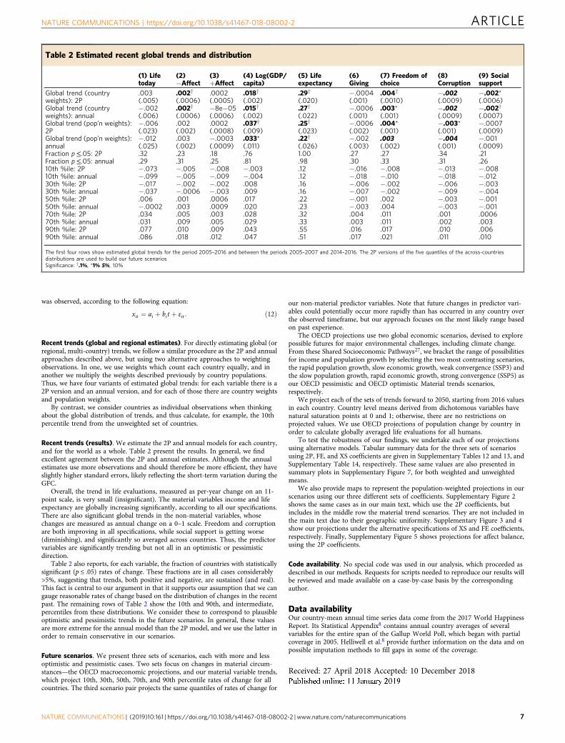
Recent trends (results). We estimate the 2P and annual models for each country,and for the world as a whole. Table 2 present the results. In general, we findexcellent agreement between the 2P and annual estimates. Although the annualestimates use more observations and should therefore be more efficient, they haveslightly higher standard errors, likely reflecting the short-term variation during theGFC.

Overall, the trend in life evaluations, measured as per-year change on an 11-point scale, is very small (insignificant). The material variables income and lifeexpectancy are globally increasing significantly, according to all our specifications.There are also significant global trends in the non-material variables, whosechanges are measured as annual change on a 0–1 scale. Freedom and corruptionare both improving in all specifications, while social support is getting worse(diminishing), and significantly so averaged across countries. Thus, the predictorvariables are significantly trending but not all in an optimistic or pessimisticdirection.

Table 2 also reports, for each variable, the fraction of countries with statisticallysignificant (p ≤ .05) rates of change. These fractions are in all cases considerably>5%, suggesting that trends, both positive and negative, are sustained (and real).This fact is central to our argument in that it supports our assumption that we cangauge reasonable rates of change based on the distribution of changes in the recentpast. The remaining rows of Table 2 show the 10th and 90th, and intermediate,percentiles from these distributions. We consider these to correspond to plausibleoptimistic and pessimistic trends in the future scenarios. In general, these valuesare more extreme for the annual model than the 2P model, and we use the latter inorder to remain conservative in our scenarios.

Future scenarios. We present three sets of scenarios, each with more and lessoptimistic and pessimistic cases. Two sets focus on changes in material circum-stances—the OECD macroeconomic projections, and our material variable trends,which project 10th, 30th, 50th, 70th, and 90th percentile rates of change for allcountries. The third scenario pair projects the same quantiles of rates of change for

our non-material predictor variables. Note that future changes in predictor vari-ables could potentially occur more rapidly than has occurred in any country overthe observed timeframe, but our approach focuses on the most likely range basedon past experience.

The OECD projections use two global economic scenarios, devised to explorepossible futures for major environmental challenges, including climate change.From these Shared Socioeconomic Pathways27, we bracket the range of possibilitiesfor income and population growth by selecting the two most contrasting scenarios,the rapid population growth, slow economic growth, weak convergence (SSP3) andthe slow population growth, rapid economic growth, strong convergence (SSP5) asour OECD pessimistic and OECD optimistic Material trends scenarios,respectively.

We project each of the sets of trends forward to 2050, starting from 2016 valuesin each country. Country level means derived from dichotomous variables havenatural saturation points at 0 and 1; otherwise, there are no restrictions onprojected values. We use OECD projections of population change by country inorder to calculate globally averaged life evaluations for all humans.

To test the robustness of our findings, we undertake each of our projectionsusing alternative models. Tabular summary data for the three sets of scenariosusing 2P, FE, and XS coefficients are given in Supplementary Tables 12 and 13, andSupplementary Table 14, respectively. These same values are also presented insummary plots in Supplementary Figure 7, for both weighted and unweightedmeans.

We also provide maps to represent the population-weighted projections in ourscenarios using our three different sets of coefficients. Supplementary Figure 2shows the same cases as in our main text, which use the 2P coefficients, butincludes in the middle row the material trend scenarios. They are not included inthe main text due to their geographic uniformity. Supplementary Figure 3 and 4show our projections under the alternative specifications of XS and FE coefficients,respectively. Finally, Supplementary Figure 5 shows projections for affect balance,using the 2P coefficients.

Code availability. No special code was used in our analysis, which proceeded asdescribed in our methods. Requests for scripts needed to reproduce our results willbe reviewed and made available on a case-by-case basis by the correspondingauthor.

Data availabilityOur country-mean annual time series data come from the 2017 World HappinessReport. Its Statistical Appendix8 contains annual country averages of severalvariables for the entire span of the Gallup World Poll, which began with partialcoverage in 2005. Helliwell et al.8 provide further information on the data and onpossible imputation methods to fill gaps in some of the coverage.

Received: 27 April 2018 Accepted: 10 December 2018

Table 2 Estimated recent global trends and distribution

(1) Lifetoday

(2)−Affect

(3)+Affect

(4) Log(GDP/capita)

(5) Lifeexpectancy

(6)Giving

(7) Freedom ofchoice

(8)Corruption

(9) Socialsupport

Global trend (countryweights): 2P

.003 .002† .0002 .018† .29† −.0004 .004† −.002 −.002*(.005) (.0006) (.0005) (.002) (.020) (.001) (.0010) (.0009) (.0006)

Global trend (countryweights): annual

−.002 .002† −8e−05 .015† .27† −.0006 .003* −.002 −.002†(.006) (.0006) (.0006) (.002) (.022) (.001) (.001) (.0009) (.0007)

Global trend (pop’n weights):2P

−.006 .002 .0002 .037† .25† −.0006 .004* −.003* −.0007(.023) (.002) (.0008) (.009) (.023) (.002) (.001) (.001) (.0009)

Global trend (pop’n weights):annual

−.012 .003 −.0003 .033* .22† −.002 .003 −.004 −.001(.025) (.002) (.0009) (.011) (.026) (.003) (.002) (.001) (.0009)

Fraction p≤.05: 2P .32 .23 .18 .76 1.00 .27 .27 .34 .21Fraction p≤.05: annual .29 .31 .25 .81 .98 .30 .33 .31 .2610th %ile: 2P −.073 −.005 −.008 −.003 .12 −.016 −.008 −.013 −.00810th %ile: annual −.099 −.005 −.009 −.004 .12 −.018 −.010 −.018 −.01230th %ile: 2P −.017 −.002 −.002 .008 .16 −.006 −.002 −.006 −.00330th %ile: annual −.037 −.0006 −.003 .009 .16 −.007 −.002 −.009 −.00450th %ile: 2P .006 .001 .0006 .017 .22 −.001 .002 −.003 −.00150th %ile: annual −.0002 .003 .0009 .020 .23 −.003 .004 −.003 −.00170th %ile: 2P .034 .005 .003 .028 .32 .004 .011 .001 .000670th %ile: annual .031 .009 .005 .029 .33 .003 .011 .002 .00390th %ile: 2P .077 .010 .009 .043 .55 .016 .017 .010 .00690th %ile: annual .086 .018 .012 .047 .51 .017 .021 .011 .010

The first four rows show estimated global trends for the period 2005–2016 and between the periods 2005–2007 and 2014–2016. The 2P versions of the five quantiles of the across-countriesdistributions are used to build our future scenariosSignificance: †.1%, *1% 5%, 10%

NATURE COMMUNICATIONS | https://doi.org/10.1038/s41467-018-08002-2 ARTICLE

NATURE COMMUNICATIONS | (2019) 10:161 | https://doi.org/10.1038/s41467-018-08002-2 | www.nature.com/naturecommunications 7

References1. Samir, K. C. & Wolfgang, L. The human core of the shared socioeconomic

pathways: population scenarios by age, sex and level of education for allcountries to 2100. Glob. Environ. Change 42, 181–192 (2017).

2. Hsiang, S. et al. Estimating economic damage from climate change in theUnited States. Science 356, 1362–1369 (2017).

3. Diener, E., Oishi, S. & Tay, L. Advances in subjective well-being research. Nat.Hum. Behav. 2, 253-260 (2018).

4. Global Happiness Council. Global Happiness Policy Report (Global HappinessCouncil, 2018).

5. Zhang, X., Zhang, X. & Chen, X. Happiness in the air: how does a dirty skyaffect mental health and subjective well-being? J. Environ. Econ. Manag. 85,81–94 (2017).

6. Tella, R. D., MacCulloch, R. J. & Oswald, A. J. The macroeconomics ofhappiness. Rev. Econ. Stat. 85, 809–827 (2003).

7. Helliwell, J. F., Huang, H., Grover, S. & Wang, S. Empirical linkagesbetween good governance and national well-being. J. Comp. Econ. 46,1332–1346 (2018).

8. Helliwell, J., Huang, H. & Wang, S. in World Happiness Report 2017 (edsHelliwell, J., Layard, R. & Sachs, J.) Ch. 2 (Sustainable Development SolutionsNetwork, 2017).

9. Tay, L., Herian, M. N. & Diener, E. Detrimental effects of corruption andsubjective well-being: whether, how, and when. Soc. Psychol. Pers. Sci. 5,751–759 (2014).

10. Aknin, L. B. et al. Prosocial spending and well-being: cross-cultural evidencefor a psychological universal. J. Pers. Soc. Psychol. 104, 635–652 (2013).

11. Pereira, H. M. et al. Scenarios for global biodiversity in the 21st century.Science 330, 1496–1501 (2010).

12. Rahmstorf., S. A semi-empirical approach to projecting future sea-level rise.Science 315, 368–370 (2007).

13. Thomas, C. D. et al. Extinction risk from climate change. Nature 427, 145(2004).

14. Mastrandrea, M. D. & Schneider, S. H. Probabilistic integrated assessment of“dangerous” climate change. Science 304, 571–575 (2004).

15. Warszawski, L. et al. The inter-sectoral impact model intercomparison project(ISI–MIP): project framework. Proc. Natl Acad. Sci. USA 111, 3228–3232(2014).

16. Pachauri, R. K. et al. Climate Change 2014: Synthesis Report. Contribution ofWorking Groups I, II and III to the Fifth Assessment Report of theIntergovernmental Panel on Climate Change (IPCC, Geneva, 2014).

17. Helliwell, J. F., Huang, H. & Wang, S. in Happiness Report 2016 (eds John, H.,Richard, L. & Jeffrey, F.) Ch. 2 (Sustainable Development Solutions Network,2016).

18. Easterlin, R. A. in Nations and Households in Economic Growth: Essays inHonour of Moses Abramovitz (eds David, P. A. & Reder, M. W.) 98–125(Academic Press, New York, 1974).

19. Easterlin, R. A., McVey, L. A., Switek, M., Sawangfa, O. & Zweig, J. S. Thehappiness–income paradox revisited. Proc. Natl Acad. Sci. USA 107, 22463-22468 (2010).

20. Oswald, A. J. & Powdthavee, N. Does happiness adapt? A longitudinal studyof disability with implications for economists and judges. J. Public Econ. 92,1061–1077, 6 (2008).

21. Tella, R. D., New, J. H.-D. & MacCulloch, R. Happiness adaptation to incomeand to status in an individual panel. J. Econ. Behav. Organ. 76, 834–852(2010).

22. Helliwell, J. F.& Barrington-Leigh, C. in The Social Cure: Identity, Health, andWell-being (eds Jetten, J., Haslam, C. & Haslam, S. A.) 55–71 (Taylor &Francis 2011).

23. Clark, A. E., Frijters, P. & Shields, M. A. Relative income, happiness, andutility: an explanation for the Easterlin paradox and other puzzles. J. Econ. Lit.46, 95–144 (2008).

24. Knack, S. & Keefer, P. Does social capital have an economic payoff? a cross-country investigation. Q. J. Econ. 112, 1251–1288 (1997).

25. Helliwell, J. F., Barrington-Leigh, C. P., Harris, A. & Huang, H. inInternational Differences in Well-Being (eds Diener, E., Helliwell, J. F. &Kahneman, D.) 213–229 (Oxford University Press, Oxford, 2010).

26. Layard, R., Clark, A. & Senik, C. in World Happiness Report (eds John, H.,Richard, L. & Jeffrey, F.) Ch. 3 (Earth Institute, 2012).

27. Dellink, R., Chateau, J., Lanzi, E. & Magné, B. Long-term economic growthprojections in the shared socioeconomic pathways. Glob. Environ. Change 42,200–214 (2017).

AcknowledgementsC.B.-L. acknowledges financial support from Canada’s Social Sciences and HumanitiesResearch Council grant 435-2016-0531. E.D.G. acknowledges financial support from theEuropean Research Council (ERC) under the European Union’s Horizon 2020 researchand innovation programme (grant agreement no. 682602), and from the Spanish Min-istry of Science, Innovation and Universities, through the María de Maeztu program forUnits of Excellence (MDM-2015-0552).

Author contributionsC.B.-L. and E.D.G. designed the research. C.B.-L. performed the data analysis andmodeling. C.B.-L. and E.D.G. wrote the paper.

Additional informationSupplementary Information accompanies this paper at https://doi.org/10.1038/s41467-018-08002-2.

Competing interests: The authors declare no competing interests.

Reprints and permission information is available online at http://npg.nature.com/reprintsandpermissions/

Journal peer review information: Nature Communications thanks the anonymousreviewers for their contribution to the peer review of this work. Peer reviewer reports areavailable.

Publisher’s note: Springer Nature remains neutral with regard to jurisdictional claims inpublished maps and institutional affiliations.

Open Access This article is licensed under a Creative CommonsAttribution 4.0 International License, which permits use, sharing,

adaptation, distribution and reproduction in any medium or format, as long as you giveappropriate credit to the original author(s) and the source, provide a link to the CreativeCommons license, and indicate if changes were made. The images or other third partymaterial in this article are included in the article’s Creative Commons license, unlessindicated otherwise in a credit line to the material. If material is not included in thearticle’s Creative Commons license and your intended use is not permitted by statutoryregulation or exceeds the permitted use, you will need to obtain permission directly fromthe copyright holder. To view a copy of this license, visit http://creativecommons.org/licenses/by/4.0/.

© The Author(s) 2019

ARTICLE NATURE COMMUNICATIONS | https://doi.org/10.1038/s41467-018-08002-2

8 NATURE COMMUNICATIONS | (2019) 10:161 | https://doi.org/10.1038/s41467-018-08002-2 | www.nature.com/naturecommunications