Embed Size (px)
Citation preview
i
›
FEASIBILITY STUDY OF CONTINUOUS REAL-TIME SPATIAL INTERPOLATION OF PHENOMENA USING BUILT-IN FUNCTIONLITY OF
A COMMERCIAL DATA STREAM MANAGEMENT SYSTEM
By Balaji Venkatesan
Project Advisor: Dr. Silvia Nittel
An Abstract of the Project Presented
in Partial Fulfillment of the Requirements for the
Degree of Master of Science
(in Spatial Information Science and Engineering)
May, 2013
Smartphones and tablets have made users crave for instant and latest updates. People extensively
rely and use these modern devices to know their surroundings. They have a dual role to play:
they get information and also can act as sensors, which can share data. This is made possible due
to the integration of low-cost, microsensors like accelerometers, proximity sensors, GPS,
ambient light sensors, compasses, etc. However, in the near future it is a possibility that
environmental sensors like those measuring humidity, temperature, certain particulate matters,
radiation levels, etc. might get deployed as well and then these sensors can act as mobile stations
which can share and update phenomenon of their surroundings. However, such applicability
means that spatial interpolation of the mass-measured phenomena must be done at near real time
so that users can also be clients ‘seeing’ the entirety of the phenomenon in their vicinity.
Managing such mass data updates from mobile sensors requires novel data management
technology that can keep up with processing this data onslaught, i.e. data stream management
ii
systems. There are a few out-of-the-box data stream solution offered by industries today. Some
prominent ones are Esper, IBM InfoSphere Streams, Microsoft StreamInsight, Oracle CEP,
StreamBase, etc. However, not much work has been done to use a DSMS and test out with
respect to real time spatial interpolation of continuous phenomena. The project explores whether
this type of real-time spatial interpolation of a continuous phenomena based on large number of
discrete sensor data streams can be accomplished by using the off-the-shelf functionalities
available in commercial DSMS available today. The project also introduces the concept of
spatial field data model, which provides a robust and an extensible framework to define fields
and their behavior. Finally, a DSMS application was built and tested with simulated data from
the Fukushima nuclear plant accident in Japan 2011. Experiments were conducted to test the
performance and analyze the bottlenecks of using a commercial DSMS.

iii
I would like to extend my sincere gratitude to all my friends, family and the Department of
Spatial Information Science and Engineering for their kind support and guidance. Especially, I
would like to thank my advisor Dr. Silvia Nittel for her guidance and support throughout the past
two years. Without her valuable inputs this project would not have obtained its fruitful result. I
shall also thank the members of the Geosensor Network Lab: Qinghan Liang and Mark A
Plummer for their feedback during project meetings. A special thanks to Professor Sytze de
Bruin and J.C. Whittier, for assisting with their expertise while developing the dataset for
running experiments. I like to thank Professors Kate Beard and Harlan Onsurd for serving as my
committee members and other professors who have impacted me in the past years.
I am grateful to my roommates Hengshan Li and Matthew Dube and other graduate students in
the School for their support and encouragement. Last but not the least, I thank the Graduate
School at the University of Maine and the Office of International Programs for their kind
support.
ACKNOWLEDGEMENT
iv
ACKNOWLEDGEMENT .................................................................................................................................. 3
TABLE OF CONTENTS ................................................................................................................................... 4
LIST OF FIGURES ........................................................................................................................................... 6
Chapter 1 : INTRODUCTION ...................................................................................................................... 1-‐1
1.1 Motivation ................................................................................................................................ 1-‐1
1.2 Project Objectives ..................................................................................................................... 1-‐3
1.3 Organization Of Project ............................................................................................................. 1-‐3
Chapter 2 : BACKGROUND AND RELATED WORK ........................................................................................ 4
2.1 Data Stream Management Systems (DSMS) ................................................................................ 4
2.2 Commercial DSMS Systems .......................................................................................................... 6
2.3 Oracle CEP .................................................................................................................................... 7
2.3.1 Architecture ......................................................................................................................... 7
2.3.2 Stream Queries .................................................................................................................... 9
2.4 Bottlenecks ................................................................................................................................ 10
2.5 Oracle Point Cloud (PC) .............................................................................................................. 11
2.6 Oracle Georaster (GR) ................................................................................................................ 12
Chapter 3 : REAL-‐TIME MONITORING OF CONTINUOUS PHENOMENA USING ORACLE CEP/SPATIAL ...... 14
3.1 Overview .................................................................................................................................... 14
3.2 Application Layer ....................................................................................................................... 15
3.2.1 Architecture ....................................................................................................................... 15
3.3 Components ............................................................................................................................... 16
3.4 Spatial Field Generator (SFG) ..................................................................................................... 17
3.5 Storage Architecture .................................................................................................................. 18
3.6 Visualization ............................................................................................................................... 19
Chapter 4 : Optimization ............................................................................................................................ 22
4.1 Overview .................................................................................................................................... 22
4.2 Multi-‐threaded IDW ................................................................................................................... 23
4.3 Block Read/Write via BLOBs ...................................................................................................... 24
TABLE OF CONTENTS
v
Chapter 5 : Performance Evaluation .......................................................................................................... 27
5.1 Overview .................................................................................................................................... 27
5.2 Data sets .................................................................................................................................... 27
5.3 Test Setup .................................................................................................................................. 29
5.3.1 Client Setup ........................................................................................................................ 29
5.3.2 Server Setup ....................................................................................................................... 30
5.4 Experiment Configuration .......................................................................................................... 31
5.4.1 IDW Interpolation Performance Result .............................................................................. 32
5.4.2 Visualization/Georaster Creation Performance Result ...................................................... 34
5.4.3 Discussion of Results ......................................................................................................... 36
Chapter 6 : Conclusions And Future Work ................................................................................................. 37
BIBLIOGRAPHY ........................................................................................................................................... 39
vi
Figure 2.1: Data stream ............................................................................................................................... 4
Figure 2.2: Oracle CEP Architecture ............................................................................................................ 8
Figure 2.3: A generic EPN ............................................................................................................................ 9
Figure 2.4: Temperature Point Cloud over Orono .................................................................................... 11
Figure 2.5: Point Cloud Data Type Storage ............................................................................................... 12
Figure 2.6: Oracle Georaster Data model ................................................................................................. 13
Figure 3.1: Overview ................................................................................................................................. 14
Figure 3.2: Event Processing Network ...................................................................................................... 16
Figure 3.3: Spatial Field Generator ........................................................................................................... 17
Figure 3.4: Sensor Data Storage Architecture ........................................................................................... 18
Figure 4.1: Work Order/Tile ...................................................................................................................... 23
Figure 4.2: Producer Consumer IDW interpolation module ..................................................................... 24
Figure 4.3: BLOB read/write ..................................................................................................................... 25
Figure 5.1: Data Set Generation in NetLogo ............................................................................................. 28
Figure 5.2: Load Generator with 128 sensors ........................................................................................... 29
Figure 5.3: Oracle CEP JRockit Server ........................................................................................................ 30
Figure 5.4: IDW Interpolation Performance Test Result ........................................................................... 33
Figure 5.5: Georaster Creation Performance Test Results ........................................................................ 35
LIST OF FIGURES
1
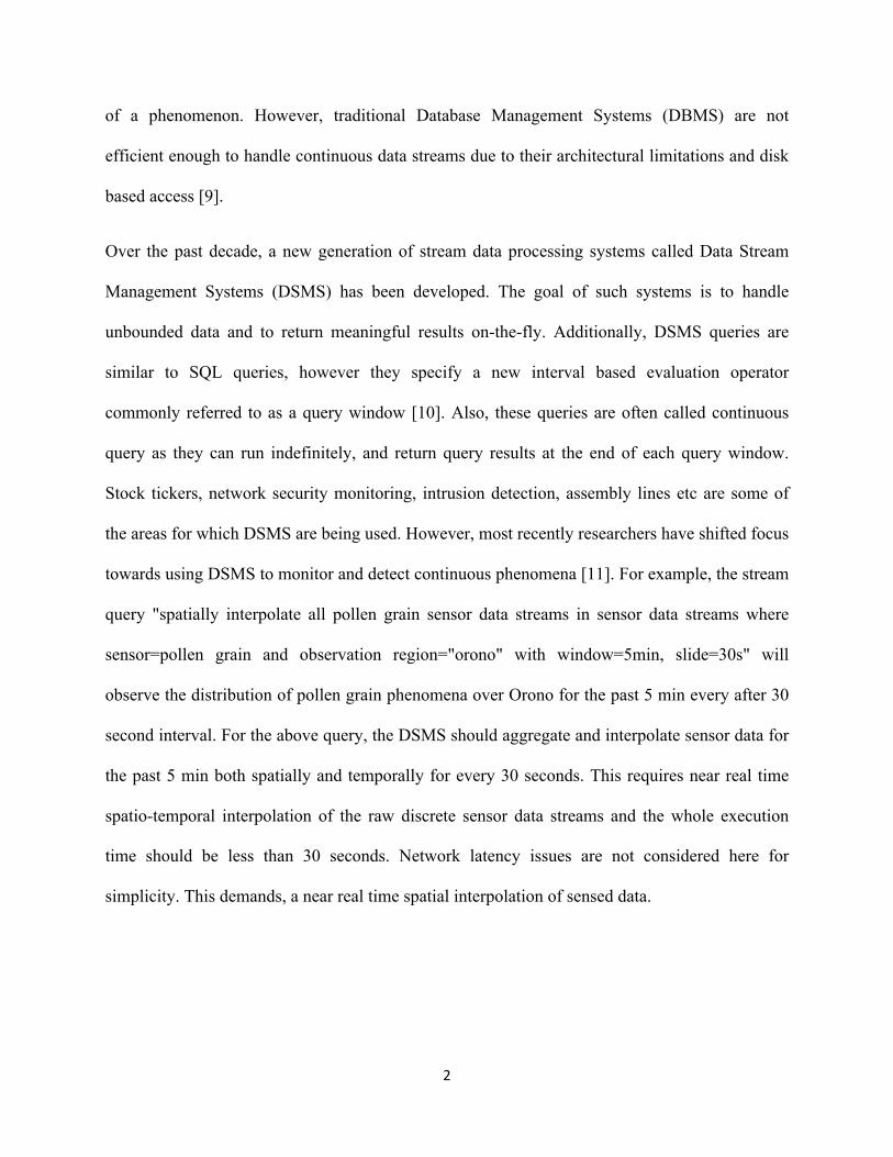
1.1 Motivation
The unprecedented developments in the micro-electromechanical systems (MEMS) [6] world are
producing robust, inexpensive sensors ranging in size from a few microns to millimeters. Our
mobile phones for instance carry a host of sensors like accelerometer, proximity, GPS, ambient
light, compass etc. As Smartphones and tablets are becoming more and more sophisticated, it is
only a matter of time when they will come shipped with other environmental sensors like those
measuring temperature, noise, air quality, ozone, radiation level etc [7]. The reason why these
handheld devices are favorites as sensors for measuring physical phenomena is because they
have access to wireless networks and can accurately measure their location using GPS.
Altogether, in the near future, common users can become mobile sensing stations and can
perform participatory sharing [7] of their surroundings, which could help people to have a more
precise understanding of their locality.
Imagine a person suffering from asthma and he/she would like to take an evening stroll in the
park. All the other visitors who are currently in the park can continuously participate in
streaming air quality data, which could enable the asthma affected person to make a better
informed decision about when to take a stroll in a park or which route is safer. Since mobile
sensor data stream provides point based physical quantity measurement of a specific geographic
region, they provide discrete representation of the underlying phenomena. So, spatial
interpolation of individual sensor data stream is necessary to generate continuous representation
Chapter 1 : INTRODUCTION
2
of a phenomenon. However, traditional Database Management Systems (DBMS) are not
efficient enough to handle continuous data streams due to their architectural limitations and disk
based access [9].
Over the past decade, a new generation of stream data processing systems called Data Stream
Management Systems (DSMS) has been developed. The goal of such systems is to handle
unbounded data and to return meaningful results on-the-fly. Additionally, DSMS queries are
similar to SQL queries, however they specify a new interval based evaluation operator
commonly referred to as a query window [10]. Also, these queries are often called continuous
query as they can run indefinitely, and return query results at the end of each query window.
Stock tickers, network security monitoring, intrusion detection, assembly lines etc are some of
the areas for which DSMS are being used. However, most recently researchers have shifted focus
towards using DSMS to monitor and detect continuous phenomena [11]. For example, the stream
query "spatially interpolate all pollen grain sensor data streams in sensor data streams where
sensor=pollen grain and observation region="orono" with window=5min, slide=30s" will
observe the distribution of pollen grain phenomena over Orono for the past 5 min every after 30
second interval. For the above query, the DSMS should aggregate and interpolate sensor data for
the past 5 min both spatially and temporally for every 30 seconds. This requires near real time
spatio-temporal interpolation of the raw discrete sensor data streams and the whole execution
time should be less than 30 seconds. Network latency issues are not considered here for
simplicity. This demands, a near real time spatial interpolation of sensed data.
3
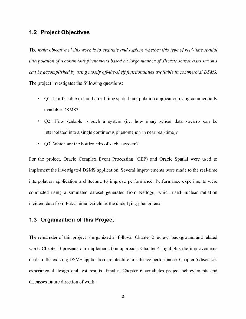
1.2 Project Objectives
The main objective of this work is to evaluate and explore whether this type of real-time spatial
interpolation of a continuous phenomena based on large number of discrete sensor data streams
can be accomplished by using mostly off-the-shelf functionalities available in commercial DSMS.
The project investigates the following questions:
• Q1: Is it feasible to build a real time spatial interpolation application using commercially
available DSMS?
• Q2: How scalable is such a system (i.e. how many sensor data streams can be
interpolated into a single continuous phenomenon in near real-time)?
• Q3: Which are the bottlenecks of such a system?
For the project, Oracle Complex Event Processing (CEP) and Oracle Spatial were used to
implement the investigated DSMS application. Several improvements were made to the real-time
interpolation application architecture to improve performance. Performance experiments were
conducted using a simulated dataset generated from Netlogo, which used nuclear radiation
incident data from Fukushima Daiichi as the underlying phenomena.
1.3 Organization of this Project
The remainder of this project is organized as follows: Chapter 2 reviews background and related
work. Chapter 3 presents our implementation approach. Chapter 4 highlights the improvements
made to the existing DSMS application architecture to enhance performance. Chapter 5 discusses
experimental design and test results. Finally, Chapter 6 concludes project achievements and
discusses future direction of work.
4
2.1 Data Stream Management Systems (DSMS)
A Data Stream Management System [13] is a software system designed to manage continuous
data streams as found in financial application, and real-time traffic, emergency or intrusion
monitoring applications. Data streams are considered continuous because the amount of data
arriving at a particular time is unbounded or cannot be pre-determined. Common sources of these
data are readings generated from sensors that measure physical properties of their surroundings
like temperature, pressure, noise, air quality, radiation etc. Other sources include process that
need constant monitoring like the share price data from stock markets, data packets from
network for detecting threats and so on. An important property of these data sources is that they
are push-based. They sense and keep transmitting sensed value to their destination at a specific
rate. Additionally, these sensors can timestamp the data before sending, or in some cases, DSMS
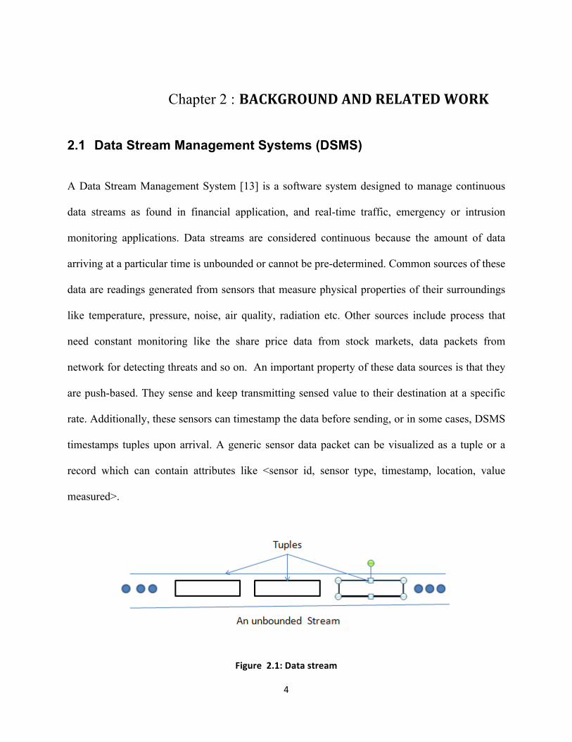
timestamps tuples upon arrival. A generic sensor data packet can be visualized as a tuple or a
record which can contain attributes like <sensor id, sensor type, timestamp, location, value
measured>.
Figure 2.1: Data stream
Chapter 2 : BACKGROUND AND RELATED WORK
5
In traditional DBMS, queries are evaluated by pulling data from disk. However, in DSMS this is
reversed: here queries get evaluated based on data pushed by data sources [14]. Moreover,
traditional queries are executed one time, whereas queries running in DSMS are continuously re-
evaluated and often run indefinitely on the arriving data. This reversal of roles for data and query
meant that new strategies have to developed to handle new challenges:
• Continuous Query Model: Traditional DBMS queries operate on a finite data set (i.e. a
relation) and assume a set-based semantics on data, i.e. they don't have to consider the
order of data. However, continuous queries operate indefinitely on an unbounded data set
and take order of data into consideration using additional specification for query
evaluation intervals also called query windows [10].
• Low Latency: Data from streams generally are critical for answering real time queries, so
their significance is short-lived. For instance, pollen grain distribution over a park will
keep on changing with time, due to wind influence. So, latest data from a sensor stream is
more important than past data here. Past data could be used for prediction and performing
other statistical inferences. Nevertheless, stream data processing must be done at near real
time with very low latency to leverage real time data.
• Variable data rate: The data arrival rate for stream based application could be from few
hundreds to millions updates per second. Additionally, the data could be busty in nature
due to fluctuations in the sensor update rates or due to transmission delays. Irrespective
of the bottlenecks, DSMS must be robust and high performance oriented.
6
2.2 Commercial DSMS Systems
Today, research in DSMS has resulted in several commercial DSMS, among them are open
source Esper [1], IBM InfoSphere Streams [2], Microsoft StreamInsight [3], StreamBase [5] and
Oracle CEP [4] as major ones.
Esper [1] stands for event stream processing and correlation. It is a real time data stream
processing solution from EsperTech Inc. Released in July 2006, it is available in three variations
- Esper Enterprise Edition, Esper and EsperHA. It is mainly written in Java and can be embedded
into any java process. A open source version is also available.
In IBM InfoSphere Streams, applications are built by developing graphical data flow graphs. A
data flow graph serves as an overview of the entire system, which consists of set of nodes which
are distributed in no-sharing clusters and interconnected by streams [2]. There are several
operators defined to perform data stream analytics. Each node consists of Processing
Elements(PE) which serves as a container for operators.
Microsoft StreamInsight [3] is a platform to develop and deploy complex event based application
using.Net framework. The product is included with SQL Server 2008 R2. The queries are written
in LINQ (Language Integrated Query). LINQ enables specifying query constructs as strong
typed classes thereby eliminating the need to learn query syntax for different databases.
However, StreamInsight uses an adapter model for the input and output of data [17]. This means
that one can build generic components, which could be reused in different applications.
StreamBase LiveView [5] is a push-based real time analytics solution that consumes data from
streaming real time data sources. It uses Dynamic Stream Compiler technology, which compiles

7
multiple queries into one efficient execution query. Queries are written in StreamSQL, which is
an extension of the standard SQL model. Applications can be developed in Java, C++ and
Python and offers a range of adapters, which could be used to connect to files, databases,
visualization and statistical tools.
Oracle Complex Event Processing (CEP) [4] is an event driven architecture for handling stream
data. Users can create application by designing an Event Processing Network (EPN) whose
nodes represents event sources, sinks, processors and stream channels. Processors are
components capable of processing events by defining queries in Continuous Query Language
(CQL). CQL is an extension of standard SQL with additional constructs to support stream
processing.
Therefore, most commercial applications offer almost similar benefits of lower latency, high
scalability, higher throughput, and better performance. The choice of selecting one application
over another depends upon business model, license, cost effectiveness and ease of
implementation. However, Oracle CEP was chosen to implement and run experiments for this
project simply due to easy of development and familiarity of the programming language used as
well as the spatial functionality available with the Oracle product family
2.3 Oracle CEP
2.3.1 Architecture
The heart of the Oracle Complex Event Processing architecture is the CEP server. The CEP
server provides a run time environment to deploy DSMS application. It also provides adapters to
interface with other external application via HTTP, Java Messaging Service, and ODBC

8
protocols. Oracle CEP provides rich libraries, which define components that could be used to
build DSMS application using a development IDE like Eclipse.
Figure 2.2: Oracle CEP Architecture
Applications are built by modeling data flow streams in a graphical interface called Event
Processing Network (EPN) as shown in Figure 2.3. Some important stream processing
components available to build an EPN are:
• Adapters - Converts incoming raw data stream packets into a normalized tuple/event that
can be queried. They directly interface to inbound/outbound stream, sources and sinks.
They are data transformation component that connects to an external application or
sensors.
• Channels- Act like streams through which tuple/event data travels.
• Processors- Continuous queries are managed and run inside a processor component.
These are sites for continuous query execution and management.
• Beans- Beans are basically classes with different roles like client, event etc. A client bean
class can listen to events/tuples generated from query execution. An event bean class can
9
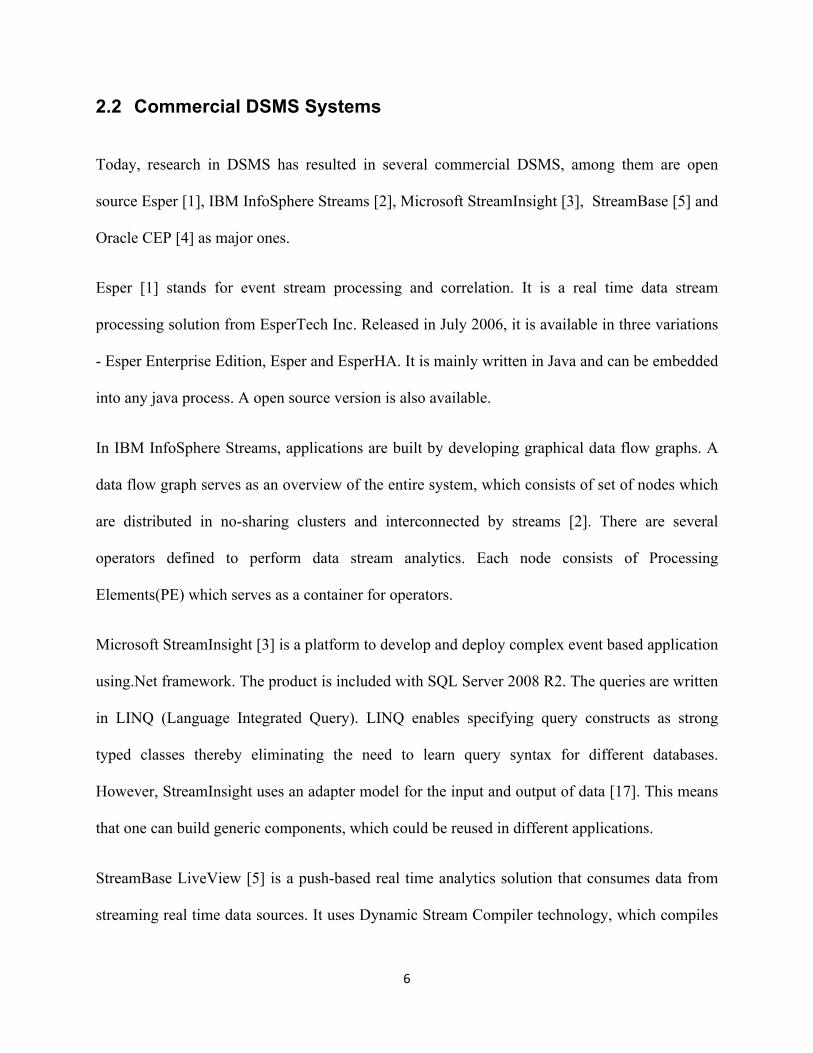
be used to normalize raw sensor data to an event type object. Adapters use event bean for
normalization of raw sensor data.
Figure 2.3: A generic EPN
2.3.2 Stream Queries
Stream Queries are defined using Continuous Query Language (CQL) that run inside a PE, as
shown in the Figure 2.3. CQL is a stream query language that is built by extending the standard
Structured Query Language (SQL) library. Therefore, both syntax and semantics of defining a
query remains intact. However, new operators are defined to support stream processing like
STREAM, RELATION, NOW, RANGE, PARTITION, JOIN, SLIDE, WINDOW,
UNBOUNDED, ISTREAM, DSTREAM, RSTREAM etc [19].
A STREAM is a sequence of time stamped tuples. It has no bounds. A RELATION is a bag of
tuples at a particular instance of time. RELATION is the same concept as a traditional table and
hence supports execution of all traditional query operators. NOW represents current time.
10
WINDOW represents a query interval which could be time or value based. RANGE is used to
define time based window length. SLIDE is used to define continuous window query interval.
For example, a slide of 5 seconds defined for a query window will execute the query every after
every 5 seconds.
For example a query, ISTREAM( select max(temperature) from temperature sensor stream where
window(range 5min,slide 1min) ) will produce an output stream with maximum temperature
value for the past 5 minutes after every 1 minute interval.
2.4 Bottlenecks
Oracle CEP, like other commercial DSMS described before, lacks an in-built solution to handle
spatial data. Most commercial systems provide adapters to external DBMS that provides a rich
spatial data model [3]. So, DSMS uses database drivers to establish connection to store, manage
and query spatial data. Oracle CEP uses JDBC drivers to use Oracle Spatial for spatial data
management.
Stream queries monitoring environmental data are rich in spatial data. An end user will normally
be interested in a phenomenon surrounding his/her location. So, stream query language must
provide constructs to define spatial queries. Consider a query from our motivation scenario:
"spatially interpolate all pollen grain sensor data streams in sensor data streams where
sensor=pollen grain and observation region="orono" with window=5min, slide=30s". The
following query has to filter stream data based on its extent information (orono) and also
interpolate all the valid tuples to produce a continuous representation of phenomena as output.
Therefore, DSMS can use traditional DBMS to leverage spatial operations such as indexing,
interpolation and querying of spatial data. DSMS stores data in memory, whereas DBMS stores

11
data on disk. This is a big limitation because memory-based significantly access is faster than
disk-based. To improve read performance, DBMS offers options like caching, temporary table
and in-memory database. However, most options currently do not support spatial data, and pre-
caching of spatial tables although improves read performance, but requires a disk access upon
update.
2.5 Oracle Point Cloud (PC)
Oracle Point Cloud (SDO_PC) data type is generally used to store, manage and query multi-
dimensional point data inside Oracle Spatial. It can store up to 4x10¹⁸ points in a single point
cloud object. Imagine the Figure 2.4 shows the temperature phenomenon over Orono. Here
individual pixels can be considered as three-dimensional points with latitude, longitude, and
temperature attributes. These points collectively are stored inside a point cloud object, which has
the extent of Orono.
Figure 2.4: Temperature Point Cloud over Orono
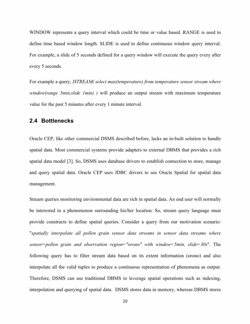
PC data is stored in two tables [20] - one that contains the logical representation of the point
cloud object and the other contains the individual data blocks of spatially indexed BLOB data,
which stores point data in raw format as shown in Figure 2.5.
12
Figure 2.5: Point Cloud Data Type Storage
The raw data of PC objects are spatially indexed. By default Oracle uses R-Tree indexing for
spatial data. Spatial operations like SDO_INTERACT, SDO_NN, SDO_FILTER, CLIP_PC can
be used on PC. SDO_INTERACT tests whether two features intersect each other. SDO_NN
operator returns the nearest neighbor given a distance. SDO_FILTER operator can be used to
find all the points inside a point cloud, which satisfies a given condition. Finally, SDO_CLIP
operator extracts a subset of a point cloud given an intersecting extent.
2.6 Oracle Georaster (GR)
Oracle Georaster (GR) [21] is an Oracle component that enables storing, indexing, querying,
analyzing and visualizing gridded or raster data. The GR objects can be geo-referenced and can
be used to find a cell in an image corresponding to a location on earth or vice-versa. Oracle
provides both Java and the SQL API to manage GR data. Also, it provides tools to export and
visualize GR data in various image formats such as GeoTIFF, DEM, JPEG, BMP . GR data is
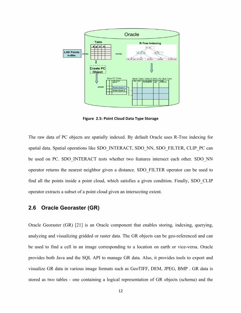
stored as two tables - one containing a logical representation of GR objects (schema) and the
13
other containing the spatially indexed data as BLOBS partitioned into several blocks as shown in
Figure 2.6.
Figure 2.6: Oracle Georaster Data model
Each GR contains two coordinate systems: the cell coordinate system –it is used to describe cells
in raster matrix, and the model coordinate system also called ground coordinate system- it is used
to describe points on earth. GR have multi-layer or multi-band concept where each layer can be a
raster with a different timestamp. Such a GR is called time series multilayer image. Also, Oracle
provides a rich set of libraries with functions to manipulate, create, query, and export GR
objects.
14
3.1 Overview
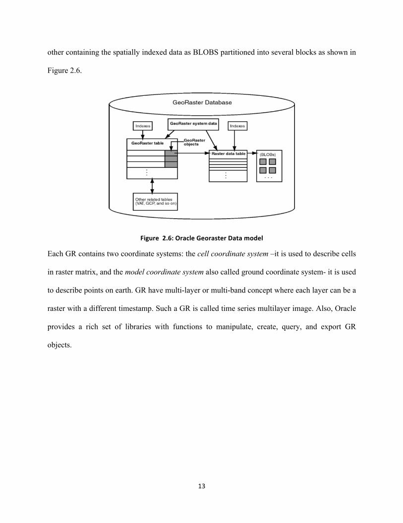
Figure 3.1 gives an overview of the implemented real-time phenomenon monitoring DSMS
application implemented in Oracle CEP. There are three layers - the data layer (bottom), the
application layer (middle), and the client layer (top most). The data layer consists of mobile
sensors, which continuously sense and transmit data over a wireless medium.
Figure 3.1: Overview
. The Application layer is the heart of the DSMS, which operates on the raw sensor data stream
and converts them into meaningful results for end users. The application layer was implemented
the following way: a) it uses in-built components from both Oracle CEP and Oracle Spatial, and
Chapter 3 : REAL-‐TIME MONITORING OF CONTINUOUS PHENOMENA USING ORACLE
CEP/SPATIAL
15
b) two new components, i.e. the Spatial Field Generator Module and the Interpolation Module,
were implemented. In this project, we abstract continuous phenomena as Spatial Fields, thus, the
Spatial Field Generator maps raw sensor data streams to Spatial Fields. The spatial field object
provides an abstract/logical representation of a physical field. Users or end application can use
libraries or functions defined for spatial field object to visualize, query, and manipulate field
data. Therefore, users only interact with the spatial field object for their submitted queries. In the
project, additionally the Interpolation component was implemented which ‘exports’ a spatial
field as a raster image. The Spatial Field Generator Module is deployed on Oracle CEP, whereas
the Interpolation Module is installed on Oracle Spatial.
3.2 Application Layer
3.2.1 Architecture
An Oracle CEP application is built by constructing a data stream query network called EPN
(Event Processing Networks), which consists of different components like Adapters, Channels,
Processors, Beans and Event Beans as discussed in the previous chapter. Each component
operates in a non-blocking fashion by pulling, processing, and pushing tuples from an inbound
stream into an outbound stream. Streams are basically implemented as a queue, which holds
tuples. All the components simultaneously produce and consume tuples. A continuous query
executes a process element component, which validates tuples from an incoming sensor stream
and outputs the selected tuples into an output channel. The selected tuples can be stored to a
memory or a disk. Leveraging, this feature the Spatial Field Generator (SFG) was built, which
16
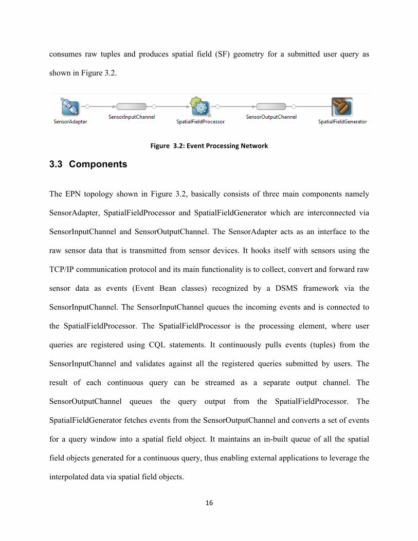
consumes raw tuples and produces spatial field (SF) geometry for a submitted user query as
shown in Figure 3.2.
Figure 3.2: Event Processing Network
3.3 Components
The EPN topology shown in Figure 3.2, basically consists of three main components namely
SensorAdapter, SpatialFieldProcessor and SpatialFieldGenerator which are interconnected via
SensorInputChannel and SensorOutputChannel. The SensorAdapter acts as an interface to the
raw sensor data that is transmitted from sensor devices. It hooks itself with sensors using the
TCP/IP communication protocol and its main functionality is to collect, convert and forward raw
sensor data as events (Event Bean classes) recognized by a DSMS framework via the
SensorInputChannel. The SensorInputChannel queues the incoming events and is connected to
the SpatialFieldProcessor. The SpatialFieldProcessor is the processing element, where user
queries are registered using CQL statements. It continuously pulls events (tuples) from the
SensorInputChannel and validates against all the registered queries submitted by users. The
result of each continuous query can be streamed as a separate output channel. The
SensorOutputChannel queues the query output from the SpatialFieldProcessor. The
SpatialFieldGenerator fetches events from the SensorOutputChannel and converts a set of events
for a query window into a spatial field object. It maintains an in-built queue of all the spatial
field objects generated for a continuous query, thus enabling external applications to leverage the
interpolated data via spatial field objects.

17
3.4 Spatial Field Generator (SFG)
Figure 3.3: Spatial Field Generator
The Spatial Field Generator is an independent, pluggable component, which can be reused to
convert raw sensor data into spatial field object. The spatial field data model consists of a
hierarchy of classes, which store data either in memory or in a database. The Spatial Field can be
seen as a collection of n-dimensional points (Point Cloud) over a geographic region. Each point
in a Point Cloud (PC) contains location and other physical/logical information such as
timestamp, measured value, and sensor id. For instance, a point in a temperature field can consist
of latitude, longitude, timestamp, temperature value, device id, and other metadata information.
These parameters can be used to index points spatially, temporarily or parametrically. Generally
a two dimensional indexing is built using the location coordinates. However, other parameters
from a multi-dimensional point could be used to index in other dimensions as well.
The SFG produces objects of type spatial field. A spatial field object encapsulates point data and
specifies a set of properties and rules to manipulate or interact with data. This opens up a whole
new way of working with data as fields. The fields can also interact with each other as in the real
18
world: for example, an interaction of a wind field with a fire field, or an interaction of pollen
grain over a wind field. However, the interaction among spatial fields is beyond the scope of this
project. The goal of this project is to prototype a basic spatial field data model framework with
built-in commercial DSMS functionality and test the scalability and performance of such code
when performing spatial interpolation in near real time.
3.5 Storage Architecture
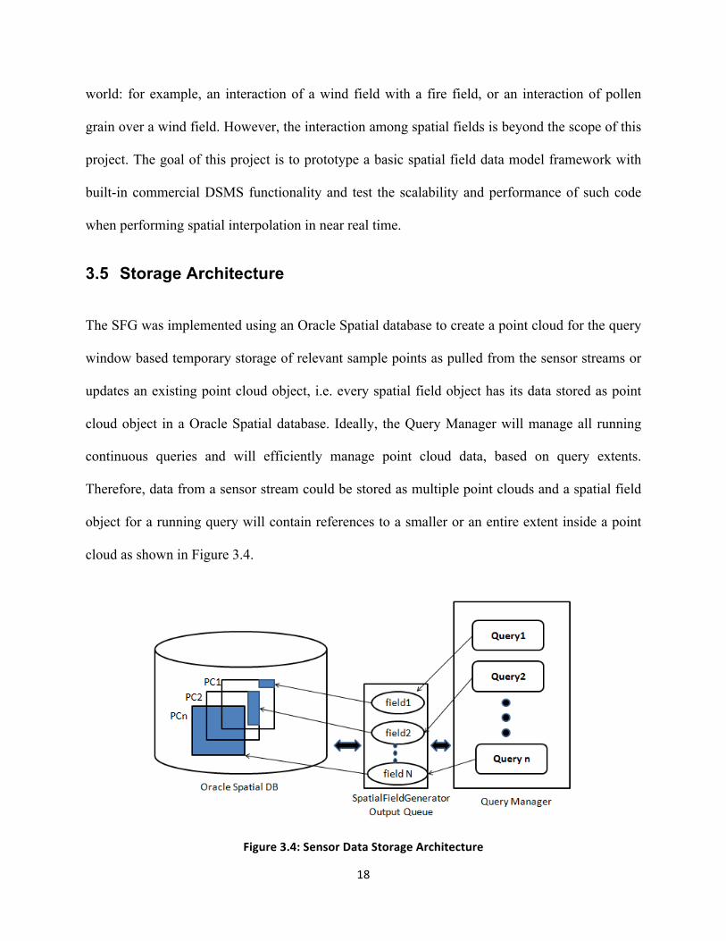
The SFG was implemented using an Oracle Spatial database to create a point cloud for the query
window based temporary storage of relevant sample points as pulled from the sensor streams or
updates an existing point cloud object, i.e. every spatial field object has its data stored as point
cloud object in a Oracle Spatial database. Ideally, the Query Manager will manage all running
continuous queries and will efficiently manage point cloud data, based on query extents.
Therefore, data from a sensor stream could be stored as multiple point clouds and a spatial field
object for a running query will contain references to a smaller or an entire extent inside a point
cloud as shown in Figure 3.4.
Figure 3.4: Sensor Data Storage Architecture
19
Oracle Point Cloud can support millions of data points and has capabilities to perform filter,
query, index, and extract operations. N-dimensional point geometry can be stored in a point
cloud and these dimensions can be used for spatial indexing as well. For example, latitude,
longitude, and timestamp information from a point can be used to spatially index a point cloud
data in both space and time. Therefore, point cloud provides a very convenient and flexible
approach to temporarily store and manage raw sensor data. As sensor data arrives via sensor data
streams, they are mapped to respective event (tuple) and converted to a 3D point, and inserted
into an existing point cloud, which is indexed by space and timestamp. Lets denote all the data
points belonging to a specific time interval as a layer. Since data in a DSMS arrives indefinitely,
older layers are either archived or deleted from a point cloud. So, at a specific time, only n
number of layers in a point cloud object exist. The value for n and management of layers in a
point cloud object is beyond the scope of this project. However, it must be noted that an
optimum value for n is determined based on currently active queries and may change whenever a
new query is submitted by a user.
3.6 Visualization
Each output for a query window is a spatial field object, which can be visualized in various
ways. The simplest form of visualization is a raster image after interpolation using IDW, Kriging
or any other spatial interpolation method. However, IDW is chosen for the project because of its
simplicity and ease of implementation as discussed in Chapter 2. Inverse Distance Weighing
(IDW) is a deterministic spatial interpolation technique that uses weighted average function to
calculate values at unknown points. The basic idea is that things that are closer in space are more
likely to be alike than if they are farther apart. To predict a value at an unmeasured location,
20
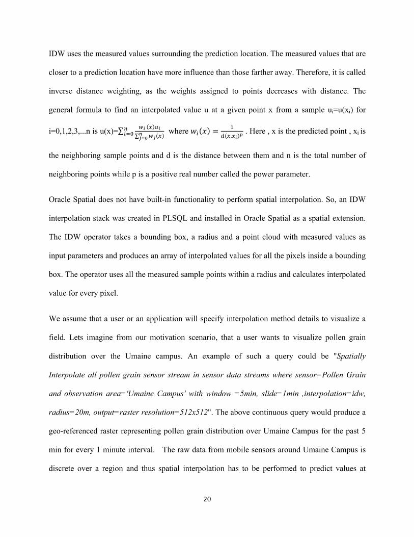
IDW uses the measured values surrounding the prediction location. The measured values that are
closer to a prediction location have more influence than those farther away. Therefore, it is called
inverse distance weighting, as the weights assigned to points decreases with distance. The
general formula to find an interpolated value u at a given point x from a sample ui=u(xi) for
i=0,1,2,3,...n is u(x)= !! ! !!!! !!
!!!
!!!! where 𝑤! 𝑥 = !
! !,!! ! . Here , x is the predicted point , xi is
the neighboring sample points and d is the distance between them and n is the total number of
neighboring points while p is a positive real number called the power parameter.
Oracle Spatial does not have built-in functionality to perform spatial interpolation. So, an IDW
interpolation stack was created in PLSQL and installed in Oracle Spatial as a spatial extension.
The IDW operator takes a bounding box, a radius and a point cloud with measured values as
input parameters and produces an array of interpolated values for all the pixels inside a bounding
box. The operator uses all the measured sample points within a radius and calculates interpolated
value for every pixel.
We assume that a user or an application will specify interpolation method details to visualize a
field. Lets imagine from our motivation scenario, that a user wants to visualize pollen grain
distribution over the Umaine campus. An example of such a query could be "Spatially
Interpolate all pollen grain sensor stream in sensor data streams where sensor=Pollen Grain
and observation area='Umaine Campus' with window =5min, slide=1min ,interpolation=idw,
radius=20m, output=raster resolution=512x512". The above continuous query would produce a
geo-referenced raster representing pollen grain distribution over Umaine Campus for the past 5
min for every 1 minute interval. The raw data from mobile sensors around Umaine Campus is
discrete over a region and thus spatial interpolation has to be performed to predict values at
21
unmeasured location. The output raster image of 512x512 resolution is first geo-referenced to a
query region and then its pixel values are determined by the interpolation method defined in a
query. Oracle Spatial provides the Georaster type to create raster objects, which can be geo-
referenced and allows capabilities like filter, query, extract and index operation as discussed in
Chapter 2. Therefore, once a Georaster object is created, it can be used by end applications to
query and extract information according to their needs, at a future time as well.
22
4.1 Overview
This project is a feasibility study implementing the spatial interpolation of large numbers of
sensor data streams continuously into raster representation using built-in functionality of a
commercial DSMS. In Chapter 3, we showed the overview of this approach. In this chapter, we
discuss bottlenecks of the implementation and several optimizations we implemented.
At the core of the problem is that spatial interpolation algorithms are both memory and CPU
expensive operation [12]. Generally, spatial interpolation time depends upon resolution and
extent of an interpolated region, and the interpolation algorithm used. A 512x512 resolution
image contains a quarter million points. To perform interpolation at each point, an IDW
interpolator fetches neighboring sample points that are located within a defined radius and
calculates a new predicted value. Here, processing time is directly proportional to both number
of points and radius. However, both the parameters mentioned are variable and defined by a user
query.
Different approaches have been developed to reduce processing time by applying strategies like
finding the kNN points and adaptive kNN for skewed, which reduces the number of neighboring
cells needed for interpolating a point [23]. However, this project aims primarily at exploring
spatial interpolation performance using the traditional IDW operator within a DSMS and DBMS
mixed environment and foremost faster read/write access, which are a basic bottleneck in a
mixed data stream/database environment, were explored to improve performance.
Chapter 4 : Optimization
23
4.2 Multi-threaded IDW
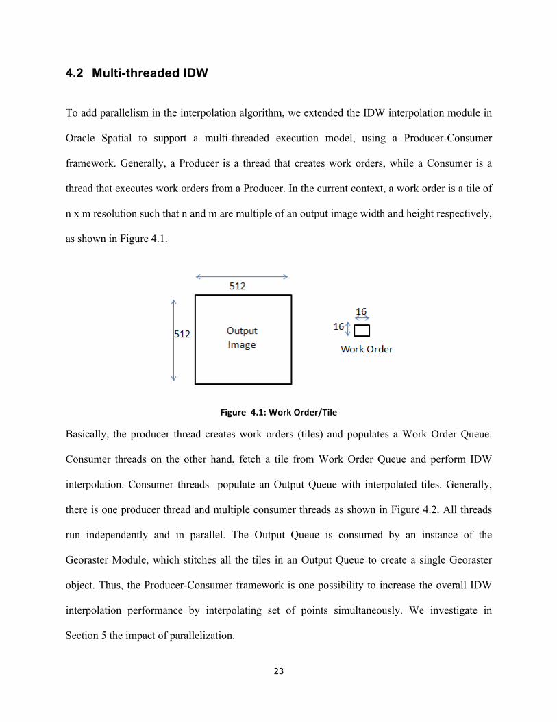
To add parallelism in the interpolation algorithm, we extended the IDW interpolation module in
Oracle Spatial to support a multi-threaded execution model, using a Producer-Consumer
framework. Generally, a Producer is a thread that creates work orders, while a Consumer is a
thread that executes work orders from a Producer. In the current context, a work order is a tile of
n x m resolution such that n and m are multiple of an output image width and height respectively,
as shown in Figure 4.1.
Figure 4.1: Work Order/Tile
Basically, the producer thread creates work orders (tiles) and populates a Work Order Queue.
Consumer threads on the other hand, fetch a tile from Work Order Queue and perform IDW
interpolation. Consumer threads populate an Output Queue with interpolated tiles. Generally,
there is one producer thread and multiple consumer threads as shown in Figure 4.2. All threads
run independently and in parallel. The Output Queue is consumed by an instance of the
Georaster Module, which stitches all the tiles in an Output Queue to create a single Georaster
object. Thus, the Producer-Consumer framework is one possibility to increase the overall IDW
interpolation performance by interpolating set of points simultaneously. We investigate in
Section 5 the impact of parallelization.
24
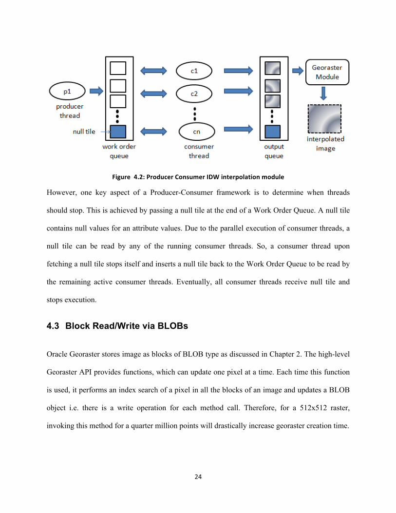
Figure 4.2: Producer Consumer IDW interpolation module
However, one key aspect of a Producer-Consumer framework is to determine when threads
should stop. This is achieved by passing a null tile at the end of a Work Order Queue. A null tile
contains null values for an attribute values. Due to the parallel execution of consumer threads, a
null tile can be read by any of the running consumer threads. So, a consumer thread upon
fetching a null tile stops itself and inserts a null tile back to the Work Order Queue to be read by
the remaining active consumer threads. Eventually, all consumer threads receive null tile and
stops execution.
4.3 Block Read/Write via BLOBs
Oracle Georaster stores image as blocks of BLOB type as discussed in Chapter 2. The high-level
Georaster API provides functions, which can update one pixel at a time. Each time this function
is used, it performs an index search of a pixel in all the blocks of an image and updates a BLOB
object i.e. there is a write operation for each method call. Therefore, for a 512x512 raster,
invoking this method for a quarter million points will drastically increase georaster creation time.
25
Alternatively, reading a BLOB object and updating all its content in memory and writing all the
updated values at once will improve performance. In this approach, for each BLOB there is a
single write operation, whereas in the previous approach each pixel update accompanies a write
operation. The Interpolation module works at tile level such that, a tile extent is same as block
extent i.e. there is 1:1 mapping between an interpolated tile and a georaster block object. For
each interpolated tile, a matching georaster block object is read into memory, and the pixel
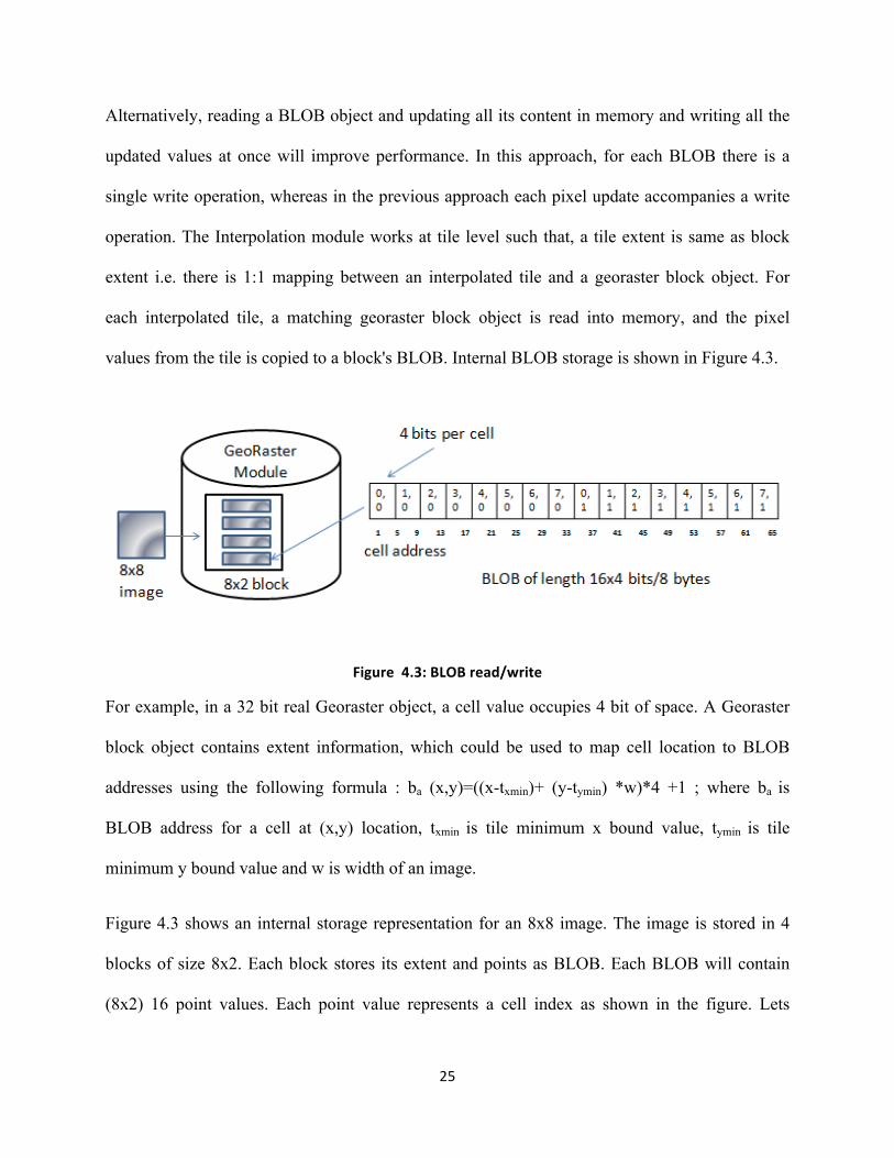
values from the tile is copied to a block's BLOB. Internal BLOB storage is shown in Figure 4.3.
Figure 4.3: BLOB read/write
For example, in a 32 bit real Georaster object, a cell value occupies 4 bit of space. A Georaster
block object contains extent information, which could be used to map cell location to BLOB
addresses using the following formula : ba (x,y)=((x-txmin)+ (y-tymin) *w)*4 +1 ; where ba is
BLOB address for a cell at (x,y) location, txmin is tile minimum x bound value, tymin is tile
minimum y bound value and w is width of an image.
Figure 4.3 shows an internal storage representation for an 8x8 image. The image is stored in 4
blocks of size 8x2. Each block stores its extent and points as BLOB. Each BLOB will contain
(8x2) 16 point values. Each point value represents a cell index as shown in the figure. Lets

26
calculate, the BLOB address for a cell point at 2,1 in a block (tile) with 0,0,7,1 as extent. Using
the above formula: ba (2,1)=((2-0)+ (1-0) *8)*4 +1=(2+1*8)*4+1=10*4+1=41.
However, the key here is to fetch a BLOB object and update all its values in memory and
perform a single write operation. This approach should be relatively faster than the original
approach since it combines multiple write operations into a single write operation of sequential
cells inside a BLOB. Both the optimization approaches were integrated into the DSMS
application architecture and the performance test of the overall approach is described in Chapter
5.
27
5.1 Overview
This section discusses the experimental set-up and results, with respect to the discussed DSMS
architecture, i.e. to analyze performance of near real-time spatial interpolation using our data
stream interpolation query of sensor data streams implemented with Oracle CEP and Oracle
Spatial. The proposed DSMS architecture was built with a version of Eclipse IDE with support
for Oracle CEP Tools downloaded from [8]. Oracle 11g R2 was used as back end database for
storing and managing spatial data.
5.2 Data sets
As test data set, we use simulated sensor data streams produced from a partially crowd-sensed
data set collected after the Fukushi nuclear plant accident in Japan in 2011; we scaled up this
data set to a larger number of data streams to test the implementation. In detail, the data set was
created in the following way:
On 11 March 2011, around 2:46 p.m. local time, near the Japanese island of Honshu an
earthquake of 9 on the Richter scale took place. The earthquake resulted in a tsunami, which
caused a series of nuclear meltdown and release of radioactive materials into the atmosphere in
and around Fukushima Daiichi. Since the incident, several private and government organization
collected radiation measurements in the affected areas; published data sets are SPEEDI [24] and
Safecast data [25]. We chose the SPEEDI data set since it contains all the radiation
measurements from sensor stations around Japan in an archive file and dates before and after the
Chapter 5 : Performance Evaluation
28
incident. We used data from the first three weeks after the incident and loaded it into a Netlogo
application.
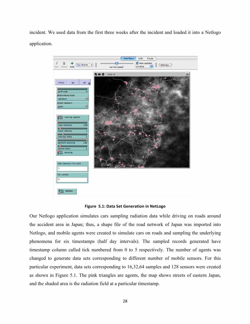
Figure 5.1: Data Set Generation in NetLogo
Our Netlogo application simulates cars sampling radiation data while driving on roads around
the accident area in Japan; thus, a shape file of the road network of Japan was imported into
Netlogo, and mobile agents were created to simulate cars on roads and sampling the underlying
phenomena for six timestamps (half day intervals). The sampled records generated have
timestamp column called tick numbered from 0 to 5 respectively. The number of agents was
changed to generate data sets corresponding to different number of mobile sensors. For this
particular experiment, data sets corresponding to 16,32,64 samples and 128 sensors were created
as shown in Figure 5.1. The pink triangles are agents, the map shows streets of eastern Japan,
and the shaded area is the radiation field at a particular timestamp.
29
5.3 Test Setup
The DSMS application was built using Oracle CEP (Java-based development environment). The
application was run using the Oracle JRockit Runtime server. The application was developed as
a client-server model, in which sensors are clients and DSMS application is the server. Both
clients and server communicate via the TCP/IP protocol.
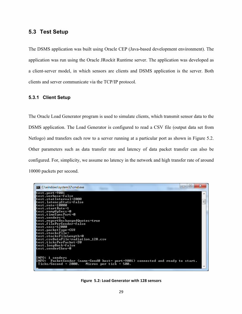
5.3.1 Client Setup
The Oracle Load Generator program is used to simulate clients, which transmit sensor data to the
DSMS application. The Load Generator is configured to read a CSV file (output data set from
Netlogo) and transfers each row to a server running at a particular port as shown in Figure 5.2.
Other parameters such as data transfer rate and latency of data packet transfer can also be
configured. For, simplicity, we assume no latency in the network and high transfer rate of around
10000 packets per second.
Figure 5.2: Load Generator with 128 sensors
30
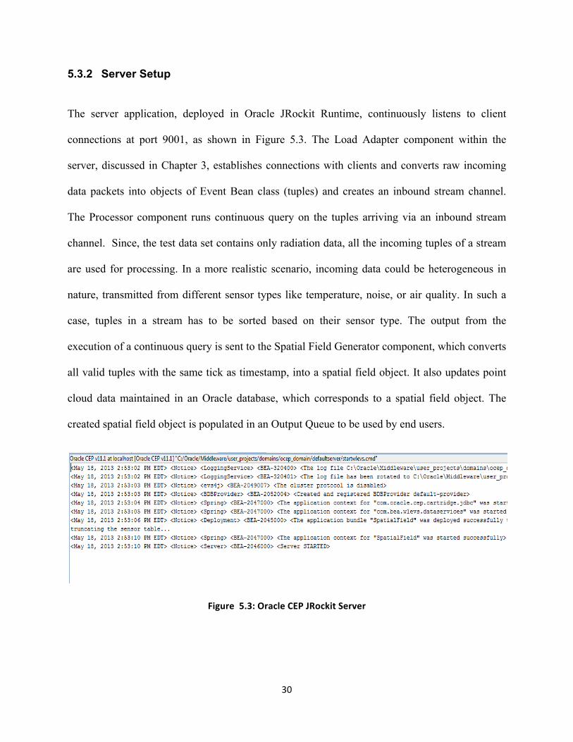
5.3.2 Server Setup
The server application, deployed in Oracle JRockit Runtime, continuously listens to client
connections at port 9001, as shown in Figure 5.3. The Load Adapter component within the
server, discussed in Chapter 3, establishes connections with clients and converts raw incoming
data packets into objects of Event Bean class (tuples) and creates an inbound stream channel.
The Processor component runs continuous query on the tuples arriving via an inbound stream
channel. Since, the test data set contains only radiation data, all the incoming tuples of a stream
are used for processing. In a more realistic scenario, incoming data could be heterogeneous in
nature, transmitted from different sensor types like temperature, noise, or air quality. In such a
case, tuples in a stream has to be sorted based on their sensor type. The output from the
execution of a continuous query is sent to the Spatial Field Generator component, which converts
all valid tuples with the same tick as timestamp, into a spatial field object. It also updates point
cloud data maintained in an Oracle database, which corresponds to a spatial field object. The
created spatial field object is populated in an Output Queue to be used by end users.
Figure 5.3: Oracle CEP JRockit Server
31
5.4 Experiment Configuration
An experiment module was created inside the DSMS server application, which runs in a separate
thread. This module fetches spatial field objects from the Spatial Field Generator 's Output
Queue and executes performance test. The experiment can be configured with the following
parameters for a test:
• iterations - number of runs for each configuration
• radius list - a list of radius for testing IDW interpolation
• tile length - work order unit
• threads - number of parallel IDW interpolation threads
• visualize - georaster creation on/off flag
Four data sets of 16, 32, 64 and 128 sensors were used to run the experiment with 16x16 work
order tiles and four parallel IDW threads. The visualize parameter was always on to create
georaster objects after interpolation. The radius sizes used were 0, 10, 20, 30 and 40 units. The
above configuration was each run for five iterations. However, Oracle Spatial performs internal
caching of the query plan of previously run queries. This impacts performance on consecutive
iterations. Therefore, to eliminate such effects in test results caused by caching, all internal cache
and buffers were flushed for every experiment run configuration. The above factors have to be
considered to obtain mutually exclusive test results for each run.
All the test configurations for the experiment were run on a Lenovo Ideapad z570 laptop with a
2.0 GHz Intel Core i7 (Model i7-2630QM; a quad core processor with eight virtual cores), 8 GB
DDR3 memory at 1067 MHz on a Windows 7 (64 bit) operating system with Java 1.6.0_29 (64
bit).
32
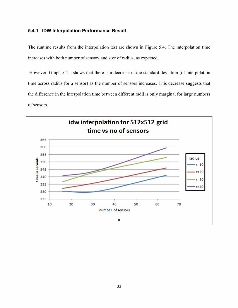
5.4.1 IDW Interpolation Performance Result
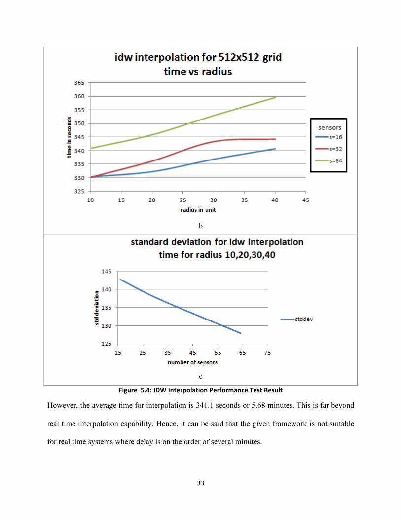
The runtime results from the interpolation test are shown in Figure 5.4. The interpolation time
increases with both number of sensors and size of radius, as expected.
However, Graph 5.4 c shows that there is a decrease in the standard deviation (of interpolation
time across radius for a sensor) as the number of sensors increases. This decrease suggests that
the difference in the interpolation time between different radii is only marginal for large numbers
of sensors.
a
33
b
c
Figure 5.4: IDW Interpolation Performance Test Result
However, the average time for interpolation is 341.1 seconds or 5.68 minutes. This is far beyond
real time interpolation capability. Hence, it can be said that the given framework is not suitable
for real time systems where delay is on the order of several minutes.
34
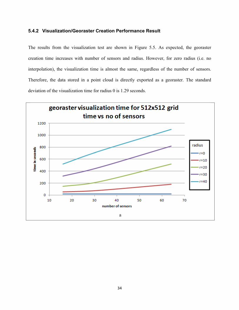
5.4.2 Visualization/Georaster Creation Performance Result
The results from the visualization test are shown in Figure 5.5. As expected, the georaster
creation time increases with number of sensors and radius. However, for zero radius (i.e. no
interpolation), the visualization time is almost the same, regardless of the number of sensors.
Therefore, the data stored in a point cloud is directly exported as a georaster. The standard
deviation of the visualization time for radius 0 is 1.29 seconds.
a
35
B
c
Figure 5.5: Georaster Creation Performance Test Results
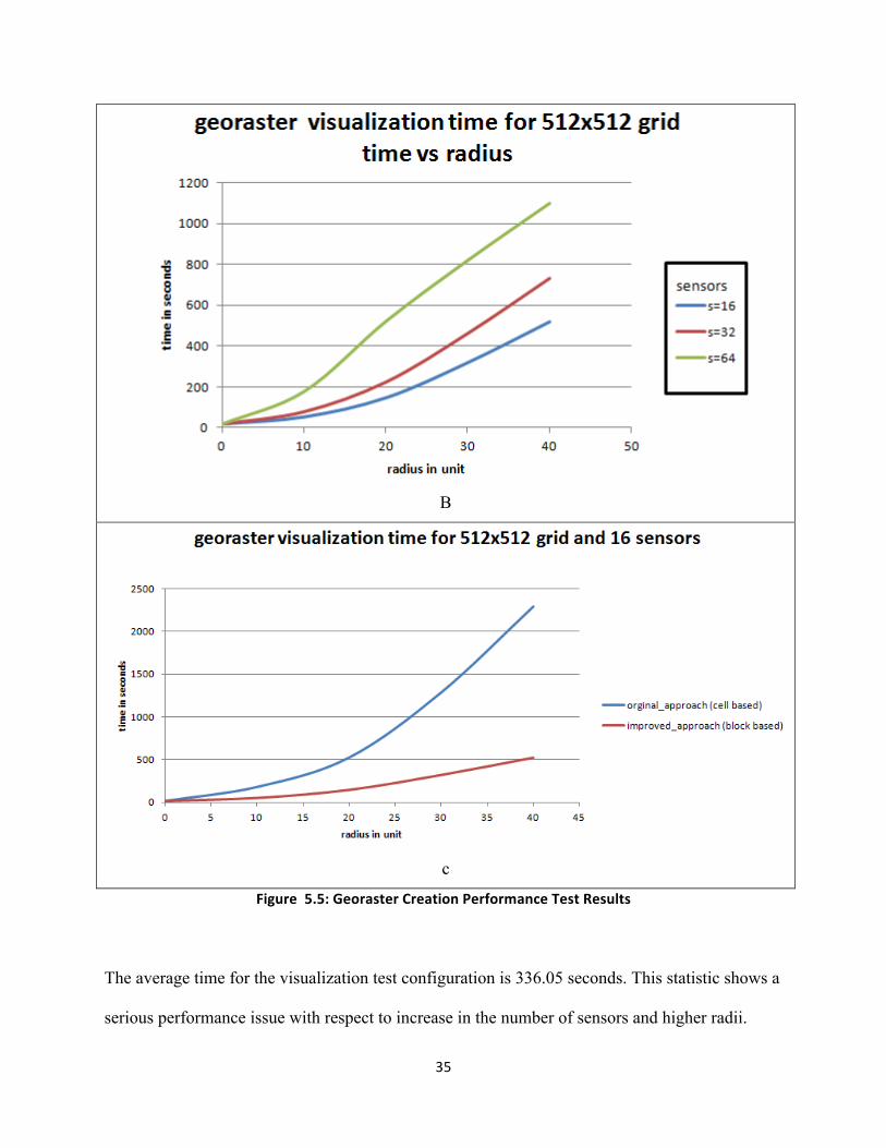
The average time for the visualization test configuration is 336.05 seconds. This statistic shows a
serious performance issue with respect to increase in the number of sensors and higher radii.
36
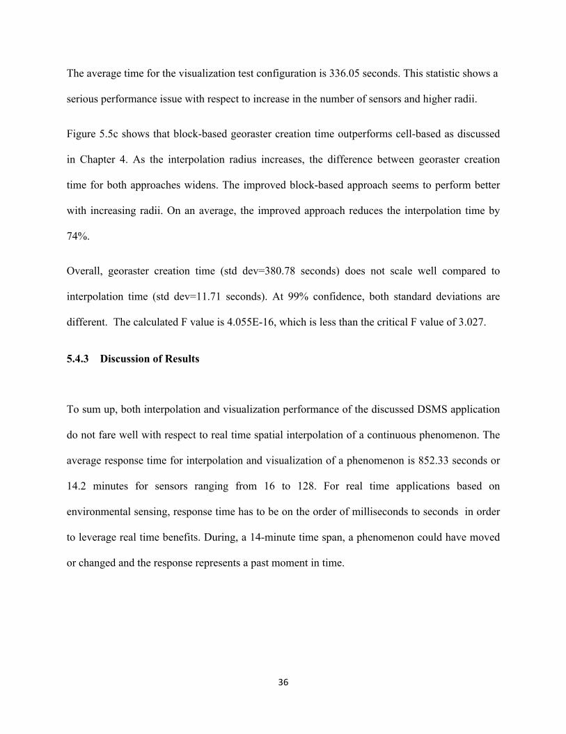
The average time for the visualization test configuration is 336.05 seconds. This statistic shows a
serious performance issue with respect to increase in the number of sensors and higher radii.
Figure 5.5c shows that block-based georaster creation time outperforms cell-based as discussed
in Chapter 4. As the interpolation radius increases, the difference between georaster creation
time for both approaches widens. The improved block-based approach seems to perform better
with increasing radii. On an average, the improved approach reduces the interpolation time by
74%.
Overall, georaster creation time (std dev=380.78 seconds) does not scale well compared to
interpolation time (std dev=11.71 seconds). At 99% confidence, both standard deviations are
different. The calculated F value is 4.055E-16, which is less than the critical F value of 3.027.
5.4.3 Discussion of Results
To sum up, both interpolation and visualization performance of the discussed DSMS application
do not fare well with respect to real time spatial interpolation of a continuous phenomenon. The
average response time for interpolation and visualization of a phenomenon is 852.33 seconds or
14.2 minutes for sensors ranging from 16 to 128. For real time applications based on
environmental sensing, response time has to be on the order of milliseconds to seconds in order
to leverage real time benefits. During, a 14-minute time span, a phenomenon could have moved
or changed and the response represents a past moment in time.

37
This project investigated the potential runtime performance of near real-time spatial interpolation
of sensor data streams to approximate a dynamic continuous phenomenon using mostly built-in
Oracle CEP and Oracle Spatial functionality. We implemented a framework within a DSMS that
converts raw sensor data into an abstract spatial field object, which is implemented as a stream
query and stores its data in a traditional DBMS temporarily until it is interpolated and
materialized using Oracle’s georaster. The results showed that commercial DSMSs like Oracle
CEP/Spatial are not yet equipped to perform real-time spatial interpolation due to various
architectural bottlenecks. Novel architectural components need to be added to a DSMS to
support adequate support for real-time spatial interpolation if sensor data streams should be
processed and to provide a response time in the order of milliseconds to seconds.
The main reasons for the inadequate performance of Oracle CEP with Oracle Spatial are
today:(1) there is no support for in-memory spatial databases in Oracle Spatial. Although the
concept of virtual tables or temporary tables exists, currently there is no support for partitioning,
clustering or indexing of spatial data within virtual tables. (2) BLOB storage of point cloud and
raster data is highly scalable and enables us to utilize the traditional benefits such as indexing of
DBMS, but it makes read/write operation slower. Having said that, there are ways of improving
the performance of the discussed application by using higher processing power [15] and running
interpolation in clouds for processing very large extent maps (basically ‘throwing machines are
the problem’).
Chapter 6 : Conclusions And Future Work

38
For future work, the spatial field data model developed from this project could be extended to
formalize a spatial field data model that could be integrated into a DSMS but it needs more
specialized stream-oriented spatial support. Some interesting questions remain: How to extend
the spatial filed data model to define interaction among spatial field objects?
39
[1]. http://esper.codehaus.org/tutorials/tutorial/tutorial.html
[2].Biem, A., Bouillet, E., & Feng, H. (2010). IBM InfoSphere Streams for Scalable , Real-
Time, Intelligent Transportation Services. SIGMOD ’10: Proceedings of the 2010 ACM
SIGMOD International Conference on Management of Data (pp. 1093–1103).
Indianapolis, IN.
[3].Ali, M., Chandramouli, B., Raman, B. S., & Katibah, E. (2010). Real-time spatio-
temporal analytics using Microsoft StreamInsight. Proceedings of the 18th SIGSPATIAL
International Conference on Advances in Geographic Information Systems - GIS ’10
(pp. 542–543). New York, New York, USA: ACM
[4].Oracle. (2009). Oracle Complex Event Processing : Lightweight Modular Application
Event Stream Processing in the Real World.
[5].http://streambase.com/developers/docs/latest/streamsql/index.html
[6].Heeren, H. V., & Salomon, P. (n.d.). MEMS - Recent Developments, Future Directions.
[7].Paulos, E., Honicky, R., & Hooker, B. (2008). Citizen science: Enabling participatory
urbanism. Urban Informatics: community Integration and Implementation (pp. 1–16).
[8].http://download.oracle.com/technology/software/cep-ide/11
[9].Zdonik, S. (2004). Streaming for Dummies
[10].Jain, N., Mishra, S., Srinivasan, A., Gehrke, J., Widom, J., Balakrishnan, H.,
Cetintemel, U., et al. (2008). Towards a streaming SQL standard. Proceedings of the
VLDB Endowment, 1(2), 1379-1390.
BIBLIOGRAPHY
40
[11].Ali, M. H., Aref, W. G., Bose, R., Elmagarmid, A. K., Helal, A., Kamel, I., & Mokbel,
M. F. (2005). NILE-PDT: A phenomenon detection and tracking framework for data
stream management systems. Proceedings of the 31st international conference on Very
large data bases (pp. 1295–1298).
[12].Mitas, L., & Mitasova, H. (1999). Spatial interpolation. In P. Longley, M. F.
Goodchild, D. J. Maguire, & D. W. Rhind (Eds.), Geographical Information Systems:
Principles, Techniques, Management and Applications (2nd ed., pp. 481-492). Wiley.
[13].http://en.wikipedia.org/wiki/Data-stream_management_system
[14].Emine Nesime Tatbul , Load Shedding Techniques for Data Stream Management
Systems” Ph.D thesis, Brown University, May 2007
[15].http://data-informed.com/fast-database-emerges-from-mit-class-gpus-and-students-
invention
[16].Management, D. S. (2010). Data Stream Management and Complex Event Processing
in Esper.
[17].http://msdn.microsoft.com/en-us/library/ee362541.aspx
[18].Oracle, A., & Paper, W. (2008). Oracle Complex Event Processing Performance Oracle
Complex Event Processing Performance, (November).
[19].http://docs.oracle.com/cd/E16764_01/doc.1111/e12048/operators.htm#CHDFGJGJ
[20].Introduction, I. (n.d.). Point Cloud : Storage , Loading , and Visualization by Siva
Ravada, Mike Horhammer, Baris M. Kazar, Oracle Spatial, Oracle USA, Inc., One
Oracle Drive, Nashua, NH 03062, USA
[21].Oracle. (2007). Oracle Spatial 11g GeoRaster , An Oracle Technical White Paper June
2007

41
[22].Stonebraker, M., & Centintemel, U. (2005). One size fits all: An idea whose time has
come and gone. Proceedings of International Conference on Data Engineering
(ICDE’05) (pp. 2-11). Tokyo, Japan.
[23].Nittel, S., Whittier, J. C., & Liang, Qi. (2012). Real-time Spatial Interpolation of
Continuous Environmental Data Streams using Mobile Sensor Streams. SIGSPATIAL
2012. Redondo Beach, CA.
[24].http://www.sendung.de/japan-radiation-open-data
[25].http://blog.safecast.org/