Embed Size (px)
Citation preview

2014
HIIFP-000
Ministry of Transportation University of Waterloo
Feasibility of Using Traffic Data for Winter Road Maintenance Performance Measurement

Publication Title
Author(s) Luchao (Johnny) Cao and Liping Fu
iTSS Lab, Department of Civil and Environmental Engineering, University of
Waterloo
Originating Office Design and Contract Standards Office, MTO
Report Number
Publication Date 2014
Ministry Contact HIIFP/AURORA - Development of Output and Outcome Models for End-results
Based Winter Road Maintenance Standards
Abstract The research presented in this report is motivated by the need to develop an outcome
based WRM performance measurement system with a specific focus on investigating
the feasibility of inferring WRM performance from a traffic state. The research studied
the impact of winter weather and road surface conditions (RSC) on the average traffic
speed of rural highways with the intention of examining the feasibility of using traffic
speeds from traffic sensors as an indicator of WRM performance. Detailed data on
weather, RSC, and traffic over three winter seasons from 2008 to 2011 on rural
highway sites in Iowa, US are used in this investigation. Three modelling techniques
are applied and compared to model the relationship between traffic speed and various
road weather and surface condition factors, including multivariate linear regression,
artificial neural networks (ANN), and time series analysis. Multivariate linear
regression models are compared by temporal aggregation (15 minutes vs. 60 minutes),
types of highways (two-lane vs. four-lane), and model types (separated vs. combined).
The research then examined the feasibility of estimating/classifying RSC based on
traffic speed and winter weather factors using multi-layer logistic regression
classification trees. The modelling results have confirmed the expected effects of
weather variables including precipitation, temperature, and wind speed; it verified the
statistically strong relationship between traffic speed and RSC, suggesting that speed
could potentially be used as an indicator of bare pavement conditions and thus the
performance of WRM operations. It is also confirmed that a time series model could
be a valuable tool for predicting real-time traffic conditions based on weather forecast
and planned maintenance operations, and that a multi-layer logistic regression
classification tree model could be applied for estimating RSC on highways based on
average traffic speed and weather conditions.
Key Words Winter Road Maintenance, Speed, Modeling
Distribution Unrestricted technical audience.
Feasibility of Using Traffic Data for Winter Road Maintenance Performance Measurement

Ministry of Transportation University of Waterloo
HIIFP-000
Feasibility of Using Traffic Data for Winter Road Maintenance
Performance Measurement
2014
Prepared by Luchao (Johnny) Cao and Liping Fu
iTSS Lab Department of Civil and Environment Engineering
University of Waterloo
200 University Avenue, Waterloo, Ontario, Canada N2L 3G1
Tel: (519) 888-4567
Published without prejudice as to the application of the
findings. Crown copyright reserved.

Acknowledgements
The authors wish to acknowledge the assistance of the Ministry of Transportation Ontario
(MTO) and Iowa Department of Transportation (Iowa DOT) for providing the data and
financial support to this project. In particular, a special thanks should be given to Max
Perchanok and Tina Greenfield for all the coordination, guidance and assistance.
This report was developed on the basis of Mr. Luchao (Johnny) Cao’s Master’s thesis
completed under the supervision of Dr. Liping Fu, director of the iTSS Lab, Department
of Civil and Environmental Engineering, University of Waterloo. The authors also wish
to acknowledge the assistance of various members of the iTSS Lab and the University of
Waterloo’s community who have assisted in the research and in the preparation of this
report, including Lalita Thakali who provided assistance for part of the analysis, Tae J.
Kwon for reviewing part of this work, Matthew Muresan for his assistance in preparing
this report, Taimur Usman, Garrett Donaher and Feng Feng for providing suggestions and
assistance on this research. Thanks should also be given to Dr. Chaozhe Jiang, Ramona
Mirtorabi, Kamal Hossain and Raqib Omer, for their support and motivation.

- i -
Impact of Winter Road Conditions on Highway Speed and Volume; HIIFP-000
Table of Contents
Acknowledgements .............................................................................................................. iii
Table of Contents .................................................................................................................... i
List of Figures ......................................................................................................................... v
List of Abbreviations and Notations ..................................................................................... vii
Executive Summary............................................................................................................. viii
Introduction .......................................................................................................................... 1
Background ............................................................................................................................................. 1
Winter Road Maintenance and Performance Measurement ................................................................. 1
Research Objectives ................................................................................................................................ 3
Document Organization .......................................................................................................................... 4
Literature Review .................................................................................................................. 5
WRM Performance Measurement .......................................................................................................... 5
Performance Measurement System ................................................................................................. 5
WRM Performance Measurement System ....................................................................................... 6
Current WRM Performance Measures ............................................................................................. 8
Using Traffic Speed as a WRM Performance Measure ................................................................... 13
Factors Affecting Winter Traffic Speed ................................................................................................. 18
Winter RSC Monitoring and Estimation ................................................................................................ 30
Stationary Based RSC Monitoring and Estimation ......................................................................... 31
Mobile Based RSC Monitoring and Estimation ............................................................................... 32
Summary ............................................................................................................................................... 33
Effect of Weather and Road Surface Conditions on Traffic Speed of Rural Highways ............ 35
Problem Definition ................................................................................................................................ 35
Data Collection ...................................................................................................................................... 35
Data Processing ..................................................................................................................................... 37
Data Processing Framework ........................................................................................................... 37
Snow Event Definition and Extraction ............................................................................................ 41
Exploratory Analysis .............................................................................................................................. 43
Methodology ......................................................................................................................................... 50
Multivariate Linear Regression ....................................................................................................... 50
Artificial Neural Network ................................................................................................................ 51
Time Series Analysis ........................................................................................................................ 52
Model Calibration ................................................................................................................................. 54
Multivariate Linear Regression ....................................................................................................... 54
Artificial Neural Network ................................................................................................................ 65

- ii -
Impact of Winter Road Conditions on Highway Speed and Volume; HIIFP-000
Time Series Analysis ........................................................................................................................ 66
Model Comparison ......................................................................................................................... 70
Model Validation................................................................................................................................... 73
Model Validation for Each Site ....................................................................................................... 73
Case Studies .................................................................................................................................... 79
Summary ............................................................................................................................................... 81
Inferring Road Surface Condition from Traffic and Weather Data ......................................... 83
Problem Definition ................................................................................................................................ 83
Data Collection ...................................................................................................................................... 83
Methodology ......................................................................................................................................... 84
Road Surface Condition Classification ............................................................................................ 84
Logistic Regression ......................................................................................................................... 85
Multi-Layer Logistic Regression Classification Tree ........................................................................ 85
Evaluation of Classification Quality ................................................................................................ 86
Exploratory Analysis .............................................................................................................................. 87
Model Calibration and Validation ......................................................................................................... 92
Two Lane Highways ........................................................................................................................ 92
Four Lane Highways ....................................................................................................................... 97
Discussion ........................................................................................................................................... 105
Association with Average Speed................................................................................................... 105
Association with Standard Deviation of Traffic Speed ................................................................. 106
Association with Average Volume and % Long Vehicles .............................................................. 106
Association Wind Speed ............................................................................................................... 106
Association with Air Temperature ................................................................................................ 107
Association with Precipitation Intensity ....................................................................................... 107
Association with Night .................................................................................................................. 108
- iii -
Impact of Winter Road Conditions on Highway Speed and Volume; HIIFP-000
Summary ............................................................................................................................................. 110
Conclusions and Future Work ............................................................................................. 111
Major Findings .................................................................................................................................... 111
Limitations and Future Work .............................................................................................................. 111
References ......................................................................................................................... 113
Appendices ............................................................................................................................ 1
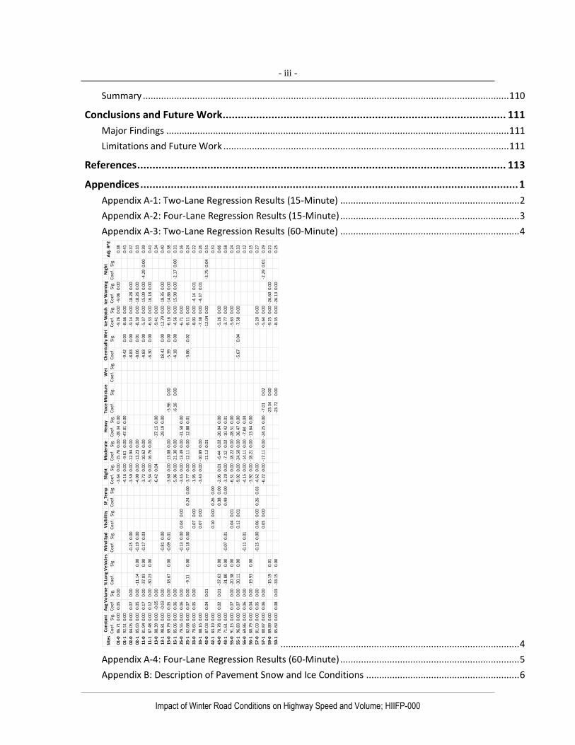
Appendix A-1: Two-Lane Regression Results (15-Minute) ..................................................................... 2
Appendix A-2: Four-Lane Regression Results (15-Minute) ..................................................................... 3
Appendix A-3: Two-Lane Regression Results (60-Minute) ..................................................................... 4
............................................................................................ 4
Appendix A-4: Four-Lane Regression Results (60-Minute) ..................................................................... 5
Appendix B: Description of Pavement Snow and Ice Conditions ........................................................... 6
Co
ef.
Sig.
Co
ef.
Sig.
Co
ef.
Sig.
Co
ef.
Sig.
Co
ef.
Sig.
Co
ef.
Sig.
Co
ef.
Sig.
Co
ef.
Sig.
Co
ef.
Sig.
Co
ef.
Sig.
Co
ef.
Sig.
Co
ef.
Sig.
Co
ef.
Sig.
Co
ef.
Sig.
Co
ef.
Sig.
01-0
86.7
10.
000.
050.
00-3
.64
0.00
-15.
760.
00-2
8.34
0.00
-9.2
60.
00-9
.06
0.00
0.38
01-1
92.5
10.
00-4
.16
0.00
-9.6
10.
00-4
7.01
0.00
-9.4
20.
03-8
.66
0.00
0.41
02-0
84.0
50.
000.
070.
00-0
.25
0.00
-3.5
90.
00-1
2.94
0.00
-8.8
30.
00-9
.14
0.00
-18.
280.
000.
37
02-1
85.6
30.
000.
050.
00-1
1.14
0.00
-0.1
90.
00-4
.00
0.00
-13.
230.
00-8
.06
0.01
-8.3
00.
00-1
8.26
0.00
0.33
11-0
81.9
40.
000.
170.
00-3
7.03
0.00
-0.1
70.
03-3
.72
0.00
-10.
620.
00-4
.83
0.00
-5.3
70.
00-1
5.09
0.00
-4.2
90.
000.
39
11-1
87.4
80.
000.
120.
00-3
0.23
0.00
-5.3
40.
00-1
6.76
0.00
-6.3
00.
00-6
.33
0.00
-16.
180.
000.
41
13-0
88.3
90.
00-0
.05
0.00
-6.4
20.
04-3
7.15
0.00
-9.4
10.
000.
34
13-1
98.8
10.
00-0
.03
0.00
-0.8
10.
00-2
9.19
0.00
-18.
420.
00-1
2.79
0.00
-18.
350.
000.
40
15-0
89.7
90.
000.
050.
00-1
8.67
0.00
-0.0
90.
01-3
.60
0.00
-13.
080.
00-5
.96
0.00
-5.3
90.
00-6
.16
0.00
-14.
860.
000.
38
15-1
85.0
60.
000.
060.
00-5
.06
0.00
-21.
300.
00-6
.16
0.00
-4.1
80.
00-4
.56
0.00
-15.
900.
00-2
.17
0.00
0.31
25-0
79.5
50.
000.
060.
00-0
.13
0.00
0.04
0.00
-3.4
50.
00-1
3.39
0.00
-31.
580.
00-6
.71
0.00
0.16
25-1
82.6
80.
000.
070.
00-9
.11
0.00
-0.1
80.
000.
240.
00-3
.77
0.00
-12.
110.
00-1
2.88
0.01
-3.8
60.
02-8
.11
0.00
0.24
33-0
79.6
50.
000.
050.
000.
070.
00-1
.95
0.00
-8.0
30.
00-4
.14
0.01
0.22
33-1
88.1
60.
000.
070.
00-3
.43
0.00
-10.
890.
00-7
.38
0.00
-4.3
70.
010.
26
42-0
87.0
30.
000.
040.
01-1
1.12
0.01
-12.
040.
00-3
.75
0.04
0.51
42-1
83.1
90.
000.
100.
000.
260.
000.
31
43-0
70.7
80.
000.
020.
01-3
7.63
0.00
0.38
0.00
-2.0
50.
01-6
.44
0.02
-20.
040.
00-5
.26
0.00
0.66
43-1
71.6
10.
00-3
1.80
0.00
-0.0
70.
010.
490.
00-3
.20
0.00
-7.1
20.
02-1
0.42
0.01
-3.7
70.
000.
58
55-0
91.1
50.
000.
070.
00-2
0.38
0.00
0.04
0.01
-6.3
10.
00-1
8.22
0.00
-28.
510.
00-5
.63
0.00
0.24
55-1
96.8
30.
000.
070.
00-3
0.11
0.00
0.12
0.01
-9.0
20.
00-2
4.50
0.00
-36.
470.
00-5
.67
0.04
-7.5
80.
000.
33
56-0
69.8
60.
000.
060.
00-0
.11
0.01
-4.1
50.
00-1
4.11
0.00
-7.8
40.
040.
12
56-1
80.7
90.
000.
040.
00-1
9.93
0.00
-3.9
20.
00-1
8.21
0.00
-13.
640.
000.
15
57-0
81.0
30.
000.
050.
00-0
.25
0.00
0.06
0.00
0.26
0.03
-4.6
20.
00-5
.20
0.00
0.27
57-1
80.8
70.
000.
060.
000.
050.
00-6
.22
0.00
-17.
110.
00-2
4.25
0.00
-7.0
10.
02-5
.64
0.00
-2.2
90.
010.
29
59-0
89.8
90.
00-1
5.19
0.01
-23.
340.
00-9
.25
0.00
-26.
600.
000.
21
59-1
85.6
90.
000.
080.
03-3
3.15
0.00
-23.
720.
00-8
.35
0.00
-26.
130.
000.
25
Ad
j. R
^2C
he
mic
ally
We
tIc
e W
atch
Ice
War
nin
gN
igh
tW
et
Vis
ibil
ity
Site
sC
on
stan
tA
vg V
olu
me
% L
on
g V
eh
icle
sW
ind
Sp
dSF
_Te
mp
Slig
ht
Mo
de
rate
He
avy
Trac
e M
ois
ture

- iv -
Impact of Winter Road Conditions on Highway Speed and Volume; HIIFP-000

- v -
Impact of Winter Road Conditions on Highway Speed and Volume; HIIFP-000
List of Figures
Figure 2.1 WRM Performance Measurement Model (Maze, 2009) ................................................ 7
Figure 2.2 Quality of Winter Road Maintenance Urban and Rural Comparisons (Kreisel,
2012) .......................................................................................................................... 13
Figure 2.3 Speed Recovery Duration as a Performance Measure (Lee et al., 2008) ..................... 14
Figure 2.4 Base Values of Speed Reduction and SSI Equation (Iowa DOT, 2009) ......................... 16
Figure 2.5 Identification of SRST, LST, RST of Speed Variation During Snow Event (Kwon
et al., 2012) ................................................................................................................ 17
Figure 2.6 Model Calibration Results (Liang et al., 1998) .............................................................. 19
Figure 2.7 Model Calibration Results (Knapp et al., 2000) ............................................................ 20
Figure 2.8 Comparison of Model Results with HCM 2000 (Agrwal et al., 2005) ........................... 21
Figure 2.9 Model Calibration Results (Rakha et al., 2007) ............................................................ 22
Figure 2.10 Model Calibration Results (Camacho et al., 2007) ..................................................... 23
Figure 2.11 Model Calibration Results (Kwon et al., 2013) ........................................................... 25
Figure 2.12 Event Based Model (Garrett, 2014) ............................................................................ 27
Figure 3.1 Study Sites in Iowa ........................................................................................................ 36
Figure 3.2 Data Processing Framework ......................................................................................... 39
Figure 3.3 Snow Event Extraction Algorithm ................................................................................. 42
Figure 3.4 Typical MLP-NN Architecture (Huang & Ran, 2003) ..................................................... 52
Figure 3.5 Effect of Precipitation Intensity .................................................................................... 61
Figure 3.6 Effect of Road Surface Condition.................................................................................. 63
Figure 3.7 Site Effect of Two-Lane Highways ................................................................................ 64
Figure 3.8 Site Effect of Four-Lane Highways ................................................................................ 65
Figure 3.9 Overall RMSE Comparison for Combined Models ........................................................ 70
Figure 3.10 Observed vs. Estimated by Regression 60 minutes Combined .................................. 71
Figure 3.11 Observed vs. Estimated by MLP-NN 60 minutes Combined ...................................... 72
Figure 3.12 Observed vs. Estimated by ARIMAX 60 minutes Combined....................................... 72
Figure 3.13 RMSE Comparison for Two-Lane Highways 10% Holdout Data ................................. 77
Figure 3.14 RMSE Comparison for Four-Lane Highways 10% Holdout Data ................................. 79
Figure 3.15 Estimation on Two-Lane Highways (Site 01-0 on Dec. 11th.-12th., 2010) ................. 80
Figure 3.16 Estimation on Four-Lane Highways (Site 00-0 on Jan 10th., 2009) ............................ 81
Figure 4.5 Sample Multi-layer Logistic Regression Classification Tree for RSC
Discrimination ............................................................................................................ 86
Figure 4.1 Boxplots for Site 11-1 (15-Minute Interval) ................................................................. 88
Figure 4.2 Boxplots for Site 11-1 (60-Minute Interval) ................................................................. 89
Figure 4.3 Boxplots for Site 00-0 (15-Minute Interval) ................................................................. 90
Figure 4.4 Boxplots for Site 00-0 (60-Minute Interval) ................................................................. 91

- vi -
Impact of Winter Road Conditions on Highway Speed and Volume; HIIFP-000
Figure 4.6 Calibrated Classification Tree for Site 11-1 .................................................................. 92
Figure 4.7 Calibrated Classification Tree for Site 00-0 .................................................................. 98
Figure 4.8 Overall Validation Hit Rate Summary of Site 11-1...................................................... 109
Figure 4.9 Overall Validation Hit Rate Summary of Site 00-0...................................................... 109

- vii -
Impact of Winter Road Conditions on Highway Speed and Volume; HIIFP-000
List of Abbreviations and Notations
WRM Winter road maintenance
RSC Road Surface Condition
MTO Ministry of Transportation Ontario
FHWA Federal Highway Administration
LOS Level of Service
NHTSA National Highway Traffic Safety Administration
HCM Highway Capacity Manual
FFS free flow speed
ANN Artificial Neural Network
AVL Automated Vehicle Location
GPS Global Positioning System
DEA Data Envelopment Analysis
TAS Total Area Served
DOT Department of Transportation
WPI Winter Performance Index
WMI Winter Mobility Index
RWIS Road Weather Information Systems
CCTV Closed Circuit Television
ESS Environmental Sensor Systems
CFM continuous friction measurement
ARIMA Autoregressive Integrated Moving Average
MLP Multi-Layer Perceptron
ACF Autocorrelation Factor
PACF Partial Autocorrelation Factor
AIC Akaike Information Criterion
BIC (Bayesian Information Criterion)

- viii -
Impact of Winter Road Conditions on Highway Speed and Volume; HIIFP-000
Executive Summary
Winter road maintenance (WRM) operations, such as plowing, salting and sanding, are
significant to maintain both safety and mobility of highways, especially in countries like
Canada. Traditionally, WRM performance is measured using bare pavement regain time
and snow depth/coverage, which are reported by maintenance or quality assurance
personnel based on periodic visual inspection during and after snow events. However, the
increasing costs associated with WRM and the lack of objectivity and repeatability of
traditional performance measurement have stimulated significant interest in developing
alternative performance measures.
The research presented in this report is motivated by the need to develop an outcome
based WRM performance measurement system with a specific focus on investigating the
feasibility of inferring WRM performance from a traffic state. The research studied the
impact of winter weather and road surface conditions (RSC) on the average traffic speed
of rural highways with the intention of examining the feasibility of using traffic speeds
from traffic sensors as an indicator of WRM performance. Detailed data on weather,
RSC, and traffic over three winter seasons from 2008 to 2011 on rural highway sites in
Iowa, US are used in this investigation. Three modeling techniques are applied and
compared to model the relationship between traffic speed and various road weather and
surface condition factors, including multivariate linear regression, artificial neural
networks (ANN), and time series analysis. Multivariate linear regression models are
compared by temporal aggregation (15 minutes vs. 60 minutes), types of highways (two-
lane vs. four-lane), and model types (separated vs. combined). The research then
examined the feasibility of estimating/classifying RSC based on traffic speed and winter
weather factors using multi-layer logistic regression classification trees.
The modeling results have confirmed the expected effects of weather variables including
precipitation, temperature, and wind speed; it verified the statistically strong relationship
between traffic speed and RSC, suggesting that speed could potentially be used as an
indicator of bare pavement conditions and thus the performance of WRM operations. It is
also confirmed that a time series model could be a valuable tool for predicting real-time
traffic conditions based on weather forecast and planned maintenance operations, and that
a multi-layer logistic regression classification tree model could be applied for estimating
RSC on highways based on average traffic speed and weather conditions.

1
Introduction
Background
For many people, winter is the most beautiful season. However, in countries like Canada and
United States, people’s daily life can be significantly impacted by severe cold weathers, wind
chills and heavy snow storms during winter seasons. Highway transportation is one of the
many aspects that could severely be impacted by adverse weather conditions. Snow covered
road surface conditions (RSC), low temperature and poor visibility can all result in slow
traffic speeds and an increased risk of fatal collisions.
Substantial research work has been carried out to address the impact of adverse weather on
highway safety and mobility. According to the 2010 Ontario Road Safety Annual Reports,
over 22.8% of fatal collisions, 24.8% of personnel injury collisions and 28.3% of property
damage collisions are related with wet/snow/icy RSC. Among all types of collisions, over
19.1% occurred under adverse weather conditions. Based on fourteen-year averages from
1995 to 2008 of the National Highway Traffic Safety Administration data (NHTSA), Noblis
(2013) found that about 24% of vehicle crashes, 21% of crash injuries and 17% of crash
fatalities occurred in the presence of adverse weather and/or slick pavement. The Highway
Capacity Manual (HCM 2010) also provided some research results about the impact of
weather conditions on freeway traffic speed, citing a drop of 8-10 percent in free flow speed
(FFS) due to light snow, 30-40 percent due to heavy snow, compared with clear and dry
conditions.
In order to keep road networks clear of snow and ice and to ensure safe and efficient travel
throughout winter seasons, many transportation authorities in countries like Canada and US
are facing mounting financial and environmental challenges. According to the FHWA
Statistics, WRM accounts for roughly 20 percent of state DOT maintenance budgets, with an
average annual spend of more than 2.3 billion dollars on snow and ice control operations.
(http://www.fhwa.dot.gov/policy/ohpi/hss/hsspubs.cfm). Similarly, Canada spends
significant amounts of resources on WRM every year, including over $1 billion dollars of
direct investment and use of an average of five million tons of road salts. The increasing
maintenance costs, public concerns over the detrimental effects of road salt on the
environment and vehicles stimulated significant interest in developing performance
measures. It therefore becomes increasingly important to develop a rigorous performance
measurement system that can show clear linkage between the inputs of WRM and its
outcomes such as mobility and safety benefits.
Winter Road Maintenance and Performance Measurement
Generally, WRM is the maintenance activities conducted by governments, institutions and
individuals to remove or control the amount of ice and snow brought by snow events on
roadway surface, and to make travel easier and reduce the risk of collisions.
WRM methods can be divided into two categories: mechanical and chemical (Minsk, 1998).

Impact of Winter Road Conditions on Highway Speed and Volume; HIIFP-000
Mechanical methods include plowing, sweeping and blowing using maintenance trucks and
equipment. The main chemical method is the application of temperature suppressant
chemicals on road surface. These chemicals, either liquid or solid, can lower the freezing-
point, thus melting snow/ice or preventing ice bonding on the road surface and making
plowing easier.
Based on the timing of the operation, WRM operations can also be classified into three
categories: before, during and after snow events. Before event operations include check for
changing road and weather conditions, plan and prepare operations, and apply liquid
chemicals to road surface. During and after maintenance event includes operations such as
plowing snow and ice; spreading salt and sand on road surface to provide traction and safer
driving; cleaning up roadways and continually checking road, weather and traffic conditions
after snow events.
The choice of proper methods depends on various factors, for example, the severity of the
snow events, topology of the area, road surface temperature and wind speed, etc. Because of
the high efficiency and effectiveness in clearing snow and ice, plowing and salting are the
two most commonly used methods in practice. Plowing involves in removing snow layer
from the road surface with trucks. The snow layer is usually a mixture of snow, ice, water,
chemicals and dirt, and is not excessively bonded to the road surface such that it can be
picked up by plow equipped maintenance trucks and casted to sideways off the road for
storage. Salting involves the applications of solid and liquid chemicals, such as Magnesium
Chloride (MgCl), Calcium Chloride (CaCl) and Sodium Chloride (NaCl), and can be divided
into two types, anti-icing and de-icing. Anti-icing is the application of salt or brine to
roadway prior to snow events so as to prevent the bonding of snow and ice to the road
surface. De-icing is the application of salt to snow and ice that is bonded to road surface for
the purpose of melting the snow or ice, thereby ensuring safe driving conditions. Operation
frequency and chemical application rate can be determined based on road weather and
surface conditions as well as the level of service requirements. For different types of
roadways, the priorities of WRM are different. For example, the priorities of highways,
arterial roads, business districts and bus lanes are higher while the priorities of local
industrial roadways and residential streets are relatively lower.
WRM is a typical example that its activities and performance need to be measured so as to
achieve the optimum maintenance outcome while utilizing the minimum amount of
resources. According to a handbook published by the U.S. Department of Energy in 1995,
performance measures quantitatively summarize some important indicators of the products,
services and the process that produce them. A performance measurement system should
consist of a comprehensive set measures, processes and standards that can be used by the
government agencies and maintenance contractors to assess:
How well we are doing
If we are meeting our goals
If our customers are satisfied

Impact of Winter Road Conditions on Highway Speed and Volume; HIIFP-000
If our processes are in statistical control
If and where improvements are necessary
Many WRM performance measures have been developed in the past, which can be generally
divided into three categories: input measures, output measures and outcome measures.
However, there are still many problems of each category. For example, input measures such
as salt usage, labor and equipment investment are not directly linked to WRM objectives and
goals, and cannot provide measures of quality, efficiency or effectiveness of WRM.
Although output measures such as lane-miles plowed or salted are more meaningful
compared with input measures, they can only measure the physical accomplishment or the
efficiency of WRM, and do not reflect the level of impact on the ultimate goal of WRM.
Outcome measures such as bare pavement regain time, friction level, delay and the number
of collisions can produce the most meaningful results. However, these measures also have
drawbacks. Firstly, because of the limitations of data collection methods, some data used in
these measures is still subjective. Others highly depend on data quality and availability (e.g.
friction models), therefore cannot be applied without enough properly formatted datasets
(Maze, 2009; Qiu, 2008). Secondly, models used for estimating outcomes are often relatively
complex and are time-consuming to calibrate, which leaves a huge barrier to practical usage.
Furthermore, as a potential alternative WRM outcome performance measure, traffic speed
can be easily obtained with high quality. However, due to the limitations on modeling
methodologies and spatial/temporal coverage of most past studies, it still has not been used
widely. The reasons are, firstly, most past studies focused on the differences in speed or other
traffic variables between adverse and normal weather conditions using data under all weather
conditions. Secondly, most of the past studies utilized linear regression models to quantify
the effect of weather and surface condition variables on traffic speed, which may not capture
the possible non-linear effects of some factors. Thirdly, most studies focused on freeways
only, in which the effect of weather on traffic speed could be easily confounded by traffic
congestion, making the models less reliable. Lastly, few of the past studies have used data
with large spatial/temporal coverage and taken a full account of the variation in winter RSCs,
and the results are therefore not immediately useful for showing the feasibility of using speed
as a performance indicator of WRM. Further studies are needed to either improve the current
measures or come up with alternative measures so that these problems can be addressed.
Research Objectives
With the problems of the current WRM performance measures mentioned in the previous
section, this research has the following two major objectives:
1. To investigate the impact of winter weather and RSC on the average traffic speed of
rural highways with the intention of examining the feasibility of using traffic speed
from traffic sensors as a new WRM performance measure;
2. To develop statistical models and methodologies to estimate/classify RSC based on
traffic and weather data.

Impact of Winter Road Conditions on Highway Speed and Volume; HIIFP-000
The main task for Objective 1 is to develop and compare models calibrated with different
time aggregation intervals, highway types and statistical algorithms, quantify the impact of
winter weather and road surface factors on average traffic speed, and examine if average
traffic speed is sensitive to winter weather, especially RSC on rural highways. Objective 2
addresses the problem of inferring RSC based on traffic speed and other factors. The main
task is to develop reliable RSC classification models/frameworks using data that is easy and
inexpensive to collect such as traffic speed and weather factors.
Document Organization
This report consists of five chapters:
Chapter 1 introduces the research problem and objectives and some basic concepts.
Chapter 2 reviews the existing methods, standards, guidelines and policies used for WRM
performance measurement in practice. It also reviews previous studies on the mobility impact
of winter weather and road surface factors as well as RSC monitoring and estimation.
Chapter 3 calibrates and compares different types of models, and describes the results of the
investigation of the impact of winter weather and RSC on the average traffic speed of rural
highways.
Chapter 4 presents the calibration process, validation and discussion of the RSC
classification model/framework.
Chapter 5 summarizes the major findings and provides recommendations for future studies.

Impact of Winter Road Conditions on Highway Speed and Volume; HIIFP-000
Literature Review
Much research work has been carried out on WRM performance measurement. This chapter
covers a review of the WRM performance measurement system and some most widely used
WRM performance measures in practice. Additionally, past studies on factors affecting
average traffic speed in winter seasons are reviewed and summarized. Finally, previous
research on equipment and methodologies for winter RSC monitoring and estimation is
presented and discussed.
WRM Performance Measurement
Winter road maintenance operations are performed to minimize winter weather related
collisions and the impact of adverse winter weather on travel times. This section reviews the
WRM performance measurement system and the pros and cons of traditional WRM
performance measures.
Performance Measurement System
According to a handbook published by the U.S. Department of Energy in 1995, performance
measures quantitatively summarize some important indicators of the products, services and
the process that produce them. Performance measurement is the process of collecting and
analyzing data and assessing the performance of a system, individual or organization
(FHWA, 2004). It is about how to show with convincing evidence that the activities and
work have been done towards achieving the targeted results and pre-specified objectives
(Schacter, 2002).
The fundamental reason why performance measurement is important is that it makes
accountability possible, which is significant to decision making. Kane (2005) suggested that
the purpose of measuring performance by transportation agencies is to advise customers how
well transportation agencies are doing in improving transportation services. A report
prepared by the Transportation Association of Canada in 2006 also suggested that the most
common purpose of conducting performance measurement is the need to be accountable to
the public. The public expects to know how their fund is spent on maintaining the
transportation system, and the effect of expenditures upon it. Performance measurement is
essential to that process.
Central to a performance measurement system is a set of indicators, numerical or non-
numerical, which measure different aspects of the activities. Most literature suggested that
input, output and outcome are considered to be the three most common aspects of
performance related activities. Delorme et al. (2011) in their report about performance
measurement and its indicators from the perspective of government decision making and
policy evaluation, classified performance measures into five types, namely input, output,
outcome, impact and context. Similarly, Probst (2009) suggested that inputs, outputs,

Impact of Winter Road Conditions on Highway Speed and Volume; HIIFP-000
efficiency, service quality and outcome should be taken into consideration when measuring
local government decision performance.
When it comes to selecting proper performance measures, firstly, it is important to determine
what aspect of the activity is to be measured. Input measures reflect the resources that are
used in the activity process, output measures reflect the products of the activity, and outcome
measures, however, reflect the impact of the products and are directly related with the
agency’s strategic goals (Dalton et al, 2005). Secondly, it is also significant to consider data
availability, quality, the cost and time in data collection. It must be possible to collect the
necessary data with relatively high quality, but low cost. The performance measure that is to
be adopted must be possible to be generated with the existing technology and resources
available to transportation agencies. According to a report on TRB 2000, there are other
issues to be considered when selecting performance measures:
Forecastability: is it possible to compare future alternative projects or strategies
using this measure?
Clarity: is it likely to be understood by transportation professionals, policy makers
and the public?
Usefulness: Does the measure reflect the issue or goal of concern? Does it capture
cause-and-effect between the agency’s actions and condition?
Ability to diagnose problems: Is there a connection between the measure and the
actions that affect it? Is the measure too aggregated to be helpful to agencies
trying to improve performance?
Temporal Effects: Is the measure comparable across time?
Relevance: Is the measure relevant to planning and budgeting processes? Will
changes in activities and budget levels affect a change in the measure that is
apparent and meaningful? Can the measure be reported with a frequency that will
be helpful to decision makers?
WRM Performance Measurement System
Qiu (2008) proposed a general performance measurement system from the perspective of
WRM, and suggested that to develop a comprehensive performance measurement system, the
following factors need to be taken into consideration:
Input measures: indicating the amount of resource used (e.g. equipment, material
and labor);
Uncontrollable factors: indicating those factors that are controllable in normal
conditions, but related with performance (e.g. natural hazard and emergency);

Impact of Winter Road Conditions on Highway Speed and Volume; HIIFP-000
Output measures: indicating efficiency of resources transformed to service (e.g.
the lane-miles plowed or salted);
Outcome measures: reflecting effectiveness of the operation on pre-specified
objectives (e.g. lower travel costs to customers).
Maze(2009) systematically summarized the performance measurement system for WRM. As
shown in the ‘Fish Bone Model’ in Figure 0.1, the government pays contractors to invest in
WRM equipment, chemical materials and personnel (i.e. the input). Contractors then conduct
WRM operations before, during and after snow events and make sure that road surface is
clean and the bare-pavement regain time meets the standard specified on the WRM
guidelines (i.e. the output). Roadway users benefited from WRM in terms of both safety and
mobility while travelling (i.e. the outcome).
Figure 0.1 WRM Performance Measurement Model (Maze, 2009)
Qiu and Maze have suggested different types of measures that can be used as indicators of
WRM performance while these measures vary from one to another in terms of cost, data
availability, measuring frequency, reliability and repeatability. Next section will review some
of the most widely used WRM performance measures in practice, and discuss their pros and
cons.
Terrain & Solar Wind Air
Geography Energy Precipitation RSC Speed Temperature
Anti- Cycle Truck Abrasives Salt RWIS Operation
Icing Length Management
Inputs - Labor
- Equipment
- Materials
- Management
- Information
Snow and Ice Removal - Outputs
Outcomes
-
Safety
&
Mobilit
y
-
Travele
rs
Satisfactio
n (LOS)

Impact of Winter Road Conditions on Highway Speed and Volume; HIIFP-000
Current WRM Performance Measures
Effective WRM performance measures are significant to both the government and
maintenance contractors. By measuring maintenance performance and benchmarking
outcomes, the government is able to tell how well the job is done by maintenance contractors
while maintenance contractors can make more informed decisions, and conduct better
planned maintenance operations toward specific objectives (Qiu, 2008). Many performance
measures have been developed in the past to measure different aspects of WRM.
Input Measures
Input measures indicate the amount of resources (e.g. labor, equipment and materials)
utilized to perform WRM operations, therefore are directly associated with maintenance
costs. For instance, for studying the budget and forecast of maintenance equipment needs,
Adams et al. (2003) utilized automated vehicle location (AVL), global positioning system
(GPS), material sensors and equipment sensors to collect data, and systematically developed
a set of performance measures dealing with material application rate, material inventory and
equipment cost, which have been implemented in the State of Wisconsin. For example, the
following equations show the measures for quantity of material used for each event and
patrol section:
𝑸𝒔𝒂𝒍𝒕,𝒑,𝒆 = [ ∑ 𝑴𝑨𝑹𝒔𝒂𝒍𝒕,𝒚,𝒑,𝒆/𝟐𝒀𝒔𝒂𝒍𝒕,𝒑,𝒆]𝑳𝒔𝒂𝒍𝒕,𝒑,𝒆
𝒀𝒔𝒂𝒍𝒕,𝒑,𝒆
𝒚=𝟏
𝑸𝒔𝒂𝒏𝒅,𝒑,𝒆 = [ ∑ 𝑴𝑨𝑹𝒔𝒂𝒏𝒅,𝒚,𝒑,𝒆/𝟐𝒀𝒔𝒂𝒏𝒅,𝒑,𝒆]𝑳𝒔𝒂𝒏𝒅,𝒑,𝒆
𝒀𝒔𝒂𝒏𝒅,𝒑,𝒆
𝒚=𝟏
𝑸𝒑𝒘,𝒑,𝒆 = [ ∑ 𝑴𝑨𝑹𝒑𝒘,𝒚,𝒑,𝒆/𝟐𝒀𝒑𝒘,𝒑,𝒆]𝑳𝒑𝒘,𝒑,𝒆
𝒀𝒑𝒘,𝒑,𝒆
𝒚=𝟏
𝑸𝒂𝒏𝒕𝒊_𝒊𝒄𝒆,𝒑,𝒆 = [ ∑ 𝑴𝑨𝑹𝒂𝒏𝒕𝒊_𝒊𝒄𝒆,𝒚,𝒑,𝒆/𝟐𝒀𝒂𝒏𝒕𝒊_𝒊𝒄𝒆,𝒑,𝒆]𝑳𝒂𝒏𝒕𝒊_𝒊𝒄𝒆,𝒑,𝒆
𝒀𝒂𝒏𝒕𝒊_𝒊𝒄𝒆,𝒑,𝒆
𝒚=𝟏
Where,
𝑴𝑨𝑹𝒎𝒂𝒕𝒆𝒓𝒊𝒂𝒍,𝒚,𝒑,𝒆 = 𝒚𝒕𝒉 material application rate reading for patrol section p and for the
event e
𝑳𝒎𝒂𝒕𝒆𝒓𝒊𝒂𝒍,𝒑,𝒆 = Number of treated lane miles in patrol section p over which material was
distributed during event e
𝒀𝒎𝒂𝒕𝒆𝒓𝒊𝒂𝒍,𝒑,𝒆 = Total number of material application rate readings for event e and patrol
section p

Impact of Winter Road Conditions on Highway Speed and Volume; HIIFP-000
y = Index for material application rate reading
e = Index for event
The authors suggested that developing new performance measures is time consuming, and
the measures in the paper can serve as a quick starting point for agencies who want to utilize
winter vehicle data to improve the performance of WRM.
Input measures have the advantages of controllable and are the easiest to monitor; however,
as stated by Maze (2009), because inputs are applied at the beginning of the winter
maintenance process, they are not directly linked to WRM objectives and goals, and cannot
provide measures of quality, efficiency or effectiveness of WRM.
Output Measures
Output measures represent the amount of work that accomplished by transportation agencies
or maintenance contractors using WRM resources. Typical output measures are lane-km
plowed/salted/sanded, lane-km to which anti-icing chemical was applied (Maze, 2003; Qiu,
2008). Fallah-Fini & Triantis (2009) utilized Data Envelopment Analysis (DEA) in
combination with regression analysis, analytic hierarchy process and classification methods
to measure the efficiency of winter maintenance operations on highways over four years
from 2003 to 2007 within eight counties across the State of Virginia, US. According to the
authors, total area served (TAS), which represents the amount of road surface maintained by
each county, was considered as one of the WRM output variables. The authors suggested that
TAS can affect the performance of the maintenance crew and consequently the quality of the
maintenance efforts performed to meet the required level of service. Similarly, Adams et al.
(2003) also suggested that the following equations can be used measure the total operating
distance for different equipment:
For plow and scraper units:
𝑬𝑫𝒖 = ∑(𝑳𝑴𝒖𝒑 − 𝑳𝑴𝒅𝒐𝒘𝒏)𝒌
𝑲𝒖
𝒌
For spreader and spray bar units:
𝑬𝑫𝒖 = ∑(𝑳𝑴𝒐𝒇𝒇 − 𝑳𝑴𝒐𝒏)𝒌
𝑲𝒖
𝒌
For truck units:
𝑬𝑫𝒖 = ∑(𝑳𝑴𝒕𝒓𝒖𝒄𝒌_𝒍𝒆𝒂𝒗𝒆𝒔_𝒑 − 𝑳𝑴𝒕𝒓𝒖𝒄𝒌_𝒆𝒏𝒕𝒆𝒓𝒔_𝒑)𝒌
𝑲𝒖
𝒌

Impact of Winter Road Conditions on Highway Speed and Volume; HIIFP-000
Where,
𝑲𝒖 = Total number of time periods equipment unit u was in use
k = Index for time period for equipment use
LM = Linear Measures
u = Index for equipment unit
Although output measures, like those mentioned above, are more meaningful compared with
input measures, they can only measure the physical accomplishment of WRM, and cannot
reflect the level of impact on the ultimate goal or the effectiveness of WRM.
Outcome measures
Outcome measures assess the effectiveness of winter maintenance operations, and can clearly
reflect the impact of the operations on highway mobility and safety as well as customer
satisfaction, therefore are considered the most meaningful to WRM management.
Almost 70% of transportation agencies use bare pavement regain time or similar measures as
the main indicator of WRM, according to a survey conducted by the CTC & Associates LLC
of Wisconsin DOT Research & Library Unit in 2009. One major problem of bare pavement
regain time is that it is usually reported by maintenance or quality assurance personnel based
on periodic visual inspection during and after snow events, therefore lacks of objectivity and
repeatability (Feng et al., 2010). Another problem is it can only reflect the road condition
after snow storms, but cannot capture the variation during snow storms.
Many transportation agencies around the world including US, Canada, Japan and Europe
(especially Finland and Norway) have found that friction level correlates to collision risk,
traffic speed and volume so that it can be used as an acceptable measure for snow and ice
control operations. Friction level is a value ranges from 0 to 1 with 0 indicating icy/most
slippery surface condition and 1 indicating bare/dry surface condition. Some studies have
been conducted regarding using friction level as WRM performance measurement. For
example, Jensen et al. (2013) from Idaho DOT proposed Winter Performance Index (WPI)
with the following form:
𝑺𝒕𝒐𝒓𝒎 𝑺𝒆𝒗𝒆𝒓𝒊𝒕𝒚 𝑰𝒏𝒅𝒆𝒙 = 𝑾𝑺(𝑴𝒂𝒙) + 𝑾𝑬𝑳(𝑴𝒂𝒙) + 𝟑𝟎𝟎/𝑺𝑻(𝑴𝒊𝒏)
Where,
𝑾𝑺 = Wind Speed (mph)
𝑾𝑬𝑳 = Water Equivalent Layer (millimeters)
𝑺𝑻 = Surface Temperature (degrees F)
𝑾𝒊𝒏𝒕𝒆𝒓 𝑷𝒆𝒓𝒇𝒐𝒓𝒎𝒂𝒏𝒄𝒆 𝑰𝒏𝒅𝒆𝒙 = 𝑰𝒄𝒆_𝑼𝒑 𝑻𝒊𝒎𝒆 (𝒉𝒐𝒖𝒓𝒔) / 𝑺𝒕𝒐𝒓𝒎 𝑺𝒆𝒗𝒆𝒓𝒊𝒕𝒚 𝑰𝒏𝒅𝒆𝒙
Where:

Impact of Winter Road Conditions on Highway Speed and Volume; HIIFP-000
𝑰𝒄𝒆_𝑼𝒑 𝑻𝒊𝒎𝒆 is when the friction level is below 0.6 for at least a 30 minute period, and
the goal is to have a Winter Performance Index of 0.50 or less.
Dahlen (1998) reported that Norway is also using friction level to measure WRM
performance. On high volume roads, a friction level of 0.4 must be regained within a certain
amount of time that is dependent on the road’s AADT. For example, friction level of 0.4
must be regained within 4 hours after a snow storm on a road with AADT of between 3001
and 5000.
Some literatures, however, claimed that friction models highly depend on data quality and
availability, therefore its large scale application is still questionable at this stage (Al-Qadi, et
al., 2002; CTC & Associates LLC, 2007).
Apart from the above measures, many other WRM performance measures have been
proposed in the past. Blackburn et al. (2004) developed a pavement snow and ice condition
index (PSIC) to evaluate the effectiveness of snow and ice control strategies and tactics (see
Appendix B). The index was used to evaluate both within-event and end-of-event LOS
achieved by winter maintenance treatments.
Table 2.1 and 2.2 show the within and after event LOS categories based on the PSICs and the
time to achieve a PSIC of 1 or 2. Table 2.3 shows the LOS expectations for different
strategies and tactics based on the LOS categories in Table 2.1 and 2.2.
Table 0.1 Within Event LOS Categories
Within Event LOS PSIC
Low 5 and 6
Medium 3 and 4
High 1 and 2
Table 0.2 After Event LOS Categories
After Event LOS Time to Achieve a PSIC
of 1 or 2 (hour)
Low > 8.0
Medium 3.1 – 8.0
High 0 – 3.0

Impact of Winter Road Conditions on Highway Speed and Volume; HIIFP-000
Table 0.3 Strategies and Tactics and LOS Expectations
Strategies and Tactics
Within Event LOS After Event LOS
Low Medium High Low Medium High
Anti-icing X X
De-icing X X X X
Mechanical Alone X X
Mechanical and abrasives X X
Mechanical and anti-icing X X
Mechanical and de-icing X X X X
Mechanical and pre-wetted
abrasives X X
Anti-icing for frost/black ice/icing
protection X X
Mechanical and abrasives
containing > 100 lb/lane-mile of
chemical
X X X X X X
Chemical treatment before or early
in event, mechanical removal
during event, and de-icing at end
of event
X X
Customer satisfaction survey is also used in some areas to measure the WRM performance.
For example Kreisel (2012) conducted a public satisfaction survey about the local
government service in the Strathcona County, Alberta. In the section about WRM, the author
found that more people living in the rural areas felt the quality of WRM was higher than
those living in the urban area (shown in Figure 2.2). By comparing historical data from 2008
to 2012, the author also found that the percentage of urban residents who felt the WRM work
was very high or high decreased to 44.4% in 2012, while it was 50.1% in 2011 and 45.7% in
2010. On the other side, the percentage of rural residents who felt the WRM work was very
high or high is 60.9% in 2012 which is close to 2011 (61.1%) and higher than 2010 (56.3%),
2009 (53.1%) and 2008 (58.9%). Based on the survey results, the author finally suggested
maintenance contractors to clear and sand residential side streets more often, and graders and
sanders should get out earlier than they do to deal with the snow.

Impact of Winter Road Conditions on Highway Speed and Volume; HIIFP-000
Figure 0.2 Quality of Winter Road Maintenance Urban and Rural Comparisons (Kreisel, 2012)
Although outcome measures can produce the most meaningful results, they also have a series
of problems. Firstly, because of the limitation of data collection methods, some data used in
these measures is still subjective and costly (e.g. bare pavement regain time). Other models
highly depend on data quality and availability (e.g. friction models), therefore cannot be
applied without enough properly formatted datasets (Maze, 2009; Qiu, 2008). Secondly,
models used for estimating outcomes are often relatively complex and are time-consuming to
calibrate, which leaves a huge barrier to practical usage. Table 2.4 illustrates some of the
mostly used WRM performance measures and their evaluation metrics.
Table 0.4 Evaluation Metrics for WRM Performance Measures
Category Measure Meaningful Controllable Easy to
Monitor Robust
Support
Benchmarking
Input Salt Usage L H H H L
Work Hours L H H H L
Output
Lane-km Plowed M M H H L
Lane-km Salted M M H H L
Total cost per lane-
km M M H H L
Outcome
Average Collision
Rate H L H L L
BP Regain Time H M H M M
Friction Level H M L M M
Using Traffic Speed as a WRM Performance Measure
Compared with other WRM performance measures, traffic speed is easier and cheaper to

Impact of Winter Road Conditions on Highway Speed and Volume; HIIFP-000
monitor and has high reliability. Therefore, it could be a meaningful performance measure of
WRM, and can easily be used to support benchmarking. This section will review some of the
previous studies of using traffic speed as a WRM performance measure.
Lee et al. (2008) conducted a study to investigate vehicle speed changes during winter
weather events using regression tree method, and proposed speed recovery duration (SRD) as
a new WRM performance measure. A total of 954 winter maintenance logs collected from 24
counties in the State of Wisconsin over three seasons were analyzed. Figure 2.3 shows the
definition of SRD, and the following linear model shows how SRD is calculated:
𝑺𝒑𝒆𝒆𝒅 𝑹𝒆𝒄𝒐𝒗𝒆𝒓𝒚 𝑫𝒖𝒓𝒂𝒕𝒊𝒐𝒏 = 𝟗. 𝟔𝟖 + 𝟗. 𝟗𝟐𝟔 ∗ 𝑴𝑺𝑹𝑷𝑪𝑬𝑵𝑻
− 𝟎. 𝟖𝟔𝟔 ∗ 𝑺𝒕𝒐𝑺𝟐𝑴𝑺𝑹 + 𝟎. 𝟒𝟗𝟑 ∗ 𝑪𝒓𝒆𝒘𝑫𝒆𝒍𝒂𝒚𝒆𝒅 − 𝟎. 𝟐𝟐𝟐 ∗ 𝑺𝒏𝒐𝒘𝑫𝒆𝒑𝒕𝒉
Where,
𝑴𝑺𝑹𝑷𝑪𝑬𝑵𝑻 is maximum speed reduction percent
𝑺𝒕𝒐𝑺𝟐𝑴𝑺𝑹 is time to maximum speed reduction after snowstorm starts
𝑪𝒓𝒆𝒘𝑫𝒆𝒍𝒂𝒚𝒆𝒅 is time lag to deploy maintenance crew after snowstorm starts
𝑺𝒏𝒐𝒘𝑫𝒆𝒑𝒕𝒉 is snow precipitation
Figure 0.3 Speed Recovery Duration as a Performance Measure (Lee et al., 2008)

Impact of Winter Road Conditions on Highway Speed and Volume; HIIFP-000
The author concluded that vehicle speed can represent RSC during winter snow events and
can be a good measure of WRM. SRD was found to be a dependent variable, defined as a
possible evaluation of WRM using vehicle speed data.
Qiu and Nixon (2009) used a traffic data related WRM performance measure, which is based
on the comparison between the actual measured speed reduction with the acceptable speed
reduction during a snow storm. The acceptable speed reduction is calculated based on a
storm’s severity, which is an index defined with the consideration of several weather-related
factors.
𝑨𝒄𝒄𝒆𝒑𝒕𝒂𝒃𝒍𝒆 𝑺𝒑𝒆𝒆𝒅 𝑹𝒆𝒅𝒖𝒄𝒕𝒊𝒐𝒏 = 𝑩𝑽𝑺𝑹 ∗ 𝑺𝑺𝑰
Where,
𝑩𝑽𝑺𝑹 (Base Value of Speed Reduction) is the maximum acceptable speed reduction for
a given route under the worst storm.
𝑺𝑺𝑰 (Storm Severity Index) is generated based on the storm type, wind level and
pavement temperatures during and after the storm.
Figure 2.4 shows the base values of speed reduction and the SSI equation. As can be seen in
the figure, different types of routes have different base values of speed reduction (i.e. type A,
B and C). SSI is calculated with considering storm type, storm temperature, wind conditions
in storm, early storm behavior, post storm temperature and post storm wind conditions.

Impact of Winter Road Conditions on Highway Speed and Volume; HIIFP-000
Figure 0.4 Base Values of Speed Reduction and SSI Equation (Iowa DOT, 2009)
Based on Qiu and Nixon’s model, Greenfield et al. (2012) proposed a revised 𝑺𝑺𝑰 calculation
model (shown below) and applied it for real-time winter road performance analysis. The new
model takes into account uncertainty in the sensor-based inputs and yielded better
performance both on estimating in-storm and post-storm effect on traffic speed.
𝑆𝑆𝐼 = 𝑐 ∗ (1
𝑏∗ ((𝐸𝑠 ∗ 𝐸𝑇 ∗ 𝐸𝑤) + 𝐵𝑖 − 𝑎))0.5
Similarly, Kwon et al. (2012) developed a traffic data-based automatic process to determine
the road condition recovered times that can be used as the estimates for the bare pavement
regain time.
Firstly, the authors tried to identify speed change points in a speed-time space with smoothed
and quantized speed data, for example, speed reduction starting time (SRST), low speed time
(LST) and recovery starting time (RST) as shown in Figure 2.5. Secondly, the authors
defined speed recovered time to FFS (SRTF) and speed recovered time to congested speed

Impact of Winter Road Conditions on Highway Speed and Volume; HIIFP-000
(SRTC) as follows:
Time point 𝒕 satisfies the following condition is considered as SRTF:
𝑼𝒔,𝒊,𝒕 ≥ (𝑼𝒊,𝒍𝒊𝒎𝒊𝒕 − ∆)𝒇𝒐𝒓 𝒐𝒏𝒆 𝒉𝒐𝒖𝒓
Where,
𝑼𝒊,𝒍𝒊𝒎𝒊𝒕 is the speed limit at location i
∆ is parameter to reflect the measurement error, only for 𝑼𝒊,𝒍𝒊𝒎𝒊𝒕 ≥ 𝟔𝟎 𝒎𝒑𝒉
Time point 𝒊 satisfies the following conditions in the quantized speed-time graph is found as
the initial SRTC:
{𝑼𝒋 − 𝑼𝒊 < 𝟎
𝑲𝒋 − 𝑲𝒊 > 𝟎 𝒘𝒉𝒆𝒓𝒆 𝒋 > 𝒊 𝒇𝒐𝒓 𝒂𝒕 𝒍𝒆𝒂𝒔𝒕 𝟐 𝒕𝒊𝒎𝒆 𝒊𝒏𝒆𝒓𝒗𝒂𝒍𝒔
Figure 0.5 Identification of SRST, LST, RST of Speed Variation During Snow Event (Kwon et al., 2012)
Then, the authors tried to identify the road condition recovered (RCR) time with both SRTF

Impact of Winter Road Conditions on Highway Speed and Volume; HIIFP-000
and SRTC cases. For the case with SRTF, if speed level at RST <= (50 – β) mph, RCR time
= the last significant speed change point before the speed reaches its posted speed limit, Else,
RCR time = the last significant speed change point before SRTF. Where, β = threshold range
parameter, e.g., 2 mph. For the case with SRTC, RCR is defined as the time when the
significant speed change is occurred between RST and SRTC. The model was then validated
with data collected on two routes for four snow events, and it was found that for the three
events, 64-65% of all the segments have less than 30 minute differences between the
estimated road condition recovered times and the reported bare pavement regain times, while
one event on January 23, 2012, has only 44% of all the segments with less than a 30 minute
difference.
Using traffic speed as a WRM performance measure is relatively new compared with
traditional performance measures, and still lacks of systematic researches. Most of the above
studies focused on the speed reduction during winter snow events, however, few studies
systematically analyzed the effect of both weather and RSC on traffic speed. Since both
weather and maintenance activities can impact traffic speed, the effect of weather must be
considered before making any assumptions about the quality of the WRM using traffic speed
(Greenfield et al., 2012). Next section will review some of the previous studies on both
weather and RSC factors on traffic speed.
Factors Affecting Winter Traffic Speed
Traffic speed on highways can be influenced by many factors, such as time of day, driving
habits, the vehicle, traffic volume, highway class and design, etc. During winter seasons,
both weather and RSC play an important role in traffic speed change on highways. This
section reviews studies on the effect of weather and RSC on winter road mobility, and
compares different modelling methodologies.
Much research work has been carried out to address the impact of adverse weather on traffic
speed. HCM (2010) provides information about the impact of weather condition on traffic
speed on freeways. Precipitation was categorized into two categories: light and heavy snow.
Accordingly, there is a drop of 8-10 percent in FFS due to light snow while heavy snow can
reduce the FFS between 30–40 percent compared with normal conditions. Another research
conducted by FHWA (1977) reported that the freeway speed reduction caused by adverse
road conditions are 13% for wet and snowing, 22% for wet and slushy, 30% for slushy in
wheel paths, 35% for snowy and sticking and 42% for snowing and packed.
Ibrahim and Hall (1994) conducted a study to quantify the effect of adverse weather on
freeway speed using the data collected on Queen Elizabeth Way (QEW), Mississauga,
Ontario. It was found that light snow resulted in a drop of 3 km/h in FFS, while heavy snow
resulted in a drop of 37.0 to 41.8 km/h (35 to 40 percent). Although the authors considered
two intensity categories of rain and snow, other weather factors such as temperature and
visibility were not considered. Also, the data used in this analysis is limited covering only six
clear, two rainy, and two snowy days. Therefore the results may not be reliable and

Impact of Winter Road Conditions on Highway Speed and Volume; HIIFP-000
applicable to other sites.
Both Liang et al. (1998) and Kyte et al. (2001) took additional variables into consideration:
visibility, wind speed and RSC. Liang et al. (1998) reported that under the 10 km visibility
threshold, every one km reduction in visibility resulted in reduction from 3 to 5 km/h in
average traffic speed. Every one degree reduction in temperature resulted in reduction from 2
to 4 km/h. Snow covered road surface resulted in a reduction of 3 to 5 km/h. The effect of
wind speed was found to be significant over 40 km/h where it reduced vehicle speed
approximately by 1.1 km/h for every kilometer per hour that the wind speed exceeded 40
km/h. The regression results are summarized below:
Figure 0.6 Model Calibration Results (Liang et al., 1998)
Kyte et al. (2001) reported that when visibility is lower than 0.28 km (the critical visibility),
traffic speed reduced by 0.77 km/h for every 0.01 km below the critical visibility. Wet or
snow covered pavement resulted in a speed reduction from 10 to 16 km/h. High wind speed
resulted in a speed reduction over 11 km/h. A combination of snow-covered pavement, low
visibility and high wind speed resulted in a speed reduction of about 35 to 45 km/h. The
model calibrated is shown below:
𝒔𝒑𝒆𝒆𝒅 = 𝟏𝟎𝟎. 𝟐 – 𝟏𝟔. 𝟒𝒔𝒏𝒐𝒘 – 𝟗. 𝟓𝒘𝒆𝒕 + 𝟕𝟕. 𝟑𝒗𝒊𝒔 – 𝟏𝟏. 𝟕𝒘𝒊𝒏𝒅
Where,
𝒔𝒑𝒆𝒆𝒅 is passenger-car speed (km/h),
𝒔𝒏𝒐𝒘 indicating presence of snow on roadway,
𝒘𝒆𝒕 indicating that pavement is wet,
𝒗𝒊𝒔 is visibility variable that takes on value of 0.28 km when visibility exceeds 0.28 km
and value of visibility when visibility is below 0.28 km, and
𝒘𝒊𝒏𝒅 indicating that wind speed exceeds 24 km/h.

Impact of Winter Road Conditions on Highway Speed and Volume; HIIFP-000
Compared with Liang et al.’s study, Kyte et al. used more RSC categories (dry, wet and
snow/ice covered) while Liang et al. used more factors, e.g. temperature and day/night.
However, both studies did not consider precipitation type and intensity. Using two RSC
categories is also limited as it cannot capture the full range of the RSC variation during and
after snow events.
Similar with Ibrahim and Hall’s research, Knapp et al. (2000) utilized multiple regression
analysis to model the relationship between traffic speed and weather factors using data
collected over seven winter snow events in 1998 and 1999 in Iowa. As is shown in the
following figure, poor visibility and the snow covered roadway resulted in about 6.24 km/h
(3.88 mph) and 11.64 km/h (7.23 mph) reduction in average vehicle speed, respectively.
Figure 0.7 Model Calibration Results (Knapp et al., 2000)
There are some limitations with this study. First, the research data is collected for the
northbound traffic flow at one site only (i.e. only 83 data points were used). Second, due to
the lack of data collection facilities, some of the RSC and visibility data were manually
collected, therefore their reliability and objectivity are limited. As mentioned by the authors,
the results generated by this study should be used with caution.
Agrwal et al. (2005) investigated the impact of different weather types and intensities on
urban freeway traffic flow characteristics using traffic and weather data collected in the Twin
Cities, Minnesota. Rain, snow, temperature, wind speed and visibility were considered, and
each of these variables was categorized into 3 to 5 categories by intensity ranges. Average
traffic speeds were calculated for different weather types and weather intensities. The
research finally suggested that light and moderate snow show similar speed reductions with
the HCM 2000 while heavy snow has significantly lower impact on speed reduction than
those recommended by the manual. In addition, it was found that lower visibility caused 6%

Impact of Winter Road Conditions on Highway Speed and Volume; HIIFP-000
to 12% reductions in speed while temperature and wind speed had almost no significant
impact on average traffic speed. Figure 2.8 shows the comparison between the model results
and those values suggested on HCM 2000.
Figure 0.8 Comparison of Model Results with HCM 2000 (Agrwal et al., 2005)
Rakha et al. (2007) published results of a systematic study on the impact of inclement
weather on key traffic stream parameters, including FFS, speed-at-capacity, capacity, and
jam density. The analysis was conducted using weather data and loop detector data obtained
from Baltimore and Twin Cities in US. A general multiple regression model was proposed to
estimate the weather adjustment factor (WAF) for key traffic stream parameters. The model
is shown below and the calibration results are shown in Figure 2.9:
𝑭 = 𝒄𝟏 + 𝒄𝟐 𝒊 + 𝒄𝟑 𝒊 + 𝒄𝟒 𝒗 + 𝒄𝟓 𝒗 + 𝒄𝟔𝒊𝒗
Where,
𝐹 is WAF
𝑖 is the precipitation intensity (cm/h)
𝑣 is the visibility (km)
𝑣𝑖 is the interaction term between visibility and precipitation intensity

Impact of Winter Road Conditions on Highway Speed and Volume; HIIFP-000
Figure 0.9 Model Calibration Results (Rakha et al., 2007)
The results revealed that compared to normal conditions, light snow (0.01 cm/h) produces
reductions in FFS in the range of 5 to 16 percent. Heavy snow intensity (0.3 cm/h) resulted in
FFS reduction in the range of 5 to 19 percent. FFS reductions in the range of 10 percent are
observed for a reduction in visibility from 4.8 to 0.0 km. However, Rakha et al.’s study
suffered from small sample size (8 from Baltimore and 32 from Twin Cities) and few
weather factors (visibility and precipitation intensity only).
Camacho et al. (2010) also utilized multiple regression analysis to model the relationship
between FFS and traffic and weather factors such as truck percentage, visibility, wind speed,
precipitation intensity, air temperature and snow layer depth. Three years’ of data from 2006
to 2008 was collected from fifteen freeway sites in northwestern Spain. Four regression
models were proposed correspond to four different types of climate:
Climate 1: without precipitation and air temperature is above 0°C:
𝒗 = 𝒂 + 𝒃 ∗ 𝑰𝒕 + 𝒄 ∗ 𝒍𝒐𝒈 (𝒗𝒊𝒔
𝟐, 𝟎𝟎𝟎) + 𝑾 ∗ 𝒅 ∗ (𝑽𝒘 − 𝟖)

Impact of Winter Road Conditions on Highway Speed and Volume; HIIFP-000
Climate 2: without precipitation and air temperature is below 0°C:
𝒗 = 𝒂 + 𝒃 ∗ 𝑰𝒕 + 𝒄 ∗ 𝒍𝒐𝒈 (𝒗𝒊𝒔
𝟐, 𝟎𝟎𝟎) + 𝒅 ∗ 𝑽𝒘
Climate 3: with precipitation and air temperature is above 0°C (rain condition):
𝒗 = 𝒂 + 𝒃 ∗ 𝑰𝒕 + 𝒄 ∗ 𝒍𝒐𝒈 (𝒗𝒊𝒔
𝟐, 𝟎𝟎𝟎) + 𝑾 ∗ 𝒅 ∗ (𝑽𝒘 − 𝟖) +
𝒇
𝒆𝑰𝒑
Climate 4: with precipitation and air temperature is below 0°C (snow condition):
𝒗 = 𝒂 + 𝒃 ∗ 𝑰𝒕 + 𝒄 ∗ 𝒍𝒐𝒈 (𝒗𝒊𝒔
𝟐, 𝟎𝟎𝟎) + 𝑾 ∗ 𝒅 ∗ (𝑽𝒘 − 𝟖) +
𝒇
𝒆𝑰𝒑+ 𝒈 ∗ 𝒔
The model calibration results are shown below:
Figure 0.10 Model Calibration Results (Camacho et al., 2007)

Impact of Winter Road Conditions on Highway Speed and Volume; HIIFP-000
The authors reported that snow layer depth could cause reduction in speed, ranging from 9.0
to 13.7 km/h. The effect of visibility loss had a logarithmical form and has a large effect on
speed reduction when it is low. Wind speed affected speed only when it goes beyond 8 m/s.
It was also found that the effect of weather factors (i.e. visibility, wind speed and
precipitation intensity) on vehicle speed was higher in snow conditions than in the other three
conditions; the effects differed between different locations.
Camacho et al.’s study was well designed, utilizing a large dataset covering three years and
15 sites. However, their study also suffers several limitations. For instance, like other studies,
RSC was not considered in the study. Although snow layer factor was included in the models
as one of the independent variables, its data was collected by meteorological stations at
roadside rather than by embedded surface sensors. Second, the assumption made for
classifying climate types is not reliable. The categorization of climate is helpful for
understanding the relationship between speed reduction and weather factors under different
weather conditions; but, the weather stations used in this research could not distinguish
between rain and snow precipitation, assumptions were introduced to distinguish rain and
snow based on temperature (above 0°C was assumed as rain; below 0°C was assumed as
snow).
Zhao et al. (2011) proposed a new weather indexing framework for weather factors. Instead
of using sensor data directly, the framework transformed the data into weather indices
include Visibility_Index, WeatherType_Index, Temperature_Index, WindSpeed_index and
Precipitation_Index. The calibrated model is shown in the following equation:
𝑨𝒗𝒈 𝑺𝒑𝒆𝒆𝒅 = 𝟕. 𝟐𝟑 + 𝟎. 𝟕𝟕𝟎 ∗ 𝑽𝒊𝒔𝒊𝒃𝒊𝒍𝒊𝒕𝒚_𝑰𝒏𝒅𝒆𝒙 + 𝟎. 𝟑𝟓𝟖
∗ 𝑾𝒆𝒂𝒕𝒉𝒆𝒓𝑻𝒚𝒑𝒆_𝑰𝒏𝒅𝒆𝒙 + 𝟎. 𝟏𝟑𝟐 ∗ 𝑻𝒆𝒎𝒑𝒆𝒓𝒂𝒕𝒖𝒓𝒆_𝑰𝒏𝒅𝒆𝒙
− 𝟎. 𝟎𝟒𝟔𝟗 ∗ 𝑾𝒊𝒏𝒅𝑺𝒑𝒆𝒆𝒅_𝑰𝒏𝒅𝒆𝒙 − 𝟏. 𝟗𝟐
∗ 𝑪𝒖𝒎𝒖𝑷𝒓𝒆𝒄𝒊𝒑_𝑰𝒏𝒅𝒆𝒙 (𝑼𝒑𝒅𝒂𝒕𝒆𝟏𝟐𝒂𝒎) + 𝟎. 𝟖𝟓𝟑
∗ 𝑵𝒐𝒓𝒎_𝑯𝒓_𝑺𝒑𝒆𝒆𝒅 – 𝟎. 𝟗𝟑𝟓 ∗ 𝑫𝒂𝒚_𝑰𝒏𝒅𝒆𝒙
The calibrated regression model suggested that an increase in the visibility index (better
visibility) leads to higher speeds, with the speed increasing by about 2 km/h for each 1 km
increase in visibility. The coefficient of WeatherType_Index indicated that the more severe
the weather type, the slower the traffic speed. Morever, temperatures above the freezing point
results in a 1.58 km/h higher traveling speed compared to temperatures below freezing. High
wind speed has a negative impact on traffic speed, with the speed decreasing by about 1.3
km/h for each 10 km/h increase in wind speed. The report mentioned that to ensure proper
match between weather (hourly data) and traffic data (10-minute interval data), traffic data
observed during the last 10 minutes interval of every hour was used to match the weather
data (e.g. 0:50 – 1:00am, 1:50-2:00pm). This indicates that the traffic data (average traffic
speed, volume) may not be representative of that hour. Moreover, RSC was not used in the
weather indexing framework so that the relationship between traffic speed and RSC cannot

Impact of Winter Road Conditions on Highway Speed and Volume; HIIFP-000
be revealed by the model.
Kwon et al. (2013) examined the relationship between freeway traffic capacity and FFS and
various weather and RSC factors. Traffic, weather and RSC data were used to calibrate
multiple linear regression models for estimating capacity and FFS as a function of several
weather variables, such as snow intensity, visibility, air temperature, road surface index (RSI)
and wind speed. As is shown in Figure 2.11, it was found that snow intensity is highly
correlated with visibility while both can statistically significant affect FFS. Hourly snow
intensity rates of 2.0 mm/h and 15.0 mm/h would cause percent reductions of 1.8% and
13.5% in FFS, respectively. As visibility increases, FFS also increases. Visibility greater than
1.0 km had less than 5% reductions in FFS. Increased RSI (i.e., better road conditions) are
correlated with increased FFS. For example, under the given snow intensity of 5 mm/h, at
RSI = 0.2 (snow covered), FFS is reduced by 17.01%, whereas at RSI = 0.8 (bare wet), FFS
is reduced about 11.01%.
Figure 0.11 Model Calibration Results (Kwon et al., 2013)

Impact of Winter Road Conditions on Highway Speed and Volume; HIIFP-000
The authors finally suggested that larger dataset with wider study area coverage can improve
the applicability of the developed models. In addition, the potential non-linear effect should
be tested and additional factors, such as number of lanes and road geometry should be
considered as well if possible.
Donaher (2014) conducted a research with six years’ data collected from 21 sites in Ontario,
Canada. The author developed two types of regression models, namely, hourly based and
event based. For hourly based models, to isolate the effect of volumes approaching capacity
on speed on non-rural freeways, the traffic data was divided into two groups “rural” and
“urban” highways. Each event hour was paired with the typical median speed established
based on non-event data. The difference between the observed median speed and the typical
median speed was used as the dependent variable for regression modelling. Weather factors
and RSI were used as independent variables. For event based models, each storm event was
summarized in terms of weather and RSC factors over the duration of the event. Each event
is also compared with average conditions of a clear weather period in the week before or
after of the same duration. The event model in Figure 0.12 on the next page.

Impact of Winter Road Conditions on Highway Speed and Volume; HIIFP-000
Figure 0.12 Event Based Model (Garrett, 2014)

Impact of Winter Road Conditions on Highway Speed and Volume; HIIFP-000
The hourly model for rural sites is shown below:
𝜟𝑽 = −𝟏𝟓. 𝟐𝟖𝟕 − 𝟎. 𝟎𝟑𝟑 ∗ 𝑾𝒊𝒏𝒅𝑺𝒑𝒆𝒆𝒅 + 𝟎. 𝟐𝟒𝟔 ∗ 𝑽𝒊𝒔𝒊𝒃𝒊𝒍𝒊𝒕𝒚 − 𝟎. 𝟒𝟕𝟐
∗ 𝑷𝒓𝒆𝒄𝒊𝒑𝒊𝒕𝒂𝒕𝒊𝒐𝒏 + 𝟏𝟎. 𝟖𝟖𝟕 ∗ 𝑹𝑺𝑰 + 𝟒. 𝟑𝟕𝟖 ∗ 𝑽/𝑪 + 𝟐. 𝟗𝟎𝟑 ∗ 𝑫𝒂𝒚𝒍𝒊𝒈𝒉𝒕
The hourly model for urban sites is shown below:
𝜟𝑽 = −𝟐𝟐. 𝟏𝟗𝟐 + 𝟎. 𝟒𝟐𝟎 ∗ 𝑻𝒆𝒎𝒑𝒆𝒓𝒂𝒕𝒖𝒓𝒆 − 𝟎. 𝟎𝟒𝟖 ∗ 𝑾𝒊𝒏𝒅𝑺𝒑𝒆𝒆𝒅 + 𝟎. 𝟓𝟐𝟕
∗ 𝑽𝒊𝒔𝒊𝒃𝒊𝒍𝒊𝒕𝒚 − 𝟎. 𝟗𝟑𝟖 ∗ 𝑷𝒓𝒆𝒄𝒊𝒑𝒊𝒕𝒂𝒕𝒊𝒐𝒏 + 𝟏𝟕. 𝟏𝟒𝟑 ∗ 𝑹𝑺𝑰 − 𝟒. 𝟒𝟕𝟐 ∗ 𝑽/𝑪
+ 𝟐. 𝟑𝟔𝟒 ∗ 𝑫𝒂𝒚𝒍𝒊𝒈𝒉𝒕
Some major findings include that for hourly based models, a 0.1 drop in RSI was correlated
with a 1.09 km/h drop in median speed on rural highways while it is 1.71 km/h for urban
highways. For event based models, the same 0.1 drop in RSI was correlated with a 1.70 km/h
drop in median speed.
Table 2.5 shows a summary of literature about factors affecting winter traffic speed. While
differing in research objectives, circumstances and data used, past studies have all confirmed
that adverse winter weather has a negative effect on average traffic speed. However, there
were inconsistency in findings in terms of weather factors being significant and the size of
the effects for these variables that were found significant. This is partially due to the different
traffic and environmental characteristics of the study sites. It can also be caused by the
sources and quality of the data used in these studies. Some of the limitations of previous
studies include firstly, most past studies focused on the differences in speed or other traffic
variables between adverse and normal weather conditions using data under all weather
conditions. Secondly, most of the past studies utilized linear regression models to quantify
the effect of weather and surface condition variables on traffic speed, which cannot capture
the possible non-linear effects of some factors. Thirdly, most studies focused on freeways
only, in which the effect of weather on traffic speed could be easily confounded by traffic
congestion, making the model less reliable. Lastly, few of the past studies have used large
spatial/temporal coverage datasets and taken a full account of the variation in winter RSCs,
and the results are therefore not immediately useful for showing the feasibility of using speed
as a performance indicator of WRM.
Table 0.5 Summary of Literature Winter Traffic Speed Reduction
Source RSC Precipitation Wind Speed Temperature Visibility
FHWA
(1977)
3% for wet and
snowing; 22% for
wet and slushy;
30% for slushy in
wheel paths; 35%

Impact of Winter Road Conditions on Highway Speed and Volume; HIIFP-000
for snowy and
sticking; 42% for
snowing and
packed
HCM
(2010)
8-10% for light
snow; 30-40%
for heavy snow
Ibrahim
and Hall
(1994)
3 km/h for light
snow;
37.0 – 41.8 km/h
(35-40%) for
heavy snow
Liang et
al.
(1998)
3-5 km/h for snow
covered RSC
1.1 km/h for 1
km/h wind
speed
exceeded 40
km/h
2-4 km/h for
1 degree
temperature
reduction
3-5 km/h for
1 km
visibility
reduction
Knapp et
al.
(2000)
11.64 km/h for
snow covered RSC
6.24 km/h if
visibility is
less than 0.4
km
Kyte et
al.
(2001)
10-16 km/h for
wet/snow covered
RSC
11 km/h if
wind speed
exceeded 24
km/h
0.77 km/h for
every 0.01
km below
0.28km
Agrwal
et al.
(2005)
3-10% for light
snow; 11-15%
for heavy snow
No significant
effect
No
significant
effect
6-12% for
low visibility
Rakha et
al.
(2007)
5-16% for light
snow; 5-19% for
heavy snow
10% for a
reduction
from 4.8 to
0.0 km
Camach
o et al.
(2010)
9 km/h for light
snow; 13.7 km/h
for heavy snow
Has effect if
goes beyond 8
m/s
Has large
effect if
visibility is
low
Zhao et
al. 1.3 km/h for
each 10 km/h
1.58 km/h
lower if
2 km/h for
each 1 km

Impact of Winter Road Conditions on Highway Speed and Volume; HIIFP-000
(2011) increase temperatur
es below
freezing
reduction in
visibility
Kwon et
al.
(2013)
Increased RSI
(i.e., better road
conditions) are
correlated with
increased FFS
1.8% and
13.5% for 2.0
mm/h and 15.0
mm/h snow
less than 5%
if visibility
is greater
than 1 km
Donaher
(2014)
Hourly: 1.09
km/h (rural) or
1.71 km/h (urban)
for 0.1 drop of
RSI;
Event: 1.7km/h
for 0.1 drop of
RSI
Hourly:
0.47km/h
(rural) or
0.97km/h
(urban) drop for
1 cm increase
Event: 1.3 km/h
for 1 cm
increase
Hourly: 0.33
km/h (rural)
or 0.48km/h
(urban) drop
for 10km/h
increase
Event:
0.8km/h for
10km/h
increase
Hourly:
4.2km/h
(urban) for
10 degree
increase
Event:
small effect
Hourly:
2.5km/h
(rural) or
5.3km/h
(urban) drop
for 10km
drop
Event:
3.1km/h for
each 10km/h
drop
Winter RSC Monitoring and Estimation
Since many WRM performance measurements rely on the measures of RSC which has huge
impact on road safety and mobility, it is of great importance for transportation agencies to
monitor or estimate RSC during winter seasons. This section summarizes some major RSC
monitoring and estimation technologies that are being used currently or proposed recently.
Their pros and cons are discussed at the end of each subsection.
Traditionally, RSC is visually monitored and reported by highway maintenance or patrol
staff during and after snow events. However, as mentioned in section 1.1, human report is
labor intensive and lacks of objectivity and repeatability, therefore is expensive and usually
tends to be biased. With the development of modern sensing and network technologies, more
and more RSC monitoring and estimation systems and methodologies have been proposed
and developed. RSC indicators like road surface contaminant, contaminant type, temperature
and friction can be measured by these sensors, and RSC can be inferred either directly or
indirectly based on the measured indicators. By operation mechanism, RSC
monitoring/estimation systems can be divided into two categories, namely stationary based
and mobile based. Each category has its own advantages and disadvantages, and serves
different purposes in terms of spatial and temporal coverage (Omer, 2011).

Impact of Winter Road Conditions on Highway Speed and Volume; HIIFP-000
Stationary Based RSC Monitoring and Estimation
Stationary based systems rely on devices and infrastructure constructed at a fixed location
close to highways for proper functioning. Video surveillance measuring, road weather
information systems (RWIS) and spectral/optical sensor measuring are three typical
stationary based RSC monitoring systems.
Video surveillance measuring refers to use close circuit television (CCTV) and web cams to
collect RSC condition, and transfer data through the network to RSC monitoring staff and
road users (Feng, 2013). Kido et al., (2002) introduced a CCTV based winter RSC
monitoring and road management system as part of the local ITS project to the city of
Sapporo, located in northern Japan. It was reported that the system effectively reduced the
snow removal cost, and significantly improved winter maintenance efficiency. Video
surveillance is a good alternative to traditional methods as it does not require onsite
patrolling and can continuously provide road information, however, because human
judgment still plays an important role during the classification process, its reliability and
classification objectivity are limited (Yamamoto et al., 2005).
RWIS, a combination of sensing technologies, however, does not rely on direct human
judgment, and can use both historical and current climatological data to provide real time
road and weather condition, and aid in roadway-related decision making (http://www.aurora-
program.org/rwis.cfm). With the environmental sensor systems (ESS) which is usually
installed at the roadside or embedded in the roadway, RWIS is capable of collecting both
weather and road surface data which can be transmitted and processed on a central server for
reporting, forecasting, data archiving and distribution purposes. RWIS has been under
continuous and active development in the past few years, and is now the most widely adopted
weather and road surface data collection system in North America. In spite of all the benefits
that RWIS brought to road users, researchers and transportation agencies, the major
limitation of RWIS is that its measurement is site-specific, and cannot reflect the variation of
RSC along highways. Moreover, the current installation cost of a single RWIS station with
basic configuration is from $45,000 to $50,000 (CAD), which makes it financially difficult
for transportation agencies to install RWIS stations with high spatial density along highways
at this stage (Buchanan & Gwartz, 2005).
Another popular technique of stationary RSC monitoring is spectral/optical based sensing.
The difference between video surveillance and spectral/optical sensing is that the later not
only utilizes visible spectrum to monitor RSC, but also applies built-in image detection
algorithms or infrared band techniques. Yamamoto et al. (2005) studied the application of
visible image road surface sensor for road surface management. According to the authors, the
sensor can estimate RSC by applying image processing algorithms to road condition images
captured by CCTV cameras, which makes it much easier for later judgment. Feng and Fu
(2008) evaluated two new Vaisala sensors for road surface conditions monitoring located on
highway 417, Ontario, Canada. Two infrared sensors are analyzed in the study, namely the
Vaisala Remote Road Surface State Sensor (DSC111) mainly used to detect RSC and the
Vaisala Remote Road Surface Temperature Sensor (DST111) mainly used to detect road

Impact of Winter Road Conditions on Highway Speed and Volume; HIIFP-000
surface temperature. The validation shows that the matching rate of RSC measurements is
over 85%, and the temperature measurements accuracy is generally high. The authors,
however, also suggested that although Vaisala sensors have acceptable performance in terms
of RSC and temperature monitoring, the spatial coverage of sampling area is limited, and
tend to underestimate the road surface condition severity while the road surface is snow or
ice covered.
Mobile Based RSC Monitoring and Estimation
Mobile based RSC monitoring requires systems and devices that installed on moving
vehicles while functioning. It is significantly different with stationary based methodologies in
terms of cost, modelling techniques, spatial and temporal coverage. Typical mobile based
RSC monitoring systems include thermal mapping, friction based measuring and image
detection based measuring.
Thermal mapping is the technology that utilizes infrared thermometer mounted on the
operating vehicle for sensing the temperature on road surfaces. Joshi (2002) investigated and
developed a lightweight, vehicle-mounted RSC sensor system based on backscatter of
infrared radiation emitted by an onboard light source from the road surface. The detected
temperature signals are transmitted to an onboard computer, processed by a microprocessor
and displayed on a map for visualization in real-time. The developed prototype was
calibrated and tested in Hanover, New Hampshire, US, and the results revealed that the
prototype has the potential to discriminate RSC types, but still needs to be adjusted in many
ways to retrieve better results. One concern of thermal mapping is that because road surface
temperature is affected by various factors, e.g. air temperature, traffic volume, maintenance
operations, and is usually site specific, the reliability of using temperature as the only
indicator of RSC is yet to be proven.
Friction based measuring is the estimation of RSC based on measurements of the friction
coefficient between the vehicle tires and the road surface. Similar with road surface
temperature, friction measures can be used to estimate RSC using modelling techniques.
Perchanok (2002) utilized three friction related measures: peak resistance (𝑭𝒑), slip speed at
which the peak resistance occurs (𝑽𝒄𝒓𝒊𝒕) and locked wheel resistance (𝑭𝟔𝟎) to estimate RSCs.
Feng (2010) applied continuous friction measurement (𝑪𝑭𝑴), sample standard deviation
(𝑺𝒕𝒅), sample skewness (𝑺𝒌𝒆𝒘) of friction measurements as well as the mean spectral power
of the frequency range 0.0-0.2 periods/point (𝑳𝒐𝒘𝑭𝒓𝒆𝒒) and mean spectral power of 0.3-0.5
periods/point (𝑯𝒊𝒈𝒉𝑭𝒓𝒆𝒒), and calibrated multi-layer logistic regression classification tree
to classify different RSC types. Both of these studies have shown the high correlation
between road friction and RSC and the reliability of using CFM as an indicator of different
RSC types. Because of the high performance of friction based RSC estimation models,
friction has been used in many European countries as a powerful tool for RSC monitoring
and estimation (Norwegian Ministry of Transport and Communication, 2003). The main
limitation of friction based models is data collection and quality. Firstly, as claimed by Omer
(2011), the operation cost of friction data collection is high due to the high cost of equipment

Impact of Winter Road Conditions on Highway Speed and Volume; HIIFP-000
e.g. friction trailer, dedicated vehicles and drivers for operation. Secondly, no matter friction
trailers, acceleration/deceleration based friction measurement devices or optical sensor based
friction measurement devices, all suffer the drawback of measuring only a particular lane of a
highway, which makes it difficult to model highways with multiple lanes especially those
highways with different traffic patterns on different lanes (Naavasoja et al., 2012).
Another mobile based RSC measuring technique is utilizing image detection/processing
approaches to estimate RSC with data collected by onboard cameras or sensors. A typical
this type of system was developed by Omer in 2011. With the application of onboard digital
cameras and SVM classification algorithm on the server, Omer’s system is capable of
collecting, transferring and classifying RSC images in real-time. The author stated that since
digital cameras are relatively cheap, and the system supports real-time RSC classification, it
has huge potential for application in the near future. Similarly, Kim et al. (2013) published
research results on the development of mobile road surface condition detection system
utilizing image processing. The authors installed stereo cameras, GPS, temperature and
humidity sensors on a probe car to collect road surface images, location, temperature and
humidity data, and applied K-means clustering algorithm to classify RSC types. Although the
above research results have demonstrated the high potential of the image
detection/processing techniques, it is still relatively new to the RSC monitoring and
estimation sector. One of the issues of image detection/processing is that the classification
accuracy highly depends on the quality of the images (e.g. environment light, exposure
accuracy, resolution, speed of the vehicle, etc.). Further research needs to be done in order to
improve the quality of image collecting hardware configuration and image pre-processing
techniques.
Summary
In summary, compared with input and output measures, outcome measures can produce the
most meaningful results. However, outcome measures are usually hard to model, and highly
depend on data quality and availability. Data collection of some popular outcome measures
like bare pavement regain time is still subjective and costly. Further studies are needed to
either improve the current measures or come up with alternative measures to avoid these
problems.
As a potential alternative WRM performance measure, traffic speed can be easily obtained
with high quality and reliability. Past studies have all confirmed that adverse winter weather
has a negative effect on traffic speed. However, most studies have limitations in terms of
modeling methodologies and spatial/temporal coverage. Firstly, most past studies focused on
the differences in speed or other traffic variables between adverse and normal weather
conditions using data under all weather conditions. Secondly, most of the past studies utilized
linear regression models to quantify the effect of weather and surface condition variables on
traffic speed, which cannot capture the possible non-linear effects of some factors. Thirdly,
most studies focused on freeways only, in which the effect of weather on traffic speed could
be easily confounded by traffic congestion, making the model less reliable. Lastly, few of the

Impact of Winter Road Conditions on Highway Speed and Volume; HIIFP-000
past studies have used large spatial/temporal coverage datasets and taken a full account of the
variation in winter road surface conditions, and the results are therefore not immediately
useful for showing the feasibility of using speed as a performance indicator of WRM.
For RSC monitoring and estimation, many methodologies and new technologies have been
proposed and developed in the past few years. However, most stationary based systems
suffer from high installation and maintenance cost and lack of spatial coverage while mobile
based systems are also costly in terms of the investment on equipment and personnel, and are
not feasible to provide measures with high temporal coverage. This study proposed a method
to estimate RSC based on traffic and weather data which are much easier to collect compared
with other RSC related factors. With the rapid development of smart phone technologies, this
modelling technique has a high potential to utilize speed data, GPS data and weather data
collected from road users’ smart phones, and generate real time RSC estimation with high
spatial and temporal coverage, which may potentially have the benefits of both stationary and
mobile based systems, and dramatically reduce the overall cost.

Impact of Winter Road Conditions on Highway Speed and Volume; HIIFP-000
Effect of Weather and Road Surface Conditions on Traffic Speed of Rural Highways
Problem Definition
In order to study the feasibility of using traffic speed as an alternative WRM performance
measure, it is essential to understand the relationship between traffic speed and different
types of RSC. However, this relationship could be easily confounded by other human or
environmental factors, for example, traffic volume, type of the highway, weather condition
and time of the day, etc. In addition, a large dataset with high spatial/temporal coverage is
also required for modelling this relationship.
To address these challenges, the study presented in this chapter focuses on the impact of
winter weather and RSC on the average traffic speed of rural highways. Detailed data on
weather, RSC, time of day, and traffic over three winter seasons from 35 rural highway sites
in the State of Iowa, US, are used for this investigation. Three modeling techniques are
applied and compared for modeling the relationship between traffic speed and various road
weather and surface condition factors, including multivariate linear regression, Artificial
Neural Network (ANN) and time series analysis.
Data Collection
This analysis was performed using three datasets: traffic, weather and surface condition, over
three winter seasons from 2008 to 2011 collected from 35 rural highway sites in the State of
Iowa, US. As shown in Figure 3.1, among the 35 sites, 14 are located on two-lane highways
(shown in green) while 21 are located on four-lane highways (shown in blue).

Impact of Winter Road Conditions on Highway Speed and Volume; HIIFP-000
Figure 0.1 Study Sites in Iowa
The traffic, road weather as well as RSC at each of these sites are monitored by a RWIS
station located at roadside. The traffic sensors are all radar detectors installed on the RWIS
towers, and can provide traffic speed and volume data. The RWIS weather sensors provide
observations on atmosphere while the RWIS pavement sensors are embedded in the
pavement and connected to the main tower by cables, and can provide RSC data of the site.
Most of the traffic records have a time interval of 2 minutes while the time interval of the
atmosphere and surface data ranges from 9 minutes to over 30 minutes with a majority of 10
minutes. Traffic data contains normal traffic volume, percentage of long traffic volume (i.e.
truck and recreational vehicles) and average traffic speed. Atmosphere data includes
precipitation, visibility, air temperature, and wind speed. Precipitation is given in two forms,
precipitation intensity in centimeters per hour and categorical description of intensity, light
snow (< 0.25 cm/15 min), moderate snow (0.25-0.755 cm/15 min) and heavy snow (>0.755
cm/15 min). RSC data includes surface temperature and road surface states with the
following six types in the order of severity from lowest to highest:
Dry (moisture free surface, bare pavement)
Trace Moisture (thin or spotty film of moisture above freezing and detected in absence of
precipitation)

Impact of Winter Road Conditions on Highway Speed and Volume; HIIFP-000
Wet (continuous film of moisture on the pavement sensor with a surface temperature
above freezing as reported when precipitation has occurred)
Chemically Wet (continuous film of water and ice mixture at or below freezing with
enough chemical to keep the mixture from freezing, it is also reported when precipitation
has occurred)
Ice Watch (thin or spotty film of moisture at or below freezing and reported when
precipitation is not occurring)
Ice Warning (continuous film of ice and water mixture at or below freezing with
insufficient chemical to keep the mixture from freezing again, reported when
precipitation occurs)
Data Processing
The dataset used in this analysis is collected by RWIS and traffic sensors and is still in its
raw format which may contain errors and outliers due to software or hardware failures,
therefore cannot be used directly for this analysis. This section presents a data pre-processing
framework developed for this dataset and a snow event extraction algorithm used to extract
snow events from the data. Both the data processing framework and the snow event
extraction algorithm can be easily modified to be applied to other datasets.
Data Processing Framework
For spatial aggregation, many previous traffic studies combined both directions together and
developed site specific models based on the combined datasets. However, because drivers’
driving habits, traffic patterns and surface conditions may be different in different directions
of the same site, the effect of RSC on traffic speed on different directions may also have a
big difference. To address this problem, this study separates the traffic and surface data
collected on different directions from the same site, and calibrates models for each direction
respectively. In other words, after the three data sources were aggregated, each sample was
averaged over the lane based on the directional flow of traffic. Corresponding directional
RSC data was used for each direction.
For temporal aggregation, as the three types of data were collected separately by different
sensors, it is necessary to aggregate them based on a consistent time interval. In this study,
both 15 minutes and 60 minutes intervals were selected to aggregate these three datasets.
Note that the 15 minutes and 60 minutes intervals are also commonly used in many other
traffic studies.
Figure 0.2 shows the data processing framework which is developed with the programming
language Python. Algorithms Atmospheric, Surface, Traffic clean up atmosphere, surface
and traffic datasets, respectively, and remove obvious outliers and errors such as those with
zero speed and volume as well as those attribute values don’t make intuitive sense or
exceeded low limit or high limit specified in the metadata file. TrafficCombine calculates
directional average speed and volume. ATSFAggregate algorithm aggregates atmosphere and

Impact of Winter Road Conditions on Highway Speed and Volume; HIIFP-000
surface data into a single table based on time and surface sensor ID while TrafficAggregate
algorithm converts the traffic data into a dataset with 15 minutes or 60 minutes time interval,
and generates standard deviation of traffic speed, time of day etc. for each interval.
AllAggregate is the core algorithm that combines all three data source into a single table
based on time and surface ID/lane ID, and generates average temperature, wind speed and
precipitation rate, etc. EventExtraction generates snow events utilizing an event generation
algorithm which will be discussed in detail in the next section. Finally, GenerateAnalysis
creates dummy variables of categorical variables, and changes the format of the data to make
it analysis ready. All algorithms have been developed with flexibility to accept time intervals
and site IDs as parameters to control the data processing and generate customized results.

Impact of Winter Road Conditions on Highway Speed and Volume; HIIFP-000
Figure 0.2 Data Processing Framework
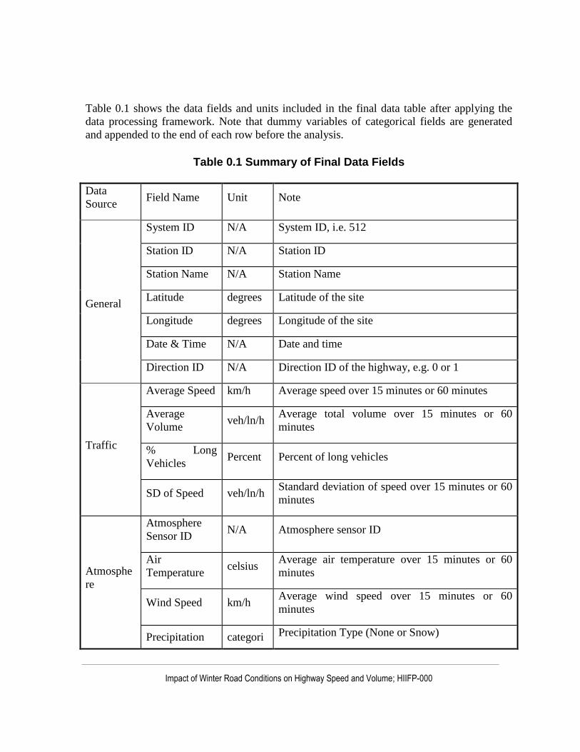
Impact of Winter Road Conditions on Highway Speed and Volume; HIIFP-000
Table 0.1 shows the data fields and units included in the final data table after applying the
data processing framework. Note that dummy variables of categorical fields are generated
and appended to the end of each row before the analysis.
Table 0.1 Summary of Final Data Fields
Data
Source Field Name Unit Note
General
System ID N/A System ID, i.e. 512
Station ID N/A Station ID
Station Name N/A Station Name
Latitude degrees Latitude of the site
Longitude degrees Longitude of the site
Date & Time N/A Date and time
Direction ID N/A Direction ID of the highway, e.g. 0 or 1
Traffic
Average Speed km/h Average speed over 15 minutes or 60 minutes
Average
Volume veh/ln/h
Average total volume over 15 minutes or 60
minutes
% Long
Vehicles Percent Percent of long vehicles
SD of Speed veh/ln/h Standard deviation of speed over 15 minutes or 60
minutes
Atmosphe
re
Atmosphere
Sensor ID N/A Atmosphere sensor ID
Air
Temperature celsius
Average air temperature over 15 minutes or 60
minutes
Wind Speed km/h Average wind speed over 15 minutes or 60
minutes
Precipitation categori Precipitation Type (None or Snow)

Impact of Winter Road Conditions on Highway Speed and Volume; HIIFP-000
Type es
Precipitation
Intensity
categori
es
Precipitation Intensity (None, Slight, Moderate or
Heavy)
Precipitation
Rate cm/h
Average precipitation rate over 15 minutes or 60
minutes
Surface
Surface Sensor
ID N/A Surface sensor ID
Surface
Condition
categori
es
RSC types (Dry, Trace Moisture, Wet, Chemically
Wet, Ice Watch or Ice Warning)
Surface
Temperature celsius Surface temperature
Others Time of Day
categori
es Day (6:00am – 6:00pm) Night (6:00pm – 6:00am)
Event ID N/A The ID of each event
Snow Event Definition and Extraction
In this study, a snow event extraction algorithm was proposed and developed based on the
data available in the datasets. To study the impact of both weather and RSC on traffic speed,
snow events should not only include the periods with snow precipitation, but also include
those with continuous ice/snow covered RSC during and after snow precipitation.
Figure 0.3 shows the definition of a snow event and the processes of the algorithm. The
algorithm uses precipitation type equals snow as the start of each event, and then checks if
snow or Ice Watch/Ice Warning surface condition occurs within the next hour (i.e.
continuous snow precipitation or the RSC is ice/snow covered during or after a snow event).
If any of these cases happens, the algorithm adds the next hour of data to the event bucket,
and then repeats the process. If none of these cases happens, the algorithm will add one more
hour of non-event data before and after the snow event to the event bucket, and write all data
in the event bucket to an event file, the final output of the algorithm. Finally, the algorithm
checks if this is the end of the file, if yes, save the event file and stop the process; otherwise,
move to the next data row and repeat the whole process again.

Impact of Winter Road Conditions on Highway Speed and Volume; HIIFP-000
Figure 0.3 Snow Event Extraction Algorithm

Impact of Winter Road Conditions on Highway Speed and Volume; HIIFP-000
Exploratory Analysis
Before proceeding with modelling, an exploratory data analysis was performed on the dataset
to investigate the patterns of the data, potential outliers and correlation between variables. It
was found that air temperature and surface temperature are highly correlated (i.e. 0.85 and
0.77 for two-lane and four-lane highways, respectively). Hence air temperature is removed
from the dataset and is not considered in the subsequent modelling analysis.
A summary statistics are subsequently generated.

Impact of Winter Road Conditions on Highway Speed and Volume; HIIFP-000
Table 0.2 shows the summary statistics of all numerical variables that will be used in this
analysis with different highway types and time intervals. Table 0.3 shows the sample size of
each categorical variable. Table 0.4 shows the sample size percentage of each site among all
the sites of the same highway type.
As can be seen in

Impact of Winter Road Conditions on Highway Speed and Volume; HIIFP-000
Table 0.2, most summary statistics are identical for both 15 minutes and 60 minutes dataset,
except that the standard deviations of the 15 minutes dataset are higher than those of the 60
minutes dataset. It can also be found that four-lane highways have relatively higher average
speed and average volume than two-lane highways. Although the maximum volume for some
highways (Site 13, 14 and 48) are relatively high (e.g. over 2500 veh/ln/h), the average
volume for both two-lane and four-lane highways are only around 100 veh/ln/h and 300
veh/ln/h, respectively. All highways have maximum average volume equal to or under
capacity, therefore traffic on these highways can be considered as free flow conditions.

Impact of Winter Road Conditions on Highway Speed and Volume; HIIFP-000
Table 0.2 Summary Statistics
15-Minute Interval
Two-Lane (67830 Obs.) Four-Lane (124314 Obs.)
Field Name Unit Min Max Mean SD Min Max Mean SD
Average Speed km/h 8.04 149.64 81.33 14.55 11.26 140.38 95.93 19.55
Average Volume veh/ln/h 30.00 2730.00 111.42 84.15 30.00 4140.00 332.66 326.19
% Long Vehicles % 0% 50% 18% 16% 0% 50% 31% 14%
Wind Speed km/h 0.00 85.00 16.05 9.97 0.00 87.00 16.44 10.67
Precipitation
Rate cm/h 0.00 77.98 0.07 0.85 0.00 81.92 0.12 1.31
Visibility km 0.00 114.26 34.20 43.56 0.00 162.54 13.11 27.81
Surface
Temperature Celsius -30.15 36.35 -4.89 5.02 -24.80 39.55 -4.57 5.73
60-Minute Interval
Two-Lane (15905 Obs.) Four-Lane (30507 Obs.)
Field Name Unit Min Max Mean SD Min Max Mean SD
Average Speed km/h 8.04 145.97 80.00 14.48 11.26 136.87 93.86 19.39
Average Volume veh/ln/h 30.00 2610.00 116.59 81.17 30.00 3930.00 309.37 302.78
% Long Vehicles % 0% 50% 20% 14% 0% 50% 32% 14%
Wind Speed km/h 0.00 85.00 16.44 10.43 0.00 70.00 16.35 10.88
Precipitation
Rate cm/h 0.00 49.55 0.09 0.83 0.00 62.75 0.13 1.12
Visibility km 0.00 114.26 35.11 43.30 0.00 162.54 12.42 26.79
Surface
Temperature Celsius -29.50 34.15 -5.05 4.92 -24.83 38.80 -4.98 5.68

Impact of Winter Road Conditions on Highway Speed and Volume; HIIFP-000
Table 0.3 Categorical Variable Sample Size
15-Minute Interval
Field Name Categories Two-Lane Four-Lane
Size % Size %
Precipitation
Intensity
None 32074 47.29% 58207 46.82%
Slight 34445 50.78% 63014 50.69%
Moderate 957 1.41% 2375 1.91%
Heavy 354 0.52% 718 0.58%
Surface Condition
Dry 11756 17.33% 33726 27.13%
Trace Moisture 2176 3.21% 6006 4.83%
Wet 5299 7.81% 7495 6.03%
Chemically Wet 2592 3.82% 3279 2.64%
Ice Watch 42918 63.27% 69761 56.12%
Ice Warning 3089 4.55% 4047 3.26%
Precipitation Type None 32074 47.29% 58207 46.82%
Snow 35756 52.71% 66107 53.18%
Time of Day Day 37278 54.96% 66715 53.67%
Night 30552 45.04% 57599 46.33%
60-Minute Interval
Field Name Categories Two-Lane Four-Lane
Size % Size %
Precipitation
Intensity
None 5973 37.55% 11248 36.87%
Slight 9487 59.65% 18292 59.96%
Moderate 322 2.02% 737 2.42%
Heavy 123 0.77% 230 0.75%
Surface Condition
Dry 2430 15.28% 7281 23.87%
Trace Moisture 520 3.27% 1403 4.60%
Wet 1165 7.32% 1733 5.68%
Chemically Wet 635 3.99% 752 2.47%
Ice Watch 10469 65.82% 18295 59.97%
Ice Warning 686 4.31% 1043 3.42%
Precipitation Type None 5973 37.55% 11248 36.87%
Snow 9932 62.45% 19259 63.13%
Time of Day Day 9072 57.04% 16988 55.69%
Night 6833 42.96% 13519 44.31%

Impact of Winter Road Conditions on Highway Speed and Volume; HIIFP-000
Table 0.4 Site Sample Size Percentage (15-Minute Interval)
Two-Lane Four-Lane
Direction 0 Direction 1 Direction 0 Direction 1
Site Size % Size % Site Size % Size %
01 1419 2.09% 1451 2.14% 00 2439 1.96% 2842 2.29%
02 5033 7.42% 5263 7.76% 06 472 0.38% 709 0.57%
11 1902 2.80% 2027 2.99% 08 2596 2.09% 2310 1.86%
13 981 1.45% 1254 1.85% 10 1931 1.55% 2072 1.67%
15 3531 5.21% 3722 5.49% 14 5072 4.08% 4925 3.96%
25 4729 6.97% 4386 6.47% 19 1247 1.00% 1397 1.12%
33 4043 5.96% 4581 6.75% 20 3227 2.60% 3186 2.56%
42 295 0.43% 311 0.46% 27 2581 2.08% 2228 1.79%
43 796 1.17% 804 1.19% 28 1565 1.26% 2104 1.69%
55 1932 2.85% 1951 2.88% 30 2601 2.09% 3103 2.50%
56 4271 6.30% 4460 6.58% 32 1325 1.07% 1177 0.95%
57 3539 5.22% 3707 5.47% 36 4252 3.42% 4444 3.57%
59 749 1.10% 693 1.02% 37 7131 5.74% 6236 5.02%
Total 67830 100% 41 1825 1.47% 2599 2.09%
44 371 0.30% 333 0.27%
46 1441 1.16% 2956 2.38%
47 3933 3.16% 3175 2.55%
48 2970 2.39% 2818 2.27%
49 4792 3.85% 4963 3.99%
50 2586 2.08% 1943 1.56%
53 3859 3.10% 3868 3.11%
58 3552 2.86% 3158 2.54%
Total 124314 100%

Impact of Winter Road Conditions on Highway Speed and Volume; HIIFP-000
Table 0.5 Site Sample Size Percentage (60-Minute Interval)
Two-Lane Four-Lane
Direction 0 Direction 1 Direction 0 Direction 1
Site Size % Size % Site Size % Size %
01 328 2.06% 328 2.06% 00 526 1.72% 573 1.88%
02 1149 7.22% 1208 7.60% 06 148 0.49% 212 0.69%
11 415 2.61% 428 2.69% 08 691 2.27% 604 1.98%
13 256 1.61% 342 2.15% 10 457 1.50% 457 1.50%
15 773 4.86% 823 5.17% 14 1074 3.52% 1082 3.55%
25 1177 7.40% 1084 6.82% 19 326 1.07% 385 1.26%
33 1049 6.60% 1112 6.99% 20 736 2.41% 736 2.41%
42 65 0.41% 65 0.41% 27 715 2.34% 634 2.08%
43 150 0.94% 152 0.96% 28 513 1.68% 646 2.12%
55 542 3.41% 565 3.55% 30 568 1.86% 677 2.22%
56 865 5.44% 848 5.33% 32 372 1.22% 358 1.17%
57 902 5.67% 908 5.71% 36 987 3.24% 1045 3.43%
59 188 1.18% 183 1.15% 37 1711 5.61% 1570 5.15%
Total 15905 100% 41 523 1.71% 666 2.18%
44 75 0.25% 69 0.23%
46 564 1.85% 777 2.55%
47 859 2.82% 764 2.50%
48 702 2.30% 679 2.23%
49 1182 3.87% 1209 3.96%
50 659 2.16% 574 1.88%
53 827 2.71% 838 2.75%
58 890 2.92% 847 2.78%
Total 30507 100%

Impact of Winter Road Conditions on Highway Speed and Volume; HIIFP-000
Methodology
Multivariate Linear Regression
In order to quantify the impact of adverse weather and surface factors on traffic speed, a
multivariate linear regression analysis is carried out in this study. With the intension of
investigating the feasibility of using traffic speed as an alternative measure of WRM, the
regression models should be capable of revealing the relationship between traffic speed and
weather and surface factors, especially the significance of RSC with the minimum
confounding effects of traffic volume. For rural highways, traffic speed is less likely to be
affected by volume due to lack of traffic congestion, thus making the models more reliable
than using urban highways. This has been confirmed in the exploratory data analysis in the
previous section.
Different directions of the same highway may have different traffic patterns, therefore with
the 15 minutes and 60 minutes time interval, a set of models are developed separately for
both directions of each study site, and two combined models for all sites of the same type of
highways are also developed for both two-lane and four-lane highways. This results in 144
models in total. The reason for developing combined models is that the effect of most
external factors on speed is expected to be similar for a given type of highways. In addition, a
combined model is expected to be more generalizable or transferable than a highway specific
model.
Table 3.6 summaries the three dimensions of the regression analysis which include
aggregation interval, highway type and model type. The goal of setting these dimensions is to
firstly investigate the impact of each dimension on the performance of the regression model;
secondly, to find out similarities and improve the simplicity of the models; thirdly, to find out
the best modeling methodology that fits a specific dataset, which can also be used in the
following advanced analysis.
Table 0.6 Dimensions of the Regression Analysis
Name Dimensions
Aggregation Interval 15 minutes vs. 60 minutes
Highway Type Two-Lane vs. Four-Lane
Model Type Separated vs. Combined
The effect of precipitation on speed is tested in two representation forms, namely, categorical
(precipitation intensity) and continuous (precipitation rate). It is found that the categorical

Impact of Winter Road Conditions on Highway Speed and Volume; HIIFP-000
form results in a higher explanation power, i.e., higher adjusted 𝑹𝟐 value suggesting its non-
linear effect on traffic speed. Categorical form is thus used in the final models.
For each categorical variable such as RSC, dummy variables are created, and a base category
is defined in advance. “Dry”, “No Snow” and “Day” are used for RSC, precipitation intensity
and Day/Night as the initial base conditions, respectively. Note that in the actual calibration,
combination of base conditions will be used if two or more categories show the similar effect
with the initial base condition or not statistically significant compared with the initial base
condition. For example, as the effect of dry, trace moisture, wet and chemically wet are
almost zero at Site 01 direction 0, the base condition, therefore, is the combination of all
these four conditions.
For site variables in the combined models, dummy variables are also created for each site.
Site 01 (direction 0) and Site 00 (direction 0) are used as base sites for the two-lane
combined and four-lane combined models, respectively.
The statistical significance of each variable is decided using a significance level of 5%. Any
variables with p-value of greater than 5% or don’t make intuitive sense are eliminated
sequentially from the model. The data set from each direction of each site is divided into two
parts randomly: one includes 90% of the data to be used for model calibration and the
remaining 10% of data is held out for subsequent model validation. The overall performance
of the regression model is assessed using adjusted 𝑹𝟐 and Root Mean Square Error (RMSE).
Artificial Neural Network
ANN is a non-parametric method for modeling complex non-linear relationships. Unlike
regression models that need an explicitly defined function to relate the input and the output,
the ANN can approximate a function and associate input with specific output through the
process of training. Therefore, ANN can be used to evaluate the robustness of regression
models (Martin et al., 1995).
In this study, the most commonly used ANN, multi-layer perceptron neural network (MLP-
NN) is selected for modeling the relationship between traffic speed and various influencing
factors. As can be seen in Figure 0.4, MLP-NN consists of an input layer, one or more hidden
layers, and an output layer. The input layer includes input nodes representing the weather,
road and traffic factors - same as the independent variables used in a regression model, while
the output layer includes the dependent variable to be predicted, i.e., traffic speed. The
hidden layer provides a mechanism to transfer inputs to output through activation functions
and weights (Martin et al., 1995). In this research, the popular sigmoid function is selected as
the activation functions for the hidden layers, and a linear activation function is selected for
the output layer. The weights of MLP-NN are calibrated by back propagation algorithm with
a learning rate of 0.1, a momentum of 0.8. The back propagation algorithm minimizes the
sum of squared deviation of the output from the target value at the nodes of the output layer
by adjusting the value of weight at nodes. For the sake of comparison, the significant
independent variables found in the combined regression analysis will be used as the input

Impact of Winter Road Conditions on Highway Speed and Volume; HIIFP-000
factors of the MLP-NN.
Figure 0.4 Typical MLP-NN Architecture (Huang & Ran, 2003)
Time Series Analysis
The data used in this research consist of time series of observations over various snowstorm
events. The observations within each event could therefore be correlated to each other due to
the similarity in weather and environmental conditions. This auto correlation violates the
assumption of randomness and independency between observations required by the
multivariate regression method. To address this issue, time series analysis is attempted to
explicitly model the correlation between successive observations by considering the effect on
current behavior of variables in terms of linear relationships with their past values (Wei,
1989). In this research, one of the most popular time series models - univariate autoregressive
integrated moving average (ARIMA) with additional exogenous variables (ARIMAX), is
utilized for predicting the traffic speed based on traffic volume, weather and surface data.
Since the focus of this study is to investigate the speed variation during snow events, adjacent
events are stitched together in model calibration.
According to Shumway and Stoffer (2006), a combination of an autoregressive integrated
(AR(p)) process and a moving average (MA(q)) process is called ARMA(p,q) which can be
expressed as below:
𝒙𝒕 = 𝝓𝟏𝒙𝒕−𝟏 + 𝝓𝟐𝒙𝒕−𝟐 + ⋯ + 𝝓𝒑𝒙𝒕−𝒑 + 𝝎𝒕 + 𝜽𝟏𝝎𝒕−𝟏 + ⋯ + 𝜽𝒒𝝎𝒕−𝒒
Where,
𝒙𝒕 is a stationary time series

Impact of Winter Road Conditions on Highway Speed and Volume; HIIFP-000
𝝎𝒕 is white noise 𝑵(𝟎, 𝝈𝟐)
𝝓 and 𝜽 are coefficients of the model
The above equation can be written in vector form:
𝝓(𝑩)𝒙𝒕 = 𝜽(𝑩)𝝎𝒕
If a d order differencing is added, the general form of ARIMA(p, d, q) model is given below:
𝝓(𝑩)(𝟏 − 𝑩)𝒅𝒙𝒕 = 𝜽(𝑩)𝝎𝒕
Where
𝒙𝒕 is a stationary time series
𝝎𝒕 is white noise 𝑵(𝟎, 𝝈𝟐)
𝑩 is the back slash operator, 𝑩𝒙𝒕 = 𝒙𝒕−𝟏
𝝓(𝑩) = 𝟏 − 𝝓𝟏𝑩 − 𝝓𝟐𝑩𝟐 − ⋯ − 𝝓𝒑𝑩𝒑
𝜽(𝑩) = 𝟏 − 𝜽𝟏𝑩 − 𝜽𝟐𝑩𝟐 − ⋯ − 𝜽𝒒𝑩𝒒
p is the number of autoregressive terms
d is the number of non-seasonal differences
q is the number of lagged forecast errors in the prediction equation
The ARMAX model is extended from general ARMA model by adding additional
exogenous/explanatory variables. The general form of the ARMAX model is given below:
𝒙𝒕 = 𝝓𝟏𝒙𝒕−𝟏 + 𝝓𝟐𝒙𝒕−𝟐 + ⋯ + 𝝓𝒑𝒙𝒕−𝒑 + 𝝎𝒕 + 𝜽𝟏𝝎𝒕−𝟏 + ⋯ + 𝜽𝒒𝝎𝒕−𝒒 + 𝜞𝑼𝒕
Where
𝒙𝒕 is a stationary time series (speed at time t)
𝝎𝒕 is white noise 𝑵(𝟎, 𝝈𝟐)
𝝓 and 𝜽 are coefficients of the model
𝐔𝐭 is the vector of exogenous variables (explanatory variables including AR, MA,
weather and surface variables)
𝚪 is the coefficient vector of exogenous variables
The above equation is equivalent to:
𝝓(𝑩)𝒙𝒕 = 𝜽(𝑩)𝝎𝒕 + 𝜞𝑼𝒕
If a d order differencing is added, the general form of ARIMAX(p, d, q) model is given
below:

Impact of Winter Road Conditions on Highway Speed and Volume; HIIFP-000
𝝓(𝑩)(𝟏 − 𝑩)𝒅𝒙𝒕 = 𝜽(𝑩)𝝎𝒕 + 𝜞𝑼𝒕
Where
𝒙𝒕 is a stationary time series
𝝎𝒕 is white noise 𝑵(𝟎, 𝝈𝟐)
𝑩 is the back slash operator, 𝑩𝒙𝒕 = 𝒙𝒕−𝟏
𝝓(𝑩) = 𝟏 − 𝝓𝟏𝑩 − 𝝓𝟐𝑩𝟐 − ⋯ − 𝝓𝒑𝑩𝒑
𝜽(𝑩) = 𝟏 − 𝜽𝟏𝑩 − 𝜽𝟐𝑩𝟐 − ⋯ − 𝜽𝒒𝑩𝒒
p is the number of autoregressive terms
d is the number of non-seasonal differences
q is the number of lagged forecast errors in the prediction equation
𝐔𝐭 is the vector of exogenous variables (explanatory variables including AR, MA,
weather and surface variables)
𝚪 is the coefficient vector of exogenous variables
If the time series is non-stationary, it must be transformed into a stationary time series by the
method of differencing first. This can be determined using autocorrelation factor (ACF) and
partial autocorrelation factor (PACF). The model parameters are estimated using maximum
likelihood method with 95% confidence level. Therefore, covariates, AR and MA variables
of different time lags with p-values greater than 0.05 are excluded.
Model Calibration
Multivariate Linear Regression
Statistical software R is used to calibrate the multivariate linear regression models. Appendix
A-1 to A-4 show the models developed for individual study sites. It can be found that the
average traffic speed constant of all two-lane highways are below 100 km/h while most four-
lane highways have the average traffic speed constant over 110 km/h. This makes sense as
four-lane highways normally have higher level of service than two-lane highways.
Significant factors for highways of the same type are mostly identical: average volume, wind
speed, all precipitation intensity categories, chemically wet, ice watch and ice warning are
statistically significant and make intuitive sense for most two-lane highways. Average
volume, % long vehicles, wind speed, all precipitation intensity categories, chemically wet,
ice watch, ice warning and night are statistically significant and make intuitive sense for most
four-lane highways. In terms of model performance, in general, four-lane highways have
relatively higher adjusted 𝑹𝟐 (about 0.45 on average) than two-lane highways (about 0.25 on
average). The reason is four-lane highways have relatively higher volume (larger sample
size) which leads to less variation in average traffic speed while two-lane highways have
higher variation in average traffic speed between vehicles due to smaller sample size.
Table 3.7 and 3.8 show the combined models for two-lane and four-lane highways,

Impact of Winter Road Conditions on Highway Speed and Volume; HIIFP-000
respectively. For two-lane combined, except % long vehicles and night, all the variables are
statistically significant and make intuitive sense for both 15 minutes and 60 minutes models.
The adjusted 𝑹𝟐 of the 60 minutes model is 0.34 which is slightly higher than the value of
the 15 minutes model (0.31). Both values are higher than the average adjusted 𝑹𝟐 generated
by the separated models (about 0.25). The RMSE are 12.06 and 11.74 for the 15 minutes and
60 minutes model, respectively.
For four-lane combined, surface temperature and trace moisture are not significant for the 15
minutes model while surface temperature, trace moisture and visibility are found not
significant for the 60 minutes model. Similar with two-lane models, the adjusted 𝑹𝟐 of both
15 minutes (0.68) and 60 minutes (0.70) are increased significantly compared with separated
models (about 0.45). The RMSE are 11.01 and 10.64 for the 15 minutes and 60 minutes
model, respectively.
The results above confirmed that firstly, combined models have advantages over separated
models, and are acceptable to be used to estimate average traffic speed for most study sites.
The adjusted 𝑹𝟐 of the combined models are higher than most separated models for both
highway types. In addition, due to lack of data on certain types of categorical variables at
some sites, some categories’ coefficients are zero in the separated models. For example,
heavy snow for Site 20 and ice warning for Site 06 were observed rarely, which results in
zero coefficients. With the combined models, this type of relationship could be captured
utilizing the data from other sites of the same highway type. Secondly, 60 minutes models’
performance is higher than 15 minutes models. Although the 15 minutes models can generate
average traffic speed estimations with higher temporal resolution, 60 minutes models are
based on smoother and more generalized dependent and independent variables, and their
adjusted 𝑹𝟐 are higher than the 15 minutes models.
Based on these two conclusions, the combined models will be used to analyze the effects of
each variable on average traffic speed, and the combined datasets with 60 minutes time
interval will be used in the subsequent ANN and time series analysis model calibration.

Impact of Winter Road Conditions on Highway Speed and Volume; HIIFP-000
Table 0.7 Regression Model Calibration Results for Two-Lane Highways Combined
Coef. Std. Error t-value P-value Coef. Std. Error t-value P-value
(Intercept) 94.85 0.37 258.22 0.00 96.40 0.76 126.63 0.00
Average Volume -0.01 0.00 -8.17 0.00 -0.01 0.00 -7.90 0.00
% Long Vehicles
Wind Speed -0.13 0.01 -25.89 0.00 -0.15 0.01 -15.41 0.00
Visibility 0.03 0.00 19.49 0.00 0.04 0.00 10.94 0.00
Surface Temp 0.05 0.01 4.49 0.00 0.10 0.02 4.16 0.00
Slight -5.12 0.10 -52.82 0.00 -4.65 0.20 -22.92 0.00
Moderate -13.14 0.41 -32.33 0.00 -10.52 0.70 -15.06 0.00
Heavy -32.25 0.67 -48.09 0.00 -28.08 1.13 -24.87 0.00
Trace Moisture -0.60 0.30 -1.99 0.05 -2.24 0.60 -3.71 0.00
Wet -1.22 0.22 -5.68 0.00 -1.94 0.45 -4.31 0.00
Chemically Wet -4.31 0.27 -16.11 0.00 -5.54 0.54 -10.34 0.00
Ice Watch -7.81 0.13 -58.18 0.00 -9.13 0.28 -32.55 0.00
Ice Warning -10.02 0.27 -37.80 0.00 -12.19 0.54 -22.48 0.00
Night 0.00 0.00 0.00 0.00
01-1 -1.13 0.45 -2.51 0.01 -0.85 0.92 -0.93 0.35
02-0 -3.87 0.38 -10.32 0.00 -4.29 0.76 -5.63 0.00
02-1 -3.26 0.37 -8.73 0.00 -3.90 0.76 -5.14 0.00
11-0 -1.93 0.43 -4.49 0.00 -2.71 0.88 -3.08 0.00
11-1 2.05 0.43 4.83 0.00 1.64 0.88 1.87 0.06
13-0 -11.86 0.52 -22.98 0.00 -12.98 1.01 -12.82 0.00
13-1 -10.77 0.49 -22.15 0.00 -14.63 0.95 -15.34 0.00
15-0 3.28 0.39 8.43 0.00 3.64 0.79 4.59 0.00
15-1 2.47 0.39 6.41 0.00 2.50 0.79 3.18 0.00
25-0 -6.75 0.37 -18.15 0.00 -7.51 0.75 -10.02 0.00
25-1 -8.85 0.37 -23.69 0.00 -9.77 0.75 -13.00 0.00
33-0 -2.11 0.38 -5.51 0.00 -2.36 0.76 -3.08 0.00
33-1 1.14 0.38 3.02 0.00 0.78 0.76 1.02 0.31
42-0 -1.04 0.78 -1.32 0.19 0.78 1.61 0.48 0.63
42-1 -1.12 0.77 -1.46 0.14 0.66 1.61 0.41 0.68
43-0 -25.40 0.54 -46.93 0.00 -24.60 1.17 -20.98 0.00
43-1 -27.29 0.54 -50.60 0.00 -26.71 1.17 -22.89 0.00
55-0 2.90 0.43 6.82 0.00 2.73 0.83 3.30 0.00
55-1 4.78 0.42 11.26 0.00 3.97 0.82 4.82 0.00
56-0 -9.82 0.38 -25.99 0.00 -9.57 0.78 -12.34 0.00
56-1 -3.07 0.38 -8.16 0.00 -2.85 0.78 -3.67 0.00
57-0 -1.88 0.39 -4.82 0.00 -2.17 0.78 -2.79 0.00
57-1 0.07 0.39 0.18 0.86 -0.44 0.78 -0.56 0.57
59-0 -5.79 0.55 -10.57 0.00 -5.48 1.08 -5.07 0.00
59-1 -3.55 0.56 -6.32 0.00 -5.59 1.09 -5.12 0.00
RMSE 12.06 Adj. R^2 0.31 RMSE 11.74 Adj. R^2 0.34
15 Minutes Interval 60 Minutes Interval

Impact of Winter Road Conditions on Highway Speed and Volume; HIIFP-000
Table 0.8 Regression Model Calibration Results for Four-Lane Highways Combined
Coef. Std. Error t-value P-value Coef. Std. Error t-value P-value
(Intercept) 121.30 0.27 457.07 0.00 122.20 0.59 206.41 0.00
Average Volume 0.01 0.00 68.77 0.00 0.01 0.00 38.45 0.00
% Long Vehicles -16.64 0.29 -56.47 0.00 -22.07 0.67 -32.72 0.00
Wind Speed -0.18 0.00 -56.84 0.00 -0.21 0.01 -31.93 0.00
Visibility 0.01 0.00 4.92 0.00
Surface Temp
Slight -4.69 0.06 -73.99 0.00 -4.19 0.14 -30.58 0.00
Moderate -13.36 0.23 -58.73 0.00 -11.98 0.43 -27.83 0.00
Heavy -15.62 0.41 -38.14 0.00 -17.25 0.75 -22.87 0.00
Trace Moisture 0.00 0.00 0.00 0.00
Wet -3.78 0.14 -27.49 0.00 -4.27 0.30 -14.30 0.00
Chemically Wet -7.86 0.20 -39.69 0.00 -9.26 0.43 -21.57 0.00
Ice Watch -9.10 0.07 -124.03 0.00 -9.94 0.16 -63.29 0.00
Ice Warning -11.39 0.19 -60.63 0.00 -12.17 0.39 -31.34 0.00
Night -0.94 0.06 -15.08 0.00 -0.41 0.13 -3.06 0.00
00-01 -0.50 0.29 -1.71 0.09 -0.73 0.67 -1.09 0.28
06-0 0.36 0.54 0.66 0.51 1.12 1.04 1.08 0.28
06-1 -3.39 0.46 -7.42 0.00 -2.14 0.90 -2.37 0.02
08-0 -28.90 0.31 -93.54 0.00 -27.87 0.65 -42.56 0.00
08-1 -29.48 0.32 -92.61 0.00 -29.18 0.68 -43.11 0.00
10-0 -13.70 0.33 -41.47 0.00 -14.18 0.72 -19.75 0.00
10-1 -16.68 0.32 -51.62 0.00 -18.00 0.72 -25.12 0.00
14-0 -9.21 0.28 -32.55 0.00 -9.87 0.64 -15.50 0.00
14-1 0.55 0.27 2.08 0.04 1.11 0.59 1.88 0.06
19-0 -7.81 0.37 -20.89 0.00 -8.29 0.78 -10.60 0.00
19-1 -9.14 0.36 -25.42 0.00 -9.09 0.74 -12.23 0.00
20-0 -45.98 0.30 -155.09 0.00 -46.10 0.65 -70.68 0.00
20-1 -47.68 0.29 -164.20 0.00 -46.36 0.64 -72.96 0.00
27-0 -6.75 0.31 -22.07 0.00 -7.40 0.64 -11.51 0.00
27-1 -7.07 0.32 -22.34 0.00 -10.10 0.66 -15.35 0.00
28-0 -11.28 0.35 -32.32 0.00 -13.39 0.69 -19.37 0.00
28-1 -1.84 0.32 -5.72 0.00 -3.56 0.66 -5.43 0.00
30-0 -6.64 0.31 -21.56 0.00 -8.60 0.68 -12.59 0.00
30-1 -0.80 0.29 -2.72 0.01 -1.42 0.65 -2.17 0.03
32-0 -8.88 0.37 -24.04 0.00 -9.49 0.76 -12.50 0.00
32-1 -3.42 0.38 -8.96 0.00 -3.89 0.76 -5.11 0.00
36-0 -44.68 0.29 -156.28 0.00 -44.96 0.63 -71.38 0.00
36-1 -40.08 0.28 -144.11 0.00 -39.85 0.61 -65.38 0.00
37-0 -1.48 0.26 -5.65 0.00 -1.92 0.57 -3.36 0.00
37-1 -0.79 0.27 -2.94 0.00 -1.23 0.58 -2.11 0.03
41-0 -34.63 0.34 -101.22 0.00 -35.11 0.71 -49.45 0.00
41-1 -40.07 0.31 -128.05 0.00 -39.87 0.67 -59.34 0.00
44-0 -13.90 0.60 -23.34 0.00 -13.80 1.37 -10.10 0.00
44-1 -3.69 0.62 -5.90 0.00 -3.67 1.42 -2.59 0.01
46-0 -14.62 0.36 -40.71 0.00 -14.59 0.68 -21.39 0.00
46-1 -12.54 0.30 -42.52 0.00 -12.76 0.63 -20.23 0.00
47-0 -1.13 0.28 -4.09 0.00 -1.31 0.62 -2.12 0.03
47-1 1.36 0.29 4.70 0.00 1.78 0.63 2.82 0.00
48-0 -6.84 0.30 -22.64 0.00 -6.86 0.66 -10.39 0.00
48-1 -10.38 0.30 -34.42 0.00 -11.24 0.66 -17.16 0.00
49-0 1.84 0.27 6.90 0.00 2.65 0.58 4.57 0.00
49-1 -0.81 0.26 -3.04 0.00 -0.25 0.58 -0.43 0.66
50-0 -3.76 0.30 -12.32 0.00 -4.32 0.65 -6.62 0.00
50-1 -4.92 0.33 -15.01 0.00 -5.71 0.67 -8.49 0.00
53-0 -2.84 0.28 -10.25 0.00 -3.54 0.62 -5.73 0.00
53-1 -3.65 0.28 -13.17 0.00 -3.75 0.62 -6.09 0.00
58-0 -6.85 0.28 -24.10 0.00 -6.57 0.61 -10.73 0.00
58-1 -2.31 0.29 -7.94 0.00 -2.49 0.62 -4.03 0.00
RMSE 11.01 Adj. R^2 0.68 RMSE 10.64 Adj. R^2 0.70
15 Minutes Interval 60 Minutes Interval

Impact of Winter Road Conditions on Highway Speed and Volume; HIIFP-000
Effect of Average Volume and % Long Vehicles
Two-Lane Highways:
It can be found from Table 0.7 that traffic volume has the same negative effect on average
traffic speed for both 15 minutes and 60 minutes models. The modeling results show that for
each 100 veh/ln/h increase in average traffic volume, speed will decrease by 1 km/h.
Considering the low average traffic volume on two-lane highways, this effect is relatively
small. The proportion of truck and recreational vehicles is found not statistically significant
for both the 15 minutes and 60 minutes models.
Four-Lane Highways:

Impact of Winter Road Conditions on Highway Speed and Volume; HIIFP-000
Table 0.8 shows that different from two-lane highways, traffic volume has positive effect
on average traffic speed for four-lane highways. Both 15 minutes and 60 minutes models
have the same coefficient: for each 100 veh/ln/h increase in traffic volume, speed could
increase by 1 km/h. This relationship is somehow counterintuitive as the opposite is
commonly observed, at least, under normal weather conditions. This positive effect of
traffic may be attributed to its positive effect on improving road surface conditions
through tire compaction, which might not have been fully captured by the RSC variable
on four-lane highways. Another possible reason could be that on rural highways where
traffic is generally low presence of other vehicles in visual range may have a positive
effect on how fast a driver would be comfortable to drive under adverse weather
conditions. The proportion of truck and recreational vehicles is found to have a negative
effect on the average traffic speed. For the 15 minutes model, every 10% increase in %
long vehicles is expected to decrease average traffic speed by 1.7 km/h. For the 60
minutes model, every 10% increase in % long vehicles is expected to decrease average
traffic speed by 2.2 km/h.
Effect of Wind Speed
Two-Lane Highways:
As expected, wind speed has a statistically significant effect on average traffic speed.
Higher wind speed is found to be associated with lower average traffic speed. One
possible explanation is that high wind speed is normally associated with adverse weathers
which will obviously slow down the traffic. The results in Table 0.7 shows that on
average, every 10 km/h increase in wind speed would slow traffic by approximately 1.3
and 1.5 km/h for the 15 minutes and 60 minutes models, respectively.
Four-Lane Highways:
Compared with two-lane highways, the effect of wind speed is slightly higher on four-
lane highways. Every 10 km/h increase in wind speed would slow traffic speed by
approximately 1.8 and 2.1 km/h for the 15 minutes and 60 minutes models, respectively.
Effect of Visibility
Two-Lane Highways:
As is shown in Table 0.7, visibility has positive effect on average traffic speed. On
average, every 10 km increase in visibility would increase traffic speed by approximately
0.3 and 0.4 km/h for the 15 minutes and 60 minutes models, respectively. This makes
intuitive sense, as high visibility indicates good weather and driving conditions which
would have positive effect on average traffic speed.
Four-Lane Highways:

Impact of Winter Road Conditions on Highway Speed and Volume; HIIFP-000
Compared with two-lane highways, the effect of visibility is only statistically significant
for the 15 minutes model. Every 10 km increase in visibility would increase traffic speed
by approximately 0.1 km/h which is small.
Effect of Surface Temperature
Two-Lane Highways:
Surface temperature is found to have a positive effect on average traffic speed for two-
lane highways. One possible explanation is that lower road surface temperature had
contributed to worsening of road surface conditions and decreasing in road surface
friction. However, the effect of this factor is relatively small, as for each degree of drop
in road surface temperature, there was only an average reduction of equal to or less than
0.1 km/h in average traffic speed.
Four-Lane Highways:
Surface temperature is not statistically significant for four-lane highways.
Effect of Night
Two-Lane Highways:
As is shown in Table 0.7, the categorical variable night doesn’t have statistically
significant effect on average traffic speed for two-lane highways, which may be caused
by lack of vehicles during the night.
Four-Lane Highways:
For four-lane highways, night has a negative effect on average traffic speed. The average
traffic speed at night time is approximately 0.94 km/h and 0.41 km/h lower than day time
traffic speed for the 15 minutes and 60 minutes models, respectively. Like surface
temperature, this effect is also considered to be very small.
Effect of Precipitation Intensity
Two-Lane Highways:
Figure 0.5 shows a comparison of the coefficients of the three precipitation intensity
categories. The modeling results suggest that precipitation has huge negative effect on
average traffic speed, especially heavy snow. Compared with no snow, heavy snow could
cause an average reduction of about 32.25 km/h (34.0%) and 28.08 km/h (29.1%) in
average traffic speed for the 15 minutes and 60 minutes models, respectively. Average
speed reduction caused by moderate snow is 13.14 km/h (13.9%) and 10.52 km/h
(10.9%) for the 15 minutes and 60 minutes models, respectively. Slight snow causes
average speed reduction by 5.12 km/h (5.4%) and 4.65 km/h (4.8%) for the 15 minutes

Impact of Winter Road Conditions on Highway Speed and Volume; HIIFP-000
and 60 minutes models, respectively. The effects of precipitation intensity are very close
in the two models with different time intervals. The effects in the 15 minutes model are
slightly higher than in the 60 minutes model. The speed reduction caused by heavy and
light snow is fairly close with the numbers suggested in HCM 2010 (30-40% for heavy
snow and 8-10% for light snow).
Four-Lane Highways:
Similar with two-lane highways, the effect of precipitation intensity is also significant for
four-lane highways. Compared with no snow, heavy snow could cause an average
reduction of about 15.62 km/h (12.9%) and 17.25 km/h (14.1%) in average traffic speed
for the 15 minutes and 60 minutes models, respectively. Compared with two-lane
highways, these effects are lower for four-lane highways. Average speed reduction
caused by moderate snow is 13.36 km/h (11.0%) and 11.98 km/h (9.8%) for the 15
minutes and 60 minutes models, respectively. Slight snow could cause average speed
reduction by 4.69 km/h (3.9%) and 4.19 km/h (3.4%) for the 15 minutes and 60 minutes
models, respectively. Similarly, the effects of precipitation intensity are very close in the
two models with different time intervals. Compared with the numbers suggested in HCM
2010, both heavy and slight snow result in relatively lower speed reduction on four lane
highways.
Figure 0.5 Effect of Precipitation Intensity
Effect of Road Surface Conditions
Two-Lane Highways:
-35.00
-30.00
-25.00
-20.00
-15.00
-10.00
-5.00
0.00
Slight Moderate High Slight Moderate High
Co
eff
icie
nt
Two-Lane Four-Lane
15 minutes 60 minutes
Impact of Winter Road Conditions on Highway Speed and Volume; HIIFP-000
Figure 0.6 shows the coefficients of RSC categories. The modeling results suggest that
RSC also has significant negative effect on average traffic speed. Among all categories,
ice warning causes the most significant speed reduction. Compared with dry condition, it
causes an average reduction of about 10.02 km/h (10.6%) and 12.19 km/h (12.6%) for the
15 minutes and 60 minutes models, respectively. Ice watch causes an average reduction
of about 7.81 km/h (8.2%) and 9.13 km/h (9.5%) for the 15 minutes and 60 minutes
models, respectively. Chemically wet causes an average reduction of about 4.31 km/h
(4.5%) and 5.54 km/h (5.7%) for the 15 minutes and 60 minutes models, respectively.
Compare with the first three categories, wet and trace moisture have limited effects on
average traffic speed. Wet causes an average reduction of about 1.22 km/h (1.3%) and
1.94 km/h (2.0%) for the 15 minutes and 60 minutes models, respectively. Trace moisture
causes an average reduction of about 0.60 km/h (0.6%) and 2.24 km/h (2.3%) for the 15
minutes and 60 minutes models, respectively. Again, the effects of RSC are very close in
the two models with different time intervals. The effects in the 60 minutes model are
slightly higher than in the 15 minutes model.
Four-Lane Highways:
The effects of RSC on average traffic on four-lane highways show the same pattern with
two-lane highways. Compared with dry condition, ice warning causes an average
reduction of about 11.39 km/h (9.4%) and 12.17 km/h (10.0%) for the 15 minutes and 60
minutes models, respectively. Ice watch causes an average reduction of about 9.10 km/h
(7.5%) and 9.94 (8.1%) km/h for the 15 minutes and 60 minutes models, respectively.
Chemically wet causes an average reduction of about 7.86 km/h (6.5%) and 9.26 km/h
(7.6%) for the 15 minutes and 60 minutes models, respectively. The effect of chemically
wet increased by about 4 km/h than the effect in the two-lane models. Wet causes an
average reduction of about 3.78 km/h (3.1%) and 4.27 km/h (3.5%) for the 15 minutes
and 60 minutes models, respectively. These values are also doubled compared with the
values in the two-lane highways. Trace moisture is found to be not statistically significant
for four-lane highways. Again, the effects of RSC are very close in the two models with
different time intervals. The effects in the 60 minutes model are slightly higher than in
the 15 minutes model. These results clearly show the high degree of impact of the RSC
on average traffic speed.
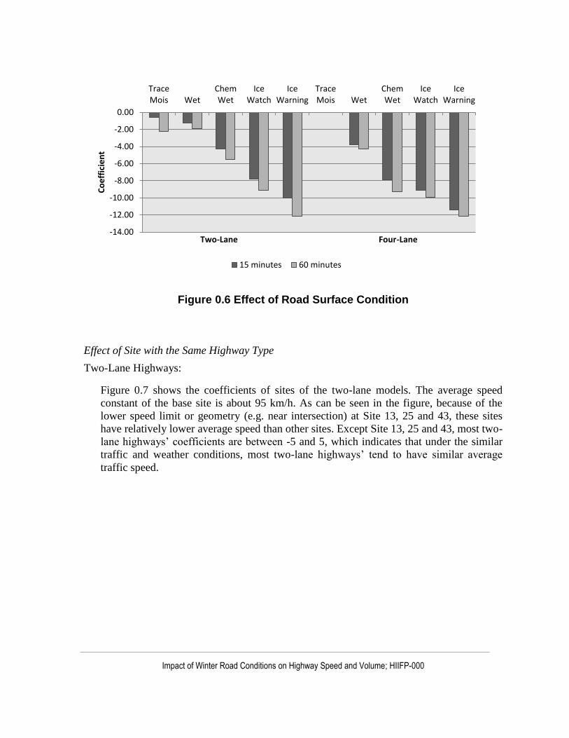
Impact of Winter Road Conditions on Highway Speed and Volume; HIIFP-000
Figure 0.6 Effect of Road Surface Condition
Effect of Site with the Same Highway Type
Two-Lane Highways:
Figure 0.7 shows the coefficients of sites of the two-lane models. The average speed
constant of the base site is about 95 km/h. As can be seen in the figure, because of the
lower speed limit or geometry (e.g. near intersection) at Site 13, 25 and 43, these sites
have relatively lower average speed than other sites. Except Site 13, 25 and 43, most two-
lane highways’ coefficients are between -5 and 5, which indicates that under the similar
traffic and weather conditions, most two-lane highways’ tend to have similar average
traffic speed.
-14.00
-12.00
-10.00
-8.00
-6.00
-4.00
-2.00
0.00
TraceMois Wet
ChemWet
IceWatch
IceWarning
TraceMois Wet
ChemWet
IceWatch
IceWarning
Co
eff
icie
nt
Two-Lane Four-Lane
15 minutes 60 minutes

Impact of Winter Road Conditions on Highway Speed and Volume; HIIFP-000
Figure 0.7 Site Effect of Two-Lane Highways
Four-Lane Highways:
Figure 0.8 shows the coefficients of sites of the four-lane models. The average speed
constant of the base site is about 122 km/h. As can be seen in the figure above, most four-
lane highways’ site coefficients are negative, therefore under the default traffic and
weather conditions, these highways’ average traffic speeds are mostly lower than the base
site. Also, Because of the lower speed limit or geometry (e.g. near intersection) at Site 08,
20, 36 and 41, these sites have relatively lower average speed than other sites. Most four-
lane highways’ coefficients are between -10 and 5, which indicates that under the default
traffic and weather condition, most four-lane highways’ also tend to have similar average
traffic speed (i.e. 112 km/h to 127 km/h). Note that the lower bound of this range (e.g.
112 km/h) is much higher than the higher bound of the two-lane highways’ range (i.e.
100 km/h). This clearly shows the different traffic speed patterns on these two types of
highways.
-30.00
-25.00
-20.00
-15.00
-10.00
-5.00
0.00
5.00
10.00
01
-1
02
-0
02
-1
11
-0
11
-1
13
-0
13
-1
15
-0
15
-1
25
-0
25
-1
33
-0
33
-1
42
-0
42
-1
43
-0
43
-1
55
-0
55
-1
56
-0
56
-1
57
-0
57
-1
59
-0
59
-1
Co
eff
icie
nt
Site
15 minutes 60 minutes

Impact of Winter Road Conditions on Highway Speed and Volume; HIIFP-000
Figure 0.8 Site Effect of Four-Lane Highways
Artificial Neural Network
The two combined datasets with 60 minutes time interval are used for MLP-NN model
calibration in the statistical software R. The significant independent variables found in the
previous combined regression models are included as the input factors of the MLP-NN.
Table 0.9 shows the results of MLP-NN for the two types of highways. Note that a single
hidden layer with nine nodes and two hidden layers with nine nodes in first layer and two
nodes in second layer were found to be optimal for the two-lane and four-lane highways,
respectively. The corresponding RMSE is 10.13 and 9.68, which are slightly higher than the
RMSE of the combined regression models. Detailed model comparison will be given in the
next section.
Table 0.9 MLP-NN Model Calibration Results
Site Variables
MLP-NN Architecture
(Hidden Layers & Nodes) Overall
RMSE First Layer Second Layer
Two-Lane 60 minutes
Combined
Average Volume, Wind Speed,
Visibility, Surface Temp,
Precipitation Intensity, RSC
and Sites
9 0 10.13
Four-Lane 60 minutes
Combined
Average Volume, % Long
Vehicles, Wind Speed,
Precipitation Intensity, RSC,
Night and Sites
9 2 9.68
-60.00
-50.00
-40.00
-30.00
-20.00
-10.00
0.00
10.00
00
-01
06
-1
08
-1
10
-1
14
-1
19
-1
20
-1
27
-1
28
-1
30
-1
32
-1
36
-1
37
-1
41
-1
44
-1
46
-1
47
-1
48
-1
49
-1
50
-1
53
-1
58
-1
Co
eff
icie
nt
Site
15 minutes 60 minutes

Impact of Winter Road Conditions on Highway Speed and Volume; HIIFP-000
Time Series Analysis
Similar with previous two analysis, time series analysis is also calibrated in the statistical
software R. It is found that observed speed doesn’t show any trend of being non-stationary;
therefore, no differentiation was required for the data. All independent variables used in the
regression model calibration are included as the independent variables of the ARIMAX
model. Based on the investigation of several combinations of ARIMAX models, ARIMAX
(2,0,2) is found to be optimal and finally selected and calibrated for both two-lane and four-
lane highways.
Note that the goodness of fit of the model is estimated based on the model statistics generated
by R called AIC (Akaike Information Criterion) and AICc (i.e. AIC with a greater penalty for
extra parameters) which are measures of the relative quality of a statistical model for the
trade-off between the goodness of fit of the model and the complexity of the model (Akaike,
1974). The lower the AIC/AICc values, the better quality the model has. Another model
statistic generated by R that could be potentially used is BIC (Bayesian Information
Criterion). However, a comparison of AIC/AICc and BIC given by Burnham & Anderson
(2002, 2004) suggest that AIC/AICc can be derived in the same Bayesian framework as BIC,
and has theoretical advantages over BIC. As a result, only AIC/AICc is used to justify the
model quality in this analysis.
Table 3.10 and 3.11 show the final results of ARIMAX model for two-lane and four-lane
highways, respectively. The results show that % long vehicles and night are not found to be
significant for two-lane highways while visibility and night are not significant for four-lane
highways. The results also suggest that similar with the multivariate linear regression results,
precipitation intensity (i.e. up to -6.62 and -7.80) and RSC (i.e. up to -6.28 and -6.84) have a
significant effect on the average traffic speed. The RMSE values are 8.92 and 8.05,
respectively, which are improved significantly compared with the values in the regression
analysis (11.74 and 10.64), and also better than MLP-NN (10.13 and 9.68).
Table 0.10 ARIMAX Model Calibration Results for Two-Lane Combined (60-Minute Interval)
Intercept
89.45
(2.60)
AR1
1.68
(0.04)
AR2
-0.70
(0.03)
MA1
-1.19
(0.04)
MA2
0.26
(0.02)
Average Volume
-0.01
(0.00)
% Long Vehicles
Wind Speed
-0.09
(0.01)
Visibility
0.01
(0.00)
Surface Temperature
0.23
(0.03)

Impact of Winter Road Conditions on Highway Speed and Volume; HIIFP-000
None
0.00
0.00
Slight
-1.08
(0.17)
Moderate
-3.73
(0.56)
Heavy
-6.62
(0.99)
Dry
0.00
0.00
Trace Moisture
-0.77
(0.59)
Wet
-0.53
(0.42)
Chemically Wet
-2.95
(0.47)
Ice Watch
-3.80
(0.29)
Ice Warning
-6.28
(0.52)
Day Night
01-0
0.00
0.00
02-0
-4.08
(2.95)
11-0
-2.71
(3.42)
13-0
-19.26
(3.79)
15-0
1.54
(3.10)
01-1
-1.99
(3.40)
02-1
-4.43
(2.93)
11-1
0.44
(3.41)
13-1
-9.99
(3.71)
15-1
2.42
(3.07)
25-0
-5.46
(2.94)
33-0
-0.46
(2.98)
42-0
2.48
(5.09)
43-0
-24.87
(4.30)
55-0
2.10
(3.27)
25-1
-8.12
(2.96)
33-1
2.84
(2.96)
42-1
1.53
(5.15)
43-1
-27.15
(4.24)
55-1
4.41
(3.25)
56-0
-10.07
(3.05)
57-0
-0.46
(3.03)
59-0
-6.26
(4.04)
56-1 57-1 59-1

Impact of Winter Road Conditions on Highway Speed and Volume; HIIFP-000
-4.16
(3.05)
1.31
(3.03)
-5.00
(4.19)
AIC
114854.30
AICc
114854.50
BIC
115184.30
Log Likelihood
-57384.15
Overall RMSE
8.92
Table 0.11 ARIMAX Model Calibration Results for Four-Lane Combined (60-Minute Interval)
Intercept
112.68
(1.76)
AR1
1.65
(0.03)
AR2
-0.67
(0.03)
MA1
-1.02
(0.04)
MA2
0.12
(0.01)
Average Volume
0.01
(0.00)
% Long Vehicles
-15.61
(0.61)
Wind Speed
-0.14
(0.01)
Visibility Surface Temperature
0.03
(0.02)
None
0.00
0.00
Slight
-1.31
(0.10)
Moderate
-4.78
(0.33)
Heavy
-7.80
(0.60)
Dry
0.00
0.00
Trace Moisture
0.00
0.00
Wet
-0.72
(0.28)
Chemically Wet
-4.83
(0.33)
Ice Watch
-4.61
(0.17)
Ice Warning
-6.84
(0.33)
Day
Night
00-0
0.00
06-0
5.01
08-0
-26.39
10-0
-11.27
14-0
-5.23

Impact of Winter Road Conditions on Highway Speed and Volume; HIIFP-000
0.00 (3.24) (2.18) (2.39) (2.03)
00-1
-0.47
(2.22)
06-1
-0.76
(2.93)
08-1
-27.81
(2.24)
10-1
-16.16
(2.38)
14-1
3.22
(2.01)
19-0
-7.57
(2.60)
20-0
-43.86
(2.15)
27-0
-5.84
(2.16)
28-0
-10.48
(2.33)
30-0
-3.92
(2.27)
19-1
-8.19
(2.49)
20-1
-45.00
(2.15)
27-1
-8.95
(2.21)
28-1
-1.94
(2.21)
30-1
1.59
(2.19)
32-0
-7.45
(2.51)
36-0
-42.58
(2.04)
37-0
1.09
(1.89)
41-0
-32.48
(2.32)
44-0
-4.76
(3.96)
32-1
-2.72
(2.54)
36-1
-38.13
(2.02)
37-1
1.97
(1.91)
41-1
-38.34
(2.20)
44-1
-1.82
(4.04)
46-0
-13.04
(2.28)
47-0
-0.59
(2.09)
48-0
-3.51
(2.18)
49-0
4.23
(1.98)
50-0
-3.01
(2.20)
46-1
-11.38
(2.13)
47-1
2.62
(2.13)
48-1
-8.33
(2.19)
49-1
0.91
(1.97)
50-1
-4.21
(2.26)
53-0
-1.63
(2.10)
58-0
-5.58
(2.07)

Impact of Winter Road Conditions on Highway Speed and Volume; HIIFP-000
53-1
-1.83
(2.10)
58-1
-1.39
(2.10)
AIC
213970.50
AICc
213970.80
BIC
214478.40
Log Likelihood
-106924.30
Overall RMSE
8.05
Model Comparison
Figure 0.9 shows the overall RMSE comparison of the regression, MLP-NN and ARIMAX
models calibrated based on the 60 minutes combined datasets. As can be seen in the figure,
the regression models have the highest RMSE, about 12 and 11 for two-lane and four-lane
highways. The MLP-NN models have slightly better performance than the regression
models, about 10 for both two-lane and four-lane highways, which validates the robustness
of the combined regression models. The ARIMAX models have the best performance among
the three, about 9 and 8 for two-lane and four-lane highways.
Figure 0.9 Overall RMSE Comparison for Combined Models
0
2
4
6
8
10
12
14
16
18
Two-Lane Two-Way Four-Lane Two-Way
RM
SE
Regression 60 minutes Combined MLP-NN 60 minutes Combined ARIMAX 60 minutes Combined

Impact of Winter Road Conditions on Highway Speed and Volume; HIIFP-000
Figure 0.10, Figure 0.11 and Figure 0.12 show the observed vs. predicted scatter plots of the
three models using the 60 minutes combined calibration data. Ideally, all the points should be
aligned on the diagonal blue line. These figures reveal the similar results with Figure 0.9.
Figure 0.10 clearly shows that the two-lane regression model tends to overestimate when the
average traffic speed is low, and underestimate when the average traffic speed is high.
Particularly when the observed average traffic speed is between 0 to 20 km/h, the predicted
speed ranges from 0 to over 80 km/h. The four-lane regression model is slightly better,
however, there are still some points with observed speed between 40 to 60 km/h are predicted
as 80 to 100 km/h. As can be seen in Figure 0.11, the MLP-NN models show very similar
pattern with the regression models for both two-lane and four-lane highways. Although the
overestimate and underestimate issue still exists in both models, performance improvement
can be observed compared with the regression models, especially four-lane highways. By
comparing the pattern in Figure 0.12 with the previous two figures, it can be found that most
points of the ARIMAX models are roughly diagonally distributed, therefore the ARIMAX
models have the best prediction performance among the three types of models.
Figure 0.10 Observed vs. Estimated by Regression 60 minutes Combined

Impact of Winter Road Conditions on Highway Speed and Volume; HIIFP-000
Figure 0.11 Observed vs. Estimated by MLP-NN 60 minutes Combined
Figure 0.12 Observed vs. Estimated by ARIMAX 60 minutes Combined

Impact of Winter Road Conditions on Highway Speed and Volume; HIIFP-000
Model Validation
Model Validation for Each Site
This section demonstrates the model validation using the 10% holdout data for each site.
Since the ARIMAX model requires continuous time series data, it will be validated with the
holdout event data and compared with other models in the next section. Therefore, only
separated regression models, combined regression models and MLP-NN will be validated in
this section.

Impact of Winter Road Conditions on Highway Speed and Volume; HIIFP-000
Table 0.12 and Figure 0.13 show the model validation for two-lane highways. RMSE values
of each site are summarized both numerically and graphically. As can be seen in

Impact of Winter Road Conditions on Highway Speed and Volume; HIIFP-000
Table 0.12, most sites have RMSE lower than 10 for all three models. The RMSE of MLP-
NN is the lowest among all the three models for most sites, which indicates that MLP-NN’s
performance is the best among the three models. The RMSE of the separated regression
model is slightly higher, but very close to the MLP-NN for most sites. The RMSE of the
combined regression model is slightly higher than the separated regression model and the
MLP-NN for most sites. In general, all the three models have very similar RMSE (i.e.
performance) for most sites. Therefore, similar with the model calibration results, the results
of the validation of two-lane highways confirm the robustness of the regression models, both
separated and combined.
The only exception, as can be seen in Figure 0.13, is Site 13 in which the RMSE of the MLP-
NN is much lower than both the separated regression model and the combined regression
model. This reveals that MLP-NN probably works the best for Site 13, and regression models
may not be the best choice for speed prediction purpose.

Impact of Winter Road Conditions on Highway Speed and Volume; HIIFP-000
Table 0.12 RMSE Comparison for Two-Lane Highways 10% Holdout Data
Regression 60
minutes by Site
Regression 60
minutes Combined
MLP-NN 60 minutes
Combined
01-0 7.65 8.16 7.06
01-1 7.12 7.96 7.19
02-0 8.63 9.92 8.05
02-1 9.08 9.45 8.17
11-0 9.15 10.1 7.2
11-1 8.79 9.53 8.08
13-0 19.09 21.83 11.64
13-1 22.98 27.4 19.19
15-0 6.95 7.91 6.83
15-1 7.34 8.65 6.89
25-0 11.14 10.96 10.05
25-1 13.55 13.82 12.89
33-0 9.81 10.54 9.49
33-1 8.39 8.56 7.87
42-0 4.69 5.28 4.43
42-1 9.81 10.9 11.69
43-0 4.48 7.39 5.76
43-1 5.49 6.84 5.46
55-0 9.53 10.92 9.22
55-1 13.89 14.26 13.16
56-0 10.38 10.54 9.8
56-1 8.45 8.9 7.91
57-0 13.14 14.52 11.97
57-1 13.2 13.96 12.89
59-0 10.43 10.86 9.95
59-1 11.17 11.74 9.47

Impact of Winter Road Conditions on Highway Speed and Volume; HIIFP-000
Figure 0.13 RMSE Comparison for Two-Lane Highways 10% Holdout Data
Error! Not a valid bookmark self-reference. and Figure 0.14 show the model validation
for four-lane highways. As can be seen in Error! Not a valid bookmark self-reference., the
RMSE ranges from lower than 5 to higher than 25. Most sites have RMSE lower than or
around 10 for all three models. Again, similar with two-lane highways, the RMSE of MLP-
NN is the lowest among all the three models for most sites, which indicates that MLP-NN’s
performance is the best among the three models for four-lane highways as well. The RMSE
of the separated regression model and combined regression model also follow the similar
pattern with two-lane highways. In general, the results of the validation of four-lane
highways also confirm the robustness of the regression models, both separated and
combined.
0
5
10
15
20
25
30
01
-0
01
-1
02
-0
02
-1
11
-0
11
-1
13
-0
13
-1
15
-0
15
-1
25
-0
25
-1
33
-0
33
-1
42
-0
42
-1
43
-0
43
-1
55
-0
55
-1
56
-0
56
-1
57
-0
57
-1
59
-0
59
-1
RM
SE
Site
Regression 60 minutes by Site Regression 60 minutes Combined MLP-NN 60 minutes Combined

Impact of Winter Road Conditions on Highway Speed and Volume; HIIFP-000
Table 0.13 RMSE Comparison for Four-Lane Highways with 10% Holdout Data
Regression 60
minutes by Site
Regression 60 minutes
Combined
MLP-NN 60
minutes Combined
00-0 8.2 8.62 7.65
00-1 10.64 11.21 8.53
06-0 5.85 7.67 5.19
06-1 8.3 8.83 7.53
08-0 6.98 27.67 7.07
08-1 6.15 28.4 6.28
10-0 8.63 24.58 12.05
10-1 9.88 25.49 21.46
14-0 11.54 10.81 9.56
14-1 9.05 9.65 8.19
19-0 10.61 11.2 9.52
19-1 11.51 12.1 10.7
20-0 5.12 6.88 5.23
20-1 7.48 9.39 7.06
27-0 11.89 13.35 10.43
27-1 17.1 18.88 15.22
28-0 18.56 19.69 17.65
28-1 15.47 17.17 13.04
30-0 10.38 12.02 10.24
30-1 11.12 11.72 11.08
32-0 8.86 9.12 7.85
32-1 11.79 12.84 13.15
36-0 4.12 5.48 3.83
36-1 3.61 4.95 3.69
37-0 8.73 9.05 8.49
37-1 8.12 8.11 8.03
41-0 6.06 6.62 6.32
41-1 6.65 6.82 7.15
44-0 15.32 19.28 11.24
44-1 3.93 6.34 5.76
46-0 11.34 12.21 11.94
46-1 8.41 8.7 8.73
47-0 11.87 14.39 10.92
47-1 11.08 12.88 10.23
48-0 9.96 9.85 9.44
48-1 11.47 11.41 8.75
49-0 7.82 8.19 8.11
49-1 10.13 10.25 10.46
50-0 11.89 12.43 11.62
50-1 10.89 11.85 11.08
53-0 11.98 12.57 11.93
53-1 12.77 13.01 12.52
58-0 8.39 9.09 7.74
58-1 11.41 11.94 11.43

Impact of Winter Road Conditions on Highway Speed and Volume; HIIFP-000
Figure 0.14 RMSE Comparison for Four-Lane Highways 10% Holdout Data
There are also exceptions. For example, both Site 08 and 10’s combined regression models
have extremely high RMSE values (i.e. over 25) indicating that combined regression models
may not the best choice among the three models. For both sites, the model with the best
performance is, however, the separated regression model rather than the MLP-NN. This
again suggests the need of developing different types of models for each site, therefore
different models can be compared and the one with the best performance can be found.
Case Studies
To show the performance of the ARIMAX model for estimating traffic speed, the calibrated
ARIMAX model is applied to estimate the traffic speed at a given time over two selected
events based on past speed observations and current weather conditions. The calibrated
regression models (both separated and combined) and MLP-NN model are also used to
predict the traffic speed over the same events for comparison purpose.
Figure 0.15 shows the results of speed estimation by the four models on Site 01-0 which is
one of the two-lane highways. The y-axis represents the average speed and the x-axis
represents the time in hour. It can be observed that the regression models and MLP-NN
model have fairly accurate estimation for the first 20 hours. However, underestimation begins
0
5
10
15
20
25
30
00
-00
0-1
06
-00
6-1
08
-00
8-1
10
-01
0-1
14
-01
4-1
19
-01
9-1
20
-02
0-1
27
-02
7-1
28
-02
8-1
30
-03
0-1
32
-03
2-1
36
-03
6-1
37
-03
7-1
41
-04
1-1
44
-04
4-1
46
-04
6-1
47
-04
7-1
48
-04
8-1
49
-04
9-1
50
-05
0-1
53
-05
3-1
58
-05
8-1
RM
SE
SiteRegression 60 minutes by Site Regression 60 minutes Combined MLP-NN 60 minutes Combined
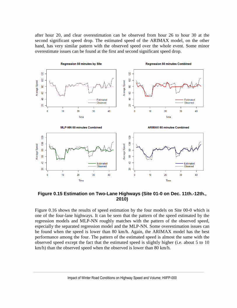
Impact of Winter Road Conditions on Highway Speed and Volume; HIIFP-000
after hour 20, and clear overestimation can be observed from hour 26 to hour 30 at the
second significant speed drop. The estimated speed of the ARIMAX model, on the other
hand, has very similar pattern with the observed speed over the whole event. Some minor
overestimate issues can be found at the first and second significant speed drop.
Figure 0.15 Estimation on Two-Lane Highways (Site 01-0 on Dec. 11th.-12th., 2010)
Figure 0.16 shows the results of speed estimation by the four models on Site 00-0 which is
one of the four-lane highways. It can be seen that the pattern of the speed estimated by the
regression models and MLP-NN roughly matches with the pattern of the observed speed,
especially the separated regression model and the MLP-NN. Some overestimation issues can
be found when the speed is lower than 80 km/h. Again, the ARIMAX model has the best
performance among the four. The pattern of the estimated speed is almost the same with the
observed speed except the fact that the estimated speed is slightly higher (i.e. about 5 to 10
km/h) than the observed speed when the observed is lower than 80 km/h.

Impact of Winter Road Conditions on Highway Speed and Volume; HIIFP-000
Figure 0.16 Estimation on Four-Lane Highways (Site 00-0 on Jan 10th., 2009)
Overall, the two regression models and the MLP-NN have been outperformed by the
ARIMAX model. This result is somehow expected as the later used the past speed
observations and thus has the advantage of making use of more information than the other
three alternatives.
Summary
This chapter investigates the impact of adverse weather and road surface conditions on traffic
speed with the intention of exploring the feasibility of applying speed as a performance
indicator of WRM. Data from 35 sites, 14 on two-lane and 21 on four-lane highways, in
Iowa, US are used in the analysis. Separated and combined regression models, MLP-NN and
ARIMAX models are developed for these two highway types.
It is found that precipitation and road surface conditions have a relatively higher effect on the
average traffic speed than other factors such as surface temperature and wind speed.
Different from the linear regression models, the MLP-NN could capture the non-linear effect
of independent variables on the average traffic speed. However, the modeling results don’t

Impact of Winter Road Conditions on Highway Speed and Volume; HIIFP-000
confirm the superiority of the MLP-NN over the regression models. This indifference,
however, validates the appropriateness of the multivariate linear regression models. By
taking into account both the autocorrelation nature of the data as well as the effects of cross-
sectional variables, the ARIMAX model provided much improved explanatory and
prediction power as compared to regression models and MLP-NN. It should be noted that the
ARIMAX model makes use of recent past observations in estimating the travel speed of the
current time period. In contrast, the regression models and MLP-NN models estimate speeds
based on external factors only.
The analysis results clearly indicated the dependency of traffic speed on road surface
conditions, suggesting the feasibility of applying speed as a performance monitoring tool. For
example, under a given weather and traffic condition, the reduction in speed can be
established from a comparison to baseline values and attributed to the change in surface
conditions. Based on the degree of speed reduction, the road surface condition can be
predicted and their performance can be gauged accordingly and/or maintenance activities can
be mobilized.
It should be noted that this chapter only focus on investigating the correlation between traffic
speed and RSCs. Next chapter focuses on developing quantitative models that can be used to
infer RSCs (e.g. bare pavement status) based on observed traffic speed and other known road
and weather parameters.

Impact of Winter Road Conditions on Highway Speed and Volume; HIIFP-000
Inferring Road Surface Condition from Traffic and Weather Data
Problem Definition
One of the purposes of studying the effect of weather and RSC factors on traffic speed in the
previous chapter is to confirm the relationship between traffic speed and RSC so that the
feasibility of using traffic speed as WRM performance measure can be investigated. The
results showed that adverse RSC is highly correlated with significant speed reduction on both
two-lane and four-lane rural highways.
On the other hand, it is essential for WRM management to accurately determine the RSC
during snow storms. Traditional RSC monitoring by visual observation and web cams are
subjective and/or costly requiring high workload. Additionally, modern embedded surface
monitoring sensors suffer from high installation and maintenance costs, low reliability and
scalability, therefore cannot be deployed in a large scale at this point.
This chapter studies the reverse problem of Chapter 3, and proposes a model to estimate RSC
based on traffic and weather data which are often readily available from existing traffic
sensors. With the rapid development of smart phone technologies, this modelling technique
has a high potential to utilize speed data, GPS data and weather data collected from road
users’ smart phones, and generate real time RSC estimation with high spatial and temporal
coverage, which may potentially have the benefits of both stationary and mobile based
surface monitoring systems, and dramatically reduce the overall cost.
Data Collection
Dataset used in this chapter is the same with Chapter 3. To ensure enough sample size of
each RSC categories, Site 11-1 (two-lane) and 00-0 (four-lane) with both 15 and 60 minutes
time intervals are selected for model calibration and validation. The following variables are
used as explanatory variables in model calibration. Note that the analysis assumes no surface
data is available and only traffic and weather data is available. Due to lack of enough valid
data points, visibility is not included in this analysis.

Impact of Winter Road Conditions on Highway Speed and Volume; HIIFP-000
Table 0.1 Explanatory Variables used in Model Calibration
Data
Source Field Name Unit Note
Traffic
Average Speed km/h Average speed over 15 minutes or 60 minutes
Average
Volume veh/ln/h
Average total volume over 15 minutes or 60
minutes
% Long
Vehicles percent Percent of long vehicles
SD of Speed N/A Standard deviation of speed over 15 minutes or 60
minutes
Atmosphe
re
Wind Speed km/h Average wind speed over 15 minutes or 60
minutes
Air
Temperature celsius Air temperature
Precipitation
Intensity
categori
es
Precipitation Intensity (None, Slight, Moderate or
Heavy)
Others Time of Day categori
es Day (6:00am – 6:00pm) Night (6:00pm – 6:00am)
Methodology
Road Surface Condition Classification
RSC used in this analysis includes the following six types in the order of severity from
lowest to highest. The rest of the chapter will reference the RSC with type ids instead of type
names.
Type 0: Dry (moisture free surface, bare pavement)
Type 1: Trace Moisture (thin or spotty film of moisture above freezing and detected in
absence of precipitation)
Type 2: Wet (continuous film of moisture on the pavement sensor with a surface
temperature above freezing as reported when precipitation has occurred)
Type 3: Chemically Wet (continuous film of water and ice mixture at or below freezing
with enough chemical to keep the mixture from freezing, it is also reported when

Impact of Winter Road Conditions on Highway Speed and Volume; HIIFP-000
precipitation has occurred)
Type 4: Ice Watch (thin or spotty film of moisture at or below freezing and reported
when precipitation is not occurring)
Type 5: Ice Warning (continuous film of ice and water mixture at or below freezing with
insufficient chemical to keep the mixture from freezing again, reported when
precipitation occurs)
Logistic Regression
Logistic regression is a special form of generalized linear model (Mc-Cullagh & Nelder,
1999) and is one of the supervised classification methods. A logistic regression model has the
following form:
𝒍𝒏𝑷(𝒀 = 𝑪𝒌)
𝟏 − 𝑷(𝒀 = 𝑪𝒌)= 𝜼(𝑿) ∀𝑪𝒌 ∈ 𝑪
Where
𝒀 is the categorical response variable
𝑪 is the set of classifications. In this case, it represents the set of different RSC types
𝑪𝒌 is a state in 𝑪
𝑷(𝒀 = 𝑪𝒌) is the probability of 𝒀 in the state of 𝑪𝒌
𝑿 is the explanatory variable vector of d features
𝜼(𝑿) is a linear function describing the dependence of 𝒀 on the explanatory variables
defined as follows:
𝜼(𝑿) = 𝜷𝟎 + 𝜷𝟏𝒙𝟏 + ⋯ + 𝜷𝒅𝒙𝒅
Where 𝜷𝟎, 𝜷𝟏 ⋯ 𝜷𝒅 are model coefficients to be estimated. With this special model format,
the probability of 𝒀 belonging to any specific state can be estimated by explanatory variables.
The logistic regression model can be rewritten as
𝑷(𝒀 = 𝑪𝒌) =𝒆𝜼(𝑿)
𝟏 + 𝒆𝜼(𝑿)
Multi-Layer Logistic Regression Classification Tree
RSC classification is a typical classification problem and can be addressed by various
traditional classification modeling approaches, e.g. supervised and unsupervised methods.
The basic idea of the classification tree is to partition the space of explanatory variables into
successively smaller hyper-rectangles in order to make the sample more and more pure in
terms of response variable’s class within the new hyper-rectangles that are created.

Impact of Winter Road Conditions on Highway Speed and Volume; HIIFP-000
One of the major problems of classification tree is that some classes are usually similar with
other classes, and it is insufficient to use only one explanatory variable to discriminate two
classes at each split. To solve this problem, in this chapter, a multi-layer logistic regression
classification tree is proposed and used to classify RSC categories. At each split of the
classification tree, a binary logistic regression model with multiple explanatory variables is
calibrated.
Figure 0.1 shows a sample classification tree.
Figure 0.1 Sample Multi-layer Logistic Regression Classification Tree for RSC Discrimination
For each dataset, firstly, a multi-layer logistic regression classification tree with the best
discriminant performance will be developed. Secondly, 90% of all the data records will be
randomly selected from the database to calibrate the logistic regression models at each split
using the backward stepwise likelihood ratio method. Finally, the developed models will be
validated using the rest 10 % holdout data records, and the classification hit rate of the
models will be evaluated and compared. 0.05 is selected as the significance level threshold of
the explanatory variables.
Evaluation of Classification Quality
The quality of the logistic regression classification is measured by an evaluation matrix (i.e.
confusion matrix) as shown below. The diagonal cells represent the number of points for
which the predicted type is equal to the observed type, while those off-diagonal cells are mis-
Split 1
Split 2 1
0 Split 3
2 3
Binary Logistic Regression Model
1
Binary Logistic Regression Model
3
Binary Logistic Regression Model
2

Impact of Winter Road Conditions on Highway Speed and Volume; HIIFP-000
predicted by the classifier. The higher the diagonal values of the confusion matrix or the
higher percentage correct, the better performance the classifier has.
Table 0.2 Example of Logistic Regression Evaluation Matrix
Calibration Data Validation Data
Predicted Percentage
Correct Predicted
Percentage Correct
0 1 0 1
Observed 0 7 3 70.0 20 5 80.0
1 1 9 90.0 25 50 66.7
Overall Percentage 80.0 70.0
Exploratory Analysis
Figure 0.2 and Figure 0.3 show the box-plots of all variables, i.e. average speed, standard
deviation of traffic speed, average volume, % long vehicles, wind speed and air temperature
of each RSC type on Site 11-1 with 15 minutes and 60 minutes time intervals, respectively. It
can be found from both figures that average speed under chemically wet, ice watch and ice
warning condition are mostly lower than those under dry, trace moisture and wet condition.
Standard deviation of traffic speed of all the six types overlapped a lot, however, ice watch
and ice warning tend to have relatively higher standard deviation of traffic speed in general.
The air temperature for trace moisture and wet are mostly above zero while it is mostly
below zero for chemically wet, ice watch and ice warning. Although the box-plot of air
temperature shows some difference among all the six types, the other five types are all
bracketed by dry. Average volume, % long vehicles and wind speed overlapped a lot, and no
obvious pattern can be found.
Figure 0.4 and Figure 0.5 show the same box-plots for Site 00-0 with 15 minutes and 60
minutes time intervals, respectively. The patterns of average speed, standard deviation of
traffic speed as well as air temperature are mostly similar with the patterns found in Figure
0.2 and Figure 0.3. No obvious pattern can be found in average volume, % long vehicles and
wind speed as well. The overlapped patterns of the six RSC types suggest that nested logistic
regression models are needed.

Impact of Winter Road Conditions on Highway Speed and Volume; HIIFP-000
Figure 0.2 Boxplots for Site 11-1 (15-Minute Interval)

Impact of Winter Road Conditions on Highway Speed and Volume; HIIFP-000
Figure 0.3 Boxplots for Site 11-1 (60-Minute Interval)

Impact of Winter Road Conditions on Highway Speed and Volume; HIIFP-000
Figure 0.4 Boxplots for Site 00-0 (15-Minute Interval)

Impact of Winter Road Conditions on Highway Speed and Volume; HIIFP-000
Figure 0.5 Boxplots for Site 00-0 (60-Minute Interval)

Impact of Winter Road Conditions on Highway Speed and Volume; HIIFP-000
Model Calibration and Validation
Two Lane Highways
Based on the exploratory analysis as well as the calibration results of different alternative tree
designs, it is found that the following multi-layer classification tree yields the best
discriminant performance on Site 11-1 for both the 15 minutes and 60 minutes datasets. Note
that because of the similarity of Type 1 and Type 2 as well as Type 4 and Type 5 at Site 11-1,
the calibrated models lack of discriminate power to separate them with acceptable hit rate.
Therefore, Type 1 and Type 2 have been combined together as a single Type, and the same
with Type 4 and Type 5. Split 1 at the root of the tree firstly estimates the two probabilities
respective to Type (0, 1, 2, 3) and Type (4, 5). Split 2 then estimates the two probabilities
respective to Type 0 and Type (1, 2, 3). Accordingly, Split 3 estimates the two probabilities
respective to Type (1, 2) and Type 3. Based on this classification tree, three logistic
regression models in total are calibrated.
Figure 0.6 Calibrated Classification Tree for Site 11-1
Table 4.3 shows the calibration results of Split 1 with 15 minutes time interval for Site 11-1.
As can be seen above, average speed, standard deviation of traffic speed, average volume,
wind speed, air temperature as well as night are all statistically significant. The negative
coefficients suggest that the higher the average speed, average volume, wind speed, and air
temperature and time is night, the more likely that the RSC is Type (0, 1, 2, 3). The positive
Split 1
Split 2 4, 5
0 Split 3
3 1, 2

Impact of Winter Road Conditions on Highway Speed and Volume; HIIFP-000
coefficients suggest that the higher standard deviation of traffic speed, the higher probability
that the RSC is Type (4, 5). The results make intuitive sense and are consistent with the
pattern found in the box-plots in the exploratory data analysis.
Table 4.4 shows the classification results, which consists of two parts, the calibration data
and the 10% holdout validation data. Class 0 represents Type (0, 1, 2, 3) and class 1
represents Type (4, 5). A cutoff value of 0.5 is used to define these two classes. When the
estimated probability of belonging to class 1 is equal to or greater than 0.5, and the observed
class is 1, the model is considered as making a correct prediction. When the estimated
probability of belonging to class 1 is less than 0.5, and the observed class is 0, the model is
also considered as making a correct prediction. Otherwise, it is considered as a missing. The
overall percentage is the ratio of correct predicts to the total number of observations in the
group.
For the calibration data, 399 and 1061 samples are correctly classified for class 0 and class 1,
respectively. The hit rates for the two classes are 62.9% and 88.6%, respectively. The
validation data shows the similar results. 39 and 117 cases are correctly classified for class 0
and class 1, respectively. The hit rates for class 0 and 1 are 60.9% and 88.6%, respectively.
The overall hit rates for the calibration data and the validation data are 79.7% and 79.6%.
Table 0.3 Model Calibration of Site 11-1 Split 1 (15-Minute Interval)
B S.E. Wald df Sig. Exp(B)
Average Speed -.048 .006 70.364 1 .000 .954
Average Volume -.004 .002 5.331 1 .021 .996
SD of Traffic Speed .031 .013 5.211 1 .022 1.031
Wind Speed -.060 .010 34.947 1 .000 .942
Air Temp -.296 .019 248.607 1 .000 .744
Night -.356 .121 8.590 1 .003 .701
Constant 4.695 .550 72.905 1 .000 109.432

Impact of Winter Road Conditions on Highway Speed and Volume; HIIFP-000
Table 0.4 Classification Results of Site 11-1 Split 1 (15-Minute Interval)
Calibration Data Validation Data
Predicted Percentage
Correct Predicted
Percentage Correct
0 1 0 1
Observed 0 399 235 62.9 39 25 60.9
1 136 1061 88.6 15 117 88.6
Overall Percentage 79.7 79.6
Table 4.5 shows the calibration results of Split 2 with 15 minutes time interval for Site 11-1.
It shows that the higher the average speed and wind speed, the more likely that the RSC is
Type 0 while the higher air temperature and precipitation intensity is slight, the higher
probability that the RSC is Type (1, 2, 3). Table 4.6 shows that for the calibration data, the
hit rates for class 0 and 1 are 70.4% and 77.3%, respectively. For the validation data, the hit
rates for class 0 and 1 are 80.6% and 66.7%, respectively. The overall hit rates for the
calibration data and the validation data are 74.3% and 73.4%.
Table 0.5 Model Calibration of Site 11-1 Split 2 (15-Minute Interval)
B S.E. Wald df Sig. Exp(B)
Average Speed -.075 .013 30.900 1 .000 .928
Wind Speed -.074 .016 21.017 1 .000 .928
Air Temp .158 .025 39.053 1 .000 1.171
Slight 1.861 .210 78.335 1 .000 6.430
Constant 7.270 1.304 31.071 1 .000 1.436E3
Table 0.6 Classification Results of Site 11-1 Split 2 (15-Minute Interval)
Calibration Data Validation Data
Predicted Percentage
Correct Predicted
Percentage Correct
0 1 0 1
Observed 0 195 82 70.4 25 6 80.6
1 81 276 77.3 11 22 66.7
Overall Percentage 74.3 73.4

Impact of Winter Road Conditions on Highway Speed and Volume; HIIFP-000
Table 4.7 shows the calibration results of Split 3 with 15 minutes as the time interval for Site
11-1. It can be found that only the air temperature is statistically significant, and the higher
the air temperature, the higher the probability that the RSC is Type (1, 2). Table 4.8 shows
the classification results. Compared with the previous two splits, the hit rates of both classes
are much higher for both the calibration and validation data. The overall percentages for the
calibration data and the validation data are 96.9% and 93.9%, respectively.
Table 0.7 Model Calibration of Site 11-1 Split 3 (15-Minute Interval)
B S.E. Wald df Sig. Exp(B)
Air Temp -7.155 1.468 23.753 1 .000 .001
Constant -.623 .336 3.433 1 .064 .537
Table 0.8 Classification Results of Site 11-1 Split 3 (15-Minute Interval)
Calibration Data Validation Data
Predicted Percentage
Correct Predicted
Percentage Correct
0 1 0 1
Observed 0 193 4 98.0 19 1 95.0
1 7 153 95.6 1 12 92.3
Overall Percentage 96.9 93.9
Table 4.9 shows the calibration results of Split 1 with 60 minutes as the time interval for Site
11-1. Compared with the 15 minutes model, only average speed, wind speed and air
temperature are statistically significant. The coefficients of these independent variables
remain similar with the 15 minutes model. Table 4.10 reveals that for the calibration data, the
hit rates for class 0 and 1 are 64.1% and 89.5%, respectively. For the validation data, the hit
rates for class 0 and 1 are 63.6% and 82.1%, respectively. The overall percentages for the
calibration data and the validation data are 81.0% and 76.9%.
Table 0.9 Model Calibration of Site 11-1 Split 1 (60-Minute Interval)
B S.E. Wald df Sig. Exp(B)
Average Speed -.060 .013 22.562 1 .000 .942
Wind Speed -.084 .022 14.881 1 .000 .919
Air Temp -.377 .047 63.587 1 .000 .686
Constant 5.611 1.150 23.814 1 .000 273.496

Impact of Winter Road Conditions on Highway Speed and Volume; HIIFP-000
Table 0.10 Classification Results of Site 11-1 Split 1 (60-Minute Interval)
Calibration Data Validation Data
Predicted Percentage
Correct Predicted
Percentage Correct
0 1 0 1
Observed 0 84 47 64.1 7 4 63.6
1 27 231 89.5 5 23 82.1
Overall Percentage 81.0 76.9
Table 4.11 displays the calibration results of Split 2 with 60 minutes as the time interval for
Site 11-1. The model has the same significant independent variables with the 15 minutes
model, and the coefficients of these explanatory variables are also identical with the 15
minutes model. It can be found in Table 4.12 that for the calibration data, the hit rates for
class 0 and 1 are 66.7% and 86.2%, respectively. For the validation data, the hit rates for
class 0 and 1 are 60.0% and 100.0%, respectively. The overall percentages for the calibration
data and the validation data are 78.6% and 81.8%.
Table 0.11 Model Calibration of Site 11-1 Split 2 (60-Minute Interval)
B S.E. Wald df Sig. Exp(B)
Average Speed -.098 .032 9.122 1 .003 .907
Wind Speed -.095 .036 6.848 1 .009 .909
Air Temp .236 .069 11.844 1 .001 1.267
Slight 1.830 .497 13.573 1 .000 6.235
Constant 9.865 3.155 9.779 1 .002 1.925E4
Table 0.12 Classification Results of Site 11-1 Split 2 (60-Minute Interval)
Calibration Data Validation Data
Predicted Percentage
Correct Predicted
Percentage Correct
0 1 0 1
Observed 0 34 17 66.7 3 2 60.0
1 11 69 86.2 0 6 100.0
Overall Percentage 78.6 81.8

Impact of Winter Road Conditions on Highway Speed and Volume; HIIFP-000
Table 4.13 demonstrates the calibration results of Split 3 with 60 minutes as the time interval
for Site 11-1. Again, only air temperature is statistically significant, and the effect of surface
temperature is also identical with the 15 minutes model. As is shown in Table 4.14, for the
calibration data, the hit rates for class 0 and 1 are also high, 97.8% and 95.1%, respectively.
For the validation data, the hit rates for class 0 and 1 are both100.0%. The overall
percentages for the calibration data and the validation data are 96.5% and 100.0%.
Table 0.13 Model Calibration of Site 11-1 Split 3 (60-Minute Interval)
B S.E. Wald df Sig. Exp(B)
Air Temp -9.755 1.589 4.519 1 .034 .000
Constant -.092 .726 .016 1 .899 .912
Table 0.14 Classification Results of Site 11-1 Split 3 (60-Minute Interval)
Calibration Data Validation Data
Predicted Percentage
Correct Predicted
Percentage Correct
0 1 0 1
Observed 0 44 1 97.8 4 0 100.0
1 2 39 95.1 0 4 100.0
Overall Percentage 96.5 100.0
Four Lane Highways
The classification tree of Site 00-0 is similar with the one of Site 11-1, except that Type 1
and 2 are no longer combined as they can be separated with acceptable hit rate. Split 1 at the
root of the tree firstly estimates the two probabilities respective to Type (0, 1, 2, 3) and Type
(4, 5). Split 2 then estimates the two probabilities respective to Type 0 and Type (1, 2, 3).
Split 3 then estimates the two probabilities respective to Type (1, 2) and Type 3. Finally,
Split 4 estimates the two probabilities respective to Type 1 and Type 2. Based on this
classification tree, four logistic regression models in total are calibrated.

Impact of Winter Road Conditions on Highway Speed and Volume; HIIFP-000
Figure 0.7 Calibrated Classification Tree for Site 00-0
Table 4.15 demonstrates the calibration results of Split 1 with 15 minutes as the time interval
for Site 00-0. As can be seen, average speed, standard deviation of traffic speed, average
volume, wind speed, air temperature, slight as well as night are all statistically significant.
The negative coefficients suggest that the higher the average speed, average volume, wind
speed, and air temperature, precipitation intensity is slight and time is night, the more likely
that the RSC is Type (0, 1, 2, 3). The positive coefficients suggest that the higher standard
deviation of traffic speed, the higher probability that the RSC is Type (4, 5). The results
make intuitive sense and are consistent with the pattern of the box-plots obtained in the
exploratory analysis. Table 4.16 reveals that for the calibration data, the hit rates for the two
classes are 65.4% and 86.0%, respectively. For the validation data, the hit rates for class 0
and 1 are 62.2% and 85.0%, respectively. The overall percentages for the calibration data and
the validation data are 78.7% and 77%.
Split 1
Split 2 4, 5
0 Split 3
3 Split 4
1 2
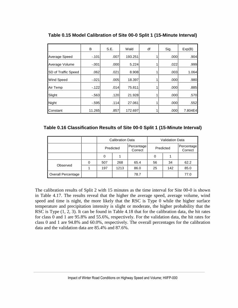
Impact of Winter Road Conditions on Highway Speed and Volume; HIIFP-000
Table 0.15 Model Calibration of Site 00-0 Split 1 (15-Minute Interval)
B S.E. Wald df Sig. Exp(B)
Average Speed -.101 .007 193.251 1 .000 .904
Average Volume -.001 .000 5.224 1 .022 .999
SD of Traffic Speed .062 .021 8.908 1 .003 1.064
Wind Speed -.021 .005 18.397 1 .000 .980
Air Temp -.122 .014 75.811 1 .000 .885
Slight -.563 .120 21.928 1 .000 .570
Night -.595 .114 27.061 1 .000 .552
Constant 11.265 .857 172.697 1 .000 7.804E4
Table 0.16 Classification Results of Site 00-0 Split 1 (15-Minute Interval)
Calibration Data Validation Data
Predicted Percentage
Correct Predicted
Percentage Correct
0 1 0 1
Observed 0 507 268 65.4 56 34 62.2
1 197 1213 86.0 25 142 85.0
Overall Percentage 78.7 77.0
The calibration results of Split 2 with 15 minutes as the time interval for Site 00-0 is shown
in Table 4.17. The results reveal that the higher the average speed, average volume, wind
speed and time is night, the more likely that the RSC is Type 0 while the higher surface
temperature and precipitation intensity is slight or moderate, the higher probability that the
RSC is Type (1, 2, 3). It can be found in Table 4.18 that for the calibration data, the hit rates
for class 0 and 1 are 95.8% and 55.6%, respectively. For the validation data, the hit rates for
class 0 and 1 are 94.8% and 60.0%, respectively. The overall percentages for the calibration
data and the validation data are 85.4% and 87.6%.

Impact of Winter Road Conditions on Highway Speed and Volume; HIIFP-000
Table 0.17 Model Calibration of Site 00-0 Split 2 (15-Minute Interval)
B S.E. Wald df Sig. Exp(B)
Average Speed -.055 .013 17.500 1 .000 .946
Average Volume -.004 .001 24.459 1 .000 .996
Wind Speed -.030 .009 12.477 1 .000 .970
Air Temp .302 .029 105.907 1 .000 1.352
Slight .685 .213 10.363 1 .001 1.984
Moderate 1.657 .574 8.338 1 .004 5.243
Night -.427 .204 4.361 1 .037 .652
Constant 7.116 1.496 22.626 1 .000 1.232E3
Table 0.18 Classification Results of Site 00-0 Split 2 (15-Minute Interval)
Calibration Data Validation Data
Predicted Percentage
Correct Predicted
Percentage Correct
0 1 0 1
Observed 0 546 24 95.8 73 4 94.8
1 88 110 55.6 8 12 60.0
Overall Percentage 85.4 87.6
Table 4.19 shows the calibration results of Split 3 with 15 minutes as the time interval for
Site 00-0. Similar with Site 11-1, only the air temperature is statistically significant, and the
higher the air temperature, the higher the probability that the RSC is Type (1, 2). Table 4.20
also shows the similar results with Site 11-1. Compared with the previous two splits, the hit
rates of both classes are much higher for both the calibration and validation data. The overall
percentages for the calibration data and the validation data are 97.5% and 95.0%,
respectively.

Impact of Winter Road Conditions on Highway Speed and Volume; HIIFP-000
Table 0.19 Model Calibration of Site 00-0 Split 3 (15-Minute Interval)
B S.E. Wald df Sig. Exp(B)
Air Temp -7.821 1.449 10.200 1 .001 .000
Constant -1.034 .648 2.544 1 .111 .356
Table 0.20 Classification Results of Site 00-0 Split 3 (15-Minute Interval)
Calibration Data Validation Data
Predicted Percentage
Correct Predicted
Percentage Correct
0 1 0 1
Observed 0 100 2 98.0 12 1 92.3
1 3 93 96.9 0 7 100.0
Overall Percentage 97.5 95.0
The calibration results of Split 4 with 15 minutes as the time interval for Site 00-0 can be
found in Table 4.21. The results reveal that the higher the standard deviation of traffic speed
and time is night, the more likely that the RSC is Type 1 while the higher average volume
and wind speed, the higher probability that the RSC is Type 2. Table 4.22 reveals that for the
calibration data, the hit rates for class 0 and 1 are 67.4% and 83.3%, respectively. For the
validation data, the hit rates for class 0 and 1 are 75.0% and 100.0%, respectively. The
overall percentages for the calibration data and the validation data are 76.4% and 88.9%.
Table 0.21 Model Calibration of Site 00-0 Split 4 (15-Minute Interval)
B S.E. Wald df Sig. Exp(B)
Average Volume .006 .002 10.785 1 .001 1.006
SD of Traffic Speed -.292 .124 5.523 1 .019 .747
Wind Speed .076 .022 12.582 1 .000 1.079
Night -1.046 .508 4.248 1 .039 .351
Constant -2.123 .783 7.346 1 .007 .120

Impact of Winter Road Conditions on Highway Speed and Volume; HIIFP-000
Table 0.22 Classification Results of Site 00-0 Split 4 (15-Minute Interval)
Calibration Data Validation Data
Predicted Percentage
Correct Predicted
Percentage Correct
0 1 0 1
Observed 0 31 15 67.4 3 1 75.0
1 10 50 83.3 0 5 100.0
Overall Percentage 76.4 88.9
Table 4.23 shows the calibration results of Split 1 with 60 minutes as the time interval for
Site 00-0. Compared with the 15 minutes model, only average speed, wind speed, air
temperature and night are statistically significant. The coefficients of these independent
variables remain similar with the 15 minutes model. As can be seen in Table 4.24, for the
calibration data, the hit rates for class 0 and 1 are 68.9% and 88.8%, respectively. For the
validation data, the hit rates for class 0 and 1 are 77.3% and 90.5%, respectively. The overall
percentages for the calibration data and the validation data are 82.3% and 85.9%.
Table 0.23 Model Calibration of Site 00-0 Split 1 (60-Minute Interval)
B S.E. Wald df Sig. Exp(B)
Average Speed -.118 .015 64.602 1 .000 .889
Wind Speed -.024 .010 5.594 1 .018 .976
Air Temp -.112 .028 15.814 1 .000 .894
Night -.660 .252 6.868 1 .009 .517
Constant 13.204 1.671 62.407 1 .000 5.423E5
Table 0.24 Classification Results of Site 00-0 Split 1 (60-Minute Interval)
Calibration Data Validation Data
Predicted Percentage
Correct Predicted
Percentage Correct
0 1 0 1
Observed 0 104 47 68.9 17 5 77.3
1 35 278 88.8 4 38 90.5
Overall Percentage 82.3 85.9
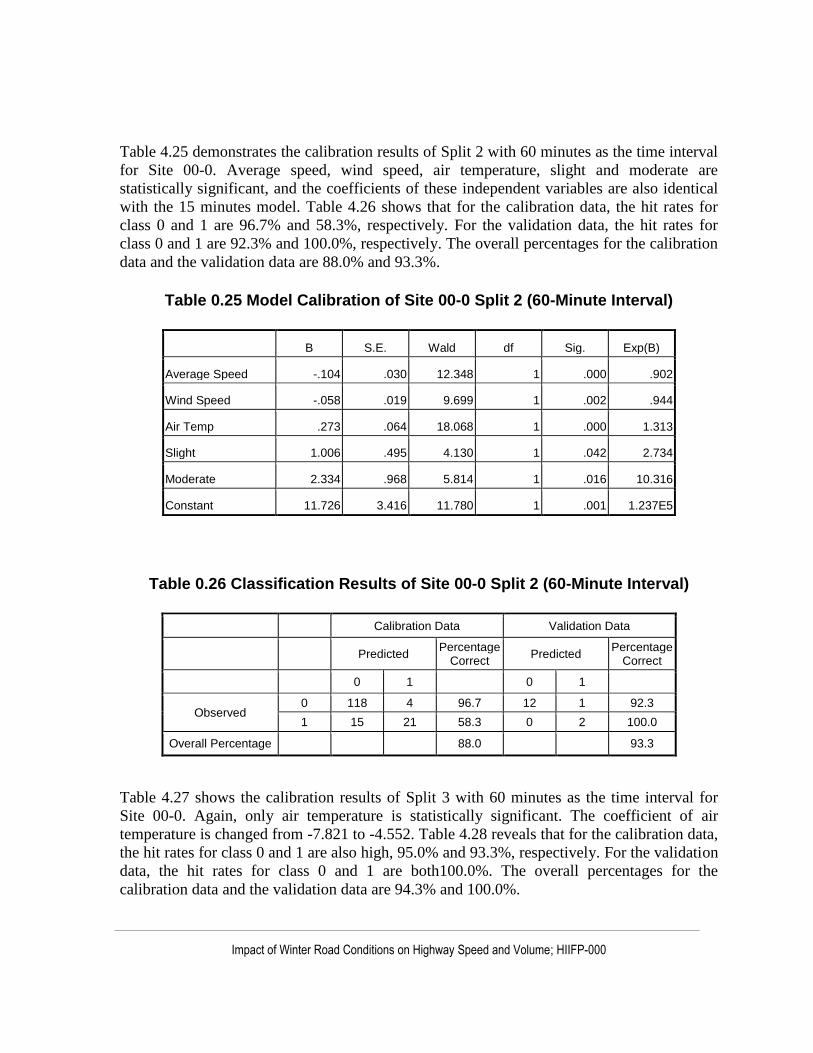
Impact of Winter Road Conditions on Highway Speed and Volume; HIIFP-000
Table 4.25 demonstrates the calibration results of Split 2 with 60 minutes as the time interval
for Site 00-0. Average speed, wind speed, air temperature, slight and moderate are
statistically significant, and the coefficients of these independent variables are also identical
with the 15 minutes model. Table 4.26 shows that for the calibration data, the hit rates for
class 0 and 1 are 96.7% and 58.3%, respectively. For the validation data, the hit rates for
class 0 and 1 are 92.3% and 100.0%, respectively. The overall percentages for the calibration
data and the validation data are 88.0% and 93.3%.
Table 0.25 Model Calibration of Site 00-0 Split 2 (60-Minute Interval)
B S.E. Wald df Sig. Exp(B)
Average Speed -.104 .030 12.348 1 .000 .902
Wind Speed -.058 .019 9.699 1 .002 .944
Air Temp .273 .064 18.068 1 .000 1.313
Slight 1.006 .495 4.130 1 .042 2.734
Moderate 2.334 .968 5.814 1 .016 10.316
Constant 11.726 3.416 11.780 1 .001 1.237E5
Table 0.26 Classification Results of Site 00-0 Split 2 (60-Minute Interval)
Calibration Data Validation Data
Predicted Percentage
Correct Predicted
Percentage Correct
0 1 0 1
Observed 0 118 4 96.7 12 1 92.3
1 15 21 58.3 0 2 100.0
Overall Percentage 88.0 93.3
Table 4.27 shows the calibration results of Split 3 with 60 minutes as the time interval for
Site 00-0. Again, only air temperature is statistically significant. The coefficient of air
temperature is changed from -7.821 to -4.552. Table 4.28 reveals that for the calibration data,
the hit rates for class 0 and 1 are also high, 95.0% and 93.3%, respectively. For the validation
data, the hit rates for class 0 and 1 are both100.0%. The overall percentages for the
calibration data and the validation data are 94.3% and 100.0%.

Impact of Winter Road Conditions on Highway Speed and Volume; HIIFP-000
Table 0.27 Model Calibration of Site 00-0 Split 3 (60-Minute Interval)
B S.E. Wald df Sig. Exp(B)
Air Temp -4.552 2.959 2.366 1 .024 .011
Constant -1.091 1.113 .961 1 .327 .336
Table 0.28 Classification Results of Site 00-0 Split 3 (60-Minute Interval)
Calibration Data Validation Data
Predicted Percentage
Correct Predicted
Percentage Correct
0 1 0 1
Observed 0 19 1 95.0 2 0 100.0
1 1 14 93.3 0 1 100.0
Overall Percentage 94.3 100.0
The calibration results of Split 4 with 60 minutes as the time interval for Site 00-0 can be
found in Table 4.29. Except the standard deviation of traffic speed, the rest significant
variables are the same with the 15 minutes models, and the coefficients are close to the 15
minutes as well. Table 4.30 displays that for the calibration data, the hit rates for class 0 and
1 are also high, 85.7% and 90.0%, respectively. For the validation data, the hit rates for class
0 and 1 are 66.7 and 100.0%. The overall percentages for the calibration data and the
validation data are 88.2% and 80.0%.
Table 0.29 Model Calibration of Site 00-0 Split 4 (60-Minute Interval)
B S.E. Wald df Sig. Exp(B)
Average Volume .012 .002 10.785 1 .001 1.012
Wind Speed .086 .022 12.582 1 .000 1.09
Night -1.021 .508 4.248 1 .039 .36
Constant -1.112 .783 7.346 1 .007 .329

Impact of Winter Road Conditions on Highway Speed and Volume; HIIFP-000
Table 0.30 Classification Results of Site 00-0 Split 4 (60-Minute Interval)
Calibration Data Validation Data
Predicted Percentage
Correct Predicted
Percentage Correct
0 1 0 1
Observed 0 6 1 85.7 2 1 66.7
1 1 9 90.0 0 2 100.0
Overall Percentage 88.2 80.0
Discussion
Table 4.31 shows the summary of models for both Site 11-1 and Site 00-0. Based on this
table, the effects of each variable for all the splits can be summarized below:
Table 0.31 Model Summary for Site 11-1 and Site 00-0
Association with Average Speed
Based on the results of Split 1, it can be found that average speed is statistically significant in
distinguishing good RSC (Type 0, 1, 2, 3) from poor RSC (Type 4, 5), and the higher the
speed, the higher probability that the RSC belongs to Type (0, 1, 2, 3) – good conditions. For
Site 11-1, every one km/h increase in average speed, the log odds of Type (4, 5) versus Type
(0, 1, 2, 3) decreases by 0.048 and 0.06 based on the 15 minutes and 60 minutes models,
respectively. For Site 00-0, every one km/h increase in average speed, the log odds of Type
15 min 60 min 15 min 60 min 15 min 60 min 15 min 60 min 15 min 60 min 15 min 60 min 15 min 60 min
Average Speed -0.048 -0.06 -0.075 -0.098 -0.101 -0.118 -0.055 -0.104
Average Volume -0.004 -0.001 -0.004 0.006 0.012
% Long Vehicles
SD of Speed 0.031 0.062 -0.292
Wind Speed -0.06 -0.084 -0.074 -0.095 -0.021 -0.024 -0.03 -0.058 0.076 0.086
Air Temperature -0.296 -0.377 0.158 0.236 -7.155 -9.755 -0.122 -0.112 0.302 0.273 -7.821 -4.552
Slight 1.861 1.83 -0.563 0.685 1.006
Moderate 1.657 2.334
Heavy
Night -0.356 -0.595 -0.66 -0.427 -1.046 -1.021
Constant 4.695 5.611 7.27 9.865 -0.623 -0.092 11.265 13.204 7.116 11.726 -1.034 -1.091 -2.123 -1.112
Calibration Overall
Percentage Correct79.7 81.0 74.3 78.6 96.9 96.5 78.7 82.3 85.4 88.0 97.5 94.3 76.4 88.2
Validation Overall
Percentage Correct79.6 76.9 73.4 81.8 93.9 100.0 77.0 85.9 87.6 93.3 95.0 100.0 88.9 80.0
Split 4
Site 11-1 Site 00-0
Split 1 Split 2 Split 3 Split 1 Split 2 Split 3

Impact of Winter Road Conditions on Highway Speed and Volume; HIIFP-000
(4, 5) versus Type (0, 1, 2, 3) decreases by 0.101 and 0.118 for the 15 minutes and 60
minutes models, respectively.
In addition, average speed is also statistically significant in classifying Type 0 and Type (1,
2, 3) at Split 2, and the higher the value, the higher probability that the RSC is Type 0. For
Site 11-1, every one km/h increase in average speed, the log odds of Type (1, 2, 3) versus
Type 0 decreases by 0.075 and 0.098 for the 15 minutes and 60 minutes models, respectively.
For Site 00-0, every one km/h increase in average speed, the log odds of Type (1, 2, 3) versus
Type 0 decreases by 0.055 and 0.104 for the15 minutes and 60 minutes models, respectively.
Association with Standard Deviation of Traffic Speed
Standard deviation of traffic speed is also statistically significant in distinguishing good RSC
(Type 0, 1, 2, 3) from poor RSC (Type 4, 5). The more varied the speed, the higher
probability that the RSC is in poor conditions. For Site 11-1, every one unit increase in
standard deviation of traffic speed, the log odds of Type (4, 5) versus Type (0, 1, 2, 3)
increases by 0.031for the 15 minutes model. For Site 00-0, every one unit increase in
standard deviation of traffic speed, the log odds of Type (4, 5) versus Type (0, 1, 2, 3)
increases by 0.062 for the 15 minutes model.
In addition, it turns out that standard deviation of traffic speed is also statistically significant
in classifying Type 1 and Type 2. For Site 00-0, every one unit increase in standard deviation
of traffic speed, the log odds of Type 2 versus Type 1 decreases by 0.292 for the 15 minutes
model.
Association with Average Volume and % Long Vehicles
% long vehicles is found not statistically significant in all models. Average volume is in
distinguishing good RSC (Type 0, 1, 2, 3) from poor RSC (Type 4, 5), and the higher the %
long vehicles, the higher probability that the RSC is Type (0, 1, 2, 3). For Site 11-1, every
one veh/ln/h increase in average volume, the log odds of Type (4, 5) versus Type (0, 1, 2, 3)
decreases by 0.004 for the 15 minutes model. For Site 00-0, every one veh/ln/h increase in
average volume, the log odds of Type (4, 5) versus Type (0, 1, 2, 3) decreases by 0.001 for
the 15 minutes model.
In addition, average volume is also found statistically significant in classifying Type 0 and
Type (1, 2, 3) as well as Type 1 and Type 2. For Site 00-0, every one veh/ln/h increase in
average volume, the log odds of Type (1, 2, 3) versus Type 0 decreases by 0.004 for the 15
minutes model. For Site 00-0, every one veh/ln/h increase in average volume, the log odds of
Type 2 versus Type 1 increases by 0.006 and 0.012 for the 15 minutes and 60 models.
Association Wind Speed
Wind speed is statistically significant in distinguishing good RSC (Type 0, 1, 2, 3) from poor
RSC (Type 4, 5), and the higher the wind speed, the higher probability that the RSC is Type
(0, 1, 2, 3). For Site 11-1, every one km/h increase in wind speed, the log odds of Type (4, 5)

Impact of Winter Road Conditions on Highway Speed and Volume; HIIFP-000
versus Type (0, 1, 2, 3) decreases by 0.06 and 0.084 for the 15 minutes and 60 minutes
models, respectively. For Site 00-0, every one km/h increase in wind speed, the log odds of
Type (4, 5) versus Type (0, 1, 2, 3) decreases by 0.021 and 0.024 for the 15 minutes and 60
minutes models, respectively.
In addition, wind speed is also statistically significant in distinguishing Type 0 from Type (1,
2, 3), and the higher the wind speed, the higher probability that the RSC is Type 0. For Site
11-1, every one km/h increase in average speed, the log odds of Type (1, 2, 3) versus Type 0
decreases by 0.074 and 0.095 for the 15 minutes and 60 minutes models, respectively. For
Site 00-0, every one km/h increase in average speed, the log odds of Type (1, 2, 3) versus
Type 0 decreases by 0.03 and 0.058 for the15 minutes and 60 minutes models, respectively.
Lastly, wind speed is also statistically significant in distinguishing Type 1 from Type 2. For
Site 00-0, every one km/h increase in wind speed, the log odds of Type 2 versus Type 1
increases by 0.076 and 0.086 for the 15 minutes and 60 minutes models, respectively.
Association with Air Temperature
Air temperature is statistically significant in distinguishing good RSC (Type 0, 1, 2, 3) from
poor RSC (Type 4, 5), and the higher the air temperature, the higher probability that the RSC
is Type (0, 1, 2, 3). For Site 11-1, every one degree increase in air temperature, the log odds
of Type (4, 5) versus Type (0, 1, 2, 3) decreases by 0.296 and 0.377 for the 15 minutes and
60 minutes models, respectively. For Site 00-0, every one degree increase in air temperature,
the log odds of Type (4, 5) versus Type (0, 1, 2, 3) decreases by 0.122 and 0.112 for the 15
minutes and 60 minutes models, respectively.
In addition, air temperature is also statistically significant in distinguishing Type 0 from Type
(1, 2, 3), and the higher the air temperature, the higher probability that the RSC is Type (1, 2,
3). For Site 11-1, every one degree increase in air temperature, the log odds of Type (1, 2, 3)
versus Type 0 increases by 0.158 and 0.236 for the 15 minutes and 60 minutes models,
respectively. For Site 00-0, every one degree increase in air temperature, the log odds of
Type (1, 2, 3) versus Type 0 decreases by 0.302 and 0.273 for the15 minutes and 60 minutes
models, respectively.
Lastly, air temperature is also statistically significant in distinguishing Type (1, 2) from Type
3, and the higher the air temperature, the higher probability that RSC is Type (1, 2). For Site
11-1, every one degree increase in air temperature, the log odds of Type (1, 2, 3) versus Type
0 decreases by 7.155 and 9.755 for the 15 minutes and 60 minutes models, respectively. For
Site 00-0, every one degree increase in air temperature, the log odds of Type (1, 2, 3) versus
Type 0 decreases by 7.821 and 4.552 for the15 minutes and 60 minutes models, respectively.
Association with Precipitation Intensity
Slight is statistically significant in distinguishing good RSC (Type 0, 1, 2, 3) from poor RSC
(Type 4, 5). For Site 00-0, slight can cause the log odds of Type (4, 5) versus Type (0, 1, 2,
3) decrease by 0.563 for the 15 minutes model.

Impact of Winter Road Conditions on Highway Speed and Volume; HIIFP-000
Additionally, both slight and moderate are statistically significant in distinguishing Type 0
from Type (1, 2, 3) at Split 2. For Site 11-1, slight can cause the log odds of Type (1, 2, 3)
versus Type 0 increase by 1.861 and 1.83 for the 15 minutes and 60 minutes models,
respectively. For Site 00-0, slight can cause the log odds of Type (1, 2, 3) versus Type 0
increase by 0.685 and 1.006 for the15 minutes and 60 minutes models, respectively.
Moderate can cause the log odds of Type (1, 2, 3) versus Type 0 increase by 1.657 and 2.334
for the15 minutes and 60 minutes models, respectively.
Association with Night
Night is statistically significant in distinguishing good RSC (Type 0, 1, 2, 3) from poor RSC
(Type 4, 5). For Site 11-1, night can cause the log odds of Type (4, 5) versus Type (0, 1, 2, 3)
decreases by 0.356 for the 15 minutes model. For Site 00-0, night can cause the log odds of
Type (4, 5) versus Type (0, 1, 2, 3) decrease by 0.595 and 0.66 for the 15 minutes and 60
minutes models, respectively.
In addition, night is also found statistically significant in distinguishing Type 0 from Type (1,
2, 3) as well as Type 1 and Type 2. For Site 00-0, night can cause the log odds of Type (1, 2,
3) versus Type 0 decrease by 0.427 for the 15 minutes model. For Site 00-0, night can cause
the log odds of Type 2 versus Type 1 decrease by 1.046 and 1.021 for the 15 minutes and 60
models.
Figure 0.8 and Figure 0.9 show the overall validation hit rate summary for each split of Site
11-1 and Site 00-0, respectively. As can be found in Figure 0.8, both Split 1 and 2 of Site 11-
1 have the overall hit rate at around 80% for both the 15 minutes and 60 minutes models.
Split 3 has even higher overall hit rate than Split 1 and 2, i.e. over 90% for the 15 minutes
model and 100% for the 60 minutes model. Figure 0.9 reveals that similar with Site 11-1,
both Split 1 and 2 of Site 00-0 have the overall hit rate at around 80%. Again, Split 3 has the
highest overall hit rate, i.e. over 90% for the 15 minutes model and 100% for the 60 minutes
model. Split 4 of Site 00-0 also has relatively high hit rate. It is about 90% for the 15 minutes
model, and about 80% for the 60 minutes model.

Impact of Winter Road Conditions on Highway Speed and Volume; HIIFP-000
Figure 0.8 Overall Validation Hit Rate Summary of Site 11-1
Figure 0.9 Overall Validation Hit Rate Summary of Site 00-0
0
20
40
60
80
100
120
Split 1 Split 2 Split 3
Hit
Rat
e
15 minutes 60 minutes
0
20
40
60
80
100
120
Split 1 Split 2 Split 3 Split 4
Hit
Rat
e
15 minutes 60 minutes

Impact of Winter Road Conditions on Highway Speed and Volume; HIIFP-000
Summary
This study investigates the feasibility of classifying different RSC types on uninterrupted
traffic flow using multi-layer logistic regression classification tree based on both traffic and
weather data. Tested explanatory variables include average speed, average volume, % long
vehicles, and standard deviation of traffic speed, wind speed, air temperature, precipitation
intensity and time of day. The results clearly show that with proper design of classification
trees, traffic and weather data can be utilized to discriminate most RSC types.
It is found that splits that classify the same RSC types for both Site 11-1 (two-lane two-way)
and Site 00-0 (four-lane) have similar significant explanatory variables. For example, for
discriminating Type (0, 1, 2, 3) and Type (4, 5) at Split 1 of both sites, average speed,
average volume, standard deviation of traffic speed, wind speed, air temperature and night
are all statistically significant for the 15 minutes models while average speed, wind speed
and air temperature are all statistically significant for the 60 minutes models. For
discriminating Type 0 and Type (1, 2, 3) at Split 2 of both sites, average speed, wind speed,
air temperature and slight are all statistically significant for both the 15 minutes and the 60
minutes models. For discriminating Type (1, 2) and Type 3 at Split 3 of both sites, air
temperature is statistically significant for both the 15 minutes and the 60 minutes models. In
terms of model performance, the overall hit rates for models of all splits are around 80% or
higher, which indicating that the calibrated models have relatively high performance and
reliability.
With the rapid development of smart phone technologies, the proposed modelling technique
has a high potential to utilize speed data, GPS data and weather data collected from road
users’ smart phones, and generate real time RSC estimation with high spatial and temporal
coverage, which may potentially have the benefits of both stationary and mobile based
surface monitoring systems, and dramatically reduce the overall cost.

Impact of Winter Road Conditions on Highway Speed and Volume; HIIFP-000
Conclusions and Future Work
Major Findings
This research has firstly investigated the impact of adverse weather and RSC on traffic speed
with the intention of exploring the feasibility of applying speed as a performance indicator of
WRM. Traffic, weather and surface condition data, over three winter seasons from 2008 to
2011 collected from 35 rural highway sites (i.e. 14 on two-lane and 21 on four-lane
highways) in Iowa, US are used in this research. Multivariate linear regression models with
both 15 minutes and 60 minutes time intervals, MLP-NN and ARIMAX models are
developed for the two highway types.
The results of the multivariate regression analysis confirm that both adverse weather
conditions (e.g. snow precipitation) and snow/ice coverage can result in significant speed
reduction during snow events on both two-lane and four-lane rural highways. The MLP-NN
is capable of capturing the non-linear effect, however, it is only slightly better in speed
estimation performance than the multivariate linear regression models. This result suggests
the robustness of the multivariate linear regression models. Compared with the multivariate
regression models and the MLP-NN model, the ARIMAX model provides much improved
explanatory and prediction power in estimating the travel speed of the current time period by
making use of both recent past speed observations and external factors. The analysis results
clearly indicated the dependency of traffic speed on RSC, suggesting the feasibility of
applying speed as a performance monitoring indicator.
Secondly, the research investigates the feasibility of classifying different RSC types using
multi-layer logistic regression classification tree based on both traffic and weather data. The
results show that splits that classify the RSC types for both Site 11-1 (two-lane) and Site 00-0
(four-lane) have similar significant explanatory variables. In particular, to discriminate ice
watch/warning and other RSC types at Split 1, standard deviation of traffic speed is found
statistically significant in the 15 minutes model while average speed, wind speed and air
temperature are all statistically significant for both the 15 minutes and 60 minutes models.
The overall hit rates for models of all splits are 80% or higher, which confirms the reliability
of the multi-layer logistic classification regression tree in discriminating RSC types using
traffic and weather data on both two-lane and four-lane highways.
Limitations and Future Work
There are still some limitations of this research, and the following improvements can be
pursued to gain a better understanding of the relationship between traffic speed and RSC, and
improve the reliability of applying the results in WRM performance measurement:
This study only considered the first order of the independent variables in the multivariate
linear regression analysis. Further studies can be performed to investigate the need to

Impact of Winter Road Conditions on Highway Speed and Volume; HIIFP-000
consider higher orders and interaction among variables.
Data used in this study is collected at stations located on highways, which indicates that
the dataset is point measurement only. To improve the spatial coverage of the RSC
classification models, mobile data (e.g. GPS, real time speed and weather condition)
collected from highway users or patrol personnel need to be utilized.
This study only applied logistic regression for classifying RSC types. Further studies
need to be conducted to investigate other classification algorithms, especially machine
learning algorithms, e.g. support vector machine.
This study analyzed three winter seasons data collected from 35 sites. General models
have been developed for both two-lane and four-lane highways. More sites should be
covered to improve the transferability of the models.

Impact of Winter Road Conditions on Highway Speed and Volume; HIIFP-000
References
Adams, T. M., Danijarsa, M., Martinelli, T., Stanuch, G., & Vonderohe, A. (2003). Performance
Measures For Winter Operations. Transportation Research Board. Washington D.C.,USA.
Agarwal, M., Maze, T. H., & Solleyrette, R. (2005). Impacts of Weather on Urban Freeway Traffic
Flow Characteristics and Facility Capacity. Mid-Continent Transportation Symposium. Ames,
Iowa.
Agarwal, M., Maze, T. H., & Souleyrette, R. (2005). Impact of Weather on Urban Freeway Traffic
Flow Characteristics and Facility Capacity. Iowa State University. Ames, IA, USA: Center
for Transportation Research and Education.
Akaike, H. (1974, December 06). A New Look at the Statistical Model Identification. Automatic
Control, IEEE Transactions on, pp. 716-723.
Al-Qadi, I. L., Loulizi, A., Flintsch, G. W., Roosevelt, D. S., Decker, R., Wambold, J. C., et al.
(2002). Feasibility of Using Friction Indicators to Improve Winter Maintenance Operations
and Mobility. Washington D.C.,USA: National Cooperative Highway Research Program,
Transportation Research Board of the National Academies.
Andrey, J., Hambly, D., Mills, B., & Afrin, S. (2013). Insights into driver adaptation to inclement
weather in Canada. Journal of Transport Geography, 28, 192-203.
Bartlett, A., Lao, W., Zhao, Y., & Sadek, A. (2012). Impact of Inclement Weather on Hourly Traffic
Volumes in Buffalo, New York. Transportation Research Board 92nd Annual Meeting.
Washington, D.C.
Blackburn, R., Amsler, D., & Bauer, K. (2004). Guidelines for Snow and Ice Control Materials and
Methods In Transportation Research Circular. Washington, D.C., USA: Transportation
Research Board, National Research Council.
Breiman, L., Friedman, J., Olsen, R., & Stone, C. (1984). Classification and Regression Trees.
Belmont, California: Wadsworth.
Buchanan, F., & Gwartz, S. (2005). Road Weather Information Systems at the Ministry of
Transportation Ontario. Calgary, Alberta, Canada: Annual Conference of the Transportation
Association of Canada.
Burnham, K., & Anderson, D. (2002). Model Selection and Multimodel Inference: A Practical
Information-Theoretic Approach (2nd. ed.). Springer-Verlag.

Impact of Winter Road Conditions on Highway Speed and Volume; HIIFP-000
Burnham, K., & Anderson, D. (2004). Multimodel Inference: Understanding AIC and BIC in Model
Selection. Sociological Methods and Research 33, pp. 261-304.
Call, D. (2011). The Effect of Snow on Traffic Counts in Western New York State. WEATHER ,
CLIMATE, AND SOCIETY, 3, 71-75.
Camacho, F. J., Garcia, A., & Belda, E. (2010). Analysis of Impact of Adverse Weather on Freeway
Free-Flow Speed in Spain. Transportation Research Record, 2169, pp. 150-159.
Cao, L., Thakali, L., Fu, L., & Donaher, G. (2013). Effect of Weather and Road Surface Conditions
on Traffic Speed of Rural Highways. Annual Meeting of the Transportation Research Board.
Chin, S., Franzese, O., Greene, D., Hwang, H., & Gibson, R. (2004). Temporary Losses of Highway
Capacity and Impacts on Performance: Phase 2. Oak Ridge, Tennessee: Oak Ridge National
Laboratory.
CTC & Associates LLC. (2007). Using Friction Measurements. Research and Communication
Services, Wisconsin Department of Transportation,USA.
CTC & Associates LLC. (2009). Levels of Service in Winter Maintenance Operations: A Survey of
State Practice. Wisconsin, USA: Research & Library Unit, Wisconsin Department of
Transportation.
Dahlen, J. (1998). Winter Maintenance in Norway. Washington, D.C.: Transportation Research
Board.
Dalton, D., Nestler, J., Nordbo, J., St. Clair, B., Wittwer, E., & Wolfgram, M. (2005).
“Transportation Data and Performance Measurment”in Performance Measures to Improve
Transportation Systems: Summary of the Second National Conference. Washington, D.C.:
National Academy Press.
Datla, S., & Sharma, S. (2008). Impact of Cold and Snow on Temporal and Spatial Variations of
Highway Traffic Volumes. Journal of Transport Geography, 16(5), 358-372.
Datla, S., & Sharma, S. (2010). Variation of Impact of Cold Temperature and Snowfall and Their
Interaction on Traffic Volume. Transportation Research Record, 2169, 107-115.
Delorme, P., & Chatelain, O. (2011). Policy Steering - The Role and Use of Performance
Measurement Indicators. Aid Delivery Methods Programme.
Donaher, G. (2014). Impact of Winter Road Conditions on Highway Speed and Volume. University of
Waterloo, Department of Civil and Environmental Engineering, Waterloo, Ontario, Canada.
Environment Canada. (2000). Canadian Climate Normals or Averages 1971-2000. Retrieved April
2013, from http://climate.weatheroffice.gc.ca/climate_normals/index_e.html

Impact of Winter Road Conditions on Highway Speed and Volume; HIIFP-000
Fallah-Fini, S., & Triantis, K. (2009). Performance Measurement of Highway Maintenance
Operation Using Data Envelopment Analysis: Environmental Considerations. Virginia Tech,
System Performance Laboratory, Grado Department of Industrial & Systems Engineering,
Falls Church, Virginia, USA.
Fay, L., Veneziano, D., Ye, Z., Williams, D., & Shi, X. (2010). Costs and Benefits of Tools to
Maintain Winter Roads. Transportation Research Record, 2169, 174-186.
Feng, F. (2013). Winter Road Surface Condition Estimation and Forecasting. University of Waterloo,
Civil and Environmental Engineering, Waterloo, Ontario, Canada.
Feng, F., & Fu, L. (2008). Evaluation of Two New Vaisala Sensors for Road Surface Conditions
Monitoring. University of Waterloo, Department of Civil and Environmental Engineering.
Waterloo, Ontario, Canada: Ministry of Transportation Provincial highways Management
Division Report Highway Infrastructure Inoovation Funding Program.
Feng, F., Fu, L., & Perchanok, M. S. (2010). Comparison of Alternative Models for Road Surface
Condition Classification. Washington D.C., USA: Transportation Research Board.
FHWA. (1977). Economic Impact of Highway Snow and Ice Control, Report Number FHWA-RD-77-
95. Washington, D.C., USA: Federal Highway Administration.
FHWA. (1996). Manual of Practice for An Effective Anti-Icing Program. Washington D.C., US.
Fu, L., Cao, J., Thakali, L., Perchanok, M. S., & McClintock, H. (2013). Winter Road Maintenance -
A Comparison of Alternative Performance Measures and Service Standards. University of
Waterloo, Department of Civil and Environmental Engineering, Waterloo, Ontario, Canada.
Gerlough, D., & Huber, M. (1975). Traffic Flow Theory: a Monograph (Special Report 165).
Washington D.C.: Transportation Research Board.
Greenfield, T., Haubrich, M., Kaiser, M., Zhu, Z., Fortin, D., & Li, J. (2012). Winter Performance
Measurement Using Traffic Speed Modeling. Transportation Research Circular E-C162:
Winter Maintenance and Surface Transportation Weather, pp. 187-197.
Greenfield, T., Kaiser, M., Zhu, Z., Fortin, D., & Li, J. (2012). Winter Performance Measurement
Using Traffic Speed Modelling. Transportation Research Circular, E-C162.
Haavasoja, T., Nylander, J., & Nylander, P. (2012). Experience of Mobile Road Condition
Monitoring. Finland: Teconer Ltd.
Hainen, A., Remias, S., Brennan, T., Day, C., & Bullock, D. (2012). Probe Vehicle Data for
Characterizing Road Conditions Associated with Inclement Weather to Improve Road
Maintenance Decisions. Intelligent Vehicles Symposium. 2012 Intelligent Vehicles
Symposium.

Impact of Winter Road Conditions on Highway Speed and Volume; HIIFP-000
Hanbali, R. M., & Kuemmel, D. A. (1993). Traffic Volume Reduction Due to Winter Storm
Conditions. TRR 1387, 159-164.
http://www.fhwa.dot.gov/policy/ohpi/hss/hsspubs.cfm. (1997 to 2005). Retrieved from Highway
Statistics Publictions, Highway Finance Tables SF-4C and LGF-2.
Huang, S., & Ran, B. (2003). An Application of Neural Network on Traffic Speed Prediction Under
Adverse Weather Condition. Washington D.C., US: Transportation Research Board.
Ibrahim, A., & Hall, F. (1994). Effects of Adverse Weather Conditions on Speed-Flow-Occupancy
Relationships. Transportation Research Record, 1457, pp. 184-191.
Iowa Highway Research Board(IHRB). (2009). Performance Measurement for Highway Winter
Maintenance Operation. Ames, Iowa.
Islam, M., & Qiu, T. (2012). Adverse Weather Impact on Traffic Mobility and Safety: Case Study for
Edmonton in Canada. 9th International Transportation Specialty Conference. Edmonton,
Alberta.
Jensen, D., Koeberlein, B., Bala, E., & Bridge, P. (2013). Development of Winter Maintenance
Performance Measures. Boise, Idaho, USA: Idaho Transportation Department.
Joshi, P. (2002). A Mobile Road Condition Sensor as Winter Maintenance Aid. Washington D.C.,
USA: Transportatio Research Board, National Research Council.
Kane, T. (2005). “Opening Session Welcome” in Performance Measures to Improve Transportation
Systems: Summary of the Second National Conference. Washington, D.C.: National Academy
Press.
Kido, H., Masaoka, H., & Ota, Y. (2002). Management of Roads in Winter Using CCTV Cameras.
XIth International Winter Road Congress.
Kim, Y., Baik, N., & Kim, J. (2013, October 10). A Study on Development of Mobile Road Surface
Condition Detection System Utilizing Probe Car. Journal of Emerging Trends in Computing
and Information Sciences, 4.
Knapp, K. K., Kroeger, D., & Giese, K. (2000). Mobility and Safety Impacts of Winter Storm Events
in A Freeway Environment. Iowa State University.
Knapp, K. K., Kroeger, D., & Giese, K. (2000). Mobility and Safety Impacts of Winter Storm Events
In a Freeway Environment Final Report. Iowa State University, Center for Transportation
Research and Education, Ames, IA, USA.
Kreisel, P. (2012). Strathcona County Public Satisfaction Survey Results. Strathcona County, Alberta,
Canada: Corporate Planning & Intergovernmental Affairs.

Impact of Winter Road Conditions on Highway Speed and Volume; HIIFP-000
Kumar, M., & Wang, S. (2006). Impacts of Weather on Rural Highway Operations. U.S. Department
of Transportation.
Kumar, M., & Wang, S. (2006). Impacts of Weather on Rural Highway Operations. Montana State
University, College of Engineering. Western Transportation Institute.
Kwon, E., Hong, S., & Kim, S. (2012). Estimation of Winter Snow Operation Performance Measures
with Traffic Data. St. Paul, Minnesota: Minnesota Department of Transportation Research
Services.
Kwon, T. J., Fu, L., & Jiang, C. (2013). Effect of Winter Weather and Road Surface Conditions on
Macroscopic Traffic Parameters. Transportation Research Record, pp. 54-62.
Kyte, M., Khatib, Z., Shannon, P., & Kitchener, F. (2001). Effect of Environmental Factors on Free-
Flow Speed. Transportation Research Record, 1776, pp. 60-68.
Lee, C., Loh, W.-Y., Qin, X., & Sproul, M. (2008). Development of New Performance Measure for
Winter Maintenance by Using Vehicle Speed Data. Transportation Research Record, pp. 89-
98.
Liang, W. L., Kyte, M., Kitchener, F., & Shannon, P. (1998). Effect of Environmental Factors on
Driver Speed, a Case Study. Transportation Research Record 1635, 151-161.
Liang, W., Kyte, M., Kitchener, F., & Shannon, P. (1998). Effect of Environmental Factors on Driver
Speed. Transportation Research Record, 1397, pp. 155-161.
Martin, T., Howard, B., & Mark, B. (1995). Neural Network Design. US: An International Thomson
Publishing Company.
May, A. (1990). Traffic Flow Fundamentals. Englewood Cliffs, NJ, USA: Prentice Hall Publishing.
Maze, T. (2009). Winter Maintenance Performance Measures. Center for Weather Impacts on
Mobility and Safety.
Mc-Cullagh, P., & Nelder, J. (1999). Generalized Linear Models (Second Edition ed.). Chapman &
Hall/CRC.
Minsk, L. (1998). Snow and Ice Control Mannual for Transportation Facilities. New York, US:
McGraw-Hill.
Norwegian Ministry of Transport and Communication. (2003). Standard for Maintenance and
Operations, Handbook 111. NMTC.
Omer, R. (2011). An Automatic Image Recognition System for Winter Road Surface Condition
Monitoring. University of Waterloo, Civil and Environmental Engineering, Waterloo,
Ontario, Canada.

Impact of Winter Road Conditions on Highway Speed and Volume; HIIFP-000
Perchanok, M. (2002). Patchiness of Snow Cover and Its Relation to Quality Assurance in Winter
Operations. New Challenges for Winter Road Service. XIth. International Winter Road
Congress.
Probst, A. (2009). Performance Measurement, Benchmarking & Outcome-Based Budgeting for
Wisconsin Local Government. Local Government Center, University of Wisconsin-Extension
.
Qiu, L. (2008). Performance Measurement for Highway Winter Maintenance Operations. University
of Iowa.
Qiu, L., & Nixon, W. (2009). Performance Measurement for Highway Winter Maintenance
Operations. University of Iowa, College of Engineering.
Rakha, H., Farzaneh, M., Arafeh, M., Hranac, R., Sterzin, E., & Krechmer, D. (2007). Empirical
Studies on Traffic Flow in Inclement Weather. Richmond, VA: Virginia Department of
Transportation.
Rakha, H., Farzaneh, M., Arafeh, M., Hranac, R., Sterzin, E., & Krechmer, D. (2007). Empirical
Studies on Traffic Flow in Inclement Weather. Blacksburg, VA, USA: Virginia Tech
Transportation Institute.
Schacter, M. (2002). Practitioner’s Guide to Measuring the Performance of Public Programs.
Ottawa, Canada: Institute On Governance.
Shahdah, U., & Fu, L. (2010). Assessing the Mobility Effect of Alternative Winter Road Maintenance
Standards. International Winter Road Congress. Quebec.
Shahdah, U., & Fu, L. (2010). Quantifying the Mobility Benefits of Winter Road Maintenance – A
Simulation Based Analysis. Transportation Research Board 89th Annual Meeting.
Washington D.C.
Shumway, R., & Stoffer, D. (2006). Time Series Analysis and Its Applications With R Examples.
Springer.
Special Projects Group, U.S. Department of Energy. (1995). How To Measure Performance A
Handbook of Techniques And Tools.
The Aurora Program. (n.d.). Retrieved 06 20, 2014, from http://www.aurora-program.org/rwis.cfm
Transportation Association of Canada. (2005). Salt SMART Spreading, Maintenance, Application
Rates & Timing Learning Guide.
Transportation Association of Canada. (2006). Performance Measures for Road Networks: A Survey
of Canadian Use.

Impact of Winter Road Conditions on Highway Speed and Volume; HIIFP-000
Transportation Research Board (TRB). (2000). NCHRP Report 446: A Guidebook for Performance-
Based Transportation Planning. Washington, D.C.: National Academy Press.
Transportation Research Board. (2010). Highway Capacity Manual. Washington D.C.: Transportation
Research Board.
Usman, T. (2011). Models for Quantifying Safety Benefit of Winter Road Maintenance. University of
Waterloo, Department of Civil and Environmental Engineering, Waterloo, Ontario, Canada.
Usman, T., Fu, L., & Miranda-Moreno, L. F. (2011). Accident prediction models for winter road
safety: does temporal aggregation of data matters? 90th Annual Meeting of the
Transportation Research Board. Washington D.C.
Usman, T., Fu, L., & Miranda-Moreno, L. F. (2010). Quantifying Safety Benefit of Winter Road
Maintenance: Accident frequency modeling. AAP Journal 42(6), 1878-1887.
Wallman, C. G., & Astrom, H. (2001). Friction measurement methods and the correlation between
road friction and traffic safety – A Literature Review. VTI report M911A.
Warrington, P., & Douglas, P. (1998). Roadsalt and Winter Maintenance for British Columbia
Municipalities. Ministry of Environment, British Columbia, Canada.
Wei, W. (1989). Time series analysis, Univariate and Multivariate methods. Redwood City,
California, US: Addison-Wesley Publishing Company, Inc.
Yamamoto, I., Kawana, M., Yamazaki, I., Tamura, H., & Ookubo, Y. (2005). The Application of
visible Image Road Surface Sensors to Winter Road Management. San
Francisco,California,USA: 12th World Congress on Intelligent Transport Systems.
Ye, Z., Veneziano, D., & Shi, X. (2013). Estimating Statewide Benefits of Winter Maintenance
Operations. TRB Annual Meeting.
Zhao, Y., Sadek, A. W., & Fuglewicz, D. (2011). Modeling Inclement Weather Impact on Freeway
Traffic Speed at the Macroscopic and Microscopic Levels. Washington D.C., USA:
Transportation Research Board.

- 1 -
Impact of Winter Road Conditions on Highway Speed and Volume; HIIFP-000
Appendices

- 2 -
Impact of Winter Road Conditions on Highway Speed and Volume; HIIFP-000
Appendix A-1: Two-Lane Regression Results (15-Minute)
Co
ef.
Sig.
Co
ef.
Sig.
Co
ef.
Sig.
Co
ef.
Sig.
Co
ef.
Sig.
Co
ef.
Sig.
Co
ef.
Sig.
Co
ef.
Sig.
Co
ef.
Sig.
Co
ef.
Sig.
Co
ef.
Sig.
Co
ef.
Sig.
Co
ef.
Sig.
Co
ef.
Sig.
Co
ef.
Sig.
01-0
88.2
30.
000.
020.
000.
020.
03-3
.16
0.00
-8.0
80.
00-2
7.91
0.00
-3.1
00.
00-5
.83
0.00
-9.3
30.
00-7
.86
0.00
0.29
01-1
90.3
60.
000.
010.
03-3
.77
0.00
-11.
720.
00-2
8.28
0.00
-10.
980.
00-6
.82
0.00
-12.
410.
00-1
.48
0.00
0.24
02-0
88.7
40.
000.
040.
00-0
.24
0.00
-5.1
70.
00-1
3.91
0.00
-19.
770.
00-8
.00
0.00
-8.5
30.
00-9
.80
0.00
0.29
02-1
88.7
50.
000.
030.
00-4
.30
0.00
-0.1
60.
00-5
.55
0.00
-14.
710.
00-1
6.83
0.00
-4.9
30.
00-7
.28
0.00
-16.
550.
000.
27
11-0
89.9
90.
000.
060.
00-1
3.26
0.00
-0.1
30.
00-4
.03
0.00
-13.
900.
00-3
0.87
0.00
-3.6
50.
00-5
.09
0.00
-8.3
90.
00-1
6.39
0.00
-2.0
20.
000.
32
11-1
90.3
30.
000.
090.
00-1
7.10
0.00
-6.3
30.
00-1
6.56
0.00
-7.0
80.
00-7
.03
0.00
-16.
400.
000.
31
13-0
97.1
10.
00-0
.04
0.00
-0.2
80.
00-5
.66
0.00
-7.1
10.
03-3
5.00
0.00
-9.2
60.
00-1
2.54
0.00
0.40
13-1
99.6
40.
00-0
.03
0.00
-0.5
40.
00-4
.98
0.00
-32.
760.
00-1
7.30
0.00
-13.
440.
00-1
9.17
0.00
0.42
15-0
90.4
90.
000.
040.
00-5
.74
0.00
-0.0
80.
00-4
.09
0.00
-23.
350.
00-4
.22
0.00
-5.2
90.
00-1
3.70
0.00
0.30
15-1
87.4
50.
000.
040.
00-0
.04
0.02
-5.5
80.
00-2
8.35
0.00
-2.9
30.
00-3
.72
0.00
-14.
510.
00-1
.04
0.00
0.28
25-0
81.2
90.
000.
030.
00-0
.13
0.00
0.04
0.00
-2.7
60.
00-1
1.48
0.00
-34.
250.
00-5
.51
0.00
-0.9
10.
010.
12
25-1
83.5
20.
000.
020.
00-0
.24
0.00
0.04
0.00
0.23
0.00
-2.8
70.
00-8
.87
0.00
-20.
850.
00-2
.27
0.00
-6.5
80.
000.
19
33-0
82.7
60.
000.
050.
000.
060.
00-3
.16
0.00
-12.
070.
00-2
9.25
0.01
-3.6
40.
00-8
.46
0.00
-4.4
70.
000.
20
33-1
89.2
10.
000.
010.
01-0
.03
0.04
0.06
0.00
-4.4
20.
00-1
2.45
0.00
-27.
730.
00-6
.26
0.00
-3.2
30.
000.
20
42-0
89.5
40.
000.
020.
000.
080.
000.
160.
00-2
6.84
0.00
-3.7
70.
00-1
0.09
0.00
-25.
560.
00-6
.59
0.00
0.51
42-1
85.8
20.
00-0
.15
0.04
0.13
0.00
0.25
0.00
-8.9
50.
00-1
9.87
0.01
-4.5
10.
000.
40
43-0
68.5
70.
000.
030.
00-2
8.46
0.00
0.30
0.00
-2.3
60.
00-7
.68
0.00
-14.
020.
00-1
4.02
0.00
-6.3
10.
000.
52
43-1
67.2
80.
000.
020.
00-2
3.61
0.00
-0.0
60.
000.
360.
00-3
.34
0.00
-6.5
20.
00-3
.82
0.00
-2.5
00.
000.
41
55-0
93.4
20.
000.
040.
00-1
2.84
0.00
0.04
0.00
-7.1
70.
00-2
1.72
0.00
-28.
700.
00-3
.80
0.00
-5.4
90.
000.
21
55-1
94.1
20.
000.
060.
00-1
7.52
0.00
0.04
0.00
-7.7
60.
00-2
5.40
0.00
-33.
770.
00-4
.21
0.00
-1.1
60.
040.
22
56-0
72.3
70.
000.
040.
00-0
.14
0.00
-3.8
10.
00-1
4.78
0.00
-9.5
20.
000.
09
56-1
83.9
30.
000.
020.
00-1
2.60
0.00
-0.1
40.
00-3
.98
0.00
-17.
350.
00-1
2.12
0.00
0.10
57-0
85.1
50.
000.
030.
00-0
.09
0.00
0.04
0.00
0.33
0.00
-5.8
10.
00-1
6.64
0.00
-22.
980.
00-4
.91
0.04
-5.7
30.
000.
16
57-1
86.4
10.
000.
020.
000.
050.
00-6
.46
0.00
-20.
480.
00-2
0.14
0.00
-5.5
50.
00-1
.93
0.00
0.19
59-0
88.2
70.
00-0
.09
0.02
-3.2
20.
00-1
7.29
0.00
-47.
340.
00-8
.63
0.00
0.19
59-1
91.2
20.
00-6
.05
0.03
-4.5
10.
00-1
9.52
0.00
-33.
420.
00-6
.25
0.00
-8.5
80.
000.
23
Site
sSl
igh
tM
od
era
teH
eav
yTr
ace
Mo
istu
reC
on
stan
tA
vg V
olu
me
% L
on
g V
eh
icle
sW
ind
Sp
dV
isib
ilit
ySF
_Te
mp
Ad
j. R
^2Ic
e W
atch
Ice
War
nin
gN
igh
tW
et
Ch
em
ical
ly W
et

- 3 -
Impact of Winter Road Conditions on Highway Speed and Volume; HIIFP-000
Appendix A-2: Four-Lane Regression Results (15-Minute)
Co
ef.
Sig.
Co
ef.
Sig.
Co
ef.
Sig.
Co
ef.
Sig.
Co
ef.
Sig.
Co
ef.
Sig.
Co
ef.
Sig.
Co
ef.
Sig.
Co
ef.
Sig.
Co
ef.
Sig.
Co
ef.
Sig.
Co
ef.
Sig.
Co
ef.
Sig.
Co
ef.
Sig.
Co
ef.
Sig.
00-0
113.
640.
000.
030.
00-1
5.16
0.00
-0.1
40.
00-6
.78
0.00
-10.
860.
00-2
0.96
0.00
-6.9
60.
00-8
.91
0.00
-6.8
90.
00-1
.48
0.00
0.44
00-1
104.
450.
000.
040.
00-0
.16
0.00
-7.9
70.
00-1
3.93
0.00
-19.
550.
00-4
.07
0.00
-8.0
70.
00-9
.13
0.00
-1.4
20.
000.
47
06-0
117.
300.
00-0
.21
0.00
0.51
0.00
-1.6
90.
04-3
.15
0.00
-11.
230.
000.
35
06-1
107.
080.
000.
010.
000.
910.
00-2
.20
0.00
-7.3
70.
00-2
.45
0.00
0.42
08-0
86.0
90.
000.
010.
00-1
4.05
0.00
0.18
0.00
-3.8
40.
00-1
4.39
0.00
-15.
410.
00-3
.95
0.00
-5.3
20.
00-2
.12
0.00
0.25
08-1
83.6
50.
000.
030.
00-2
3.79
0.00
-4.0
70.
00-1
0.51
0.00
-20.
140.
00-4
.54
0.00
-5.7
40.
00-1
.50
0.00
0.32
10-0
113.
800.
000.
010.
00-4
3.38
0.00
-0.0
20.
000.
190.
00-6
.07
0.00
-15.
200.
00-1
8.69
0.00
-5.1
20.
00-8
.49
0.00
-7.5
80.
000.
50
10-1
104.
600.
000.
010.
00-3
1.61
0.00
-0.0
20.
00-6
.87
0.00
-16.
900.
00-2
2.04
0.00
-4.1
90.
00-6
.92
0.00
-6.9
00.
01-0
.85
0.03
0.45
14-0
136.
300.
00-5
6.20
0.00
-0.1
00.
000.
020.
00-4
.15
0.00
-23.
330.
00-1
5.89
0.00
-2.4
80.
00-7
.99
0.00
-13.
100.
00-1
9.56
0.00
-3.4
00.
000.
45
14-1
122.
500.
000.
010.
00-1
1.52
0.00
-0.0
60.
000.
020.
00-4
.20
0.00
-20.
450.
00-8
.32
0.03
-2.4
40.
00-2
.87
0.00
-9.0
80.
00-1
5.65
0.00
-26.
650.
00-1
.12
0.00
0.38
19-0
112.
120.
000.
030.
00-2
9.34
0.00
-0.0
80.
020.
440.
00-6
.50
0.00
-15.
230.
00-1
0.61
0.00
-8.0
40.
00-1
6.33
0.00
0.37
19-1
101.
720.
000.
030.
00-0
.07
0.04
0.39
0.00
-8.4
60.
00-2
6.13
0.00
-34.
020.
00-9
.49
0.00
-11.
350.
010.
39
20-0
78.3
80.
00-1
8.03
0.00
-0.2
30.
000.
090.
00-2
.90
0.00
-11.
240.
00-1
.73
0.00
-4.9
80.
00-5
.83
0.00
-1.9
10.
01-3
.23
0.00
0.32
20-1
100.
100.
00-0
.01
0.00
-61.
960.
00-0
.38
0.00
0.13
0.00
-2.3
60.
00-6
.04
0.00
-6.3
80.
00-6
.67
0.00
-0.9
90.
000.
37
27-0
109.
590.
000.
050.
00-2
8.06
0.00
-0.1
30.
00-4
.49
0.00
-23.
530.
00-4
.01
0.03
-12.
530.
00-7
.97
0.00
-20.
760.
000.
33
27-1
98.3
50.
000.
050.
00-9
.17
0.00
-28.
130.
00-2
6.92
0.00
-8.6
50.
00-1
4.23
0.00
0.29
28-0
108.
050.
000.
040.
00-3
7.50
0.00
-0.2
30.
00-2
5.19
0.00
-7.5
40.
00-1
3.00
0.00
-12.
520.
00-1
5.60
0.00
0.18
28-1
118.
590.
000.
030.
00-3
6.32
0.00
-6.7
20.
00-2
2.20
0.00
-14.
970.
00-1
0.31
0.00
-25.
100.
000.
34
30-0
110.
100.
000.
010.
00-1
0.63
0.00
-0.1
30.
000.
040.
00-6
.23
0.00
-17.
820.
00-3
2.06
0.00
0.23
30-1
113.
000.
000.
010.
00-0
.09
0.00
0.03
0.00
-4.7
80.
00-1
3.67
0.00
-25.
600.
00-6
.37
0.00
-8.4
60.
00-1
0.22
0.00
-1.1
70.
000.
30
32-0
114.
750.
000.
020.
00-1
9.30
0.00
-0.2
80.
000.
330.
00-3
.99
0.00
-21.
780.
00-2
6.32
0.02
-3.6
10.
01-3
.43
0.00
-11.
440.
00-1
2.35
0.00
-18.
050.
000.
36
32-1
98.2
20.
000.
060.
000.
250.
02-3
.98
0.00
-18.
240.
00-5
6.21
0.00
-10.
640.
00-2
4.40
0.00
0.39
36-0
68.4
70.
000.
010.
00-1
9.16
0.00
-0.0
80.
00-1
.52
0.00
-10.
540.
00-1
1.53
0.00
-3.2
40.
00-1
.61
0.00
-2.0
00.
000.
41
36-1
76.4
10.
00-2
2.78
0.00
-0.1
10.
00-1
.89
0.00
-8.7
00.
00-8
.11
0.00
-3.6
90.
00-1
.53
0.00
-2.0
50.
000.
45
37-0
118.
040.
000.
010.
00-1
8.75
0.00
-0.3
10.
000.
060.
00-1
.33
0.00
-23.
160.
00-1
.42
0.00
-8.6
70.
00-6
.07
0.00
-32.
500.
00-0
.80
0.00
0.34
37-1
115.
610.
000.
020.
00-1
4.27
0.00
-0.2
00.
00-1
.22
0.00
-17.
000.
00-1
2.57
0.00
-2.4
80.
00-2
.48
0.00
-5.9
00.
00-6
.70
0.00
-32.
520.
00-1
.72
0.00
0.26
41-0
85.3
00.
000.
010.
00-3
3.47
0.00
-0.0
70.
000.
310.
00-2
.76
0.00
-9.5
90.
00-8
.91
0.03
-2.6
20.
00-2
.33
0.00
-8.1
50.
00-5
.87
0.00
-8.8
70.
000.
47
41-1
76.7
00.
000.
020.
00-2
1.68
0.00
-3.5
20.
00-9
.48
0.00
-11.
480.
00-2
.46
0.00
-1.6
40.
00-9
.20
0.00
-7.3
80.
00-1
2.47
0.00
-1.5
60.
000.
40
44-0
110.
550.
000.
020.
00-3
6.16
0.00
-0.4
30.
000.
070.
000.
940.
00-1
7.57
0.00
-22.
470.
02-5
.01
0.00
-7.7
90.
00-3
.44
0.00
0.68
44-1
132.
150.
00-5
6.78
0.00
-0.1
50.
021.
080.
00-1
7.82
0.00
-3.7
50.
01-5
.69
0.00
0.55
46-0
119.
650.
00-3
0.07
0.00
-0.3
70.
000.
740.
00-3
.59
0.00
-14.
440.
00-1
6.03
0.00
-4.6
10.
02-7
.61
0.00
-15.
260.
00-1
0.53
0.00
-18.
020.
00-1
.26
0.04
0.37
46-1
117.
370.
00-3
7.81
0.00
-0.1
40.
000.
100.
02-5
.44
0.00
-15.
440.
00-2
2.95
0.00
-3.1
10.
00-7
.91
0.00
-7.1
70.
00-1
0.96
0.00
-2.7
90.
000.
37
47-0
120.
740.
000.
020.
00-1
9.46
0.00
-0.2
30.
00-5
.64
0.00
-14.
650.
00-3
8.70
0.00
-7.2
40.
00-1
1.70
0.00
-10.
950.
00-5
.37
0.00
-9.2
10.
000.
31
47-1
120.
340.
000.
030.
00-8
.81
0.00
-0.3
40.
00-4
.59
0.00
-15.
170.
00-3
4.30
0.00
-9.3
80.
00-1
3.88
0.00
-14.
340.
00-6
.87
0.00
-7.6
70.
00-2
.12
0.00
0.36
48-0
108.
850.
000.
010.
00-0
.16
0.00
-6.7
10.
00-1
5.58
0.00
-20.
420.
00-1
1.22
0.00
-8.9
40.
00-1
4.53
0.00
-2.4
70.
000.
39
48-1
117.
700.
000.
010.
00-3
2.35
0.00
-0.1
20.
00-6
.37
0.00
-14.
410.
00-1
8.26
0.00
-3.1
10.
00-1
1.14
0.00
-10.
180.
00-1
8.34
0.00
-1.9
50.
000.
43
49-0
113.
500.
000.
020.
00-9
.62
0.00
-0.1
10.
000.
040.
00-2
.59
0.00
-14.
320.
00-2
0.13
0.00
-6.5
40.
00-7
.10
0.00
-8.6
90.
00-1
.17
0.00
0.33
49-1
113.
410.
000.
010.
00-1
0.31
0.00
-0.1
40.
000.
040.
00-3
.45
0.00
-20.
970.
00-2
6.65
0.00
-7.5
10.
00-7
.52
0.00
-3.5
90.
00-1
.59
0.00
0.33
50-0
121.
730.
000.
020.
00-3
9.55
0.00
-0.1
90.
00-4
.59
0.00
-12.
200.
00-2
5.14
0.04
-10.
460.
00-1
0.09
0.00
-13.
270.
000.
36
50-1
116.
050.
000.
030.
00-2
6.07
0.00
-0.2
10.
00-4
.00
0.00
-8.1
60.
01-1
0.11
0.00
-9.8
50.
00-1
5.67
0.00
0.35
53-0
119.
500.
000.
010.
00-4
.70
0.01
-0.3
00.
000.
600.
00-4
.63
0.00
-14.
710.
00-2
0.29
0.00
-4.0
70.
00-1
2.16
0.00
-10.
810.
00-1
8.07
0.00
0.46
53-1
124.
400.
000.
010.
00-1
6.83
0.00
-0.3
40.
000.
010.
010.
480.
00-3
.82
0.00
-8.8
40.
00-1
3.30
0.00
-4.6
10.
00-1
3.36
0.00
-11.
050.
00-1
8.56
0.00
0.42
58-0
106.
990.
000.
020.
00-8
.40
0.00
-0.2
20.
000.
010.
00-3
.06
0.00
-3.5
20.
00-5
.09
0.00
-3.2
50.
00-9
.12
0.00
0.32
58-1
114.
230.
000.
030.
00-1
1.36
0.00
-0.3
10.
000.
010.
03-3
.83
0.00
-4.6
10.
00-8
.57
0.00
-2.3
30.
04-2
.60
0.00
-9.8
60.
00-1
.72
0.00
0.34
Ad
j. R
^2C
he
mic
ally
We
tIc
e W
atch
Ice
War
nin
gN
igh
tW
et
Vis
ibil
ity
Site
sC
on
stan
tA
vg V
olu
me
% L
on
g V
eh
icle
sW
ind
Sp
dSF
_Te
mp
Slig
ht
Mo
de
rate
He
avy
Trac
e M
ois
ture

- 4 -
Impact of Winter Road Conditions on Highway Speed and Volume; HIIFP-000
Appendix A-3: Two-Lane Regression Results (60-Minute)
Co
ef.
Sig.
Co
ef.
Sig.
Co
ef.
Sig.
Co
ef.
Sig.
Co
ef.
Sig.
Co
ef.
Sig.
Co
ef.
Sig.
Co
ef.
Sig.
Co
ef.
Sig.
Co
ef.
Sig.
Co
ef.
Sig.
Co
ef.
Sig.
Co
ef.
Sig.
Co
ef.
Sig.
Co
ef.
Sig.
01-0
86.7
10.
000.
050.
00-3
.64
0.00
-15.
760.
00-2
8.34
0.00
-9.2
60.
00-9
.06
0.00
0.38
01-1
92.5
10.
00-4
.16
0.00
-9.6
10.
00-4
7.01
0.00
-9.4
20.
03-8
.66
0.00
0.41
02-0
84.0
50.
000.
070.
00-0
.25
0.00
-3.5
90.
00-1
2.94
0.00
-8.8
30.
00-9
.14
0.00
-18.
280.
000.
37
02-1
85.6
30.
000.
050.
00-1
1.14
0.00
-0.1
90.
00-4
.00
0.00
-13.
230.
00-8
.06
0.01
-8.3
00.
00-1
8.26
0.00
0.33
11-0
81.9
40.
000.
170.
00-3
7.03
0.00
-0.1
70.
03-3
.72
0.00
-10.
620.
00-4
.83
0.00
-5.3
70.
00-1
5.09
0.00
-4.2
90.
000.
39
11-1
87.4
80.
000.
120.
00-3
0.23
0.00
-5.3
40.
00-1
6.76
0.00
-6.3
00.
00-6
.33
0.00
-16.
180.
000.
41
13-0
88.3
90.
00-0
.05
0.00
-6.4
20.
04-3
7.15
0.00
-9.4
10.
000.
34
13-1
98.8
10.
00-0
.03
0.00
-0.8
10.
00-2
9.19
0.00
-18.
420.
00-1
2.79
0.00
-18.
350.
000.
40
15-0
89.7
90.
000.
050.
00-1
8.67
0.00
-0.0
90.
01-3
.60
0.00
-13.
080.
00-5
.96
0.00
-5.3
90.
00-6
.16
0.00
-14.
860.
000.
38
15-1
85.0
60.
000.
060.
00-5
.06
0.00
-21.
300.
00-6
.16
0.00
-4.1
80.
00-4
.56
0.00
-15.
900.
00-2
.17
0.00
0.31
25-0
79.5
50.
000.
060.
00-0
.13
0.00
0.04
0.00
-3.4
50.
00-1
3.39
0.00
-31.
580.
00-6
.71
0.00
0.16
25-1
82.6
80.
000.
070.
00-9
.11
0.00
-0.1
80.
000.
240.
00-3
.77
0.00
-12.
110.
00-1
2.88
0.01
-3.8
60.
02-8
.11
0.00
0.24
33-0
79.6
50.
000.
050.
000.
070.
00-1
.95
0.00
-8.0
30.
00-4
.14
0.01
0.22
33-1
88.1
60.
000.
070.
00-3
.43
0.00
-10.
890.
00-7
.38
0.00
-4.3
70.
010.
26
42-0
87.0
30.
000.
040.
01-1
1.12
0.01
-12.
040.
00-3
.75
0.04
0.51
42-1
83.1
90.
000.
100.
000.
260.
000.
31
43-0
70.7
80.
000.
020.
01-3
7.63
0.00
0.38
0.00
-2.0
50.
01-6
.44
0.02
-20.
040.
00-5
.26
0.00
0.66
43-1
71.6
10.
00-3
1.80
0.00
-0.0
70.
010.
490.
00-3
.20
0.00
-7.1
20.
02-1
0.42
0.01
-3.7
70.
000.
58
55-0
91.1
50.
000.
070.
00-2
0.38
0.00
0.04
0.01
-6.3
10.
00-1
8.22
0.00
-28.
510.
00-5
.63
0.00
0.24
55-1
96.8
30.
000.
070.
00-3
0.11
0.00
0.12
0.01
-9.0
20.
00-2
4.50
0.00
-36.
470.
00-5
.67
0.04
-7.5
80.
000.
33
56-0
69.8
60.
000.
060.
00-0
.11
0.01
-4.1
50.
00-1
4.11
0.00
-7.8
40.
040.
12
56-1
80.7
90.
000.
040.
00-1
9.93
0.00
-3.9
20.
00-1
8.21
0.00
-13.
640.
000.
15
57-0
81.0
30.
000.
050.
00-0
.25
0.00
0.06
0.00
0.26
0.03
-4.6
20.
00-5
.20
0.00
0.27
57-1
80.8
70.
000.
060.
000.
050.
00-6
.22
0.00
-17.
110.
00-2
4.25
0.00
-7.0
10.
02-5
.64
0.00
-2.2
90.
010.
29
59-0
89.8
90.
00-1
5.19
0.01
-23.
340.
00-9
.25
0.00
-26.
600.
000.
21
59-1
85.6
90.
000.
080.
03-3
3.15
0.00
-23.
720.
00-8
.35
0.00
-26.
130.
000.
25
Ad
j. R
^2C
he
mic
ally
We
tIc
e W
atch
Ice
War
nin
gN
igh
tW
et
Vis
ibil
ity
Site
sC
on
stan
tA
vg V
olu
me
% L
on
g V
eh
icle
sW
ind
Sp
dSF
_Te
mp
Slig
ht
Mo
de
rate
He
avy
Trac
e M
ois
ture

- 5 -
Impact of Winter Road Conditions on Highway Speed and Volume; HIIFP-000
Appendix A-4: Four-Lane Regression Results (60-Minute)
Co
ef.
Sig.
Co
ef.
Sig.
Co
ef.
Sig.
Co
ef.
Sig.
Co
ef.
Sig.
Co
ef.
Sig.
Co
ef.
Sig.
Co
ef.
Sig.
Co
ef.
Sig.
Co
ef.
Sig.
Co
ef.
Sig.
Co
ef.
Sig.
Co
ef.
Sig.
Co
ef.
Sig.
Co
ef.
Sig.
00-0
107.
300.
000.
040.
00-1
6.01
0.00
-0.1
10.
00-4
.90
0.00
-8.3
90.
00-2
0.29
0.00
-5.4
90.
04-8
.84
0.00
-7.8
80.
000.
49
00-1
94.9
90.
000.
060.
00-0
.11
0.00
-5.2
30.
00-1
0.51
0.00
-17.
070.
00-7
.69
0.00
-9.2
50.
00-2
.08
0.03
0.55
06-0
112.
500.
000.
960.
01-3
.23
0.04
-5.7
80.
02-2
7.33
0.00
0.31
06-1
106.
750.
001.
420.
00-5
.12
0.00
0.43
08-0
88.6
20.
00-1
7.35
0.00
0.20
0.00
-3.4
90.
00-1
4.77
0.04
-4.9
00.
00-6
.18
0.00
-2.7
60.
000.
27
08-1
84.5
90.
000.
030.
00-2
6.64
0.00
-3.7
20.
00-5
.44
0.00
-6.5
30.
00-1
.31
0.02
0.35
10-0
117.
170.
00-5
9.80
0.00
-0.0
20.
00-4
.94
0.00
-14.
800.
00-1
6.83
0.00
-6.3
10.
00-8
.73
0.00
0.55
10-1
109.
520.
000.
010.
00-6
1.36
0.00
-0.0
20.
00-4
.47
0.00
-15.
500.
00-1
6.90
0.00
-4.5
50.
00-6
.38
0.00
0.49
14-0
158.
600.
000.
010.
00-1
01.5
00.
00-0
.19
0.00
-2.1
20.
00-2
1.22
0.00
-3.5
60.
01-7
.91
0.00
-13.
570.
00-1
6.90
0.00
-3.5
30.
000.
46
14-1
141.
200.
000.
010.
00-5
7.16
0.00
-0.1
30.
00-1
.59
0.02
-17.
820.
00-3
.59
0.02
-3.6
40.
01-9
.57
0.00
-16.
130.
00-2
1.18
0.00
0.42
19-0
116.
210.
000.
050.
00-5
3.19
0.00
-7.6
80.
00-1
2.59
0.00
-9.7
60.
00-2
5.98
0.00
0.38
19-1
89.9
40.
000.
080.
00-7
.88
0.00
-20.
840.
00-3
6.26
0.00
-9.5
80.
00-1
3.97
0.02
0.43
20-0
79.5
20.
00-3
1.06
0.00
-0.2
20.
00-2
.19
0.00
-11.
180.
00-4
.22
0.00
-5.7
20.
00-3
.18
0.00
0.40
20-1
121.
000.
00-0
.01
0.00
-115
.00
0.00
-0.3
40.
00-1
.74
0.00
-4.7
50.
01-5
.77
0.00
-4.5
60.
02-6
.61
0.00
-1.6
20.
010.
48
27-0
114.
320.
000.
070.
00-4
9.56
0.00
-0.2
30.
00-5
.25
0.00
-10.
910.
02-1
1.35
0.00
-7.5
50.
00-2
3.16
0.00
0.42
27-1
87.1
00.
000.
100.
00-9
.50
0.00
-13.
840.
04-2
7.41
0.00
-9.6
00.
000.
36
28-0
104.
330.
000.
060.
00-5
1.36
0.00
-0.4
00.
00-1
3.42
0.03
-8.6
80.
000.
21
28-1
123.
710.
000.
030.
00-4
8.21
0.00
-8.3
90.
00-2
1.70
0.00
-23.
230.
00-1
2.14
0.00
-25.
610.
000.
38
30-0
108.
610.
000.
020.
00-1
1.12
0.01
-0.2
20.
000.
050.
05-5
.38
0.00
-17.
540.
00-3
5.64
0.00
-12.
750.
040.
32
30-1
113.
580.
000.
010.
00-0
.19
0.00
0.04
0.02
-5.6
00.
00-1
3.40
0.00
-32.
360.
00-1
2.65
0.00
-9.1
00.
00-1
1.85
0.00
0.36
32-0
120.
120.
00-3
7.19
0.00
-0.4
20.
000.
330.
02-1
3.80
0.00
-17.
010.
00-1
2.38
0.00
0.43
32-1
97.3
80.
000.
060.
00-0
.21
0.02
0.40
0.04
-5.7
40.
02-1
2.97
0.00
-39.
700.
000.
41
36-0
68.0
20.
000.
010.
00-2
7.88
0.00
-0.0
90.
00-0
.70
0.03
-8.9
30.
00-1
1.40
0.00
-2.8
10.
00-2
.48
0.00
0.54
36-1
78.1
70.
000.
010.
00-3
7.65
0.00
-0.1
10.
00-0
.94
0.00
-5.2
10.
00-6
.27
0.00
-2.9
10.
00-2
.21
0.00
0.61
37-0
120.
250.
000.
010.
04-2
6.48
0.00
-0.3
30.
00-2
.19
0.00
-16.
400.
00-1
3.80
0.00
-6.9
30.
00-3
4.10
0.00
0.39
37-1
114.
960.
000.
030.
00-1
5.61
0.00
-0.2
40.
00-1
.62
0.01
-24.
840.
00-3
7.04
0.00
-13.
060.
00-7
.47
0.00
-24.
410.
00-1
.58
0.00
0.34
41-0
84.3
60.
000.
010.
01-4
0.06
0.00
0.19
0.00
-3.1
90.
00-7
.96
0.00
-6.4
80.
00-1
5.07
0.00
0.58
41-1
75.7
90.
000.
030.
00-2
4.51
0.00
-3.6
20.
00-8
.69
0.00
-14.
870.
00-9
.86
0.00
-7.1
60.
00-1
2.67
0.00
-1.8
00.
000.
45
44-0
80.9
80.
000.
060.
00-0
.50
0.00
-18.
420.
02-9
.14
0.00
0.60
44-1
129.
980.
00-6
4.71
0.00
1.55
0.00
0.53
46-0
121.
040.
00-3
6.00
0.00
-0.4
70.
000.
670.
00-2
.85
0.00
-8.4
80.
00-1
4.61
0.01
-9.8
50.
00-1
0.38
0.01
-10.
820.
00-2
3.70
0.00
0.37
46-1
122.
280.
00-5
5.31
0.00
-0.1
60.
00-5
.29
0.00
-14.
330.
00-3
1.09
0.00
-9.4
70.
00-7
.94
0.00
-2.9
80.
000.
42
47-0
121.
860.
000.
030.
00-2
9.85
0.00
-0.2
80.
00-5
.62
0.00
-10.
540.
00-4
4.66
0.00
-6.6
40.
00-1
1.36
0.00
-18.
430.
00-4
.60
0.00
-8.8
90.
020.
40
47-1
112.
090.
000.
050.
00-0
.36
0.00
-4.2
30.
00-1
6.25
0.00
-36.
160.
00-1
0.64
0.00
-17.
270.
00-5
.90
0.00
-8.2
10.
04-2
.58
0.01
0.38
48-0
107.
200.
000.
010.
00-0
.21
0.00
-6.1
20.
00-1
3.82
0.00
-13.
480.
00-8
.72
0.00
-21.
800.
00-2
.76
0.00
0.40
48-1
117.
480.
000.
010.
00-4
2.70
0.00
-0.1
70.
00-5
.85
0.00
-11.
340.
00-1
2.48
0.00
-9.0
70.
00-2
1.52
0.00
-1.9
30.
040.
44
49-0
111.
420.
000.
020.
00-1
0.55
0.00
-0.1
10.
000.
050.
00-2
.13
0.00
-15.
830.
00-2
3.10
0.00
-7.1
70.
00-8
.87
0.01
-1.3
00.
020.
37
49-1
112.
500.
000.
020.
00-1
2.89
0.00
-0.1
80.
000.
040.
00-3
.11
0.00
-22.
870.
00-3
1.67
0.00
-8.4
90.
00-8
.27
0.00
-5.7
80.
02-1
.63
0.01
0.38
50-0
119.
500.
000.
030.
00-4
1.75
0.00
-0.1
20.
00-3
.14
0.00
-12.
340.
00-1
2.27
0.00
-13.
380.
000.
35
50-1
109.
880.
000.
040.
00-2
6.05
0.00
-0.1
10.
00-2
.83
0.01
-10.
920.
04-1
3.21
0.01
-11.
220.
00-1
7.50
0.00
0.34
53-0
115.
230.
000.
020.
00-0
.39
0.00
0.46
0.00
-10.
110.
00-1
6.26
0.00
-5.3
20.
02-1
4.73
0.00
-12.
760.
00-2
1.09
0.00
0.52
53-1
118.
580.
000.
010.
00-9
.09
0.04
-0.3
80.
000.
360.
00-2
.08
0.02
-7.0
50.
00-1
1.52
0.00
-12.
120.
00-1
1.81
0.00
-18.
240.
000.
45
58-0
106.
570.
000.
020.
00-9
.41
0.00
-0.2
50.
00-2
.31
0.00
-3.9
80.
00-7
.59
0.00
-10.
280.
000.
36
58-1
115.
000.
000.
030.
00-1
6.19
0.00
-0.3
70.
00-3
.69
0.00
-5.7
20.
00-1
2.59
0.00
-11.
100.
00-1
.67
0.04
0.38
Ad
j. R
^2C
he
mic
ally
We
tIc
e W
atch
Ice
War
nin
gN
igh
tW
et
Vis
ibil
ity
Site
sC
on
stan
tA
vg V
olu
me
% L
on
g V
eh
icle
sW
ind
Sp
dSF
_Te
mp
Slig
ht
Mo
de
rate
He
avy
Trac
e M
ois
ture

- 6 -
Impact of Winter Road Conditions on Highway Speed and Volume; HIIFP-000
Appendix B: Description of Pavement Snow and Ice Conditions
Condition 1: All snow and ice are prevented from bonding and accumulating on the road
surface. Bare/wet pavement surface is maintained at all times. Traffic does not experience
weather-related delays other than those associated with wet pavement surfaces, reduced
visibility, incidents, and “normal” congestion.
Condition 2: Bare/wet pavement surface is the general condition. There are occasional
areas having snow or ice accumulations resulting from drifting, sheltering, cold spots,
frozen melt-water, etc. Prudent speed reduction and general minor delays are associated
with traversing those areas.
Condition 3: Accumulations of loose snow or slush ranging up to 5 cm (2 in.) are found
on the pavement surface. Packed and bonded snow and ice are not present. There are
some moderate delays due to a general speed reduction. However, the roads are passable
at all times.
Condition 4: The pavement surface has continuous stretches of packed snow with or
without loose snow on top of the packed snow or ice. Wheel tracks may range from
bare/wet to having up to 4 cm (1.5 in.) of slush or unpacked snow. On multilane
highways, only one lane exhibits these pavement surface conditions. The use of snow
tires is recommended to the public. There is a reduction in traveling speed with moderate
delays due to reduced capacity. However, the roads are passable.
Condition 5: The pavement surface is completely covered with packed snow and ice that
has been treated with abrasives or abrasive/chemical mixtures. There may be loose snow
of up to 5 cm (2 in.) on top of the packed surface. The use of snow tires is required.
Chains and/or four- wheel drive may also be required. Traveling speed is significantly
reduced, and there are general moderate delays with some incidental severe delays.
Condition 6: The pavement surface is covered with a significant buildup of packed snow
and ice that has not been treated with abrasives or abrasives/chemical mixtures. There
may be over 5 cm (2 in.) of loose or wind-transported snow on top of the packed surface
due to high snowfall rate and/or wind. There may be deep ruts in the packed snow and ice
that may have been treated with chemicals, abrasives, or abrasives/chemical mixtures.
The use of snow tires is the minimum requirement. Chain– and snow tire–equipped four-
wheel drive is required in these circumstances. Travelers experience severe delays and
low travel speeds due to reduced visibility, unplowed loose or wind-compacted snow, or
ruts in the packed snow and ice.
Condition 7: The road is temporarily closed. This may be the result of severe weather
(low visibility, etc.) or road conditions (drifting, excessive unplowed snow, avalanche
potential or actuality, glare ice, accidents, vehicles stuck on the road, etc.).